Large-eddy simulation of the turbulent structure in compound open-channel flows

1

Large-eddy simulation of the turbulent structure in compound open-

channel flows

Zhihua Xie, School of Engineering, Cardiff University, Cardiff, CF24 3AA, UK.

Email: [email protected]

Binliang Lin, State Key Laboratory of Hydroscience and Engineering, Tsinghua

University, Beijing, 10084, China; and

School of Engineering, Cardiff University, Cardiff, CF24 3AA, UK.


Tel: +86(0)10-62796544; +44(0)29-20874696 (author for correspondence)

Roger A. Falconer, School of Engineering, Cardiff University, Cardiff, CF24 3AA,

UK.


2

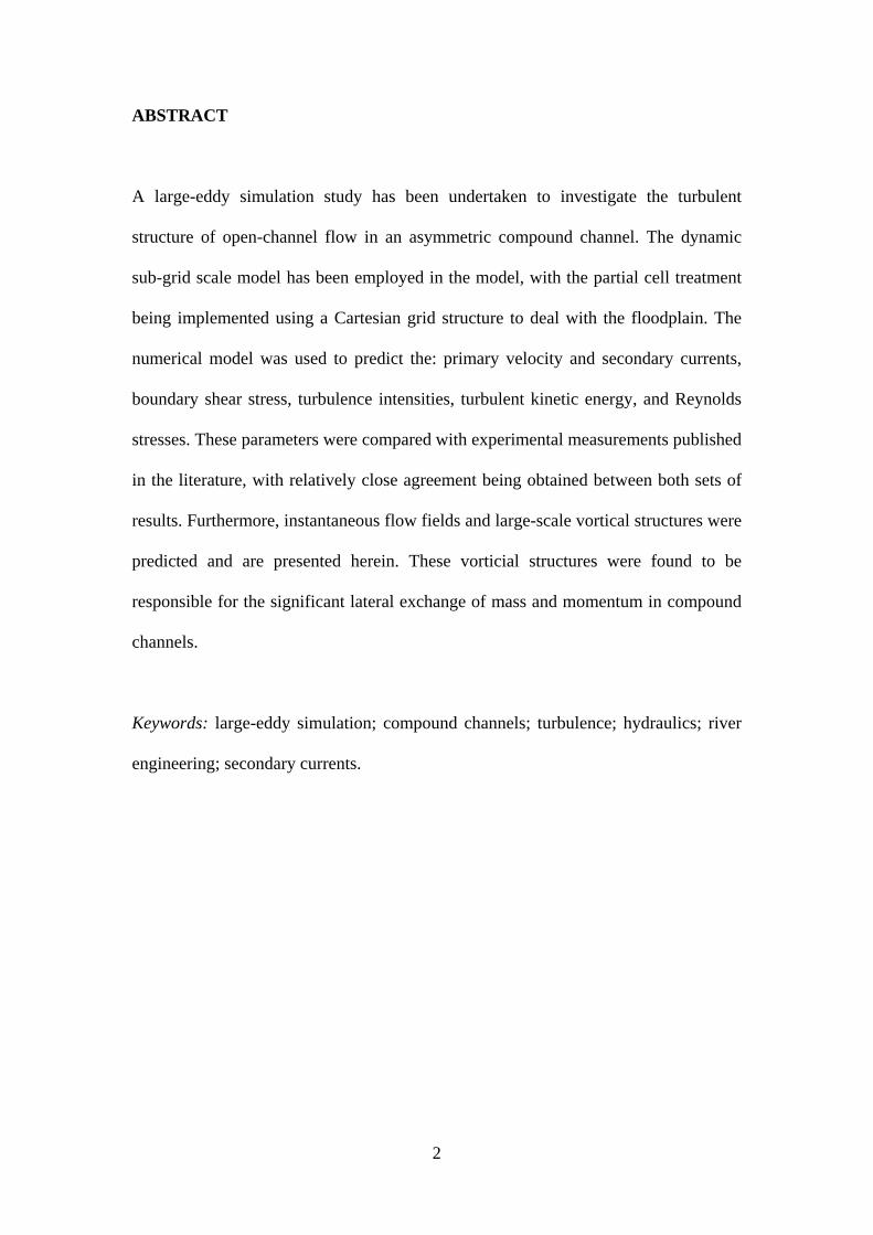
ABSTRACT

A large-eddy simulation study has been undertaken to investigate the turbulent

structure of open-channel flow in an asymmetric compound channel. The dynamic

sub-grid scale model has been employed in the model, with the partial cell treatment

being implemented using a Cartesian grid structure to deal with the floodplain. The

numerical model was used to predict the: primary velocity and secondary currents,

boundary shear stress, turbulence intensities, turbulent kinetic energy, and Reynolds

stresses. These parameters were compared with experimental measurements published

in the literature, with relatively close agreement being obtained between both sets of

results. Furthermore, instantaneous flow fields and large-scale vortical structures were

predicted and are presented herein. These vorticial structures were found to be

responsible for the significant lateral exchange of mass and momentum in compound

channels.

Keywords: large-eddy simulation; compound channels; turbulence; hydraulics; river

engineering; secondary currents.

3

1. Introduction

Compound open-channel flows appear in most natural rivers and are of vital

importance in river engineering and flood risk management. The shear layer generated

between the higher speed main-channel flow and lower speed flood-plain flow,

together with secondary currents, cause a significant lateral exchange of mass and

momentum. Therefore, it is important to investigate and be able to model accurately

the turbulent structure within such compound open-channel flows.

Many experimental studies have been carried out to investigate the mean velocity

and boundary shear stress in compound open-channel flows using a Pitot static tube

and a Preston tube (for example [1-5]). It has been found that the distributions of

velocity and shear stress are affected by the relative depths and widths of the

floodplain in compound channels. More detailed measurements of turbulent structure

and secondary currents in compound open-channel flows have been conducted by

making use of hot-film anemometers [6, 7] and two-component laser Doppler

anemometers [8-12]. Strong inclined secondary currents have been observed in the

vicinity of the junction between the main channel and the floodplain. These

experimental measurements, having provided much insight into the complex turbulent

flow structure, have not only helped to better understand the complicated interaction

between flows in the main channel and the floodplain, but have also assisted in

developing turbulence models in numerical model simulations.

There are several numerical model studies of turbulent flow in compound open

channels reported in the literature, which provide more detailed space-time resolution

of the flow field when compared to experimental investigations, acting as a

complementary approach to gain further insight into the turbulent flow dynamics.

4

Most of the numerical model simulations were based on the Reynolds-averaged

Navier-Stokes (RANS) equations, in which all of the unsteadiness has been averaged

out and considered as a part of the turbulence, and simulated using an algebraic stress

model [13], a non-linear k model [14], a non-linear k model [15], and a more

sophisticated Reynolds stress model [16-18]. Such RANS models are able to provide

satisfactory mean flow fields, but cannot provide detailed instantaneous flow

dynamics and coherent turbulent structure predictions. In addition, many previous

RANS model studies were focused primarily on the distribution of the mean velocity

and boundary shear stress, where the turbulence statistics were neglected. To

overcome these limitations some highly resolved computations, based on the large-

eddy simulation (LES) approach with the Smagorinsky sub-grid scale (SGS) model,

have been performed for turbulent flow in compound open channels [19, 20]. In these

studies the mean velocity field, turbulence intensity, and Reynolds shear stresses were

predicted, with the results being generally found to be in good agreement with the

corresponding experimental results. However, most previous studies of compound

channel flows have focused mainly on the mean flow field, whereas little attention has

been paid to the instantaneous flow field.

The objective of the study presented in this paper is to report on the use of the

LES approach with a dynamic SGS model to investigate the turbulent structure in

compound open-channel flows, including large-scale vortical structures and

instantaneous secondary flows, which play an important part in the flow resistance

and hence the sediment transport fluxes. Model predicted mean velocity and boundary

shear stress distributions, secondary currents, and turbulence statistics are presented

and compared with the available detailed experimental measurements of Tominaga

and Nezu [12]. Details are given in the remainder of the paper of: (i) the mathematical

5

model and numerical solution method, (ii) the computational model setup, (iii) the

numerical model results and discussions, and finally, (iv) some conclusions.

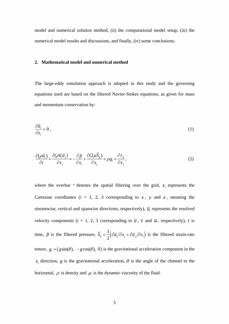
2. Mathematical model and numerical method

The large-eddy simulation approach is adopted in this study and the governing

equations used are based on the filtered Navier-Stokes equations, as given for mass

and momentum conservation by:

ui

xi

0 , (1)

(ui )

t(uiu j )

x j

p

xi

(2Sij )

xj

gi ij

x j

, (2)

where the overbar denotes the spatial filtering over the grid, xi represents the

Cartesian coordinates (i = 1, 2, 3 corresponding to x , y and z , meaning the

streamwise, vertical and spanwise directions, respectively), ui represents the resolved

velocity components (i = 1, 2, 3 corresponding to u , v and w , respectively), t is

time, p is the filtered pressure, Sij 1

2ui x j uj xi is the filtered strain-rate

tensor, gi gsin( ), gcos( ), 0 is the gravitational acceleration component in the

xi direction, g is the gravitational acceleration, is the angle of the channel to the

horizontal, is density and is the dynamic viscosity of the fluid.

6

The term ij uiuj uiuj is the SGS stress tensor and the anisotropic part of the

SGS term is modelled by an eddy-viscosity model of the form:

ij 1

3 ij kk 2tSij , (3)

where

t Cd2 S , S 2SijSij 1 2

, (4)

with the cut-off length scale xyz 1 3 and a model coefficient Cd . In this

study, the dynamic sub-grid model [21, 22] is used to determine the model coefficient

Cd , as given by:

Cd 1

2

Lij Mij

Mij Mij

, (5)

where Lij uiu j uiu j and Mij

2 S Sij 2 S Sij . In these equations, the hat

represents spatial filtering over the test filter. The symbol for spatial filtering is

dropped hereinafter for simplicity.

In this study, the governing equations were discretised using the finite volume

method on a staggered Cartesian grid. The advection terms were discretised by a high-

resolution scheme [23], which combined the high order accuracy with monotonicity,

whereas the gradients in pressure and diffusion terms were obtained by central

7

difference schemes. In order to deal with complex geometries in Cartesian grids, a

partial cell treatment [24] was utilised in the finite volume discretisation, in which the

advective and diffusive fluxes at cell faces, as well as cell volume, were modified in

cut cells. The SIMPLE algorithm [25] was employed for the pressure-velocity

coupling and Gear’s second-order method was used for the time derivative, which led

to an implicit scheme for the governing equations. The code was parallelised using

MPI (Message Passing Interface) and a domain decomposition technique.

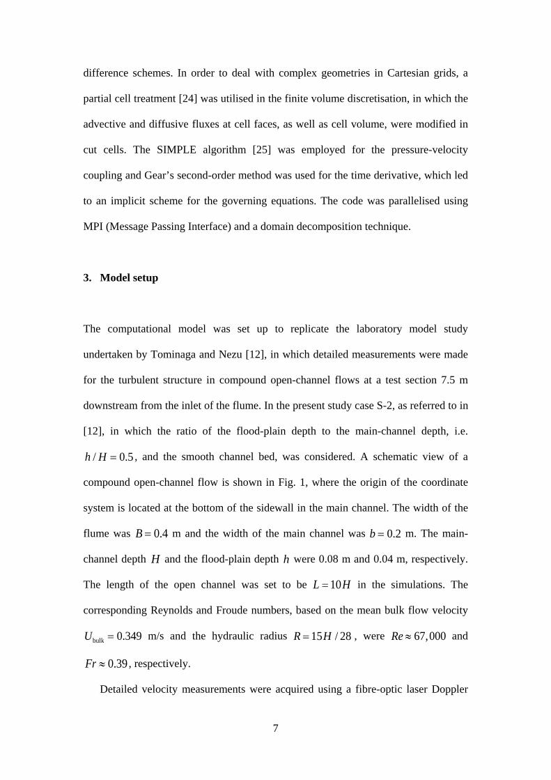
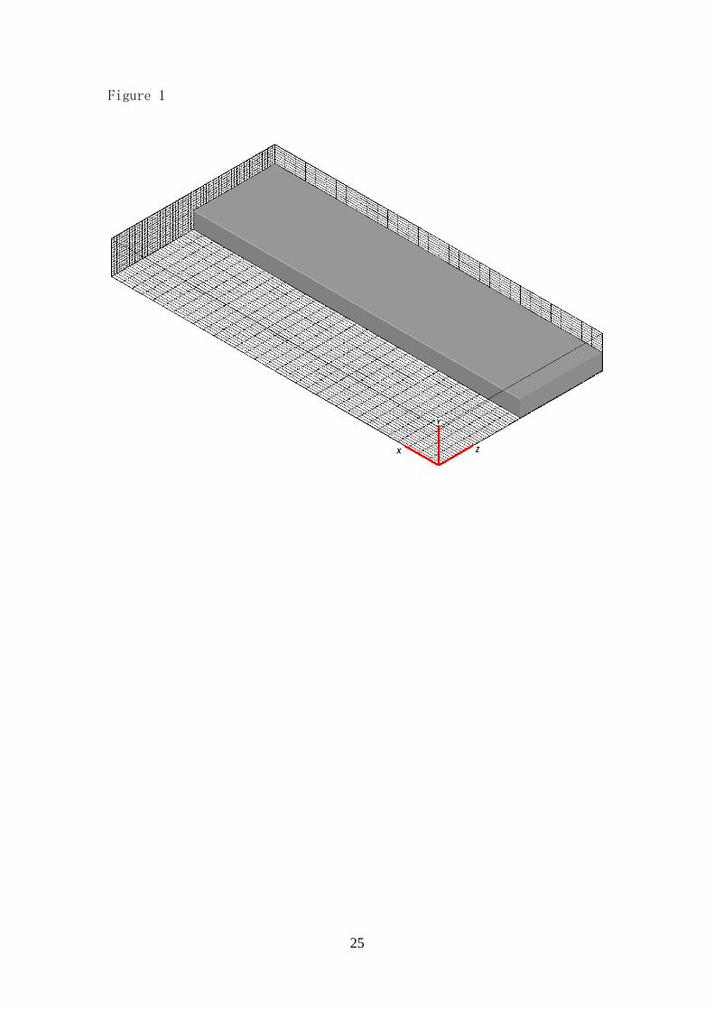
3. Model setup

The computational model was set up to replicate the laboratory model study

undertaken by Tominaga and Nezu [12], in which detailed measurements were made

for the turbulent structure in compound open-channel flows at a test section 7.5 m

downstream from the inlet of the flume. In the present study case S-2, as referred to in

[12], in which the ratio of the flood-plain depth to the main-channel depth, i.e.

h / H 0.5 , and the smooth channel bed, was considered. A schematic view of a

compound open-channel flow is shown in Fig. 1, where the origin of the coordinate

system is located at the bottom of the sidewall in the main channel. The width of the

flume was B 0.4 m and the width of the main channel was b 0.2 m. The main-

channel depth H and the flood-plain depth h were 0.08 m and 0.04 m, respectively.

The length of the open channel was set to be L 10H in the simulations. The

corresponding Reynolds and Froude numbers, based on the mean bulk flow velocity

Ubulk 0.349 m/s and the hydraulic radius R 15H / 28 , were Re 67,000 and

Fr 0.39, respectively.

Detailed velocity measurements were acquired using a fibre-optic laser Doppler

8

anemometer in the experiments. These data, shown as contour plots in [12], were used

to test the numerical model. The computational domain of 10H H 5H was

discretised using a grid of 192 96 384 cells in the streamwise, vertical, and

spanwise directions, respectively (shown in Fig. 1). Periodic boundary conditions

were used in the streamwise direction. The near-wall modelling approach [26] was

employed for the bed and sidewalls of the open channel, in which the instantaneous

shear stress was related to the velocity adjacent to the solid boundary, by using a time-

averaged wall law. The free surface was modelled as a rigid lid (i.e. a free-slip

boundary condition), which has been successfully used in previous LES studies of

turbulent open-channel flow [19, 27]. The flow was driven by the gravity force, i.e.

gsin( ) , in the streamwise direction. The calculations were started with initial

conditions that consisted of the mean bulk flow velocity, with random perturbations

superimposed in all three directions. After a statistically steady state was reached, the

simulations were continued for about 22 flow-through times (i.e. L /Ubulk ) for

acquiring turbulence statistics.

4. Results and discussion

In this section, the LES results of the mean flow field and turbulence statistics of the

compound open-channel flow are shown and discussed. Moreover, the instantaneous

flow fields, including the secondary flow, are presented and analysed. In the

following, the angular bracket, , represents averaging over time, and the resolved

variable is decomposed into a mean value and a resolved fluctuation as:

, (6)

9

where the prime denotes fluctuation with respect to the mean resolved quantity. The

turbulence intensity is obtained using:

rms 2. (7)

It is worth noting that for comparisons to be made with the experimental data all of

the predicted mean flow and turbulence statistics were further averaged along the

streamwise direction.

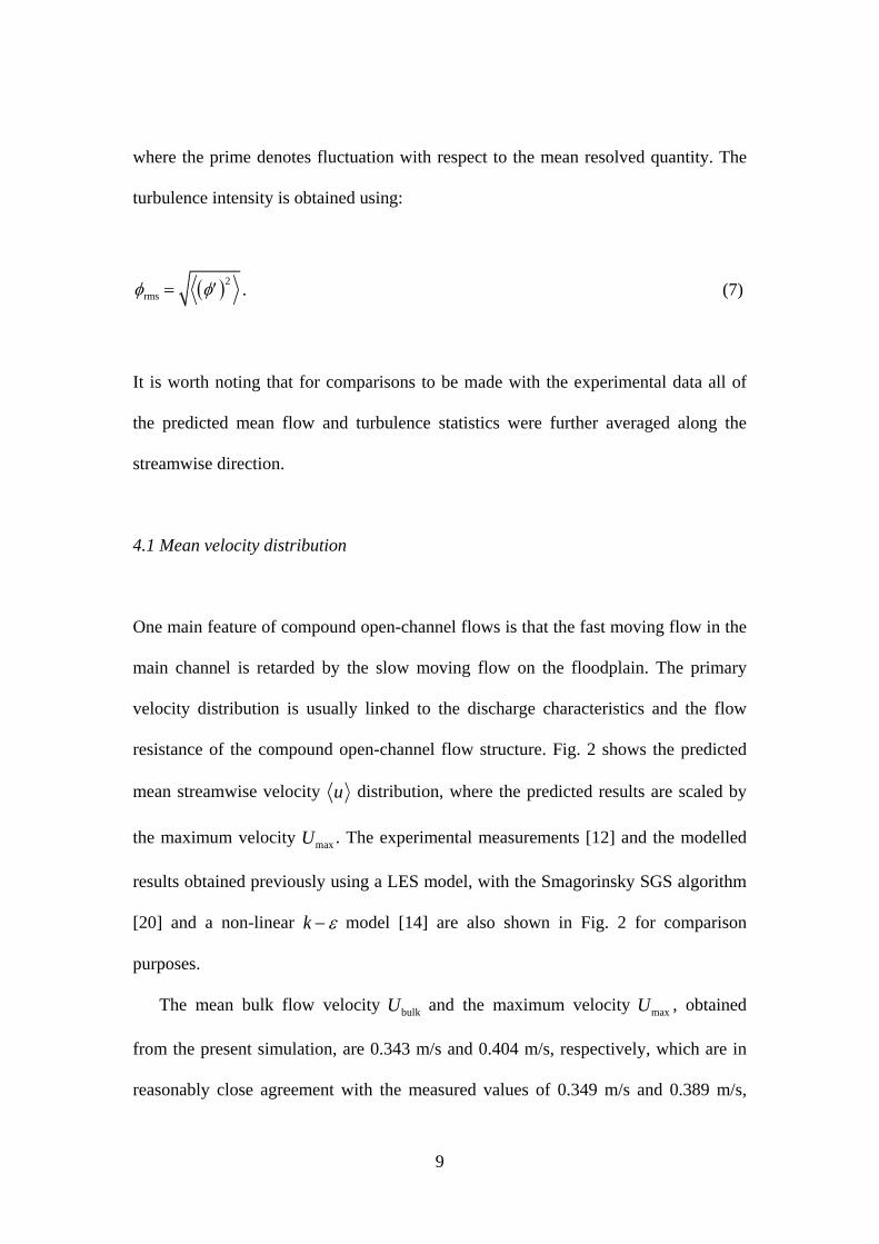
4.1 Mean velocity distribution

One main feature of compound open-channel flows is that the fast moving flow in the

main channel is retarded by the slow moving flow on the floodplain. The primary

velocity distribution is usually linked to the discharge characteristics and the flow

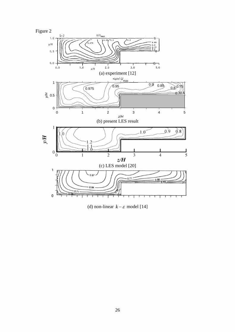
resistance of the compound open-channel flow structure. Fig. 2 shows the predicted

mean streamwise velocity u distribution, where the predicted results are scaled by

the maximum velocity Umax . The experimental measurements [12] and the modelled

results obtained previously using a LES model, with the Smagorinsky SGS algorithm

[20] and a non-linear k model [14] are also shown in Fig. 2 for comparison

purposes.

The mean bulk flow velocity Ubulk and the maximum velocity Umax , obtained

from the present simulation, are 0.343 m/s and 0.404 m/s, respectively, which are in

reasonably close agreement with the measured values of 0.349 m/s and 0.389 m/s,

10

respectively. The main flow pattern of compound open-channel flows is satisfactorily

reproduced by the present LES model, especially in locations near the main-

channel/flood-plain (M/F) junction edge and the main-channel bottom. The contour

lines bulge towards the free surface in the vicinity of the M/F junction edge, with flow

deceleration due to the low-speed flow being transported by the secondary currents

(which will be shown later in Fig. 3) away from the wall. In contrast, the contour lines

bulge towards the wall on both sides of the M/F junction edge, with flow acceleration

due to the high-speed flow being transported by the secondary currents towards the

wall, which is consistent with the experimental measurements [12]. The flow

deceleration can also be observed near the free surface in the sidewall region and near

the bottom of the main channel, which is well predicted in the present study.

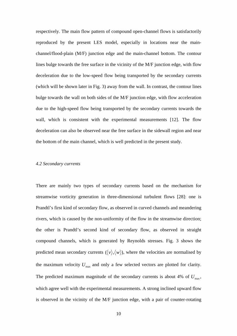
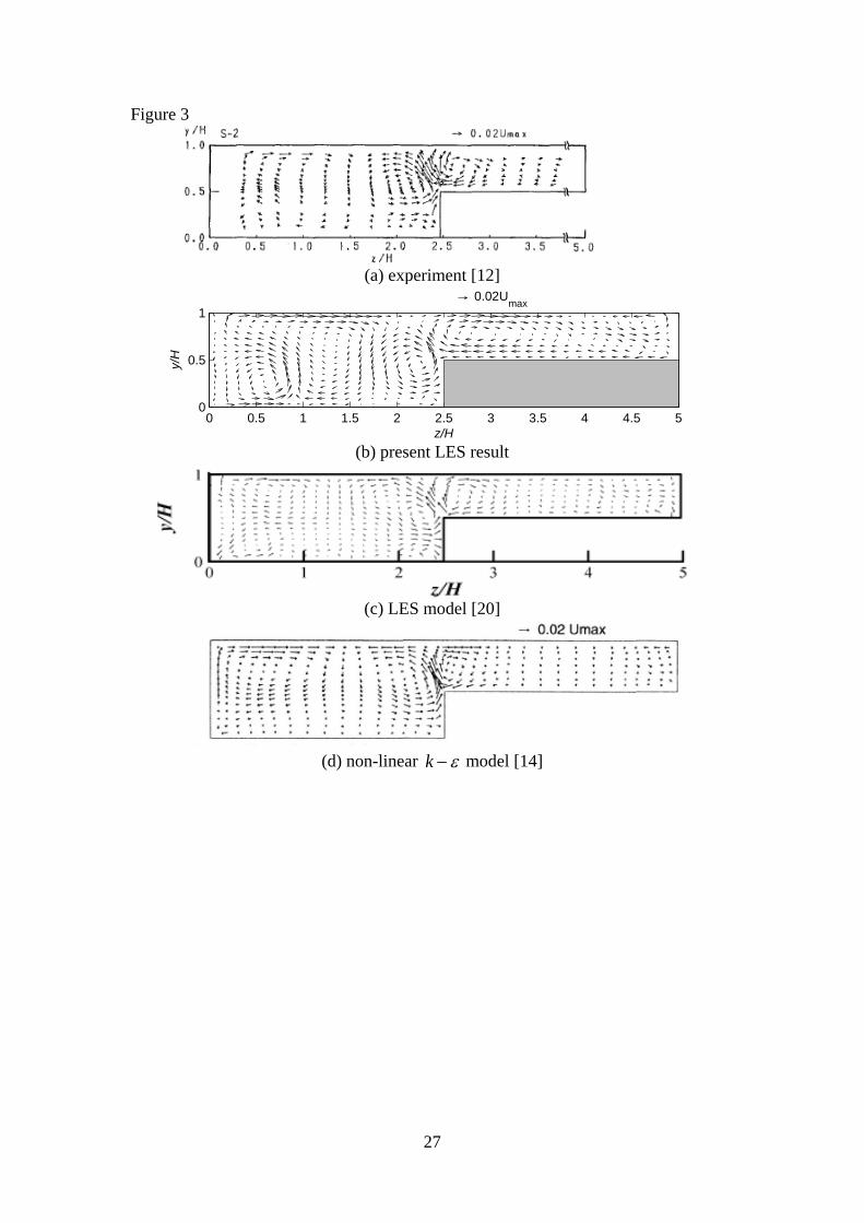
4.2 Secondary currents

There are mainly two types of secondary currents based on the mechanism for

streamwise vorticity generation in three-dimensional turbulent flows [28]: one is

Prandtl’s first kind of secondary flow, as observed in curved channels and meandering

rivers, which is caused by the non-uniformity of the flow in the streamwise direction;

the other is Prandtl’s second kind of secondary flow, as observed in straight

compound channels, which is generated by Reynolds stresses. Fig. 3 shows the

predicted mean secondary currents ( v , w ), where the velocities are normalised by

the maximum velocity Umax and only a few selected vectors are plotted for clarity.

The predicted maximum magnitude of the secondary currents is about 4% of Umax ,

which agree well with the experimental measurements. A strong inclined upward flow

is observed in the vicinity of the M/F junction edge, with a pair of counter-rotating

11

streamwise vortices occurring on both sides, namely: the main-channel vortex and the

flood-plain vortex [12]. Two additional vortices, namely: the free-surface vortex and

bottom vortex, appear in the sidewall region, which are in good agreement with the

experimental observations.

In the vicinity of the M/F junction edge, better results are obtained by the non-

linear k model [14] in terms of the inclined angle of the secondary currents. In the

present model, there is a slight discrepancy for the inclined angle when compared to

the experimental measurements, this is thought to be caused mainly by the rigid lid

treatment for the free surface and the corresponding limitations in predicting the

vertical velocities. In the sidewall region, the bottom vortex is not captured by the

non-linear k model, but it is predicted by both LES models. Similar secondary

circulation patterns are obtained for most part of the compound channel in the LES

model predictions. Due to the rigid lid treatment mentioned above, near the free

surface there is a discrepancy between the predicted secondary currents and the

experimental results on the main channel side of the junction, whereas better

agreement is obtained in [20] using a height function for the free surface. However,

their model is unable to predict the flow deceleration zone on the left side near the bed

(see Figs 2a and 2c), which is thought to be due to the weak bottom vortex predicted

in [20] (shown in Fig. 3c).

In general, the predicted secondary currents closely resemble the experimental

measurements, which affect the structure of the mean primary velocity (shown in Fig.

2) and the velocity-dip phenomenon in open-channel flows [28], and play an essential

role in the spanwise transport of mass, momentum, and heat in compound channels.

4.3 Bed shear stress distribution

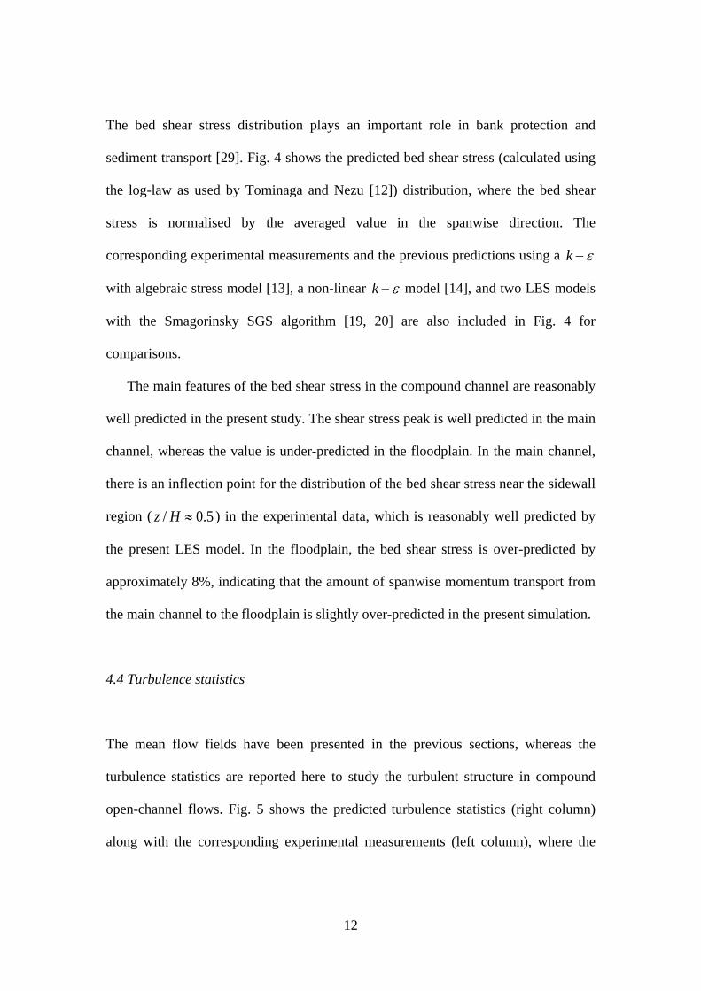
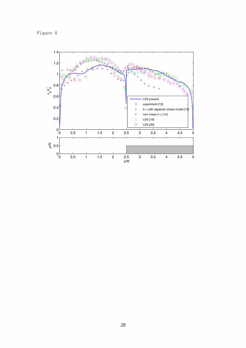
12

The bed shear stress distribution plays an important role in bank protection and

sediment transport [29]. Fig. 4 shows the predicted bed shear stress (calculated using

the log-law as used by Tominaga and Nezu [12]) distribution, where the bed shear

stress is normalised by the averaged value in the spanwise direction. The

corresponding experimental measurements and the previous predictions using a k

with algebraic stress model [13], a non-linear k model [14], and two LES models

with the Smagorinsky SGS algorithm [19, 20] are also included in Fig. 4 for

comparisons.

The main features of the bed shear stress in the compound channel are reasonably

well predicted in the present study. The shear stress peak is well predicted in the main

channel, whereas the value is under-predicted in the floodplain. In the main channel,

there is an inflection point for the distribution of the bed shear stress near the sidewall

region ( z / H 0.5 ) in the experimental data, which is reasonably well predicted by

the present LES model. In the floodplain, the bed shear stress is over-predicted by

approximately 8%, indicating that the amount of spanwise momentum transport from

the main channel to the floodplain is slightly over-predicted in the present simulation.

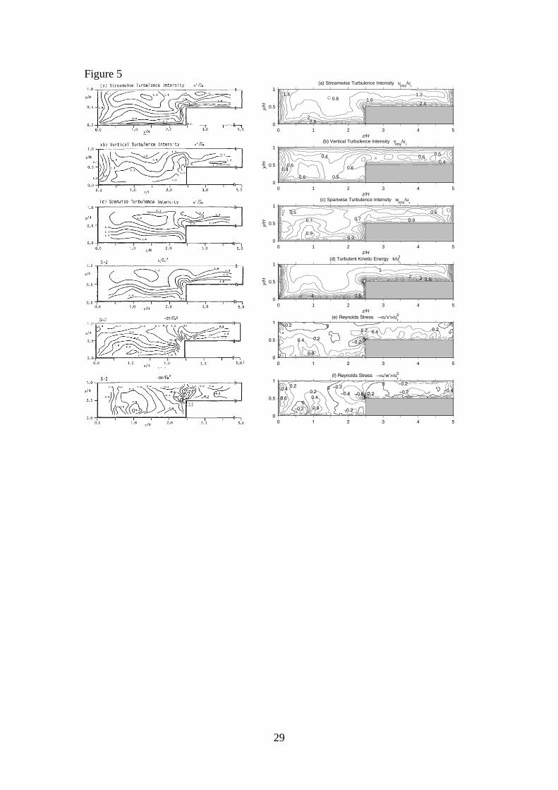
4.4 Turbulence statistics

The mean flow fields have been presented in the previous sections, whereas the

turbulence statistics are reported here to study the turbulent structure in compound

open-channel flows. Fig. 5 shows the predicted turbulence statistics (right column)

along with the corresponding experimental measurements (left column), where the

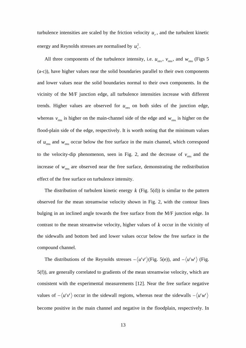
13

turbulence intensities are scaled by the friction velocity u , and the turbulent kinetic

energy and Reynolds stresses are normalised by u2 .

All three components of the turbulence intensity, i.e. urms, vrms, and wrms (Figs 5

(a-c)), have higher values near the solid boundaries parallel to their own components

and lower values near the solid boundaries normal to their own components. In the

vicinity of the M/F junction edge, all turbulence intensities increase with different

trends. Higher values are observed for urms on both sides of the junction edge,

whereas vrms is higher on the main-channel side of the edge and wrms is higher on the

flood-plain side of the edge, respectively. It is worth noting that the minimum values

of urms and wrms occur below the free surface in the main channel, which correspond

to the velocity-dip phenomenon, seen in Fig. 2, and the decrease of vrms and the

increase of wrms are observed near the free surface, demonstrating the redistribution

effect of the free surface on turbulence intensity.

The distribution of turbulent kinetic energy k (Fig. 5(d)) is similar to the pattern

observed for the mean streamwise velocity shown in Fig. 2, with the contour lines

bulging in an inclined angle towards the free surface from the M/F junction edge. In

contrast to the mean streamwise velocity, higher values of k occur in the vicinity of

the sidewalls and bottom bed and lower values occur below the free surface in the

compound channel.

The distributions of the Reynolds stresses u v (Fig. 5(e)), and u w (Fig.

5(f)), are generally correlated to gradients of the mean streamwise velocity, which are

consistent with the experimental measurements [12]. Near the free surface negative

values of u v occur in the sidewall regions, whereas near the sidewalls u w

become positive in the main channel and negative in the floodplain, respectively. In

14

the vicinity of the M/F junction edge, negative peak values of u v and u w

are found below the inclined upflow in the main-channel side, whereas positive peak

values of u v and u w are found above the inclined upflow in the flood-plain

side. However, the distributions of the two Reynolds stresses differ near the junction

edge, as u v increase in the vertical direction and u w increase in the

spanwise direction. All the signs of u v and u w correspond well to those for

u / y and u / z . It is worth noting that one important feature of compound

open-channel flows can be recognised from the distribution of u w near the

junction edge, indicating a spanwise transport of momentum from the main channel

towards the floodplain ( u w / z 0).

In general, the predicted distributions of turbulence statistics agree closely with

the experimental measurements, which provide a useful tool for investigating more

detailed turbulent structures in compound open-channel flows.

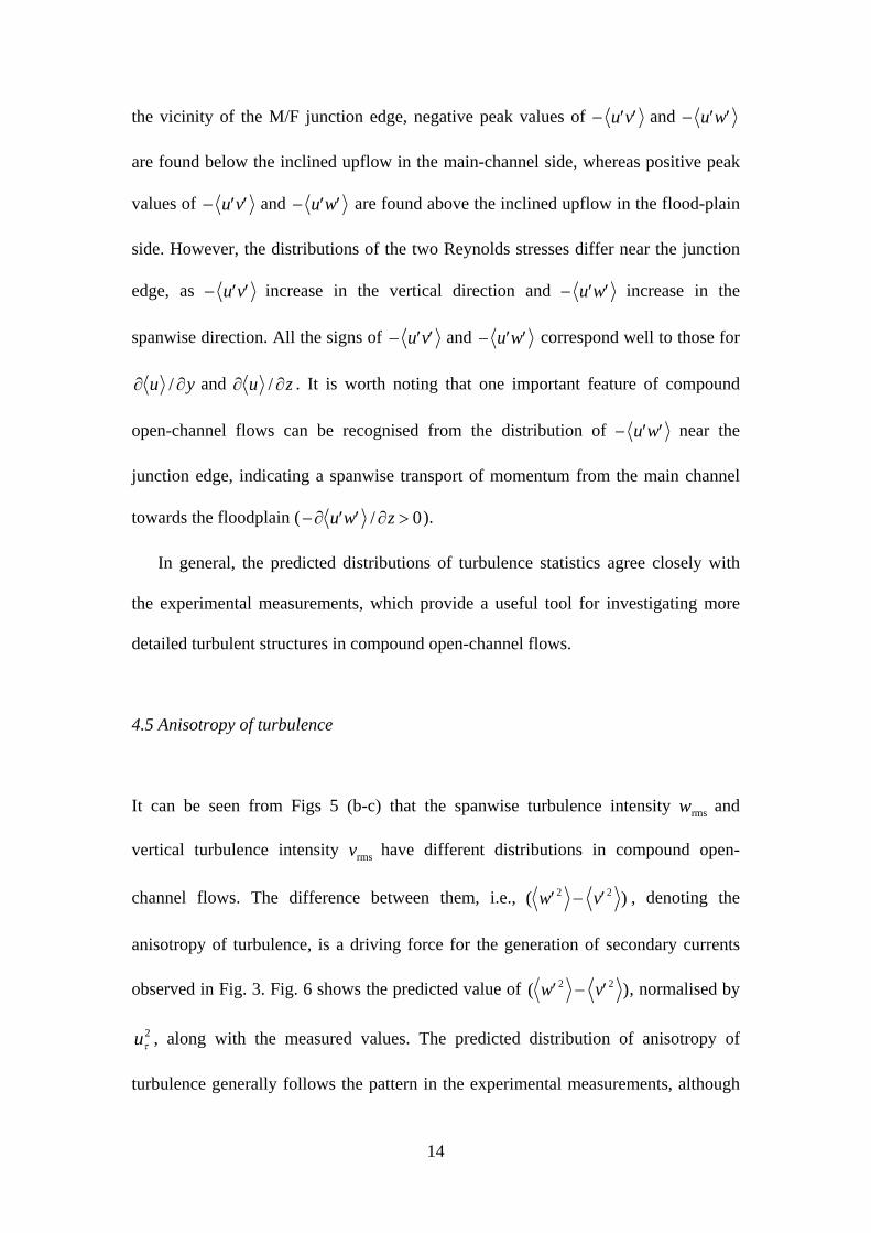
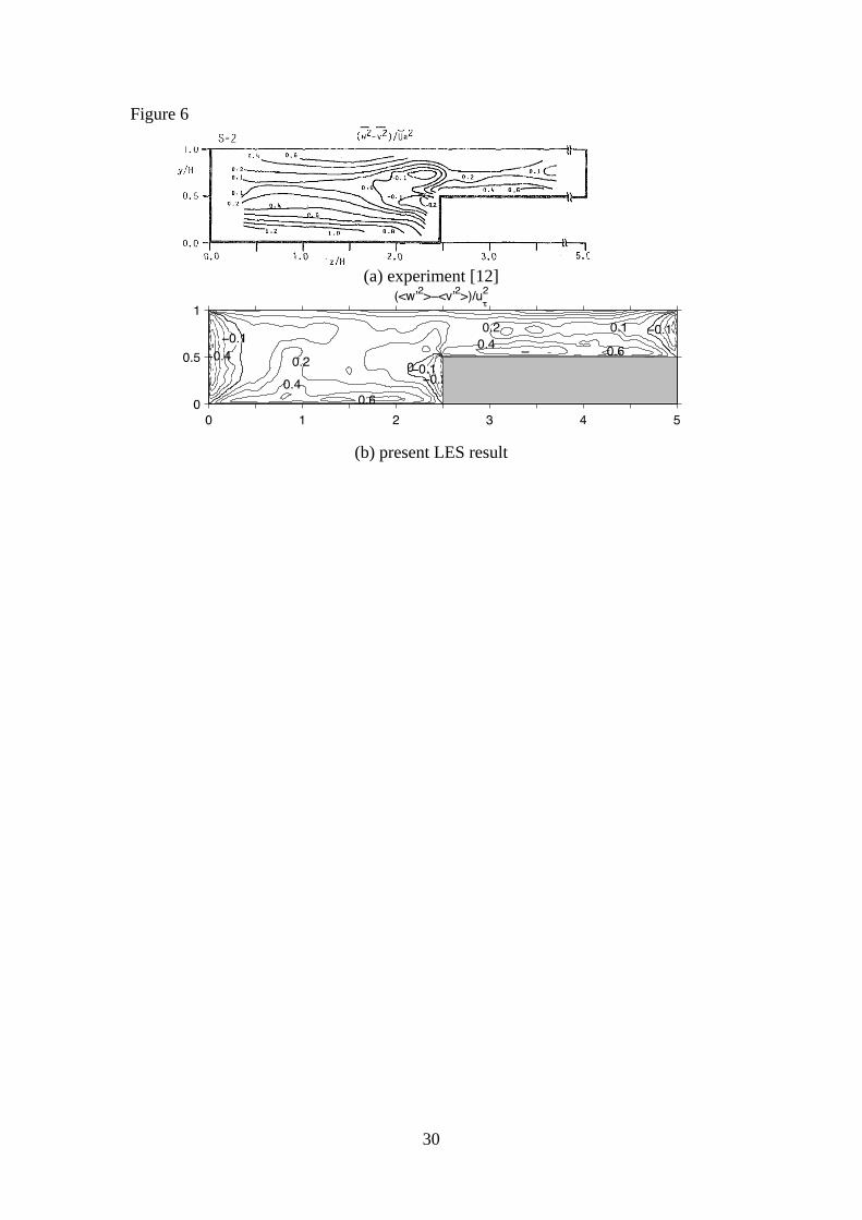
4.5 Anisotropy of turbulence

It can be seen from Figs 5 (b-c) that the spanwise turbulence intensity wrms and

vertical turbulence intensity vrms have different distributions in compound open-

channel flows. The difference between them, i.e., ( w 2 v 2 ) , denoting the

anisotropy of turbulence, is a driving force for the generation of secondary currents

observed in Fig. 3. Fig. 6 shows the predicted value of ( w 2 v 2 ), normalised by

u2 , along with the measured values. The predicted distribution of anisotropy of

turbulence generally follows the pattern in the experimental measurements, although

15

the predicted negative region of ( w 2 v 2 ) is smaller and lower in the vicinity of

the M/F junction edge when compared to the measured values. This discrepancy is

thought to be due to the rigid lid approximation affecting the distribution of the

vertical turbulence intensity, and causing the difference between the predicted and

measured secondary currents near the junction edge, as shown in Fig. 3. The value of

( w 2 v 2 ) decreases in the vertical direction from the bottom bed, and increases

towards the free surface after attaining the negative peak value in the upper flow

region of the channel. At the M/F junction edge, the value of ( w 2 v 2 ) changes

from negative in the main channel to positive on the floodplain. The anisotropy of

turbulence in the compound open-channel flow is responsible for the generation of the

streamwise vortices, which is consistent with the experimental observations [12].

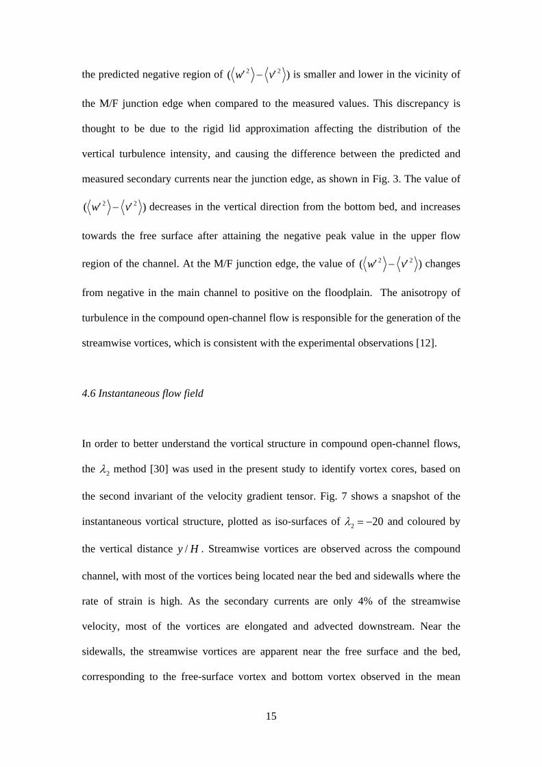
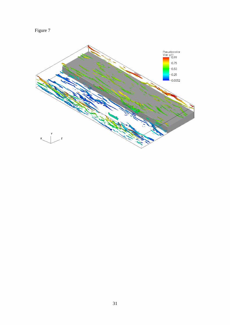
4.6 Instantaneous flow field

In order to better understand the vortical structure in compound open-channel flows,

the 2 method [30] was used in the present study to identify vortex cores, based on

the second invariant of the velocity gradient tensor. Fig. 7 shows a snapshot of the

instantaneous vortical structure, plotted as iso-surfaces of 2 20 and coloured by

the vertical distance y / H . Streamwise vortices are observed across the compound

channel, with most of the vortices being located near the bed and sidewalls where the

rate of strain is high. As the secondary currents are only 4% of the streamwise

velocity, most of the vortices are elongated and advected downstream. Near the

sidewalls, the streamwise vortices are apparent near the free surface and the bed,

corresponding to the free-surface vortex and bottom vortex observed in the mean

16

secondary currents. In the vicinity of the M/F junction edge, streamwise vortices are

developed, resulting in secondary flows being formed, which are responsible for the

momentum transfer between the main channel and the floodplain. The location of the

vortex cores varies in the streamwise direction, corresponding to the chaotic flow

field at the cross-sections.

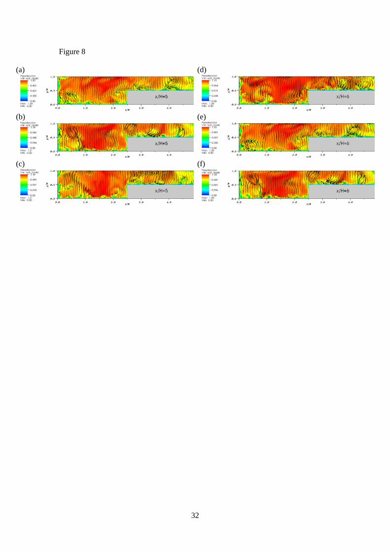
In order to study the temporal and spatial development of the secondary currents,

a detailed analysis has been undertaken for the streamwise vortices using the

instantaneous velocities predicted by the present LES model. Fig. 8 shows snapshots

of the distributions of instantaneous streamwise velocity u and secondary currents

(v,w) at two cross-sections: x / H = 5 (Fig. 8(a-c)) and x / H = 6 (Fig. 8(d-f)), for a

constant time interval of 0.1L /Ubulk . Both the instantaneous distributions of the

streamwise velocity and the secondary currents are different from their mean values,

as shown in Figs 2 and 3 respectively, demonstrating the temporal variations of the

turbulent flow field. In the near-wall region, the transport of low-speed flow towards

the wall and high-speed flow away from the wall can be recognised. It can be

observed that the flow near the bed or sidewalls is more turbulent than the flow in the

interior region, which is consistent with the high values for turbulence statistics in the

near-wall region. At x / H = 5 (from Fig. 8(a) to Fig. 8(c)), the development of a

strong clockwise vortex on the floodplain near the M/F junction edge is apparent,

corresponding to the streamwise vortices moving downstream towards the floodplain.

By comparing the instantaneous streamwise velocity and secondary flows between

x / H = 5 (Fig. 8(a-c)) and x / H = 6 (Fig. 8(d-f)) at a same time, it is shown that their

flow patterns are different, demonstrating spatial variations of the three-dimensional

turbulent flow field. However, it is interesting to note that similar flow patterns are

observed between Fig. 8(a) and Fig. 8 (e) and between Fig. 8(b) and Fig. 8(f). As the

17

time interval between each figure from the top to the bottom is 0.1L /Ubulk ,

corresponding to a streamwise distance x / H = 1, it is suggested that the secondary

flows are affected by the main velocity, transported downstream with the streamwise

velocity. Most of the flow patterns observed at x / H = 5 can be seen at x / H = 6 at

the next time interval, with small differences occurring near the solid boundaries.

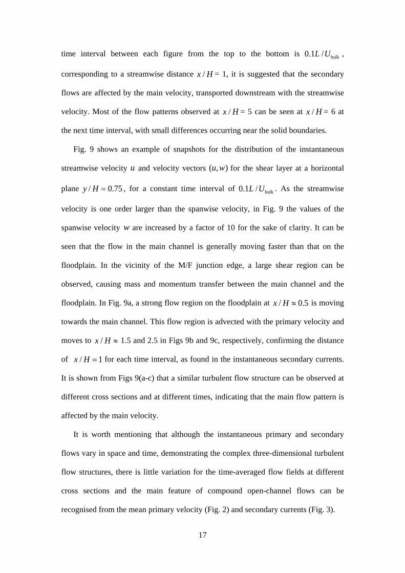
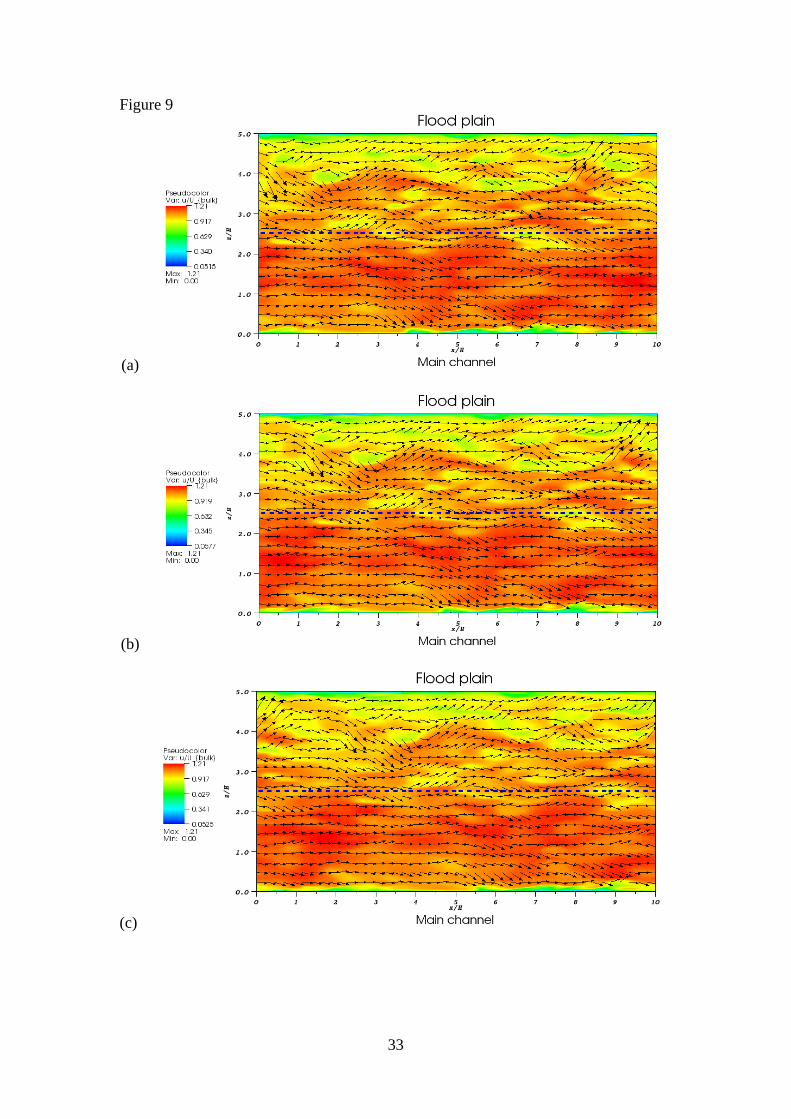
Fig. 9 shows an example of snapshots for the distribution of the instantaneous

streamwise velocity u and velocity vectors (u,w) for the shear layer at a horizontal

plane y / H 0.75 , for a constant time interval of 0.1L /Ubulk . As the streamwise

velocity is one order larger than the spanwise velocity, in Fig. 9 the values of the

spanwise velocity w are increased by a factor of 10 for the sake of clarity. It can be

seen that the flow in the main channel is generally moving faster than that on the

floodplain. In the vicinity of the M/F junction edge, a large shear region can be

observed, causing mass and momentum transfer between the main channel and the

floodplain. In Fig. 9a, a strong flow region on the floodplain at x / H 0.5 is moving

towards the main channel. This flow region is advected with the primary velocity and

moves to x / H 1.5 and 2.5 in Figs 9b and 9c, respectively, confirming the distance

of x / H 1 for each time interval, as found in the instantaneous secondary currents.

It is shown from Figs 9(a-c) that a similar turbulent flow structure can be observed at

different cross sections and at different times, indicating that the main flow pattern is

affected by the main velocity.

It is worth mentioning that although the instantaneous primary and secondary

flows vary in space and time, demonstrating the complex three-dimensional turbulent

flow structures, there is little variation for the time-averaged flow fields at different

cross sections and the main feature of compound open-channel flows can be

recognised from the mean primary velocity (Fig. 2) and secondary currents (Fig. 3).

18

5. Conclusions

In this paper a large-eddy simulation model of the turbulent structure in compound

open-channel flows has been presented and the predictions were compared with

available experimental data. The principal flow features measured in the experiments

were generally well reproduced, including: the distributions of the mean velocity and

secondary currents, boundary shear stress, turbulence intensities, turbulent kinetic

energy, and Reynolds stresses. The anisotropy of the turbulence was also investigated

in this study, with this being a driving force for the generation of secondary currents.

Furthermore, the instantaneous flow fields and large-scale vortical structures were

presented, with a stronger turbulent flow in the near-wall region and a significant

lateral transport of momentum being shown. It was found that although there are

significant temporal and spatial variations for the three-dimensional turbulent flow

field, their time-averaged results are similar at different cross sections.

The study demonstrates the capability of the present LES model in providing

reliable detailed mean velocity field characteristics and turbulence statistics for

compound open-channel flows, which can act as a complementary approach to

experimental investigations to gain further insight into the turbulent flow dynamics.

The main future extension of this study would be to include a solute transport module

and roughness effect to investigate mass exchange between the main channel and the

floodplain.

Acknowledgements

19

The research was supported by the UK Engineering and Physical Sciences Research

Council (EP/G014264/1). This work was performed using the computational facilities

of the Advanced Research Computing @ Cardiff (ARCCA) Division, Cardiff

University.

References

[1] Myers RC, Elsawy EM. (1975) Boundary shear in channel with flood plain. J

Hydraulic Division ASCE 1975; 101 (7): 933–946.

[2] Rajaratnam N, Ahmadi RM. Hydraulics of channels with floodplains. J Hydraulic

Res 1981; 19 (1): 43–60.

[3] Knight DW, Demetriou JD. Flood plain and main channel flow interaction. J

Hydraulic Eng ASCE 1983; 109 (8): 1073–1092.

[4] Knight DW, Hamed ME. Boundary shear in symmetric compound channels. J


[5] Nalluri C, Judy ND. Interaction between main channel and flood plain flow.

Proceedings of 21st IAHR Congress, Melbourne, Australia, 1985, p. 378–382.

[6] Tominaga A, Ezaki K. Hydraulic characteristics of compound channel flow.

Proceedings of 6th Congress of Asian and Pacific Division, IAHR, Kyoto, Japan,

1988, p. 465–472.

[7] Tominaga A, Nezu I, Ezaki K, Nakagawa H. Three-dimensional turbulent

structure in straight open channel flows. J Hydraulic Res 1989; 27 (1): 149–173.

[8] Arnold U, Stein J, Rouve G. Sophisticated measurement techniques for

experimental investigation of compound open channel flow. Computational

20

Modelling and Experimental Methods in Hydraulics, Elsevier, Dubrovnik,

Yugoslavia, 1989, p. 11–21.

[9] Tominaga A, Nezu I, Ezaki K. Experimental study on secondary currents in

compound open channels. Proceedings of 23rd IAHR Congress, Ottawa, Canada,

1989, p. A 15–22.

[10] Shiono K, Knight DW. Vertical and transverse Reynolds stress measurements in

a shear layer region of a compound channel. Proceedings of 7th Symposium on

Turbulent Shear Flows, Stanford, USA, 1989, p. 28.1.1–28.1.6.

[11] Knight DW, Shiono K. Turbulence measurements in a shear layer region of a

compound channel. J Hydraulic Res 1990; 28 (2): 175–196.

[12] Tominaga A, Nezu I. Turbulent structure in compound open-channel flows. J


[13] Naot D, Nezu I, Nakagawa H. Hydrodynamic behavior of compound rectangular

open channels. J Hydraulic Eng ASCE 1993; 119 (3): 390–408.

[14] Lin B, Shiono K. Numerical modelling of solute transport in compound channel

flows. J Hydraulic Res 1995; 33 (6): 773–788.

[15] Sofialidis D, Prinos P. Numerical study of momentum exchange in compound

open channel flow. J Hydraulic Eng ASCE 1999; 125 (2): 152–165.

[16] Cokljat D, Younis BA. Second-order closure study of open-channel flows. J


[17] Kang H, Choi SU. Turbulence modeling of compound open-channel flows with

and without vegetation on the floodplain using the Reynolds stress model. Adv

Water Resour 2006; 29 (11): 1650–1664.

21

[18] Jing H, Li C, Guo Y, Xu W. Numerical simulation of turbulent flows in

trapezoidal meandering compound open channels. Int J Numer Methods Fluids

2011; 65 (9): 1071–1083.

[19] Thomas TG, Williams JJR. Large eddy simulation of turbulent flow in an

asymmetric compound open channel. J Hydraulic Res 1995; 33 (1): 27–41.

[20] Cater JE, Williams JJR. Large eddy simulation of a long asymmetric compound

open channel. J Hydraulic Res 2008; 46 (4): 445–453.

[21] Germano M, Piomelli U, Moin P, Cabot WH. A dynamic subgrid-scale eddy

viscosity model. Phys Fluids A 1991; 3 (7): 1760–1765.

[22] Lilly DK. A proposed modification of the Germano-subgrid-scale closure

method. Phys Fluids A 1992; 4 (3): 633–635.

[23] Hirsch C. Numerical computation of internal and external flows introduction to

the fundamentals of CFD. new ed. Oxford: Butterworth-Heinemann; 2007.

[24] Torrey MD, Cloutman LD, Mjolsness RC, Hirt CW. NASA-VOF2D: a

computer program for incompressible flows with free surfaces. Tech. Rep. LA-

10612-MS, Los Alamos Scientific Laboratory; 1985.

[25] Patankar SV. Numerical heat transfer and fluid flow. London: Taylor & Francis;

1980.

[26] Schumann U. Subgrid scale model for finite difference simulations of turbulent

flows in plane channels and annuli. J Comput Phys 1975;18 (4): 376–404.

[27] Zedler EA, Street RL. Large-eddy simulation of sediment transport: Currents

over ripples. J Hydraulic Eng ASCE 2001; 127 (6): 444–452.

[28] Nezu I, Nakagawa H. (1993) Turbulence in open-channel flows, International

Association for Hydraulic Research monograph series. Rotterdam: A.A. Balkema;

1993.

22

[29] Shiono K, Knight DW. Turbulent open-channel flows with variable depth across

the channel. J Fluid Mech 1991; 222: 617–646.

[30] Jeong J, Hussain F. On the identification of a vortex. J Fluid Mech 1995; 285:

69–94.

23

Figure captions

Fig. 1. Schematic of computational domain and numerical grid for turbulent open-

channel flow in a compound channel (only every sixth grid line plotted for clarity).

Fig. 2. Distribution of primary mean velocity u /Umax .

Fig. 3. Secondary current vectors.

Fig. 4. Distribution of bed shear stress.

Fig. 5. Comparison between predicted turbulence statistics (right column) and

experimental measurements [12] (left column): (a) streamwise turbulence intensity;

(b) vertical turbulence intensity; (c) spanwise turbulence intensity; (d) turbulent

kinetic energy; (f) Reynolds stress u v ; (g) Reynolds stress u w .

Fig. 6. Distribution of ( w 2 v 2 ).

Fig. 7. Snapshot of instantaneous vortical structure plotted as iso-surfaces of

2 20 and coloured by the vertical distance y / H in compound open-channel

flows.

24

Fig. 8. Snapshots of the distribution of instantaneous streamwise velocity u and

secondary velocity vectors (v,w) at two cross-sections: x / H = 5 and 6, for a constant

time interval of 0.1L /Ubulk .

Fig. 9. Snapshots for the distribution of instantaneous streamwise velocity u and

velocity vectors (u,w) for the shear layer at a horizontal plane y / H 0.75 , for a

constant time interval of 0.1L /Ubulk . The values of w are increased by a factor of 10

for the sake of clarity.

25

Figure 1

26

Figure 2

(a) experiment [12]

0.9750.95 0.9 0.85

0.8 0.75

0.70.6

z/H

y/H

<u>/ Umax

0 1 2 3 4 50

0.5

1

(b) present LES result

(c) LES model [20]

(d) non-linear k model [14]

27

Figure 3

(a) experiment [12]

0 0.5 1 1.5 2 2.5 3 3.5 4 4.5 50

0.5

1

z/H

y/H

0.02Umax


(c) LES model [20]

(d) non-linear k model [14]

28

Figure 4

29

Figure 5

z/H

y/H

0.81.2

1.6

22.8

1.6

2.4

(a) Streamwise Turbulence Intensity urms

/u

0 1 2 3 4 50

0.5

1

z/H

y/H

(b) Vertical Turbulence Intensity vrms

/u

0.6

0.4

0.80.6

0.6 0.5

0.50.6

0.4

0 1 2 3 4 50

0.5

1

z/H

y/H

(c) Spanwise Turbulence Intensity wrms

/u

0.5

0.9

0.7 0.7

0.9

0.9

0.6

0 1 2 3 4 50

0.5

1

z/H

y/H

12 3 3.5

3.54

(d) Turbulent Kinetic Energy k/u2

0 1 2 3 4 50

0.5

1

30

Figure 6

(a) experiment [12]


31

Figure 7

32

Figure 8

(a) (d)

(b) (e)

(c) (f)

33

Figure 9

(a)

(b)

(c)

Large-eddy simulation of the turbulent structure in compound open-channel flows

Documents

Transcript of Large-eddy simulation of the turbulent structure in compound open-channel flows