
Large Eddy Simulation of Stratified Turbulent Flows over Heterogeneous Landscapes
Upload
independentCategory
view
3download
0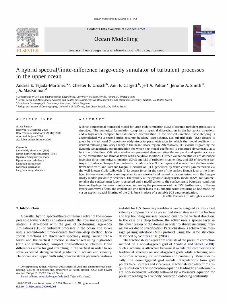
Ocean Modelling 30 (2009) 115–142
Contents lists available at ScienceDirect
Ocean Modelling
journal homepage: www.elsevier .com/locate /ocemod
A hybrid spectral/finite-difference large-eddy simulator of turbulent processesin the upper ocean
Andrés E. Tejada-Martínez a,*, Chester E. Grosch b, Ann E. Gargett b, Jeff A. Polton c, Jerome A. Smith d,J.A. MacKinnon d
a Department of Civil and Environmental Engineering, University of South Florida, Tampa, FL, United Statesb Ocean, Earth and Atmospheric Sciences and Center for Coastal Physical Oceanography, Old Dominion University, Norfolk, VA, United Statesc Proudman Oceanographic Laboratory, Liverpool, United Kingdomd Scripps Institution of Oceanography, University of California, San Diego, La Jolla, CA, United States
a r t i c l e i n f o
Article history:Received 4 December 2008Received in revised form 29 May 2009Accepted 14 June 2009Available online 26 June 2009
Keywords:Large-eddy simulation (LES)Direct numerical simulation (DNS)Dynamic Smagorinsky modelUpper ocean turbulenceLangmuir turbulenceLangmuir circulationLangmuir subgrid-scales
1463-5003/$ - see front matter � 2009 Elsevier Ltd. Adoi:10.1016/j.ocemod.2009.06.008
* Corresponding author. Address: Department of Cneering, College of Engineering, University of SoutAvenue, Tampa, FL 33620, United States.
E-mail address: [email protected] (A.E. Tejada-
a b s t r a c t
A three-dimensional numerical model for large-eddy simulation (LES) of oceanic turbulent processes isdescribed. The numerical formulation comprises a spectral discretization in the horizontal directionsand a high-order compact finite-difference discretization in the vertical direction. Time-stepping isaccomplished via a second-order accurate fractional-step scheme. LES subgrid-scale (SGS) closure isgiven by a traditional Smagorinsky eddy-viscosity parametrization for which the model coefficient isderived following similarity theory in the near-surface region. Alternatively, LES closure is given by thedynamic Smagorinsky parametrization for which the model coefficient is computed dynamically as afunction of the flow. Validation studies are presented demonstrating the temporal and spatial accuracyof the formulation for laminar flows with analytical solutions. Further validation studies are describedinvolving direct numerical simulation (DNS) and LES of turbulent channel flow and LES of decaying iso-tropic turbulence. Sample flow problems include surface Ekman layers and wind-driven shallow waterflows both with and without Langmuir circulation (LC), generated by wave effects parameterized viathe well-known Craik–Leibovich (C–L) vortex force. In the case of the surface Ekman layers, the innerlayer (where viscous effects are important) is not resolved and instead is parameterized with the Smago-rinsky models previously described. The validity of the dynamic Smagorinsky model (DSM) for parame-terizing the surface inner layer is assessed and a modification to the surface stress boundary conditionbased on log-layer behavior is introduced improving the performance of the DSM. Furthermore, in Ekmanlayers with wave effects, the implicit LES grid filter leads to LC subgrid-scales requiring ad hoc modelingvia an explicit spatial filtering of the C–L force in place of a suitable SGS parameterization.
� 2009 Elsevier Ltd. All rights reserved.
1. Introduction suitable for LES. Boundary conditions can be assigned as prescribed
A parallel, hybrid spectral/finite-difference solver of the incom-pressible Navier–Stokes equations under the Boussinesq approxi-mation is developed with the goal of performing large-eddysimulations (LES) of turbulent processes in the ocean. The solveruses a second-order time-accurate fractional-step method; hori-zontal directions are discretized spectrally using Fourier trans-forms and the vertical direction is discretized using high-order(fifth and sixth-order) compact finite-difference schemes. Finitedifferences allow for grid stretching in the vertical in order to re-solve expected strong vertical gradients in scalars and velocity.The solver is equipped with subgrid-scale stress parameterizations
ll rights reserved.
ivil and Environmental Engi-h Florida, 4202 East Fowler
Martínez).
velocity components or as prescribed shear stresses at the bottomand top bounding surfaces perpendicular to the vertical direction.In the case of a deep bottom, the solver uses a sponge layer inthe lower region of the domain in order to absorb incoming inter-nal waves due to stratification. Parallelization is achieved via mes-sage passing interface (MPI) protocol using the same structuredescribed by Winters et al. (2004).
The fractional-step algorithm consists of the pressure correctionmethod on a non-staggered grid of Armfield and Street (2000).Such a scheme is attractive because it avoids the complexities oftraditional schemes on non-staggered grids while achieving sec-ond-order accuracy for momentum and continuity. More specifi-cally, the non-staggered grid avoids interpolations from gridpoints to cell centers and vice versa. Fractional-step algorithms re-quire solution of the momentum equation leading to an intermedi-ate non-solenoidal velocity followed by a Poisson’s equation forpressure leading to a velocity correction enforcing continuity.

116 A.E. Tejada-Martínez et al. / Ocean Modelling 30 (2009) 115–142
In the method of Armfield and Street (2000), nonlinear terms inthe momentum-solve are discretized explicitly with the second-or-der Adams–Bashforth scheme while linear viscous terms are dis-cretized implicitly with the second-order Crank–Nicholsonscheme. This second-order accurate time discretization of themomentum equation is complemented with a second-order accu-rate time discretization of the continuity equation inherently satis-fied through a Poisson’s equation for pressure, as shown by Fringeret al. (2003).
A similar solver to the present model is that of Slinn and Riley(1998). Both models use a similar time-stepping algorithm andboth use a single spatial (collocated) grid for all variables. Further-more, both models are hybrid, employing Fourier transforms intwo directions and compact finite differences in the third direction.Three major differences between the two models are (1) the use ofhigher order compact finite-difference schemes in the presentmodel, (2) the implicit treatment of the molecular viscous stressin the present model and (3) inclusion of the gradient of pressurein the momentum equation in the present model. The model ofSlinn and Riley (1998) uses fourth-order compact finite differencesin the vertical direction. Meanwhile, the present model uses fifth-and sixth-order compact finite differences in the vertical direction.The current model treats the molecular viscous stress implicitly viathe Crank–Nicholson scheme whereas the model of Slinn and Rileytreats it explicitly via Adams–Bashforth. Explicit treatment of themolecular viscous stress terms leads to more stringent restrictionsof the time step. Inclusion of the pressure gradient in our momen-tum equation (following the work of Armfield and Street (2000))leads to a second-order accurate in time fractional-step scheme.The model of Slinn and Riley excludes this pressure gradient reduc-ing the accuracy of their scheme to first-order in time.
In this article, the previously described discretization is shownto yield expected rates of spatial and temporal convergence. Fur-thermore, the above-mentioned discretization is validated by per-forming LES of benchmarks problems such as turbulent channelflow and isotropic turbulence. The discretization is also shown tobe effective for oceanic turbulent processes in shallow water andwithin the surface mixed layer in deep water.
The wide range of spatial and temporal scales in typical turbu-lent processes makes their explicit computation untractable. Com-putational constraints make it impossible to resolve the inner layerin typical oceanic turbulent boundary layers occurring at extre-mely high-Reynolds number. Following Piomelli and Balaras(2002), boundary layers can be divided into two regions: the innerlayer where viscous effects are important and the outer layerwhere direct viscous effects on mean velocity are negligible. Twoalternatives exist for dealing with the difficulty in resolving the in-ner layer. In one alternative, the turbulence is simulated at a muchlower Reynolds number than in the ocean. The relatively low-Rey-nolds number of the simulated flow permits near full resolution ofboundary layers through either direct numerical simulation (DNS)or LES with near-wall partial resolution (LES-NWR), the latter termcoined by Pope (2000). Although LES-NWR directly refers to par-tially resolved wall-bounded boundary layers, this terminology ap-plies to the resolution of boundary layers in general.
In DNS all of the scales in the turbulence are explicitly com-puted or resolved, while in LES the more energetic scales are re-solved and the remaining smaller scales are parameterized.Furthermore, in principle, the LES should have sufficient resolutionto capture a part of the inertial sub-range. The importance of this isthat scales within and below the inertial sub-range are universaland thus can be parameterized with a subgrid-scale model applica-ble to any flow condition. Scales within and below the inertial sub-range become smaller as bottom or surface boundary layers are ap-proached, requiring smaller grid sizes near those regions, ulti-mately leading to LES-NWR.
A drawback of LES-NWR is its limitation to low-Reynolds num-ber flows, much lower than those typically observed in the actualocean. In this case, the simulated flow may be strongly affectedby low-Reynolds number effects and may not scale-up favorablyto the actual flow at a greater Reynolds number. Thus, comparisonof computational results with observational field data is crucial.
An alternative to LES-NWR is to perform LES with near-wallmodeling or LES-NWM (Pope, 2000). In this approach, small turbu-lent scales and the inner layer are not resolved and instead areparameterized. In LES-NWM, parameterizations typically consistof those used for LES-NWR modified to capture the net effect ofthe unresolved inner layer in a Reynolds-average sense (Piomelliand Balaras, 2002; Sullivan et al., 1994). A drawback of this ap-proach is that results near the unresolved inner layer tend to heav-ily depend on the parameterization. A extensive review of LES-NWM is given by Piomelli and Balaras (2002). Here we limit ourdiscussion of LES-NWM to issues related to our computations.
In LES, the governing equations are spatially filtered leading to asubfilter-scale (SFS) stress (often referred to as the subgrid-scale(SGS) stress) which must be parameterized. This stress accountsfor the effect of the unresolved small scales on the resolved largerscales. Reference to SGS instead of SFS is appropriate for implicitLES methodologies where a combination of the grid and numericalscheme assumes the role of the filter, often referred to as the gridfilter. In well-resolved regions, the SGS scales are within the iner-tial sub-range, and the resolved scales (given by the LES solution)tend to be insensitive to details of the SGS stress parametrization.However, in poorly resolved or unresolved regions, such as innerlayers in LES-NWM, the resolved scales greatly depend on theSGS stress parametrization. In these cases, the unresolved fractionof the total turbulence increases as the unresolved inner layer isapproached. Thus, often inner layer parameterizations in LES-NWM resemble those in RANS-based models. For example, in theLES-NWM of tidal boundary layers of Li et al. (2005), the SGS stressat the bottom is given through a quadratic drag law based on log-layer similarity theory. The same formulation is used to set the bot-tom SGS stress in the RANS-based coastal circulation computationsof Durski et al. (2004). Other LES-NWM involving similar innerlayer parameterizations within the geophysical flows communityinclude the atmospheric boundary layer simulations of Beareet al. (2006) and the oceanic surface layer simulations of McWil-liams et al. (1997), Skyllingstad and Denbo (1995) and Zikanovet al. (2003). Note that in these simulations, molecular viscosityis deemed much smaller than the turbulent viscosity thus the vis-cous stress is neglected with respect to the SGS stress. Further-more, given that the inner layer is not resolved, the SGS stress isdesigned so that it matches the prescribed surface stress therebytransmitting fluxes from the surface to the interior in the absenceof the viscous stress. This in contrast to the LES-NWR approach inwhich the viscous stress matches the surface stress while the SGSstress decreases to zero as the surface is approached.
Since its derivation in the early 1990s, the dynamic Smagorin-sky SGS stress model (Germano et al., 1991; Lilly, 1992) has gainedpopularity due to its dynamically computed model coefficientbased on local flow conditions allowing it to adapt to numerousconditions. The derivation of the dynamic Smagorinsky model(DSM) assumes that the computation resolves down to withinthe inertial sub-range, relying on the scale-similarity characteriz-ing this region. Thus, traditionally, the model has been used inLES-NWR. Recently, the DSM has also been used for LES-NWM ofthe atmospheric boundary layer (Porté-Agel et al., 2000). In thesesimulations, the DSM has been shown to yield low values of theSGS stress in the surface region which has been attributed to a lackof resolution of the inertial sub-range in that region, clearly thecase since the inner layer is not resolved. In order to alleviate thisproblem, Lund et al. (2003), following ideas proposed by Sullivan
A.E. Tejada-Martínez et al. / Ocean Modelling 30 (2009) 115–142 117
et al. (1994), introduced a hybrid SGS parametrization smoothlyvarying between the DSM far from the surface and a more tradi-tional eddy-viscosity parametrization based on Reynolds-averagednear-surface similarity close to the surface. Porté-Agel et al. (2000)introduced a new dynamic Smagorinsky parametrization for whichnear-surface resolution of the inertial sub-range is not required,ultimately leading to a scale-dependent parameterization. Similarto the parametrization of Lund et al. (2003), their parametrizationalso led to higher values of the SGS stress.
Use of the DSM for LES-NWM of the ocean surface mixed layerhas been limited to the simulations of Zikanov et al. (2003). Theydid not report the difficulties described earlier for the case ofLES-NWM of the atmospheric boundary layer. Here we demon-strate that for LES-NWM of the ocean surface mixed layer, theDSM does lead to excessive low values of the SGS stress near thesurface. For staggered grid methods, such as the method used byZikanov et al. (2003), the surface wind stress boundary conditionis not imposed at the surface, but rather at a distance half the ver-tical grid cell size away from the surface. Such a condition greatlyalleviates the difficulties of the DSM near the surface, as will beshown through our non-staggered grid method.
In the upcoming sections, the dimensionless governing equa-tions are described along with appropriate parameterizations ofthe SGS stress. This will be followed by a description of the frac-tional-step scheme and the spatial discretization. Applications ofthe solver to oceanic turbulence in shallow and deep water involv-ing LES-NWR and LES-NWM will be shown. We will focus on a sim-ple modification to the surface SGS stress boundary conditionleading to an improvement in the performance of the DSM forLES-NWM on non-staggered grids. The resulting boundary condi-tion enforces an SGS stress behavior consistent with log-layer sim-ilarity. We will also show results from LES of Langmuir circulation(LC) in shallow water and in deep water. LC consists of parallel,counter-rotating vortices approximately aligned in the directionof the wind. In our formulation, LC is generated by the Craik–Leibo-vich (C–L) vortex force (Craik and Leibovich, 1976) in the momen-tum equation parameterizing the interaction between surfacewaves and the wind-driven shear current. Note that this interactionand thus the C–L force mechanism do not involve viscous processes,thus the C–L force can be used to represent LC regardless of whetheror not LES-NWR or LES-NWM is being performed. We will highlightthe need to spatially filter the C–L vortex force in order to damp un-bounded energy growth injected by the force through subgrid-scaleLC. This low-pass spatial filtering operation acts as a surrogate mod-el of LC subgrid-scales induced by the LES grid filter.
Validation studies demonstrating the temporal and spatial con-vergence of the discretization will be presented in Appendix. Final-ly, results from application of the discretization to canonicalturbulence problems (such as turbulent channel flow and decayingisotropic turbulence) will be shown.
2. Governing equations
2.1. The filtered equations
The Boussinesq approximated filtered Navier–Stokes equationsaugmented with the Craik–Leibovich vortex force accounting forthe phased-averaged surface waves and their generation of LC are
@�ui
@xi¼0;
@ui
@tþ�uj
@�ui
@xjþ 1
RoFi¼�
@P@xiþRið�h�hbÞdi3þ
1Re@2�ui
@x2j
þ@ssgs
ij
@xjþ 1
La2t
�ijk/sj�xk;
@�h@tþ �ujþ
1La2
t
/j
!@�h@xj¼ 1
RePr@2�h
@x2j
þ@ksgs
j
@xj; ð1Þ
where�ijk is the totally antisymmetric third rank tensor and ðx1; x2; x3Þis a right-handed coordinate system with x1 and x2 denoting the hor-izontal directions and x3 denoting the vertical direction. The filteredvelocity vector is ð�u1; �u2; �u3Þ and �p is the filtered pressure divided bythe reference density, qo. The over-bar denotes the application of aspatial filter. The filtered temperature is �h and hb ¼ h�hih is the bulktemperature with h�ih denoting an average over horizontal directionsx1 and x2. Note that the temperature has been decomposed as
�h ¼ hb þ �h0; ð2Þ
and thus the filtered pressure in (1) is the pressure that remainsafter the component of pressure that is in hydrostatic balance withthe bulk temperature field is removed. This treatment of the buoy-ancy term in the momentum equation has been previously used byothers (e.g. Armenio and Sarkar, 2002; Basu and Porté-Agel, 2006).
Equations in (1) have been made dimensionless with half-depth, d, and wind stress friction velocity, us. The Reynolds numberis Re ¼ usd=m and the Prandtl number is Pr ¼ m=j where m is themolecular kinematic viscosity and j is the molecular diffusivity.The subgrid-scale stress, ssgs
ij , is defined as
sresij � �ui�uj � uiuj; ð3Þ
and the subgrid-scale buoyancy flux is defined as
ksgsj ¼ �uj
�h� ujh: ð4Þ
The last term on the right-hand side of the momentum equationin (1) is the C–L vortex force defined as the Stokes drift velocitycrossed with the filtered vorticity �xi (Craik and Leibovich, 1976).The C–L vortex force is a parameterization of the interaction be-tween phase-averaged surface waves and the wind-driven currentleading to Langmuir turbulence characterized by LC. The non-dimensional Stokes drift velocity is defined as
/s1 ¼
coshð2jx3Þ2 sinh2ðjHÞ
and /s2 ¼ /s
3 ¼ 0; ð5Þ
where H ¼ 2d is the depth of the domain and j is the dominantwavenumber of the phased-averaged surface gravity waves.
The Stokes-modified Coriolis force, Fi, in (1) is ð��u2 � /s2=La2
t ; �u1
þ/s1=La2
t ;0Þ and the Rossby number is Ro ¼ u�=f d with f the Coriolisparameter. Meanwhile, the turbulent Langmuir number appearingin the Coriolis force and C–L vortex force is defined asLat ¼ ðus=usÞ1=2, where us ¼ xja2 is a characteristic Stokes driftvelocity with x being the dominant frequency; j, the dominantwavenumber and a, the amplitude of the surface waves.
The non-dimensional, modified, filtered pressure is defined as
P ¼ �pþ 12
C; ð6Þ
where �p is the filtered dynamic pressure divided by density, qo, and
C ¼ 1La4
t
/si /
si þ
2La2
t
�ui/si : ð7Þ
The buoyancy term in the momentum equation involves theRichardson number defined as
Ri ¼ ggd2
u2s
d�hdx3
� �x3¼0
; ð8Þ
where ðd�h=dx3Þx3¼0 is the fixed vertical temperature gradient at thethermocline (i.e. at the bottom of the domain) in our stratified sur-face mixed layer flows, and g is the coefficient of thermal expansion.
2.2. Subgrid-scale closure
The SGS stress, ssgsij , is parameterized using the Smagorinsky clo-
sure (Smagorinsky, 1963) via a dynamic procedure discussed by

118 A.E. Tejada-Martínez et al. / Ocean Modelling 30 (2009) 115–142
Lilly (1992) and references within. Specifically, the deviatoric partof ssgs
ij (i.e. ssgsdij � ssgs
ij � dijssgskk =3) is parameterized using the dy-
namic Smagorinsky closure and the dilatational part (i.e. dijssgskk =3)
is added to the pressure. The Smagorinsky closure expresses thedeviatoric part of the SGS stress as
ssgsdij ¼ 2 ðCsDÞ2jSj|fflfflfflfflfflffl{zfflfflfflfflfflffl}
eddy viscosity; me
Sij; ð9Þ
where D is the width of the grid filter (i.e. the smallest characteristiclength scale resolved by the discretization), Cs is the Smagorinskycoefficient, Sij ¼ ð�ui;j þ �uj;iÞ=2 is the filtered strain rate tensor andjSj ¼ ð2SijSijÞ1=2 is its norm. Note that the splitting of ssgs
ij into a devi-atoric part, ssgsd
ij , and a dilatational part is done for mathematicalconsistency, as both sides of (9) are trace free. The model coefficientis computed dynamically (Lilly, 1992) based on resolved fields as
ðCsDÞ2 ¼12
LijMij� �MklMklh i ; ð10Þ
where
Lij ¼g�ui�uj � e�uie�uj; ð11Þ
and
Mij ¼ gjSjSij � b2jeSjeSij: ð12Þ
An over-tilde, ~�, denotes the application of a homogeneous, low-pass,spatial test filter in the x1 and x2 directions. Angle brackets in (10) de-note averaging over homogeneous directions as means of preventinginstabilities due to potential negative values of the model coefficient.Finally, b is a parameter referred to as the filter width ratio, oftenapproximated as the test filter width divided by the grid cell size, h.Simulations with the dynamic Smagorinsky model to be presentedlater were performed using the well-known box filter of width 2h(Pope, 2000) approximated using the trapezoidal rule. The width ofthe resulting discrete filter is
ffiffiffi6p
h (Lund, 1997), thus b ¼ffiffiffi6p
.The derivation of the model coefficient in (10) is based on the
Germano identity (Germano et al., 1991) which relates SGS stressesat two different scales ultimately leading to a model coefficient (i.e.the Smagorinsky coefficient) determined dynamically as a functionof resolved quantities. The grid-level SGS stress arises from filter-ing at the grid-scale (defined by the grid filter) while the test-levelSGS stress arises from filtering at a test-scale (defined by a test fil-ter) usually taken as twice the grid-scale. Assuming scale-invari-ance, both SGS stresses are modeled via Smagorinsky modelswith identical Smagorinsky coefficients. This assumption is validif the grid-scale and test-scale are within the inertial sub-rangeof the turbulence. However, often the grid-scale and/or test-scalefall outside of the inertial sub-range as is the case when inner lay-ers are not resolved.
Similarly, the subgrid-scale buoyancy flux is parameterized as
ksgsj ¼ ðC�hDÞ2jSj|fflfflfflfflfflffl{zfflfflfflfflfflffl}
eddy diffusivity; je
@�h@xj
; ð13Þ
where the model coefficient is computed as
ðC�hDÞ2 ¼12
LiMih iMkMkh i ; ð14Þ
with
Li ¼ f�h�uj � e�he�uj; ð15Þ
and
Mi ¼g
jSj @�h
@xi� b2jeSjf@�h
@xi: ð16Þ
Applications of the dynamic Smagorinsky model in LES-NWM ofgeophysical flows are recent and have been primarily performedfor the atmospheric boundary layer (see Porté-Agel et al., 2000).For the most part, LES-NWM of geophysical flows have been con-ducted using the Smagorinsky model without dynamic determina-tion of the model coefficient. Instead, the model coefficient orbetter yet the mixing length, k � CsD, is obtained by following sim-ilarity theory which ultimately leads to a representation satisfyingthe condition that k � z (Mason and Thomson, 1992) where z is thedistance to the bottom, say in an atmospheric boundary layer. Thesame behavior of the model coefficient has been adopted by Lewis(2005) in his LES-NWM of the near-surface region of the upperocean mixed layer (UOML). We have adopted the same behaviorin our simulations of the UOML to be presented later. In this case,the model coefficient is obtained from
1
ðCsDÞ2¼ 1
ðCoDÞ2þ 1
j2ðzþ zoÞ2: ð17Þ
Furthermore, following Lewis (2005) and references within, we takeje ¼ me=Pr in (13). In Eq. (17), z is the dimensionless distance to thetop surface and zo is the sea surface roughness length scale both non-dimensionalized with d;j ¼ 0:4 is the von Kármán constant, CoD isthe mixing length far from the surface and Co is an adjustable param-eter usually ranging from 0.1 to 0.3. In our implementation we havetaken Co ¼ 0:16. Furthermore, we have taken D ¼ ðDx1Dx2Dx3Þ1=3.Note that Dx3 varies with depth. Roughness length scale zo has beentaken as O(0.1 m) following Lewis (2005), who used the UK Meteo-rological Office LES code (Blasius version 3.03) and McWilliams et al.(1997), who used the subgrid-scale model of Sullivan et al. (1994).Non-dimensionalizing with a half-depth of 45 m, which the half-depth of the mixed layers in the simulations of Lewis (2005) andMcWilliams et al. (1997), leads to a dimensionless roughness lengthof O(0.00222). In the absence of a better approximation, we havechosen the dimensionless roughness length as the dimensionlessdistance between the domain surface and the first horizontal planeof grid points below the surface, which is O(0.001) for the simula-tions to be presented later. Coefficient Co is taken as 0.16, followingthe analytical work of Lilly as described by Pope (2000). This result isvalid for high-Reynolds number turbulence under the assumptionthat resolved scales are within the inertial sub-range, which is in-deed the case in LES-NWM far from boundaries. Note that near thesurface, the Co term in Eq. (17) (i.e. the first term on the right-handside (rhs) of (17)) is negligible compared to the second term in therhs of (17). The second term decreases with depth and thusCs � Co ¼ 0:16 in regions far below the surface.
3. Numerical method
3.1. Temporal discretization
The non-dimensionalized governing equations in (1) withappropriate boundary conditions are solved on a non-staggeredgrid using the second-order time-accurate semi-implicit frac-tional-step method analyzed by Armfield and Street (2000). Frac-tional-step methods integrate the governing equations in asegregated manner. In other words, the momentum equationsare first solved for the velocity and then some form of Poisson’sequation is solved for pressure. Poisson’s equation is derived usingthe continuity and momentum equations. Thus, the solution of thisequation provides the pressure and also acts to enforce continuity.
Our experience with the fractional-step method previouslymentioned has been similar to that of Armfield and Street (2000)in that spurious oscillations of the pressure, characteristic ofnon-staggered grids, are inherently suppressed by the method.Armfield and Street implemented their fractional-step method
A.E. Tejada-Martínez et al. / Ocean Modelling 30 (2009) 115–142 119
using a low-order, finite volume spatial discretization and did notobserve spurious pressure oscillations. In our implementation, ahigh-order, spectral/finite-difference spatial discretization alsohelps to minimize the spurious pressure oscillations, as noted byShih et al. (1989) and Lamballais et al. (1998).
For simplicity, advection, the Coriolis force, the gradient of theSGS stress and the C–L vortex force are gathered into function Hi as
Hið�ukÞ¼�uj@�ui
@xjþ Fi
Ro�Rið�h�hbÞdi3�
@ssgsdij
@xj��ij3
1Ro
�ujþ1
La2t
/sj
!��ijk
1Lat
/sj �xk:
ð18ÞReverting to vector notation (i.e. �u ¼ ð�u1; �u2; �u3Þ; $ ¼ ð@x1 ; @x2 ; @x3 Þ;H ¼ ðH1;H2;H3Þ and so on) the terms in (18) are explicitly discret-ized using the second-order time-accurate Adams–Bashforthscheme as
Nð�un; �un�1Þ ¼ 32
Hð�unÞ � 12
Hð�un�1Þ; ð19Þ
where the superscripts refer to time steps n and n� 1. Using thesecond-order time-accurate Crank–Nicholson scheme to discretizethe molecular viscous stress, the semi-discrete momentum equa-tion may be expressed as
1Dt� 1
2Re$2
� �D�unþ1
� ¼ �Nð�un; �un�1Þ þ 1Re
$2 �un � $�pn in X;
�unþ1� ¼ �un þ D�unþ1
� in Xþ @X;ð20Þ
where �unþ1� ¼ ð�unþ1
1� ; �unþ12� ; �u
nþ13� Þ;Dt is the time step, @X denotes the
boundary and X denotes the interior of the domain excluding theboundaries. Solution of (20) is facilitated by boundary conditionssatisfied by the velocity field at time tnþ1; �unþ1, imposed on theintermediate solution at time tnþ1; �unþ1
� . Our horizontal spatial dis-cretization to be described later is spectral, thus all variables satisfyperiodicity in x1 and x2. The spatial discretization in the verticaldirection (i.e. in x3) uses high-order compact finite differences,thereby permitting Dirichlet, Neumann or periodic boundary condi-tions at the top and bottom bounding surfaces of our flow domains.For all our cases with non-periodic boundary conditions in x3 (i.e.Neumann or Dirichlet boundary conditions) the boundary conditionon the x3 component of the velocity, �u3, is zero. This condition is notenforced on the intermediate velocity �unþ1
3� . Instead, following Slinnand Riley (1998), Eq. (20) is solved on the top and bottom bound-aries using one-sided vertical derivative approximations, giving riseto a solution for �unþ1
3� at these boundaries. The solution for �unþ13� is re-
tained for later use in the boundary condition for pressure. Informa-tion regarding our prescription of one-sided and central derivativeapproximations in the vertical direction are given in Appendix.
The intermediate solution, �unþ1� , obtained from (20) with appro-
priate boundary conditions does not satisfy the divergence-freecondition. To enforce this condition, the following Poisson’s equa-tion for pressure is solved:
$2ðD�pnþ1Þ ¼ 1Dt
$ � �unþ1� in Xþ @X;
@D�pnþ1
@x3¼ 1
Dt�unþ1
3� on @X
�pnþ1 ¼ �pn þ D�pnþ1 in Xþ @X:
ð21Þ
The divergence-free velocity is finally obtained as
�unþ1 ¼ �unþ1� � Dt $ðD�pnþ1Þ in Xþ @X: ð22Þ
As mentioned earlier, while solving Eq. (20), the component of theintermediate velocity normal to the bottom and top boundaries(i.e. �unþ1
3� on @X) is not specified and thus kept free as given by thesolution of (20). In turn, this free velocity affects the solution ofPoisson’s equation for pressure through the boundary condition in
(21). As discussed by Slinn and Riley (1998), this is required to en-sure convergence of the method. However, at the end of the timestep, when the final velocity is computed via (22), �unþ1
3 is set to zeroon @X, thus satisfying the true boundary condition. Validation stud-ies shown in Appendix along with the theoretical results of Fringeret al. (2003) have demonstrated that this splitting of the momen-tum and continuity equation together with the chosen Adams–Bashforth and Crank–Nicholson schemes is second-order accuratein time for finite Reynolds number.
Finally, the temperature equation is discretized in similar fash-ion as the momentum equation. Let
Hð�uk; �hÞ ¼ �uj þ1
Lat/j
� �@�h@xj� @k
sgs
@xj; ð23Þ
discretizing H using the Adams–Bashforth scheme as
Nð�unk ;
�hn; �un�1k ; �hn�1Þ ¼ 3
2Hð�un
k ;�hnÞ � 1
2Hð�un�1
k ; �hn�1Þ; ð24Þ
and the molecular diffusion term using the Crank–Nicholsonscheme, the temperature equation becomes
1Dt� 1
2RePr$2
� �D�hnþ1 ¼ �Nð�un
k ;�hn; �un�1
k ; �hn�1Þ þ 1RePr
$2�hn in X;
�hnþ1 ¼ �hn þ D�hnþ1 in Xþ @X;ð25Þ
Depending on the problem, Dirichlet or Neumann boundary condi-tions in the vertical direction can be assigned to the filtered temper-ature �h.
3.2. Spatial discretization
The spatial discretization is hybrid, making use of fast Fouriertransforms in the horizontal directions (x1 and x2) and high-orderfinite differences in the vertical direction (x3). Taking the two-dimensional Fourier transform of the semi-discrete momentumequation in (20) and denoting a Fourier transformed quantity withan over-hat, �̂, leads to
1Dtþ 1
2Rejkhj2 �
12Re
d2
dx23
!cD�unþ1� ¼ �bNð�un; �un�1Þ � $s
b�pn
þ 1Re
�jkhj2 þd2
dx23
( )b�un in X;
b�unþ1� ¼ b�un þ cD�unþ1
� in X;
ð26Þ
where kh ¼ k1e1 þ k2e2 and k1 (viz. e1) and k2 (viz. e2) are the wave-numbers (viz. unit vectors) in the x1 and x2 directions, respectively.The operator d=dx3 denotes the finite-difference approximation of@=@x3 and $s ¼ ðik1; ik2; d=dx3Þ. Further information regarding the fi-nite-difference operators can be found in Appendix.
Approximation of vertical ðx3Þ derivatives in (26) via higher or-der compact finite differences leads to a linear system of the formAiðk1 ;k2Þx
iðk1 ;k2Þ ¼ bi
ðk1 ;k2Þ for each intermediate velocity increment,cD�unþ1i� , at each horizontal wavenumber pair (i.e. at each k1 and k2
pair). One-sided derivative approximations are used at and nearboundaries in x3. In the resulting system, A is a matrix and x andb are vectors. Vector x contains the solution cD�unþ1
i�
� at each x3 grid
level. Matrix A is ðnz þ 1Þ � ðnz þ 1Þ and vectors x and b areðnz þ 1Þ � 1, where nz þ 1 is the number of grid levels or grid pointsin x3. The rows of the system correspond to the discretization ofeither the x1; x2 or x3 momentum equation in (26) at each x3 level.Rows 1 and ðnz þ 1Þ correspond to Eq. (26) at the bottom and topboundaries of the domain, respectively. However, if for example,a Dirichlet bottom boundary (BC) condition is applied, then thefirst row of A is replaced by vector ð1;0;0; . . . ;0Þ and the first entry

Fig. 1. Sketch of domains for (a) LES-NWR of LSC in shallow water, (b) LES-NWM ofan unstratified Ekman layer and (c) LES-NWM of a stratified Ekman layer with LC.
120 A.E. Tejada-Martínez et al. / Ocean Modelling 30 (2009) 115–142
of vector b is replaced by a 0, when solving the x1 or x2 momentumequation (i.e. when for �unþ1
1� and �unþ12� ). If a Neumann BC is applied,
then the first row or equation in the linear system is replaced bythe compact finite-difference approximation of the Neumann BC.As mentioned earlier, Dirichlet or Neumann BCs are never imposedon �unþ1
3� , thus the first and last rows of the system always remainunchanged when solving the x3 momentum equation. Finally,when periodic boundary conditions are applied in x3, one-sidedderivative approximations are not required to solve the momen-tum equation, as no boundaries are present and the domain wrapsaround itself. That is the solution at the first x3-level (or the firstequation of the system) is the same as the solution at the last x3-level (or the last equation of the system).
Taking the Fourier transform of the temperature equation in(25), we have
1Dtþ 1
2RePrjkhj2 �
12RePr
d2
dx23
!cD�hnþ1� ¼ �cN �un
k ;�hn; �un�1
k ; �hn�1 �þ 1
RePr�jkhj2 þ
d2
dx23
( )b�hn in X;
b�hnþ1� ¼ b�hn þ cD�hnþ1
� in X:
ð27Þ
Dirichlet and Neumann boundary conditions for (27) are imposedsimilar to those in the momentum equation described earlier.
Taking the two-dimensional Fourier transform of Poisson’sequation in (21) leads to
�jkhj2þd2
dx23
!cD�pnþ1¼ 1Dt
ik1b�unþ1
1� þ ik2b�unþ1
2� þd
dx3
b�unþ13�
� �in Xþ@X;
dcD�pnþ1
dx3¼ 1
Dtb�unþ1
3� on @X;
b�pnþ1¼ b�pnþcD�pnþ1 in Xþ@X:ð28Þ
The velocity at time step nþ 1 becomes
b�unþ11 ¼ b�unþ1
1� � i Dt k1cD�pnþ1 in Xþ @X;b�unþ1
2 ¼ b�unþ12� � i Dt k2
cD�pnþ1 in Xþ @X;
b�unþ13 ¼ b�unþ1
3� � Dtd
dx3
cD�pnþ1 in Xþ @X:
ð29Þ
The nonlinear advection terms in Eqs. (18) and (23) generatescales at high wavenumbers (i.e. small scales) unresolvable bythe grid. This effect is reflected through an accumulation of energyat the smallest resolved scales, often referred to as aliasing. In or-der to prevent this spurious accumulation, de-aliasing is performedusing the well-known 3/2-rule in the horizontal directions. Thehigh-order (fourth-order) filter discussed by Slinn and Riley(1998) (see Appendix) is applied in the vertical direction to theadvection terms at each time step in order to attenuate the spuri-ous high wavenumber energy accumulation while preserving themore energetic scales at lower wavenumber and the high-orderaccuracy of the spatial scheme.
Next we describe our experiences in applying the previously de-scribed discretization to shallow water and deep water surfacemixed layer flows.
4. Numerical results
4.1. Langmuir supercells in shallow water
Historically, Langmuir cells have been measured within theupper ocean surface mixed layer in deep water far above the bot-
tom. Recently, Gargett et al. (2004) and Gargett and Wells (2007)reported detailed acoustic Doppler current profiler (ADCP) mea-surements of Langmuir cells engulfing the entire water columnlasting as long as 18 h in a shallow water region off the coast ofNew Jersey. Measurements were made at Rutgers’ LEO15 cabledobservatory in 15 m depth water. Gargett et al. (2004) denotedthe observed full-depth cells as Langmuir supercells (LSC) becauseof their important role as vectors for the transport of sediment andbioactive material on shallow shelves.
Using the discretization previously described, Tejada-Martı́nezand Grosch (2007) performed LES-NWR of a finite-depth, homoge-neous, wind-driven shear current with LSC under wind and waveforcing representative of the conditions during the LEO15 LSCevent. A sketch of the domain is given in Fig. 1a. The computationaldomain was taken 4pd long in the downwind direction, 8pd=3wide in the crosswind direction and 2d deep, sufficient for theresolution of one LSC, where d is half-depth, as noted earlier. Thegrid comprised 32 dealiased modes in the x1 and x2 (horizontal)directions and 97 points in the x3 (vertical) direction (i.e.ð32� 32� 96Þ). Henceforth the number of horizontal grid pointsgiven in all computations presented will correspond to the numberof de-aliased Fourier modes. Furthermore, the C–L vortex force wasset with turbulent Langmuir number ðLatÞ of 0.7 and dominantsurface wave wavelength ðkÞ of 6H where H is depth. The no-slipcondition was prescribed at the bottom of the domain and a windstress (given as ss ¼ qou2
s , where us is the wind stress frictionvelocity) was prescribed at the top of the domain in the x1-direc-tion. In dimensionless terms, application of this wind stress resultsin d�u1=dx3 ¼ Re and d�u2=dx3 ¼ 0 at the surface.
Predictions from the LES compared favorably with the in-watermeasurements. The reader is directed to the companion articles ofGargett and Wells (2007) and Tejada-Martı́nez and Grosch (2007)for details of this comparison and the computational setup. Herewe point to some aspects of the LES relevant to our discussion inthe Section 1. We note that the LES-NWR was made at a much low-

Fig. 2. Instantaneous fluctuating downwind, crosswind and vertical velocity components as recorded in the field (at LEO15) by an ADCP while Langmuir supercells werebeing advected in the crosswind direction. The fluctuations reveal one Langmuir supercell. The lowermost 1.25 m were not measurable by the ADCP; measurements of u01 andu02 above �10 m (denoted by a dashed line) were affected by sidelobe contamination.
A.E. Tejada-Martínez et al. / Ocean Modelling 30 (2009) 115–142 121
er Reynolds number (Res ¼ 395 based on wind friction velocity andhalf-depth) than that of the field observations ðRes ¼ Oð50;000ÞÞ.In spite of this, the LES was able to capture the main features ofa Langmuir supercell manifested as a secondary, coherent turbu-lent structure advected by the mean shear flow. Figs. 2 and 3 com-pare the observed structure with the LES-computed structure.Notice that in both, field observation and LES, the downwelling re-gion (i.e. the region of negative vertical velocity fluctuations) of thecell coincides with a region of positive downwind velocity fluctua-tions. Furthermore, the region of positive downwind velocity fluc-tuations in the LES is characterized by near-bottom intensificationsimilar to the field-measured structure. The LES variables weremade dimensionless with the wind stress friction velocity, and
0
5
10
15
0 10 20 30
0
5
10
15
0
5
10
15
Fig. 3. Instantaneous fluctuating downwind, crosswind and vertical velocity componentwind stress friction velocity recorded in the field during the observations of Gargett and
when scaled by the field-measured wind stress friction velocity,the magnitudes of the LES-predicted velocity fluctuations are inclose agreement with those measured in the field. A similar agree-ment is also seen in terms of the magnitude of the Reynolds stresscomponents (not shown).
In addition to the secondary structure previously described, thefull turbulent structure computed in the LES is in agreement withthe field-measured structure. This is reflected through the depth-trajectory of the second and third invariants of the Reynolds stressanisotropy tensor which must lie inside the Lumley triangle (Pope,2000) for all realizable turbulent flows. As seen in Fig. 4, the map ofthe invariants computed in the LES agrees well with the map of theinvariants measured in the field, especially in the lower third por-
−8
−4
0
4
8
40 50 60−4
−2
0
2
4
−8
−4
0
4
8
s measured in LES. Computational velocities have been made dimensional with theWells (2007).
Fig. 4. Trajectory of Lumley invariant maps in (a) LES and (b) observations ofLangmuir supercells. Blue symbols denote trajectory of map in the lower third ofthe water column, green symbols denote the trajectory in the middle third and thered symbols denote the trajectory in the upper third. (For interpretation of colormentioned in this figure the reader is referred to the web version of the article.)
122 A.E. Tejada-Martínez et al. / Ocean Modelling 30 (2009) 115–142
tion of the water column. In this region, the map lies in the interiorof the triangle in proximity to the upper curved edge. This is indic-ative of the dominant, near-bottom two-component turbulentstructure of the flow characterized by strong downwind velocityfluctuations generated by the mean shear and strong crosswindvelocity fluctuations generated by the bottom convergences anddivergences of the cells. In the absence of LSC and thus strong
Fig. 5. (a) Shear stress components in the upper fourth of the water column and (b) meacomputational domain extends from x3=d ¼ �1 to x3=d ¼ 1. Furthermore, xþ3 ¼ ðx3=dþ 1
crosswind fluctuating velocity component, the map would liealong the right-hand side edge of the triangle, indicative ofshear-dominated turbulence.
Overall, agreement between the observed and computed turbu-lent structures is primarily within the lower half of the water col-umn. Comparison in the upper half is more difficult asuncertainties in ADCP measurements are prominent, especially inthe upper 3–5 m of the water column (Gargett and Wells, 2007).Furthermore, this region is expected to be influenced by wave-breaking, which the LES is not capable of representing.
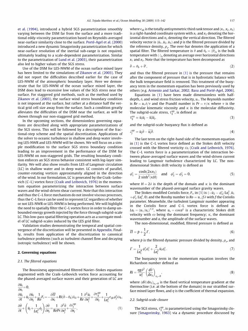
Fig. 5a shows shear (1–3) components of viscous, Reynolds andSGS stress in LES with and without LSC (i.e. without wave effects).In both simulations, the SGS stress is given by the dynamic Smago-rinsky model in (9) and (10). The SGS stress goes to zero at the bot-tom and at the surface of the domain following the behavior of themodel coefficient in (10). At the surface, the viscous shear stressmatches the wind stress thereby transmitting momentum fluxfrom the surface to the interior. Once in the interior, the flux istransmitted by the Reynolds shear stress to depths where viscouseffects are negligible.
Fig. 5b shows mean downwind velocity in LES with and withoutLSC. These mean velocity profiles demonstrate the impact of LSC onthe viscous wall region and the log-layer region. The presence ofLSC disrupts the typical log-law behavior of the mean velocity
n velocity in the lower half of the water column in LES of Langmuir supercells. TheÞRes .

A.E. Tejada-Martínez et al. / Ocean Modelling 30 (2009) 115–142 123
inducing what resembles a law of the wake-like behavior. The lawof the wake in traditional boundary layers has been attributed tolarge-scale turbulent mixing (Coles, 1956). LSC enhances this mix-ing and, as seen in Fig. 5b, generates a large wake region stretchingdown through the would-be log-layer region and into the bufferregion. Note that our LES of the flow without LSC yields a clearlog-law region. Thus, the previously described disruption of thelog-layer in the presence of LSC is strictly due to C–L vortex forcing.
Further evidence of disruption of the log-layer by LSC comesfrom the analysis of turbulent velocity variances measured duringthe LSC event at LEO15 and a more recent event measured at theNavy’s R2 tower on the Goergia shelf (Gargett and Savidge,2008). Both measurements were made under similar wind andwave forcing conditions but different tidal forcing condition. Undera strong tidal current at R2, the near-constancy of the turbulent ki-netic energy (TKE) in the lower third portion of the water columnwas indicative of a bed stress log-layer. However, a similar near-constancy of TKE was noticeably absent from the LEO15 LSC event,characterized by a much weaker tidal current. This non-constancyof TKE was also the case in our LES of LSC guided by the LEO15measurements (Tejada-Martı́nez and Grosch, 2007).
4.2. Unstratified Ekman layer
In this subsection we present results from LES-NWM of anunstratified, surface wind-driven Ekman layer. We will focus onthe performance of the dynamic Smagorinsky parametrization in(9)–(12) and the Smagorinsky parametrization based on similarityin (9) and (17) (henceforth referred to as the Smagorinsky–Masonparametrization).
The computational domain for the Ekman layer is taken to beL1 ¼ d long in the downwind direction and L2 ¼ d wide in the cross-wind direction, following the simulation of Zikanov et al. (2003)(see Fig. 1b). In the vertical direction the domain extends from 0to 2d, thus the dimensionless vertical coordinate extends fromx3=d ¼ 0 to x3=d ¼ 2. The grid consists of ð32� 32� 129Þ points.A hyperbolic stretching function is employed in order to clustermore grid points near the surface (around x3 ¼ 2d) where velocitygradients are expected to be strongest. With this stretching, at thebottom of the domain the grid cell aspect ratio is D3=D1 � 0:75varying down to D3=D1 � 0:2 at the surface, where Di is the gridspacing in the ith direction. We have excluded the C–L vortex termappearing in the momentum equation, thereby excluding wave ef-fects, and the Rossby number is Ro ¼ 1.
The downwind ðx1Þ and crosswind ðx2Þ directions are homoge-neous, thus periodic boundary conditions are taken in these direc-tions. At the bottom of the Ekman layer ðx3 ¼ 0Þ, we impose zeronormal velocity, that is fu3gx3¼0 ¼ 0 and zero tangential stress, that is
�ssgsd13
n ox3¼0¼ 0 and �ssgsd
23
n ox3¼0¼ 0: ð30Þ
At the surface ðx3 ¼ 2dÞ, we impose zero normal velocity (i.e.fu3gx3¼2d ¼ 0). Furthermore, the 1–3 component of the SGS stressis set equal to a specified wind stress, ss � qou2
s in the x1 direction,while the 2–3 component of the SGS stress is set equal to zero. Indimensionless form these conditions become
�ssgsd13
n ox3¼2d
¼ 1 and �ssgsd23
n ox3¼2d
¼ 0: ð31Þ
Note that the simulation methodology chosen is LES-NWM forwhich the SGS stress matches the surface stress prescribed at theboundaries. This is in contrast to the LES-NWR of LSC described ear-lier, in which the molecular viscous stress matches the surfacestress at the surface and the SGS stress decays to zero.
For all Ekman layer simulations (stratified and unstratified),regardless of the SGS model (dynamic Smagorinsky or Smagorin-
sky–Mason), we resort to similarity theory to impose control ofthe solution at the surface together with explicit use of Eq. (9). Fol-lowing similarity theory (reviewed by Lewis (2005)) and the sur-face boundary condition �u3 ¼ 0 applied to Eq. (9), at the surface
ssgsd13
n ox3¼2d
� ðCsDÞ2x3¼2d
d�u1
dx3
� �2
x3¼2d
; ð32Þ
As noted by Eq. (31), ssgsd13 ¼ 1 at the surface. Using this condition
with Eq. (32) mentioned above, we may solve for d�u1=dx3 at thesurface:
d�u1
dx3
� �x3¼2d
¼ 1ðCsDÞx3¼2d
; ð33Þ
where ðCsDÞx3¼2d is obtained by evaluating the similarity equation in(17) at the surface ðz ¼ 0Þ. The remaining boundary conditions onsolution derivatives are taken as d�u2=dx3 ¼ 0 at the surface andd�u1=dx3 ¼ d�u2=dx3 ¼ 0 at the bottom which also follow from theboundary conditions on ssgsd
ij appearing in Eqs. (30) and (31) andthe use of (9).
Following Zikanov et al. (2003) we employ the followingdecomposition of the instantaneous velocity �ui:
�ui ¼ Uiðx3; tÞ þ �u0i; ð34Þ
where Ui ¼ h�uii and h�i denotes averaging over the horizontal(homogeneous) directions (x1 and x2) (i.e. the horizontal average).The instantaneous bulk velocity is defined as
Ubi ðtÞ ¼
12
Z x3¼2d
x3¼0Uiðx3; tÞdx3: ð35Þ
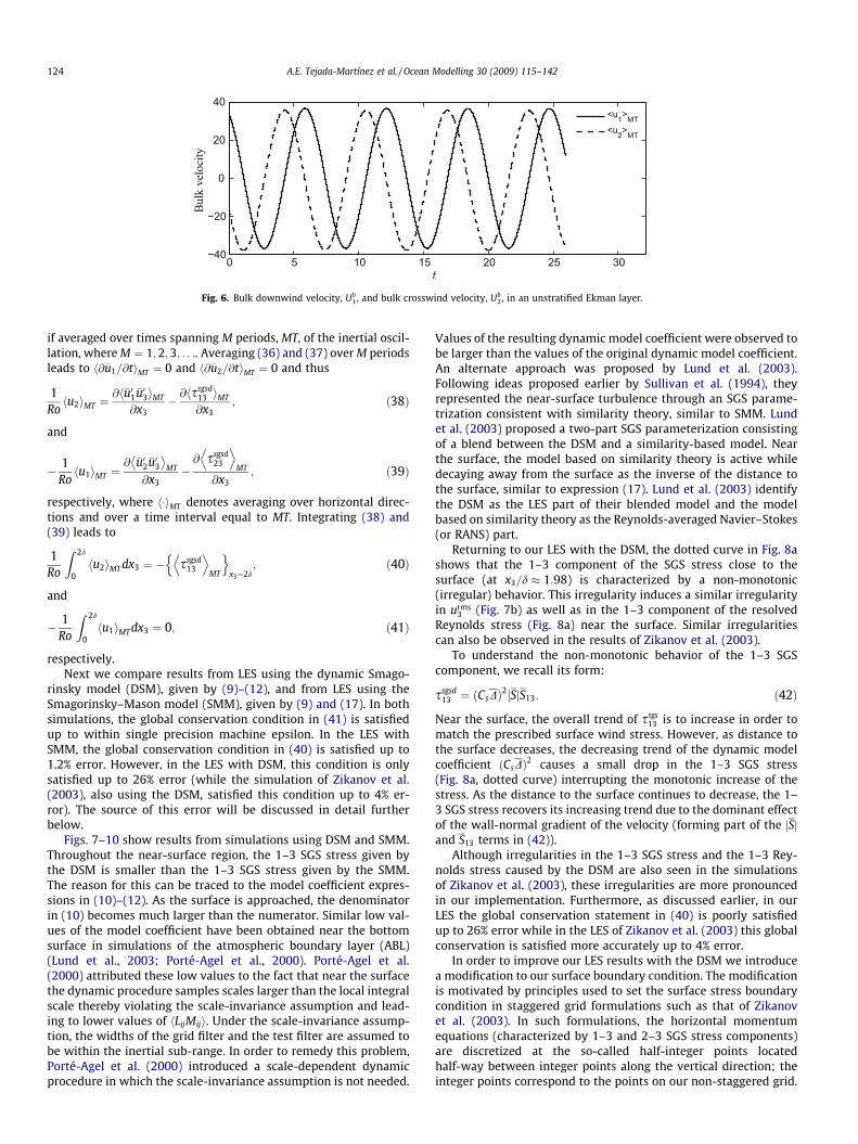
Fig. 6 shows the x1 and x2 bulk velocity components during our sim-ulation. These components exhibit the undamped oscillation dis-cussed by Lewis and Belcher (2004). Lewis and Belcheranalytically solved the unsteady, linearized, wind-driven, finite-depth Ekman layer equations with constant eddy-viscosity. Notethat their eddy-viscosity parameterizes all of the turbulence andis not the same as the eddy-viscosity in our LES. They solved twoseparate problems each characterized by different boundary condi-tions at the bottom of the domain: (1) @u1=@x3 ¼ @u2=@x3 ¼ 0 atx3 ¼ 0 and (2) u1 ¼ u2 ¼ 0 at x3 ¼ 0. The first condition is the sameas in our simulation. Condition (2) leads to solutions composed of asteady-state component plus a damped temporal oscillatory com-ponent. As the name suggests, the damped component decays intime, thus eventually the solution becomes purely steady. Condition(1) leads to a solution composed of a steady-state component plusan undamped temporal oscillatory component. This undamped, theso-called, inertial oscillation remains part of the solution for alltimes, a characteristic exhibited by our numerical solution inFig. 6. The undamped oscillations in Ub
1 and Ub2 have a period of
2pRo consistent with the non-dimensionalized version of the solu-tion of Lewis and Belcher (2004) (Eq. (17), page 322 of their paper).Furthermore, Ub
1 and Ub2 are out of phase with each other by p=2,
consistent with the result of Lewis and Belcher (2004).Taking the horizontal average of the x1 and x2 momentum equa-
tions in (1) excluding the buoyancy force and the C–L vortex force(i.e. letting Lat ¼ 1) and letting Re ¼ 1 leads to
@U1
@t¼ � @h
�u01�u03i@x3
þ @hssgsd13 i
@x3þ 1
RoU2; ð36Þ
and
@U2
@t¼ � @h
�u02�u03i@x3
þ @hssgsd23 i
@x3� 1
RoU1; ð37Þ
respectively, where h�u0i�u0ji is the instantaneous resolved Reynoldsstress. The flow under consideration is steady in a statistical sense
0 5 10 15 20 25 30−40
−20
0
20
40<u1>MT<u2>MT
Fig. 6. Bulk downwind velocity, Ub1, and bulk crosswind velocity, Ub
2, in an unstratified Ekman layer.
124 A.E. Tejada-Martínez et al. / Ocean Modelling 30 (2009) 115–142
if averaged over times spanning M periods, MT, of the inertial oscil-lation, where M ¼ 1;2;3; . . .. Averaging (36) and (37) over M periodsleads to h@�u1=@tiMT ¼ 0 and h@�u2=@tiMT ¼ 0 and thus
1Rohu2iMT ¼
@h�u01�u03iMT
@x3� @hs
sgsd13 iMT
@x3; ð38Þ
and
� 1Rohu1iMT ¼
@ �u02�u03� �
MT
@x3�@ ssgsd
23
D EMT
@x3; ð39Þ
respectively, where h�iMT denotes averaging over horizontal direc-tions and over a time interval equal to MT. Integrating (38) and(39) leads to
1Ro
Z 2d
0u2h iMT dx3 ¼ � ssgsd
13
D EMT
n ox3¼2d
; ð40Þ
and
� 1Ro
Z 2d
0hu1iMT dx3 ¼ 0; ð41Þ
respectively.Next we compare results from LES using the dynamic Smago-
rinsky model (DSM), given by (9)–(12), and from LES using theSmagorinsky–Mason model (SMM), given by (9) and (17). In bothsimulations, the global conservation condition in (41) is satisfiedup to within single precision machine epsilon. In the LES withSMM, the global conservation condition in (40) is satisfied up to1.2% error. However, in the LES with DSM, this condition is onlysatisfied up to 26% error (while the simulation of Zikanov et al.(2003), also using the DSM, satisfied this condition up to 4% er-ror). The source of this error will be discussed in detail furtherbelow.
Figs. 7–10 show results from simulations using DSM and SMM.Throughout the near-surface region, the 1–3 SGS stress given bythe DSM is smaller than the 1–3 SGS stress given by the SMM.The reason for this can be traced to the model coefficient expres-sions in (10)–(12). As the surface is approached, the denominatorin (10) becomes much larger than the numerator. Similar low val-ues of the model coefficient have been obtained near the bottomsurface in simulations of the atmospheric boundary layer (ABL)(Lund et al., 2003; Porté-Agel et al., 2000). Porté-Agel et al.(2000) attributed these low values to the fact that near the surfacethe dynamic procedure samples scales larger than the local integralscale thereby violating the scale-invariance assumption and lead-ing to lower values of hLijMiji. Under the scale-invariance assump-tion, the widths of the grid filter and the test filter are assumed tobe within the inertial sub-range. In order to remedy this problem,Porté-Agel et al. (2000) introduced a scale-dependent dynamicprocedure in which the scale-invariance assumption is not needed.
Values of the resulting dynamic model coefficient were observed tobe larger than the values of the original dynamic model coefficient.An alternate approach was proposed by Lund et al. (2003).Following ideas proposed earlier by Sullivan et al. (1994), theyrepresented the near-surface turbulence through an SGS parame-trization consistent with similarity theory, similar to SMM. Lundet al. (2003) proposed a two-part SGS parameterization consistingof a blend between the DSM and a similarity-based model. Nearthe surface, the model based on similarity theory is active whiledecaying away from the surface as the inverse of the distance tothe surface, similar to expression (17). Lund et al. (2003) identifythe DSM as the LES part of their blended model and the modelbased on similarity theory as the Reynolds-averaged Navier–Stokes(or RANS) part.
Returning to our LES with the DSM, the dotted curve in Fig. 8ashows that the 1–3 component of the SGS stress close to thesurface (at x3=d � 1:98) is characterized by a non-monotonic(irregular) behavior. This irregularity induces a similar irregularityin urms
3 (Fig. 7b) as well as in the 1–3 component of the resolvedReynolds stress (Fig. 8a) near the surface. Similar irregularitiescan also be observed in the results of Zikanov et al. (2003).
To understand the non-monotonic behavior of the 1–3 SGScomponent, we recall its form:
ssgsd13 ¼ ðCsDÞ2jSjS13: ð42Þ
Near the surface, the overall trend of ssgs13 is to increase in order to
match the prescribed surface wind stress. However, as distance tothe surface decreases, the decreasing trend of the dynamic modelcoefficient ðCsDÞ2 causes a small drop in the 1–3 SGS stress(Fig. 8a, dotted curve) interrupting the monotonic increase of thestress. As the distance to the surface continues to decrease, the 1–3 SGS stress recovers its increasing trend due to the dominant effectof the wall-normal gradient of the velocity (forming part of the jSjand S13 terms in (42)).
Although irregularities in the 1–3 SGS stress and the 1–3 Rey-nolds stress caused by the DSM are also seen in the simulationsof Zikanov et al. (2003), these irregularities are more pronouncedin our implementation. Furthermore, as discussed earlier, in ourLES the global conservation statement in (40) is poorly satisfiedup to 26% error while in the LES of Zikanov et al. (2003) this globalconservation is satisfied more accurately up to 4% error.
In order to improve our LES results with the DSM we introducea modification to our surface boundary condition. The modificationis motivated by principles used to set the surface stress boundarycondition in staggered grid formulations such as that of Zikanovet al. (2003). In such formulations, the horizontal momentumequations (characterized by 1–3 and 2–3 SGS stress components)are discretized at the so-called half-integer points locatedhalf-way between integer points along the vertical direction; theinteger points correspond to the points on our non-staggered grid.

Fig. 7. (a) Mean velocity and (b) components of root mean square (rms) of velocity in unstratified Ekman layer. Time averaging was performed over M = 5 periods of inertialoscillation.
A.E. Tejada-Martínez et al. / Ocean Modelling 30 (2009) 115–142 125
More precisely, the horizontal momentum equations are nevertreated at the surface; instead they are treated at locations Dz=2below the surface, where Dz is the vertical distance between thesurface and the first horizontal plane of grid (or integer) points be-low the surface. Thus, the boundary conditions on the 1–3 and 2–3SGS stress components in (31) are assigned at a distance Dz=2 be-low the surface. This implies a constant stress layer spanning theregion between the surface and the first plane of half integer pointsbelow the surface. This is consistent with the fact that the simula-tion does not resolve the inner layer surface region, but rather onlyresolves up to the log-layer region where the 1–3 stress is nearlyconstant and equal to the surface stress (Pope, 2000). Analogously,we postulate a similar constant stress layer in our LES, and the 1–3stress boundary condition in (31) is prescribed at the surface and atthe first horizontal plane of grid points below the surface in a Rey-nolds-average sense. The dimensionless, prescribed 1–3 SGS stressis obtained form:
�h�u01�u03ih þ ssgsd13 ¼ 1; ð43Þ
where h�u01�u03ih denotes averaging the instantaneous quantity �u01�u03over horizontal directions x1 and x2. Note that on the surfaceh�u01�u03ih ¼ 0, thus ssgsd
13 ¼ 1 just as in Eq. (31). On the horizontal planeof grid points below the surface ssgsd
13 ¼ 1þ h�u01�u03ih. The effect of this
modification (denoted as BC2 in the figure legends) greatly im-proves results relative to the original boundary condition (denotedas BC1) in which the SGS stress is prescribed only at the surface.Figs. 9 and 10 compare results between the LES with BC1 and theLES with BC2. Irregularities present in the 1–3 SGS stress, 1–3 Rey-nolds stress and urms
3 predicted in LES-BC1 are less pronounced thanthose in LES-BC2. Overall, the results obtained from LES-BC2 are incloser agreement with those obtained in LES of Zikanov et al.(2003). For example, the peak value of the 1–3 Reynolds stressand the mean crosswind velocity at the surface are closer to thosepresented by Zikanov et al. (2003).
In LES-BC2, the global conservation statement in (40) is satisfiedup to within less than 5% in close agreement with the 4% reportedin the LES of Zikanov et al. (2003). Recall that this error in LES-BC1is much greater at 26%. As described earlier, nonlinear terms in themomentum equation are discretized in time with the second-orderAdams–Bashforth scheme (AB2), which is unconditionally unstablefor the treatment of a pure convective equation. Thus the error inEq. (40) may be associated with instability of the AB2 scheme trig-gered by low values of the SGS stress. We have implemented thethird-order Runge–Kutta (RK3) scheme described by Garg et al.(1997) (replacing the AB2 scheme) and tested it in LES-BC2.Unlike AB2, RK3 can be conditionally stable for a purely convectiveequation. The new simulation with RK3 was performed with the
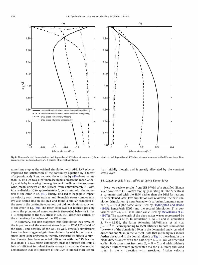
Fig. 8. Near-surface (a) downwind-vertical Reynolds and SGS shear stresses and (b) crosswind-vertical Reynolds and SGS shear stresses in an unstratified Ekman layer. Timeaveraging was performed over M = 5 periods of inertial oscillation.
126 A.E. Tejada-Martínez et al. / Ocean Modelling 30 (2009) 115–142
same time step as the original simulation with AB2. RK3 schemeimproved the satisfaction of the continuity equation by a factorof approximately 3 and reduced the error in Eq. (40) down to lessthan 1%. RK3 led to a slight increase in bulk crosswind mean veloc-ity mainly by increasing the magnitude of the dimensionless cross-wind mean velocity at the surface from approximately 5 (withAdams–Bashforth) to approximately 6, consistent with the reduc-tion of the error in Eq. (40). Finally, RK3 led to negligible impacton velocity root mean squares and Reynolds stress components.We also tested RK3 in LES-BC1 and found a similar reduction ofthe error in the continuity equation, but did not obtain a reductionof the error in Eq. (40). The latter error was not reduced possiblydue to the pronounced non-monotonic (irregular) behavior in the1–3 component of the SGS stress in LES-BC1, described earlier, orthe excessively low values of the SGS stress.
In summary, our non-staggered grid formulation has revealedthe importance of the constant stress layer in DSM LES-NWM ofthe UOML and possibly of the ABL as well. Previous simulationshave involved staggered grid formulations for which the constantstress layer is the only choice, thereby obscuring its effects. A num-ber of researchers have reported difficulties with the DSM leadingto a small 1–3 SGS stress component near the surface and thus alack of sufficient turbulent kinetic energy dissipation. Our resultsdemonstrate that this problem of the DSM is indeed more severe
than initially thought and is greatly alleviated by the constantstress layer.
4.3. Langmuir cells in a stratified turbulent Ekman layer
Here we review results from LES-NWM of a stratified Ekmanlayer flows with C–L vortex forcing generating LC. The SGS stressis parameterized with the SMM rather than the DSM for reasonsto be explained later. Two simulations are reviewed. The first sim-ulation (simulation 1) is performed with turbulent Langmuir num-ber Lat ¼ 0:334 (the same value used by Skyllingstad and Denbo(1995); henceforth SD95) and the second (simulation 2) is per-formed with Lat ¼ 0:3 (the same value used by McWilliams et al.(1997)). The wavelength of the deep water waves represented bythe C–L force is 60 m. In simulation 1, Ro ¼ 1 and in simulation2, Ro ¼ 1:3556, the latter following McWilliams et al. (i.e.f ¼ 10�4 s�1, corresponding to 45N latitude). In both simulationsthe extent of the domain is 150 m in the downwind and crosswinddirections and 90 m in the vertical. Note that in the figures shownfurther ahead and in the domain sketch of Fig. 1c these lengths aremade dimensionless with the half-depth ðd ¼ 45 mÞ, as describedearlier. Both cases start from rest ð�ui ¼ P ¼ 0Þ and with suddenlyimposed surface waves (represented via the C–L force) and windstress in the x1 direction with associated friction velocity
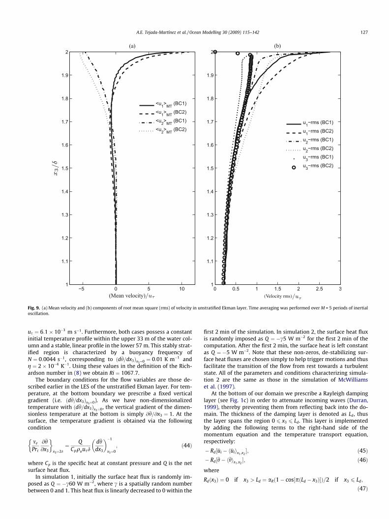
Fig. 9. (a) Mean velocity and (b) components of root mean square (rms) of velocity in unstratified Ekman layer. Time averaging was performed over M = 5 periods of inertialoscillation.
A.E. Tejada-Martínez et al. / Ocean Modelling 30 (2009) 115–142 127
us ¼ 6:1� 10�3 m s�1. Furthermore, both cases possess a constantinitial temperature profile within the upper 33 m of the water col-umn and a stable, linear profile in the lower 57 m. This stably strat-ified region is characterized by a buoyancy frequency ofN ¼ 0:0044 s�1, corresponding to ðd�h=dx3Þx3¼0 ¼ 0:01 K m�1 andg ¼ 2� 10�4 K�1. Using these values in the definition of the Rich-ardson number in (8) we obtain Ri ¼ 1067:7.
The boundary conditions for the flow variables are those de-scribed earlier in the LES of the unstratified Ekman layer. For tem-perature, at the bottom boundary we prescribe a fixed verticalgradient (i.e. ðd�h=dx3Þx3¼0). As we have non-dimensionalizedtemperature with ðd�h=dx3Þx3¼0, the vertical gradient of the dimen-sionless temperature at the bottom is simply @�h=@x3 ¼ 1. At thesurface, the temperature gradient is obtained via the followingcondition
me
Prt
@�h@x3
� x3¼2d
¼ QCpqousd
d�hdx3
� ��1
x3¼0; ð44Þ
where Cp is the specific heat at constant pressure and Q is the netsurface heat flux.
In simulation 1, initially the surface heat flux is randomly im-posed as Q ¼ �c60 W m�2, where c is a spatially random numberbetween 0 and 1. This heat flux is linearly decreased to 0 within the
first 2 min of the simulation. In simulation 2, the surface heat fluxis randomly imposed as Q ¼ �c5 W m�2 for the first 2 min of thecomputation. After the first 2 min, the surface heat is left constantas Q ¼ �5 W m�2. Note that these non-zeros, de-stabilizing sur-face heat fluxes are chosen simply to help trigger motions and thusfacilitate the transition of the flow from rest towards a turbulentstate. All of the parameters and conditions characterizing simula-tion 2 are the same as those in the simulation of McWilliamset al. (1997).
At the bottom of our domain we prescribe a Rayleigh dampinglayer (see Fig. 1c) in order to attenuate incoming waves (Durran,1999), thereby preventing them from reflecting back into the do-main. The thickness of the damping layer is denoted as Ld, thusthe layer spans the region 0 6 x3 6 Ld. This layer is implementedby adding the following terms to the right-hand side of themomentum equation and the temperature transport equation,respectively:
� Rd½�ui � h�uiix1 ;x2; ð45Þ
� Rd½�h� h�hix1 ;x2; ð46Þ
where
Rdðx3Þ ¼ 0 if x3 > Ld ¼ aRð1� cos½pðLd � x3ÞÞ=2 if x3 6 Ld;
ð47Þ
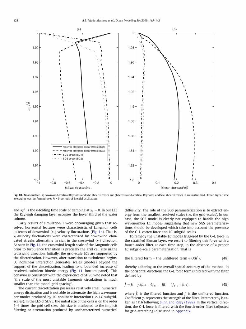
Fig. 10. Near-surface (a) downwind-vertical Reynolds and SGS shear stresses and (b) crosswind-vertical Reynolds and SGS shear stresses in an unstratified Ekman layer. Timeaveraging was performed over M = 5 periods of inertial oscillation.
128 A.E. Tejada-Martínez et al. / Ocean Modelling 30 (2009) 115–142
and a�1R is the e-folding time scale of damping at x3 ¼ 0. In our LES
the Rayleigh damping layer occupies the lower third of the watercolumn.
Early results of simulation 1 were encouraging given that re-solved horizontal features were characteristic of Langmuir cellsin terms of downwind ðx1Þ velocity fluctuations (Fig. 14). That is,x1-velocity fluctuations were characterized by downwind elon-gated streaks alternating in sign in the crosswind ðx2Þ direction.As seen in Fig. 14, the crosswind length scale of the Langmuir cellsprior to turbulence transition is precisely the grid cell size in thecrosswind direction. Initially, the grid-scale LCs are supported bythe discretization. However, after transition to turbulence begins,LC nonlinear interaction generates scales (modes) beyond thesupport of the discretization, leading to unbounded increase ofresolved turbulent kinetic energy (Fig. 11, bottom panel). Thisbehavior is consistent with the experience of SD95 who noted that‘‘the scale of the most unstable Langmuir circulations is muchsmaller than the model grid spacing”.
The current discretization possesses relatively small numericalenergy dissipation and is not able to attenuate the high wavenum-ber modes produced by LC nonlinear interaction (i.e. LC subgrid-scales). In the LES of SD95, the initial size of the cells is on the order5–6 times the grid cell size; this size is attributed to the implicitfiltering or attenuation produced by uncharacterized numerical
diffusivity. The role of the SGS parameterization is to extract en-ergy from the smallest resolved scales (i.e. the grid-scales). In ourcase, the SGS model is clearly not equipped to handle the highwavenumber LC modes suggesting that new SGS parameteriza-tions should be developed which take into account the presenceof the C–L vortex force and LC subgrid-scales.
To remedy the unstable LC modes triggered by the C–L force inthe stratified Ekman layer, we resort to filtering this force with afourth-order filter at each time step, in the absence of a properLC subgrid-scale parameterization. That is
the filtered term ¼ the unfiltered termþ Oðh4Þ; ð48Þ
thereby adhering to the overall spatial accuracy of the method. Inthe horizontal directions the C–L force term is filtered with the filterdefined by
~f ¼ fi � cf ðfiþ2 � 4f iþ1 þ 6f i � 4f i�1 þ fi�2Þ; ð49Þ
where ~f i is the filtered function and fi is the unfiltered function.Coefficient cf represents the strength of the filter. Parameter cf is ta-ken as 1/16 following Slinn and Riley (1998). In the vertical direc-tion, the C–L force is filtered with the fourth-order filter (adjustedfor grid-stretching) discussed in Appendix.

Fig. 11. Time history of turbulent kinetic energy components at x3=d ¼ 1:886 in a stratified Ekman layer (simulation 1) (a) with and (b) without explicit filtering of the vortexforce. Surface is at x3=d ¼ 2.
A.E. Tejada-Martínez et al. / Ocean Modelling 30 (2009) 115–142 129
The effectiveness of filtering the C–L force term can be seen inFig. 11(top) as velocity fluctuations do not grow unbounded anddo approach a statistically steady state after transition from rest.Additionally, we observe that the characteristic horizontal size ofthe initial Langmuir cells is about two times larger in the simula-tion with the filtered C–L force (Fig. 15) than in the simulation withthe unfiltered force (Fig. 14). Ultimately, the coherence of the ini-tial cells breaks down as a Langmuir turbulent state is reached(see Figs. 15–17). Once the cells reach the base of the mixed layer,they interact with the thermocline leading to internal wave activ-ity. Recently Polton et al. (2008) analyzed in detail the resultinginternal wave field in our simulations and found that high-fre-quency internal waves drain energy and momentum from theUOML over decay timescales comparable to the inertial oscillation.
Our results indicate that we may control the smallest Langmuirscales resolved in the computation via explicit filtering of the C–Lforce. This is a desirable attribute given that the unfiltered forceleads to Langmuir scales of the same size as the grid. Scales of thissize are greatly susceptible to aliasing and truncation errors andthus are poorly resolved. In traditional turbulent flows, small scaleson the order of the grid size are not very energetic, thus their poorresolution does not greatly jeopardize the resolved large scales.However, this is not the case in Langmuir turbulence, as untreated(unfiltered) nonlinear interaction between Langmuir small scalesserves to produce scales (modes) beyond the support of the dis-
cretization, which can lead to numerical instability. Generally ithas proven difficult to compare the growth of Langmuir cells incomputations with field observations as the growth and initial sizeof Langmuir cells can be strongly affected by numerical diffusivity(e.g. truncation errors) (see SD95) and also aliasing. In the LES ofSD95, the initial size of the Langmuir cells is on the order 5–6 timesthe grid cell size; according to Skyllingstad and Denbo, the exactdependence of this size on numerical diffusivity is not known. Fil-tering of the C–L force presents an explicit way of controlling thesize of the cells, and thus may pave the way for a future study ofthe growth of Langmuir cells without the uncertainties and ad-verse effects of numerical errors.
After transition towards a statistically steady state is achievedin simulation 1 (with filtered C–L force and Lat ¼ 0:334) averagesrequired for various statistical quantities are collected. These aver-ages are taken over five inertial periods. A similar transition is alsoobserved in simulation 2 (with filtered C–L force and Lat ¼ 0:3).Averages over five inertial periods are also collected after a statis-tical steady state is reached. Various statistical quantities areshown in Figs. 12 and 13. An increase in the amplitude of the sur-face waves leads to a decrease in Lat . In the simulation with lowerLat (simulation 2), the strength of the cells is greater, leading to amore homogeneous mean downwind velocity and stronger verticalvelocity fluctuations. Recall that simulation 2 is performed withthe same parameters as those in the simulation of McWilliams
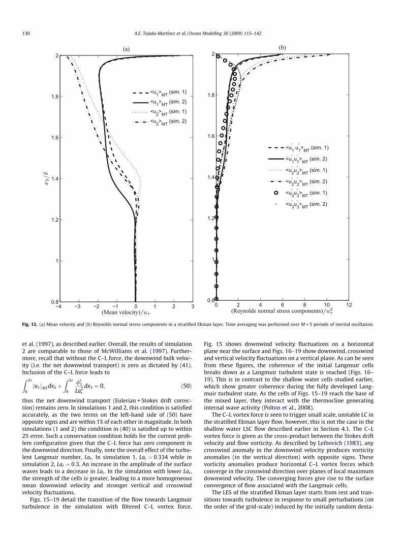
Fig. 12. (a) Mean velocity and (b) Reynolds normal stress components in a stratified Ekman layer. Time averaging was performed over M = 5 periods of inertial oscillation.
130 A.E. Tejada-Martínez et al. / Ocean Modelling 30 (2009) 115–142
et al. (1997), as described earlier. Overall, the results of simulation2 are comparable to those of McWilliams et al. (1997). Further-more, recall that without the C–L force, the downwind bulk veloc-ity (i.e. the net downwind transport) is zero as dictated by (41).Inclusion of the C–L force leads toZ 2d
0hu1iMT dx3 þ
Z 2d
0
/s1
La2t
dx3 ¼ 0; ð50Þ
thus the net downwind transport (Eulerian + Stokes drift correc-tion) remains zero. In simulations 1 and 2, this condition is satisfiedaccurately, as the two terms on the left-hand side of (50) haveopposite signs and are within 1% of each other in magnitude. In bothsimulations (1 and 2) the condition in (40) is satisfied up to within2% error. Such a conservation condition holds for the current prob-lem configuration given that the C–L force has zero component inthe downwind direction. Finally, note the overall effect of the turbu-lent Langmuir number, Lat . In simulation 1, Lat ¼ 0:334 while insimulation 2, Lat ¼ 0:3. An increase in the amplitude of the surfacewaves leads to a decrease in Lat . In the simulation with lower Lat ,the strength of the cells is greater, leading to a more homogeneousmean downwind velocity and stronger vertical and crosswindvelocity fluctuations.
Figs. 15–19 detail the transition of the flow towards Langmuirturbulence in the simulation with filtered C–L vortex force.
Fig. 15 shows downwind velocity fluctuations on a horizontalplane near the surface and Figs. 16–19 show downwind, crosswindand vertical velocity fluctuations on a vertical plane. As can be seenfrom these figures, the coherence of the initial Langmuir cellsbreaks down as a Langmuir turbulent state is reached (Figs. 16–19). This is in contrast to the shallow water cells studied earlier,which show greater coherence during the fully developed Lang-muir turbulent state. As the cells of Figs. 15–19 reach the base ofthe mixed layer, they interact with the thermocline generatinginternal wave activity (Polton et al., 2008).
The C–L vortex force is seen to trigger small scale, unstable LC inthe stratified Ekman layer flow, however, this is not the case in theshallow water LSC flow described earlier in Section 4.1. The C–Lvortex force is given as the cross-product between the Stokes driftvelocity and flow vorticity. As described by Leibovich (1983), anycrosswind anomaly in the downwind velocity produces vorticityanomalies (in the vertical direction) with opposite signs. Thesevorticity anomalies produce horizontal C–L vortex forces whichconverge in the crosswind direction over planes of local maximumdownwind velocity. The converging forces give rise to the surfaceconvergence of flow associated with the Langmuir cells.
The LES of the stratified Ekman layer starts from rest and tran-sitions towards turbulence in response to small perturbations (onthe order of the grid-scale) induced by the initially random desta-
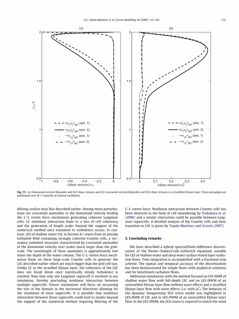
Fig. 13. (a) Downwind-vertical Reynolds and SGS shear stresses and (b) crosswind-vertical Reynolds and SGS shear stresses in a stratified Ekman layer. Time averaging wasperformed over M = 5 periods of inertial oscillation.
A.E. Tejada-Martínez et al. / Ocean Modelling 30 (2009) 115–142 131
bilizing surface heat flux described earlier. Among these perturba-tions are crosswind anomalies in the downwind velocity feedingthe C–L vortex force mechanism generating coherent Langmuircells. LC nonlinear interaction leads to a loss of cell coherencyand the generation of length scales beyond the support of thenumerical method once transition to turbulence occurs. In con-trast, LES of shallow water LSC in Section 4.1 starts from an alreadyturbulent field containing strongly coherent Couette cells, a sec-ondary turbulent structure characterized by crosswind anomaliesof the downwind velocity over scales much larger than the grid-scale. The wavelength of these anomalies is approximately twotimes the depth of the water column. The C–L vortex force mech-anism feeds on these large-scale Couette cells to generate theLSC described earlier which are much bigger than the grid cell size.Unlike LC in the stratified Ekman layer, the coherence of the LSCdoes not break down once statistically steady turbulence isreached. Note that only one Langmuir supercell is resolved in oursimulation, thereby precluding nonlinear interaction betweenmultiple supercells. Future simulations will focus on increasingthe size of the domain in the horizontal directions allowing forthe resolution of more supercells. It is possible that nonlinearinteraction between these supercells could lead to modes beyondthe support of the numerical method requiring filtering of the
C–L vortex force. Nonlinear interaction between Couette cells hasbeen observed in the form of cell meandering by Tsukahara et al.(2006) and a similar interaction could be possible between Lang-muir supercells. A detailed analysis of the Couette cells and theirtransition to LSC is given by Tejada-Martı́nez and Grosch (2007).
5. Concluding remarks
We have described a hybrid spectral/finite-difference discreti-zation of the Navier–Stokes/Craik–Leibovich equations suitablefor LES of shallow water and deep water surface mixed layer turbu-lent flows. Time integration is accomplished with a fractional-stepscheme. The spatial and temporal accuracy of the discretizationhas been demonstrated for simple flows with analytical solutionsand for benchmark turbulent flows.
Additional simulations with the method focused on LES-NWR ofshallow water flow with full-depth LSC and on LES-NWM of anunstratified Ekman layer flow without wave effects and a stratifiedEkman layer flow with wave effects (i.e. with LC). The behavior ofthe dynamic Smagorinsky SGS stress model was highlighted inLES-NWR of LSC and in LES-NWM of an unstratified Ekman layerflow. In the LES-NWM, the SGS stress is required to match the wind
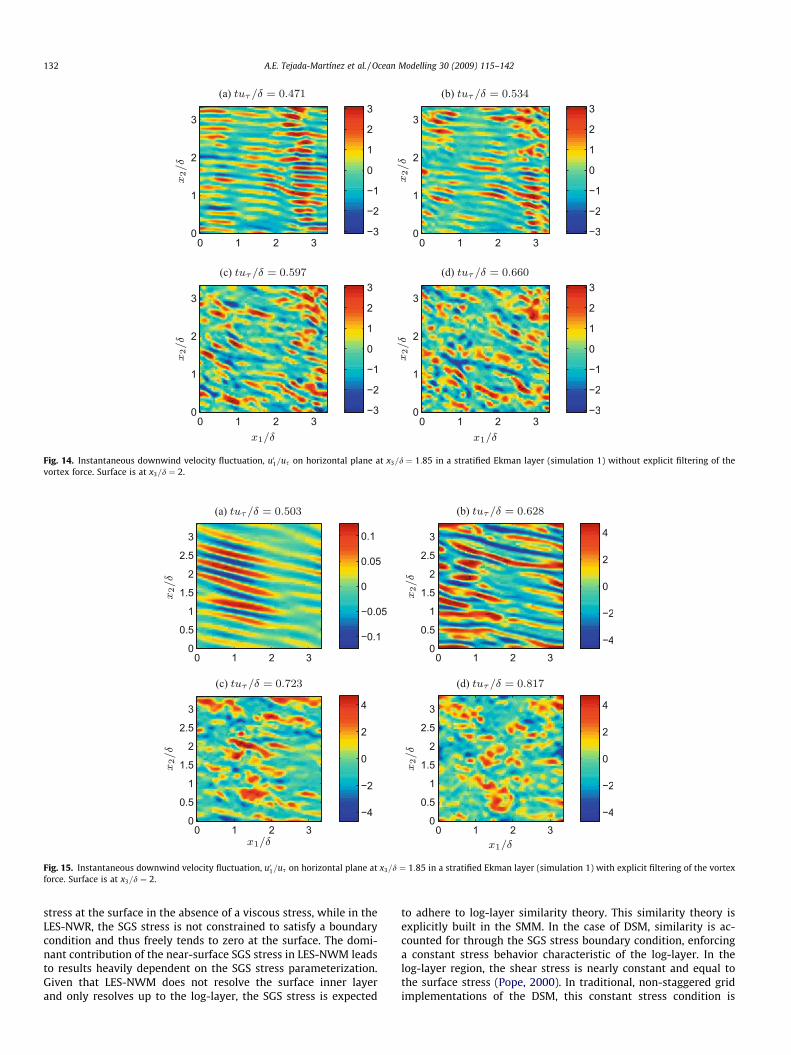
Fig. 14. Instantaneous downwind velocity fluctuation, u01=us on horizontal plane at x3=d ¼ 1:85 in a stratified Ekman layer (simulation 1) without explicit filtering of thevortex force. Surface is at x3=d ¼ 2.
Fig. 15. Instantaneous downwind velocity fluctuation, u01=us on horizontal plane at x3=d ¼ 1:85 in a stratified Ekman layer (simulation 1) with explicit filtering of the vortexforce. Surface is at x3=d ¼ 2.
132 A.E. Tejada-Martínez et al. / Ocean Modelling 30 (2009) 115–142
stress at the surface in the absence of a viscous stress, while in theLES-NWR, the SGS stress is not constrained to satisfy a boundarycondition and thus freely tends to zero at the surface. The domi-nant contribution of the near-surface SGS stress in LES-NWM leadsto results heavily dependent on the SGS stress parameterization.Given that LES-NWM does not resolve the surface inner layerand only resolves up to the log-layer, the SGS stress is expected
to adhere to log-layer similarity theory. This similarity theory isexplicitly built in the SMM. In the case of DSM, similarity is ac-counted for through the SGS stress boundary condition, enforcinga constant stress behavior characteristic of the log-layer. In thelog-layer region, the shear stress is nearly constant and equal tothe surface stress (Pope, 2000). In traditional, non-staggered gridimplementations of the DSM, this constant stress condition is

Fig. 16. Instantaneous velocity fluctuations on vertical plane at x1=d ¼ 10=6 and tus=d ¼ 0:503 (simulation 1) with explicit filtering of the vortex force.
Fig. 17. Instantaneous velocity fluctuations on vertical plane at x1=d ¼ 10=6 and tus=d ¼ 0:628 (simulation 1) with explicit filtering of the vortex force.
A.E. Tejada-Martínez et al. / Ocean Modelling 30 (2009) 115–142 133
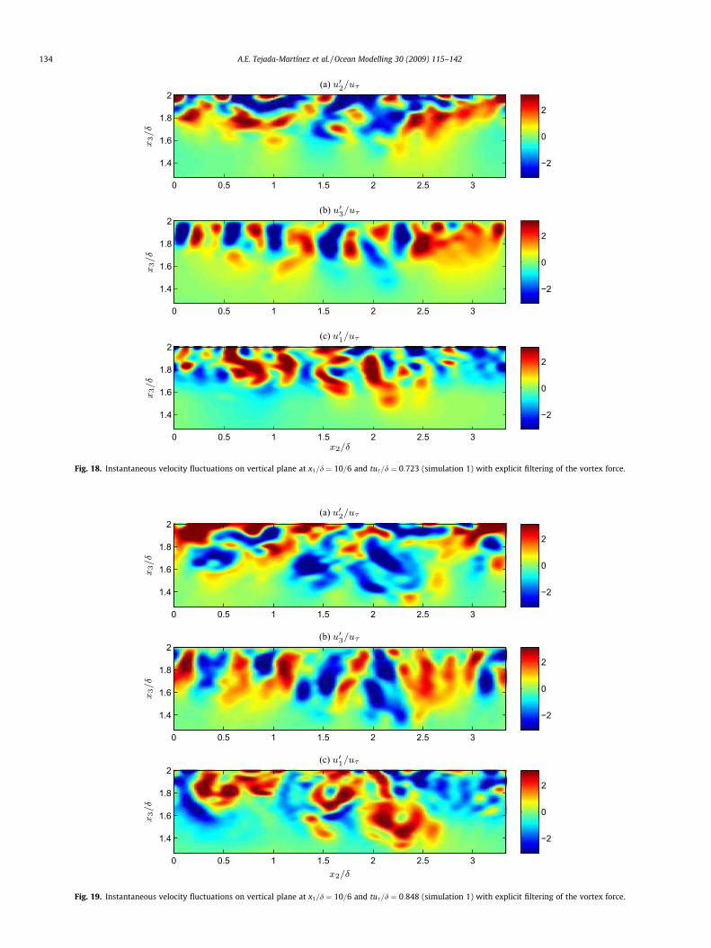
Fig. 18. Instantaneous velocity fluctuations on vertical plane at x1=d ¼ 10=6 and tus=d ¼ 0:723 (simulation 1) with explicit filtering of the vortex force.
Fig. 19. Instantaneous velocity fluctuations on vertical plane at x1=d ¼ 10=6 and tus=d ¼ 0:848 (simulation 1) with explicit filtering of the vortex force.
134 A.E. Tejada-Martínez et al. / Ocean Modelling 30 (2009) 115–142
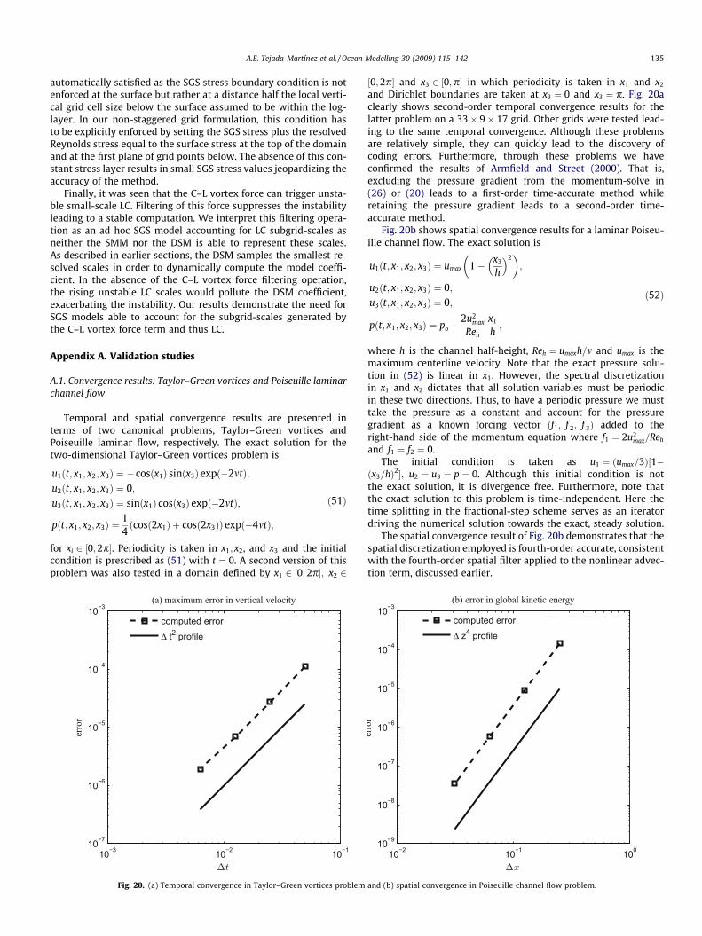
A.E. Tejada-Martínez et al. / Ocean Modelling 30 (2009) 115–142 135
automatically satisfied as the SGS stress boundary condition is notenforced at the surface but rather at a distance half the local verti-cal grid cell size below the surface assumed to be within the log-layer. In our non-staggered grid formulation, this condition hasto be explicitly enforced by setting the SGS stress plus the resolvedReynolds stress equal to the surface stress at the top of the domainand at the first plane of grid points below. The absence of this con-stant stress layer results in small SGS stress values jeopardizing theaccuracy of the method.
Finally, it was seen that the C–L vortex force can trigger unsta-ble small-scale LC. Filtering of this force suppresses the instabilityleading to a stable computation. We interpret this filtering opera-tion as an ad hoc SGS model accounting for LC subgrid-scales asneither the SMM nor the DSM is able to represent these scales.As described in earlier sections, the DSM samples the smallest re-solved scales in order to dynamically compute the model coeffi-cient. In the absence of the C–L vortex force filtering operation,the rising unstable LC scales would pollute the DSM coefficient,exacerbating the instability. Our results demonstrate the need forSGS models able to account for the subgrid-scales generated bythe C–L vortex force term and thus LC.
Appendix A. Validation studies
A.1. Convergence results: Taylor–Green vortices and Poiseuille laminarchannel flow
Temporal and spatial convergence results are presented interms of two canonical problems, Taylor–Green vortices andPoiseuille laminar flow, respectively. The exact solution for thetwo-dimensional Taylor–Green vortices problem is
u1ðt; x1; x2; x3Þ ¼ � cosðx1Þ sinðx3Þ expð�2mtÞ;u2ðt; x1; x2; x3Þ ¼ 0;u3ðt; x1; x2; x3Þ ¼ sinðx1Þ cosðx3Þ expð�2mtÞ;
pðt; x1; x2; x3Þ ¼14
cosð2x1Þ þ cosð2x3Þð Þ expð�4mtÞ;
ð51Þ
for xi 2 ½0;2p. Periodicity is taken in x1; x2, and x3 and the initialcondition is prescribed as (51) with t ¼ 0. A second version of thisproblem was also tested in a domain defined by x1 2 ½0;2p; x2 2
Fig. 20. (a) Temporal convergence in Taylor–Green vortices problem
½0;2p and x3 2 ½0;p in which periodicity is taken in x1 and x2
and Dirichlet boundaries are taken at x3 ¼ 0 and x3 ¼ p. Fig. 20aclearly shows second-order temporal convergence results for thelatter problem on a 33� 9� 17 grid. Other grids were tested lead-ing to the same temporal convergence. Although these problemsare relatively simple, they can quickly lead to the discovery ofcoding errors. Furthermore, through these problems we haveconfirmed the results of Armfield and Street (2000). That is,excluding the pressure gradient from the momentum-solve in(26) or (20) leads to a first-order time-accurate method whileretaining the pressure gradient leads to a second-order time-accurate method.
Fig. 20b shows spatial convergence results for a laminar Poiseu-ille channel flow. The exact solution is
u1ðt; x1; x2; x3Þ ¼ umax 1� x3
h
� 2� �
;
u2ðt; x1; x2; x3Þ ¼ 0;u3ðt; x1; x2; x3Þ ¼ 0;
pðt; x1; x2; x3Þ ¼ po �2u2
max
Reh
x1
h;
ð52Þ
where h is the channel half-height, Reh ¼ umaxh=m and umax is themaximum centerline velocity. Note that the exact pressure solu-tion in (52) is linear in x1. However, the spectral discretizationin x1 and x2 dictates that all solution variables must be periodicin these two directions. Thus, to have a periodic pressure we musttake the pressure as a constant and account for the pressuregradient as a known forcing vector ðf1; f 2; f 3Þ added to theright-hand side of the momentum equation where f1 ¼ 2u2
max=Reh
and f1 ¼ f2 ¼ 0.The initial condition is taken as u1 ¼ ðumax=3Þ½1�
ðx3=hÞ2; u2 ¼ u3 ¼ p ¼ 0. Although this initial condition is notthe exact solution, it is divergence free. Furthermore, note thatthe exact solution to this problem is time-independent. Here thetime splitting in the fractional-step scheme serves as an iteratordriving the numerical solution towards the exact, steady solution.
The spatial convergence result of Fig. 20b demonstrates that thespatial discretization employed is fourth-order accurate, consistentwith the fourth-order spatial filter applied to the nonlinear advec-tion term, discussed earlier.
and (b) spatial convergence in Poiseuille channel flow problem.
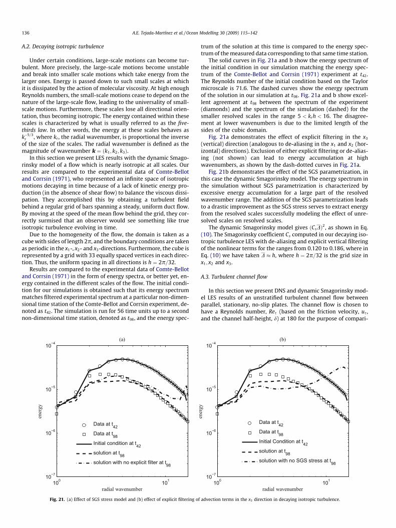
136 A.E. Tejada-Martínez et al. / Ocean Modelling 30 (2009) 115–142
A.2. Decaying isotropic turbulence
Under certain conditions, large-scale motions can become tur-bulent. More precisely, the large-scale motions become unstableand break into smaller scale motions which take energy from thelarger ones. Energy is passed down to such small scales at whichit is dissipated by the action of molecular viscosity. At high enoughReynolds numbers, the small-scale motions cease to depend on thenature of the large-scale flow, leading to the universality of small-scale motions. Furthermore, these scales lose all directional orien-tation, thus becoming isotropic. The energy contained within thesescales is characterized by what is usually referred to as the five-thirds law. In other words, the energy at these scales behaves ask�5=3
r , where kr , the radial wavenumber, is proportional the inverseof the size of the scales. The radial wavenumber is defined as themagnitude of wavenumber k ¼ ðk1; k2; k3Þ.
In this section we present LES results with the dynamic Smago-rinsky model of a flow which is nearly isotropic at all scales. Ourresults are compared to the experimental data of Comte-Bellotand Corrsin (1971), who represented an infinite space of isotropicmotions decaying in time because of a lack of kinetic energy pro-duction (in the absence of shear flow) to balance the viscous dissi-pation. They accomplished this by obtaining a turbulent fieldbehind a regular grid of bars spanning a steady, uniform duct flow.By moving at the speed of the mean flow behind the grid, they cor-rectly surmised that an observer would see something like trueisotropic turbulence evolving in time.
Due to the homogeneity of the flow, the domain is taken as acube with sides of length 2p, and the boundary conditions are takenas periodic in the x1-, x2- and x3-directions. Furthermore, the cube isrepresented by a grid with 33 equally spaced vertices in each direc-tion. Thus, the uniform spacing in all directions is h ¼ 2p=32.
Results are compared to the experimental data of Comte-Bellotand Corrsin (1971) in the form of energy spectra, or better yet, en-ergy contained in the different scales of the flow. The initial condi-tion for our simulations is obtained such that its energy spectrummatches filtered experimental spectrum at a particular non-dimen-sional time station of the Comte-Bellot and Corrsin experiment, de-noted as t42. The simulation is run for 56 time units up to a secondnon-dimensional time station, denoted as t98, and the energy spec-
Fig. 21. (a) Effect of SGS stress model and (b) effect of explicit filtering of
trum of the solution at this time is compared to the energy spec-trum of the measured data corresponding to that same time station.
The solid curves in Fig. 21a and b show the energy spectrum ofthe initial condition in our simulation matching the energy spec-trum of the Comte-Bellot and Corrsin (1971) experiment at t42.The Reynolds number of the initial condition based on the Taylormicroscale is 71.6. The dashed curves show the energy spectrumof the solution in our simulation at t98. Fig. 21a and b show excel-lent agreement at t98 between the spectrum of the experiment(diamonds) and the spectrum of the simulation (dashed) for thesmaller resolved scales in the range 5 < krh < 16. The disagree-ment at lower wavenumbers is due to the limited length of thesides of the cubic domain.
Fig. 21a demonstrates the effect of explicit filtering in the x3
(vertical) direction (analogous to de-aliasing in the x1 and x2 (hor-izontal) directions). Exclusion of either explicit filtering or de-alias-ing (not shown) can lead to energy accumulation at highwavenumbers, as shown by the dash-dotted curves in Fig. 21a.
Fig. 21b demonstrates the effect of the SGS parametrization, inthis case the dynamic Smagorinsky model. The energy spectrum inthe simulation without SGS parametrization is characterized byexcessive energy accumulation for a large part of the resolvedwavenumber range. The addition of the SGS parametrization leadsto a drastic improvement as the SGS stress serves to extract energyfrom the resolved scales successfully modeling the effect of unre-solved scales on resolved scales.
The dynamic Smagorinsky model gives ðCsDÞ2, as shown in Eq.(10). The Smagorinsky coefficient Cs computed in our decaying iso-tropic turbulence LES with de-aliasing and explicit vertical filteringof the nonlinear terms for the ranges from 0.120 to 0.186, where inEq. (10) we have taken D � h, where h ¼ 2p=32 is the grid size inx1; x2 and x3.
A.3. Turbulent channel flow
In this section we present DNS and dynamic Smagorinsky mod-el LES results of an unstratified turbulent channel flow betweenparallel, stationary, no-slip plates. The channel flow is chosen tohave a Reynolds number, Res (based on the friction velocity, us,and the channel half-height, d) at 180 for the purpose of compari-
advection terms in the x3 direction in decaying isotropic turbulence.
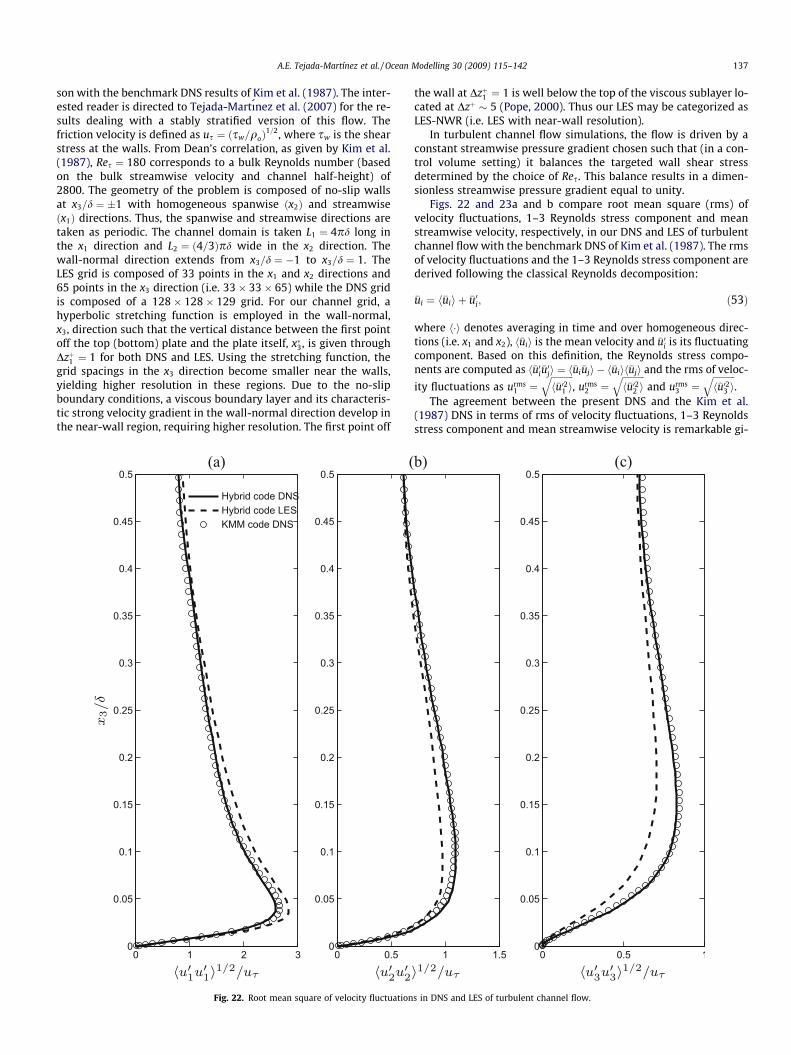
A.E. Tejada-Martínez et al. / Ocean Modelling 30 (2009) 115–142 137
son with the benchmark DNS results of Kim et al. (1987). The inter-ested reader is directed to Tejada-Martı́nez et al. (2007) for the re-sults dealing with a stably stratified version of this flow. Thefriction velocity is defined as us ¼ ðsw=qoÞ
1=2, where sw is the shearstress at the walls. From Dean’s correlation, as given by Kim et al.(1987), Res ¼ 180 corresponds to a bulk Reynolds number (basedon the bulk streamwise velocity and channel half-height) of2800. The geometry of the problem is composed of no-slip wallsat x3=d ¼ �1 with homogeneous spanwise ðx2Þ and streamwiseðx1Þ directions. Thus, the spanwise and streamwise directions aretaken as periodic. The channel domain is taken L1 ¼ 4pd long inthe x1 direction and L2 ¼ ð4=3Þpd wide in the x2 direction. Thewall-normal direction extends from x3=d ¼ �1 to x3=d ¼ 1. TheLES grid is composed of 33 points in the x1 and x2 directions and65 points in the x3 direction (i.e. 33� 33� 65) while the DNS gridis composed of a 128� 128� 129 grid. For our channel grid, ahyperbolic stretching function is employed in the wall-normal,x3, direction such that the vertical distance between the first pointoff the top (bottom) plate and the plate itself, x�3, is given throughDzþ1 ¼ 1 for both DNS and LES. Using the stretching function, thegrid spacings in the x3 direction become smaller near the walls,yielding higher resolution in these regions. Due to the no-slipboundary conditions, a viscous boundary layer and its characteris-tic strong velocity gradient in the wall-normal direction develop inthe near-wall region, requiring higher resolution. The first point off
Fig. 22. Root mean square of velocity fluctuation
the wall at Dzþ1 ¼ 1 is well below the top of the viscous sublayer lo-cated at Dzþ � 5 (Pope, 2000). Thus our LES may be categorized asLES-NWR (i.e. LES with near-wall resolution).
In turbulent channel flow simulations, the flow is driven by aconstant streamwise pressure gradient chosen such that (in a con-trol volume setting) it balances the targeted wall shear stressdetermined by the choice of Res. This balance results in a dimen-sionless streamwise pressure gradient equal to unity.
Figs. 22 and 23a and b compare root mean square (rms) ofvelocity fluctuations, 1–3 Reynolds stress component and meanstreamwise velocity, respectively, in our DNS and LES of turbulentchannel flow with the benchmark DNS of Kim et al. (1987). The rmsof velocity fluctuations and the 1–3 Reynolds stress component arederived following the classical Reynolds decomposition:
�ui ¼ h�uii þ �u0i; ð53Þ
where h�i denotes averaging in time and over homogeneous direc-tions (i.e. x1 and x2), h�uii is the mean velocity and �u0i is its fluctuatingcomponent. Based on this definition, the Reynolds stress compo-nents are computed as h�u0i�u0ji ¼ h�ui�uji � h�uiih�uji and the rms of veloc-
ity fluctuations as urms1 ¼
ffiffiffiffiffiffiffiffiffiffih�u021 i
q, urms
2 ¼ffiffiffiffiffiffiffiffiffiffih�u022 i
qand urms
3 ¼ffiffiffiffiffiffiffiffiffiffih�u023 i
q.
The agreement between the present DNS and the Kim et al.(1987) DNS in terms of rms of velocity fluctuations, 1–3 Reynoldsstress component and mean streamwise velocity is remarkable gi-
s in DNS and LES of turbulent channel flow.
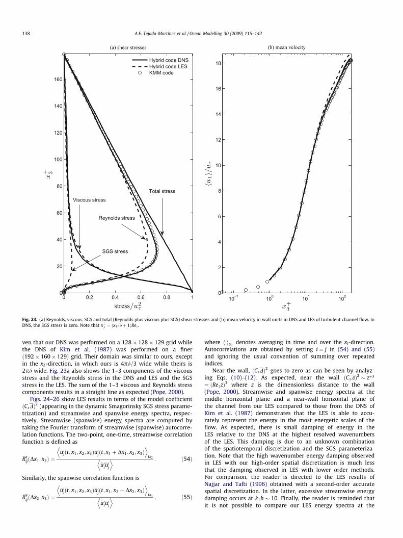
Fig. 23. (a) Reynolds, viscous, SGS and total (Reynolds plus viscous plus SGS) shear stresses and (b) mean velocity in wall units in DNS and LES of turbulent channel flow. InDNS, the SGS stress is zero. Note that xþ3 ¼ ðx3=dþ 1ÞRes .
138 A.E. Tejada-Martínez et al. / Ocean Modelling 30 (2009) 115–142
ven that our DNS was performed on a 128� 128� 129 grid whilethe DNS of Kim et al. (1987) was performed on a finerð192� 160� 129Þ grid. Their domain was similar to ours, exceptin the x2-direction, in which ours is 4pd=3 wide while theirs is2pd wide. Fig. 23a also shows the 1–3 components of the viscousstress and the Reynolds stress in the DNS and LES and the SGSstress in the LES. The sum of the 1–3 viscous and Reynolds stresscomponents results in a straight line as expected (Pope, 2000).
Figs. 24–26 show LES results in terms of the model coefficientðCsDÞ2 (appearing in the dynamic Smagorinsky SGS stress parame-trization) and streamwise and spanwise energy spectra, respec-tively. Streamwise (spanwise) energy spectra are computed bytaking the Fourier transform of streamwise (spanwise) autocorre-lation functions. The two-point, one-time, streamwise correlationfunction is defined as
RxijðDx1; x3Þ ¼
�u0iðt; x1; x2; x3Þ�u0jðt; x1 þ Dx1; x2; x3ÞD E
tx2
�u0i�u0j
D E : ð54Þ
Similarly, the spanwise correlation function is
RyijðDx2; x3Þ ¼
�u0iðt; x1; x2; x3Þ�u0jðt; x1; x2 þ Dx2; x3ÞD E
tx1
�u0i�u0j
D E ; ð55Þ
where h�itxidenotes averaging in time and over the xi-direction.
Autocorrelations are obtained by setting i ¼ j in (54) and (55)and ignoring the usual convention of summing over repeatedindices.
Near the wall, ðCsDÞ2 goes to zero as can be seen by analyz-ing Eqs. (10)–(12). As expected, near the wall ðCsDÞ2 � zþ3
¼ ðReszÞ3 where z is the dimensionless distance to the wall(Pope, 2000). Streamwise and spanwise energy spectra at themiddle horizontal plane and a near-wall horizontal plane ofthe channel from our LES compared to those from the DNS ofKim et al. (1987) demonstrates that the LES is able to accu-rately represent the energy in the most energetic scales of theflow. As expected, there is small damping of energy in theLES relative to the DNS at the highest resolved wavenumbersof the LES. This damping is due to an unknown combinationof the spatiotemporal discretization and the SGS parameteriza-tion. Note that the high wavenumber energy damping observedin LES with our high-order spatial discretization is much lessthat the damping observed in LES with lower order methods.For comparison, the reader is directed to the LES results ofNajjar and Tafti (1996) obtained with a second-order accuratespatial discretization. In the latter, excessive streamwise energydamping occurs at k1h � 10. Finally, the reader is reminded thatit is not possible to compare our LES energy spectra at the

Fig. 24. Mean dynamic coefficient, hC2s D
2i, in LES of turbulent channel flow.
Fig. 25. Streamwise one-dimensional energy spectra in LES of turbulent channel flow.
A.E. Tejada-Martínez et al. / Ocean Modelling 30 (2009) 115–142 139
same near-wall locations as those of Kim et al. (1987) due todifferent grids between our LES and their DNS. As a result,LES energy spectra in terms of wall-normal fluctuations atzþ ¼ 4:75 are lower than the DNS counterpart at zþ ¼ 5:34 forall wavenumbers resolved in the LES.
Appendix B. Finite-difference stencils
Most of the description of the finite-difference stencils appearsin Tejada-Martı́nez and Grosch (2007). We present it here forcompleteness.
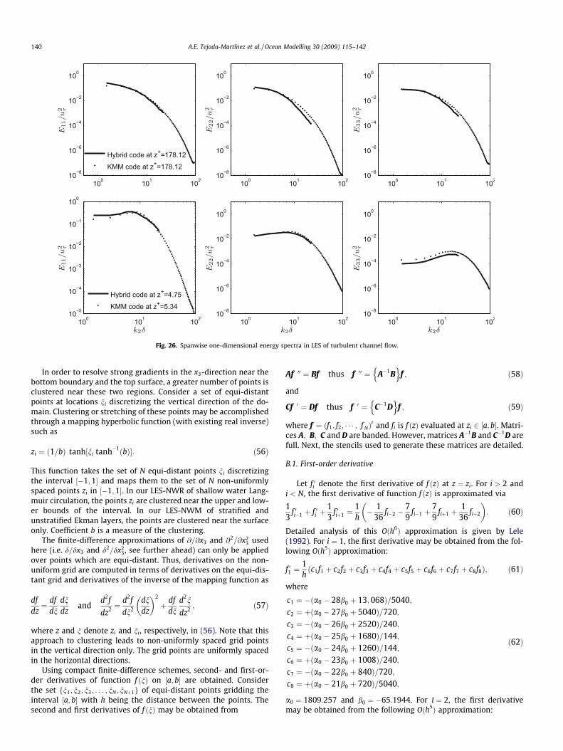
Fig. 26. Spanwise one-dimensional energy spectra in LES of turbulent channel flow.
140 A.E. Tejada-Martínez et al. / Ocean Modelling 30 (2009) 115–142
In order to resolve strong gradients in the x3-direction near thebottom boundary and the top surface, a greater number of points isclustered near these two regions. Consider a set of equi-distantpoints at locations ni discretizing the vertical direction of the do-main. Clustering or stretching of these points may be accomplishedthrough a mapping hyperbolic function (with existing real inverse)such as
zi ¼ ð1=bÞ tanh½ni tanh�1ðbÞ: ð56Þ
This function takes the set of N equi-distant points ni discretizingthe interval ½�1;1 and maps them to the set of N non-uniformlyspaced points zi in ½�1;1. In our LES-NWR of shallow water Lang-muir circulation, the points zi are clustered near the upper and low-er bounds of the interval. In our LES-NWM of stratified andunstratified Ekman layers, the points are clustered near the surfaceonly. Coefficient b is a measure of the clustering.
The finite-difference approximations of @=@x3 and @2=@x23 used
here (i.e. d=dx3 and d2=dx23, see further ahead) can only be applied
over points which are equi-distant. Thus, derivatives on the non-uniform grid are computed in terms of derivatives on the equi-dis-tant grid and derivatives of the inverse of the mapping function as
dfdz¼ df
dndndz
andd2f
dz2 ¼d2f
dn2
dndz
� �2
þ dfdn
d2n
dz2 ; ð57Þ
where z and n denote zi and ni, respectively, in (56). Note that thisapproach to clustering leads to non-uniformly spaced grid pointsin the vertical direction only. The grid points are uniformly spacedin the horizontal directions.
Using compact finite-difference schemes, second- and first-or-der derivatives of function f ðnÞ on ½a; b are obtained. Considerthe set fn1; n2; n3; . . . ; nN; nNþ1g of equi-distant points gridding theinterval ½a; b with h being the distance between the points. Thesecond and first derivatives of f ðnÞ may be obtained from
Af 00 ¼ Bf thus f 00 ¼ A�1Bn o
f ; ð58Þ
and
Cf 0 ¼ Df thus f 0 ¼ C�1Dn o
f ; ð59Þ
where f ¼ ðf1; f2; � � � ; f NÞt and fi is f ðzÞ evaluated at zi 2 ½a; b. Matri-
ces A; B; C and D are banded. However, matrices A�1B and C�1D arefull. Next, the stencils used to generate these matrices are detailed.
B.1. First-order derivative
Let f 0i denote the first derivative of f ðzÞ at z ¼ zi. For i > 2 andi < N, the first derivative of function f ðzÞ is approximated via
13
f 0i�1 þ f 0i þ13
f 0iþ1 ¼1h� 1
36fi�2 �
79
fi�1 þ79
fiþ1 þ1
36fiþ2
� �: ð60Þ
Detailed analysis of this Oðh6Þ approximation is given by Lele(1992). For i ¼ 1, the first derivative may be obtained from the fol-lowing Oðh5Þ approximation:
f 01 ¼1h
c1f1 þ c2f2 þ c3f3 þ c4f4 þ c5f5 þ c6f6 þ c7f7 þ c8f8ð Þ; ð61Þ
where
c1 ¼ �ða0 � 28b0 þ 13; 068Þ=5040;c2 ¼ þða0 � 27b0 þ 5040Þ=720;c3 ¼ �ða0 � 26b0 þ 2520Þ=240;c4 ¼ þða0 � 25b0 þ 1680Þ=144;c5 ¼ �ða0 � 24b0 þ 1260Þ=144;c6 ¼ þða0 � 23b0 þ 1008Þ=240;c7 ¼ �ða0 � 22b0 þ 840Þ=720;c8 ¼ þða0 � 21b0 þ 720Þ=5040;
ð62Þ
a0 ¼ 1809:257 and b0 ¼ �65:1944. For i ¼ 2, the first derivativemay be obtained from the following Oðh5Þ approximation:
A.E. Tejada-Martínez et al. / Ocean Modelling 30 (2009) 115–142 141
f 02 ¼1h
d1f1 þ d2f2 þ d3f3 þ d4f4 þ d5f5 þ d6f6 þ d7f7 þ d8f8ð Þ; ð63Þ
where
d1 ¼ �ða1 � 21b1 þ 720Þ=5040;d2 ¼ þða1 � 20b1 � 1044Þ=720;d3 ¼ �ða1 � 19b1 � 720Þ=240;d4 ¼ þða1 � 18b1 � 360Þ=144;d5 ¼ �ða1 � 17b1 � 240Þ=144;d6 ¼ þða1 � 16b1 � 180Þ=240;d7 ¼ �ða1 � 15b1 � 144Þ=720;d8 ¼ þða1 � 14b1 � 120Þ=5040;
ð64Þ
a1 ¼ �262:16 and b1 ¼ �26:6742. Similar expressions for the firstderivatives are defined at i ¼ N and i ¼ N þ 1. The stencils in(61)–(64) are analyzed in detail by Carpenter et al. (1993).
B.2. Alternate first-order derivative
The previously described vertical derivative at i ¼ 1 andi ¼ N þ 1 proved effective for non-zero shear stress and no-slipboundary conditions. However, in the case of the zero shear stressboundary conditions at the bottom of the domain in Ekman layersimulations, this approximation leads to undesired inaccuracies.For example, consider imposing du1=dx3 ¼ 0 at the bottom of thedomain, as is the case for the unstratified and stratified Ekmanlayer simulations. Following the previously described formulation,
du1
dx3¼ du1
dndndx3¼ 0; ð65Þ
where dn=dx3 is the vertical derivative of stretching function nðx3Þwhich maps a set of stretched grid points on x3 to a set of regularlyspaced grid points on n. The derivative du1=dn in (65) mentionedabove is approximated through Eq. (61) valid for a regularly spacedgrid. A major deficiency of the formulation previously described isthat Eq. (65) implies that
du1
dn¼ 0: ð66Þ
Thus, the true zero derivative boundary condition on a stretchedgrid is not imposed and instead is replaced by an erroneous zeroderivative on a regularly spaced grid. A more accurate approxima-tion of the derivative was implemented at the bottom withoutrequiring the stretching function derivative (i.e. dn=dz). A third-or-der accurate expression for the first derivative was implemented,derived via Taylor series expansions taking into consideration thevertical variability of the grid. The vertical derivative of a quantityf (i.e. df=dx3) at the bottom of the domain was taken as
f 01 ¼ �a1f1 � a2f2 � a3f3; ð67Þ
where
a1 ¼ �1=k1; a2 ¼ k2=k1; a3 ¼ k3=k1; ð68Þ
with
k1 ¼�h1h2ðh1 þ h2Þðh1 þ h2Þ2 � h2
1
; k2 ¼ðh1 þ h2Þ2
ðh1 þ h2Þ2 � h21
;
k3 ¼h2
1
ðh1 þ h2Þ2 � h21
: ð69Þ
In the previous expression h1 is the vertical distance between thefirst two grid points starting at the bottom, and so on. A similarexpression for df=dx3 at the surface was also implemented for con-sistency. Although the previous approximation of the first-orderderivative is third-order accurate, it is well known that boundary
stencils may be one order less than interior stencils without degrad-ing the overall spatial accuracy of the interior scheme (e.g. see Kre-iss, 1972). Our interior scheme is fourth-order accurate, as wasshown in the validation studies and is described further in theupcoming subsection.
B.3. Second-order derivative
For i > 2 and i < N, the second derivative of function f ðzÞ iscomputed using the following Oðh6Þ approximation discussed byLele (1992):
211
f 0i�1þ f 0i þ2
11f 0iþ1¼
1
h2
344
fi�2þ1211
fi�1�5122
fiþ1211
fiþ1þ3
44fiþ2
� �:
ð70Þ
For i ¼ 1, the second derivative may be obtained from the followingOðh5Þ approximation:
f 001 ¼1
h2 c1f1 þ c2f2 þ c3f3 þ c4f4 þ c5f5 þ c6f6 þ c7f7 þ c8f8ð Þ; ð71Þ
where c1 ¼ 5:211; c2 ¼ �22:300; c3 ¼ 43:950; c4 ¼ �52:722; c5 ¼41:000; c6 ¼ �20:100; c7 ¼ 5:661 and c8 ¼ �0:700. For i ¼ 2, thesecond derivative may be obtained from the following Oðh5Þapproximation:
f 002 ¼1
h2 d1f1 þ d2f2 þ d3f3 þ d4f4 þ d5f5 þ d6f6 þ d7f7 þ d8f8ð Þ; ð72Þ
where d1 ¼ 0:700; d2 ¼ �0:389; d3 ¼ �2:700; d4 ¼ 4:750; d5 ¼�3:722; d6 ¼ 1:800; d7 ¼ �0:500 and d8 ¼ 0:061. Similar expres-sions for the second derivatives are defined at i ¼ N and i ¼ N þ 1.The stencils in (71) and (72) are courtesy of Jackson (University ofIllinois at Urbana-Champaign, personal communication) and maybe derived using a similar approach to that of Carpenter et al.(1993).
When solving Poisson’s equation for pressure in (28), the fol-lowing alternate expressions are used (instead of (71) and (72))leading to lower round-off errors. For i ¼ 1
f 001 ¼ �1h
4910
f 01
þ 1
h2
13;4891800
f1 þ 12f 2 �152
f3 þ409
f4 �158
f5 þ1225
f6 �1
18f7
� �;
ð73Þ
with truncation error 0:6572h6d8f=dz8. Note that the Neumannpressure boundary condition in (28) is assigned through the firstterm on the right-hand side of (73). For i ¼ 2,
11128
f 00i�1 þ f 00i þ11
128f 00iþ1
¼ 1
h2
585512
f1 �14164
f2 þ459512
f3 þ9
32f4 �
85512
f5 þ3
64f6 �
3512
f7
� �;
ð74Þ
with truncation error 0:02101h6d8f=dz8. Similar expressions areused for i ¼ N þ 1 and i ¼ N. The approximations in (73) and (74)and their corresponding truncation errors were derived via Taylorseries analysis.
B.4. Spatial filtering of advection terms
As discussed earlier, the advection terms in the momentumequations are spatially filtered in the vertical direction at each timestep in order to damp out scales of motion unresolvable by thegrid. The following fourth-order compact filter adapted for a non-uniform grid (Slinn and Riley, 1998) is used:
142 A.E. Tejada-Martínez et al. / Ocean Modelling 30 (2009) 115–142
0:4~f i�1 þ ~f i þ 0:4~f iþ1
¼ 0:4f i�1 þ fi þ 0:4f iþ1 �1
80ðfiþ2 � 4f iþ1 þ 6f i � 4f i�1 þ fi�2Þ
� h80
6c2ðziÞc2
1ðziÞ
� �fiþ2 � 2f iþ1 þ 2f i�1 � fi�2
2
� �� h2
804c3ðziÞc3
1ðziÞþ 3c2
2ðziÞc4
1ðziÞ
� �ðfiþ1 � 2f i þ ui�1Þ
� h3
80c4ðziÞc4
1ðziÞ
� �fiþ1 � fi�1
2
� �; ð75Þ
where c1 ¼ @n=@z; c2 ¼ @2n=@z2; c3 ¼ @
3n=@z3 and c4 ¼ @4n=@z4 and
n is a mapping function in (56). Note that this stencil is not valid forpoints at the bottom and top boundaries and for the first two hor-izontal planes of points off from these boundaries. In the currentimplementation the filter is not applied at these points. This omis-sion does not have a negative impact on the results.
A formal derivation of this compact filter can be made throughTaylor series analysis. From this analysis one can see that the fil-tered function is an approximation of the unfiltered function upto fourth-order. That is
~f ¼ f þ Oðh4Þ: ð76Þ
The finite-difference approximations of the first and second deriva-tives in the vertical ðx3Þ direction (discussed in the previous subsec-tion) introduce an error of Oðh5Þ or higher. Filtering the advectionterms in the vertical direction using (75) introduces an error ofOðh4Þ. Furthermore, using a spectral discretization in the horizontal(x1 and x2) directions introduces an error of much higher order thanthe previously discussed finite differencing and filtering operations.Thus, the current spatial discretization is at least of Oðh4Þ. A higherorder filter could potentially be introduced, however, this would in-volve a more expensive computation at the expense of only mini-mally changing results.
References
Armenio, V., Sarkar, S., 2002. An investigation of stably stratified turbulent channelflow using large-eddy simulation. J. Fluid Mech. 459, 1–42.
Armfield, S.W., Street, R., 2000. Fractional step methods for the Navier–Stokesequations on non-staggered grids. ANZIAM J. 42, C134–C156.
Basu, S., Porté-Agel, F., 2006. Large-eddy simulation of stably stratified atmosphericboundary layer turbulence: a scale-dependent dynamic modeling approach. J.Atmos. Sci. 63, 2074–2091.
Beare, R.J., MacVean, M.K., Holtslag, A.A.M., Cuxart, J., Esau, I., Golaz, J.C., Jimenez,M.A., Khairoutdinov, M., Kosovic, B., Lewellen, D., Lund, T.S., Lundquist, J.K.,McCabe, A., Moene, A.F., Raasch, N.Y.S., Sullivan, P., 2006. An intercomparison oflarge-eddy simulations of the stable boundary layer. Bound. Layer Meteor. 118,247–272.
Carpenter, M.H., Gotlieb, D., Abarbanel, S., 1993. The stability of numericalboundary treatments for compact high-order finite difference schemes. J.Comput. Phys. 108, 272–292.
Coles, D., 1956. The law of the wake in the turbulent boundary layer. J. Fluid Mech.1, 191–226.
Comte-Bellot, G., Corrsin, S., 1971. Simple Eulerian time correlation of full andnarrow-band velocity signals in grid-generated isotropic turbulence. J. FluidMech. 48, 273–337.
Craik, A.D.D., Leibovich, S., 1976. A rational model for Langmuir circulation. J. FluidMech. 73, 401–426.
Durran, D.R., 1999. Numerical Methods for Wave Equations in Geophysical FluidDynamics. Springer.
Durski, S.M., Glenn, S.M., Haidvogel, D.B., 2004. Vertical mixing schemes in thecoastal ocean: comparison of the level 2.5 Mellor–Yamada scheme with anenhanced version of the K profile parameterization. J. Geophys. Res. 109,C01015.
Fringer, O.B., Armfield, S.W., Street, R.L., 2003. A nonstaggered curvilinear gridpressure correction method applied to interfacial waves. In: 2nd InternationalConference on Heat Transfer, Fluid Mechanics, and Thermodynamics (HEFAT),Victoria Falls, Zambia, Paper F01.
Garg, R.P., Ferziger, J.H., Monismith, S.G., 1997. Hybrid spectral finite differencesimulations of stratified turbulent flows on distributed memory architectures.Int. J. Numer. Methods Fluids 24, 1129–1158.
Gargett, A.E., Wells, J.R., Tejada-Martnez, A.E., Grosch, C.E., 2004. Langmuirsupercells: a mechanism for sediment resuspension and transport in shallowseas. Science 306, 1925–1928.
Gargett, A.E., Wells, J.R., 2007. Langmuir turbulence in shallow water: Part I.Observations. J. Fluid Mech. 576, 27–61.
Gargett, A.E., Savidge, D.K., 2008. The role of Langmuir supercells in seasonallytuned cross-shelf transport of bioactive material. Abstracts, AGU Ocean SciencesMeeting, Orlando, FL.
Germano, M., Piomelli, U., Moin, P., Cabot, W., 1991. A dynamic subgrid-scale eddyviscosity model. Phys. Fluids 3, 1760–1765.
Kim, J., Moin, P., Moser, R., 1987. Turbulence statistics in fully developed channelflow at low Reynolds number. J. Fluid Mech. 177, 133–166.
Kreiss, H.O., 1972. Difference approximations for boundary and eigenvalueproblems for ordinary differential equations. Math. Comput. 26, 605–624.
Lamballais, E., Metais, O., Lesieur, M., 1998. Spectral-dynamic model for large-eddysimulations of turbulent rotating channel flow. Theor. Comput. Fluid Dyn. 12,149–177.
Leibovich, S., 1983. The form and dynamics of Langmuir circulations. Annu. Rev.Fluid Mech. 15, 391–427.
Lele, S.K., 1992. Compact finite difference schemes with spectral-like resolution. J.Comput. Phys. 103, 16–42.
Lewis, D.M., Belcher, S.E., 2004. Time-dependent, coupled, Ekman boundary layersolutions incorporating Stokes drift. Dyn. Atmos. Oceans 37, 313–351.
Lewis, D.M., 2005. A simple model of plankton population dynamics coupled with aLES of the surface mixed layer. J. Theor. Biol. 223, 565–591.
Li, M., Sanford, L., Chao, S.-Y., 2005. Effects of time dependence in unstratified tidalboundary layers: results from large eddy simulations. Estuar. Coast. Shelf Sci.62, 193–204.
Lilly, D.K., 1992. A proposed modification of the Germano subgrid-scale closure.Phys. Fluids 3, 2746–2757.
Lund, T.S., 1997. On the use of discrete filters for large-eddy simulation. In: AnnualResearch Briefs. Center for Turbulence Research, NASA Ames/StanfordUniversity, pp. 83–95.
Lund, T., Poulos, G., Sullivan, P., 2003. LES of an Antarctic stable boundary layerusing dynamic models. In: GEWEX Atmospheric Boundary Layer StudyWorkshop, Palma de Mallorca, Spain.
Mason, P.J., Thomson, D.J., 1992. Stochastic backscatter in large-eddy simulations ofboundary layers. J. Fluid Mech. 242, 51–78.
McWilliams, J.C., Sullivan, P.P., Moeng, C.-H., 1997. Langmuir turbulence in theocean. J. Fluid Mech. 334, 1–30.
Najjar, F.M., Tafti, D.K., 1996. Study of discrete test filters and finite differenceapproximations for the dynamic subgrid-scale stress model. Phys. Fluids 8,1076–1088.
Piomelli, U., Balaras, E., 2002. Wall-layer models for large-eddy simulations. Annu.Rev. Fluid Mech. 34, 349–374.
Polton, J.A., Smith, J.A., MacKinnon, J.A., Tejada-Martnez, A.E., 2008. Rapidgeneration of high-frequency internal waves beneath a wind and wave forcedoceanic surface mixed layer. Geophys. Res. Lett. 35, L13602.
Pope, S.B., 2000. Turbulent Flows. Cambridge University Press.Porté-Agel, F., Meneveau, C., Parlange, M.B., 2000. A scale-dependent dynamic
model for large-eddy simulation: application to a neutral atmosphericboundary layer. J. Fluid Mech. 415, 261–284.
Shih, T.M., Tan, C.H., Hwang, B.C., 1989. Effects of grid staggering on numericalschemes. Int. J. Numer. Methods Fluids 9, 193–212.
Skyllingstad, E.D., Denbo, D.W., 1995. An ocean large-eddy simulation of Langmuircirculations and convection in the surface mixed layer. J. Geophys. Res. 100,8501–8522.
Slinn, D.N., Riley, J.J., 1998. A model for the simulation of turbulent boundary layersin an incompressible stratified flow. J. Comput. Phys. 144, 550–602.
Smagorinsky, J., 1963. General circulation experiments with the primitiveequations. I. The basic experiment. Mon. Weather Rev. 91, 99–164.
Sullivan, P.P., McWilliams, J.C., Moeng, C.-H., 1994. A subgrid-scale model for large-eddy simulation of planetary boundary-layer flows. Bound. Layer Meteor. 71,247–276.
Tejada-Martı́nez, A.E., Grosch, C.E., 2007. Langmuir turbulence in shallow water:Part II. Large-eddy simulation. J. Fluid Mech. 576, 63–108.
Tejada-Martı́nez, A.E., Grosch, C.E., Gatski, T.B., 2007. Temporal large-eddysimulation of unstratified and stratified turbulent channel flows. Int. J. HeatFluid Flow 28, 1244–1261.
Tsukahara, T., Kawamura, H., Shinghai, K., 2006. DNS of turbulent Couette flow withemphasis on the large-scale structure in the core region. J. Turbul. 7, 19.
Winters, K.B., MacKinnon, J.A., Mills, B., 2004. A spectral model for processstudies of rotating density-stratified flows. J. Atmos. Ocean. Technol. 21, 69–94.
Zikanov, O., Slinn, D.N., Dhanak, M.R., 2003. Large-eddy simulations of the wind-induced turbulent Ekman layer. J. Fluid Mech. 495, 343–368.
Copyright © 2022 FDOKUMEN