The Wageningen Lowland Runoff Simulator (WALRUS)
22
Hydrol. Earth Syst. Sci., 18, 4007–4028, 2014 www.hydrol-earth-syst-sci.net/18/4007/2014/ doi:10.5194/hess-18-4007-2014 © Author(s) 2014. CC Attribution 3.0 License. The Wageningen Lowland Runoff Simulator (WALRUS): application to the Hupsel Brook catchment and the Cabauw polder C. C. Brauer, P. J. J. F. Torfs, A. J. Teuling, and R. Uijlenhoet Hydrology and Quantitative Water Management Group, Wageningen University, Wageningen, the Netherlands Correspondence to: C. C. Brauer ([email protected]) Received: 2 January 2014 – Published in Hydrol. Earth Syst. Sci. Discuss.: 12 February 2014 Revised: 28 August 2014 – Accepted: 6 September 2014 – Published: 10 October 2014 Abstract. The Wageningen Lowland Runoff Simulator (WALRUS) is a new parametric (conceptual) rainfall–runoff model which accounts explicitly for processes that are im- portant in lowland areas, such as groundwater-unsaturated zone coupling, wetness-dependent flowroutes, groundwater– surface water feedbacks, and seepage and surface water sup- ply (see companion paper by Brauer et al., 2014). Lowland catchments can be divided into slightly sloping, freely drain- ing catchments and flat polders with controlled water levels. Here, we apply WALRUS to two contrasting Dutch catch- ments: the Hupsel Brook catchment and the Cabauw polder. In both catchments, WALRUS performs well: Nash–Sutcliffe efficiencies obtained after calibration on 1 year of discharge observations are 0.87 for the Hupsel Brook catchment and 0.83 for the Cabauw polder, with values of 0.74 and 0.76 for validation. The model also performs well during floods and droughts and can forecast the effect of control opera- tions. Through the dynamic division between quick and slow flowroutes controlled by a wetness index, temporal and spa- tial variability in groundwater depths can be accounted for, which results in adequate simulation of discharge peaks as well as low flows. The performance of WALRUS is most sen- sitive to the parameter controlling the wetness index and the groundwater reservoir constant, and to a lesser extent to the quickflow reservoir constant. The effects of these three pa- rameters can be identified in the discharge time series, which indicates that the model is not overparameterised (parsimo- nious). Forcing uncertainty was found to have a larger effect on modelled discharge than parameter uncertainty and uncer- tainty in initial conditions. 1 Introduction Lowlands exist all over the world (often in river deltas; Fan et al., 2013). They are generally densely populated and cen- tres of agricultural production, economic activity and trans- portation. Therefore, socio-economic consequences of natu- ral hazards are especially large in these areas. In addition, the lack of topography increases their vulnerability to flooding, climate change, and deterioration of water quality. To mitigate natural and human disasters, hydrological models can be used by water managers as a tool for risk as- sessment and infrastructure design. There is growing aware- ness that for simulation and prediction of water and energy fluxes in lowland areas, models need to account explicitly for the dynamic groundwater table (Alley et al., 2002; Maxwell and Miller, 2005; Kollet and Maxwell, 2006; Bierkens and van den Hurk, 2007; Maxwell and Kollet, 2008). In many modelling approaches, existing models of vertical water movement in the unsaturated zone are coupled to groundwa- ter models which simulate the horizontal flow (e.g. Gilfedder et al., 2012; Zampieri et al., 2012). This approach, however, has clear limitations in flat lowland areas, where the shal- low groundwater table (< 2 m below the surface) often rises to within the unsaturated model domain, or even to the land surface (Appels et al., 2011; Brauer et al., 2011). In addi- tion, surface water networks are generally dense, and sur- face water levels influence drainage fluxes and groundwater levels (Sophocleous and Perkins, 2000). These groundwater– surface water interactions are important in both freely drain- ing catchments and polders. Systems of fully coupled mod- els can be successful in simulating water balances in lowland catchments (e.g. Krause et al., 2007), but may be too com- plex to simulate the discharge dynamics after rainfall events efficiently. Simple, lumped hydrological models with a more Published by Copernicus Publications on behalf of the European Geosciences Union.
-
Upload
khangminh22 -
Category
Documents
-
view
2 -
download
0
Transcript of The Wageningen Lowland Runoff Simulator (WALRUS)

Hydrol. Earth Syst. Sci., 18, 4007–4028, 2014www.hydrol-earth-syst-sci.net/18/4007/2014/doi:10.5194/hess-18-4007-2014© Author(s) 2014. CC Attribution 3.0 License.
The Wageningen Lowland Runoff Simulator (WALRUS):application to the Hupsel Brook catchment and the Cabauw polderC. C. Brauer, P. J. J. F. Torfs, A. J. Teuling, and R. Uijlenhoet
Hydrology and Quantitative Water Management Group, Wageningen University, Wageningen, the Netherlands
Correspondence to:C. C. Brauer ([email protected])
Received: 2 January 2014 – Published in Hydrol. Earth Syst. Sci. Discuss.: 12 February 2014Revised: 28 August 2014 – Accepted: 6 September 2014 – Published: 10 October 2014
Abstract. The Wageningen Lowland Runoff Simulator(WALRUS) is a new parametric (conceptual) rainfall–runoffmodel which accounts explicitly for processes that are im-portant in lowland areas, such as groundwater-unsaturatedzone coupling, wetness-dependent flowroutes, groundwater–surface water feedbacks, and seepage and surface water sup-ply (see companion paper byBrauer et al., 2014). Lowlandcatchments can be divided into slightly sloping, freely drain-ing catchments and flat polders with controlled water levels.Here, we apply WALRUS to two contrasting Dutch catch-ments: the Hupsel Brook catchment and the Cabauw polder.In both catchments, WALRUS performs well: Nash–Sutcliffeefficiencies obtained after calibration on 1 year of dischargeobservations are 0.87 for the Hupsel Brook catchment and0.83 for the Cabauw polder, with values of 0.74 and 0.76for validation. The model also performs well during floodsand droughts and can forecast the effect of control opera-tions. Through the dynamic division between quick and slowflowroutes controlled by a wetness index, temporal and spa-tial variability in groundwater depths can be accounted for,which results in adequate simulation of discharge peaks aswell as low flows. The performance of WALRUS is most sen-sitive to the parameter controlling the wetness index and thegroundwater reservoir constant, and to a lesser extent to thequickflow reservoir constant. The effects of these three pa-rameters can be identified in the discharge time series, whichindicates that the model is not overparameterised (parsimo-nious). Forcing uncertainty was found to have a larger effecton modelled discharge than parameter uncertainty and uncer-tainty in initial conditions.
1 Introduction
Lowlands exist all over the world (often in river deltas;Fanet al., 2013). They are generally densely populated and cen-tres of agricultural production, economic activity and trans-portation. Therefore, socio-economic consequences of natu-ral hazards are especially large in these areas. In addition, thelack of topography increases their vulnerability to flooding,climate change, and deterioration of water quality.
To mitigate natural and human disasters, hydrologicalmodels can be used by water managers as a tool for risk as-sessment and infrastructure design. There is growing aware-ness that for simulation and prediction of water and energyfluxes in lowland areas, models need to account explicitly forthe dynamic groundwater table (Alley et al., 2002; Maxwelland Miller, 2005; Kollet and Maxwell, 2006; Bierkens andvan den Hurk, 2007; Maxwell and Kollet, 2008). In manymodelling approaches, existing models of vertical watermovement in the unsaturated zone are coupled to groundwa-ter models which simulate the horizontal flow (e.g.Gilfedderet al., 2012; Zampieri et al., 2012). This approach, however,has clear limitations in flat lowland areas, where the shal-low groundwater table (< 2 m below the surface) often risesto within the unsaturated model domain, or even to the landsurface (Appels et al., 2011; Brauer et al., 2011). In addi-tion, surface water networks are generally dense, and sur-face water levels influence drainage fluxes and groundwaterlevels (Sophocleous and Perkins, 2000). These groundwater–surface water interactions are important in both freely drain-ing catchments and polders. Systems of fully coupled mod-els can be successful in simulating water balances in lowlandcatchments (e.g.Krause et al., 2007), but may be too com-plex to simulate the discharge dynamics after rainfall eventsefficiently. Simple, lumped hydrological models with a more
Published by Copernicus Publications on behalf of the European Geosciences Union.

4008 C. C. Brauer et al.: Application of WALRUS to two contrasting lowland catchments
traditional structure (i.e. without coupling and feedbacks) of-ten fail to reproduce discharge dynamics in lowland catch-ments (Bormann and Elfert, 2010; Koch et al., 2013). Thus,instead of coupling existing models, hydrological models forapplication in lowland areas should be derived from a con-ceptually sound and strong coupling between groundwaterand the unsaturated zone as well as between groundwater andsurface water.
We developed a rainfall–runoff model for application inlowland areas. This model, the Wageningen Lowland RunoffSimulator (WALRUS), is described in detail in the accom-panying paper (Brauer et al., 2014). The structure of WAL-RUS (see Fig.1) is different from that of traditional lumpedrainfall–runoff models. Firstly, the unsaturated and saturatedzones are tightly coupled, so that any increase in ground-water level automatically leads to a decrease in unsatu-rated zone thickness and vice versa. Secondly, the modelconceptualises the varying contribution of fast flowroutesthrough a wetness-dependent divider (inspired byStrickerand Warmerdam, 1982). Finally, the model explicitly ac-counts for groundwater–surface water interaction through theinclusion of a surface water reservoir, which represents thechannel network. This allows for negative feedbacks on sub-surface flow during peak discharges or as a result of surfacewater supply.
WALRUS consists of three reservoirs: a soil reservoir (in-cluding vadose zone and groundwater), a quickflow reser-voir and a surface water reservoir (Fig.1). At the land sur-face, water is added to the different reservoirs by precipita-tion (P ). A fixed fraction is led to the surface water reservoir(PS). The soil wetness index (W ) determines which fractionof the remaining precipitation percolates slowly through thesoil matrix (PV) and which fraction flows towards the surfacewater via quick flow routes (PQ). Water is removed by evap-otranspiration from the vadose zone (ETV) and surface waterreservoir (ETS). The vadose zone is the upper part of the soilreservoir and extends from the soil surface to the dynamicgroundwater table (dG), including the capillary fringe. Thedryness of the vadose zone is characterised by a single state:the storage deficit (dV), which represents the effective thick-ness of empty pores (or the amount of water necessary to sat-urate the profile). It controls the evapotranspiration reduction(β) and the wetness index (W ). The phreatic groundwater ex-tends from the groundwater depth (dG) downwards, therebyassuming that there is no shallow impermeable soil layerand allowing groundwater to drop below the bottom of thedrainage channels (cD) in dry periods. The groundwater ta-ble responds to changes in the storage deficit and determines,together with the surface water level, groundwater drainageor infiltration of surface water (fGS). All water that does notflow through the soil matrix, passes through the quickflowreservoir to the surface water (fQS). This represents macrop-ore flow through drainpipes, animal burrows and soil cracks,but also local ponding and overland flow. The surface waterreservoir has a lower boundary (the channel bottom;cD), but
Vadose zone
GroundwaterSurfacewater
Quickflow
dG
hS
hQ
dV
dV
aG aS
cD
cW
cV
cG
cQ
fGS
fQS
ETpot
ETVETS
QfXG fXS
P
PS
PV
PQW
β
Figure 1. Overview of the model structure with the five compart-ments: land surface (purple), vadose zone within the soil reservoir(yellow/red hatched), groundwater zone within the soil reservoir(orange), quickflow reservoir (green) and surface water reservoir(blue). Fluxes are black arrows, model parameters brown diamondsand states in the colour of the reservoir they belong to. For a com-plete description of all variables, see TableA and the accompanyingpaper (Brauer et al., 2014). The names of the fluxes are derived fromthe reservoirs (for example,fXS: f stands for flow, X for externaland S for surface water – water flowing from outside the catchmentinto the surface water network).
no upper boundary. Discharge (Q) is computed from the sur-face water level (hS). Water can be added to or removed fromthe soil reservoir by seepage (fXG) and to/from the surfacewater reservoir by surface water supply or pumping (fXS).Model equations and abbreviations of variables used in thispaper are listed in TableA. For a more detailed model de-scription (Brauer et al., 2014).
Whenever models are developed from a certain conceptu-alisation of reality, they should be tested thoroughly underdifferent circumstances to find out whether the model yieldsthe intended outcome and to understand the feedbacks be-tween states, fluxes and parameters thoroughly (e.g.Klemeš,1986; Oreskes et al., 1994; Refsgaard and Knudsen, 1996;Beven, 2007; Kavetski and Fenicia, 2011). Evaluation ofrainfall–runoff models can focus on (1) performance, oftenmeasured with objective functions such as the Nash–Sutcliffeefficiency, (2) uncertainty in parameter values and modelstructure or (3) realism of the simulated processes, by com-paring it to the modeller’s understanding of the hydrologi-cal system and the intended function of model components
Hydrol. Earth Syst. Sci., 18, 4007–4028, 2014 www.hydrol-earth-syst-sci.net/18/4007/2014/

C. C. Brauer et al.: Application of WALRUS to two contrasting lowland catchments 4009
ET
PQout
fXS
●Elevation[m]
−2 to −1.5−1.5 to −1−1 to −0.5−0.5 to 00 to 0.5 0 200 m
Cabauw
CabauwHupsel
Elevation[m]
−10 − 00−1010−2020−3030−4040−100100−320
0 100 km
Netherlands
P+ET
Q
●
●
●
●
●
●
Perennial water coursesEphemeral water coursesDischarge measurementMeteorological measurementsSoil moisture measurementGroundwater measurement
Elevation[m]
22−2424−2626−2828−3030−3232−3434−36
0 1 kmHupsel
Figure 2. Elevation maps of the Cabauw polder (left), the Netherlands (middle) and the Hupsel Brook catchment (right) with measurementlocations and surface water networks. Soil moisture measurements in the Cabauw polder (circles) consist of four arrays of TDR sensors;piezometers (diamonds) are ordered in a transect;fXS denotes surface water supply. In the Hupsel Brook catchment, the circles denotelocations of the soil moisture and groundwater observations from the period 1976–1984 and the diamonds denote piezometers used afterJanuary 2012.
(Wagener, 2003). Here we focus our evaluation on these dif-ferent aspects.
In this paper we will use hydrological measurements fromone freely draining catchment and one polder with controlledwater levels (Sect.2) to evaluate the performance of WAL-RUS. The main simulation results are discussed in Sect.3,where the calibration procedure and resulting model outputare described in detail, and in Sect.4, which reports on afull year validation of discharge and other model variablesas well as several case studies. Additional analyses can befound in Sects.5 and6: in Sect.5, we examine the sensitivityof WALRUS to parameters and objective functions used forcalibration and default functions, and in Sect.6 we investi-gate the effect of uncertainty in forcing, initial conditions andparameters on modelled discharge.
2 Field sites
Lowland catchments can be divided into freely draining areaswith (mildly) sloping land surfaces and groundwater tablesand (nearly) flat areas (called polders) where water levels arecontrolled by pumping water from and supplying water toa man-made drainage network. In reality, the distinction be-tween freely draining and controlled areas is less clear, sincewater levels in freely draining lowland catchments are oftencontrolled as well, e.g. by man-made channels, drainpipes,(adjustable) weirs and redirection of surface water during wetperiods.
In the Netherlands, a distinction can be made between thefreely draining High Netherlands (above mean sea level, al-though this can still be considered lowland) in the east andsouth of the country and the Low Netherlands with controlledwater levels (below, or a few metres above, mean sea level)
in the west and north (Fig.2). Some areas with deep ground-water tables (> 10 m) exist in the far south (Limburg) andon the old glacier ridges in the middle of the country (e.g.Veluwe).
Since WALRUS should be applicable to both the HighNetherlands (except for the far south and the glacier ridges)and the Low Netherlands, we test it for two field sites thatare characteristic of these areas and for which observationsof precipitation, evapotranspiration, discharge, groundwaterand soil moisture are available. The Hupsel Brook catch-ment is located in the relatively high eastern part of theNetherlands, and the Cabauw polder in the low-lying west-ern part (Fig.2). Both sites have an extensive drainage net-work with ditches and drainpipes and have very limited orno relief, which makes it extremely difficult to use classicaltopography-driven models (e.g.Beven and Freer, 2001a).
2.1 Hupsel Brook catchment
The Hupsel Brook catchment has been a well-known fieldsite for hydrological studies since the 1960s. It has beenused for studies on evapotranspiration (Stricker and Brut-saert, 1978), soil physical properties (Hopmans and van Im-merzeel, 1988; Hopmans and Stricker, 1989), rainfall–runoffmodelling (Stricker and Warmerdam, 1982; Bierkens andPuente, 1990) and relations between flow routes and waterquality (Van den Eertwegh, 2002; Rozemeijer et al., 2010;Van der Velde et al., 2012). The catchment of 6.5 km2 isslightly sloping (0.8 %). Its soil consists of a loamy sandlayer (with some clay, peat and gravel) of 0.2 to 10 m thick-ness on an impermeable clay layer of more than 20 m thick-ness (Table1). A more detailed catchment description can befound inBrauer et al.(2011) andVan der Velde et al.(2010).
www.hydrol-earth-syst-sci.net/18/4007/2014/ Hydrol. Earth Syst. Sci., 18, 4007–4028, 2014

4010 C. C. Brauer et al.: Application of WALRUS to two contrasting lowland catchments
No surface water is supplied upstream in the Hupsel Brookcatchment and the elevations of several weirs and flumes inthe catchment are fixed. Some small water courses (large gul-lies) cross the catchment boundary (Fig.2), but these onlycarry water in winter. The catchment boundary is based ona steady-state groundwater map simulated with MODFLOW(Van der Velde et al., 2012), but in reality the boundaryis believed to shift slightly during the year, depending onthe catchment wetness and slopes of the active flow paths(groundwater gradient, drainpipe slope or channel slope).There may be some lateral groundwater flow across thecatchment boundary, but this is assumed to be small in com-parison with the other water balance terms.
In the Hupsel Brook catchment, many hydrological vari-ables have been measured intermittently since the 1960s.Daily data of precipitation (P ), potential evapotranspira-tion (ETpot) and discharge (Q) have been available since1976, and hourly data since April 1979, with a gap betweenMarch 1987 and February 1992. For 8 % of the hours in theperiods 1979–1987 and 1992–2013, at least one of the vari-ablesP , ETpot orQ was missing.
Precipitation was measured with a rain gauge located atthe meteorological station in the catchment (Fig.2). Dailyvalues of potential evapotranspiration (ETpot) have beencomputed using data from the same meteorological station.Before 1988, the method ofThom and Oliver(1977) wasused. Since 1989, the method ofMakkink (1957) has beenused. For our approach, daily sums of ETpot have been dis-aggregated to hourly sums by multiplication with the rel-ative contribution of hourly global radiation sums to thedaily global radiation sums. During the growing seasons(15 April–14 September) of 1979 through 1982, daily sumsof actual evapotranspiration (ETact) have been computedwith the energy budget method: net radiation was measuredand the sensible and ground heat fluxes were estimated fromwind and temperature profiles. Evapotranspiration was thenestimated as a residual of the energy budget (for more infor-mation, seeStricker and Brutsaert, 1978).
Discharge was measured by a type of H-flume at the catch-ment outlet (Brauer et al., 2011). Groundwater data werecollected continuously at the meteorological station between1976 and 2006. In addition, groundwater and soil moisturewere measured intermittently at additional locations. From1976 through 1984, soil moisture content and groundwaterlevel were measured biweekly at 6 sites (circles in Fig.2).Soil moisture content was measured with a neutron probe at12 depths, ranging from 0.15 to 2.05 m. Since January 2012,groundwater levels have been measured hourly at 4 locations(diamonds in Fig.2). Additional groundwater and soil mois-ture data are available from a field next to the meteorologicalstation for a period around an extreme rainfall and flood eventin 2010.
Table 1.The main catchment characteristics and the average annualwater budget.fXS denotes surface water supply andfXG seepage(for all abbreviations, see TableA).
Hupsel Cabauw
Size (km2) 6.5 0.5Elevation (m a.s.l.) 22–35 −1Slope (%) 0.8 0Soil type 0.2–11 m sand 0.7 m clay
on clay on peatLand use: grass (%) 59 ∼ 80
maize (%) 33 ∼ 15forest (%) 3 0impervious (%) 5 0surface water (%) 1 5
AnnualP (mm) 790 780ETpot (mm) 560 620Q (mm) 310 970fXS (mm) 0 630fXG (mm) 0 100
2.2 Cabauw polder
The Cabauw polder area used as a catchment in this studyis 0.5 km2 and part of a larger polder (Table1). Its soil con-sists of heavy clay on peat and is characterised by an inten-sive drainage network of channels and drainpipes. Water issupplied upstream into the area from a more elevated watercourse through a variable inlet controlled by the water au-thority and through two small pipes with relatively constantdischarge (Fig.2). Surface water supply is necessary to raisegroundwater levels for optimal crop growth and to preventpeat oxidation, while maintaining surface water flow velocityto avoid algal blooms in standing water. Downstream of theoutlet is a larger water course, from which water is pumpedinto the river Lek (a large branch of the Rhine delta). It isimportant to note that there is no pumping station within thecatchment, and hence drainage is driven by gravity. The sur-face water levels are regulated by two weirs, which are set10 cm higher in summer than in winter. The variable inletis used to maintain these surface water levels. Surface waterlevels vary to keep groundwater at an optimal depth: deepenough to avoid waterlogging and to provide a firm groundfor tractors (wet clay and peat are too unstable), and highenough to avoid oxidation of peat and plant water stress. Inwinter, groundwater levels are convex between ditches be-cause precipitation exceeds evapotranspiration, and as a con-sequence groundwater flows towards the ditches. In sum-mer, groundwater levels are concave between ditches be-cause evapotranspiration exceeds precipitation, and hencewater infiltrates from ditches into the soil.
Hydrol. Earth Syst. Sci., 18, 4007–4028, 2014 www.hydrol-earth-syst-sci.net/18/4007/2014/
C. C. Brauer et al.: Application of WALRUS to two contrasting lowland catchments 4011
The “catchment” is part of the Cabauw Experimental Sitefor Atmospheric Research (CESAR), which is well known inthe international meteorological community (Russchenberget al., 2005; Van Ulden and Wieringa, 1996; Chen et al.,1997; Leijnse et al., 2010). The site is maintained by theRoyal Netherlands Meteorological Institute (KNMI) anda consortium of 8 Dutch institutes (including WageningenUniversity). The site contains a 213 m high measurementtower, a separate flux tower for studies on land surface–atmosphere interaction (a FLUXNET location,Baldocchiet al., 2001), and many additional instruments. Extensivesummaries can be found inRusschenberg et al.(2005) andLeijnse et al.(2010). Data from Cabauw have been used inhydro(meteoro)logical studies to estimate land-surface fluxeswith SWAP (Gusev and Nasonova, 1998), to investigatethe effect of spatial variability in rainfall on soil moisture,groundwater and discharge with SIMGRO (Schuurmans andBierkens, 2007), and to assess the transferability of land-surface hydrology models (Devonec and Barros, 2002).
Precipitation is measured with an automatic rain gauge,potential evapotranspiration is estimated with the approachof Makkink (1957) and actual evapotranspiration is deter-mined by measuring net radiation, ground heat flux andBowen ratio (with an eddy covariance set-up) and closing theenergy balance (Beljaars and Bosveld, 1997; Foken, 2008).ETact estimated with this method was on average 4 % higherthan ETpot during well-watered conditions (meaning that thestorage deficit was below 100 mm). Overestimation of thedaily evapotranspiration sum may be caused by an underes-timation of dew formation at night (De Roode et al., 2010).As a quick fix, we divided ETact by 1.04. Using ETact esti-mated from the eddy covariance set-up directly was not anoption due to the underestimation of eddy-covariance mea-surements which is often reported in the literature (e.g.Twineet al., 2000) and amounts to 18 % in the Cabauw polder.
Discharge has been measured since May 2007 using a V-notch weir (downstream of the variable inlet) and a trape-zoidal Rossum weir (outlet), of which the stage–dischargerelations have been obtained by laboratory calibration. Theuncertainty associated with the discharge measurement ofsurface water supply is large because the V-notch weir wasoften submerged due to the small topographical gradient. Inaddition, the two small inlets (pipes) with relatively constantdischarge were maintained by local residents and could notbe measured continuously.
Groundwater levels have been measured since Au-gust 2003 with 9 piezometers in the transect in the southeast-ern corner of the catchment (Fig.2): 5 automatically (4 h res-olution) and 4 manually (biweekly resolution). Soil moisturecontents were measured daily between November 2003 andAugust 2010 with a TDR set-up developed byHeimovaaraand Bouten(1990), consisting of four arrays of six sensorsbetween 5 and 73 cm below the soil surface.
05
10Q
, ET p
ot [m
m d
−1]
200
P [m
m d
−1]
Hup
sel
05
10
PETpotQfXS
1 Nov 2007 1 Feb 1 May 1 Aug 1 Nov 2008
Q, E
T pot
[mm
d−1
]
200
P [m
m d
−1]
Cab
auw
050
100
Exce
edan
ce [%
]
0.001 0.01 0.1 1Q [mm h−1]
HupselCabauw
0 200 400 600 800dV [mm]
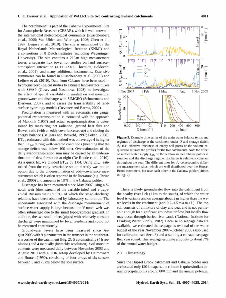
Figure 3. Example time series of the main water balance terms andregimes of discharge at the catchment outletQ and storage deficitdV (i.e. effective thickness of empty soil pores or the volume re-quired to saturate the profile) for the two catchments. Note the effectof surface water supplyfXS on the outflow in the Cabauw polder insummer and the discharge regime: discharge is relatively constantthroughout the year. The different lines fordV correspond to differ-ent measurement sites, which are well distributed over the HupselBrook catchment, but near each other in the Cabauw polder (circlesin Fig. 2).
There is likely groundwater flow into the catchment fromthe nearby river Lek (1 km to the south), of which the waterlevel is variable and on average about 2 m higher than the wa-ter levels in the catchment (and 0.2–1.5 m a.m.s.l.). The topsoil consists of a mixture of clay and peat and is not perme-able enough for significant groundwater flow, but locally flowmay occur through buried river sands (National Institute forDrinking Water Supply, 1982). Because no seepage data areavailable, we estimated the seepage as residual of the waterbudget of the year November 2007–October 2008 (also usedfor calibration, see Sect.3) and assuming a constant seepageflux year round. This seepage estimate amounts to about 7 %of the annual water budget.
2.3 Climatology
Since the Hupsel Brook catchment and Cabauw polder areaare located only 120 km apart, the climate is quite similar: an-nual precipitation is around 800 mm and the annual potential
www.hydrol-earth-syst-sci.net/18/4007/2014/ Hydrol. Earth Syst. Sci., 18, 4007–4028, 2014

4012 C. C. Brauer et al.: Application of WALRUS to two contrasting lowland catchments
evapotranspiration amounts to 600 mm (Table1). The actualevapotranspiration (ETact) in the Hupsel Brook catchment isusually within 5 % of ETpot (based on 4 years of combinedobservations). In the Cabauw polder, shallow groundwatertables prevent a strong soil moisture limitation on evapo-transpiration (Brauer et al., 2014). Precipitation occurs on50 % of the days, but quantities are typically low: on 15 %of the days more than 5 mm was measured and on 5 % morethan 10 mm. During 11 % of the hours precipitation was ob-served, of which 75 % had accumulations of less than 1 mm.Hourly rainfall sums above 10 mm occur on average 3 timesper year (at a given location and based on clock hours ratherthan a moving window).
Snow is of limited importance, even though freezing con-ditions are common. Sub-zero daily average temperatures oc-cur on average on 28 (Hupsel) and 18 (Cabauw) days peryear, leading to freezing of ponds on the land surface, waterin soil cracks and drainpipes, and a top layer of slowly flow-ing or standing surface water. On the majority of these days,the daily maximum temperature is above zero, leading todaily cycles of freezing and thawing. Cold winter conditionsare often caused by persistent high-pressure systems with lit-tle precipitation: on average 0.4 (Hupsel) and 0.3 (Cabauw)mm of precipitation on days with daily mean temperaturesbelow zero, leading to on average 12 (Hupsel – 1.5 % of totalP ) and 6 (Cabauw – 0.8 % of totalP ) mm of precipitationannually.
It should be noted that water input from dew can be con-siderable.Jacobs et al.(2006, 2010) estimated dew to amountto 4.5 % of the annual precipitation sum at Wageningen (lo-cated roughly halfway between the Hupsel Brook catchmentand the Cabauw polder). Unfortunately, dew measurementswere not available for either catchment. Therefore, dew is notconsidered separately in the water balance, but is assumed tobe included in the rain gauge measurements.
Water balance terms show seasonal variation (Fig.3).Evapotranspiration exceeds precipitation between April andAugust, which means that excess water stored in winter and,in the case of the Cabauw polder, surface water supply (fXS)and seepage (fXG) are used in summer for bothQ and ET.The influence of water management in the Cabauw polderis clearly visible: discharges remain high in summer due tosurface water supply, on 6 May 2008 discharge suddenlydropped to zero as a result of the increase of weir elevation,and on 16 November 2007 and 15 October 2008, dischargeincreased because the weir was lowered. The influence of wa-ter management in the Cabauw polder is discernible in threeways: (1) discharges remain high in summer due to surfacewater supply, (2) on 6 May 2008 discharge suddenly droppedto zero as a result of the increase of weir elevation, and(3) on 16 November 2007 and 15 October 2008, dischargeincreased because the weir was lowered. The surface watersupply flux in the Cabauw polder is large and variable andcan reach 800 mm in some years. In the Cabauw polder, thereis always water in all branches of the surface water network,
●
0.5
0.7
NS
356
●
0.2
●
5
●
3
Hup
sel
●
1100.5
0.7
NS
100 300cW [mm]
●
14 0 10
cV [h]
●
1180 100cG [.106 mm h]
●
760 50
cQ [h]
Cab
auw
Figure 4. Relation between Nash–Sutcliffe efficiency and param-eter values for the Hupsel Brook catchment (top row) and theCabauw polder (bottom row). The 10 000 coloured dots are ob-tained with Monte Carlo analyses. The black circles and numbersindicate the parameter values and resulting Nash–Sutcliffe efficien-cies obtained with HydroPSO.
whereas the headwaters of the Hupsel Brook frequently rundry. Discharge at the outlet of the Hupsel Brook catchmentdropped to zero during three months in 1976, a month in1982 and several shorter periods in 1983, 1988 and 2011.
3 Calibration
Because geology, slope and drainage densities differ betweencatchments, the model parameters expressing the effects ofthese characteristics differ as well. Although the parametershave physical connotations (the effect of each parameter willbe investigated in Sect.5.1), they are effective values rep-resenting the entire catchment (including the effect of het-erogeneity). Therefore, they cannot be estimated from fieldmeasurements directly, but have to be calibrated. Fitting sim-ulations to observations yields catchment-specific parametervalues, which (as they are assumed to be time invariant) canbe used to simulate discharge during other periods.
3.1 Calibration methods
For both the Hupsel Brook catchment and the Cabauwpolder, we optimised four model parameters: the wetnessindex parameter (cW), vadose zone relaxation time (cV),groundwater reservoir constant (cG) and the quickflow reser-voir constant (cQ; see Fig.1 and TableA for a completeoverview of all model variables, parameters and relations).We used the stage–discharge relations of the outlet weirs(which were calibrated in the laboratory) and channel depthscD of 1500 mm (estimated from observations). The weir level(hS, min) in the Cabauw polder was set to 500 (winter) and600 (summer) mm from the channel bottom (based on fieldestimates). We used default functions forW(dV), dV, eq(dG)
andβ(dV) and soil physical parametersb, ψae andθs based
Hydrol. Earth Syst. Sci., 18, 4007–4028, 2014 www.hydrol-earth-syst-sci.net/18/4007/2014/

C. C. Brauer et al.: Application of WALRUS to two contrasting lowland catchments 4013
Figure 5. Model output after calibration for the Hupsel Brook catchment (left panels) and the Cabauw polder (right panels). Evapotranspira-tion data are 5 day moving averages to eliminate daily cycles and focus on long-term differences between ETpot and ETact. The dotted partof Qobs in February 2012 denotes a period with sub-zero temperatures. The surface water levelhS is measured with respect to the channelbottom, while the groundwater depth is measured with respect to the soil surface. The channel depthcD relates the two to each other. Thestorage deficitdV is not a measurable depth, but rather an effective thickness.
on observations in the Hupsel Brook catchment and theCabauw polder (seeBrauer et al., 2014).
For the calibration, we used hourly data of the periodsNovember 2011–October 2012 (Hupsel) and October 2007–September 2008 (Cabauw). Unfortunately, it was not possi-ble to use the same period for both catchments, since timeseries were not continuous. Both periods are not exception-ally dry or wet and do not contain long periods of sub-zerotemperatures (except February 2012). It was not necessaryto use a warming-up period. The initial groundwater depthwas calibrated together with the parameters. The other initialstates followed from the observed discharge at the start of theperiod, the stage–discharge relation and the model equationsand parameters (seeBrauer et al., 2014). Several choices of
objective functions are compared in Sect.5.5, but a classicalNash–Sutcliffe efficiency of the discharge was used as themain objective function (Nash and Sutcliffe, 1970).
We used a particle swarm optimisation technique byZambrano-Bigarini and Rojas(2013), called HydroPSO,which is less sensitive to discontinuities in the response sur-face (i.e. due to thresholds in the model) and more likely tofind a global optimum than other gradient-based methods.The parameter values obtained with this HydroPSO calibra-tion are used throughout the paper. A comparison of opti-misation algorithms is outside the scope of this paper. Inaddition to the calibration with HydroPSO, a Monte Carloanalysis was used to explore uncertainty in and dependencybetween parameters (in Fig.4, and Sects.5.4 and6.1). For
www.hydrol-earth-syst-sci.net/18/4007/2014/ Hydrol. Earth Syst. Sci., 18, 4007–4028, 2014

4014 C. C. Brauer et al.: Application of WALRUS to two contrasting lowland catchments
Table 2. Water balance terms (mm) for the calibration and validation periods.1S denotes a change in soil moisture storage – a negativechange in soil moisture storage denotes a depletion of the soil reservoir. It is possible for ETact to exceed ETpot in the Hupsel Brook catchmentin the validation period because measurements were independent.
Hupsel Cabauw
Cal. Val. Cal. Val.
Obs. Mod. Obs. Mod. Obs. Mod. Obs. Mod.∑P 725 – 682 – 723 – 594 –∑ETpot 587 – 480 – 607 – 635 –∑ETact – 531 496 454 574 604 606 629∑Q 230 249 286 239 668 688 969 1012∑fXG 0 – 0 – 97 – 96 –∑fXS 0 – 0 – 359 – 803 –∑fGS – 74 – 57 – 22 – 13∑fQS – 174 – 189 – 303 – 203
1S – −54 −15 −11 −62 −110 −92 −143
Residual – 0 −78 0 0 0 10 0
the Monte Carlo analysis, we generated 10 000 random pa-rameter sets with ranges 100–500 mm (cW), 0.1–20 h (cV),0.1–150× 106 mm h (cG) and 1–100 h (cQ).
3.2 Calibrated parameter values
The optimal parameter values found with HydroPSO and therelations between parameter values and Nash–Sutcliffe effi-ciencies obtained with the Monte Carlo analysis are shownin Fig. 4. Finding optimal parameter values is not trivial (e.g.Beven and Freer, 2001b; Melsen et al., 2014). We used Hy-droPSO to obtain one optimal parameter set, but the dot-ted plots show that equally good results (in terms of Nash–Sutcliffe efficiency) could have been obtained with differentcombinations.
When comparing the Cabauw polder to the Hupsel Brookcatchment, differences in parameter values can be observedand explained (although we stress that physical interpreta-tions of conceptual model parameters should be handled withcare). ParameterscV , cG andcQ are higher, indicating that allflow is slower. ParametercW is smaller, causing later activa-tion of quick flowroutes (at lower storage deficits). Comparedto the Hupsel Brook catchment, the clayey soil in the Cabauwpolder is less permeable, leading to slower groundwater flow(cG) and a slower response of groundwater to changes in theunsaturated zone (cV). There are more cracks, gullies anddrainpipes per unit area, but quickflow is activated later (cW)because connectivity is limited. Quickflow is slower (cQ) be-cause slopes of land surface (overland flow) and drainpipesare more gentle. It is not a coincidence that the drainage den-sity increases when permeability decreases. Farmers installdrainpipes and dig gullies when ponding hampers agricul-tural activities, animals (moles, mice and muskrats) dig moreburrows to drain their dens and cracks occur more quickly inclayey soils.
3.3 Calibrated results
Discharge is reproduced well during the calibration period,both for peaks in winter and for low flows and small peaks insummer (Fig.5). Nash–Sutcliffe efficiencies of 0.87 for theHupsel Brook catchment and 0.83 for the Cabauw polder arereached. This shows that the model with the optimal param-eters is able to capture the hydrological response of lowlandcatchments.
In February 2011 the headwaters of the Hupsel Brookwere frozen, which caused a decrease in observed discharge.Because WALRUS in the present form does not take freezingconditions and snow into account, the simulated dischargedoes not decrease as quickly.
WALRUS simulates the discharge in summer relativelywell. Although the groundwater level dropped below thechannel bottom (in agreement with reality), the channel didnot run dry, because both discharge and infiltration of surfacewater decrease rapidly at low water levels. Only evapotran-spiration can empty the channel completely. During summerfield visits, we frequently observed that, while a large partof the surface water network is dry, some storm water is stilldischarged at the outlet after rain events. Even when the soilis dry, some quickflow will occur close to the ditches or overpaved areas.
The modelled groundwater depthdG shows seasonal vari-ation, but does not respond quickly to rainfall events. In themodel, percolating water is significantly delayed in the va-dose zone and the dynamic response to rainfall is modelledby the quickflow reservoir. The groundwater depth does in-fluence the catchment’s quick response to rainfall events, be-cause when groundwater is shallow, percolation is slow andstorage deficits are small, resulting in a high wetness indexand a large portion of the rain being led through the quick-flow reservoir.
Hydrol. Earth Syst. Sci., 18, 4007–4028, 2014 www.hydrol-earth-syst-sci.net/18/4007/2014/

C. C. Brauer et al.: Application of WALRUS to two contrasting lowland catchments 4015
Table 3.Periods used during calibration and different validation case studies.
Cal./Val. Case study Hupsel Cabauw
Calibration 2011-11-1 – 2012-10-31 2007-10-1 – 2008-09-30Validation Global validation (Fig.6) 1979-4-15 – 1980-04-14 2008-11-1 – 2009-10-31Validation Groundwater dynamics analysis (Fig.7) 2012-12-1 – 2012-12-31 2008-1-5 – 2008-2-5Validation Flood (Fig.8) 2010-8-24 – 2010-9-3Validation Drought (Fig.9) 1976-3-3 – 1976-10-31Validation Water management (weir elevation; Fig.10) 2009-11-9 – 2009-11-25Validation Water management (surface water supply; Fig.10) 2009-4-20 – 2009-5-14
Groundwater drainage (fGS) shows both long-term andshort-term dynamics. The seasonality infGS is caused byseasonality in groundwater levels, which are higher in win-ter due to the precipitation surplus. The quick decreases arecaused by fluctuations in surface water level, which riseand fall rapidly after rainfall events. This shows that thegroundwater–surface water feedback is implemented appro-priately: during discharge peaks, drainage is limited by highsurface water levels.
The surface water levels are much more constant in theCabauw polder than in the Hupsel Brook catchment. Surfacewater supply prevents headwaters from running dry in sum-mer. In addition, the Cabauw polder has a five times largerfraction of surface water, which acts as a buffer and absorbsinflow peaks caused by rainfall events.
3.4 Water budget
In the Hupsel Brook catchment, quickflow (fQS) accounts for70 % of total drainage (fGS+ fQS; Table2). This is consis-tent with the important role of quickflow found in previousstudies.Van der Velde et al.(2011) measured drainpipe flowin one field in the Hupsel Brook catchment and found thatthe contribution of drainpipe flow (one of the components ofquickflow) to the total drainage was 80 % for that field, andestimated it to be 25–50 % for the entire catchment.
In the Cabauw polder, the contribution of groundwaterdrainage is limited. However, the groundwater depth playsan important role in dividing the water between the soil reser-voir and the quickflow reservoir.
In both catchments the change in storage in the soil reser-voir is considerable:−54 mm in the Hupsel Brook catchmentand −110 mm in the Cabauw polder. Observations of dis-charge in the Hupsel Brook catchment (as a proxy for stor-age) and soil moisture in the Cabauw polder show that bothyears chosen for calibration ended drier than they started.However, the decrease in storage in the Cabauw polder wasoverestimated.
Evapotranspiration reduction is negligible in the Cabauwpolder (604/607= 0.5 %), but significant in the HupselBrook catchment (531/587= 10 %), caused by the largersoil moisture deficits.
4 Validation
4.1 Validation methods
The parameter values obtained during the calibration runs de-scribed in the previous section were used in validation stud-ies for whole years, a short period to focus on groundwaterdynamics, major flood and drought events, and a case withmanagement operations. We altered the initial groundwaterdepth for every validation run to match the real catchmentwetness at the start of each validation period (because in con-trast to parameters, initial conditions are not time-invariant).No warming-up period was used. Observations of groundwa-ter depth and storage deficit were used for a qualitative ap-preciation of the internal model dynamics. The periods usedfor validation are shown in Table3
4.2 Validation on yearly timescale
For both catchments, we selected one year for which actualevapotranspiration, soil moisture and groundwater data wereavailable: the period 15 April 1979–15 April 1980 for theHupsel Brook catchment and 1 November 2008–1 Novem-ber 2009 for the Cabauw polder. These additional data areused to test whether the model only reproduces the observeddischarge or also the hydrological processes involved. Therequirement of these additional data and allowing no gapslimited the choice of years for validation studies to one ortwo (different) years for each catchment. The selected yearsare not exceptionally dry or wet and do not contain long pe-riods of freezing conditions (except January 2009).
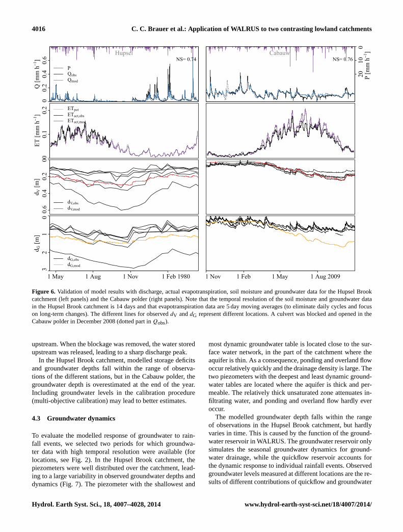
Model results and measurements are shown in Fig.6 andsome annual sums of water balance terms are shown inTable 2. For both catchments, Nash–Sutcliffe efficienciesare lower for the validation runs than for the calibrationruns, but still acceptable: they decrease from 0.87 to 0.74for the Hupsel Brook catchment and from 0.83 to 0.76 forthe Cabauw polder. This relatively small decrease in per-formance indicates that the model is parsimonious. In bothcatchments the highest discharge peaks are underestimated.
During a field visit in the Cabauw polder in Decem-ber 2008, a culvert was found clogged with loose vegeta-tion, reducing discharge capacity and raising water levels
www.hydrol-earth-syst-sci.net/18/4007/2014/ Hydrol. Earth Syst. Sci., 18, 4007–4028, 2014
4016 C. C. Brauer et al.: Application of WALRUS to two contrasting lowland catchments
00.
20.
40.
6Q
[mm
h−1
] NS= 0.74Hupsel
PQobsQmod
00.
10.
2ET
[mm
h−1
]
ETpotETact,obsETact,mod
0.6
0.4
0.2
0d V
[m]
dV,obsdV,mod
32
10
d G [m
]
1 May 1 Aug 1 Nov 1 Feb 1980
dG,obsdG,mod
NS= 0.76
2010
0
P [m
m h
−1]Cabauw
1 Nov 1 Feb 1 May 1 Aug 2009
Figure 6. Validation of model results with discharge, actual evapotranspiration, soil moisture and groundwater data for the Hupsel Brookcatchment (left panels) and the Cabauw polder (right panels). Note that the temporal resolution of the soil moisture and groundwater datain the Hupsel Brook catchment is 14 days and that evapotranspiration data are 5 day moving averages (to eliminate daily cycles and focuson long-term changes). The different lines for observeddV anddG represent different locations. A culvert was blocked and opened in theCabauw polder in December 2008 (dotted part inQobs).
upstream. When the blockage was removed, the water storedupstream was released, leading to a sharp discharge peak.
In the Hupsel Brook catchment, modelled storage deficitsand groundwater depths fall within the range of observa-tions of the different stations, but in the Cabauw polder, thegroundwater depth is overestimated at the end of the year.Including groundwater levels in the calibration procedure(multi-objective calibration) may lead to better estimates.
4.3 Groundwater dynamics
To evaluate the modelled response of groundwater to rain-fall events, we selected two periods for which groundwa-ter data with high temporal resolution were available (forlocations, see Fig.2). In the Hupsel Brook catchment, thepiezometers were well distributed over the catchment, lead-ing to a large variability in observed groundwater depths anddynamics (Fig.7). The piezometer with the shallowest and
most dynamic groundwater table is located close to the sur-face water network, in the part of the catchment where theaquifer is thin. As a consequence, ponding and overland flowoccur relatively quickly and the drainage density is large. Thetwo piezometers with the deepest and least dynamic ground-water tables are located where the aquifer is thick and per-meable. The relatively thick unsaturated zone attenuates in-filtrating water, and ponding and overland flow hardly everoccur.
The modelled groundwater depth falls within the rangeof observations in the Hupsel Brook catchment, but hardlyvaries in time. This is caused by the function of the ground-water reservoir in WALRUS. The groundwater reservoir onlysimulates the seasonal groundwater dynamics for ground-water drainage, while the quickflow reservoir accounts forthe dynamic response to individual rainfall events. Observedgroundwater levels measured at different locations are the re-sults of different contributions of quickflow and groundwater
Hydrol. Earth Syst. Sci., 18, 4007–4028, 2014 www.hydrol-earth-syst-sci.net/18/4007/2014/

C. C. Brauer et al.: Application of WALRUS to two contrasting lowland catchments 4017
32
10
d G [m
]
Hupsel
1 Dec 16 Dec 1 Jan '13
soil surface 2
0
5 Jan 20 Jan 5 Feb '08
Cabauw
00.
5f Q
S [m
m h
−1]
P [m
m h
−1]
PdG,obsdG,modfQS
Figure 7. Comparison of modelled and observed groundwaterdepths. The different black lines are observations at different loca-tions in the catchments (denoted as diamonds on the map in Fig.2).
flow. The most dynamic groundwater tables in Fig.7 can becompared to a combination of the quickflow and ground-water reservoirs, while the least dynamic groundwater ta-bles mainly represent the groundwater reservoir alone. In theCabauw polder, observed groundwater depths are much morevariable than simulated ones (Fig.7). This indicates that thecontribution of quickflow is large in all measured locations.
By using two reservoirs to simulate the characteristic“coupled dynamics” of groundwater tables, the discharge canbe reproduced well. Using groundwater time series for cali-bration or validation is possible, but not trivial (as is the casefor all lumped rainfall–runoff models). In addition, piezome-ters are often situated in locations with large seasonal dynam-ics. The 6 piezometers used in the Hupsel Brook catchmentin the 1970s and 1980s overestimate the variation in totalcatchment storage (reflecting the seasonal variation), whichmay be caused by the installation of piezometers in the centreof fields rather than near the channels (Brauer et al., 2013).
4.4 Extreme rainfall and flash flood
On 26 August 2010, an extreme rainfall event occurred inthe Hupsel Brook catchment (Brauer et al., 2011). In 24 h,about 160 mm rainfall was observed, corresponding to a re-turn period of more than 1000 years. This resulted in soil sat-uration, overland flow and inundation. Some of the lessonslearnt from the analysis of this flash flood event, such as theimportance of the groundwater–surface water feedback andwetness-dependent flowroutes, were taken into account dur-ing the development of WALRUS (Brauer et al., 2014). Theflood in August 2010 has triggered a model intercomparisonstudy (without WALRUS) initiated by the Netherlands Hy-drological Society (NHV), in which teams from Dutch con-sultancy firms, institutes and universities participated (NHV,2013).
We used the calibrated model to simulate this extremeevent (not part of the calibration period). We used the meanof the observed groundwater depths as initial groundwaterlevel for the simulation, mimicking a real flood forecasting
situation, where information about the discharge in the fu-ture is not available. This yielded a relatively good dis-charge response, considering that neither parameters nor ini-tial conditions were fitted to the data of the event (Fig.8).The Nash–Sutcliffe efficiency, however, was relatively low(0.64), mostly because the timing of the peak was slightly off.The total discharge was overestimated by WALRUS: 98 mm,compared to 87 mm observed (runoff ratios of 0.50 and 0.44).The peak discharge was simulated accurately, but the top wasflatter than observed, because surface water levels exceededthe soil surface and water flowed overland to the groundwa-ter reservoir. The peak was capped at the bankfull discharge,which has been defined by the stage–discharge relation. Inreality, the peak had been capped in many channels at differ-ent heights and the combination of many thresholds probablyled to the observed smooth curve. Altogether, WALRUS per-forms better than many models used in the intercomparisonstudy, in which peak discharges were reported ranging from0.2 to 10 mm h−1 (NHV, 2013).
In the model, complete catchment saturation is neverreached in the soil reservoir. However, the wetness indexreached 0.87, which means that 87 % of the precipitationis led through the quickflow reservoir. So even though theeffective groundwater depth did not reach the soil surface,ponding and overland flow occurred in a large part of thecatchment. The wetness index reproduces an increasing frac-tion of ponding and overland flow in local depressions in thelandscape and near the channels, while local elevations inthe landscape remain unsaturated. With this technique, thislumped model can account for spatial variability of ground-water depths.
Observations show that groundwater reached the soil sur-face before overland flow occurred (Fig.8), while accordingto the model, water flowed overland from the surface waterto the soil reservoir. Of course, the observations are pointmeasurements and it is likely that areas closer to the chan-nels have been flooded before reaching saturation, while lo-cal elevations in the landscape remained dry. This exampleshows that relating modelled (catchment-effective) variables(groundwater depth and storage deficit) to point measure-ments of groundwater depth and soil moisture content is nottrivial.
The satisfactory results indicate that WALRUS can be ap-plied for flood forecasting. The initial storage deficit (andgroundwater level) has a large influence on the simulated dis-charge. It determines when quickflow starts, when the surfacewater reaches the soil surface and when overland flow to-wards the groundwater reservoir starts. State updating couldreduce the predictive uncertainty resulting from uncertaintyin initial conditions when used in an operational flood fore-casting/early warning system.
www.hydrol-earth-syst-sci.net/18/4007/2014/ Hydrol. Earth Syst. Sci., 18, 4007–4028, 2014

4018 C. C. Brauer et al.: Application of WALRUS to two contrasting lowland catchments
01
23
Q
[mm
h−1
]
NS= 0.64
4020
0
P
[mm
h−1]
PQobs
Qmod
o$fQ
S 0
24
68
f QS
[mm
h−1
]
00.
51
W [−
]
WfQS
0.15
0.1
0.05
0
d V [m
]
3040
θ
[Vol
%]θobs
dV
1.5
10.
50
d
[m]
dG,obs
dG
cD−hS
25 Aug 28 Aug 31 Aug 3 Sep '10
Figure 8. Simulation of the flash flood in the Hupsel Brook catch-ment after the extreme rainfall event in August 2010. Groundwaterobservations were available from two piezometers near the meteo-rological station: one in a local depression and one in a local ele-vation (as shown inBrauer et al., 2011). Soil moisture content wasmeasured in the same field (in a local elevation).
4.5 Extreme summer drought
In 1976, much of western Europe including the Netherlandsexperienced one of the worst summer droughts in recent his-tory (Van Huijgevoort et al., 2013). The annual precipita-tion sum in the Hupsel Brook catchment was 549 mm forthe whole year, compared to 790 mm on average. High evap-otranspiration accelerated the development of large storagedeficits (Teuling et al., 2013). During this summer, intensivefield observations in the Hupsel Brook catchment took place(Stricker and Brutsaert, 1978). Because hourly data were notavailable, daily data were used as input.
In general, the discharge was simulated well. The sim-ulated initial recession in April and May is too steep andthe response to rainfall events in late May and June is toostrong, but the limited response to rainfall later on is simu-lated correctly. It should be noted that extreme drought con-ditions can temporarily change soil properties and hydrologic
00.
51
Q [m
m d
−1] 20
0
P
[mm
d−1]
NS= 0.84
PQobs
Qmod
02
4E
T [m
m d
−1]
ETpot
ETact,obs
ETact,mod
0.8
0.4
0 d V
[m]
dV,obs
dV,mod
43
21
0
d G [m
]
1 Mar 1 May 1 Jul 1 Sep '76
dG,obs
dG,mod
Figure 9. Simulation of the extremely dry summer of 1976 in theHupsel Brook catchment. Note that in contrast to previous modelruns, these model output and rainfall and discharge data are daily,groundwater and soil moisture data are biweekly and evapotranspi-ration are 5 day moving averages.
response (Seneviratne et al., 2012), which might explainthe slight model mismatch in this period. Even during thisextremely dry summer, some discharge was observed afterrainfall events. This is simulated well by WALRUS, wherea small portion of the rainfall is led through the quickflowreservoir, mimicking runoff from paved surfaces or throughdepressions near the surface water network. This shows theadded value of the quickflow reservoir and the surface wa-ter reservoir – in models with only a groundwater reservoir,all rainfall would infiltrate into the soil and discharge wouldremain zero.
No observations of actual evapotranspiration were madebefore 15 April and after 15 September. It was assumed thatit would not deviate much from its potential value in win-ter, which is confirmed by the data: ETact is close to ETpotin late April and early September (Fig.9). Between Mayand August, a large evapotranspiration reduction is observed.The model simulates the evapotranspiration reduction well,apart from a slight underestimation at the start and a slight
Hydrol. Earth Syst. Sci., 18, 4007–4028, 2014 www.hydrol-earth-syst-sci.net/18/4007/2014/

C. C. Brauer et al.: Application of WALRUS to two contrasting lowland catchments 4019
00.
20.
4Q
[mm
h−1
] PQobs
Qmod
fXS
105
0
P [m
m h−1
]
real situationno management
0.5
0.6
0.7
h [m
]
10 Nov 20 Nov '09
hShS,min
20 Apr 1 May 10 May '09
Figure 10. Reproduction of the Cabauw polder response to watermanagement interventions: weir level decrease (left panels) and in-crease in surface water supply (right).
overestimation at the end of the period. For the whole periodshown in Fig.9, modelled evapotranspiration reduction was30 % compared to the 26 % observed. Depletion of ground-water and soil moisture were slightly underestimated, but fallwell within the range of observed values.
4.6 Effect of water management
WALRUS can incorporate water management operations,which is important if it is to be used in human-influencedlowlands. To investigate if the model can also be used forwater management scenario analyses or to separate naturaland human effects on the hydrological system (seeVan Loonand van Lanen, 2013, and references therein), we simulatedthe change in the hydrological variables as a result of watermanagement operations in the Cabauw polder. As mentionedin Sect.2.2, surface water levels in the Cabauw polder arecontrolled by adjusting weir elevations and regulating sur-face water supply.
In Fig. 10 model results are shown for situations with andwithout management operations, being lowering of the weirand increasing surface water supply. Observations of the ac-tual situation (i.e. with management operations) are shownas well. The model reproduces the discharge response to wa-ter management operations well, although time delays be-come visible when we zoom into the short time windowsin Fig. 10. Lowering the weir causes a discharge peak, asthe water stored in the top 10 cm of the surface water isreleased quickly (left panels). As 5 % of the catchment iscovered by surface water, this amounts to (0.05× 100=)5 mm of water averaged over the catchment area. A suddenincrease in surface water supply also leads to a dischargerise, but less rapidly, because first the extra water has to be
distributed over the surface water network. This delay repre-sents mostly the response time of the surface water system,which is determined by the surface water area fraction andthe stage–discharge relation. This indicates that a surface wa-ter reservoir (such as incorporated in WALRUS) is necessaryto simulate the effect of the water buffer.
5 Sensitivity analyses
We performed three types of analyses to assess the sensitiv-ity of modelled discharge to changes in parameter values:Sect.5.1focusses on parameter identifiability through a timeseries analysis, Sect.5.2 focusses on the parameter sensitiv-ity with a novel statistical technique (DELSA) and Sect.5.4focusses on parameter uncertainty and dependence using ananalysis of response surfaces. In addition, we investigate thesensitivity to the choice of objective function for calibrationin Sect.5.5 and choice of user-defined parameterisations inSect.5.6 (described inBrauer et al., 2014, and listed in Ta-bleA).
5.1 Parameter identifiability
Calibration is improved and the risk of equifinality reducedwhen the influence of each parameter can be distinguishedin the discharge time series. In this section, the derivative ofdischarge to each of the parameters (∂Q/∂c) is determined,keeping the others fixed. This sensitivity is approximated by
a numerical difference(Q(c+1c)−Q(c)
1c
), with1c = 10−4.
The parameter sensitivity is plotted in Fig.11 for all fourcalibration parameters, focusing on the Hupsel Brook catch-ment in December 2011 and January 2012 (part of Fig.5). Tofacilitate comparison, we scaled each sensitivity time serieswith the parameter value in question.
The sensitivity series ofcW, cG andcQ are clearly differentenough to make these parameters identifiable. Moreover, thedifferences can be understood. Sensitivity to the wetness in-dex parametercW is large at the start of the period, when thewetness index (W ) is increasing after the dry summer periodand decreases as the winter progresses. With a larger value ofcW,W will be larger at the same value ofdV , leading to morequickflow and higher discharge peaks initially. Because lesswater is led to the soil reservoir in comparison to the originalsimulation,dV decreases less quickly, and the same value ofW is reached with a different combination ofcW anddV .
As cV , cG andcQ cause delay and attenuation, an increasein these parameters dampens the discharge signal. The effectof cQ is easily understood, because there are no direct feed-backs between the quickflow and surface water reservoirs:an increase incQ causes a lower and longer discharge peak.The peak decreases (negative1Q/1c) and the tail height in-creases (positive1Q/1c). A larger value ofcG causes a de-crease of groundwater drainage and lower discharge between
www.hydrol-earth-syst-sci.net/18/4007/2014/ Hydrol. Earth Syst. Sci., 18, 4007–4028, 2014

4020 C. C. Brauer et al.: Application of WALRUS to two contrasting lowland catchments
00.
20.
4Q
[mm
h−1
]
PQobs
Qmod
100
P [m
m h−1
]
∆Q ∆c⋅c
[mm
h−1
]
0.1
10−4
0.1
0.1
cW
cV
cG
cQ
cW
1 Dec 1 Jan 1 Feb '12
Figure 11. Identifiability of model parameters in the discharge timeseries. Top: observed and modelled discharge. Bottom: sensitivityof discharge to a change in each parameter.
peaks. Surface water infiltration during peak flows is limitedas well, leading to increased discharge peaks.
Discharge is about 1000 times less sensitive to the vadosezone relaxation time parametercV than to the other parame-ters (see the length of the vertical coloured bars in Fig.11).The time series of sensitivity tocV is inversely proportionalto the sensitivity tocW. This indicates that it is impossible todistinguish the effect ofcV in the discharge time series andthat calibration of this parameter with discharge data alone isimpossible.
5.2 Parameter sensitivity
A more sophisticated method to determine the sensitivityof WALRUS to model parameters is the Distributed Eval-uation of Local Sensitivity Analysis (DELSA, seeRakovecet al., 2014, for a complete explanation of the method). Inshort, this hybrid local–global sensitivity method decom-poses the variance of a performance measure into contri-butions from individual parameters using multiple evalua-tions of local parameter sensitivities, which are distributedthroughout parameter space. The current implementation ofthe DELSA method provides first-order sensitivities for eachof the model parameters. This means that only main effectson the total variance are captured and no parameter interac-tions are considered. In addition, the DELSA values conve-niently scale between 0 and 1 and – when all variance is ex-plained by one parameter, its DELSA sensitivity is 1. Finally,
00.
51
DE
LSA
sen
sitiv
ity [−
]
SS( Q)SS(Q)SS(Q2)
cW cV cG cQ cW cV cG cQ cW cV cG cQ
SS( Q)SS(Q)SS(Q2)
00.1
0.25
0.75
0.91
qu
an
tile
s
Figure 12. Parameter sensitivity computed with the DistributedEvaluation of Local Sensitivity Analysis (Rakovec et al., 2014), ob-tained for three objective functions: SS(Q2), SS(Q) and SS(
√Q).
The bars show variation between parameter sets as quantiles. Be-cause there are many realisations with low sensitivity, the lowerquantiles are zero for most parameters, exceptcW for SS(Q) andSS(
√Q).
the advantage of DELSA is that a rather small sample size(yielding low computational cost) provides robust results.
To compute the DELSA values, we initially created100 parameter sets (the base set). Next, we took the base setand perturbed one of the parameters, which we repeated foreach of the four parameters. We ran WALRUS with these500 sets and we evaluated the model output using three per-formance measures: the sum of squares (SS) ofQ, of Q2
(to focus on peaks) and of√Q (to focus on low flows). For
each of the four parameters, the DELSA sensitivity was com-puted from the difference in parameter value and model per-formance between the base run and the run with the perturbedparameter.
Figure12 shows boxplots of the obtained DELSA sensi-tivity for each parameter and each performance measure, inwhich the ranges indicate the variation between parametersets. As expected, the parameter sensitivity changes with theobjective function, which indicates that the importance of aparameter changes between high and low flows. The sensitiv-ity to cV is again small and the sensitivity tocQ is only largewhen extra focus is placed on the peaks (SS(Q2)). Thesetwo parameters only change the discharge temporarily, whilecW and cG have a long-lasting effect through groundwaterrecharge (cW) and recession (cG). WALRUS is sensitive tocW for many parameter sets (high sensitivity for low quan-tiles), especially when focussing on low flows (SS(
√Q)).
BecausecW determines the amount of water that is led tothe soil reservoir, and consequently the starting level of re-cession periods, a small change in this parameter can lead tooverestimation or underestimation of baseflow.
5.3 Conclusions of parameter sensitivity analyses
In conclusion, the discharge is most sensitive to parame-terscW, cG andcQ. These parameters are identifiable in thedischarge time series. This gives confidence that the modelis not overparameterised, which facilitates calibration and
Hydrol. Earth Syst. Sci., 18, 4007–4028, 2014 www.hydrol-earth-syst-sci.net/18/4007/2014/
C. C. Brauer et al.: Application of WALRUS to two contrasting lowland catchments 4021
0.5
9
0.5
92
0.5
92
0.594
0.5
94
0.594 0.596
0.5
96
0.598 0.6
0.602
0.604
cW [mm]
c Q [h
]
360 400 440
020
4060
80
0.542 0.544
0.546 0.548 0.55
0.552
0.554 0.556
cG [106 mm h] 0 10 20 30 40
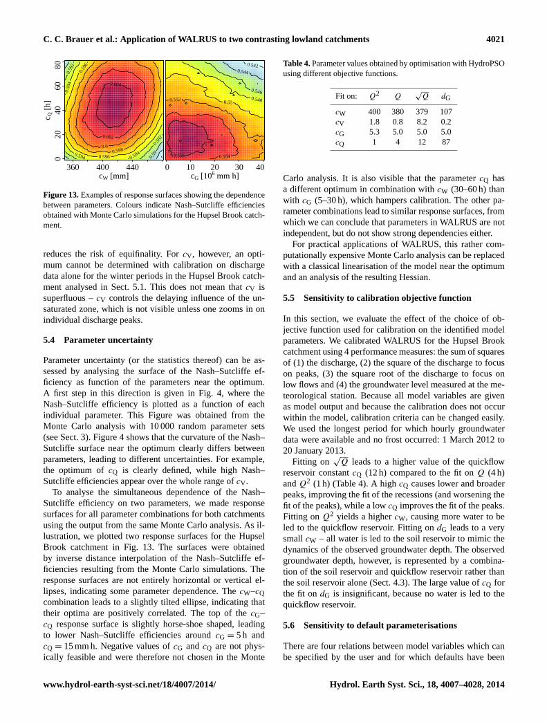
Figure 13.Examples of response surfaces showing the dependencebetween parameters. Colours indicate Nash–Sutcliffe efficienciesobtained with Monte Carlo simulations for the Hupsel Brook catch-ment.
reduces the risk of equifinality. ForcV , however, an opti-mum cannot be determined with calibration on dischargedata alone for the winter periods in the Hupsel Brook catch-ment analysed in Sect.5.1. This does not mean thatcV issuperfluous –cV controls the delaying influence of the un-saturated zone, which is not visible unless one zooms in onindividual discharge peaks.
5.4 Parameter uncertainty
Parameter uncertainty (or the statistics thereof) can be as-sessed by analysing the surface of the Nash–Sutcliffe ef-ficiency as function of the parameters near the optimum.A first step in this direction is given in Fig.4, where theNash–Sutcliffe efficiency is plotted as a function of eachindividual parameter. This Figure was obtained from theMonte Carlo analysis with 10 000 random parameter sets(see Sect.3). Figure4 shows that the curvature of the Nash–Sutcliffe surface near the optimum clearly differs betweenparameters, leading to different uncertainties. For example,the optimum ofcQ is clearly defined, while high Nash–Sutcliffe efficiencies appear over the whole range ofcV .
To analyse the simultaneous dependence of the Nash–Sutcliffe efficiency on two parameters, we made responsesurfaces for all parameter combinations for both catchmentsusing the output from the same Monte Carlo analysis. As il-lustration, we plotted two response surfaces for the HupselBrook catchment in Fig.13. The surfaces were obtainedby inverse distance interpolation of the Nash–Sutcliffe ef-ficiencies resulting from the Monte Carlo simulations. Theresponse surfaces are not entirely horizontal or vertical el-lipses, indicating some parameter dependence. ThecW–cQcombination leads to a slightly tilted ellipse, indicating thattheir optima are positively correlated. The top of thecG–cQ response surface is slightly horse-shoe shaped, leadingto lower Nash–Sutcliffe efficiencies aroundcG = 5 h andcQ = 15 mm h. Negative values ofcG andcQ are not phys-ically feasible and were therefore not chosen in the Monte
Table 4.Parameter values obtained by optimisation with HydroPSOusing different objective functions.
Fit on: Q2 Q√Q dG
cW 400 380 379 107cV 1.8 0.8 8.2 0.2cG 5.3 5.0 5.0 5.0cQ 1 4 12 87
Carlo analysis. It is also visible that the parametercQ hasa different optimum in combination withcW (30–60 h) thanwith cG (5–30 h), which hampers calibration. The other pa-rameter combinations lead to similar response surfaces, fromwhich we can conclude that parameters in WALRUS are notindependent, but do not show strong dependencies either.
For practical applications of WALRUS, this rather com-putationally expensive Monte Carlo analysis can be replacedwith a classical linearisation of the model near the optimumand an analysis of the resulting Hessian.
5.5 Sensitivity to calibration objective function
In this section, we evaluate the effect of the choice of ob-jective function used for calibration on the identified modelparameters. We calibrated WALRUS for the Hupsel Brookcatchment using 4 performance measures: the sum of squaresof (1) the discharge, (2) the square of the discharge to focuson peaks, (3) the square root of the discharge to focus onlow flows and (4) the groundwater level measured at the me-teorological station. Because all model variables are givenas model output and because the calibration does not occurwithin the model, calibration criteria can be changed easily.We used the longest period for which hourly groundwaterdata were available and no frost occurred: 1 March 2012 to20 January 2013.
Fitting on√Q leads to a higher value of the quickflow
reservoir constantcQ (12 h) compared to the fit onQ (4 h)andQ2 (1 h) (Table4). A high cQ causes lower and broaderpeaks, improving the fit of the recessions (and worsening thefit of the peaks), while a lowcQ improves the fit of the peaks.Fitting onQ2 yields a highercW, causing more water to beled to the quickflow reservoir. Fitting ondG leads to a verysmallcW – all water is led to the soil reservoir to mimic thedynamics of the observed groundwater depth. The observedgroundwater depth, however, is represented by a combina-tion of the soil reservoir and quickflow reservoir rather thanthe soil reservoir alone (Sect.4.3). The large value ofcQ forthe fit ondG is insignificant, because no water is led to thequickflow reservoir.
5.6 Sensitivity to default parameterisations
There are four relations between model variables which canbe specified by the user and for which defaults have been
www.hydrol-earth-syst-sci.net/18/4007/2014/ Hydrol. Earth Syst. Sci., 18, 4007–4028, 2014

4022 C. C. Brauer et al.: Application of WALRUS to two contrasting lowland catchments
0
0.05
0.1
Q [m
m h
−1]
par
s. d
efau
lt re
latio
nP Qobs
Qmod 100
P [m
m h−1
]
power law fit Hupselpower law loamy sandlinear fit Hupsel
00.
050.
1Q
[mm
h−1
]
pars
. eac
h re
latio
n
1 Apr 1 May 1 Jun '12
0 0.5 1 1.5
00.
2
dG [m]
d V,e
q [m
]
Figure 14. Effect of the relation between groundwater depth andequilibrium storage deficit. Three options for this relation are plot-ted in the inset: the relation based on a power-law soil moistureprofile (the default), fitted on soil moisture and groundwater obser-vations in the Hupsel Brook catchment (solid), the relation basedon the theoretical power-law soil moisture profile for loamy sand(dashed;Brooks and Corey, 1964) and a linear fit between soilmoisture and groundwater observations in the Hupsel Brook catch-ment (dotted).
implemented: (1) the wetness index relationW(dV), (2) theevapotranspiration reduction functionβ(dV), (3) the relationbetween equilibrium storage deficit and groundwater depthdV, eq(dG), and (4) the stage–discharge relationQ(hS) (Ta-ble A). These parameterisations are considered to be identi-fiable without calibration. Nevertheless, they are also proneto some uncertainty. To examine how sensitive the model isto changes in these relations (i.e. the effect of choices), weran the model with different options for these functions, withand without recalibrating for each function.
As an example, the results for three options fordV, eq(dG)
are shown in Fig.14. The default option is the relation basedon a power law soil moisture profile and data from the HupselBrook catchment (Brauer et al., 2014). We also used the rela-tion based on a power law soil moisture profile of loamy sand(Brooks and Corey, 1964) and a linear fit through observa-tions in the Hupsel Brook catchment. The different relationsare shown in the inset of Fig.14.
In the top panel of Fig.14, the same values for the fourmodel parameters (cW, cV , cG and cQ) were used. Thesewere obtained from calibration using the default option fordV, eq(dG). The initial conditions are computed automaticallyfor each run, assuming stationary groundwater drainage (im-plemented as default). In the bottom panel, the model param-eters were calibrated using thedV, eq(dG) function in ques-tion.
This figure illustrates that parameters obtained using onefunction cannot be used directly with another function. Thedifference between the linear and power-law based fit onthe data is limited, but for the theoretical relation peaks arestrongly overestimated when the original parameter set isused. However, calibration using this relation yielded simi-lar results.
6 Uncertainty propagation
Because WALRUS is computationally efficient, it is feasi-ble to estimate the effect of different types of uncertainty bycreating ensembles of model output. In this section we inves-tigate the consequences of uncertainty in parameter values,initial conditions and forcing data.
6.1 Propagation of parameter uncertainty
To examine the effect of parameter uncertainty, we created10 000 parameter sets randomly by selecting from uniformdistributions with ranges displayed in Fig.4. We selectedthe 100 sets which yielded the highest Nash–Sutcliffe effi-ciencies for the calibration period used in Sect.3 (Novem-ber 2011–October 2012). These 100 parameters sets wereused for 100 simulations of the period April 2012–May 2012.
The range between the 10th and 90th percentile is shownin Fig. 15a. Parameter uncertainty causes the largest devi-ations during peak flows and decreases to almost zero dur-ing recessions. The uncertainty around the large peak of0.07 mm h−1 is quite large: the range between the 10th and90th percentiles is from 0.004 to 0.14 mm h−1.
6.2 Propagation of initial condition uncertainty
Initial groundwater depth and quickflow reservoir level canbe specified by providing the fraction of discharge att = 0which originates from groundwater (Gfrac). The remainder(1−Gfrac) is used to compute the quickflow reservoir level.To investigate the effect of these initial conditions, the modelcalibrated in Sect.3 is run with an initial groundwater depthbased on 0 and 100 % of discharge originating from drainage(Gfrac of 0 and 1).
For this catchment and period, uncertainty in initial con-ditions has less effect on simulated discharge than uncer-tainty in parameter values (Fig.15b). The range around thelarge peak is 0.04–0.07 mm h−1. The difference between thesimulations with wet and dry initial conditions decreases intime. During this period, groundwater dropped 22 mm for thewet initial condition (100 % drainage) and 16 mm for the dryinitial condition (0 % drainage) and the discharge range de-creased slowly as well.
Hydrol. Earth Syst. Sci., 18, 4007–4028, 2014 www.hydrol-earth-syst-sci.net/18/4007/2014/
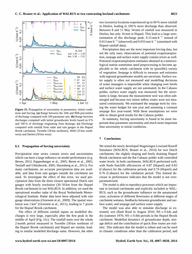
C. C. Brauer et al.: Application of WALRUS to two contrasting lowland catchments 4023
0
0.05
0.1
Q [m
m h
−1]
aPQobs
Qmod
40
P [m
m h−1
]
0
0.05
0.1
Q [m
m h
−1]
Initial condition uncertainty
b Qobs
Qmod
dG [m]wet: 1.43→ 1.59dry: 1.30→ 1.52
0
0.05
0.1
Q [m
m h
−1]
Forcing uncertainty
c Qobs
QmodQmod,radar
Qmod,30NE
Qmod,35SW
Qmod,50W
−−−−−−
ΣP ΣQ97 1497 13102 1599 12123 15154 27
1 Apr 1 May 1 Jun '12
Figure 15. Propagation of uncertainty in parameters, initial condi-tions and forcing.(a) Range between the 10th and 90th percentilesof discharge computed with 100 parameter sets.(b) Range betweendischarges computed with initial groundwater levels based on 0 %and 100 % of discharge originating from drainage.(c) Dischargecomputed with rainfall from radar and rain gauges in the HupselBrook catchment, Twenthe (30 km northeast), Wehl (35 km south-west) and Deelen (50 km west).
6.3 Propagation of forcing uncertainty
Precipitation time series contain errors and uncertaintieswhich can have a large influence on model performance (e.g.Beven, 2012; Pappenberger et al., 2005; Berne et al., 2005;Tetzlaff and Uhlenbrook, 2005; Hazenberg et al., 2011). Formany catchments, no accurate precipitation data are avail-able, and data from rain gauges outside the catchment areused. To investigate the effect of this error, we used pre-cipitation data from the three closest operational Dutch raingauges with hourly resolution (30–50 km from the HupselBrook catchment) to run WALRUS. In addition, we used theoperational weather radar of the Royal Netherlands Meteo-rological Institute. Radar data have been adjusted with raingauge observations (Overeem et al., 2009). The spatial reso-lution was 1 km2 (Overeem et al., 2011), leading to 7 pixelsfor the Hupsel Brook catchment.
The effect of different rainfall inputs on modelled dis-charges is very large, especially after the first peak in themiddle of April (Fig.15c). The rainfall sums over the whole2 month period measured in Twenthe (30 km northeast ofthe Hupsel Brook catchment) and Hupsel are similar, lead-ing to similar modelled discharge sums. However, the other
two (western) locations experienced up to 60 % more rainfallin Deelen, leading to 100 % more discharge than observed.Between 8 and 11 May 34 mm of rainfall was measured inDeelen, but only 16 mm in Hupsel. This lead to a large over-estimation of this discharge peak: 0.15 mm h−1 instead of0.013 mm h−1 (observed) and 0.033 mm h−1 (simulated withHupsel rainfall data).
Precipitation data are the most important forcing data, butnot the only ones: observations of potential evapotranspira-tion, seepage and surface water supply contain errors as well.Potential evapotranspiration estimates obtained at a meteoro-logical station sometimes need preprocessing to become ap-plicable to the whole catchment with its (possible) varietyof vegetation. Seepage is difficult to measure and estimateswith regional groundwater models are uncertain. Surface wa-ter supply is often not measured and modelling decisionsof water managers is impossible when changing weir levelsand surface water supply are not automated. In the Cabauwpolder, surface water supply was measured, but the uncer-tainty is large, because the measurement weir was often sub-merged and because two minor inflow routes were not mea-sured continuously. We estimated the seepage term by clos-ing the water budget for one year and assuming a constantseepage flux year-round. With these assumptions we wereable to obtain good results for the Cabauw polder.
In summary, forcing uncertainty is found to be more im-portant than parameter uncertainty and much more importantthan uncertainty in initial conditions.
7 Conclusions
We tested the newly developed Wageningen Lowland RunoffSimulator (WALRUS,Brauer et al., 2014) for two Dutchcatchments: the slightly sloping and freely draining HupselBrook catchment and the flat Cabauw polder with controlledwater levels. In both catchments, WALRUS performed well,with Nash–Sutcliffe efficiencies of 0.87 (Hupsel) and 0.83(Cabauw) for the calibration periods and 0.74 (Hupsel) and0.76 (Cabauw) for the validation period. This limited de-crease in performance indicates that the model is not over-parameterised.
The model is able to reproduce processes which are impor-tant in lowland catchments and explicitly included in WAL-RUS, such as the groundwater influence on the unsaturatedzone, activation of different flowroutes at different stages ofcatchment wetness, feedbacks between groundwater and sur-face water, and seepage and surface water supply.
The model was also able to simulate discharge in ex-tremely wet (flash flood in August 2010; NS= 0.64) anddry (summer 1976; NS= 0.84) periods in the Hupsel Brookcatchment. Modelled dynamics of groundwater depth, stor-age deficit and the contribution of quick flow routes are real-istic. This indicates that the model is robust and can be usedin climatic conditions other than the calibration period, and
www.hydrol-earth-syst-sci.net/18/4007/2014/ Hydrol. Earth Syst. Sci., 18, 4007–4028, 2014

4024 C. C. Brauer et al.: Application of WALRUS to two contrasting lowland catchments
it suggests that the model can also be used to simulate thehydrologic consequences of climate change (assuming thatthe parameters are not affected by climate change). In addi-tion, it can possibly be used for early warning of floods anddroughts.
The effect of water management operations (varying weirelevations and surface water supply) are also simulated well,owing to the explicit modelling of surface water. This indi-cates that WALRUS is suitable for catchments that are heav-ily influenced by human activity, that it can be used to sep-arate the effects of natural processes and human actions onthe hydrological variables and that WALRUS is suitable forforecasting the effect of different water management prac-tices (scenario analyses).
Comparing modelled catchment-effective variables topoint measurement is not trivial. Observed groundwater lev-els are influenced both by slow and quick flowroutes andshould therefore be compared to the (spatially varying) com-bination of modelled groundwater depth and quickflow reser-voir level rather than to the groundwater depth alone.
WALRUS is most sensitive to the wetness index param-eter cW and the groundwater reservoir constantcG, and toa lesser extent to the quickflow reservoir constantcQ. Theeffect of these three parameters could be identified in thedischarge times series, which suggests that the model is notoverparameterised. The vadose zone relaxation time param-etercV , however, has a limited effect, cannot be identified indischarge time series alone and may be redundant for mostapplications. We tested the effect of uncertainty in parame-ters, initial conditions and forcing, and found that the forcinguncertainty was the most important.
In conclusion, the good correspondence between modeland observations, identifiability of parameters and compu-tational efficiency are positive characteristics which makeWALRUS applicable for research and practice. Recommen-dations for further research include investigating the possi-bilities for data assimilation (Liu and Gupta, 2007; Rakovecet al., 2012) and multi-objective calibration (Gupta et al.,1998; Efstratiadis and Koutsoyiannis, 2010), testing themodel in catchments with different climates and areas, andregionalisation of model parameters for application in un-gauged basins (Merz and Blöschl, 2004).
Hydrol. Earth Syst. Sci., 18, 4007–4028, 2014 www.hydrol-earth-syst-sci.net/18/4007/2014/

C. C. Brauer et al.: Application of WALRUS to two contrasting lowland catchments 4025
Appendix A
Table A1. Overview of variables, parameters and functions. All fluxes are catchment averages, both external ones (includingQ andfXS)and internal fluxes (which are multiplied with the relative surface area of the reservoir in question). Note thatdV , hQ andhS result fromthe mass balances in the three reservoirs, whiledG is only used as a pressure head to compute the groundwater drainage flux. The names ofthe fluxes are derived from the reservoirs (for example,fXS: f stands for flow,X for external andS for surface water – water flowing fromoutside the catchment into the surface water network).
States
dV Storage deficit →ddVdt = −
fXG+PV−ETV−fGSaG
(mm)
dG Groundwater depth →ddGdt =
dV−dV,eqcV
(mm)
hQ Level quickflow reservoir →dhQdt =
PQ−fQSaG
(mm)
hS Surface water level →dhSdt =
fXS+PS−ETS+fGS+fQS−QaS
(mm)
Dependent variables
W Wetness index = func(dV) (–)β Evapotranspiration reduction factor = func(dV) (–)dV,eq Equilibrium storage deficit = func(dG) (mm)
External fluxes: input
P Precipitation (mm h−1)ETpot Potential evapotranspiration (mm h−1)Qobs Discharge (for calibration andQ0) (mm h−1)fXG Seepage (up/down)/extraction (mm h−1)fXS Surface water supply/extraction (mm h−1)
External fluxes: output
ETact Actual evapotranspiration = ETV + ETS (mm h−1)Q Discharge = func(hS) (mm h−1)
Internal fluxes
PS Precipitation into surface water reservoir = P · aS (mm h−1)PV Precipitation into vadose zone = P · (1−W) · aG (mm h−1)PQ Precipitation into quickflow reservoir = P ·W · aG (mm h−1)ETV Actual evapotranspiration vadose zone = ETpot ·β · aG (mm h−1)ETS Actual evapotranspiration surface water = ETpot · aS (mm h−1)
fGS Groundwater drainage/surface water infiltration= (cD−dG−hS)·max((cD−dG),hS)cG
· aG (mm h−1)
fQS Quickflow =hQcQ
· aG (mm h−1)
Model parameters
cW Wetness index parameter (mm)cV Vadose zone relaxation time (h)cG Groundwater reservoir constant (mm h)cQ Quickflow reservoir constant (h)
Supplied parameters
aS Surface water area fraction (–)aG Groundwater reservoir area fraction = 1− aS (–)cD Channel depth (mm)
User-defined functions with defaults
W(dV) Wetness index = cos(
max(min(dV ,cW),0)·πcW
)·
12 +
12 (–)
β(dV) Evapotranspiration reduction factor =1−exp[ζ1(dV−ζ2)]1+exp[ζ1(dV−ζ2)]
·12 +
12 (–)
dV, eq(dG) Equilibrium storage deficit = θs
(dG −
d1−1/bG
(1−1b)ψ
−1/bae
−ψae1−b
)(mm)
Q(hS) Stage–discharge relation = cS
(hS−hS,mincD−hS,min
)xS(mm h−1)
Parameters for default functions
ζ1 Curvature ET reduction function (–)ζ2 Translation ET reduction function (mm)b Pore size distribution parameter (–)ψae Air entry pressure (mm)θs Soil moisture content at saturation (–)cS Surface water parameter: bankfullQ (mm h−1)xS Stage–discharge relation exponent (–)hS,min Surface water level whenQ= 0 (mm)
www.hydrol-earth-syst-sci.net/18/4007/2014/ Hydrol. Earth Syst. Sci., 18, 4007–4028, 2014
4026 C. C. Brauer et al.: Application of WALRUS to two contrasting lowland catchments
Acknowledgements.We thank all data providers: KNMI forprecipitation and potential evapotranspiration data in the HupselBrook catchment (after 1990) and the Cabauw polder, Water BoardRijn and IJssel for the Hupsel Brook discharge data after 2000 andprecipitation data from station Wehl, Rijkswaterstaat (1979–1982)and Deltares (August 2010) for soil moisture and groundwater datain the Hupsel Brook catchment, Fred Bosveld (KNMI) for actualevapotranspiration data of the Cabauw polder and Aart Overeem(KNMI) for radar rainfall data. We thank Han Stricker, JantineBokhorst, Wilco Terink, Matthijs Boersema. Jacques Warmer, WimHovius and Marcel Brinkenberg for help with the field work in theCabauw polder. We thank Olda Rakovec for help with the DELSAparameter sensitivity analysis.
Edited by: A. Bronstert
References
Alley, W. M., Healy, R. W., LaBaugh, J. W., and Reilly, T. E.: Flowand storage in groundwater systems, Science, 296, 1985–1990,2002.
Appels, W. M., Bogaart, P. W., and van der Zee, S. E. A. T. M.: In-fluence of spatial variations of microtopography and infiltrationon surface runoff and field scale hydrological connectivity, Adv.Water Resour., 34, 303–313, 2011.
Baldocchi, D., Falge, E., Gu, L., Olson, R., Hollinger, D., Run-ning, S., Anthoni, P., Bernhofer, C., Davis, K., Evans, R. Fuentes,J., Goldstein, A., Katul, G., Law, B., Lee, X., Malhi, Y., Meyers,T., Munger, W., Oechel, W., Paw, K. T., Pilegaard, K., Schmid, H.P., Valentini, R., Verma, S., Vesala, T., Wilson, K., and Wofsy, S.:FLUXNET: a new tool to study the temporal and spatial variabil-ity of ecosystem-scale carbon dioxide, water vapor, and energyflux densities, B. Am. Meteorol. Soc., 82, 2415–2434, 2001.
Beljaars, A. C. M. and Bosveld, F. C.: Cabauw data for the vali-dation of land surface parameterization schemes, J. Climate, 10,1172–1193, 1997.
Berne, A., ten Heggeler, M., Uijlenhoet, R., Delobbe, L., Dier-ickx, Ph., and de Wit, M.: A preliminary investigation of radarrainfall estimation in the Ardennes region and a first hydrologicalapplication for the Ourthe catchment, Nat. Hazards Earth Syst.Sci., 5, 267–274, doi:10.5194/nhess-5-267-2005, 2005.
Beven, K.: Towards integrated environmental models of every-where: uncertainty, data and modelling as a learning process,Hydrol. Earth Syst. Sci., 11, 460–467, doi:10.5194/hess-11-460-2007, 2007.
Beven, K. J.: Rainfall–Runoff Modelling: the Primer, 2nd edn., JohnWiley & Sons, LTD, Chichester, UK, 2012.
Beven, K. and Freer, J.: A dynamic topmodel, Hydrol. Process., 15,1993–2011, 2001a.
Beven, K. and Freer, J.: Equifinality, data assimilation, and uncer-tainty estimation in mechanistic modelling of complex environ-mental systems using the GLUE methodology, J. Hydrol., 249,11–29, 2001b.
Bierkens, M. F. P. and Puente, C. E.: Analytically derived runoffmodels based on rainfall point processes, Water Resour. Res., 26,2653–2659, 1990.
Bierkens, M. F. P. and van den Hurk, B. J. J. M.: Ground-water convergence as a possible mechanism for multi-year
persistence in rainfall, Geophys. Res. Lett., 34, L02402,doi:10.1029/2006GL028396, 2007.
Bormann, H. and Elfert, S.: Application of WaSiM-ETH model toNorthern German lowland catchments: model performance inrelation to catchment characteristics and sensitivity to land usechange, Adv. Geosci., 27, 1–10, doi:10.5194/adgeo-27-1-2010,2010.
Brauer, C. C., Teuling, A. J., Overeem, A., van der Velde, Y., Hazen-berg, P., Warmerdam, P. M. M., and Uijlenhoet, R.: Anatomy ofextraordinary rainfall and flash flood in a Dutch lowland catch-ment, Hydrol. Earth Syst. Sci., 15, 1991–2005, doi:10.5194/hess-15-1991-2011, 2011.
Brauer, C. C., Teuling, A. J., Torfs, P. J. J. F., and Uijlenhoet, R.:Investigating storage–discharge relations in a lowland catchmentusing hydrograph fitting, recession analysis, and soil moisturedata, Water Resour. Res., 49, 4257–4264, 2013.
Brauer, C. C., Teuling, A. J., Torfs, P. J. J. F., and Uijlenhoet, R.: TheWageningen Lowland Runoff Simulator (WALRUS): a lumpedrainfall-runoff model for catchments with shallow groundwater,Geosci. Model Dev., 7, 2313–2332, doi:10.5194/gmd-7-2313-2014, 2014.
Brooks, R. H. and Corey, A.. T.: Hydraulic Properties of Porous Me-dia, Hydrology Paper 3, Colorado State University, Fort Collins,CO, 27 pp., 1964.
Chen, T. H., Henderson-Sellers, A., Milly, P. C. D., Pitman, A. J.,Beljaars, A. C. M., Polcher, J., Abramopoulos, F., Boone, A.,Chang, S., Chen, F., Dai, Y., Desborough, C. E., Dickinson, R. E.,Dümenil, L., Ek, M., Garratt, J. R., Gedney, N., Gusev, Y. M.,Kim, J., Koster, R., Kowalczyk, E. A., Laval, K., Lean, J., Let-tenmaier, D., Liang, X., Mahfouf, J.-F., Mengelkamp, H.-T.,Mitchell, K., Nasonova, O. N., Noilhan, J., Robock, A., Rosen-zweig, C., Schaake, J., Schlosser, C. A., Schulz, J.-P., Shao, Y.,Shmakin, A. B., Verseghy, D. L., Wetzel, P., Wood, E. F., Xue, Y.,Yang, Z.-L., and Zengi, Q.: Cabauw experimental results fromthe Project for Intercomparison of Land-Surface Parameteriza-tion Schemes, J. Climate, 10, 1194–1215, 1997.
De Roode, S. R., Bosveld, F. C., and Kroon, P. S.: Dew formation,eddy-correlation latent heat fluxes, and the surface energy imbal-ance at Cabauw during stable conditions, Bound.-Lay. Meteorol.,135, 369–383, 2010.
Devonec, E. and Barros, A. P.: Exploring the transferability ofa land-surface hydrology model, J. Hydrol., 265, 258–282, 2002.
Efstratiadis, A. and Koutsoyiannis, D.: One decade of multi-objective calibration approaches in hydrological modelling: a re-view, Hydrolog. Sci. J., 55, 58–78, 2010.
Fan, Y., Li, H., and Miguez-Macho, G.: Global patterns of ground-water table depth, Science, 339, 940–943, 2013.
Foken, T.: The energy balance closure problem: an overview, Ecol.Appl., 18, 1351–1367, 2008.
Gilfedder, M., Rassam, D., Stenson, M., Jolly, I., Walker, G.,and Littleboy, M.: Incorporating land-use changes and surface–groundwater interactions in a simple catchment water yieldmodel, Environ. Modell. Softw., 38, 62–73, 2012.
Gupta, H. V., Sorooshian, S., and Yapo, P. O.: Toward improved cal-ibration of hydrologic models: multiple and noncommensurablemeasures of information, Water Resour. Res., 34, 751–763, 1998.
Gusev, Y. M. and Nasonova, O. N.: The land surface parameteri-zation scheme SWAP: description and partial validation, GlobalPlanet. Change, 19, 63–86, 1998.
Hydrol. Earth Syst. Sci., 18, 4007–4028, 2014 www.hydrol-earth-syst-sci.net/18/4007/2014/

C. C. Brauer et al.: Application of WALRUS to two contrasting lowland catchments 4027
Hazenberg, P., Leijnse, H., and Uijlenhoet, R.: Radar rain-fall estimation of stratiform winter precipitation in theBelgian Ardennes, Water Resour. Res., 47, W02507,doi:10.1029/2010WR009068, 2011.
Heimovaara, T. J. and Bouten, W.: A computer-controlled 36-channel time domain reflectometry system for monitoring soilwater contents, Water Resour. Res., 26, 2311–2316, 1990.
Hopmans, J. W. and Stricker, J. N. M.: Stochastic analysis of soilwater regime in a watershed, J. Hydrol., 105, 57–84, 1989.
Hopmans, J. and van Immerzeel, C.: Variation in evapotranspirationand capillary rise with changing soil profile characteristics, Agr.Water Manage., 13, 295–305, 1988.
Jacobs, A. F. G., Heusinkveld, B. G., Kruit, R. J. W., and Berkow-icz, S. M.: Contribution of dew to the water budget of a grass-land area in The Netherlands, Water Resour. Res., 42, W03415,doi:10.1029/2005WR004055, 2006.
Jacobs, A. F. G., Heusinkveld, B. G., and Holtslag, A. A. M.: Eightyyears of meteorological observations at Wageningen, the Nether-lands: precipitation and evapotranspiration, Int. J. Climatol., 30,1315–1321, 2010.
Kavetski, D. and Fenicia, F.: Elements of a flexible ap-proach for conceptual hydrological modeling: 2. Applicationand experimental insights, Water Resour. Res., 47, W11511,doi:10.1029/2011WR010748, 2011.
Klemeš, V.: Operational testing of hydrological simulation models,Hydrolog. Sci. J., 31, 13–24, 1986.
Koch, S., Bauwe, A., and Lennartz, B.: Application of the SWATModel for a tile-drained lowland catchment in North-EasternGermany on subbasin scale, Water Resour. Manag., 27, 791–805,2013.
Kollet, S. J. and Maxwell, R. M.: Integrated surface–groundwaterflow modeling: a free-surface overland flow boundary conditionin a parallel groundwater flow model, Adv. Water Resour., 29,945–958, 2006.
Krause, S., Jacobs, J., and Bronstert, A.: Modelling the impacts ofland-use and drainage density on the water balance of a lowland-floodplain landscape in Northeast Germany, Ecol. Model., 200,475–492, 2007.
Leijnse, H., Uijlenhoet, R., van de Beek, C. Z., Overeem, A.,Otto, T., Unal, C. M. H., Dufournet, Y., Russchenberg, H. W. J.,Figueras i Ventura, J., Klein Baltink, H., and Holleman, I.: Pre-cipitation measurement at CESAR, the Netherlands, J. Hydrom-eteorol., 11, 1322–1329, 2010.
Liu, Y. and Gupta, H. V.: Uncertainty in hydrologic modeling: to-ward an integrated data assimilation framework, Water Resour.Res., 43, W07401, doi:10.1029/2006WR005756, 2007.
Makkink, G. F.: Testing the Penman formula by means of lysime-ters, Int. J. Water. Eng., 11, 277–288, 1957.
Maxwell, R. M. and Kollet, S. J.: Interdependence of groundwaterdynamics and land-energy feedbacks under climate change, Nat.Geosci., 1, 665–669, 2008.
Maxwell, R. M. and Miller, N. L.: Development of a coupled landsurface and groundwater model, J. Hydrometeorol., 6, 233–247,2005.
Melsen, L. A., Teuling, A. J., van Berkum, S. W., Torfs, P. J. J. F.,and Uijlenhoet, R.: Catchments as simple dynamical systems:a case study on methods and data requirements for parameteridentfication, Water Resour. Res., 50, 5577–5596, 2014.
Merz, R. and Blöschl, G.: Regionalisation of catchment model pa-rameters, J. Hydrol., 287, 95–123, 2004.
Nash, J. E. and Sutcliffe, J. V.: River flow forecasting through con-ceptual models, Part I – A discussion of principles, J. Hydrol.,10, 282–290, 1970.
National Institute for Drinking Water Supply: Possible Locationsfor Deep Groundwater Extraction in West-Utrecht, Tech. rep.,1982 (in Dutch).
NHV: Modelling the Hupsel Brook catchment – contributionsfrom Querner, E., Klutman, W., Droogers, P., Terink, W.,Schuphof, A., van Meekeren, B., Verhagen, F., Vermue, H.,van der Wal, B., Brauer, C., Kloosterman, P., Teuling, R.,Uijlenhoet, R., Pavelková, H., Swierstra, W., Veldhuizen, A., andWillems, G.: Stromingen, in press, 2014 (in Dutch).
Oreskes, N., Shrader-Frechette, K., and Belitz, K.: Verification, val-idation, and confirmation of numerical models in the earth sci-ences, Science, 263, 641–646, 1994.
Overeem, A., Holleman, I., and Buishand, A.: Derivation of a 10-year radar-based climatology of rainfall, J. Appl. Meteorol.Clim., 48, 1448–1463, 2009.
Overeem, A., Leijnse, H., and Uijlenhoet, R.: Measuring ur-ban rainfall using microwave links from commercial cellularcommunication networks, Water Resour. Res., 47, W12505,doi:10.1029/2010WR010350, 2011.
Pappenberger, F., Beven, K. J., Hunter, N. M., Bates, P. D.,Gouweleeuw, B. T., Thielen, J., and de Roo, A. P. J.: Cascad-ing model uncertainty from medium range weather forecasts (10days) through a rainfall-runoff model to flood inundation predic-tions within the European Flood Forecasting System (EFFS), Hy-drol. Earth Syst. Sci., 9, 381–393, doi:10.5194/hess-9-381-2005,2005.
Rakovec, O., Weerts, A. H., Hazenberg, P., Torfs, P. J. J. F.,and Uijlenhoet, R.: State updating of a distributed hydrologicalmodel with Ensemble Kalman Filtering: effects of updating fre-quency and observation network density on forecast accuracy,Hydrol. Earth Syst. Sci., 16, 3435–3449, doi:10.5194/hess-16-3435-2012, 2012.
Rakovec, O., Hill, M. C., Clark, M. P., Weerts, A. H., Teuling, A. J.,and Uijlenhoet, R.: Distributed Evaluation of Local SensitivityAnalysis (DELSA), with application to hydrologic models, Wa-ter Resour. Res., 50, 1–18, doi:10.1002/2013WR014063, 2014.
Refsgaard, J. C. and Knudsen, J.: Operational validation and inter-comparison of different types of hydrological models, Water Re-sour. Res., 32, 2189–2202, 1996.
Rozemeijer, J. C., van der Velde, Y., van Geer, F. C., de Rooij, G. H.,Torfs, P. J. J. F., and Broers, H. P.: Improving load estimates forNO3 and P in surface waters by characterizing the concentra-tion response to rainfall events, Environ. Sci. Technol., 44, 6305–6312, 2010.
Russchenberg, H., Bosveld, F., Swart, D., ten Brink, H., deLeeuw, G., Uijlenhoet, R., Arbesser-Rastburg, B., van derMarel, H., Ligthart, L., Boers, R., and Apituley, A.: Ground-based atmospheric remote sensing in the Netherlands: Europeanoutlook, IEICE Trans. Commun., E88-B, 2252–2258, 2005.
Schuurmans, J. M. and Bierkens, M. F. P.: Effect of spatial distri-bution of daily rainfall on interior catchment response of a dis-tributed hydrological model, Hydrol. Earth Syst. Sci., 11, 677–693, doi:10.5194/hess-11-677-2007, 2007.
www.hydrol-earth-syst-sci.net/18/4007/2014/ Hydrol. Earth Syst. Sci., 18, 4007–4028, 2014

4028 C. C. Brauer et al.: Application of WALRUS to two contrasting lowland catchments
Seneviratne, S. I., Lehner, I., Gurtz, J., Teuling, A. J., Lang, H.,Moser, U., Grebner, D., Menzel, L., Schroff, K., Vitvar, T., andZappa, M.: Swiss prealpine Rietholzbach research catchment andlysimeter: 32 year time series and 2003 drought event, Water Re-sour. Res., 48, W06526, doi:10.1029/2011WR011749, 2012.
Sophocleous, M. and Perkins, S. P.: Methodology and applicationof combined watershed and ground-water models in Kansas, J.Hydrol., 236, 185–201, 2000.
Stricker, J. N. M. and Brutsaert, W.: Actual evapotranspiration overa summer in the Hupsel Catchment, J. Hydrol., 39, 139–157,1978.
Stricker, J. N. M. and Warmerdam, P. M. M.: Estimation of the waterbalance in the Hupselse Beek basin over a period of three yearsand a first effort to simulate the rainfall–runoff process for a com-plete year, in: Proceedings of the International Symposium onHydrological Research Basins and their Use in Water ResourcesPlanning, 21–23 September 1982, Bern, Switzerland, 379–388,1982.
Tetzlaff, D. and Uhlenbrook, S.: Significance of spatial variabilityin precipitation for process-oriented modelling: results from twonested catchments using radar and ground station data, Hydrol.Earth Syst. Sci., 9, 29–41, doi:10.5194/hess-9-29-2005, 2005.
Teuling, A. J., van Loon, A. F., Seneviratne, S. I., Lehner, I.,Aubinet, M., Heinesch, B., Bernhofer, C., Grünwald, T.,Prasse, H., and Spank, U.: Evapotranspiration amplifies Eu-ropean summer drought, Geophys. Res. Lett., 40, 2071–2075,doi:10.1002/grl.50495, 2013.
Thom, A. and Oliver, H.: On Penman’s equation for estimating re-gional evaporation, Q. J. Roy. Meteor. Soc., 103, 345–357, 1977.
Twine, T. E., Kustas, W. P., Norman, J. M., Cook, D. R.,Houser, P. R., Meyers, T. P., Prueger, J. H., Starks, P. J., and We-sely, M. L.: Correcting eddy-covariance flux underestimates overa grassland, Agr. Forest Meteorol., 103, 279–300, 2000.
Van den Eertwegh, G. A. P. H.: Water and nutrient budgets at fieldand regional scale: travel times of drainage water and nutri-ent loads to surface water, Ph.D. thesis, Wageningen University,2002.
Van der Velde, Y., Rozemeijer, J. C., de Rooij, G. H., van Geer, F. C.,and Broers, H. P.: Field scale measurements for separation ofcatchment discharge into flow route contributions, Vadose ZoneJ., 9, 25–35, 2010.
Van der Velde, Y., Rozemeijer, J. C., de Rooij, G. H., van Geer, F. C.,Torfs, P. J. J. F., and de Louw, P. G. B.: Improving catchmentdischarge predictions by inferring flow route contributions froma nested-scale monitoring and model setup, Hydrol. Earth Syst.Sci., 15, 913–930, doi:10.5194/hess-15-913-2011, 2011.
Van der Velde, Y., Torfs, P. J. J. F., van der Zee, S. E. A. T. M., andUijlenhoet, R.: Quantifying catchment-scale mixing and its effecton time-varying travel time distributions, Water Resour. Res., 48,W06536, doi:10:1029/2011WR011310, 2012.
Van Huijgevoort, M. H. J., Hazenberg, P., van Lanen, H. A. J., Teul-ing, A. J., Clark, D. B., Folwell, S., Gosling, S. N., Hanasaki, N.,Heinke, J., Koirala, S., Stacke, T., Voss, F., Sheffield, J., and Ui-jlenhoet, R.: Global multimodel analysis of drought in runoff forthe second half of the twentieth century, J. Hydrometeorol., 14,1535–1552, 2013.
Van Loon, A. F. and van Lanen, H. A. J.: Making the distinction be-tween water scarcity and drought using an observation-modelingframework, Water Resour. Res., 49, 1483–1502, 2013.
Van Ulden, A. P. and Wieringa, J.: Atmospheric boundary layer re-search at Cabauw, Bound.-Lay. Meteorol., 78, 39–69, 1996.
Wagener, T.: Evaluation of catchment models, Hydrol. Process., 17,3375–3378, 2003.
Zambrano-Bigarini, M. and Rojas, R.: A model-independent parti-cle swarm optimisation software for model calibration, Environ.Modell. Softw., 43, 5–25, 2013.
Zampieri, M., Serpetzoglou, E., Anagnostou, E. N., Nikolopou-los, E. I., and Papadopoulos, A.: Improving the representationof river–groundwater interactions in land surface modeling at theregional scale: observational evidence and parameterization ap-plied in the Community Land Model, J. Hydrol., 420, 72–86,2012.
Hydrol. Earth Syst. Sci., 18, 4007–4028, 2014 www.hydrol-earth-syst-sci.net/18/4007/2014/