The Foundation for Study and Research of Environmental Factors (S.R.E.F.) acknowledges the support by the following:

Wageningen Agricultural University

Department of Ecological Agriculture, Wageningen Agricultural University

Nederlandse Middenstandsbank

Ministerie van Volkshuisvesting, Ruimtelijke Ordening en Milieubeheer

Triodos Borgstellingsfonds B.A.

Iona-Foundation

Akzo N.V.

Hoogovens Groep B.V.

Weleda Handelsonderneming B.V.

C & A • Nederland

Nashua Nederland B.V.

Biohorna Beheer B.V.

Lemniscaat B.V.

Stichting Publieksvoorlichting voor Wetenschap en Techniek (P.W.T.)

r^ - e - \ -I',i '•• ^ - A ^ ^

f-} - « > v

Geo-cosmic relations; the earth and its macro-environment

Proceedings of the First International Congress on Geo-cosmic Relations, organized by the Foundation for Study and Research of Environmental Factors (S.R.E.F.), Amsterdam, 19-22 April 1989

Editors: G.J.M. Tomassen (editor in chief), W. de Graaff, A.A. Knoop, R. Hengeveld

, s«,,-,, LANDBOUWHOGESCHOOL

Alternatieve Methoden in de Land- en Tuinbouw

Hdb. 31 No.: û\ - ^

a Pudoc, Wageningen, 1990

1

CIP data Koninklijke Bibliotheek, Den Haag

Geo-cosmic

Geo-cosmic relations : the earth and its macro-environment: proceedings of the first internatio­nal congress on geo-cosmic relations, organized by the Foundation for Study and Research of Environmental Factors (S.R.E.F.), Amsterdam, 19-22 April 1989/eds. G.J.M. Tomassen ... [et al]. -Wageningen : Pudoc ISBN 90-220-1006-6 geb. SISO 552 UDC 55:524.8 NUGI 829 Subject heading: geo-cosmology.

© Pudoc, Centre for Agricultural Publishing and Documentation, Wageningen, Netherlands, 1990.

All rights reserved. Nothing from this publication may be reproduced, stored in a computerized system or published in any form or in any manner, including electronic, mechanical, repro­graphic or photographic, without prior written permission from the publisher, Pudoc, P.O. Box 4, 6700 AA Wageningen, Netherlands.

The individual contributions in this publication and any liabilities arising from them remain the responsibility of the authors.

Insofar as photocopies from this publication are permitted by the Copyright Act 1912, Article 16B and Royal Netherlands Decree of 20 June 1974 (Staatsblad 351) as amended in Royal Netherlands Decree of 23 August 1985 (Staatsblad 471) and by Copyright Act 1912, Article 17, the legally defined copyright fee for any copies should be transferred to the Stichting Reporecht (P.O. Box 882,1180 AW Amstelveen, Netherlands). For reproduction of parts of this publication in compilations such as anthologies or readers (Copyright Act 1912, Article 6), permission must be obtained from the publisher.

Printed in the Netherlands.

mmoTHEm LANDBOUWUNIVERSITEIT

WACEN'INCFPJ

Address of the Foundation S.R.E.F.: P.O. Box 84, 6700 AB Wageningen, The Netherlands.

Board of Directors of the Foundation S.R.E.F.:

Chairman: Drs. W. Beekman Secretary/Treasurer: Ir. G.J.M. Tomassen Members: J.S.H.J.W. Bouma

Dr. Ir. E.A. Goewie Prof. Dr. A.A. Knoop

Members of the International S.R.E.F. Advisory Board - Prof. Dr. B.G. Cumming, Dept. of Biology, Univ. of New Brunswick, Canada. - Dr. G. Dean, Subiaco, Western Australia. - Prof. Dr. A.P. Dubrov, Library on Natural Science, Acad, of Sciences, Moscow,

U.S.S.R. - Prof. Dr. S. Ertel, Inst, of Psychology, Göttingen University, FRG. - Prof. Dr. H.J. Eysenck, Inst, of Psychiatry, Univ. of London, U.K. - Dr. P. Faraone, Lab. di Igiene e Profilassi, Roma, Italy. - Prof. S.J. Kardas Jr., Laboratório de Investigaciones Sobre Biorritmos Humanos, La

Atlantida, Espana I U.S.A. - Prof. Dr. N.V. Krasnogorskaya, Inst, of the Lithosphère, Moscow, U.S.S.R. - Dr. D. Mikhov, Inst, of Neurology, Psychiatry, Neurosurgery, Sofia, Bulgaria. - Dr. B. Primault, Agro- and Bio-meteorologist, Zürich, Switzerland. - Dr. M.F. Ranky, Central Research Inst, of Physics, Budapest, Hungary. - Prof. Dr. J.P. Rozelot, Centre d'études et de recherches geo-dynamique et astronomi­

que, Grasse, France. - Prof. Dr. P.A.H. Seymour, Dept. of Marine Science and Technology, Polytechnic

South West, Plymouth, U.K. - R. Swenson, Director of the Center for Study of Complex Systems, New York, U.S.A. - Dr. N.V. Udaltsova, Inst, of Biophysics, Moscow, U.S.S.R. - Dr. T. Zeithamer, Geophysical Inst., Acad, of Sciences, Praha, Czechoslovakia.

Chairman of the Congress: Prof. Drs. J.D. van Mansvelt, Department of Ecological Agriculture, Wageningen University

Organizing Committee:

Chairman: Drs. W. Beekman, Biologist, Director of the Amsterdam Botanical Gardens Secretary/Treasurer: Ir. G.J.M. Tomassen, Agriculturist Members: - Dr. Ir. J. Buis, Agriculturist/Historian - Prof. Dr. W. de Graaff, Emeritus Prof.of Astronomy, Utrecht University - Dr. H.J.L. Hagebeuk, Physicist, Eindhoven University - Dr. R. Hengeveld, Biologist, R.I.N. (Research Inst, for Nature Management) - Drs. W. Heukelom, Physicist - Dr. P.H. Jongbloet, Physician, Amsterdam University (VU) - Prof. Dr. A.A. Knoop, Medical Physiologist, Amsterdam University (VU) - Ir. C. van der Mark, Biologist - Drs. M.Y. Widdershoven, Physician - Ir. J. van Langen, Sociologist

COMMITTEE OF RECOMMENDATION:

Prof. Dr. Ir. L.C.A. Corsten, Emeritus Professor of Mathematical Statistics, Wageningen University; Ir. N.D. van Egmond, Director of the National Institute of Public Health and Environmental Protection (R.I.V.M.); Prof. Drs. J.D. van Mansvelt, Professor of Ecological Agriculture, Wageningen University; Prof. Dr. A.A. Oldeman, Professor of Forestry, Wageningen University; H.A. Quarles van Ufford M.Sc, retired Meteorologist, Royal Dutch Meteorological Institute (K.N.M.I.); Prof. Dr. F.N. Schmidt, Emeritus Professor of Meteorology, Utrecht University; Prof. Dr. D. de Zeeuw, past Chairman of the Executive Board of the University of Wageningen; Prof. Dr. A.J.B. Zehnder, Professor of Micro Biology, Wageningen University; Dr. Ir. B.C.J. Zoeteman, deputy Director General for Environmental Protection, Ministry of the Environment, The Netherlands.

Organized by the "Foundation for Study and Research of Environmental Factors" (S.R.E.F.), Wageningen. Supported by the "International Committee for Research and Study of Environmental Factors" (I.C.E.F.), Université Libre de Bruxelles. On the initiative of Prof. Drs. J.D. van Mansvelt, Agricultural University, Department of Ecological Agriculture, Wageningen.

Contents Editorial introduction, conclusions and remarks - Ir. G.J.M. Tomassen, 1 editor and secretary-treasurer of the Foundation for Study and Research of Environmental Factors (SREF)

Opening Address by the Rector of the University of Wageningen - 3 Prof. Dr. H.C. van der Plas

Opening Speech by the Chairman of the Congress - Prof. Drs. J.D. van 5

Mansvelt, Dept. of Ecological Agriculture, Wageningen University

Introductory papers 9

Dynamics of the solar system - W. de Graaff 11

Radiation in our environment, from the atmosphere and from space - 17

E. Wedler

Biological cyclicity in relation to some astronomical parameters: a review - 31

B.G. Cumming

Biological clocks and the role of subtle geophysical factors - H.M. Webb 56

Man in a rhythmic universe - A.A. Knoop 65

Water as receptor of environmental information: a challange to 75 reproducibility in experimental research. The Piccardi scientific endeavour -C. Capel-Boute

Application to climatic variations of the energy transfer between the earth 92

and the sun: the new concept of helioclimatology - J.P. Rozelot

The earth and its macro-environment, a multi-disciplinary approach 103

The possible influence of some astro-physical factors on micro-organisms - 105

P. Faraone

Lunar cycle and nuclear DNA variations in potato callus or root meristem - 116 M. Rossignol, S. Benzine-Tizroutine and L. Rossignol

Cellular effects of low level microwaves - W. Grundler 127

Quantitative evaluation of the geomagnetic activity - D. Mikhov 135

Ovulation and seasons - Vitality and month-of-birth - P.H. Jongbloet 143

Note on human response to the lunar synodic cycle - N. Kollerstrom 157

Influence of abiotical ecological factors on daily rhythm activity of 161 mitochondrial and lysosomal ferments of blood leucocytes in human ontogenesis - N. Kacergiené, N. Dailidiene and R. Vernickaite

ELF electromagnetic fields as a new ecological parameter - N.A. Temuryants, 169 V.G. Sidyakin, V.B. Makejev, B.M. Vladimlrsky

The possible gravitational nature of factors influencing discrete macroscopic 174 fluctuations - N.V. Udaltsova, V.A. Kolombet and S.E. Shnoll

Macroscopic fluctuations with discrete structure distributions as a result of 181 universal causes including cosmophysical factors — S.E. Shnoll, N.V. Udaltsova and N.B. Bodrova

Geo-cosmic relations and some aspects of their realization - 189

N.V. Krasnogorskaya and G. Ya. Vasilyeva

Influence of solar activity on ELF sferics of 3 Hz range - /. Örményi 198

Links between moon phases and ELF atmospherics of 3 Hz range - 206

/. Örményi

Possible influence of equinoxes and solstices on ELF sferics of 3 Hz. range - 210 /. Örményi

Analysis of weak magnetic field effects of the Piccardi test and Belousov- 214 Zhabotinsky reaction - L.P. Agulova, A.M. Opalinskaya

Relationships between the electromagnetic VLF-radiation of the atmosphere 223 and chemical as well as biochemical processes - J. Eichmeier and H. Baumer

Periodicities of meteorological parameters at Schiermonnikoog. A simple 233 explanation - H.F. Vugts

Mars and temperature-changes in the Netherlands: an empirical study - 240 J. W. M. Venker and M.C. Beeftink

Possible planetary effects at the time of birth of successful professionals: a 246 discussion of the 'Mars-effect' -M. Gauquelin

Gauquelin's contentions scrutinized - S. End 255

Introversion-Extraversion; sunsign-effect and sunsign-knowledge - J.J. F. van 267 Rooij, M.A. Brak and J.J.F. Commandeur

Effect sizes of some pre-scientific geo-cosmic theories - G. Dean 272

Theoretical and background contributions 279

The changing concept of physical reality - J. Hilgevoord 281

Biological order - E. Schoffeniels 291

The earth as an incommensurate field at the geo-cosmic interface: fundamentals 299 to a theory of emergent evolution - R. Swenson /

Resonant magneto-tidal coupling between the components of the solar system 307 and some of its terrestrial consequences -P.A.H. Seymour

Nonlinear dynamics and deterministic chaos. Their relevance for biological 315 function and behaviour - F. Kaiser

Structural stability of the earth's magnetosphere - T. Zeithamer 321

Geo-solar-cosmic electric relations in electrostatics with field E screening by 327 matter — L.A. Pokhmelnykh

An attempt of interpretation of Piccardi chemical tests. Effects of metallic 336 screens -L. Boulanger, R. Chauvin

Understanding geo-cosmic relations: some philosophical remarks on the nature 343 of reality - T. Saat

Abstracts 351

How does man fit into nature? - R. Augros, G. Stanciu 353

Basis of judgement for geo-cosmic relations - H.J. Eysenck 353

Correlation of hospital mortality with the phases of the tidal variations of gravitation - W. Raibstein

354

The time course of the ©limactic syndrome and the role of geographical factors -I.V. Verulashvili

354

Changes in the earth's rate of rotation - A. Poma, E. Proverbio

On the problems of the effect of the sun and planetary system on meteorological disturbances in the atmosphere - K. Kudrna

The role of the geomagnetism (GMF) and gravity (GRF) in creating fundamental peculiarities of living beings -A. P. Dubrov

354

355

355

Cycles in the history of forestry - / . Buis 356

Cosmic and environmental influences on plants, testing of sowing calendar on 356 beans (Phaseolus vulgaris) in Brazil. Research done in this area until today and its future implications in agriculture -A . Harkaly

Modifications of the growth of seedling roots versus time on a scale of copper sulphate solutions - E. Graviou

357

Dynamic responses tests quantifying complex properties of plants: how living structures could reveal their geo-cosmic past - M.F. Ranky

358

A dynamic biological-atmospheric-cosmic energy continuum: some old and new evidence - J. DeMeo

358

Solar-terrestrial factors and ontogenesis (clinical experimental tests) -R.P. Narcissov, S.V. Petrichuk, V.M. Shishchenko, Z.N. Duchova and G.F. Suslova

358

Statistical identification of the planetary modulation of the solar activity by the determination of third order moments and the estimation of the volterra kernels - C. Gaudeau, E. Daubourg and P. David

359

Geocosmic bonds in anomal human behaviour - A.N. Kornetov

Macroscopic fluctuations as a fundamental physical phenomenon -V.A. Kolombet

359

360

List of authors 361

List of keywords 362

EDITORIAL INTRODUCTION, CONCLUSIONS AND REMARKS

G.J.M. Tomassen

Secretary-treasurer of the Foundation for Study and Research of Environ­mental Factors (SREF), P.O.Box 84, 6700 AB Wageningen, The Netherlands. Guest-researcher Dept. of Ecological Agriculture, Wageningen University, Haarweg 333, 6709 RZ Wageningen, The Netherlands.

More than two years of preparations resulted in the 19th of April 1989 being imprinted in our memory as the opening day of the "First Internatio­nal Congress on Geo-Cosmic Relations; the earth and its macro-environment". During the preceding period every effort was made to develop what in the first stage was no more than the vague outline of faint initial objectives only. It was a long way, from that primordial starting point 'the concept' to that very ultimate stage wherein so many representatives of so many disciplines, both familiar and less familiar, coming from so many countries all over the world, were gathered in the magnificent Amsterdam N.M.B.-building for the opening ceremony of three long days of focusing on the main conference topic: 'The Earth and its macro surroundings'.

The Foundation SREF's main objective is to advance the interdisciplinary study of the Earth as a macro-system, and in particular the interaction between terrestrial and extraterrestrial phenomena. In doing so it intends to contribute to the implementation of the resolution adopted during the Tenth International Congress of the International Society of Biometeorology at Tokyo on July 29, 1984. This resolution calls for interdisciplinary efforts in the study of complex relationships between living organisms and their near and far environment. The full text is included in the memorandum of association of the Foundation. It is also included in the contribution of C. Capel-Boute (past President of CIFA, Univ. Libre de Bruxelles) who can be considered as one of its architects and successful promotors.

This Congress was in line with the intentions of the latter resolution, but apart from this it was also because of our esteem and regard for the prodigious body of knowledge shaped by the scientific endeavour of so many eminent scholars during the past decades that SREF felt called upon to organize this event. It was their thorough and sometimes even brave scrutiny which set the scene for that challenging new field of research: "Geo-Cosmic Relations", wherein we are prompted to shift our scope from our limited near environment to the entire solar system, and -on the highest scale- to space.

It may be said: the Congress Programme is a testimony of the growing awareness about the coherence of all constituents of the global system. During three days the participants were involved in tens of lectures uncovering intricate and even gripping matters reflecting recent results or sometimes the state of the art of a multitude of disciplines. Notwith­standing this multidisciplinary approach (which of course made the audience run the risk of losing its bearings more than once) the Congress kept its atmosphere of transparency until last concluding word.

Hard work has been done. And, as a matter of fact, this justifies con­tinuation at more or less short notice. It is needless to stipulate the importance of building on those first few milestones. Without further coherent strains in the near future we will miss our mark.

In view of this some important resolutions were passed during the Congress business meeting on April 21, 1989. Firstly we may recall the establishment

of the International SREF Advisory Board, to be considered as a sign of support and moreover as a coherent strengthening of our very diverse forces. We are convinced that this International Body will facilitate and even stream-line our future targets, in direct conformity with the contents of the Tokyo-resolution. Secondly, following a resolution adopted during the same meeting the "Second International Congress on Geo-Cosmic Relations; the earth and its macro-environment" will take place in Amsterdam on April 1992. This next Congress will be organized again by the Foundation for Study and Research of Environmental Factors (SREF). We hope that the past Congress and the projected second one may provoke a continuous series of stimulating future meetings, thus contributing to further exchange of knowledge and building on the growing expertise.

A small working group took charge of formulating more detailed proposals, reflecting in more specific terms the general intentions of the above mentioned Tokyo-resolution. During the second Congress we intend to come back on this in more detail.

Without a written, printed testimony, time undoubtedly would soon wipe out all traces of this Congress. Thus, it was decided at an early stage to prepare and publish its Proceedings as soon as possible. Unfortunately, this proved to be more difficult than anticipated. Recommendations concerning lay-out, format, length, and deadline had to be revised halfway, resulting in additional work and costs for our authors. We sincerely apologize for these inconveniences.

We do not need to emphasize every author's own responsibility for the contents of the individual contributions. The editors are responsible for the selection of the papers and for the order in which they appear. Papers were included when their subject was within the scope of the Congress, and when their scientific merits seemed acceptable. Linguistic corrections were only applied when considered unavoidable, and care has been taken to preserve the original meaning. Some papers were included although their authors were unable to attend the Congress. In a number of cases it was decided for various reasons to include a paper in the form of an abstract. In general, the aim of the editors was to present the best overview possible of present-day knowledge with regard to 'the Earth and its Foreign Affairs' as presented at the Congress.

We express our utmost gratitude to all those individuals and institutions who, by their support and contributions of any kind made this effort possible and recommend the result to your kind attention.

OPENING ADDRESS FOR THE GEO-COSMIC CONGRESS, AMSTERDAM APRIL 1989

Prof.dr. H.C. van der Plas Rector of the Agricultural University, Wageningen

LADIES AND GENTLEMEN,

It is a great honour and pleasure for me to make a few introductory remarks at this international congress on Geo-Cosmic relations, with highlight contributions on astrophysical, chemical, biological and human phenomena and theoretical aspects. There are two features of the congress that I would like to emphasize because they are in line with the aims and ambitions of the Agricultural University of Wageningen.

I would f i rs t like to mention the interdiscipl inary character of the scientific contributions to the congress, which is quite unusual. When I look at the disciplines concerned, I can see a s t r ik ing resemblance to the main categories of scientific work at our university. Human Phenomena, for example, we can recognize as food science in relation to human health, but also as various social sciences; physical and chemical phenomena we f ind in soil, crop and zoological sciences, and of course biological phenomena in the various applications studied here. This multidisciplinary approach is something that should be en­couraged. It is what is urgently needed for the investigation and solution of the large-scale problems, such as the hole in the ozone layer, and the destruction of the tropical rain forest with all their far-reaching consequences, that we are meeting today and shall be con­fronted with in the near fu ture. Mister Deetman, the present Minister of Education and Sciences, has earlier expressed the hope that more interdisciplinary research will be carried out in the Netherlands, part icularly because scientists working together from dif ferent disci­plines could achieve important breakthroughs. The barriers between different sciences must indeed be lowered and even disappear to make this possible. Maybe this congress will make a contribution to this relatively new approach of interdisciplinary research, but it is the start that is important, however modest it may be.

And now, after praising the interdiscipl inary approach, 1 would like to stress the other important feature of this congress, namely, that i t focusses attention on the care of the environment and, with regard to its management and repair, encourages th inking on a much wider, larger scale. Care of the environment is not only a local affair; i t appears to be increasingly a supra-regional, a world-wide problem -and who knows, may even have astronomical dimensions! In a way, i t is brave of you to consider the cosmic aspects of the problems of the Earth, because there is scarcely a scientific frame­work on which to base an understanding of the relationship between processes on earth and those in surrounding Universe, or at least the solar system. In all the different aspects you will be discussing in the next days; i t is therefore good to discuss fundamentals, the theory behind the

application. In this way, new areas of research that will be relevant in the next few decades, can be opened up. Also at the Wageningen Uni­versi ty a similar approach is being adopted and I was pleased to note that the Department of Ecological Agr icul ture has taken the init iative for this meeting.

I hope that your papers and discussions will be f ru i t fu l and contri­bute to the establishment of a wider way of th inking in all f ields.

On behalf of the Wageningen Agricultural University, I declare this f i r s t international congress on Geo-Cosmic relations to be opened.

Thank you

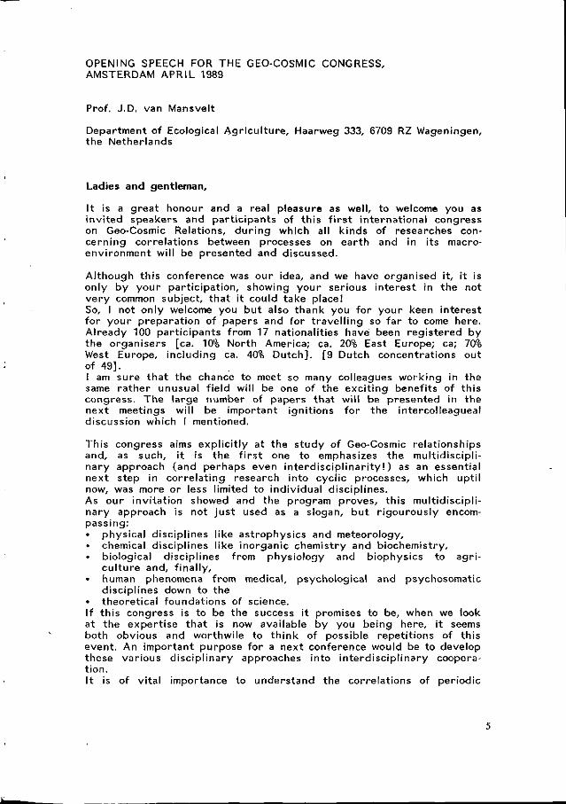
OPENING SPEECH FOR THE GEO-COSMIC CONGRESS, AMSTERDAM APRIL 1989

Prof. J.D. van Mansvelt

Department of Ecological Agricul ture, Haarweg 333, 6709 RZ Wageningen, the Netherlands

Ladies and gentleman.

It is a great honour and a real pleasure as well, to welcome you as invited speakers and participants of this f i r s t international congress on Geo-Cosmic Relations, dur ing which all kinds of researches con­cerning correlations between processes on earth and in its macro-environment will be presented and discussed.

Although this conference was our idea, and we have organised it, it is only by your participation, showing your serious interest in the not very common subject, that it could take place! So, I not only welcome you but also thank you for your keen interest for your preparation of papers and for t ravell ing so far to come here. Already 100 participants from 17 nationalities have been registered by the organisers [ca. 10% North America; ca. 20% East Europe; ca; 70% West Europe, including ca. 40% Dutch]. [9 Dutch concentrations out of 49]. I am sure that the chance to meet so many colleagues working in the same rather unusual f ield will be one of the exciting benefits of this congress. The large number of papers that will be presented in the next meetings will be important ignitions for the intercolleagueal discussion which I mentioned.

This congress aims explicit ly at the study of Geo-Cosmic relationships and, as such, it is the f i rs t one to emphasizes the multidiscipli-nary approach (and perhaps even interdiscipl inarity ! ) as an essential next step in correlating research into cyclic processes, which uptil now, was more or less limited to individual disciplines. As our invitation showed and the program proves, this multidiscipli-nary approach is not just used as a slogan, but r igourously encom­passing: • physical disciplines like astrophysics and meteorology, • chemical disciplines like inorganic chemistry and biochemistry,

biological disciplines from physiology and biophysics to agri­culture and, f inally,

• human phenomena from medical, psychological and psychosomatic disciplines down to the

• theoretical foundations of science. If this congress is to be the success it promises to be, when we look at the expertise that is now available by you being here, it seems both obvious and worthwile to think of possible repetitions of this event. An important purpose for a next conference would be to develop these various disciplinary approaches into interdisciplinary coopera­tion. It is of vital importance to understand the correlations of periodic

processes within the solarsystem with the variety of periodicities within the biosphere; that a thorough understanding needs to be based on interdisciplinary research will become evident dur ing the next days.

However the connection between these disciplines and the Geo-Cosmic Relationships that are the subjects of this congress, needs a scien­t i f ic explanation. Of course, each of you will have something specific to add to these general remarks, and so help to complete the picture of this challenging object of study.

Looking more closely at the conceptual problems surrounding the kind of research that we will discuss these days, a main problem is that we miss a clear concept of causalities l inking the cycles of the solar-system and its continuously changing constellations to the variety of processes in the biosphere. The question is whether this kind of research demands a revision of our usual concept of causality or, in other words, whether the usual concept effectively prevents or even prohibits the continuation of this kind of research. This causality question confronts us also with the question whether only one type of causes can ever be sufficient to understand the whole range of processes indicated before. Could it be that some levels of reality, some realms of nature, need a modified causality-concept instead of the one that was developed to explain material phenomena in physics? Leaving aside the common concept of causes exterior to the affected phenomena, some philosophers propose interna! causes in human beings in addition to, or instead of, the external causes that govern phy­sical matter.

I r retr ievably l inked with the concept of causes is the question of in how far, for example, human beings are influenced or even governed by such not yet sharply defined influences from within our solar system - "solar system" sounds much closer than "outer space"! - because such influences would interfere with our notion of freedom and responsi­bi l i ty. The results of the research that is to be presented dur ing the next days, will probably emphasize at least the need for a very discering and subtle approach of this causality question, lying between the dogmatic wholly predestinated and the wholly coincidental concept of human life, which is just as dogmatic. This subtle approach of causality might also help us f i r s t to accept, and subsequentially to gradually understand some of the di f ferent degrees of dependence on cosmic influences, represented by di f ferent types of correlations, that can appear, for example, between verte­brates and invertebrates, animals and plants, seed plants and spore-bearing plants etc.

Another characteristic of natural sciences, especially in so far as they claim to be exact sciences, is the question of variabi l i ty of the experimental results, namely the variance of the data. Here, the rela­tionship between the rationality of natural laws, the randomness or i rrat ionali ty of chance and all that can influence the data such as experimental errors, sampling errors, errors of measurement, biases and deviations is at stake. Much of the research that will be pre-

sented dur ing this congress would never have been found if the usual variabi l i ty of experimental data had been taken as inherent for the object under study. Many of them may have started as inquiries into the rest-varience of some kind of variance-analyses. In other words, our problem can be reformulated as the question of neutrality of time, namely the reproducibi l i ty of the process or pro­cesses under studie. The more we suppose them to be unaffected by time or, in other words, the less we can or want to imagine those processes to be influenced by temporal alterations of any - as yet unknown - factor, the more we will tend to stress the inherent nature of the observed variabi l i ty and regard any research into the underlying cycles as irrelevant.

The problem of the relationship between rational scientific concepts (laws, theories) and accepted i rrationali ty (part ly diguised as the ratio of coincidence), also confronts us with the contrast between the empirical roots of natural sciences and the conceptual or theoretical ones, or, in other words, the inductive versus the primarily deductive

,approach. If we f ind in empirical data reliable correlations that we cannot yet explain (understand) within the usual framework of concepts, should we then deny or disregard these data, for example by averaging them, or should we feel obliged to take the data for facts of the studied mat­ter, and t r y to widen or adept the existing concepts to account for the additional evidence we have found. '

As an agricultural ist I would like to f inish this introduction by con­sidering possible applications of the knowledge that this conference wants to contribute to. However, in this interdisciplinary context I should start to emphasize that agriculture is much more than the production of milk, pigs and potatoes. It ranges from food production over food processing and con­sumption to nutr i t ion and personal health; but also from farming over landscaping and nature conservation to the sustainable management of a healthy environment. Agriculture is the basis of biosphere-manage­ment.

Now suppose that the term biotechnology would be a neutral descriptive term indicating "the art of life-proces-management", then agriculture (or "biosphere management") would be r ight from the start a type of bio-technology. Medicine would then be another important type of bio­technology, and, somehow, a counterpart of agriculture. Both are, at least part ly, applied life sciences. Like all other arts or technolo­gies, it would develop throug time and reflect the cultural develop­ment, the history of those practising it.

Reviewing the agricultural development in this century, there is a clear tendency to develop techniques that make agriculture increasingly independent of the capriciousness of nature. By severing an unreflected number of ecological relationships these interventions have generated a whole range of unforeseen side effects that we are now discovering all over the world.

Bio-technology, in the usual sense of the word goes a step fu r ther by creating a fully-controled artif icial environment wherein rigorously disconnected processes, ranging from biosyntheses to embryology, can

proceed in a very controlled way. Some people, though highly impressed by the level of technical sophis­tication and investment of intellect, are, at the same time, worried by the huge amount of money and fossil energy that must be invested to realise this intellectual planning, and fur ther more worried by the problems of reintegration of the disconnected processes into the world outside the biotechnological plants.

Would another possibil i ty, for the development of Bio-technology, be increasing our knowledge of Geo-Cosmic relationships, and seeing how this can be implemented in, for example, the practice of agriculture [biosphere management], climatology, meteorology and medicine? The more we know about the interactions of various lifecycles, the more we can make our cultural activities f i t in with the rhythms of nature in a rational, reasonable way. Instead of constantly f ight ing against what we perceive as natures capricious i rrat ionali ty, we could develop a rationally supported intuition or even feeling for her cycles, and, consequently, change over to working with nature. Then we could make use of those cyclical forces in some kind of bio-synthetic time management.

It is clear to me that this last option of Biotechnology would not be possible to realise in a short time. But, interestingly, the same is t rue for the approach of Biotechnology described in "Brave-new wor ld".

To make sure that the next generations will get a fair chance to choose the kind of fu ture they want, the kind of research that wil l be presented dur ing this and future Geo-Cosmic congresses, and in the proceedings and other publication arising from them, should get the attention and financial support it deserves. It deserves maximum sup­port because it is both environmentally sound and relevant. It is th rust ing back the f ront iers of our present knowledge; opening the way to a re-integration of our human management of life procesess in the biosphere into a harmony with nature.

With these words I now have the pleasure and honour to declare the working sessions of the First International Congress on Geo-Cosmic Relations opened.

Prof.drs. J.D. van Mansvelt Apr i l 20th 1989

Introductory papers

DYNAMICS OF THE SOLAR SYSTEM

W. de Graaff

Em. professor of astronomical space research, State University of Utrecht, 3992 JD Houten, The Netherlands

Summary

The dominant factor governing the behaviour of the Solar System is the Sun's gravitational attraction which determines, a.o,, the orbital motion of the planets around the Sun. In addition, the mutual attraction of the planets is responsible for periodic perturbations of these orbits. The same force fields also determine the motions of the smaller bodies in the Solar System, such as the planetary satellites, the asteroids, the comets, and the meteoroids. In a number of cases these perturbations lead to resonances between the orbits of different objects. As for the larger bodies, the dimensions of which cannot be neglected as compared with their distances, differential gravitational forces (tidal forces) more or less strongly set the conditions in the surface and adjacent interior layers of these bodies.

The temperature balance of the planets and the smaller objects is dominated by the electromagnetic radiation from the Sun which is partly reflected, and partly absorbed and re-emitted in some form or other by these objects Keywords: Solar System, dynamics, resonances, tidal effects, radiative equilibrium.

Introduction

In discussing geo-cosmic relations, i.e. relations between the Earth and its environment, some of the first types of relations which come to mind are the one which binds that environment, the Solar planetary system, together, and the one which, among other things, makes life possible on Earth. It is the purpose of this paper to describe the present state of knowledge with respect to these relations.

1 Gravitational attraction

1.1 History and general properties

It was the German astronomer Johannes Kepler who, in the first decades of the 17-th century, discovered the laws which govern the motion of the planets around the Sun and which still bear his name: (1) Planetary orbits around the Sun are ellipses, with the Sun in one of the two focal points (2) The radius vector from the Sun to the planet covers equal areas in equal periods of time (3) The.square of the orbital period of a planet is proportional to the cube of the semi-major axis of the orbital ellipse.

In the latter part of the 17-th century, Isaac Newton formulated

11

the fundamental law of gravitational attraction: Two point masses attract each other with a force which is directly-proportional to each of the two masses, and inversely proportional to the square of their distance.

This law is equivalent to the three laws of Kepler. The gravitational force was instrumental in the evolution of the Solar system from a huge interstellar cloud consisting mainly of gas and dust to the form in which it presents itself to us today.

With over 99»8 percent of the total mass of the present Solar system concentrated in the Sun, it is clear that in a first approximation each planet can be considered to move around the Sun. When higher accuracies are required and possible, the mutual attraction between the planets and the mass ratios between the Sun and the planets have to be taken into account. This results in weaker or stronger perturbations of the ideally Keplerian orbits of the individual planets.

That the Earth had a true companion, our Moon, was known from times immemorial. However, that it was not the only planet to have such a companion was discovered by Galileo Galilei in l6l0, when he saw through a telescope four tiny lights moving about Jupiter. Today we know that all four of the giant planets are accompanied by between 8 and 25 satellites. Moreover, we also know that not only Saturn, but all four of the giant planets have rings. Apparently rings, too, are a general, rather than a peculiar phenomenon.

We find that the Solar system is full of cyclic motions at two levels: the motion of the planets, as well as the smaller bodies of the Solar system such as the asteroids, the comets and the meteoroids around the Sun, and the motion of the satellites and ring particles around their parent planet. The motions of these bodies interact in various ways with each other as well as with the mass distribution within the bodies themselves.

1.2 Gravitational resonances

In complex systems such as our planetary, satellite and ring systems application of the lav/ of gravitational attraction produces a number of special features. In many-body systems the mutual attraction of all of its members as superimposed upon the attraction of the central body will produce what is called resonance effects. These effects occur when the orbital periods of two or more small objects orbiting a much more massive central body have a ratio equal to the ratio of two small integers. The general understanding at present is that the orbits slowly expand at different rates due to tidal interaction with the central body (see section 1.3). When a state of commensurability is reached, the orbital periods become locked in resonance, and remain so for the foreseeable future. As an example of this, the inner three Galilean moons of Jupiter, i.e. Io, Europa and Ganymede, have orbital periods which are proportional to 1, 2 and k, respectively (see Table 1). It should be remarked here that perfect resonance (i.e. to at least nine digits) occurs not for the sidereal periods shown in the table, but for the anomalistic periods, i.e. the periods with respect to the common line of apsides (major axis) of the orbital ellipses which itself rotates with a sidereal period of ^86.811 days. These anomalistic periods are equal to I.762 731 8,

12

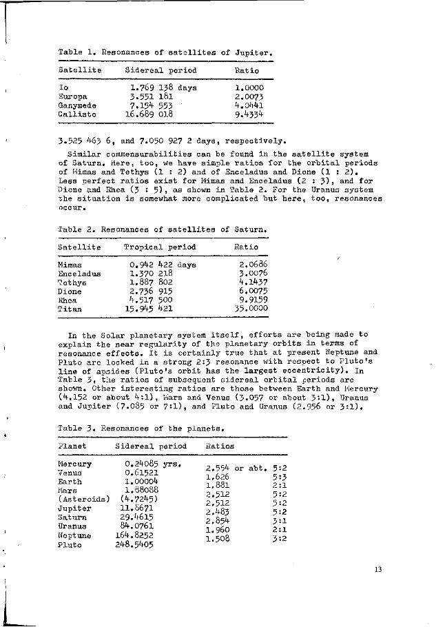
Table 1. Resonances of satellites of Jupiter.

Satellite Sidereal period Ratio

Io Europa Ganymede Callisto

I.769 158 days 3.551 lol 7.154 553 •

I6.689 018

1.0000 2.OO73 4.0441 9.433^

3.525 463 6, and 7.050 927 2 days, respectively.

Similar commensurabilities can be found in the satellite system of Saturn. Here, too, we have simple ratios for the orbital periods of Mimas and Tethys ( 1 : 2 ) and of Enceladus and Dione (1 : 2 ) . Less perfect ratios exist for Mimas and Enceladus (2 : 3 ) , and for Dione and Rhea (3 '• 5) , as shown in Table 2. For the Uranus system the situation is somewhat more complicated but here, too, resonances occur.

Table 2. Resonances of satellites of Saturn.

Satellite Tropical period Ratio

Mimas Enceladus Tethys Dione Rhea Titan

0.942 422 days I.37O 218 I.887 802 2.736 915 4.517 500

15.945 421

2.0686 3.OO76 4.1437 6.0075 9.9159

35.0000

In the Solar planetary system itself, efforts are being made to explain the near regularity of the planetary orbits in terms of resonance effects. It is certainly true that at present Neptune and Pluto are locked in a strong 2:3 resonance with respect to Pluto's line of apsides (Pluto's orbit has the largest eccentricity), in Table 3, the ratios of subsequent sidereal orbital periods are shown. Other interesting ratios are those between Earth and Mercury (4.152 or about 4:1), Hars and Venus (3.057 or about 3:1), Uranus and Jupiter (7.085 or 7:1), and Pluto and Uranus (2.956 or 3:1).

Table 3. Resonances of the planets.

Planet Sidereal period Ratios

Mercury Venus Earth Mars (Asteroids) Jupiter Saturn Uranus Neptune Pluto

0.24085 yrs. O.6152I 1.00004 I.88088

(4.7245) II.8671 29.4615 84.0761

164.8252 248.5405

2.554 or abt. I.626 1.881 2.512 2.512 2.483 2.854 I.96O I.508

5:2 5:3 2:1 5:2 5:2 5:2 3:1 2:1 3:2

13

If one examines the distribution of orbital periods of the asteroids in comparison with the orbital period of Jupiter, peaks are found at fractions of 2/3 and 3 A times the period of Jupiter, and gaps at fractions of 1/2, 3/7, 2/5, 1/3, and 1/k. Furthermore, at least part of the detailed structure of the various ring systems can be explained in terms of resonance effects due to nearby satellites.

1.3 Tidal forces

Another special feature of gravitation occurs when the dimensions of the objects involved are not negligible as compared to their mutual distances. When that is the case, the masses of the objects can no longer be considered as point masses, and the mutual attraction of different parts of the objects must be taken into account. If, as an example, we consider the Earth-Moon system and take the centre of the Earth as a point of reference, the part of the Earth nearest to the Moon will be attracted by the Moon more strongly than the centre, and the part farthest away from the Moon less strongly. These differential gravitational forces are called tidal forces, and their effects upon the surface of the Earth include the familiar tidal waves of the oceans. It can easily be seen that tidal forces are inversely proportional to the cube of the distance between the mass centres of the objects involved.

The tidal forces of the Moon and, to a lesser degree, those of the Sun lead to the transportation across the Earth's surface of large amounts of ocean water. The friction which these water masses encounter during their motion produces a small, but observable deceleration of the Earth's rotation velocity. On the Moon, as on nearly all other planetary satellites, this tidal friction has resulted in locked motions, i.e. the rotational period of the satellite has become equal to its orbital period. Thus, the same hemisphere of the satellite is always directed towards the planet.

If the orbit is elliptical instead of circular, the tidal forces will vary during each revolution, and this will in general produce frictional heat inside the body of the satellite. The results of this are most clearly seen on the surfaces of the inner two satellites of Jupiter: lo with its active volcanoes, and Europa with its constantly reworked icy surface.

2 Electromagnetic energy

2.1 Sources

Apart from the direct effects of gravitational attraction, we have an important indirect effect in the form of electromagnetic radiation emitted by the Sun. As is well known this radiation is produced in the central parts of the Sun by the spontaneous fusion of hydrogen to helium. This fusion occurs due to the extreme conditions prevailing in the core: pressures up to some two billion atmospheres, and temperatures up to some fifteen million degrees. These conditions result from gravitational forces tending to pull matter inward until a pressure is reached capable of withstanding further contraction. When the proper conditions for fusion are reached it will start spontaneously, and the resulting energy production will help to oppose the gravitational contraction. This

14

energy will then tie transported outward, and emitted from the Solar surface at a temperature of about 6000 K. The equilibrium achieved in the process will last approximately 10 billion years, about half of which have elapsed so far.

The energy radiated into space by the Sun is partly reflected, and partly absorbed and re-emitted in some other form by the planets and the smaller objects in the Solar system. In addition, only the larger planets seem to have energy sources of their own. The amount of energy emitted by these sources is of the same order of magnitude as the amount of Solar energy intercepted by the planetary surfaces. In general, however, it is the Solar energy which dominates the conditions near the surfaces of the planets and other objects, and in particular their temperature.

2.2 Effects on planets and satellites

The equilibrium temperature of the outer layers of planets and satellites including, if applicable, their atmospheres, is determined by the amount of Solar energy absorbed by these layers and by the size of the objects. On the Earth, these equilibrium conditions have led to the emergence of life.

The ways in which life evolved on Earth depended strongly upon its physical and chemical properties, such as its orbit around the Sun, its seasons caused by its rotation about an axis which is not perpendicular to its orbit, the original structure and composition of its atmosphere and surface, in particular the presence of large oceans of liquid water, the tidal effects, and many others. Since the tidal effects, although partly due to the Sun, are dominated by the Moon, our natural satellite, too, exerts some physical influence upon the evolution of life on Earth.

As far as we know, the Earth is the only object in the Solar system on which life has emerged. This means that the conditions prevailing on Earth shortly after it originated must have been rather strict.

3 Relative influences upon the Earth of Sun, Moon and planets

3.1 Gravitational attraction

We have seen that both the Sun and the Moon exert an appreciable influence upon the Earth in terms of gravitational attraction. If we want to compare these forces with those of other objects in the Solar system, we have to apply Newton's law and take into account the masses and distances of these objects. Thus, if we put the gravitational attraction of the Sun at one million, we find for the relative force of the Moon about 5^00, of Jupiter 5^, of Venus 32, of Saturn k, of wars 1.2, and of the other objects less than 1.

3.2 Tidal forces

As we have mentioned, the Moon exerts the strongest tidal force upon the Earth, with the Sun as a good second. If this time, therefore, we put the Moon's tidal force equal to one million, we find '+80 000 for the Sun, 56 for Venus, 6 for Jupiter, 1.1 for liars, and less than 1. In all of these cases we have used the distances at closest approach to the Earth.

15

3.3 Electromagnetic radiation

Here v/e must take into account the fact that the Sun is virtually the only source of electromagnetic radiation in our Solar system. The radiation we receive from the planets is in most cases only, and in the other cases mainly reflected Solar radiation. Therefore, the ratios are still larger here than in the previous sections. Thus, if we now put the radiation received from the Sun at 10 billion (10 000 000 000), we find 25 000 for the full Moon, 15 for Venus, 3.3 for Mars, 2.8 for Jupiter, 1.3 for Mercury, 0.3 for Saturn, and much less for the other objects. The values for the planets apply to the condition of maximum brightness.

Conclusions

The physical influences of the planets of our Solar system upon the conditions on Earth are many orders of magnitude smaller than those exerted by the Sun and the Hoon. Cnly in the case of resonance the effects might, under exceptionally suitable conditions, become much larger than they normally would be. Sven in general the effects need not be totally negligible. However, any theory dealing with geo-cosmic relations in \rtiich these planets play a role should take account of those facts.

Literature

Patterson, C.W., 1987. Kesonance capture and the evolution of the planets. Icarus 70:319-333.

.Resonant explanations, July 198l. Scientific American 2Ä5 No. 1: 5^-56.

Seidelman, P.K., Dogett, L.E. & DeLuccia, M.R., 197^. Mean elements of the principal planets. Astronomical J. 79:57-60.

The Astronomical Almanac for the year 1989. Washington: O.S. Government Printing Office, London: Het Majesty's Stationery Office.

16

RADIATION IN OUR ENVIRONMENT FROM THE ATMOSPHERE AND FROM SPACE

E. Wedler Institut für Meteorologie, Freie Universität Berlin, Dietrich-Schäfer-Weg 6-10, D-1000 Berlin 41 (F.R.G.)

Abstract

The several radiation ranges of the electromagnetic spectrum, i.e. the radiation intensities and their variations being effective in the human's living space, are shown. This includes light radiation (IR...UV), x-ray and particle radiation of solar and cosmic origin as well as solar meter and decimeter wave radiation and atmospherics within the low-frequency ELF-VLF range. Additionally, the man-made radio noise as well as the ter­restrial kinds of radiation with biological efficacy possibilities are dealt with.

Introduction

As well as for other complexes of environmental factors producing effects on biological systems (Wedler, 1976), for the radiation complex we have to differentiate between strong and weak environmental factors (Weihe, 1983). Strong factors are for instance air temperature and air moisture as compo­nents of the thermic complex. Weak factors for instance are the atmosphe­rics as components of the electro-magnetic complex.

2 Solar and atmospheric radiation (UV-IR)

One of the well known strong radiation factors in the human's living space are the solar and the environmental radiation in the range from 280 nanometers to 1000 micrometers wavelength, e.g. from ultraviolet (UV) over visible light to infrared (IR) radiation. Fig. 1 shows, that incoming solar radiation gives a total energy flux of S0=1.4 kW/m^ ("solar con­stant"). Annual variations of this value related to the earth's surface - caused by the excentricity of the path of the earth around the sun- are + 1.5.10-^ , solar cycle variations only + 1.10-5.

2.1 Radiation components (UV-IR)

On the direct way to the Earth only 31% of the incoming solar radiation reach the earth's surface. Three processes in the atmosphere cause that:

1. Reflection: In total 36% of incoming radiation energy SQ are going back into space by reflection especially from top of clouds. This represents the so-called albedo. About 6% of S are reflected from the earth's surface (component R ) .

2. Absorption: 17% of S 0 are absorbed in the atmosphere especially by the water vapour (H2O).

3. Scattering: Incoming solar radiation is scattered within the atmos­phere so that 22% of this component H (heavens radiation) comes down to the earth's surface.

S and H are the short wave components in the range of 300 nm to 4 um wave­length reaching earth surface. Together they give 53% of S Q in the global scale.

17

The long wave radiation components in the troposphere for the range of 4 to 100 fim wavelength are:

1. the infrared radiation from the earth's surface into the atmosphere E and

2. the atmospheric infrared radiation A coming from clouds and from the water vapour in the troposphere to the earth's surface.

400 km

+ IONOSPHERE

~75km * MESOSPHERE ~ 4 5 km * STRATOSPHERE

10 km •« TROPOSPHERE (BIOSPHERE)

Fig. 1. Solar and atmospheric radiation in the atmosphere (UV-IR) (modified after Tanck, 1969). Solar Constant SQ= 1.4 kW/i ,2 ± 1.5.10 l (Annual variations)

(Solar cycle variations) ± 1 .10-5 Radiation components at earth surface: Short wave (0.3-4 m) : S,H,R Long wave (4-100 ]m) : E,A,r (R,r : Reflection components)

Each of these two components with S 0 percentages of 98 or 78 respectively is bigger than the total of incoming short wave radiation components at the earth surface (see Fig. 1). But the net value of these long wave com­ponents is only 20% of S0. In the global average only 7% coming from the infrared component E reach space. Additionally, 57% comes from the top of clouds and from the gases and aerosols in the atmosphere. It means that totally 64% goes out into space. So the global net energy flux for the earth of short and long wave components is zero.

Nendritzky and Niibler (1981) illustrated the components of the human radient energy budget in open air, short wave as well as long wave compo­nents coming from above, from trees, house walls, streets etc.

2.2. Energy spectrum (UV-IR)

Fig. 2 shows the energy spectrum of the solar radiation and of the IR emission of the earth's surface depending on the wavelength. Black body radiation from the sun (6000 K) and from the earth's surface (300 K) and their variations by absorption processes in the atmosphere - especially

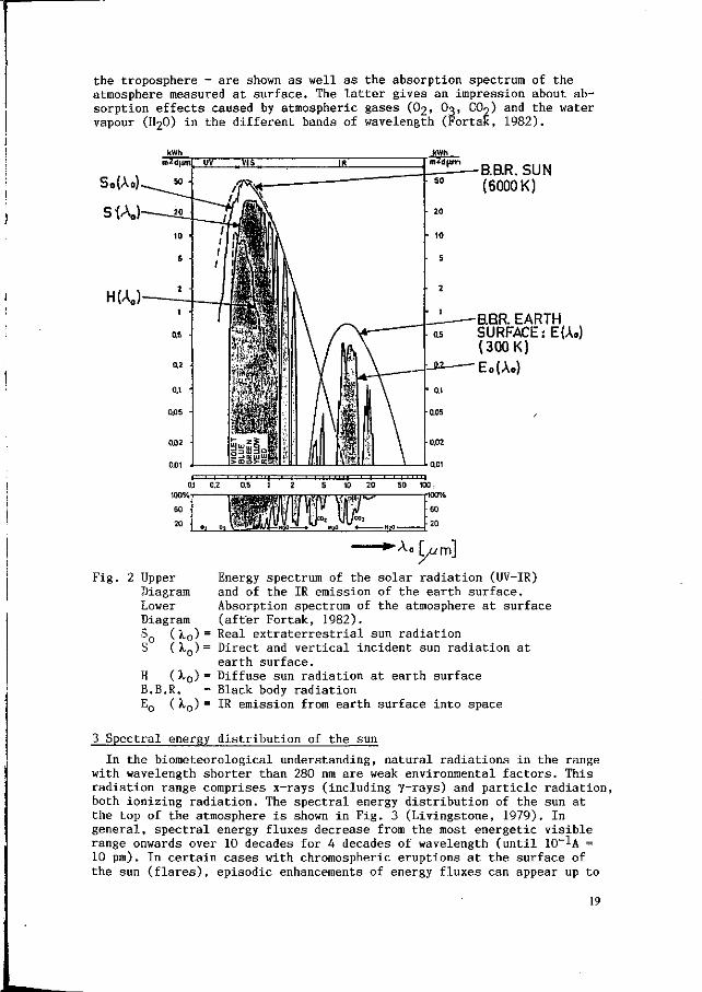
the troposphere - are shown as well as the absorption spectrum of the atmosphere measured at surface. The latter gives an impression about ab­sorption effects caused by atmospheric gases (O2, O3, CO9) and the water vapour (H2O) in the different bands of wavelength (Fortak, 1982).

B.B.R. SUN (6000 K)

B.BR. EARTH SURFACE: E(Ao) (300 K)

Eo(A.)

Fig. 2 Energy spectrum of the solar radiation (UV-IR) and of the IR emission of the earth surface. Absorption spectrum of the atmosphere at surface (after Fortak, 1982). Real extraterrestrial sun radiation Direct and vertical incident sun radiation at earth surface.

( X 0 ) = Diffuse sun radiation at earth surface Black body radiation IR emission from earth surface into space

Upper Diagram Lower Diagram

s0 U0) = s U0) = H U 0 ) -B.B.R.

E0 U0> =

3 Spectral energy distribution of the sun

In the biometeorological understanding, natural radiations in the range with wavelength shorter than 280 nm are weak environmental factors. This radiation range comprises x-rays (including y-rays) and particle radiation, both ionizing radiation. The spectral energy distribution of the sun at the top of the atmosphere is shown in Fig. 3 (Livingstone, 1979). In general, spectral energy fluxes decrease from the most energetic visible range onwards over 10 decades for 4 decades of wavelength (until 10~^A = 10 pm). In certain cases with chromospheric eruptions at the surface of the sun (flares), episodic enhancements of energy fluxes can appear up to

19

WAVELENGTH

Fig.3 Spectral energy distribution of the quiet/active sun

(after Livingstone, 1979) .

5 decades. A, B, C, M and X are the different energy levels of flares introduced 1969 by the US National Oceanic and Atmospheric Administration (Space Environment Services Center, 1988). Values are related to measure­ments at satellite level.

4 Solar-terrestrial radiation relations

Solar-terrestrial radiation relations include the components of the wave radiation, such as x-rays, light waves within the range of ultraviolet to infrared as well as radio waves and particles radiation of various energy scales such as solar wind, low and high energy protons (Fig. 4; Space En­vironment Services Center, 1974). The electromagnetic wave radiation (from radio waves to x-rays) almost propagates with the velocity of light (300.000 km/s) and therefore it has a transit time from the sun to the earth of about 8.3 min. The velocities of the particle radiation are cor­related with their kinetic energy. Thus, high-energy particles of E ^ ^ ^ I O MeV show a shorter transit time (from half an hour to a few hours) than low-energy particles ranging from 10 eV to 5 keV, where transit times up to 3 days (v = 500 km/s) and more are registered.

The lower the kinetic energy of the charged particles, the more they are influenced by the interplanetary and the earth's magnetic field. The latter directs these particles to polar latitudes. This effect is demonstrated in

Solar Wind High Energy Protons Low Energy Protons

X-Ray and Radio Waves

f Aurora

i Ionosphere » Communications

Fig. 4 Solar-terrestrial radiation relations (Space Environment Services Center, 1974)

21

Fig. 5 as result of a meridional section across America from 0° to 60° N geomagnetic latitude: maxima of the total vertical intensity of solar/ cosmic particle radiation increases with increasing latitude (Bartels, 1960).

C\J i

>-i -H CO

o

0,50

0,40

0,30

0,20

0,10

r

A

/ B \ l/c\

D \ / / E \

I

A

B

C

D

E

1

Saskatoon,

Omaha

Ft. Worth,

Acapulco

Peru

'

L 60° H 51° N

42° N

25° N

0°

t

2ÖÖ 400 6ÛÔ 800"

ATMOSPHERIC DEPTH (9 _2

cm <L)

Fig. 5. Total vertical intensity of solar/cosmic radiation in a meridional section across America at different geomagnetic latitudes ß m as a function of atmospheric depth (Bartels, 1960)

Energy densities of the solar radiation components for all wavelengths ranging from 10 pm to m are presented in Table 1 (Livingstone, 1979).

The energy of the solar wave and of the particle radiation within a time scale from minutes to several hours is increased transitory by solar flares. Flares with little energy increases often appear; those with strong to very strong energy increases (e.g. proton events of ^±n^ 10 MeV) are rarely found. In general, the flare activity is modulated by the nearly 11-year sun activity cycle (Solar-Geophysical Data, 1989).

5 Solar/cosmic particle radiations through the atmosphere

The question arises which of the solar/cosmic radiation components reach the biosphere with which intensities, i.e. the living space of man, animal and plant. Fig. 6 shows the absorption height of incoming radiation from space as a function of the wavelength (after Schulze, 1970). The diagram gives two atmospheric windows: the optical and the radio window. For wavelength X0

below 280 nm, the radiation absorption (UV-c, x-rays) nearly amounts to 100 per cent in the upper atmospheric levels (ionosphere/stratosphere). The intensity of these radiation components at sea level is zero.

Regarding the particle radiation, things are different: Incident solar and cosmic particles react with molecules within the atmos­phere and develop a wide spectrum of secondary particles and wave radia-

22

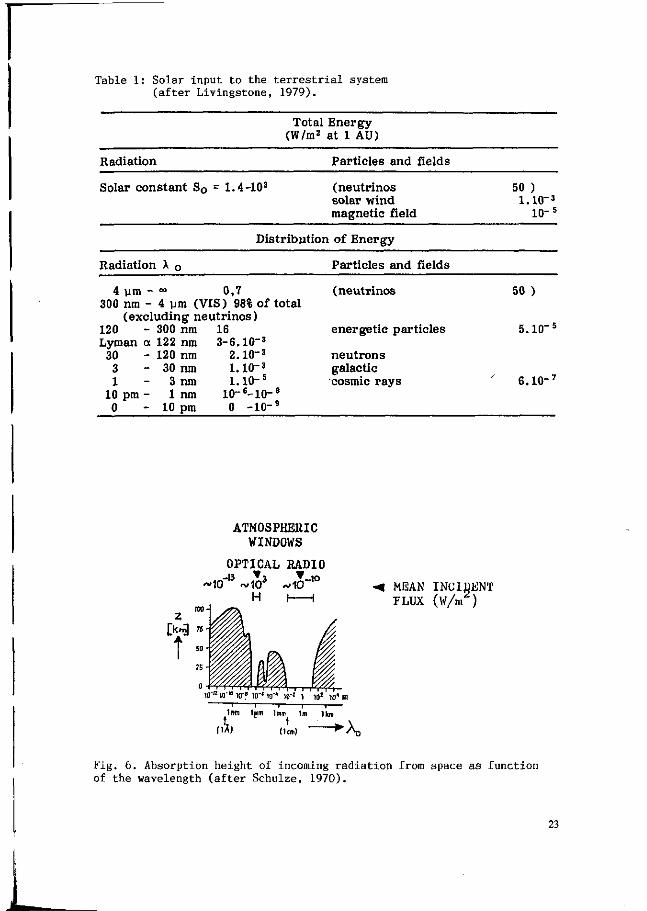
Table 1 : Solar input to the terrestrial system (after Livingstone, 1979).

Radiation

Solar constant S0 : = 1.4-103

Total (W/m2

Energy at 1 AU)

Particles and fields

(neutrinos solar wind magnetic field

50 ) 1.10"3

io-5

Distribution of Energy

Radiation X 0 Particles and fields

4 pm - °° 0,7 300 nm - 4 um (VIS) 98% of total

(excluding neutrinos) 120 - 300 nm Lyman a 122 nm 30 - 120 nm 3 - 30 nm 1 3 nm

10 pm - 1 nm 0 - 10 pm

16 3-6.10"3

2.10"3

1.10"3

1.10-5

io-6-io-e

0 - i o - 9

(neutrinos

energetic i

neutrons galactic cosmic ray

50 )

5.10"5

6.10-7

ATMOSPHERIC WINDOWS

OPTICAL RADIO

• MEAN INCIDENT FLUX (W/m )

1nm 1pm 1mm Im U m

("•*) (1cm) ^ A j

Fig. 6. Absorption height of incoming radiation from space as function of the wavelength (after Schulze, 1970).

23

L

top of otmosptwt

muonic component

Fig.7. Schematic representation of the development of particle

production through the atmosphere caused by an incident primary

proton arriving from space (Allkofer, 1975) .

E to' MUONS

ELECTRONS

PROTONS

SEA\LEVEL

0 200 400 600 800 1000

—~ ATMOSPHERIC DEPTH [pcm'^J

Fig.8. Altitude variation on vertical intensity of the main

solar/cosmic particle radiation components (Allkofer, 1975).

tions. A great part of these secondary particles is absorbed within deeper atmospheric layers. But partly they reach the sea level, possibly in the 5th, 6th or 7th reaction step (Fig. 7; Allkofer, 1975). Fig. 8 illustrates the altitude variation of the main particle radiation components within the atmosphere as a function of atmospheric depth (All­kofer, 1975): Muons decrease more slowly than electrons and protons. This is caused by the fact that the interaction of muons with atmospheric par­ticles is weaker than those of protons and electrons (see Fig. 7 ) . Protons and electrons as well as muons reach sea level with relatively small but measurable rates:

10_2(i/cm2.s.sr) : muons 10-3(i/cm .s.sr) : electrons 10~^(l/cm2.s.sr) : protons

1 gKXXJ

a uu 8:990 o oc £960 Q. t o O | 970

< 1-0

> UJ

23-0

1-1.0 a 56-0 0

3 70 z < X " 8 0 è?

:

.

' • 1

!i\ ?! * !

• 1

1 • 1 1 1 1 1

2 3 4 5 6 7 8

\ 4i

H m ! I

• 1 1 1 1 1 1

2 3 4 5 6 7 6

V 1 y 1 1 1 1 t 1 1 1 1 \'\jf< 9 tO 11 12 13 14 15 16 n J ^ S f j

f •'{ 1 ;i

;!• Ai: #'

1 > ' Wi ' ';l,"i 'ij: :' '• i :

• 1 1 1 '1 1 1 1 1 1 1

9 10 11 12 13 .14 15 16 n 18 19 ^ TIME (DAYS)

1 1 1 1 1 t 1 . 1 20 21 22 23 24 25 26 27 08' i ,

V;; '

» > : ! i ,

il: if' : • ,. 'Mi; ,f.i|!

<ï«; .,rs,

V''\.

v> 20 21 22 23 24 25 26 27 -i"

Fig. 9. The atmospheric pressure and the intensity of the muon component of the solar/cosmic radiation as functions of time for February 1954, at Sverdlovsk, USSR (Rochester, 1962).

At the 175 (g/cm^) level muons and electrons exhibit a maximum of the vertical intensity. At 52°N this value corresponds to a height of about 13 km above sea level, while within the logarithmic scale the vertical in­tensity of the protons decreases almost linearly from the upper boundary of the atmosphere down to sea level.

As a result, both the barometric pressure and the muon component of the solar/cosmic particle radiation at a given place as a function of time show inverse fluctuations: increasing particle intensity coincides with decreasing barometric pressure and vice versa (Fig. 9; Rochester, 1962).

6 Ionizing particle radiation stress of man

Fig. 10 illustrates the entire field of the solar/cosmic ionizing radia­tion components within the atmosphere (Schaefer, 1974), showing isolines of the radiation intensity (= dose rate) depending on the geographical

25

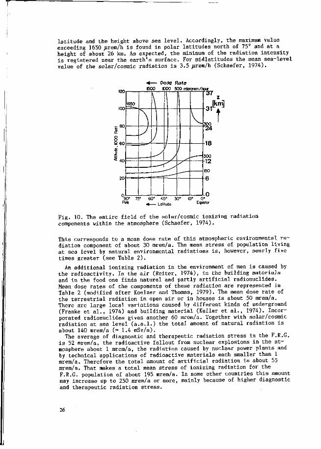
latitude and the height above sea level. Accordingly, the maximum value exceeding 1650 .urem/h is found in polar latitudes north of 75° and at a height of about 26 km. As expected, the minimum of the radiation intensity is registered near the earth's surface. For midlatitudes the mean sea-level value of the solar/cosmic radiation is 3.5 /irem/h (Schaefer, 1974).

120

IOOF

- 80 •

1Ï

S 60

•8

** 40

20

4 — Dose Rate 1500 OOO 500 rricrorem/hour

^37 1650

.. ._,.

" ) J

\

)

\

1

\

I

L

90° 75° 60° Pole ^

45° Latitude

30°

-31 [km]

•300 '24

•18

300 12 I50

6

I5° 0° Equator

t

Fig. 10. The entire field of the solar/cosmic ionizing radiation components within the atmosphere (Schaefer, 1974).

This corresponds to a mean dose rate of this atmospheric environmental ra­diation component of about 30 mrem/a. The mean stress of population living at sea level by natural environmental radiations is, however, nearly five times greater (see Table 2 ) .

An additional ionizing radiation in the environment of men is caused by the radioactivity. In the air (Reiter, 1974), in the building materials and in the food one finds natural and partly artificial radionuclides. Mean dose rates of the components of these radiation are represented in Table 2 (modified after Koelzer and Thomas, 1979). The mean dose rate of the terrestrial radiation in open air or in houses is about 50 mrem/a. There are large local variations caused by different kinds of underground (Franke et al., 1974) and building material (Keller et al., 1974). Incor­porated radionuclides gives another 60 mrem/a. Together with solar/cosmic radiation at sea level (a.s.1.) the total amount of natural radiation is about 140 mrem/a (= 1.4 mSv/a).

The average of diagnostic and therapeutic radiation stress in the F.R.G. is 52 mrem/a, the radioactive fallout from nuclear explosions in the at­mosphere about 1 mrem/a, the radiation caused by nuclear power plants and by technical applications of radioactive materials each smaller than 1 mrem/a. Therefore the total amount of artificial radiation is about 55 mrem/a. That makes a total mean stress of ionizing radiation for the F.R.G. population of about 195 mrem/a. In some other countries this amount may increase up to 250 mrem/a or more, mainly because of higher diagnostic and therapeutic radiation stress.

26

Table 2: Natural and artificial environmental ionizing radiation mean dose rates of FRG population 1984 (modified after Koelzer and Thomas, 1979) (1 mSv = 100 mrem)

Type of irradiation Mean dose rate (mSv/a

Solar/cosmic radiation (a.s.1.)

terrestrial radiation in open air

terrestrial radiation in houses

incorporated radionuclides

0,30

0,43

0,57

0,60

Total of natural radiation 1,40

Medicine (diagnostics and therapy) 0,52

radioactive fallout from nuclear explosions 0,01

radiation by nuclear power plants <T0,01

technical applications of radiation materials <0,01

Total of artificial radiation 0,55

Total 1,95

10

30

100

300

1000

a 3000

10,000

' ' 30,000

20 30 40 50 Time (Minutes of 1er start of f l a re )

Fig. 11. A typical dynamic spectrum that might be produced by a large flare (importance 2B or larger).

Type I : Storm bursts Type IV : Prolonged continuum Type II : Slow drift bursts Type V : Brief continuum burst Type III : Fast drift bursts (normally following (Solar-Geophysical Data, 1987) Type III bursts)

27

i.

L

(vO-°i

ca co

fi

3 « a W U 0) 4J IM CD

e 3

i j

o a

•H O Ö

u •H •P 0) c Ol <s e o u •P o ai H w

o •H

eo

U fi (U 3 o iu

4-1

> ai vi m

•o

Vi (U s o o. U) in

•H 0

c •c 0) N

• H pH m e u o •z

n) M e g i i a c

•H -H e e in O)

• H O C O) 3

0)

o

Su r-l e

"O

•H o 0) 3 O (U >•<

>1 u (U

>

b EL,

— W >

o •H •U I«

•H •o ni U

V •H •P 0) G O (d

O 01

ü pa il u

S » o m

O

X v m

1

7 Non-ionizing wave radiation

Electromagnetic waves in the radio range are non-ionizing radiations. In the biometeorological understanding these natural wave radiations are weak environmental factors too. From the most energetic visible range of the natural electromagnetic spectrum down to meter-waves solar spectral energy fluxes decrease over 26 decades for 7 decades of wavelength or frequency (Fig. 3 ) , so that for 10 m wavelength )30 MHz) spectral irradiance is about 10-22w/m2. um.

In the meter and decimeter range one can find as well solar continuum radiation as episodic enhancements of energy fluxes, so-called bursts. In the most of the cases the latter are correlated with optical flares.

The average energy flux in the wavelength range of the atmospheric radio windows is very low, ca. 10~10W/m2 (Fig. 6 ) . The solar continuum flux is modulated by the solar activity cycle as shown by registrations at 10.7 cm (2800 MHz) since 1947 (Solar-Geophysical Data, 1987). The mean max/min-ratio of wave energy at this frequency within the very active 19th solar cycle (1954-1964) was more than 3:1.

Fig. 11 demonstrates a typical dynamic spectrum of bursts in the fre­quency range from 10 to 30.000 MHz (30 m to 1 cm) that might be produced by a large flare (importance 2B and larger) (Solar Geophysical Data, 1987). Individual flares exhibit many variations to this spectrum.

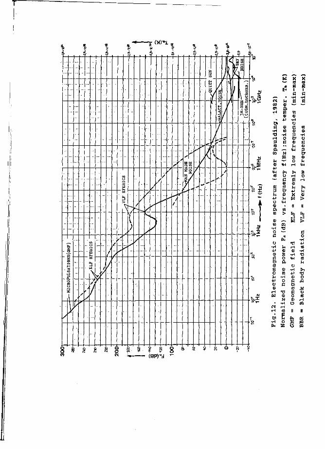
/ 7.1 Electromagnetic noise spectrum

The electromagnetic noise spectrum (Fig. 12) completes the electromagne­tic waves in the environment of men. This spectrum includes micropulsations of the geomagnetic field (=GMF), ELF and VLF atmospherics (=sferics) as well as man made electromagnetic noise and atmospheric, solar and galactic noise. In general, spectral noise energy decreases over 32 decades for 12 decades of increasing frequency from 0,1 Hz to 100 GHz (Spaulding, 1982).

In respect to possible biological effects of one or the other of these radio components in the environment of men, one had to look not only for the energy flux but also at the time structure of signals. In the above range of electromagnetic basis frequencies, time structure can be expressed by pulse frequencies of signals. There are some known examples from atmos­pherics with pulse repetition frequencies in the range of 0 to 10 Hz (König, 1975; Wedler, 1976; Wever, 1979).

8 References

Allkofer, O.C., 1975: Introduction to Cosmic Radiation. Thiemig, München, 221 pp.

Bartels, J. (Editor), 1960: Geophysik. Fischer, Frankfurt am Main, 373 pp. Fortak, H., 1982: Meteorologie. 2nd edition, Reimer, Berlin, 287 pp. Franke, Th., Keil, R. and Schales, F., 1974: Externe Exposition durch

terrestrische Strahlung im Freien. In: K. Aurand et.al. (Editors), Die natürliche Strahlenexposition des Menschen. Thieme, Stuttgart, pp. 62-69.

Jendritzky, G. and Nübler, W., 1981: A Model Analysing the Urban Thermal Environment in Physiologically Significant Terms. Arch.Met.Geoph.Biokl., Ser.B, 29: 313-326.

Keller, G., Schmier, H. and Seelentag, W.jr., 1974: Externe Exposition durch terrestrische Strahlung in Gebäuden (Baustoffe). In: K. Aurand et. al. (Editors), Die natürliche Strahlenexposition des Menschen. Thieme, Stuttgart, pp. 70-79.

Koelzer, W. and Thomas, P. 1979: Die Belastung des Menschen durch ionisie­rende Strahlung. In: Sicherheit und Strahlen-schutz. Kernforschungs-

29

Zentrum Karlsruhe, pp. 2-10. Koenig, H.L., 1975: Unsichtbare Umwelt. Moos, München, 176 pp. Livingstone, W.C., 1979: Solar Input to the Terrestrial System. In: B.M.

McCormac and T.A. Seliga (Editors), Solar-Terrestrial Influences on Weather and Climate. Reidel, Dordrecht, Boston, London, pp. 45-57.

Reiter, R., 1974: Physical and Chemical Properties of the Lower Atmosphere (Boundary Layer and Lower Troposphere). In: S.W. Tromp, J.J. Bouma (Edi­tors), Progress in Biometeorology, Div.A, Progress in Human Biometeoro-logy, Vol. 1, Part IA, Period 1963-70. Swets&Zeitlinger, Amsterdam, pp. 25-45.

Rochester, G.D., 1962: Cosmic Rays and Meteorology. Quart.J.Roy.Meteor.Soc., 88: 369-381.

Schaefer, H.J., 1974: Das Hbhenprofil der kosmischen Strahlen-dosis. In: K. Aurand et.al. (Editors), Die natürliche Strahlen-exposition des Menschen. Thiem, Stuttgart, pp. 1-9.

Schulze, R., 1970: Strahlenklima der Erde. (Wissenschaftliche Forschungs­berichte, 72). Steinkopff, Darmstadt, 217 pp.

Solar-Geophysical Data, 1987: Explanation of data reports, 515 (Supplement). U.S. Dept. of Commerce, NOAA, Boulder, Col., 83 pp.

Solar-Geophysical Data, 1989: 533, Part I, p.11; Part II, p.33. U.S. Dept. of Commerce, NOAA, Boulder, Col.

Space Environment Services Center, Space Environment Laboratory,ERL, 1974: Preliminary Report and Forecast of Solar Geophysical Data. National Oceanic and Atmospheric Administration, Boulder, Col., SESC-PRF 183.

Space Environment Services Center, 1988: Descriptive Text, Preliminary Report and Forecast of Solar Geophysical Data. National Oceanic and At­mospheric Administration, Boulder, Col., p.3.

Spaulding, A.D., 1982: Atmospheric Noise and its Effects on Telecommunica­tion Systems Performance. In: H. Volland (Editor), Handbook of Atmosphe­rics, Vol. I. CRC Press, Boca Raton, Fia., pp. 289-328.

Tanck, H.-J., 1969: Meteorologie. Rowohlt, Hamburg, 136 pp. Wedler, E., 1976: Sferics als möglicher biotroper Wetterfaktor.

Z.f.Phys.Med., 5: 77-78. Weihe, W.H., 1983: Adaptive Modifications and the Responses of Man to

Weather and Climate. In: D. Overdieck et.al. (Editors), Biometeorology 8, Part 2, Proceedings of the Ninth Int. Biomet. Congress (Osnabrück 1981). Swets & Zeitlinger, Lisse, pp. 53-68.

Wever, R.A., 1979: The Circadian Systems of Man. Springer, New York, Heidelberg, Berlin, 276 pp.

30

BIOLOGICAL CYCLICITY IN RELATION TO SOME ASTRONOMICAL PARAMETERS: A REVIEW

Bruce Gordon dimming

Department of Biology, University of New Brunswick, Fredericton, Canada

Summary

This review considers some of the known geo-cosmic factors in our environment that may influence biological phenomena.

Numerous experiments have proven the existence of circadian and other rhythms that are exhibited in the absence of such obvious extrinsic timing inputs as light or temperature perturbations. Nevertheless, no intrinsic (endogenous) master clock mechanism has been discovered to account for the free-running cyclic timing characteristics of biological rhythms. A physiological puzzle is the frequent manifestation of a Q10 near unity for endogenous rhythms (i.e. relative temperature independence), and the multiplicity of regularly occurring ultra- and infra-dian rhythms (shorter and longer than circadian, respectively) that are shown in different organisms.

Since endogenous rhythms with an external correlate (e.g. the sun and, or moon) are the ones where temperature independence seems most readily explicable, one can posit the importance of investigating whether subtle extrinsic geophysical factors (particularly, different forms of energy fluctuations of extra-terrestrial origin reaching our biosphere), influence rhythmic phenomena. This is because such factors exhibit both short- and long-term periodicities that can be measured, and perhaps duplicated experimentally, to determine directly causative factors for biological periodicities (including possible predictable climatic periodicities).

Some of the more substantive indications of possible geo-cosmic related biological phenomena include: (1) Correlations between sunspot activity and (i) germination of seeds; (ii) the growth or seasonal productivity of plants and animals (terrestrial and aquatic environment). (2) The anomalous "ten-year cycle" of animals. (3) Correlations between lunar cycles and the growth or activity of plants. (4) The germination and, or the growth of plants in response to a magnetic field.

Key words: Plants, animals, climate. Biological clocks, photoperiodism, rhythmicity, cyclicity. Circadian, ultra- and infra-dian rhythms. Interactions: solar, lunar, tidal cycles. Correlations: sunspots, germination, growth, plants, seasonal productivity animals. Terrestrial, aquatic environment. Ozone, ultra-violet light, animals' "ten-year cycle".

Introduction

I wrote the following in 1967 as a somewhat ironic "Soliloquy" on our attempts to understand biological rhythms: Intrinsic, or extrinsic: that is the question: Whether 'tis circadian in the light and dark to suffer The synchronizer a and Zeitgebers of outrageous lunar cycles,

31

Or should we take arms against a sea of unioorns, And by opposing phase them? To damp, to oscillate No more; and by a feedback repress the end-product. The hourglass and the thousand sinusoidal curves That harmonic is entrained to, 'tis an amplitude Devoutly to be induced. To perturb, to oscillate; To synchronize : perchance to force: ay, that's the photoperiod; For in that linear trend what rhythmic processes may come When we have shuffled off this raw data Must give us something worthwhile. There 's a respect That makes linearity of a half life

But who would bare the photophiles and skotophiles of time, The pendulum effects, the enzymatic lack of uniformity, The rhythmic processes and the transient phase delay.

- Modified from William Shakespeare (Cumming & Wagner, 1968) Referring to the basis of photoperiodic time measurement in the same

review article it was noted that "there have been two approaches to the problem of photoperiodic time measurement...(a) the conception now universally known as Biinning's hypothesis; (b) the hourglass model. Along with these two approaches we consider a third [c], the extrinsic rhythm hypothesis, primarily attributable to Brown but supported by work from diverse sources, merits full and objective consideration" (Cumming & Wagner, 1968) .

I shall not be discussing the classical work of Garner and Allard (1920) on the photoperiodic control of various responses in plants and animals because it is tangential to our present context. However, the relationship of that work to Biinning's hypothesis is discussed in some detail elsewhere (e.g. Bünning, 1967, 1972; Cumming, 1972).

(a) Biinning's hypothesis of the physiological clock considers that the measurement of photoperiod is controlled by an endogenous free-running oscillation with a periodicity of approximately 24 hr [circadian (Halberg et al., 1959)]. Each oscillation involves a regular alternation of two half-cycles of about 12 hr which Bünning termed "photophile" and "skotophile" phases. He postulated that each phase has characteristically different innate biochemical properties, as well as different sensitivities to external controllers. Two fundamental properties of the endogenous free-running rhythm can endow the subjective organism with two distinctive but essentially characteristic responses: first, the photoperiodic induction of a particular phenomenon, and second, the ability of the rhythmic response to be rephased or entrained by light (Cumming, 1972). Pittendrigh (1966) suggested that a more explicit term than "skotophile" could serve to recognize these two distinctive responses to light. Cumming and Wagner (1968) suggested the word "transduction" to replace skotophile and it will be used here.

(b) The main concepts of the hourglass model are recognized in many physiological reactions. For example, in photoperiodism, the effective element in the daily cycle can be the duration of darkness rather than light. Thus, inductive darkness is often effective independently of the duration of the associated light periods. It can be considered that the dark period initiates a non-cyclic process, functioning as an hourglass (Cumming, 1972).

(c) The principles of the extrinsic rhythm hypothesis (otherwise known as the exogenous rhythm hypothesis) are still largely unknown, but the concept refers to the influence of subtle uncontrolled geophysical factors that may be continually imparted to an organism, even under so-called constant conditions. Brown (1965) suggested that "the organism

32

under natural conditions possesses no intrinsic daily rhythmicity but is, instead, rhythmic as a consequence of responding simultaneously and continuously to such rhythmical geophysical factors as light and temperature on the one hand, and to subtle pervasive geophysical factors on the other." Brown (1965) conceded that both intrinsic and extrinsic factors may be involved in the timing of biological periodisms. The organism may act as a "variable frequency transformer" deriving different periods from a specific period input through "autophasing." Autophasing involves the assumption that a circadian rhythm may bear any phase-angle relationship to the environmentally imposed 24-hr periodic input - even locking to it in such a manner. This theory is supported by the demonstrations of organism sensitivities to very weak subtle geophysical forces and their proven association with "clock" and "compass" phenomena, and by very specialized adjustments of the receptive system to natural ambient field strengths.

In a previous symposium on circadian rhythmicity held at Wageningen in 1971, there was the following commentary (Cumming, 1972): "K. Hoffmann (Germany) noted the difficulty of reconciling Brown's postulation that all circadian rhythms with periods differing from 24 hours are based on a 24-hour (extrinsic) input. Although, theoretically, such a system could be constructed or envisaged, it would be highly complicated and, from an evolutionary standpoint, it would be most implausible. Cumming pointed out that we should perhaps remember that as recently as the 1950's many scientists were disputing the possibility of the existence of endogenous rhythms because there was no obvious mechanistic' basis for such rhythms, and because the basic conception seemed to be too 'mystical' and therefore unscientific. While some features of Brown's theory, such as the concept of autophasing, may be difficult to reconcile with our present knowledge of circadian rhythms, we should not close our minds to the possibility that some such mechanism(s) may have evolved in certain organisms that are adapted to particular environments in which the photoperiodic factor has been less decisive".

It had been previously observed (Cumming & Wagner, 1968) that, at the 1959 Botanical Congress in Montreal, several influential botanists disputed any role of an endogenous free-runnlng-circadian biological rhythm as a timing mechanism in photoperiodic response. The particular point of dispute was whether biological clocks could be self-sustaining in supposedly constant conditions and independent of, although still responsive to, such obvious cyclic factors as visible light.

Since then, numerous experiments have proven the existence of circadian and other rhythms that are exhibited in the absence of such obvious extrinsic timing inputs as light or temperature perturbations (Bünning, 1967; Sollberger, 1965). Nevertheless, no intrinsic (endogenous) master clock mechanism has been discovered to account for the free-running-cyclic-timing characteristics of biological rhythms.

A physiological puzzle is the frequent manifestation of a Q10 near unity for endogenous rhythms (i.e. relative temperature independence). Sollberger (1965) reviews a number of examples that may involve "compensation" or "insensitivity" in relation to temperature changes. He also provides examples of the multiplicity of regularly occurring ultra-and infra-dian rhythms (shorter and longer than circadian, respectively), that are shown in different organisms.

Since endogenous rhythms with an external correlate (e.g. the sun or moon) are the ones where temperature independence seems most readily explicable, one can posit the importance of investigating whether subtle extrinsic geophysical factors (particularly, different forms of energy fluctuations of extra-terrestrial origin reaching our biosphere),

33

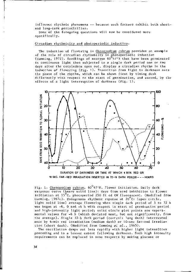
influence rhythmic phenomena — because such factors exhibit both short-and long-term periodicities.

Some of the foregoing questions will now be considered more specifically.

Circadian rhythmicity and photoperiodic induction.

The induction of flowering in Chenopodium rubrum provides an example of the role of circadian rhythmicity in photoperiodic induction (Cumming, 1972). Seedlings of ecotype 60 47'N that have been germinated in continuous light then subjected to a single dark period one or two days after the cotyledons open out, display a circadian rhythm in the induction of flowering (Fig. 1 ) . Transition from light to darkness sets the phase of the rhythm, which can be shown first by timing dusk differently with respect to the start of germination, and second, by the effects of a light interruption of darkness (Fig. 1).

10 20 30 40 50 60 70

DURATION OF DARKNESS OR TIME AT WHICH 4 MIN. RED OR

10 SEC. FAR-RED IRRADIATION INSERTED IN 72-H DARK PERIOD HOURS

Fig. 1. Chenopodium rubrum, 60 47'N. Flower initiation. Daily dark response curve (heavy solid line): days from seed imbibition to flower initiation at 15 C, photoperiod 250 ft cd CW fluorescent. (Modified from Cumming, 1967c). Endogenous rhythmic réponse at 20 C: (open circle, light solid line) average flowering when single dark period of 3 to 72 h was begun at -6, 0 and +6 h with respect to start of germination period and high-intensity light period; solid circle plot points are experi­mental values for -6 h (which deviated most, but not significantly, from the average). Single 72-h dark period (control: long dash) interrupted once by 4-min red irradiation (medium dash) or 10-sec far-red irradia­tion (short dash). (Modified from Cumming et at., 1965).

The oscillation damps out less rapidly with higher light intensities preceding and to a lesser extent following darkness. Such high intensity requirements can be replaced in some respects by making glucose or

34

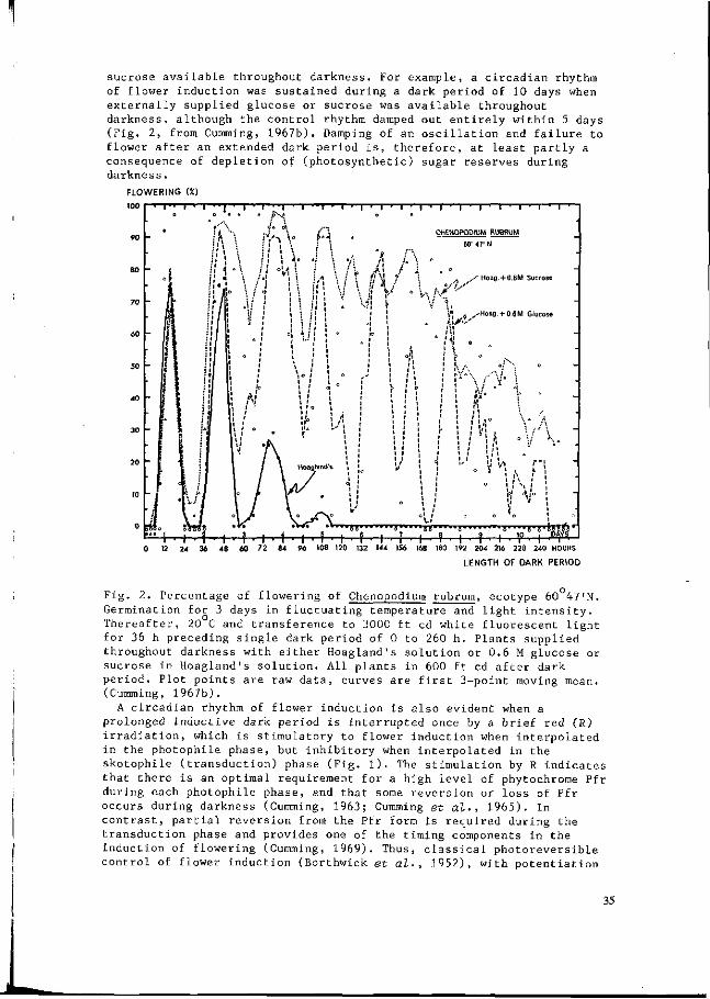
sucrose available throughout darkness. For example, a circadian rhythm

of flower induction was sustained during a dark period of 10 days when

externally supplied glucose or sucrose was available throughout

darkness, although the control rhythm damped out entirely within 5 days

(Fig. 2, from Cummlng, 1967b). Damping of an oscillation and failure to

flower after an extended dark period is, therefore, at least partly a

consequence of depletion of (photosynthetic) sugar reserves during

darkness.

FLOWERING (X)

I • I ,ul ' I I • I

CHENOPODIUM RUBRUM

60' 47' N

•' Hoag. + 0.6M Sucrose

M--' Hoag. + 0.6M Glucose

1 *

\1.

4—1- 'm^'V^s 108 120 132 144 154 168 ISO 192 204 216 228 240 HOURS

LENGTH OF DARK PERIOD

Fig. 2. Percentage of flowering of Chenopodium rubrum, ecotype 60 47'N. Germination for 3 days in fluctuating temperature and light intensity. Thereafter, 20 C and transference to 3000 ft cd white fluorescent light for 36 h preceding single dark period of 0 to 260 h. Plants supplied throughout darkness with either Hoagland's solution or 0.6 M glucose or sucrose in Hoagland's solution. All plants in 600 ft cd after dark period. Plot points are raw data, curves are first 3-point moving mean. (Cummlng, 1967b).

A circadian rhythm of flower induction is also evident when a prolonged inductive dark period is interrupted once by a brief red (R) irradiation, which is stimulatory to flower induction when interpolated in the photophile phase, but inhibitory when interpolated in the skotophile (transduction) phase (Fig. 1). The stimulation by R indicates that there is an optimal requirement for a high level of phytochrome Pfr during each photophile phase, and that some reversion or loss of Pfr occurs during darkness (Cumming, 1963; (Humming et al-, 1965). In contrast, partial reversion from the Pfr form is required during the transduction phase and provides one of the timing components in the induction of flowering (Cumming, 1969). Thus, classical photoreversible control of flower induction (Borthwick ez al., 1952), with potentiation

35

by R and depotentiation by FR (far-red), can be obtained during the photophile phase(s) in prolonged darkness, but reversibility is much less evident during the transduction phase(s) (Cumming et al-, 1965). The latter effect seems to express a feature of the rhythmic change in the optimum Pfr level required for flower induction: namely, that this level has a far more critical balance in the transduction than in the photophile phases (Gumming, et al-, 1965). Furthermore, the degree of similarity between the effects of light interruption of darkness and short-term glucose application suggests that this reducing sugar is involved directly or indirectly in the oscillatory mechanism in providing substrate for Pfr action or mediation during darkness, with Pfr acting as a type of master gate, pacemaker, or valve, and exerting some control over sugar availability and utilization (Cumming, 1967b). Phasing of the Pfr-substrate interaction appears to be set by the beginning of darkness, and it has been postulated that the substrate supply is lower during the transduction than during the photophile phases. A less specific action of sucrose than glucose has been indicated by the lack of any inhibition of flower induction when sucrose was supplied during a transduction phase (Cumming, 1967b).

Part of the foregoing discussion provides an example of interactions that may occur between clrcadian rhythmicity on the one hand, and hourglass timing, mediated by phytochrome, on the other hand.

In daily light:dark cycles, earliest (optimal) flower initiation of C. rubrum occurs in a particular range of photoperiodic cycles, depending on genotype and environmental conditions. The time elapsed before flower initiation, when plotted as a dependent variable of the length of the daily dark period, provides a response curve that can be very similar to the first oscillation of the endogenous circadian rhythm that is elicited by a single dark period (Fig. 1). This similarity is substantial evidence that the endogenous circadian rhythm provides a primary basis for time measurement in the daily photoperiodic control of flower initiation. The more advanced (earlier) phasing of the photoperiodic response curve, as compared with the free-running circadian rhythm (Fig. 1), can be explained on the basis that the daily dusk and(or) dawn signals entrain the endogenous rhythm of 30 hours; the position of the peak is in effect advanced to an earlier time in darkness, and the rhythm is entrained from its subjective (30 hr) circadian period to a 24-hour (solar) period. King and Cumming (1972a & b) have shown that the phase of the rhythm in C. rubrum - 60 47'N can be advanced or delayed according to the timing and duration of light pulses, and the significance of these results has been discussed in more detail elsewhere (Cumming, 1972).

I should note here that the endogenous rhythmic flower induction responses of different latitudinal ecotypes show specific character­istics that are also expressed in daily photoperiodic cycles — indicating the importance of genotype(s) and the physiological clock processes in adapting organisms to their environment. Thus, in C. rubrum, the most northern North American ecotypes flower in the widest range of daily dark periods. Earliest flowering at any particular temperature is in shorter daily dark periods in the northern than the southern ecotypes. Also, the ability to measure small changes in night length and the absolute requirement for darkness, is greater in the southern than northern ecotypes. This accords with the fact that day to day changes in night length are least near the equator and progressively greater towards the north pole, while the night length during the bulk of the growing season is progressively shorter towards the north pole. In the northern hemisphere, therefore, if a plant near the equator is to

36

flower at a certain time between the spring and autumn equinox each year (i.e. daily night length less than 12 hours) then the qualitative and quantitative control of induction must be over a narrower range of differences in length of dark period - with critical dark periods of relatively longer absolute length than for the more northerly ecotypes (Cumming, 1963; 1972).

Interaction of circadian oscillation with extrinsic (lunar-day) cycle in Hantzschla virgata.

During low tides, cells of this diatom migrate to the surface of the sands of Barnstable Harbour, Massachusetts, in such immense numbers that they impart a greenish to golden brown color. Before the tide returns, the cells reburrow below the surface of the sand. This alga can be prevented from re-emerging onto the surface by artificially darkening the area just as the tide recedes; furthermore, cells will reburrow if their surroundings are artificially darkened (Palmer & Round, 1967). Unlike some other related algae, there is only one migration per day even when there are two low tides during the hours of light. When the time of low tide approaches sunset, the cells rephase their emergence to the early morning hours of light (i.e. to the next low tide 12.4 hr later).

To explain these intriguing results, Palmer & Round (1967) have postulated an interacting dual-clock system. Such a system would consist of a clock that keeps in time with the lunar day i.e., the hand moves forward about 50 min per day and measures periods of 24.8 hr (summation of 12.4 hr lunar cycles), and therefore is responsible for a bimodal migration rhythm; superimposed is a solar-day (circadian) clock that is responsible for the suppression of the night-time suprasurface phase of the lunar-cycle migration rhythm. This suppression is evident from the fact that cells never appear on the surface during the time equivalent to the night phase. Even in light:dark (L:D) cycles in the laboratory, a lunar-day rhythm still persisted for 11 days in approximate synchrony with the time of daytime low tide, in that vertical migration was about 50 min later each day. More remarkable still, the same 50 min per day change in phase, and the late afternoon rephasing to early morning, occurred in the laboratory in continuous light (LL), so that there was never more than one emergence per 24.8 hr. The rephasing from dusk to dawn in LL can be explained if a major fraction of the circadian clock is suppressive to the approximately 4.5 hr above-surface phase of the 12.4-hr lunar cycle, so that only one of two migration potentials is expressed in every 24.8-hr period. A further interesting feature of the on-surface period is that a sign reversal in phototactic response of H. amphioxys has been observed: cells that responded positively to light during the initial and middle portion of this period became indifferent or negative to light just before the time that the tide returned (Fauré-Fremiet, 1951; Palmer, 1960).

Validity of the dual-clock-system concept is supported by similarities in response of other intertidal organisms (Barnwell, 1963; Naylor, 1958).

Geo-cosmic related biological phenomena

Some of the more substantive indications of possible geo-cosmic related biological phenomena include: (1) Correlations between sunspot activity and (i) the germination of seeds; also (ii), the growth or seasonal productivity of plants (including marine organisms), and,

37

animals. (2) The anomalous "ten-year cycle" of animals. (3) Correlations between lunar cycles and the growth or activity of plants. (4) The germination and, or, the growth of plants in response to a magnetic field.

(1) (i) Correlations between sunspot activity and the germination of seeds.

There were pronounced fluctuations in the percentage germination of seeds of Chenopodium botrys that were kept stored in darkness under carefully controlled conditions of temperature, humidity, and barometric pressure, that allowed comparisons of these different factors to be made over more than a two-year period with the same stored seed population. The fluctuations in percentage germination showed no evident correlation with the ambient lunar cycle or the ambient vertical and horizontal magnetic intensity (Cumming, 1967a).

The upper set of data in Fig. 3 represents the 7-day mean values of solar radio flux at Ottawa, Ontario from February, 1961 to May, 1963. These data were calculated from the daily measurements made at Ottawa and provide an accurate indication of changes in sunspot activity. The lower set of data in Fig. 3 represents the weekly percentage germination of C. botrys-8 (in Ottawa) at the end of each 3-weekly period on moistened filter paper. The germination results are lagged 3 weeks behind solar flux. Thus, the terminal date of each weekly mean solar flux reading is directly above the germination percentage of the test started on the same respective date. Referring to Fig. 3, an example may clarify this: the first observation of germination on 3 March, 1961 is lagged 3 weeks to coincide with the 10.7 cm solar radio flux of the week ending 11 February (21 days earlier), and this is the date on which seeds for this germination test were wetted. Periodogram analysis of the raw weekly data for solar flux and percentage germination, provided two periodograms with 15 closely corresponding peaks, showing that the component periods for both phenomena are quite similar. The 17 peaks for solar flux and the 16 peaks for germination (-, peak missing) were (in days):

Solar flux : 17,21,25,28, -, 35,39,44,50,54,59,64,73,83,93,109,151,221 Germination: 17,20,25,28,31, 34,39,46,50,55, -,62,69,85, -,110,146,211

The linear trends in solar flux and germination were opposite (Fig. 3 ) . Sunspot activity was declining from 1961 to 1963, reaching the minimum of an 11-year cycle in 1965. The linear trend in C. botrys germination could be ascribed to gradual loss of "dormancy" of the seed population resulting in a progressively higher percentage germination. The correlation coefficients between the third 3-point moving averages for solar flux and germination, after removal of the respective linear trends, indicated some very highly significant positive correlations, depending on the lag between the two sets of data. The best correlation (very highly significant, r = 0.65 with 89 degrees of freedom) was obtained with germination lagged 3 weeks as in Fig. 3. This correlation may become clearer by referring to the curves for the second 3-point moving averages in Fig. 3. These show the close correspondence of approximately 11 of the 16 peaks for germination with 11 of the 17 peaks for solar flux (i.e. approximately 707„). The calculated correlations were successively less significant, then changed from positive to negative, when the lag was increased or decreased.

Other experiments were designed to test whether seeds that were stored

38

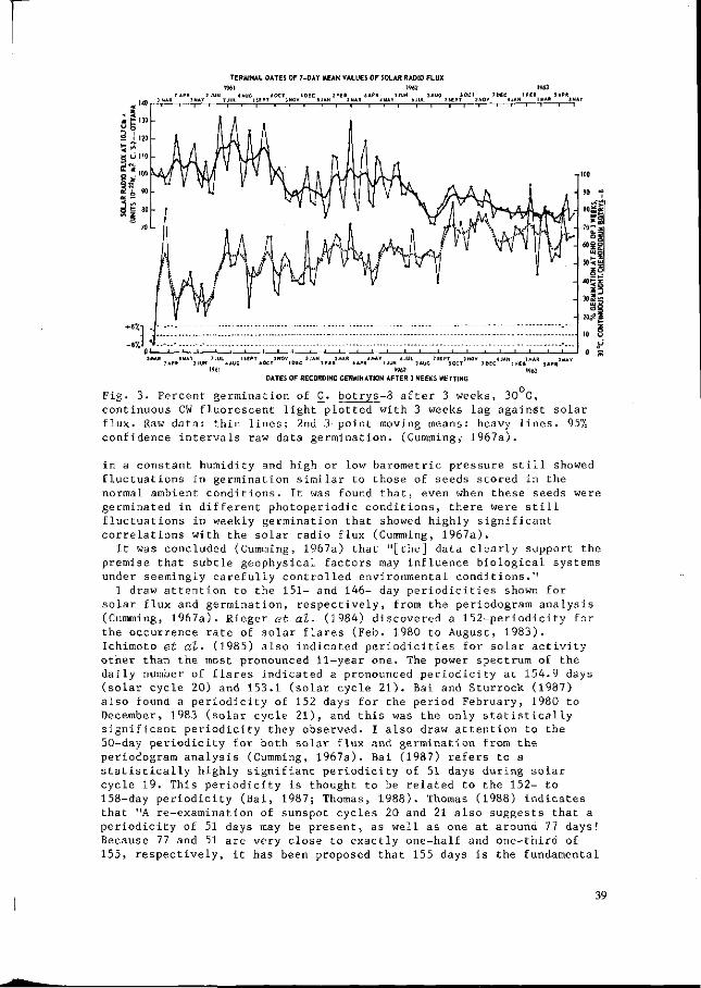
TERMINAL DATES OF 7-DAY MEAN VALUES OF SOLAR RADIO FLUX

1961 1962 ! JUN «AUG «OCT IDEC 2FEB 6APR

DATES OF RECORDING GERMINATION AFTER 3 WEEKS WETTING

Fig. cont flux conf

3. Percent germination of C. botrys-3 after 3 weeks, 30 C, inuous CW fluorescent light plotted with 3 weeks lag against so . Raw data: thin lines; 2nd 3-point moving means: heavy lines, idence intervals raw data germination. (Cumming,- 1967a).

lar 95%

in a constant humidity and high or low barometric pressure still showed fluctuations in germination similar to those of seeds stored in the normal ambient conditions. It was found that, even when these seeds were germinated in different photoperiodic conditions, there were still fluctuations in weekly germination that showed highly significant correlations with the solar radio flux (Cumming, 1967a).

It was concluded (Cumming, 1967a) that "[the] data clearly support the premise that subtle geophysical factors may influence biological systems under seemingly carefully controlled environmental conditions."

I draw attention to the 151- and 146- day periodicities shown for solar flux and germination, respectively, from the periodogram analysis (Cumming, 1967a). Rieger et al. (1984) discovered a 152-periodicity for the occurrence rate of solar flares (Feb. 1980 to August, 1983). Ichimoto et al. (1985) also indicated periodicities for solar activity other than the most pronounced 11-year one. The power spectrum of the daily number of flares indicated a pronounced periodicity at 154.9 days (solar cycle 20) and 153.1 (solar cycle 21). Bai and Sturrock (1987) also found a periodicity of 152 days for the period February, 1980 to December, 1983 (solar cycle 21), and this was the only statistically significant periodicity they observed. I also draw attention to the 50-day periodicity for both solar flux and germination from the periodogram analysis (Cumming, 1967a). Bai (1987) refers to a statistically highly signifiant periodicity of 51 days during solar cycle 19. This periodicity is thought to be related to the 152- to 158-day periodicity (Bai, 1987; Thomas, 1988). Thomas (1988) indicates that "A re-examination of sunspot cycles 20 and 21 also suggests that a periodicity of 51 days may be present, as well as one at around 77 days! Because 77 and 51 are very close to exactly one-half and one-third of 155, respectively, it has been proposed that 155 days is the fundamental

39

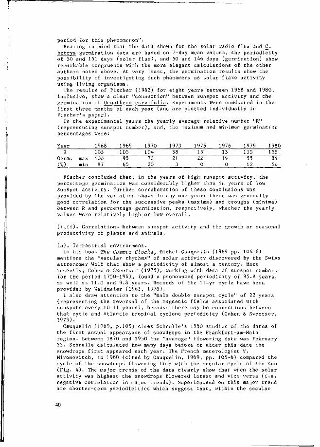
period tor this phenomenon". Bearing in mind that the data shown for the solar radio flux and C.

botrys germination data are based on 7-day mean values, the periodicity of 50 and 151 days (solar flux), and 50 and 146 days (germination) show remarkable congruence with the more elegant calculations of the other authors noted above. At very least, the germination results show the possibility of investigating such phenomena as solar flare activity using living organisms.

The results of Fischer (1982) for eight years between 1968 and 1980, inclusive, show a clear "connection" between sunspot activity and the germination of Oenothera curvifolia. Experiments were conducted in the first three months of each year (and are plotted individually in Fischer's paper).

In the experimental years the yearly average relative number "R" (representing sunspot number), and, the maximum and minimum germination percentages were:

Year R

Germ. (%)

max min

1968 105 100

87

1969 105

95 65

1970 104

70 20

1973 38 21

3

1975 15' 22

0

1976 13 19

0

1979 155

55 12

1980 155 84 54

Fischer concluded that, in the years of high sunspot activity, the percentage germination was considerably higher than in years of low sunspot activity. Further corroboration of these conclusions was provided by the variation shown in any one year: there was generally good correlation for the successive peaks (maxima) and troughs (minima) between R and percentage germination, respectively, whether the yearly values were relatively high or low overall.

(i,ii). Correlations between sunspot activity and the growth or seasonal productivity of plants and animals.

(a), Terrestrial environment. In his book The Cosmic Clocks, Michel Gauquelin (1969 pp. 104-6)

mentions the "secular rhythms" of solar activity discovered by the Swiss astronomer Wolf that show a periodicity of almost a century. More recently, Cohen & Sweetser (1975), working with data of sunspot numbers for the period 1750-1963, found a pronounced periodicity of 95.8 years, as well as 11.0 and 9.8 years. Records of the 11-yr cycle have been provided by Waldmeier (1961, 1978).

I also draw attention to the "Hale double sunspot cycle" of 22 years (representing the reversal of the magnetic fields associated with sunspots every 10-11 years), because there may be connections between that cycle and Atlantic tropical cyclone periodicity (Cohen & Sweetser, 1975).

Gauquelin (1969, p.105) cites Schnelle's 1950 studies of the dates of the first annual appearance of snowdrops in the Frankfurt-am-Main region. Between 1870 and 1950 the "average" flowering date was February 23. Schnelle calculated how many days before or after this date the snowdrops first appeared each year. The French meterologist V. Mironovitch, in 1960 (cited by Gauquelin, 1969, pp. 105-6) compared the cycle of the snowdrops flowering time with the secular cycle of the sun (Fig. 4). The major trends of the data clearly show that when the solar activity was highest the snowdrops flowered latest and vice versa (i.e. negative correlation in major trends). Superimposed on this major trend are shorter-term periodicities which suggest that, within the secular

40

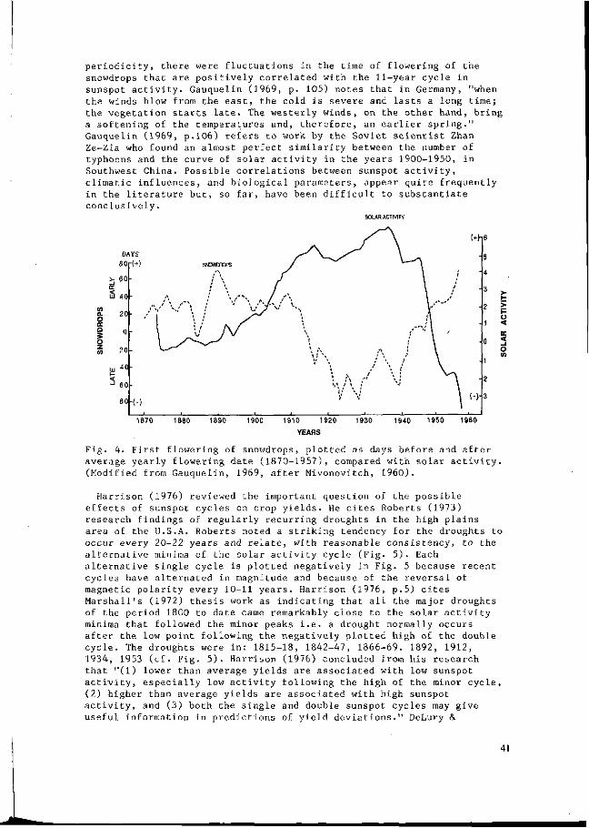
periodicity, there were fluctuations in the time of flowering of the snowdrops that are positively correlated with the 11-year cycle in sunspot activity. Gauquelin (1969, p. 105) notes that in Germany, "when the winds blow from the east, the cold is severe and lasts a long time; the vegetation starts late. The westerly winds, on the other hand, bring a softening of the temperatures and, therefore, an earlier spring." Gauquelin (1969, p.106) refers to work by the Soviet scientist Zhan Ze-Zia who found an almost perfect similarity between the number of typhoons and the curve of solar activity in the years 1900-1950, in Southwest China. Possible correlations between sunspot activity, climatic influences, and biological parameters, appear quite frequently in the literature but, so far, have been difficult to substantiate conclusively.

SOLAR ACTIVITY

> ~J oc s

0. O CE o O z 0)

LU L-

3

DAYS

80

60

40

20

0

20

40

60

80

r(+)

-/'"'''

-

"(-)

,.-, t \ '" \

SNCWDROPS

(' \ > \

; 1

\l /v

i =

\ , / / \ \ '' J* *>/ **x

y^ \

\ X

\

i i

1 i \ / \

', /' \ \ l

V s'

/ \ /

y j \

v \

, ,

t

/

<+)i

-

i

6

5

4

3

2

1

0

1

2

3

< o

1880 1900 1910 1920 1930

YEARS

1940 1950 1960

Fig. 4. First flowering of snowdrops, plotted as days before and after average yearly flowering date (1870-1957), compared with solar activity. (Modified from Gauquelin, 1969, after Mivonovitch, 1960).

Harrison (1976) reviewed the important question of the possible effects of sunspot cycles on crop yields. He cites Roberts (1973) research findings of regularly recurring droughts in the high plains area of the U.S.A. Roberts noted a striking tendency for the droughts to occur every 20-22 years and relate, with reasonable consistency, to the alternative minima of the solar activity cycle (Fig. 5). Each alternative single cycle is plotted negatively in Fig. 5 because recent cycles have alternated in magnitude and because of the reversal of magnetic polarity every 10-11 years. Harrison (1976, p.5) cites Marshall's (1972) thesis work as indicating that all the major droughts of the period 1800 to date came remarkably close to the solar activity minima that followed the minor peaks i.e. a drought normally occurs after the low point following the negatively plotted high of the double cycle. The droughts were in: 1815-18, 1842-47, 1866-69. 1892, 1912, 1934, 1953 (cf. Fig. 5). Harrison (1976) concluded from his research that "(1) lower than average yields are associated with low sunspot activity, especially low activity following the high of the minor cycle, (2) higher than average yields are associated with high sunspot activity, and (3) both the single and double sunspot cycles may give useful information in predictions of yield deviations." DeLury &

41

0'Conner (1936) have reported differences in weather response to numbers of sunspots in different geographical regions. For example, at Edmonton, Alberta, at the period of few sunspots, the rainfall may be 50 percent greater and the temperature may be as much as 4 F higher than at the time of the maximum. At coastal regions, such as St. John's, Newfoundland, rainfall is 20% higher at the time of maximum than at minimum sunspot activity.

A recent report by Campbell (1987) indicates that "Sino-Himalayan bamboos generally flower and die after vegetative periods which are integral multiples (x 1-8) of 10-12.5 years, or, in the west [Central Nepal to Eastern Kashmir], 14-16.5 years. Flowering is concentrated after droughts, which are related to the 11 or 22 year sun-spot cycles. Flowering rhythms appear to have evolved links with predictable components of climate fluctuations." An interesting "tangential" point is mentioned by Campbell (1987) who notes that some Chinese scientists consider that earthquakes are also associated with droughts and bamboo flowering: "Periodicity of 22 years... is evident during 1901-76 among earthquakes of at least magnitude 6 ... in Sino-Tibetan seismic zone The extent of local association is not clear, with Yunnan earthquakes showing only 11 year periodicity when considered alone, and Sichuan showing 18 year periodicity, suggesting some lunar relationship." Campbell continues: "Even if not related directly to bamboo flowering, earthquakes have massive regional effects on vegetation in forests with bamboos, so that any regularity in earthquake frequency may have influenced the evolution of life cycles".

1740 1760 1780 1800 1820 1840 1860 1880 1900 1920 1940 1960 1980

Drought Periods

Fig. 5. Drought periods in Nebraska plotted against double sunspot cycle, 1750-1974 (modified from Roberts, 1973).

King (1973) suggested that the sunspot number is "a relatively crude index of solar activity which should be abandoned in future work on solar-weather relationships, in favour of a more meaningful index such as the velocity of the solar wind or even the 10.7 cm solar flux." His paper provides evidence that important climatic features such as drought, rainfall and length of the growing season depend on the solar cycle. For example, he refers to evidence that, at Eskdalemuir, Scotland, between 1916 and 1969, the length of the growing season (which is a useful parameter for evaluating the impact of climate on agricultural production) varies during the solar cycle and is on average

42

about 25 days longer near sunspot maxima than sunspot minima. King (1973) also concluded that the "physical mechanisms by which solar radiation and the weather are connected are undoubtedly complex....»[but] investigations of how to incorporate solar activity into long-range weather forecasts issued for agricultural planning purposes, for example, may yield significant returns for the effort involved." A further paper'by King et al. (1974) on agriculture and sunspots provides other intriguing indications of correlations. These authors refer to increases in wheat production in the Northern Hemisphere at around sunspot maxima (e.g. in North and Central America, China, and the Soviet Union), whereas there seems to have been an inverse relationship in the Southern Hemisphere. Turnip, swede and potato yields in Britain between 1937 and 1957 appear to have been inversely correlated with sunspot number although the average temperature and rainfall in London was positively correlated with sunspot number during the same period. Note that these are some of the crops that grow optimally with relatively lower (than higher) maximum night temperatures. The average rainfall at Kew (1891-1930) was 17% greater around the sunspot maxima than the minima.

More recent evidence of an association between the Earth's weather and the solar cycle relates to the quasi-biennial oscillation (QBO) and storm tracks in the North Atlantic. When only the westerly phases (winds) of the QBO are considered a strong correlation emerges between the solar cycle and atmospheric temperatures and pressures in £he Northern Hemisphere. For example, Labitzke (1987), Labitzke & van Loon (1988), van Loon & Labitzke (1988), found that high solar activity seems to inhibit cooling of air high above the Earth's poles; above the North Pole the air was fastest and coldest at sunspot minima. Reports by Kerr (1987), Geller (1988), and Monastersky (1988) refer to the foregoing research findings by Karin Labitzke, Harry van Loon, and Brian Tinsley.

An article by Stuiver & Quay (1980) notes that, during intervals of low sunspot activity the magnetic shielding properties of the solar wind are such that a larger galactic cosmic-ray flux arrives in the upper atmosphere, whereas cosmic ray fluxes are lower during periods of higher sunspot numbers. The authors note that the changes in cosmic ray flux cause variations in atmospheric neutron production, and: "Because the production rate of [Cl4] is dependent on the interaction of neutrons with atmospheric nitrogen, the [C140„] activity levels in the atmosphere reflect the changes in cosmic ray intensity, which in turn reflect solar variability. Thus the record of atmospheric [C14] activity, as given by the decay-corrected [C14] activity in tree rings, can provide important information on prehistoric solar changes Thus, the 860-year [C14] record indicates three episodes when sunspots apparently were absent: AD 1654 to 1714 (Maunder minimum), 1416 to 1534 (Spörer minimum), and 1282 to 1342 (Wolf number)... The part of this record after AD 1645 correlates well with the basic features of the historical record of sunspot numbers. The magnitude of the calculated [C14] production rates points to a further increase in cosmic-ray flux when sunspots [and auroral activity] are absent."

In the Netherlands, Wijmstra et aï. (1984) used pollen density measurements in addition to [C14] analysis, for dating pollen, spores and, macro-remains in deposits of peat. Periodicities of approximately 22, 40, 85, 145, 200, 350, 500, 600, 800, 1000, and 1450 years were established with reasonable confidence. The underlined periods correspond with known sunspot cycles of 22, 40, 80-90, 150, 200, 500 and possibly 1000 years (Bracewell, 1986; Eddy, 1976; Schove, 1967). The Dutch authors suggest that such results "open a whole new area for

43

future palaeoecological-palaeoclimatological research, that may become of considerable importance f or meteorology and long-term weather forecasting."Indeed Eddy (1976, 1977) had previously found a close correlation between the Maunder sunspot minimum (ca. 1650-1700 A.D.) and a maximum of [C14] content of the atmosphere and the winter severity index. He used the fluctuations of [Cl4] content, established by analysis of tree rings, to estimate fluctuations of solar activity back to 3000 B.C.

Heikkinen (1982) has summarized some of the relationships between sunspots and terrestrial phenomena. Aurorae are produced when charged particles of the solar wind interact with the Earth's magnetic field and molecules in the atmosphere; they are strongly positively correlated with sunspot numbers. Sunspots affect the [C14] production rate in the upper atmosphere, because the solar wind modulates the [C14]-producing cosmic ray flux impacting the Earth's atmosphere. During sunspot maxima the solar wind increases and the stream of cosmic rays reaching the atmosphere decreases and the [C14] production rate is abnormally low. At sunspot minima the situation is reversed. The [C14] isotope has a half-life of 5730 years and is carried as CO through photosynthetic pathways into plants. Determining [C14] content of tree rings yields information on [G14] changes and, thus, of past solar activity. Tree-ring derived [C14] values correlate strongly with sunspot numbers. For example, during the Maunder minimum the [C14] production was efficient, as in the Spörer, Wolf and Oort (1010-1050) minima.

Heikkinen (1982) notes the possibility that the solar activity influences atmospheric electricity, which might increase the frequency of thunder showers. Also, jet streams in the upper atmosphere may fluctuate with the 11-year solar cycle and this could change climatic conditions. In addition, small variations in solar luminosity may be related to the 11-year sunspot rhythm.

King et al- (1974) have noted that "It is well known that the period around 1700 was relatively cold; it is referred to as the 'Little Ice Age' [see also Thompson et al.-, 1983]. Temperature data...for central England...show that the average length of the growing season during the decade 1691-1700 was about 220 days. Temperatures from Kew for the particularly favourable decade 1931-40 show that the average length of the growing season was approximately 280 days A return to the growing conditions which existed around 1700 would obviously result, from an agricultural point of view, in a much less favourable environment than that which existed during the twentieth century."

The chemical test of Piccardi has been offered as an index (P) for integrating all cosmic effects from solar origin which are able to influence biological phenomena (Piccardi & Becker, 1956; Verfaillie, 1969). Solar emissions accompanying each solar eruption are of two kinds: electromagnetic and corpuscular (Verfaillie, 1969). The electromagnetic wave, travelling at the speed of light, reaches the earth in 8 minutes, giving the "Sun Flare Effect" (SFE). The corpuscular front, travelling at 2,000 km/sec, reaches the earth after 21 hours giving rise to ionospheric effects that can last for several days with decreasing intensity, and, daily periodicity due to rotation of the earth. Using rice seedlings, Verfaillie (1969) determined whether their fluctuations in growth rate were in phase with the P indices of the chemical test. He found that there was a strong negative correlation between the rice seedlings growth rate (and the coefficient of variation affecting it) and the P indices. Verfaillie (1969) concluded that the biological effects appeared to be due to electromagnetic radiations of the solar eruptions, whereas the chemical test appeared to be influenced

44

by the subsequent corpuscular emissions. I refer now to the fascinating series of comparisons made by

Huntington (1945) in his book Mainsprings of Civilization. While it is impossible in many instances to determine whether correlations have a common causative relationship, Huntington's extensive collection of data are well worth studying. I note that he shows (p.519, Fig. 75), for the period 1885-1940, extensive positive correlations between cyclicity in sunspot number and "storm track" data of Kullmer for the entire United States and Southern Canada, as well as some separate regions — even the alternate high and low maxima for the 22-year sunspot cycle are reflected in much of the data.

Across to Russia, Huntington (1945) indicates (p.520, Fig. 76) a striking positive correlation of sunspot numbers with thunderstorms in Siberia from 1887 to 1923 (based on data of Septer).

The research of an Australian, R.G. Vines (1977), provides more equivocal data that are valuable in showing distinctive patterns for different regions that may preclude overall generalizations. Vines studied crop production and rainfall patterns in S.E. Australia and the Canadian prairies in such crops as wheat, oats, barley and hay. He observed quasi-periodic fluctuations in yields, reflecting similar long-term fluctuations in rainfall, which are possibly associated with changes in solar activity. Analysis of long-term rainfall trends showed "consistency" with cyclic crop yield patterns and with the incidence of disastrous forest fires in Canada and Australia — that are promoted in drought conditions. He concluded that major droughts are determined by weather patterns distinctive to the areas concerned and these patterns suggest certain connections with the sunspot cycle. Campbell & Gardiner (1979) questioned the validity of forecasts based on Vines' results due to "inherent déficiences" in his conclusions.

(b) Aquatic environment

An extensive survey of the Laminariaceae growing around the coast of Scotland, involving aerial photographic surveys, quadrat sampling from boats, during all times of the year, between 1946-55, was reported by Walker (1956). He found a close positive correlation between the variations in the mean fresh weight per unit area of the Laminariaceae and mean monthly sunspot numbers applicable to Scotland. Walker concluded that the laminarian periodicity is not a direct consequence of sunspot activity but the indirect result of such activity producing metereological conditions that, in turn, are reflected in the marine environment.

British workers, Southward et at. (1975), have provided evidence (based on data of H.H. Lamb) of a secular trend of sea surface temperatures (SST), and 10-11 yr cyclicity, in very close agreement with curves of annual mean sunspot number — with an identical phase relationship. These SST results applied to the Plymouth Sound area and the North Atlantic. Correlations between sea temperature and various biological components in the English Channel near Plymouth were calculated. It was found that, in general, the warm water species (e.g. hake, red mullet, John Dory, megrim, and the barnacle Chthamalus) were positively correlated with temperature, while the cold water species (e.g. cod, haddock, and the barnacle Balanus balanoides) were negatively correlated. Southward et al- (1975) noted that "the longer term trends... belong to a family of similar changes which have been found in several parts of the northern hemisphere and have been tentatively linked with the secular trend of sea temperature; these include

45

fluctuations in arctic fishes and invertebrates, phytoplankton and zooplankton of the northern North Atlantic, North Sea fisheries and fish and invertebrates of the English Channel."

Southward et dl- (1975) observed that the peak of the secular temperature cycle was reached in the 1940's or 1950's. "If the suggested link between the biological trends, the temperature trends, and the solar and planetary cycles is correct....then the temperature trend should continue in reverse until 1990 or later. These authors indicate the possibility of predicting the trend of cold and warm species on the basis of secular and shorter-term cycles.

Other recent work stresses some additional features regarding long-term trends in solar activity. These findings come from studies of sediments ("varves") laid down in ancient lakes by annual flood waters. Changes in the thickness of varves indicate changes in local rainfall and provide indications of possible links between climatic variations and solar activity. Bracewell (1986) has used the varves as a tracer of solar activity covering a period of 1337 years. He has shown that the basic 11- and 22-year cycles are modulated by 314- and 350-year cycles. The 11-year cycle varies from 8 to 15 years and this shift is caused by the 350-year modulation (Bracewell, 1986). The 314-year cycle provides an envelope which seems to determine the strength of the peak of activity reached in the 11-year cycle. Bracewell (1986) predicted a steady rise in solar activity from 1986.5 to 1991, with a peak sunspot number then of over 100.

Reid (1987) reported: "Recent measurements have shown that the total solar irradiance decreased at a rate of 0.0197= per year between 1980 and 1985, and may still be decreasing. Presumably, this reflects a cyclical variation that may or may not be related to the well-known cycles of solar activity. Using data on globally averaged sea surface temperature (SST) over the past 120 yr, I show that the solar irradiance may have varied in phase with the 80-90 yr [secular] cycle represented by the envelope of the 11-yr solar-activity cycle. As the last peak of the cycle occurred in 1955-60, the next minimum should be reached about the end of the century, by which time the solar irradiance will be reduced from its peak value by 1% if the present decay rate of 0.019% per year is typical." Reid also postulates: "The intriguing possibility that the link might be provided by a small variation in the sun's luminosity keyed to the 80-90 yr Gleissberg [1985] cycle in solar activity has been explored with a simple ocean thermal model, and the range of variation has been found to be less than 1% over the 130-yr period. The implied rate of change in luminosity is consistent with the magnitude of the long-term decay that has been directly observed in recent years. Though entirely circumstantial and speculative, such clues to the causes of natural climate variability may prove valuable in future attempts to assess the climatic impact of man's activities."

Driver (1978) has observed that "Annual landings of shrimp (Crangon crangon) in the Lancashire and Western Sea Fisheries District (UK) have previously been predicted 1 year in advance on the basis of rainfall and air temperature records of the previous year. For the port of Lytham, abundance of shrimp [1965-1975] has been found to be correlated with mean sunspot number. Since sunspot number can be predicted fairly acccurately, this correlation has given the prediction of landings a greater accuracy than was formerly possible. Sunspot numbers can be predicted for a considerable period of time in advance, and therefore abundance of C. crangon at Lytham can be estimated for several years."

Stimulated by Driver's (1978) work, Love and Westphal (1981) in the U.S.A. studied the relationship between the Dungeness crab off the west

46

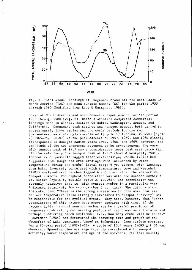
CO (S z 5 z <

< => z z <

o I-

60

50

40

30

20

m

-

•

•

ƒ/

'f

******* \

•

\ *\

\ *' / \ 1 - - - /

/

/

.

TAL

\

ss \

\ \

'* \^ .

4

; \

/ /

/

/

j i •

200

160

oc ai m

120 S Z

80

40

O CL m z 3 CO

54 56 58 60 62 64 66 68 70 72 74 76 78 80

YEAR

Fig. 6. Total annual landings of Dungeness crabs off the West Coast of North America (TAL) and mean sunspot number (SS) for the period 1955 through 1980 (Modified from Love & Westphas, 1981).

coast of North America and mean annual sunspot number for the period 1955 through 1980 (Fig. 6 ) . Catch statistics comprised commercial landings made in Alaska, British Columbia, Washington, Oregon, and California. "Dungeness crab catches and sunspot numbers both varied in approximately 11-yr cycles and the cycle periods for the two [parameters] were strongly correlated ([cycle l] 1955-64, r=0.90: [cycle 2] 1965-75, r=0.87) as the peak catches of 1957, 1969, and 1980 closely corresponded to sunspot maxima years 1957, 1968, and 1969. However, the amplitude of the two phenomena appeared to be asynchronous. The very high sunspot peak of 1957 saw a considerably lower peak crab catch than did the relatively low sunspot peak of 1969" (Love & Westphal, 1981). Indicative of possible lagged interrelationships, Woelke (1971) had suggested that Dungeness crab landings were influenced by water temperature during the crabs' larval stage 4 yr. before, with landings then being inversely correlated with temperature. Love and Westphal (1981) analysed crab catches lagged 4 and 5 yr. after the respective sunspot numbers. The highest correlation was with the sunspot number 5 yr. before (cycle 1, r=0.82; cycle 2, r=0.95). The correlation was strongly negative; that is, high sunspot number in a particular year indicated relatively low crab catches 5 yr. later. The authors also indicated that "There is the strong suggestion in this work that sea surface temperature (also strongly correlated to sunspot activity) may be responsible for the cyclical event." They note, however, that "other correlations of this nature have proven spurious with time. If the pattern holds...annual sunspot number may be a useful predictor of Dungeness crab catch, delineating periods of catch maxima and minima and perhaps predicting catch amplitude, i.e., how many crabs will be taken."

Hartmann (1984) has determined the spawning time and growth of the whitefish of Lake Constance, based on information from various sources, for a 90-year period (1892-1982). A cycle of 10.4 years (KONF ± 1.0) was observed. Spawning time was significantly correlated with sunspot activity, water temperature and age of the spawners. The fish usually

47

spawned early in the years near a minimum of solar activity and later near a maximum, respectively. In 14 out of 18 cycles the extremes (min./max.) of the yearly sunspot activity are not more than 1 calendar year off the year with the corresponding extreme of spawning time (Chi test: only a 5 cycle correspondence expected by chance). It is assumed from this work that the later the growing season the later the spawning season sets in. Hartmann (1984) posits whether fluctuations of radiation of extreme wave length may play a more important role than the visible light through climate, in these results; he also suggests that the effect of temperature on spawning time seems stronger than that of solar activity. "From the cycles of sunspot activity and spawning time alone, early spawning around 1986 and late spawning around 1991 [sunspot maximum] is to be expected" (Hartman, 1984).

Kitano (1981) has referred to the Kuroshio — a narrow intensive ocean current that generally flows along the eastern coast of Japanese Islands. It is characterized by a large-scale oceanic jet stream, comparable to the atmospheric jet stream, and a counterpart to the North Atlantic Gulf Stream. The cold water region enlarges when the speed of the Kuroshio weakens. The Kuroshio meander south of Japan exists for a period of years, disappears in other years, then reappears. Kitano (1981) concluded that the cold water mass (off Enshunada) in this century has so far been generated adjacent to the sunspot minimum or maximum year but mostly generated adjacent to the years of sunspot minima.

(2) The anomalous "ten-year cycle" of animals.

The so-called "ten-year cycle" of a wide range of animals, but particularly "wildlife" (Keith, 1963; Rowan 1950, 1954), raises intriguing questions that most authors on the subject have raised, then dropped for lack of an experimental approach. Huntington (1945) typifies the periodicity as being 9 2/3 years. The most extensive data have been discussed by Elton (1924) and Elton & Nicholson (1942a & b ) . Lynx data, for example, were based on Hudson's Bay Company Northern Development yearly records for lynx pelts from animals trapped during two centuries: 1735-1934 (Elton & Nicholson, 1942b). While I find this aspect of Canadian history particularly repugnant from an ethical-animal-rights viewpoint (Cumming, 1988), the data provide valuable evidence of wildlife's 9 2/3-year cycle. Elton (1924) originally thought that this cyclicity might be related to sunspot activity. However, MacLulich (1937) made it abundantly clear that, for example, with the lynx and varying hare data, the pronounced 9.7-yr periodicity characteristic of both species, while in phase with sunspot cycles at certain periods, was out of phase at other periods — as would be expected for a higher frequency periodicity.

Huntington (1945; Fig. 68 p.489, Fig. 69 p.494) provides intriguing comparisons between the cyclicity of tent caterpillars in New Jersey (Headlee, 1934), New Brunswick salmon fishing on the Restigouche River (Phelps & Belding, 1931), Canadian lynx (Elton & Nicholson, 1942b), deaths from heart disease in the northeastern U.S.A. (Vital Statistics, U.S.A., 1943), and atmospheric ozone measured in Paris and London (using a somewhat primitive litmus paper test). All of these parameters show 9 2/3-yr cycles that fairly closely parallel each other in positive phase relationships, although the time spans of the data are limited for all except salmon and lynx. However, Shelford & Flint (1943) have provided data of another insect, the chinch bug (a major pest of cereals in Canada and the U.S.A.) that span the period 1823-1940. The periodicity

48

of this insect's population averaged 9.6 years. The authors state: "There is correlation with sunspot numbers, but the use of average time between sunspot maxima and population maxima are rejected as meaningless because of the variation in both. During one period [1923-1938] in which both [variables] are available, the correlation of population with ultra-violet [UV] intensity is closer than with sunspot numbers." The intensity of UV, measured at Mount Wilson Observatory, was greater when sunspots were most numerous.

Huntington (1945) refers to the effect of temperature and moisture on ozone (e.g. higher levels maintained in cool dry air) and the interactions between ozone and UV light. There are other more recent general discussion of these aspects (e.g. Gribbin, 1988; Schwarzschild, 1986), including the possible effects of different parts of the UV spectrum on biological systems.

Huntington (1945; Table 25 p.503) also provides comparisons of the dates of maximum numbers among animals in relation to maximum ozone. The number of years before the ozone maximum was: fisher: 5.7, muskrat: 2.7, snowshoe rabbit: 1.7, marten: 0.7; while, after the ozone maximum, it was: mink: 0.3, chinch bug: 0.5, red fox: 0.6, skunk: 0.9. lynx: 1.2, salmon: 1.5, tent caterpillar: 1.5, deaths from heart disease: 3.0. Huntington (1945; p.503) contends: "It seems impossible that insects, fish, rodents, and carnivores living far apart and having life spans that range from a few weeks to several years should all independently have an inherent biological rhythm of the same length, and that this rhythm should in one case [lynx] persist unchanged for 200 year's. It seems still more unlikely that the rhythm should be so adjusted that the animals all [except fisher] independently attain their maximum numbers within periods of 3 years which happen to center on years when ozone is at a maximum."

(3) Correlations between lunar cycles and the growth or activity of plants.

Lunar-tidal rhythmicity has already been discussed in relation to circadian rhythmicity. I am not attempting to review the extensive work of Brown and his colleagues because M. Webb is discussing that in these proceedings.

Abrami (1971), worked with Galanthus nivalis, Corydalis cava, Anemone nemorosa, Symphytum tuberosum, Allium ursinum, Aegopodium podagraria, and Campanula rapunculoides under field conditions. Curves of growth showing an exogenous periodic component of 14.7 and 29.5 days were found in almost all of the species considered. These periodicities were correlated with the lunar phases. The changes in growth showed, for example, that the conditions corresponding with the time of full noon were less satisfactory for maximum plant growth. Abrami (1971) questioned whether the moon is directly responsible for such effects, or whether it acts to mediate forces originating from outer space.

Abrami's (1971) results agree with those of Maw (1967) who studied the stimulatory effect of either positive or negative air ions on the growth of Lepidium sativum — in which the highest rate of growth occurred at or near the time of the new moon. Maw suggested that the moon acts in some way as a shield against the negative effects of cosmic rays and of other harmful radiation on growth. The maximum of interference could take place during the period of new moon when the satellite moon is between the earth and the sun (the sun being the main source of radiations influencing the flow of cosmic particles to Earth). The minimum of interference could take place at full moon, when the

49

satellite is most distant from the sun.

(4) The germination and, or, the growth of plants in response to a magnetic field.

Krylov & Tarakanova (1960) found that differences in the geomagnetic and experimentally-applied magnetic fields influence the earliness of germination as well as seedling growth of some cereal species.

Pittman (1963) found that seeds of Chinook wheat, Compana barley, victory oats, common fall rye, and Redwood flax, germinated faster and grew more in 48 hr when they were oriented longitudinally parallel to the lines of force in a magnetic field, than when oriented horizontally at right angles to those lines of force. Growth responses of approximately the same nature and magnitude were obtained when the orientation treatment during germination was relative to the direction of the lines of force of, either, the geomagnetic, or, an introduced magnetic field. Pittman (1965) conducted similar studies on corn and beans.

Pittman (1962) also determined that Kharkov winter wheat generally matures 4-6 days earlier when seeded in rows orientated north and south than east and west, on dry land at Lethbridge, Alberta. Regardless of seed-row orientation, most plants have their easily visible roots oriented in a north-south direction. Where Kharkov seedlings were grown in stationary root cages in artificial light there was a strong tendency for the roots to orientate themselves in a north-south direction. When plants were rotated 90 horizontally each day they were omni­directional. Thus, there was evidence that the root growth response was not directly heliotropic but rather magnetotropic or geo-magnetotropic. It is noteworthy that farmers in southern Alberta generally seed winter wheat in rows oriented north and south, to lessen soil erosion by the prevailing westerly winds. In view of Pittman's findings there may be other advantages to such a practice, including the possibility that, with some crops, cultivation practices executed in a north-south direction will be less deleterious to the crop than those oriented in an east-west direction, because of less root damage.

Conclusion

I have attempted to cover a lot of territory, literately if not literally, but am very much aware that it is a demanding challenge. Ambiguities and tantalizing puzzles remain. One needs to look at the original references to gain a true perspective of the possible complexities — including positive and inverse relationships for a particular phenomenon.

But there are also encouraging indications and pointers that may enlighten our way in the future. For example, some clearly causative relationships, or, less definitive correlations, have been shown between rhythmicity in living systems and solar and lunar influences. The causative role of photoperiodic light in circadian rhythmicity is, at least descriptively, well-established. But the master oscillator(s) for free-running rhythm(s) still remain an elusive puzzle. How is it that an organic function can oscillate so accurately in presumed constant conditions? Are the environmental conditions really constant and is the organism entirely responsible for such dependable rhythmicity? Or, are subtle pervasive geophysical factors still being perceived by the organism?

Possible experimental approaches towards causality exist in using

50

organisms that show correlations of their functions with sunspot periodicity. And the opportunities for detecting causal links with sunspot activity are enhanced by the extreme range of periodicities indicated for sunspot cyclicity.

The question of possible relationships between sunspot (and even remoter stars') activity, ozone, and ultra-violet light can only be mooted at this stage — but, again, experimental approaches seem feasible.

I end with lines written by Henry Vaughan (1665) in Silex Scintillons, nearly 350 years ago. What a pity we couldn't invite him to this first International Congress on Geo-Cosmic Relations!

"I saw eternity the other night, Like a great ring of pure and endless light, All calm, as it was bright; And round beneath it, Time in hours, days, years, Driv'n by the spheres, Like a vast shadow mov 'd; in which the world And all her train were hurl'd. "

Acknowledgements

I thank Chris Steeves, also Eszter Schwenke and other Staff of the University of New Brunswick libraries for help with the literature search and procurement. Also, Penny Farris for work on the typescript.

References

Abrami, G., 1971. Correlations between lunar phases and rhythmicities in plant growth under field conditions. Can. J. Bot. 50: 2157-2266.

Bai, T., 1987. Periodicities of the flare occurrence rate in solar cycle 19. Astrophys. J. 318: L85-L91.

Bai, T. & P.A. Sturrock, 1987. The 152-day periodicity of the solar flare occurrence rate. Nature 327: 601-604.

Barnwell, F.H., 1963. Observations on daily and tidal rhythms in some fiddler crabs from equatorial Brazil. Biol. Bull., 130:1-7.

Borthwick, H.A., S.B. Hendricks, & M.W. Parker, 1952. The reaction controlling floral initiation, Proc. Nat. Acad. Sei. U.S.A. 38: 929-934.

Bracewell, R.N., 1986. Simulating the sunspot cycle. Nature 323: 516-518.

Brown, F.A., Jr., 1965. A unified theory for biological rhythms. In: J. Aschoff (Ed.): Circadian Clocks. Proc. Feldafing Summer School, North Holland Publishing Co., Amsterdam: p.231-261.

Bünning, E., 1967. The physiological clock. 2nd ed., Springer-Verlag, New York.

Bünning, E., 1972. Symptoms, problems and common features of circadian rhythms in plants and animals. In: Circadian rhythmicity. Proc. Int. Symp. Circadian rhythmicity (Wageningen, 1971). Pudoc, Wageningen: p.11-31.

Campbell, J.J.N., 1987. The history of Sino-Himalayan bamboo flowering. Droughts and sunspots. J. Bamboo Res. 6:2-15.

Campbell, R.B. & B. Gardiner, 1979. A comment on possible relationships between rainfall, crop yields and the sunspot cycle. J. Austral.Inst. Agric. Sei. 45: 50-51.

Cohen, T.J., and E.I. Sweetser, 1975. The 'spectra' of the solar cycle and of data for Atlantic tropical cyclones. Nature 256: 295-296.

51

Cumming, B.G., 1963. Evidence of a requirement for phytochrome-Pfr in the floral initiation of Chenopodium rubrum. Can. J. Bot. 41: 901-926.

Cumming, B.G., 1967a. Correlations between periodicities in germination of Chenopodium botrys and variations in solar radio flux. Can. J. Bot. 45: 1105-1113.

Cumming, B.G., 1967b. Circadian rhythmic flowering responses in Chenopodium rubrum: effects of glucose and sucrose. Can. J. Bot. 45: 2173-2193.

Cumming, B.G., 1967c. Early-flowering plants. In: F.H. Wilt & N.K. Wessels (Ed.), Methods in developmental biology. T.Y. Crowell Co., New York. p.277-299.

Cumming, B.G., 1969. Circadian rhythms of flower induction and their significance in photoperiodic response. Can. J. Bot. 47:309-324.

Cumming, B.G., 1972. The role of circadian rhythmicity in photoperiodic induction in plants. In: Circadian rhythmicity. Proc. Int. Symp. Circadian rhythmicity (Wageningen, 1971). Pudoc, Wageningen: p.33-85.

Cumming, B. 1988. Tina and the trapper's snare. In: A. Doncaster (Ed.): Skinned. International Wildlife Coalition, North Falmouth, Mass., and Mississauga, Ont.: p.44-88.

Cumming, B.G., S.B. Hendricks & H.A. Borthwick, 1965. Rhythmic flowering responses and phytochrome changes in a selection of Chenopodium rubrum. Can. J. Bot. 43: 825-853.

Cumming, B.G. & E. Wagner, 1968. Rhythmic processes in plants. Ann. Rev. Plant Physiol. 19: 381-416.

DeLury, R.E., & J.L. 0'Conner, 1936. Regional types of response of wild life to the sunspot cycle. Trans. 1st N.A. Wild Life Conf. Govt. Printing Office, 74th Cong., 2nd Session.

Driver, P.A., 1978. The prediction of shrimp landings from sunspot activity. Marine Biology 47: 359-361.

Eddy, J.A., 1976. The Maunders Minimum. Science 192: 1189-1202. Eddy, J.A., 1977. The case of the missing sunspots. Scientific American

236: 80-88. Elton, C., 1924. Periodic fluctuations in the numbers of animals: their

causes and effects. The British J. of Exp. Biol. 2: 119-163. Elton, C S . and M. Nicholson, 1942a. Fluctuations in numbers of the

muskrat (Ondatra zibethica) in Canada. J. Animal Ecol. 2: 96-126. Elton, C , and M. Nicholson, 1942b. The ten-year cycle in numbers of the

lynx in Canada. J. Animal Ecol. 2: 215-244. Fauré-Fremiet, E., 1951. The tidal rhythm of the diatom Hantzschia

amphioxys. Biol. Bull. 100: 173-177. Fischer, H.P., 1982. Langzeitbeobachtungen über den Zusammenhang von

Samenkeimung und Sonnenfleckentätigkeit. Ber. Deutsch. Bot. Ges. Bd. 95, S. 457-464.

Garner, W.H. & H.A. Allard, 1920. Effects of the relative length of day and night and other factors of the environment on growth and reproduction in plants. J. Agric. Res. 18: 553-606.

Gauquelin, M., 1969. The cosmic clocks. Avon, New York. Geller, M.A., 1988. Solar cycles and the atmosphere. Nature, 332:

584-585. Gleissberg, P.A., 1958. The eighty-years sunspot cycle. J. Brit. Astron.

Assoc. 68: 148-152. Gribbin, J., 1988. The hole in the sky. Man's threat to the ozone layer.

Corgi Books, Transworld Publishers Ltd., London.

52

Halberg, F., E. Halberg, C.P. Barnum & J.J. Bittner, 1959. Physiologie 24-hour periodicity in human beings and mice, the lighting regime and daily routine. In: R.B. Withrow (Ed.), Photoperiodism and related phenomena in plants and animals, p.803-878. Amer. Assoc, for Advanc. Science, Washington, D.C.

Harrison, V.L., 1976. Do sunspot cycles affect crop yields? Agricultural Economic Report No. 327, Economic Res. Serv., U.S.D.A.

Hartmann, J., 1984. 11-year cycle of spawning time and growth of the whitefish (Coregonus lavaretus) of Lake Constance. Schweiz. Z. Hydrol. 46: 163-170.

Headlee, T.J., 1934. Cycles of abundance of the eastern tent caterpillar (Malacosoma americana Fabr.). New Jersey Agric. Exp. Sta., Bull. 579.

Heikkinen, 0., 1982. Sunspots and their relation to terrestrial phenomena. Terra 94: 207-214. [in Finnish with English Summary].

Huntington, E., 1945. Mainsprings of civilization. John Wiley & Sons, Inc., New York.

Ichimoto, K., J. Kubota, M. Suzuki, I. Tohmura, & H. Kurokawa. 1985. Periodic behaviour of solar flare activity. Nature 316: 422-424.

Keith, L.B., 1963. Wildlife's ten-year cycle. The University of Wisconsin Press, Madison, Wis.

Kerr, R.A., 1987. Sunspot-weather correlation found. Science, 238: 479-480.

King, J.W., 1973. Solar radiation changes and weather. Nature 245: 443-446.

King, J.W., E. Hurst, A.J. Slater, P.A. Smith and B. Tamkin, 19,74. Agriculture and sunspots. Nature 252: 2-3.

King, R.W. & B.G. Cumming, 1972a. The role of phytochrome in photoperiodic time measurement and its relation to rhythmic timekeeping in the control of flowering in Chenopodium rubrum. Planta 108: 39-57.

King, R.W. & B.G. Cumming, 1972b. Rhythms as photoperiodic timers in the control of flowering in Chenopodium rubrum. Planta 108: 281-301.

Kitano, K., 1981. A note on the correlation between fluctuation in the sunspot number and generation of cold water mass off Enshunada. Bull. Hokkaido Reg. Fish. Res. Lab. No. 46, Aug.: 145-147.

Krylov, A.V., & G.A. Tarakanova, 1960. Magnetotropism of plants and its nature. Plant Physiol. 7: 156-160 (Translation from Fiziologiya Rastenii).

Labitzke, K., 1987. Sunspots, the QB0, and the stratospheric temperature in the north polar region. Geophys. Res. Letts. 14: 535.

Labitzke, K., & K. van Loon, 1988. Associations between the 11-year solar cycle, the QB0, and the atmosphere. I. The troposphere and the stratosphere in the northern hemisphere in winter. J. Atmos. Terres. Phys. 50: 197-206.

Love, M.S., & W.V. Westphal, 1981. A correlation between annual catches of Dungeness crab, Cancer magister, along the west coast of North America and mean annual sunspot number. Fishery Bull. 79: 794-796.

MacLulich, D.A., 1937. Fluctuations in the numbers of the varying hare (Lepus americanus). University of Toronto Studies, Biol. Series, No. 43, The University of Toronto Press, Toronto.

Marshall, J.R., 1972. Precipitation patterns of the U.S. and sunspots. Ph.D. thesis, Univ of Kansas.

Maw, M.G., 1967. Periodicities in the influence of air ions on the growth of garden cress, Lepidium sativum L. Can. J. Plant Sei. 47: 499-505.

Monastersky, R., 1988. Winter storms in North Atlantic follow the solar cycle. Science News, 133: 310.

53

Naylor, E., 1958. Tidal and diurnal rhythms of locomotory activity in Carcinus meanas (L). J. Exp. Biol., 35: 602-610.

Palmer, J.D., 1960. The role of moisture and illumination on the expression of the rhythmic behavior of the diatom, Hantzschia amphioxys. Biol. Bull. 119: 330.

Palmer, J.D. & F.E. Round, 1967. Persistent, vertical-migration rhythms in benthic microflora. VI. The tidal and diurnal nature of the rhythm in the diatom. Hantzschia virgata. Biol. Bull. 132: 44-55.

Phelps, E.B., & D.L. Belding, 1931. A statistical study of the records of salmon fishing on the Restlgouche River, p. 1-39.

Piccardi, G. & U. Becker, 1956. Chemical test and solar activity. Geof. Meteor. 4: 103-104.

Pittendigh, C.S., 1966. The circadian oscillation in Drosophila pseudoobscura pupae: a model for the photoperiodic clock. Z. Pfl. Physiol. 54: 275-307.

Pittman, U.J., 1962. Growth reaction and magnetotropism in roots of winter wheat (Kharkov 22 M.C.). Can. J. Plant Sei. 42: 430-436.

Pittman, U.J., 1963. Magnetism and plant growth. I. Effect on germination and early growth of cereal seeds. Can. J. Plant Sei. 43: 513-518.

Pittman, U.J., 1965. Magnetism and plant growth. III. Effect on germination and early growth of corn and beans. Can. J. Plant Sei. 45: 549-555.

Reid, G.C., 1987. influence of solar variability on global sea surface temperatures. Nature 329: 142-143.

Rieger, I., G.H. Share, D.J. Forrest, G. Kanbach, C. Reppin, & E.L. Chupp, 1984. A 154-day periodicity in the occurrence of hard solar flares? Nature 312: 623-625.

Roberts, W.0. 1973. Relationships between solar activity and climate change. University Corp. for Atmospheric Res., Boulder, Colo.

Rowan, W., 1950. Canada's premier problem of animal conservation. In: M.L. Johnson & M. Abercrombie (Ed.): New Biology 9: 38-57. Penguin Books Ltd., Harmondsworth, Middlesex.

Rowan, W. 1954. Reflections on the biology of animal cycles. J. Wildlife Management 18: 52-60.

Schove, D.J., 1967. Sunspot cycles. In: W. Fairbridge (Ed.): The Encyclopedia of Atmospheric Science & Astrogeology, Amsterdam, London, New York: 963-968.

Schwarzschild, B., 1986. Ozone hole attributed to solar maximum. Phys. Today/Dec: 20.

Shelford, V.E., & W.P. Flint, 1943. Populations of the chinch bug in the Upper Mississippi Valley from 1823-1940. Ecology 24: 435-455.

Sollberger, A., 1965. Biological rhythm research. Elsevier, Amsterdam. Southward, A.J., E.I. Butler, and L. Pennycuick, 1975. Recent cyclic

changes in climate and in abundance of marine life. Nature 253: 714-717.

Stuiver, M. & P.D. Quay, 1980. Changes in atmospheric carbon-14 attributed to a variable sun. Science. 207: 11-19.

Thomas, R.J. 1988. What makes solar flares recur at 155 or 51 days? Physics Today, 41: S12-S13.

Thompson, L.G., E. Mosley-Thompson, W. Dansgaard, & F.M. Grootes, 1986. The Little Ice Age as recorded in the stratigraphy of the tropical Quelccaya ice cap. Science 234: 361-364.

van Loon, H., & K. Labitzke, 1988. Association between the 11-year solar cycle, the QB0, and the atmosphere. II. Surface and 700 mb in the Northern Hemisphere in winter. J. Clim. (USA) 1: 905-920.

54

Verfaillie, G.R.M., 1969. Correlation between the rate of growth of rice seedlings and the P-indices of the chemical test of Piccardi. A solar hypothesis. Int. J. Biometeor. 13: 113-121.

Vines, R.G., 1977. Possible relationships between rain, crop yields and the sunspot cycle. J. Austral. Inst. Agric. Sei. 43: 3-13.

Vital Statistics Rates in the United States, 1900 to 1940. 1943. Government Printing Office, Washington, D.C.

Waldmeier, M., 1961. The sunspot activity in the years 1610-1960. Schulthess & Co. Zur. Switz.

Waldmeier, M., 1978. Solar activity 1964-1976 (cycle no. 20). Astronom. Mitt. Eig. Sternwaste Zur. 368.

Walker, F.T., 1956. Periodicity of the Laminariaceae around Scotland. Nature 181: 1246.

Wijmstra, T.A., S. Hoekstra, B.J. DeVries, & T. van der Hammen, 1984. A preliminary study of periodicities in percentage curves dated by pollen density. Acta Bot. Neerl. 33: 547-557.

Woelke, C.E., 1971. Some relationships between temperature and Pacific Northwest shellfish. Proc. 51st Annu. Conf. Wester. Assoc. Game Fish Comm. p. 132-135.

55

BIOLOGICAL CLOCKS AND THE ROLE OF SUBTLE GEOPHYSICAL FACTORS

H . Marguerite Webb

Marine Biological Laboratory Woods Hole, Massachusetts, U.S.A., 02543

Key Words: Circadian clocks, animal orientation, magnetotaxis

The studies of biological clocks begun in Brown's laboratory in 1947 coincided with a revival of interest in the problem following the disruption of research caused by World War II. There was already a guite extensive literature describing persistent rhythms in many different organisms, much of which had been reviewed by Bunning (1935). On the basis of his own work with beans and fruit flies and his examination of the literature, Bunning concluded that these persistent rhythms were endogneous in nature with the period being genetically determined.

The subject of Brown's first study was the daily rhythm of color change in fiddler crabs. The rhythm was found to persist in constant darkness (DD) and the period was apparently temperature independent through a range of 6 to 26 C (Brown and Webb, 1948) . It persisted in constant light (LL) although at high light intensities the rhythm might be masked by the constant dispersion of the pigment in response to light. The phases could be shifted by appropriate light stimuli and the rhythm then persisted in constant conditions with the new phase relations. The response to a specific phase shifting stimulus depended on the time of day (or phase of the cycle) at which the stimulus was presented - i.e. the sensitivity to phase shifting varied with phase of the cycle. A single phase-shifting stimulus might produce its final effect only after several days (Brown and Webb, 1949; Webb, 1950). In the past the persistence of "unnatural" phase relations had usually been taken as supportive evidence for the endogenous nature of the rhythms. However, the investigators who were firmly convinced of the endogenous nature of clocks came to that conclusion when they found that the organisms they were studying showed periods consistently different from 24 hours when kept in constant conditions. A particular species might show a period longer than 24 hours in LL and a shorter than 24-hour period in DD. In the absence of any alternative explanation this was considered proof of endogenicity.

The color change rhythm clearly shared most of the characteristics generally ascribed to biological clocks -i.e. phaselability, persistence in constant conditions, apparent temperature independence, etc. but it appeared to lack the ultimate "proof" of endogenicity. There was no indication that the period differed from 24 hours; even after several weeks of constant conditions there was no indication of drift in phase relations. There was also the

56

problem of explaining the temperature independence in poikilotherms. Our conclusion was that there were significant endogenous components of the clock while the question of exogenous participation in the clock mechanism remained open.

By the mid 1950's Brown and his students had expanded their studies to include recording locomotor activity of fiddler crabs and oxygen-consumption of crabs, snails, seaweeds, potatoes and carrots. The measurements of O.-consumption were made under conditions constant with respect to light, temperature and barometric pressure. The results of these studies led to increasing doubts about the adequacy of endogenous timing as a total explanation of the rhythms.

Oxygen consumption of potato plugs was eventually monitored over an eleven year period (Brown, 1 9 7 9 ) . Although records showed large, random variations it was found that underlying these there were low-amplitude, solar-daily, lunar-daily, and monthly rhythms. Analysis of the data also showed that there were significant correlations between the 6 A.M. metabolic values and the 2 to 6 A.M. changes in barometric pressure. In addition, the noontime values of 0„-consumption correlated with mean daily ground level temperature. Since both temperature and pressure were constant within the recording apparatus neither environmental factor could be directly responsible for the correlations. There were two possible interpretations: either these were "nonsense" correlations or the organism was receiving (and using) information from some temperature and pressure correlated factor in the environment.

A comparison of fluctuations in primary cosmic radiation with the concomitant biological fluctuations (Brown et a l . , 1958) did nothing to allay the suspicion that organisms were sensitive to a factor in the environment not normally controlled in biological experiments. A total of 20 comparisons were m a d e , each involving a one month period during 1954, 1955, or 1956. The organisms studied included fiddler crabs, potatoes, carrots, sea weed (0_-consumption), quahogs (valve o p e n i n g ) , and running activity of the laboratory rat. All showed similarities of relationship between organismic and radiation fluctuations. Three types of relationship were found. The fiddler crab data exhibited nearly perfect mirror imaging of the radiation pattern in two years in spite of the fact that the patterns were inverted from one year to the next. In other cases (e.g. valve opening in the quahog) there was agreement through half of the day and mirror-imaging in the other half. The third pattern was one of close agreement between biological and radiation data. None of the rhythms, with the possible exception of that of the fiddler crab were overt - i.e. they became evident only when data for periods of a semi-month or longer were averaged. Furthermore, none could be attributed to the factor with which they correlated. Primary cosmic radiation does not reach the earth's surface although it is correlated with a number of factors measurable at surface levels.

57

L

The widespread occurrence of these low-amplitude rhythms with solar-day, lunar-day, semi-monthly, and monthly periods raised the question their relationship, if any, with the overt rhythms which, in nature, exhibit these geophysical periods. The non-overt rhythms appeared to be more stable with respect to maintaining period than were most overt rhythms under standard laboratory "constant" conditions. If any of these rhythms were attributable to some geophysical

factor (or factors) it would be important to establish to which factors the organisms were sensitive,. It also seemed wise to reconsider the assumptions that period lability was proof of endogenicity.

Investigations to test organismic sensitivity to geomagnetic fields focussed on possible effects on orientation and utilized as the main test organisms mud snails (Brown, 1960; Brown et al., 1960a, 1960b, 1960c) and planarian worms (Brown, 1962, 1971; Brown and Park 1965a, 1965b, 1966). The series of experiments with planarians was the most extensive and will serve to illustrate the results obtained. The experimental design was simple: the paths taken by the worms released in an asymmetric light field under a variety of conditions were recorded and mean paths calculated for each condition. In the first of the series the apparatus was positioned so that the planaria were headed to geographic North, South, East and West, with the directions presented in shuffled order. Since the asymmetric light source was to the animals' right and they are negatively phototactic their paths tended to turn toward the left. When deviations of the paths for each direction were compared it was seen tha.t for the North and South directions the paths deviated to the right (in a clockwise direction) and for the East and West directions the path deviated to the left (counterclockwise). In a second series of experiments the observation chamber was always directed Northward but now a magnet was placed beneath the apparatus so that the magnet's North pole was directed North, South, East and West, again in shuffled order. The distance of the magnet from the -test field was such as to provide a 10 Gauss horizontal field at the level of the worms. Under these conditions the worms showed a clockwise deviation in the East and West fields and a counterclockwise deviation in the North and South fields. Moreover, there was a significant différence between North and South paths, which had not been true in the Earth's field. The experimental field was about 50 times the natural one.

In a third series the difference between North and West directed paths was examined as the magnetic field strength was varied from 0.25 to 10 Gauss. The difference was very small and counterclockwise at 0.25 Gauss, increased with increasing strength of the experimental field to maximal counterclockwise deviation at 5 Gauss. In the 10 Gauss field the deviation was small and was now in a clockwise direction.

In the final series testing directional perception the apparatus was North directed throughout and a magnet was placed at a level to yield a 5 Gauss field. The paths taken were recorded with the magnet parallel to the Earth's field

58

and oriented so that it augmented the field. The magnet was then rotated through 90 so that the artificial north was now West directed, thus producing the effect of having rotated the apparatus 90 to the East. The worm paths were recorded at each 15 interval throughout the rotation. There was a smooth transition of the deviations from the control paths with the experimental paths deviating first to the right of the controls, gradually switching over, and ending by turning well to the left of the controls.

When the paths taken by planarians North-bound in the Earth's field were examined for any systematic variation with time it was seen that there was a clear monthly rhythm from November through February characterized by maximum left turning at full moon and maximum right turning at new moon. In April, May and June the phases were reversed - i.e. maximum left turning occurred at new moon and maximum right turning at full moon. In the intervening months the direction of turning was more or less randomly distributed. The pattern was repeated during more than 4 years of observation. The rhythm was partly suppressed when planarians were exposed to a 4 Gauss field oriented in an East-West direction and completely suppressed when the 4 Gauss field was oriented North-South.

The immediate effect of a change in geographical direction was examined during that part of the year when the monthly rhythm for North-bound worms was characterized by maximal right turning at full moon. In these experiments worms were first tested with the apparatus North-directed in the earth's field then the apparatus was rotated to South-directed and the same worms were immediately re-tested. Under these conditions the South-directed paths were such that the monthly cycle had the same form as that for the North-directed worms but was 180 out of phase with it. Now they showed maximal right turning at new moon and maximal left turning at full moon. When the reverse experiment was performed with the worms first South-bound and immediately re-tested North-bound, the two sets of paths were nearly identical and bore little or no resemblance to the paths seen in the previous test. Further investigations of the persistent showed that there was an exponential decay of the effect of a reversed field over a 20 to 25 minute period.

Similar extensive investigations of orientation in mud snails (Ilyanassa) yielded completely comparable results. Additional experiments showed that weak electrostatic fields well within the range normally experienced by organisms were able to evoke similar responses as was also weak gamma radiation.

With the accumulating evidence that organisms were sensitive to most subtle geophysical factors and the fact that these factors were known to contain all of the periods to which organisms were entrained in nature, the scarcity of reports from clock students dealing with these factors is surprising. A major cause was the fact that the vast majority of clock students had become convinced that the clocks were endogenous self-sustaining oscillators. They therefore considered the endogenous vs. exogenous debate

59

closed. Their attention was devoted to identifying more and more "sub-clocks" utilizing advanced oscillator theory to link the various sub-clocks to each other and to the postulated master clock, to identifying the master clock at first anatomically and later at the biochemical and molecular levels, and to developing explanations of the adaptive advantages of possessing endogenous clocks which required daily phase shifts to match the periods of the natural environment.

When Brown (1958) introduced his theory of autophasing it was an attempt to re-open a discussion of the endogenous vs. exogenous basis of biological clocks. It will be recalled that the strongest argument for the endogenous theory came from the observation that organisms generally showed periods different from 24 hours in constant conditions in those rhythms which were in phase with the solar day under natural conditions. The argument's strength came from the lack of an alternative to the supposition that these deviant periods represented the natural periods of the oscillators. The autophasing theory was based on the recognized ability of light changes to cause phase shifts. Such shifts could also

• be evoked by steps up or down in light intensity. A second basis for the theory was the established daily variations in sensitivity to phase shifting stimuli. What Brown suggested was that an organism in constant light would perceive the light intensity as increasing and decreasing as its sensitivity changes. As a result of such perceived changes in light intensity phase shifts would occur and would be repeated in each cycle. Since temperature changes can also evoke phase shifts and the sensitivity to this stimulus also varies throughout the cycle it was possible that changes in perception of temperature might account for the deviant periods in constant darkness. Given the general acceptance of the bases for this theory it does not seem that the proposal should offer any insurmountable conceptual difficulty. Nevertheless an inability to understand what was meant by autophasing was generally cited in conjunction with the rejection of the theory (e.g. Hardeland, 1983). Not until 18 years after the theory was proposed wa£ an alternative to autophasing proposed to explain the dependence of "free running" periods in LL on light intensity. Daan and Pittendrigh (1976) suggested that velocity of oscillation was altered to a different extent by different light intensities. They state "...the effect of light intensity...is most readilyunderstood as an artifact related to the sensitivity of the pacemaker to stimuli of the LD cycle." A footnote adds: "The hypothesis of velocity response curves corresponds closely to the 'autophasing' hypothesis proposed to reconcile the external timing theory with the fact that circadian rhythms typically have periods different from 24 hours and is therefore prone to misinterpretation. While different circadian periods may indeed be related to different environmental conditions and to varying sensitivity to these conditions in the course of the pacemaker's motion, such phenomena would add nothing to the non-existing evidence for external driving of the oscillations." This last sentence indicates clearly the

60

basis for a great deal of misunderstanding. It should be obvious that autophasing could not be considered as proof of exogenous timing. It does, however, considerably weaken the argument that the persistence of rhythms with periods different from 24 hours constitutes proof that timing is endogenous. The question that arises from the results of the experiments dealing with effect of subtle geophysical factors is: what relationship is there, between these effects and the biological clock problem? One kind of clue came from studies of bird navigation. It had been established by Schmidt-Koenig (1958) that phase shifting the biological clock of pigeons affected their homing ability. For example, a 6-hour phase shift of the clock resulted in a comparable (90 ) shift in the pigeons' initial flight direction. If birds whose clock had been shifted so that their clock was 6 hours fast were released at 12 noon at a point due South of the loft they would head westward. At 12 noon north is directly away from sun azimuth (in the northern hemisphere) whereas at 6 P.M. the sun will be at one's left when heading North. The birds behaved as if it were 6 P.M. and kept the (noonday) sun to their left and therefore headed West. Thus it appeared that the birds used the sun as a compass. When it was subsequently discovered (Keeton, 1969) that pigeons could home under complete overcast, the question of the "compass" under these conditions naturally arose. Many years earlier the magnetic field had been suggested as a factor in bird navigation but no evidence of magnet effects could be found. Brown's work had now shown that at least some organisms were sensitive to fields near those of the natural strengths and Keeton (1972) reinvestigated the effects of magnets on birds under overcast conditions. He found that although experienced birds could home under complete overcast, inexperienced birds could not. When magnets were attached to experienced birds, thus disrupting their immediate field, they became disoriented under overcast skies. Inexperienced birds were disoriented when magnets were attached even under sunny skies. It seemed evident that young birds needed both the sun and magnetic cues to "learn" to orient homeward. Although adult birds no longer need to have magnetic cues at all times, the magnetic compass remains available for "emergency" use. The situation described suggests a possible function for subtle geophysical factors in clock development. Would organisms developing entirely in the absence of rhythmic geophysical factors as some do under standard laboratory conditions constant with respect to light and temperature show any persistent rhythms?

Brown's hypothesis concerning the nature of the clock -the most basic biological rhythmicity was that it consisted essentially of a response system. It would be responding to any or all of the various fluctuating geophysical factors and thus be dependent on such factors for its rhythmicity. All of the various overt rhythms might have some capacity to oscillate but this capacity was much more limited than called for in the endogenous theory. He was extremely hesitant to attribute to the master clock features derived from direct observation of the overt rhythms. He made no

61

proposal concerning the nature of the coupling that must occur between the overt rhythms and the most basic clock. On the other hand specific coupling mechanisms can only be established when the specific nature of the basic clock is determined. Edmunds (1988) has recently pointed out that there are a number of competing models currently available. These range from biochemical feedback loops to genetic transcription to membrane diffusion models. All are supported by some evidence but none are acceptable as the universal basic clock.

Aside from any possible contribution of geophysical factors to the operation of the basic clock, there is evidence in the literature that these factors are influential in regulating the period under "free running" conditions. Wever (1971) reported studies which involved the isolation of human beings in one of two nearly identical chambers. The only difference between the two chambers was that one was shielded in such a way as to exclude electromagnetic forces while the other was not. He found that rhythms of body temperature and activity which are normally synchronized become desynchronized in the absence of the normal electromagnetic fields. Also the free-running periods were consistently shorter in the presence of the fields than in their absence. When an artificial 10 Hertz field was continuously administered to subjects in the shielded room the periods of the rhythm were shortened and the tendency of the two rhythms to desynchronize disappeared. When the 10 Hertz field was administered in a cyclic manner the rhythms of some individuals were entrained at least temporarily to that of the test cycle. Thus it appears that both coupling between rhythms and overt period length can be regulated by the electromagnetic field tested.

Entrainment by electrostatic fields has also been reported. Dowse and Palmer (1969) studying locomotor activity of the mouse, Mus musculus. found that of the individuals studied about half were entrained by a cycling electrostatic field. An interesting aspect of their study is that of the mice that were entrained half restricted their activity to the phase of the cycle in which the field was on and the other half exhibited activity only in the field off part of the experimental cycle. With the "normal" entraining agents the rhythms are phase-locked by the entraining cycle - i.e. a specific phase of the biological rhythm occurs in only one phase of the entraining cycle for all individuals.

A final consideration that seems relevant to the question of external vs. internal time comes from studies of the stability of periods of the rhythms. It was noted by Pittendrigh and Daan (1976) that there was a direct relationship between the free running periods of several species of rodents and the tendency to undergo spontaneous changes of period under free-running conditions. The closer to 24 hours was the free running period the less the tendency for spontaneous changes. Brown (1983) noted that among a large group of organisms for which temperature coefficient's had been reported the closer the free running period was to 24 hours, the closer to 1.0 was the

62

temperature coefficient. One might speculate that the overt rhythms, by means of which these characteristics are made evident, are more strongly coupled to an underlying very stable clock than are the more unstable ones.

REFERENCES

Brown, F.A., Jr., 1957. Responses of a living organism, under "constant conditions" including pressure, to a barometric pressure-correlated, cyclic external variable. Biol. Bull., 115: 288-304.

, 1958. An exogenous reference clock for persistent, temperature-independent, labile biological rhythms. Biol. Bull., 115:81-100.

1979. Seasonal, uni-modal lunar day oscillations in potato 0 ? consumption. J. Interdise. Cycle Res., 10: 165-171.

1983. The biological clock phenomena: exogenous timing hypothesis. J. Interdise. Cycle Res., 14: 137-162.

Brown, F.A. Jr., et. al. , 1954. Persistent daily and tidal rhythms of 02-consumptions in fiddler crabs. J. Cell, and Comp. Physiol., 44: 477-506. ,

Brown, F.A. Jr. & H.M. Webb, 1948. Temperature relations of an endogenous daily rhythmicity in the fiddler crab, Uca. Physiol. Zool. 21: 371-381.

& , 1949. Studies of the daily rhythmicity of the fiddler crab, Uca. Modifications by light. Physiol. Zool., 22: 136-148.

Brown, F.A., Jr., et. al. , 1958. Comparison of some fluctuations in cosmic radiation and organismic activity during 1954, 1955, and 1956. Amer. J. Physiol., 195: 237-243.

Bunning, E., 1935. Zur Kenntnis der endonomen Tagesrhythmik bei Insecten un hei Pflanzen. Ber. d.deutsch bot. Gesellsch., 53: 394-623.

Daan, S. & C S . Pittendrigh, 1976. Circadian pacemakers III. Effects of constant light and D-O. J. Comp. Physiol., 106: 267-290.

Dowse, H.0. & J.D. Palmer, 1969. Entrainment of Circadian Activity Rhythms in Mice by Electrostatic Fields. Nature, 222 (56152): 564-566.

Edmunds, L.N., Jr., 1988. Cellular and Molecular Bases of Biological Clocks. Springer-Verlag, New York and Berlin, ch. 5.

Hardeland, R., 1983. Chronocolloquium. J. Interdise. Cycle Res., 14: 163-167.

Keeton, W.T., 1969. Orientation by Pigeons: Is the Sun Necessary? Science, 165: 922-928.

, 1972. Effects of magnets on pigeon homing.In: Animal orientation and navigation. NASA Ep. 262 pp. 579-594. Galler, S.R., Schmidt-Koenig, K., Jacobs, G.J., Belleville, A.E. (Eds.) Washington D.C., U.S. Printing Office, 1972.

63

Pittendrigh, C S . & Daan, S., 1976. Circadian Pacemakers I Stability and lability of circadian pacemakers in nocternal rodents. J. Comp. Physiol., 106: 223-252.

Schmidt-Koenig, K., 1960. Internal Clocks and Homing. Cold Spring Harbor Symposium on Quantitative Biology, 25:

389-393. Wever, P.. , 1971. Influence of Electric Fields on Some

Parameters of Circadian Rhythms in Man. In: Biochronometry, M. Menaker (Ed.), National Academy of Sciences, Washington D.C., pp. 117-133.

Webb, H.M., 1950. Diurnal variations in response to light in the fiddler crab, Uca. Physiol. Zool., 23: 310-337.

64

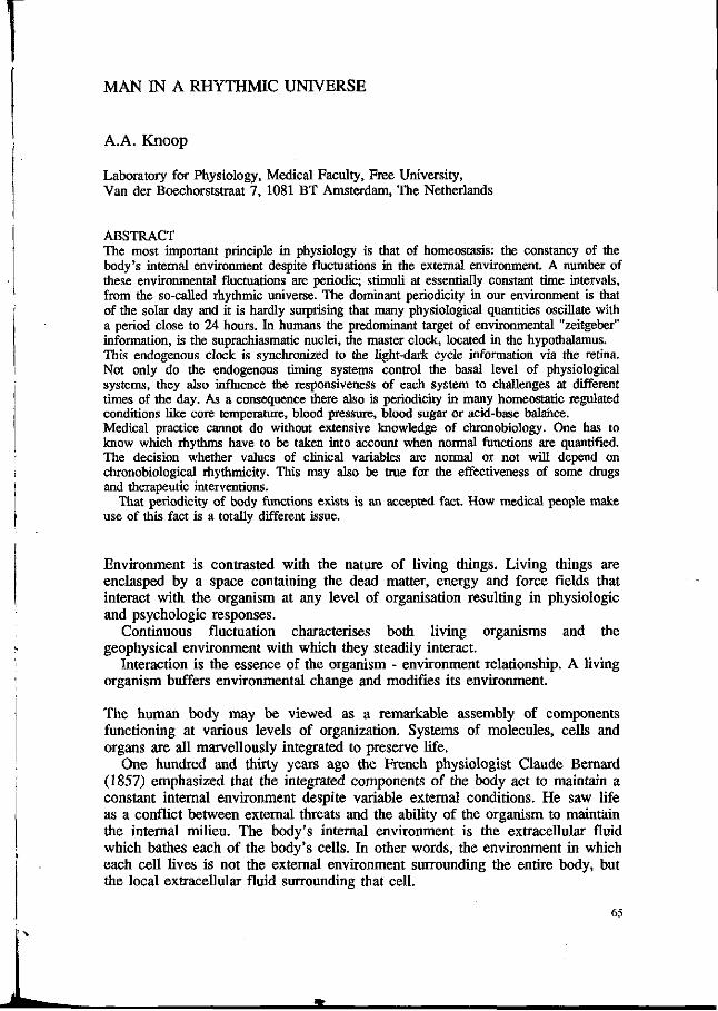
MAN IN A RHYTHMIC UNIVERSE

A.A. Knoop

Laboratory for Physiology, Medical Faculty, Free University, Van der Boechorststraat 7, 1081 BT Amsterdam, The Netherlands

ABSTRACT The most important principle in physiology is that of homeostasis: the constancy of the body's internal environment despite fluctuations in the external environment. A number of these environmental fluctuations are periodic; stimuli at essentially constant time intervals, from the so-called rhythmic universe. The dominant periodicity in our environment is that of the solar day and it is hardly surprising that many physiological quantities oscillate with a period close to 24 hours. In humans the predominant target of environmental "Zeitgeber" information, is the suprachiasmatic nuclei, die master clock, located in the hypothalamus. This endogenous clock is synchronized to the light-dark cycle information via the retina. Not only do the endogenous timing systems control the basal level of physiological systems, they also influence the responsiveness of each system to challenges at different times of the day. As a consequence there also is periodicity in many homeostatic regulated conditions like core temperature, blood pressure, blood sugar or acid-base balaftce. Medical practice cannot do without extensive knowledge of chronobiology. One has to know which rhythms have to be taken into account when normal functions are quantified. The decision whether values of clinical variables are normal or not will depend on chronobiological rhythmicity. This may also be true for the effectiveness of some drugs and therapeutic interventions.

That periodicity of body functions exists is an accepted fact. How medical people make use of this fact is a totally different issue.

Environment is contrasted with the nature of living things. Living things are enclasped by a space containing the dead matter, energy and force fields that interact with the organism at any level of organisation resulting in physiologic and psychologic responses.

Continuous fluctuation characterises both living organisms and the geophysical environment with which they steadily interact.

Interaction is the essence of the organism - environment relationship. A living organism buffers environmental change and modifies its environment.

The human body may be viewed as a remarkable assembly of components functioning at various levels of organization. Systems of molecules, cells and organs are all marvellously integrated to preserve life.

One hundred and thirty years ago the French physiologist Claude Bernard (1857) emphasized that the integrated components of the body act to maintain a constant internal environment despite variable external conditions. He saw life as a conflict between external threats and the ability of the organism to maintain the internal milieu. The body's internal environment is the extracellular fluid which bathes each of the body's cells. In other words, the environment in which each cell lives is not the external environment surrounding the entire body, but the local extracellular fluid surrounding that cell.

65

N

Claude Bernard advanced the concept that the blood in the circulatory system mediated between the internal environment ("le milieu interieur") and the external environment ("le milieu exterieur").

"The fixity of the internal milieu is the necessary condition for free existence." It was Walter B. Cannon in 1929, who coined the word "homeostasis" as the wisdom of the body. He wrote

"The highly developed living being is an open system having many relations to its surroundings - in the respiratory and alimentary tracts and through surface receptors, neuromuscular organs and bony levers. Changes in the surroundings excite reactions in the system, or affect it directly, so that internal disturbances of the system are produced. Such disturbances are normally kept within narrow limits, because automatic adjustments within the system are brought into action, and thereby wide oscillations are prevented and the internal conditions are held fairly constant ...

The coordinated physiological reactions which maintain most of the steady states of the body are so complex, and are so peculiar to the living organism, that it has been suggested that a specific designation for these states be employed -homeostasis."

Although the basic concepts of "la fixité du milieu interieur" as expounded by Claude Bernard and modified by Walter Cannon, still hold, the body's internal environment is no longer considered to be fixed in any individual. The capacity for rhythmic change is namely an other inherent characteristic of living things. These rhythms are of an endogenous origin, but in nature they are maintained within exact periods by external synchronizers such as, in the human being, by the solar light-dark cycles in an direct way and the social cues (Zeitgeber) in an indirect way. It became necessary to replace the usual concept of homeostasis, for living things are not constant, rather they are changing, dynamic, interrelated biological systems (Fig. 1).

RHYTHS IN HOHEOSTATIC "CONSTANTS"

• 3

••NORMAL" L IMITS ' | | | L J^_»7==|^ „„„„, 2 , 5 . 8

TIME I N D E P E H O E N T J =g=k »4 ß C Z Z Z ^ ^ , r \ .,„„,,. , , 3 | , i 6 i 7

" n o r m a l " 1 , 2 , <t, 5 6 , £

abnormal 3 , 7

l_ 18

O value of analysis

JfNORMAL LIMITS i? -Sr ! l ' 0 IN I „

I l lut OtrlNUlNI

J I L 6 I? 18 ?l|

TIME OF DAY ( h r )

Two facts: First, the homeostatic mechanisms of the body do not maintain a controlled variable exactly at the setpoint; the value of the controlled variable oscillates always about its reference point.

66

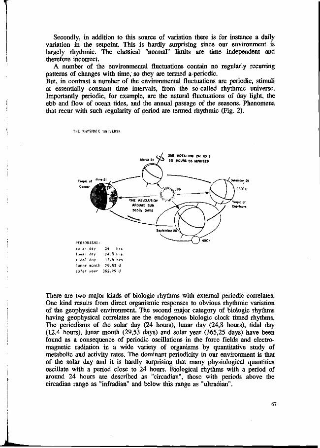
Secondly, in addition to this source of variation there is for instance a daily variation in the setpoint. This is hardly surprising since our environment is largely rhythmic. The classical "normal" limits are time independent and therefore incorrect.

A number of the environmental fluctuations contain no regularly recurring patterns of changes with time, so they are termed a-periodic. But, in contrast a number of the environmental fluctuations are periodic, stimuli at essentially constant time intervals, from the so-called rhythmic universe. Importantly periodic, for example, are the natural fluctuations of day light, the ebb and flow of ocean tides, and the annual passage of the seasons. Phenomena that recur with such regularity of period are termed rhythmic (Fig. 2).

THE RHYTHMIC UNIVERSE

Morctt 21 ONE ROTATION ON AXIS

23 HOURS 56 MINUTES

Tropic of Capricorn

PERIODISMS:

solar day 24 hrs

lunar day 24.8 hrs

tidal day 12.4 hrs

lunar month 29.53 d

solar year 365.25 d

There are two major kinds of biologic rhythms with external periodic correlates. One kind results from direct organismic responses to obvious rhythmic variation of the geophysical environment. The second major category of biologic rhythms having geophysical correlates are the endogenous biologic clock timed rhythms. The periodisms of the solar day (24 hours), lunar day (24,8 hours), tidal day (12,4 hours), lunar month (29,53 days) and solar year (365,25 days) have been found as a consequence of periodic oscillations in the force fields and electro­magnetic radiation in a wide variety of organisms by quantitative study of metabolic and activity rates. The dominant periodicity in our environment is that of the solar day and it is hardly surprising that many physiological quantities oscillate with a period close to 24 hours. Biological rhythms with a period of around 24 hours are described as "circadian", those with periods above the Orcadian range as "infradian" and below this range as "ultradian".

67

It has been shown in individuals screened from all time cues, (in polar regions, deep caves, isolation units) that many circadian rhythms can continue as self-sustained oscillations. The periods of these free running rhythms deviates from an exact 24 hours; for this reason Halberg (1959) introduced the term circadian.

The existence of free running rhythms indicates that there must be some innate timing mechanism capable of controlling these rhythms. These endogenous, free running rhythms deviate from the exact 24 hours periodicity (= circadian). Specific external periodic influences ("Zeitgeber of synchronizer) interact with the endogenous timing mechanism to synchronize the clock to the same period. This process is known as "entrainment". In man the synchronizers are the light-dark cycle (a direct synchronizer) and the social cues (an indirect synchronizer). Circadian rhythmicity is present in single cells, in plants and in animals. It has a very long evolutionary history and has very important survival value.

To what extent the clock properties are inherited rather than determined by the exposure to environmental conditions is not definitely confirmed. Of the theories of rhythm-causation, most of the support goes to the concept of the inherited circadian clock. This theory assumes a genetically endowed fundamental pure-rhythm with a natural period of 23 to 25 hours.

A mammal's first exposure to a cyclic environment is in the uterus. Mother's circadian rhythmicity is apparently a strong enough signal to entrain the circadian oscillators of the fetus. But in the first days of neonatal life the body temperature didn't show a circadian rhythm. The development of such rhythm begins already in the first weeks and reaches a peak by the age of 10 years. The endogenous nature of the human circadian system was not confirmed until Aschoff and Waver in 1962 isolated individuals in absence of any environ­mental time cue. The experiments revealed that the free running period of the human activity-rest cycle was greater than 24 hours, indicating that humans have an endogenous circadian system.

The first direct search for circadian pacemakers in mammals was not undertaken until the 1960s (Richter 1965, 1967). Lesions that destroyed nuclei in the anterior-ventral hypothalamus would disrupt circadian rhythmicity in wheel-running behaviour in rodents. In 1972, Moore and Eichler and Stephan and Zucker identified a bilateral pair of nuclei in the anterior hypothalamus, the supra chiasmatic nuclei (SCN) as a potential circadian pacemaker. In humans is the predominant target of environmental Zeitgeber information the supra-chiasmatic nuclei, the master clock (Kronauer et al. 1982). This part of the hypothalamus receives a major input of light-dark cycle information via the retino-hypothalamic tract (RITT) and via the lateral geniculate nuclei.

The evidence currently available indicates that the suprachiasmatic nucleus is the master circadian pacemaker in the mammalian brain. This conclusion is according to Shibata and Moore (1988) based on the following facts:

- Ablation of the suprachiasmatic nuclei results in a loss of circadian rhythms in rodents; transplantation of fetal SCN tissue restores circadian rhythms.

68

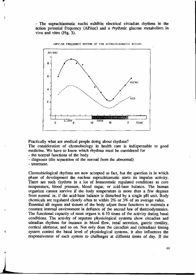
- The suprachiasmatic nuclei exhibits electrical Orcadian rhythms in the action potential frequency (AP/sec) and a rhythmic glucose metabolism in vivo and vitro (Fig. 3).

IMPULSE FREQUENCY RHYTHM OF THE SUPRACHIASMATIC NUCLEI

AP

8 -

6 -

4 -

2 -

->

/SEC

9 *\ f \ *

1 1 1 1 1 1

N \

1 >

LIGHT 0 6 1

DARK 2

/YOUNG

/ , ' ' OLD k ,''

. . M , ' , . . , . . , ! , < _ I , . . l ' '

Émàmmâ 18 0 TIME

/

I

Practically what are medical people doing about rhythms? The consideration of chronobiology in health care is indispensable to good medicine. We have to know which rhythms must be considered for - the normal functions of the body - diagnosis (the separation of the normal from the abnormal) - treatment.

Chronobiological rhythms are now accepted as fact, but the question is in which phase of development the nucleus suprachiasmatic starts its impulse activity. There are such rhythms in a lot of homeostatic regulated conditions as core temperature, blood pressure, blood sugar, or acid-base balance. The human organism cannot survive if the body temperature is more than a few degrees from normal or, if the acid-base balance is disturbed by a single pH unit. Body chemicals are regulated closely often to within 2% or 3% of an average value. Essential all organs and tissues of the body adjust these functions to maintain a constant internal environment in defiance of the second law of thermodynamics. The functional capacity of most organs is 6-10 times of the activity during basal conditions. The activity of separate physiological systems show circadian and ultradian rhythms for instance in blood flow, renal secretion, gastric motility, cortical alertness, and so on. Not only does the circadian and (ultradian) timing system control the basal level of physiological systems, it also influences the responsiveness of each system to challenges at different times of day. If the

69

daily timing of the challenge is highly predictable, an internal circadian clock can enable the organism to place the body "in a state of alert". Such anticipatory actions may be particularly valuable to prevent a delay of several hours when synthesis of enzymes or hormones is required in achieving the corrective response.

Control systems

The functions of the body are regulated by two major control systems: the nervous system and the endocrine system. In general, the autonomic part of the nervous system and the hormonal system are concerned principally with control of the internal functions of the body. Almost all functioning of both systems is controlled by the hypothalamus. Not surprising is that the circadian timing system of the suprachiasmatic nuclei uses circadian rhythms in the autonomic nervous system and in plasma hormone levels to transmit temporal information and ensure the internal synchronization of the multitude of rhythmic functions in the various body tissues.

The autonomic nervous system has two subdivisions called the sympathetic and the parasympathetic system. The major neurotransmitter in the sympathetic system is adrenalin and in the parasympathetic system acetylcholine. The general effect of the sympathetic adrenergic system is ergotropic (energy delivery) and of the parasympathetic cholinergic system trophotropic (energy accumulation).

The amplitude of circadian rhythms diminishes with age (Lobban and Tredre 1976, Knoop 1984) and immediately before death circadian rhythmicity may disappear altogether (Fig. 3) (Albers, Gerall and Axelson 1981). With old age there is, like in the newborn, a weakening of the coupling to environmental time cues. In newborn organisms neural pathways - essential and responsible for entrainment, mature. In old organisms the neural canal capacity diminishes.

Circadian temperature rhythms

Body temperature is causally connected with the rhythms in performance of many functions. The temperature rhythm is one of the most stable, with a large endogenous component and it is least affected by exogenous influence. William Ogle undertook in 1866 some careful observations of the daily body temperature rhythm in man. He wrote "There is a rise in the early morning while we are still asleep, and a fall in the evening while we are still awake" (Fig. 4).

The circadian rhythm of core body temperature is generated by an endogenous internal time keeping system and is not simply a passive response to the environment or behaviour. The temperature setpoint is located in the posterior hypothalamus (Hammel et al. 1963). If core temperature is sensed as being too high, metabolism will be reduced and skin heat loss will be increased. Although the regulated variable of the thermoregulatory system - core body temperature - is relatively constant, the constancy is achieved at the expense of large fluctuations in skin temperature (Fig. 5.)

70

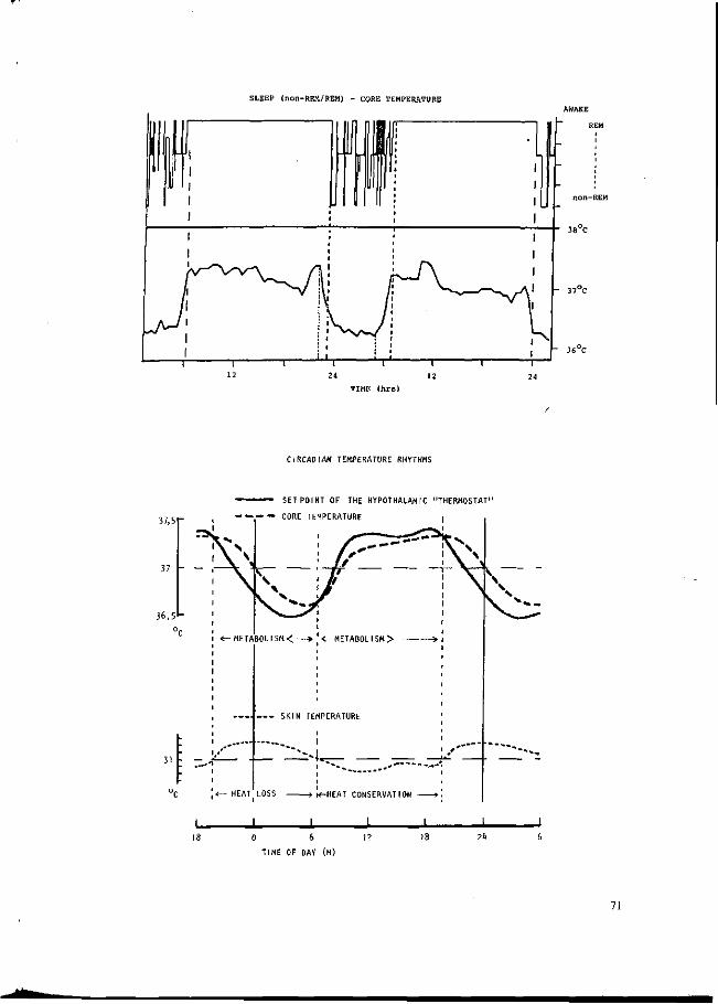
SLEEP (non-REM/REM) - CORE TEMPERATURE

CIRCADIAN TEMPERATURE RHYTHMS

SET POINT OF THE HYPOTHALAMIC "THERMOSTAT"

37,5f

37 -

- « - - — CORE TEMPERATURE

36,5'"

31 - -

0 6 12

TIME OF DAY (H)

2k

71

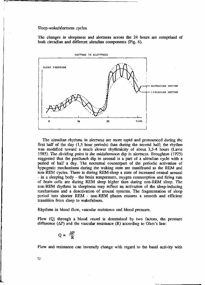
Sleep-wake/alertness cycles

The changes in sleepiness and alertness across the 24 hours are comprised of both circadian and different ultradian components (Fig. 6).

RHYTHMS IN ALERTNESS

ULTRADIAN RHYTHM

CIRCADIAN RHYTHM

The ultradian rhythms in alertness are more rapid and pronounced during the first half of the day (1,5 hour periods) than during the second half; the rhythm was modified toward a much slower rhythmicity of about 3,5-4 hours (Lavie 1985). The dividing point is the midafternoon dip in alertness. Broughton (1975) suggested that the postlunch dip in arousal is a part of a ultradian cycle with a period of half a day. The nocturnal counterpart of the periodic activation of hypogenic mechanisms during the waking state are manifested as the REM and non-REM cycles. There is during REM-sleep a state of increased central arousal - in a sleeping body - the brain temperature, oxygen consumption and firing rate of brain cells are during REM sleep higher than during non-REM sleep. The non-REM rhythms in sleepiness may reflect an activation of the sleep-inducing mechanisms and a deactivation of arousal systems. The fragmentation of sleep period into shorter REM - non-REM phases ensures a smooth and efficient transition from sleep to wakefulness.

Rhythms in blood flow, vascular resistance and blood pressure.

Flow (Q) through a blood vessel is determined by two factors, the pressure difference (AP) and the vascular resistance (R) according to Ohm's law:

Q = — ^ R

Flow and resistance can inversely change with regard to the basal activity with

72

a factor of 6-10 and a relatively constant blood pressure. In all the three, circadian and ultradian rhythms are present.

The circadian rhythm of heart rate, myocardial contractility, stroke volume, vascular resistance and arterial pressure is associated with a corresponding circadian alteration in catecholamine secretion (Wertheimer et al. 1974; Bartter 1974). During maximum daytime catecholamine secretion there is a peak in ventricular performance particularly. There is from 12 midnight to 6 am a significant fall in myocardial functional capacity, with an increased vulnerability of the heart to stress.

Nocturnal cardiac decompensation including acute congestive heart failure, arrhythmias and sudden death is an observed frequent occurrence in patients with significant heart disease (Wertheimer et al. 1974). Knowledge of these circadian alterations must be incorporated in the understanding and the treatment of cardiovascular disease.

CONCLUSION

The maxim "life is never simple" is most appropriately applied to the practice of medicine. The most important principle in physiology and clinical medicine is that of homeostasis: the constancy of the body's internal environment despite fluctuations in the external environment. Essential all organs and tissues of the body adjust these functions to maintain a constant internal environment in defiance of the second law of thermodynamics.

The body has anticipatory mechanisms to place the body in "state of alert", if the daily timing of challenges are highly predictable. Therefore the organism has the need for an internal circadian clock. The consequences are rhythms in a lot of homeostatic regulated conditions and rhythms in the performance of most organs.

LITERATURE

Albers, H.E. Gerall, A.A. & Axelson, J.F., 1981. Circadian rhythm dissociation in the rat -effects of long-term constant illumination. Neurosci. Letters 25: 89-94

Aschoff, J. & Wever, R„ 1962. Spontan Periodik des Menschen bei Ausschluss aller Zeitgeber. Naturwissenschaften 49: 337-343

Bartter, F.C., 1974. Periodicity and medicine. In: Chronobiology. (E. Scheving, F. Halberg & J.E. Pauly, eds.). Thieme, Stuttgart, 6-13

Broughton, R.J., 1975. Biorhythmic variations in consciousness and psychological functions. Can. Psychol. Rev. 16: 217-235

Halberg, F., 1959. Physiologic 24-hour periodicity in human beings and mice, the lighting regimen and daily routine. In: Photoperiodism and Related Phenomena in Plants and Animals (R.B. Withrow, ed.). Washington: Amer. Assoc, for the Advancement of Science, 803-878

Hammel, H.T., Jackson, D.C., Stolwijk, J.A.J., Hardy, J.D., & Stromme, S.B., 1963. Temperature regulation by hypothalamic proportional control with an adjustable set point. J. Appl. Physiol. 18: 1146-1154

73

Knoop, A.A., 1984. Vitaliteit, bioritmiek en veroudering. Geriatrie Informatorium, Samson Stafleu, Alphen a/d Rijn, E 2205, 1-15

Kronauer, R.E., Czeisler, CA., Pilato, S.E, Moore-Ede, M.C., & Weitzman, E.D., 1982. Mathematical model of the human circadian system with two interacting oscillators. Editorial. Amer. J. Physiol. 242: R3-R17

Lavie, P., 1985. Ultradian rhythms: Gates of sleep and wakefulness. Experimental Brain Research. Suppl. 12, 148-164

Lobban, M.C. & Tredre, B.E., 1967. Diurnal rhythms of renal excretion and of body temperature in aged subjects. J. Physiol. (London) 188: 48P-49P

Moore, R.Y. & Eichler, V.B., 1972. Loss of a circadian adrenal corticosterone rhythm following suprachiasmatic lesions in the rat. Brain Res. 42: 201-206

Moore-Ede, M.C, Sulzman, F.M. & Fuller, CA., 1982. The Clocks That Time Us. Harvard University Press, Cambridge Mass./London

Ogle, J.W., 1866. On the diurnal variations in temperature of the human body in health. St. George's Hospital Report 1, 220-245

Richter, C.P., 1965. Biological Clocks in Medicine and Psychiatry. C.C. Thomas, Springfield, Illinois

Richter, C.P., 1967. Sleep and activity: their relation to the 24-hour clock. Proc. Assoc. Res. Nerv. Ment. Dis. 45: 8-27

Shibata, S. & Moore, R.Y., 1988. Electrical and metabolic activity of suprachiasmatic nucleus neurons in hamster hypothalamic slices. Brain Res. 438: 374-378

Stephan, F.K. & Zucker, I., 1972a. Rat drinking rhythms: central visual pathways and endocrine factors mediating responsiveness to environmental illumination. Physiol. Behav. 8: 315-326

Stephan, F.K. & Zucker, I., 1972b. Circadian rhythms in drinking behavior and locomotor activity of rats are eliminated by hypothalamic lesions. Proc. Natl. Acad. Sei. USA 69: 1583-1586

Wertheimer, L., Hassen, A., Delman, A., & Yaseen, A., 1974. Cardiovascular circadian rhythm in man. In: Chronobiology. (E. Scheving, F. Halberg & J.E. Pauly, eds.). Thieme, Stuttgart, 742-747

74

WATER AS RECEPTOR OF ENVIRONMENTAL INFORMATION : A CHALLENGE TO REPRODUC­IBILITY IN EXPERIMENTAL RESEARCH THE PICCARDI SCIENTIFIC ENDEAVOUR

C. Capel-Boute

Inter. Committee for Research and study of environmental factors, Université Libre de Bruxelles 50 avenue F.D. Roosevelt (BP 196), 1050 Bruxelles, Belgique 1

Summary

For Piccardi and myself, two major intriguing conclusions had emerged in 1950, from studies, carried out quite independently on different devices and processes, involving low energy physical treatment of water 1) a "memory" in water itself kept for hours or days 2) a strange variability in results observed in any effects, in the aqueous medium, on different physico-chemical as well as biological systems.

With an original methodology, Piccardi started in 1951 to ascertain that such a strange non-reproducibility of experiments had not to be consider­ed as "experimental errors" but as time-series of fluctuating phenomena, related to the movements of the earth and to solar activity.

From long and short series of coordinated research it could be proved with such"Plccardi chemical tests", that the disturbing factors were of external origin and of the same nature as those used, under control, for physical treatment of water : that is low-energy electric, magnetic, E.M. fields and ionizing radiation also existing and fluctuating uncontrolled in our environment.

Their effects on unstable physico-chemical and biological processes could be explained by their action on the complex structure of water itself or even its primary radiolysis, with consequences on irreversible processes involving the colloidal state in aqueous solutions.

Piccardi concluded already in 1968, that the so-called "Piccardi-effect" could be characterized by a general law : "heteregeneous systems out of equilibrium, if complex enough, will respond to any external signal, even of very low-energy level. Inorganic colloids in evolution, in general, are complex enough to present this property, and colloids in living organisms even more".

For such systems, reproducibility is a mythe as there is no way to isolate them completely from the rest of the Universe : they all behave thermodynamically as open systems. The adequate methodology for experimental research has to take time into account as an irreversible coordinate bound to the conditions in the surrounding space.

This new paradigm sustains chemical as biological irreversibility bound to cosmic irreversibility : since the birth of life on Earth, in the pre-biological state of physico-chemical reactions in aqueous medium, water itself is a receptor of environmental information, acting on the kinetics of unstable processes in evolution.

Keywords : precipitation reactions, Piccardi-tests, water treatment, non-reproducibility, time, complex systems, fluctuating phenomena, environ­ment, radiation, information, irreversibility, paradigm.

1. Private address : 51 av. de la Tenderie, 1170 Bruxelles, Belgique

75

Introduction

Technical problems raise fundamental questions

Already in the years 30 to 50, various empirical devices, involving a variety of low-energy physical factors, appeared in industry to prevent scaling in boilers by deposits from hard waters of evaporated solutions. They all claimed changing only the structure of the deposits resulting from a subsequent heating of the treated water or solution.

Research-workers were asked reliable laboratory-tests to predict and evaluate possible effects of a "treated" against the same "untreated" water as control; and to explain variable results and possible ways of actions of such physical treatments.

These problems had already attracted the attention of Professor Giorgio Piccardi since 1935, extending his interest to the effects observed in a great number of different chemical processes in aqueous medium, and in biological systems.

Before the interruption of this research by the war in 1942, he was already convinced that many chemical reactions were not reproducible in experimental conditions traditionally considered as identical and well-controlled.

The variable results observed were specially found in unstable processes involving large interphases, as colloids in evolution. (Piccardi, 1962)

It was only in 1948 that I was asked, as an electrochemist, to study under direction of Dr. Pourbaix, an electrochemical device for treatment of hard waters using a small (240 mA) alternating current (50Hz) on iron electrodes.

In 1950, we had come to the conclusion that there were surely signifi­cant effects on the kinetics of thermal precipitation of calcium carbonate (COgCa) and on the structure of the deposits, as well in laboratory tests as at the industrial scale, with similar consequences as those claimed with many other patented physical treatments of hard waters. (Capel-Boute, 1960).

In this case I could explain such effects by electrode reactions produ­cing a weak primary radiolysis of water (the formation of free H and OH radicals) initiating chain reactions in water itself. (Pourbaix et al., 1951).

This working hypothesis could be reasonably applied also to explain similar effects at the industrial scale, claimed with devices using ultra­sound, ultraviolet radiation or radioactive substances.

But it could not explain such effects also claimed with physical treatments involving low-energy, magnetic, or electro-magnetic fields as the "mercury bulb", already studied by Piccardi. The "mercury bulb" is a pyrex glass globe containing about 2ml of pure mercury and sealed under reduced pressure of neon or argon. When agitated it generates an electri­cal discharge by friction of the mercury against glass (triboluminescence) with an EM emission found in the low frequences of 3.4 KHz modulated about 10 Hz (Halla 1958).

But that was not the only fundamental problem, that brought me to meet him, in 1950, in the Institute of Physical Chemistry of the University of Florence, of which he was director.

In fact, after this first phase of research carried out quite independ­ently, on different devices and chemical processes, two major problems had emerged for both of us : 1) the "memory" in water itself, that could be kept for hours or days after treatment. 2) the strange variability in the results observed on any effects of such

76

treatments, on different physico-chemical inorganic processes in the aqueous medium, as well as on biological systems. Laboratory-tests lacked sometimes the expected reproducibility, in condi­tions traditionally considered as identical to compare effects of treated against untreated water, even with periods of significantly opposite results. This second problem was a real challenge to the reproducibility traditionally required in experimental research, as a must for laborato­ry tests aimed to quantify effects of any controlled factor studied.

1. The Piccardi-effect

Piccardi's answer to this most puzzling question was that external factors of the same nature as those used for water treatment could act uncontrolled in the environment.

To test this working hypothesis he devised a crucial method : the so-called "Piccardi-chemical tests", based on a hydrolysis precipitation reaction (BiCl3 + H2O = BiOCl + 2 HCl) carried out in adequate standard­ized conditions to evaluate by a numerical index- just the variability in the course of time of the effect observed in the kinetics of reaction (Piccardi, 1960, 1962 & Capel-Boute, 1960).

He started the systematic collection of daily data in March 1951 in Florence, carrying series of ten couples of experiments twice a day, comparing the effect of treated against untreated water, in normal (test F) or screened conditions (test D ) .

He came to Brussels in October 1952, to standardize in my laboratory similar experiments, after major conclusions had already been obtained in support of this working hypothesis, that is : - after one month (600 experiments in March 1951) it was clear that opposite results and patterns of variability were obtained outside (mean value of test F = 75%) or inside (mean value of test D = 30%) a Faraday cage screening for electrical parameters in the environment. - after one year (more than 7000 experiments) there was an unusual shape of annual pattern, later confirmed and explained with his "solar hypo­thesis". This takes into account the helicoidal movement of the earth in the galaxy and its consequences, for the magnetic dipole earth moving in any possible galactic field of forces with very different speeds at Spring and Autumn equinoxes. In fact, results showing this unusual seasonal variation appeared similar in the northern and southern hemisphere, and not symmetrically opposite, as the usual pattern of climatic parameters like temperature. - after 4 years of experiments (more than 30,000 in Florence), there was a trend in the variability related with the minimum of solar activity, and correlations could be established between the fluctuations observed in Brussels and Florence.

May I recall the colloquium held at the Max-Planck Institut fur Bio­physik in Frankfurt/Main nearly 35 years ago (October 1954) under direction of Dr. Rajewsky, "über den Einfluss atmosphärischen und kosmi­schen Phenomen auf physikalisch-chemische, biochemische und biologische Prozesse". He concluded that Professor Piccardi had "opened the roof of

1. %T = percentage of cases, in series of minimum 10 couples of precipi­tation reactions, in which the sedimentation of the precipitate occurs faster with the effect of the controlled factor studied, (effect of treatment of water, or effect of a screen for example). Mean values of 50% would mean just hazard or no effect.

77

our laboratories" to unexpected environmental factors, and that could make many scientists feel very uneasy (Piccardi, 1955)(Boute C , 1955)(Becker U. 1955). This "crucial experiment" with the Piccardi chemical tests was repeated in more than 30 different places in the world, from the Arctic to the Antarctic, in friendly international and interdisciplinary cooperation. Fluctuating results confirming the"Piccardi effect" were again submitted to a large interdisciplinary discussion in the "1st International Sympo­sium on Solar-terrestrial relationships in physical chemistry and biology" held in October 1958 in the Royal Observatory of Brussels under direction of Professor Paul Bourgeois. But although Piccardi could already claim that with this "new conceptual paradigm we could solve the problems that have led the old one to a crisis" to use the words of Kuhn in his "Structure of scientific revolutions" (1964,pl52) it is true again that "the subsequent battle over its acceptance" is still not yet completely won in the entire scientific community.

Still following Kuhn (1964,pl21) "given a paradigm, interpretation of data is* central to the enterprise that explores it".

This is not an easy task with the complex interrelated environmental factors acting in the biosphere; as well as with their direct or indirect effects on such complex systems as are even water itself, a fortiori un­stable physico-chemical processes and moreover, living organisms.

The study of this "Piccardi-effect" in function of time, latitude, screening conditions and with different controlled physical factors used for treatment of water, have clearly contributed to clear the origin and nature of the disturbing factors involved; and their ways of action, inclu­ding as well non-ionizing as ionizing radiation in our near and far envi­ronment .

Already in his monography "The chemical basis of medical climatology" (Piccardi, 1962 - translated in Russian in 1967) (Capel-Boute, 1974), Piccardi brought also an answer to the fundamental question of explaining the effects on water of low-energy electric, magnetic and EM fields, specially in the low-frequency range. He attracted attention on the peculiar structure of water and its anomalous physico-chemical properties. He developed this hypothesis, set forth first in 1959 (Piccardi, 1959) of effects of low-energy physical factors on the labile and complex quasi cristalline structure of water, as a coherent explanation as well for possible effects of low frequency radio waves in the environment.

It can also explain the hysteresis effects, or "memory" retained by water for hours or even several days, observed on effects of a previous physical treatment, as when water has been submitted to known structural changes by heating or freezing.

From the amount of data collected in short or long series of experiments by many different research workers all over the world to study the Piccar­di-effect, we can here only shortly recall first some of the environment­al factors appearing responsible for fluctuating phenomena and some spe­cial series of experiments sustaining the prominant role of water as receptor of environmental information.

2. Radiation in the environment responsible for fluctuating phenomena

2.1. The need for long-term observations

From the amount of facts collected during the second phase of research between 1951 and 1957, it appeared that different physical factors in the environment, related with various effects observed, were strongly inter­related and depending on the period of solar activity.

Let us remind shortly some examples, first to show how dangerous it may

78

L

be to draw definitive conclusions from more or less short series of data collected in different places and time; or a fortiori from a limited num­ber of experiments considered sufficient to ascertain the effect of any controlled factor, within the limits of "experimental errors" admissible in conditions "traditionally considered as identical".

The Piccardi chemical tests carried out in Florence inside (test D = dentro) a grounded Faraday cage (0,1 mm copper sheet)were obviously protected from daily variations of the atmospheric electric potential, measured outside next to the laboratory where F-tests (F = fuori) were performed in normal laboratory conditions. These yielded results fluctu­ating parallel with the electric potential.

Nevertheless, results inside the Faraday cage still showed important variations : ordered in long time-series from 1951 to 1954 (decaying pe­riod of the 18th solar cycle) tests F and D presented strong opposite patterns of annual variation, with no significant correlation coefficient (Bravais-Pearson = 0,077) between 40 monthly means of about 600 experi­ments for each test; furthermore, differences between them could have led to very different conclusions for the effect of screening, depending from the month and the year.

During the same decaying period of the 18th solar cycle, series of tests made in Brussels between October 1952 and July 1954, showed a significant correlation coefficient between F-tests in Florence and Brussels (p = 0,45 P<3.10~-;'), while there was no correlation between the D-tests with different screening conditions : D-tests shielded also even against the electric components of a large spectrum of EM fields (in a 1,5mm AL-Faraday cage) in Brussels showed that these were evidently not the only disturbing factors; nor the one responsible for the latitude effect, appearing from mean values always higher in Brussels than in Florence.

The minimum of solar activity reached in July 1954 was marked in Brus­sels like in Florence with very low values of both tests. These facts suggested also a possible important effect of cosmic rays from galactic origin, reaching our atmosphere with maximum intensity when solar activi­ty is minimum (Forbush-effect). This view was also supported by the fact that an horizontal sheet of copper could have about the same secondary effects as a full Faraday-cage, and that the effect of such an horizontal screen depended on the conductibility and thickness of the sheet of metal used. The investigation of effects of geophysical factors during at least a full 11-year solar cycle was necessary.

This led Piccardi in 1955 to build a "synchronous mixer" suitable to perform easier and simultaneously 10 couples of differential experiments; comparing the effects of treated against untreated water, either with a horizontal copper screen above it when mixing the reagents (D-test) or without it (F-test).

This enabled to study also on long term series the screen-effect alone, either on normal water (Ppj-test) or on "activated" water (P^-test) (Piccardi, 1960) (Capel-Boute, 1960).

In fact new patterns of fluctuations were observed during the next pe­riod of increasing sunspot activity at the beginning of the 19th solar-cycle, between 1954 and 1957.

They showed now in Florence a parallel behaviour for F and D-tests with variations of smaller amplitude but with a very significant positive corre­lation coefficient between them (p = 0,51 with 10~°<P C.0~'T-

Similarly in Brussels a parallel behaviour of F and D-tests gave a positive correlation coefficient somewhat lower (p = 0,34 P ( 10-^) than in Florence.

But after a first rapidly increasing trend like in Florence, the mean-values of both F and D-tests in Brussels dropped systematically under

79

those of Florence, giving a latitude effect quite opposite with the one observed before the minimum.

Furthermore, a real "mirror effect" between the values of F-test in Brussels and Florence (Capel-Boute, 1960, p76) appeared in 1956-57 as soon as Wolf's number passed 100, and contributed to a very significant negative correlation coefficient (p = -0,42 with 10-6<"P <10-^) instead of the positive one obtained before the minimum.

It can be explained by effects of charged particles from solar and cos­mic origin that are deviated by the magnetic field of the earth towards the poles where they produce such well-known visible effects as aurora-borealis; with high sunspot activity the aurora borealis zone may reach the latitude of Brussels (51° N)considered as the line of "cut-off" while Florence is definitely below (43° N ) .

But the correllogram established by Becker (1960, pll4) for the rela­tion between D-test in Florence and Wolf's number showed also a clear "saturation effect" when the relative number of sunspots reached about 80.

Furthermore,no significant relation is found between D-test and solar eruptions while it is highly significant with F-test, without any delay. This would mean effects of elecromagnetic radiowaves reaching the earth's atmosphere in 8 minutes with consequences on the ozone layer and the iono­sphere while particle effects are delayed 2 or 3 days, depending on their energy and are responsible for geomagnetic disturbances. As the state of the ionosphere and geomagnetic disturbances are both responsible for variations in the transmission of radiowaves of terrestrial origin, direct and indirect effects may be involved at earth level like sudden enhance­ment of atmospherics.

Piccardi was particularly concerned with the Very Low Frequency (VLF) natural electromagnetic fields, particularly able to influence colloidal systems in evolution . A differential Piccardi-test carried out comparing effects of a 10 W-10 KHz transmitter at 2 m and 20 m distance showed on 1720 couples of such a "near-far" test, (11 September 1955 to 29 February 1956) a retarding effect with the higher intensity of the electromagnetic field near the generator, in the period indicated.

He would have liked to correlate the results of his chemical tests with the intensity of VLF atmospherics but these were not measured in Italy at that time.

If I wanted to recall such facts, it is because they showed clearly that Piccardi's endeavour to uncover environmental factors responsible for fluctuating phenomena appeared already 'at our first Brussels Symposium in 1958 as a long-term enterprise. It requires structures and means other than usually available for research in any University department, to carry on such standardized routine tests for at least a complete Hale solar cycle (22 years). (Piccardi et al., 1972).

Piccardi created with private support in Florence a special Centro Universitario Fenomeni Fluttuanti (CUFF) where he was able to continue his research after retiring from the direction of the Institute of physi­cal chemistry of the University. But it was closed a few months before his death (22/12/72).

In Brussels, I got support from my University to start in 1963 an inter­disciplinary center for research and study of environmental factors (Centre Interdisciplinaire de Recherche et Etude des facteurs de l'Ambi­ance - CIEEFA) but it was closed at the end of 1978 a few months before I retired.

The data collected in Florence (1951-1972) on 3 Piccardi-tests (F,D,P) and in Brussels (1956-1978) on 4 Piccardi-tests (F,D',Pjj,P ) were analysed by different methods of time-series statistical analysis by De Meyer from the Royal Meteorological Institute in Brussels (Uccle). By spectral

80

analysis he could confirm the significance of the peak of annual variation, appearing on all these tests (De Meyer et al., 1987).

But the period of 22 years was still too short to insure the significance of long term peaks, appearing more of less evidently around the 11 year-solar peak or its harmonics.

Observatories or geophysical and meteorological institutes have appro­priate structures, staff and equipment for long-term collection of physical data and statistical analysis of their relationships, but usually not the interdisciplinary staff necessary to investigate the effects of such factors on physico-chemical and biological systems.

Most physicists were not ready to include officially these questions in the program of the International Geophysical Year (IGY-1957/1958) and the following geophysical cooperation for the International Quiet Sun Year (IQSY-1964/1965) in spite of our efforts.

2.2. The need for interdisciplinary and international cooperation

Even without any structural and financial support for this third phase in the development of research, Piccardi tried to benefit as much as possible from these first necessary steps in a better understanding of "solar-terrestrial relationships in physics"to which the IGY ans IQSY wanted to limit their aims. With 20 standardized "Piccardi-synchronous mixers" freely distributed by the University of Florence in the northern and southern hemisphere, a network of volunteers in observatories, research institutes and universities accepted to cooperate friendly to collect data with adequate instructions to carry out the standardized Piccardi-tests, for more or less long periods (Piccardi, 1962, p83-108).

Piccardi had also joined scientists from eastern and western countries for interdisciplinary cooperation in an International committee for fluctu­ating phenomena (CIFF)and in a permanent working-group in the International Society of Biometeorology.

Taking into account the difficulties encountered by scientists of eastern countries to join scientific meetings in western countries, Piccardi went himself to Russia and established with them direct rela­tions and fruitfull cooperation. His research brought basic processes in physical chemistry in support to the developments in heliobiology, initi­ated there by the pioneering work of Tchijewsky now raising increasing interest. (Capel-Boute, 1974).

A new point of the situation was made again in Brussels 10 years after the 1st International Symposium now extending the subject of the 2nd one, to "Solar terrestrial relationships in physical-chemistry and life scien­ces" (held in the University of Brussels 1/7 September 1968 - unpublished proceedings).

Scientists trained in more than 20 different disciplines, contributed to the theme in astrophysics, geophysics, meteorology and statistics to con­front actual knowledge with fluctuating phenomena observed in physical chemistry, biology, médecine, sociology, economy, psychology and their con­sequences in philosophy of science.

Already in 1963 Piccardi had organized a seminar on the question of cau­sality and methodology in scientific research in the presence of uncontrol­led (and possibly even unknown) environmental factors acting in the bio­sphere.

In the meantime the results of the IGY and IQSY cooperation and the new developments in space research had made more familiar the concept that the earth was to be considered as a space vehicle on solar orbit : travelling with the sun in the galaxy, we will never come back to the same point in space.

Perfect cyclic responses to everchanging environmental factors must not be expected but spectral analysis of long time-series of data proved to be a usefull statistical tool to assure the geocosmic origin of the distur­bing factors.

In spite of the very different pattern of fluctuations observed in the Piccardi-tests during the 19th solar cycle, the evidence of an annual variation was confirmed, and the mirror-effect between the F-tests in Brussels and Florence observed in 1956-57, appeared clearly again 11 years later when Wolf's number raised above 100 in 1967.

This is enough to demonstrate also that no significant correlation coefficient between such effects observed in the biosphere and sunspot numbers could be expected even for fluctuating phenomena evidently moni­tored by sunspot activity and other complex effects on geophysical and meteorological factors in our environment. The systems observed seemed to integrate them in "global effects" varying with prevalence of one or ano­ther physical factor, depending on time, space, screening conditions of the experiments and the role played by water in the different unstable phases of the complex processes in evolution observed.

Concerning the nature of the systems undergoing "fluctuating phenomena", Piccardi could already draw a general law to characterize them: "Hetero­geneous systems out of equilibrium if complex enough, will respond to any external signal, even of very low-energy level. Inorganic colloids in evolution, in general, are complex enough to present this property and colloids in living organisms even more".

Thus many chemical reactions and all biological processes may be influ­enced by external factors bound to a physical state of the surrounding space that may not happen any more.

The field of research opened by this effort of interdisciplinary syn­thesis brought the participants in 1968 to the decision to create the "International Committee for research and study of Environmental Factors" (ICEF or CIFA in French)"responsible for fluctuating phenomena in exact, natural and human sciences". It obtained the official status of an inter­national scientific association recognized by the Belgian Law and its re­gistered office in the University of Brussels.

The CIFA-committee held its first General Assembly in September 1969, in Montreux, after the 5th International Congress of the International Socie­ty of Biometeorology.

It was the last time that Professor Giorgio Piccardi could attend a scientific meeting abroad, just 20 years ago; but he was confident as its first founder president that our Committee would be able to continue his ambitious endeavour to develop this field of research as he had so successfully done it, on the basis of friendship and full cooperation between all scientists concerned.

3. Water as receptor of environmental information

The striking point in all observations on inorganic precipitation reac­tions, carried out since 1950 to study the "Piccardi-effect" is the nature and the low level of energy involved in the factors who appeared to act, controlled or uncontrolled, on such systems : electric, magnetic, and electromagnetic fields or particles from man-made or natural origin.

Low-energy levels is also a characteristic of all forms of information brought to an organism from his environment with often considerable effects on its behaviour.

At this point it seems interesting to recall some less known laboratory experiments that show effects on complex inorganic systems in aqueous me­dium, of the sensitivity of water itself to a wide range of low-energy

82

physical factors such as those ever existing in our natural environment. Such facts have brought me to raise the question of "water as receptor

of environmental information ?" (Capel-Boute, 1985) and its consequences in the theme of "Man's relations with his environment : extending biomete-orology in space and time" after the contributions of Schoffeniels (1985) to this theme at the 10th International Congress of Biometeorology (Tokyo, 1984) and of Wedler (1985). •

3.1. Some effects of non-ionizing radiation on physico-chemical processes in aqueous medium

Fischer et al. (1968) were entrusted by W.O. Roberts, director of NCAR (National Center for Atmospheric Research - Boulder, USA) to investigate the Piccardi-effect. With a device much similar to the Piccardi synchro­nous mixer, but different mixing conditions, they obtained results for the precipitation of B10C1 similar to those from the usual Piccardi chemical tests and accordingly they investigated first screen effects and pre-treatment of water, with different electric, magnetic and electromagnetic low energy sources among which the mercury bulb.

Like Piccardi they concluded that their results suggested "the hypothe­sis that the causative agent was electromagnetic radiation", with an ef­fect that "persisted in water for an extended period, since the interval between activation and mixing was several minutes". Moreover the authors remark that reversals of behaviour, as those observed with the Piccardi chemical tests, even with better controlled low-energy sources 'of radio-waves, "indicates that other influences of presently unknown origin can act upon chemical systems". However, "it was not yet clear (to them) what stage of the overall process from chemical reaction to final sedimentation was affected. (Fischer et al., 1966-internal report, unpublished).

Their following series of differential sedimentation experiments were carried out with samples of a stock suspension of silica in an aqueous solution (KOH, 4,1.10-%), irradiated during sedimentation. Oscillators were used as low energy sources and a solid Faraday screen protected the non-irradiated controls. With low-energy E.M. single frequency fields applied, ranging from Hz to GHz, mean results are presented as an action spectrum : it shows invariably an increase in the sedimentation rate of the silica particles, more pronounced in some frequencies than for others; notably 10 KHz. Similarly, the electrophoretic mobility of the negatively charged silica particles was invariably increased by a pre-treatment from 100 Hz to 100 MHz of the KOH stock solution used to prepare the silica suspension. The diluted suspensions showed increasing mobilities for pe­riods up to 2hrs, finally decreasing slowly but not returning to the ori­ginal value for as long as 5hrs after the E.M. pre-treatment.

This indicated as for the pre-treatment of water with the mercury bulb radiation a kind of storage of the absorbed energy in more organized struc­tural changes dissipating then slowly through random collision.

Their last step was to investigate effects of the same range of E.M.waves on pure water, adequate to compare changes in resistivity. The low-level energy alternating EM fields in general increased the resistivity. Visco­sity measurements on de-ionized water showed small but significant increa­se for samples treated with the mercury bulb.

Fischer and Perdue (1964) showed also that treatment with the bulb cau­sed supercooled water to freeze at higher temperatures when subjected to shock while there was no effect on spontaneous freezing temperatures.

They concluded that the EM treatment did not act on freezing nuclei but could favour freezing under shock by introducing a pre-existing organiza­tion in water.

83

For Fischer and co-workers as for Piccardi all the above quoted facts could be explained by changes brought in the structure of water and their effects on the electrical double layer and electrokinetic properties of colloidal particles in the aqueous medium.

3.2. Some effects of ionizing radiation on the BiOCl precipitation reac­tion

Bueger (1963) under direction of Eichmeier has investigated with the BiOCl-reaction carried out as in the Piccardi chemical tests, the effect of IR, visible light, UV, X-rays and y -rays comparing 10 couples of si­multaneous precipitations in each experiment.

He first observed that the irradiation must occur at the moment of the mixing of the water with the acid solution of BiClg to have a significant effect. While observing fluctuations in all the different series of expe­riments, the mean values obtained for each series show significant values above 50% of cases of accelerated sedimentation for IR and regularly de­creasing all under 50% from visible light to y-rays. This effect is more pronounced if the non-irradiated controls are protected by a 5 cm lead screen against uncontrolled radiation from the environment as cosmic rays.

Mean sedimentation time measured on single experiments confirm the in­creasing delayed sedimentation observed with increasing frequency of the radiation in the electromagnetic spectrum. The opposite effect of IR is easy to ascribe to its well known thermal effects.

The author ascribes the Piccardi-effect to cosmic rays alone and consi­ders only the ionization of BiO-ions,and the whole process merely as a matter of "coagulation of a colloidal solution", to explain the effects of ionizing radiation. Other views will be discussed further.

3.3. Structure of water and kinetics of precipitation reactions in aqueous medium

The writer was able to develop with different students, Van Winnendael (1963), Stordeur (1965), Lacave (1965) another approach to understand the mechanisms involved in the Piccardi-effect by investigating with electo-chemical methods the kinetics of another precipitation reaction (CaCl2 + C03Na2 = C03Ca + 2NaCl) in very dilute solutions.

This reaction was more adequate to follow the processes of nucleation and growth of the precipitate, with conductivity measurements as a func­tion of time, to investigate mechanisms involved and possible effects of uncontrolled external factors in the nucleation rate and final particle size. It soon appeared from identical experiments systematically repea­ted with the same reagents (CaCl2 and C O ß ^ b o t h 6,7 10~3 M/l) at diffe­rent hours of the day or different days that the curves were not reproducible and could even take very different patterns (Van Winnendael, 1963) in spite of the most carefully standardized mixing and thermostati-zation conditions (Stordeur, 1965). Some curves X =(t) could present a constant conductivity for a variable period of time, currently considered as an "induction period" for the germination phase of the process .followed by the step of growth of particles decreasing the conductivity more or less rapidly to its final value of equilibrium, corresponding to the con­ductivity of the non-reacting ions. This "induction period" seemed absent on many curves , the conductivity X dropping abruptly immediately after mixing.

Even more intriguing were curves X =f(t)showing a variable period of in­creasing conductivity, followed by a more or less rapid decay. Curves of this type seemed to appear more frequently on some days than others. The

84

intitial values of conductivity measured 30 sec after mixing, were not ve­ry different for all types of curves and in all cases lower than the ex­pected values calculated from the mobilities of the ions from the reagents or measured before mixing. They are coherent with the order of magnitude of a solubility product for small particles of solid calcium carbonate.

These facts do not support the concept of any "induction period" (often considered from turbidity measurements) as the time necessary for ions and undissociated molecules to join up to the size of germs of the new solid phase. Although no precipitate is visible in such dilute solutions, tur­bulent mixing of the reagents must rather produce immediately particles of the solid phase with a gaussian distribution of size, depending on the mixing conditions and any external factors acting at that moment. This distribution curve may have its maximum peak above or below the critical size of the thermodynamically stable germ, corresponding to a maximum of its free energy of formation as a function of radius (La Mer, 1952) (Defay, 1960).

Particles with radius above the critical radius R must grow by taking ions from the solution while those smaller than R must go back into the solution, increasing its conductivity. Such a competition may generate any of the different patterns observed in the conductivity versus time cur­ves even an apparent induction period.

This interpretation of the conductivity measurements following the kine­tics of germination and growth of the precipitate can account better for the influence of cosmic rays, or any incident particle or ionizing radia­tion acting at the moment of mixing, as observed by Bueger (19630.

Along the tracks of any incident radiation producing primary radiolysis of water itself in the metastable state of the solution of mixing reagents, germination of the solid phase will be favoured with an enhanced number of nuclei resulting in a finer precipitate, with lower sedimentation rate.

Such an effect on the germination phase of the precipitant can also in particular account for the erratic distribution and striking differences observed between the 20 precipitation reactions carried out simultaneously with a device like the Piccardi Synchronous Mixer, even in blank tests and control reactions. These are always submitted to secondary effects of cosmic rays in the atmosphere varying at earth level with the local baro­metric pressure.

But as clearly shown by Wedler (1985) describing "Radiation in our en­vironment from the atmosphere and from space", this is not the only fac­tor possibly responsible for uncontrolled environmental conditions and in particular for the diurnal and day-to-day variations clearly observed in the kinetics of the calcium carbonate precipitation reaction.

As we have seen previously they may act also on other phases of the glo­bal process to influence the final sedimentation rate of a precipitate.

Now, as effects of the mercury bulb and other low-energy sources of non­ionizing radiation have been explained by their possible action on the structure of water, we have investigated the effect of temperature between 20 and 50°C on theX = f(t) curves.

It was particularly interesting to consider the temperature range be­tween 30 and 40°C in which many anomalous properties of water have been ascribed to its change of structure, to see how it could effect the kine­tics of the precipitation reaction.

All types of curves previously observed at 20°C were also obtained at any other temperature, evidently still depending on the day and hour of the experiment with evident differences in the patterns of theX=f(t) curves registered at the same temperature either in the morning, around noon hours, or later in the afternoon, all in the same day.

It was rather easy also to carry on a series of experiments with either

85

regularly decreasing or increasing of temperatures all the same day but we soon noticed that it was far more difficult to take into account the diurnal variation. Initial values of conductivity measured 30 sec after mixing showed a perfect linear increase with temperature for experiments all carried out the same day but with a positive constant slope different from one day to another.

To take a rough measurement of the velocity of the reaction we measured on each curve the difference in conductivity i j , , plotted at the 1st and 5th minute after mixing of the reagents. If these values were plotted as a function of time for the same temperature, they clearly showed a more or less pronounced pattern of diurnal variation with usually increasing va­lues in the morning and decreasing in the afternoon. But the first impor­tant conclusion was that this diurnal effect could be even more pronounced that the temperature effect between 20 and 50°C : apparent constant tem­perature coefficients could be obtained either under 30°C or above 35°C, but their values and even sign were day and hour-dependent, with strong discontinuities between 30 and 40°C.

The results could present a surprising increase in the morning of the velocity of the reaction with decreasing temperature, with a jump down between 35 and 30°C from a 1st straight line to a nearly parallel 2nd one. The same experimental program carried out in the afternoon could lead to a linear decrease in.the velocity of the reaction with a jump upwards under 30°C to another parallel straight line : what could be usually condi-dered as either a negative "temperature coefficient" or a positive "tem­perature coefficient" could be observed if the diurnal effect was ignored.

The obvious discontinuity in the temperature effect between 30 and 40°C observed on A/,,- could appear somewhat lower or higher than 35°C depen­ding on whether that ill-defined critical value for a structural change in water was reached with decaying or rising temperatures, demonstrating a kind of hysteresis that is also time-dependent. It could be shown that in this critical range of temperature around 35°C,the velocity of the reaction would present a minimum less pronounced at noon hours than ear­lier in the morning or later in the afternoon.

We may conclude that such a metastable state as the germination and growth of a new solid phase in aqueous medium is extremely sensitive to the known structural changes in water, linked with temperature; but evi­dently also to other uncontrolled environmental factors. These are res­ponsible for a similar pattern of diurnal variation,observed as well under 35°C as above, changing from day to day, that can entirely mask the effect expected from the temperature increase on the kinetics of the reattion.

In spite of such variations it was possible to see the effect on the conductivity curvesX=f(t) of the mercury bulb pretreatment of distilled water used to dilute the reagents to the concentration of 6,7 1 0 ~ 3 M / L , from stock solutions at 0.134M/L. Experiments with these "activated" solutions were carried out alternately in the course of time with those using the normal "non-activated" reagents.

Initial values of conductivity are slightly lower with the treated re­agents, indicating some effect in the germination phase. The curves ob­tained with the "activated reagents" showed less variations from day to day and hour to hour than those from non-activated reagents. The treat­ment effect was more evident on days of slow reactions with the untreated solutions.

The initial values of conductivity X 0 c (measured 30 sec after mixing) are only slightly lower with the same ' constant slope throughout the whole temperature range. The treatment effect on AXi_5 i s clearly marked only under 35°C, with enhanced velocity of the reaction and no more discon­tinuity as if the structural change in water had already taken place.

86

Many other experiments (Lacave, 1965) have shown us similarly that con­trolled low-energy physical factors seem to act on water as if introdu­cing more order, resulting in more reproducible effects, than those obser­ved with untreated water.

3.4. Conclusions

We can at least conclude from this review of facts that low energy phy­sical factors, including many different types of radiation from one extre­mity to the other of the electromagnetic spectrum can trigger important kinetic effects in the germination and growth of a new phase in aqueous medium with structural consequences and macroscopic effects.

Water appears to be a most sensitive medium to many physical factors radiated in our environment from the atmosphere and from space, from which it cannot be completely isolated.

By chain-reactions or structural changes in water itself, the aqueous medium seems able to transmit effects of ionizing or non-ionizing radia­tions more rapidly throughout the medium than the diffusion of uncharged particles or mobility of ions (other than those of water itself, H + and OH-) could achieve.

With a low-energy input as in any information process,water may thus re­ceive, transmit, and even memorize or amplify effects from the ever-chan­ging physical conditions originating in the far-environment.

Water is also the necessary medium for all metabolic reactions in living organisms and the near environment of all cellular processes.

May we suppose that in the course of evolution this "structural infor­mation" received by water has provided specific physico-chemical means to stimulate adequate adaptative processes to ever changing environmental conditions, from which the different acting physical factors may even be only usefull indicators?

Can biologists tell us how homeothermic animals came to adjust so strictly their temperature around 37°C corresponding to that state of transition in the structure of water, with unpredictible effects on kine­tics of irreversible processes which may allow enlarged possibilities for adaptative reactions?

These questions came back particulary to my mind with the remarkable examples given by a zoologist P. Brien (1974) of coordinated processes taking place in different organs to adapt their functions to new environ­mental conditions, requiring a coordinating medium (Capel-Boute, 1983).

From the origin of life on Earth (Buvet, 1974) it seems that low energy physical factors in the environment, as those still existing actually, may have played a role in the appearance of the complex prebiological com­pounds as first obtained in laboratory experiments by Miller in 1953 with an electrical discharge. Many others since then have used different mi­nute but concentrated sources of energy, to act on a mixture of reduc­tive gases in presence of condensed water to obtain the 20 amino-acids common to all living organisms; their number is strictly limited as the only possible compounds of carbon in water.

These appear therefore not determined by enzimes nor genomes but only by the properties of liquid water and the possibilities of complexity that it may bring in inert systems, with its acid-base and redox limits of thermodynamic stability. Properties of water have thus brought a first unifying element, at molecular level, common to inert and living matter since the origin of life.

Already in 1968, at our 2nd Brussels Symposium (unpub.), Piccardi had also concluded from his extended research on fluctuating phenomena (Capel-Boute, 1974) that many chemical systems and all biological systems,

87

that are complex heterogeneous systems, far from equilibrium in aqueous medium, shared not only the property of being, from the thermodynamic point of view, open systems exchanging matter and energy with the envi­ronment .

But from the kinetic point of view they shared also the property to react to external signals, even of very low-energy level, with results fluctuating in the course of time.

Chemical irreversibility of time has been demonstrated with the Piccar-di Chemical Tests as well as the impossibility to screen reactions in aqueous medium from all physical factors in the environment, acting on water with structural consequences.

Such facts join the views developed by E. Schoffeniels (1973) in his book on "Anti-chance" and the need to consider from the kinetic point of view his generalization of the theory of information to open systems, in the sequences of metabolic processes leading to biological evolution and irreversibility of time.

Benjamin Gal-Or (1972) in a discussion on the origin of irreversibility in Nature questions the concept and even the possibility of existence of a thermodynamical isolated system, and concluded "is it possible therefore to assume that the origin of irreversibility is due to the impossibility of completely isolating a system from the rest of the universe ? We don't know yet."

For us in 1972 when Giorgio Piccardi died, the above facts had already long brought an answer to that question with new support to the facts and views that Piccardi himself had developped along 40 years of careful and patient research in the investigation of fluctuating phenomena, in physi­cal chemistry and biology taking into account time as an irreversible pa­rameter. Further research is needed and will surely contribute to iden­tify more known or still unknown environmental factors responsible for this Piccardi-effect, but many may ever act uncontrolled in our labora­tory experiments as in Nature. The above facts could even suggest that water may be an essential link to couple cosmologie and electromagnetic asymétries in the expanding universe with the irreversible biologic evo­lution o f Life on Earth.

4. Transition to a new paradigm

"Paradigm changes do cause scientists to see the world of their research-engagement differently".

"What were ducks in the scientist's world before the revolutions are rabbits afterwards" (Kuhn, 1964, pllO).

What were previously experimental errors and non-significant results in some laboratory experiments have become for us fluctuating phenomena when ordered in function of time.

Many research workers have faced like us experiments that can not be repeated in any place and at any time with reproducible results to ascer­tain quantitative observed effects. With the long-term series of Piccardi Chemical Tests we have shown that the nature of the effect and the origin of its variability can at least be investigated by observing it in func­tion of time as in chronobiology. We may have to come back to observe and respect the laws of Nature with more patience and less certitude than the physicist thought he could obtain, even from controlled laboratory experiments in so-called "constant conditions".

R.H. Dicke (quoted by Benjamin Gal-Or, 1972) said "from the very begin­ning the physicist has kept his sanity and made the most progress with his science by isolating his problem, eliminating unwanted disturbances, and ignoring the complexities of the rest of the Universe. It would indeed be

disquieting if now it were to be found that the laboratory could not be isolated even in principle".

Much research is urgently needed while there is no easy way to obtain clear results in a short time : as in any field of research in biometeo-rology we must be aware that neither living organisms nor any more or less limited environment can be considered as remaining constant in the course of time, as well at the scale of geological ages as for the short dura­tion of a laboratory experiment : there is no way for a magic enclosure to ensure constant environmental conditions.

Not only a new vision of the world is required from scientists to accept such a concept but new tools and structures are urgently needed in funda­mental and applied research, as stated in the resolution of our CIFA committee in 1984.

"The International Committee for Research and Study of Environmental Fac­tors .

after - meeting in Paris on June 23, 1984 with the International Socie­ty of Biomathematics (President, Prof. Dr. Collot),- meeting for a two-days seminar in Tours on 25-26 June 1984 on the subject of "Interaction of living organisms with their environment", in the Department of physiology of the Faculty of médecine of Tours, (Director, Prof. J. Thouvenot), suggests to the International Society of Biometeorology, on the occasion of its 10th International Congress of Biometeorology held in Tokyo on 26-30 July 1984, and in which it was responsible for the theme of Plenary Session 1 on "Man's relations with his environment : extending biometeoro­logy in space and time" to support the following resolution :

"As scientific workers from all disciplines concerned with the problems of the complex relationship of living organisms with their near and far environment, we stress for the urgent need to create interdisciplinary institutes for biosystemic research and long-term observations in this field".

The need for data and adequate bio-indices collected systematically in the course of time, on a long-term scale, should be coped for in such institutes by interdisciplinary teams permanently trained to work toge­ther .

Such biosystemic institutes should provide for the permanent appropriate frame, similar to those of astronomical, geophysical and meteorological institutes, to ensure continuity in observations, centralisation and sto­rage of data, and efficient interdisciplinary cooperation in improving methods and interpreting results.

The power of man and its ability to change rapidly the environmental conditions in the Biosphere, assign him the responsability to preserve Life on Earth with improved means for fundamental knowledge on relation­ships of all living organisms with the environment and consequent control of short and long-term effects of his own activities."

Man-made sources of energy disturbing natural signals from our near or far environment can induce direct or indirect effects possibly more specifically on the kinetics of the complex sequences of adaptation reactions inherited from all the steps of evolution (Capel-Boute, 1976, 1977, 1980).

Environmental factors may include more subtle factors than we can actually measure or consciously perceive, to insure that sense of harmony with Nature and the whole Universe so often expressed by Poets and Philosophers.

89

5. References

Becker, U., 1955. Relation between bismuth oxichloride precipitation (Piccardi's inorganic Test) and solar activity. Archiv, fur Meteor. Geoph. u. Bioklimat., B6, 511.

Becker, U., 1960. Sonnenaktivitat und chemische Test. In Symposium Inter­national sur les relations entre Phénomènes solaires et terrestres en chimie physique et en biologie. Presses Académiques Européennes, Bruxelles, p. 113-116.

Boute, C , 1955. Wirkungen elektrische Felder und Strahlungen atmosphä­rischen und kosmischen Ursprungs auf das Wasser. Archiv, fur Meteor. Geoph. u. Bioklim., B7, 547.

Brien, P., 1974. Le Vivant - Propos d'un zoologiste, Epigénèse, Evoluti­on épigénétique. Presses universitaires de Bruxelles.

Bueger, P., 1963. Der Einfluss elektromagnetischer Strahlung auf chemi­sche Testreaktionen und auf spezifische physikalische Eigenschaften organischer Losungen. Diplomarbeit angefertigt am Institut fur Techni­sche Hochschule München.

Buvet, R., 1974. L'origine des Etres Vivants et des processus biologiques, Masson, Paris.

Capel-Boute, C., 1960. Observations sur les tests chimiques de Piccardi effectués à Bruxelles de 1950 à 1958. In Symposium International sur les Relations entre Phénomènes solaires et terrestres en chimie-physique et en biologie, Presses Académiques Européennes, Bruxelles, p. 51-111.

Capel-Boute, C., 1974. L'oeuvre scientifique de G. Piccardi, Medicina Termale e Climatologia 22, p. 69-74.

Capel-Boute, C , 1976. New energy forms and the quality of life, Biosci. Commun., 2:350-361.

Capel-Boute, C , 1977. Les effets d'écran et de facteurs physiques am­biants en chimie physique dans les milieux aqueux, In Les facteurs d'am-bianceet les Climats intérieurs, Cahiers de médecine du travail, Bruxelles, XIV-2, p. 213-225.

Capel-Boute, C , 1980. Assessment of origin and Effects from Natural Fluctuations and Man-Made Alterations of our Physical Environment, Bio-meteorology 7, Part 2 Suppl. to Int. J. Biometeor. 24:173-182.

Capel-Boute, C., 1983. Simulation des relations entre les organismes vi­vants et l'environnement : Position deu problème, In C.R. 1981 et 1982 de Séminaires de Tours sur la modélisation des systèmes vivants com­plexes et les interactions avec leur environnement, Lab.de physiologie U.E.R. Médecine - Université de Tours.

Capel-Boute, C., 1983. Fluctuating Phenomena in Physical Chemistry and Biology, Cycles 34-2:49-53.

Capel-Boute, C , 1985. Water as receptor of environmental information, Biometeorology 10, Part 2, Suppl. to Int. J. Biometeor. 29:71-88.

Conway, B.E., 1952. Electrochemical Data, Elsevier Pub. Co, New York. Defay, R., 1960. Cours de thermodynamique chimique, Presses universitai­

res de Bruxelles. De Meyer, F., C. Capel-Boute, 1987. Statistical analysis of Piccardi

chemical tests, Int. J. Biometeor., 31-4, p. 301-322. Eichmeier, J., P. Bueger, 1969. Ueber den Einfluss elektromagnetischer

Strahlung auf die Bismutchloridfallungreaktion nach Piccardi, Int. J. Biometeor., 13, p. 239-256.

Fischer, W.H., G.E. Sturdy, M.E. Ryan, R. Pugh, 1968. Laboratory studies on fluctuating phenomena, Int. J. Biometeor., 12, p. 15-19.

Fischer, W.H., G.E. Sturdy, M.E. Ryan, R. Pugh, 1968. Electromagnetic effects on behavious of water and colloids, Private Communication of the Report of the Laboratory of Atmospheric Sciences National Center

90

for Atmospheric Research, Boulder, Colorado, USA. Gal-Or, B., 1972. The crisis about the origin of irreversibility and time

anisotropy, Science 176, 4030:11-17. Halla, F., H.E. Novotny, 1958. Special processes for the physical

descaling of boilers, Metall. Reinung und Vorbehandlung, 7:107. Krivsky, L., G. Piccardi, D. Senatra, 1968. Proton flares and chemical

P-test, Geof. Meteor. 17. Kuhn, T.S., 1962. The structure of scientific revolutions, The Univer­

sity Chicago press., (1st Phoenix ed., 1964). Lacave, J., 1965. Etude de l'effet de facteurs ambiants sur la précipi­

tation automatiquement répétée du carbonate de calcium, Trav. fin d'études, Fac. Se. Appl., U.L.B., Bruxelles.

La Mer, K., 1952. Ind. Engg. Chem. 44:1270-1277. Piccardi, G., 1959. On the structure of water and the influx of low-

frequency electromagnetic fields, La Ricerca Scientifica 29:1252. Piccardi, G., 1960. Exposé introductif - les tests chimiques, In Sympo­

sium international sur les relations entre phénomènes solaires et terrestres en chimie-physique et biologie, Presses Académiques Européennes, Bruxelles, p. 9-49.

Piccardi, G., 1962. The chemical Basis of Medical Climatology, Charles C. Thomas, Springfield.

Piccardi, G., 1965. Intensity of solar corona, Wolf's number biological and chemical tests. Geof. Meteor., 14.

Piccardi, G., C. Capel-Boute, 1972. The 22-year solar cycle and^chemi-cal tests, J. Interdiscip. Cycle Res., 3:413-417.

Pourbaix, M., C. Rorive-Boute, 1951. Procédés électrochimiques antiincrus-tants, In Proceedings 2nd meeting of CITCE, Tamburini, Milano, p. 240-241.

Schoffeniels, E.,1973. L'anti-hasard, Gallimard, Paris. Schoffeniels, E., 1976. Anti-chance (translated by L.B. Reid), Pergamon

Press, Oxford. Schoffeniels, E., 1985. Generalizing information theory to an open

system - Biometeorology,10, Part 2, Suppl. to Int. J. Biometeor, 29:41-56.

Stordeur, P., 1965. Etudes par méthodes électrochimiques de la cinéti­que de la précipitation du CaCog en solutions diluées, Travail de fin d'études, Université Libre de Bruxelles.

Van Winnendael, R., 1963. Précipitation du carbonate de calcium en solutions diluées. Méthodes électrochimiques appliquées à l'étude de la reproductibilité de la période de germination, Travail de fin d'études, Fac. Se. Appl., U.L.B., Bruxelles.

Wedler, E. , 1985. Radiation in our environment from the atmosphere and from space, Biometeorology, 10, Part 2, Suppl. to Int. J. Biometeor., 29:59-70.

91

APPLICATION TO CLIMATIC VARIATIONS OF THE ENERGY TRANSFER BETWEEN THE EARTH AND THE SUN: THE NEW CONCEPT OF HELIOCLIMATOLOGY

J.P. ROZELOT

Observatoire de la Côte d'Azur (CERGA) Av. Copernic, 06130 Grasse (France)

ABSTRACT

The desire to predict the weather of the Earth for the next days and its evolution over a longer period of time, is certainly of central importance to mankind. But, even if we know now with some certainty that the Earth's climate is not constant, we are still ignorant of a great number of real physical causes behind these changes. Amongst several questions, a crucial one is to determine whether solar disturbances do influence the Earth's climate.

In this scope, we are reviewing here both the recent studies on the Sun's luminosity evolution, possibly linked with the solar radius changes, and the physical aspects of the various solar sources, mainly in terms of related energy and time scale. Although the energy loss due to electromagnetic radiation dominates corpuscular radiation by several orders of magnitude, it is the solar wind which closely links the solar atmosphere with the upper layers of our atmosphere. These, it is emphasized, are probably not in a true equilibrium of state and may respond to the shocked solar wind. Our perspective on the nature of the supply mechanisms for the climatic reservoirs may thus undergo a radical evolution.

The implication of such coupling mechanisms involving solar-terrestrial processes offers the scientific community fascinating new challenges. As an attempt to reorder the "solar-terrestrial-energy programmes applied to climatic-changes", it is proposed that this field of research be named "helioclimatology". Keywords: solar physics, climatology, solar-terrestrial effects.

INTRODUCTION

Most past efforts concerning Sun-weather connections have looked for direct relations between visible solar activity (especially sunspots) and climatic changes, either global or local. Attention has recently been directed to related energetic X-ray flares and geomagnetic activity, and is now being refocused to the links between Sun's irregular motions and blocking type general circulation (Landscheidt, 1988). in fact, scientific literature is replete with statistical results, solar cycle-climate relationships, spectral analysis showing significant correlated peaks in the two sets of data: those coming from the Sun and those deriving from the weather. Of the more than one hundred papers written over the past century that addressed this subject (Table 1), very few indeed have survived detailed critical analysis. The problem is that while solar variability is a prime candidate to account for many changes in our climate, the reliability we can ascribe to the various demonstrations still remains controversial. However, with the growth of observational aeronomy and astrophysics, with the quantum leap in computing facilities, what with the fantastic development of all kinds of spacecraft, it is more and more clear that an exogenetic role must be acknowledged behind terrestrial effects.

While the history of the solar-terrestrial processes remains to be drawn up, it is interesting to note that the existence of positive evidence for a cause-and-effect relationship was widely accepted at the end of the last century. With the 20 th century, as pointed out by Fairbrige (1984), came "improved statistical methods, more data, and a growing scepticism. By the mid-20 th, it became a virtual paradigm of both meteorology and climatology that no solar forcing function could be recognized". To-day, it is time again to evaluate causal relationships and to design the strategies that will help us replace speculation with knowledge.

92

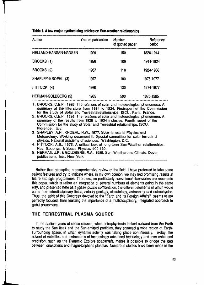
Table 1. A few major synthesising articles on Sun-weather relationships

Author Year of publication Number Reference of quoted paper period

HELLAND-HANSEN-NANSEN 1920 150 1826-1914

BROOKS (1)

BROOKS (2)

SHAPLEY-KROEHL (3)

PITTOCK (4)

HERMAN-GOLDBERG (5)

1926

1957

1977

1978

1985

100

110

100

130

500

1914-1924

1924-1956

1975-1977

1974-1977

1875-1985

1 . BROOKS, C.E.P., 1926. The relations of solar and meteorological phenomena. A summary of the littérature from 1914 to 1924. Firstreport of the Commission for the study of Solar and Terrestrialrelationships. ISCU, Paris, France.

2. BROOKS, C.E.P., 1936. The relations of solar and meteorological phenomena. A summary of the results from 1925 to 1934 inclusive. Fourth report of the Commission for the study of Solar and Terrestrial relationships. ISCU, Florence, Italy.

3. SHAPLEY, A.H., KROEHL, H.W., 1977. Solar-terrestrial Physics and Meteorology, Working document II. Special committee for solar-terrestrial physics, National academy of sciences, Washington, D.C.

4 . PITTOCK, A.B., 1978. A critical look at long-term Sun-Weather relationships, Rev. Geophys. & Space Physics, 400-420.

5. HERMAN, J.R. & GOLDBERG, R.A., 1985. Sun, Weather and Climate. Dover publications, Inc., New York.

Rather than attempting a comprehensive review of the field, I have preferred to take some salient features and try to indicate where, in my own opinion, we may find promising results in future strategic programmes. Therefore, no particularly sensational discoveries are reportedin this paper, which is rather an integration of several numbers of elements going in the same way, and presented here as a jigsaw puzzle combination, the different elements of which would come from interdisciplinary fields, notably geology, climatology, astronomy and astrophysics. Thus, the spirit of this Congress devoted to the "Earth and its Foreign Affairs" seems to me perfectly focused, from realizing the importance of a multidisciplinary, integrated approach to global phenomena.

THE TERRESTRIAL PLASMA SOURCE

In the earliest years of space science, when astrophysicists looked outward from the Earth to study the Sun itself and the Sun-emitted particles, they scanned a wide region of Earth-surrounding space, in which dynamic activity was taking place continuously. To-day, the advent of satellites and instruments of increasingly advanced technology and ever-enhanced precision, such as the Dynamic Explore spacecraft, makes it possible to bridge the gap between ionospheric and magnetospheric plasmas. Numerous studies have been made in the

93

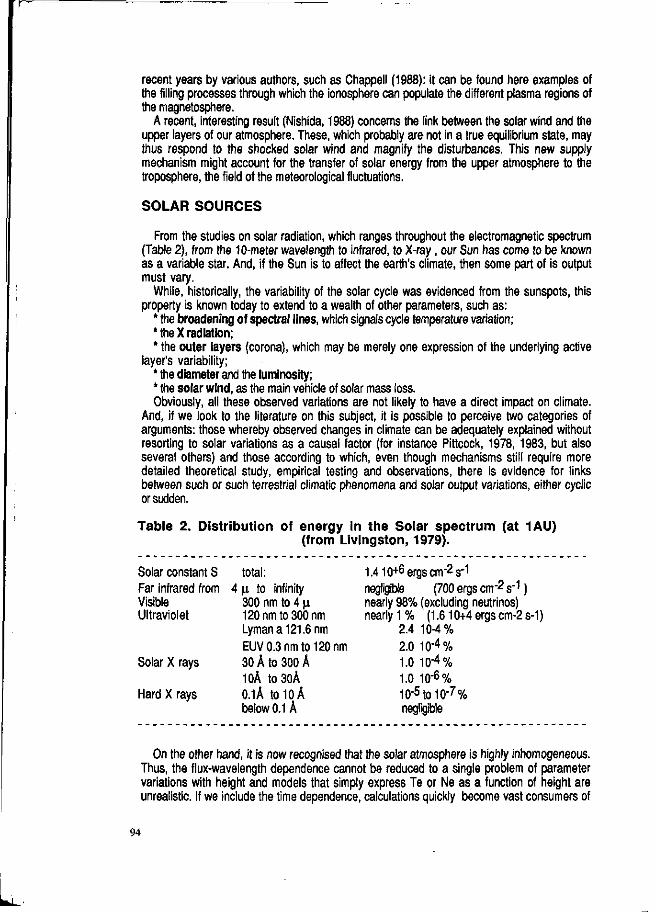
recent years by various authors, such as Chappell (1988): it can be found here examples of the filling processes through which the ionosphere can populate the different plasma regions of the magnetosphere.

A recent, interesting result (Nishida, 1988) concerns the link between the solar wind and the upper layers of our atmosphere. These, which probably are not in a true equilibrium state, may thus respond to the shocked solar wind and magnify the disturbances. This new supply mechanism might account for the transfer of solar energy from the upper atmosphere to the troposphere, the field of the meteorological fluctuations.

SOLAR SOURCES

From the studies on solar radiation, which ranges throughout the electromagnetic spectrum (Table 2), from the 10-meter wavelength to infrared, to X-ray, our Sun has come to be known as a variable star. And, if the Sun is to affect the earth's climate, then some part of is output must vary.

While, historically, the variability of the solar cycle was evidenced from the sunspots, this property is known today to extend to a wealth of other parameters, such as:

* the broadening of spectral lines, which signals cycle temperature variation; * the X radiation; * the outer layers (corona), which may be merely one expression of the underlying active

layer's variability; * the diameter and the luminosity; * the solar wind, as the main vehicle of solar mass loss. Obviously, all these observed variations are not likely to have a direct impact on climate.

And, if we look to the literature on this subject, it is possible to perceive two categories of arguments: those whereby observed changes in climate can be adequately explained without resorting to solar variations as a causal factor (for instance Pittcock, 1978, 1983, but also several others) and those according to which, even though mechanisms still require more detailed theoretical study, empirical testing and observations, there is evidence for links between such or such terrestrial climatic phenomena and solar output variations, either cyclic or sudden.

Table 2. Distribution of energy in the Solar spectrum (at 1AU) (from Livingston, 1979).

Solar constant S total : 1.410+6 ergs cm"2 s"1

Far infrared from 4 p. to infinity negligible (700 ergs cm"2 s"1 ) Visible 300 nm to 4 p. nearly 98% (excluding neutrinos) Ultraviolet 120 nm to 300 nm nearly 1 % (1.610+4 ergs cm-2 s-1)

Lyman a 121.6 nm 2.4 10-4% EUV0.3nmto120nm 2.0 10"4%

Solar X rays 30 Â to 300 Â 1.0 10"4 % 10Â to30Â 1.0 10"6%

Hard X rays 0.1Â to 10 A 10"5 to10"7% below 0.1 Â negligible

On the other hand, it is now recognised that the solar atmosphere is highly inhomogeneous. Thus, the flux-wavelength dependence cannot be reduced to a single problem of parameter variations with height and models that simply express Te or Ne as a function of height are unrealistic. If we include the time dependence, calculations quickly become vast consumers of

94

computer time... Our present physical understanding of known features or solar variability including sunspots, flares, plages, coronal disturbances provides no hint that these transient events should alter the total flux from the Sun in an appreciable way.

Below 10 Â, the X-rays emitted by energetix X-ray flares, are a major source of ionisation in the D-region of the ionosphere, where they generate Sudden Ionospheric Disturbances (SID) including Short Wawe Fade-out (SWF). The atmosphere can be penetrate by X-rays as fa as down 60 to 70 km altitudes.

At last, it is now commonly accepted that the Sun's radius did in fact contract by some 0.5 arcsecond between 1715 and 1979, and for shorter periods of time the fluctuations of the radius seem to be periodical, with a cycle of the order of 900 days. Dicke (1979) wrote that "the more sunspots, the milder may be the climate" which can be restated as: the bigger the Sun, the lower the luminosity (correlating with a drop in activity), which led to some climatic cooling down on the Earth (e.g. Little Ice Age). Those first clues demonstrate the reason for obtaining precise measurements of the solar radius spanning long periods of time.

THE SOLAR LUMINOSITY VARIATIONS

The evolving composition of the terrestrial atmosphere due to the solar energy input on biospheric species must have strongy influence on the climate. An example is the apparent absence of glaciation in a period when the solar luminosity was substantially smaller than at present time (known as the "young Sun luminosity paradox"). The most convincing explanation proposed so far assumes the existence of larger amounts of gases radiatively active in the infrared in the ancient Earth's atmosphere. At that time, about 4 200 Up BP, the temperature of the Earth was relatively warm (between 38 °C and 54 °C), in spite of a low solar luminosity which prevailed at that time.

ERB Nimbus 7 channel 10C: 9 1 /2 years

0 .0 Nov - 7 8 N o v - 7 9 N o v - 8 0 N o v - 8 1 N a v - 8 2 N o v - 8 3 N o v - B 4 N o v - a 5 N o v - 8 6 N o v - 8 7 N o v - 8 8 N o v - 8 9

Fig. 1. Daily mean solar irradiance from Nov. 16,1978 to April, 30,1988. Lower spot is Sunspot Number for the same period (after Lee, 1988).

95

While poorly known for a very long time because of the fluctuations of atmospheric absorption phenomena, the Sun's luminosity is continously evolving giving rise to climatic disturbances: this variation nonetheless exceeds the threshold, set at 0.1 %, of the present climatic model's sensitivity to solar energy variations.

Measurements of the solar luminosity, now in practice for quite a few years following experiments carried out on spacecraft like ACRIM on SMM, point out to both short-term and long-term variations. Over the last decade, the solar constant S grew by an approximate amount of 0.02 % from 1984 until 1986, then decreased by some 0.03% over the 1986-1988 period (Figure 1 after Lee, 1988; see also Hickey, 1988). We note that the energy emitted is up by a few ten thousandths in periods of peak activity. A recent application of solar max ACRIM data to analysis of solar-driven climatic variability on Earth (Hoffert et al., 1988) yielded the following evidence: while the solar luminosity variations appear unlikely as a major factor in global-scale climate change over the period under study, nevertheless currently available satellite data are sufficient to rule out a major solar variation effect on surface temperature in the short term, with longer term effects possible if long time-series irradiance monitoring from space is operational facts.

RECONSTRUCTION OF PAST CLIMATE

Reconstruction of the past climates draws on a broad variety of sources: instrumental data and their records, documentary historical data and proxy data. Out of a wealth of usable techniques, the following may be listed :

- dendrochronology, or the study of trees' annual rings, whose variations in thickness are now known with certainty to reflect variations in climate. They can be traced a long way back in time (thus in 1919, Douglass was able to read the annual rings of Californian pine and redwood, covering a period from 1420 to 1909 A.D.).

- isotopic variations in the oxygen of foraminifera shells, variations of which are directly linked with those organisms' growth temperatures. Studies on cored samples of marine sediments yield knowledge of climate variations over several millennia.

- isotopic variations in fossilised trees (deuterium, hydrogen), from studies addressing only the last millennium.

- analysis of the deep ice samples, for example from Greenland or Antarctica (dome C), where C02 variations can be measured over several millennia, thus providing a key to past climate variations.

- critical analysis of old documents, i.e. vintage dates, naval log books, parish registers, mediaeval-time clerical (church or university) account books, curves of foodcrop prices... forms the baseline for detailed study of such periods as harsh winters, early springs, abnormally dry seasons, etc... - the advance or retreat of glaciers are well known as indicators of local climate oscillations (see for example the extensive studies on the Fernau glacier history).

- analysis of pollen (palynology), which directly reflects drought or wetness periods through examination of the appropriate species.

- the annual number of cometary observations, revealing of variations in night-time cloudiness.

- the analysis of fluvial or marine sediments, for example those that represent annual alternations of melting in a periglacial lake.

- analysis of Earth's orbital variations. The theory of Milankovitch (1931) evidences cycles of several tens of thousand years each, and accounts for the glaciation or warming periods. Ranking among the best of today's models, it forecasts some cooling down in the future, which a first deep freeze looming at about 5,000 years from now, followed by warming in 15,000 years, by a sustained cold period centred around 23,000 hence, and by a significant glaciation in 60,000 years...

96

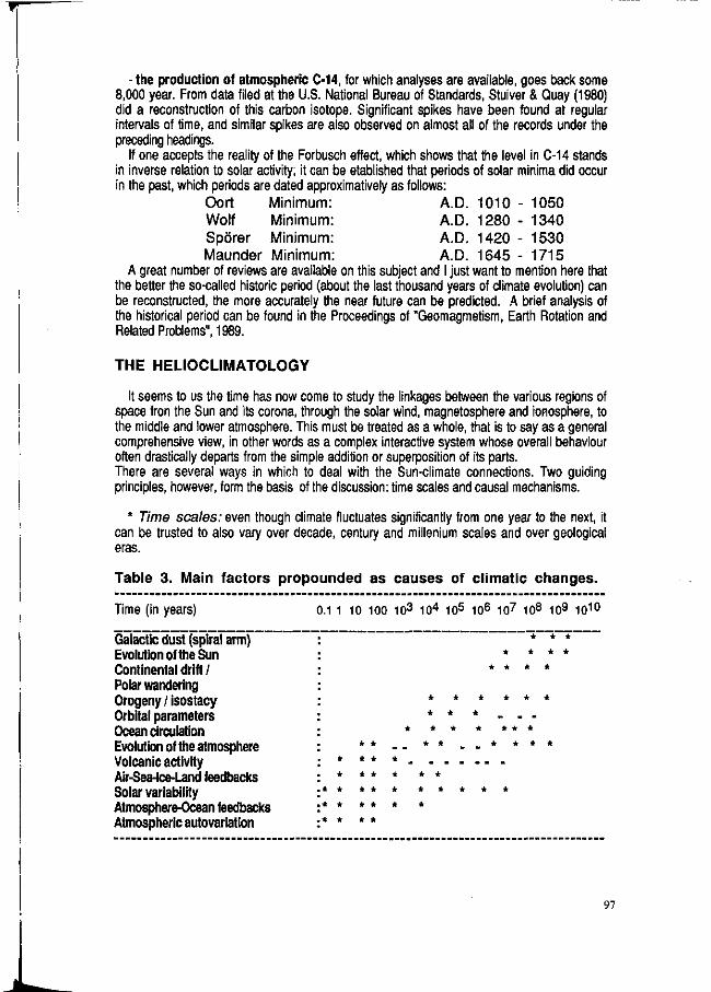
- the production of atmospheric C-14, for which analyses are available, goes back some 8,000 year. From data filed at the U.S. National Bureau of Standards, Stuiver & Quay (1980) did a reconstruction of this carbon isotope. Significant spikes have been found at regular intervals of time, and similar spikes are also observed on almost all of the records under the preceding headings.

If one accepts the reality of the Forbusch effect, which shows that the level in C-14 stands in inverse relation to solar activity, it can be etablished that periods of solar minima did occur in the past, which periods are dated approximatively as follows:

Oort Minimum: A.D. 1010 - 1050 Wolf Minimum: A.D. 1280 - 1340 Spörer Minimum: A.D. 1420 - 1530 Maunder Minimum: A.D. 1645 - 1715

A great number of reviews are available on this subject and I just want to mention here that the better the so-called historic period (about the last thousand years of climate evolution) can be reconstructed, the more accurately the near future can be predicted. A brief analysis of the historical period can be found in the Proceedings of "Geomagmetism, Earth Rotation and Related Problems", 1989.

THE HELIOCLIMATOLOGY

It seems to us the time has now come to study the linkages between the various regions of space fron the Sun and its corona, through the solar wind, magnetosphere and ionosphere, to the middle and lower atmosphere. This must be treated as a whole, that is to say as a general comprehensive view, in other words as a complex interactive system whose overall behaviour often drastically departs from the simple addition or superposition of its parts. There are several ways in which to deal with the Sun-climate connections. Two guiding principles, however, form the basis of the discussion: time scales and causal mechanisms.

* Time scales: even though climate fluctuates significantly from one year to the next, it can be trusted to also vary over decade, century and millenium scales and over geological eras.

Table 3. Main factors propounded as causes of climatic changes.

Time (in years) 0.1 1 10 100 103 104 105 106 107 108 109 1010

Galactic dust (spiral arm) Evolution of the Sun Continental drift / Polar wandering Orogeny / isostacy Orbital parameters Ocean circulation Evolution of the atmosphere Volcanic activity Air-Sea-Ice-Land feedbacks Solar variability Atmosphere-Ocean feedbacks Atmospheric autovariation

* *

* *

97

* Causal mechanisms. The most important can be listed as follow: interstellar dust (passage of the Earth through a spiral arm of the galaxy every 270 Myr),

evolution of the Sun, like other stars, continental drift and polar wandering, orogeny-isostasy (changes in the elevation of landmasses for the first term and effects of ice loading in deforming the land for the second), Earth orbital variations (Milankovitch theory, described as the climatic variability due to changes in solar insolation resulting from variations in the Earth's orbit that occur in response to predictable changes in the gravitational field experienced by the Earth) as well as planetary beats (Fairbridge, 1989), ocean circulation, changes in the concentration of the Earth's atmosphere, volcanic activity, air-sea-ice-land feedbacks, solar variability and coupled ocean-atmosphere system.

Table 3, adapted from Kutzbach (1976), summarises the main factors propounded as causes of climatic changes on various timescales and, in this prospect, I suggest that the effects of our Sun on our planet, be dubbed HELIOCLIMATOLOGY.

Magnetic energy Rotational energy Nuclear energy

Radiation f lux

Di f ferent ia l

Rotation

Act ive

Regions

Convection

Super

Granulation

Mechanical

Flux

Corona

Flares X-Ray Flux Solar Wind

Fig.2 . Schematic representation of the solar energy sources, their interaction and the origin of high energy phenomena like flares and the solar corona. Circles denote coupling or interaction between different phenomena.

Thus, HELIOCLIMATOLOGY can be defined as the study of impact of the Sun's output on the Earth's climate. This concerns mainly the study of energy and mass transfers in the solar-terrestrial system, including relevant physical and chemical interaction mechanisms, as well as

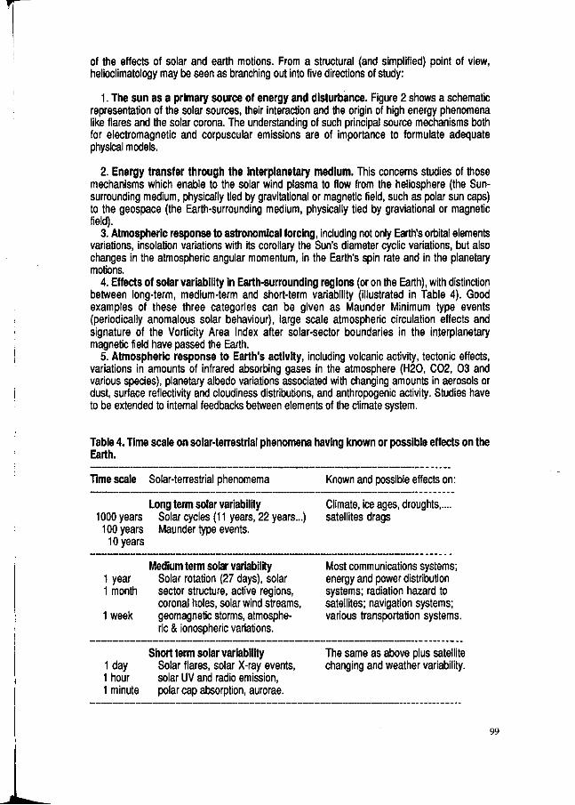
of the effects of solar and earth motions. From a structural (and simplified) point of view, helioclimatology may be seen as branching out into five directions of study:

1. The sun as a primary source of energy and disturbance. Figure 2 shows a schematic representation of the solar sources, their interaction and the origin of high energy phenomena like flares and the solar corona. The understanding of such principal source mechanisms both for electromagnetic and corpuscular emissions are of importance to formulate adequate physical models.

2. Energy transfer through the interplanetary medium. This concerns studies of those mechanisms which enable to the solar wind plasma to flow from the heliosphere (the Sun-surrounding medium, physically tied by gravitational or magnetic field, such as polar sun caps) to the geospace (the Earth-surrounding medium, physically tied by graviational or magnetic field).

3. Atmospheric response to astronomical forcing, including not only Earth's orbital elements variations, insolation variations with its corollary the Sun's diameter cyclic variations, but also changes in the atmospheric angular momentum, in the Earth's spin rate and in the planetary motions.

4. Effects of solar variability in Earth-surrounding regions (or on the Earth), with distinction between long-term, medium-term and short-term variability (illustrated in Table 4). Good examples of these three categories can be given as Maunder Minimum type events (periodically anomalous solar behaviour), large scale atmospheric circulation effects and signature of the Vorticity Area Index after solar-sector boundaries in the interplanetary magnetic field have passed the Earth.

5. Atmospheric response to Earth's activity, including volcanic activity, tectonic effects, variations in amounts of infrared absorbing gases in the atmosphere (H20, C02, 03 and various species), planetary albedo variations associated with changing amounts in aerosols or dust, surface reflectivity and cloudiness distributions, and anthropogenic activity. Studies have to be extended to internal feedbacks between elements of the climate system.

Table 4. Time scale on solar-terrestrial phenomena having known or possible effects on the Earth.

Time scale Solar-terrestrial phenomema Known and possible effects on:

Long term solar variability Solar cycles (11 years, 22 years...) 1000 years Solar cycles (11 years,

100 years Maunder type events. 10 years

Climate, ice ages, droughts,, satellites drags

Medium term solar variability 1 year Solar rotation (27 days), solar 1 month sector structure, active regions,

coronal holes, solar wind streams, 1 week geomagnetic storms, atmosphe­

ric & ionospheric variations.

Most communications systems; energy and power distribution systems; radiation hazard to satellites; navigation systems; various transportation systems.

Short term solar variability 1 day Solar flares, solar X-ray events, 1 hour solar UV and radio emission, 1 minute polar cap absorption, aurorae.

The same as above plus satellite changing and weather variability.

99

i CONCLUSION

Starting less than a decade ago, mankind has enterred into a new-frangled relationship with our planet. Unless we quickly and profoundly change the course of our civilisation, we are faced with the doom of the worldwide ecological system. Listen:

* the Earth's forests are being destroyed at a very fast rate, about one Tennessee's or three Switzerland's worth every year;

* an enormous hole Is opening In the ozone layer, reducing the Earth's ability to protect life from deadly ultraviolet radiation;

* living species die out at quite an unprecedented rate, and one or two may disappear within a man's lifetime; * chemical wastes, in growing volumes, seep downward to poison ground water and upward to destroy the

atmosphere's delicate balance; ' huge quantities of carbon dioxide, methane and chlore- fluorocarbons in the atmosphere have trapped heat and

raised global temperatures. Why are these dramatic changes taking place? Not only because the human population is surging, but also

because the industrial and technological revolutions magnify the environmental impact of these increases, and also because we tolerate self-destructive behaviour and environmental pollution on a global scale. It is one of the reasons, to my sense, for which scientists have to try to improve our understanding of the basic processes of our evolving climate. Moreover, as man is becoming to extends his fontiers beyond the surface of the home planet, we must know the impact of sun's variability on the space medium in which manned spacecraft of to morrow will operate. The need to predict climate in space will be as strong as it is to-day to become masters of the production cycles and so better manage our resources.

Time has come to join our forces, and the 1990's must be the decade of decision. Scientists must pool their efforts to better understand this complex chain going from the Sun to the Earth, anefcreate a new global approach to Solar-Terrestrial phenomena, focusing the scope on the coupling mechanisms that are responsible for the transfer of energy and mass from one region of Sun-Earth system to another. I am an enthousiastic "helioclimatologist".

REFERENCES

Chappell, CR., 1988. The terrestrial plasma source: a new perspective in solar-terrestrial processes from Dynamics Explorer. Rev. of Geophys., 26-2: 229-248. Dicke R.H., 1979. Solar luminosity and the sunspots cycle. Nature, 280:24-27. Fairbridge, R. W., 1974. Planetary periodicidies and terrestrial climate stress. In: N.A. Mörner and W. Karlen

(editors), D. Reidel publishing C°. Climatic Changes on a Yearly to Millennial basis, pp. 509-520. Fairbridge, R. W., 1989. Planetary beats and Geology. In N.A. Mörner and S. Flodmark (editors),

Geomagmetism, Earth rotation and related problems, to be published. Geomagmetism, Earth rotation and related problems: N.A. Mörner and S. Flodmark (editors). Conference held in

Stockholm, 10-12 October 1988, to be published. Hickey, J.R., Aton, B.M., Kylr, H I . , Major, E.R., 1988. Observation of total irradiance variability from Nimbus satellite.

COSPAR, 27 th Plenary meeting, Helsinki, paper 12.1.1. Hoffert, M.I., Frei, A. and Narayanan, V.K., 1988. Application of Solar Max ACRIM data to analysis of solar-driven

climatic variability on Earth. Climatic Change, 13:267-285. Kutzbach, J.E.,1976. Quaternary Research, 6:471. Landscheidt, T.,1988. Solar rotation, impulses of the torque in the Sun's motion, and climatic variation. Climatic

change, 12:265-295. Livingston, W.C.,1979. Solar input in the terrestrial system. In: B.M. Comae and T.A. Saliga (editors), D. Reidel

publishing C°. Solar-Terrestrial Influences on Weather and Climate, pp. 43-57. Lee, R.B., Barkstrom, B.R., Harrison, E.F., Gibson, M.A., Natazrajan, S.M., Edmonds, W.L., Mecherikunnel, AT., Kyle, L,

1988. Earth Radiation Budget satellite extra terrestrial solar constant measurements. COSPAR, 27 th Plenary meeting, Helsinki, paper N° 12.1.3.

Milankovitch, M., 1931. Variations séculaires des éléments astronomiques de l'orbite terrestre. Glas. Srp. Kralyerske Akad., 1243,1 rst class, N° 70.

Nishida, A., 1988. Magnetosphere-ionosphere Response to solar wind. COSPAR, 27 th Plenary meeting, Helsinki, p. 409. Pittcock, A.B.,1978. A critical look at long-term Sun-weather relationship. Rev. Geophys. Space Phys.,16:400-420. Pittcock, A.B., 1983. Solar variability, Weather and Climate: an update. Quartely Journal of the Royal Meteorological Society, 109: 23-55. Stuiver, M. and Quay, P.D., 1980. Changes in the atmospheric carbon-14 attributed to a variable sun. Science, 207: 4426, 11-19.

100

The earth and its macro-environment, a multidisciplinary approach

103

THE POSSIBLE INFLUENCE OF SOME ASTRO-PHYSICAL FACTORS ON MICRO-ORGANISMS

P. Faraone Laboratório di Igiene e Profilassi, Reparto Medico, USL RM5, Rome, Italy

Summary

The incidence of differentiated sector colonies (CSD) of heterogeneous bacteria, collected from the outside air was studied by the author from 1970 to 1982 by daily exposing Petri's plates to the open air. Variations in the CSD incidence in specimens of Staphylococcus Aureus were also observed daily by the same author from 1984 to 1989. This research in which fresh broth is inoculated daily with the bacteria being studied is continuing. As a result of these works, the hypothesis of an influence of solar activity plus galactic cosmic radiations on cellular phenomena in air bacteria as advanced in preceding studies has been confirmed by more recent studies in laboratory bacteria cultures of Staphylococcus Aureus.

Introduction

It is well known today that some environmental factors, for example solar activity, the earth's motion and electromagnetic fields, fluctuate. These fluctuations may influence biological, physical and chemical systems in the biosphere. Many authors (Piccardi 1960a, 1960b, 1962, 1969; Takata 1951; Capel-Boute 1960, 1974, 1977, 1980; Tromp 1981; Ogata, cited by Capel-Boute, 1985) have come to this conclusion after systematic studies using colloid tests. The author (1971), observing the seasonal variations of air bacteria during the year, noted also the variable CSD frequence. The abbreviation CSD is derived from the Italian expression 'colonia a settore differenziato' (in English, 'differentiated sector colony). The author prefers to use the Italian abbreviation to remain consistent with the terminology of previous research. Wayne and Umbreit (1962) called CSD colony sectoring. After having observed these CSD variations, the author decided to carry out several researches to put in evidence the frequency of appearance of CSD in long term daily observations (1973, 1978, 1979, 1983, 1984, 1985). The later CSD works have reinforced the suggestion of a causal relationship between usually uncontrolled environmental factors and fluctuating physicochemical and biological phenomena. This report summarizes the research carried out with such CSD tests. The CSD is a bacterial colony that shows sectors differing in some visible characteris­tics (color, transparency, surface type, thickness or general appearance) from the parent strain grown simultaneously and competing successfully with it (Servin-Massieu, 1961). Wayne and Umbreit (1962) deemed such phenomena not really rigorous enough to be proof of genetic mutations, although CSD's are explained most easily (and perhaps only) in terms of mutations. We point them out merely as very simple examples of mutations that do not require elaborate experiments for detection. CSD's were con­sidered as rare events by Lamanna and Mallette (1959)*. The induction of CSD formation in E.Coli was demonstrated by Witkin (1951)*, who studied cultures subjected to the mutagenic influence of ultraviolet light, re­sulting in the formation of lactose positive and lactose negative sectors. CSD's arising from Salmonella Typhimurium obtained by transduction have been observed by Demerec (Lamanna & Mallette*, Witkin*, Demerec, cited by Servin-Massieu 1961) 1956. Servin-Massieu (1961) observed different

105

types of colonies derived from a single strain of Staphylococcus Aureus that had undergone successive passages from broth to agar plates. Some were orange, others white, and about 10% of the total were sectored. Some of the latter contained small mutant areas, whereas others contained large ones (more than half of the colony). This was the first report of the spontaneous appearance of CSD's in S. Aureus cultures. Faraone (1985) later showed differences in bacterial antibiotic resistance and sensiti­vity to phage activity in CSD mutant areas of various strains of S.Aureus. The same author, studying variations in CSD frequency as function of time, showed that CSD frequency was a typical example of fluctuating biological phenomena not only for heterogeneous bacteria culled from the air (1970-1982) but also successively for pure laboratory strains of S.Aureus (1984-1989 and ongoing experiments).

Materials and Methods

The first series of experiments (1970-1982) involved heterogeneous air bacteria divided into the following groups: total count of bacteria; mycetes (excluding Hyphomycetes), spore bearing bacteria, chromogenic bacteria and micrococcaceae (reflecting the order, from mycetes, of in­creasing frequency of CSD's observed, during our research). However, only the total count of bacteria was indicated in the CSD frequency diagram (fig. 2 ) . The Hyphomycetes were inhibited by actidione. Other mycetes not inhibited were not considered because in these, CSD's were on the whole extremely rare. Air bacteria were culled by exposed Difco tryptose-agar plates, 90 mm in diameter. The agar concentration was raised to 20 ppt and actidione was added at a rate of 100 jig/ml tryptose-agar to inhibit moulds (Hyphomycetes), which would otherwise have invaded the medium, making it very difficult, if not impossible, to distinguish colonies one from another in the plates. The plates were exposed 30 to 60 minutes daily in the open air in the morning or afternoon (generally some time between 10 a.m. and 4 p.m.), the length of exposure being determined by the pre­vailing wind conditions and recent precipitation. Colonies that increased in size after incubation at 37°C for two days and 20-23°C for another four days were considered. The CSD frequency was expressed as a percentage of all of the colonies counted on the plates, excluding mycetes. An ave­rage of 200-250 colonies were read each day. The plates were exposed putting them in several round containers with a vertical side less high than the plate sides, and fixed to a grated metal support, placed one meter above the pavement of the Institute's rooftop terrace about 25-30 meters above street level. The procedure was carried out under the same conditions at the LIP (Laboratory Health and Hygiene) in Milan (1970-1976) and then at Rome's LIP from February 1976 to July 1982; both buildings being located on the outskirts of their respective cities surrounded by trees and little traffic and free of natural or manmade obstacles on their roofs. Strong lenses using incident, transmitted light, at 8x or lOx mag­nification were used for all readings. For special difficulties a micros­cope at 50x magnification was used.

The second series of experiments (1984-1989) involved strains of S.Au­reus isolated from throat cultures. At first, only one strain of S.Aureus, labeled "Nn", was used. Starting in February 1986 two other strains, referred to as "Kl" and "K2", were included in the experiment. A third strain, "K3", was added in November 1986. Fig. 1, shows the inoculation and culturing protocol of S.Aureus strains studied for CSD frequency in laboratory experiments. This is proceeding on the same way and on every subsequent day; from Brain-hearth (BH) Difco, S.Aureus brothculture (A), after 24h incubation at 37°C, a loop was put in a BH sterile broth (B)

106

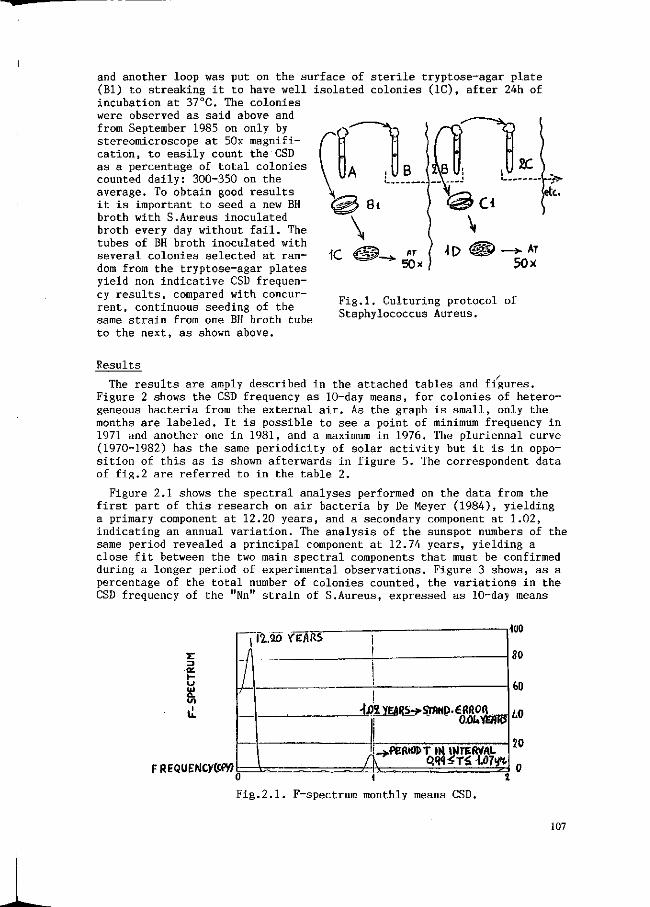
and another loop was put on the surface of sterile tryptose-agar (Bl) to streaking it to have well isolated colonies (1C), after incubation at 37°C. The colonies were observed as said above and from September 1985 on only by stereomicroscope at 50x magnifi­cation, to easily count the CSD as a percentage of total colonies counted daily: 300-350 on the average. To obtain good results it is important to seed a new BH broth with S.Aureus inoculated broth every day without fail. The tubes of BH broth inoculated with several colonies selected at ran­dom from the tryptose-agar plates yield non indicative CSD frequen­cy results, compared with concur­rent, continuous seeding of the same strain from one BH broth tube to the next, as shown above.

plate 24h of

Fig.1. Culturing protocol Staphylococcus Aureus.

of

Results

The results are amply described in the attached tables and figures. Figure 2 shows the CSD frequency as 10-day means, for colonies of hetero­geneous bacteria from the external air. As the graph is small, only the months are labeled. It is possible to see a point of minimum frequency in 1971 and another one in 1981, and a maximum in 1976. The pluriennal curve (1970-1982) has the same periodicity of solar activity but it is in oppo­sition of this as is shown afterwards in figure 5. The correspondent data of fig.2 are referred to in the table 2.

Figure 2.1 shows the spectral analyses performed on the data from the first part of this research on air bacteria by De Meyer (1984), yielding a primary component at 12.20 years, and a secondary component at 1.02, indicating an annual variation. The analysis of the sunspot numbers of the same period revealed a principal component at 12.74 years, yielding a close fit between the two main spectral components that must be confirmed during a longer period of experimental observations. Figure 3 shows, as a percentage of the total number of colonies counted, the variations in the CSD frequency of the "Nn" strain of S.Aureus, expressed as 10-day means

I2..0O YEARS

r CK

u Ul

a.

FREQUENCyCCW ——ZJjs A _i.PEW0J>T IM »NrERVAL

i

F i g . 2 . 1 . F-spectrum monthly means CSD.

80

60

L0

20

0

107

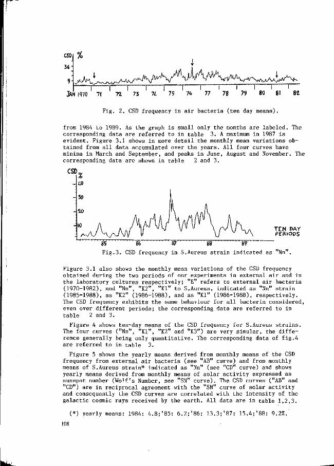
CSD

9 H

%

i i i" i i i r i ' r T p "T*"* JAN W O ' 7t ' 7a 73 7t '75 76 77 78 7? 80 8t 82

Fig. 2. CSD frequency in air bacteria (ten day means).

from 1984 to 1989. As the graph is small only the months are labeled. The corresponding data are referred to in table 3. A maximum in 1987 is evident. Figure 3.1 shows in more detail the monthly mean variations ob­tained from all data accumulated over the years. All four curves have minima in March and September, and peaks in June, August and November. The corresponding data are shown in table 2 and 3.

CSD

TEN DAY PERIODS

85 '8fe '& 88 89

Fig.3. CSD frequency in S.Aureus strain indicated as "Nn".

Figure 3.1 also shows the monthly mean variations of the CSD frequency obtained during the two periods of our experiments in external air and in the laboratory cultures respectively; "E" refers to external air bacteria (1970-1982), and "Nn", "K2", "Kl" to S.Aureus, indicated as "Nn" strain (1985-1988), as "K2" (1986-1988), and as "Kl" (1986-1988), respectively. The CSD frequency exhibits the same behaviour for all bacteria considered, even over different periods; the corresponding data are referred to in table 2 and 3.

Figure 4 shows ten-day means of the CSD frequency for S.Aureus strains. The four curves ("Nn", "Kl", "K2" and "K3") are very simular, the diffe­rence generally being only quantitative. The corresponding data of fig.4 are referred to in table 3.

Figure 5 shows the yearly means derived from monthly means of the CSD frequency from external air bacteria (see "AB" curve) and from monthly means of S.Aureus strain* indicated as "Nn" (see "CD" curve) and shows yearly means derived from monthly means of solar activity expressed as sunspot number (Wolf's Number, see "SN" curve). The CSD curves ("AB" and "CD") are in reciprocal agreement with the "SN" curve of solar activity and consequently the CSD curves are correlated with the intensity of the galactic cosmic rays received by the earth. All data are in table 1,2,3.

(*) yearly means: 1984: 4.8;'85: 6.2;'86: 13.3;'87: 15.4;'88: 9.2%.

108

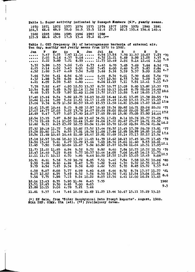
Table 1 . Solar a c t i v i t y indicated by S un spot Numbers (£)*, / e a r l y means. 1970 1971 1972 1973 1974 1975 1976 1977 1978 1979 1980 1981

104,5 66.6 68.9 38.0 34.5. 15.5 12.6 27.5 92.5 155.4 154.6 140.4 1982 1983 1984 1985 1986 1987 1988

115.9 66.6 45.9 17.9 13.4 29.2 81.1»*

Table 2 . CSD frequency (#) of heterogeneous bac te r i a of ex ternal a i r . Ten day, monthly and yearly means from 1970 t o 1982. Jan P Mr Ap II Jun J u l Au S O N S

3.47 2.25 7.43 11.14 8.56 17.56 7.38 11.57 10.07 7.25 '70 2.03 5.16 4.37 9.06 6.32 11.21 5.69 9.99 13.25 3.37 , Q 2.22 9.89 7.21 6.99 11.73 10.48 2.96 9.14 12.46 4.10 7 ' 8

3.72 3.98 1.33 3.96 7.65 6.73 4.63 6.70 3.65 3.69 7.66 6.56 '71 6.25 2.14 4.02 3.43 6.91 5.22 5.45 6.00 2.68 5.23 5.83 2.84 . , 4.52 1.88 3.47 4.48 7.54 5.20 3.66 5.36 3.59 3.37 5.99 2.99 4 # '

3.66 7.50 5.41 6.56 6.35 4.44 8.34 9.01 7.30 6.66 7.54 '72 4.32 1.88 3.35 6.94 6.99 7.57 12.50 6.33 7.50 7.28 5.63 , = 4.21 4.09 2.98 5.63 4.80 8.26 11.19 7.11 7.91 12.41 5.15 b # 5

7.78 7.92 4.67 4.93 12.53 13.37 8.72 10.77 13.09 9.60 13.82 12.37 '73 10.54 5.69 3.65 9.72 11.16 11.56 13.66 10.13 10.48 8.79 20.06 16.48 l f t ,

8.68 5.93 5.29 7.97 11.40 11.96 13.72 12.17 10.28 7.42 18.03 17.72 x u ' b

17.40 13.46 9.54 3.82 12.75 16.03 10.22 16.44 12.81 17.85 15.38 20.53 '74 10.84 11.14 5.89 5.04 11.51 19.13 11.09 15.49 14.50 17.53 23.77 1 5 . 0 7 , , « 13.06 9.36 6.79 11.52 20.57 18.45 13.53 11.58 16.81 13.06 17.87 18.42 i 3 - B

16.41 13.85 10.44 9.25 9.99 12.97 18.69 19.34 20.82 16.71 29.96 20.20 '75 17.07 14.77 12.03 5.22 13.76 14.27 22.24 26.02 20.02 29.05 30.87 ,no 16.69 9.47 7.97 5.03 17.80 16.07 17.05 29.66 15.80 23.05 23.90T 16.46 l , i

12.54 13.55 7.87 8.52 14.18 13.42 34.51 17.21 8.14 19.76 19.77 23.25 '76 17.76 15.48 9.14 13.03 12.44 15.82 24.06 13.22 20.67 23.27 16.71 2 4 . 5 2 . , 9 12.82 8.31 8.23 23.22 12.73 20.94 11.64 10.70 12.02 20.94 20.36 21.84 ° 27.32 19.18 11.72 7.01 12.82 23.52 13.44 26.32 15.45 17.39 26.39 23.81 '77 23.28 20.80 11.74 8.53 17.91 18.36 11.08 17.64 12.85 18.99 18.85 14.62 1 7 , 18.54 11.68 10.63 16.46 21.69 18.42 15.81 22.69 19.14 23.13 22.12 13.54 i ' ' b

15.18 12.57 10.86 10.10 13.22 11.65 14.39 12.62 18.13 17.45 10.73 17.65 '78 16.96 13.42 9.61 6.27 11.29 13.66 7.60 18.36 15.06 11.60 9.53 1 8 . 8 1 , , . 11.65 7.50 7.80 10.04 11.67 5.94 10.92 15.87 10.58 11.04 10.31 1 7 . 93 1 'x

11.73 11.22 11.85 6.94 9.32 9.72 9.92 8.40 7.84 12.73 12.72 10.73 '79 12.43 14.40 7.19 8.66 5.77 10.37 10.44 14.09 7.06 14.63 14.15 1 1 . 7 3 , n = 12.11 11.71 10.12 6.70 5.85 8.46 10.20 12.52 13.25 13.03 12.45 g .OS 1 0 - 3

10.31 8.61 5.36 7.39 10.76 8.05 7.51 5.42 7.54 7-58 12.32 10.06 »80 8.2 9.99 5.88 8.60 4.84 9.67 5.70 5.82 9.46 5.70 9.72 12.35 10.15

9.79 6.54 7.63 9.34 9.36 6.89 4.62 7.51 5.70 8.83 13.72 7.57 4.58 8.07 8.08 3.77 4.98 4.40 6.48 6.44 8.30 8.74 13.57 11.77 '81 8.23 12.02 6.95 3.49 8.32 5.54 8.50 12.36 7.41 12.54 13.04 11.84 „ .-5.56 7.75 5.98 7.15 5.94 10.22 8.03 12.36 6.41 12.00 16.24 13.65 B , b

12.14 13.43 8.35 5.90 11.84 8.43 7.35 1982 13.51 12.63 9.30 6.65 7.00 8.03 Q , 13.88 10.15 9.06 4.78 7.21 7.46 * ° 11.81 9.37 7.44 7.46 10.58 11.69 11.23 13.44 10.67 13.11 15.29 13.15

(*) SN data , from "Solar Geophysical Data Prompt Reports" . August, 1988. N0AA DBF. COfflU. USA (ed) . (**) Preliminary datum.

r-

Table 3 . CSS frequenoy(#) of S . Aureus s t r a i n s ; monthly and 10 da/ means. Jan ï Mr Ap M Jun J u l Au S 0 N D

"HH„(1 4.10 3.45 3.81 3.15 2.95 6.81 10.30 , H ,

- t r a i n 2 « ° 2 3 » ' 1 5.02 4.76 3.05 3.91 10.28 7.25 °* 3.47 2.70 1.96 5.97 2.19 5.73 12.66 5.21

'85 4.58 5.09 2.08 4.37 3.50 2.76 7.24 2.45 6.04 7.42 11.58 18.50 3.80 2.93 1.67 4.80 2.67 5.42 4.95 3.68 1.99 9.08 13.84 13.69 5.20 2.60 3.37 4.20 3.33 8.99 3.47 7.54 3.99 9.28 16.14 10.59

15.95 2.87 11.27 11.07 15.77 16.23 10.59 13.46 8.45 7.34 12.32 20.25 I Q , 8.79 3.94 14.19 9.34 16.11 19.56 8.39 18.31 8.96 12.54 17.48 29.31 6

11.69 9.71 9.67 9.57 15.26 10.85 8.38 12.50 7.18 13.43 36.81 21.51 21.25 14.70 7.60 13.11 8.22 18.16 12.10 15.71 16.10 20.30 15.27 21.00 ,„., 17.35 16.80 6.32 14.97 13.09 15.59 8.59 18.56 11.36 20.24 23.10 19.30 B ' 14.07 10.13 10.21 10.82 14.82 18.60 8.73 20.58 16.88 15.10 26.70 19.07 16.50 10.13 2.91 3.12 9.35 7.85 8.98 15.59 6.08 9.18 13.29 7.53 IBfl 12.35 7.41 2.78 6.79 10.15 7.12 13.08 10.29 5.71 14.50 11.67 7.20 8 B

11.19 6.14 2.40 8.83 8.95 9.20 19.00 7.66 6.64 11.78 11.32 7.88 7.50 6.47 5.26 1QflQ 4.91 7.80 4.65 1 9 8 9

5.10 8.11 2.86 11.9 7.7 6.2 8.4 10.1 11.7 9.4 12.2 8.2 12.5 17.4 16.3 !Ü%8

„_,,, 4 .81 14.10 11.68 13.72 17.33 8.75 15.18 7.00 10.07 19.37 21.56 ,„--J±ï 2 .61 13.80 11.34 14.97 16.56 9.93 21.33 6.45 12.71 23.48 22.71 B 6

s t r . 7.85 12.94 10.38 17.41 7.80 11.26 16.10 6.60 15.00 23.78 15.13 15.06 8.40 6.65 9.34 8.45 15.43 9.88 9.74 13.52 11.41 12.80 16.56 , „ , 14.50 9.70 4.47 11.67 11.36 11.64 8.09 13.44 8.82 15.27 16.25 13.70 B ' 12.01 7.00 6.41 10.51 15.31 10.17 7.38 14.05 9.58 13.40 19.95 17.53 16.86 9.43 4.84 2.30 8.80 4.01 4.79 12.66 4.96 8.85 11.64 11.47 , H a 12.66 9.15 1.71 2.98 6.26 1.49 9.11 10.22 6.03 12.05 11.93 7.47 BB

10.44 9.00 1.58 4.67 5.66 2.81 12.70 7.30 7.07 11.54 11.58 10.51

1989 8.15 7.36 6.84 6.44 8.56 4.42 6.70 5.80 3.13

13.5 7.5 6.6 8.3 11.3 9.7 9 .1 13.3 7.7 12.2 16.7 15.1 ^éa

„ r 9 a 1.34 6.29 8.98 11.89 16.54 5.64 14.31 9.85 7.68 20.25 16.03 ,ac ÄZ 2.61 6.84 10.20 13.78 15-34 7.26 20.81 9.28 12.38 21.15 17.62 B 6

" r * 4.79 5.37 7.65 12.64 10.44 7.62 13.78 6.47 15.34 20.87 14.13 15.00 7.87 5.54 10.16 5.36 10.48 8.22 8.10 12.24 9.41 7.97 13.15 , „ , 11.60 7.23 3.99 8.46 7.10 11.59 7.20 9.16 7-04 8.92 11.01 13.21 B ' 11.04 9.19 6.24 6.97 7.96 14.23 6.23 11.65 6.36 6.68 14.87 10.37 9.71 6.76 2.03 3.62 8.50 4.95 2.63 11.63 8.61 5.28 1.62 3.02 7.48 3.08 7.37 6.85 6.88 3.32 1.55 5.14 6.54 4.95 13.16 5.33

4 b 6

51 10 51

7 9 8

41 .90 03

7 6 4

35 11 77

4 3 3

.59

.08

.16 '88

1989 4.58 4.06 3.15 3.62 3.88 3.63 3.33 4.38 3.11

10.4 5.3 4 .3 7.1 9.0 10.1 7.2 11.3 7.4 9.5 12.7 10.6 8^88

• n n . . . . . . . . . . . . . . . . . . . . . . . . . . . . . . 7.84 22.65 ,n<-- K 17.82 22.95 8 6 8 x r * 34.26 17.11 21.70 11.74 4.85 10.78 10.61 19.42 13.46 17.76 13.90 13.64 13.47 19.51 i a , 15.70 12.05 3.35 12.31 14.47 17.76 13.00 17.73 10.22 14.34 19.88 19.60 B ' 16.32 7.43 8.44 10.97 17.52 18.93 11.20 20.60 11.40 12.19 20.88 18.97 16.29 10.14 2.27 5.51 12.57 7.76 7.09 10.93 5.19 9.81 12.10 6.84 1QQ 13.36 8.31 2.27 5.80 10.92 5.61 10.07 7.47 5.93 11.98 10.35 6.21 u b

11.94 6.87 1.92 9.73 10.20 7.14 10.68 9.50 6.85 9.76 6.29 7.73 7.55 5.75 3.31 6.40 5.24 3.12 5.13 3.24 3.06

1989

ft

\6

\L

n

\o

8

6

U

1

°/0 CSD

Mr Juri Au S N

"N«1

i — i — i — i — r — i — | — i — i — i — i — i — i — i — r mi ontks

Fig. 3.1. CSD frequency means of S. Aureus strains and air bacteria.

; ' l " l M i i n i i I !J i ' i ' ' ' ' ' ' ' ' I " " '' 'i ) " l ' ' I • ' I " T ' ' I ' ' I ' 11 •' l " ) ' ' 1 1 1 1 " I ' • I •' I ' ' i • ' I J I ' 'I '

F JM JAN JAN

86 87 88 8? Ten day periods

Fig. 4. CSD frequency of S. Aureus strains.

Ill

Discussion

As indicated by Capel-Boute (1985), Fisher and co-workers (1964, 1968) gathered further experimental evidence that the so-called Piccardi effect of fluctuating phenomena stemmed from a physical change_ in the structure of water. Using similar chemical tests, Eichmeier and Büger (1969) and Fisher (1968) confirmed the effects of ionizing and non-ionizing electro­magnetic radiation on precipitation reactions in an aqueous medium. In 1971 Piccardi also concluded from extensive research on fluctuating pheno­mena (Capel-Boute, 1974) that "many chemical systems and all biological systems that are complex heterogeneous systems, shared .... the property to react to external signals, even of very low-energy level, with results fluctuating in the course of time." Whatever may be the opinion of re­searchers, it is the author's conviction that bacteria which are unicellar biological systems (where the water is a fundamental component) are fairly complex organic systems, although they are not as complex as the higher multicellular organisms (man among them) which can develop a more elaborate physiological response to counteract the effects of outside stimuli than bacteria can. Thus bacteria may, due precisely to their structural simpli­city, be better suited as a means of revealing some biological effects of external fluctuating phenomena. The CSD may be one of these biological effects. Consequently the following questions are not mere speculations. Is it possible that CSD's are caused by direct induction from some compo­nents of galactic cosmic rays? As it is said in this paper, CSD's are pro­duced in the laboratory by radiant power. Is it also possible that CSD's are produced by a resonance effect of environmental EM waves on bacteria cell structures and DNA? Is it also possible that CSD's are derived by changes in the water structure of bacterial protoplasm's colloid system, under the effect of external energy sources? Is there some possibility that this external signal may trigger the transformation of latent phages, known as pro-phages, found in some bacteria cells (termed lysogenic bac­teria) , into mature phages which can in turn modify the DNA of several bacteria by transduction mechanism? This was produced already in the labo­ratory by radiant sources. In the present research we observed indeed the occasional presence of several holes on colonies surfaces of S.Aureus strains, interpreted as areas of phagical lysis, especially noticed (fig. 6) when CSD's were more frequent than in 1987. Is it possible that the combination of several factors mentioned above influences the appearance of CSD? It is clear that all of the CSD frequency curves plotted over time in the first and second parts of this research are similar, and also in the second part for several strains of S.Aureus simultaneously. The only noticeable differences are quantitative. It is very improbable that these correlations are all purely coincidental. The CSD test data were obtained in simple typical forms (in the present studies the CSD's were read daily, always by the author of this paper). We think it to be useful that as many researchers as possible examine more carefully the CSD-study, to verify its results. In geocosmic relations there is perhaps a common law for small energies on the basis of these environmental phenomena conditioning their frequency, rhytm, and biorhytm; perhaps connected with galactic cosmic rays and solar activity. Is it ridiculous to accept such a possi­bility? This is a problem related with life itself.

Conclusions

Our data showed annual fluctuations in the CSD frequency with a marked minimum generally in March and another one less constant and less pro­nounced in September. Maxima of frequencies generally occurred in.June, August and November, the last peak being more pronounced and more constant

112

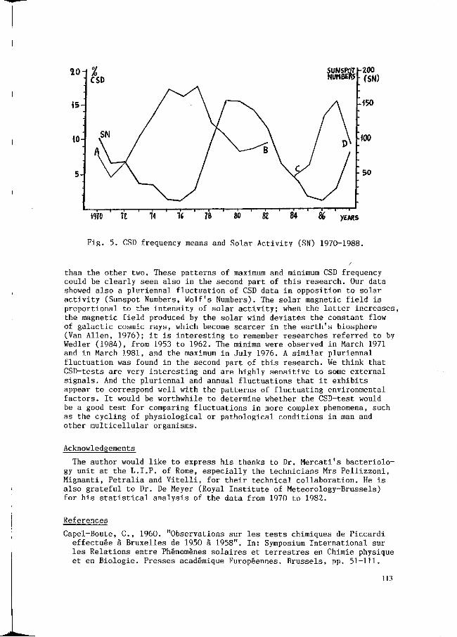
ÎO

45-

10-

5-

% CSD

SüNSPOT NUMBER?

•200 (SN)

-150

100

50

— i — i — i 1 — i — i — i — i 1 1 — i — i — i — i — - i — i — i i i "

WO 11 74 % 78 80 8Z 84 % YEARS

Fig. 5. CSD frequency means and Solar Activity (SN) 1970-1988.

than the other two. These patterns of maximum and minimum CSD frequency could be clearly seen also in the second part of this research. Our data showed also a pluriennal fluctuation of CSD data in opposition to solar activity (Sunspot Numbers, Wolf's Numbers). The solar magnetic field is proportional to the intensity of solar activity; when the latter increases, the magnetic field produced by the solar wind deviates the constant flow of galactic cosmic rays, which become scarcer in the earth's biosphere (Van Allen, 1976); it is interesting to remember researches referred to by Wedler (1984), from 1953 to 1962. The minima were observed in March 1971 and in March 1981, and the maximum in July 1976. A similar pluriennal fluctuation was found in the second part of this research. We think that CSD-tests are very interesting and are highly sensitive to some external signals. And the pluriennal and annual fluctuations that it exhibits appear to correspond well with the patterns of fluctuating environmental factors. It would be worthwhile to determine whether the CSD-test would be a good test for comparing fluctuations in more complex phenomena, such as the cycling of physiological or pathological conditions in man and other multicellular organisms.

Acknowledgements

The author would like to express his thanks to Dr. Mercati's bacteriolo­gy unit at the L.I.P. of Rome, especially the technicians Mrs Pellizzoni, Mignanti, Petralia and Vitelli, for their technical collaboration. He is also grateful to Dr. De Meyer (Royal Institute of Meteorology-Brussels) for his statistical analysis of the data from 1970 to 1982.

References

Capel-Boute, C , 1960. "Observations sur les tests chimiques de Piccardi effectuée à Bruxelles de 1950 à 1958". In: Symposium International sur les Relations entre Phénomènes solaires et terrestres en Chimie physique et en Biologie. Presses académique Européennes. Brussels, pp. 51-111.

113

Capel-Boute, C , 1974. "L'oeuvre scientifique de G.Piccardi". Med. Term. e Climatologia, 22: 69-74.

1977. "Les effets d'écran et de facteurs physiques ambiantes en chimie physique, dans les milieux aqueux". In: Les Facteurs d'Ambiance et les Climats intérieurs. Cahiers de medicine du travail, Bruxelles, XIV-2: 213-225.

1980. "Assessment of origin and effects from natural fluctuations and man-made alterations of our physical environment". Biometeorology 7, part 2. Suppl. to Int.J.Biometeor., 24: 173-182.

1985. "Water as receptor of environmental information?" Proc. 10th International Congress of Biometeorology. Tokyo, July 26-30, 1984. Bio­meteorology 10, part 2. Suppl. to Int.J.Biometeor., 29: 71-88.

De Meyer, M., 1984. "Some statistical observations on CSD data and sunspot numbers of Faraone's communication presented in: Séminaire interdiscipl. mod.syst.viv. et interact, avec leur environnement", Fresnes/Paris, June 23, 1984 (unpublished).

Eichmeier, J. and Bueger, P., 1969. "Ueber den Einfluss elektromagnetischer Strahlung auf die Bismut-chloridfallungsreaktion nach Piccardi", Int.J. Biometeor. 13: 239-256.

Faraone, P., 1971. "Ricerce sull'inquinamento batterico dell'aria esterna nel quadro dei dati metereologici, attraverso un anno e mezzo di osser-vazioni. La frequenza délie colonie a settore differenzlato". In: Lacus­trine Climatology. Proc. of the International Congress, Como, May 20-23, 1971. Univ. Milano (ed), pp. 474-508.

1973. "La frequenza délie colonie a settore differenziato (CSD), fra i batteri in sospensione nell'aria esterna, in tre anni di osservazione". Annali Sclavo, 15: 207-224.

1978. "Frequenza délie colonie a settore differenziato (CSD), origi­nate dai batteri isolati nell'aria esterna. Possibilité di un loro bio-ritmo, dopo sette anni di osservazione". Med.Term, e Climatologica, 37-38: 25-30.

1979. "La frequenza délie colonie a settore differenziato originate dai germi in sospensione nell'aria esterna. Possibilité di un bioritmo dopo un decennio di osservazioni". Simposio Internazionale di Scienze Ambientali in Colle Isarco (unpublished).

1983. "Correlazione fra fenomeni astrofisici e microbiologia ambien-tale". Inquinamento, 9: 55-58.

1984. "The influence of some astrophysical factors on the microorga­nisms of external ambient". Séminaire interdiscipl.mod.syst.viv. et interact, avec leur environnement", Fresnes/Paris, June 23, 1984. Séminaire sur les interactions entre organismes vivants et leur environ­nement". Fac. of Medicine, Dept. of Physiology, Tours, June 25-26, 1984 (unpublished).

1985. "L'influenza di alcuni fattori astrofisici sui microorganismi. Approfondimenti sperimentali". Inquinamento, 7-8: 49-54.

Fischer, W.H. and Perdue, C.R., 1964*. "Effect of electromagnetic field on shock freezing of water". Nature, 204: 764-765.

Fischer, W.H., Sturdy, G.E., Ryan, M.E. and Pugh, R., 1968. "Electromagne­tic effects on behaviour of water and colloids". Int.J.Biometeor., 12: 15-19. Cited by Capel-Boute (1985).

Piccardi, G., 1960a. "Une hypothèse solaire". In: Symposium international sur les relations entre phénomènes solaires et terrestres en chimie-physique et en biologie". Presses académiques Européennes, Brussels, pp. 121-130.

1960b. "Exposé introductif - les tests chimiques". In: Symposium international sur les relations entre phénomènes solaires et terrestres en chimie-physique et en biologie". Presses académiques Européennes, Brussels, pp. 9-49.

114

Piccardi, G., 1962. "The Chemical Basis of Medical Climatology". Charles C. Thomas (ed), Springfield, U.S.A.

1969. "I tests chimici in astrofisica, in geofisica e nelle scienze della vita". Coelum, 37: 101-111.

Servin-Massieu, M., 1961. "Spontaneous appearance of sectored colonies in S.Aureus cultures". J.Bacteriology, 82: 316-317.

Takata, M., 1951. "Ueber eine neue biologisch wirksame Komponente der Sonnenstrahlung". C. Thomas, Publisher, Springfield, U.S.A.

Tromp, S.W., 1981. "Long periodical changes in the physicochemical state of human blood". Cycles, 32: 212-219.

Van Allen, J.A., 1976. "Particelle e campi interplanetary" In: II Sistema solare nelle Esplorazioni spaziali. Le Scienze, S.p.A. (ed), Milano, pp. 43-51.

Wayne, W. and Umbreit, 1962. "Modern Microbiology". Whitaker, D.M., Emer­son, R. and Beadle, G.W. (ed.). S.Francisco, U.S.A., pp. 201-213.

Wedler, P.E., 1984. "Communication au Seminaire sur les interactions entre organismes vivants et leur environnement". Fac. of Medicine, Dept. of Physiology, Tours, June 25-26, 1984 (unpublished).

115

LUNAR CYCLE AND NUCLEAR DNA VARIATIONS IN POTATO CALLUS OR ROOT MERISTEM

M. Rossignol, S. Benzine-Tizroutine and L. Rossignol

Laboratoire de Morphogenese Végétale Expérimentale - Bâtiment 360 Université PARIS XI - 91405 - ORSAY CEDEX

Summary

The resul ts w e deal w i t h in this paper a re pa r t of the var ia t ion observed (experiment at ORSAY, april - may 1988) in potato callus or root mer is tem of a dihaploid semi-ear ly clone BF 15 (2x) Hi and concerning 2C diploid cells.

When comparing nuclear mass means from callus or root mer i s tems of plants cul tured a t different periods, w e observe differences related to their composition. They a re not homogeneous but composed of groups of cells characterized by different DNA masses. We thus identified 3 forms of DNA molecules coexisting in a same callus or root mer is tem. Their relat ive frequencies depend on the l unar phase at the t ime when the first mitotic divisions in the in vitro cu l ture medium s ta r t . Arguments a r e given in Discussion to explain w h y they can be considered as the expression of an adaptative process. Keywords: cytogenetic s tudy, adaptation, l una r phases.

Introduction

The data w e used in this paper we r e extracted from a doctorat thesis conducted by S. Benzine-Tizroutine in the Morphogenesis Laboratory at ORSAY. The thesis subject w a s oriented toward the Somaclonal Variation origin. When w e began to exploit the f irst resul ts , w e w e r e far from thinking of their implication in so m a n y scientific fields: physiology, genetics, molecular biology... Some problems as biological clocks, phytochrom use in p lants , regulation of the DNA molecule may be approached under a n ew angle. Our inqui ry continues but w e thought useful to give the informations concerning the f irst step.

Material and methods

The plant mater ia l w a s a dihaploid semi-ear ly clone BF 15(2x) HI obtained from a tetraploid french cul t ivar BF 15 (4x). by pollinization w i t h Solanum phureja

Cuttings and callus production

The plants used as control a r e produced in vitro by vegetative multiplication of one node cuttings on a MS cul ture medium (Murashige and Skoog, 1962), w i t h Morel v i tamins (Morel and Wetmore, 1951) and 20 g.1"1

saccharose + 7,5 g.1-* agar. Nodes -without bud, or leaves from vi t roplants w e r e put on a C3 medium

•with g rowth regulators (Quraishi and coll., 1979) a t different t imes. Physical conditions of the cul ture room during initiation and g rowth of

callus we re : t empera tu re , 25°C + 1; photoperiod , 12 h day - 1 ; light intensity , 80 [IE m~2 sec - 1 ; re lat ive humidi ty, 508.

116

Samples of protoplasts from callus we r e prelevated for analyzing at different ages of the callus.

Cells from root mer i s tems of the in vitro control BF 15(2x) HI

Roots we r e cut and cells prelevated on the in vitro p lants, ten days after culturing the one node cuttings.

Protoplasts and cells fixation

Protoplasts from callus and cells from root mer is tems we r e fixed on slides by the smear technic. They we r e stained during 1 hour w i t h the SCHIFF reagent.

Nuclear DNA mass measures

(i) Cytophotometer method Nuclear DNA mass of cells w a s measured w i t h a Leitz MPV I

cytophotometer and evaluated w i t h the PATAU two lengthwaves method (Patau, 1952). Measures we r e a lways taken in cells a t the "prophase" period of the mitotic cycle, when DNA molecule has doubled its volume and mass .

For each callus, 75 nuclei we r e observed, two successive measures (2 repeated observations, XI and X2) being taken for each nucleus, (ii) Results analysis /

(a) Nuclear mass means comparison The different mass means of callus we r e compared two by two. Because of

the unequali ty of va r iances , a modified Student - FISHER test -was used f or. (bilateral equality test). (b) Mass frequencies distribution in a same callus (b. 1) Fitting values

Considering a nuclear mass dot d iagram of the Xi - X2 pairs (repetitions) observed in a same callus :

- if no i n s t rumenta l or personal e r ro r , the dots a re distributed along a s traight line (the regression line) whe r e the slope b is at the r a te of one unit of X2 per uni t of Xi, t ha t is b = 1. The estimated values should be Xi= X2 = Xj + X2

2 - if i ns t rumenta l and /or personal e r ro r , the dots lie in a band shaped like

an ellipse, w i t h the major axis sloping upward toward the r ight -when r (correlation coefficient) is positive. The best estimation of a nuclear mass measure is given by calculating: x e = Xai + Xa2 ; whe r e Xai and Xa2 a r e the fitted values for one Xi - X2 pair ,

2 tha t is: - for X2, the corresponding value on the sample regression line, the equation of which being: (Xa2 - Xa2) = bXa2/Xal (Xai - Xai) Ü> - for XI, the corresponding value on the sample regression line, the equation of which being: (Xai - Xai) = bXal/Xa2 (Xa2 - Xa2) (2) (b.2) Groups analysis (Heterogeneity s tudy)

Taking into account the resul ts from other wo r k s as Jacques and coll.(1987), we choiced the log. normal model.

Groups may be sorted w i th a computer, or more laboriously by plotting the values on a probit paper w i t h cumulat ive frequencies as the abciss and, as the ordinate, the decimal logarithm of DNA mass means calculated for each class of 50 u . a . ( a rb i t r a ry units).

117

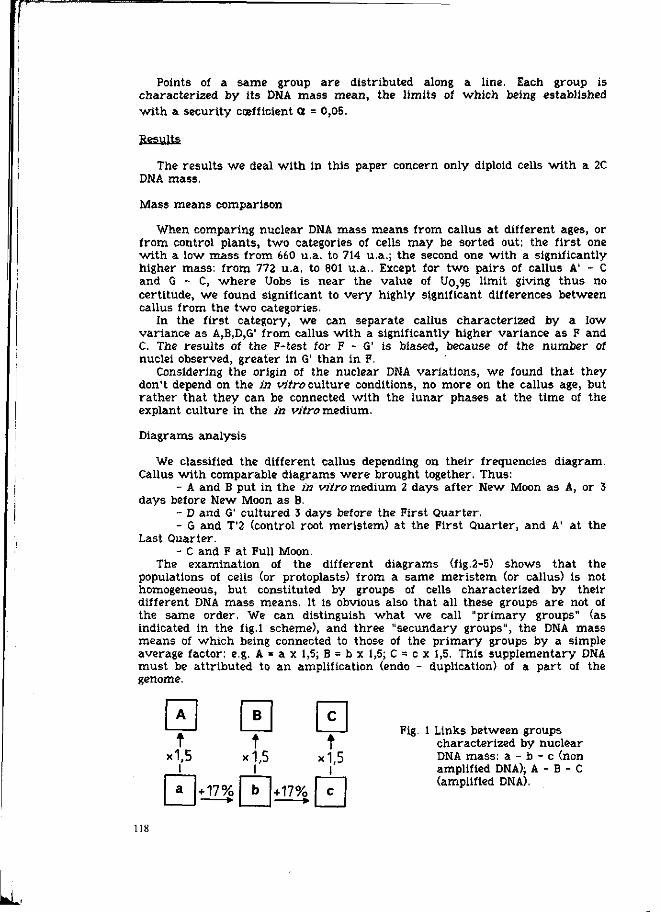
Points of a same group are distributed along a line. Each group is characterized by its DNA mass mean, the limits of which being established •with a security coefficient a = 0,05.

Results

The results we deal with in this paper concern only diploid cells with a 2C DNA mass.

Mass means comparison

When comparing nuclear DNA mass means from callus at different ages, or from control plants, two categories of cells may be sorted out: the first one •with a low mass from 660 u.a. to 714 u.a.; the second one with a significantly higher mass: from 772 u.a. to 801 u.a.. Except for two pairs of callus A' - C and G - C, where Uobs is near the value of Uo,95 limit giving thus no certitude, we found significant to very highly significant differences between callus from the two categories.

In the first category, we can separate callus characterized by a low variance as A,B,D,G' from callus with a significantly higher variance as F and C. The results of the F-test for F - G' is biased, because of the number of nuclei observed, greater in G' than in F.

Considering the origin of the nuclear DNA variations, we found that they don't depend on the in vitro culture conditions, no more on the callus age, but rather that they can be connected with the lunar phases at the time of the expiant culture in the in vitro medium.

Diagrams analysis

We classified the different callus depending on their frequencies diagram. Callus •with comparable diagrams •were brought together. Thus:

- A and B put in the in vitro medium 2 days after New Moon as A, or 3 days before New Moon as B.

- D and G' cultured 3 days before the First Quarter. - G and T'2 (control root meristem) at the First Quarter, and A' at the

Last Quarter. - C and F at Full Moon.

The examination of the different diagrams (fig.2-5) shows that the populations of cells (or protoplasts) from a same meristem (or callus) is not homogeneous, but constituted by groups of cells characterized by their different DNA mass means. It is obvious also that all these groups are not of the same order. We can distinguish what we call "primary groups" (as indicated in the fig.1 scheme), and three "secundary groups", the DNA mass means of which being connected to those of the primary groups by a simple average factor: e.g. A = a x 1,5; B = b x 1,5; C = c x 1,5. This supplementary DNA must be attributed to an amplification (endo - duplication) of a part of the genome.

A

t x1,5

I

FY 17% — >

B

t x1,5

i

b +17% *•

C

t *1,5

c

Fig. 1 Links between groups characterized by nuclear DNA mass: a - b - c (non amplified DNA); A - B - C (amplified DNA).

118

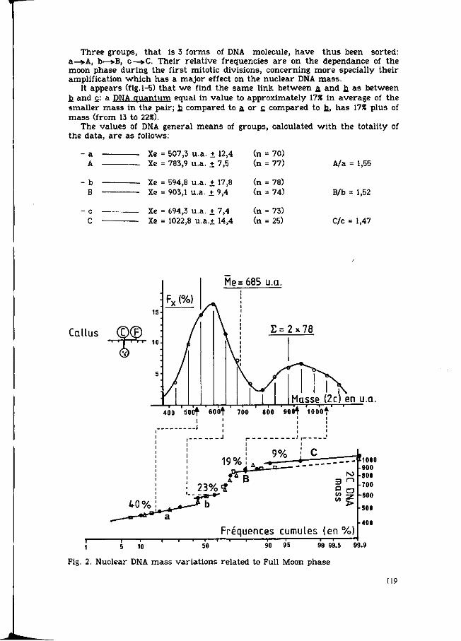
Three groups, tha t is 3 forms of DNA molecule, have thus been sorted: a-^»A, b—»B, c—»C. Their relative frequencies a r e on the dependance of the moon phase during the first mitotic divisions, concerning more specially their amplification wh ich has a major effect on the nuclear DNA mass .

It appears (fig. 1-5) t ha t w e find the same link between a and b. as between b and £: a DNA quan tum equal in value to approximately 178 in average of the smaller mass in the pair; b. compared to a, or c. compared to fc, has 178 plus of mass (from 13 to 22«),

The values of DNA general means of groups, calculated w i t h the totality of the data, a r e a s follows:

a A

Xe = 507,3 u.a. ± 12,4 (n = 70) Xe = 783,9 u.a. + 7,5 (n = 77) A/a = 1,55

b B

Xe = 594,8 u.a. ± 17,8 (n = 78) Xe = 903,1 u.a. + 9,4 (n = 74) B/b = 1,52

Xe = 694,3 u.a. + 7,4 (n = 73) Xe = 1022,8 u.a.+ 14,4 (n = 25) C/c = 1,47

Me=685 u.a.

15

Callus (D© 1 ' l ' ~ » 10

J Masse (2c) en u.a. 400

I ' i ' i • i ' i • i ' i i i i . i r—r 500f 600t 700 800 900f 1000Î

r T 1 1 r 50

Fréquences cumules (en %) 1 5 10 50 90 95 99 99.5 99.9

Fig. 2. Nuclear DNA mass var ia t ions related to Full Moon phase

119

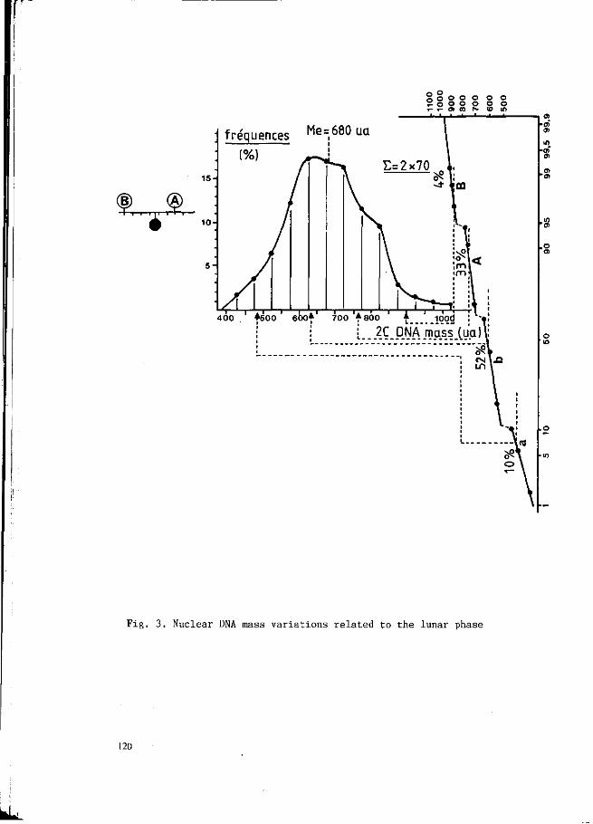
„ o o o o o o ° o o o o o o r- y- O) 00 r - (O W

400 f500 600* 700 * 800 * iqod

o 'm

Fig. 3. Nuclear DNA mass variations related to the lunar phase

120

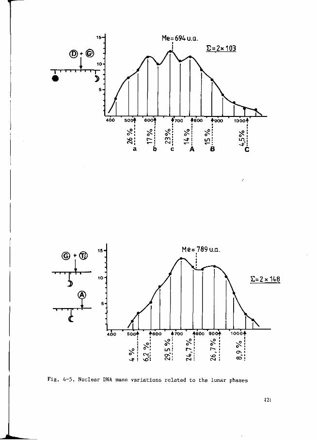
1 • •

15-

®*@ :

| , . .

3>:

5-

400 5odf ' 600*

a b

Me = 694 u.a. .1 £=2x103

T T ^ *VoO f800 ' *900 ' 1000*' ! ' ' '

^ : ^si -^! spi

c A B c

© * © i i i ii T i —

3>

f T-T—i-p—r-f

c

Me=789u.a.

T 400 500* f600 +700 4800 900f

^ O^

o^ ! LTl!

5 5 1000*

i

^ ! o^ •

I 0 \ i

•» I OO i

Fig. 4-5. Nuclear DNA mass variations related to the lunar phases

121

Analyzing the frequencies distributions (fig.2-5), two main features may be pointed at:

- first, the fact that groups (a + A) and (b + B) are the most abundant at Full Moon as well as at New Moon (the only ones represented at New Moon). During the First and the Last Quarter phases we note the presence of a third group (c + C), the relative frequencies of which increasing sometimes up to 46 % (T'2 results).

- secondly, the choice of the group -where the nuclear DNA molecule is amplified (x 1,5) depends also on the lunar phase at the time when the in vitro culture starts: during New Moon, the a DNA molecule form is amplified in most cases; during Full Moon it is the b molecule form which is preferably amplified; during the Quarter phases, a and h are undifferently (equally) amplified, the amplification of ç being always very scarce (less than 10 %).

Discussion

The first question we have to answer is: what is the nature and the meaning of these different forms of DNA molecule?

The DNA molecule forms: a, b, c.

Saltatory changes, considered as evolutive nuclear DNA quanta, have already been cited in littérature: Many characteristics of the plant genome appear to be capable of saltatory changes (Lee and Philipps, 1988). Changes may be observed at different taxonomie levels : family (Rothfels & al., 1966), or genus (Chooi, 1971) or even species, cultivars.populations (Essad, 1988).

But the most interesting report of variations observed in a same genome was the results of Evans and coll. (1966) on flax. In stress conditions (for instance a strong increase of phosphate in the culture medium), two genotrophic forms L and S appear, phenotypically different from the parents, with a 16 % DNA mass difference. This DNA quantum may be compared -with the 17 % DNA supplementary mass between h and a or between £ and b_.

The supplementary DNA seems to be a part of the genome connected with repetitive sequences. Changes inducted in the flax genome illustrate its adaptative capacity to the environnement. After Lee and Phillips (1988), when plants are cultivated in stress conditions, changes in the most important part of the repetitive portion of the flax genome may occur in just one generation.

The proposed model of regulation

We observed that a and b molecule forms are the most constant, the £ form appearing occasionally: scarcely during Full Moon and more often during the Quarter phases. It seems that the plant program has the possibility to choose between the two forms, a and b, depending on the environmental conditions, the e form intervening -when duplication is stopped because of the stress effect. The stress may be either chemical as in the flax experiment, or physical. Anyhow in most events and at the cell level, it finds expression in thermic shock, -whether by oxydation or by radiation. The temperature increase might be responsible for the bad efficiency of the DNA polymerase enzym which is necessary in the polymerarization of the DNA molecule.

Changing the genes expression is necessary to obtain a less sensitive enzym, and we could think of a process comparable to those described in other species (Nina Fedoroff, 1984) -where unstable mutations and reversion occur thanks to the transposition of a genetic transposable element of the genome. When growth regulators like cytokinin are added in the in vitro medium, it happens

122

with the chromosome break the loose of the active element and a stable change in the expression of the gene which makes the enzym more per f or mant.

As for the expression of a or b_, we consider the supplementary DNA of b_ as the result of an old adaptative process. Regulation of a. and b_ might be of a different nature than in the c form. It might appeal to a cyclic element (of the Spm family forjnstance) the suppressor function of which being alternatively active or inactive according to the environmental conditions we have to define.

Our results and the theoretical model fit in very well with the results of a tridimensional study of atoms in biological molecules, made recently by two teams of scientists (Orsay University In France, Cambridge University in U.K.). After crystallizing the DNA molecule, its structure was visualized with X rays (Doucet, 1989). It was established that 3 geometric forms of DNA molecule coexist in organisms (essentially the form named B, but also -what they called A and Z), It was supposed that they intervene in the recognizing process between DNA and other molecules as proteins engaged in the modulation of genes activity.

They just obtained, in the "cristallin" matrix, and it is interesting to notice it, fragments of the B form localized in channels constituted by A form fragments (fig.6).

Fig.6. DNA molecule aspect after cristallizing (photo in X rays). (Cliché in Doucet, 1989)

We consider that the B fragments inside A might precisely be the pieces of the supplementary DNA characterizing what we call the b_ form of DNA molecule (the mass of which representing 17 % of the DNA mass of fragments around them).

Now what about the lunar effect? For answering this question, we have to analyze more in detail the frequencies variation with time of each DNA form.

Lunar effect

(i) Frequency variation curves Curves from fig.7 and 8 -were established with the results from our

cytogenetic experiment.

* O c • >

( D w Fig.7.. Relative frequency variation of the different forms of the DNA molecule

We see at first sight that curves concerning the choice of the molecule form (fig.7) differ slightly from curves representing variation in time of the amplified molecule A or B or C (fig.8):

123

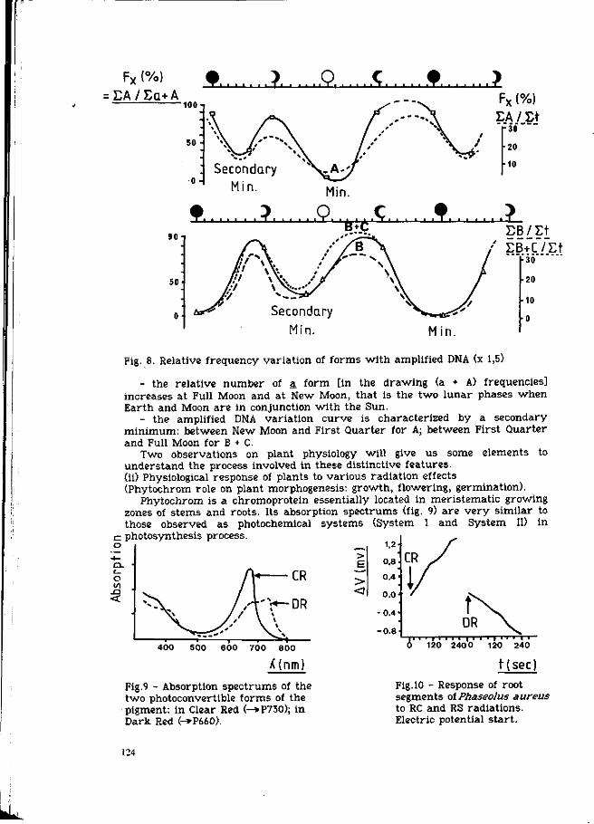
Fx (%) EA/Ea+A

T I i i i i i i T i i i i i I T I i i i i I T i i i i i i l l i i i i i i T

•100

50

Fx (%) EA/Et

Secondary Min.

T "T i

30

20

10

Min.

90n

50

0-

,0 ç * ? i T l i j - l l i T l l l I I I I I I I I I I I I

°*C EB/Et

Min.

,'' EB+C/Et 30

h 20

10

•0 Min.

Fig. 8. Relative frequency variation of forms with amplified DNA (x 1,5)

- the relative number of a form [in the drawing (a + A) frequencies] increases at Full Moon and at New Moon, that is the two lunar phases when Earth and Moon are in conjunction with the Sun.

- the amplified DNA variation curve is characterized by a secondary minimum: between New Moon and First Quarter for A; between First Quarter and Full Moon for B + C.

Two observations on plant physiology will give us some elements to understand the process involved in these distinctive features, (ii) Physiological response of plants to various radiation effects (Phytochrom role on plant morphogenesis: growth, flowering, germination).

Phytochrom is a chromoprotein essentially located in meristematic growing zones of stems and roots. Its absorption spectrums (fig. 9) are very similar to those observed as photochemical systems (System

c photosynthesis process. I and System II) in

o. • o 10

<

400 500 600 700 800

X(nm)

Fig.9 - Absorption spectrums of the two photoconvertible forms of the pigment: in Clear Red (-*P730); in Dark Red (~»P660).

>

> <

1,2

0.8

0.4'

0.0

•0.4

- 0 . 8

f DR

• • • • • I I I

120 240 0 ~r 120

T T 240

r(sec) Fig. 10 - Response of root segments olPhaseolus aureus to RC and RS radiations. Electric potential start.

124

In the obscurity, absorption of radiations in the visible spectrum t r ans fo rms the pigment into two photoconvertible forms depending on the lengthwave of the absorbed radiation.

Absorbing the Clear Red radiation a round 660 nm. the CR form P^èO i s

t ransformed in P?30- The t ransformation of P730 form in P660 'when absorbing the Dark Red radiation, is not direct. There is a de novo synthesis of P^ÈO molecules in the da rkness , after degradation of the P730 molecules.

It resul ts from many experiments using short i l lumination (flashes) of low intensity, the following resul ts on plant morphogenesis (Blanc et al., 1986):

- w i t h DR light (730 nm.), s tem internode g rowth is s trongly s t imulated, whe r ea s the effect is inverted for leaves and stomatic index.

_ w i t h CR light (660 nm.), s tem growth is reduced and leaf g rowth as well as photosynthesis activated. According to Jaffe's experiment on bean roots in 1968 (Mazliak, 1982), it also induces a positive bioelectric potential in cells (fig. 10), associated w i t h an inhibition of secondary root g rowth and w i t h acetylcholine production.

The Clear Red morphogenetic effect is annulated if the last i l lumination before da rkness is in the DR light. Another important point to underl ine is t ha t the switching off the RC action w i t h a PR light is possible only if the DR light beam is in a polarization plan perpendicular to the RC beam.

A last feature w e have to point at is the relation between photosynthesis and phytochrom action : a s trong increase of energy in the CR as -well as in the DR light gives a bad physiological response because of exergonic oxydoreductions in the electron t r anspor t chain giving photophos£horylation either in System I or in System II.

In short tha t is to say tha t the modulation of the plant morphogenetic p rogram will depend on the physical conditions (radiation na ture) prevailing, jus t before da rkness , at the t ime of mitotic divisions in the proliférant meris tematic cells, (iii) Electromagnetic phenomenons related to l unar phases - A geo-cosmic clock

At d awn and dusk, jus t before da rkness , an important light feature occurs wh ich m a y be related to a physical effect called diffraction.

According to Huyghens theory, when a p a r t of a light wave is intercepted by an opaque screen or restr icted by holes or slits, the subsisting portion of the wave may be considered as many synchrone light sources or wavele ts t ransmi t t ing their momentum beyond the screen. Fresnel added the hypothesis, verified since then, tha t the wavele ts can interfere. The geometrical shadow of the screen is not neat but a l ternat ively d a rk and glittering at i ts edge due to the redistr ibution of energy in space or t ime.

The wave mus t be coherent and monochromatic. In the Earth a tmosphere there a re coherent beams w i th a definite relation in phase because they originate in the same source, the Sun, and the waves a re quasi monochromatic because of the diffusion on numerous particles and molecules in the low and middle a tmosphere. A pa r t only of the wh i t e light spect rum ( towards the Red lengthwaves) is rest i tuted w i t h the same momentum as the source light. The r esu l tan t light is then more homogeneous. There a r e in fact wave groups of slightly different frequency moving in the same direction. At the edge of the geometrical shadow of the Ear th screen, they do interfere to produce beats, a l ternat ive reinforcements and cancellations of pa r t s of the disturbance tha t a r e periodic w i t h t ime. These beats give r ise to an a l ternat ive cu r r en t wh ich in t u r n pe r tu rbs the electromagnetic field at the level of plants, or mer is temat ic cells or callus protoplasts.

At Full Moon and at New Moon, when Earth and Moon a r e in conjunction •with the Sun, the Red light is more homogeneous because of the increasing of the particles density on each side of the upright of the Sun (Thermic tide phenomenon). We know the effect of the Red light on phytochrom. Then the choice of the DNA form is the a form, and the expression of the p rogram

125

(amplification of the a. molecule) is oriented towards storage of carbohydrates (tuberization) at New Moon. At Full Moon, moon waves interfere in the Dark Red ( X # 700 nm). They are parallel and they move from the opposite side of the solar waves producing a steady wave due to resonance. The physiological response is bad (a few molecules amplified) and when there is a response the amplified molecule is b_. The expression of the program is oriented towards plant growth and flowering. But the best configuration for the growth program is given during the First and just before the Last Quarter when the Dark Red light beam from the Moon is in a polarization plan perpendicular to the Clear Red beam from the Sun. The RC action is switched off.

Conclusion

Though presently -we can just elaborate hypothesis concerning mechanisms utilized by proliférant cells in the modulation of the plant program, our theoretical model fits well enough with observations from other scientific fields and encourages us to pursue in this way. We are checking now the repetition of the response to environmental factors, adding the seasonal action. The stake is important. As a matter of fact that is the adaptative process and the evolution origin -which are concerned.

References

Blanc, A., Mery, J.C.& Boisard, J., 1986. Action des radiations de lumière rouge sur la survie et la tubérisation de germes de pomme de terre cultivés in vitra influence de leur âge physiologique. Potato Research, 29: 381-389.

Chooi, W.Y., 1971. Variation in nuclear DMA content in the genus Vicia. Genetics, 68:195-211

Doucet,J., 1989. in La Recherche n° 209, Avril 1989, Des cristaux d'ADN composites, vol. 20, p. 503,

Essad,S., 1988. Mise en évidence des variations saltatoires de l'ADN nucléaire dans et entre les espèces du genre Medicago L.. Genoma - 16p, 4Tabl., 5fig..

Evans, G.M., Durrant, A. & Rees, H., 1966. Associated nuclear changes in the induction of flax genotrophs. Nature, 212: 687- 689.

Fedoroff, N., 1984. Les éléments génétiques transposables du mais. Pour la Science. Revue Août 1984, pp. 25-36.

Lee, M. & Phillips, R.L., 1988. The chromosomal basis of somaclonal variation. Ann. Rev. Plant Physiol. Plant Mol. Biol., 39: 413-437.

Mazliak, P., 1982. Croissance et développement. Physiol, végét. II, Hermann Paris, 110-112.

Morel, G. & Wetmore, R.H., 1951. Fern callus tissue culture. Am. J. Bot., 38: 141-143.

Murashige, T.& Skoog, F., 1962. A revised medium for rapid growth and bioassays with tobacco tissue cultures. Physiol. Plant., 15: 473-497.

Patau, K., 1952. Absorption microphotometry of irregular shaped objects. Chromosoma 5: 341-352.

Rothfels, K., Sexsmith, E., Heimburger, M. & Krause, M.O., 1966. Chromosome size and DNA content of species of Anemone and related genera. Chromosoma, 20: 57-74.

Acknowledgments We are very grateful to Gaisne C, Ambroise A. and Defoug M.J. for their

help in the achievement of this work.

126

CELLULAR EFFECTS OF LOW LEVEL MICROWAVES

W. Grundier

Gesellschaft für Strahlen- und Umweltforschung mbH,Institut für Blophyslkallsche Strahlenforschung, 8042 Neuherberg, FRG

Summary

Research on biological effects of microwaves is characterized by a large number of open questions. While many authors have reported certain effects to exist, repeat of their studies by others led to an opposite conclusion in several cases. Only in a limited number of cases agreement on the existence of the effects has been reached.

The reason for the unsatisfactory state of the field may well lie in the complexity of either the biological processes or of the microwave interaction. The reported microwave effects are subtle, indeed often at the limit of observability. The yeast growth experiments reported here are in some sense an exception since even though the microwave effects are small the continuity of the laboratory work has allowed a repeated establishment of the resonant feature of this effect. In this contribution we demonstrate both a novel way of observing the growth of yeast cells and in part a confirmation of the resonant microwave effect, near 42 GHz, even under the new experimental conditions. The apparatus is built to observe the growth of cells fixed in space. The well-separated cells can be subjected to microwave exposure which is constant in time. Thus the setup can serve to investigate specific influences, e.g. of either microwave power or microwave polarization.

Keywords: cell growth, microwave bioeffect, resonance, coherence.

Introduction

Since nearly one decade, cellular effects of low intensity microwaves have been the subject of a great number of studies and many different reactions were reported using a great variety of cellsystems. The acceptance level is low, however, due to difficulties both in reproducing the effects and in demonstrating their real athermal nature. These problems will probably remain as long as the mechanisms of these subtle effects are unknown. It seems worth thinking of new concepts for experimental investgations in low level bioeleetromagnetics. To focus on fundamental mechanisms, experiments must be oriented strongly by theoretical concepts. For a fundamental explanation of frequency dependent growth rate changes of cells measured by us with different methods, for instance, a hypothesis has been developed taking into account a nonlinear interaction between the biological object and the microwave radiation. Especially, nonlinear oscillators inside a cell have been assumed driven by intentel energy and disturbed by the external fields (F. Kaiser 1984 and this meeting).

127

Our own experimental procedures for the mm-wave bioeffect studies used have been developed in a three stepped way. In a first experimental series, we have analyzed the growth behaviour of yeast cultures in aqueous suspension, by monitoring the visible light extinction. We found an exponential growth rate reproducible within + 4% limits. When the cultures were Irradiated by continuous wave microwave fields of a few mW/cm, the growth rate either stayed constant or was considerably enhanced or reduced depending on frequency around 42 GHz. A spectral fine structure with a width of the order of 10 MHz was observed. Careful temperature monitoring excludes a trivial thermal origin of this effect (Grundler et al. 1977; Grundler and Kellmann 1978). Repetlon of this experiment has confirmed that the growth of aqueous yeast cultures Is indeed affected by weak microwave radiation in a frequency-selective manner (Grundler et al. 1983; Grundler and Keilmann 1983). To exclude a possibly Influence of uncontrolled experimental parameters, many improvements were added in these studies. These Include a refined frequency stabilization, refined power recording, impedance matching elements, two geometrically different antenna structures and two recording photometers. Laser thermometry was employed to locate any hot spots (Kellmann 1983). The results of these towfold growth study using two different types of antennae and described above are shown in figure 1.

NORMALIZED GROWTH RATE a)

1.2 * ^ f o r k

41700 41800 MHz

Fig. 1. Normalized growth rate of yeast cultures vs. microwave Irradiation frequency using (a) fork-shaped or (b) tubular antennae. The curves were obtained by single three-point smoothing.

128

These data prove that the microwave Irradiation leads to fairly reproducible effects, increasing or decreasing the growth rate by up to about 10%, depending on the frequency of irradiation

These results, however, are obtained as an average reaction of nearly 106 cells. No exact measurement can be made of the power actually applied or of the time during which a cell is affected by irradiation.

To overcome these disadvantages inherent in the photometer experiment, a new method was developed for studying the kinetics of single cell growth during the influence of microwave radiation. Yeast cells are fixed to the lower surface of a thin transparent agar layer. Each cell develops into a microcolony of eight cells. To apply the radiation microwaves are guided through a sapphire plate (multi-mode chamber) on which the cells are spread in a monolayer. The data obtained from this second experimental setup prove again the existence of a microwave effect on the growth on yeast cells (Grundler et al. 1988). Specifically, while we observe now that for the individual cell the effect can be a shortened or prolonged duration of the cycle, we find that for an ensemble of cells located in close vicinity the average effect does not vanish but lies in the order of magnitude of the effect established ealier with the photometric measurement.

Due to difficulties in reproduction of the observed cell reactions further improvements seem to be necessary, since the theory (s.a.) demands apart from highly stabilized frequencies, known intensity for the irradiation of every single cell and a definable orientation of the biological object, in respect to the field. It will be shown, how to meet these requirements experimentally and what the fiijt observations are achieved from irradiated yeast cells.

Microwave growth experiment

As described before, yeast cells are fixed to the lower surface of a thin transparent agar layer. The agar layer rests now on a quartz needle broadened by quartz plates on both sides and mounted in a temperature stabilized chamber. The chamber is scanned under a microscope for automatic observation of the cells. To apply the radiation microwaves are guided through the gold coated quartz needle and radiated out of a slot on which the cells are spread in a monolayer. An automatic image processing method is used to continuously record the development of about 20 microcolonies.

Materials and Preparation

Diploid yeast cells (Saccharomyces cerevlsiae) were obtained from a stock culture of stationary state cells on solid nutrient agar (20 g/1 glucose, 20 g/1 Bacto agar, 5 g/1 yeast extract, 0.5 g/l Mg SO4; 4° C) and suspended in phosphate buffer. A synchronized subpopulation (early G^-phase) was selected by volume sedimentation and used for a series of experiments. For every experiment 10 yl of a medium suspension containing 4 • 10^ cell/ml are filled in the cell chamber (Grundler et al. 1988).

129

Microwave Irradiation

The quartz needle Is part of the microwave circuit, in fact it is the dielectric in a dielectric-filled metal waveguide. The needle is mostly covered with gold to confine the microwaves, except at the ends (where the microwave is coupled in and out to standard waveguide by proper tapers), and within a radiating slot (0.4 • 1,7 mm2) where the cells are placed, ft similar opening is provided at the opposite surface to allow microscope viewing, but this is covered with a fine metallic mesh structure which completely (-50 db) suppresses leakage of microwaves to that side.

in this setup the microwave field in the radiating slot can be expected to be monomode. This is experimentally tested and shown in figure 2.

SLOT-LENGTH-

Fig. 2 intensity distribution of a radiating slot (1,7 mm length) measured at the both long bounderies.

The electric field is polarized and oszlllates in the y-direction only;

surrounded by the magnetic field in the xz-plane. The intensity radiated out is proved to be a sin2-distribution. Using a fixed set-up and standard adaption procedures, the output power is strongly correlated to the transmitted one and can be estimated over 9 decades on an absolute scale within an accurasy of a factor of + 5.

130

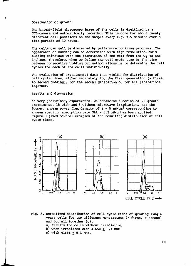
Observation of growth

The bright-field microscope image of the cells is digitized by a CCD-camera and automatically recorded. This is done for about twenty different cell positions on the sample every e.g. 7,5 minutes over a time periode of 10 hours.

The cells can well be discerned by pattern-recognizing programs. The appearance of budding can be determined with high resolution. This budding coincides with the transition of the cell from the G^ to the S-phase. Therefore, when we define the cell cycle time by the time between consecutive budding our method allows us to determine the cell cycles for each of the cells individually.

The evaluation of experimental data thus yields the distribution of cell cycle times, either separately for the first generation (= first-to-second budding), for the second generation or for all generations together.

Results and discussion

As very preliminary experiments, we conducted a series of 20 growth experiments, 15 with and 5 without microwave irradiation. For the former, a mean power flux density of I = 5 yW/cm 2 corresponding to a mean specific absorption rate SAR = 0 . 2 mW/g has been applied. Figure 3 gives several examples of the resulting distribution of cell cycle times.

t m < m o ce o.

OL

o

-

-

-

-

-

-

(a) i

1 !

1 IX

(b)

1 -

-

-

-

-

-

(<

1 i l

0

1

CELL CYCLE TIME'

Fig. 3. Normalized distribution of cell cycle times of growing single yeast cells for two different generations (• first, x second) and for all together ( o ) . a) Results for cells without irradiation b) when irradiated with 41654 +0,1 MHz c) with 41651 + 0,1 MHz.

131

In these runs the control experiments resulted In the narrowest distributions. The effect of irradiation can be seen in Fig. 3 to be an asymmetric deformation of the distribution, ftny broadening must mean that not all cells respond In the same way. For further evaluations we disregard this effect and concentrate on the shift of the distribution, by calculating the average cycle time te

distribution. in each

By taking the inverse of t a v we obtain the average growth rate tiv' which we further normalize to the mean value obtained in the control runs. Figure 4 shows the resulting normalized growth rate for different frequencies.

1.2-

1.1-

0.9-

0.8-

i i NORMALIZED (second division)

J ] I : \ 1

•

\ /I

[ 1 " [ J

'u' \ /

< >

l _ l 1 1 L _

GROWTHRATE

) 1 \ \ \

i V \

% • ]\ -,

\ \ /

i '

(x

T - 5 ^ 2 c m '

SÄR = 0.2 ° ^

FREQUENCY »• L _ L _ 1 I . I U _ L _

41650 41655 41660 MHz

Fig. 4 Normalized growth rate of population obtained by averaging over individually determined cell cycle times in dependence on frequencies round 42 GHz.

The data obtained from the new experimental setup prove again the existence of a microwave effect on the growth on yeast cells. Specifically, while we observe now that for the individual cell the effect can be a shortened or prolonged duration of the cycle, we find that for an ensemble of cells the average effect does not vanish but lies in the order of magnitude of the effect established earlier (see fig. 1).

The agreement between the ealier and the present experiments is further supported by the frequency dependence. The present experiment yields a resonance of growth enhancement centered near 41655 MHz with a width of about 7 MHz, in accordance to what was observed with the photometer, except that the former maximum has been centered round

132

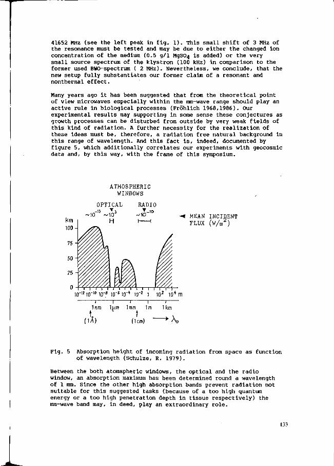
41652 MHz (see the leEt peak in fig. 1 ) . This small shift of 3 MHz of the resonance must be tested and may be due to either the changed ion concentration of the medium (0.5 g/1 MgSC>4 is added) or the very small source spectrum of the klystron (100 kHz) in comparison to the former used BWO-spectrum ( 2 MHz). Nevertheless, we conclude, that the new setup fully substantiates our former claim of a resonant and nonthermal effect.

Many years ago it has been suggested that from the theoretical point of view microwaves especially within the mm-wave range should play an active rule in biological processes (Fröhlich 1968,1986). Our experimental results may supporting in some sense these conjectures as growth processes can be disturbed from outside by very weak fields of this kind of radiation. A further necessity for the realization of these ideas must be, therefore, a radiation free natural background in this range of wavelength. And this fact is, indeed, documented by figure 5, which additionally correlates our experiments with geocosmlc data and, by this way, with the frame of this symposium.

ATMOSPHERIC WINDOWS

OPTICAL -13 •

MEAN INCIDENT FLUX (W/m )

10~'210"'° 10"8 10"f 10~* 10"2 1 10z 104m

1nm 1um 1mm 1m 1km

MA) (1cm) • A>

Fig. 5 Absorption height of incoming radiation from space as function of wavelength (Schulze, R. 1979).

Between the both atomspheric windows, the optical and the radio window, an absorption maximum has been determined round a wavelength of 1 mm. Since the other high absorption bands prevent radiation not suitable for this suggested tasks (because of a too high quantum energy or a too high penetration depth in tissue respectively) the mm-wave band may, in deed, play an extraordinary role.

133

Acknowledgement

We gratefully acknowledge financial support by the "Stiftung zur Förderung der Erfahrensheilkunde im Stifterverband für die Deutsche Wissenschaft".

References

1 Fröhlich, H., 1968. Long range coherence and energy storage in biological systems. Int. J. Quantum Chem. 2: 641

2 Fröhlich, H ., 1986. Coherent excitation in active biological systems. In: F. Gutmann & H. Keyzer (Ed.): Modern bioelectrochemistry. Plenum, New York, p 2241-261.

3 Grundler, W., F. Keilmann & H. Fröhlich, 1977. Resonant growth rate response of yeast cells irradiated by weak microwaves. Phys. Lett. 62A: 463.

4 Grundler, W. & F. Keilmann, 1978. Nonthermal effects of millimeter microwaves on yeast growth. Z. Naturforsch. 33c: 15-22.

5 Grundler, W., F. Keilmann, V. Putterlik, L. Santo, D. Strube & 1. Zimmermann, 1983. Nonthermal resonant effects of 42 GHz microwaves on the growth of yeast cultures. In: H. Fröhlich & F. Kreraer (Ed.): Coherent excitations in biological systems. Springer, Berlin-Heidelberg, New York. p. 21-37.

6 Grundler, W. & F. Keilmann, 1983. Sharp resonances in yeast prove nonthermal sensitivity to microwaves. Phys. Rev. Lett. 51, No. 13: 1214-1216

7 Grundier, W., U. Jentzsch, F. Keilmann & V. Putterlik, 1988. Resonant Cellular Effects of low intensity microwaves. In: H. Fröhlich (Ed.): Biological coherence and response to external stimuli. Springer Verlag, Heidelberg p. 65-85.

8 Kaiser, F., 1984. Entrainment-quasiperiodlcity-chaos-collapse, bifurcation routes of externally driven self-sustained oscillating systems. In: W.R. Adey & A.F. Lawrence, (Ed.): Nonlinear electrodynamics in biological systems. Plenum, New York, p. 393-412.

9 Keilmann, F., 1983. Experimental RF and MW resonant nonthermal effects. In: M. Grandolfo, S.M. Miehaelson & A. Rindi, (Ed.): Biological effects and dosimetry of nonionizing radiation. Plenum, New York, p. 283-297.

10 Schulze, R., 1970. Strahlenklima der Erde. D. Steinkopf, Darmstadt, p. 14.

134

QUANTITATIVE EVALUATION OF THE GEOMAGNETIC ACTIVITY

D. Mikhov

Institute of Neurology, Psychiatry and Neurosurgery, 1113 Sofia, Bulgaria

Summary

When studying the influence of geomagnetic disturbances on living organisms, it will be totally erroneous if the geomagnetic activity (GMA) is determined quantitatively through some of the geomagnetic (GM) indices existing in geophysics. It is shown in the work that the calculated coefficients of correlation between the GMA and the death-rate in some diseases depend strongly on the way in which the GMA has been evaluated. The different types of GM varia­tions were found to have different biological effects. This is presented graphically by a bell-shaped curve, which in its turn suggests the existence of a resonance effect. If from all active unfavourable factors we exlude one, then the share of the remaining factors in the total adverse effect will increase. The excluding of the winter season as a factor led to an increase in the correlation coefficients between the death-rate and the GMA. Keywords: geomagnetic *Field, geomagnetic activity, geomag­netic, magnetic.

Introduction

When investigating the biological influence of the GMA, a frequently occurring error, made by many researchers, is that the GMA is evaluated with the help of various indices used in geophysics for characterizing and describing the changes of the geomagnetic field (GMF). There are different indices and now I will try to present them briefly. The most popular and applicable indices have the following characte­ristics: C-index is equal to 0, 1, 2, and expresses a degree of curling of the magnetogram. It is defined visually. The quantity C obtained from all observatories is averaged with an accuracy up to 0.1 for every twenty-four-hour period. Thus we get the international Ci-index beginning from 0.0 for the calmest days and reaching 2.0 for the stormiest ones. The local three-hour K-index is defined for each of the eight three-hour intervals in the 24-hour period by taking only the maximal difference in the course of the GMF compo­nent, which undergoes the strongest change. For the Earth between the equator and the polar circle this is the H-component. When determining the K-index we do not bear in mind the sundiurnal and lunardiurnal variations of the GMF. Likewise we do not take into account the small changes of the GMF provoked by the ultra-violet and X-rays during sun

135

eruption. The amplitude difference of the H-component, expressed in gammas (1 gamma = 1/4w.10~2 A/m), is translated into K-indices according to a special scale of quasi-loga-ritmic character shown on Table 1.

Table 1. Three-hour K-indices corresponding to different extreme H-component differences measured in gammas.

Difference 0 4 8 16 30 50 85 140 . 230 350

K-index 1 2 3 4 5 6 7 8 9

In order to take into consideration the effect of the lati­tude, there are other scales for the K-index. They are created in such way that the different observatories give the same K-index during one and the same three-hour interval. Kp-index, called planetary three-hour index or Bartel's index, is obtained after averaging twelve values of K-indi­ces from twelve observatories with different latitude, a^-indices, called 3-hour equivalent amplitude, are given by a scale for which an amplitude from 0 to 400 gammas corres­ponds to each 3-hour K-index. Ak-indices, called 24-hour equivalent amplitude, are obtain­ed after summing up all eight 3-hour equivalent amplitudes for the same 24-hour period. The other geophysical indices are as follows: the planetary equivalent 3-hour amplitude ap, the planetary 24-hour equi­valent amplitude Ap, daily planetary characteristic Cp -in­dex and Cg-index. The first three indices are determined according to the 3-hour planetary indices, to the daily pla­netary index, and to the planetary 24-hour equivalent ampli­tude respectively. The Cg-index has values from 0 to 9 and corresponds in a definite way to the Cp-index.

Criticism

All GM indices, including the most precise of them - the three-hour K-index, do not give an idea about the number and the form of the GM fluctuations. The above mentioned data can be illustrated with the following examples shown on Fi­gure 1. In istance "A" the amplitude variation of the H-com­ponent for the three-hour interval is equal to 60 gammas. This fluctuation will be presented with K-index 5, which corresponds to amplitude change of H from 50 to 85 gammas. If there were amplitude variations of H-component similar to d, e, g, then they would be described with one and the same K-index. This means that the K-index does not give an idea about the velocity of the GM fluctuations. In istance "B" the most considerable amplitude change of H-component appears between 11h 20m and 12h 28m GMT, where the amplitude difference amounts to 96 gammas. With the help of the K-index the fluctuation will be presented as two separate amplitude variations, which have arisen in two adjacent three-hour intervals from 9h to 12h and from 12h to 15 h GMT.

136

Fig. 1. Examples of H-component changes within different three-hour intervals.

Fig. 2. Relative biological significance of various types of geomagnetic variations.

For both intervals the K-index will be equal to 4, which corresponds to amplitude difference of H-component from 30 to 50 gammas. In this case, using the K-index, we get a

137

distorted picture of the maximal amplitude change of the H-component. In instance "C" there are several fluctuations of the H-component in two successive 3-hour intervals. If we express these variations by means of the K-index, the number, amplitude and frequency of H-fluctuations will not be reflec­ted. That means that all H-variations similar to examples k, m, will be expressed with the same K-index.

New method

Hence, all GM indices are unfit for quantitative evaluati­on of the GMA when its biological effect is investigated. We developed a special method for this purpose. Its essence is as follows. We analysed each twenty-four-hour magnetogram in order to define the GMA for the same period. Each GM varia­tion of the H-component is described by measuring the ampli­tude change in gammas for the time it has been manifested. The only GM variation is presented as a ratio of the ampli­tude change AH to the time interval of its change At. In order to exclude the sundiurnal and the lunardiurnal varia­tions of the GMF, we take into consideration only these changes for which AH/At > 0.7. For the same reason we re­gister only these amplitude changes of the H-component which exceed 30 gammas. Thus the further quantitative evaluation of the GMA will include only inspecified GM changes. Bearing in mind the requirement that AH/At > 0.7, we divided the observed range of this ratio into 45 equal intervals. This means that the new method, created by us, distinguishes 45 different types of GM variations.

The dialy GMA consists of all GM variations which appeared during the same 24-hour period. Thus the quantitative expression of the monthly GMA will be as follows:

v>m(x) = a^"1 + a,x™ + . . . . + a^x* (1) l1A1 "2 2 - • • • • - a45A45

vk where x?1 - is the number of GM variations in the k-th

interval for the m-th month;

¥>m(x) - is the GMA of the m-th month;

a, - is proportionality coefficient reflecting the biological influence of the k-th GM variation.

For the investigated period of six consecutive years (1968-1973) 72 similar polynomials of 1st degree were obtained. In this expression the quantities a^ are unknown, while the values of x^ were obtained after processing of the respecti­ve magnetograms. On the basis of the assumption, confirmed in many scientific studies, that the GM disturbances have an adverse effect on organisms, we used a method of least squares in order to find the values of a^. This means that we tried to find such a function i> (x) which is similar to the polynomials and besides for the m-th month would have values which are close to the values of Ym (death-rate in persons with cerebrovascular disease in the m-th month) . The requirement that the function $(x) ought to have close values to Y™ means that the function

138

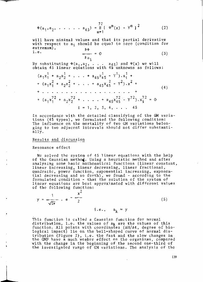
72 9

* ( a r a 2 , a45) = S [ *m(x) - Ym ] (2) m=1

will have minimal values and that its partial derivative with respect to a^ should be equal to zero (condition for extremum), 3<I) i-e- = 0 (3)

3 ai By substituting *(a,,a2, . . . 345) and *(x) we will obtain 45 linear equations with 45 unknowns as follows:

(alXl + a2x2 + . . . + a4 5x4 5 - Y ).x± +

, 2 2 2 v 2 . 2 (a1x1 + a7x7 + . . . + a.rX.r - Y ).x +

l1A1 *2A2 * * • 45 45 (4) +

, 72 L 72 ^ 72 . „72. 72 ( a l X l + a 2 x 2 + . . . . + a 4 5 x 4 5 - Y ) . X i

i = 1, 2, 3, 4, . . . 45

In accordance with the detailed classifying of the GM varia­tions (45 t y p e s ) , we formulated the following condition: The influence on the mortality of two GM variations belon­ging to two adjacent intervals should not differ substanti­ally.

Results and discussion

Resonance effect

We solved the system of 45 linear equations with the help of the Gaussian metho^- Using a heuristic method and after analysing some basic mathematical functions (linear constant, linear increasing, linear decreasing, linear fractional, quadratic, power function, exponential increasing, exponen­tial decreasing and so f o r t h ) , we found - according to the formulated condition - that the solution of the system of linear equations are best approximated with different values of the following function:

2 1

V2ir (5)

i.e., a k

This function is called a Gaussian function for normal distribution, i.e. the values of a^ are the values of this function. All points with coordinates (AH/At, degree of bio­logical impact) lie on the bell-shaped curve of normal dis­tribution (Figure 2 ) , i.e. the fast and the slow changes in the GMF have a much weaker effect on the organisms, compared with the change in the beginning of the second one-third of the investigated range of GM variations. The analysis of the

139

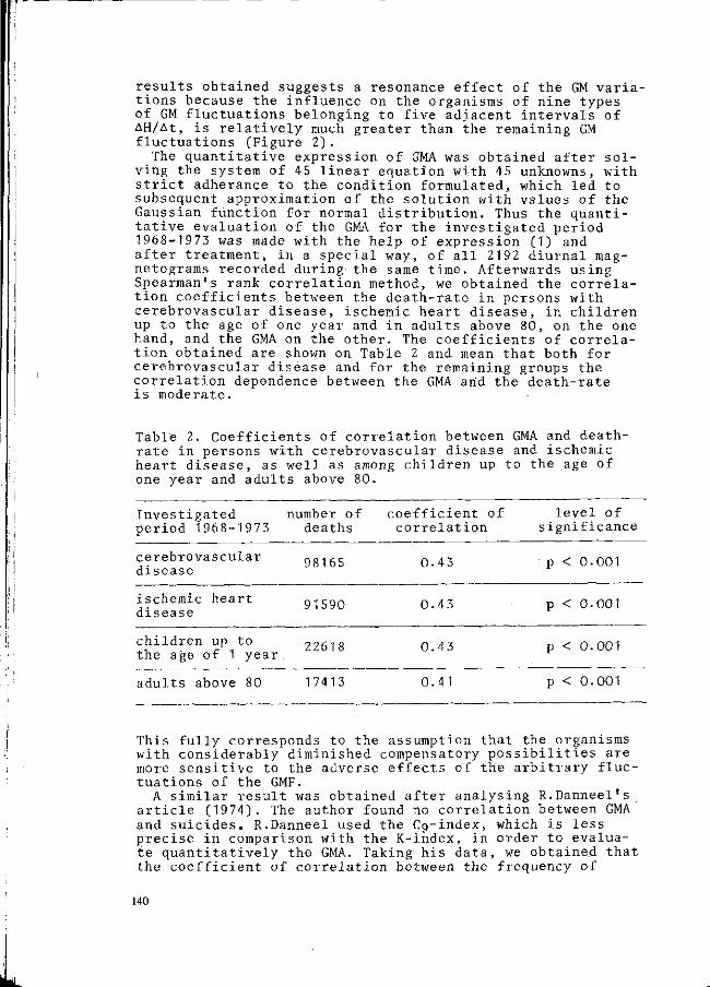
results obtained suggests a resonance effect of the GM varia­tions because the influence on the organisms of nine types of GM fluctuations belonging to five adjacent intervals of AH/At, is relatively much greater than the remaining GM fluctuations (Figure 2).

The quantitative expression of GMA was obtained after sol­ving the system of 45 linear equation with 45 unknowns, with strict adherance to the condition formulated, which led to subsequent approximation of the solution with values of the Gaussian function for normal distribution. Thus the quanti­tative evaluation of the GMA for the investigated period 1968-1973 was made with the help of expression (1) and after treatment, in a special way, of all 2192 diurnal mag-netograms recorded during- the same time. Afterwards using Spearman's rank correlation method, we obtained the correla­tion coefficients between the death-rate in persons with cerebrovascular disease, ischemic heart disease, in children up to the age of one year and in adults above 80, on the one hand, and the GMA on the other. The coefficients of correla­tion obtained are shown on Table 2 and mean that both for cerebrovascular disease and for the remaining groups the correlation dependence between the GMA arid the death-rate is moderate.

Table 2. Coefficients of correlation between GMA and death-rate in persons with cerebrovascular disease and ischemic heart disease, as well as among children up to the age of one year and adults above 80.

Investigated number of coefficient of level of period 1968-1973 deaths correlation significance

cerebrovascular Q g l 6 5 Q 4 3 p < 0.001 disease

ischemic heart g 1 5 9 0 0 4 3 < 0 . 0 0 1

disease

children up to 2 2 6 u Q _ 4 3 < 0 > 0 0 1

the age of 1 year

adults above 80 17413 0.41 p < 0.001

This fully corresponds to the assumption that the organisms with considerably diminished compensatory possibilities are more sensitive to the adverse effects of the arbitrary fluc­tuations of the GMF.

A similar result was obtained after analysing R.Danneel's article (1974). The author found no correlation between GMA and suicides. R.Danneel used the Cg-index, which is less precise in comparison with the K-index, in order to evalua­te quantitatively the GMA. Taking his data, we obtained that the coefficient of correlation between the frequency of

140

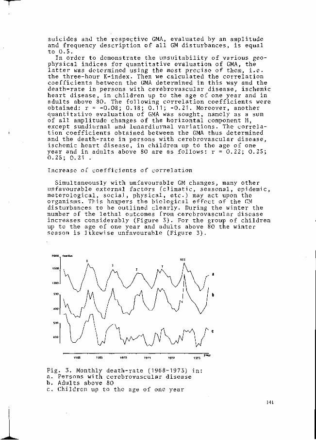
suicides and the respective GMA, evaluated by an amplitude and frequency description of all GM disturbances, is equal to 0.5.

In order to demonstrate the unsuitability of various geo­physical indices for quantitative evaluation of GMA, the latter was determined using the most precise of them, i.e. the three-hour K-index. Then we calculated the correlation coefficients between the GMA determined in this way and the death-rate in persons with cerebrovascular disease, ischemic heart disease, in children up to the age of one year and in adults above 80. The following correlation coefficients were obtained: r = -0.08; 0.18; 0.11; -0.21. Moreover, another quantitative evaluation of GMA was sought, namely as a sum of all amplitude changes of the horizontal component H, except sundiurnal and lunardiurnal variations. The correla­tion coefficients obtained between the GMA thus determined and the death-rate in persons with cerebrovascular disease, ischemic heart disease, in children up to the age of one year and in adults above 80 are as follows: r = 0.22; 0.25; 0.25; 0.21 .

Increase of coefficients of correlation

Simultaneously with unfavourable GM changes, many other unfavourable external factors (climatic, seasonal, epidemic, meterological, social, physical, etc.) may act upon the organisms. This hampers the biological effect of the GM disturbances to be outlined clearly. During the winter the number of the lethal outcomes from cerebrovascular disease increases considerably (Figure 3). For the group of children up to the age of one year and adults above 80 the winter season is likewise unfavourable (Figure 3).

2000 deaths

Fig. 3. Monthly death-rate (1968-1973) in: a. Persons with cerebrovascular disease b. Adults above 80 c. Children up to the age of one year

141

During the cold months the number of colds increases, which undoubtedly influences the death-rate of these two groups. Hence, after eliminating the winter season (December, January and February), the coefficient of correlation between the GMA and death-rate in persons with cerebrovascular disease, in children up to the age of 1 year and adults above 80 ought to increase. The new coefficients of correlation ob­tained are higher and have the following values: r = 0.56; 0.59; 0.53; p < 0.001 .

Conclusion

It is erroneus to quantify GMA through some geophysical indices when its biological influence is studied. The quanti­tative evaluation of GMA should be obtained taking into account all H-component variations for which AH > 30 gammas and the velocity of H-changes is equal or more than 0.7 . A moderate correlation was found between GMA and death-rate in persons with cerebrovascular disease, ischemic heart di­sease, in children up to the age of one year and in adults above 80. After eliminating the winter season, when the death-rate is higher, the coefficients of correlation between GMA and death-rate in persons with cerebrovascular disease, in children up to the age of one year and adults above 80 increased.

References

Danneel, R. , 1974. Der Einfluß geophysikalischer Faktoren auf die Selbstmordhäufigkeit. Archiv für Psychiatrie und Nerven­krankheiten. 219, (2): 153-157.

142

OVULATION AND SEASONS - VITALITY AND MONTH-OF-BIRTH

P.H. Jongbloet

"Maria Roepaan", Centre for the Mentally Handicapped, Siebengewaldseweg 15, 6595 NX Ottersum (The Netherlands); EMGO-Institute, Free University, Van der Boechorststraat 7, 1081 BT Amsterdam (The Netherlands)

Summary

Seasonal distortion of the month-of-birth distribution curves has been found in individuals affected by chromosomal aberrations and deve­lopmental field anomalies, such as oral clefts, heart anomalies and ce­rebral defects. This seasonality effect has also been reported for pa­thological conditions manifesting itself in later life, such as diabetes mellitus and schizophrenia and even for biological variables, such as neonatal body length and weight, fecundity, intelligence, etc. In chro­mosomal nondisjunctions the winter conception deficit and the springtime excess indicate that geocosmic factors interfere with the maturation of the oocyte, as predicted by the seasonal preovulatory overripeness ovo-pathy (SPrOO-)hypothesis. The underlying biological assumptions find a formal basis in the following phenomena of animal and human physiology: (i) alternation of seasons associated with either increased or stabili­zed ovulation rate; (ii) preovulatory delay of ovulation, inherent to the restoration and inhibition of the "ovulatory" seasons; and (iii) teratological consequences of this delay. The most crucial and at the same time, the most surprising assumption, is the first one, namely the seasonal cyclicity of the ovulatory pattern, at least in a number of women. That means, that the about 10 to 20% anovulatory cycles - even in sound and fecund women - do not occur randomly throughout the year but seasonally clustered. Such a seasonal cyclicity explains many repro­ductive characteristics at the pineal, the pituitarian and the ovarian level as well as at the population level. Hence, this is no longer an assumption, as it is supported by direct and circumstantial evidence. Preovulatory overripeness ovopathy as a biological determinant for re­productive casualties emerges as a unifying concept explaining not only the month-of birth effect, but also that of maternal age (at both sides of reproductive life), interpregnancy interval, maternal constitution, etc., all conditions related to a maturing egg-at-risk. Keywords: SPrOO-hypothesis; month-of-birth; month-of-conception; seaso­

nally fluctuating ovulation rate; maternal fecundity.

Introduction

There is at present overwhelming evidence that there are excesses and deficits in a number of reproductive casualties during specific months of the year. Circannual increases and decreases of pathological births are also reported in animals that breed throughout the year (De Ley & de Moor, 1977), but particularly in man (Dalen, 1975). It is possible that the awareness of this periodicity has led to the astrological beliefs of the Assyrians, Babylonians and Ancient Egyptians, for whom the 12 con­stellations of the zodiac indicated 12 chronological milestones of the year. Intentional attachment to nature might have revealed a temporal relationship, as was the case for the annual flooding and retreat of

143

t he i r r i ve rs . Their high pr iests were supposed to t ranslate the w i l l of the gods, al legedly wr i t ten in the heavens. However, neither these i n ­terpretat ions, nor those of t he i r fol lowers in present day media detract from these or ig inal observations.

One of the prototypes of reproductive casualties i s the syndrome of Down or trisomy-21 which i s known to or ig inate by a nondisjunction of the chromosomes, j u s t before or at conception. In a t ime-series analysis of neonates with trisomy 21 in West-Jerusalem a highly s ign i f i can t bimo-dal b i r th d i s t r i bu t ion was found in 6 of the 7 years, independently of maternal age and standard of l i v i n g (Harlap, 1974). The d i s to r t ion of the month-of-birth d i s t r ibu t ion of Down's syndrome indiv iduals has been shown to be pa r t i cu la r l y moulded by the 60% or ig inat ing during maternal meiosis I , i . e . during the ult imate maturation stage of the egg, j u s t before the f o l l i c l e bursts. This d i s to r t ion i s interdependent on the change rates of the standard conception curve, as evidenced by a l inear regression analysis: the stronger the to ta l conception rate increases or decreases, the more pathological conceptions are found (Jongbloet et a l . , 1982a, Jongbloet 1985; Jongbloet & Vrieze, 1985).

In (non-chromosomal) developmental f i e l d anomalies manifest at b i r t h , adolescence or adulthood, the same excesses and de f i c i t s are seen, e.g. in anencephaly (Jongbloet, 1975; Jongbloet et a l . , 1982b), congenital anomalies of the heart (Miettinen et a l . , 1970), id iopathic mental r e ­tardat ion (Lander e t . a l . , 1964; Jongbloet et a l . , 1976), schizophrenia (Dalén, 1974), diabetes mel l i tus (Jongbloet et a l . , 1988), e t c . . Less conspicuous physical character is t ics , such as weight and length at b i r t h ( I f f y et a l . , 1978), i n te l l igence, monthly reproductive performance (Jongbloet, 1986) also appear to apply to t h is ru le . This d isproport io-nal seasonal i ty-of -b i r th i s s imi la r ly present in the Southern hemi­sphere, however, as expected, six months removed. The same is t rue in the United States, where the major and minor standard b i r t h peaks are reversed, for s t i l l unknown reasons.

In order to explain such a world-wide phenomenon a fundamental b io lo ­gical p r inc ip le i s needed. Viral in fect ions - that act e i ther during pregnancy, pa r tu r i t i on or even neonatal l i f e - have been presumed as being the cause (Miura et a l . , 1987). U l t rav io le t rays, cosmic rays, hypoproteinaemia and hypovitaminaemia in the mother also have been invo­ked. However, many arguments m i l i t a t e against infect ions as the causal fac tor , as e.g. the time of chromosomal nondisjunctions, l im i ted and f ixed around conception, the for tu i tous coexistence of a spectrum of developmental f i e l d anomalies, the consistency and ubiquity of winter d e f i c i t s , i n contrast to springtime excesses.

Photoperiodicity i n te r fe r ing with the maturating oocyte, as formulated in the seasonal preovulatory overripeness ovopathy (SPrOO-)hypothesis (Jongbloet, 1971, 1975), does o f fer a fundamental b iological p r i nc ip le , which not only integrates various research t rad i t ions in animal re ­search, but also agrees with the empirical knowledge concerning the ae­t io logy of chromosomal aberrations, developmental f i e l d anomalies and physical character is t ics , e.g. the ef fects of maternal age at both sides of reproductive l i f e , interpregnancy i n t e r va l , maternal cons t i tu t ion , maternal diabetologic s ta te, e tc . . A l l these conditions are related to the maturing egg-at-r isk (Jongbloet & Zwets, 1976a; Jongbloet, 1986).

2 The seasonal preovulatory overripeness ovopathy (SPrOO-)hypothesis

In 1971, we reported pathological conceptions running more or less synchronously with the periodic f luctuat ions of to ta l conception curve, though with a greater amplitude. They occurred disproport ionately more

144

frequently during the seasons characterised by a high conception rate and less frequently during those characterised by a low conception rate. Their increase during spring and autumn and the decrease during winter and summer were hypothesized to be caused by interference of two basic oestric patterns, hampering the preovulatory (or intrafollicular) matu­ration of the egg (Jongbloet, 1971).

At the Seattle Symposium on Aging Gametes, we tried to maximize the time of the "pathological" conceptions caused by preovulatory overripe-ness ovopathy: they are expected to occur more frequently at the outset and at the end "of the total conception peaks, i.e. at the moment of the seasonal breakthrough and breakdown of the ovulatory pattern. This montn-oT-conception errect cou id De interpreted in concert witn other transitional conditions related to the maturing egg-at-risk (Jongbloet 1975, see Fig.1).

OVULATION RATE

anovulation [ r a te

CONCEPTION RATE

average numbei per month = 100

BIRTH RATE

average number per month =100

i

Oct nov dec j an febr mar apr may June July aug sept oct nov dec jan

Fig.1A-C. Graphical representation of the SPrOO-hypothesis: A. Alter­nation of seasonal "ovulatory" and "anovulatory" seasons. The restora­tion and inhibition stages are indicated by arrows. B_. and C. Seaso­nal fluctuation of normal (—) compared with pathological (---1 concep­tions or births due to preovulatory overripeness ovopathy. The horizon­tal line represents the average number of conceptions or births per month (Jongbloet, 1975).

The SPrOO-hypothesis, thus, presumes (i) the existence - also in hu­mans - of an alternation of seasons characterised by higher and lower ovulation rates, at least in a number of women; (ii) the occurrence - also in humans - of preovulatory ovulation delay inherent to the res­toration and inhibition stage of "ovulatory" seasons; and (iii) the tera-

145

togenic consequences - also in humans - of this delay of ovulation, i.e. preovulatory overripeness ovopathy (PrOO) especially occurring during these seasonal (SPrOO) transitional stages. The first assumption certainly is the most surprising and at the same time the most crucial one, while the second and third are rather consequences of it, tightly interlocked as the links of a chain. Apart from testing the predictions of the SPrOO-hypothesis, each of these assumptions should be substanti­ated and documented by empirical data from animal and human research. In this paper, we will restrict ourselves to this first and basic as­sumption, gathering the arguments in the library rather than in the laboratory and identifying new areas where imaginative approaches are likely to accelerate and to intensify research.

3 The nature of seasonal alternation of higher and lower ovulation rate, at least in a number of women

3.1 Seasonality of reproductive characteristics as an evolutionary re­lict

In the animal kingdom the neurohormonal rhythms are now well known to initiate and to control the duration and pattern of annual processes. At any given latitude, the breeding period is synchronized with the season that is most favourable for the survival of the young. Spring and autumn are the favourite breeding seasons during which the ovarian follicles and testicular functions are stimulated, by which animals are allowed to precisely "anticipate" the yearly events, for example, win­ter maximum survivorship .

Some animals are polyoestric and breed almost throughout the year. However, even under fairly uniform conditions of environment and nutri­tion in the laboratory, they still exhibit seasonal variation in the incidence of births with maximal and minimal fertility (Huntington, 1938, pg.36; Zuckerman, 1957). Yet, in the wild, this seasonal rhythm is far more marked, e.g. in some nonhuman primates, in whom temporal amenorrhoea and low stable levels of serum progesterone coincide with the nonbreeding season, while return of regular menstruation, ovulation and inherent cyclic endocrine patterns coincide with the breeding sea­son. The degree of seasonality of menstrual blood loss often depends on outdoor or indoor housing (Keverne & Michael, 1970; Nozaki & Oshima, 1987). Seasonal presence and absence of ovarian follicles and/or cor­pora lutea have been directly connected with the breeding and nonbree­ding seasons, respectively (van Herwerden, 1905, 1925, 1929). Hence, a similar phenomenon in man has already been presumed by her in order to explain the seasonal month-of birth distribution in the Northern hemi­sphere figuring as a mirror image of that of the Southern. Similar sea­sonal changes and ranges from nearly complete spermatogenic arrest to florid spermatogenesis or ejaculatory performance have been reported in free ranging males (Zamboni et al., 1974).

It is reasonable to suppose that more pronounced seasonal reproduc­tion has had its advantages, in human evolution, i.e. adaptive value, particularly during early harsh nomadic conditions. Interestingly, an old paediatricians' dogma tells us that infants are stronger when born early in the year than in the second half (Blonsky, 1929), advantaged as they are by summer ultraviolet energy of sunlight. An increase of serum vitamin D metabolite concentrations found after six months in winter-born (unsupplemented) breast fed children, in contrast to the status quo in summer-born ones (Greer & Marshall, 1989) seems to sub­stantiate this old statement.

146

3.2 Seasonality of pineal (melatonin) secretion and pituitarian (gonado­troph!' c) activity

The crucial role for melatonin, beit antigonadal in the one species or progonadal in the other, is recognized in reproductive physiology as well as in other seasonally bound characteristics, such as moulting and food intake (Reiter, 1972; Tamarkin et al. 1985). This neurohormone is released from the pineal gland in all species, nocturnal or diurnal, and its daily rhythm closely reflects the lighting cycle of the annual chan­ges in day length (the photoperiod). The daily melatonin profile, cha­racterised either by the duration of its secretion, the amplitude or the phase, has the potential of imparting temporal cues or temporal informa­tion to the hypophyseal-pituitary-gonadal axis in order to coordinate the reproductive activities during breeding and nonbreeding seasons.

The antigonadotrophic mechanism of melatonin in humans is complex and its relation to seasonal suppression of the ovulatory pattern begins to become unravelled by the finding of a biannual melatonin synthesising activity in human pineals of both sexes (Smith et al, 1978) and more particularly of low levels of plasma melatonin during spring and autumn contrary to the high levels in summer and winter (see Fig.2 from Arendt et al., 1979).

Plasma melatonin (pg lm\ ) mean + S E M

S e r u m melatonn ( pg/ml) mean

0800 1976

0election limit -mean

Detection limit-mean

M A M J

Fig.2. Circulat ing human melatonin at three d i f fe ren t time points at monthly in terva ls throughout one year ( for fur ther explanation, see Arendt et a l . , 1979).

In subarctic regions (at around 65° l a t i t u d e ) , with t he i r extreme c l i ­matic and photoperiodic character is t ics , the short photoperiod (day length + 5 h.) has been correlated with higher night-t ime secretion of melatonin on day 2 and 10 of the menstrual f o l l i c u l a r (preovulatory)

147

phase, a lower LH-secretion at mid-cycle and the reverse i s t rue in June-July (day length + 22 h.) (Kivel'à et a l . , 1988; Ronkainen et a l . 1985; Kaupilla e t a l . Î987a and b ) . Seasonal var ia t ion of the melatonin secretion and gonadotrophs st imulat ion appears not to be confined to these high l a t i t udes , as in France where the LH-surges occur more often during day-time during spring (52%) than in the other seasons (13%) (Testart et a l . , 1982).

3.3 Seasonality of ovarian funct ion: the d i rec t evidence

The ovulation rate in women of 19-34 years of age, having given b i r t h to at least one ch i l d 6 to 18 months ea r l ie r and not regularly using any medication, surpr is ingly does not reach almost 100%, as would be expec­ted i f each cycle were ovulatory and the ovulation rate independent on seasons, but about 80% (Cole e t a l . , 1976). Otherwise, un fa i l ing ovula­t ion in every consecutive cycle occurs in 62% of young women aged 20-24 years, in 88% when aged 25-29, i n 91% when 30 and over; s im i l a r l y , in 59.5% of students being more l i ab le to s t ress, compared to 83.5 % in non-students of the same age (Metcalf and MacKenzie, 1980).

Monophasic and/or prolonged (anovulatory) cycles are well known to be par t i cu la r ly associated with menarchal and menopausal t rans i t ion (Co l le t t et a l , 1954; Döring, 1969; Treloar et a l . , 1967), to restora­t ion of the ovulatory pattern j us t a f ter abortion and pa r tu r i t i on (see Jongbloet & Zwets, 1976a), to stress s i tuat ions (Metcalf and MacKenzie, 1980; Nagata et a l . , 1986), to const i tut ional subfecundity (see Jong­bloet , 1986), e t c . . These disturbed and/or anovulatory cycles are they seasonally clustered or randomly d is t r ibuted throughout the year? The answer to t h i s crucial guestion i s evidenced in the European subarctic area (Oulu, Finland; 67 N) with i t s extreme c l imatological condit ions: ovarian hormone levels (oestradiol and free oestradiol index) at the time of ovulation are higher in spring than in the other seasons and the f o l l i c u l a r size more pronounced; in contrast, during the dark-winter the granulosa ce l l a c t i v i t y i s diminished and the f o l l i c u l a r development disordered, independently on running or jogging a c t i v i t i e s (Ronkainen et a l . , 1985, Kaupil la et a l . , 1987 a,b) .

3.4 Seasonality of the ovarian funct ion: the i nd i rec t evidence

(a) The circannual character ist ics of reproductive parameters: basic body temperature charts and menstrual in terva ls have been shown to be l i ab l e to seasonal influences (Engle and Shelesnyak, 1934; K i rchof f , 1937; Malek, e t a l . , 1962; Nagata et a l . , 1986; Nakamura & Yamakawa, 1988). In Treloars' data, concerning the menstrual experience during more than 38,000 women-years (between 20 and 40 years of age), accumula­ted between 1936 and 1970 in Minnesota (USA) and assessed by Sundararaj et a l . , 1978) a c lear bimodal d i s t r ibu t ion was seen (see F ig. 3) corres­ponding with the U.S. standard month-of-birth pattern during the periods 1942-1961 and 1962-1981 in Minnesota (Lam & Miron, 1987).

In a Helsinki gynaecologie department the increased frequency ofen dometrial (cyst ic) hyperplasias (characterised by anovulation) has been shown to be inversely re lated to the seasonally f luc tuat ing number of conceptions, decreasing during the dark months of the year and increa­sing in springtime (see F ig. 4, from Timonen et a l . , 1964).

Seasonal c luster ing of ovulatory cycles is also suggested by the four-month cessation of menstruation in Eskimo women concomittant with suppression of a l l sexual desire during the prolonged absence of sun­l i g h t of the pole winter and by the springtime reestablishment of men-

148

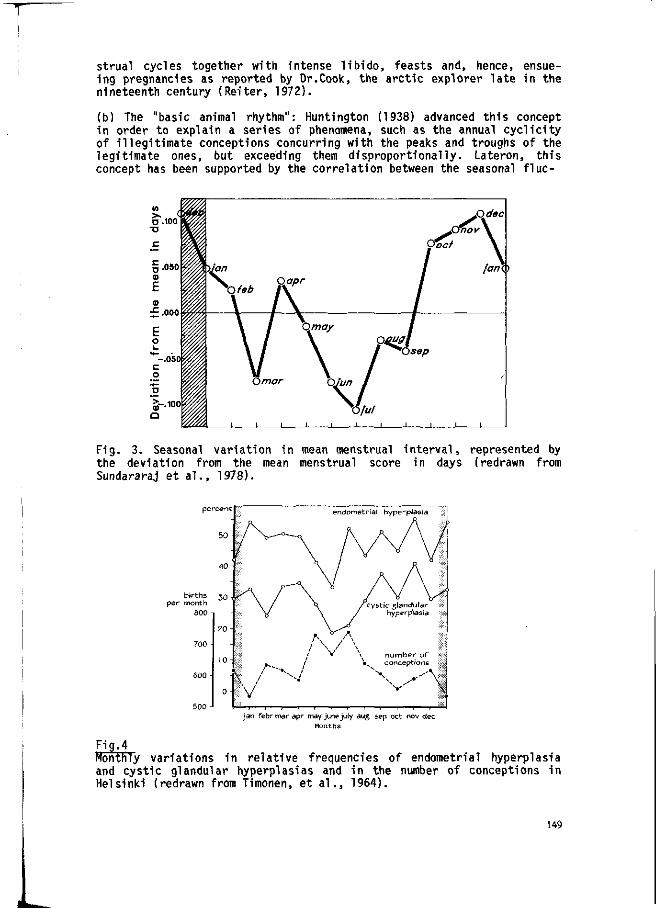
strual cycles together with intense libido, feasts and, hence, ensue-ing pregnancies as reported by Dr.Cook, the arctic explorer late in the nineteenth century (Reiter, 1972).

(b) The "basic animal rhythm": Huntington (1938) advanced this concept in order to explain a series of phenomena, such as the annual cyclicity of illegitimate conceptions concurring with the peaks and troughs of the legitimate ones, but exceeding them disproportionally. Lateron, this concept has been supported by the correlation between the seasonal flue-

Fig. 3. Seasonal variation in mean menstrual interval, represented by the deviation from the mean menstrual score in days (redrawn from Sundararaj et al., 1978).

births 3o per month

800

number o f •^ conceptions

— 7 i r i i n 1 ! ' - r - " " i i • i jan febr mar apr may June July aug sep Oct nov dec

Months

FTg.4 Monthly variations in relative frequencies of endometrial hyperplasia and cystic glandular hyperplasias and in the number of conceptions in Helsinki (redrawn from Timonen, et a l . , 1964).

149

tuation of conceptions (based on births) at the one side, and the average in sales of "conventional" contraceptives (1963-1966, before the Pill became respectable; Parkes, 1968) or the frequency of induced abortions (in their majority unwanted pregnancies; Cohen & Bracken, 1977) at the other side. An inversed indeed curve would have been expec­ted if the conception peaks and troughs were caused by contraceptive behaviour.

(c) The standard month-of-birth distrubution: the classic picture of a European pattern of more births in the first half of the year and less in the second half being caused only by the major springtime conception surge and the reverse in the southern hemisphere, is too simplistic. Sociocultural factors, of course, again and again are more important, as seen in the birth distribution of various racial groups within the same country (Johnson et al., 1978) and in diachronic changes in the last decades, characterized by modern family planning practices. One can still wonder about the consistency of the standard month-of-birth dis­tribution which is a compound of fertility patterns in different mater­nal age categories, birth orders, socioeconomic groups, etc. (Sandahl, 1978; Ronnike, 1981; Mathers and Harris, 1983). In a thorough study of a new set of estimates of a large number of countries, continents and time periods Lam and Miron (1987) came to the conclusion that two emerging seasonal patterns remain present across both hemispheres, namely, the United States pattern and the European pattern: "the recurrence of two simple patterns in a large number of populations which are culturally and economically diverse, the similarity of patterns between rural and urban populations and the persistence of seasonal patterns over long periods in many populations are broadly suggestive that forces such as climate or photoperiod may play a more important role in explaining birth seasonality than forces such as economic variables or marriage". The true nature of alternating seasons associated with higher and lower ovulation rate in humans can be unravelled further by analysing the monthly distribution of polyovulations (unlike sexed twins) and of preg­nancy wastage according to maternal age and birth order, preferably in an era prior to the demographic transition.

(d) The seasonal variation of fertilisation capacity of the ovulated egg: Paraskevaides et al. (1988) conclude that conceptions achieved by artificial insemination between 1974 and 1982 peaked from October to January and to a lesser extent from May to July. This is in analogy with the seasonal variation of in vitro maturation and fertilization capacity of nonhuman primate oocytes, obtained during breeding and non-breeding seasons (Smith et al., 1978; Chan et al., 1982).

(e) The oscillatory pattern of conception rates after discontinuation of oral contraceptives: a short delay in the return to maximum fertility after discontinuation of contraceptive steroids resulted in a harmonic oscillation pattern of conceptions. This has been interpreted as "a pre­viously unrecognised natural cycle" (Janerich et al., 1976) and in agreement with the "basic animal rhythm" (Jongbloet & Zwets, 1976b).

(f) The seasonally related interval between month of marriage and that of first conception: although the month of marriage can be based on socio-cultural traditions, again correlated with the "basic animal rhythm", many authors have wondered about the consistency of the month-of -birth distribution of the (matrimonial) first born, hardly differing from that of the later born(Wolda, 1927; Huntington, 1938, p.51; Mattila,

150

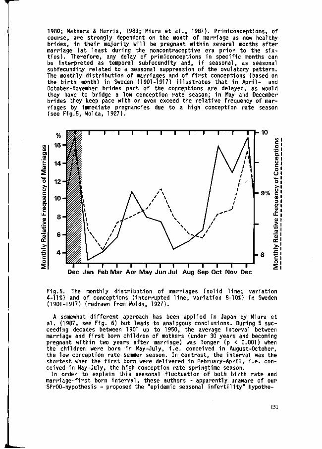
1980; Mathers & Harris, 1983; Miura et al., 1987). Primiconcept!ons, of course, are strongly dependent on the month of marriage as new healthy brides, in their majority will be pregnant within several months after marriage (at least during the noncontraceptive era prior to the six­ties). Therefore, any delay of primiconceptions in specific months can be interpreted as temporal subfecundity and, if seasonal, as seasonal subfecundity related to a seasonal suppression of the ovulatory pattern. The monthly distribution of marriages and of first conceptions (based on the birth month) in Sweden (1901-1917) illustrates that in April- and October-November brides part of the conceptions are delayed, as would they have to bridge a low conception rate season; in May and December brides they keep pace with or even exceed the relative frequency of mar­riages by immediate pregnancies due to a high conception rate season (see Fig.5, Wolda, 1927).

T — i — i — i — i — i — i — i — r Dec Jan Feb M a r Apr M a y Jun Jul Aug Sep Oct Nov Dec

Fig.5. The monthly distribution of marriages (solid line; variation 4-11%) and of conceptions (interrupted line; variation 8-10%) in Sweden (1901-1917) (redrawn from Wolda, 1927).

A somewhat different approach has been applied in Japan by Miura et al. (1987, see Fig. 6) but leads to analogous conclusions. During 5 suc­ceeding decades between 1901 up to 1950, the average interval between marriage and first born children of mothers (under 30 years and becoming pregnant within two years after marriage) was longer (p < 0.001) when the children were born in May-July, i.e. conceived in August-October, the low conception rate summer season. In contrast, the interval was the shortest when the first born were delivered in February-April, i.e. con­ceived in May-July, the high conception rate springtime season.

In order to explain this seasonal fluctuation of both birth rate and marriage-first born interval, these authors - apparently unaware of our SPrOO-hypothesis - proposed the "epidemic seasonal infertility" hypothe-

151

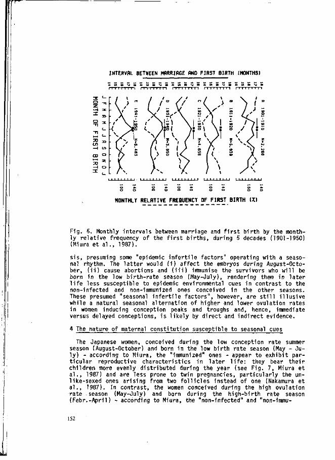
INTERVAL BETWEEN MARRIfiGE RND FIRST BIRTH (MONTHS)

i i i i i i i i i i 1 1 i i i i i i i i i i i i i i i i i i i i i i i i i i i i i i i i

1 I ' ' I ' • ' } • • I M ' I I ' • I • • ' ' • ' ' i i i i i i i i i i i i i i i i i i

o o o o o

MONTHLY RELATIVE FREQUENCY OF FIRST BIRTH (Z)

Fig. 6. Monthly intervals between marriage and first birth by the month­ly relative frequency of the first births, during 5 decades (1901-1950) (Miura et al., 1987).

sis, presuming some "epidemic infertile factors" operating with a seaso­nal rhythm. The latter would (i) affect the embryos during August-Octo­ber, (ii) cause abortions and (iii) immunise the survivors who will be born in the low birth-rate season (May-July), rendering them in later life less susceptible to epidemic environmental cues in contrast to the non-infected and non-immunized ones conceived in the other seasons. These presumed "seasonal infertile factors", however, are still illusive while a natural seasonal alternation of higher and lower ovulation rates in women inducing conception peaks and troughs and, hence, immediate versus delayed conceptions, is likely by direct and indirect evidence.

4 The nature of maternal constitution susceptible to seasonal cues

The Japanese women, conceived during the low conception rate summer season (August-October) and born in the low birth rate season (May - Ju­ly) - according to Miura, the "immunized" ones - appear to exhibit par­ticular reproductive characteristics in later life: they bear their children more evenly distributed during the year (see Fig. 7, Miura et al., 1987) and are less prone to twin pregnancies, particularly the un-like-sexed ones arising from two follicles instead of one (Nakamura et al., 1987). In contrast, the women conceived during the high ovulation rate season (May-July) and born during the high-birth rate season (Febr.-April) - according to Miura, the "non-infected" and "non-immu-

152

fi 1935-1939

cc ce

cc

OQ

1.2

- J

CC

z o '-o CD

CC

B 1936a'

\ HOSPITAL N

l L-

NOV FEB MRT AUG NOV / / / / /

JAN APR JUL OCT JAN

BIRTH SERSON OF OFFSPRINGS

Fig. 7. Seasonal distributions by the season of mother's birth; a compa­rison of data from two different sources mothers born in May-July; Mothers born in the other months; a) Year of chil­dren's births; *p < 0,05; **p > 0.01 by x test (df = D W u r a et al., 1987).

ni zed" women - would be more susceptible to seasonal infertile factors and more twin prone. According to our concept, the former do so because they are the "better conceived" individuals and thus "constitutionally better off", as they are conceived independently on seasonal cues. In contrast, the latter are the "less optimum conceived" individuals and thus "constitutionally less-off", who are traceable by subfecund charac­teristics, such as a propensity to meiotic nondisjunctions and/or deve­lopmental field anomalies in their progeny (Jongbloet, 1975, 1986). They only look like more fecund, but are rather subfecund, dependent as they are on seasonal cues and having often to bridge low ovulation rate sea­sons in order to conceive and to proceed from an anovulatory season into an ovulatory season or vice versa.

Hence, the maternal constitution, incl. reproductive capacity, not only depends on the genome but also on the quality of the fertilized egg, influenced by the seasonal alternation of the ovulatory pattern of the grandmother, the grandmothers constitution, the grandmothers age at mothers birth, the nutrition (social class of the maternal grandfather), her hormonal state, etc.. I suggest that individuals more susceptible to seasonal environmental cues are also those with larger seasonal varia­tion of plasma melatonin, as shown by Arendt et al. (1979).

153

5 Conclusions

The key-question of the SPrOO-hypothesis i s the existence of a sea­sonally f luc tuat ing ovulation rate i n humans, as i s the ru le i n an i ­mals. Besides the d i rec t v isual isat ion of the seasonally changing f o l l i ­cular diameter, there i s c ircumstantial evidence fo r i t .The dr iv ing force for such an a l ternat ion can be interpreted in evolutionary terms and i s manifest i n p inea l , p i t u i t a r i an and ovarian a c t i v i t y , A large bo­dy of physiological observations cannot be understood without a seasonal f luc tuat ion of ovulatory cycles, at least i n a number of women. I t i s no longer a surprise to learn that the seasonal dependency in reproduction (ensuing SPrOO) i s caused i t s e l f by ovopathy, induced not only by seasonality of t he i r own conception (SPrOO), but also other egg-at-r isk conditions such as grandmaternal age, hormonal state and ma lnut r i t ion .

6 References

Arendt, J . et a l . , 1979. Long-term studies on. immunoreactive human-mela-ton in . Ann. C l in . Biochem. 16:307-312.

Blonsky, P.P., 1929. Früh- und Spätjahrkinder. Jahrbuch Jugend Kinder-he i l k . 74:115-120.

Chan, P.J. , R.J. Hutz, W.R. Dukelow, 1982. Nonhuman primate in v i t r o f e r ­t i l i z a t i o n : seasonality, cumulus c e l l s , cyc l ic nucleotides, r ibo-nu-c le ic ac id, and v i a b i l i t y assays. F e r t i l . S t e r i l . 38:609-615.

Cohen, I .C. , M.B. Bracken, 1977. Monthly var ia t ion in conceptions leading to induced abort ion. Social B io l . 24: 235-250.

Co l l e t t , M.E., G.E. Wertenberger, V.M. Fishe, 1954. The e f fec t of age upon the pattern of the menstrual cycle. F e r t i l . S t e r i l . 5:437.

Cole, Ph., J.B. Brown, B. McMahon, 1976. Oestrogen p ro f i les of parous and null iparous women. Lancet i i :596-598.

Dalén, P., 1974. Season of b i r t h i n Schizophrenia and Other Mental Disor­ders. North-Holland Publishing Company, Göteborg.

Dalén, P., 1975. Season of b i r t h . North-Holland Publishing Company, Amsterdam, p. 15-57.

De Ley, G., A. de Moor, 1977. Seizoensinvloeden i n het voorkomen van Spastische parese b i j het rund. Vlaams Diergeneesk. T i jdschr. 46/3: 179-184.

Döring, G.K., 1969. The incidence of anovular cycles in women. J . Reprod. Fert. Suppl., 6:77.

Engle, E.T., M.C. Shelesnyak, 1934. F i r s t menstruation and subsequent menstrual cycles of pubertal g i r l s . Hum. B i o l . 6:431-453.

Greer, F.R., S.R.N. Marshall, 1989. Bone mineral content, serum vitamin metabolite concentrations, and u l t r av i o l e t B l i g h t exposure in infants fed human milk and without vitamin D2supplements. J . Ped. 114: 204-212.

Harlap, S. , 1974. A time series analysis of the incidence of Down's syn­drome in West Jerusalem. Am. J . Epi dem. 99:210-217.

Huntington, E., 1938. Season of B i r t h . I t s re la t ion to human a b i l i t i e s . J.Wiley & Sons, i n c . , New York.p. 52-54.

I f f y , L. et a l . , 1978. The e f fec t of maternal age, pa r i t y , fe ta l sex and season upon early in t rauter ine development. I n t . J . Gynaecol Obstet. 16:210-214.

Janerich, D.T., D.E. Lawrence, H.T. Jacobson, 1976. F e r t i l i t y patterns a f ter discontinuation of use of oral contraceptives.Lancet i : l051-1053.

Johnson, J .T . , T.B. Ann, V.T. Palan, 1975. Seasonality of b i r ths fo r West Malaysia's two main rac ia l groups. Hum. B i o l . 47:295-307.

Jongbloet, P.H., 1971. Month of b i r t h and gametopathy. An invest igat ion

154

in to patients with Down's, K l i ne fe l t e r ' s and Turner's syndrome. C l in . Genet. 2:315-325.

Jongbloet, P.H., 1975. The ef fects of pre-ovulatory overripeness of human eggs on development. I n : Aging Gametes, ed. R.J. Blandau. Karger, Basel, p. 300-329.

Jongbloet, P.H., J .H.J, van Erkelens-Zwets, G. Holleman-van der Woude, 1976. The s ignif icance of seasonality of b i r t h in mental def iciency. REAP 2: 243-263.

Jongbloet, P.H., J .H.J. Zwets, 1976a. Preovulatory Overripeness of the Egg in the Human Subject. I n t . J . Gynaecol. Obstet. 14:111-116.

Jongbloet, P.H., J .H.J. Zwets, 1976b. F e r t i l i t y - r a t e s a f ter oral contra­ceptives. Lancet i i :101-102.

Jongbloet, P.H., A.M. Mulder, A.J.H. Hamers, 1982a. Seasonality of Pre­ovulatory Non-Disjunction and the Aetiology of Down Syndrome. A European Collaborative Study. Hum. Genet. 62:134-138.

Jongbloet, P.H. et a l . , 1982b. Seasonality of Anencephalic B i r ths . I t s re la t ion to Pre-ovulatory Overripeness Ovopathy. Chronobiologia 9:273-280.

Jongbloet, P.H., 1985. The ageing gamete in re la t ion to b i r t h control f a i lu res and Down Syndrome. Eur. J . Pediatr. 144:343-347.

Jongbloet, P.H., O.J. Vrieze, 1985. Down's Syndrome: Increased frequency of maternal meiosis I nondisjunction during the t rans i t iona l stages of the ovulatory seasons. Hum. Genet. 71:241-248.

Jongbloet, P.H., 1986. Background Biological Ef fects. Prepregnancy Care: A Manual fo r Practice. I n : G.Chamberlain, J.Lumley (Eds.) 3: 31-52. John Wiley & Sons, London.

Jongbloet, P.H., M. van Soestbergen, E.A. van der Veen, 1988. Month-of-B i r th d i s t r ibu t ion of diabetics and ovopathy: a new aet io logical view. Diabetes Res. 9:51-58.

Kaupi l la, A. et a l . , 1987a. The e f fec t of season on the c i r cu la t ing con­centrations of anter ior p i t u i t a r y , ovarian and adrenal cortex hor­mones and hormone binding proteins in the subarctic area; evidence of increased a c t i v i t y of the p i tu i tary-ovar ian axis in spring. Gyn. En­docr inol . 1:137-150.

Kaupi l la, A. et a l . , 1987. Inverse seasonal re lat ionship between melato­nin and ovarian a c t i v i t y in humans in a region with a strong seasonal contrast in luminosity. J . C l in . Endocrinol. Metab. 65:823-828.

Keverne, E.B., R.P. Michael, 1970. Annual changes in the menstruation of rhesus monkeys. J . Endocrinol. 48:669-670.

K i rchof f , H., 1937. Jahreszeiten und Belichtungen in Ihrem Einfluss auf weibliche Genitalfunktionen. Arch. Gynäk. 163:141-185.

Kivelä, A. et a l . , 1988. Seasonal, menstrual and circadian secretions of melatonin, gonadotropins and pro lact in in women. Acta Physiol. Scand. 132:321-327.

Lam, D.A., J.A. Miron, 1987. The Seasonality of Bir ths in Human Popula­t ions . Res. Reports 87:114:1-58.

Lander, E., H. Forssman, H.0. Akesson, 1964. Season of b i r t h and mental def ic iency. Acta Genet. (Basel) 14:265-280.

Malek, J . , J . Gleich, V. Maly, 1962. Characterist ics of the dai ly rhythm of menstruation and labor. Ann. N.Y. Acad. Sei. 98:1042-1055.

Mathers, C D . , R.S. Harr is, 1983. Seasonal D is t r ibut ion of Bir ths in Aust ra l ia . I n t . J . Epidem. 12:326-331.

Ma t t i l a , R.E., 1980. Variations in conceptions, twin frequency and sex ra t io in Finland 1751-1969. Kangasalan Kirjapaino Of fsetrotaat io, Hels inki .

Metcalf, M.G., J.A. McKenzie, 1980. Incidence of ovulation in young women. J . biosoc. Sei. 12:345-352.

155

Miettinen, O.S., M.L. Reiner, A.S. Nadas, 1970. Seasonal incidence of co­arctation of the aorta. Br. Heart J. 32:103-107.

Miura, T., et al., 1987. Epidemic seasonal infertility.In: H.Lieth (Ed.): Prog. Biometeorol. Vol. 6: p. 45-55.

Nagata, I., et al., 1986. Ovulatory Disturbances. Causative Factors Among Japanese Student Nurses in a Dormitory. J. Adolesc. Hlth. Care 7:1-5.

Nakamura, I., et al., 1987. Seasonality in twinning during 60 years in Japan. In: H.Lieth (Ed.): Prog. Biometeorol. Vol. 6: p. 65-76.

Nakamura, I, Yamakawa, J., 1988. Seasonality of Menstrual Frequency. Triennial Rep. Vol. 5: 28.

Nozaki, M., K. Oshima, 1987. Seasonal changes of the gonadotropic func­tion in the female Japanese monkey. In: T.Miura (Ed.): Season Effects on Reproduction, Infection and Psychoses. (Prog. Biometeorol, Vol.5) SPB Academic Publishing, The Hague, p. 41-49.

Paraskevaides, E.C., G.W. Pennington, S. Naik, 1988. Seasonal distribu­tion in conceptions achieved by artificial insemination by donor. Br. Med. J. 297:1309-1310.

Parkes, A.S., 1968. Seasonal variation in human sexual activity. Eugen. Soc. Symp. 4:128-145.

Reiter, R.J., 1972. The role of the pineal in reproduction. In: H.Balin, S.Glasser (Ed.): Reprod. Biol.(Excerpta Medica), Amsterdam, p. 100-114.

Ronkainen, H., et al., 1985. Physical Exercise-Induced Changes and Sea­son-Associated Differences in the Pituitary Ovarian Function of Runners and Joggers. J. Clin. Endocrinol. 60:416-422.

Ronnike, F., 1981. Seasonal conception by women in various age groups compared with the season of menarche. Dan. Med. Bull. 28:148-153.

Sandahl, B., 1978. Seasonal birth pattern in Sweden in relation to birth order and maternal age. Acta Obstet. Gynecol. Scand 57:393-396.

Smith, D.M., C.H. Conaway, W.T. Kerber, 1978. Influences of season and age on maturation in vitro of rhesus monkey oocytes. J. Reprod. Fert. 54:91-95.

Smith, J.A., T.J.X. Mee, E.D., Bird, 1978. Human post-mortem pineal me­tabolic correlations with serum and CSF melatonin in man. Neurosci. Lett. 1:214.

Sundararaj, M., et al., 1978. Seasonal behavior of human menstrual cy­cles: a biométrie investigation. Hum. Biol. 50:15-31.

Tamarkin, L., C.J. Baird, O.F.S. Almeida, 1985. Melatonin: A Coordina­ting Signal for Mammalian Reproduction? Science 227:714-720.

Testart, J., R. Frydman, M. Roger, 1982. Seasonal Influence of Diurnal Rhythms in the Onset of the Plasma Luteinizing Hormone Surge in Women. J. Clin. Endocrinol. Metab. 55:374-377.

Timonen, S., B. Franzas, K. Wichmann, 1964. "Photosensibility of the hu­man pituitary". Ann. Chir. Gyn. Fenn. 53:165-172.

Treloar, A.E., et al., 1967. Variation of the human menstrual cycle through reproductive life. Int. J. Fertil. 77:163-175.

Van Herwerden, M.A., 1905. Bijdrage tot de kennis van menstrueelen cyclus en Puerperium. Dissertatie, Utrecht.

Van Herwerden, M.A., 1929. Zusammenhang zwischen menstruellem Zyklus und Ovulation. Klin. Wochenschr. 42:1948-1950.

Van Herwerden, M. A., 1925. Some remarks on the polyoestrus of primates. Anat. Rec. 30:221-223.

Wolda, G., 1927. Akklimatisierung und Deklimatisierung. Genetica, Neder­lands tijdschrift voor erfelijkheids- en afstammelingsleer, 9.

Zamboni, L., C.H. Conaway, L. Van Pelt, 1974. Seasonal Changes in Pro­duction of Semen in Free-Ranging Rhesus Monkeys. Biol. Reprod. 11:251-267.

Zuckerman, S., 1957. The human breeding season. N. Sei. 12-14, 4 April.

156

NOTE ON HUMAN RESPONSE TO THE LUNAR SYNODIC CYCLE

N. Kollerstrom, 15 Cooper Road, GUI 3LY Guilford / Surrey, U.K.

Recent articles in US psychology journals have reviewed published inves­tigations of lunar influence on human behaviour. The conclusion of their 'meta-analysis' as the authors termed it, was that no valid evidence exis­ted for any influence of the Moon upon human behaviour. The papers are:

'A meta-analysis of lunar-lunacy research' Rotton and Kelly, Psychological Bulletin, 1985, 97.

'Moon mechanisms and myths, a critical appraisal' Culver, Rotton and Kelly, Psychological Reports, 1988, 62.

The authors accept the evidence that lunar cycles exist in a wide variety of animal behaviour patterns, in the rhythms of plant growth and in geo­physical factors: distribution of rainfall, of sunshine, of thunderstorms and of geomagnetic field strength, of ionosphere disturbances and of ozone thickness, as well as meteor activity. However, the authors argue and per­haps quite rightly that none of these geophysical factors can convincingly account for lunar influences upon man. The authors conclude by querying whether any further studies in this field are really necessary,/in view of the many negative results they claim to have surveyed. The fact that about 50% of students when asked believed that the Moon did have effects on hu­man life is treated in terms of the psychology of illusion.

These works can be recommended as giving a thorough and up-to-date survey of the relevant literature, though their conclusions should be dismissed as premature. Their argument, that 'The lack of a satisfactory mechanism lowers the credibility of the lunar effect hypothesis' (Culver et al., p. 704) suffers from two principal defects.

Firstly, there is the fact that a large variety of animals and marine creatures exhibit behaviour patterns which are manifestly tuned in to the lunar cycle, demonstrating that in some way this cycle is influencing living things. If scientists cannot comprehend how this takes place, it is a matter of secondery importance. Sea-horses lay their eggs at Full Moon, continuing to do so in a laboratory tank without any evident source of information concerning the lunar cycle, and many such instances could be cited, as the authors do not dispute. If this happens with animals, it can happen with humans.

Secondly, the menstrual period in womankind is indistinguishable in its mean duration from the 29.5 day lunar cycle, as was shown by the Menakers amongst others1. Its mean period is not 28 days, as is normally asserted by the medical profession, anxious to avoid the question as to what the lunar cycle is doing in the reproductive processes of womankind. The Menakers also found from their (very large) sample that the mean duration of pregnancy, that is the time from conception to birth, was 9.00 lunar months to within a fraction of a day. They concluded from this that the lunar cycle had some biological significance, though unsure as to what this might be. The fact that womankind is adapted to this lunar synodic cycle, in a manner not found in other animals, leads one to expect that there will be other instances of human adaptation to this cycle.

157

The purpose of my address today is merely to note that there are four surveys carried out hitherto, which deserve to be replicated. These are recommended as providing the basis for a scientific investigation of the subject. They concern monthly rhythms within autonomic functions of the human body, as opposed to conscious actions. Surveys of the latter have spawned centuries of colourful debate which have established little: thus, one hospital publishes a report claiming that its nurses are more busy over the Full Moon, then another reports finding no such thing; a police station claims its members are busier over the Full Moon, then another contradicts thisS and so an inconclusive debate has continued. We are not puppets of the Moon, and there seems to be no overall change in behaviour to be observed, such as for example people committing suicide more frequently at some part of the lunar month.

The four reports are as follows:

'A lunar rhythm in the occurrence of blood-borne factors in cockroaches, mice and men' H. Rounds, Comparative Biochemistry and Physiology, 1975, 50.

'Moon talk: the cyclic periodicity of postoperative haemmorage' E.A. Andrews, Journal of the Florida Medical Association, 1961, 46.

'Lunar and Menstrual phase locking'. W.B. Cutler, American Journal of Obstetrics and Gynecology, 1980, 137.

'Periodic changes in the electromagnetic field in health and disease'. J.R. Ravitz, Annals of the New York Academy of Sciences, 1962, 98.

These papers make large and definite claims that have not yet been adequately confirmed by replication. Cutler's finding has been replicated on a small scale and confirmed but the others have not. One I would expect positive results to be obtained by properly conducted time-sequence experiments employing their approach.

Biochemist Dr. H. Rounds noted that certain stress-related hormones, as found in daily blood samples of mice and men, peaked sharply twice a month at or rather just after the syzygy positions of Full and New Moon. This increase was sharp and well-defined, and was regular over a three-month period. This finding gives a clear, biochemical basis for certain findings indicating that stress-related symptoms and activities tend to increase over the Full Moon. Rounds also did the experiment with mice and men who had been exposed to 'stress'-running up and down stairs for human volunteers, or being moved about in a box for the mice - and he still found a bimonthly tidal rhythm in the stress-hormones, but in a different pattern. The Culver et al. paper dismissed the Rounds study by claiming that a three-month period was not long enough for such an effect to be determined, but it is hard to see any sense in this objection.

Dr. Andrews found that in his hospital in Florida, the medical records showed a clear Full-Moon effect. He discovered that operations which had complications due to excessive bleeding tended to occur more frequently at this part of the month. In a sample of one thousand operations, he found a huge differential, with several hundred percent more such operations where excessive bleeding occurred at the Full Moon, than at New Moon. He repeated this over several different wards of the hospital, for different types of operations, and always found the same effect. It is odd that no attempt to replicate this vitality important finding, which has far-reaching ethical and even legal implications, has ever been published. It is a finding which echoes millenia of folk-tradition, for example Pliny the Roman naturalist said that farmers should not geld their animals over the Full-Moon period.

158

My inquiries in the U.K. indicate that complications due to excessive bleeding in surgical operations would not normally find their way into the hospital records; which may be one reason why replications of Andrews' finding have not been forthcoming. The Culver et al. paper unaccoutably omits to mention Dr. Andrews' finding.

Long and inconclusive debates have continued as to whether the female menstrual cycle is to any degree phase-locked to the lunar cycle. One survey finds a peak at the Full Moon, another at the New, and then a third finds no peak at all. A sensible approach to the matter has at least been adopted by W.B. Cutler, who realised that only women whose monthly period approximated to the lunar cycle had the possibility of being phase-linked to this cycle, and so only included such in his survey. As pregnant woman and those on the Pill were excluded from the survey, so also were those whose mean period duration fell outside a 28-30 day range. The 'lunar period cyclers' as he called them showed a marked degree of phase-locking to the Moon, with menstruation tending to occur over the Full Moon rather than the New. Culver et al. rightly point out that this finding contradicts certain other surveys which assume that the menstrual period is naturally phased to the New Moon, but this merely indicates that the theoretical issues involved are not resolved, which is certainly the case.

Lastly, an old 1962 paper by J.R. Ravitz is here exhumed, which could throw light on the traditional distinction in English law between lunacy and insanity. As a neuro-psychiatrist at Duke University School of Médecine, Dr. Ravitz came measured the variable potential difference between head and chest of mental patients as well as normal 'controls'. Using a specially developed millivoltmeter, he followed this 50-millivolt or so potential difference over an eight-month period, in three groups of subjects. It may be added that he was not employed to investigate lunar rhythms and no-one had asked him to do it: he had devised the apparatus for a quite different psychological problem, which need not concern us. Very often in lunar influence reports the initial purpose of the survey is a quite different matter, perhaps because grants for monthly-period research are not easy to come by. Together with daily electrical measurements Ravits gathered mood reports from his patients.

All three of his groups displayed a tidal rhythm in potential, which peaked twice a month arond the times of Full and New Moon. Normally the forehead was electrically positive in relation to the chest but sometimes this would change around. The largest swings in potential were found in the seriously maladjusted group, i.e. its members were more responsive to the Moon's motion than were 'normal' cases. For this group Ravitz claimed to be able to predict when disturbed conditions would be experienced, using these fortnightly oscillations. For one depressive patient Ravitz followed the head-chest potential through a solar eclipse and found that it varied therewith.

The only patients in whom Ravitz found no bimonthly tide occuring were schizophrenics in a state of exhaustion and inactivity. It is hard to comprehend how such a fascinating and original approach to an ancient theme has not stimulated any attempts at replication. Culver et al. describe Ravitz' work as 'precariously anecdotal at times', which perhaps means that the rhythms he observed were not as regular as the tides of the sea - but then, human beings are different. All that Culver et al. were prepared to conclude from Ravitz' work was that "Perhaps the safest conclusion to be drawn from this report is that there are individual differences in temporal variations in DC potential", a conclusion which should be criticised as unduly timid.

159

Dr. Ravitz was a disciple of Professor Harold Saxton Burr of Harvard Medical College, known for his pioneering work on the electric fields around living organisms; for example, Burr could determine at which end of a fertilised chicken egg the head of the chicken was going to develop, merely by the egg's field potential. Burr measured tree electric potentials, between different heights of the trunk, and noted a tidal, semi-monthly variation therein. Thus Ravitz' work was an extension of professor Burr's work from trees to humans. After ascertaining that tree potentials over a large area were fluctuating in a comparable manner, he kept one maple tree wired up and monitored continuously for fifteen years. A computer harmonic analysis of this data was performed by Markson, who found that this lunar-monthly rhythm in electric potential was stronger than any solar component .

About the author: Nick Kollerstrom, M.A. Cantab., F.R.A.S., has published 'Plant response to the Synodic Lunar Cycle - a Review' which summarises the different investigations involved (in Cycles, 1980, 31), and also the result of his experiment with seed germination, 'Wheat seed germination and lunar phase: a pilot study', (Correlation, 198, May '84, pp 25-31), Copies are available on request.

References 1) Menaker & Menaker, 'Lunar periodicity in human reproduction: a likely

unit of biological time'. Amer. Jnl. Obst. & Gynec. 1959, 77, 905-914. Strictly one should state that the menstrual cycle averages the lunar period in its duration over the peak childbearing years: Theloar et al. in 'Variation of the human menstrual cycle through reproductive life'. Int. J. of Fertility, 1967, 12, 77, found that its mean duration decreased with age, so that for example it averaged 28 days in women aged 35.

2) A. Leiber, in 'The Lunar Effect', 1979, claimed that crimes of violence varied with the lunar phase, but not many people were convinced by his statistics.

3) Burr's work was published under the perhaps unhelpful title, 'Blue­print for Immortality' in 1978, with an appendix containing Markson's analysis of tree potentials. See also R. Markson, 'Geophysical influences in biological cycles', J. of Interdisciplinary Cycle Research, 1972, 3, 134.

160

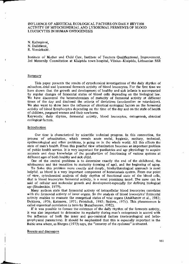
INFLUENCE OF ABIOTICAL ECOLOGICAL FACTORS ON DAILY RHYTHM ACTIVITY OF MITOCHONDRIAL AND LYSOSOMAL FERMENTS OF BLOOD LEUCOCYTES IN HUMAN ONTOGENESIS

N. Kacergiené, N. Dailidiené, R. Vernickaitè.

Institute of Mother and Child Care, Institute of Teachers Qualificational, Improvement, 3rd Materniry Consultation at Klaipeda town hospital, Vilnius—Klaipeda, Lithuanian SSR

Summary

This paper presents the results of cytochemical investigations of the daily rhythm of mitochondrial and lysosomal ferments activity of blood leucocytes. For the first time we have shown that the growth and development of healthy and sick infants is accompanied by regular changes of fermental status of blood cells depending on the biological law. We have discovered the heterochronism of maturity of fermental activity at different times of the day and disclosed the criteria of deviations (acceleration or retardation). We also want to show here the influence of abiotical ecological factors on the fermental activity of blood lymphocytes depending on the time of the day and on the state of health of children, pregnant women and their newborns. Keywords: daily rhytms, fermental activity, blood leucocytes, ontogenesis, abiotical ecological factors.

Introduction

Our time is characterized by scientific technical progress. In this connection, the process of urbanization, which reveals acute social, hygienic, sanitary, technical, epidemiological and other problems, is going on in the whole world. All this effects the state of man's health. From this pointof view urbanization becomes an important problem of public health service. It is very important for paediatrics and age physiology to acquire accurate and deep knowledge of the peculiarities of functioning of various systems at different ages of both healthy and sick child.

One of the central problems is to determine exactly the end of the childhood, the adolescence and the transition to maturity (coming of age), and the beginning of aging.

To Solve this problem more exactly and deeply, biorhythmological approach is most helpful, as blood is a very important component of homeostasis system. From our point of view, cytochemical analysis of daily rhythm of functional state of the blood cells, that is blood leucocytes fermental activity, is a most promising trend. The same can be said of cellular and molecular growth and development-especially for defining biological age (Studenikin, 1979).

Many authors state that fermental activity of intracellular blood leucocytes correlates with the fermental activity of inner organs. So the analysis of blood leucocytes' fermental activity enables to evaluate the energetical status of vital organs (Atakhanov et al., 1982; Dukhova, 1976; Katosova, 1971; Petrichuk, 1985; Suslova, 1975). This phenomenon is called ergontical correlation (a term by Shmalhauzen, 1982).

If it was possible to foresee the existence of the daily rhythm of the ferments activity, it was also important to determine its regularity during man's ontogenesis in accord with the influence of both the inner and geo-cosmical factors (meteorological and helio-geophysical parameters). It should be emphasized that this is especially important in the Baltic area where, as Blutgen (1973) says, the "cemetry of the cyclones" is situated.

Results and discussion

161

r p -

Materials

To prove this, the blood of 322 healthy and sick children and adults (beginning with the second day of life till 50 years of age) in acute and chronic (respirationis and cardio-vascularis systems) diseases was tested during the day. We examined 30 healthy children, 14—15 years old, who are not active in sprots, 30 pregnant women, 85 women right after childbirth and newborns of these mothers. This investigation was made in the morning only.

Methods

The quantitative cytochemical method by Nartsissov (1968, 1969) was used to determine the activity of dehydrogenases (such as succinicdehydrogenasis — 1.3.99.1, a-glycero-phosphatdehydrogenasis — 1.1.2.1, glutaminicdehydrogenasis — 1.4.1.2, NAD.H2-dia-phorasis — 1.6.4.3) and hydrolases (such as alcalic-1.1.3.1 and acid — 3.1.1.2 phosphatases) in lymphocytes and neutrophyls blood at different times: at 9 o'clock in the morning and 5 o'clock in the evening. Fermental status of dehydrogenases was evaluated by parameters applied in clinical cytochemy (Nartsissov, 1984), and the quantitative activity of hydrolases was evaluated according to Shubich's (1965) principle.

To establish the influence of geo-cosmic factors on the fermental activity of blood leucocytes we performed a correlational analysis between intracellular fermental activity and meteorological factors (air temperature, relative and absolute air moisture, atmospheric pressure), the parameters of Solar activity (the quantity of Solar spots — W, the diameter of Solar spots — Sp, the density of the stream of Solar rays — F, the geomagnetic field of the Earth - A k ) .

The parameters of Solar activity were kindly submitted to us by the Murmansk laboratory of Ionosphere and meteorological data — by Lithuanian hydrometeorological station (tables TMM-1).

The statistical validity was evaluated according to Stjudent criterion (Urbakh, 1975). The biological law of the daily rhythm of mitochondrial and lysosomal ferments activity

has been shown with the help of the ontogenesis formula by Komissarova (1984). In Table 1 we are presenting only the main data of the succinicdehydrogenasis (SDH).

One can see that for the first time here we have shown that the growth and development of infants is accompanied by regular changes of fermental status of blood cells depending on the time of the day as is clearly seen in Table 1. Daily changes consist either in increasing of the activity of dehydrogenases of decreasing of the activity of hydrolases (alcalic phosphatase). The daily rhythm of changes in medium activity population cells is expressed most clearly in part of the cells with high activity and the variety of cells according to the fermental activity (Kacergienê, 1986).

The formula by Komissarova (1984) characterizing the dynamic of cytochemical index in ontogenesis, was used to reveal general biological regularities in the dynamics and the ripening (of the daily rhythm of blood leucocytes fermental status — Fig. 1). Formula of ontogenesis (by Komissarova, 1984):

i l i l Q =a- t1 • e - ßtJ, Aß = a- t1 • e - ßi1. (1)

Meanings: Q — average succinicdehydrogenasis (SDH) activity in one lymphocytes; Aß — amplitude daily rhythm activity SDH in one lymphocyte; ti — square root of age (the intrauterine period included); e — the basis of natural logarithms; a, ß — constants received on the basis of empiric data by the method of minimal squares.

One more formula is necessary, i.e. the formula of the rate of growth:

V = Q ( -L -ß), (2)

V' which can be used to find the time of achieving the maximum:

162

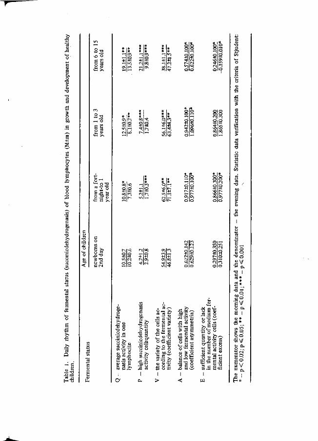
Si

ft O

•o

5 o

E +i

o

T3

o

3

60 O

>> X !

E •B >>

•e >>

Q

- ! C S

•7Ï ^ 'S1 3

HTS

S »

o 2

l-H

ra Ä o

U-i

o 00

<;

o co E ä-O rt

A - O

"2 « S3 C (N

fe

* * f—1

+1 >-; ON

*-<

# * Oï

a *n ro »-<

» * * •~i +ï n r—i

( N

<D

8> 2

T3 >> 'S e T3 O .a e S "~ 'o £> , 3 > S w ' ^ o « ä 2 « W D l

ï> a E

# # < s "1 r-i i—<

# f " :

§ GO

* * * 00,

9 • ^

t ~

8

# 0 0

a oq O

VO

S ro i ^

•—j

+ï <"S i n

1~ :

9 i n

O

"*?

S fS o

r i

+Î r--«fr

O

I* >> •S3 •ga O o o 3 £• « . w 73)'-C

5 S X" js ta I I

* * "> +î °i r- •tf

o o * - H

s' • *

r 1/-3

d

o o >—< a M <N M3

d

O

> . T ; Ö H •>

fi e • 2 ^ o

>. O O

'S * o •G M Ä

o .£; o -S o

a

U'S la ^'•g'-S

<L> Ö ta t i g «

I H <u S3 O <4-i <D

73 - 5

I <!

o

* *

fl • * .

ro vo

o o 1—1

?l c» • *

o> o

o

'—' 9 VO ON o •—'

o o <s 9 •* VO oq o

o o m

s' i n •o oq t—<

9

s <n

o c <u « 3 o

o » »

S i-> ^*-^-

l i a s ' 3 D J C B 5 ß 2 ä . S E c I

w

3

•c

6 si

'$ a o

•c

E o CD

• O

•B •a c t a

o p o'

V

| #

TO *

| v / o c* Ë I O *

«s >=. o o S fi u< O

e° 3 V C ft U |

H *

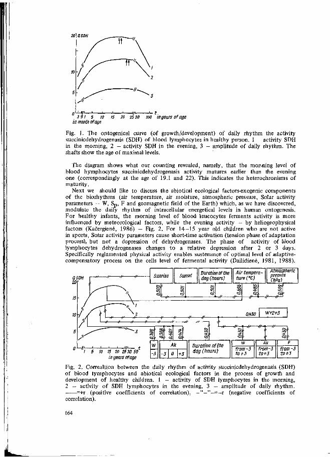
20 a SD H

->-t fl4i"—'—'—'—'—// 397 5 w 15 20 25 30 wo w years of age

in month of age

Fig. 1. The ontogenical curve (of growth/development) of daily rhythm the activity succinicdehydrogenasis (SDH) of blood lymphocytes in healthy person. 1 - activity SDH in the morning, 2 — activity SDH in the evening, 3 — amplitude of daily rhythm. The shafts show the age of maximal levels.

The diagram shows what our counting revealed, namely, that the morvning level of blood hymphocytes succinicdehydrogenasis activity matures earlier than the evening one (correspondingly at the age of 19.1 and 22). This indicates the heterochronisms of maturity.

Next we should like to discuss the abiotical ecological factors-exogenic components of the biorhythms (air temperature, air moisture, atmospheric pressure, Solar activity parameters — W, Sp, F and geomagnetic field of the Earth) which, as we have discovered, modulate the daily rhythm of intracellular energetical levels in human ontogenesis. For healthy infants, the morning level of blood leucocytes ferments activity is more influenced by meteorological factors, while the evening activity — by heliogeophysical factors (Kacergienè, 1986) — Fig. 2. For 14—15 year old children who are not active in sports, Solar activity parameters cause short-time activation (tension phase of adaptation process), but not a depression of dehydrogenases. The phase of activity of 61ood lymphocytes dehydrogenases changes to a relative depression after 2 or 3 days. Specifically reglamented physical activity enables sustenance of optimal level of adaptive-compensatory process on the cells level of fermental activity (Dailidiené, 1981, 1988).

1 S 10 IS 20 2530 SO

in years of age

from-3 to-t-3

Fig. 2. Correaltion between the daily rhythm of activity succinicdehydrogenasis (SDH) of blood lymphocytes and abiotical ecological factors in the process of growth and development of healthy children. I — activity of SDH lymphocytes in the morning, 2 — activity of SDH lymphocytes in the evening, 3 — amplitude of daily rhythm. —•—=+r (positive coefficients of correlation), —"—"—=—r (negative coefficients of correlation).

164

Solar activity parameters: W - quantity of Solar spots, Sp — diameter of Solar spots, F - density of stream of Solar rays, Ak - geomagnetic field of the Earth. O — on the day of cytochemical investigation, - 1 , - 2 , - 3 - days preceding the investigation and, +1, +2, +3 — days succeeding the investigation.

Sunrise and Sunset cause changes in the physical parameters of the surroundings. We can suppose that the child is not an exception. We carried out the cytochemical twice during the day (special determination of the fermental activity at the moment of Sunrise and Sunset was not performed because of ethical causes). However, retrognosis is possible (the calculations were made by method of linear regression — see Fig. 3).

The diagram shows that a certain tendency of the depression of succinicdehydrogenases activity levels after Sunrise becomes apparent and, vice versa activation apears — towards Sunset (but the level is different: the elevation here is less expressed).

Sunset' After Sunrise

*""3""~* Before Sunset

4 Time in the hauer

Fig. 3. The activity succinicdehydrogenases (SDH) of blood lymphocytes in healthy children depending on Sunrise and Sunset.(o, •) — empirical data the SDH of blood lymphocyte in the morning and the evening; theoretical data (curve). Thickenings on the absciss line — range ±a.

We have a sick child with morphogenesis not yet finished, so the peculiarities of the blood leucocytes fermental status daily rhythm in acute and chronic diseases are of great interest. We want to note in a few words, that we have found all types of daily rhythm disturbances in infants with acute and chronic diseases (respirationis and cardiovascularis systems), such as absence or disturbances of daily rhythm (deviations from normal daily rhythm), also elevation or depression of the amplitude. The changes of the blood leucocytes fermental status daily rhythm are detected for a longer period of time in individuals with chronic diseases.

We have established the criteria such as acceleration and retardation in age dynamics of the blood leucocytes fermental status daily rhythm (see Table 2).

Abiotical ecological factors influence the fermental activity of blood leucocytes depending on health status: for healthy infants the influence of the geophysical factors is more expressed in the evening and for a sick child — in the morning. In children with preclinical symptoms and before treatment of disease of respiratory and cardiovascular systems, we revealed external desynchronosis. Adequate therapy enables synchronization of the activity of analyzed blood leucocytes ferments activity with abiotical ecological factors.

For pregnant women increased index Ak causes decreasing of the energetical metabolism of blood lymphocytes and influences the physical development of a newborn: it depends on the intensity and prolongation of the in4luence of abiotical ecological factors in the critical periods of pregnancy ("around" terms of conception and organogenesis): we can expect either birth lowweight or newborns with a symptom of disharmonious development (Kaêergienè, 1988). When Solar activity is high, the bursting of amniotic waters can be

165

43

43 R

O 43 o, E >. •o o o

R

2 •o >> -S •o

o 43 O.

60

S •o >.

o 'S '3 o 3 00 f R

« E > 2 » E o

tS.s

3 co

£ .g o cd

43 H

c-j <u 3 « H

Vi o > R

R

2 •o ra •s «4—c O co

3 O hi Ü

o CN

m|<N r i h CN|O

u->ic*i "n <*l o i o

f i

?

O)

O)

?

~.j°Q O O

?

«i

-S2 o

cd o> • d T3 o —, Cd 4-J

• * R

« 60

2 R

o +- e .= 3 <3 > 2 S O'S o.

fl'SO

3 H C/3 cd cd O

O O ON «

•o O o r~

cd 'ß ca o .t i * §

8 4 3 " ° O Ö0 Q>

> to <U

•8<g2

e «o o

X I cd T3

, > e«

O CD cd .<2 R -o

'<" "É 2 <3

•S "^ cd (Ü

Ë | CD O1

5Cd.

<?

o> O

•O

q

cd R M a 3 S EIS CO (ü

••g* E 2 3 O

O ••e o

<2 2 •S<2 cd U

»e s

'S t3 c U CO (Ü

£.2 « • ^ 3 3 co

M-

• * '

f «?

o

M O

'c« C O

O

cd o 'S

^ • v

R O

"cd t-H

(U J-I o 0 " H

*-> CJ e 42

>> 42

E *+-! O co

'co co

II 45 .E

(D E <- <U =2 43 § 00 •a.S

O 43 1 cd

cd T3

+-» <o R

43 <D

I o. - .2 2 > R -a

S R o S O 43

~°% - ^ BÛ

c o

"O co

M>§ .3 o S 2 Ë ^ ^ CO

« a1

^ co

Ü1 O.R

« E

l 'a R °

expected 3 days before delivery; when the atmospheric level is higher, weakness of labor can be expected (Vernickaité, 1983; Vernickaitè et. al., 1988).

In conclusion, the ecological situation (that of elevated geophysical parameters) is an additional unfavourable factor which can disturb the adaptive-compensatory processes on the cell ferrmental (mitochondrial, lysosomal) levels in different times of the day and at different periods of human ontogenesis and can influence the decline of intrauterine and postnatal ontogenesis. The results dictate the necessity to create preservative means against the unfavourable influence of the geo-cosmical factors in order to optimize health status both of the growing generation and the whole population.

References

Atakhanov, Sh. E. et al., 1982. Correlation of dehydrogenasis activity of lymphocytes and inner organs. Medical Journal of "Uzbekistan". 5: 63—68.

Blutgen, 1., 1973. Geography of Climates (A shortened translation from German by Chap-lytina). 2. (in Russian).

Dailidiené, N. K., 1981. The State of health of pupils of the 7th and 8th forms who are not active in sports and its dependance on the level of physical training at school. Medi­cal Candidate's thesis. Vilnius.

Dailidiené, N. K., 1988. Peculiarities of adaptation of energy status of blood leucocytes of schoolchildren who are not active in sports depending on the parameters of Solar activity. In: The 5th Ail-Union symposium "Ecological-physiological problems of adaptation'. Moscow. P. 68—69.

Dukhova, Z. N., 1976. Changes of enzymic activity of lympocytes and different organs under the influence of hypoxishe factor. Biology Candidate's thesis. Moscow.

Kacergiené, N. B., 1986. Daily rhythm of ferment status of blood leucocytes in healthy and sick children. Medical doctorate's thesis. Vilnius. 1.

Kacergiené, N. B., 1988. Peculiarities of adaptation of the energetics of blood cells in women during childbirth and in their newborns depending of the ecological situation during the critical periods ot intrauterine ontogenesis. In: The 5th All-Union symposium "Ecological-physiological problems of adaptation". Moscow, p. 100—101.

Katosova, L. K., 1971. Cyto- and hystochemical analysis of lymphocytes and of some organs under experimental immunization and hypersensitivity of retarded type. Author's review of biology candidate's thesis. Moscow.

Komissarova, I. A., 1984. lnformativeness of ferment status of blood leucocytes for evalua­ting the state of health of normal and sick children. Medical doctorate's thesis. Moscow.

Nartsissov, R. P., 1968. Cytochemical analysis of nuclear and cytoplasmic structures in blood cells in children with leucaemia. In: Hystochemical methods in tumour diagnostics. Moscow, p. 134—141.

Nartsissov, R. P., 1969. The Use of violet para-nytrotetrazolium for quantitative cyto­chemistry of dehydrogenasis of man's lympphocytes. Journal Archives of Anatomy, Hystology and Embriology, 56(5): 85—91.

Nartsissov, R. P., 1984. Possibilities tor prognosis of clinical cytochemy. In: Soviet pae­diatrics. Moscow. 2. p. 267-274.

Petrichuk, S. V., 1985. The influence of electromagnetic field of infra-low frequency and of slight atmospheric changes on the fermental status of lymphocytes. Author's review of biology candidate's thesis. Moscow.

Studenikin, M. J., 1979. Criteria for the growth and development of the healthy child. In: Abstracts 'The healthy child" First International Paediatric Conference of European Countries. Moscow, p. 3.

Suslova, G. F., 1975. The Dynamics of some fermental systems of leucocytes and organs under the conditions of normal and pathological development. Biology Candidate's thesis. Moscow.

Shmalhauzen, I. I., 1982. Organism as a whole in its individual and historic development. Selected research works. Moscow. 383.

Shubich, M. G., 1965. Cytochemical definition of alcalise phosphatasis of leucocytes. Journal Laboratory Research. 1. 10—15.

167

Urbakh, V. J., 1975. Statistical analysis in biological and medical research. Moscow. Vernickaitè, R. B., 1983. Pathological changes in pregnant women and in their newborns

on the basis of cytochemical investigations of blood leucocytes. Medical candidate's thesis. Vilnius.

Vernickaitè, R. B., Kacergiené, N. B., 1988. Fermental activity of blood leucocytes in women, in pregnant women and in their newborns and its dependence upon ecological factors. In: The 5th All-Union symposium "Ecological-physiological problems of adap­tation". Moscow, p. 48-49.

168

ELF ELECTROMAGNETIC FIELDS AS A NEW ECOLOGICAL PARAMETER

Temurjants, N.A., Sidyakin, V.G., Makejev, V.B., Simferopol State University, USSR. Vladimirsky, B.M., Crimean Astrophysics Observatory, USSR.

Summary

A short review of the investigated problem 'Solar activity and the Bios­phere' is presented below. The research was being carried out by the Sim­feropol State University, the Crimean Medical Institute and the Crimean Astrophysics Observatory in the years 1972-1985. The main conclusion is that the effect of solar activity upon medical and biological processes can be explained if one takes into account a new essential parameter in ecology - an electromagnetic background field at the Earth's surface in the VLF -ELF range.

Introduction

The problem of the effect of solar activity upon the Biosphere is an old controversy and has had a long history. At present the problem in question hardly seems to attract the attention of scientists. The overwhelming ma­jority of researchers considers the effects of solar activity on the bio-phere to be a myth or at least a pseudoscientific activity of some small groups of 'adherents'. However, we think that there is no basis for such an opinion. For the last ten years strong empirical evidence of correlations between the indices of solar (geomagnetic) activity and some biological parameters (or medical statistical data) has been obtained. In lots of ca­ses these correlations have a strong statistical significance, they are based on a large body of measurements and have been verified by independant groups in different laboratories. Unfortunately, there is no possibility here to present a full survey of the literature on the problem. Some impor­tant results were published in the collections of the articles edited by Gnevyshev, M.N. and 01', A.I. in 1972 /l/ and 1983 HI (one more paper is being prepared: / 3 / ) . An extensive discussion of the problem under study is given by the authors of the present paper in their monograph /4/.

The interdependence of solar activity variations and biological processes is a widely-spread phenomenon. It has revealed the major divisions of bio­logical systematics including bacteriology, entomology, ornitology, etc. The same type of regularity is observed in many topics of medicine, such as cardiovascular diseases, ophtalmology, nervous system diseases, psychiatry, pediatrics, etc. All the data are conditioned by uncontrolled environ­mental factors. The most essential feature of this operating agent can be defined by comparing the results of various observations. The main peculi­arities are as follows:

1. The operating physical agent penetrates into a laboratory room but it is modified by an electromagnetic screen.

2. This agent is constantly present, and yet it has diurnal and seasonal variations.

3. Some parameters of the agent (intensity?) change with variation of the geographic latitude from the equator to the pole.

4. The modification of the agent parameters due to solar activity vari­ations is controlled both by solar wind variations and ionospheric disturbances.

Of all the known physical factors among the above mentioned characteristics

169

the variations of the Earth's electromagnetic field intensity in the very low frequency - extremely low frequency range satisfy very well. They are the VLF emission of the magnetosphere, the atmospheric and geomagnetic micropulsations. Nowadays the electromagnetic nature of the operating fac­tors is established by considering the discovery of the biological sys­tem's very high sensitivity to electromagnetic fields in the VLF range. This discovery seems to be the most important event throughout the long history of investigating the problem in question.

We present here a short review including the major results of the inves­tigations done by the researchers of the Simferopol State University, the Crimean Medical Institute and the Crimean Astrophysics Observatory. In this paper we shall confine ourselves to exemplifying the most relevant findings without going into additional details (see also /4/ and the refe­rences therein).

Influence of very weak electromagnetic fields

Several types of experiments with small intensity alternating magnetic fields have been carried out. Fig. 1 shows typical results obtained for pigeons. The birds were exposed to a magnetic field of 8 Hz-frequency (in­tensity - 5000 nT) for 3 hours per day. To test the nervous system perfor­mance the capacity of fulfilling classical conditioned reflexes was used. In fig. 1 this is shown by the upper curves as a function of time (1: mo­del; 2: experiment). One can see some reduction of the reflexes following the exposure to the field (up to 70%). It should be noted that during mag­netic storms the reduction of the reflex performance was also observed (for details see / 5 / ) . An influence of alternating magnetic fields on the nervous system of birds measured in different tests was revealed to be de­pendent upon the electromagnetic field parameters. To study these depen­dences large numbers of experiments were carried out.

Spectrum measurement of alternating magnetic field Biological activity

Special series of experiments were done to study the frequency-dependent field activity. Up to 15 different biological indices for rats were mea­sured for each value of frequency. Forty frequencies ranging from 0.01 Hz to 100 Hz for the three intensity levels of 5000 nT, 500 nT and 5 nT were analysed. The experiments were carried out in a special screened chamber. An exposure of 3 hour duration was used in each experiment. The typical situation is given in fig.2. Here the ordinate points to the activity of one of the enzymes in the rat's blood. The abscissa indicates frequency (Hz). Vertical lines at the bottom are measures of the statistical signi­ficance of the difference between the model and the experiment. It is evi­dent that the biological effect of the field has a strong dependence upon the frequency: at some frequency values the enzymatic activity is enlarged, at the other it is decreased. Several hundreds of experiments were perfor­med to verify the reproductivity of measurements. As a result, 'active' frequencies were revealed. Within the above-mentioned range these frequen­cies are as follows: 0.02 Hz, 0.5-0.6 Hz, 5-6 Hz, 8-11 Hz. One of these 'active' frequencies is close to the standard frequency of Pc 3 geomagne­tic micropulsations (0.02 Hz). An other such frequency coincides with the well-known fundamental frequency of the ionospheric waveguide (8 Hz). The activity spectrum has been found out to be partly dependant upon the field intensity.

170

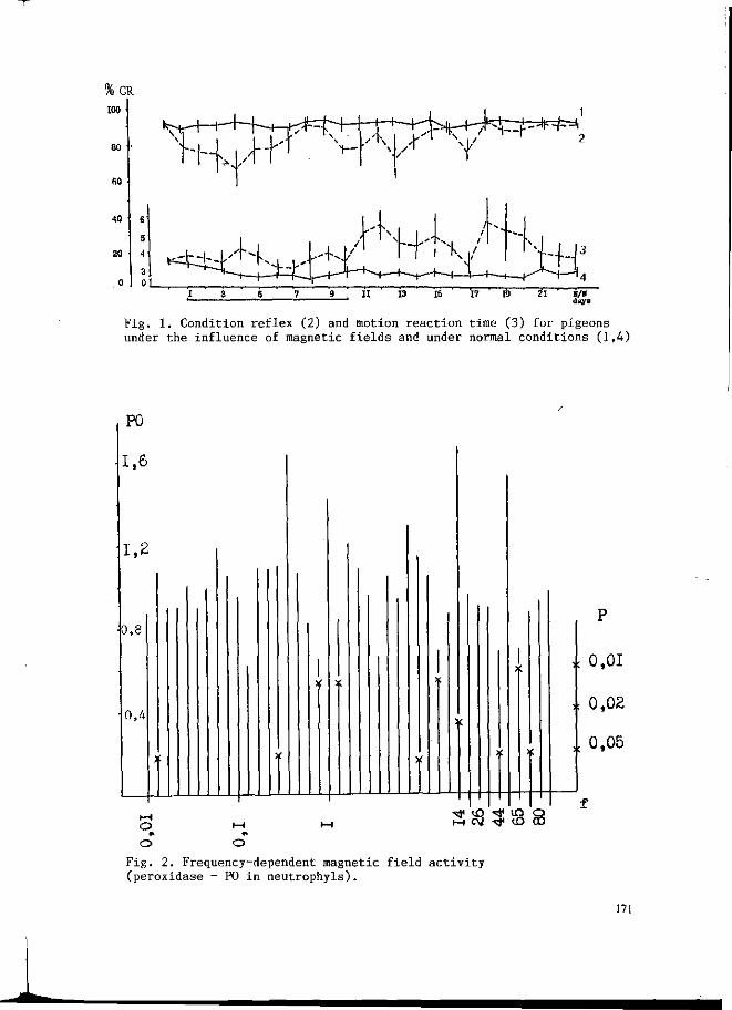
%GR

100

fiO

40

20

WH

3 .0 I 0 t

^H^jX^k, yX^Y 7 9 , II 13 15 17 19 21 H/H

days

Fig. 1. Condition reflex (2) and motion reaction time (3) for pigeons under the influence of magnetic fields and under normal conditions (1,4)

P0

1,6

1.2

0.Î

0,4

O O

•^ O "tf lO

Fig. 2. Frequency-dependent magnetic field activity (peroxidase - P0 in neutrophyls).

P

0,01

0,02

0,05

171

Fig. 3. Correlations between biological effects and field intensity.

Interdependence between biological effects and field intensity

Special experiments were also carried out to examine the dependence of biological effects upon the field intensity for the only one frequency value. An example is presented in fig. 3. In this case only one isolated frequency was used - 8 Hz. The ordinate shows the glycogen concentration in the rabbit's blood. It is clear that growth in the field intensity gives no rise to stronger biological effects. The presence of a certain optimum intensity in some intensity range is clearly seen in these expe­riments. Thus, the dependence of biochemical or physiological changes upon the field intensity has in general a very complex non-linear form.

It is important to mention that while certain biological and biochemi­cal changes were taking place the minimum field intensity for mammalia was as small as 0.2 nT (with a frequency of 8 Hz and an exposure time of 3 hours). For the electric field the exposure was about 0.1 V/m.

Traditionally, biophysicists have considered specific effects of the electromagnetic field in biological tissue to be hardly possible for such small intensities. However, over the past two decades we have been wit­nessing growing awareness that very weak alternate electric and magnetic fields do have clear effects on a living organism. Such effects are, of course, hardly explainable in the simplified terms of Joule heating. A new approach to understanding these results is necessary (a number of reviews on this new branch of investigation, i.e. biological action of non-ionising radiation, are available - see / 6 / ) .

172

Conclusion

Our most relevant conclusion is that natural electromagnetic fields within the low frequency - extreme low frequency range should be regarded as an essential factor in ecology. These electromagnetic background fluc­tuations are closely related to solar activity variations. Thus, the solar activity influence upon medical and biological processes can be explained by taking into account this new ecological agent.

References

1. Gnevyshev, M.N., 01', A.I. (Eds.): "Effects of Solar Activity on the Earth's Atmosphere and Biosphere". In: Progr. Sei. Transi., Jerusa­lem, Israel, 1977, 245 p. or In: Moscow, 1971, 224 p. (in Russian).

2. Effects of Solar Activity on Biosphere. In: Problems of Space Biolo­gy. Moscow: Nauka, 1982. Vol. 43, 265 p. (in Russian).

3. Clinical and Biophysical Aspects of Heliobiology. In: Problems of Space Biology. Moscow: Nauka, 1988. Vol. 56, 250 p. (in Russian).

4. Sidyakin, V.G., Temurjants, N.A. , Makejev, V.B., Vladimirsky, B.M. (1985): "Space Ecology". Kiev: Naukova Dumka, 176 p. (in Russian).

5. Sidyakin, V.G. (1986): "Effects of Global Ecological Factors on the Nervous System". Kiev: Naukova Dumka, 159 p. (in Russian).^

6. Temurjants, N.A., Vladimirsky, B.M., Tishkin, O.G. (1989): "Extremely Low Frequency Signals in the World of Biology". Kiev: Naukova Dumka, (in Russian - to be printed).

173

THE POSSIBLE GRAVITATIONAL NATURE OF FACTORS INFLUENCING DISCRETE MACROSCOPIC FLUCTUATIONS

N.V. Udaltsova, V.A. Kolombet and S.E. Shnol'

Physical Biochemistry Laboratory, Institute of Biological Physics Acad. Sei. USSR, 142292 Puschino, Moscow Region (USSR)

Summary

An amplitude of the "scatter in the results" of measurements of various processes changes with time in a very complicated way. The fluctuation amplitude and the shape of the spectrum of the states of objects of dif­ferent natures depend on universal cosmophysical factors. Phenomena are described which permit the assumption that a set of discrete states of environmental objects is associated with some type of gravitational ef­fects.

1 Cosmophysical correlations of macroscopic fluctuations

The amplitude of fluctuations of many processes and discrete distribu­tions of measurement results are fine indicators of cosmophysical pro­cesses (Udaltsova et al., 1983, 1987). "Macroscopic fluctuations" (MF) manifest themselves as spontaneous synchronous transitions of some pro­perties of macroscopic objects from one discrete state to another (Shnol' & Kolombet, 1980).

The 30-year investigations of our laboratory show that the value of the fluctuation amplitude when measuring the rates of biochemical and chemi­cal reactions depends on Solar activity. During the years of high Solar activity the average amplitude was low, whereas during the years of low Solar activity a rather large fluctuation amplitude was observed (Udalt­sova et al., 1983).

The MF amplitude changes two days ahead of the sector boundaries of the interplanetary magnetic field (IMF). Such a relation allows us to assume the rate of changes of the MF "cause".

Fig. 1 shows deviations of the MF amplitude from the mean value around the days of the sign change of the IMF sector (summation by the method of superimposed epoch).

The spectral frequency analyses of daily measurements of the mean-root-square MF amplitude has shown that there is a reliable period of 29.5 days (see Fig.2). This period is in agreement with the period of the Moon phase changes. The analysis of latent periodicities, according to the data obtained in various years, showed the existence of periodicities of i , 1,2 and 4 years in the changes of average monthly MF amplitudes of biochemical and chemical processes. Such periods vary in intensity in different years. These variations may depend on the Solar activity.

2 Macroscopic fluctuations and the Moon position

During continuous measurements, which lasted for several months with 1-min intervals, of a-decay of 239pu samples the shape of histograms of the results of measurements was found to correlate with the position of the Moon relative to the horizon. The shapes of histograms, each plotted by 60 measurements of 239pu a -decay, were similar during the moon-rise and the following moonset. A quantitative estimation of the similarity in

174

-4 -2 A 2 4

0.4 •

0.2 -

0.0 -

-0.2 -

-0.4 +

2 4 days

Fig. 1. MF amplitude on days of the sign change of the IMF sector (1976-1984). The Y-axis is a diviation of the amplitude from the mean value during those days. /

i r 1 r n r 10 20

—r 30

I

40 T (days)

Fig. 2. Spectral density of daily MF amplitude values (1981-1985). 95% reliable intervals are indicated.

175

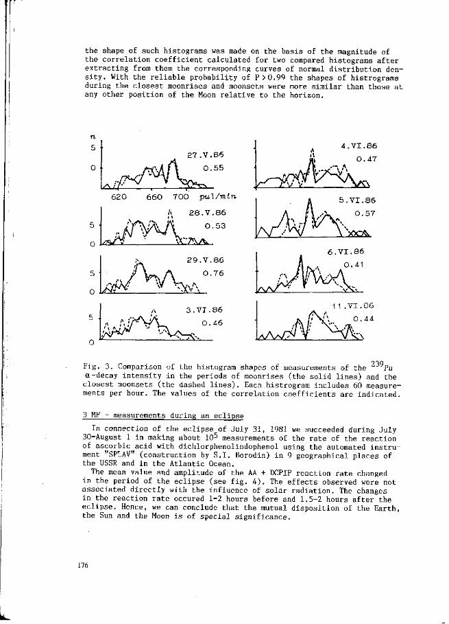
the shape of such histograms was made on the basis of the magnitude of the correlation coefficient calculated for two compared histograms after extracting from them the corresponding curves of normal distribution den­sity. With the reliable probability of P>0.99 the shapes of histrograms during the closest moonrises and moonsets were more similar than those at any other position of the Moon relative to the horizon.

620 660 700 pul/mln

l\ E8.V.86

0.53 / A'* l'\ 'X.

'V /

5 .VI .86 0 .57

f"\ /* ll

6 . V I . 8 6

N " °'4"1 < \ * . A / \ A / \ — / \ \/V" /^ \

Fig. 3. Comparison of the histogram shapes of measurements of the Pu «-decay intensity in the periods of moonrises (the solid lines) and the

closest moonsets (the dashed lines). Each histrogram includes 60 measure­ments per hour. The values of the correlation coefficients are indicated.

3 MF - measurements during an eclipse

In connection of the eclipse of July 31, 1981 we succeeded during July 30-August 1 in making about 105 measurements of the rate of the reaction of ascorbic acid with dichlorphenolindophenol using the automated instru­ment "SPLAV" (construction by S.I. Borodin) in 9 geographical places of the USSR and in the Atlantic Ocean.

The mean value and amplitude of the AA + DCPIP reaction rate changed in the period of the eclipse (see fig. 4 ) . The effects observed were not associated directly with the influence of solar radiation. The changes in the reaction rate occured 1-2 hours before and 1.5-2 hours after the eclipse. Hence, we can conclude that the mutual disposition of the Earth, the Sun and the Moon is of special significance.

176

4 5 6 7

hours of the day

Fig. 4. a - Measurements of two components of the AA + DCPIP reaction rate obtained by G.I. Zadonsky (Moscow) in the period of the Solar eclipse on July 31, 1981. V-i is the first component of the reaction rate. V£ is the second com­ponent. The X-axis is the Moscow time in hours of the day. b - Histograms of the measurements shown in fig. 5a : 1 -before the eclipse maximum, 2 - after the eclipse maximum.

177

During the eclipse and sunsets a reliable decrease in the rate of the reaction of AA with DCPIP was observed. Fig. 5 shows the changes of the mean values of the AA + DCPIP reaction rate, (a), the summation accor­ding to the moment of the sunset, (b), the summation according to the eclipse maximum (data at 5 geographical points close to the line of the full eclipse: the Caucasus, Tomsk, Bratsk, the Baikal, Sachalin). Stan­dard deviations are indicated. Data were normalized.

Fig. 6 shows the daily course of hourly averages of the AA + DCPIP reaction rate during the period of July 30 - August 1 at 5 geographical points: the White Sea, the Caucasus, the Baikal, Sachalin, the Atlantic Ocean. Average values of the reaction rate do not depend on temperature variations as fig. 6l> shows (data at the same geographical points).

The daily course and the observed effects of the changes in the measure­ment values of the AA + DCPIP reaction rate allow us to assume a relation with the rotation of the Earth around its axis.

n

0.5 |-

0

-0.5

0.5

0

-0.5

sunset

5 min

V n

0 .5

0

-0.5

a

1

/

'W r r**

sunr i se

-*

\ V. sunset

50 min

iJt^t^^irfte} 1 ' J ._ _1__1 L__l- _L

12 18 24

hours of the day

Fig. 5 MF in the periods of the eclipse and the sunset

Fig. 6 The daily course of hourly averages of model reaction rate

178

4 Macroscopic fluctuations and the Earth surface vibrations

It is possible to presume that a set of discrete states of environmen­tal objects is associated with some type of gravitational effects. A com­parison of the shapes of histograms of the results of measurements of the Earth surface vibrations taken with a vertical seismometer*, and histograms of the results of measurements of 239pu a-decay synchronous with the previous ones (see fig. 7 ) , can be considered as a corrobora­tion of the conclusion on the gravitational nature of the analized phenomenon.

E.v

20-40 ^

10.. 20

-100 O 100 mm*70 680 660 640 pul/min

Fig . 7 . Comparison of the histogram shapes of t he measurements of the a -decay of 239pu sample in Pushchino ( the dashed l i n e s ) and the Earth surface v i b r a t i ons in T b i l i s i ( the s o l i d l i n e s ) . Each histogram was obtained during 6 hours . 1 - from 19:12 V.26.86 2 - from 1:52 V.27.86 3 - from 8:32 V.27.86 4 - from 15:12 V.27.86 5 - from 21:52 V.27.86 6 - from 4:32 V.28.86 7 - from 11:12 V.27.86 8 - from 17:52 V.28.86

179

5 Conclusion

The following results evidence in favour of the gravitational na­ture of the external factor:

(1) changes in the measured values during sunsets and eclipses (the mutual disposition of the Sun, the Earth and the Moon is of great importance);

(2) the similarity in the shapes of histograms during moonsets and moon-rises;

(3) the similarity in the shapes of histograms of the results of simul­taneous measurements of radioactivity and amplitudes of the Earth surface vibrations;

(4) the period of 29.5 days in the changes of the MF amplitude (the period of changes of the Moon phases);

(5) the independence of the observed effects on the nature of the shields (Udaltsova et al., 1987);

(6) a change in the MF amplitude two days before a change occurs in the sign of the IMF (the relativistic rate of the changes of the MF "cause");

(7) the daily course of the changes in the measurement values and the MF amplitude (relation to the rotation of the Earth around its axis).

References

Shnol', S.E. & Kolombet, V.A. (1980) "Macroscopic fluctuations and sta­tistical spectral analyses of the states of aqueous protein solutions" In: Sov.Sci.Rev. (D) OPA. 1(4): 399-445.

Udaltsova, N.V., Kolombet, V.A. and Shnol', S.E. (1987) "Possible cosmo-physical explanation of macroscopic fluctuations in processes of dif­ferent nature". Pushchino, (in Russian).

Udaltsova, N.V., Agulova, L.P., and Shnol', S.E. (1983) "Correlation of macroscopic fluctuation amplitude of different characteristics of aqueous solutions of proteins and other substances with some cosmogeo-physical factors". In: Physico-chemical bases of cell functioning. Pushchino. p. 21-30 (in Russian).

(*) We express our gratitude to E.M. Lin'kov and L.N. Petrova (Leningrad University) for correspondent data.

180

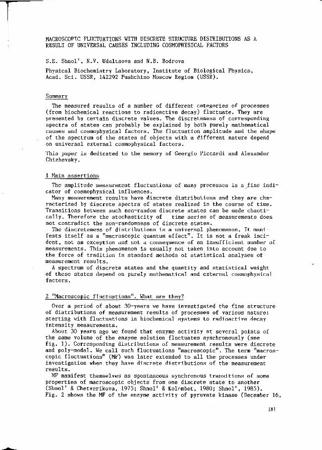
MACROSCOPIC FLUCTUATIONS WITH DISCRETE STRUCTURE DISTRIBUTIONS AS A RESULT OF UNIVERSAL CAUSES INCLUDING COSMOPHYSICAL FACTORS

S.E. Shnol', N.V. Udaltsova and N.B. Bodrova

Physical Biochemistry Laboratory, Institute of Biological Physics, Acad. Sei. USSR, 142292 Pushchino Moscow Region (USSR).

Summary

The measured results of a number of different categories of processes (from biochemical reactions to radioactive decay) fluctuate. They are presented by certain discrete values. The discreteness of corresponding spectra of states can probably be explained by both purely mathematical causes and cosmophysical factors. The fluctuation amplitude and the shape of the spectrum of the states of objects with a different nature depend on universal external cosmophysical factors.

This paper is dedicated to the memory of Georgio Piccardi and Alexander Chizhevsky.

1 Main assertions

The amplitude measurement fluctuations of many processes is a £ine indi­cator of cosmophysical influences.

Many measurement results have discrete distributions and they are cha­racterized by discrete spectra of states realized in the course of time. Transitions between such non-random discrete states can be made chaoti­cally. Therefore the stochasticity of time series of measurements does not contradict the non-randomness of discrete states.

The discreteness of distributions is a universal phenomenon. It mani­fests itself as a "macroscopic quantum effect". It is not a freak inci­dent, not an exception and not a consequence of an insufficient number of measurements. This phenomenon is usually not taken into account due to the force of tradition in standard methods of statistical analyses of measurement results.

A spectrum of discrete states and the quantity and statistical weight of these states depend on purely mathematical and external cosmophysical factors.

2 "Macroscopic fluctuations". What are they?

Over a period of about 30-years we have investigated the fine structure of distributions of measurement results of processes of various nature: starting with fluctuations in biochemical systems to radioactive decay intensity measurements.

About 30 years ago we found that enzyme activity at several points of the same volume of the enzyme solution fluctuates synchronously (see fig. 1). Corresponding distributions of measurement results were discrete and poly-modal. We call such fluctuations "macroscopic". The term "macros­copic fluctuations" (MF) was later extended to all the processes under investigation when they have discrete distributions of the measurement results.

MF manifest themselves as spontaneous synchronous transitions of some properties of macroscopic objects from one discrete state to another (Shnol' & Chetverikova, 1975; Shnol' & Kolombet, 1980; Shnol', 1985). Fig. 2 shows the MF of the enzyme activity of pyruvate kinase (December 16,

181

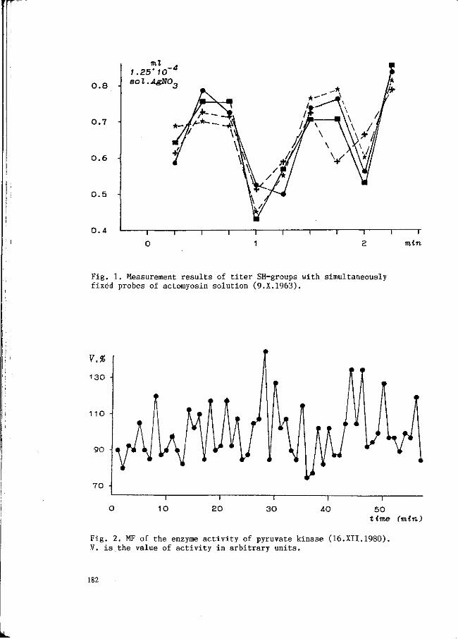
0 . 8

0 . 7

0 .6 •

0 . 5

0 . 4

ml - 4 1.25'10 so~l.AgN03

"T" 0

i r "i r mtn

Fig. 1. Measurement results of titer SH-groups with simultaneously fixed probes of actomyosin solution (9.X.1963).

V.%

130

110

90 -

70

I 0 10

I 2 0

I 3 0

I 40

I 5 0

time (min)

Fig. 2. MF of the enzyme activity of pyruvate kinase (16.XII.1980). V. is the value of activity in arbitrary units.

182

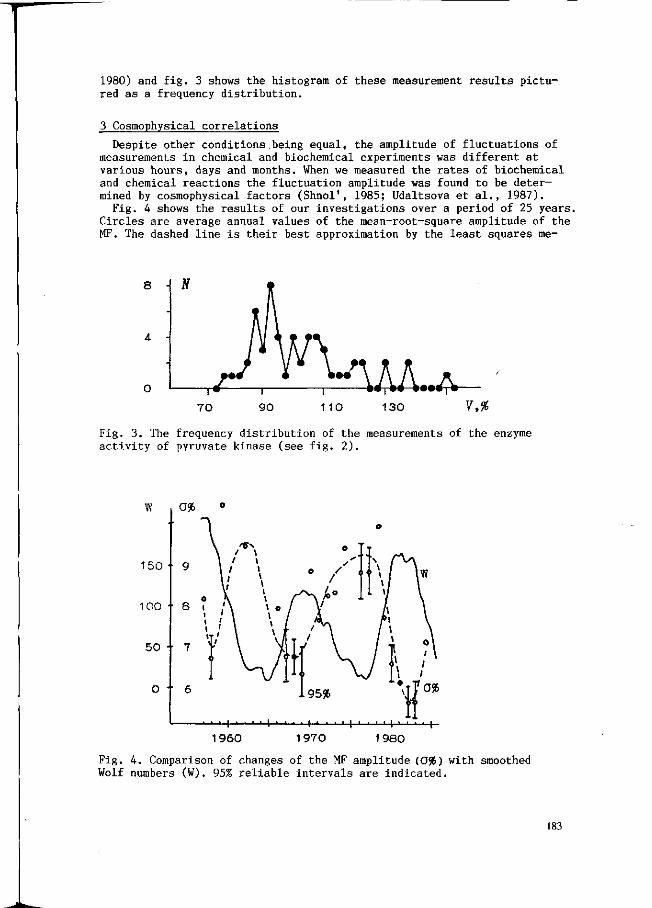
1980) and fig. 3 shows the histogram of these measurement results pictu­red as a frequency distribution.

3 Cosmophysical correlations

Despite other conditions being equal, the amplitude of fluctuations of measurements in chemical and biochemical experiments was different at various hours, days and months. When we measured the rates of biochemical and chemical reactions the fluctuation amplitude was found to be deter­mined by cosmophysical factors (Shnol', 1985; Udaltsova et al., 1987).

Fig. 4 shows the results of our investigations over a period of 25 years. Circles are average annual values of the mean-root-square amplitude of the MF. The dashed line is their best approximation by the least squares me-

8

UÂ-A-130 7,%

Fig. 3. The frequency distribution of the measurements of the enzyme activity of pyruvate kinase (see fig. 2).

w

150 •

100 •

50 •

o •

a%

9

• 8

• 7

' 6

0

\ 1ÏN

\ ' »

V » ^ \ A \ • / i i M \ i i Un

• - ' i • • • • i ' • • •

o

o

o / ' ,

•Vit- 1 y

• V

A ' \ / / \ /

f \ '

9556

l i i i i i i i i i i

f l !

\->->-

W

o\ ; \ / /

1960 19T0 1980

Fig. 4. Comparison of changes of the MF amplitude (ö%) with smoothed Wolf numbers (W). 95% reliable intervals are indicated.

183

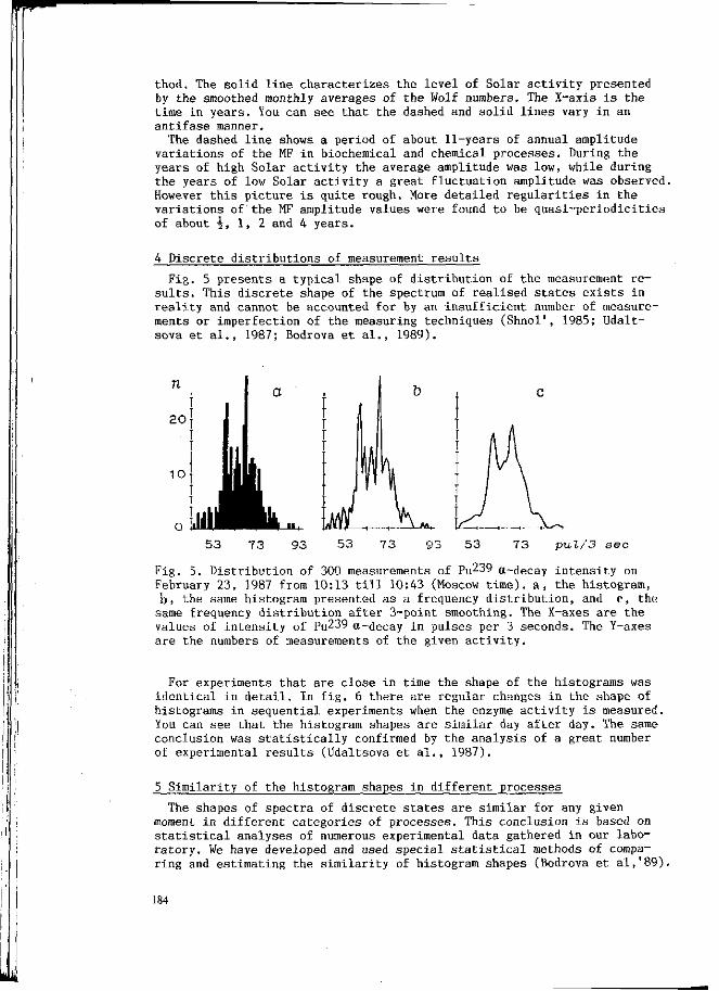
thod. The solid line characterizes the level of Solar activity presented by the smoothed monthly averages of the Wolf numbers. The X-axis is the time in years. You can see that the dashed and solid lines vary in an antifase manner.

The dashed line shows a period of about 11-years of annual amplitude variations of the MF in biochemical and chemical processes. During the years of high Solar activity the average amplitude was low, while during the years of low Solar activity a great fluctuation amplitude was observed. However this picture is quite rough. More detailed regularities in the variations of the MF amplitude values were found to be quasi-periodicities of about $, 1, 2 and 4 years.

4 Discrete distributions of measurement results

Fig. 5 presents a typical shape of distribution of the measurement re­sults. This discrete shape of the spectrum of realised states exists in reality and cannot be accounted for by an insufficient number of measure­ments or imperfection of the measuring techniques (Shnol', 1985; Udalt-sova et al., 1987; Bodrova et al., 1989).

ijrtLk* 53 T3 92 53 73 53 73 pul/3 sec

Fig. 5. Distribution of 300 measurements of Pu239 a-decay intensity on February 23, 1987 from 10:13 till 10:43 (Moscow time), a, the histogram, b, the same histogram presented as a frequency distribution, and c, the

same frequency distribution after 3-point smoothing. The X~axes are the values of intensity of Pu239 a-decay in pulses per 3 seconds. The Y-axes are the numbers of measurements of the given activity.

For experiments that are close in time the shape of the histograms was identical in detail. In fig. 6 there are regular changes in the shape of histograms in sequential experiments when the enzyme activity is measured. You can see that the histogram shapes are similar day after day. The same conclusion was statistically confirmed by the analysis of a great number of experimental results (Udaltsova et al., 1987).

5 Similarity of the histogram shapes in different processes

The shapes of spectra of discrete states are similar for any given moment in different categories of processes. This conclusion is based on statistical analyses of numerous experimental data gathered in our labo­ratory. We have developed and used special statistical methods of compa­ring and estimating the similarity of histogram shapes (Bodrova et al,'89)

184

Fig. 6. Regular changes in the shape of histograms in sequential experiments with measurements of the enzymatic acti­vity: 1 - hexokinase, 13.12.77, morning; 2 - creatine kinase (CK), 13.12.77, evening; 3 - CK, 14.12.77, morning; 4 - CK, 14.12.77, evening; 5 - CK, 15.12.77, morning; 6 - CK, 15.12.77; evening; 7 - CK, 16.12.77, morning; 8 - CK, 16.12.77, evening; The abscissa axis shows values of enzymatic activity in arbitrary units; the ordinate axis shows the number of samples with the given enzymatic activity.

Fig. 7 shows histograms of simultaneous measurements of a model chemi­cal reaction rate (in the left hand column) and the a-decay intensity (in the middle). In the column on the right there are comparisons of synchro­nous histograms. You can see that synchronous histograms of different processes are similar and the sequentional histograms of each process are different. Such synchronization is often observed even when the distance between the laboratories is hundreds or thousands of kilometers.

In Fig. 8 there are combined histograms of the measurements obtained in Pushchino, Moscow Region and in Tomsk, Siberia (both around the latitude of 56° North). In Pushchino we measured a model chemical reaction rate and at the same time in Tomsk Ludmila Agulova measured the amplitude of auto-oscillation in the Belousov-Zhabotinsky reaction. The measurements were obtained simultaneously and you can see that synchronous histograms are similar.

The existence of universal cosmophysical causes or factors determining at any moment the spectrum of discrete states of different objects under investigation follows from these and other similar results. Thus, cosmo­physical factors determine the amplitude of fluctuations or width of corresponding distributions and also the shape of spectra of the states.

6 Arithmetical hypothesis of the discreteness of histograms

Any process is the result of some given interactions. Hence each process has discrete distributions. How is this obtained? A reaction rate, a radioactive decay intensity at any moment are results of multiplications of the interaction probability, that is concentrations of initial sub­stances (Bodrova et al., 1989).

Generally we can write: V = K * C * D, where V is the reaction rate or intensity of the process, C and D are concentrations or probabilities of

185

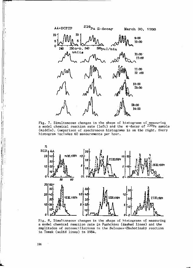
AA+DCPIP

10

339. Pu a-de cay- March. 30. 1988

00 00

140 I50ar-b. 540 SMpul/min

y

:00 00

^

Fig. 7. Simultaneous changes in the shape of histograms of measuring a model chemical reaction rate (left) and the a-decay of 239pu sample (middle). Comparison of synchronous histograms is on the right. Every histogram includes 60 measurements per hour.

ivrnsz* 10 •20-

•10

10 imsat

Fig. 8. Simultaneous changes in the shape of histograms of measuring a model chemical reaction rate in Pushchino (dashed lines) and the amplitudes of autooscillations in the Belousov-Zhabotinsky reaction in Tomsk (solid lines) in 1984.

186

interactions. C and D fluctuate within the range of their corresponding values. Measuring V we can obtain various values with different proba­bilities. For example we cannot obtain prime numbers. The probability of obtaining a given value is defined by the number of ways of obtaining this value by multiplication. This probability is proportional to the number of multipliers of the value V. So, for two-symbol numbers after multiplication we can obtain 12 in 2 ways (2*6 and 3*4), 24 in 3 ways, 60 in 5 ways and prime numbers in no way.

Fig. 9.

Tl - number of multipliers for values V

Our values have many symbols, but the shape of the distribution of the number of multipliers persists for the numbers with many symbols. You can see sections of this distribution in fig. 10.

2 0 Ï

•—~- 1 2 0

*--*- 9 0 0 N

Fig. 10. Distribution of the number of multipliers for different inter­vals of the numerical axis.

Thus the distribution of measurement values should be discrete because of pure mathematical reasons. However, to explain the main phenomena, which included simultaneous changes and similarity in the shapes of histograms in different-nature processes, external cosmophysical reasons have to be assumed. The discrete shape of experimental histograms should correspond to the shape of distribution of the number of multipliers at certain intervals on the numerical axis. The location and length of these inter­vals may depend on cosmophysical factors.

7 Conclusion

The following conclusions can be made reviewing the thirty-year studies of macroscopic fluctuations: (1) Macroscopic fluctuations, i.e. transitions of macroscopic objects

187

from one discrete state to another, can be recorded in processes of dif­ferent nature: from biochemical reactions to radioactive decay. (2) The discreteness of corresponding spectra of states can probably be explained by the fact that the measured values are determined by produc­tion of probabilities of reagent interactions. (3) The fluctuation amplitude and the shape of the spectrum of the states of objects with a different nature depend on universal external cosmo-physical factors.

Acknowledgements

The authors are thankful to A.S. Dansky, L.M. Ovchinnikova, T.Ya. Brit-sina, N.P. Ivanova, T.S. Malova and A.N. Zaikin for making experiments and to V.A. Namiot, F.I. Ataullakhanov, E.V. Khmaladze, L.A. Blumenfeld and A.S. Botin for numerous valuable discussions.

References

Bodrova, N.B., Udaltsova, N.V., Ivanov, P.S. and Shnol', S.E. (1979) "On the non-randomness of the shape of 'inconsistent' histograms". Push-chino (in Russian).

Shnol', S.E. and Chetverikova, E.P. (1975) "Synchronous reversible alte­rations in enzymatic activity (conformational fluctuations) in actomyo-sin and creatine kinase preparations". Biochem. Biophys. Acta. 403: 89-97.

Shnol', S.E. and Kolombet, V.A. (1980) "Macroscopic fluctuations and statis­tical spectral analyses of the states of aqueous protein solutions". In: Sov.Sci.Rev. (D). OPA. 1(4): 399-445.

Shnol', S.E. (1985) "Macroscopic fluctuations with discrete distribution of values in 1/F processes of different nature". In: General problems of physico-chemical biology. VINITI, Moscow. 5: 30-201 (in Russian).

Udaltsova, N.V., Kolombet, V.A. and Shnol', S.E. (1987) "Possible cosmo-physical origin of macroscopic fluctuations in processes of different nature". Pushchino (in Russian).

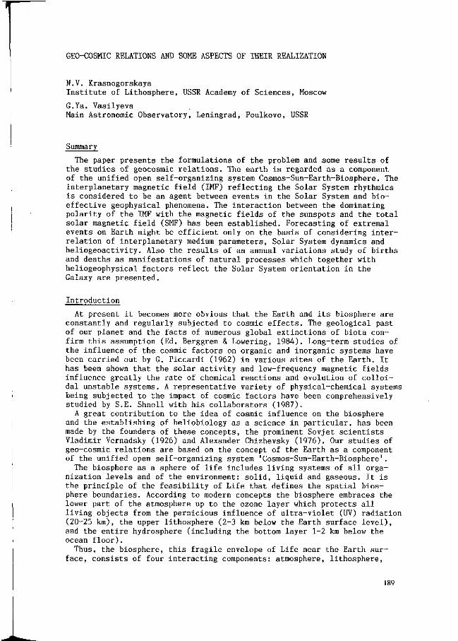
GEO-COSMIC RELATIONS AND SOME ASPECTS OF THEIR REALIZATION

N.V. Krasnogorskaya Institute of Lithosphère, USSR Academy of Sciences, Moscow

G.Ya. Vasilyeva Main Astronomic Observatory, Leningrad, Poulkovo, USSR

Summary

The paper presents the formulations of the problem and some results of the studies of geocosmic relations. The earth is regarded as a component of the unified open self-organizing system Cosmos-Sun-Earth-Biosphere. The interplanetary magnetic field (IMF) reflecting the Solar System rhythmics is considered to be an agent between events in the Solar System and bio-effective geophysical phenomena. The interaction between the dominating polarity of the IMF with the magnetic fields of the sunspots and the total solar magnetic field (SMF) has been established. Forecasting of extremal events on Earth might be efficient only on the basis of considering inter­relation of interplanetary medium parameters, Solar System dynamics and heliogeoactivity. Also the results of an annual variations study of births and deaths as manifestations of natural processes which together with heliogeophysical factors reflect the Solar System orientation in the Galaxy are presented.

Introduction

At present it becomes more obvious that the Earth and its biosphere are constantly and regularly subjected to cosmic effects. The geological past of our planet and the facts of numerous global extinctions of biota con­firm this assumption (Ed. Berggren & Lowering, 1984). Long-term studies of the influence of the cosmic factors on organic and inorganic systems have been carried out by G. Piccardi (1962) in various sites of the Earth. It has been shown that the solar activity and low-frequency magnetic fields influence greatly the rate of chemical reactions and evolution of colloi­dal unstable systems. A representative variety of physical-chemical systems being subjected to the impact of cosmic factors have been comprehensively studied by S.E. Shnoll with his collaborators (1987).

A great contribution to the idea of cosmic influence on the biosphere and the establishing of heliobiology as a science in particular, has been made by the founders of these concepts, the prominent Sovjet scientists Vladimir Vernadsky (1926) and Alexander Chizhevsky (1976). Our studies of geo-cosmic relations are based on the concept of the Earth as a component of the unified open self-organizing system 'Cosmos-Sun-Earth-Biosphere'.

The biosphere as a sphere of life includes living systems of all orga­nization levels and of the environment: solid, liquid and gaseous. It is the principle of the feasibility of Life that defines the spatial bios­phere boundaries. According to modern concepts the biosphere embraces the lower part of the atmosphere up to the ozone layer which protects all living objects from the pernicious influence of ultra-violet (UV) radiation (20-25 km), the upper lithosphère (2-3 km below the Earth surface level), and the entire hydrosphere (including the bottom layer 1-2 km below the ocean floor).

Thus, the biosphere, this fragile envelope of Life near the Earth sur­face, consists of four interacting components: atmosphere, lithosphère,

189

hydrosphere and biota. All four components are closely interconnected, so the ecologie changes in any link of this indissoluble natural chain causes as a rule violations in the other links even far remoted in space and time. It is the neglect of this unity, the ignorance of the general regularities of biospheric evolution as a unified system (moreover ignoring them at a social level) that led mankind to hard and sometimes irreversible conse­quences of its interference into the life of the Nature.

The existence of the biosphere as a life medium of biosystems is feasible only under the conditions of constant energy supply. This is what openness means: the entire biosphere as a unified non-linear multi-level system continuously exchanges matter, energy and information with the outer envi­ronments, such as the upper atmospheric layers, outer space and the Galaxy from one side and the Earth interior from another.

The task is to elaborate optimal scientific approaches to the systematic study of interaction between the outer environment and the Earth, and also to find efficient ways to preserve the life and biospheric resources. This complex problem can be solved only by combined efforts of various specia­lists who for this purpose comes as the necessary condition for success of the common cause. One main trend in these studies is to reveal the leading mechanisms of the external factors' effect on the biosphere and to fore­cast the consequences of this effect.

Electromagnetic and gravitational interactions present at any level of the Universe proved to be universal among the exterior and interior fac­tors effecting the biosphere (Ed. Krasnogorskaya, 1984). In particular, solar electromagnetic and corpuscular radiations subjected to various transformations on their way to the Earth do not reach its surface direct­ly. Only a part of the electromagnetic radiation in the optical and radio ranges and a small part of U-V radiation come via the Earth's atmosphere. While moving in its orbit Earth crosses the anisotropic interplanetary medium formed by the solar corpuscular radiation - the solar wind, the Solar System orientation in the Galaxy and the dynamics of the planetary system.

The variations of the solar wind velocity and interplanetary medium pa­rameters result in changes of the Earth's magnetosphere boundaries regis­tered by ground stations as the beginning of magnetic storms. Transfer and transformation of energy from the Sun to the biosphere run as a chain of events: changing of solar wind influences on the magnetosphere - ionosphe­ric disturbances - induction of telluric electric currents - origin of magnetic and electric fields variations registered practically everywhere and any time near the Earth's surface.

Simultaneous changes of vertical electrical and horizontal geomagnetic components of infra-low frequency (ILF) electromagnetic field (EMF) served as an experimental testimony of their time interrelation (Krasnogorskaya & Remizov, 1973). As geomagnetic pulsations are known to have a magneto-hydrodynamic nature, there are grounds to suppose that the measured elec­tric pulsations are also of cosmic origin.

The experimental modelling of ILF EMF influences on biological systems at various levels of organization shows that geomagnetic pulsations (Ben'kova, Shevnin, 1984) are biologically active factors and may be used to monitor the living systems (Krasnogorskaya & Rudakov, 1986).

Manifestation of a space-time structure of interplanetary magnetic fields in life rhythms

Heliogeoactivity is a property of the Solar System as a whole and the result of a manifestation of its self-organizing in the Galaxy. A solution of the heliogeoactivity problem may be suggested by considering the unified

190

open self-organizing system of the Universe in which the Sun, the plane­tary system and the interplanetary medium act as sub-systems.

The influence of cosmic factors on the biosphere is mediated by the Earth's atmosphere circulation, currents, Earth rotation parameters, vari­ations of gravity acceleration, etc. These factors in turn can be sensi­tive indicators of processes in the Solar System. In other words: the anisotropic distribution of the IMF in the Earth's orbit and plasmic in­stabilities deform the Earth magnetosphere on one hand, while on the other hand space-time changes of IMF serve as indicators of gravity effects, revealed in the Earth's rotation parameters. It is reasonable to trace correlational links of space-time changes of IMF parameters and biosphere components while searching for the mechanism of cosmic effects.

The similarity between cosmic conditions as the origin of solar flares and of extreme phenomena on the Earth, in particular of earthquakes (Bag-by, 1973) suggests that these events are one class of processes within the entire self-organizing Solar System. The energetic source for both solar flares and earthquakes is likely to be absorption of extremely low-frequency waves (with wave length close to the sizes of the Solar System) while the Solar System itself acts as a kind of antenna of the variable profile and directivity with episodic radiation focussing on the Sun and the earth (Vasilyeva et al.). Seismic regions on the Earth and active areas on the Sun may be compared to a receiver tuned to a given frequency range. We believe that effective forecasting of extremal events on the Earth may be provided only on the basis of interrelation of parameters of the interplanetary medium, Solar System dynamics and heliogeoactivity.

To establish common regularities of the biosphere evolution it is neces­sary to have an opportunity to compare the behaviour of different nature systems influenced by extremal factors. For this purpose it was suggested (Krasnogorskaya, 1988) to use the fluctuation level as a common parameter of the investigated processes. In the frame of geo-cosmic relations the IMF intensity (induction) fluctuations may be such a parameter. Thus, reflecting the rhythmicity of solar magnetosphere activity, the interpla­netary medium appears to be a suitable agent between events occuring in the Solar System and bio-effective geophysical phenomena.

Methods and results of the investigations

Nature stipulates the harmony of life in the Universe. Thus, a question appears: could the outer effects including the cosmic ones influence the evolution of psycho-physiologic features of the man's organism during the embrional period and at the moment of birth, at the moment of abrupt changes of the environment?

To answer the question this study was based on the assumption that the life of a human being, the choice of profession might be stimulated by psycho-physiological features, which together with the social factors reflect the cosmic conditions of embrional evolution, the moment of birth, and further life. Let us try to evaluate annual variations of the extre­mely vital points, births and deaths, accounting for the influence on the biosphere of solar activity and interplanetary media parameter distribu­tion, and a great variety of other cosmic factors acting in the vicinity of the Earth. It is necessary to choose only those which can be used as a basis for predicting extreme biospheric phenomena. The solution of this complicated and complex problem is possible under the condition of the unity of functional and genetic links of the Sun, the planetary systems and the interplanetary medium. Annual variations, evolution of birth and death rates in a 22-year cycle, solar activity and the dominating IMF po­larity, taking into consideration the changes of the magnetic moment's

191

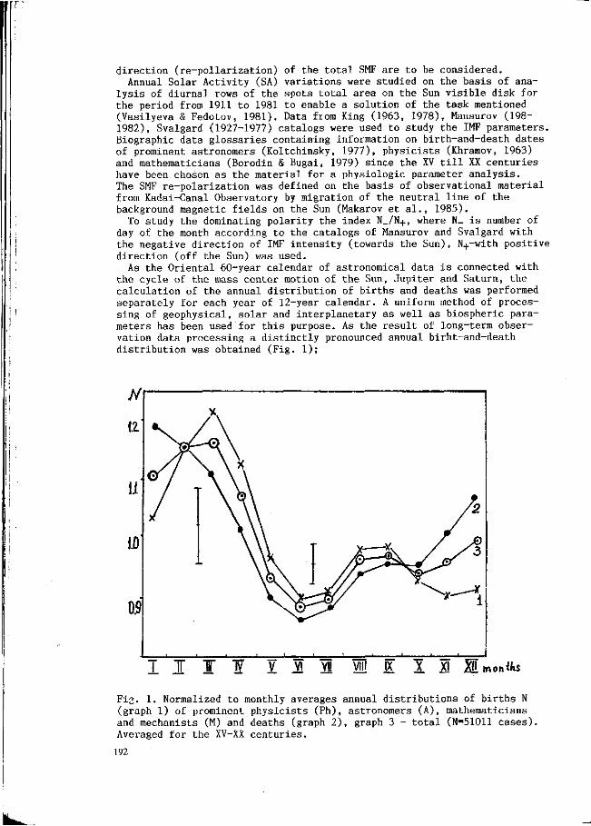
direction (re-pollarization) of the total SMF are to be considered. Annual Solar Activity (SA) variations were studied on the basis of ana­

lysis of diurnal rows of the spots total area on the Sun visible disk for the period from 1911 to 1981 to enable a solution of the task mentioned (Vasilyeva & Fedotov, 1981). Data from King (1963, 1978), Mansurov (198-1982), Svalgard (1927-1977) catalogs were used to study the IMF parameters. Biographic data glossaries containing information on birth-and-death dates of prominent astronomers (Koltchinsky, 1977), physicists (Khramov, 1963) and mathematicians (Borodin & Bugai, 1979) since the XV till XX centuries have been chosen as the material for a physiologic parameter analysis. The SMF re-polarization was defined on the basis of observational material from Kadai-Canal Observatory by migration of the neutral line of the background magnetic fields on the Sun (Makarov et al., 1985).

To study the dominating polarity the index N_/N+, where N_ is number of day of the month according to the catalogs of Mansurov and Svalgard with the negative direction of IMF intensity (towards the Sun), N+-with positive direction (off the Sun) was used.

As the Oriental 60-year calendar of astronomical data is connected with the cycle of the mass center motion of the Sun, Jupiter and Saturn, the calculation of the annual distribution of births and deaths was performed separately for each year of 12-year calendar. A uniform method of proces­sing of geophysical, solar and interplanetary as well as biospheric para­meters has been used for this purpose. As the result of long-term obser­vation data processing a distinctly pronounced annual birht-and-death distribution was obtained (Fig. 1);

i J T I V YS YJ VIII K X XI Mwontfis

Fi£. 1. Normalized to monthly averages annual distributions of births N (graph 1) of prominent physicists (Ph), astronomers (A), mathematicians and mechanists (M) and deaths (graph 2 ) , graph 3 - total (N=51011 cases). Averaged for the XV-XX centuries.

192

Maxima are falling in January-March and August-September, whereas the minima are distinctly falling in the summer period. A tendency of life duration changes with 3-4 per cent amplitude modulation during the year with the same phase is also observed (Table 1).

Table 1. Normalized to monthly averages of annual variations of births (B) and deaths (D) of prominent scientists: physicists (Ph), astronomers (A), mathematicians and mechanists (M) during the XV-XX centuries. Solid line contours the areas of higher birth and death rates.

?h Ph

Ph

Ph

Ph

Ph

Ph

h

A

M

ri

M

M —

235

235

668

668

685

685

1099

297

588

593

595

m \m *r

m 1.0 6

125

m \i\ 1.05

m ,115

w 116

HO

\M m ±

m 019

uo 115

m 155

115

1.07

>1.Q0

1.11

107

115 106 T

m m m 110

1.15

147

110

112

1.11

108

uz 106

ion W

Q.91

ilj) 0-95 10 to

100

\1\

\m m 1.16

HO

100

1Q4

109 IV

0.85

0.97

0.80

0.89

0.84

0.85

0.96

\ü£\

105

1.00

L0j> §91

101 V

0.80

0.85

Ö.8Ö

0.9Z

0.84

078

0.96

0.89

0.91

0.B9

0.9M

095

0.Q5

vT

0.Q5

0.89

0.88

0.92

0.68

0.85

m 0.92

0.90

076

0.97

Q.91

Q.89

"Vf

0.97

0.98

Q.9ÏÏ

0.97

0.98

0.94

0.9M

0.91

0.98

0.90

a.99

0.97

1.01

0.92

0.99

0.97

0.98

0.98

0.95

0.96

0.9S

Î09

0.96

0.87

1.00

1.00

YL 1 W

0.87

0.&4

0.94

0.96

0.94

0.83

0.89

f.03

108

Û.9&

0.Ô7

0.94

0.99

X

0.98

0.76

f.05

100

(04

0.82.

0.96

100

Ö.97

100

4M 076

108

100

107

0.75

0.98

104

0.87

108

0.0^106

0.99

0.92 XI

(.02

0.99 XII

D

B

D

ß

D

&

& D

B D

&

D

B

Along with the annual variations of the total sun spots area an 11-long month period was distinguished, while there were two periods determined for the dominating polarity: a 11 - months for the case when the southern polarity is observed on the northern pole of the Sun and a 13-month one tor the southern polarity on the southern pole. The appearance of new periods with duration about one year proved to be the result of addition or subtraction of variations with one year and 12-years period

The study of births and deaths distribution in the 12-year cycle of the Oriental calendar revealed apart from the one-year variation the existence of periods close to one year (0.9-1.1 year). The annual birth variations SMF t,he^Ce-time IMF regularity corresponding to the negative total lu I u , d e a t h s " t o t h e P ° s i t " e one. It has been established that the annual birth-and-death variations (Fig. 1) fall within the phase of the 11-year cycle minimum of SA variations. Births and deaths annual variations (Fig. 1) are in anti-phase with the C-form circulation of the

193

Earth atmosphere (Fig. 2 ) .

Thus, the analysis of a large amount of data from biographic glossaries shows that the annual birth-death variations reflect the distribution of IMF dominating polarity on the Earth's orbit. Gradual phase changes of the annual variations in the transition from year to year in the Oriental calendar system correlates well with the phase changes of the IMF domina­ting polarity variations in the transition from year to year during the periods between SMF re-polarizations (Fig. 1).

Fig. 2. Normalized to monthly averages of annual variations of dominating polarity (N_/N+) averaged for the period of 1927-1970 (graph 1 ) , annual variations of a number of days "n" in a month characterized by C-form, at­mospheric circulation by Vanheim, averaged for 1906-1970, for the epochs when the SMF has negative polarity (graph 2) and positive polarity (graph 3).

While moving in its orbit in June the Earth crosses the line of galaxial equator nodes on the ecliptic near the summer equinox, while in August it crosses the projection of galaxial magnetic field on the ecliptic, what is reflected by annual birth-and-death variation. This is important for the perception of life as a cosmic phenomenon and a definition of biospheric reactions to the space-time rhythmics of the solar system. Birth-and-death decrease coincides with the epoch when the Earth crosses the IMF minimal absolute intensity with minimal solar wind velocities and IMF dominating positive direction.

A phase analysis of variations of the SA observations (Wolf's numbers and the total area of sunspots on the visible Sun disk) at the frequencies of planetary revolutions provided an opportunity to reveal anisotropy of the medium surrounding the Sun. This conclusion is supported by results of direct cosmic experiments during investigation of Lyman-Alpha emission

194

distribution of the night sky (Bertaux, 1971), and galaxial gamma-radiation (Mazets et al., 1977), cosmic rays variations and the orientation of the Solar System in the Galaxy.

The main directions characterizing the orientation of the Solar System in the Galaxy were distinguished by the comparison of SA phase variations at the frequency of outer planetary revolutions. In other words there is an organic relation between the SA and IMF parameters and the planetary system.

Conclusion

The consideration of the unified open self-organizing Solar System com­posed by a hierarchic community of different level sub-systems permits a new approach ot the solution of the components interaction problem of the Sun-Earth-Biosphere system. The study of interrelation of annual variations of the IMF dominating polarity at the Earth's orbit and SA variations du­ring re-polarization of the SMF permitted to establish for the first time the interrelation between the IMF dominating polarity, sun spots magnetic fields and SMF (Vasilyeva et al., 1981). The 22-year SA cycle turned out to be presented by auto-wave 22-year spatial structure of interplanetary medium, localized within the Mars orbit (Vasilyeva & Fedotov, 1981). IMF regularities at the Earth's orbit are controlled evidently by three main factors: the solar wind reflecting the distribution of background fields on the Sun with the sector structure, a 22-year Solar cycle provided by the dynamics of the Solar System, and its orientation in the Galaxy.

The fact that near-the-Sun magnetic field structure allows to relate SA and planetary dynamics from one side and three types of fields (SMF, IMF at the Earth's orbit, and sunspots field) from the other side supports the assumption that the space surrounding the Sun is functional (as well as it is for the biota); the events present the process, not only the motion along trajectories. These concepts should be considered while discussing the structure of the Solar magnetosphere and its role in heliogeoactivity formation.

The functional relation between planetary system parameters, the inter­planetary medium and heliogeoactivity acquires a special significance in the view of a theoretical approach to the Solar System as a wave dynamic one, quantization of energy and parameters of which is the evidence of energy and information exchange between the Solar System and the external medium (Chechelnitsky, 1980). Such a quantization is impossible for closed systems, what is another testimony for the open solar system receiving negative entropy from outside.

We believe that the main trend in the study of natural processes should be based on the investigations of general regularities in the evolution of a cosmic hierarchy - the Galaxy, stars, planets, biosphere, presenting the aggregates of energy and matter in their interaction with the outer medium. The Earth and its biosphere should be regarded as a united open self-regulating system developing in the space-time continuum which is defined by the regularities of the solar system evolution. The complex heliogeoactivity study proved that the helioactivity manifestations on Earth (which at the first sight seem random) actually are a regular res­ponse to the determined signal from a system of a higher level in the cosmic hierarchy. The genetic code of the solar system of galaxial origin should be searched for the spectral distribution of such a community of signals, which would provide the particular structure of the solar system, its position in the interaction with the system of a higher level. Probably the fundamental wave spectrum of the solar system is a part of this genetic code. A search for similarity should also reasonable be conducted in the

195

activity manifestations of the Earth and the Sun as equal "partners" in their response to the whole mutual outer signals.

Self-organizing processes in the solar system reveal themselves in the IMF parameters variations in the Earth's orhit and are reflected in the evolution of the Biosphere. A similarity of events in the life of the Sun and the Earth with its biosphere provides the ground for efficient helio-geophysical forecasting.

References

Bagby, J.P., (1973) "Further evidence of tidal influence in earthquake incidence". The Moon. 6:398-404.

Ben'kova, N.P., Shernin, A.D., (1984) "Geomagnetic fields and their varia­tions". In: Electromagnetic fields in the biosphere. Krasnogorskaya (Ed.), Nauka, Moscow, p. 200-217.

Bertaux, J.L., Blanont, J.E., (1971) "Evidence for a source of an extrater­restrial hydrogen Lyman-Alpha emission . The Interstellar Wind". Astro­

physics (11): 200-217. Borodin, A.L., Bugai, A.S., (1979) "Biographic glossary of mathematicians".

Radjanska shkola. Kiev, 608 p. (1984) "Catastrophes and Earth History". Ed. W.A. Berggeren & J.A.

van Couvering. Princeton University Press, 441 p. Checheclnitsky, A.M.,. (1980) "Extremity, Stability, Resistency in Astro-

dynamics and Astronautics". Mashonostrojeniye, Moscow, 312 p. Chizhevsky, A.L., (1976) "Earth's echo of Solar Flares". Mysl, Moscow, 267p. Hramov, Yu.A., (1983) "Biographic Glossary of Physicists", Nauka, Moscow,

400 p. Koltchinsky, I.G., Korsun, A.A. and Rodrigues, M.G., (1977) "Biographic

Glossary 'Astronoms'". Nuakova dumka, Kiev, 115 p. Krasnogorskaya, N.V. and Remizov, V.P., (1973) "On some results of the

Earth's electric fields' variation measurements". The USSR Acad, of Sei. Reports, vol. 212(2), 345-349.

Krasnogorskaya, N.V. (Ed.) (1984) "Electromagnetic fields in the Biosphere", Nauka, Moscow, v. 1, 365 p., v. 2, 226 p.

Krasnogorskaya, N.V. and Rudakov, Ya.Ya., (1986) "The Infra-Low-Frequency Electromagnetic Fields' Role in Stimulation of Biosystems Growth". The third All-union Symposium on Atmospheric Electricity. Tartu, p. 46.

Krasnogorskaya, N.V. (1988) "Biosphere and its outer relations". In: Non-periodical fast-running processes in the environment". Tomsk (part III): 5-8.

Makarov, V.l. and Sivaraman, K.P., (1985) "Poleward migration of the mag­netic neutral line and reversal of the filedson the Sun Solar Physics" (85): 227-233.

Mazets, E.P., Golenatsky, S.V. and Illinsky, V.N., (1977) "The isotropic metagalactic background and the galactic gamma-radiation in the 0.03-4.1 MeV range". From Cosmoc 461 Measurements Alpha letters (18):155-158.

Piccardi, G., (1962) "The chemical basis of medical climatology". Charles C. Thomas (Ed.), Springfield, U.S.A.

Udaltsova, N.V., Kolombet, V.A. and Shnoll, S.E., (1977) "Possible cosmo-physical stipulation of Macroscopic Fluctuations in processes of diffe­rent nature". Pushchino, p. 96.

Vasilyeva, G.Ya., Kuznetsov, M.A. and Kotlyar, L.M., (1981) "Annual and semi-annual variations of the geo- and helioactivlty as an evidence of the background interplanetary magnetic fields' structure at the Earth's orbit". Physica Solari Terrestris, Potsdam (17):57-70.

Vasilyeva, G.Ya. & Fedotov, P.M. (1981) "The evolution of interplanetary medium structure within the Mars' orbit". Izvestija AN SSSR, Serija Phy-

196

sica, vol. 45(7):1335-13A5. Vasilyeva, N.V., Shpitalnaya, A.A. and Petrova, N.S., (1980) "On the pre­

diction of Solar activity taking into account its extrareons conditio­nally". In: Solar Terrestrial Prediction Proceedings Boulder, Col.: A45-A57.

Vernadsky, V.l., (1926) "The Biosphere". Leningrad Technic-Sclentific Publishing House, 71 p.

197

INFLUENCE OF SOLAR ACTIVITY ON ELF SFERICS OF 3 Hz RANGE

I . Örmény i

National Institute for Rheumatics and Physiotherapy, Labora­tory for E IectrobiometeoroIogy, 1023, Budapest, Frankel Leo str, 27-29, Hungary

Summary

Since 1966 ELF Atmosferics of 3 Hz range have been registe­red at Budapest in the E Iectrobiometeoro IogicaI Laboratory of the National Institute for Rheumatics and Physiotherapy. A low frequency receiver was applied tho this instrument. The antenna height was 9 metre long situated on a cupel of 160 metre lenght. The outcoming signal was registered by a line recor­der. Analysing the effect of solar activity it was detected the existence of 11 year's solar activity. Proton flares are fol­lowed by the increase of ELF sferics of 3 Hz range. The influ­ence of solar radio flux of 2800 MHz and 200 MHz is accompa­nied by the increase resp.deer ease of ELF Atmosferics of 3 Hz range. The influence of geomagnetic disturbances is variable. When the elongation in horizontal intensity is between 60-100, nT,resp.above 230 nT the number of impulses are increasing.On the contrary when the amplitude of horizontal intensity of a day is between 100 and 200 nT, ELF sferics of 3 Hz is decre­asing. This situation is restricted to the moderate zone of geomagnetic latitude. Keywords: ELF sferics of 3Hz, synoptic-weather situations, pro­ton flare, solar radio fluxes, geomagnetic activity.

Int roduct i on

A significant range of atmosferic electromagnetic radiation is in the ELF (Extremely Low Frequency) sferics range which is between 3 Hz and 30 Hz according to the recommendation of the XIII.C.C.I.R.PIenaryMeeting. This frequency is less known in the field of e Iectrometeoro-logy, though it has an important biorneteoroIogicaI role par-ticulary according to König's and AnkermüI I er's (1960) in­vestigations. As for physiological researches 3 Hz and 10 Hz radiation has a significant role in biology. Investigations have proved that the change in 3 Hz sferics implies the in­crease in parasympathetic tone of the vegetative nervous system, whi le the change in 10 Hz sferics that of sympathe­tic tone. Based on these investigations, changes in ELF sfe­rics have been recorded since May 1966 in the Biometeoro Io-gical Laboratory of the National Institute for Rheumatics and Physiotherapy in Budapest.

Materials and methods

Equ i pment

198

The measuring apparatus was designed by the Research Insti­tute for Geophysics and Geodesy of the Hungarian Academy of Sciences in Sopron. The measuring apparatus can be tuned continously 2 Hz and 30 Hz and is built of a double "T" filter and high cut-off band filter. For radio noise supression 50 Hz high cut-off filter built into the apparatus behind the imput stage. The areal antenna is which a U metre long rod antenna, is fitted to a 6 metre long mast on 160 metre high dome of St Lucas Spa. The antenna is connected through adapter by means of screened coaxial cable is to the receiver and makes impedance transformation from 2500 Ohm to 75 Ohm. The low resistance down lead provides for that the down lead cable receives no outher noise disturbance. 3 dB points of the band filter are 3 - 0,2 Hz at this frequency. The receiver is dri­ven by N-375-1 type recorder which continiosly records the amplified and peak-detected signals. The apparatus is fitted with transferer supplied from 6V battery. Imput impedance of the equipment amounts to 1 MOhm and the imput sensitivity is 1 ^ J V . The apparatus operates with 2000 x amplification. Time constant of the signal that drives the recorder, amounts to 22 sec.

Methods

Signals were evaluated so that the recorder was set to 50 mV sensitivity and recorded at fulI deflection. The recor­ding sheet is devided into 25 parallel lines. A deflection of 1 unit (2mV) on recording sheet was estimated to be one pulse. It is to point out that this is an arbitary interpre­tation since the recorded value means the series of counts. Three characteristics were taken into account: 1) counts/ hour, 2) maximum of the enveloping curve (amplitude maximum) 3) minimum of the enveloping curve (amplitude m i n i m u m ) . The average/hour of the daily turn of these characteristics was evaluated by the conventional c I imato IogicaI processing method. Monthly and hourly averages were also taken into account. On the other hand mathematical - statistical cal­culations were also made by the Chree method. It is known from literature that atmospheric electromag­netic radiation is affected by several factors in the ran­ge between the Earth and the Ionosphere, thus the solar activity and last, but no least "man made noise". Accor­ding to VoI I and (1982) the latter influencing factor is the least sensible at this frequency.

Resu I t s

Weather factors

From weather factors, influences of fronts are shown in Fig.1.CycI ones (Low pressure area = L) and anticyclones (High pressure area = H) are indicated in the upper part, isobaric surfaces and data of warm and cold fronts in section AB.Data of sferics are shown in the lower part, so lack of pulses can be seen in warm front (line with half circles) passages while in the instability line (broken curve) in cold front passage (line with triangles) a

199

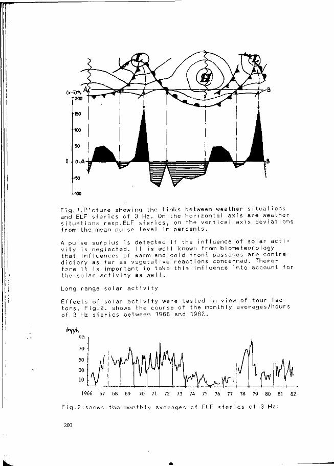
i-WO

Fig.1.Picture showing the links between weather situations and ELF sterics of 3 Hz. On the horizontal axis are weather situations resp.ELF sferics, on the vertical axis deviations from the mean pulse level in percents.

A pulse surplus is detected if the influence of solar acti­vity is neglected. It is well known from biometeoro Iogy that influences of warm and cold front passages are contra­dictory as far as vegetative reactions concerned. There­fore it is important to take this influence into account for the solar activity as well.

Long range solar activity

Effects of solar activity were tested in view of four fac­tors. Fig.2. shows the course of the monthly averages/hour s of 3 Hz sferics between 1966 and 1982.

90

70

50

30

10

1966 67 68 69 70 71 72 73 74 75 76 77 78 79 80 81 82

F i g . 2 . s h o w s t h e m o n t h l y a v e r a g e s o f ELF s f e r i c s o f 3 H z .

200

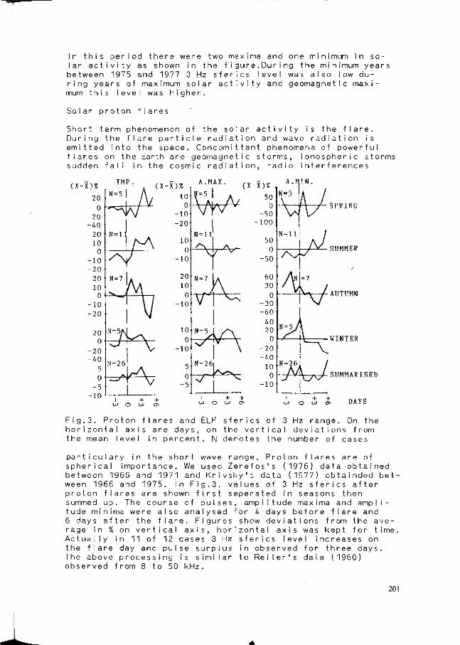
In this period there were two maxima and one minimum in so­lar activity as shown in the figure.During the minimum years between 1975 and 1977 3 Hz sferics level was also low du­ring years of maximum solar activity and geomagnetic maxi­mum this level was higher.

Solar proton flares

Short term phenomenon of the solar activity is the flare. During the fiare particle radiation and wave radiation is emitted into the space. Concomittant phenomena of powerful flares on the Earth are geomagnetic storms, ionospheric storms sudden fal i in the cosmic radiation, radio interferences

(x-x); IMP.

20 0

-20 -40

20 10

0 -10 -20

20 10

0 -10 -20

20 0 •

-20 -40

5 0

-5 -10

N = 5 1

""U N = 7 L

i V ""7W ^ 1

N = 26

M l'A V

(X-X)%

10 0

-10 -20

10 0

-10

20 10 0

-10

10 0

-10

5 0

-5

A.MAX.

SPRING

i + + W O LO O

SUMMARISED

Fig.3. Proton flares and ELF sferics of 3 Hz range. On the horizontal axis are days, on the vertical deviations from the mean level in percent. N denotes the number of cases

particulary in the spher i caI impor t an between 1966 and 1 ween 1966 and 1975 proton flares are summed up. The cou tude minima were a 6 days after the f rage in % on ver t i ActuaI I y in 11 of the flare day and The above processi observed from 8 to

short wave range. Proton flares are of ce. We used Zerefos's (1976) data obtained 971 and Krivsky's data (1977) obtainded bet-. In Fig.3. values of 3 Hz sferics after shown first seperated in seasons then rse of pulses, amplitude maxima and amp I i-I so analysed for 4 days before flare and lare. Figures show deviations from the ave-cai axis, horizontal axis was kept for time. 12 cases 3 Hz sferics level increases on pulse surplus in observed for three days, ng is similar to Reiter's data (1960)

50 kHz.

201

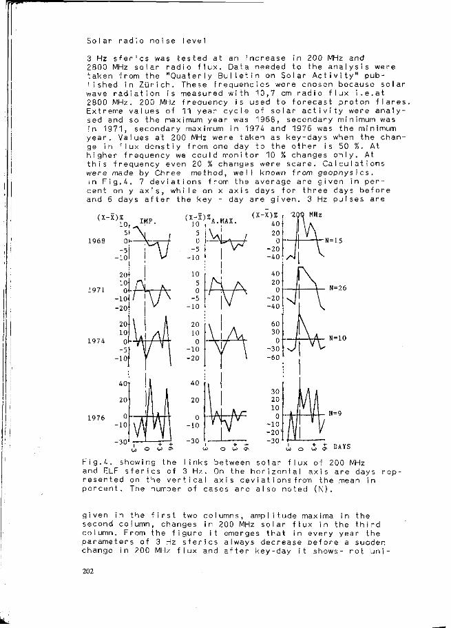
Solar radio noise level

3 Hz sferics was tested at an increase i 2800 MHz solar radio flux. Data needed t taken from the "Quaterly Bulletin on Sol I ished in Zürich. These frequencies were wave radiation is measured with 10,7 cm 2800 MHz. 200 MHz frequency is used to f Extreme values of 11 year cycle of solar sed and so the maximum year was 1968, se in 1971, secondary maximum in 1974 and 1 year. Values at 200 MHz were taken as ke ge in flux denstiy from one day to the o higher frequency we could monitor 10 % c this frequency even 20 % changes were sc were made by Chree method, wel I known f In Fig.4. 7 deviations from the average cent on y axis, while on x axis days for and 6 days after the key - day are given

n 200 MHz and o the analysis were ar Act i v i ty" pub-

chosen because solar radio flux i.e.at orecast proton flares,

activity were analy-condary minimum was 976 was the minimum y-days when the chan-ther is 50 %. At hanges only. At ar e. Ca I eu I at i ons rom geophys î cs. are g i ven in per-

three days before 3 Hz pulses are

(X-X)% 10 IMP.

1968

1971

1974

1976

<VoX>,XA-«>AX

5

-30

= 15

N=26

N=10

N=9

DAYS

Fig.4. showing the links and ELF sferics of 3 Hz. resented on the vertical

between solar flux of 200 MHz On the horizontal axis are days axis deviations f rom the mean in

rep-

percent. The number of cases are also noted (N)

given in the first two columns, amplitude maxima in the second column, changes in 200 MHz solar flux in the third column. From the figure it emerges that in every year the parameters of 3 Hz sferics always decrease before a sudden change in 200 MHz flux and after key-day it shows- not uni-

202

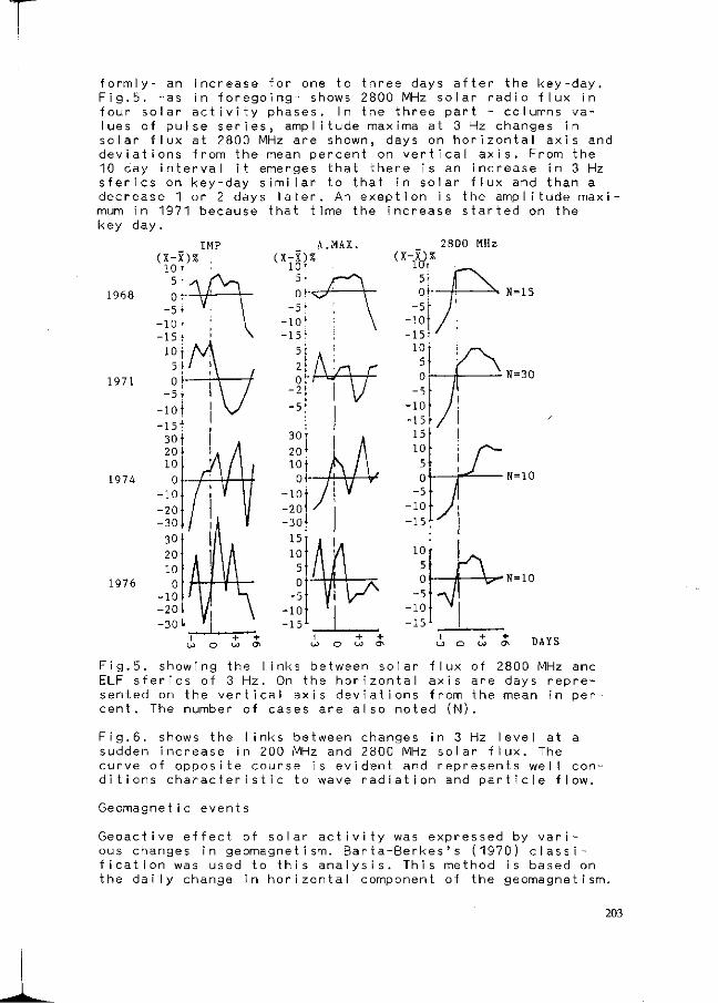
f orm I Fig.5 four I ues solar dev i a 10 ca s f er i decre mum i key d

1968

y- an increas . -as in fore solar activit of pulse seri

f lux at 2800 fions f rom th y interval it es on key-day ase 1 or 2 da n 1971 becaus ay.

e for one to three days after the key-day. going- shows 2800 MHz solar radio flux in y phases. In the three part - columns va-es, amplitude maxima at 3 Hz changes in

MHz are shown, days on horizontal axis and e mean percent on vertical axis. From the

emerges that there is an increase in 3 Hz similar to that in solar flux and than a

ys later. An exeption is the amplitude maxi -e that time the increase started on the

MAX. 2800 MHz

1971

1974

1976

N=15

N=30

N=10

N = 10

DAYS

F i g . 5 . s h o w i n g the links b e t w e e n s o l a r f l u x of 2 8 0 0 M H z and E L F s f e r i c s of 3 H z . O n t h e h o r i z o n t a l a x i s a r e d a y s r e p r e ­s e n t e d on t h e v e r t i c a l a x i s d e v i a t i o n s f r o m t h e m e a n in p e r ­c e n t . T h e n u m b e r of c a s e s a r e a l s o n o t e d ( N ) .

F i g . 6 . s h o w s t h e links b e t w e e n c h a n g e s in 3 H z level at a s u d d e n i n c r e a s e in 2 0 0 M H z a n d 2 8 0 0 M H z s o l a r f l u x . T h e c u r v e of o p p o s i t e c o u r s e is e v i d e n t a n d r e p r e s e n t s w e l l c o n ­d i t i o n s c h a r a c t e r i s t i c to w a v e r a d i a t i o n a n d p a r t i c l e f l o w .

Geomagnetic events

Geoactive effect of solar activity was expressed by vari­ous changes in geomagnetism. Barta-Berkes's (1970) classi­fication was used to this analysis. This method is based on the dai ly change in horizontal component of the geomagnetism.

203

(X-X) x

H = 43

N= 10

3Mz MAX-200MHz

3Hz MAX-2800HHZ

DAYS

Fig.6. showing amplitude maximum of ELF sferics of 3 Hz range at the time of alteration of solar flux of 200 MHz resp.2800 M H z . On the vertical deviations from the mean in percent. The number of cases are also marked by N.

the the

The i n

four de-s

60

ges h

Six geomagnetic stages are taken into account. Changes in internationally approved K index are also indicated with stages. The investigation was made between 1966 and 1978. fact that weather factors affect the result, was here kept view as well. There are 18 part-figures in Fig.7. Data of days before and after the key-day are given on x-axis and vi at ions from the mean in % the y-axis. The number of case was also indicated. All data are given in the first column It is eveident that there is no significant changes below nT daily amplitude. It is also confirmed by the fact that according to our physiological and pathological investiga­tions they show no bioactivity. It is obvious that at sta 2 and 5 there is a positive deviation, and at stages 3 and a negative. In compliance with it cases observed during si nificant changes in weather are seperated and indicated in the second column. In the third column clear cases are giv and so it is evident that if the horizontal intensity vari between 60 nT and 100 nT or exceeds 230 nT, there is a sig nificant increase ( P < 0 , 0 0 1 ) in pulse series of 3 Hz sferi on the key-day. The contrary is true if the horizontal int sity varies between 100 nT and 230 nT (P<T0,001). It proves that for physiology the influence of geomagne­tism is not the same as with front passages. During warm front passages and geomagnetic storms of 3 and 4 stages the vegetative nervous system tends towards sympathetic tone. During cold front passages and geomagnetic disturbances resp. very intense storms of 2 and 5 stages the autonomic nervous system tends towards parasympathetic tone. (This result con­firmes our previous investigations (Örményi, 1 9 8 5 ) .

en es

es en-

204

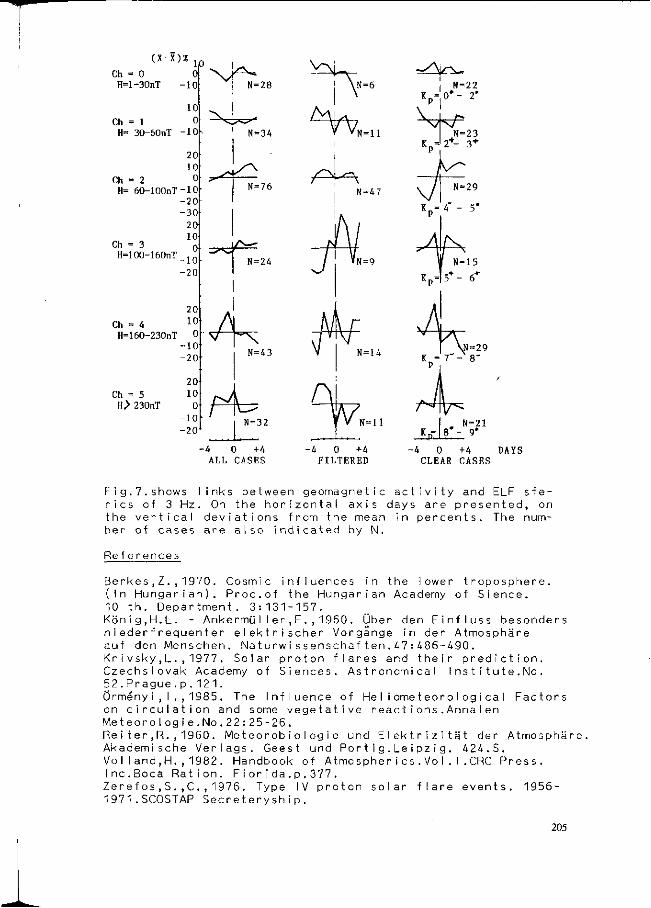
T (X-X)%

lp Ch = O O H=l-30nT -10

10 Ch = 1 O H= 30-60nT -10

20 10

Ch = 2 O H= 60-100nT-10

-20 -30

20 10

Ch = 3 0i H=100-160nT_10

r

-20

20

Ch - 4 1 0

H=160-230nT O -10 -20

Ch = 5 H> 230nT

20 10

O -10

-20

! N=28

N=34

N=76

N = 43

N=32

-4 O +4 ALL CASES

>=H-

^V«,

N = 47

N = 9

N = 14

N = ll

-4 O +4 FILTERED

_V ! \N=6 | N=22

I \ Kp=0'- 2'

vk^ K„=

= 29

-4 O +4 DAYS CLEAR CASES

Fig.7.shows links between geomagnetic activity and ELF sfe-rics ot 3 H z . On the horizontal axis days are presented, on the vertical deviations from the mean in percents. The num­ber of cases are also indicated by N.

References

Berkes,Z.,1970. Cosmic (In H u n g a r i a n ) . Proc.of 10 th. Department. 3:13 König,H.L. - Ankermülle niederfrequenter e Iektr auf den Menschen. Natur Krivsky,L.,1977. Solar Czechslovak Academy of 52.Prague.p.121. Örmény i , I ., 1985. The In on circulation and some Meteorologie.No.22:25-2 Reiter,R. , 1960. Meteoro Akademische Verlags. Ge Vol land,H.,1982. Handbo Inc.Boca Ration. Florid Zerefos,S.,C.,1976. Typ 1971.SCOSTAP Secreterys

influences in the lower troposphere. the Hungarian Academy of Sience.

1-157. r,F.,1960. Über den Einfluss besonders ischer Vorgange in der Atmosphäre wi ssenschaften.47:486-490. proton flares and their prediction. Siences. Astronomical Institut e.No.

f Iuence of He I iometeoro IogicaI Factors vegetative reactions.Anna I en

6. biologie und Elektrizität der Atmosphäre, est und Portig.Leipzig. 424.S. ok of Atmospheries.VoI.I.CRC Press, a.p.377. e IV proton solar flare events. 1956-h i p .

205

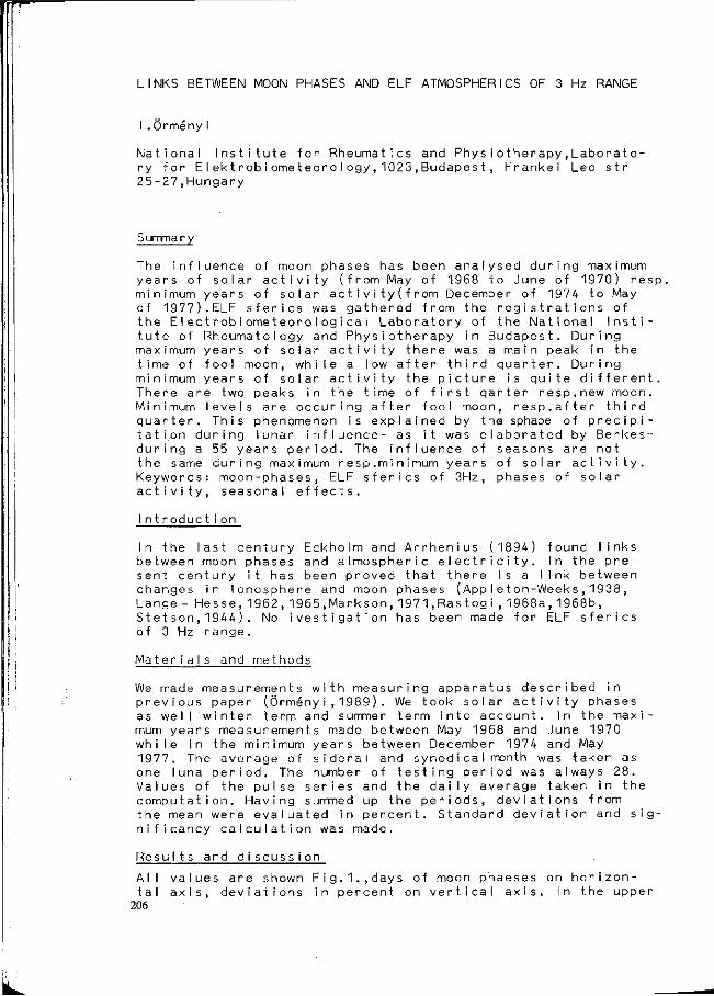
LINKS BETWEEN MOON PHASES AND ELF ATMOSPHERICS OF 3 Hz RANGE

I .Örmény i

National Institute for Rheumatics and Physiotherapy,Laborato-ry for E Iektrobiometeoro Iogy,1023,Budapest, Frankel Leo str 25-27,Hungary

Summary

The influence of moon phases has been analysed during maximum years of solar activity (from May of 1968 to June of 1970) resp. minimum years of solar activity(from December of 1974 to May of 1977).ELF sferics was gathered from the registrations of the E Iectrobiometeoro IogicaI Laboratory of the National Insti­tute of Rheumatology and Physiotherapy in Budapest. During maximum years of solar activity there was a main peak in the time of fool moon, while a low after third quarter. During minimum years of solar activity the picture is quite different. There are two peaks in the time of first qarter resp.new moon. Minimum levels are occuring after fool moon, resp.after third quarter. This phenomenon is explained by the sphape of precipi­tation during lunar influence- as it was elaborated by Berkes-during a 55 years period. The influence of seasons are not the same during maximum resp.minimum years of solar activity. Keywords: moon-phases, ELF sferics of 3Hz, phases of solar activity, seasonal effects.

Int roduct i on

In the last century Eckholm and Arrhenius (1894) found links between moon phases and atmospheric electricity. In the pre­sent century it has been proved that there is a I ink between changes in Ionosphere and moon phases (AppI eton-Weeks,1938, Lange - Hes se,1962,1965.Mark s on,1971,Ras togi ,1968a,1968b, St et s o n , 1 9 4 4 ) . No ivestigation has been made for ELF sferics of 3 Hz range.

Materials and methods

We made measurements with measuring apparatus described in previous paper (Örményi , 1989 ) . We took solar activity phases as wel I winter term and summer term into account. In the maxi­mum years measurements made between May 1968 and June 1970 while in the minimum years between December 1974 and May 1977. The average of sidéral and synodicaI month was taken as one I una period. The number of testing period was always 28. Values of the pulse series and the daily average taken in the computation. Having summed up the periods, deviations from the mean were evaluated in percent. Standard deviation and sig-nificancy calculation was made.

Results and discussion

All values are shown Fig.1.,days of moon phaeses on horizon­tal axis, deviations in percent on vertical axis. In the upper

206

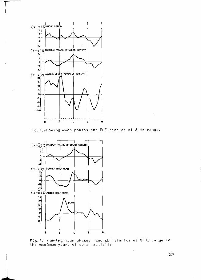
_ I I I ( x - x ) % W H 0 L E PERI0D

10

5

0

-5

-» ( X-X ) % M A X I M U M YEARS OF SOLAR ACTIVITY

W

5

0

-5

-K)

( X - X ) % M I N I M U M YEARS OF SOLAR ACTIVITY 20

Fig.1.showing moon phases and ELF sferics of 3 Hz range.

_ i "i i ~r ( X - X ) % MAXIMUM YEARS OF SOLAR ACTIVITY

10

5

0

-5

-10

( X - X ) % SUMMER HALF YEAR

20T

10

0

-» -20

, ( X - X ) % WINTER HALF YEAR

Fig.2. showing moon phases and ELF sferics of 3 Hz range in the maximum years of solar activity.

207

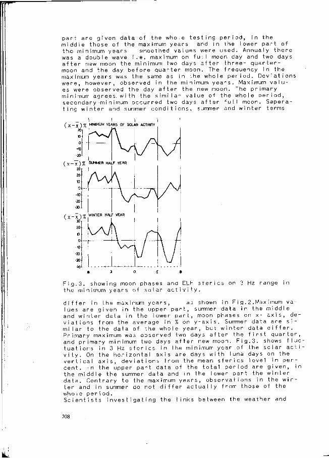
part are g i v middle those the min imum was a doubI e after new mo moon and the max imum year were, howeve es were obse mi n imum agre secondary mi ting winter

en data of the whole t of the maximum years

years smoothed value wave i.e. maximum on

on the minimum two day day before quarter mo

s was the same as in t r, observed in the min rved the day after the es with the similar va nimum occurred two day and summer conditions,

esting period, in the and in the lower part of

s were used. Annualy there fulI moon day and two days s after three- quarter-on. The frequency in the he whole period. Deviations imum years. Maximum valu-

new moon. The primary lue of the whole period, s after fulI moon. Sepera-

surrmer and winter terms

( x - x ) 20

10

0

-10

-20

(x -7)% 30 T

20

10

0

-10

-20

-30

( x - x ) % 30 T

20

10

0

-W

-20

-30

40

I MINIMUM YEARS OF SOLAR ACTIVITY

SUMMER HALF YEAR

WINTER HALF YEAR

h i g . 3. s h o w i n g m o o n p h a s e s a n d hl_F s f e r i c s t h e m i n i m u m y e a r s of s o l a r a c t i v i t y .

on H z r a n g e

d i f f er lues a a n d w i v i a t i o mi I ar P r i m a r and pr tuat i o v i ty . ver t i c cent . the mi data ter an whole Scient

i n r e g n t er ns f to t y ma imar ns i On t a I a In t ddle Con t d i n per i ists

the maximum years, as iven in the upper part, data in the iower part,

rom the average in % on he data of the whole yea ximum was observed two d y minimum two days after n 3 Hz sferics in the mi he horizontal axis are d xis, deviations from the he upper part data of th

the summer data and in rary to the maximum year

summer do not differ ac od.

investigating the links

shown i n summer da moon pha

y-ax i s . S r, but w i ays after

new moon n imum yea ays with

mean sfe e total p the Iower s, observ tua I I y fr

r i g t a i ses urrme n t e r

t h e . F i r o f I una r i e s e r i o

p a r a t i o o m t

.2.Ma n the on x-r dat

data firs

g.3. the days I eve

d are t the ns in hose

x imum v middle axis,

a are s d i f f er

t quar t shows f solar a

on the I i n p e

g i v e n , w i n t e r the w i

of the

a-

de-

er , I uc-c t i -

between the weather and

208

moon phases, are of the opinion that lunar effects cannot be attributed solely to the effect of the moon, but there are luni-solar effects as well. It is also confirmed by Berkes (1942,1944) analysis of the distribution of precipitation between 1887 and 1942 in Budapest where the maximum was at full-moon and this agrees with the meteorological part of our observations. Berkes (1953) also proved that the socalled V/b cyclones that arrive from the Mediterranean to the Car­pathian basin on van-Bebber's pathes, are twice as frequent between new-moon and fulI-moon as between fulI-moon and new moon. According to Fraser-Smith's (1982) observations in the Loackhead Magnetic Observatory in geomagnetic pulsation between 0,2 Hz and 5 H z , it was found that maximum can be observed at fulI moon which is even more powerful during a great geomagnetic storm (K ^ 3 0 ) and this agrees with the results of our investigation.

References

AppIeton,E.,-Weekes,K.,1938. Tides in the upper Atmosphere. Union Radio Sei. Internat.5: part 1.24. Berkes,Z., 1942. Die Mondphasen und der Gang der NiderschI age. Meteor.Z.59: 402-405. Berkes,Z., 1944 . Über die Realität der Mondperiode des Wetters. Meteor.Z.61: 249-251. ' Berkes,Z.,1953. On the influence of changes of moonlight to the europian pressure distribution.Rev.of the Hungarian Meteorological Institute. (In Hungarian).XV I I I : 179-188. EckhoIm,N. ,-Arrhenius,S. , 1894 . Über den Einfluss des Mondes auf dem elektrischen Zustand der Erde. Meteor.Z.1. Fraser-Smith,A.C., 1982. Is there an increase of geomagnetic activity preceding total lunar eclipses.J.Geophys.Res.87:895. Lange-Hesse,G. , -Scho11,E. , 1962. I onisations Schwankungen in der Ionosphäre mittlerer Breiten und Variation der brauchbaren Frequenzen in KurzweIIen-weitverkehr als Wirkung lunaren Gezeiten.A.E.Ü.36: 205-212. Lange-Hesse,G. , 1965. Grossenordnung verschiedener lonisations-schwankungen in der F 2 Schicht äquatorialer Breiten. Kleinheubacher Berichte.Nr.11: 61-66. Markson,R. , 1971 . Considerations regarding solar and lunar modulation of geophysical parameters, atmospheric electri­city and thunderstorms. PAGEOH.84: 161-200. Ormény i , I . ,1989. Influence of solar activity on ELF atmo s -ferics of 3 Hz range. Proc.lst International Congress on Geo-cosmic Re I ations.Amsterdam. Rastogi,R,C.,1968.a. Lunar tidal oscillations in H at Huancayo during IGY/IGC. Annales de Geophisique.Paris.24(3): 779-788. Rastogi,R.C.,1968.b.Luni- so I ar tidal oscillations in hori­zontal megnetic intensity H and in f F2 at Huancayo during low-solar activity period. J.Atm.Terr.Phys.30 : 497-512. St etson,H,T. , 1944. On the observational evidence for changes in ionization of the upper atmosphere attributable of the

Moon. Terr. Magn. 49: 9-24.

209

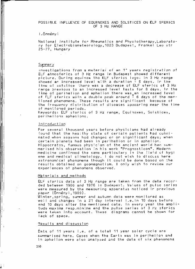
POSSIBLE INFLUENCE OF EQUINOXES AND SOLSTICES ON ELF SFERICS OF 3 Hz RANGE

I .Örmény i

National Institute for Rheumatics and Physio therapy,Labor ato-ry for E Iectrobiometeoro Iogy,1023 Budapest, Frankel Leo str 25-27, Hungary

Summary

Investigations from a material of an 11 years registration of ELF atmosferics of 3 Hz range in Budapest showed different picture. During equinox the ELF sferics I eye I in 3 Hz range showed an increased level with a duration - 6 days. In the time of solstice there was a decrease of ELF sferics of 3 Hz range previous to an increased level lasts for 8 days. In the time of perihelion and aphelion there was an increased level of ELF sferics with a double peak around - 6 days of the m e n ­tioned phenomena. These results are significant becouse of the frequency distribution of diseases appearing near the time of mentioned periods. Keywords: ELF sferics of 3 Hz range, Equinoxes, Solstices, perihelions aphelions.

Int roduct i on

For several thousand years before physicians had already found that the healthy state of certain patients had culmi­nated when seasons had changed or on significant days; when certain planets had been in perihelion or in aphelion. Hippocrates, famous physician of the ancient world had sum­marised his observation in his work "Prognosticon". Modern medicine confirmed the same particulary in the field of hygi­ene and medical climatology. I do not wish to discuss here astronomical phenomena though it could be done based on the results obtained on geomagnetism. I only wish to review our experiences of phenomena observed.

Materials and methods

ELF sferics data of 3 Hz range are taken from the data recor­ded between 1966 and 1976 in Budapest. Values of pulse series were measured by the measuring apparatus noticed in previous paper (Örményi ,1989 ) . Wi nter,spring, summer and autumn data were monitored as well and changes in a 21 day interval i.e.in 10 days before and 10 days after the mentioned data. In every year the ampli­tude maxima resp.minima and the pulse series of 3 Hz sferics were taken into account. These diagrams cannot be shown for Iack of space.

Results and discussion

Data of 11 years i.e. of a total 11 year solar cycle are summarised here. Cases when the Earth was in perihelion and in aphelion were also analysed and the data of six phenomena

210

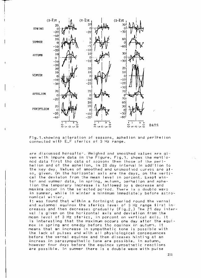
(X-X)%

SPRING

SUMMER

AUTUMN

WINTER

APHELION

PERIHELION

20 0

- 20 -40

10

0

- 10 -20

10

0

- 10 - 20

20 10 0

- 10 - 20

20

0

- 20

20

0

- 20 -40

(X-X)%

20

0

- 20

5

- 5 - 10

10

- 10

20 10

0 - 10 -20

20

0 - 20

20 10

- 10 -20

t^h x^ AM frv / ' v

^ > / i

•V' i

, Ay

/T

If \/» V-

i l + +

O Ln O Ln O

(X-X)% ,

301

0* -30

60 0

- 60

» 30 0

- 30

20 10 0

- 10 - 20

- 30

70

(r -70 60 30

- 30 -60

O Ui O ii O DAYS

Fig.1.showing alteration of seasons, aphelion and perihelion connected with ELF sferics of 3 Hz range.

are discussed hereafter. Weighed and smoothed values are gi­ven with impure data in the Figure. Fig.1. shows the mentio­ned data first the data of seasons then those of the peri­helion and of the aphelion, in 20 day interval in addition to the key-day. Values of smoothed and unsmoothed curves are al­so, given. On the horizontal axis are the days, on the verti­cal the deviaton from the mean level in percent. Exept win­ter and summer data, in spring, autumn, perhelion and aphe-I ion the temporary increase is f.o I lowed by a decrease and

maxima occur in the selected period. There is a double wave in summer, while in winter a minimum immediately before astro-nomi cal winter. It was found that within a fortnight period round the vernal and automnal equinox the sferics level of 3 Hz range first in­creases and then decreases gradually (Fig.2.) The 21 day inter­val is given on the horizontal axis and deviation from the mean level of 3 Hz sferics, in percent on vertical axis. It is interesting that the maximum occurs one day after the equi­nox in spring and one day before the equinox in autumn. It means that an increase in sympathetic tone is possible with the lack of pulses and with all physiological consequences before the vernal equinox and then diseases hinting at an increas in parasympathetic tone are possible. In autumn, however four days before the equinox sympathetic reactions are possible. In summer there is a double wave with pulse

211

(x-x)'/.

•10 DAYS

Fig.2. AIterat on of seasons and ELF sferics of 3 Hz range.

after the solstice, while in winter there is a lack of pulses, then pulse surplus before the mentioned period. The whole thing can be traced back to cLi ma tic characteristics, too, with a sudden rise in temperature between Christmas and New Year in the Carpathian basin leads to strong I abi I ization, in­versions of cold air in the upper air strata and to puise sur­plus after the changes of seasons. Fig.3. shows phenomen observed in winter when the Earth is in perihelion, resp. in summer when the Earth is in aphelion. Days are given on x-axis, deviations' from the mean of 21 day interval in % on y-axis. Perihelion data are drawn with full

(x-x)*/ «Or

30

20

10

0

-10

-20

-30-

, APHELION

PERHELION

+5 *10 DAYS

Fig.3. Alterations of aphelions and perihelions in connecti­on with ELF sferics of 3 Hz range.

line, aphelion data with dashed line. In both cases peaks occur before and after the key-day with an increase for 10 days. In perihel ion peak occurs one day before key-day and in aphelion two days after it. It means that influences like that can be encountered at least in Europe in the Carpathian

212

basin.

Cone I us i ons

Summing up the formation of ELF sferics of 3 Hz range depends not only on one factor, but in addition to mete­orological and solar activity factors, moon phases, equinox and solstice are also of importance.

Acknow Iedgment s

The author is indebted to M r s . Jolanda Majer-Hock for tec-nical assistance in calculations and in drawings.

References

Kapfer e,R. ,1934.Die Werke des Hippokrates. Hippokrates Verlag. Stuttgart-Leipzig. Örményi,I.,1989. Influence of solar activity on ELF sferics of 3 Hz range. Proc.lst international congress on geo-cosmic relations. Amsterdam.

213

ANALYSIS OF WEAK MAGNETIC FIELD EFFECTS ON THE PICCARDI TEST AND THE BELOUSOV-ZHABOTINSKY REACTION

L.P. Agulova and A.M. Opalinskaya* Cardiology Institute of Tomsk Research Centre of the USSR AMS * Institute of Petroleum Chemistry, USSR Academy of Sciences, Tomsk, 634055, USSR.

Summary The paper presents the results of experiments for verification of a

hypothesis about the important role of Earth's magnetic field variations in the Sun-biospheric communications. The experiments were carried out with model systems (Piccardi-test, Belousov-Zhabotinsky self-oscillatary chemical reaction). The influence of a man-made sinusoidal magnetic field, corresponding by frequency and amplitude to the Earth's magnetic field variations on these reactions was studied.

Both reactions were found to be sensitive to the exposure of weak magnetic fields. The complex polyphase (polyextremal) dependance on frequency and strength of measured characteristics of the reactions is shown. Such a dependence suggests that the dynamics of dissipative systems in the instable state (transformations from one quasi-steady state into the other) changes the controlling parameters of these systems.

The experimental results and hypothesis about the possible mechanism of weak magnetic field effects on self-oscillotary reaction are briefly treated.

The common features and regularities of the reactions of the systems with a different physical nature, sensitive to variations in heliogeo-physical factors and to the action of weak electromagnetic fields as well as the problems of results replication are discussed.

Keywords: Belousov-Zhabotinsky reaction, Piccardi test, electromagnetic fields, fluctuations, variability.

Introduction As early as in the beginning of our century the sensitivity of living

organisms to solar activity (SA) effects, was related to the non-equi­librium of these systems by A.A. Chizhevsky -the founder of heliobiology. Later on the researchers emphasized time and again that unbalancement is a required state of systems to percept various effects of SA.

On account of advances in the thermodynamics of non-equilibrium proces­ses and synergetics development it is currently well known that in the dynamics of dissipative systems existing far from equilibrium the determinant role is played by fluctuations both internal (inherent to the system itself) and external (Haken, 1985; Horsthemke, Lefever, 1987).

For several years we have conducted the experimental analyses to examine the contribution of cosmogeophysical factors in stimulation of fluctuations that are usually observed with unbalanced systems.

For our studies we have chosen two reactions: bismuth chloride hydrolysis -Piccardi test and self-oscillatory chemical reaction of oxidation of malonic acid with bromate at presence of Ce ions as a catalyst Belousov-Zhabotinsky reaction. We studied the effects of various cosmophysical factors using these reactions comprehensively. The results of the experi­ments showed that measured characteristics of the reactions varied in the wide temporal range from several minutes to some years. Fluctuations are not purely stochastic processes. Periodic components, ranging from some minutes to some days, were recognised. Similarly multiday periods are found in cosmogeophysic environment parameters. In their work F. de Meyer

214

and C. Capel-Boute (1987) demonstrated about-a-year and multiyears perio­dicity of the Piccardi test. The fluctuations in the non-equilibrium systems are shown to be significantly affected by electromagnetic and, possibly, by corpuscular factors. This conclusion is based on the results of studies of correlation with cosmogeophysical indices, on the latitude-longitude tests, on the experiments done during solar eruptions, geomagne­tic storms, atmospheric thunderstorms, in the periods of change in inter­planetary magnetic field polarity and during the rotation of the Sun around its axis; on the tests with various screens; wooden, cartoon, aluminium, steel, brass, leaden, permalloy as well as on the tests with the reactions exposed to man-made magnetic fields (MF) corresponding to natural ones by amplitude and frequency.

In this report we consider some results of an analysis of MF effects on Piccardi tests and Belousov-Zhabotinsky reactions.

The Piccardi test is a water disperse system, the Belousov-Zhabotinsky reaction is a halogen reaction in strong concentrated (1.5N) hydrochloric acid with continious mixing. The Belousov-Zhabotinsky reaction was thermostated (38±0.5°C), the Piccardi test was conducted under room tem­perature. The reaction procedures, recording and processing of the results are given in detail in our earlier reports (Opalinskaya, Agulova, 1984).

Results and discussion Piccardi-test :

In the Piccardi test exposure to MF,both direct and alternating, the shortening of BiOCl precipitation relative to the control test at all the frequencies and strengths was observed (Table 1 ) . Precipitation fluctu­ations were reduced in 79% of the cases due to reaction stabilization by sinusoidal MF against the background of electromagnetic noises of the environment. The field nonuniformity in the active volume specified by the sole-noid configuration did not exceed 30% of the estimated value. It is seen from the table that the dependencies of precipitation-duration and fime fluctuations on frequency and MF strength are complex and poly-extremal: with certain values strength and MF frequency the measured characteristics are clearly reduced; with others they are likewise clearly increased. As a result one can observe a number of extrema in the curves of corresponding dependencies. The measure of fluctuations was the root-mean-square deviation from the mean (<r) or relation of the root-mean-square deviation to mean value, expressed in a percentage, i.e. in a variation coefficient: <*

V = - 3 - x 100 % M

Belousov-Zhabotinsky reaction : The MF dependencies on strength and frequency were studied. Field non-

uniformity amounted to about 50%. The dependance on strength with reaction exposure to constant and alter-

nive MF was studied. The amplitudes of self-oscillations and fluctuations are found to be changed with the action of a constant MF with strengths M = 0.2; 0.4; 0.8; 2; 0; 4.0; 8.0; 20.0; 40.0; 80.0 A/m. The dependencies of variations in these values against the control on field strength are polyextremal. No other peculiarities in amplitude variation and amplitude fluctuations in this case were found. Dependencies on alternative MF strength (f = 0.01 Hz) were examined at strengths H = 0.4; 0.8; 2; 4; 8; 20; 40; 80; 200; 400 A/m. The fundamental frequency of oscillations was changed in the course of the experiment ranging from 0.025 Hz to^0.02 Hz (a closed system was examined). The averaged results of the tests are shown in Fig. 1. It is seen that the dependences of amplitude and ampli­tude fluctuations on alternating MF strengths as well as on constant MF

215

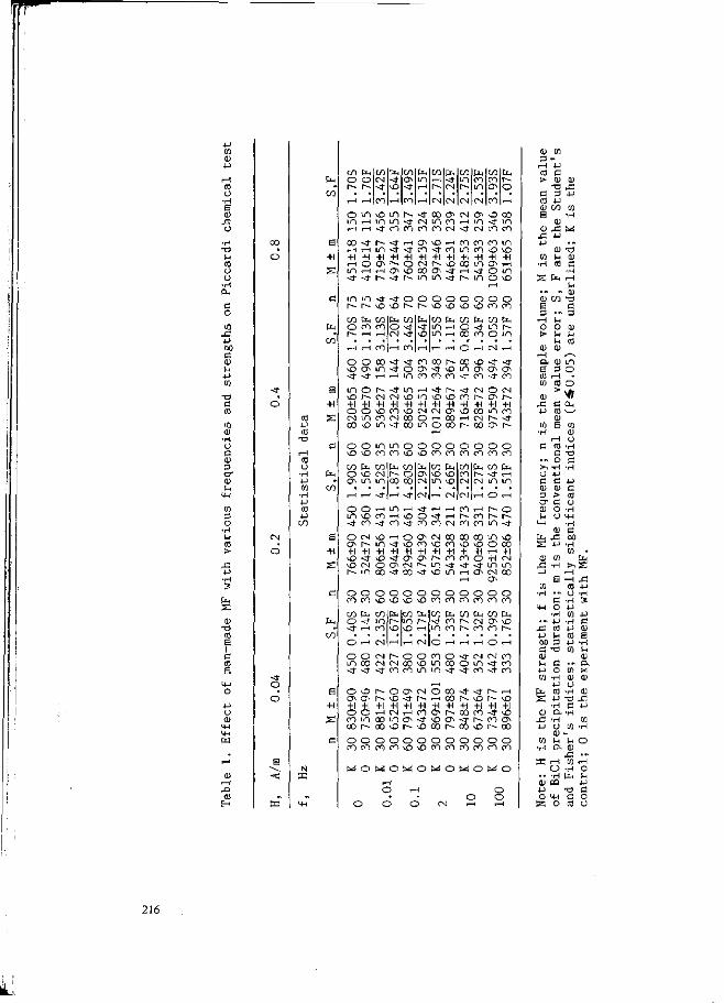
CÖ o •rl e CU

- G O

C O

CO X ! 4-1 00 C CD U 4J CO

c CO

co CU

•I-I o c (U 3 er-CU

4-1

ta S

eu - o co a i c CO

4-1 O <u

.o (0

co

o

d

co 4-1

C/2

o

E N

CO ta O O

t-H t—1

CO CN < f

co

CO

co

ta m t—<

i—i

co

CN

CN

CN

co i n

CN

ta co m

CN

co CO o

co

ta M o

70S

75

13F

75

13S

64

t—l t—) CO

<r o o r-

ta co O ^ f CN -< f

t -H CO

o r-

ta

I—1

O O O O O O O O vD vO CO CO

co ta co ta co ta I O H 0 4 1 0 N l O H C o t o o i n

r-H t-H O i—1 CN i—1

o o c o < f < t c o c » r - - o O i O < f < r > D ( ? l C 1 ^ 0 0 1 ^ > u l f l O v O ^ C > < - < f t - i ^ - i i n c o c o c o < i - c o < r c o

m o r ^ - < j - i n T - H < - r ^ < j - c N O c N \ O t ^ - c N C N \ o m v O v O c o r ^ o r - ~ -+l +i +i +l +i +i +i +i +i +i +i +i O O O C O v O C N C N O N ^ O C O i n c O c N i n c o c N c o o ^ H O O ^ c N r ^ - c r o o ^ O L n < f c o m o c o i - - c o o r - -

ta co

o i n v o m r ^ - t f o o o c N c ^ v o c o i O r - i i n m s j " C N i n c O t - H i n ^ j " m t—It—<<t-COCOCOCOCN-H/CNCOCO

E c o < t r - - < f ' - H O \ £ > f - < c o c o c o i n t - H ^ H L n < f s r c o < f c o m c o o c D

+1 +1 +1 +1 +1 +1 +1 +1 +1 +1 +1 +1 +1 H O o ^ N O c J N \ 0 ( » i n ^ H m - — ( r - i o ^ o c o o < j * i — i ^ o i o < t - < f r - ~ ~ * r - ~ i n i n < f r ^ m o ^ D

ta co

e +i

E

+1

ta co

O O

co ta O vO o i n

m m o co co o

ta co r- O co oo

o o o o o o o o co co co co co co

co ta ta co ta r— < f t-H cN m m

O o i n *£> <f co

O CN cr> r— +1 +1 vo <r \0 CN r-- m

r-i m i—I CO r-l \D <t CO - t f

VO t-H O m - j - vo +1 +1 +1 \0 <t o O O CN co o- co

o o o \0 ^O \0

CN t-H CN CN t-H O T-H

< t t-H i-H CO t-H r~- o o sj- «-H r~- co r-~ r--co co CN co co m <t

o cN co co co m o CO « CO J ) vD O CO +1 +1 +1 +1 +1 r-< +1 O M O ( O O t ( N M O •* <t <t in lO <r vo m t-i o cN co

r-H O

o o o o o o o *o co co co co co co

co ta co O < f i n - Î H CO

O --H CN

ta r-

t-H

co ta i n I - -\ D t-H

t-H CN

co ta co ta co ta - l t ( O N ( M C I H O m co r~. co co r~

O t-H t-H t-H O t-H

o o m co

cN r-- o CN CN 00 -4" co co

O CO O <f CN CN CO iO IO 03 O lO <t CO m m <r <a- co -J co

O i D N O O i M O C O v t ' J h H o o r-- \ o <r r— — i c o r ~ - c o r ~ - o +i +i +i +l +i +1 +i +i +i +i +1 +i o O t - H C N t - H c o o r - o o c o - o - v O c o i o o o i n o < f « o - } N c o o c o r ~ - c o o r ^ ^ D c o r ~ - c o ^ O f - ~ c o

o o o o o o o o o o o o C O C O C O C O c O ^ O C O C O C O C O C O C O

« 0 « 0 « O l ^ i O « 0 1 ^ ! 0

o d

o o

cu 3

f—1 CO

> c CO <u E CU

J 3 4 J

ra • r l

10

•-4-1 G (U

- O 3 4-1

CO

cu x : 4-1

<U U CO

S ta

• •• eu E 3

t -H O

> CU

t-H O .

E CO CO

<u - G 4-1

CO • H

C

• r.

!=-> O C CU 3 er cu u

I4H

ta S

eu j = : 4-1

ra • H

MH

... - C 4-1 0 0

c cu u 4-1 CO

ta S CU

J 3 4-1

ra • r l

3 3

• • 0) 4-1 O

SS

.• CO

• r.

(-. O lH SH

cu

<u 3

t -H CO

> G CO

CU

E i-H CO

c o

• H 4-1 C <D

> G O O

<1> J 3 4-1

CO • H

E

• ~ G O

• r l 4-1 CO i-t 3

T J

G O

• H 4-1 CO 4-1 • r l O .

• r l O <U ^ 1

O .

r H C J • H

pa C4H O

cu X 4-1

CO • r l

^ • n

•o <u c

• H r H

>H

CU X I G 3

O) 1-1 CO

,—s i n o

o V> ta w

ra cu o

• H

-o G

• H

4-1 G CO U

• H 4 H • H G 0 0

• H CO .

ta !> .S r-i r-i C0 U

• H 4-1 CO

• H 4-1 CO 4-1 CO

• f

ra eu Ü

• r l • ö G

• r l

CO

— u <u

co • r t

ta •o G CO

- G 4-J • H 3 4-1 G (D E

• H i n <U O .

« CU

(U - C 4-1

CO • H

O ...

r H O ( H

4 J G O Ü

216

AK, H VmF/VK,3r

+ 1 + 2 O +1 +2

lg H, A/m 19 H/ A/m

Fig. 1. Dependence of self-oscillation amplitude (a) and amplitude fluc­

tuations (b) on MF strength (f = 0.01 Hz). A,

and A„ are mean values of self-oscillation ai

with MF action and control ones respectively. V,

(A, 'MF AK) / AK,/where A M p

and A„ are mean values of self-oscillation amplitude in the experiments

„p. and V„ are the coeffi­

cients for variations. The solid points are the variations confident with

the significance level P<0.01.

10 A/m

X----X 8 A/m

-3 -Z -1 0 1 2 lg £, HZ

Fig. 2. Dependence of oscillation amplitude on MF frequency. The curves

correlate with a significance level P<0.01. The notations as in Fig. 1.

217

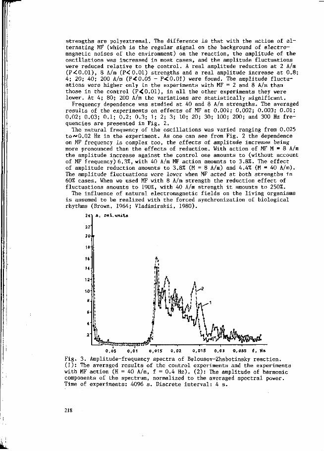
strengths are polyextremal. The difference is that with the action of al­ternating MF (which is the regular signal on the background of electro­magnetic noises of the environment) on the reaction, the amplitude of the oscillations was increased in most cases, and the amplitude fluctuations were reduced relative to the control. A real amplitude reduction at 2 A/m (P40.01), 8 A/m (P<0.01) strengths and a real amplitude increase at 0.8; 4; 20; 40; 200 A/m (P<£0.05 - P<0.01) were found. The amplitude fluctu­ations were higher only in the experiments with MF = 2 and 8 A/m than those in the control (P<0.01), in all the other experiments they were lower. At 4; 80; 200 A/m the variations are statistically significant.

Frequency dependence was studied at 40 and 8 A/m strengths. The averaged results of the experiments on effects of MF at 0.001; 0.002; 0.003; 0.01; 0.02; 0.03; 0.1; 0.2; 0.3; 1; 2; 3; 10; 20; 30; 100; 200; and 300 Hz fre­quencies are presented in Fig. 2.

The natural frequency of the oscillations was varied ranging from 0.025 to"0.02 Hz in the experiment. As one can see from Fig. 2 the dependence on MF frequency is complex too, the effects of amplitude increase being more pronounced than the effects of reduction. With action of MF M = 8 A/m the amplitude increase against the control one amounts to (without account of MF frequency) 6.3%, with 40 A/m MF action amounts to 3.8%. The effect of amplitude reduction amounts to 3.8% (M = 8 A/m) and 4.4% (M = 40 A/m). The amplitude fluctuations were lower when MF acted at both strengths in 60% cases. When we used MF with 8 A/m strength the reduction effect of fluctuations amounts to 190%, with 40 A/m strength it amounts to 250%.

The influence of natural electromagnetic fields on the living organisms is assumed to be realized with the forced synchronization of biological rhythms (Brown, 1964; Vladimirskii, 1980).

241 a, rel. units

22

2 O-h

18

16

14

12

10

8

*fc~A—-. .,,,

0,05 0,01 0,015 0,02 0,015 0,03 0,035 f, Hz

Fig. 3. Amplitude-frequency spectra of Belousov-Zhabotinsky reaction. (1): The averaged results of the control experiments and the experiments with MF action (H = 40 A/m, f = 0.4 Hz). (2): The amplitude of harmonic components of the spectrum, normalized to the averaged spectral power. Time of experiments: 4096 s. Discrete interval: 4 s.

218

To verify this hypothesis a set of experiments was carried out for exa­mining the alternating MF effect on self-oscillatary reactions ât H = 40 A/m, with frequencies similar or multiple to basic frequencies (modes) of a self-oscillatary reaction: 0.01; 0.015; 0.02; 0.025; 0.03; 0.04; 0.05; 0.06; 0.08; 0.1; 0.12; 0.16; 0.2; 0.24; 0.32; 0.4; 0.48; 0.8; Hz.

The results of the control experiments demonstrated the variations of spectra through the experiments and their complex structure in which one can highlight three main regions (Fig. 3 ) .

Low frequency region (2f0 - 0.005 Hz) is attributed to slow changes in the mean optical density.

The middle region of the spectra is due to quasi-harmonic oscillations of reagent concentrations. According to the realization period this spec­trum region has single or several modes. Polymodality can be attributed to a closed system under study. In the onset of the reaction the basic frequency of oscillations (Ä0.025 Hz) is the first mode. With the rea­gents transformation during a reaction the frequency of oscillations decreased and the second mode occured $V0.02 Hz). Then the third one (&0.015 Hz) and so on. The shifts are rather abrupt due to saddle form of this spectrum region.

The third spectrum region is likely to be caused by the fact that the oscillations are not strictly harmonic due to nonlinear properties of the system under study.

In the experiments with MF action on the self-oscillatary reaction of synchronization and resonance at any individual frequency we diu not find self-oscillations.

Meanwhile such characteristics as mean spectral power and the number of degrees of freedom (NDF) were changed against the control with MF frequency growth being polyextremely, almost periodically (Fig. 4 ) .

The NDF of a discrete Fourier spectrum is a spectral characteristic displaying the degree of the process ordering (disordering) (Vidal, 1984).

(?P)2

NDF = £ 2

n^ p l

where P is the power at a frequency iAf; i = l....n; n is the overall number of frequencies in the discrete spectrum. For a pure sinusoidal wave NDF = 1/n and for white noise NDF = 1.

From Fig. 4 it is seen that, alongside with polyextremicity, trends to spectrum power growth and noise level reduction are observed with MF frequency increase. This trend is denoted with a dashed line. The spec­trum power growth against the noise reduction may be attributed to the enhancement of the harmonics amplitude with the action of MF with definite frequencies. In exposure of MF (H = 40 A/m); f = 0.4 Hz) to the reaction narrowing the middle region of the spectrum and enhancing the harmonic amplitude are practically found at all the fundamental frequen­cies.

The analysis of NDF individually for the low and middle frequency regions of the spectrum showed that in a low-frequency region (0-0.005Hz) caused by slow change of mean optical density the MF effects are more pronounced then in the middle spectrum region caused by concentrated oscillations.

At present the mechanism of a weak MF effect is not clear. The weak MF effect on water systems is supposed to involve the change in MF probabi­lity of protons transfering the chain of H„ bonds (Semikhina, 1988). In recent years an experimentally verified theory of the MF effect on the rate of radical chemical reactions has been formed. This theory is based

219

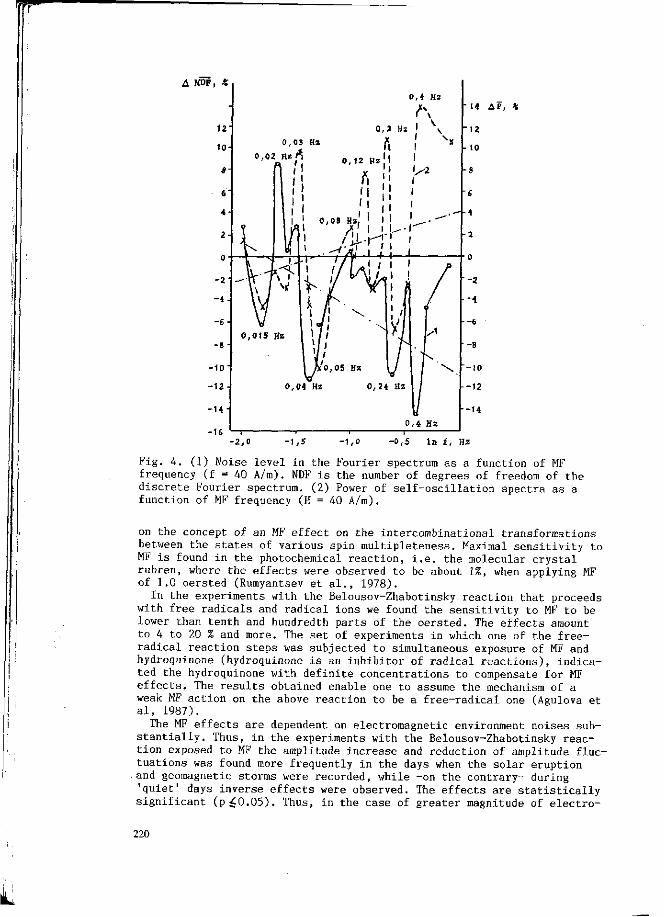
rr

A KDF, *

• M AP,

0,4 Hz

In f, Hz

Fig. 4. (1) Noise level in the Fourier spectrum as a function of MF frequency (f = 40 A/m). NDF is the number of degrees of freedom of the discrete Fourier spectrum. (2) Power of self-oscillation spectra as a function of MF frequency (H = 40 A/m).

on the concept of an MF effect on the intercombinational transformations between the states of various spin multipleteness. Maximal sensitivity to MF is found in the photochemical reaction, i.e. the molecular crystal rubren, where the effects were observed to be about 1%, when applying MF of 1.0 oersted (Rumyantsev et al., 1978).

In the experiments with the Belousov-Zhabotinsky reaction that proceeds with free radicals and radical ions we found the sensitivity to MF to be lower than tenth and hundredth parts of the oersted. The effects amount to 4 to 20 % and more. The set of experiments in which one of the free-radical reaction steps was subjected to simultaneous exposure of MF and hydroquinone (hydroquinone is an inhibitor of radical reactions), indica­ted the hydroquinone with definite concentrations to compensate for MF effects. The results obtained enable one to assume the mechanism of a weak MF action on the above reaction to be a free-radical one (Agulova et al, 1987).

The MF effects are dependent on electromagnetic environment noises sub­stantially. Thus, in the experiments with the Belousov-Zhabotinsky reac­tion exposed to MF the amplitude increase and reduction of amplitude fluc­tuations was found more frequently in the days when the solar eruption and geomagnetic storms were recorded, while -on the contrary- during 'quiet' days inverse effects were observed. The effects are statistically significant (p^0.05). Thus, in the case of greater magnitude of electro-

220

magnetic environment noises the weak sinusoidal MF stabilises the reac­tion, and in the case of comparatively quiet electromagnetic states the same weak MF plays a destabilization role.

The present evidence and our experiments and observations indicate that the biological and chemical species which have well-defined effects of cosmogeophysical influences, effects of weakly electric and electromagne­tic fields as well as other factors with small magnitudes show features common and universal for systems of different physical nature. Specific to them are: significant nonequilibrium states, nonspecific reaction responses, cooperative effects, multiphase (polyextremal) nature of reac­tion response to the growth of frequency or field strength, substantial changes in measured parameters, a delayed period of reduction (or absence of reduction) of an original state after perturbation, unsatisfactory re­plication of experiments (Agulova et al., 1987). In exposures exceding the critical level (for living organisms the extreme states on verge of life) a similar behaviour of species with different nature is found too.

Similar behaviour of systems with various physical nature is specific for the regions with instability, i.e. at the border of transformation or in transforming onto the new states. For instance, it is specific for the systems performing phase changes and changes over stochastic dynamics (Nikolis et al., 1979; Haken, 1985).

This analogue speaks much for the fact that behaviour of systems with various physical nature under definite conditions on certain steps of their evolution are subjected to the same fundamental laws. In such pro­cesses the leading role is played by cooperative effects, one of the essential features of which is the formation of long wave correlations between individual spatial regions of the system. The origin of collective behaviour demands many reactants. Availability of many reactants, in its turn, suggests fluctuations. The latter is of prominent in transforming from one state into the other. The sensitivity of systems in the unstable regions to external, even negligible, perturbations is very high and grows by some orders (Anisimov, 1974; Nikolis & Prigogine, 1979; Horsthemke & Lefever, 1987).

In search of the physical mechanism of the effects of cosmogeophysical factors and weak man-made fields, the consideration of two mechanism is obviously needed: one at the molecular level and the other providing the efficiency of weak fields perception. We have inferred that the latter is associated with the dynamics of complex nonequilibrium systems that is characteristic of fluctuating states.

The peculiarities of systems behaviour in the unstable region are close­ly connected with the problem to replicate the experiments.

The traditional way to overcome the problem of bad replication of expe­riments is searching general rules in the states of species and in the external factors: singling out the criterion specifying these states, finding the methods to work with essentially nonequilibrium systems. These observations are likely to need further careful improvement.

References

Agulova, L.P., Opalinskaya, A.M., & Kir'yanov, V.S., (1987) "Rate varia­tion of trivalent Ce bromate oxidation in the Belousov-Zhabotinsky reaction under the influence of weak magnetic field and of hydroquinone" Theoretical and experimental chemistry, in press.

Agulova, L.P., Opalinskaya, A.M., & Kir'yanov, V.S., (1988) "Features of reactions of species with different nature sensitive to cosmophysical factors change and to weak man-made electromagnetic fields". Cosmic Biology Problems, in press.

221

Anisimov, M.A. (1974) "Analysis of critical phenomena in liquids". Physi­cal Sciences Advances. 114: 250-254.

Brown, F.A. (1965) "A unified theory for biological rhythms". In: Circa-dian Clocks. Ed. J. Aschoff, Amsterdam. 231 p.

Buchachenko, A.L., Sagdeev, R.L. & Salikhov, K.M. (1978) "Magnetic and spin effects in chemical reactions". Nauka, Novosibirsk. 294 p.

Haken, M. (1985) "Advanced synergetics instability hierarchives of self-organizing systems and devices". World, Moscow, 419 p.

Horsthemke, W. & Lefever, R. (1987) "Noise-induced transitions" Theory and applications in physics, chemistry and biology. World, Moscow, 400 p

Meyer, F. de & Capel-Boute, C. (1987) "Statistical analysis of Piccardi chemical tests". Int. J. Biometeor. 31: 301-322.

Nikolis, G. & Prigogine, I. (1979) "Self-organization in nonequilibrium systems. From dissipative structures to order through fluctuations".

Opalinskaya, A.M. & Agulova, L.P. (1984) "Cosmoheliogeophysical factors and weak man-made electromagnetic field effects on physico-chemical and biological systems" Tomsk University Press, Tomsk. 190 p.

Rumyantsev, B.M., Lesin, B.L. & Frakevich, E.L. (1978) "Magnetic field effect on rubren fluorescence intensity with admixure presence". High-Voltage Chemistry. 12: 42-47.

Semikhina, L.P. & Kisilev, L.P. (1988) "Weak magnetic fields. Effect on water and ice properties". Izvestia Vuzov. 5: 13-17.

Vidal, K. (1984) "Dynamic instabilities observed in the Belousov-Zhabo-tinsky system". In: BB. Kadomeev (Ed.), Synergetic. World, Moscow, p. 109-125.

Vladimirsky, B.M. (1980) "Biological rhythms and solar activity" Cosmos biology problems. Nauka, Moscow. 41: 289-312.

222

RELATIONSHIP BETWEEN THE ELECTROMAGNETIC VLF-RADIATION OF THE ATMOSPHERE AND CHEMICAL AS WELL AS BIOCHEMICAL PROCESSES

J. Eichmeier and H. Baumer

Institut für Grundlagen der Elektrotechnik der Technischen Universität, München Fed. Rep. of Germany

Summary

Chemical and biochemical processes show random variations which are closely related to the intensity of natural elec­tromagnetic VLF-radiation (atmospherics) in definite fre­quency intervals. Examples are: (1) the diffusion behaviour of Fe3+- and Cl~-ions in gelatin films, (2) the crystal growth in a special solution (Fitzroy-effect) and (3) changes of biochemical processes which are the basis for a number of diseases such as epileptic fits, heart attacks and bacterial inflammations.

As the predominant forms, frequency spectra and repeti­tion rates of atmospherics impulses are typical for each weather situation, the atmospherics activity seems to be a particular environmental phenomenon which is of impor­tance for the sensitivity of living organisms to weather changes. Relationships between atmospherics impulse patterns and different weather situations are demonstrated. Keywords: VLF-radiation, atmosphere, atmospherics, chemical processes.

Introduction

Since 1977 atmospherics impulses have been received and analyzed at a measuring station in Pfaffenhofen situated 45 km to the north of Munich. It was found that the predomi­nant impulse forms, frequency spectra and pulse repetition rates of atmospherics are significantly and reproducibly dependent on weather processes such as development and mo­tion of warm and cold fronts or, generally speaking, to horizontal and vertical air mass movements (Sönning, Baumer & Eichmeier, 1981, 1984; Sönning, 1984; Baumer & Eichmeier, 198o, 1982, 1983). Atmospherics impulses could also be re­ceived, if no thunderstorms with lightnings occured within the range of our antenna system (about 5oo km around).

During the last years atmospherics in a wide frequency band between 1 and loo kHz as well as in narrow frequency windows at 4, 6, 8, lo, 12, 28 and 5o kHz have been ana­lyzed.

Concurrently with these investigations correlations bet­ween atmospherics pulse rates at these frequencies and the development of some chemical and biochemical processes have been studied, namely: (1) the diffusion times of Fe^+ - and Cl~ -ions penetrating gelatin films, (2) the

223

r

crystal growth in a special solution (Fitzroy-effect) and (3) changes of biochemical processes influencing diseases such as epileptic fits, heart attacks and bacterial inflam­mations .

The measuring station

The atmospherics receiving and analyzing system in Pfaf-fenhofen consists of a receiving antenna on the roof of the measuring station and electronic devices for data proces­sing. The antenna bodies of the receiving antenna contain 7 ferrite rods, surrounded by a receiving coil, and an elec­tronic amplifier circuit. The antenna bodies detect the mag­netic component of the electromagnetic impulse radiation of the atmosphere (atmospherics) . The electronic equip­ment for data processing consists of: a monitor for satel­lite pictures of clouds, sferics selectors for impulses with horizontal and vertical magnetic field components, a sferics frequency analyzer, a digital storage unit for sfe­rics impulses and a control unit for a special direction finding antenna, two Tascam magnetic tape recorders, a Me-teosat equipment for satellite cloud pictures, a computer for magnetic tape recording, a selector for impulse forms and for the pulse repetition frequency of sferics, a recor­der and finally a device, called atmospherics emission computer tomograph.

The atmospherics emission computer tomograph (AECT) pro­duces patterns, i.e. computer tomograms, of the lo kHz-atmospherics activity in the troposphere. For the AECT a special rotating direction finding antenna was used which performs a horizontal 36o°-scan of the troposphere.

The atmospherics impulses, received by automatically scanning the troposphere, are analyzed in an atmospherics signal processor. The resulting computer tomogram is shown on a monitor with color code.

Some of the devices mentioned have been described in previous papers (Baumer & Eichmeier 198o, 1981a, Eichmeier & Baumer 1982) .

Recordings of atmospherics

Atmospherics are random electromagnetic impulses origina­ting from dynamic processes in the atmosphere. They have a pulse duration of the order of ten to some hundred micro­seconds, they oscillate with frequencies between about 1 and 6o kHz and their pulse repetition rate varies between zero and more than 15o Hz. The atmospherics activity can be ana­lyzed in several ways: (1) recording and storing of single pulses of different shapes, (2) recording of the pulse rate in the whole frequency band between 1 and about 6o kHz, (3) recording of the pulse rate within definite frequency windows, (4) determination of the cumulative frequency spectrum of the impulses during definite time periods and, finally, (5) recording of the atmospherics emission compu­ter tomogram.

224

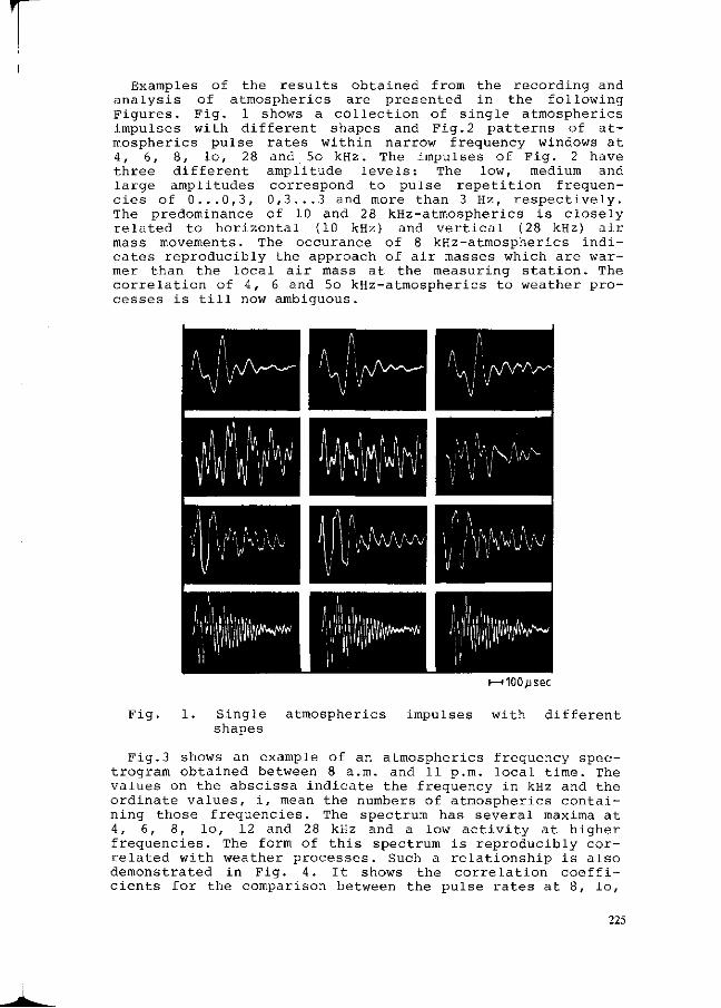
Examples of the results obtained from the recording and analysis of atmospherics are presented in the following Figures. Fig. 1 shows a collection of single atmospherics impulses with different shapes and Fig.2 patterns of at­mospherics pulse rates within narrow frequency windows at 4, 6, 8, lo, 28 and 5o kHz. The impulses of Fig. 2 have three different amplitude levels: The low, medium and large amplitudes correspond to pulse repetition frequen­cies of 0...0,3, 0,3...3 and more than 3 Hz, respectively. The predominance of 10 and 28 kHz-atmospherics is closely related to horizontal (10 kHz) and vertical (28 kHz) air mass movements. The occurance of 8 kHz-atmospherics indi­cates reproducibly the approach of air masses which are war­mer than the local air mass at the measuring station. The correlation of 4, 6 and 5o kHz-atmospherics to weather pro­cesses is till now ambiguous.

»100,jjsec

Fig. 1. Single atmospherics impulses with different shapes

Fig. 3 shows an example of an atmospherics frequency spec­trogram obtained between 8 a.m. and 11 p.m. local time. The values on the abscissa indicate the frequency in kHz and the ordinate values, i, mean the numbers of atmospherics contai­ning those frequencies. The spectrum has several maxima at 4, 6, 8, lo, 12 and 28 kHz and a low activity at higher frequencies. The form of this spectrum is reproducibly cor­related with weather processes. Such a relationship is also demonstrated in Fig. 4. It shows the correlation coeffi­cients for the comparison between the pulse rates at 8, lo,

225

10kHz

8kHz

^^Hi^Kia <ï"m>-

28kHz 50kHz

Fig. 2. Patterns of atmospherics pulse rates within narrow frequency windows at 4, 6, 8, lo, 28 and 5o kHz.

12 and 28 kHz, respectively, and the temperature values at different altitudes measured over a period of six months. The white dots correspond to midnight and the black dots to noon. The P values under the abscissa indicate the levels of significance. It can be seen that the correlation is very good for lo kHz-atmospherics and weak but significant for 28 kHz-atmospherics.

• ! • ! • 28 45 55

Fig. 3. Example of an atmospherics frequency spectrogram. The numbers on the abscissa indicate the frequen­cy in kHz.

226

28kHz 8kHz 12kHz 10kHz

Fig. 4.Correlation coefficients for the comparison between atmospherics pulse rates and the temperature values at different altitudes.

Fig. 5 shows two examples of atmospherics emission compu­ter tomograms (left side) together with a simultaneously received satellite picture of cloud formation (right side) during the passage of a low from north to south. In the to­mograms the white areas indicate a weak, the grey areas a medium and the dark areas within the white ones a strong at­mospherics activity (in this case in the lo kHz-range). The baseline of the tomograms represents the location of the measuring station in Pfaffenhofen and the vertical coordi­nates indicate the directions to the south (-9o°), west (0°) and north (+9o°). The activity tomograms agree well with the movement of clouds indicated by the white areas in Fig. 5 (right). The black rectangle in this Figure describes the section shown in the tomograms.

Atmospherics and chemical or biochemical processes

At a printing-works in Munich it was observed over a pe­riod of several years, in fully air-conditioned rooms, that the diffusion times of Fe- and Cl-ions, penetrating a gelatin layer during the etching process of the printing cylinders, showed a statistically significant correlation with the pulse rates of atmospherics, recorded at the fre­quencies of lo and 27 kHz, respectively. It was found (Fig. 6) that the difference AS of the atmospherics pulse rates at lo and 27 kHz correlates with the variations of the diffu­sion time values TQ . The correlation coefficient was o.75. It was supposed that the natural electromagnetic radiation is able to change the chemical structure of the gelatin re­sulting in the observed variations of diffusion times of

227

ions (Baumer & Eichmeier, 198ob)

18.10 h

18.20 h

Fig. 5. Two examples of atmospherics emission computer to­mograms (left) and corresponding satellite picture of cloud formation during the passage of a low.

T D m i n S D -

1 5 —

-

A S h

- + - io' : /

- o

- - i o

1 •

/ /

V

. . .

\ \

\

' '

' • - . . . . - ^

• 1 ' ' ' ' 1

X

' ' ' ' 1 1 5

J U N E 2 5 3 0

1 9 7 B

Fig.6. Correlation between the measured diffusion times, TD , of ions in gelatin films, and the difference, AS = Sio - S27 , of the diurnal mean values of the atmospherics pulse rates per hour in the lo kHz-(Slo) and 27 kHz-channel (S27) .

228

a

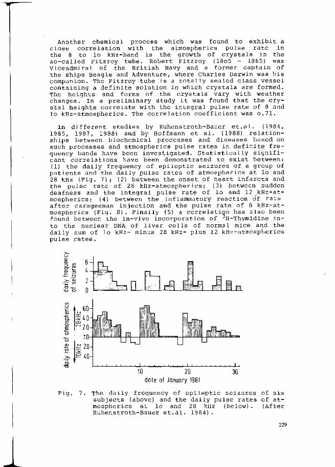
Another chemical process which was found to exhibit a close correlation with the atmospherics pulse rate in the 8 to lo kHz-band is the growth of crystals in the so-called Fitzroy tube. Robert Fitzroy (18o5 - 1865) was Viceadmiral of the British Navy and a former captain of the ships Beagle and Adventure, where Charles Darwin was his companion. The Fitzroy tube is a totally sealed glass vessel containing a definite solution in which crystals are formed. The heights and forms of the crystals vary with weather changes. In a preliminary study it was found that the cry­stal heights correlate with the integral pulse rate of 8 and lo kHz-atmospherics. The correlation coefficient was o.71.

In different studies by Ruhenstroth-Bauer et.al. (1984, 1985, 1987, 1988) and by Hoffmann et al. (1988) relation­ships between biochemical processes and diseases based on such processes and atmospherics pulse rates in definite fre­quency bands have been investigated. Statistically signifi­cant correlations have been demonstrated to exist between: (1) the daily frequency of epileptic seizures of a group of patients and the daily pulse rates of atmospherics at lo and 28 kHz (Fig. 7); (2) between the onset of heart infarcts and the pulse rate of 28 kHz-atmospherics; (3) between sudden deafness and the integral pulse rate of lo and 12 kHz-at­mospherics; (4) between the inflammatory reaction of rats after carageenan injection and the pulse rate of 8 kHz-at­mospherics (Fig. 8). Finally (5) a correlation has also been found between the in-vivo incorporation of jH-Thymidine in­to the nuclear DNA of liver cells of normal mice and the daily sum of lo kHz- minus 28 kHz- plus 12 kHz-atmospherics pulse rates.

10 20 dote of January 1981

30

Fig. 7. The daily frequency of epileptic seizures of six subjects (above) and the daily pulse rates of at­mospherics at lo and 28 kHz (below). (After Ruhenstroth-Bauer et.al. 1984).

229

0.00 T — i — i — i — i — i — i — i — i — i — i — i — i — i — i — i — i — i — r 13. 20. 20. 24. 28. 4. 8. 12. 18. 22. 25. 24. 25. 2. 7. 14. 17. 4. 18. 16. 20. 5. 5. 6. 6. 6. 7. 7. 7. 7. 7. 7. 9. 9. 10. 10. 10. 10. 11. 11. 12. 12.

1985 • — • RCJ D--a AS>':8kHz

Fig.8. Relationship between the inflammatory reaction of rats to a carageenan injection (RCJ) into the hind paw and the mean daily pulse rate of atmospherics at 8 kHz. The correlation coefficient is o.49. The differences of paw weights (left-right) were the measure of the inflammation oedema. (After Ruhen-stroth-Bauer et.al., 1988).

Discussion

The statistically significant correlations between the at­mospherics pulse rates in definite frequency bands and che­mical or biochemical processes raise the question about the mechanism by which atmospherics could directly influence chemical or biological systems. In the case of the behavior of gelatin films it was found that only definite types of atmospherics with characteristic waveforms and frequency spectra seem to exert a direct influence on the diffusion time of ions in gelatin films (Baumer & Eichmeier, 1982). A hypothesis concerning the absorption of atmospherics in gelatin films says that incident atmospherics impulses can change the bond angles of distinct atoms in the polypeptide chains of the gelatin (Baumer & Eichmeier, 1983b). Similar processes could also be involved in the other cases descri­bed above.

One of the so far unsolved questions is raised by the re­sult that there are different narrow frequency windows in which atmospherics correlate with chemical or biochemical processes. The answer to this and other questions can possibly be given if the effects of artificially produced atmospherics on chemical or biological systems in labora­tory experiments are studied in detail. Such investigations have been started.

The analysis of atmospherics and of the corresponding weather processes demonstrates that the atmospherics repre­sent an electromagnetic code which must be deciphered. This

230

code can tell us the detailed story about the dynamic wea­ther processes.

In 1956 Hans Israel wrote: "It is necessary to learn un­derstanding the: language of Sferics - so far a largely un­solved problem". 21 years later, in 1977 (when we started our research work in atmospherics) , a member of the VLF ra­dio meteorology group in Berlin stated: "Today the situation has not basicly changed. The complex language of the Sfe­rics is still difficult to understand and often puzzling. The sources of Sferics produce continuously varying impulse forms which make the analysis of the Sferics an adventure".

Now we have started to learn that mysterious language of the atmosphere. This adventure was the exciting expe­rience in our research work during the last 12 years.

References

Baumer, H. & Eichmeier, J., 1978. Elimination of meteorotro-pic coagulation of gelatin films by means of a Faraday cage. Int. J. Biometeor., 22: 227-232.

Baumer, H. & Eichmeier, J., 1979. Relationship between the diffusion time of ions in gelatin films and the absolute humidity in free air. Int. J. Biometeor., 23: 69-^75.

Baumer, H. & Eichmeier, J., 198oa. Eine Anlage zur Regi­strierung der Atmospherics bei lo und 27 kHz. Arch. Met. Geoph. Biokl. Ser. A, 29: 143-155.

Baumer, H. & Eichmeier, J., 198ob. Relationship between the pulse rate of atmospherics and the diffusion time of ions in gelatin films. Int. J. Biometeor., 24: 271-276.

Baumer, H. & Eichmeier. J., 1981a. Ein digitaler Bildspei­cher zur oszilloskopischen Darstellung einzelner Atmosphe­rics-Impulse. Arch. Met. Geoph. Biokl. Ser. A, 3o: 399-4o4.

Baumer, H. & Eichmeier, J., 1981b. Relationship between the atmospherics pulse rate in the lo and 27 kHz range, air mass movements and the diffusion time of ions in gelatin films. Int. J. Biometeor., 25: 263-268.

Baumer, H. & Eichmeier, J., 1982. The biophysically active waveforms of atmospherics incident on gelatin films. Int. J. Biometeor., 26: 85-9o.

Baumer, H. & Eichmeier, J., 1983a. Die verschiedenen At-mospherics-Impulsformen und ihre Ausbreitungsbedingungen. Arch. Met. Geoph. Biocl. Ser. A, 32: 155-164.

Baumer, H. & Eichmeier, J., 1983b. A hypothesis concerning the absorption of atmospherics in photo gelatin films. Int. J. Biometeor., 27: 125-131.

Baumer H. & Eichmeier, J., 1983c. Die Transformation des elektromagnetischen Impulsfrequenzspektrums der Atmosphäre in ein hörbares Klangbild, Arch. Met. Geoph. Biocl. Ser. A, 32: 399-4o4.

Baumer, H., Metz, W. & Eichmeier, J., 1981. Ein digitaler Bildspeicher zur oszilloskopischen Darstellung einzelner Atmospherics-Impulse. Arch. Met. Geoph. Biocl. Ser. A, 3o: 399-4o4.

Baumer, H., Sönning, W. & Eichmeier, J., 1988. Correlation between the pulse rates of atmospherics and temperature

231

variations of the atmosphere. Int. J. Biometeor., 32: 271-274.

Eichmeier, J. & Baumer, H., 1982. Das natürliche elektromag­netische Impulsfrequenzspektrum der Atmosphäre. Arch. Met. Geoph. Biocl. Ser. A, 31: 249-261.

Hoffmann, G., Vogl, S., Baumer, H. & Ruhenstroth-Bauer, G., 1988. Significant correlations between atmospherics and the in vivo incorporation of -^H-Thymidine into the nuclear DNA of liver cells. Naturwissenschaften, 75: 459-46o.

Ruhenstroth-Bauer, G., Baumer, H., Kugler, J., Spatz, R., Sönning, W. & Fipiliak, B., 1984. Epilepsy and wea­ther: a significant correlation between the onset of epi­leptic seizures and specific atmospherics - a pilot study, int. J. Biometeor., 28: 333-34o.

Ruhenstroth-Bauer, G., Baumer, H., Burkel, E.M., Sönning, W., & Fipiliak, B., 1985. Myocardial infarction and the weather: a significant positive correlation between the onset of heart infarct and 28 kHz atmospherics - a pilot study. Clin. Cardiol., 8: 149-151.

Ruhenstroth-Bauer, G., Mees, K., Sandhagen, R., Baumer, H. & Fipiliak, B., 1987. Demonstration of statistically signi­ficant correlations between 8 and 12 kHz atmospherics and sudden deafness. Zeitschr. Naturforsch., Teil C, 42: 999-1000.

Ruhenstroth-Bauer, G., Rösing, 0., Baumer, H., Sönning W. & Lehmacher, W., 1988. Demonstration of correlations between the 8 and lo kHz atmospherics and the inflammatory reac­tion of rates after carageenan injection. Int. J. Biome-teor., 32: 2ol-2o4.

Sönning, W., 1984. Über die Abhängigkeit des Tagesgangs der Atmospherics-Impulsrate bei lo und 27 kHz von meteoro­logischen Bedingungen. Arch. Met. Geoph. Biocl., Ser. A, 33: 77-87.

Sönning, W., Baumer, H. & Eichmeier, J., 1981. Die Atmosphe-rics-Aktivität bei lo und 27 kHz als Indikator für die Dynamik der troposphärischen Wettervorgänge. Arch. Met. Geoph. Biocl., Ser. B, 29: 299-312.

Sönning, W., Baumer, H. & Eichmeier, J., 1984. Untersuchung des Tagesgangs der Atmospherics-Impulsrate bei lo und 27 kHz. Arch. Met. Geoph. Biocl., Ser. A, 33: 69-75.

232

PERIODICITIES OF METEOROLOGICAL PARAMETERS AT SCHIERMONNIKOOG A SIMPLE EXPLANATION

H.F. Vugts

Institute of Earth Sciences, Department of Meteorology, Free University, De Boelelaan 1085, 1081 HV Amsterdam, The Netherlands

Summary In a sea area consisting partly of periodically drying

tidal flats, the semidiurnal lunar tide, interacting with the daily variation of solar radiation, gives rise to both a beat in the amplitude of the daily water temperature cycle with a period of 14.76 d, and a variation of the daily mean temperature, with the same period. This is shown theoretically and by observation. Another weather phenomena which can be found in a tidal area is the influence of the tide on both rainfall depth and intensity. It is shown that under special conditions this occurs during the summer months and autumn. Keywords: periodicities, tidal influences, sea temperature, rainfall.

The heat balance of a tidal - flat sea

Theoretical considerations

In a sea which covers tidal flats the tidal currents cause both a periodical translation of water masses and a periodical flooding of tidal flats. In consequence, the area of interface between the sea water and the atmosphere will differ during different phases of the tide. At low tide a given volume water will collect in deeper tidal channels and will thus have a smaller surface area than at high tide when part of the same volume will be spread out over the tidal flats. The influence of such a periodically varying surface area on the heat balance of the water volume, has been described by Vugts and Zimmerman (1975, 1985). From a simplified model experiment it can be concluded that the daily mean water temperature and amplitude are varying with a period of about 14.76 d. The phenomenon of interaction of the daily heat balance and tidal cycle can be understood from Fig. 1. Here, for two days separated by a time interval of seven days, the variation of surface area (S(t)) because of the M2 tide is shown together with net radiation, predominated by the solar radiation. For day 1 the maximum of the net radiation coincides with the maximum of the water surface, whereas at day 8 at its minimum. The consequence is a variation in the amplitude of the daily temperature cycle and its mean value with a period of 14.76 d.

233

w

S(t)

DAY 1

24

O(t)

12 24 12 24 12 24 12

24 12 24 12

DAY 8

Fig. 1. Variation of surface area S(t) and net radiation Q(t) during a day for a couple of days, upper two figures, separated by a time interval of seven days, lower two figures.

234

Real situation

Extensive measurements were carried out in the Dutch Wadden Sea, which is a part of an estuarine inshore area along the Dutch, German and Danish coasts, separated from the North Sea b6y a chain of islands. An important part of the area called "Wadden", emerges at low tide as muddy sand flats. A typical part of this tidal-flat sea is the Mok bay, situated at the southern tip of Texel island (Fig.2). A tidal channel connects the bay with the western part of the Wadden Sea. Through this channel water which covers the tidal flats flows in and out with the tide. The tide in this area is dominated by the M2 tidal cycle. In the tidal channel the temperature was recorded at three different depths, at intervals of 5 minutes. On that basis, the daily mean temperature was calculated. The accuracy of water temperature measurements was checked with reversing thermometers, and seemed to be 0.1 °C. About 110 days of records were available for analysis. As is to be expexted in this area, due to "atmospheric noise" (such as varying cloudiness and advection of different air masses, for instance by depressions, interchanging heat with the earth's surface), daily mean values and daily amplitudes of water temperature varied greatly. At one of the tidal flats all of the relevant meteorological parameters were recorded; these included net radiation, air temperature, humidity and windvelocity.

Ä O 0 Q*ROTTUMEROOG SCHIERMONNIKOOG

• 1 Weathsrstation 2» Wast Tarschall ing "::.Tidal f l a t

Fig. 2. Map of the tidal flat area with the different locations.

To separate short-term fluctuations of the daily mean water temperature from background long background long term variations, such as increasese or decreases of water

235

temperature caused by seasonal heating or cooling, the daily mean difference between the temperature of the channel and that of the adjacent North Sea was calculated. After smoothing the data, six periods, each covering 15 d were considered. After normalizing these six periods an average curve for a 15-d period was constructed, in such a way that days having high tides at approximately the same time as one another occupied the same place in the sequence. The resulting curve gives the daily deviations of the tidal water temperature from the period mean, which is shown in Fig. 3a.

Fig. 3. A, average curve of the deviation of daily mean water temperature of Mok Bay from its mean value over a 15-d period. B, average curve of the difference between daily maximum and minimum water temperatures. Bars denoting the standard deviations.

There is a significant difference between the temperature deviation curve and any straight line and the curve agrees well with the predicted periodicity of the daily mean water temperature in a tidal flat area. It has also been checked that this result is not caused by any accidental variation in the energy input, having the same period, or air temperature. As predicted theoretically, the daily amplitude varies with a period of about 15 d as well, which is shown in Fig. 3b. The asymmetrical behaviour of the curve of Fig. 3a could be explained by the fact that, in this area, the moment of high tide itself shifts in a asymmetrical way during a 15-d period. Of course, part of the asymmetry may be caused by a variation in the atmospheric background, which has not been removed by averaging over only six periods. Nonetheless, it may be stated that a qualitative agreement exits between theory and experiment.

The rainfall on a "Wadden" island

Introduction

Natural convection is very important in the proces of development of shower clouds. The convection involves the vertical exchange of masses of air, each carrying a store of heat, momentum and water vapour, which can give rise, in the

236

higher layers, to condensation. The natural convection is mainly caused by heating from below, which makes the air unstable. Thus the surface temperature is the determining factor for cloud formation, and therefore it is clear that above a colder surface this instability will decrease, resulting in less condensation. In this example we are dealing with a tidal flat area. The tidal flats are periodically covered with water, which means that at low tide a "Wadden" island is virtually connected with the mainland, while about six hours later it really will be an island. Since the moment of high tide is roughly one hour later every day, a tidal flat is a most suitable area over which to study the influence of different surface temperatures on rainfall. Each day gives a specific situation which is repeated in about fourteen days. If some influence does exist, therefore, it should be easy to detect if the observation series is sufficient long.

Description of the area

One of the Dutch islands of interesr to the present study is Schiermonnikoog, which is 16 kilometres long, 4 kilometres wide and oriented in a west-east direction (Fig. 2 ) . The island consists of sand beaches, dunes, meadows and salt marshes, the distance between Schiermonnikoog and the mainland coast being 8-10 kilometres. At low tide 85 per cent of the tidal flat area is dry and only the tidal channels contain water. At high tide the tidal flat is covered by water to a depth of about one metre. Its temperature is strongly related to the North Sea water temperature, but also influenced by the energy balance of the tidal flat -previously investigated by Vugts en Zimmerman (1975, 1985). In 1971 the Department of Meteorology of the Free University Amsterdam established a weather station on the island of Schiermonnikoog (Fig. 2) to serve as a reference station for student meteorological experiments during the, summer season. The following meteorological parameters are recorded: air temperature, relative humidity, windspeed and direction, rainfall, sunshine, global radiation and air pressure. The chemical composition of precipitation is analysed monthly.

Data analysis and discussion

The measuring period used for the analyses extends from September 1971 to August 1985. Rainfall was measured by a Pluviograph with an interval time of five minutes and a resolution of 0.1 mm, values of rainfall depth and duration being summarised each hour. In order to detect any significant influence by the tidal flats the observations were divided into four groups using the "external" parameters: high tide (HT), low tide (LT), wind from the mainland (LB) and from the North Sea (SB), resulting in the combinations HTLB, HTSB, LTLB, LTSB. For the sake of this study in first approximation high tide is defined as the period between three hours before and three hours after high tide, while the low tide period contains the remaining six hours. Because the tidal cycle is about 12.5 hours, one hour was added to the low tide period after two tidal cycles and two tidal cycles later the extra hour was

237

added to the high tide period and so on. Thus for the period of investigation the total hours of high tide and low tide were the same. A land-breeze (LB) is wind coming from the sector between 90° and 260°, the sea-breeze (SB) being from the remaining directions (see Fig. 2). For each month the difference in rainfall has been calculated between the situations HTLB and LTLB.

-t-e mm + 8-

+ 4

+2 •

-10

4C HTSB-LTSB

'*$*¥ i-w-i—1\- ^vr/

2.2

1.8-

1.4'

1.0

©

r ï ^ s -^

» « HTLB / \ o LTLB

-' A. /A. / \

i m / /h

2.4-

^

.A « HTSB l%\ . . LTSB

J F M A M J J A S O N D N D

Fig. 4. a, mean monthly difference in rainfall depth between high and low tide during land-breeze. Bars indicate standard errors. b, mean monthly rainfall intensity at high and low tide during land-breeze. c, mean monthly difference in rainfall depth between high and low tide during sea-breeze. Bars indicate standard errors. d, mean monthly rainfall intensity at high and low tide during sea-breeze. e, mean monthly difference between water temperature and soil temperature at a depth of 2 cm. f, mean monthly raifall depth during land-breeze and sea-breeze.

238

The average of individual differences for each month and the standard error of the mean were also calculated, the results are graphically represented in Fig. 4a. It is clear from Fig. 4a that the differences found depart significantly (i.e. by more than one standard error) from zero during summertime and are less pronounced with opposite sign during autumn. Average monthly rainfall is given in Fig. 4f divided into LB and SB conditions. The results indicate that in July, for example, rainfall depth is approximately 14 mm for the HTLB situation and in the LTLB situation case about 22 mm. A similar comparison of surface temperatures is given in Fig. 4e, which shows the differences between the monthly water temperature (based on a 60-year series) at West Terschelling (see Fig. 2) and mean monthly soil temperature at a depth of 2 cm (20 year series) for De Bilt (Können 1983). The data indicate that during summer months the daytime land surface temperature tends to be much higher than the water surface temperature, while at night they are approximately the same. The calculations were also carried out for that part of the day when the air will be most unstable (afternoon and first part of the evening). These results are comparable with those presented above for complete days. For each month of the year the average rainfall duration was also derived for the situations HTLB and LTLB, thus allowing calculations of the rainfall intensities. These results are plotted in Fig. 4b. From this figure it is clear that rainfall intensity is suppressed by the colder water during the summer period, which is in agreement with the result in Fig. 4a. An additional check on the above results is via a "reverse investigation". Thus during the SB situation the wind and rain reaching the weather station are always coming from the North Sea and can hardly be influenced by the tide and tidal flat area. These results are given in Figs. 4c and 4d and do not indicate any systematic behaviour. Further, the calculated differences (HT-LT) in rainfall for the period March to August (summer half year) are found to be -3.75±0.90 mm for the land-breeze condition and for the sea-breeze condition 0.60+0.78 mm. This again indicates a significant difference. Finally, a "control" on the mainland was carried out for the summer months (June, July and August) for the rainfall measured at Leeuwarden, the nearest station with hourly data. Data were available for the period 1981-85. The result is that HTLB-LTLB for Leeuwarden is 0.93+2.06, while for the same months for the island the difference is -7.35 mm+3.69. It is thus concluded that both rainfall depth and intensity are influenced by the tide on the island of Schiermonnikoog.

References

Können, G.P., 1983. Het weer in Nederland. Thieme, Zutphen. Vugts, H.F. and Zimmerman, J.T.F., 1975. Interaction between

daily heat balance and the tidal cycle.Nature,225,113-117. Vugts, H.F. and Zimmerman, J.T.F., 1985. The heat balance of

a tidal flat area. Neth. J. Sea Res., 19, 1-14.

239

MARS AND TEMPERATURE-CHANGES IN THE NETHERLANDS: AN EMPIRICAL STUDY

J.W.M. Veiiker and M.C. B e e f t i n k Meteorological consultants, P.O. Box 30, St.Anthonls, NL

SUMMARY

This paper describes the results of an empirical study of a possible relation between the GEOCENTRIC positions of the planet MARS and tempera­ture-changes. As a result of this study it is shown that this relation is statistically significant. Earlier observations of a cyclic relation between temperature changes and the geocentric position of Mars (with a cycle length of 30 degr. of arc) are confirmed [17]. The study was based on samples of daily average temperatures at De Bilt, Netherlands during a continuous period of 27 years (1961-1988 = 9861 daily temperatures). The corresponding geo­centric positions of Mars were calculated to an accuracy of approx. 0.01 degrees of arc at 12.00 GMT. Finally the Chi-square test was used in order to measure the significance level. It is shown that when Mars is observed on the 26th and 27th degree of each sector, the probability that colder air will be advected is higher than on any other position of Mars (p=.018). When warmer air is advected (only during the summer months) this will happen when Mars is mainly found on the 20th and 21st degree with a significance-level of p-.029

1.INTRODUCTION

Scientific interest in the role of near- and far-environmental factors exists for quite some time already. During the last few decades the knowledge of these factors such as solar parameters, cosmic rays and electromagnetic fields, to mention only a few, is also growing with very interesting results in several cases.

A relationship between lunar parameters and some weather-parameters were discovered by Adderley and Bowen (1), Otten (12), Currie (4), Zahnle and Walker (18). The endeavour of Reiter (13), Roberts and Olson (14), Schuurmans and Oort (16) and King (8) revealed a relation between the solar cycle and changes of physical parameters in the atmosphere. Sanford (15), Huntington (7), Bigg (2), Gribbin (6) and Landscheidt (9) focused their interest on the planetary constituents of the solar system.

The research presented in this paper originated in the author's interest in observational phenomena in widely different fields and their possible interrelations. Author and co-worker noticed an apparent relation between specific planetary positions and major breaks in the weather (17). Based on these observations the author worked out a model and produced, during the years 1983 and 1984, a list with long series of expected major weather changes in the Netherlands. Quarles van Ufford (Chief Climatologist of the Dutch Royal Meteorological Institute "K.N.M.I.") carried out a synoptical evaluation with positive results .

Due to day-to-day synoptical evaluations, it was confirmed that the expected number of notable weather changes corresponded rather well with the number of notable weather changes that actually occurred, whereas at least 2 out of 3 forecasts proved to be correct. Encouraged by the results of this 'pilot-study' a second, statistical, investigation was carried out. This second investigation consists of the test of two samples as described below.

240

2.PRELIMINARY STUDY EXAMINING PLANETARY CYCLES IN RELATION TO THE WEATHER.

Concerning changing weather-parameters in relation to astronomical factors, an empirical study was produced by J. Venker in 1987 [17]. He observed a cyclic relation between the GEOCENTRIC position of the planet MARS and major weather-changes in 1981-82, at De Bilt, Netherlands.

The astronomical criterium in this study is the TROPICAL ZODIAC (ecliptic) divided into 12 sectors of 30 degrees each. In other words, the ecliptic was used as a reference grid. In order to define the Mars-positions (angles), the main reference point was the Spring-Equinox or 0 degr.Aries-point.

In a remarkable percentage of cases it was found that when the planet MARS was passing the last degrees of the noted sector a weather break was observed; likewise, when the geocentric position of this planet was at a few degrees distance before the sector limits, the probability of such a weather break appeared to be low. Of the various elements that make up the weather, temperature was singled out as the most suitable element for the statistical analyses described below.

3.TEST METHOD

It is evident that, if there is a cyclic relation between the position of Mars and temperature changes, a recurrent change in temperature should be observable at equal angular distances, respective to an arbitrary reference point in the cycle (e.g. the beginning of the cycle, i.e. the Sprang Equinox or 0 degrees Aries).

The frequency of these recurrent temperature changes should be considerably higher than the frequencies to be expected due to random changes in temperature. As mentioned above the cycle length was expected to be 30 degrees of arc of the geocentric longitude of Mars. The distance from Mars' position to the beginning of the cycle may be expressed as mod(Mars,30) being the remainder after division by 30 (of Mars' geocentric longitude).

In order to apply the chosen statistical test the above mentioned sectors of 30 degrees of the Tropical Zodiac were divided into 15 classes of 2 degrees each (with an average of approximately 18 and 24 observations, respectively for both samples tested).

The number of temperature changes can now be counted for each class of 2 degrees, and compared with the frequency expected in case of a random distribution of temperature changes over the classes of the sectors. Finally, using the Chi-square test we may decide if there is a sufficiently large probability that the results found can be expected from a random distribu­tion.

4.DATA TRANSFORMATIONS

4.1.Temperature change parameter.

The most simple temperature change parameter is the difference in tempera­ture between two consecutive days. However, this parameter is in a high degree subject to random effects. Using some sort of average or moving average smoothens the random effects, but at the same time smoothens the effects we are looking for. The variable dT3 (see "DEFINITIONS") seemed to be a good compromise. It was however found that temperature change parameters showed a marked seasonal variation (Fig 1, next page).

241

dT3 monthly averages and 95X canf.lnt. dT3 monthly standard deviations 1951-1907 1963-1987

X \7 ~XZ7

month ~rTT

month IT

Figure 1 : Monthly averages of dT3 and their 95% confidence intervals (i.e. at any month within the period from 1961-1987 the probability that the average is found between the higher and lower bounds is 95%).

The right-hand part shows that temperature changes in winter tend to be more severe than in the summer. The standard deviation of dT3 in December is nearly twice as high as in August. To eliminate this effect dT3 has been "normalised" into dT3N by subtracting the monthly average and dividing the result by the standard deviation for that particular month. As a result dT3N is no longer expressed in centigrade but in units of standard deviation. A temperature change was considered to be important if the value of dT3N was larger or smaller than 1 unit of standard deviation. The frequency distribu­tion of dT3N is almost identical with the Normal Distribution. In other words, approx. 16% of the observations show a value of dT3N>l.

4.2.Classification of geocentric longitude

Because of the apparent cyclic relation between Mars's geocentric longi­tude and the temperature changes, the calculated longitudes were converted into classes according the formula : M30=2*int(l+mod(longtd,30)/2) in which mod(longtd,30) means the remainder after dividing the geocentric longitude by 30. So M30 has the integer values of 2..30 with an increment of 2 [degrees of arc].

4.3.Rétrogradation

A possible artefact was detected and tested in relation to the rétrogra­dation and the associated slow movement of Mars (during several weeks) once in every 2 years as this phenomenon could possibly distort the validity of the test results. However, even after excluding the noted rétrogradation periods from the test, it hardly changed the results. In order to exclude any influence of rétrogradation effects, data where Mars' angular velocity was less than 0.4 degree per day were ignored. The entire angular velocity range is from -0.4 up to +0.8 degrees/day.About 20% of the time the angular velocity is less than 0.4 degrees/day.

5.FIRST SAMPLE TEST RESULTS

For every day in an arbitrary period from 1 January 1964 to 1 May 1969, the value of dT3N and the related positions of Mars were computed [11]. The results of the computation were treated as described in par. 4.

242

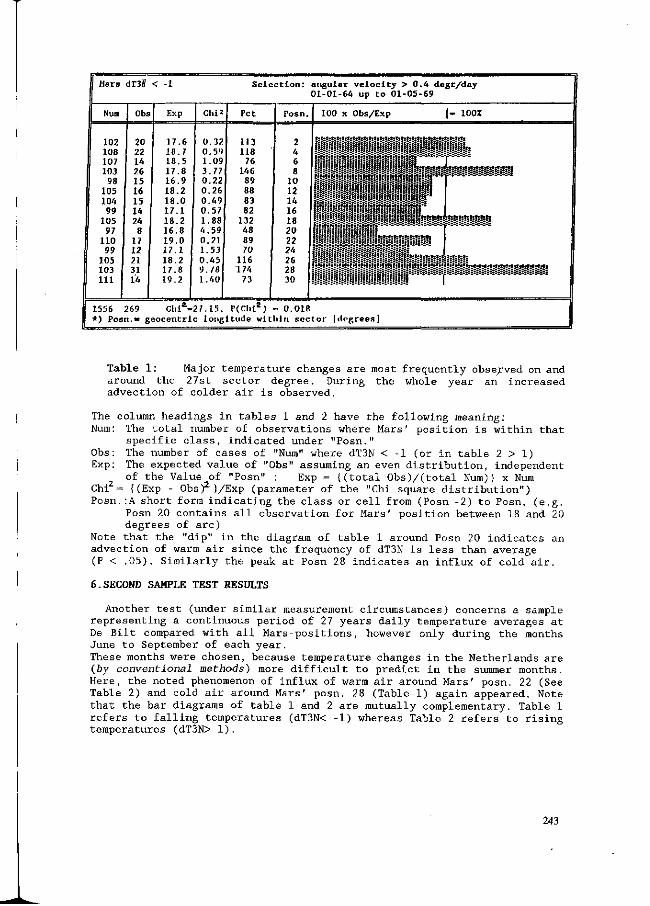
Hars dT3» < -1 Selection: angular velocity > 0.4 degr/day 01-01-64 up to 01-05-69

Num Obs Exp Chi2 Pet Posn. 100 x Obs/Exp | - 100X

102 108 107 103 98

105 104 99

105 97

110 99

105 103 111

20 22 14 26 15 16 15 14 24 8

17 12 21 31 14

17.6 18.7 18.5 17.8 16 .9 18.2 18 .0 17 .1 18 .2 16.8 19 .0 17 .1 18.2 17 .8 19.2

0 .32 0 .59 1.09 3 .77 0 .22 0 .26 0 .49 0 1 4 0 1 0 9 1

57 .88 59 21 53 45 78 40

113 118

76 146 89 88 83 82

132 48 89 70

116 174 73

I

2 4 6 8

10 12 14 16 18 20 22 24 26 28 30

{:>:!:*:**!:!:£:!:!:*:!:!:!:!:!:!:!:!:!:!:!:!:!:

£|i||fiff|i|i|jfifz|£il|ffif||ifiâs^|gï«|^

|i|f|i|i|||f|f|i|||:|i|||s|I|i|£|£|s|l^«=ç=f=«=JUç=ç=ç-s.BSB=«=ç-

l|l|||i|i|||I||||||||£||||i|||||5|l;=-=--=-==-=-=^r-~---=-=-=-=-r-=-s-=-=-=-^

1556 269 Chi -2 *) Posn.e geocentric

7.15. P(Chl') -longitude with

O.OIR In sector |degrees]

Table 1: Major temperature changes are most frequently observed on and around the 27st sector degree. During the whole year an increased advection of colder air is observed.

The column headings in tables 1 and 2 have the following meaning: Num: The total number of observations where Mars' position is within that

specific class, indicated under "Posn." Obs: The number of cases of "Num" where dT3N < -1 (or in table 2 > 1) Exp: The expected value of "Obs" assuming an even distribution, independent

of the Value of "Posn" : Exp = ((total 0bs)/(total Num)) x Num Chi = {(Exp - Obs^J/Exp (parameter of the "Chi square distribution") Posn.:A short form indicating the class or cell from (Posn -2) to Posn, (e.g.

Posn 20 contains all observation for Mars' position between 18 and 20 degrees of arc)

Note that the "dip" in the diagram of table 1 around Posn 20 indicates an advection of warm air since the frequency of dT3N is less than average (P < .05). Similarly the peak at Posn 28 indicates an influx of cold air.

6.SECOND SAMPLE TEST RESULTS

Another test (under similar measurement circumstances) concerns a sample representing a continuous period of 27 years daily temperature averages at De Bilt compared with all Mars-positions, however only during the months June to September of each year. These months were chosen, because temperature changes in the Netherlands are (by conventional methods) more difficult to predict in the summer months. Here, the noted phenomenon of influx of warm air around Mars' posn. 22 (See Table 2) and cold air around Mars' posn. 28 (Table 1) again appeared. Note that the bar diagrams of table 1 and 2 are mutually complementary. Table 1 refers to falling temperatures (dT3N< -1) whereas Table 2 refers to rising temperatures (dT3N> 1).

243

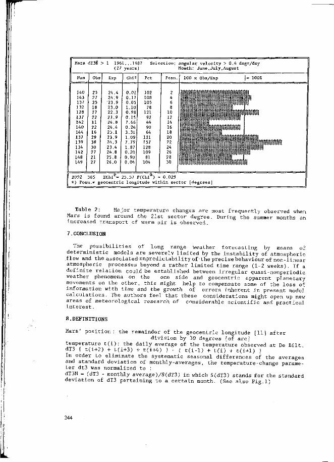
Mars dT3K > 1 1961...1987 (27 years)

Selection: angular velocity > 0.4 degr/day Month: June,July,August

Exp Chi* Posn. 100 x Obs/Exp 1007.

140 143 137 132 128 137 142 140 144 137 139 134 142 148 149

24.4 24:9 23.9 23.0 22 23 24 24 25 23 24 23 24.8 25.8 26.0

0.01 0.17 0.05 1.10 0.98 0.15 7.66 0.24 3.31 1.09 7.79 1.87 0.20 0.90 0.04

102 108 105

78 121

92 44

90 64

121 157 128 109

81 104

2 4 6 8

10 12 14 16 18 20 22 24 26 28 30

!!;!!ï!-! ;!'!"!'!J!«!»!"!:!!!!:::::::!:i*:'! I

!:t;t:i:t:i:t:t;

2092 365 EChi - 25.57 P(Chi ) - 0.029 *) Posn.» geocentric longitude within sector [degrees]

Table 2: Major temperature changes are most frequently observed when Mars is found around the 21st sector degree. During the summer months an increased transport of warm air is observed.

7.CONCLUSION

The possibilities of long range weather forecasting by means of deterministic models are severely limited by the instability of atmospheric flow and the associated-unpredictability of the precise behaviour of non-linear atmospheric processes beyond a rather limited time range (1-2 weeks). If a definite relation could be established between irregular quasi-nonperiodic weather phenomena on the one side and geocentric apparent planetary movements on the other, this might help to compensate some of the loss of information with time and the growth of errors inherent in present model calculations. The authors feel that these considerations might open up new areas of meteorological research of considerable scientific and practical interest.

8.DEFINITIONS

Mars' position : the remainder of the geocentric longitude [11] after division by 30 degrees [of arc]

temperature t(i): the daily average of the temperature observed at De Bilt dT3=( t(i+2) + t(i+3) + t(i+4) ) - { t(i-l) + t(i) + t(i+l) } In order to eliminate the systematic seasonal differences of the averages and standard deviation of monthly-averages, the temperature-change parame­ter dt3 was normalized to : dT3N = (dT3 - monthly average)/S(dT3) in which S(dT3) stands for the standard deviation of dT3 pertaining to a certain month. (See also Fig.1)

244

9.REFERENCES

1. Adderley, E.E., Bowen, E.G. (1962): "Lunar component in precipitation data". Science, vol.137, p.749-750.

2. Bigg, E.K. (1963): "A lunar influence on ice nucleus concentrations". Nature, vol.197, p.172-173.

3. Bradley, D.A., Woodburry, M.A. (1962) :"Lunar Synodical Period and Widespread Precipitation". Science, vol.137, p. 748-749.

4. Currie, R. (1987): in "Lunar link with Nile Floods", New Scientist, 8 October 1987, p.38.

5. Gleick. J.,(1988):"Chaos", Viking, New York, N.Y., U.S.A ,p. 11-31 6. Gribbin, J., (1973): "Planetary Allignments" , Solar Activity and Climatic

Change". Nature, London, U.K., 246, 453-454. 7. Huntington, E., (1948): "Civilisation and Climate". Yale Univ. Press, New

Haven, Ct., p.453. 8. King, J.W., (1973): "Solar Radiation Changes the Weather". Nature.

(London) 245, 443-446. 9. Landscheidt, T. (1981): "Swinging Sun, 79-year-cycle and Climatic

Change". J.Interdescipl.Cycle Res. vol. 1, 3-20. 10. Lorentz, E., (1963): "Deterministic Non Periodic Flow", Journ. of the

Atm.Sciences 20, p.130-141 11. Meeus, J., (1985): "Marsalgorhythm", Astronomical Formulae for Cal

culators, Wlllman-Bell Inc., Richmond, Vir.,USA. 12. Otten, H. , (1987): in J. of Climate & Appl. Meteorl. , Oct. 1987 /

Weather, Nov. 1987. 13. Reiter, R. , (1971): "Further Evidence for the Impact of Solar Activity

upon Potential Gradient and Air Current in the Lower Troposphere", Pure Appl. Geoph. 94 (2), p. 218-225

14. Roberts, W., Olson, R.H., (1973): "New Evidence for Effects of Corpuscular Emission of the Weather".

15. Sanford, F., (1936): "Influence of Planetary Configurations upon the Frequency of Visible Sunspots", Publ. Smithonian Inst. Wash., DC, U.S.A.

16. Schuurmans, C.J.E. and Oort, A.H. (1969): "A Statistical Study of Pressure Changes in the Troposphere and Lower Stratosphere after Strong Solar Flares". Pure Appl. Geoph. 75 (4), 233-246.

17. Venker. J., (1985): "Mars en het Temperatuurverloop te De Bilt", KNMI-Library, nr. 11.o. 938, De Bilt, Netherlands.

18. Zahnle, K., Walker, J., (1987): in "Ancient Climates linked to Lunar Cycles". New Scientist 22 oct. 1987, p.34.

245

POSSIBLE PLANETARY EFFECTS AT THE TIME OF BIRTH OF SUCCESSFUL PROFESSIONALS^ DISCUSSION OF THE »MARS EFFECT"

M.Gauquelin

Laboratoire d'Etude des Relations entre Rythmes Cosmiques et Psychophysiologiques^

Summary

Since his first book :Gauquelin(1955), the author have publi­shed a series of very significant correlations between planeta­ry positions and times of birth of successful people. In parti­cular, sports champions tend to be born more often than ordina­ry people when the planet Mars is rising or culminating. This observation, later called"the Mars effeet" , has been checked se­veral times by scientists. The present article briefly shows: 1) How the Belgian Para Committee gathered a fresh sample of athletes and found the same Mars effect again(1976); 2) Why A-merican professors Abell, Kurtz &. Zelen eventually stated that "Gauquelin adequately allowed for demographic and astronomical factors in predicting the expected distribution of Mars"(1983); 3) How German professor Ertel demonstrated the validity of the 'eminence effect', a claim made by the author since the begin­ning of his work, i.e., the more famous the sports champions are, the stronger the Mars effect is(1988). Keywords: time of birth, successful professionals, Mars effect, Belgian Para Committee,CSICOP, Zelen test,citation frequencies.

Introduction

In 1949 I initiated an investigation on several thousands of successful professionals. It led me to observe a statistically very significant relationships between the daily birth hours and certain factors of the cosmic environment. Methodology,data, results, and conclusions have been published in details since my first book in French :Gauquelin( 1 955 ) and published in English and other languages since then, the latest publication being: Gauquelin( 1988). In this article, only the minimum of informa­tion is given necessary to understand it. The observed effect appeared to be related to the diurnal move­ment of the moon and the nearest most massive planets. Each day, according to the 24 hour revolution period of the earth, celes­tial bodies rise at the horizon, culminate at the meridian, set and rise again the next day. Let us consider, for instance, the diurnal movement of the planet Mars in Paris on February 6,1924: Mars rises at 3:13 a.m., culminates at 7:29 a.m., sets at 11:44 a.m., and rises again the next morning at about the same time as the day before. Of course, the diurnal schedule of the planet changes over days, months,years.In order to perform statistics, it is possible to divide the diurnal movement of the planet in several sectors, say 12,18 or 3.6 sectors :Gauquelin ( 1 955 ,1 988 ) .

1. Present address: 8,rue Amyot, 75005 Paris, France

246

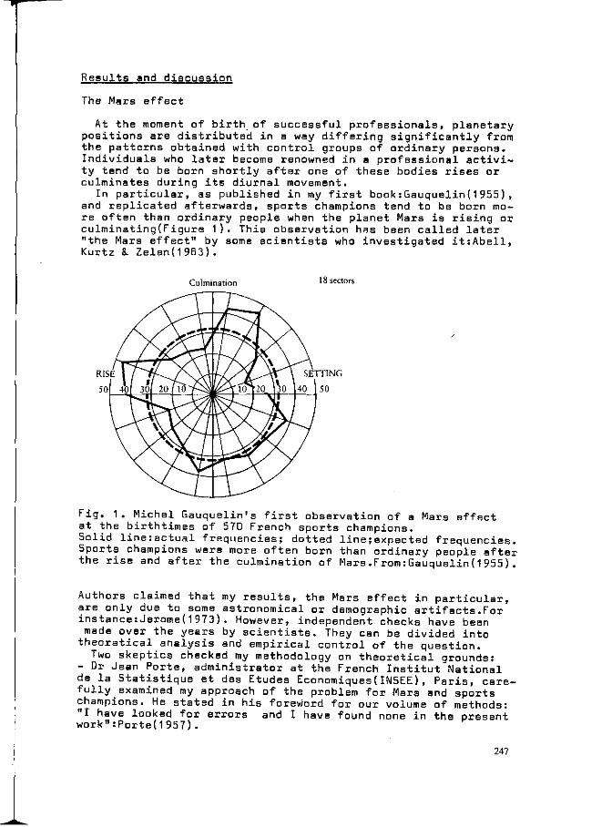
Results and discussion

The Mars effect

At the moment of birth of successful pro positions are distributed in a way differi the patterns obtained with control groups Individuals who later become renowned in a ty tend to be born shortly after one of th culminates during its diurnal movement.

In particular, as published in my first and replicated afterwards, sports champion re often than ordinary people when the pla culminating(Figure 1). This observation ha "the Mars effect" by some scientists who i Kurtz k Zelen(1983).

fessionals, planetary ng significantly from of ordinary persons.

professional activi-ese bodies rises or

book:Gauquelin(1955), s tend to be born mo-net Mars is rising or s been called later nvestigated it:Abell,

Culmination 18 sectors

Fig. 1. Michel Gauquelin's first observation of a Mars effect at the birthtimes of 570 French sports champions. Solid line:actual frequencies; dotted line ; expected frequencies. 5ports champions were more often born than ordinary people after the rise and after the culmination of Mars.From :Gauquelin(1955).

Authors claimed that my results, the Mars effect in particular, are only due to some astronomical or demographic artifacts.For instance:Jerome(1973). However, independent checks have been made over the years by scientists. They can be divided into

theoreticalanalysis and empirical control of the question. Two skeptics checked my methodology on theoretical grounds:

- Dr Jean Porte, administrator at the French Institut National de la Statistique et des Etudes Economiques(INSEE) , Paris, care­fully examined my approach of the problem for Mars and sports champions. He stated in his foreword for our volume of methods: "I have looked for errors and I have found none in the present work":Porte(1957).

247

- Twenty years 1 produced a memor cal objection ag objection. Rawli to astronomical objection. He sa made fair allowa (1978).

Now, the contr cal basis. Skept trois I carried by them. They wa their own proced ment and the Zel

ater, skeptic astronomer Dennis Rawlins has andum in which he studied the main methodologi-ainst the Mars effect, i.e., the demographic ns called it "the dawn factor" problem. Owing and mathematical arguments, Rawlins rejects the ys:"therefore, one concludes that Gauquelin has nee for the effect under investigation": Rawlins

ols of the expected frequencies have an empiri-ics were generally ignorant of the numerous con-out or, understandably, they were not convinced nted to carry out controls for themselves using ure. So were born the Para Committee's experi-en test.

Para Committee's replication

The Belgian Committee for the Scientific Investigation of Al­leged Paranormal Phenomena(in abbreviation Para Committee) is composed of scientists,including astronomers»demographers, and statisticians. This committee is highly skeptical and strongly opposed to the recognition of any 'paranormal' phenomena. Not convinced by the statistical proofs I had brought, they decided to gather another group of 535 sports champions, and they ob­tained quite similar results(Figure 2).

180-

Gûuquelin experiment (number of coses 1553)

15 100

| Para Committee R n j _ experiment (number

| of cases D35)

P M 38

CT

C

Î J _ J _ _L _1_ J L _1_ _L

65

45

25

10 II 12 1 2 3 4 5 6 7 8 9 sectors of diurnal movement

Fig. 2, The Mars effect and Sports Champions : comparison of Gau­quelin and Para Committee results.From :Gauquelin(1960,1972 ) , Para Committee(1976) .

Provided that a lot of misunderstanding had happened about Para Committee's successful replication, I would like to inclu­de here a copy of the table published in Committee's own re­port: Para Committeed 976) .

248

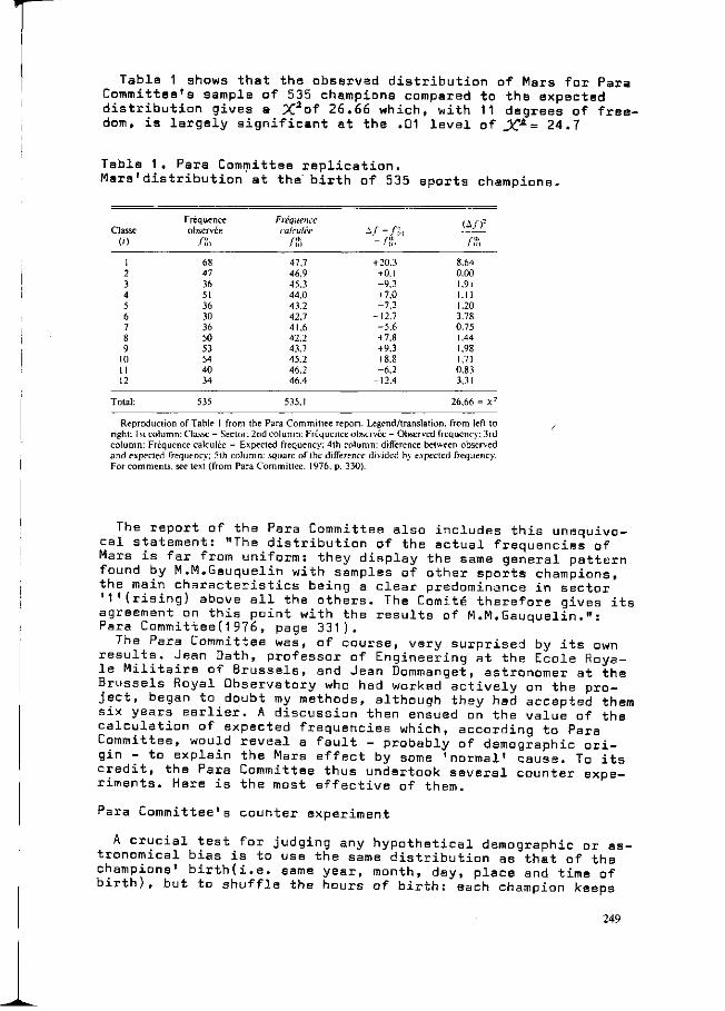
Table 1 shows that the observed distribution of Mars for Para Committee's sample of 535 champions compared to the expected distribution gives a X 2 o f 26.66 which, with 11 degrees of free­dom, is largely significant at the .01 level of J£*= 24.7

Table 1. Para Committee replication. Mars'distribution at the birth of 535 sports champions.

Classe (/)

1 2 3 4 5 6 7 8 9

10 11 12

Total:

Fréquence observée

/Si

68 47 36 51 36 30 36 50 53 54 40 34

535

Frequence calculée

J i i i

47,7 46,9 45,3 44,0 43.2 42.7 41.6 42,2 43.7 45.2 46,2 46.4

535.1

\f 'ft,, -.C +20.3 + 0.1 -9.3 + 7,0 -7,2

-12.7 -5.6 +7.8 +9.3 + 8.8 -6.2

-12.4

(A/)3

/ft 8.64 0.00 1.91 1,11 1.20 3.78 0.75 1.44 1,98 1,71 0,83 3,31

26,66 = X2

Reproduction of Table 1 from the Para Committee report. Legend/translation, from left to right: 1st column: Classe - Sector: 2nd column: Fréquence observée = Observed frequency: 3rd column: Fréquence calculée = Expected frequency; 4th column: difference between observed and expected frequency. 5th column: square of the difference divided by expected frequency. For comments, see text (from Para Committee. 1976. p. 330).

The report of the Para Committee also includes this unequivo­cal statement: "The distribution of the actual frequencies of Mars is far from uniform: they display the same general pattern found by M.M.Gauquelin with samples of other sports champions, the main characteristics being a clear predominance in sector '1'(rising) above all the others. The Comité therefore gives its agreement on this point with the results of M.M.Gauquelin. ": Para Committee(1976, page 331).

The Para Committee was, of course, very surprised by its own results. Jean Dath, professor of Engineering at the Ecole Roya­le Militaire of Brussels, and Jean Dommanget, astronomer at the Brussels Royal Observatory who had worked actively on the pro­ject, began to doubt my methods, although they had accepted them six years earlier. A discussion then ensued on the value of the calculation of expected frequencies which, according to Para Committee, would reveal a fault - probably of demographic ori­gin - to explain the Mars effect by some 'normal' cause. To its credit, the Para Committee thus undertook several counter expe­riments. Here is the most effective of them.

Para Committee's counter experiment

A crucial test for judging any hypothetical demographic or as­tronomical bias is to use the same distribution as that of the champions' birth(i.e. same year, month, day, place and time of birth), but to shuffle the hours of birth: each champion keeps

249

his real birth date and place, but is given the birth hour of the preceding champion according to the alphabetical order.Thus the new group has exactly the same demographic and astronomical conditions as the champions'group with real birth hours.

The Para Committee repeated this test nine times, each time shifting the birth hour from one champion to the next one. For example, in the first control test, the champion number 4 keeps his birth date and place, but receives the birth hour of cham­pion number 3, and so on. In the second control test, champion number 4 receives the birth hour of champion number 2, champion number 3 receives the birth hour of champion number 1, and so on. In the third control test, champion number 4 receives the birth hour of champion number 1, champion number 3 receives the birth hour of champion number 535, and so on. The results of the test are given in Table 2: Dommanget(1970),Gauquelin(1972,1982).

Table 2. Para Committee's counter-experiment for sports champions.

Classement Alphabétique

cl

1 2 3 4 5 6 7 8 9

10 11 12

/o

68 47 36 51 36 30 36 51 53 53 40 34

X2

P

f,

45 50 46 58 35 38 31 36 48 48 54 46

33,0

—

fi

55 43 47 44 42 35 48 34 51 45 48 43

24.9 0,8$

fl

44 38 52 50 40 50 34 40 52 48 34 53

36.1

—

ƒ«

44 46 46 45 42 41 37 52 48 38 49 47

32,2

—

/s

56 37 43 54 31 41 44 46 51 40 46 46

21.6 3%

ƒ.

38 52 45 49 54 31 33 40 46 53 49 45

40.8

—

fi

47 49 51 32 44 43 50 44 38 53 42 42

43.1

—

ƒ.

50 45 45 53 44 43 37 50 42 40 37 49

25.8 0.6%

ƒ9

40 56 42 42 50 46 36 39 40 39 41 64

60.4

—

ƒ,.,

46,6 46,2 46,3 47,4 42.4 40,9 38.9 42.3 46,2 44,9 44,4 48.3

25.4 0.7%

Explanations and comments: "Classement alphabétique"' is alphabetical order. From left to right: cl = Mars sectors: f0 = actual distribution of Mars at the birth of the champions: ƒ , through ƒ9 = distributions for the nine counter-experiments: / l t = means of the nine counter-experiments, by Mars sector. The bottom rows marked x : and p designate the chi-square statistic and its probability under the null hypothesis, respectively. Values are obtained by comparing the actual distribution, f0, with the respective distribution of each counter-ex­periment, ƒ 1, f 2i. • . , ƒ9. All nine differences are significant: Those between ƒ0 and f 1. fi. /A> f 6> ƒ i> and ƒ9 are significant at p < .001. The remainder range from p < .05 top < .01. The overall comparison between f0 and ƒ ,.9 (last column) yields;; < .01 (after Dommanget. 1970).

The distributions of Mars for the nine counter-experiments differ significantly from the distribution obtained with the real times of birth of the champions. Our conclusion is accor­dingly, that the Mars effect, again replicated by the Para Com­mittee, cannot be considered a(procedural)error or demographic artifact.Moreover, the values in Table 2, column f1,9 are very close to the theoretical(expBcted) values I calculated by my methodology and which were previously used by the Para Commit­tee itself(see Table 1, third column).

That was not, surprisingly enough, the final conclusion in the Para Committee's report. Actually, the Para Committee discarded the results of their own counter-experiments.According to their

250

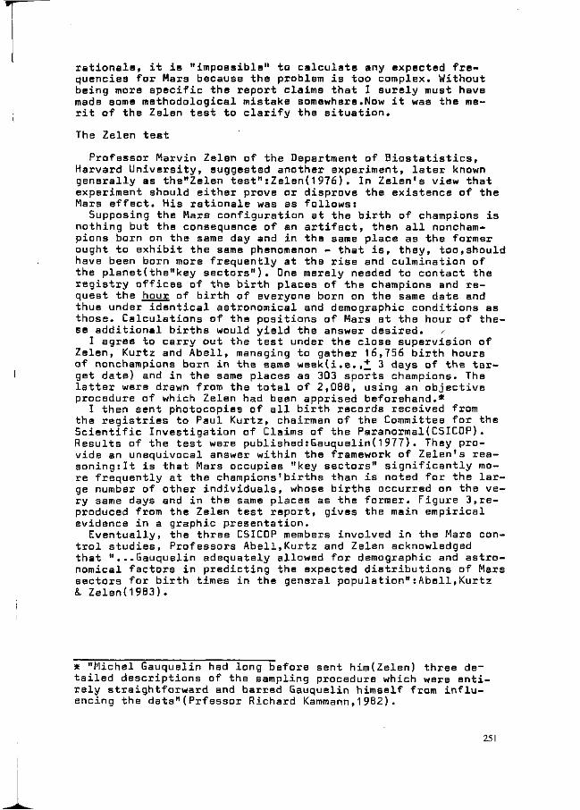
rationale, it is "impossible" to calculate any expected fre­quencies for Mars because the problem is too complex. Without being more specific the report claims that I surely must have made some methodological mistake somewhere.Now it was the me­rit of the Zelen test to clarify the situation.

The Zelen test

Professor Marvin Zelen of the Department of Biostatistics, Harvard University, suggested another experiment, later known generally as the"Zelen test":Zelen(1976). In Zelen's view that experiment should either prove or disprove the existence of the Mars effect. His rationale was as follows:

Supposing the Mars configuration at the birth of champions is nothing but the consequence of an artifact, then all noncham-pions born on the same day and in the same place as the former ought to exhibit the same phenomenon - that is, they, too,should have been born more frequently at the rise and culmination of the planet(the"key sectors"). One merely needed to contact the registry offices of the birth places of the champions and re­quest the hour of birth of everyone born on the same date and thus under identical astronomical and demographic conditions as those. Calculations of the positions of Mars at the hour of the­se additional births would yield the answer desired. /

I agree to carry out the test under the close supervision of Zelen, Kurtz and Abell, managing to gather 16,756 birth hours of nonchampions born in the same week(i.e.,+ 3 days of the tar­get date) and in the same places as 303 sports champions. The latter were drawn from the total of 2,088, using an objective procedure of which Zelen had been apprised beforehand.*

I then sent photocopies of all birth records received from the registries to Paul Kurtz, chairman of the Committee for the Scientific Investigation of Claims of the Paranormal(CSICOP). Results of the test were published:Gauquelin(1977). They pro­vide an unequivocal answer within the framework of Zelen's rea­soning:^ is that Mars occupies "key sectors" significantly mo­re frequently at the champions * births than is noted for the lar­ge number of other individuals, whose births occurred on the ve­ry same days and in the same places as the former. Figure 3,re­produced from the Zelen test report, gives the main empirical evidence in a graphic presentation.

Eventually, the three CSICOP members involved in the Mars con­trol studies, Professors Abell,Kurtz and Zelen acknowledged that "...Gauquelin adequately allowed for demographic and astro­nomical factors in predicting the expected distributions of Mars sectors for birth times in the general population":Abell,Kurtz L Zelen(1983).

* "Michel Gauquelin had long before sent him(Zelen) three de­tailed descriptions of the sampling procedure which were enti­rely straightforward and barred Gauquelin himself from influ­encing the data"(Prfessor Richard Kammann,1982).

251

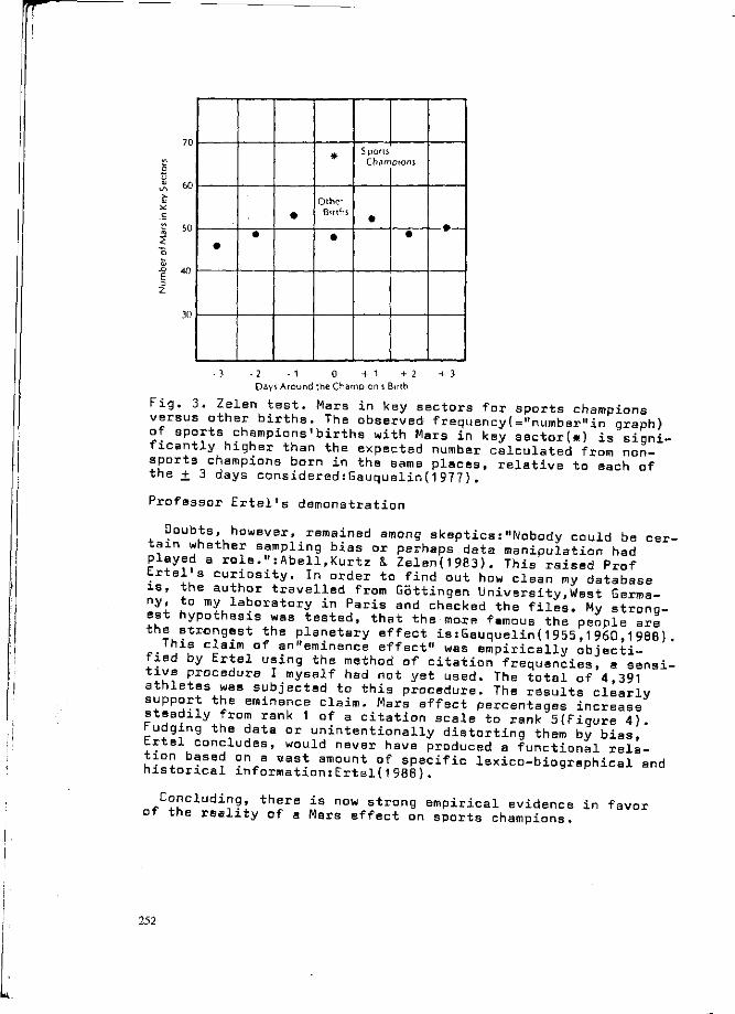
70

50

• •

•

#

Other Births

•

Sports Champions

• •

30

- 3 - 2 - 1 0 + 1 + 2 + 3 Days Around the Champion s Birth

Fig. 3. Zelen test. Mars in key sectors for sports champions versus other births. The observed frequency(="number"in graph) of sports champions'births with Mars in key sectorU) is signi­ficantly higher than the expected number calculated from non-sports champions born in the same places, relative to each of the + 3 days considered:Gauquelin(1977).

Professor Ertel's demonstration

Doubts, however, remained among skeptics :"Nobody could be cer­tain whether sampling bias or perhaps data manipulation had played a role.»:Abell,Kurtz & Zelen(1983). This raised Prof trtel s curiosity. In order to find out how clean my database is, the author travelled from Göttingen University.West Germa­ny, to my laboratory in Paris and checked the files. My stronq-est hypothesis was tested, that the more famous the people are the strongest the planetary effect is :Gauquelin(1955,1960,19BB).

This claim of an"eminence effect" was empirically objecti­fied by Ertel using the method of citation frequencies, a sensi­tive procedure I myself had not yet used. The total of 4,391 athletes was subjected to this procedure. The results clearly support the eminence claim. Mars effect percentages increase steadily from rank 1 of a citation scale to rank 5(Figure 4). fudging the data or unintentionally distorting them by bias, trtel concludes, would never have produced a functional rela­tion based on a vast amount of specific lexico-biographical and historical information:Ertel(1988).

Concluding, there is now strong empirical evidence in favor of the reality of a Mars effect on sports champions.

252

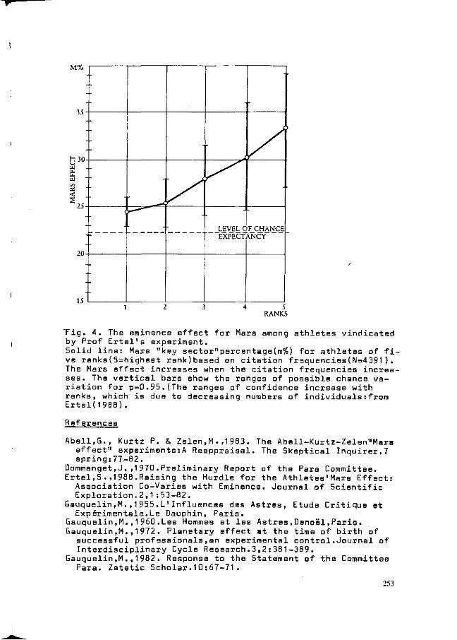
M%

Tig. 4. The eminence effect for Mars among athletes vindicated by Prof Ertel's experiment. Solid line: Mars "key sector"percentage(m%) for athletes of fi­ve ranks(5=highest rank)based on citation frequencies(N=4391). The Mars effect increases when the citation frequencies increa­ses. The vertical bars show the ranges of possible chance va­riation for p=0.95.{The ranges of confidence increase with ranks, which is due to decreasing numbers of individuals : from Ertel(1988).

References

Abell.G., Kurtz P. &. Zelen,M . ,1983. The Abell-Kurtz-Zelen"Mars effect" experiments:A Reappraisal. The Skeptical Inquirer,7 spring:77-S2.

Dommanget,J. ,1970.Preliminary Report of the Para Committee. Ertel,S.,1988.Raising the Hurdle for the Athletes•Mars Effect:

Association Co-Varies with Eminence. Journal of Scientific Exploration,2,1:53-82.

Gauquelin,M.,1955.L'Influences des Astres, Etude Critique et Expérimentale.Le Dauphin, Paris.

Gauquelin,M.,1960.Les Hommes et les Astres.Denoël,Paris . Gauquelin,M.,1972. Planetary effect at the time of birth of

successful professionals.an experimental control.Journal of Interdisciplinary Cycle Research.3,2 : 381-389.

Gauquelin,M.,1982. Response to the Statement of the Committee Para. Zetetic Scholar.10 : 67-71.

253

Gauquelin.M.,1983. The Truth about Astrology.Blackwell,Oxford. Gauquelin.M.,1988. Is There a Mars Effect ? Journal of Scien­

tific Exploration.2,1:29-52. Gauquelin.M.,1988. Written in the Stars - The Best of Michel

Gauquelin.Aquarian Press, Wellingborough,U.K. Gauquelin.M.,Gauquelin,F.,1977. The Zelen test of the Mars ef­

fect. The Humanist(November/December):30-35. Jerome,L.,1973. Astrology and Modern Sciencs:A Critical Analy­

sis. Leo nar do. 6 : 121-129 . Kammann,R.,1982. The True Disbelievers:Mars effect drives Skep­

tics to Irrationality. Zetetic Scholar.10:50-65. Para Committee(Comité Para), 1976. Considérations critiques sur

une recherche faite par M.M.Gauquelin dans le domaine des in­fluences planétaires.Nouvelles Brèves.43 : 327-343.

Porte,J.,1957. Foreword for M.F.&. M.Gauquelin. Méthodes pour étudier la répartition des astres dans le mouvement diurne. LERRCP,Paris.

Rawlins,D.,1978. Memorandum on the relation of Mars'solar pro­ximity to M.Gauquelin* s Mars-sports results and claims. Phe­nomena.2 ,2:22.

Zelen,M.,1976. Astrology and Statistics, a Challenge. The Huma­nist.36 ,1:32-33.

254

GAUQUELIN'S CONTENTIONS SCRUTINIZED

S. Ertel

Institut für Psychologie, Georg-August-Universität, D-3400 Göttingen, Goßlerstraße 14 (Federal Republik of Germany).

Summary

Since 1955, Michel Gauguelin claims to have discovered statistical relations between planetary positions and birth frequencies of eminent professionals. Former empirical trials of skeptics to refute this claim were unsuccessful. The author obtained evidence in favor of planetary relations (1) by scru­tinizing eminence variation: an objective indicator of emi­nence, frequency of citations, does correlate with the amount of planetary deviations; (2) by factor analysis: "key sector zones" are reproduced by unrotated first factors which rule out interpretation of planetary effects in terms of demogra­phic artefact; (3) by cluster analysis: hierarchical clusters of professions based on planetary data match prefectly with clusters based on human judgements. ' Keywords: extraterrestrical relations, planetary effects, Gauquelin claims, eminent professionals.

Overview

Michel Gauquelin claims to have found statistical relations between planetary positions and birth frequencies of eminent professionals. The following report is about my trials as to whether this contention holds.

First, a replication study performed by the skeptics Kurtz, Zelen, and Abell (1979-1980) (K-Z-A) will be scrutinized, the only study so far showing results allegedly contradicting Gau­quelin' s MARS effect. Does the failure of K-Z-A indicate that Gauquelin cannot be trusted?

Thereafter Gauquelin's own studies will be put to the test: If Gauquelin's planetary phenomenon is mere hazy illusion it should vanish if we look at it carefully by incorruptible op­tics.

Finally, results of multivariate analyses will be reported to which Gauquelin's data pool has been subjected: If Gauque­lin' s successive binding together of MARS with sports cham­pions, JUPITER with actors, SATURN with physicians etc. is mere manipulation, meaningful structure can hardly emerge from such data-.

Kurtz et al.'s replication failure

In 1979/80, Kurtz, Zelen, and Abell (K-Z-A) failed to re­plicate Gauquelin's MARS effect. What had happened? According to Gauquelin, the percentage of athletes' births with MARS in

255

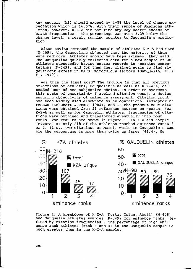
key sectors (kS) should exceed by 4-5% the level of chance ex­pectation which is 16.67%. With their sample of American ath­letes, however, K-Z-A did not find any key sector excess of birth frequencies - the percentage was even 3.2% below the chance level, a result running counter to Gauguelin's predic­tion.

After having screened the sample of athletes K-Z-A had used (N=409), the Gauguelins objected that the majority of them were mediocre. Athletes should have been skimmed, they said. The Gauqueiins quickly collected data for a new sample of US-athletes supposedly having better records in sporting compe-tetions (N=349), and for them they claimed again to find si­gnificant excess in MARS' miraculous sectors (Gauquelin, M. & F., 1979).

Was this the final word? The trouble is that all previous selections of athletes, Gauquelin's as well as K-Z-A's, de­pended upon ad hoc subjective choice. In order to overcome this state of uncertainty 1 applied citation count, a device ensuring objectivity of eminence assessment. Citation count has been widely used elsewhere as an operational indicator of renown (Schubert & Toma, 1984), and in the present case cita­tions were obtained from 21 reference sources on sports. For K-Z-A as well as for Gauquelin athletes, frequencies of cita­tions were obtained and transformed eventually into four ranks. The results are shown in Figure 1. In K-Z-A's sample (Figure la) only 21% of the athletes reached eminence ranks 3 or 4, (i.e., two citations or more), while in Gauquelin's sam­ple the percentage is more than twice as large (46.4). We

%

60 KZA athletes

'N=216 M total

• KZA unique

2 3 4

eminence ranks

% GAUQUELIN athletes

60 r

m total • GAUQUELIN unique

1 2 3 4 eminence ranks

Figure 1. A breakdown of K-Z-A (Kurtz, Zelen, Abell) (N=408) and Gauquelin athletes samples (N=349) for eminence ranks de­fined by citation frequencies . The percentage of high emi­nence rank athletes (rank 3 and 4) in the Gauquelin sample is much greater than in the K-Z-A sample.

256

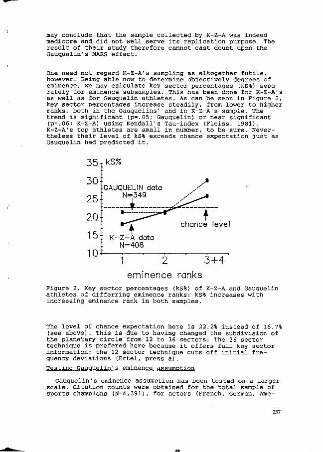
may conclude that the sample collected by K-Z-A was indeed mediocre and did not well serve its replication purpose. The result of their study therefore cannot cast doubt upon the Gauquelin's MARS effect.

One need not regard K-Z-A's sampling as altogether futile, however. Being able now to determine objectively degrees of eminence, we may calculate key sector percentages (ks%) sepa­rately for eminence subsamples. This has been done for K-Z-A's as well as for Gauquelin athletes. As can be seen in Figure 2, key sector percentages increase steadily, from lower to higher ranks, both in the Gauquelins' and in K-Z-A's sample. The trend is significant (p=.05; Gauquelin) or near significant (p=.06; K-Z-A) using Kendall's Tau-index (Fleiss, 1981). K-Z-A's top athletes are small in number, to be sure. Never­theless their level of kS% exceeds chance expectation just as Gauquelin had predicted it.

3 5 T kS%

30

25

20{

15

10

GAUQUELIN data N=349

chance level

K -Z -A data N=408

1 2 3 + 4 eminence ranks

Figure 2. Key sector percentages (kS%) of K-Z-A and Gauquelin athletes of differring eminence ranks: kS% increases with increasing eminence rank in both samples.

The level of chance expectation here is 22.2% instead of 16.7% (see above). This is due to having changed the subdivision of the planetary circle from 12 to 36 sectors: The 36 sector technique is prefered here because it offers full key sector information; the 12 sector technique cuts off initial fre­quency deviations (Ertel, press a).

Testina Gauquelin's eminence assumption

Gauquelin's eminence assumption has been tested on a larger scale. Citation counts were obtained for the total sample of sports champions (N=4,391), for actors (French, German, Ame-

257

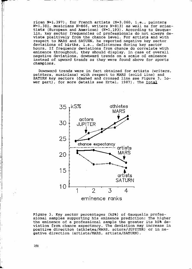
rican N=l,397), for French artists (N=3,060, i.e., painters N=l,381, musicians N=866, writers N=813) as well as for scien­tists (European and American) (N=l,193). According to Gauque-lin, key sector frequencies of professionals do not always de­viate positively from the chance level. For artists and with respect to MARS and SATURN, he reported negative key sector deviations of births, i.e., déficiences during key sector hours. If frequency deviations from chance do correlate with eminence throughout, they should display, in case of overall negative deviations, downward trends on a scale of eminence instead of upward trends as they were found above for sports champions.

Downward trends were in fact obtained for artists (writers, painters, musicians) with respect to MARS (solid line) and SATURN key sectors (dashed and crossed line see Figure 3, lo­wer part), for more details see Ertel, 1987). The total

35-

30-

25-

20-

15

m .

rkS%

actors • JUPITER

athletes MARS

chance expectancy

k '^ X s«f.-+—••—

•

Ur U Ö I S

- » MARS

k artists

SATURN

1 2 3 4 eminence ranks

Figure 3. Key sector percentages (kS%) of Gauquelin profes­sional samples supporting his eminence prediction: The higher the eminence of a professional sample the greater its kS% de­viation from chance expectancy. The deviation may increase in positive direction (athletes/MARS, actors/JUPITER) or in ne­gative direction (artists/MARS, artists/SATURN).

258

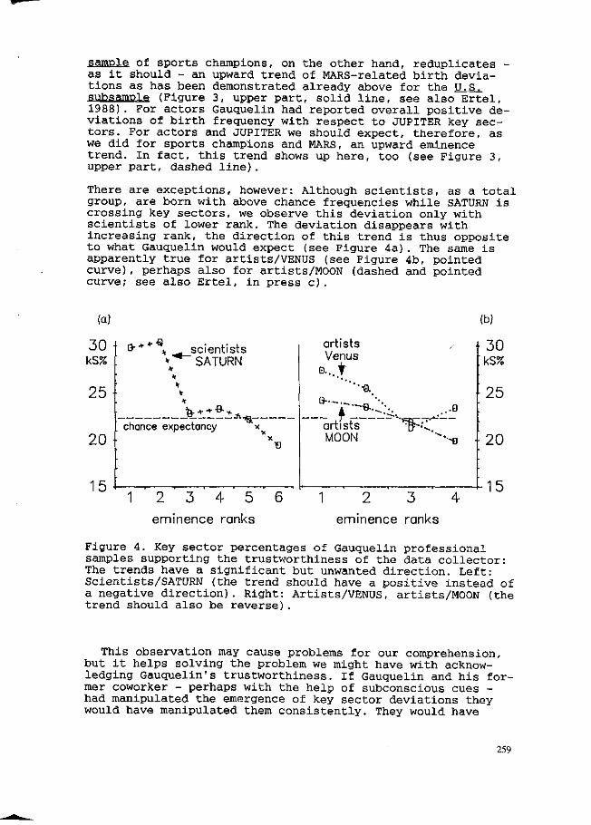
sample of sports champions, on the other hand, reduplicates -as it should - an upward trend of MARS-related birth devia­tions as has been demonstrated already above for the U.S. subsample (Figure 3, upper part, solid line, see also Ertel, 1988) . For actors Gauquelin had reported overall positive de­viations of birth frequency with respect to JUPITER key sec­tors. For actors and JUPITER we should expect, therefore, as we did for sports champions and MARS, an upward eminence trend. In fact, this trend shows up here, too (see Figure 3, upper part, dashed line).

There are exceptions, however: Although scientists, as a total group, are born with above chance frequencies while SATURN is crossing key sectors, we observe this deviation only with scientists of lower rank. The deviation disappears with increasing rank, the direction of this trend is thus opposite to what Gauquelin would expect (see Figure 4a). The same is apparently true for artists/VENUS (see Figure 4b, pointed curve), perhaps also for artists/MOON (dashed and pointed curve; see also Ertel, in press c).

(a) (b)

30 f ks% :

25

20

15

0"* * ^ s c i e n t i s t s "'m~ SATURN

ÏLlLlLtï^ chance expectancy •^r-

t)

artists Venus

B...t

a-—

._ fi: artists MOON

•a,

-S-..J-

' ^

.•0

•^o

2 3 4 5 eminence ranks

1 2 3 4 eminence ranks

30 [kS%

25

20

15

Figure 4. Key sector percentages of Gauquelin professional samples supporting the trustworthiness of the data collector: The trends have a significant but unwanted direction. Left: Scientists/SATURN (the trend should have a positive instead of a negative direction). Right: Artists/VENUS, artists/MOON (the trend should also be reverse).

This observation may cause problems for our comprehension, but it helps solving the problem we might have with acknow­ledging Gauquelin's trustworthiness. If Gauquelin and his for­mer coworker - perhaps with the help of subconscious cues -had manipulated the emergence of key sector deviations they would have manipulated them consistently. They would have

259

avoided, not produced, results like those obtained here showing trends in unwanted directions.

Multivariate Analyses

The trustworthiness of the Gauquelins' work can also be tested by analyzing, with the help of more sophisticated mul­tivariate procedures, the total body of their data. This has been done first by intercorrelating and factor analyzing sec­torial birth frequencies (36 sector frequencies across 11 pro­fessions * 5 planets), and second by cluster analyzing the di­stances between 11 professions defined by sector proportions (three proportions across 5 planets). One should ..ot be able to extract clean patterns from an aggregate of unclean data samples.

Factor analysis of 36 sector frequencies

Table 1 (see Appendix) shows the raw frequencies of Gauque-lin data, i.e., the frequencies of births for eleven samples of professions distributed across 36 sectors of the MOON, of VENUS, MARS, JUPITER, and SATURN. As the total numbers of in­dividuals differ between professions, we have standardized the means and variances of each row of the table by a z-transfor-mation.

Next we have to consider that birth frequencies expected by chance need not be evenly distributed across 3 6 planetary sec­tors. The position of VENUS in the sky, e.g., is not inde­pendent from the position of the SUN in the sky (being an in­ner planet). Since birth frequencies display diurnal cycles concomitant with diurnal SUN positions ("demographic" va­riance) they also display, with diminished amplitude, diurnal cycles concomitant with VENUS positions. There are additional interfering factors, foremost astronomical (and not only with respect to VENUS) which should be controlled when studying key sector deviations.

A simple control which has apparently not yet been thought of before is to equate, by z-transformation, means and vari­ances of sector frequencies across professions, separately for each planet. That is, z-transformations of birth frequencies were calculated for the MOON, VENUS, MARS, JUPITER and SATURN, across 11 professions, within each of the 36 columns of Table 1. The first z-transformation above (rows) equalized differences between professional samples due to unequal sample sizes. The second z-transformation (columns) equalized diffe­rences between planets due to unequal sectorial chance fre­quencies. What remains after row and column transformation should be just error variance if professional birth frequen­cies were unrelated (or equally related) to planetary positi­ons. If, however, professional birth frequencies are differen­tially related to planetary positions, inter-professional va­riance should exist. This variance may be separated from error variance as a first factor by principle component analysis (variables: 36 z-values, measurements: 5 planets * 11 profes­sions) .

260

The result of factor analyzing the standardized scale frequencies can be seen in Figure 5. If inter-professional va­riance does not exist the loadings of the first (unrotated) factor should show irregular zigzags across 36 sectors (ab­scissa) without relation to the planets' geocentric positions. This is what we find indeed with ordinary people (see the pointed curve), which served as a large control group divided on a random basis into eleven subsamples corresponding in num­ber and size to the professional samples. Only for the latter, however, do we find a regular pattern, i.e., cycle-like varia­tion of first factor loadings across sectors. The cycle is clearly related to distinct planetary positions, i.e., the first key sector zone (rise) and the second key sector zone (midheaven) have been replicated by this factorial test. The present procedure has the advantage of not presupposing any astronomical or demographic assumption, thus is circumventing all difficulties which former Gauquelin critics had regarded as severe: i.e., difficulties due to intruding astronomical factors (Comité Para) as well as demographic factors (Zelen).

professionals (11 professions N=20,398)

ordinary people (11 subsamples N=24,614)

ower culmination

11 13 15 17 19 21 23 25 27 29 31

Figure 5. Loadings of the 3 6 planetary sector variables on the first principle component factor, obtained by correlating the variables across professions (11) and planets (5). For ordi­nary people (dotted) no regularity is observable, for profes­sionals a regular oscillation emerges with marked peaks after planetary rise and upper culmination.

Cluster analysis of sector proportions

Whenever birth frequencies display peaks in key sector zones (peak I: sector nos. 36, 1, 2, 3, peak II: sector nos. 9, 10, 11, 12) one may notice moderate dips between the peaks. Sec­tors of dip areas may be called counter-key sectors (sector nos. 7, 8, 15, 16, 17, 22, 23, 24, 25, 32, 33, 34). Sectors

261

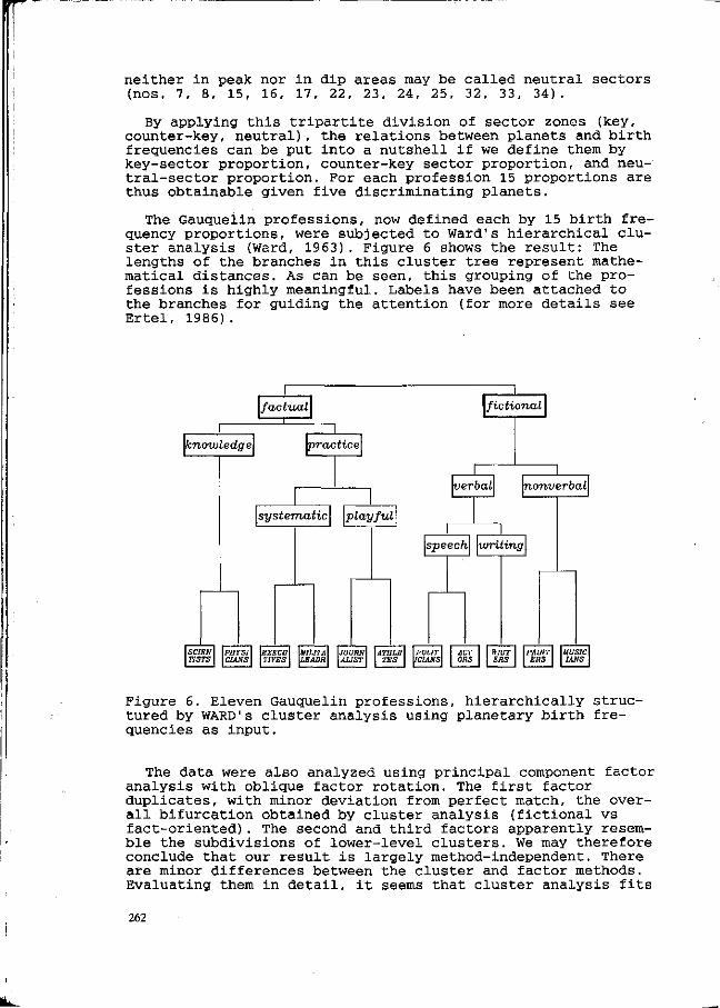
neither in peak, nor in dip areas may be called neutral sectors (nos. 7, 8, 15, 16, 17, 22, 23, 24, 25, 32, 33, 34).

By applying this tripartite division of sector zones (key, counter-key, neutral), the relations between planets and birth frequencies can be put into a nutshell if we define them by key-sector proportion, counter-key sector proportion, and neu­tral-sector proportion. For each profession 15 proportions are thus obtainable given five discriminating planets.

The Gauquelin professions, now defined each by 15 birth fre­quency proportions, were subjected to Ward's hierarchical clu­ster analysis (Ward, 1963). Figure 6 shows the result: The lengths of the branches in this cluster tree represent mathe­matical distances. As can be seen, this grouping of the pro­fessions is highly meaningful. Labels have been attached to the branches for guiding the attention (for more details see Ertel, 1986).

r factual fictional

knowledge practice

verbal

systematic playful

SCIEN TISTS

PHYS1 EXECV CIANS T1VES

UIUTA LEABR

1 nonverbal

I I

JOURN ALIST

speech writing

ATHLE POUT TES JC1ANS

ACT ORS

WRIT ERS

PAINT ERS

Figure 6. Eleven Gauquelin professions, hierarchically struc­tured by WARD'S cluster analysis using planetary birth fre­quencies as input.

The data were also analyzed using principal component factor analysis with oblique factor rotation. The first factor duplicates, with minor deviation from perfect match, the over­all bifurcation obtained by cluster analysis (fictional vs fact-oriented). The second and third factors apparently resem­ble the subdivisions of lower-level clusters. We may therefore conclude that our result is largely method-independent. There are minor differences between the cluster and factor methods. Evaluating them in detail, it seems that cluster analysis fits

262

somewhat better than factor analysis to the order our minds would impose on the professions.

The order our minds tend to impose on the professions has also been objectified. A sample of 30 students were given the 11 profession terms printed on cards. They were asked to group them in as many or as few groups of kindred items as they li­ked. The numbers of times two professions had been paired by the students while sorting them served as elements of a di­stance matrix, the latter was subjected to the same cluster procedure as the one used above (Ward).

The result is shown in Figure 7. Comparing Figure 7 (order produced by the human minds) with Figure 6 (order produced by planet-birth behavior) we find a near perfect match. There is one sample standing out: Politicians have been grouped by the human mind under what is here called fact-orientation, the planetary order had preferred to assign politicians to the fictional cluster! After all, attributing fictional or arti­stic features to politicians does not even seem to be far-fet­ched from certain terrestrial perspectives.

subjective / \ suDjecuve \ a ' procedure: student subjects

(b) objective' procedure: planets

1.!

t.l

2.12

M.

11

3.2:2:

3.2.1

3.1.2

3.1.1

i l l

pu RA*

AC

WR

SR

JO

PO

Ml

EX

PH

SC

m tik**

^-

AC1

f .

BO T....Î.. A

SP

JO

Ml

EX

PH

SC

2.22

3.2.2

32,1

221

3.1.2

3.1.1 2.1.2

ZU

12

Figure 7. The arrangement of Gauquelin professions of Figure 6 has been turned by 90° on the right. On the left a correspon­ding arrangement of professions is shown obtained by analyzing results of a sorting experiment: The correspondence is near perfect (MU=musicians, PA=painters, WR=writers, AC=actors, PO=politicians, SP=sports champions, JO=journalists, MI=mili-tary leaders, EX=executives, PH=physicians, SC=scientists).

We have now established the Gauquelin findings on firm em­pirical ground, but a new problem looms. This may be called,

263

without overstating the situation, as stupendous: What kind of mediation links planetary positions with births of profes­sionals? Gauquelin suggested some psycho-physiological mecha­nism: there might exist some unknown terrestrial resonance to cosmic events triggering hormonal processes within the fetal organism leading eventually to child birth (Gauquelin, 1984). I myself could not find sufficient empirical facts to approve of this line of reasoning although I tried hard to find some (Ertel, in press b). A hot backstage debate between Michel Gauquelin and myself is going on about this question, but agreement is not yet in sight. Subsequent surprises are likely to come, however, at least for all those who are willing to accept, with an open mind, Gauquelin's basic planetary message as surprise no.1 to which all future insights must be related.

Ac knowledaement

Nick Kollerstrom kindly corrected the author's text linguisti­cally, he also gave some useful suggestions to improve it.

References

Ertel, S. (1986). Wissenschaftliche Qualität und progressive Dynamik im Gauquelin-Paradigma. Zeitschrift für Para­psychologie und Grenzgebiete der Psychologie, 28, 104-135.

Ertel, S. (1987). Further grading of eminence. Planetary correlations with musicians, painters, writers. Correlation, 7(1), 4-17.

Ertel, S. (1988). Raising the hurdle for the athletes' Mars effect: Association covaries with eminence. Journal of Scientific Exploration, 2, 53-82.

Ertel, S. (in press,a). An assessment of the Mars effect. Zetetic Scholar.

Ertel, S. (in press,b). Purifying Gauquelin's "Grain of Gold": Planetary effects defy physical interpretation. Correlation.

Ertel, S. (in press,c). Reversed eminence correlations. Com­ments on an article review. Astro-Psychological Problems.

Fleiss, J. L. (1981). Statistical methods for rates and proportions. New York: Wiley.

Gauquelin, M. (1984). Profession and heredity experiments: Computer reanalysis and new investigations on the same ma­terial. Correlation, 4(1), 8-24.

Gauquelin, M., & Gauquelin, F. (1979-1980). Star U.S. sports­men display the Mars effect. A comment on the Kurtz-Zelen-Abell experiment. The Skeptical Inquirer, 4(2), 31-43.

Kurtz, P., Zelen, M., & Abell, G. 0. (1979-1980). Results of the U.S. test of the "Mars effect" are negative. The Skep­tical Inquirer, 4(2), 19-26.

Schubert, A., & Toma, 0. (1984). Quantitative studies of science. A selected bibliography (1980-1984) (Unpublished. Department of Scientometrics, Information and Sciento-metrics. Hungarian Academy of Science.). Budapest, Hungary.

Ward, J. H. (1963). Hierarchical grouping to optimize an ob­jective function. Journal of the American Statistical Asso­ciation, 58, 236-244.

264

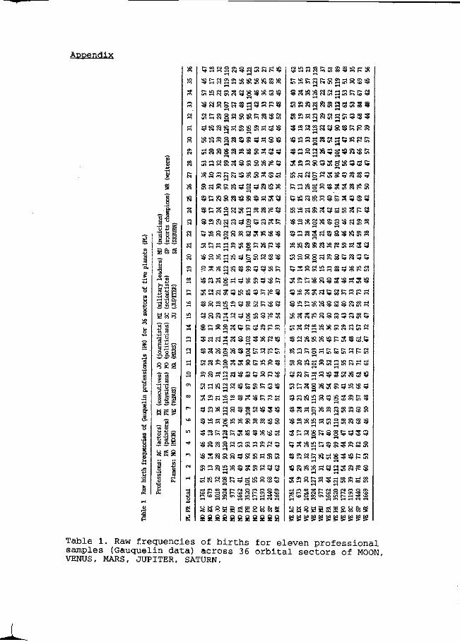
Appendix

te

3 3 3

assss

g y >?

s g g

ö £ g

CM r - o> Q N (

i x » <T) VO «W

o> <n c*J VU t o

vo t n i n i H

rH O i n oa

m *-t

\o o c l »H

O t-H m es]

00 04

s C4 c i

o

O OO

8S5 r-1

r » r—

CT. O*

CO

o

**

s

VO 00

en

VO o~»

o

i n

T-4

o i n

O i n

s i - i

rH

ca

C3

VO -3"

o m VO " *

VO • »

* 0 r n

vo m

vo on

a i r - o> o «

i-H r^ rH . - ( o*i • i n T H * n t - i m |

' rH rH ^ » ^ <

i l f | f n i > l f )

i T-t vo m r - O m vo

I 1-4 OJ r H r H •

I vo t - t vo I " i H m O i

•«f cû i *J« rH <

i-H m co •"* vo E— T-t cq r - vo o c-i

p « N O M M O C l r~ I Û N [ * c h t * vo o"» vo m r - t - t xJ1 vo

H M r t H M H

g g g g g g g g g g g

O O C h H M C M N H P - f n w g i n H n N C M i f l f n i n ' a ' i û ^ »H t - t

3c o N » N N O e o r - o m r H n v H 0 3 « * o S ^ ] ' ( * i r - * n

i o w i n o ^ ^ ' M o û ' *

( n w N O M v c n m N i

o i n o o ^ H T i o i û i n a i c o

i N n c o ^ o ) 1 » ^

•*j< m r - vo o o •«* » i f t H H C O N * J " 0 0 '

i o~t c q »sf co m m r » «

( n p » f O v o < * m H i r ) « ) H i n T - t c s o t N i n o * > ^ f « ^ - i v o ^ F

m m i n m o m m i n < j o vu fO i o f

3 r - o î v p p - o c o r — T - i ^ m t H f ^ O ( ^ a ' * o • ^ • , q ' v o ^ ^ ,

« x j i « r - i f l H i û ' f i n p - f o

i H * n o o - « i " r - f s i o o a r n o o ? > v o r - t H o r - v o c v j r - a i * ï vo M o o c n c n v o i n r - H ^ v o

Table 1. Raw f r e quenc i e s of b i r t h s f o r e l even p r o f e s s i o n a l samples (Gauquelin d a t a ) a c r o s s 36 o r b i t a l s e c t o r s of MOON, VENUS, MARS, JUPITER, SATURN.

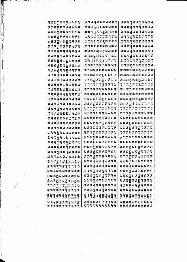
t M (M TJ N

co en o ^ f r-

W « 5 CO H t •e* r-i CO O PS

r - en oo 5 | eg I r t r l r t Q «

"• S *** o i i o o H tn m rt (^ H M

»H

i n H N m M

r— vo . H "dp «* *# iH OS O co

<» rtN CO (

m en • * O

S S *-( e n •"1" t -

v o m m e n

PS o

e n o m en

«• en ^ 0 0

m oo *f 0 0

m T H » H

9 | CO 00

r— en •"T 00

i n

CT« M "

VO

en

r -

CO

O l

i n

r— i n

u t

m

e s m

e s U">

O S m

00 e n

i n e n

e n e s

o e n

•*• c o

s o o e-a

c o e s

c o

e s c o

e s

v o • #

VO VO

o o t—

e n r -m vo

e n v o VO CO

en o

^ r e s

T-i T-f

e n 00

r— oo VO ^

CM T-l oo i n

g m g o T-j w n w A*

c o

M»

(43

m

3 e s VO

r—

O

i n -*3>

s c o

VO

S ** c o

0>

m

e s PS

s en

o o s

y * e s

e s

e n e s

H e s

e s e n

e n e s

e n e s

e s

i n e s

VO

VO

e s

00 e s

e n e s

e n e s

r-t

m e s

c o

e n m

e s e n

e s O

i n o

r— 00

00 o tH

e n

o e n

o e n

v o e n

e n . H

v o e s

O

. H

3 m o

e n e s

e s

m

e s

vo

c o e s

e n m

o a

m

O c o

e n o s

c o e s

VO e s

c o e s

»-H U~>

f

OO

c o

O

O •Kf

O

p -

i n

o i n

i n

r -e o

e s c o

00 CO

m m

00 00

r -o o

VO

en

e s e n

VO

en

r—

e n

t— t n

VO

v o i n

8 3 VO OO

e s e n

S e n e n

e n e n

c o e s

v o

8

i n

e-a

m

CO CO

OO

i n

i n

CO

m e s

c o

l£> c o

o*> e s

c o

c o e s

CO

CO

o CO

m CO

CO

CO

lO e s

r -

O r—

en VO

c o i n

KO

i n

e n i n

VO

e n v o

e n

r-i

r-

en VO

t n

o

e n

c o

c o

3 i n ••3"

C0

VO m

m CO

m e s

3

i-< m i n en • *& es co es i

> e s >-* oo t ( ^ CO S" f

I O v o ( » o m r

) vp co e » O ^* r

i Q vo TH e i ^ en ^* r

i os m ^* T i vo co • * l

i H1 es i n <•

S o e . "-o r

•—i co co *» î— vo t— iH es r~ M Û O O M Ï » T-* »H co

es O (*i vo es p-vo m r-

r a s s i s e s

co o en en "«p vo ^-t *# vo »H es »—i

v o o o o ^ o e n ^ v p e s e s o o m ^ ^ e ^ i - t c s i n o S - v c o i n i o

i n e n e s o t - g ; e n i n o ^ 4 v o

o o i n e n o a ' ö ' o o o p v o e s c o v o c o t H o a o c o c o o m c o r - ^ i «

• q î i H O î O c o i n g ^ c o c o ^

i n r - i o a e n c o i n e n ^ «

i H O o o c n c o t — e o e s c o i H v o t f i C M W C i N f l ' O ^ ' n c O v r H c o c o r - o a e n i n c o c o o o p -i n e s c o w e s ^ o o ^ c o v o m

es en »H vo t— oo JH î

i n ^ i n o o s ^ r r — m r - m « « ^ i H e s e n c o i n o i n e s v o ^ f

t — ^ • o o ^ f e s c o e o o c o O e s ^ " O s e s o o e s ^ p o v o c o v o t o

^ j ' i - H e s o o c o ' O ' O i n e s v o '

^ H N C O N ^ C n i n N f l 1 !

» o o ^ v p c o o o e n i n ^ f O r s

r - r - v o e s e s o o o e n ^ e n i n T j « i - H C O C O C O C O C O ^ " ^ " m ^ i

i o co m o co co p^ *

v o e o e s c o e s T j ' O v o e s v o ^ i

e x 3 o r - v o i n r - o c o ^ * , ' « i « i / > v o c o c o e s e s c o o ^ c s t - - ^ i

i - ) c o o o * j < r - e s o > c o c o O e n vor— H N M O H r - c n ^ i o r - v o o e n e n v o i n r - r - t ^ a > v o r-t H C l rtPlHHNrt

a Ö % a g g s s a & s

co m en vo co en i n

i n c s c s o o s m e n ^ f c o r — in

S e n c o o v o o o e s i n o c o e n rtNHMinciinfnin'if

i o r t N H n ^ | o > , < f ^ | c - '

i c o e n e s ^ r H i n c o v o c o

i n c o m

, t— vo •& i es vo -^

_ . _ . _ J es rH o c o e s c s v o e n t n c o v o i n

e s o e s e s « - * i n r - e n o t — es t f o 5 e s * - < c o ' « j ' o o ^ » , ^ j ' v o ^ » «

« « r e n ^ f t H e n c o v o c o e n v o v o

O P - c o e o i r v i n v i n o i t - i N r— r l M H N ^ H l f l n h ^ 1

o i n r p v p c o o c o v o e s c o v o

i c o vo c o

* O H N O N V O < Î '

• » » e s c o o c o - ^ e n ^ f i

i n en i-i 3* p* i n T-i co o TH

r— co i n co P -

^« es es e s en ss \ o i n vo * f

( n ^ c o e n v o o r - e s ^ a î r - v o ^ H N O N T O ^ ^ > û l ' l

T-i iH.

^ H c n o o ^ f p - o a c n c n c n o o e n v o r — » H e s r - v o ^ H p * e n ç o v o r— v o o m a i v o m r - r H ^ v o »H » - t n T H r O i - l i H O S i r H

INTROVERSION-EXTRAVERSION; SUNSIGN-EFFECT AND SUNSIGN-KNOWLEDGE

J.J.F. van Rooij, M.A. Brak, J.J.F. Commandeur

Department of Psychology, University of Leyden, the Netherlands

Summary In 1978 Mayo, White & Eysenck found a significant relation

between sunsign and extraversion. Later Eysenck reconsidered this study and claimed that the result could be explained by the psychological phenomenon of self-attribution. In the present study a replication of Mayo's study is performed in such a way that the self-attribution process unlikely is to play a role. Nevertheless, the sunsign-effeet is found as well. The proposition is made that the self-attribution-effect only is present when subjects receive a cue that the study in which they participate does pertain to astrology. Keywords: astrology, sunsign-effeet, self-attribution.

Introduction In 1978 one of the first experimental studies into

astrology was performed by Mayo, White & Eysenck (1978). The study confirmed the astrological supposition that people born with the sun in an odd-numbered sign of the zodiac (Aries, Gemini, Leo, Libra, Sagittarius, Aquarius) show a tendency towards extraversion, whilst those born with the sun in an even-numbered sign (Taurus, Cancer, Virgo, Scorpio, Capricorn, Pisces) show a tendency towards introversion. The demonstration of this odd-even effect (also called the sunsign-effeet) caused some commotion, both among astrologers and psychologists and several replication studies were performed (a fact that in itself is rather unique in psychology). Broadly speaking the odd-even effect could be replicated by Smithers & Cooper (1978) and by Jackson (1979), but not by Veno & Pamment (1979), Jackson & Fiebert (1980), Saklofske et.al. (1982), Russell & Wagstaff (1983), Fourie (1984) and by Mohan & Gulati (1986).

However, in later publications Eysenck (Eysenck, 1979, 1981; Eysenck & Nias, 1982; see also Gauquelin, 1983) reconsidered the Mayo-study. He was concerned by the fact that the subjects were recruited by Mayo, a well known astrologer. In fact the subjects were Mayo's 'apprentices', as is mentioned by Gauquelin (1983), who knew their birth-sign and had some knowledge of interpreting astrological sunsigns. At least, one might say that these subjects had a positive attitude towards astrology. Allthough in the Mayo-study a correction was made for astrological knowledge with the subjects, more stringent tests showed a remarkable phenomenon. It proved (Eysenck & Nias, 1982) that the odd-even effect only could be demonstrated with subjects that had a little knowledge of astrology, that is to say knowledge of the signs of the zodiac and their corresponding

267

characteristics. In a more elaborated study the same result was found by Pawlik & Buse (1979). Eysenck explains this phenomenon as follows. Subjects ignorant of astrology cannot be influenced by any astrological knowledge at all, when they are filling out a personality-questionnaire. Subjects with considerable knowledge of astrology will realise that besides the sun-position many other astrological factors are important for the description of one's personality. On the other hand, when subject's knowledge is limited to the sun-position, the sunsign will be the only salient astrological factor to which the subject can relate the questionnaire-items. Therefore Eysenck concluded that the odd-even effect could be explained by self-attribution : "Prior knowledge does influence the subject into seeing his own personality in conformity with what astrology tells him to expect..." (Eysenck & Nias, 1982, page 59). This conclusion implies that the sunsign-effect actually is a psychological effect, rather than an astrological one.

However, we would like to make some comments on Eysenck's conclusion and argue that it is drawn too quicly. It is not clear why an astrological knowledgeable subject will not be influenced by the sunsign-knowledge, in spite of his or her mars-knowledge, ascendant-knowledge and so on. In fact the argument might be used the other way around. Knowledgeable subjects generally will have a more positive attitude toward astrology and therefore might be influenced even more by their astrological knowledge. The point that the knowledgeable subjects' realise that besides the sun-position other astrological factors are important in characterizing one's personality is not relevant in this, for the subjects do not know to which astrological factor the study pertains.

But then, how should the results of Eysenck & Nias (1982) and of Pawlik & Buse (1979) be accounted for? In our view the following might have happened. The subjects in the Mayo-study in one way or another have got a cue. that the study pertained to astrology. Now, for the Mayo-study itself this cannot be decided definitely, for the study is not described in great detail. We like to comment that a minor cue in the experimental set up may serve as such a cue. For example, the mere mentioning of Mayo's name in the announcement of the experiment might alert his apprentices that the study has something to do with astrology. Fortunately the study of Pawlik & Buse (1979) is better documented. Subjects were recruited by newspaper-advertisements and the study was explicitly announced as a scientific study into astrology. In other words the cue for astrology is obvious. Furthermore, besides a personality-questionnaire, a questionnaire was send along about knowledge of astrology and attitude towards astrology. In it were items as 'do you know what type of personality goes with your sunsign?' and 'do you believe that sunsign and character go together?'. It is not farfetched that subjects will infer on basis of such questions that the study pertains to the sunsign. We believe that in a situation in which such demanding cues are given

268

indeed a factual influence is possible of astrological knowledge on the filling out of personality-questionnaires. In the present study it was tried to replicate the odd-even effect in a situation in which definitely no cue for astrology was present. Such a situation was created in the following way.

Method

The data were questionnaire-data that were gathered in the period 1980-1985. Furthermore, they were gathered by other people than than the present authors and for a purpose other than reaserch into astrology. Both the persons who administered the questionnaire and those who filled it out, at that time did not know that the data later would be considered in relation to astrology. Birth-dates and extraversion scores were available for 992 subjects (885 men, 107 women). Subjects were non-university-students, age range 19-61, mean age 30. Extraversion was measured by the Amsterdamse Biografische Vragenlijst (Amsterdam Biografical Questionnaire - de Wilde, 1961).

Results

In figure presented for odd-numbered than average groups have 1 Virgo and t analysis was gender factor

1 the means of the raw extraversion scores are the twelve sunsigns. It can be seen that all sign-groups have extraversion-scores higher

except for Libra and that the even numbered ower scores than average, with the exception of o a small degree Pisces. A' three-way factor-

performed on the extraversion-scores. The had two levels, __male and female. The second

vor»g«

Arlat Qamlnl Lao Libra Saglttarlu« Aquarius Tauru» Cancar Virgo Scorpio Capricorn Pl«c»t

SUNSIGNS

Figur« 1 Extravartlon Scora« for p«rton» having dKfarent surulgn* (n = 992)

269

i

1

factor also had two levels, odd versus even. Following the Mayo-study a dummy factor was introduced to check whether a significant difference is present between the signs within the group 'odd signs' and within the group 'even signs'. The odd-even effect proved to be statistically significant (p=.056), the gender effect was not significant (p=.70) and there are no significant interaction-effects. Though the significance-level of the odd-even factor is not as striking as found by Mayo et. al., the odd-even pattern closely matches Mayo's.

Discussion

The present study succesfully replicated the result found by Mayo et. al. that extraversion is related to sunsign. However, the odd-even effect in itself is not strong. Both in the present study as in the Mayo-study the actual differences between the mean extraversion-scores for the twelve signs are marginal. But, in this respect the folowing should be taken in account. The hypothesis tested is wellknown in astrology, but at the same time it is a very general one. Mankind is divided in only two groups and many astrological factors, like planets and 'houses', are not taken into consideration. The pattern of these additional factors varies greatly with the individual. To eliminate this idiosyncrasy a large number of subjects seems to be required and only then the sunsign-effeet becomes visible.

However, the main result of the present study is that the odd-even effect could be demonstrated in a situation in which subjects could not have got any cue that the study pertained to astrology. Now, does this finding imply that the self-attribution explanation can be ruled out definitely? Unfortunaely not. It still is possible that our subjects did have knowledge of astrology and that the internalisation of this knowledge did influence the filling out of the questionnaire. in fact our result might be interpreted the other wya around; critics may hold, as Ertel (1989) points out, that our study only proves that astrological self-attribution works, even without apparent cues . Now the self-attribution explanation does have one far-reaching implication, namely that every score on a personality-questionnaire should be corrected for astrological knowledge with the person being tested. Then there is the finding of Pawlik & Buse (1979) that subjects who both had no knowledge of astrology and got a cue for astrology did not show the odd-even effect. This finding of course favors the self-attribution explanation. It is clear that a third study is needed to establish definitely which role is played by astrological knowledge. One may imagine the following design. Three groups of subjects would be needed, subjects with no-, a lot-, or only 'sunsign' knowledge. These groups are told that the study pertains either to 'personality' or to 'personality and astrology'. One group receives as an additional cue that the study pertains the sunsign, a fourth group is given a 'false' cue,

270

that is to say a cue for the planet mars, the moon or any-other astrological factor. When 'sunsign-knowledge' subjects would show the sunsign-effeet only when a cue for the sunsign is given and not when the 'false' cue is given, the self-attribution explanation would be corroborated. On beforehand it may be said that corroboration of the self-attribution explanation would imply a tremendous effect of astrology, a much stronger effect than both proponents and opponents of astrology ever could have imagined!

References Ertel, S. , 1989. Personal communication.

Eysenck, H.J., 1979. Astrology, science or superstition? Encounter, november: 85-90.

Eysenck, H.J., 1981. Die wissenschaftliche Erforschung der Astrologie und die Förderung nach "naiven" Versuchspersonen. Zeitschrift für Parapsychologie und Grenzgebiete der Psychologie. Vol. 23, no, 2:89-95.

Eysenck, H.J., & D.K.B. Nias, 1982. Astrology, science or superstition? Maurice Temple Smith, London.

Fourie, D.P., 1984. Self-attribution theory and the sunsign. Journal of Psychology: 122, 121-126.

Gauquelin, M., 1983. The truth about astrology. Basil Blackwell, Oxford.

Jackson, MacD, P., 1979. Extraversion, neuroticism and date of birth: a southern hemisphere study. Journal of Psychology, 101: 197-198.

Jackson, M. & M.S. Fiebert, 1980. Introversion-extraversion and astrology. Journal of Psychology, 105: 155-156.

Mayo, J., O. White & H.J. Eysenck, 1978. An empirical study of the relation between astrological factors and personality. Journal of Social Psychology, 105: 229-236.

Mohan, J. & A. Gulati, 1986. Zodiac signs and personality: a pilot study. Correlation, vol. 6, no 1: 11-14.

Pawlik, K. & L. Buse, 1979. Selbst Attribuierung als differentiell-psychologische Moderatorvariabele: Nachprü­fung und Erklärung von Eysencks Astrologie Persönlich­keits-Korrelationen. Zeitschrift für Sozialpsychologie, 10: 54-69.

Russell, J. & G.F. Wagstaff, 1983. Extraversion, neuroticism and time of birth. British Journal of Social Psychology, 22: 27-31.

Saklofske, D.H., I.W. Kelly & P.W. McKerracker, 1982. An empirical study of personlaity and astrological factors. Journal of Psychology, 110: 275-280.

Smithers, A.g. & H.J. Cooper, 1978. Personality and the season of birth. Journal of Social Psychology, 105: 237-241.

Veno, A. & P. Pamntent, 1979. Astrological factors and personality; a southern hemisphere replication. Journal of psychology, 101: 73-77.

Wilde, G.J.S. de, 1961. Neurotische labiliteit, gemeten volgens de vragenlijstmethode. Van Rossum, Amsterdam.

271

EFFECT SIZES OF SOME PRE-SCIENTIFIC GEO-COSMIG THEORIES

By Geoffrey Dean

PO Box 466, Subiaco 6008, Western Australia

Abstract

The use of the correlation coefficient as a measure of effect size is explained with examples. A survey of over 100 controlled studies of the correspondence between astrological factors (signs, aspects, houses, the whole birth chart) and human personality and behaviour gives a mean effect size of =<.05. For lunar effects on behaviour (37 studies) the mean effect size is .01. For practical purposes these results are equivalent to no effect at all.

Introduction

At various times there have been many interesting pre-scientific geo-cosmic theories, by which I mean ideas about extra-terrestial influences that arose other than by scientific inquiry. For example:

- People born at sunrise will be clever. - It is unlucky to point at the moon. - A comet in the sky means the king will die. - People born under Mars are warlike and contentious.

Are such theories mere superstition, with no basis in fact? Or do they reflect perhaps some special sensitivity to extra-terrestial influences that man is currently unaware of?

In what follows I will briefly survey the experimental evidence for the validity of such pre-scientific theories.

Correlation as a measure of effect size

The question I shall be asking is not whether such theories are true, yes or no, but to what extent such theories are true. That is, to what extent are people who are born at sunrise, or under Mars, more clever or more warlike than those born at other times?

Research into such theories has usually focussed on significance level, that is, on whether the results can be explained by chance. This tells us nothing about how big the effect is. So here I will ignore significance and ask only how large is the effect size?

Effect size can be measured in several ways. One common measure, which I shall be using here, is the correlation coefficient. To illustrate how it works, Tables 1 and 2 present some correlations observed in two different areas, namely geophysics and human affairs. Look at Table 1 first (see next page).

272

Table 1. Examples of correlations from geophysics

Correlation Hit rate if probability of a hit = 50%

\ \ PERFECT Example eg feet 1.0 5/5 vs metres .9 Tide height vs moon position.

.5 Shortwave radio quality vs geomagnetic activity.

MINIMUM TO BE 0.4 5/7 USEFUL .3 Shortwave radio quality

vs quality 27 days earlier. -<.1 Earthquakes vs moon position.

USELESS eg coin - 0.0 5/10 --- -tossing

At top, a correlation of 1.0 means the correlation is perfect, as between feet and metres. You always get 5 hits in every 5 trials.

At bottom, 0.0 means there is no correlation at all, as between the tosses of two coins. On average you get 5 hits in every 10 trials, or exactly chance. So zero correlation is as useless as you can get. '

Negative correlations (not shown) mean that two things vary inversely. Like more light means less dark. Now for a crucial point:

How useful is useful?

Or how small can an effect size be before it ceases to be useful?

The answer depends on where you are coming from. In physics a metre rule that correlated .9 with an exact measure would give results accurate to only plus or minus 20%. It would therefore be more or less useless.

But in psychology the minimum effect size for tests generally regarded as being useful is around .4. With .4 you get 71% hits (5 in 7) instead of the 50% expected by chance. This may not seem impressive, but in a casino such a system would break the bank in an hour.

Because the present areas of interest fall under psychology rather than physics. I have adopted .4 as the minimum useful effect size.

And as you can see from the examples given in Table 1, this also applies quite well to geophysics. Thus moon position is excellent for predicting tides but useless for predicting earthquakes. And shortwave radio quality is moderately well indicated by geomagnetic activity but not by the quality one solar revolution earlier.

Now look at Table 2 for examples from human affairs.

273

Table 2. Examples of correlations from human affairs

Correlat

PERFECT eg feet vs metres

MINIMUM TO BE USEFUL

tossing

ion

\

- i

- 0

- 0

0 --

4 --

0 --

Hit rate \

3/3

- - D/ 1

if probability of a hit = 50%

Example

.95

.7

.5

.3

.2

.1

Arm length right vs left. Adult height and weight. IQ of husbands and wives.

Height of husbands and wives. IQ vs appreciation of music. IQ vs head size.

At .95 in Table 2 is the near-perfect correlation between right and left arm lengths, which supports our everyday observation that any difference is small.

At .7 is the less-perfect correlation between height and weight; heavyweights tend to be tall while lightweights tend to be short, but there are individual exceptions.

At .5 we have the extent to which bright men prefer bright women, and vice versa. Perhaps surprisingly, it is more marked than the preference of tall men for tall women at .3.

The correlation between music appreciation and IQ is around .2, which means that one is not a useful guide to the other.

Even worse is the almost negligible correlation between IQ and head size, which among other things seems to express the problems of phrenology in a nutshell.

Observed effect sizes of some pre-scientific geo-cosmic theories.

The situation is summarised on the next page in Table 3.

Here the pre-scientific geocosmic theories being addressed have been subsumed under astrological effects and lunar effects. To provide perspective, I have included the effect sizes for a few orthodox areas such as IQ and Rorschach inkblots. Note that the figures are illustrative only and often hide considerable individual variation. For example IQ is better at predicting science exam results, and worse at predicting art exam results, than the figure given here. But for the present purpose this variation is of no consequence.

The correlation coefficients cited are variously Pearson r, point biserial r, and phi, depending on the source data. Although these are not exactly equivalent to each other, for the present purpose the differences are of no consequence. Means have been calculated in the proper way using Fisher z-transforms.

274

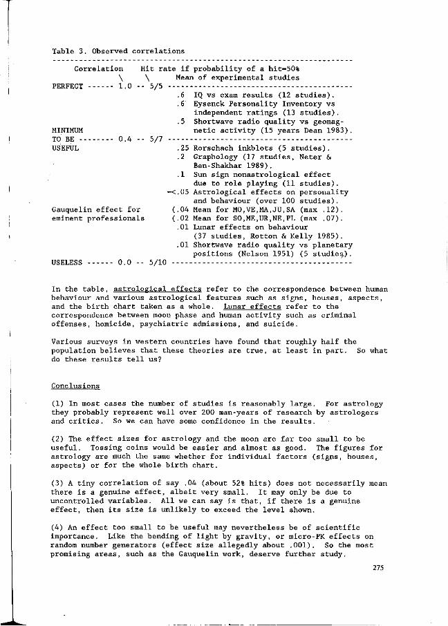
Table 3. Observed correlations

Correlation

\ PERFECT 1.0

MINIMUM TO BE 0.4 USEFUL

Hit rate if probability of a hit=50%

\ 5/5

5/7

Mean of experimental studies

.6 IQ vs exam results (12 studies).

.6 Eysenck Personality Inventory vs independent ratings (13 studies).

.5 Shortwave radio quality vs geomag­netic activity (15 years Dean 1983) .

Gauquelin effect for eminent professionals

.25 Rorschach inkblots (5 studies).

.2 Graphology (17 studies, Neter & Ben-Shakhar 1989).

.1 Sun sign nonastrological effect due to role playing (11 studies).

-<.05 Astrological effects on personality and behaviour (over 100 studies).

(.04 Mean for MO,VE.MA,JU,SA (max .12). (.02 Mean for SO,ME,UR,NE,PL (max .07).

.01 Lunar effects on behaviour

(37 studies, Rotton & Kelly 1985). .01 Shortwave radio quality vs planetary

positions (Nelson 1951) (5 studies.). USELESS 0.0 5/10

In the table, astrological effects refer to the correspondence between human behaviour and various astrological features such as signs, houses, aspects, and the birth chart taken as a whole. Lunar effects refer to the correspondence between moon phase and human activity such as criminal offenses, homicide, psychiatric admissions, and suicide.

Various surveys in western countries have found that roughly half the population believes that these theories are true, at least in part. So what do these results tell us?

Conclusions

(1) In most cases the number of studies is reasonably large. For astrology they probably represent well over 200 man-years of research by astrologers and critics. So we can have some confidence in the results.

(2) The effect sizes for astrology and the moon are far too small to be useful. Tossing coins would be easier and almost as good. The figures for astrology are much the same whether for individual factors (signs, houses, aspects) or for the whole birth chart.

(3) A tiny correlation of say .04 (about 52% hits) does not necessarily mean there is a genuine effect, albeit very small. It may only be due to uncontrolled variables. All we can say is that, if there is a genuine effect, then its size is unlikely to exceed the level shown.

(4) An effect too small to be useful may nevertheless be of scientific importance. Like the bending of light by gravity, or micro-PK effects on random number generators (effect size allegedly about .001). So the most promising areas, such as the Gauquelin work, deserve further study.

275

(5) The results do not deny the therapeutic utility of astrological beliefs (for a detailed survey see Dean 1987). If invalid beliefs worked in bloodletting, they can certainly do the same in astrology.

End of survey. But two more things should be said:

Because the areas addressed here border on the paranormal, they tend to be dismissed as unworthy of serious consideration. But I think this is short­sighted. These areas do require serious consideration, if only because so many people believe in them. On the other hand, we should proceed with caution, simply because research has revealed little more than a consistent failure to demonstrate adequate effect sizes. Which is not to say that genuine effects, however small, may not be of scientific importance. Therefore, in the future, those with research dollars to spend should be selective. The safest approach would be to concentrate on those areas that, on the basis of past research, seem most likely to produce worthwhile outcomes.

Finally, what do the results tell us about the sensitivity of man to extra-terrestial influences? They tell us that the people tested were insensitive to the alleged influences studied. They do not deny that man may be sensitive to other influences such as solar eruptions or geomagnetic storms.

Sources for Table 3

Articles through mid-1989 from the main journals reporting scientific studies of astrology, namely Astro-Psychological Problems, Correlation, NCGR Journal, and Skeptical Inquirer. Plus the following: Eysenck HJ and Nias DKB. Astrology: Science or Superstition?

St Martin's Press, NY 1982. Dean G. Shortwave radio propagation non-correlation with

planetary positions. Correlation 1983,3(1),4-37. 45 references. Summarised in Skeptical Inquirer 1983,8(1),48-56.

Dean G. Can astrology predict E and N? Part 3. Discussion and further research. Correlation 1986,6(2),7-52. Gives a detailed presentation (many pages) of the effect sizes in astrology summarised here. Includes sources for IQ, EPI, and Rorschach.

Dean G. Does astrology need to be true? Skeptical Inquirer 1987,9(2), 166-184 and 1987,9(3),257-273. Focusses on therapeutic utility. In two parts with 100 references.

Nelson JH. Shortwave radio propagation correlation with planetary positions. RCA Review March 1951,26-34. Sets out Nelson's early claims, which became the best hard evidence for astrology. For later claims and an analysis of 5507 of Nelson's forecasts, see Dean 1983.

Neter E and Ben-Shakhar G. The predictive validity of graphological inferences: a meta-analytic approach. Personality and individual Differences 1989,10(7), 737-745. Focusses on the use of graphology for personnel selection. Graphologists (mean effect size .17) were outperformed by psychologists with no knowledge of graphology (mean effect size .22), which suggests that any validity is due to content rather than to graphological indicators.

Rotton J and Kelly IW. Much ado about the full moon: a meta-analysis of lunar-lunacy research. Psvcholoeical Bulletin 1985, 97, 286-306. Very detailed. 152 references.

Startup MJ. The validity of astrological theory as applied to personality. PhD thesis, London University 1984. The pioneering work on effect size in astrology.

276

Theoretical and background contributions

279

THE CHANGING CONCEPT OF PHYSICAL REALITY

J. Hilgevoord

Department of History and Foundations of Mathematics and Science, University of Utrecht, Utrecht, The Netherlands

Summary

It is shown how quantum mechanics affects our concept of physical reality. Keywords: quantum mechanics, probability, causality, observation,

EPR-experiment, locality, Bell's theorem.

It is a great pleasure for me to talk on this conference on the changing concept of reality in quantum physics. Although some of the results of quantum mechanics may appear as puzzling as some of the results that have been presented at this conference, I do not think myself that the two subjects are / actually closely related. The reason for this is that the typical quantum effects can hardly manifest themselves at a macroscopic level. It is certainly true that macroscopic quantum effects do exist, but their production requires the very special circumstances and precautions that can only be realized in the laboratory. If there is any link between quantum mechanics and the subject of this conference, it should be sought, I believe, not at the factual level but at the conceptual level, or at the level of analogy. It will therefore be my purpose to discuss with you the conceptual situation in quantum physics quite independently of any possible connections with other fields of investigation and I will leave it to you to decide, at the end of my talk, whether or not such connections exist.

In quantum mechanics two things stand out most. The first is the special role of probability. The second is what is called locality, or rather the lack of locality, that is implied by quantum mechanics. Both points are rather subtle. So let me begin by considering the first aspect of quantum mechanics, the probability aspect. Quantum mechanics is a statistical theory in the sense that it only allows one to calculate the probability that a certain event will occur. Now, statistical theories, of course, are well-known in physics. However, quantum mechanics is not an ordinary statistical theory. As an illustration, let me consider the process of radioactive decay. If you have a sample of radioactive atoms of a certain kind, U"-' say, you will observe that the atoms desintegrate in the course of time. However, they do not all decay at the same moment. Some atoms decay after a very short time while others seem to stay intact indefinitely. However, the mean lifetime in a sample of atoms of a certain kind turns out to be always the same if the sample is big enough. This situation may sound quite familiar to you. A sample of

281

radioactive atoms seems to resemble very much a collection of living beings, say the population of a certain country. However, there is a very fundamental difference between a collection of radioactive atoms and a collection of living beings. In a human population the life expectancy of the individual members of the population differ from one individual to the other because of the differences that exist between the individuals. Some may be still very young, while others are old, some may be ill, whereas others are healthy, some are male, some are female, and so on. By means of a suitable selection it is possible to choose from the total population a subset the mean lifetime of which is very different from that of the original population. In fact, by basing the selection on ever more distinctions that can be discerned between the individuals it is, at least in principle, possible to narrow down the spread in the life expectancies in the subset to the point where the statistical element is completely removed. The subset then only contains individuals with the same life expectancy; there is no statistical spread within the subset anymore. In the case of the radioactive atoms the situation is totally different. It is impossible to select from a sample of radioactive atoms a subset that has different statistical properties from the original sample. This means that all the atoms in the sample must be considered to be identical. There are no differences between individual atoms of a certain kind. Yet, the atoms do not have equal lifetimes. In ordinary statistical theory, the statistical properties are a consequence of differences between the individuals that make up the sample. The statistical description is necessary only because we do not have a complete knowledge about the individuals. The mean life expectancy of a population is a property of that population, it is not a property of the individuals, it makes no sense to say that one particular individual has a mean life expectancy. By contrast, the mean lifetime in a sample of radioactive atoms must be taken to be a property of the individual atoms themselves. The occurrence of chance in quantum mechanics is not related to a lack of knowledge about the individual atoms, it is an objective property of the atoms, quite independent of what we know or do not know. At this point we can already enter into the issue of the interpretation of quantum mechanics. This issue has given rize to vehement discussions among physicists, most notably between Einstein and Bohr. Einstein took the position that quantum mechanics actually is a statistical theory like any other statistical theory. This means that the difference between the lifetimes of individual atoms must, according to Einstein, be ascribed to differences between individual atoms. If we would know everything that can be known about the atoms we would then be able to explain why different atoms have different lifetimes, and we would even be able, at least in principle, to predict on the basis of this knowledge the exact moment at which a given atom would desintegrate. It might be the case that we will never be able to obtain all the required knowledge for making such a prediction but that does not make quantum mechanics fundamentally different from other statistical theories. Thus, if one adopts this point of view of Einstein, one could be

282

led to believe that there exist variables that are still unknown to us, and perhaps may remain so forever, that govern the decay of the radioactive atoms in such a way that the knowledge of these variables would enable us to do away with the statistical element of quantum mechanics. Theories which assume the existence of such hypothetical variables are called Hidden Variables Theories. Bohr, on the other hand, ardently defended the view that the probabilities that arise in quantum mechanics have an inherent character, that they cannot be removed, that they are final. Bohr also extensively explained the grounds on which he based this view. Quantum mechanics arose from the discovery of the quantum by Max Planck in 1900. Planck discovered the fact that the interaction between matter and light, or more generally between matter and electromagnetic radiation, is quantized, i.e. the exchange of energy in the interaction process is always a whole number of "atoms of energy" or quanta. This means that the exchange of energy is a basically discontinuous process. Here we face a fundamental break with classical physics. According to classical physics all processes proceed in a continuous manner. The continuity of all changes constitutes the basis for the causal description of processes in classical physics. If, however, elementary interaction processes are discontinuous, they can no longer be described in a causal manner. That is why, according to Bohr, causality is lost in elementary quantum processes and why certainty has become replaced by probability in quantum mechanics. So, the decay of an atom has no cause. This explains why the atoms can be identical and still do not decay all at the same time. Also, because the quantum of interaction is indivisible, the process of interaction cannot be analysed in ever further detail. Every analysis must ultimately stop at the indivisible quantum, one cannot look inside a quantum. To put this differently: to look means to interact. The process of "looking" or observation, involves the exchange of quanta. The exchange of energy between the object and the apparatus that does the looking for us cannot be made arbitrarily small: it must at least comprise one quantum or there will be no observation at all. Because the quantum is indivisible, this means that in the process of observation the object and the apparatus form an indivisible whole. Therefore, the true subject of physics can only be that whole or the "phenomenon" as it is called by Bohr. Quantum physics, therefore, does not deal with objects in isolation. It does not deal with an object as it "is" but only with objects in-a well-defined observational situation. Bohr not only holds that probability is final in quantum mechanics; the reasons he gives for this also led him to a deep revision of what physics is about. What one can know in physics are not the properties of atomic objects in isolation; one can only know the phenomena that are produced by these objects in a well-defined experimental set up. This is what Bohr has called the "epistomological lesson" that quantum mechanics taught him. Einstein most strongly opposed Bohr on this. According to Einstein the business of physics must remain what it always had been, namely, to describe the outside world as it is independent of our observation of it. Does the moon change when a mouse looks at the moon, he asked rhetorically. According to Einstein, observations only serve to reveal to us what was the case already just before the observation and what would also be the case if we did not

283

observe at all. It is a remarkable fact that quantum mechanics itself seemed to come to the aid of Einstein on this point. This leads us to the subject of the famous Einstein, Podolsky and Rosen thought experiment and to the concept of locality. But let me first make a remark on Bohr's position in order to prevent a possible confusion. If Bohr speaks of an observation he means a normal observation by means of an ordinary measuring apparatus. He does not mean to include the act of cognition by the observer as a person who becomes aware of the result of the observation. He only wants to assert that because every observation must in the last resort contain an unanalysable interaction with the object, because of the indivisibility of the quantum, it just makes no sense to say that the object possesses the measured property in isolation. Or does it? The EPR thought experiment was precisely designed to show that Bohr was wrong on this point. A proper explanation of the EPR-experiment would require some knowledge of the formalism of quantum mechanics. So my discussion must be a bit informal here. But I think that the essential point can be made clear if you are willing to believe that quantum mechanics indeed says what I will assert that it says. Suppose that you could predict the precize outcome of a measurement of the length of a certain object, say a stick, on the basis of some knowledge that you have obtained without in any way interfering with the stick, would you not believe that the stick had the length that is measured already at the instant just before the measurement is performed? The condition that your knowledge must be obtained without interfering with the stick must be added lest you could base your prediction on your ability to stretch or compress the stick to some desired length just before the measurement, like Procrustus, who found that all his guests had the same length by stretching or compressing them to fit exactly the size of his bed. So suppose that you could make your exact prediction about the length of the stick while you are miles away from the stick. Would you not believe that the outcome of the measurement does reveal the length that the stick already had just before the measurement? I do not know what you believe, but at any rate this is what Einstein, Podolsky and Rosen believed. And it sounds pretty obvious to any unsuspecting physicist too. Now the situation I am describing here actually is realized in the EPR thought experiment. In this experiment there are two elementary particles, say electrons or photons, that are produced close together. They then move far apart. They are in a quantum state in which the relative position of the two particles at a given time is precisely known, or to speak in quantum mechanical terms, they are in a state in which the relative position that is found upon measurement can be predicted with certainty, that is with probability 1. This means that if the position of the first particle is measured, let us call this particle 1, then one can predict with certainty the position at which the second particle will be found upon measurement because the relative position of the particles is known. It is also obvious, in this case, that you can make this prediction without in any way disturbing the second particle. Indeed, the particles may be miles away form each other. The important point to note is that all that has been said so far is in complete agreement with quantum mechanics. Einstein, Podolsky and Rosen conclude from this that the second particle

284

must already have the position at which it is found just before this position is measured. Let me repeat: because a measurement of the position of particle 1 enables one to predict with certainty the position at which particle 2 will be found if we measure its position, particle 2 must already have that position just before the measurement of it. But because the measurement on particle 1 can have no influence whatsoever on particle 2, which is miles away, our conclusion about the position of particle 2 must remain valid also if we do not actually measure the position of particle 1 at all. The fact that we could predict with certainty, if we wished, the position of particle 2 by a measurement made on the remote particle 1, already is sufficient to conclude that particle 2 must have had a definite position independent of the measurement of it. The same argument evidently applies if the roles of the particles are interchanged. So the EPR thought experiment shows that both particles have definite, although unknown, positions all the time. Moreover, what has been said about the position is also valid for the velocity of the particles. The EPR-argument can also be used to show that both particles must have definite velocities. However, by asserting this one departs from quantum mechanics! In the quantum state in which the particles are assumed to be, no definite position and velocity is assigned to the separate particles. The EPR-argument is meant to show that in actual fact the particles do possess separate positions and velocities. The conclusion of Einstein, Podolsky and Rosen is that quantum mechanics is incomplete on this point. It may be correct in what it says, but it does not say everything that could be said about the particles. Quantum mechanics should therefore be amended or changed in such a way that the particles do have positions and velocities independently of any measurement. I myself find the EPR-argument quite convincing. The EPR-paper was published in 1935. Bohr reacted immediately. Unfortunately, whereas the EPR argument is very clear, Bohr's answer is utterly hard to understand. Famous physicists have confessed that they didn't understand it. Einstein, in a letter to Schrödinger, called it a tranquillizing philosophy. In recent times, John Bell, of whom we will hear more shortly, admits that despite many efforts he has not been able to understand the argument let alone accept it. In light of this it is amazing that in 1935 the majority of the physics community seems to have accepted Bohr's answer as a satisfactory refutation of the EPR-argument. The explanation of this remarkable fact may be that at the time the discussion between Einstein and Bohr already lasted for several years and seemed mainly concerned with philosophical issues. Meanwhile quantum mechanics had shown itself to be a marvellously fruitful physical theory. Most physicists contented themselves with the fact that Bohr had at least shown the logical consistency of this beautiful theory. They didn't care too much about conceptual problems anyway, and preferred to go on applying the theory.

From what I have said it may be clear that it is not possible to fully discuss Bohr's answer within the framework of this talk. Bohr insisted that also in the EPR case it makes only sense to use a concept like the position of a particle within the context of an experiment that actually measures this position. Only if the

285

position of particle 1 is actually being measured can one consistently speak of its position. The special and may be most puzzling aspect of the EPR situation is that a measurement of the position of particle 1 at the same time makes it possible to talk consistently also about the position of particle 2 even if that position is not measured. That is, fixing the observational situation for particle 1 immediately also fixes the observational situation for particle 2. This is a consequence of the special character of the total quantum state according to which the positions of the two particles are strictly correlated. The fixation of the context by the measuring instrument is therefore not a physical interaction in the sense that the observation changes the object, for the instrument has no interaction with the second particle at all. The experimental set up rather defines what can meaningfully be said about the object; this defining action propagates itself instantaneously over the whole of space. So if we measure the position of particle 1 we can meaningfully say that particle 2 also has a position even if we do not measure it. But we can say this only if we actually do measure the position of particle 1. If we measure some other quantity, say the velocity of particle 1, rather then its position, or if we do not measure at all, then we cannot say that the particles have a position without running into contradictions. And what has been said about the position also holds for the velocity. Now, the quantum formalism is such that in no state both the position and the velocity can be predicted with certainty. Bohr takes this to mean that no measuring apparatus can simultaneously measure the position and the velocity of a particle. As a consequence, we must choose what kind of measurement we shall perform on particle 1. If we measure the position of particle 1 we can predict with certainty the position of particle 2 and we are allowed to say that particle 2 has a position. If, however, we measure the velocity of particle 1 we can predict with certainty the velocity of particle 2 and we are then allowed to say that particle 2 has a velocity. But because we cannot simultaneously measure the position and the velocity of particle 1 we are not allowed to say that particle 2 has a position and a velocity. The two pictures are complementary, they cannot be merged into one single picture.

I have only given you the flavor of Bohr's answer. What Bohr in fact does is to state in ordinary words how the quantum formalism works. He shows how one must talk about quantum processes if one is to avoid contradictions. He teaches us the quantum language. For somebody like Einstein, who finds quantum mechanics an unsatisfactory theory, such an explanation is hardly convincing. In fact, till the end of his life in 1955, Einstein remained critical about quantum mechanics as a physical theory; he insisted that it is basic for physics that one assumes a real world existing independently from any act of perception. That should remain the programme of physics. If that programme would turn out not to be feasible he would rather be a cobbler than a physicist.

The issue between Bohr and Einstein remained undecided and the whole subject of the interpretation of quantum mechanics almost disappeared from the physical scene. However, a small band of physicists went on struggling with this problem. Foremost among

286

them was David Böhm. Böhm had written a textbook on quantum mechanics in which he gave a detailed interpretation of the theory according to the viewpoint of Bohr. In the course of doing this he became dissatisfied and he started to think about the possibility of an interpretation of the quantum formalism in which particles do have positions, velocities etc., independently of any act of observation. He found that such an interpretation is indeed possible but that the picture of reality that emerges from it is very different from the classical picture. Whereas in classical physics the interaction between particles is local, which means that what is going to happen to a particle the next instant is completely determined by what is going on in the immediate vicinity of the particle, Böhm found that in his version of quantum mechanics there is in addition to a normal interaction also an instantaneous influence from all other parts of the system. This influence does not diminish with the distance. Moreover, it does not carry any energy; it only carries information about the trajectory the particle must follow. Böhm compared this to a ship that is guided into a harbor by a radar signal. The energy that is necessary for the ship's motion is provided by its engines, whereas the radar signal carries virtually no energy. Thus Böhm found that it is possible to save the idea that particles have positions, follow trajectories etc., but that''one has to pay a heavy price: the theory becomes thoroughly non-local. All parts of the system instantaneously influence one another. For example, in the EPR experiment, a measurement on particle 1 instantaneously causes particle 2 to behave in a correlated way with regard to the measured quantity. As a physical theory Böhm's theory met with very little approval. It starts from the formalism of quantum mechanics and derives exactly the same results as the usual theory does in a much simpler way; it adds nothing new. From a philosophical point of view, however, the theory is important, because it shows the possibility, in principle, of an interpretation according to which particles have their usual properties independent of observation, just as Einstein would have liked it. But one must then allow for influences that make themselves felt instantaneously, and this Einstein most certainly would not have liked!

At this point John Bell enters the scene. He was very dissatisfied with Niels Bohr's interpretation of quantum mechanics as we have seen. He was pleased with David Böhm's result that the act of observation could be removed from the interpretation. But he wondered whether the non-locality that accompanied this step in Böhm's theory could be avoided. He concentrated his efforts on a very simple situation, the situation of the EPR thought experiment. He wanted to describe this experiment with a model theory in which the particles have their properties independent of observation. He also wanted to avoid the non-locality of Böhm's theory. Therefore, he demanded that the predictions that can be made about the results of measurements on the one particle are independent of what is being done with the other particle. He made the astounding discovery that no theory obeying these plausible requirements could reproduce quantum mechanics in what it predicts about the EPR experiment.

287

There are two important aspects of Bell's result. The first is its great generality. It applies to every model theory that obeys the two requirements, namely, the requirement that the particles possess their properties independent of observation, and the requirement that what can be predicted about the one particle is independent of what at the same time is being done to the other particle. The second important thing about Bell's result is that the discrepancy with quantum mechanics turns out to be finite, i.e. it is not possible to approximate the results of quantum mechanics by making the model theory more and more complicated. There must remain a finite gap. Moreover this gap is big enough to be experimentally measurable. These two aspects of Bell's theorem, as it is usually called, its generality and its measurability, prompted experimental physicists to try to really do the EPR thought experiment. This could be done for a slightly different version of the experiment, suggested by David Böhm, which actually is an improvement from the theoretical point of view also. In this experiment one measures not the position of the particles but a certain internal property of the particles, called the spin. And the locality condition now is that the predictions the theory makes about spin measurements on the one particle may not depend on what at the same moment is being done to the other particle.

Bell's paper was published in 1965. The first EPR experiment was performed by Freedman and Clauser in 1972. Several other EPR-type experiments have been done by other groups. Probably the best experiments are those of the group of Alain Aspect in France, which were published in 1981 and 1982. In their experiment the particles were at a distance of 13 meter of each other at the moment that their spins were measured. On the scale of elementary particles this is a very big distance. The result of these experiments was that quantum mechanics was beautifully confirmed. This means at the same time that a theory of the EPR experiment that satisfies Bell's two requirements is not possible. That is, it is not possible to account for the experimentally observed phenomena by a theory that is local and in which the act of observation plays no fundamental role. I am sure that this result would have shocked Einstein had he still be alive, because these two requirements are exactly the ones that Einstein believed should be maintained at any price.

In my discussion of the EPR experiment and of Bell's theorem I stayed rather close to how things actually are in physics. However I am aware of the fact that it may be quite difficult to understand the essential point of the argument expecially if you hear it for the first time. So let me try to make the essential point clear by means of a less realistic example. Suppose you have a box with two balls in it, a white ball and a black ball. Suppose you and your friend each take a ball, blindfolded. You then travel to the United States and your friend travels to the Soviet Union. If you open your hand and observe the color of your ball you can immediately predict with certainty what your friend will see if she opens her hand. There is, of course, nothing strange about this. You conclude that the balls had their colors already before you looked. In fact, they had the colors already all the time, and everything was fixed already the moment you picked your ball from the box. By your observation of the color of the ball you just

288

became aware of a situation that existed already. This example of the colored balls illustrates what may be called a classical correlation. Let us now look at the situation in quantum mechanics. In this case the two balls are replaced with coins. Each of you takes a coin and again travels to the United States and the Soviet Union. Now you flip your coin and suppose that if it comes down heads you would immediately know that the coin of your friend will come down tails if she flips her coin. And if your coin comes down tails you could immediately predict with certainty that hers will come down heads. This is the situation in quantum mechanics! We have here a correlation that has not yet materialized itself while the coins are at a great distance of each other; it is a potential correlation. This kind of correlation is very hard to understand. Your reaction to it will probably be to say, well, there must also in this case exist a correlation between the coins that has already materialized, some hidden mechanism that we do not yet know but that is responsible for the correlated behavior of the coins. This is what Einstein thought. What Bell has shown is that such a mechanism cannot exist. It cannot exist, unless it operates with infinite velocity at a distance as in the theory of Böhm.

Let me summarize. I discussed two important aspects of quantum physics, causality and locality, or rather, non-causality and non-locality. Of the various interpretations of quantum mechanics that have been proposed I have discussed those of Niels Bohr and of David Böhm which in my opinion represent two main lines. In Böhm's theory objects like particles have positions and velocities and do follow trajectories just as in classical physics. The statistical element also enters in the same way as it enters in ordinary statistical theories, i.e. it expresses our lack of knowledge about a situation which actually is determinate. However, the price one has to pay for this "normality" of particles and statistics is a thorough non-locality of the theory. Böhm's theory is holistic to a very large degree. What is going to happen here and now cannot be deduced, in general, from what is the case here and now. It also depends in an instantaneous way on what is the case in all other parts of the system. In Bohr's theory, on the other hand, positions and velocities may not be assigned to objects as properties that these objects have independently of the experimental situation. The statistical element is not an expression of our ignorance about the actual situation. It expresses the fact that causality is lost at the quantum level. Probability is an inherent aspect of the theory that cannot be removed. Probability itself is now the primary object of theory. At the level of probability the theory is well-behaved, i.e. it is causal and local. The probabilities are derived from the quantum mechanical wave function which propagates in a causal and local way just as classical wave functions do. Thus, by giving up causality in individual processes, causality and locality can be retained at the level of the probabilities. Nonetheless, also in Bohr's interpretation there remain holistic features although they are much less explicit than in Böhm's theory. Performing a measurement on particle 1 in an EPR experiment does not change what is the case at particle 2, simply, because in Bohr's theory nothing is. the case independently of a measurement. The

289

measurement on particle 1, however, does change the kind of predictions that can be made about particle 2.

I have tried to give you some idea of the problems one is faced with if one wants to visualize the structure of the physical world as it is represented in quantum theory. I have tried to do this as objectively as I could. Indeed, it is very easy in quantum mechanics to leap into unwarranted anthropomorphic conclusions. For example, I could have ended by saying that quantum mechanics has shown beyond all doubt that a mouse really can change the state of the moon. I think that would not have been very tactful at a conference where one contemplates the possibility that, on the contrary, it is the moon that changes the state of the mouse. So I suggest that I stop here and save this problem for the discussion.

Literature

Bell, J.S. (1987): "Speakable and unspeakable in quantum mechanics". Cambridge University Press.

Folse, H. (1985): "The philosophy of Niels Bohr". North Holland Phy­sics Publishing, Amsterdam.

290

BIOLOGICAL ORDER

E. Schoffeniels

Laboratory of general and comparative Biochemistry, University of Liège, 17, place Delcour, B-4020 Liège, Belgium

Summary

The ecosystem earth is in direct interaction with its planetary envi­ronment in which the sun plays a proeminent role. The feedback loops es­tablished through the entire hierarchy explain why the whole system must evolve in relation to the energy flowing from source to drain with the consequence of dissipative structure formation.

The biosphere belongs to a class of physical system whose main charac­teristics is its existence far from an equilibrium state as conceived by the second principle. Its entropy is not therefore maximum and there is a continuous flow of energy through the system. In steady-state condi­tions, the energy flow from source to sink evolves towards a constant value and the intensity factors of the different energy parameters (tem­perature, concentration, pressure, etc.) become equally constant with respect to time. In other systems undergoing an energy flow and which are far from equilibrium (without being in a stationary state), the exact significance of the intensity factors is not always clear.

Let us consider a stationary system formed by three compartments in se­ries. The first compartment, 1, is the energy source and compartment 3 is the sink. The energy flows through the intermediary compartment 2. The second principle states that dS + dS„ > 0, where dS., is the entropy va­riation of the source and of the sink and dS„ the variation of entropy of the intermediate system.

As dS., is greater than 0 the sole limitation concerning dS„ imposed by the second principle is that -dS„ < dS.,.

Consequently the entropy of the system undergoing an energy flow can decrease. In other words the energy which crosses the system is utilized to produce the work necessary to maintain a state far from equilibrium. A biological system, statistically speaking, tends to attain the state which is the most probable, that is to say equilibrium (death). This si­tuation is avoided, at least temporarily, by the utilization of energy to maintain the system in a less probable state, far from equilibrium. An isolated system is not able to perform work indefinitely. It is necessary that it be in communication with a source of energy and a sink. The work accomplished in the intermediate system is associated with an energy flow between the source and the sink, and, in considering the system in its totality, the production of entropy is positive. When Schrödinger wrote that biological systems feed on negative entropy he meant to say therefore that their existence depends upon a continual increase in the entropy of the- environment.

This concept has been proposed at a time when bioenergetics being still in its infancy, the reconciliation of the second principle and the biolo­gical fact was reached with difficulty. An organism feeds not on negative entropy, but on energy which permits it to maintain its entropy constant and eventually even to decrease. Since the whole process represents an apparent violation of the fundamental rule of the increase in entropy, the overall appearance is of a consumption of a hypothetical negative

291

entropy supplied by the environment. This is toying with words (always this fascination with words ! ) representing the state of ignorance within which the biologist and the physicist debated at the end of the Second World War. It is thanks to the work of Meyerhof and especially of tipmann that the notion of biochemical coupling has been defined and that finally a little light has been thrown on the subject of transducers characteris­tic of the biological systems. If we do not know in their finest detail all the phenomena of coupling, we have nevertheless a very satisfactory view of the mechanism leading to the transformation of chemical energy into mechanical work (muscular contraction), light (bioluminescence) and into osmotic work (active transport of ions), etc. Also the transforma­tion of radiant energy of the sun into sugars (photosynthesis) is general­ly speaking well understood.

In order to cope with this entropy flow from the environment, Prigogine has presented an extended version of the second principle equally appli­cable to isolated as to open systems. The inequality governing the varia­tion of entropy during a time interval dt takes the form :

dS = d S + d.S, d.S > 0 (1) e l l

where d S is the entropy flow due to exchanges with the external environ­ment ana d.S the production of entropy due to irreversible processes in the interior of the system such as diffusion, chemical reactions, heat conduction, etc. The system will attain stability when

dS = 0 or d S = - d.S ^ 0 (2) e l

This equation implies that the system remains far from equilibrium, otherwise d.S would tend towards zero. Thus a simple system provided with an energy source and a sink can structure itself, maintaining this struc­ture in a state far from equilibrium.

The creation of order by fluctuations in open systems far from equilibrium

Thermodynamic analysis of the above considerations (Glansdorff and Prigogine, 1971) permits the demonstration that the energy flow through a system produces an organization of the system : there is creation of order. The simplest example illustrating this concept is furnished by Knudsen's membrane. Two compartments, 1 and 2, contain a perfect gas. The compartments are separated by a membrane possessing pores whose diameters are small when compared with the free mean path of the molecules. Compart­ment 1 is brought to a temperature T. different from that of T„ in com­partment 2. The membrane is adiabetic and the sole energy flow crossing this barrier is the movement of the gas molecules. The temperature gra­dient is localized at the level of the membrane. Under these conditions it can be demonstrated that the concentration of gas molecules in 1 will be different from that in 2. Another famous example is that of Benard's rings. At the beginning of this century, Benard, a French physicist, ob­served at a critical temperature difference between the depth and the surface of a vessel containing water the formation of convection currents organized in the form of a hexagonal network. The experiment is simple to perform : one places a vessel of sufficiently large surface on a warm plate taking care to avoid all other perturbations. One is dealing with the phenomenon of structuration corresponding to a high degree of molecu­lar co-operation : the macroscopic convection currents are formed from a great number of molecules. To pass from the disordered state to the

292

structured one, the system goes through an unstable state which is accom­panied by an accumulation of energy. In order to maintain this state ener­gy must be continually fed in the form of a thermal gradient. Before the appearance of instability, the energy of the system is entirely defined by the disordered thermal agitation. After the appearance of instability at the critical temperature, structures thus created are maintained only be continual exchanges with- the external environment in conditions of nonequilibrium.

Prigogine gives the following physical interpretation of this phenome­non : parallel with the increase in thermal gradient small convection currents form which appear as fluctuations but which continually regress. The raising of the temperature approaching the critical gradient produces an amplification of some fluctuations which then give rise to the macros­copic current. This is the creation of order by fluctuation. The flow of energy between source and sink is associated with the formation of struc­tures qualified as dissipative by Prigogine, and thus with the organiza­tion of the system.

The appearance of dissipative structures in non-linear systems far from equilibrium can be demonstrated theoretically as well as practically. The simple- system just described presents interesting analogies with complex biological systems.

The virtue of its analysis lies in the demonstration that an energy flow is able to engender a molecular organization and that once order is at­tained, it is necessary to furnish continually the system with energy to maintain this state. In examples complicated progressively beyóVid that chosen above, it is possible to show not only theoretically but also ex­perimentally that in simple molecular systems (HO, C0„ and N„ for exam­ple) undergoing an energy flow one obtains through cyclical chain reac­tions compounds whose concentration is different from that theoretically predicted for stationary equilibrium conditions. The biological importan­ce of this conclusion is evident since the concentration of intermediary compounds of a metabolic cycle are different from those presumed under the conditions of stationary equilibrium. Effectively this is observed in the case of glycolysis. The properties of the different enzymes cons­tituting the sequence are sufficiently known to permit setting up effec­tive mathematical models. Because the concentrations of chemical consti­tuents participating in glycolytic reactions present oscillations, using the mathematical model, it has been possible to study the nature of these oscillations, which reveal a constant periodicity and amplitude. They originate beyond a zone of instability characteristic of a system in a stationary regime of flux far from equilibrium. This constitutes a tempo­ral dissipative structure.

A dissipative structure is so organized that it increases its internal energy and dissipates more efficiently the flow of energy which traverses it. This proposal which implies a maximum accumulation of energy in the system finds it biological expression in the law of growth of an organism and in population dynamics.

Population dynamics deals with the spatio-temporal evolution of living species in relation to each other. The concepts of ecological niche, territoriality and of aggregates (different species at the same site) are examples of spatio-temporal populations.

The increase in the complexity of natural systems proceeds in the direction of a greater hierarchy through a competition between the systems and their environment. And human ecology does not escape that law.

Thus even in a simple physical system, the transfer of energy across the system causes an organization of this system. Once organized, in or­der to maintain itself in this state, the system must remain under the

293

influence of an energy flow. A state far from thermodynamic equilibrium is thus installed which can undergo fluctuations and which is characteri­zed by the formation of cycles.

Analysis of these systems according to the formalism of irreversible thermodynamics allows the conclusion, important for biologists, that the tendency towards organization is a very general property of certain clas­ses of physical systems and is not specifically characteristic of living systems. Similarly it shows that biological systems imply instabilities which certainly can only be developed far from thermodynamic equilibrium, that is to say in open systems.

Variation of information in a biological structure

A living organism existing in a state of continuous exchange with its environment is an open system (Schoffeniels, 1985). The environment is that part of the external medium acting on a structure or submitting to the action of this structure. Information being a physical action accom­panying an effect on the receptor, the law of .variation of information dl of a structure, during time dt, can be expressed as a function of the in­formation flow due to exchanges of energy and matter with the environment d I and to loss of information from irreversible processes within the same structure d.I as follows :

l

dl = d I + d.I (3) e l

with d.I < 0. This equation is the extension to an open system of the law of varia­

tion of information as a function of time. It is homologous with the law of entropy variation of open systems as proposed by Prigogine.

We can establish a balance sheet for the information content of a biological system based on the exchanges which it effects in the course of its existence.

Figure 1 represents the flow of information traversing an organism. The edge is the surface separating the environment and the organism. This envelope plays the role of selector of information both at the input (receptor) (d I) and output (effector (d I) levels. Within the organism, degradation of information is represented by d.i.

The selective nature of the envelope, with different receptors and multiple sources of information, is especially obvious in considering biological structures sensitive to physical (light, sound, etc.) and chemical (odour, taste, osmotic pressure, etc.) characteristics of the environment (Schoffeniels, 1977; 1984).

The balance sheet is established in the following way. From its forma­tion (fertilization) the organism possesses information I representing an integration of information acquired in the course of evolution. As conceived in molecular biology it is localized essentially in DNA. Information penetrating the organism thus permits : (1) maintenance of structure'despite the irreversible degradation of information by irrever­sible phenomena. Such structure is essentially dissipative in the sense defined by Prigogine; (2) development of the structure (growth); (3) multiplication of the structure (reproduction); (4) a reaction on the environment.

In the case of the human and other animal species capable of training by apprenticeship, the intellectual information, the result of prolonged accumulation and interpretation of experience of preceding generations, represents a patrimony profitable to the various individuals of the community.

294

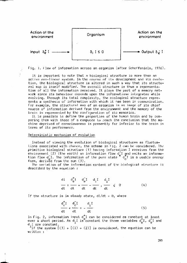
Action of the environment

Input 5g I

Organism

5j I < 0

Action on the environment

Output 5 ê 1

Fig. 1. Flow of information across an organism (after Schoffeniels, 1976).

It is important to note that a biological structure is more than an active non-linear system. In the course of its development and its evolu­tion, the biological structure is altered in such a way that its structu­ral map is itself modified. The overall structure is thus a representa­tion of all the information received. It plays the part of a memory net­work since its behaviour depends upon the informations integrated while evolving. Through its total complexity, the biological structure repre­sents a synthesis of information with which it has been in communication. For example, the structural map of an organism is an image of its chief source of information derived from the environment and the memory of the brain is represented by the configuration of its memories.

It is possible to define the properties of the human brain and by com­paring them with those of a computer to reach the conclusion that the ma­chine deprived of consciousness is presently far inferior to the brain in terms of its performance.

Deterministic mechanism of evolution

Instead of viewing the evolution of biological structures as fluctua­tions associated with chance, the scheme in Fig. 2 can be considered. The primitive biological structure (1) having information I receives from the environment (2) (the earth) an information flow d I and emits an informa-

— e + tion flow d I. The information of the pure state d T is a usable energy form, derived from the sun (3).

The variation of the information content of the biological structure is described by the equation :

dl d+I e

d I e

.1 d.I l

4 0 (4) dt dt dt dt dt

If the structure is in steady state, dl/dt = 0, where

d+I e

dt

d I e

dt

d.I l

dt (5)

In Fig. 2, information input d I can be considered as constant at least over a short period. As d.I is constant the three variables d I, d~I and

i e e d.I are constant.

If the system [(3) + [(1) + (2)] is considered, the equation can be written :

295

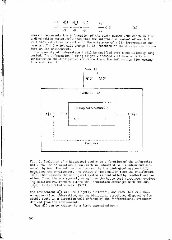
d+T e

dT

dt dt

d T e

dt

d.T ï

dt

d.T i

< O dt

(6)

where T represents the information of the earth system (the earth is also a dissipative structure). From this the information content of earth T will vary with time by virtue of the existence of : (1) irreversible phe­nomena d^J < 0 which will change T; (2) feedback of the dissipative struc­ture on its environment.

The quantity of information T will be modified over a sufficiently long period. The information T being slightly changed will have a different influence on the dissipative structure I and the information flux coming from and given to

Sun(3)

Vtr s;y

* • I »

Earth (2) ¥

Biological structure(l)

3j I I

*• J e l

Feedback

Fig. 2. Evolution of a biological system as a function of the informatio­nal flow. The informational sun-earth is submitted to circadian and sea­sonal rhythms. The information produced by the biological system (d I) modulates the environment. The output of information from the environment (d I) that crosses the biological system is controlled by feedback mecha­nisms. Thus, the environment, as well as the biological structure, evolves. The modified environment alters the information exchanges with the sun (d±T). (after Schoffeniels, 1976).

the environment d I will be slightly different, and from this will have an action (i.e. information) on the biological structure, displacing its stable state in a direction well defined by the "informational pressure" derived from the environment.

Thus d I can be written to a first approximation :

296

d

- d + I = dt 6

dd"" e

dT

(d; i )t = ( < i }t ^ - H E ^ t* ^ - v (7)

o where t* e ] , t_[ is the time interval necessary for an evident, t - t„ change of d I.

The second term can be equally expressed :

dT

— (8)

dt

where T = T (t, dT, dl, etc.). Since biological structures are non linear, they retain modifications,

which they have undergone memory-fashion, integrated within their genetic information. Their evolution being bound to perturbations which they have imposed on the environment, it can be deduced that genetic information is essentially the integration of these perturbations. Evolution can, in this way, be envisaged as progressive adaptation of biological structures in the face of modifications in the environment.

This feedback may be either positive or negative. In the first case the system will evolve in the direction of an increase of its complexity or contrarily, it will evolve in the direction of a degradation of its own information leading eventually to a complete involution. In the second case it will remain identical to itself.

The presence of oxygen in the atmosphere results from photosynthetic activity of plants. This event results in the formation of a layer of ozo­ne which has modified the sun-earth exchange relationships (d T of fig. 2). Correspondingly, d I was itself greatly modified and it is at this point, at the dawn of the Cambrian, that the rich burgeoning of multicellular eukaryotes is observed. As forecast by the theory of fluctuation this event is sudden as can also be inferred from the non-linear character of biological structures.

In conclusion, generalization of classical information theory as applied to open systems allows an explanation of the fact that the content of a biological system increases in the course of its development since it re­presents an integration of all the modifications which it has undergone and which it has imposed on the environment. Thus it is on the background of genetic information that systems develop which allow interaction of an informational nature with the environment. Herein lies the importance of the generalization, epitomized in the feedback organism-environment, that in an evolving environment, an organism can only evolve.

It is certainly reasonable to postulate that prebiological evolution occurring in the absence of oxygen was a period wherein interactions be­tween polynucleotides and polypeptides were not unidirectional. The fore­going considerations, showing the possibility of information transfer be­tween neighbouring structures S. and S„ which have similarly high infor­mation content renders such an hypothesis very plausible. Two evolutiona­ry mechanisms could thus be countenanced, one involving a reciprocal in­formation exchange between polynucleotides and polypeptides ending with the formation of the photosynthetic prokaryotes. The other, not necessa­rily excluding this information exchange, and particularly active at the start of the Cambrian, is to be found amongst the laws governing the brewing of genetic material.

The latter would be efficient only after the formation of an oxygen-rich atmosphere which allowed the development of eukaryote cells and multicel­lular forms. It is in the course of the first phase of the history of life and in an anoxic atmosphere that the prokaryotes would have been formed as a response to environmental stimuli. Bioenergetic processes of

297

contemporary cells are all very ancient in the sense that for the most part they are anaerobic. The great novelty of the respiratory chain is only possible after the formation of an oxygen-rich atmosphere. By now the various energy options have appeared opening the way for the forma­tion of multicellular organisms, as well as the appearance of sexual reproduction adding a further dimension to primitive evolutionary proces­ses.

References

Glansdorff, P. and Prigogine, I., 1971. Thermodynamic theory of structure stability and fluctuations. Wiley Interscience, London.

Schoffeniels, E., 1976. Anti-Chance (translated by L.B. Reid). Pergamon Press, Oxford.

Schoffeniels, E., 1977. Physiologie des Régulations. Masson, Paris. Schoffeniels, E. 1984. Biochimie comparée (Collection de Biologie evolu­

tive, vol.9). Masson, Paris. Schoffeniels, E. 1985. Generalizing information theory to an open system.

Biometeorology 10. Part 2 Suppl. to Int. J. Biometeor. 29 : 41-56. Schrodinger, E., 1945. What is life ? Cambridge University Press, London.

298

THE EARTH AS AN INCOMMENSURATE FIELD AT THE GEO-COSMIC INTERFACE: FUNDAMENTALS TO A THEORY OF EMERGENT EVOLUTION

R. Swenson

Center for the Study of Complex Systems, 84 Thomas Street, N.Y., N.Y. 10013

Summary

The earth and its atmosphere since Hadean times have comprised a volume of relatively constant mass which can be thought of as a thermodynamic flow field embedded within a larger field which is its cosmic environment. To the extent that nonequilibrium energy distributions in the cosmic field impinge on the earth field they constitute thermodynamic or generalized forces; the solar gradient being the most prominent example. The microscopic and bulk motions of matter on earth constitute flows or diffusivities that through their motions act as sinks for the gradient of the cosmic field. The study of evolution is the study of how these diffusivity patterns change over time in terms of the distribution of mass and velocity. It is shown that where the field forces exceed the magnitude of the flows in such a system it belongs to a class called "incommensurate" and its evolution follows predictive macroscopic laws. In particular, the time-dependent behavior will be such that the field will extend the space-time dimensions of its diffusive surfaces through the spontaneous emergence of new levels of dynamical behavior progressively selecting its own accessible mi-crostates so as to maximize the rate of its mass specific global diffusivity subject to the constraints. A master equation that gives a dimensionless number providing an index to evolution and emergence is given. Keywords: evolution, emergence, the law of maximum entropy production, nonequilibrium thermodynamics, dissipation, diffusivity, Q. number.

Introduction

The universe by its expansion generates disequilibrium, and by the laws of physics at the same time attempts to restore its broken symmetry. In the words of Clausius the entropy of the universe "strives to a maximum" (Clausius, 1865). The earth and its atmosphere can be described as a flow field comprising a volume of relatively constant mass embedded in the flow field of the larger cosmic volume with which i t interacts. The disequilibrium of the cosmic field produces generalized thermodynamic or field forces characterized by gradients that drive the motion of the earth field. The geo-cosmic interface is the region where these two fields meet, and i t is the nature of the interface, in particular, the degree of commensuration between the two fields that determines the evolution of the embedded system. Where two fields interact and the forces of the impinging field are mild the fields are commensurate, but where the forces of the impinging

299

field are strong the fields are incommensurate and the embedded field exhibits emergent evolutionary behavior.

I have introduced elsewhere (Swenson, 1988a, b, c) the fundamental principles to a theory of general evolution, TGE, including the law of maximum entropy thermodynamic entropy production, here maximization of the rate of mass specific diffusivity, which underlies the spontaneous emergence of levels in complex systems and governs the time-independent future state to which they are attracted. Here a dimensionless ration, £2, is introduced which can be used globally or in its local form, Q.x , to predict the emergence of levels and their macroscopic time-dependent behavior regardless of the particular components or what level they are on or the particular gradients or forces that characterize the particular level. Finally, it should be noted that it is precisely because orthodox evolutionary theory is divorced from the physics of the universe, and the geo-cosmic interface in particular, that it cannot recognize a direction to evolution, and hence fails to make predictions. Likewise, it cannot explain emergence, or spontaneous level building because it has no place for macroscopic constraints to come from in its bottom-up theory.

Results and Discussion

A master equation where a dimensionless ratio that provides an index to evolution and emergence can be given as follows

fl.^1 (1) it

where o = the macroscopic diffusivity (diffusion produced by macroscopic or "bulk" motion) within a field of flow,|F| = the scalar (magnitude) of the vector

n

sum of the generalized field forces, F = ^ F r a , and k- the microscopic diffusivity

(diffusion from microscopic motions alone without macroscopic or bulk flow), a, k, and |F| are all measurable for the volume of the entire field = V or for any point, component or volume, V? (£ = l,...,n) , within the field in relation to a fixed set of coordinates. The field forces result from nonequilibrium distributions of mat­ter/energy and thus take the form of gradients, so that, e.g., F, = heat, F2 = chemical, F3 = matter, and F„ = various other gradients at whatever particular level of observation, the magnitude of which is determined by their steepness.

The total microscopic diffusivity coefficient of the field can be written as

k = ^/fcf, where k^ = the microscopic diffusivity of the £th component volume

V?(Ç = l,...,n), and

k;=f(Yi,xi,\Ft\) (2)

where y | (a = l,...,n) = the potential microscopic diffusivity of the ath mat-

300

erial constituent of V { , JE£= the weight fraction of the a th constituent,

 - c> where p c is the mass density of Ve and pi = the mass density of the P "

ath constituent, and | F | | is the magnitude of the vector sum Fj = ^ F , L of the the conjugate field forces that drive the transformations that characterize theath constituent.

The relations in (2) make a fundamental point immediately obvious. Because the rates of flows or diffusivities increase proportionately to the forces, and the magnitude of the forces increases with the steepness of the gradient, the farther

the field from equilibrium the greater the magnitude of | F | | , and the greater

the magnitude of 7« . But this creates a problem: the potential microscopic dif-fusivity yi of any constituent, e.g., heat conduction, kinematic viscosity, stoi­chiometric coefficient, etc. is finite, and the range is small when compared to the potential magnitude of IFJ|. What happens to y ? when IF^I exceeds the limit of y£ and hence the limit of kc? The answer is precisely expressed in the master equation (1) where at the limit of k the numerator equals the denomina­tor and £2 = 1. This unity condition is the condition for the emergence of macroscopic flow; the solution to the problem of the limit of fc is a. In any field, the diffusivity limit of k is attributable to two factors: (i) the finite potential interactions or relations that define 7« , and (ii) the space-time geometry that defines all -fields in general, o lifts the latter constraint by deforming the space-time dimensions of the field.

How does this work? Since all diffusion in matter/energy flow fields where structure is seen to emerge is ultimately a function of the rate of molecule to molecule interaction, or rate of surface contact per unit time, in fc-fields which by definition are confined to the geometry of mean free path distances and relaxa­tion times this rate is exceedingly limited. Emergent flow superposes a new field of motion on top of the previously incoherent microscopic interactions extending the space-time dimensions, and hence the diffusive surfaces of the field by orders of magnitude. Where IF^I = the magnitude of the vector sum of the field forces

acting on some volume, yf, that is macroscopically large relative to the mean free path distances of its microscopic components, then £2? = the dimensionless

ratio for y f and |K|1 = £2C < 1, and IF/J = £2? > lwhere the subscript "c" designates

the criticality threshold of | F ? | where £2 = 1. When JFC| = |F|C|, and hence £2f < 1,

the diffusivity is described completely by k^, and o exists in y f as non-average fluctuations above the mean. With £2Ç < 1, &? = a "hungry sink" and these are quickly scavanged. In addition, negative fluctuations average out the positive ones so the net effect is still the average behavior that typifies a fc-field (see Fig. 1. at t t ).

As soon as |F^.|, and therefore £2? > 1, the situation completely reverses; k-fields are not hungry when £2?>1, but (J-fields are. At the moment when £2? > 1 there results in V^ what I have called a "crisis in space-time" (Swenson 1989a, 1989b) where the space-time extension of the field presents a barrier to

301

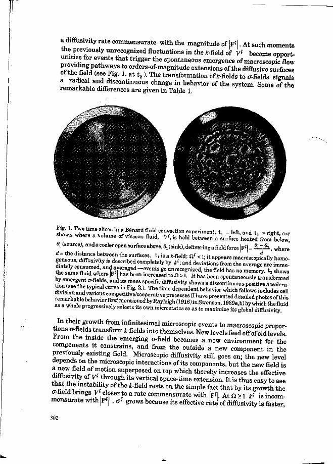
a dxffusivity rate commensurate with the magnitude of |F< I. At such moments the previously unrecognized fluctuations in the afield of y< become opport­unities for events that trigger the spontaneous emergence of macroscopic flow K S T ? o rders-° f-magnitude extensions of the diffusive surfaces of the field (see Pig. 1. at t2 ). The transformation of Wields to cr-fields signals LZT7,a^dlscontinuous c h a nge in behavior of the system. Some of the remarkable differences are given in Table 1.

Fig. 1. Two time slices in a Benard fluid convection experiment, t, = left, and t , = rieht are shown where a volume of viscous fluid, V<,is held between 'a surface'heated^rom below! 0, (source), and a cooler open surface above,Ö2(smk),deliveringafieldforce|Ff|=£^., w h e r e

™ u S n C e b f " ' T t h e .SUJr f a ce s- 4 ' i s a H e l d : ° C < V- * a PP e a r s macroscopkally homo­

geneous, diffusivity is described completely by k<; and deviations from the average are imme-

£ a m e flT >,' ^ Ü l f T * * ~ 6 V e n t S g ° u™ c°g™*d, the field has no merno^ t2 7Zs the same fluid where F ' has been increased to Q > 1. It has been spontaneously transfomld

M o X X t f ' &nk l tSr'S f6 CifiC d i f f u s i v i t y S h 0 w s a d i s c o n t i n u o u s 3 t t i t r a ­tion (see the typical curve in F l g . 2.). The time-dependent behavior which follows includes ceU

as a whole progressively selects its own microstates so as to maximize its global diffusivity

In their growth from infinitesimal microscopic events to macroscopic propor­tions cr-fields transform Wields into themselves. New levels feed off of old levels *rom the inside the emerging cx-field becomes a new environment for the components it constrains, and from the outside a new component in the previously existing field. Microscopic diffusivity still goes on; the new level depends on the microscopic interactions of its components, but the new field is a new field of motion superposed on top which thereby increases the effective diflusivity of £ through its vertical space-time extension. It is thus easy to see that the instability of the *-field rests on the simple fact that by its growth the cr-field brings;^ closer to a rate commensurate with IF^I. A tQ>l *c is incom­mensurate with |F'| . J grows because its effective rate of diffusivity is faster,

302

viz., it reduces the incommensuration.

Table 1. Principal Differences Between £-Field and cr-Field Behavior

it-field (Q < 1)

Describable by mean free path distances and relaxation times of microscopic components, e.g., of the order of 10"8 cm andlCT15 sec. in a simple fluid (see Fig. la).

Infinitesimal energy fluctuations above the mean (i) are immediately consumed by the field, and(ii) averaged by fluctuations with the opposite sign, and thus have no non-average effects. £-field hungry; <r-field poised, but with no effect.

Consumption by k results in the destruction of constraints on microscopic degrees offreedom. Consumption (of gradient) and destruction (of constraints or structure) are the same.

Linear. Initial conditions and events are lost with time. No learning; no memory.

The attractor (the time-independent state it spontaneously evolves toward) is the state of maximum homogeneity; the least highly speci­fied macrostate relative to number of acces­sible microstates.

cr-field(Q>l)

Macroscopic motion superposed on the micro­scopic field at many orders of magnitude greater space-time scales not describable by mean free path distances and relaxation times, e.g., to cm and sec. in same fluid (see Fig. lb).

Infinitesimal non-average fluctuations above the mean become events amplified to macro­scopic proportions. Averaging of microscopic behavior fails. Jfc-field saturated; <r-fields hungry, active, and opportunistic.

Consumption by cis through the spontaneous emergence of constraints. The amplification of an infinitesimal fluctuation from an incoherent jfc-field into coherent macroscopic flow requires the progressive selection, or reduction of accessible microstates; a progres­sive imposition of macroscopic constraints by the field on itself. Consumption and produc­tion are the same.

All-or-none behavior defined by the circular (nonlinear) relations between components. Inherently self-amplifying; effects become causes, and small unobservable changes in initial conditions can lead to large macro­scopic differences.

Maximize their diffusivity by selecting their own microstates so as to extend their diffu­sive surfaces at the fastest possible rate. The attractor is the state of maximum macro­scopic diffusivity, the state with maximally extended diffusive surfaces, given the magni­tude of |F| and the constraints.

The same rate-dependent logic which explains the emergence of levels is more deeply applied showing how levels interact with time. In V? where k( is not commensurate with |F?| we can expect fc? at t t to become &f<,+1>, <T?(,0>, £f(M) at t2 where <rf<'0) = emergent macroscopic flow, k(0+1) = the k- field from which <7?(,0) emerges, k(i'~l) - the microscopic or component level that comprises o^im, and (/O), (/ +1), (/ -1) = the focal level, level without, and level within respect­ively. We can further predict that unless the incommensuration is extremely limited that if we get k((M\ aim, *f(W) at t2 then we will get <T?(,+1\ aim, of('_1) 0' = l,...,n) at t3. How do we know this and why does it happen? tr-fields

303

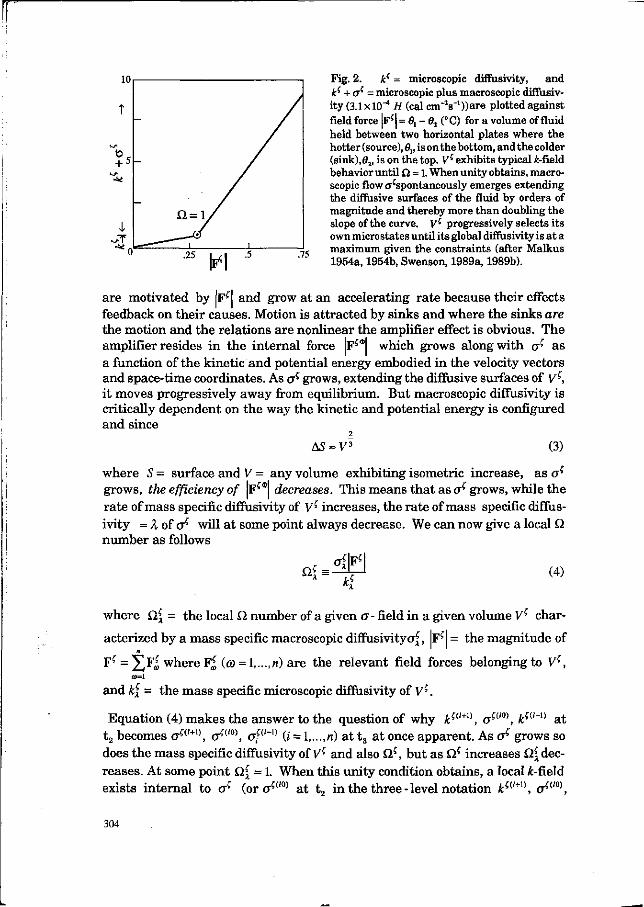
Fig. 2. k( = microscopic diffusivity, and

H 5

k{- •• microscopic plus macroscopic diffusiv­ity (3.1 x 10" H (cal ernes'1 »are plotted against field force |Ff | =ei-0ï (°C) for a volume of fluid held between two horizontal plates where the hotter (source), 9V is on the bottom, and the colder (sink),ô2, is on the top. V( exhibits typical £-field behavior until fl = 1. When unity obtains, macro­scopic flow spontaneously emerges extending the diffusive surfaces of the fluid by orders of magnitude and thereby more than doubling the slope of the curve. Vs progressively selects its own microstates until its global diffusivity is at a maximum given the constraints (after Malkus 1954a, 1954b, Swenson, 1989a, 1989b).

are motivated by |Ff I and grow at an accelerating rate because their effects feedback on their causes. Motion is attracted by sinks and where the sinks are the motion and the relations are nonlinear the amplifier effect is obvious. The amplifier resides in the internal force |Ff*| which grows along with (j? as a function of the kinetic and potential energy embodied in the velocity vectors and space-time coordinates. As cxf grows, extending the diffusive surfaces of Vf, it moves progressively away from equilibrium. But macroscopic diffusivity is critically dependent on the way the kinetic and potential energy is configured and since

AS = V 3 (3)

where S = surface and V = any volume exhibiting isometric increase, as a1' grows, the efficiency of F?*j decreases. This means that as a( grows, while the rate of mass specific diffusivity of V? increases, the rate of mass specific diffus­ivity = % of <yf will at some point always decrease. We can now give a local Q number as follows

cjflF?l

4 (4)

where Çi[ = the local Q. number of a given a - field in a given volume V? char­

acterized by a mass specific macroscopic diffusivityo|, F f = the magnitude of n

F ? = ^ F | where Fj; (co = l,...,n) are the relevant field forces belonging to Vf,

and k{ = the mass specific microscopic diffusivity of V^.

Equation (4) makes the answer to the question of why kw+l\ oçm, kw~n a t t2 becomes aw+X), a' HI») TCC-D a ^ (i = l,...,n) at t3 a t once apparent. As (r grows so does the mass specific diffusivity of V? and also S2C, but as Qc increases Q,[ dec­reases. At some point Çl[ = 1. When this unity condition obtains, a local £-field exists internal to <r? (or oim a t t , in the three - level notation kliM), o;m,

304

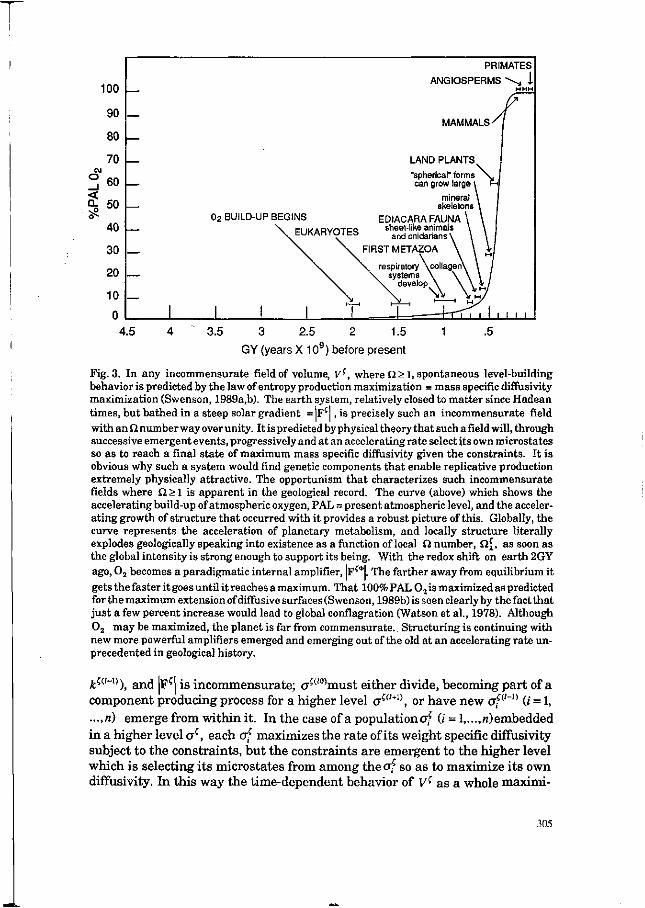
GY (years X 10 ) before present

Fig. 3. In any incommensurate field of volume, Kc, where £2 > 1, spontaneous level-building behavior is predicted by the law of entropy production maximization = mass specific diffusivity maximization (Swenson, 1989a,b). The earth system, relatively closed to matter since Hadean times, but bathed in a steep solar gradient = |F ? | , is precisely such an incommensurate field with an Q number way over unity. It is predicted by physical theory that such afield will, through successive emergent events, progressively and at an accelerating rate select its own microstates so as to reach a final state of maximum mass specific diffusivity given the constraints. It is obvious why such a system would find genetic components that enable replicative production extremely physically attractive. The opportunism that characterizes such incommensurate fields where Q > 1 is apparent in the geological record. The curve (above) which shows the accelerating build-up of atmospheric oxygen, PAL = present atmospheric level, and the acceler­ating growth of structure that occurred with it provides a robust picture of this. Globally, the curve represents the acceleration of planetary metabolism, and locally structure literally explodes geologically speaking into existence as a function of local fl number, Qj , as soon as the global intensity is strong enough to support its being. With the redox shift on earth 2GY ago, 0 2 becomes a paradigmatic internal amplifier, |Ff*|. The farther away from equilibrium it gets thefaster it goes until it reaches a maximum. That 100% PAL 0 2 is maximized as predicted for the maximum extension of diffusive surfaces (Swenson, 1989b) is seen clearly by the fact that just a few percent increase would lead to global conflagration (Watson et al., 1978). Although 0 2 may be maximized, the planet is far from commensurate. Structuring is continuing with new more powerful amplifiers emerged and emerging out of the old at an accelerating rate un­precedented in geological history.

k^' 15), and F ? is incommensurate; cr?<'0)must either divide, becoming part of a component producing process for a higher level oilM\ or have new af°'n (i = 1, ...,n) emerge from within it. In the case of a population erf (i = l,...,n)embedded in a higher level <7?, each of maximizes the rate of its weight specific diffusivity subject to the constraints, but the constraints are emergent to the higher level which is selecting its microstates from among the erf so as to maximize its own diffusivity. In this way the time-dependent behavior of V? as a whole maximi-

305

zes its global weight specific diffusivity. The dimensionless number Q provides a powerful new tool which when coupled with the law of maximum entropy production previously stated (Swenson, 1988,1989a,b,c), or equivalently weight specific diffusivity maximization, gives great insight into the behavior that can be expected from the interaction of two incommensurate fields such as those that characterize the geo-cosmic interface.

Acknowledgements

The author thanks Bruce H. Weber for help with a technical problem, and acknowledges useful discussions with colleagues from the ISSS emergence and evolution study group. All errors are the author's.

References

Clausius, R., 1865. Ueber verchiedene fur die anwendun bequeme formen der hauptgleichungen der mechaischen warmetheorie. Annalen der Phys. und Chem. 7:389-400. _ ^ Malkus, W., 1954a, Discrete transitions in turbulent convection. Proc.Roy.Soc.Lon. 225:185-195. Malkus, W., 1954b. The heat transport and spectrum of thermal turbulence. Proc.Roy.Soc.Lon. 225:196. Rayleigh, 1916. On the convective currents in a horizontal layer of fluid. Phil.Mag. 32:529-546. Swenson, R. 1988. Emergence and principle of maximum entropy production. Abst. 32ndAnn.Meet.Soc.Gen.Syst.Res. 23-27 May, St. Louis, Mo., 180. Swenson, R., 1989a. Emergent attractors and the law of maximum entropy production. AAAS Ann.MeetAbstr. 14-19 January, San Francisco, CA, 180. Swenson, R., 1989b, Emergent attractors and the law of maximum entropy production: foundations to a theory of general evolution. Systems Research 6 (3), pp. 187-197. Swenson, R., 1989c. Emergent evolution and the global attractor: the evolution­ary epistemology of entropy production maximization. Proc.33rd Ann.Meet. ISSS 2-7 July, Edinburgh, Scotland.

306

RESONANT MAGNETO-TIDAL COUPLING BETWEEN THE COMPONENTS OF THE SOLAR SYSTEM AND SOME OF ITS TERRESTRIAL CONSEQUENCES

P.A.H.SEYMOUR

Department of Marine Science and Technology, Polytechnic South West, Plymouth, united Kingdom

Summary

This paper discusses the principles of resonant coupling between the t ides of the planets and magnetic osci l lat ions of the evolving magnetic field of the Sun, and the consequences of this resonance for the variations of the t e r r e s t r i a l magnetosphere. After introducing the general principles involved, I then propose a mathematical model for the whole process of interaction, and I describe some numerical r e su l t s obtained from the model. In conclusion I briefly describe resonant interactions between the osci l lat ions of the t e r r e s t r i a l magnetosphere and the bir th processes of a foetus, based on an e lect r ical c i rcui t analogy for the biological clock that could act as the timing device used for the count down to b ir th. Keywords: resonance, t idal coupling, magnetic osci l la t ions, biological clocks.

Introduction

Resonance is a well known phenomenon in the physical world. In INTRODUCTION TO THEORETICAL PHYSICS by Slater and Frank (1933) they mention a variety of examples involving resonance. As an example of mechanical resonance they discuss the simple pendulum, and as examples of acoustical resonance they discuss the tuning fork and Helmholz resonators. They then move on to e lect r ical c i rcui t s , with these words: "The resonance of e lec t r ica l c i rcui t s is i l lus t ra ted in the tuned c i rcui t s of the radio, which respond only to sending s ta t ions of a part icular wavelength, and practically not a t a l l to other s ta t ions." To the l i s t of Slater and Frank we could add many others. One very relevant to the present discussion is t idal resonance.

Tidal resonance

The body of water in a bay or estuary has i t s own natural frequency. If this is the same as the t idal tug, due to gravitat ion, of the Moon on such a body of water, then the t ides a re much higher than one would predict on the basis of the equilibrium theory of t ides. George Biddell Airy (1845), worked out the theory for the t ides in a canal paral lel to the Earth's equator. He was able to show that the speed with which a free wave would propagate along such a canal would depend on the cross-sectional dimensions of the canal. He showed that if these dimensions were so chosen that the speed of this free wave was exactly equal to the speed a t which the sub-lunar point moved over the surface of the Earth, then the t ides would tend to infinity. Furthermore Airy also showed that in such a canal the t ides could be e i ther direct or inverted, i.e. there could be e i ther a high or low t ide below the Moon, depending on the velocity of the free wave propagating along the canal. The t ide would be direct if the velocity of the free wave were greater than the velocity of the sub-lunar point and inverted if the reverse were t rue.

307

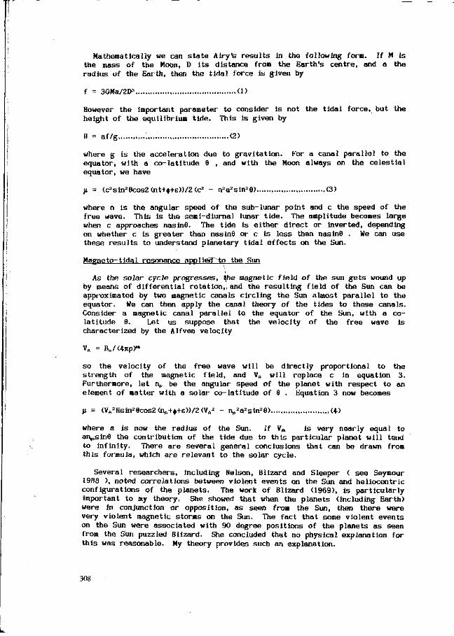
Mathematically we can s t a t e Airy's r e su l t s in the following form. If M is the mass of the Moon, D i t s distance from the Earth's centre, and a the radius of the Earth, then the t idal force is given by

f = SGMa/ZD3 <1>

However the important parameter to consider is not the t idal force, but the height of the equilibrium t ide. This is given by

H = af/g (2)

where g is the acceleration due to gravitat ion. For a canal paral lel to the equator, with a co- lat i tude 8 , and with the Moon always on the ce les t ia l equator, we have

H = {c2sin26cos2(nt+*+e)}/2(c2 - n2a2sin28> <3>

where n is the angular speed of the sub-lunar point and c the speed of the free wave. This is the semi-diurnal lunar t ide . The amplitude becomes large when c approaches nas in 8. The tide is e i ther direct or inverted, depending on whether c is greater than nasinS or c is less than nasinS , We can use these r e su l t s to understand planetary t idal effects on the Sun.

Magneto-tidal resonance applié(T~to the Sun \

As the solar cycle progresses, ^he magnetic field of the sun ge t s wound up by means of d ifferential rotat ion, and the resul t ing field of the Sun can be approximated by two magnetic canals circling the Sun almost paral lel to the equator. We can then apply the canal theory of the t ides to these canals. Consider a magnetic canal paral lel to the equator of the Sun, with a co-lat i tude 8. Let us suppose that the velocity of the free wave is characterized by the Alfven velocity

Vn = B0/<4np)M

so the velocity of the free wave will be directly proportional to the s trength of the magnetic field, and Vn will replace c in equation 3. Furthermore, le t np be the angular speed of the planet with respect to an element of matter with a solar co-lat i tude of 8 . Equation 3 now becomes

H = fV02Hsin28cos2 ÖV+^+E)}/2 (VA

2 - np2a2sin2e> (4)

where a i s now the radius of the Sun. If Vß i s very nearly equal to anpsin8 the contribution of the t ide due to this part icular planet will tend to infinity. There are several general conclusions that can be drawn from th is formula, which are relevant to the solar cycle.

Several researchers, including Nelson, Blizard and Sleeper ( see Seymour 1988 ), noted correlations between violent events on the Sun and heliocentric configurations of the planets. The work of Blizard (1969), is part icularly important to my theory. She showed that when the planets (including Earth) were in conjunction or opposition, as seen from the Sun, then there were very violent magnetic storms on the Sun. The fact that some violent events on the Sun were associated with 90 degree positions of the planets as seen from the Sun puzzled Blizard. She concluded that no physical explanation for this was reasonable. My theory provides such an explanation.

308

If we consider two planets 1 and 2 with angular speeds n' and n" respectively with respect to an element of n a t t e r with solar la t i tude 6 , then the s i tuat ion could a r ise when V„ is g reater than n'asinO but less than n"asin6. In th is case the t ide due to one planet will be d irect and that due to the other planet will be inverted. This means that the t idal effect of the two planets would be additive when they a re separated by 90 degrees of solar longitude. I t is then possible that a t some s tage in the solar cycle additive effects could occur when the planets are separated by 90 degrees. At other times the t idal effects of a l l the planets could a l l be direct < or a l l inverted ) if the angular velocit ies a re a l l g reater than the Alfven speed in a magnetic canal ( or a l l g rea ter than the Alfven speed). In both cases, conjunctions and oppositions a s seen from the Sun will give r i s e to additive t idal e ffects . This theory then provides an astronomical basis for heliocentric planetary aspects. Violent events are likely on the Sun for heliocentric conjunctions, oppositions and squares of the planets. However the par t icular combinations necessary for such events will depend on their r e la t ive times within the overall solar cycle.

Numerical t es t ing of the basic theory

In order to t es t the theory numerically, Turner a t Polytechnic South West carried out a number of calculations on a few simple models. In these models he assumed that the magnetic canals were a l l very close to the solar equator, and that a l l the planets moved in circular orbi ts which were coplanar with the solar equator. He tested a variety of different models in which the s t rength of the magnetic field varied in different ways as the solar cycle bui l t up to maximum. In some of these models the field s t rength varied in a saw tooth form - s t a r t ing from zero and increasing linearly unti l i t reached a chosen maximum, and then falling abruptly to zero. In some of the other models the field s t rength varied as a s ine curve. The maxima chosen in both s e t s of models were consistant with measured field s lengths in sunspots. These r e su l t s provided considerable support to the basic theory and led us to investigate more complex models. For example, we are investigating the effect of allowing the magnetic canals to migrate towards the equator, in a way that will simulate the observed migration of sunspots. We are a lso considering the effect of rea l e l l ip t ica l o rb i ts for the planets, as well as the effects of non-zero angular distances of the planes of the planetary o rbi ts with respect to the solar equator. These investigations are continuing. Instead of allowing the s t rength of the magnetic field in the canals to follow a s ine wave curve, we are investigating the effects of planetary control on the overall evolution of the solar cycle.

Overall planetary control of the solar cycle

Measurements of the Sun's magnetic field show that the field has opposite polarity a t the poles ( resembling the s t ruc ture of the field of a dipole magnet), but this polarity changes a t the s t a r t of a new sunspot cycle. According to my theory, the mechanism for the reversal of the original dipole field is different from that responsible for ' t r iggering' the onset of f lares and proton events. This is in keeping with an observation made by Blizard. She concluded that two different links be twen the Sun and the planets were involved, because a l l the planets were involved, not jus t those with the s t rongest effect on the movement of the Sun about the common centre of mass of the solar system, or those with the s t rongest t idal tug on the Sun. The correlation between change of sign of the solar magnetic field, and the ra te of change of solar angular momentum (due largely to the five outer planets)

309

f i r s t noted by Jose (1965), can be explained as follows. In my theory the rapid change in angular momentum, from increasing to decreasing, causes a change in the direction of the meridional cyclonic motions, so that these motions now convect the toroidal field to give r i s e to a dipolar field which has opposite polarity to the original field. I am currently investigating a model in which the s t rength of the magnetic field in the magnetic canals is d irectly proportional to the r a te of change of angular momentum of the Sun about the common centre of mass of the solar system. Although these investigations are not yet complete, the in i t ia l r e su l t s are very similar to those obtained for a s ine wave curve.

The effect of the solar cycle on the geomagnetic f ield

Many researchers have noted the effect of the variation of sunspot numbers on the behaviour of the geomagnetic field. The most important work in this area, germane to my theory, is that of (see Lange! 1987). (/sing the minimum entropy method he was able to show that many of the long term variations of the geomagnetic field, of longer than one year, were related to the solar cycle and i t s harmonics. Via the well known physical mechanism of modulation, these longer term effects also have a direct effect on the solar daily magnetic variation and i t s harmonics, a s noted by Bullard (1967). In h is Harold Jeffreys Lecture of the 3 December 1965, on ELECTROMAGNETIC INDUCTION IN THE EARTH, he had th is to say: "In fact most of the information has been obtained from the daily period and i t s f i r s t three harmonics of 12, 8 and 6 hours The amplitudes of the terms varies with the season of the year and with the sunspot cycle: i t might be more convenient to regard these changes not as changes in the amplitude of a term with a single frequency but as beats between a group of terms with s l ight ly different frequencies." This suggestion_^is^_eonsistent with the general mathematical theory of amplitude modulation. When Bullard delivered this lecture in 1965 he a lso noted that; "It is curious that no attempt seems to have been made to resolve this fine structure by the methods of power spectrum analysis." This situation has changed as a result of the work of de Meyer of the Royal Meteorological Institute in Bruxelles. He was able to show that some of the terms of the solar daily magnetic variation did indeed have such fine structure ( see Langel 1987 ).

It is well known in atomic physics that the spectral lines of atoms can be broadened by the Doppler effect, and other mechanisms. I propose that the lines of the solar daily magnetic variation and the fine structure lines flanking these lines, do have a finite width. This width arises, I suggest, in the following way. The distortion of the magnetosphere can be considered to be transverse Alfven waves propagating around the Earth, and concentrated mainly in the Van Allen radiation belts. These belts resemble doughnuts, they having finite thickness with different inner and outer radii. Since the Alfven speed depends on magnetic field strength and density, and since both these quantities change with distance from the surface of the Earth, the angular speed of these waves will be spread about the angular speed with which the Earth is spinning with respect to the Sun. This will give rise to a finite width for the basic solar daily magnetic variation, for each of the harmonics associated with this variation and also for the side bands related to longer term modulations of this solar variation. Since the mean planetary days are very close to the mean solar day, some of the waves propagating through the Van Allen radiation belts will have the same angular speed as the planetary tides, and as a result they will become phase-locked to these

310

t ides. One nay think of this mechanism as the magnetospheric equivalent of a laser. The d is tort ion of the magnetosphere by the solar wind is doing the pumping, whereas the planetary t ides are causing coherent phase-locking of some of the A If ven waves. Perhaps we should cal l i t a MATLAW Magnetospheric Amplification of Tides by phase-Locking of Alfven Waves.

The Moon gives r i se to the lunar daily magnetic variation. This is done via the t idal tug of the Moon on the ionised upper layers of our atmosphere. This causes changes in pressure, giving r i se to winds, which generate e lec t r ic currents and these will produce an additional magnetic field. The lunar daily magnetic variation has been studied in great de ta i l , and i t s mechanism is re lat ively well understood. However, the lunar day d iffers from the solar day by almost one hour, so i t will not give r i s e to the type of resonant phase locking of Alfven waves which we have just discussed. The basic harmonic of th i s variation, the one that does not change phase with the lunar month, has two peaks and troughs per lunar day. If the Gauquelin lunar type personality possessed a magnetic sensor of some sor t , tuned to the lunar daily magnetic variation, but responding to the magnetic power in this variation (i.e. to the square of the amplitude) then i t very naturally explains the r e su l t s obtained by Gauquelin. Before discussing a magnetic model for th i s sensor, I would f i r s t like to discuss some general biological consequences of variations in the geomagnetic field.

Biological consequences of geomagnetic variations

Many researchers, including Dubrov, Brown, Gould and Becker, have investigated the effects of the geomagnetic field on living organism. A discussion and assessment of some of th is work is to be found in Dubrov's book THE GEOMAGNETIC FIELD AKD LIFE (1978). More recent comments on the importance of this interaction, by Western s c i en t i s t s , include those of Brown, Gould and Becker (1981). Brown showed that the abi l i ty of many animals to know the time of the t ides, the time of day, the phases of the Moon, and the time of year, could not a l l be explained in terms of l ight cues, and he further demenstrated that the geomagnetic field was actually influencing the biological clocks and internal compasses of many different species of animal. Further experiments by Gould showed that i t was very likely that the magnetic field of Earth was second only to the Sun and sky in helping animals to know the time, their location and direction.

Becker suggested a mechanism for th is interaction between the geomagnetic field and l ife. Start ing with the well known fact that e lec t r ica l potential differences existed between the various par ts of a living body, he went on to suggest that th is potential was the biasing control of the a c t iv i t i e s of the body. He further suggested that this DC potential system was frequency sensi t ive, responding to certain frequencies and not to o thers. He concluded that over aeons the biological clocks of every living organism had, in a sense, become phased-locked to specific pulsations of the geomagnetic field, since a l l of l ife had evolved in this field. I here propose a mathematical model to quantify th is theory.

A mathematical model for Gauquelin's planetary effect

The history of theoretical physics provides many interesting insights into the t r i a l s and t r ibulat ions which have to be faced by those who seek to give mathematically quantifiable descriptions of natural phenomena. The development of our understanding of a tonic s t ruc ture provides a very relevant specific example. Fraunhofer, Kirchhoff and Bunsen laid the

311

observational and experimental foundations of atomic spectroscopy, which enable s c i en t i s t s to identify chemical elements by the spectral lines they emitted or absorbed. I t was soon a f te r th is that Stokes, Thompson, Stewart, Kirchhoff and others suggested that certain resonant frequencies characterized each element. This idea was further developed Lorentz. Although a t th is time s c i en t i s t s had vir tual ly no idea about atomic s t ruc ture , i t was known that e lec t r ic current was made up of charged par t ic les , and Lorentz suggested, in about 1890, that atoms might also contained these par t ic les . He applied the theory of damped resonant simple harmonic motion to these par t ic les , and thus he was able to explain some of the basic properties of the interaction between electromagnetic radiation and the atoms of specific elements. In this connection I would like to complete the quotation from Slater and Frank (1933), with which I s t a r ted my paper: "In optics, the theory of refractive index and absorption coefficient is closely connected with resonance. As is shown by the sharp spectrum l ines, atoms contain osc i l la tors capable of damped simple harmonic motion, or a t any r a te they act as if they did; the real theory, using wave mechanics, is complicated but leads essent ial ly to this resul t ."

We thus see that th i s simple theory of Lorentz provided a basis for indentifying atoms from their spectra, and hence deducing their physical and chemical propert ies, long before Bohr, Sommerfeldt, Heisenberg, Schrodinger and Dirac developed quantum mechanics, which allowed us to understand these character is t ics in terms of the electronic personali t ies of atoms. I believe the work of Gauquelin < 198+ ) points to a resonant interaction between some physical ent i ty in our environment, that is linked to geocentric planetary motion, and the internal personality of the individual, which can be used to label some of the character is t ics of the person. In th is sense h is work is similar to that of Fraunhofer, Bunsen and Kirchhoff. Although we are not, a t the moment, able to deduce the 'electronic s t ruc ture of personality ' from th is response, I think we can take s teps similar to those taken by Lorentz, and propose a mathematical model of the Gauquelin b i r th clock, based on the theory of resonance. In doing so I am making use of some ideas put forward by Winfree in h is book THE GEOMETRY OF BIOLOGICAL TIME. Here he says: •Trom cel l division to heartbeat, clock like rhythms pervade the ac t iv i t i e s of every living organism. The cycles of l ife are ultimately biochemical in mechanism but many of the principles that dominate their orchestration are essent ial ly mathematical" I also made use of some ideas discuss by Hoppensteadt in h is book AN INTRODUCTION TO THE MATHEMATICS OF NEURONS. He said:

"Neurons, ,are the basic timers in our bodies. They also play a central role in s tor ing and processing information in our brains. As t imers, neurons drive higher level biological clocks in much the same manner as an a l ternat ing e lec t r ic current drives an e lec t r ic clock." Most attempts to describe the e lect r ical behaviour of the neuron have been based on e lect r ical c i rcui t analogies and their associated mathematical models. My proposal is that the influence of the geomagnetic f luctuations on the neural network as a whole can a lso be described in terms of an e lec t r ica l c i rcui t and i t s associated mathematics.

In th is model I am proposing that the internal linkages between the various neural loops of the central nervous system are to some extent genetically inherited, and that th is linking determines not only the personality of the individual, but the way in which the nervous system acts as the coordinator of the bir th process in response to specific changes in the geomagnetic field. I further propose that the behaviour of the central nervous system, when i t ac ts as the birth t r igger, can be modelled by a

312

circui t consisting of an inductance, a capacitance and a r e s i s to r , a l l connected together in s e r ies . The inductance a lso ac ts as a solenoid through which passes a bar of soft iron, suspended on one arm of a balance. When the current flowing through the system is sufficiently large, the soft iron bar is drawn into the solenoid and t r ips the b i r th switch. The e lect r ic power for th is c i rcui t is provided by the changes of the geomagnetic field which thread their way through the c i rcui t . However only those f luctuations that are resonant with the natural frequency of the c i rcui t will produce a large enough current to t r igger the switch. In order to clarify the model further, I want to use the analogy of the magnetic mine which was used in the Second World War. This mine was detonated by a device triggered by the magnetic field of a passing ship. In such a mine there would be, in addition to the magnetic t r igger, a timing device which would arm the bomb some time before i t was triggered by a magnetic field. Thus mines could be placed safely without being triggered by the fields of the ship laying the mines. If we consider b i r th as an explosion, the biochemical and biophysical energy of the mother and the child a s the explosive, and the other biological processes in child and mother < including the breaking of the water ) as the timer which arms the bomb, then the nervous system is the magnetic aer ia l tuned to specific f luctuations of the geomagnetic field which detonates the explosion. This then represents my complete model of Gauquelin's Planetary Effect.

Conclusion. ,

Resonant phenomena play a v i t a l part in a very large c lass of natural phenomena, ranging from the nuclei of atoms, through large engineering s t ruc tures and the t ides of es tuar ies , r ight up to the dynamics of Saturns r ings and the Asteroid bel t . Gauquelin's work has shown us that cosmic links with human personality is another facet of th is effect. An important point to note is that although the physical de ta i l s change from one member to another, the mathematics of resonance remains essent ial ly unchanged and i t is largely independent of the physics. The progress of science will no doubt change some of the sc ient i f ic de ta i l s of the model here presented, but the basic mathematical features are likely to remain unchanged as long as we have the Gauquelin data as the prime source of evidence in this area. Popper said: * the essence of a good mathematical model is that i t should embody the bold ideas, unjustified assumptions and speculations which a re our only means of interpreting nature. The good sc ien t i s t then puts his own model to the hazard of refutation." It is in th is s p i r i t that I present this theory for some of Gauque'tn's work, I would like to thank Gauquelin for providing us with such challenging data, Eysenck and Nias (1982) for causing me to take a second look a t the material with their book on the subject and to Dean and Mather (1976) for sowing the seed regarding resonance with their statement.' "Resonance is an essent ia l consideration in any theory of astrological causation."

References

Airy, G.B., 1845. Section VI, Encycl. Metrop.

Blizard, J.B., 1969. Long Range Solar Flare Prediction, NASA Contractor Report, NASA CR 61316.

Brown, F., Gould, J. and Becker, R.,1981. Magnet Earth - BBC TV Horizon Programme.

313

Bullard, E.C., 1967. Electromagnetic Induction In the Earth, QJ. of the RAS, 8, 143 - 160.

Dean, G. and Mather, A., 1976. Recent Advances in Natal Astrology, The Astrological Association.

Dubrov, A.P., 1978. The Geomagnetic Field and Life, Plenum.

Eysenck, H.J. and Nias, D.K.B., 1982. Astrology : Science or Superstit ion, Maur Ice Temp Ie Sm 1 th.

Gauquelln, M„ 1984, The Truth About Astrology, Hutchinson.

Hoppensteadt, F.C., 1986. An Introduction to the Mathematics of Neurons, Cambridge.

Jose, P.D., 1965. Astron. J., 70, 193 - 200.

Lange 1, R.A.,1987. The Main Field. In: J.AJacobs. Geomagnetism-Vol. 1 .Academic Press, 249 - 492.

Seymour, P., 1988. Astrology : The Evidence of Science, Lennard Publishing.

Slater, J.C. and Franck, N.H., 1933. Introduction to Theoretical Physics, McGraw-Hill.

Turner, A.J., 1987. Planetary Effects on the Solar Cycle, Plymouth Polytechnic.

Winfree, A.S., 1980. The Geometry of Biological Time, Springer-Ver lag.

314

NONLINEAR DYNAMICS AND DETERMINISTIC CHAOS THEIR RELEVANCE FOR BIOLOGICAL FUNCTION AND BEHAVIOUR

F.Kaiser

Institute of Applied Physics, Theory, Technical University, 6100 Darmstadt FRG

Summary

Nonlinear processes are of fundamental importance in all dynamical systems far from thermal equilibrium. In these systems, including biological systems, externally perturbed internal rhythmic processes offer a great variety of behaviour with respect to their specific response. Examples are sharp resonances, strong sensitivities with respect to the frequency and a very weak intensity and different types of behaviour for the same internal and external conditions. In addition, an extreme sensitivity on in­itial conditions and the loss of final state predictability is inherent in its motion, when the system is chaotic in a completely deterministic manner. This behaviour both offers and necessitates new ways of investigations and discussions for those experimental facts which in the traditional physical picture look strange or mysterious or which seem to be outside our conventional physical understanding. '

Keywords: nonlinear dynamics, deterministic chaos, rhythmic processes, predictability.

Introduction

The analysis of nonlinear physical phenomena has its foundation in the last century. Though the interest never ceased, the fundamental and universal role of nonlinear dy­namics has been recognized only within the last 15 years. Nonlinear motion is now wellknown in many disciplines, such as physics (including Laserphysics, nonlinear op­tics, semiconductors, hydrodynamics, plasma- and astrophysics), chemistry, biophysics, biology and even medicine. Nonlinear dynamics is the essential basis for instabilities and the formation of temporal, spatial and spatio-temporal structures. It offers new types of behaviour, among which the transition to a completely irrgular motion in time (determinisitic chaotic motion) and to a completely irregular spatial structure (fractal structure, turbulence) are of paramount importance.

Chaotic systems, the irregular behaviour of which is deterministic, combine sto­chastic and regular components in their dynamics. The arbitrariness stems from the sensitive dependence on the initial conditions, the regular motion is based on the inhe­rent nonlinear dynamics. Deterministic chaos adds a new quality of irregular motion to the well-known components of stochasticity. The latter have their origins either in their many particle dynamics (thermodynamic stochasticity) or in the fundamen­tal principle of uncertainty (quantum mechanical stochasticity), whereas deterministic chaos originates from the nonlinear and deterministic motion.

In the present contribution, some reflections are developed on the possible relevance of nonlinear dynamics and of chaotic motion within biological systems and functions. The consequences with respect to the realization of experiments and to the analysis of experimental data in weakly irradiated biological systems are discussed.

Nonlinear resonances are of fundamental importance in perturbed rhythmic sy-

315

stems. Externally driven self-excited oscillations offer a great variety with respect to their behaviour. Examples are sharp resonances in the harmonic, sub- and superhar-monic region, synchronization and entrainment, small signal amplification, frequency selection, frequency and intensity windows, multiperiodicity, coexisting oscillating sta­tes etc. Besides bifurcation techniques which are standard and more refined techniques required by a chaotic motion, symmetries, nonlinear resonances and Farey series are analyzed.

Frequency and amplitude dependent bifurcations lead to quasiperiodic and chaotic motions. Différent routes, each of which of a certain universality, are included. The chaotic solutions create a fundamental limit with respect to the long time predictabi­lity, though an excellent short time predictability is exhibited. As a consequence of a deterministic chaotic motion, experimental data sets, which look completely random, or noisy, presumably are based on strong deterministic laws. The underlying dynamics is then only governed by a few irreducible degrees of freedom. Well known examples are certain rhythms found in the brain (EEG) or in the heart beat, where for some states the chaotic motion and not the regular rhythm has to be viewed as the normal situation.

From Harmony and Symmetry to Chaos and Fractals

Cosmos and Harmony

Since thousands of years people have been concerned with the stability of the solar system. The Greeks at the time of Ptolemy thought that all motion can be decomposed into perfect circular motion. The Platonic ideal found its expression in the statement that all motion is periodic or quasiperiodic. In 1596 the famous astronomer J. Kepler published his ideas on the harmony of the planetary motion and of the whole universe (Mysterium cosmographicum). These ideas were justified by his well-known three laws for the planetary motion. G. Galilei (1623) introduced mathematics as the relevant tool of description for the natural sciences and some years later, I. Newton (1687) presen­ted his theory of the movement of planets. Many mathematicians (Laplace, Lagrange, Poisson ....) studied the question of stability of planetary motion and at the end of the 18th century, stability seemed to be proved.

Cosmos and Chaos

In 1889 H. Poincaré when working about the three-body problem and the dynamic equations succeeded to show by strong topological considerations, that no principle exists, which forbids a collapse of Kepler's harmonic universe. Later on mathematical concepts and theorems (KAM theorem....) proved the existence of regular and irre­gular motion, for example for the perturbed three-body motion. There is numerical evidence now that the motion of the planet Pluto is chaotic (Sussman &; Wisdom 1988).

Nature and Symmetry

In Platon's ideal world, all things in nature are composed of five perfect bodies, the polyhedra (tetrahedron, octahedron, hexahedron, icosahedron, dodecahedron). These are the only bodies, which can be realized by regular polygons. J. Kepler combined these polyhedra with the harmony of the planetary orbits. From a general point of

316

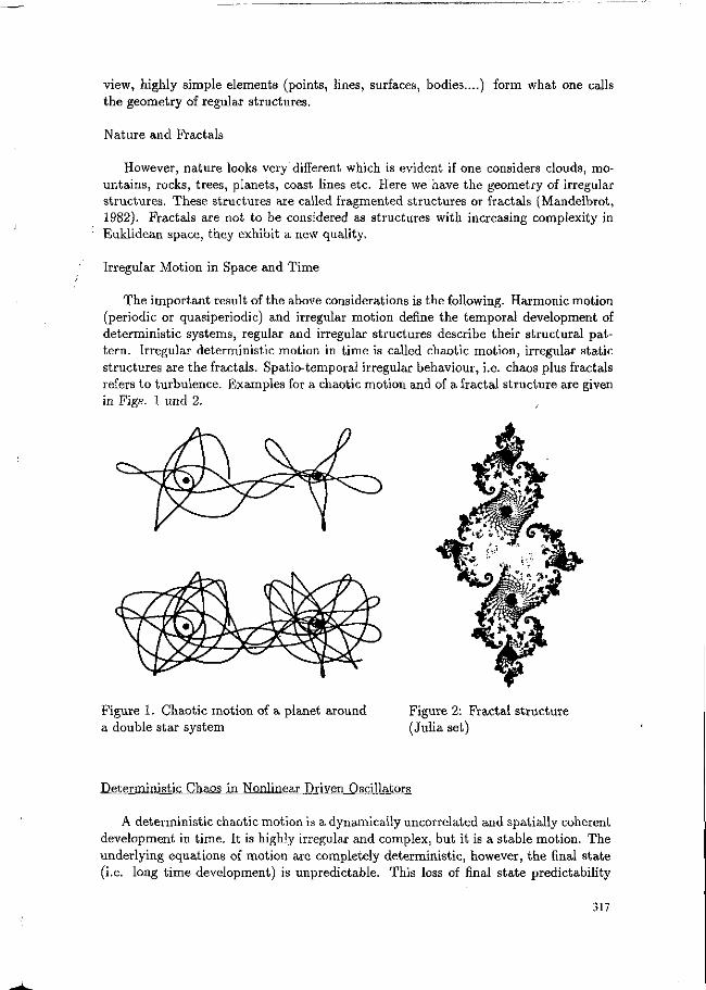
view, highly simple elements (points, lines, surfaces, bodies....) form what one calls the geometry of regular structures.

Nature and Fractals

However, nature looks very'different which is evident if one considers clouds, mo­untains, rocks, trees, planets, coast lines etc. Here we have the geometry of irregular structures. These structures are called fragmented structures or fractals (Mandelbrot, 1982). Fractals are not to be considered as structures with increasing complexity in Euklidean space, they exhibit a new quality.

Irregular Motion in Space and Time

The important result of the above considerations is the following. Harmonic motion (periodic or quasiperiodic) and irregular motion define the temporal development of deterministic systems, regular and irregular structures describe their structural pat­tern. Irregular deterministic motion in time is called chaotic motion, irregular static structures are the fractals. Spatio-temporal irregular behaviour, i.e. chaos plus fractals refers to turbulence. Examples for a chaotic motion and of a fractal structure are given in Figs. 1 und 2.

< ^ .

Figure 1. Chaotic motion of a planet around a double star system

Figure 2: Fractal structure (Julia set)

Deterministic Chaos in Nonlinear Driven Oscillators

A deterministic chaotic motion is a dynamically uncorrelated and spatially coherent development in time. It is highly irregular and complex, but it is a stable motion. The underlying equations of motion are completely deterministic, however, the final state (i.e. long time development) is unpredictable. This loss of final state predictability

317

originates from the sensitive dependence on initial conditions. This means that nearby trajectories exhibit an exponential divergence caused by a permanent stretching and folding of the whole flow describing the motion (see Schuster 1987 for details).

Deterministic chaotic motion neither requires a quantummechanical uncertainty nor an internal or external noise source for its stochastic components. Sufficient prerequi­sites are nonlinear equations of motion and only a few degrees of freedom.

Now it is known that perfectly deterministic systems, even very simple, low-dimensional systems, exhibit chaos. Many mathematical models and many physical experiments allow scientists to predict and to explain a wide variety of physical beha­viour that previously could be very poorly - or not at all - understood.

Well-known examples for the occurence of chaos are externally driven nonlinear os­cillators (see Kaiser 1988 for details). Very briefly, some essential results are discussed. Fig. 3 shows schematically the frequency and amplitude response with respect to the field strength F\ and the frequency A of the externally applied field for both, linear and nonlinear oscillators. In Fig. 4 the typical structure of a resonance is given. Within the horn in Fi — A space, the internal oscillation synchronizes with the external driver.

IS

super \ / s u b

(harmonisch)

WLC X

Figure 3: Frequency (u>s) and amplitude (Xs) res­ponse of driven and nonlinear oscillators F(t) = FxcosXt

Figure 4: Resonance horn (main resonance for F(t) = Fi cos At)

A more detailed behaviour is shown in Figs. 5 und 6 for the well-known Van der Pol oscillator (prototype of a self-excited oscillator).

Its equation of motion reads

x + fj.(x2 — l)x -\- x = FicosXt

Without external perturbation (FicosXt = 0), the system performs a self-excited os­cillation (limit cycle), created by the competition of a linear (—/iX) and a nonlinear

318

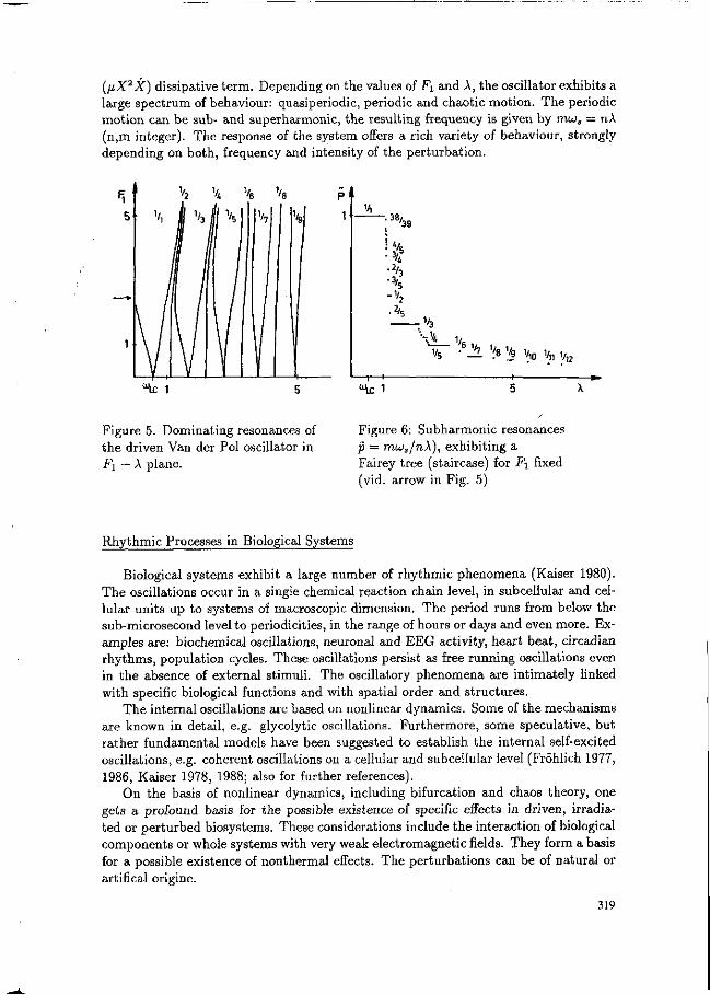
(/j,X2X) dissipative term. Depending on the values of F% and A, the oscillator exhibits a large spectrum of behaviour: quasiperiodic, periodic and chaotic motion. The periodic motion can be sub- and superharmonic, the resulting frequency is given by mu , = n\ (n,m integer). The response of the system offers a rich variety of behaviour, strongly depending on both, frequency and intensity of the perturbation.

V2 \ \ %

1 .38/ '39

•3/î

-V 3

<% 1

H Vsv 9 > V„v,2

Figure 5. Dominating resonances of the driven Van der Pol oscillator in JFI — A plane.

Figure 6: Subharmonic resonances p = mios/n\), exhibiting a Fairey tree (staircase) for Fx fixed (vid. arrow in Fig. 5)

Rhythmic Processes in Biological Systems

Biological systems exhibit a large number of rhythmic phenomena (Kaiser 1980). The oscillations occur in a single chemical reaction chain level, in subcellular and cel­lular units up to systems of macroscopic dimension. The period runs from below the sub-microsecond level to periodicities, in the range of hours or days and even more. Ex­amples are: biochemical oscillations, neuronal and EEG activity, heart beat, circadian rhythms, population cycles. These oscillations persist as free running oscillations even in the absence of external stimuli. The oscillatory phenomena are intimately linked with specific biological functions and with spatial order and structures.

The internal oscillations are based on nonlinear dynamics. Some of the mechanisms are known in detail, e.g. glycolytic oscillations. Furthermore, some speculative, but rather fundamental models have been suggested to establish the internal self-excited oscillations, e.g. coherent oscillations on a cellular and subcellular level (Fröhlich 1977, 1986, Kaiser 1978, 1988; also for further references).

On the basis of nonlinear dynamics, including bifurcation and chaos theory, one gets a profound basis for the possible existence of specific effects in driven, irradia­ted or perturbed biosystems. These considerations include the interaction of biological components or whole systems with very weak electromagnetic fields. They form a basis for a possible existence of nonthermal effects. The perturbations can be of natural or artifical origine.

319

The results are unexpected and surprising. The most important of them are: non­linear resonancelike response, frequency and intensity windows (where either an effect only occurs or where it vanishes), extreme sensitivities, small-signal amplification, com­plex or long-lasting transients, coexisting states of behaviour (i.e. hysteresis, where the actual state depends on the initial conditions and the way, the parameters are chan­ged). Bifurcations can create new states of function and order. If chaotic states exist, modern theoretical concepts and refined experimental techniques must be applied in order to understand the behaviour. For example, large sets of experimental data are required for a detailed analysis and a complete understanding of the processes and the dynamics involved.

Since different nonlinear dynamical systems exhibit a rich, but restricted number of possible motion and pattern, general results can be extracted from some experimental systems or from very few models. Though a rich variety of dynamic states can occur, the existence of universality, of scaling-laws and of self-similarity facilitate an analysis. For example, very distinct systems and very different nonlinear models show only a few main routes from periodic or quasiperiodic states to chaos.

Conclusions

The existence of deterministic chaotic states (irregularity in time) and of fractal structures (irregularity in space) offers new ways for an understanding of complex pattern of motion and behaviour. Especially responses to weak and even unknown perturbations of systems in the living nature which are beyond any explanation on a physical or scientific basis deserve a hard repetition and profound discussions of the results within the new concepts of chaos theory. The requirements to the experimen­tal data are at the frontiers of realizability, possible answers to enigmas and puzzles without mysterious forces, i.e. on a physical basis, presumably are the valuable conse­quences.

References

Fröhlich, H. 1977. Long range coherence in biological systems. Riv.Nuovo Cim.7: 399-418.

Fröhlich, H. 1986. Coherent excitations in active biological systems. In: F. Gutmann & H. Kayser(eds): Modern Bioelectrochemistry. Plenum, New York. p. 241-261.

Kaiser, F. 1978. Coherent oscillations in biological systems. Z.Naturforsch 33a: 294-304 and 418-431.

Kaiser, F. 1980. Nonlinear oscillations in physical and biological systems. In: P.L.E. Uslenghi (Ed): Nonlinear Electromagnetics. Academic Press, New York. p. 343-389.

Kaiser, F. 1988. Theory of non-linear excitations. In: H. Fröhlich (Ed.): Biological Coherence and Response to External Stimuli. Springer Verlag, Berlin, p . 24-48.

Mandelbrot, B. 1982. The Fractal Geometry of Nature. Freeman, New York. Schuster, H.G. 1987. Deterministic Chaos. Physik-Verlag, Weinheim. Sussman, G.J. & Wisdom, J. 1988. Numerical evidence that the motion of Pluto is

chaotic. Science 241: 17-23.

320

STRUCTURAL STABILITY OF THE EARTH S MAGNETOSPHERE

T. Zeithamer

Geophysical Institute, Prague, Czechoslovakia

Summary The magnetosphere is considered to be a plasma system controlled pre­

dominantly by the solar wind and the behaviour of the external magneto-sphere is modelled by means of a qualitative theory of differential equa­tions. The equations of motion for the outer magnetosphere are obtained and the structural stability of this system is proved in local scale. Keywords! magnetospheric physics, storms and substorms, qualitative theory of differential equations, catastrophe theory.

Introduction

The behaviour of most real systems, which we meet in the solar-terrestrial relations, is modelled by means of distributed parameter systems described by sets of partial differential equations where the state function, except the time, still depends on further independent variables. We shall try to substitute these systems by those ifeth lumped parameters, described by sets of ordinary differential equations for the state function, in which the time is usually taken as the only independent variable. The transfer must be made in such a way as to prevent the loss of information on the real system studied.

The magnetosphere is a system with distributed parameters. From this reason, the behaviour of the magnetosphere during its interaction with solar wind structural elements has been described by the system of (magneto-hydrodynamic or kinetic) partial differential equations. To characterize the behaviour of the outer magnetosphere globally and not by means of a change of the state of its individual parts, we will substitute the magne­tospheric system with distributed parameters by that with lumped parameters. For this purpose we will use a qualitative theory of differential equations. The finding of the class of equivalent phase portraits appertaining to the differential equations system is one of the main tasks of this theory. Differential equations which we choose for describing the model are these most elementary equations with a necessary behaviour. No special demands have been put on them because the causative mechanisms of the magnetosphere dynamics are not being made precise. We deal with qualitative signs of phase portraits only, which can be accepted as a mathematical description of magne­tospheric substorm.

Equations of motion for the outer magnetosphere

The behaviour of the outer magnetosphere has three general features which form the base of a mathematical model, (a) An equilibrium stable state exists to which the outer magnetosphere tries to asymptotically return, (b) A mar­ginal state exists in which the more efficient mechanism of energy dissipa­tion is switched on. (c) The return to the equilibrium state by means of series of fast changes of the state, i.e. by means of jumping changes, of the state. These three fundamental features of the outer magnetosphere behaviour have been defined from the experimental results of prof. S.-I. Akasofu,

321

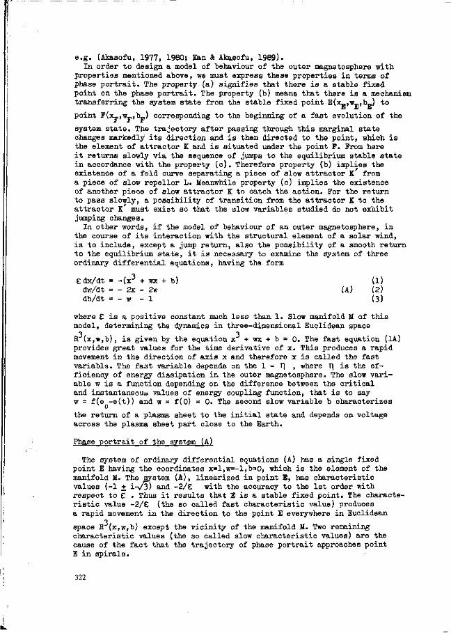
e.g. (Akasofu, 1977, 1980; Kan & Akasofu, 1989). In order to design a model of behaviour of the outer magnetosphere with

properties mentioned above, we must express these properties in terms of phase portrait. The property (a) signifies that there is a stable fixed point on the phase portrait. The property (b) means that there is a mechanism transferring the system state from the stable fixed point E(x_,w_,b_) to

point F(x_,w_,b_) corresponding to the beginning of a fast evolution of the

system state. The trajectory after passing through this marginal state changes markedly its direction and is then directed to the point, which is the element of attractor K and is situated under the point F. From here it returns slowly via the sequence of jumps to the equilibrium stable state in accordance with the property (c). Therefore property (b) implies the existence of a fold curve separating a piece of slow attractor K from a piece of slow repellor L. Meanwhile property (c) implies the existence of another piece of slow attractor K to catch the action. For the return to pass slowly, a possibility of transition from the attractor K to the attractor K must exist so that the slow variables studied do not exhibit jumping changes.

In other words, if the model of behaviour of an outer magnetosphere, in the course of its interaction with the structural element of a solar wind, is to include, except a jump return, also the possibility of a smooth return to the equilibrium state, it is necessary to examine the system of three ordinary differential equations, having the form

Edx/dt = -(x3 + wx + b) (1) dw/dt = - 2x - 2w (A) (2) db/dt = - w - 1 (3)

where £ is a positive constant much less than 1. Slow manifold M of this model, determining the dynamics in three-dimensional Euclidean space

3 3 H (x,w,b), is given by the equation x + wx + b = 0. The fast equation (1A) provides great values for the time derivative of x. This produces a rapid movement in the direction of axis x and therefore x is called the fast variable. The fast variable depends on the 1 - f| , where T\ is the ef­ficiency of energy dissipation in the outer magnetosphere. The slow vari­able w is a function depending on the difference between the critical and instantaneoua values of energy coupling function, that is to say w = f(e -e(t)) and w = f(0) = 0. The second slow variable b characterizes

c the return of a plasma sheet to the initial state and depends on voltage across the plasma sheet part close to the Earth.

Phase portrait of the system (A)

The system of ordinary differential equations (A) has a single fixed point E having the coordinates x=l,w=-l,b=0, which is the element of the manifold M. The system (A), linearized in point E, has characteristic values (-1 + i-/3) and -2/E with the accuracy to the 1st order with respect to È . Thus it results that E is a stable fixed point. The characte­ristic value -2/Ç (the so called fast characteristic value) produces a rapid movement in the direction to the point E everywhere in Euclidean

3 space R (x,w,b) except the vicinity of the manifold M. Two remaining characteristic values (the so called slow characteristic values) are the cause of the fact that the trajectory of phase portrait approaches point E in spirals.

322

Ground state of the outer magnetosphere

The outer magnetosphere passes asymptotically to the ground state when an interplanetary magnetic field directed approximately to the North has an average positive value of 5 nT for the duration of 6 to 12 hours. If the outer magnetosphere is in such a state, the auroral oval attains its mini­mum size and no characteristic auroral substorm features can be observed along it (Akasofu, 1977).

Dynamics of the outer magnetosphere expressed by means of system (A)

Let ua suppose that the energy coupling function e(t) (defined by Perreault & Akasofu (1978)) increases from tne value e to that of e,

o which is higher than e . Here e corresponds to the ground state of the

outer magnetosphere, e is the critical value of energy coupling function

when the outer magnetosphere can but also need not develop a more effi­cient mode of energy dissipation. To the values of energy coupling function correspond those of a slow variable w: w(e -e ) = w , w(e -e ) •

e g g c c = w(0) = 0 = w , w(e -e) = w > w . The outer magnetosphere passes to

point E(l,-1,0), which lies on the left from the fold curve separating a piece of slow attractor K from a piece of slow repellor L. At the same time the voltage across the plasma sheet part close to the Earth begins to change in such a way that the outer magnetosphere state passes to marginal state, the image of which is one of the points of fold curve. This point is designated as F. At this state the current interruption is expected or the reconnection process begins to take place. From the view point of systems theory the outer magnetosphere develops a more efficient mode of the energy dissipation. This leads to a rapid change of the magnitude x from the value x_ in the point F(x_,w_,h_) to the value x_, corresponding

to point R(x_,w_,,b_1) which lies below point F on the lower part of the

manifold M formed by attractor K. In other words, the fast equation (1A) carries the state F rapidly to the state R. The trajectory passing through point R is going in the close proximity of the manifold M. The slow equa­tions carry the state from R to Q. The point Q represents the state of the outer magnetosphere when the current across the plasma sheet part close to the Earth is fully renewed. Point Q is the element of fold curve sepa­rating a piece of repellor L from that of attractor K. Then the outer magnetosphere goes through the jump return to the upper part of slow mani­fold to point S(x_,w.,b ) , which is the element of attractor K surface

S Q Q and afterwards the next cycle begins. Each cycle represents the magneto-spheric substorm. This occurs as long as the excess energy is available in the magnetotail. The result is a series of cycles corresponding to the series of magnetospheric substorms. When the excess of energy in the mag­netotail is completely dissipated the outer magnetosphere makes a transi­tion to the ground state. Such transition occurs rarely, perhaps at most a few times a month (Akasofu, 1977).

After returning to the upper part of the manifold, the state of the outer magnetosphere does not often manage to return to the ground state. Owing to a premature interaction of the outer magnetosphere with the structural element of a solar wind, the energy coupling function e(t) increases again. Then to the starting state the point E corresponds, which is close to point E but different. From E' the whole cycle starts to develop again. The sys­tem of equations (A) passes to that of (B)

323

e dx/dt = -(x3 + wx + b) (1) dw/dt = - 2x - 2w (B) (2) db/dt = - w - q (3)

o where q is determined by point E and depends on the energy residue

accumulated in the tail as well as on the immediate value of energy coupling function when starting the interaction of the outer magnetosphere with a new structural element of a solar wind.

Structural stability of the outer magnetosphere in the neighbourhood of equilibrium states

The meaning of structural stability of differential equations system consists in the following. Let us consider an ordinary vector differential equation

dx/dt = v(x) (4)

where x is the real vector function of real variable t from one-dimensional 1 3

Euclidean space R into three-dimensional Euclidean space R . The mapping - 3 3 v from R into R is called a vector field of differential equation. At present we are not able to solve analytically the majority of such nonlinear differential equations. However, it is often necessary to find only the qualitative behaviour of real system described by the differential equation (4), for example, the number of equilibrium states, the periodicity of solution, etc.. In such case we need not solve the differential equation mentioned, but we must know how to assign the relevant class of equivalent phase portraits to the differential equation examined. This is one of the main tasks for the qualitative theory of differential equations.

The finding of such class of the equivalent phase portraits is closely connected with the structural stability of differential equations system. Let us indicate Lr(R ) topological space of all vector fields v = (v-^x^x-,

x ),v0(x,,x„,x ),v,(x ,x ,x )) on R having continuous partial derivatives - r 3 - r 3

up to the order r respectively. Let w€_L_(R )_and s € L (R ) be vector fields. Differential equations dx/dt = w(x), dx/dt_= s(x) are called topo-logically equivalent, if there is a homeomorphism h from three-dimensional

3 3 Euclidean space into three-dimensional Euclidean space, i.e. h; R —>- R , that carries the trajectories of the first differential equation into those of the second without changing their orientations. The orientation of the trajectory is simply the direction in which the points move along the curve as parameter t increases. Phase portraits of topologically equivalent differential equations are also called topologically equiva­lent or qualitatively the same. Vector field v of differential equation (4) is called structurally stable if there exists a neighbourhood of field

v in space_Lr(R ) so that the differential equations dx/dt = v(x) and dx/dt = w(x) are topologically equivalent for each w £ U.

If the system of differential equations (4) is structurally stable, then a small perturbation of the right side of the system will not qualitatively change the phase portrait. In other words, certain features of phase por­trait must be preserved under small perturbation. Such small perturbation is caused by the change of outer conditions in which the real process takes place.

But if the system of ordinary differential equations (4) is structurally

324

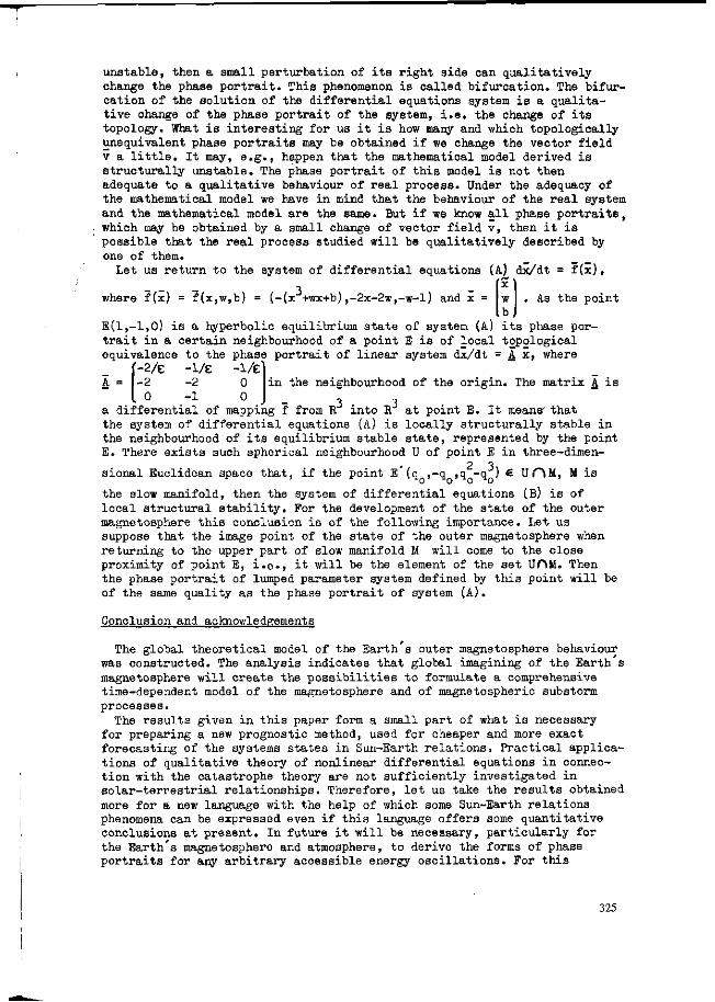
unstable, then a small perturbation of its right aide can qualitatively change the phase portrait. This phenomenon is called bifurcation. The bifur­cation of the solution of the differential equations system is a qualita­tive change of the phase portrait of the system, i.e. the change of its topology. What is interesting for us it is how many and which topologically unequivalent phase portraits may be obtained if we change the vector field v a little. It may, e.g., happen that the mathematical model derived is structurally unstable. The phase portrait of this model is not then adequate to a qualitative behaviour of real process. Under the adequacy of the mathematical model we have in mind that the behaviour of the real system and the mathematical model are the same. But if we know all phase portraits, which may be obtained by a small change of vector field v, then it is possible that the real process studied will be qualitatively described by one of them.

Let us return to the system of differential equations (A) dx/dt = f(x),

-- - 3 - fJl where f(x) = f(x,w,b) = (-(x +wx+b),-2x-2w,-w-l) and x = w . A s the point

lb J E(l,-1,0) is a hyperbolic equilibrium state of system (A) its phase por­trait in a certain neighbourhood of a point E is of local topological equivalence to the phase portrait of linear system dx/dt = A x, where

'-2/e - i /e -i/e" in the neighbourhood of the origin. The matrix A is

A = -2 -2 0 0 - 1 0

• - - 3 • 3 a differential of mapping f from R into R at point E. It means' that the system of differential equations (A) is locally structurally stable in the neighbourhood of its equilibrium stable state, represented by the point E. There exists such spherical neighbourhood U of point E in three-dimen-

' 2 3 sional Euclidean space that, if the point E (q ,-q ,q -q ) € U O M , M is

the slow manifold, then the system of differential equations (B) is of local structural stability. For the development of the state of the outer magnetosphere this conclusion is of the following importance. Let us suppose that the image point of the state of the outer magnetosphere when returning to the upper part of slow manifold M will come to the close proximity of point E, i.e., it will be the element of the set U O M . Then the phase portrait of lumped parameter system defined by this point will be of the same quality as the phase portrait of system (A).

Conclusion and acknowledgements

The global theoretical model of the Earth s outer magnetosphere behaviour was constructed. The analysis indicates that global imagining of the Earth s magnetosphere will create the possibilities to formulate a comprehensive time-dependent model of the magnetosphere and of magnetospheric substorm processes.

The results given in this paper form a small part of what is necessary for preparing a new prognostic method, used for cheaper and more exact forecasting of the systems states in Sun-Earth relations. Practical applica­tions of qualitative theory of nonlinear differential equations in connec­tion with the catastrophe theory are not sufficiently investigated in solar-terrestrial relationships. Therefore, let us take the results obtained more for a new language with the help of which some Sun-Earth relations phenomena can be expressed even if this language offers some quantitative conclusions at present. In future it will be necessary, particularly for the Earth's magnetosphere and atmosphere, to derive the forms of phase portraits for any arbitrary accessible energy oscillations. For this

325

purpose, however, it will be necessary to learn to know by far better the physical substance of the phenomena occuring here.

At the conclusion I would like to say that it is a great honour for me to have been allowed to present at this outstanding scientific assembly a part of results which 1 have obtained during the preparatory phase for solving a research program called "The man and the solar plasma in the geosphere" (e.g. Zeithamer, 1988). Allow me therefore to express my sincere thanks for this opportunity to both the International Committee for Research and Study of Environmental Factors and the Dutch Foundation for Study and Research of Environmental Factors.

References

Akasofu, S.-I., 1977. Physics of magnetospheric substorms. (Astrophysics and Space Science Library, 47) D. Reidel Publ. Co., Dordrecht.

Akasofu, S.-I., 1980. What is a magnetospheric substorm? In: S.-I. Akasofu (Ed.): Dynamics of the magnetosphere. (Astrophysics and Space Science Library, 78 Proceedings) D. Reidel Publ. Co., Dordrecht, p. 447-460.

Kan, J.R. & S.-I. Akasofu, 1989. Electrodynamics of solar wind-magneto-sphere-ionosphere interactions. IEEE Trans. Plasma Sei. 17:83-108.

Perreault, P. & S.-I. Akasofu, 1978. A study of geomagnetic storms. Geophys. J. Roy. Astron. Soc. 54:547-573.

Zeithamer, T., 1988. Solar-terrestrial physics and its participation in the solution of the global problems of mankind. Proceedings of Czechoslovak Academy of Agriculture, 123:76-85. (in Czech)

326

GEO-SOLAR-COSMIC ELECTRIC RELATIONS IN ELECTROSTATICS WITH

FIELD E SCREENING BY MâTTER

L.A. Pokhmelnykh

S c i e n t i f i c - I n d u s t r i a l C o r p o r a t i o n "Radon", Moscow, U .S .S .R .

Summary

An electrostatics is developed on the assumption, that there is a screening of the electrostatic field by neutral matter.The electrostatics is used for development of a model of electric relations between space and bodies of the solar system. The model includes quantitative description of atmo­spheric electricity, geomagnetism, electricity and magnetism of the sun and planets. Consequences of the model agree with experimental data. Analytical expressions for calculation of electric and magnetic parameters of arbitrary cosmic body are presented. 11-years periodic reversals of magnetic moments of inferior planets are predicted. /

Introduction

The main problem of atmospheric electricity - a cause of global elecrification of the earth and its atmosphere have not been solved satisfactorily so far (Chalmers,1967 ). This justified the search for possible fundamental ways to over­come this problem» It was taken into account, that the Cou­lomb's electrostatics and its base - field E radial dependen­ce of a point charge Q had been tested only in laboratory scale (Bartlett et al.,1970) and therefore we utilize extra­polated physical dependences in atmospheric and space elec­tricity. In these cases scales of electrostatics utilization exceeds the laboratory one by the factor 1(P and even more. In the scale of the Earth it is possible to find many radial dependences weakly differing from r""2 but remaining in agre­ement with results of laboratory experiments. I examined two noncoulomb's radial dependences (Pokhmelnykh,1987), one of them is

f(r) = 4îT£oE / Q = r~2 exp (- p r /ae ), (1)

where ae - constant, p - mass density in ambient medium.

Dependence (1) corresponds to the assumption that there is a screening of the electrostatic field by neutral matter in the same way as in the case with the screening of the light by a body» Two electrostatics and later two models of geo-cosmic electric relations were developed on the dependences f(r). Comparison of these models with experimental data and with consequences of Coulomb's electrostatics has reveal ad­vantage of the electrostatics with field E screening by mat-

327

ter (EFES) developed on the dependence (1).

Main equations of EFES

Prom (1) one can deduce , that electrostatic field strength, on the flat boundary between two infinite charged half-spa­ces with densities q , q2 and mass densities o.., o« is

E =5rae(4Sr£or1 (q1/o1 - q2/p2) . (2)

According to (2) the state of electrostatic equilibrium bet­ween the half-spaces is realized when

<ll/p1 ΠV?2 * (3)

It is possible to prove , that (3) describes the state of electrostatic equilibrium of arbitrary body residing in charged medium. In this case (3) can be written as

V?b -Vfm ' (4)

where %»%,»?>,»? "" c*l a rSe and mass densities in the body and ambient Bedium within the screening radius

rs - ae/ ƒ . (5) Electrostatic potential difference between two points with parameters q , c^, q2, p2 is

^ - ^ =îrae2(4T£or1(??1 +5»;1 ) (q i /? 1 - i 2 /?2 } - (6)

Field E in charged medium with a gradient of q or o is

E - - gradP » - 23rae?(4tf£or'1 $>"1gracL(q/ç ) . (7)

Evidence of EPES realization in nature

Let us consider electric relations between cosmic bodies of solar system in logic of EPES. Let us assume, that the ratio qg/p in space within the solar system is not null and varies ällsthe time according to a quasiperiodic law sugges­ted by Galaxie« In this case cosmic bodies change their in­terior charges« In periods sufficient for the cosmic body to get its electrostatic equilibrium with space (4) variations of q/p in the body and space coincide« In short periods <ljps variations lead to loss of electrostatic equilibrium of the body and to appearance of radial potential difference (6) between the body and space« The potential difference gives rise to radial quasistatic field E around the body, to the radial electric current recharging the body and to accelera­tion of charged particles in space. According to(4) all cos­mic bodies being in charged space must carry interior space

328

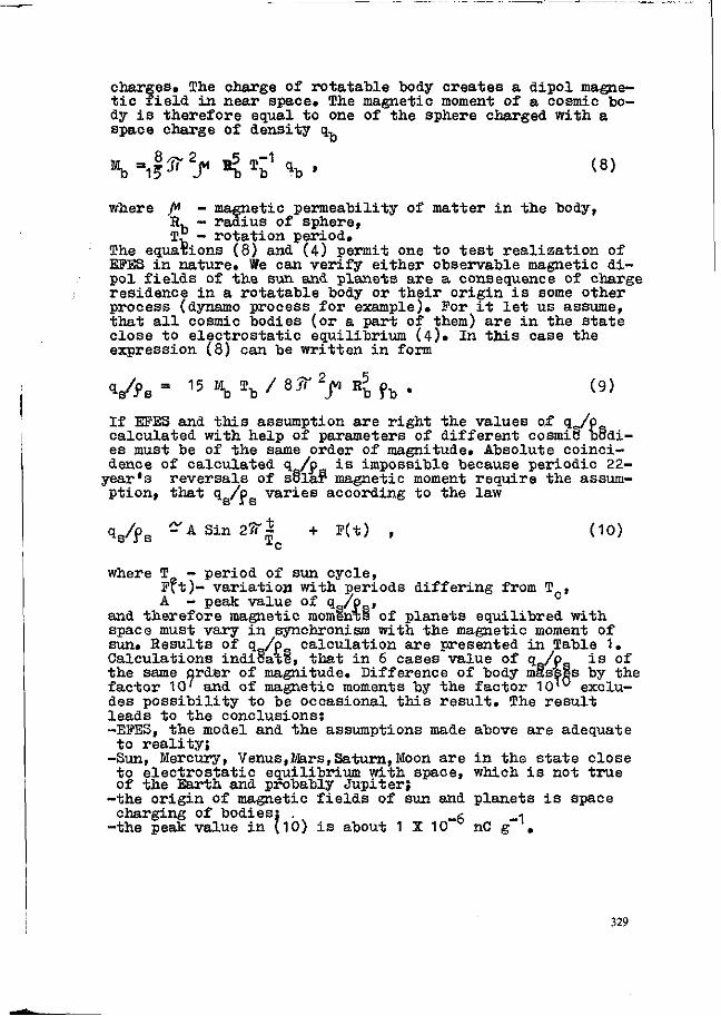
charges. The charge of rotatable body creates a dipol magne­tic field in near space» The magnetic moment of a cosmic bo­dy is therefore equal to one of the sphere charged with a space charge of density q.

\^§V2f H 5 ^ % , (8)

where ft - magnetic permeability of matter in the body, R. - radius of sphere, T? - rotation period.

The equations (8) and (4) permit one to test realization of EFES in nature. We can verify either observable magnetic di­pol fields of the sun and planets are a consequence of charge residence in a rotatable body or their origin is some other process (dynamo process for example). For it let us assume, that all cosmic bodies (or a part of them) are in the state close to electrostatic equilibrium (4)» In this case the expression (8) can be written in form

V>B- 15 \ \ / ^ 2 r Hbfb- <9> If EFES and this assumption are right the values of <l8/?s calculated with help of parameters of different cosmic bodi­es must be of the same order of magnitude. Absolute coinci­dence of calculated <?L/pq is impossible because periodic 22-

year's reversals of solar magnetic moment require the assum­ption, that q /p varies according to the law

q8/pa S'A Sin 25T| + F(t) , (10)

where T - period of sun cycle, Pft)- variation with periods differing from T , A - peak value of Qs/Ps»

and therefore magnetic moments of planets equilibred with space must vary in synchronism with the magnetic moment of sun. Results of qs/ps calculation are presented in Table 1. Calculations indicate, that in 6 cases value of qa/ps is of the same order of magnitude. Difference of body masses by the factor 10' and of magnetic moments by the factor 10'° exclu­des possibility to be occasional this result. The result leads to the conclusions: -EFES, the model and the assumptions made above are adequate to reality;

-Sun, Mercury, Venus,Mars,Saturn, Moon are in the state close to electrostatic equilibrium with space, which is not true of the Earth and probably Jupiter;

-the origin of magnetic fields of sun and planets is space charging of bodies; , g «

-the peak value in (10) is about 1 X 10" nC g .

329

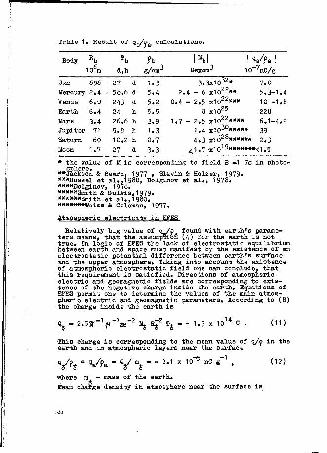
Table 1• Result of qs/p„ calculations.

Body R b

106m

Sun 696 Mercury 2.4 Venus 6.0

Earth. 6.4

Mars 3.4

Jupiter 71 Saturn 60

Moon 1.7

* the value sphere.

Tb d,h

27 d 58.6 a

243 d 24 h 26.6 h

9.9 h 10.2 h

27 d

fb g/cm3

1.3 5.4 5.2

5.5

3.9 1.3 0.7 3.3

2.

0.4

1.7

of M is corresponding

Kl I« Gsxcm3 10"

3.3x1032*

4 - 6 x1022**

-2.5 x1022*** 8 x1025

-2.5 x1022****

1.4 X1030***** 4.3 x1028******

lS/f s I '7nC/g

7.0

5.3-1.4 10 -1.8 228 6.1-4.2

39 2.3

< 1.7 x101********< 1.5

to field B =1 as in photo-

**Jackson & Beard, 1977 , Slavin & Holzer, 1979. ***Russel et al.,1980, Dolginov et al., 1978. ****Dolginov, 1978. ***«*Smith & Gulkis,1979. ******Smith et al.,1980. *******Weiss & Coleman, 1977.

Atmospheric electricity in EffES

Relatively big value of <!„/$> found with earth's parame­ters means, that the assumption (4) for the earth is not true. In logic of EFES the lack of electrostatic equilibrium between earth and space must manifest by the existence of an electrostatic potential difference between earth's surface and the upper atmosphere. Taking into account the existence of atmospheric electrostatic field one can conclude, that this requirement is satisfied. Directions of atmospheric electric and geomagnetic fields are corresponding to exis­tence of the negative charge inside the earth. Equations of EFES permit one to determine the values of the main atmos-piieric electric and geomagnetic parameters. According to (8) the charge inside the earth is

Qo = 2 - 5 5 T V 1 * " 2 % *f *4 • - 1.3 x 10

14 (11)

This charge is corresponding to the mean value of q/o in the earth and in atmospheric layers near the surface

V?*s vk ra T ~t where m, - mass of the earth.

Q y m^ • - 2.1 x 10~5 nC g""1 (12)

Mean charge density in atmosphere near the surface is

330

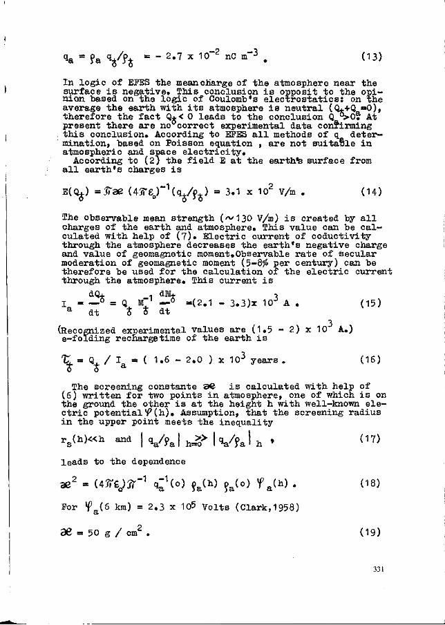
qa * ?a V k - - 2.7 x 10"2 nC m~3 . (13)

In logic of EFES the mean charge of the atmosphere near the surface is negative. This conclusion is opposit to the opi­nion based on the logic of Coulomb's electrostatics: on the average the earth with its atmosphere is neutral (Q++Q =0), therefore the fact Q+< 0 leads to the conclusion Q^>-Oa At present there are no correct experimental data confirming this conclusion. According to EFES all methods of q deter­mination, based on Poisson equation , are not suitable in atmospheric and space electricity.

According to (2) the field E at the earthfe surface from all earth's charges is

B(QJ) «JTae (45reer1(qg/p£) - 3.1 x 102 v/m . (14)

The observable mean strength (^130 V/m) is created by all charges of the earth and atmosphere. This value can be cal­culated with help of (7). Electric current of coductivity through the atmosphere decreases the earth's negative charge and value of geomagnetic moment»Observable rate of Secular moderation of geomagnetic moment (5-8$ per century) can be therefore be used for the calculation of the electric current through the atmosphere. This current is

dQ* « dM+ , ï = _ ° = Q M ' — ° =(2.1 - 3.3)x 10J A . (15)

a dt t o" dt

(Recognized experimental values are (1.5 - 2) x 10 A.) e-folding rechargetime of the earth is

t. - Q / Ift - ( 1.6 - 2.0 ) x 103 years . (16)

The screening constante s© is calculated with help of (6) written for two points in atmosphere, one of which is on the ground the other is at the height h with well-known ele­ctric potential^(h). Assumption, that the screening radius in the upper point meets the inequality

rs(h)«h and | qa/p& | h>> | c^/o ft | h , (17)

leads to the dependence

ae2 = ( 4 Ï T Ê O ) ^ 1 q;1(o) oa(h) ?a(o) f a(h) . (18)

Por ^ a ( 6 km) = 2 .3 x 105 Vol t s (Clark,1958)

ae = 50 g / cm2 . (19)

331

In logic of EPES recent electric state of the earth and exi­stence of the atmospheric field E result from the long-time qg/p deviation from zero in the past over a period more than 1Dot) years. Multiple reversals of the geomagnetic moment in the past of the earth indicate, that the deviations of qVp were both with positive and negative signes. So, atmosphlriS electricity doesn't need the global electric generator loca­ted in the troposphere» 22-years cyclic variation of qe/p_. (10) is capable to change the mean strength of the atmosphe­ric field E for about 10#in this period. At the same time magnetic moments and quasistatic radial electric fields of planets,residing in the state close to (4) and having proba­bly a short e-folding recharge time, must experience rever­sals every 11 years in step with the magnetic moment of the sun.

Electricity of the sun

Observable variations of solar magnetic moment in 22-years cycles according to approximative law

M@ - Mp Sin 2JT I , where Mp - 3.3 x 1032Gs cm3 (20)

is corresponding to a solar charge variation

L - Q Sin 2T\ t © p T

Q m O Sin 2jr| , (21) c

where according to (8)

Q m |jr~1 M ~1 M T = 1.2 x 1018 C, (22) p 2 J p ©

T - sun cycle period, GL - rotation period of the sun. Radial electric current recharging the sun is

I . IS© . I Cos 2JT J , where I - 1.1 x 1010A. (23) © dt P xc P

e-folding recharge time of the sun is

tJ± Q„ / I - 3.5 years . (24) C5» P P

Maximal possible potential difference between solar surface and space according to (6) is

P® " ' s = ^ 3 ß 2 % f;2(4îTeo)"1 - 5 x 1024 Volts. (25) max

The upper limit of realized power of the solar recharge pro­cess is

332

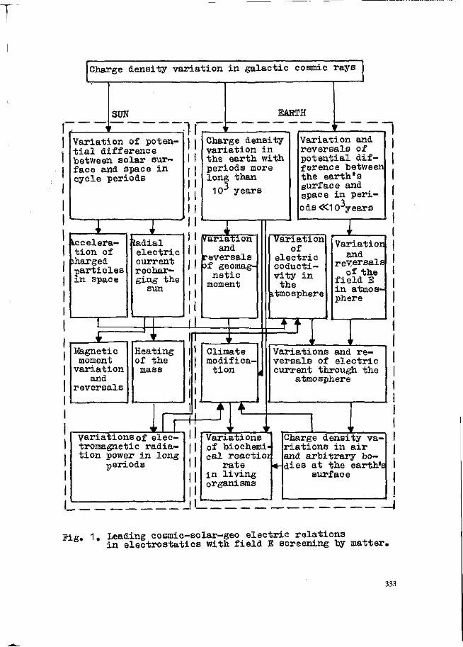
Charge density variation in galactic cosmic rays

SUN

1 EÄRTH

Variation of poten­tial difference between solar sur­face and space in cycle periods

accelera­tion of

:harged particles in space

'. iadial electric current rechar­ging the

sun

.£=Z Magnetic moment

variation and

reversals

i Heating of the mass

Variations of elec­tromagnetic radia­tion power in long

periods

Charge density variation in the earth with periods more long than

10^ years

Variation and

reversals of geomag­

netic moment

Climate modifica­

tion

Variation and reversals of potential dif­ference between the earth's surface and space in peri­ods «10^years

Variation of

electric coducti-vity in

the itmosphere

ZT

Variation and

reversals of the

field E in atmos­phere

Variations and re­versals of electric current through the

atmosphere

Variations of biochemi­cal reactior

rate in living organi sms

Charge density va­riations in air and arbitrary bo­dies at the earth's

surface

Fig. 1. Leading cosmic-solar-geo electric relations in electrostatics with field E screening by matter.

333

Pmax - W ',)« = 3 x 1 ° 3 4 W a ^ (ZO Taking into account the measured power of the solar electro­magnetic radiation (4 x 1026Watt") one can conclude, that the solar recharging process can he one of main causes of the sun heating.

Leading cosmic-solar-geo electric relations in logic of EPES are presented in Figure 1•

Concluding remarks

an advantage of EPES over Coulomb's electrostatics con­sists in possibility to describe quantitatively in unified model electricity and magnetism of the earth, sun, planets and space in agreement with main experimental data. At the same time EFES does not contradict Coulomb's electrosta­tics in engineering electricity. The field of EPES applica­tion is natural electricity. The laws of EPES can be obser­ved in laboratories if a metering equipment is sensitive enough. EPES makes it possible:

- to calculate magnetic moments of arbitrary cosmic bodies provided mechanic parameters are known and vice versai

- to predict a solar cyclic activity and a long-time varia­tion of radiation power of the sun by observing cyclic activities of near stars in direction of sourse of the galactic running charge wave;

-to forecast the evolution of geomagnetic and atmospheric electric fields for 10 and more years ahead;

- to substantiate influence of space on the earth, its bio­sphere and living organisms through charge density varia­tions. Thus, to solve the problem of geo-solar-cosmic relations

we must take into account the fact that EPES is probably realized in nature, which makes it nesessary to test its consequences in all scales of linear dimensions from nuclear to metagalactical.

Acknoledgement

The author express his sincere thanks to Dr. N.V.Krasno-gorskaya for organization of valuable discussions.

References

Bartlett, D.P., P.E. Goldhagen & E.E. Phillips, 1970. Expe­rimental test of Coulomb's law. Phys. Rev.,D,2,N3:483-487.

Chalmers,J.A., 1967. Atmospheric electricity. Pergamon Press. ClarK, J.P., 1958. The fair-weather atmospheric electric po­

tential and its gradient. In: Recent Advances in Atmosphe­ric Electricity. Pergamon Press,Oxford, p.61.

334

Dolginov, Sh. Sh., 1978. On the magnetic field of Mars. Mars 2 and 3 evidence. Geophys. Res. Lett.,5,N1: 89 - 92.

Dolginov, Sh. Sh., L.N. Juzglov, V.A. Sharova & V.B. Buzin, 1978. The magnetic field and magnitosphere of Venus. Kos-micheskie issledovania, 16, N6: 827-863 (Russ.).

Jackson, D.J. & D.B. Beard, 1977. The magnetic field of Mer­cury. J. Geophys. Res.,82, nl9: 2828-2836.

Pokhmelnykh, L.A1, 1987. Electricity of the atmosphere,earth and cosmos in the logic of noncoulomb's electrostatics. Dep. in VINITY, Moscow, N5933-B87: 71 PP (Russ.).

Rüssel, CT., R.C. Elphie, J.C. labmann & J.A. Slavin, 1980. On the search for an intensic magnetic field at Venus. lunar and Planet Sei. Abstr. Pap. 11th Conf., Houston: 963-965.

Slavin, J.A. & R.E. Hölzer, 1979. The effect of erosion of the solar wind stand-off distance at Mercury. J. Geophys. Res., A84, N6: 2976-2082.

Smith, E.J., L.J. Davis, P.E. Jones, P.J. Coleman, D.S.Col-purn, P. Dyal & O.P. Sonnet, 1980. Saturn's magnitosphere end its interaction with the solar wind. J.Geophys. Res., A85, N11: 5655-5674.

Smith, E.J. & S. Gulkis,1979»The magnetic field of Jupiter: comparison of radio astronomy and spacecraft observations. Annu. Rev. Earth and Planet Sei», Palo Alto, Calr- , 7: 385-415.

Weiss, H. & P.J. Jr. Coleman, 1977. The Moon's permanent magnetic field: a cratered chell model. Moon, 16, N3: 311-315.

335

AN ATTEMPT OF INTERPRETATION OF PICCARDI CHEMICAL TESTS. EFFECTS OF METALLIC SCREENS

L. Boulanger, 43 bis rue Mallifaud, F38100 Grenoble, France R. Chauvin, Chateau d'Ivoy le Pré, F18380 La Chapelle d'Angillon, France

Summary A detailed .study of Piccardi's works in the light of the hypothesis of

the cosmic radiations on the water (X rays, gamma rays, ultra violet light, proton screams, radio waves) suggests an effect of variations of low fre­quency atmospheric electric fields (high impedance electromagnetic fields from a hundred Hertz to a thousand Hertz).

The screens utilised by Piccardi had different effects depending on their nature (copper, zinc, lead, aluminium, gold), their thickness, their shape (cylindrical or plane) and disposition (horizontal or other). The screen effect may be due to variations of low frequency vertical atmos­pheric electric fields (reflection and attenuation of electromagnetic high impedance fields through metallic screens). Keywords: Piccardi's chemical tests, low frequency variations of electric atmospheric field.

Introduction G. Piccardi (1955, 1958) and H. Bortels (1954) emphasized the influence

of certain atmospheric or cosmic phenomena on physico-chemical biological and biochemical processes.

R. Chauvin (1956) has recalled in "l'année biologique" the essential of these scientist's conclusions, suggesting the possible existence of "Bortels-Piccardi's waves".

We recall briefly the experimental proceedings of G. Piccardi. He carries out an experiment on a chemical reaction which may produce quickly colloidal system: the hydrolysis of bismuth chloride in presence of acid with formation of bismuth oxychloride undissolvable in water according to the reaction: - ^ ^ + ^ + B i o c l + M c l

An experiment is made with "activated water" with a mercury buoy (a globe containing a drop of quick silver), another with ordinary water.

The results from these groups of experiments are relative and indepen­dent of pressure, humidity, purity of reagents, quality of water and so on.

The precipitation of BiOCl may be faster in "activated water" than in normal water (called case T ) , or slower (called case R ) .

G. Piccardi simultaneously makes a great number of differential preci­pitations. He keeps a record of the number of T's and R's and calculates the rate of percentage of T.

Let's try and see from the point of view of the theory of electromagne­tic waves how this phenomenon may be understood.

A paper from Novotny and Halla (1958) about a mercury buoy, and a perso­nal work on pure water conductivity (unpublished) suggest, contrary to common ideas, an action of low-frequency electromagnetic waves.

Low frequency waves go through metallic screens being reflected and attenuated. The shielding and screen theory has been studied by Schelku-noff (1942) and put into practical form by Cowdell (1967) and Heitzmann (1987).

The shielding efficiency of a screen is a function of desadaptation between the incident wave impedance and intrinsic impedance of the metal of the screen: we will define these two parameters.

336

Characteristic wave impedance An important factor in all the field studies is the characteristic wave

impedance defined as the ratio of the electric component and the magnetic component of the field :

(1) Z w =\/H

In plane waves systems, when the distance from the source is larger than

2TT' the impedance called free space impedance is

M Z„ = — = 120 IT = 377 Ohms

(2)

Electromagnetic fields are called high or low impedance fields according to the impedance being larger or lower than 377 Ohms.

The graph of figure 1 represents the wave impedance versus the distance from the source for a low impedance generator (magnetic) or high impedance (electric).

0,4 0,S 0,7 T" 2 3 Distance de la source en unités de £=À/2ÏÏ

Fig.1. Wave impedance as a function of the distance from the source. (I: champ électrique ou de haute impédance; II: champ proche ou champ d'induction; III: champ magnétique ou de basse impédance; IV: champ lointain ou de radiation)

All homogeneous metals are defined by their specific impedance Z^ which

has the value:

- t f ai M

When an electromagnetic wave is propagating through a metal, the wave impedance Zw tends towards Z .

The global efficiency of a shielding is the global specification atte­nuation of a material towards electromagnetic wave propagation.

When an electromagnetic wave meets a shielding, one part of its energy is reflected by the first surface, and another part crosses the shield, and is attenuated by heating dissipation through shielding thickness be­fore being partially reflected inside by the second surface and partially irradiated outside (figure 2).

The global efficiency is equivalent to: S = R + A + B (4)

with S (dB) = absorption losses. R = Rl + R2 (total of primary and secondary reflections). (5)

B (dB) = correction factor (only if A <10 dB) If ?i is the power of the incident wave, and ?2 the power

attenuated by the shield, we can write: P 1 - P 2 = R + A + B = S = 1 0 log10 (P1/P2) (6)

These equations are written in power terms. However, at low frequencies

of the wave

337

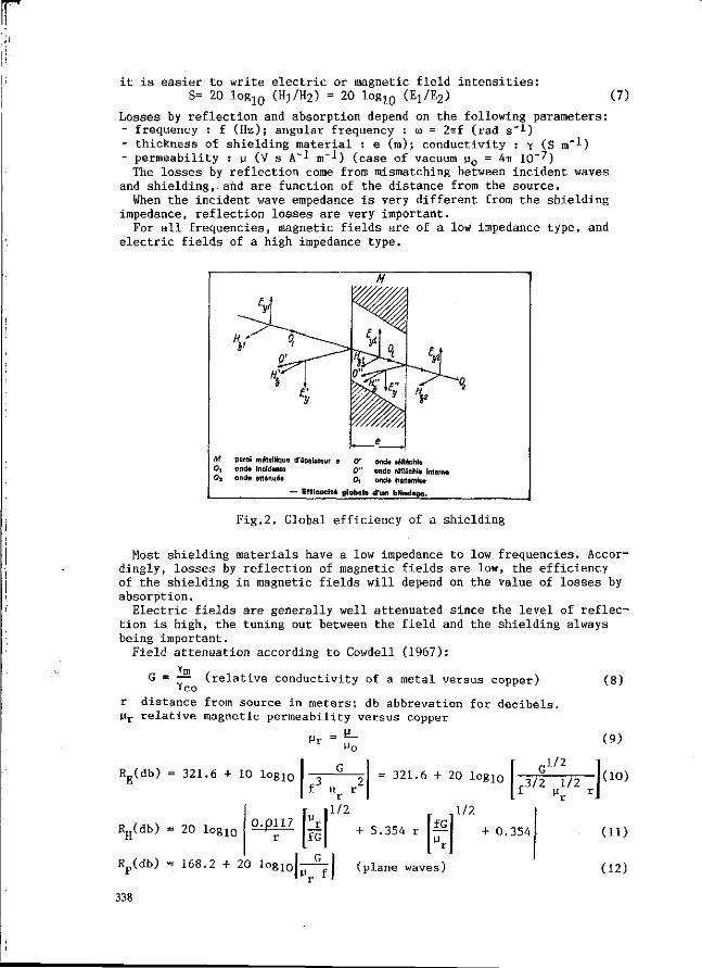
it is easier to write electric or magnetic field intensities: S= 20 log10 (H!/H2) = 20 log10 ( E ^ ) (7)

Losses by reflection and absorption depend on the following parameters: - frequency : f (Hz); angular frequency : u) = 2nf (rad s_i) - thickness of shielding material : e (m); conductivity : y (S m"l) - permeability : u (V s A~l m"^) (case of vacuum u0 = 4-rr 10"^)

The losses by reflection come from mismatching between incident waves and shielding, and are function of the distance from the source.

When the incident wave empedance is very different from the shielding impedance, reflection losses are very important.

For all frequencies, magnetic fields are of a low impedance type, and electric fields of a high impedance type.

M paroi métallique d'épaisseur e 0 ' onde réfléchie 0 , onde Incidente 0 " onde réfléchie interne O, onde atténuée <J, onde transmits

— Efficacité globale d'un blindage.

Fig.2. Global efficiency of a shielding

Most shielding materials have a low impedance to low frequencies. Accor­dingly, losses by reflection of magnetic fields are low, the efficiency of the shielding in magnetic fields will depend on the value of losses by absorption.

Electric fields are generally well attenuated since the level of reflec­tion is high, the tuning out between the field and the shielding always being important.

Field attenuation according to Cowdell (1967):

G = — (relative conductivity of a metal versus copper) 'co

r distance from source in meters; db abbrevation for decibels. Mr relative magnetic permeability versus copper

HO

R (db) = 321.6 + 10 log10

RH(db) = 20 log10 0.pil7

G

r3 2 f u r

r

fG

1/2

+

= 321.6 + 20 log10

1/2

, 1 / 2

. 3 / 2 1/2 f u r

r

+ 5 . 354 r

R ( d b ) = 1 68 . 2 + 20 l o g 1 0 P

338

+ 0.354

Mr f (plane waves)

(8)

(9)

(10)

(11)

(12)

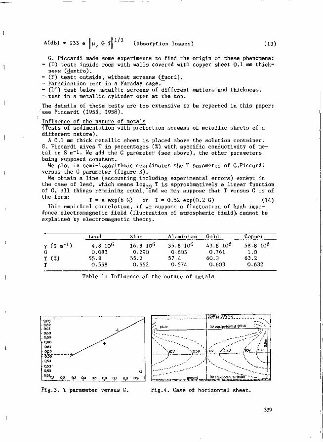
A(db) = 133 e Mr G f 1/2

(absorption losses) (13)

G. Piccardi made some experiments to find the origin of these phenomena: - (D) test: inside room with walls covered with copper sheet 0.1 mm thick­

ness (dentro). - (F) test: outside, without screens (fuori). - Faradisation test in a Faraday cage. - (D') test below metallic screens of different matters and thickness. -: test in a metallic cylinder open at the top.

The details of these tests are too extensive to be reported in this paper: see Piccardi (1955, 1958).

Influence of the nature of metals (Tests of sedimentation with protection screens of metallic sheets of a different nature).

A 0.1 mm thick metallic sheet is placed above the solution container. G. Piccardi gives T in percentages (%) with specific conductivity of me­tal in S m_l. We add the G parameter (see above), the other parameters being supposed constant.

We plot in semi-logarithmic coordinates the T parameter of G.Piccardi versus the G parameter (figure 3 ) .

We obtain a line (accounting including experimental errors) except in the case of lead, which means logip T is approximatively a linear function of G, all things remaining equal, and we may suppose that T versus G is of the form: T = & ^ ^ Q ) o r T = 0.52 exp(0.2 G) (14)

This empirical correlation, if we suppose a fluctuation of high impe­dance electromagnetic field (fluctuation of atmospheric field), cannot be explained by electromagnetic theory.

Y (S m"1) G T (%) T

Lead

4.8 106

0.083 55.8 0.558

Zinc

16.8 106

0.290 55.2 0.552

Aluminium

35.8 106

0.603 57.4 0.574

Gold

43.8 106

0.761 60.3 0.603

Copper

58.8 106

1.0 63.2 0.632

Table 1: Influence of the nature of metals

/ ' plate

\ l O V \2.5V

ground

25V(E:iOÛV/m)

OV equlpotential OVolt . Z ~ \ N ^

,'OV Z2.SJ ,'lOV ;15V

OVequïpotenlfal OVbff ~~ _

imrimr-fi f i r nTTTTmi i f r u rm i i n i i n i i*n

Fig.3. T parameter versus G. Fig.4. Case of horizontal sheet.

339

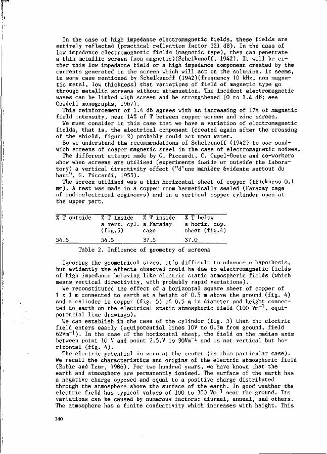
In the case of high impedance electromagnetic fields, these fields are entirely reflected (practical reflection factor 321 dB). In the case of low impedance electromagnetic fields (magnetic type), they can penetrate a thin metallic screen (non magnetic)(Schelkunoff, 1942). It will be ei­ther this low impedance field or a high impedance component created by the currents generated in the screen which will act on the solution. It seems, in some case mentioned by Schelkunoff (1942)(frequency 10 kHz, non magne­tic metal, low thickness) that variations of field of magnetic type go through metallic screens without attenuation. The incident electromagnetic waves can be linked with screen and be strengthened (0 to 1.4 dB; see Cowdell monographs, 1967).

This reinforcement of 1.4 dB agrees with an increasing of 17% of magnetic field intensity, near 14% of T between copper screen and zinc screen.

We must consider in this case that we have a variation of electromagnetic fields, that is, the electrical component (created again after the crossing of the shield, figure 2) probably could act upon water.

So we understand the recommendations of Schelkunoff (1942) to use sand­wich screens of copper-magnetic steel in the case of electromagnetic noises.

The different attempt made by G. Piccardi, C. Capel-Boute and co-workers show when screens are utilised (experiments inside or outside the labora­tory) a vertical directivity effect ("d'une manière évidente surtout du haut", G. Piccardi, 1955).

The screen utilised was a thin horizontal sheet of copper (thickness 0.1 mm). A test was made in a copper room hermetically sealed (Faraday cage of radioelectrical engineers) and in a vertical copper cylinder open at the upper part.

% T outside % T inside % T inside % T below a vert. cyl. a Faraday a horiz. cop. (fig.5) cage sheet (fig.4)

54.5 54_J5 37^5 37^0

Table 2. Influence of geometry of screens

Ignoring the geometrical sizes, it's difficult to advance a hypothesis, but evidently the effects observed could be due to electromagnetic fields of high impedance behaving like electric static atmospheric fields (which means vertical directivity, with probably rapid variations).

We reconstituted the effect of a horizontal square sheet of copper of 1 x 1 m connected to earth at a height of 0.5 m above the ground (fig. 4) and a cylinder in copper (fig. 5) of 0.5 m in diameter and height connec­ted to earth on the electrical static atmospheric field (100 Vm-!, equi-potential line drawings).

We can establish in the case of the cylinder (fig. 5) that the electric field enters easily (equipotential lines 10V to 0.3m from ground, field 62Vm_l). In the case of the horizontal sheet, the field on the median axis between point 10 V and point 2.5.V is 30Vm-l and is not vertical but ho­rizontal (fig. 4 ) .

The electric potential is zero at the center (in this particular case). We recall the characteristics and origins of the electric atmospheric field (Roble and Tzur, 1986). For two hundred years, we have known that the earth and atmosphere are permanently ionised. The surface of the earth has a negative charge opposed and equal to a positive charge distributed through the atmosphere above the surface of the earth. In good weather the electric field has typical values of 100 to 300 Vm~l near the ground. Its variations can be caused by numerous factors: diurnal, annual, and others. The atmosphere has a finite conductivity which increases with height. This

340

conductivity (10 1 4 S i ^ is maintained by ionisation from cosmic rays. From the surface of the earth the conductivity is sufficiently large to

destroy electric fields in a time from 5 to 40 mn. Yet, the local electrical field is maintained by continuous supplies.

Modern theories on electrical atmospheric field say that this is generated by three different supplies:

The first supply comes from the thunderstorm global electrical circuit (Dolezalek, 1972), (Roble and Tzur, 1986). The whole effect of all thunder­storms at the same time can be considered as a global generator which

; charges the ionosphere with an electric potential of several hundred kilo-volts in relation to the surface of the earth, and creates a potential gra­dient of about 100 V m _ 1 and a ionic current of 10~12 A m~2. Ionospheric dynamo:

The second supply is composed of different local generators as precipi­tations (rains), convection currents (charges shifted by means of other

V - ^ _ |40V(E:ioovArL - - - ,

^ > - - - 30V_ - - - - „ ' /# V \

* W - \™--' //I \\\ \ \ ^ • / / ' ' l

\ \ \ \

N^- i W . x '

around ^-4 > i > •> ' i • > i i . '

Fig. 5. Case of vertical cylinder

th^n electrical forces), atmospheric tides, snow and dust winds. Magnetospheric dynamo (Roble and Tzur, 1986):

The third supply (which in our opinion is fundamental to understand the phenomenon described by G. Piccardi and H. Bortels), comes from the vari­able ionisation of the high atmosphere due to solar activity. This activity is variable with an eleven year cycle in relation with solar sunspots (Forbush, 1966; Roble and Tzur, 1986), solar wind proton events (fast phenomenons) and is a function of latitude. Variations of about 20 % during periods of quiet sun of the atmospheric electrical field can be­come more important during geomagnetic storms (sudden storms beginning S.S.C.).

The triple origin of the electrical atmospheric field without common bonds may explain up to a point the difficulties encountered by G.Piccardi, C. Capel-Boute and co-workers as they were described at the UCCLE Sympo­sium, 1958.

It would be very interesting to repeat chemical Piccardi's tests with a well known geometry of screens and measurements of electric atmospheric field variations in the proximity of the screens with a field mill elec­trometer correlated with meteorological and solar data (see B. Primault 1984).

References

Bortels, H., 1954. "Zwei einfache Modelle meteorologischen Reaktionen in ihren Beziehungen zu Luftdruckanderungen und der Solaraktivität".

A.M.G.B., 5, pp. 235-257.

Chauvin, R., 1956. "Quelques phénomènes étranges qui intriguent les biolo-

341

gistes. L'année biologique, 22, 7-8. Cowdell, R.B., 1967. Nomograms solve tough problems of shielding.

Electronics, 92, ap. 17. Forbush, S.E., 1966. Time variations of cosmic rays. Handbuch der Physik

Geophysic 3. J. Bartels ed. Springer Verlag New York. Halla, F. und Növotny, H.E., 1958. Spezial verfarhen zur kesselsteinver-hütung. Metall. Reiningung und Vorbehandlung, 7, 107. Heitzmann, J., 1987. Cages de Faraday. Techniques de l'Ingénieur,

E-1550-1, Paris. Marking and Read, 1976. Electrostatic lenses. Elsevier Amsterdam. Piccardi, G., 1955. Über einen Zusammenhang zwischen atmosphärischen une

kosmischen phänomenen und physikalisch-chemischen processen. A.M.G.B., 6, p. 487-505.

Piccardi, G., 1960. Symposium International sur les relations entre phé­nomènes solaires et terrestres en chimie-physique et biologie. Observa­toire Royal de Belgique UCCLE-BRUXELLES, 8-10, 1958. Presses Acadé­miques Européennes, 98 chaussée de Charleroi, Bruxelles 6.

Primault, B., 1984. Relations entre phénomènes solaires et terrestres. Rapports de travail de l'Institut Suisse de Météorologie n° 121, avril. Krähblühlstrasse 58 case oistake Cg-8044. Zürich.

Roble, L.G. and Tzur, I., 1986. The eart's electrical environment. Natio­nal Academy Press, Washningston D.C.

Schelkunoff, S.A., 1943. Electromagnetic waves. The D. Van NOstrand Co Princeton N.J.

Zworikin, W.K. and al., 1962. Electron optics and the electron micros­cope, John Wiley and Sons N.Y.

342

UNDERSTANDING GEO-COSMIC RELATIONS : SOME PHILOSOPHICAL REMARKS ON THE NATURE OF REALITY

Tom Saat

Department of Ecological Agriculture, Haarweg 333, NL-6709 RZ Wageningen, The Netherlands

Summary

This paper deals with the question of causality of geo-cosmic relations. Within our common thinking about causality, within our common scientific world view, it's not very plausible that cosmic constellations can cause an effect on our terrestric 'affairs'. That however says more about our scientific concepts than about the reality of these relations. In this paper the common concept of causality is criticised as one of the main barriers in studying geo-cosmic relations.

It is argued that the necessary conditions for the appropiateness of the causality concept are only fullfflled in the field of physical science and not in other fields of reality. In searching for more adequate concepts to study geo-cosmic relations it is shown that we can learn a lot from the 'organismic' approach within the life sciences. The suitability of the 'organismic' approach to study geo-cosmic will be elucidated. It will be showm that geo-cosmic relations can not be understood in terms of spatial causality but as 'inner' relationships between cosmic and terrestric phenomena, which can be understood by 'reading' their inner physiognomy.

Introduction

One of the most important reasons that, generally speaking, scientists have no great inclination to study geo-cosmic relations is that most of them are not able to presuppose any causal relationship between cosmic and terrestrical events. Such a causality is not just improbable, it even contradicts our present views on causality.

But as demonstrated during this conference, there are many correlations to be found between cosmic and terrestrical phenomena,whenever we trouble to look for them. Thus we seriously have to pose the question about the causality of these phenomena.

When I settle that - as I would take it as a starting point for the dicussion - it is in fact very implausible that we can explain these correlations in terms of material or mechanistic causality, we can consider two other (theoretical) possibilities to account for these phenomena. The first possibility to be considered would be that our present accepted view on causality has to be corrected, as some interpreters of modern physics state and the second possibility, which I will explore in this lecture, is that causality - by which I mean thinking in terms of cause and effect,( we can also call this causalgenesis : explaining the generation of a phenomenon by cause and effect) - is only

343

appropiate in the field of physical science and in other fields of science we have to look for other approaches.

Before I will work out the second option, which is to my opinion the most fruitful one, I will first make some comments on the first one as it is quite a popular option.

In modern physics it is commonly agreed that we have to see the (physical) reality as a structure of mathematic formulae. That however does not mean, as some interpreters of modern physics, such as Fritjof Capra or David Böhm (Böhm, 1980, Capra 1981) want to conclude, that modern physics has overcome the causalgenetic view on reality, as also there where we cannot give any certain statement following the 'law of causality', we have to be aware that this very fact appears within the range of causalgenetic relations. So the reality of such 'modern laws' as Heisenberg's uncertainty-principle can only be judged in a proper way when you take into account the (causalgenetic) 'setting' in which such a law can be formulated. Classical and new physics are related with each other as groundstock and first floor of a building. When you forget about the groundstock, the first floor loses its fundament and the whole building will collapse (Saat, 1988).

So much more than criticising the causalgenetic view in the field of physical sciences I would like to investigate the limits of the causalgenetic view. To work out the limits of causalgenetic thinking, to develop the second option, I would like to discuss the necessary conditions within which causalgenesis is applicable. From the field of physics we can observe an enormous extrapolation of causalgenetic thinking to other branches of science. However the success of this approach within the physical sciences does not prove its appropiateness to other realms of reality as for example to geo-cosmic relations. In limiting the fields of reality to which causalgenesis is applicable, we make room for other approaches to understand the other fields of reality, such as geo-cosmic relations.

The law of causality

Discussing the limits of the 'law of causality' means discussing its necessary conditions. An essential condition to be able to apply the principle of causality is that the phenomena which are ruled by a certain law and the law itself are external to each other.That is to say that the notions we use to determine the objects of physical sciences (a falling stone) are different from the notions with which we formulate the physical law (the law of gravity) (Kant,1783). And it is the principle of causality which brings these two kinds of notions together. To say that the the law or idea of an object is external to that object means that we don't develop the appropiate notions to understand that object from the object itself. Our understanding of gravity is not advanced if we study the form or the colour of a falling stone. It is characteristic of all physical science, that we develop the notions, the laws on a different level from the level of the directly visible objects.

So, when for example a physicist would (as a physicist!) attend this lecture, he would not attend to the meaning of what I am saying, but he would register sounds and think about the electrical background of its causation.

Now, when we turn to the subject of this congress, the geo-cosmic relations, the first thing we notice is that here we do

344

not have these two levels, one for the objects and one for the laws. Here we deal directly with the perceivable, or rather visible, objects, namely the constellations of stars and planets, which can be observed in the sky. We relate these observed phenomena to empirical data of terrestrical processes or events. So when we speak about the causality of these phenomena it is clear that we cannot apply the principle of cause and effect (on this level). And when we are not able to find this other level of explanation, as the present available knowledge suggests, we cannot apply the law of causality at all. This however makes the question of how we can understand these relations still more intriguing. Do we have to presume another type of causality? I think a solution to this question can be found if we study the nature of the different domains of reality, if we study the difference in level of being between physical objects and other entities (Witzenmann, 1985). In respect to geo-cosmic relations (and to the limits of the causality-principle) I think it's very interesting to study the difference between the nature of the anorganic and the organic world.

The essence of an organism

In the anorganic world we can say that all phenomena, all objects are relative to each other. Nothing there exists in itself, everything is related to everything else. That is what the causality-principle expresses. In the organic world this is different. Here also we are dealing (partly) with the relativity of the phenomena, which can be very well illustrated in the plant kingdom. In botany we deal with the relationships between plant growth and the environment and we can describe these as cause-effect relations. But now it's important to see what elements of plant growth we can include into these cause-effect relations and what factors of plant growth are beyond it's scope. For example, it would be ridiculous to state that the specific form of a leaf or of the blossom of a plant is caused (generated) by an environmental factor. Everybody will admit that the characteristic forms of a rose are not generated by the environment in which that rose grows but by let's say the heriditary flow of the rose species. We would ascribe such specific characteristics to what we call the genotype and the modification of this genotype by the environmental influence the fenotype. Thus we are dealing with a causal modification instead of a causal generation. Now we can also try to explain the existence of this rather stable factor, the genotype by the selective effect of the environment, as in (Neo-)Darwinism. The big problem however in reducing this stable factor, the genotype - or the generative factor as opposed to the modificatory factor - to environmental factors is that we always have to presume a genotype which can undergo the environmental influences. So when we explain a genotype by a previous one, we have to presume the generative factor as such. All modern explanations of life deal with this basic problem that we can understand a life form which we can deduce from a previous one, but explanation of life as such is a big problem as it presupposes that we are able to reduce the generative factor to the level of modification, or to put it differently that we can reduce the level of self-generation to the level of environmental causality, in other words to the level of cause and effect.

345

The cosmos as an organism

Now, you might ask why I made this loop into such complicated biological questions. Well, what I would like to show is that in discussing the reality of the physical phenomena of the universe we face the same discussion as above. I already emphasized the relativity of the physical phenomena, but when we list the interrelations of the physical universe, we come closer and closer to the universe as such. We can explain all single objects of the universe by mutual causal interdependency with other objects and laws. Every object refers to another, we don't meet with an object which is a wholeness in itself, which does not derive its origin, its existence from another object.But when we face the universe, the cosmos-as such, we face an object which shows such wholeness as we cannot explain the cosmos-as-such by any other entity. The universe-as-such does not derive its origin from something else, the universe is in itself! And now it's interesting to see the similarity of this level of the-universe-as-such with the level of the organism-as-such. In both cases we are dealing with a generative factor as modificative or causal factors are not sufficient. Now, I do not want to go into such theories as the Big Bang to explain the genesis of the universe or into variations of that theory to explain the genesis of life on earth, I just want to point out the fact that in both fields of science we are dealing with the same problem.

The universe and the organism are two entities which are as it were in-itself. These are entities which are not ruled by something else,not ruled by external laws, but by inner laws. Now what conclusion can we draw from this for the geo-cosmic relations? I have been trying to explain that when we talk about the whole universe that we talk on an organismic level. But what universe do we mean when we talk about cosmic constellations? A constellation is an expression, it's the way the universe is organized at that very moment, the way it expresses itself. So we are not talking on the level of physical objects, but we deal with the universe as a whole, with the universe as an organism. When we look at the elements of the universe on this organismic level, we look to them in the same way as we look to the different organs of an organism. When we compare the organs of a plant or an animal with each other, we do not compare factors which are external to each other, but factors which are similar just because the same totality, the same wholeness expresses itself in the parts. So we can say that the way as for example the plant kingdom has specialized itself in different families and species, the universe has specialized itself in different planets and stars.

So this means that when we talk about geo-cosmic relations we don't talk on the level of modification of terrestric processes by cosmic constellations but we talk on the organismic level at which we deal with two comparable magnitudes, the universe which is a cosmos in itself and the organism, which is a cosmos in itself. The cosmos is divided into subsystems on which causality is applicable and the organism is related to the environment, which can be understood by causal modification (Diagram 1). Understanding relations between these two, the cosmos and the organism, means understanding the similarity of the physiognomy of the cosmic constellation, the macrocosmos, and the physiognomy of the terrestric proces or event, the microcosmos. So when for

346

organism

universe environment

Diagram 1: P resenta t ion of geo-cosmic r e l a t i o n s as physiognomic r e a l a t i on sh ip s

organism

/ landscape

earth

universe causa/ity

Diagram 2: Presentation of geo-cosmic relations as causal relationships

example we talk about the cosmic influence on the weather, we do not talk about the weather as a physical object with physical causation, but we talk about the weather as an organism which means that when we look for a certain physiognomy, a certain quality in the cosmic constellation this can also be shown in a certain physiognomy, a certain quality of the weather. To elucidate what I mean with this type of relation ,it is possible to contrast my hypothesis with a more generally accepted hypothesis on geo-cosmic relations, which I show in Diagram 2. In this diagram we see that the size of the ecosystem is indicative of its place in the hierarchy. In other words the processes on the micro-level are caused by those of the macro-level. Well this scheme is of course very helpful for studying the physical (modificative) relationships between the different levels of the

;ecosystem, but we have to drop this scheme in order to understand geo-cosmic relations. Here we are dealing with an organismic level where we are not concerned with external relations such as an outer hierarchy. Studying organisms means studying a wholeness and this wholeness, this totality doesn't exist separately from its parts, but generates its parts, its organs. We study the inner law, the generation of an organism. And just as the inner law of an organism is specialized in different species and families of organisms, the cosmos is specialized in its different constellations, planets and stars. And we can understand these specializations when we are able to read the expression, the physiognomy of a certain constellation and when we can relate this to the physiognomy of a terrestrical process (Kranich, 1979) .

Conclusion

When we approach geo-cosmic relations this way, not limiting ourselves to simply assessing correlations, but actively experiencing the generative power of the macrocosmos in a microcosmic shape, we will carry this branch of science much further then when we try to understand these relations in terms of spatial causality.

References

Böhm, D., 1980. Wholeness and the implicate order. ARK paperbacks, London Capra, F., 1981. The turning point: Science, society and the

rising culture. Fontana, London Kant, I., 1783. Kritik der Urteilskraft. Meiner verlag, Hamburg Kranich, E. M., 1976. Die Formensprache der Pflanze: Grundlinien

einer kosmologischen Botanik. Freies Geistesleben, Stuttgart Saat, T., 1988. Holisme: oude wijn in nieuwe zakken. Universiteit

van Amsterdam, Amsterdam Witzenmann,H., 1985. Verstandesblindheit und Ideenschau : die

Ueberwindung des Intellektualismus als Zeitforderung. Spicker, Dornach

348

Abstracts

351

HOW DOES MAN FIT INTO NATURE?

R. Augros, St. Anselm College, Manchester, NH 03102, USA. G. Stanciu, Magdalen College, Bedford, NH 03102, USA.

Abundant evidence from physics, chemistry, and cosmology demonstrates that our universe, its history, and its material laws are uniquely suited for life. If the strong nuclear force coupling constant were slightly weaker, hydrogen would be the only element in the universe. If this force were only 'slightly greater, the di-proton would exist, rendering ordinary hydrogen explosive. Either way life would be impossible. This same pattern recurs with many other fundamental constants in physics. Similarly, the parameters of the universe must lie within certain highly restricted ranges. The ex­pansion of the universe determines what kind of stars, if any, form in the universe. For life to exist, this expansion must be exquisitely finetuned. The conditions necessary for life were built in the Big Bang; so the uni­verse at its beginning was aiming at life. But why should human life appear in the universe? To answer that question we must compare and contrast man with animals. Numerous animal studies establish that animal perception is limited by very narrow boundaries of utility. Animals perceive only what is necessarily to maintain their way of life. An animal's world is not the world we see at all, but more closely resembles a small, poorly furnished room. Consequently, without human beings, things would, of course, go on as usual, but nature would be like a splendid drama with no crowd to applaud its power. Nature is a pageant that yearns to be known, and no animal's perception mirrors nature as man's perception does. Therefore, part of man's natural purpose is to contemplate the world.

BASIS OF JUDGMENT FOR GEO-COSMIC RELATIONS

H.J. Eysenck, Inst, of Psychiatry, Univ. of London, U.K.

In theory, all scientific investigations are equal, and require the same kind of proof. In fact, this is not so; contributions which are based on a firm and well-known theory, and which confirm the theory, require much less support than do contributions which are not so based, and in particular which may contradict firmly held views. This is the fate of contributions in the field of extra-sensory perception, and in the field of geo-cosmic relations. In this paper I shall deal with the extra requirements in this field, and the differences between work on extrasensory perception and astrology, the former falling in line with these requirements, and being more widely accepted, while the latter does not, and is fairly universally rejected. It is argued that the work of the Gauquelin's is almost the only set of studies to fulfil the requirements of science for such esoteric contribu­tions, and a detailed discussion will be given of the reasons for this judgment. Of particular importance in judging contributions such as those of the Gauquelins are instances where general principles enable one to make pre­dictions which can be tested on the database furnished by the Gauquelins, but where the particular prediction was not actually made or investigated by them. An example is the greater degree to which females than males show the Mars effect for sports champions, which can be predicted on the basis

353

of a psychological principle (the dual-threshold effect). It is argued on the basis of this and other effects that the work of the Gauquelins fulfils all the requirements of a scientific demonstration.

***

CORRELATION OF HOSPITAL MORTALITY WITH THE PHASES OF THE TIDAL VARIATIONS OF GRAVITATION

W. Raibstein, Regional Clinical Hospital, 460018, Orenburg, USSR.

The moments of deaths of 1914 patients with different diseases were determined according to local time. Tidal variations of gravitation were computed with the program composed by Z. Taranova and 0. Ostatsch (Moscow Institute of Geodesy). Statistical analysis of the data revealed a high degree of correlation between death time and phases of semi-diurnal tidal waves of gravitation (r=0.98 ± 0.0010). Phase coordinates were estimated by the time of zero velocity and zero acceleration of semi-diurnal tidal waves. A dependance of the mortality rate upon direction of vectors of tidal waves of gravitation (X^ criterium 0.05) has also been observed. The largest number of deaths occured in the period when acceleration of semidiurnal tidal waves changed from zero to minimum, and the least mor­tality was noticed when acceleration of waves raised from zero to maximum.

THE TIME COURSE OF THE CLIMACTERIC SYNDROME AND THE ROLE OF GEOGRAPHICAL FACTORS

I.V. Verulashvili, Inst, for Postgraduate Training, Tbilisi, Georgia, USSR

1. We evaluated the effects of geographical factors on patients with a climacteric syndrome inhabiting different climatic/geographical territories.

2. Geographical factors were shown to affect the development of cardio­vascular diseases and functional disorders in our patients. Hypertensive disease was diagnosed in 83.3% of patients in the temperate climatic zones, while 71.2% of patients in the Northern tundra zone developed neurocircu­latory asthenia of the hypertensive type.

3. Studies were carried out on the influence of geographical factors on the pituitary gonadotrophic functions and ovarial steroidogenesis. Seasonal variations in hormonal secretion were detected.

CHANGES IN THE EARTH'S RATE OF ROTATION

A. Poma & E. Proverbio, Stazione Astronomica di Latitudine Cagliari, Italy and Istituto di Astronomia & Fisica Superiore, Univ. di Cagliari, Italy.

A great number of researches of astronomers, geophysicists, paleontolo­gists and geologists indicate that the rate of the Earth's rotation in the past and in the present is not constant and various geophysical and meteo­rological phenomena have been proposed to account for these fluctuations, but a large number of problems remains.

354

If the annual and semiannual variability can be well explained by seasonal climatic systems, solar periods of 11 and 22 years are more controversial and a roughly 30-yr periodicity is unexplained.

These variations are discussed in some detail and evidence of correla­tions between changes in rate and direction of the spin axis, suggesting the existence of non axially-symmetrical forces acting upon Earth, is presented.

***

ON THE PROBLEMS OF THE EFFECT OF THE SUN AND PLANETARY SYSTEM ON METEOROLOGICAL DISTURBANCES IN THE ATMOSPHERE

K. Kudrna Agricultural University, 165 21 Prague 6-Suchdol (Czechoslovakia)

The problem of finding features of organization and regularities in the chaotic occurrence of disturbance within the mass and energy transfer in the system of the Sun-Earth-planets was examined by means of the theory of systems, based on the information theory (its conservation, processing and transfer between the directing and the directed object). The occurrence of anomalous response to these disturbances in the troposphere of phe Earth is characterised by the positions of terrestrial planets in the heliosphere. The differences between the maximum and minimum value of rainfall in the month of opposition or conjunction of Mars (superior planet) or in the month of superior of inferior conjunction of inferior planets are used as a measurable symptom for the level of anomalous response in the troposphere. The process of mass and energy transfer between the Sun and the planets is simulated by the transfer functions of linear, automatically selfregulated circuit. The analysis of transfer functions proves, that the rise and development of above-normal or subnormal rainfall is characterised by the triple: Sun-Mercury-Earth. The Sun has the function of a main directing element, Mercury has the function of a disturbance element and the Earth has the function of a transfer and acceptor element in a model selfregula-ted circuit. On the basis of the presented results, the occurrence of ex­tremal rainfall in the Czech Socialist Republic was forecast and the pro-gnostical forecast of extremal yield of the main field crops was determined. Reliability depends on the accuracy of the graphical evaluation and the shift of electrical fields at the beginning and at the end of the month. For the time being, a 90 percent precision has been reached.

THE ROLE OF THE GEOMAGNETISM (GMF) AND GRAVITY (GRF) IN CREATING FUNDAMENTAL PECULIARITIES OF LIVING BEINGS

A.P. Dubrov, Library on natural Science, Acad.Sei., Novatorov Ul., 34-4-188, 117421 Moscow.

1. The GMF and GRF have a decisive role in biosphere influences. 2. GMF and GRF act on rhythmic, symmetric phenogenetic and orientation

properties of biological objects. 3. The main significance in biological action of GMF and GRF has vector

characteristics in these fields. 4. Living beings have a specific and a non-specific sensitivity to these

355

fields. Specific: magnetit, otolits; non-specific: through membrane permeability.

5. There are three basic types of bioreactivity: left, right and symme­trical.

The data are in: Dubrov, A.P. (1978): "Geomagnetic Field and Life". N.Y. Plenum Press. Dubrov, A.P. (1988): "Symmetry of Biorhythms and Reactivity", Lnd.-N.Y.

Gordon & Breach. Dubrov, A.P. (1989): "Lunar Rhythms in Humans", Moscow, Médecine.

CYCLES IN THE HISTORY OF FORESTRY

J. Buis, Prins Bernhardlaan 15, 3941 EA Doorn, NL.

During my research of sources of the Dutch (c.q. Western European) Forest history, I met with a remarkable phenomenon. This phenomenon seems to be more or less periodical. It results in a decline of production of agrarian products and in problems with the supplies of wood and forest products. Probably these phenomena were caused by a very small change of climatolo-gical circumstances.

The facts: The appearance of great ecological problems starting at the seventies of the present century could be taken as a point of departure. Not only the so-called "Acid Rain" contributes to these problems: a small, problably climatological reason could be contributor also. At the beginning of our millennium other but comparable phenomena occured. An increasing of the so-called Wüstungen and an expansion of shifting sands, together with a decline of agrarian productivity can be noticed. This pro­bably points to a small change in ecological c.q. climatological circum­stances. In the middle of our millennium, the end of the 14th, beginning of the 15th centuries, we notice comparable situations. In this period also a decline of agrarian production, together with severe problems in forestry and the supply of wood and timber occured. This fall-back cannot be explained solely by the consequences of the Black Death. About the sixth century, at last, the culmination of the people's wanderings took place. At that time also the expansion of the Vikings was beginning. Among the causes mentioned, the possibility of a small climatological has to be taken in account.

Although the above mentioned cases are not thoroughly worked out, one cannot deny that a periodically reappearing phenomenon has to be taken in account.

COSMIC AND ENVIRONMENTAL INFLUENCES ON PLANTS, TESTING OF SOWING CALENDAR ON BEANS (Phaseolus vulgaris) IN BRAZIL, RESEARCH DONE IN THIS AREA UNTIL TODAY AND ITS FUTURE INPLICATIONS IN AGRICULTURE

A. Harkaly, Brazil. c/o Dept. Ecological Agriculture, Wageningen

Cosmic and environmental influences on plants have always awakened inte­rest in man, because they are a very useful means to investigate such phe­nomena. Since the 19th century, with the development of modern age, methods have been developed, to study such influences which were only known and

356

applied to agriculture due to the accumulated but also scarce "peasant wisdom" information transmitted to us until today through sayings, poems or calendars. Such methods have proven to be coherent because today diffe­rent cosmic and environmental influence knowledge systems (sometimes con­tradictory) have been described, which reflects a rather confusing but also challenging situation: Due to the difficulty in developing standardized methodologies, mechanisms and common working patterns, the present situation indicates a young and undeveloped scientific area.

A general overview on the different research methodologies on the diffe­rent knowledge systems developed will be presented indicating the conflic­ting areas. Results have been achieved analysing different aspects of plant life such as juice, oil or fat percentage, phenotypical variation such as leaf size, colour, root development, fruit quality and productivity. Results also indicate that in some cases plant varieties sensitive to such influences can be developed and that new ways for plant breeding could be suggested. The study of old cultural forms suggests that agricultural plants were bred by the use of specific calendars associated to other spe­cific bodies of agricultural knowledge. In Brazil, at the Instituto Bio-dinamico in Botucatu, State of Sao Paulo, the author has been applying some knowledge systems to test cosmic and environmental influences on plants due to the great succes obtained in Europe, where many farmers and gardners have adopted the use of agricultural calendars to achieve higher plant quality and productivity. Research is being developed to investigate the applicability of the knowledge systems used in Europe by farmers, under brazilian agricultural conditions. Subjects as these are important to be researched, not only for porduction purposes but also to provide new ele­ments which can help the human being to locate himself in a world where the knowing of geo-cosmic relations may give him new elements to decide on issues related to world development.

MODIFICATIONS OF THE GROWTH OF SEEDLING ROOTS VERSUS TIME ON A SCALE OF COPPER SULPHATE SOLUTIONS

E. Graviou, Laboratoire de Botanique Faculté de Pharmacie, 8 Avenue Rockefeller 69373 Lyon Cedex 08 France.

We have several times observed on seedlings a higher growth at the equi­nox and near to the first lunar quarter. It did not always appear at the same first quarter when growth differed. We intended to compare versus time the root growth of seedlings on a scale of copper sulfate solutions. A first experiment was performed for 7 months on 1978-1979 and published in the Bull, du Groupe d'Etude des Rythmes Biologiques t.17 no. 3-4 pp. 94-96, 1987. A second experiment was performed for 6 months, from March 30 to October 9, 1988 as follows: Seeds of Phaseolus vulgaris L. were put into germination for 48 h on copper sulphate solutions (0.5, 1.0, 1.5 and 2.10-4) in tubes placed in a water bath at 28.5° at dark. Every day a new series of seeds were put into germination on new solutions and the 48 h. roots were measured. The populations of data are not gaussian. The monthly medians were estimated from the new and from the full moons. The higher germination differs according to the series (Mood test). Those higher re­sults oscillate either part of a straight curve from the distilled water series, March, to the 2.10-^ CuSo^ series, October, thus for 6 to 7 months for the total scale. The correlation (Spearman rank correlation test) is positive between nearly synchronous series (some weeks apart), series that differ by 1.5 . 10-^ CuSO^ between them. The 4 day medians show that a

357

higher germination exist near to the first or third lunar quarter and a lower germination some days later (Kolmogorov and Smirnov test) when the above monthly germination is higher. The results agree, as for the first experiment, with the hypothesis of a circadian sensitive phase for roots to the lunar solar conjunctions.

**#

DYNAMIC RESPONSE TESTS QUANTIFYING COMPLEX PROPERTIES OF PLANTS: HOW LIVING STRUCTURES COULD REVEAL THEIR GEO-COSMIC PAST

M.F. Ranky, Hungarian Academy of Sciences, Central Research Institute of Physics, PO Box 49 Budapest 1525.

All living organisms are influenced by innumerable environmental effects during their growth. It is obvious that at any moment of investigation the sum of all past influences can be found stored in the plant under test. However, a clear separation of these effects is rarely possible.

Hence measurements revealing information quantifying the sum of past effects can be extremely beneficial. Dynamic vibrational energy tests have been developed from sophisticated vibrational analysis that can sense even minute changes in aerospace probes. These techniques will be presented quantifying the complex dynamic behaviour of living structures.

A DYNAMIC BIOLOGICAL-ATMOSPHERIC-COSMIC ENERGY CONTINUUM: SOME OLD AND NEW EVIDENCE

J. DeMeo, Orgone Biophysical Research Laboratory, PO Box 1395, El Cerrito, CA 94530 USA

From 1934 to 1957, Wilhelm Reich published a series of experimental re­ports demonstrating the existance of a specific biologically and meteoro­logically active energy continuum at work within the atmospheric ocean, and in high vacuum; he called this energy the orgone. Reich developed unique experimental devices, notably a layered organic/metallic energy-accumulating enclosure, which he called the orgone energy accumulator, and a special water-grounded pipe antenna for affecting clouds and weather patterns from a distance, called the cloudbuster. His research findings on these question span over 30 years, and there has been an additional 30 years of corroborative work by others, undertaken since his death in 1957; this paper will therefore be confined to only a few aspects of Reich's works that have been investigated and confirmed by the author. Additionally, a few parallel discoveries by other scientists will be reviewed, and con­trasted to those of Reich.

***

SOLAR-TERRESTRIAL FACTORS AND ONTOGENESIS (CLINICAL EXPERIMENTAL TESTS)

R.P. Narcissov, S.V. Petrichuk, V.M. SHishchenko, Z.N. Duchova and G.F. Suslova. Scientific Research Institute of Pediatry, Academy of Medical Science, Lomonosov avenu, 2/62, Moscow (USSR)

200 pregnant women, 176 healthy children, 86 premature newborns and 36 children with cardiac rhythm failure were studied to evaluate the influence

358

of solar-earth factors on ontogenesis. The experimental part included 445 strain animals. The enzyme activity of limphocyte (SDG, GPhDG) was shown to correlate with solar activity and amplitude geomagnetic field. The developmental difference in enzyme activity was shown during the onto­genesis and different sensitivity in healthy and sick patients in critical period resulted in diseases and shortening of ontogenetic cycle. The application of metabolic therapy was shown to be effective on improving the cellular metabolism and reduced unfavourable heliogeophysical effects on ontogenesis.

Keywords: limphocyte, activity of succinate dehydrogenase (SDG), magnetic .field, atmospheric pressure, solar activity.

STATISTICAL IDENTIFICATION OF THE PLANETARY MODULATION OF THE SOLAR ACTIVITY BY THE DETERMINATION OF THIRD ORDER MOMENTS AND THE ESTIMATION OF THE VOLTERRA KERNELS

C. Gaudeau, CNRS, Lab. de Bio-Informatique, 32, rue Emile Zola, 3700 Tours E. Daubourg and P. David, Ecole supérieure d'Informatlque-Electronique-Automatisme, E.S.I.E.A., Paris, France.

In this article, we offer our services to present a statistical method, based on the study of the non-linear systems characterized by séries of Volterra, whose aim consists of the estimation of the Volterra nucleuses, by the intermediary of the calculation of the crosscorrelation functions.

In a first part, we explain, on the one hand, the essential properties linked to the junctional representation of the non-linear systems, by series of Volterra, on the other hand, the proposed statistical method.

In the second part, we apply this method to the identification of the processes of generation of the sunspots.

GE0C0SMIC BONDS IN ANOMAL HUMAN BEHAVIOUR

A.N. Kornetov, Dept. of Psychiatry, Crimean Medical Institute, Crimean Medical-biological Center, USSR.

In 1979 the Interplanetary Magnetic Field (IMF)-effect in schizophrenia was described by us in sign change of structure IMF type (+), (-) and the considerable increase of the number of psychoses in the population. During the following 10 years we studied: 1) bonds of schizophrenia frequency and the particularities of it's clinical symptoms with calculation of sun acti­vity, geomagnetic effects, meteo-climatic factors depending on sex, disease form, the ecology of the permanent residence of the patients; 2) analogical bonds in Mania-Depressive psychoses, alcohol psychoses and epilepsy; 3) ana­logical bonds in agressive and suicidal behaviour of mentally disordered patients; 4) a bond of Ontogenesis (birth-date) of individuals with anomal behaviour and ecological geocosmic background with following manifestation of mental illness, it's intensity and frequency.

Now the main strategy of studying geocosmic bonds in anomal human behaviour, based on evolutionary ecology, has been elaborated. The full clinical typo­logy and ethology of anomal behaviour has been taking into consideration as well as anthromorphoscopic characteristics of humans, birth-time and pro­posal time of conception and sensitivity to therapy. Ontogenesis (pre- and post-natal) and the periods of anomal behaviour correlate with ecological geo-cosmic background. The critical ontogenesis periods were discovered in

359

which man is maximum sensitive to geo-cosmic factors, priorities of stimu­lating and damaging action of factors and the sensitivity to concrete fac­tors. The studied data possibly confirm that: 1) endogenous ontogeny periods are fixed in evolution and anthropogenesis by geocosmic rhythms; 2) sensi­tivity to geocosmic rhythms is different according to it's hierarchy and anthropogenous ecology, which supports the proposal of the possible reverse bond in the anthropo-geocosmic system.

MACROSCOPIC FLUCTUATIONS AS A FUNDAMENTAL PHYSICAL PHENOMENON

V.A. Kolombet, Physical Biochemistry Laboratory, Institute of Biological Physics, USSR Academy of Science, Pushchino, Moscow Region, USSR.

The results of measurements of different biospheric and cosmophysical processes are always fluctuating values. It is generally accepted that these fluctuations are mainly caused by the complex and variable nature of processes under study. The usual way of analysis of these results of mea­surements is to search for periodicities. The most famous of them are 11-year, annual, lunar, circadian and others. Our research line is somewhat different. Our attention is concentrated on an analysis of the form of dis­tributions of data obtained. It appears that as a rule the distirbutions have a regular many-peaks shape. The distributions are not smooth at all as it is generally accepted, they are spectra of states like quantum states in quantum physics. Transitions between these 'quantum' states we call macros­copic fluctuations (MF).

Relative values of MF of different physical values differ drastically. The largest MF one can see in biochemical measurements (/*/10~1 ), in some other physical values measurements one can obtain MF, for example, of the order of 10~5.

The MF-explorations we develop in two directions: 'mathematical' and 'physical'. The material presented shows some achievements in the 'physical' direction.

We have proved that MF may be described by means of world constants and integer numbers like in quantum physics. But the description of MF does not contain the Plank constant h»t lO--^^ ergxsec. It may mean that there appears a factor of nearly 10+34 an(j transitions become macroscopic. Moreover, there is 'scaling' in MF: identical MF are observed both in a case of electron mass measurements and in a case of macroscopic mass measurements. There also exist the same MF of dimensionless coupling con­stants of fundamental interactions, MF of chemical and biochemical reaction rates and probably MF of some other physical values, in particular, a-decay rate.

A characteristic feature of MF mathematical description is presence of 'power two thirds' expressions. It may be a hint on the relation between MF and weak interactions (mainly neutrino including processes). Our attempts to understand MF lead us to a new way of fundamental forces unification. Some results of a phenomenological unified theory presented here are inte­resting not only for physics, but also for astronomy and biology.

For 'geo-cosmic relations' some consequences of the probable coincidence of electron mass macroscopic fluctuations and the experimentally determined value of electron neutrino mass may be of great importance. For example, it may explain some of the unusual neutrino data presented here.

###

360

LIST OF AUTHORS

Agulova, L.P. / 214 Augros, R. / 353 Baumer, H. / 223 Beeftink, M.C. / 240 Benzine-Tizroutine, S. / 116 Bodrova, N.B. / 181 Boulanger, L. / 336 Brak, M.A. / 267 Buis, J. / 356 Capel-Boute, C. / 75 Chauvin, R. / 336 Commandeur, J.J. F. / 267 Cumming, B.G. / 31 Dailidiene, N. / 161 Dauburg, E / 359 David, P. / 359 Dean, G. / 272 DeMeo, J. / 358 Dubrov, A.P. / 355 Duchova, Z.N. / 358 Eichmeier, J. / 223 Ertel, S. / 255 Eysenck, H.J. / 353 Faraone, P. / 105 Gaudeau, C. / 359 Gauquelin, M. / 246 Graaff, de, W. / 11 Graviou, E. / 357 Grundler, W. / 127 Harkaly, A. / 356 Hilgevoord, J. / 281 Jongbloet, P.H. / 143 Kaéergiené, N. / 161 Kaiser, F. / 315 Knoop, A.A. / 65 Kollerstrom, N. / 157 Kolombet, V.A. / 174 / 360 Kornetov, A.N. / 359 Krasnogorskaya, N.V. / 189 Kudrna, K. / 355 Makejev, V.B. / 169 Mansvelt, van, J.D. / 5 Mikhov, D. / 135 Narcissov, R.P. / 358 Örményi, I. / 198 / 206 / 210 Opalinskaya, A.M. / 214 Petrichuk, S.V. / 358 Plas, van der, H.C. / 3 Pokhmelnykh, L.A. / 327 Poma, A. / 354

Proverbio, E. / 354 Raibstein, W. / 354 Ranky, M.F. / 358 Rooij, van, J.J.F. / 267 ' Rossignol, M. / 116 Rossignol, L. / 116 Rozelot, J.P. / 92 Saat, T. / 343 Schoffeniels, E. / 291 Seymour, P.A.H. / 307 Shishchenko, V.M. / 358 Shnoll, S.E. / 174 / 181 Sidyakin, V.G. / 169 Stanciu, G. / 353 Suslova, G.F. / 358 Swenson, R. / 299 Temuryants, N.A. / 169 Tomassen, G.J.M. / 1 Udaltsova, N.V. / 174 / 181 Vasilyeva, G.Ya. / 189 Venker, J.W.M. / 240 ' Vernickaite, R. / 161 Verulashvili, I.V. / 354 Vladimirsky, B.M. / 169 Vugts, H.F. / 233 Webb, H.M. / 56 Wedier, E. / 17 Zeithamer, T. / 321

361

LIST OF KEYWORDS

abiotical ecological factors / 161 activity of succinate dehydro­

genase (SDG) / 358 adaptation / 116 advection of colder/warmer air / 240 agragrian production decline / 356 agricultural knowledge / 356 air micro-organisms c.s.d. / 105 animal orientation / 56 animal cycles / 31 animals / 31 anomal human behaviour / 359 aphelions / 210 astrological factors / 272 astrology / 267 astronomical cycles / 240 astrophysics and biological

factors / 105 atmosphere / 223 atmospheric electricity,

quantitative description / 327 atmospheric pressure / 358 atmospherics / 17 / 223 Belgian Para Committee / 246 Bell's theorem / 281 Belousov-Zhabotinsky reaction / 214 bifurcations / 315 biological clocks / 31 / 56 / 307 biological activity and

alternate magnetic field / 169 biological phenomena indexes / 105 biological-atmospheric-cosmic

energy continuum / 358 bioreactivity / 355 biosphere influences / 355 biosphere and cosmos / 189 birth and death /

cosmic rhythms / 189 blood leucocytes / 161 c.s.d. as differentiated

sector colonies / 105 catastrophe theory / 321 causality concept / 281 / 343 cell growth / 127 chemical processes / 223 chemical and biochemical

reaction rates / 174 / 181 chronobiology (see circadian

rhythms / 65 circadian clocks / 56 circadian / 31 circadian rhythms and internal

environment / 65 and body temperature / 65

circadian rhythms and sleep-, wake- and alertness-cycles / 65 in bloodpressure / 65

citation frequencies / 246 climacteric syndrome / 354 climatological variations / 356 climatology / 92 cloudbuster / 358 coherence / 127 coherent oscillations / 315 complex systems / 75 conditions for life / 353 correlations / 31 cosmophysical correlations / 174 / 181 critical ontogenesis periods / 359 crops, yields variations / 355 CSIC0P / 246 cycles, history of forestry / 356 cyclicity / 31 / 240 cytogenetic study / 116 daily rhythms / 161 deathrate / 135 deterministic chaos / 315 differentiated sector colonies / 105 diffusivity / 299 discrete distributions / 181 dissipation / 299 driven oscillations / 315 dual-threshold effect / 353 dynamics / 11 earth's rotation rate / 354 earth surface vibrations / 174 eclipses / 174 ecological problems / 356 effect size in astrology / 272 electric relations, space and

solar system, model / 327 electromagnetic fields / 214 electromagnetic field:

VLF - ELF range / 169 electrostatics / 327 ELF sferics of 3 Hz range / 198 /

206 / 210 emergence / 299 eminent professionals / 255 energy flow / 291 environment / 75 enzyme activity / 181/ 169 EPR-experiment / 281 equinoxes / 210 / 240 evolution / 299

extraterrestrial relations / 255 feedback organism and

environment / 291

362

fermentai activity / 161 fluctuating phenomena / 75 / 105 fluctuations / 214 / 291 fundamental constants / 353 / 360 galactic cosmic rays / 105 Gauquelin claims / 255 Gauquelin, Mars effect / 353 geo-cosmic relations / 353 geo-cosmic background / 359 geocentric positions of the

planet Mars / 240 geographical factors / 354 geomagnetic activity / 135 / 198 geomagnetic fields / 135 geomagnetism / 327 / 355 germination / 31 / 357 gravitation / 174 / 354 gravity (GRF) / 355 growth / 31 heliogeoactivity / 189 human behaviour / 359 human response / 157 information / 75 information theory / 291 instabilities / 315 interactions: solar, lunar,

and tidal cycles / 31 interplanetary magnetic field (IMF)

/ 189 / 359 irreversibility / 75 laboratory c.s.d. / 105 law of maximum entropy production

/ 299 limit cycles / 315 locality / 281 low frequency variations of electr.

atmosph. field / 336 lunar effects on human behaviour

/ 272 lunar phases and plant growth / 357 lunar phases / 116 lunar synodic cycle / 157 lymphocyte / 358 macroscopic fluctuations / 174 /

/ 181 / 360 magnetic oscillations / 307 magnetic field / 358 magnetic moment of inferior

planets, prediction / 327

magnetospheric storms and substorms / 321

magnetospheric physics / 321 magnetotaxis / 56 marine environment / 31 Mars effect / 240 / 246 / 255 mass measurements / 360 maternal fecundity / 143

meteorological disturbances / 355 micro-organisms mutations / 105 microwave bioeffect / 127 month-of-birth / 143 month-of-conception / 143 moon and " " P u a-decay / 174 moon and seedling roots / 357 moon-phases / 31 / 56 / 116 / 157 /

/206 / 233 / 357 mortality / 135 / 354 / 189 non-equilibrium sytems / 189 nonequilibrium thermodynamics / 299 nonlinear oscillations / 315 nonlinear dynamics / 315 nonreproducibility / 75 numeric models / 240 observation / 281 omega ( ÎÎ ) number / 299 ontogenesis / 161 / 359 organismic approach / 343 orgone energy / 358 ozone / 31 paradigm / 75 peasant wisdom / 356 ' perihelions / 210 periodicities / 233 periodicities, annual, semiannual,

11 yr, 22 yr, 30 yr / 354 phases of solar activity / 206 photoperiodism / 31 Piccardi chemical test / 75 / 214 / 336 planetary system / 355 planetary effects / 255 planetary modulation of

solar activity / 359 planets / 327 plants, quantifying of past

environmental effects / 358 plants and environment / 358 plants / 31 plants / cosmic influences / 356 plutonium: 239pu a-decay / 174 / 181

/ 360 precipitation reactions / 75 predictability / 315 probability / 281 proton flare / 198 qualitative theory of differential

equations / 321 quantum mechanics / 281 radiation / 75 radiation / biological efficacy / 17 radiation, from space / 17 radiation, from the atmosphere / 17 radiative equilibrium / 11 radioactive decay / 174 / 181 / 360 rainfall / 233 / 355 / 358

363

Reich, Wilhelm / 358 VLF-radiation / 223 resonance / 11 / 127 / 307 / 315 water treatment / 75 rhythmic processes / 315 weather parameters / 240 screening by neutral matter / 327 Zelen test / 246 sea temperature / 233 zodiacal sector limits / 240 seasonal productivity / 31 seasonal variations / 354 seasonal effects / 206 seasonally fluctuation

ovulation rate / 143 seedling roots / 357 self-attribution / 267 sferics / 17 / 198 / 206 / 210

/ 223 solar system, mass and

energy transfer / 355 solar physics / 92 solar system dynamics / 189 solar system, electricity

and magnetism / 327 solar cycle / 327 solar radio fluxes / 198 solar system / 11 solar activity effects upon

biosphere / 169 solar eclipse 1981 / 174 solar activity / 105 / 359 solar-terrestrial effects / 92 solstices / 210 sowing calendar / 356 spin-axis, rate and

direction of / 354 spring-equinox / 240 SPrOO-hypothesis / 143 staphylococcus aureus c.s.d. / 105 successful professionals / 246 / 255 sunsign-effect / 267 sunspots / 31 supernova 1987a / 360 supra-chiasmatic nucleus / 65 synoptic weather situations / 198 temperature changes / 240 terrestrial / 31 terrestrial charge / 327 tidal influences / 233 tidal variations / 354 tidal coupling / 307 tidal effects / 11 time / 75 time of birth / 246 tropical zodiac / 240 ultra and infra-dian rhythms / 31 ultra-violet light / 31 unified theory / 360 universe / 353 variability / 214

364