Seediscussions,stats,andauthorprofilesforthispublicationat:http://www.researchgate.net/publication/267684254

SamplingStrata:AnRPackagefortheOptimizationofStratifiedSampling

ARTICLEinJOURNALOFSTATISTICALSOFTWARE·NOVEMBER2014

ImpactFactor:3.8

CITATION

1

DOWNLOADS

45

VIEWS

33

1AUTHOR:

GiulioBarcaroli

ItalianNationalInstituteofStatistics

44PUBLICATIONS32CITATIONS

SEEPROFILE

Availablefrom:GiulioBarcaroli

Retrievedon:12July2015

JSS Journal of Statistical SoftwareOctober 2014, Volume 61, Issue 4. http://www.jstatsoft.org/

SamplingStrata: An R Package for the Optimization

of Stratified Sampling

Giulio BarcaroliItalian National Institute of Statistics (Istat)

Abstract

When designing a sampling survey, usually constraints are set on the desired precisionlevels regarding one or more target estimates (the Y ’s). If a sampling frame is available,containing auxiliary information related to each unit (the X’s), it is possible to adopt astratified sample design. For any given stratification of the frame, in the multivariate caseit is possible to solve the problem of the best allocation of units in strata, by minimizing acost function subject to precision constraints (or, conversely, by maximizing the precisionof the estimates under a given budget). The problem is to determine the best stratificationin the frame, i.e., the one that ensures the overall minimal cost of the sample necessaryto satisfy precision constraints. The X’s can be categorical or continuous; continuousones can be transformed into categorical ones. The most detailed stratification is givenby the Cartesian product of the X’s (the atomic strata). A way to determine the beststratification is to explore exhaustively the set of all possible partitions derivable by theset of atomic strata, evaluating each one by calculating the corresponding cost in termsof the sample required to satisfy precision constraints. This is unaffordable in practicalsituations, where the dimension of the space of the partitions can be very high. Anotherpossible way is to explore the space of partitions with an algorithm that is particularlysuitable in such situations: the genetic algorithm. The R package SamplingStrata, basedon the use of a genetic algorithm, allows to determine the best stratification for a pop-ulation frame, i.e., the one that ensures the minimum sample cost necessary to satisfyprecision constraints, in a multivariate and multi-domain case.

Keywords: genetic algorithm, theory of partitions, optimal stratification, sample design, sam-ple allocation, R package.

1. Introduction

Let us suppose we need to design a sample survey, having available a complete frame contain-

2 SamplingStrata: Optimization of Stratified Sampling in R

ing information on the target population (identifiers plus auxiliary information). If our sampledesign is a stratified one, we need to choose how to form strata in the population, in order toget the maximum advantage of the available auxiliary information. In other words, we haveto decide how to combine the values of the auxiliary variables (henceforth, the X variables) inorder to determine a new categorical variable, called stratum. To do so, we have to take intoconsideration the target variables of our sample survey (henceforth, the Y variables): if, toform strata, we choose the X variables most correlated to the Y , the efficiency of the samplesdrawn by the resulting stratified frame may be greatly increased. In order to handle the wholeauxiliary information in a homogeneous way, we have to reduce continuous data to categorical(by calculating equal frequency intervals, or using a k-means clustering technique, or othersuitable methods). Then, for every set of candidate auxiliary variables X, we have to decide(i) what variables to consider as active variables in strata determination, and (ii) for eachactive variable, what set of values (in general, what aggregation of atomic values) have to beconsidered. Each choice determines a particular stratification of the target population, i.e., apossible solution to the problem of best stratification. Here, by best stratification, we meanthe stratification that ensures the minimum cost of the sample, necessary to satisfy precisionconstraints, set on the estimates of the target variables Y (constraints expressed as maximumexpected coefficients of variation in different domains of interest). Therefore, the validity of aparticular stratification can be measured by the associated minimum cost of a sample, whoseestimates are expected to satisfy given precision levels. In general, the number of possiblealternative stratifications for a given population frame may be very high, in some cases eveninnumerable. In these cases it is not possible to enumerate them in order to find the beststratification. Instead, adopting the evolutionary approach, the use of a genetic algorithmenables to explore the range of possible solutions in order to find a near-optimal solutionafter an affordable number of iterations. The implementation of the genetic algorithm in thepackage SamplingStrata (Barcaroli, Pagliuca, and Willighagen 2014) makes use of a modifiedversion of the functions available in the genalg package (Willighagen 2014).

The remaining paper is organized as follows: Section 2 describes in brief the general approachfollowed for the implementation of the package (for a more detailed illustration of methodolog-ical aspects see Ballin and Barcaroli 2013); Section 3 illustrates how to employ the packagein practical situations; Section 4 evaluates the performance of the genetic algorithm methodby comparing it, in the univariate case, to the methods implemented in package stratification(Baillargeon and Rivest 2012a); Section 5 concludes the paper.

2. The general approach

In the field of stratified sampling, many studies dealing with the problem of optimizing strat-ification have been conducted. A general review of the proposed methods is contained inGonzales and Eltinge (2010). Basically, the optimization can be conceived as based on fourdistinct components:

1. objective function;

2. constraints;

3. input parameters;

4. decision variables.

Journal of Statistical Software 3

The total cost associated with a specific sample (depending on the allocation of units inthe strata, and on the per unit interviewing cost, that may vary from stratum to stratum),and the expected precision related to each target estimate, can be associated to the first twocomponents in an interchangeable way: in fact, it is possible to minimize the total cost under aset of precision constraints, or to maximize precision levels under given budget constraints. Inboth cases, optimization is performed on the basis of input parameters such as the variancesof the target variables and the number of population units in each stratum. While in generalit is not difficult to assign population units to the different strata, as this only depends on theauxiliary information in the frame (which is available by definition), much more complex is toget the information necessary to estimate the variability of target variables in each stratum.In fact, this information is not available at unit level (otherwise we would not carry out aspecific survey on these variables), so it is necessary to estimate their variability by harnessingdifferent possible sources:

1. census data;

2. data from previous rounds of the same survey;

3. data on proxy variables.

In the first case, the lower the time gap, the higher the reliability of the estimate. In thesecond, together with the time gap also the sampling errors on the estimates should be takeninto account. Finally, in the third case also the correlation between target and proxy variablesmust be considered when evaluating the quality of the estimates. An effort should be made tomodel the relationships between target variables and all the available information, includingthe auxiliary one in the sampling frame, in order to increase this quality. Henceforth weassume that estimates of acceptable reliability of the variability of target variables in strataare available. Should this assumption not apply, the method here proposed would not beapplicable.

A first important distinction can be made between the case where the precision of only onetarget variable is taken into consideration in the objective function or in the constraints(univariate case), or when more than one of them are considered (multivariate case). Afurther complication may be given by the necessity to consider different domains to whichestimates (and related precision levels) have to be referred to (multi-domain case).

A second, more important, distinction is related to the decision variables. Many optimizationmethods are based on decision variables that state how many population units have to beselected in each stratum: in other words, strata in the population are assumed as given, andthe optimization consists in determining the best allocation of sampling units in populationstrata. Under this setting, the optimization problem can be solved using an application of theCauchy-Schwarz inequality (Cochran 1977) or Lagrangian multipliers (Varberg and Purcell1997). Well known solutions in the multivariate case are the ones given by Bethel (1989) andChromy (1987).

However, the way the population is stratified is of the greatest importance with respect tothe optimization of the sample design. The relationships between the survey target variablesand the stratification variables are at the basis of the stratified sampling. In order to takemaximum advantage of these relationships, choices regarding the way we define populationstrata should enter into the optimization process together with the allocation choices. Up until

4 SamplingStrata: Optimization of Stratified Sampling in R

recently, on the contrary, optimization of stratified sampling has been considered as a two-stepprocess: first, a stratification is chosen, by exploiting all the auxiliary information availableon sampling units, or only a subset, selected on the basis of known correlations between targetand stratification variables; then, given the chosen stratification, the problem of allocation issolved (Dalenius and Hodges 1959). The Lavallee and Hidiroglou method for the stratificationof a population which is skewed with respect to a unique stratification variable (Lavalleeand Hidiroglou 1988) can be considered an exception, as it allows to determine both, strataboundaries and best allocation, but only in the univariate case. Also the method proposed byKeskinturk and Er (2007), which makes use of the genetic algorithm approach, suffers fromthe same limitation.

The approach, which is implemented in the R (R Core Team 2014) package SamplingStrataavailable from the Comprehensive R Archive Network (CRAN) at http://CRAN.R-project.org/package=SamplingStrata, permits a joint optimization of both population stratificationand sampling units allocation, in the multivariate and multi-domain case. It is based on thefollowing assumptions:

1. the optimal stratification of a population frame depends on the particular sample surveythat has to be planned;

2. the optimality of the solution can be measured against its cost, expressed in terms of thenumber of units to be sampled (together with the per unit interview cost), required tosatisfy precision constraints, set on estimates of totals or means of the target variables;

3. the multivariate and multi-domain case must be contemplated in order to ensure gen-erality;

4. the availability of auxiliary information in the population frame permits to define aspace of alternative stratifications: this space should be rigorously generated and, inprinciple, the best solution could be found by exhaustively evaluating each stratificationwith regard to the cost of the associated sample;

5. as in practical situations it is not possible to enumerate the space of stratifications(because of its dimension), a heuristic is necessary in order to explore this space without(or with a negligible) loss of optimality: from this point of view genetic algorithms havebeen proven to be particularly efficient.

2.1. Best allocation for a given stratification

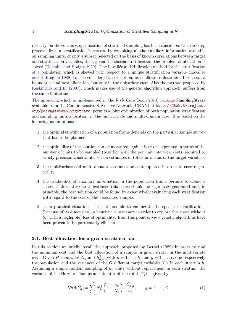
In this section we briefly recall the approach proposed by Bethel (1989) in order to findthe minimum cost and the best allocation of a sample in given strata, in the multivariatecase. Given H strata, let Nh and S2

h,g (with h = 1, . . . ,H and g = 1, . . . , G) be respectivelythe population and the variances of the G different target variables Y ’s in each stratum h.Assuming a simple random sampling of nh units without replacement in each stratum, thevariance of the Horvitz-Thompson estimator of the total (Yg) is given by

VAR(Yg) =

H∑h=1

N2h

(1− nh

Nh

)·S2h,g

nh, g = 1, . . . , G. (1)

Journal of Statistical Software 5

Let us consider now the following cost function:

C(n1, . . . , nH) = C0 +

H∑h=1

Chnh. (2)

In this function we can distinguish a fixed component (C0, not dependent on sample size andits allocation), and a variable one (the sum of the products between the cost for interviewingone unit in the stratum (Ch) and the allocation of units in that stratum (nh)). If we defineupper limits on the expected sampling variances defined by Equation 1 by setting

VAR(Yg) ≤ Ug, (3)

then to find the best solution to the problem of sample allocation in a stratified designis equivalent to finding the vector of the allocations nh that minimizes Equation 2 givenEquation 3.

An algorithm that is proved to converge to the solution was provided by (Bethel 1989).The package SamplingStrata provides the function bethel that allows to determine the bestallocation given two different inputs:

1. information on the distribution of the Y ’s in the strata;

2. precision constraints on the Y ’s.

In this particular implementation, precision constraints are expressed in terms of maximumexpected coefficient of variation (CV) for each Y :

CV (Yg) =

√VAR(Yg)

E(Yg)(4)

By so doing, we are able to remove the dependence on the scale (or range) of the valuesassociated with the different Y ’s.

So the problem becomes:

C0 +H∑

h=1

Chnh → min

CV (Y1) ≤ U1

CV (Y2) ≤ U2

. . .

CV (YG) ≤ UG

(5)

The Bethel algorithm implemented in the bethel function can be used not only for its originalpurpose (to determine the best allocation on the basis of the precision constraints), but also toevaluate any given stratification of the population frame. In other words, given two differentstratifications adopted for the same population frame, we should prefer the one for which thesolution identified by the Bethel algorithm has a smaller cost.

2.2. Space of stratifications for a given frame

Let us consider a sampling frame, that is a set of N records containing information relatedto N units belonging to the reference population. The available information can be groupedinto two distinct sets of variables:

6 SamplingStrata: Optimization of Stratified Sampling in R

� the variables allowing the identification of units, in order to be able to contact themwhile carrying out the survey;

� the variables useful to optimize the sample design (the auxiliary variables X).

In our setting, we assume that:

1. a set of M auxiliary variables Xm (m = 1, . . . ,M) are available;

2. only categorical (nominal or ordinal) auxiliary variables are considered: when continuousvariables are present in the set, they have to be converted into categorical ones by meansof a transformation algorithm (for example, by applying a k-means clustering algorithm,see Hartigan and Wong 1979);

3. with each (categorical) auxiliary variable we can associate a domain set given by thevector dm = {x1, . . . , xkm}, where an integer value is assigned to each value in thedomain.

Under these assumptions, the most detailed stratification for the frame is given by consideringthe Cartesian product CP = X1 ×X2 × . . .×XM .

The maximum number of strata is equal to K =∏M

m=1 km − I∗, where I∗ is the number ofnon-valid or missing combinations in the frame.

We call atomic strata the result of the Cartesian product, i.e., the strata obtained by cross-classifying the units using all the values of all the auxiliary variables, and indicate the corre-sponding set as L = {l1, l2, . . . , lK}.Starting from this set of atomic strata, it is possible to derive the set of all possible partitionsP1, P2, . . . , PB, where each partition is defined as a collection of sets T1, T2, . . . , Tq (1 ≤ q ≤ K)where each Ti is a subset of L.

Accordingly to the theory of partitions (Hankin and West 2007) the following conditions musthold:

Ti ∩ Tj = ∅ if i 6= j,⋃qi=1 Ti = L,

Ti 6= ∅ for i = 1, . . . , q.(6)

Each partition is equivalent to a given stratification of the frame. The set of all possiblepartitions can be considered as the space of stratifications.

For example, let us consider a set of atomic strata L = {l1, l2, l3}. The different partitionsthat can be generated by this set are:

P1 = {(l1, l2, l3)}, P2 = {(l1), (l2, l3)},P3 = {(l2), (l1, l3)}, P4 = {(l3), (l1, l2)},P5 = {(l1), (l2), (l3)}.

The cardinality of the set of all the possible partitions is given by the Bell number :

BK =

K−1∑i=0

(n

i

)·Bi, (B0 = 1). (7)

Journal of Statistical Software 7

2.3. Choosing the best stratification by applying the genetic algorithm

In principle, having fixed precision constraints on a set of target estimates for a given samplesurvey, it is possible to choose the best stratification for a population frame where a set ofauxiliary variables are available, by executing the following steps:

1. determine the set of atomic strata by cross-classifying sampling units using all the valuesof all auxiliary variables;

2. calculate distributional parameters (mean and variance) of target variables if informa-tion related to Y ’s is available for each unit in the frame (or, if not, by using proxyinformation by other sources) in atomic strata;

3. solve the allocation problem for the atomic strata and associate the cost of the solutionfound;

4. generate all possible partitions from the set of atomic strata (in order to generate allthe possible partitions it is possible to use the package partitions; Hankin 2013);

5. for each generated partition:

� calculate distributional parameters (mean and variance) of target variables in cur-rent strata by aggregating the corresponding information available in atomic strata;

� solve the allocation problem for the current partition and associate the cost of thesolution;

6. choose the best stratification as the one given by the partition with the minimal asso-ciated cost.

Unfortunately, this procedure, that is based on an exhaustive enumeration of all possiblepartitions, is in most cases not feasible, as the number of partitions to be evaluated is toohigh. In fact, considering the formula for the calculation of the Bell number reported inEquation 7, this number grows very rapidly with regard to the dimension of the set of atomicelements (for example, B3 = 5, B4 = 15, B10 = 115,975 and B100 ∼ 4.76× 10115).

The function optimizeStrata available in package SamplingStrata allows to explore thespace of stratifications without being obliged to exhaustively enumerate it, by using a searchtechnique known as the genetic algorithm.

Genetic algorithms belong to the class of evolutionary algorithms that make use of techniquesbased on concepts derived by biology, such as inheritance, mutation, crossover, fitness andselection (DeJong 2006).

In order to apply the genetic algorithm to the problem of finding the best stratification, thefollowing setting has been adopted:

1. a given stratification is considered as an individual in a population (or generation ofindividuals);

2. an individual is characterized by a genome that is optimized in the course of the evolu-tion;

8 SamplingStrata: Optimization of Stratified Sampling in R

3. the genome is represented by a vector whose dimension is given by the number of atomicstrata (K): with each position in this vector an atomic stratum is associated;

4. to each element in the vector an integer value lying in the interval [1,K] is assignedrandomly: atomic strata that share the same integer value, collapse in an aggregatestratum;

5. the fitness of each individual is evaluated by solving the system reported in Equation 5(using the Bethel algorithm);

6. in the passage from one generation to the next, the fittest individuals are privileged: apercentage of those with highest fitness are directly moved to the next generation, theothers are randomly selected with probability proportional to their fitness, in order tolet them procreate children;

7. each child is procreated by applying crossover to their parents (a swap of the genescontained in the two genomes), and applying mutation to the resulting genome.

At the end of the evolution (the chain of generations), the individual with the absolute bestfitness will be chosen: the genome of this individual represents a stratification in which all orsome of the atomic strata have been aggregated.

3. A general procedure for the use of package SamplingStrata

The optimization of the sampling design starts by considering the available population frame,defining the target estimates of the survey and establishing precision constraints on them.It is then possible to determine the best stratification and the optimal allocation. Finally,the sample can be drawn from the frame stratified accordingly to the optimal stratification.Formally, these are the required steps:

1. analysis of the frame data: identification of available auxiliary information;

2. manipulation of auxiliary information: in case auxiliary variables are of continuous type,they have to be transformed into categorical variables;

3. construction of atomic strata: on the basis of the categorical auxiliary variables availablein the sampling frame, the set of atomic strata can be obtained by cross-classifying theunits by using all the values of all the auxiliary variables;

4. characterization of each atomic stratum with the information related to the target vari-ables (mean and standard deviation for each Y , estimated by using available informa-tion: by census, previous surveys or proxy variables data);

5. choice of the precision constraints for each target estimate, possibly differentiated bydomain;

6. optimization of stratification and determination of required sample size and allocation;

7. analysis of the resulting optimized strata;

Journal of Statistical Software 9

8. association of new labels to sampling frame units, each of them indicating the new strataresulting from the optimal aggregation of the atomic strata;

9. selection of units from the sampling frame with a stratified random sample selectionscheme;

10. analysis of the solution found.

In the following, we will illustrate each step starting from a real sampling frame, the dataframe swissmunicipalities that is available in the R package sampling (Tille and Matei2012).

3.1. Analysis of the frame data and manipulation of auxiliary information

As a first step, we have to define a frame data frame containing the following information:

� a unique identifier of the unit (no restriction on the name, for instance id);

� the (optional) identifier of a pre-defined stratum to which the unit belongs;

� the values of M auxiliary variables (named from X1 to XM);

� the (optional) values of G target variables (named from Y1 to YG);

� the values of the domain of interest for which we want to produce estimates (nameddomainvalue).

By executing the following statements in the R environment:

R> data("swissmunicipalities", package = "sampling")

we get the swissmunicipalities data frame, that contains 2,896 observations (each obser-vation refers to a Swiss municipality in 2003). Among the others, we can find the followingvariables:

� REG: Swiss region,

� Nom: municipality name,

� Surfacesbois: wood area,

� Surfacescult: area under cultivation,

� Alp: mountain pasture area,

� Airbat: area with buildings,

� Airind: industrial area,

� Pop020: number of men and women aged between 0 and 19,

� Pop2040: number of men and women aged between 20 and 39,

10 SamplingStrata: Optimization of Stratified Sampling in R

� Pop4065: number of men and women aged between 40 and 64,

� Pop65P: number of men and women aged 65 and over,

� POPTOT: total population.

First, we define the identifier of the frame:

R> frame <- NULL

R> frame$id <- swissmunicipalities$Nom

Let us suppose to plan a survey whose target estimates are the totals of the population byage class in each Swiss region. In this case, the Y ’s variables will be:

� Y1: number of men and women aged between 0 and 19,

� Y2: number of men and women aged between 20 and 39,

� Y3: number of men and women aged between 40 and 64,

� Y4: number of men and women aged 65 and over.

Consequently, the following statements are executed:

R> frame$Y1 <- swissmunicipalities$Pop020

R> frame$Y2 <- swissmunicipalities$Pop2040

R> frame$Y3 <- swissmunicipalities$Pop4065

R> frame$Y4 <- swissmunicipalities$Pop65P

We suppose that the values of these variables in the frame have been obtained from pastsurveys (for instance, from a census), or from administrative data: it should always be takeninto account that they could be out of date, or not completely reliable.

As for the auxiliary variables (X’s), we can use all those characterizing the area use (surfacespertaining wood, mountain or pasture, cultivations, industries, buildings). As these variablesare of continuous type, we have to transform them into categorical (ordinal) form first. Inorder to do that, it is possible to apply a k-means clustering method by using the functionvar.bin:

R> library("SamplingStrata")

R> set.seed(1508)

R> frame$X1 <- var.bin(swissmunicipalities$POPTOT, bins = 18)

R> frame$X2 <- var.bin(swissmunicipalities$Surfacesbois, bins = 3)

R> frame$X3 <- var.bin(swissmunicipalities$Surfacescult, bins = 3)

R> frame$X4 <- var.bin(swissmunicipalities$Alp, bins = 3)

R> frame$X5 <- var.bin(swissmunicipalities$Airbat, bins = 3)

R> frame$X6 <- var.bin(swissmunicipalities$Airind, bins = 3)

Now, we have six different auxiliary variables of categorical type, the first with 18 differentmodalities, the others with 3 modalities.

Finally, we have to set the values of the domainvalue variable, which is mandatory. As wewant to obtain estimates for each one of the seven regions, we set:

Journal of Statistical Software 11

R> frame$domainvalue <- swissmunicipalities$REG

R> frame <- as.data.frame(frame)

Now, the frame data frame looks like:

R> head(frame)

id Y1 Y2 Y3 Y4 X1 X2 X3 X4 X5 X6 domainvalue

1 Zurich 57324 131422 108178 66349 18 3 2 1 3 3 4

2 Geneve 32429 60074 57063 28398 17 1 1 1 3 2 1

3 Basel 28161 50349 53734 34314 17 1 1 1 3 3 3

4 Bern 19399 44263 39397 25575 17 2 3 1 3 3 2

5 Lausanne 24291 44202 35421 21000 17 2 2 1 3 2 1

6 Winterthur 18942 28958 27696 14887 16 3 3 1 3 3 4

This is the format required by the package.

3.2. Construction of atomic strata

The strata data frame reports information regarding each stratum in the population. Thereis one row for each stratum. The total number of strata is given by the number of differentcombinations of X values in the frame. For each stratum, the following information is required:

1. the identifier of the stratum (named STRATO), concatenation of the values of the variablesX’s;

2. the values of the M auxiliary variables (named X1 to XM ) corresponding to those in theframe;

3. the total number of units in the population belonging to the stratum (named N);

4. a flag (named CENS) indicating if the stratum is to be censused (= 1) or sampled (= 0);

5. a variable indicating the cost of interviewing a single unit in the stratum (named COST);

6. for each target variable Y , its estimated mean and standard deviation (named respec-tively Mi and Si);

7. the value of the domain of interest to which the stratum belongs (named DOM1 andcorresponding to the variable domainvalue in the frame data frame).

If in the frame data frame the values of the target Y ’s variables (from a census, or fromadministrative data) are also present, it is possible to automatically generate the strata dataframe by invoking the buildStrataDF function. Let us consider again the frame data framethat we have built in previous steps. We can apply to it the buildStrataDF function:

R> strata <- buildStrataDF(frame)

Computations have been done on population data

12 SamplingStrata: Optimization of Stratified Sampling in R

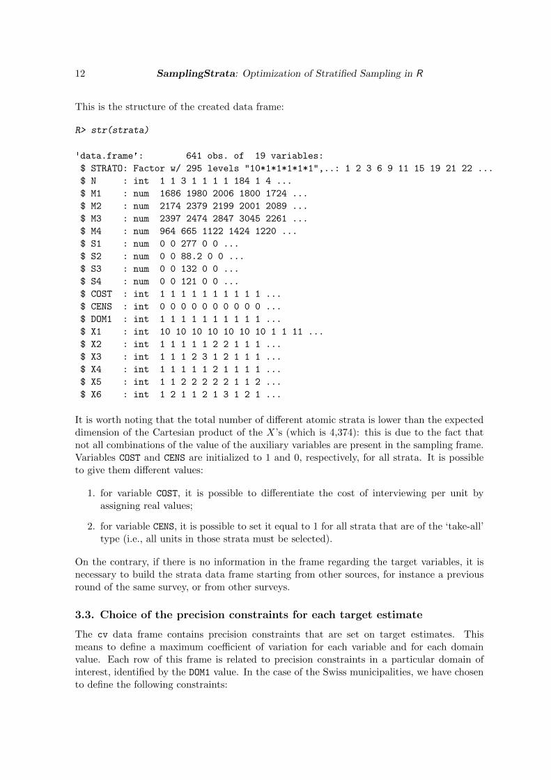
This is the structure of the created data frame:

R> str(strata)

'data.frame': 641 obs. of 19 variables:

$ STRATO: Factor w/ 295 levels "10*1*1*1*1*1",..: 1 2 3 6 9 11 15 19 21 22 ...

$ N : int 1 1 3 1 1 1 1 184 1 4 ...

$ M1 : num 1686 1980 2006 1800 1724 ...

$ M2 : num 2174 2379 2199 2001 2089 ...

$ M3 : num 2397 2474 2847 3045 2261 ...

$ M4 : num 964 665 1122 1424 1220 ...

$ S1 : num 0 0 277 0 0 ...

$ S2 : num 0 0 88.2 0 0 ...

$ S3 : num 0 0 132 0 0 ...

$ S4 : num 0 0 121 0 0 ...

$ COST : int 1 1 1 1 1 1 1 1 1 1 ...

$ CENS : int 0 0 0 0 0 0 0 0 0 0 ...

$ DOM1 : int 1 1 1 1 1 1 1 1 1 1 ...

$ X1 : int 10 10 10 10 10 10 10 1 1 11 ...

$ X2 : int 1 1 1 1 1 2 2 1 1 1 ...

$ X3 : int 1 1 1 2 3 1 2 1 1 1 ...

$ X4 : int 1 1 1 1 1 2 1 1 1 1 ...

$ X5 : int 1 1 2 2 2 2 2 1 1 2 ...

$ X6 : int 1 2 1 1 2 1 3 1 2 1 ...

It is worth noting that the total number of different atomic strata is lower than the expecteddimension of the Cartesian product of the X’s (which is 4,374): this is due to the fact thatnot all combinations of the value of the auxiliary variables are present in the sampling frame.Variables COST and CENS are initialized to 1 and 0, respectively, for all strata. It is possibleto give them different values:

1. for variable COST, it is possible to differentiate the cost of interviewing per unit byassigning real values;

2. for variable CENS, it is possible to set it equal to 1 for all strata that are of the ‘take-all’type (i.e., all units in those strata must be selected).

On the contrary, if there is no information in the frame regarding the target variables, it isnecessary to build the strata data frame starting from other sources, for instance a previousround of the same survey, or from other surveys.

3.3. Choice of the precision constraints for each target estimate

The cv data frame contains precision constraints that are set on target estimates. Thismeans to define a maximum coefficient of variation for each variable and for each domainvalue. Each row of this frame is related to precision constraints in a particular domain ofinterest, identified by the DOM1 value. In the case of the Swiss municipalities, we have chosento define the following constraints:

Journal of Statistical Software 13

R> cv <- data.frame(DOM = "DOM1", CV1 = 0.05, CV2 = 0.05, CV3 = 0.05,

+ CV4 = 0.05, domainvalue = 1:7)

R> cv

DOM CV1 CV2 CV3 CV4 domainvalue

1 DOM1 0.05 0.05 0.05 0.05 1

2 DOM1 0.05 0.05 0.05 0.05 2

3 DOM1 0.05 0.05 0.05 0.05 3

4 DOM1 0.05 0.05 0.05 0.05 4

5 DOM1 0.05 0.05 0.05 0.05 5

6 DOM1 0.05 0.05 0.05 0.05 6

7 DOM1 0.05 0.05 0.05 0.05 7

In this way, we have set a maximum of 5% to the coefficients of variation expected for variablesY1, Y2, Y3 and Y4, in each of the 7 different domains (Swiss regions) in domain level DOM1.Of course we could differentiate the precision constraints region by region. It is important tounderline that the values of domainvalue are the same than those in the frame data frame,and correspond to the values of variable DOM1 in the strata data frame.

If we want to determine the total size of the sample required to satisfy these precision con-straints, considering the current stratification of the frame (the 641 atomic strata), we can dothis by simply using the function bethel (it is worth noting that the format of the constraintsdata frame for the bethel function is different from the one accepted by the optimizeStrata

function, as in bethel it is not possible to differentiate precision levels in the various subdo-mains) :

R> errors <- cv[1, 1:5]

R> allocation <- bethel(strata, errors)

R> length(allocation)

[1] 641

R> sum(allocation)

[1] 893

This is the required amount of units to be sampled when the frame stratification is mostdetailed. In general, after the optimization, this number is greatly reduced.

3.4. Optimization of frame stratification

Once the cv and the strata data frames have been prepared, it is possible to apply thefunction that optimizes the stratification of the frame, that is optimizeStrata. This functionoperates on all subdomains, identifying the best solution for each one of them. Among theparameters to be passed to optimizeStrata, the most important are:

1. cv: the (mandatory) data frame containing the precision levels expressed in termsof maximum acceptable coefficients of variation that refer to the estimates on targetvariables Y ’s of the survey;

14 SamplingStrata: Optimization of Stratified Sampling in R

2. strata: the (mandatory) data frame containing the information related to atomicstrata;

3. initialStrata: the initial upper limit on the number of strata for each solution. De-fault value is nrow(strata), i.e., the number of atomic strata;

4. minnumstr: the minimum number of units that must be allocated in each stratum.Default is 2, that is the minimum value necessary to calculate sampling variance;

5. iter: the number of iterations (= generations) to be performed by the algorithm.Default is 20;

6. pops: the dimension of each generation in terms of individuals. Default is 50;

7. mut_chance (mutation chance): for each new individual, the probability that the valueof a given chromosome (i.e., one bit in the solution vector), is changed. Default is 0.05;

8. elitism_rate: this parameter indicates the rate of fittest solutions that must be trans-ferred from one generation to another. Default is 0.2.

In the case of the Swiss municipalities, optimizeStrata is performed with the following valuesfor the parameters:

R> solution <- optimizeStrata(errors = cv, strata = strata, cens = NULL,

+ strcens = FALSE, initialStrata = nrow(strata), addStrataFactor = 0.00,

+ minnumstr = 2, iter = 400, pops = 20, mut_chance = 0.005,

+ elitism_rate = 0.2, highvalue = 1e+08, suggestions = NULL,

+ realAllocation = TRUE, writeFiles = TRUE)

Input data have been checked and are compliant with requirements

GA Settings

Population size = 20

Number of Generations = 400

Elitism = 4

Mutation Chance = 0.005

The results of the execution are contained in the list solution, composed by two elements:

1. solution$indices: the vector of the indices that indicates to what aggregated stratumeach atomic stratum belongs;

2. solution$aggr_strata: the data frame containing information on the optimal aggre-gated strata.

As we have set to ‘1’ the cost of interviewing a unit in each atomic stratum, the cost of thebest solution is given by the total size of the sample required to satisfy precision constraints.In our case:

Journal of Statistical Software 15

0 100 200 300 400

3040

5060

7080

90

Iteration (Generation)Bes

t (bl

ack

low

er li

ne)

and

mea

n (r

ed u

pper

line

) ev

alua

tion

valu

e

Domain # 3 − Sample cost 31

Figure 1: This graph illustrates the convergence of the solution in the course of the iterations.Along the x-axis the executed iterations are reported, from 1 to the maximum, while on they-axis the cost of the sample required to satisfy precision constraints is reported. The upper(red) line represents the average sample size in each iteration, while the lower (black) lineindicates the best solution found up to the ith iteration.

R> sum(ceiling(solution$aggr_strata$SOLUZ))

[1] 365

It can be seen that there has been a noticeable reduction in the size of the sample, comparedto the solution found in the case of atomic strata.

The execution of optimizeStrata implies an independent optimization in each one of the 7different domains (regions): the optimization run for region 3 is reported in Figure 1.

3.5. Analysis of results

A given solution represents an aggregation of the atomic strata. In order to analyze howatomic strata have been aggregated, it is possible to apply the function updateStrata, thatassigns the labels of the new strata to the initial ones in the data frame strata, and produces:

1. a new file named ‘newstrata.txt’ containing all the information in the strata data frame

16 SamplingStrata: Optimization of Stratified Sampling in R

related to atomic strata, plus a label indicating to which new stratum a given atomicstratum belongs;

2. a table, contained in the file ‘strata aggregation.txt’, showing in which way the auxiliaryvariables X determine the new strata.

The function is invoked in this way:

R> newstrata <- updateStrata(strata, solution, writeFiles = TRUE)

R> head(newstrata)

STRATO N M1 M2 M3 M4 S1 S2 S3

1 10*1*1*1*1*1 1 1686.000 2174.000 2397.000 964.000 0.0000 0.00000 0.0000

2 10*1*1*1*1*2 1 1980.000 2379.000 2474.000 665.000 0.0000 0.00000 0.0000

3 10*1*1*1*2*1 3 2006.333 2198.667 2847.333 1121.667 277.4074 88.21313 131.6215

4 10*1*2*1*2*1 1 1800.000 2001.000 3045.000 1424.000 0.0000 0.00000 0.0000

5 10*1*3*1*2*2 1 1724.000 2089.000 2261.000 1220.000 0.0000 0.00000 0.0000

6 10*2*1*2*2*1 1 1811.000 2013.000 2488.000 1203.000 0.0000 0.00000 0.0000

S4 COST CENS DOM1 X1 X2 X3 X4 X5 X6 LABEL STRATUM

1 0.000 1 0 1 10 1 1 1 1 1 11 10*1*1*1*1*1

2 0.000 1 0 1 10 1 1 1 1 2 16 10*1*1*1*1*2

3 121.206 1 0 1 10 1 1 1 2 1 4 10*1*1*1*2*1

4 0.000 1 0 1 10 1 2 1 2 1 6 10*1*2*1*2*1

5 0.000 1 0 1 10 1 3 1 2 2 4 10*1*3*1*2*2

6 0.000 1 0 1 10 2 1 2 2 1 4 10*2*1*2*2*1

Now, the atomic strata are associated with the aggregate strata defined in the optimal solu-tion, by means of the variable LABEL. If we want to analyze in detail the new structure of thestratification, we can look at the ‘strata_aggregation.txt’ file:

R> strata_aggregation <- read.delim("strata_aggregation.txt")

R> head(strata_aggregation)

DOM1 AGGR_STRATUM X1 X2 X3 X4 X5 X6

1 1 1 4 1 1 2 1 1

2 1 1 6 1 1 1 2 1

3 1 1 6 2 1 1 1 1

4 1 1 6 2 2 2 2 1

5 1 1 7 1 1 1 1 2

6 1 1 9 3 2 2 2 2

In this structure, for each aggregate stratum the values of the X’s variables in each con-tributing atomic stratum are reported. It is then possible to understand the meaning of eachaggregate stratum produced by the optimization.

3.6. Updating the frame and selecting the sample

Once the optimal stratification has been obtained, to be operational we need to accomplishthe following two steps:

Journal of Statistical Software 17

1. to update the frame units with new stratum labels (combination of the new values ofthe auxiliary variables X);

2. to select the sample from the frame stratified accordingly to the solution found.

To do the first, we execute the following command:

R> framenew <- updateFrame(frame, newstrata, writeFiles = TRUE)

The function updateFrame receives, as arguments, the indication of the data frame in whichthe frame information is saved, and of the data frame produced by the execution of theupdateStrata function. The execution of this function produces a data frame (framenew),and also a file (named ‘framenew.txt’) containing, for each unit, the label indicating to whichaggregated stratum the unit belongs. The allocation of units is contained in the SOLUZ variablein the data frame solution$aggr_strata. It is now possible to select the sample from thisnew version of the frame:

R> sample <- selectSample(framenew, solution$aggr_strata, writeFiles = TRUE)

*** Sample has been drawn successfully ***

365 units have been selected from 183 strata

==> There have been 33 take-all strata

from which have been selected 43 units

The function selectSample produces two datasets:

1. ‘sample.csv’ containing the units of the frame that have been selected, together withthe weights that have been calculated for each one of them;

2. ‘sample.chk.csv’ containing information on the selection: for each stratum, the numberof units in the population, the planned sample, the number of selected units, the sumof their weights (that must equalise the number of units in the population).

3.7. Evaluation of the found solution

In order to be confident about the quality of the found solution, the function evalSolution

allows to run a simulation, based on the selection of a desired number of samples from theframe to which the stratification, identified as the best, has been applied.

The user can invoke this function also indicating the number of samples to be drawn:

R> evalSolution(framenew, solution$aggr_strata, nsampl = 1000,

+ writeFiles = TRUE)

For each drawn sample, the estimates related to the Y ’s are calculated. Their means andstandard deviations are also computed, in order to produce the CV related to each variablein every domain. These CV’s are written to an external CSV file:

18 SamplingStrata: Optimization of Stratified Sampling in R

1 2 3 4

0.03

80.

040

0.04

20.

044

0.04

60.

048

Distribution of CV's in the domains

Variables Y

Val

ue o

f CV

Figure 2: Distribution of expected CV’s in the different domains for each target variable.

R> expected_cv <- read.csv("expected_cv.csv")

R> expected_cv

CV1 CV2 CV3 CV4 dom

1 0.04456437 0.03996783 0.04139047 0.04374294 DOM1

2 0.04319048 0.04165655 0.04408840 0.04333896 DOM2

3 0.04303537 0.04375964 0.04291049 0.04793896 DOM3

4 0.04499780 0.04443586 0.04667874 0.04649659 DOM4

5 0.04284689 0.04302516 0.04120950 0.04344615 DOM5

6 0.04267311 0.04352299 0.04274853 0.04426018 DOM6

7 0.04431571 0.04131362 0.03807466 0.04797181 DOM7

These values are on average compliant with the precision constraints set (see also Figure 2).

4. A comparative assessment of the GA method

The R package stratification (Baillargeon and Rivest 2012b) implements various methods inorder to choose strata boundaries and determine the best allocation in the univariate case,i.e., in the case of only one stratification variable (and only one target variable, that can becoincident with the stratification one), having set the number of strata. These methods are:

� the cumulative root frequency method, proposed by Cochran (1977);

� the geometric stratification method, introduced by Gunning and Horgan (2004);

� the Lavallee and Hidiroglou (LH) stratification method (Lavallee and Hidiroglou 1988),with two different optimization algorithms: Sethi’s algorithm (Sethi 1963) and Kozak’srandom search algorithm (Kozak 2004).

The package contains a number of datasets, namely Debtors, UScities, UScolleges andUSbanks. It is possible to apply to each dataset the different methods available in package

Journal of Statistical Software 19

Method Sample size

Geometric 109Cumulative Root Frequency 113LH (Sethi algorithm) 107LH (Kozak algorithm) 91

Table 1: Sample sizes obtained by different methods applied to USbanks dataset.

stratification, together with the genetic algorithm in package SamplingStrata, and verify theperformance of each of them. The goal is to minimize the total sample size n under a givenconstraint on the CV of the unique target variable. For instance, considering the datasetUSbanks,

R> library("stratification")

R> data("USbanks", package = "stratification")

R> LHkozak <- strata.LH(x = USbanks, CV = 0.01, Ls = 5,

+ alloc = c(0.5, 0, 0.5), takeall = 0, algo = "Kozak")

R> LHkozak

Given arguments:

x = USbanks

CV = 0.01, Ls = 5, takenone = 0, takeall = 0

allocation: q1 = 0.5, q2 = 0, q3 = 0.5

model = none

algo = Kozak: minsol = 1000, idopti = nh, minNh = 2, maxiter = 10000,

maxstep = 20, maxstill = 200, rep = 5, trymany = TRUE

Strata information:

| type rh | bh E(Y) Var(Y) Nh nh fh

stratum 1 | take-some 1 | 115.5 93.05 177.82 110 10 0.09

stratum 2 | take-some 1 | 169.5 139.25 173.85 101 9 0.09

stratum 3 | take-some 1 | 257.5 208.19 429.85 54 8 0.15

stratum 4 | take-some 1 | 376.5 312.94 860.51 35 7 0.20

stratum 5 | take-all 1 | 978.0 597.42 34630.14 57 57 1.00

Total 357 91 0.25

Total sample size: 91

Anticipated population mean: 225.6246

Anticipated CV: 0.009846464

Note: CV=RRMSE (Relative Root Mean Squared Error) because takenone=0.

The application of the LH method (making use of Kozak’s algorithm) yields a total samplesize of 91. It is the best solution compared to the others obtained by applying the geometricand the cumulate root frequency. The results obtained by the different methods are reportedin Table 1.

We now apply the genetic algorithm to the same problem:

20 SamplingStrata: Optimization of Stratified Sampling in R

R> frame <- data.frame(Y1 = USbanks,

+ X1 = rep(1:length(unique(USbanks)), table(USbanks)),

+ domainvalue = rep(1, length(USBanks)))

R> frame$id <- row.names(frame)

R> strata <- buildStrataDF(frame)

R> strata <- strata[order(strata$X1), ]

R> cv <- data.frame(DOM = "DOM1", CV1 = 0.01, domainvalue = 1)

R> pop <- 20

R> z <- cut(strata$M1,quantile(strata$M1, probs = seq(0, 1, 0.2)),

+ label = FALSE, include.lowest = TRUE)

R> v <- matrix(z, nrow = pop - 1, ncol = nrow(strata), byrow = TRUE)

R> solution <- optimizeStrata(cv, strata, cens = NULL, strcens = FALSE,

+ alldomains = TRUE, dom = NULL, initialStrata = 5, addStrataFactor = 0.0,

+ minnumstr = 2, iter = 10000, pops = pop, mut_chance = 0.0005,

+ elitism_rate = 0.2, highvalue = 1e+08, suggestions = v,

+ realAllocation = TRUE, writeFiles = TRUE)

These are the resulting aggregated strata (graphically represented in Figure 3) :

R> solution$aggr_strata

STRATO M1 S1 N DOM1 COST CENS SOLUZ

1 1 93.0545 13.3347 110 1 1 0 9.926579

2 2 139.2475 13.1852 101 1 1 0 9.012219

3 3 208.1852 20.7329 54 1 1 0 7.576654

4 4 314.8056 30.9523 36 1 1 0 7.540829

5 5 601.3036 185.4436 56 1 1 0 56.000000

R> sum(bethel(solution$aggr_strata, cv))

[1] 92

If we compare the strata obtained by the best method in package stratification and the onesobtained by the execution of optimizeStrata function in package SamplingStrata, we noticethey are almost the same except for very small differences (Table 2). In particular, the firstthree strata are equal, the only difference is in the allocation equal to ‘10’ in the secondstratum, due to the rounding of the value 9.01 to the next upper integer.

The execution of all methods is repeated for each one of the four data frame, and relatedresults are reported in Table 3.

Analyzing these results, we can say that the results of the application of the genetic algorithmare in general the second best after the LH method (with Kozak’s algorithm). We should re-mark, however, that the differences between the GA and LH methods are due to the roundingrule (i.e., rounding to the next upper integer) of the GA method: without this penalizationthe two methods would be practically equivalent.

In conclusion, the fact that the genetic algorithm method is able to reproduce the resultsof consolidated methods in the univariate case, certifies its validity. In addition, it has to

Journal of Statistical Software 21

1 2 3 4 5

200

400

600

800

1000

Strata

Res

ourc

es (

mill

ions

$)

of c

omm

erci

al U

S b

anks

Figure 3: Strata resulting from the execution of the genetic algorithm.

LH upper GA upper LH GA LH GAStratum bound bound population population allocation allocation

1 115.5 115.5 110 110 10 102 169.5 169.5 101 101 9 103 257.5 257.5 54 54 8 84 376.5 386.0 35 36 7 85 977.0 977.0 57 56 57 56

Table 2: Strata obtained by LH method (Kozak’s algorithm) and GA (genetic algorithm).

Dataset CV Strata Geometric CumFreq LH (Sethi) LH (Kozak) Genetic

UScities 0.01 5 180 175 183 172 172UScolleges 0.01 5 197 190 162 158 161USbanks 0.01 5 109 113 107 91 92Debtors 0.0359 5 103 84 81 80 81

Table 3: Results of application of all methods to the four datasets.

be underlined that the GA is characterized by a general applicability to the multivariateand multi-domain cases, while all the other methods are strictly limited to the univariatesingle-domain case.

5. Conclusions

The approach implemented in the R package SamplingStrata allows to determine the best

22 SamplingStrata: Optimization of Stratified Sampling in R

stratification of a population frame, i.e., the one that ensures the minimization of the samplecost. When the data collection cost is the same in each stratum, the total cost is directlyproportional to the number of units in the sample, and in this case what is minimized is thesample size. Its application is convenient whenever the following conditions occur:

1. a number of different auxiliary variables X’s are available in the population frame, sothat different alternative solutions can be defined;

2. the number of different domains is not too high, and for each domain the first conditionabove is satisfied;

3. information directly or indirectly related to target variables Y ’s is available for eachunit in the population frame.

For instance, the above conditions hold in the case of agricultural surveys in the ItalianNational Institute of Statistics. In this statistical domain, the sampling frame contains theDecennial Agricultural Census data, and in many cases the survey target variables are asubset of those contained in the frame. In other cases, we may have a yearly survey on acensus basis, and a monthly survey is carried out on a subset of the units surveyed yearly.In these cases the Y variables are the same, and the method implemented in the packageworks ideally. If the Y variables are not directly available, their values in the frame could beestimated by means of a predictive approach, using previous rounds of the same survey toestimate models linking target and auxiliary variables.

In any case, strong assumptions based on (explicit or implicit) models are made, and thisshould be taken into account when designing the sample.

References

Baillargeon S, Rivest LP (2012a). “The Construction of Stratified Designs in R with thePackage stratification.” Survey Methodology, 37(1), 53–65.

Baillargeon S, Rivest LP (2012b). stratification: Univariate Stratification of SurveyPopulations. R package version 2.2-3, URL http://CRAN.R-project.org/package=

stratification.

Ballin M, Barcaroli G (2013). “Joint Determination of Optimal Stratification and SampleAllocation Using Genetic Algorithm.” Survey Methodology, 39(2), 369–393.

Barcaroli G, Pagliuca D, Willighagen E (2014). SamplingStrata: Optimal Stratificationof Sampling Frames for Multipurpose Sampling Surveys. R package version 1.0-2, URLhttp://CRAN.R-project.org/package=SamplingStrata.

Bethel J (1989). “Sample Allocation in Multivariate Surveys.” Survey Methodology, 15(1),47–57.

Chromy JB (1987). “Design Optimization with Multiple Objectives.” In Proceedings of theAmerican Statistical Association Section on Survey Research Methods, pp. 194–199.

Journal of Statistical Software 23

Cochran WG (1977). Sampling Techniques. 3rd edition. John Wiley & Sons, New York.

Dalenius T, Hodges JL (1959). “Minimum Variance Stratification.” Journal of AmericanStatistical Association, 54(285), 88–101.

DeJong KA (2006). Evolutionary Computation: A Unified Approach. MIT Press, Boston.

Gonzales JM, Eltinge JL (2010). “Optimal Survey Design: A Review.” In Section on Sur-vey Research Methods – JSM, October 2010. URL https://http://www.bls.gov/osmr/

abstract/st/st100270.htm.

Gunning P, Horgan JM (2004). “A New Algorithm for the Construction of Stratum Boundariesin Skewed Populations.” Survey Methodology, 30(2), 159–166.

Hankin RKS (2013). partitions: Additive Partitions of Integers. R package version 1.9-15,URL http://CRAN.R-project.org/package=partitions.

Hankin RKS, West LJ (2007). “Set Partitions in R.” Journal of Statistical Software, CodeSnippets, 23(2), 1–12. URL http://www.jstatsoft.org/v23/c02/.

Hartigan JA, Wong MA (1979). “A K-Means Clustering Algorithm.” Journal of the RoyalStatistical Society C, 28(1), 100–108.

Keskinturk T, Er S (2007). “A Genetic Algorithm Approach to Determine Stratum Boundariesand Sample Sizes of Each Stratum in Stratified Sampling.” Computational Statistics & DataAnalysis, 52(1), 53–67.

Kozak M (2004). “Optimal Stratification Using Random Search Method in Agricultural Sur-veys.” Statistics in Transition, 6(5), 797–806.

Lavallee P, Hidiroglou M (1988). “On the Stratification of Skewed Populations.” SurveyMethodology, 14(1), 33–43.

R Core Team (2014). R: A Language and Environment for Statistical Computing. R Founda-tion for Statistical Computing, Vienna, Austria. URL http://www.R-project.org/.

Sethi VK (1963). “A Note on the Optimum Stratification of Populations for Estimating thePopulation Means.” Australian Journal of Statistics, 5(1), 20–33.

Tille Y, Matei A (2012). sampling: Survey Sampling. R package version 2.5, URL http:

//CRAN.R-project.org/package=sampling.

Varberg D, Purcell EJ (1997). Calculus. 7th edition. Prentice Hall, New Jersey.

Willighagen E (2014). genalg: R Based Genetic Algorithm. R package version 0.1.1.1, URLhttp://CRAN.R-project.org/package=genalg.

24 SamplingStrata: Optimization of Stratified Sampling in R

Affiliation:

Giulio BarcaroliItalian National Institute of Statistics (Istat)Methods, Tools and Methodological Support DivisionE-mail: barcarol@istat.it

Journal of Statistical Software http://www.jstatsoft.org/

published by the American Statistical Association http://www.amstat.org/

Volume 61, Issue 4 Submitted: 2012-12-05October 2014 Accepted: 2014-05-22