Package 'rstpm2'

Package ‘rstpm2’March 3, 2021

Type Package

Title Smooth Survival Models, Including Generalized Survival Models

Version 1.5.2

Date 2021-02-21

Depends R (>= 3.0.2), methods, survival, splines

Imports graphics, Rcpp (>= 0.10.2), stats, mgcv, bbmle (>= 1.0.20),fastGHQuad, deSolve, utils, parallel

Suggests eha, testthat, ggplot2, lattice, readstata13, mstate, scales,survPen

LinkingTo Rcpp,RcppArmadillo,BH

Maintainer Mark Clements <[email protected]>

Description R implementation of generalized survival models (GSMs), smooth accelerated fail-ure time (AFT) models and Markov multi-state mod-els. For the GSMs, g(S(t|x))=eta(t,x) for a link function g, survival S at time t with covari-ates x and a linear predictor eta(t,x). The main assumption is that the time ef-fect(s) are smooth <doi:10.1177/0962280216664760>. For fully parametric models with natu-ral splines, this re-implements Stata's 'stpm2' function, which are flexible parametric sur-vival models developed by Royston and colleagues. We have extended the parametric mod-els to include any smooth parametric smoothers for time. We have also extended the model to in-clude any smooth penalized smoothers from the 'mgcv' package, using penalized likeli-hood. These models include left truncation, right censoring, interval censoring, gamma frail-ties and normal random effects <doi:10.1002/sim.7451>, and copu-las. For the smooth AFTs, S(t|x) = S_0(t*eta(t,x)), where the baseline survival func-tion S_0(t)=exp(-exp(eta_0(t))) is modelled for natural splines for eta_0, and the time-dependent cumulative acceleration factor eta(t,x)=\{}int_0^t exp(eta_1(u,x)) du for log accelera-tion factor eta_1(u,x). The Markov multi-state models allow for a range of mod-els with smooth transitions to predict transition probabilities, length of stay, utili-ties and costs, with differences, ratios and standardisation.

URL https://github.com/mclements/rstpm2

BugReports https://github.com/mclements/rstpm2/issues

License GPL-2 | GPL-3

LazyData yes

1

https://github.com/mclements/rstpm2

https://github.com/mclements/rstpm2/issues

2 R topics documented:

Encoding UTF-8

NeedsCompilation yes

Author Mark Clements [aut, cre],Xing-Rong Liu [aut],Benjamin Christoffersen [aut],Paul Lambert [ctb],Lasse Hjort Jakobsen [ctb],Alessandro Gasparini [ctb],Gordon Smyth [cph],Patrick Alken [cph],Simon Wood [cph],Rhys Ulerich [cph]

Repository CRAN

Date/Publication 2021-03-03 17:10:02 UTC

R topics documented:Rstpm2-package . . . . . . . . . . . . . . . . . . . . . . . . . . . . . . . . . . . . . . 3aft . . . . . . . . . . . . . . . . . . . . . . . . . . . . . . . . . . . . . . . . . . . . . . 4aft-class . . . . . . . . . . . . . . . . . . . . . . . . . . . . . . . . . . . . . . . . . . . 5brcancer . . . . . . . . . . . . . . . . . . . . . . . . . . . . . . . . . . . . . . . . . . . 6coef<- . . . . . . . . . . . . . . . . . . . . . . . . . . . . . . . . . . . . . . . . . . . . 7colon . . . . . . . . . . . . . . . . . . . . . . . . . . . . . . . . . . . . . . . . . . . . 8cox.tvc . . . . . . . . . . . . . . . . . . . . . . . . . . . . . . . . . . . . . . . . . . . . 9eform.stpm2 . . . . . . . . . . . . . . . . . . . . . . . . . . . . . . . . . . . . . . . . . 10grad . . . . . . . . . . . . . . . . . . . . . . . . . . . . . . . . . . . . . . . . . . . . . 10gsm . . . . . . . . . . . . . . . . . . . . . . . . . . . . . . . . . . . . . . . . . . . . . 11gsm.control . . . . . . . . . . . . . . . . . . . . . . . . . . . . . . . . . . . . . . . . . 16incrVar . . . . . . . . . . . . . . . . . . . . . . . . . . . . . . . . . . . . . . . . . . . . 17legendre.quadrature.rule.200 . . . . . . . . . . . . . . . . . . . . . . . . . . . . . . . . 18lines.stpm2 . . . . . . . . . . . . . . . . . . . . . . . . . . . . . . . . . . . . . . . . . 18markov_msm . . . . . . . . . . . . . . . . . . . . . . . . . . . . . . . . . . . . . . . . 20nsx . . . . . . . . . . . . . . . . . . . . . . . . . . . . . . . . . . . . . . . . . . . . . . 28nsxD . . . . . . . . . . . . . . . . . . . . . . . . . . . . . . . . . . . . . . . . . . . . . 30numDeltaMethod . . . . . . . . . . . . . . . . . . . . . . . . . . . . . . . . . . . . . . 32plot-methods . . . . . . . . . . . . . . . . . . . . . . . . . . . . . . . . . . . . . . . . 33popmort . . . . . . . . . . . . . . . . . . . . . . . . . . . . . . . . . . . . . . . . . . . 34predict-methods . . . . . . . . . . . . . . . . . . . . . . . . . . . . . . . . . . . . . . . 35predict.nsx . . . . . . . . . . . . . . . . . . . . . . . . . . . . . . . . . . . . . . . . . . 37predictnl . . . . . . . . . . . . . . . . . . . . . . . . . . . . . . . . . . . . . . . . . . . 38predictnl-methods . . . . . . . . . . . . . . . . . . . . . . . . . . . . . . . . . . . . . . 40pstpm2-class . . . . . . . . . . . . . . . . . . . . . . . . . . . . . . . . . . . . . . . . 40residuals-methods . . . . . . . . . . . . . . . . . . . . . . . . . . . . . . . . . . . . . . 42rstpm2-internal . . . . . . . . . . . . . . . . . . . . . . . . . . . . . . . . . . . . . . . 43stpm2-class . . . . . . . . . . . . . . . . . . . . . . . . . . . . . . . . . . . . . . . . . 43tvcCoxph-class . . . . . . . . . . . . . . . . . . . . . . . . . . . . . . . . . . . . . . . 45vuniroot . . . . . . . . . . . . . . . . . . . . . . . . . . . . . . . . . . . . . . . . . . . 46

Rstpm2-package 3

Index 50

Rstpm2-package Flexible parametric survival models.

Description

The package implements the stpm2 models from Stata. Such models use a flexible parametricformulation for survival models, using natural splines to model the log-cumulative hazard. Modelpredictions are rich, allowing for direct estimation of the hazard, survival, hazard ratios, hazarddifferences and survival differences. The models allow for time-varying effects, left truncation andrelative survival.

The R implementation departs from the Stata implementation, using the ns() function, which isbased on a projection of B-splines, rather than using truncated power splines as per Stata.

Details

Package: Rstpm2Type: PackageVersion: 1.0Date: 2011-07-06License: GPL-2LazyLoad: yesDepends: methods, bbmleImports: splines, survival, stats, graphics

The package exports the stpm2 object, which inherits from the mle2 object from the bbmle package.Methods are specified for the stpm2 object, including predict and plot methods.

Author(s)

Mark Clements and Paul Lambert.

Maintainer: <[email protected]>

See Also

stpm2

Examples

data(brcancer)summary(fit <- stpm2(Surv(rectime,censrec==1)~hormon,data=brcancer,df=3))summary(fit.tvc <- stpm2(Surv(rectime,censrec==1)~hormon,data=brcancer,df=3,

tvc=list(hormon=3)))anova(fit,fit.tvc)plot(fit.tvc,newdata=data.frame(hormon=0),type="hr",var="hormon")

4 aft

aft Parametric accelerated failure time model with smooth time functions

Description

This implements the accelerated failure time models S_0(t exp(beta x)) and S_0(int_0^t exp(betax(u)) du). The baseline function S_0(t*) is modelled as exp(-exp(eta_0(log(t*)))), where eta_0(log(t*))is a linear predictor using natural splines.

Usage

aft(formula, data, smooth.formula = NULL, df = 3,tvc = NULL, control = list(parscale = 1, maxit = 1000),init = NULL, weights = NULL, timeVar = "", time0Var = "",log.time.transform = TRUE,reltol = 1e-08, trace = 0, contrasts = NULL, subset = NULL,use.gr = TRUE, ...)

Arguments

formula a formula object, with the response on the left of a ~ operator, and the regressionterms (excluding time) on the right. The response should be a survival objectas returned by the Surv function. The terms can include linear effects for anytime-varying coefficients. [required]

data a data-frame in which to interpret the variables named in the formula argument.[at present: required]

smooth.formula a formula for describing the time effects for the linear predictor, excluding thebaseline S_0(t*), but including time-dependent acceleration factors. The time-dependent acceleration factors can be modelled with any smooth functions.

df an integer that describes the degrees of freedom for the ns function for modellingthe baseline log-cumulative hazards function (default=3).

tvc a list with the names of the time-varying coefficients. This uses natural splines(e.g. tvc=list(hormon=3) is equivalent to smooth.formula=~...+hormon:nsx(log(time),df=3)),which by default does not include an intercept (or main effect) term.

control control argument passed to optim.

init init should either be FALSE, such that initial values will be determined usingCox regression, or a numeric vector of initial values.

weights an optional vector of ’prior weights’ to be used in the fitting process. Should beNULL or a numeric vector.

timeVar string variable defining the time variable. By default, this is determined fromthe survival object, however this may be ambiguous if two variables define thetime.

time0Var string variable to determine the entry variable; useful for when more than onedata variable is used in the entry time.

aft-class 5

log.time.transform

logical for whether to log-transform time when calculating the design matrix forthe derivative of S_0 with respect to time.

reltol relative tolerance for the model convergence

trace integer for whether to provide trace information from the optim procedure

contrasts an optional list. See the contrasts.arg of model.matrix.default.

subset an optional vector specifying a subset of observations to be used in the fittingprocess.

use.gr logical indicating whether to use gradients in the calculation

... additional arguments to be passed to the mle2.

Details

The implementation extends the mle2 object from the bbmle package. The model inherits all of themethods from the mle2 class.

Value

An stpm2-class object that inherits from mle2-class.

Author(s)

Mark Clements.

See Also

survreg, coxph

Examples

summary(aft(Surv(rectime,censrec==1)~hormon,data=brcancer,df=4))

aft-class Class "stpm2" ~~~

Description

Regression object for aft.

Objects from the Class

Objects can be created by calls of the form new("aft",...) and aft( ...).

Slots

args: Object of class "list" ~~

6 brcancer

Extends

Class "mle2", directly.

Methods

plot signature(x = "aft",y = "missing"): ...

predict signature(object = "aft"): ...

predictnl signature(object = "aft",...): ...

Examples

showClass("aft")

brcancer German breast cancer data from Stata.

Description

See https://www.stata-press.com/data/r11/brcancer.dta.

Usage

data(brcancer)

Format

A data frame with 686 observations on the following 15 variables.

id a numeric vector

hormon hormonal therapy

x1 age, years

x2 menopausal status

x3 tumour size, mm

x4 tumour grade

x5 number of positive nodes

x6 progesterone receptor, fmol

x7 estrogen receptor, fmol

rectime recurrence free survival time, days

censrec censoring indicator

x4a tumour grade>=2

x4b tumour grade==3

x5e exp(-0.12*x5)

https://www.stata-press.com/data/r11/brcancer.dta

coef<- 7

Examples

data(brcancer)## maybe str(brcancer) ; plot(brcancer) ...

coef<- Generic method to update the coef in an object.

Description

Generic method to update the coef in an object.

Usage

coef(x) <- value

Arguments

x object to be updated

value value of the coefficient to be updated.

Details

This simple generic method is used for the numerical delta method.

Value

The updated object is returned.

Examples

##---- Should be DIRECTLY executable !! ----##-- ==> Define data, use random,##--or do help(data=index) for the standard data sets.

## The function is currently defined asfunction (x, value)UseMethod("coef<-")

8 colon

colon Colon cancer.

Description

Diagnoses of colon cancer.

Usage

data(colon)

Format


sex Sex (1=male, 2=female))

age Age at diagnosis

stage Clinical stage at diagnosis (1=Unknown, 2=Localised, 3=Regional, 4=Distant)

mmdx Month of diagnosis

yydx Year of diagnosis

surv_mm Survival time in months

surv_yy Survival time in years

status Vital status at last contact (1=Alive, 2=Dead: cancer, 3=Dead; other, 4=Lost to follow-up)

subsite Anatomical subsite of tumour (1=Coecum and ascending, 2=Transverse, 3=Descendingand sigmoid, 4=Other and NOS)

year8594 Year of diagnosis (1=Diagnosed 75-84, 2=Diagnosed 85-94)

agegrp Age in 4 categories (1=0-44, 2=45-59, 3=60-74, 4=75+)

dx Date of diagnosis

exit Date of exit

Details

Caution: there is a colon dataset in the survival package. We recommend using data(colon,package="rstpm2")to ensure the correct dataset is used.

Examples

data(colon,package="rstpm2") # avoids name conflict with survival::colon## maybe str(colon) ; ...

cox.tvc 9

cox.tvc Test for a time-varying effect in the coxph model

Description

Test for a time-varying effect in the coxph model by re-fitting the partial likelihood including atime-varying effect, plot the effect size, and return the re-fitted model. The main advantage ofthis function over the tt() special is that it scales well for moderate sized datasets (cf. tt whichexpands the dataset and scales very poorly).

Usage

cox.tvc(obj, var=NULL, method="logt")

Arguments

obj A coxph object. Currently restricted to right censoring with Breslow ties andwithout stratification, etc.

var String for the effect name. Currently assumes simple continuous effects.

method A string representing the possible time transformations. Currently only "logt".

Value

Returns a tvcCoxph object (which inherits from the mle2 class) of the re-fitted model.

See Also

coxph, cox.zph

Examples

## As per the example for cox.zph:fit <- coxph(Surv(futime, fustat) ~ age + ecog.ps,

data=ovarian)temp <- rstpm2:::cox.tvc(fit, "age")print(temp) # display the resultsplot(temp) # plot curves

10 grad

eform.stpm2 S3 method for to provide exponentiated coefficents with confidence in-tervals.

Description

S3 method for to provide exponentiated coefficents with confidence intervals.

Usage

eform(object, ...)## S3 method for class 'stpm2'eform(object, parm, level = 0.95, method = c("Profile","Delta"), name = "exp(beta)")

Arguments

object regression object

parm not currently used

level significance level for the confidence interval

method Currently only the profile method is available.

name name for the fitted value

... other arguments

grad gradient function (internal function)

Description

Numerical gradient for a function at a given value (internal).

Usage

grad(func, x, ...)

Arguments

func Function taking a vector argument x (returns a vector of length>=1)

x vector of arguments for where the gradient is wanted.

... other arguments to the function

Details

(func(x+delta,...)-func(x-delta,...))/(2 delta) where delta is the third root of the machine precisiontimes pmax(1,abs(x)).

gsm 11

Value

A vector if func(x) has length 1, otherwise a matrix with rows for x and columns for func(x).

Author(s)

Mark Clements.

See Also

numDelta()

gsm Parametric and penalised generalised survival models

Description

This implements the generalised survival model g(S(t|x)) = eta, where g is a link function, S issurvival, t is time, x are covariates and eta is a linear predictor. The linear predictor can includeeither parametric or penalised smoothers for the time effects, for time:covariate interactions andfor covariate effects. The main model assumption is that the time effects in the linear predictorare smooth. This extends the class of flexible parametric survival models developed by Roystonand colleagues. The model has been extended to include relative survival (excess hazards), Gammafrailties and normal random effects.

Usage

gsm(formula, data, smooth.formula = NULL, smooth.args = NULL,df = 3, cure = FALSE,tvc = NULL, tvc.formula = NULL,control = list(), init = NULL,weights = NULL, robust = FALSE, baseoff = FALSE,timeVar = "", time0Var = "", use.gr = NULL,optimiser=NULL, log.time.transform=TRUE,reltol=NULL, trace = NULL,link.type=c("PH","PO","probit","AH","AO"), theta.AO=0,contrasts = NULL, subset = NULL,robust_initial=NULL,coxph.strata = NULL, coxph.formula = NULL,logH.formula = NULL, logH.args = NULL,bhazard = NULL, bhazinit=NULL, copula=FALSE,frailty = !is.null(cluster) & !robust & !copula,cluster = NULL, logtheta=NULL,nodes=NULL, RandDist=c("Gamma","LogN"), recurrent = FALSE,adaptive = NULL, maxkappa = NULL,sp=NULL, criterion=NULL, penalty=NULL,smoother.parameters=NULL, Z=~1, outer_optim=NULL,alpha=1, sp.init=1,

12 gsm

penalised=FALSE,...)

stpm2(formula, data, weights=NULL, subset=NULL, coxph.strata=NULL, ...)pstpm2(formula, data, weights=NULL, subset=NULL, coxph.strata=NULL, ...)

Arguments

formula a formula object, with the response on the left of a ~ operator, and the parametricterms on the right. The response must be a survival object as returned by theSurv function. Specials include cluster and bhazard. [required]

data a data.frame in which to interpret the variables named in the formula argument.

smooth.formula either a parametric formula or a penalised mgcv::gam formula for describing thetime effects and time-dependent effects and smoothed covariate effects on thelinear predictor scale (default=NULL). The default model is equal to ~s(log(time),k=-1)where time is the time variable.

df an integer that describes the degrees of freedom for the ns function for modellingthe baseline log-cumulative hazard (default=3). Parametric model only.

smooth.args a list describing the arguments for the s function for modelling the baseline timeeffect on the linear predictor scale (default=NULL).

tvc a list with the names of the time-varying coefficients. For a parametric model,this uses natural splines (e.g. tvc=list(hormon=3) is equivalent to smooth.formula=~...+hormon:nsx(log(time),df=3)),which by default does not include an intercept (or main effect) term. For a pe-nalised model, this uses cubic splines (e.g. tvc=list(hormon=-1) is equiv-alent to smooth.formula=~...+s(log(time),by=hormon,k=-1)), which bydefault does include an intercept (or main effect) term (and this code will re-move any main effect from formula).

tvc.formula separate formula for the time-varying effects. This is combined with smooth.formulaor the default smooth.formula.

baseoff Boolean used to determine whether fully define the model using tvc.formularather than combining logH.formula and tvc.formula

logH.args as per smooth.args. Deprecated.

logH.formula as per smooth.formula. Deprecated.

cure logical for whether to estimate a cure model (parametric model only).

control list of arguments passed to gsm.control.

init init should either be NULL, such that initial values will be determined usingCox regression, or a numeric vector of initial values.

coxph.strata variable in the data argument for stratification of the coxph model fit for esti-mating initial values.

weights an optional vector of ’prior weights’ to be used in the fitting process. Should beNULL or a numeric vector.

robust Boolean used to determine whether to use a robust variance estimator.

bhazard variable for the baseline hazard for relative survival

gsm 13

bhazinit scalar used to adjust the background cumulative hazards for calculating initialvalues. Default=0.1. Deprecated argument: use of the control argument ispreferred.

copula logical to indicate whether to use a copula model (experimental)

timeVar variable defining the time variable. By default, this is determined from the sur-vival object, however this may be ambiguous if two variables define the time

sp fix the value of the smoothing parameters.

use.gr in R, a Boolean to determine whether to use the gradient in the optimisation. De-fault=TRUE, Deprecated argument: use of the control argument is preferred.

criterion in Rcpp, determine whether to use "GCV" or "BIC" for for the smoothing pa-rameter selection.

penalty use either the "logH" penalty, which is the default penalty from mgcv, or the"h" hazard penalty. Default="logH". Deprecated argument: use of the controlargument is preferred.

smoother.parameters

for the hazard penalty, a list with components which are lists with componentsvar, transform and inverse.

alpha an ad hoc tuning parameter for the smoothing parameter.

sp.init initial values for the smoothing parameters.

trace integer for trace reporting; 0 represents no additional reporting. Default=0. Dep-recated argument: use of the control argument is preferred.

contrasts an optional list. See the contrasts.arg of model.matrix.default.

subset an optional vector specifying a subset of observations to be used in the fittingprocess.

coxph.formula additional formula used to improve the fitting of initial values [optional andrarely used].

time0Var string variable to determine the entry variable; useful for when more than onedata variable is used in the entry time.

link.type type of link function. For "PH" (generalised proportional hazards), g(S)=log(-log(S)); for "PO" (generalised proportional odds), g(S)=-logit(S); for "probit"(generalised probit), g(S)=-probit(S); for "AH" (generalised additive hazards),g(S)=-log(S); for "AO" (generalised Aranda-Ordaz), g(S)=log((S^(-theta.AO)-1)/theta.AO).

theta.AO theta parameter for the Aranda-Ordaz link type.

optimiser select which optimiser is used. Default="BFGS". Deprecated argument: use ofthe control argument is preferred.

log.time.transform

should a log-transformation be used for calculating the derivative of the designmatrix with respect to time? (default=TRUE)

recurrent logical for whether clustered, left truncated data are recurrent or for first event(where the latter requires an adjustment for the frailties or random effects)

frailty logical for whether to fit a shared frailty model

14 gsm

cluster variable that determines the cluster for the frailty. This can be a vector, a stringfor the column, or a name. This can also be specified using a special.

logtheta initial value for log-theta used in the gamma shared frailty model (defaults tovalue from a coxph model fit)

nodes number of integration points for Gaussian quadrature. Default=9. Deprecatedargument: use of the control argument is preferred.

RandDist type of distribution for the random effect or frailty

adaptive logical for whether to use adaptive or non-adaptive quadrature, Default=TRUE.Deprecated argument: use of the control argument is preferred.

maxkappa double float value for the maximum value of the weight used in the constraint.Default=1000. Deprecated argument: use of the control argument is preferred.

Z formula for the design matrix for the random effects

reltol list with components for search and final relative tolerances. Default=list(search=1e-10, final=1e-10, outer=1e-5). Deprecated argument: use of the control ar-gument with arguments reltol.search, reltol.final and reltol.outer ispreferred.

outer_optim Integer to indicate the algorithm for outer optimisation. If outer_optim=1 (de-fault), then use Neldear-Mead, otherwise use Nlm.

robust_initial logical for whether to use Nelder-Mead to find initial values (max 50 iterations).This is useful for ill-posed initial values. Default= FALSE. Deprecated argu-ment: use of the control argument is preferred.

penalised logical to show whether to use penalised models with pstpm (penalised=TRUE)or parametrics models with stpm2 (penalised=FALSE).

... additional arguments to be passed to the mle2.

Details

The implementation extends the mle2 object from the bbmle package.

The default smoothers for time on the linear predictor scale are nsxs(log(time),df=3) for theparametric model and s(log(time)) for the penalised model.

A frequently asked question is: why does rstpm2 give different spline estimates to flexsurv andStata’s stpm2? The short answer is that rstpm2 uses a different natural spline basis comparedwith flexsurv and Stata’s stpm2 and slightly different knot placement than Stata’s stpm2. If the knotplacement is the same, then the predictions and other coefficients are expected to be very similar. Asa longer answer, the default smoother in rstpm2 is to use an extension of the splines::ns function(rstpm2::nsx), which uses a QR projection of B-splines for natural splines. In contrast, flexsurvand Stata’s stpm2 use truncated power splines for the natural spline basis (also termed ’restrictedcubic splines’). The B-splines are known to have good numerical properties, while Stata’s stpm2implementation defaults to using matrix orthogonalisation to account for any numerical instabilityin the truncated power basis. Furthermore, rstpm2 allows for any smooth parametric function to beused as a smoother in stpm2/gsm, which is an extension over flexsurv and Stata’s stpm2. Finally, itmay be difficult to get rstpm2 and Stata’s stpm2 to return the same estimates: although nsx includesan argument stata.stpm2.compatible = FALSE (change to TRUE for compatibility), the designmatrix for rstpm2 is based on individuals with events, while Stata’s stpm2 determines the splineknots from the individuals with events and the design matrix is otherwise based on all individuals.

gsm 15

Value

Either a stpm2-class or pstpm2-class object.

Author(s)

Mark Clements, Xing-Rong Liu, Benjamin Christoffersen.

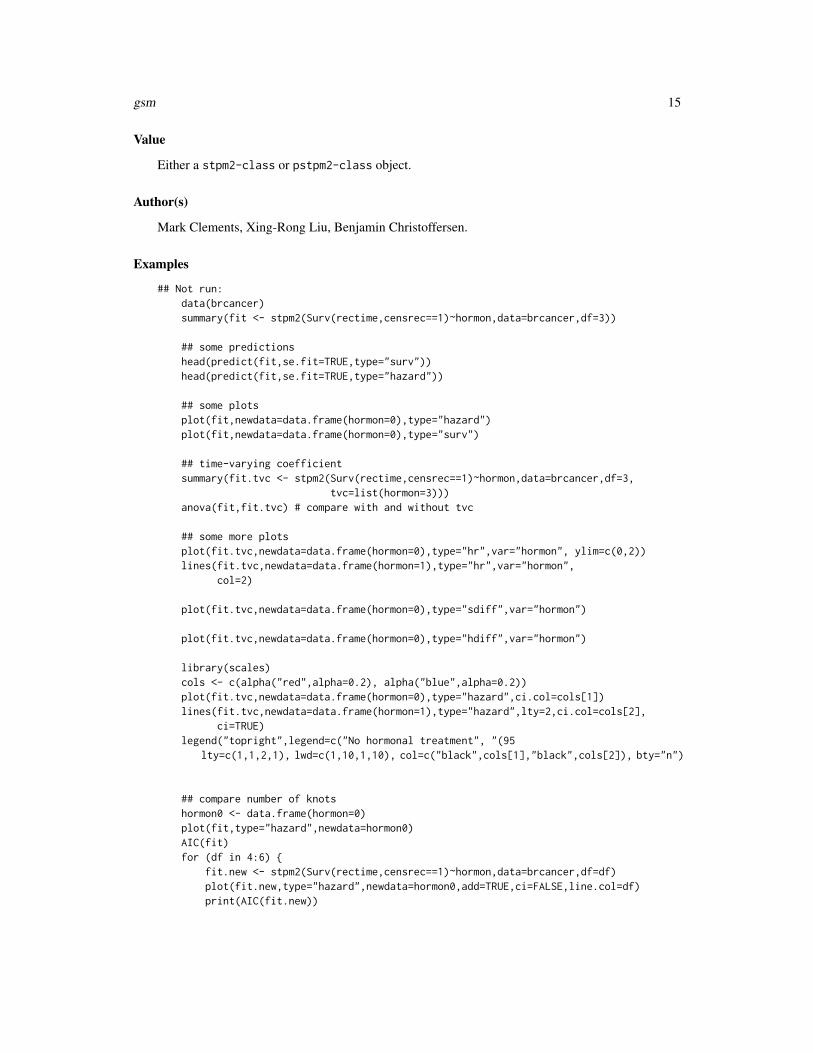
Examples

## Not run:data(brcancer)summary(fit <- stpm2(Surv(rectime,censrec==1)~hormon,data=brcancer,df=3))

## some predictionshead(predict(fit,se.fit=TRUE,type="surv"))head(predict(fit,se.fit=TRUE,type="hazard"))

## some plotsplot(fit,newdata=data.frame(hormon=0),type="hazard")plot(fit,newdata=data.frame(hormon=0),type="surv")

## time-varying coefficientsummary(fit.tvc <- stpm2(Surv(rectime,censrec==1)~hormon,data=brcancer,df=3,

tvc=list(hormon=3)))anova(fit,fit.tvc) # compare with and without tvc

## some more plotsplot(fit.tvc,newdata=data.frame(hormon=0),type="hr",var="hormon", ylim=c(0,2))lines(fit.tvc,newdata=data.frame(hormon=1),type="hr",var="hormon",

col=2)

plot(fit.tvc,newdata=data.frame(hormon=0),type="sdiff",var="hormon")

plot(fit.tvc,newdata=data.frame(hormon=0),type="hdiff",var="hormon")

library(scales)cols <- c(alpha("red",alpha=0.2), alpha("blue",alpha=0.2))plot(fit.tvc,newdata=data.frame(hormon=0),type="hazard",ci.col=cols[1])lines(fit.tvc,newdata=data.frame(hormon=1),type="hazard",lty=2,ci.col=cols[2],

ci=TRUE)legend("topright",legend=c("No hormonal treatment", "(95

lty=c(1,1,2,1), lwd=c(1,10,1,10), col=c("black",cols[1],"black",cols[2]), bty="n")

## compare number of knotshormon0 <- data.frame(hormon=0)plot(fit,type="hazard",newdata=hormon0)AIC(fit)for (df in 4:6) {

fit.new <- stpm2(Surv(rectime,censrec==1)~hormon,data=brcancer,df=df)plot(fit.new,type="hazard",newdata=hormon0,add=TRUE,ci=FALSE,line.col=df)print(AIC(fit.new))

16 gsm.control

}

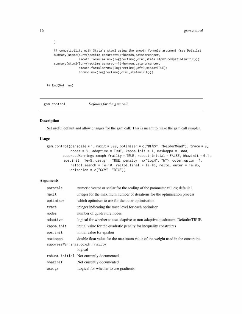
## compatibility with Stata's stpm2 using the smooth.formula argument (see Details)summary(stpm2(Surv(rectime,censrec==1)~hormon,data=brcancer,

smooth.formula=~nsx(log(rectime),df=3,stata.stpm2.compatible=TRUE)))summary(stpm2(Surv(rectime,censrec==1)~hormon,data=brcancer,

smooth.formula=~nsx(log(rectime),df=3,stata=TRUE)+hormon:nsx(log(rectime),df=3,stata=TRUE)))

## End(Not run)

gsm.control Defaults for the gsm call

Description

Set useful default and allow changes for the gsm call. This is meant to make the gsm call simpler.

Usage

gsm.control(parscale = 1, maxit = 300, optimiser = c("BFGS", "NelderMead"), trace = 0,nodes = 9, adaptive = TRUE, kappa.init = 1, maxkappa = 1000,

suppressWarnings.coxph.frailty = TRUE, robust_initial = FALSE, bhazinit = 0.1,eps.init = 1e-5, use.gr = TRUE, penalty = c("logH", "h"), outer_optim = 1,

reltol.search = 1e-10, reltol.final = 1e-10, reltol.outer = 1e-05,criterion = c("GCV", "BIC"))

Arguments

parscale numeric vector or scalar for the scaling of the parameter values; default 1

maxit integer for the maximum number of iterations for the optimisation process

optimiser which optimiser to use for the outer optimisation

trace integer indicating the trace level for each optimiser

nodes number of quadrature nodes

adaptive logical for whether to use adaptive or non-adaptive quadrature, Default=TRUE.

kappa.init initial value for the quadratic penalty for inequality constraints

eps.init initial value for epsilon

maxkappa double float value for the maximum value of the weight used in the constraint.suppressWarnings.coxph.frailty

logical

robust_initial Not currently documented.

bhazinit Not currently documented.

use.gr Logical for whether to use gradients.

incrVar 17

penalty Not currently documented.

outer_optim Not currently documented.

reltol.search Relative tolerance. Not currently documented.

reltol.final Relative tolerance. Not currently documented.

reltol.outer Relative tolerance. Not currently documented.

criterion Not currently documented.

incrVar Utility that returns a function to increment a variable in a data-frame.

Description

A functional approach to defining an increment in one or more variables in a data-frame. Givena variable name and an increment value, return a function that takes any data-frame to return adata-frame with incremented values.

Usage

incrVar(var, increment = 1)

Arguments

var String for the name(s) of the variable(s) to be incremented

increment Value that the variable should be incremented.

Details

Useful for defining transformations for calculating rate ratios.

Value

A function with a single data argument that increments the variables in the data list/data-frame.

Examples


## The function is currently defined asfunction (var, increment = 1){

n <- length(var)if (n > 1 && length(increment)==1)

increment <- rep(increment, n)function(data) {

for (i in 1:n) {

18 lines.stpm2

data[[var[i]]] <- data[[var[i]]] + increment[i]}data

}}

legendre.quadrature.rule.200

Legendre quadrature rule for n=200.

Description

Legendre quadrature rule for n=200.

Usage

data(legendre.quadrature.rule.200)

Format


x x values between -1 and 1

w weights

Examples

data(legendre.quadrature.rule.200)## maybe str(legendre.quadrature.rule.200) ; ...

lines.stpm2 S3 methods for lines

Description

S3 methods for lines

lines.stpm2 19

Usage

## S3 method for class 'stpm2'lines(x, newdata = NULL, type = "surv", col = 1, ci.col= "grey",lty = par("lty"), ci = FALSE, rug = FALSE, var = NULL,exposed = incrVar(var), times = NULL,type.relsurv = c("excess", "total", "other"),ratetable = survival::survexp.us, rmap, scale = 365.24, ...)## S3 method for class 'pstpm2'lines(x, newdata = NULL, type = "surv", col = 1,ci.col= "grey",lty = par("lty"), ci = FALSE, rug = FALSE, var = NULL,exposed = incrVar(var), times = NULL, ...)

Arguments

x an stpm2 object

newdata required list of new data. This defines the unexposed newdata (excluding theevent times).

type specify the type of prediction

col line colour

lty line type

ci.col confidence interval colour

ci whether to plot the confidence interval band (default=TRUE)

rug whether to add a rug plot of the event times to the current plot (default=TRUE)

var specify the variable name or names for the exposed/unexposed (names are givenas characters)

exposed function that takes newdata and returns the exposed dataset. By default, thisincrements var

times specifies the times. By default, this uses a span of the observed times.

type.relsurv type of predictions for relative survival models: either "excess", "total" or "other"

scale scale to go from the days in the ratetable object to the analysis time used inthe analysis

rmap an optional list that maps data set names to the ratetable names. See survexp

ratetable a table of event rates used in relative survival when type.relsurv is "total" or"other"

... additional arguments (add to the plot command)

20 markov_msm

markov_msm Predictions for continuous time, nonhomogeneous Markov multi-statemodels using parametric and penalised survival models.

Description

A numerically efficient algorithm to calculate predictions from a continuous time, nonhomogeneousMarkov multi-state model. The main inputs are the models for the transition intensities, the initialvalues, the transition matrix and the covariate patterns. The predictions include state occupancyprobabilities (possibly with discounting and utilities), length of stay and costs. Standard errors arecalculated using the delta method. Includes, differences, ratios and standardisation.

Usage

markov_msm(x, trans, t = c(0,1), newdata = NULL, init=NULL,tmvar = NULL,

sing.inf = 1e+10, method="adams", rtol=1e-10, atol=1e-10, slow=FALSE,min.tm=1e-8,utility=function(t) rep(1, nrow(trans)),utility.sd=rep(0,nrow(trans)),use.costs=FALSE,

transition.costs=function(t) rep(0, sum(!is.na(trans))), # per transitiontransition.costs.sd=rep(0,sum(!is.na(trans))),state.costs=function(t) rep(0,nrow(trans)), # per unit timestate.costs.sd=rep(0,nrow(trans)),discount.rate = 0,block.size=500,spline.interpolation=FALSE,debug=FALSE,...)

## S3 method for class 'markov_msm'vcov(object, ...)## S3 method for class 'markov_msm'as.data.frame(x, row.names=NULL, optional=FALSE,

ci=TRUE,P.conf.type="logit", L.conf.type="log",

C.conf.type="log",P.range=c(0,1), L.range=c(0,Inf),

C.range=c(0,Inf),state.weights=NULL, obs.weights=NULL,...)

## S3 method for class 'markov_msm_diff'as.data.frame(x, row.names=NULL, optional=FALSE,

P.conf.type="plain", L.conf.type="plain",C.conf.type="plain",

P.range=c(-Inf,Inf), L.range=c(-Inf,Inf),C.range=c(-Inf,Inf),

markov_msm 21

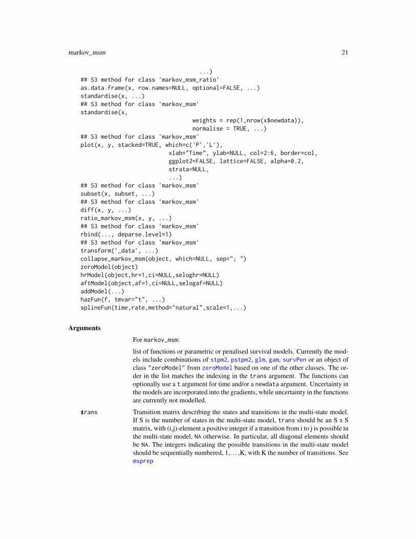
...)## S3 method for class 'markov_msm_ratio'as.data.frame(x, row.names=NULL, optional=FALSE, ...)standardise(x, ...)## S3 method for class 'markov_msm'standardise(x,

weights = rep(1,nrow(x$newdata)),normalise = TRUE, ...)

## S3 method for class 'markov_msm'plot(x, y, stacked=TRUE, which=c('P','L'),

xlab="Time", ylab=NULL, col=2:6, border=col,ggplot2=FALSE, lattice=FALSE, alpha=0.2,strata=NULL,...)

## S3 method for class 'markov_msm'subset(x, subset, ...)## S3 method for class 'markov_msm'diff(x, y, ...)ratio_markov_msm(x, y, ...)## S3 method for class 'markov_msm'rbind(..., deparse.level=1)## S3 method for class 'markov_msm'transform(`_data`, ...)collapse_markov_msm(object, which=NULL, sep="; ")zeroModel(object)hrModel(object,hr=1,ci=NULL,seloghr=NULL)aftModel(object,af=1,ci=NULL,selogaf=NULL)addModel(...)hazFun(f, tmvar="t", ...)splineFun(time,rate,method="natural",scale=1,...)

Arguments

For markov_msm:

list of functions or parametric or penalised survival models. Currently the mod-els include combinations of stpm2, pstpm2, glm, gam, survPen or an object ofclass "zeroModel" from zeroModel based on one of the other classes. The or-der in the list matches the indexing in the trans argument. The functions canoptionally use a t argument for time and/or a newdata argument. Uncertainty inthe models are incorporated into the gradients, while uncertainty in the functionsare currently not modelled.

xtrans Transition matrix describing the states and transitions in the multi-state model.If S is the number of states in the multi-state model, trans should be an S x Smatrix, with (i,j)-element a positive integer if a transition from i to j is possible inthe multi-state model, NA otherwise. In particular, all diagonal elements shouldbe NA. The integers indicating the possible transitions in the multi-state modelshould be sequentially numbered, 1,. . . ,K, with K the number of transitions. Seemsprep

22 markov_msm

t numerical vector for the times to evaluation the predictions. Includes the starttime

newdata data.frame of the covariates to use in the predictions

init vector of the initial values with the same length as the number of states. Defaultsto the first state having an initial value of 1 (i.e. "[<-"(rep(0,nrow(trans)),1,1)).

tmvar specifies the name of the time variable. This should be set for regression modelsthat do not specify this (e.g. glm) or where the time variable is ambiguous

sing.inf If there is a singularity in the observed hazard, for example a Weibull distributionwith shape < 1 has infinite hazard at t=0, then as a workaround, the hazardis assumed to be a large finite number, sing.inf, at this time. The resultsshould not be sensitive to the exact value assumed, but users should make sureby adjusting this parameter in these cases.

method For markov_msm, the method used by the ordinary differential equation solver.Defaults to Adams method ("adams") for non-stiff differential equations.For splineFun, the method jused for spline interpolation; see splinefun.

rtol relative error tolerance, either a scalar or an array as long as the number of states.Passed to lsode

atol absolute error tolerance, either a scalar or an array as long as the number ofstates. Passed to lsode

slow logical to show whether to use the slow R-only implementation. Useful for de-bugging. Currently needed for costs.

min.tm Minimum time used for evaluations. Avoids log(0) for some models.

utility a function of the form function(t) that returns a utility for each state at time tfor the length of stay values

utility.sd a function of the form function(t) that returns the standard deviation for theutility for each state at time t for the length of stay values

use.costs logical for whether to use costs. Default: FALSEtransition.costs

a function of the form function(t) that returns the cost for each transitiontransition.costs.sd

a function of the form function(t) that returns the standard deviation for thecost for each transition

state.costs a function of the form function(t) that returns the cost per unit time for eachstate

state.costs.sd a function of the form function(t) that returns the standard deviation for thecost per unit time for each state

discount.rate numerical value for the proportional reduction (per unit time) in the length ofstay and costs

block.size divide newdata into blocks. Uses less memory but is slower. Reduce this num-ber if the function call runs out of memory.

spline.interpolation

logical for whether to use spline interpolation for the transition hazards ratherthan the model predictions directly (default=TRUE).

markov_msm 23

debug logical flag for whether to keep the full output from the ordinary differentialequation in the res component (default=FALSE).

... other arguments. For markov_msm, these are passed to the ode solver fromthe deSolve package. For plot.markov_msm, these arguments are passed toplot.default

For as.data.frame.markov_msm:

row.names add in row names to the output data-frame

optional (not currently used)

ci logical for whether to include confidence intervals. Default: TRUE

P.conf.type type of transformation for the confidence interval calculation for the state occu-pancy probabilities. Default: log-log transformation. This is changed for diffand ratio_markov_msm objects

L.conf.type type of transformation for the confidence interval calculation for the length ofstay calculation. Default: log transformation. This is changed for diff andratio_markov_msm objects

C.conf.type type of transformation for the confidence interval calculation for the length ofstay calculation. Default: log transformation. This is changed for diff andratio_markov_msm objects

P.range valid values for the state occupancy probabilities. Default: (0,1). This is changedfor diff and ratio_markov_msm objects

L.range valid values for the state occupancy probabilities. Default: (0,Inf). This ischanged for diff and ratio_markov_msm objects

C.range valid values for the state occupancy probabilities. Default: (0,Inf). This ischanged for diff and ratio_markov_msm objects

state.weights Not currently documented

obs.weights Not currently documentedFor standardise.markov_msm:

weights numerical vector to use in standardising the state occupancy probabilities, lengthof stay and costs. Default: 1 for each observation.

normalise logical for whether to normalise the weights to 1. Default: TRUEFor plot.markov_msm:

y (currently ignored)

stacked logical for whether to stack the plots. Default: TRUE

xlab x-axis label

ylab x-axis label

col colours (ignored if ggplot2=TRUE)

border border colours for the polygon (ignored if ggplot=TRUE)

ggplot2 use ggplot2

alpha alpha value for confidence bands (ggplot)

lattice use lattice

24 markov_msm

strata formula for the stratification factors for the plotFor subset.markov_msm:

subset expression that is evaluated on the newdata component of the object to filter (orrestrict) for the covariates used for predictionsFor transform.markov_msm:

_data an object of class "markov_msm"For rbind.markov_msm:

deparse.level not currently usedFor collapse.states:

which either an index of the states to collapse or a character vector of the state namesto collapse

sep separator to use for the collapsed state namesFor zeroModel to predict zero rates:

object survival regression object to be wrappedFor hrModel to predict rates times a hazard ratio:

hr hazard ratio

seloghr alternative specification for the se of the log(hazard ratio); see also ci argumentFor aftModel to predict accelerated rates:

af acceleration factor

selogaf alternative specification for the se of the log(acceleration factor); see also ciargumentaddModel predict rates based on adding rates from different modelshazFun provides a rate function without uncertainty:

f rate function, possibly with tmvar and/or newdata as argumentssplineFun predicts rates using spline interpolation:

time exact times

rate rates as per time

scale rate multiplier (e.g. scale=365.25 for converting from daily rates to yearlyrates)

Details

The predictions are calculated using an ordinary differential equation solver. The algorithm uses asingle run of the solver to calculate the state occupancy probabilities, length of stay, costs and theirpartial derivatives with respect to the model parameters. The predictions can also be combined tocalculate differences, ratios and standardised.

The current implementation supports a list of models for each transition.

The current implementation also only allows for a vector of initial values rather than a matrix. Thepredictions will need to be re-run for different vectors of initial values.

For as.data.frame.markov_msm_ratio, the data are provided in log form, hence the default trans-formations and bounds are as per as.data.frame.markov_msm_diff, with untransformed data onthe real line.

TODO: allow for one model to predict for the different transitions.

markov_msm 25

Value

markov_msm returns an object of class "markov_msm".

The function summary is used to obtain and print a summary and analysis of variance table of theresults. The generic accessor functions coef and vcov extract various useful features of the valuereturned by markov_msm.

An object of class "markov_msm" is a list containing at least the following components:

time a numeric vector with the times for the predictions

P an array for the predicted state occupancy probabilities. The array has threedimensions: time, state, and observations.

L an array for the predicted sojourn times (or length of stay). The array has threedimensions: time, state, and observations.

Pu an array for the partial derivatives of the predicted state occupancy probabilitieswith respect to the model coefficients. The array has four dimensions: time,state, coefficients, and observations.

Lu an array for the partial derivatives of the predicted sojourn times (or lengthof stay) with respect to the model coefficients. The array has four dimensions:time, state, coefficients, and observations.

newdata a data.frame with the covariates used for the predictions

vcov the variance-covariance matrix for the models of the transition intensities

trans copy of the trans input argument

call the call to the function

For debugging:

res data returned from the ordinary differential equation solver. This may includemore information on the predictions

Author(s)

Mark Clements

See Also

pmatrix.fs, probtrans

Examples

## Not run:library(readstata13)library(mstate)library(ggplot2)library(survival)## Two states: Initial -> Final## Note: this shows how to use markov_msm to estimate survival and risk probabilities based on## smooth hazard models.two_states <- function(model, ...) {

26 markov_msm

transmat = matrix(c(NA,1,NA,NA),2,2,byrow=TRUE)rownames(transmat) <- colnames(transmat) <- c("Initial","Final")rstpm2::markov_msm(list(model), ..., trans = transmat)

}## Note: the first argument is the hazard model. The other arguments are arguments to the## markov_msm function, except for the transition matrix, which is defined by the new function.death = gsm(Surv(time,status)~factor(rx), data=survival::colon, subset=(etype==2), df=3)cr = two_states(death, newdata=data.frame(rx="Obs"), t = seq(0,2500, length=301))plot(cr,ggplot=TRUE)

## Competing risks## Note: this shows how to adapt the markov_msm model for competing risks.competing_risks <- function(listOfModels, ...) {

nRisks = length(listOfModels)transmat = matrix(NA,nRisks+1,nRisks+1)transmat[1,1+(1:nRisks)] = 1:nRisksrownames(transmat) <- colnames(transmat) <- c("Initial",names(listOfModels))rstpm2::markov_msm(listOfModels, ..., trans = transmat)

}## Note: The first argument for competing_risks is a list of models. Names from that list are## used for labelling the states. The other arguments are as per the markov_msm function,## except for the transition matrix, which is defined by the competing_risks function.recurrence = gsm(Surv(time,status)~factor(rx), data=survival::colon, subset=(etype==1), df=3)death = gsm(Surv(time,status)~factor(rx), data=survival::colon, subset=(etype==2), df=3)cr = competing_risks(list(Recurrence=recurrence,Death=death),

newdata=data.frame(rx=levels(survival::colon$rx)),t = seq(0,2500, length=301))

## Plot the probabilities for each state for three different treatment armsplot(cr, ggplot=TRUE) + facet_grid(~ rx)## And: differences in probabilitiescr_diff = diff(subset(cr,rx=="Lev+5FU"),subset(cr,rx=="Obs"))plot(cr_diff, ggplot=TRUE, stacked=FALSE)

## Extended example: Crowther and Lambert (2019)mex.1 <- read.dta13("http://fmwww.bc.edu/repec/bocode/m/multistate_example.dta")transmat <- rbind("Post-surgery"=c(NA,1,2),

"Relapsed"=c(NA,NA,3),"Died"=c(NA,NA,NA))

colnames(transmat) <- rownames(transmat)mex.2 <- transform(mex.1,osi=(osi=="deceased")+0)levels(mex.2$size)[2] <- ">20-50 mm" # fix typomex <- mstate::msprep(time=c(NA,"rf","os"),status=c(NA,"rfi","osi"),

data=mex.2,trans=transmat,id="pid",keep=c("age","size","nodes","pr_1","hormon"))

mex <- transform(mex,size2=(unclass(size)==2)+0, # avoids issues with TRUE/FALSEsize3=(unclass(size)==3)+0,hormon=(hormon=="yes")+0,Tstart=Tstart/12,Tstop=Tstop/12)

##c.ar <- stpm2(Surv(Tstart,Tstop,status) ~ age + size2 + size3 + nodes + pr_1 + hormon,

data = mex, subset=trans==1, df=3, tvc=list(size2=1,size3=1,pr_1=1))

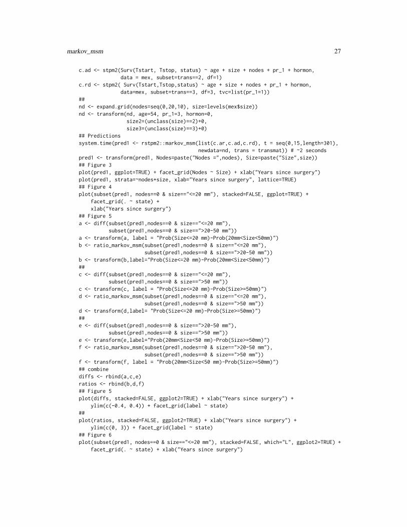
markov_msm 27

c.ad <- stpm2(Surv(Tstart, Tstop, status) ~ age + size + nodes + pr_1 + hormon,data = mex, subset=trans==2, df=1)

c.rd <- stpm2( Surv(Tstart,Tstop,status) ~ age + size + nodes + pr_1 + hormon,data=mex, subset=trans==3, df=3, tvc=list(pr_1=1))

##nd <- expand.grid(nodes=seq(0,20,10), size=levels(mex$size))nd <- transform(nd, age=54, pr_1=3, hormon=0,

size2=(unclass(size)==2)+0,size3=(unclass(size)==3)+0)

## Predictionssystem.time(pred1 <- rstpm2::markov_msm(list(c.ar,c.ad,c.rd), t = seq(0,15,length=301),

newdata=nd, trans = transmat)) # ~2 secondspred1 <- transform(pred1, Nodes=paste("Nodes =",nodes), Size=paste("Size",size))## Figure 3plot(pred1, ggplot=TRUE) + facet_grid(Nodes ~ Size) + xlab("Years since surgery")plot(pred1, strata=~nodes+size, xlab="Years since surgery", lattice=TRUE)## Figure 4plot(subset(pred1, nodes==0 & size=="<=20 mm"), stacked=FALSE, ggplot=TRUE) +

facet_grid(. ~ state) +xlab("Years since surgery")

## Figure 5a <- diff(subset(pred1,nodes==0 & size=="<=20 mm"),

subset(pred1,nodes==0 & size==">20-50 mm"))a <- transform(a, label = "Prob(Size<=20 mm)-Prob(20mm<Size<50mm)")b <- ratio_markov_msm(subset(pred1,nodes==0 & size=="<=20 mm"),

subset(pred1,nodes==0 & size==">20-50 mm"))b <- transform(b,label="Prob(Size<=20 mm)-Prob(20mm<Size<50mm)")##c <- diff(subset(pred1,nodes==0 & size=="<=20 mm"),

subset(pred1,nodes==0 & size==">50 mm"))c <- transform(c, label = "Prob(Size<=20 mm)-Prob(Size>=50mm)")d <- ratio_markov_msm(subset(pred1,nodes==0 & size=="<=20 mm"),

subset(pred1,nodes==0 & size==">50 mm"))d <- transform(d,label= "Prob(Size<=20 mm)-Prob(Size>=50mm)")##e <- diff(subset(pred1,nodes==0 & size==">20-50 mm"),

subset(pred1,nodes==0 & size==">50 mm"))e <- transform(e,label="Prob(20mm<Size<50 mm)-Prob(Size>=50mm)")f <- ratio_markov_msm(subset(pred1,nodes==0 & size==">20-50 mm"),

subset(pred1,nodes==0 & size==">50 mm"))f <- transform(f, label = "Prob(20mm<Size<50 mm)-Prob(Size>=50mm)")## combinediffs <- rbind(a,c,e)ratios <- rbind(b,d,f)## Figure 5plot(diffs, stacked=FALSE, ggplot2=TRUE) + xlab("Years since surgery") +

ylim(c(-0.4, 0.4)) + facet_grid(label ~ state)##plot(ratios, stacked=FALSE, ggplot2=TRUE) + xlab("Years since surgery") +

ylim(c(0, 3)) + facet_grid(label ~ state)## Figure 6plot(subset(pred1, nodes==0 & size=="<=20 mm"), stacked=FALSE, which="L", ggplot2=TRUE) +

facet_grid(. ~ state) + xlab("Years since surgery")

28 nsx

## Figure 7plot(diffs, stacked=FALSE, which="L", ggplot2=TRUE) + xlab("Years since surgery") +

ylim(c(-4, 4)) + facet_grid(label ~ state)plot(ratios, stacked=FALSE, which="L", ggplot2=TRUE) + xlab("Years since surgery") +

ylim(c(0.1, 10)) + coord_trans(y="log10") + facet_grid(label ~ state)

## End(Not run)

nsx Generate a Basis Matrix for Natural Cubic Splines (with eXtensions)

Description

Generate the B-spline basis matrix for a natural cubic spline (with eXtensions).

Usage

nsx(x, df = NULL, knots = NULL, intercept = FALSE,Boundary.knots = range(x), derivs = if (cure) c(2, 1) else c(2, 2),log = FALSE, centre = FALSE,cure = FALSE, stata.stpm2.compatible = FALSE)

Arguments

x the predictor variable. Missing values are allowed.

df degrees of freedom. One can supply df rather than knots; ns() then choosesdf -1 -intercept + 4 -sum(derivs) knots at suitably chosen quantiles of x(which will ignore missing values).

knots breakpoints that define the spline. The default is no knots; together with thenatural boundary conditions this results in a basis for linear regression on x.Typical values are the mean or median for one knot, quantiles for more knots.See also Boundary.knots.

intercept if TRUE, an intercept is included in the basis; default is FALSE.

Boundary.knots boundary points at which to impose the natural boundary conditions and anchorthe B-spline basis (default the range of the data). If both knots and Boundary.knotsare supplied, the basis parameters do not depend on x. Data can extend beyondBoundary.knots

derivs an integer vector of length 2 with values between 0 and 2 giving the derivativeconstraint order at the left and right boundary knots; an order of 2 constrains thesecond derivative to zero (f”(x)=0); an order of 1 constrains the first and secondderivatives to zero (f’(x)=f”(x)=0); an order of 1 constrains the zero, first andsecond derivatives to zero (f(x)=f’(x)=f”(x)=0)

log a Boolean indicating whether the underlying values have been log transformed;(deprecated: only used to calculate derivatives in rstpm2:::stpm2Old

centre if specified, then centre the splines at this value (i.e. f(centre)=0) (default=FALSE)

nsx 29

cure a Boolean indicated whether to estimate cure; changes the default derivs ar-gument, such that the right boundary has the first and second derivatives con-strained to zero; defaults to FALSE

stata.stpm2.compatible

a Boolean to determine whether to use Stata stpm’s default knot placement;defaults to FALSE

Value

A matrix of dimension length(x) * df where either df was supplied or if knots were supplied, df= length(knots) + 1 + intercept. Attributes are returned that correspond to the arguments to ns,and explicitly give the knots, Boundary.knots etc for use by predict.nsx().

nsx() is based on the functions ns and spline.des. It generates a basis matrix for representingthe family of piecewise-cubic splines with the specified sequence of interior knots, and the naturalboundary conditions. These enforce the constraint that the function is linear beyond the boundaryknots, which can either be supplied, else default to the extremes of the data. A primary use is inmodeling formula to directly specify a natural spline term in a model.

The extensions from ns are: specification of the derivative constraints at the boundary knots;whether to centre the knots; incorporation of cure using derivatives; compatible knots with Stata’sstpm2; and an indicator for a log-transformation of x for calculating derivatives.

References

Hastie, T. J. (1992) Generalized additive models. Chapter 7 of Statistical Models in S eds J. M.Chambers and T. J. Hastie, Wadsworth & Brooks/Cole.

See Also

ns, bs, predict.nsx, SafePrediction

Examples

require(stats); require(graphics); require(splines)nsx(women$height, df = 5)summary(fm1 <- lm(weight ~ ns(height, df = 5), data = women))

## example of safe predictionplot(women, xlab = "Height (in)", ylab = "Weight (lb)")ht <- seq(57, 73, length.out = 200)lines(ht, predict(fm1, data.frame(height=ht)))

30 nsxD

nsxD Generate a Basis Matrix for the first derivative of Natural CubicSplines (with eXtensions)

Description

Generate the B-spline basis matrix for the first derivative of a natural cubic spline (with eXtensions).

Usage

nsxD(x, df = NULL, knots = NULL, intercept = FALSE,Boundary.knots = range(x), derivs = if (cure) c(2, 1) else c(2, 2),log = FALSE, centre = FALSE,cure = FALSE, stata.stpm2.compatible = FALSE)

Arguments

x the predictor variable. Missing values are allowed.

df degrees of freedom. One can supply df rather than knots; ns() then choosesdf -1 -intercept + 4 -sum(derivs) knots at suitably chosen quantiles of x(which will ignore missing values).

knots breakpoints that define the spline. The default is no knots; together with thenatural boundary conditions this results in a basis for linear regression on x.Typical values are the mean or median for one knot, quantiles for more knots.See also Boundary.knots.

intercept if TRUE, an intercept is included in the basis; default is FALSE.

Boundary.knots boundary points at which to impose the natural boundary conditions and anchorthe B-spline basis (default the range of the data). If both knots and Boundary.knotsare supplied, the basis parameters do not depend on x. Data can extend beyondBoundary.knots

derivs an integer vector of length 2 with values between 0 and 2 giving the derivativeconstraint order at the left and right boundary knots; an order of 2 constrains thesecond derivative to zero (f”(x)=0); an order of 1 constrains the first and secondderivatives to zero (f’(x)=f”(x)=0); an order of 1 constrains the zero, first andsecond derivatives to zero (f(x)=f’(x)=f”(x)=0)

nsxD 31

log a Boolean indicating whether the underlying values have been log transformed;(deprecated: only used to calculate derivatives in rstpm2:::stpm2Old

centre if specified, then centre the splines at this value (i.e. f(centre)=0) (default=FALSE)

cure a Boolean indicated whether to estimate cure; changes the default derivs ar-gument, such that the right boundary has the first and second derivatives con-strained to zero; defaults to FALSE

stata.stpm2.compatible

a Boolean to determine whether to use Stata stpm’s default knot placement;defaults to FALSE

Value

A matrix of dimension length(x) * df where either df was supplied or if knots were supplied, df= length(knots) + 1 + intercept. Attributes are returned that correspond to the arguments to ns,and explicitly give the knots, Boundary.knots etc for use by predict.nsxD().

nsxD() is based on the functions ns and spline.des. It generates a basis matrix for representingthe family of piecewise-cubic splines with the specified sequence of interior knots, and the naturalboundary conditions. These enforce the constraint that the function is linear beyond the boundaryknots, which can either be supplied, else default to the extremes of the data. A primary use is inmodeling formula to directly specify a natural spline term in a model.

The extensions from ns are: specification of the derivative constraints at the boundary knots;whether to centre the knots; incorporation of cure using derivatives; compatible knots with Stata’sstpm2; and an indicator for a log-transformation of x for calculating derivatives.

References

Hastie, T. J. (1992) Generalized additive models. Chapter 7 of Statistical Models in S eds J. M.Chambers and T. J. Hastie, Wadsworth & Brooks/Cole.

See Also

ns, bs, predict.nsx, SafePrediction

Examples

require(stats); require(graphics); require(splines)nsx(women$height, df = 5)summary(fm1 <- lm(weight ~ ns(height, df = 5), data = women))

## example of safe predictionplot(women, xlab = "Height (in)", ylab = "Weight (lb)")ht <- seq(57, 73, length.out = 200)lines(ht, predict(fm1, data.frame(height=ht)))

32 numDeltaMethod

numDeltaMethod Calculate numerical delta method for non-linear predictions.

Description

Given a regression object and an independent prediction function (as a function of the coefficients),calculate the point estimate and standard errors

Usage

numDeltaMethod(object, fun, gd=NULL, ...)

Arguments

object A regression object with methods coef and vcov.

fun An independent prediction function with signature function(coef,...).

gd Specified gradients

... Other arguments passed to fun.

Details

A more user-friendly interface is provided by predictnl.

Value

Estimate Point estimates

SE Standard errors

See Also

See Also predictnl.

plot-methods 33

Examples


## The function is currently defined asfunction (object, fun, ...){

coef <- coef(object)est <- fun(coef, ...)Sigma <- vcov(object)gd <- grad(fun, coef, ...)se.est <- as.vector(sqrt(colSums(gd * (Sigma %*% gd))))data.frame(Estimate = est, SE = se.est)

}

plot-methods plots for an stpm2 fit

Description

Given an stpm2 fit, return a plot

Usage

## S4 method for signature 'stpm2'plot(x,y,newdata,type="surv",

xlab="Time",line.col=1,ci.col="grey",add=FALSE,ci=TRUE,rug=TRUE,var=NULL,exposed=incrVar(var),times=NULL,...)

## S4 method for signature 'pstpm2'plot(x,y,newdata,type="surv",

xlab="Time",line.col=1,ci.col="grey",add=FALSE,ci=TRUE,rug=TRUE,var=NULL,exposed=incrVar(var),times=NULL,...)

Arguments

x an stpm2 object

y not used (for generic compatibility)

newdata required list of new data. This defines the unexposed newdata (excluding theevent times).

type specify the type of prediction

xlab x-axis label

line.col line colour

34 popmort

ci.col confidence interval colour

ci whether to plot the confidence interval band (default=TRUE)

add whether to add to the current plot (add=TRUE) or make a new plot (add=FALSE)(default=FALSE)

rug whether to add a rug plot of the event times to the current plot (default=TRUE)


exposed function that takes newdata and returns the exposed dataset. By default, thisincrements var

times specifies the times. By default, this uses a span of the observed times.

... additional arguments (add to the plot command)

Methods

x = "stpm2", y = "missing" an stpm2 fit

See Also

stpm2

popmort Background mortality rates for the colon dataset.

Description

Background mortality rates for the colon dataset.

Usage

data(popmort)

Format


sex Sex (1=male, 2=female)

prob One year probability of survival

rate All cause mortality rate

age Age by single year of age through to age 105 years

year Calendar period

Examples

data(popmort)## maybe str(popmort) ; ...

predict-methods 35

predict-methods Predicted values for an stpm2 or pstpm2 fit

Description

Given an stpm2 fit and an optional list of new data, return predictions

Usage

## S4 method for signature 'stpm2'predict(object, newdata=NULL,

type=c("surv","cumhaz","hazard","density","hr","sdiff","hdiff","loghazard","link","meansurv","meansurvdiff","meanhr","odds","or","margsurv","marghaz","marghr","meanhaz","af","fail","margfail","meanmargsurv","uncured","rmst","probcure","lpmatrix", "gradh", "gradH"),grid=FALSE,seqLength=300,type.relsurv=c("excess","total","other"), scale=365.24,rmap, ratetable=survival::survexp.us,se.fit=FALSE,link=NULL,exposed=incrVar(var),var=NULL,keep.attributes=FALSE, use.gr=TRUE,level=0.95,n.gauss.quad=100,full=FALSE,...)

## S4 method for signature 'pstpm2'predict(object, newdata=NULL,

type=c("surv","cumhaz","hazard","density","hr","sdiff","hdiff","loghazard","link","meansurv","meansurvdiff","meanhr","odds","or","margsurv","marghaz","marghr","meanhaz","af","fail","margfail","meanmargsurv","rmst","lpmatrix","gradh", "gradH"),grid=FALSE,seqLength=300,se.fit=FALSE,link=NULL,exposed=incrVar(var),var=NULL,keep.attributes=FALSE, use.gr=TRUE,level=0.95,n.gauss.quad=100,full=FALSE,...)

Arguments

object an stpm2 or pstpm2 object

newdata optional list of new data (required if type in ("hr","sdiff","hdiff","meansurvdiff","or","uncured")).For type in ("hr","sdiff","hdiff","meansurvdiff","or","af","uncured"), this definesthe unexposed newdata. This can be combined with grid to get a regular set ofevent times (i.e. newdata would not include the event times).

type specify the type of prediction:

• "surv"survival probabilities• "cumhaz"cumulative hazard• "hazard"hazard

36 predict-methods

• "density"density• "hr"hazard ratio• "sdiff"survival difference• "hdiff"hazard difference• "loghazard"log hazards• "meansurv"mean survival• "meansurvdiff"mean survival difference• "odds"odds• "or"odds ratio• "margsurv"marginal (population) survival• "marghaz"marginal (population) hazard• "marghr"marginal (population) hazard ratio• "meanhaz"mean hazard• "meanhr"mean hazard ratio• "af"attributable fraction• "fail"failure (=1-survival)• "margfail"marginal failure (=1-marginal survival)• "meanmargsurv"mean marginal survival, averaged over the frailty distribu-

tion• "uncured"distribution for the uncured• "rmst"restricted mean survival time• "probcure"probability of cure• "lpmatrix"design matrix

grid whether to merge newdata with a regular sequence of event times (default=FALSE)

seqLength length of the sequence used when grid=TRUE

type.relsurv type of predictions for relative survival models: either "excess", "total" or "other"

scale scale to go from the days in the ratetable object to the analysis time used inthe analysis

rmap an optional list that maps data set names to the ratetable names. See survexp

ratetable a table of event rates used in relative survival when type.relsurv is "total" or"other"

se.fit whether to calculate confidence intervals (default=FALSE)

link allows a different link for the confidence interval calculation (default=NULL,such that switch(type,surv="cloglog",cumhaz="log",hazard="log",hr="log",sdiff="I",hdiff="I",loghazard="I",link="I",odds="log",or="log",margsurv="cloglog", marg-haz="log",marghr="log"))

exposed a function that takes newdata and returns a transformed data-frame for thoseexposed or the counterfactual (defaults to incrementing “var”)


keep.attributes

Boolean to determine whether the output should include the newdata as an at-tribute (default=TRUE)

predict.nsx 37

use.gr Boolean to determine whether to use gradients in the variance calculations whenthey are available (default=TRUE)

level confidence level for the confidence intervals (default=0.95)

n.gauss.quad number of Gauassian quadrature points used for integrations (default=100)

full logical for whether to return a full data-frame with predictions and newdatacombined. Useful for lattice and ggplot2 plots. (default=FALSE)

... additional arguments (for generic compatibility)

Details

The confidence interval estimation is based on the delta method using numerical differentiation.

Value

A data-frame with components Estimate, lower and upper, with an attribute "newdata" for thenewdata data-frame.

Methods

object= "stpm2" an stpm2 fit

See Also

stpm2

predict.nsx Evaluate a Spline Basis

Description

Evaluate a predefined spline basis at given values.

Usage

## S3 method for class 'nsx'predict(object, newx, ...)

Arguments

object the result of a call to nsx having attributes describing knots, degree, etc.

newx the x values at which evaluations are required.

... Optional additional arguments. At present no additional arguments are used.

38 predictnl

Value

An object just like object, except evaluated at the new values of x.

These are methods for the generic function predict for objects inheriting from classes "nsx". Seepredict for the general behavior of this function.

See Also

nsx.

Examples

basis <- nsx(women$height, df = 5)newX <- seq(58, 72, length.out = 51)# evaluate the basis at the new datapredict(basis, newX)

predictnl Estimation of standard errors using the numerical delta method.

Description

A simple, yet exceedingly useful, approach to estimate the variance of a function using the numeri-cal delta method. A number of packages provide functions that analytically calculate the gradients;we use numerical derivatives, which generalises to models that do not offer analytical derivatives(e.g. ordinary differential equations, integration), or to examples that are tedious or error-prone tocalculate (e.g. sums of predictions from GLMs).

Usage

## Default S3 method:predictnl(object, fun, newdata=NULL, gd=NULL, ...)## S3 method for class 'lm'predictnl(object, fun, newdata=NULL, ...)## S3 method for class 'predictnl'print(x, ...)## S3 method for class 'formula'predict(object,data,newdata,na.action,type="model.matrix",...)## S3 method for class 'predictnl'confint(object, parm, level=0.95, ...)

Arguments

object An object with coef, vcov and `coef<-` methods (required).

fun A function that takes object as the first argument, possibly with newdata andother arguments (required). See notes for why it is often useful to includenewdata as an argument to the function.

predictnl 39

newdata An optional argument that defines newdata to be passed to fun.

gd An optional matrix of gradients. If this is not specified, then the gradients arecalculated using finite differences.

parm currently ignored

level significance level for 2-sided confidence intervals

x a predictnl object to be printed.

data object used to define the model frame

na.action passed to model.frame

type currently restricted to "model.matrix"

... Other arguments that are passed to fun.

Details

The signature for fun is either fun(object,...) or fun(object,newdata=NULL,...).

The different predictnl methods call the utility function numDeltaMethod, which in turn callsthe grad function for numerical differentiation. The numDeltaMethod function calls the standardcoef and vcov methods, and the non-standard `coef<-` method for changing the coefficients in aregression object. This non-standard method has been provided for several regression objects andessentially mirrors the coef method.

One potential issue is that some predict methods do not re-calculate their predictions for the fitteddataset (i.e. when newdata=NULL). As the predictnl function changes the fitted coefficients, itis required that the predictions are re-calculated. One solution is to pass newdata as an argumentto both predictnl and fun; alternatively, newdata can be specified in fun. These approaches aredescribed in the examples below. The numDeltaMethod method called by predictnl provides awarning when the variance estimates are zero, which may be due to this cause.

For completeness, it is worth discussing why the example predictnl(fit,predict) does notwork for when fit is a glm object. First, predict.glm does not update the predictions for thefitted data. Second, the default predict method has a signature predict(object,...), whichdoes not include a newdata argument. We could then either (i) require that a newdata argumentbe passed to the fun function for all examples, which would make this corner case work, or (ii)only pass the newdata argument if it is non-null or in the formals for the fun function, whichwould fail for this corner case. The current API defaults to the latter case (ii). To support thisapproach, the predictnl.lm method replaces a null newdata with object$data. We also providea revised numdelta:::predict.lm method that performs the same operation, although its use isnot encouraged due to its clumsiness.

Value

Returns an object of class an object with class c("predictnl","data.frame") elements c("fit","se.fit","Estimate","SE")and with methods print and confint. Note that the Estimate and SE fields are deprecated and theiruse is discouraged, as we would like to remove them from future releases.

Author(s)

Mark Clements

40 pstpm2-class

Examples

df <- data.frame(x=0:1, y=c(10, 20))fit <- glm(y ~ x, df, family=poisson)

predictnl(fit,function(obj,newdata)diff(predict(obj,newdata,type="response")))

predictnl-methods ~~ Methods for Function predictnl ~~

Description

~~ Methods for function predictnl ~~

Methods

predictnl signature(object = "mle2",...): Similar to predictnl.default, using S4 methods.

pstpm2-class Class "pstpm2"

Description

Regression object for pstpm2.


Objects can be created by calls of the form new("pstpm2",...) and pstpm2( ...).

Slots

xlevels: Object of class "list" ~~

contrasts: Object of class "listOrNULL" ~~

terms: Object of class "terms" ~~

gam: Object of class "gam" ~~

logli: Object of class "function" ~~

timeVar: Object of class "character" ~~

time0Var: Object of class "character" ~~

time0Expr: Object of class "nameOrcall" ~~

timeExpr: Object of class "nameOrcall" ~~

pstpm2-class 41

like: Object of class "function" ~~

model.frame: Object of class "list" ~~

delayed: Object of class "logical" ~~

frailty: Object of class "logical" ~~

x: Object of class "matrix" ~~

xd: Object of class "matrix" ~~

termsd: Object of class "terms" ~~

Call: Object of class "character" ~~

y: Object of class "Surv" ~~

sp: Object of class "numeric" ~~

nevent: Object of class "numeric" ~~

link: Object of class "list" ~~

edf: Object of class "numeric" ~~

edf_var: Object of class "numeric" ~~

df: Object of class "numeric" ~~

call: Object of class "language" ~~

call.orig: Object of class "language" ~~

coef: Object of class "numeric" ~~

fullcoef: Object of class "numeric" ~~

vcov: Object of class "matrix" ~~

min: Object of class "numeric" ~~

details: Object of class "list" ~~

minuslogl: Object of class "function" ~~

method: Object of class "character" ~~

data: Object of class "list" ~~

formula: Object of class "character" ~~

optimizer: Object of class "character" ~~


Extends


Methods

plot signature(x = "pstpm2",y = "missing"): ...

lines signature(x = "pstpm2",...): ...

anova signature(object = "pstpm2",...): ...

AIC signature(object = "pstpm2",...,k=2): ...

42 residuals-methods

AICc signature(object = "pstpm2",...,nobs=NULL,k=2): ...

BIC signature(object = "pstpm2",...,nobs = NULL): ...

qAICc signature(object = "pstpm2",...,nobs = NULL,dispersion = 1,k = 2): ...

qAIC signature(object = "pstpm2",...,dispersion = 1,k = 2): ...

summary signature(object = "pstpm2",...): ...

eform signature(object = "pstpm2",...): ...

predictnl signature(object = "pstpm2",...): ...

Examples

showClass("pstpm2")

residuals-methods Residual values for an stpm2 or pstpm2 fit

Description

Given an stpm2 or pstpm2 fit, return residuals

Usage

## S4 method for signature 'stpm2'residuals(object, type=c("li","gradli"))

## S4 method for signature 'pstpm2'residuals(object, type=c("li","gradli"))

Arguments

object an stpm2 or pstpm2 object

type specify the type of residuals:

• "li"log-likelihood components (not strictly residuals)• "gradli"gradient of the log-likelihood components (not strictly residuals)

Details

The gradients are analytical.

Value

A vector or matrix.

Methods

object= "stpm2" an stpm2 fit

rstpm2-internal 43

See Also

stpm2

rstpm2-internal Internal functions for the rstpm2 package.

Description

Various utility functions used internally to the rstpm2 package.

Usage

lhs(formula)rhs(formula)lhs(formula) <- valuerhs(formula) <- value

Arguments

formula A formula

value A symbolic value to replace the current value.

stpm2-class Class "stpm2" ~~~

Description

Regression object for stpm2.


Objects can be created by calls of the form new("stpm2",...) and stpm2( ...).

Slots

xlevels: Object of class "list" ~~

contrasts: Object of class "listOrNULL" ~~

terms: Object of class "terms" ~~

logli: Object of class "function" ~~

lm: Object of class "lm" ~~

timeVar: Object of class "character" ~~

time0Var: Object of class "character" ~~

timeExpr: Object of class "nameOrcall" ~~

44 stpm2-class

time0Expr: Object of class "nameOrcall" ~~

delayed: Object of class "logical" ~~

frailty: Object of class "logical" ~~

interval: Object of class "logical" ~~

model.frame: Object of class "list" ~~

call.formula: Object of class "formula" ~~

x: Object of class "matrix" ~~

xd: Object of class "matrix" ~~

termsd: Object of class "terms" ~~

Call: Object of class "character" ~~

y: Object of class "Surv" ~~

link: Object of class "list" ~~














Extends


Methods

plot signature(x = "stpm2",y = "missing"): ...

lines signature(x = "stpm2",...): ...

predictnl signature(object = "stpm2",...): ...

summary signature(object = "stpm2",...): ...

eform signature(object = "stpm2",...): ...

Examples

showClass("stpm2")

tvcCoxph-class 45

tvcCoxph-class Class "tvcCoxph"

Description

Experimental approach to modelling time-dependent effects in Cox regression.


Objects can be created by calls of the form new("tvcCoxph",...) or cox.tvc(...). See the"mle2" documentation.

Slots













Extends


Methods

plot signature(x = "tvcCoxph",y = "missing"): ...

Examples

showClass("tvcCoxph")

46 vuniroot

vuniroot Vectorised One Dimensional Root (Zero) Finding

Description

The function vuniroot searches the interval from lower to upper for a root (i.e., zero) of thevectorised function f with respect to its first argument.

Setting extendInt to a non-"no" string, means searching for the correct interval = c(lower,upper)if sign(f(x)) does not satisfy the requirements at the interval end points; see the ‘Details’ section.

Usage

vuniroot(f, interval, ...,lower, upper,f.lower = f(lower, ...), f.upper = f(upper, ...),extendInt = c("no", "yes", "downX", "upX"), check.conv = FALSE,tol = .Machine$double.eps^0.25, maxiter = 1000, trace = 0)

Arguments

f the function for which the root is sought.

interval a matrix with two columns containing the end-points of the interval to be searchedfor the root.

... additional named or unnamed arguments to be passed to f

lower, upper the lower and upper end points of the interval to be searched.

f.lower, f.upper

the same as f(upper) and f(lower), respectively. Passing these values from thecaller where they are often known is more economical as soon as f() containsnon-trivial computations.

extendInt character string specifying if the interval c(lower,upper) should be extendedor directly produce an error when f() does not have differing signs at the end-points. The default, "no", keeps the search interval and hence produces an error.Can be abbreviated.

check.conv logical indicating whether a convergence warning of the underlying vunirootshould be caught as an error and if non-convergence in maxiter iterations shouldbe an error instead of a warning.

tol the desired accuracy (convergence tolerance).

maxiter the maximum number of iterations.

trace integer number; if positive, tracing information is produced. Higher values giv-ing more details.

vuniroot 47

Details

Note that arguments after ... must be matched exactly.

Either interval or both lower and upper must be specified: the upper endpoint must be strictlylarger than the lower endpoint.

The function values at the endpoints must be of opposite signs (or zero), for extendInt="no", thedefault. Otherwise, if extendInt="yes", the interval is extended on both sides, in search of a signchange, i.e., until the search interval [l, u] satisfies f(l) · f(u) ≤ 0.

If it is known how f changes sign at the root x0, that is, if the function is increasing or decreas-ing there, extendInt can (and typically should) be specified as "upX" (for “upward crossing”) or"downX", respectively. Equivalently, define S := ±1, to require S = sign(f(x0 + ε)) at the so-lution. In that case, the search interval [l, u] possibly is extended to be such that S · f(l) ≤ 0 andS · f(u) ≥ 0.

vuniroot() uses a C++ subroutine based on ‘"zeroin"’ (from Netlib) and algorithms given in thereference below. They assume a continuous function (which then is known to have at least one rootin the interval).

Convergence is declared either if f(x) == 0 or the change in x for one step of the algorithm is lessthan tol (plus an allowance for representation error in x).

If the algorithm does not converge in maxiter steps, a warning is printed and the current approxi-mation is returned.

f will be called as f(x,...) for a numeric value of x .

The argument passed to f has special semantics and used to be shared between calls. The functionshould not copy it.

Value

A list with at least three components: root and f.root give the location of the root and the valueof the function evaluated at that point. iter gives the number of iterations used.

Further components may be added in future: component init.it was added in R 3.1.0.

Source

Based on ‘zeroin.c’ in http://www.netlib.org/c/brent.shar.

References

Brent, R. (1973) Algorithms for Minimization without Derivatives. Englewood Cliffs, NJ: Prentice-Hall.

See Also

uniroot for the standard single root solver polyroot for all complex roots of a polynomial;optimize, nlm.

http://www.netlib.org/c/brent.shar

48 vuniroot

Examples

require(utils) # for str

## some platforms hit zero exactly on the first step:## if so the estimated precision is 2/3.f <- function (x, a) x - astr(xmin <- vuniroot(f, lower=c(0, 0), upper=c(1,1), tol = 0.0001, a = c(1/3,2/3)))

## handheld calculator example: fixed point of cos(.):vuniroot(function(x) cos(x) - x, lower = -pi, upper = pi, tol = 1e-9)$root

str(vuniroot(function(x) x*(x^2-1) + .5, lower = -2, upper = 2,tol = 0.0001))

str(vuniroot(function(x) x*(x^2-1) + .5, lower = -2, upper = 2,tol = 1e-10))

## Find the smallest value x for which exp(x) > 0 (numerically):r <- vuniroot(function(x) 1e80*exp(x) - 1e-300, cbind(-1000, 0), tol = 1e-15)str(r, digits.d = 15) # around -745, depending on the platform.

exp(r$root) # = 0, but not for r$root * 0.999...minexp <- r$root * (1 - 10*.Machine$double.eps)exp(minexp) # typically denormalized

##--- vuniroot() with new interval extension + checking features: --------------

f1 <- function(x) (121 - x^2)/(x^2+1)f2 <- function(x) exp(-x)*(x - 12)

tools::assertCondition(vuniroot(f1, cbind(0,10)),"error", verbose=TRUE)

tools::assertCondition(vuniroot(f2, cbind(0, 2)),"error", verbose=TRUE)

##--> error: f() .. end points not of opposite sign

## where as 'extendInt="yes"' simply first enlarges the search interval:u1 <- vuniroot(f1, cbind(0,10),extendInt="yes", trace=1)u2 <- vuniroot(f2, cbind(0,2), extendInt="yes", trace=2)stopifnot(all.equal(u1$root, 11, tolerance = 1e-5),

all.equal(u2$root, 12, tolerance = 6e-6))

## The *danger* of interval extension:## No way to find a zero of a positive function, but## numerically, f(-|M|) becomes zero :tools::assertCondition(u3 <- vuniroot(exp, cbind(0,2), extendInt="yes", trace=TRUE),

"error", verbose=TRUE)

## Nonsense example (must give an error):tools::assertCondition( vuniroot(function(x) 1, cbind(0,1), extendInt="yes"),

"error", verbose=TRUE)

vuniroot 49

## Convergence checking :sinc_ <- function(x) ifelse(x == 0, 1, sin(x)/x)curve(sinc_, -6,18); abline(h=0,v=0, lty=3, col=adjustcolor("gray", 0.8))

vuniroot(sinc_, cbind(0,5), extendInt="yes", maxiter=4) #-> "just" a warning

## now with check.conv=TRUE, must signal a convergence error :

vuniroot(sinc_, cbind(0,5), extendInt="yes", maxiter=4, check.conv=TRUE)

### Weibull cumulative hazard (example origin, Ravi Varadhan):cumhaz <- function(t, a, b) b * (t/b)^afroot <- function(x, u, a, b) cumhaz(x, a, b) - u

n <- 10u <- -log(runif(n))a <- 1/2b <- 1## Find failure timesru <- vuniroot(froot, u=u, a=a, b=b, interval= cbind(rep(1.e-14,n), rep(1e4,n)),

extendInt="yes")$rootru2 <- vuniroot(froot, u=u, a=a, b=b, interval= cbind(rep(0.01,n), rep(10,n)),

extendInt="yes")$rootstopifnot(all.equal(ru, ru2, tolerance = 6e-6))

r1 <- vuniroot(froot, u= 0.99, a=a, b=b, interval= cbind(0.01, 10),extendInt="up")

stopifnot(all.equal(0.99, cumhaz(r1$root, a=a, b=b)))

## An error if 'extendInt' assumes "wrong zero-crossing direction":

vuniroot(froot, u= 0.99, a=a, b=b, interval= cbind(0.1, 10), extendInt="down")

Index

∗ Coxcox.tvc, 9

∗ classesaft-class, 5pstpm2-class, 40stpm2-class, 43tvcCoxph-class, 45

∗ datasetsbrcancer, 6colon, 8legendre.quadrature.rule.200, 18popmort, 34

∗ methodsplot-methods, 33predict-methods, 35predictnl-methods, 40residuals-methods, 42

∗ optimizevuniroot, 46

∗ packageRstpm2-package, 3

∗ smoothaft, 4nsx, 28nsxD, 30predict.nsx, 37

∗ survivalaft, 4gsm, 11markov_msm, 20

∗ time-varyingcox.tvc, 9

addModel (markov_msm), 20aft, 4aft-class, 5aftModel (markov_msm), 20AIC,pstpm2-method (pstpm2-class), 40AICc,pstpm2-method (pstpm2-class), 40anova,pstpm2-method (pstpm2-class), 40

array, 25as.data.frame.markov_msm (markov_msm),

20as.data.frame.markov_msm_diff

(markov_msm), 20as.data.frame.markov_msm_ratio

(markov_msm), 20

BIC,pstpm2-method (pstpm2-class), 40brcancer, 6bs, 29, 31

class, 25coef<-, 7collapse_markov_msm (markov_msm), 20colon, 8confint.predictnl (predictnl), 38cox.tvc, 9cox.zph, 9coxph, 5, 9

data.frame, 22, 25diff, 23diff (markov_msm), 20

eform (eform.stpm2), 10eform,pstpm2-method (pstpm2-class), 40eform,stpm2-method (stpm2-class), 43eform.stpm2, 10

gam, 21glm, 21, 22grad, 10gsm, 11gsm.control, 12, 16

hazFun (markov_msm), 20hrModel (markov_msm), 20

incrVar, 17

50

INDEX 51

legendre.quadrature.rule.200, 18lhs (rstpm2-internal), 43lhs<- (rstpm2-internal), 43lines,pstpm2-method (pstpm2-class), 40lines,stpm2-method (stpm2-class), 43lines.pstpm2 (lines.stpm2), 18lines.stpm2, 18lsode, 22

markov_msm, 20mle2, 3, 5, 6, 14, 41, 44, 45model.matrix.default, 5, 13msprep, 21

nlm, 47ns, 29, 31nsx, 28, 37, 38nsxD, 30numDeltaMethod, 32

ode, 23optimize, 47

plot,aft,missing-method (aft-class), 5plot,pstpm2,missing-method

(pstpm2-class), 40plot,pstpm2-method (plot-methods), 33plot,stpm2,missing-method

(stpm2-class), 43plot,stpm2-method (plot-methods), 33plot,tvcCoxph,missing-method

(tvcCoxph-class), 45plot-methods, 33plot.default, 23plot.markov_msm (markov_msm), 20pmatrix.fs, 25polygon, 23polyroot, 47popmort, 34predict, 38predict,aft-method (aft-class), 5predict,pstpm2-method

(predict-methods), 35predict,stpm2-method (predict-methods),

35predict-methods, 35predict.formula (predictnl), 38predict.nsx, 37predictnl, 32, 38

predictnl,aft-method (aft-class), 5predictnl,mle2-method

(predictnl-methods), 40predictnl,pstpm2-method (pstpm2-class),

40predictnl,stpm2-method (stpm2-class), 43predictnl-methods, 40print.predictnl (predictnl), 38probtrans, 25pstpm2, 21pstpm2 (gsm), 11pstpm2-class, 40

qAICc,pstpm2-method (pstpm2-class), 40

ratio_markov_msm, 23ratio_markov_msm (markov_msm), 20rbind.markov_msm (markov_msm), 20residuals,pstpm2-method

(residuals-methods), 42residuals,stpm2-method

(residuals-methods), 42residuals-methods, 42rhs (rstpm2-internal), 43rhs<- (rstpm2-internal), 43Rstpm2 (Rstpm2-package), 3rstpm2-internal, 43Rstpm2-package, 3

SafePrediction, 29, 31spline.des, 29, 31splineFun (markov_msm), 20standardise (markov_msm), 20stpm2, 3, 21, 34, 37, 43stpm2 (gsm), 11stpm2-class, 43subset.markov_msm (markov_msm), 20summary,pstpm2-method (pstpm2-class), 40summary,stpm2-method (stpm2-class), 43Surv, 4, 12survPen, 21survreg, 5

transform.markov_msm (markov_msm), 20tvcCoxph-class, 45

uniroot, 47

vcov.markov_msm (markov_msm), 20vuniroot, 46, 46

52 INDEX

zeroModel, 21zeroModel (markov_msm), 20

Package 'rstpm2'

Documents

Transcript of Package 'rstpm2'