


Algorithm Experiment
27
CSC301: ALGORITHMS AND COMPLEXITY [PROJECT REPORT] OBJECTIVE: AN EXPERIMENT TO COMPARE THE PERFORMANCE/EFFICIENCY OF STRAIGHT INSERTION SORT, HEAP SORT AND QUICK SORT ALGORITHMS. GROUP 11 SURU EARNEST ERIHBRA 100805076. OSUJI IFEANYI THADDEUS 100805063. EJIOGU NKEMDILIM DOLAPO 110805033. ONATOLU OLUWAFEMI 100805060. NDUKWE RUTH CHISOM 100805043 ONI ADEOLA VICTORIA 100805061 [email protected]
Transcript of Algorithm Experiment

CSC301: ALGORITHMS AND COMPLEXITY
[PROJECT REPORT]
OBJECTIVE: AN EXPERIMENT TO COMPARE THE PERFORMANCE/EFFICIENCY OF STRAIGHT INSERTION SORT, HEAP SORT AND QUICK SORT ALGORITHMS.
GROUP 11
SURU EARNEST ERIHBRA 100805076.
OSUJI IFEANYI THADDEUS 100805063.
EJIOGU NKEMDILIM DOLAPO 110805033.
ONATOLU OLUWAFEMI 100805060.
NDUKWE RUTH CHISOM 100805043
ONI ADEOLA VICTORIA 100805061

CONTENTSAbstract
Introduction
Description and theoretical complexities of each algorithm
Code Listings
Experimental setup and outcomes
1.0 Abstract It is not unusual to encounter daunting challenges in software development that often requires us to choose the best design patterns, the best programming language and the most suitable algorithm for the task at hand among several options available. This is simply because failure to consider these will often create an after effect on the overall performance of the software product. Hence, the main objective of this project is to compare the practical performance/efficiency of the three sorting algorithms – straight insertion sort, heap sort and quick sort by experimental technique.We know that an experiment can yield the wrong or biased results when certain conditions are not satisfied, so to reduce or eliminate such possibilities the following techniques were applied:
1. We choose never to use the machine’s timing system but the number of basic operations in each algorithm itself to measurethe runtime per input.
2. We ensured that each algorithm is correctly implemented (i.e.free of logical error) in visual studio 2012 using the visual C#.net of the Microsoft’s platform.
2.0 Introduction

In computer science, a sorting algorithm is an algorithm thatputs elements of a list in a certain order. The most-used orders are numerical order and lexicographical order. Efficient sorting isimportant for optimizing the use of other algorithms (such as search and merge algorithms) that require sorted lists to work correctly; more formally, the output must satisfy two conditions:
1. The output is in non-decreasing order (each element is no smaller than the previous element according to the Desired total order);
2. The output is a permutation, or reordering, of the input.
In this project, among the several and ubiquitous sorting algorithms developed since the dawn of computing, our focus is onlyon three which are straight insertion sort, heap sort and quick sort.
We discussed in as much detail as necessary the algorithms and their theoretical computational complexities in two different cases(the worst case and average case), the practical performance of each under suitable working conditions and concluded with observations from our experiment.
3.0 Description and Theoretical Complexities A theoretical discussion of each algorithm in terms of their respective average and worst case runtime complexity analysis.
Straight Insertion Sort This is a comparison based and an in-place sorting algorithmthat builds the final sorted array (list) one item at a time. Insertion sort iterates, consuming one input element each repetition and growing a sorted output list. Each iteration [email protected]
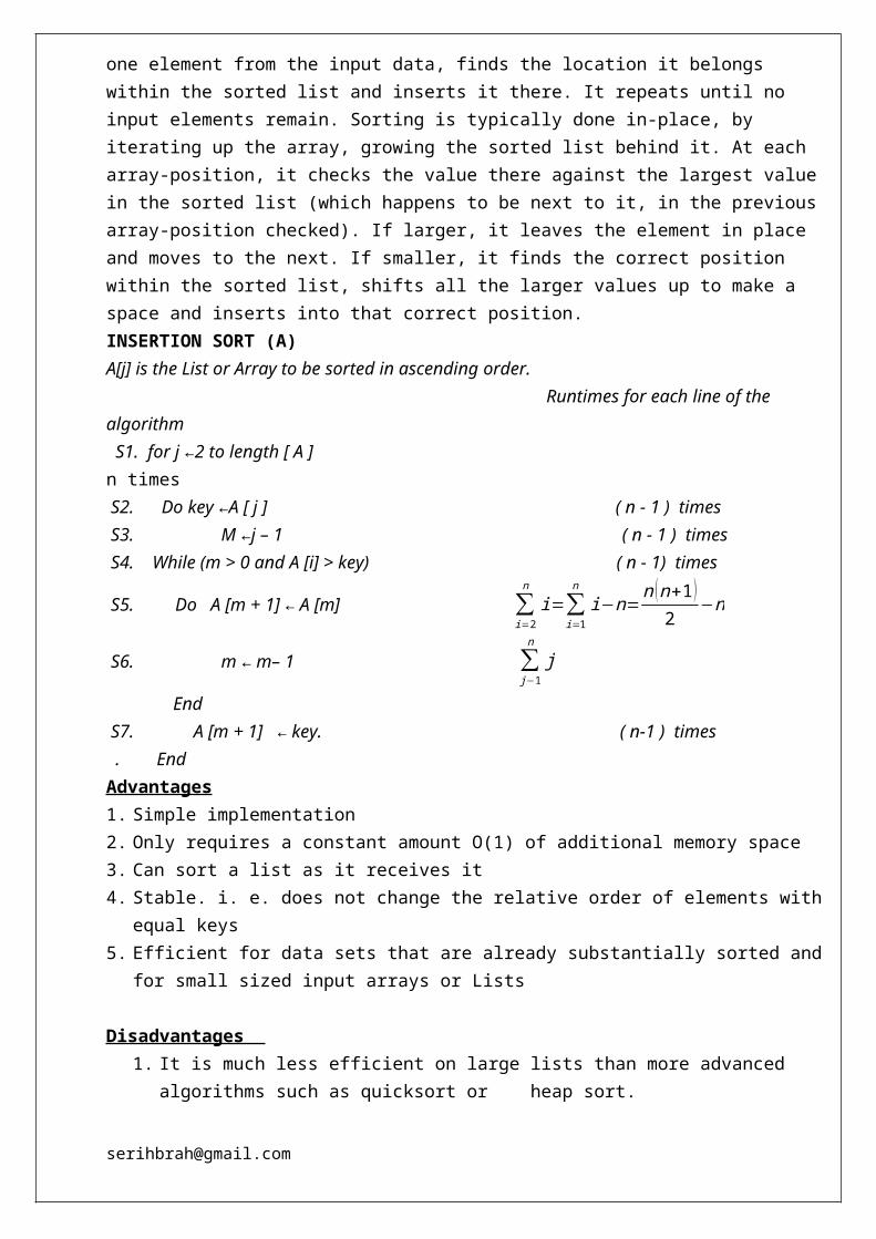
one element from the input data, finds the location it belongs within the sorted list and inserts it there. It repeats until no input elements remain. Sorting is typically done in-place, by iterating up the array, growing the sorted list behind it. At each array-position, it checks the value there against the largest valuein the sorted list (which happens to be next to it, in the previousarray-position checked). If larger, it leaves the element in place and moves to the next. If smaller, it finds the correct position within the sorted list, shifts all the larger values up to make a space and inserts into that correct position.INSERTION SORT (A)A[j] is the List or Array to be sorted in ascending order. Runtimes for each line of the algorithm S1. for j 2 to length [ A ] ← n times S2. Do key A [ j ] ( n - 1 ) times← S3. M j – 1 ( n - 1 ) times← S4. While (m > 0 and A [i] > key) ( n - 1) times
S5. Do A [m + 1] A [m] ← ∑i=2
ni=∑
i=1
ni−n=
n (n+1)2
−n
S6. m m– 1 ← ∑j−1
nj
End S7. A [m + 1] key. ( n-1 ) times← . EndAdvantages1. Simple implementation2. Only requires a constant amount O(1) of additional memory space3. Can sort a list as it receives it4. Stable. i. e. does not change the relative order of elements with
equal keys5. Efficient for data sets that are already substantially sorted and
for small sized input arrays or Lists
Disadvantages 1. It is much less efficient on large lists than more advanced
algorithms such as quicksort or heap sort.

Theoretical Complexity Analysis of Straight Insertion SortAverage Case A(n):A (n) = Summation of all the runtimes from the above Insertion Sortalgorithm
A (n) = n + (n-1) + (n-1) + (n-1) + n (n+1)2
–n + ∑j−1
nj + (n-1)
A (n) = n2+4n−4 = O(n2)Thus, the expected running time of the Straight Insertion Sort, A(n) = O(n2).Worst Case W(n):The Worst case occurs when the input array or list is reverse-sorted.Considering the ith pass;
1. First I keys have been sorted and about to insert (i+1)th keyThere are (i-1) slots between currently sorted keys and two more places and positions at the end of this list giving (i+1) possible positions where next key can be inserted.
2. Assume that the new key is likely to be inserted into any of
these (i+1) possible positions with P = 1i+1
3. Let Xi be the random variable which equals the number of comparisons needed to place key (i+1) into the correct placein this pass.
E(Xi) = 1(1
i+1) + 2(1
i+1) + 3(1
i+1) + …+(i-1)( 1
i+1) + i(1
i+1)
= ( 1i+1){1 + 2 + 3 + … + (i-1) + i}
E(Xi) = ( i2
+i
1+i)

Let Y be the random variables that denotes the total number of comparisons in the sort, then Y = X1+ X2+X3+…+Xn−1fori=1,2,3…,n−1 . The Average time complexity A(n) =E(Y) = E(Xi)
A (n)=(12+12)+(22+
23 )+…+(n−1
2+n−1n )
¿ 12{1+2+…+(n−1)} + {12+2
3+…+n−1
n }
=12∑i=1
n−1i+∑
i=1
n−1 ii+1 and by simplifying further
A (n)=n2
2+3n4
−∑i=1
n 1i=O(n2)
Hence the theoretical runtime complexity analysis of the Straight Insertion sort algorithm is given asA (n)=O (n2 )∧W (n )=O(n2).
Quick Sort This is a comparison based algorithm that sorts a given list orarray of number in place using the divide – and – conquer approach. DIVIDE: Usually, an array A[p,…,r] is partitioned into two partsA[p,…,q-1] and A[q+1…r] with an index q as the pivotvalue such that A[q] is greater than every element in A[p,…q-1] andless than every element in A[q+1,…r].
CONQUER: recursively quick Sort the sub-arrays A[p,…,q-1] andA[q+1,…,r],so that the entire array A[p ,..,r] would have beensorted in place without having to create an extra storage.
QUICKSORT (A, p, r)1. if p < r

2. then q PARTITION( A , p , r )←4. QUICKSORT( A , p , q 1)−5. QUICKSORT( A , q + 1, r )6. End
To sort an entire array the initial call will beQUICKSORT(A,1,Length[A]).The algorithm for the procedure Partition (A, p, r) that helps toperform the partitioning is given below:
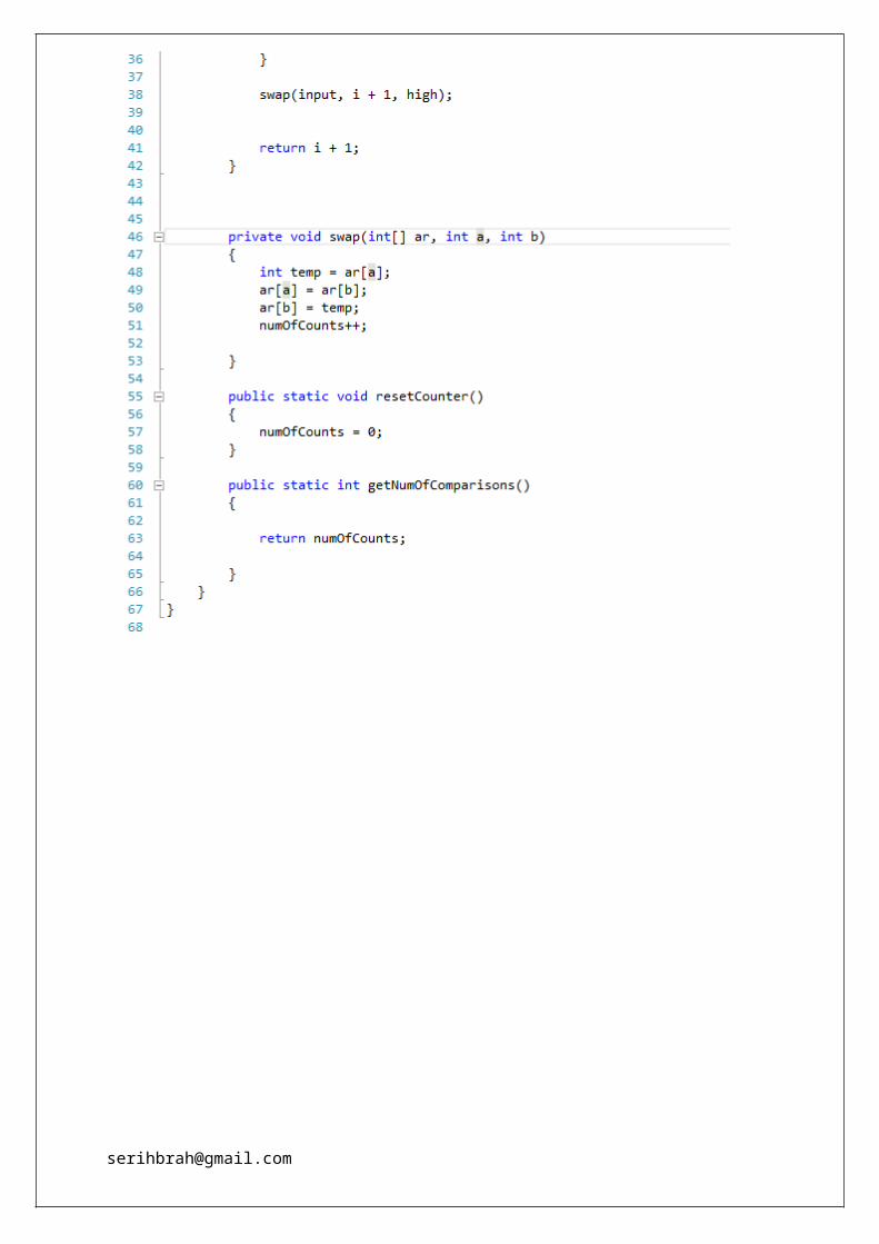
PARTITION (A, p, r)1. x A [r ]←2. i p 1← −3. for j p to r 1← −4. do if A [ j ] x≤5. then i i + 1←6. exchange A [i ] A [ j ]↔7. exchange A [i + 1] A [r ]↔8. return i + 19. End
Theoretical Complexity analysis of the Quick sort algorithmThe performance/efficiency of quick sort algorithm depends so much on the whether or not the partitioning is balanced.To ensure balanced partitioning, the ideas below can be used:1. Choose the Right most or Left most elements as the pivot (or
partitioning element). 2. Get the median of randomly selected three elements from the
Array3. Randomly choose a pivot element from the given array.
Worst Case Complexity analysis, W (n):
The Worst case runtime complexity usually occurs when the partitionis absolutely is not balanced. Basically, this can happen when the array to be sorted using quicksort is already sorted.The implication is that the array will be partitioned into two sub-arrays; one with (n-1) elements and the other with zero elements (i.e. empty).

Let W (n) = total running time complexity of quick sort in the worst case, T(n-1) = running time for sorting the sub-array of size (n-1), T(0) = running time for sorting the sub-array of size 0, T(n) = running time for the Partition procedure = Θ(n), From the above notations we derive, W (n) = T(0) + T(n-1) + T(n), but T(0) = Θ (1)=0 W (n) = T(n-1) + T(n), Using substitution method,
Thus, W (n) =Θ (n2 ).
Average Case Complexity Analysis, A(n):
Since the complexity of quick sort in the average case is very muchclose to its value in the best case than in the worst case, we can derive the best case and equate it to be the value of the average case.For the best case, the Array A[p,…,r] will be partitioned into two sub-arrays each of size n/2 .The Recurrence,
T (n)=2T(n2)+nisobtained∧whenresolvedusingtheMastersTheorem
T (n)=O (nlogn )=A(n) .Thus, the conclusion that the complexity of Quicksort in the average case is alwaysA (n)=O (nlogn ).
Advantages1. It is recursive, hence can be easily implemented.2. It is stable.3. It has an extremely short inner loop4. Has been thoroughly subjected to diverse mathematical analysis
and proven to be very good.Disadvantages 1. The iterative version is very complicated to implement2. It is fragile i.e., a simple mistake in the implementation can
go unnoticed and cause it to perform badly.

3. It requires a quadratic running time complexity in the worst case.
HEAPSORT
This is a comparison-based sorting algorithm to create a sorted array (or list) and is part of the selection sort family. Although somewhat slower in practice on most machines than a well-implemented quicksort, it has the advantages of a more favourable worst-case O(n log n) runtime. It sorts in place. .i.e. only a constant number of array elements are stored outside the input array at any time. Heap sort only requires a constant amount of additional memory but it changes the relative order of elements with equal keys. Thus, heap sort combines the better attributes of the merge and straight insertion sorting algorithms.
Heap sort also introduces another algorithm design technique: the use of a data structure, in this case one we call a “heap,” to manage information during the execution of the algorithm. Not only is the heap data structure useful for heap sort, but it also makes an efficient priority queue. The heap data structure will reappear in algorithms in later chapters.
Algorithm
The heap data structure is an array object that can be viewed as a nearly complete binary tree. Each node of the tree corresponds to an element of the array that stores the value in the node. The treeis completely lled on all levels except possibly the lowest, whichfiis lled from the left up to a point. An array A that represents a fiheap is anobject with two attributes: [email protected]

length[A], which is the number of elements in the array, and heap-size[A], which is the number of elements in the heap stored within array A.That is, although A[1..length[A]] may contain valid numbers, no element past A[heap-size[A]], where heap-size[A]≤ length[A], is an element of the heap.
Heap sort’s algorithm can be summarised as follows:1. A heap is built out of the data2. A sorted array is created by repeatedly removing the largest
element from the heap and inserting it into the array. The heap is reconstructed after each removal. Once all objects have been removed from the heap, we have a sorted array.
The direction of the sorted element can be varied by choosing a min-heap or max-heap in step 1. In both kinds, the values in the nodes satisfy a heap property, the speci cs of which depend on the fikind of heap.In a max-heap, the max-heap property is that for every node i otherthan the root, A[PARENT(i)]≥ A[i]
Thus, the largest element in a max-heap is stored at the root and the sub tree rooted at a node contains values no larger than that contained at the node itself.A min-heap is organized in the opposite way; the min-heap property is that for every node i other than the root,
A[PARENT(i)]≤ A[i].The smallest element in a min-heap is at the root.For the heap sort algorithm, we use max-heaps.The function of MAX-HEAPIFY algorithm is to let the value at A[i] “ oat down” in the maxheap so that the sub tree rooted at index i flbecomes a max-heap.
MAX-HEAPIFY(A,i)1 l← LEFT(i)2 r← RIGHT(i)3 if l≤ heap-size[A] and A[l]> A[i]4 then largest ← l5 else largest ← i

6 if r≤ heap-size[A] and A[r]> A[largest]7 then largest ← r8 if largest ≠ i9 then exchange A[i] ↔ A[largest]10 MAX-HEAPIFY(A, largest)
The root of the tree is A[1], and given the index, I, of a node, the indices of its parentPARENT(i),left child LEFT(i), and right child RIGHT(i) can be computed simply:PARENT(i)
returni/2LEFT(i)
return 2iRIGHT(i)
return 2i+1On most computers, the LEFT procedure can compute 2i in one
instruction by simply shifting the binary representation of i left one bit position. Similarly, the RIGHT procedure can quickly compute 2i+1 by shifting the binary representation of i left one bit position and adding in a 1 as the low-order bit. The PARENT procedur can computei/2 by shifting i right one bit position.
The array can be split into two parts; the sorted array and the heap.
E. g. 6 5 3 1 8 7 2 4
8 6 7
4 5 3 2
1
8 6 7 4 5 3 2 1

The root of the tree is A [1], and given the index, I, of a node, the indices of its parentPARENT(i),left child LEFT(i), and right child RIGHT(i) can be computed simply:PARENT(i)
returni/2LEFT(i)
return 2iRIGHT(i)
return 2i+1On most computers, the LEFT procedure can compute 2i in one
instruction by simply shifting the binary representation of i left one bit position. Similarly, the RIGHT procedure can quickly compute 2i+1 by shifting the binary representation of i left one bit position and adding in a 1 as the low-order bit. The PARENT procedure can compute the floor value of i/2 by shifting i right one bit position.
Analysis
Heap sort is typically somewhat slower than quicksort, but the worst-case running time for quicksort is O(n2), which is unacceptable for large data sets and can create security risks. Thus, because of the O(n log n) upper bound on heap sort’s running time and constant upper bound on its auxiliary storage, embedded systems with real-time constraints or systems concerned with security often use heap sort.
The HEAPSORT procedure takes time O(nlgn), since the call to BUILD-MAXHEAP takes time O(n) and each of the n − 1 calls to MAX-HEAPIFY takes time O(lgn).
Advantageso Heap sort both in the average and worst case performs with a runtime
complexity of O(nlgn).
Disadvantageso Heap sort is not a stable sort. i. e. it changes the order of
elements.o Heap sort is not an obvious candidate for a parallel algorithmo Heap sort cannot be used in external sorting

5.0 Experimental setup and outcomes
This experiment was conducted under the environmental conditions stated below:
Operating System :32-bit Windows 7 Ultimate RAM: 2.00 GB HDD :160 GB Processor : Pentium(R) Dual-Core CPU T4500@ 2.30 GHZ
2.30GHZ Compiler : Visual C#.Net Programming Language : C#.net Programming paradigm : Object Oriented Programming
The purpose of this experiment is to compare the practical efficiency of the aforementionedAlgorithms by empirical analysis. 5.1 Program methodology:
We randomly generated arrays of numbers input sizes N ranging from N=100,200, 400, 600, 800, 1000, 1200 (as instructed by the Professor, H.O.D Longe) using the pseudorandom number generator made available in the C# class library as seen in the code snippet below
public void GenerateArray(int N) {[email protected]

RandomArray = new int[N]; //The randon Number generator class in C# Random rdn = new Random(); for (int i = 0; i < N; i++) { //using the Next method to generate random numbers within the range of 0 and 5000 RandomArray[i] = rdn.Next(0,5000); } }
Each algorithm sorts different instances of the arrays five times for each input sizes and compute the average of the number of basic operations (i.e. number of comparisons/swaps) for each algorithm.
A Graph of runtimes (i.e. average number of basic operations) against Input sizes is plotted in the program. Note that the average number of basic operations was obtained by calculatingthe number of comparison or swapping operations in the algorithm
We make conclusion or our final deductions by observing the asymptotic order of growth of each curve on the graph.
5.2 Experimental output 4.2.1 Data Table Below are the outputs of the data table generated in three different runtimes of the program.

5.2.2 Inferences based on the outcome of the Experiment
From the programmatically generated Data table and graph, we observe that
1. From the table, the average number of basic operations (i.e. number of swaps/comparison) increases as the size of the inputarray increases and for every instances of the runtime, straight insertion sort has the highest number of basic operations compared to heap sort while quicksort has the lowest number of basic operations.
2. From the graph, we see that straight insertion sort curve grows fastest (i.e. has a quadratic order of growth – O(n2) ) followed by heap sort then quick sort (both with a sub-linear curve).
3. Therefore, we conclude that unlike straight insertion sort, quick sort is the most efficient followed by heap sort.