I. 101 white dwarf main-sequence binaries with multiple Sloan ...
17
Mon. Not. R. Astron. Soc. 382, 1377–1393 (2007) doi:10.1111/j.1365-2966.2007.12288.x Post-common-envelope binaries from SDSS – I. 101 white dwarf main-sequence binaries with multiple Sloan Digital Sky Survey spectroscopy A. Rebassa-Mansergas, 1 B. T. G¨ ansicke, 1 P. Rodr´ ıguez-Gil, 2 M. R. Schreiber 3 and D. Koester 4 1 Department of Physics, University of Warwick, Coventry CV4 7AL 2 Instituto de Astrof´ ısica de Canarias, V´ ıa L ´ actea, s/n, La Laguna, E-38205 Tenerife, Spain 3 Departamento de Fisica y Astronomia, Universidad de Valparaiso, Avenida Gran Bretana 1111, Valparaiso, Chile 4 Institut f ¨ ur Theoretische Physik und Astrophysik, University of Kiel, 24098 Kiel, Germany Accepted 2007 July 25. Received 2007 July 25; in original form 2007 May 31 ABSTRACT We present a detailed analysis of 101 white dwarf main-sequence binaries (WDMS) from the Sloan Digital Sky Survey (SDSS) for which multiple SDSS spectra are available. We detect significant radial velocity variations in 18 WDMS, identifying them as post-common- envelope binaries (PCEBs) or strong PCEB candidates. Strict upper limits to the orbital periods are calculated, ranging from 0.43 to 7880 d. Given the sparse temporal sampling and relatively low spectral resolution of the SDSS spectra, our results imply a PCEB fraction of 15 per cent among the WDMS in the SDSS data base. Using a spectral decomposition/fitting technique we determined the white dwarf effective temperatures and surface gravities, masses and secondary star spectral types for all WDMS in our sample. Two independent distance estimates are obtained from the flux-scaling factors between the WDMS spectra, and the white dwarf models and main-sequence star templates, respectively. Approximately one-third of the systems in our sample show a significant discrepancy between the two distance estimates. In the majority of discrepant cases, the distance estimate based on the secondary star is too large. A possible explanation for this behaviour is that the secondary star spectral types that we determined from the SDSS spectra are systematically too early by one to two spectral classes. This behaviour could be explained by stellar activity, if covering a significant fraction of the star by cool dark spots will raise the temperature of the interspot regions. Finally, we discuss the selection effects of the WDMS sample provided by the SDSS project. Key words: accretion, accretion discs – binaries: close – novae, cataclysmic variables. 1 INTRODUCTION A large fraction of all stars in the sky are part of binary or multiple systems (Iben 1991). If the initial separation of the main-sequence binary is small enough, the more massive star will engulf its compan- ion while evolving into a red giant, and the system enters a common envelope (CE; e.g. Livio & Soker 1988; Iben & Livio 1993). Fric- tion within the CE leads to a rapid decrease of the binary separation and orbital period, and the energy and angular momentum extracted from the binary orbit eventually ejects the CE. Products of CE evo- lution include a wide range of important astronomical objects, such as, e.g. high- and low-mass X-ray binaries, double degenerate white dwarf and neutron star binaries, cataclysmic variables and supersoft X-ray sources – with some of those objects evolving at later stages E-mail: [email protected] into type Ia supernova and short gamma-ray bursts. While the con- cept of CE evolution is simple, its details are poorly understood, and are typically described by parametrized models (Paczynski 1976; Nelemans et al. 2000; Nelemans & Tout 2005). Consequently, pop- ulation models of all types of CE products are subject to substantial uncertainties. Real progress in our understanding of close binary evolution is most likely to arise from the analysis of post-CE binaries (PCEBs) that are both numerous and well understood in terms of their stel- lar components – such as PCEBs containing a white dwarf and a main-sequence star. 1 While detailed population models are al- ready available, (e.g. Willems & Kolb 2004), there is a clear lack of 1 Throughout this paper, we will use the term white dwarf main-sequence bi- naries (WDMS) to refer to the total class of white dwarf plus main-sequence binaries, and PCEBs to those WDMS that underwent a CE phase. C 2007 The Authors. Journal compilation C 2007 RAS Downloaded from https://academic.oup.com/mnras/article/382/4/1377/1141213 by guest on 01 June 2022
-
Upload
khangminh22 -
Category
Documents
-
view
2 -
download
0
Transcript of I. 101 white dwarf main-sequence binaries with multiple Sloan ...
Mon. Not. R. Astron. Soc. 382, 1377–1393 (2007) doi:10.1111/j.1365-2966.2007.12288.x
Post-common-envelope binaries from SDSS – I. 101 white dwarfmain-sequence binaries with multiple Sloan Digital Sky Surveyspectroscopy
A. Rebassa-Mansergas,1� B. T. Gansicke,1 P. Rodrıguez-Gil,2 M. R. Schreiber3
and D. Koester4
1Department of Physics, University of Warwick, Coventry CV4 7AL2Instituto de Astrofısica de Canarias, Vıa Lactea, s/n, La Laguna, E-38205 Tenerife, Spain3Departamento de Fisica y Astronomia, Universidad de Valparaiso, Avenida Gran Bretana 1111, Valparaiso, Chile4Institut fur Theoretische Physik und Astrophysik, University of Kiel, 24098 Kiel, Germany
Accepted 2007 July 25. Received 2007 July 25; in original form 2007 May 31
ABSTRACTWe present a detailed analysis of 101 white dwarf main-sequence binaries (WDMS) from
the Sloan Digital Sky Survey (SDSS) for which multiple SDSS spectra are available. We
detect significant radial velocity variations in 18 WDMS, identifying them as post-common-
envelope binaries (PCEBs) or strong PCEB candidates. Strict upper limits to the orbital periods
are calculated, ranging from 0.43 to 7880 d. Given the sparse temporal sampling and relatively
low spectral resolution of the SDSS spectra, our results imply a PCEB fraction of �15 per cent
among the WDMS in the SDSS data base. Using a spectral decomposition/fitting technique we
determined the white dwarf effective temperatures and surface gravities, masses and secondary
star spectral types for all WDMS in our sample. Two independent distance estimates are
obtained from the flux-scaling factors between the WDMS spectra, and the white dwarf models
and main-sequence star templates, respectively. Approximately one-third of the systems in our
sample show a significant discrepancy between the two distance estimates. In the majority of
discrepant cases, the distance estimate based on the secondary star is too large. A possible
explanation for this behaviour is that the secondary star spectral types that we determined from
the SDSS spectra are systematically too early by one to two spectral classes. This behaviour
could be explained by stellar activity, if covering a significant fraction of the star by cool dark
spots will raise the temperature of the interspot regions. Finally, we discuss the selection effects
of the WDMS sample provided by the SDSS project.
Key words: accretion, accretion discs – binaries: close – novae, cataclysmic variables.
1 I N T RO D U C T I O N
A large fraction of all stars in the sky are part of binary or multiple
systems (Iben 1991). If the initial separation of the main-sequence
binary is small enough, the more massive star will engulf its compan-
ion while evolving into a red giant, and the system enters a common
envelope (CE; e.g. Livio & Soker 1988; Iben & Livio 1993). Fric-
tion within the CE leads to a rapid decrease of the binary separation
and orbital period, and the energy and angular momentum extracted
from the binary orbit eventually ejects the CE. Products of CE evo-
lution include a wide range of important astronomical objects, such
as, e.g. high- and low-mass X-ray binaries, double degenerate white
dwarf and neutron star binaries, cataclysmic variables and supersoft
X-ray sources – with some of those objects evolving at later stages
�E-mail: [email protected]
into type Ia supernova and short gamma-ray bursts. While the con-
cept of CE evolution is simple, its details are poorly understood, and
are typically described by parametrized models (Paczynski 1976;
Nelemans et al. 2000; Nelemans & Tout 2005). Consequently, pop-
ulation models of all types of CE products are subject to substantial
uncertainties.
Real progress in our understanding of close binary evolution is
most likely to arise from the analysis of post-CE binaries (PCEBs)
that are both numerous and well understood in terms of their stel-
lar components – such as PCEBs containing a white dwarf and
a main-sequence star.1 While detailed population models are al-
ready available, (e.g. Willems & Kolb 2004), there is a clear lack of
1 Throughout this paper, we will use the term white dwarf main-sequence bi-
naries (WDMS) to refer to the total class of white dwarf plus main-sequence
binaries, and PCEBs to those WDMS that underwent a CE phase.
C© 2007 The Authors. Journal compilation C© 2007 RAS
Dow
nloaded from https://academ
ic.oup.com/m
nras/article/382/4/1377/1141213 by guest on 01 June 2022
1378 A. Rebassa-Mansergas et al.
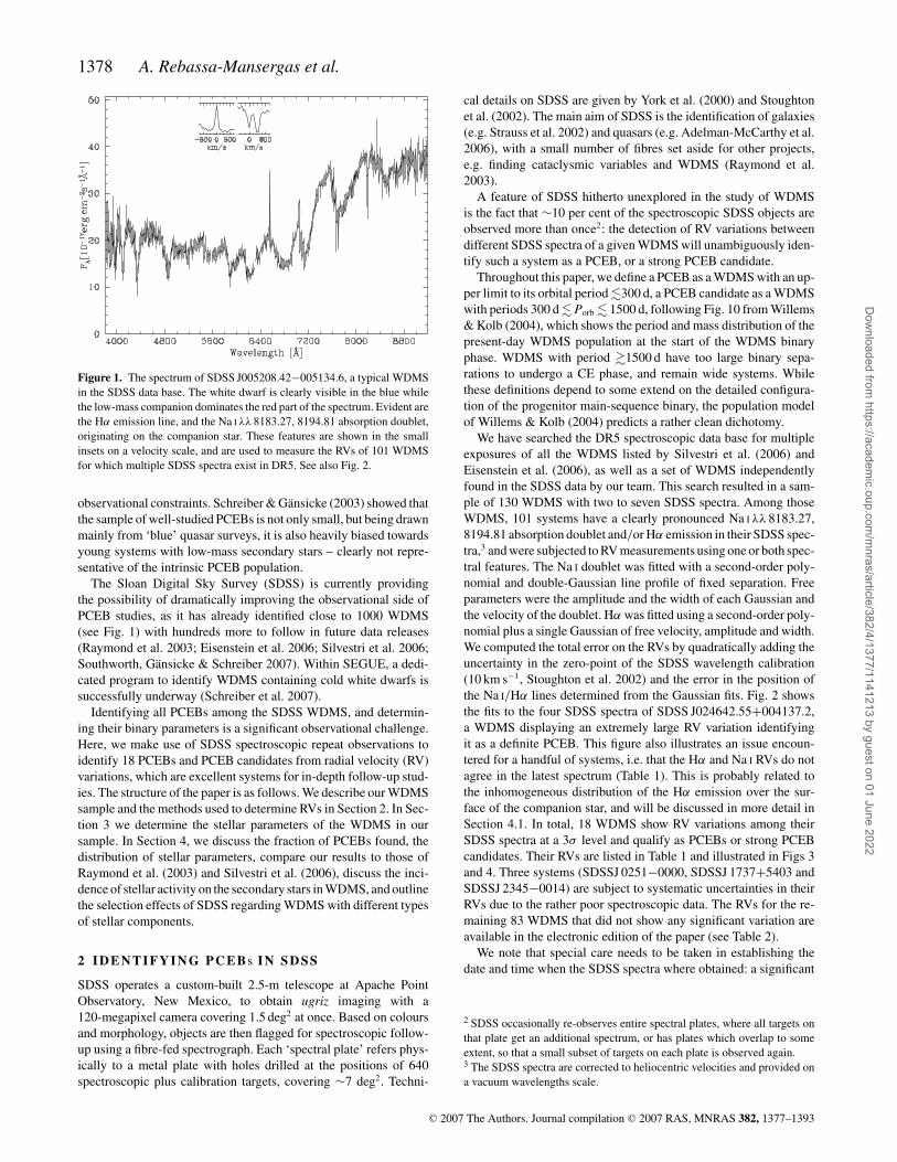
Figure 1. The spectrum of SDSS J005208.42−005134.6, a typical WDMS
in the SDSS data base. The white dwarf is clearly visible in the blue while
the low-mass companion dominates the red part of the spectrum. Evident are
the Hα emission line, and the Na I λλ 8183.27, 8194.81 absorption doublet,
originating on the companion star. These features are shown in the small
insets on a velocity scale, and are used to measure the RVs of 101 WDMS
for which multiple SDSS spectra exist in DR5. See also Fig. 2.
observational constraints. Schreiber & Gansicke (2003) showed that
the sample of well-studied PCEBs is not only small, but being drawn
mainly from ‘blue’ quasar surveys, it is also heavily biased towards
young systems with low-mass secondary stars – clearly not repre-
sentative of the intrinsic PCEB population.
The Sloan Digital Sky Survey (SDSS) is currently providing
the possibility of dramatically improving the observational side of
PCEB studies, as it has already identified close to 1000 WDMS
(see Fig. 1) with hundreds more to follow in future data releases
(Raymond et al. 2003; Eisenstein et al. 2006; Silvestri et al. 2006;
Southworth, Gansicke & Schreiber 2007). Within SEGUE, a dedi-
cated program to identify WDMS containing cold white dwarfs is
successfully underway (Schreiber et al. 2007).
Identifying all PCEBs among the SDSS WDMS, and determin-
ing their binary parameters is a significant observational challenge.
Here, we make use of SDSS spectroscopic repeat observations to
identify 18 PCEBs and PCEB candidates from radial velocity (RV)
variations, which are excellent systems for in-depth follow-up stud-
ies. The structure of the paper is as follows. We describe our WDMS
sample and the methods used to determine RVs in Section 2. In Sec-
tion 3 we determine the stellar parameters of the WDMS in our
sample. In Section 4, we discuss the fraction of PCEBs found, the
distribution of stellar parameters, compare our results to those of
Raymond et al. (2003) and Silvestri et al. (2006), discuss the inci-
dence of stellar activity on the secondary stars in WDMS, and outline
the selection effects of SDSS regarding WDMS with different types
of stellar components.
2 I D E N T I F Y I N G P C E B s I N S D S S
SDSS operates a custom-built 2.5-m telescope at Apache Point
Observatory, New Mexico, to obtain ugriz imaging with a
120-megapixel camera covering 1.5 deg2 at once. Based on colours
and morphology, objects are then flagged for spectroscopic follow-
up using a fibre-fed spectrograph. Each ‘spectral plate’ refers phys-
ically to a metal plate with holes drilled at the positions of 640
spectroscopic plus calibration targets, covering ∼7 deg2. Techni-
cal details on SDSS are given by York et al. (2000) and Stoughton
et al. (2002). The main aim of SDSS is the identification of galaxies
(e.g. Strauss et al. 2002) and quasars (e.g. Adelman-McCarthy et al.
2006), with a small number of fibres set aside for other projects,
e.g. finding cataclysmic variables and WDMS (Raymond et al.
2003).
A feature of SDSS hitherto unexplored in the study of WDMS
is the fact that ∼10 per cent of the spectroscopic SDSS objects are
observed more than once2: the detection of RV variations between
different SDSS spectra of a given WDMS will unambiguously iden-
tify such a system as a PCEB, or a strong PCEB candidate.
Throughout this paper, we define a PCEB as a WDMS with an up-
per limit to its orbital period �300 d, a PCEB candidate as a WDMS
with periods 300 d � Porb � 1500 d, following Fig. 10 from Willems
& Kolb (2004), which shows the period and mass distribution of the
present-day WDMS population at the start of the WDMS binary
phase. WDMS with period �1500 d have too large binary sepa-
rations to undergo a CE phase, and remain wide systems. While
these definitions depend to some extend on the detailed configura-
tion of the progenitor main-sequence binary, the population model
of Willems & Kolb (2004) predicts a rather clean dichotomy.
We have searched the DR5 spectroscopic data base for multiple
exposures of all the WDMS listed by Silvestri et al. (2006) and
Eisenstein et al. (2006), as well as a set of WDMS independently
found in the SDSS data by our team. This search resulted in a sam-
ple of 130 WDMS with two to seven SDSS spectra. Among those
WDMS, 101 systems have a clearly pronounced Na I λλ 8183.27,
8194.81 absorption doublet and/or Hα emission in their SDSS spec-
tra,3 and were subjected to RV measurements using one or both spec-
tral features. The Na I doublet was fitted with a second-order poly-
nomial and double-Gaussian line profile of fixed separation. Free
parameters were the amplitude and the width of each Gaussian and
the velocity of the doublet. Hα was fitted using a second-order poly-
nomial plus a single Gaussian of free velocity, amplitude and width.
We computed the total error on the RVs by quadratically adding the
uncertainty in the zero-point of the SDSS wavelength calibration
(10 km s−1, Stoughton et al. 2002) and the error in the position of
the Na I/Hα lines determined from the Gaussian fits. Fig. 2 shows
the fits to the four SDSS spectra of SDSS J024642.55+004137.2,
a WDMS displaying an extremely large RV variation identifying
it as a definite PCEB. This figure also illustrates an issue encoun-
tered for a handful of systems, i.e. that the Hα and Na I RVs do not
agree in the latest spectrum (Table 1). This is probably related to
the inhomogeneous distribution of the Hα emission over the sur-
face of the companion star, and will be discussed in more detail in
Section 4.1. In total, 18 WDMS show RV variations among their
SDSS spectra at a 3σ level and qualify as PCEBs or strong PCEB
candidates. Their RVs are listed in Table 1 and illustrated in Figs 3
and 4. Three systems (SDSSJ 0251−0000, SDSSJ 1737+5403 and
SDSSJ 2345−0014) are subject to systematic uncertainties in their
RVs due to the rather poor spectroscopic data. The RVs for the re-
maining 83 WDMS that did not show any significant variation are
available in the electronic edition of the paper (see Table 2).
We note that special care needs to be taken in establishing the
date and time when the SDSS spectra where obtained: a significant
2 SDSS occasionally re-observes entire spectral plates, where all targets on
that plate get an additional spectrum, or has plates which overlap to some
extent, so that a small subset of targets on each plate is observed again.3 The SDSS spectra are corrected to heliocentric velocities and provided on
a vacuum wavelengths scale.
C© 2007 The Authors. Journal compilation C© 2007 RAS, MNRAS 382, 1377–1393
Dow
nloaded from https://academ
ic.oup.com/m
nras/article/382/4/1377/1141213 by guest on 01 June 2022
Post-common-envelope binaries from SDSS 1379
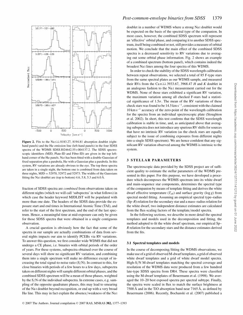
Figure 2. Fits to the Na I λλ 8183.27, 8194.81 absorption doublet (right-
hand panels) and the Hα emission line (left-hand panels) in the four SDSS
spectra of the WDMS SDSS J024642.55+004137.2. The SDSS spectro-
scopic identifiers (MJD, Plate-ID and Fibre-ID) are given in the top left-
hand corner of the Hα panels. Na I has been fitted with a double-Gaussian of
fixed separation plus a parabola, Hα with a Gaussian plus a parabola. In this
system, RV variations are already obvious to the eye. The top three spectra
are taken in a single night, the bottom one is combined from data taken on
three nights, MJD = 52970, 52972 and 52973. The widths of the Gaussians
fitting the Na I doublet are (top to bottom) 4.6, 5.8, 5.3 and 6.0 Å.
fraction of SDSS spectra are combined from observations taken on
different nights (which we will call ‘subspectra’ in what follows) in
which case the header keyword MJDLIST will be populated with
more than one date. The headers of the SDSS data provide the ex-
posure start and end times in International Atomic Time (TAI), and
refer to the start of the first spectrum, and the end of the last spec-
trum. Hence, a meaningful time at mid-exposure can only be given
for those SDSS spectra that were obtained in a single contiguous
observation.
A crucial question is obviously how the fact that some of the
spectra in our sample are actually combinations of data from sev-
eral nights impacts our aim to identify PCEBs via RV variations.
To answer this question, we first consider wide WDMS that did not
undergo a CE phase, i.e. binaries with orbital periods of the order
of years. For these systems, subspectra obtained over the course of
several days will show no significant RV variation, and combining
them into a single spectrum will make no difference except of in-
creasing the total signal-to-noise ratio (S/N). In contrast to this, for
close binaries with periods of a few hours to a few days, subspectra
taken on different nights will sample different orbital phases, and the
combined SDSS spectrum will be a mean of those phases, weighted
by the S/N of the individual subspectra. In extreme cases, e.g. sam-
pling of the opposite quadrature phases, this may lead to smearing
of the Na I doublet beyond recognition, or end up with a very broad
Hα line. This may in fact explain the absence/weakness of the Na I
doublet in a number of WDMS where a strong Na I doublet would
be expected on the basis of the spectral type of the companion. In
most cases, however, the combined SDSS spectrum will represent
an ‘effective’ orbital phase, and comparing it to another SDSS spec-
trum, itself being combined or not, still provides a measure of orbital
motion. We conclude that the main effect of the combined SDSS
spectra is a decreased sensitivity to RV variations due to averag-
ing out some orbital phase information. Fig. 2 shows an example
of a combined spectrum (bottom panel), which contains indeed the
broadest Na I lines among the four spectra of this WDMS.
In order to check the stability of the SDSS wavelength calibration
between repeat observations, we selected a total of 85 F-type stars
from the same spectral plates as our WDMS sample, and measured
their RVs from the Ca II λλ 3933.67, 3968.47 H and K doublet in
an analogous fashion to the Na I measurement carried out for the
WDMS. None of those stars exhibited a significant RV variation,
the maximum variation among all checked F-stars had a statisti-
cal significance of 1.5σ . The mean of the RV variations of these
check stars was found to be 14.5 km s−1, consistent with the claimed
10 km s−1 accuracy of the zero-point of the wavelength calibration
for the spectra from an individual spectroscopic plate (Stoughton
et al. 2002). In short, this test confirms that the SDSS wavelength
calibration is stable in time, and, as anticipated above that averag-
ing subspectra does not introduce any spurious RV shifts for sources
that have no intrinsic RV variation (as the check stars are equally
subject to the issue of combining exposures from different nights
into a single SDSS spectrum). We are hence confident that any sig-
nificant RV variation observed among the WDMS is intrinsic to the
system.
3 S T E L L A R PA R A M E T E R S
The spectroscopic data provided by the SDSS project are of suffi-
cient quality to estimate the stellar parameters of the WDMS pre-
sented in this paper. For this purpose, we have developed a proce-
dure which decomposes the WDMS spectrum into its white dwarf
and main-sequence star components, determines the spectral type
of the companion by means of template fitting and derives the white
dwarf effective temperature (Teff) and surface gravity (log g) from
spectral model fitting. Assuming an empirical spectral type–radius
(Sp–R) relation for the secondary star and a mass–radius relation for
the white dwarf, two independent distance estimates are calculated
from the flux-scaling factors of the template/model spectra.
In the following sections, we describe in more detail the spectral
templates and models used in the decomposition and fitting, the
method adopted to fit the white dwarf spectrum, our empirical Sp–
R relation for the secondary stars and the distance estimates derived
from the fits.
3.1 Spectral templates and models
In the course of decomposing/fitting the WDMS observations, we
make use of a grid of observed M-dwarf templates, a grid of observed
white dwarf templates and a grid of white dwarf model spectra.
High-S/N M-dwarf templates matching the spectral coverage and
resolution of the WDMS data were produced from a few hundred
late-type SDSS spectra from DR4. These spectra were classified
using the M-dwarf templates of Beuermann et al. (1998). We aver-
aged the 10–20 best exposed spectra per spectral subtype. Finally,
the spectra were scaled in flux to match the surface brightness at
7500 Å and in the TiO absorption band near 7165 Å, as defined by
Beuermann (2006). Recently, Bochanski et al. (2007) published a
C© 2007 The Authors. Journal compilation C© 2007 RAS, MNRAS 382, 1377–1393
Dow
nloaded from https://academ
ic.oup.com/m
nras/article/382/4/1377/1141213 by guest on 01 June 2022
1380 A. Rebassa-Mansergas et al.
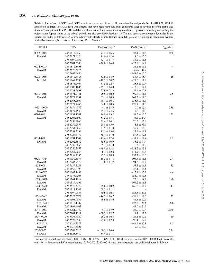
Table 1. RVs of our 18 PCEBs and PCEB candidates, measured from the Hα emission line and/or the Na I λλ 8183.27, 8194.81
absorption doublet. The HJDs for SDSS spectra that have been combined from exposures taken in several different nights (see
Section 2) are set in italics. PCEB candidates with uncertain RV measurements are indicated by colons preceding and trailing the
object name. Upper limits of the orbital periods are also provided (Section 4.2). The two spectral components identified in the
spectra are coded as follows. DA = white dwarf with clearly visible Balmer lines; DC = clearly visible blue continuum without
noticeable structure; blx = weak blue excess; dM = M-dwarf.
SDSS J HJD RV(Hα) km s−1 RV(Na) km s−1 Porb (d) <
0052−0053 245 1812.3463 71.3 ± 16.6 23.4 ± 14.9 280
DA/dM 245 1872.6216 11.0 ± 12.0 18.0 ± 12.7
245 1907.0834 −62.1 ± 11.7 −37.7 ± 11.6
245 2201.3308 −26.0 ± 16.0 −23.8 ± 14.9
0054–0025 245 1812.3463 21.6 ± 15.3 4
DA/dM 245 1872.6216 −25.6± 44.2
245 1907.0835 −144.7 ± 17.2
0225+0054 245 1817.3966 53.0 ± 14.9 58.6 ± 15.4 45
blx/dM 245 1869.2588 −19.2 ± 20.7 −21.6 ± 11.6
245 1876.2404 37.5 ± 22.4 25.3 ± 12.4
245 1900.1605 −25.1 ± 14.0 −12.8 ± 17.0
245 2238.2698 27.9 ± 22.3 37.4 ± 12.8
0246+0041 245 1871.2731 −95.5 ± 10.2 −99.3 ± 11.1 2.5
DA/dM 245 2177.4531 163.1 ± 10.3 167.2 ± 11.3
245 2965.2607 140.7 ± 10.8 135.3 ± 11.0
245 2971.7468 64.0 ± 10.5 125.7 ± 11.3
:0251–0000: 245 2174.4732 4.1 ± 33.5 0.0 ± 15.4 0.58
DA/dM 245 2177.4530 −139.3 ± 24.6 15.8 ± 18.3
0309–0101 245 1931.1241 44.8 ± 13.2 31.5 ± 13.7 153
DA/dM 245 2203.4500 51.2 ± 14.1 48.7 ± 24.4
245 2235.2865 27.4 ± 14.1 76.3 ± 16.2
245 2250.2457 28.8 ± 15.0 8.1 ± 33.0
245 2254.2052 53.9 ± 11.8 55.7 ± 14.3
245 2258.2194 15.5 ± 13.0 27.9 ± 19.9
245 3383.6493 50.7 ± 11.0 56.5 ± 12.8
0314–0111 245 1931.1242 −41.6 ± 12.4 −51.7 ± 12.4 1.1
DC/dM 245 2202.3882 35.6 ± 10.9 35.2 ± 14.4
245 2235.2865 9.1 ± 11.0 10.3 ± 14.2
245 2250.2457 −49.8 ± 12.2 −128.2 ± 13.9
245 2254.2053 −66.7 ± 12.8 −111.7 ± 10.9
245 2258.2195 87.3 ± 10.8 135.2 ± 13.5
0820+4314 245 1959.3074 118.3 ± 11.4 106.3 ± 11.5 2.4
DA/dM 245 2206.9572 −107.8 ± 11.2 −94.6 ± 10.8
1138–0011 245 1629.8523 53.5 ± 16.9 35
DA/dM 245 1658.2128 −38.1 ± 18.6
1151–0007 245 1662.1689 −15.8 ± 15.1 4.4
DA/dM 245 1943.4208 154.0 ± 19.5
1529+0020 245 1641.4617 73.0 ± 14.8 0.96
DA/dM 245 1989.4595 −167.2 ± 11.8
1724+5620 245 1812.6712 125.6 ± 10.2 160.6 ± 18.4 0.43
DA/dM 245 1818.1149 108.3 ± 11.1 –
245 1997.9806 −130.6 ± 10.3 −185.5 ± 20.1
1726+5605 245 1812.6712 −44.3 ± 16.7 −38.9 ± 12.9 29
DA/dM 245 1993.9805 46.6 ± 14.6 47.3 ± 12.5
:1737+5403: 245 1816.1187 −123.5 ± 28.6 6.6
DA/dM 245 1999.4602 44.0 ± 24.0
2241+0027 245 3261.2749 9.1 ± 17.9 22.0 ± 12.4 7880
DA/dM 245 2201.1311 −60.3 ± 12.7 8.1 ± 12.2
2339–0020 245 3355.5822 −29.2 ± 10.4 −27.1 ± 12.3 120
DA/dM 245 2525.3539 −93.6 ± 12.3 −90.1 ± 12.7
:2345-0014: 245 2524.3379 −141.5 ± 22.9 9.5
DA/dM 245 3357.5821 −19.8 ± 19.3
2350-0023 245 1788.3516 −160.3 ± 16.6 0.74
blx/dM 245 2523.3410 154.4 ± 31.3
Notes on individual systems: 0246+0041, 0314−0111, 2241+0027, 2339−0020: variable Hα EW; 0251–0000: faint, weak Hα
emission with uncertain RV measurements; 1737+5403, 2345−0014: very noisy spectrum; see additional notes in Table 3.
C© 2007 The Authors. Journal compilation C© 2007 RAS, MNRAS 382, 1377–1393
Dow
nloaded from https://academ
ic.oup.com/m
nras/article/382/4/1377/1141213 by guest on 01 June 2022
Post-common-envelope binaries from SDSS 1381
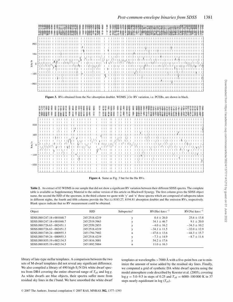
Figure 3. RVs obtained from the Na I absorption doublet. WDMS �3σ RV variation, i.e. PCEBs, are shown in black.
Figure 4. Same as Fig. 3 but for the Hα RVs.
Table 2. An extract of 83 WDMS in our sample that did not show a significant RV variation between their different SDSS spectra. The complete
table is available as Supplementary Material to the online version of this article on Blackwell Synergy. The first column gives the SDSS object
name, the second the HJD of the spectrum, in the third column we quote with ‘y’ and ‘n’ those spectra which are composed of subspectra taken
in different nights, the fourth and fifth columns provide the Na I λλ 8183.27, 8194.81 absorption doublet and Hα emission RVs, respectively.
Blank spaces indicate that no RV measurement could be obtained.
Object HJD Subspectra? RV(Hα) km s−1 RV(Na) km s−1
SDSS J001247.18+001048.7 245 2518.4219 y 0.4 ± 26.0 25.6 ± 13.8
SDSS J001247.18+001048.7 245 2519.3963 y 34.1 ± 46.7 9.1 ± 20.0
SDSS J001726.63−002451.1 245 2559.2853 y −4.0 ± 16.2 −34.3 ± 10.2
SDSS J001726.63−002451.2 245 2518.4219 y −34.1 ± 11.5 −32.0 ± 12.9
SDSS J001749.24−000955.3 245 1794.7902 n −47.6 ± 13.6 −44.3 ± 15.7
SDSS J001749.24−000955.3 245 2518.4219 y −7.3 ± 14.9 −8.7 ± 11.6
SDSS J001855.19+002134.5 245 1816.3001 y 54.2 ± 17.6
SDSS J001855.19+002134.5 245 1892.5884 n 11.0 ± 16.3
library of late-type stellar templates. A comparison between the two
sets of M-dwarf templates did not reveal any significant difference.
We also compiled a library of 490 high-S/N DA white dwarf spec-
tra from DR4 covering the entire observed range of Teff and log g.
As white dwarfs are blue objects, their spectra suffer more from
residual sky lines in the I band. We have smoothed the white dwarf
templates at wavelengths >7000 Å with a five-point box car to min-
imize the amount of noise added by the residual sky lines. Finally,
we computed a grid of synthetic DA white dwarf spectra using the
model atmosphere code described by Koester et al. (2005), covering
log g = 5.0–9.5 in steps of 0.25 and Teff = 6000–100 000 K in 37
steps nearly equidistant in log (Teff).
C© 2007 The Authors. Journal compilation C© 2007 RAS, MNRAS 382, 1377–1393
Dow
nloaded from https://academ
ic.oup.com/m
nras/article/382/4/1377/1141213 by guest on 01 June 2022
1382 A. Rebassa-Mansergas et al.
3.2 Spectral decomposition and typing of the secondary star
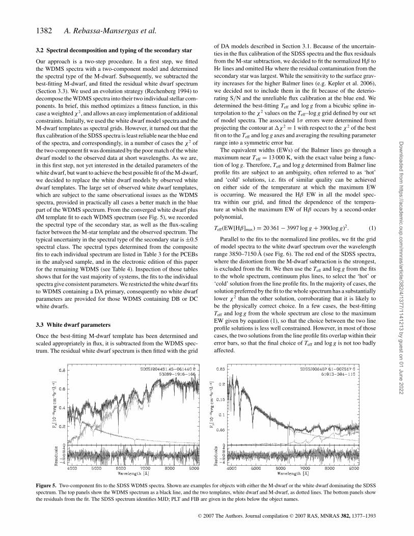
Our approach is a two-step procedure. In a first step, we fitted
the WDMS spectra with a two-component model and determined
the spectral type of the M-dwarf. Subsequently, we subtracted the
best-fitting M-dwarf, and fitted the residual white dwarf spectrum
(Section 3.3). We used an evolution strategy (Rechenberg 1994) to
decompose the WDMS spectra into their two individual stellar com-
ponents. In brief, this method optimizes a fitness function, in this
case a weighted χ2, and allows an easy implementation of additional
constraints. Initially, we used the white dwarf model spectra and the
M-dwarf templates as spectral grids. However, it turned out that the
flux calibration of the SDSS spectra is least reliable near the blue end
of the spectra, and correspondingly, in a number of cases the χ2 of
the two-component fit was dominated by the poor match of the white
dwarf model to the observed data at short wavelengths. As we are,
in this first step, not yet interested in the detailed parameters of the
white dwarf, but want to achieve the best possible fit of the M-dwarf,
we decided to replace the white dwarf models by observed white
dwarf templates. The large set of observed white dwarf templates,
which are subject to the same observational issues as the WDMS
spectra, provided in practically all cases a better match in the blue
part of the WDMS spectrum. From the converged white dwarf plus
dM template fit to each WDMS spectrum (see Fig. 5), we recorded
the spectral type of the secondary star, as well as the flux-scaling
factor between the M-star template and the observed spectrum. The
typical uncertainty in the spectral type of the secondary star is ±0.5
spectral class. The spectral types determined from the composite
fits to each individual spectrum are listed in Table 3 for the PCEBs
in the analysed sample, and in the electronic edition of this paper
for the remaining WDMS (see Table 4). Inspection of those tables
shows that for the vast majority of systems, the fits to the individual
spectra give consistent parameters. We restricted the white dwarf fits
to WDMS containing a DA primary, consequently no white dwarf
parameters are provided for those WDMS containing DB or DC
white dwarfs.
3.3 White dwarf parameters
Once the best-fitting M-dwarf template has been determined and
scaled appropriately in flux, it is subtracted from the WDMS spec-
trum. The residual white dwarf spectrum is then fitted with the grid
Figure 5. Two-component fits to the SDSS WDMS spectra. Shown are examples for objects with either the M-dwarf or the white dwarf dominating the SDSS
spectrum. The top panels show the WDMS spectrum as a black line, and the two templates, white dwarf and M-dwarf, as dotted lines. The bottom panels show
the residuals from the fit. The SDSS spectrum identifies MJD; PLT and FIB are given in the plots below the object names.
of DA models described in Section 3.1. Because of the uncertain-
ties in the flux calibration of the SDSS spectra and the flux residuals
from the M-star subtraction, we decided to fit the normalized Hβ to
Hε lines and omitted Hα where the residual contamination from the
secondary star was largest. While the sensitivity to the surface grav-
ity increases for the higher Balmer lines (e.g. Kepler et al. 2006),
we decided not to include them in the fit because of the deterio-
rating S/N and the unreliable flux calibration at the blue end. We
determined the best-fitting Teff and log g from a bicubic spline in-
terpolation to the χ2 values on the Teff–log g grid defined by our set
of model spectra. The associated 1σ errors were determined from
projecting the contour at χ2 = 1 with respect to the χ2 of the best
fit on to the Teff and log g axes and averaging the resulting parameter
range into a symmetric error bar.
The equivalent widths (EWs) of the Balmer lines go through a
maximum near Teff = 13 000 K, with the exact value being a func-
tion of log g. Therefore, Teff and log g determined from Balmer line
profile fits are subject to an ambiguity, often referred to as ‘hot’
and ‘cold’ solutions, i.e. fits of similar quality can be achieved
on either side of the temperature at which the maximum EW
is occurring. We measured the Hβ EW in all the model spec-
tra within our grid, and fitted the dependence of the tempera-
ture at which the maximum EW of Hβ occurs by a second-order
polynomial,
Teff(EW[Hβ]max) = 20 361 − 3997 log g + 390(log g)2. (1)
Parallel to the fits to the normalized line profiles, we fit the grid
of model spectra to the white dwarf spectrum over the wavelength
range 3850–7150 Å (see Fig. 6). The red end of the SDSS spectra,
where the distortion from the M-dwarf subtraction is the strongest,
is excluded from the fit. We then use the Teff and log g from the fits
to the whole spectrum, continuum plus lines, to select the ‘hot’ or
‘cold’ solution from the line profile fits. In the majority of cases, the
solution preferred by the fit to the whole spectrum has a substantially
lower χ 2 than the other solution, corroborating that it is likely to
be the physically correct choice. In a few cases, the best-fitting
Teff and log g from the whole spectrum are close to the maximum
EW given by equation (1), so that the choice between the two line
profile solutions is less well constrained. However, in most of those
cases, the two solutions from the line profile fits overlap within their
error bars, so that the final choice of Teff and log g is not too badly
affected.
C© 2007 The Authors. Journal compilation C© 2007 RAS, MNRAS 382, 1377–1393
Dow
nloaded from https://academ
ic.oup.com/m
nras/article/382/4/1377/1141213 by guest on 01 June 2022
Post-common-envelope binaries from SDSS 1383
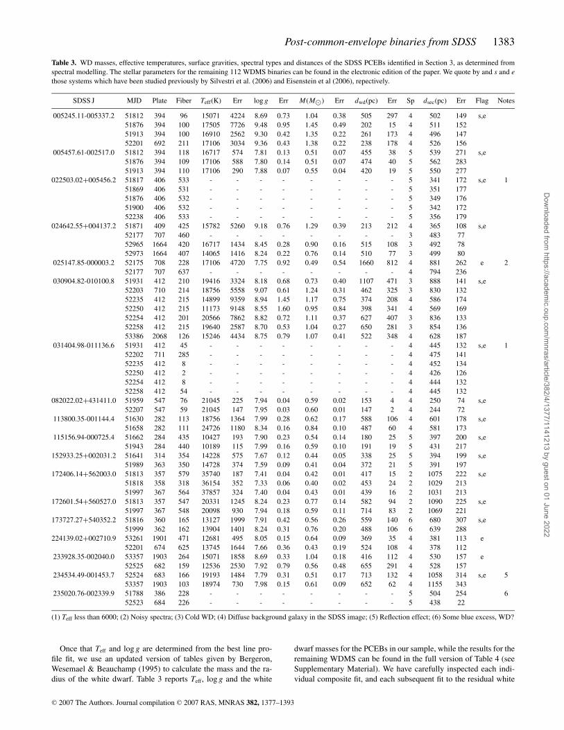
Table 3. WD masses, effective temperatures, surface gravities, spectral types and distances of the SDSS PCEBs identified in Section 3, as determined from
spectral modelling. The stellar parameters for the remaining 112 WDMS binaries can be found in the electronic edition of the paper. We quote by and s and ethose systems which have been studied previously by Silvestri et al. (2006) and Eisenstein et al (2006), repectively.
SDSS J MJD Plate Fiber Teff(K) Err log g Err M(M�) Err dwd(pc) Err Sp dsec(pc) Err Flag Notes
005245.11-005337.2 51812 394 96 15071 4224 8.69 0.73 1.04 0.38 505 297 4 502 149 s,e
51876 394 100 17505 7726 9.48 0.95 1.45 0.49 202 15 4 511 152
51913 394 100 16910 2562 9.30 0.42 1.35 0.22 261 173 4 496 147
52201 692 211 17106 3034 9.36 0.43 1.38 0.22 238 178 4 526 156
005457.61-002517.0 51812 394 118 16717 574 7.81 0.13 0.51 0.07 455 38 5 539 271 s,e
51876 394 109 17106 588 7.80 0.14 0.51 0.07 474 40 5 562 283
51913 394 110 17106 290 7.88 0.07 0.55 0.04 420 19 5 550 277
022503.02+005456.2 51817 406 533 - - - - - - - - 5 341 172 s,e 1
51869 406 531 - - - - - - - - 5 351 177
51876 406 532 - - - - - - - - 5 349 176
51900 406 532 - - - - - - - - 5 342 172
52238 406 533 - - - - - - - - 5 356 179
024642.55+004137.2 51871 409 425 15782 5260 9.18 0.76 1.29 0.39 213 212 4 365 108 s,e
52177 707 460 - - - - - - - - 3 483 77
52965 1664 420 16717 1434 8.45 0.28 0.90 0.16 515 108 3 492 78
52973 1664 407 14065 1416 8.24 0.22 0.76 0.14 510 77 3 499 80
025147.85-000003.2 52175 708 228 17106 4720 7.75 0.92 0.49 0.54 1660 812 4 881 262 e 2
52177 707 637 - - - - - - - - 4 794 236
030904.82-010100.8 51931 412 210 19416 3324 8.18 0.68 0.73 0.40 1107 471 3 888 141 s,e
52203 710 214 18756 5558 9.07 0.61 1.24 0.31 462 325 3 830 132
52235 412 215 14899 9359 8.94 1.45 1.17 0.75 374 208 4 586 174
52250 412 215 11173 9148 8.55 1.60 0.95 0.84 398 341 4 569 169
52254 412 201 20566 7862 8.82 0.72 1.11 0.37 627 407 3 836 133
52258 412 215 19640 2587 8.70 0.53 1.04 0.27 650 281 3 854 136
53386 2068 126 15246 4434 8.75 0.79 1.07 0.41 522 348 4 628 187
031404.98-011136.6 51931 412 45 - - - - - - - - 4 445 132 s,e 1
52202 711 285 - - - - - - - - 4 475 141
52235 412 8 - - - - - - - - 4 452 134
52250 412 2 - - - - - - - - 4 426 126
52254 412 8 - - - - - - - - 4 444 132
52258 412 54 - - - - - - - - 4 445 132
082022.02+431411.0 51959 547 76 21045 225 7.94 0.04 0.59 0.02 153 4 4 250 74 s,e
52207 547 59 21045 147 7.95 0.03 0.60 0.01 147 2 4 244 72
113800.35-001144.4 51630 282 113 18756 1364 7.99 0.28 0.62 0.17 588 106 4 601 178 s,e
51658 282 111 24726 1180 8.34 0.16 0.84 0.10 487 60 4 581 173
115156.94-000725.4 51662 284 435 10427 193 7.90 0.23 0.54 0.14 180 25 5 397 200 s,e
51943 284 440 10189 115 7.99 0.16 0.59 0.10 191 19 5 431 217
152933.25+002031.2 51641 314 354 14228 575 7.67 0.12 0.44 0.05 338 25 5 394 199 s,e
51989 363 350 14728 374 7.59 0.09 0.41 0.04 372 21 5 391 197
172406.14+562003.0 51813 357 579 35740 187 7.41 0.04 0.42 0.01 417 15 2 1075 222 s,e
51818 358 318 36154 352 7.33 0.06 0.40 0.02 453 24 2 1029 213
51997 367 564 37857 324 7.40 0.04 0.43 0.01 439 16 2 1031 213
172601.54+560527.0 51813 357 547 20331 1245 8.24 0.23 0.77 0.14 582 94 2 1090 225 s,e
51997 367 548 20098 930 7.94 0.18 0.59 0.11 714 83 2 1069 221
173727.27+540352.2 51816 360 165 13127 1999 7.91 0.42 0.56 0.26 559 140 6 680 307 s,e
51999 362 162 13904 1401 8.24 0.31 0.76 0.20 488 106 6 639 288
224139.02+002710.9 53261 1901 471 12681 495 8.05 0.15 0.64 0.09 369 35 4 381 113 e
52201 674 625 13745 1644 7.66 0.36 0.43 0.19 524 108 4 378 112
233928.35-002040.0 53357 1903 264 15071 1858 8.69 0.33 1.04 0.18 416 112 4 530 157 e
52525 682 159 12536 2530 7.92 0.79 0.56 0.48 655 291 4 528 157
234534.49-001453.7 52524 683 166 19193 1484 7.79 0.31 0.51 0.17 713 132 4 1058 314 s,e 5
53357 1903 103 18974 730 7.98 0.15 0.61 0.09 652 62 4 1155 343
235020.76-002339.9 51788 386 228 - - - - - - - - 5 504 254 6
52523 684 226 - - - - - - - - 5 438 22
(1) Teff less than 6000; (2) Noisy spectra; (3) Cold WD; (4) Diffuse background galaxy in the SDSS image; (5) Reflection effect; (6) Some blue excess, WD?
Once that Teff and log g are determined from the best line pro-
file fit, we use an updated version of tables given by Bergeron,
Wesemael & Beauchamp (1995) to calculate the mass and the ra-
dius of the white dwarf. Table 3 reports Teff, log g and the white
dwarf masses for the PCEBs in our sample, while the results for the
remaining WDMS can be found in the full version of Table 4 (see
Supplementary Material). We have carefully inspected each indi-
vidual composite fit, and each subsequent fit to the residual white
C© 2007 The Authors. Journal compilation C© 2007 RAS, MNRAS 382, 1377–1393
Dow
nloaded from https://academ
ic.oup.com/m
nras/article/382/4/1377/1141213 by guest on 01 June 2022
1384 A. Rebassa-Mansergas et al.
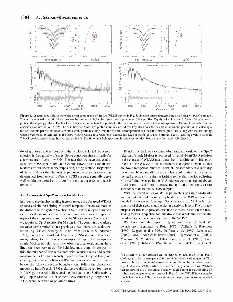
Figure 6. Spectral model fits to the white dwarf components of the two WDMS shown in Fig. 5, obtained after subtracting the best-fitting M-dwarf template.
Top left-hand panels: best fit (black lines) to the normalized Hβ to Hε (grey lines, top to bottom) line profiles. Top right-hand panels: 3, 5 and 10σ χ2 contour
plots in the Teff–log g plane. The black contours refer to the best line profile fit, the red contours to the fit of the whole spectrum. The solid line indicates the
occurrence of maximum Hβ EW. The best ‘hot’ and ‘cold’ line profile solutions are indicated by black dots, the best fit to the whole spectrum is indicated by a
red dot. Bottom panels: the residual white dwarf spectra resulting from the spectral decomposition and their flux errors (grey lines) along with the best-fitting
white dwarf model (black line) to the 3850–7150 Å wavelength range (top) and the residuals of the fit (grey line, bottom). The Teff and log g values listed in
Table 3 are determined from the best line profile fit. The fit to the whole spectrum is only used to select between the ‘hot’ and ‘cold’ line fit.
dwarf spectrum, and are confident that we have selected the correct
solution in the majority of cases. Some doubt remains primarily for
a few spectra of very low S/N. The fact that we have analysed at
least two SDSS spectra for each system allows us to assess the ro-
bustness of our spectral decomposition/fitting method. Inspection
of Table 3 shows that the system parameter of a given system, as
determined from several different SDSS spectra, generally agree
well within the quoted errors, confirming that our error estimate is
realistic.
3.4 An empirical Sp–R relation for M-stars
In order to use the flux-scaling factor between the observed WDMS
spectra and the best-fitting M-dwarf templates for an estimate of
the distance to the system (Section 3.5), it is necessary to assume a
radius for the secondary star. Since we have determined the spectral
types of the companion stars from the SDSS spectra (Section 3.2),
we require an Sp–R relation for M-dwarfs. The community working
on cataclysmic variables has previously had interest in such a re-
lation (e.g. Mateo, Szkody & Bolte 1985; Caillault & Patterson
1990), but while Baraffe & Chabrier (1996) derived theoretical
mass/radius/effective temperature–spectral type relationships for
single M-dwarfs, relatively little observational work along these
lines has been carried out for field low-mass stars. In contrast to
this, the number of low-mass stars with accurate mass and radius
measurements has significantly increased over the past few years
(see e.g. the review by Ribas 2006), and it appears that for masses
below the fully convective boundary stars follow the theoretical
models by Baraffe et al. (1998) relatively well. However, for masses
� 0.3 M�, observed radii exceed the predicted ones. Stellar activity
(e.g. Lopez-Morales 2007) or metallicity effects (e.g. Berger et al.
2006) were identified as possible causes.
Besides the lack of extensive observational work on the Sp–Rrelation of single M-dwarfs, our need for an M-dwarf Sp–R relation
in the context of WDMS faces a number of additional problems. A
fraction of the WDMS in our sample have undergone a CE phase, and
are now short-period binaries, in which the secondary star is tidally
locked and hence rapidly rotating. This rapid rotation will enhance
the stellar activity in a similar fashion to the short-period eclipsing
M-dwarf binaries used in the M–R relation work mentioned above.
In addition, it is difficult to assess the age4 and metallicity of the
secondary stars in our WDMS sample.
With the uncertainties on stellar parameters of single M-dwarfs
and the potential additional complications in WDMS in mind, we
decided to derive an ‘average’ Sp–R relation for M-dwarfs irre-
spective of their ages, metallicities and activity levels. The primary
purpose of this is to provide distance estimates based on the flux-
scaling factors in equation (4), but also to assess potential systematic
peculiarities of the secondary stars in the WDMS.
We have compiled spectral types and radii of field M-
dwarfs from Berriman & Reid (1987), Caillault & Patterson
(1990), Leggett et al. (1996), Delfosse et al. (1999), Leto et al.
(2000), Lane, Boden & Kulkarni (2001), Segransan et al. (2003),
Maceroni & Montalban (2004), Creevey et al. (2005), Pont
et al. (2005), Ribas (2006), Berger et al. (2006), Bayless &
4 In principle, an age estimate can be derived by adding the white dwarf
cooling age to the main-sequence lifetime of the white dwarf progenitor. This
involves the use of an initial mass–final mass relation for the white dwarf,
e.g. Dobbie et al. (2006), which will not be strictly valid for those WDMS
that underwent a CE evolution. Broadly judging from the distribution of
white dwarf temperatures and masses in Fig. 10, most WDMS in our sample
should be older than 1 Gyr, but the data at hand do not warrant a more detailed
analysis.
C© 2007 The Authors. Journal compilation C© 2007 RAS, MNRAS 382, 1377–1393
Dow
nloaded from https://academ
ic.oup.com/m
nras/article/382/4/1377/1141213 by guest on 01 June 2022
Post-common-envelope binaries from SDSS 1385
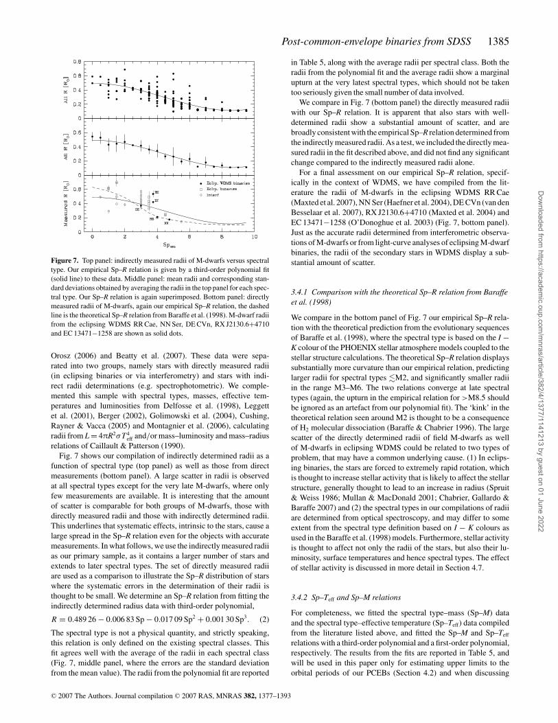
Figure 7. Top panel: indirectly measured radii of M-dwarfs versus spectral
type. Our empirical Sp–R relation is given by a third-order polynomial fit
(solid line) to these data. Middle panel: mean radii and corresponding stan-
dard deviations obtained by averaging the radii in the top panel for each spec-
tral type. Our Sp–R relation is again superimposed. Bottom panel: directly
measured radii of M-dwarfs, again our empirical Sp–R relation, the dashed
line is the theoretical Sp–R relation from Baraffe et al. (1998). M-dwarf radii
from the eclipsing WDMS RR Cae, NN Ser, DE CVn, RX J2130.6+4710
and EC 13471−1258 are shown as solid dots.
Orosz (2006) and Beatty et al. (2007). These data were sepa-
rated into two groups, namely stars with directly measured radii
(in eclipsing binaries or via interferometry) and stars with indi-
rect radii determinations (e.g. spectrophotometric). We comple-
mented this sample with spectral types, masses, effective tem-
peratures and luminosities from Delfosse et al. (1998), Leggett
et al. (2001), Berger (2002), Golimowski et al. (2004), Cushing,
Rayner & Vacca (2005) and Montagnier et al. (2006), calculating
radii from L = 4πR2σT4eff and/or mass–luminosity and mass–radius
relations of Caillault & Patterson (1990).
Fig. 7 shows our compilation of indirectly determined radii as a
function of spectral type (top panel) as well as those from direct
measurements (bottom panel). A large scatter in radii is observed
at all spectral types except for the very late M-dwarfs, where only
few measurements are available. It is interesting that the amount
of scatter is comparable for both groups of M-dwarfs, those with
directly measured radii and those with indirectly determined radii.
This underlines that systematic effects, intrinsic to the stars, cause a
large spread in the Sp–R relation even for the objects with accurate
measurements. In what follows, we use the indirectly measured radii
as our primary sample, as it contains a larger number of stars and
extends to later spectral types. The set of directly measured radii
are used as a comparison to illustrate the Sp–R distribution of stars
where the systematic errors in the determination of their radii is
thought to be small. We determine an Sp–R relation from fitting the
indirectly determined radius data with third-order polynomial,
R = 0.489 26 − 0.006 83 Sp − 0.017 09 Sp2 + 0.001 30 Sp3. (2)
The spectral type is not a physical quantity, and strictly speaking,
this relation is only defined on the existing spectral classes. This
fit agrees well with the average of the radii in each spectral class
(Fig. 7, middle panel, where the errors are the standard deviation
from the mean value). The radii from the polynomial fit are reported
in Table 5, along with the average radii per spectral class. Both the
radii from the polynomial fit and the average radii show a marginal
upturn at the very latest spectral types, which should not be taken
too seriously given the small number of data involved.
We compare in Fig. 7 (bottom panel) the directly measured radii
with our Sp–R relation. It is apparent that also stars with well-
determined radii show a substantial amount of scatter, and are
broadly consistent with the empirical Sp–R relation determined from
the indirectly measured radii. As a test, we included the directly mea-
sured radii in the fit described above, and did not find any significant
change compared to the indirectly measured radii alone.
For a final assessment on our empirical Sp–R relation, specif-
ically in the context of WDMS, we have compiled from the lit-
erature the radii of M-dwarfs in the eclipsing WDMS RR Cae
(Maxted et al. 2007), NN Ser (Haefner et al. 2004), DE CVn (van den
Besselaar et al. 2007), RX J2130.6+4710 (Maxted et al. 2004) and
EC 13471−1258 (O’Donoghue et al. 2003) (Fig. 7, bottom panel).
Just as the accurate radii determined from interferometric observa-
tions of M-dwarfs or from light-curve analyses of eclipsing M-dwarf
binaries, the radii of the secondary stars in WDMS display a sub-
stantial amount of scatter.
3.4.1 Comparison with the theoretical Sp–R relation from Baraffeet al. (1998)
We compare in the bottom panel of Fig. 7 our empirical Sp–R rela-
tion with the theoretical prediction from the evolutionary sequences
of Baraffe et al. (1998), where the spectral type is based on the I −K colour of the PHOENIX stellar atmosphere models coupled to the
stellar structure calculations. The theoretical Sp–R relation displays
substantially more curvature than our empirical relation, predicting
larger radii for spectral types �M2, and significantly smaller radii
in the range M3–M6. The two relations converge at late spectral
types (again, the upturn in the empirical relation for >M8.5 should
be ignored as an artefact from our polynomial fit). The ‘kink’ in the
theoretical relation seen around M2 is thought to be a consequence
of H2 molecular dissociation (Baraffe & Chabrier 1996). The large
scatter of the directly determined radii of field M-dwarfs as well
of M-dwarfs in eclipsing WDMS could be related to two types of
problem, that may have a common underlying cause. (1) In eclips-
ing binaries, the stars are forced to extremely rapid rotation, which
is thought to increase stellar activity that is likely to affect the stellar
structure, generally thought to lead to an increase in radius (Spruit
& Weiss 1986; Mullan & MacDonald 2001; Chabrier, Gallardo &
Baraffe 2007) and (2) the spectral types in our compilations of radii
are determined from optical spectroscopy, and may differ to some
extent from the spectral type definition based on I − K colours as
used in the Baraffe et al. (1998) models. Furthermore, stellar activity
is thought to affect not only the radii of the stars, but also their lu-
minosity, surface temperatures and hence spectral types. The effect
of stellar activity is discussed in more detail in Section 4.7.
3.4.2 Sp–Teff and Sp–M relations
For completeness, we fitted the spectral type–mass (Sp–M) data
and the spectral type–effective temperature (Sp–Teff) data compiled
from the literature listed above, and fitted the Sp–M and Sp–Teff
relations with a third-order polynomial and a first-order polynomial,
respectively. The results from the fits are reported in Table 5, and
will be used in this paper only for estimating upper limits to the
orbital periods of our PCEBs (Section 4.2) and when discussing
C© 2007 The Authors. Journal compilation C© 2007 RAS, MNRAS 382, 1377–1393
Dow
nloaded from https://academ
ic.oup.com/m
nras/article/382/4/1377/1141213 by guest on 01 June 2022
1386 A. Rebassa-Mansergas et al.
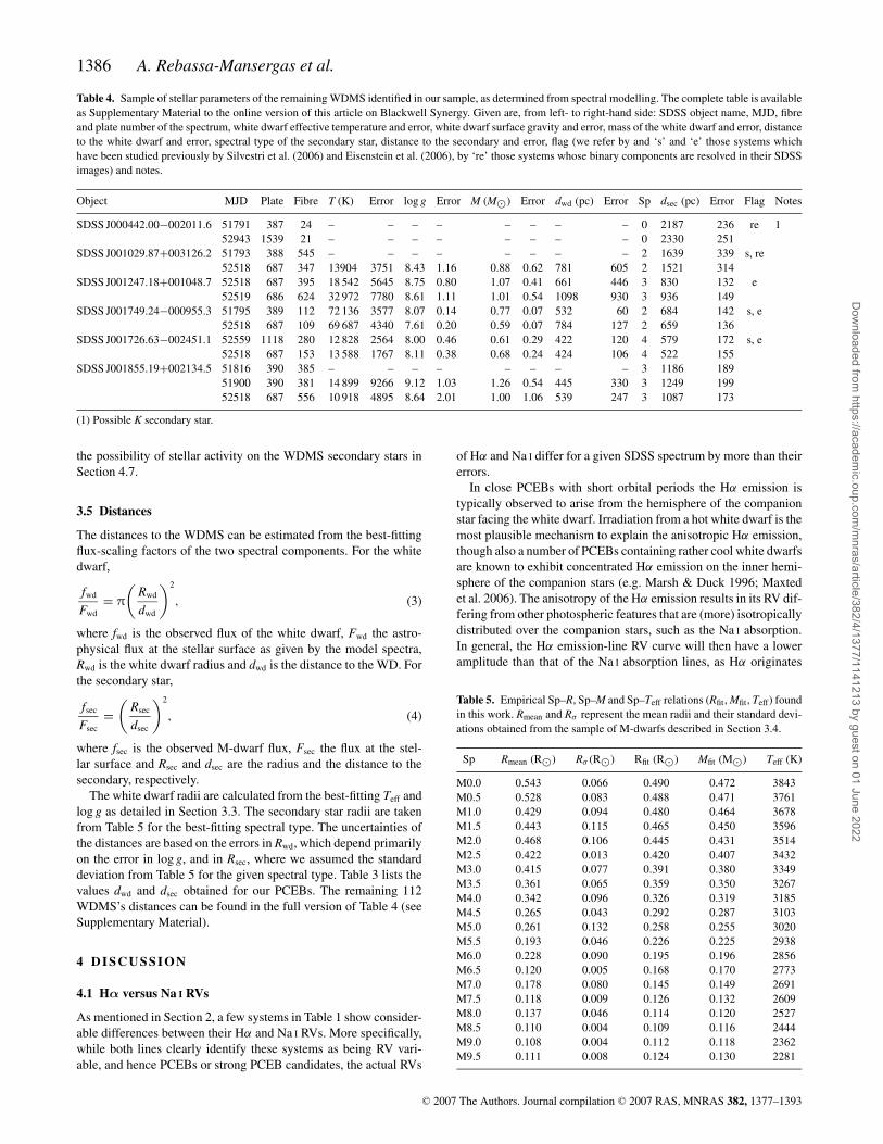
Table 4. Sample of stellar parameters of the remaining WDMS identified in our sample, as determined from spectral modelling. The complete table is available
as Supplementary Material to the online version of this article on Blackwell Synergy. Given are, from left- to right-hand side: SDSS object name, MJD, fibre
and plate number of the spectrum, white dwarf effective temperature and error, white dwarf surface gravity and error, mass of the white dwarf and error, distance
to the white dwarf and error, spectral type of the secondary star, distance to the secondary and error, flag (we refer by and ‘s’ and ‘e’ those systems which
have been studied previously by Silvestri et al. (2006) and Eisenstein et al. (2006), by ‘re’ those systems whose binary components are resolved in their SDSS
images) and notes.
Object MJD Plate Fibre T (K) Error log g Error M (M�) Error dwd (pc) Error Sp dsec (pc) Error Flag Notes
SDSS J000442.00−002011.6 51791 387 24 – – – – – – – – 0 2187 236 re 1
52943 1539 21 – – – – – – – – 0 2330 251
SDSS J001029.87+003126.2 51793 388 545 – – – – – – – – 2 1639 339 s, re
52518 687 347 13904 3751 8.43 1.16 0.88 0.62 781 605 2 1521 314
SDSS J001247.18+001048.7 52518 687 395 18 542 5645 8.75 0.80 1.07 0.41 661 446 3 830 132 e
52519 686 624 32 972 7780 8.61 1.11 1.01 0.54 1098 930 3 936 149
SDSS J001749.24−000955.3 51795 389 112 72 136 3577 8.07 0.14 0.77 0.07 532 60 2 684 142 s, e
52518 687 109 69 687 4340 7.61 0.20 0.59 0.07 784 127 2 659 136
SDSS J001726.63−002451.1 52559 1118 280 12 828 2564 8.00 0.46 0.61 0.29 422 120 4 579 172 s, e
52518 687 153 13 588 1767 8.11 0.38 0.68 0.24 424 106 4 522 155
SDSS J001855.19+002134.5 51816 390 385 – – – – – – – – 3 1186 189
51900 390 381 14 899 9266 9.12 1.03 1.26 0.54 445 330 3 1249 199
52518 687 556 10 918 4895 8.64 2.01 1.00 1.06 539 247 3 1087 173
(1) Possible K secondary star.
the possibility of stellar activity on the WDMS secondary stars in
Section 4.7.
3.5 Distances
The distances to the WDMS can be estimated from the best-fitting
flux-scaling factors of the two spectral components. For the white
dwarf,
fwd
Fwd
= π
(Rwd
dwd
)2
, (3)
where fwd is the observed flux of the white dwarf, Fwd the astro-
physical flux at the stellar surface as given by the model spectra,
Rwd is the white dwarf radius and dwd is the distance to the WD. For
the secondary star,
fsec
Fsec
=(
Rsec
dsec
)2
, (4)
where fsec is the observed M-dwarf flux, Fsec the flux at the stel-
lar surface and Rsec and dsec are the radius and the distance to the
secondary, respectively.
The white dwarf radii are calculated from the best-fitting Teff and
log g as detailed in Section 3.3. The secondary star radii are taken
from Table 5 for the best-fitting spectral type. The uncertainties of
the distances are based on the errors in Rwd, which depend primarily
on the error in log g, and in Rsec, where we assumed the standard
deviation from Table 5 for the given spectral type. Table 3 lists the
values dwd and dsec obtained for our PCEBs. The remaining 112
WDMS’s distances can be found in the full version of Table 4 (see
Supplementary Material).
4 D I S C U S S I O N
4.1 Hα versus Na I RVs
As mentioned in Section 2, a few systems in Table 1 show consider-
able differences between their Hα and Na I RVs. More specifically,
while both lines clearly identify these systems as being RV vari-
able, and hence PCEBs or strong PCEB candidates, the actual RVs
of Hα and Na I differ for a given SDSS spectrum by more than their
errors.
In close PCEBs with short orbital periods the Hα emission is
typically observed to arise from the hemisphere of the companion
star facing the white dwarf. Irradiation from a hot white dwarf is the
most plausible mechanism to explain the anisotropic Hα emission,
though also a number of PCEBs containing rather cool white dwarfs
are known to exhibit concentrated Hα emission on the inner hemi-
sphere of the companion stars (e.g. Marsh & Duck 1996; Maxted
et al. 2006). The anisotropy of the Hα emission results in its RV dif-
fering from other photospheric features that are (more) isotropically
distributed over the companion stars, such as the Na I absorption.
In general, the Hα emission-line RV curve will then have a lower
amplitude than that of the Na I absorption lines, as Hα originates
Table 5. Empirical Sp–R, Sp–M and Sp–Teff relations (Rfit, Mfit, Teff) found
in this work. Rmean and Rσ represent the mean radii and their standard devi-
ations obtained from the sample of M-dwarfs described in Section 3.4.
Sp Rmean (R�) Rσ (R�) Rfit (R�) Mfit (M�) Teff (K)
M0.0 0.543 0.066 0.490 0.472 3843
M0.5 0.528 0.083 0.488 0.471 3761
M1.0 0.429 0.094 0.480 0.464 3678
M1.5 0.443 0.115 0.465 0.450 3596
M2.0 0.468 0.106 0.445 0.431 3514
M2.5 0.422 0.013 0.420 0.407 3432
M3.0 0.415 0.077 0.391 0.380 3349
M3.5 0.361 0.065 0.359 0.350 3267
M4.0 0.342 0.096 0.326 0.319 3185
M4.5 0.265 0.043 0.292 0.287 3103
M5.0 0.261 0.132 0.258 0.255 3020
M5.5 0.193 0.046 0.226 0.225 2938
M6.0 0.228 0.090 0.195 0.196 2856
M6.5 0.120 0.005 0.168 0.170 2773
M7.0 0.178 0.080 0.145 0.149 2691
M7.5 0.118 0.009 0.126 0.132 2609
M8.0 0.137 0.046 0.114 0.120 2527
M8.5 0.110 0.004 0.109 0.116 2444
M9.0 0.108 0.004 0.112 0.118 2362
M9.5 0.111 0.008 0.124 0.130 2281
C© 2007 The Authors. Journal compilation C© 2007 RAS, MNRAS 382, 1377–1393
Dow
nloaded from https://academ
ic.oup.com/m
nras/article/382/4/1377/1141213 by guest on 01 June 2022
Post-common-envelope binaries from SDSS 1387
closer to the centre of mass of the binary system. In addition, the
strength of Hα can vary greatly due to different geometric projec-
tions in high inclination systems. More complications are added in
the context of SDSS spectroscopy, where the individual spectra have
typical exposure times of 45–60 min, which will result in the smear-
ing of the spectral features in the short-period PCEBs due to the
sampling of different orbital phases. This problem is exacerbated in
the case that the SDSS spectrum is combined from exposures taken
on different nights (see Section 2). Finally, the Hα emission from
the companion may substantially increase during a flare, which will
further enhance the anisotropic nature of the emission.
Systems in which the Hα and Na I RVs differ by more than 2σ
are: SDSS J005245.11−005337.2, SDSS J024642.55+004137.2,
SDSS J030904.82−010100.8, SDSS J031404.98−011136.6 and
SDSS J172406.14+562003.0. Of these, SDSS J0246+0041,
SDSS J0314−0111 and SDSS J1724+5620 show large-amplitude
RV variations and substantial changes in the EW of the Hα emission
line, suggesting that they are rather short orbital period PCEBs
with moderately high inclinations, which most likely explains
the observed differences between the observed Hα and Na I RVs.
Irradiation is also certainly important in SDSS J1724+5620 which
contains a hot (�36 000 K) white dwarf. SDSS J0052−0053
displays only a moderate RV amplitude, and while the Hα and
Na I RVs display a homogeneous pattern of variation (Figs 3 and
4), Hα appears to have a larger amplitude which is not readily
explained. Similar discrepancies have been observed, e.g. in the
close magnetic WDMS binary WX LMi, and were thought to be
related to a time-variable change in the location of the Hα emission
(Vogel, Schwope & Gansicke 2007). Finally, SDSS J0309−0101 is
rather faint (g = 20.4), but has a strong Hα emission that allows
reliable RV measurements that identify the system as a PCEB.
The RVs from the Na I doublet are more affected by noise, which
probably explains the observed RV discrepancy in one out of its
seven SDSS spectra.
4.2 Upper limits to the orbital periods
The RVs of the secondary stars follow from Kepler’s third law and
depend on the stellar masses, the orbital period, and are subject
to geometric foreshortening by a factor of sin i, with i the binary
inclination with regards to the line of sight:
(Mwd sin i)3
(Mwd + Msec)2= Porb K 3
sec
2πG(5)
with Ksec the RV amplitude of the secondary star, and G the grav-
itational constant. This can be rearranged to solve for the orbital
period,
Porb = 2πG(Mwd sin i)3
(Mwd + Msec)2 K 3sec
. (6)
From this equation, it is clear that assuming i = 90◦ gives an upper
limit to the orbital period.
The RV measurements of our PCEBs and PCEB candidates
(Table 1) sample the motion of their companion stars at random
orbital phases. However, if we assume that the maximum and min-
imum values of the observed RVs sample the quadrature phases,
e.g. the instants of maximum RV, we obtain lower limits to the true
RV amplitudes of the companion stars in our systems. From equa-
tion (6), a lower limit to Ksec turns into an upper limit to Porb.
Hence, combining the RV information from Table 1 with the
stellar parameters from Table 3, we determined upper limits to the
orbital periods of all PCEBs and PCEB candidates, which range be-
tween 0.46–7880 d. The actual periods are likely to be substantially
shorter, especially for those systems where only two SDSS spectra
are available and the phase sampling is correspondingly poor. More
stringent constraints could be obtained from a more complex exer-
cise where the mid-exposure times are taken into account – however,
given the fact that many of the SDSS spectra are combined from data
taken on different nights, we refrained from this approach.
4.3 The fraction of PCEB among the SDSS WDMS binaries
We have measured the RVs of 101 WDMS which have multiple
SDSS spectra, and find that 15 of them clearly show RV variations,
three additional WDMS are good candidates for RV variations (see
Table 1). Taking the upper limits to the orbital periods at face value,
and assuming that systems with a period �300 d have undergone a
CE (Willems & Kolb 2004, see also Section 2), 17 of the systems
in Table 1 qualify as PCEBs, implying a PCEB fraction of ∼15
per cent in our WDMS sample, which is in rough agreement with
the predictions by the population model of Willems & Kolb (2004).
However, our value is likely to be a lower limit on the true fraction of
PCEBs among the SDSS WDMS binaries for the following reasons.
(1) In most cases only two spectra are available, with a non-
negligible chance of sampling similar orbital phases in both ob-
servations. (2) The relatively low spectral resolution of the SDSS
spectroscopy (λ/λ� 1800) plus the uncertainty in the flux calibra-
tion limit the detection of significant RV changes to ∼15 km s−1 for
the best spectra. (3) In binaries with extremely short orbital periods
the long exposures will smear the Na I doublet beyond recognition.
(4) A substantial number of the SDSS spectra are combined, av-
eraging different orbital phases and reducing the sensitivity to RV
changes. Follow-up observations of a representative sample of SDSS
WDMS with higher spectral resolution and a better defined cadence
will be necessary for an accurate determination of the fraction of
PCEBs.
4.4 Comparison with Raymond et al. (2003)
In a previous study, Raymond et al. (2003) determined white dwarf
temperatures, distance estimates based on the white dwarf fits, and
spectral types of the companion star for 109 SDSS WDMS. They
restricted their white dwarf fits to a single gravity, log g = 8.0, and a
white dwarf radius of 8 × 108 cm (corresponding to Mwd = 0.6 M�),
which is a fair match for the majority of systems (see Section 4.6
below). Our sample of WDMS with two or more SDSS spectra has
28 objects in common with Raymond’s list, sufficient to allow for
a quantitative comparison between the two different methods used
to fit the data. As we fitted two or more spectra for each WDMS,
we averaged for this purpose the parameters obtained from the fits
to individual spectra of a given object, and propagated their errors
accordingly. We find that ∼2/3 of the temperatures determined by
Raymond et al. (2003) agree with ours at the ∼20 per cent level,
with the remaining being different by up to a factor 2 (Fig. 8, left-
hand panels). This fairly large disagreement is most likely caused
by the simplified fitting Raymond et al. adopted, i.e. fitting the white
dwarf models in the wavelength range 3800–5000 Å, neglecting the
contribution of the companion star. The spectral types of the com-
panion stars from our work and Raymond et al. (2003) agree mostly
to within ±1.5 spectral classes, which is satisfying given the com-
posite nature of the WDMS spectra and the problems associated
with their spectral decomposition (Fig. 8, right-hand panels). The
biggest discrepancy shows up in the distances, with the Raymond
C© 2007 The Authors. Journal compilation C© 2007 RAS, MNRAS 382, 1377–1393
Dow
nloaded from https://academ
ic.oup.com/m
nras/article/382/4/1377/1141213 by guest on 01 June 2022
1388 A. Rebassa-Mansergas et al.
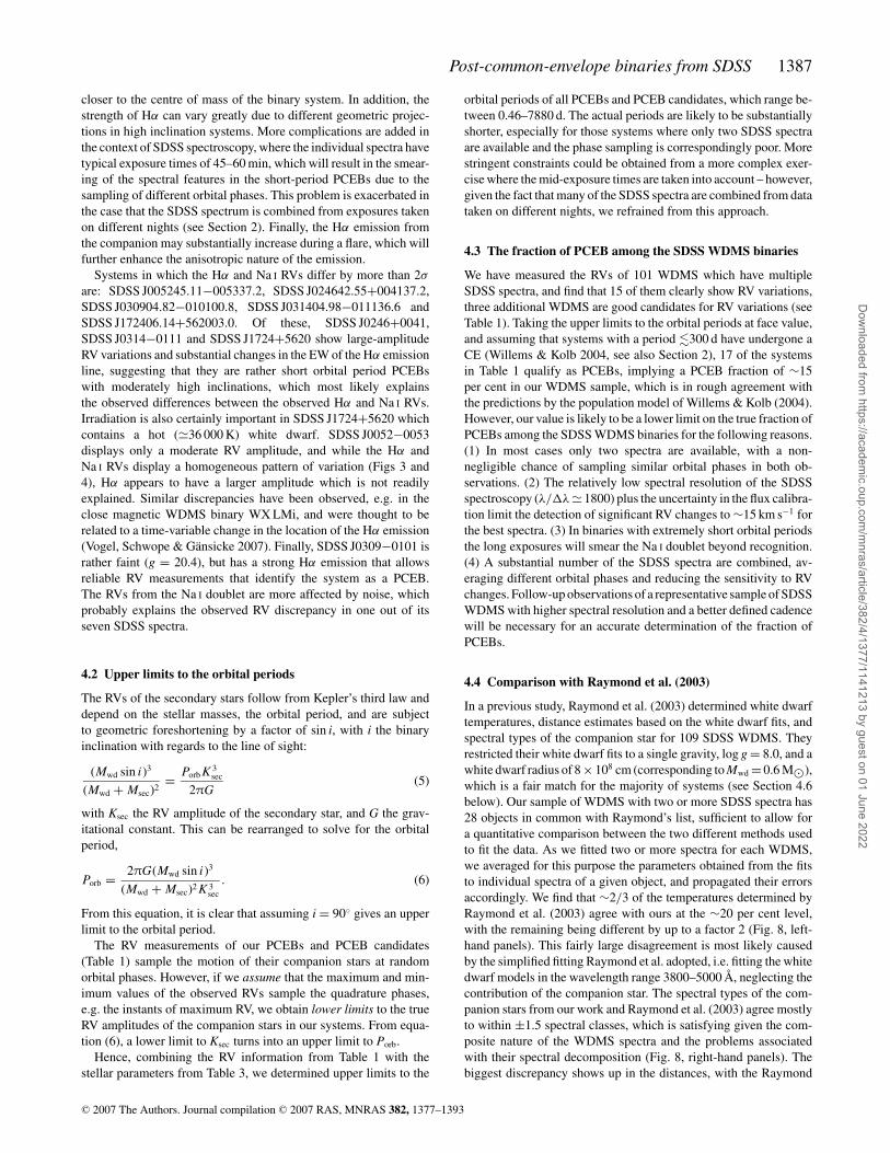
Figure 8. Comparison of the white dwarf effective temperatures, distances based on the white dwarf fit, and the spectral types of the secondary stars determined
from our fits (Sections 3.2, 3.3 and Table 3), and those of Raymond et al. (2003). Top panels, from left- to right-hand side: the ratio in Teff, the ratio in d and
the difference in the secondary’s spectral types from the two studies as a function of the white dwarf temperature.
et al. distances being systematically lower than ours (Fig. 8, middle
panels). The average of the factor by which Raymond et al. under-
predict the distances is 6.5, which is close to 2π, suggesting that
the authors may have misinterpreted the flux definition of the model
atmosphere code they used (TLUSTY/SYNSPEC from Hubeny & Lanz
1995, which outputs Eddington fluxes), and hence may have used a
wrong constant in the flux normalization (equation 3).
4.5 Comparison with Silvestri et al. (2006)
Having developed an independent method of determining the stellar
parameters for WDMS from their SDSS spectra, we compared our
results to those of Silvestri et al. (2006). As in Section 4.4 above,
we average the parameters obtained from the fits to the individual
SDSS spectra of a given object. Fig. 9 shows the comparison be-
tween the white dwarf effective temperatures, surface gravities and
spectral types of the secondary stars from the two studies. Both
studies agree in broad terms for all three fit parameters (Fig. 9,
bottom panels). Inspecting the discrepancies between the two inde-
pendent sets of stellar parameters, it became evident that relatively
large disagreements are most noticeably found for Teff � 20 000 K,
with differences in Teff of up to a factor of 2, an order of mag-
nitude in surface gravity, and a typical difference in spectral type
of the secondary of ±2 spectral classes. For higher temperatures
the differences become small, with nearly identical values for Teff,
log g agreeing within ±0.2 mag and spectral types differing by
±1 spectral classes at most (Fig. 9, top panels). We interpret this
strong disagreement at low to intermediate white dwarf tempera-
tures to the ambiguity between hot and cold solutions described in
Section 3.3.
A quantitative judgement of the fits in Silvestri et al. (2006) is
difficult, as the authors do not provide much detail on the method
used to decompose the WDMS spectra, except for a single exam-
ple in their fig. 1. It is worth noting that the M-dwarf component
in that figure displays constant flux at λ < 6000 Å, which seems
rather unrealistic for the claimed spectral type of M5. Unfortunately,
Silvestri et al. (2006) do not list distances implied by their fits to
the white dwarf and main-sequence components in their WDMS
sample, which would provide a test of internal consistency (see
Section 4.7).
We also investigated the systems that the method of Silvestri et al.
(2006) failed to fit, and found that we were able to determine rea-
sonable parameters for most of them. It appears that our method
is more robust in cases of low S/N, and in cases where one of the
stellar components contributes relatively little to the total flux. Ex-
amples of the latter are SDSS J204431.45−061440.2, where an M0
secondary star dominates the SDSS spectrum at λ � 4600 Å, or
SDSS J172406.14+562003.1, which is a close PCEB containing a
hot white dwarf and a low-mass companion. An independent anal-
ysis of the entire WDMS sample from SDSS appears therefore a
worthwhile exercise, which we will pursue elsewhere.
4.6 Distribution of the stellar parameters
Having determined stellar parameters for each individual system in
Section 3, we are looking here at their global distribution within
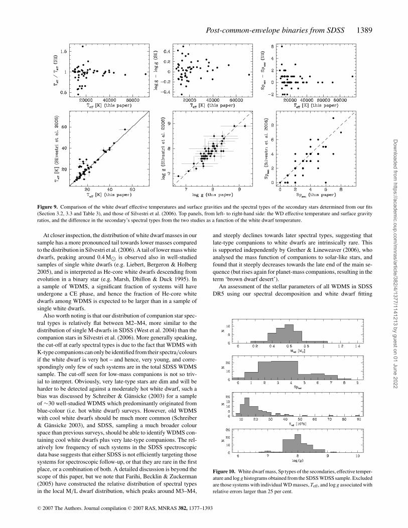
our sample of WDMS. Fig. 10 shows histograms of the white dwarf
effective temperatures, masses, log g and the spectral types of the
main-sequence companions.
As in Sections 4.4 and 4.5 above, we use here the average of the fit
parameters obtained from the different SDSS spectra of each object.
Furthermore, we exclude all systems with relative errors in their
white dwarf parameters (Twd, log g, Mwd) exceeding 25 per cent to
prevent smearing of the histograms due to poor-quality data and/or
fits, which results in 95, 81, 94 and 38 WDMS in the histograms for
the companion spectral type, log g, Twd and Mwd, respectively. In
broad terms, our results are consistent with those of Raymond et al.
(2003) and Silvestri et al. (2006): the most frequent white dwarf
temperatures are between 10 000 and 20 000 K, white dwarf masses
cluster around Mwd � 0.6 M� and the companion stars have most
typically a spectral type M3–M4, with spectral types later than M7
or earlier than M1 being very rare.
C© 2007 The Authors. Journal compilation C© 2007 RAS, MNRAS 382, 1377–1393
Dow
nloaded from https://academ
ic.oup.com/m
nras/article/382/4/1377/1141213 by guest on 01 June 2022
Post-common-envelope binaries from SDSS 1389
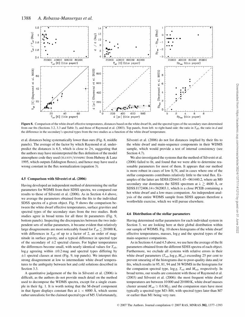
Figure 9. Comparison of the white dwarf effective temperatures and surface gravities and the spectral types of the secondary stars determined from our fits
(Section 3.2, 3.3 and Table 3), and those of Silvestri et al. (2006). Top panels, from left- to right-hand side: the WD effective temperature and surface gravity
ratios, and the difference in the secondary’s spectral types from the two studies as a function of the white dwarf temperature.
At closer inspection, the distribution of white dwarf masses in our
sample has a more pronounced tail towards lower masses compared
to the distribution in Silvestri et al. (2006). A tail of lower mass white
dwarfs, peaking around 0.4 M� is observed also in well-studied
samples of single white dwarfs (e.g. Liebert, Bergeron & Holberg
2005), and is interpreted as He-core white dwarfs descending from
evolution in a binary star (e.g. Marsh, Dhillon & Duck 1995). In
a sample of WDMS, a significant fraction of systems will have
undergone a CE phase, and hence the fraction of He-core white
dwarfs among WDMS is expected to be larger than in a sample of
single white dwarfs.
Also worth noting is that our distribution of companion star spec-
tral types is relatively flat between M2–M4, more similar to the
distribution of single M-dwarfs in SDSS (West et al. 2004) than the
companion stars in Silvestri et al. (2006). More generally speaking,
the cut-off at early spectral types is due to the fact that WDMS with
K-type companions can only be identified from their spectra/colours
if the white dwarf is very hot – and hence, very young, and corre-
spondingly only few of such systems are in the total SDSS WDMS
sample. The cut-off seen for low-mass companions is not so triv-
ial to interpret. Obviously, very late-type stars are dim and will be
harder to be detected against a moderately hot white dwarf, such a
bias was discussed by Schreiber & Gansicke (2003) for a sample
of ∼30 well-studied WDMS which predominantly originated from
blue-colour (i.e. hot white dwarf) surveys. However, old WDMS
with cool white dwarfs should be much more common (Schreiber
& Gansicke 2003), and SDSS, sampling a much broader colour
space than previous surveys, should be able to identify WDMS con-
taining cool white dwarfs plus very late-type companions. The rel-
atively low frequency of such systems in the SDSS spectroscopic
data base suggests that either SDSS is not efficiently targeting those
systems for spectroscopic follow-up, or that they are rare in the first
place, or a combination of both. A detailed discussion is beyond the
scope of this paper, but we note that Farihi, Becklin & Zuckerman
(2005) have constructed the relative distribution of spectral types
in the local M/L dwarf distribution, which peaks around M3–M4,
and steeply declines towards later spectral types, suggesting that
late-type companions to white dwarfs are intrinsically rare. This
is supported independently by Grether & Lineweaver (2006), who
analysed the mass function of companions to solar-like stars, and
found that it steeply decreases towards the late end of the main se-
quence (but rises again for planet-mass companions, resulting in the
term ‘brown dwarf desert’).
An assessment of the stellar parameters of all WDMS in SDSS
DR5 using our spectral decomposition and white dwarf fitting
Figure 10. White dwarf mass, Sp types of the secondaries, effective temper-
ature and log g histograms obtained from the SDSS WDSS sample. Excluded
are those systems with individual WD masses, Teff, and log g associated with
relative errors larger than 25 per cent.
C© 2007 The Authors. Journal compilation C© 2007 RAS, MNRAS 382, 1377–1393
Dow
nloaded from https://academ
ic.oup.com/m
nras/article/382/4/1377/1141213 by guest on 01 June 2022
1390 A. Rebassa-Mansergas et al.
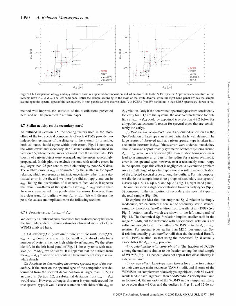
Figure 11. Comparison of dsec and dwd obtained from our spectral decomposition and white dwarf fits to the SDSS spectra. Approximately one-third of the
systems have dsec �= dwd. The left-hand panel splits the sample according to the mass of the white dwarfs, while the right-hand panel divides the sample
according to the spectral types of the secondaries. In both panels systems that we identify as PCEBs from RV variations in their SDSS spectra are shown in red.
method will improve the statistics of the distributions presented
here, and will be presented in a future paper.
4.7 Stellar activity on the secondary stars?
As outlined in Section 3.5, the scaling factors used in the mod-
elling of the two spectral components of each WDMS provide two
independent estimates of the distance to the system. In principle,
both estimates should agree within their errors. Fig. 11 compares
the white dwarf and secondary star distance estimates obtained in
Section 3.5, where the distances obtained from the individual SDSS
spectra of a given object were averaged, and the errors accordingly
propagated. In this plot, we exclude systems with relative errors in
dwd larger than 25 per cent to avoid cluttering by poor-S/N data.
The relative error in dsec is dominated by the scatter in the Sp–Rrelation, which represents an intrinsic uncertainty rather than a sta-
tistical error in the fit, and we therefore did not apply any cut in
dsec. Taking the distribution of distances at face value, it appears
that about two-thirds of the systems have dsec � dwd within their
1σ errors, as expected from purely statistical errors. However, there
is a clear trend for outliers where dsec > dwd. We will discuss the
possible causes and implications in the following sections.
4.7.1 Possible causes for dsec �= dwd
We identify a number of possible causes for the discrepancy between
the two independent distance estimates observed in ∼1/3 of the
WDMS analysed here.
(1) A tendency for systematic problems in the white dwarf fits.dsec > dwd could be a result of too small white dwarf radii for a
number of systems, i.e. too high white dwarf masses. We therefore
identify in the left-hand panel of Fig. 11 those systems with mas-
sive (>0.75 M�) white dwarfs. It is apparent that the outliers from
the dsec = dwd relation do not contain a large number of very massive
white dwarfs.
(2) Problems in determining the correct spectral type of the sec-ondary. If the error on the spectral type of the companion star de-
termined from the spectral decomposition is larger than ±0.5, as
assumed in Section 3.2, a substantial deviation from dsec = dwd
would result. However, as long as this error is symmetric around the
true spectral type, it would cause scatter on both sides of the dsec =
dwd relation. Only if the determined spectral types were consistently
too early for ∼1/3 of the systems, the observed preference for out-
liers at dsec > dwd could be explained (see Section 4.7.2 below for
a hypothetical systematic reason for spectral types that are consis-
tently too early).
(3) Problems in the Sp–R relation. As discussed in Section 3.4, the
Sp–R relation of late-type stars is not particularly well defined. The
large scatter of observed radii at a given spectral type is taken into
account in the errors in dsec. If those errors were underestimated, they
should cause an approximately symmetric scatter of systems around
dsec = dwd, which is not observed (the Sp–R relation being non-linear
lead to asymmetric error bars in the radius for a given symmetric
error in the spectral type, however, over a reasonably small range
in the spectral type this effect is negligible). A systematic problem
over a small range of spectral types would result in a concentration
of the affected spectral types among the outliers. For this purpose,
we divide our sample into three groups of secondary star spectral
classes, Sp > 5, 3 � Sp � 5, and Sp < 3 (Fig. 11, right-hand panel).
The outliers show a slight concentration towards early-types (Sp <
3) compared to the distribution of secondary star spectral types in
the total sample (Fig. 10).
To explore the idea that our empirical Sp–R relation is simply
inadequate, we calculated a new set of secondary star distances,
using the theoretical Sp–R relation from Baraffe et al. (1998) (see
Fig. 7, bottom panel), which are shown in the left-hand panel of
Fig. 12. The theoretical Sp–R relation implies smaller radii in the
range M3–M6, but the difference with our empirical relation is not
sufficient enough to shift the outlying WDMS on to the dsec = dwd
relation. For spectral types earlier than M2.5, our empirical Sp–
R relation actually gives smaller radii than the theoretical Baraffe
et al. (1998) relation, so that using the theoretical Sp–R actually
exacerbates the dsec > dwd problem.
(4) A relationship with close binarity. The fraction of PCEBs
among the outliers is similar to the fraction among the total sample
of WDMS (Fig. 11), hence it does not appear that close binarity is
a decisive issue.
(5) An age effect. Late-type stars take a long time to contract
to their zero-age main-sequence (ZAMS) radii, and if some of the
WDMS in our sample were relatively young objects, their M-dwarfs
would tend to have larger radii than ZAMS radii. As briefly discussed
in footnote 4, the majority of the WDMS in our sample are likely
to be older than ∼1 Gyr, and the outliers in Figs 11 and 12 do not
C© 2007 The Authors. Journal compilation C© 2007 RAS, MNRAS 382, 1377–1393
Dow
nloaded from https://academ
ic.oup.com/m
nras/article/382/4/1377/1141213 by guest on 01 June 2022
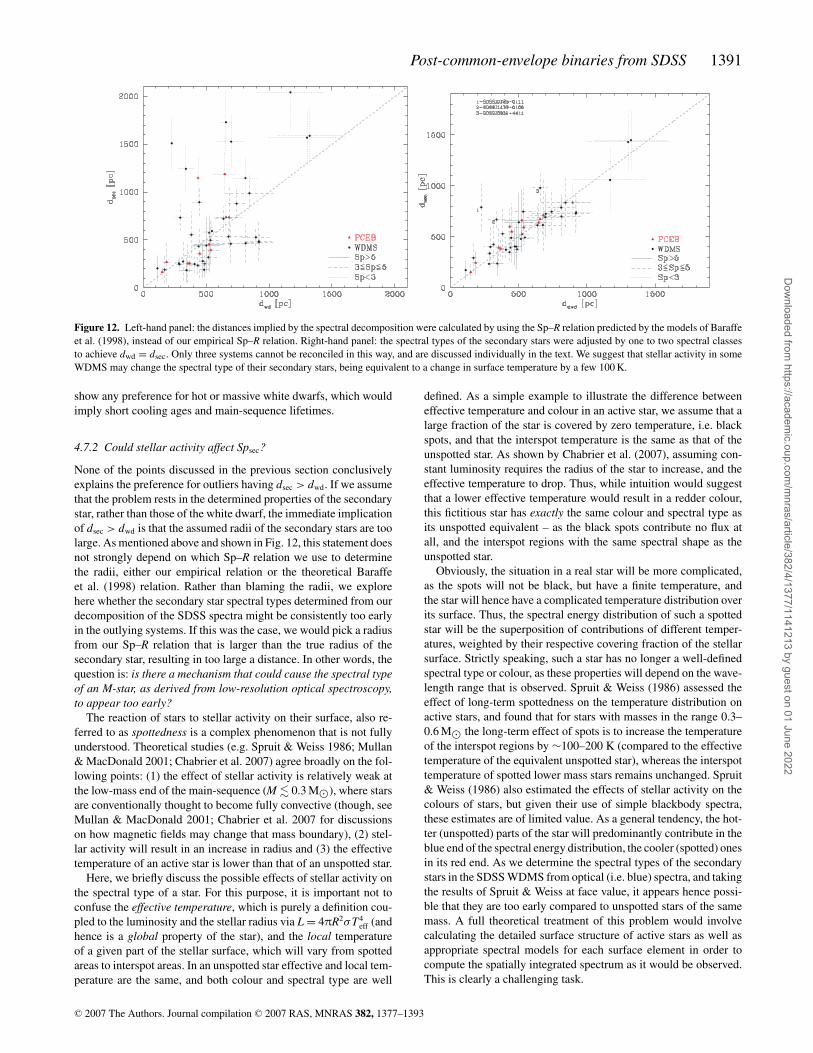
Post-common-envelope binaries from SDSS 1391
Figure 12. Left-hand panel: the distances implied by the spectral decomposition were calculated by using the Sp–R relation predicted by the models of Baraffe
et al. (1998), instead of our empirical Sp–R relation. Right-hand panel: the spectral types of the secondary stars were adjusted by one to two spectral classes
to achieve dwd = dsec. Only three systems cannot be reconciled in this way, and are discussed individually in the text. We suggest that stellar activity in some
WDMS may change the spectral type of their secondary stars, being equivalent to a change in surface temperature by a few 100 K.
show any preference for hot or massive white dwarfs, which would
imply short cooling ages and main-sequence lifetimes.
4.7.2 Could stellar activity affect Spsec?
None of the points discussed in the previous section conclusively
explains the preference for outliers having dsec > dwd. If we assume
that the problem rests in the determined properties of the secondary
star, rather than those of the white dwarf, the immediate implication
of dsec > dwd is that the assumed radii of the secondary stars are too
large. As mentioned above and shown in Fig. 12, this statement does
not strongly depend on which Sp–R relation we use to determine
the radii, either our empirical relation or the theoretical Baraffe
et al. (1998) relation. Rather than blaming the radii, we explore
here whether the secondary star spectral types determined from our
decomposition of the SDSS spectra might be consistently too early
in the outlying systems. If this was the case, we would pick a radius
from our Sp–R relation that is larger than the true radius of the
secondary star, resulting in too large a distance. In other words, the
question is: is there a mechanism that could cause the spectral typeof an M-star, as derived from low-resolution optical spectroscopy,to appear too early?
The reaction of stars to stellar activity on their surface, also re-
ferred to as spottedness is a complex phenomenon that is not fully
understood. Theoretical studies (e.g. Spruit & Weiss 1986; Mullan
& MacDonald 2001; Chabrier et al. 2007) agree broadly on the fol-
lowing points: (1) the effect of stellar activity is relatively weak at
the low-mass end of the main-sequence (M � 0.3 M�), where stars
are conventionally thought to become fully convective (though, see
Mullan & MacDonald 2001; Chabrier et al. 2007 for discussions
on how magnetic fields may change that mass boundary), (2) stel-
lar activity will result in an increase in radius and (3) the effective
temperature of an active star is lower than that of an unspotted star.
Here, we briefly discuss the possible effects of stellar activity on
the spectral type of a star. For this purpose, it is important not to
confuse the effective temperature, which is purely a definition cou-
pled to the luminosity and the stellar radius via L = 4πR2σT4eff (and
hence is a global property of the star), and the local temperature
of a given part of the stellar surface, which will vary from spotted
areas to interspot areas. In an unspotted star effective and local tem-
perature are the same, and both colour and spectral type are well
defined. As a simple example to illustrate the difference between
effective temperature and colour in an active star, we assume that a
large fraction of the star is covered by zero temperature, i.e. black
spots, and that the interspot temperature is the same as that of the
unspotted star. As shown by Chabrier et al. (2007), assuming con-
stant luminosity requires the radius of the star to increase, and the
effective temperature to drop. Thus, while intuition would suggest
that a lower effective temperature would result in a redder colour,
this fictitious star has exactly the same colour and spectral type as
its unspotted equivalent – as the black spots contribute no flux at
all, and the interspot regions with the same spectral shape as the
unspotted star.
Obviously, the situation in a real star will be more complicated,
as the spots will not be black, but have a finite temperature, and
the star will hence have a complicated temperature distribution over
its surface. Thus, the spectral energy distribution of such a spotted
star will be the superposition of contributions of different temper-
atures, weighted by their respective covering fraction of the stellar
surface. Strictly speaking, such a star has no longer a well-defined
spectral type or colour, as these properties will depend on the wave-
length range that is observed. Spruit & Weiss (1986) assessed the
effect of long-term spottedness on the temperature distribution on
active stars, and found that for stars with masses in the range 0.3–
0.6 M� the long-term effect of spots is to increase the temperature
of the interspot regions by ∼100–200 K (compared to the effective
temperature of the equivalent unspotted star), whereas the interspot
temperature of spotted lower mass stars remains unchanged. Spruit
& Weiss (1986) also estimated the effects of stellar activity on the
colours of stars, but given their use of simple blackbody spectra,
these estimates are of limited value. As a general tendency, the hot-
ter (unspotted) parts of the star will predominantly contribute in the
blue end of the spectral energy distribution, the cooler (spotted) ones
in its red end. As we determine the spectral types of the secondary
stars in the SDSS WDMS from optical (i.e. blue) spectra, and taking
the results of Spruit & Weiss at face value, it appears hence possi-
ble that they are too early compared to unspotted stars of the same
mass. A full theoretical treatment of this problem would involve
calculating the detailed surface structure of active stars as well as
appropriate spectral models for each surface element in order to
compute the spatially integrated spectrum as it would be observed.
This is clearly a challenging task.
C© 2007 The Authors. Journal compilation C© 2007 RAS, MNRAS 382, 1377–1393
Dow
nloaded from https://academ
ic.oup.com/m
nras/article/382/4/1377/1141213 by guest on 01 June 2022
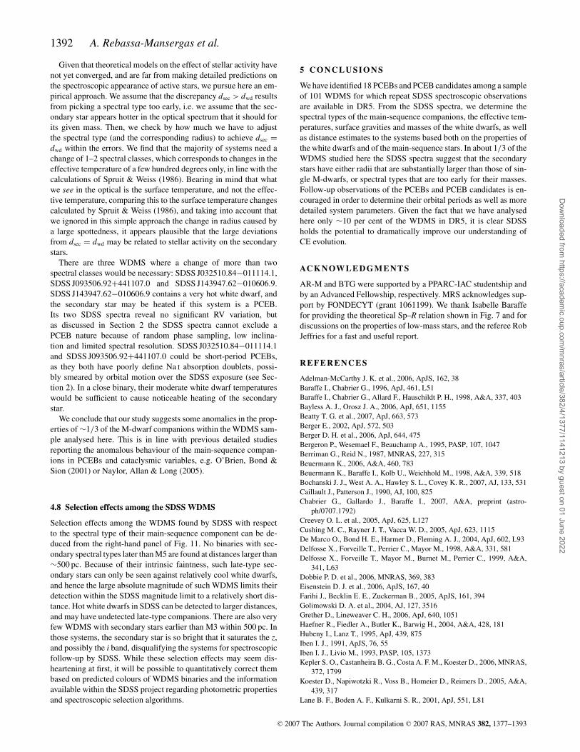
1392 A. Rebassa-Mansergas et al.
Given that theoretical models on the effect of stellar activity have
not yet converged, and are far from making detailed predictions on
the spectroscopic appearance of active stars, we pursue here an em-
pirical approach. We assume that the discrepancy dsec > dwd results
from picking a spectral type too early, i.e. we assume that the sec-
ondary star appears hotter in the optical spectrum that it should for
its given mass. Then, we check by how much we have to adjust
the spectral type (and the corresponding radius) to achieve dsec =dwd within the errors. We find that the majority of systems need a
change of 1–2 spectral classes, which corresponds to changes in the
effective temperature of a few hundred degrees only, in line with the
calculations of Spruit & Weiss (1986). Bearing in mind that what
we see in the optical is the surface temperature, and not the effec-
tive temperature, comparing this to the surface temperature changes
calculated by Spruit & Weiss (1986), and taking into account that
we ignored in this simple approach the change in radius caused by
a large spottedness, it appears plausible that the large deviations
from dsec = dwd may be related to stellar activity on the secondary
stars.
There are three WDMS where a change of more than two
spectral classes would be necessary: SDSS J032510.84−011114.1,
SDSS J093506.92+441107.0 and SDSS J143947.62−010606.9.
SDSS J143947.62−010606.9 contains a very hot white dwarf, and
the secondary star may be heated if this system is a PCEB.
Its two SDSS spectra reveal no significant RV variation, but
as discussed in Section 2 the SDSS spectra cannot exclude a
PCEB nature because of random phase sampling, low inclina-
tion and limited spectral resolution. SDSS J032510.84−011114.1
and SDSS J093506.92+441107.0 could be short-period PCEBs,
as they both have poorly define Na I absorption doublets, possi-
bly smeared by orbital motion over the SDSS exposure (see Sec-
tion 2). In a close binary, their moderate white dwarf temperatures
would be sufficient to cause noticeable heating of the secondary
star.
We conclude that our study suggests some anomalies in the prop-
erties of ∼1/3 of the M-dwarf companions within the WDMS sam-
ple analysed here. This is in line with previous detailed studies
reporting the anomalous behaviour of the main-sequence compan-
ions in PCEBs and cataclysmic variables, e.g. O’Brien, Bond &
Sion (2001) or Naylor, Allan & Long (2005).
4.8 Selection effects among the SDSS WDMS
Selection effects among the WDMS found by SDSS with respect
to the spectral type of their main-sequence component can be de-
duced from the right-hand panel of Fig. 11. No binaries with sec-
ondary spectral types later than M5 are found at distances larger than
∼500 pc. Because of their intrinsic faintness, such late-type sec-
ondary stars can only be seen against relatively cool white dwarfs,
and hence the large absolute magnitude of such WDMS limits their
detection within the SDSS magnitude limit to a relatively short dis-
tance. Hot white dwarfs in SDSS can be detected to larger distances,
and may have undetected late-type companions. There are also very
few WDMS with secondary stars earlier than M3 within 500 pc. In
those systems, the secondary star is so bright that it saturates the z,
and possibly the i band, disqualifying the systems for spectroscopic
follow-up by SDSS. While these selection effects may seem dis-
heartening at first, it will be possible to quantitatively correct them
based on predicted colours of WDMS binaries and the information
available within the SDSS project regarding photometric properties
and spectroscopic selection algorithms.
5 C O N C L U S I O N S
We have identified 18 PCEBs and PCEB candidates among a sample
of 101 WDMS for which repeat SDSS spectroscopic observations
are available in DR5. From the SDSS spectra, we determine the
spectral types of the main-sequence companions, the effective tem-
peratures, surface gravities and masses of the white dwarfs, as well
as distance estimates to the systems based both on the properties of
the white dwarfs and of the main-sequence stars. In about 1/3 of the
WDMS studied here the SDSS spectra suggest that the secondary
stars have either radii that are substantially larger than those of sin-
gle M-dwarfs, or spectral types that are too early for their masses.
Follow-up observations of the PCEBs and PCEB candidates is en-
couraged in order to determine their orbital periods as well as more
detailed system parameters. Given the fact that we have analysed
here only ∼10 per cent of the WDMS in DR5, it is clear SDSS
holds the potential to dramatically improve our understanding of
CE evolution.
AC K N OW L E D G M E N T S
AR-M and BTG were supported by a PPARC-IAC studentship and
by an Advanced Fellowship, respectively. MRS acknowledges sup-
port by FONDECYT (grant 1061199). We thank Isabelle Baraffe
for providing the theoretical Sp–R relation shown in Fig. 7 and for
discussions on the properties of low-mass stars, and the referee Rob
Jeffries for a fast and useful report.
R E F E R E N C E S
Adelman-McCarthy J. K. et al., 2006, ApJS, 162, 38
Baraffe I., Chabrier G., 1996, ApJ, 461, L51
Baraffe I., Chabrier G., Allard F., Hauschildt P. H., 1998, A&A, 337, 403
Bayless A. J., Orosz J. A., 2006, ApJ, 651, 1155
Beatty T. G. et al., 2007, ApJ, 663, 573
Berger E., 2002, ApJ, 572, 503
Berger D. H. et al., 2006, ApJ, 644, 475
Bergeron P., Wesemael F., Beauchamp A., 1995, PASP, 107, 1047
Berriman G., Reid N., 1987, MNRAS, 227, 315
Beuermann K., 2006, A&A, 460, 783
Beuermann K., Baraffe I., Kolb U., Weichhold M., 1998, A&A, 339, 518
Bochanski J. J., West A. A., Hawley S. L., Covey K. R., 2007, AJ, 133, 531
Caillault J., Patterson J., 1990, AJ, 100, 825
Chabrier G., Gallardo J., Baraffe I., 2007, A&A, preprint (astro-
ph/0707.1792)
Creevey O. L. et al., 2005, ApJ, 625, L127
Cushing M. C., Rayner J. T., Vacca W. D., 2005, ApJ, 623, 1115
De Marco O., Bond H. E., Harmer D., Fleming A. J., 2004, ApJ, 602, L93
Delfosse X., Forveille T., Perrier C., Mayor M., 1998, A&A, 331, 581
Delfosse X., Forveille T., Mayor M., Burnet M., Perrier C., 1999, A&A,
341, L63
Dobbie P. D. et al., 2006, MNRAS, 369, 383
Eisenstein D. J. et al., 2006, ApJS, 167, 40
Farihi J., Becklin E. E., Zuckerman B., 2005, ApJS, 161, 394
Golimowski D. A. et al., 2004, AJ, 127, 3516
Grether D., Lineweaver C. H., 2006, ApJ, 640, 1051
Haefner R., Fiedler A., Butler K., Barwig H., 2004, A&A, 428, 181
Hubeny I., Lanz T., 1995, ApJ, 439, 875
Iben I. J., 1991, ApJS, 76, 55
Iben I. J., Livio M., 1993, PASP, 105, 1373
Kepler S. O., Castanheira B. G., Costa A. F. M., Koester D., 2006, MNRAS,
372, 1799
Koester D., Napiwotzki R., Voss B., Homeier D., Reimers D., 2005, A&A,
439, 317
Lane B. F., Boden A. F., Kulkarni S. R., 2001, ApJ, 551, L81
C© 2007 The Authors. Journal compilation C© 2007 RAS, MNRAS 382, 1377–1393
Dow
nloaded from https://academ
ic.oup.com/m
nras/article/382/4/1377/1141213 by guest on 01 June 2022
Post-common-envelope binaries from SDSS 1393
Leggett S. K., Allard F., Berriman G., Dahn C. C., Hauschildt P. H., 1996,
ApJS, 104, 117
Leggett S. K., Allard F., Geballe T. R., Hauschildt P. H., Schweitzer A.,
2001, ApJ, 548, 908
Leto G., Pagano I., Linsky J. L., Rodono M., Umana G., 2000, A&A, 359,
1035
Liebert J., Bergeron P., Holberg J. B., 2005, ApJS, 156, 47
Livio M., Soker N., 1988, ApJ, 329, 764
Lopez-Morales M., 2007, ApJ, 660, 732
Maceroni C., Montalban J., 2004, A&A, 426, 577
Marsh T. R., Duck S. R., 1996, MNRAS, 278, 565
Marsh T. R., Dhillon V. S., Duck S. R., 1995, MNRAS, 275, 828
Mateo M., Szkody P., Bolte M., 1985, PASP, 97, 45
Maxted P. F. L., Marsh T. R., Morales-Rueda L., Barstow M. A., Dobbie P.
D., Schreiber M. R., Dhillon V. S., Brinkworth C. S., 2004, MNRAS,
355, 1143
Maxted P. F. L., Napiwotzki R., Dobbie P. D., Burleigh M. R., 2006, Nat,
442, 543
Maxted P. F. L., O’Donoghue D., Morales-Rueda L., Napiwotzki R., 2007,
MNRAS, 376, 919
Montagnier G. et al., 2006, A&A, 460, L19
Mullan D. J., MacDonald J., 2001, ApJ, 559, 353
Naylor T., Allan A., Long K. S., 2005, MNRAS, 361, 1091
Nelemans G., Tout C. A., 2005, MNRAS, 356, 753
Nelemans G., Verbunt F., Yungelson L. R., Portegies Zwart S. F., 2000,
A&A, 360, 1011
O’Brien M. S., Bond H. E., Sion E. M., 2001, ApJ, 563, 971
O’Donoghue D., Koen C., Kilkenny D., Stobie R. S., Koester D., Bessell
M. S., Hambly N., MacGillivray H., 2003, MNRAS, 345, 506
Paczynski B., 1976, in Eggleton P., Mitton S., Whelan J., eds, IAU
Symp. 73, Structure and Evolution of Close Binary Systems. Reidel,
Dordrecht, p. 75
Pont F., Melo C. H. F., Bouchy F., Udry S., Queloz D., Mayor M., Santos
N. C., 2005, A&A, 433, L21
Raymond S. N., Szkody P., Hawley S. L., 2003, AJ, 125, 2621
Rechenberg I., 1994, Evolutionsstrategie ‘94. Froomann–Holzboog,
Stuttgart
Ribas I., 2006, Ap&SS, 304, 89
Schreiber M., Nebot Gomez-Moran A., Schwope A., 2007, in Napiwotzki
R., Burleigh R., eds, ASP Conf. Ser., 15th European Workshop on White
Dwarfs, preprint (astroph/0611461)
Schreiber M. R., Gansicke B. T., 2003, A&A, 406, 305
Segransan D., Kervella P., Forveille T., Queloz D., 2003, A&A, 397, L5
Silvestri N. M. et al., 2006, AJ, 131, 1674
Southworth J., Gansicke B., Schreiber M. 2007, MNRAS, submitted
Spruit H. C., Weiss A., 1986, A&A, 166, 167
Stoughton C. et al., 2002, AJ, 123, 485
Strauss M. A. et al., 2002, AJ, 124, 1810
van den Besselaar E. J. M. et al., 2007, A&A, 466, 1031
Vogel J., Schwope A. D., Gansicke B. T., 2007, A&A, 464, 647
West A. A. et al., 2004, AJ, 128, 426
Willems B., Kolb U., 2004, A&A, 419, 1057
York D. G. et al., 2000, AJ, 120, 1579
S U P P L E M E N TA RY M AT E R I A L
The following supplementary material is available for this article.
Table 2. 83 WDMS in our sample that did not show a significant a
significant RV variation between their different SDSS spectra. The
first column gives the SDSS object name, the second the HJD of
the spectrum, in the third column we quote with ‘Y’ and ‘n’ those
spectra which are composed of subspectra taken in different nights,
the fourth and fifth columns provide the Na I λλ 8183.27, 8194.81
absorption doublet and Hα emssion RVs, respectively. Blank spaces
indicate that no RV measurement could be obtained.
Table 4. Stellar parameters of the remaining WDMS identified in our
sample, as determined from spectral modelling. Given are, from left-
to right-hand side, SDSS object name, MJD, fibre and plate number
of the spectrum, white dwarf effective temperature and error, white
dwarf surface gravity and error, mass of the white dwarf and error,
distance to the white dwarf and error, spectral type of the secondary
star, distance to the secondary and error, flag and notes.
This material is available as part of the online paper
from: http://www.blackwell-synergy.com/doi/abs/10.1111/j.1365-
2966.2007.12288.x
(this link will take you to the article abstract).
Please note: Blackwell Publishing are not responsible for the con-
tent or functionality of any supplementary materials supplied by
the authors. Any queries (other than missing material) should be
directed to the corresponding author for the article.
This paper has been typeset from a TEX/LATEX file prepared by the author.
C© 2007 The Authors. Journal compilation C© 2007 RAS, MNRAS 382, 1377–1393
Dow
nloaded from https://academ
ic.oup.com/m
nras/article/382/4/1377/1141213 by guest on 01 June 2022