arX

iv:a

stro

-ph/

9802

278v

1 2

1 Fe

b 19

98

The halo white dwarf population

Jordi Isern1, Enrique Garcıa-Berro2, Margarida Hernanz1, Robert Mochkovitch3, and

Santiago Torres4

Received ; accepted

1Institut for Space Studies of Catalonia–CSIC, Edifici Nexus–104, Gran Capita 2–4, 08034

Barcelona, Spain

2Departament de Fısica Aplicada, Universitat Politecnica de Catalunya & Institut for

Space Studies of Catalonia–UPC, Jordi Girona Salgado s/n, Modul B-5, Campus Nord,

08034 Barcelona, Spain

3Institut d’Astrophysique de Paris, C.N.R.S., 98 bis Bd. Arago, 75014 Paris, France

4Departament de Telecomunicacio i Arquitectura de Computadors, EUP de Mataro,

Universitat Politecnica de Catalunya, Avda. Puig Cadafalch 101, 08303 Mataro, Spain

– 2 –

ABSTRACT

Halo white dwarfs can provide important information about the properties

and evolution of the galactic halo. In this paper we compute, assuming a

standard IMF and updated models of white dwarf cooling, the expected

luminosity function, both in luminosity and in visual magnitude, for different

star formation rates. We show that a deep enough survey (limiting magnitude

>∼ 20) could provide important information about the halo age and the duration

of the formation stage. We also show that the number of white dwarfs produced

using the recently proposed biased IMFs cannot represent a large fraction

of the halo dark matter if they are constrained by the presently observed

luminosity function. Furthermore, we show that a robust determination of the

bright portion of the luminosity function can provide strong constraints on the

allowable IMF shapes.

Subject headings: stars: white dwarfs – stars: luminosity function – Galaxy:

stellar content

– 3 –

1. Introduction

One way to understand the structure and evolution of the Galaxy is to study the

properties of one of its fossil stars: white dwarfs. Their luminosity function has been

extensively studied since it provides important information about the properties of the

Galaxy and new deep surveys will open the possibility to observe the white dwarf population

beyond the cutoff reported by Liebert, Dahn & Monet (1988) and Oswalt et al. (1996) as

well as to discriminate, on the basis of their kinematical properties, those that belong to the

halo. If the halo was formed sometime before the disk as a burst of short duration (Eggen

et al. 1962), it would be possible to obtain information about the time elapsed between

the formation of both structures (Mochkovitch et al. 1990). If mergers of protogalactic

fragments have played an important role in the formation of the galactic halo (Searle &

Zinn 1978), their signature should be apparent in the white dwarf luminosity function.

The observed properties of halo white dwarfs are very scarce. These properties can

be summarized as follows: a) Liebert, Dahn & Monet (1989) provided a very preliminary

luminosity function using six white dwarfs, which were identified as halo members because

of their high tangential velocities. b) Flynn, Gould & Bahcall (1996) have found that the

number of stellar objects in the Hubble Deep Field (HDF) with V − I > 1.8 is smaller than

3, while Mendez et al. (1996) have identified 6 objects with 0 < V − I < 1.2 that could be

white dwarfs (although they recommend to reject them as white dwarf candidates because

of their colors). Both values can be considered as reliable upper limits to the number

of white dwarfs in the HDF. c) A recent analysis of the microlensing events towards the

Large Magellanic Cloud suggests that they are produced by halo objects with an average

mass ∼ 0.5 M⊙ (Alcock et al. 1997) and the total contribution of such objects to the total

halo mass could be as high as 40%. Obviously, white dwarfs are one of the most natural

candidates to explain such observations. If this interpretation of the microlensing data

– 4 –

turns out to be correct, the tight constraints imposed by galactic properties should demand

the use of biased non-standard initial mass functions (Adams & Laughlin 1996; Fields,

Mathews & Schramm 1996; Chabrier, Segretain & Mera 1996).

These IMFs are characterized by a pronounced shortfall below ∼ 1 M⊙ and above

∼ 7 − 10 M⊙ in order to avoid the overproduction of red dwarfs in the first case, and

to avoid problems with the luminosity of galactic haloes at high redshift (Charlot & Silk

1995) or to overproduce heavy elements by the explosion of massive stars in the second

case. The problem is that the IMF determines the contribution of each kind of star to

galactic evolution and, therefore, any ad-hoc change introduced to solve a problem, riscs to

introduce a desadjustement in other apparently well settled fields. In the case of the IMFs

quoted here, the problem is twofold. First, the quantity of astrated mass that is returned

on average to the interstellar medium through stellar winds and planetary nebula ejection

is very high, it lies in the range of 40 to 80%. If white dwarfs contribute substantially to

the mass budget of the halo, the total energy necessary to eject this unwanted mass to the

intergalactic medium is ∼ 1060 erg, assuming a typical halo radius of 50 kpc and a mass of

1012 M⊙. Since the number of massive stars has already been suppressed to avoid an excess

of supernovae, an important part of this material would remain locked into the galaxy (Isern

et al. 1997a). Furthermore, since intermediate mass stars are the main producers of carbon

and nitrogen, it would be hard to account for the [C,N/O] ratios observed in Population II

stars if an important part of this matter is invested in the formation of these stars (Gibson

& Mould 1997). Second, even if these problems were solved, the huge increase of white

dwarfs would increase the number of Type Ia supernovae unless new ad-hoc and completely

unjustified hypothesis about the properties of binary stars are adopted. The resulting

overproduction of Fe and the excessively high rate of supernova explosions have recently led

(Canal, Isern & Ruiz-Lapuente 1997) to the conclusion that, in all cases, the contribution of

white dwarfs to the halo mass should be well below 5–10 %. At this point, it is worthwhile

– 5 –

to point out that both the estimated mass of the objects causing the microlensing events

and the total mass of the population responsible of such events are still preliminary (Mao

& Paczynski 1996; Nakamura, Kan-ya & Nishi 1996, Zaritsky & Lin 1997).

In view of the interest of the luminosity function of halo white dwarfs and since there is

not any recent study of such stars using standard hypothesis, it is worthwhile to construct

an updated series of standard models of halo white dwarf populations for comparison

purposes.

2. The luminosity function

The luminosiy function is defined as the number of white dwarfs per unit volume and

per unit of bolometric magnitude,Mbol:

n(Mbol, T ) =∫ Ms

Mi

Φ(M) Ψ(T − tcool − tMS) τcool dM (1)

where M is the mass of the parent star (for convenience all white dwarfs are labelled with

the mass of their main sequence progenitors), τcool = dt/dMbol is the characteristic cooling

time, Ms and Mi are the maximum and the minimum masses of the main sequence stars

able to produce a white dwarf of magnitude Mbol at the time T , tcool is the time necessary

to cool down to this magnitude, tMS is the main sequence lifetime and T is the age of the

population under study (disk, halo. . . ). Of course, for evaluating equation (1) a relationship

between the mass of the white dwarf and the mass of its progenitor must be provided.

It is also necessary to provide a relationship between the mass of the progenitor and its

main sequence lifetime. We have used those of Wood (1992) instead of those of Iben &

Laughlin (1989) as we usually did in previous papers in order to compare with Adams &

Laughlin (1996). In order to properly compare with the observations, it is desirable to bin

– 6 –

this function in intervals of magnitude ∆Mbol, usually of one or half magnitudes, in the

following way:

〈n(Mbol, T )〉∆Mbol=

1

∆Mbol

∫ Mbol+0.5∆Mbol

Mbol−0.5∆Mbol

n(Mbol, T ) dMbol (2)

2.1. The cooling sequences

The values taken by tcool and τcool depend on the adopted evolutionary models of white

dwarfs. Since there have been some misunderstandings about the cooling process, it is

worthwhile to summarize here the most relevant points. After integrating over the entire

star and assuming that the release of nuclear energy is negligible, the energy balance can

be written as (Isern et al. 1997b):

L + Lν = −∫ MWD

0Cv

dT

dtdm −

∫ MWD

0T

(

∂P

∂T

)

V,X0

dV

dtdm +

(

ls + eg

)

mc (3)

where L and Lν are the photon and the neutrino luminosities respectively, mc is the rate at

which the crystallization front moves outwards, and the rest of the symbols have their usual

meaning. Neutrinos are dominant for luminosities larger than 10−1 L⊙. Nevertheless, since

the phase dominated by the neutrino cooling is very short and the luminosity function of

very bright halo white dwarfs is still unknown we start our calculations at 10−1 L⊙.

All the four terms in the right hand side of this equation depend on the detailed

chemical composition of the white dwarf. We have adopted the chemical profiles of Salaris

et al. (1997a,b) for C–O white dwarfs (white dwarf masses in the range of 0.5–1 M⊙ and

progenitors in the mass range 0.7–8 M⊙), which take into account the presence of high

quantities of oxygen in the central regions due to the high rates of the 12C(α, γ)16O reaction,

and from Garcıa-Berro et al. (1997) for O–Ne white dwarfs (white dwarf masses >∼ 1 M⊙

– 7 –

and progenitors in the mass range 8–11 M⊙).

The first term of the right hand side of equation (3) represents the well known

contribution of the heat capacity of the star to the total luminosity (Mestel 1952). It

strongly decreases when the bulk of the star enters into the Debye regime (Lamb & Van

Horn 1975). The second term takes into account the net contribution of compression to

the luminosity. It is in general small since the major part of the compressional work is

invested into increasing the Fermi energy of electrons (Lamb & Van Horn 1975, Shaviv

& Kovetz 1976). The largest contribution to this term comes from the outer, partially

degenerate layers. In fact, when the white dwarf enters into the Debye regime, this term can

provide in some cases about 80% of the total luminosity preventing in this way the sudden

disappearence of the star (D’Antona and Mazzitelli 1989). Of course, the relevance and

the details of this contribution strongly depend on the characteristics of the envelope. It is

clear, therefore, that extrapolating the behavior of the coldest white dwarfs just assuming

that their unique source of energy is the heat capacity may not necessarily be the best

procedure.

The third term in the right hand side represents the energy release associated to

solidification. The term ls corresponds to release of the latent heat (∼ kTs/nucleus, where

Ts is the solidification temperature), and the term eg corresponds to the gravitational

energy release associated to the chemical differentiation induced by the freezing process

(Mochkovitch 1983, Isern et al. 1997b). It is important to notice here that the C–O models

of Salaris et al. (1997a,b) predict very high oxygen abundances in the central region.

This fact minimizes the effect of the chemical differentiation as compared with the models

assuming half carbon and half oxygen homogeneously distributed along the star. It is also

interesting to notice that this effect is almost completely negligible in the case of O–Ne

white dwarfs (Garcıa-Berro et al. 1997).

– 8 –

The main difference between C–O and O–Ne models is that the last ones cool down

more quickly. For instance, two white dwarfs of 1 M⊙, one made of C–O and the other one

of O–Ne take 11.3 Gyr and 8.1 Gyr respectively to reach a luminosity of 10−5 L⊙. This is

due to the smaller heat capacity and to the negligible influence of chemical differentiation

settling in O–Ne mixtures — see Garcıa-Berro et al. (1997) for a detailed discussion.

We would like to stress the importance of the outer layers of the white dwarf in the

cooling process. They not only can provide a major contribution to the total luminosity

during the late stages, as previously stated, but also control the power radiated by the star.

The difficulties come from the fact that matter is far from ideal conditions and that the

convective envelope reaches the partially degenerate layers. Although our models take into

account reasonably well the energy released by the compression of the outer layers, the rate

at which the energy is radiated away remains quite uncertain.

2.2. Computational procedure

The white dwarf luminosity function averaged over bins of width ∆Mbol as given in

equation (2) can also be directly computed in the following way. Assume a population that

was formed according an arbitrary star formation rate Ψ(t). After a time T since the origin

of the Galaxy, the number of white dwarfs that have a bolometric magnitude in the interval

Mbol ± 0.5∆Mbol is:

N(Mbol, T ) =∫

t

∫

MΦ(M) Ψ(t) dM dt (4)

where the integral is constrained to the domain that satisfies the condition:

– 9 –

T − tcool(M, Mbol − 0.5∆Mbol) ≤ t + tMS(M) ≤ T − tcool(M, Mbol + 0.5∆Mbol) (5)

Dividing this result by ∆Mbol we obtain equation (2).

This expression can be easily computed using standard methods and, since it does not

make use of the characteristic cooling time (which demands the use of numerical derivatives

to evaluate it) it easily allows to obtain the luminosity function in visual magnitudes or in

any other photometric band.

Figure 1 displays the luminosity function of a burst of constant star formation rate of

arbitrary strength and a duration of 0.1 Gyr that started 13 Gyr ago obtained using both

methods. The upper solid line has been obtained using equation (1), the lower lines have

been obtained by applying the binning procedure of equation (2) to equation (1), solid line,

and equations (4) and (5), dotted line. The last two lines have arbitrarily been shifted

downwards by a fixed amount to allow comparison. The differences can be considered as

negligible. It is worthwhile to note here how the sudden rise produced by crystallization at

log(L/L⊙) ≃ −3.7 in the luminosity function (upper curve) is smeared out when bins are

taken. Note as well that the observational luminosity functions are actually derived using

such binning. In all cases calculations were stoped at log(L/L⊙) = −5 to save computing

time.

3. Results and discussion

3.1. Standard initial mass function

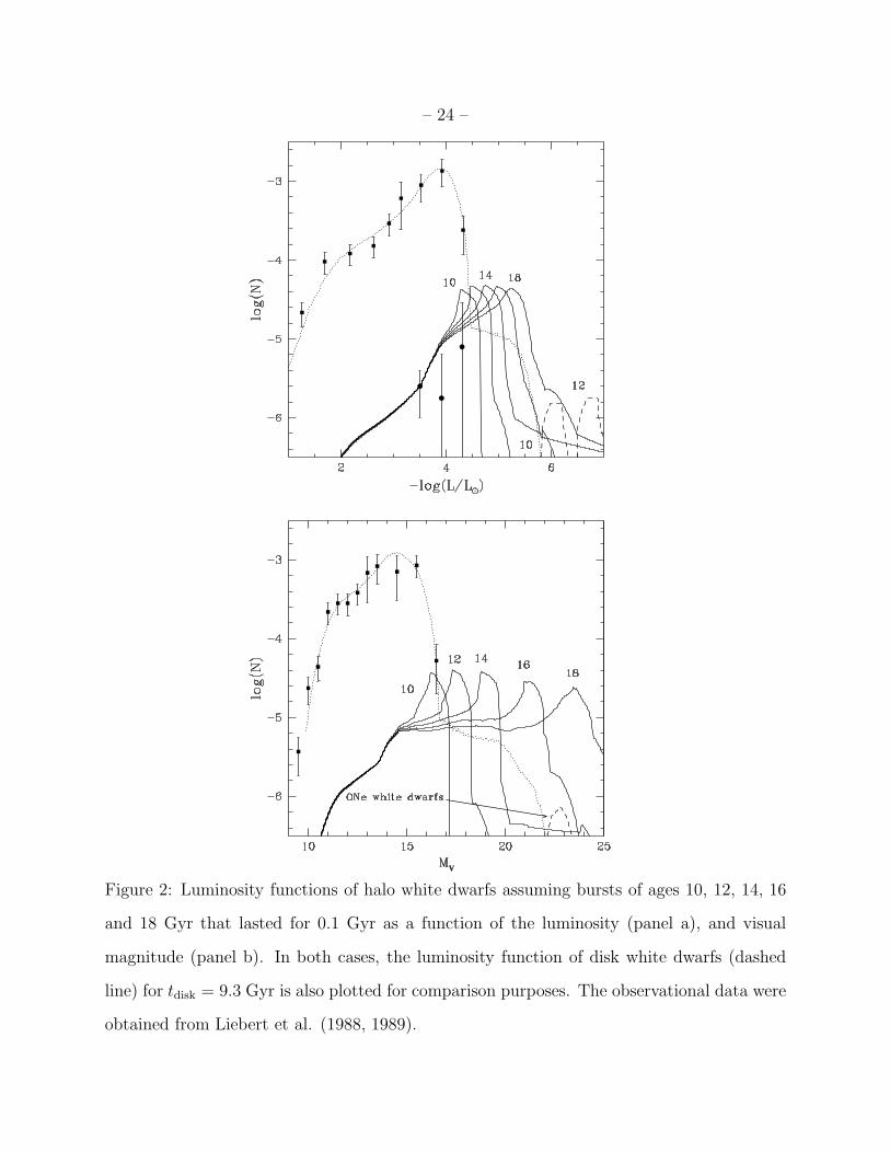
Figure 2a displays the luminosity functions of halo and disk white dwarfs computed with

a standard initial mass function (Salpeter 1961). The observational data for both the disk

– 10 –

and the halo have been taken from Liebert et al. (1988, 1989). The theoretical luminosity

functions have been normalized to the points log(L/L⊙) ≃ −3.5 and log(L/L⊙) ≃ −2.9

for the halo and the disk respectively due to their smaller error bars. The luminosity

function of the disk was obtained assuming an age of the disk of 9.3 Gyr and a constant star

formation rate per unit volume for the disk, and those of the halo assuming a burst that

lasted 0.1 Gyr and started at thalo= 10, 12, 14, 16 and 18 Gyr respectively. Due to their

higher cooling rate, O–Ne white dwarfs produce a long tail in the disk luminosity function

and a bump (only shown in the cases thalo= 10 and 12 Gyr) in the halo luminosity function.

It is important to realize here that the faintest white dwarf known, ESO 439–26, which has

a mass M = 1.1 − 1.2 M⊙ (Ruiz et al. 1995) and a luminosity log(L/L⊙) ≃ −5 is clearly

an O–Ne white dwarf and cannot be a halo white dwarf unless the halo stopped its star

formation activity less than 8 Gyr ago, since the time necessary for O–Ne white dwarfs to

reach this luminosity is at maximum 8 Gyr. In order to make easier the comparison with

observations, we display in Figure 2b the same luminosity function in visual magnitudes.

The photometric corrections were obtained from the atmospheric tables of Bergeron et al.

(1995). Beyond MV>∼ 17 these corrections were obtained by extrapolating those tables. It

is interesting to notice that the distance between the peaks of the halo luminosity functions

has increased due to the fact that more and more energy is radiated in the infrared as white

dwarfs cool down. Therefore, the detection of such peaks should allow the determination of

the age of the galactic halo. It is also convenient to remark here that the disk white dwarf

luminosity function of figure 2b was obtained with the age and normalization factor used

for figure 2a.

If the halo formed from the merging of protogalactic fragments, the time scale for

halo formation should be larger than 0.1 Gyr and therefore, the white dwarf luminosity

function should be different from those of Figure 2. To show that we have computed the

luminosity function for bursts that, starting at 12 Gyr, lasted 0.1, 1 and 3 Gyr. The last

– 11 –

one was inspired by the age distribution of the globular cluster sample of Salaris & Weiss

(1997). We see from Figure 3 that because of the relative lack of sensitivity to the age and

shape of the star formation rate of the hot portion of the luminosity function, the different

curves merge when we normalize them to a fixed observational bin. As a consequence, it

is necessary to have precise information about the white dwarf population in the region

MV>∼ 16 before being able to reach any conclusion.

The shape of the Hertzprung–Russell diagram of halo white dwarfs also provides useful

information about the halo population. Figure 4 displays the color–magnitude diagram for

each one of the bursts of figure 2 using a simulated Monte Carlo sample of 2,000 stars.

They can be interpreted as the isochrones, including the lifetime in the main sequence,

of this halo population. The diagram displays a characteristic Z–shape produced by the

combination of the different cooling times of white dwarfs and main sequence lifetimes of

their progenitors. This feature moves downwards with the age and ultimately disappears.

Therefore, its detection could provide an indication of the halo age.

The duration of the process of formation of the halo is also reflected in the color–

magnitude diagram. If the halo took a relatively large time to form, the Z–feature would

cover a large region of the color–magnitude diagram and its width could be used as a

duration indicator if enough white dwarfs with good photometric data were available.

Figure 5 displays the color–magnitude diagram for a burst of constant star formation rate

that was 12 Gyr old and lasted 3 Gyr.

Another useful quantity is the discovery function. This function gives the number

of white dwarfs per interval of magnitude which can be detected in the whole sky by a

survey limited to a given apparent magnitude mλ in a photometric band centered at λ

(Mochkovitch et al. 1990). If we limit ourselves to nearby halo white dwarfs, this volume

can be considered spherical and the discovery function, ∆H(Mλ), is readily obtained from

– 12 –

the luminosity function

∆H(Mλ) =4π

3d3(Mλ)nH(Mλ) (6)

where d(Mλ) is the distance at which a white dwarf of absolute magnitude Mλ has an

apparent magnitude mλ:

d(Mλ) = 101+0.2(mλ−Mλ) (7)

where d is in parsecs. Since white dwarfs with luminosities log(L/L⊙) ∼ −5 have effective

temperatures of ∼ 3000 K and radiate most of their energy in the red or infrared, we have

computed the discovery function for both the V and I bands assuming in both cases a

limiting magnitude MV,I ≃ 20. For reasonable ages of the halo (thalo ∼ 12–16 Gyr), the

discovery function in both the V and I band yield ∼ 500 stars/magnitude for bright objects

and have a steady decrease with the magnitude. This decrease is more pronounced for the

V band (Figure 6). In any case, the total number of stars that we would expect to find in a

survey of such characteristics is about 1,500 stars. This implies that the average number of

white dwarfs that we expect to find in a typical Schmidt plate of 6 × 6 is about 1.5. One

third of them should be brighter than magnitude 12.

At this point it is interesting to examine, just as an exercise, the impact of the

recently discovered white dwarf WD 0346+246 (Hambly, Smartt & Hodgkin 1997). The

first analysis indicates that this white dwarf is placed at a distance d ∼ 40 pc and it has a

tangential velocity vT ∼ 250 km/s, which indicates that it probably belongs to the halo. Its

absolute visual magnitude is estimated to be in the range 16.2 <∼MV

<∼ 16.8. Therefore, if we

assume that it is the only star of these characteristics within this distance, the luminosity

function would take the value of ∼ 1.5 × 10−5 mag−1pc−3 at MV ≈ 16.5, which is in perfect

– 13 –

agreement with the results plotted in Figure 2b. Note also that the standard halo models

could accomodate a density larger by a factor ∼ 3 to that quoted here just assuming that

the luminosity function has a peak in this region. In this case, the halo should be as young

as ∼ 11 Gyr. If the density finally turned out to be larger we could start to think about

non conventional hypothesis. It is also interesting to notice that the expected number of

white dwarfs per plate with 16 ≤ MI ≤ 17 is in the range of 10−1 to 3 × 10−2.

We have also computed the total number of white dwarfs per stereoradian in the

direction of the Hubble Deep Field assuming a spheroidal distribution of stars of the kind

ρ(r) = ρ0a2/(a2 + r2), with a = 2.5 kpc, a distance of the Sun to the galactic center of 8.5

kpc, and a limiting apparent visual magnitude V = 26.3. The total number of halo white

dwarfs in this photometric band goes from a minimum of 315,000 stars/str for the 10 Gyr

burst to 321,000 stars/str for the 16 Gyr one, while the number of white dwarfs redder than

V − I = 1.8 ranges from a minimum of 233 stars/str for the first case to 2,000 stars/sr for

the second case. The number of stars in the window 0 < V − I < 1.2 takes values in the

range 195,000 to 198,000 stars/str. This behavior can be easily understood if we note that,

due to the normalization procedure, the bright portion of the luminosity function is nearly

coincident in all cases and that counts limited to a given apparent magnitude are dominated

by the brightest stars. On the contrary, if we limit ourselves to the very red ones, which are

also the dimmest ones, we are eliminating the brightest white dwarfs and, therefore, the

number of them in the pencil becomes sensitive to the age. Unfortunately, the HDF pencil

is so narrow (∆Ω = 4.4 arc min2 = 3.723 × 10−7 str) that it is impossible to extract from it

any valuable information of the properties of the different bursts.

The local density of halo white dwarfs obtained from our luminosity functions ranges,

depending on the adopted age of the halo, from 5.8 × 10−5 to 1.1 × 10−4 white dwarfs per

pc3 (that is from 0.24 to 0.46 white dwarfs in a sphere of 10 pc of radius around the Sun).

– 14 –

If we assume that the characteristic mass of halo white dwarfs is ∼ 0.6 M⊙, this density

represents at most the 0.6% of the local dark halo density, 0.01 M⊙/pc3 (Gilmore 1997).

Finally, we have to mention that if we chose to normalize to the total density of discovered

white dwarfs as in Mochkovitch et al. (1990), all the curves will move downwards by

approximately a factor 0.3 dex.

3.2. Biased initial mass functions

In order to account for the MACHO results in terms of an halo white dwarf population,

Adams & Laughlin (1996), and Chabrier et al. (1996) introduced ad-hoc non-standard

initial mass functions that fall very quickly below ∼ 1 M⊙ and above ∼ 7 M⊙. These

functions avoid the overproduction of red dwarfs, the overproduction of heavy elements by

the explosion of massive stars (Ryu, Olive & Silk 1990) and the luminosity excess of the

haloes of galaxies at large redshift (Charlot & Silk 1995) and, since the formation of very

massive and very small stars has been inhibited, the proposed IMFs allow to increase the

number of white dwarfs per unit of astrated mass.

Table 1 displays the mass density in the form of white dwarfs for bursts of star

formation that started at different ages and lasted 0.1 Gyr using the IMFs proposed by

Adams & Laughlin (1996), with mc = 2.3 and σ = 0.44 — AL case — and the IMFs

proposed by Chabrier et al. (1996) — CSM1 and CSM2 cases. The main differences

between our calculations and those of Adams & Laughlin (1996) are that we have computed

the luminosity function without neglecting the time spent in the main sequence, we take

into account the full effects of crystallization and we normalize to the best known bin of the

observed halo luminosity function instead of trying to reproduce a given density of white

dwarfs in the halo. The main differences with the Chabrier et al. (1996) calculations rely

on the normalization procedure and on the fact that we use realistic carbon–oxygen profiles

– 15 –

instead of assuming that C–O white dwarfs are made of an homogeneous mixture of half

carbon and half oxygen. Besides that, we use average binned functions.

Concerning the AL case, the maximum densities that can be reached are smaller than

the 10% of the dark halo for any reasonable age of the Galaxy. The same happens with the

CSM1 case. Only in the CSM2 case white dwarfs can represent a noticeable fraction of the

halo dark matter. In fact, in the case of an age ∼ 16 Gyr the halo would be saturated with

white dwarfs. The differences with Chabrier et al (1996) are essentially due to the different

normalization procedure used here. Therefore, it is clear that a robust determination of

the bright portion of the halo white dwarf luminosity function would introduce strong

constraints on the allowed shapes of the IMFs.

Figure 7 displays the luminosity functions obtained with the aforementioned IMFs for

bursts that started 12 (left panel) and 14 Gyr (right panel) ago (dotted lines), which we

believe are realistic values for the age of the halo, normalized to the brightest and more

reliable observational bin. The luminosity function corresponding to the standard case is

also displayed for comparison (thick solid line). As expected, the position of the peak does

not change but its height increases since the number of main sequence stars below ∼ 1 M⊙

is severely depleted. This behavior is due to two different effects: i) The non-standard IMFs

have been built to efficiently produce white dwarfs (0.18, 0.39, 0.53 and 0.44 white dwarfs

per unit of astrated mass for the standard, AL, CSM1 and CSM2 cases respectively and for

a burst 14 Gyr old for instance). ii) The time that a white dwarf needs to cool down to

the luminosity of the normalization bin, log(L/L⊙) = −3.5, is ∼ 1.8 Gyr and only main

sequence stars with masses smaller than 1 M⊙ are able to produce a white dwarf with such

a high luminosity if the halo is taken to be older than 12 Gyr. Since the new IMFs have

been taylored to reduce the number of stars below ∼ 1 M⊙, it is necessary to shift the

luminosity function to very high values to fit the normalization criterion. For instance, the

– 16 –

values that the different IMFs take at M = 0.98 M⊙, the mass of the main sequence star

that produces a white dwarf with the aforementioned luminosity, are ΦS = 0.23, ΦAL = 0.06,

ΦCSM1 = 0.2, and ΦCSM2 = 0.01.

Figure 7 also shows that all the luminosity functions, except the one obtained from

the standard IMF, are well above the detection limit of Liebert et al. (1988) (shown as

triangles). This is due to the normalization condition adopted here. If we had normalized

the luminosity function to obtain a density of 1.35 × 10−5 white dwarfs per cubic parsec

brighter than log(L/L⊙) = −4.35 as in Mochkovitch et al. (1990), all the luminosity

functions (long dashed in Figure 7) would have been shifted downwards and only those

corresponding to the CSM2 case would have remained above the detection limit. Note,

however, that except for unrealistic ages of the galactic halo, these IMFs are not only

unable to provide an important contribution to the halo (see Table 1 below), but also to fit

the observed bright portion of the luminosity function of halo white dwarfs. For instance,

no one of the CSM2 cases appearing in Figure 2 of Chabrier et al. (1996) fits the brightest

bin. Therefore a robust determination of the bright portion of the luminosity function could

introduce severe constraints to the different allowable IMFs.

As we have already mentioned in section 2, one of the major uncertainties is the

transparency of the envelopes when white dwarfs are very cool. If they turn out to be more

opaque than the models used here, the cooling would be slowed down and the height of the

peaks would be consequently increased. On the contrary, if the atmospheres turn out to be

more transparent, white dwarfs could be able to reach, for a given age, smaller luminosities

and the peaks of Figure 7 would therefore be reduced. There is however one limitation: the

properties of the envelopes for white dwarfs brighter than log(L/L⊙) ≈ −4 are reasonably

well known. Consequently, we have checked this behavior by arbitrarily increasing the

transparency below log(L/L⊙) ≈ −4. Adopting the appropriate factor, it is possible to

– 17 –

reduce the height of the peaks of figure 7 below the detection limits. Nevertheless, since

the properties of the luminosity function at the normalization point have not changed, the

contributions of white dwarfs to the halo mass budget remain the same as those quoted in

Table 1. We have also checked if a change in the initial–final mass relationship (in the sense

of favouring the formation of massive white dwarfs) could reduce the number of bright white

dwarfs, but we have only obtained a slight change in the morphology of the peak since the

bright part of the luminosity function is dominated by long lived main sequence stars.

4. Conclusions

We have computed the luminosity function of halo white dwarfs for different

photometric bands assuming a standard IMF and several star formation rates. We have

shown that a detailed knowledge of this function can provide critical information about

the halo properties, in particular its age and duration of the process of formation. The

discovery functions computed in this way show that the luminosity function can only be

obtained if deep enough, M >∼ 20, surveys in the I or R bands are performed.

We have also examined the constraints introduced by the Huble Deep Field and we

have found that it is too narrow to be useful in this issue. The differences between our

results and those of Kawaler (1996) are probably due to the fact that we do not neglect the

lifetime in the main sequence since this assumption is not true for bright dwarfs, which are

dominant in the star counts below a given magnitude.

Finally, we have shown that, even using biased IMFs, it is impossible to appreciably

fill the dark halo with white dwarfs if the luminosity functions are normalized to the

observational bin with the smallest error bar. Besides the lack of any physical reason able to

justify the radical changes introduced in biased IMFs and the secondary effects mentioned

– 18 –

in the Introduction, it is necessary to assume that white dwarfs become very transparent

when they cool down below log(L/L⊙) ≈ −4 (or that for some reason halo white dwarfs

cool down more quickly than disk white dwarfs, or that they suffered some kind of selection

effect) in order to have escaped detection during previous surveys.

Acknowledgements One of us (J.I.) is very indepted to A. Burkert and J. Truran for

very useful discussions. This work has been supported by DGICYT grants PB94-0111,

PB94–0827-C02-02, by the CIRIT grant GRC94-8001, by the AIHF 1996–106 and by the

C4 consortium.

– 19 –

REFERENCES

Adams, F., Laughlin, G., 1996, ApJ, 468, 586.

Alcock, C., Allsman, R.A., Alves, D., Axelrod, T.S., Becker, A.C., Bennett, D.P., Cook,

K.H., Freeman, K.C., Griest, K., Guern, J., Lehner, M.J., Mashall, S.L., Peterson,

B.A., Pratt, M.R., Quinn, P.J., Rodgers, A.W., Stubbs, C.W., Sutherland, W.,

Welch, D.L., 1997, ApJ, 486, 697

Bergeron, P., Wesemael, F., Beauchamp, A., 1995, PASP, 107, 1047

Canal, R., Isern, J., Ruiz-Lapuente, P., 1997, ApJ, 488, L35

Chabrier, G., Segretain, L., Mera, D., 1996, ApJ, 468, L21.

Charlot, S., Silk, J., 1995, ApJ, 445, 124

D’Antona, F., Mazzitelli, I., 1989, ApJ, 347, 934

Eggen, O. J., Lynden-Bell, D., Sandage, A.R., 1962, ApJ, 136, 748

Fields, B.D., Mathews G.J., Schramm D.N., 1997, ApJ, 483, 625

Flynn, C., Gould, A., Bahcall, J.N., 1996, ApJ, 466, L55

Garcıa-Berro, E., Isern, J., Hernanz, M., 1997, MNRAS, 289, 973

Gibson, B.K., Mould J.R., 1997, ApJ, 482, 98

Gilmore, G., 1997, in “Dark matter” (World Scientific), astro-ph/9702081

Hambly, N.C., Smartt, S.J., Hodgkin, S.T., 1997, ApJ, 489, L157

Iben, I., Laughlin, G., 1989, ApJ, 341, 312

Isern, J., Garcıa-Berro, E., Itoh, N., Hernanz, M., Mochkovitch, R., 1997a, in “White

Dwarfs”, Eds.: J. Isern, M. Hernanz, E. Garcia-Berro (Kluwer), p. 113

Isern, J., Mochkovitch, R., Garcıa-Berro, E., Hernanz, M., 1997b, ApJ, 485, 308

– 20 –

Kawaler, S., 1996, ApJ, 467, L61

Lamb, D.Q., Van Horn, H.M., 1975, ApJ, 200, 306

Liebert, J., Dahn, C.C., Monet, D.G., 1988, ApJ, 332, 891

Liebert, J., Dahn, C.C., Monet, D.G., 1989, in “White Dwarfs”, Eds.: Wegner, G., IAU

Coll. 114, Springer Verlag, 15

Mao, S., Paczynski, B., 1996, ApJ, 473, 57

Mendez, R.A., Minnitti, D., De Marchi, G., Baker, A., Couch, W.J., 1996, MNRAS, 283,

666.

Mestel, L., 1952, MNRAS, 112, 583

Mochkovitch, R., 1983, A&A, 122, 212

Mochkovitch, R., Garcıa-Berro, E., Hernanz, M., Isern, J., Panis, J.F., 1990, A&A, 233, 456

Nakamura, T., Kan-ya, Y., Nishi R., 1996, ApJ, 473, L99

Oswalt, T.D., Smith, J.A., Wood, M.A., Hintzen, P., Nature, 382, 692

Ruiz, M.T., Bergeron, P., Leggett, S.K., Anguita, C., 1995, ApJ, 455, L159

Ryu, D., Olive K.A., Silk, J., 1990, ApJ, 353, 81

Salaris, M., Hernanz, M., Isern, J., Domınguez, I., Garcıa-Berro, E., Mochkovitch, R.,

1997a, in “White Dwarfs”, Eds.: J. Isern, M. Hernanz, E. Garcıa-Berro (Kluwer), p.

27

Salaris, M., Domınguez, I., Garcıa-Berro, E. Hernanz, M., Isern, J., Mochkovitch, R., 1997b,

ApJ, 486, 413

Salaris, M., Weiss, A., 1997, A&A, 327, 107

Salpeter, E.E., 1961, ApJ, 134, 669

Shaviv, G., Kovetz, A., 1976, A&A, 51, 383

– 21 –

Searle L., Zinn R., 1978, ApJ, 225, 357

Wood , M.A., 1992, ApJ, 386, 539

Zaritsky, D., Lin, D.N.C., 1997, AJ, in press, astro-ph/9709055

This manuscript was prepared with the AAS LATEX macros v4.0.

– 22 –

Table 1: Local density of halo white dwarfs (M⊙/pc3) for different IMFs and ages of the

halo

IMF 12 Gyr 14 Gyr 16 Gyr

Standard 4.3 × 10−5 5.1 × 10−5 5.6 × 10−5

AL 3.4 × 10−4 5.3 × 10−4 7.6 × 10−4

CSM1 1.2 × 10−4 2.1 × 10−4 3.5 × 10−4

CSM2 1.6 × 10−3 4.4 × 10−3 1.2 × 10−2

– 23 –

Figure 1: Luminosity functions corresponding to a burst with a constant star formation rate

that started at T = 13 Gyr and lasted ∆t = 0.1 Gyr (upper solid line). The luminosity

functions obtained with the two methods, after binning in intervals of 1 magnitude, are

displayed below (they have been arbitrarely shifted for clarity). The differences between the

usual method, solid line, and the direct method, dotted line, are very small.

– 24 –

Figure 2: Luminosity functions of halo white dwarfs assuming bursts of ages 10, 12, 14, 16

and 18 Gyr that lasted for 0.1 Gyr as a function of the luminosity (panel a), and visual

magnitude (panel b). In both cases, the luminosity function of disk white dwarfs (dashed

line) for tdisk = 9.3 Gyr is also plotted for comparison purposes. The observational data were

obtained from Liebert et al. (1988, 1989).

– 25 –

Figure 3: Luminosity functions for three bursts that started at T = 12 Gyr and lasted 0.1,

1 and 3 Gyr.

– 26 –

Figure 4: Color–magnitude diagrams for the same bursts of figure 2.

– 27 –

Figure 5: Color–magnitude diagrams for a burst of age 12 Gyr that lasted 3 Gyr.

– 28 –

Figure 6: Discovery function of halo white dwarfs in the I band (upper panel) and in the V

band (lower panel) for bursts that started at 12, 14 and 16 Gyr and lasted 0.1 Gyr. In all

cases, the limiting magnitude is MV,I = 20.

– 29 –

Figure 7: Comparison between the luminosity functions of halo white dwarfs of ages 12 and

14 Gyr and different IMFs (see text for details).