Monte Carlo simulations of the disc white dwarf population

Monte Carlo simulations of the disc white dwarf population

Enrique GarcõÂa-Berro,1* Santiago Torres,2 Jordi Isern3 and Andreas Burkert4

1Departament de FõÂsica Aplicada, Universitat PoliteÁcnica de Catalunya & Institut d'Estudis Espacials de Catalunya/UPC, Jordi Girona Salgado s/n,

MoÁdul B-4, Campus Nord, 08034 Barcelona, Spain2Departament de TelecomunicacioÂ i Arquitectura de Computadors, EUP de MataroÂ, Universitat PoliteÁcnica de Catalunya, Av. Puig i Cadafalch 101,

08303 MataroÂ, Spain3Institut d'Estudis Espacials de Catalunya/CSIC, Edi®ci Nexus, Gran CapitaÁ 2±4, 08034 Barcelona, Spain4Max-Planck-Institut fuÈr Astronomie, Koenigstuhl 17, 69117 Heidelberg, Germany

Accepted 1998 September 3. Received 1998 August 4; in original form 1998 March 24

A B S T R A C T

In order to understand the dynamical and chemical evolution of our Galaxy it is of fundamental

importance to study the local neighbourhood. White dwarf stars are ideal candidates to probe

the history of the solar neighbourhood, since these `fossil' stars have very long evolutionary

time-scales and, at the same time, their evolution is relatively well understood. In fact, the

white dwarf luminosity function has been used for this purpose by several authors. However, a

long-standing problem arises from the relatively poor statistics of the samples, especially at

low luminosities. In this paper we assess the statistical reliability of the white dwarf luminosity

function by using a Monte Carlo approach.

Key words: stars: luminosity function, mass function ± white dwarfs ± solar neighbourhood ±

Galaxy: stellar content.

1 I N T R O D U C T I O N

The white dwarf luminosity function has become an important tool

to determine some properties of the local neighbourhood, such as its

age (Winget et al. 1987; GarcõÂa-Berro et al. 1988; Hernanz et al.

1994), or the past history of the star formation rate (Noh & Scalo

1990; DõÂaz-Pinto et al. 1994; Isern et al. 1995a,b). This has been

possible because now we have improved observational luminosity

functions (Liebert, Dahn & Monet 1988; Oswalt et al. 1996;

Leggett, Ruiz & Bergeron 1998), and because we have a better

understanding of the physics of white dwarfs and, consequently,

reliable cooling sequences ± at least up to moderately low

luminosities.

The most important features of the luminosity function of white

dwarfs are a smooth increase up to luminosities of

log�L=L(� , ÿ4:0, and the presence of a pronounced cut-off at

log�L=L(� , ÿ4:4, although its exact position is still today some-

how uncertain since it hinges on the statistical signi®cance of a

small subset of objects, on how the available data are binned and on

the ®ne details of the sampling procedure. Most of the information

on the early times of the past history of the local neighbourhood is

concentrated on this uncertain low-luminosity portion of the white

dwarf luminosity function.

A major drawback of the luminosity function of white dwarfs is

that it measures the volumetric density of white dwarfs and, there-

fore, in order to compare with the observations one must use the

volumetric star formation rate, i.e., the star formation rate per cubic

parsec, whereas for many studies of Galactic evolution the star

formation rate per square parsec is required and, consequently,

®tted to the observations.

Another important issue is the fact that the sample from which

the low-luminosity portion �MV > 13 mag� of the white dwarf

luminosity function is derived has been selected on a kinematical

basis (white dwarfs with relatively high proper motions). Therefore,

some kinematical biases or distortions are expected. Although there

are some studies of the kinematical properties of white dwarf stars

(see, e.g., Sion et al. 1988, and references therein), a complete and

comprehensive kinematical study of the sample used to obtain the

white dwarf luminosity function remains to be done. It is important

to realize that a conventional approach to computing theoretical

luminosity functions (Wood 1992; Hernanz et al. 1994) does not

take into account the kinematical properties of the observed sample.

A Monte Carlo simulation of a model population of white dwarfs is

expected to allow the biases and effects of sample selection to be

taken into account, so their luminosity function could be corrected

± or, at least, correctly interpreted ± provided that a detailed

simulation from the stage of source selection is performed accu-

rately. Of course, a realistic model of the evolution of our Galaxy is

required for that purpose.

Finally, the available white dwarf luminosity functions (Leggett

et al. 1998; Liebert et al. 1988; Oswalt et al. 1996) have been

obtained using the 1=Vmax method (Schmidt 1968), which assumes a

uniform distribution of the objects, yet nothing in our local

neighbourhood is, strictly speaking, homogeneous. In fact, stars

in the solar neighbourhood are concentrated in the plane of the

Mon. Not. R. Astron. Soc. 302, 173±188 (1999)

q 1999 RAS

* E-mail: [email protected]

Dow

nloaded from https://academ

ic.oup.com/m

nras/article/302/1/173/1042149 by guest on 01 April 2022

Galactic disc. Moreover, it is expected that old objects should have

larger scaleheights than young ones. This dependence on the

scaleheight probably has effects on the observed white dwarf

luminosity function ± especially on its low-luminosity portion

where old objects concentrate ± and, once again, a realistic

model of Galactic evolution is required for evaluating the effects

of the departures from homogeneity of the observed samples. To our

knowledge, this effect was only taken into account for the bright

portion of the white dwarf luminosity function (Fleming, Liebert &

Green 1986) and not for the low-luminosity portion where the

effects are expected to be more dramatic.

Perhaps the most sucessful application of the white dwarf

luminosity function has been its invaluable contribution as an

independent galactic chronometer to a better understanding of our

Galaxy. Despite this fact there have been very few attempts ± those

of GarcõÂa-Berro & Torres (1997), Wood (1997) and Wood & Oswalt

(1998) being the only serious ones ± to investigate systematically

the statistical uncertainties associated with the derived age of the

disc. Nevertheless, the approach used by Wood & Oswalt makes use

of the observed kinematic properties of the white dwarf population

instead of using a standard model of the evolution of our Galaxy,

which presumably should include the effects of a scaleheight law.

Besides, these authors use the theoretical white dwarf luminosity

function obtained from standard methods to assign probabilities

and, ultimately, to assign luminosities to the white dwarfs in the

sample. Finally, in their calculations Wood & Oswalt computed the

cooling times of all the white dwarfs in their sample by interpolating

in a model cooling sequence of a 0.6-M( white dwarf, thus

neglecting the effects of the full mass spectrum of white dwarfs.

In this paper we explore the statistical reliability and complete-

ness of the white dwarf luminosity function taking into account all

of the above-mentioned effects that were disregarded in previous

studies. Special emphasis will be placed on the statistical signi®-

cance of the reported cut-off in the white dwarf luminosity function.

For that purpose we will use a Monte Carlo method, coupled

with Bayesian inference techniques, within the frame of a consistent

model of Galactic evolution, and using improved cooling sequences.

To be precise, we want speci®c answers for the following

questions. Are the kinematics of the derived white dwarf population

consistent with the observational data? Which are the effects of a

scaleheight in the observed samples? Is the sample used to derive

the white dwarf luminosity function representative of the whole

white dwarf population? Or, at least, is this sample compatible with

the white dwarf population within the limits imposed by the

selection procedure? Which are the statistical errors for each

luminosity bin? Which is the typical sampling error in the derived

age of the disc?

The paper is organized as follows. In Section 2 we describe how

the simulated population of white dwarfs is built. In Section 3 we

describe the kinematical properties of the samples obtained in this

way and we compare them with those of a real, although very

preliminary and possibly uncomplete, sample. In Section 4 we

study the spatial distribution of the samples, we assess the statistical

reliability and completeness of the white dwarf luminosity function,

and we derive an estimate of the error budget in the determination of

the age of the disc. Finally, in Section 5 our results are summarized,

followed by conclusions and suggestions for future improvements.

2 B U I L D I N G T H E S A M P L E

The basic ingredient of any Monte Carlo code is a generator of

random variables distributed according to a given probability density.

The simulations described in this paper have been done using a

random number generator algorithm (James 1990) which provides a

uniform probability density within the interval �0; 1� and ensures a

repetition period of *1018, which is virtually in®nite for practical

simulations. When Gaussian probability functions are needed we have

used the Box±Muller algorithm as described in Press et al. (1986).

We randomly choose two numbers for the Galactocentric polar

coordinates �r; v� of each star in the sample within approximately

200 pc from the Sun, assuming a constant surface density. The

density changes due to the radial scalelength of our Galaxy are

negligible over the distances we are going to consider here, and can

be completely ignored. Next, we draw two more pseudo-random

numbers: the ®rst for the mass �M� on the main sequence of each

star ± according to the initial mass function of Scalo (1998) ± and

the second for the time at which each star was born �tb� ± according

to a given star formation rate. We have chosen an exponentially

drecreasing star formation rate per unit time and unit surface:

w ~ eÿt=ts . This choice of the shape of the star formation rate is

fully consistent with our current understanding of the chemical

evolution of our Galaxy ± see, for instance, Bravo, Isern & Canal

(1993). Once we know the time at which each star was born, we

assign the z coordinate by drawing another random number

according to an exponential disc pro®le. The scaleheight of newly

formed stars adopted here decreases exponentially with time:

Hp�t� � zi eÿt=th � zf . This choice for the time dependence of the

scaleheight is essentially arbitrary, although it can be considered

natural. We will, however, show that using these prescriptions for

both the surface star formation rate and the scaleheight law to

compute the theoretical white dwarf luminosity function leads to

an excellent ®t to the observations (see Isern et al. 1995a,b and

Section 4) which does not result in a con¯ict with the observed

kinematics of the white dwarf population (see Section 3). The

values of the free parameters for both the surface star formation rate

and the scaleheight have been taken from Isern et al. (1995a,b),

namely ts � 24 Gyr, th � 0:7 Gyr, zi=zf � 485.

In order to determine the heliocentric velocities in the B3 system,

�U; V ; W�, of each star in the sample, three more quantities are

drawn according to normal laws:

n�U� ~ eÿ�UÿU00�

2 =j2U ;

n�V� ~ eÿ�VÿV 00�

2 =j2V ; �1�

n�W� ~ eÿ�WÿW 00�

2=j2W ;

where �U00; V 0

0; W 00� take into account the differential rotation of the

disc (Ogorodnikov 1965), and derive from the peculiar velocity

�U(; V(; W(� of the Sun for which we have adopted the value

�10; 5; 7� km sÿ1 (Dehnen & Binney 1998).

The three velocity dispersions �jU; jV; jW�, and the lag velocity,

V0, of a given sample of stars are not independent of the scaleheight.

From main-sequence star counts, Mihalas & Binney (1981) obtain

the following relations, when the velocities are expressed in km sÿ1

and the scaleheight is expressed in kpc:

174 E. GarcõÂa-Berro et al.

q 1999 RAS, MNRAS 302, 173±188

Dow


ic.oup.com/m


U0 � 0;

V0 � ÿj2U=120;

W0 � 0; �2�

j2V=j2

U � 0:32 � 1:67 10ÿ5j2U;

j2W=j2

U � 0:50;

Hp � 6:52 10ÿ4j2W;

which is what we adopt here (see also Section 3.3). Note, however,

that our most important input is the scaleheight law, from which

most of the kinematical quantities are derived.

Since white dwarfs are long-lived objects, the effects of the

Galactic potential on their motion, and therefore on their positions

and proper motions, can be potentially large, especially for very old

objects which populate the tail of the white dwarf luminosity

function. Therefore, the z coordinate is integrated using the Galactic

potential proposed by Flynn, Sommer-Larsen & Christensen

(1996). This Galactic potential includes the contributions of the

disc, the bulge and the halo, and reproduces very well the local disc

surface density of matter and the rotation curve of our Galaxy. We

do not consider the effects of the Galactic potential in the r and v

coordinates. This is the same as assuming that the number of white

dwarfs that enter into the sector of the disc that we are considering

(the local column) is, on average, equal to the number of white

dwarfs that are leaving it. Of course, with this approach we are

neglecting the possibility of a global radial ¯ow, and thus the

possible effects of diffusion across the disc. However, the observed

disc kinematics suggest that radial mixing is ef®cient up to

distances much larger than the maximum distance we have used

in our simulations (Carney, Latham & Laird 1990).

From this set of data we can now compute parallaxes and proper

motions for all the stars �, 200 000� in the sample. Given the age of

the disc �tdisc�, we can also compute how many of these stars have

had time to evolve to white dwarfs and, given a set of cooling

sequences (Salaris et al. 1997), what are their luminosities. This set

of cooling sequences includes the effects of phase separation of

carbon and oxygen upon crystallization, and has been computed

taking into account detailed chemical pro®les of the carbon±

oxygen binary mixture present in most white dwarf interiors.

These chemical pro®les have been obtained using the most up-to-

date treatment of the effects of an enhanced reaction rate for the12C�a; g�16O reaction. Of course, a relationship between the mass

on the main sequence and the mass of the resulting white dwarf is

needed. Main-sequence lifetimes must be provided as well. For

these two relationships we have used those of Iben & Laughlin

(1989). The size of this new sample of white dwarfs typically is of

, 60 000 stars (hereinafter `original' sample). Finally, for all white

dwarfs belonging to this sample bolometric corrections are calcu-

lated by interpolating in the atmospheric tables of Bergeron,

Wesemael & Beauchamp (1995) and their V magnitude is obtained,

assuming that all are non-DA white dwarfs.

Since the ®nal goal is to compute the white dwarf luminosity

function using the 1=Vmax method (Schmidt 1968), a set of restric-

tions is needed for selecting a subset of white dwarfs which, in

principle, should be representative of the whole white dwarf

population. We have chosen the following criteria for selecting

the ®nal sample: mV # 18:5 mag and m $ 0:16 arcsec yrÿ1 (Oswalt

et al. 1996). We do not consider white dwarfs with very small

parallaxes �p # 0:005 arcsec�, since these are unlikely to belong to

a realistic observational sample. All white dwarfs brighter than

MV # 13 mag are included in the sample, regardless of their proper

motions, since the luminosity function of hot white dwarfs has been

obtained from a catalogue of spectroscopically identi®ed white

dwarfs (Green 1980; Fleming et al. 1986), which is assumed to be

complete. Additionally, all white dwarfs with tangential velocities

larger than 250 km sÿ1 were discarded (Liebert, Dahn & Monet

1989), since these would be probably classi®ed as halo members.

These restrictions determine the size of the ®nal sample, which

typically is , 200 stars (hereinafter the `restricted' sample). Finally,

we normalize the total density of white dwarfs obtained in this way

to its observed value in the solar neighbourhood (Oswalt et al.

1996).

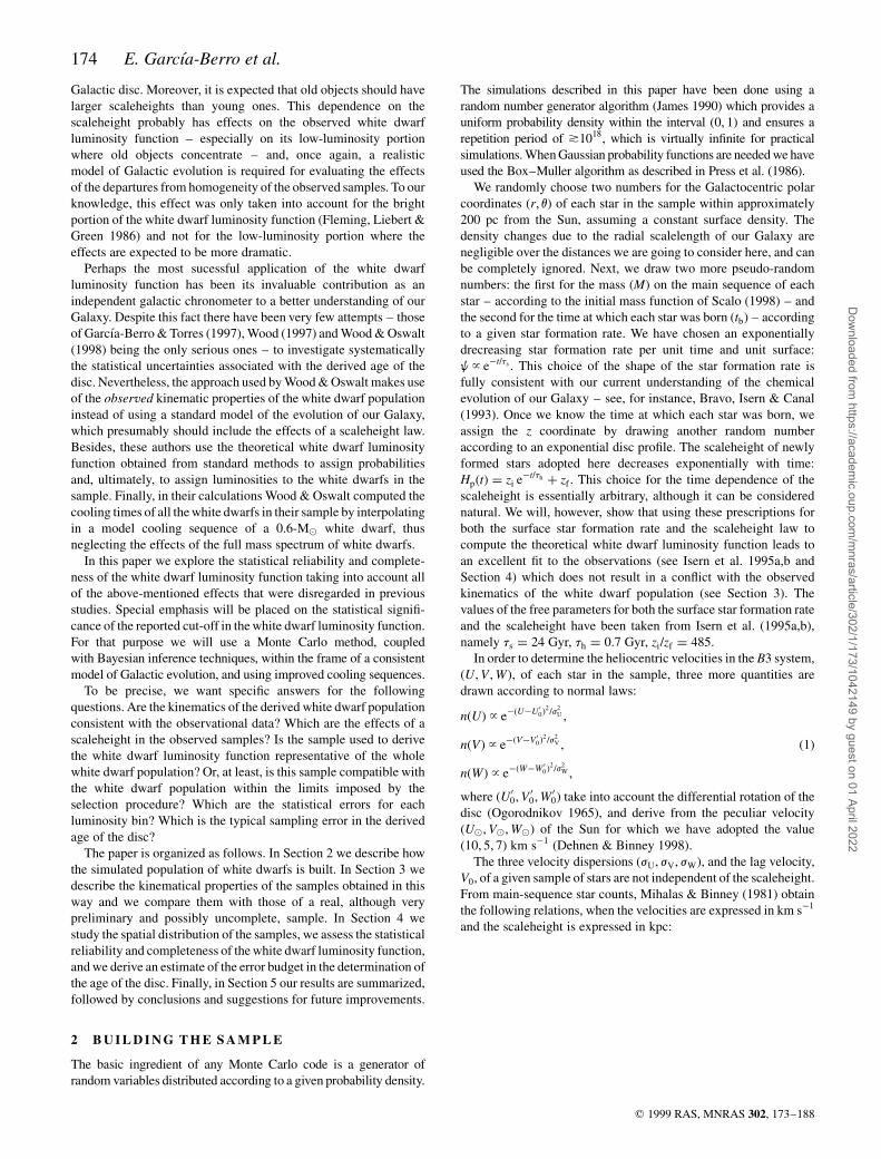
In Fig. 1 we show a summary of the most relevant results for a

disc age of 13 Gyr. In the top panel the mass distribution of those

stars that have been able to become white dwarfs (solid line, left-

hand scale) and of those white dwarfs that are selected for comput-

ing the luminosity function (dotted line, right-hand scale) are

shown. Both distributions are well behaved, follow closely each

other, and peak at around 0:55 M(, in very good agreement with the

observations (Bergeron, Saffer & Liebert 1992). In this sense, the

restricted sample could be considered as representative of the whole

white dwarf population.

In the middle panel of Fig. 1 we show the raw distribution of

Simulations of the disc white dwarf population 175

q 1999 RAS, MNRAS 302, 173±188

Figure 1. Some relevant distributions obtained from a single Monte Carlo

simulation; the solid lines correspond to the original sample, whereas the

dotted lines correspond to the restricted sample. See text for details.

Dow


ic.oup.com/m


luminosities for the stars in the original (solid line, left-hand scale)

and the restricted (dotted line, right-hand scale) samples. The

differences between the two distributions are quite apparent: ®rst,

the restricted sample has a broad peak centred at log�L=L(� , ÿ3:5,

whereas the original sample is narrowly peaked at a smaller

luminosity (0.6 dex). Obviously, since the restricted sample is

selected on a kinematical basis ± see the bottom panel of Fig. 1,

where the distribution of proper motions for both samples is shown

± some very faint and low proper motion white dwarfs are

discarded. Thus the restricted sample is biased towards larger

luminosities. Therefore the cut-off of the observational luminosity

function should be biased as well towards larger luminosities.

However, it is important to realize that only , 0.6 per cent of the

total number of white dwarfs with log�L=L(� > ÿ4:0 are selected

for the restricted sample and therefore, used in computing the white

dwarf luminosity function. This number decreases to , 0.04 per

cent if we consider the low-luminosity portion of the white dwarf

luminosity function ± that is, white dwarfs with log�L=L(� < ÿ4:0

± where most of the information regarding the initial phases of our

Galaxy is recorded. The distribution of proper motions (lower right

panel of Fig. 1) shows that most white dwarfs for both the original

and the restricted sample have proper motions smaller than

0:4 arcsec yrÿ1. However, the restricted sample has a pronounced

peak at m , 0:3 arcsec yrÿ1, and shows a de®cit of very low proper

motion white dwarfs, as should be the case for a kinematically

selected sample, whereas the original sample smoothly decreases

for increasing proper motions.

3 T H E K I N E M AT I C P R O P E RT I E S O F T H E

W H I T E DWA R F P O P U L AT I O N

Since the pioneering work of Sion & Liebert (1977), very few

analysis of the kinematics of the white dwarf population have been

done, with that of Sion et al. (1988) being the most relevant one,

despite the fact that the low-luminosity portion of the white dwarf

luminosity function is actually derived from a kinematically

selected sample. Sion et al. used a speci®c subset of the proper

motion sample of spectroscopically identi®ed white dwarfs to

check kinematically distinct spectroscopic subgroups and test

different scenarios of white dwarf production channels. However,

a major disadvantage of this subset of the white dwarf population is

that the three components of the velocity are derived only from the

tangential velocity, since the determination of radial velocities for

white dwarfs is not an easy task, especially for very cool ones.

Obviously, it would be better to have the complete description of the

space motions of this sample, but it is none the less true that we

already have two-thirds of the motion available for comparison with

the simulated samples, and that the latter samples can account for

this observational bias.

The sample of Sion et al. (1988) consists of 626 stars with known

distances and tangential velocities (of which 421 white dwarfs

belong to the spectral type DA, and 205 stars belong to other

spectral types). In this proper motion sample there are 523 white

dwarfs for which masses, radii and effective temperatures could be

derived ± see Sion et al. for the computational details ± of which

372 have masses larger than 0.5 M( and are therefore expected to

have carbon-oxygen cores. Of this latter group of white dwarfs there

are 305 with spectral type DA and 67 belong to other spectral types.

For this particular sample of white dwarfs cooling ages were

derived using the cooling sequences of Salaris et al. (1997) and,

given a relationship between the initial mass on the main sequence

and the ®nal mass of the white dwarf (Iben & Laughlin 1989), main-

sequence lifetimes (Iben & Laughlin 1989) were also assigned, and

the birth time of their progenitors was computed. However, the

errors in the determination of the mass of the progenitor can

produce large errors in the determination of the total age of low-

mass white dwarfs. For instance, for a typical 0:6-M( white dwarf

an error in the determination of its mass of 0:05 M( leads to an error

in its cooling age of , 0:3 Gyr at log�L=L(� � ÿ2:0, and of , 0:8

Gyr at log�L=L(� � ÿ4:0, whereas the error in the determination of

its main-sequence lifetime is of , 2 Gyr. Thus the mass dependence

of the cooling sequences is relatively small, whereas the mass

dependence of the main-sequence lifetimes is very strong. Finally, it

could be argued that since this sample includes both DA and non-

DA white dwarfs, appropiate cooling sequences should be used

for each spectral type. However, the errors introduced by using

unappropiate cooling sequences (that is cooling sequences for He-

dominated white dwarf envelopes) in the calculation of the cooling

times of DA white dwarfs are small when compared to the errors

introduced in dating white dwarfs by poor mass estimates. There-

fore the temporal characteristics of the white dwarf population from

them derived should be viewed with some caution. Note also that

there is not any guarantee that the sample of Sion et al. is

representative of the whole population of white dwarfs, since it is

by no means complete, and therefore some cautions are required

when drawing conclusions. To be more precise, the sample of Sion

et al. has very few low-luminosity white dwarfs. In fact, this sample

contains only 12 white dwarfs belonging to the low-luminosity

sample of Liebert et al. (1988), of which only four have mass,

tangential velocity, and effective temperature determinations.

Therefore we have added to this sample ± hereinafter `observa-

tional' sample ± three additional white dwarfs of the sample of

Liebert et al. (1988) for which a mass estimate could be found

(DõÂaz-Pinto et al. 1994). Nevertheless, this sample provides a

unique opportunity to test the results obtained from a simulated

white dwarf sample.

3.1 The overall kinematical properties of the samples

First, we compare the overall kinematical properties of the white

dwarf simulated samples with those of the observational sample,

regardless of the birth time of their progenitors. In Fig. 2 we show

the distributions of the tangential and radial velocities for both the

original and the restricted sample. The tangential velocity distribu-

tion of the original sample is shown in the upper left panel, and the

tangential velocity distribution of the restricted sample is shown as

a solid line (left-hand scale) in the upper right panel. The restricted

sample, which is kinematically selected, has a smaller tangential

velocity dispersion �jtan , 80 km sÿ1� than the original sample

�jtan , 100 km sÿ1�. Here we have de®ned, for operational pur-

poses only, the dispersions to be as the full-width at half-maximum

of the distributions. Moreover, both samples are peaked at different

tangential velocities: at Vtan , 45 km sÿ1 for the original sample,

and at Vtan , 65 km sÿ1 for the restricted sample, showing clearly

that the restricted sample is biased towards larger tangential

velocities, as it should be for a proper motion-selected sample. In

fact, the most probable tangential velocity of the restricted sample is

almost one-third larger than that of the total sample of white dwarfs.

This kinematical bias is clearly seen as well in the behaviour of the

distribution at low tangential velocities where the restricted sample

shows a de®cit of low-velocity stars, as expected from a kinema-

tically selected sample. Note also the existence of an extended tail at

high tangential velocities, indicating the presence of high proper

motion white dwarfs. Of course, all these effects are simply due to


q 1999 RAS, MNRAS 302, 173±188

Dow


ic.oup.com/m


the selection criteria, particularly to the assumed restriction in

proper motion. The distribution of radial velocities of the original

sample is shown in the lower left panel of Fig. 2, and the radial

velocity distribution of the restricted sample is shown as a solid line

(left-hand scale) of the lower right panel. The two distributions have

similar dispersions �jrad , 90 km sÿ1) and both are well behaved

and centred at Vrad � 0, as they should be since there is not any

constraint on the radial velocities of the restricted sample.

In Fig. 3 the tangential velocity distribution of the observational

sample is shown. By comparing the tangential velocity distributions

in Fig. 2 (upper panels) and Fig. 3 we can ensure that the

observational sample does not have a clear kinematical bias,

since it does not show a clear de®cit of low tangential velocity

white dwarfs ± the ratio between the height of the peak and the

height of the lowest velocity bin is the same for both the original

sample and the observational sample: roughly 1/4 ± and does not

have an extended tail at high tangential velocities, as the restricted

sample does. Moreover, the observational sample peaks at

Vtan , 40 km sÿ1, whereas the original sample (which is not

kinematically selected) peaks at a very similar tangential velocity

�Vtan , 45 km sÿ1�. However, the tangential velocity dispersion

�jtan , 60 km sÿ1� of the observational sample is roughly one-third

smaller than that of the original sample. This might be due to the

absence of low-luminosity white dwarfs in the observational

sample. Notice that intrisically dim white dwarfs are selected on

the basis of a large proper motion and are therefore expected to

have, on average, larger tangential velocities, thus increasing the

velocity dispersion. To check this assumption, we have run our

Monte Carlo code with a looser restriction on proper motions

�m $ 0:08 arcsec yrÿ1�. The result is shown in the upper right panel

of Fig. 2 as a dotted line (right-hand scale). Although the number of


q 1999 RAS, MNRAS 302, 173±188

Figure 2. Tangential (upper left panel) and radial (lower left panel) velocity distributions for the original sample, and the corresponding distributions for the

restricted sample (upper and lower right panels, respectively). Also shown as dotted lines are the tangential and radial velocity distributions of the restricted

sample with a looser restriction in proper motions (see text for details).

Figure 3. Tangential velocity distribution of the sample of Sion et al. (1988).

Dow


ic.oup.com/m


selected white dwarfs increases from , 85 to almost 250, the

tangential velocity dispersion decreases from jtan , 80 km sÿ1 to

jtan , 60 km sÿ1, in good agreement with the tangential velocity

dispersion of the observational sample. A ®nal test can be per-

formed by imposing a tighter restriction on visual magnitudes

(mV # 15:5 mag). The resulting sample is now smaller ± 58

white dwarfs ± as would be expected, whereas the tangential

velocity dispersion decreases to jtan , 40 km sÿ1 and the most

probable tangential velocity remains almost unchanged (Vtan , 40

km sÿ1). On the other hand, the radial velocity distribution ± dashed

line and right-hand scale in the lower right panel of Fig. 2 ± is nearly

indistinguishable from the previous sample, selected with a tighter

restriction. Nevertheless, the differences between the observational

sample and the simulated samples could be considered as minor.

Therefore we conclude that the simulated population of white dwarfs

is fairly representative of the real population of white dwarfs.

3.2 The temporal behaviour of the samples

Up to this moment we have compared the global kinematical

characteristics of the simulated samples with those of the sample

of Sion et al. (1988), but one of the major advantages of this latter

sample is that all the mass determinations have been obtained using

the same procedure, and consequently, in this sense, the sample is

relatively homogeneous. Therefore we can tentatively obtain the

temporal variations of the kinematical properties as a function of the

birth time of the progenitors of the white dwarfs belonging to the

observational sample, and compare them with those of the simu-

lated samples.

In this regard, in Fig. 4 we show the histograms of the distribution

of the birth times of white dwarfs belonging to the observational

sample (shaded histogram) and to the restricted sample (non-shaded

histogram). The number of objects in each time bin is also shown on

top of each bin of the histogram. Time runs backwards, and

therefore old objects are located at the left of the diagrams, whereas

young objects contribute to the time bins of the right part of the

diagrams. It is important to realize that old bins may include

kinematical data coming from either bright, low-mass white

dwarfs, or dim, massive white dwarfs. The time bins have been

chosen in such a way that the distribution of white dwarfs in the

observational sample is ef®ciently binned. The ®rst bin in time

corresponds to objects older than 7 Gyr and has only ®ve objects,

most of them corresponding to intrinsically faint objects belonging

to the sample of Liebert et al. (1988). The last bin corresponds to

objects younger than 1 Gyr. The remaining three bins are equally

spaced in time and correspond to white dwarf progenitors with ages

running from 1 to 7 Gyr in 2-Gyr intervals. All the bins have been

centred at the average age of the objects belonging to them (,7.7,

5.9, 3.7, 1.9 and 0.5 Gyr, respectively).

Since the youngest time bin corresponds to intrinsically bright

white dwarfs, it is expected that this time bin is reasonably complete

in the observational sample. We have therefore chosen the total

number of stars in the simulated samples in such a way that the

restricted sample has a number of objects in the youngest time bin

comparable with that of the observational sample. Since there is no

clear restriction in the ages of white dwarfs belonging to the

restricted sample, the statistical reliability of the remaining time

bins of the observational sample can be readily assessed. Note the

huge difference in the number of white dwarfs between the

observational sample and the restricted sample for the oldest time

bins in Fig. 4. Clearly, the completeness of the observational sample

decreases dramatically as the birth time increases. The percentage

of missing white dwarfs �h� in the observational sample as a

function of the birth time of their corresponding progenitors is

also shown in Fig. 4 as a solid line, assuming that the youngest time

bin of the restricted sample is complete. We have considered the

observational sample to provide reasonable estimates of the tem-

poral variations of the velocity when one-third of the expected

number of white dwarfs is present in the corresponding time bin.

This roughly corresponds to birth times smaller than 3.7 Gyr.

Therefore, the only time bins that we are going to consider

statistically signi®cant are the youngest three bins.

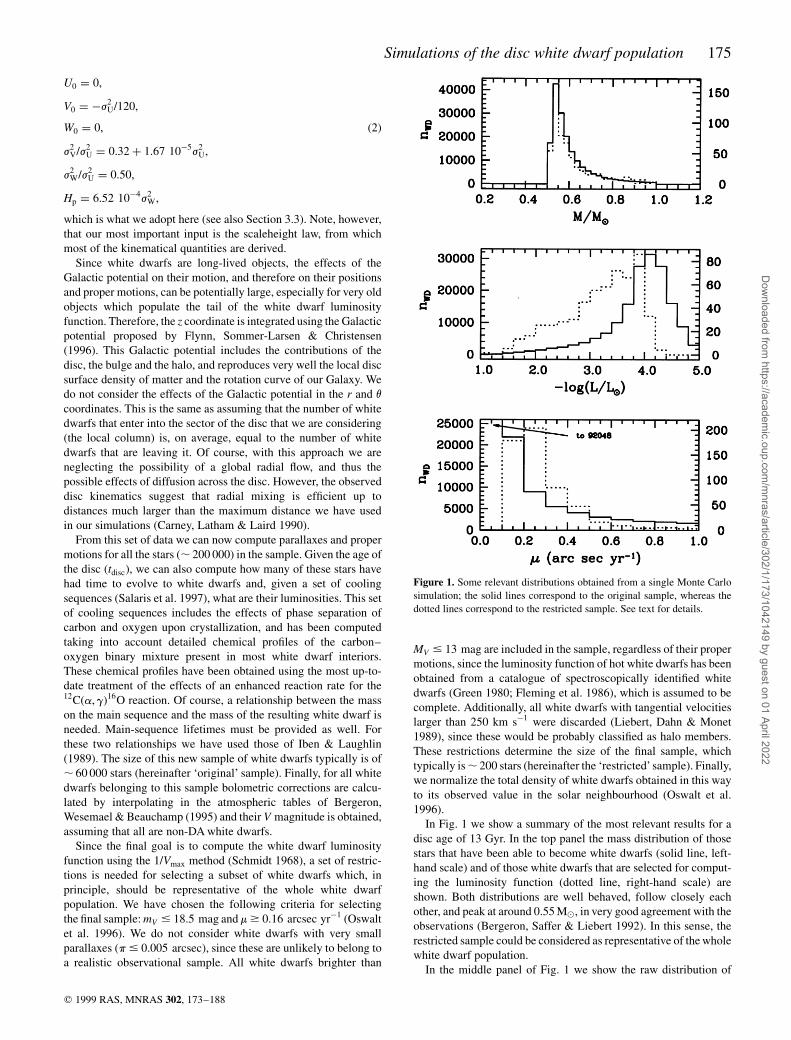
In Fig. 5 we show as solid lines the temporal variation of the

components of the tangential velocity as a function of the total age

(white dwarf cooling age plus main-sequence lifetime of the

corresponding parent star) of white dwarfs belonging to the

restricted sample (left-hand panels), and the same quantities for

white dwarfs belonging to the observational sample (right-hand

panels). Although we have not considered the data for ttotal > 3:7

Gyr to be reliable due the incompleteness of the observational

sample, we also show the temporal variations of all the three

components of the tangential velocity for these times as dotted

lines for the sake of completeness. The thinner vertical line

corresponds to ttotal � 3:7 Gyr. As can be seen in this ®gure, the

general trend for young objects is very similar for both samples. In

particular, both the restricted and the observational sample have

negative velocities across the Galactic plane with velocities of

W , ÿ10 km sÿ1, both samples lag behind the Sun with similar

velocities of V , ÿ25 and ÿ20 km sÿ1, respectively, and both

samples have positive radial velocities of roughly U , 20 km sÿ1.

Finally, old objects in both samples lag behind the Sun (middle

panels) the lag velocity being comparable for the two samples:

V , ÿ20 and ÿ25 km sÿ1, respectively. Moreover, we have com-

puted the time-averaged values of the velocities shown in Fig. 5, and

we have found hUi , 10 and 12 km sÿ1, hVi , ÿ28 and ÿ23

km sÿ1, and hWi , ÿ8 and ÿ7 km sÿ1, respectively. We have also

computed the time-averaged values of the velocity dispersions for

the restricted and the observational samples: hjUi , 41 and 42

km sÿ1, hjVi , 27 and 30 km sÿ1, and hjWi , 25 and 25 km sÿ1,

and we have found that they are also in good agreement.

As already noted in Section 2, the most important ingredient

needed to ®t adequately the kinematics of white dwarfs is the exact

shape of the scaleheight law. In fact, the luminosity function (see


q 1999 RAS, MNRAS 302, 173±188

Figure 4. Time distributions of the restricted sample (non-shaded diagram)

and the observational sample (shaded diagram) and percentage of missing

white dwarfs in the observational sample. The total number of objects in

each time bin is shown on top of the corresponding bin.

Dow


ic.oup.com/m


Section 4 below) is only sensitive to the ratio of the initial to ®nal

scaleheights �zi=zf� of the disc and to the time-scale of disc

formation �th�, but not to the exact value of, say, zf . However,

when the kinematics of the sample are considered, the reverse is

true. That is, the kinematics of the simulated samples are very

sensitive to the exact value adopted for the ®nal scaleheight. This is

clearly illustrated in Table 1, where the time-averaged values for the

three components of the tangential velocity and the tangential

velocity dispersions are shown for several choices of the ®nal

scaleheight, but keeping constant the above-mentioned ratio. As

can be seen there, the time-averaged radial component of the

tangential velocity, hUi, and the time-averaged perpendicular

component of the tangential velocity, hWi, are not very sensitive

to the choice of zf , whereas the time-averaged lag velocity is very

sensitive to its choice. Regarding the velocity dispersions, all three

components are sensitive. We have chosen the value of zf which best

®ts the average values of the observed sample. In order to produce

the results of Figs 4 and 5, a value of 500 pc was adopted for zf,

which is typical of a thick disc population. It is important to point

out here that increasing (decreasing) zf by a factor of 2 without

keeping constant the ratio �zi=zf� doubles (halves) jW for objects in

the youngest time bin, which is the most reliable one, thus making

incompatible the simulated and the observational samples. Simi-

larly, increasing th by a factor of 2 changes dramatically the

behaviour of the lag velocity, since it changes the value of V for

objects in the youngest time bin from , ÿ 20 to , ÿ 10 km sÿ1.

We conclude that the proposed scaleheight law is not in con¯ict

with the observed kinematics of the white dwarf population.

3.3 A ®nal remark on the reliability of the samples

Finally, it is interesting to compare the results of a kinematical

analysis of the observational sample with the predictions obtained

from main-sequence star counts as given by equation (2). In Fig. 6

we show the correlations between the V component of the tangen-

tial velocity (top panel), the ratio jV=jU (middle panel), and the

ratio jW=jU (bottom panel) as a function of the radial velocity

dispersion jU obtained from the data of main-sequence stars


q 1999 RAS, MNRAS 302, 173±188

Figure 5. Components of the tangential velocity as a function of the birth time of the white dwarf progenitors for the restricted (left-hand panels) and the

observational sample (right-hand panels); see text for details.

Table 1. Average values of the three components of the tangential velocity

and their corresponding dispersions (both in km sÿ1) for several choices of

zf (in kpc).

zf hUi hVi hWi hjUi hjVi hjWi

0.05 11.93 ÿ13:87 ÿ3:54 12.33 7.43 8.03

0.10 12.77 ÿ16:60 ÿ5:42 20.42 11.09 10.85

0.20 12.00 ÿ19:86 ÿ4:02 27.84 15.25 16.06

0.30 9.40 ÿ24:95 ÿ5:16 31.52 19.54 20.70

0.40 10.13 ÿ24:93 ÿ7:33 36.57 21.40 24.08

0.50 9.34 ÿ27:77 ÿ7:70 41.38 26.75 24.74

0.60 11.45 ÿ29:90 ÿ5:83 41.92 26.98 30.63

Dow


ic.oup.com/m


compiled by Sion et al. (1988). Except for the last bin the agreement

between the data obtained from the white dwarf sample and the data

obtained from main-sequence stars is fairly good (j2V=j2

U , 0:3,

j2W=j2

U , 0:5 and V=j2U , ÿ20). However, it should be taken into

account that the data coming from the last bin is obtained, as

previously mentioned, with only ®ve stars. Moreover, all these

objects belong to the low-luminosity sample of Liebert et al. (1988),

which is strongly biased towards large tangential velocities and,

besides, systematic errors affecting either mass and radius determi-

nations or luminosity determinations (the bolometric corrections

adopted in the latter work are highly uncertain) can mask the true

behaviour of the sample.

A ®nal test of the validity of the assumptions adopted in this

paper to derive the simulated populations can be performed by

comparing the results of this section with the kinematical analysis

of a sample of main-sequence F and G stars (Edvardsson et al.

1993). These authors measured distances, proper motions and radial

velocities (among other data) for a sample of 189 F and G stars.

They also assigned individual ages for all the stars in the sample

from ®ts in the Teff ÿ log g plane. The same sample has been

reanalysed very recently by Ng & Bertelli (1998), using distances

based on Hipparcos parallaxes and improved isochrones. We refer

the reader to the latter work for a detailed analysis of the errors and

uncertainties involved in dating individual objects. Although an

analysis similar to that performed in Section 3.2 can be done, for the

sake of conciseness we will only refer here to the average values of

the three components of the tangential velocity and its correspond-

ing dispersions. For this purpose, in Table 2 we show the averaged

values of the three components of the tangential velocity and their

corresponding dispersions for the restricted sample of our Monte

Carlo simulation, labelled MC, the observational sample, labelled

WD, and the three components of the velocity and their dispersions

for the Edvardsson et al. (1993) sample, labelled E93. As already

discussed in Section 3.2, the agreement between the Monte Carlo

simulation and the observational sample is fairly good. The com-

parison of both samples with the sample of Edvardsson et al. reveals

that the agreement between the average values of the three samples

is remarkably good, even if the dating procedure for individual

objects is very different in both observational samples. The same

holds for the averaged values of the three velocity dispersions. We

conclude that our equation (2) represents fairly well the kinematical

properties of the observed white dwarf population.

4 T H E W H I T E DWA R F L U M I N O S I T Y

F U N C T I O N

4.1 The spatial distribution and completeness of the simulated

white dwarf population

The 1=Vmax method (Schmidt 1968; Felten 1976), when applied to

our simulated white dwarf population, should provide us with an

unbiased estimator of its luminosity function, assuming complete-

ness of the simulated samples in both proper motion and apparent

magnitude, and provided that the spatial distribution of white

dwarfs is homogeneous. Strictly speaking, this means that the

maximum distance at which we ®nd an object belonging to the

sample is independent of the direction. In our case this is clearly not

true ± and, most probably, for a real sample this would certainly be

the case as well ± since we have derived the simulated samples


q 1999 RAS, MNRAS 302, 173±188

Figure 6. Overall kinematical properties of the observational sample.

Table 2. Average values of the three components of the tangential velocity

and their corresponding dispersions (both in km sÿ1) for the Monte Carlo

simulation, the observational sample, and the Edvardsson et al. (1993)

sample.

Sample hUi hVi hWi hjUi hjVi hjWi

MC 10 ÿ28 ÿ8 41 27 25

WD 12 ÿ23 ÿ7 42 30 25

E93 14 ÿ21 ÿ8 39 29 23

Figure 7. Histogram of the z distribution for both the original sample (right-

hand scale) and the restricted sample (left-hand scale).

Dow


ic.oup.com/m


assuming an exponential density pro®le across the Galactic plane.

Since the scaleheight law exponentially decreases with time (see

Section 2) it is dif®cult to say `a priori' which is the ®nal spatial

con®guration of the simulated white dwarf samples introduced in

the previous sections.

In the histogram of Fig. 7 we show the logarithmic distribution of

the number of white dwarfs as a function of the absolute value of the

z coordinate for both the original sample (right-hand scale) and the

restricted sample (left-hand scale). Clearly, both distributions

correspond to exponential disc pro®les with different scaleheights.

Also shown in Fig. 7 are the best ®ts to these distributions. The

corresponding scaleheights from them derived are <1:3 kpc for the

original sample, which is typical of a thick disc population, and

considerably smaller (<129 pc) for the restricted sample which can

be considered typical of a thin disc population. This is not an

evident result since, as has been explained in Section 2, the

simulated populations take naturally into account the fact that old

objects are distributed over larger volumes (that is, with larger

scaleheights and therefore with larger velocity dispersion perpen-

dicular to the plane of the Galaxy) than young ones. One could

therefore expect that the ®nal spatial distribution of the restricted

white dwarf population ± which is kinematically selected ± should

re¯ect properties of an intermediate thin±thick disc population, and

certainly this is not the case. Obviously, since there is not any

restriction in the distances (within the local column) at which a

white dwarf belonging to the original sample can be observed the

expected ®nal scaleheight for this sample should be much larger, in

good agreement with the simulations. Regarding the restricted

sample, our results clearly indicate that we are selecting for this

sample white dwarfs lying very close to the Galactic plane. More-

over, if we change zf by a factor of 2 as explained in Section 3, the

®nal scaleheight of the restricted sample does not change appreci-

ably and, on the other hand, the dispersion of velocities perpen-

dicular to the Galactic plane does not agree with its observed value.

Therefore, the ®nal scaleheight of the restricted sample is clearly

dominated by the selection criteria. It is important to realize that this

scaleheight, taken at face value, is not negligible at all when

compared with the value of the maximum distance at which a

parallax is likely to be measured with relatively good accuracy ±

which is typically 200 pc ± and which imposes an additional

selection criterion (see Section 2) for white dwarfs belonging to

the restricted sample, which are the white dwarfs that are going to

be used in the process of determination of the white dwarf

luminosity function. The 1=Vmax method must therefore be general-

ized to take into account a space-density gradient. For this reason

we have used the density law in Fig. 7 to de®ne a new density-

weighted volume element dV 0� r�z� dV (Felten 1976; Avni &

Bahcall 1980; Tinney, Reid & Mould 1993), being r�z� the density

law derived from Fig. 7. This new, corrected, estimator provides a

more accurate determination of the white dwarf luminosity function

and, ultimately, a more realistic value of the space density of white

dwarfs. All in all, for reasonable choices of a scaleheight law its

effects on the derived white dwarf luminosity function in principle

cannot be considered negligible.

The second, and probably more important issue, is the complete-

ness of the samples used to build the white dwarf luminosity

function. This is a central issue, since the 1=Vmax method assumes

completeness of the samples. The reader should keep in mind that

the original sample is complete by construction, since it consists of

all white dwarfs generated by the Monte Carlo code, regardless of

their distance, proper motion, apparent magnitude and tangential

velocity, whereas the restricted sample is built with white dwarfs

culled from the original sample according to a set of selection

criteria, and therefore its completeness remains to be assessed.

In Fig. 8 we explore the completeness of the simulated samples.

For this purpose, the cumulative star counts of white dwarfs with

apparent magnitude smaller than mV for the original sample are

shown in the top left panel of Fig. 8, whereas the corresponding

diagram for the restricted sample is shown in the top right panel.

Also shown in Fig. 8 are the cumulative star counts of white dwarfs

with proper motions larger than m belonging to the original sample

(bottom left panel) and to the restricted sample (bottom right panel).

For a complete sample distributed according to a homogenous

spatial density, the logarithm of the cumulative star counts of white

dwarfs with apparent magnitude smaller than mV are proportional to

mV with a slope of 0.6 (see, e.g., Mihalas & Binney 1981). We also

show in the top panels of Fig. 8 a straight line with such a slope. It is

evident from the previous discussion that our samples are not, by

any means, distributed homogenously. Note also that the effects of a

scaleheight law are tangled in the standard test of completeness of

the samples. Nevertheless, the effects of a scaleheight law can be

disentangled, since they should be quite apparent in the cumulative

star counts diagram of the original sample, which is complete. A

look at the top left panel of Fig. 8 reveals that the effects of the

scaleheight law are evident for surveys with limiting magnitude

mV * 19 mag. Therefore we can now assess the completeness in

apparent magnitude of the restricted sample, since the turn-off for

this sample (see top right panel of Fig. 8) occurs at mV , 17 mag.

Consequently, the effects of the scaleheight law can be completely

ruled out, and this value can be considered as a safe limit for which

the restricted sample is complete in apparent magnitude.

The completeness of the restricted sample in proper motion can

be assessed in a similar way. Again, the assumption of an homo-

genous and complete sample in proper motion leads to the conclu-

sion that the logarithm of the cumulative star counts of white dwarfs

with proper motion larger than m should be proportional to m with a

slope of ÿ3 (see, e.g., Oswalt & Smith 1995 and Wood & Oswalt

1998). A look at the bottom left panel of Fig. 8 reveals that for the

original sample this is not by far the case. In other words, since this

particular sample is complete by construction, the hypothesis of an


q 1999 RAS, MNRAS 302, 173±188

Figure 8. Cumulative histograms of apparent magnitude and proper motion

for both the original and the restricted sample. See text for details.

Dow


ic.oup.com/m


homogenous distribution of proper motions must be dropped. This

is again one, and probably the most important, of the effects

associated with a scaleheight law since the kinematics of the

samples are highly sensitive to the choice of the scaleheight law

(see Section 2, equation (2) and Table 1). It is important to realize

that the effects of a scaleheight law are more prominent in proper

motion than in the spatial distribution, and this can be directly

checked for a real sample, thus providing a direct probe of the

history of the star formation rate per unit volume. Finally, in the

lower right panel of Fig. 8 the cumulative star counts in proper

motion of white dwarfs belonging to the restricted sample are

shown. As expected, the effects of a scaleheight law are in this case

negligible, since we are culling white dwarfs with high proper

motion for which the original sample is reasonably complete (see

the lower left panel of Fig. 8). The exact value of the turn-off is in

this case m , 0:3 arcsec yrÿ1, in close agreement with the results of

Wood & Oswalt.

It is quite clear from the previous discussions that one of the

ingredients that has proven to be essential in the determination of

the white dwarf luminosity function is the adopted scaleheight law.

In principle, one should expect two kinds of competing trends. On

the one hand, the effects of the scaleheight law should be more

dramatic for old objects, because old objects have a larger velocity

dispersion (although the effects of a spatial inhomogeneity should

be, as well, less apparent) and the tail of the white dwarf

luminosity function is populated predominantly by this kind of

white dwarfs (intrinsically dim, high proper motion objects). One

should therefore expect that the cut-off in the white dwarf

luminosity function is in¯uenced either by the spatial distribution

of white dwarfs or by their velocity distribution, or by a combina-

tion of both. On the other hand, objects populating the tail of the

luminosity function are intrinsically dim objects and, therefore,

in order to be selected for the restricted sample they must be

close neighbours. This, in turn, implies that the average distance

at which we are looking for white dwarfs is small and, consequently,

the effects of a scaleheight law should be less apparent. The

reverse is true at moderately high luminosities. It is therefore

interesting to see which are the dominant effects as a function of

the luminosity. For this purpose, in Fig. 9 we show several

average properties of white dwarfs belonging to the restricted

sample as a function of their luminosity for a typical Monte Carlo

simulation.

In the top panel of Fig. 9 we show the average distance to the

Galactic plane of white dwarfs belonging to the restricted sample.

As can be seen, the average distance to the Galactic plane of

intrinsically bright white dwarfs can be as high as 100 pc, which

is a sizeable fraction of the derived scaleheights of the white dwarf

samples. Consequently, we expect that the effects of an inhomoge-

neous spatial distribution should be very prominent at high lumin-

osities. Conversely, the average distance to the Galactic plane for

white dwarfs near the observed cut-off in the white dwarf lumin-

osity function is only , 10 pc. Therefore as the luminosity

decreases, we are probing smaller volumes and the effects of an

inhomogenous spatial distribution at low luminosities are expected

to be, from this point of view, small (but see, however, the

discussion in Section 4.4).

In the middle panel of Fig. 9 the average tangential velocity of

objects belonging to the restricted sample is shown as a function of

the luminosity. The observational data is shown as solid circles and

has been obtained from Liebert et al. (1988). Their adopted

restriction in proper motion, m0 � 0:80 arcsec yrÿ1, is signi®cantly

larger than the one we adopt here, m0 � 0:16 arcsec yrÿ1, which is

consistent with the cut-off in proper motion adopted by Oswalt et al.

(1996). Therefore we expect a smaller average tangential velocity.

The agreement is fairly good since, given the ratio of proper motion

cut-offs, the average tangential velocity of our restricted sample

should be roughly a 20 per cent smaller: a closer look at the middle

panel of Fig. 9 shows that the average tangential velocity reported

by Liebert et al. (1988) is , 120 km sÿ1, whereas we obtain , 90

km sÿ1. These ®gures reinforce the general idea that our simulations

are fully consistent with the observed kinematics of the white dwarf

population.

Finally, in the bottom panel of Fig. 9 the average proper motion

distribution of those stars belonging to the restricted sample is

shown as a function of the luminosity. As can be seen there, low-

luminosity white dwarfs belonging to the restricted sample have, on

average, large proper motions. As expected from the discussion of

the two previous panels, the distribution of proper motions is

smoothly increasing for luminosities in excess of , 10ÿ3 L(:

since the average value of the tangential velocity remains approxi-

mately constant, and we are selecting objects with smaller average

distances, the net result is an increase in the average proper motion.

Moreover, white dwarfs belonging the low-luminosity portion of

the white dwarf luminosity function are preferentially culled from

the original sample because of their high proper motion. That is the

same as saying that the selection criterion is primarily the proper


q 1999 RAS, MNRAS 302, 173±188

Figure 9. Average properties of the restricted sample as a function of the

luminosity. Top panel: average z coordinate of white dwarfs of the restricted

sample; middle panel: average tangential velocity for these white dwarfs, the

observational data have been taken from Liebert et al. (1988); and bottom

panel: average proper motion of these objects.

Dow


ic.oup.com/m


motion one, and that the criterion on apparent magnitude has little

to do for these luminosities, in agreement with the results of Wood

& Oswalt (1998). As a ®nal consequence, the effects of an

inhomogenous distribution in proper motions will be more evident

at high luminosities, where the average proper motion is smaller

(see the discussion of the lower left panel of Fig. 8). All in all, the

effects of the inhomogeneities in both proper motion and z will be

more prominent at high luminosities, where the observational

luminosity function already takes into account these effects

(Fleming et al. 1986).

4.2 The Monte Carlo simulated white dwarf luminosity

functions

In Fig. 10 we show a set of panels containing the white dwarf

luminosity functions obtained from 10 different Monte Carlo

simulations. Thus 10 different initial seeds were chosen for the

random number generator and, consequently, 10 independent

realizations of the white dwarf luminosity function were computed

(in fact, we have computed 20 independent realizations, of which

only 10 are shown in Fig. 10). The adopted age of the disc was

tdisc � 13 Gyr and the set of restrictions used to build the sample is

that of Section 2, which is the same set as used by Oswalt et al.

(1996) to derive their observational white dwarf luminosity func-

tion. The simulated white dwarf luminosity functions were com-

puted using a generalized 1=Vmax method (Felten 1976; Tinney et al.

1993; Qin & Xie 1997) which takes into account the effects of the

scaleheight. The error bars of each bin were computed according to

Liebert et al. (1988): the contribution of each star to the total error

budget in its luminosity bin is conservatively estimated to be the

same amount that contributes to the resulting density; the partial

contributions of each star in the bin are squared and then added, and

the ®nal error is the square root of this value. The resulting white

dwarf luminosity functions are plotted as solid squares; a solid line

linking each one of their points is also shown as a visual help. Also

plotted in each one of the panels is the observational white dwarf

luminosity function of Oswalt et al. (1996), which is shown as solid

circles linked by a dotted line. For each realization of the white

dwarf luminosity function the value obtained for hV=Vmaxi is also

shown in the upper left corner of the corresponding panel. Finally,

and for sake of completeness, the total number of objects in the

restricted sample, NWD, of the different realizations of the white

dwarf population, and the distribution of objects, Ni, in each

luminosity bin, i, of the Monte Carlo simulated white dwarf

luminosity functions is shown in Table 3. The total number of

white dwarfs belonging to the restricted sample is roughly 200,

which is the typical size of the samples used to build the currently

available observational luminosity functions. This number is

important, since the assigned error bars are strongly dependent on

the number of objects in each luminosity bin.

It is important to notice the overall excellent agreement between

the simulated data and the observational luminosity function.

However, there are several points that deserve further comments.

First, the simulated white dwarf luminosity functions are system-

atically larger than the observational luminosity functions for

luminosities in excess of log�L=L(� � ÿ2:0. This behaviour re¯ects

the effects of the spatial inhomogeneity of the simulated white

dwarf samples. It is important to realize that the hot portion of the

white dwarf luminosity function of Oswalt et al. (1996) has been

derived without taking into account the effects of a scaleheight, in

contrast with the procedure adopted by Fleming et al. (1986), where

those effects were properly taken into account. When one compares

the luminosity functions obtained in this section with that of

Fleming et al., the agreement is excellent. Also of interest is the

fact that the hot portion of the white dwarf luminosity function

varies quite considerably for the different realizations. The reason

for this behaviour is that at high luminosities the evolution is

dominated by neutrino losses, and it is fast. Therefore the prob-

ability of ®nding such white dwarfs is relatively small, and the

statistical signifance of those bins is low. Consequently, the exact

shape of the luminosity function at log�L=L(� $ ÿ3:0 is strongly

dependent of the initial seed of the pseudo-random number gen-

erator. This is further con®rmed by comparing the second and the

third column of Table 3, where the total number of objects in

the restricted sample and the number of objects in the ®rst bin of the

white dwarf luminosity function of each realization of the Monte

Carlo simulations are shown. As a consequence, the real error bars

that should be assigned to each bin are presumably larger than those

in Fig. 10. Moreover, any attempt to derive the volumetric star

formation rate using data from the bins at high luminosities (Noh &

Scalo 1990) is based on very weak grounds. It is also important to

notice that the completeness of the simulated samples as derived


q 1999 RAS, MNRAS 302, 173±188

Figure 10. Panel showing different realizations of the simulated white dwarf

luminosity function ± ®lled squares and solid lines ± compared to the

observational luminosity function of Oswalt et al. (1996) ± ®lled circles and

dotted line.

Dow


ic.oup.com/m


from the value of hV=Vmaxi is relatively large. In fact, for a complete

and homogeneous sample this value should be equal to 0.5; since

the simulated sample samples are not homogenous, the values

obtained here can be considered as reasonable.

Finally, it is convenient to point out here that we have done a x2

test of the compatibility of the Monte Carlo simulated samples. The

results are shown in Table 4, where the probability of an indepen-

dent observer ®nding the realizations compatible is shown for each

pair of realizations. As can be seen, this probability can be as low as

0.01, which is the same as saying that the corresponding luminosity

functions are completely incompatible, even if they have derived

from the same set of input parameters and selection criteria.

Obviously, the conclusion is that for a reasonable number of objects

in the restricted sample, the white dwarf luminosity function is

dominated by the selection criteria.

4.3 A Bayesian analysis of the simulated samples

As previously stated, changing the initial seed of the random

function generator the Monte Carlo code provides different inde-

pendent realizations of the white dwarf luminosity function. All

these realizations are `a priori' equally good. Besides, since the

number of objects that is used to compute the white dwarf

luminosity function is relatively small, large deviations are

expected, especially at relatively high luminosities for which the

cooling time-scales are short. This, in turn, results in very probable

underestimates of the associated uncertainties, especially at lumin-

osities larger than log�L=L(� * ÿ3:0. Consequently, we have used

Bayesian statistical methods (Press 1996) to obtain a realistic

estimation of the errors involved and the most probable value of

the density of white dwarfs for each luminosity bin.


q 1999 RAS, MNRAS 302, 173±188

Table 3. Total number of white dwarfs, NWD, and white dwarfs in each bin, Ni, for each of the 20 realizations of

the simulated white dwarf luminosity functions.

i NWD N1 N2 N3 N4 N5 N6 N7 N8 N9

1 200 1 8 5 14 42 38 42 44 6

2 216 1 6 11 18 29 48 49 53 1

3 203 0 4 8 22 36 39 45 43 6

4 176 0 6 6 17 18 35 41 44 9

5 210 1 5 8 17 24 49 48 53 5

6 191 1 7 10 23 24 37 44 37 8

7 202 0 3 12 29 27 42 50 35 4

8 222 0 1 16 18 38 41 50 57 1

9 197 0 5 12 20 22 34 51 47 6

10 198 1 1 9 16 28 44 49 47 3

11 204 0 5 10 21 25 38 44 53 8

12 198 1 3 14 20 33 36 50 35 6

13 175 0 3 14 20 23 32 44 37 2

14 182 0 6 9 15 28 40 43 35 6

15 185 2 6 6 19 30 31 44 43 4

16 213 1 3 16 21 33 31 45 56 7

17 189 2 2 11 25 22 32 43 44 8

18 207 1 4 7 17 33 38 41 61 5

19 217 1 10 10 28 17 47 55 42 7

20 210 0 4 13 19 31 38 46 55 4

Table 4. x2 test of the compatibility of the Monte Carlo simulated samples.

i 2 3 4 5 6 7 8 9 10 11 12 13 14 15 16 17 18 19 20

1 0.24 0.80 0.21 0.41 0.37 0.05 0.03 0.16 0.24 0.33 0.32 0.04 0.70 0.86 0.17 0.06 0.75 0.02 0.34

2 0.46 0.09 0.93 0.26 0.31 0.59 0.48 0.79 0.48 0.30 0.37 0.36 0.47 0.29 0.11 0.67 0.19 0.86

3 0.40 0.69 0.81 0.78 0.22 0.73 0.69 0.88 0.90 0.44 0.89 0.85 0.67 0.56 0.81 0.16 0.89

4 0.63 0.86 0.13 0.01 0.81 0.20 0.88 0.19 0.24 0.77 0.60 0.14 0.57 0.36 0.37 0.26

5 0.65 0.35 0.16 0.80 0.90 0.92 0.38 0.26 0.68 0.65 0.39 0.43 0.90 0.54 0.84

6 0.77 0.01 0.92 0.32 0.89 0.86 0.59 0.94 0.85 0.44 0.89 0.32 0.83 0.49

7 0.11 0.68 0.52 0.47 0.89 0.80 0.55 0.34 0.27 0.61 0.11 0.42 0.50

8 0.12 0.67 0.11 0.23 0.20 0.03 0.06 0.46 0.04 0.31 0.01 0.76

9 0.58 0.99 0.77 0.82 0.77 0.68 0.77 0.83 0.53 0.59 0.92

10 0.54 0.69 0.58 0.54 0.57 0.45 0.51 0.74 0.07 0.81

11 0.56 0.41 0.72 0.67 0.85 0.81 0.87 0.46 0.95

12 0.79 0.84 0.67 0.77 0.77 0.29 0.15 0.71

13 0.62 0.51 0.38 0.60 0.15 0.10 0.63

14 0.79 0.24 0.38 0.40 0.25 0.56

15 0.47 0.65 0.82 0.16 0.61

16 0.78 0.79 0.04 0.96

17 0.38 0.28 0.50

18 0.04 0.93

19 0.12

Dow


ic.oup.com/m


The problem can be stated as follows. For a given luminosity, L,

we want to know the most probable value of the white dwarf

luminosity function, N, given a set of Ni simulations assuming

that all simulations are equally good. To compute N, one must

maximize the probability distribution

P�N=Ni� ~Y

i

1

2

�PGi

� PBi

�; �3�

where PG and PB are the probability of being a good and a bad

simulation, respectively. We can calculate them following closely

Press (1996):

PGi� exp

�ÿ

�Ni ÿ N�2

2j2i

�;

PBi� exp

�ÿ

�Ni ÿ N�2

2S2

�;

(4)

where ji is the error bar of each bin of the luminosity function, and

S is a large but ®nite number characterizing the maximum

expected deviation in Ni. We recall that the contribution to the

error of each white dwarf is equal to the inverse of its maximum

volume squared.

The results are shown in Fig. 11, where the probability distribu-

tions corresponding to each luminosity bin, computed with the

previous method, are displayed. The logarithm of the luminosity of

each bin in solar units is shown in the upper right corner of each

panel. All the probability distributions, except that of the brightest

luminosity bin, have a Gaussian pro®le. This is a direct conse-

quence of the poor statistical signi®cance of the ®rst bin. In order to

produce these probability distributions, 20 independent realizations

of the simulated samples were used. This is a reasonable number:

increasing the total number of simulations does not introduces

substantial improvements in the statistical signi®cance of the ®rst

bin, which is the less signi®cant. From these probability distribu-

tions a better estimate of the statistical noise can be obtained. We

have estimated the resulting error bars by assuming a conservative

95 per cent con®dence level (approximately 2j). In Table 5 we show

the computed deviations for each of the 20 realizations of the Monte

Carlo simulated white dwarf luminosity functions and the most

probable error bars computed at the 95 per cent con®dence level.

The error bars obtained from a Bayesian analysis of the 20 Monte

Carlo simulations compare favourably, roughly speaking, with

those of each individual Monte Carlo simulation. However, for

samples where the total number of white dwarfs is smaller than 200

(the simulations presented here) the errors for each of the lumin-

osity bins are severe underestimates of the real errors, especially at

low luminosities.

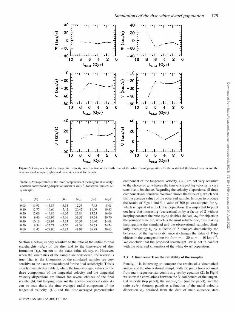
In Fig. 12 the most probable white dwarf luminosity function ±

hereinafter the Bayesian white dwarf luminosity function ± with its

corresponding error bars is shown, obtained by maximizing the

probability distributions in Fig. 11. Except for moderately high


q 1999 RAS, MNRAS 302, 173±188

Figure 11. Probability distribution functions for each luminosity bin.

Dow


ic.oup.com/m


luminosities ± i.e., for luminosities larger than log�L=L(� � ÿ2:0 ±

where the effects of the spatial inhomogeinities are most obvious,

the agreement between the observational luminosity function and

the Bayesian luminosity function is excellent. Moreover, for the

Bayesian white dwarf luminosity function we have computed a

synthetic value of hV=Vmaxi as an average of the corresponding

values for each of the 20 realizations with the weights given by the

probability of each realization obtained from the probability dis-

tributions in Fig. 11. We have obtained a value of hV=Vmaxi � 0:464,

which remains close to the canonical value of hV=Vmaxi � 0:5, valid

for an homogenous and complete sample.

4.4 The age of the disc

Perhaps one of the most surprising results of the simulations

presented here is the age of the disc itself. The value of 13 Gyr

adopted in this paper ®ts nicely the observational data of Oswalt

et al. (1996), as can be seen in Fig. 12. This a direct consequence of

the adopted scaleheight law, since using the same set of cooling

sequences and a conventional approach to compute the white dwarf

luminosity function with a constant volumetric star formation rate,

Salaris et al. (1997) derived an age for the solar neighbourhood of

11 Gyr when the effect of phase separation upon crystallization was

taken into account, and of 10 Gyr when phase separation was

neglected. Thus the ultimate reason of the increase in the adopted

age of the solar neighbourhood is not due to the details of the

adopted cooling sequences. Instead, this increase can be easily

explained in terms of the model of Galactic evolution. We recall that

the white dwarf luminosity function measures the number of white

dwarfs per cubic parsec and unit bolometric magnitude. Therefore,

in order to evaluate it, the volumetric star formation rate is required.

In our case we can de®ne the effective star formation rate per cubic

parsec as weff�t� < w�t�=Hp�t�. With the laws adopted here for w�t�

and Hp�t� it is easy to verify that the effective star formation rate

only becomes signi®cant after , 2 Gyr (Isern et al. 1995a,b).

4.5 Statistical uncertainties in the derived age of the disc

The easier and more straightforward way to assess the statistical

errors associated with the measurement of the age of the solar

neighbourhood is trying to reproduce the standard procedure. That

is, we have ®tted the position of the `observational' cut-off of each

of the Monte Carlo realizations with a standard method (Hernanz et

al. 1994) to compute the white dwarf luminosity function using

exactly the same inputs adopted to simulate the Monte Carlo

realizations, except, of course, the age of the disc, which is the

only free parameter. The results are shown in Fig. 13 for 10 of the 20

realizations. As is usual with real observational luminosity func-

tions, the theoretical white dwarf luminosity functions were nor-

malized to the bin with minimum error bars. The derived ages of the

disc for each one of the realizations are shown in the upper left

corner of the corresponding panel. As can be seen, there is a clear

bias: the derived ages of the disc are systematically larger than the


q 1999 RAS, MNRAS 302, 173±188

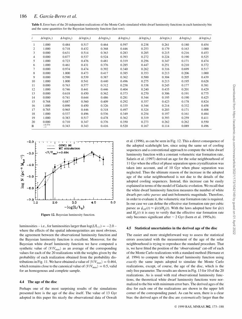
Table 5. Error bars of the 20 independent realizations of the Monte Carlo simulated white dwarf luminosity functions in each luminosity bin

and the same quantities for the Bayesian luminosity function (last row).

i D log�n1� D log�n2� D log�n3� D log�n4� D log�n5� D log�n6� D log�n7� D log�n8� D log�n9�

1 1.000 0.484 0.517 0.464 0.597 0.238 0.261 0.180 0.454

2 1.000 0.718 0.432 0.368 0.446 0.253 0.179 0.163 1.000

3 0.000 0.631 0.514 0.363 0.283 0.285 0.215 0.216 0.453

4 0.000 0.877 0.537 0.524 0.393 0.272 0.224 0.190 0.525

5 1.000 0.723 0.476 0.481 0.319 0.256 0.347 0.171 0.474

6 1.000 0.461 0.431 0.376 0.285 0.447 0.251 0.210 0.372

7 0.000 0.974 0.474 0.392 0.340 0.262 0.316 0.699 0.517

8 0.000 1.000 0.473 0.417 0.385 0.353 0.213 0.206 1.000

9 0.000 0.590 0.539 0.387 0.362 0.500 0.304 0.205 0.439

10 1.000 1.000 0.541 0.440 0.496 0.275 0.213 0.195 0.628

11 0.000 0.763 0.577 0.312 0.258 0.338 0.245 0.177 0.381

12 1.000 0.746 0.441 0.446 0.404 0.240 0.435 0.201 0.429

13 0.000 0.618 0.450 0.362 0.373 0.270 0.306 0.191 0.775

14 0.000 0.741 0.644 0.486 0.281 0.344 0.195 0.190 0.425

15 0.768 0.887 0.560 0.409 0.292 0.357 0.423 0.178 0.824

16 1.000 0.890 0.450 0.326 0.335 0.344 0.214 0.332 0.458

17 0.785 0.965 0.446 0.318 0.497 0.324 0.203 0.171 0.408

18 1.000 0.537 0.496 0.536 0.349 0.254 0.197 0.161 0.484

19 1.000 0.383 0.517 0.478 0.362 0.319 0.393 0.259 0.411

20 0.000 0.710 0.347 0.376 0.350 0.273 0.262 0.262 0.550

B �0:574ÿ¥ 0.343 0.343 0.416 0.520 0.167 0.114 0.089 0.496

Figure 12. Bayesian luminosity function.

Dow


ic.oup.com/m


input age of the Monte Carlo simulator by about half a Gyr. This a

direct consequence of the binning procedure, since we are grouping

white dwarfs belonging to the maximum of the white dwarf

luminosity function in the lowest luminosity bin, and can be

avoided by using the cumulative white dwarf luminosity function,

which minimizes the effects of the binning procedure.

We have used the Bayesian inference techniques described in

Section 4.3 to assign a purely statistical error to our age estimates.

In order to do this, we need to know a formal uncertainty for

each one of the independent realizations. Since the value of

hV =Vmaxi is a good measure of the overall quality of the sample

(despite the fact that the samples are inhomogenous), we have

adopted ji � 2 �0:5 ÿ hV=Vmaxi� tdisc. The correspoding probability

distribution is shown in Fig. 14, which leads to a most probable age

of the disc of tdisc � 13:5 6 0:8 Gyr at the 95 per cent con®dence

level (2j), which has to be compared with the adopted input age in

our Monte Carlo simulation, which was taken to be 13 Gyr. This

uncertainty is in good agreement with the results of Wood & Oswalt

(1998). If one relaxes the con®dence level to 1j, the associated error

bar is 6 0:4 Gyr. It is none the less important to realize that there is a

systematic increase in the inferred disc ages of , 5 per cent.

5 C O N C L U S I O N S

We have built a Monte Carlo code which has allowed us to

reproduce quite accurately the process of building the white

dwarf luminosity function from the stage of object selection and

data binning. Our Monte Carlo simulation includes a model of

Galactic evolution based on well established grounds. The simu-

lated samples obtained with our code reproduce very well the

overall kinematical properties of the observed white dwarf popula-

tion. We have explored as well the temporal evolution of such

properties, and we have found that there is a fair agreement between

the observed distributions and the simulated ones. However, we

have shown that observed sample has very few old white dwarfs,

and this has constrained our kinematical analysis to the most recent

3.7 Gyr, which can be considered as reasonably secure. Never-

theless, we have shown that the precise shape of the temporal

distributions encode a wealth of information, and therefore more

detailed analysis should be undertaken with improved observational

samples. We have also extended our kinematical analysis by

comparing the averaged properties of both the observational

white dwarf sample and the Monte Carlo simulated sample with a

sample of old main-sequence F and G stars. The results of this

comparison lead to the conclusion that our model of Galactic

evolution is fully compatible with the properties of the observed

samples.

Using our synthetic populations, we have assessed the complete-

ness of the samples used to derive the white dwarf luminosity

function and have studied their spatial distribution and, given a set

of selection criteria consistent with the observational procedures,

we have built several independent realizations of the white dwarf

luminosity function and compared them to the observational

luminosity function of Oswalt et al. (1996). Our results regarding

the white dwarf luminosity function can be summarized as follows.

(i) Given the selection criteria adopted by Oswalt et al. (1996),

our Monte Carlo simulation strongly suggest that the observational

samples are complete up to 17 mag, and that the primary selection

criterion at low luminosities is the proper motion one, in agreement

with Wood & Oswalt (1998).

(ii) The Monte Carlo simulated white dwarf luminosity func-

tions present an excellent agreement with the observational data.

(iii) The effects of a scaleheight law are not negligible at all in

the spatial distribution of the samples, especially at moderately

large luminosities were they are more prominent. A scaleheight of

roughly 130 pc is derived from the Monte Carlo simulations for the

objects used in building the white dwarf luminosity function.


q 1999 RAS, MNRAS 302, 173±188

Figure 13. Panel showing different simulated luminosity functions (®lled

squares) and their corresponding ®t using a standard method.

Figure 14. Bayesian analysis of the derived age of the disc.

Dow


ic.oup.com/m


However, we have established without any doubt that the effects of a

scaleheight law should be more apparent in the cumulative dis-

tribution of proper motions. Although the effects of the scaleheight

law on the tail of the white dwarf luminosity function seem to be

negligible at ®rst glance, a detailed analysis reveals that this

in¯ation effect increases the derived ages of the disc by a consider-

able amount, which can be typically 2 Gyr.

(iv) By using Bayesian inference techniques we have been able

to establish that the current procedure to assign the observational

error bars to the white dwarf luminosity function is reasonably for a

sample of 200 stars.

(v) Finally, the statistical uncertainty in the age of the disc

derived from a Bayesian analysis is roughly 1 Gyr, in agreement

with Wood & Oswalt (1998), and we have determined that there is a

systematic trend due to the binning procedure which increases the

disc ages inferred from the observational luminosity function by

roughly 5 per cent.

Nevertheless, a good deal of work remains to be done. Future

improvements may include a more detailed analysis of the kine-

matical properties of the sample of old white dwarfs. For this

purpose, it would be very useful to have more reliable observational

samples. In our case this means not only complete samples but also

more accurate mass determinations. It would be also convenient to

analyse the three-dimensional motion of the white dwarf population

but, for the moment, this seems to be unavoidable for the faintest

white dwarfs due to the absence of spectral features. Also of interest

is to study the contamination of the input samples used in the

process of building the white dwarf luminosity function with white

dwarfs belonging to the Galactic halo. This, in principle, cannot be

discarded, since halo members are selected on the basis of high

proper motion, which is the dominant selection criterion at the dim

end of the disc white dwarf luminosity function. A detailed

statistical analysis of the cumulative counts of white dwarfs still

remains to be done, instead of using the differential space density.

Last but not least, the tests proposed in this paper could be applied to

a real sample, thus providing us with very useful hints about the

structure and evolution of our Galaxy.

AC K N OW L E D G M E N T S

This work has been supported by DGICYT grants PB94±0111 and

PB94±0827-C02-02, and by the CIRIT grant GRQ94±8001.

REFERENCES

Avni Y., Bahcall J. N., 1980, ApJ, 235, 694

Bergeron P., Saffer R. A., Liebert J., 1992, ApJ, 394, 228

Bergeron P., Wesemael F., Beauchamp A., 1995, PASP, 107, 1047

Bravo E., Isern J., Canal R., 1993, A&A, 270, 288

Carney B. W., Latham D. W., Laird J. B., 1990, AJ, 99, 572

Dehnen W., Binney J. J., 1998, MNRAS, 298, 397

DõÂaz-Pinto A., GarcõÂa-Berro E., Hernanz M., Isern J., Mochkovitch R.,

1994, A&A, 282, 86

Edvardsson B., Andersen J., Gustafsson B., Lambert D. L., Nissen P. E.,

Tomkin J., 1993, A&A, 275, 101

Felten J. E., 1976, ApJ, 207, 700

Fleming T. A., Liebert J., Green R. F., 1986, ApJ, 308, 176

Flynn C., Sommer-Larsen J., Christensen P. R., 1996, MNRAS, 281, 1027

GarcõÂa-Berro E., Torres S., 1997, in Isern J., Hernanz M., GarcõÂa-Berro E.,

eds, White Dwarfs. Kluwer Academic Publishers, Dordrecht, p. 97

GarcõÂa-Berro E., Hernanz M., Mochkovitch R., Isern J., 1988, A&A, 193,

141

Green R. F., 1980, ApJ, 238, 685

Hernanz M., GarcõÂa-Berro E., Isern J., Mochkovitch R., Segretain L.,

Chabrier G., 1994, ApJ, 434, 652

Iben I., Laughlin G., 1989, ApJ, 341, 312

Isern J., GarcõÂa-Berro E., Hernanz M., Mochkovitch R., Burkert A., 1995a,

in Koester D., Werner K., eds, White Dwarfs. Springer Verlag, Berlin,

p. 19

Isern J., GarcõÂa-Berro E., Hernanz M., Mochkovitch R., Burkert A., 1995b,

in Alfaro E. J., Delgado A. J., eds, The Formation of the Milky Way.

Cambridge Univ. Press, Cambridge, p. 19

James F., 1990, Comput. Phys. Commun., 60, 329

Leggett S. K., Ruiz M. T., Bergeron P., 1998, ApJ, 497, 294

Liebert J., Dahn C. C., Monet D. G., 1988, ApJ, 332, 891

Liebert J., Dahn C. C., Monet D. G., 1989, in Wegner G., ed., White Dwarfs.

Springer Verlag, Berlin, p. 15

Mihalas D., Binney J., 1981, Galactic Astronomy. W. H. Freeman & Co.,

New York

Ng Y. K., Bertelli G., 1998, A&A, 329, 943

Noh H.-R., Scalo J., 1990, ApJ, 352, 605

Ogorodnikov K. F., 1965, Dynamics of Stellar Systems. Pergamon Press,

Amsterdam

Oswalt T. D., Smith J. A., 1995, in Koester D., Werner K., eds, White

Dwarfs. Springer Verlag, Berlin, p. 24

Oswalt T. D., Smith J. A., Wood M. A., Hintzen P., 1996, Nat, 382, 692

Press W. H., 1996, in Ostriker J. P., ed., Unsolved problems in Astrophysics.

Princeton Univ. Press, Princeton, p. 35

Press W. H., Flannery B. P., Teukolsky S. A., Vetterling W. T., 1986,

Numerical Recipes. Cambridge Univ. Press, Cambridge

Qin Y. P., Xie G. Z., 1997, ApJ, 486, 100

Salaris M., DomõÂnguez I., GarcõÂa-Berro E., Hernanz M., Isern J., Mochko-

vitch R., 1997, ApJ, 486, 413

Scalo J., 1998, in Gilmore G., Parry I., Ryan S., eds, ASP Conf.

Ser. Vol. ?, The Stellar Initial Mass Function. Astron. Soc.

Pac., San Francisco, p. 142

Schmidt M., 1968, ApJ, 151, 393

Sion E. M., Liebert J., 1977, ApJ, 213, 468

Sion E. M., Fritz M. L., McMullin J. P., Lallo M. D., 1988, AJ, 96,

251

Tinney C. G., Reid I. N., Mould J. R., 1993, ApJ, 414, 254

Winget D. E., Hansen C. J., Liebert J., Van Horn H. M., Fontaine

G., Nather R., Kepler S. O., Lamb D. K., 1987, ApJ, 315, L77

Wood M. A., 1992, ApJ, 386, 539

Wood M. A., 1997, in Isern J., Hernanz M., GarcõÂa-Berro E., eds,

White Dwarfs. Kluwer Academic Publishers, Dordrecht, p.

105

Wood M. A., Oswalt T. D., 1998, ApJ, 497, 870

This paper has been typeset from a TEX=LATEX ®le prepared by

the author.


q 1999 RAS, MNRAS 302, 173±188

Dow


ic.oup.com/m


Monte Carlo simulations of the disc white dwarf population

Documents

Transcript of Monte Carlo simulations of the disc white dwarf population