Optically Selected Compact Stellar Regions and Tidal Dwarf ...
214
arXiv:1202.5179v1 [astro-ph.CO] 23 Feb 2012 Optically Selected Compact Stellar Regions and Tidal Dwarf Galaxies in (Ultra)Luminous Infrared Galaxies Universidad Autónoma de Madrid Facultad de Ciencias Departamento de Física Teórica Consejo Superior de Investigaciones Científicas Centro de Astrobiología Departamento de Astrofísica Daniel Miralles Caballero
-
Upload
khangminh22 -
Category
Documents
-
view
1 -
download
0
Transcript of Optically Selected Compact Stellar Regions and Tidal Dwarf ...

arX
iv:1
202.
5179
v1 [
astr
o-ph
.CO
] 2
3 Fe
b 20
12
Optically Selected CompactStellar Regions and
Tidal Dwarf Galaxies in(Ultra)Luminous Infrared Galaxies
Universidad Autónoma de Madrid
Facultad de Ciencias
Departamento de Física Teórica
Consejo Superior de Investigaciones Científicas
Centro de Astrobiología
Departamento de Astrofísica
Daniel Miralles Caballero


Optically Selected CompactStellar Regions and
Tidal Dwarf Galaxies in(Ultra)Luminous Infrared Galaxies
PhD Thesis by
Daniel Miralles Caballero
Universidad Autónoma de Madrid
Facultad de Ciencias
Departamento de Física Teórica
Consejo Superior de Investigaciones Científicas
Centro de Astrobiología
Departamento de Astrofísica
Director: Dr. Luis Colina Robledo CAB-CSIC, MadridTutora: Dra. Ángeles Díaz Beltrán Universidad Autónoma, Madrid
Madrid, November 2011


A mi abuela


Acknowledgments
Como en un programa de televisión, en donde la gente sólo conoce generalmente alpresentador pero detrás hay una ingente cantidad de personas haciendo que el programafuncione, esta tesis no sólo es trabajo de uno. Sí, presenta el trabajo de investigaciónque he realizado durante estos últimos cuatro años. Sin embargo, no es únicamente frutode mi completa dedicación, sino también de la colaboración y apoyo de otras personas einstituciones. Sin ellos mi programa no habría funcionado.
En primer lugar, quería agradecer el apoyo, dedicación y consejos que me ha propiciadomi director de tesis, Luis Colina. Gracias por el espíritu crítico que me ha transmitido,tan necesario en este campo. Agradezco también el apoyo prestado por Almudena ySantiago. Asimismo, agradezco a mi tutora, Prof. Ángeles Díaz, por su interés y ayudaprestada en los momentos finales, y enlace con la UAM.
Quisiera expresar mi agradecimiento a todos los desarrolladores que, muchos de ellossin ánimo de lucro, ponen a disposición de la comunidad programas y herramientas detrabajo que simplifica muchos aspectos del trabajo.
Todo empezó en una nave ubicada en el CSIC de Serrano. Gracias a todas las per-sonas que han pasado por ella, por las risas, las barritas, las sugerencias y muchas otrasexperiencias que hemos pasado juntos. En especial quería agradecer a Maca su ayudaprestada recién llegado. Gracias también a las otras personas del Departamento de As-trofísica Molecular Infrarroja del CSIC, trasaladadas ahora al Centro de Astrobiologíaen el INTA. Lo cual me lleva también a agradecer a los nuevos compañeros de la becaríadel mismo centro, donde he finalizado mi trabajo. Gracias a la gente que está y a lagente que estuvo, por todas esas cosas que hacen que todo sea mucho más llevadero ydivertido. Gracias por los momentos que hemos pasado juntos (y espero pasar), sobretodo fuera de la becaría.
La asistencia a congresos internacionales y la realización de estancias en centros deinvestigación extranjeros me ha ofrecido la posibilidad de conocer a muchas personas.A todas ellas les agradezco el tiempo compartido. En particular, me gustaría agradecerla buena acogida, disposición, interacción y colaboración de Pierre-Alain en el IAP enParís. Asimismo, a su estudiante Pierre-Emmanuel, a Frédéric y a la gente del telescopioespacial Herschel, que me han propiciado una estancia muy agradable. Y, cómo no, ami casera Martine y a Gabriela. Gracias a todos vosotros la estancia en París ha sidoinolvidable.
vii

Acknowledgments
Gracias también a mis amigos de Gandía y Valencia, de por España, de por elmundo . . . Amigos de antes, de ahora y de siempre. Vosotros habéis sido capaces de“soportarme” y me habéis apoyado y animado principalmente en estos últimos mesestan difíciles e intensos en cuanto a trabajo que han culminado en el presente proyecto.Vuestra compañía y amistad han sido y serán impagables.
La presente tesis no habría sido posible sin la financiación del Ministerio de Educacióny Ciencia (hoy Ministerio de Ciencia e Innovación) a través de la beca BES-2007-16198 yla financiación del Consejo Superior de Investigaciones Científicas a través de los proyec-tos ESP2005-01480, ESP2007-65475-C02-01 y AYA2010-21161-C02-01.
Last but not least, agradezco profundamente a las personas que siempre han estado ami lado, en los buenos y en los malos momentos. Gracias Javi, por aguantarme sobretodo desde que empecé a escribir la tesis. Gracias a toda mi familia, que en ningúnmomento ha dudado en apoyar y secundar todas las decisiones que he tomado. Graciasa mis padres, a mis hermanas, a mis prim@s, a mis tí@s y, en especial, a mi abuela que,aunque no le gustara nada que me fuera tan lejos del pueblo, siempre ha estado pendientede su nieto y le ha apoyado en todo.
viii

Abstract
Galaxy mergers can transform the type of the parent galaxy into another and, dur-ing their occurrence, drive phenomena that are extraordinary compared to the pro-cesses that take place in quiescent galaxies. Specifically, simulations and observa-tions show that they trigger star formation events, and young objects at least asmassive as globular clusters can be formed. Among the merger environments, lumi-nous (LIRGs; Lbol ∼ LIR = L[8−1000µm] = 1011-1012 L⊙ ) and ultraluminous (ULIRGs;LIR = L[8−1000µm] = 1012-1013 L⊙) infrared galaxies show the most extreme cases of starformation.
It is not surprising that the studies carried out so far on (U)LIRGs have found youngcompact star forming regions. However, only a few studies have been carried out to datefor these kind of systems. This thesis work is devoted to the analysis of compact starforming regions (knots) in a representative sample of 32 (U)LIRGs, the largest sampleused for this kind of study in these systems. The project is based mainly on opticalhigh angular resolution images taken with the ACS and WFPC2 cameras on boardthe HST telescope, data from a high spatial resolution simulation of a major galaxyencounter, and with the combination of optical integral field spectroscopy (IFS) takenwith the INTEGRAL (WHT) and VIMOS (VLT) instruments. This is the first time thatsuch combination of different types (photometric, spectroscopic and numerical) of a largeamount of data, and such detailed study is performed on these systems. A few thousandknots –a factor of more than one order of magnitude higher than in previous studies– areidentified and their photometric properties are characterized as a function of the infraredluminosity of the system and of the interaction phase. These properties are comparedwith those of compact objects identified in simulations of galaxy encounters. Finally,and with the additional use of IFS data, we search for suitable candidates to tidal dwarfgalaxies, setting up constraints on the formation of these objects for the (U)LIRG class.The main findings and conclusions are summarized as follows:
• With a typical size of tens of pc, the knots are in general compact. Most of themare likely to contain sub-structure, thus to constitute complexes or aggregates ofstar clusters.
• Even though (U)LIRGs are known to have most of their star formation hidden bydust and re-emitted in the infrared, we have observed a fraction of 15% of blue,almost free of extinction and luminous knots, with masses similar to or even higher
ix

than the super star clusters observed in other less luminous interacting systems.
• An extinction correction, characterized by an exponential probability density func-tion, has to be applied to the colors of the compact stellar regions identified insimulations of major mergers so as to reproduce the rather broad range of colorssampled in knots in (U)LIRGs.
• Knots in ULIRGs, with higher star formation rate per unit area and gas contentthan less luminous interacting galaxies, are intrinsically more luminous (likely mostmassive) due to size-of-sample effects.
• Knots in ULIRGs can have both sizes and masses characteristic of stellar complexesor clumps detected in galaxies at high redshifts (z & 1), intrinsically more massivethan stellar complexes in less luminous interacting galaxies.
• The aging of the knots rules the evolution of the color distribution during theinteraction. Theoretical and observational evidence shows that, as a consequenceof the interaction process, only the most massive knots remain when the systemrelaxes.
• The slope of the luminosity function (LF) of the knots, compatible with α ⋍ 2,is independent of the luminosity of the galaxy. There are, however, slight indi-cations that it varies with the interaction phase, becoming steeper from early tolate phases of the interaction process. Supported by the simulation of a majorgalaxy encounter, higher knot formation rates at early phases of the interactionwith respect to late phases, would explain this evolution of the LF.
• Among extranuclear star-forming Hα clumps identified in 11 (U)LIRGs, with typ-ical size up to several hundreds of pc, we identify 9 as candidates to tidal dwarfgalaxies. They fulfill certain criteria of mass, self-gravitation and stability. Witha production rate of 0.1 candidates per (U)LIRG systems, only a few fraction(< 10 %) of the general dwarf satellite population could be of tidal origin.
x

Resumen
Como resultado de las interacciones galácticas, las galaxias que intervienen puedensufrir importantes transformaciones y, durante el proceso, se pueden dar fenómenos deuna envergadura extraordinaria si se compara con los procesos que tienen lugar en ga-laxias con poca formación estelar. En concreto, tanto las simulaciones como las ob-servaciones han demostrado que estas interacciones desencadenan eventos de formaciónestelar en donde se pueden formar objetos jóvenes tan o más masivos que los cúmulosglobulares. Las galaxias luminosas (LIRGs; Lbol ∼ LIR = L[8−1000µm] = 1011-1012 L⊙ )y ultraluminosas (ULIRGs; LIR = L[8−1000µm] = 1012-1013 L⊙) en el infrarrojo muestranlos casos más extremos de formación estelar dentro del entorno de las interacciones.
Por ello, no es de extrañar que se hayan detectado regiones compactas de formaciónestelar reciente en todas las investigaciones llevadas a cabo en muestras de (U)LIRGs.No obstante, sólo unos pocos estudios se han preocupado por este tipo de sistemas.La presente tesis se centra en analizar regiones de formación estelar compacta (nodos)en una muestra representativa de 32 (U)LIRGs, la muestra más cuantiosa que se hautilizado para este tipo de estudio en estos sistemas. El proyecto se basa principalmenteen el análisis de imágenes de alta resolución angular tomadas en el visible con las cámarasACS y WFPC2, instaladas a bordo del telescopio espacial Hubble (HST), su combinacióncon espectroscopía de campo integral (IFS) obtenida con los espectrógrafos INTEGRAL(WHT) y VIMOS (VLT), y con datos obtenidos con una simulación numérica de altaresolución espacial de una interacción mayor de galaxias. Por primera vez, se ha realizadoun estudio tan detallado en este tipo de sistemas y con tal combinación de diversostipos (fotometría, espectroscopía y simulaciones numéricas) y cantidad de datos. Se hanidentificado unos pocos miles de nodos, más de un orden de magnitud que en estudiosanteriores. Se ha procedido a realizar una caracterización completa de sus propiedadesfotométricas en función de la luminosidad en infrarrojo del sistema y según la fase deinteracción. Se han comparado dichas propiedades con las de objetos compactos quese han identificado en simulaciones de interacciones de galaxias. Por último, y con eluso combinado de datos de espectroscoía integral, hemos llevado a cabo una búsquedade candidatos a galaxias enanas de marea, y se han podido establecer restricciones a laformación de este tipo de objectos para las galaxias tipo (U)LIRG. Los resultados másrelevantes se resumen a continuación:
• Con un tamaño típico de decenas de pc, los nodos son generalmente compactos.La mayoría de los mismos contienen probablemente subestructura y constituyen,
xi

por lo tanto, complejos o agregados de cúmulos estelares.
• Pese a que en los sistemas (U)LIRGs la mayor parte de la formación estelarestá escondida por el polvo, el 15% de los nodos que se han detectado son muyazules, con poca extinción y muy luminosos. Estos nodos azules poseen unamasa semejante e incluso mayor los a supercúmulos que se han observado eninteracciones de galaxias menos luminosas.
• Para reproducir el ancho rango de colores de los nodos detectados en (U)LIRGs setiene que aplicar cierta extinción a los colores obtenidos de regiones estelarescompactas que se han identificado en simulaciones de interacciones mayores. Enconcreto, la extinción aplicada está caracterizada por una función de densidad deprobabilidad exponencial.
• Los nodos en ULIRGs, sistemas que poseen una mayor tasa de formación estelarpor unidad de área y contenido en gas respecto a sistemas en interacción menosluminosos, son intrínsecamente más luminosos (seguramente más masivos) debidoa efectos del tamaño de la muestra.
• Los nodos en ULIRGs pueden ser de un tamaño y tener una masa característicasimilar a la de los complejos o estructuras estelares que se han detectado a altosdesplazamientos al rojo (z & 1), intrínsecamente más massivos que los complejosestelares observados en interaciones de galaxias menos luminosas.
• El envejecimiento de los nodos gobierna la evolución de su distribución de coloresa lo largo del proceso de interacción. Hay evidencias teóricas y observacionales deque, debido a la interacción, únicamente los nodos más masivos sobreviven cuandoel sistema se encuentra finalmente relajado.
• La pendiente de la función de luminosidad de los nodos, compatible con α ⋍ 2,no depende de la luminosidad de la galaxia. No obstante, hay indicaciones de unaligera variación con la fase de interacción, de tal modo que dicha pendiente sevuelve más pronunciada desde épocas tempranas a fases tardías de la interacción.Una simulación numérica de una interacción mayor apoya este resultado, unavariación de la pendiente que se puede explicar si la tasa de formación de nodosestelares es mayor en fases tempranas de la interacción.
• De entre las estructuras de formación estelar extranucleares que se han identificadoen 11 (U)LIRGs y que poseen un tamaño típico de hasta varios cientos de pc,
xii

nueve de ellas se han reconocido como candidatas a galaxias enanas de marea.Estas candidatas cumplen ciertos criterios de masa, auto-gravitación y estabilidad.Con una tasa de producción estimada de 0.1 candidatas por sistema (U)LIRG, sólouna pequeña fracción (< 10 %) de la polación de galaxias satélites enanas se puedehaber formado como una TDG.
xiii

Table of Contents
Front Page . . . . . . . . . . . . . . . . . . . . . . . . . . . . . . . . . . . . iAcknowledgments . . . . . . . . . . . . . . . . . . . . . . . . . . . . . . . . viiAbstract . . . . . . . . . . . . . . . . . . . . . . . . . . . . . . . . . . . . . ixResumen . . . . . . . . . . . . . . . . . . . . . . . . . . . . . . . . . . . . . xiList of figures . . . . . . . . . . . . . . . . . . . . . . . . . . . . . . . . . . . xixList of tables . . . . . . . . . . . . . . . . . . . . . . . . . . . . . . . . . . . xxiAcronyms . . . . . . . . . . . . . . . . . . . . . . . . . . . . . . . . . . . . . xxiii
General Introduction 1
1 Star Formation in Interactions . . . . . . . . . . . . . . . . . . . . . . . 11.1 General Concept . . . . . . . . . . . . . . . . . . . . . . . . . . . . . 11.2 Star Formation in Violent Environments . . . . . . . . . . . . . . . 2
2 Compact Star-Forming Regions in Galaxy Interactions . . . . . . . . . . 52.1 Super Star Clusters and Associations . . . . . . . . . . . . . . . . . 52.2 Tidal Dwarf Galaxies . . . . . . . . . . . . . . . . . . . . . . . . . . 12
3 (U)LIRGs, Extreme in Star Formation . . . . . . . . . . . . . . . . . . . 173.1 Discovery & Characterization of (U)LIRGs . . . . . . . . . . . . . . 183.2 Star Formation & Dynamical Processes in (U)LIRGs . . . . . . . . . 223.3 Young Compact Star-forming Structures in (U)LIRGs . . . . . . . . 233.4 (U)LIRGs in the High-z Universe . . . . . . . . . . . . . . . . . . . 24
4 Thesis Project . . . . . . . . . . . . . . . . . . . . . . . . . . . . . . . . 26
I Sample Selection, Dataset and Data Treatment 29
1 Sample Selection and General Properties . . . . . . . . . . . . . . . . . . 291.1 The Sample . . . . . . . . . . . . . . . . . . . . . . . . . . . . . . . 291.2 Morphologies Sampled . . . . . . . . . . . . . . . . . . . . . . . . . 31
2 Data Acquisition . . . . . . . . . . . . . . . . . . . . . . . . . . . . . . . 332.1 Photometric Data: Images from the HST . . . . . . . . . . . . . . . 332.2 Spectroscopic Data . . . . . . . . . . . . . . . . . . . . . . . . . . . 402.3 Data from numerical Simulations . . . . . . . . . . . . . . . . . . . 43
3 General Photometric and Spectroscopic Analysis Techniques . . . . . . . 44
xv

3.1 Determination of Sizes . . . . . . . . . . . . . . . . . . . . . . . . . 453.2 Stellar Population Models . . . . . . . . . . . . . . . . . . . . . . . 473.3 Luminosity and Mass Functions . . . . . . . . . . . . . . . . . . . . 493.4 Relative HST -IFS Astrometry . . . . . . . . . . . . . . . . . . . . . 503.5 Metallicity Calibrators . . . . . . . . . . . . . . . . . . . . . . . . . 513.6 Mass Determinations . . . . . . . . . . . . . . . . . . . . . . . . . . 52
II Optically-selected Compact Star-Forming Regions in (U)LIRGs 55
1 Introduction . . . . . . . . . . . . . . . . . . . . . . . . . . . . . . . . . 552 Source Detection and Photometry . . . . . . . . . . . . . . . . . . . . . . 573 Distance Dependence of the Photometric Properties . . . . . . . . . . . . 594 General Properties of the Knots . . . . . . . . . . . . . . . . . . . . . . . 61
4.1 Magnitudes and Colors. Average Values . . . . . . . . . . . . . . . . 614.2 Magnitudes and Colors. Radial Distribution . . . . . . . . . . . . . 634.3 Effective Radius of the Knots . . . . . . . . . . . . . . . . . . . . . 634.4 The Bluest Knots. Age and Mass Estimates . . . . . . . . . . . . . 674.5 Mass-radius Relation of the Bluest Knots . . . . . . . . . . . . . . . 694.6 Luminosity Function of the Knots in the Closest Systems . . . . . . 71
5 Properties of the Knots as a Function of Infrared Luminosity . . . . . . 725.1 Magnitudes and Colors of the Knots as a Function of LIR . . . . . . 755.2 Spatial Distribution of the Knots as a Function of LIR . . . . . . . 775.3 Effective Radius of the Knots as a Function of LIR . . . . . . . . . 775.4 Mass-radius Relation of the Bluest Knots as a Function of LIR . . . 785.5 Luminosity Function of the Knots as a Function of LIR . . . . . . . 80
6 Properties of the Knots as a Function of Interaction Phase . . . . . . . . 806.1 Magnitudes and Colors as a Function of Interaction Phase . . . . . 836.2 Spatial Distribution as a Function of Interaction Phase . . . . . . . 866.3 Effective Radius as a Function of Interaction Phase . . . . . . . . . 866.4 Mass-radius Relation of the Bluest Knots with Interaction Phase . . 866.5 Luminosity Function as a Function of Interaction Phase . . . . . . . 88
7 Knots in (U)LIRGs vs. Star-forming Clumps at high-z . . . . . . . . . . 888 Summary and Conclusions . . . . . . . . . . . . . . . . . . . . . . . . . . 92
III Comparative Study with High Spatial Resolution Simulations 95
1 Introduction . . . . . . . . . . . . . . . . . . . . . . . . . . . . . . . . . 952 Additional Analysis Treatment and Definitions . . . . . . . . . . . . . . 96
2.1 Derivation of the Photometric Properties of the Simulated Knots . . 962.2 Interaction Phases Under Comparison . . . . . . . . . . . . . . . . . 99
3 Observed Knots vs. Simulated Knots . . . . . . . . . . . . . . . . . . . . 100
xvi

3.1 Luminosities and Colors . . . . . . . . . . . . . . . . . . . . . . . . 1003.2 Mass and Luminosity Functions . . . . . . . . . . . . . . . . . . . . 1063.3 Evolution of the Spatial Distributions of the Properties of the Knots 110
4 Summary and Conclusions . . . . . . . . . . . . . . . . . . . . . . . . . . 115
IV TDG Candidates in Low-z (U)LIRGs 119
1 Introduction . . . . . . . . . . . . . . . . . . . . . . . . . . . . . . . . . 1192 The Subsample . . . . . . . . . . . . . . . . . . . . . . . . . . . . . . . . 1203 Hα-Emitting Complexes in (U)LIRGs . . . . . . . . . . . . . . . . . . . 121
3.1 Identification . . . . . . . . . . . . . . . . . . . . . . . . . . . . . . . 1213.2 Structure and Location . . . . . . . . . . . . . . . . . . . . . . . . . 124
4 Characterization of the Hα-Emitting Complexes . . . . . . . . . . . . . . 1244.1 Photometric Properties of the Complexes . . . . . . . . . . . . . . . 1254.2 Hα Luminosities and Equivalent Widths . . . . . . . . . . . . . . . 1274.3 Metallicities . . . . . . . . . . . . . . . . . . . . . . . . . . . . . . . 130
5 From Hα Complexes to TDG Candidates in (U)LIRGs . . . . . . . . . . 1315.1 Selection of Hα-emitting Likely to Represent TDG Candidates . . . 1325.2 Are They Massive Enough to Constitute a TDG? . . . . . . . . . . 1335.3 Are They Unaffected by the Forces from the Parent Galaxy? . . . . 1435.4 How Common is TDG Formation in (U)LIRGs? . . . . . . . . . . . 144
6 Summary and Conclusions . . . . . . . . . . . . . . . . . . . . . . . . . . 148
General Conclusions & Perspectives 151
Conclusiones y Perspectivas de Futuro 157
A Completeness Tests 165
B Galfit Analysis 169
Bibliography 173
xvii


List of Figures
1 Sequence of four snapshots showing the merger evolution . . . . . . . . 42 The main bodies of The Antennae viewed with the ACS/HST . . . . . 73 Mass and luminosity functions in The Antennae and M51 . . . . . . . 104 N-body model of NGC 7252 . . . . . . . . . . . . . . . . . . . . . . . . 145 Luminosity function and SED for infrared galaxies . . . . . . . . . . . 196 True-color images of some LIRGs taken with the NOT telescope . . . . 207 HST (WFPC2/F814W) images of some ULIRGs . . . . . . . . . . . . 218 Star formation rate versus time for some galaxy mergers . . . . . . . . 229 Evolution of the co-moving bolometric IR luminosity density with z . . 25
I.1 Distribution of the systems in the luminosity-redshift plane . . . . . . 30I.2 False color composite images of the (U)LIRGs under study . . . . . . . 34I.3 Normalized response curves for the optical filters . . . . . . . . . . . . 37I.4 The four main techniques of integral field spectroscopy . . . . . . . . . 41I.5 XY projection of the 3D particle distributions at different snapshots . 44I.6 Sizes of the knots . . . . . . . . . . . . . . . . . . . . . . . . . . . . . . 45I.7 Color-magnitude diagrams of simple stellar population models . . . . . 48I.8 Hα and EW evolution of young population, according to two SB99 models 49I.9 Relative HST-IFS Astrometry for IRAS 08355-4944 . . . . . . . . . . . 51
II.1 Photometric properties for real and simulated data . . . . . . . . . . . 59II.2 Color-magnitude diagrams for the identified knots . . . . . . . . . . . . 62II.3 Spatial distribution of the knots . . . . . . . . . . . . . . . . . . . . . . 64II.4 Effective radius for inner and outer knots . . . . . . . . . . . . . . . . 67II.5 Ages and masses estimated for the bluest knots . . . . . . . . . . . . . 68II.6 Mass vs. radius relation for knots in (U)LIRGs . . . . . . . . . . . . . 70II.7 Luminosity functions for the knots identified in the closest systems . . 72II.8 Photometric properties of the sample in three LIR intervals . . . . . . . 75II.9 Color-magnitude diagrams of the knots at different LIR intervals . . . . 76II.10 Absolute F814W magnitude as a function of size for clusters . . . . . . 78II.11 Mass vs. radius relation for knots in (U)LIRGs with LIR . . . . . . . . 79
xix

II.12 Photometric properties as a function of merging phase . . . . . . . . . 82II.13 Mass vs. radius relation for knots in (U)LIRGs with interaction phase 87II.14 Mass vs. projected distance for complexes in simulated ULIRGs at z=1 91
III.1 Number of simulated knots newly formed and destroyed with time . . . 101III.2 Mass, I -band magnitude and color distributions for the simulated knots 103III.3 Temporal evolution of the slope of the MF LF of the simulated knots . 107III.4 Spatial distribution of the observed and simulated knots . . . . . . . . 111III.5 Properties of the simulated knots and galactocentric distance . . . . . 113III.6 Properties of the observed knots and galactocentric distance . . . . . . 114
IV.1 Systems under study with the Hα maps obtained from IFS . . . . . . . 122IV.2 Zoomed view of all the identified Hα complexes . . . . . . . . . . . . . 123IV.3 Hα luminosity and EW distribution of the identified complexes . . . . 129IV.4 Metallicity-luminosity relation of the complexes . . . . . . . . . . . . . 130IV.5 Flux ratios of the blue and red filters with Hα . . . . . . . . . . . . . . 134IV.6 Velocity dispersion vs. estimated effective radius and vs. LHα . . . . . 137
A.1 Result of the completeness test for IRAS 04315-0840 . . . . . . . . . . 166A.2 Result of the completeness test for IRAS 17208-0014 . . . . . . . . . . 167
B.1 GALFIT output images . . . . . . . . . . . . . . . . . . . . . . . . . . 171
xx

List of Tables
1 Acronyms and definitions used by the IRAS catalog . . . . . . . . . . . . 18
I.1 Sample of (U)LIRGs . . . . . . . . . . . . . . . . . . . . . . . . . . . . . 32I.2 Available data from observations for this thesis . . . . . . . . . . . . . . . 39
II.1 Slopes of the LF for nearby systems . . . . . . . . . . . . . . . . . . . . . 73II.2 Photometric properties of the sample as a function of LIR . . . . . . . . 74II.3 Photometric properties of the sample as a function of interaction phase . 81II.4 Infrared to ultraviolet luminosity ratio as a function of interaction phase 83II.5 Comparison of knots in ULIGRs with high-z clumps . . . . . . . . . . . . 89
III.1 Mean properties of the simulated and observed knots . . . . . . . . . . . 102III.2 Slopes of the MF and LF of the simulated and observed knots with time 108
IV.1 Photometric properties of the identified star-forming complexes . . . . . 126IV.2 Spectral observables and dynamical parameters of the star-forming complexes128IV.3 Derived characteristics and dynamics of the star-forming complexes . . . 138IV.4 Summary of the criteria used to investigate the nature of the complexes . 145
xxi

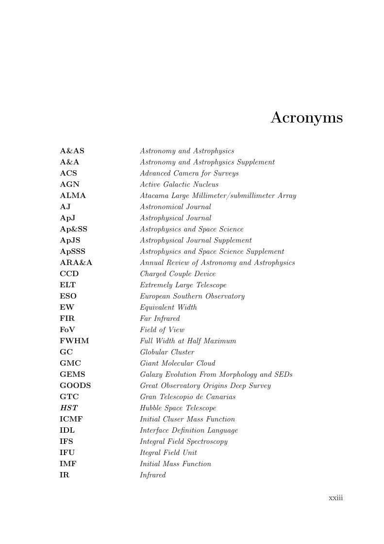
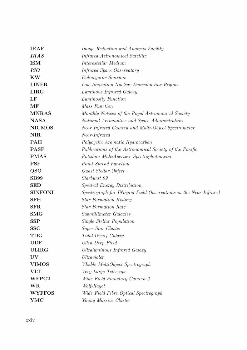
Acronyms
A&AS Astronomy and Astrophysics
A&A Astronomy and Astrophysics Supplement
ACS Advanced Camera for Surveys
AGN Active Galactic Nucleus
ALMA Atacama Large Millimeter/submillimeter Array
AJ Astronomical Journal
ApJ Astrophysical Journal
Ap&SS Astrophysics and Space Science
ApJS Astrophysical Journal Supplement
ApSSS Astrophysics and Space Science Supplement
ARA&A Annual Review of Astronomy and Astrophysics
CCD Charged Couple Device
ELT Extremely Large Telescope
ESO European Southern Observatory
EW Equivalent Width
FIR Far Infrared
FoV Field of View
FWHM Full Width at Half Maximum
GC Globular Cluster
GMC Giant Molecular Cloud
GEMS Galaxy Evolution From Morphology and SEDs
GOODS Great Observatory Origins Deep Survey
GTC Gran Telescopio de Canarias
HST Hubble Space Telescope
ICMF Initial Cluser Mass Function
IDL Interface Definition Language
IFS Integral Field Spectroscopy
IFU Itegral Field Unit
IMF Initial Mass Function
IR Infrared
xxiii
IRAF Image Reduction and Analysis Facility
IRAS Infrared Astronomical Satellite
ISM Interestellar Medium
ISO Infrared Space Observatory
KW Kolmogorov-Smirnov
LINER Low-Ionization Nuclear Emission-line Region
LIRG Luminous Infrared Galaxy
LF Luminosity Function
MF Mass Function
MNRAS Monthly Notices of the Royal Astronomical Society
NASA National Aeronautics and Space Administration
NICMOS Near Infrared Camera and Multi-Object Spectrometer
NIR Near-Infrared
PAH Polycyclic Aromatic Hydrocarbon
PASP Publications of the Astronomical Society of the Pacific
PMAS Potsdam MultiAperture Spectrophotometer
PSF Point Spread Function
QSO Quasi Stellar Object
SB99 Starburst 99
SED Spectral Energy Distribution
SINFONI Spectrograph for INtegral Field Observations in the Near Infrared
SFH Star Formation History
SFR Star Formation Rate
SMG Submillimeter Galaxies
SSP Single Stellar Population
SSC Super Star Cluster
TDG Tidal Dwarf Galaxy
UDF Ultra Deep Field
ULIRG Ultraluminous Infrared Galaxy
UV Ultraviolet
VIMOS VIsible MultiObject Spectrograph
VLT Very Large Telescope
WFPC2 Wide-Field Planetary Camera 2
WR Wolf-Rayet
WYFFOS Wide Field Fibre Optical Spectrograph
YMC Young Massive Cluster
xxiv

General Introduction
Overview
This Chapter gives a short review of the star formation pro-cesses in interacting galaxies and presents the main propertiesof the most extreme star-forming systems in the local Universe,upon which the project is based on. It also contains a short de-scription of the formation and dynamical evolution processes ofthe compact star-forming regions that will be studied through-out this thesis.
1 Star Formation in Interactions
1.1 General Concept
A large fraction, if not all, of stars are thought to be born within some type of clusterenvironment (e.g., Lada & Lada 2003; Porras et al. 2003). Thus, the formation of starclusters is intimately linked to the process of star formation. The use of star clustersas a tool to study the (extra)galactic star formation processes is therefore of majorimportance. The most massive are long lived and therefore potentially carry informationabout the entire star formation histories of their host galaxies and they are also bright SFR
enough to be observed at much greater distances than individual stars (Larsen 2010).
In the last two decades young, massive, compact clusters have been observed in manyexternal galaxies and different environments: dwarf galaxies (Billett et al. 2002), spi-ral disks (Larsen & Richtler 1999), barred galaxies, starburst galaxies (Meurer et al.1995; Barth et al. 1995), interacting galaxies (Whitmore et al. 1993, 1999, 2007; Biket al. 2003; Weilbacher et al. 2000; Knierman et al. 2003; Peterson et al. 2009) andcompact groups of galaxies (Iglesias-Páramo & Vílchez 2001; Temporin et al. 2003). Itis commonly assumed that at least some of these are young counterparts of the ancientglobular clusters, which are ubiquitous in all major galaxies. However, the link between GC
1
General Introduction
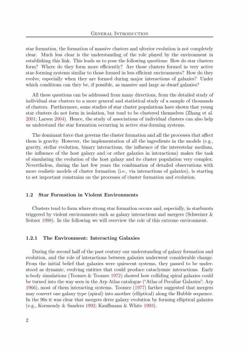
star formation, the formation of massive clusters and ulterior evolution is not completelyclear. Much less clear is the understanding of the role played by the environment inestablishing this link. This leads us to pose the following questions: How do star clustersform? Where do they form more efficiently? Are those clusters formed in very activestar-forming systems similar to those formed in less efficient environments? How do theyevolve, especially when they are formed during major interactions of galaxies? Underwhich conditions can they be, if possible, as massive and large as dwarf galaxies?
All these questions can be addressed from many directions, from the detailed study ofindividual star clusters to a more general and statistical study of a sample of thousandsof clusters. Furthermore, some studies of star cluster populations have shown that youngstar clusters do not form in isolation, but tend to be clustered themselves (Zhang et al.2001; Larsen 2004). Hence, the study of associations of individual clusters can also helpus understand the star formation occurring in active star-forming systems.
The dominant force that governs the cluster formation and all the processes that affectthem is gravity. However, the implementation of all the ingredients in the models (e.g.,gravity, stellar evolution, binary interactions, the influence of the interestelar medium,the influence of the host galaxy and/or other galaxies in interactions) makes the taskof simulating the evolution of the host galaxy and its cluster population very complex.Nevertheless, during the last few years the combination of detailed observations withmore realistic models of cluster formation (i.e., via interactions of galaxies), is startingto set important constrains on the processes of cluster formation and evolution.
1.2 Star Formation in Violent Environments
Clusters tend to form where strong star formation occurs and, especially, in starburststriggered by violent environments such as galaxy interactions and mergers (Schweizer &Seitzer 1998). In the following we will overview the role of this extreme environment.
1.2.1 The Environment: Interacting Galaxies
During the second half of the past century our understanding of galaxy formation andevolution, and the role of interactions between galaxies underwent considerable change.From the initial belief that galaxies were quiescent systems, they passed to be under-stood as dynamic, evolving entities that could produce cataclysmic interactions. Earlyn-body simulations (Toomre & Toomre 1972) showed how colliding spiral galaxies couldbe turned into the way seen in the Arp Atlas catalogue (“Atlas of Peculiar Galaxies”; Arp1966), most of them interacting systems. Toomre (1977) farther suggested that mergersmay convert one galaxy type (spiral) into another (elliptical) along the Hubble sequence.In the 90s it was clear that mergers drive galaxy evolution by forming elliptical galaxies(e.g., Kormendy & Sanders 1992; Kauffmann & White 1993).
2
1 - Star Formation in Interactions
Mergers not only transform one galaxy type into another but, during their occurrence,drive phenomena that are extraordinary compared to the processes that take place inquiescent galaxies. Simulations by Toomre & Toomre (1972) also showed that largeamount of gas would be funneled into the galaxy centers. Shortly after, evidence forrecent burst of star formation was reported in the Arp Atlas (Larson & Tinsley 1978),which was suggested to occur due to galaxy interactions like those described by Toomre.
1.2.2 A Typical Merger. End Product
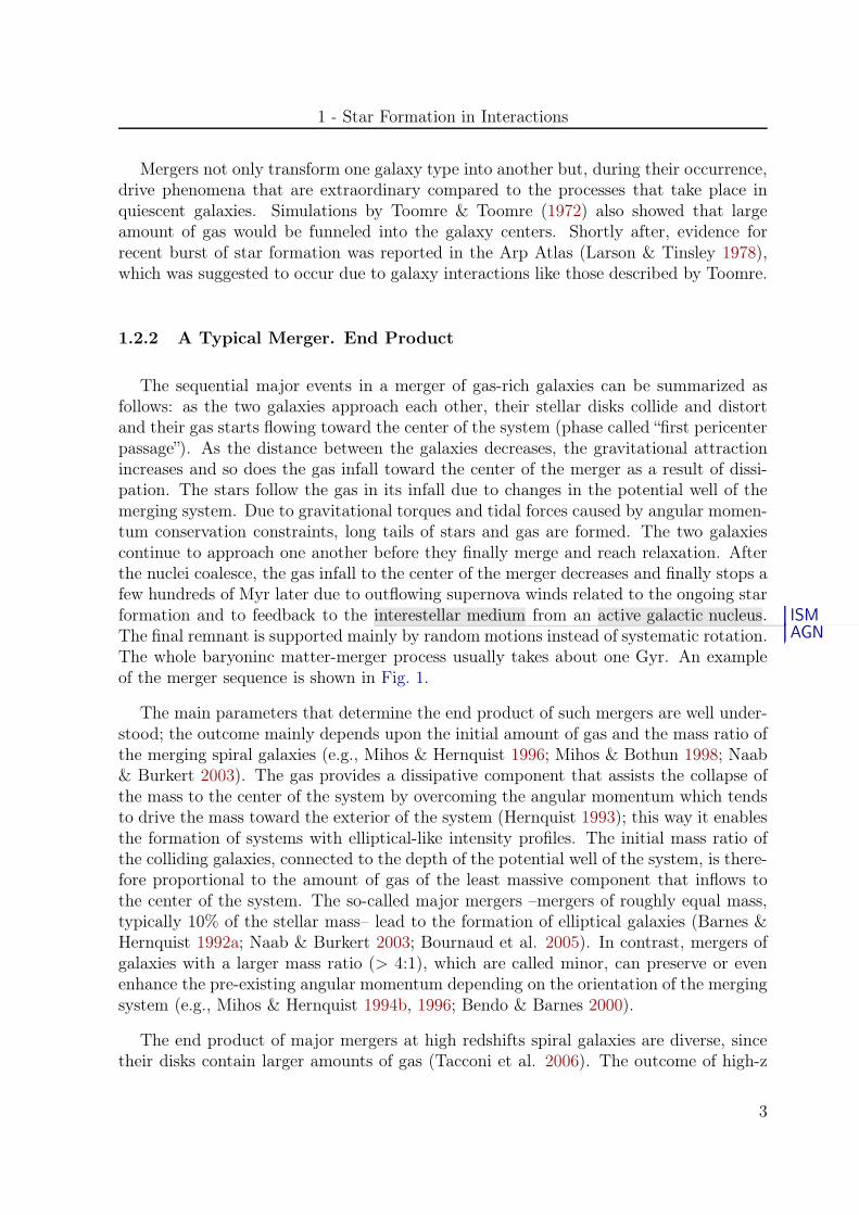
The sequential major events in a merger of gas-rich galaxies can be summarized asfollows: as the two galaxies approach each other, their stellar disks collide and distortand their gas starts flowing toward the center of the system (phase called “first pericenterpassage”). As the distance between the galaxies decreases, the gravitational attractionincreases and so does the gas infall toward the center of the merger as a result of dissi-pation. The stars follow the gas in its infall due to changes in the potential well of themerging system. Due to gravitational torques and tidal forces caused by angular momen-tum conservation constraints, long tails of stars and gas are formed. The two galaxiescontinue to approach one another before they finally merge and reach relaxation. Afterthe nuclei coalesce, the gas infall to the center of the merger decreases and finally stops afew hundreds of Myr later due to outflowing supernova winds related to the ongoing starformation and to feedback to the interestellar medium from an active galactic nucleus. ISM
AGNThe final remnant is supported mainly by random motions instead of systematic rotation.The whole baryoninc matter-merger process usually takes about one Gyr. An exampleof the merger sequence is shown in Fig. 1.
The main parameters that determine the end product of such mergers are well under-stood; the outcome mainly depends upon the initial amount of gas and the mass ratio ofthe merging spiral galaxies (e.g., Mihos & Hernquist 1996; Mihos & Bothun 1998; Naab& Burkert 2003). The gas provides a dissipative component that assists the collapse ofthe mass to the center of the system by overcoming the angular momentum which tendsto drive the mass toward the exterior of the system (Hernquist 1993); this way it enablesthe formation of systems with elliptical-like intensity profiles. The initial mass ratio ofthe colliding galaxies, connected to the depth of the potential well of the system, is there-fore proportional to the amount of gas of the least massive component that inflows tothe center of the system. The so-called major mergers –mergers of roughly equal mass,typically 10% of the stellar mass– lead to the formation of elliptical galaxies (Barnes &Hernquist 1992a; Naab & Burkert 2003; Bournaud et al. 2005). In contrast, mergers ofgalaxies with a larger mass ratio (> 4:1), which are called minor, can preserve or evenenhance the pre-existing angular momentum depending on the orientation of the mergingsystem (e.g., Mihos & Hernquist 1994b, 1996; Bendo & Barnes 2000).
The end product of major mergers at high redshifts spiral galaxies are diverse, sincetheir disks contain larger amounts of gas (Tacconi et al. 2006). The outcome of high-z
3

General Introduction
Figure 1: (a) Sequence of four snapshots showing the merger evolution. Time is indicatedin Myr after the first pericenter passage. The total stellar mass density is shown. (b) Surfacedensity of “young” stars (defined as those formed after the first pericenter passage) at the endof the wet merger simulation, 950 Myr after the first pericenter passage. Figure taken fromBournaud et al. (2008b).
gas-rich mergers may either be an elliptical or even a spiral galaxy that possesses amassive bulge (Springel et al. 2005; Springel & Hernquist 2005). The result againdepends on the amount of gas in the initial galaxies and on the presence of a bulge (itdelays the star formation events) and an AGN (it suppresses the star formation events,producing a negative feedback).
1.2.3 Star Formation Bursts in Mergers
While the picture we have for the end product of gas-rich mergers is well understood,that for the intermediate merger phases (i.e., between first pericenter passage and fi-nal relaxation) is rather unclear. The uncertainties mainly originate from the simplifiedtreatment of the ISM (i.e., the gas and the dust). The role played by interactions andmergers in enhancing star formation has also been subject of intense debate in the pastfew decades by means of numerical simulations (e.g., Barnes & Hernquist 1992a; Mihos
4
2 - Compact Star-Forming Regions in Galaxy Interactions
& Hernquist 1994b; Mihos & Hernquist 1996; Springel 2000; Barnes 2004; Springel et al.2005; Bournaud & Duc 2006; Cox et al. 2006; Di Matteo et al. 2007; Di Matteo et al.2008; Teyssier et al. 2010). Although it has become clear that the star formation effi-ciency is highly dependent upon the numerical recipe adopted for star formation (densityor shock dependent) and feedback assumptions, all the studies have supported the factthat galaxy interactions induce star formation.
It is not well understood either at what point in time the gas infall to the centerof the merger is maximum and hence, it is unclear at what point the strongest starformation or starburst events occur. Statistically, it is thought that the SFR peaksroughly between the first encounter and shortly after the nuclear coalescence (Mihos &Hernquist 1996; Springel et al. 2005; Di Matteo et al. 2008). The result mainly dependson the size of the galaxy bulges (large bulges stabilize the gas and delay its fall to thecenter of the system), the presence of a black hole (it acts as a strong gravitational pointat the center of the system), and the strength of the winds from the supernovae and theAGN (they produce a negative feedback).
2 Compact Star-Forming Regions in Galaxy Interactions
2.1 Super Star Clusters and Associations
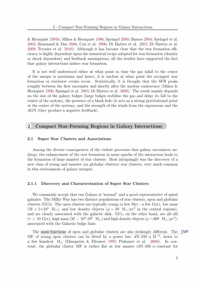
Among the diverse consequences of the violent processes that galaxy encounters un-dergo, the enhancement of the star formation in some epochs of the interaction leads tothe formation of large number of star clusters. Most intriguingly was the discovery of anew class of young and massive (as globular clusters) star clusters, very much commonin this environment of galaxy mergers.
2.1.1 Discovery and Characterization of Super Star Clusters
We commonly accept that our Galaxy is “normal” and a good representative of spiralgalaxies. The Milky Way has two distinct populations of star clusters, open and globularclusters (GCs). The open clusters are typically young (a few Myr - a few Gyr), low mass(M < 5×10⁴ M⊙), and low density objects (ρ ∼ 20 M⊙/pc3 in the central regions),and are clearly associated with the galactic disk. GCs, on the other hand, are all old(τ > 10 Gyr), high mass (M = 104-106 M⊙) and high density objects (ρ ∼400 M⊙/pc3),associated with the Galactic bulge/halo.
The mass functions of open and globular clusters are also strikingly different. The MF
MF of young open clusters can be fitted by a power law, dN/dM ∝ M−2, down toa few hundred M⊙ (Elmegreen & Efremov 1997; Piskunov et al. 2008). In con-trast, the globular cluster MF is rather flat at low masses (dN/dM ∝ constant for
5

General Introduction
M < 105 M⊙; McLaughlin & Pudritz 1996), whereas the high-mass end can be fittedby a power law with slope of -2, as for the open clusters. Given the clear dichotomybetween these two systems, traditionally it has been established that open and globularclusters formed by two separate mechanisms.
However, for the past few decades a significant population of extragalactic massive(M > 5×10⁴ M⊙) young (τ < 1 Gyr) clusters has been detected in many environments:in the LMC (Elson & Fall 1985), in normal spirals (e.g., Larsen 2000; Larsen 2004, instarburst galaxies (e.g., in M82; O’Connell et al. 1995; de Grijs et al. 2005), in ongoingmergers (e.g., in The Antennae; Whitmore et al. 1999) and in merger remnants (e.g., inNGC 7252; Schweizer & Seitzer 1998; Maraston et al. 2001). Nowadays, these objectsare known as young massive clusters or super star clusters.YMC
SSC
The HST caused a revolution in the field of extragalactic clusters. Its high angularresolution first allowed to establish an upper limit to the size on young extragalacticclusters. Shortly after, with improved optics, the WFPC2 camera on board HST wasable to resolve individual star clusters in external galaxies, showing that they did indeedhave sizes (1-20 pc) comparable to globular clusters in our Galaxy (e.g., Whitmore et al.1999).
The first environments that were discovered to contain copious amounts of massivestar clusters were those of galaxy mergers. Holtzman et al. (1992) were the first in a longlist of studies which used the HST to discover massive young clusters in mergers. Theystudied a recent galaxy merger (NGC 1275), and found a population of blue point-likesources, with ages of less than 300 Myr old and masses between 105-108 M⊙. These youngmassive clusters were also found in the prototypical merger remnant NGC 7252, with agesranging from 34 to 500 Myr, consistent with having been formed during the interactionprocess (Whitmore et al. 1993). Many more examples soon followed, like those in NGC3597 (Holtzman et al. 1996), in NGC 3921 (Schweizer et al. 1996), in NGC 3256 (Zepfet al. 1999), in NGC 4038/4039 (Whitmore et al. 1993, 1995, 1999, 2010; Bastian et al.2006), in M51 (Bastian et al. 2005a, 2005b) and in Arp284 (Peterson et al. 2009), amongothers. An example of many SSCs candidates found in The Antennae, the youngest andnearest example of a pair of merging disk galaxies in the Toomre (1977) sequence, isshown in Fig. 2.
The SSCs found in these systems have many of the same properties as the galacticglobular clusters, namely size and mass (and hence stellar density). On the other hand,their ages, metallicities, and mass functions are much more similar to those in galacticopen clusters. This mixture of properties led to their designation as young globularclusters, implying that they are the same as the old globular clusters in our Galaxy(only younger) and that any differences between these populations are simply due toevolutionary effects.
6

2 - Compact Star-Forming Regions in Galaxy Interactions
Figure 2: The main bodies of The Antennae viewed with the Advanced Camera for Surveys(ACS/HST ). Top: Top half of The Antennae (NGC 4038) with the 50 most luminous clusters(blue circles) and the 50 most massive clusters (all with a mass higher than 5×10⁵ M⊙ ; redcircles) marked. Also marked are the 25 IR-brightest clusters (white circles). Bottom: Sameinformation but for the bottom half of The Antennae (NGC 4039). Figure taken from Whitmoreet al. (2010).
7

General Introduction
2.1.2 Formation of SSCs
The problem of cluster formation is intimately linked to that of star formation. Starformation is closely associated with dense molecular gas and proto-clusters are observedto form deeply embedded within giant molecular clouds. The GMCs are themselvesGMC
part of a larger hierarchy of structure in the interstellar medium (Elmegreen & Falgar-one 1996; Elmegreen 2007), and tend to be organized into giant molecular complexes(Wilson et al. 2003). The average particle density of molecular gas in a GMC is low(nH ∼102-103 cm−3), but stars only form in the densest regions (i.e., nH > 105 cm−3).Therefore, in general star formation is an inefficient process and only a few percent ofthe mass of a given GMC is converted into stars before the cloud is dispersed.
The GMC mass function in the Milky Way has a characteristic upper-mass of about6×106 M⊙ and the mass spectrum of clumps within GMCs appears to follow a similarpower law as that of the GMCs, dN/dM ∝ Mα, with α ∼ -2 (Mac Low & Klessen 2004).From there an upper-limit to a cluster mass of few 105 M⊙ is derived, consistent withother constraints on the initial cluster mass function in spiral galaxies (Larsen 2009).
It is hard to understand how the most massive clusters observed in some externalgalaxies, with masses of 106 M⊙ or higher, could form from Milky Way-like GMCs.In order for a GMC to reach the average mean density required to form a massivecluster (i.e., nH >105 cm−3), it should collect the amount of gas typical of a massiveGalactic GMC within a volume only a few pc across, essentially turning such a cloudinto one big clump (Larsen 2010). Such high dense and massive clumps exist in starburstsand interacting galaxies, which may allow denser and more massive GMCs to condense(Escala & Larson 2008). The presence of shocks and compressive tides in mergers alsohelp these massive GMCs condense (Ashman & Zepf 2001; Renaud et al. 2008, 2009).In even more extreme environments, such as in (U)LIRGs (see Section 3), GMCs maybe both denser and more massive (Murray et al. 2010), consistent with the presence ofclusters with M > 107 M⊙ in some merger remnants (W3 in NGC 7252; Maraston et al.2004; Bastian et al. 2006).
2.1.3 Dynamical Evolution of SSCs
All clusters undergo at birth an embedded phase in the progenitor molecular cloudthat lasts at least a few Myr (i.e., τ . 3 Myr), with high gas column densities andrelatively large amounts of dust extinction of AV ∼ 1-8 mag (Larsen 2009). Stellar winds,ionizing flux from massive stars, and stellar feedback expel the remaining gas eventually(see Goodwin 2009 for a recent review). If all stars are formed in clusters, then only asmall percentage remain still within clusters at the end of the embedded phase (Lada &Lada 2003, 2010). In fact, while expelling the gas many clusters become unbound andsubsequently disperse into the surrounding medium.
8

2 - Compact Star-Forming Regions in Galaxy Interactions
An embedded cluster will not necessarily remain bound after gas expulsion (Ladaet al. 2010). If the stars and gas are initially in virial equilibrium, the velocity dispersionof the stars will be too high to match the shallower potential once the gas is expelled. Inpractise, cluster expansion and gas expulsion does not occur instantly so the stars havesome time to adjust to the new potential. Simulations suggest that a small fraction ofthe stars may remain bound for star formation efficienciesa of less than 20-30% (Boily SFE
& Kroupa 2003; Baumgardt & Kroupa 2007). This process, known as ’infant mortality’or ’mass-independent disruption mechanism’ can last for several tens of Myr until thecluster settles into a new equilibrium (Goodwin & Bastian 2006; Whitmore et al. 2007).
This picture is consistent with observations. Lada & Lada (2003) estimated that about95% of clusters formed in the Milky Way dissolve in less than 100 Myr. Although theuniversality of this process is poorly quantified, some efforts have been made by observingthe cluster demographics in extragalactic clusters, especially in interacting galaxies. Forinstance, the age distribution of mass-limited cluster samples in The Antennae galaxies,the well-known archetype of a major merger, is approximately dN/dτ ⋍ τ−1 for ages (τ)of up to 108-109 yr (Fall et al. 2005), suggesting that 80-90% of the clusters disappearper decade in age, independent of mass (Whitmore et al. 2007). However, over such alarge age range, it is unlikely that disruption can still be attributed to gas expulsion.
During the last few years the has been a controversy about this issue, since estimat-ing disruption parameters for interacting systems is not straightforward. Bastian et al.(2009) fitted the age distribution of clusters in The Antennae with a model in which thecluster formation rate has increased over the past few hundreds of Myr (Mihos et al.1993), as suggested by simulations of the ongoing interaction (e.g., Cox et al. 2008). Inthis model the mass-independent disruption mechanism only lasts for . 20 Myr. A highdisruption fraction (∼ 70%) was also claimed in M51 (Bastian et al. 2005b), but thiscan be partly due to age-dating artifacts around 10 Myr (Gieles 2009a).
Clusters that survive the infant mortality process will continue to evolve dynamicallyon longer timescales as a result of internal two-body relaxation, external shocks and massloss due to stellar evolution (Vesperini 2010). This evolution (known as ’secular evolu-tion’) will lead to the gradual evaporation of any star cluster and, eventually, its totaldissolution on timescales dependent on the mass of the cluster (Spitzer 1987; Baumgardt& Makino 2003). Two-body relaxation causes the velocities of the stars in the cluster toapproach a Maxwellian distribution, and stars with velocities above the escape velocitywill gradually evaporate from the cluster. Shocks may be due to encounters with spiralarms, GMCs or, for GCs on eccentric orbits, passages through the galactic disc or nearthe bulge. Finally, stellar evolution causes mass loss as stars are turned into much lessmassive remnants. Over a 10 Gyr time span, about one third of the initial cluster stellarmass is lost this way (e.g., Bruzual & Charlot 2003).
a SFE = Mcl
Mcl+Mgas, where Mcl is the total mass of stars formed in the embedded cluster and Mgas is
the mass of the gas not converted into stars
9

General Introduction
Figure 3: Left: Mass functions for young (τ <200 Myr) clusters in spiral galaxies (Larsen2009 and The Antennae (Whitmore et al. 1999). Center and right: Luminosity functions ofclusters in M51 (center) and The Antennae galaxies (right). Also shown are modeled LFs as-suming Schechter initial cluster MFs with Mc = 2×10⁵ and 2×10⁶ M⊙ (solid and dashed lines,respectively), scaled to match the data. Figure taken from Larsen (2010).
2.1.4 Cluster Mass and Luminosity Functions
The basic stellar dynamical mechanisms responsible for the evolution of the MF arethe same for all clusters, although the importance of one mechanism or another (i.e.,two-body relaxation vs. shocks) differs. However, the initial cluster mass function onICMF
which these mechanisms operate might still vary with environment. Nowadays, there areauthors who support these dependent mechanisms (e.g., Larsen 2009) and others whoclaim that the physical processes responsible for the formation of the clusters are thesame, thus the ICMF is universal (e.g., Whitmore et al. 2007; Fall et al. 2009).
Determinations of the MF are only available for a few young cluster systems. Gen-erally, they are well-represented by power laws, dN/dM ∝ M−α, with slopes of α ∼ 2,although the mass ranges over which these slopes are derived vary considerably (fromfew × 103 to few × 106 M⊙; Gieles et al. 2006; Larsen 2009). However, when comparingthe MFs of young massive star clusters (i.e., M > 105 M⊙ and τ <200 Myr) in spiralsand more active star-forming galaxies (like The Antennae), small differences may showup (see Fig. 3, left). Although a uniform power law with no truncation is consistent withthe data, a fit using a Schechter (1976) function may be also possible,
dN
dM∝
(
M
Mc
)−α
exp
(
−M
Mc
)
(1)
This function usually fits well the high-mass end of the MF in old GCs sys-tems. A fit to the spiral data in Fig. 3 for a fixed α = 2 yields a truncationmass Mc = (2.1 ± 0.4) × 105 M⊙ (Larsen 2009). A fit to The Antennae data givesMc = (1.7 ± 0.7) ×106 M⊙ (Jordán et al. 2007; Larsen 2009; Gieles 2009a), although
10
2 - Compact Star-Forming Regions in Galaxy Interactions
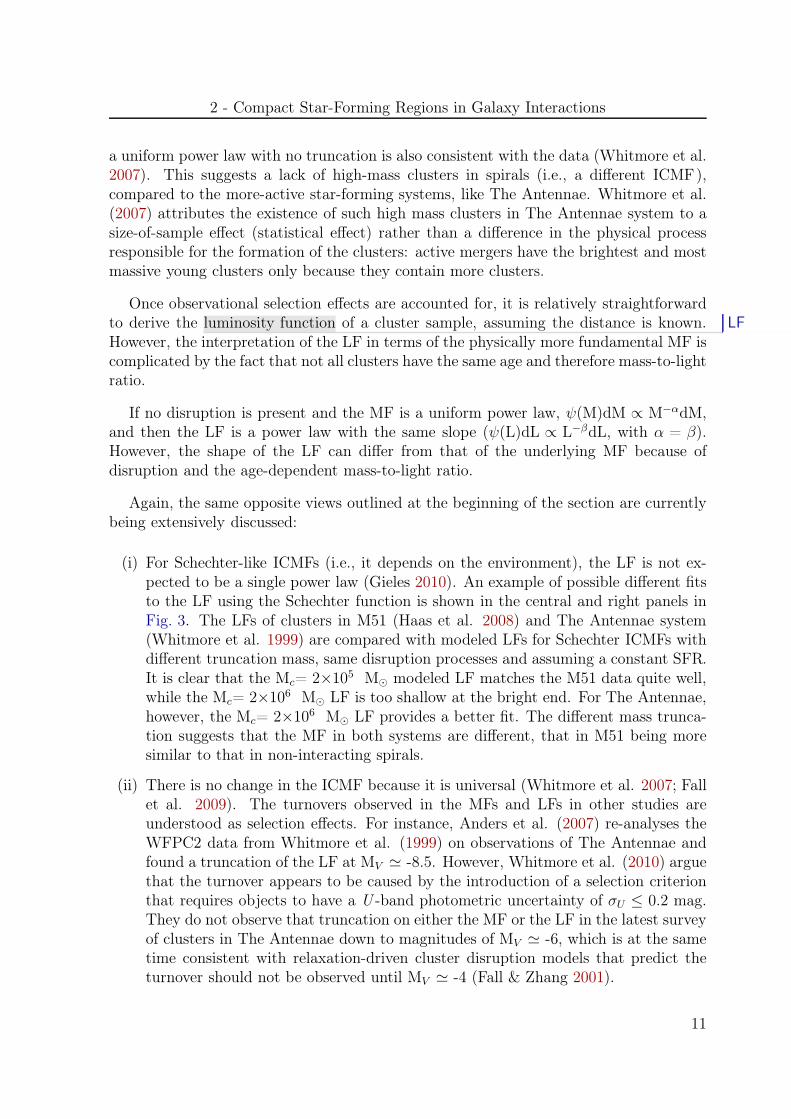
a uniform power law with no truncation is also consistent with the data (Whitmore et al.2007). This suggests a lack of high-mass clusters in spirals (i.e., a different ICMF),compared to the more-active star-forming systems, like The Antennae. Whitmore et al.(2007) attributes the existence of such high mass clusters in The Antennae system to asize-of-sample effect (statistical effect) rather than a difference in the physical processresponsible for the formation of the clusters: active mergers have the brightest and mostmassive young clusters only because they contain more clusters.
Once observational selection effects are accounted for, it is relatively straightforwardto derive the luminosity function of a cluster sample, assuming the distance is known. LF
However, the interpretation of the LF in terms of the physically more fundamental MF iscomplicated by the fact that not all clusters have the same age and therefore mass-to-lightratio.
If no disruption is present and the MF is a uniform power law, ψ(M)dM ∝ M−αdM,and then the LF is a power law with the same slope (ψ(L)dL ∝ L−βdL, with α = β).However, the shape of the LF can differ from that of the underlying MF because ofdisruption and the age-dependent mass-to-light ratio.
Again, the same opposite views outlined at the beginning of the section are currentlybeing extensively discussed:
(i) For Schechter-like ICMFs (i.e., it depends on the environment), the LF is not ex-pected to be a single power law (Gieles 2010). An example of possible different fitsto the LF using the Schechter function is shown in the central and right panels inFig. 3. The LFs of clusters in M51 (Haas et al. 2008) and The Antennae system(Whitmore et al. 1999) are compared with modeled LFs for Schechter ICMFs withdifferent truncation mass, same disruption processes and assuming a constant SFR.It is clear that the Mc= 2×10⁵ M⊙ modeled LF matches the M51 data quite well,while the Mc= 2×10⁶ M⊙ LF is too shallow at the bright end. For The Antennae,however, the Mc= 2×10⁶ M⊙ LF provides a better fit. The different mass trunca-tion suggests that the MF in both systems are different, that in M51 being moresimilar to that in non-interacting spirals.
(ii) There is no change in the ICMF because it is universal (Whitmore et al. 2007; Fallet al. 2009). The turnovers observed in the MFs and LFs in other studies areunderstood as selection effects. For instance, Anders et al. (2007) re-analyses theWFPC2 data from Whitmore et al. (1999) on observations of The Antennae andfound a truncation of the LF at MV ≃ -8.5. However, Whitmore et al. (2010) arguethat the turnover appears to be caused by the introduction of a selection criterionthat requires objects to have a U -band photometric uncertainty of σU ≤ 0.2 mag.They do not observe that truncation on either the MF or the LF in the latest surveyof clusters in The Antennae down to magnitudes of MV ≃ -6, which is at the sametime consistent with relaxation-driven cluster disruption models that predict theturnover should not be observed until MV ≃ -4 (Fall & Zhang 2001).
11
General Introduction
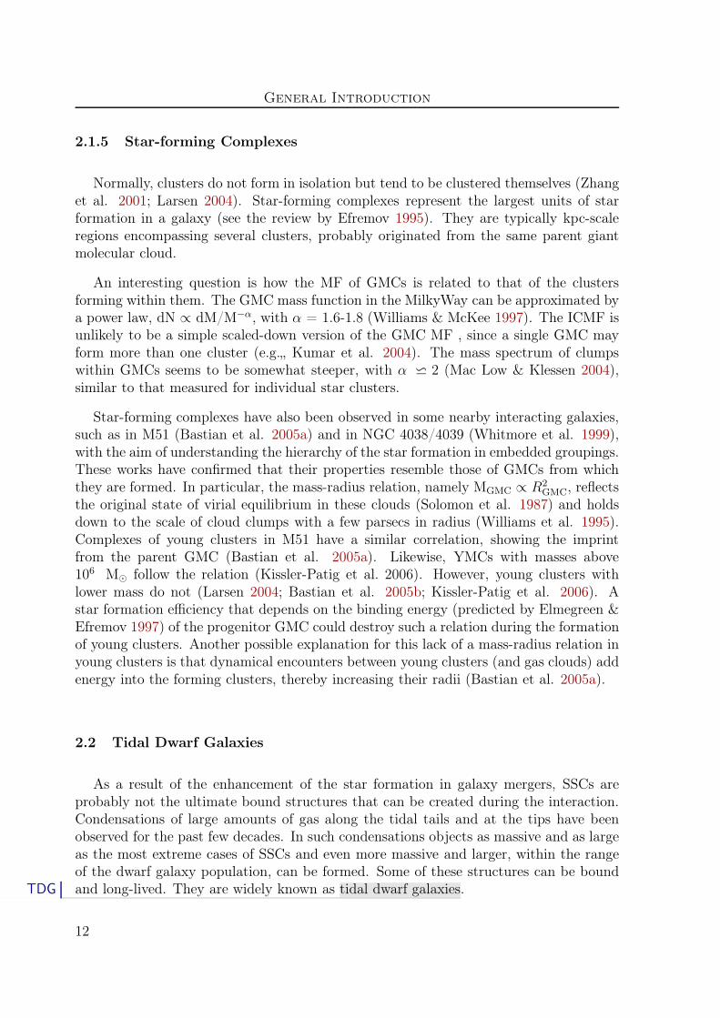
2.1.5 Star-forming Complexes
Normally, clusters do not form in isolation but tend to be clustered themselves (Zhanget al. 2001; Larsen 2004). Star-forming complexes represent the largest units of starformation in a galaxy (see the review by Efremov 1995). They are typically kpc-scaleregions encompassing several clusters, probably originated from the same parent giantmolecular cloud.
An interesting question is how the MF of GMCs is related to that of the clustersforming within them. The GMC mass function in the MilkyWay can be approximated bya power law, dN ∝ dM/M−α, with α = 1.6-1.8 (Williams & McKee 1997). The ICMF isunlikely to be a simple scaled-down version of the GMC MF , since a single GMC mayform more than one cluster (e.g.„ Kumar et al. 2004). The mass spectrum of clumpswithin GMCs seems to be somewhat steeper, with α ⋍ 2 (Mac Low & Klessen 2004),similar to that measured for individual star clusters.
Star-forming complexes have also been observed in some nearby interacting galaxies,such as in M51 (Bastian et al. 2005a) and in NGC 4038/4039 (Whitmore et al. 1999),with the aim of understanding the hierarchy of the star formation in embedded groupings.These works have confirmed that their properties resemble those of GMCs from whichthey are formed. In particular, the mass-radius relation, namely MGMC ∝ R2
GMC, reflectsthe original state of virial equilibrium in these clouds (Solomon et al. 1987) and holdsdown to the scale of cloud clumps with a few parsecs in radius (Williams et al. 1995).Complexes of young clusters in M51 have a similar correlation, showing the imprintfrom the parent GMC (Bastian et al. 2005a). Likewise, YMCs with masses above106 M⊙ follow the relation (Kissler-Patig et al. 2006). However, young clusters withlower mass do not (Larsen 2004; Bastian et al. 2005b; Kissler-Patig et al. 2006). Astar formation efficiency that depends on the binding energy (predicted by Elmegreen &Efremov 1997) of the progenitor GMC could destroy such a relation during the formationof young clusters. Another possible explanation for this lack of a mass-radius relation inyoung clusters is that dynamical encounters between young clusters (and gas clouds) addenergy into the forming clusters, thereby increasing their radii (Bastian et al. 2005a).
2.2 Tidal Dwarf Galaxies
As a result of the enhancement of the star formation in galaxy mergers, SSCs areprobably not the ultimate bound structures that can be created during the interaction.Condensations of large amounts of gas along the tidal tails and at the tips have beenobserved for the past few decades. In such condensations objects as massive and as largeas the most extreme cases of SSCs and even more massive and larger, within the rangeof the dwarf galaxy population, can be formed. Some of these structures can be boundand long-lived. They are widely known as tidal dwarf galaxies.TDG
12
2 - Compact Star-Forming Regions in Galaxy Interactions
2.2.1 Discovery & Characterization of TDGs
The scenario of low mass (i.e., dwarf) galaxy formation during giant galaxy collisionswas first proposed by Zwicky (1956), though without strong observational evidence. Dur-ing the following two decades the concept that galaxies were static entities was beingdiverted into an opposite direction. They started to be understood as dynamic, evolvingobjects with a high possibility of close encounters that radically change their morphology(see Section 1.2).
The first thorough analysis of an apparent dwarf galaxy built in a tidal tail waspresented by Schweizer (1978). He noted the young age of the stars in an area at thetip of the southern tail of The Antennae system and their higher than expected metalcontent for a location at such large radii. Questions about stable dwarf galaxies formingat this location arose.
Some years later, Mirabel et al. (1991,1992) went on with the investigation of thisspecific mode of galaxy formation by claiming to have found at least one dwarf galaxyin the long tails of The Superantennae merger (AM 1925-724). Hernquist (1992a) notedthe possibility that more dwarf galaxies could be formed during the collisions of largergalaxies.
The first numerical simulations of the dynamics of interacting galaxies with the aimof studying the formation of TDGs were carried out by Barnes & Hernquist (1992b) andElmegreen et al. (1993), who showed that the formation of dwarf galaxies as a result ofa major interaction is possible. Barnes & Hernquist (1992b) also noted that TDGs arenot likely to contain a large amount of dark matter, contrary to normal dwarf galaxies(in particular, dwarf spheroidals), because their material is drawn from the spiral diskwhile the dark matter is thought to surround the galaxy in an extended halo.
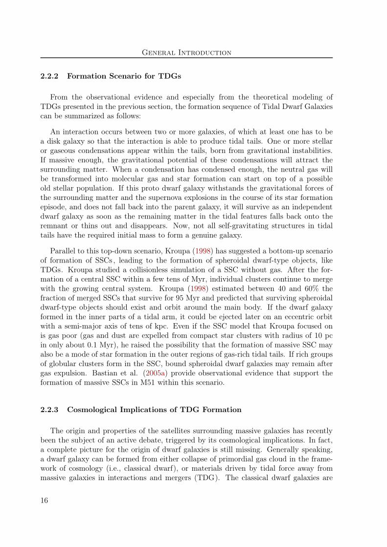
Motivated by the theoretical prediction of these models and in order to study thenature of these kind of objects, several campaigns were launched in interacting systems,such as in NGC 2782 (Yoshida et al. 1994), Arp 105 (Duc & Mirabel 1994; Duc et al.1997), NGC 7252 (Hibbard et al. 1994), NGC 5291 (Duc & Mirabel 1998; Higdon et al.2006), Arp 245 (Duc et al. 2000), small samples (Weilbacher et al. 2000, 2003; Kniermanet al. 2003; Monreal-Ibero et al. 2007) and Arp 305 (Hancock et al. 2009). Hibbard& Mihos (1995) also developed a successful dynamical N-body model of NGC 7252 (seeFig. 4). According to that model, most of the tidal material will remain bound to thecentral merger, but a significant amount of matter will not fall back within a Hubble time.It is expected that the two TDG candidates in NGC 7252 –if they remain stable entities–will attain long-lived orbits around the merger. Some other investigations have tried tofind TDGs in the specific environment of compact galaxy groups (e.g., Hunsberger et al.1996; Iglesias-Páramo & Vílchez 2001; Temporin et al. 2003; Nishiura et al. 2002).
Based on these observations, TDG candidates are characterized by a luminosity higherthan B = -10.65, typically B = -13, and can be as luminous as B = -19. Their color is
13

General Introduction
Figure 4: Top: The CTIO 4m B-band image of NGC 7252 from Hibbard et al. (1994).Bottom: The best-fit projection of the N-body model of NGC 7252 at 580 Myr since orbitalperiapse. A clump that develops in the NW tail is clearly seen. Figure taken from Hibbard &Mihos (1995).
14

2 - Compact Star-Forming Regions in Galaxy Interactions
typically blue (B-I=0.7-2), indicative of young stellar population. The presence of youngpopulation is firmly proved with the detection of strong Hα emission with and equivalentwidth higher than tens of Å. The half-light radius of these kpc-sized structures rangesfrom few hundreds of pc to less than 2 kpc, comparable to that in observed dwarf galaxiesin different galaxy groups and to the so-called Blue Compact Dwarf galaxies.
All spectroscopic observations of TDGs have showed that the luminosity-metallicitycorrelation found for normal dwarf galaxies does not hold up for TDGs. While dwarfgalaxies have lower oxygen abundances for lower luminosities, TDGs have an approxi-mately constant metallicity of around one-third of the solar value as determined fromgaseous emission lines (see e.g., Duc et al. 2000; Weilbacher et al. 2003). On this basis,Hunter et al. (2000) confirmed the metallicity of TDGs as one of the best criteria tofind old dwarf galaxies in merger remnants. Supplementing this criterion with estimatesabout rotational properties and stellar populations, they also presented a list of nearbydwarf irregulars which might be good candidates for old TDGs.
For normal galaxies is easy to know if they are real galaxies and if they will survivelong enough to deserve being called galaxies. Most galaxies are very isolated, withoutmuch matter nearby to disturb their stability. Some starburst galaxies may lose muchof their gas by strong stellar winds and supernova driven outflows, but in most casesthere is no doubt that the stellar component will remain bound and stable, even withoutgas, for several billion years. The same is true for normal dwarf galaxies in less denseenvironments.
But is not straightforward the identification of the observed TDG candidates as realgalaxies. They are embedded in a tidal tail and, most probably, do not have massivedark matter halos (Barnes & Hernquist 1992b; Braine et al. 2001; Wetzstein et al. 2007.Tidal forces of the parent galaxy disturb their gravitational field, strong star formationmight blow away the recently accreted gas, and some of the TDGs may even fall backinto the central merger (Hibbard & Mihos 1995). An accepted definition that tries toensure that only those objects which, called Tidal Dwarf Galaxies, deserve to be named“galaxy” is: A Tidal Dwarf Galaxy is a self-gravitating entity of dwarf-galaxy mass builtfrom the tidal material expelled during interactions (Duc et al. 2000; Weilbacher &Fritze-v. Alvensleben 2001).
Taking into account evaporation and fragmentation processes plus tidal disruption,Duc et al. (2004) suggested that a total mass as high as 109 M⊙ may be necessaryfor a new formed TDG to become a long-lived object. This is the typical mass of thegiant HI accumulations observed near the tip of several long tidal tails. Less massivecondensations may evolve, if they survive, into objects more similar to globular clusters.However this mass criterion is not well established, and less massive objects (a total massof few 107-few 109 M⊙) have been normally considered as TDG candidates (Duc et al.2007, Sheen et al. 2009, Hancock et al. 2009).
15
General Introduction
2.2.2 Formation Scenario for TDGs
From the observational evidence and especially from the theoretical modeling ofTDGs presented in the previous section, the formation sequence of Tidal Dwarf Galaxiescan be summarized as follows:
An interaction occurs between two or more galaxies, of which at least one has to bea disk galaxy so that the interaction is able to produce tidal tails. One or more stellaror gaseous condensations appear within the tails, born from gravitational instabilities.If massive enough, the gravitational potential of these condensations will attract thesurrounding matter. When a condensation has condensed enough, the neutral gas willbe transformed into molecular gas and star formation can start on top of a possibleold stellar population. If this proto dwarf galaxy withstands the gravitational forces ofthe surrounding matter and the supernova explosions in the course of its star formationepisode, and does not fall back into the parent galaxy, it will survive as an independentdwarf galaxy as soon as the remaining matter in the tidal features falls back onto theremnant or thins out and disappears. Now, not all self-gravitating structures in tidaltails have the required initial mass to form a genuine galaxy.
Parallel to this top-down scenario, Kroupa (1998) has suggested a bottom-up scenarioof formation of SSCs , leading to the formation of spheroidal dwarf-type objects, likeTDGs. Kroupa studied a collisionless simulation of a SSC without gas. After the for-mation of a central SSC within a few tens of Myr, individual clusters continue to mergewith the growing central system. Kroupa (1998) estimated between 40 and 60% thefraction of merged SSCs that survive for 95 Myr and predicted that surviving spheroidaldwarf-type objects should exist and orbit around the main body. If the dwarf galaxyformed in the inner parts of a tidal arm, it could be ejected later on an eccentric orbitwith a semi-major axis of tens of kpc. Even if the SSC model that Kroupa focused onis gas poor (gas and dust are expelled from compact star clusters with radius of 10 pcin only about 0.1 Myr), he raised the possibility that the formation of massive SSC mayalso be a mode of star formation in the outer regions of gas-rich tidal tails. If rich groupsof globular clusters form in the SSC, bound spheroidal dwarf galaxies may remain aftergas expulsion. Bastian et al. (2005a) provide observational evidence that support theformation of massive SSCs in M51 within this scenario.
2.2.3 Cosmological Implications of TDG Formation
The origin and properties of the satellites surrounding massive galaxies has recentlybeen the subject of an active debate, triggered by its cosmological implications. In fact,a complete picture for the origin of dwarf galaxies is still missing. Generally speaking,a dwarf galaxy can be formed from either collapse of primordial gas cloud in the frame-work of cosmology (i.e., classical dwarf), or materials driven by tidal force away frommassive galaxies in interactions and mergers (TDG). The classical dwarf galaxies are
16

3 - (U)LIRGs, Extreme in Star Formation
characterized by small size and dominated by a dark matter halo (Aaronson 1983; Simon& Geha 2007; Geha et al. 2009). They are metal poor because of inefficient chemicalenrichment in shallow gravitational potential which keeps little metal against supernovawinds (Tremonti et al. 2004), and thus sensitive for testing physical mechanisms drivinggalaxy evolution (e.g. supernova feedback). The cosmologically-originated dwarf galaxiesgive rise to a well-known challenge to the theory of galaxy formation (i.e., the “missingsatellites problem”; Klypin et al. 1999) since, although the number of known satelliteskeeps increasing with time (e.g., Belokurov et al. 2007), it is still lower than the numberof primordial satellites predicted by standard cosmological hierarchical scenarios.
The situation could even be worse, as claimed by Bournaud & Duc (2006), who pointedout that the cosmological models do not take into account the fact that second-generation(or recycled) galaxies may be formed during collisions. As mentioned in previous sections,TDG galaxies are believed to contain no dark matter halo and be metal rich. Theyoften have episodic star formation historie (Weisz et al. 2008) compared to the constant SFHs
SFH for classical dwarfs (Marconi et al. 1995; Tolstoy et al. 2009). Understanding thecontribution of TDGs to the local dwarf population is therefore an important issue indwarf galaxy astrophysics. According to the hierarchical scenario, massive galaxies weregradually assembled through a number of merger events (Eisenstein et al. 2005, andreferences therein), providing potential space for numerous TDGs produced over cosmictime. However, TDGs are exclusively associated with tidal tails driven by rotation-support systems. They are also affected by the tidal friction with their parent galaxies.It is likely that only a small fraction of TDGs are able to live longer than 10 Gyr,depending on their mass and distance to the parent galaxies.
An early study by Okazaki & Taniguchi (2000) showed that TDGs can contributesignificantly to the total population of dwarf satellites in addition to primordial dwarfs,even that the overall dwarf population could be of tidal origin. However, it has beenrecently claimed that only a marginal fraction (less than 10%) of dwarf galaxies in thelocal universe could actually be of tidal origin (Bournaud & Duc 2006; Wen et al. 2011).The issue is still controversial. Additionally, it is difficult to identify TDGs once thetidal tail fades away. Only a few works have found TDG candidates with an importantfraction of old population in post-merger galaxies (Duc et al. 2007; Sheen et al. 2009).
3 (U)LIRGs, Extreme in Star Formation
As outlined in previous sections, the observation of galactic mergers offers a spe-cial opportunity for learning more about the star formation in general and, specifically,the star cluster formation process. Interacting galaxies were common in the early Uni-verse but they also continue today, producing the strongest known starbursts (Sanders& Mirabel 1996). In some systems, the extreme burst of star formation is hidden bylarge amounts of dust and its energy output re-emitted at longer wavelengths (i.e., the
17

General Introduction
Table 1: Acronyms and definitions used by the IRAS catalog
FFIR 1.26 × 10−14 · (2.58f60 + f100)[Wm−2]LFIR L(40-500µm) = 4πD2
LCFFIR[L⊙]FIR 1.8 × 10−14 · (13.48f12 + 5.16f25 + 2.58f60 + f100)[W−2]LIR L(8-1000µm) = 4πD2
LFIR[L⊙]LIRG Luminous IR Galaxy, LIR > 1011 L⊙
ULIRG Ultra-Luminous IR Galaxy, LIR > 1012 L⊙
HyLIRG Hyper-Luminous IR Galaxy, LIR > 1013 L⊙
Notes. The quantities f12, f25, f60, and f100 are the IRAS flux densi-ties in Jy at 12, 25, 60 and 100µm. The scale factor C (typically in therange 1.4-1.8) is the correction factor required to account mainly for theextrapolated flux long-ward of the IRAS 100µm filter. DL corresponds tothe luminosity distance. Table adapted from Sanders & Mirabel 1996.
infraredb). These systems, known as Luminous and Ultraluminous Infrared Galaxies,IR
LIRG
ULIRGdeserve special consideration in this context.
3.1 Discovery & Characterization of (U)LIRGs
The launch of the InfraRed Astronomical Satellite (Neugebauer et al. 1984) caused aIRASrevolution for the infrared astronomy, since it increased the number of catalogued sourcesby about 70%. It took images in four bands centered at 12, 25, 60 and 100 µm, anddetected many extragalactic sources with an emission in the IR higher than in any otherspectral range.
Owing to the discovery of such luminous extragalactic objects in the IR, the def-inition of Luminous and Ultraluminous Infrared Galaxies was made. LIRGs andULIRGs are objects with infrared luminosities of 1011L⊙ ≤ Lbol ∼ LIR < 1012L⊙ and1012L⊙ ≤ LIR
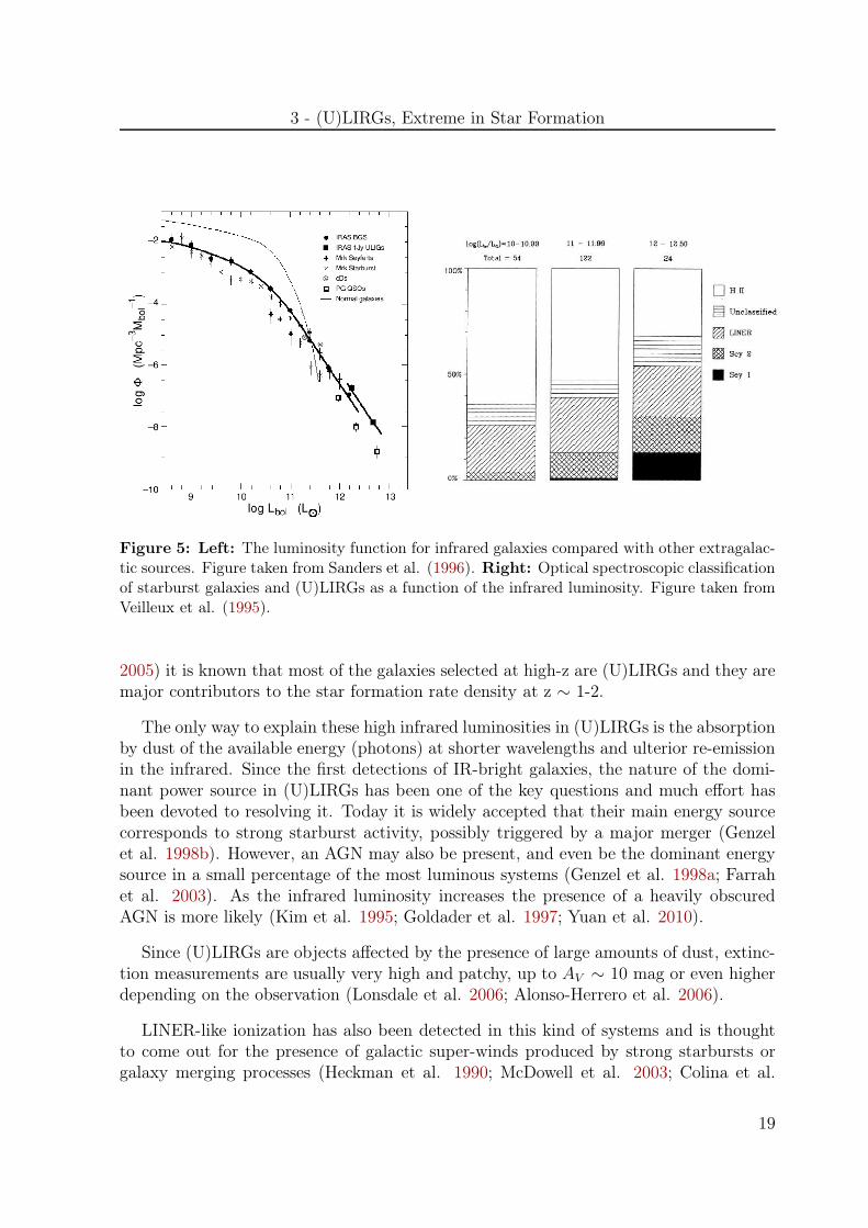
c < 1013L⊙, respectively (Sanders & Mirabel 1996). This classification isbased on the definitions in Table 1. Although they comprise the dominant populationof extragalactic objects at Lbol > 1011 L⊙ and are even twice as numerous as opticallydetected QSOs with same bolometric luminosity (see Fig. 5, left), they are relatively rarein the local Universe (Soifer et al. 1987, 1989). In fact, their space density is severalorders of magnitude lower than that of the normal galaxies.
Thanks to observations with Spitzer (Pérez-González et al. 2005; Le Floc’h et al.
b The IR spectral range covers from about 0.75 µm to 350 µm, and it is normally divided into threeregions: the near-IR (from 0.75 to 5 µm), the mid-IR (from 5 to 25 µm), and the far-IR (from 25 to350µm) (Glass 1999).
c For simplicity, we will identify the infrared luminosity as LIR (L⊙ ) ≡ log (LIR) .
18
3 - (U)LIRGs, Extreme in Star Formation
Figure 5: Left: The luminosity function for infrared galaxies compared with other extragalac-tic sources. Figure taken from Sanders et al. (1996). Right: Optical spectroscopic classificationof starburst galaxies and (U)LIRGs as a function of the infrared luminosity. Figure taken fromVeilleux et al. (1995).
2005) it is known that most of the galaxies selected at high-z are (U)LIRGs and they aremajor contributors to the star formation rate density at z ∼ 1-2.
The only way to explain these high infrared luminosities in (U)LIRGs is the absorptionby dust of the available energy (photons) at shorter wavelengths and ulterior re-emissionin the infrared. Since the first detections of IR-bright galaxies, the nature of the domi-nant power source in (U)LIRGs has been one of the key questions and much effort hasbeen devoted to resolving it. Today it is widely accepted that their main energy sourcecorresponds to strong starburst activity, possibly triggered by a major merger (Genzelet al. 1998b). However, an AGN may also be present, and even be the dominant energysource in a small percentage of the most luminous systems (Genzel et al. 1998a; Farrahet al. 2003). As the infrared luminosity increases the presence of a heavily obscuredAGN is more likely (Kim et al. 1995; Goldader et al. 1997; Yuan et al. 2010).
Since (U)LIRGs are objects affected by the presence of large amounts of dust, extinc-tion measurements are usually very high and patchy, up to AV ∼ 10 mag or even higherdepending on the observation (Lonsdale et al. 2006; Alonso-Herrero et al. 2006).
LINER-like ionization has also been detected in this kind of systems and is thoughtto come out for the presence of galactic super-winds produced by strong starbursts orgalaxy merging processes (Heckman et al. 1990; McDowell et al. 2003; Colina et al.
19

General Introduction
2004; Monreal-Ibero et al. 2010).
Figure 6: True-color images of some local LIRGs taken with the NOT (Nordic Optical Tele-scope) from a sample of local LIRGs. Figure taken from Arribas et al. (2004).
Most local LIRGs show the typical morphology of a spiral or a system undergoing anearly stage of interaction, with the presence of star-forming regions and often tails withdust (Surace et al. 2000; Scoville et al. 2000; Alonso-Herrero et al. 2002, 2006, 2009; Ar-ribas et al. 2004; Rodríguez-Zaurín et al. 2011). Yet, an important fraction (at least25%) presents a perturbed morphology or is clearly involved in an interaction process.A few examples of the morphology of these systems are shown in Fig. 6.
The vast majority of ULIRGs (at least 90%), on the other hand, are interactinggalaxies undergoing different phases of the merging process, according to optical andnear infrared studies (Melnick & Mirabel 1990; Clements et al. 1996; Bushouse et al.NIR
20

3 - (U)LIRGs, Extreme in Star Formation
Figure 7: HST (WFPC2/F814W ) images of some ULIRGs. Figure taken from García-Marínet al. (2009b)
2002; Evans et al. 2002; Veilleux et al. 2002, 2006). The images in these bands showULIRGs with a peculiar morphology, tidal tails, bridges, shells and condensations of starformation, typical of systems undergoing a merging process. Not only are most or allthe ULIRGs in the different samples studied involved in an interaction process, but theirnuclei also show complex structures (Surace et al. 1998, 2000; Farrah et al. 2001, 2003).Using high angular resolution images taken with the Hubble Space Telescope, some au- HSTthors have suggested that a few ULIRGs are under a multiple merger process (e.g., Borneet al. 2000; Bushouse et al. 2002). A few examples of the morphology of these systemsare shown in Fig. 7.
21
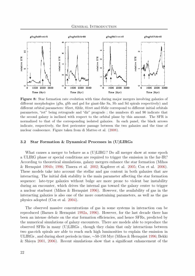
General Introduction
Figure 8: Star formation rate evolution with time during major mergers involving galaxies ofdifferent morphologies (gSa, gSb and gsd for giant-like Sa, Sb and Sd spirals respectively) anddifferent orbital parameters: 05ret, 02dir, 01ret and 05dir correspond to different initial orbitalsparameters, “ret” being retrograde and “dir” prograde ; the numbers 45 and 90 indicate thatthe second galaxy is inclined with respect to the orbital plane by this amount. The SFR isnormalized to that of the corresponding isolated galaxies. In each panel, the black arrowsindicate, respectively, the first pericenter passage between the two galaxies and the time ofnuclear coalescence. Figure taken from di Matteo et al. (2008).
3.2 Star Formation & Dynamical Processes in (U)LIRGs
What causes a merger to behave as a (U)LIRG? Do all merger show at some epocha ULIRG phase or special conditions are required to trigger the emission in the far-IR?According to theoretical simulations, galaxy mergers enhance the star formation (Mihos& Hernquist 1994b; 1996; Tissera et al. 2002; Kapferer et al. 2005; Cox et al. 2006).These models take into account the stellar and gas content in both galaxies that areinteracting. The initial disk stability is the main parameter affecting the star formationsequence: late-type galaxies without bulge are more prone to violent bar instabilityduring an encounter, which drives the internal gas toward the galaxy center to triggera nuclear starburst (Mihos & Hernquist 1996). However, the availability of gas in theinteracting galaxies is also one of the more constraining parameters, as well as the gasphysics adopted (Cox et al. 2004).
The observed massive concentrations of gas in some systems in interaction can bereproduced (Barnes & Hernquist 1992a, 1996). However, for the last decade there hasbeen an intense debate on the star formation efficiencies, and hence SFRs, predicted bythe numerical simulations of galaxy encounters. There are models able to reproduce theobserved SFRs in many (U)LIRGs , though they claim that only interactions betweentwo gas-rich spirals are able to reach such high luminosities to explain the emission inULIRGs , and during short periods in time, ∼50-150 Myr (Mihos & Hernquist 1996; Bekki& Shioya 2001, 2006). Recent simulations show that a significant enhancement of the
22

3 - (U)LIRGs, Extreme in Star Formation
SFR during a major merger at low redshifts (given by the linear resolution achieved andthe initial gas content of the parent galaxies) is quite rare (Bournaud & Duc 2006; Coxet al. 2008; Di Matteo et al. 2008). It seems to be highly dependent on the mass ratioof the galaxies involved in the interaction, an equal-mass ratio of two gas-rich spiralsbeing the most favored. The orbital geometry represent a secondary factor, though theenhancement is more efficient for galaxies in retrograde orbits. Some examples of theSFH of simulations of mergers are shown in Fig. 8.
There is both theoretical (Toomre & Toomre 1972; Hernquist 1992b; 1993) and obser-vational (Stanford & Bushouse 1991; Genzel et al. 2001; Colina et al. 2001; Tacconi et al.2002; Dasyra et al. 2006) evidence that in (U)LIRGs the end product of the encounterbetween two disk galaxies can be an early-type galaxy with a moderate mass of 0.1-1 m∗
(m∗ = 1.4 × 10¹¹ M⊙) and a de Vaucoulers surface brightness profile (r1/4), althoughthis view was initially refused for two reasons:
• How do the observed GCs in elliptical form? The discovery of SSCs (see Section 2.1,page 5) hidden by dust in interacting systems was proposed by some authors asprecursors of GCs (Whitmore & Schweizer 1995; Kassin et al. 2003).
• As ellipticals barely contain gas, how can such large amounts of gas involved inthe merging process disappear? Galactic superwinds and supernovae explosionsare a likely explanation. Additionally, the jets coming from the AGNs also expelsignificant amount of gas toward the extra-galactic medium.
Another aspect of the dynamical evolution of ULIRGs which is worth mentioningis the presence of compact star-forming regions at all galactocentric scales, especiallywithin the tidal tails, in which knots or condensations of star formation have been ob-served (e.g., Surace et al. 1998). The next section will present in more detail the compactstar-forming structures that have been observed in (U)LIRGs (i.e., SSCs and TDG can-didates).
3.3 Young Compact Star-forming Structures in (U)LIRGs
As already mentioned in previous sections, the high infrared luminosity in (U)LIRGs isbelieved to be mainly caused by the re-emission of hidden starburst activity, which istriggered by a merger process in a significant percentage of LIRGs and practically inall ULIRGs. It is not surprising that the studies carried out on these systems havefound young compact star-forming regions at all galactocentric distances. Copious stud-ies on The Antennae –on the border line between the non-LIRG and the LIRG class,with a luminosity of LIR=10.99– have been carried out (e.g., Whitmore & Schweizer1995, 1999, 2005, 2010; Fall et al. 2005; Bastian et al. 2006; Mengel et al. 2008). Giventhe proximity of the system and the use of high angular resolution images from the HST,
23
General Introduction
these works have reported the properties of thousands of clusters with typical half-lightradii of a few pc, the most luminous (MV > −14.6) being young (typically τ . 100 Myr)and spanning the mass range 105-106 M⊙, typical properties of SSCs.
For more luminous systems only a few studies of compact, massive (i.e., 105-107 M⊙)and extremely young (i.e., τ < 10 Myr) circumnuclear star clusters have been reported(Scoville et al. 2000; Alonso-Herrero et al. 2002; Díaz-Santos et al. 2007), using NIR im-ages. Moreover, compact condensations compatible with massive young star formationin the outermost regions have been detected with near-UV and optical images (Suraceet al. 1998; Surace et al. 2000). The systems sampled in these works are located at suchdistances (between 40 to hundreds of Mpc) that the observation of intrinsically faintclusters was not possible. Additionally, blending can occur and thus, although severalsystems were sampled in each study, only a total of dozens or few hundreds of cluster-likeobjects were detected.
With half-light radii between about ten to few hundreds of pc, most of the cluster-likeojects detected in (U)LIRGs may actually be complexes of star clusters. However, thesize of the largest objects is similar to that of a typical dwarf galaxy. Given the interactingnature of (U)LIRGs (especially ULIRGs) there have also been searches of TDG candi-dates there. Despite the fact that a priori they have the appropriate nature to harbourthese dwarf galaxies, only few studies have been performed so far. The TDG candidatein The Superantennae (Mirabel et al. 1991) turned out to be a background object (Weil-bacher et al. 2003). Mihos & Bothun (1998) identified only three more candidates ina sample of one LIRG and three ULIRGs. More recently, Monreal-Ibero et al. (2007)have performed a systematic search of TDGs in a sample of nine ULIRGs. A total oftwelve candidates were identified and characterized. They share similar properties toobserved TDG candidates in other samples, such as high metallicty (i.e., Z⊙ or Z⊙/3),effective radii of a few hundreds of pc and total masses higher than 108 M⊙. That workalso studied the stability of their candidates against internal motions and forces from theparent galaxy and found that five out of the twelve show high- medium or high likelihoodof survival as future TDG.
3.4 (U)LIRGs in the High-z Universe
With the advent of satellites and ground-based instruments working on the IR, mil-limeter and radio wavelenghts, many high-z luminous infrared galaxies have been dis-covered. Although these galaxies do not dominate the luminosity function in the localUniverse, they become more important as we observe them farther. Surveys carried onwith the InfraRed Space Observatory showed that the evolution of the luminosity den-ISOsity in these galaxies is very rapid until z = 1, and no much farther increase is left forthe higher redshifts (Franceschini et al. 2001).
The Spitzer telescope, working in the 3-180 µm range, allowed to survey the
24

3 - (U)LIRGs, Extreme in Star Formation
Figure 9: Evolution of the co-moving IR luminosity density with redshift (red solid line). Theblue dashed and the orange dotted-dashed lines show the contributions of LIRGs and ULIRGs ,respectively, at different redshifts. Figure taken from Caputi et al. (2007).
(U)LIRG population up to redshift z ∼ 3 (Le Floc’h et al. 2005; Franceschini et al.2005; Pérez-González et al. 2005; Caputi et al. 2007). From these studies we know thatat z > 1 LIRGs are the major contributors of the co-moving star formation rate densityof the Universe, and at z ≃ 2, (U)LIRGs have similar contributions (see Fig. 9), and theyaccount for at least half of the newly born stars by z ∼ 1.5.
It is also believed that at these redshifts the main source of energy in (U)LIRGs cor-responds to star formation activity. Studies carried out with Spitzer data confirm theimportance of the polycyclic aromatic hydrocarbons up to z ∼ 2.5 (Yan et al. 2005), and PAH
works on the millimeter and radio wavelenghts have estimated that only about 25% ofthe (U)LIRG population harbour an AGN (Ivison et al. 2004; Egami et al. 2004).
Sources with SFRs up to ten times higher than in ULIRGs , known assub-millimeter galaxies, were detected with the sub-millimeter instrument SCUBA, op- SMG
erating at 450 and 850 µm (Smail et al. 1997). Given their peculiar morphologies, highluminosities and energy spectral distributions, it is very likely that they are the counter-parts of (U)LIRGs at high redshifts (z & 2; Smail et al. 1997; Blain et al. 2002; Frayeret al. 2004). Follow-up multi-wavelength observations of SMGs showed that some of thesegalaxies exhibit multiple components, a clear indication of ongoing interaction processes(Ivison et al. 2002; Smail et al. 2002).
25
General Introduction
(U)LIRGs can also become relevant in the context of clumpy galaxies at high red-shifts. Star-forming galaxies become increasingly irregular at higher redshifts, with a blueclumpy structure, asymmetry and lack of central concentration (Abraham et al. 1996; vanden Bergh et al. 1996; Im et al. 1999). It has been claimed that clumps in clumpy galax-ies represent star-forming complexes intrinsically more massive by one or two ordersof magnitudes than similar-size complexes in local galaxies (Efremov 1995; Elmegreenet al. 2009; Gallagher et al. 2010). Although most of the clumpy galaxies, observed atz = 0.7-2, do not show signs of interactions, they might share the extreme star formationproperties with local (U)LIRGs .
Since all these galaxies at high redshift seem to be equivalent to the (U)LIRGs observedin the local Universe, in order to understand them and the role they have played on thestar and galaxy formation in the early Universe it is important to know in detail thephysical properties and the dynamical processes that take place in local (U)LIRGs .
4 Thesis Project
In general, the investigation of compact star-forming objects in galaxies can be doneusing two different approaches: (i) surveys of a significative number of galaxies, usefulto study the global integrated properties and to make statistical studies; (ii) and theanalysis of a particular galaxy to study in detail the star formation and disruption pro-cesses occurring there. For the past few decades much effort has been applied to studyhow the interaction of galaxies affects the star and galaxy formation, using the state-of-the-art instrumentation (e.g., HST studies in M51, NGC 4038/4039 or NGC 7252;integral field unit spectroscopic observations of TDG candidates). Numerical modelingIFU
of galaxy encounters, with a continuous improvement of the spatial resolution and the en-largement of the number of simulations that allows us to explore each time more realisticscenarios, has also become an important complementation to observations to advance inthe field. All these theoretical and observational studies have provided significant resultsand observational restrictions to the physical processes occurring in galaxy mergers (e.g.,the role of the infant mortality, physical constrains of the galaxies under interaction forthe star formation to be enhanced more effectively, etc.).
But, is the star formation in (U)LIRGs ruled by the same processes as in less lu-minous galaxy interactions? Can a different mode of star formation, in which moremassive objects can be formed as a result of the interaction, take place there? Doesthe star formation evolve as the interaction proceeds? Are the formation and disruptionprocesses universal? These are some questions that remain unanswered because, apartfrom very few and limited studies, the most energetic systems in the local Universe haveremained barely explored in this field. This is in part because (U)LIRGs normally arelocated at such distances (i.e., normally at luminosity distances farther than 60 Mpc andDL
there is only one ULIRG closer than 100 Mpc) that the detection of large number of
26

4 - Thesis Project
individual compact star-forming regions is not possible with the best instrumentationavailable today. The studies with the largest samples correspond to those of Surace etal. (1998, 2000), that encompass less than a dozen of ULIRGs each and detect a fewhundred compact regions.
This thesis presents the study of compact star-forming regions in the most lumi-nous low-z (U)LIRGs. With a sample of 32 systems, larger than in previous works,it increases considerably the statistics with the detection of a few thousand compactstar-forming regions. The galaxies in the sample represent different interaction phases(first-contact, pre-merger, merger and post-merger) and cover a wide luminosity range(11.46 ≤ LIR ≤ 12.54). The project is based mainly on optical high resolution im-ages taken with the ACS on board the HST telescope, data from a high linear res-olution simulation of a major galaxy encounter, and with the combination of opticalIntegral Field Spectroscopy from the INTEGRAL (WHT) and VIMOS (VLT) instru- IFS
ments. The main topics covered in this project are: (i) the identificantion and empiricalcharacterization of the compact star-forming regions identified in our sample of low-z(U)LIRGs; (ii) the comparison of their properties with those of compact objects identifiedin a high linear resolution of a galaxy encounter; (iii) the identification and characteriza-tion of Hα -emitting complexes, and the study if their nature is compatible with beingprogenitors to TDGs. The sample selection, the different sets of data analyzed and thegeneral analysis techniques are presented in Chapter I. Then, this thesis is divided intothe three main topics, each one covered in one Chapter:
• Characterization of compact star-forming regionsIn Chapter II we present an empirical characterization of optically-selected compactstar-forming regions (knots) in a representative sample of 32 low-z (i.e., z < 0.1)(U)LIRGs. It shows the first attempt at obtaining an homogeneous and statisticallysignificant study of the photometric properties (luminosities, colors and sizes) ofoptically-selected knots of star formation found in these systems as a function of theinfrared luminosity, morphology (i.e., interaction phase) and radial distance to thenucleus of the galaxy. The luminosity function is also evaluated and compared withthat obtained in other studies. Finally, their properties are compared to clumpystructures identified in high-z star-forming galaxies.
• Comparison with a high linear resolution simulation of a major mergerThe previous chapter represents the starting point in Chapter III, where the firstdirect comparison of the properties of stellar regions (simulated knots) identifiedin the high spatial resolution galaxy simulation of Bournaud et al. (2008b) withthe knots detected in our sample is performed. Using stellar population synthesistechniques, the luminosities, colors and LFs of the simulated knots are evaluatedat different interaction phases. A direct comparison with the properties of theobserved knots makes possible a physical interpretation of the results from obser-vations. How close are the predictions of the simulation from real encounters? How
27

General Introduction
can we understand some of the properties of the observed knots? These are somequestions we investigate throughout the chapter.
• Search and characterization of TDG candidatesThe third part of the thesis is presented in Chapter IV. We characterize the ex-tranuclear star-forming regions of a sample of (U)LIRGs using the combined in-formation of Integral Field Spectroscopy (IFS) data together with high resolutionimages from the HST. This chapter is devoted to the search of potential TDG can-didates in local (U)LIRGs. Properties such as the metallicity, extinction, age andmass of the young stellar population, Hα luminosity, dynamical mass, velocitydispersion, relative velocity etc., are derived and compared with those of TDG can-didates in the literature. We use these parameters to estimate the likelihood ofsurvival of these regions as future TDGs. We also estimate the implications ofTDG formation to the overall dwarf population and primordial dwarf formation athigh-z.
28

Chapter I
Sample Selection, Dataset and DataTreatment
Overview
This Chapter presents the sample upon which this thesis isbased. The selection criteria and the main morphological prop-erties of the galaxies are described. The different sets of datapresented and the general analysis techniques applied to per-form this study are also discussed in detail.
1 Sample Selection and General Properties
1.1 The Sample
The galaxies for this thesis were selected from the flux-limited IRAS Revisited GalaxySample (RBGS, Sanders et al. 2003) and from the sample of Sanders et al. (1988), usingthe following additional criteria:
• To sample the wide range of IR luminosities in (U)LIRGs.
• To cover all types of nuclear activity (i.e., different ionization mechanisms) to avoidbiases.
• To span different phases of interaction, from first approach to final merger phases.
• To optimize the linear scales by selecting low-z galaxies, which would allow us tohave a relatively high linear resolution and to detect intrinsically faint compactregions.
29
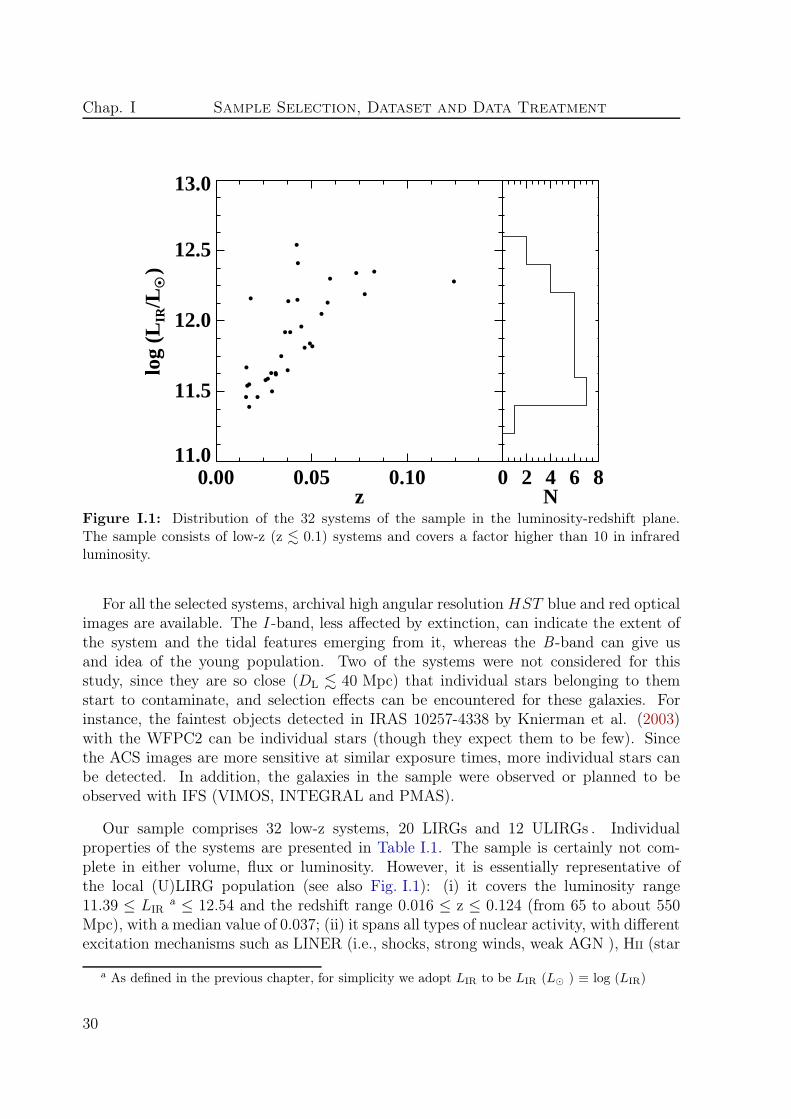
Chap. I Sample Selection, Dataset and Data Treatment
0.00 0.05 0.10 z
11.0
11.5
12.0
12.5
13.0
log
(LIR
/LO • )
0 2 4 6 8N
Figure I.1: Distribution of the 32 systems of the sample in the luminosity-redshift plane.The sample consists of low-z (z . 0.1) systems and covers a factor higher than 10 in infraredluminosity.
For all the selected systems, archival high angular resolution HST blue and red opticalimages are available. The I -band, less affected by extinction, can indicate the extent ofthe system and the tidal features emerging from it, whereas the B -band can give usand idea of the young population. Two of the systems were not considered for thisstudy, since they are so close (DL . 40 Mpc) that individual stars belonging to themstart to contaminate, and selection effects can be encountered for these galaxies. Forinstance, the faintest objects detected in IRAS 10257-4338 by Knierman et al. (2003)with the WFPC2 can be individual stars (though they expect them to be few). Sincethe ACS images are more sensitive at similar exposure times, more individual stars canbe detected. In addition, the galaxies in the sample were observed or planned to beobserved with IFS (VIMOS, INTEGRAL and PMAS).
Our sample comprises 32 low-z systems, 20 LIRGs and 12 ULIRGs . Individualproperties of the systems are presented in Table I.1. The sample is certainly not com-plete in either volume, flux or luminosity. However, it is essentially representative ofthe local (U)LIRG population (see also Fig. I.1): (i) it covers the luminosity range11.39 ≤ LIR
a ≤ 12.54 and the redshift range 0.016 ≤ z ≤ 0.124 (from 65 to about 550Mpc), with a median value of 0.037; (ii) it spans all types of nuclear activity, with differentexcitation mechanisms such as LINER (i.e., shocks, strong winds, weak AGN ), HII (star
a As defined in the previous chapter, for simplicity we adopt LIR to be LIR (L⊙ ) ≡ log (LIR)
30
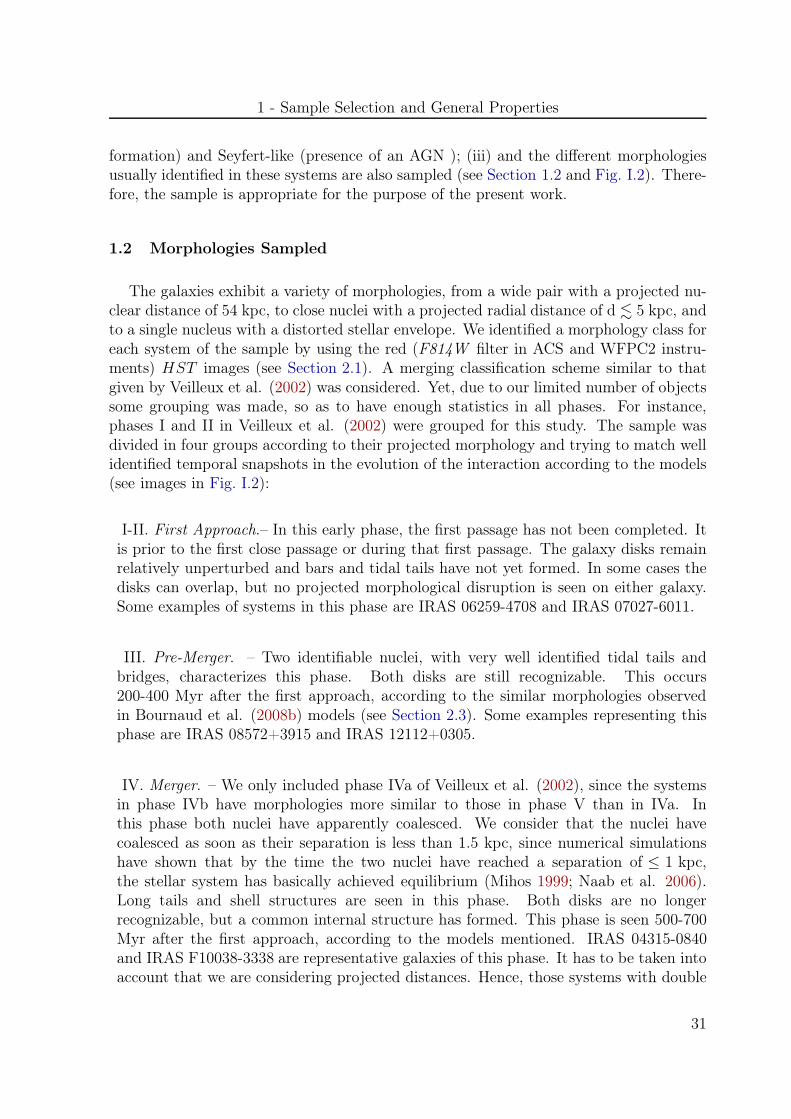
1 - Sample Selection and General Properties
formation) and Seyfert-like (presence of an AGN ); (iii) and the different morphologiesusually identified in these systems are also sampled (see Section 1.2 and Fig. I.2). There-fore, the sample is appropriate for the purpose of the present work.
1.2 Morphologies Sampled
The galaxies exhibit a variety of morphologies, from a wide pair with a projected nu-clear distance of 54 kpc, to close nuclei with a projected radial distance of d . 5 kpc, andto a single nucleus with a distorted stellar envelope. We identified a morphology class foreach system of the sample by using the red (F814W filter in ACS and WFPC2 instru-ments) HST images (see Section 2.1). A merging classification scheme similar to thatgiven by Veilleux et al. (2002) was considered. Yet, due to our limited number of objectssome grouping was made, so as to have enough statistics in all phases. For instance,phases I and II in Veilleux et al. (2002) were grouped for this study. The sample wasdivided in four groups according to their projected morphology and trying to match wellidentified temporal snapshots in the evolution of the interaction according to the models(see images in Fig. I.2):
I-II. First Approach.– In this early phase, the first passage has not been completed. Itis prior to the first close passage or during that first passage. The galaxy disks remainrelatively unperturbed and bars and tidal tails have not yet formed. In some cases thedisks can overlap, but no projected morphological disruption is seen on either galaxy.Some examples of systems in this phase are IRAS 06259-4708 and IRAS 07027-6011.
III. Pre-Merger. – Two identifiable nuclei, with very well identified tidal tails andbridges, characterizes this phase. Both disks are still recognizable. This occurs200-400 Myr after the first approach, according to the similar morphologies observedin Bournaud et al. (2008b) models (see Section 2.3). Some examples representing thisphase are IRAS 08572+3915 and IRAS 12112+0305.
IV. Merger. – We only included phase IVa of Veilleux et al. (2002), since the systemsin phase IVb have morphologies more similar to those in phase V than in IVa. Inthis phase both nuclei have apparently coalesced. We consider that the nuclei havecoalesced as soon as their separation is less than 1.5 kpc, since numerical simulationshave shown that by the time the two nuclei have reached a separation of ≤ 1 kpc,the stellar system has basically achieved equilibrium (Mihos 1999; Naab et al. 2006).Long tails and shell structures are seen in this phase. Both disks are no longerrecognizable, but a common internal structure has formed. This phase is seen 500-700Myr after the first approach, according to the models mentioned. IRAS 04315-0840and IRAS F10038-3338 are representative galaxies of this phase. It has to be taken intoaccount that we are considering projected distances. Hence, those systems with double
31

Chap. I Sample Selection, Dataset and Data Treatment
Table I.1: Sample of (U)LIRGs
IRAS Other R. A. DEC DL LIR Morphology Interaction Spectral Class Refname name (J2000) (J2000) (Mpc) phase (Optical)(1) (2) (3) (4) (5) (6) (7) (8) (9) (10)
00506+7248 00:54:04.91 +73:05:05.5 65.3 11.46 IP III HII [1]02512+1446 02:54:01.99 +14:58:26.2 131.3 11.63 IP III HII [2]04315-0840 NGC 1614 04:33:59.99 -08:34:42.8 66.1 11.67 SN IV (2) HII [3]05189-2524 05:21:01.42 -25:21:48.3 180.6 12.15 SN V (2) Sy2 [4],[5]06076-2139 06:09:45.98 -21:40:25.6 158.3 11.65 IP III (1) Sy/L-HII [6]06259-4708 06:27:22.53 -47:10:45.4 164.2 11.92 MI I-II (1) HII-HII [7]07027-6011 07:03:27.46 -60:16:00.2 131.8 11.62 IP I-II (0) Sy2 [7]08355-4944 NGC 2623 08:37:01.98 -49:54:27.5 108.5 11.58 SN IV (2) HII [8]08520-6850 08:52:28.86 -69:02:00.3 197.1 11.81 IP I-II (1) - -08572+3915 09:00:25.62 +39:03:54.1 250.6 12.13 IP III L/HII [9], [10]09022-3615 09:04:12.26 -36:26:58.1 256.4 12.30 SN IV (2) - -F10038-3338 10:06:05.04 -33:53:14.8 143.8 11.75 DN IV (2) - -10173+0828 10:20:00.10 +08:13:33.3 209.4 11.84 SN V - -12112+0305 12:13:45.82 +02:48:38.0 318.3 12.34 IP III L-L [4], [5], [9]12116-5615 12:14:21.77 -56:32:27.6 113.7 11.59 SN V (2) HII [7]12540+5708 Mrk 231 12:56:13.73 +56:52:29.6 178.9 12.54 SN V (2) Sy1 [2], [5]13001-2339 13:02:52.49 -23:55:19.6 90.7 11.46 DN IV (2) L [11]13428+5608 Mrk 273 13:44:41.93 +55:53:12.3 159.8 12.14 DN IV L-Sy2 [2]13536+1836 Mrk 463 13:56:02.80 18:22:17.20 215.0 11.82 DN III Sy1-Sy2 [12]14348-1447 14:37:40.36 -15:00:29.4 361.6 12.35 DN III L [5], [9]15206+3342 15:22:38.00 +33:31:35.9 559.6 12.28 SN V HII [5], [13]15250+3609 15:26:59.05 +35:58:38.0 236.3 12.05 SN IV L [5]15327+2340 Arp 220 15:34:54.63 +23:29:40.5 75.5 12.16 DN IV L [13]16104+5235 NGC 6090 16:11:40.10 +52:27:21.5 123.1 11.50 IP III HII [2]F17138-1017 17:16:35.64 -10:20:34.9 72.2 11.39 SN V (2) HII [14]17208-0014 17:23:19.14 -00:17:22.5 181.7 12.41 SN V L [5], [15]F18093-5744 IC 4686 18:13:38.66 -57:43:53.7 72.2 11.55 MI III (1) HII-HII [7]18329+5950 NGC 6670 18:33:37.06 +59:53:19.3 121.2 11.63 IP III - -20550+1656 20:57:23.51 +17:07:34.6 152.5 11.92 IP III HII [2]22491-1808 22:51:45.79 -17:52:22.5 338.6 12.19 DN III (1) HII [5]23007+0836 23:03:16.92 +08:53:06.4 67.9 11.54 IP I-II Sy1-Sy2/L [2]23128-5919 23:15:46.46 -59:04:01.9 189.6 11.96 DN III (1) Sy/L-HII [5], [9]
Notes. Col (1): object designation in the IRAS Point and Faint Source catalogs. Col (2): other name.Cols (3) and (4): right ascension (hours, minutes and seconds) and declination (degrees, arcminutes,arcseconds) taken from the from the NASA Extragalactic Database (NED). Col (5): luminosity distancesderived assuming a ΛCDM cosmology with H0 = 73 kms−1Mpc−1, ΩΛ=0.73 and ΩM=0.27, and usingthe Eduard L. Wright Cosmology calculator, which is based in the prescription given by Wright (2006).Col (6): logarithm of the infrared luminosity in units of solar bolometric luminosity, computed using thefluxes in the four IRAS bands, as prescribed in Table 1. Col (7): MI stands for Multiple Interactinggalaxies, IP interacting pair, DN double nucleus and SN single nucleus. Col (8): Morphological classi-fication used in this study, where I-II stands for first approach, III for pre-merger, IV for post-mergerand V for relaxed system (see text). Between brackets the classification by Rodriguez-Zaurin et al.(2011) is given, when available. In their study, class 0 corresponds to classes I-II, class 1 to class III andclass 2 to classes IV-V in this study, respectively. Note a disagreement in IRAS 06259-4708 and IRAS08520-6850 due to the slight different of the definitions of the early interaction phases in both studies(see text). Col (9): Spectral class in the optical. A slash between two different classes indicates thatno clear classification is known between both, whereas a dash separates the class of each nucleus in thesystem when known. L stands for LINER and Sy refers to a Seyfert activity. Col (10): References tothe spectral class– [1] Alonso-Herrero et al. (2009), [2] Wu et al. (1998), [3] Kotilainen et al. (2001),[4] Risaliti et al. (2006), [5] Nardini et al. (2008), [6] Arribas et al. (2008), [7] Kewley et al. (2001),[8] Cohen (Cohen 1992), [9] Evans et al. (2002), [10] Arribas et al. (2000), [11] Zenner & Lenzen (1993),[12] García-Marín et al. (2007), [13] Kim et al. (1998), [14] Corbett et al. (2003), [15] Arribas & Colina(2003).
32

2 - Data Acquisition
nuclei allocated to this phase could well belong to the previous phase if the real sepa-ration of both nuclei is considerably greater (i.e., orbital position along our line of sight).
V. Post-Merger. – We also included phase IVb of Veilleux et al. (2002). In this phasethere are no prominent and bright tidal tails or bridges, since their surface brightnessstarts to fall below the detection limit, though some shell structures around the nucleuscan still be detected. These isolated nuclei can have disturbed stellar envelopes, similarto those in the previous phase, indirectly indicating the past interaction. Typical agesof τ & 1 Gyr after the first passage characterizes the timescale of this phase, accordingto the models mentioned. IRAS 05189-2524 and IRAS 12116-5615 are good examplesof systems in this phase.
Since this classification was performed only by evaluating the apparent morphologyof the systems under study, it is always subject to improvements based on data with ahigher angular resolution and sensitivity, and deeper imaging (i.e., to observe envelopesin post-mergers). Therefore, misclassification could occur in a few systems. Moreover,for certain studies, slightly different and simpler classifications have been used previously(Rodríguez-Zaurín et al. 2011; see also Table I.1). Although they have the advantage ofreducing subjectivity and therefore uncertainty, their classification is too coarse for detailcomparison with model predictions. While the classification of a few objects can differ,as is the case for IRAS 06259-4807 and IRAS 08520-6850 in common with Rodríguez-Zaurín’s sample (the definitions of the early phases in both studies are slightly different),the agreement between both classifications is excellent. Using this classification, 4 sys-tems were assigned to category I-II, 13 to category III, 8 to category IV and 7 to categoryV (see Table I.1).
2 Data Acquisition
For this thesis we used a variety of different but complementary data sets: high angularresolution imaging as observed with the Hubble Space Telescope, IFS data from the fiber-based optical IFU instruments and data from a high linear resolution simulation of awet galaxy merger. They are all based on completely different concepts, and each onerequires a different treatment, in terms of data reduction and analysis techniques. Theavailable dataset from observations for each galaxy is shown in Table I.2.
2.1 Photometric Data: Images from the HST
Observations with the HST , a 2.4m reflector telescope carried into orbit by a spaceshuttle in 1990, have great advantages compared to ground-based facilities. Thanks tothe absence of the atmospheric veil the observations are not limited by seeing conditions
33
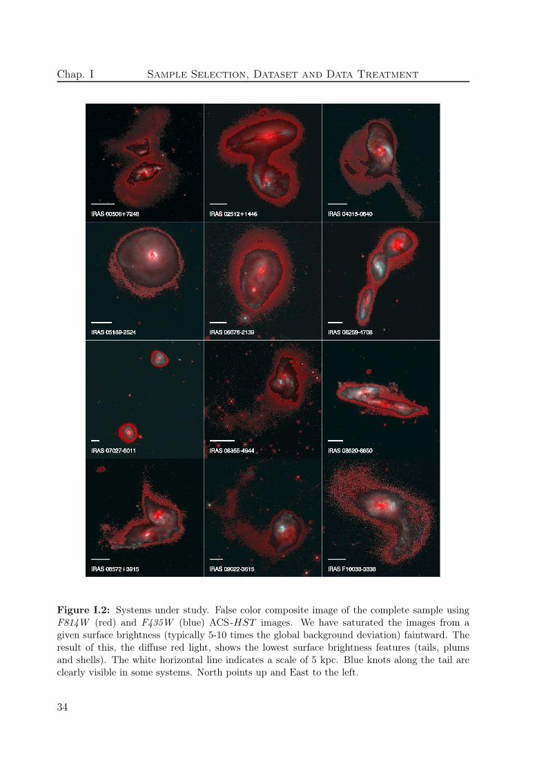
Chap. I Sample Selection, Dataset and Data Treatment
Figure I.2: Systems under study. False color composite image of the complete sample usingF814W (red) and F435W (blue) ACS-HST images. We have saturated the images from agiven surface brightness (typically 5-10 times the global background deviation) faintward. Theresult of this, the diffuse red light, shows the lowest surface brightness features (tails, plumsand shells). The white horizontal line indicates a scale of 5 kpc. Blue knots along the tail areclearly visible in some systems. North points up and East to the left.
34

2 - Data Acquisition
Figure I.2: - Continued
35

Chap. I Sample Selection, Dataset and Data Treatment
Figure I.2: - Continued
(i.e., it can provide an angular resolution in the optical of 0.05′′ vs. the 1.0′′ ground-based one), and the stability of the observing conditions makes the calibrations quitestable. The main photometric datasets used in this thesis cover the optical spectralrange, though complementary infrared images are also used.
2.1.1 Optical Images
In this thesis, we mainly use archive data from the Advanced Camera for Surveys,ACS
a third generation axial instrument aboard the HST . It includes three independentchannels that cover the ultraviolet to the near-infrared spectral range: the Wide FieldChannel (WFC), the High-Resolution Channel (HRC) and the Solar Blind Channel.
36
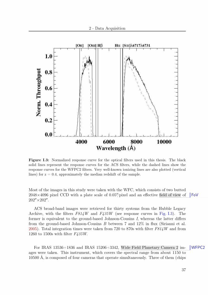
2 - Data Acquisition
Figure I.3: Normalized response curve for the optical filters used in this thesis. The blacksolid lines represent the response curves for the ACS filters, while the dashed lines show theresponse curves for the WFPC2 filters. Very well-known ionizing lines are also plotted (verticallines) for z = 0.4, approximately the median redshift of the sample.
Most of the images in this study were taken with the WFC, which consists of two butted2048×4096 pixel CCD with a plate scale of 0.05′′/pixel and an effective field of view of FoV
202′′×202′′.
ACS broad-band images were retrieved for thirty systems from the Hubble LegacyArchive, with the filters F814W and F435W (see response curves in Fig. I.3). Theformer is equivalent to the ground-based Johnson-Cousins I, whereas the latter differsfrom the ground-based Johnson-Cousins B between 7 and 12% in flux (Sirianni et al.2005). Total integration times were taken from 720 to 870s with filter F814W and from1260 to 1500s with filter F435W.
For IRAS 13536+1836 and IRAS 15206+3342, Wide Field Planetary Camera 2 im- WFPC2
ages were taken. This instrument, which covers the spectral range from about 1150 to10500 Å, is composed of four cameras that operate simultaneously. Three of them (chips
37

Chap. I Sample Selection, Dataset and Data Treatment
2, 3, 4) have a plate scale of 0.1′′/pixel and a FoV of 80′′×80′′, and form the Wide FieldCamera. The fourth (chip 1), with a plate scale of 0.046′′/pixel and a FoV of 36′′×36′′,is the so-called Planetary Camera (PC). Images were taken with the filters F814W andF439W (see response curves in Fig. I.3), being equivalent to ground-based Johnsons Iand B, respectively (Origlia & Leitherer 2000). Total integration times of about 350swere taken with filter F814W and of 1000s with filter F439W. Here, the systems fall inthe PC chip.
Whenever both ACS and WFPC2 images were available in both filters, ACS imageswere preferred for its superior sensitivity and larger FoV. From now on, we will refer tothe blue filter as F435W for ACS and WFPC2 for simplicity.
Images were reduced on the fly (HST pipeline), with the highest quality availablereference files at the time of retrieval. The calibrated ACS F435W images had only fewcosmic rays remaining, since 3 images had been observed and then combined. However,all the ACS F814W images were severely contaminated with cosmic rays in a 6′′-widthband across the entire FoV. Two exposures had been taken and when they did not overlapthe HST pipeline was not able to discriminate the cosmic rays. In most cases that bandwent through part of the system, covering about 10-20% of its extension. Cosmic rayrejection was then carried out using the IRAFb task credit with the aid of the blue imagessince they were barely contaminated. Most of the systems have observations that coverthe entire FoV with only this instrument and the two filters, so the aid of multi-bandimages was limited to few systems.
Once the photometric data is processed, the derived counts can be transformed intothe Vega system magnitudes using:
mλ = −2.5× log (DN) + Zeropointλ (I.1)
where λ refers to photometric band (I or B), DN corresponds to the integrated countsper second in the defined aperture, and Zeropoint a constant of value 25.536 and 25.759for the ACS F814W and F435W broadbands, respectively (21.678 and 20.877 for theWFPC2 filters). The Zeropoints were derived using the calibration reference papersby Sirianni et al. (2005) and Holtzman et al. (1995), for the ACS and WFPC2 datarespectively.
b IRAF software is distributed by the National Optical Astronomy Observatory (NOAO), which isoperated by the Association of Universities for Research in Astronomy (AURA), Inc., in cooperationwith the National Science Foundation.
38

2-
Data
Acquisition
Table I.2: Available data: HST archive and IFS data
IRAS name HST optical PI and Obs. Exp. HST NIR PI and Obs. Exp. IFS data PI and Obs. Exp.data proposal ID date time (s) data proposal ID date time (s) project ID date time (s)
(1) (2) (3) (4) (5) (6) (7) (8) (9) (10) (11) (12) (13)
00506+7248 ACS Evans, 10592 09/05 800, 1500 NICMOS Alonso-Herrero, 10169 10/04 311 - - - -02512+1446 ACS Evans, 10592 07/06 720, 1260 - - - - - - - -04315-0840 ACS Evans, 10592 08/06 720, 1260 NICMOS Rieke, 7218 02/98 191 VIMOS Arribas, 076.B-0479(A) 03/08 288005189-2524 ACS Evans, 10592 08/06 730, 1275 NICMOS Veilleux, 9875 08/04 2560 VIMOS Arribas, 076.B-0479(A) 12/06 300006076-2139 ACS Evans, 10592 11/05 720, 1260 WFC3 Surace, 11235 06/09 2395 VIMOS Arribas, 076.B-0479(A) 12/06 300006259-4708 ACS Evans, 10592 04/06 780, 1350 NICMOS Surace, 11235 06/08 4990 VIMOS Arribas, 076.B-0479(A) 12/06 300007027-6011 ACS Evans, 10592 09/05 830, 1425 NICMOS Surace, 11235 06/08 4990 VIMOS Arribas, 076.B-0479(A) 12/06 600008355-4944 ACS Evans, 10592 09/05 780, 1350 NICMOS Surace, 11235 06/08 2495 VIMOS Arribas, 076.B-0479(A) 03/07 300008520-6850 ACS Evans, 10592 04/06 870, 1485 NICMOS Surace, 11235 05/08 2300 VIMOS Arribas, 076.B-0479(A) 03/07 300008572+3915 ACS Evans, 10592 12/05 750, 1305 NICMOS Maiolino, 9726 03/04 160 INTEGRAL Colina, 98ACAT26 & C4 04/98 16200
- - - - - - - - INTEGRAL Colina, 98ACAT26 & C4 01/11 900009022-3615 ACS Evans, 10592 06/06 750, 1305 - - - - VIMOS Arribas, 076.B-0479(A) 03/07 3000F10038-3338 ACS Evans, 10592 11/05 740, 1290 - - - - VIMOS Arribas, 076.B-0479(A) 03/07 300010173+0828 ACS Evans, 10592 12/05 720, 1260 - - - - VIMOS Arribas, 076.B-0479(A) 03/08 288012112+0305 ACS Evans, 10592 02/06 720, 1260 NICMOS Scoville, 7219 11/97 192 INTEGRAL Colina, 98ACAT26 & C4 04/98 9000
- - - - - - - - INTEGRAL Colina, 98ACAT26 & C4 01/11 750012116-5615 ACS Evans, 10592 09/05 830, 1425 NICMOS Surace, 11235 07/07 2495 VIMOS Arribas, 076.B-0479(A) 03/07 225012540+5708 ACS Evans, 10592 05/06 830, 1425 NICMOS Veilleux, 9875 09/04 2560 INTEGRAL Colina, D 03/02 360013001-2339 ACS Evans, 10592 02/06 720, 1260 - - - - VIMOS Arribas, 076.B-0479(A) 03/07 600013428+5608 ACS Evans, 10592 11/05 820, 1425 NICMOS Maiolino, 9726 05/04 599 INTEGRAL Colina, 98ACAT26 04/98 450013536+1836 WFPC2 Sanders, 5982 11/95 360, 1030 NICMOS Low, 7213 12/97 480 INTEGRAL Colina, C4 04/01 450014348-1447 ACS Evans, 10592 04/06 720, 1260 NICMOS Scoville, 7219 12/97 480 INTEGRAL Colina, 98ACAT26 04/98 720015206+3342 WFPC2 Sanders, 5982 09/95 343, 750 - - - - INTEGRAL Colina, 98ACAT26 04/98 720015250+3609 ACS Evans, 10592 01/06 750, 1305 NICMOS Scoville, 7219 11/97 223 INTEGRAL Colina, 98ACAT26 04/98 900015327+2340 ACS Evans, 10592 01/06 720, 1260 NICMOS Maiolino, 9726 01/04 599 INTEGRAL Colina, W/200A/27 05/01 900016104+5235 ACS Evans, 10592 09/05 800, 1380 NICMOS Maiolino, 9726 12/03 599 - - - -F17138-1017 ACS Evans, 10592 03/06 720, 1260 NICMOS Alonso-Herrero, 10169 09/04 240 VIMOS Arribas, 081.B-0108(A) 06/09 340017208-0014 ACS Evans, 10592 04/06 720, 1260 NICMOS Scoville, 7219 10/97 223 INTEGRAL Colina, 98ACAT26 04/98 7800F18093-5744 ACS Evans, 10592 04/06 830, 1425 NICMOS Alonso-Herrero, 10169 09/04 240 VIMOS Arribas, 081.B-0108(A) 06/09 680018329+5950 ACS Evans, 10592 10/05 830, 1425 NICMOS Surace, 11235 03/09 2495 - - - -20550+1656 ACS Evans, 10592 04/06 720, 1260 - - - - INTEGRAL Arribas, P15 07/06 450022491-1808 ACS Evans, 10592 05/06 720, 1260 NICMOS Scoville, 7219 11/97 480 VIMOS Arribas, 081.B-0108(A) 07/09 680023007+0836 ACS Evans, 10592 06/06 720, 1260 NICMOS Scoville, 7219 11/97 351 - - - -23128-5919 ACS Evans, 10592 03/06 830, 1425 NICMOS Maiolino, 9726 10/03 599 VIMOS Arribas, 081.B-0108(A) 07/09 3400
Notes. Col (1): object designation in the IRAS Point and Source Catalogs. Col (2): optical instruments used on board HST to observe theretrieved F814W and F435W images. For observations with the WFPC2 the blue filter corresponds to F439W. Col (3): last name of theprincipal investigator, followed by the proposal ID of the optical observation. Col (4): day when the optical observation was taken. Col (5):total exposure times for each galaxy, with filter F814W (left) and filter F435W (right). Col (6): NIR instruments used on board HST toobserve the retrieved F160W images. For all these observations the camera used was NIC2. Col (7): same as (3) for the infrared data. Col(8): same as (4) for the infrared data. Col (9): same as (5) for the infrared data. Col (10): optical ground-based instruments used to observethe IFS data. Since two observations were taken for two sources at different epochs, two rows are provided for each of them. Col (11): sameas (3) for the IFS data. Col (12): sames as (4) for the IFS data. Col (13): same as (5) for the IFS data.
39

Chap. I Sample Selection, Dataset and Data Treatment
2.1.2 Complementary NIR Images
The Near Infrared Object and Spectrometer consists of three individual camerasNICMOS
(NIC1, NIC2, NIC3) located in one side of the HST FoV and designed to operate inde-pendently. These cameras operate at different magnification scales (0.043′′, 0.075′′ and0.2′′ for NIC1, NIC2 and NIC3, respectively). Its spectral coverage ranges from 0.8 to2.5 µm. Since it works in the NIR, the detector is cooled to cryogenic temperaturesto avoid the thermal contamination coming from the environment and the instrumentelectronics itself.
Complementary NICMOS broad-band images with filter F160W (∼H ) were also avail-able for the majority of galaxies, which were helpful to locate the nuclei of the systems.However, they were not included in the main photometric study since they have smallFoV (20′′×20′′), not covering the outskirts of the systems or interacting tail-bridge struc-tures.
These data were also calibrated on the fly (HST pipeline), with the highest qualityavailable reference files at the time of retrieval. There is one effect that appears in theNICMOS data and that is not included in the standard pipeline: the so-called pedestaleffect. This is an additive signal that appears in the NICMOS images when the amplifiersare switched on, and that have different values depending on the camera quadrant. Thiseffect is detected as flat-field residuals in the calibrated images. In the present case norelevant residuals related to the pedestal effects were detected, and thus no additionalcorrection was applied to the images. The only aspect that was improved with respectto the pipeline was the re-combination of the dithered individual exposures to removethe values of the column 128, which is thought to be affected by uncertainties in detectorshading corrections (it is considered as a bad column).
For IRAS 06076-2139 we also retrieved recently released data (end of 2010) from theWide Field Camera 3, a fourth-generation UVIS/IR imager aboard the HST . With aWFC3
FoV of 135′′×127′′ and a pixel scale of 0.13′′/pixel, the near infrared channel coversa much higher field than its predecessor, the NICMOS instrument. We retrieved theprocessed WFC3/IR H -band (F160W) image.
2.2 Spectroscopic Data
2.2.1 Integral Field Spectroscopy
The general term 3D-spectroscopy refers to those techniques that allow to obtainspatially-resolved spectra over a two dimensional field. In an extragalactic context, eachpoint of the galaxy (α, δ) has associated a spectrum (λ), and all the information has to bestored in a two-dimensional detector. The Integral Field Spectroscopy (IFS) is one of themost widely used 3D-spectroscopy methods. This technique simultaneously obtains the
40

2 - Data Acquisition
spectral and spatial information for a given telescope pointing (Allington-Smith 2007).One of the fundamental advantages with respect to other 3D-spectroscopy methods isthe data homogeneity. This technique presents a good compromise between the exposuretime, resolution, and homogeneity of the data.
Figure I.4: A summary of the four main techniques of integral field spectroscopy. Figure takenfrom Allington-Smith (2007).
Since the ’80s several instruments have been designed using different IFS techniques.Allington-Smith (2007) gives a recent review of the most popular present and futureIFUs (see also Fig. I.4). All these techniques are based on dividing the light coming fromthe source and dispersing each of the subdivisions to obtain its spectrum. The data forthis thesis were taken using fiber arrays or their combination with lenslets as integralfield unit (IFU):
• Fiber Array: In this case, a fiber array is used to subdivide the FoV in thefocal plane of the telescope. The fibers are then reordered forming a pseudo-slitand the information dispersed by a conventional spectrograph (Fig. I.4, secondpanel). The low cross-talk derived from the reordering of the fibers and the largespectral coverage represent the best advantages of this configuration. However,this configuration has two main disadvantages: round fibers cannot fill a two-dimensional region completely and the light beam is widen as it travels across thefiber (focal degradation). The INTEGRAL instrument (Arribas et al. 1998) usesthis IFU.
• Lenslets+Fiber: Some disadvantages associated to the pure fiber-based IFU (e.g.,flux losses and focal degradation) can be avoided by coupling them to a lens array
41

Chap. I Sample Selection, Dataset and Data Treatment
at the focal plane. This way, the spatial coverage is optimal, and the small pupilcreated at the entrance of the fiber core avoid light losses and minimize the focalratio degradation. However, in general these systems need for additional opticalmechanisms that can lead to a decrease of the system efficiency. Among others,PMAS (Roth et al. 2005) and VIMOS (LeFevre et al. 2003) instruments make useof this technique.
2.2.2 Observations and Spectral Maps
Most of the LIRGs and a few ULIRGs in our sample were observed with VIMOS(mounted on the Nasmyth focus B on the VLT). The observations were carried out withthe high-resolution mode “HR-Orange” (grating GG435), whose spectral range coversfrom about 5200 to 7400 Å. The FoV and the spatial scale in this mode are 27′′×27′′ and0.67′′ per fiber, respectively (i.e., 40×40 fibers, 1600 spectra). A square four-pointingdithering pattern was used, with a relative offset of 2.7′′. The exposure time per pointingwas between 720 and 850 seconds and therefore, the total integration time per galaxyis in general 2880-3400 seconds. Details on the data reduction and calibration can befound in Arribas et al. (2008) and in Rodríguez-Zaurín et al. (2011). To summarize,the data were reduced with a combinations of the pipeline recipe Esorex (included in thepipeline provided by ESO), and a series of IDL and IRAF customized scripts. Esorexperformed the basic data reduction (bias subtraction, flat field correction, spectra tracingand extraction, correction of fiber and pixel transmission and relative flux calibration).Then, the four quadrants per pointing were reduced individually and combined intoa single data-cube associated to each pointing. The final data-cube per object wasgenerated combining the four independent dithered pointings, containing a total of 1936spectra.
The rest of the ULIRGs in our sample were observed with INTEGRAL, connectedto the camera WYFFOS (Bingham et al. 1994) and mounted on the 4.2 m WilliamHerschel Telescope. The observations were carried out with the grating R600B, with aspectral range that covers from about 5000 to 8000 Å. The FoV varies depending on theINTEGRAL dithering and pointings used, though in general it is around 23.0′′× 16.3′′.The angular sampling is 0.90′′ per fiber. In general, between 4 and 6 pointings of 1500seconds were taken and therefore, the total integration time per galaxy is 6000-9000 sec-onds. Details on the data reduction and calibration can be found in García-Marín et al.(2009b) and references therein. To summarize, the data reduction of the two-dimensionalfiber spectra was performed using the IRAF environment, following the standard pro-cedures applied for this type of data: bias subtraction, scattered light subtraction andcross-talk corrections, spectra tracing and extraction, wavelength calibration, flat-fieldcorrection, sky subtraction, relative flux calibration, image combination and absoluteflux calibration.
The absolute flux uncertainty for the VIMOS and INTEGRAL data corresponds to
42

2 - Data Acquisition
about 10-20%. After the data reduction, every galaxy has a set of spectra, each oneassociated with the region observed with the individual fibers. The emission lines fromeach galaxy were analyzed by fitting them to Gaussian profiles. In both sets of data,the Hα line lays within the spectral range and, once calibrated, Hα line maps were thengenerated. Each pixel on the map (commonly called spaxel) has the information of theregion observed with the individual fibers. Maps with the Hα equivalent width, the[NII] lines, and the oxygen ([OIII] λλ4959,5007) and Hβ lines for galaxies observed withINTEGRAL were also produced. In this thesis, we make use of the maps published inGarcía-Marín et al. (2009b) and in Rodríguez-Zaurín et al. (2011) for the systems in oursample.
2.3 Data from numerical Simulations
We analyzed the wet galaxy merger simulation of Bournaud et al. (2008b) at differenttimes. The simulation is performed with a particle-mesh code based on a FFT Poissonsolver for the gravity. The gas dynamics is modeled with a sticky-particle scheme, anda Schmidt law is used for star formation. Supernovae feedback is taken into account inthe simulation with the scheme proposed by Mihos and Hernquist (1994a). The initialsetup was chosen so as to be representative of an equal-mass wet merger of two spiralsat z < 1 with an initial gas fraction of 17%. The encounter corresponds to a progradeorbit for one galaxy and a retrograde orbit for the other, with an inclination angle of theencounter of 30° and 70°, respectively. A total number of 36 million particles are usedin the simulation, corresponding to 6 million particles per galaxy per component (gas,stars and dark matter), having each stellar disk an initial mass of 2×10¹¹ M⊙ .
The dataset corresponds to 81 datacubes with the spatial distribution of young parti-cles of equal mass (8333 M⊙) regularly spaced in time, 13 Myr between two time-steps,covering the temporal evolution of the galaxy encounter up to 1053 Myr. Thus, eachdatacube corresponds to one snapshot of the simulation. All the components of the sim-ulation (gas, young stars, old stars and dark matter) were also simulated but the studywas carried out only on young stars. We extracted a total of 78 snapshots, since thestar formation is triggered at t=39 Myr, where our analysis starts. Example of totalstellar mass density maps at different interaction times, showing how the morphologiesevolve with the merging process, are shown in Bournaud et al. (2008b), while the wholeseries is presented in Belles. et al. (in prep). Fig. I.5 shows similar maps, but referringto the mass density of the stellar particles created in the simulation (excluding the oldcomponent prior to the merger epoch). This way we give an idea on how the new formedstars distribute throughout the merging process.
To identify the stellar regions (simulated knots), the datacube with the 3D positionof the particles was projected on three 2D-planes. Knots were then identified using analgorithm based on particle counts and extracted above a S/N with respect to the localbackground. Finally, they were cross-correlated between the planes to recover their 3D
43

Chap. I Sample Selection, Dataset and Data Treatment
Figure I.5: XY projection of the 3D particle distributions at different snapshots, where tindicates the time elapsed from the beginning of the simulation. The position of both nucleiis marked with crosses. The horizontal line indicates a scale of 10 kpc. From top to bottomand left to right, every 2 snapshots could be identified with the interaction phases defined inprevious sections.
positions. Thus, the simulated knots represent a group of bound sticky particles. Athorough description of the analysis and the methodology applied to the detection, mea-surement of the mass and tracking of a knot is explained in Belles et al. (in preparation).The linear resolution achieved (the softening length of the gravitational potential) inthis model corresponds to 32 pc. With a stellar mass resolution of about 105 M⊙ , thesimulated knots are typically more massive than 106 M⊙ and up to 109 M⊙.
3 General Photometric and Spectroscopic Analysis Techniques
In this section, we describe the general methodology and tools used to derive thedifferent properties of the objects under study in this thesis (i.e., compact regions ofstar formation in our sample). Some of these techniques are based only on the use ofphotometric data (e.g., analysis of the LFs), others on spectroscopic data (e.g., metallicityderivations) and a few of them combine both datasets (e.g., stellar population models,dynamical mass derivations). The subsequent chapters in this thesis include additionalanalysis procedures (e.g., detection of the compact regions of interest) that have beenkept there for a better comprehension of the text.
44

3 - General Photometric and Spectroscopic Analysis Techniques
3.1 Determination of Sizes
The knowlege of the size of a stellar object is important to set up constraints onits nature and properties. The derivation of its size is not straightforward since someconsiderations have to be taken into account, such as the shape of the light profile, thecontamination of the point spread function, the usage of different photometric filters, PSF
ect.
In this section, we explain how the sizes of the stellar objects under study in thisthesis were derived. Specifically, the effective radius –identified as an approximation tothe half-light radius– and the total size.
3.1.1 Effective Radius
10 100r eff
F814W knot (pc)
10
100
r eff F43
5W k
not (
pc)
10 100 1000r eff
F814W (pc)
10
100
1000
radi
us (
pc)
radius = (2.3±0.1)reff + (38±5)
Figure I.6: Left: Relation between effective radii of all the knots measured in images with filterF814W and F435W. The line indicates a ratio of unity. Right: Relation between effective radiiand total radii of the knots for which we could estimate the total size value with an uncertaintyof less than 50%. The fit for the data is shown at the bottom-right corner. Both axes are in logscale.
Size measurements were performed by fitting radial Gaussians, technique that hasbeen successfully used in other works (e.g., Surace et al. 1998; Whitmore et al. 1993).The measured radial profile of a knot (compact region of star formation) corresponds tothe convolved profile of the PSF with the intrinsic profile of the knot. We then fitted2D-Gaussians to each knot and to foreground stars in the image (to compute the PSF pro-file). We can estimate the σ for the intrinsic profile of the knot as σ =
√
σ2m − σ2
PSF ,where σm corresponds to the σ of the measured profile (average of σ in the x and y direc-tion) and σPSF to that of the PSF profile. An effective radius, reff, was derived as the halfvalue of the full width half maximum derived from the computed σ (FWHM=2.354σ). FWHM
45

Chap. I Sample Selection, Dataset and Data Treatment
Note that reff defined in this study does not strictly correspond to the half-light radius(which is the common definition of reff), since the light profile of the globular clusters andyoung massive clusters detected in the Milky way and in other galaxies is not necessarilyGaussian. However, given the fact that the distance of 80% of the systems is larger than100 Mpc (distance at which the linear resolution of our data is about 20 pc per pixel) wedo not expect to measure resolved sizes as small as the typical size of YMCs (typically,reff < 20 pc; Whitmore et al. 1999). Sizes of globular clusters in the Milky Way areeven slightly smaller. Therefore, it is not worth using more robust methods (e.g., Larsen1999) that better characterize the light profile of the source, and where the derived reff iscloser to the half-light radius. The main interest here is the relative changes in the sizesof the knots among the different systems.
The rms scatter around the 1:1 line in Fig. I.6 (left) is about 30%, from 3 pc to 90pc for knots with sizes of 10 and 300 pc, respectively. This should give a reasonableestimate of the uncertainty in the measurement of reff . Differential extinction, which iswavelength dependent, is also responsible for part of the scatter. Then, under similarlocal background conditions, knots look a bit more extended when observed with theF814W filter. Another source of uncertainty comes from the young population. Infact, faint young blue knots easily detectable in the F435W image but with low S/Nratio in the F814W image will look more extended in the blue ones. In any case, thismeasurement is unlikely to be affected by the nebular emission-lines (i.e., Hα , Hβ oroxygen lines), since in the vast majority of the systems these lines do not significantlycontaminate the HST filters used in this study (see Fig. I.3).
To assess the minimum size we can achieve by using this technique we estimatedwhich would be the Gaussian that, convolved with that of the PSF profile, would givea total FWHM = FWHMPSF + 3STD, where STD gives the standard deviation of theFWHM distribution measured for all the stars that were used to compute the PSF profile.For the closest systems we are typically limited to about 10 pc and for the farthestsystems, 40 pc.
The method described is appropriate to estimate reff of cluster-like objects with a sizesimilar to the PSF. If we want to compute reff of a galaxy, whose light profile is normallyvery different, other techniques should be applied. Appendix B describes the procedurefollowed to estimate reff of the galaxies by fitting their 2D profile.
3.1.2 Total Size
The total size of the knots was obtained from the F814W images, since this filter isless affected by extinction than the other photometric filter in this study and thereforeis more convenient to measure the radial extent of the light of the knots. We derived theedge of the knots at the point where the surface brightness (Σ), as a function of radius,equals that of the local background. To determine this point, we assumed that the knots
46
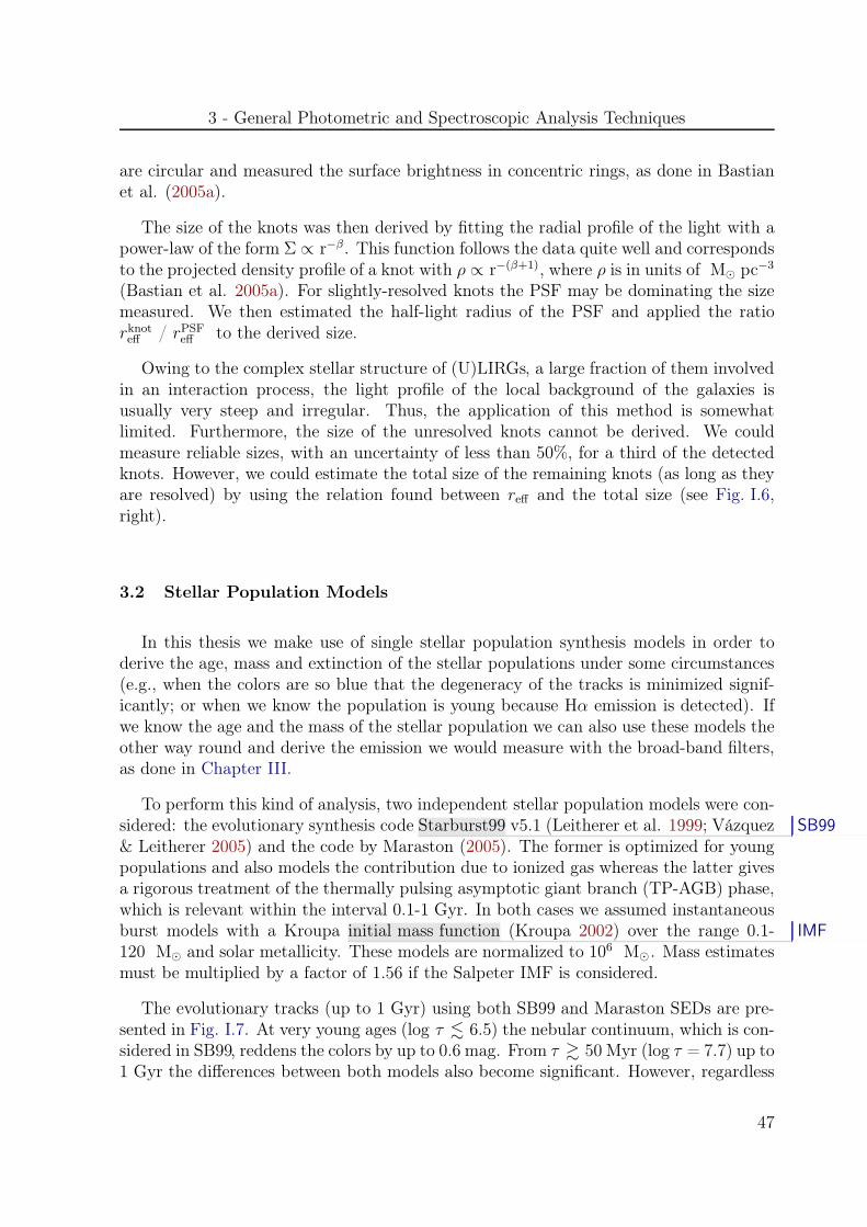
3 - General Photometric and Spectroscopic Analysis Techniques
are circular and measured the surface brightness in concentric rings, as done in Bastianet al. (2005a).
The size of the knots was then derived by fitting the radial profile of the light with apower-law of the form Σ ∝ r−β. This function follows the data quite well and correspondsto the projected density profile of a knot with ρ ∝ r−(β+1), where ρ is in units of M⊙ pc−3
(Bastian et al. 2005a). For slightly-resolved knots the PSF may be dominating the sizemeasured. We then estimated the half-light radius of the PSF and applied the ratiorknoteff / rPSFeff to the derived size.
Owing to the complex stellar structure of (U)LIRGs, a large fraction of them involvedin an interaction process, the light profile of the local background of the galaxies isusually very steep and irregular. Thus, the application of this method is somewhatlimited. Furthermore, the size of the unresolved knots cannot be derived. We couldmeasure reliable sizes, with an uncertainty of less than 50%, for a third of the detectedknots. However, we could estimate the total size of the remaining knots (as long as theyare resolved) by using the relation found between reff and the total size (see Fig. I.6,right).
3.2 Stellar Population Models
In this thesis we make use of single stellar population synthesis models in order toderive the age, mass and extinction of the stellar populations under some circumstances(e.g., when the colors are so blue that the degeneracy of the tracks is minimized signif-icantly; or when we know the population is young because Hα emission is detected). Ifwe know the age and the mass of the stellar population we can also use these models theother way round and derive the emission we would measure with the broad-band filters,as done in Chapter III.
To perform this kind of analysis, two independent stellar population models were con-sidered: the evolutionary synthesis code Starburst99 v5.1 (Leitherer et al. 1999; Vázquez SB99
& Leitherer 2005) and the code by Maraston (2005). The former is optimized for youngpopulations and also models the contribution due to ionized gas whereas the latter givesa rigorous treatment of the thermally pulsing asymptotic giant branch (TP-AGB) phase,which is relevant within the interval 0.1-1 Gyr. In both cases we assumed instantaneousburst models with a Kroupa initial mass function (Kroupa 2002) over the range 0.1- IMF
120 M⊙ and solar metallicity. These models are normalized to 106 M⊙ . Mass estimatesmust be multiplied by a factor of 1.56 if the Salpeter IMF is considered.
The evolutionary tracks (up to 1 Gyr) using both SB99 and Maraston SEDs are pre-sented in Fig. I.7. At very young ages (log τ . 6.5) the nebular continuum, which is con-sidered in SB99, reddens the colors by up to 0.6 mag. From τ & 50 Myr (log τ = 7.7) up to1 Gyr the differences between both models also become significant. However, regardless
47

Chap. I Sample Selection, Dataset and Data Treatment
-1 0 1 2 3MF435W - MF814W
-10
-11
-12
-13
-14
-15
-16
MF
814W
AV=1
marastonsb99
-1 0 1 2 3MF435W - MF814W
-10
-11
-12
-13
-14
-15
-16
MF
435W
AV=1
Figure I.7: Color-magnitude diagrams according to the SB99 and the Maraston single stelarpopulation models. The curves are normalized to 106 M⊙ . Filled circles, stars and trianglesindicate the age in the SB99 track in steps of 1 Myr (from 1 to 9 Myr), 10 Myr (from 10 to 90Myr) and 100 Myr (from 100 to 1000 Myr), respectively. Open symbols show the same for theMaraston tracks. The de-reddening vector (AV = 1 mag), computed using the curve of Calzettiet al.(2000), is shown in both plots.
of the model used, the degeneracy in color within the range MF435W -MF814W = 0.6-1.4 isconsiderable for two reasons: stellar populations with ages within the interval 50-500 Myrhave the sameMF435W -MF814W color in the range 0.6-0.8; the Red Super Giant populationreddens the tracks at ages τ ∼ 7-14 Myr, when this population dominates the luminosity,hence making it indistinguishable from a population of up to τ ∼ 1 Gyr. Consideringthis, there is a clear age degeneracy for the color interval MF435W -MF814W = 0.6-1.4.Since the mass-to-light ratio (M/L) depends on the age of the population, this age de-generacy translates into an uncertainty of about a factor of 100 in the mass estimates.Hence, although the ignorance of the extinction contributes as well, the age degeneracyrepresents the primary source of uncertainty.
If we have access to spectroscopic measurements, we can use the SB99 models toconstrain the properties of recent episodes of star formation. It is widely known thatHα emission can be used to constrain the properties of recent episodes of star forma-tion. In fact, if the population for which we want to estimate the mass is young (i.e.,τ < 10 Myr), the Hα emission line and its equivalent width are generally used to con-EW
48
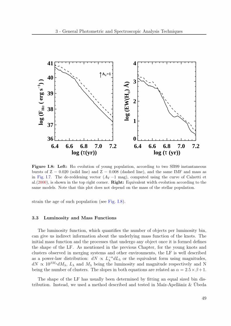
3 - General Photometric and Spectroscopic Analysis Techniques
6.4 6.6 6.8 7.0 7.2log (τ(yr))
36
37
38
39
40
41
log
(FH
α (
erg
s−1 )
)
AV=1
6.4 6.6 6.8 7.0 7.2log (τ (yr))
0
1
2
3
4
log
(EW
(Hα)
Å)
Figure I.8: Left: Hα evolution of young population, according to two SB99 instantaneousbursts of Z = 0.020 (solid line) and Z = 0.008 (dashed line), and the same IMF and mass asin Fig. I.7. The de-reddening vector (AV =1 mag), computed using the curve of Calzetti etal.(2000), is shown in the top right corner. Right: Equivalent width evolution according to thesame models. Note that this plot does not depend on the mass of the stellar population.
strain the age of such population (see Fig. I.8).
3.3 Luminosity and Mass Functions
The luminosity function, which quantifies the number of objects per luminosity bin,can give us indirect information about the underlying mass function of the knots. Theinitial mass function and the processes that undergo any object once it is formed definesthe shape of the LF. As mentioned in the previous Chapter, for the young knots andclusters observed in merging systems and other environments, the LF is well describedas a power-law distribution: dN ∝ L−α
λ dLλ or the equivalent form using magnitudes,dN ∝ 10βMλdMλ, Lλ and Mλ being the luminosity and magnitude respectively and Nbeing the number of clusters. The slopes in both equations are related as α = 2.5×β+1.
The shape of the LF has usually been determined by fitting an equal sized bin dis-tribution. Instead, we used a method described and tested in Maíz-Apellániz & Úbeda
49
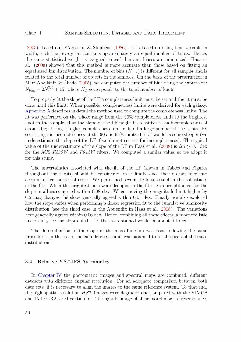
Chap. I Sample Selection, Dataset and Data Treatment
(2005), based on D’Agostino & Stephens (1986). It is based on using bins variable inwidth, such that every bin contains approximately an equal number of knots. Hence,the same statistical weight is assigned to each bin and biases are minimized. Haas etal. (2008) showed that this method is more accurate than those based on fitting anequal sized bin distribution. The number of bins (Nbins) is different for all samples and isrelated to the total number of objects in the samples. On the basis of the prescription inMaíz-Apellániz & Úbeda (2005), we computed the number of bins using the expression:Nbins = 2N
2/5C + 15, where NC corresponds to the total number of knots.
To properly fit the slope of the LF a completeness limit must be set and the fit must bedone until this limit. When possible, complenetness limits were derived for each galaxy.Appendix A describes in detail the method used to compute the completeness limits. Thefit was performed on the whole range from the 90% completeness limit to the brightestknot in the sample, thus the slope of the LF might be sensitive to an incompleteness ofabout 10%. Using a higher completeness limit cuts off a large number of the knots. Bycorrecting for incompleteness at the 90 and 95% limits the LF would become steeper (weunderestimate the slope of the LF if we do not correct for incompleteness). The typicalvalue of the underestimate of the slope of the LF in Haas et al. (2008) is ∆α . 0.1 dexfor the ACS F435W and F814W filters. We computed a similar value, so we adopt itfor this study.
The uncertainties associated with the fit of the LF (shown in Tables and Figuresthroughout the thesis) should be considered lower limits since they do not take intoaccount other sources of error. We performed several tests to establish the robustnessof the fits. When the brightest bins were dropped in the fit the values obtained for theslope in all cases agreed within 0.08 dex. When moving the magnitude limit higher by0.5 mag changes the slope generally agreed within 0.05 dex. Finally, we also exploredhow the slope varies when performing a linear regression fit to the cumulative luminositydistribution (see the third case in the Appendix in Haas et al. 2008). The variationshere generally agreed within 0.06 dex. Hence, combining all these effects, a more realisticuncertainty for the slopes of the LF that we obtained would be about 0.1 dex.
The determination of the slope of the mass function was done following the sameprocedure. In this case, the completeness limit was assumed to be the peak of the massdistribution.
3.4 Relative HST -IFS Astrometry
In Chapter IV the photometric images and spectral maps are combined, differentdatasets with different angular resolution. For an adequate comparison between bothdata sets, it is necessary to align the images to the same reference system. To that end,the high spatial resolution HST images were degraded and compared with the VIMOSand INTEGRAL red continuum. Taking advantage of their morphological resemblance,
50
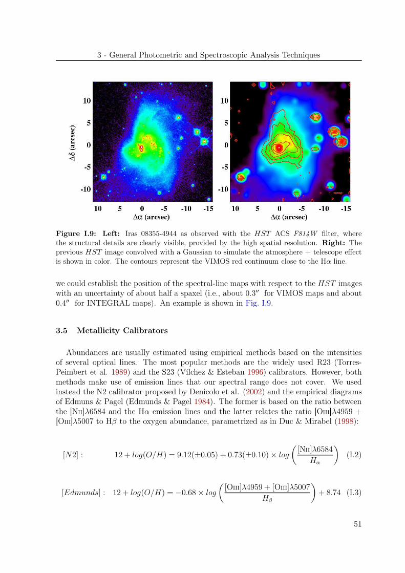
3 - General Photometric and Spectroscopic Analysis Techniques
Figure I.9: Left: Iras 08355-4944 as observed with the HST ACS F814W filter, wherethe structural details are clearly visible, provided by the high spatial resolution. Right: Theprevious HST image convolved with a Gaussian to simulate the atmosphere + telescope effectis shown in color. The contours represent the VIMOS red continuum close to the Hα line.
we could establish the position of the spectral-line maps with respect to the HST imageswith an uncertainty of about half a spaxel (i.e., about 0.3′′ for VIMOS maps and about0.4′′ for INTEGRAL maps). An example is shown in Fig. I.9.
3.5 Metallicity Calibrators
Abundances are usually estimated using empirical methods based on the intensitiesof several optical lines. The most popular methods are the widely used R23 (Torres-Peimbert et al. 1989) and the S23 (Vílchez & Esteban 1996) calibrators. However, bothmethods make use of emission lines that our spectral range does not cover. We usedinstead the N2 calibrator proposed by Denicolo et al. (2002) and the empirical diagramsof Edmuns & Pagel (Edmunds & Pagel 1984). The former is based on the ratio betweenthe [NII]λ6584 and the Hα emission lines and the latter relates the ratio [OIII]λ4959 +[OIII]λ5007 to Hβ to the oxygen abundance, parametrized as in Duc & Mirabel (1998):
[N2] : 12 + log(O/H) = 9.12(±0.05) + 0.73(±0.10)× log
(
[NII]λ6584
Hα
)
(I.2)
[Edmunds] : 12 + log(O/H) = −0.68 × log
(
[OIII]λ4959 + [OIII]λ5007
Hβ
)
+ 8.74 (I.3)
51
Chap. I Sample Selection, Dataset and Data Treatment
Given the spectral range of the VIMOS data, metallicity determinations were onlypossible using the N2 calibrator for systems observed with this instrument. The typ-ical uncertainties of the determined metallicities are about 0.2 dex. For the galaxiesobserved with INTEGRAL, given these uncertainties, the differences between both indi-cators (usually within 0.2 dex) are not relevant, and thus we adopted the average valueof both determinations.
3.6 Mass Determinations
3.6.1 Stellar Masses
The flux measured with broad-band filters is usually used for mass determinations ofstellar populations. In this study, however, only two filters are used and degeneracy issuescan make these estimates very much uncertain. However, under some circumstances (i.e.,MF435W -MF814W < 0.5) a first-order estimate of the age of an instantaneous burst can beachieved, according to the SB99 models (see Fig. I.7 in Section 3.2). Assuming a singleburst, once the age of the stellar population is known, the mass-to-light ratio (M/L)given by the models is used to derive the stellar mass of the population that dominatesthe broad-band emission (in our case under the assumption that only one populationdominates such emission).
As mentioned in Section 3.2, the Hα emission can be used to constrain the propertiesof recent episodes of star formation (see Fig. I.8). Alghough the EW does not dependon the mass of the population and is not affected by internal extinction, an underlyingold population which does not contribute significantly to the broad-band filters (i.e., theACS F435W and F814W ), if considerably more massive than the young population(i.e., more massive than one order of magnitude), can affect the Hα continuum andconsequently the value of the measured EW. Therefore, the age determined by using theEW is normally assumed to be an upper-limit to the real age of the young componentin a hypothetical case of a composite stellar population (young and old). As in the caseof using only broad-band filters, once the age is known, the mass-to-light ratio given bythe models is applied to derive the young stellar mass of the population.
3.6.2 Dynamical Masses
The difference between dynamical (i.e., stars + gas + dark matter) and stellar massesrelies on the fact that the first is derived taking into account the gravitational field,
52

3 - General Photometric and Spectroscopic Analysis Techniques
whereas the latter is obtained based on the integrated light assuming a mass-to-light ratio.The dynamical mass of a bound system can be derived using the virial theorem, under thefollowing assumptions: (i) the system is spherically symmetric; (ii) it is gravitationallybound; and (iii) it has an isotropic velocity distribution [σ2(total)=3×σ2
LOS], where σLOS
is the line-of-sight velocity dispersion.
Assuming virialization, the dynamical of a stellar system is given by two parameters:its velocity dispersion (σ) and its half mass radius (rhm). Depending on the object understudy (cluster- or galaxy-like) different relations are typically used:
Mdyn/M⊙ = m106rhm × σ2 (I.4)
Mdyn/M⊙ = ηreff × σ2
LOS
G(I.5)
Equation I.4 is generally used for galaxy-/ellipsoidal-like objects. The parameter rhmis given in kpc, σ in km s−1 and the factor m is a dimensionless function of the assumedmass distribution and ranges from 1.4 for a King stellar mass distribution that adequatelyrepresents ellipticals (Bender et al. 1992; Tacconi et al. 2002) to 1.75 for a polytropicsphere with a density index covering a range of values (Spitzer 1987) and 2.09 for a deVaucoluleurs mass distribution (Combes et al. 1995).
Equation I.5 is generally used for cluster-like objects. Here, reff is given in pc, σLOS
in km s−1 and the gravitational constant G=4.3×10⁻³ pc M⊙−1 (km s−1)2 (Spitzer
1987) and η = 9.75 for a wide range of light profiles. However, some studies have shownthat η is not a constant, and can vary with time (η ∼ 3− 10), depending on, for exam-ple, the degree of mass segregation and the binary fraction of the cluster (Fleck et al.2006; Kouwenhoven & de Grijs 2008). Since we do not have that information we useη = 9.75.
The half-mass radius is not an observable and cannot be measured directly. It hasto be inferred indirectly by measuring the half-light radius (reff ). The broadening ofthe emission lines is produced by a few fundamental effects, as described by Melnick etal. (1999): mainly thermal broadening, virial broadening, natural broadening and localdynamical effects as expanding shells, filaments and outflows. Once the widths of theprincipal components (σobs) were measured and corrected for instrumental broadening(σins), additional corrections had to be applied for natural (σn) and thermal (σth) broad-ening to obtain what we denote as the virial width according to the following relation:
σ =√
σ2obs − σ2
n − σ2th − σ2
ins (I.6)
53
Chap. I Sample Selection, Dataset and Data Treatment
The natural broadening is a constant for hydrogen and corresponds to 3 kms−1 (O’dell& Townsley 1988; Rozas et al. 2006a). For HII regions with temperatures of 5000 K,10000 K, and 15000 K, Osterbrock (1989) provides Doppler widths of σth = 6.4, 9.1, and11.1 kms−1, respectively. In the absence of the temperature information for our sample,a uniform value of σth = 9.1 kms−1 was adopted. Given the uncertainties of σobs (higherthan 5-10 kms−1 in our case), the ignorance of the temperature is not worrisome.
54

Chapter II
Optically-selected CompactStar-Forming Regions in (U)LIRGs
Overview
This Chapter presents a comprehensive characterization of thegeneral properties (luminosity functions, mass, size, ages, etc)of optically-selected compact stellar objects (knots) in a rep-resentative sample of 32 low-z Luminous and UltraluminouosInfrared Galaxies. These properties are important to under-stand their formation and evolution in these systems, whichrepresent the most extreme cases of starbursts in the low-zUniverse. Specifically, we investigate how they depend on theinfrared luminosity of the system and on the interaction phaseit is undergoing. We also investigate how similar these knotsare to clumpy structures in galaxies at high-z.
1 Introduction
The observation of young and massive compact clusters in different environments(e.g., Meurer et al. 1995; Larsen & Richtler 1999; Whitmore et al. 1999, 2007; Weilbacheret al. 2000; Gallagher et al. 2010; Mullan et al. 2011) has provided important clues tounderstand the formation and evolutionary processes in interacting systems. With massesof 104− 106 M⊙ and a median size in terms of effective radius around 3.5 pc, their lightfollow the same luminosity function (LF ) in the optical in a wide range of galacticenvironments, a power-law (ψ(L)dL ∝ L−αdL) with an index of α = 2. Yet, there issome controversy, since the range is rather large depending on the study (see GeneralIntroduction, Section 2.1). These clusters associate in star-forming complexes, whichrepresent the largest units of star formation in a galaxy (Efremov 1995). The observationof these objects (e.g., Whitmore et al. 1999; Bastian et al. 2005a) has provided a deeper
55

Chap. II Optically-selected Compact Star-Forming Regions in (U)LIRGs
knowledge on the hierarchy of the star formation in embedded groupings.
Although much effort has been made to understand the star formation and evolu-tionary processes in interacting systems, little is known for Luminous (LIRGs) and Ul-traluminous (ULIRGs) Infrared Galaxies, which represent the most extreme cases ofstarbursts and interactions in our nearby Universe. Given the significant contributionof these galaxies to the star formation rate density at z ∼ 1-2 (Pérez-González et al.2005; Caputi et al. 2007) and their resemblance with sub-millimeter galaxies at higherredshifts (Smail et al. 1997; Blain et al. 2002; Frayer et al. 2004), their properties canalso have important cosmological implications. They are natural laboratories for probinghow star formation is affected by major rearrangements in the structure and kinematicsof galactic disks. Establishing the general properties (luminosity functions, mass, size,ages, etc) of the compact stellar objects in (U)LIRGs as a function of luminosity and in-teraction phase can provide relevant information in order to understand the mechanismsthat govern the star formation and evolution in these systems. It is not known eitherwhether the processes that (U)LIRGs undergo produce stellar objects similar or verydifferent in terms of size or luminosity than in less luminous (non-) interacting galaxies.
In fact, previous studies of compact stellar structures in (U)LIRGs were focused onlyon small samples, mostly with low angular resolution ground-based imaging (Suraceet al. 1998; Surace et al. 2000), or on detailed multi-frequency studies of compact stellarobjects in individual galaxies (Surace et al. 2000; Díaz-Santos et al. 2007). Thus, nostudy has been done so far on a representative sample of luminous infrared galaxiescovering the different phases of the interaction process as well as the entire LIRG andULIRG luminosity range.
This Chapter presents the first attempt at obtaining an homogeneous and statisticallysignificant study of the photometric properties (magnitudes, colors, sizes and luminosityfunction) of optically-selected compact stellar objects found in these systems as a functionof infrared luminosity, morphology (i.e., interaction phase) and radial distance to thenucleus of the galaxy. For this study we make use of the photometric B - and I -bandACS images (Chapter I, Section 2.1) of the representative 32 (U)LIRGs that compriseour sample (Chapter I, Section 1.1). The detected stellar objects, some of them identifiedas Super Star Cluster candidates for the closest galaxies (i.e., at DL . 60 Mpc) and mostof them as cluster complexes further away, will be referred to as “knots”.
Specifically, the Chapter is organized as follows: we first describe the procedure fol-lowed to detected the knots under study in Section 2; we then characterize the bias thatwe will encounter throughout the Chapter caused by the distribution of distances of thegalaxies in our sample, distance effects, in Section 3; in Section 4 the main photometricproperties of the identified knots are presented; next, we characterize these properties asa function of the infrared luminosity of the system in Section 5; the characterization as afunction of the interaction phase is developed in Section 6; Section 7 compares the prop-erties of the detected knots with star-forming clumps in high-z galaxies; finally, Section 8gives a brief summary of the most relevant results and the main conclusions.
56

2 - Source Detection and Photometry
2 Source Detection and Photometry
Compact regions with high surface brightness (knots hereafter) that are usually bluerthan the underlying galaxy were identified for each galaxy. They were detected in-side a box that encloses each system including the diffuse emission observed in the redband. They appear similar to the bright blue knots found in interacting galaxies likein NCG 7252 (Whitmore et al. 1993), NGC 4038/39 (Whitmore & Schweizer 1995),some ULIRGs (Surace et al. 1998), M51 (Bik et al. 2003; Lee et al. 2005 and Arp284(Peterson et al. 2009). These knots were identified on the basis of having a flux abovethe 5σ detection level of the local background. Owing to the irregular and distortedmorphologies for most of the systems, we performed a two step analysis to identify thecompact regions: we first smoothed the image, averaging in a box of 30x30 pixels, andsubtracted this smoothed image from the original one in order to make a first roughlocal background subtraction; we then ran SExtractor (Bertin & Arnouts 1996) on theresulting image to detect the knots. Given the steepness of the light profile of the localbackground in the inner regions and its larger deviation with respect to outer regions,an appropriate background subtraction was not always possible and some inner knotswere never detected. Thus, visual inspection was needed afterward to include some innerknots and also to eliminate some spurious detections.
Once the knots were detected, all photometric measurements were done using thetasks PHOT and POLYPHOT within the IRAF (Tody 1993) environment. We firstidentified the point-like sources against the extended ones, since the photometry of theformer requires aperture corrections. We fitted the knots with a Moffat profile, andthose with a FWHM . 1.5×FHWM the profile of the stars in the field were consideredas point-like knots. Note that although they actually consist of point-like and slightlyresolved objects, they are considered as point-like objects here just to assign an apertureradius, since both require aperture corrections when the photometry is done. Once theirsize was derived via psf fitting (see Chapter I, Section 3.1) we differentiated betweenresolved and unresolved knots.
Aperture photometry with a 3 pixel aperture radius (0.15′′) was performed for thepoint-like knots. For the resolved knots, we used aperture radii between 5 and 7 pixels(0.25-0.35′′), depending on when the radial profile reached background levels. The 7-pixelapertures were large enough to include practically all the light from the knot but smallenough to avoid confusion with other sources and to avoid adding more noise to themeasurements. In some cases, the irregular shape of the knots demanded the use ofpolygonal apertures. In some cases, especially for knots belonging to the most distantgalaxies, the polygonal apertures were larger than 7 pixels. Estimates of the underlyingbackground flux were made by using the mode of flux values measured in an 8-13 pixelannulus centered on the computed centroid with POLYPHOT, and eliminating the 10%of the extreme values at each side of the flux background distribution (e.g., if there is anearby knot it adds spurious flux at the bright end of the distribution). Most of the knots
57

Chap. II Optically-selected Compact Star-Forming Regions in (U)LIRGs
are apart from each other by more than 7 pixels (0.35′′), hence confusion does not seemto be a serious problem, though in the inner regions of few systems (IRAS 04315-0840,IRAS 15206+3342 and IRAS 20550+1656) there is some overcrowding.
Photometric calibrations were performed following Sirianni et al. (2005) for theACS images and Holtzman et al. (1995) for the WFPC2 images (hereafter calibrationreference papers), and magnitudes computed in VEGA system, as explained in Chap-ter I, Section 2.1.1. Correction for charge transfer efficiency (CTE) was needed in theWFPC2 photometry but was not applied to the ACS photometry, since tests in someimages showed that the effect was less than 1% for the faintest regions identified. Aper-ture corrections were considered for the point-like knots. To that end, we performed thephotometry for isolated stars in the field (from a few to about a hundred, dependingon the image) in the same way as we did for the point-like knots, then a second timebut using a 10 pixel radius. The ratio of both values gives us an aperture correction upto 10 pixels. From 10 pixels to an infinite aperture radius the values in the calibrationreference papers were taken, since the PSF profile from 10 pixels on is stable enough re-gardless of the observing conditions. Typical aperture corrections were about 0.3 and 0.2mag for the F814W and F435W filters, respectively. Using the deviation of the differentaperture corrections computed with stars in the field we estimated the uncertainty dueto the aperture corrections to be of the order of 0.05-0.1 mag in both filters. Typicalphotometric uncertainties for all the knots lie between 0.05 and 0.15 mag, depending onthe brightness of the knot. According to the completeness test performed in Appendix A,the systematics affect both filters nearly equally, thus the typical uncertainty in color isbetween 0.10 and 0.20 mag.
We corrected all the magnitudes for reddening due to our galaxy taking the values di-rectly from the NASA/IPAC Extragalactic Database (NED), computed following Schlegelet al. (1998). Apart from this, no internal reddening corrections have been applied tothe magnitudes reported in this chapter.
Initially, we probably detected old globular clusters, super star clusters, star com-plexes, HII regions, foreground stars, background objects, etc. Some of them were rejectedafter the photometry was made. Foreground stars were mostly easily identified by theirhigh brightness and red colors and their status as point-like objects. The fields in systemsat low galactic latitudes (IRAS 08355-4944, IRAS 09022-3615 and IRAS 12116-5615) areso crowded with foreground stars that some may still contaminate the photometric sam-ple knots after rejection, especially if a faint foreground star lies within the inner regionsof the galaxy. No cluster/knot with color MF435W -MF814W & 2.2 fits in stellar populationmodels for an extinction-free starburst at redshift z ∼ 0. Since we do not expect muchextinction in the outer parts of the galaxies (usually where we do not see diffuse emissionfrom the galaxy in the red band), all the red knots outside the diffuse emission of thesystems are likely to be background objects and were also rejected. After these rejectionsa total of 2961 knots were considered under study.
The nuclei of the systems were identified using the H -band images and with the
58

3 - Distance Dependence of the Photometric Properties
−18 −14 −10 MF814W
0.00
0.05
0.10
0.15
Fra
ctio
n
N=1360
< MF814W > =−11.36
α=1.71±0.04
−1 0 1 2 3 4 5MF435W − MF814W
0.00
0.05
0.10
0.15
0.20< MF435W − MF814W > =1.13
−− Systems at < DL > = 99 Mpc −−
0 100 200 300 400r eff
F814W
0.0
0.1
0.2
0.3
0.4< reff
F814W > = 25 pc
−18 −14 −10 MF814W
0.00
0.05
0.10
0.15
Fra
ctio
n
N=839
< MF814W > =−12.45
α=1.56±0.03
−1 0 1 2 3 4 5MF435W − MF814W
0.00
0.05
0.10
0.15
0.20< MF435W − MF814W > =1.12
−− Simulated systems at < DL > = 258 Mpc −−
0 100 200 300 400r eff
F814W
0.0
0.1
0.2
0.3
0.4< reff
F814W > = 78 pc
Figure II.1: Photometric properties for real (top) and simulated (bottom) data. The medianvalues (between brackets < > throughout the chapter) of the magnitude, color and reff distri-butions are shown. The slope of the LF for the magnitude distributions is also presented (α).Throughout the Chapter N represents the number of detected knots in any given distribution.
aid of other works that have detected them in radio (e.g., Dinshaw et al. 1999). Theidentification of the true nucleus is of relevance in the derivation of the projected distancesof the knots with respect to the closest nucleus, to properly study the spatial distributionof these knots.
3 Distance Dependence of the Photometric Properties
Before going any further, we first consider a selection effect that we can encounterwhen studying the photometric properties of the knots in (U)LIRGs located at differentdistances. The classical Malmquist bias is caused by the fact that systematically brighterobjects are observed as distance (and volume) increases, as a result of a combination ofthe selection and the intrinsic scatter of absolute magnitudes.
Our sample is affected by this bias, since the systems are located at different distances
59
Chap. II Optically-selected Compact Star-Forming Regions in (U)LIRGs
(from 65 to 560 Mpc). As the system stands further, the faintest knots become undetectedand we can only see the bright ones. Furthermore, for the same angular resolution thespatial resolution decreases linearly with distance, and therefore the knots that we detectat large distances can consist of associations of knots instead of individual knots as thoseobserved in less distant systems. Thus, larger sizes are computed. Though this is not acomplete sample, Fig. I.1 in Chapter I shows that in general more distant galaxies havehigher infrared luminosity. The same tendency is seen if the galaxies from the IRASRevisited Galaxy Sample (RBGS, Sanders et al. 2003) are taken. This effect has to besubtracted in order to observe reliable intrinsic differences between systems at differentdistances.
We divided the sample in three LIR intervals, so as to study the dependence of the pho-tometric properties with the total infrared luminosity of the system (see Section 5). Toasses how the photometric properties depend on the distance of the system a simulationwas performed. The median distance of the low luminosity interval (LIR < 11.65) corre-sponds to 99 Mpc, whereas that of ULIRGs (the high luminosity interval) is 258 Mpc.Hence, for this sample ULIRGs are located a factor of 2.6 further away than the lowluminous LIRGs. We simulated the light emission of galaxies within the first LIR intervalas if they were a factor of 2.6 further, obtaining the same median distance as in ULIRGs.To that end, the HST images were convolved with a Gaussian at the resolution of thePSF at the new distance of each galaxy and re-binned in order to have the same “pixelsize” at that distance. Using foreground stars we computed a multiplication factor foreach image in order to preserve the flux, since the flux of the point-like objects must bepreserved. Then, photometry was carried out as in the original images, with circular andin some cases polygonal apertures.
The results of the simulation for the F814W filter are presented in Fig. II.1. Themagnitudes and the sizes increase by about 1.1 mag (a factor of 2.8 in flux) and by afactor of 3, respectively. The number of detected objects drops by about a factor of 1.6.Therefore, in the simulated image, individual knots are associations of knots from theoriginal one. As a result, not only do the sizes become larger, but its distribution alsoflattens. The median values of the reff distribution in the simulation are 25 and 78 pcfor the real and simulated knots, respectively.
The flattening of the luminosity function (from α = 1.71 to 1.56) is also expected,since as the knots are artificially grouped due to angular resolution effects the bright tailof the LF starts to get more populated. Another expected result of the simulation is thatthe color distribution does not change significantly.
If we consider the spatial distribution of the knots (inner and outer knots, with pro-jected distances of less and more than 2.5 kpc to the nucleus, respectively), some changesare also observed; the ratio of inner to outer knots shifts from 0.7 to 0.5. Owing to thehigher surface brightness and steeper background profile in the inner regions, when con-volving the images to get lower linear resolution, a large fraction of inner knots are dilutedby the local background, in contrast to a lower dilution degree in the outermost regions.
60

4 - General Properties of the Knots
Furthermore, more grouping is expected in the innermost regions, where there is morecrowding, hence also losing a larger number of inner knots when compared with thoselocated in the outer regions.
4 General Properties of the Knots
Owing to the high angular resolution and sensitivity of the ACS camera, and to thedefinition of our large sample, covering a wider LIR range than previous studies focusedonly on ULIRGs (Surace et al. 1998; Surace et al. 2000), we have detected close to3000 knots. This is more than a factor of ten larger than in previous investigations andallows us to carry out a statistical study exploring the different physical properties ofthe knots over the entire LIRG and ULIRG luminosity range. We have then performedthe photometry in both F435W and F814W filters for these knots. For this study weconsider the knots with positive detection in both filters. The objects identified as thenuclei were not, since many of them are believed to be contaminated by an AGN (seeChapter I, Table I.1, and the references regarding the spectral class).
4.1 Magnitudes and Colors. Average Values
The knots detected in our sample of luminous infrared galaxies have observedF814W and F435W absolute magnitudes (uncorrected for internal extinction) in the-20 . MF814W . -9 and -19.5 . MF435W . -7 range, respectively, while colors cover the-1 . MF435W -MF814W . 5 range (see Fig. II.2). The corresponding median magnitudesare < MF814W >=-11.96 and < MF435W >=-10.84. The median color of the knots cor-responds to < MF435W -MF814W > = 1.0, which clearly indicates the presence of a youngstellar population (about half of the knots have colors bluer than that value). By con-trast, the mean color of the diffuse local background light, which traces the old stellarpopulation in the host galaxies, is 1.72, consistent with the typical colors measured inspirals (B-I=1.80; Lu et al. 1993).
A small fraction of the knots (2% of the total) show extreme red colors(MF435W -MF814W= 3 or redder), likely tracing regions with very high internal obscu-ration, usually located in the more central regions (Alonso-Herrero et al. 2006; García-Marín et al. 2009a). If the stellar population in these knots was dominated by youngstars (i.e., τ ∼ 10 Myr), the extinction could be as high as AV = 5-7 mag. Heavily ob-scured young clusters with AV = 5-10 mag have also been detected in the optical in lessluminous interacting systems like the Antennae (e.g., clusters S1_1 and 2000_1, whoseextinction was computed with the aid of infrared spectroscopy; Mengel et al. 2008).
61

Chap. II Optically-selected Compact Star-Forming Regions in (U)LIRGs
Figure II.2: Color-magnitude diagrams for the identified knots. Top: All knots. The reddashed line indicates the median of the distribution and the gray band covers 80 % of the totalnumber of knots in each plot, rejecting the 10 % at either side of the distribution. No reddeningcorrections have been applied to the magnitudes given. A de-reddening vector of AV = 1 magis shown in the top right corner. Middle: the same diagrams for the knots in this study within2.5 kpc. Bottom: same as before but for knots further than 2.5 kpc from the closest nucleus.
62

4 - General Properties of the Knots
4.2 Magnitudes and Colors. Radial Distribution
To understand the star formation in luminous infrared galaxies, it is important toinvestigate whether the observed properties of the knots (magnitudes, colors and sizes)do show dependence on the galactocentric distance. The spatial distribution of the knotsis shown in Fig. II.3, where their sizes are related to their absolute magnitude and theircolor to the photometric color MF435W -MF814W . About one-third of the knots lie withina projected galactocentric radius of 2.5 kpc while this fraction increases up to abouttwo-thirds within a radius of 5 kpc. Thus, a substantial fraction of the knots are locatedclose to the nucleus at distances of less than 5 kpc. Also, as can be seen in the figure,they mainly represent the population with the reddest colors, likely indicative of higherinternal extinction, although an older population can not be excluded. Yet, there is alsoan external population of knots (10.8% of the total) at distances of more than 10 kpcand up to 40 kpc, located along the tidal tails and at the tip of these tails. Most ofthese external knots are blue (MF435W -MF814W < 1), and some (5.7%) are very luminous(MF435W < -12.5), suggesting the presence of young massive (M > 105 M⊙ in youngstars) objects in the outer parts of these systems. Examples of these knots can be seenat the northern tip in IRAS 23128-5919 and in IRAS 09022-3675, along the northern tailin IRAS 14348-1447, etc.
Throughout the chapter, we identify the inner sample of knots as those with pro-jected distances of less than 2.5 kpc to the closest nucleus, and the outer sample asthose with distances of at least 2.5 kpc. Both distributions have a significantly differentmagnitude and color distribution (see Fig. II.2), the inner knots being 2 mag brighter(in the F814W filter) and 0.3 mag redder than the outer knots. These two distribu-tions are different, and do not come from the same parent distribution according to theAdvanced Kolmogorov-Smirnov test (using the idl routine KSTWO; Press et al. 1992). KW
Finally, the inner knots also have a larger color dispersion with a tail toward red colors.This is likely the effect of having higher and patchier internal extinction in the innermostregions, in agreement with recent spectroscopic studies of these systems (Alonso-Herreroet al. 2006; García-Marín et al. 2009a). Additionally, the brighter blue magnitudes inthe inner regions suggest that there must be more young star formation there than inthe outer field.
4.3 Effective Radius of the Knots
The angular resolution limit (and therefore upper sizes for unresolved knots) variesfrom around 10 to 40 pc, depending on the distance to the galaxy. The detected knotsdo show a wide range of sizes ranging from unresolved (12%) to a few with very extendedsizes (a radius of 200 pc, and up to 400 pc). The median size of the resolved knots is32 pc, with about 65% of them smaller than 40 pc. This is significantly larger than thelargest knots found in other systems, and several times larger than their mean knot radii
63
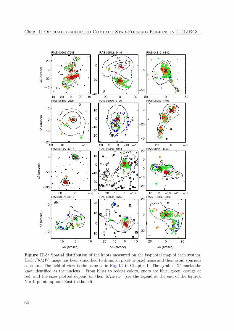
Chap. II Optically-selected Compact Star-Forming Regions in (U)LIRGs
Figure II.3: Spatial distribution of the knots measured on the isophotal map of each system.Each F814W image has been smoothed to diminish pixel-to-pixel noise and then avoid spuriouscontours. The field of view is the same as in Fig. I.2 in Chapter I. The symbol ’X’ marks theknot identified as the nucleus . From bluer to redder colors, knots are blue, green, orange orred, and the sizes plotted depend on their MF814W (see the legend at the end of the figure).North points up and East to the left.
64

4 - General Properties of the Knots
Figure II.3: - Continued
65

Chap. II Optically-selected Compact Star-Forming Regions in (U)LIRGs
Figure II.3: - Continued
M ≤ −15 M ≤ −12.5 M > −15
M ≤ −10 M > −12.5
M > −10
C ≤ 0.5
C ≤ 1.2 C > 0.5
C ≤ 2.0 C > 1.2
C > 2.0
M: M F814W
C: MF814W − MF435W
(e.g., 10 pc in Whitmore et al. 1999). Given the distances of the galaxies in the sample(from about 65 Myr to more than 500 Myr) and the resolution limit, in general the knotsidentified in our galaxies are likely aggregates of individual clusters, which would increasetheir (apparent) size. According to the simulations (see Section 3), the apparent size ofthe knots changes from an average of 25 pc to 78 pc when galaxies at an average distanceof 100 Mpc are moved at distances 2.6 times further away.
If we consider the sample of inner and outer knots, their distributions are similar(Fig. II.4), so there is no evidence of a radial dependence of the sizes at the angularresolution of our data.
66
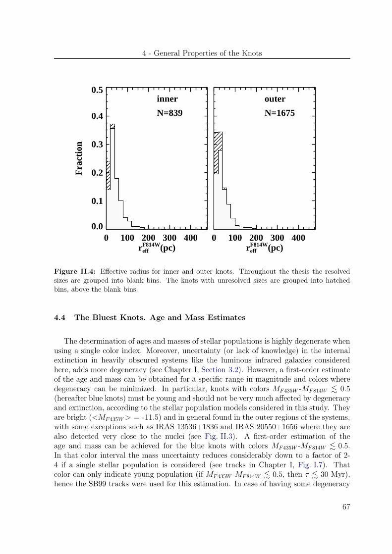
4 - General Properties of the Knots
0 100 200 300 400r eff
F814W(pc)
0.0
0.1
0.2
0.3
0.4
0.5F
ract
ion
inner
N=839
0 100 200 300 400r eff
F814W(pc)
outer
N=1675
Figure II.4: Effective radius for inner and outer knots. Throughout the thesis the resolvedsizes are grouped into blank bins. The knots with unresolved sizes are grouped into hatchedbins, above the blank bins.
4.4 The Bluest Knots. Age and Mass Estimates
The determination of ages and masses of stellar populations is highly degenerate whenusing a single color index. Moreover, uncertainty (or lack of knowledge) in the internalextinction in heavily obscured systems like the luminous infrared galaxies consideredhere, adds more degeneracy (see Chapter I, Section 3.2). However, a first-order estimateof the age and mass can be obtained for a specific range in magnitude and colors wheredegeneracy can be minimized. In particular, knots with colors MF435W -MF814W . 0.5(hereafter blue knots) must be young and should not be very much affected by degeneracyand extinction, according to the stellar population models considered in this study. Theyare bright (<MF435W> = -11.5) and in general found in the outer regions of the systems,with some exceptions such as IRAS 13536+1836 and IRAS 20550+1656 where they arealso detected very close to the nuclei (see Fig. II.3). A first-order estimation of theage and mass can be achieved for the blue knots with colors MF435W -MF814W . 0.5.In that color interval the mass uncertainty reduces considerably down to a factor of 2-4 if a single stellar population is considered (see tracks in Chapter I, Fig. I.7). Thatcolor can only indicate young population (if MF435W -MF814W . 0.5, then τ . 30 Myr),hence the SB99 tracks were used for this estimation. In case of having some degeneracy
67
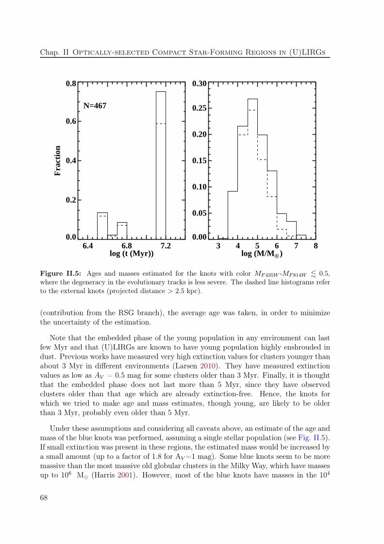
Chap. II Optically-selected Compact Star-Forming Regions in (U)LIRGs
6.4 6.8 7.2 log (t (Myr))
0.0
0.2
0.4
0.6
0.8
Fra
ctio
n
N=467
3 4 5 6 7 8log (M/M O • )
0.00
0.05
0.10
0.15
0.20
0.25
0.30
Figure II.5: Ages and masses estimated for the knots with color MF435W -MF814W . 0.5,where the degeneracy in the evolutionary tracks is less severe. The dashed line histograms referto the external knots (projected distance > 2.5 kpc).
(contribution from the RSG branch), the average age was taken, in order to minimizethe uncertainty of the estimation.
Note that the embedded phase of the young population in any environment can lastfew Myr and that (U)LIRGs are known to have young population highly enshrouded indust. Previous works have measured very high extinction values for clusters younger thanabout 3 Myr in different environments (Larsen 2010). They have measured extinctionvalues as low as AV = 0.5 mag for some clusters older than 3 Myr. Finally, it is thoughtthat the embedded phase does not last more than 5 Myr, since they have observedclusters older than that age which are already extinction-free. Hence, the knots forwhich we tried to make age and mass estimates, though young, are likely to be olderthan 3 Myr, probably even older than 5 Myr.
Under these assumptions and considering all caveats above, an estimate of the age andmass of the blue knots was performed, assuming a single stellar population (see Fig. II.5).If small extinction was present in these regions, the estimated mass would be increased bya small amount (up to a factor of 1.8 for AV =1 mag). Some blue knots seem to be moremassive than the most massive old globular clusters in the Milky Way, which have massesup to 106 M⊙ (Harris 2001). However, most of the blue knots have masses in the 104
68

4 - General Properties of the Knots
to few 106 M⊙ range, similar to those of giant HII regions and brightest Young MassiveClusters in other less luminous interacting galaxies (e.g., Bastian et al. 2005b; Whitmoreet al. 1999; Mengel et al. 2008; Konstantopoulos et al. 2009). Complexes of less massivestar clusters can also constitute these blue knots.
It is interesting to mention that the blue knots in the outermost regions (i.e.,d > 2.5 kpc) represent the 80% of the total number, while most of the star forma-tion is likely to be occurring within the central regions of the galaxies, as mentionedin Section 4.2. This suggests that in general in the outermost regions the dust extinctionis very low in (U)LIRGs. Hence, the most obscured knots must be located close to thenuclei, as mentioned in the previous section and in agreement with recent spectroscopicstudies of these systems (Alonso-Herrero et al. 2006; García-Marín et al. 2009a). Part ofthe difference between the number of blue knots in the inner and outer regions may alsobe caused by a stronger disruption process in the central regions, as claimed by Haas etal. (2008), as well as by different histories of star formation of the knots in both fields.
The number of blue knots with estimated masses higher than 106 M⊙ (∼ 10%) dropsrapidly in the external areas (the dashed line histogram in Fig. II.5). Hence, the mostmassive young knots are also located close to the nuclei. Nevertheless, there are still somefew knots in the outskirts of the galaxies as massive as 106-107 M⊙ in young stars. Somecontribution in mass of older population and gas would easily boost their mass to thetypical dynamical mass of a dwarf galaxy (107-109 M⊙). Hence, the presence of suchknots is very promising in the field of Tidal Dwarf Galaxies and the main motivation forsearching and characterizing these kind of objects in (U)LIRGs, as done in Chapter IV.
4.5 Mass-radius Relation of the Bluest Knots
In general, the knots represent associations of star clusters created in clumps. Asingle giant molecular cloud (GMC ) does not usually produce a single star cluster, buta complex of star clusters (Elmegreen & Elmegreen 1983; Bastian et al. 2005a). Thus,it is interesting to see how these complexes fit into the hierarchy of star formation bysearching for a relation between the mass and the radius of the knots. This can be donefor the bluest knots, for which an estimation of the mass with an uncertainty of lessthan a factor of 4 was achieved (Section 4.4). Their radius was derived as explained inChapter I, Section 3.1. We could obtain reliable measurements of both values for a totalof 294 knots, which is about a 10% of the total number of knots or about two-thirds ofthe total number of blue knots.
The surface brightness profile of the bluest knots is well fitted by a power-law withindex β = 0.37 ± 0.33, which corresponds to (assuming sphericity) a three dimensionaldensity profile of ρ ∝ rβ, with β = 1.37. This power-law profile is similar to that observedfor GMCs associated with high-mass star-forming regions (β = 1.6 ± 0.3; Pirogov 2009).The similarity between the profiles in GMCs and the subsample of bluest knots suggests
69

Chap. II Optically-selected Compact Star-Forming Regions in (U)LIRGs
1.5 2.0 2.5 3.0log (radius/pc)
3
4
5
6
7
8
log
(M/M
O • )
γ=1.91±0.14
Figure II.6: The mass vs. radius relation for knots in (U)LIRGs. The solid red line is apower-law fit to the data, with index γ. The typical uncertainty associated with the data isshown in the right bottom corner.
that the amount of luminous material formed is proportional to the gas density. Ob-viously, measurements of the gas in molecular clouds in (U)LIRGs are needed to provethis.
Although with high dispersion, the bluest knots follow a mass-radius relation(see Fig. II.6). We fitted a function of the form M ∝ Rγ , with index γ = 1.91 ± 0.14.The size and the mass of GMCs in the Milky Way are also related, Mcloud ∝ R2
cloud, asa consequence of virial equilibrium (Solomon et al. 1987). This relation has also beenfound for extragalactic GMCs (e.g., Ashman & Zepf 2001; Bastian et al. 2005a). Ourresult is therefore consistent with the bluest knots having the same mass-radius relationas GMCs in general, contrary to what is measured for individual young star clusters (e.g.,Bastian et al. 2005b). An offset between both relations can be used to estimate the starformation efficiency within the cloud, as done in Bastian et al. (2005a). Data from theALMA observatory, which will be able to reach sub-arcsecond resolution, will permit theachivement of this estimation for (U)LIRG systems.
70

4 - General Properties of the Knots
4.6 Luminosity Function of the Knots in the Closest Systems
The large number of detected knots allows us to study their luminosity function andcompare it with that for other less luminous and/or interacting galaxies. However, thiscomparison should be restricted to the closest (U)LIRGs, since given the sizes measuredcomplexes of star clusters are detected only for galaxies located at distances larger than100 Mpc with the resolution of the ACS. Although many knots detected in our closestsystems may still consist of complexes of star clusters, in order to minimize distanceeffects (see Section 3) we focus here on a subsample that comprises the seven systemscloser to this distance (see specific distances in Chapter I, Table I.1).
To compute the slope of the LF for the knots in both the blue and red filters (asexplained in Chapter I, Section 3.3), we assigned a lower limit cutoff to the brightestvalue of the 90% completeness limit in order to ensure the same level of completeness forthe whole subsample. The single power-law fits to our blue and red luminosity functionsare not significantly different, with slopes of α = 1.95 and α = 1.89 for the F435W (blue)and the F814W (red) filters, respectively (see Fig. II.7).
The slopes in this study are in disagreement with the much flatter slopes previouslymeasured in ULIRGs (Surace et al. 1998). Surace and coworkers argued that the flat-tening of the slope is the artificial consequence of not resolving individual clusters, butassociations of clusters (the bright end is overpopulated), the same bias that we en-counter but more severe. In addition, other factors could contribute to the flattening ofthe LF in that study, as well as in other works (see Table II.1): (i) the slopes are notcorrected for incompleteness (like in NGC 7252 in Miller et al. 1997 and NGC 4038/39in Whitmore et al. 1999), (ii) the statistics are more limited, since the distribution of lessthan 90 knots is fitted within their completeness limit interval, and (iii) ACS imaging ismore sensitive than WFPC2, and since we are observing closer systems, the LF can bemeasured to intrinsically fainter magnitudes.
The slopes measured for our subsample are however similar to those obtained forother less luminous interacting galaxies such as in NGC 4038/39, NGC 3921, NGC 7252and Arp 284 (see Table II.1). As the studies start to resolve individual clusters andcorrections for incompleteness are applied the slopes tend to consolidate around a valueof 2-2.2. For instance, reff (between 5 or unresolved, and 50 pc) derived in early studies(Whitmore & Schweizer 1995) for clusters in NGC 4038/39, indicate that some blendingexisted and thus the slope of the LF is somewhat flatter than in more recent studieswhich detect only individual clusters and corrections for incompleteness are applied aswell (Whitmore et al. 1999,2010); see values in Table II.1. In any case, we did notexpected noticeable flattening of the slope, since the mass function of molecular cloudsin the Local Group (Blitz et al. 2007) and in different ISM models (Fleck 1996; Wadaet al. 2000; Elmegreen 2002) is consistent with a slope of index 2, like the mass functionfor clusters in interacting systems (e.g., Bik et al. 2003; Gieles 2009a). This similaritycan be reflected in the LF. Given the fact that several clusters can be formed from a
71

Chap. II Optically-selected Compact Star-Forming Regions in (U)LIRGs
−16 −14 −12 −10 −8MF435W
0
1
2
3
log
(dN
/dM
λ )
α=1.95±0.02
−16 −14 −12 −10 −8MF814W
α=1.89±0.04
Figure II.7: Luminosity functions for the knots identified in both the red and the blue filters forthe subsample of (U)LIRGs closer than 100 Mpc. The line shows the fit up to the completenesslimit computed for each filter.
single molecular cloud, if there is not much blending (like in our case of nearby systems),a similar slope of the LF is expected.
Therefore, the result obtained in this study extends the universality of the slope ofthe luminosity function regardless of the intensity of the star formation in interactinggalaxies, to extreme star-forming systems like the luminous and ultraluminous infraredgalaxies, at least for systems closer than 100 Mpc.
5 Properties of the Knots as a Function of Infrared Luminosity
For most (U)LIRGs the infrared luminosity comes mainly from the re-emission bydust of light emitted in intense episodes of star formation. In this study we span arange of a factor of 15 in infrared luminosities from LIR = 11.39 to LIR = 12.54. Toinvestigate whether the properties of the star-forming knots do show dependence on theinfrared luminosity (i.e., star formation rate), we divided the initial sample into threeLIR intervals. We aim at covering the low, intermediate and high luminosity regimeswhile preserving a similar number of systems per luminosity bin for the subsequent
72

5 - Properties of the Knots as a Function of Infrared Luminosity
Table II.1: Slopes of the LF computed for this work and for other interactingsystems
Galaxy DL (Mpc) Band α Uncertainty Ref.(1) (2) (3) (4) (5) (6)
ULIRGs Surace 422 I 1.39 0.08 [1]NGC 3921 84.5 V 2.10 0.30 [2]Nearby (U)LIRGs 72.8 B,I 1.95,1.89 0.02,0.04 This work*NCG 7252 62.2 V 1.84 0.06 [3]Arp 284 33.6 I 2.30 0.30 [4]NGC 4038/39 27.5 V 1.78 0.05 [5]NGC 4038/39a 27.5 V 2.01 0.11 [6]NGC 4038/39 27.5 V 2.13 0.07 [7]*
Notes. Col (1): Galaxy name or designation for a sample of galaxies. Col (2):Luminosity distance, taken from NED. For the (U)LIRG samples (this work andthat by Surace et al. 1998) the mean distance is given. Col (3): Photometricband. Col (4): Derived slope of the luminosity function. In some works theyalso fit a double power-law, but the slopes given in this table correspond to asingle power-law fitting. Col (5): Uncertainty of α. In our case only uncertaintiesassociated to the fit. Col (6): References– [1] Surace et al. (1998), [2]Schweizeret al. (1996), [3] Miller et al. (1997), [4] Peterson et al. (2009), [5] Whitmore& Schweizer (1995), [6] Whitmore et al. (1999) and [7] Whitmore et al. (2010).In asterisk, studies that have used the prescription in Maíz-Apellániz & Úbeda(2005).
a Computed for cluster-rich regions on the PC chip.
statistical analysis. We therefore chose the following luminosity intervals: LIR < 11.65(low), 11.65 ≤ LIR < 12.0 (intermediate) and LIR ≥ 12.0 (high). The number of systemsthat lie in each interval is 11, 9 and 12, being at an average distance of 99, 166 and 258Mpc, respectively. A summary of the properties of the knots per luminosity bin is givenin Table II.2 and will be discussed in detail in subsequent subsections.
As shown in Chapter I, Fig. I.1, systems with higher infrared luminosity are in generalintrinsically more distant. We tried to get rid of any distance effects by selecting asubsample of systems located at a similar distance (those at 65-75 Mpc) and samplingall the LIR bins. This subsample, not homogeneously distributed, includes only onesystem in the intermediate and high luminosity bins (4,1 and 1 systems, respectivelyper luminosity bin). Furthermore, the results based only on the ULIRG Arp 220 (IRAS15327+2340) are not reliable since it is known to suffer extreme obscuration from itssilicate features (Spoon et al. 2007). We need to include a larger number of systems inthe defined luminosity bins in order to achieve more reliable statistics, thus we inevitablyhave to deal with distance effects.
73
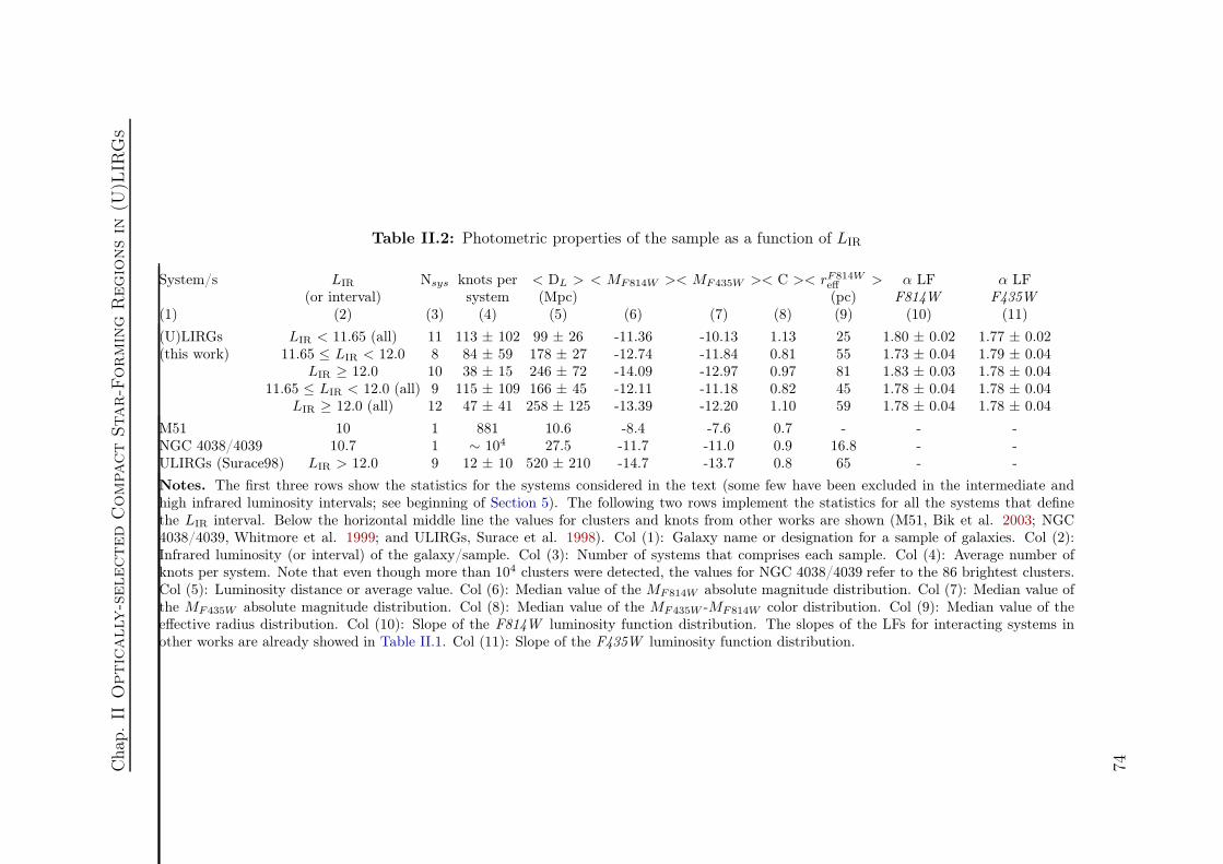
Cha
p.II
Optic
ally
-selected
Com
pact
Star-F
orm
ing
Regio
ns
in(U
)LIR
Gs
Table II.2: Photometric properties of the sample as a function of LIR
System/s LIR Nsys knots per < DL > < MF814W >< MF435W >< C >< rF814Weff > α LF α LF
(or interval) system (Mpc) (pc) F814W F435W
(1) (2) (3) (4) (5) (6) (7) (8) (9) (10) (11)
(U)LIRGs LIR < 11.65 (all) 11 113 ± 102 99 ± 26 -11.36 -10.13 1.13 25 1.80 ± 0.02 1.77 ± 0.02(this work) 11.65 ≤ LIR < 12.0 8 84 ± 59 178 ± 27 -12.74 -11.84 0.81 55 1.73 ± 0.04 1.79 ± 0.04
LIR ≥ 12.0 10 38 ± 15 246 ± 72 -14.09 -12.97 0.97 81 1.83 ± 0.03 1.78 ± 0.0411.65 ≤ LIR < 12.0 (all) 9 115 ± 109 166 ± 45 -12.11 -11.18 0.82 45 1.78 ± 0.04 1.78 ± 0.04
LIR ≥ 12.0 (all) 12 47 ± 41 258 ± 125 -13.39 -12.20 1.10 59 1.78 ± 0.04 1.78 ± 0.04
M51 10 1 881 10.6 -8.4 -7.6 0.7 - - -NGC 4038/4039 10.7 1 ∼ 104 27.5 -11.7 -11.0 0.9 16.8 - -ULIRGs (Surace98) LIR > 12.0 9 12 ± 10 520 ± 210 -14.7 -13.7 0.8 65 - -
Notes. The first three rows show the statistics for the systems considered in the text (some few have been excluded in the intermediate andhigh infrared luminosity intervals; see beginning of Section 5). The following two rows implement the statistics for all the systems that definethe LIR interval. Below the horizontal middle line the values for clusters and knots from other works are shown (M51, Bik et al. 2003; NGC4038/4039, Whitmore et al. 1999; and ULIRGs, Surace et al. 1998). Col (1): Galaxy name or designation for a sample of galaxies. Col (2):Infrared luminosity (or interval) of the galaxy/sample. Col (3): Number of systems that comprises each sample. Col (4): Average number ofknots per system. Note that even though more than 104 clusters were detected, the values for NGC 4038/4039 refer to the 86 brightest clusters.Col (5): Luminosity distance or average value. Col (6): Median value of the MF814W absolute magnitude distribution. Col (7): Median value ofthe MF435W absolute magnitude distribution. Col (8): Median value of the MF435W -MF814W color distribution. Col (9): Median value of theeffective radius distribution. Col (10): Slope of the F814W luminosity function distribution. The slopes of the LFs for interacting systems inother works are already showed in Table II.1. Col (11): Slope of the F435W luminosity function distribution.
74
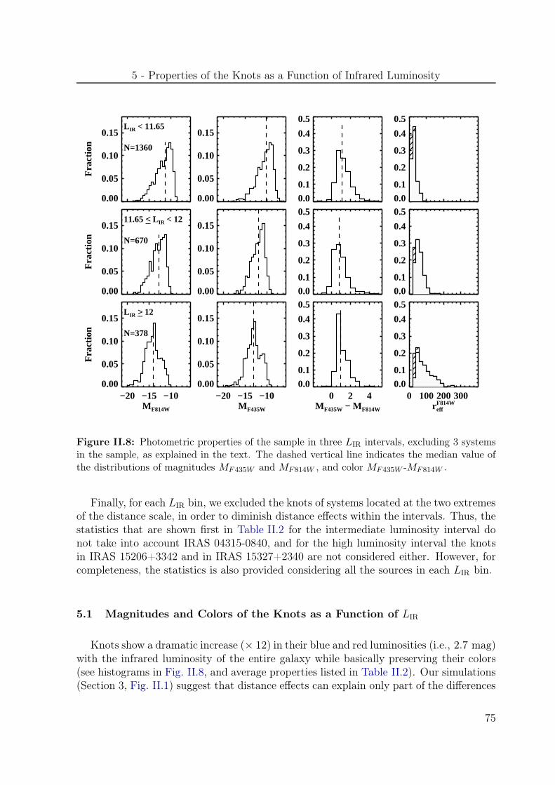
5 - Properties of the Knots as a Function of Infrared Luminosity
0.00
0.05
0.10
0.15
Fra
ctio
n
L IR < 11.65
N=1360
0.00
0.05
0.10
0.15
0.0
0.1
0.2
0.3
0.4
0.5
0.0
0.1
0.2
0.3
0.4
0.5
0.00
0.05
0.10
0.15
Fra
ctio
n
11.65 <_ L IR < 12
N=670
0.00
0.05
0.10
0.15
0.0
0.1
0.2
0.3
0.4
0.5
0.0
0.1
0.2
0.3
0.4
0.5
−20 −15 −10MF814W
0.00
0.05
0.10
0.15
Fra
ctio
n
L IR >_ 12
N=378
−20 −15 −10MF435W
0.00
0.05
0.10
0.15
0 2 4MF435W − MF814W
0.0
0.1
0.2
0.3
0.4
0.5
0 100200300r eff
F814W
0.0
0.1
0.2
0.3
0.4
0.5
Figure II.8: Photometric properties of the sample in three LIR intervals, excluding 3 systemsin the sample, as explained in the text. The dashed vertical line indicates the median value ofthe distributions of magnitudes MF435W and MF814W , and color MF435W -MF814W .
Finally, for each LIR bin, we excluded the knots of systems located at the two extremesof the distance scale, in order to diminish distance effects within the intervals. Thus, thestatistics that are shown first in Table II.2 for the intermediate luminosity interval donot take into account IRAS 04315-0840, and for the high luminosity interval the knotsin IRAS 15206+3342 and in IRAS 15327+2340 are not considered either. However, forcompleteness, the statistics is also provided considering all the sources in each LIR bin.
5.1 Magnitudes and Colors of the Knots as a Function of LIR
Knots show a dramatic increase (× 12) in their blue and red luminosities (i.e., 2.7 mag)with the infrared luminosity of the entire galaxy while basically preserving their colors(see histograms in Fig. II.8, and average properties listed in Table II.2). Our simulations(Section 3, Fig. II.1) suggest that distance effects can explain only part of the differences
75

Chap. II Optically-selected Compact Star-Forming Regions in (U)LIRGs
Figure II.9: Color-magnitude diagrams of all the identified knots (black) at different LIR in-tervals, compared with other interacting systems from the literature. The gray band covers the80% of the total number of knots in each plot, as in Fig. II.2. The colors refer to clusters/knotsmeasured in M51 (orange) taken from Bik et al. (2003), in the ULIRG sample of Surace et al.(1998) (pink) and in NGC 4038/4039 (blue, those younger than 10 Myr; green, those between250 and 1000 Myr; and red, those older than 1 Gyr), taken from Whitmore et al. (1999).
revealed by the data. If the same type of galaxies are located at the average distanceof the low, intermediate and high luminosity subsamples, the distance effect does notchange significantly the colors while increasing the luminosity (absolute magnitude) byonly a factor of 2.8 (1.1 mag). Therefore, we conclude that knots in highly luminousgalaxies are at least a factor of four more luminous than knots located in systems withlower infrared luminosity.
It is interesting to mention that when comparing these results with those indepen-dently obtained for nearby, less luminous systems (the weakly and strongly interactinggalaxies M51 and NGC 4038/4039, respectively), and more distant ULIRGs (Surace et al.1998), the same trend with infrared luminosity appears (see Fig. II.9 and Table II.2).In nearby systems like M51 and NGC 4038/4039, the angular resolution is such thatindividual clusters, instead of aggregates as in more distant galaxies, are detected, andtherefore the difference in the luminosity of clusters and knots can be partly due to adistance effect. Knots in distant ULIRGs tend to be as luminous as knots detected in ourcloser high-luminosity galaxies (also ULIRGs) while having colors similar to those knotsdetected in our sample and clusters in M51 and NGC 4038/4039 (The Antennae). Themost luminous clusters in the Antennae cover a luminosity range close to the medianvalue for knots detected in our low-luminosity systems. Finally, clusters in the very lowluminosity, weakly interacting M51 galaxy are on average about 3 mag fainter (i.e., x15less luminous) than knots in our low-luminosity galaxies.
If we assume a statistically similar extinction and age for the star-forming knots
76

5 - Properties of the Knots as a Function of Infrared Luminosity
regardless of the LIR of the system, the most plausible explanation for the luminosityexcess measured in the intermediate and high luminosity systems has to invoke a massand/or density effects:
• Mass effect. More high-mass knots are sampled in the most luminous systems.
• Density effect. The knots are aggregates of an intrinsically larger number of clustersas the infrared luminosity of the system increases.
The star formation rate as well as the gas content in ULIRGs is higher than in lessluminous systems and as a consequence, these systems form more clusters. Therefore, itis matter of simple statistics rather than a difference in physical formation mechanismsthat in ULIRGs we find the brightest knots. Given the stability of the colors amongthe different infrared luminosity sample, they likely represent the most massive knots.This stochastic process, known as size-of-sample effect (Whitmore et al. 2007), canexplain the demographics of star cluster systems in the merging environment, where thestar formation is enhanced. Therefore, although density effects cannot be discarded ourresult is compatible with a mass effect (which in turn corresponds to a size-of-sampleeffect), explained by statistics.
5.2 Spatial Distribution of the Knots as a Function of LIR
One important aspect to investigate is whether the spatial distribution of the knotsshows dependence on the luminosity of the system. We measure a ratio of inner to outerknots (Ninner/Nouter) that changes with LIR from 0.68 to 0.49 and 0.31 for the three(low-, intermediate- and high-) luminosity intervals, respectively). According to oursimulations, these differences are consistent with being purely due to a distance effect(see Table II.2 for the average distance of the different luminosity bins), and thereforeno evidence for the dependence of the spatial distribution of the knots on the infraredluminosity of the systems is found.
5.3 Effective Radius of the Knots as a Function of LIR
If there is a change in the luminosity of the knots with the bolometric luminosity of thesystem, their size could show a variation as well. At first glance, this seems to be the case(see Fig. II.8 and Fig. II.10). As the luminosity of the system increases, the distributionof reff shows a broadening with a non negligible fraction of the knots having sizes largerthan 100 pc. This is more clear for the high-luminosity systems (ULIRGs ). However,as our simulations have shown (see Fig. II.1), this changes can be explained purely asa distance effect. On the one hand, the distribution of reff of the knots in ULIRGs issimilar to the simulated reff distribution. Moreover, the median value of reff in ULIRGs is
77
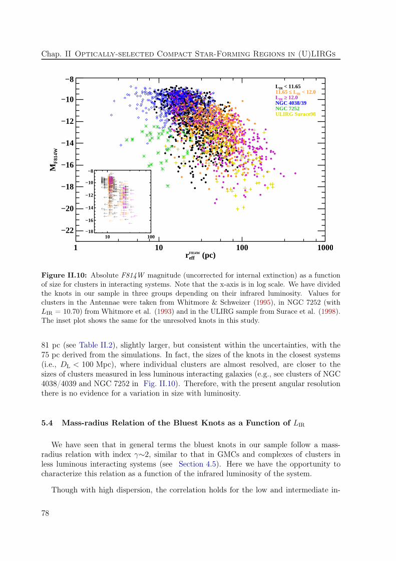
Chap. II Optically-selected Compact Star-Forming Regions in (U)LIRGs
1 10 100 1000r eff
F814W (pc)
−22
−20
−18
−16
−14
−12
−10
−8
MF
814W
L IR < 11.6511.65 ≤ L IR < 12.0L IR ≥ 12.0NGC 4038/39NGC 7252ULIRG Surace98
10 100−18
−16
−14
−12
−10
−8
Figure II.10: Absolute F814W magnitude (uncorrected for internal extinction) as a functionof size for clusters in interacting systems. Note that the x-axis is in log scale. We have dividedthe knots in our sample in three groups depending on their infrared luminosity. Values forclusters in the Antennae were taken from Whitmore & Schweizer (1995), in NGC 7252 (withLIR = 10.70) from Whitmore et al. (1993) and in the ULIRG sample from Surace et al. (1998).The inset plot shows the same for the unresolved knots in this study.
81 pc (see Table II.2), slightly larger, but consistent within the uncertainties, with the75 pc derived from the simulations. In fact, the sizes of the knots in the closest systems(i.e., DL < 100 Mpc), where individual clusters are almost resolved, are closer to thesizes of clusters measured in less luminous interacting galaxies (e.g., see clusters of NGC4038/4039 and NGC 7252 in Fig. II.10). Therefore, with the present angular resolutionthere is no evidence for a variation in size with luminosity.
5.4 Mass-radius Relation of the Bluest Knots as a Function of LIR
We have seen that in general terms the bluest knots in our sample follow a mass-radius relation with index γ∼2, similar to that in GMCs and complexes of clusters inless luminous interacting systems (see Section 4.5). Here we have the opportunity tocharacterize this relation as a function of the infrared luminosity of the system.
Though with high dispersion, the correlation holds for the low and intermediate in-
78

5 - Properties of the Knots as a Function of Infrared Luminosity
3
4
5
6
7
log
(M/M
O • )
L IR < 11.65γ=2.54±0.39
3
4
5
6
7
log
(M/M
O • )
11.65 <_ L IR < 12γ=2.12±0.23
1.5 2.0 2.5 3.0log (radius/pc)
3
4
5
6
7
log
(M/M
O • )
L IR >_ 12γ=1.35±0.53
Figure II.11: The mass vs. radius relation for knots in (U)LIRGs as a function of LIR. Thesolid red line is a power-law fit to the data, with index γ.
79

Chap. II Optically-selected Compact Star-Forming Regions in (U)LIRGs
frared luminosity intervals (see Fig. II.11). The fit for the bluest knots in ULIRGs givesa shallower index, though it could still be consistent with a value of γ=1.9 given thelarge dispersion on the index values. The fit is affected in any case by the small numberof blue knots in ULIRGs and probably by distance effects. Therefore, according to ourdata, there is no clear variation of the mass-radius relation with the infrared luminosityof the system.
5.5 Luminosity Function of the Knots as a Function of LIR
The derived slopes of the luminosity functions with values between 1.7 and 1.8(see Table II.2) do not show any clear trend of variation with the luminosity of thesystem. However, our simulations of the distance effect show that the slope of theLF becomes shallower by about 0.15 dex when moving the low-luminosity systems tothe average distance of the high-luminosity subsample (see Fig. II.1). This change in theslope is due to the reduction in the linear resolution such that knots that appear resolvedin the closer, low-luminosity systems appear to be more luminous aggregates in the moredistant luminous systems. Therefore, the distance-corrected slopes for the intermediateand high-luminosity subsamples would be about 1.9-2, in the range of those measured inother low-z interacting galaxies (see Table II.1).
We know that these slopes were derived using the luminosity of complexes of clusters,especially in the case of systems in the intermediate and high infrared luminosity intervals.Thus, the slopes here might not reflect the physics beneath the formation and dissolutionof star clusters, as normally do for nearby galaxies. However, we have investigated howdistance effects can distort these slopes. Therefore, we conclude that, in absence of betterangular resolution images, our data suggest that the LF remains universal with slopesabout α = 2 within the (U)LIRG luminosity range. Based on the universality of theLF, Whitmore et al. (2007) claim that active mergers have the brightest clusters onlybecause they contain more clusters (i.e., size-of-sample effect). Thus, if the discrepancybetween the luminosities of knots in ULIRGs and in LIRGs is explained by this effect(which is likely to be the case), then the physics underlying the disruption of clusters inthe highest luminous infrared galaxies can be the same as in less luminous systems.
6 Properties of the Knots as a Function of Interaction Phase
Strong interactions and mergers provide a natural laboratory for probing how starformation is affected by tidal forces and major rearrangements of the gaseous componentduring the different phases of the interaction. Most of the systems in our sample areinteracting systems, hence we divided the sample into four groups, depending on themorphology seen in the F814W HST images. Each group represents snapshots of thedifferent phases of the interaction/merger: first approach, pre-merger, merger and post-
80

6-
Properties
ofthe
Knots
asa
Functionof
InteractionP
hase
Table II.3: Photometric properties of the sample as a function of interaction phase
Interaction phase Nsys knots per < DL > < MF814W > < MF435W > < C > < rF814Weff > α LF F814W α LF F435W
system (Mpc) (pc)
First Approach 3 153 ± 127 121 ± 49 -11.25 -10.26 0.93 24 1.50 ± 0.09 1.63 ± 0.06Pre-merger 8 145 ± 81 126 ± 42 -11.91 -10.77 1.06 35 1.84 ± 0.03 1.86 ± 0.04Merger 6 139 ± 123 107 ± 37 -11.23 -10.24 0.96 25 2.00 ± 0.04 1.86 ± 0.03Post-Merger 5 34 ± 19 145 ± 50 -13.35 -11.49 1.49 44 1.76 ± 0.12 1.58 ± 0.17
First Approach 4 131 ± 113 140 ± 55 -11.54 -10.66 0.92 27 1.53 ± 0.10 1.67 ± 0.02Pre-merger 13 103 ± 83 192 ± 98 -12.29 -11.12 1.04 40 1.93 ± 0.03 1.86 ± 0.03Merger 8 112 ± 115 142 ± 71 -11.41 -10.38 0.96 26 1.83 ± 0.02 1.78 ± 0.03Post-Merger 7 29 ± 18 213 ± 159 -13.51 -11.73 1.55 49 - -
Notes. The interaction groups above the horizontal middle line includes only systems having similar distance. Below the horizontal middle lineall the systems have been considered, regardless their distance (note the higher dispersion in the distance of the systems here). Apart from thefirst column, which refers to the different interaction groups defined in Chapter I (Section 1.2), the rest indicate the same as shown in Table II.2.
81

Chap. II Optically-selected Compact Star-Forming Regions in (U)LIRGs
0.00
0.05
0.10
0.15
Fra
ctio
n
First ApproachN=459
0.00
0.05
0.10
0.15
0.00.1
0.2
0.3
0.4
0.5
0.00.1
0.2
0.3
0.4
0.5
0.00
0.05
0.10
0.15
Fra
ctio
n
Pre−mergerN=1157
0.00
0.05
0.10
0.15
0.00.1
0.2
0.3
0.4
0.5
0.00.1
0.2
0.3
0.4
0.5
0.00
0.05
0.10
0.15
Fra
ctio
n
MergerN=832
0.00
0.05
0.10
0.15
0.00.1
0.2
0.3
0.4
0.5
0.00.1
0.2
0.3
0.4
0.5
−20 −15 −10MF814W
0.00
0.05
0.10
0.15
Fra
ctio
n
Post−MergerN=171
−20 −15 −10MF435W
0.00
0.05
0.10
0.15
0 2 4MF435W − MF814W
0.00.1
0.2
0.3
0.4
0.5
0 50 100150200r eff
F814W
0.00.1
0.2
0.3
0.4
0.5
Figure II.12: Photometric properties as a function of merging phase for systems with sim-ilar DL. Dashed vertical lines indicate the median value of the distributions of magnitudesMF814W and MF435W , and color MF435W -MF814W , as in Fig. II.8. The relevant parametersof the plots are shown in the first four rows in Table II.3.
merger. The morphology class is explained in Chapter I (Section 1.2) and the selectionis shown in the same chapter (Section 1.1). In order to know how the star formationevolves with the interaction process, in this section we study the photometric propertiesof the knots for each of the four morphology groups.
82

6 - Properties of the Knots as a Function of Interaction Phase
Table II.4: Infrared to ultraviolet luminosity ratio as a function of interaction phase
Interaction phase Nsys < IR/UV > IR /UV < IR25/UV > IR25 /UVrange range
(1) (2) (3) (4) (5) (6)
First Approach 2 - [15,130] - [4,11]Pre-merger 6 48 [14,189] 7 [2,45]Merger 6 248 [114,1235] 32 [14,117]Post-merger 2 - [385,895] - [86,93]
Notes. Since the IR/UV ratio is not affected by distance effects (we compute it forthe whole system) we give the statistics for all the systems per interaction phase withavailable UV image. Col (1): interaction phase. Col (2): number of systems withIR and UV data available. Col (3): median of the IR/UV ratio when more than twovalues are derived. Col (4): range covered of the ratio IR/UV for each interactionphase. Col (5): same as (3), but in this case only the contribution of the flux at 25µmis taken to compute LIR. Col (6): same as (4), but only the contribution of the fluxat 25µm is taken to compute LIR.
6.1 Magnitudes and Colors as a Function of Interaction Phase
The magnitudes and colors of the knots in the first three interaction phases differsignificantly from those of the knots in the post-merger phase (see results in Table II.3).Even if in a strictly statistical sense (Kolmogoroff-Smirnov test at a confidence level ofat least 98%) the population of knots in the first three phases are different, their medianvalues and distributions are very similar suggesting the lack of strong differences. Thisis true in particular if, in order to minimize the distance effect, only galaxies at similardistances in each phase are considered (see Table II.3 and Fig. II.12). However, thepopulation of knots in the post-merger phase are significantly more luminous (medianI -band magnitude difference of up to 2 mag), and significantly redder than in any ofthe three earlier phases. Furthermore, the population of knots in the post-merger phaseshows in its color distribution an extension toward redder colors (MF435W -MF814W > 3).The fact that knots in the post-merger phase have redder colors means that they likelyrepresent either a more obscured or an older population. In the following we exploreboth alternatives:
1. To investigate whether the knots in the post-merger phase are intrinsically moreobscured than in any of the previous phases, we define the infrared to ultraviolet UV
luminosity ratio (IR/UV) as:
IR/UV =LIR
λLλ(FUV) + λLλ(NUV)(II.1)
83

Chap. II Optically-selected Compact Star-Forming Regions in (U)LIRGs
where LIR stands for the infrared luminosity, λ to the pivot wavelength of a given fil-ter and Lλ to the flux in the near (NUV) and far (FUV) ultraviolet emission (Howellet al. 2010). This ratio is a useful empirical measurement of the dust absorptionand emission in these heavily obscured systems. We searched for UV images inthe Galaxy Evolution Explorer (GALEX ) catalog, using the Multimission Archiveat STScI (MASTa) facility. With a typical angular resolution of about 4-5′′in theFUV-NUV (λ = 1528-2271) range, we can estimate an average value of IR/UV foreach system assuming that the far infrared and ultraviolet flux is emitted in thesame regions. Even if this is not necessarily true, taking into account that mostof the nuclear star formation is obscured in (U)LIRGs, we can have a first-orderestimate on which systems have a higher average extinction.
A total of 16 systems were detected in the GR5 data set, most of them in theAll-Sky Imaging survey (ASIb). The other systems were either not detected or notobserved. In this dataset, the images are already reduced, the sources detectedand the photometry performed. In general the photometry was performed usingan aperture that covers the entire galaxy (if two galaxies form the system we addup the flux values). We then take the value of the flux provided by the data setfacility.
With the flux in the far and near UV and the infrared luminosity we estimatedan average value of the IR/UV ratio for each system. Although the assumptionby Kennicutt (1998) that the great majority of the luminosity from young starswould be absorbed by dust and re-radiated in the far-IR is likely to be correct,observationally there may be other contributions to the total IR luminosity fromolder populations of stars or other luminosity sources (e.g., see the review by Tuffs& Popescu 2005). For that reason, we also computed the IR/UV ratio taking onlythe contribution at 25µm in IRAS (IR25), based on the good relation between themid-IR 24µm-25µm (MIPS-IRAS) and the number of ionizing photons as derivedfrom extinction corrected Paα and Hα luminosities (Wu et al. 2005; Alonso-Herreroet al. 2006; Calzetti et al. 2007). This way we select only hot dust, heated by theradiation of young population, and avoid any contribution from colder dust, heatedby older stars.
Bearing in mind that we are dealing with a small number of statistics, there is atrend toward higher values of the IR/UV ratio in not only the post-merger but alsothe merger phase, with respect to early phases represented by the first approachand pre-merger (see values in Table II.4). Since this ratio is related to an averagedust absorption, this result suggests that knots in the late phases of an interactioncould be suffering on average intrinsically more extinction than in early phases. Forinstance, an additional average extinction of AV =1 can already redden the colorsby about 0.6, according to the SB99 models (see Chapter I, Fig. I.7). If this werethe case, the population of clusters in the late phases of a merger would be more
a http://archive.stsci.edu/b Visit the GALEX website, http://www.galex.caltech.edu/, for more information
84

6 - Properties of the Knots as a Function of Interaction Phase
luminous than in previous phases. Therefore, we would need to invoke a physicalprocess responsible for this significant increase in luminosity. Note however thatdust absorption shows significant structure on scales of a kiloparsec or less (García-Marín et al. 2009a), and therefore the measured IR/UV ratios do not necessarilyrepresent the intrinsic absorption toward the individual optically-selected clusters.A larger set of high angular resolution UV and mid-IR imaging is required beforeany firm conclusion is derived.
2. An alternative scenario to explain the differences in color and luminosity of theknots identified in the post-merger phase with respect to early phases can invokeevolutionary effects. As proposed by Kroupa (1998), many dozens or even hun-dreds of massive individual star clusters with masses of 105-107 M⊙ could mergeinto extremely massive super star clusters (SSCs) after a few hundred Myr. Thishierarchical star formation evolution was also suggested to be happening in com-plexes of clusters in M51 (Bastian et al. 2005a). As the interaction proceeds, thesmaller SSCs would be destroyed by disruption effects (e.g., by the mechanismsproposed in Whitmore et al. 2007) and a few massive individual clusters wouldstill be able to form. Note that, although with a large dispersion, while the numberof knots per system stays about the same (140-150) in the first three phases, thisnumber drops by a factor of 4 to 5 in the post-merger phase (34 knots per system).Thus, in the post-merger phase systems we might be detecting only the evolved,extremely massive SSCs and a few massive individual clusters. The knots withthe reddest colors could be evolved SSCs as massive as 107−9 M⊙ with an opticalextinction (AV ) of 3 mag, or massive young clusters with higher extinction.
Kroupa (1998) estimated that after 100 Myr or so an object with these character-istics can be formed. If the merging of clusters started during the early phases ofthe interaction we would have already detected some of them in the merger phase.Given the degeneracy of the MF435W -MF814W color we could only set an upper-limit to the number of merged superclusters in this phase. Thus, with a colorhigher than MF435W -MF814W = 0.6 and a luminosity higher than MF814W = -15,an object could be more massive than 107 M⊙, were it around or older than 100Myr. About three such knots per system are detected in our sample of (U)LIRGs.
Obviously, photometry at other wavelengths is necessary to better constrain theages and masses of these knots and thus to check the validity of this scenario for(U)LIRG systems. Likewise, simulations of galactic encounters help us know if thisscenario can occur in this environment. A detailed comparison of the present obser-vational results with state-of-the-art high-resolution numerical simulations (Bour-naud et al. 2008b) is presented in Chapter III, to further investigate this scenario.
85

Chap. II Optically-selected Compact Star-Forming Regions in (U)LIRGs
6.2 Spatial Distribution as a Function of Interaction Phase
We investigated the relative fraction of inner (inside 2.5 kpc radius) and outer (outside2.5 kpc radius) knots in the four interaction phases defined above in order to know ifmajor mergers have an impact on the spatial distribution of the knots. Although thenumber of systems in each phase is small (3, 8, 6 and 5 for the first approach, pre-merger,merger, and post-merger) the ratio Ninner/Nouter is 0.50, 0.65, 0.52, 0.68 from the firstapproach to the post-merger.
We do not see any correlation toward a more dispersed or concentrated spatial distri-bution of the knots with interaction phase. However, in the pre- and post-merger phases,where the magnitudes are higher compared to the other phases, there is some evidenceof greater concentration toward the nuclear regions. The greater the number of knotsin the central regions, the harder it is to detect them, and therefore, only the brightestones are identified given the local background conditions (bright and steep light profiles).Hence, this effect can contribute to a small increase in the luminosity distribution of theknots in these phases. Assuming that the knots in the pre-merger phase have a luminos-ity similar to that in the first contact and merger phases, this effect would increase themedian luminosity by a factor of almost 2. Since the ratio Ninner/Nouter in this phase issimilar to the ratio in the post-merger phase, an additional increase of a factor of about5 would still be unexplained by the first scenario explored in the previous section. Alarger sample of galaxies would be required to establish a firmer result.
6.3 Effective Radius as a Function of Interaction Phase
All size distributions are statistically different with a high degree of confidence (higherthan 99%), yet the median value of reff is similar during the three first interaction phasesindicating that these differences must be rather small. However, knots in the post-merger phase tend to be larger by factors of 1.3 to 2 than in any of the previous phases(see Table II.3). This result is not very robust, given the uncertainties in the determi-nation of sizes, but if confirmed, it would support the hierarchical star formation sce-nario proposed by Kroupa (1998). According to this scenario, the merged super clusterswould have a half-mass radius of about rh = 45-95 pc. Under the assumption of virialequilibrium and isotropic velocity distribution the effective and half-mass radius can berelated as reff = 3/4×rh. Then, the merged extremely massive super clusters would havereff = 30-70 pc, similar to the values measured for knots in the post-merger sample.
6.4 Mass-radius Relation of the Bluest Knots with Interaction Phase
The broad-band emission of the knots for which we have measured the mass is verymuch likely to come from young population (i.e., τ < 30 Myr; see Section 4.4). Based
86
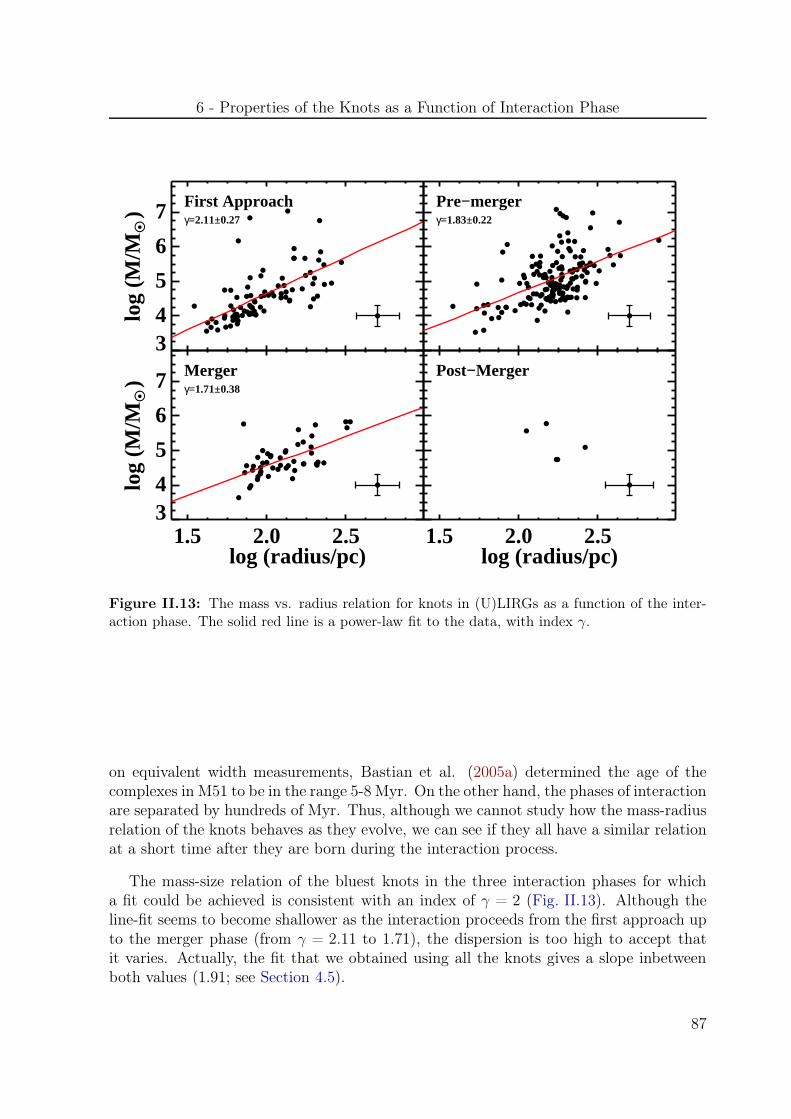
6 - Properties of the Knots as a Function of Interaction Phase
34
5
6
7
log
(M/M
O • )
First Approachγ=2.11±0.27
Pre−mergerγ=1.83±0.22
1.5 2.0 2.5log (radius/pc)
34
5
6
7
log
(M/M
O • )
Mergerγ=1.71±0.38
1.5 2.0 2.5log (radius/pc)
Post−Merger
Figure II.13: The mass vs. radius relation for knots in (U)LIRGs as a function of the inter-action phase. The solid red line is a power-law fit to the data, with index γ.
on equivalent width measurements, Bastian et al. (2005a) determined the age of thecomplexes in M51 to be in the range 5-8 Myr. On the other hand, the phases of interactionare separated by hundreds of Myr. Thus, although we cannot study how the mass-radiusrelation of the knots behaves as they evolve, we can see if they all have a similar relationat a short time after they are born during the interaction process.
The mass-size relation of the bluest knots in the three interaction phases for whicha fit could be achieved is consistent with an index of γ = 2 (Fig. II.13). Although theline-fit seems to become shallower as the interaction proceeds from the first approach upto the merger phase (from γ = 2.11 to 1.71), the dispersion is too high to accept thatit varies. Actually, the fit that we obtained using all the knots gives a slope inbetweenboth values (1.91; see Section 4.5).
87
Chap. II Optically-selected Compact Star-Forming Regions in (U)LIRGs
6.5 Luminosity Function as a Function of Interaction Phase
There appears to be a trend in the slopes of the LFs of the knots with interaction phasesuch that they become steeper as the interaction evolves from first contact to pre-mergerand up to merger and post-merger (see Table II.3). This is particularly more visiblewhen only systems at similar distances and I -band LFs, i.e., less affected by extinctioneffects, are considered (slopes of 1.50, 1.84, 2.0 and 1.76, respectively). Note, however,that the slope of the LF for the post-merger phase is computed with less than 100 knots(brighter than the completeness limit), hence it is statistically less significant than theother slopes. Also note that the systematic uncertainties of the slope of the LF canbe as high as about 0.1 dex (the tables give the uncertainty related only to the fit), asmentioned in Chapter I (Section 3.3). Thus, the observed trend is very weak.
If we select only systems closer than 100 Mpc (see Section 4.6), the phases are alsosampled. We can try to further minimize distance effects by computing the LF only forthese systems. While 400-600 measurements can be used in each of the other phases, onthe post-merger phase we are instead restricted to only about 30 knots and thus, we willnot include this phase in this analysis. The slopes derived for the closest systems are1.68-1.68-1.92 (1.75-1.77-1.99) for the I - (B -) band LF for the first contact, pre-mergerand merger phases, respectively. It is interesting to note that in this case the LF stillbecomes steeper when the systems evolve from the pre-merger to the merger phases.
(U)LIRGs are known to have high SFRs at all phases of interaction. However, thiscan be concentrated at small scales or more dispersed and, at the same time, less or morehidden by dust. For instance, 80% of the total infrared luminosity in IRAS 20550+1656comes from an extremely compact, red source not associated with the nuclei of themerging galaxies but with a buried starburst (Inami et al. 2010). If, on average, wedetect more young knots in the optical at early phases of interaction than in more evolvedphases, they can overpopulate the bright end of the luminosity function, and thus themeasured slope would be shallower. In Chapter III we compare the observed LFs withthose computed from the mass functions in numerical simulations by Bournaud et al.(Bournaud et al. 2008b) and stellar population synthesis models (i.e., mass to lightratios). This comparision can help us learn if the observed trend (change of the slope asthe interaction evolves) is real and allow us to investigate its origin.
7 Knots in (U)LIRGs vs. Star-forming Clumps at high-z
(U)LIRGs represent the extreme cases of low-redshift star-forming galaxies associatedwith spirals, interacting galaxies and mergers. Deep cosmological imaging and spec-troscopic surveys at redshifts z ∼ 1-4 have identified massive star-forming galaxies withirregular structures where the star formation appears to proceed in large clumps,withsizes in the 0.1-1.5 kpc range. The most recent are the surveys conducted in the
88

7 - Knots in (U)LIRGs vs. Star-forming Clumps at high-z
Table II.5: Comparison of knots in ULIGRs with clumps in the high-z Universe
System /field rest-frame redshift N clumps Mass range Total size Ref.band / line per galaxy ( M⊙) (kpc)
(1) (2) (3) (4) (5) (6) (7)
UDF field B 0.5 - 4 ∼ 5 107 - 109 1 - 2.5 [1], [2]Lensed galaxies Hα 1.7 - 3.1 - 6×10⁸ - 3×10⁹ 0.3 - 1 [3]star-forming galaxies at z∼2 optical g, UV, Hα 2.2 - 2.4 4.5 9×10⁷ - 9×10⁹ 0.3 - 1.5 [4]GEMS & GOODS fields B 0.1 - 1.4 ∼ 4 5×10⁶ - 108 0.2 - 7 [5]Simulated ULIRGs at z=1 I 1 6.7 2×10⁵ - 7×10⁷ 0.4 - 3.5 This workTDG candidates in (U)LIRGs I 0 - 0.1 ∼ 1 106 - 4×10⁷ 1 - 2 [6]
Notes. Col (1): Type of systems and deep fields. Col (2): Rest-frame photometric band. Col (3):Redshift interval of the galaxies. Col (4): Average number of clumps per galaxy. Col (5): Total stellarmass range of the clumps, except for the lensed galaxies, where the dynamical mass of the clumps isprovided. Col (6): Total diameter of the clumps. For star-forming galaxies at z = 2 the full-width athalf-maximum from the clump radial light profiles after subtraction of the local background is given.Col (7): References–[1] Elmegreen & Elmegreen (2005); [2] Elmegreen (2007); [3] Jones et al. (2010); [4]Schreiber et al. (2011b); [5] Elmegreen & Elmegreen (2006); [6] Chapter IV in this thesis.
GEMS and GOODS fields (Elmegreen & Elmegreen 2006, 2007), in the Ultra DeepField (UDF; Elmegreen & Elmegreen 2005, 2007, 2009) and in the Spectroscopic Imag-ing survey in the Near-infrared with SINFONI (SINS; Förster Schreiber et al. 2011b).While some of these galaxies show structural characteristics of being involved in mergers(Elmegreen et al. 2007; Förster Schreiber et al. 2011a), most systems appear as thickturbulent disks (Elmegreen et al. 2009). Faint tidal features are difficult to discern athigher redshifts because of cosmological dimming. It is important therefore to make adirect comparison between the star-forming knots in (U)LIRGs and in clumpy high-zgalaxies in order to understand the similarities and differences of the star formation inthe present Universe and at cosmological distances.
The clumps in high-z galaxies are less numerous and intrinsically brighter and moremassive (by a factor of 10-1000) than the largest star-forming complexes in local galaxies(Efremov 1995; Elmegreen & Elmegreen 2005; Elmegreen et al. 2007, 2009; FörsterSchreiber et al. 2011b). The integrated luminosity of these clumps usually accounts forabout 10-25% of the total luminosity. The larger masses in the high-redshift galaxies arethought to be the result of high turbulence in the disks. In fact, velocity dispersions of 40km s−1 have been derived from spectroscopic observations of UDF6462, a z = 1.6 galaxy(Bournaud et al. 2008a). This large-scale star formation can also be reproduced bymeans of numerical simulations which require velocity dispersions several times higherthan in local quiescent galaxies (Bournaud et al. 2007). Finally, these high velocitydispersions have already been observed in clumps in local ULIRGs (Monreal-Ibero et al.2007), since gravitational torques in major mergers can also induce star formation inlarge condensations of gas. Yet, the last mention has to be taken with care since strongwinds and shocks in mergers can also induce large gradients in the velocity fields (i.e.,high velocity dispersions).
89
Chap. II Optically-selected Compact Star-Forming Regions in (U)LIRGs
In the standard ΛCDM cosmology (Spergel et al. 2007) the angular size is nearlyconstant over the redshift range 0.7 < z < 4. At closer redshifts, the angular size de-creases approximately linearly with increasing redshift. A kpc-sized clump correspondsto 3-4 pixels in the ACS images at high redshift values. Thus, clumps much smaller thanthis could not be measured at high redshifts. On the other hand, if there were clumpssignificantly larger than this in nearby galaxies, they would be easily discernible. Thelack of spatial resolution at high redshifts can make a complex of star formation look likea clump since the light from the different clusters combines, blurs and some contrast withthe local background is lost. Whether the high-z clumps correspond to a single entity orto complexes of star formation, the largest complexes can be identified and compared inboth local and high-redshift galaxies. The high-z galaxy clumps have masses typicallybetween 107 and 109 M⊙ from z = 1 to 4, decreasing to about 106 M⊙ at z = 0.1-0.2.The star-forming regions in the few interacting clumpy galaxies observed have sizes sim-ilar to star complexes in local interacting systems (i.e., the Antennae or M51), and theirmass is 10-1000 times higher. On the other hand, complexes in the Hickson CompactGroup 31 (HCG 31), stellar complexes, which are sensitive to the magnitude of disk tur-bulence, have both sizes and masses more characteristic of z = 1-2 galaxies (Gallagheret al. 2010).
In Section 5.1 we saw that knots in ULIRGs are intrinsically more luminous than knotsin less luminous systems. This means that for complexes of similar sizes and similarpopulation (Table II.2 shows that the colors of the knots in LIRGs and ULIRGs aresimilar) the knots in ULIRGs (they could also be understood as clumps or complexes ofstar clusters) can be more massive than in our low luminous LIRGs by at least a factorof 4. Although the knots in our ULIRGs only account for 0.5-2% of the total luminosity(much less than clumps at high redshift), we can compare them with the complexes inhigh-redshift galaxies in order to determine if the star formation is similar or not tothat in clumpy galaxies . Already at z ≃ 0.05-0.1 a significant percentage of knots inULIRGs are more luminous than MF814W= -15 mag (see Fig. II.9). According to themodels used in this study, if we assume that these knots are formed by a single young(e.g., τ ∼ 6 Myr) population they can be as massive as few 104 - few 107 M⊙, with amedian value of 1.4×10⁵ M⊙ . An older population (e.g., τ ∼ 50 Myr) implies a knotwith higher mass by one order of magnitude. Correction for internal extinction makesthe population even more massive. Thus, these values have to be understood as a lowerlimit. To compare the knots in these ULIRGs with the clumps at high-redshift galaxies,we applied a Gaussian blur to our images in such a way that we simulate their appearanceat z = 1 (the scale at this redshift corresponds to 7.69 kpc/′′), using the same techniqueas explained in Section 3.
The knots in the blurred images (hereafter high-z knots) were measured. Table II.5show the results together with the values for clumps in galaxies at high redshifts andTDGs candidates found in our sample of (U)LIRGs (Chapter IV). Some of the high-zknots were not recognizable in the blurred images because they were too faint or toosmall; a few were blended with other knots that were too close or with the nucleus.
90
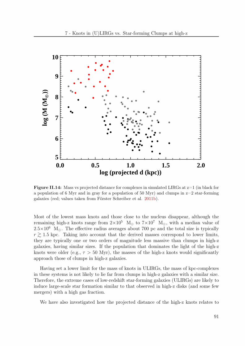
7 - Knots in (U)LIRGs vs. Star-forming Clumps at high-z
0.0 0.5 1.0 1.5 2.0log (projected d (kpc))
5
6
7
8
9
10
log
(M (
MO • )
)
Figure II.14: Mass vs projected distance for complexes in simulated LIRGs at z=1 (in black fora population of 6 Myr and in gray for a population of 50 Myr) and clumps in z=2 star-forminggalaxies (red; values taken from Förster Schreiber et al. 2011b).
Most of the lowest mass knots and those close to the nucleus disappear, although theremaining high-z knots range from 2×10⁵ M⊙ to 7×10⁷ M⊙ , with a median value of2.5×106 M⊙ . The effective radius averages about 700 pc and the total size is typicallyr & 1.5 kpc. Taking into account that the derived masses correspond to lower limits,they are typically one or two orders of magnitude less massive than clumps in high-zgalaxies, having similar sizes. If the population that dominates the light of the high-zknots were older (e.g., τ > 50 Myr), the masses of the high-z knots would significantlyapproach those of clumps in high-z galaxies.
Having set a lower limit for the mass of knots in ULIRGs, the mass of kpc-complexesin these systems is not likely to lie far from clumps in high-z galaxies with a similar size.Therefore, the extreme cases of low-redshift star-forming galaxies (ULIRGs) are likely toinduce large-scale star formation similar to that observed in high-z disks (and some fewmergers) with a high gas fraction.
We have also investigated how the projected distance of the high-z knots relates to
91

Chap. II Optically-selected Compact Star-Forming Regions in (U)LIRGs
their mass (see Fig. II.14. While other works do not find any clear relation, we measurelower mass high-z knots with increasing distance. Although, according to our results itis clear that the mass is mainly concentrated at small distances in ULIRGs, we can onlycompare with one study of high-z galaxies and we explore larger distances by a factor of10.
8 Summary and Conclusions
A comprehensive study of bright compact knots (most of them apparent associations ofclusters) in a representative sample of 32 (U)LIRGs as a function of infrared luminosityand interaction phase has been performed using HST /ACS B - and I -band imaging,providing linear resolutions of 10 to 40 pc, depending on the distance of the galaxy.The sample has been divided into three infrared luminosity intervals (low, LIR < 11.65;intermediate, 11.65 ≤ LIR < 12.0; and high, LIR ≥ 12.0) and in the 4 interaction phasesdefined in Chapter I (Section 1.2), namely first approach, pre-merger, merger and post-merger. We have extended toward lower infrared luminosities previous studies focusedonly on ULIRGs (e.g., Surace et al. 1998, 2000), and have detected close to 3000 knots,larger than a factor of ten more than in the previous studies of ULIRGs. The mainconclusions derived from this study are the following:
1. The knots span a wide range in magnitudes (-20 . MF814W . -9 and-19.5 . MF435W . -7.5), and color (-1 . MF435W -MF814W . 5). The medianvalues are MF435W = -10.84, MF814W = -11.96 and MF435W -MF814W = 1.0.
2. The knots are in general compact, with a median effective radius of 32 pc, being12% unresolved and a few very extended, up to 200-400 pc. With these sizes,in general (and particularly for galaxies located at 100 Mpc or more) the knotsconstitute complexes or aggregates of star clusters. Within the resolution limitsthere is no evidence of a luminosity dependence on the size. A slight dependence onthe interaction phase, in particular in the post-merger phase, needs confirmationwith larger samples and better angular resolution.
3. A non-negligible fraction (15%) of knots are blue and luminous. Given their color(MF435W -MF814W < 0.5) and magnitude (<MF435W>= -11.5) they appear to beyoung (ages of about 5 to 30 Myr), almost free of extinction, and have massessimilar to and up to one order of magnitude higher than the young massive clustersdetected in other less luminous interacting systems. In addition, some (5.7%) veryluminous (MF435W < -12.5), and relatively blue (MF435W -MF814W < 1.0) knotsappear along the tidal tails and at their tips. These objects could be candidates
92

8 - Summary and Conclusions
to Tidal Dwarf galaxies.
4. Unlike for isolated young star clusters in other systems, we find a clear correlationbetween the knot mass and radius, M∝ R2, similar to that found for complexes ofstar clusters in less luminous interacting galaxies (e.g., M51 and the Antennae) andGalactic and extragalactic giant molecular clouds. This relation does not seem tobe dependent on the infrared luminosity of the system or on the interaction phase.
5. The star formation is characterized by B - and I -band luminosity functions (LF)with slopes close to 2, extending therefore the universality of the LF measured ininteracting galaxies at least for nearby systems (i.e., DL < 100 Mpc), regardlessof the total luminosity (i.e., the strength of the global star formation). This resulthas to be taken with caution because the LF of our knots (which can be mainlyformed of complexes of star clusters) may not reflect the same physics as theLF of individual star clusters. Nevertheless, there are slight indications that theLF evolves as the interaction progresses becoming steeper (from about 1.5 to 2 forthe I -band) from first approach to merger and post-merger phases.
6. Taking into account distance effects, knots in high luminosity systems (ULIRGs)are intrinsically more luminous (a factor of about 4) than knots in less luminoussystems. Given the star formation rate in ULIRGs is higher than in less lumi-nous systems, size-of-sample effects are likely to be the natural explanation for this.
7. Knots in ULIRGs would have both sizes and masses characteristic of stellar com-plexes or clumps detected in galaxies at high redshifts (z & 1), were their populationabout 50 Myr or older. Thus, there is evidence that the larger-scale star formationstructures are reminiscent of those seen during the epoch of morphological galaxytransformations in dense environments.
8. Knots in systems undergoing the post-merger phase are on average redder andmore luminous than those in systems in earlier phases. Scenarios involving eithera different spatial distribution of the obscuration or a different evolutionary phasein which small knots do not survive for long are considered. The evolutionaryscenario could also explain the trend in size toward higher values in post-mergersystems. A comparison with numerical simulations to further investigate thesescenarios are presented in Chapter III.
93


Chapter III
Comparative Study with High SpatialResolution Simulations
Overview
This Chapter complements the previous one by including thetheoretical frame in the analysis and characterization of thedata. We present the first direct comparison of the propertiesof stellar regions (simulated knots) identified in a high spatialresolution simulation of a major merger with knots detected inour sample of (U)LIRGs. The main purpose of the comparisonis to be able to interpret some of the properties measured in theprevious Chapter and to constrain the results of the simulation.
1 Introduction
The role played by interactions and mergers in enhancing star formation has beenwidely studied in the past few decades by means of numerical simulations (e.g., Barnes& Hernquist 1992a; Mihos & Hernquist 1994b; Mihos & Hernquist 1996; Springel2000; Barnes 2004; Springel & Hernquist 2005; Bournaud & Duc 2006; Cox et al. 2006; DiMatteo et al. 2007; Di Matteo et al. 2008; Teyssier et al. 2010). These studies havesupported the fact that major mergers induce star formation, though it has become clearthat the star formation efficiency is highly dependent upon the numerical recipe adoptedfor star formation (density or shock dependent) and feedback assumptions. The spatialresolution achieved by the model is also decisive (Teyssier et al. 2010). The higherthe resolution the better the models can handle the inner phenomena affecting the starformation.
Even though numerical simulations represent a powerful tool to study galaxy mergers,none of the previous studies has been able to monitor the physical evolution of the star-forming regions at typical scales of Super Star Clusters (SSCs) or associations of few
95

Chap. III Comparative Study with High Spatial Resolution Simulations
clusters. Bournaud et al. (2008b) presented a simulation of a wet galaxy merger withthe highest resolution in mass and spatial sampling reached until then. With a spatialresolution of 32 pc, they were able to directly identify dense structures with typicalmasses of 106-108 M⊙ , similar to the most massive SSCs and aggregates of few clusters.They argued that these dense structures are tightly bound and likely progenitors oflong-lived globular clusters. Models capable of resolving compact star-forming regions atsimilar spatial scales to observations at z ≤ 0.1 offer the opportunity to make a one-to-onecomparison.
This Chapter presents the first direct comparison of the properties of stellar regions(simulated knots) identified in the galaxy simulation by Bournaud et al. (2008b) withknots detected in (U)LIRGs. Belles et al. (in preparation) has performed the physicalcharacterization of the most massive simulated knots (i.e., log M ( M⊙ ) ≥ 7.5). In thisthesis we also extend the statistics to all mass ranges, down to about log M ( M⊙ ) ∼ 6.With the available data from the simulation (see Chapter I, Section 2.3) and using stel-lar population synthesis techniques, the magnitudes, colors, and LFs of the simulatedknots are evaluated at different interaction phases. This enables us to perform a directcomparison with the properties of the observed knots studied in the previous Chapter, astudy of stellar regions in an observational and theoretical frame simultaneously.
To avoid distance effects in this study, we only consider the knots detected in theprevious Chapter that belong to systems located at similar distances in each phase (seeChapter II, Section 6). That is, a total of about 2200 knots in 22 (U)LIRGs. The galaxiesare located at a median distance of 125 Mpc, with a dispersion of 40 Mpc.
The layout of the Chapter is as follows: Section 2 provides the description of ad-ditional analysis treatment of the data from the simulations and the definition of theinteraction phases under comparison; the comparison of the properties of the knots de-tected in observations and simulations is performed in Section 3, along with the temporalevolution of their physical and spatial distributions with the interaction process; finally,we summarize the main conclusions in Section 4.
2 Additional Analysis Treatment and Definitions
2.1 Derivation of the Photometric Properties of the Simulated Knots
The output of the simulation corresponds to the mass and the position of each particleat any given snapshot. However, the observational data consist of photometric (light)measurements. To compare both sets of data, we have chosen to convert the mass ofthe simulated knots into light and compare the modeled luminosities because we knowtheir age with an uncertainty of a few Myr. These estimates are more reliable than thedetermination of masses from the observed luminosity, which can be uncertain by large
96

2 - Additional Analysis Treatment and Definitions
factors (10-100 or even larger) if we only have the knowledge of the luminosities in theF435W and F814W bands (see Fig. I.7 in Chapter I, Section 3.2).
To perform such analysis, we first have to know the star formation history of thesimulated knots and then apply stellar population synthesis techniques to obtain theobservables (luminosities) we need to compare with the observed knots.
2.1.1 Initial Mass and Growth Phase in the Simulation
Reliable estimates of the magnitudes of the simulated knots require to know as well aspossible their mass and age, and if they are formed by one or more populations. Belleset al. (in prep) argue that the knots undergo a rapid growth phase in which their massincreases by up to a factor of about 100 during their first 100 Myr or so of existence.During this phase, the number of new stars within each knot increases, while the numberof old stars does not vary significantly. This suggests a scenario in which clumps of gasform first and then collapse to form stars. However, the model does not have enoughresolution for us to know if the clump fragments and form little clusters which then mergetogether, or if the collapse is monolithic.
Once this phase ends, the mass of the knots stabilizes to what it is defined as the initialmass (Mini). Later on, they lose mass (due to dynamical friction, two-body relaxation,etc.), generally in a much moderate way. Since the simulated knots are tracked untilthey disappear or until the end of the simulation, we assumed their initial mass to be themass value 80-100 Myr (i.e., 6-8 snapshots) after it is detected for the first time. Then, ifa knot is massive enough for us to follow all the growth phase in the simulation, after 6-8snapshots it will have reached the initial mass already. If, on the other hand, the knotis less massive, we will have missed this phase partially or completely. However, after6-8 snapshots its mass will be very similar to the initial mass because statistically it willlose mass in a much moderate way after having reached Mini. Thus, the initial mass wastaken as the peak value 80-100 Myr after it is detected for the first time.
Once the initial mass of the knots was known, we studied this phase of rapid growthfor the most massive knots. If a knot has an initial mass higher than Mini = 108 M⊙,at the time when it is identified for the first time (at the beginning of this phase) it isstill massive enough (i.e., M > 106.2 M⊙) to be detected against the local background.Hence, the rapid growth phase is completely tracked for the most massive knots. Incontrast, this phase is missed partially or completely for a knot with lower initial masssince, assuming that the rapid growth phase is similar, its mass at the beginning of thephase would be too low for the knot to be detected. In the extreme case where the initialmass of a knot is lower than M > 106.5 M⊙, we identify it for the first time when ithas already reached the initial mass. This mass (106.5 M⊙) represents the global masscompletition limit defined in Belles et al. (in preparation).
97

Chap. III Comparative Study with High Spatial Resolution Simulations
We decomposed the growth phase in successive bursts of star formation. Since thisphase lasts approximately six snapshots, the knots are formed by a combination of sixdifferent stellar population, with different masses and ages. For each population, wederived the mass fraction and dragged it throughout the whole evolution of the simula-tion. Thus, for instance, when a massive knot appears for the first time, it has only onepopulation. One additional population is created per snapshot until the knot reaches itsinitial mass. Then, the mass fraction of each population is frozen and used as such untilthe end of the simulation or its dissolution.
2.1.2 Modeling the Stellar Populations
Characterizing the growth phase of the simulated knots involves identifying each pop-ulation present in a knot and, especially, its age.
To characterize the growth phase of the simulated knots we need to identify as well aspossible each population present in a knot. With that information and the use of stellarpopulation synthesis models we were able to derive observables, such as the luminositiesof the simulated knots.
The tracks of the SB99 models with solar metallicity, optimized for young ages, areused up to τ = 100 Myr. At older ages, the tracks by Maraston et al. (2005) areconsidered, where a rigorous treatment of the thermally pulsing asymptotic giant branch(TP-AGB) phase has been applied (relevant within the interval 0.1-1 Gyr). We considerthis rather high metallicity even at large radii because global mixing of the ISM inmergers, due to gas inflows and outflows, flattens any metallicity gradient of the parentgalaxies (Rupke et al. 2010; Di Matteo et al. 2011; Perez et al. 2011). Given therelatively small gas mass at large radii, mixing of small amounts of more enriched gaseasily raises the gas metallicity in these regions.
The growth phase is not completely tracked in the simulation for knots less massivethan 108 M⊙ , thus we assumed that they are characterized in the same way as themassive ones. When computing the mass fraction of the six stellar populations, weapplied a gradual correction:
(i) For knots in the interval 107 < Mini ( M⊙) < 108 (first interval) we assumed wehad missed the growth phase for 2 snapshots.
(ii) For knots in the interval 106.5 < Mini ( M⊙) ≤ 107 (second interval), we had missedit for 4 snapshots.
(iii) Finally, for knots less massive than the detection threshold (third interval, i.e.,Mini < 106.5 M⊙), we had missed it for 6 snapshots (i.e., the whole phase).
Thus, when a knot in the first interval was detected for the first time we assumed
98

2 - Additional Analysis Treatment and Definitions
it was already formed by three stellar populations, with ages τ = 6.5 Myr (detected),6.5+13 (19.5) Myr (missed) and 6.5+13+13 (32.5) Myr (missed), respectively. Then, inorder to estimate the luminosity we used the averaged mass fractions computed for allthe massive knots when they are formed by three populations. In the following snapshot,the knot was assumed to be formed by four stellar populations (the older two we missedand the younger two in which the knot was detected). The new mass fractions of thenon-detected with respect to the detected populations were computed using the averagemass fractions that we had derived for all the massive knots. Once the knot reached thesix stellar populations (at the fourth snapshot in this case), the final mass fraction valueswere frozen and dragged until the knot disappeared or until the end of the simulation.A similar analysis procedure was followed for the knots in the second interval. Theknots in the third interval were assumed to have already reached their initial mass whenthey were first detected (i.e., they are already formed by the six stellar populations).Hence, we dragged all the populations from the beginning and the mass fractions appliedcorrespond to the average values that we had derived for the most massive knots.
This process introduce a typical uncertainty of 5-25 % in the knowledge of the massfor each of the six populations for the least massive knots. Another major source ofuncertainty comes from the age of the young population. When a knot appeared for thefirst time in the simulation we assumed the youngest out of the six populations is 6.5 Myrold, since the age elapsed between two consecutive snapshots is 13 Myr. To know howthis is translated into an uncertainty in magnitude, we assumed that the ages distributefollowing a Gaussian function in the interval 0-13 Myr, with a mean value of 6.5 Myrand a one-sigma (1σ) deviation of 6.5/3 (i.e., 2.17) Myr. According to the SB99 models,this introduces a 1σ uncertainty of up to 0.5 mag in the F814W band and up to 0.3 magin the F435W band. These uncertainties decrease considerably due to the aging of theknots while they evolve throughout the interaction. After about 50 Myr, they becomenegligible (less than 0.1 mag) compared to the uncertainties related to the mass fractionfor each of the six populations. Hence, considering both major sources of uncertainties,the error in the estimated magnitudes for the new knots (at the snapshot where theyappear for the first time) can be as high as 0.75 mag. About three snapshots later thiserror drops below 0.2-0.3 mag, since at that time the new population with an age of6.5 Myr represents a very small fraction in mass. About seven snapshots later the mainsource of uncertainty comes from the mass fraction for each of the six populations, andthe magnitudes computed are reliable within less than 0.2 mag.
2.2 Interaction Phases Under Comparison
Although a single 1:1 simulation was carried out, it is rather typical and characteristicof many observed real systems. For instance, NGC 7252, the Mice and The Antennaecan be modeled by roughly equal-mass mergers with high gas fractions, from 12.5 to 20%(Hibbard & Mihos 1995; Barnes 2004). Three out of the four double system ULIRGs inColina et al. (2005) also have a mass ratio of 1:1, and most ULIRGs in García-Marín et al.
99

Chap. III Comparative Study with High Spatial Resolution Simulations
(2007) are compatible with a mass ratio of 1:1 and 1:2. However, other parameters suchas the orbit inclination differs significantly from system to system. On the other hand,the observational data come from a sample of dozens of systems, surely with galaxieshaving different initial configurations. Therefore, we only expect to find general trendsbetween both observed and simulated data.
In Chapter I (Section 1.2), we classified the (U)LIRG sample according to four interac-tion phases, depending on the optical morphology of the systems. A similar classificationscheme to that in Veilleux et al. (2002) was followed, though with a few simplifications.An age interval for each morphological class was assigned. Given the uncertainties in-volved when performing morphological classifications and in order to make a more real-istic comparison, we assigned in the simulation a typical age to each morphological classdefined in Chapter I (Section 1.2) and considered a window of about 150 Myr to charac-terize the properties of each class. We then identify in the simulation typical ages (centralages in the window) for the pre-merger, merger and post-merger interaction phases to be299, 585 and 988 Myr. We thus considered snapshots covering ± 75 Myr to define theinteraction phase. Owing to computing time issues, the simulation in this study extendsonly up to 1 Gyr. However, the duration of a merger can be more extended in time untilthe system relaxes (e.g., simulations by Di Matteo et al. 2008 extend to longer than 2Gyr). As a consequence, the comparison of this simulation with very relaxed galaxies(i.e., a very old elliptical galaxy) is not appropriate. Nevertheless, a comparison witha (U)LIRG remnant, with past signs of interaction (e.g., outer asymmetries), no fullyrelaxed, is not worrysome.
Some galaxies were identified to be in a first-contact phase (before the first pericenterpassage). This phase, corresponding to the first snapshots in the simulation, was notconsidered for this study because only a few simulated knots were detected (e.g., only34 knots in the snapshot number 8, at t=104 Myr). This unrealistic early scenario isthe consequence of how the star formation was implemented in the code, in such a waythat no star formation existed before the encounter. Therefore, the knots in the threeinteraction phases pre-merger, merger and post-merger were compared for both sets ofdata.
3 Observed Knots vs. Simulated Knots
3.1 Luminosities and Colors
3.1.1 Preliminary Considerations
In this section we aim at comparing the luminosities and color distributions of boththe simulated and observed knots during the interaction process. In order to understanddifferences and similarities we first make the following considerations:
100
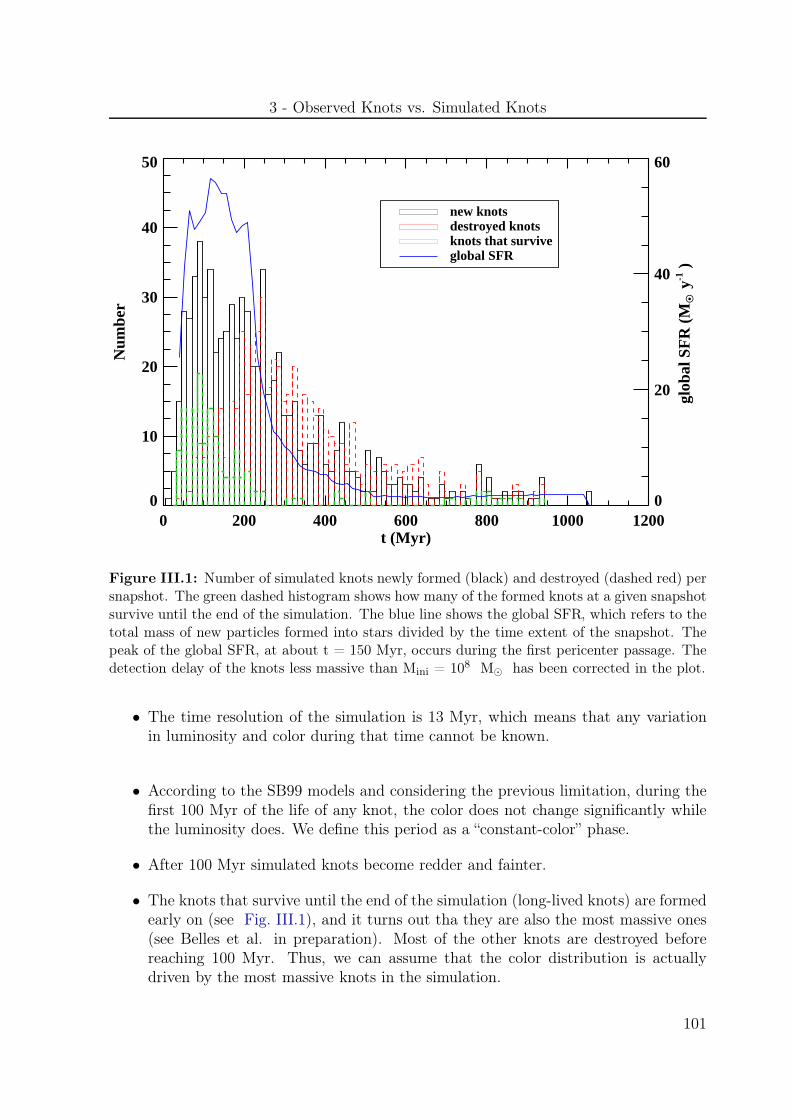
3 - Observed Knots vs. Simulated Knots
0 200 400 600 800 1000 1200t (Myr)
0
10
20
30
40
50
Num
ber
0
20
40
60
glob
al S
FR
(M
O • y
-1 )
new knotsdestroyed knotsknots that surviveglobal SFR
Figure III.1: Number of simulated knots newly formed (black) and destroyed (dashed red) persnapshot. The green dashed histogram shows how many of the formed knots at a given snapshotsurvive until the end of the simulation. The blue line shows the global SFR, which refers to thetotal mass of new particles formed into stars divided by the time extent of the snapshot. Thepeak of the global SFR, at about t = 150 Myr, occurs during the first pericenter passage. Thedetection delay of the knots less massive than Mini = 108 M⊙ has been corrected in the plot.
• The time resolution of the simulation is 13 Myr, which means that any variationin luminosity and color during that time cannot be known.
• According to the SB99 models and considering the previous limitation, during thefirst 100 Myr of the life of any knot, the color does not change significantly whilethe luminosity does. We define this period as a “constant-color” phase.
• After 100 Myr simulated knots become redder and fainter.
• The knots that survive until the end of the simulation (long-lived knots) are formedearly on (see Fig. III.1), and it turns out tha they are also the most massive ones(see Belles et al. in preparation). Most of the other knots are destroyed beforereaching 100 Myr. Thus, we can assume that the color distribution is actuallydriven by the most massive knots in the simulation.
101
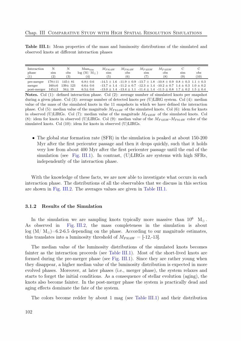
Chap. III Comparative Study with High Spatial Resolution Simulations
Table III.1: Mean properties of the mass and luminosity distributions of the simulated andobserved knots at different interaction phases
Interaction N N Masssim MF814W MF814W MF435W MF435W C Cphase sim obs log (M/ M⊙ ) sim obs sim obs sim obs(1) (2) (3) (4) (5) (6) (7) (8) (9) (10)
pre-merger 178±11 145± 81 6.8± 0.6 -14.5 ± 1.6 -11.9 ± 0.9 -13.7 ± 1.8 -10.8 ± 0.9 0.8 ± 0.3 1.1 ± 0.3merger 160±6 139± 123 6.6± 0.6 -13.7 ± 1.4 -11.2 ± 0.7 -12.3 ± 1.4 -10.2 ± 0.7 1.4 ± 0.3 1.0 ± 0.2post-merger 145±2 34± 19 6.5± 0.6 -13.0 ± 1.4 -13.4 ± 1.1 -11.4 ± 1.4 -11.5 ± 0.8 1.7 ± 0.2 1.5 ± 0.4
Notes. Col (1): defined interaction phase. Col (2): average number of simulated knots per snapshotduring a given phase. Col (3): average number of detected knots per (U)LIRG system. Col (4): medianvalue of the mass of the simulated knots in the 11 snapshots in which we have defined the interactionphase. Col (5): median value of the magnitude MF814W of the simulated knots. Col (6): idem for knotsin observed (U)LIRGs. Col (7): median value of the magnitude MF435W of the simulated knots. Col(8): idem for knots in observed (U)LIRGs. Col (9): median value of the MF435W -MF814W color of thesimulated knots. Col (10): idem for knots in observed (U)LIRGs.
• The global star formation rate (SFR) in the simulation is peaked at about 150-200Myr after the first pericenter passage and then it drops quickly, such that it holdsvery low from about 400 Myr after the first pericenter passage until the end of thesimulation (see Fig. III.1). In contrast, (U)LIRGs are systems with high SFRs,independently of the interaction phase.
With the knowledge of these facts, we are now able to investigate what occurs in eachinteraction phase. The distributions of all the observables that we discuss in this sectionare shown in Fig. III.2. The averages values are given in Table III.1.
3.1.2 Results of the Simulation
In the simulation we are sampling knots typically more massive than 106 M⊙ .As observed in Fig. III.2, the mass completeness in the simulation is aboutlog (M/ M⊙)=6.2-6.5 depending on the phase. According to our magnitude estimates,this translates into a luminosity threshold of MF814W = [-12,-13].
The median value of the luminosity distributions of the simulated knots becomesfainter as the interaction proceeds (see Table III.1). Most of the short-lived knots areformed during the pre-merger phase (see Fig. III.1). Since they are rather young whenthey disappear, a higher median value of the luminosity distribution is expected in moreevolved phases. Moreover, at later phases (i.e., merger phase), the system relaxes andstarts to forget the initial conditions. As a consequence of stellar evolution (aging), theknots also become fainter. In the post-merger phase the system is practically dead andaging effects dominate the fate of the system.
The colors become redder by about 1 mag (see Table III.1) and their distribution
102

3 - Observed Knots vs. Simulated Knots
0.00
0.05
0.10
0.15
0.20
0.25
Fra
ctio
n
pre-merger
N = 1907
N = 1157
-1 0 1 2 3 4 50.0
0.1
0.2
0.3
0.4
0.5
0.00
0.05
0.10
0.15
0.20
0.25
Fra
ctio
n
merger
N = 1731
N = 832
-1 0 1 2 3 4 50.0
0.1
0.2
0.3
0.4
0.5
1.2 1.4 1.6 1.80.700.750.800.850.90
5 6 7 8 9log (M/M O •)
0.00
0.05
0.10
0.15
0.20
0.25
Fra
ctio
n
post-merger
-20 -15 -10 -5MF814W
N = 1575
N = 171
-1 0 1 2 3 4 5MF435W - MF814W
0.0
0.1
0.2
0.3
0.4
0.5
1.2 1.4 1.6 1.80.700.750.800.850.90
Figure III.2: Mass, I -band magnitude and color distributions for the simulated knots (in black)adding up the knots identified in each of the 11 snapshots in which we defined an interactionphase. The vertical dashed line indicates the luminosity of a single stellar population with a massof 106.2−6.5
M⊙ (the mass completeness, as inferred from the mass distributions showed) andthe same age as the oldest simulated knot in each phase, in order to give an idea of the magnitudethreshold of the distribution. Red line histograms show the same distributions for the observeddata (see Chapter II). N gives the number of detected knots in each case. Green line histogramsshow the distribution of the simulated knots applying an extinction following an exponentialprobability density function and that best matches the red wing (i.e., MF435W -MF814W > 1-1.5)of the color distribution of the observed knots (see text). The inset plots in the third columnextend the y-axis to better visualize the peak of the color distribution of the simulated data.
103

Chap. III Comparative Study with High Spatial Resolution Simulations
becomes more peaked (see Fig. III.2) as the interaction proceeds. In the simulation theSFR peaks just after the pre-merger phase starts, then it drops very rapidly in a periodwhich already exceeds the “constant color” phase (see Fig. III.1). All the long-livedknots, which are likely to affect most significantly the color distribution, are formed.As a consequence, basically blue populations (those which formed last), intermediate-color populations and rather minor red populations are present in this early phase. Inthe merger phase, as the system starts to relax and to forget the initial conditions, thecolor distribution is basically driven by the most massive knots (formed early on), andit starts to redden. Since the presence of a young population is hugely diminished, thecolor becomes less spread and peaks toward redder values. In the post-merger phase, theknots become even redder, since only aging effects play the role.
3.1.3 Observations vs. Simulations. General Comparison
In the previous section we estimated that the faint end of the luminosity distribution ofthe simulated knots is affected by the limited mass resolution of the simulation. This canexplain why in the pre-merger and merger phases the luminosity of the observed knotsis on average up to a factor of 15 (3 mag) lower than the luminosity of the simulatedknots (see Table III.1). In fact, the luminosity threshold in the simulation is about thisamount higher than the luminosities at the peak of the distributions for the observedknots (see Fig. III.2), more or less the completeness limits.
The numerical simulation was designed to reproduce correctly the most massive struc-tures, while it misses the low mass ones. Thus, if this less massive population were notmissed the median value of the luminosity distributions of observed and simulated knotswould approach. Once this bias understood, we see that the evolutionary trend due toaging is also observed in (U)LIRGs during these two early phases (knots become fainterby about 0.7 mag).
During the post-merger phase we see the following changes:
• On the one hand, there is a good agreement between the observed and simulatedluminosity distributions. In this case, the faintest knots in observed systems seem tohave disappeared. This might not be just a coincidence since, according to studieson long-term evolution of cluster populations (e.g., Whitmore et al. 2007; Fall et al.2009), low mass clusters (populating the faint end of the luminosity distribution)have more probabilities than the most massive ones to be disrupted. Thus, duringthe pre-merger and merger phases this faint end of the luminosity distribution isnot sampled in the simulation by resolution issues. And in the post-merger phaseit is probably not sampled because there are no low-mass knots to sample, sincethey have dissolved in the interestelar medium.
• On the other hand, the observed knots in this phase are more luminous (by about
104

3 - Observed Knots vs. Simulated Knots
2 mag) than in previous phases, (see Fig. III.2 and Table III.1). We would expectthat, by aging effects (predicted by the simulations), the population became fainter.The merging of smaller clusters into massive superclusters, as suggested by Kroupa(1998) and argued in Chapter II, could be responsible for the lack of fainter knotsin post-mergers (U)LIRGs. As mentioned before, this process can not resolved inthe simulation given its spatial resolution.
In summary, both theoretical and observational data support that after the dynamicalprocess of interaction in galaxy mergers the population is concentrated in the mostmassive structures.
3.1.4 Broadening of the Color Distribution of Knots in (U)LIRGs
The color distributions of the observed knots become redder as the interaction pro-ceeds, a behavior that the simulation predicts and it is explained by aging effects (seespecific values in Table III.1). However, the rather peaked color distributions of the simu-lated knots are quite different from the broader color distributions of the observed knots,as Fig. III.2 shows. These differences are actually expected, given the intrinsic charac-teristics of observations and simulations. In the following, we investigate the broadeningof the color distribution of knots in (U)LIRGs.
Despite the fact that no extinction is implemented in the simulations, a significantpercentage of the observed knots are still bluer than the simulated knots at any in-teraction phase (blue wing; typically MF435W -MF814W < 0.5-1). As mentioned before,(U)LIRGs are known to preserve high SFRs independently of the interaction phase, whilein the simulation the SFR is high only during the pre-merger phase (see Fig. III.1). Thus,the star formation history of (U)LIRGs implies that the young knots, with blue colors, arecontinuously being formed in all phases. In contrast, the formation of knots is quickly sup-pressed in the simulations after the pre-merger phase. Moreover, given the time resolutionon the simulation, we are not able to sample colors as blue as MF435W -MF814W . 0.4,whereas in (U)LIRGs younger population with bluer colors can exist.
Since the effect of obscuration by dust is not implemented in the simulation, it isworth investigating the difference of the color distributions of simulated and observedknot to understand how the extinction is distributed in (U)LIRGs. In this case, we focuson the red wing (i.e., MF435W -MF814W > 1.5) of the color distribution of the observedknots.
We investigated how the colors of the simulated knots would change if they weresuffering some extinction, so as to recover the red wing of the color distribution of theobserved knots. To that end, a test was performed by applying an extinction distributionwith a probability density function of an exponential decay with the form P(AV )=λe−λAV
to the simulated colors, where 1/λ (ln2/λ) represents the mean (median) value of the
105
Chap. III Comparative Study with High Spatial Resolution Simulations
distribution. The test was performed from 1/λ values of 0.01 to 2 mag and the bestmatch by means of a Kolmogorov-Smirnov test (KS) of the simulated (with extinction)and observed color distribution was selected. The comparison between both distributionswas done from the peak of the initial distribution of the simulated colors toward reddercolors.
We were able to obtain similar shapes for the red wing of the observed and sim-ulated knots (see green histograms in Fig. III.2). We derived the mean values of1/λ = [1.3,1.4,1.1] mag for the pre-merger, merger and post-merger phase, respectively.With this mean values, the simulated knots would suffer extinctions typically in therange AV = 0-5 mag, with a probability distribution that peaks around 0-1 mag anddecays exponentially. Therefore, based on this result we conclude that the obscurationfor optically-selected knots in (U)LIRGs is likely to be distributed with a probabilitydensity function of an exponential decay. In fact, this range of extinctions is only slightlysmaller than that reported in (U)LIRGs in the optical and near infrared (Alonso-Herreroet al. 2006; García-Marín et al. 2009a).
We estimated the corrected magnitude distribution of the simulated knots as if theywere affected by dust extinction (green histograms in Fig. III.2), using the obtainedvalues of 1/λ. Interestingly, the extinction values derived, similar to those observed in(U)LIRGs, do not contribute significantly to dimming the luminosity of the simulatedknots (less than 1 mag on average).
3.2 Mass and Luminosity Functions
3.2.1 MF and LF of the Simulated Knots
We have the opportunity to study the evolution of the MF and the LF of the simulatedknots with the merging process. In general, the MF and LF of young stellar objects (clus-ters, SSCs, YMCs, complexes of clusters) are well described as power-law distributions:dN ∝ m−αMF dm (MF) and dN ∝ L−αLF
λ dLλ (LF). We applied the same methodologyas in Chapter II, explained in Chapter I (Section 3.3), based on fitting equal-sized bindistributions, to fit both the MF and LF. The lower mass and brightness for which thesimulated knots sample is complete was determined assuming a simple power law formfor the knot mass distribution. The uncertainties associated to the fit of the LF (shownin tables and figures) do not include other sources of systematic error (e.g., droppingthe brightest bins, adopting another method of binning, moving the magnitude limit).Therefore, like in Chapter II, we consider a systematic uncertainty of 0.1 dex.
The slope of the mass function of the simulated knots (αMF ) is typically 1.8(see Fig. III.3). Although a visual trend may be observed toward steeper slopes fromthe pre-merger to the merger phase, given the uncertainties involved there is no clearevidence of an evolution of the slope with the phase of the merger. Even though in gen-
106
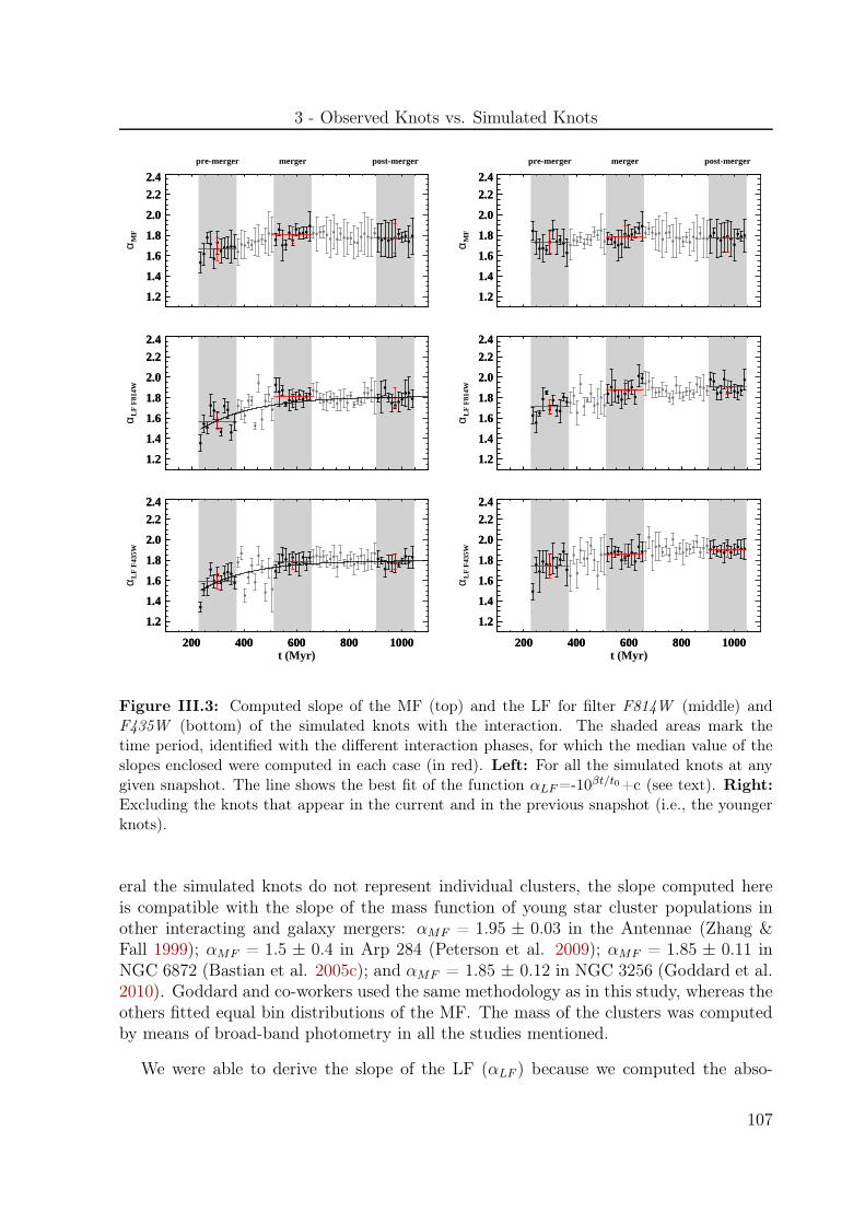
3 - Observed Knots vs. Simulated Knots
1.2
1.4
1.6
1.8
2.0
2.2
2.4
α MF
1.2
1.4
1.6
1.8
2.0
2.2
2.4pre-merger merger post-merger
1.2
1.4
1.6
1.8
2.0
2.2
2.4
α LF
F81
4W
1.2
1.4
1.6
1.8
2.0
2.2
2.4
200 400 600 800 1000t (Myr)
1.2
1.4
1.6
1.8
2.0
2.2
2.4
α LF
F43
5W
200 400 600 800 1000
1.2
1.4
1.6
1.8
2.0
2.2
2.4
1.2
1.4
1.6
1.8
2.0
2.2
2.4
α MF
1.2
1.4
1.6
1.8
2.0
2.2
2.4pre-merger merger post-merger
1.2
1.4
1.6
1.8
2.0
2.2
2.4
α LF
F81
4W
1.2
1.4
1.6
1.8
2.0
2.2
2.4
200 400 600 800 1000t (Myr)
1.2
1.4
1.6
1.8
2.0
2.2
2.4
α LF
F43
5W
200 400 600 800 1000
1.2
1.4
1.6
1.8
2.0
2.2
2.4
Figure III.3: Computed slope of the MF (top) and the LF for filter F814W (middle) andF435W (bottom) of the simulated knots with the interaction. The shaded areas mark thetime period, identified with the different interaction phases, for which the median value of theslopes enclosed were computed in each case (in red). Left: For all the simulated knots at anygiven snapshot. The line shows the best fit of the function αLF=-10βt/t0+c (see text). Right:Excluding the knots that appear in the current and in the previous snapshot (i.e., the youngerknots).
eral the simulated knots do not represent individual clusters, the slope computed hereis compatible with the slope of the mass function of young star cluster populations inother interacting and galaxy mergers: αMF = 1.95 ± 0.03 in the Antennae (Zhang &Fall 1999); αMF = 1.5 ± 0.4 in Arp 284 (Peterson et al. 2009); αMF = 1.85 ± 0.11 inNGC 6872 (Bastian et al. 2005c); and αMF = 1.85 ± 0.12 in NGC 3256 (Goddard et al.2010). Goddard and co-workers used the same methodology as in this study, whereas theothers fitted equal bin distributions of the MF. The mass of the clusters was computedby means of broad-band photometry in all the studies mentioned.
We were able to derive the slope of the LF (αLF ) because we computed the abso-
107

Chap. III Comparative Study with High Spatial Resolution Simulations
Table III.2: Slopes of the mass and luminosity distributions of the simulated and observedknots at different interaction phases
Interaction NY (%) αMF αLF F814W αLF F814W αLF F435W αLF F435W
phase sim obs sim obs sim
pre-merger 12±7 1.67 ± 0.11 1.84 ± 0.03 1.57 ± 0.08 1.86 ± 0.05 1.59 ± 0.07merger 2±1 1.80 ± 0.08 2.00 ± 0.04 1.81 ± 0.07 1.86 ± 0.02 1.79 ± 0.08post-merger 1±1 1.77 ± 0.15 1.76 ± 0.12 1.80 ± 0.10 1.58 ± 0.17 1.78 ± 0.07
Notes. Col (1): defined interaction phase. Col (2): number of young simulated knots (see text) withrespect to the total number of simulated knots. Col (3): average of the median values of the slopes of theMF computed for the 11 distributions per interaction phase. Col (4): slope of the luminosity function(filter F814W ) at a given interaction phase. Col (5): average of the median values of the slopes of theLF (filter F814W ) computed for the 11 distributions per interaction phase. Col (6): same as column(4), but with data observed with the filter F435W. Col (7) same as column (5), but with filter F435W.
lute magnitude distribution of the simulated knots and αLF = 2.5β + 1, where β is theslope of the fit for the magnitude distribution. In this case, there is a slight trend to-ward steeper αLF for the simulated knots as the merger proceeds up to about 500 Myr(see Fig. III.3, left). This trend is less significant for the filter F435W (see Table III.2).We tried to fit empirically the values of αLF at each snapshot with a function of the formαLF = -10γt/t0 + c, a kind of an exponential decay (with index γ). However, as shownin Fig. III.3 (left), the fit is not very well constrained since the dispersion is very high.Hence, even though the trend can be real, within the uncertainties we cannot characterizeit given the large dispersions in the different slopes.
We suspect the young population can be responsible for the variation of the slope ofthe LF, since it can be up to a factor of 10-100 more luminous than an old population(i.e., 1 Gyr) with the same mass. (see Fig. I.7 in Chapter I). For instance, a populationof 100 Myr can be up to 5 mag fainter than a population of less than 10 Myr having thesame mass. If there is a significant fraction of young population, it can overpopulate thebright end of the LF, making it flat.
To prove the validity of this hypothesis we explore the same plot (αLF vs. time)but excluding those knots that appear for the first time in the simulation in the currentsnapshot and in the previous one (i.e., normally the youngest knots). We refer to themas the young simulated knots. When these young knots are excluded from the fit, thetrend tends to disappear in both filters (Fig. III.3, right). Since in the simulation theknot formation rate is very low during the merger and the post-merger phases, thenumber of young simulated knots is negligible then compared to the pre-merger phase(see Table III.2). Therefore, these youngest knots are the responsible for overpopulatingthe bright end of the LF, which makes its slope flatten.
108
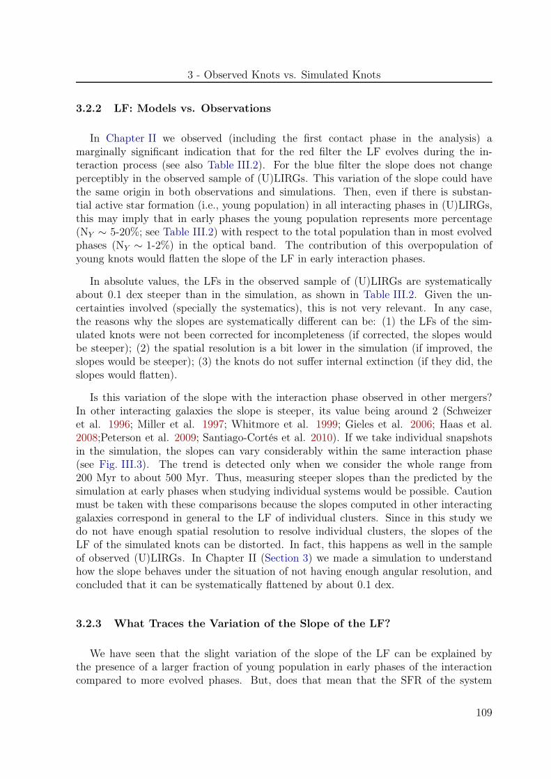
3 - Observed Knots vs. Simulated Knots
3.2.2 LF: Models vs. Observations
In Chapter II we observed (including the first contact phase in the analysis) amarginally significant indication that for the red filter the LF evolves during the in-teraction process (see also Table III.2). For the blue filter the slope does not changeperceptibly in the observed sample of (U)LIRGs. This variation of the slope could havethe same origin in both observations and simulations. Then, even if there is substan-tial active star formation (i.e., young population) in all interacting phases in (U)LIRGs,this may imply that in early phases the young population represents more percentage(NY ∼ 5-20%; see Table III.2) with respect to the total population than in most evolvedphases (NY ∼ 1-2%) in the optical band. The contribution of this overpopulation ofyoung knots would flatten the slope of the LF in early interaction phases.
In absolute values, the LFs in the observed sample of (U)LIRGs are systematicallyabout 0.1 dex steeper than in the simulation, as shown in Table III.2. Given the un-certainties involved (specially the systematics), this is not very relevant. In any case,the reasons why the slopes are systematically different can be: (1) the LFs of the sim-ulated knots were not been corrected for incompleteness (if corrected, the slopes wouldbe steeper); (2) the spatial resolution is a bit lower in the simulation (if improved, theslopes would be steeper); (3) the knots do not suffer internal extinction (if they did, theslopes would flatten).
Is this variation of the slope with the interaction phase observed in other mergers?In other interacting galaxies the slope is steeper, its value being around 2 (Schweizeret al. 1996; Miller et al. 1997; Whitmore et al. 1999; Gieles et al. 2006; Haas et al.2008;Peterson et al. 2009; Santiago-Cortés et al. 2010). If we take individual snapshotsin the simulation, the slopes can vary considerably within the same interaction phase(see Fig. III.3). The trend is detected only when we consider the whole range from200 Myr to about 500 Myr. Thus, measuring steeper slopes than the predicted by thesimulation at early phases when studying individual systems would be possible. Cautionmust be taken with these comparisons because the slopes computed in other interactinggalaxies correspond in general to the LF of individual clusters. Since in this study wedo not have enough spatial resolution to resolve individual clusters, the slopes of theLF of the simulated knots can be distorted. In fact, this happens as well in the sampleof observed (U)LIRGs. In Chapter II (Section 3) we made a simulation to understandhow the slope behaves under the situation of not having enough angular resolution, andconcluded that it can be systematically flattened by about 0.1 dex.
3.2.3 What Traces the Variation of the Slope of the LF?
We have seen that the slight variation of the slope of the LF can be explained bythe presence of a larger fraction of young population in early phases of the interactioncompared to more evolved phases. But, does that mean that the SFR of the system
109

Chap. III Comparative Study with High Spatial Resolution Simulations
traces the slope of the LF? This is a key issue, since (U)LIRGs are known to have highSFRs, but in advanced phases (merger and post-merger) the slope of the LF of the knotsis the same.
At t = 250 Myr the global SFR in the simulation drops dramatically (see Fig. III.1).The shape of the histogram that represents the knot formation rate (black histogramin Fig. III.1) is similar, though wider. It is a difference not related to the detection thresh-old of the knot, because the black histogram was corrected for that. At t = 300 Myrthe global SFR is already very low (less than 10 M⊙ yr−1) compared to the peak(PeakSFR ∼ 50 M⊙ yr−1), and the slope of the LF can still be quite flat (αLF = 1.5-1.6).Yet, the knot formation rate remains still high. Therefore, the variation of the slope ofthe LF is likely to be related only to the knot formation rate, and not necessarily to theglobal SFR. This implies that if a system has a high SFR (i.e., a LIRG or a ULIRG), butthe current star formation is concentrated on very few knots or mainly obscured (i.e., notobservable in the optical), the young population does surely not affect the slope of theLF. Might this be occurring in advanced phases (merger and post-merger) in (U)LIRGs?
3.3 Evolution of the Spatial Distributions of the Properties of the Knots
The comparison of the evolution of the spatial distributions of the simulated andobserved knots as a function of the interaction phase can provide additional informationon the physical processes that govern the production of star clusters. For this study,we defined 6 bins of galactocentric distance, each separated by a factor of 2 from d=2.5kpc: 0-2.5, 2.5-5, 5-10, 10-20, 20-40, and 40-80 kpc. The distances for the observed knotsin Fig. III.4 correspond to projected galactocentric distances. However, in the simulationwe have access to the real galactocentric distance of the knots at any given snapshot (the3D-distance). We thus study the spatial distribution of the photometric properties usingthe 3D-distance and the 3 projected distances on each of the three planes in the simulation(XY, XZ and YZ). In general, either if we are dealing with the 3D or with any projecteddistance the trends in the simulation do not change significantly. In any case, we decidedto make the comparison with the observations taking a projected distance because wehave more statistics at smaller galactocentric distances and the distances measured inthe sample of (U)LIRGs are also projected.
Finally, if there is not enough statistics in a given distance bin, then the mean value(red and green in Fig. III.5 and Fig. III.6) is not shown in the plot.
3.3.1 Spatial Distribution of the Knots
The spatial distribution of the observed and simulated knots is significantly differentat any given interaction phase. While more than 60% of the total number of knots arewithin a projected distance of 5 kpc in the sample of (U)LIRGs, only about 20% are
110

3 - Observed Knots vs. Simulated Knots
0.0
0.1
0.2
0.3
0.4
Fra
ctio
nObserved knots
pre-merger
0.0
0.1
0.2
0.3
0.4
Fra
ctio
n
merger
Radius (kpc)
0.0
0.1
0.2
0.3
0.4
Fra
ctio
n
0 2.5 5 10 20 40 80
post-merger
0.0
0.1
0.2
0.3
0.4
Fra
ctio
n
Simulated knots
pre-merger
0.0
0.1
0.2
0.3
0.4
Fra
ctio
n
merger
Radius (kpc)
0.0
0.1
0.2
0.3
0.4
Fra
ctio
n
0 2.5 5 10 20 40 80
post-merger
Figure III.4: Spatial distribution of the observed (left) and simulated (right) knots. For thesimulated knots the distance correspond to the projected galactocentric distance in the XYplane.
located below that distance in the simulation. Recent hydrodynamic simulations of amajor merger (Teyssier et al. 2010) showed that models limited in spatial and massresolution, and/or the absence of a model for gas cooling below ∼104 K, cannot resolveproperly the process of gas fragmentation into massive clouds and rapid star formation.Teyssier and co-workers ran their simulation in a low and high resolution mode, usinga softening of ∆x=96 and 12 pc, respectively. The ISM becomes much more clumpy inthe high resolution mode, especially in the inner regions and then more clusters/knotscan be formed. Furthermore, gas is more extended, allowing formation of SSCs at higherradii.
In the simulation by Bournaud et al. (Bournaud et al. 2008b), even if the spatialresolution is still very high, it is three times lower than the high resolution mode in
111

Chap. III Comparative Study with High Spatial Resolution Simulations
the hydrodynamic simulations mentioned and neglect the thermal pressure of the gasa.Additionally, it may be more difficult to detect low-mass knots in the central regionsof the simulated galaxies given the large diffuse background there. Therefore, we haveto be cautious when comparing the evolution of spatial distributions of the magnitudesand colors of the observed and simulated knots at galactocentric distances smaller thand < 5 kpc.
3.3.2 Evolution of the Spatial Distribution of Luminosities.
During the pre-merger phase, we see a trend of the luminosities of the simulated knotswith the radial distance, in such a way that they become fainter as the distance increases.As the interaction proceeds, in the merger phase this trend (if real) is very weak. By thetime the post-merger phase is reached the spatial distribution of luminosities is completelyflat (see Fig. III.5). Both the spatial distribution of magnitudes and masses follow thesame trends at any given interaction phase. This could indicate that the star formation inthe simulation is not centrally concentrated. However, if we select the youngest simulatedknots (new knots, circled light blue dots in Fig. III.5) we realize that during the pre-merger phase, close to the peak of the SFR, 45% are formed within the central 5 kpc andthe median value of their mass distribution corresponds to log (M/ M⊙) = 7.25 againstthe value of 6.57 for knots located at larger distances. Later on, this percentage dropsto 30% and 0% in the merger and post-merger phase, respectively. In the merger phasethe new knots in the central 5 kpc are still significantly more massive than the moreexternal ones (log (M/ M⊙) of 6.55 against 6.18). Hence, the trend can be due to twocontributions:
(1) the star formation in the simulation is more concentrated in the nuclear regionsduring the first phases of the interaction. The knots are more luminous there, sincethey are on average younger than knots in the outermost regions.
(2) the most massive knots tend to form in the central regions. Thus, they are also moremassive, i.e., more luminous there.
The trend tends to disappear as the interaction proceeds since at later phases the knotformation process (though not very strong given that SFR is very low in the simulation)is more efficient in the external regions (i.e., in tidal tails). Younger population willbe more luminous being even less massive there. Note that given the limitation of thesimulation on forming knots in the innermost regions, discussed in the previous section,
a The sticky particle scheme used in this simulation assumes that the turbulent pressure dominates:the turbulent pressure and turbulence dissipation are modeled by the interactions of sticky particles,and the thermal pressure is neglected. This may be a realistic sub-grid treatment for molecular andcool/cold atomic phases (which are dominated by supersonic turbulence, e.g., Burkert & Bodenheimer1996) but the more important thermal pressure in warmer phases (≥ 104 K) is neglected.
112

3-
Observed
Knots
vs.Sim
ulatedK
nots
Figure III.5: Spatial distribution of the mass, luminosity and color for the simulated knots at the three interaction phases definedin this study. In each case we plot the values in the 11 snapshots for which the interaction phases have been defined, and taking theprojected galactocentric distance in the XY plane (black dots). Those dots circled in light blue refer to the knots that appear for thefirst time in one of the 11 snapshots that define an interaction phase. Mean and standard deviation of each 0.3 dex (log 2) bin indistance is shown in red (green) taking the 3D-distance (projected distance in the XY plane), starting from the bin [0,2.5] kpc. Thered line is not a fit and marks the mean values within each bin.
113
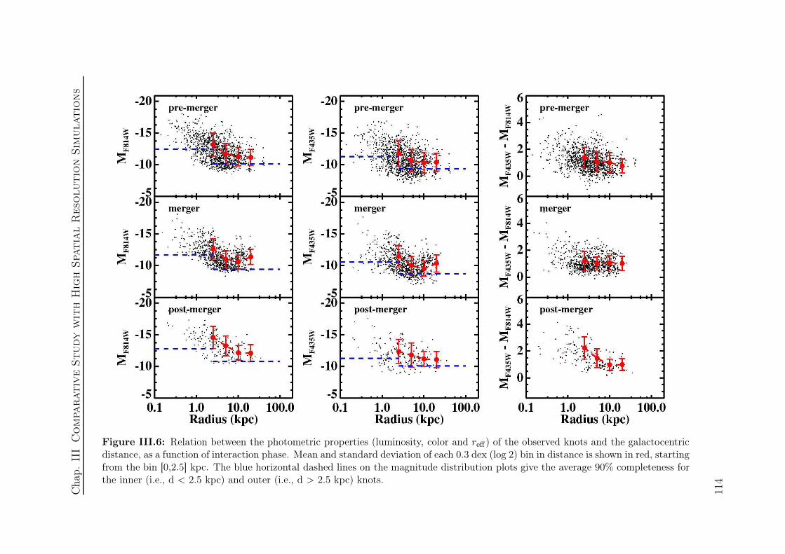
Cha
p.II
IC
om
parativ
eStudy
wit
hH
igh
Spa
tia
lR
eso
lutio
nSim
ulatio
ns
Figure III.6: Relation between the photometric properties (luminosity, color and reff ) of the observed knots and the galactocentricdistance, as a function of interaction phase. Mean and standard deviation of each 0.3 dex (log 2) bin in distance is shown in red, startingfrom the bin [0,2.5] kpc. The blue horizontal dashed lines on the magnitude distribution plots give the average 90% completeness forthe inner (i.e., d < 2.5 kpc) and outer (i.e., d > 2.5 kpc) knots.
114
4 - Summary and Conclusions
the percentages given should be considered as a lower limits. Thus, in the pre-mergerphase, we expect that actually more than half of the knots are formed within the central5 kpc instead of 45%. However, given this limitation we cannot quantify by how much.
In the sample of (U)LIRGs, a similar variation to that in the pre-merger phase of thesimulation of luminosities with distance persists up to the merger phase (see Fig. III.6).Actually, part of this trend can be due to incompleteness in detecting the knots in thecentral regions of the galaxies, where the surface brightness of the underlying backgroundis high. For that reason, knots fainter than the 90% completeness limit are not detected.Nevertheless, there are not very bright knots in the outermost regions, independently ofthe completeness limit. Therefore, this variation might remain, meaning that on averagethe brightest objects are located within the first few kpc of the galaxies at any giveninteraction phase, as the simulation predicts only for the pre-merger phase. Then, whydoes the trend remain up to more advanced phases in (U)LIRGs? These systems cansustain high rates of star formation at any interaction phase. If we assume that thisvariation has the same origin as in the simulation, then at least half of the current starformation is always concentrated within 5 kpc, no matter which phase of the interactionthe systems are undergoing (the variation is kept during the whole interaction). This hasbeen observed in galaxies at different phases of interaction, like in the central regions ofthe Antennae (Mengel et al. 2008; Whitmore et al. 2010 and in NGC 7252 (Miller et al.1997). As a main conclusion, our theoretical and empirical data suggest that wheneverthe global star formation rate is high in interacting environments, it is likely to be mainlyconcentrated in the central regions.
3.3.3 Evolution of the Spatial Distribution of Colors.
As we have seen before, the young knots in the simulation are more concentratedduring the pre-merger phase. The spatial distribution of colors confirm this, since youngerknots are bluer, and knots with bluer color are located in central regions during this phase(Fig. III.5). In contrast, the knots in (U)LIRGs show a trend toward redder colors in theinner regions, in the pre-merger and post-merger phase (Fig. III.6). This is an indicationof higher internal extinction in the central regions of this systems. Based on the previousconclusion that most of the current star formation appears to be concentrated towardthe central regions in (U)LIRGs, then the extinction must be even more severe, as it hasbeen measured in these kind of systems (e.g., Alonso-Herrero et al. 2006; García-Marínet al. 2009b).
4 Summary and Conclusions
This Chapter shows the results of the first direct comparison of the star formationin interacting galaxies obtained with high spatial resolution numerical simulations with
115
Chap. III Comparative Study with High Spatial Resolution Simulations
observations of galaxy interactions on scales of 30-100 pc. We have compared the evo-lution of the observed photometric properties of the stellar regions (knots) in a sampleof 22 (U)LIRGs with those predicted in a simulation of a major merger of two galaxieswith roughly equal initial mass ratio and large fraction of gas, similar to some observedsystems. Three different interaction phases have been defined: pre-merger, merger andpost-merger, occurring in the simulation at about t = 200-400 Myr, 500-700 Myr and1 Gyr, respectively. The high resolution model reproduces and/or explains in a coherentway some observed properties of the star-forming regions in major mergers. We drawthe following conclusions:
1. As a consequence of the aging of the knots during the merging process, observa-tions and simulations show an evolutionary trend in which knots become fainterand have redder MF435W -MF814W colors as the interaction proceeds from thepre-merger to the merger phase. Later on, during the post-merger phase, thereis theoretical and observational evidence that only the most massive structuresremain, although it is still not clear how they form: (i) as individual massiveentities; (ii) or after a merging process of clusters into superclusters.
2. The color distribution of the simulated knots span a very narrow range(MF435W -MF814W = 0.5-2) compared to the observed color distribution of theknots in (U)LIRGs. To reproduce the observed color distribution an extinctioncorrection has to be applied to the colors of the simulated knots, characterizedby an exponential probability density function of median value AV = 1.1-1.4 mag.The derived typical obscuration peaks at AV = 0-1 mag, and ranges from 0 to 5mag.
3. The shape of the mass function (MF) of the simulated knots is practically constantalong the interaction process. The derived slope of the MF, typically αMF ∼ 1.8,is similar to that obtained for observed individual star clusters in less luminousinteracting environments.
4. The slope of the luminosity function (LF) may evolve throughout the interactionprocess. A weak trend toward steeper slopes of the LFs of the simulated knots isobserved during the pre-merger phase up to the merger phase, when it stabilizesaround αLF = 1.8-1.9. According to the simulation, this slight variation is likelyto be due to high knot formation rates at early phases of the interaction withrespect to the knot formation rates at late phases. However, there is not clearevidence that it is correlated with the global star formation rate of the system.The same origin could explain the slight variation of the LF of the observed knotsin (U)LIRGs provided that the global star formation is concentrated in few knotsduring intermediate and advanced interaction phases.
116

4 - Summary and Conclusions
5. Numerical issues considered on the formation and detection of knots at smalldistances (galactocentric distance d < 5 kpc), the simulation confirms that whenthe global star formation is high (pre-merger) the star formation is mainlyconcentrated in the central regions. The spatial distribution of luminosities in(U)LIRGs suggests that the star formation in these systems is mainly concentratedin the central regions in general (no matter the interaction phase), in agreementwith previous studies of these systems.
117


Chapter IV
TDG Candidates in Low-z (U)LIRGs
Overview
In this Chapter we use the combination of the photometricdata from previous chapters, and spectroscopic data to investi-gate the nature of the extreme extranuclear young population,detected in our sample of (U)LIRGs in the context of TDG for-mation. We make use of several criteria (e.g., Hα luminosity,dynamical mass content, signs of self-gravitation, etc.) to in-vestigate their nature as TDGs and the chances of survival aslong-lived entities. The knowledge of the production rate oflong-lived TDGs for the (U)LIRG class also provides clues toconstrain the dwarf galaxy formation at high redshifts.
1 Introduction
Interacting systems (and remnants) constitute the optimal environment for finding theso-called tidal dwarf galaxies (TDG): a self-gravitating entity of dwarf-galaxy mass builtfrom the tidal material expelled during interactions (General Introduction, Section 2.2).Although many studies devoted to searching and characterizing TDGs in nearby inter-acting systems have been carried out in the past few decades, only a few searches forTDG candidates have been performed to date in LIRGs and ULIRGs.
In previous chapters we have disentangled the photometric properties of knots ofstar formation in a representative sample of (U)LIRGs. Interestingly, very bright (i.e.,MF814W < -12.5) and blue (i.e., MF435W -MF814W < 0.5) knots along the tidal tails andat the tip, indicative of massive (i.e., M = 104-106 M⊙) young populations, have beendetected in those systems. On the basis of previous studies of nearby interacting galaxies(e.g., Duc et al. 1997, 1998; Weilbacher et al. 2000; Temporin et al. 2003; Monreal-Iberoet al. 2007), TDG candidates are normally identified as extreme star forming regionsin tidal tails. With the additional aid of optical IFS data, this chapter is devoted to
119

Chap. IV TDG Candidates in Low-z (U)LIRGs
studying more in detail extranuclear Hα-emitting clumps linked to the knots and asso-ciations investigated in previous chapters. With dynamical masses up to 108-1010 M⊙,these knots and associations represent the most massive case of young star formation in(U)LIRGs, toward the typical range of dwarf galaxies.
This Chapter extends the previous study of Monreal-Ibero et al. (2007) by includinggalaxies in the LIRG class and with additional (i.e., B -band) and more sensitive photo-metric data. Section 2 presents the subsample with available photometric and IFS datasimultaneously. We then identify and characterize the luminosities, colors, metallicities,etc., of extranuclear Hα-emitting complexes in Section 3 and Section 4, respectively. Insection Section 5 we select the complexes that are most likely to constitute TDG can-didates and discuss their total mass content and the likeliness of the survival of theseregions as future TDGs , and the implications for the formation of TDGs at high-z.Finally, we draw our conclusions in Section 6.
2 The Subsample
The initial sample for this study is presented in Chapter I (Section 1.1). Since thisstudy combines our photometric (see Chapter I, Section 2.1) and spectroscopic (see Chap-ter I, Section 2.2) data, we have selected those systems with available data in both setssimultaneously at the moment of the analysis. That is a total of 27 systems.
As explained in section Section 3.1, regions of interest were selected as any high surfacebrightness compact region (Hα clumps) in the emission line maps (obtained from theIFS data) at a projected distance from the nucleus of the galaxy greater than 2.5 kpc,and associated with one or several of the star-forming regions (knots) in the ACS images.On the basis of these criteria, Hα-emitting complexes have been identified in 11 systems.We did not identify other complexes in the remaining sample basically for two reasons:(1) based on the above criteria, in some systems knots are detected but no Hα emission isfound in the outskirts in the Hα line map (e.g., in IRAS 22491-1808); (2) the FoV coveredby the IFS data is not large enough to encompass the full extent of some systems. Hence,the nature of blue knots along the tidal tail and at its tip, where TDGs are normallyfound, cannot be assessed using the IFS data.
Therefore, the final subsample consists of 11 systems with at least one region ofinterest (see table Table IV.1), or more precisely 7 LIRGs and 4 ULIRGs. For complete-ness we also include in our tables the results of Monreal-Ibero et al. (2007) for IRAS16007+3743, for which an image in the B photometric band was unavailable. Accordingto the classification scheme defined in Chapter I (Section 1.2), IRAS 04315-0840, IRAS08355-4944, IRAS F10038-3338 and IRAS 15250+3609 are in an advanced phase of themerger (merger phase) where the nuclei have apparently coalesced. However, the tailsare still recognizable in the images, in some cases very prominently. The rest of thesystems are in earlier stages of the merging process, first contact or pre-merger phases,
120
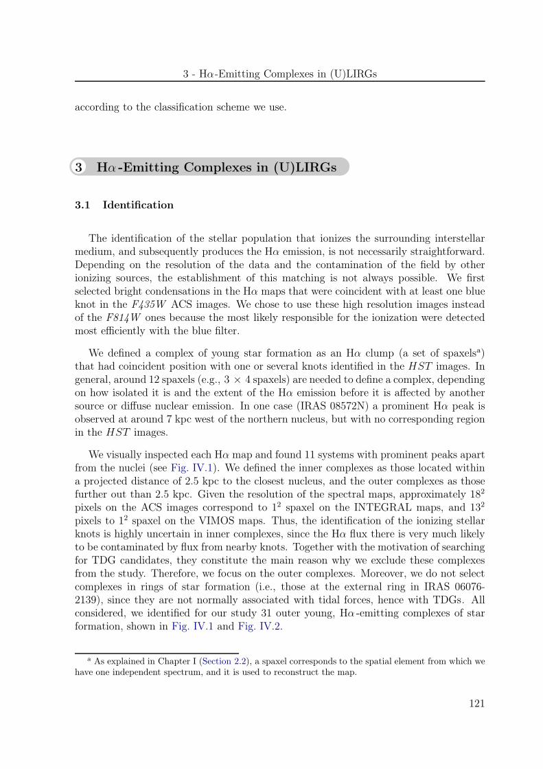
3 - Hα-Emitting Complexes in (U)LIRGs
according to the classification scheme we use.
3 Hα -Emitting Complexes in (U)LIRGs
3.1 Identification
The identification of the stellar population that ionizes the surrounding interstellarmedium, and subsequently produces the Hα emission, is not necessarily straightforward.Depending on the resolution of the data and the contamination of the field by otherionizing sources, the establishment of this matching is not always possible. We firstselected bright condensations in the Hα maps that were coincident with at least one blueknot in the F435W ACS images. We chose to use these high resolution images insteadof the F814W ones because the most likely responsible for the ionization were detectedmost efficiently with the blue filter.
We defined a complex of young star formation as an Hα clump (a set of spaxelsa)that had coincident position with one or several knots identified in the HST images. Ingeneral, around 12 spaxels (e.g., 3 × 4 spaxels) are needed to define a complex, dependingon how isolated it is and the extent of the Hα emission before it is affected by anothersource or diffuse nuclear emission. In one case (IRAS 08572N) a prominent Hα peak isobserved at around 7 kpc west of the northern nucleus, but with no corresponding regionin the HST images.
We visually inspected each Hα map and found 11 systems with prominent peaks apartfrom the nuclei (see Fig. IV.1). We defined the inner complexes as those located withina projected distance of 2.5 kpc to the closest nucleus, and the outer complexes as thosefurther out than 2.5 kpc. Given the resolution of the spectral maps, approximately 182
pixels on the ACS images correspond to 12 spaxel on the INTEGRAL maps, and 132
pixels to 12 spaxel on the VIMOS maps. Thus, the identification of the ionizing stellarknots is highly uncertain in inner complexes, since the Hα flux there is very much likelyto be contaminated by flux from nearby knots. Together with the motivation of searchingfor TDG candidates, they constitute the main reason why we exclude these complexesfrom the study. Therefore, we focus on the outer complexes. Moreover, we do not selectcomplexes in rings of star formation (i.e., those at the external ring in IRAS 06076-2139), since they are not normally associated with tidal forces, hence with TDGs. Allconsidered, we identified for our study 31 outer young, Hα -emitting complexes of starformation, shown in Fig. IV.1 and Fig. IV.2.
a As explained in Chapter I (Section 2.2), a spaxel corresponds to the spatial element from which wehave one independent spectrum, and it is used to reconstruct the map.
121
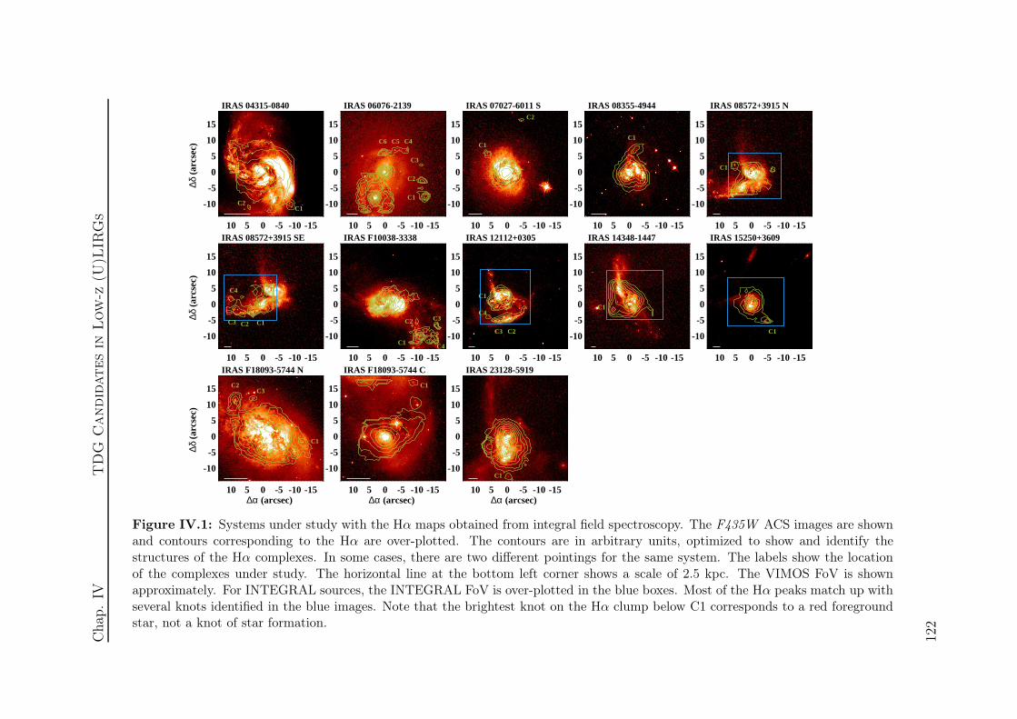
Cha
p.IV
TD
GC
andid
ates
inLow
-z(U
)LIR
Gs
10 5 0 -5 -10 -15
-10
-5
0
5
10
15
∆δ (
arcs
ec)
IRAS 04315-0840
C1C2
10 5 0 -5 -10 -15
-10
-5
0
5
10
15
IRAS 06076-2139
C1
C2
C3
C4C5C6
10 5 0 -5 -10 -15
-10
-5
0
5
10
15
IRAS 07027-6011 S
C1
C2
10 5 0 -5 -10 -15
-10
-5
0
5
10
15
IRAS 08355-4944
C1
10 5 0 -5 -10 -15
-10
-5
0
5
10
15
IRAS 08572+3915 N
C1
10 5 0 -5 -10 -15
-10
-5
0
5
10
15
∆δ (
arcs
ec)
IRAS 08572+3915 SE
C1C2C3
C4
10 5 0 -5 -10 -15
-10
-5
0
5
10
15
IRAS F10038-3338
C1
C2 C3
C4
10 5 0 -5 -10 -15
-10
-5
0
5
10
15
IRAS 12112+0305
C1
C2C3
C4
10 5 0 -5 -10 -15
-10
-5
0
5
10
15
IRAS 14348-1447
C1
10 5 0 -5 -10 -15
-10
-5
0
5
10
15
IRAS 15250+3609
C1
10 5 0 -5 -10 -15∆α (arcsec)
-10
-5
0
5
10
15
∆δ (
arcs
ec)
IRAS F18093-5744 N
C1
C2C3
10 5 0 -5 -10 -15∆α (arcsec)
-10
-5
0
5
10
15
IRAS F18093-5744 C
C1
10 5 0 -5 -10 -15∆α (arcsec)
-10
-5
0
5
10
15
IRAS 23128-5919
C1
Figure IV.1: Systems under study with the Hα maps obtained from integral field spectroscopy. The F435W ACS images are shownand contours corresponding to the Hα are over-plotted. The contours are in arbitrary units, optimized to show and identify thestructures of the Hα complexes. In some cases, there are two different pointings for the same system. The labels show the locationof the complexes under study. The horizontal line at the bottom left corner shows a scale of 2.5 kpc. The VIMOS FoV is shownapproximately. For INTEGRAL sources, the INTEGRAL FoV is over-plotted in the blue boxes. Most of the Hα peaks match up withseveral knots identified in the blue images. Note that the brightest knot on the Hα clump below C1 corresponds to a red foregroundstar, not a knot of star formation.
122
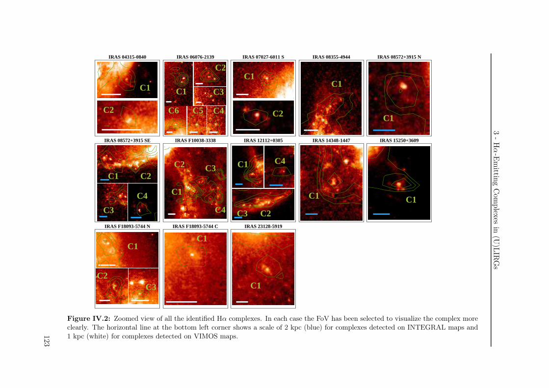
3-
Hα
-Em
ittingC
omplexes
in(U
)LIR
Gs
IRAS 04315-0840
C1
C2
IRAS 06076-2139
C1
C2
C3
C4C5C6
IRAS 07027-6011 S
C1
C2
IRAS 08355-4944
C1
IRAS 08572+3915 N
C1
IRAS 08572+3915 SE
C1 C2
C3
C4
IRAS F10038-3338
C1
C2 C3
C4
IRAS 12112+0305
C1
C2C3
C4
IRAS 14348-1447
C1
IRAS 15250+3609
C1
IRAS F18093-5744 N
C1
C2C3
IRAS F18093-5744 C
C1
IRAS 23128-5919
C1
Figure IV.2: Zoomed view of all the identified Hα complexes. In each case the FoV has been selected to visualize the complex moreclearly. The horizontal line at the bottom left corner shows a scale of 2 kpc (blue) for complexes detected on INTEGRAL maps and1 kpc (white) for complexes detected on VIMOS maps.123

Chap. IV TDG Candidates in Low-z (U)LIRGs
3.2 Structure and Location
Owing to the higher angular resolution of the HST images, we identified theHα clumps (observed in the spectral maps) with a complex of star-forming knots (ob-served in the photometric images). The number of knots in the ACS image per Hα com-plex is on average 2.2. However, the structure of these clumps is in general quite simple.As can be seen in Fig. IV.2 and Table IV.1, the position of the Hα -emission peak iscoincident or quite close to a prominent blue knot. In most cases, only one bright knot isobserved within the area defined for the Hα complex (e.g., C1 in IRAS 08572+3915 N) ora centered bright knot plus a few fainter knots located at the border of the Hα complex(e.g., C1 in IRAS 04315-0840). In a few cases, the structure is quite complex, with severalbright blue knots spread inside the area of the clump (e.g., C2 in IRAS 12112+0305).
When characterizing the Hα complexes, given the rich structure of some of them, weassume that every knot detected in the HST images within the area of the complex isan Hα emitter. With the current data, the estimate of the contribution of each knot tothe total Hα emission or if a knot is not an Hα emitter (i.e., it is older than 10 Myr, atwhich the Hα emission declines abruptly) for all the complexes, is not possible. We alsoassume that only the detected knots are responsible for the whole Hα emission of thecomplex.
The Hα complexes are located at distances in the range 3.3-13.7 kpc from the nucleusof the parent galaxy, with a median value of 9.3 kpc (see Table IV.1). These distances,owing to projection effects, represent lower limits to the real distances. They are relativelyclose distances to the parent galaxy compared to those of the TDG candidates (35-100kpc; e.g., Duc & Mirabel 1998; Sheen et al. 2009; Hancock et al. 2009), although someTDG candidates have been reported at such distances (e.g., Iglesias-Páramo & Vílchez2001; Weilbacher et al. 2003). At these distances, some of the Hα complexes lie along thetidal tails (see Fig. IV.1), and the diffuse low surface brightness Hα emission (which isnot subtracted in our measurements of the Hα flux) is either undetected or considerablydiminished, thus does not contaminate the emission from the knots. Others also appearto be simply a non-nuclear giant HII region.
4 Characterization of the Hα -Emitting Complexes
We now investigate the physical properties of the bright Hα complexes identified. Thischaracterization includes the analysis of the stellar continuum magnitudes (MF435W andcolor), spectral features (Hα luminosity and equivalent width), as well as physical sizesand an estimate of the metallicity. All these observables are compared to those measuredin extragalactic HII regions, dwarf galaxies, and other TDG candidates.
124
4 - Characterization of the Hα-Emitting Complexes
4.1 Photometric Properties of the Complexes
4.1.1 Broad-band Luminosities and Colors
The integrated blue absolute magnitude MF435W and color (MF435W -MF814W ) of theyoung stellar population within the Hα complexes were estimated by adding all the fluxof the knots inside a complex. We cover a magnitude range MF435W = [-9.32, -15.77],and a color range MF435W -MF814W = [-0.23, 2.34] (see Table IV.1). The median valuescorrespond to -12.06 and 0.63 mag, respectively. The typical uncertainties are between0.05 and 0.1 mag.
The integrated luminosities are in general higher than in embedded clusters in nearbyextragalactic HII regions in spirals (Bresolin & Kennicutt 1997) and more typical of thosefound in extragalactic giant HII regions (Mayya 1994; Ferreiro et al. 2008). Althoughearly studies in extragalactic HII regions only focus on nearby galaxies (DL < 20 Mpc),Ferreiro and co-workers observed minor mergers at distances (DL = 40-170 Mpc) similarto our sample, detecting also only the most luminous giant HII regions, the external onescovering the range MB ≃ [-11.7, -17.4], typically 2 magnitudes more luminous than therange sampled in this study.
Nearby dwarf galaxies are typically more luminous than B . -13.0, with col-ors in the range MF435W -MF814W = 0.7-2 (Hunter & Gallagher 1986; Marlowe et al.1997; Cairós et al. 2001). In addition, the luminosities observed for nearby (Ducet al. 1997, 1998, 2007) and more distant (Weilbacher et al. 2000; Temporin et al.2003) TDG candidates are generally more luminous than B = -10.65, as for most of ourHα complexes.
The integrated broad-band luminosities of the embedded stellar population in ourHα complexes is, therefore, compatible with the luminosities measured in giant HII re-gions and TDG candidates.
4.1.2 Sizes and Compactnesses
Owing to the higher angular resolution of the HST images, estimates of the sizes andcompactnesses of the Hα emitting clumps were derived from the ACS images. All theknots within a complex were assumed to represent the ionizing stellar population. Wethen added the area of each knot (derived as explained in Chapter I, Section 3.1) withinan Hα complex, computing a total area AT. With this area, we derived an equivalenttotal radius, given by r =
√
AT/π (see Table IV.1). Had we used the spectral maps tomeasure the radius of the complexes (rHα in Table IV.1), we would have overestimatedit in general by more than a factor of two. The radii r range from somewhat less than100 pc to about 900 pc, the median value being 280 pc. These sizes are similar tothose for the largest giant extragalactic HII regions observed in nearby (DL < 20 Mpc)
125
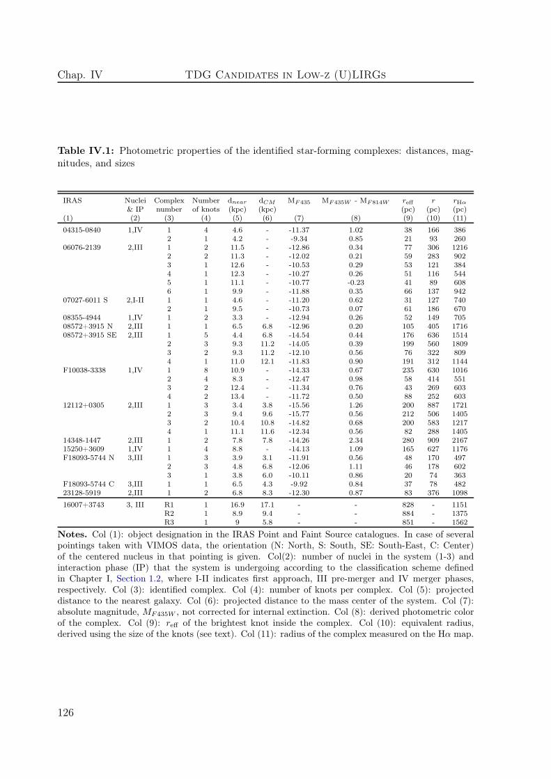
Chap. IV TDG Candidates in Low-z (U)LIRGs
Table IV.1: Photometric properties of the identified star-forming complexes: distances, mag-nitudes, and sizes
IRAS Nuclei Complex Number dnear dCM MF435 MF435W - MF814W reff r rHα
& IP number of knots (kpc) (kpc) (pc) (pc) (pc)(1) (2) (3) (4) (5) (6) (7) (8) (9) (10) (11)
04315-0840 1,IV 1 4 4.6 - -11.37 1.02 38 166 3862 1 4.2 - -9.34 0.85 21 93 260
06076-2139 2,III 1 2 11.5 - -12.86 0.34 77 306 12162 2 11.3 - -12.02 0.21 59 283 9023 1 12.6 - -10.53 0.29 53 121 3844 1 12.3 - -10.27 0.26 51 116 5445 1 11.1 - -10.77 -0.23 41 89 6086 1 9.9 - -11.88 0.35 66 137 942
07027-6011 S 2,I-II 1 1 4.6 - -11.20 0.62 31 127 7402 1 9.5 - -10.73 0.07 61 186 670
08355-4944 1,IV 1 2 3.3 - -12.94 0.26 52 149 70508572+3915 N 2,III 1 1 6.5 6.8 -12.96 0.20 105 405 171608572+3915 SE 2,III 1 5 4.4 6.8 -14.54 0.44 176 636 1514
2 3 9.3 11.2 -14.05 0.39 199 560 18093 2 9.3 11.2 -12.10 0.56 76 322 8094 1 11.0 12.1 -11.83 0.90 191 312 1144
F10038-3338 1,IV 1 8 10.9 - -14.33 0.67 235 630 10162 4 8.3 - -12.47 0.98 58 414 5513 2 12.4 - -11.34 0.76 43 269 6034 2 13.4 - -11.72 0.50 88 252 603
12112+0305 2,III 1 3 3.4 3.8 -15.56 1.26 200 887 17212 3 9.4 9.6 -15.77 0.56 212 506 14053 2 10.4 10.8 -14.82 0.68 200 583 12174 1 11.1 11.6 -12.34 0.56 82 288 1405
14348-1447 2,III 1 2 7.8 7.8 -14.26 2.34 280 909 216715250+3609 1,IV 1 4 8.8 - -14.13 1.09 165 627 1176F18093-5744 N 3,III 1 3 3.9 3.1 -11.91 0.56 48 170 497
2 3 4.8 6.8 -12.06 1.11 46 178 6023 1 3.8 6.0 -10.11 0.86 20 74 363
F18093-5744 C 3,III 1 1 6.5 4.3 -9.92 0.84 37 78 48223128-5919 2,III 1 2 6.8 8.3 -12.30 0.87 83 376 1098
16007+3743 3, III R1 1 16.9 17.1 - - 828 - 1151R2 1 8.9 9.4 - - 884 - 1375R3 1 9 5.8 - - 851 - 1562
Notes. Col (1): object designation in the IRAS Point and Faint Source catalogues. In case of severalpointings taken with VIMOS data, the orientation (N: North, S: South, SE: South-East, C: Center)of the centered nucleus in that pointing is given. Col(2): number of nuclei in the system (1-3) andinteraction phase (IP) that the system is undergoing according to the classification scheme definedin Chapter I, Section 1.2, where I-II indicates first approach, III pre-merger and IV merger phases,respectively. Col (3): identified complex. Col (4): number of knots per complex. Col (5): projecteddistance to the nearest galaxy. Col (6): projected distance to the mass center of the system. Col (7):absolute magnitude, MF435W , not corrected for internal extinction. Col (8): derived photometric colorof the complex. Col (9): reff of the brightest knot inside the complex. Col (10): equivalent radius,derived using the size of the knots (see text). Col (11): radius of the complex measured on the Hα map.
126
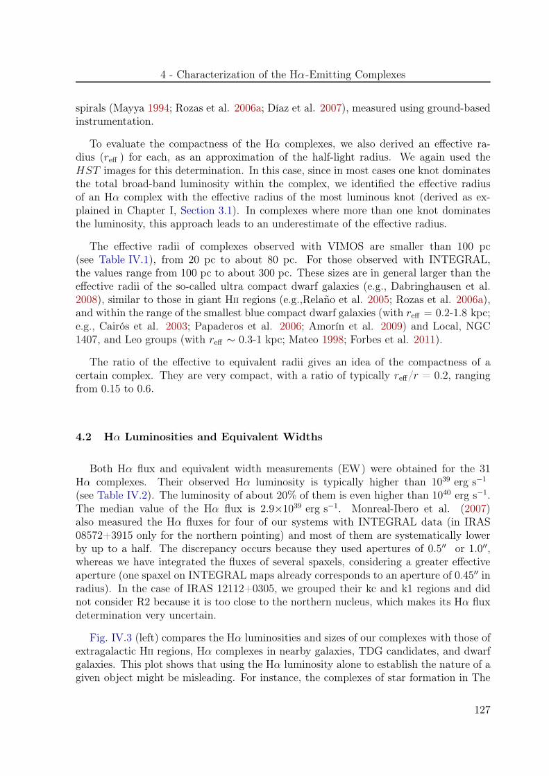
4 - Characterization of the Hα-Emitting Complexes
spirals (Mayya 1994; Rozas et al. 2006a; Díaz et al. 2007), measured using ground-basedinstrumentation.
To evaluate the compactness of the Hα complexes, we also derived an effective ra-dius (reff ) for each, as an approximation of the half-light radius. We again used theHST images for this determination. In this case, since in most cases one knot dominatesthe total broad-band luminosity within the complex, we identified the effective radiusof an Hα complex with the effective radius of the most luminous knot (derived as ex-plained in Chapter I, Section 3.1). In complexes where more than one knot dominatesthe luminosity, this approach leads to an underestimate of the effective radius.
The effective radii of complexes observed with VIMOS are smaller than 100 pc(see Table IV.1), from 20 pc to about 80 pc. For those observed with INTEGRAL,the values range from 100 pc to about 300 pc. These sizes are in general larger than theeffective radii of the so-called ultra compact dwarf galaxies (e.g., Dabringhausen et al.2008), similar to those in giant HII regions (e.g.,Relaño et al. 2005; Rozas et al. 2006a),and within the range of the smallest blue compact dwarf galaxies (with reff = 0.2-1.8 kpc;e.g., Cairós et al. 2003; Papaderos et al. 2006; Amorín et al. 2009) and Local, NGC1407, and Leo groups (with reff ∼ 0.3-1 kpc; Mateo 1998; Forbes et al. 2011).
The ratio of the effective to equivalent radii gives an idea of the compactness of acertain complex. They are very compact, with a ratio of typically reff/r = 0.2, rangingfrom 0.15 to 0.6.
4.2 Hα Luminosities and Equivalent Widths
Both Hα flux and equivalent width measurements (EW) were obtained for the 31Hα complexes. Their observed Hα luminosity is typically higher than 1039 erg s−1
(see Table IV.2). The luminosity of about 20% of them is even higher than 1040 erg s−1.The median value of the Hα flux is 2.9×1039 erg s−1. Monreal-Ibero et al. (2007)also measured the Hα fluxes for four of our systems with INTEGRAL data (in IRAS08572+3915 only for the northern pointing) and most of them are systematically lowerby up to a half. The discrepancy occurs because they used apertures of 0.5′′ or 1.0′′,whereas we have integrated the fluxes of several spaxels, considering a greater effectiveaperture (one spaxel on INTEGRAL maps already corresponds to an aperture of 0.45′′ inradius). In the case of IRAS 12112+0305, we grouped their kc and k1 regions and didnot consider R2 because it is too close to the northern nucleus, which makes its Hα fluxdetermination very uncertain.
Fig. IV.3 (left) compares the Hα luminosities and sizes of our complexes with those ofextragalactic HII regions, Hα complexes in nearby galaxies, TDG candidates, and dwarfgalaxies. This plot shows that using the Hα luminosity alone to establish the nature of agiven object might be misleading. For instance, the complexes of star formation in The
127

Chap. IV TDG Candidates in Low-z (U)LIRGs
Table IV.2: Spectral observables, metallicity, and dynamical parameters of the identified star-forming complexes
IRAS Complex Fobs (Hα) Lobs (Hα) EW (Hα) Peak EWPeak EWEW (Hα)
σ (Hα) vrel Adoptednumber (10−16 erg s−1 cm−2) (1039 erg s−1) (Å) (Å) (km s−1) (km s−1) 12+log(O/H)
(1) (2) (3) (4) (5) (6) (7) (8) (9) 10
04315-0840 1 19.3 1.4 41.7 78 1.9 16 -26 8.722 2.2 0.2 8.6 12 1.5 34 -103 8.99
06076-2139 1 15.1 5.8 48.8 173 3.6 22 421 8.502 5.8 2.2 41.3 80 2.0 26 442 8.683 0.6 0.2 26.3 44 1.7 23 442 8.754 1.1 0.4 27.0 41 1.6 26 432 8.535 1.6 0.6 17.8 28 1.6 18 430 8.736 6.8 2.6 11.0 24 2.2 - 426 8.66
07027-6011 S 1 10.4 2.9 68.9 303 4.4 31 24 8.652 2.2 0.6 - - - - 73 -
08355-4944 1 40.8 40.5 83.0 190 2.3 30 -25 8.6408572+3915 N 1 7.0 6.0 56.6 242 4.3 46 196 8.5308572+3915 SE 1 15.8 13.6 52.2 183 3.5 74 148 8.54
2 5.8 5.0 4.1 85 21.0 62 207 8.503 1.0 0.8 - - - - 228 8.534 1.0 0.8 8.8 28 3.2 - - 8.56
F10038-3338 1 12.6 4.1 86.0 374 4.4 19 19 8.682 0.6 0.2 34.3 74 2.2 - -11 8.323 2.0 0.6 - - - 17 -32 -4 2.2 0.7 - - - 27 4 8.24
12112+0305 1 44.8 60.6 71.1 252 3.6 72 96 8.592 11.9 16.1 26.3 41 1.6 81 -204 8.813 8.7 11.8 11.5 36 3.1 - -349 8.594 4.9 6.7 6.9 53 7.7 - -266 8.62
14348-1447 1 29.5 65.7 88.9 149 1.7 54 106 8.6315250+3609 1 8.1 5.7 168.9 258 1.5 69 124 8.61F18093-5744 N 1 32.8 2.6 48.1 213 4.4 23 -76 8.75
2 71.8 5.6 67.0 263 3.9 24 60 8.773 9.5 0.7 15.8 21 1.4 39 48 8.90
F18093-5744 C 1 3.8 0.3 26.0 57 2.2 18 119 8.6223128-5919 1 5.8 2.8 32.0 51 1.6 69 2 -
16007+3743 R1 12 57.1 40 - - 61 -41 8.7R2 35.5 189.5 234 - - 76 92 8.7R3 5.85 8.8 80 - - 85 338 8.7
Notes. Col (1): object designation as in Table IV.1. Col (2): identified complex. Col (3): observed Hα flux.As stated in García-Marín et al. (2009b) and in Rodríguez-Zaurín et al. (2011), typical uncertainties inthe absolute flux calibration are between 15 and 20%. Col (4): derived Hα luminosity with no correctionfor internal extinction, except for IRAS 16007+3743. Col (5): computed equivalent width (EW) from theHα and EW maps (see text). Col (6): spaxel with the largest value of the EW. Col (7): ratio of the peakof the EW to the derived EW for the whole complex. Col (8): central velocity dispersion. Col (9): relativevelocity with respect to the mass center of the system. Col (10): adopted metallicity for the complex,derived using two different line-ratio calibrators (see text).
128
4 - Characterization of the Hα-Emitting Complexes
1.0 1.5 2.0 2.5 3.0 3.5 4.0log (Diameter (pc))
37
38
39
40
41
42
log
(LH
α (e
rg s-1
))
0 100 200 300 400 500 600 700EW (Hα)
0.00
0.05
0.10
0.15
0.20
0.25
Fra
ctio
n
N = 32N = 16N = 158
Figure IV.3: Left: Relation between the Hα luminosity and the size of the identified Hα com-plexes in our sample (black dots), extremely luminous Hα complexes in The Antennae (blueplusses; Bastian et al. 2006), different samples of isolated giant HII regions in spirals and mi-nor mergers (red symbols; Terlevich & Melnick 1981; Ferreiro & Pastoriza 2004; Rozas et al.2006a), TDG candidates in CG J1720-67.8 (green diamonds; Temporin et al. 2003) and nearbydwarf amorphous (yellow crosses; Marlowe et al. 1997). None of the luminosities on the plotare corrected for internal extinction. Right: Equivalent widths measured for the complexes inthis study (black), for extragalactic HII regions (green; Mayya 1994) and for TDG candidates(red; Iglesias-Páramo & Vílchez 2001; Temporin et al. 2003).The number of objects is indicatedfor each case.
Antennae have an Hα luminosity comparable to the brightest extragalactic HII or evento dwarf galaxies, while these complexes are generally much smaller. Our complexes aretypically located where the giant extragalactic HII regions and the dwarf-type objects lieon the plot.
We also estimated the total equivalent width of a given complex from the EW and theHα spectroscopic line maps. Since in a spaxel the EW ∝ Flux Hα / Flux continuum, wefirst determined the continuum per spaxel. We then integrated all the continuum withina complex to compute the total continuum of the complex. Finally, we divided the totalHα flux by the total continuum flux for each complex. Their integrated EW span arange of two orders of magnitudes, from 4.1Å to about 170Å (see Table IV.2). For eachcomplex, we also give the value of the spaxel with the highest EW (EWpeak). The highestvalue corresponds to EWpeak = 374Å. Its median value (< EWpeak > = 85Å) doublesthe median value of the integrated EW computed for the complexes. The Hα equivalentwidths derived, which is indicative of a very young stellar population, are comparable tothose measured for extragalactic HII regions and TDG candidates (see Fig. IV.3, right).
The ratio Peak EWEW (Hα)
was defined for each complex, where Peak EW refers to EWpeak.This ratio helps us understand how the ionizing population is distributed. If two com-plexes have a similar underlying old population, the ionizing population in the one withthe larger ratio is probably more concentrated (i.e., less knots) than the other with thesmaller ratio. And if it is less concentrated (i.e., has more knots), most of the knots are
129

Chap. IV TDG Candidates in Low-z (U)LIRGs
-20 -18 -16 -14 -12 -10MF435W
7.0
7.5
8.0
8.5
9.0
9.512
+ L
og (
O/H
)
Figure IV.4: Metallicity-luminosity relation for external HII regions in Stephan’s Quintet (yel-low open circles; Mendes de Oliveira et al. 2004), nearby irregular galaxies (black plusses, Pi-lyugin et al. 2004; black asterisks, van Zee & Haynes 2006), TDG candidates (green filled trian-gles, Weilbacher et al. 2000, 2003; red crosses, Duc & Mirabel 1998; blue open squares, Temporinet al. 2003), and our complexes (black dots with errors). The line shows the correlation foundby van Zee. Only the luminosities given by Pilyugin are corrected from internal extinction. Forthose Hα complexes for which an estimate of the extinction has been made (see Section 5.2.1),the metallicity-luminosity relation is also shown (dots with dashed line errors).
probably somewhat older (low EW) and only a few are very young (high EW), leading toan older average population. In fact, the complexes with large ratios (Peak EW
EW (Hα)& 3) have
typically a few knots (1-3), such as C1 in IRAS 06076-2139, C1 in IRAS 08572+3915 N,and C4 in IRAS 12112+0305.
4.3 Metallicities
Numerical studies have claimed that during an interaction large amounts of gas flowtoward the central regions, carrying less enriched gas from the outskirts of the galaxyinto the central regions (Rupke et al. 2010; Montuori et al. 2010). Indications of thismixing process, which usually disrupts any metallicity gradient and dilutes the centralmetallicity, have been observed in merging (U)LIRGs (Rupke et al. 2008), in galaxy pairs(Kewley et al. 2006; Ellison et al. 2008; Michel-Dansac et al. 2008), and in star-forminggalaxies at high-z (Cresci et al. 2010). As a consequence of the metal enrichment of the
130

5 - From Hα Complexes to TDG Candidates in (U)LIRGs
external regions of the mergers, additional star formation can occur from reprocessedmaterial there. We investigated whether the interaction process affects the metallicity ofour Hα complexes.
The adopted metallicities (see Chapter I, Section 3.5) for all the candidates are shownin the last column in Table IV.2. With values compatible to a solar metallicity, theygenerally range from 12 + logO/H = 8.5 to 8.8 (with the exception of two candidateswith lower abundances). The values for complexes observed with VIMOS have to beconsidered with care and must be checked with other metallicity indicators, since theN2 calibrator might be affected by ionization from strong shocks in the external regionsof these galaxies (Monreal-Ibero et al. 2010). Moreover, spatially resolved studies ofstar-forming regions indicate that the assumption of spherical geometry is unrealistic inmost cases, which has a direct impact on the derivation of metallicities. Ercolano et al.(2007) estimated the systematic errors in the metallicity determinations when assumingspherical geometry using different calibrations. In the worst-case scenario, the derivedoxygen abundances might be overestimated by 0.2-0.3 dex by the use of the calibratorsconsidered in this study, in which case the derived metallicites for the Hα complexeswould then approach Z⊙/3.
The Hα complexes in this study do not follow the well-known metallicity-luminosityrelation for nearby isolated dwarf galaxies (see Fig. IV.4). Most galaxies also followthis relation (Weilbacher et al. 2003). On the other hand, HII regions in compactgroups of galaxies and TDGs in general deviate significantly from the relation and havea metallicity that is independent of their luminosity, an indication that all these objectsconsist of recycled material.
5 From Hα Complexes to TDG Candidates in (U)LIRGs
Most Hα-emitting complexes have similar observational properties (i.e., Hα equivalentwidths and luminosities, MF435W magnitudes, metallicities, radii) to the most luminousextragalactic giant HII regions in spirals and mergers, as well as more massive objectssuch as TDGs or TDG progenitors. Associations of young star-forming regions with alarge HI reservoir have been found in TDGs, for instance by Duc et al. (2007). Wemay then consider whether the Hα-emitting complexes in our sample are dynamicallyunbound associations of objects with masses similar to observed Super Star Clusters(SSCs) or larger, more massive, and self-gravitating objects such as dwarf galaxies.
TDGs are self-gravitating objects with masses and sizes typical of dwarf galaxies(i.e., a total mass of 107-109 M⊙ ), formed with recycled material from the parentgalaxies involved in an interaction/merger (Duc et al. 2000; see also General Introduc-tion, Section 2.2). Hence, they are stable entities with their own established dynamicalstructure. To evaluate whether our complexes constitute real TDGs or TDG progeni-tors and assess their chance of survival, we need to answer a few basic questions: Is the
131
Chap. IV TDG Candidates in Low-z (U)LIRGs
complex massive enough to be considered as a dwarf galaxy? Is it stable enough to beunaffected by its internal motion? Are the gravitational forces too strong to disrupt it?We disscuss here these questions.
5.1 Selection of Hα-emitting Likely to Represent TDG Candidates
Although old TDGs have been observed (e.g., Duc et al. 2007), their identification isnot straightforward. When an old TDG is detected, the tail from its place of origin willprobably have completely disappeared and the TDG may be classified as another typeof dwarf galaxy. A determination of the metallicity and, especially, the total mass of theobject is needed to establish its tidal origin and mass. With spectroscopic data, we areable to study (though with some limitations and biases) the metal content, the dynamicalmass, and different methods to establish whether a given candidate can withstand bothinternal and external forces. It is awkward to identify luminous enough condensations ofold populations (i.e., very massive) and obtain kinematic information because the stellarabsorption lines that would have to be used often have too low a signal-to-noise ratio(S/N). Although TDGs containing only old populations may be present in our sample,we are unable to detect them. Another way of searching for TDG candidates is basedon either analyzing the Hα emission clumps (for that we have a sufficiently high S/N)and/or combining spectral and photometric data of blue Hα-emitting objects in inter-acting systems (e.g., Iglesias-Páramo & Vílchez 2001; Weilbacher et al. 2003; Temporinet al. 2003; López-Sánchez et al. 2004). Therefore, the selection of TDG candidates inour sample of (U)LIRGs is based on the detection of Hα emission clumps with stellarcounterparts, which is similar to our identification of Hα complexes.
However, we are limited by the angular resolution of the spectral data. To make ourestimates as accurate as possible, we do not consider in our discussion here complexes withmultiple luminous star-forming knots. Different types of motions within the componentsof a given complex can strongly affect the derivations mentioned before. The mostcharacteristic examples of complicated complexes are C1 in IRAS F10038-3338 and C2in IRAS 12112+0305. This does not mean that the possibility of these complexes beingTDGs is ruled out, just that we do not have enough resolution to study the kinematicsof each knot, thus determine whether they are kinematically bound or not.
We consider only complexes with simple structures, that is, mainly where only oneknot is detected. We also include complexes with several knots, one of which (normallycentered on the Hα peak emission) dominates the broad-band luminosity. The complexC1 in IRAS 04315-0840 would be a good example. On the basis of these criteria, thekinematic and dynamical properties of 22 complexes are derived and compared with thoseexpected for a TDG.
If we detect more than one knot within the selected complexes, we consider only thebroad-band luminosity of the brightest knot. In these cases, the Hα luminosity of the
132
5 - From Hα Complexes to TDG Candidates in (U)LIRGs
complex is scaled in the same way as the F435W flux is scaled to the total F435W broad-band flux of the complex in Table IV.1. In practice, we multiply the Hα luminosity bya factor that in general is higher than 0.5 (a factor of 1 means that there is only oneknot emitting the whole broad-band flux, thus responsible for the full Hα emission). Thekinematic measurements, such as the velocity dispersion, are not performed for the wholecomplex, but only for the spaxels close to and located at the peak of the Hα emission.This permits us to avoid any contamination by a faint knot in the border of the complex(e.g., faint knots within C1 in IRAS 04315-0840).
Using the kinematic information provided by the IFU data as well as the photometricmeasurements, we assess the origin and likelihood of survival of the 22 selected Hα com-plexes, and evaluate whether they can be the progenitors of Tidal Dwarf Galaxies.
5.2 Are They Massive Enough to Constitute a TDG?
5.2.1 Age and Mass Estimates of the Young Population
The Hα emission can be used to constrain the properties of any recent episodes of starformation. According to the starburst99 models (SB99 , Leitherer et al. 1999; Vázquez& Leitherer 2005), the detection of an Hα flux and EW larger than about 13 Å(see Table IV.2 for specific values) implies that the stellar population is younger than 10Myr (see Fig. I.8 in Chapter I). With the broad-band luminosities of the brightest knotwithin the complex and the scaled Hα luminosity, we can estimate to first order the ageand the mass of the young population of the selected complexes. We note that, owingto the distance of the systems (DL < 270 Mpc) and the shape of the HST filters, theHα emission-line does not contaminate these broad-band filters. We have made use ofthe synthetic stellar population model SB99, which is optimized for young populationand also provides information on the ionized gas. The parameters used in the model(IMF , metallicity, etc.) are defined in Chapter I, Section 3.2.
We computed the mass-independent evolutionary track shown in Fig. IV.5 using in-formation about the ratio of the flux of the modeled population in the broad-band filtersto the flux of the ionized gas in the Hα line. Placing these ratios on a plot for all observedcomplexes, we now estimate the age of the young population. Once the age is known(hence a M/L ratio), the mass can be derived. However, before going any further andbased on the assumptions made, we first assess the sources of uncertainty that a prioricould affect our results:
• The internal extinction is unknown. In general, the extinction in the inner regionsis patchy with high peaks in (U)LIRGs, up to AV ≃ 8 mags (see Alonso-Herreroet al. 2006 and García-Marín et al. 2009a), though it decreases considerablywith the galactocentric distance. Were complexes to have low extinction values
133
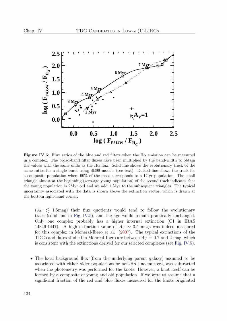
Chap. IV TDG Candidates in Low-z (U)LIRGs
0.0 0.5 1.0 1.5 2.0 2.5log ( FF814W / FHα
)
0.0
0.5
1.0
1.5
2.0
2.5
log
( F F
435W
/ F H
α )
3 Myr
4 Myr 5 Myr
6 Myr
7 Myr
AV=12 Myr
Figure IV.5: Flux ratios of the blue and red filters when the Hα emission can be measuredin a complex. The broad-band filter fluxes have been multiplied by the band-width to obtainthe values with the same units as the Hα flux. Solid line shows the evolutionary track of thesame ratios for a single burst using SB99 models (see text). Dotted line shows the track fora composite population where 99% of the mass corresponds to a 1Gyr population. The smalltriangle almost at the beginning (zero-age young population) of the second track indicates thatthe young population is 2Myr old and we add 1 Myr to the subsequent triangles. The typicaluncertainty associated with the data is shown above the extinction vector, which is drawn atthe bottom right-hand corner.
(AV . 1.5mag) their flux quotients would tend to follow the evolutionarytrack (solid line in Fig. IV.5), and the age would remain practically unchanged.Only one complex probably has a higher internal extinction (C1 in IRAS14349-1447). A high extinction value of AV ∼ 3.5 mags was indeed measuredfor this complex in Moneral-Ibero et al. (2007). The typical extinctions of theTDG candidates studied in Monreal-Ibero are between AV = 0.7 and 2 mag, whichis consistent with the extinctions derived for our selected complexes (see Fig. IV.5).
• The local background flux (from the underlying parent galaxy) assumed to beassociated with either older populations or non-Hα line-emitters, was subtractedwhen the photometry was performed for the knots. However, a knot itself can beformed by a composite of young and old population. If we were to assume that asignificant fraction of the red and blue fluxes measured for the knots originated
134
5 - From Hα Complexes to TDG Candidates in (U)LIRGs
from an older population, the evolutionary track would change (see the compositepopulations in Fig. IV.5); the young population would then be even younger thaninitially predicted and consequently less massive. Almost half of the complexesare incompatible with the composite track, since their flux ratios would be toosmall, even smaller than for a zero-age young population. The other complexes,for which the values are compatible with the composite track, would typically havea young population of about or younger than 4 Myr. Were this to be the case,the extinction would be negligible and the equivalent widths would be about 200 Å.
• It can also happen that the measured Hα flux is emitted by possible embedded(and undetected) star-forming knots. The existence of undetected Hα-emitters isjustified with the Hα-emitter in IRAS 08572+3915 N (clump on the North-West).We estimated how many undetected knots there can be with an age derived fromthe peak values of the EW (typically between 5 and 10 Myr, according to thestellar population models used in Section 5.2.1) that can contribute significantly tothe total broad-band luminosity of the knots. Since they would have a similar age,an embedded population of knots with a combined broad-band flux similar to thatof the detected knots would emit half of the Hα flux. We then estimated how manyknots at the detection limit would be needed to double either the F435W or theF814W flux. A total of 9 and 75 undetected knots per complex would be neededand we detected an average of 2.2 knots per complex. Thus, between 4 and 37 timesmore knots fainter by 2.4-4.7 magnitudes would be needed only in one complex.Assuming a luminosity function with slope of 2 we would need practically one-thirdof the total knots predicted for the whole galaxy inside a complex, which is unlikely.
• Had we included some Hα contribution from the neighboring zones then the Hα fluxmeasured would have been overestimated. The Hα flux drops considerably as ageincreases across the age interval we consider (by up to more than one order ofmagnitude), but if the Hα flux is weaker the mass of the young population decreasesaccordingly. The mass estimated using the red filter can vary by up to a factor offour within the age interval 1-10 Myr, according to the stellar population modelsused in this study. The age estimate would be older by no more than 1 Myr, if wehad overestimated the flux by a half. Thus, this correction would in our case benegligible.
Taking into account these sources of uncertainty, the first-order estimates of the agewere performed for the young population inside a complex, assuming a single burst. Weestimated the age by considering the extinction value that we would need to shift thelocation of each dot (flux quotients) along the evolutionary tracks. The estimated agesrange from 2 to 5 Myr (Ageph; see Table IV.3), the typical age range in which an in-stantaneous burst of star formation displays Wolf-Rayet features in its spectra (Leitherer WR
et al. 1999). Given the spectral range covered in this study, we would expect to see
135

Chap. IV TDG Candidates in Low-z (U)LIRGs
the well-known red WR bump, which is the result of the blend of the [CIII] λ5698 and[CIV] λ5808 broad emission lines (Kunth & Schild 1986). We tried to find these featuresin the spectra of the complexes, but could find no clear evidence of these bumps. Thisbump is much more difficult to detect than the other bump (such as the blue bump) char-acteristic of WRs because it is always weaker (e.g., Fernandes et al. 2004; López-Sánchez& Esteban 2009). Sometimes it is not even detected again in Wolf-Rayet galaxies whereit was previously seen (López-Sánchez & Esteban 2009). Therefore, the non-detectionof WR features does not definitely exclude the hypothesis that the young population inour complexes spans the age range 2-5 Myr.
An upper limit to the age can be estimated by using the EW (Hα), as it decreasesstrongly with time. Using the EW peaks (see Table IV.2), we estimate that the age is inthe range 5-10 Myr (AgeEW ; see Table IV.3). In many cases, the EW peaks are not strongenough to explain population as young as our former age estimates. This is unsurprisingbecause within a complex and a spaxel itself the underlying older population contributessignificantly to the Hα continuum but not to the emission line. The contribution of thiscontinuum minimizes the total EW within a complex. The broad-band flux of the knotstypically represents between 1% and 40% of the total flux within the area of the complex.We consider for instance a 3 Myr-old population whose broad-band flux represents 10%of its overall broad-band flux within the complex. According to the models we use, theequivalent width of the young population without contamination would be ∼1000 Å.However, the contamination of a 1 Gyr-old population would diminish the equivalentwidth to a measured value of 70 Å for the whole complex, the same value as a singlepopulation of 6 Myr without contamination. Therefore, with the observed EW we canonly set an upper limit to the age in each case.
As a conservative approach, instead of directly using the youngest estimates to derivethe mass of the young population, we use the average of the two estimates, Ageph andAgeEW . Thus, once the age and extinction were estimated, the mass was directly obtainedvia the extinction-corrected F814W magnitude.
Under these assumptions, the derived mass of the young population of the selectedHα complexes is between 104.5 M⊙ and 105.5 M⊙, with the exception of three complexesfor which the derived mass is about or close to 107 M⊙ (M[I]; Table IV.3). Thesecomplexes have extinctions of AV ∼ 1-2 mag, with the exception of C1 in IRAS 14348-1447 (AV = 4.2 mag). The uncertainty in this mass is typically smaller than a factorof two. This rather small uncertainty is expected, since during the first 1-7 Myr ofthe starburst the broad-band luminosities do not change significantly. However, if wecompute the mass using the Hα luminosity (M[Hα]; Table IV.3) the uncertainties increaseconsiderably. This is also expected because the Hα flux for a population of a givenmass evolves significantly with the age of the starburst. The few cases in which bothmeasurements are incompatible suggest that the age of the burst is closer to the youngestvalue (Ageph). The corresponding M[Hα] would be lower toward a value similar to M[I].
An old population of a few Gyr (prior to the interaction, and in the parent galaxy) in
136

5 - From Hα Complexes to TDG Candidates in (U)LIRGs
0.0 0.5 1.0 1.5 2.0 2.5 3.0log (σ (km s-1) )
0
1
2
3
4
5
log
(ref
f (pc
) )
giant HIIellipticalelliptical+globular
0.8 1.0 1.2 1.4 1.6 1.8 2.0log (σ (km s-1) )
38
39
40
41
42
43
log
(LH
αZ (
erg
s-1))
Figure IV.6: Left: elocity dispersion vs. estimated effective radius. Dots correspond to therelation for our selected complexes. The typical size for errors is shown in the bottom right cor-ner. The lines show the fit for extragalactic HII regions (continuous), elliptical galaxies (dashed)and globular + elliptical galaxies (dotted) obtained by Terlevich & Melnick (1981). The othersymbols represent different samples of dynamically hot systems: open triangles in blue, inter-mediate and giant ellipticals (Bender et al. 1992); open squares in red, dwarf ellipticals (Benderet al. 1992; Geha et al. 2003); crosses in yellow, dwarf spheroidals (Bender et al. 1992); plussesin green, the TDG candidates in Monreal-Ibero et al. (2007); diamonds in orange, massiveglobular clusters in NGC 5128 (Martini & Ho 2004); inverse triangles, globular clusters in theGalaxy (Trager et al. 1993) and in M31 (Dubath & Grillmair 1997); and asterisks in pink,clusters in the Antennae (Mengel et al. 2008). Right: Velocity dispersion vs. Hα luminositycorrected for internal extinction and metallicity effects. The lines show different fits for extra-galactic giant HII regions which are approximately in virial equilibrium, given by: Terlevich &Melnick (1981) (solid line), Relaño et al. (2005) (dotted line) and Rozas et al. (2006a) (dashedline).
TDG candidates that contributes to most of the stellar mass has been reported (e.g.,Sheenet al. 2009). Large HI reservoirs have also been found in a few TDGs (Duc et al.2007) that can sustain star formation on a Gyr scale. We have seen previously thatthe colors of some complexes can be compatible with a composite population where a1 Gyr-old population is 99% more massive than a young burst. Thus, we consider itworth investigating this possibility also here. Table IV.3 shows the estimates of the ageof the young (AgeCyoung) and the mass of both populations (MCyoung and MCold). Thestellar mass of the complexes generally ranges from 105.5 M⊙ to 106.5 M⊙ , an order ofmagnitude higher than the previous estimates.
5.2.2 Conditions for Self-gravitation
Measuring velocity gradients helps us assess whether there is either any independentrotation (Weilbacher et al. 2002; Bournaud et al. 2004; Bournaud et al. 2008b) or
137

Cha
p.IV
TD
GC
andid
ates
inLow
-z(U
)LIR
Gs
Table IV.3: Derived characteristics of the stellar populations and dynamics of the identified star-forming complexes
IRAS Complex Ageph AgeEW AV M[I] M[Hα] AgeCyoung AV C MCold MCyoung Mdyn Mneartid MCM
tid Mdyn/Mtidal vesc|vesc|vrel
number (Myr) (Myr) (mags) (Myr) (mags) (km s−1)(1) (2) (3) (4) (5) (6) (7) (8) (9) (10) (11) (12) (13) (14) (15) (16) (17)
04315-0840 1 3.4 6.0 1.7 ± 0.3 4.9 ± 0.1 5.4 ± 0.3 2.1 0.2 ± 0.4 5.8 ± 0.1 3.8 ± 0.1 7.5 ± 0.3 6.6 ± 0.3 - 8.1 224 8.62 4.0 10.0 1.5 ± 0.4 4.2 ± 0.2 5.8 ± 0.5 2.8 0.7 ± 0.5 5.5 ± 0.2 3.5 ± 0.2 7.8 ± 0.3 6.0 ± 0.3 - > 10 235 2.3
06076-2139 1 2.9 5.4 1.1 ± 0.3 5.4 ± 0.2 5.9 ± 0.2 - - - - 8.0 ± 0.5 5.8 ± 0.2 - > 10 96 0.22 3.0 6.0 1.0 ± 0.4 4.9 ± 0.2 5.4 ± 0.3 - - - - 8.0 ± 0.3 5.7 ± 0.2 - > 10 96 0.23 4.4 6.4 0.6 ± 0.3 4.6 ± 0.1 5.1 ± 0.2 2.9 0.0 ± 0.0 5.6 ± 0.1 3.6 ± 0.1 7.9 ± 0.3 4.5 ± 0.2 - > 10 92 0.24 3.0 6.5 0.8 ± 0.4 4.5 ± 0.2 5.0 ± 0.5 - - - - 8.0 ± 0.3 4.5 ± 0.2 - > 10 93 0.25 2.9 6.8 0.4 ± 0.2 4.4 ± 0.2 5.1 ± 0.4 - - - - 7.6 ± 0.4 4.3 ± 0.2 - > 10 97 0.26 2.8 7.0 1.0 ± 0.3 5.2 ± 0.1 5.9 ± 0.8 - - - - - 5.0 ± 0.2 - - 103 0.2
07027-6011 S 1 2.1 5.0 1.2 ± 0.3 4.9 ± 0.2 5.6 ± 0.3 - - - - 7.9 ± 0.4 6.1 ± 0.3 - > 10 180 7.52 3.2 - 0.6 ± 0.3 4.5 ± 0.1 4.6 ± 0.2 - - - - - 5.6 ± 0.3 - - 125 1.7
08572+3915 N 1 2.8 5.2 0.7 ± 0.3 5.4 ± 0.2 5.9 ± 0.2 - - - - 8.7 ± 0.3 7.2 ± 0.4 7.4 ± 0.3 > 10 233 1.208572+3915 SE 3 4.9 - 0.9 ± 0.3 5.1 ± 0.1 5.1 ± 0.2 3.1 0.0 ± 0.6 6.1 ± 0.2 4.1 ± 0.2 - 6.6 ± 0.4 6.6 ± 0.3 - 225 1.0
4 4.9 6.9 1.4 ± 0.4 5.5 ± 0.2 6.1 ± 0.2 3.2 0.6 ± 0.5 6.5 ± 0.2 4.5 ± 0.2 - 6.3 ± 0.4 6.5 ± 0.3 - 207 -F10038-3338 3 3.6 - 0.7 ± 0.3 4.4 ± 0.1 4.5 ± 0.1 2.7 0.0 ± 0.0 5.7 ± 0.1 3.7 ± 0.1 7.6 ± 0.3 5.8 ± 0.3 - > 10 117 3.6
4 4.9 - 0.9 ± 0.3 5.0 ± 0.1 5.2 ± 0.1 3.0 0.0 ± 0.6 6.0 ± 0.2 4.0 ± 0.2 8.2 ± 0.3 5.6 ± 0.3 - > 10 113 26.212112+0305 1 3.4 5.2 2.2 ± 0.3 7.1 ± 0.2 7.3 ± 0.2 2.2 0.8 ± 0.4 8.0 ± 0.1 6.0 ± 0.1 9.4 ± 0.2 9.2 ± 0.3 9.6 ± 0.2 0.7 496 5.1
4 2.1 6.3 1.1 ± 0.3 5.4 ± 0.2 6.1 ± 0.3 - - - - - 6.2 ± 0.3 6.7 ± 0.2 - 275 1.014348-1447 1 3.3 5.5 4.2 ± 0.3 7.7 ± 0.1 8.1 ± 0.2 1.5 2.5 ± 0.3 8.5 ± 0.1 6.5 ± 0.1 9.3 ± 0.2 9.1 ± 1.1 9.2 ± 0.3 1.3 575 5.415250+3609 1 5.4 5.2 2.4 ± 0.3 6.6 ± 0.1 6.7 ± 0.2 3.9 1.1 ± 0.4 7.5 ± 0.1 5.5 ± 0.1 9.3 ± 0.3 7.7 ± 0.2 - > 10 214 1.7F18093-5744 N 3 2.9 7.2 1.9 ± 0.3 5.0 ± 0.2 5.8 ± 0.5 - - - - 7.9 ± 0.4 4.1 ± 0.1 5.1 ± 0.2 > 10 220 4.6F18093-5744 C 1 3.5 6.2 1.6 ± 0.3 4.8 ± 0.1 5.2 ± 0.3 2.4 0.4 ± 0.4 5.7 ± 0.1 3.7 ± 0.1 7.6 ± 0.5 3.6 ± 0.3 5.6 ± 0.2 > 10 175 1.523128-5919 1 3.3 6.3 1.8 ± 0.3 5.7 ± 0.2 6.1 ± 0.5 2.0 0.3 ± 0.4 6.5 ± 0.2 4.5 ± 0.2 9.0 ± 0.2 7.1 ± 0.2 7.0 ± 0.3 > 10 222 85.7
16007+3743 R1 - 7.1 1.7 8.8 - - - - - 9.8 8.2 8 > 10 302 7.4R2 - 5.4 1.2 8.8 - - - - - 10 9.2 10.1 0.9 408 4.4R3 - 6.4 2.3 7.8 - - - - - 10.1 10 9.1 1.2 519 1.5
Notes. Col (1): object designation as in Table IV.1. Col (2): identified complex. Col (3): age of the young population, derived using the photometricinformation (Fig. IV.5). Col (4): age of the young population using the EW (Hα). Col (5): internal extinction. Col (6): derived mass of the youngpopulation using the I magnitude. All masses in the table are given in log (M ( M⊙)). Col (7): derived mass of the young population using theHα flux. Col (8): derived age of the young component, assuming that the candidate consists of a composite population. Col(9): derived internalextinction of the composite population. Col (10): derived mass of the old population (i.e., 1Gyr), assuming a composite population (see text). Col(11): derived mass of the estimated young population, assuming a composite population. Col (12): dynamical mass. Col (13): tidal mass assumingthe potential is created by the nearest galaxy. Col (14): tidal mass assuming the potential is created by a point mass at the mass center of thesystem. Col (15): ratio of the dynamical to the tidal mass. Col (16): escape velocity. Col (17): ratio of the escape to the relative velocity.
138

5 - From Hα Complexes to TDG Candidates in (U)LIRGs
outflows. However, given the spatial resolution achieved with the IFS instruments, wecannot in general resolve any velocity field across the extranuclear condensations. In thiscase, other indirect methods must be used to assess whether the internal motions of ourcomplexes can affect their stability.
Iglesias-Páramo & Vílchez (2001) established an empirical luminosity criterion(L(Hα) > 1039 erg s−1) that must be reached by their HII complexes to ensure self-gravitation. This criterion, however, has not been supported by any kinematic study.More than 50% of our own complexes fulfill this criterion, as shown in Table IV.2. If wecorrected for internal extinction, only three would be less luminous than 1039 erg s−1.
Another method that can be used to establish whether the selected complexes arestable is to study their location in well-known empirical correlations followed by otherself-gravitating entities such as elliptical galaxies, bulges of spiral galaxies, globular clus-ters, and/or giant HII regions: the radius-velocity dispersion and the luminosity-velocitydispersion relations (Terlevich & Melnick 1981). Here, we consider these relations be-cause they provide more reliable constraints than the Hα luminosity of the complexes.We plot these relations for our complexes in Fig. IV.6.
In the radius-velocity dispersion diagram, we superimpose the data of samples ofdynamically hot systems such as massive globular clusters, dwarf elliptical and spheroidalgalaxies, intermediate and giant ellipticals, and TDG candidates. Within all of theuncertainties, the velocity dispersions of six of the complexes selected here are too highto ensure self-gravitation.
For a giant HII region, the lower envelope in the log LHα- logσ plane is closely repre-sented by a straight line of the form LHα= c + Γ× logσ, where σ refers to the velocitydispersion, the constant c ranges from 34.5 to 36.8, and Γ is between 2 and 4 (see line fitsand references in Fig. IV.6, right). This is known as the luminosity-velocity (L-σ) dis-persion relation, and implies that the giant extragalactic HII regions above the envelopeare gravitationally bound complexes of stars and gas and that the widths of the nebularemission lines reflect the motions of discrete ionized gas clouds in the gravitational fieldof the underlying stellar and gaseous mass (Terlevich & Melnick 1981). The kinematicsof the HII regions below the envelope may be dominated by processes other than gravita-tional motions, such as stellar winds and expanding shells (Relaño et al. 2005; Relaño &Beckman 2005; Rozas et al. 2006a; Rozas et al. 2006b). That is, if the relation for giantHII regions lies above the envolope, then the non-gravitational processes are identifiedwith broad, low-intensity components that do not considerably affect the physical prop-erties of the main spectral component (i.e., gravitational motions). Thus, although thevelocity of these fenomena could be similar or even larger than the σ measured in thispaper, if the relation for our complexes is above the envelope, the spectral componentcorresponding to the gravitational motions will probably not be affected.
In any case, we estimated the expansion speeds of bubbles in the interstellar medium,so as to quantify how broad these non-gravitational components are. We evaluated the
139

Chap. IV TDG Candidates in Low-z (U)LIRGs
equivalent number of O3(V) stars using the Hα luminosity of a given complex and thevalue given by Vacca et al. (1996) for the ionizing photon output of an O3(V) star.We then derived the kinetic energy input from the stellar winds, using the estimate byLeitherer (1998) of the wind luminosity for an O3(V) star, integrated over the time thestar is on the main sequence. Assuming a typical average electron density of 100 cm−3,obseved in (U)LIRGs (Veilleux et al. 1995, 1999), the expansion speeds are expected tobe (Lamers & Cassinelli 1999) between several km s−1 for the least luminous complexesand less than 30 km s−1 for the most luminous ones.
Given the metallicity range of our selected complexes, we applied a metallicity cor-rection to the Hα luminosity, in such a way that ∆log (F(Hα)) = 127z - 1.17 (Terlevich& Melnick 1981), where z denotes the metallicity value (z=0.02 for solar metallicity).Within the uncertainties, all the selected complexes but two are consistent with the linefits or above the envelope (Fig. IV.6, right). Interestingly, these two outlying complexesare consistent with the radius-velocity dispersion correlation. Although the values foranother complex are below the envelope, we note that its Hα luminosity was not cor-rected because its metallicity is unknown. Thus, no complex fails both criteria at thesame time. According to these results, self-gravitation should be ensured for more than ahalf of the complexes for which a determination of the velocity dispersion was achieved.For the remainder, self-gravitation is neither guaranteed nor excluded because at leastthey generally satisfy one of the two criteria used.
5.2.3 Dynamical Mass Estimates
Upper limits to the dynamical masses (Mdyn ) of the selected complexes were de-rived under the following assumptions: (i) the systems are spherically symmetric;(ii) they are gravitationally bound; and (iii) they have isotropic velocity distributions[σ2(total) = 3×σ2
LOS], where σLOS is the line-of-sight velocity dispersion. In the pre-vious section, we have seen that more than a half of these complexes are likely to begravitationally bound.
The equations to obtain the dynamical mass of a virialized stellar (cluster- or galaxy-like) system are presented in Chapter I, Section 3.6.2. The observables needed to derivedit are the effective radius and the velocity dispersion. Since the star-forming knots havea cluster-like light profile (similar to a Gaussian) the use of Equation I.5 to derive thedynamics of the selected complexes seems appropriate. The corresponding masses, givenin Table IV.3, are between a few 107 and a few 109 M⊙, with an uncertainty of a factorof 2-3.
140

5 - From Hα Complexes to TDG Candidates in (U)LIRGs
5.2.4 Total Mass: Discrepancy Between the Stellar and the DynamicalMasses
It is unclear where to draw the line between a high-mass young super cluster and a low-mass dwarf galaxy in terms of stellar mass. We derive masses only for young population,and those complexes less massive than 106 M⊙ are comparable to the brightest youngclusters or complexes hosting recent star formation in other less luminous interactinggalaxies (e.g., Mengel et al. 2008; Bastian et al. 2009). However, does the estimatedmass of the young stellar population represent the total mass of the candidates? Only afew studies have reported stellar masses for TDGs. The dynamical mass of our complexesis in the range of the typical total baryonic mass of a TDG (M = 107-109 M⊙; e.g., Ducet al. 2004; Higdon et al. 2006; Hancock et al. 2009). However, the ratio of thedynamical to the most massive photometric mass in our complexes is suspiciously high(Mdyn/m[MI ] ∼ 50-1000). Several factors can explain this ratio.
If we assume that the stellar mass represents the total mass of a given complex, thismass might be underestimated, because:
• Although the most recent bursts of stars are responsible for the bulk of theionization of the gas - hence of the emitted flux- the kinematics of the ionizinggas is affected by those of previous stellar generations. In regions of mixedpopulations, the light is generally dominated by the young stars and the massby the older population. As outlined before, Sheen et al. (2009) derived a totalstellar mass of 3.1×10⁷ M⊙ for one of their TDG candidates, a fraction of no morethan 2% being contained in populations younger than 6 Myr. The mass-to-light(M/L) ratio of young (e.g., 5 Myr) and old (e.g., 1 Gyr) populations differs byabout a factor of 100. The Hα to the broad-band luminosity colors of some of ourcandidates are also consistent with those of composite populations. Our complexesmight indeed consist of young star-forming knots and evolved population fromthe complexes themselves and the parent galaxy that has been accreted by thecomplex. We estimated the total stellar mass of the complex if practically all theF814W flux measured inside the whole complex (minus the flux from the knots)belonged to it and came from a 1 Gyr-old population. This total stellar massapproaches significantly to the dynamical mass measured for most of the complexes.
• The total stellar population does not normally represent the total baryonic mass(gas + stellar), and we do not have access to the mass of the gas. Normally,the efficiency of star formation in molecular clouds is very low (typically about1%). In (U)LIRGs the efficiency can be higher, but the mass of a molecular cloudundergoing a starburst episode may still be higher than the mass of the starburstby more than one order of magnitude. The candidates in Hancock et al. (2009)have total stellar masses of 1-7×10⁶ M⊙, the HI mass being 6×10⁷ M⊙ . Studiesbased on radio HI observations have found that the gas mass of a TDG with a
141

Chap. IV TDG Candidates in Low-z (U)LIRGs
typical diameter of a few kpcs lies within the range between a few 107 and several109 M⊙ (e.g., Duc et al. 2000; Bournaud et al. 2004; Duc et al. 2007).
On the other hand, if we assume that the dynamical mass represents the total massof a given complex, we might be overestimating it, because:
• In each case, Mdyn represents normally an upper limit to the dynamical mass.For instance, given the complex dynamics in interacting systems, high velocitydispersions might not necessarily indicate high masses, but might alternativelyrepresent tidal-flows induced from the merging process and strong winds fromLINER-like regions (Colina et al. 2005; Monreal-Ibero et al. 2010). However,at least for the systems that we previously observed with VIMOS, these strongwinds may not affect significantly the determination of the velocity dispersions(Monreal-Ibero et al. 2010).
• Dark matter might contribute significantly to the total TDG mass. However,TDGs are unlikely to contain a large amount of dark matter (Barnes & Hern-quist 1992b) because their material is drawn from the spiral disk, while the darkmatter is thought to surround the galaxy in an extended halo.
On the basis of all these arguments, it is clear that the total masses of these complexesis somewhere between the photometric and the dynamical masses. Other independentcriteria also show that more than a half of the selected complexes are in virial equilib-rium, thus the velocity dispersion traces more likely the dynamical mass rather thanother processes (see Section 5.2.2). Given all the caveats and uncertainties previouslyconsidered when determining the dynamical and stellar masses, we assume as a masscriterion that the complexes with photometric mass estimates using the broad-band lu-minosities (single or composite population) that are compatible with 106 M⊙ are likelyto have a sufficient total mass to become a tidal dwarf galaxy. This assumption shouldobviously be verified using multi-wavelength photometric and spectroscopic data. Onlysix of the selected complexes (plus the three candidates in IRAS 16007+3743) fulfill thismass criterion. Had we assumed that a complex with a dynamical mass compatiblewith 108 M⊙ or higher has sufficient mass to become a TDG, then 15 of the selectedcomplexes would fulfill the mass criterion.
142
5 - From Hα Complexes to TDG Candidates in (U)LIRGs
5.3 Are They Unaffected by the Forces from the Parent Galaxy?
5.3.1 Tidal Forces
If the complex is massive enough to constitute a dwarf galaxy and gravitationallybound, its fate basically depends on the ratio of its mass to the so-called tidal mass(Binney & Tremaine 1987; Mendes de Oliveira et al. 2001). The tidal mass conditionwill tell us whether it is massive enough to survive the tidal forces exerted by the parentgalaxy. The tidal mass is defined as
Mtid = 3M×
(
R
D
)3
(IV.1)
where M refers to the mass of the parent galaxy, R is the radius of the complex (herethe size of the most luminous knot in a complex), and D is the distance to the parentgalaxy. This equation is valid when the size (R) of a certain region is small in comparisonwith the distance (D) to the parent galaxy, which is the case for all of the complexes(the ratio “size/projected distance” is typically below 0.04). If the tidal mass of an objectis lower than the total mass, then the object is unaffected by the forces applied by theparent galaxy.
In general, the gravitational potential of interacting galaxies, as in ULIRGs , is acomplex function of the mass distribution of the system, which evolves with time. Nev-ertheless, as a first approximation, we assumed that the distribution is dominated by themasses of the main bodies of the system. Two different approaches were applied in thisstudy: the gravitational potential depends either on: i) the nearest galaxy (Mnear
tid ) or ii)a point mass in the mass center and the total mass of the system (MCM
tid ). The highestvalue obtained using the different approaches was taken to compare with the dynamicalmass of the complex.
In each case, we used the measured projected distances dnear and dCM, respectively(see Table IV.1). Since the projected distance is always smaller than the real one, weactually estimated upper limits to the real tidal masses. To derive the tidal mass, weneed to know the mass of the parent galaxy, which in each case is identified with itsdynamical mass. Under the same hypothesis as in Section 5.2.3 of a virialized system,the dynamical mass of a galaxy-like object can be obtained using Equation I.4 (Chap-ter I, Section 3.6.2), but assuming this time a constant value of m = 1.75 (a scaling factorfor a polytropic sphere), like in Colina et al. (2005). In each case, we used the averagevalue of the velocity dispersion at the peak and nearby surrounding spaxels, coveringabout a radius of 1′′. Finally, the effective radii of the parent galaxies were derived usingthe H -band NICMOS and WFC3 images of the galaxies and fitting their two-dimensionallight profiles with GALFIT (Peng et al. 2002; Peng et al. 2010). In many cases, the
143

Chap. IV TDG Candidates in Low-z (U)LIRGs
NICMOS images do not cover the full extent of the galaxies, which meant that we hadto use the values given in Arribas et al. (in prep.).
In summary, two values (Mneartid and MCM
tid ) for the tidal mass were obtained us-ing Equation IV.1, and the maximum value was compared to the dynamical mass ofthe selected complexes derived in Section 5.2.3. The ratio Mdyn/Mtid is in general > 10(see Table IV.3), which ensures that the complexes are unaffected by the tidal forcesexerted by the parent galaxy. Only one complex fails this condition and another one isclose to failing because of large uncertainties in its dynamical mass estimate.
5.3.2 Escape Velocity
If the complex does not have a large enough relative velocity (vrel) with respect to thegalaxy to escape, it might still fall back towards the center of the system because of thegravitational force exerted by the parent galaxy. It is interesting to consider whether acomplex does indeed exceed the effective escape velocity (vesc). This criterion, however,should not have the same weight as the others since it is subject to many uncertainties:(i) the real distance of the complex is always larger than the projected one; (ii) only onecomponent of the velocity is measured and there is no information about the movementsin the plane of the sky; and (iii) two possibilities for the relative movements between theregion and the system are always possible, since for a given configuration it is impossibleto determine whether the complex is closer or further away from the observer than themass center. We include this criterion in this study for completeness.
For simplicity, we assume that the gravitational potential is created by a point massrepresenting the total mass of the system, that is located at the mass center. The ratio|vesc|/vrel (last column in Table IV.3) is smaller than 1 for 7 of the selected complexes outof the 22, that is, they could escape. If we take into account projection effects statistically,a complex escapes if |vrel| − |vesc × cos(π/4)| > 0. In this case, an additional complexsatisfies the criterion.
5.4 How Common is TDG Formation in (U)LIRGs?
5.4.1 TDG Candidates in (U)LIRGs
None of the developed criteria can help us determine wheter a given complex will sur-vive the merging process. Projection effects and observational constraints, especially theneed for higher angular resolution spectroscopic data (which would allow us to search forvelocity gradients), ensure that it is difficult to assess the fate of the selected complexes.In any case, we can investigate which have the higher probabilities of surviving as a TDG,based on the fulfillment of a few or most of the criteria viewed in this study. The resultsare summarized in Table IV.4.
144

5 - From Hα Complexes to TDG Candidates in (U)LIRGs
Table IV.4: Summary of the different criteria used to investigate the nature of thecomplexes
IRAS Complex Mass L (Hα) σ vs. reff σ vs. LHα Mtid vs. Mdyn vesc vs. vrel Probnumber
04315-0840 1 N Y Y Y Y N Medium2 N N N Y Y N Low
06076-2139 1 N Y Y Y Y Y Medium-high2 N Y Y Y Y Y Medium-high3 N N Y Y Y Y Medium4 N N Y N Y Y Medium5 N Y Y Y Y Y Medium-high6 ? Y ? ? ? Y Low
07027-6011 S 1 N Y N Y Y N Medium2 N Y ? ? ? Y Low
08572+3915 N 1 N Y Y Y Y N Medium08572+3915 SE 3 ? Y ? ? Y Y Low
4 Y Y ? ? ? ? LowF10038-3338 3 N Y Y ? Y N Medium
4 Y Y Y N Y N Medium-high12112+0305 1 Y Y N Y N N Medium
4 ? Y ? ? ? Y Low14348-1447 1 Y Y Y Y Y N High15250+3609 1 Y Y N Y Y N Medium-highF18093-5744 N 3 N Y N Y Y N MediumF18093-5744 C 2 N Y Y Y Y N Medium23128-5919 1 Y Y N ? N N Low
16007+3743 R1 Y Y Y Y Y N HighR2 Y Y Y Y N N High-mediumR3 Y Y Y Y Y N High
Notes. The different criteria are explained throughout the text. The letter Y indicates that the givencomplex satisfies the criterion, while the letter N indicates that it fails. Symbols with a question markare either doubtful or indicate that we do not have the data to study the criterion. The last columnindicates the probability that a given complex constitutes a TDG candidate based on these criteria.
We assigned different weights to the diverse criteria we studied and derived a probabil-ity that a certain complex could survive as a TDG by adding the weights for the criteriathat it achieves. The mass criterion is considered to be the most important since, even ifit is self-gravitating, if it does not have enough mass the complex could be either a boundsuper cluster or any other entity rather than a low-mass dwarf galaxy. For this reason,it is assigned a weight of 30%. The criteria with the least importance (each having aweight of 10%) correspond to the Hα luminosity and the escape velocity ones, since theformer comes from empirical considerations and the latter is the least reliable of all. Weassigned a weight of 20% to the Mtid versus (vs.) Mdyn criterion. Finally, we considereda somewhat lower weight (15%) for each of the self-gravitating criterion (σ vs. reff andσ vs. LHα), since they prove the same condition. In practice, the complexes that satisfymost of the criteria have the highest probabilities of being TDG progenitors.
Once the percentage was computed based on which criteria the complexes fulfill, dif-ferent probabilities that a complex constitutes a TDGs were defined: low (prob ≤ 40%),medium (40 < prob ≤ 60), medium-high (60 < prob ≤ 80), and high (prob > 80). Onlythree complexes (counting IRAS 16007+3743 have a high probability. A total of 6 of the
145

Chap. IV TDG Candidates in Low-z (U)LIRGs
22 selected complexes (9 of 25 if we include those from IRAS 16007+3743) have medium-high or high probabilities of being TDG progenitors, and from now on we consider theseas our TDG candidates.
We detect candidates in both LIRGs and ULIRGs, although the three candidateswith a high probability are only found in LIRGs . This suggests that TDG produc-tion may be more efficient in systems with higher infrared luminosities. However,this statistic is of very limited robustness because of the low number of candidatesfound. If we consider only systems for which IFS data are available and located ata distance (i.e., DL > 130 Mpc) where at least a galactocentric radius of 10-15 kpc iscovered with the spectroscopic data, we obtain a production rate of about 0.3 candi-dates per system for the (U)LIRG class. Other TDGs have been observed at largerdistances (d > 30 kpc; Sheen et al. 2009; Hancock et al. 2009) not covered by theFoV of our IFS data. The detection of bright and blue knots (i.e., MF814W > -12.5and MF435W -MF814W < 0.5) in the tidal tails and their tips in the ACS images of some(U)LIRGs (regions not covered with the IFS data; see Fig. II.3 in Chapter II), indicativeof a young population more massive than 105 M⊙, may increase the number of candidatesfor the (U)LIRG class.
5.4.2 Dynamical Evolution of the TDG Candidates
The number of candidates in systems undergoing the early phases of the interactionprocess (i.e., phases I-II and II) is 7, significantly larger than the 2 detected in moreevolved systems. Normalized to the total number of systems in early and advancedphases, we obtain 0.5 and 0.13 candidates per system, respectively. Therefore, TDGs aremore likely to be formed during the first phases of the interaction in (U)LIRGs .
To analyze the meaning of this trend we need to consider both the life expectancyof these candidates as well as their detectability during their lifetime. Our result doesnot mean that the total number of candidates in each phase decreases at all. Althoughlarge HI reservoirs have been found in a few TDGs (Duc et al. 2007) that would be ableof sustaining star formation on a Gyr scale, it is unknown whether these are common.Our candidates are indeed Hα-selected. We might have been unable to identify candi-date objects as old as 20 Myr and older, for which their Hα emission is undetectable.There is a score of knots in the initial sample of 32 galaxies at a projected galactocen-tric distance larger than 2.5 kpc, with colors (MF435W -MF814W > 1.5) and luminosities(MF814W < -15), such that if the population were about 100-1000 Myr old the stellarmass would be higher than 107-108 M⊙, close to or similar to the total stellar mass ofobserved TDG candidates.
Bournaud & Duc (2006) ivestigated a set of 96 N-body simulations of colliding galaxieswith various mass ratios and encounter geometries, including gas dynamics and starformation. They investigated the dynamical evolution of the TDG candidates found in
146

5 - From Hα Complexes to TDG Candidates in (U)LIRGs
the various simulations up to t = 2 Gyr after the first pericenter of the relative orbit ofthe two galaxies. On the basis of the comparison with a higher resolution simulation ofa major merger by Bournaud et al. (2008b), we can roughly assign different dynamicaltimes after the first pericenter for the different phases of interaction defined in this thesis.In this way, the first phases of the interaction (I-II and III) are likely to occurr duringthe first 400 Myr of the interaction process. If we consider only the observed candidatesin (U)LIRGs during these early phases and these systems for which we have availableIFS data that cover at least 10-15 kpc of galactocentric radius we derive a productionrate of about 0.6 candidates per system. Although the simulations of Bournaud & Duc(2006) continue up to t = 2 Gyr, they fit the number of their TDG candidates versustime with an exponential decay and a lifetime of 2.5 Gyr. They estimate the numberof candidates that survive (long-lived candidates that neither fall back nor lose a largefraction of their mass) after 10 Gyr corresponds to 20% of the TDG candidates formedduring the early phases of the interaction (i.e., t < 500 Myr after the first pericenter).According to this percentage, we estimate a production rate of about 0.1 (20% of 0.6)long-lived TDG candidates per system for the (U)LIRG class.
The average production rate of 0.1 long-lived TDGs per system can either becomelower or higher depending on follow-up studies with IFS capable of providing higherspatial resolution (i.e., adaptive optics assisted systems) and covering a FoV that willeven allow us to study galactocentric distances greater than 30 kpc. Modeling andobservations claim that the most prominent TDGs are found along the tidal tails andin particular at their tips (e.g Hibbard & Mihos 1995; Duc & Mirabel 1998; Weilbacheret al. 2000; Higdon et al. 2006; Duc et al. 2007; Bournaud et al. 2008b; Hancock et al.2009). Thus, it would be unsurprising that when covering the whole field of the local(U)LIRG systems with IFS facilities, more TDG candidates will be found. Moreover,kinematic data of higher spatial resolution would allow us to determine more reliablywhether the candidates are bound.
5.4.3 Implications for TDG Formation at High-z
After estimating the production rate of long-lived TDG candidates per system forthe (U)LIRG class, we can now roughly estimate whether satellites of tidal origin arecommon, and more specifically, the contribution of TDGs in the early Universe to thedwarf population we see in the local universe. Local (U)LIRGs represent an appropriateclass of objects to study the importance of TDGs at high redshift because: (i) they aremajor contributors to the star formation rate density at z ∼ 1-2 (Pérez-González et al.2005); and (ii) ULIRGs resemble the sub-millimeter galaxies detected at higher redshiftsin the sense that they are merging systems with extremely high rates of star formation(Chapman et al. 2003; Frayer et al. 2003; Engel et al. 2010).
Okazaki & Taniguchi (2000) studied a scenario in which galaxy interactions and/ormerger events act as the dominant formation mechanism of dwarf galaxies in any environ-
147
Chap. IV TDG Candidates in Low-z (U)LIRGs
ment and these interactions occur in the context of the hierarchical structure formationin the Universe. They claimed that all dwarfs in the Universe might have a tidal origin.On the basis of this scenario, their statement assumed a production rate of 1 to 2 tidaldwarfs per merger, which has a lifetime of at least 10 Gyr. The production rate weestimate for long-lived candidates in (U)LIRGs is a factor of 10-20 lower, such that theircontribution to the overall dwarf population is only 10-5%. Therefore, we do not findstrong evidence that all the local dwarf galaxy population have a tidal origin. This resultis consistent with recent estimates implying that the contribution of TDGs to the overalldwarf population is insignificant (Bournaud & Duc 2006; Wen et al. 2011; Kaviraj et al.2011).
The study by Okazaki & Taniguchi (2000) covers a wide range of mass ratios forthe interacting systems. In our sample, the systems with more than one nucleus spanmass ratios from 1:1.7 to 1:3.6, which is the most favorable range for long-lived TDGs,according to the simulations of Bournaud & Duc (2006). Were high-z interactions tohave similar mass ratios, the production rate estimated by Okazaki & Taniguchi wouldbe higher than the predicted 1-2 tidal dwarf per merger. Thus, our production rate wouldbe a factor of more than 10-20 higher, and the contribution of TDGs to the overall dwarfpopulation would become even lower than 10-5%. Rodighiero et al. (2011) claimed thatmergers at z ∼ 2 have a very low contribution (∼ 10%) to the cosmic star formation ratedensity. Were this result to be confirmed, the contribution of TDGs to the overall dwarfpopulation would still be lower, to a negligible value.
6 Summary and Conclusions
In this Chapter, we have combined high angular resolution HST images with spectro-scopic data from IFS facilities to characterize Hα-emitting clumps in an initial sample of27 (U)LIRGs. Our study has extended the search of TDG candidates by Monreal-Iberoet al. (Monreal-Ibero et al. 2007) by considering both LIRG systems and additional andmore sensitive images. In particular, we have detected a total of 31 extranuclear star-forming complexes in 11 (U)LIRGs and characterized the main physical and kinematicproperties of these complexes. Using structural, physical, and kinematic information, wehave also estimated the stellar and dynamical mass content of the complexes and studiedtheir likelihood of resisting the effects of internal as well as external forces based on dif-ferent dynamical tracers. With all these parameters, we have identified which complexeshave the highest probabilities of being long-lived TDG candidates in (U)LIRGs. We drawthe following conclusions:
1. Located at an average projected distance of 9.3 kpc from the nucleus, within therange 3.3-13.4 kpc, the structures of the complexes are generally simple, consistingof one or a few compact star-forming regions (knots) in the HST images, though afew of them reside in a richer cluster environment. The complexes have typical B
148

6 - Summary and Conclusions
luminosities (MF435W < -10.65), sizes (from few hundreds of pc to about 2 kpc),and B - I colors (MF435W -MF814W . 1.0) that are similar to those observed ingiant HII regions and dwarf-like objects. The relatively high metallicities derived,of normally Z⊙-Z⊙/3 (independent on the luminosity of the complex), reflect themixing of the metal content in interacting environments, as observed in a fewextragalactic HII regions and TDG candidates.
2. The measured Hα luminosities of the complexes are comparable to those of ex-tremely luminous Hα complexes in nearby systems, giant extragalactic HII regions,TDG candidates, and normal dwarfs. Their sizes seem to be more related to thenature of the system. In our case, many complexes have sizes typical of dwarf-likeobjects.
3. Twenty-two complexes with very simple structures were selected to study theirnature as TDGs. The stellar masses derived for these complexes using the Hα andbroad-band luminosities and equivalent widths of a single burst or a compositepopulation (young burst + 1 Gyr) range from a few 104 to 108 M⊙ . Nevertheless,it is typically below 106.5 M⊙ , which is the lower limit to the total mass. Incontrast, the complexes have dynamical masses that are a factor of 50-1000 higher,which provides an upper limit to the total mass.
4. A total of 9 complexes, namely TDG candidates, have the highest probabilitiesof becoming dwarf galaxies, at least up to 1-2 Gyr. They are probably massiveenough and satisfy most of our criteria for self-gravitation (i.e., the position in theradius-σ and the luminosity-σ planes) and resistance to the forces from the parentgalaxy. We have found evidence that their formation takes place more often inearly phases of the interaction.
5. When we consider only systems for which the IFS data cover a significant fractionof the whole system, the production rate of candidates averages about 0.3 persystem. This rate is expected to decrease to 0.1 for a long-lived 10 Gyr dwarf,according to recent galaxy merger simulations. Were this to be the case, fewerthan 5-10% of the general dwarf satellite population could be of tidal origin.
149


General Conclusions & Perspectives
Overview
This Chapter gives a general overview of this thesis. We sum-marize the most relevant conclusions achieved throughout thisstudy and propose new perspectives that this work opens. Themost interesting lines of research upon the work carried out inthis thesis, together with the possibilities that telescopes andfacilities available currently and in the near future will offer,are also outlined.
This thesis work has explored the physical and dynamical properties of optically-selected compact stellar regions in low-z galaxies with extreme episodes of star formation,Luminous and Ultraluminous Infrared Galaxies. The cornerstone of this project is theuse of high angular resolution HST imaging of a representative sample of (U)LIRGs.To that end, archival data from the optical cameras ACS and WFPC2 were retrieved.For the first time, this kind of analysis has been carried out in an extensive (32) sampleof these systems, covering the entire infrared luminosity range and morphological types(indicative of different phases in the dynamical evolution of the interaction process theyare undergoing). These data were combined with optical integral field spectroscopic (IFS)data obtained with INTEGRAL and VIMOS spectrographs, mounted on the WilliamHerschel Telescope and on the VLT, respectively. Finally, with the use of a datasetfrom a numerical simulation of a galaxy encounter, we have also been able to investigatethe dynamical evolution of the properties of the compact stellar regions all along theinteraction process. This thesis covers three main aspects:
- With a sample of 32 representative (U)LIRGs we are able to detect close to 3000compact star-forming regions (knots), more than one order of magnitude higher thanin previous studies in these kind of sytems. The present work thus takes a stepforward in charaterizing their properties. We study the dependence of the physicalproperties of the knots (e.g., luminosities, colors, sizes, etc.) on different parameterssuch as the infrared luminosity of the system (i.e., a proxy of its global star formation
151
General Conclusions & Perspectives
rate) or the interaction phase (i.e., dynamical evolution). Given the importance of(U)LIRGs at z ∼ 1-2, we also evaluate the resemblance of these knots with clumpystructures observed at intermediate and high redshifts.
- We also performed a direct comparison with the predicted properties of compactstar-forming regions in a high spatial resolution simulation of a galaxy encounter.Since simulated and observed systems cover different phases of the interaction withsimilar spatial resolutions (30-100 pc), the sample used in this thesis is appropriatefor such comparison. This study allows us to test the predictions of the simulationson real data and interpret empirical results obtained with the observations of (U)LIRGs.
- The search for potential long-lived tidal dwarf galaxy (TDG ) candidates in local(U)LIRGs is the last issue we investigate in this thesis. We characterize the extranuclearHα-emitting complexes and, with the derived properties (metallicity, Hα luminosity,dynamical mass, etc.), we select and evaluate the likelihood of survival of those com-plexes likely to represent long-lived TDGs. This study is relevant to understand theformation of primordial dwarf galaxies at high-z and their contribution to the overalldwarf population.
The most relevant results of this thesis are the following:
• The knots in (U)LIRGs span a wide range in observed luminosities(-20 . MF814W . -9 and -19.5 . MF435W . -7.5). They are in general moreluminous than observed star-forming regions in less luminous interacting systemssuch as the Antennae or M51. In fact, distance effects considered, knots inULIRGs are intrinsically a factor of 4 more luminous than in LIRGs . Size-of-sample effects are likely to be the natural explanations, since the star formationrate in ULIRGs is higher than in less luminous systems.
• The knots are in general compact, with a median effective radius of 32 pc, 12%being unresolved and a few very extended, up to 200-400 pc. Most of them arelikely to contain sub-structure and therefore to constitute complexes or aggregatesof star clusters. In fact, we find a clear correlation between the knot mass andtotal radius, M∝R2, similar to that found for complexes of star clusters in lessluminous interacting galaxies (e.g., M51 and the Antennae) and Galactic andextragalactic giant molecular clouds.
• Even though (U)LIRGs are known to have most of their star formation hiddenby dust, a fraction of 15% of the optically-selected knots in these systems areextremely blue (MF435W -MF814W < 0.5) and luminous (<MF435W> -11.5). This
152
clearly indicates the presence of a young stellar population (i.e., between a few toabout few tens of Myr), almost free of extinction and with masses (104-107 M⊙)similar to and up to one order of magnitude higher than the Young MassiveClusters detected in other less luminous interacting systems.
• Knots in ULIRGs can have both sizes and masses characteristic of stellar complexesor clumps detected in clumpy galaxies at high redshifts (z & 1), as long as theirpopulation is a few dozens of Myr or older. Thus, there is evidence that thelarger-scale star formation structures are reminiscent of those seen during theepoch of mass assembly and galaxy formation.
• The optically-selected knots span a wide range in color (MF435W -MF814W = [-1,5]).In contrast, the color distribution of the simulated knots in simulations of majormergers span a narrower range (MF435W -MF814W = [0.5,2]). Agreement betweenthe reddish tail (i.e., MF435W -MF814W > 1) of the observed and simulated colors isobtained if an exponential probability density function of median value AV =1.1-1.4mag (typical obscuration in the range AV =[0,5] mag) is applied to the simulatedcolors. On the other hand, in order to explain the bluish part of the broadening ofthe color distribution (bluish tail, MF435W -MF814W < 0 − 1), the combination oftwo effects must be taken into account: (1) the age uncertainty in the simulation,which affects significantly the color estimation of the youngest population; (2) thefact that (U)LIRGs constitute systems with high SFRs (very young population,i.e., blue colors) at all interaction phases, whereas in the simulation the SFR isonly enhanced in the pre-merger phase.
• The star formation in (U)LIRGs is characterized by B - and I -band luminosityfunctions (LF ) with slopes close to 2, extending therefore the universal-ity of the LF measured in interacting galaxies at least for nearby systems(i.e., DL < 100 Mpc), regardless of the bolometric luminosity of the systems (i.e.,the strength of the global star formation). There are, however, slight indicationsthat the LF evolves with the interaction phase, becoming steeper (from about1.5 to 2 for the I -band) from early to late phases of interaction. A high linearresolution simulation of a major merger shows some evidence for the variationof the slope of the LFwith the interaction, which is likely due to higher knotformation rates during the early phases of the interaction with respect to latephases. However, there is no evidence that this variation is correlated with theglobal star formation rate of the system. The same origin could explain theslight variation of the LF of the knots in (U)LIRGs provided that the globalstar formation is concentrated in few knots during intermediate and advancedinteraction phases.
153
General Conclusions & Perspectives
• We find theoretical and observational evidence that only the most massivestructures remain after the interaction process is completed, although it is stillnot clear how they form: (i) as individual massive entities; (ii) or after a mergingprocess of clusters into superclusters.
• A total of 31 luminous extranuclear star-forming Hα clumps have been identifiedin 11 (U)LIRGs. These clumps, associated to stellar complexes, are usually locatedalong the tidal tails of the systems and do show in general simple structure (i.e., oneor a few knots on the HST images). They have integrated properties (luminosities,colors and sizes) similar to those observed in giant HII regions and dwarf-likeobjects, and a relatively high metallicities (Z⊙-Z⊙/3), which reflects the mixing ofthe metal content in interacting environments. The measured Hα luminosities ofthe complexes are comparable with extremely luminous Hα complexes in nearbysystems, giant extragalactic HII regions, TDG candidates and normal dwarfs.
• Twenty-two of the complexes with very simple structures were selected to studytheir nature as TDG. Applying several different criteria related to the luminosity,mass and empirical evidence that suggests self-gravitation and stability againstforces from the parent galaxy, only 9 complexes, namely TDG candidates, have thehighest probabilities to survive as dwarfs. If we consider only systems for whichthe IFS covers a high fraction of its optical extent we obtain a rate production ofabout 0.1 of long-lived TDG candidates per (U)LIRG system. This result suggeststhat only a small fraction (< 10 %, and compatible with a negligible fraction) ofthe general dwarf satellite population could be of tidal origin.
All this information has helped us draw a global picture of the unobscured or mildyobscured star formation and evolution of compact structures in systems with extremestar formation. Although some properties of these optically-selected star-forming regionscan be similar to those in less luminous interacting environment (e.g., presence of youngpopulation in the optical despite the high extinction measured in the innermost regionsof some systems, luminosity functions, presence of TDG candidates), others reflect thepeculiarities of (U)LIRG systems. The identification of intrinsically more luminous pop-ulations in systems with higher luminosity, the presence of young populations (i.e., bluecolors) throughout all the phases of interaction, the evidence that clusters may mergein superclusters efficiently, and the similarity (in terms of mass and size) of the knotsto observed structures in high-z clumpy galaxies, show that the extreme environment in(U)LIRGs have some effect on the the star formation and evolution at local scales.
However, this study has to be seen as a starting point, since there is a lot to be donein order to obtain a deeper understanding of all the peculiarities of the star formationand evolution of compact structures in (U)LIRGs. First, it is of paramount importanceto observe these structures at other wavelengths to break the degeneracy between the
154

extinction and the age of the stellar population, as well as to characterize knots withmultiple stellar populations and to have a detailed knowledge of the star formation historyof the systems. For instance, Lee et al. (2005) show how photometric observations inthe U -band breaks the degeneracy in young reddened clusters in M51. Information fromhigh resolution near-infrared (NIR) photometry which covers the complete FoV of thesystems is also important so as to make reliable estimations of the mass of the compactstellar structures. With the use of WFC3 on board the HST, we can now deal with thesechallenges, since this imager covers the UV, visible and near-infrared bands at resolutionssimilar to the optical images used in this study.
Simulations of major mergers are catching up observations of nearby systems in termsof spatial resolution. The development of these numerical tools that let us understandthe environment of interacting galaxies is nowadays growing up very rapidly. Specifically,new hydrodynamic simulations of major mergers by Teyssier et al. (2010), which achievespatial resolutions up to 12 pc and implement gas cooling below ∼104 K, resolve properlythe process of gas fragmentation into massive clouds and rapid star formation. Themodel used in this thesis has some issues (i.e., gas fragmentation) at small galactocentricdistances (i.e., d < 5 kpc) that the new set of models are able to sort out, and with higherspatial resolution. A large number of compact stellar objects extending to lower massescan be identified, thus the comparison with the knots in our systems can be improvedsignificantly.
The formation, evolution and survival of tidal dwarf galaxies is subject to intensedebate. In order to farther investigate the existence and true nature of the candidateswe first need to observe in Hα the full extent of the systems, sampling the tidal tails andespecially the tips. With a FoV larger than the ACS camera and the possibility to tunethe narrow-band Hα filter throughout the redshift range our sample spans, the OSIRISimager, currently operating on the Gran Telescopio de Canarias, is the ideal instrument GTC
to perform this task. In the near-infrared we can also find tracers of recent star formation(i.e., Brγ, at ∼ 2.17 µm). Thus, once the interesting Hα-emitting complexes are selected,their kinematic and dynamical properties can be explored with IFS observations takenwith the Spectrograph for INtegral Field Observations in the Near Infrared, mounted on SINFONI
the Very Large Telescope. The use of adaptive optics would allow us to achieve an VLT
angular resolution of ∼ 0.1′′. Since the Brγ line is relatively weak, with a flux about 100times weaker than that of Hα (Osterbrock 1989), only the most luminous candidates (i.e.,those with LHα & a few ×1039 erg s−1 for the typical distance of the local LIRGs sampledand LHα & a few ×1040 erg s−1 for ULIRGs ) would be observed. A similar study butusing the Paα line (at 1.87 µ and less than a factor 10 fainter than the Hα line) can bedone for less luminous candidates. However, it is not possible to observe this line fromthe ground and we will have to wait until the James Web Space Telescope is launched. JWST
The integral field unit mounted on NIRSpec (a NIR spectrograph) will be able to performsuch task. Once the spectroscopic data retrieved, the velocity fields of the candidateswould also be resolved and a more detailed study than that presented in this thesis couldbe performed.
155

General Conclusions & Perspectives
Information at (sub-)millimetric wavelengths also represents a valuable tool tocharacterize the structure of the cold molecular gas in (U)LIRGs . With theAtacama larger millimeter/submillimeter array, planned to be commissioned for ob-ALMA
servers at the end of 2011, we will be able to reach sub-arcsecond resolution while coveringa relatively large FoV. With this interferometer, the field of search and characterizationof TDGs in (U)LIRGs will be surely revolutionized. Furthermore, the knowledge of theproperties of a molecular cloud in (U)LIRGs will provide the necessary information toestimate the star formation efficiency within the cloud, as done in Bastian et al. (2005a)for the nearby M51 by computing an offset between mass-radius relation of GMCs andcomplexes of star clusters.
Obviously, higher spatial resolution is always needed to observe substructure (i.e.,individual clusters instead of knots in our case). In fact, (U)LIRGs are yet to be placed inthe clustered star formation framework since most of them lie farther away than 100 Mpcand at these distances individual star clusters cannot be distinguished (normally apparentassociations are detected). Future large telescopes, as the extremely large telescope, withELT
extremely improved adaptative optics will allow the observation on pc or even sub-pcscales at the distances where our local (U)LIRGs are. Then, individual clusters will beobserved and some results obtained in this thesis will be tested (e.g., the universality ofthe slope of the luminosity function, if clusters in ULIRGs are intrinsically more luminousthan in less luminous systems, etc.). However, we may still have to wait for long and ofcourse new questions will arise ...
156
Conclusiones y Perspectivas de Futuro
Resumen
Este Capítulo trata de dar una visión general del trabajo detesis. Se resumen las conclusiones más importantes de dichoestudio. Asmismo, se exponen las líneas de investigación quepodrían resultar más interesantes en base en lo realizado en estatesis, junto con las posibilidades que ofrecen los telescopios ylas instalaciones operativas actualmente y en el futuro próximo.
En esta tesis se han explorado las propiedades físicas y dinámicas de regiones estelarescompactas seleccionadas en el visible en galaxias a bajo z con episodios extremos de for-mación estelar, las Galaxias Luminosas y Ultraluminosas en el Infrarrojo, (U)LIRGs (porsus siglas en inglés). La piedra angular de este proyecto radica en el uso de imágenes dealta resolución angular tomadas con el HST de una muestra representativa de (U)LIRGs.Para ello se han empleado imágenes de archivo tomadas con las cámaras ópticas ACS yWFPC2. Es la primera vez que este tipo de estudio se ha completado para una muestraextensa (32) de estos sistemas. La muestra cubre por completo el rango de luminosidadesen el infrarrojo y diferentes morfologías, que representan diferentes fases en la evolucióndinámica del proceso de interacción que se está llevando a cabo. Los datos fotométricos sehan combinado con datos de espectroscopía de campo integral (IFS, por sus siglas en in-glés), tomados con los espectrógrafos INTEGRAL y VIMOS, instalados en los telescopiosWilliam Herschel y VLT, respectivamente. Por último, hemos sido capaces de investigarla evolución dinámica de las propiedades de las regiones compactas estelares durante elproceso de interacción gracias a los datos obtenidos en una simulación numérica de unacolisión de dos galaxias. Los tres objetivos fundamentales que se desarrollan en esta tesisson:
- Hemos sido capaces de detectar cerca de 3000 regiones de formación estelar compacta(nodos) en una muestra representativa de 32 (U)LIRGs, más de un orden de magnitudque en estudios previos llevados a cabo con muestras de estos sistemas. Se ha estu-diado la dependencia de las propiedades físicas de los nodos (luminosidades, colores,
157
Conclusiones y Perspectivas de Futuro
tamaños, etc.) con diferentes parámetros tales como la luminosidad en el infrarrojo(indicador de la tasa de formación estelar global) o la fase de interacción (evolucióndinámica). Puesto que la presencia de los sistemas (U)LIRGs es importante a z ∼ 1-2,también se ha valorado la semejanza de estos nodos con estructuras aglutinadas quese han observado a desplazamientos al rojo moderados y altos.
- Asimismo, se ha llevado a cabo una comparación directa con las propiedades deregiones compactas de formación estelar que se predicen en una simulación deuna interación de galaxias de alta resolución espacial. Dado que las observacionesy las simulaciones abarcan las diferentes fases de interacción y las resolucionesespaciales son similares (30-100 pc), la muestra observacional que utilizamos enestas tesis es adecuada para este tipo de comparaciones. Este estudio nos permitecomprobar las predicciones de las simulación con datos reales e interpretar los re-sultados empíricos que se han obtenido con las observaciones de los sistemas (U)LIRGs.
- La búsqueda de cadidatos a galaxias enanas de marea (TDG, por sus siglas en inglés) en(U)LIRGs locales constituye el último punto a tratar en esta tesis. Se han caracterizadopropiedades tales como la metalicidad, luminosidad en Hα, masa dinámica, etc., de loscomplejos de emisión de Hα extra-nucleares. Con ello se han seleccionado y evaluadola probabilidad de supervivencia de aquellos complejos propensos a constituir TDGs delarga duración. Este estudio es relevante para entender la formación de las galaxiasenanas primigenias a alto z y la contribución de enanas de marea en el conjunto de lapoblación de galaxias enanas.
Los resultados más notables que se han obtenido en esta tesis son los siguientes:
• Los nodos detectados en la muestra de (U)LIRGs abarcan un amplio rango deluminosidades observadas (-20 . MF814W . -9 y -19.5 . MF435W . -7.5). Engeneral, son más luminosos que las regiones de formación estelar que se hanobservado en sistemas con menor luminosidad en el infrarrojo, tales como en LaAntenna o M51. De hecho, y teniendo en cuenta efectos de distancia, los nodos enULIRGs son intrínsicamente cuatro veces más luminosos que los nodos en LIRGs .Efectos debidos al “tamaño de la muestra” suponen la explicación más lógica, ya quela tasa de formación estelar en ULIRGs es mayor que en sistemas menos luminosos.
• Los nodos son compactos, siendo 32 pc el valor mediano del radio efectivo. Eltamaño de un 12% de los nodos no se puede resolver, mientras que unos pocosse extienden considerablemente, hasta los 200-400 pc. Es muy probable que lamayoría de ellos contengan subescructura y, por tanto, constituyan complejos oagregados de cúmulos estelares. De hecho, existe una clara correlación entre la
158

mass de los nodos y su radio total, M∝R2, parecida a la que se ha observado paracomplejos de cúmulos estelares en galaxias en interacción con menor luminosidad(por ejemplo, en M51 o en La Antena) y para nubes moleculares gigantes galácticasy extragalácticas.
• Pese a que se sabe que la mayor parte de la formación estelar se encuentraescondida por el polvo en los sistemas (U)LIRGs , aproximadamente un 15%de los nodos –que se han detectado en el visible– muestran unos colores azulesextremos (MF435W -MF814W < 0.5) y son muy luminosos (<MF435W > = -11.5).Estas propiedades indican claramente la presencia de población estelar joven(entre unos pocos Myr y unas pocas decenas de Myr) y con muy poca extinción.Con unas masas entre 104 y 107 M⊙ , estos nodos de población estelar joven sontan masivos (y en algunos casos hasta un orden de magnitud más masivos) comolos supercúmulos jóvenes masivos que se han observado en galaxias en interacciónmenos luminosas.
• El tamaño y las masas típicas de los nodos de formación estelar en ULIRGs y enestructuras aglutinadas que se han detectado en galaxias a alto redshift (z & 1)son muy similares, siempre que dicha población en ULIRGs sea mayor a unaspocas decenas de Myr. Por lo tanto, se han encontrado evidencias de que laformación de estructuras a alta escala siempre ha sido muy semejante (tanto en elUniverso Local como en épocas tempranas).
• Los nodos abarcan un amplio rango de colores (MF435W -MF814W = [-1,5]). Sinembargo, la distribución de los colores de los nodos en las simulaciones de inter-acciones mayores se extiende en un rago muy estrecho (MF435W -MF814W = [0.5,2]).Se puede lograr un acuerdo entre la parte roja (i.e., MF435W -MF814W > 1) de ladistribución de colores de los nodos simulados y observados si se le aplica unaextinción a los colores simulados, tal que siga una función con una densidadde probabilidad exponencial con un valor mediano AV =1.1-1.4 mag (recorre unextincción típica entre 0 y 5 mag). Por otro lado, se puede explicar el ensan-chamiento de la parte azul (cola azul, MF435W -MF814W < 0− 1) de la distribuciónde colores de los nodos observados mediante la combinación de dos efectos: (1)la incertidumbre en edad en la simulación, lo cual afecta considerablemente laestimación del color de la población más joven; (2) el hecho de que los sistemas(U)LIRGs tengan tasas de formación estelar tan grandes (población muy joveno, lo que es lo mismo, colores azules), mientras que en la simulación la tasa deformación estelar sólo aumenta significativamente la fase pre-fusión.
• La formación estelar en (U)LIRGs se caracteriza por una función de luminosidad(LF), obtenida en bandas B e I, con una pendiente próxima a 2. Este resultado
159

Conclusiones y Perspectivas de Futuro
extiende la universalidad de la LF en sistemas en interacción con independencia dela luminosidad bolométrica de los sistemas (es decir, la intensidad de la formaciónestelar global), almenos para sistemas cercanos (DL < 100 Mpc). No obstante, seha encontrado una ligera evidencia de que la función de luminosidad evolucionacon la fase de interacción, de tal modo que durante el paso de fases tempranas afases tardías de la interacción la pendiente se vuelve más pronunciada (de 1.5 a2 para el caso de la banda I ). El análisis de una simulación de una interacciónmayor de galaxias arroja un resultado similar. Según la simulación, ello es debidoa que la tasa de formación de nodos con respecto al total de la población es mayoren fases tempranas con relación a fases tardías de la interacción. Sin embargo, nohay evidencias claras de que este comportamiento de la pendiente esté relacionadocon la tasa de formación global del sistema. Este mismo origen podría explicarla variación de la pendiente de la LF de los nodos observados en los sistemas(U)LIRGs. Para ello la formación estelar global se debería concentrar en pocosnodos durante las fases intermedias y avanzadas de la interacción.
• Se encuentran evidencias teóricas y observacionales de que únicamente las estruc-turas más masivas sobreviven cuando el proceso de interacción se ha completado,aunque todavía no está claro cómo se forman: (i) entidades masivas individuales;(ii) o tras un proceso de interacción y fusión de cúmulos en supercúmulos.
• Se han identificado 31 regiones de formación estelar, emisores en Hα y extranu-cleares en un total de 11 (U)LIRGs. Se pueden asociar complejos de formaciónestelar a dichas regiones, las cuales se detectan generalmente a lo largo de las colasde marea de los sistemas y cuya estructura es normalmente bastante simple (uno odos nodos en las imágenes del HST ). Las propiedades integradas (luminosidades,colores y tamaños) de estas regiones/complejos son semejantes a las que se hanobtenido en regiones HII gigantes y objetos tipo galaxia enana. Asimismo, sumetalicidad es relativamente alta (Z⊙-Z⊙/3), lo cual refleja la mezcla de metalesen interacciones. Las luminosidades en Hα de estas regiones son compara-bles con las de complejos extremadamente luminosos en sistemas cercanos, las deregiones HII gigantes extragalácicas, candidatos a TDG y galaxias enanas normales.
• Se ha realizado un estudio acerca de la naturaleza de 22 complejos con una es-tructura muy simple, como posibles candidatos a galaxias enanas de marea. Trasaplicar varios criterios relacionados con la luminosidad, masa y evidencia empíricaque sugiere autogravitación y estabilidad frente a las fuerzas de la galaxia progen-itora, 9 complejos se han identificado como candidatos a TDG. La probabilidadde que estos candidatos sobrevivan como galaxias enanas son mayores que el restode complejos. Si nos basamos en aquellos sistemas cuyo campo de visión de losdatos de espectroscopía integral cubre casi íntegramente, la tasa de producción de
160

candidatos a TDG por sistema se situa alrededor de 0.1. Este resultado sugiere queúnicamente una pequeña fracción (< 10 %, e incluso despreciable) de la poblaciónde galaxias enanas satélite se puede haber formado como una TDG.
Toda esta información nos ha ayudado a obtener una idea global de la formación este-lar y evolución de estructuras compactas poco oscurecidas o sin extinción en sistemas conformación estelar extrema. Algunas de las propiedades de estas regiones de formaciónestelar son muy parecidas a las que se observan en interacciones con menor luminosidad:la presencia de población joven en el visible a pesar de las altas extinciones que se mi-den en las zonas internas de algunos sistemas, las funciones de luminosidad, la presenciade candidatos a TDG, etc. Sin embargo, otras propiedades reflejan las peculiaridadesde los sistemas (U)LIRGs, tales como: la identificación de una población intrínseca-mente más luminosa en galaxias con mayor luminosidad en el infrarrojo, la presenciade población joven (colores azules) durante todas las fases de interación, la evidenciade que los cúmulos puedan interaccionar entre ellos de un modo eficiente y fusionarseformando supercúmulos, y la semejanza (en términos de masa y tamaño) entre los nodosen (U)LIRGs y las estructuras que se han observado galaxias de formación estelar a altoz. Estas peculiaridades demuestran que el entorno extremo en (U)LIRGs se plasma dealgún modo en la formación y evolución estelar a escala local.
No obstante, este trabajo se tiene que considerar como un punto de partida paralograr entender en profundidad todas las peculiaridades de la formación y evoluciónestelar de estructuras compactas en (U)LIRGs, pues todavía queda mucho por hacer. Enprimer lugar, es imprescindible llevar a cabo observaciones de dichas estructuras en otraslongitudes de onda, para así ser capaces de romper la degeneración entre la extinción yla edad de la población estelar. Estas observaciones también nos permitirían caracterizarpoblaciones estelares múltiples en los nodos y obtener un conocimiento más detallado dela historia de formación estelar de los sistemas. A modo de ejemplo, Lee et al. (2005)demuestra que con observaciones en la banda U es capaz de romper la degeneración decúmulos jóvenes oscurecidos en la galaxia M51. Asimismo, la fotometría de imágenes dealta resolución en el infrarrojo cercano (NIR, por sus siglas en inglés) que abarquen todala extensión de los sistemas es necesaria a la hora de realizar estimaciones fidedignasde la masa de structuras estelares compactas. Hoy en día, todos estos retos se puedenllevar a cabo con la cámara WFC3, a bordo del HST . Con una resolución similar a lasimágenes utilizadas en esta tesis, la cámara WFC3 cubre los rango ultravioleta, visibley NIR.
Las resoluciones espaciales que alcanzan las simulaciones de interacciones mayores degalaxias se acercan cada vez más a las resoluciones de las observaciones. El desarrollode estas herramientas numéricas, que son de gran utilidad para entender el entorno deinteracciones de galaxias, sigue un ritmo frenético. En concreto, las nuevas simulacioneshidrodinámicas desarrolladas por Teyssier et al. (2010) ya alcanzan resoluciones espa-ciales alrededor de los 12 pc y, a su vez, implementan el enfriamento del gas por debajode ∼104 K. Estas nuevas simulaciones resuelven de un modo más fehaciente el proceso
161

Conclusiones y Perspectivas de Futuro
de fragmentación del gas en nubes masivas y subsiguiente formación estelar rápida. Elmodelo numérico que se ha utilizado en esta tesis tiene problemas para resolver correc-tamente la fragmentación del gas a distancias galactocéntricas pequeñas (d < 5 kpc). Elnuevo set de modelos es capaz de solventar estos problemas, y a la vez, alcanzar mayorresolución espacial. Con ello se podrán identificar un número mayor de objetos estelarescompactos y con mayor resolución en masa. Por lo tanto, se podrá mejorar el estudiocomparativo con los nodos estelares observados en (U)LIRGs.
En la actualidad persiste un debate muy intenso en torno a la formación, evolución ysupervivencia de galaxias enanas de marea. Es imprescindible realizar observaciones quesean capaces de cubrir la extensión completa de los sistemas en interacción a la hora deinvestigar más en detalle la existencia y naturaleza real de candidatos. De este modo, sepodrán muestrear las colas de marea y, en especial, los extremos. Con un campo de visiónmayor al de la cámara ACS y la posibilidad de sintonizar el filtro de banda estrecha Hα alo largo de los diferentes desplazamientos al rojo que la muestra de esta tesis recorre, lacámara OSIRIS, operativa en el Gran Telescopio de Canarias, supone el instrumento idealpara realizar tal tarea. En el infrarrjo cercano también podemos encontrar trazadoresde formación estelar reciente, tales como la línea de recombinación Brγ, a ∼ 2.17 µm.Así pues, una vez se seleccionen los complejos emisores en Hα de interés utilizandoOSIRIS, se pueden ivestigar sus propiedades cinemáticas y dinámicas con observacionesde espectroscopía de campo integral con SINFONI, que se encuentra instalado en el VLT.Con el uso de técnicas de óptica adaptativa se pueden alacanzar resoluciones angularesdel orden de 0.1′′. Debido a que la línea de emisión Brγ es relativamente débil encomparación con Hα (aproximadamente 100 más débil; Osterbrock 1989), únicamentese podrán detectar las candidatas más luminosas con: LHα & pocos ×1039 erg s−1 a lasdistancias típicas de las LIRGs locales muestreadas; y LHα & pocos ×1040 erg s−1 a lasdistancias típicas de las ULIRGs locales muestreadas. Se puede realizar un estudio similarpara candidatas menos luminosas utilizando la línea de emisión Paα (a 1.87 µ y menosde un factor 10 más débil que Hα). Sin embargo, esta línea no se puede observar desdetierra y tendremos que esperar hasta el lanzamiento del telescopio espacial James Web(JWST). Dicha tarea se podrá realizar con la unidad integral instalada en el espectrógrafoen el infrarrojo cercano NIRSpec. Una vez se tengan los datos espectroscópicos, se podráresolver el campo de velocidades de las candidatas y se podrá realizar un estudio másdetallado que el que se presenta en esta tesis.
Observaciones en longitudes de onda (sub-)milimétricas permiten caracterizar la es-tructura del gas molecular frío en (U)LIRGs. El interferómetro ALMA, cuyo servicio ala comunidad científica se iniciará a finales de 2011, será capaz de alcanzar resolucionespor debajo del segundo de arco y cubriendo al mismo tiempo un campo de visión rela-tivamente grande. Seguramente este instrumento supondrá un avance revolucionario enla investigación en la búsqueda y caracterización de TDGs en (U)LIRGs. Asimismo, elconocimiento de las propiedades de las nubes moleculares en (U)LIRGs proporcionará lainformación necesaria para estimar la eficiencia de la formación estelar, como en Bastianet al. (2005a). Bastian y colaboradores estiman dicha eficiencia para complejos estelares
162

en M51, calculado el offset entre la relación de masa-tamaño para las nubes molecularesy para complejos de cúmulos estelares.
Obviamente, simpre se necesita mayor resolución espacial para observar subestructura(cúmulos individuales en lugar de nodos en nuestro caso). De hecho, todavía no se sabequé lugar ocupan los sistemas (U)LIRGs en el marco de formación estelar de cúmulos,ya que la mayoría de estos sistemas se encuentran a distancias más lejanas a 100 Mpc.Hoy en día, a estas distancias no se pueden distinguir cúmulos indiviuales, sino que másbien lo que se suele detectar es agrupaciones aparentes de cúmulos. Con telescopios degran tamaño, tales como el ELT, que posean un sistema de óptica adaptativa consider-ablemente mejorada, se podrán llevar a cabo observaciones a escalas del pc (e inclusopor debajo) de sistemas que se encuentren a la misma distancia que las (U)LIRGs deeste estudio. En tal caso, se podrán observar cúmulos individuales y algunos de los re-sultados que se han obtenido en este trabajo de tesis (la universalidad de la pendiente dela función de luminosidad, si los cúmulos en ULIRGs son intrínsicamente más luminososque en sistemas con menor luminosidad, etc. ) se pondrán a prueba. No obstante, puedeque tengamos que esperar todavía largo tiempo y nuevas preguntas surgirán ...
163


Appendix A
Completeness Tests
Overview
This Appendix describes the technique used to estimate theincompleteness of our photometric data.
We have run a series of artificial star tests in order to assess the completeness andmeasurement quality of the photometric data set. Some considerations were taken beforeapplying the tests:
- Since each galaxy has a different local background level we had to run a test perHST image. The same happens if we consider different filters.
- In the central regions of the galaxies the local background level is higher and steeperthan in the outer regions. Hence, different completeness levels are expected as thegalactocentric distance increases. To that end we defined two surface brightnessregions based on the median value across the system: the inner region, correspondingto high surface brightness levels, and the outer region, corresponding to low surfacebrightness levels. Using this approach, we ran completeness tests separately for eachregion and afterwards we weighted each computed value by the number of knotswithin each region. Some works have used more varying levels of background (e.g., 7in Whitmore et al. 1999, 3 in Haas et al. 2008), but given the angular size of most ofthe systems in this study it is not worth defining such number of levels in this study.
- We have also taken into account the size of the knots, since most of them are actu-ally slightly resolved. To include this effect we also ran two tests separately. First,we added artificial stars with a PSF computed using foreground stars. Addition-ally, we artificially broadened that PSF by convolving it with a Gaussian that gives aFWHM ∼ 1.5 × FWHM of the initial PSF. We have then taken the average value ofthe completeness limit in each case.
165

Appendix A Completeness Tests
0.00.20.40.60.81.01.2
C F
ract
ion
20 22 24 26 28 30mF814W
-1.0
-0.5
0.0
0.5
1.0
∆mF
814W
PSF star, inner
22 24 26 28 30mF814W
PSF star, outer
22 24 26 28 30mF814W
Convolved PSF, inner
22 24 26 28 30mF814W
Convolved PSF, outer
0.00.20.40.60.81.01.2
C F
ract
ion
20 22 24 26 28 30mF435W
-1.0
-0.5
0.0
0.5
1.0
∆mF
435W
22 24 26 28 30mF435W
22 24 26 28 30mF435W
22 24 26 28 30mF435W
Figure A.1: Result of the completeness test for IRAS 04315-0840. In each case, from leftto right, the curve is shown for the inner region using the PSF of foreground stars, the outerregion with the same PSF , and then the same using the convolved PSF. From top to bottom,completeness fraction for filter F814W, input-output of the recovered stars in black and 1σ valueadded and subtracted in gray are shown, and the same for filter F435W. The solid vertical lineindicates a completeness level of 95%, the dashed line a level of 90% and the pointed one a levelof 50%.
The tests were run by adding artificial stars from apparent magnitudes of 20 to 30,in bins of 0.2 mag. We followed several steps to run a completeness for each of the50 magnitude bins defined. We first added 1000 artificial stars per bin in a randomposition inside a field that covers the entire system. Poisson noise was added and onlystars which were more than 10 pixels apart were selected to avoid contamination betweenthem. Next, we determined in which of the two defined regions with different surfacebrightness (inner and outer) each artificial star was located. Finally, artificial stars wererecovered by performing the photometry in the same way as we did for the knots.
166

0.00.20.40.60.81.01.2
C F
ract
ion
20 22 24 26 28 30mF814W
-1.0
-0.5
0.0
0.5
1.0
∆mF
814W
PSF star, inner
22 24 26 28 30mF814W
PSF star, outer
22 24 26 28 30mF814W
Convolved PSF, inner
22 24 26 28 30mF814W
Convolved PSF, outer
0.00.20.40.60.81.01.2
C F
ract
ion
20 22 24 26 28 30mF435W
-1.0
-0.5
0.0
0.5
1.0
∆mF
435W
22 24 26 28 30mF435W
22 24 26 28 30mF435W
22 24 26 28 30mF435W
Figure A.2: Result of the completeness test for IRAS 17208-0014. Same labels and complete-ness levels are showed as in Fig. A.1.
Since the artificial stars were placed in random positions, some could reside in thesame position as a real cluster/star/knot in the original image, increasing the measuredflux. In order to avoid this, we rejected those cases where a recovered magnitude differedfrom the input magnitude by more than a certain value. We have taken the value of 0.75mag because, as seen in the Figures, the systematic uncertainty for faint magnitudesis of the order of 0.4 mag, thus a 2σ rejection level seems reasonable. False-positivedetections with that filtering for the brightest artificial stars are not expected, since fewreal bright objects are encountered in the images. The completeness at each magnitudelevel is computed as the number ratio of recovered over added artificial stars. All theprocess was done 10 times and an average completeness value at each magnitude levelwas computed. Two examples of the result, for the images of IRAS 04315-0840 and IRAS17208-0014, are shown in Fig. A.1 and Fig. A.2.
The mean difference between input and output magnitudes of the artificial stars(∆mF814W and ∆mF435W in the Figures) gives an estimate of the aperture correction,
167

Appendix A Completeness Tests
which is about -0.3 mag for the F814W filter and a value close to -0.25 mag for theF435W filter. This is consistent with the aperture corrections applied in the photometryof the sources (see Chapter II, Section 2). Its standard deviation also represents a robustestimate of the actual photometric error to be associated with each magnitude bin. Thiserror is obviously larger than that computed by Poisson statistics only, especially to-wards the fainter magnitudes, since the former consider both the systematic and randomuncertainties (see gray curve in Figures). Therefore, a more realistic uncertainty valuefor the knots with magnitudes near the 50% completeness limit would move up to 0.3-0.4mag.
The systems are 90% complete within the intervals mF814W=[23,25] andmF435W=[25,26.5], but due to the colors of the regions the F435W completeness limitusually shifts to brighter magnitudes. We do not see a significant difference in the com-pleteness limits when the PSF is convolved for the F435W filter (less than 0.05 mag),but for the red filter the value of ∆mF814W is increased by 0.1 mag when the PSF isconvolved. Some difference is expected, since as the PSF widens we recover less flux byusing the same aperture.
168
Appendix B
Galfit Analysis
Overview
This Appendix details the technique to perform 2D fits to thegalaxy profile in order to derive the effective radius of the galax-ies.
To derive detailed information about the structural properties of our galaxies we per-formed a 2-dimensional decomposition of them using GALFIT (Peng et al. 2002; Penget al. 2010) to fit the light profiles of the F160W images (from NICMOS or the WFC3).Since merger systems consists of two or more galaxies, we have taken advantage of GAL-FITs ability to fit simultaneously multiple components at different spatial regions.
Although most of the galaxies in our sample are ongoing mergers, and hence exhibitdisturbed outer disks, in general we did not attempt to obtain a precise model for theentire merger system, since the global parameters (i.e., the total galaxy luminosity) arenot affected (Peng et al. 2010). Instead, we mainly focused on an accurate measurementof the bulge luminosity and central concentration indices, as these parameters provideimportant information about the build-up of stellar mass in the center of galaxies duringthe merger process. The main goal of the fit was to obtain an estimate of the reff of eachgalaxy and we checked that in general if we try to fit the spiral arms the modeling becomesmuch more complicated and the derived reff does not change significantly. Yet, we alwaystried to fit the asymmetric tidal features of the systems , since they can contribute to aconsiderable change of the total light of the system (i.e., the determination of the reff ).We performed a careful analysis of each galaxy, also identifying cases where a globalbulge-disk decomposition would not work.
Running GALFIT on an image requires initial preparation. The desired fitting regionand sky background must be provided, like the PSF image. Images of ULIRGs cover thefull extent of the merger, whereas in LIRGs only the central regions are sampled. Thus,the derived reff for LIRGs must be understood as a lower limit to the real value. Skybackgrounds were measured separately using a region where no emission is present anddesignated as fixed parameters for all GALFIT procedures.
169

Appendix B Galfit Analysis
After these preparation steps were carried out, we used an iterative process to performa 1-3 component decomposition of the images. GALFIT requires initial guesses foreach component it fits and uses a Levenberg-Marquardt downhill-gradient algorithm todetermine the minimum χ2 based on the input guesses. The iterative process is describedas follows:
• We first fitted single Sérsic profiles that are centered on the galaxies nuclei (typically1-2 nuclei per image). The Sérsic profile has the following form:
Σ = Σee−k[(r/reff )
1/ns−1] (B.1)
with the effective radius reff , the surface brightness Σe at reff , the power law in-dex ns and k coupled to ns such that half of the total flux is always within reff .The advantage of the Sérsic profile is that it is very useful for modeling differentcomponents of a galaxy such as bulges, flat disks, and bars, simply by varyingthe exponent. As the index ns becomes smaller, the the core flattens faster forr < reff , and the intensity drops more steeply for r > reff . Classical bulges typi-cally have a Sérsic index of n = 4 (in general known as de Vaucouleurs profile), butcan vary between 1 < n < 10, while the outer disk follows an exponential profile(n = 1). We then added another component (Sérsic or exponential). When tidalfeatures are present we also included in the model Fourier modes, which accountedfor asymmetries of the light distribution. The GALFIT output parameters basedon a single Sérsic profile from the previous step were used as initial parametersfor the multi-component fitting. The center coordinates were then fixed for thesubsequent fitting steps. For each galaxy, a variety of different multi-componentfits were performed (typically 1-3; Sérsic bulge + exponential disk was normally agood solution) and compared afterwards. Fitted models were selected only as longas the model parameters were all well behaved, i.e., requiring that all parameterssuch as bulge radius and Sérsic index converged within the range of reasonablevalues (e.g., ns < 10). Three examples of GALFIT models and residual (differencebetween the original and the modeled image) images are shown in Fig. B.1.
GALFIT calculates the χ2 for each model, which generally declines as more free pa-rameters or Sérsic components are given. However, a small χ2 does not necessarily meanthat the solution with an extra component is more correct physically. Thus, we addedextra components as long as the morphology of the modeled galaxy was improved andresembled significantly better that of the F160W image.
For objects with central point sources such as an AGN, the bulge Sérsic index canbe overestimated unless an extra nuclear component (PSF component) is added to themodel. We used GALFIT in a first attempt without a central PSF component and cal-culated the central residual excess light from the residual image of the final fit. In caseswhere a central residual was present we re-ran GALFIT with an additional PSF compo-nent to take into account the extra central light originating from a central point source.
170
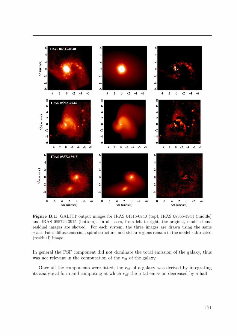
Figure B.1: GALFIT output images for IRAS 04315-0840 (top), IRAS 08355-4944 (middle)and IRAS 08572+3915 (bottom). In all cases, from left to right, the original, modeled andresidual images are showed. For each system, the three images are drawn using the samescale. Faint diffuse emission, spiral structure, and stellar regions remain in the model-subtracted(residual) image.
In general the PSF component did not dominate the total emission of the galaxy, thuswas not relevant in the computation of the reff of the galaxy.
Once all the components were fitted, the reff of a galaxy was derived by integratingits analytical form and computing at which reff the total emission decreased by a half.
171


Bibliography
Aaronson, M. 1983, ApJ, 266, L11, ADS
Abraham, R. G., Tanvir, N. R., Santiago, B. X., Ellis, R. S., Glazebrook, K., & van denBergh, S. 1996, MNRAS, 279, L47, ADS, arXiv:astro-ph/9602044
Allington-Smith, J. R. 2007, in Revista Mexicana de Astronomia y Astrofisica, vol. 27,Vol. 28, Revista Mexicana de Astronomia y Astrofisica Conference Series, ed. S. Kurtz,17–23, ADS
Alonso-Herrero, A., García-Marín, M., Monreal-Ibero, A., Colina, L., Arribas, S.,Alfonso-Garzón, J., & Labiano, A. 2009, A&A, 506, 1541, ADS, 0907.5105
Alonso-Herrero, A., Rieke, G. H., Rieke, M. J., Colina, L., Pérez-González, P. G., &Ryder, S. D. 2006, ApJ, 650, 835, ADS, arXiv:astro-ph/0606186
Alonso-Herrero, A., Rieke, G. H., Rieke, M. J., & Scoville, N. Z. 2002, AJ, 124, 166,ADS, arXiv:astro-ph/0203494
Amorín, R., Aguerri, J. A. L., Muñoz-Tuñón, C., & Cairós, L. M. 2009, A&A, 501, 75,ADS, 0903.2861
Anders, P., Bissantz, N., Boysen, L., de Grijs, R., & Fritze-v. Alvensleben, U. 2007,MNRAS, 377, 91, ADS, arXiv:astro-ph/0702413
Arp, H. 1966, ApJS, 14, 1, ADS
Arribas, S., Bushouse, H., Lucas, R. A., Colina, L., & Borne, K. D. 2004, AJ, 127, 2522,ADS, arXiv:astro-ph/0402375
Arribas, S. et al. 1998, in Society of Photo-Optical Instrumentation Engineers (SPIE)Conference Series, Vol. 3355, Society of Photo-Optical Instrumentation Engineers(SPIE) Conference Series, ed. S. D’Odorico, 821–827, ADS
Arribas, S., & Colina, L. 2003, ApJ, 591, 791, ADS, arXiv:astro-ph/0304138
Arribas, S., Colina, L., & Borne, K. D. 2000, ApJ, 545, 228, ADS
Arribas, S., Colina, L., Monreal-Ibero, A., Alfonso, J., García-Marín, M., & Alonso-
173
Bibliography
Herrero, A. 2008, A&A, 479, 687, ADS, 0710.2761
Ashman, K. M., & Zepf, S. E. 2001, AJ, 122, 1888, ADS, arXiv:astro-ph/0107146
Barnes, J. E. 2004, MNRAS, 350, 798, ADS, arXiv:astro-ph/0402248
Barnes, J. E., & Hernquist, L. 1992a, ARA&A, 30, 705, ADS
Barnes, J. E., & Hernquist, L. 1992b, Nature, 360, 715, ADS
Barnes, J. E., & Hernquist, L. 1996, ApJ, 471, 115, ADS
Barth, A. J., Ho, L. C., Filippenko, A. V., & Sargent, W. L. 1995, AJ, 110, 1009, ADS
Bastian, N., Emsellem, E., Kissler-Patig, M., & Maraston, C. 2006, A&A, 445, 471,ADS, arXiv:astro-ph/0509249
Bastian, N., Gieles, M., Efremov, Y. N., & Lamers, H. J. G. L. M. 2005a, A&A, 443,79, ADS, arXiv:astro-ph/0508110
Bastian, N., Gieles, M., Lamers, H. J. G. L. M., Scheepmaker, R. A., & de Grijs, R.2005b, A&A, 431, 905, ADS, arXiv:astro-ph/0408043
Bastian, N., Hempel, M., Kissler-Patig, M., Homeier, N. L., & Trancho, G. 2005c, A&A,435, 65, ADS, arXiv:astro-ph/0502561
Bastian, N., Trancho, G., Konstantopoulos, I. S., & Miller, B. W. 2009, ApJ, 701, 607,ADS, 0906.2210
Baumgardt, H., & Kroupa, P. 2007, MNRAS, 380, 1589, ADS, 0707.1944
Baumgardt, H., & Makino, J. 2003, MNRAS, 340, 227, ADS, arXiv:astro-ph/0211471
Bekki, K., & Shioya, Y. 2001, ApJS, 134, 241, ADS, arXiv:astro-ph/0012365
Bekki, K., Shioya, Y., & Whiting, M. 2006, MNRAS, 371, 805, ADS,arXiv:astro-ph/0607349
Belokurov, V. et al. 2007, ApJ, 654, 897, ADS, arXiv:astro-ph/0608448
Bender, R., Burstein, D., & Faber, S. M. 1992, ApJ, 399, 462, ADS
Bendo, G. J., & Barnes, J. E. 2000, MNRAS, 316, 315, ADS, arXiv:astro-ph/0003248
Bertin, E., & Arnouts, S. 1996, A&AS, 117, 393, ADS
Bik, A., Lamers, H. J. G. L. M., Bastian, N., Panagia, N., & Romaniello, M. 2003,A&A, 397, 473, ADS, arXiv:astro-ph/0210594
Billett, O. H., Hunter, D. A., & Elmegreen, B. G. 2002, AJ, 123, 1454, ADS,
174

Bibliography
arXiv:astro-ph/0112260
Bingham, R. G., Gellatly, D. W., Jenkins, C. R., & Worswick, S. P. 1994, in Society ofPhoto-Optical Instrumentation Engineers (SPIE) Conference Series, Vol. 2198, Societyof Photo-Optical Instrumentation Engineers (SPIE) Conference Series, ed. D. L. Craw-ford & E. R. Craine, 56–64, ADS
Binney, J., & Tremaine, S. 1987, Galactic dynamics, ed. Binney, J. & Tremaine, S.,ADS
Blain, A. W., Smail, I., Ivison, R. J., Kneib, J., & Frayer, D. T. 2002, Phys. Rep., 369,111, ADS, arXiv:astro-ph/0202228
Blitz, L., Fukui, Y., Kawamura, A., Leroy, A., Mizuno, N., & Rosolowsky, E. 2007,Protostars and Planets V, 81, ADS, arXiv:astro-ph/0602600
Boily, C. M., & Kroupa, P. 2003, MNRAS, 338, 673, ADS, arXiv:astro-ph/0211026
Borne, K. D., Bushouse, H., Lucas, R. A., & Colina, L. 2000, ApJ, 529, L77, ADS,arXiv:astro-ph/9912151
Bosch, G., Terlevich, E., & Terlevich, R. 2009, AJ, 137, 3437, ADS, 0811.4748
Bournaud, F. et al. 2008a, A&A, 486, 741, ADS, 0803.3831
Bournaud, F., Duc, P., Amram, P., Combes, F., & Gach, J. 2004, A&A, 425, 813, ADS,arXiv:astro-ph/0406169
Bournaud, F., Duc, P., & Emsellem, E. 2008b, MNRAS, 389, L8, ADS, 0806.1386
Bournaud, F., & Duc, P.-A. 2006, A&A, 456, 481, ADS, arXiv:astro-ph/0605350
Bournaud, F., Elmegreen, B. G., & Elmegreen, D. M. 2007, ApJ, 670, 237, ADS,0708.0306
Bournaud, F., Jog, C. J., & Combes, F. 2005, A&A, 437, 69, ADS,arXiv:astro-ph/0503189
Braine, J., Duc, P.-A., Lisenfeld, U., Charmandaris, V., Vallejo, O., Leon, S., & Brinks,E. 2001, A&A, 378, 51, ADS, arXiv:astro-ph/0108513
Bresolin, F., & Kennicutt, Jr., R. C. 1997, AJ, 113, 975, ADS
Bruzual, G., & Charlot, S. 2003, MNRAS, 344, 1000, ADS, arXiv:astro-ph/0309134
Burkert, A., & Bodenheimer, P. 1996, MNRAS, 280, 1190, ADS
Bushouse, H. A. et al. 2002, ApJS, 138, 1, ADS, arXiv:astro-ph/0108261
175
Bibliography
Cairós, L. M., Caon, N., Papaderos, P., Noeske, K., Vílchez, J. M., García Lorenzo, B.,& Muñoz-Tuñón, C. 2003, ApJ, 593, 312, ADS, arXiv:astro-ph/0306307
Cairós, L. M., Caon, N., Vílchez, J. M., González-Pérez, J. N., & Muñoz-Tuñón, C.2001, ApJS, 136, 393, ADS
Calzetti, D., Armus, L., Bohlin, R. C., Kinney, A. L., Koornneef, J., & Storchi-Bergmann, T. 2000, ApJ, 533, 682, ADS, arXiv:astro-ph/9911459
Calzetti, D. et al. 2007, ApJ, 666, 870, ADS, 0705.3377
Caputi, K. I. et al. 2007, ApJ, 660, 97, ADS, arXiv:astro-ph/0701283
Chapman, S. C., Windhorst, R., Odewahn, S., Yan, H., & Conselice, C. 2003, ApJ, 599,92, ADS, arXiv:astro-ph/0308197
Clements, D. L., Sutherland, W. J., McMahon, R. G., & Saunders, W. 1996, MNRAS,279, 477, ADS
Cohen, M. 1992, AJ, 103, 1734, ADS
Colina, L., Arribas, S., & Clements, D. 2004, ApJ, 602, 181, ADS,arXiv:astro-ph/0310604
Colina, L., Arribas, S., & Monreal-Ibero, A. 2005, ApJ, 621, 725, ADS
Colina, L. et al. 2001, ApJ, 563, 546, ADS
Combes, F., Boisse, P., Mazure, A., Blanchard, A., & Seymour, M. 1995, Galaxies andCosmology, ed. Combes, F., Boisse, P., Mazure, A., Blanchard, A., & Seymour, M. ,ADS
Corbett, E. A. et al. 2003, ApJ, 583, 670, ADS, arXiv:astro-ph/0210197
Cox, T. J., Jonsson, P., Primack, J. R., & Somerville, R. S. 2006, MNRAS, 373, 1013,ADS, arXiv:astro-ph/0503201
Cox, T. J., Jonsson, P., Somerville, R. S., Primack, J. R., & Dekel, A. 2008, MNRAS,384, 386, ADS, 0709.3511
Cox, T. J., Primack, J., Jonsson, P., & Somerville, R. S. 2004, ApJ, 607, L87, ADS,arXiv:astro-ph/0402675
Cresci, G., Mannucci, F., Maiolino, R., Marconi, A., Gnerucci, A., & Magrini, L. 2010,Nature, 467, 811, ADS, 1010.2534
Dabringhausen, J., Hilker, M., & Kroupa, P. 2008, MNRAS, 386, 864, ADS, 0802.0703
D’Agostino, R. B., & Stephens, M. A. 1986, Goodness-of-fit techniques, ed. M. A.
176

Bibliography
D’Agostino, R. B. & Stephens, ADS
Dasyra, K. M. et al. 2006, ApJ, 651, 835, ADS, arXiv:astro-ph/0607468
de Grijs, R., Parmentier, G., & Lamers, H. J. G. L. M. 2005, MNRAS, 364, 1054, ADS,arXiv:astro-ph/0509721
Denicoló, G., Terlevich, R., & Terlevich, E. 2002, MNRAS, 330, 69, ADS,arXiv:astro-ph/0110356
Di Matteo, P., Bournaud, F., Martig, M., Combes, F., Melchior, A., & Semelin, B. 2008,A&A, 492, 31, ADS, 0809.2592
Di Matteo, P., Combes, F., Melchior, A., & Semelin, B. 2007, A&A, 468, 61, ADS,arXiv:astro-ph/0703212
Di Matteo, P., Montuori, M., Lehnert, M. D., Combes, F., & Semelin, B. 2011, ArXive-prints, ADS, 1102.2234
Díaz, Á. I., Terlevich, E., Castellanos, M., & Hägele, G. F. 2007, MNRAS, 382, 251,ADS, 0709.1236
Díaz-Santos, T., Alonso-Herrero, A., Colina, L., Ryder, S. D., & Knapen, J. H. 2007,ApJ, 661, 149, ADS, arXiv:astro-ph/0701557
Dinshaw, N., Evans, A. S., Epps, H., Scoville, N. Z., & Rieke, M. 1999, ApJ, 525, 702,ADS, arXiv:astro-ph/9907395
Dubath, P., & Grillmair, C. J. 1997, A&A, 321, 379, ADS, arXiv:astro-ph/9610194
Duc, P., Bournaud, F., & Masset, F. 2004, A&A, 427, 803, ADS, arXiv:astro-ph/0408524
Duc, P., Braine, J., Lisenfeld, U., Brinks, E., & Boquien, M. 2007, A&A, 475, 187, ADS,0709.2733
Duc, P., Brinks, E., Springel, V., Pichardo, B., Weilbacher, P., & Mirabel, I. F. 2000,AJ, 120, 1238, ADS, arXiv:astro-ph/0006038
Duc, P.-A., Brinks, E., Wink, J. E., & Mirabel, I. F. 1997, A&A, 326, 537, ADS
Duc, P.-A., & Mirabel, I. F. 1994, A&A, 289, 83, ADS
Duc, P.-A., & Mirabel, I. F. 1998, A&A, 333, 813, ADS
Edmunds, M. G., & Pagel, B. E. J. 1984, MNRAS, 211, 507, ADS
Efremov, Y. N. 1995, AJ, 110, 2757, ADS
Egami, E. et al. 2004, ApJS, 154, 130, ADS, arXiv:astro-ph/0406359
177

Bibliography
Eisenstein, D. J. et al. 2005, ApJ, 633, 560, ADS, arXiv:astro-ph/0501171
Ellison, S. L., Patton, D. R., Simard, L., & McConnachie, A. W. 2008, AJ, 135, 1877,ADS, 0803.0161
Elmegreen, B. G. 2002, ApJ, 564, 773, ADS, arXiv:astro-ph/0112528
Elmegreen, B. G. 2007, ApJ, 668, 1064, ADS, 0707.2252
Elmegreen, B. G., & Efremov, Y. N. 1997, ApJ, 480, 235, ADS
Elmegreen, B. G., & Elmegreen, D. M. 1983, MNRAS, 203, 31, ADS
Elmegreen, B. G., & Elmegreen, D. M. 2005, ApJ, 627, 632, ADS,arXiv:astro-ph/0504032
Elmegreen, B. G., & Falgarone, E. 1996, ApJ, 471, 816, ADS
Elmegreen, B. G., Kaufman, M., & Thomasson, M. 1993, ApJ, 412, 90, ADS
Elmegreen, D. M., & Elmegreen, B. G. 2006, ApJ, 651, 676, ADS,arXiv:astro-ph/0607579
Elmegreen, D. M., Elmegreen, B. G., Ferguson, T., & Mullan, B. 2007, ApJ, 663, 734,ADS, 0704.0911
Elmegreen, D. M., Elmegreen, B. G., Marcus, M. T., Shahinyan, K., Yau, A., & Petersen,M. 2009, ApJ, 701, 306, ADS, 0906.2660
Elson, R. A. W., & Fall, S. M. 1985, PASP, 97, 692, ADS
Engel, H. et al. 2010, ApJ, 724, 233, ADS
Ercolano, B., Bastian, N., & Stasińska, G. 2007, MNRAS, 379, 945, ADS, 0705.2726
Escala, A., & Larson, R. B. 2008, ApJ, 685, L31, ADS, 0806.0853
Evans, A. S., Mazzarella, J. M., Surace, J. A., & Sanders, D. B. 2002, ApJ, 580, 749,ADS, arXiv:astro-ph/0208541
Fall, S. M., Chandar, R., & Whitmore, B. C. 2005, ApJ, 631, L133, ADS,arXiv:astro-ph/0509293
Fall, S. M., Chandar, R., & Whitmore, B. C. 2009, ApJ, 704, 453, ADS, 0910.1044
Fall, S. M., & Zhang, Q. 2001, ApJ, 561, 751, ADS, arXiv:astro-ph/0107298
Farrah, D., Afonso, J., Efstathiou, A., Rowan-Robinson, M., Fox, M., & Clements, D.2003, MNRAS, 343, 585, ADS, arXiv:astro-ph/0304154
178
Bibliography
Farrah, D. et al. 2001, MNRAS, 326, 1333, ADS, arXiv:astro-ph/0106275
Fernandes, I. F., de Carvalho, R., Contini, T., & Gal, R. R. 2004, MNRAS, 355, 728,ADS, arXiv:astro-ph/0409114
Ferreiro, D. L., & Pastoriza, M. G. 2004, A&A, 428, 837, ADS, arXiv:astro-ph/0409150
Ferreiro, D. L., Pastoriza, M. G., & Rickes, M. 2008, A&A, 481, 645, ADS
Fleck, J.-J., Boily, C. M., Lançon, A., & Deiters, S. 2006, MNRAS, 369, 1392, ADS,arXiv:astro-ph/0604194
Fleck, Jr., R. C. 1996, ApJ, 458, 739, ADS
Forbes, D., Spitler, L., Graham, A., Foster, C., Hau, G., & Benson, A. 2011, ArXive-prints, ADS, 1101.2460
Förster Schreiber, N. M., Shapley, A. E., Erb, D. K., Genzel, R., Steidel, C. C., Bouché,N., Cresci, G., & Davies, R. 2011a, ApJ, 731, 65, ADS, 1011.1507
Förster Schreiber, N. M. et al. 2011b, ArXiv e-prints, ADS, 1104.0248
Franceschini, A., Aussel, H., Cesarsky, C. J., Elbaz, D., & Fadda, D. 2001, A&A, 378,1, ADS, arXiv:astro-ph/0108292
Franceschini, A. et al. 2005, AJ, 129, 2074, ADS, arXiv:astro-ph/0412476
Frayer, D. T., Armus, L., Scoville, N. Z., Blain, A. W., Reddy, N. A., Ivison, R. J., &Smail, I. 2003, AJ, 126, 73, ADS, arXiv:astro-ph/0304043
Frayer, D. T. et al. 2004, ApJS, 154, 137, ADS, arXiv:astro-ph/0406351
Gallagher, S. C. et al. 2010, AJ, 139, 545, ADS, 1002.3323
García-Marín, M. 2007, 2D structure and kinematics of a representative sample of low-zultra-luminous infrared galaxies, http://www.tesisenred.net/handle/10803/13774
García-Marín, M., Colina, L., & Arribas, S. 2009a, A&A, 505, 1017, ADS, 0907.2218
García-Marín, M., Colina, L., Arribas, S., & Monreal-Ibero, A. 2009b, A&A, 505, 1319,ADS, 0907.2408
Geha, M., Guhathakurta, P., & van der Marel, R. P. 2003, AJ, 126, 1794, ADS,arXiv:astro-ph/0304537
Geha, M., Willman, B., Simon, J. D., Strigari, L. E., Kirby, E. N., Law, D. R., &Strader, J. 2009, ApJ, 692, 1464, ADS, 0809.2781
Genzel, R. et al. 1998a, ApJ, 498, 579, ADS, arXiv:astro-ph/9711255
179
Bibliography
Genzel, R., Lutz, D., & Tacconi, L. 1998b, Nature, 395, 859, ADS
Genzel, R., Tacconi, L. J., Rigopoulou, D., Lutz, D., & Tecza, M. 2001, ApJ, 563, 527,ADS, arXiv:astro-ph/0106032
Gieles, M. 2009a, MNRAS, 394, 2113, ADS, 0901.0830
Gieles, M. 2009b, Ap&SS, 324, 299, ADS, 0801.2676
Gieles, M. 2010, in Astronomical Society of the Pacific Conference Series, Vol. 423,Galaxy Wars: Stellar Populations and Star Formation in Interacting Galaxies, ed.B. Smith, J. Higdon, S. Higdon, & N. Bastian, 123–+, 0908.2974, ADS
Gieles, M., Larsen, S. S., Bastian, N., & Stein, I. T. 2006, A&A, 450, 129, ADS,arXiv:astro-ph/0512297
Glass, I. S. 1999, Handbook of Infrared Astronomy, ed. Glass, I. S., ADS
Goddard, Q. E., Bastian, N., & Kennicutt, R. C. 2010, MNRAS, 491, ADS, 1002.2894
Goldader, J. D., Joseph, R. D., Doyon, R., & Sanders, D. B. 1997, ApJS, 108, 449, ADS
Goodwin, S. P. 2009, Ap&SS, 324, 259, ADS, 0802.2207
Goodwin, S. P., & Bastian, N. 2006, MNRAS, 373, 752, ADS, arXiv:astro-ph/0609477
Haas, M. R., Gieles, M., Scheepmaker, R. A., Larsen, S. S., & Lamers, H. J. G. L. M.2008, A&A, 487, 937, ADS, 0806.3752
Hancock, M., Smith, B. J., Struck, C., Giroux, M. L., & Hurlock, S. 2009, AJ, 137,4643, ADS, 0904.0670
Harris, W. E. 2001, in Saas-Fee Advanced Course 28: Star Clusters, ed. L. Labhardt &B. Binggeli, 223–+, ADS
Heckman, T. M., Armus, L., & Miley, G. K. 1990, ApJS, 74, 833, ADS
Hernquist, L. 1992a, Nature, 360, 105, ADS
Hernquist, L. 1992b, ApJ, 400, 460, ADS
Hernquist, L. 1993, ApJ, 409, 548, ADS
Hibbard, J. E., Guhathakurta, P., van Gorkom, J. H., & Schweizer, F. 1994, AJ, 107,67, ADS
Hibbard, J. E., & Mihos, J. C. 1995, AJ, 110, 140, ADS, arXiv:astro-ph/9503030
Higdon, S. J., Higdon, J. L., & Marshall, J. 2006, ApJ, 640, 768, ADS,
180

Bibliography
arXiv:astro-ph/0511422
Holtzman, J. A. et al. 1992, AJ, 103, 691, ADS
Holtzman, J. A. et al. 1995, PASP, 107, 156, ADS
Holtzman, J. A. et al. 1996, AJ, 112, 416, ADS
Howell, J. H. et al. 2010, ApJ, 715, 572, ADS, 1004.0985
Hunsberger, S. D., Charlton, J. C., & Zaritsky, D. 1996, ApJ, 462, 50, ADS,arXiv:astro-ph/9510160
Hunter, D. A., & Gallagher, III, J. S. 1986, PASP, 98, 5, ADS
Hunter, D. A., Hunsberger, S. D., & Roye, E. W. 2000, ApJ, 542, 137, ADS,arXiv:astro-ph/0005257
Iglesias-Páramo, J., & Vílchez, J. M. 2001, ApJ, 550, 204, ADS, arXiv:astro-ph/0011115
Im, M., Griffiths, R. E., Naim, A., Ratnatunga, K. U., Roche, N., Green, R. F., &Sarajedini, V. L. 1999, ApJ, 510, 82, ADS, arXiv:astro-ph/9901424
Inami, H. et al. 2010, AJ, 140, 63, ADS, 1004.3543
Ivison, R. J. et al. 2004, ApJS, 154, 124, ADS, arXiv:astro-ph/0406158
Ivison, R. J. et al. 2002, MNRAS, 337, 1, ADS, arXiv:astro-ph/0206432
Jones, T. A., Swinbank, A. M., Ellis, R. S., Richard, J., & Stark, D. P. 2010, MNRAS,404, 1247, ADS, 0910.4488
Jordán, A. et al. 2007, ApJS, 171, 101, ADS, arXiv:astro-ph/0702496
Kapferer, W., Knapp, A., Schindler, S., Kimeswenger, S., & van Kampen, E. 2005,A&A, 438, 87, ADS, arXiv:astro-ph/0503559
Kassin, S. A., Frogel, J. A., Pogge, R. W., Tiede, G. P., & Sellgren, K. 2003, AJ, 126,1276, ADS, arXiv:astro-ph/0306325
Kauffmann, G., & White, S. D. M. 1993, MNRAS, 261, 921, ADS
Kaviraj, S., Darg, D., Lintott, C., Schawinski, K., & Silk, J. 2011, ArXiv e-prints, ADS,1108.4410
Kennicutt, Jr., R. C. 1998, ARA&A, 36, 189, ADS, arXiv:astro-ph/9807187
Kewley, L. J., Groves, B., Kauffmann, G., & Heckman, T. 2006, MNRAS, 372, 961,ADS, arXiv:astro-ph/0605681
181
Bibliography
Kewley, L. J., Heisler, C. A., Dopita, M. A., & Lumsden, S. 2001, ApJS, 132, 37, ADS
Kim, D., Sanders, D. B., Veilleux, S., Mazzarella, J. M., & Soifer, B. T. 1995, ApJS, 98,129, ADS
Kim, D.-C., Veilleux, S., & Sanders, D. B. 1998, ApJ, 508, 627, ADS,arXiv:astro-ph/9806149
Kissler-Patig, M., Jordán, A., & Bastian, N. 2006, A&A, 448, 1031, ADS,arXiv:astro-ph/0512360
Klypin, A., Kravtsov, A. V., Valenzuela, O., & Prada, F. 1999, ApJ, 522, 82, ADS,arXiv:astro-ph/9901240
Knierman, K. A., Gallagher, S. C., Charlton, J. C., Hunsberger, S. D., Whit-more, B., Kundu, A., Hibbard, J. E., & Zaritsky, D. 2003, AJ, 126, 1227, ADS,arXiv:astro-ph/0307383
Konstantopoulos, I. S., Bastian, N., Smith, L. J., Westmoquette, M. S., Trancho, G., &Gallagher, J. S. 2009, ApJ, 701, 1015, ADS, 0906.2006
Kormendy, J., & Sanders, D. B. 1992, ApJ, 390, L53, ADS
Kotilainen, J. K., Reunanen, J., Laine, S., & Ryder, S. D. 2001, A&A, 366, 439, ADS,arXiv:astro-ph/0011428
Kouwenhoven, M. B. N., & de Grijs, R. 2008, A&A, 480, 103, ADS, 0712.1748
Kroupa, P. 1998, MNRAS, 300, 200, ADS, arXiv:astro-ph/9806206
Kroupa, P. 2002, Science, 295, 82, ADS, arXiv:astro-ph/0201098
Kumar, M. S. N., Kamath, U. S., & Davis, C. J. 2004, MNRAS, 353, 1025, ADS,arXiv:astro-ph/0406639
Kunth, D., & Schild, H. 1986, A&A, 169, 71, ADS
Lada, C. J., & Lada, E. A. 2003, ARA&A, 41, 57, ADS, arXiv:astro-ph/0301540
Lada, C. J., Lombardi, M., & Alves, J. F. 2010, ApJ, 724, 687, ADS, 1009.2985
Lamers, H. J. G. L. M., & Cassinelli, J. P. 1999, Introduction to Stellar Winds, ed.Lamers, H. J. G. L. M. & Cassinelli, J. P., ADS
Larsen, S. S. 1999, A&AS, 139, 393, ADS, arXiv:astro-ph/9907163
Larsen, S. S. 2000, MNRAS, 319, 893, ADS, arXiv:astro-ph/0008191
Larsen, S. S. 2004, A&A, 416, 537, ADS, arXiv:astro-ph/0312338
182

Bibliography
Larsen, S. S. 2009, A&A, 494, 539, ADS, 0812.1400
Larsen, S. S. 2010, Royal Society of London Philosophical Transactions Series A, 368,867, ADS, 0911.0796
Larsen, S. S., & Richtler, T. 1999, A&A, 345, 59, ADS, arXiv:astro-ph/9902227
Larson, R. B., & Tinsley, B. M. 1978, ApJ, 219, 46, ADS
Le Floc’h, E. et al. 2005, ApJ, 632, 169, ADS, arXiv:astro-ph/0506462
Lee, M. G., Chandar, R., & Whitmore, B. C. 2005, AJ, 130, 2128, ADS,arXiv:astro-ph/0510144
LeFevre, O. et al. 2003, in Society of Photo-Optical Instrumentation Engineers (SPIE)Conference Series, Vol. 4841, Society of Photo-Optical Instrumentation Engineers(SPIE) Conference Series, ed. M. Iye & A. F. M. Moorwood, 1670–1681, ADS
Leitherer, C., ed. 1998, Stellar astrophysics for the local group : VIII Canary IslandsWinter School of Astrophysics, eds., Aparicio, C., Herrero, A., Sánchez, F., p527, ADS
Leitherer, C. et al. 1999, ApJS, 123, 3, ADS, arXiv:astro-ph/9902334
Lonsdale, C. J., Farrah, D., & Smith, H. E. 2006, Ultraluminous Infrared Galaxies, ed.Mason, J. W. (Springer Verlag), 285–+, ADS
López-Sánchez, A. R., & Esteban, C. 2009, A&A, 508, 615, ADS, 0910.1578
López-Sánchez, Á. R., Esteban, C., & Rodríguez, M. 2004, A&A, 428, 425, ADS,arXiv:astro-ph/0409050
Lu, N. Y., Hoffman, G. L., Groff, T., Roos, T., & Lamphier, C. 1993, ApJS, 88, 383,ADS
Mac Low, M., & Klessen, R. S. 2004, Reviews of Modern Physics, 76, 125, ADS,arXiv:astro-ph/0301093
Maíz Apellániz, J., & Úbeda, L. 2005, ApJ, 629, 873, ADS, arXiv:astro-ph/0505012
Maraston, C. 2005, MNRAS, 362, 799, ADS, arXiv:astro-ph/0410207
Maraston, C., Bastian, N., Saglia, R. P., Kissler-Patig, M., Schweizer, F., & Goudfrooij,P. 2004, A&A, 416, 467, ADS, arXiv:astro-ph/0311232
Maraston, C., Kissler-Patig, M., Brodie, J. P., Barmby, P., & Huchra, J. P. 2001, A&A,370, 176, ADS, arXiv:astro-ph/0101556
Marconi, G., Tosi, M., Greggio, L., & Focardi, P. 1995, AJ, 109, 173, ADS,arXiv:astro-ph/9409013
183
Bibliography
Marlowe, A. T., Meurer, G. R., Heckman, T. M., & Schommer, R. 1997, ApJS, 112,285, ADS
Martini, P., & Ho, L. C. 2004, ApJ, 610, 233, ADS, arXiv:astro-ph/0404003
Mateo, M. L. 1998, ARA&A, 36, 435, ADS, arXiv:astro-ph/9810070
Mayya, Y. D. 1994, AJ, 108, 1276, ADS
McDowell, J. C. et al. 2003, ApJ, 591, 154, ADS, arXiv:astro-ph/0303316
McLaughlin, D. E., & Pudritz, R. E. 1996, ApJ, 457, 578, ADS
Melnick, J., & Mirabel, I. F. 1990, A&A, 231, L19, ADS
Melnick, J., Tenorio-Tagle, G., & Terlevich, R. 1999, MNRAS, 302, 677, ADS
Mendes de Oliveira, C., Cypriano, E. S., Sodré, Jr., L., & Balkowski, C. 2004, ApJ, 605,L17, ADS
Mendes de Oliveira, C., Plana, H., Amram, P., Balkowski, C., & Bolte, M. 2001, AJ,121, 2524, ADS, arXiv:astro-ph/0101226
Mengel, S., Lehnert, M. D., Thatte, N. A., Vacca, W. D., Whitmore, B., & Chandar,R. 2008, A&A, 489, 1091, ADS, 0805.2559
Meurer, G. R., Heckman, T. M., Leitherer, C., Kinney, A., Robert, C., & Garnett, D. R.1995, AJ, 110, 2665, ADS, arXiv:astro-ph/9509038
Michel-Dansac, L., Lambas, D. G., Alonso, M. S., & Tissera, P. 2008, MNRAS, 386,L82, ADS, 0802.3904
Mihos, C. 1999, Ap&SS, 266, 195, ADS, arXiv:astro-ph/9903115
Mihos, J. C., & Bothun, G. D. 1998, ApJ, 500, 619, ADS
Mihos, J. C., Bothun, G. D., & Richstone, D. O. 1993, ApJ, 418, 82, ADS
Mihos, J. C., & Hernquist, L. 1994a, ApJ, 437, 611, ADS
Mihos, J. C., & Hernquist, L. 1994b, ApJ, 431, L9, ADS
Mihos, J. C., & Hernquist, L. 1996, ApJ, 464, 641, ADS, arXiv:astro-ph/9512099
Miller, B. W., Whitmore, B. C., Schweizer, F., & Fall, S. M. 1997, AJ, 114, 2381, ADS
Mirabel, I. F., Dottori, H., & Lutz, D. 1992, A&A, 256, L19, ADS
Mirabel, I. F., Lutz, D., & Maza, J. 1991, A&A, 243, 367, ADS
184
Bibliography
Monreal-Ibero, A., Colina, L., Arribas, S., & García-Marín, M. 2007, A&A, 472, 421,ADS, 0706.1145
Monreal-Ibero, A., Vílchez, J. M., Walsh, J. R., & Muñoz-Tuñón, C. 2010, A&A, 517,A27+, ADS, 1003.5329
Montuori, M., Di Matteo, P., Lehnert, M. D., Combes, F., & Semelin, B. 2010, A&A,518, A56+, ADS, 1003.1374
Mullan, B. et al. 2011, ApJ, 731, 93, ADS, 1101.5393
Murray, N., Quataert, E., & Thompson, T. A. 2010, ApJ, 709, 191, ADS, 0906.5358
Naab, T., & Burkert, A. 2003, ApJ, 597, 893, ADS, arXiv:astro-ph/0110179
Naab, T., Jesseit, R., & Burkert, A. 2006, MNRAS, 372, 839, ADS,arXiv:astro-ph/0605155
Nardini, E., Risaliti, G., Salvati, M., Sani, E., Imanishi, M., Marconi, A., & Maiolino,R. 2008, MNRAS, 385, L130, ADS
Neugebauer, G. et al. 1984, ApJ, 278, L1, ADS
Nishiura, S., Shioya, Y., Murayama, T., Sato, Y., Nagao, T., Taniguchi, Y., & Sanders,D. B. 2002, PASJ, 54, 21, ADS, arXiv:astro-ph/0201178
O’Connell, R. W., Gallagher, III, J. S., Hunter, D. A., & Colley, W. N. 1995, ApJ, 446,L1+, ADS
O’dell, C. R., & Townsley, L. K. 1988, A&A, 198, 283, ADS
Okazaki, T., & Taniguchi, Y. 2000, ApJ, 543, 149, ADS, arXiv:astro-ph/0006006
Origlia, L., & Leitherer, C. 2000, AJ, 119, 2018, ADS, arXiv:astro-ph/0001408
Osterbrock, D. E. 1989, Astrophysics of gaseous nebulae and active galactic nuclei, ed.Osterbrock, D. E., ADS
Papaderos, P., Guseva, N. G., Izotov, Y. I., Noeske, K. G., Thuan, T. X., & Fricke, K. J.2006, A&A, 457, 45, ADS, arXiv:astro-ph/0607443
Peng, C. Y., Ho, L. C., Impey, C. D., & Rix, H.-W. 2002, AJ, 124, 266, ADS,arXiv:astro-ph/0204182
Peng, C. Y., Ho, L. C., Impey, C. D., & Rix, H.-W. 2010, AJ, 139, 2097, ADS, 0912.0731
Perez, J., Michel-Dansac, L., & Tissera, P. 2011, ArXiv e-prints, ADS, 1106.4556
Pérez-González, P. G. et al. 2005, ApJ, 630, 82, ADS, arXiv:astro-ph/0505101
185

Bibliography
Peterson, B. W., Struck, C., Smith, B. J., & Hancock, M. 2009, MNRAS, 400, 1208,ADS, 0908.2619
Pilyugin, L. S., Vílchez, J. M., & Contini, T. 2004, A&A, 425, 849, ADS,arXiv:astro-ph/0407014
Pirogov, L. E. 2009, Astronomy Reports, 53, 1127, ADS, 0911.4421
Piskunov, A. E., Kharchenko, N. V., Schilbach, E., Röser, S., Scholz, R., & Zinnecker,H. 2008, A&A, 487, 557, ADS, 0806.2217
Porras, A., Christopher, M., Allen, L., Di Francesco, J., Megeath, S. T., & Myers, P. C.2003, AJ, 126, 1916, ADS, arXiv:astro-ph/0307510
Press, W. H., Teukolsky, S. A., Vetterling, W. T., & Flannery, B. P. 1992, Numericalrecipes in FORTRAN. The art of scientific computing, ed. Press, W. H., Teukolsky,S. A., Vetterling, W. T., & Flannery, B. P. , ADS
Relaño, M., & Beckman, J. E. 2005, A&A, 430, 911, ADS, arXiv:astro-ph/0410415
Relaño, M., Beckman, J. E., Zurita, A., Rozas, M., & Giammanco, C. 2005, A&A, 431,235, ADS, arXiv:astro-ph/0410484
Renaud, F., Boily, C. M., Fleck, J., Naab, T., & Theis, C. 2008, MNRAS, 391, L98,ADS, 0809.2927
Renaud, F., Boily, C. M., Naab, T., & Theis, C. 2009, ApJ, 706, 67, ADS, 0910.0196
Risaliti, G. et al. 2006, MNRAS, 365, 303, ADS, arXiv:astro-ph/0510282
Rodighiero, G. et al. 2011, ArXiv e-prints, ADS, 1108.0933
Rodríguez-Zaurín, J., Arribas, S., Monreal-Ibero, A., Colina, L., Alonso-Herrero, A., &Alfonso-Garzón, J. 2011, A&A, 527, A60+, ADS, 1009.0112
Roth, M. M. et al. 2005, PASP, 117, 620, ADS, arXiv:astro-ph/0502581
Rozas, M., Richer, M. G., López, J. A., Relaño, M., & Beckman, J. E. 2006a, A&A,455, 539, ADS
Rozas, M., Richer, M. G., López, J. A., Relaño, M., & Beckman, J. E. 2006b, A&A,455, 549, ADS
Rupke, D. S. N., Kewley, L. J., & Barnes, J. E. 2010, ApJ, 710, L156, ADS, 1001.1728
Rupke, D. S. N., Veilleux, S., & Baker, A. J. 2008, ApJ, 674, 172, ADS, 0708.1766
Sanders, D. B., Mazzarella, J. M., Kim, D., Surace, J. A., & Soifer, B. T. 2003, AJ, 126,1607, ADS, arXiv:astro-ph/0306263
186
Bibliography
Sanders, D. B., & Mirabel, I. F. 1996, ARA&A, 34, 749, ADS
Sanders, D. B., Soifer, B. T., Elias, J. H., Madore, B. F., Matthews, K., Neugebauer,G., & Scoville, N. Z. 1988, ApJ, 325, 74, ADS
Santiago-Cortés, M., Mayya, Y. D., & Rosa-González, D. 2010, MNRAS, 496, ADS,1002.3370
Schechter, P. 1976, ApJ, 203, 297, ADS
Schlegel, D. J., Finkbeiner, D. P., & Davis, M. 1998, ApJ, 500, 525, ADS,arXiv:astro-ph/9710327
Schweizer, F. 1978, in IAU Symposium, Vol. 77, Structure and Properties of NearbyGalaxies, ed. E. M. Berkhuijsen & R. Wielebinski, 279–284, ADS
Schweizer, F., Miller, B. W., Whitmore, B. C., & Fall, S. M. 1996, AJ, 112, 1839, ADS
Schweizer, F., & Seitzer, P. 1998, AJ, 116, 2206, ADS, arXiv:astro-ph/9809026
Scoville, N. Z. et al. 2000, AJ, 119, 991, ADS, arXiv:astro-ph/9912246
Sheen, Y. et al. 2009, AJ, 138, 1911, ADS, 0910.2351
Simon, J. D., & Geha, M. 2007, ApJ, 670, 313, ADS, 0706.0516
Sirianni, M. et al. 2005, PASP, 117, 1049, ADS, arXiv:astro-ph/0507614
Smail, I., Ivison, R. J., & Blain, A. W. 1997, ApJ, 490, L5+, ADS,arXiv:astro-ph/9708135
Smail, I., Ivison, R. J., Blain, A. W., & Kneib, J. 2002, MNRAS, 331, 495, ADS,arXiv:astro-ph/0112100
Soifer, B. T., Boehmer, L., Neugebauer, G., & Sanders, D. B. 1989, AJ, 98, 766, ADS
Soifer, B. T., Sanders, D. B., Madore, B. F., Neugebauer, G., Danielson, G. E., Elias,J. H., Lonsdale, C. J., & Rice, W. L. 1987, ApJ, 320, 238, ADS
Solomon, P. M., Rivolo, A. R., Barrett, J., & Yahil, A. 1987, ApJ, 319, 730, ADS
Spergel, D. N. et al. 2007, ApJS, 170, 377, ADS, arXiv:astro-ph/0603449
Spitzer, L. 1987, Dynamical evolution of globular clusters, ed. Spitzer, L., ADS
Spoon, H. W. W., Marshall, J. A., Houck, J. R., Elitzur, M., Hao, L., Armus, L., Brandl,B. R., & Charmandaris, V. 2007, ApJ, 654, L49, ADS, arXiv:astro-ph/0611918
Springel, V. 2000, MNRAS, 312, 859, ADS
187

Bibliography
Springel, V., Di Matteo, T., & Hernquist, L. 2005, MNRAS, 361, 776, ADS,arXiv:astro-ph/0411108
Springel, V., & Hernquist, L. 2005, ApJ, 622, L9, ADS, arXiv:astro-ph/0411379
Stanford, S. A., & Bushouse, H. A. 1991, ApJ, 371, 92, ADS
Surace, J. A., Sanders, D. B., & Evans, A. S. 2000, ApJ, 529, 170, ADS,arXiv:astro-ph/9909085
Surace, J. A., Sanders, D. B., Vacca, W. D., Veilleux, S., & Mazzarella, J. M. 1998,ApJ, 492, 116, ADS
Tacconi, L. J., Genzel, R., Lutz, D., Rigopoulou, D., Baker, A. J., Iserlohe, C., & Tecza,M. 2002, ApJ, 580, 73, ADS, arXiv:astro-ph/0207405
Tacconi, L. J. et al. 2006, ApJ, 640, 228, ADS, arXiv:astro-ph/0511319
Temporin, S., Weinberger, R., Galaz, G., & Kerber, F. 2003, ApJ, 587, 660, ADS,arXiv:astro-ph/0301105
Terlevich, R., & Melnick, J. 1981, MNRAS, 195, 839, ADS
Teyssier, R., Chapon, D., & Bournaud, F. 2010, ApJ, 720, L149, ADS, 1006.4757
Tissera, P. B., Domínguez-Tenreiro, R., Scannapieco, C., & Sáiz, A. 2002, MNRAS, 333,327, ADS, arXiv:astro-ph/0202160
Tody, D. 1993, in Astronomical Society of the Pacific Conference Series, Vol. 52, Astro-nomical Data Analysis Software and Systems II, ed. R. J. Hanisch, R. J. V. Brissenden,& J. Barnes, 173–+, ADS
Tolstoy, E., Hill, V., & Tosi, M. 2009, ARA&A, 47, 371, ADS, 0904.4505
Toomre, A. 1977, in Evolution of Galaxies and Stellar Populations, ed. B. M. Tinsley &R. B. Larson, 401–+, ADS
Toomre, A., & Toomre, J. 1972, ApJ, 178, 623, ADS
Torres-Peimbert, S., Peimbert, M., & Fierro, J. 1989, ApJ, 345, 186, ADS
Trager, S. C., Djorgovski, S., & King, I. R. 1993, in Astronomical Society of the Pa-cific Conference Series, Vol. 50, Structure and Dynamics of Globular Clusters, ed.S. G. Djorgovski & G. Meylan, 347–+, ADS
Tremonti, C. A. et al. 2004, ApJ, 613, 898, ADS, arXiv:astro-ph/0405537
Tuffs, R. J., & Popescu, C. C. 2005, in American Institute of Physics Conference Series,Vol. 761, The Spectral Energy Distributions of Gas-Rich Galaxies: Confronting Models
188
Bibliography
with Data, ed. C. C. Popescu & R. J. Tuffs, 344–363, arXiv:astro-ph/0502179, ADS
Vacca, W. D., Garmany, C. D., & Shull, J. M. 1996, ApJ, 460, 914, ADS
van den Bergh, S., Abraham, R. G., Ellis, R. S., Tanvir, N. R., Santiago, B. X., &Glazebrook, K. G. 1996, AJ, 112, 359, ADS, arXiv:astro-ph/9604161
van Zee, L., & Haynes, M. P. 2006, ApJ, 636, 214, ADS, arXiv:astro-ph/0509677
Vázquez, G. A., & Leitherer, C. 2005, ApJ, 621, 695, ADS, arXiv:astro-ph/0412491
Veilleux, S. et al. 2006, ApJ, 643, 707, ADS, arXiv:astro-ph/0601565
Veilleux, S., Kim, D., & Sanders, D. B. 1999, ApJ, 522, 113, ADS,arXiv:astro-ph/9904149
Veilleux, S., Kim, D., Sanders, D. B., Mazzarella, J. M., & Soifer, B. T. 1995, ApJS, 98,171, ADS
Veilleux, S., Kim, D.-C., & Sanders, D. B. 2002, ApJS, 143, 315, ADS,arXiv:astro-ph/0207401
Vesperini, E. 2010, Royal Society of London Philosophical Transactions Series A, 368,829, ADS, 0911.0793
Vílchez, J. M., & Esteban, C. 1996, MNRAS, 280, 720, ADS
Wada, K., Spaans, M., & Kim, S. 2000, ApJ, 540, 797, ADS, arXiv:astro-ph/0005330
Weilbacher, P. M., Duc, P.-A., & Fritze-v. Alvensleben, U. 2003, A&A, 397, 545, ADS,arXiv:astro-ph/0210393
Weilbacher, P. M., Duc, P.-A., Fritze v. Alvensleben, U., Martin, P., & Fricke, K. J.2000, A&A, 358, 819, ADS, arXiv:astro-ph/0004405
Weilbacher, P. M., & Fritze-v. Alvensleben, U. 2001, A&A, 373, L9, ADS,arXiv:astro-ph/0105282
Weilbacher, P. M., Fritze-v. Alvensleben, U., Duc, P., & Fricke, K. J. 2002, ApJ, 579,L79, ADS, arXiv:astro-ph/0210173
Weisz, D. R., Skillman, E. D., Cannon, J. M., Dolphin, A. E., Kennicutt, Jr., R. C.,Lee, J., & Walter, F. 2008, ApJ, 689, 160, ADS, 0809.5059
Wen, Z.-Z., Zheng, X.-Z., Zhao, Y.-H., & Gao, Y. 2011, ArXiv e-prints, ADS, 1103.2546
Wetzstein, M., Naab, T., & Burkert, A. 2007, MNRAS, 375, 805, ADS,arXiv:astro-ph/0510821
189
Bibliography
Whitmore, B. C., Chandar, R., & Fall, S. M. 2007, AJ, 133, 1067, ADS,arXiv:astro-ph/0611055
Whitmore, B. C. et al. 2010, AJ, 140, 75, ADS, 1005.0629
Whitmore, B. C. et al. 2005, AJ, 130, 2104, ADS, arXiv:astro-ph/0507706
Whitmore, B. C., & Schweizer, F. 1995, AJ, 109, 960, ADS
Whitmore, B. C., Schweizer, F., Leitherer, C., Borne, K., & Robert, C. 1993, AJ, 106,1354, ADS
Whitmore, B. C., Zhang, Q., Leitherer, C., Fall, S. M., Schweizer, F., & Miller, B. W.1999, AJ, 118, 1551, ADS, arXiv:astro-ph/9907430
Williams, J. P., Blitz, L., & Stark, A. A. 1995, ApJ, 451, 252, ADS
Williams, J. P., & McKee, C. F. 1997, ApJ, 476, 166, ADS
Wilson, C. D., Scoville, N., Madden, S. C., & Charmandaris, V. 2003, ApJ, 599, 1049,ADS, arXiv:astro-ph/0308545
Wright, E. L. 2006, PASP, 118, 1711, ADS, arXiv:astro-ph/0609593
Wu, H., Cao, C., Hao, C.-N., Liu, F.-S., Wang, J.-L., Xia, X.-Y., Deng, Z.-G., & Young,C. K.-S. 2005, ApJ, 632, L79, ADS, arXiv:astro-ph/0509281
Wu, H., Zou, Z. L., Xia, X. Y., & Deng, Z. G. 1998, A&AS, 132, 181, ADS
Yan, L. et al. 2005, ApJ, 628, 604, ADS, arXiv:astro-ph/0504336
Yoshida, M., Taniguchi, Y., & Murayama, T. 1994, PASJ, 46, L195, ADS
Yuan, T., Kewley, L. J., & Sanders, D. B. 2010, ApJ, 709, 884, ADS, 0911.3728
Zenner, S., & Lenzen, R. 1993, A&AS, 101, 363, ADS
Zepf, S. E., Ashman, K. M., English, J., Freeman, K. C., & Sharples, R. M. 1999, AJ,118, 752, ADS, arXiv:astro-ph/9904247
Zhang, Q., & Fall, S. M. 1999, ApJ, 527, L81, ADS, arXiv:astro-ph/9911229
Zhang, Q., Fall, S. M., & Whitmore, B. C. 2001, ApJ, 561, 727, ADS,arXiv:astro-ph/0105174
Zwicky, F. 1956, Ergebnisse der exakten Naturwissenschaften, 29, 344, ADS
190