
Dynamics of optically levitated nanoparticles in high vacuum
163
ICFO PhD Dissertation Dynamics of optically levitated nanoparticles in high vacuum Author: Jan Gieseler Supervisor: Prof. Romain Quidant Co-Supervisor: Prof. Lukas Novotny February 3 rd , 2014
-
Upload
khangminh22 -
Category
Documents
-
view
2 -
download
0
Transcript of Dynamics of optically levitated nanoparticles in high vacuum

ICFO
PhD Dissertation
Dynamics of optically levitatednanoparticles in high vacuum
Author:Jan Gieseler
Supervisor:Prof. Romain Quidant
Co-Supervisor:Prof. Lukas Novotny
February 3rd, 2014

Dedicated to Marie Emilia Gieseler
ii

Contents
Introduction vii0.1 Motivation . . . . . . . . . . . . . . . . . . . . . . . . . . . . vii0.2 Overview and state of the art . . . . . . . . . . . . . . . . . viii
0.2.1 Optomechanics and optical trapping . . . . . . . . . ix0.2.2 Complex systems . . . . . . . . . . . . . . . . . . . . x0.2.3 Statistical physics . . . . . . . . . . . . . . . . . . . xi
1 Experimental Setup 11.1 Optical setup . . . . . . . . . . . . . . . . . . . . . . . . . . 1
1.1.1 Overview of the optical setup . . . . . . . . . . . . . 21.1.2 Detector signal . . . . . . . . . . . . . . . . . . . . . 61.1.3 Homodyne measurement . . . . . . . . . . . . . . . . 91.1.4 Heterodyne measurement . . . . . . . . . . . . . . . 12
1.2 Feedback Electronics . . . . . . . . . . . . . . . . . . . . . . 141.2.1 Bandpass filter . . . . . . . . . . . . . . . . . . . . . 151.2.2 Variable gain amplifier . . . . . . . . . . . . . . . . . 161.2.3 Phase shifter . . . . . . . . . . . . . . . . . . . . . . 171.2.4 Frequency doubler . . . . . . . . . . . . . . . . . . . 171.2.5 Adder . . . . . . . . . . . . . . . . . . . . . . . . . . 18
1.3 Particle Loading . . . . . . . . . . . . . . . . . . . . . . . . 181.3.1 Pulsed optical forces . . . . . . . . . . . . . . . . . . 191.3.2 Piezo approach . . . . . . . . . . . . . . . . . . . . . 201.3.3 Nebuliser . . . . . . . . . . . . . . . . . . . . . . . . 21
iii

Contents
1.4 Vacuum system . . . . . . . . . . . . . . . . . . . . . . . . . 221.4.1 Towards ultra-high vacuum . . . . . . . . . . . . . . 23
1.5 Conclusion . . . . . . . . . . . . . . . . . . . . . . . . . . . . 24
2 Theory of Optical Tweezers 272.1 Introduction . . . . . . . . . . . . . . . . . . . . . . . . . . . 272.2 Optical fields of a tightly focused beam . . . . . . . . . . . . 282.3 Forces in the Gaussian approximation . . . . . . . . . . . . 32
2.3.1 Derivation of optical forces . . . . . . . . . . . . . . 332.3.2 Discussion . . . . . . . . . . . . . . . . . . . . . . . . 36
2.4 Optical potential . . . . . . . . . . . . . . . . . . . . . . . . 412.5 Conclusions . . . . . . . . . . . . . . . . . . . . . . . . . . . 41
3 Parametric Feedback Cooling 433.1 Introduction . . . . . . . . . . . . . . . . . . . . . . . . . . . 433.2 Description of the experiment . . . . . . . . . . . . . . . . . 45
3.2.1 Particle dynamics . . . . . . . . . . . . . . . . . . . . 453.2.2 Parametric feedback . . . . . . . . . . . . . . . . . . 46
3.3 Theory of parametric feedback cooling . . . . . . . . . . . . 483.3.1 Equations of motion . . . . . . . . . . . . . . . . . . 493.3.2 Stochastic differential equation for the energy . . . . 493.3.3 Energy distribution . . . . . . . . . . . . . . . . . . . 543.3.4 Effective temperature . . . . . . . . . . . . . . . . . 55
3.4 Experimental results . . . . . . . . . . . . . . . . . . . . . . 563.4.1 Power dependence of trap stiffness . . . . . . . . . . 563.4.2 Pressure dependence of damping coefficient . . . . . 573.4.3 Effective temperature . . . . . . . . . . . . . . . . . 58
3.5 Towards the ground state . . . . . . . . . . . . . . . . . . . 603.5.1 The standard quantum limit . . . . . . . . . . . . . . 623.5.2 Recoil heating . . . . . . . . . . . . . . . . . . . . . . 633.5.3 Detector bandwidth . . . . . . . . . . . . . . . . . . 64
3.6 Conclusion . . . . . . . . . . . . . . . . . . . . . . . . . . . . 66
iv

Contents
4 Dynamics of a parametrically driven levitated particle 674.1 Introduction . . . . . . . . . . . . . . . . . . . . . . . . . . . 674.2 Theoretical background . . . . . . . . . . . . . . . . . . . . 68
4.2.1 Equation of motion . . . . . . . . . . . . . . . . . . . 694.2.2 Overview of modulation parameter space . . . . . . . 704.2.3 Secular perturbation theory . . . . . . . . . . . . . . 734.2.4 Steady state solution . . . . . . . . . . . . . . . . . . 76
4.3 Dynamics below threshold (linear regime) . . . . . . . . . . 774.3.1 Injection locking . . . . . . . . . . . . . . . . . . . . 784.3.2 Linear instability . . . . . . . . . . . . . . . . . . . . 784.3.3 Frequency pulling . . . . . . . . . . . . . . . . . . . . 794.3.4 Off-resonant modulation (low frequency) . . . . . . . 80
4.4 Dynamics above threshold (nonlinear regime) . . . . . . . . 814.4.1 Nonlinear frequency shift . . . . . . . . . . . . . . . 824.4.2 Nonlinear instability . . . . . . . . . . . . . . . . . . 834.4.3 Modulation frequency sweeps . . . . . . . . . . . . . 834.4.4 Modulation depth sweeps . . . . . . . . . . . . . . . 854.4.5 Relative phase between particle and external modu-
lation . . . . . . . . . . . . . . . . . . . . . . . . . . 874.4.6 Nonlinear mode coupling . . . . . . . . . . . . . . . . 894.4.7 Sidebands . . . . . . . . . . . . . . . . . . . . . . . . 91
4.5 Conclusions . . . . . . . . . . . . . . . . . . . . . . . . . . . 95
5 Thermal nonlinearities in a nanomechanical oscillator 975.1 Introduction . . . . . . . . . . . . . . . . . . . . . . . . . . . 985.2 Description of the experiment . . . . . . . . . . . . . . . . . 98
5.2.1 Origin of nonlinear frequency shift . . . . . . . . . . 1005.2.2 Nonlinear spectra . . . . . . . . . . . . . . . . . . . . 101
5.3 Experimental results . . . . . . . . . . . . . . . . . . . . . . 1045.3.1 Frequency and energy correlations . . . . . . . . . . 1045.3.2 Pressure dependence of frequency fluctuations . . . . 1065.3.3 Frequency stabilization by feedback cooling . . . . . 108
5.4 Conclusion . . . . . . . . . . . . . . . . . . . . . . . . . . . . 109
v

Contents
6 Dynamic relaxation from an initial non-equilibrium steadystate 1116.1 Introduction . . . . . . . . . . . . . . . . . . . . . . . . . . . 1116.2 Description of the experiment . . . . . . . . . . . . . . . . . 113
6.2.1 Average energy relaxation . . . . . . . . . . . . . . . 1156.3 Fluctuation theorem . . . . . . . . . . . . . . . . . . . . . . 116
6.3.1 General case . . . . . . . . . . . . . . . . . . . . . . 1166.3.2 Relaxation from an initial equilibrium state . . . . . 1206.3.3 Relaxation from a steady state generated by paramet-
ric feedback . . . . . . . . . . . . . . . . . . . . . . . 1206.4 Experimental results . . . . . . . . . . . . . . . . . . . . . . 122
6.4.1 Relaxation from feedback cooling . . . . . . . . . . . 1226.4.2 Relaxation from excited state . . . . . . . . . . . . . 125
6.5 Conclusion . . . . . . . . . . . . . . . . . . . . . . . . . . . . 129
Appendix 131A Calibration . . . . . . . . . . . . . . . . . . . . . . . . . . . 132
A.1 Calibration factor . . . . . . . . . . . . . . . . . . . . 132A.2 Effective temperature . . . . . . . . . . . . . . . . . 133A.3 Natural damping rate . . . . . . . . . . . . . . . . . 133
Bibliography 134
vi

Introduction
0.1 Motivation
Nanotechnology was named one of the key enabling technologies by theeuropean commission [Europe, 2012] and it’s tremendous impact on tech-nology was envisioned early by 20th century physicist R.Feynman in his nowoft-quoted talk "Plenty of Room at the bottom" [Feynman, 1960].Nanotechnology and nanoscience deal with structures barely visible withan optical microscope, yet much bigger than simple molecules. Matter atthis mesoscale is often awkward to explore. It contains too many atoms tobe easily understood by straightforward application of quantum mechanics(although the fundamental laws still apply). Yet, these systems are not solarge as to be completely free of quantum effects; thus, they do not sim-ply obey the classical physics governing the macroworld. It is preciselyin this intermediate regime, the mesoworld, that unforeseen properties ofcollective systems emerge [Roukes, 2001]. To fully exploit the potential ofnanotechnology, a thorough understanding of these properties is paramount.
The objective of the present thesis is to investigate and to control thedynamics of an optically levitated particle in high vacuum. This systembelongs to the broader class of nanomechanical oscillators. Nanomechani-cal oscillators exhibit high resonance frequencies, diminished active masses,low power consumption and high quality factors - significantly higher thanthose of electrical circuits [Ekinci and Roukes, 2005]. These attributes make
vii

Introduction
them suitable for sensing [Chaste et al., 2012; Moser et al., 2013; Cleland andRoukes, 1998; Yang et al., 2006; Arlett et al., 2011], transduction [Lin et al.,2010; Bagci et al., 2013; Unterreithmeier et al., 2009] and signal process-ing [Liu et al., 2008]. Furthermore, nanomechanical systems are expectedto open up investigations of the quantum behaviour of mesoscopic systems.Testing the predictions of quantum theory on meso- to macroscopic scales isone of todays outstanding challenges of modern physics and addresses fun-damental questions on our understanding of the world [Kaltenbaek et al.,2012].
The state-of-the-art in nanomechanics itself has exploded in recent years,driven by a combination of interesting new systems and vastly improved fab-rication capabilities [Verhagen et al., 2012; Eichenfield et al., 2009; Sankeyet al., 2010]. Despite major breakthroughs, including ground state cooling[O’Connell et al., 2010], observation of radiation pressure shot noise [Purdyet al., 2013], squeezing [Safavi-Naeini et al., 2013] and demonstrated ultra-high force [Moser et al., 2013] and mass sensitivity [Chaste et al., 2012;Hanay et al., 2012; Yang et al., 2006], difficulties in reaching ultra-high me-chanical quality (Q) factors still pose a major limitation for many of theenvisioned applications. Micro-fabricated mechanical systems are approach-ing fundamental limits of dissipation [Cleland and Roukes, 2002; Mohantyet al., 2002], thereby limiting their Q-factors. In contrast to micro-fabricateddevices, optically trapped nanoparticles in vacuum do not suffer from clamp-ing losses, hence leading to much larger Q-factors.
0.2 Overview and state of the art
At the beginning of the present PhD thesis (early 2009), quantum optome-chanics had just emerged as a promising route toward observing quantumbehaviour at increasingly large scales. Thus far, most experimental effortshad focused on cooling mechanical systems to their quantum ground states,but significant improvements in mechanical quality (Q) factors are gener-
viii
Overview and state of the art
ally needed to facilitate quantum coherent manipulation. This is difficultgiven that many mechanical systems are approaching fundamental limits ofdissipation [Cleland and Roukes, 2002; Mohanty et al., 2002]. To overcomethe limitations set by dissipation, I developed an experiment to trap andcool nanoparticles in high vacuum.
Figure 1 summarises the content of the thesis. It consists of six chapters,ranging from a detailed description of the experimental apparatus (chap-ter 1) and proof-of-principle experiments (parametric feedback cooling -chapter 3) to the first observation of phenomena owing to the unique pa-rameters of this novel optomechanical system (thermal nonlinearities - chap-ter 5). Aside from optomechanics and optical trapping, the topics coveredinclude the dynamics of complex (nonlinear) systems (chapter 4) and the ex-perimental and theoretical study of fluctuation theorems (non-equilibriumrelaxation - chapter 6), the latter playing a pivotal role in statistical physics.
0.2.1 Optomechanics and optical trapping
Except for Ashkin’s seminal work on optical trapping of much larger micro-sized particles from the early seventies [Ashkin, 1970, 1971; Ashkin andDziedzic, 1976], there was no further experimental work and little theo-retical work [Libbrecht and Black, 2004] on optical levitation in vacuumpublished at the time. Still, trapping in air had been demonstrated by dif-ferent groups [Summers et al., 2008; Omori et al., 1997]. Two years later,Li et al. demonstrated linear feedback cooling of micron sized particles [Liet al., 2011] in high vacuum. However, due to fundamental limits set by re-coil heating, nanoscale particles are necessary to reach the quantum regime.During my thesis, I developed a novel parametric feedback mechanism forcooling and built an experimental setup, which is capable of trapping andcooling nanoparticles in high vacuum (c.f. chapters 3 and 1). The com-bination of nanoparticles and vacuum trapping results in a very light andultra-high-Q mechanical oscillator. In fact, the Q-factor achieved with thissetup is the highest observed so far in any nano- or micromechanical system.
ix

Introduction
SummaryChapter
Trapping of nanoparticles in high vacuum is achieved by a novel parametric feedback scheme, which allows for thee dimensional cooling with a single laser beam.Subwavelength particles can be trapped by single beam because the optical gradient force dominates over the scattering force. Demonstrated cooling from room temperature to 50mK and ultra-high Q-factors exceeding 100 million.
Main Result
First observation of nonlinear thermal motion in a mechanical oscillator, enabled by a combination of high Q and low mass.
Validation of fluctuation theorem for relaxation dynamics from non-equilibrium steady states.
Experimental Setup1.
Parametric Feedback Cooling
3.
Thermal Nonlinearities
5.
Relaxation from non-Equilibrium
6. Study of relaxation dynamics to thermal equilibrium from non-equilibrium steady states.
Study of the dynamics of a levitated nanoparticle under stochastic (thermal) driving.
Experimental demonstration of parametric feedback cooling.
Description of the experimental apparatus, which allows to trap and cool single dielectric nanoparticles in high vacuum.
Dynamics of driven particle
4. Study of the nonlinear dynamics of a levitated nanoparticle under deterministic parametric driving
Theory of optical tweezers
2. A simple model is provided to gain insight into the optical forces and the conditions under which single beam trapping in vacuum can be achieved.
Particle dynamics is well explained by a Duffing model. The Duffing nonlinearity has it’s origin in the shape of the optical potential.
Figure 1: Overview of the thesis. The thesis consists of the six chapterssummarised above.
0.2.2 Complex systems
Discovering new effects by either pushing existing techniques to their fun-damental limit or by developing new ones is the main motivation behind
x

Overview and state of the art
fundamental research. The exceptional high Q-factor in combination withthe low mass of the vacuum trapped nanoparticle allowed me to observe anovel dynamic regime in which thermal excitations suffice to drive a me-chanical oscillator into the nonlinear regime (c.f. chapter 5). The interplayof thermal random forces and the intrinsic nonlinearity of the oscillatorgives rise to very rich dynamics. Yet, compared to other systems wherethis effect can become important (i.e. lattice vibrations in a solid state),a vacuum trapped nanoparticle is simple enough that it can be modelledefficiently starting from first principles, thereby making it amenable to rig-orous theoretical analysis. Therefore, a vacuum trapped nanoparticle is anideal testbed to study complex nonlinear dynamics both theoretically andexperimentally.
0.2.3 Statistical physics
Due to low coupling to the environment, random forces act on a vacuumtrapped particle on timescales much larger than the characteristic timescaleof the system (i.e. the oscillation period). However, despite these randomforces being small, they still dominate the dynamics of the particle. Thisinsight initiated me to study fluctuation relations in the context of optome-chanics. Fluctuation relations are a generalisation of thermodynamics onsmall scales and have been established as tools to measure thermodynamicquantities in non-equilibrium mesoscopic systems. However, it is paramountto study the theoretical predictions on controlled experiments in order toapply them to more complex systems.During my PhD, I studied experimentally and theoretically non-equilibriumrelaxation of a vacuum trapped nanoparticle between initial and final steadystate distributions. In a newly formed collaboration with Prof. ChristophDellago (University of Vienna, Austria), we showed experimentally and the-oretically (c.f. chapter 6) the validity of the fluctuation theorem for relax-ation of a non-thermal initial distribution. The same framework allows alsoto study experimentally non-equilibrium fluctuation theorems for arbitrarysteady states and can be extended to investigate quantum fluctuation the-orems [Huber et al., 2008] and situations where detailed balance does not
xi

Introduction
hold [Dykman, 2012].
xii

CHAPTER 1
Experimental Setup
The experimental setup is at the very heart of all experimental results pre-sented in this PhD thesis and its design and development constitute a mainpart of the PhD work. The purpose of this chapter is to provide guidelinesfor a researcher interested in reproducing a similar experimental setup.The setup consists of an optical trap in a vacuum chamber, a loading mech-anism, optical detection, feedback electronics and data acquisition. Dataacquisition is performed with LabView and will not be detailed in this chap-ter. The other parts are described in detail in the following sections.
1.1 Optical setup
The optical setup serves two purposes, trapping of a nano-particle with anoptical tweezer and detection of the particle motion.In section 1.1.1 we give a detailed description of the optical setup. Section1.1.2 gives the mathematical analysis of the detected signal. Sections 1.1.3and 1.1.4 discuss the differences between measuring the backscattered or theforward scattered light as well as homodyne versus heterodyne detection.
1

Experimental Setup
1.1.1 Overview of the optical setup
The optical setup for trapping and cooling is depicted schematically in fig-ure 1.1. The light source is an ultra-stable low noise Nd:YAG laser1 withan optical wavelength of λ = 1064 nm (Fig. 1.1). The optical table2 hasactive vibration isolation to reduce mechanical noise.A stable single beam optical trap is formed by focusing the laser (∼ 80mW
at focus) with a high NA objective3 (c.f. chapter 2), which is mounted in-side a vacuum chamber. To parametrically actuate the particle, the beampasses through a Pockels cell (EOM)4 before entering the vacuum chamber.We use parametric actuation to either cool (c.f. chapter 3) or drive theparticle (c.f. chapter 4).
For feedback cooling the particle position must be monitored with highprecision and high temporal resolution. This is achieved with optical in-terferometry. The particle position is imprinted into the phase of lightscattered by the particle. Through interference of the scattered light witha reference beam, the phase modulation induced by particle motion is con-verted into an intensity modulation. The intensity modulation is measuredwith fast balanced photodetectors. We have chosen to measure the forwardscattered light. In this configuration, the non-scattered part of the incidentbeam serves as a reference. Since light scattered in the forward directionand the transmitted beam follow the same optical path, the relative phasebetween the two is fixed in the absence of particle motion. If the parti-cle moves, the interference of scattered light and transmitted beam causesan intensity modulation of the light propagating in forward direction. Wecollimate the light propagating in forward direction with an aspheric lens5
which is mounted on a three dimensional piezo stage6 for alignment withrespect to the objective (Fig. 1.2b).
1InnoLight Mephisto 1W2CVI Melles Griot3Nikon LU PLan Fluor 50x, NA = 0.84Conoptics 350-160 and amplifier M25A5Thorlabs AL1512-C, NA = 0.5466Attocube 2×ANPx101, 1×ANPz101
2

Optical setup
D-mi
rror
Figure 1.1: Optical Detection(a) The beam from the laser source is splitin two polarisations. The bulk (horizontally polarised) passes a EOM whilethe rest (vertically polarised) is frequency shifted by an AOM. Before thevacuum chamber the two beams are recombined with a second PBS. (b) In thechamber the light is focused with a high-NA objective to form a single beamtrap. The scattered and the transmitted light are collected with an asphericlens. (c) After the vacuum chamber the two polarisations are separated. Thehorizontally polarised part of the beam is dumped. The vertically polarisedpart of the beam is sent to three balanced photodetectors for detection ofparticle motion in all three spatial directions. (d) The detector signal isprocessed by a home-built electronic feedback unit and sent to the EOM.
3

Experimental Setup
To detect particle displacement along the transversal x and y axes, wesplit the collimated beam with a D-shaped mirror1 vertically and horizon-tally, respectively. The two parts of each beam (∼ 200µW each) are sentto the two ports of a fast (80MHz) balanced detector2. The signal propor-tional to z is obtained by balanced detection of the transmitted beam witha constant reference (Fig. 1.1c). Note that the reference beam for the bal-anced detection in z is not interfered with the beam that carries the signal.The interferometric signal is already contained in the signal beam. Here,the reference beam only cancels the offset. This could also be achieved bya standard photodetector and an electronic high pass filter.
At the detectors, the optical intensity is converted into an electrical sig-nal. This signal is processed by an electronic feedback unit (c.f. section 1.2)and used to drive the EOM which modulates the intensity of the trappinglaser to cool the motion of the particle. Since an intensity modulation atthe detector resulting from motion of the particle can not easily be distin-guished from an intensity modulation due to an applied signal at the EOM,we use an auxiliary beam for detection. The auxiliary beam is obtained bysplitting off a small fraction (ratio 1:20) of the original laser beam beforeit enters the EOM. To avoid interference in the laser focus, the auxiliarybeam is cross polarised and frequency shifted by an acusto optic modula-tor (AOM)3. Before the chamber the auxiliary beam is recombined withthe trapping beam with a polarising beam splitter (PBS) and separatedagain after the chamber by another PBS. The trapping beam (horizontalpolarisation) is dumped because it contains both the feedback signal andthe particle motion. The auxiliary beam (vertical polarisation), which con-tains only the particle motion, is sent to the photodetectors (Fig. 1.2c). Aphotograph of the experimental setup is depicted in figure 1.2.
1Thorlabs, BBD1-E032Newport, 1817-FS3Brimrose 410-472-7070, rf-driver AA opto-electronic MODA110-B4-34
4

Optical setup
aa
b
c
b
c
x
y
z
Figure 1.2: Experimental Setup (a) The laser source is split into twopolarisations. One (horizontally polarised) is used for trapping and the other(vertically polarised) is used for detection. (b) The high-NA objective ismounted inside the vacuum chamber. The scattered and the transmitted lightis collected with an aspheric lens which is mounted on a piezoelectric stagefor alignment. (c) The vertically polarised light is sent to three balanceddetectors to detect the particle motion is all three spatial directions.
5

Experimental Setup
1.1.2 Detector signal
In this section we look into the formalism of interferometric detection. Thishelps us to get a better understanding of how particle motion is related tothe detected signal.
We consider an incident Gaussian beam polarised along x. The electricfield at position r = (x, y, z) is given by
E00(r) = E0w0
w(z)e− ρ2
w(z)2 ei
(kz−η(z)+ kρ2
2R(z)
)nx (1.1)
with beam waist w0, Rayleigh range z0, radial position ρ = (x2 + y2)1/2,wavevector k electric field at focus E0 and polarisation vector nx.We used the following abbreviations
w(z) = w0
√1 + z2/z20 beam radius (1.2)
R(z) = z(1 + z20/z
2)
wavefront radius (1.3)η(z) = arctan (z/z0) phase correction. (1.4)
The incident field excites a dipole moment µdp (rdp) = αE00 (rdp) in aparticle situated at rdp with polarisability α. The induced dipole in turnradiates an electric field
EDipole(r, rdp) = ω2µ0G(r, rdp)µdp, (1.5)
where G(r, rdp) is the dyadic Green’s function [Novotny and Hecht, 2006]of an electric dipole loacted at rdp. µ0 and ω are the vacuum permeabilityand optical frequency, respectively.
In the paraxial approximation (z ≫ x, y, hence z ≈ f), the far field ofthe dipole at distance f from the focus is a spherical wave
Edp(r, rdp) = Edp exp i(kf + ϕdp)nx (1.6)
6

Optical setup
with amplitude Edp ∝ 1/f and phase ϕdp, which depend on the particleposition. A lens with focal length f transforms the spherical wave intoa plane wave with k = xk/f (c.f. Fig. 1.3). Here, x = (x, y, f) is theposition on the reference sphere. Hence, the scattered light that arrives atthe detector is a plane wave with amplitude
Edp = E0αω2µ0
4πfe−ρ2dp/w0
2
(1.7)
and phase
ϕdp =− k · rdp + (k − 1 /z0 ) zdp (1.8)=− kxxdp − kyydp − kzzdp + (k − 1 /z0 ) zdp
≈− kxxdp − kyydp − k(1 /kz0 −
[k2x + k2y
] /2k2
)zdp,
where we used the approximation kz ≈ k(1− [k2x+k2y]/2k2). For clarity, we
dropped the propagation phase k(f + d), where d is the distance betweenlens and detector. Both the amplitude and the phase depend on the particleposition rdp(t). But for small displacements of the nano-particle (|rdp| ≪w0, z0), the dependency of the amplitude is weak. Thus, for the sake ofsimplicity we assume in the further discussion that the amplitude of thescattered field is constant.
As argued in the previous paragraph, the particle motion is primarilyimprinted into the phase of the scattered light. Thus, a phase sensitivemeasurement is required. Additionally, the scattering cross section σs =k4α2
/6πϵ20 is only 258 nm2 for a a = 75nm SiO2 particle. This means that
the total scattered light intensity is very weak (typically a few µW ). Toread out the phase and to amplify the signal, the scattered light is interferedwith a reference beam field Eref . As a result, the intensity distribution atthe detector is
I(r, rdp) ∝ |Etotal|2 = |Edp +Eref |2 (1.9)
=E2dp + 2EdpEref cos (ϕdp(r, rdp) + ϕref) + E2
ref ,
7

Experimental Setup
outgoing plane wave
outgoing spherical wave
reference sphere
focus
f
z
d
rdp
y / ky
x / k
x
detector
Figure 1.3: Light collection In the far field, light scattered from the particlehas the form of a spherical wave. A lens with focal length f maps thespherical wave into a plane wave. Hence, each k-vector is mapped onto apoint in the detector plane.
where ϕref depends on the relative phase between the scattered light and thereference. If the intensity of the reference is much larger than the scatteredintensity, the first term of the last expression in (1.9) is small compared tothe other two and can be neglected.
For detection of the longitudinal displacement z we focus the transmittedbeam on one port of a balanced detector. This amounts to integration of(1.9) over the full detector area. Due to the symmetry of I(r, rdp), thedependency on x and y vanishes (c.f. Fig. 1.4b). Hence, the detectoroutput only depends on z. To cancel the constant offset E2
ref , we focus asecond beam of equal intensity on the second port of the balanced detector.Thus, the detector signal reads:
Sz = 2
∫ kmax
0
∫ 2π
0EdpEref cos (ϕdp(r, rdp) + ϕref) dkdϕ. (1.10)
Here, kmax = kNAdet is the maximum k vector that is detected and whichdepends on the numerical aperture NAdet of the collimating lens.
8

Optical setup
For the detection of the lateral displacement x (y), we split the beamvertically (horizontally) with a D-shaped mirror (c.f. Fig. 1.4a). Each ofthe two parts is focused onto one of the two ports of a balanced detector.Thus, the detector signal for x (y) is given by:
Sx (y) =
∫ kmax
0
∫ 3π/2 (π)
π/2 (0)I(r, rdp) dkdϕ−
∫ kmax
0
∫ π/2 (2π)
3π/2 (π)I(r, rdp) dkdϕ.
(1.11)Since the polarisation of the beam is aligned parallel (perpendicular) to theedge of the D-shaped mirror, the symmetry of the beam is conserved. As aconsequence, the orthogonal displacement cancels and we measure a signalthat only depends on xdp (ydp).
1.1.3 Homodyne measurement
We now consider the situation in which the scattered light interferes with areference beam at the same optical frequency. This is the situation encoun-tered when analysing the forward scattered light. In that case the referenceis simply the non-scattered transmitted beam. Alternatively, we can alsoanalyse the backscattered light. However, in that case, we have to manu-ally set up a reference beam. Under the assumption that the scattered lightintensity is much weaker than the reference and that the term E2
ref can beeliminated by balanced detection, the intensity distribution is given by
2EdpEref cos (ϕdp(r, rdp) + ϕref) . (1.12)
To first approximation, the motion of the particle is harmonic, that isϕdp ≈ q0 cosΩ0 with oscillation amplitude q0 and angular frequency Ω0.With the identity
eia cos(b) = J0(a) + 2
∞∑k=1
ikJk(a) cos(kb), (1.13)
we find that the spectrum of the detected signal (1.12) consists of harmon-ics of the particle oscillation frequency Ω0. The relative strength of the
9
Experimental Setup
a b
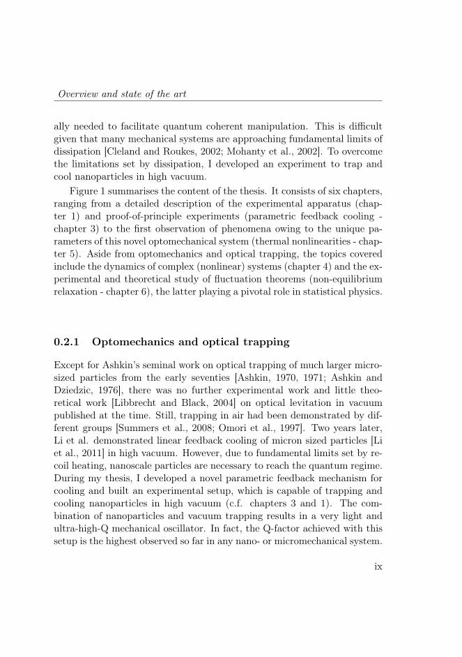
Figure 1.4: Optical detection of the particle position. The total lightthat propagates towards the detector consists of the transmitted beam (red)and the scattered light (black). The red arrow indicated the direction ofbeam propagation. (a) To detect lateral displacements, the transmitted lightis split and the two resulting beams are detected in differential mode. Be-cause scattered light from the particle travels distances that are different forthe two detectors, the accumulated phase at each detector is different. Atthe detector the scattered light interferes with the unscattered light, whichserves as reference beam, making the detector signal sensitive to changes inthe phase. Since the phase depends on the position of the particle, the de-tector signal is proportional to the motion of the particle. (b) To detect themotion along the optical axis, the entire transmitted beam is detected. Thetotal intensity at the detector is the sum of scattered light and transmittedbeam. The former has a phase that depends on the particle’s position on theoptical axis. Due to interference of the two, the detector signal is sensitiveto the phase and therefore to the position of the particle. Note that this de-tection is not dependent on lateral displacement as the phase due to lateraldisplacements at one half of the detector cancels with the phase at the otherhalf of the detector.
harmonics is given by Bessel functions Jk and depends on the particle am-plitude q0. For small amplitudes only the first terms contribute significantly.
10

Optical setup
The homodyne signal (1.12) is the real part of (1.13). If ϕref = −π/2we get an additional factor i in (1.13). Hence, the main contribution to thesignal is ∝ J1(q0) cosΩ0t. In contrast, if the relative phase is ϕref = 0, themain contribution is ∝ J2(q0) cos 2Ω0t. Therefore, to get a detector signalthat is a linear function of the particle displacement, the relative phase ϕref
has to be fixed to −π/2.Note that, if the phase is fixed to 0, the detector signal is ∝ cos 2Ω0t.This is the signal required for feedback cooling. Hence, if we can interferethe scattered light with a reference that is in-phase, we can circumvent anelectronic frequency doubler (c.f. section 1.2).
Forward detection
In forward detection the reference beam is the non-scattered transmittedbeam. In the paraxial approximation, the far-field of the transmitted Gaus-sian is a spherical wave
Eref(r) = Eref exp i(kR− π/2)nx, (1.14)
with amplitude Eref ≈ E0z0/R and phase −π/2, known as the Gouy phaseshift. The spherical wave is collected by a lens and propagates as a planewave to the detector. Since the transmitted beam and the forward scat-tered light follow the same optical path, they acquire the same propagationphase. Hence, the phase difference at the detector is given by the Gouyphase shift ϕref = −π/2 and the detector signal is linear with respect toparticle position.
Note that in forward scattering the scattered light and the reference areboth proportional to the incident laser Edp ∝ Eref ∝ E0. As a consequence,if the trapping laser is used for detection, the intensity of the reference (thelast term of (1.9)) is time dependent because of the feedback signal. If thedetectors are not 100% balanced, they will pickup the intensity modulationand feed it back into the feedback circuit. This results in undesired back-action. To resolve this problem, we chose to split off a part of the incidentbeam before it is modulated as explained in section 1.1.1. But it also means
11

Experimental Setup
that we do not use the scattered light from the trapping beam, which ismuch more intense than the scattered light from the auxiliary beam. Hence,the sensitivity is not as high as it potentially could be if we could use thescattered light from the trapping beam.
Backward detection
In backward detection we use the same lens for collection as for focusing ofthe light. The collected light is interfered with an independent reference.This gives us the freedom to choose the strength of the reference field freelyand to optimise it to get the best signal-to-noise ratio (SNR). The light scat-tered back into the objective is of the same form as the forward scatteredlight of equation (1.6) because the dipole radiation pattern is symmetric.Hence, the detector signal is given by (1.12). However, since the referencebeam and backscattered light do not follow the same optical path, the rel-ative phase of reference and backscattered light ϕref is not fixed anymore.It depends on the relative path difference and is therefore subject to anynoise source that alters the optical path length, for example air currentsand mechanical drift of the optical elements.
1.1.4 Heterodyne measurement
Measuring in back-reflection not only allows us to choose the intensity ofthe reference field but also it’s frequency. If the optical frequency of thereference differs from that of the scattered light, it is called a heterodynemeasurement. The detector signal is then given by
2EdpEref cos (ϕdp(r, rdp) + ϕref +∆ωt) , (1.15)
where ∆ω is the difference in optical frequency. For ∆ω = 0 (1.15) reducesto (1.12). The spectrum of the detector signal is now shifted to ∆ω withsidebands at ∆ω ± Ω0. In order to benefit from a lower noise floor athigh frequencies, one would typically choose ∆ω ≫ Ω0. With a lock-inamplifier that locks to the modulation frequency ∆ω one can measure both
12
Optical setup
left sideband right sideband
! !m ! + !m!
02EdpEref
EdpEref
!m
!
0
2EdpEref
EdpEref
20
! + 20! 20
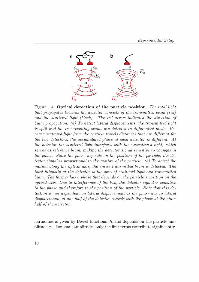
Figure 1.5: Spectrum of detector signal. In the heterodyne measurementthe spectrum is shifted to ∆ω. The particle oscillation shows up as side-peaksaround ∆ω at harmonics of the particle oscillation frequency Ω0 (black). Amodulation of the intensity at ωm reproduces the main structure at side-frequencies ∆ω ± ωm (red and blue). The feedback modulates the intensityof the laser at ωm = 2Ω0. As a consequence, the sidebands overlap with themain peaks (see inset). However, since the phase of the intensity modulationis fixed to the particle oscillation, this results only in a constant phase offset,which is eliminated by the lock-in.
quadratures of (1.13) and extract, therefore, the phase ϕdp + ϕref . To getrid of the low frequency spurious phase ϕref , the lock-in amplifier outputhas to be high-pass filtered.
Note that the bandwidth B of the lock-in has to be large enough sothat the signal from the particle passes, that is B ≫ Ω0. This requirementis quite demanding, given that typical particle frequencies are of the orderof 100kHz-1Mhz. For an ideal harmonic oscillator, the damping Γ0 deter-mines the timescale on which the energy and the phase change. Thus, theminimum required bandwidth for an harmonic oscillator is of the order Γ0,which is a factor Q ∼ 108 less than Ω0. However, since for efficient feed-back cooling the phase stability is paramount, a higher bandwidth might be
13

Experimental Setup
necessary (still ≪ Ω0) if there are additional sources of phase noise such asfrequency fluctuations due to nonlinear amplitude to frequency conversion(c.f. chapter 5). A detection scheme with a bandwidth B ∼ Γ0 ≪ Ω0 couldbe realized for instance with a phase locked loop (PLL), where the particleitself acts as the frequency determining element.
Detection with the trapping laser
As mentioned before, we would get a much stronger signal if we could usethe scattered light from the trapping laser. Let’s assume the trapping laseris modulated at frequency ωm and modulation depth ϵ. The scattered fieldis ∼ Edp(1+ ϵ cosωmt). Hence, the spectrum of the detector signal exhibitssidebands at the modulation frequency ωm and amplitude ∝ ϵEdpEref asshown in figure 1.5. However, for small modulation ϵ the amplitude of themain signal ∝ EdpEref is much stronger than the sidebands.
If the trapping laser is used for detection, the intensity modulation is atωm = 2Ω0. Therefore, the sidebands from the intensity modulation overlapwith the main signal. But, since the feedback fixes the phase of the sidebandto the main signal, this results only in a constant phase, which is eliminatedby lock-in detection.
1.2 Feedback Electronics
For feedback cooling of the particle’s center of mass (CoM) motion we usean analog electronic feedback signal. The signal is used to modulate theintensity of the trapping laser with an EOM.Figure 1.6 shows the electronic feedback system. It consists of five units:a bandpass filter, a variable amplifier, a phase shifter, a frequency doublerand an adder. The first four units are replicas of the same electronic circuit,each one optimised for one specific frequency. The frequencies correspondto the three oscillation frequencies of the vacuum trapped particle. Table1.1 shows the feedback parameters for the three axes. The fifth unit adds
14

Feedback Electronics
in
bandpass filtervariable gainfrequency doublerand phase shifter
sum
outin
out
gain
monitor
in
out
phase
monitorgain
in
out
TTL in
attenuate
aux. in
Figure 1.6: The Feedback Electronics consist of of five modules. Abandpass filter (red), variable gain (white), frequency doubler (green), phaseshifter (same module, also green) and adder.
the three signals together and sends the resulting signal to the EOM.
The following sections describe the functionality of each of the individualmodules.
1.2.1 Bandpass filter
The signal of interest is at the natural frequency of the particle. However,there are low frequency components because of mechanical drift and beampointing instability. Furthermore, the auxiliary beam and the part of thetrapping beam that leaks through the polarising beam splitter interfere atthe detector and create a high frequency beating at the AOM frequency. Theunwanted frequency components can have a detrimental effect on the outputsignal because each electronic circuit has a maximum range of input voltagesbefore it saturates. Since the peak values at the unwanted frequencies exceed
15

Experimental Setup
axes
parameters x y z
f0 [kHz] 125 140 38
ϕ(f0) [] 12 149 159
BW [kHz] 15-250 15-250 15-150
Table 1.1: Parameters of electronic feedback. Each stage of the elec-tronic circuit is optimised for one specific particle frequency. f0 is the fre-quency of the frequency doubler. ϕ is the phase difference between a sinu-soidal input at the bandpass filter and the frequency doubled output at theadder. BW is the bandwidth of the bandpass filter. All subsequent moduleshave a higher cut-off frequency.
the peak values at the signal frequency, it is necessary to filter them at anearly stage of the feedback circuit. Therefore, each of the three signals fromthe balanced photodetectors is filtered by a second order bandpass filter1.Because every electronic circuit adds noise, the detector signals are alsoamplified at this first stage of the feedback by a factor ×20. This mitigatesthe noise contribution from subsequent stages of the feedback and therebygives a better SNR at the output of the feedback circuit.
1.2.2 Variable gain amplifier
To get the optimum SNR at the end of the feedback circuit, it is importantamplify the signal enough to mitigate subsequent additive noise, but nottoo much to saturate any of the circuits. Therefore, to tune to the optimumgain, the bandpass is followed by a variable gain amplifier2 from ×1 to ×10that is controlled with a potentiometer.
1multiple feedback, AD8172OPA1611AID
16
Feedback Electronics
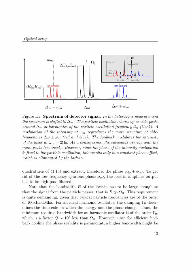
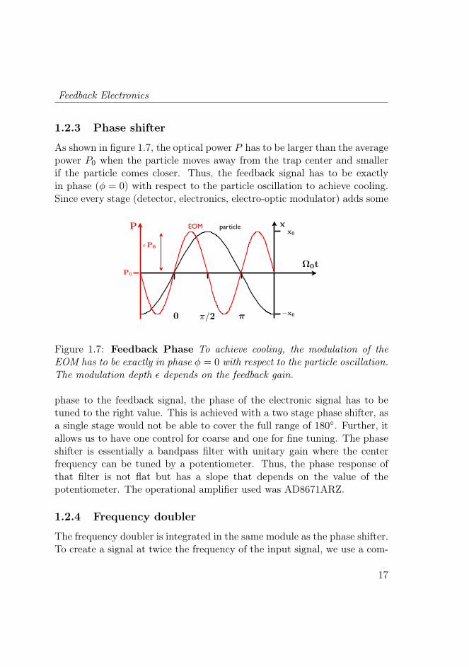
1.2.3 Phase shifter
As shown in figure 1.7, the optical power P has to be larger than the averagepower P0 when the particle moves away from the trap center and smallerif the particle comes closer. Thus, the feedback signal has to be exactlyin phase (ϕ = 0) with respect to the particle oscillation to achieve cooling.Since every stage (detector, electronics, electro-optic modulator) adds some
EOM particle
/2 0
0t
xP
P0
x0
x0
P0
Figure 1.7: Feedback Phase To achieve cooling, the modulation of theEOM has to be exactly in phase ϕ = 0 with respect to the particle oscillation.The modulation depth ϵ depends on the feedback gain.
phase to the feedback signal, the phase of the electronic signal has to betuned to the right value. This is achieved with a two stage phase shifter, asa single stage would not be able to cover the full range of 180. Further, itallows us to have one control for coarse and one for fine tuning. The phaseshifter is essentially a bandpass filter with unitary gain where the centerfrequency can be tuned by a potentiometer. Thus, the phase response ofthat filter is not flat but has a slope that depends on the value of thepotentiometer. The operational amplifier used was AD8671ARZ.
1.2.4 Frequency doubler
The frequency doubler is integrated in the same module as the phase shifter.To create a signal at twice the frequency of the input signal, we use a com-
17

Experimental Setup
mercial multiplier circuit1. For an input signal Xin = X0 sinωt, the resultingsignal is Xout = X2
0ω cos 2ωt /(10V ) . Hence, the device is optimised for asingle frequency where an input amplitude of 10V gives and output also at10V .
1.2.5 Adder
To cool the particle in all three spatial dimensions, we sum the three pro-cessed signals together2 and send it to the EOM. The summed signal canbe switched off through a TTL signal by an analog switch3. This featureis used in the relaxation experiment of chapter 6. Additionally, there is anextra input that is added to the output. This is needed in chapter 4 to driveand cool the particle simultaneously.
1.3 Particle Loading
Loading a particle into the optical trap is a critical first step. In a liquidparticles can be captured easily. By moving the chamber that contains theliquid with a translation stage, the suspended particles are dragged alongand can thereby be brought into close vicinity of the trapping laser. Incontrast, particles in a gas will quickly fall down due to gravity.
The size of the optical trap is of the order of the focal volume ∼ λ3.Therefore, a particle that passes the focus at a distance larger than ∼ λ willnot be captured. Furthermore, if a particle enters the volume at high speed,the low damping in vacuum will not slow the particle down sufficiently. Themaximum allowed speed is vmax ∼ λΓ0, where Γ0 is the damping constant.In water Γ0 is given by Stokes formula Γ0 = 6πηa/m, where a and m arethe radius and mass of the particle and η the viscosity of the surroundingmedium. In water η(water) = 890µPa s. Hence, the maximum velocity for a
1AD734/AD2AD8173NC7SB3157P6X
18

Particle Loading
a = 75nm SiO2 particle is v(water)max = 344m/s. In air the viscosity is about
two orders of magnitude smaller η(air) = 18µPa s. Hence, the particle ve-locity should not exceed v
(air)max = 7m/s. The challenge lies, therefore, in
finding a technique by which a slow single nano-particle is brought into thefocal volume.
One strategy to bring a nano-particle into the focal volume in a con-trolled manner, is to place it onto a substrate, which can be manipulatedwith high accuracy by piezo-electric actuators. However, a particle on asubstrate remains there due to dipole-dipole interactions known as van derWaals (VdW)-forces. The VdW-force in the "DMT limit" of the Derjaguin-Muller-Toporov theory is given by [Israelachvili]
FVdW = 4πaγ, (1.16)
where a is the radius of the particle and γ is the effective surface energy.Measurements on silica spheres on glass give FVdW = 176 nN for a = 1µm[Heim et al., 1999]. For comparison, the gravitational force for a particleof this size is only ∼ 0.1 pN and therefore much too weak to remove theparticle.
Sections 1.3.1 and 1.3.2 discuss two approaches that aim at removingnano-particles form a surface, pulsed optical forces and inertial forces. Bothare found to be insufficient to overcome the forces that keep the particle onthe surface. Section 1.3.3 gives a detailed description of the successfull neb-uliser approach. The nebuliser creates an aerosol of nano-particles, whichare then trapped by the optical tweezer.
1.3.1 Pulsed optical forces
The maximum force from a typical continuous wave optical tweezer (∼ 1 nN)is two to three orders of magnitude weaker than the VdW-force. The opticalforce depends linearly on the optical power. A pulsed laser can have a peakpower much higher than a continuous wave laser (CW-laser). Therefore, itwas suggested in [Ambardekar and Li, 2005] that a pulsed laser should have
19

Experimental Setup
a maximum force strong enough to overcome the VdW-force. Generally, theshorter the pulse the higher the maximum peak power that can be achieved.However, the force has to bring the particle at least to a critical distancedcrit, so that the VdW-force doesn’t pull the particle back to the surfaceonce the pulse ends. Hence, assuming a constant acceleration throughoutthe pulse, the minimum pulse duration is τpulse = (2dcritm/Fpulse)
1/2.
We used a Nd:YAG laser with a pulse duration of ∼ 50ns and a totalenergy per pulse of ∼ 0.1mJ at the sample. Thus, the maximum power(∼ 2kW) is three orders of magnitude higher than what can be achievedwith a CW-laser. Indeed, we managed to remove several silica particlesfrom a glass coverslip that was coated with a thin film (∼ 20nm) of eitheraluminium or gold. However, the laser pulse often left a crater behind.This suggests that actually thermal forces due to light absorption in themetal film removed the particle. Some of the released particles disappearedfrom the field of view and some landed a few µm away from their initialposition. Still, we did not manage to trap any of the released particles witha second superimposed CW laser and decided to pursue other approaches.In retrospective, this is not too surprising. To trap a particle, we do notonly have to remove it, but also shoot it close to the optical trap with nottoo much kinetic energy. From the above discussion about the trap volumeand the required particle speed, it is clear that the probability of catchinga particle is rather small.
1.3.2 Piezo approach
Already Ashkin in his pioneering experiments [Ashkin, 1971] used a piezo-electric transducer to overcome the VdW-forces. This method was also usedto trap and cool microspheres to mK temperatures [Li et al., 2011] and is de-scribed in detail in reference [Li, 2011]. For a sinusoidally driven piezo withoscillation amplitude qp and frequency ωp, the force due to the particle’sinertia is
Fpiezo = mω2pqp, (1.17)
20

Particle Loading
where m is the mass of the particle. Consequently, the acceleration neededto release the particle is
ap = ω2pqp = 4πaγ/m ∝ a−2. (1.18)
Hence, for a given maximum acceleration the piezo can provide, there isa minimum particle size that can be shaken off. For typical values thisis amin ∼ 1µm. Therefore, this approach can not be used to shake nano-particles off a substrate.
1.3.3 Nebuliser
From the preceding sections it is clear that optical, gravitational and inertialforces are too weak to remove a particle from a substrate. In this section wedescribe a surprisingly simple but functional approach to load the trap withnanoparticles [Summers et al., 2008]. We use a commercial nebuliser1 anda highly diluted solution of silica beads2 of 147 nm diameter. The dilutedsolution is obtained from mixing 10µl initial solution (50 mg/ml) with ∼1ml of ethanol. The nebuliser consists essentially of a mesh on top of a piezoelement. A little bit of liquid is brought into the space between the piezo andthe mesh. The motion of the piezo pushes the liquid through the mesh. Themesh breaks the liquid into little droplets of diameter smaller than 2µm.Under standard humidity conditions, the droplets quickly evaporate andonly the solid component is left behind. The concentration of the solutionis such that on average there is one or no particles in a single droplet. Asshown in figure 1.8, we use a nozzle in an upside down configuration tofunnel the falling particles close to the laser focus. Through a viewport onthe side of the vacuum chamber we observe the falling particles with a CCDcamera3 and wait until one is trapped. Then we remove the nozzle, closethe chamber and pump down. Note that because the light scattered by theparticle has a dipole radiation pattern the polarisation of the laser beam
1Omron NE-U22-W2Microparticles SIO2-R-B11813Hamamatsu C8484-05G01
21

Experimental Setup
a
b
c
Figure 1.8: Particle loading. The particle is loaded by spraying a solutionof nano-particles through a nozzle which is placed above the focus. (a) Po-sitioning of the nozzle in the vacuum chamber. (b) Trapped particle imagedwith a CCD camera from the side. (c) Nozzle to funnel the falling particlestowards the focus of the trapping laser.
should be orthogonal to the direction of observation to see the particle withthe camera.
1.4 Vacuum system
Figure 1.9 shows the vacuum system. Close to the main chamber there aretwo gauges to measure the pressure as close to the particle as possible.
22

Vacuum system
One is a convection gauge1 which can be read with the computer and thatcovers the range 1.3×10³−10−4 mBar. The other one is a combined Piraniand cold cathode gauge2 which can be read off at the display of the pumpstation and that covers 102 − 5× 10⁻⁹ mBar.The chamber is evacuated in a first stage with a membrane pump3 and laterwith a turbo-molecular pump4. Both are integrated in a pump station5.Between the chamber and the pumps is an all-metal valve6 that can beclosed to disconnect the pump from the chamber. The valve is also used toevacuate the chamber adiabatically from ∼ 1mBar down to ∼ 10−3mBar,which is a regime of high particle losses in the absence of feedback cooling.In that case, the valve is closed, while the pump is still running. As aresult, a pressure difference builds up between the chamber and the pump.When the pump is at a lower pressure than the main chamber, the rate atwhich the pressure in the main chamber decreases can be controlled withthe valve. The minimum pressure we can achieve with the pump station is∼ 10−6mBar.
1.4.1 Towards ultra-high vacuum
To go to lower pressure, we have an ion pump installed. The ion pumpcan achieve ultra high vacuum below 10−10mBar. However, to reach suchextreme values, the chamber has to be kept clean with high diligence andbaked to temperatures of ∼ 300. This is currently not compatible with ourloading mechanism because the chamber has to be opened to load a particle.Thus, even with the ion pump we can not improve the vacuum. To achieve,ultrahigh vacuum we are implementing a load-lock. The load-lock consistsof two chambers and a translation stage. In the loading chamber, a particleis trapped and brought to high vacuum (10−6mBar). The transfer system
1CVM-201 "Super bee", InstruTec2PKR 251, Pfeiffer vacuum3MVP 015-2, Pfeiffer vacuum4TMH 071, Pfeiffer vacuum5TSH 071E, Pfeiffer vacuum6Hositrad technology
23

Experimental Setup
valve
ion pump
to pump station
vacuum chamber
gauge 1.3 103 104 mBar
gauge 102 106 mBar
Figure 1.9: The Vacuum System consists of a vacuum chamber, with twogauges, that cover pressure ranges from 1.3×10³−10−3 mBar and 103−10−6
mBar, respectively. The chamber is connected to a pump station and an ionpump.
translates the trapped particle under high vacuum into the main chamber.After the particle has been loaded into the main chamber, the main chamberis disconnected from the rest of the vacuum system and pumped down toultra high vacuum. Hence, the main chamber will always be under a highvacuum and it is possible to pump down to ultra high vacuum with the ionpump.
1.5 Conclusion
In this chapter we presented the technical details of an experimental setupwhich allows for trapping, cooling and parametrically driving of nanopar-ticles in high vacuum. This is a major step towards employing trappednano-particles for ultra-sensitive detection and ground state cooling. How-
24

Conclusion
ever, to exploit the full capabilities of the system, improved detection andhigher vacuum are required.An improved detection can be achieved by several means. One way is todetect the scattered light of the trapping beam by heterodyne interferome-try as discussed in section 1.1.4. An alternative way is to place the particleinside a high finesse cavity. The cavity modes are very sensitive to changesin optical path length. The optical path length depends on the particleposition inside the cavity. Therefore, light which is transmitted though orreflected from the cavity becomes highly correlated with the particle mo-tion. Since the light inside the cavity also exerts a force on the particle,a cavity can not only be used as a detector but also to cool the particlemotion [Chang et al., 2010; Romero-Isart et al., 2010; Kiesel et al., 2013].Better vacuum requires that the vacuum chamber is always kept under highvacuum. This is incompatible with our current loading technique, which re-quires operation at ambient pressure. To reconcile the two requirements weare currently developing a load-lock.
25

Experimental Setup
26
CHAPTER 2
Theory of Optical Tweezers
To understand the working principle of optical tweezers, we have to under-stand the forces exerted by electromagnetic fields. To this end we discuss asimple analytical model based on the Rayleigh approximation and a Gaus-sian description of the trapping laser.
2.1 Introduction
The optical force has two components, the gradient force and the scatter-ing force. The former points toward the region of highest intensity and,therefore, allows for stable trapping in the focus of a laser beam. The latterpoints in the direction of beam propagation and therefore pushes the parti-cle out of the trap. Thus, to achieve a stable trap, the scattering force hasto be eliminated or the gradient force has to overcome the scattering force.The scattering force can be cancelled by two counter propagating beams.However, the two beams have to be well aligned and symmetric in shapeand power [Ashkin, 1970]. Instead of a second independent beam one canalso use the back-reflection from a mirror to form a standing wave [Zemáneket al., 1998, 1999]. The scattering force of a single beam can also be compen-
27
Theory of Optical Tweezers
sated by any other force, for example as in Ashkin’s pioneering experiments[Ashkin, 1971], by gravity. However, alignment inaccuracies tend to makeall these configurations unstable. If the scattering force is not cancelled, thegradient force has to dominate over the scattering force to achieve stabletrapping. This configuration requires a tightly focused laser beam [Ashkinet al., 1986] and is known as optical tweezer. The conditions under whicha sub-wavelength particle can be trapped with an optical laser tweezer isdiscussed in this chapter.
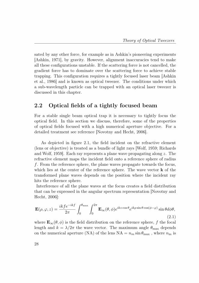
2.2 Optical fields of a tightly focused beam
For a stable single beam optical trap it is necessary to tightly focus theoptical field. In this section we discuss, therefore, some of the propertiesof optical fields focused with a high numerical aperture objective. For adetailed treatment see reference [Novotny and Hecht, 2006].
As depicted in figure 2.1, the field incident on the refractive element(lens or objective) is treated as a bundle of light rays [Wolf, 1959; Richardsand Wolf, 1959]. Each ray represents a plane wave propagating along z. Therefractive element maps the incident field onto a reference sphere of radiusf . From the reference sphere, the plane waves propagate towards the focus,which lies at the center of the reference sphere. The wave vector k of thetransformed plane waves depends on the position where the incident rayhits the reference sphere.Interference of all the plane waves at the focus creates a field distribution
that can be expressed in the angular spectrum representation [Novotny andHecht, 2006]:
E(ρ, φ, z) =ikfe−ikf
2π
∫ θmax
0
∫ 2π
0E∞(θ, ϕ)eikz cos θeikρ sin θ cos(ϕ−φ) sin θdϕθ,
(2.1)where E∞(θ, ϕ) is the field distribution on the reference sphere, f the focallength and k = λ/2π the wave vector. The maximum angle θmax dependson the numerical aperture (NA) of the lens NA = nm sin θmax , where nm is
28

Optical fields of a tightly focused beam
incoming ray
refracted ray
reference sphere
focus
f
z
Figure 2.1: Focusing of the optical field. An incoming ray is refracted ata lens with focal length f . The wave vector of the refracted ray is determinedby the position where the incident ray hits a reference sphere with radius f
the refractive index of the surrounding medium. The above integral is alsoknown as the Debye integral.
For lenses with high NA, wave vectors with high angles are involved inthe construction of the field at the focus. As a consequence, new polarisa-tions are generated and the field distribution is slightly elongated along thedirection of polarisation nx of the incident field [Novotny and Hecht, 2006].Even for a high NA lens the aperture of the lens is finite. Hence, field com-ponents with very high spatial frequencies are cut-off. Therefore, the field isdefracted and the spatial profile of the focus has oscillatory side-lobes (c.f.Fig. 2.2).
In the limit of weak focusing and neglecting the finite size of the aperture,the above integral (2.1) can be solved analytically. For an incident Gaussianbeam we obtain the familiar paraxial expression [Novotny and Hecht, 2006]
29

Theory of Optical Tweezers
E(ρ, z) = E0
[1 + (z/z0)
2]−1/2
e− ρ2
w2(z)+iϕ(z,ρ)
nx, (2.2)
where nx is the direction of polarisation, w0 is the beam waist and E0
the electrical field at the focus. For clarity, we have defined the followingquantities
w(z) = w0
√1 + z2/z20 beam radius (2.3)
ϕ(z, ρ) = kz − η(z) + kρ2 /2R(z) phase (2.4)
R(z) = z(1 + z20/z
2)
wavefront radius (2.5)η(z) = arctan (z/z0) phase correction. (2.6)
The gradual phase shift η(z) as the beam propagates through the focus isknown as the Gouy phase shift.
Despite the strong approximations that lead to equation (2.2), the exactintensity distribution even for a tightly focused beam is very similar tothat of a Gaussian beam. However, the Rayleigh range and focal widthare no longer given by the simple paraxial expressions z0 = w0
2/2 andw0 = 2/kθmax, respectively. Instead, they are free parameters that areobtained by a fit to the exact solution (2.1) (see Table 2.1). Thus, theanalytical expression of the focal field is given by a slightly modified equation(2.2):
E(ρ, z) = E0
[1 + (z/z0)
2]−1/2
e−(
x2
w2x(z)
+ y2
w2y(z)
)+iϕ(z,ρ)
nx, (2.7)
where the separate beam waists wx and wy account for the asymmetry of thefocus along x and y, respectively. Note that in this model, the asymmetryof the focus is only accounted for in the amplitude but not in the phase.Figure 2.2 shows the field distribution in the focal planes. The first row
shows the intensity distribution calculated with the Debye integral (2.1)in the x-z and x-y plane, respectively. For comparison, the bottom row
30

Optical fields of a tightly focused beam
!1.0 !0.5 0.0 0.5 1.0!1.0
!0.5
0.0
0.5
1.0
x !"m"
y!"m"
Intensity x!y plane
!1.0 !0.5 0.0 0.5 1.0!1.0
!0.5
0.0
0.5
1.0
x !"m"
z!"m"
Intensity x!z plane
!1.0!0.5 0.0 0.5 1.0!1.0
!0.5
0.0
0.5
1.0
x !"m"
y!"m"
Intensity x!y plane #Gauss$
!1.0!0.5 0.0 0.5 1.0!1.0
!0.5
0.0
0.5
1.0
x !"m"
z!"m"
Intensity x!z plane #Gauss$
!1.0 !0.5 0.0 0.5 1.00.0
0.2
0.4
0.6
0.8
1.0
Position !"m"
E2!V2 #"
m2 "
Intensity distribution
b
zx
y
a
129 [V2/µm2]
0
E2
c
d e
Figure 2.2: Intensity distribution of tightly focused optical fields.(a) The intensity distribution computed with the Debye integral (2.1) isshown as black lines for the three mayor axes. The coloured lines are fits tothe Gaussian model (2.2). The exact solution exhibits side lobes as a conse-quence of diffraction. Both models take the asymmetry of the focal spot intoaccount. (b,c) The intensity distribution computed with the Debye integralin the x-y plane and y-z plane, respectively. (d,e) The same fields computedwith the Gaussian model. In the calculation we assumed focusing in air witha NA= 0.8 objective, a filling factor (ratio between beam waist of incidentbeam and lens aperture) of 2 and wavelength λ = 1064nm. For a detaileddescription of how to apply equation (2.1) see reference [Novotny and Hecht,2006].
shows the same distributions obtained with the Gaussian model (2.7). TheGaussian model does not include diffraction and therefore doesn’t have side-lobes. However, up to λ/2 away from the center, the Gaussian model fitsthe exact solution well.
31

Theory of Optical Tweezers
Beam parameter Paraxial approx.
wx 687 nm 423 nm
wy 542 nm 423 nm
z0 1362 nm 529 nm
Table 2.1: Beam parameters for the computation of the field at the focus.The parameters are obtained from a fit to the exact numerical solution.For comparison, the right column shows the parameters obtained with theparaxial approximation.
2.3 Forces in the Gaussian approximation
From the optical field we will now calculate the optical forces. Generally,these forces are summarised by the Maxwell stress tensor [Novotny andHecht, 2006]
F =
∫∂V
↔T · n(r)da, (2.8)
which is a derivation of the conservation laws of electromagnetic energyand momentum. Remarkably, the Maxwell stress tensor and therefore theoptical forces are entirely determined by the electromagnetic fields at thesurface of the object. That is, all the information is contained in the elec-tromagnetic fields and no material properties enter in (2.8). To calculate↔T, the self-consistent fields are needed. Generally, this is a non-trivial taskbecause the presence of the object changes the incident field. Hence, if thebody deforms, the boundary conditions in (2.8) change. Consequently, thematerial properties enter the problem through the changed boundary condi-tions. However, in the following we will assume that the body is rigid. Evenunder the assumption that the body is rigid, evaluation of (2.8) is generallycomputationally expensive. Furthermore, equation (2.8) has to be evalu-ated for each particle position. Thus, for practical purposes it is desirableto have a closed-form expression or a numerically efficient approximation of
32

Forces in the Gaussian approximation
the integral (2.8) [Rohrbach and Stelzer, 2001].
For a spherical object of arbitrary size, Mie-theory provides an exactanalytical solution [Van De Hulst, 1981] in form of an infinite series ofmultipoles [Neto and Nussenzveig, 2000]. The bigger the sphere, the moremultipoles have to be taken into account. Forces on large dielectric spheres(a ≫ λ) can be calculated by ray-optics [Ashkin, 1992]. The ray-opticscalculation uses Snells law and the Fresnel formulas. If the particle is smallcompared to the wavelength of the incident radiation (Rayleigh limit a ≪λ), the only significant contribution comes from the electric dipole term.
~nx
da(~r)
@V
Figure 2.3: Dielectric body The optical forces are determined by the totalelectromagnetic fields at the surface ∂V of the object.
2.3.1 Derivation of optical forces
It is instructive to write the optical force as a sum of two terms, the gradientforce Fgrad(r) and the scattering force Fscatt(r) [Novotny and Hecht, 2006;Rohrbach and Stelzer, 2001]:
F(r) = Fgrad(r) + Fscatt(r). (2.9)
Under the assumption that we can represent the complex amplitude of theelectric field in terms of a real amplitude E0 and phase ϕ, the forces aregiven by
Fgrad(r) = α′/4 ∇I0(r) (2.10)
33

Theory of Optical Tweezers
andFscatt(r) = α′′/2 I0(r)∇ϕ(r), (2.11)
where I0(r) = E20(r) is the field intensity and α′ and α′′ are the real and
imaginary part of the polarisability, respectively. This approximation isvalid if the phase varies spatially much stronger than the amplitude. Thisis the case for weakly focused fields and for the fields given by Eq. (2.7).
For a spherical particle with volume V = 4/3πa3 and dielectric con-stant εp embedded in a medium with dielectric constant εm, the polaris-ability is given by Clausius-Mossotti relation (also Lorentz-Lorenz formula)[Rohrbach and Stelzer, 2001; Novotny and Hecht, 2006]:
α = 3V ϵ0(ϵp − ϵm)/(ϵp + 2ϵm). (2.12)
Generally, α is a tensor of rank two. However, for a spherical particle αbecomes a scalar.
The gradient force is proportional to the dispersive (real) part α′, whereasthe scattering force is proportional to the dissipative (imaginary) part α′′
of the complex polarisability α. The phase ϕ(r) can be written in termsof the local k vector ϕ(r) = k · r. Hence, the scattering force results frommomentum transfer from the radiation field to the particle. Momentumcan be transferred either by absorption or scattering of a photon. Photonscattering by the particle changes the electric field. This, in turn, modifiesthe optical force acting on the particle. This backaction effect also knownas radiation reaction is accounted for by an effective polarisability [Novotnyand Hecht, 2006]
αeff = α
(1− i
k3
6πϵ0α
)−1
. (2.13)
Consequently, even for a lossless particle (Im(ϵp) = 0), the scattering forcedoes not vanish completely!
34

Forces in the Gaussian approximation
From (2.10), (2.11) and (2.7) we calculate the optical forces in the Gaus-sian approximation
Fgrad(r) = −α′effI0(r)
×
x z20/w2x(z
2 + z20)y z20
/w2y(z
2 + z20)
z[(z/z0)
2 +(1− 2x/w2
x − 2y/w2y
)] [z20/2(z2 + z20)
] (2.14)
and
Fscatt(r) =α′′eff
2I0(r)k
×
x /R(z)y /R(z)
1 +(x2 + y2
)z20/z2R(z)2 −
[x2 + y2 + 2z z0
]/2zR(z)
, (2.15)
where I0(r) = E20
[1 + (z/z0)
2]−1
exp(−2[x2/w2
x(z) + y2/w2y(z)
]).
The field intensity at the focus, E20 , is related to the total power of the
Gaussian beam by
P =
∫ ∞
−∞
∫ ∞
−∞⟨S⟩nzdxdy = cϵ0πwxwyE
20 /4 , (2.16)
where c is the speed of light, nz is the direction of beam propagation and⟨S⟩ = ⟨H×E⟩ is the the Poynting vector.
For small displacements |r| ≪ λ, we expand equations (2.14) and (2.15)to get the first order nonlinear terms
Fgrad(r) ≈ −
k(x)trap
[1− 2x2/w2
x − 2y2/w2y − 2z2/z20
]x
k(y)trap
[1− 2x2/w2
x − 2y2/w2y − 2z2/z20
]y
k(z)trap
[1− 4x2/w2
x − 4y2/w2y − 2z2/z20
]z
(2.17)
and
Fscatt(r) ≈α′′eff
α′eff
k(z)trap
k xzk yz
γ0 + γzz2 + γxx
2 + γyy2,
(2.18)
35

Theory of Optical Tweezers
where
γ0 = z0(z0k − 1), (2.19a)γz = (2− z0k)/z0, (2.19b)
γx =[k/2− 2(z0 − k z20)
/w2x
]and (2.19c)
γy =[k/2− 2(z0 − k z20)
/w2y
]. (2.19d)
are constants that depend only on the optical field but not on the propertiesof the particle.
The longitudinal and transversal trap stiffness are given by
k(x)trap = α′
effE20/w
2x, (2.20a)
k(y)trap = α′
effE20/w
2y and (2.20b)
k(z)trap = α′
effE20/2z
20 , (2.20c)
respectively. As expected, the trap stiffness increases with polarisability,laser power and field confinement.
2.3.2 Discussion
Since the scattering force points mainly in the direction of beam propaga-tion, the equilibrium position zeq. is not exactly at the intensity maximumbut is displaced along z. For the Gaussian model we find
zeq. ≈α′′eff
α′eff
γ0. (2.21)
If the scattering force is too strong, the particle is pushed out of theoptical trap. Expanding (2.13) to lowest order αeff ≈ α(1 + ik3[6πϵ0]
−1α),we find that
α′′eff/α
′eff ∝ (ka)3∆ϵ, (2.22)
where ∆ϵ = (ϵp − ϵm)/(ϵp + 2ϵm) ≈ (ϵp − ϵm) /3ϵm is the relative dielec-tric contrast between the particle and the surrounding medium. Hence,
36

Forces in the Gaussian approximation
the relative strength of the scattering force decreases for smaller particlesand lower dielectric contrast. For SiO2, the dielectric contrast is about fivetimes higher in air/vacuum (∆ϵair = 0.15) than in water (∆ϵwater = 0.03).Consequently, it is more difficult to trap big SiO2 particles in air/vacuumthan in water. However, the total optical force F ∝ a3∆ϵ scales with thevolume and the relative dielectric contrast. This makes it easier to trapsmall SiO2 particles in air/vacuum than in water.
The optical force becomes weak for small particles. If it becomes tooweak, any external disturbance destabilises the trap. In vacuum, the maindisturbance comes from collisions with residual air molecules (c.f. section2.4). In consequence, to successfully trap particles with a single laser beamwe have to choose a particle size in the intermediate region where the gra-dient force dominates over the scattering force but the total optical force isstill strong enough to dominate all other forces. The range of stable trap-ping is shown as a white region in Figs. 2.4, 2.6 and 2.7.
Figure 2.4 shows the optical force in the direction of beam propagation atthe focus as a function of particle radius. The force has been calculated withfull Mie theory following reference [Neto and Nussenzveig, 2000]. Due tosymmetry, the gradient force vanishes at the focus and the total force equalsthe scattering force. For small particles, the scattering force is negligible andthe trap center coincides with the focus. The force increases with particlesize. It is always positive and, therefore, pushes the particle away from thefocus. As the particle moves away from the focus, the gradient force (whichis zero at the focus and points toward the focus otherwise) increases untilthe total force is zero and a stable trap is formed ahead of the optical focus.Interference of scattered and incident light gives rise to Mie-resonances andleads to a more complex dependency for bigger particles. For particles largerthan ∼ 120 nm, the scattering force is too strong and the particle is pushedout of the trap, except of a few special resonances. For particle smaller than∼ 35 nm, thermal excitations destabilise the trap.
Figure 2.5 shows the force profile along the optical axes for a a = 75nm
37

Theory of Optical Tweezers
= 1064nm
= 532nm0 200 400 600 800 10000
10
20
30
40
50
60
70
r !nm"
Optical Force at focus !pN"
a [µm]0.20 0.4 0.6 0.8 1
Opt
ical
forc
e at
focu
s [p
N]
0
30
50
70
10
Figure 2.4: Optical force at focus along z axis as a function ofparticle size calculated for λ = 1064nm and λ = 532nm. At the focus,the gradient force vanishes and the total optical force equals the scatteringforce. For small particle size, the force is almost zero and a stable trap isformed near the focus. The force at the focus is always positive and scaleswith the volume for small particles . Therefore, the particle is pushed alongthe optical axes and the equilibrium position is displaced ahead of the focus.Interference of scattered and incident light gives rise to Mie-resonances andleads to a more complex dependency for bigger particles. For particles largerthan a ∼ 120 nm, the scattering force is too strong and the particle is pushedout of the trap, except of a few special resonances. For particle smaller thana ∼ 35 nm, thermal excitations destabilize the trap. The region where stabletrapping is possible is shown in white.
Silica particle calculated with Mie theory [Neto and Nussenzveig, 2000],from the Debye integral (equations (2.1), (2.10) and (2.11)) and with theGaussian model (equations (2.17) and (2.18)). All three models yield sim-ilar results close to the trap center. For larger distances (> 0.5µm), theoptical fields are not accurately described by the Gaussian model (see also2.2) and the simple model fails. However, we are mostly interested in smalldisplacements from the trap center (zeq. ≈ 0.2µm) for which the model stillgives good results. The inset of figure 2.5 shows the optical forces for alarger a = 250 nm particle. For this particle size the dipolar approximation
38

Forces in the Gaussian approximation
breaks down and the values obtained with the dipolar models (Debye andGauss) differ significantly from the exact Mie-solution. The two dipolarmodels predict that there is no stable trapping position anywhere on theoptical axis, whereas Mie theory finds a stable position at ≈ 1.5µm.Figure 2.6 shows the position of the trap center and the trap stiffness as a
!1000 0 1000 2000 3000
!0.15
!0.10
!0.05
0.00
0.05
0.10
0.15
0.20
z !nm"
Optical Force on z axis !pN" 75 nmMie
Gauss
Debye
!1000 0 1500 30000
20
40
z !nm"
Optical Force !pN" 250 nm
zeq.
z [µm]
Opt
ical
For
ce [p
N] 2
50 n
m
-1 1 2 30
0.2
0.1
0
-0.1
-0.15
z [µm]0 1.5 3-1
40
20
0
Opt
ical
For
ce o
n z
axis
[pN
] 75
nm
Figure 2.5: Optical forces along axis for 75nm particle calculated withdifferent models. Around the center of the trap (zeq. ≈ 0.2µm) all modelsgive similar results. At larger distances the Gaussian description of theoptical fields breaks down. Inset: For bigger particles (here a = 250 nm),the dipole approximation for the polarisability fails. The two dipolar modelsdon’t find a stable trap, whereas Mie theory predicts a stable, albeit shallowtrap at ≈ 1.5µm.
function of particle size calculated with all three models. The trap stiffnessis given by the slope of the optical force at the trap center. For particleslarger than ∼ 120nm the center of the trap is already more than half awavelength away from the focus and trapping with a single beam is verydifficult. A stable trapping position does not exist because the scatteringforce is always stronger than the gradient force. Mie theory still finds afew exceptional particle sizes where trapping of larger particles is possible.
39

Theory of Optical Tweezers
When the particle size is commensurate with the optical wavelength, theparticle acts as a resonator. As a consequence the scattered field and there-fore the optical forces exhibit resonances (see also Fig. 2.4), which can resultin a stable optical trap even for bigger particles (But a stable trap does notexist for all optical resonances!). However, the range of particle sizes forwhich resonant trapping is possible is very narrow. This makes trapping ofparticles larger than ∼ 120 nm impractical for the experimental parametersconsidered here.
0 50 100 1500
200
400
600
800
1000
1200
1400
r !nm"
trappingposition!nm"
0 50 100 1500.0
0.5
1.0
1.5
r !nm"
trapstiffness!pN#
!m" Mie
Gauss
Debye
a bMie
Gauss
Debye
trap
ping
pos
ition
[µm
]
0
0.4
1.2
0.8
trap
stif
fnes
s [p
N/µ
m]
0
0.5
1
1.5
a [nm]0 50 100 150
a [nm]0 50 100 150
Figure 2.6: Trap position and trap stiffness as a function of particleradius a. We compare the three models discussed in the text. (a) Trapposition along z. The black dashed line marks where the equilibrium positionzeq. is half a wavelength ahead of the focus. For larger displacements of zeq.,we assume that the trap is unstable. The white space marks the particlesizes for which stable trapping is possible. (b) Trap stiffness along z axis.The two dipolar models, Gauss and Debye, don’t find a solution for particleslarger than a ≈ 100 nm and a ≈ 160 nm, respectively. The exact Mie theoryfinds a solution up to a ≈ 300 nm. For larger particles, a stable trap onlyexists when very specific resonance conditions are fulfilled (not shown here).
40

Optical potential
2.4 Optical potential
In this section we introduce the concept of an optical potential. From theoptical potential we can estimate a lower bound of particle size for which astable trap can be formed.
Strictly speaking a potential can only be defined for a conservative force.As we have seen in the previous section, the scattering force is not a con-servative force (c.f. Eq. (2.11)). However, for sub-wavelength particles, thenon-conservative scattering force is negligible and we can define a potentialU = −α′/4 I0(r) (c.f. Eq. (2.10)). With (2.16) the depth of the potentialis given by
∆U = α′ /πcϵ0wxwy P . (2.23)
Comparing the depth of the potential to the thermal energy of the envi-ronment we can estimate a lower bound of particle sizes for which a sta-ble trap exists. If the thermal energy is comparable to or larger than thedepth of the potential, a thermally excited particle can escape. The en-ergy of the thermal bath follows a Maxwell-Boltzmann distribution withmean value of kBT0. Since the tail of the distribution extends to highenergies, the potential depth should be at least ≃ 10kBT0 [Ashkin et al.,1986] to make particle escape through thermal excitation unlikely (Thelikelihood of finding the particle with energy 10 kBT0 is less than 0.02%).Assuming that the trap becomes unstable at ≃ 10kBT0, we can measure thepotential depth at optical power P0 by measuring the optical power Plost
when the particle is lost. For our typical experimental conditions we find∆U(P0) = 10 kBT0 P0/Plost ≈ 28kBT0.
2.5 Conclusions
In conclusion, we have derived a simple analytical model of the opticalforces. The model is based on a Gaussian description of the focal fieldand the dipolar approximation for the particle polarisability. Thus, it isvalid for small sub-wavelength particles and small displacements from the
41

Theory of Optical Tweezers
0 10 20 30 40 50 60 700
10
20
30
40
50
60
70
r !nm"
Potentialdepth!k BT
"
a [nm]
Figure 2.7: Potential Depth as a function of particle size for P = 0.1W,NA = 0.8 and λ = 1064 nm. The gray region marks the particle sizes wherethe potential depth is below 10 kBT0. Hence, trapping at the given power willbe difficult for particles with radius of less than ∼ 35 nm.
trap center. These requirements are generally fulfilled for our experimentalconditions. The model allows us to understand the dependence of the trapparameters (trap stiffness and trap position) on the experimental conditions(optical power, field confinement and particle polarisability). For typicalexperimental conditions we find that a stable optical trap exists for particlesin the range a ≈ 35 . . . 120 nm. For smaller particles, thermal excitationshave a high probability to kick the particle out of the trap. Bigger particlesexperience a strong scattering force, which pushes them out of the trap.
Optical forces not only allow us to cool and drive the mechanical os-cillator but they also determine the mechanical properties of the device.This is different from conventional nanomechanical oscillators, where themechanical properties depend on the material properties and the fabrica-tion process. There exist also an intermediate solution, where the intrinsicmechanical properties are enhanced by optical forces [Chang et al., 2012].
42

CHAPTER 3
Parametric Feedback Cooling of aLaser-trapped Nanoparticle
We optically trap a single nanoparticle in high vacuum and cool its threespatial degrees of freedom by means of active parametric feedback. Usinga single laser beam for both trapping and cooling we demonstrate a tem-perature compression ratio of four orders of magnitude. The absence of aclamping mechanism provides robust decoupling from the heat bath and elim-inates the requirement of cryogenic precooling. The small size and mass ofthe nanoparticle yield high resonance frequencies and high quality factorsalong with low recoil heating, which are essential conditions for ground statecooling and for low decoherence. The trapping and cooling scheme presentedhere opens new routes for testing quantum mechanics with mesoscopic ob-jects and for ultrasensitive metrology and sensing.
3.1 Introduction
The interaction between light and matter sets ultimate limits on the accu-racy of optical measurements. Vladimir B. Braginsky predicted that thefinite response time of light in an optical interferometer can lead to me-
43

Parametric Feedback Cooling
chanical instabilities [Braginsky, 1977] and impose limits on the precisionof laser-based gravitational interferometers. Later, it was demonstratedthat this “dynamic back-action mechanism" can be used to reduce the os-cillation amplitude of a mechanical system and to effectively cool it belowthe temperature of the environment [Metzger and Karrai, 2004; Cohadonet al., 1999; Arcizet et al., 2006; Gigan et al., 2006; Schliesser et al., 2006;Usami et al., 2012] and even to its quantum ground state [Chan et al., 2011;Teufel et al., 2011; Verhagen et al., 2012]. In addition to the fascinating pos-sibility of observing the quantum behavior of a mesoscopic system, manyapplications have been proposed for such systems ranging from detectionof exotic forces [Geraci et al., 2010; Romero-Isart et al., 2011b; Manjavacasand García de Abajo, 2010] to the generation of non-classical states of lightand matter [Chang et al., 2010; Romero-Isart et al., 2010].
Most of the mechanical systems studied previously are directly con-nected to their thermal environment, which imposes limits to thermaliza-tion and decoherence. As a consequence, clamped systems require cryo-genic precooling. A laser-trapped particle in ultrahigh vacuum, by contrast,has no physical contact to the environment [Ashkin and Dziedzic, 1976,1977], which makes it a promising system for ground state cooling even atroom temperatures [Chang et al., 2010; Romero-Isart et al., 2010]. Cool-ing of micron-sized particles to milli-Kelvin temperatures has recently beenachieved by applying an active optical feedback inspired by atom cooling ex-periments [Li et al., 2011]. A particle is trapped by two counter-propagatingbeams and cooling is performed with three additional laser beams via ra-diation pressure. However, because light scattering leads to recoil heatingthere is a limit for the lowest attainable temperature. Eliminating recoilheating as the limiting factor for ground state cooling requires considerablysmaller mechanical systems, such as single dielectric nanoparticles [Changet al., 2010; Romero-Isart et al., 2010]. Here we demonstrate for the firsttime optical trapping in high vacuum of a fused silica nanoparticle of radiusa ∼ 70 nm. Additionally, we employ a novel cooling scheme based on theoptical gradient force to cool its motional degrees of freedom from roomtemperature to ∼ 50mK (compression factor of ∼ 104).
44

Description of the experiment
3.2 Description of the experiment
In our experiments we use a laser beam of wavelength λ = 1064 nm (∼100mW), focused by an NA=0.8 lens mounted in a vacuum chamber (de-tails chapter 1). A single nanoparticle is trapped by means of the opticalgradient force, which acts towards the center of the trap for all three transla-tional degrees of the nanoparticle (c.f. Fig. 3.1). For particles much smallerthan the wavelength, the polarisability scales as α ∝ a3 and the gradi-ent force dominates over the scattering force (c.f. chapter 2). Scatteredlight from the particle is measured interferometrically with three separatephotodetectors that render the particle’s motion in the x, y, and z direc-tions (c.f. section 1.1). This phase-sensitive detection scheme makes useof balanced detection and yields a noise floor of ∼ 1.2 pm/
√Hz. Fig. 3.1
shows a photograph of a trapped nanoparticle along with a typical timetrace of the particle’s x coordinate. Trapping times of several days havebeen achieved at pressures below 10−5 mBar, indicating that the particle’sinternal temperature does not affect the center of mass motion [Chang et al.,2010] and that melting of the particle is not a concern.
3.2.1 Particle dynamics
At ambient pressure the particle’s motion is dominated by the viscous force(Stokes force) due to the random impact of gas molecules. However, asshown in Fig. 3.1(b), the inertial force dominates in a vacuum of a fewmillibars as the particle’s motion becomes ballistic [Li et al., 2010].For small oscillation amplitudes, the trapping potential is harmonic and thethree spatial dimensions are decoupled. Each direction can be characterisedby a frequency Ω0, which is defined by the particle mass mand the trapstiffness ktrap as Ω0 =
√ktrap/m. The equation of motion for the particle’s
45

Parametric Feedback Cooling
0 100t (!s)
200
0
100
-100
x (nm
)
a
b
0 100t (!s)
200
0
100
-100
x (nm
)
a
b
ba
Figure 3.1: Trapping of a nanoparticle. (a) light scattered from a trappedsilica nanoparticle (arrow). The object to the right is the outline of theobjective that focuses the trapping laser. (b) Time trace of the particle’s xcoordinate (transverse to the optical axis) at 2mBar pressure.
motion (q = x, y, z) is
q(t) + Γ0 q(t) + Ω20 q(t) =
1
m[Ffluct(t) + Fopt(t)] , (3.1)
where Ffluct is a random Langevin force that satisfies ⟨Ffluct(t)Ffluct(t′)⟩ =
2mΓ0 kBT0 δ(t−t′) according to the fluctuation-dissipation theorem. Fopt(t) =∆ktrap(t) q(t) is a time-varying, non-conservative optical force introduced byparametric feedback. It leads to shifts δΓ and δΩ in the particle’s naturaldamping rate Γ0 and oscillation frequency Ω0, respectively.
3.2.2 Parametric feedback
To control and stabilise the particle’s motion in the optical trap we im-plemented an active feedback loop (c.f. 1.1). All three spatial degrees offreedom are controlled with the same laser used for trapping. To cool theCoM motion of the particle we employ a parametric feedback scheme, simi-lar to parametric amplification of laser fields [Yariv, 1989] and stabilizationof nanomechanical oscillators [Villanueva et al., 2011]. After trapping asingle nanoparticle at ambient temperature and pressure we evacuate the
46

Description of the experiment
vacuum chamber in order to reach the desired vacuum level.
Parametric feedback is activated as soon as we enter the ballistic regime.In a time-domain picture, the feedback loop hinders the particle’s motionby increasing the trap stiffness whenever the particle moves away from thetrap center and reducing it when the particle falls back toward the trap.In the frequency domain, this corresponds to a modulation at twice thetrap frequency with an appropriate phase shift. Our parametric feedbackis fundamentally different from previous active feedback schemes based onradiation pressure [Poggio et al., 2007]. Radiation pressure acts only alongthe direction of beam propagation and therefore requires a separate coolinglaser for every oscillation direction [Li et al., 2011]. In contrast, the gradientforce points towards the center of the trap, thus allowing us to cool all threedirections with a single laser beam.
Fig. 3.2 illustrates our parametric feedback mechanism. To obtain a sig-nal at twice the oscillation frequency we multiply the particle’s position q(t)with it’s time derivative. The resulting signal q(t) q(t) is then phase-shiftedby a controlled amount in order to counteract the particle’s oscillation. Notethat depending on the latency of the feedback loop we can achieve damp-ing or amplification of the particle’s oscillation. In the absence of activefeedback, the particle’s oscillation naturally locks to the modulation phasein such a way as to achieve amplification [Yariv, 1989]. Cooling thereforerequires active feedback to adjust the modulation phase constantly.
In our cooling scheme, frequency doubling and phase shifting is doneindependently for each of the photodetector signals x, y and z. Since thethree directions are spectrally separated (see Fig. 3.3b), there is no cross-coupling between the three signals, that is, modulating one of the signalsdoes not affect the other signals. Therefore, it is possible to sum up all threefeedback signals and use the result to drive a single EOM that modulatesthe power P of the trapping laser. Thus, using a single beam we are ableto effectively cool all spatial degrees of freedom.
47

Parametric Feedback Cooling
x
y
z
2!"#$S(!)
1
23
4
a b
Figure 3.2: Principle of parametric feedback cooling. (a) The center-of-mass motion of a laser-trapped nanoparticle in ultrahigh vacuum is mea-sured interferometrically with three detectors, labeled x, y, and z. Eachdetector signal is frequency doubled and phase shifted. The sum of thesesignals is used to modulate the intensity of the trapping beam. (b) The par-ticle’s motion is hindered by increasing the trap stiffness whenever the par-ticle moves away from the trap center. When the particle falls back towardsthe center of the trap the power decreases, thereby reducing the potentialenergy of the particle. As a result of the modulation, the particle’s energydecreases.
3.3 Theory of parametric feedback cooling
Starting from Eq. (3.1), we now derive a stochastic differential equation forthe energy in the limit of a highly underdamped system (Q ≫ 1)1
E(p, q) =1
2mΩ2
0q2 +
p2
2m. (3.2)
It turns out that in the low friction limit, the stochastic equation of motionfor the energy (or rather, for the square root of the energy) can be written ina form which resembles over-damped Brownian motion. As a result, we canconsider the energy as the only variable2. As a side product we also obtainthe energy distribution in the non-equilibrium steady state generated by the
1This section is based on a private note from C.Dellago.2note that this works only in the low friction limit
48
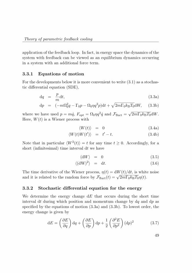
Theory of parametric feedback cooling
application of the feedback loop. In fact, in energy space the dynamics of thesystem with feedback can be viewed as an equilibrium dynamics occurringin a system with an additional force term.
3.3.1 Equations of motion
For the developments below it is more convenient to write (3.1) as a stochas-tic differential equation (SDE),
dq =p
mdt, (3.3a)
dp = (−mΩ20q − Γ0p− Ω0ηq
2p)dt+√
2mΓ0kBT0dW, (3.3b)
where we have used p = mq, Fopt = Ω0ηq2q and Ffluct =
√2mΓ0kBT0dW .
Here, W (t) is a Wiener process with
⟨W (t)⟩ = 0 (3.4a)⟨W (t)W (t′)⟩ = t′ − t. (3.4b)
Note that in particular ⟨W 2(t)⟩ = t for any time t ≥ 0. Accordingly, for ashort (infinitesimal) time interval dt we have
⟨dW ⟩ = 0 (3.5)⟨(dW)2⟩ = dt. (3.6)
The time derivative of the Wiener process, η(t) = dW (t)/dt, is white noiseand it is related to the random force by Ffluct(t) =
√2mΓ0kBT0η(t).
3.3.2 Stochastic differential equation for the energy
We determine the energy change dE that occurs during the short timeinterval dt during which position and momentum change by dq and dp asspecified by the equations of motion (3.3a) and (3.3b). To lowest order, theenergy change is given by
dE =
(∂E
∂q
)dq +
(∂E
∂p
)dp+
1
2
(∂2E
∂p2
)(dp)2 (3.7)
49

Parametric Feedback Cooling
Note that this equation differs from the usual chain rule because we haveto keep the term proportional to (dp)2. The reason is that according to Eq.(3.3b), dp depends on dW which is of order
√dt. Hence, if we want to keep
all terms at last up to order dt, we cannot neglect the second order term inthe above equation because (dp)2 is of order dt. In contrast, we can safelyneglect the terms proprtional to (dq)2 and dqdp, because they are of orderdt and (dt)3/2, respectively1.
Computing the derivatives of the energy with respect to q and p weobtain
dE = mΩ20qdq +
p
mdp+
1
2m(dp)2. (3.8)
Inserting dq and dp from Eqns. (3.3a) and (3.3b) and neglecting all termsof order (dt)3/2 or higher yields
dE = −m(Γ0+Ω0ηq2)( p
m
)2dt+
p
m
√2mΓ0kBT0dW+Γ0kBT0dW
2. (3.9)
To avoid the multiplicative noise of Eq. (3.9) we consider the variableϵ =
√E instead of the energy E. The change dϵ due to the changes dq and
dp occurring during an infinitesimal time interval dt is given by
dϵ =
(∂ϵ
∂q
)dq +
(∂ϵ
∂p
)dp+
1
2
(∂2ϵ
∂p2
)(dp)2 (3.10)
as all other terms are of order (dt)3/2 or higher. Evaluation of the partialderivatives yields
dϵ = mΩ20
q
2ϵdq +
1
2ϵ
p
mdp+
1
2
(1
2mϵ− 1
4ϵ3p2
m2
)(dp)2. (3.11)
Using the equations of motion (3.3a) and (3.3b) and exploiting that (dp)2 =
1This way to apply the chain rule is the basis of the so-called Itô calculus.
50

Theory of parametric feedback cooling
2mΓ0kBT0(dW )2 up to order dt we obtain
dϵ = −m
2ϵ(Γ0 +Ω0ηq
2)( p
m
)2dt+
√2mΓ0kBT0
2ϵ
p
mdW
+Γ0kBT0
2ϵ
(1− p2
2mϵ2
)(dW )2. (3.12)
We now integrate this equation over an oscillation period τ = 2π/Ω0 toobtain the change ∆ϵ =
∫ τ0 dϵ over one oscillation period,
∆ϵ = −Γ0
2
∫ τ
0
p2
mϵdt− Ω0η
2
∫ τ
0
q2p2
mϵdt
+√
2mΓ0kBT0
∫ τ
0
p
2mϵdW
+Γ0kBT0
∫ τ
0
1
2ϵ
(1− p2
2mϵ2
)(dW )2. (3.13)
To compute the integrals on the right hand side of the above equation, weassume that in the low-friction limit the energy E, and hence also ϵ remainsessentially constant over one oscillation period. We also assume that thefeedback mechanism changes the energy of the system slowly and that themotion of the system during one oscillation period is practically not affectedby the feedback either. In the low friction regime, where the coupling tothe bath is weak, a small feedback strength (i.e., a small η) should besufficient for considerable cooling. Accordingly, during one oscillation periodthe position q and the momentum p are assumed to evolve freely:
q(t) = ϵ
√2
mΩ20
sinΩ0t, (3.14)
p(t) = mq(t) = ϵ√2m cosΩ0t, (3.15)
where we have selected the phase of the oscillation such that the positionq = 0 at time 0. Hence, the first two integrals of (3.13) are given by∫ τ
0
p2
mϵdt = 2ϵ
∫ τ
0cos2Ω0t dt = ϵτ (3.16)
51

Parametric Feedback Cooling
and ∫ τ
0
q2p2
mϵdt =
4ϵ3
mΩ20
∫ τ
0sin2Ω0t cos
2Ω0tdt =ϵ3τ
2Ω20m
. (3.17)
Insertion of these results and of the harmonic expressions for q(t) and p(t)from above into Eq. (3.13) gives
∆ϵ = −Γ0ϵ
2τ − Ω0ηϵ
3
4mΩ20
τ
+√
Γ0kBT0∆R1
+Γ0kBT0
2ϵ∆R2. (3.18)
where ∆R1 and ∆R2 are given by
∆R1 =
∫ τ
0cosΩ0t dW (3.19)
and∆R2 =
∫ τ
0sin2Ω0t (dW )2, (3.20)
Since W (t) is a Wiener process, ∆R1 and ∆R2 are random numbers. Nextwe will determine the statistical properties of ∆R1 and ∆R2.
As ∆R1 is the result of a (weighted) sum of Gaussian random numbers,it will be a Gaussian random number, too. The mean of ∆R1 is given by
⟨∆R1⟩ = ⟨∫ τ
0cosΩ0t dW ⟩ =
∫ τ
0cosΩ0t⟨dW ⟩ = 0, (3.21)
where the angular brackets imply an average over all noise histories. Thevariance of ∆R1 is given by
⟨(∆R1)2⟩ = ⟨
∫ τ
0cosΩ0t dW
∫ τ
0cosΩ0t
′ dW ′⟩
=
∫ τ
0
∫ τ
0cosΩ0t cosΩ0t
′⟨dWdW ′⟩
=
∫ τ
0cos2Ω0t dt =
τ
2, (3.22)
52
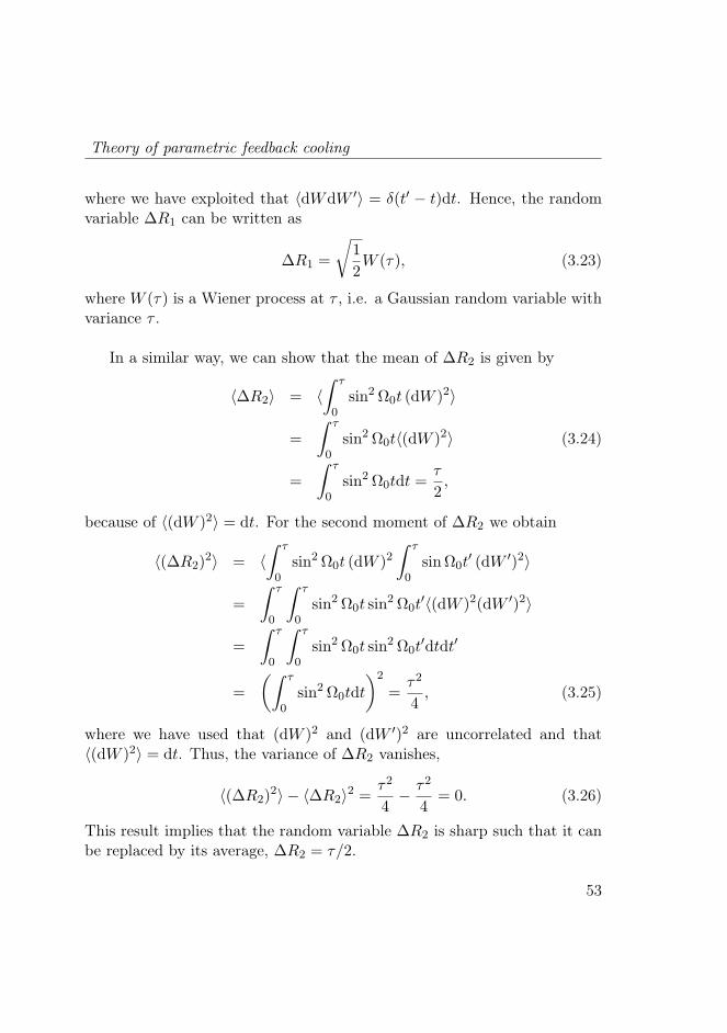
Theory of parametric feedback cooling
where we have exploited that ⟨dWdW ′⟩ = δ(t′ − t)dt. Hence, the randomvariable ∆R1 can be written as
∆R1 =
√1
2W (τ), (3.23)
where W (τ) is a Wiener process at τ , i.e. a Gaussian random variable withvariance τ .
In a similar way, we can show that the mean of ∆R2 is given by
⟨∆R2⟩ = ⟨∫ τ
0sin2Ω0t (dW )2⟩
=
∫ τ
0sin2Ω0t⟨(dW )2⟩ (3.24)
=
∫ τ
0sin2Ω0tdt =
τ
2,
because of ⟨(dW )2⟩ = dt. For the second moment of ∆R2 we obtain
⟨(∆R2)2⟩ = ⟨
∫ τ
0sin2Ω0t (dW )2
∫ τ
0sinΩ0t
′ (dW ′)2⟩
=
∫ τ
0
∫ τ
0sin2Ω0t sin
2Ω0t′⟨(dW )2(dW ′)2⟩
=
∫ τ
0
∫ τ
0sin2Ω0t sin
2Ω0t′dtdt′
=
(∫ τ
0sin2Ω0tdt
)2
=τ2
4, (3.25)
where we have used that (dW )2 and (dW ′)2 are uncorrelated and that⟨(dW )2⟩ = dt. Thus, the variance of ∆R2 vanishes,
⟨(∆R2)2⟩ − ⟨∆R2⟩2 =
τ2
4− τ2
4= 0. (3.26)
This result implies that the random variable ∆R2 is sharp such that it canbe replaced by its average, ∆R2 = τ/2.
53

Parametric Feedback Cooling
Putting everything together we get
∆ϵ =
(−Γ0ϵ
2− Ω0ηϵ
3
4mΩ20
+Γ0kBT0
4ϵ
)τ +
√Γ0kBT0
2W (τ). (3.27)
Since the oscillation period τ is assumed to be short compared to the dissi-pation time scale 1/Γ0 (also the feedback strength η needs to be appropri-ately small), we can finally write the stochastic differential equation for thevariable ϵ,
dϵ =
(−Γ0ϵ
2− Ω0ηϵ
3
4mΩ20
+Γ0kBT0
4ϵ
)dt+
√Γ0kBT0
2dW. (3.28)
This equation, in which ϵ is the only variable, is the main result of this sec-tion. It implies that the relaxation process can be understood as a Brownianmotion of ϵ (or, equivalently, of the energy) under the influence of an exter-nal “force”. Using Itô’s formula we can derive the corresponding stochasticdifferential equation for the energy E = ϵ2:
dE =
(−Γ0E − Ω0ηE
2
2mΩ20
+ Γ0kBT0
)dt+
√E√
2Γ0kBT0dW. (3.29)
Note that, in contrast to ϵ, the energy is subject to multiplicative noise.
3.3.3 Energy distribution
Equation (3.28) derived in the previous section resembles the Langevin equa-tion of a variable ϵ evolving at temperature kBT0 under the influence of anexternal force f(ϵ) at high friction ν:
dϵ =1
νf(ϵ)dt+
√2kBT0
νdW (3.30)
This equation is known to sample the Boltzmann-Gibbs distribution
ρ(ϵ) ∝ exp(−β0U(ϵ)), (3.31)
54

Theory of parametric feedback cooling
where β0 = 1/kBT0 is the inverse temperature and
U(ϵ) = ϵ2 +α
4ϵ4 − kBT0 ln ϵ. (3.32)
is the potential corresponding to the force f(ϵ) = −dU(ϵ)/dϵ. Here, wehave introduced
α =η
mΩ0Γ0(3.33)
to simplify the notation. Hence, Eq. (3.28) generates the distribution
ρ(ϵ, α) ∝ ϵ exp−β0
(ϵ2 +
α
4ϵ4)
, (3.34)
which can be viewed as the equilibrium distribution of the “potential” U(ϵ).In the above equation we have included the feedback strength α explicitly asparameter for ρ(ϵ, α) in order to indicate that this distribution is valid alsofor the non-equilibrium steady state generated by the feedback mechanism.The effect of the feedback is, however, reduced to a particular term in thispotential. As can be easily seen by a change of variables from ϵ to E, thedistribution of Eq. (3.34) corresponds to the energy distribution
ρ(E,α) =1
Zexp
−β0E − β0α
4E2
, (3.35)
where the normalisation factor Z =∫dEρ(E,α) is given by
Z =
√π
αβ0eβ0/αerfc
(√β0α
). (3.36)
3.3.4 Effective temperature
The average energy is obtained by integration over the energy distributionof Eq. (6.7),
⟨E⟩ = Z−1
∫dE E exp
−β0E − β0α
4E2
. (3.37)
55

Parametric Feedback Cooling
Evaluation of the integrals yields
⟨E⟩ = 2
β0
√
β0α
e−β0/α
√π erfc
(√β0
α
) − β0α
, (3.38)
where α is given by Eq. (3.33). Thus, the effective temperature Teff obtainedby applying the feedback mechanism is:
kBTeff = kBT0
2√αkBT0
e−1/αkBT0
√π erfc
(1√
αkBT0
) − 2
αkBT0
. (3.39)
For large values of α, the asymptotic behaviour of the effective temper-ature is given by
kBTeff ≈√
4kBT0
πα=
√4kBT0mΩΓ0
πη. (3.40)
Hence, at low friction, the effective temperature decreases as√Γ0 and in-
versely proportional to √η.
3.4 Experimental results
In this section we present the main experimental results: linear dependenceof the trap stiffness on optical power, linear dependence of the damping co-efficient on pressure and parametric feedback cooling down to Teff ∼ 50mK.
3.4.1 Power dependence of trap stiffness
We first consider the particle’s dynamics with the feedback loop deacti-vated. For small oscillation amplitudes, the particle experiences a harmonictrapping potential with a trap stiffness ktrap, which is a linear function of
56

Experimental results
P . In the paraxial and dipole approximations (small particle limit, weakfocusing) the transverse trap stiffness is calculated as
k(x)trap = α′
effE20/w0
2, (3.41)
where E02 ∝ P is the field intensity at the focus, λ is the wavelength, w0
the field confinement (beam waist) and αeff′ is the particle polarisability.
A similar expression holds for the longitudinal trap stiffness (for details seechapter 2). For the parameters used in our experiments we find that theparticle’s oscillation frequency in x direction is f
(x)0 = (ktrap/m)1/2/(2π) =
120 kHz. For the axial oscillation frequency we find f(z)0 = 37 kHz and
for the y direction we measure f(y)0 = 134 kHz. The different oscillation
frequencies in x and y directions originate from the asymmetry of the laserfocus (c.f. section 2.2). The linear dependence of the trap stiffness on laserpower has been verified for all three directions and is shown in Fig. 3.3(a).In Fig. 3.3(b) we show the spectral densities of the x, y, and z motionsrecorded at a pressure of Pgas = 6.3mBar.
3.4.2 Pressure dependence of damping coefficient
Once a particle has been trapped, the interaction with the backgroundgas thermalises its energy with the environment and, according to thefluctuation-dissipation theorem, damps the particle’s motion with the rateΓ0 in Eq. (3.1). From kinetic theory we find that [Li et al., 2011; Beresnevet al., 1990]
Γ0 =6πηa
m
0.619
0.619 + Kn(1 + cK) , (3.42)
where cK = 0.31Kn/(0.785 + 1.152Kn + Kn2), η is the viscosity coefficientof air and Kn = l/a is the Knudsen number. When the mean free pathl ∝ 1/Pgas is much larger than the radius of the particle, Γ0 becomes pro-portional to Pgas. Fig. 3.4 shows the measured value of Γ0 for all threedirections as a function of pressure. For a pressure of Pgas = 10−5 mBarwe measure a damping of Γ0 / 2π = 10mHz, which corresponds to a quality
57

Parametric Feedback CoolingS (nm
2 / Hz)
0.4P / P0
a
0.8 1.2 1.60.4
k / k 0
0.8
1.2
1.6
z
xy
40frequency (kHz)
80 120 160
b
z x y
10-5
10-4
10-3
10-2
10-1
10-6
Figure 3.3: Trap stiffness and spectral densities. (a) Normalized trapstiffness in the x, y, and z directions as a function of normalised laser power.Dots are experimental data and the solid line is a linear fit. (b) Spectraldensities of the x, y, and z motions. The trapped particle has a radius ofa = 69nm and the pressure is Pgas = 6.3mBar. The spectral separation ofthe resonances makes it possible to feedback-cool the trapped particle with asingle laser beam. The resonance frequencies are f0 = 37 kHz, 120 kHz and134 kHz, respectively. The dashed curves are fits according Eq. (3.43) andthe data on the bottom correspond to the noise floor.
factor of Q = 107, a value that is higher than the quality factors achievedwith clamped oscillators [Poot and van der Zant, 2012]. In ultrahigh vacuum(Pgas = 10−9 mBar), the quality factor will reach values as high as Q ∼ 1011.
3.4.3 Effective temperature
Activation of the parametric feedback loop gives rise to additional dampingδΓ and a frequency shift δΩ. The resulting spectral line shapes are defined
58

Experimental results
101 10310-5 10-3 10-1
pressure (mBar)
z
xy
100
102
10-2
104
106
!0 /
2"
(Hz)
Figure 3.4: Damping rate as a function of gas pressure. The damp-ing rate Γ0 decreases linearly with pressure Pgas. The dashed line is a fitaccording to Eq. (3.42).
by the power spectral density Sq(Ω), which follows from Eq. (3.1) as
Sq(Ω) =
∫ ∞
−∞
⟨q(t)q(t−t′)
⟩e−iΩt′ dt′ (3.43)
=Γ0 kBT0 / (πm)
([Ω0 + δΩ]2 − Ω2)2 +Ω2[Γ0 + δΓ]2.
Integrating both sides over Ω yields the mean square displacement⟨q2⟩
=⟨q(0)q(0)
⟩=
kBT0
m(Ω0 + δΩ)2Γ0
Γ0 + δΓ. (3.44)
According to the equipartition principle, the effective temperature Teff fol-lows from kB Teff = m(Ω0+δΩ)2
⟨q2⟩. Considering that δΩ ≪ Ω0 we obtain
Teff = T0Γ0
Γ0 + δΓ, (3.45)
59

Parametric Feedback Cooling
where T0 is the equilibrium temperature in the absence of the parametricfeedback (δΓ = 0). Thus, the temperature of the oscillator can be raised orlowered, depending on the sign of δΓ in Eq. (3.45).Note that (3.45) differs from the previously derived expression (3.39). Whilethe latter is exact, the former is only approximately valid because under theaction of feedback the particle is not in a true thermodynamic equilibriumbut rather in a steady state. In the phase space distribution the term de-pending on the squared energy E(q, p)2 causes correlations between q andp that are absent in thermal equilibrium.
The experimental results of parametric feedback cooling are shown inFig. 3.5, which depicts the dependence of the effective temperature Teff onpressure. Following the theoretical prediction (3.39), the effective temper-ature scales as Γ
1/20 for constant feedback gain η. At Pgas ∼ 4× 10⁻⁴mBar
the feedback gain is increased. This results in a sudden drop of the effectivetemperature. For lower pressures the gain is held constant again.
The cooling action of the feedback loop competes with reheating dueto collisions with air molecules, ultimately setting a minimum achievabletemperature for each pressure value. Since the area under the line shapedefined in Eq. (3.43) is proportional to Teff , feedback cooling not only in-creases the linewidth but also lowers the signal amplitude until it reaches thenoise floor. Nevertheless, we are able to reach temperatures of Teff ∼ 50mKwhile maintaining the particle in the trap.
3.5 Towards the ground state
The here introduced trapping and cooling technique represents an importantstep towards ground state cooling. In the quantum limit, a mechanicaloscillator exhibits discrete states separated in energy by h(Ω0+ δΩ) ∼ hΩ0.The mean thermal occupancy is
⟨n⟩ = kBTeff
hΩ0. (3.46)
60
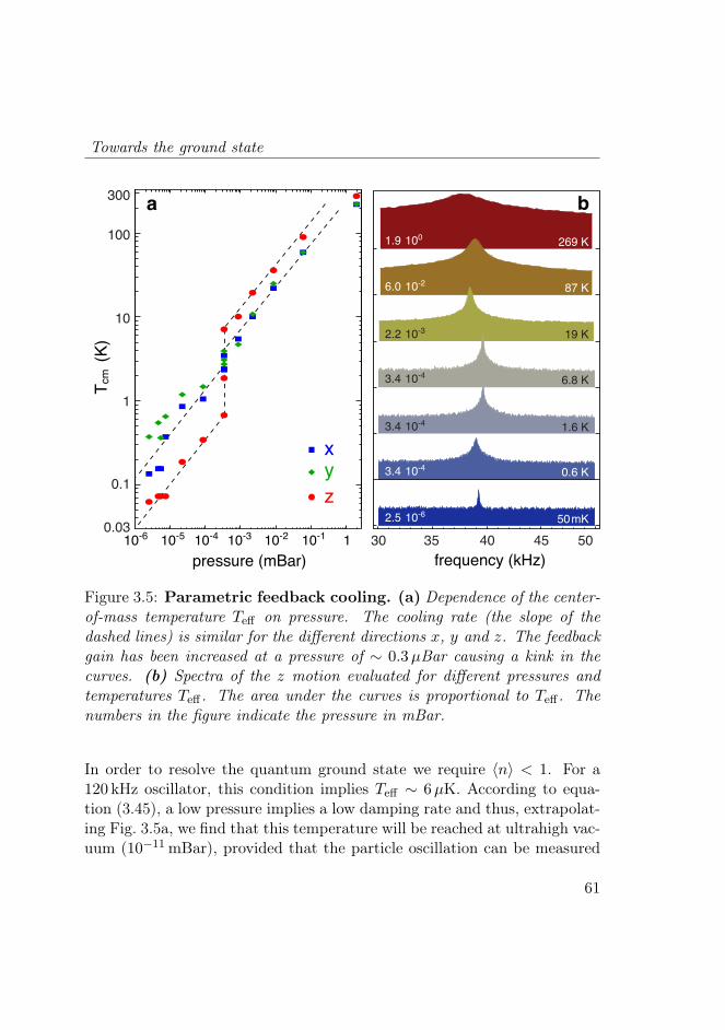
Towards the ground state
ba
110-4 10-3 10-2 10-1
pressure (mBar)10-6 10-5
300
100
10
1
0.1
T cm
(K)
0.03
z
xy
50 mK
0.6 K
1.6 K
6.8 K
19 K
87 K
269 K
30frequency (kHz)
35 40 45 502.5 10-6
3.4 10-4
3.4 10-4
3.4 10-4
2.2 10-3
6.0 10-2
1.9 100
b
Figure 3.5: Parametric feedback cooling. (a) Dependence of the center-of-mass temperature Teff on pressure. The cooling rate (the slope of thedashed lines) is similar for the different directions x, y and z. The feedbackgain has been increased at a pressure of ∼ 0.3µBar causing a kink in thecurves. (b) Spectra of the z motion evaluated for different pressures andtemperatures Teff . The area under the curves is proportional to Teff . Thenumbers in the figure indicate the pressure in mBar.
In order to resolve the quantum ground state we require ⟨n⟩ < 1. For a120 kHz oscillator, this condition implies Teff ∼ 6µK. According to equa-tion (3.45), a low pressure implies a low damping rate and thus, extrapolat-ing Fig. 3.5a, we find that this temperature will be reached at ultrahigh vac-uum (10−11mBar), provided that the particle oscillation can be measured
61

Parametric Feedback Cooling
and the feedback remains operational. Alternatively, lower occupancy canbe reached at higher pressures by an increase of the feedback gain. Laserpower noise introduces fluctuations in the trap stiffness and therefore inthe mechanical oscillation frequency. We believe that the resulting randomphase error in the feedback loop is the current limiting factor in cooling.This phase error can be minimised by using background suppression andlaser stabilisation techniques [Seifert et al., 2006]. The noise floor in ourmeasurements is currently 1.2 pm/
√Hz.
In feedback cooling, the particle’s position has to be measured in orderto operate the feedback loop. Measurement uncertainty of x, y, and zintroduced by shot-noise therefore limits the lowest attainable temperatureTeff . The measurement accuracy is fundamentally limited by the standardquantum limit, which follows from the uncertainty principle.
3.5.1 The standard quantum limit
Photons that scatter off the particle carry information about it’s position,which sub-sequentially can be read out via photo detection. The signalimproves with the number of photons Nph that interact with the particle.However, even for an ideal detector the stochastic arrival of photons addsan uncertainty to the measurement. For a laser beam with Nph photonsthe uncertainty in photon number due to shot noise is ∆n =
√Nph. Thus
the momentum uncertainty is ∆p =√
Nphhkq, where kq is the wavevectorof the scattered photon into direction q. From the uncertainty principle∆q∆p ≥ h/2 it follows that the position uncertainty is ∆q = 1/(2
√Nphkq).
Therefore, the position measurement improves as ∼ 1/√
Nph with the num-ber of photons. On the other hand, due to the momentum uncertainty∆p ∝
√Nph, the finite probability to excite the mechanical oscillator in-
creases with the number of photons. Consequently, the uncertainty in themeasured energy
∆E = 1/2(mΩ20∆q2 +∆p2/m), (3.47)
consists of two terms, measurement uncertainty and measurement back-action, respectively. The standard quantum limit is achieved when the
62

Towards the ground state
measurement uncertainty is minimized, that is when both terms contributeequally.
Figure 3.6: Measurement backaction. The standard quantum limit isreached when the measured position uncertainty is equal to the momentumimparted by the photons that carry the information about the position. Thered curve shows the measurement uncertainty, the blue curve the measure-ment back-action and the black curve shows the sum of the two.
3.5.2 Recoil heating
Evidently, the measurement uncertainty ∆q can be reduced by increasingthe signal power at the detector, for example by higher laser power or byusing a larger particle size a and hence a larger scattering cross-sectionσscatt = k4|α|2/(6πϵ20). However, strong scattering introduces recoil heating,which destroys the coherent particle motion.
In general, photon recoil is a small effect since the photon momentumis small compared to the momentum of the mechanical oscillator. However,at very low pressures, collisions of the oscillator with air molecules becomesnegligible and photon recoil becomes the dominating decoherence process.To understand the effect of recoil from our previous discussion of mea-surement backaction, consider the number of photons needed to add onequantum of mechanical energy hΩ0 to the oscillator. The recoil energy ofa single photon emitted in direction q is given by h2k2q/2m, where m is
63

Parametric Feedback Cooling
the mass of the oscillator. Therefore, Nrecoil = 2mhΩ0/h2k2q photons need
to interact with the oscillator to add one quantum of mechanical energy.The number of photons that are scattered by a particle with scatteringcross section σscatt within a time interval ∆t is Nscat = Pscat∆t/hω, wherePscat = σscattI0 is the scattered power and I0 = Pin/σfocus is the intensityat the laser focus.From this the time ∆trecoil it takes to scatter Nrecoil photons follows as
Γrecoil = 1/∆trecoil =
[h2k2q /2m
hΩ0
] [I0 σscatt
hω
]. (3.48)
Finally, to obtain the recoil rate in direction q, we consider the probabilityof observing a photon scattered in this direction. Since for a sub-wavelengthparticle, the scattered light featuers a dipolar radiation pattern, the proba-bility of observing a particle in direction θ, ϕ is P (θ, ϕ) = 3
8 sin2 θ. Thus,
the contribution to recoil from all photons in direction q is
k2q =
∫ 2π
0
∫ π
0P (θ, ϕ)(k · nq)
2 sin θdθdϕ = k2
2/5 q=y,z1/5 q=x
, (3.49)
where k · nq is the projection of the wavevector
k = (kx, ky, kz) = k(cos θ, sin θ cosϕ, sin θ sinϕ). (3.50)
in direction q. Here, x is the direction of polarisation of the incident electricfield. Since a dipole doesn’t radiate along the direction of polarisation alsothe recoil along the direction of polarisation is reduced.
3.5.3 Detector bandwidth
We continue the discussion to gain some insight into the limits of the de-tection. Consider the number of photons available to detect the particleposition q. As before Nscat = Pscat∆t/hω, where now the measurementtime ∆t = 1/B is given by the bandwidth of the detector B. The positionuncertainty is then easily found as
∆q ≥√
hcλB/(8πPscat). (3.51)
64

Towards the ground state
For our experimental values a = 70nm, P in = 100mW, λ = 1064 nm andB = 300 kHz, we find that ≈ 108 photons are scattered and that the po-sition uncertainty is ∆q ≈ 6.3 pm, which is of the order of the zero pointmotion. Our experimental parameters are therefore close to the optimum.From (3.51), one might argue that the position uncertainty can be fur-ther improved by simply reducing the bandwidth of the detector. However,for the feedback to work we need to be sensitive to changes in the ampli-tude q0(t) and phase ϕ(t) of the particle motion1. Classically, the particletrajectory can be written as q(t) = q0(t) sin(Ω0t + ϕ(t)), where q0(t) andϕ(t) are slowly varying functions that vary over timescales of the order of∼ 1/Γdecoher.. In other words, the maximum time ∆tmeas. we have for themeasurement of q(t) is the time over which q(t+∆tmeas.) is correlated withq(t).
In ultrahigh vacuum, the dominant decoherence process is recoil heat-ing and therefore Γdecoher. = Γrecoil ∝ Pscat.. Using B ≈ Γrecoil, the positionuncertainty (3.51) becomes independent of power. This is again a man-ifestation of the uncertainty principle, which tells us that the minimumuncertainty in the position measurement is given by the zero point motion.
Ultimately, we are interested in the number of coherent oscillations thatcan be observed. Employing the expression for the trap stiffness derived insection 2.3, we find that the number
Nosc =Ω0
2πΓrecoil∝ 1/(ka)3 (3.52)
of coherent oscillations also does not depend on power. Hence, we can choosethe power high enough to make photon shot noise the dominant noise source.
In conclusion, we have shown that neither the number of coherent os-cillations, nor the minimum position uncertainty depend on power. As aconsequence, we can work in a regime where the measurement uncertainty isonly limited by photon shot noise. In that case, the minimum measurement
1Actually for the feedback we only need to know the right phase. However, theamplitude gives us the energy.
65

Parametric Feedback Cooling
uncertainty is achieved by a detector with bandwidth B ≈ Γrecoil. The dis-cussion highlights the tradeoff between measurement uncertainty and recoilheating. A nanoparticle of size of a ∼ 70 nm is a good compromise betweenthe two limiting factors. Notice that Γrecoil and the photon scattering ratediffer by a factor of ∼ 10−9, and hence most of the scattered photons do notalter the center-of-mass state of the particle. The possibility of observingthe particle without destroying its quantum coherence is a critical advan-tage over atomic trapping and cooling experiments. Finally, parametriccooling should work even without continuously tracking q(t) as long as thefrequency and the phase of the center-of-mass oscillation are known.
3.6 Conclusion
We have demonstrated that an optically trapped nanoparticle in high vac-uum can be efficiently cooled in all three dimensions by a parametric feed-back scheme. The parametric feedback makes use of a single laser beamand is therefore not limited by alignment inaccuracies of additional coolinglasers. Theoretical considerations show that center-of-mass temperaturesclose to the quantum ground state are within reach. To fully exploit thequantum coherence of a laser-trapped nanoparticle, parametric feedbackcooling can be combined with passive dynamical back-action cooling [Kip-penberg and Vahala, 2007], for example by use of optical cavities [Changet al., 2010; Romero-Isart et al., 2010; Kiesel et al., 2013] or electronic res-onators [Teufel et al., 2011]. The results shown here also hold promise forultrasensitive detection and sensing [Geraci et al., 2010]. The ultrahigh qual-ity factors and small oscillation amplitudes yield force sensitivities on theorder of 10−20N/
√Hz [Stipe et al., 2001], which outperforms most other ul-
trasensitive force measurement techniques by orders of magnitude, and canfind applications for the detection of single electron or nuclear spins [Rugaret al., 2004], Casimir forces and vacuum friction, phase transitions [Lechneret al., 2013], and non-Newtonian gravity-like forces [Geraci et al., 2010].
66

CHAPTER 4
Dynamics of a parametrically drivenlevitated particle
A prerequisite for applications of a nanomechanical resonator, such as sens-ing, is a thorough understanding of the resonator response to changes in itsenvironment. The dynamic response to different external stimuli and the os-cillator parameters can be characterised by applying a known external force.In this chapter we use parametric modulation of the trapping potential to ex-cite an optically levitated particle in high vacuum and analyze its responsefor a range of different excitation modalities.
4.1 Introduction
For large oscillation amplitudes the particle motion is governed by a (Duff-ing) nonlinearity. This nonlinearity is common to most nanomechanical os-cillators, which are ideal systems to explore nonlinear dynamical behaviour,as they exhibit high mechanical quality (Q) factors fast response times andfairly low drift and can be easily excited into the nonlinear regime [Un-terreithmeier et al., 2010]. The response of a nonlinear oscillator exhibitscharacteristic phenomena such as multistability, hysteresis and discontinu-
67
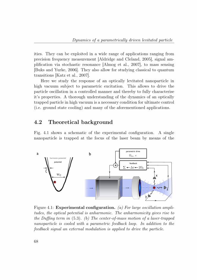
Dynamics of a parametrically driven levitated particle
ities. They can be exploited in a wide range of applications ranging fromprecision frequency measurement [Aldridge and Cleland, 2005], signal am-plification via stochastic resonance [Almog et al., 2007], to mass sensing[Buks and Yurke, 2006]. They also allow for studying classical to quantumtransitions [Katz et al., 2007].
Here we study the response of an optically levitated nanoparticle inhigh vacuum subject to parametric excitation. This allows to drive theparticle oscillation in a controlled manner and thereby to fully characteriseit’s properties. A thorough understanding of the dynamics of an opticallytrapped particle in high vacuum is a necessary condition for ultimate control(i.e. ground state cooling) and many of the aforementioned applications.
4.2 Theoretical background
Fig. 4.1 shows a schematic of the experimental configuration. A singlenanoparticle is trapped at the focus of the laser beam by means of the
a b
x
y
z
2!"#$S(!)
0+feedbac
k
feedback
20
parametric drive
m, harmonic potential
potential
w0
Figure 4.1: Experimental configuration. (a) For large oscillation ampli-tudes, the optical potential is anharmonic. The anharmonicity gives rise tothe Duffing term in (5.3). (b) The center-of-mass motion of a laser-trappednanoparticle is cooled with a parametric feedback loop. In addition to thefeedback signal an external modulation is applied to drive the particle.
68

Theoretical background
optical gradient force and cooled parametrically by a feedback loop. Inaddition to the feedback signal, we apply a modulation at frequency Ωm
and modulation depth ϵ.
4.2.1 Equation of motion
The particle motion consists of three modes, each corresponding to a spa-tial oscillation along one of the three symmetry axes of the optical in-tensity distribution. For large oscillation amplitudes, the modes couplethrough cubic nonlinearities in the optical force (c.f. chapter 2). How-ever, under the action of feedback cooling, the effective thermal amplitudeqeff =
(2kBTeff
/mΩ2
0
)1/2 of the particle oscillation is much smaller than thesize of the trap. As a consequence, coupling between the modes is negligibleand the particle dynamics is well described by a one-dimensional equationof motion:
q + Γ0q +Ω20
1 + ϵ cos (Ωmt)︸ ︷︷ ︸parametric drive
+Ω−10 Γ0qq︸ ︷︷ ︸feedback
+ ξq2︸︷︷︸Duffing term
q =Ffluct
m≈ 0.
(4.1)The damping Γ0 can be controlled by the pressure of the vacuum chamber.In addition, the third term depends on several experimental parameterswhich allow us to control the particle motion as follows
• The prefactor is proportional to the mean optical power and definesthe oscillation frequency Ω0 of the trapped particle.
• Parametric driving with modulation depth ϵ and modulation fre-quency Ωm allows to drive the particle motion. As we will see inthe following sections, the most interesting phenomena occur whenΩm is close to twice the natural frequency Ω0 of the particle.
• Nonlinear damping is due to parametric feedback cooling. Withoutparametric drive (ϵ = 0), the nonlinear damping reduces the effectivethermal energy from T0 to Teff (c.f. chapter 3). It is important to
69

Dynamics of a parametrically driven levitated particle
note that feedback cooling reduces the effective thermal motion in allthree spatial directions. In contrast, parametric driving only excitesthe mode which fulfils the condition Ωm ≈ 2Ω0.
• The Duffing nonlinearity is due to the shape of the optical potential(c.f. chapter 2). It becomes significant when the particle’s oscillationamplitude is comparable to the beam waist w0.
The right hand side of equation (5.3) is a stochastic force due to randomcollisions with residual air molecules and therefore depends on pressure.The fluctuation-dissipation relation links the strength of the thermal forceto the damping ⟨Ffluct(t)Ffluct(t
′)⟩ = 2mΓ0 kBTeff δ(t − t′). Under typicalexperimental conditions Q = Ω0/Γ0 ≫ 1. Hence, the stochastic force ismuch weaker than the nonlinear terms and the parametric driving and canbe neglected in the description of the particle dynamics.
4.2.2 Overview of modulation parameter space
The response of the particle to the external modulation depends on theparameters of the external driving force ϵ and Ωm, respectively. In thefollowing we consider resonant and non-resonant parametric driving. For theformer the condition Ωm ≈ 2Ω0 holds, whereas for the latter this condition isviolated. In addition, for resonant driving, we can also distinguish betweenexcitation below and excitation above threshold, respectively.
Resonance condition
Fig. 4.2 shows the frequency resolved particle response at 6mBar as a func-tion of modulation frequency Ωm for fixed modulation depth ϵ. Modulationat frequency Ωm produces sideband frequencies at |Ω0 ± Ωm| (red dashedlines). For very low modulation frequencies, the overlap of the sidebandsleads to an apparent broadening of the resonance peak (lower inset Fig. 4.2).In high vacuum, the resonances and consequently also the modulation side-bands become sharper and we can resolve higher order sidebands (c.f. sec-tion 4.3.4). When the lower sideband Ωm − Ω0 becomes resonant with the
70

Theoretical background
Particle Frequency kHz
Mod
ulat
ion
Freq
uenc
yk
Hz
50 100 150 200 250 3000
50
100
150
200
250
300
Ω0
Ωm
Ω0 + Ωm
Ω0 − Ωm
Ωm − Ω0
2Ω0
Ωm / 2
integrated spectral power
low frequency modulation
resonant modulation
Figure 4.2: Parametric excitation overview. The main figure showsthe power spectral density (horizontal axis) of the x-mode (Ω0 ∼ 125kHz)as a function of modulation frequency Ωm (vertical axis). Modulation atfrequency Ωm (red solid line) produces sideband frequencies at |Ω0±Ωm| (reddashed lines). When the lower sideband Ωm−Ω0 becomes resonant with theparticle resonance Ω0, energy is transferred from the sideband to the particle(upper inset). This results in a increase of the particle energy and frequencylocking to the external modulation (green solid line, c.f. section 4.3.1). Thetotal particle energy is obtained by integration of the power spectral density.The integrated power spectral density as a function of modulation frequencyis show as black data points to the right. On resonance, the thermal noiseis parametrically amplified.
particle resonance Ω0, energy is transferred from the sideband to the parti-
71

Dynamics of a parametrically driven levitated particle
cle (upper inset Fig. 4.2). This results in a increase of the particle energy.The total particle energy is obtained by integration over the power spectraldensity (black data points to the right).
Threshold condition
Near the resonance (upper inset Fig. 4.2), we distinguish between weak andstrong resonant driving. For weak modulation, the Duffing term in Eq. (5.3)can be neglected and we observe parametric amplification of the thermalnoise (black data points Fig. 4.2). However, if the driving is sufficientlystrong, the Duffing term in Eq. (5.3) becomes important and the systemmakes a transition reminiscent of a phase transition. The particle motionchanges from thermal (incoherent) motion to sustained (coherent) oscilla-tions with a fixed frequency with respect to the external modulation.
In the parameter phase space near resonance, the stability condition(c.f. chapter 4.3.2)
ϵ <2
Q
√1 +Q2 (2− Ωm/Ω0)
2, (4.2)
maps out a tongue shaped region (Arnold tongue), which is shown as greyarea in Fig. 4.3a. Typically Q ≫ 1 and the exact condition (4.2) is wellapproximated by
|δm| < ϵ/2 (4.3)
shown as dashed diagonal lines, where δm = 2 − Ωm/Ω0 is the normalisedmodulation detuning. The particle response to the external modulation fora given set of parameters ϵ,Ωm depends on the phase space trajectory ofthe two control parameters ϵ and Ωm. For simplicity we consider only caseswhere one of the two is held constant while the other is varied. In that casewe can distinguish five cases
I. Frequency up and down sweeps above threshold. The response exhibitshysteresis and is discontinuous when the resonance is approached frombelow (c.f. section 4.4.3).
72

Theoretical background
II. Amplitude up and down sweeps below resonance. The response exhibitshysteresis and is discontinuous when the threshold is crossed frombelow and from above (c.f. section 4.4.4).
III. Amplitude up and down sweeps above resonance. The response doesnot exhibit hysteresis and is continuous (c.f. section 4.4.4).
IV. Approaching the instability region. The frequency of the thermal modeis pulled towards the sideband (c.f. section 4.3.3).
V. Below threshold. The response does not exhibit hysteresis and is con-tinuous. The regime below the onset of self-sustained oscillations canbe used for mechanical parametric amplification and thermal noisesqueezing [Rugar and Gruetter, 1991; Lifshitz and Cross, 2009]. (c.f.Fig. 4.2 black data points - at the parametric resonance the thermalnoise is parametrically amplified).
4.2.3 Secular perturbation theory
Within the resonance region (grey tongue shaped region Fig. 4.3), we areinterested in solutions q(t) that are slow modulations of the linear resonanceoscillations. Therefore, we introduce a dimensionless slow time scale T =κΩ0t and displacement amplitude A(T ). With the slowly varying envelopeapproximation (SVEA)
q =q02AeiΩ0t + c.c. (4.4a)
73
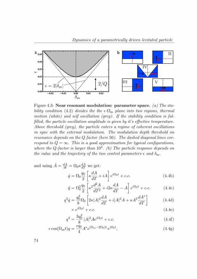
Dynamics of a parametrically driven levitated particle
2/Q
!0.02 !0.01 0.00 0.01 0.020.00
0.01
0.02
0.03
0.04
0.05
"m
#
IV
III
I II
V
a b
= 2|m|
m
Figure 4.3: Near resonant modulation: parameter space. (a) The sta-bility condition (4.2) divides the the ϵ-Ωm plane into two regions, thermalmotion (white) and self oscillation (grey). If the stability condition is ful-filled, the particle oscillation amplitude is given by it’s effective temperature.Above threshold (grey), the particle enters a regime of coherent oscillationsin sync with the external modulation. The modulation depth threshold onresonance depends on the Q factor (here 50). The dashed diagonal lines cor-respond to Q = ∞. This is a good approximation for typical configurations,where the Q-factor is larger than 104. (b) The particle response depends onthe value and the trajectory of the two control parameters ϵ and δm.
and using A = dAdt = Ω0κ
dAdT we get:
q = Ω0q02
[κdA
dT+ iA
]eiΩ0t + c.c. (4.4b)
q = Ω20
q02
[κ2
d2A
dT 2+ i2κ
dA
dT−A
]eiΩ0t + c.c. (4.4c)
q2q =q308Ω0
[2κ|A|2dA
dT+ i|A|2A+ κA2dA
∗
dT
](4.4d)
× eiΩ0t + c.c. (4.4e)
q3 =3q308
|A|2AeiΩ0t + c.c. (4.4f)
ϵ cos(Ωmt)q =ϵq04
A∗e(Ωm−2Ω0)t eiΩ0t, (4.4g)
74

Theoretical background
where c.c. stands for complex conjugate and we dropped small correctionsfrom fast oscillating terms. For a consistent expansion [Villanueva et al.,2013; Lifshitz and Cross, 2009], we apply the rescaling
γ0 =Γ0
Ω0κ; η =
η
ξ; ϵ =
ϵ
κ(4.5)
with scale factors κ = Γ0/Ω0 = Q−1 and q20 = κ/ξ. Plugging (4.4) into(5.3) yields
Ω20
q02
[κ2
d2A
dT 2+ i2κ
dA
dT−A
]eiΩ0t (4.6)
+ γ0κΩ20
q02
[κdA
dT+ iA
]eiΩ0t
+Ω20
q02AeiΩ0t
+q08Ω20ηκ
[2κ|A|2dA
dT+ i|A|2A+ κA2dA
∗
dT
]eiΩ0t + c.c.
+Ω20κ
3q08
|A|2AeiΩ0t + c.c.
+ϵq04
κA∗e−i(δΩm−2Ω0)t eiΩ0t = 0
Dropping higher order terms O(κ2) and fast oscillating terms we arriveat
dA
dT= − γ0
2A− 1
8η|A|2A+ i
3
8|A|2A+ i
ϵ
4A∗e−iδmT , (4.7)
where δm = δm/κ is the rescaled normalised detuning δm = (2− Ωm/Ω0).To get rid of the phase factor in (4.7), we substitute A = A exp(−iT δm/2).This gives
dA
dT= − γ0
2A+ i
δm2A−
[1
8η − i
3
8
]|A|2A+ i
ϵ
4A∗. (4.8)
75
Dynamics of a parametrically driven levitated particle
4.2.4 Steady state solution
In the following we investigate the steady state solution A0, which satisfiesddT A = 0. Aside from the trivial solution A0 = 0, the non-trivial steadystate solution A0 = a0e
−iϕ of (4.8) is given by
d
dTA0 = −i
[−i
(γ02
+1
8ηa20
)−
(δm2
+3
8a20
)]a0e
−iϕ
+ iϵ
4a0e
iϕ = 0, (4.9)
where
γ0 +1
4ηa20 = − ϵ
2sin 2ϕ, (4.10)
δm +3
4a20 = − ϵ
2cos 2ϕ. (4.11)
Thus, a0 and ϕ are given as the solutions to
ϕ =1
2tan−1
(γ0 +
14 ηa
20
δm + 34a
20
)(4.12)
and [γ0 +
1
4ηa20
]2+
[δm +
3
4a20
]2=
ϵ2
4. (4.13)
Fig. 4.4 shows the amplitude solution
a20 =[(η/4)2 + (3/4)2
]−1×(−[γ0η + 3δm
]/4
±√[
(η/4)2 + (3/4)2]ϵ2/4−
[ηδm/4− 3γ0/4
]2)(4.14)
as a function of detuning δm. Note that the solution with the negative signcorresponds to the unstable mode.
76

Dynamics below threshold (linear regime)
!4 !3 !2 !1 0 1 20
1
2
3
4
"m
a 02
Figure 4.4: The three steady state solutions for different detuning. Theparameters are γ0 = 1, η = 1,ϵ = 4.
4.3 Dynamics below threshold (linear regime)
To find the equation of motion for small perturbations δA from equilibrium,we make the ansatz A = A0+δA and plug it into (4.8). Linearization aroundthe trivial solution A0 = 0 yields
d
dTδA =
(− γ0
2+ i
δm2
)δA+ i
ϵ
4δA∗.
Writing δA = r exp iϕ, we find the equations of motion for the amplitudeand the phase of the parametrically driven oscillator.
r = − γ02r +
ϵ
4sin(2ϕ)r, (4.15a)
ϕ =δm2
+ϵ
4cos(2ϕ). (4.15b)
Equation (4.15b) is known as the Adler equation. It is this equation thatexplains the steady state, and in fact also the transient, injection-lockingbehaviour of a harmonic oscillator with an external signal [Siegman, 1986].
77

Dynamics of a parametrically driven levitated particle
4.3.1 Injection locking
According to the Adler equation (4.15b), a steady-state locked oscillation(ϕ = 0) has a fixed phase relative to the external drive
ϕss(δm) =1
2cos−1
(− δmϵ/2
). (4.16)
The phase lag changes from +π/4 to −π/4 as δm is tuned from −ϵ/2 to ϵ/2and changes sign at δm = 0. The Adler equation depends only on ϕ and wecan integrate it
tan(ϕ
2) =
δm∆Ωb
+ϵ/2
∆Ωbtanh
(∆Ωb (t− t0)
2
). (4.17)
Here, t0 incorporates the initial conditions and the beat frequency is given
by ∆Ωb =√
(ϵ/2)2 − δ2m [Knünz et al., 2010]. Note that ϵ/2 > |δm|, sincewe are considering the behaviour within the lock-in region. From (4.17)it follows that for an injected signal within the lock-in region, the phasewill always pull-in smoothly towards the steady-state value given by (4.16).This is easily seen by considering a small perturbation δϕ from the steadystate ϕ = ϕss + δϕ. From (4.15b) we find
δϕ = −
[(ϵ
2
)2
− δ2m
]δϕ (4.18)
Consequently, the phase relaxes exponentially to its steady state value.
4.3.2 Linear instability
Using the steady state value ϕss in (4.15a), we find that the amplitude growsexponentially at a rate
gL = − γ02
+1
2
[(ϵ
2
)2
− δ2m
](4.19)
78
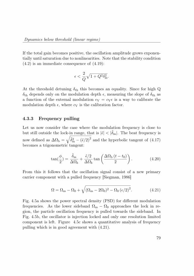
Dynamics below threshold (linear regime)
If the total gain becomes positive, the oscillation amplitude grows exponen-tially until saturation due to nonlinearities. Note that the stability condition(4.2) is an immediate consequence of (4.19):
ϵ <2
Q
√1 +Q2δ2m.
At the threshold detuning δth this becomes an equality. Since for high Qδth depends only on the modulation depth ϵ, measuring the slope of δth asa function of the external modulation ϵV = cVϵ is a way to calibrate themodulation depth ϵ, where cV is the calibration factor.
4.3.3 Frequency pulling
Let us now consider the case where the modulation frequency is close tobut still outside the lock-in range, that is |ϵ| < |δm|. The beat frequency is
now defined as ∆Ωb =√
δ2m − (ϵ/2)2 and the hyperbolic tangent of (4.17)becomes a trigonometric tangent:
tan(ϕ
2) =
δm∆Ωb
+ϵ/2
∆Ωbtan
(∆Ωb (t− t0)
2
). (4.20)
From this it follows that the oscillation signal consist of a new primarycarrier component with a pulled frequency [Siegman, 1986]
Ω = Ωm − Ω0 +
√(Ωm − 2Ω0)2 − Ω0 (ϵ/2)
2. (4.21)
Fig. 4.5a shows the power spectral density (PSD) for different modulationfrequencies. As the lower sideband Ωm − Ω0 approaches the lock in re-gion, the particle oscillation frequency is pulled towards the sideband. InFig. 4.5b, the oscillator is injection locked and only one resolution limitedcomponent is left. Figure 4.5c shows a quantitative analysis of frequencypulling which is in good agreement with (4.21).
79

Dynamics of a parametrically driven levitated particle
c
outside lock-in region
inside lock-in region
!
!
!
!
!
!
!
!
!
!
!
!
!
!
!
!
!
"
"
"""
"""
""""
"""
"
""""
"""
"
"
"""
"""""""""""
"
""
""
"
"
"
"
""""
"""""
""
"
""
"
""
"
"
210 220 230 240 250
122
123
124
125
126
modulation frequency !m !kHz"
modefrequency!0!kHz
"
b
243.0 kHz
a 241.5 kHz
242.0 kHz
242.5 kHz
243.0 kHz
sideband main mode
116 118 120 122 124 12610!5
10!4
0.001
0.01
0.1
1
10
frequency "0!2# "kHz#
PSD"nm2
!Hz#
116 118 120 122 124 12610!4
0.01
1
100
frequency "0!2# "kHz#
PSD"nm2
!Hz#
243.5 kHz
244.5 kHz
245.5 kHz
246.5 kHz
Figure 4.5: Frequency pulling. When the sideband Ωm − Ω0 approachesthe main mode Ω0, the main mode is pulled toward the sideband. (a) PSDfor modulation frequencies below the lock-in region. (b) PSD for modulationfrequencies within the lock-in region. Note that the vertical scale is differentfrom (a). For comparison a PSD from outside the lock-in region is shownin grey. (c) The frequency of the main mode as a function of modulationfrequency. The grey region mark the lock-in region. The black line is a fitto (4.21). Here, the pressure is Pgas = 1.9× 10⁻⁵mBar and the modulationdepth is ϵ = 0.04.
4.3.4 Off-resonant modulation (low frequency)
A modulation at a frequency much smaller than the particle oscillationΩm ≪ Ω0 does not affect the particle energy kBTeff . However, the oscillationfrequency is a slowly varying function of time. Hence, the particle positionis of the form
q(t) ≈ qeff cos(Ω0
[1 +
ϵ
2cos (Ωmt)
]t). (4.22)
80
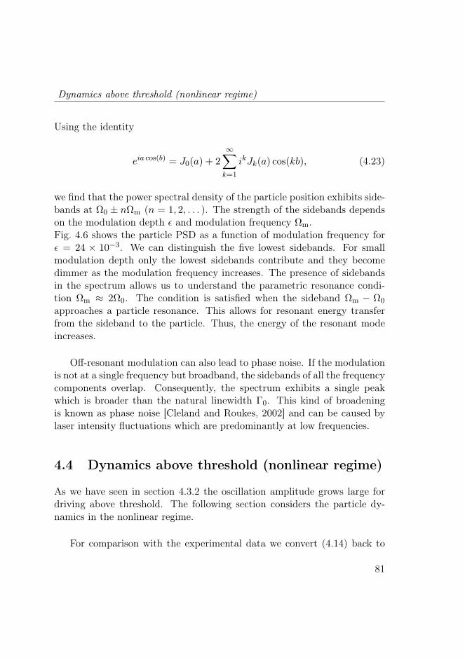
Dynamics above threshold (nonlinear regime)
Using the identity
eia cos(b) = J0(a) + 2∞∑k=1
ikJk(a) cos(kb), (4.23)
we find that the power spectral density of the particle position exhibits side-bands at Ω0 ± nΩm (n = 1, 2, . . . ). The strength of the sidebands dependson the modulation depth ϵ and modulation frequency Ωm.Fig. 4.6 shows the particle PSD as a function of modulation frequency forϵ = 24 × 10−3. We can distinguish the five lowest sidebands. For smallmodulation depth only the lowest sidebands contribute and they becomedimmer as the modulation frequency increases. The presence of sidebandsin the spectrum allows us to understand the parametric resonance condi-tion Ωm ≈ 2Ω0. The condition is satisfied when the sideband Ωm − Ω0
approaches a particle resonance. This allows for resonant energy transferfrom the sideband to the particle. Thus, the energy of the resonant modeincreases.
Off-resonant modulation can also lead to phase noise. If the modulationis not at a single frequency but broadband, the sidebands of all the frequencycomponents overlap. Consequently, the spectrum exhibits a single peakwhich is broader than the natural linewidth Γ0. This kind of broadeningis known as phase noise [Cleland and Roukes, 2002] and can be caused bylaser intensity fluctuations which are predominantly at low frequencies.
4.4 Dynamics above threshold (nonlinear regime)
As we have seen in section 4.3.2 the oscillation amplitude grows large fordriving above threshold. The following section considers the particle dy-namics in the nonlinear regime.
For comparison with the experimental data we convert (4.14) back to
81

Dynamics of a parametrically driven levitated particle
115 120 125 130 135
2
4
6
8
10
W @kHzD
Wm
@kH
zD
Figure 4.6: Low frequency modulation. For modulation frequenciesmuch smaller than the particle oscillation frequency, the PSD of the particleposition exhibits sidebands. The modulation depth is ϵ = 24× 10−3.
physical quantities
q2 =−1
ηδ2th
[3ξ
ηδm +Q−1 −
√ϵ2δ2th − δ2m + 3
ξ
ηQ−2
(2Qδm − 3
ξ
η
)]
≈ −1
ηδ2th
[3ξ
ηδm −
√ϵ2δ2th − δ2m
], (4.24)
whereδth =
√9ξ2 + η2 /2η . (4.25)
The approximation holds for Q ≫ 1. This is the case under typical experi-mental conditions and for simplicity we assume that Q → ∞ from here on.Note that we have dropped the amplitude solution with the negative sign,since it belongs to the unstable solution.
4.4.1 Nonlinear frequency shift
Additionally, typically ξ ≫ η (c.f. Eq. 5.3) and we can further approximateδth ≈ 3ξ /2η and
q2 ≈ − 4
3ξ[δm + ϵ/2] . (4.26)
For weak driving at nonzero detuning δm, the second term becomes negligi-ble and we obtain Ωm/2 = Ω0+3ξq2/8. Recalling that Ωm/2 is the particle
82

Dynamics above threshold (nonlinear regime)
oscillation frequency of the locked particle, the nonlinear frequency shift isgiven by
∆ΩNL = 3ξq2/8. (4.27)
4.4.2 Nonlinear instability
From (4.24) it follows that a solution only exists if
ϵ2δ2th − δ2m > 0. (4.28)
This condition plays a similar role as the linear stability condition (4.2).However, whereas (4.2) gives the parameter range for which the linear sys-tem is stable, (4.28) is the stability condition for the nonlinear solution.
4.4.3 Modulation frequency sweeps
In the following we consider the particle response for fixed modulation depthϵ as the modulation frequency Ωm is swept over the resonance of the x mo-tion at 2Ω0 ∼ 250kHz.
Fig. 4.7a shows a map of the particle energy as Ωm is increased from240 kHz to 255 kHz, for values of ϵ ranging from 1×10⁻³ to 24×10−3. For offresonant modulation, the particle energy remains at Teff =
mΩ20
2kBx2 ≈ 17K.
For modulation frequencies within the lock-in range, the particle energyincreases significantly. The lock-in region, as predicted by the linear stabilitycondition (4.3), is shown as black dashed lines.
Fig. 4.7b shows the frequency sweep performed in the opposite direc-tion. The high frequency threshold is still given by (4.3). However, the lowfrequency threshold is pushed towards lower frequencies (white dashed line)in agreement with the nonlinear stability condition (4.28).
Fig. 4.7c shows a horizontal cut through subfigures a and b indicatedby black dotted lines (ϵ = 22 × 10−3). When the instability region is ap-proached from below, the energy stays at Teff until the threshold is reached.Above threshold, the motion locks to the external modulation and the en-ergy is given by (4.24). As the modulation frequency is further increased,
83

Dynamics of a parametrically driven levitated particle
parameter method 1 method 2 combined
η [µm−2] 6.1 (±4%) 7.2 (±7%) 6.3 (±3%)
ξ[µm−2] −10.2 (±4%) −9.5 (±6%) −10.0 (±3%)
Table 4.1: Nonlinear coefficients extracted from experimental data of fre-quency sweeps. Method 1 extracts the parameters from the threshold valuescorresponding to figures 4.7d,e. Method 2 extracts the parameters from a fitto individual scans corresponding to figures 4.7c.
the particle energy makes a smooth transition to the off-resonant energy.Conversely, when the instability region is crossed from above, the energysmoothly increases as predicted by (4.24). Because of the (negative) Duff-ing nonlinearity, the increasing oscillation amplitude, pushes the effectiveresonance frequency Ωeff. = Ω0
(1 + 3
8ξx2)
to lower frequencies. Since thelock-in region depends on the resonance frequency, it is also dragged along.
From (4.28), we find the lower threshold frequency
Ωth = Ω0 [2− ϵδth] . (4.29)
where the particle energy falls back to the off-resonant value. At this mod-ulation frequency the particle’s oscillation amplitude reaches it’s maximumvalue
x2max =−3ξ
η2δthϵ. (4.30)
Fig. 4.7d,e show the threshold frequency Ωth and energy Emax = 12mΩ2
0x2max
together with their respective fits. From the fits and equations (4.29) and(4.30) we extract the nonlinear coefficients. Alternatively we obtain the non-linear coefficients from a fit of (4.24) to the modulation downward sweep(blue dashed curve Fig. 4.7c). The coefficients obtained with the two meth-ods are listed in table 4.1.
84

Dynamics above threshold (nonlinear regime)
1886 K/ 120 nm
4 K/ 4 nm
a b
up down
x2
up sweep
down sweep
T0
Te↵
c d
e
lock-in region down lock-in region up
fit
Emax
!!!!
!
!
!!!!!!!
!!!!!!!!!
!!!!!!!!!!!!!!
!!
!!!!!!!!!!!!!!!!!!!!!!!!!!!!!!!!!!!!!!!!!!!!!!!!!!!!!!!!!!!!!!!!!!!!!!!!!!!!
!
!
!
!!!!
!!!
!!!!!!!!!!!!!!!
!
!!!!!!!
"""
"
""""""""
""""""
"
"""
""
""""""""""""
"""""""""
""""
"""""""
""""""
"
"
"
""
"""""""""""
"
"""
""
""""""""""""""""""""""""
""
"""""""""
"
"
"""""
"""""""""""""""
240 255244 251.9249.3
17
303
1851
764
11
48
119
54
modulation frequency !m!2" "kHz#
Energy"K#
x"nm#
5 10 15 200
500
1000
1500
2000
modulation depth !10!3"
E max!K"
5 10 15 20
244245246247248249250
modulation depth !10!3"
"th#2#!k
Hz"
Figure 4.7: Frequency Sweep. (a) For fixed modulation depth and increas-ing modulation frequency, the particle energy maps out a triangular region inthe ϵ-Ωm plane. The black dashed line marks the instability threshold (4.3).(b) For decreasing modulation frequency, the lower instability threshold ispushed to lower frequencies. (c) Up and down sweep at ϵ = 22×10−3 (blackdotted line in subfigures a and b). The blue dashed line is a fit to (4.24).(d) Threshold modulation depth (white line in subfigure b) and (e) thresholdparticle energy as a function of modulation depth. The black arrows markthe data points which correspond to subfigure c.
4.4.4 Modulation depth sweeps
Next, we consider the situation where the modulation depth ϵ is variedwhile the modulation frequency Ωm is kept constant at a frequency close to
85

Dynamics of a parametrically driven levitated particle
resonance Ωm ≈ 2Ω0.
Fig. 4.8a shows a map of the particle energy as ϵ is increased from0.1 × 10−3 to 28 × 10−3, for values of Ωm ranging 247.5 kHz to 252.5 kHz.For the modulation depth given by the stability condition (4.3), the particleenergy remains at Teff ≈ 15K. For modulation depths above threshold(black dashed lines), the particle energy increases to the value given by(4.24).
Fig. 4.8b shows the modulation depth sweep performed in the oppositedirection. For modulation frequencies above resonance, the threshold is stillgiven by (4.3). In contrast, for modulation frequencies below resonance, theparticle continues to oscillate with high amplitude even if the modulationdepth is reduced significantly below the threshold value of the upward sweepdown to a minimum value ϵmin (white dashed line).
Fig. 4.8c shows a vertical cut through subfigures a and b indicatedby black dotted lines (Ωm = 248.3 kHz). When the modulation depth isincreased from zero, the particle energy stays at Teff until the thresholdϵ = 2δm is reached. Above threshold, the motion locks to the externalmodulation and the energy increases suddently to the value given by (4.24).As the modulation depth is further increased the particle energy increasesslowly. Conversely, when the modulation depth is reduced, the energy de-creases. However, the energy doesn’t fall back to Teff at ϵ = 2δm but con-tinues to follow the solution (4.24) until the minimum modulation depth
ϵth =δmδth
. (4.31)
At this modulation depth the amplitude is given by
x2min =−3ξ
η2δmϵ2th. (4.32)
Fig. 4.7d,e show the threshold modulation depth ϵth and energy Emin =12mΩ2
0x2min together with their respective fits. From the fits and equations
(4.31) and (4.32) we extract the nonlinear coefficients. Alternatively, weobtain the nonlinear coefficients from a fit of (4.24) to the modulation depth
86
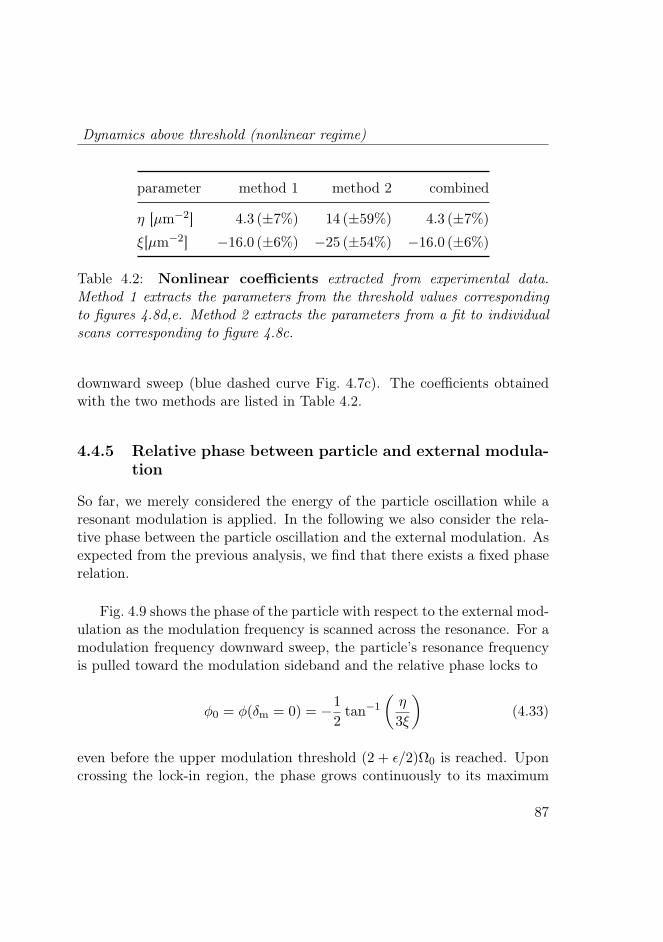
Dynamics above threshold (nonlinear regime)
parameter method 1 method 2 combined
η [µm−2] 4.3 (±7%) 14 (±59%) 4.3 (±7%)
ξ[µm−2] −16.0 (±6%) −25 (±54%) −16.0 (±6%)
Table 4.2: Nonlinear coefficients extracted from experimental data.Method 1 extracts the parameters from the threshold values correspondingto figures 4.8d,e. Method 2 extracts the parameters from a fit to individualscans corresponding to figure 4.8c.
downward sweep (blue dashed curve Fig. 4.7c). The coefficients obtainedwith the two methods are listed in Table 4.2.
4.4.5 Relative phase between particle and external modula-tion
So far, we merely considered the energy of the particle oscillation while aresonant modulation is applied. In the following we also consider the rela-tive phase between the particle oscillation and the external modulation. Asexpected from the previous analysis, we find that there exists a fixed phaserelation.
Fig. 4.9 shows the phase of the particle with respect to the external mod-ulation as the modulation frequency is scanned across the resonance. For amodulation frequency downward sweep, the particle’s resonance frequencyis pulled toward the modulation sideband and the relative phase locks to
ϕ0 = ϕ(δm = 0) = −1
2tan−1
(η
3ξ
)(4.33)
even before the upper modulation threshold (2 + ϵ/2)Ω0 is reached. Uponcrossing the lock-in region, the phase grows continuously to its maximum
87

Dynamics of a parametrically driven levitated particle
downup
a b
d
e
1886 K/ 120 nm
4 K/ 4 nm
up sweep
down sweep
T0
Te↵
fitEmin
!
!!!!!!
!
!
!!
!!
!
!!!
!!!
!
!!
!!!
!
!!
!!!!!!!
!
!
!!!!!!!!!!!!
"
"
""
"
"
"
""
"
"
"""""""
"
"
""
""
"
"
"
"""
"""""""
"
""""
"""
"
"
"""
0 5 10 15
20
386
! !10"3"
Energy!K"
clock-in region down lock-in region up
!!!
!
!!!!!
!
!!
!!!!!!
!
!!!!!
!!!
!
!!!
!!!!!!!!!!!!!!!!!!!
"""
"
""""
""""""""""""
""""""""""""""""""""""""""""""
0 5 10 15 20 25
15
300
1075
546
8
34
91
46
modulation depth ! !10"3"
Energy!K"
x!nm"
248.0 248.5 249.0 249.50
200
400
600
800
modulation frequency !kHz"
E min!K"
248.0 248.5 249.0 249.501234567
modulation frequency !kHz"
! min!10"3
"
Figure 4.8: Modulation depth sweep. (a) For fixed modulation frequencyand increasing modulation depth, the particle energy maps out a triangu-lar region in the ϵ-Ωm plane. The black dashed line marks the instabilitythreshold (4.3). (b) For decreasing modulation depth, the lower instabilitythreshold is pushed to lower modulation depth. (c) Up and down sweep atΩm = 248.3 kHz (black dotted line in subfigures a and b). The blue dashedline is a fit to (4.24). The inset shows up and down sweep above resonance,where no hysteresis is observed. (d) Threshold modulation depth (white linein subfigure b) and (e) threshold particle energy as a function of modulationdepth. The black arrows mark the data points which correspond to subfigurec.
88

Dynamics above threshold (nonlinear regime)
value1
ϕth = ϕ(δm = δth) =1
2tan−1
(3ξ
η
). (4.34)
This transition is accompanied by an increase in particle energy. For thenonlinear parameters obtained from a fit of the particle amplitude to (4.24),the theoretical phase according to (4.12) is shown as blue dashed line. Whenthe modulation frequency is swept in the opposite direction, the particlephase locks to ϕth as soon as the downward threshold modulation frequencyΩ(down)th is reached even though the amplitude remains at it’s off-resonant
value. The phase stays at ϕth until the upper Ω(up)th threshold is reached,
where the phase jumps to the solution given by (4.12).The high sensitivity of the phase to an external modulation over a widerange could be exploited to improve the sensitivity and bandwidth in thedetection of weak periodic signals.
4.4.6 Nonlinear mode coupling
Until now, we have neglected coupling between the three spatial modes.However, for large oscillation amplitudes, the modes couple because thetrap stiffness along a given direction depends on the oscillation amplitudealong any direction. The trap stiffness along x is of the form (c.f. chapter2)
k(x)trap = mΩ2
0
1−∑
i=x,y,z
ξ(x)i x2i
(4.35)
and respective expressions hold for the trap stiffness along y and z. Here,ξ(x)x = ξ is the Duffing nonlinearity we have considered so far and ξ
(x)y and
ξ(x)y are the nonlinear coupling coefficients to y and z, respectively. To il-
lustrate the nonlinear coupling we sweep the modulation frequency over awide range which covers both the x and the y resonance.
1Note that the relative phase is periodic with periodicity of π/2. Therefore, the phasewraps around to negative values when it becomes larger than π/4
89

Dynamics of a parametrically driven levitated particle
240 255244 251.9249.3
17
303
1851
764
11
48
119
54
modulation frequency m kHz
Ener
gyK
xnm
240 244. 250.7 2554
0
Π 4244. 251.9
0.107
0.679
m 2Π kHz
Φra
d
− π / 4
π / 4
a
b
c
up sweep
down sweep
up sweep
down sweep
1886 K/ 120 nm
4 K/ 4 nm
up
x2
down
Ω(up)thΩ(down)
th Ω(down)thΩ(up)
th
Figure 4.9: Phase in lock-in region (a) Relative phase ϕ between par-ticle oscillation and external modulation. As the lock in region is crossedfrom higher to lower modulation frequencies (red) the relative phase changescontinuously from close to in-phase (ϕ ≈ 0.1) to out-of-phase (ϕ ≈ π/4).Interestingly, when the modulation frequency is increased (black), the phaselocks to the external modulation as soon as Ω
(down)th is reached, while the
amplitude remains at a low value. The blue dashed line is Eq. (4.12) for theparameters obtained from the amplitude fit of subfigure b. (b) The particleamplitude in the same frequency as the phase shown in subfigure a. (c)Phase map of modulation frequency up and down sweep, respectively (upperrow) and corresponding amplitude maps (lower row). The amplitude mapsare identical to figures 4.7a,b. The range where the phase is locked to the ex-ternal modulation is larger than the range where the amplitude of the drivenparticle is above the background value.
Fig. 4.10 shows a map of a modulation frequency downward sweep withmodulation depth ϵ ∼ 8 × 10⁻³. The parametric modulation frequency is
90

Dynamics above threshold (nonlinear regime)
reduced from 285 kHz down to 230 kHz exciting the resonances of the x andy mode, respectively. Within the lock-in range energy is transferred to theparticle and the resonant mode is excited (c.f. Fig. 4.10a).
Fig. 4.10b,c show the spectra of the signals that correspond to x and ymotion of the particle as a function of modulation frequency. As discussedbefore, when the modulation frequency is close to resonance (Ωm ≈ 2Ω0),the mode locks to the external modulation and the particle energy of theresonant mode increases, while the energy of the other mode remains ata low value. However, an analysis of the power spectral density revealsthat both the frequency of the resonant mode and the frequency of the off-resonant mode are pulled to lower frequencies. This agrees with Eq. (4.35)with negative Duffing coefficients.
4.4.7 Sidebands
Aside from the oscillation at Ωm/2, the resonant mode exhibits sidebandsat Ωm/2+Ω±. The sidebands appear much weaker and much broader thanthe main peak. The origin of the sidebands can be understood from ananalysis of the dynamics of small deviations from the steady state.
To find the equation of motion for small perturbations δA from equi-librium, we make the ansatz A = A0 + δA and plug it into (4.8). Thisyields
d
dTδA =
(− γ0
2+ i
δm2
− 2
[1
8η − i
3
8
]|A0|2
)δA
−[1
8η − i
3
8
]A2
0δA∗ + i
ϵ
4δA∗ (4.36)
Now, making the ansatz δA = e−iϕ(ueiωT + v∗e−iωT ), we get(ueiωT + v∗e−iωT
)+ iω
(ueiωT − v∗e−iωT
)= i
ϵ
4ei2ϕ
[(v − u)eiωT + (u∗ − v∗)e−iωT
]−[1
8η − i
3
8
]a20[(u+ v)eiωT + (v∗ + u∗)e−iωT
].
91

Dynamics of a parametrically driven levitated particleEner
gy[K
]
115
120
125
130
130
135
140
145
x y
m/2 [kHz]
/2
[kHz]
280270260250240230
modulation sideband
natural mode x
lock-in range ylock-in range x
b
c
a
pulled mode x
pulled mode y
locked mode x
locked mode y
downward sweep
natural mode y
sidebands of locked motion
10
100
1000
z
Figure 4.10: Spectral map frequency down sweep. The parametricmodulation frequency is reduced from 285kHz down to 230 kHz exciting theresonances of the x and y mode, respectively. Within the lock-in rangeenergy is transferred to the particle and the resonant mode is excited. Theparticle oscillation of the resonant mode locks to the external modulationand oscillates at Ωm/2 with modulation sidebands at Ω±. Here, the pressureis 1.6 × 10⁻⁴mBar (Q ∼ 106). The modulation depth is ϵ = 8 × 10⁻³.(a) Only the mode near the lower modulation sideband Ω0 ≈ Ωm − Ω0 isexcited. The energy of the other modes remains at Teff . (b) PSD of x-modeon a logarithmic scale as a function of modulation frequency Ωm. Outsidethe lock-in range, the mode frequency stays at it’s natural value ∼ 126 kHz.Within the lock-in range, the mode frequency is half the external modulationfrequency. Within the lock-in range of the other mode, the frequency ispulled due to nonlinear coupling. However, the energy does not change. (c)PSD of y-mode as a function of modulation frequency Ωm.
92

Dynamics above threshold (nonlinear regime)
yielding two coupled equations of motion
u = −iωu−[1
8η − i
3
8
]a20(u+ v)− i
ϵ
4ei2ϕ(u− v)
v = −iωv −[1
8η + i
3
8
]a20(u+ v)− i
ϵ
4e−i2ϕ(u− v).
Applying the transformation
Ψ =
(cd
)= eiωTS−1
(uv
), S−1 =
(1 1−i i
), (4.37)
this readsΨ = HΨ (4.38)
with
H =
(−ηa20/4 ϵ cos(2ϕ)/23a20/4 ϵ sin(2ϕ)/2
).
Diagonalizing Λ = diag(λ+, λ−) = U−1HU with
U =
(−λ− − 1
4 ηa20 −λ+ − 1
4 ηa20
3a20/4 3a20/4
)(4.39)
where
λ± = − γ02
− η04a20 ± i
√3
4a20(
3
4a20 + δm)−
(γ02
)2
(4.40)
are the eigenvalues of H, we find the solutions
Φ = U−1Ψ =
(ϕ+ expλ+Tϕ∗− expλ−T
), (4.41)
where ϕ+, ϕ− are determined by the initial conditions. Transforming backto the original variables (
uv
)= e−iωTSUΦ, (4.42)
93

Dynamics of a parametrically driven levitated particle
we find
δA =e−iϕ
[(3
4a20 + γ0 +
1
4ηa20 + λ+
)ϕ+ − i
(3
4a20 − γ0 −
1
4ηa20 − λ+
)ϕ−
]eλ+T
+e−iϕ
[(3
4a20 + γ0 +
1
4ηa20 + λ−
)ϕ∗− − i
(3
4a20 − γ0 −
1
4ηa20 − λ−
)ϕ∗+
]eλ−T .
(4.43)
Thus, the frequencies of the modes of δA are given by (4.40) and conse-quently the sideband shift is
∆Ω± = ±
√3
4a20(
3
4a20 + δm)−
(γ02
)2
. (4.44)
Fig. 4.11 shows good agreement between the experimentally measuredsideband shift of the y-mode and the theoretically expected shift (4.44).
265 270 275 280 285
!2
!1
0
1
2
mod. Freq. " !kHz"
SidebandShift#"!kHz"
+
Theory
Experiment
data
fit
th/2
265 270 275 280 2850
20
40
60
80
100
120
140
mod. Freq. !m !kHz"
oscillationamplitude!nm"
a bqmax
Figure 4.11: Sidebands. (a) Y-mode oscillation amplitude of frequencydown sweep (c.f. Fig. 4.10a). To good approximation, the nonlinear dampingand nonlinear Duffing coefficient determine the cut-off frequency Ωth andmaximum amplitude qmax, respectively. Fitting the experimental data to(4.14), we extract the nonlinear coefficients ξ = −9µm−2 and η = 0.6µm−2.(b) Sidebands of y-mode as a function of modulation frequency Ωm. Opencircles are the experimental data and dashed lines are the theoretical curves(4.40).
94

Conclusions
4.5 Conclusions
In conclusion, we have parametrically excited an optically trapped nanopar-ticle well into the nonlinear regime. We have shown that each of the three in-dividual spatial modes can be excited independently while the other modesare cooled by parametric feedback. We can measure the parameters ofthe nanomechanical oscillator by performing either amplitude or frequencysweeps of the external modulation. This provides a method to measurethe nonlinear damping induced by parametric feedback cooling and conse-quently to optimise the feedback parameters.
Thus far, we have primarily focused on a one-dimensional descriptionof the particle equation of motion. However, there remains still room forfurther investigation of the full three dimensional dynamics. In particular,the response to resonant (multi-frequency) driving fields is not fully under-stood. Beside CoM motion, the levitated dielectric particle can also rotatefreely [Arita et al., 2011, 2013]. Further investigation along this line willpotentially reveal valuable insights into ultimate performance limits of alevitated nanoparticle in high vacuum.
95

Dynamics of a parametrically driven levitated particle
96

CHAPTER 5
Thermal nonlinearities in ananomechanical oscillator
Nano- and micromechanical oscillators with high quality (Q) factors havegained much attention for their potential application as ultrasensitive detec-tors. In contrast to micro-fabricated devices, optically trapped nanoparticlesin vacuum do not suffer from clamping losses, hence leading to much largerQ-factors. We find that for a levitated nanoparticle the thermal energy suf-fices to drive the motion of the nanoparticle into the nonlinear regime. First,we experimentally measure and fully characterize the frequency fluctuationsoriginating from thermal motion and nonlinearities. Second, we demon-strate that feedback cooling can be used to mitigate these fluctuations. Thehigh level of control allows us to fully exploit the force sensing capabilities ofthe nanoresonator. Our approach offers a force sensitivity of 20 zNHz−1/2,which is the highest value reported to date at room temperature, sufficientto sense ultra-weak interactions, such as non-Newtonian gravity-like forces.
97

Thermal nonlinearities in a nanomechanical oscillator
5.1 Introduction
Recent developments in optomechanics have evolved toward smaller andlighter resonators featuring high quality (Q) factors, which are importantfor the sensing of tiny masses [Chaste et al., 2012; Yang et al., 2006], charges[Cleland and Roukes, 1998], magnetic fields [Rugar et al., 2004] and weakforces [Stipe et al., 2001; Moser et al., 2013]. The presence of a force fieldor the adhesion of a small mass induces a change in the mechanical re-sponse and can be monitored by tracking either the oscillation frequency,phase or its amplitude. Ultimately, dissipation losses as well as thermome-chanical noise and temperature fluctuations limit the Q-factors of clampedoscillators and consequently their sensing performance [Postma et al., 2005;Cleland and Roukes, 2002; Ekinci et al., 2004]. This can be circumventedby using an optically trapped nanoparticle in high vacuum. Indeed, theQ-factor of a levitated particle is only limited by collisions with residual airmolecules and can potentially reach 1012 for small particles in ultra high-vacuum [Ashkin, 1971; Gieseler et al., 2012; Li et al., 2011; Romero-Isartet al., 2010; Chang et al., 2010]. In this chapter we first show that anoptically trapped nanoparticle is sufficiently sensitive that thermal forcesdrive it out of its linear regime. Additionally, we demonstrate that feed-back cooling can be used to mitigate frequency fluctuations associated withthe thermal nonlinearities thereby recovering the force sensing capabilitiesof the oscillator.
5.2 Description of the experiment
In our experiment, a silica nanoparticle with diameter ∼ 75nm is trappedat room temperatue in the focal region of a tightly focused NIR laserbeam (λ = 1064nm, polarized along the x-axis). The intensity near thefocus of the objective (NA = 0.8) can be well approximated by Gaus-sian functions (c.f. Fig.5.1), defining a focal volume of wx × wy × wz ≈0.69µm×0.54µm×1.36µm 1. For large displacements, the optical potential
1estimated from numerical calculation of a highly focused beam with NA=0.8
98

Description of the experiment
w0
Figure 5.1: Experimental configuration A silica nanoparticle is trappedby a tightly focused laser beam. Random collisions with residual airmolecules drive the particle into the nonlinear regime of the potential. (in-set) The focal intensity distribution forms a trap which can be approximatedby a Gaussian potential (white). The deviation from a harmonic potential(red) is described by a Duffing nonlinearity.
becomes anharmonic featuring a Duffing nonlinearity. For a Gaussian fielddistribution the nonlinear coefficients are given by
ξj = −2/wj2, (5.1)
where wi is the beam waist radius or Rayleigh range. For small displace-ments |qi| ≪ |ξ−1/2
j |, the nonlinearity is negligible and the three motionaldegrees of freedom decouple. Due to the asymmetry of the optical focus,the oscillation frequencies Ωi = (ki/m)1/2 along the three major axes aredifferent (Ωz/2π = 37kHz, Ωx/2π = 125kHz, Ωy/2π = 135kHz). The lin-ear trap stiffness is given by ki = αE2
0/w2i , where E0 is the electric field
intensity at the focus. The gradient of the optical intensity distributionexerts a restoring force F grad
i = −ki
(1 +
∑j=x,y,z ξjq
2j
)qi on a dipolar par-
ticle with polarizability α, that is displaced from the trap center by xi.For a sphere of radius a and dielectric constant ϵp, the polarizability isα = 4πa3ϵ0(ϵp − 1) /(ϵp + 2) , ϵ0 being the vacuum permittivity.
99

Thermal nonlinearities in a nanomechanical oscillator
We experimentally determine the nonlinear coefficients by parametricexcitation through modulation of the trapping laser at a frequency closethe parametric resonance Ωmod ≈ 2Ωi and find
(ξz, ξx, ξy) = (−0.98,−7.95,−10.41)µm−2, (5.2)
in good agreement with the values estimated from the size of the focus (5.1)(c.f. chapter 4).
5.2.1 Origin of nonlinear frequency shift
The equation of motion for each spatial degree of freedom (i = x, y, z) isgiven by
qi +ΩiQ−1i qi +Ω2
i
1 +∑
j=x,y,z
ξjq2j
xi = Ffluct /m . (5.3)
In the following we concentrate on a single degree of freedom and denotethe corresponding resonance frequency by Ω0 and the quality factor byQ. Random collisions with residual air molecules provide both dampingΓ0 = Ω0Q
−1 and stochastic excitation Ffluct of the trapped nanoparticle.From kinetic theory we find that the damping coefficient of a particle in ararified gas is given by [Epstein, 1923; Chang et al., 2010]
Γ0 =64a2
3mvP, (5.4)
where v = (8kBT/πµ)1/2 is the average velocity and µ is the weight of
the air molecules [O’Hanlon, 2003]. The random force Ffluct is related to thedamping coefficient by the fluctuation-dissipation theorem ⟨Ffluct(t)Ffluct(t
′)⟩ =2mΓ0kBT0δ(t− t′). The damping coefficient determines the frequency sta-bility of the harmonic oscillator ∆ΩL = Ω0Q
−1, and the temperature-dependent stochastic excitations determine the minimum oscillation am-plitude according to qth =
√2kBT0
/mΩ2
0 . The thermal amplitude qth is
100

Description of the experiment
usually small compared to the dimensions of the oscillator. However, fora small and hence light oscillator like our levitated nanoparticle, the ther-mal amplitude eventually becomes comparable to the particle size. Conse-quently, a proper description of the particle motion requires the inclusion ofnonlinearities. The latter give rise to a frequency shift ∆ΩNL = 3ξΩ0/8 q
2th
[Dykman and Krivoglaz, 1984; Lifshitz and Cross, 2009]. In contrast tolinear thermal frequency fluctuations, nonlinear frequency fluctuations addfrequency noise but do not affect the damping.
In order to resolve the nonlinear frequency shift originating from thermalmotion, the nonlinear contribution must be larger than the linear one, thatis
R =∆ΩNL
∆ΩL=
3ξQkBT0
4Ω20m
≫ 1, (5.5)
where T0 is the temperature of the residual gas and kB is Boltzmann’s con-stant. To fulfil condition (5.5) a light and high-Q mechanical resonator isrequired. In our experiment, m = 3× 10⁻¹⁸kg and Q = 108, as determinedin a ring-down measurement at a pressure of Pgas = 0.5×10⁻⁶mBar. Theseparameters place us well into the nonlinear regime. Importantly, the depen-dence of the Q-factor on pressure Pgas allows us to continuously tune thesystem between the linear and nonlinear regimes.
5.2.2 Nonlinear spectra
To demonstrate the differences between a thermally driven harmonic oscil-lator (R ≪ 1) and an anharmonic oscillator (R ≫ 1), we compare the parti-cle’s motion at high pressure (6mBar) and at low pressure (1.2×10⁻²mBar).These pressures correspond to Q-factors of 25 and 12×103, respectively. Athigh pressures (low Q) the dominant source of frequency fluctuations is lin-ear damping ∆ΩL = Γ0 and the power spectral density (PSD) of the particlemotion features a single symmetric Lorenzian peak, whose width is equal tothe linear damping coefficient Γ0 (Fig. 5.2b). In contrast, at low pressure(high Q) nonlinear frequency fluctuations ∆ΩNL = 3ξΩ0 /8 q2th dominate
101

Thermal nonlinearities in a nanomechanical oscillator
and we observe an asymmetric peak that is considerably broader than whatis expected for the equivalent linear oscillator. However, if we limit theobservation time to time intervals 1/∆ΩNL < τ < 1/∆ΩL, we find a cleanoscillation with an almost constant amplitude, corresponding to a narrowand symmetric peak in the frequency domain. For large oscillation ampli-tudes the peak appears down-shifted, consistent with the measured negativeDuffing nonlinearity. Consequently, for observation times ≫ 1/∆ΩNL, thenon-Lorenzian peak becomes a weighted average [Dykman et al., 1990]
SNL(Ω) =
∫ρ(E)SL(Ω, E)dE, (5.6)
over Lorenzian peaks centred at the shifted frequency Ω0(E) = Ω0+3ξ/(4mΩ0)Eand weighted by the Gibbs distribution ρ(E) = Z−1 exp(−E/kBT0). Here,Z =
∫ρ(E)dE is the partition function and
SL(Ω, E) =E
πmΩ20
Γ0(Ω− Ω0(E)
)2+ (Γ0/2)2
. (5.7)
is the power spectral density of a harmonic oscillator with frequency Ω0(E)and energy E.Note that (5.6) is valid in the low friction limit (Q ≫ 1). An expressionwhich holds for arbitrary R can be found in [Dykman and Krivoglaz, 1984].
102

Description of the experiment
a
d
b
c
e
Figure 5.2: Nonlinearity-induced frequency fluctuations (a) Timetrace of the particle motion along x at 1.2×10⁻²mBar. The oscillation am-plitude changes randomly and the positions are normally distributed. (b,c)However, on time scales short compared to the relaxation time τ , the particlemotion is sinusoidal with a constant oscillation amplitude over many cyclesand has a position distribution featuring two lobes (subfigure (a) right). Thepart of the timetrace when the particle oscillates with a large (small) ampli-tude is shown in red (green). (d) From the long time trace (black) and theshort time traces (red, green) we calculate the power spectral density (PSD).For short observation times we observe a Fourier limited symmetric PSDwith an amplitude dependent center frequency. The overall PSD (black) re-sults from a temporal average of the instantaneous PSDs (red, green). Incontrast, the PSD of a low Q oscillator (blue) is described by a Lorentzianpeak at all times (red thin line). (e) Time trace of particle motion at 6mBarused to calculate the (blue) Lorentzian PSD in subfigure (b).
103

Thermal nonlinearities in a nanomechanical oscillator
5.3 Experimental results
In what follows we present further evidence that the observed frequencyfluctuations are a consequence of thermal motion in the nonlinear optical po-tential. We analyze the correlations between the instantaneous frequenciesand energies and we investigate the pressure dependence of the frequencyfluctuations.
To quantify the frequency fluctuations, we continuously measure the in-stantaneous energy Ei(tj) and frequency Ωi(tj) of the three spatial modes(i = x, y, z), given by the area and the position of the maximum of the in-stantaneous PSDs, respectively (c.f. Fig. 5.2d). The instantaneous PSDs arecalculated from position time traces x(j)i (t) (where tj − τ/2 < t < tj + τ/2)of τ = 20ms duration. Figs. 5.3a,b show the timetraces of the relative fre-quency fluctuations Ωi/⟨Ωi⟩ of the three modes for high Q (low pressure)and low Q (high pressure), respectively. Fig. 5.3c shows the correlationsbetween Ei and Ωi as a function of pressure, calculated from 30min longtime traces. The nonlinearity is conservative and, thus, doesn’t change theparticle energy, which is determined only by random molecule collisions.Therefore, the energy of the three degrees of freedom are uncorrelated. Incontrast, a change in energy of one mode shifts the frequency of all modes(Eq. 5.3). At low pressure (R > 1), the nonlinearities dominate and thefrequency fluctuations are highly correlated. In contrast, at high pressure(R < 1), linear damping dominates and consequently the frequencies be-come uncorrelated.
5.3.1 Frequency and energy correlations
In Figure 5.3d we plot the oscillator amplitude response to parametric mod-ulation (black) and to thermal excitation (scatter plot) at a pressure of10−5 mBar. Independently of the origin of the excitation, there is a lin-ear relationship between the particle’s energy and the particle’s oscillationfrequency. However, while the response to an excitation at a fixed fre-quency is sharp, the thermal response is downshifted and much broader.Indeed, according to Eq. 5.3, an average thermal excitation of the orthog-
104

Experimental results
!!!!!!!!!!!!!!!!!!!!!!!!!!!!!!!!!!!!!!!!!!!!!!!!!!!!!!!!!!!!!!!!!
!!!!!!!!!!!
116 120 1250
0.01
0.02
frequency !x!2" "kHz#x2"#m2 #
!!! ! ! ! ! !
!"""
" " " " "
"### # # # # #
#
$$$ $$ $
$$
$
%%% %% %
%%
%
&&& & & & & &
&
10!5 10!3 10!1 1010
0.5
1
pressure !mBar"correlations
b
a
zxy
0 10 20 30 400.96
0.98
1
1.02
time !s"
rel.freq.fluct.
0 10 20 30 400.96
0.98
1
1.02
time !s"
rel.freq.fluct.
c
2.5 kHz
z-x
z-y
x-ya
b
d
Figure 5.3: Frequency and energy correlation. (a) Time traces of theinstantaneous oscillation frequencies Ωx, Ωy and Ωz evaluated at low pres-sure and (b) at high pressure. (c) Frequency and energy correlations as afunction of pressure. The energies (dashed, lower curves) are uncorrelatedand independent of pressure. The frequencies (solid, upper curves) are corre-lated at low pressure where nonlinear fluctuations dominate and uncorrelatedat high pressure, where linear fluctuations dominate. The points labeled ’a’and ’b’ indicate the pressures at which figures (a) and (b) were evaluated.(d) Energy vs. frequency for the oscillator in x-direction (x mode) obtainedfrom both random fluctuations (colored density plot) and from parametricexcitation (black). The thermal excitation of the orthogonal modes (y, z)shifts the resonance by ≈ 2.5 kHz in good agreement with the value esti-mated from the thermal amplitude and the measured nonlinear coefficients.
onal modes (y and z) leads to an average shift the frequency of the modeunder consideration (here x). The shift of the center of the frequency dis-tribution (≈ 2.5kHz) is in good agreement with the value estimated fromthe measured nonlinear coefficients and average thermal amplitudes (sup-
105

Thermal nonlinearities in a nanomechanical oscillator
plementary information). Additionally, since the amplitudes of the modesfluctuate independently (c.f. Fig. 5.3c), we get a distribution of frequenciesfor a given oscillation amplitude of the considered mode. In contrast, whenwe drive the system parametrically at a fixed frequency, we simultaneouslycool the orthogonal modes. Therefore, the contribution to the frequencyshift originating from the orthogonal modes is negligible and we obtain asharp response.
5.3.2 Pressure dependence of frequency fluctuations
In figure 5.4 we show the power spectral density of the relative frequencyΩ/Ω0 (fPSD) as a function of pressure. The fPSDs are calculated from30min long timetraces of the instantaneous frequencies (c.f. Fig.5.3). Forlow Q, the fPSD is flat as expected for a harmonic oscillator. In contrast forhigh Q the nonlinear coupling maps the Lorenzian power spectral density ofthe amplitude onto the frequency power spectral density, which is thereforegiven by
Sf(Ω) = IΩc/π
Ω2 +Ω2c
, (5.8)
where I is the total spectral power, which is independent of pressure. Thecharacteristic cut-off frequency Ωc has a clear pressure dependence, as shownin Fig. 5.4c. This further confirms that the fluctuations arise as a combi-nation of nonlinearities and thermal excitations.
The small mass and high Q-factor make the levitated nanoparticle an ul-trasensitive force sensor with sensitivity of SF = 4kBTmΩ0/Q ≈ (20zN)2/Hzat room temperature, which compares to the best values achieved at cryo-genic temperatures [Moser et al., 2013]. There are several ways to couple aforce to a levitated nanoparticle, including electric [Li et al., 2011] and mag-netic [Neukirch et al., 2013; Geiselmann et al., 2013] coupling or more subtleforces due to fluctuating charges within the particle [Zurita-Sánchez et al.,2004]. Additionally, in contrast to trapped ions [Knünz et al., 2010], thestill considerable mass of the particle makes it susceptible to gravitationalforces [Arvanitaki and Geraci, 2013].
106

Experimental results
x
z
ylaser
x
z
y
laser
x
z
ylaser
a b
cd
!
!
!
!
!
!
!!
"
"
"
"
"
"
""
#
#
#
#
#
#
##
10!5 10!4 10!3 10!20.02
0.1
1
4
pressure !mBar"cutofffrequency!Hz"
Figure 5.4: Pressure dependence of frequency fluctuations. Pressuredependence of frequency fluctuations. (a) At high pressures (6mBar), thefluctuations are solely determined by the linear damping (low Q). (b) Whenthe Q factor becomes larger (1e-5mBar), the fluctuations are dominatedby nonlinear amplitude-frequency conversion. In this case, the frequencypower spectral density (fPSD) exhibits a characteristic cut-off, which weextract from a fit to (5.8) (black dashed line). (c) The characteristic cut-offfrequency depends on the Q factor which scales linearly with pressure. (d)Using feedback cooling, the fluctuations can be suppressed to the level of thelaser intensity fluctuations (gray).
In addition to constant forces, a levitated nanoparticle can detect posi-tion dependent forces. A position dependent force causes a frequency shift.Therefore, following the resonance frequencies of the nanoparticle allows formeasuring a force gradient with a precision given by the noise floor of thefrequency fluctuations. In practice though, as shown above nonlinear effectslead to frequency fluctuations in ultra-high Q oscillators. It is possible tosurpass this limit by operating the oscillator at special points [Villanueva
107

Thermal nonlinearities in a nanomechanical oscillator
et al., 2013]. Furthermore, as we show in the following, nonlinear frequencyfluctuations can also be suppressed by feedback cooling [Gieseler et al.,2012]. Feedback cooling lowers the oscillation amplitude and therefore re-duces the thermal motion of the oscillator. Under the action of feedback,the effective temperature reduces to Teff = (Γ0/Γfb)T , where Γfb is the totaldamping with feedback [Mertz et al., 1993; Gieseler et al., 2012]. As shownin Fig.5.4d, we manage to reduce the frequency fluctuations to the level ofthe laser intensity fluctuations, which become the main source of frequencynoise. Using active stabilization techniques, relative laser intensity noisecan be brought to the level of 10−8/
√Hz [Seifert et al., 2006].
5.3.3 Frequency stabilization by feedback cooling
We demonstrate the improved sensitivity by mimicking a periodic potentiallandscape. A modulation at 50mHz is applied to the trapping laser. Themodulation causes a variation of the force gradient, which is measured asa frequency shift. As shown in Fig. 5.5, without feedback the signal isoverwhelmed by noise while with feedback, the fluctuations are suppresseddown to the level of laser intensity fluctuations and the applied signal isclearly visible. Using feedback cooling, we are able to improve the sensitivityof the oscillator by two orders of magnitude and achieve a relative frequencynoise floor of
√Sf/Ω0 of 3 × 10⁻³/
√Hz for frequencies below 1 Hz and
1 × 10⁻⁴/√Hz for frequencies larger than 10Hz. In the absence of laser
intensity noise the highest sensitivity is obtained when linear and nonlinearfluctuations contribute equally. However, since cooling to Teff = T Qeff/Qis required to reduce nonlinear frequency fluctuations, the effective Q-factoris reduced, too. The best compromise is achieved when the linear and the
108

Conclusion
nonlinear frequency fluctuations contribute equally, that is
∆ΩL =∆ΩNL
Ω0Q−1eff =
3
8ξΩ0r
2eff =
3ξΩ0kBTeff
4mΩ20
⇒ Q(opt)eff =
√4
3
mΩ20
ξkBTQ = R−1/2Q. (5.9)
Thus, under the assumption that with cooling the oscillation remains inthe linear regime, the frequency spectral density is given by
S(opt)f =
Ω0
Q(opt)eff
=Ω0
QR1/2. (5.10)
For the values presented here we obtain√
S(opt)f /Ω0 ∼ 10−6/
√Hz, suffi-
cient to sense ultraweak interactions, such as non-Newtonian gravity-likeforces [Geraci et al., 2010]. However, to reach this value, relative intensityfluctuation have to be suppressed down to the same level.
The ultimate cooling limit is defined by the zero point motion qzp =√h /2mΩ0 . In order to resolve the nonlinear frequency shift due to the
zero point motion ∆Ωzp, the condition
∆Ωzp
∆ΩL=
3
8Qξq2zp ≫ 1 (5.11)
has to be satisfied in analogy to (5.5). This requires a Q factor ofQ = Ω0/∆Ωzp ≈ 1010. In absence of other noise sources, this regime isreached for pressures below 10−8mBar.
5.4 Conclusion
In conclusion, we have demonstrated that a laser-trapped nanoscale par-ticle in high vacuum defines an ultrasensitive force sensor. The thermalmotion of the residual gas drives the nanoparticle into its nonlinear regime,
109

Thermal nonlinearities in a nanomechanical oscillator
0 50 100
0.99
1.01
time !s"
rel.freq
0.001 0.01 0.1 1 1010!7
10!5
0.001
0.1
frequency !Hz"
fPSD!1#Hz
"
Figure 5.5: Detection of a Periodic force gradient using feedbackcooling. A periodic potential landscape is emulated by modulating the trap-ping frequency at 50mHz. In absence of feedback cooling the small signal isoverwhelmed by noise (red). Feedback cooling reduces the random frequencyfluctuations thereby making it possible to detect the signal (blue). (inset)Time domain signal of relative frequency with (blue) and without feedback(red).
which gives rise to frequency fluctuations. Using a parametric feedbackcooling scheme, we can stabilize the nanoparticle and suppress its nonlin-earities, without sacrificing sensitivity. We expect that feedback-controllednanoparticles will find applications for sensing a wide range of interactions,including van der Waals and Casimir forces [Geraci et al., 2010], nuclearspins [Rugar et al., 2004], and gravitation [Arvanitaki and Geraci, 2013].
110
CHAPTER 6
Dynamic relaxation from an initialnon-equilibrium steady state
Fluctuation theorems are a generalisation of thermodynamics on smallscales and have been established as tools to measure thermodynamic quanti-ties in non-equilibrium mesoscopic systems. Here, we study experimentallyand theoretically non-equilibrium relaxation of a vacuum trapped nanopar-ticle from an initial steady state distribution to thermal equilibrium andshow that the Crooks fluctuation theorem holds. The here established frame-work allows to study experimentally non-equilibrium fluctuation theoremsfor arbitrary steady states and can be extended to investigate experimentallyquantum fluctuation theorems or systems which do not obey detailed balance.
6.1 Introduction
One of the tenets of statistical physics is the central limit theorem. Itallows to reduce many microscopic degrees of freedom ui (i = 1 . . . N ,N = O(1023)) to only a few macroscopic degrees of freedom U . The cen-tral limit theorem states that, independently of the distributions of the ui,
111

Dynamic relaxation from an initial non-equilibrium steady state
a macroscopic extensive quantity U , such as the total energy of a systemwith N degrees of freedom follows a Gaussian distribution with a meanvalue ⟨U⟩ ∝ N and variance σ2
U ∝ N . Consequently, for N → ∞, the rela-tive fluctuations σU/⟨U⟩ → 0 vanish and the macroscopic quantity becomessharp. However, with the advance of nanotechnology it is now possible tostudy experimentally systems small enough that the relative fluctuationsare comparable to the mean value. This gives rise to new physics whereclassical thermodynamic relations such as the second law of thermodynam-ics appear to be violated [Wang et al., 2002]. The statistical propertiesof the fluctuations are described by mathematical relations known as fluc-tuation theorems [Crooks, 1999; Jarzynski, 1997; Bochkov and Kuzovlev,1981; Machlup and Onsager, 1953], which in the limit N → ∞ recover themacroscopic thermodynamic relations.
Fluctuation relations are particularly important to understand funda-mental chemical and biological processes, which occur on the mesoscalewhere the dynamics are dominated by thermal fluctuations [Bustamanteet al., 2005]. They allow us, for instance, to relate the work along non-equilibrium trajectories to thermodynamic free-energy differences [Alemanyet al., 2012; Collin et al., 2005]. Fluctuation theorems have been experimen-tally tested on a variety of systems including pendulums [Douarche et al.,2006], trapped microspheres [Wang et al., 2002], electric circuits [Garnierand Ciliberto, 2005], electron tunneling [Küng et al., 2012; Saira et al., 2012],two-level systems [Schuler et al., 2005] and single molecules [Hummer andSzabo, 2001; Liphardt et al., 2002]. Most experiments are described byan overdamped Langevin equation. However, systems in the underdampedregime, or in quantum systems where the concept of classical trajectorylooses its usual meaning [Alemany et al., 2011], are less explored.
Here, we study experimentally the thermal relaxation of non-Gaussiansteady states of a highly underdamped nanomechanical oscillator. Becauseof the low damping, the dynamics can be precisely controlled even at thequantum level [Teufel et al., 2011; Chan et al., 2011; O’Connell et al., 2010].This high level of control allows to produce non-thermal steady states andmakes them ideal candidates for investigating non-equilibrium fluctuationsfor transitions between arbitrary steady states. To prove the basic concept
112

Description of the experiment
of our approach, we investigate the relaxation of non-thermal initial states tothermal equilibrium. While for the initial steady state detailed balance canbe violated, the relaxation dynamics are described by the Langevin equationwhich satisfies detailed balance and we can prove that the Crooks fluctua-tion theorem is fulfilled. Our experimental framework naturally extends tostudy transitions between arbitrary steady states and even to experimen-tally investigate quantum fluctuation theorems [Huber et al., 2008] for ananomechanical oscillator prepared in a quantum state [Teufel et al., 2011;Chan et al., 2011; O’Connell et al., 2010].
6.2 Description of the experiment
The experimental configuration is shown in Fig. 6.1. We consider a silicananoparticle of radius a ∼ 75nm and mass m ∼ 3×10⁻¹⁸ kg that is trappedin vacuum by an optical tweezer (Fig. 6.1). Within the trap, the particleoscillates in all three spatial directions. To first approximation, the threemotional degrees of freedom are well decoupled. Hence, the particle positionq is described by the following one-dimensional equation of motion
q + Γ0q +Ω20q = (Ffluct + Fext) /m, (6.1)
where Ω0 /2π ∼ 125kHz is the particle’s angular frequency along the di-rection of interest, Γ0 the friction coefficient and Fext is an externallyapplied force. The random nature of the collisions does not only pro-vide deterministic damping Γ0 but also a stochastic force Ffluct that ther-malises the energy of the particle. The fluctuation-dissipation theoremlinks the damping rate intimately to the strength of the stochastic force⟨Ffluct(t)Ffluct(t
′)⟩ = 2mΓ0kBT0δ(t − t′), with T0 being the bath tempera-ture and kB Boltzmann’s constant.The energy of the free harmonic oscillator with displacement q and mo-
mentum p is given by
E(q, p) =1
2
(mΩ2
0q2 + p2/m
)=
1
2mΩ2
0q0(t)2, (6.2)
113

Dynamic relaxation from an initial non-equilibrium steady state
where in the second part we use the slowly-varying amplitude approxima-tion (q(t) = q0 sin(Ω0t), q0 ≪ Ω0q0). This approximation is well satisfiedin our experiments since it takes several oscillation periods for the particleamplitude to change (inset Fig. 6.2a).
Applying an external force Fext, the system is initially prepared in asteady state with distribution ρss(u, α), where u = q, p describes thestate of the system. At time t = toff the external force is switched off andwe follow the evolution of the undisturbed system. Here, α denotes one or
x
y
zzzzz
+feedback
20
parametric drivem,
ton
to↵
Figure 6.1: Experimental setup. The particle is trapped by a tightlyfocused laser beam. In a first experiment, the particle is initially cooled byparametric feedback. At time t = toff the feedback is switched off and theparticle trajectory is followed as it relaxes to equilibrium. After relaxation,the feedback is switched on again and the experiment is repeated. In a secondexperiment the particle is initially excited by an external modulation in aaddition to feedback cooling. Again at a time t = toff , both the feedback andthe external modulation are switched off and the particle is monitored as itrelaxes.
114
Description of the experiment
several parameters such as the strength of the feedback mechanism, whichdetermines the initial steady state distribution. In general, ρss(u, α) is notknown analytically.
6.2.1 Average energy relaxation
We derive from (6.1) the corresponding stochastic differential equation forthe energy E of the unperturbed system1 (c.f. Eq. 3.29):
dE = −Γ0 (E − kBT0) dt+√E√
Γ0kBT0dW, (6.3)
which has a deterministic and stochastic contribution. Carrying out anaverage over noise realisations and exploiting that ⟨dW ⟩ = 0, the ensembleaverage of the energy evolves according to
d⟨E⟩dt
= −Γ0⟨E⟩+ Γ0kBT0. (6.4)
This differential equation can be easily solved yielding an exponential re-laxation of the average energy to its equilibrium value of kBT0
⟨E(t)⟩ = kBT0 + [⟨E(0)⟩ − kBT0]e−Γ0t, (6.5)
where ⟨E(0)⟩ is the average energy at time 0.
According to Eq. 6.5, we expect the particle’s energy to increase (de-crease) as it relaxes to equilibrium if the particle’s initial energy is below(above) the energy of the thermal bath. However, due to the smallness ofthe system, there is also a finite probability that molecule collisions furtherdecrease (increases) the particle’s energy. In the following section we showthat the fluctuation theorem
Pt(Y )
Pt(−Y )= e−Y . (6.6)
1i.e. the feedback or any other modulation is off
115

Dynamic relaxation from an initial non-equilibrium steady state
holds for the a quantity Y , which accounts for the contribution of feedbackto the particle energy. Eq. 6.6 links the probability of observing a processwere Y increases to the probability of observing a process where Y decreases.Since Y is an extensive quantity, irreversibility for macroscopic systems isa direct consequence of the fluctuation theorem.
6.3 Fluctuation theorem
The fluctuation theorem for relaxation from an arbitrary initial distributioncan be derived based on two conditions:
momentum (time) reversal symmetry for all times and
detailed balance for t > 0.
Since the energy is quadratic in the momentum p, the former condition isalways fulfilled if the distribution is a function of the energy only. This isthe case for parametric feedback cooling. The latter condition is fulfilledfor a system evolving according to a Langevin equation.
6.3.1 General case
Consider the relaxation from an initial steady state distribution
ρss(u, α) =1
Zαexp −β0Hα , (6.7)
to the equilibrium distribution
ρeq(u) =1
Zexp−β0E, (6.8)
where β0 = 1/kBT0 is the inverse temperature of the thermal bath andwhere Zα =
∫duρss(u, α) and Z = 2πkBT0/Ω0 are the partition functions
of the initial distribution and the final equilibrium distribution, respectively.The initial distribution is determined by the total energy
Hα(u) = E(u)−Mα(u), (6.9)
116

Fluctuation theorem
which we can write as the sum of the particle energy and the (negative)feedback energy Mα(u). To proof (6.6), we introduce
Y (u, v) = M(v)−M(u) = ∆E − β−10 ∆ϕ, (6.10)
which measures the difference in feedback energy between states u andv. For a simplified notation we have introduced ∆E = E(v) − E(u) and∆ϕ = ϕα(v)− ϕα(u) = β0∆Hα.
The distribution of Y at time t is obtained by averaging over all initialconditions u0 and all possible trajectory endpoints ut after time t
Pt(Y ) =
∫du0
∫dutρss(u0)pt(u0 → ut)δ [M(ut)−M(u0)− Y ] (6.11)
=
∫du
∫dvρss(u)pt(u → v)δ [M(v)−M(u)− Y ], (6.12)
where δ(u) is the Dirac function and we changed variables u0, ut → u, vto save some writing. Pt(Y )dY is the probability to observe Y in the interval[Y, Y + dY ]. Accordingly, the probability to observe −Y is
Pt(−Y ) =
∫du
∫dvρss(u)pt(u → v)δ [M(v)−M(u) + Y ] . (6.13)
Renaming integration variables yields
Pt(−Y ) =
∫dv
∫duρss(v)pt(v → u)δ [M(u)−M(v) + Y ] (6.14)
=
∫dv
∫duρss(v)pt(v → u)δ [M(v)−M(u)− Y ]
=
∫du
∫dvρss(u)
ρss(v)
ρss(u)pt(v → u)δ [M(v)−M(u)− Y ].
Additionally, by combining (6.7), (6.8) and (6.10), it is easy to show that
ρss(v)
ρss(u)=
ρeq.(v)
ρeq(u)eY (u,v). (6.15)
117

Dynamic relaxation from an initial non-equilibrium steady state
Now, we know that a system evolving according to the Langevin equationat temperature T0 obeys the detailed balance condition with respect to theequilibrium distribution ρeq.(u). In particular this holds for the unperturbedsystem (feedback off) 1
ρeq.(u)pt(u → v) = ρeq.(v)pt(v → u). (6.16)
Here, u denotes the phase space point u = q,−p obtained from u = q, pby inversion of the momenta and pt(u → v) is the probability (density) tofind the system at v at time t provided it was at u at time 0. Now, detailedbalance (6.16) implies
ρeq.(v)
ρeq.(u)pt(v → u) = pt(u → v), (6.17)
where we used that ρeq.(u) = ρeq.(u) since the energy E(u), and hencealso distribution (6.8) is symmetric with respect to momentum reversal.This symmetry also applies to the feedback energy M(u) = M(u) and,therefore, also applies to the initial steady state distribution (6.7), that is
1 Since we can derive a Langevin equation for the energy E (more precisely ϵ =√E),
this holds also true for the system evolving under feedback
118

Fluctuation theorem
ρss(u, α) = ρss(u, α) (c.f. chapter 3). Therefore, (6.14) can be written as
Pt(−Y ) =
∫du
∫dvρss(u)e
Y (u,v) ρeq.(v)
ρeq(u)pt(v → u)δ [M(v)−M(u)− Y ]
(6.18)
=
∫du
∫dvρss(u)e
Y (u,v)pt(u → v)δ [M(v)−M(u)− Y ]
=
∫du
∫dvρss(u)e
Y (u,v)pt(u → v)δ [M(v)−M(u)− Y ]
=
∫du
∫dveY (u,v)ρss(u)pt(u → v)δ [M(v)−M(u)− Y ]
=eY∫
du
∫dvρss(u)pt(u → v)δ [M(v)−M(u)− Y ]︸ ︷︷ ︸
Pt(Y )
,
where in the third line we changed variables to u and v, using∣∣∣∂(u,u)∂(u,v)
∣∣∣ = 1
and used the fact that M(u) is symmetric with respect to momentum re-versal, that is M(u) = M(u). In the fourth line we renamed the integrationvariables and in the final step we have used that the Dirac delta vanishesfor all Y (u, v) = Y 1. Note that Y (u, v) is a function of the states u and v,while Y is the value for which we evaluate the probability Pt(Y ).
Finally, we arrive at the Crooks fluctuation relation for Y :
⇒ Pt(Y )
Pt(−Y )= e−Y . (6.19)
The relation is valid for any time t > 0. Note that the time t is arbitraryand it is not required that within this time the system actually reaches the
1Y (u, v) = M(v) −M(u) = M(v) −M(u), thus all contributions Y (u, v) = Y to theintegral vanish and we can substitute Y (u, v) → Y . Since Y doesn’t depend on the statesu, v, we can pull it out of the integral.
119

Dynamic relaxation from an initial non-equilibrium steady state
equilibrium distribution, thus Pt = P . From this relation we can easilyobtain
⟨eY ⟩ =∫
dY P (Y )eY =
∫dY P (−Y ) = 1, (6.20)
where the last step involves a variable change from Y to −Y .
6.3.2 Relaxation from an initial equilibrium state
If the initial steady state ρss(u, α) is an equilibrium distribution e−βE(u)/Z(β)corresponding to the temperature T = 1/kBβ , the expressions become par-ticularly simple. In this case, ∆ϕ = β∆E and
Y = (β0 − β) (Et − E0) . (6.21)
6.3.3 Relaxation from a steady state generated by paramet-ric feedback
If the initial steady state ρss(u, α) is due to parametric feedback cooling,the total energy is given by (c.f. chapter 3)
Hα = E +α
4E2. (6.22)
In this case, ∆ϕ = β0∆H and
Y = −β0α
4
(E2
t −E20
). (6.23)
Theoretical position distribution
Based on the energy distribution ρfb(E,α) of Eqs. 6.7 and 6.22 we can derivethe phase space distribution ρfb(q, p, v) of the non-equilibrium steady stategenerated by application of the feedback. We start by writing the jointprobability distribution function ρfb(q, E, α) to observe the pair (q, E) as
ρfb(q, E, α) = ρ(q|E,α)ρfb(E,α), (6.24)
120

Fluctuation theorem
where ρ(q|E,α) is the conditional probability to observe the position q fora given energy E at feedback strength α. Assuming that the motion of theoscillator is essentially undisturbed during an oscillation period (this is theassumption that we have made all along), the distribution of positions isgiven by
ρ(q|E,α) =
Ω0
π√
2E/m−Ω20q
2if q2 ≤ 2E
mΩ20
0 else(6.25)
simply because the probability to find the system at q is inversely propor-tional to the magnitude of the velocity, |v| = |p|/m =
√2E/m− Ω2
0q2 the
system has at q. This conditional probability distribution diverges at theturning points ±q0 = ±
√2E/mΩ2
0 and it vanishes for |q| > q0. Multiplyingthe conditional distribution ρ(q|E,α) with the energy distribution from Eq.(6.7) one obtains the desired joint distribution ρfb(q, E, α). Next, we changevariables from (q, E) to (q, p). The respective distributions are related by
ρfb(q, p, α) =1
2ρfb(q, E, α)
∣∣∣∣∂(q, E)
∂(q, p)
∣∣∣∣ (6.26)
The Jacobian of the transformation is given by∣∣∣∣∂(q, E)
∂(q, p)
∣∣∣∣ =∣∣∣∣∣ ∂q∂q ∂q
∂p∂E∂q
∂E∂p
∣∣∣∣∣ = |p|m
. (6.27)
In Eq. 6.26 we have exploited that the distribution ρfb(q, p, α) is symmetricin p, and the factor 1/2 arises because p and −p correspond to the sameenergy E = mΩ2
0q2/2 + p2/2m. Thus, the phase space density ρfb(q, p, α)
becomes
ρfb(q, p, α) =1
2ρfb[E(q, p), α]
Ω0
π√
2E/m− Ω20q
2
|p|m
=Ω0
2πρfb[E(q, p), α], (6.28)
where we have used that |p|/m =√
2E/m− Ω20q
2. Note that the secondcase of Eq. (6.25) does not need to be taken into account, because for given
121

Dynamic relaxation from an initial non-equilibrium steady state
q and p, the condition q2 ≤ 2E/mΩ20 is always obeyed. Using the energy
distribution from Eqs. 6.7 and 6.22 we finally obtain
ρfb(q, p, α) =Ω0
2πZαexp
−β0E(q, p)− β0αE(q, p)2
. (6.29)
From the phase space density ρfb(q, p, α) one can get the distribution ρfb(q, α)of the positions by integration over the momenta:
ρfb(q, α) =
∫ ∞
−∞dp ρfb(q, p, α). (6.30)
Carrying out the integral yields the position distribution
ρfb(q, α) =
√β0mΩ2
0(4 + αmΩ20q
2)
8π3
exp[−β0(4+αmΩ2
0q2)2
32α
]erfc
(√β0/α
)× K1/4
[β0(4 + αmΩ2
0q2)2
32α
], (6.31)
where erfc and K1/4 are the complementary error function and a generalizedBessel function of the second kind, respectively.
6.4 Experimental results
In the following we experimentally investigate the fluctuation theorem (6.19)for two different initial steady state distributions, parametric feedback cool-ing (ss = fb) and external modulation (ss = mod), respectively.
6.4.1 Relaxation from feedback cooling
First, we enforce a non-equilibrium state on the particle by applying a forceFext = Ffb to the oscillating particle through a parametric feedback scheme
122

Experimental results
[Gieseler et al., 2012]. The feedback Ffb = −ηΩ0q2q adds a cold damping
Γfb to the natural damping Γ0. This is different to thermal damping, wherean increased damping is accompanied by an increase in fluctuations. Sinceparametric feedback adds an amplitude dependent damping Γfb(u) ∝ q2,oscillations with a large amplitude experience a stronger damping than os-cillations with a small amplitude.
Position distribution
At time t = toff the feedback is switched off. Once the feedback is switchedoff, the collisions with the surrounding molecules are no longer compensatedby the feedback and the particle energy increases and the system relaxesback to the thermal equilibrium distribution (Fig. 6.2c,d).
The relaxation experiment is carried out 104 times, i.e., we repeatedlyprepare initial conditions u0 distributed according to ρfb(u0, α) watch thesystem as it evolves from u0 to ut in time t. Along each ∼ 1s trajectorywe sample the position at a rate of 625kHz and from integration over 64successive position measurements we obtain the energy at a rate of 9.8kHz.In figure 6.2a we show the average over the individual time-traces togetherwith a fit to (6.5). Equilibrium is reached after a time of the order ofτ0 = 1/Γ0 = 0.17s. According to Eq. 6.5 and the measurement shown inFig. 6.2, the average energy of the particle increases monotonically. How-ever, due to the small size of the particle, the fluctuating part of (6.3) iscomparable to the deterministic part and hence an individual trajectorycan be quite different from the ensemble average in (6.5). Fig. 6.2b showsfour realizations of the relaxation experiment. Each particle trajectory q(t)results from switching off the feedback at a time t = toff .
Fluctuation theorem
The 104 trajectories allow us to evaluate the distributions Pfb(Y ) = ⟨δ[Y −Y (ut)]⟩ for different times t, where Y is calculated from Eq. 6.23 with theenergies E0, Et measured at time 0 and t, respectively. Fig. 6.3a shows the
123

Dynamic relaxation from an initial non-equilibrium steady state
0.0 0.2 0.4 0.6 0.80
0.5
1
t !s"
E!k BT 0
"
p(x)
0s 0.1s 0.9s
a
b
c
d
0 0.05 0.1!40
0
40
time !ms"
x!nm"
to↵
run 1
run 2
run 3
run 4
fit
experimental
0.0 0.2 0.4 0.6 0.802468
t !s"
E!k BT 0
" !150 !75 0 75 15010!5
10!3
10!1
position !nm"
p#x$103
0s
0.1s
0.9s
theory
experimental
thermalposition [nm]!15 0 15
5
50
!150 !75 0 75 15010!5
10!3
10!1
position !nm"
p#x$
!150 !75 0 75 15010!5
10!3
10!1
position !nm"
p#x$(q)
Tfb
Figure 6.2: Time evolution of relaxation of feedback cooled particle.(a) The particle is initially prepared with low energy kBTeff by parametricfeedback cooling. At time toff the feedback is switched off and the particleenergy relaxes to the equilibrium energy kBT0. The average energy increasesexponentially (The red dashed line is a fit to Eq. 6.5). (b) Each realizationof the relaxation experiment renders a different trajectory and the time ittakes the particle to acquire an energy equal to the thermal energy kBT0 de-viates considerably from the average exponential increase of subfigure a. (c)Time evolution of the position distribution resulting from switching and (d)Cross cuts at 0, 0.1s and 0.9s, respectively. The red lines are the theoreti-cal position distributions. The initial distribution shows a small deviationfrom a thermal equilibrium distribution (gray dashed line). Inset subfigurea: Over short times the particle oscillates with constant amplitude.
measured steady state distribution in excellent agreement with (6.7) and(6.22). For comparison, the equivalent thermal distribution is shown (graydashed line). As shown in Fig. 6.3a, the distributions Pfb(Y ) are symmetric
124

Experimental results
for short times, whereas they become increasingly asymmetric for longertimes, with higher probabilities for positive Y and lower probabilities fornegative Y . To apply the fluctuation theorem (6.19) to our measurementswe define
Σ(Y ) = ln
[P (Y )
P (−Y )
]= −Y, (6.32)
where Σ(Y ) is predicted to be time-independent. Using the distributionsfor Y shown in Fig. 6.3b we compute Σ(Y ). The resulting data is shownin Fig. 6.3c. Since (6.19) is time-independent, we take the time-averageddistributions to improve the statistics. Fig. 6.3d shows Σ(⟨P (Y )⟩t) in ex-cellent agreement with the fluctuation theorem!
6.4.2 Relaxation from excited state
With our experimental apparatus we can study non-equilibrium relaxationfor arbitrary initial states and transition between them. We demonstrate ourcapabilities by producing an extremely non-Gaussian initial distribution.In a second experiment, the system is driven by applying a parametricmodulation in addition to parametric feedback cooling Fext = Ffb + Fmod,where Fmod = ϵΩ2
0 cos(Ωmodt)q with modulation frequency Ωmod = 249kHzand modulation depth ϵ = 0.03.
Modulation at Ωmod/2π brings the particle into oscillation at 124.5kHzand amplitude q0. The resulting initial steady state position distributionfeatures a characteristic double-lobe distribution
ρharm(q) =π−1√q20 − q2
(6.33)
of an harmonic oscillation. As in the previous experiment, at t = toff themodulation and the parametric feedback are switched off simultaneously,and we measure the dynamics during relaxation. Fig. 6.4 shows the re-laxation of the particle’s average energy and position distribution. Theaverage initial energy is larger than the thermal energy kBT0 and relaxes
125

Dynamic relaxation from an initial non-equilibrium steady state
exponentially to the equilibrium value according to (6.5). As in the pre-vious experiment, individual realizations of the switching experiment differsignificantly from the average (Fig. 6.4b). As the system relaxes, the twolobes of the initial position distribution broaden until they merge into asingle Gaussian peak.
Since the form of the initial distribution ρmod(E) is not know analytically
!4 !2 0 2 410!3
10!2
10!1
100
Y !kBT0"
p#Y$a
c
b
d
20 ms
50 ms
100 ms
150 ms
300 ms
experimental
fit
equilibrium
experimental
theory
0 1 2 3 4 5012345
Y !kBT0"
!#Y$
0 0.1 0.2 0.3 0.410!4
10!2
100
E !kBT"
" fb#E$
0 2 4 6 80
2
4
6
8
Y !kBT0"
!#$p#Y%& t%
(hP(W
)it)
P(W
)
(W
)
W [kBT0] W [kBT0]
W [kBT0]
Figure 6.3: Fluctuation theorem for the nanoparticle in Fig. 6.2. (a) En-ergy distribution with feedback on (red circles) and fit to Eq. 6.7 (black solidline). Large amplitude oscillations experience stronger damping and aretherefore suppressed with respect to an equilibrium distribution with identi-cal average energy (gray dashed line). (b) Probability density P (Y ) evaluatedat different times after switching off the feedback. (c) The function Σ(Y )evaluated for the distributions shown in (c) and (d) evaluated for the timeaveraged distributions ⟨P (Y )⟩t is in excellent agreement with the theoreticalprediction (black dashed line).
126

Experimental results
(as it is the case for parametric feedback), we determine it experimentally.With the measured initial distribution, we calculate Y according to Eq. 6.10
0.0 0.2 0.4 0.6 0.81
2
3
t !s"
E!k BT 0
"
to↵
!150 !75 0 75 15010!510!410!310!2
position !nm"
p#x$
!150 !75 0 75 15010!510!410!310!2
position !nm"
p#x$
!150 !75 0 75 15010!510!410!310!2
position !nm"
p#x$
0.0 0.2 0.4 0.6 0.802468
t !s"
E!k BT 0
"
a
b
c
0s 0.1s 0.9s
d
run 1run 2
run 3run 4 0.1s
0.9s
0s
theory
experimental
fit
experimental
(q)
Tmod
Figure 6.4: Time evolution of relaxation of excited particle. (a) Theparticle is initially prepared with high energy kBTeff by applying a parametricmodulation in addition to parametric feedback. At time toff the feedback isswitched off and the particle energy relaxes to the equilibrium energy kBT0.The average energy decreases exponentially (The red dashed line is a fit toEq. 6.5). (b) Each realization of the relaxation experiment renders a differ-ent trajectory and the time it takes the particle to acquire an energy equalto the thermal energy kBT0 deviates considerably from the average exponen-tial decrease of subfigure a. (c) Time evolution of the position distributionresulting from switching and (d) cross cuts at 0, 0.1s and 0.9s, respectively.The red lines are the theoretical position distributions, respectively. Theinitial distribution features a sharply peaked double lobe distribution, char-acteristic for a harmonic oscillation. As the system evolves, the two peakssmear out and approach each other until they form a single Gaussian.
127

Dynamic relaxation from an initial non-equilibrium steady state
a
c
b
d20 ms
50 ms
100 ms
150 ms
300 ms
experimental
equilibrium
experimental
theory
2 2.5 3 3.5 410!3
10!2
10!1
100
E !kBT"
" mod#E$
!5 !2.5 0 2.5 510!3
10!2
10!1
Y !kBT0"
p#Y$0 1 2 3 4 5012345
Y !kBT0"
!#Y$
0 2 4 6 80
2
4
6
8
Y !kBT0"!#$p#Y
%& t%
Figure 6.5: Fluctuation theorem for the nanoparticle in Fig. 6.4. (a)The energy distribution with feedback and modulation on (red circles) differssignificantly from an equilibrium distribution with identical average energy(gray dashed line). (b) Probability density P (Y ) evaluated at different timesafter switching off the feedback. (c) The function Σ(Y ) evaluated for thedistributions shown in (c) and (d) evaluated for the time averaged distribu-tions ⟨P (Y )⟩t is in excellent agreement with the theoretical prediction (blackdashed line).
from the energies E0, Et measured at times 0 and t, respectively. Fig. 6.5ashows the initial energy distribution ρmod(E). It features a narrow spreadaround a non-zero value and therefore differs significantly from a thermaldistribution with identical effective temperature (gray dashed line). As be-fore, we calculate Σ(Y ) and Σ(⟨p(Y )⟩t) from the distributions P (Y ) andfind excellent agreement with the theoretical prediction (Fig. 6.5).
128

Conclusion
6.5 Conclusion
In conclusion, we have measured energy fluctuations of a highly under-damped nanomechanical oscillator during relaxation from non-equilibriumsteady states. Thanks to the low damping, the time scales of the randomforce and the intrinsic timescale of the oscillator separate. This allows usto control the motional degrees of freedom of the oscillator and to prepareit in an arbitrary initial state and study it’s dynamics during relaxationto equilibrium. We show both theoretically and experimentally that thefluctuation theorem is fulfilled for relaxation from a steady state to ther-mal equilibrium. The here presented experimental framework naturally ex-tends to study the transitions between arbitrary steady states and quantumfluctuation theorems similar to a recent proposal for trapped ions [Huberet al., 2008]. Further, we envision that our exponential approach of usingan highly controllable nano-mechanical oscillator for studying fluctuationtheorems will open up experimental and theoretical investigation of fluctu-ation theorems in more complex settings which arise for instance from theinterplay of thermal fluctuations and nonlinearities [Gieseler et al., 2013]and in which detailed balance might be violated [Dykman and Krivoglaz,1979; Dykman, 2012].
129

Dynamic relaxation from an initial non-equilibrium steady state
130

Appendix
131

Appendix
A Calibration
In this section we relate the measured power spectral density to the physicalone. This allows us to extract the calibration factor ccalib., the radius of theparticle a, the effective temperature Teff and the natural damping rate Γ0.
A.1 Calibration factor
We write the power spectral density in the form
S(Ω) =a1
(a23 − Ω2)2 + a22Ω2, (34)
where
a1 = (ccalib)2kBT0
πmΓ0, (35)
a2 = Γ0 + δΓ and (36)a3 = Ω0 + δΩ (37)
are the fit parameters and ccalib. is a calibration factor with units V/m.
When the feedback is switched off δΓ and δΩ are zero. Therefore, a2 =Γ0 and we find the particle radius a from the measured pressure Pgas and
a = 0.6199π√2
ηd2mρSiO2kBT0
Pgas
Γ0, (38)
where we have expanded (3.42) for small Kn−1 = a/l. This is a validapproximation for the particle size and pressures considered here. For agas at pressure Pgas and temperature T0, the free mean path is given byl = (kBT0)/(
√2d2mπPgas), where dm = 0.372 nm is the diameter of the gas
molecules [O’Hanlon, 2003]. Here, η = 18.27× 10⁻⁶ Pa s the viscosity of airand ρSiO2 = 2200 kg/m3 the density of Silica.
132

Calibration
The calibration factor is then
ccalib =
√a1a2
πm
kBT0, (39)
where m = 4π ρSiO2a3 /3 is the mass of the particle.
A.2 Effective temperature
From a calibration measurement without feedback and a measurement withfeedback on we calculate the effective temperature as
Teff = T0R(FB)
R(calib.) , (40)
where R = a1/a2. The superscripts denote measurements with feedbackon (FB) and feedback off (calib.), respectively.
A.3 Natural damping rate
In the case when the feedback is off the natural damping rate is simplygiven by a2 = Γ0. However, despite the fact that the feedback broadens theresonance, we can still determine Γ0 from the shape of the power spectraldensity. Because the coefficient a1 also depends on Γ0 we find that
Γ0 =a(FB)1
R(calib.) , (41)
where R(calib.) is determined from a calibration measurement without feed-back.
133

Appendix
134

Bibliography
J.S. Aldridge and A.N. Cleland Noise-enabled precision measurements of aDuffing nanomechanical resonator Physical Review Letters 94, 156403(2005)
A. Alemany, M. Ribezzi, and F. Ritort Recent progress in fluctuation theo-rems and free energy recovery arXiv:1101.3174 (2011)
A. Alemany, A. Mossa, I. Junier, and F. Ritort Experimental free-energymeasurements of kinetic molecular state using fluctuation theorems Na-ture Physics 8, 688694 (2012)
R. Almog, S. Zaitsev, O. Shtempluck, and E. Buks Signal amplificationin a nanomechanical Duffing resonator via stochastic resonance AppliedPhysics Letters 90, 013508 (2007)
A.A. Ambardekar and Y. Li Optical levitation and manipulation of stuckparticles with pulsed optical tweezers Optics Letters 30, 1797-1799 (2005)
O. Arcizet, P.F. Cohadon, T. Briant, M. Pinard, and A. Heidmann.Radiation-pressure cooling and optomechanical instability of a micromir-ror Nature 444, 71-74 (2006)
Y. Arita, A.W. McKinley, M. Mazilu, H. Rubinsztein-Dunlop, and K. Dho-lakia Picoliter Rheology of Gaseous Media Using a Rotating OpticallyTrapped Birefringent Microparticle Analytical Chemistry 83, 8855-8858(2011)
135

Bibliography
Y. Arita, M. Mazilu, and K. Dholakia Laser-induced rotation and coolingof a trapped microgyroscope in vacuum Nature Communications 4, 2374(2013)
J.L. Arlett, E.B. Myers, and M.L. Roukes Comparative advantages of me-chanical biosensors Nature Nanotechnology 6, 203-215 (2011)
A. Arvanitaki and A.A. Geraci Detecting High-Frequency GravitationalWaves with Optically Levitated Sensors Physical Review Letters 110,071105 (2013)
P. Asenbaum, S. Kuhn, S. Nimmrichter, U. Sezer, and M. Arndt. Cavitycooling of free silicon nanoparticles in high-vacuum Nature Communica-tions 4, 2743 (2013)
A. Ashkin Acceleration and trapping of particles by radiation pressure. Phys-ical Review Letters 24, 156-159 (1970)
A. Ashkin. Optical Levitation by Radiation Pressure. Applied Physics Let-ters 19, 283-285 (1971)
A. Ashkin. Forces of a single-beam gradient laser trap on a dielectric spherein the ray optics regime Biophysical Journal 61, 569-582 (1992)
A. Ashkin and J.M. Dziedzic Optical levitation in high vacuum AppliedPhysics Letters 28, 333-335 (1976)
A. Ashkin and J.M. Dziedzic Feedback stabilization of optically levitatedparticles. Applied Physics Letters 30, 202-204 (1977)
A. Ashkin, J.M. Dziedzic, J.E. Bjorkholm, and S. Chu Observation of asingle-beam gradient force optical trap for dielectric particles Optics Let-ters 11, 288-290 (1986)
T. Bagci, A. Simonsen, S. Schmid, L.G. Villanueva, E. Zeuthen, J. Ap-pel, J.M. Taylor, A. Sørensen, K. Usami, A. Schliesser, and E.S. PolzikOptical detection of radio waves through a nanomechanical transducerarXiv:1307.3467 (2013)
136

Bibliography
S.A. Beresnev, V.G. Chernyak, and G.A. Fomyagin. Motion of a sphericalparticle in a rarefied gas. Part 2. Drag and thermal polarization. Journalof Fluid Mechanics 219, 405-421 (1990)
G.N. Bochkov and Y.E. Kuzovlev Nonlinear fluctuation-dissipation rela-tions and stochastic models in nonequilibrium thermodynamics PhysicaA: Statistical Mechanics and its Applications 106, 443-479 (1981)
V.B. Braginsky Measurement of Weak Forces in Physics Experiments Uni-versity of Chicago Press (1977)
E. Buks and B. Yurke Mass detection with a nonlinear nanomechanicalresonator. Physical Review E 74, 046619 (2006)
C. Bustamante, J. Liphardt, and F. Ritort The Nonequilibrium Thermody-namics of Small Systems. Physics Today 58, 43-48 (2005)
M. Campisi, P. Hanggi, and P. Talkner Colloquium: Quantum fluctuationrelations: Foundations and applications Reviews of Modern Physics 83,771-791 (2011)
J. Chan, T.P. Mayer Alegre, A.H. Safavi-Naeini, J.T. Hill, A. Krause,S. Gröblacher, M. Aspelmeyer, and O. Painter Laser cooling of a nanome-chanical oscillator into its quantum ground state Nature 478, 89-92 (2011)
D.E. Chang, C.A. Regal, S.B. Papp, D.J. Wilson, J. Ye, O. Painter,H.J. Kimble, and P. Zoller Cavity opto-mechanics using an optically levi-tated nanosphere Proceedings of the National Academy of Sciences 107,1005-1010 (2010)
D.E. Chang, K.K. Ni, O. Painter, and H.J. Kimble Ultrahigh-Q mechanicaloscillators through optical trapping New Journal of Physics 14, 045002(2012)
J. Chaste, A. Eichler, J. Moser, G. Ceballos, R. Rurali, and A. BachtoldA nanomechanical mass sensor with yoctogram resolution Nature Nan-otechnology 7, 301-304 (2012)
137

Bibliography
A.N. Cleland and M.L. Roukes A nanometre-scale mechanical electrometerNature 392, 160-162 (1998)
A.N. Cleland and M.L. Roukes Noise processes in nanomechanical res-onators Journal of Applied Physics 92, 2758-2769 (2002)
P.F. Cohadon, A. Heidmann, and M. Pinard Cooling of a Mirror by Radi-ation Pressure Physical Review Letters 83, 3174 (1999)
D. Collin, F. Ritort, C. Jarzynski, S.B. Smith, I. Tinoco, and C. BustamanteVerification of the Crooks fluctuation theorem and recovery of RNA fold-ing free energies Nature 437, 231-234 (2005)
G.E. Crooks The Entropy Production Fluctuation Theorem and the Nonequi-librium Work Relation for Free Energy Differences Physical Review E 60,2721-2726 (1999)
F. Douarche, S. Joubaud, N.B. Garnier, A. Petrosyan, and S. CilibertoWork Fluctuation Theorems for Harmonic Oscillators Physical ReviewLetters 97, 140603 (2006)
M.I. Dykman Fluctuating Nonlinear Oscillators. From nanomechanics toquantum superconducting circuits Oxford University Press (2012)
M.I. Dykman and M.A. Krivoglaz Theory of fluctuational transitions be-tween the stable states of a non-linear oscillator Soviet Physics - JETP77, 60-73 (1979)
M.I. Dykman and M.A. Krivoglaz Theory of nonlinear oscillator interactingwith a medium Physics Reviews 5, 265-441 (1984)
M.I. Dykman, R.R. Mannella, P.V.E. McClintock, S.M. Soskin, andN.G. Stocks Noise-induced narrowing of peaks in the power spectra of un-derdamped nonlinear oscillators Physical Review A 42, 7041-7049 (1990)
M. Eichenfield, R. Camacho, J. Chan, K.J. Vahala, and O. Painter Apicogram- and nanometre-scale photonic-crystal optomechanical cavityNature 459, 550-555 (2009)
138

Bibliography
K.L. Ekinci and M.L. Roukes Nanoelectromechanical systems Review ofScientific Instruments, 76, 061101 (2005)
K.L. Ekinci, Y.T. Yang, and M.L. Roukes Ultimate limits to inertial masssensing based upon nanoelectromechanical systems Journal of AppliedPhysics 95, 2682-2689 (2004)
P.S. Epstein On the resistance experienced by spheres in their motionthrough gases Physical Review 23, pages 710-733 (1923)
Europe. A European strategy for Key Enabling Technologies - A bridge togrowth and jobs URL http://ec.europa.eu/enterprise/sectors/ict/
key_technologies/index_en.htm (2012)
R.P. Feynman There’s plenty of room at the bottom Engineering and Science23, 22-36 (1960)
N. Garnier and S. Ciliberto Nonequilibrium fluctuations in a resistor Phys-ical Review E 71, 060101 (2005)
M. Geiselmann, M.L. Juan, J. Renger, J.M. Say, L.J. Brown, F.J. Garcíade Abajo, F. Koppens, and R. Quidant Three-dimensional optical ma-nipulation of a single electron spin Nature Nanotechnology 8, 175-179(2013)
A.A. Geraci, S.B. Papp, and J. Kitching Short-range force detection us-ing optically cooled levitated microspheres Physical Review Letters 105,101101 (2010)
J. Gieseler, B. Deutsch, R. Quidant, and L. Novotny Subkelvin Paramet-ric Feedback Cooling of a Laser-Trapped Nanoparticle Physical ReviewLetters 109, 103603 (2012)
J. Gieseler, L. Novotny, and R. Quidant Thermal nonlinearities in ananomechanical oscillator Nature Physics 9, 806810 (2013)
139

Bibliography
S. Gigan, H.R. Boehm, M. Paternostro, F. Blaser, G. Langer,J.B. Hertzberg, K. Schwab, D. Baeuerle, M. Aspelmeyer, and A. ZeilingerSelf-cooling of a micro-mirror by radiation pressure Nature 444, 6770(2006)
M.S. Hanay, S. Kelber, A.K. Naik, D. Chi, S. Hentz, E.C. Bullard, E. Col-inet, L. Duraffourg, and M.L. Roukes Single-protein nanomechanical massspectrometry in real time Nature Nanotechnology 7, 602-608 (2012)
L.O. Heim, J. Blum, M. Preuss, and H.J. Butt Adhesion and friction forcesbetween spherical micrometer-sized particles Physical Review Letters 83,3328-3331 (1999)
K. Hornberger, S. Gerlich, P. Haslinger, S. Nimmrichter, and Markus ArndtColloquium: Quantum interference of clusters and molecules Reviews ofModern Physics 84, 157-173 (2012)
G. Huber, F. Schmidt-Kaler, S. Deffner, and E. Lutz Employing trapped coldions to verify the quantum Jarzynski equality Physical Review Letters101, 070403 (2008)
G. Hummer and A. Szabo Free energy reconstruction from nonequilibriumsingle-molecule pulling experiments Proceedings of the National Academyof Sciences 98, 3658-3661 (2001)
J.N. Israelachvili Intermolecular and Surface Forces Academic Press
C. Jarzynski Nonequilibrium equality for free energy differences PhysicalReview Letters 78, 2690-2693 (1997)
R. Kaltenbaek, G. Hechenblaikner, N. Kiesel, O. Romero-Isart,K.C. Schwab, U. Johann, and M. Aspelmeyer Macroscopic quantum res-onators (MAQRO) Experimental Astronomy 34, 123-164 (2012)
I. Katz, A. Retzker, R. Straub, and R. Lifshitz Signatures for a Classical toQuantum Transition of a Driven Nonlinear Nanomechanical ResonatorPhysical Review Letters 99, 040404 (2007)
140
Bibliography
N. Kiesel, F. Blaser, U. Delic, D. Grass, R. Kaltenbaek, and M. AspelmeyerCavity cooling of an optically levitated submicron particle Proceedings ofthe National Academy of Sciences 110, 1418014185 (2013)
T.J. Kippenberg and K.J. Vahala Cavity opto-mechanics Optics Express15, 17172-17205 (2007)
S. Knünz, M. Herrmann, V. Batteiger, G. Saathoff, T.W. Hänsch, K. Va-hala, and T. Udem Injection Locking of a Trapped-Ion Phonon LaserPhysical Review Letters 105, 013004 (2010)
B. Küng, C. Rössler, M. Beck, M. Marthaler, D. Golubev, Y. Utsumi,T. Ihn, and K. Ensslin Irreversibility on the Level of Single-Electron Tun-neling Physical Review X, 2, 011001 (2012)
W. Lechner, S.J.M. Habraken, N. Kiesel, M. Aspelmeyer, and P. Zoller Cav-ity Optomechanics of Levitated Nanodumbbells: Nonequilibrium Phasesand Self-Assembly Physical Review Letters 110, 143604 (2013)
T. Li. Fundamental tests of physics with optically trapped microspheres PhDthesis (2011)
T. Li, S. Kheifets, D. Medellin, and M. Raizen Measurement of the instan-taneous velocity of a Brownian particle Science 328, 1673-1675 (2010)
T. Li, S. Kheifets, and M. Raizen Millikelvin cooling of an optically trappedmicrosphere in vacuum Nature Physics 7, 527-530 (2011)
K.G. Libbrecht and E.D. Black Toward quantum-limited position measure-ments using optically levitated microspheres Physics Letters A 321, 99-102 (2004)
R. Lifshitz and M.C. Cross Nonlinear Dynamics of Nanomechanical andMicromechanical Resonators Review of Nonlinear Dynamics and Com-plexity, Wiley-VCH Verlag GmbH & Co. KGaA (2009)
141
Bibliography
Q. Lin, J. Rosenberg, D.E. Chang, R. Camacho, M. Eichenfield, K.J. Va-hala, and O. Painter Coherent mixing of mechanical excitations in nano-optomechanical structures Nature Photonics 4, 236242 (2010).
J. Liphardt, S. Dumont, S.B. Smith, I. Tinoco, and C. Bustamante Equilib-rium information from nonequilibrium measurements in an experimentaltest of Jarzynski’s equality Science 296, 1832-1835 (2002)
N. Liu, F. Giesen, M. Belov, J. Losby, J. Moroz, A.E. Fraser, G. McKin-non, T.J. Clement, V. Sauer, and W.K. Hiebert Time-domain control ofultrahigh-frequency nanomechanical systems Nature Nanotechnology 3,715-719 (2008)
S. Machlup and L. Onsager Fluctuations and Irreversible Processes PhysicalReview 91, 1505-1512 (1953)
A. Manjavacas and F.J. García de Abajo Vacuum friction in rotating par-ticles Physical Review Letters 105, 113601 (2010)
J. Mertz, O. Marti, and J. Mlynek Regulation of a microcantilever responseby force feedback Applied Physics Letters 62, 2344-2346 (1993)
C.H. Metzger and K. Karrai Cavity cooling of a microlever Nature 432,1002-1005 (2004)
P. Mohanty, D. Harrington, K. Ekinci, Y. Yang, M. Murphy, and M. RoukesIntrinsic dissipation in high-frequency micromechanical resonators Phys-ical Review B 66, 085416 (2002)
T.S. Monteiro, J. Millen, G.A.T. Pender, F. Marquardt, D. Chang, andP.F. Barker Dynamics of levitated nanospheres: towards the strong cou-pling regime New Journal of Physics 15, 015001 (2013)
J. Moser, J. Guttinger, A. Eichler, M.J. Esplandiu, D.E. Liu, M.I. Dykman,and A. Bachtold Ultrasensitive force detection with a nanotubemechanicalresonator Nature Nanotechnology 8, 493-496 (2013)
142
Bibliography
P.A.M. Neto and H.M. Nussenzveig Theory of optical tweezers EurophysicsLetters 50, 702708 (2000)
L.P. Neukirch, J. Gieseler, R. Quidant, L. Novotny, and A.N. VamivakasObservation of nitrogen vacancy photoluminescence from an optically lev-itated nanodiamond Optics Letters 38, 2976-2979 (2013)
L. Novotny and B. Hecht Principles of Nano-Optics Cambridge UniversityPress, 1st edition (2006)
A.D. O’Connell, M. Hofheinz, M. Ansmann, R.C. Bialczak, M. Lenan-der, E. Lucero, M. Neeley, D. Sank, H. Wang, M. Weides, J. Wen-ner, J.M. Martinis, and A.N. Cleland Quantum ground state and single-phonon control of a mechanical resonator Nature 464, 697-703 (2010)
J.F. O’Hanlon A User’s guide to Vacuum Technology Wiley-Interscience,3rd edition (2003)
R. Omori, T. Kobayashi, and A. Suzuki Observation of a single-beamgradient-force optical trap for dielectric particles in air Optics Letters22, 816-818 (1997)
J.B. Pendry Shearing the vacuum - quantum friction Journal of Physics:Condensed Matter 9, 10301 (1997)
J.B. Pendry Quantum friction-fact or fiction? New Journal of Physics 12,033028 (2010)
G. Pieplow and C. Henkel Fully covariant radiation force on a polarizableparticle New Journal of Physics 15, 023027 (2013)
M. Poggio, C. Degen, H. Mamin, and D. Rugar Feedback Cooling of a Can-tilever’s Fundamental Mode below 5 mK Physical Review Letters 99,017201 (2007)
M. Poot and H.S.J. van der Zant Mechanical systems in the quantum regimePhysics Reports 511, 273-335 2012
143

Bibliography
H.W.C. Postma, I. Kozinsky, A. Husain, and M.L. Roukes Dynamic range ofnanotube- and nanowire-based electromechanical systems Applied PhysicsLetters 86, 223105 (2005)
T.P. Purdy, R.W. Peterson, and C.A. Regal Observation of Radiation Pres-sure Shot Noise on a Macroscopic Object Science 339, 801-804 (2013)
B. Richards and E. Wolf Electromagnetic Diffraction in Optical Sys-tems. II. Structure of the Image Field in an Aplanatic System Proceed-ings of the Royal Society of London. Series A. Mathematical and PhysicalSciences 253, 358-379 (1959)
A. Rohrbach and E.H.K. Stelzer Optical trapping of dielectric particles inarbitrary fields Journal of the Optical Society of America A 18 839-853(2001)
O. Romero-Isart, A.C. Pflanzer, F. Blaser, R. Kaltenbaek, N. Kiesel, M. As-pelmeyer, and J. Cirac Large Quantum Superpositions and Interference ofMassive Nanometer-Sized Objects Physical Review Letters 107, 020405(2011)
O. Romero-Isart, A.C. Pflanzer, M.L. Juan, R. Quidant, N. Kiesel, M. As-pelmeyer, and J.I. Cirac Optically levitating dielectrics in the quantumregime: Theory and protocols Physical Review A 83, 013803 (2011)
O. Romero-Isart, M.L. Juan, R. Quidant, and J.I. Cirac Toward quantum su-perposition of living organisms New Journal of Physics 12, 033015 (2010)
M.L. Roukes Plenty of room, indeed Scientific American 285, 42-49 (2001)
D. Rugar and P. Gruetter Mechanical parametric amplification and thermo-mechanical noise squeezing Physical Review Letters 67, 699-702 (1991)
D. Rugar, R. Budakian, H. J. Mamin, and B.W. Chui Single spin detectionby magnetic resonance force microscopy Nature 430, 329-332 (2004)
144

Bibliography
A.H. Safavi-Naeini, S. Gröblacher, J.T. Hill, J. Chan, M. Aspelmeyer, andO. Painter Squeezed light from a silicon micromechanical resonator Na-ture 500, 185-189 (2013)
O.P. Saira, Y. Yoon, T. Tanttu, M. Möttönen, D. Averin, and J. PekolaTest of the Jarzynski and Crooks Fluctuation Relations in an ElectronicSystem Physical Review Letters 109, 180601 (2012)
J.C. Sankey, C. Yang, B.M. Zwickl, A.M. Jayich, and J.G.E. Harris Strongand tunable nonlinear optomechanical coupling in a low-loss system Na-ture Physics 6, 707-712 (2010)
A. Schliesser, P. Del’Haye, N. Nooshi, K.J. Vahala, and T.J. Kippenberg Ra-diation pressure cooling of a micromechanical oscillator using dynamicalbackaction Physical Review Letters 97, 243905 (2006)
S. Schuler, T. Speck, C. Tietz, J. Wrachtrup, and U. Seifert ExperimentalTest of the Fluctuation Theorem for a Driven Two-Level System withTime-Dependent Rates Physical Review Letters 94, 180602 (2005)
F. Seifert, P. Kwee, M. Heurs, B. Willke, and K. Danzmann Laser power sta-bilization for second-generation gravitational wave detectors Optics Let-ters 31, 2000-2002 (2006)
A.E. Siegman Lasers University Science Books (1986)
B.C. Stipe, H.J. Mamin, T.D. Stowe, T.W. Kenny, and D. Rugar Noncon-tact friction and force fluctuations between closely spaced bodies PhysicalReview Letters 87, 96801 (2001)
M.D. Summers, D.R. Burnham, and D. McGloin Trapping solid aerosolswith optical tweezers: A comparison between gas and liquid phase opticaltraps Optics Express 16, 7739-7747 (2008)
J.D. Teufel, T. Donner, D. Li, J.W. Harlow, M.S. Allman, K. Cicak,A.J. Sirois, J.D. Whittaker, K.W. Lehnert, and R.W. Simmonds Sidebandcooling of micromechanical motion to the quantum ground state Nature475, 359-363 (2011)
145

Bibliography
Q.P. Unterreithmeier, E.M. Weig, and J.P. Kotthaus Universal transductionscheme for nanomechanical systems based on dielectric forces Nature 458,1001-1004 (2009)
Q.P. Unterreithmeier, T. Faust, and J.P. Kotthaus Nonlinear switching dy-namics in a nanomechanical resonator Physical Review B 81, 241405(2010)
K. Usami, A. Naesby, T. Bagci, B.M. Nielsen, J. Liu, S. Stobbe, P. Lodahl,and E.S. Polzik Optical cavity cooling of mechanical modes of a semicon-ductor nanomembrane Nature Physics 8, 168-172 (2012)
H.C. Van De Hulst Light scattering by small particles Dover Publications(1981)
E. Verhagen, S. Deléglise, S. Weis, A. Schliesser, and T.J. KippenbergQuantum-coherent coupling of a mechanical oscillator to an optical cavitymode Nature 482, 63-67 (2012)
L.G. Villanueva, E. Kenig, R.B. Karabalin, M.H. Matheny, R. Lifshitz,M.C. Cross, and M.L. Roukes Surpassing Fundamental Limits of Oscil-lators Using Nonlinear Resonators Physical Review Letters 110, 177208(2013)
L.G. Villanueva, R.B. Karabalin, M.H. Matheny, E. Kenig, M.C. Cross, andM.L. Roukes A Nanoscale Parametric Feedback Oscillator Nano Letters11, 5054-5059 (2011)
G.M. Wang, E.M. Sevick, E. Mittag, D.J. Searles, and D.J. Evans Experi-mental demonstration of violations of the second law of thermodynamicsfor small systems and short time scales Physical Review Letters 89, 50601(2002)
E. Wolf Electromagnetic Diffraction in Optical Systems. I. An Integral Rep-resentation of the Image Field Proceedings of the Royal Society of LondonA: Mathematical and Physical Sciences 253, 349-357 (1959)
146

Y.T. Yang, C. Callegari, X.L. Feng, K.L. Ekinci, and M.L. RoukesZeptogram-Scale Nanomechanical Mass Sensing Nano Letters 6 583-586(2006)
A. Yariv Quantum Electronics Wiley, New York, 3rd edition (1989)
P. Zemánek, A. Jonas, L. Šrámek, and M. Liška Optical trapping of Rayleighparticles using a Gaussian standing wave Optics communications 151,273-285 (1998)
P. Zemánek, A. Jonas, L. Šrámek, and M. Liška Optical trapping of nanopar-ticles and microparticles by a Gaussian standing wave Optics Letters 24,1448-1450 (1999)
J. Zurita-Sánchez, J.J. Greffet, and L. Novotny Friction forces arising fromfluctuating thermal fields Physical Review A 69, 022902 (2004)
147

Acknowledgements
Before I started, most people would tell me that the merit of a PhD thesisis to learn how to deal with frustration. I never really believed that andthought "how bad can it be"? I was sure that if you are determined andwilling to put in an extra effort, that sooner or later you will get your re-sults. So I started off in early 2009, highly motivated by the prospect ofbeing the first to achieve the quantum ground state of a macroscopic ob-ject. This turned out to be a bit too ambitious. A little more than a yearafter I had started, ground state cooling was demonstrated by the group ofA. Cleland, while I was still struggling with trapping nanoparticles. Simi-larly, my enthusiasm suffered a mayor setback when T. Li, PhD candidatein the group of M. Raizen, published his work on levitated microspheresin Summer 2010, when I just had managed to trap and was working onthe detection, and again a year later when he demonstrated feedback cool-ing of levitated microspheres in high vacuum, while I was developing theparametric feedback. It seemed like a hopeless struggle, a race I couldn’twin. Eventually, I got the parametric feedback to work and three and a halfyears after the beginning of my PhD, I had my first paper accepted. Lateron, it turned out that even though on first sight our setup was very similarto the Raizen experiment, the differences (parametric vs. linear feedback,nanoparticles vs microparticles) were significant enough to do interestingexperiments that nobody else could do. Throughout all that time, Romainand Lukas somehow kept me going. I think they believed more in me thanI did myself. Thank you for your support and confidence.
It is an unusual situation to have two supervisors, but I am very glad Idid. Romain and Lukas are two different "species" of scientists. Nonethe-less, they are very good in what they do and I learnt a lot from both ofthem. Romain, thank you for giving me the opportunity to work on ahighly interesting and topical subject and for giving me the freedom andthe support to come up and pursue my own ideas, even though quite a fewof them never bear any fruits. Lukas, thank you for your professional andpersonal guidance and the enriching discussions we had. The way you ap-proach science and the clarity of your work will always serve me as a good
148

example.ICFO is truly a special place and I hope to see it continue its success
story for years to come. Especially, I thank the Human Resources for help-ing me out with all the administrative hurdles and for making my arrival atICFO as smooth as possible, the electronic workshop, in particularly Jose-Carlos, Jordi and Ricardo for their endless patience and for helping me todevelop the electronics for the parametric feedback and Xavi and his teamfrom the mechanical workshop for finding quick solutions for the vacuumchamber. I really enjoyed the ICFO+ program. Above all, the course on sci-entific writing by Jean-Luc Doumont was one of the best I have ever taken.I thank Darrick for patiently listening to my theory questions, Matteo andFrancois for their advice on the cavity and Jan for is advice on generaltechnical issues. I am also grateful to the people working with me on thetrapping project. Brad for explaining all the different detection schemes(homo-, hetero- pseudo-homodyne and phase shifting) to me, even thoughusually his mind went so fast that it was hard to follow, Mathieu for guidingme through my first experiences in experimental physics, Marko, Vijay andLoïc for bouncing off ideas and proof reading my thesis. The work on thefluctuation theorem would have never become so deep without the contri-bution of Christoph Dellago. When he joined, it was like someone switchingon the lights in a dark room.
Taking the risk of missing someone and realizing it on the day I receivethe printed copy of the thesis, I want to acknowledge the people I met insideand outside of ICFO. You have become good friends and I share a lot ofgood memories with you: Michael, Michelle, Camila, Esteban, Jon, Nilli,Guillaume and Jan & family for Ballena Alegre, Sebas and Nela for caña,bravas and tango, Michael and Sebas for their BBQs, Marta, Pablo, Janand Michael for having lunch on the beach many times (still, I think weshould have gone more often), Giorgio and Mark for welcoming me into thegroup, Jon, Jan and Esteban for pushing me into crazy runs in Aigüastortesand accross the Garraf, Abadá Capoeira and Nação Zumbi for helping meto keep the balance, Eyal for showing me and Camila around Israel, Rob forruns on the beach, Sebas for inviting me to his home in Argentina, Ze Ger-
149

man community, Michael, Stefan, Benny, Mussie, Dominik, Don Bratwurst,Sebas for "How beautiful is the life?!", los Sepulvedos (Gustl, Paulinha, Da-vide) for being my first home in Barcelona and Camila for being my secondand hopefully future home. Thanks to all my friends for staying in touchand keeping this friendship alive, Alex & Alex, Max, Alex K., Jan-Simon,Markus, Daniel, Thomas, Diepie, Martin, Ulf, Caro, Asier. I hope I get tosee you more often.
Last but surely not least, I thank my family. Vielen Dank für eure Un-terstützung all die Jahre. Auch wenn wir uns nur selten sehen, seit ihr sehrwichtig für mich, nicht nur als meine Eltern, Großeltern und Schwester, son-dern auch als Vorbilder und Ratgeber. Das Wissen, dass ihr für mich da seit,gibt mir die Sicherheit und das Vertrauen meinen Interessen nachzugehenund meinen Weg zu finden. Ich bin stolz auf euch und freue mich, dass ihrfast vollzählig bei meiner Verteidigung anwesend sein werdet! João, muitoobrigado também pelas suas visitas frequentes, pelas comidas boas e porme receber na sua família com muito carinho.
150
List of Publications
6. Jan Gieseler, Marko Spasenović, Lukas Novotny and Romain QuidantNonlinear mode-coupling and synchronization of a vacuum-trappednanoparticlePhysical Review Letters, under review
5. Jan Gieseler, Romain Quidant, Christoph Dellago and Lukas NovotnyDynamic relaxation of nanoscale particle from an initial non-equilibriumsteady stateNature Nanotechnology, under review
4. Jan Gieseler, Lukas Novotny and Romain QuidantThermal nonlinearities in a nanomechanical oscillatorNature Physics 9, 806-810 (2013)
3. Levi P. Neukirch, Jan Gieseler, Romain Quidant, Lukas Novotnyand A. Nick VamivakasObservation of nitrogen vacancy photoluminescence from an opticallylevitated nanodiamondOptics Letters 38, 2976-2979 (2013)
2. Jan Gieseler, Brad Deutsch, Romain Quidant and Lukas NovotnySubkelvin Parametric Feedback Cooling of a Laser-Trapped Nanopar-ticlePhysical Review Letters 109, 103603 (2012).
1. F. B. P. Niesler, N. Feth, S. Linden, J. Niegemann, J. Gieseler, K.Busch, and M. WegenerSecond-harmonic generation from split-ring resonators on a GaAs sub-strateOptics Letters 34, 1997-1999 (2009).
151