arX

iv:0

706.

2919

v1 [

astr

o-ph

] 2

0 Ju

n 20

07

Mon. Not. R. Astron. Soc. 000, 000–000 (0000) Printed 1 February 2008 (MN LATEX style file v2.2)

The statistics of ΛCDM Halo Concentrations

Angelo F. Neto1,2⋆, Liang Gao2, Philip Bett2, Shaun Cole2, Julio F. Navarro2,3†,

Carlos S. Frenk2, Simon D.M. White4, Volker Springel4, Adrian Jenkins2

1Instituto de Fısica, Universidade Federal do Rio Grande do Sul, Porto Alegre RS, Brazil2Institute of Computational Cosmology, Department of Physics, University of Durham,

Science Laboratories, South Road, Durham DH1 3LE, UK3Department of Physics and Astronomy, University of Victoria, PO Box 3055 STN CSC, Victoria, BC, V8W 3P6 Canada4Max-Planck Institute for Astrophysics, Karl-Schwarzschild Str. 1, D-85748, Garching, Germany

1 February 2008

ABSTRACT

We use the Millennium Simulation (MS) to study the statistics of ΛCDM halo con-centrations at z = 0. Our results confirm that the average halo concentration declinesmonotonically with mass; a power-law fits well the concentration-mass relation forover 3 decades in mass, up to the most massive objects to form in a ΛCDM uni-verse (∼ 1015h−1 M⊙). This is in clear disagreement with the predictions of the modelproposed by Bullock et al. for these rare objects, and agrees better with the originalpredictions of Navarro, Frenk, & White. The large volume surveyed, together with theunprecedented numerical resolution of the MS, allow us to estimate with confidencethe distribution of concentrations and, consequently, the abundance of systems withunusual properties. About one in a hundred cluster haloes (M200 ∼> 3 × 1014 h−1 M⊙)have concentrations exceeding c200 = 7.5, a result that may be used to inter-pret the likelihood of unusually strong massive gravitational lenses, such as Abell1689, in the ΛCDM cosmogony. A similar fraction (1 in 100) of galaxy-sized haloes(M200 ∼ 1012 h−1 M⊙) have c200 < 4.5, an important constraint on models that at-tempt to reconcile the rotation curves of low surface-brightness galaxies by appealingto haloes of unexpectedly low concentration. We find that halo concentrations areindependent of spin once haloes manifestly out of equilibrium are removed from thesample. Compared to their relaxed brethren, the concentrations of out-of-equilibriumhaloes tend to be lower and to have more scatter, while their spins tend to be higher.A number of previously noted trends within the halo population are induced primarilyby these properties of unrelaxed systems. Finally, we compare the result of predictinghalo concentrations using the mass assembly history of the main progenitor with esti-mates based on simple arguments based on the assembly time of all progenitors. Thelatter typically do as well or better than the former, suggesting that halo concentra-tion depends not only on the evolutionary path of a halo’s main progenitor, but onhow and when all of its constituents collapsed to form non-linear objects.

Key words: cosmology: theory, cosmology: dark matter, galaxies: haloes, methods:numerical

1 INTRODUCTION

The advent of large cosmological N-body simulations has en-abled important progress in our understanding of the struc-ture of dark matter haloes. As a result, over the past fewyears a broad consensus has emerged about the mass func-tion of these collapsed structures, about their mass profilesand shapes, and about the presence of substructure withinthe vitalised region of a halo. The spherically-averaged halo

⋆ E-mail: fausti@if.ufrgs.br† Fellow of the Canadian Institute for Advanced Research

mass profiles are of particular interest, not only because oftheir immediate applicability to a host of observational di-agnostics, such as gravitational lensing and disk galaxy ro-tation curves, but also because of the apparent simplicity oftheir structure.

Navarro, Frenk, & White (1995, 1996, 1997, hereafterNFW) argued that the density profile of a dark matter halomay be approximated by a simple formula with two freeparameters;

ρ(r)

ρcrit

=δc

(r/rs)(1 + r/rs)2, (1)

2 Neto et al.

where ρcrit = 3H20/8πG is the critical density for closure1,

δc is a characteristic density contrast, and rs is a scale ra-dius. Remarkably, this formula seems to hold for essentiallyall haloes assembled hierarchically and close to virial equi-librium, regardless of mass and of the details of the cosmo-logical model. The cosmological information is encoded incorrelations between the parameters of the NFW profile, sothat observational constraints on such parameters may betranslated directly into interesting constraints on cosmolog-ical parameters.

As discussed by NFW, such correlations arise be-cause the characteristic density of a system appears toevoke the density of the universe at a suitably definedtime of collapse. This result has been revisited andconfirmed by a rich literature on the topic (see, e.g.Kravtsov, Klypin, & Khokhlov 1997; Avila-Reese et al.1999; Jing 2000; Ghigna et al. 2000; Klypin et al. 2001;Bullock et al. 2001; Eke, Navarro, & Steinmetz 2001),which has led to the development of a number of semi-analytic and empirical procedures to explain and predictthe structural parameters of cold dark matter (CDM)haloes as a function of mass, redshift, and cosmologicalparameters. The various approaches differ in detail andlead to significantly different predictions, especially whenextrapolated to halo masses or to redshifts which were notwell sampled by the numerical data on which they werebased.

NFW, for example, proposed that the characteristicdensity is set at the time when most of the mass of a halois in non-linear, collapsed structures. Bullock et al. (2001,B01), on the other hand, argued that a better fit to their N-body results is obtained by assuming that the scale radiusof haloes of fixed virial mass is independent of redshift, lead-ing to a substantially different redshift evolution of the halostructural parameters than envisioned by NFW. This con-clusion was seconded by Eke, Navarro, & Steinmetz (2001,ENS) who proposed a modification of B01’s approach to takeinto account models with truncated power spectra, such asexpected, for example, in a warm dark matter-dominateduniverse.

The predictions of these models also differ significantlyfor extremely massive haloes, but these predictions havebeen notoriously difficult to validate since these systemsare woefully under-represented in simulations that surveya small fraction of the Hubble volume. For example, NFWargued that the characteristic density of a halo is set by themean density of the Universe at the time of collapse. Verymassive systems have, by necessity, been assembled quiterecently (indeed, they are assembling today), and thereforethey should all have similar characteristic densities. B01’smodel, on the other hand, defines collapse redshifts in a dif-ferent way, predicting much lower concentrations for verymassive objects.

Despite the (qualified) success of these models at re-producing the average mass and redshift dependence of halostructural parameters, they are in general unable to accountfor the sizable scatter about the mean relations. As first dis-cussed by Jing (2000), a sizable spread in concentration (of

1 We express the present-day value of Hubble’s constant as H0 =100 h km s−1 Mpc−1.

order σlog10 c ∼ 0.1) is seen at all halo masses, and a num-ber of models have attempted to reproduce this result us-ing semi-analytic models. Amongst the most successful arethose that ascribe variations in concentration to disparitiesin the assembly history of haloes of given mass. For example,Wechsler et al. (2002, W02) identify the scatter with varia-tions in the time when the rate of mass accretion onto themain progenitor peaks. A similar proposal was advanced byZhao et al. (2003a,b, Z01), who argued that the concentra-tion of a halo is effectively set during periods when the mostmassive progenitor is in a phase of fast mass accretion.

Given the disparities between models, it is important tovalidate their predictions in a regime different from that usedto calibrate their parameters. Indeed, with few exceptions,most of these studies have explored numerically a relativelynarrow range of halo mass and redshift, favouring (becausethey are easier to simulate) haloes with masses of the or-der of the characteristic non-linear mass, M∗, and redshiftsclose to the present day (z ∼ 0). Testing these predictionson a representative sample of haloes of mass much greateror much lower than M∗, or at very high redshift, requireseither simulations of enormous dynamic range, or especiallydesigned sets of simulations that probe various mass or red-shift intervals one at a time.

One version of the latter approach was adopted byNFW, who simulated individually haloes spanning a largerange in mass. The price paid is the relatively few haloesthat can be studied using such simulation series, as well asthe lingering possibility that the procedure used to selectthe few simulated haloes may introduce some subtle biasor artifact. Recently, Maccio et al. (2007, M07), have com-bined several simulations of varying mass resolution and boxsize in order to try and extend earlier results to M ≪ M∗

scales. This approach is not without pitfalls, however. Forexample, in order to resolve a statistically significant sam-ple of haloes with masses as low as 1010 h−1 M⊙, M07 use asimulation box as small as 14.2 h−1 Mpc on a side, leadingto concerns that the substantial large-scale power missingfrom such small periodic realisation may unduly influencethe results.

One way to overcome such shortcomings is to increasethe dynamic range of the simulation, so as to encompass avolume large enough to be representative while at the sametime having enough mass resolution to extend the analy-sis well below or well above M∗. This is the approach weadopt in this paper, where we use the Millennium Simula-

tion (MS) to address these issues. The enormous volume ofthe MS (5003h−3 Mpc3), combined with the vast number ofparticles (21603), make this simulation ideal to characterise,with minimal statistical uncertainty, the dependence of thestructural parameters of ΛCDM haloes on mass, spin, for-mation time, and departures from equilibrium. We extendand check our MS results at low masses by using an addi-tional large simulation of a 100 h−1Mpc region with about10 times better mass resolution.

For reasons discussed in detail below, numerical limita-tions impose a lower mass limit of about 1012h−1 M⊙ in ouranalysis. Thus, our study does not extend to halo masses aslow as those probed by M07 (whose smallest box is filled withparticles of mass 1.4×107 h−1 M⊙), but is aimed at extend-ing previous work to give reliable and statistically robustresults for large and representative samples of haloes over

CDM Halo Structure 3

the full range from 1012 to 1015 h−1M⊙. The large numberof haloes in the MS also allows us to study in detail devia-tions from the mean trends and, in particular, the possiblepresence of systems with unusual properties, such as clus-ters with unusually high concentrations or galaxy haloes ofunusually low density. In this paper we concentrate on theproperties of haloes at z = 0. A second paper will extendthese results to high redshift.

The plan for this paper is as follows. We describe brieflythe simulation and the halo identification technique in Sec-tion 2. After a brief introduction to the MS (Section 2.1) wedescribe our halo identification (Section 2.2) and selection(Section 2.3) techniques. We also describe the merger treesin Section 2.4 and the NFW profile fitting procedure in Sec-tion 2.5. The dependence of the halo structural parameterson mass, spin, and formation time, as well as the perfor-mance of various semi-analytic models designed to predicthalo concentrations, are discussed in Section 3. We concludewith a brief summary in Section 4.

2 HALOES IN THE MILLENNIUM

SIMULATION

Our analysis is mainly based on haloes identified in the Mil-

lennium Simulation (MS), (Springel et al. 2005a), and inthis section we describe briefly our halo identification andcataloguing procedure. For completeness, we begin with abrief summary of the main characteristics of the MS, andthen move on to a fairly detailed characterisation of the halosample. Readers less interested in these technical details maywish to gloss over this section and skip to Section 3, whereour main results are presented and discussed.

2.1 The simulations

The Millennium Simulation is a large N-body simulation ofthe concordance ΛCDM cosmogony. It follows N = 21603

particles in a periodic box of Lbox = 500 h−1Mpc on aside. The cosmological parameters were chosen to be consis-tent with a combined analysis of the 2dFGRS (Colless et al.2001; Percival et al. 2001) and first year WMAP data(Spergel et al. 2003). They are Ωm = Ωdm + Ωb = 0.25,Ωb = 0.045, h = 0.73, ΩΛ = 0.75, n = 1, and σ8 = 0.9. HereΩ denotes the present day contribution of each componentto the matter-energy density of the Universe, expressed inunits of the critical density for closure, ρcrit; n is the spectralindex of the primordial density fluctuations, and σ8 is thelinear rms mass fluctuations in 8h−1 Mpc spheres at z = 0.Compared with the parameter values now favoured by thethree-year WMAP analysis (Spergel et al. 2006), the maindifferences are that a modest tilt, n = 0.95 ± 0.02 and alower σ8 = 0.74 ± 0.05 are favoured by the analysis of theselatest data.

With our choice of cosmological parameters, the par-ticle mass in the MS is 8.6 × 108h−1M⊙. Particle pairwiseinteractions are softened on scales smaller than (Plummer-equivalent) ǫ = 5 h−1kpc. Since galaxy-sized haloes (M ∼1012 h−1 M⊙) in the MS are represented with only about1000 particles, we have verified that our results are insensi-tive to numerical resolution by comparing them with a sec-ond simulation of a smaller volume, Lbox = 100 h−1Mpc, but

of 9 times higher mass resolution. This simulation adoptedthe same cosmological model as the MS, and evolved N =9003 particles of mass 9.5 × 107h−1M⊙, softened on scalessmaller than ǫ = 2.4h−1kpc.

Both simulations were performed with a special ver-sion of the GADGET-2 code (Springel 2005b) that was spe-cially designed for massively parallel computation and forlow memory consumption, a prerequisite for a simulation ofthe size and computational cost of the MS.

2.2 Halo identification

The simulation code produced on the fly a friends of friends

(Davis et al. 1985) (FOF) group catalogue with link param-eter, b = 0.2, and at least 20 particles per group. At z = 0,this procedure identifies 1.77 × 106 groups in the MS. Wehave also used SUBFIND, the subhalo finder algorithm de-scribed in Springel et al. (2001), in order to clean up thegroup catalogue of loosely-bound FOF structures, and toanalyse the substructure within each halo (see Sec. 2.3).

Like FOF, SUBFIND keeps only substructures contain-ing 20 or more particles. In this way, each FOF halo isdecomposed into a background halo (or the most massive“substructure”) and zero or more embedded substructures.In the MS, SUBFIND finds at z = 0 a total of 1.82 × 107

substructures, with the largest FOF group containing 2328of them.

2.2.1 Halo centring

Since much of our analysis deals with radial profiles, it is im-portant to define carefully the centre of a halo. We choosethe position, rc, of the particle with minimum gravitationalpotential in the most massive substructure (the potentialcentre). Although this seems like a sensible choice, it is im-portant to check that other plausible options do not lead tolarge differences in the location of the halo centre.

We have therefore compared the potential centre withthe result of the “shrinking sphere” algorithm (Power et al.2003), which is intended to converge towards the densitymaximum of the most massive substructure, independentof the SUBFIND algorithm. It starts by enclosing all FOFparticles within a sphere and computes iteratively their cen-tre of mass, shrinking the radius of the sphere by ri =r0(1 − 0.025)i, and rejecting particles outside the sphere.The iteration stops when the shrinking sphere contains 1%of the initial number of particles.

We carried out this comparison in a sub-volume of theMS containing 2000 haloes with NFOF > 450. For 93% ofthese haloes the methods agree in the centre position, witha difference smaller than the gravitational softening, ǫ. How-ever, we note that the result can depend on the geometry ofthe FOF group. When the FOF halo is double (or multiple)and its centre of mass is far from the centre of the mostmassive substructure, the shrinking sphere may converge toanother slightly less massive substructure. We conclude thatthe potential centre is a more robust determination of thehalo centre, but that the discrepancy between the two meth-ods could be used to flag problematic haloes whose massdistributions deviate significantly from spherical symmetry.

4 Neto et al.

2.2.2 Halo boundary

Using the potential centre, we define the limiting radius rlim

of a halo by the radius that contains a specified densitycontrast ρ(r) = ∆ ρcrit. This defines implicitly an associatedmass for the halo through

M =4

3π∆ ρcritr

3lim. (2)

We note that this includes all the particles inside this spher-ical volume, and not only the particles grouped by the FOFor the SUBFIND algorithms.

The choice of ∆ varies in the literature, with someauthors using a fixed value, such as NFW, who adopted∆ = 200, and others, such as B01, who choose a value moti-vated by the spherical collapse model, where ∆ ∼ 178 Ω0.45

m

(for a flat universe), which gives ∆ = 95.4 at z = 0for our adopted ΛCDM parameters (e.g. Lahav et al. 1991;Eke, Cole, & Frenk 1996). The drawback of the latter choiceis its dependence on redshift and cosmological parameters.We keep track of both definitions in our halo catalogue, butwill quote mainly values adopting ∆ = 200. When necessary,we shall specify the choice by a subscript; e.g., M200 and r200

are the mass and radius of a halo adopting ∆ = 200; Mvir

and rvir correspond to adopting ∆ = 95.4. Unless otherwisespecified, quantities listed without subscript throughout thepaper assume ∆ = 200.

2.3 Halo selection

Dark matter haloes are dynamic structures, constantly ac-creting material and often substantially out of virial equi-librium. In these circumstances, haloes evolve quickly, sothat the parameters used to specify their properties changerapidly and are thus ill-defined. Furthermore, in the case ofan ongoing major merger, even the definition of the halocentre becomes ambiguous, so that the characterisation of asystem by spherically-averaged profiles is of little use. As weshall see below, departures from equilibrium not only addto the scatter in the correlations that we seek to establish,but can also bias the resulting trends, unless care is takento identify and correct for the effect of these transient struc-tures.

2.3.1 Relaxed and unrelaxed haloes

The equilibrium state of each halo is assessed by means ofthree objective criteria:

i) Substructure mass fraction: We compute the massfraction in resolved substructures whose centres lie insidervir: fsub =

∑Nsub

i6=0Msub,i/Mvir. Note that in this definition

fsub does not include the most massive substructure as thisis simply the bound component of the main halo.ii) Centre of mass displacement: We define s, the nor-

malised offset between the centre of mass of the halo (com-puted using all particles within rvir) and the potential cen-tre, as s = |rc − rcm|/rvir (Thomas et al. 2001).iii) Virial ratio: We compute 2T/|U |, where T is the totalkinetic energy of the halo particles within rvir and U theirgravitational self potential energy. To estimate U , we use arandom sample of 1000 particles when Ni ≥ 1000. We obtainphysical velocities with respect to the potential centre by

Figure 1. Images (top) and corresponding spherically averageddensity profiles (bottom) in four haloes of similar mass. The haloshown in the lower right panel of each set satisfies all our se-lection criteria and is, therefore, close to dynamical equilibrium.Note that the NFW profile (solid line) provides an excellent fit tothis halo. The halo mass, concentration and the values of the threequantities, fsub, s and 2T/|U | used in the selection are given inthe legend. The NFW fitting procedure, which here is performedonly over the indicated range rmin < r < rvir, is described inSection 2.5. The remaining three haloes are excluded from ourrelaxed sample as they fail at least one of the selection criteria.

The halo on the upper left has a large amount of substructure,fsub > 0.1. The one in the upper right panel is undergoing a ma-jor merger. Note that the merging partner does not contribute tofsub, since its centre lies outside the virial radius, but some of itsassociated material displaces the centre of mass of the system, re-sulting in s > 0.07. The halo in the lower left panel satisfies thesetwo criteria, but has 2T/|U | > 1.35. The corresponding panelsin the lower plot show that these unrelaxed haloes have densityprofiles that are clearly not well described by NFW profiles.

CDM Halo Structure 5

adding the Hubble flow to the peculiar velocities and thenwe compute the halo kinetic energy after subtracting fromthe velocities the motion of the halo centre of mass.

Fig. 1 shows images and spherically averaged densityprofiles for a set of three haloes of similar mass that are re-jected by just one of each of the above criteria. Systems suchas the one shown in the top-left panel (large fsub) are clearlynot relaxed and it is not surprising that the large number ofsubstructures affect halo properties such as concentration,angular momentum and shape (Gao et al. 2004; Shaw et al.2005). Note that, despite the large value of fsub, the centreof mass displacement is quite small, since the spatial distri-bution of substructures happens to be fairly symmetric.

Conversely, the halo shown in the upper-right panel ofFig. 1 has small fsub, but is rejected by our cut on the centreof mass offset s. This is clearly an ongoing merger where, be-cause the merging partner of the main halo lies just outsidethe virial radius, it contributes little to fsub. Thus the s cri-terion is complementary to fsub. This is important, becausethe ability of SUBFIND to detect self-bound substructuresis heavily resolution-dependent: fsub is likely to be substan-tially underestimated in low-mass haloes resolved with fewparticles.

These two criteria, however, make no use of kinematicinformation and so our third criterion, based on 2T/|U |,is a useful supplement able to reject haloes that, despitepassing the other two conditions, are far from dynamicalequilibrium. This is especially the case for ongoing mergersand artificially linked haloes. An example of a halo rejectedby just this criterion is shown in the lower-left panel of Fig. 1.

Finally, the lower-right panel of Fig. 1 shows an exampleof a halo that makes it into our relaxed sample. These relaxedhaloes generally have smooth density profiles and are wellfitted by NFW profiles.

2.3.2 N-dependence of selection criteria

Fig. 2 shows the various correlations between the criteriaused to identify “relaxed” haloes (fsub, s and 2T/|U |) andthe number of particles within the virial radius. Note thatthe equilibrium measures we use do not have bimodal distri-butions, but, instead, are roughly continuous, with extendedtails. This reflects the fact that haloes assemble hierarchi-cally: all haloes are in the process of accreting some materialand are, therefore, to some extent unrelaxed. (Note for ex-ample, that the median 2T/|U | is slightly greater than unity,as reported in earlier work (see, e.g. Cole & Lacey 1996)).Thus, our selection criteria just provide a simple, but some-what arbitrary, way of trimming off the tail of worst offend-ers, typically ongoing mergers.

The shaded regions in Fig. 2 show the areas of param-eter space rejected by our criteria to select relaxed haloes:fsub < 0.1, s < 0.07 and 2T/|U | < 1.35. The top-right panelshows the expected strong correlation between our measuresof asymmetry and lumpiness, as well as how the tail of highs and high fsub values is removed by the selection.

Of all the selection criteria, the one most sensitive tothe number of particles in the halo is fsub. This is clearlyseen in the top-left panel of Fig. 2, where the stepped lineshows, as a function of Nvir, the fraction of haloes withno resolved substructures, i.e., fsub = 0. This rises quickly

Figure 2. The various criteria used to define our relaxed sampleof haloes (see Section 2.3 for definitions), shown as a function ofthe number of particles within the virial radius. Shaded regionsindicate the location of “unrelaxed” haloes. The dots sample uni-formly all MS haloes with Nvir > 300 in each plot. Top left: Thefraction of halo mass in resolved substructures, fsub vs. the num-ber of particles in the halo N . The dashed line shows the detectionlimit of SUBFIND, Nmin = 20/N . The solid stepped line showsthe fraction of haloes with no resolved substructures in each massbin (i.e., those with fsub = 0). Top right: The centre of mass offsets vs the substructure fraction fsub. The criteria fsub < 0.1 ands < 0.07 reject the tail of haloes with high fsub and s. Bottom:

The criterion 2T/|U | < 1.35 is intended to reject haloes far fromdynamical equilibrium.

with decreasing Nvir, so that more than 80% of haloes with300 < Nvir < 1000 particles have no discernible substruc-tures. By contrast, essentially all haloes with more than10, 000 particles have at least one massive subhalo withinthe virial radius.

A significant fraction of haloes with fewer than 1000particles also have very large values of the virial ratio2T/|U |, as shown in the bottom-left panel of Fig. 2. As dis-cussed by Bett et al. (2007), these are loosely bound objectsconnected by a tenuous bridge of particles, or objects lyingin the periphery of much more massive systems that owetheir large kinetic energy to contamination with fast-movingmembers of the other system.

These results suggest that a minimum number of par-ticles may also be required in order to obtain robust resultsindependent of numerical artifact. We shall see below thatabout ∼ 1000 particles or more are needed in order to avoidbiases when deriving structural parameters from fits to thehalo mass profiles.

The fraction of haloes rejected by these cuts variesslowly with mass, rising from 20% at Mvir = 1012 h−1M⊙ to50% at Mvir = 1015 h−1M⊙ (see numbers given in Fig. 6 andTable 1). The criterion s < 0.07 rejects the most haloes; a

6 Neto et al.

Figure 3. Density profiles, r2ρ(r), and least squares NFW fits forfour relaxed haloes. The fits are performed over the radial range0.05 < r/rvir < 1, shown by the solid circles, and extend slightlybeyond r200. The vertical line marks the position of the massprofile convergence radius derived by Power et al (2003). This isalways smaller than the minimum fit radius, 0.05 rvir.

smaller but significant fraction of haloes that pass that cutare removed by the fsub < 0.1 criterion; while only a fewadditional haloes are rejected by the 2T/|U | < 1.35 test.

2.4 Merger trees and formation times

We use the merger trees for the MS described in detail byHarker et al. (2006) and Bower et al. (2006). These differslightly from those used by Springel (2005b), but the differ-ences are only significant for haloes undergoing major merg-ers, which would not pass the stringent selection criterialisted above. At each of the approximately 60 output red-shifts of the simulation, the merger tree provides us with alist of all the haloes that will subsequently merge to becomepart of the final halo. We exploit this information below inorder to investigate the dependence of halo concentration onformation history (see Section 3.4).

2.5 Profile fitting

For each halo identified using the procedure outlined in Sec-tion 2.2 we have computed a spherically-averaged densityprofile by binning the halo mass in equally spaced bins inlog10(r), between the virial radius and log10(r/rvir) = −2.5.After extensive testing, we concluded that using 32 bins,corresponding to ∆ log10(r) = −0.078, is enough to producerobust and unbiased results.

The density profiles of four relaxed haloes are shown inFig. 3, together with fits using the NFW profile (eq. 1). Thisprofile has two free parameters, δc and rs, which are bothadjusted to minimise the rms deviation, σfit, between thebinned ρ(r) and the NFW profile,

σ2fit =

1

Nbins − 1

Nbins∑

i=1

[

log10 ρi − log10 ρNFW(δc; rs)]2

. (3)

Note that eq. 3 assigns equal weight to each bin. We have

explicitly checked that none of our results varies significantlyif we adopt other plausible choices, such as Poisson weightingeach bin (for further discussion, see Jing (2000)).

Once the parameters δc and rs for each halo are re-trieved from the fitting procedure, they may be expressed ina variety of forms. In order to be consistent with the originalNFW work, we choose to express the results in terms of amass, M200, and a concentration, c = c200 = r200/rs, thatresult from adopting ∆ = 200 in the definition of the virialproperties of a halo (eq. 2).

The radial range adopted for the fitting procedure is im-portant, especially since haloes of different mass are resolvedto varying degree in a single cosmological simulation. Afterexperimenting at length, and especially after comparing thefit parameters obtained in the overlapping mass range of thetwo simulations (Section 2.1), we settled on carrying out thefits over a uniform radial range (in virial units). This ensuresthat all haloes, regardless of mass, are treated equally, min-imising the possibility of introducing subtle mass-dependentbiases in the analysis.

Fig 4 shows the mass-concentration dependence ob-tained for the MS (symbols) and the higher mass resolu-tion simulation (lines) for four different choices of the radialrange. The symbols and lines extend down to haloes with∼ 1000 particles within the virial radius in each case andindicate the median (solid circles and lines) as well as the20 and 80 percentiles of the distribution. To guide the com-parison, the dotted line shows a power law, c ∝ M

−1/10

200 , andis the same in all panels.

Note that, provided the minimum radius is ≥ 0.05 rvir,the fit parameters appear to depend only weakly on theradial range, but that the distribution of concentrations isnarrowest for 0.05 < r/rvir < 1. For this choice (which weadopt hereafter in our analysis) there is also good agreementbetween the two simulations on mass scales probed in bothwith at least 1000 particles.

However, as shown in Fig. 5, the mean quality of the fits,as measured by σfit, deteriorates noticeably for haloes withless than 10, 000 particles as a result of the relatively smallnumber of particles per bin. Although this does not seemto introduce a bias in the mass-concentration relation, wehave decided to retain, conservatively, only haloes with N >10, 000 for our analysis, and to combine the two simulationsin order to probe the halo mass range 1012 < M/h−1M⊙ <1015.

Finally, we considered a couple of alternative methodsfor characterising the halo concentration that do not as-sume an NFW density profile, such as the ratio of maxi-mum to virial circular velocities, Vmax/Vvir (Gao et al. 2004)or the ratio of masses enclosing different overdensities, suchas Mvir/M1000 (Thomas et al. 2001). These measures of theconcentration, presumably because they use information onjust two particular points in the profile, lead to substantiallylarger scatter in the correlations that we examine here, sowe do not consider them further in this paper.

3 RESULTS AND DISCUSSION

3.1 Concentration vs mass

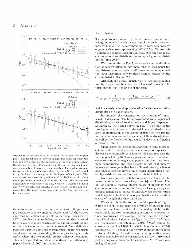
Fig. 6 shows concentration as a function of halo mass forall haloes selected following the procedure described above.

CDM Halo Structure 7

Figure 4. The median, 20 and 80 percentiles of the concentration,c200, as a function of halo mass, M200. The symbols extending tohigh masses show the results from the MS while the overlappingset of solid and dotted lines extending to lower masses show theresults from a simulation with 9× higher mass resolution. Eachpanel corresponds to a different radial range adopted for the fits.Data for each simulation are shown for haloes with N > 1000

particles, corresponding to ∼ 1012h−1 M⊙ in the MS. The dottedline shows a power law, c ∝ M−1/10, and is the same in all panels.

The upper panel is for our relaxed halo sample, while thelower panel show results for the complete sample, includingsystems that do not meet our equilibrium criteria.

In both samples, the correlation between mass and con-centration is well defined, but rather weak. A power-law fitsthe median concentration as a function of mass fairly well;we find:

c200 = 5.26(

M200/1014h−1 M⊙

)−0.10, (4)

for relaxed haloes, and

c200 = 4.67(

M200/1014h−1 M⊙

)−0.11(5)

for the complete halo sample.Our power-law fit is in good agreement with the results

of M07, who find c200 ∼ 5.6 (M200/1014h−1 M⊙)−0.098 for

the average concentration of their sample of relaxed haloes.These authors also report that concentrations are system-atically lower when considering the full sample of haloes.The small difference between our results and M07’s maybe due to variations between mean and median, as well ason the different criteria used to construct the relaxed halosample. Nevertheless, the agreement in the exponent of thepower-law is remarkable, especially considering that theseauthors explore a mass range different from ours, namely2 × 109 < M200/h−1 M⊙ < 2 × 1013. Combining these re-sults with ours, we conclude that a single power law fits

the concentration-mass dependence for about six decades in

mass.

Over the mass range covered by our simulations theconcentration-mass dependence is in reasonable agreementwith the predictions of NFW and of ENS, as shown, re-

Figure 5. The dependence of the rms residual deviation, σfit,about the best-fitting NFW density profile on the number of par-ticles per halo and on halo concentration. The boxes show themedians and the 25% and 75% centiles of the distribution, whilethe whiskers show the 5% and 95% tails. The numbers alongthe top of each panel indicate the number of haloes within eachbin. Top panels include all MS haloes with Nvir > 450 as noother selection criteria have been applied. The upturn in σfit forlow-concentration relaxed haloes is due to the inclusion of haloeswith less than 10, 000 particles. This upturn disappears once theN > 10, 000 criterion is imposed.

spectively, by the dotted and dashed lines in Fig. 6 2 . Theagreement, however, is not perfect, and both models appearto underestimate somewhat the median concentration at thelow mass end.

At the high-mass end, where there is a hint that concen-trations are approaching a constant value, the NFW modeldoes slightly better than ENS. This is because a constantconcentration for very massive objects is implicit in theNFW model, but not in ENS nor in the model of B01, whichis shown by a dot-dashed line in Fig. 6. Both ENS and B01predict a strong decline in concentration at the very highmass end. For the parameters favoured by B01, the disagree-ment for M > 1013.5h−1M⊙ is dramatic, and cautions, as al-ready pointed out by Zhao et al. (2003b), against using thismodel for predicting the concentrations of massive haloes.

Finally, we note that M07 argue that the B01 model re-produces their results better than ENS for haloes of mass afew times 109h−1 M⊙. However, the differences between thetwo models only become appreciable below ∼ 1010h−1M⊙,which corresponds to only about 700 particles in theirhighest-resolution simulation. Given (i) the large scatter in

2 These predictions use the original parameters in those papersand have not been adjusted further, except for adopting thepower-spectrum “shape” parameter, Γ = 0.15, as the best matchto the power spectrum adopted for the MS.

8 Neto et al.

Figure 6. Mass-concentration relation for relaxed haloes (toppanel) and for all haloes (bottom panel). The boxes represent the25% and 75% centiles of the distribution, while the whiskers showthe 5% and 95% tails. The numbers on the top of each panel indi-cate the number of haloes in each mass bin. The median concen-tration as a function of mass is shown by the solid line and is wellfit by the linear relations given in the legend of each panel. Thedot-dashed line shows the prediction of the Bullock et al. (2001)model (using cvir2.f available from the authors); the dashed anddotted lines corresponds to the Eke, Navarro, & Steinmetz (2001)and NFW models, respectively, with Γ = 0.15, as this approxi-mates best the input power spectrum of the MS. See text forfurther details.

the correlation; (ii) our finding that at least 1000 particlesare needed to produce unbiased results, and (iii) the worriesexpressed in Section 1 about the rather small box used byM07 to resolve low-mass haloes, we conclude that it wouldbe premature to judge conclusively on the superiority of onemodel over the other at the low mass end. More definitivetests are likely to come either from much higher resolutionsimulations or from extending this analysis to higher red-shifts, where the two models predict different behaviour.This is a topic that we intend to address in a forthcomingpaper (Gao et al. 2007, in preparation).

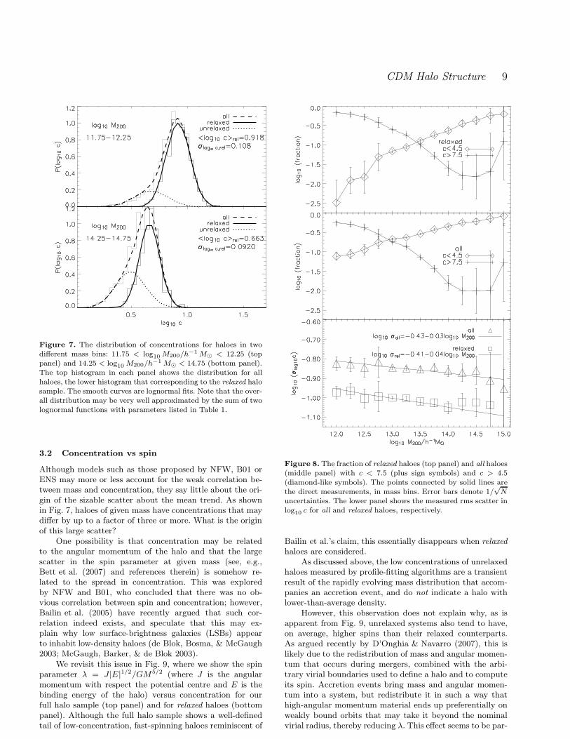
3.1.1 Scatter

The large volume covered by the MS means that we havea large number of haloes in our sample, even in the mostmassive bins of Fig. 6, corresponding to rare, very massiveobjects with masses approaching 1015h−1 M⊙. We use thisto check the common assumption that, at given halo mass,concentrations are distributed following a lognormal distri-bution (Jing 2000).

We examine this in Fig. 7, where we show the distribu-tion of concentrations in two mass bins. In each panel thetop histogram corresponds to all haloes in our sample, andthe lower histogram only to those deemed relaxed by thecriteria listed in Section 2.3.

Although the overall distribution is not approximatedwell by a lognormal function, that of relaxed haloes is. Thethick lines in Fig. 7 show fits of the form

P (log10 c) =1

σ√

2πexp

[

−1

2

(

log10 c − 〈log10 c〉σ

)2]

, (6)

which is clearly a good approximation for the concentrationdistribution of relaxed haloes.

Intriguingly, the concentration distribution of “unre-laxed” haloes may also be approximated by a lognormaldistribution, albeit of smaller mean and larger dispersion,as shown by the dotted curves in Fig. 7. The sum of thetwo lognormals (shown with dashed lines) is indeed a verygood approximation to the overall distribution. We list themedian concentration and dispersion of these distributions,as well as the fraction of “unrelaxed” haloes, as a functionof mass in Table 1.

Upon inspection, a weak but systematic trend is appar-ent in Table 1: the dispersion in concentration appears todecrease monotonically as a function of mass (see also thebottom panel of Fig 8). This suggests that massive haloes aresomehow a more homogeneous population than their lowermass counterparts, and may reflect the fact that massivehaloes are rare objects that have collapsed recently, whereasless massive systems have a much wider distribution of as-sembly redshifts. We shall return to this topic below.

One may apply the distributions shown in Fig 7 to esti-mate the abundance of relatively rare objects. These mightbe, for example, massive cluster haloes of unusually high

concentration that stand out in X-ray or lensing surveys, orperhaps galaxy-sized haloes of unusually low concentrationwhich may be notable because of peculiarities in the rotationcurves of the galaxies they may host.

We show this in the top and middle panels of Fig. 8,where the “plus” signs denote the fraction of haloes in eachmass bin that have c < 4.5. The diamond symbols, on theother hand, indicate the fraction of systems with concentra-tions exceeding 7.5. For example, we find that slightly morethan 1% of relaxed haloes with M200 ∼ 3×1014h−1 M⊙ havec > 7.5, or about 4 objects in our 5003h−3 Mpc3 volume. Soclusters such as Abell 1689, for which Limousin et al. (2006)estimate c200 = 7.6 should not be very abundant in the localUniverse. Finding, through lensing or X-ray studies, manyclusters as massive and as concentrated as Abell 1689 wouldyield strong constraints on the viability of ΛCDM as a cos-mological model.

CDM Halo Structure 9

Figure 7. The distribution of concentrations for haloes in twodifferent mass bins: 11.75 < log10 M200/h−1 M⊙ < 12.25 (toppanel) and 14.25 < log10 M200/h−1 M⊙ < 14.75 (bottom panel).The top histogram in each panel shows the distribution for allhaloes, the lower histogram that corresponding to the relaxed halosample. The smooth curves are lognormal fits. Note that the over-all distribution may be very well approximated by the sum of twolognormal functions with parameters listed in Table 1.

3.2 Concentration vs spin

Although models such as those proposed by NFW, B01 orENS may more or less account for the weak correlation be-tween mass and concentration, they say little about the ori-gin of the sizable scatter about the mean trend. As shownin Fig. 7, haloes of given mass have concentrations that maydiffer by up to a factor of three or more. What is the originof this large scatter?

One possibility is that concentration may be relatedto the angular momentum of the halo and that the largescatter in the spin parameter at given mass (see, e.g.,Bett et al. (2007) and references therein) is somehow re-lated to the spread in concentration. This was exploredby NFW and B01, who concluded that there was no ob-vious correlation between spin and concentration; however,Bailin et al. (2005) have recently argued that such cor-relation indeed exists, and speculate that this may ex-plain why low surface-brightness galaxies (LSBs) appearto inhabit low-density haloes (de Blok, Bosma, & McGaugh2003; McGaugh, Barker, & de Blok 2003).

We revisit this issue in Fig. 9, where we show the spinparameter λ = J |E|1/2/GM5/2 (where J is the angularmomentum with respect the potential centre and E is thebinding energy of the halo) versus concentration for ourfull halo sample (top panel) and for relaxed haloes (bottompanel). Although the full halo sample shows a well-definedtail of low-concentration, fast-spinning haloes reminiscent of

Figure 8. The fraction of relaxed haloes (top panel) and all haloes(middle panel) with c < 7.5 (plus sign symbols) and c > 4.5(diamond-like symbols). The points connected by solid lines arethe direct measurements, in mass bins. Error bars denote 1/

√N

uncertainties. The lower panel shows the measured rms scatter inlog10 c for all and relaxed haloes, respectively.

Bailin et al.’s claim, this essentially disappears when relaxed

haloes are considered.As discussed above, the low concentrations of unrelaxed

haloes measured by profile-fitting algorithms are a transientresult of the rapidly evolving mass distribution that accom-panies an accretion event, and do not indicate a halo withlower-than-average density.

However, this observation does not explain why, as isapparent from Fig. 9, unrelaxed systems also tend to have,on average, higher spins than their relaxed counterparts.As argued recently by D’Onghia & Navarro (2007), this islikely due to the redistribution of mass and angular momen-tum that occurs during mergers, combined with the arbi-trary virial boundaries used to define a halo and to computeits spin. Accretion events bring mass and angular momen-tum into a system, but redistribute it in such a way thathigh-angular momentum material ends up preferentially onweakly bound orbits that may take it beyond the nominalvirial radius, thereby reducing λ. This effect seems to be par-

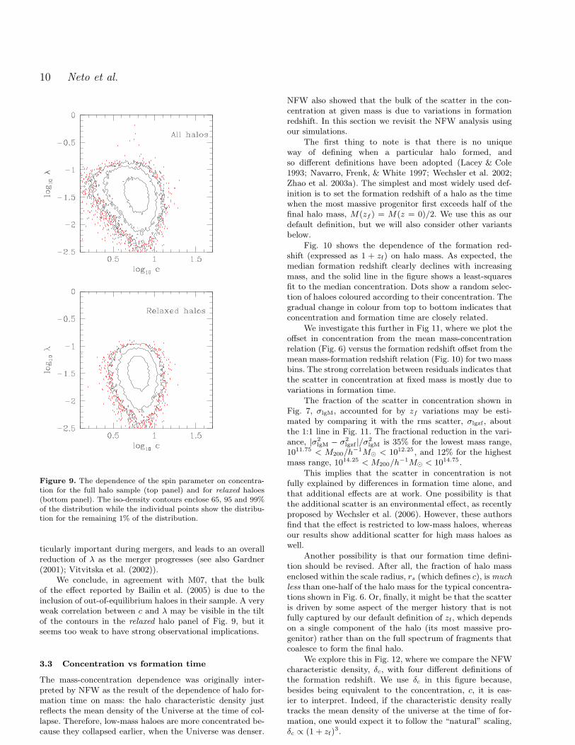
10 Neto et al.

Figure 9. The dependence of the spin parameter on concentra-tion for the full halo sample (top panel) and for relaxed haloes(bottom panel). The iso-density contours enclose 65, 95 and 99%of the distribution while the individual points show the distribu-tion for the remaining 1% of the distribution.

ticularly important during mergers, and leads to an overallreduction of λ as the merger progresses (see also Gardner(2001); Vitvitska et al. (2002)).

We conclude, in agreement with M07, that the bulkof the effect reported by Bailin et al. (2005) is due to theinclusion of out-of-equilibrium haloes in their sample. A veryweak correlation between c and λ may be visible in the tiltof the contours in the relaxed halo panel of Fig. 9, but itseems too weak to have strong observational implications.

3.3 Concentration vs formation time

The mass-concentration dependence was originally inter-preted by NFW as the result of the dependence of halo for-mation time on mass: the halo characteristic density justreflects the mean density of the Universe at the time of col-lapse. Therefore, low-mass haloes are more concentrated be-cause they collapsed earlier, when the Universe was denser.

NFW also showed that the bulk of the scatter in the con-centration at given mass is due to variations in formationredshift. In this section we revisit the NFW analysis usingour simulations.

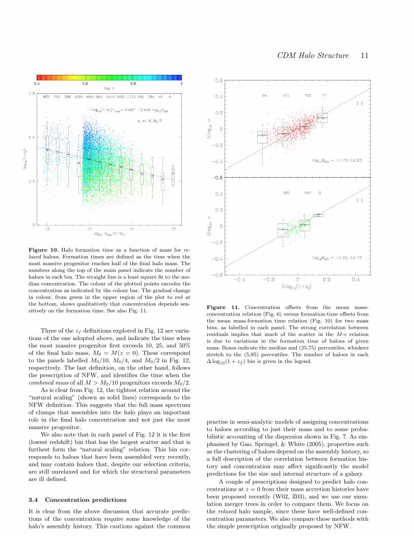
The first thing to note is that there is no uniqueway of defining when a particular halo formed, andso different definitions have been adopted (Lacey & Cole1993; Navarro, Frenk, & White 1997; Wechsler et al. 2002;Zhao et al. 2003a). The simplest and most widely used def-inition is to set the formation redshift of a halo as the timewhen the most massive progenitor first exceeds half of thefinal halo mass, M(zf ) = M(z = 0)/2. We use this as ourdefault definition, but we will also consider other variantsbelow.

Fig. 10 shows the dependence of the formation red-shift (expressed as 1 + zf) on halo mass. As expected, themedian formation redshift clearly declines with increasingmass, and the solid line in the figure shows a least-squaresfit to the median concentration. Dots show a random selec-tion of haloes coloured according to their concentration. Thegradual change in colour from top to bottom indicates thatconcentration and formation time are closely related.

We investigate this further in Fig 11, where we plot theoffset in concentration from the mean mass-concentrationrelation (Fig. 6) versus the formation redshift offset from themean mass-formation redshift relation (Fig. 10) for two massbins. The strong correlation between residuals indicates thatthe scatter in concentration at fixed mass is mostly due tovariations in formation time.

The fraction of the scatter in concentration shown inFig. 7, σlgM, accounted for by zf variations may be esti-mated by comparing it with the rms scatter, σlgzf , aboutthe 1:1 line in Fig. 11. The fractional reduction in the vari-ance, |σ2

lgM − σ2lgzf |/σ2

lgM is 35% for the lowest mass range,1011.75 < M200/h−1M⊙ < 1012.25 , and 12% for the highestmass range, 1014.25 < M200/h−1M⊙ < 1014.75 .

This implies that the scatter in concentration is notfully explained by differences in formation time alone, andthat additional effects are at work. One possibility is thatthe additional scatter is an environmental effect, as recentlyproposed by Wechsler et al. (2006). However, these authorsfind that the effect is restricted to low-mass haloes, whereasour results show additional scatter for high mass haloes aswell.

Another possibility is that our formation time defini-tion should be revised. After all, the fraction of halo massenclosed within the scale radius, rs (which defines c), is much

less than one-half of the halo mass for the typical concentra-tions shown in Fig. 6. Or, finally, it might be that the scatteris driven by some aspect of the merger history that is notfully captured by our default definition of zf , which dependson a single component of the halo (its most massive pro-genitor) rather than on the full spectrum of fragments thatcoalesce to form the final halo.

We explore this in Fig. 12, where we compare the NFWcharacteristic density, δc, with four different definitions ofthe formation redshift. We use δc in this figure because,besides being equivalent to the concentration, c, it is eas-ier to interpret. Indeed, if the characteristic density reallytracks the mean density of the universe at the time of for-mation, one would expect it to follow the “natural” scaling,δc ∝ (1 + zf)

3.

CDM Halo Structure 11

Figure 10. Halo formation time as a function of mass for re-

laxed haloes. Formation times are defined as the time when themost massive progenitor reaches half of the final halo mass. Thenumbers along the top of the main panel indicate the number ofhaloes in each bin. The straight line is a least square fit to the me-dian concentration. The colour of the plotted points encodes theconcentration as indicated by the colour bar. The gradual changein colour, from green in the upper region of the plot to red atthe bottom, shows qualitatively that concentration depends sen-sitively on the formation time. See also Fig. 11.

Three of the zf definitions explored in Fig. 12 are varia-tions of the one adopted above, and indicate the time whenthe most massive progenitor first exceeds 10, 25, and 50%of the final halo mass, M0 = M(z = 0). These correspondto the panels labelled M0/10, M0/4, and M0/2 in Fig. 12,respectively. The last definition, on the other hand, followsthe prescription of NFW, and identifies the time when thecombined mass of all M > M0/10 progenitors exceeds M0/2.

As is clear from Fig. 12, the tightest relation around the“natural scaling” (shown as solid lines) corresponds to theNFW definition. This suggests that the full mass spectrumof clumps that assembles into the halo plays an importantrole in the final halo concentration and not just the mostmassive progenitor.

We also note that in each panel of Fig. 12 it is the first(lowest redshift) bin that has the largest scatter and that isfurthest form the “natural scaling” relation. This bin cor-responds to haloes that have been assembled very recently,and may contain haloes that, despite our selection criteria,are still unrelaxed and for which the structural parametersare ill defined.

3.4 Concentration predictions

It is clear from the above discussion that accurate predic-tions of the concentration require some knowledge of thehalo’s assembly history. This cautions against the common

Figure 11. Concentration offsets from the mean mass-concentration relation (Fig. 6) versus formation-time offsets fromthe mean mass-formation time relation (Fig. 10) for two massbins, as labelled in each panel. The strong correlation betweenresiduals implies that much of the scatter in the M -c relationis due to variations in the formation time of haloes of givenmass. Boxes indicate the median and (25,75) percentiles, whiskersstretch to the (5,95) percentiles. The number of haloes in each∆ log10(1 + zf ) bin is given in the legend.

practise in semi-analytic models of assigning concentrationsto haloes according to just their mass and to some proba-bilistic accounting of the dispersion shown in Fig. 7. As em-phasised by Gao, Springel, & White (2005), properties suchas the clustering of haloes depend on the assembly history, soa full description of the correlation between formation his-tory and concentration may affect significantly the modelpredictions for the size and internal structure of a galaxy.

A couple of prescriptions designed to predict halo con-centrations at z = 0 from their mass accretion histories havebeen proposed recently (W02, Z03), and we use our simu-lation merger trees in order to compare them. We focus onthe relaxed halo sample, since these have well-defined con-centration parameters. We also compare these methods withthe simple prescription originally proposed by NFW.

12 Neto et al.

Figure 12. The correlation between the halo characteristic den-sity, δc, and different definitions of formation time for relaxed

haloes. The numbers along the top of each panel indicate thenumber of haloes in each bin. In the first three panels the forma-tion time is defined by reference to the most massive progenitor,and is set to be the redshift at which its mass was 1/2, 1/4 or1/10 of the final halo mass, M0 (see labels in each panel). In thefinal panel (labelled NFW) the formation time is defined as theredshift when half of the final halo mass is in progenitors moremassive than 1/10 of M0. The “natural scaling” δc ∝ (1+ zf )3 isindicated by the solid line in each panel.

3.4.1 Wechsler et al. prescription

W02 showed that the Mass Accretion History (MAH) of ahalo’s most massive progenitor, of mass M0 at redshift z = 0,may be approximated by a simple function,

log10 M(z) = log10 M0 − αz (7)

i.e., by a straight line with slope −α in the plane log10 M(z)vs. z (see also van den Bosch (2002)). These authors thenrelate the parameter α to a formation time via af = 1/(1 +zf) = α/2 ln(10). Their Fig. 6 shows that this definition offormation time correlates well with the halo concentrationsmeasured by B01 in their simulations and can be used topredict c at z = 0.

Fitting this correlation, they find

cW = c0/af , (8)

with c0 = 4.1, the typical concentration of haloes forming atthe present time. The implementation of this prescription inour simulations is straightforward, and we show the predic-tions in Fig. 13, after recalibrating eq. 8 with c0 = 2.26 inorder to take into account our different definition of virialradius.

3.4.2 Zhao et al. prescription

Z03 differentiate two distinct phases in the MAH; one ofearly, fast accretion, followed by a slow-accretion periodthat lasts until the present. The transition between the twophases occurs at a characteristic redshift, ztp. This “turning-point” redshift may be used to estimate the concentration,assuming that the inner properties of the halo, such as thescale radius, rs, and its enclosed mass, are set at ztp andvary weakly thereafter.

This procedure is in principle straightforward to imple-ment in our simulations but we note that there are a sub-stantial number of haloes for which the distinction betweenthe two accretion phases is not well-defined. In some cases,more than one phase of fast accretion seems to be present;in others, there is a single phase with no obvious turningpoint. This leads to ambiguities in the definition of ztp andits associated concentration that are not easily resolved andthat affect a significant fraction of haloes. A similar worryapplies to the Wechsler et al prescription, since eq. 7 is apoor approximation to the MAH of a significant number ofsystems.

3.4.3 NFW prescription

Finally, we consider NFW’s proposal to identify the forma-tion redshift with the epoch when 50% of the halo is con-tained in progenitors more massive than certain fraction, f ,of the final halo mass. NFW propose f = 0.01 in their orig-inal work in order to match the mass-concentration relationusing the extended Press-Schechter formalism, but this frac-tion is too low to allow for an accurate estimate in N-bodysimulations. As a compromise, we adopt f = 0.1 for theresults shown here.

3.4.4 Comparison between prescriptions

Note that the three prescriptions described above are basedon different features of the halo merger trees. While NFWlooks at the mass spectrum of clumps containing half of thefinal halo mass, the other methods consider just the MAH ofthe most massive progenitor. The Z03 prescription dependson the slope of the scaling relation log10 Ms vs. log10 rs inthe slow accretion phase while the W02 recipe fits the wholeMAH with a single slope.

In spite of these differences, Fig. 13 shows that allthree procedures yield concentrations that correlate rea-sonably well with the measured values. The rms scatterbetween prediction and measurement is indicated in eachpanel. It is smallest (marginally) for the NFW prescription,but even in this case it only reduces the scatter in the mass-concentration relation (Fig. 6) from σlgM = 0.092 to ∼ 0.077.Thus it only accounts for about 30% (|(σ2

lgM−σ2NFW)/σ2

lgM|)of the variance in the mass-concentration relation.

The W02 prescription does similarly well by this mea-sure, but the slope of the cpred–cmeasured relation is a bit tooshallow. The Z03 prediction has more scatter, but this isentirely due to a tail of haloes for which it predicts very lowconcentrations. We conclude that all three methods predictconcentrations that correlate well with the measured values,but none of them is able to fully account for the scatter inthe mass-concentration relation.

CDM Halo Structure 13

Figure 13. A comparison of the measured concentrations withthose predicted by the Zhao et al. (2003a) (top), Wechsler et al.(2002) (bottom left) and NFW (bottom right) prescriptions. Theplotted contours enclose 65%, 95% and 99% of the haloes with theremaining 1% plotted as points. The σ-values indicated in each

panel give the rms scatter in the prediction 〈(log10(c/cpred))2〉1/2,while σlgM is the corresponding rms scatter about the mass-concentration relation for the same set of haloes.

4 SUMMARY

We use the Millennium Simulation to examine the structuralparameters of dark matter haloes formed in the ΛCDM cos-mogony. The large volume probed by the MS, together withits unprecedented numerical resolution, allow us to probeconfidently the mass profiles of haloes spanning more thanthree decades in mass. Our main conclusions may be sum-marised as follows.

• As in earlier studies, we find that the mass profile of dy-namically relaxed haloes are well approximated by the two-parameter NFW profile. We find that at least 1000 particlesare needed in order to obtain unbiased estimates of the dis-tribution of halo concentrations and illustrate a number ofpotential pitfalls that arise from analysing poorly-resolvedhaloes, or from including in the sample haloes manifestlyout of equilibrium.

• We study the correlation between the NFW fit param-eters, which we express in terms of the halo mass and a con-centration parameter. These results extend previous studiesto much larger halo masses than hitherto reported in the lit-erature. Combining our results with those of Maccio et al.(2007), we find that a single power law reproduces the mass-concentration relation for over six decades in mass. Theseresults are in reasonable, albeit not perfect, agreement withthe predictions of the Eke, Navarro, & Steinmetz (2001) andNFW models. The model of Bullock et al. (2001) fails atlarge masses, and predicts concentrations at least a factorof ∼ 2 too low for M ∼ 1015 h−1M⊙ haloes.

• The dependence of concentration on mass, while wellestablished, is weak, and of equal importance is the broadscatter in concentration at fixed mass. The distribution of

concentrations at given mass is well fitted by a lognormalfunction where both the mean and the dispersion decreasewith increasing halo mass. These results allow us to estimatein detail the abundance of haloes with unusually low or un-usually high concentration, providing a well-defined predic-tion that may be used to interpret observations of objectsof unusual density, such as highly-effective cluster lenses orgalaxies with haloes of anomalously low density.

• We find that, once unrelaxed haloes are excluded, thereis no significant correlation between halo spin and concen-tration, contrary to the results of Bailin et al. (2005).

• We have searched for several ways to account for thelarge dispersion in concentrations at given mass. The scat-ter in concentrations seems to arise largely due to variationsin the formation time. We examined various plausible defi-nitions of the formation time, and find that concentrationsare best predicted by formation times defined taking intoaccount the collapse history of the full spectrum of progen-itors rather than the evolution of the single most massiveprogenitor.

• We compare the schemes of Zhao et al. (2003a),Wechsler et al. (2002), and a variant of the NFW prescrip-tion, and find that, while all three show a strong correlationbetween the predicted and measured concentrations, con-siderable scatter remains. In fact, none of these models isable to account for more than 30% of the intrinsic variancein the mass-concentration relation. It appears as if a largefraction of the scatter is truly stochastic or, else, dependenton aspects of the halo merger history that are not probedby these simple schemes.

ACKNOWLEDGEMENTS

The simulation used in this paper was carried out as partof the programme of the Virgo Consortium on the Regattasupercomputer of the Computing Centre of the Max-PlanckSociety in Garching. AFN would like to thank for the hos-pitality of ICC during the year 2005 and the LENAC net-work for financial support. AFN would also like to acknowl-edge John Helly for his help with the merger trees. JFNacknowledges support from Canada’s NSERC, as well asfrom the Leverhulme Trust and the Alexander von Hum-boldt Foundation. PB acknowledges the receipt of a PhDstudentship from the UK Particle Physics and AstronomyResearch Council.

REFERENCES

Avila-Reese V., Firmani C., Klypin A., Kravtsov A. V.,1999, MNRAS, 310, 527

J. Bailin, C. Power, B. K. Gibson and M. Steinmetz,arXiv:astro-ph/0502231.

Bett P., Eke V., Frenk C. S., Jenkins A., Helly J., NavarroJ., 2007, MNRAS, 376, 215

Bower R. G., Benson A. J., Malbon R., Helly J. C., FrenkC. S., Baugh C. M., Cole S., Lacey C. G., 2006, MN-RAS, 370, 645

Bullock J. S., Kolatt T. S., Sigad Y., Somerville R. S.,Kravtsov A. V., Klypin A. A., Primack J. R., DekelA., 2001, MNRAS, 321, 559

14 Neto et al.

Table 1. Parameters of the log-normal fits (eq. 6) to the distribution of concentrations as a function of mass for bins shown in Fig. 6.The first two columns are the halo mass, M200, and the number of haloes in each mass bin. The following two columns denote the medianand dispersion in the logarithm of the concentration; 〈log10 c200〉, and σlog10 c for the relaxed halo sample. The last three columns arethe fraction of unrelaxed haloes, funrel, as well as the median and dispersion in the logarithm of the concentration for that sample.

log10 M200 Nhaloes 〈log10 c〉 σlog10 c funrel 〈log10 c〉 σlog10 c

[h−1 M⊙] [relaxed] [relaxed] [unrelaxed] [unrelaxed]

11.875 - 12.125 911 0.920 0.106 0.205 0.683 0.14712.125 - 12.375 721 0.903 0.108 0.171 0.658 0.15012.375 - 12.625 403 0.881 0.099 0.199 0.646 0.13912.625 - 12.875 165 0.838 0.101 0.229 0.605 0.15812.875 - 13.125 13589 0.810 0.100 0.263 0.603 0.13613.125 - 13.375 9194 0.793 0.099 0.253 0.586 0.14013.375 - 13.625 4922 0.763 0.095 0.275 0.566 0.14213.625 - 13.875 2474 0.744 0.094 0.318 0.543 0.14013.875 - 14.125 1118 0.716 0.088 0.361 0.531 0.13114.125 - 14.375 495 0.689 0.095 0.383 0.510 0.12114.375 - 14.625 191 0.670 0.094 0.370 0.490 0.13314.625 - 14.875 49 0.635 0.091 0.484 0.519 0.12114.875 - 15.125 8 0.664 0.061 0.578 0.493 0.094

Cole S., Lacey C., 1996, MNRAS, 281, 716

Colless M., et al., 2001, MNRAS, 328, 1039

Davis M., Efstathiou G., Frenk C. S., White S. D. M., 1985,ApJ, 292, 371

de Blok W. J. G., Bosma A., McGaugh S., 2003, MNRAS,340, 657

D’Onghia E., Navarro J. F., 2007, astro,arXiv:astro-ph/0703195

Eke V. R., Cole S., Frenk C. S., 1996, MNRAS, 282, 263

Eke V. R., Navarro J. F., Steinmetz M., 2001, ApJ, 554, 114

Gao L., White S. D. M., Jenkins A., Stoehr F., Springel V.,2004, MNRAS, 355, 819

Gao L., Springel V., White S. D. M., 2005, MNRAS, 363,L66

Gardner J. P., 2001, ApJ, 557, 616

Ghigna S., Moore B., Governato F., Lake G., Quinn T.,Stadel J., 2000, ApJ, 544, 616

Harker G., Cole S., Helly J., Frenk C., Jenkins A., 2006,MNRAS, 367, 1039

Jing Y. P., 2000, ApJ, 535, 30

Klypin A., Kravtsov A. V., Bullock J. S., Primack J. R.,2001, ApJ, 554, 903

Kravtsov A. V., Klypin A. A., Khokhlov A. M., 1997, ApJS,111, 73

Lacey C., Cole S., 1993, MNRAS, 262, 627

Lahav O., Lilje P. B., Primack J. R., Rees M. J., 1991, MN-RAS, 251, 128

Limousin M., et al., 2006, arXiv:astro-ph/0612165

Maccio A. V., Dutton A. A., van den Bosch F. C., MooreB., Potter D., Stadel J., 2007, MNRAS, 378, 55

McGaugh S. S., Barker M. K., de Blok W. J. G., 2003, ApJ,584, 566

Navarro J. F., Frenk C. S., White S. D. M., 1995, MNRAS,275, 720

Navarro J. F., Frenk C. S., White S. D. M., 1996, ApJ, 462,563

Navarro J. F., Frenk C. S., White S. D. M., 1997, ApJ, 490,493

Percival W. J., et al., 2001, MNRAS, 327, 1297

Power C., Navarro J. F., Jenkins A., Frenk C. S., White

S. D. M., Springel V., Stadel J., Quinn T., 2003, MN-RAS, 338, 14

Shaw L. D., Weller J., Ostriker J. P., Bode P., 2005, AAS,37, 1330

Spergel D. N., et al., 2003, ApJS, 148, 175Spergel D. N. et al., arXiv:astro-ph/0603449v2Springel V., White S. D. M., Tormen G., Kauffmann G.,

2001, MNRAS, 328, 726Springel V., et al., 2005a, Nature, 435, 629Springel V., 2005b, MNRAS, 364, 1105Thomas P. A., Muanwong O., Pearce F. R., Couchman

H. M. P., Edge A. C., Jenkins A., Onuora L., 2001,MNRAS, 324, 450

van den Bosch, F. C. 2002, MNRAS, 331, 98Vitvitska M., Klypin A. A., Kravtsov A. V., Wechsler R. H.,

Primack J. R., Bullock J. S., 2002, ApJ, 581, 799Wechsler R. H., Bullock J. S., Primack J. R., Kravtsov A. V.,

Dekel A., 2002, ApJ, 568, 52Wechsler R. H., Zentner A. R., Bullock J. S., Kravtsov A. V.,

Allgood B., 2006, ApJ, 652, 71Zhao D. H., Mo H. J., Jing Y. P., Borner G., 2003a, MNRAS,

339, 12Zhao D. H., Jing Y. P., Mo H. J., Borner G., 2003b, ApJ,

597, L9