
Modern Industrial Statistics
587
-
Upload
khangminh22 -
Category
Documents
-
view
0 -
download
0
Transcript of Modern Industrial Statistics


Modern Industrial Statistics

STATISTICS IN PRACTICE
Series Advisors
Human and Biological SciencesStephen SennCRP-Sante, Luxembourg
Earth and Environmental SciencesMarian ScottUniversity of Glasgow, UK
Industry, Commerce and FinanceWolfgang JankUniversity of Maryland, USA
Founding EditorVic BarnettNottingham Trent University, UK
Statistics in Practice is an important international series of texts which provide detailed coverage ofstatistical concepts, methods and worked case studies in specific fields of investigation and study.With sound motivation and many worked practical examples, the books show in down-to-earth
terms how to select and use an appropriate range of statistical techniques in a particular practicalfield within each title’s special topic area.The books provide statistical support for professionals and research workers across a range of
employment fields and research environments. Subject areas covered include medicine and phar-maceutics; industry, finance and commerce; public services; the earth and environmental sciences,and so on.The books also provide support to students studying statistical courses applied to the above areas.
The demand for graduates to be equipped for the work environment has led to such courses becom-ing increasingly prevalent at universities and colleges.It is our aim to present judiciously chosen and well-written workbooks to meet everyday practical
needs. Feedback of views from readers will be most valuable to monitor the success of this aim.
A complete list of titles in this series appears at the end of the volume.

Modern Industrial Statistics
with applications in R, MINITAB and JMP
Second Edition
RON S. KENETTChairman and CEO, the KPA Group, Israel
Research Professor, University of Turin, Italy, and
International Professor, NYU, Center for Risk Engineering, New York, USA
SHELEMYAHU ZACKSDistinguished Professor,
Binghamton University, Binghamton, USA
With contributions from
DANIELE AMBERTITurin, Italy

This edition first published 2014
© 2014 John Wiley & Sons, Ltd
Registered officeJohn Wiley & Sons Ltd, The Atrium, Southern Gate, Chichester, West Sussex, PO19 8SQ, United Kingdom
For details of our global editorial offices, for customer services and for information about how to apply for permission to reuse the
copyright material in this book please see our website at www.wiley.com.
The right of the author to be identified as the author of this work has been asserted in accordance with the Copyright, Designs and
Patents Act 1988.
All rights reserved. No part of this publication may be reproduced, stored in a retrieval system, or transmitted, in any form or by any
means, electronic, mechanical, photocopying, recording or otherwise, except as permitted by the UK Copyright, Designs and Patents
Act 1988, without the prior permission of the publisher.
Wiley also publishes its books in a variety of electronic formats. Some content that appears in print may not be available in electronic
books.
Designations used by companies to distinguish their products are often claimed as trademarks. All brand names and product names
used in this book are trade names, service marks, trademarks or registered trademarks of their respective owners. The publisher is not
associated with any product or vendor mentioned in this book.
Limit of Liability/Disclaimer of Warranty: While the publisher and author have used their best efforts in preparing this book, they make
no representations or warranties with respect to the accuracy or completeness of the contents of this book and specifically disclaim any
implied warranties of merchantability or fitness for a particular purpose. It is sold on the understanding that the publisher is not
engaged in rendering professional services and neither the publisher nor the author shall be liable for damages arising herefrom. If
professional advice or other expert assistance is required, the services of a competent professional should be sought.
Library of Congress Cataloging-in-Publication Data
Kenett, Ron.
Modern industrial statistics : with applications in R, MINITAB and JMP / Ron S. Kenett, Shelemyahu
Zacks. – Second edition.
pages cm
Includes bibliographical references and index.
ISBN 978-1-118-45606-4 (cloth)
1. Quality control–Statistical methods. 2. Reliability (Engineering)–Statistical methods. 3. R (Computer
program language) 4. Minitab. 5. JMP (Computer file) I. Zacks, Shelemyahu, 1932- II. Title.
TS156.K42 2014
658.5′62–dc232013031273
A catalogue record for this book is available from the British Library.
ISBN: 978-1-118-45606-4
Typeset in 9/11pt TimesLTStd by Laserwords Private Limited, Chennai, India
1 2014

To my wife Sima, our children and their children: Yonatan, Alma, Tomer,Yadin, Aviv and Gili.
RSK
To my wife Hanna, our sons Yuval and David, and their families with love.SZ
To my wife Nadia, and my family. With a special thought to my mother andthank you to my father.
DA


Contents
Preface to Second Edition xvPreface to First Edition xvii
Abbreviations xix
PART I PRINCIPLES OF STATISTICAL THINKING AND ANALYSIS 1
1 The Role of Statistical Methods in Modern Industry and Services 31.1 The different functional areas in industry and services 3
1.2 The quality-productivity dilemma 5
1.3 Fire-fighting 6
1.4 Inspection of products 7
1.5 Process control 7
1.6 Quality by design 8
1.7 Information quality and practical statistical efficiency 9
1.8 Chapter highlights 11
1.9 Exercises 12
2 Analyzing Variability: Descriptive Statistics 132.1 Random phenomena and the structure of observations 13
2.2 Accuracy and precision of measurements 17
2.3 The population and the sample 18
2.4 Descriptive analysis of sample values 19
2.4.1 Frequency distributions of discrete random variables 19
2.4.2 Frequency distributions of continuous random variables 23
2.4.3 Statistics of the ordered sample 26
2.4.4 Statistics of location and dispersion 28
2.5 Prediction intervals 32
2.6 Additional techniques of exploratory data analysis 32
2.6.1 Box and whiskers plot 33
2.6.2 Quantile plots 34
2.6.3 Stem-and-leaf diagrams 34
2.6.4 Robust statistics for location and dispersion 36
2.7 Chapter highlights 38
2.8 Exercises 38
3 Probability Models and Distribution Functions 413.1 Basic probability 41
3.1.1 Events and sample spaces: Formal presentation of random measurements 41
3.1.2 Basic rules of operations with events: Unions, intersections 42
3.1.3 Probabilities of events 44

viii Contents
3.1.4 Probability functions for random sampling 46
3.1.5 Conditional probabilities and independence of events 47
3.1.6 Bayes formula and its application 49
3.2 Random variables and their distributions 51
3.2.1 Discrete and continuous distributions 51
3.2.2 Expected values and moments of distributions 55
3.2.3 The standard deviation, quantiles, measures of skewness and kurtosis 57
3.2.4 Moment generating functions 59
3.3 Families of discrete distribution 60
3.3.1 The binomial distribution 60
3.3.2 The hypergeometric distribution 62
3.3.3 The Poisson distribution 65
3.3.4 The geometric and negative binomial distributions 67
3.4 Continuous distributions 69
3.4.1 The uniform distribution on the interval (a, b), a < b 69
3.4.2 The normal and log-normal distributions 70
3.4.3 The exponential distribution 75
3.4.4 The gamma and Weibull distributions 77
3.4.5 The Beta distributions 80
3.5 Joint, marginal and conditional distributions 82
3.5.1 Joint and marginal distributions 82
3.5.2 Covariance and correlation 84
3.5.3 Conditional distributions 86
3.6 Some multivariate distributions 88
3.6.1 The multinomial distribution 88
3.6.2 The multi-hypergeometric distribution 89
3.6.3 The bivariate normal distribution 90
3.7 Distribution of order statistics 92
3.8 Linear combinations of random variables 94
3.9 Large sample approximations 98
3.9.1 The law of large numbers 98
3.9.2 The Central Limit Theorem 99
3.9.3 Some normal approximations 99
3.10 Additional distributions of statistics of normal samples 101
3.10.1 Distribution of the sample variance 101
3.10.2 The “Student” t-statistic 102
3.10.3 Distribution of the variance ratio 102
3.11 Chapter highlights 104
3.12 Exercises 105
4 Statistical Inference and Bootstrapping 1134.1 Sampling characteristics of estimators 113
4.2 Some methods of point estimation 114
4.2.1 Moment equation estimators 115
4.2.2 The method of least squares 116
4.2.3 Maximum likelihood estimators 118
4.3 Comparison of sample estimates 120
4.3.1 Basic concepts 120
4.3.2 Some common one-sample tests of hypotheses 122
4.4 Confidence intervals 128

Contents ix
4.4.1 Confidence intervals for 𝜇; 𝜎 known 129
4.4.2 Confidence intervals for 𝜇; 𝜎 unknown 130
4.4.3 Confidence intervals for 𝜎2 130
4.4.4 Confidence intervals for p 130
4.5 Tolerance intervals 132
4.5.1 Tolerance intervals for the normal distributions 132
4.6 Testing for normality with probability plots 134
4.7 Tests of goodness of fit 137
4.7.1 The chi-square test (large samples) 137
4.7.2 The Kolmogorov-Smirnov test 139
4.8 Bayesian decision procedures 140
4.8.1 Prior and posterior distributions 141
4.8.2 Bayesian testing and estimation 144
4.8.3 Credibility intervals for real parameters 147
4.9 Random sampling from reference distributions 148
4.10 Bootstrap sampling 150
4.10.1 The bootstrap method 150
4.10.2 Examining the bootstrap method 151
4.10.3 Harnessing the bootstrap method 152
4.11 Bootstrap testing of hypotheses 152
4.11.1 Bootstrap testing and confidence intervals for the mean 153
4.11.2 Studentized test for the mean 153
4.11.3 Studentized test for the difference of two means 155
4.11.4 Bootstrap tests and confidence intervals for the variance 157
4.11.5 Comparing statistics of several samples 158
4.12 Bootstrap tolerance intervals 161
4.12.1 Bootstrap tolerance intervals for Bernoulli samples 161
4.12.2 Tolerance interval for continuous variables 163
4.12.3 Distribution-free tolerance intervals 164
4.13 Non-parametric tests 165
4.13.1 The sign test 165
4.13.2 The randomization test 166
4.13.3 The Wilcoxon Signed Rank test 168
4.14 Description of MINITAB macros (available for download from Appendix VI of the book website) 170
4.15 Chapter highlights 170
4.16 Exercises 171
5 Variability in Several Dimensions and Regression Models 1775.1 Graphical display and analysis 177
5.1.1 Scatterplots 177
5.1.2 Multiple boxplots 179
5.2 Frequency distributions in several dimensions 181
5.2.1 Bivariate joint frequency distributions 182
5.2.2 Conditional distributions 185
5.3 Correlation and regression analysis 185
5.3.1 Covariances and correlations 185
5.3.2 Fitting simple regression lines to data 187
5.4 Multiple regression 192
5.4.1 Regression on two variables 194
5.5 Partial regression and correlation 198

x Contents
5.6 Multiple linear regression 200
5.7 Partial F-tests and the sequential SS 204
5.8 Model construction: Step-wise regression 206
5.9 Regression diagnostics 209
5.10 Quantal response analysis: Logistic regression 211
5.11 The analysis of variance: The comparison of means 213
5.11.1 The statistical model 213
5.11.2 The one-way analysis of variance (ANOVA) 214
5.12 Simultaneous confidence intervals: Multiple comparisons 216
5.13 Contingency tables 220
5.13.1 The structure of contingency tables 220
5.13.2 Indices of association for contingency tables 223
5.14 Categorical data analysis 227
5.14.1 Comparison of binomial experiments 227
5.15 Chapter highlights 229
5.16 Exercises 230
PART II ACCEPTANCE SAMPLING 235
6 Sampling for Estimation of Finite Population Quantities 2376.1 Sampling and the estimation problem 237
6.1.1 Basic definitions 237
6.1.2 Drawing a random sample from a finite population 238
6.1.3 Sample estimates of population quantities and their sampling distribution 239
6.2 Estimation with simple random samples 241
6.2.1 Properties of Xn and S2n under RSWR 242
6.2.2 Properties of Xn and S2n under RSWOR 244
6.3 Estimating the mean with stratified RSWOR 248
6.4 Proportional and optimal allocation 249
6.5 Prediction models with known covariates 252
6.6 Chapter highlights 255
6.7 Exercises 256
7 Sampling Plans for Product Inspection 2587.1 General discussion 258
7.2 Single-stage sampling plans for attributes 259
7.3 Approximate determination of the sampling plan 262
7.4 Double-sampling plans for attributes 264
7.5 Sequential sampling 267
7.6 Acceptance sampling plans for variables 270
7.7 Rectifying inspection of lots 272
7.8 National and international standards 274
7.9 Skip-lot sampling plans for attributes 276
7.9.1 The ISO 2859 skip-lot sampling procedures 276
7.10 The Deming inspection criterion 278
7.11 Published tables for acceptance sampling 279
7.12 Chapter highlights 280
7.13 Exercises 281

Contents xi
PART III STATISTICAL PROCESS CONTROL 283
8 Basic Tools and Principles of Process Control 2858.1 Basic concepts of statistical process control 285
8.2 Driving a process with control charts 294
8.3 Setting up a control chart: Process capability studies 298
8.4 Process capability indices 300
8.5 Seven tools for process control and process improvement 302
8.6 Statistical analysis of Pareto charts 305
8.7 The Shewhart control charts 308
8.7.1 Control charts for attributes 309
8.7.2 Control charts for variables 311
8.8 Chapter highlights 316
8.9 Exercises 316
9 Advanced Methods of Statistical Process Control 3199.1 Tests of randomness 319
9.1.1 Testing the number of runs 319
9.1.2 Runs above and below a specified level 321
9.1.3 Runs up and down 323
9.1.4 Testing the length of runs up and down 324
9.2 Modified Shewhart control charts for X 325
9.3 The size and frequency of sampling for Shewhart control charts 328
9.3.1 The economic design for X-charts 328
9.3.2 Increasing the sensitivity of p-charts 328
9.4 Cumulative sum control charts 330
9.4.1 Upper Page’s scheme 330
9.4.2 Some theoretical background 333
9.4.3 Lower and two-sided Page’s scheme 335
9.4.4 Average run length, probability of false alarm and conditional expected delay 339
9.5 Bayesian detection 342
9.6 Process tracking 346
9.6.1 The EWMA procedure 347
9.6.2 The BECM procedure 348
9.6.3 The Kalman filter 350
9.6.4 Hoadley’s QMP 351
9.7 Automatic process control 354
9.8 Chapter highlights 356
9.9 Exercises 357
10 Multivariate Statistical Process Control 36110.1 Introduction 361
10.2 A review of multivariate data analysis 365
10.3 Multivariate process capability indices 367
10.4 Advanced applications of multivariate control charts 370
10.4.1 Multivariate control charts scenarios 370
10.4.2 Internally derived targets 370
10.4.3 Using an external reference sample 371
10.4.4 Externally assigned targets 372

xii Contents
10.4.5 Measurement units considered as batches 373
10.4.6 Variable decomposition and monitoring indices 373
10.5 Multivariate tolerance specifications 374
10.6 Chapter highlights 376
10.7 Exercises 377
PART IV DESIGN AND ANALYSIS OF EXPERIMENTS 379
11 Classical Design and Analysis of Experiments 38111.1 Basic steps and guiding principles 381
11.2 Blocking and randomization 385
11.3 Additive and non-additive linear models 385
11.4 The analysis of randomized complete block designs 387
11.4.1 Several blocks, two treatments per block: Paired comparison 387
11.4.2 Several blocks, t treatments per block 391
11.5 Balanced incomplete block designs 394
11.6 Latin square design 397
11.7 Full factorial experiments 402
11.7.1 The structure of factorial experiments 402
11.7.2 The ANOVA for full factorial designs 402
11.7.3 Estimating main effects and interactions 408
11.7.4 2m factorial designs 409
11.7.5 3m factorial designs 417
11.8 Blocking and fractional replications of 2m factorial designs 425
11.9 Exploration of response surfaces 430
11.9.1 Second order designs 431
11.9.2 Some specific second order designs 433
11.9.3 Approaching the region of the optimal yield 438
11.9.4 Canonical representation 440
11.10 Chapter highlights 441
11.11 Exercises 442
12 Quality by Design 44612.1 Off-line quality control, parameter design and the Taguchi method 447
12.1.1 Product and process optimization using loss functions 447
12.1.2 Major stages in product and process design 448
12.1.3 Design parameters and noise factors 449
12.1.4 Parameter design experiments 450
12.1.5 Performance statistics 452
12.2 The effects of non-linearity 452
12.3 Taguchi’s designs 456
12.4 Quality by design in the pharmaceutical industry 458
12.4.1 Introduction to quality by design 458
12.4.2 A quality by design case study – the full factorial design 459
12.4.3 A quality by design case study – the profiler and desirability function 462
12.4.4 A quality by design case study – the design space 462
12.5 Tolerance designs 462
12.6 More case studies 467
12.6.1 The Quinlan experiment at Flex Products, Inc. 467
12.6.2 Computer response time optimization 469

Contents xiii
12.7 Chapter highlights 474
12.8 Exercises 474
13 Computer Experiments 47713.1 Introduction to computer experiments 477
13.2 Designing computer experiments 481
13.3 Analyzing computer experiments 483
13.4 Stochastic emulators 488
13.5 Integrating physical and computer experiments 491
13.6 Chapter highlights 492
13.7 Exercises 492
PART V RELIABILITY AND SURVIVAL ANALYSIS 495
14 Reliability Analysis 49714.1 Basic notions 498
14.1.1 Time categories 498
14.1.2 Reliability and related functions 499
14.2 System reliability 500
14.3 Availability of repairable systems 503
14.4 Types of observations on TTF 509
14.5 Graphical analysis of life data 510
14.6 Non-parametric estimation of reliability 513
14.7 Estimation of life characteristics 514
14.7.1 Maximum likelihood estimators for exponential TTF distribution 514
14.7.2 Maximum likelihood estimation of the Weibull parameters 518
14.8 Reliability demonstration 520
14.8.1 Binomial testing 520
14.8.2 Exponential distributions 521
14.9 Accelerated life testing 528
14.9.1 The Arrhenius temperature model 528
14.9.2 Other models 529
14.10 Burn-in procedures 529
14.11 Chapter highlights 530
14.12 Exercises 531
15 Bayesian Reliability Estimation and Prediction 53415.1 Prior and posterior distributions 534
15.2 Loss functions and Bayes estimators 537
15.2.1 Distribution-free Bayes estimator of reliability 538
15.2.2 Bayes estimator of reliability for exponential life distributions 538
15.3 Bayesian credibility and prediction intervals 539
15.3.1 Distribution-free reliability estimation 539
15.3.2 Exponential reliability estimation 540
15.3.3 Prediction intervals 540
15.4 Credibility intervals for the asymptotic availability of repairable systems: The exponential case 542
15.5 Empirical Bayes method 543
15.6 Chapter highlights 545
15.7 Exercises 545

xiv Contents
List of R Packages 547
References and Further Reading 549
Author Index 555
Subject Index 557
Also available on book’s website: www.wiley.com/go/modern_industrial_statistics
Appendix I: An Introduction to R by Stefano Iacus
Appendix II: Basic MINITAB Commands and a Review of Matrix Algebra for Statistics
Appendix III: mistat Manual (mistat.pdf) and List of R Scripts, by Chapter (R_scripts.zip)
Appendix IV: Source Version of mistat Package (mistat_1.0.tar.gz), also available on the
Comprehensive R Archive Network (CRAN) Website.
Appendix V: Data Sets as csv Files
Appendix VI:MINITAB Macros
Appendix VII: JMP Scripts by Ian Cox
Appendix VIII: Solution Manual

Preface to Second Edition
This book is about modern industrial statistics and it applications using R, MINITAB and JMP. It is an expanded second
edition of a book entitledModern Industrial Statistics: Design andControl of Quality and Reliability,WadsworthDuxbury
Publishing, 1998, Spanish edition: Estadistica Industrial Moderna: Diseño y Control de Calidad y la Confiabilidad,Thomson International, 2000. Abbreviated edition:Modern Statistics: A Computer-based Approach, Thomson Learning,
2001. Chinese edition: China Statistics Press, 2003 and Softcover edition, Brooks-Cole, 2004.
The pedagogical structure of the book combines a practical approach with theoretical foundations and computer sup-
port. It is intended for students and instructors who have an interest in studying modern methods by combining these
three elements. The first edition referred to S-Plus, MINITAB and compiled QuickBasic code. In this second edition we
provide examples and procedures in the now popular R language and also refer to MINITAB and JMP. Each of these
three computer platforms carries unique advantages. Focusing on only one or two of these is also possible. Exercises are
provided at the end of each chapter in order to provide more opportunities to learn and test your knowledge.
R is an open source programming language and software environment for statistical computing and graphics based
on the S programming language created by John Chambers while at Bell Labs in 1976. It is now developed by the R
Development Core Team, of which Chambers is a member. MINITAB is a statistics package originally developed at
the Pennsylvania State University by Barbara Ryan, Thomas Ryan, Jr., and Brian Joiner in 1972. MINITAB began as a
light version of OMNITAB, a statistical analysis program developed at the National Bureau of Standards now called the
National Institute of Standards and Technology (NIST). JMP was originally written in 1989 by John Sall and others to
perform simple and complex statistical analyses by dynamically linking statistics with graphics to interactively explore,
understand, and visualize data. JMP stands for John’s Macintosh Project and it is a division of SAS Institute Inc.
A clear advantage of R is that it is free open source software. It requires, however, knowledge of command language
programming. To help the reader, we developed a special comprehensive R application calledmistat that includes all the
R programs used in the book. MINITAB is a popular statistical software application providing extensive collaboration and
reporting capabilities. JMP, a product of the SAS company, is also very popular and carries advanced scripting features and
high level visualization components. Both R and JMP have fully compatible versions for Mac OS. We do not aim to teach
programming in R or using MINITAB or JMP. We also do not cover all the options and features available in MINITAB
and JMP. Our aim is to expose students, researchers and practitioners of modern industrial statistics to examples of what
can be done with these software platforms and encourage the exploration of additional options in MINITAB and JMP.
Eventually, availability and convenience determine what software is used in specific cirmcumstances. We provide here
an opportunity to learn and get acquainted with three leading modern industrial statistics software platforms. A specially
prepared appendix, downloadable from the book website, provides an introduction to R. Also available for download
are the R scripts we refer to, organized by chapter. Installations of JMP and MINITAB include effective tutorials with
introductory material. Such tutorials have not been replicated in this text. To take full advantage of this book you need
to be interested in industrial statistics, have a proper mathematical background and be willing to learn by working out
problems with software applications. The five parts of the book can be studied in various combinations with Part I used
as a foundation. The book can therefore be used in workshops or courses on Acceptance Sampling, Statistical ProcessControl, Design of Experiments and Reliability.
The three software platforms we refer to provide several simulation options. We believe that teaching modern industrial
statistics, with simulations, provides the right context for gaining sound hands-on experience. We aim at the middle road
target, between theoretical treatment and a cookbook approach. To achieve this, we provide over 40 data sets representing
real-life case studies which are typical of what one finds while performing statistical work in business and industry.
Figures in the book have been produced with R and in MINITAB and JMP as explicitly stated. In this second edition we
include contributions by Dr. Daniele Amberti who developed the R mistat package and provided many inputs to the
text. His work was supported by i4C (www.i4CAnalytics.com) and we are very grateful for it. Another change in this

xvi Preface to Second Edition
second edition is that it is published by JohnWiley and Sons and we would like to thank Heather Kay and Richard Davies
for their professional support and encouragements throughout this effort. We also acknowledge the contribution of Ian
Cox from JMP who developed for us the simulation code running the piston simulator and the bootstrapping analysis.
Thanks are due to the Genova Hotel in front of Porta Nuova in Turin where we spend countless hours updating the text
using push and pull of LaTeX files in Git from within RStudio. In fact, the whole book, with its R code and data sets has
been fully compiled in its present form to create an example of what reproducible research is all about. Gerry Hahn, Murat
Testik, Moshe Pollak, Gejza Dohnal, Neil Ullman, MosheMiller, David Steinberg, Marcello Fidaleo, Inbal Yahav and Ian
Cox provided feedback on early drafts of the new chapters included in this second expanded edition of the original 1998
book–we thank them for their insightful comments. Finally, we would like to acknowledge the help of Marco Giuliano
who translated most of TeX files from the 1998 edition to LaTeX and of Marge Pratt who helped produce the final LaTeX
version of our work.
The book is accompanied by a dedicated website where all software and data files used are available to download.
The book website URL is www.wiley.com/go/modern_industrial_statistics.The site contains: 1) all the R code included in the book which is also available on the R CRANwebsite as the mistat
package (folder scripts), 2) a source version of the mistat package for R (mistat_1.0.tar.gz), 3) all data sets as csv files
(csvFiles.zip and folder csvFiles in package mistat), 4) the MINITAB macros and JMP add-ins used in the text, 5)
an introduction to R prepared by Professor Stefano Iacus from the University of Milan and 6) solutions to some of the
exercises. Specifically, the book web site includes eight appendices: Appendix I - Introduction to R, by Stefano Iacus,
Appendix II - Basic MINITAB commands and a review of matrix algebra for Statistics, Appendix III - R code included
in the book, Appendix IV - Source version of package mistat, Appendix V - Data sets as csv files, Appendix VI -
MINITAB macros, Appendix VII - JMP scripts, by Ian Cox and Appendix VIII - Solution manual.
Special thanks are due to Professor Iacus for his generous contribution. If you are not familiar with R, we recommend
you look at this introduction specially prepared by one of the most important core developers of R. The material on the
book website should be considered part of the book. We obviously look forward to feedback, comments and suggestions
from students, teachers, researchers and practitioners and hope the book will help these different target groups achieve
concrete and significant impact with the tools and methods of industrial statistics.
Ron S. Kenett
Raanana, Israel and Turin, Italy
Shelemyahu Zacks
Binghamton, New York, USA

Preface to First Edition
Modern Industrial Statistics provides the tools for those who drive to achieve perfection in industrial processes. Learn theconcepts and methods contained in this book and you will understand what it takes to measure and improve world-class
products and services.
The need for constant improvement of industrial processes, in order to achieve high quality, reliability, productivity
and profitability, is well recognized. Furthermore management techniques, such as total quality management or business
process reengineering, are insufficient in themselves to achieve the goal without the strong backing of specially tailored
statistical procedures, as stated by Robert Galvin in the Foreword.
Statistical procedures, designed for solving industrial problems, are called Industrial Statistics. Our objective in writing
this book was to provide statistics and engineering students, as well as practitioners, the concepts, applications, and
practice of basic and advanced industrial statistical methods, which are designed for the control and improvement of
quality and reliability.
The idea of writing a text on industrial statistics developed after several years of collaboration in industrial consult-
ing, teaching workshops and seminars, and courses at our universities. We felt that no existing text served our needs in
both content and approach so we decided to develop our notes into a text. Our aim was to make the text modern and
comprehensive in terms of the techniques covered, lucid in its presentation, and practical with regard to implementation.
Ron S. Kenett
Shelemyahu Zacks
1998


Abbreviations
ANOVA Analysis of Variance
ANSI American National Standard Institute
AOQ Average Outgoing Quality
AOQL Average Outgoing Quality Limit
AQL Acceptable Quality Level
ARL Average Run Length
ASN Average Sample Number
ASQ American Society for Quality
ATI Average Total Inspection
BECM Bayes Estimation of the Current Mean
BIBD Balanced Incomplete Block Design
BP Bootstrap Population
CAD Computer Aided Design
CADD Computer Aided Drawing and Drafting
CAM Computer Aided Manufacturing
CBD Complete Block Design
c.d.f. cumulative distribution function
CED Conditional Expected Delay
cGMP current good manufacturing practices
CIM Computer Integrated Manufacturing
CLT Central Limit Theorem
CNC Computerized Numerically Controlled
CPA Circuit Pack Assemblies
CQA Critical Quality Attribute
CUSUM Cumulative Sum
DFIT Fits distance
DLM Dynamic Linear Model
DoE Design of Experiments
EBD Empirical Bootstrap Distribution
EWMA Exponentially Weighted Moving Average
FPM Failures Per Million
GRR Gage Repeatability and Reproducibility
HPD Highest Posterior Density
i.i.d. independent and identically distributed
InfoQ Information Quality
IQR Inter Quartile Range
ISC Short Circuit Current of Solar Cells (in Ampere)
KS Kolmogorov-Smirnov
LCL Lower Control Limit
LLN Law of Large Numbers
LSE Least Squares Estimators
LQL Limiting Quality Level
LSL Lower Specification Limit

xx Abbreviations
LTPD Lot Tolerance Percent Defective
LWL Lower Warning Limit
m.g.f. moment generating function
MLE Maximum Likelihood Estimator
MSD Mean Squared Deviation
MTBF Mean Time Between Failures
MTTF Mean Time To Failure
OC Operating Characteristic
p.d.f. probability density function
PERT Project Evaluation and Review Technique
PFA Probability of False Alarm
PL Product Limit Estimator
PPM Defects in Parts Per Million
PSE Practical Statistical Efficiency
QbD Quality by Design
QMP Quality Measurement Plan
QQ-Plot Quantile vs. Quantile Plot
RCBD Randomized Complete Block Design
RMSE Root Mean Squared Error
RSWOR Random Sample Without Replacement
RSWR Random Sample With Replacement
SE Standard Error
SL Skip Lot
SLOC Source Lines of Code
SLSP Skip Lot Sampling Plans
SPC Statistical Process Control
SPRT Sequential Probability Ratio Test
SR Shiryayev-Roberts
SSE Sum of Squares of Residuals
SSR Sum of Squares Around the Regression Model
SST Total Sum of Squares
STD Standard Deviation
TTC Time Till Censoring
TTF Time Till Failure
TTR Time Till Repair
TTT Total Time on Test
UCL Upper Control Limit
USL Upper Specification Limit
UWL Upper Warning Limit
WSP Wave Soldering Process

Part IPrinciples of Statistical Thinking and Analysis
Part I is an introduction to the role of statistics in modern industry and service organizations, and to statistical thinking in
general. Typical industrial problems are described and basic statistical concepts and tools are presented through case stud-
ies and computer simulations. To help focus on data analysis and interpretation of results we refer, throughout the book, to
three leading software platforms for statistical analysis: R,MINITAB and JMP. R is an open source programming language
with more than 4300 application packages available at the Comprehensive R Archive Network (http://cran.r-project.org/).
MINITAB and JMP are statistical packages widely used in business and industry (www.minitab.com, www.jmp.com) with
30 days free fully functional downloads. The R code is integrated in the text and packaged in the mistat R application
that can be downloaded from CRAN or the book’s website www.wiley.com/go/modern_industrial_statistics. For ease of
use the mistat R applications are also organized by chapter in a set of scripts. The chapter scripts include all the R
examples used in the specific chapter.
Chapter 1 is an overview of the role of statistical methods in industry and offers a classification of statistical methods in
the context of various management approaches. We call this classification the Quality Ladder and use it to organize themethods of industrial statistics covered in Parts II–V. The chapter also introduces the reader to the concept of practical
statistical efficiency (PSE) and information quality (InfoQ) that are used to assess the impact of work performed on a
given data set with statistical tools and the quality of knowledge generated by statistical analysis.
Chapter 2 presents basic concepts and tools for describing variability. It emphasizes graphical techniques to explore
and summarize variability in observations. The chapter introduces the reader to R and provides examples in MINITAB
and JMP. The examples demonstrate capabilities but it was not our intention to present introductory material on how to
use these software applications. Some help in this can be found in the book downloadable appendices.
Chapter 3 is an introduction to probability models including a comprehensive treatment of statistical distributions that
have applicability to industrial statistics. The chapter provides a reference to fundamental results and basic principles used
in later chapters.
Chapter 4 is dedicated to statistical inference and bootstrapping. Bootstrapping is introduced with examples in R,
MINITAB and JMP. With this approach, statistical procedures used in making inference from a sample to a population
are handled by computer-intensive procedures without the traditional need to validate mathematical assumptions and
models.
Chapter 5 deals with variability in several dimensions and regression models. It begins with graphical techniques that
handle observations taken simultaneously on several variables. These techniques are now widely available in software
applications such as those used throughout the book. The chapter covers linear and multiple regression models including
diagnostics and prediction intervals. Categorical data and multi-dimensional contingency tables are also analyzed.
Modern Industrial Statistics: with applications in R, MINITAB and JMP, Second Edition. Ron S. Kenett and Shelemyahu Zacks.© 2014 John Wiley & Sons, Ltd. Published 2014 by John Wiley & Sons, Ltd.Companion website: www.wiley.com/go/modern_industrial_statistics


1The Role of Statistical Methods inModern Industry and Services
1.1 The different functional areas in industry and services
Industrial statistics has played a key role in the creation of competitiveness in a wide range of organizations in the indus-
trial sector, in services, health care, government and educational systems. The tools and concepts of industrial statistics
have to be viewed in the context of their applications. These applications are greatly affected by management style and
organizational culture. We begin by describing key aspects of the industrial setting in order to lay out the foundations for
the book.
Industrial organizations typically include units dedicated to product development, manufacturing, marketing, finance,
human resources, purchasing, sales, quality assurance and after-sales support. Industrial statistics is used to resolve prob-
lems in each one of these functional units. Marketing personnel determine customer requirements and measure levels
of customer satisfaction using surveys and focus groups. Sales are responsible for providing forecasts to purchasing and
manufacturing. Purchasing specialists analyze world trends in quality and prices of rawmaterials so that they can optimize
costs and delivery time. Budgets are prepared by the finance department using forecasts that are validated periodically.
Accounting experts rely on auditing and sampling methods to ascertain inventory levels and integrity of databases. Human
resources personnel track data on absenteeism, turnover, overtime and training needs. They also conduct employee sur-
veys and deploy performance appraisal systems. The quality departments commonly perform audits and quality tests,
to determine and ensure the quality and reliability of products and services. Research and development engineers per-
form experiments to solve problems and improve products and processes. Finally, manufacturing personnel and process
engineers design process controls for production operations using control charts and automation.
These are only a few examples of problem areas where the tools of industrial statistics are used within modern industrial
and service organizations. In order to provide more specific examples we first take a closer look at a variety of industries.
Later we discuss examples from these types of industries.
There are basically three types of production systems: (1) continuous flow production; (2) job shops; and (3) discrete
mass production. Examples of continuous flow production include steel, glass and paper making, thermal power
generation and chemical transformations. Such processes typically involve expensive equipment that is very large
in size, operates around the clock and requires very rigid manufacturing steps. Continuous flow industries are both
capital-intensive and highly dependent on the quality of the purchased raw materials. Rapid customizing of products in a
continuous flow process is virtually impossible and new products are introduced using complex scale-up procedures.
Modern Industrial Statistics: with applications in R, MINITAB and JMP, Second Edition. Ron S. Kenett and Shelemyahu Zacks.© 2014 John Wiley & Sons, Ltd. Published 2014 by John Wiley & Sons, Ltd.Companion website: www.wiley.com/go/modern_industrial_statistics

4 Modern Industrial Statistics
Job shops are in many respects exactly the opposite. Examples of job shops include metal-working of parts or call
centers where customers who call in are given individual attention by non-specialized attendants. Such operations per-
mit production of custom-made products and are very labor-intensive. Job shops can be supported by special purpose
machinery which remains idle in periods of low demand.
Discrete mass production systems can be similar to continuous flow production if a standard product is produced in
large quantities.When flexible manufacturing is achieved, mass production can handle batches of size 1, and, in that sense,
appears similar to a job shop operation. Service centers with call routing for screening calls by areas of specialization are
such an example.
Machine tool automation began in the 1950s with the development of numerical control operations. In these automatic
or semi-automatic machines, tools are positioned for a desired cutting effect through computer commands. Today’s hard-
ware and software capabilities make a job-shopmanufacturing facility as much automated as a continuous-flow enterprise.
Computer-integrated manufacturing (CIM) is the integration of computer-aided design (CAD) with computer-aided man-
ufacturing (CAM). The development of CAD has its origins in the evolution of computer graphics and computer-aided
drawing and drafting, often called (CADD). As an example of how these systems are used, we follow the creation of
an automobile suspension system designed on a computer using CAD. The new system must meet testing requirements
under a battery of specific road conditions. After coming up with an initial design concept, design engineers use computer
animation to show the damping effects of the new suspension design on various road conditions. The design is then iter-
atively improved on the basis of simulation results and established customer requirements. In parallel to the suspension
system, design purchasing specialists and industrial engineers proceed with specifying and ordering the necessary raw
materials, setting up the manufacturing processes, and scheduling production quantities. Throughout the manufacturing
of the suspension system, several tests provide the necessary production controls. Of particular importance are dimension
measurements performed by coordinate measuring machines (CMM). Modern systems upload CMM data automatically
and provide the ability to perform multivariate statistical process control and integrate data from subcontractors on all
five continents (see, e.g., www.spclive365.com). Ultimately the objective is to minimize the costly impact of failures in a
product after delivery to the customer.
Statistical methods are employed throughout the design, manufacturing and servicing stages of the product. The incom-
ing raw materials have often to be inspected, by sampling, to ensure adherence to quality standards (see Chapters 6–7
in Part II). Statistical process control is employed at various stages of manufacturing and service operations to identify
and correct deviations from process capabilities (see Chapters 8–10 in Part III). Methods for the statistical design of
experiments are used to optimize the design of a system or process (see Chapters 11–13 in Part IV). Finally, tracking and
analyzing field failures of the product are carried out to assess the reliability of a system and provide early warnings of
product deterioration (see Chapters 14–15 in Part V).
CAD systems provide an inexpensive environment to test and improve design concepts. Chapter 13 is dedicated to
computer experiments and special methods for both the design and the analysis of such experiments. CMM systems
capture the data necessary for process control. Chapter 10 covers methods of multivariate statistical process control that
can fully exploit such data. Web technology offers opportunities to set up such systems without the deployment of costly
computer infrastructures. Computerized field failures tracking systems and sales forecasting are very common. Predictive
analytics and operational business intelligence systems like eCRM tag customers that are likely to drop and allow for
churn prevention initiatives. The application of industrial statistics within such computerized environments allows us to
concentrate on statistical analysis that infers the predictive behavior of the process and generates insights on associations
between measured variables, as opposed to repetitive numerical computations.
Service organization can be either independent or complementary to manufacturing type operations. For example, a
provider of communication systems typically also supports installation and after-sales services to its customers. The
service takes the form of installing the communication system, programming the system’s database with an appropriate
numbering plan, and responding to service calls. The delivery of services differs from manufacturing in many ways. The
output of a service system is generally intangible. In many cases the service is delivered directly to the customer without
an opportunity to store or fix “defective” transactions. Some services involve very large number of transactions. Federal
Express, for example, handles 1.5 million shipments per day, to 127 countries, at 1650 sites. The opportunities for error
are many, and process error levels must be of only a few defective parts per million. Operating at such low defect levels
might appear at first highly expensive to maintain and therefore economically unsound. In the next section we deal with
the apparent contradiction between maintaining low error levels and reducing costs and operating expenses.

The Role of Statistical Methods in Modern Industry and Services 5
1.2 The quality-productivity dilemma
In order to reach World War II production goals for ammunitions, airplanes, tanks, ships and other military materiel,
American industry had to restructure and raise its productivity while adhering to strict quality standards. This was partially
achieved through large-scale applications of statistical methods following the pioneering work of a group of industrial
scientists at Bell Laboratories. Two prominent members of this group were Walter A. Shewhart, who developed the
tools and concepts of statistical process control, and Harold F. Dodge, who laid the foundations for statistical sampling
techniques. Their ideas and methods were instrumental in the transformation of American industry in the 1940s, which
had to deliver high quality and high productivity. During those years, many engineers were trained in industrial statistics
throughout the United States.
After the war, a number of Americans were asked to help Japan rebuild its devastated industrial infrastructure. Two
of these consultants, W. Edwards Deming and Joseph M. Juran, distinguished themselves as effective and influential
teachers. Both Drs. Deming and Juran witnessed the impact of Walter Shewhart’s new concepts. In the 1950s they
taught the Japanese the ideas of process control and process improvements, emphasizing the role of management and
employee involvement.
The Japanese were quick to learn the basic quantitative tools for identifying and realizing improvement opportunities
and for controlling processes. By improving blue-collar and white-collar processes throughout their organizations, the
Japanese were able to reduce waste and rework, thus producing better products at a lower price. These changes occurred
over a period of several years leading eventually to significant increases in the market share for Japanese products.
In contrast, American industry had no need for improvements in quality afterWorldWar II. There was an infinite market
demand for American goods and the emphasis shifted to high productivity, without necessarily assuring high quality. This
was reinforced by the Taylor approach splitting the responsibility for quality and productivity between the quality and
production departments.Manymanagers in theUS industry did not believe that high quality and high productivity could be
achieved simultaneously. The Quality-Productivity Dilemma was born and managers apparently had to make a choice. By
focusing attention on productivity, managers often sacrificed quality, which in turn had a negative effect on productivity.
Increasing emphasis on meeting schedules and quotas made the situation even worse.
On the other hand, Japanese industrialists proved to themselves that by implementing industrial statistics tools, man-
agers can improve process quality and, simultaneously, increase productivity. This was shown to apply in every industrial
organization and thus universally resolve the Quality-Productivity Dilemma. In the 1970s, several American companies
began applying the methods taught by Deming and Juran and by the mid-1980s there were many companies in the US
reporting outstanding successes. Quality improvements generate higher productivity since they permit the shipment of
higher quality products, faster. The result was better products at lower costs–an unbeatable formula for success. The key
to this achievement was the implementation of Quality Management and the application of industrial statistics, which
includes analyzing data, understanding variability, controlling processes, designing experiments, and making forecasts.
The approach was further developed in the 1980s by Motorola who launched its famous Six Sigma initiative. A striking
testimonial of such achievements is provided by Robert W. Galvin, the former chairman of the executive committee of
Motorola Inc.:
At Motorola we use statistical methods daily throughout all of our disciplines to synthesize an abundance of data to derive con-
crete actions . . . How has the use of statistical methods within Motorola Six Sigma initiative, across disciplines, contributed to our
growth? Over the past decade we have reduced in-process defects by over 300-fold, which has resulted in a cumulative manufactur-
ing cost savings of over 11 billion dollars. Employee productivity measured in sales dollars per employee has increased three fold
or an average 12.2 percent per year over the same period. Our product reliability as seen by our customers has increased between
5 and 10 times.
Source: Forword to Modern Industrial Statistics: Design and Control of Quality and Reliability (Kenett and Zacks, 1998).
The effective implementation of industrial statistics depends on the management approach practiced in the organization.
We characterize different styles of management, by a Quality Ladder, which is presented in Figure 1.1. Management’s
response to the rhetorical question: “How do you handle the inconvenience of customer complaints?” determines the
position of an organization on the ladder. Some managers respond by describing an approach based on reactively waiting
for complaints to be filed before initiating any corrective actions. Some try to achieve quality by extensive inspections

6 Modern Industrial Statistics
Quality by Design
Fire-Fighting
Design of Experiments, Riskand Reliability Analysis
Statistical Process Control
Sampling Plans
Data Accumulation
Management Maturity Statistical Tools
Inspection
Process Improvement
Figure 1.1 The quality ladder
and implement strict supervision of every activity in the organization, having several signatures of approval on every
document. Others take a more proactive approach and invest in process improvement and quality by design.
The four management styles we identify are: (i) reactive fire-fighting; (ii) inspection and traditional supervision;
(iii) processes control and improvement and (iv) quality by design. Industrial statistics tools can have an impact only
on the top three steps in the quality ladder. Levels (iii) and (iv) are more proactive than (ii). When management’s style
consists exclusively of fire fighting, there is typically no use for methods of industrial statistics and data is simply
accumulated.
The Quality Ladder is matching management maturity level with appropriate statistical tools. Kenett et al. (2008)formulated and tested with 21 case studies, the Statistical Efficiency Conjecture which states that organizations higher
up on the Quality Ladder are more efficient at solving problems with increased returns on investments. This provides an
economic incentive for investments in efforts to increase the management maturity of organizations.
1.3 Fire-fighting
Fire fighters specialize in putting down fires. Their main goal is to get to the scene of a fire as quickly as possible. In
order to meet this goal, they activate sirens and flashing lights and have their equipment organized for immediate use,
at a moment’s notice. Fire-fighting is also characteristic of a particular management approach that focuses on heroic
efforts to resolve problems and unexpected crisis. The seeds of these problems are often planted by the same managers,
who work the extra hours required to fix them. Fire-fighting has been characterized as an approach where there is never
enough time to do things right the first time, but always sufficient time for rework and fixing problems once customers
are complaining and threaten to leave. This reactive approach of management is rarely conducive to serious improve-
ments which rely on data and teamwork. Industrial statistics tools are rarely used under fire-fighting management. As a
consequence, decisions in such organizations are often made without investigation of the causes for failures or proactive
process improvement initiatives.
In Chapters 2–5 of Part I we study the structure of random phenomena and present statistical tools used to describe
and analyze such structures. The basic philosophy of statistical thinking is the realization that variation occurs in all work
processes, and the understanding that reducing variation is essential to quality improvement. Failure to recognize the
impact of randomness leads to unnecessary and harmful decisions. One example of the failure to understand randomness
is the common practice of adjusting production quotas for the following month by relying on the current month’s sales.
Without appropriate tools, managers have no way of knowing whether the current month’s sales are within the common
variation range or not. Common variation implies that nothing significant has happened since last month and therefore
no quota adjustments should be made. Under such circumstances changes in production quotas create unnecessary, self-
inflicted problems. Fire-fighting management, in many cases, is responsible for avoidable costs and quick temporary fixes

The Role of Statistical Methods in Modern Industry and Services 7
with negative effects on the future of the organization. Moreover, in such cases, data is usually accumulated and archived
without lessons learned or proactive initiatives. Some managers in such an environment will attempt to prevent “fires”
from occurring. One approach to prevent such fires is to rely on massive inspection and traditional supervision as opposed
to leadership and personal example. The next section provides some historical background on the methods of inspection.
1.4 Inspection of products
In medieval Europe, most families and social groups made their own goods such as cloth, utensils and other household
items. The only saleable cloth was woven by peasants who paid their taxes in kind to their feudal lords. The ownership
of barons or monasteries was identified through marks put on the fabric which were also an indication of quality. Since
no feudal lord would accept payment in shoddy goods, the products were carefully inspected prior to the inscribing of
the mark. Surviving late medieval documents indicate that bales of cloth frequently changed hands repeatedly without
being opened, simply because the marks they bore were regarded everywhere as guarantees of quality. In the new towns,
fabrics were made by craftsmen who went in for specialization and division of labor. Chinese records of the same period
indicate that silks made for export were also subjected to official quality inspections. In Ypres, the center of the Flemish
wool cloth industry, weavers’ regulations were put down in writing as early as 1281. These regulations stipulated the
length and width as well as the number of warp ends and the quality of the wool to be used in each cloth. A fabric had
to be of the same thickness throughout. All fabric was inspected in the draper’s hall by municipal officials. Heavy fines
were levied for defective workmanship, and the quality of fabrics which passed inspection was guaranteed by affixing
the town seal. Similar regulations existed elsewhere in France, Italy, Germany, England and Eastern Europe. Trademarks
as a guarantee of quality used by the modern textile industry originated in Britain. They first found general acceptance
in the wholesale trade and then, from the end of the 19th century onward, among consumers. For a time manufacturers
still relied on in-plant inspections of their products by technicians and merchants, but eventually technological advances
introduced machines and processes which ensured the maintenance of certain standards independently of human inspec-
tors and their know-how. Industrial statistics played an important role in the textile industry. In fact, it was the first large
industry which analyzed its data statistically. Simple production figures including percentages of defective products were
already compiled in British cotton mills early in the 19th century. The basic approach, during the pre-industrial and post-
industrial period, was to guarantee quality by proper inspection of the cloth (Juran, 1995). In the early 1900s, researchers
at Bell Laboratories in New Jersey developed statistical sampling methods that provided an effective alternative to 100%
inspection (Dodge and Romig, 1929). Their techniques, labeled “Sampling Inspection,” eventually led to the famous
MIL-STD-105 system of acceptance sampling procedures used throughout the defense industry and elsewhere. These
techniques implement statistical tests of hypotheses, in order to determine if a certain production lot or manufacturing
batch is meeting Acceptable Quality Levels. Such sampling techniques are focused on the product, as opposed to the
process that makes the product. Details of the implementation and theory of sampling inspection are provided in Part II
(Chapters 6 and 7) that is dedicated to acceptance sampling topics. The next section introduces the approach of process
control that focuses on the performance of processes throughout the organization.
1.5 Process control
In a memorandum to his superior at Bell Laboratories Walter Shewhart documented, in 1924, a new approach to statistical
process control (Godfrey, 1986; Godfrey and Kenett, 2007). The document datedMay 16th describes a technique designed
to track process quality levels over time, which Shewhart labeled a “Control Chart.” The technique was further developed
andmore publications followed two years later (Shewhart, 1926). Shewhart realized that anymanufacturing process can be
controlled using basic engineering ideas. Control charts are a straightforward application of engineering feedback loops to
the control of work-processes. The successful implementation of control charts requires management to focus on process
performance, with emphasis on process control and process improvements. When a process is found capable of producing
products that meet customer requirements and a system of process controls is subsequently employed, one no longer needs
to enforce product inspection. Industry can deliver its products without time-consuming and costly inspection, thereby
providing higher quality at reduced costs. These are prerequisites for Just-In-Time deliveries and increased customer

8 Modern Industrial Statistics
satisfaction. Achieving quality by not relying on inspection implies quicker deliveries, less testing and therefore reduced
costs. Shewhart’s ideas are therefore essential for organizations seeking improvements in their competitive position. As
mentioned earlier, W. Edwards Deming and Joseph M. Juran were instrumental in bringing this approach to Japan in
the 1950s. Deming emphasized the use of statistical methods, and Juran created a comprehensive management system
including the concepts of management breakthroughs, the quality trilogy of planning, improvement and control and the
strategic planning of quality. Both were awarded a medal by the Japanese emperor for their contributions to the rebuilding
of Japan’s industrial infrastructure. Japan’s national industrial award, called the Deming Prize, has been awarded every
year since the early 1950s. The United States National Quality Award and the European Quality Award have been pre-
sented, since the early 1990s, to companies in the US and Europe that can serve as role models to others. Notable winners
include Motorola, Xerox, Milliken, Globe Metallurgical, AT&T Universal Cards and the Ritz Carlton. Similar awards
exist in Australia, Israel, Mexico and many other countries. Part III (Chapters 8–10) deals with implementation and theo-
retical issues of process control techniques. The next part of the book takes the ideas of process control one step further and
covers the design and analysis of experiments and reliability analysis. These require management initiatives we generally
label as Quality by Design. Quality by Design is an approach relying on a proactive management style, where problems
are sought out and products and processes are designed with “built in” quality.
1.6 Quality by design
The design of a manufactured product or a service begins with an idea and continues through a series of development
and testing phases until production begins and the product is made available to the customer. Process design involves
the planning and design of the physical facilities, and the information and control systems required to manufacture a
products or deliver a service. The design of the product, and the associated manufacturing process, determine its ultimate
performance and value. Design decisions influence the sensitivity of a product to variation in raw materials and work
conditions, which in turn affects manufacturing costs. General Electric, for example, has found that 75% of failure costs
in its products are determined by the design. In a series of bold design decisions in the late 1990s, IBM developed
the Proprinter so that all parts and sub-assemblies were built to snap together during final assembly without the use of
fasteners. Such initiatives resulted in major cost reductions and quality improvements. These are only a few examples
demonstrating how design decisions affect manufacturing capabilities with an eventual positive impact on the cost and
quality of the product. Reducing the number of parts is also formulated as a statistical problem that involves clustering and
grouping of similar parts. Take, for example, a basic mechanical part such as aluminum bolts. Many organizations find
themselves purchasing hundreds of different types of bolts for very similar applications. Multivariate statistical techniques
can be used to group together similar bolts, thereby reducing the number of different purchased parts, eliminating potential
mistakes and lowering costs.
In the design of manufactured products, technical specifications can be precisely defined. In the design of a service
process, quantitative standards may be difficult to determine. In service processes, the physical facilities, procedures,
people’s behavior and professional judgment affect the quality of service. Quantitative measures in the service industry
typically consist of data from periodical customer surveys and information from internal feedback loops such as waiting
time in hotels’ front desks or supermarket cash registers. The design of products and processes, both in service and
manufacturing, involves quantitative performance measurements.
A major contributor to modern quality engineering has been Genichi Taguchi, formerly of the Japanese Electronic
Communications Laboratories. Since the 1950s Taguchi has advocated the use of statistically designed experiments in
industry. Already in 1959 the Japanese company NEC ran 402 planned experiments. In 1976, Nippon Denso, which is a
20,000-employee company producing electronic parts for automobiles, is reported to have run 2700 designed experiments.
In the summer of 1980, Taguchi came to the United States to “repay the debt” of the Japanese to Shewhart, Deming and
Juran and delivered a series of workshops at Bell Laboratories in Holmdel, New Jersey. His methods slowly gained
acceptance in the US. Companies like ITT, Ford and Xerox have been using Taguchi methods since the mid-1980s with
impressive results. For example, an ITT electrical cable and wire plant reported reduced product variability by a factor
of 10. ITT Avionic Division developed, over a period of 30 years, a comprehensive approach to quality engineering,
including an economic model for optimization of products and processes. Another application domain which has seen
a dramatic improvement in the maturity of management is the area of system and software development. The Software

The Role of Statistical Methods in Modern Industry and Services 9
Engineering Institute (SEI) was established in 1987 to improve the methods used by industry in the development of
systems and software. SEI, among other things, designed a five-level capability maturity model integrated (CMMI) which
represents various levels of implementation of Process Areas. The tools and techniques of Quality by Design are applied
by level 5 organizations which are, in fact, at the top of the quality ladder. For more on CMMI and systems and software
development, see Kenett and Baker (2010).
A particular industry where such initiatives are driven by regulators and industrial best practices is the pharmaceutical
industry. In August 2002, the Food and Drug Administration (FDA) launched the pharmaceutical current Good Manufac-
turing Practices (cGMP) for the 21st-century initiative. In that announcement, the FDA explained the agency’s intent to
integrate quality systems and risk management approaches into existing quality programs with the goal of encouraging
the industry to adopt modern and innovative manufacturing technologies. The cGMP initiative was spurred by the fact
that since 1978, when the last major revision of the cGMP regulations was published, there have been many advances
in design and manufacturing technologies and in the understanding of quality systems. This initiative created several
international guidance documents that operationalized this new vision of ensuring product quality through “a harmonized
pharmaceutical quality system applicable across the life cycle of the product emphasizing an integrated approach to qual-
ity risk management and science.” This new approach is encouraging the implementation of Quality by Design (QbD)
and hence, de facto, encouraging the pharmaceutical industry to move up theQuality Ladder. Chapter 12 covers severalexamples of Quality by Design initiatives in the Pharmaceutical industry using statistically designed experiments. For a
broad treatment of statistical methods in healthcare, see Faltin et al. (2012).Parts IV and V present a comprehensive treatment of the principal methods of design and analysis of experiments
and reliability analysis used in Quality by Design. An essential component of Quality by Design is Quality Planning.Planning, in general, is a basic engineering and management activity. It involves deciding, in advance, what to do, how to
do it, when to do it, and who is to do it. Quality Planning is the process used in the design of any new product or process.
In 1987, General Motors cars averaged 130 assembly defects per 100 cars. In fact, this was planned that way. A cause
and effect analysis of car assembly defects pointed out causes for this poor quality that ranged from production facilities,
suppliers of purchased material, manufacturing equipment, engineering tools, etc. Better choices of suppliers, different
manufacturing facilities and alternative engineering tools produced a lower number of assembly defects. Planning usually
requires careful analysis, experience, imagination, foresight, and creativity. Planning for quality has been formalized by
Joseph M. Juran as a series of steps (Juran and Gryna, 1988). These are:
1. Identify who are the customers of the new product or process.
2. Determine the needs of those customers.
3. Translate the needs into technical terms.
4. Develop a product or process that can respond to those needs.
5. Optimize the product of process so that it meets the needs of the customers including economic and performance goals.
6. Develop the process required to actually produce the new product or to install the new process.
7. Optimize that process.
8. Begin production or implement the new process.
1.7 Information quality and practical statistical efficiency
Statistics in general, and Industrial Statistics in particular, is focused on extracting knowledge from data. Kenett and
Shmueli (2013) define information quality as an approach to assess the level of knowledge generated by analyzing data
with specific methods, given specific goals. Formally, let:
• g = a specific analysis goal
• X = the available dataset
• f = an empirical analysis method
• U = a utility measure
A goal could be, for example, to keep a process under control. The available data can be a rational sample of size 5
collected every 15 minutes, the analysis methods an Xbar-R control chart and the utility being the economic value

10 Modern Industrial Statistics
of achieving high production yield. Information quality (InfoQ) is defined as: InfoQ(f,X,g)=U(f(X|g)), that is, theutility derived by conducting an analysis f, on a given dataset X, conditioned on the goal g. In terms of our example,
it is the economic value derived from applying an Xbar-R chart on the sample data in order to keep the process
under control.
To achieve high InfoQ, Kenett and Shmueli (2013) map eight dimensions:
1. Data resolution: This is determined by measurement scale, measurement uncertainty and level of data aggregation,
relative to the task at hand. The concept of rational sample is such an example.
2. Data structure: This relates to the data sources available for the specific analysis. Comprehensive data sources combine
structured quantitative data with unstructured, semantic based data.
3. Data integration: Properly combining data sources is not a trivial task. Information system experts apply ETL (Extract-
Transform-Load) technologies to integrate data sources with aliased nomenclature and varying time stamps.
4. Temporal relevance: A data set contains information collected during a certain time window. The degree of relevance
of the data in that time window to the current goal at hand must be assessed. Data collected a year ago might no
longer be relevant in characterizing process capability.
5. Generalizability: Statistical generalizability refers to inferring from a sample to a target population. Proper sampling
of a batch implies that decisions based on the sample apply to the whole batch.
6. Chronology of data and goal: This is obvious. If a control chart is updated once a month, proper responsive process
control cannot be conducted.
7. Construct operationalization: Findings derived from analyzing data need to be translated into terms that can drive
concrete actions, and vice versa. Quoting W. Edwards Deming, “An operational definition is a procedure agreed
upon for translation of a concept into measurement of some kind.”
8. Communication: If the information does not reach the right person at the right time, then the quality of information
is necessarily poor. Data visualization is directly related to the quality of information. Poor visualization of findings
can lead to degradation of the information quality contained in the analysis performed on the data.
These dimensions can then be individually scored to derive an overall InfoQ score. In considering the various tools and
methods of Industrial Statistics presented in this book, one should keep in mind that the ultimate objective is achieving
high information quality or InfoQ. Achieving high infoQ is, however, necessary but not sufficient to make the application
of industrial statistics both effective and efficient. InfoQ is about using statistical and analytic methods effectively so that
they generate the required knowledge. Efficiency is related to the concrete organizational impact of the methods used. We
next present an assessment of efficiency called practical statistical efficiency.
The idea of adding a practical perspective to the classical mathematical definition of statistical efficiency is based on a
suggestion by Churchill Eisenhart who, in a 1978 informal “Beer and Statistics” seminar in the Shorewood Hills house
of George Box in Madison Wisconsin, proposed a new definition of statistical efficiency. Later, Bruce Hoadley from Bell
Laboratories, picked up where Eisenhart left off and added his version nicknamed “Vador.” Blan Godfrey, former head
of the quality technologies department at Bell Laboratories and, later, CEO of the Juran Institute, used this concept in
his 1988 Youden Address on “Statistics, Quality and the Bottom Line” at the Fall Technical Conference of the American
Society for Quality Control. Kenett, Coleman and Stewardson (2003) further expanded this idea adding an additional
component, the value of the data actually collected, and defined practical statistical efficiency (PSE) in an operational
way. The PSE formula accounts for eight components and is computed as:
PSE = V{D} ⋅ V{M} ⋅ V{P} ⋅ V{PS} ⋅ P{S} ⋅ P{I} ⋅ T{I} ⋅ E{R},
where:
• V{D} = value of the data actually collected.
• V{M} = value of the statistical method employed.
• V{P} = value of the problem to be solved.
• V{PS} = value of the problem actually solved.
• P{S} = probability level that the problem actually gets solved.

The Role of Statistical Methods in Modern Industry and Services 11
• P{I} = probability level that the solution is actually implemented.
• T{I} = time the solution stays implemented.
• E{R} = expected number of replications.
These components can be assessed qualitatively, using expert opinions, or quantitatively, if the relevant data exists. A
straightforward approach to evaluate PSE is to use a scale of “1” for not very good to “5” for excellent. This method of
scoring can be applied uniformly for all PSE components. Some of the PSE components can be also assessed quantita-
tively. P(S) and P(I) are probability levels, TI can be measured in months, V(P) and V(PS) can be evaluated in euros,
dollars or pounds. V(PS) is the value of the problem actually solved, as a fraction of the problem to be solved. If this
is evaluated qualitatively, a large portion would be “4” or “5,” a small portion “1” or “2.” V(D) is the value of the data
actually collected for the goal to be considered. Whether PSE terms are evaluated quantitatively or qualitatively, PSE is
a conceptual measure rather than a numerically precise one. A more elaborated approach to PSE evaluation can include
differential weighing of the PSE components and/or non-linear assessments.
1.8 Chapter highlights
The effective use of industrial statistics tools requires organizations to climb up the quality ladder presented in Figure 1.1.
As the use of data is gradually integrated into the decision process, both at the short-term operational level, and at the
long-term strategic level, different tools are needed. The ability to plan and forecast successfully is a result of accumu-
lated experience and proper techniques. Modern industrial organizations (manufacturing or services) are described and
classified in this introductory chapter. Different functional areas of a typical business are presented with typical problems
for each area. The potential benefits of industrial statistics methods are then introduced in the context of these problems.
The main theme here is that the apparent conflict between high productivity and high quality can be resolved through
improvements in work processes, by introducing statistical methods and concepts. The contributions of Shewhart, Dem-
ing and Juran to industries seeking a more competitive position are outlined. Different approaches to the management
of industrial organizations are summarized and classified using a Quality Ladder. Industrial statistics methods are then
categorized according to the steps of the ladder. These consist of Fire-Fighting, Inspection, Process Control and Quality
by Design. The chapter discusses how to match a specific set of statistical methods to the management approach and how
to assess information quality (InfoQ) and practical statistical efficiency (PSE) to ensure that industrial statistics methods
are used effectively and efficiently in organization and application areas. It is designed to provide a general background
to the application of industrial statistics.
The following chapters provide a comprehensive exposition of the tools and methods of modern industrial statistics.
In this chapter we refer to the need to develop the maturity of the management approach, to ensure high InfoQ in data
analysis and to plan for high PSE in order to achieve high impact. These aspects are complementary to the methods and
tools presented in the next 14 chapters.
The main terms and concepts introduced in this first chapter include:
• Continuous Flow Production
• Job Shops
• Mass Production Systems
• The Quality-Productivity Dilemma
• Quality Management
• The Quality Ladder
• Fire-Fighting as a Management Approach
• Inspection as a Management Approach
• Process Control and Improvement as a Management Approach
• Quality by Design as a Management Approach
• Information Quality (InfoQ)
• Practical Statistical Efficiency (PSE)

12 Modern Industrial Statistics
1.9 Exercises
1.1 Describe three work environments where quality is assured by 100% inspection.
1.2 Search periodicals, such as Business Week, Fortune, Time and Newsweek and newspapers such as the New YorkTimes and the Wall Street Journal for information on quality initiatives in service, healthcare, governmental and
industrial organizations.
1.3 Provide examples of the three types of production systems.
(i) continuous flow production.
(ii) job shops.
(iii) discrete mass production.
1.4 What management approach cannot work with continuous flow production?
1.5 What management approach characterizes
(i) a school system?
(ii) a military unit?
(iii) a football team?
1.6 Provide examples of how you, personally, apply the four management approaches
(i) as a student.
(ii) in your parents’ house.
(iii) with your friends.
1.7 Evaluate the InfoQ dimensions of following case study on predicting days with unhealthy air quality inWashington,
DC. Several tour companies’ revenues depend heavily on favorable weather conditions. This study looks at air qual-
ity advisories, during which people are advised to stay indoors, within the context of a tour company inWashington,
DC. http://galitshmueli.com/content/tourism-insurance-predicting-days-unhealthy-air-quality-washington-dc.
1.8 Evaluate the InfoQ dimensions of following case study on quality-of-care factors in U.S. nursing homes Thousands
of Americans reside in nursing homes across the US, with facilities spanning a wide range. This study looks at
the quality of care in nursing homes in the United States. http://galitshmueli.com/content/quality-care-factors-us-
nursing-homes.
1.9 Evaluate the InfoQ dimensions of a case study provided by your instructor.
1.10 Evaluate the practical statistical efficiency (PSE) of a case study provided by your instructor.

2Analyzing Variability:Descriptive Statistics
2.1 Random phenomena and the structure of observations
Many phenomena which we encounter are only partially predictable. It is difficult to predict the weather or the behavior of
the stock market. In this book we focus on industrial phenomena, like performance measurements from a product which is
beingmanufactured, or the sales volume in a specified period of a given product model. Such phenomena are characterized
by the fact that measurements performed on them are often not constant but reveal a certain degree of variability. The aim
of this chapter is to present methods to analyze this variability, in order to understand the variability structure and enhance
our ability to control, improve and predict future behavior of such phenomena. We start with a few simple examples.
Example 2.1. A piston is a mechanical device that is present in most types of engines. One measure of the performance
of a piston is the time it takes to complete one cycle. We call this measure cycle time. In Table 2.1 we present 50 cycle
times of a piston operating under fixed operating conditions (a sample data set is stored in file CYCLT.csv). We provide
with this book code in R and JMP for running a piston software simulation. If you installed JMP, download from the book
website the file com.jmp.cox.ian.piston.jmpaddin and double click on it. You will get access to a piston simulator with 7
factors that you can change using interactive sliders (see Figure 13.1 in Chapter 13). Set the number of samples to 50, leave
the sample size as 1 and click Run at the bottom of the screen. This will generate 50 cycle times that are determined by
how you set up the factors on the sliders and your computer random number generator. JMP produces an output file with
several graphical displays and summary statistics that we will discuss later. We will use this simulator when we discuss
Statistical Process Control (Chapters 8, 9 and 10) and the Design of Experiments (Chapters 11, 12 and 13). We continue
at a pedestrian pace by recreating Table 2.1 using R. All the R applications referred to in this book are contained in a
package called mistat available in Appendix III and downloadable from the CRAN website. The mistat R applications
are also organized on the book’s website, by chapter, for ease of use. The following R commands will install the mistatpackage, read the cycle time data and print them on your monitor:
> # This is a comment> install.packages("mistat", # Install mistat package
dependencies=TRUE) # and its dependencies> #> library(mistat) # A command to make our datasets> # and functions available> #> data(CYCLT) # Load specified data set
Modern Industrial Statistics: with applications in R, MINITAB and JMP, Second Edition. Ron S. Kenett and Shelemyahu Zacks.© 2014 John Wiley & Sons, Ltd. Published 2014 by John Wiley & Sons, Ltd.Companion website: www.wiley.com/go/modern_industrial_statistics

14 Modern Industrial Statistics
> # CYCLT is a vector of values> #> help(CYCLT) # Read the help page about CYCLT> #> CYCLT # Print CYCLT to Console
Notice that functions in R have parenthesis. The library() function loads an additional package to extend R function-
alities and CYCLT is an object containing a simple vector of values.
The differences in cycle times values is quite apparent and we can make the statement “cycle times are varying.” Such
a statement, in spite of being true, is not very useful. We have only established the existence of variability – we have not
yet characterized it and are unable to predict and control future behavior of the piston.
Table 2.1 Cycle times of piston (in seconds) withcontrol factors set at minimum levels
1.008 1.117 1.141 0.449 0.2151.098 1.080 0.662 1.057 1.1071.120 0.206 0.531 0.437 0.3480.423 0.330 0.280 0.175 0.2131.021 0.314 0.489 0.482 0.2001.069 1.132 1.080 0.275 0.1870.271 0.586 0.628 1.084 0.3390.431 1.118 0.302 0.287 0.2241.095 0.319 0.179 1.068 1.0091.088 0.664 1.056 1.069 0.560
◾
Example 2.2. Consider an experiment in which a coin is flipped once. Suppose the coin is fair in the sense that it is
equally likely to fall on either one of its faces. Furthermore, assume that the two faces of the coin are labeled with the
numbers “0” and “1”. In general, we cannot predict with certainty on which face the coin will fall. If the coin falls on the
face labeled “0”, we assign to a variable X the value 0; if the coin falls on the face labeled “1”, we assign to X the value 1.
Since the values which X will obtain in a sequence of such trials cannot be predicted with certainty, we call X a randomvariable. A typical random sequence of 0, 1 values that can be generated in this manner might look like the following:
0, 1, 1, 0, 1, 0, 1, 0, 1, 1, 1, 1, 1, 0, 1, 0, 1, 1, 1, 1,
0, 0, 1, 1, 1, 1, 1, 0, 0, 1, 0, 1, 1, 1, 0, 0, 0, 1, 0, 1.
In this sequence of 40 random numbers there are 15 0’s and 25 1’s. We expect in a large number of trials, since the coin
is unbiased, that 50% of the random numbers will be 0’s and 50% of them will be 1’s. In any particular short sequence,
the actual percentage of 0’s will fluctuate around the expected number of 50%. At this point we can use the computer to
“simulate” a coin tossing experiment. There are special routines for generating random numbers on the computer. We will
illustrate this by using the R environment. The following commands generate a sequence of 50 random binary numbers
(0 and 1). A similar sequence can be created with Random Functions in JMP or Random Data in MINITAB.
> X <- # Assign to object Xrbinom(n = 50, # 50 pairs of binomial variates
size = 1, # set the number of trialsprob = 0.5) # set the probability of success
> #> X # Equivalent to command print(X)> #> ls() # List the available objects> #> rm(X) # Remove object X

Analyzing Variability: Descriptive Statistics 15
The command uses a binomial function (rbinom) with the number of trials (argument size) set to 1, the first argument
n specifies the number of observations and prob is the probability of 1s. Execute this command to see another random
sequence of 50 0s and 1s. Compare this sequence to the one given earlier. ◾
Example 2.3. Another example of a random phenomenon is illustrated in Figure 2.1 where 50 measurements of the
length of steel rods are presented. This data is stored in file STEELROD.csv. To generate Figure 2.1 in R, type at the
prompt the following commands:
> data(STEELROD) # STEELROD is a vector> #> plot(STEELROD, # Plot vector STEELROD
ylab = "Steel rod Length", # set y axis titlexlab = "Index") # set x axis title
Steel rods are used in the car and truck industry to strengthen vehicle structures. Automation of assembly lines has created
stringent requirements on the physical dimensions of parts. Steel rods supplied by Urdon Industries for Peugeot car plants
are produced by a process adjusted to obtain rods of length 20 cm. However, due to natural fluctuations in the production
process, the actual length of the rods varies around the nominal value of 20 cm. Examination of this sequence of 50 values
does not reveal any systematic fluctuations. We conclude that the deviations from the nominal values are random. It is
impossible to predict with certainty what the values of additional measurements of rod length will be. However, we shall
learn later that with further analysis of this data we can determine that there is a high likelihood that new observations
will fall close to 20 cm.
0 10 20 30 40 50
18
19
20
21
22
Index
Ste
el ro
d L
ength
Figure 2.1 Length of 50 steel rods (in cm)
It is possible for a situation to arise in which, at some time, the process will start to malfunction, causing a shift to occurin the average value of the process. The pattern of variability might then look like the one in Figure 2.2. An examination
of Figure 2.2 shows that a significant shift has occurred in the level of the process after the 25th observation and that
the systematic deviation from the average value of the process has persisted constantly. The deviations from the nominal
level of 20 cm are first just random and later systematic and random. The steel rods obviously became shorter. A quick

16 Modern Industrial Statistics
23
22
21
20
19
18
17
16
15
0 10 20 30
Index
40 50
Length
of ste
el ro
d
Overlay Plot
Figure 2.2 Level shift after the first 35 observations (JMP)
investigation revealed that the process was accidentally misadjusted by a manager who played with machine knobs while
showing the plant to important guests. ◾
In formal notation, if Xi is the value of the i-th observation, then
Xi =⎧⎪⎨⎪⎩O + Ei i = 1, · · · , 25
N + Ei i = 26, · · · , 50,
whereO = 20 is the original level of the process,N = 17 is its new level after the shift, andEi is a random component. Note
that O and N are fixed and, in this case, constant nonrandom levels. Thus, a random sequence can consist of values which
0 10 20 30 40 50
−1.0
−0.5
0.0
0.5
1.0
Index
Valu
es
Figure 2.3 Random variation around a systematic trend

Analyzing Variability: Descriptive Statistics 17
have two components: a fixed component and a random component. A fixed-nonrandom pattern is called a deterministicpattern. As another example, in Figure 2.3 we present a sequence of 50 values of
Xi = Di + Ei, i = 1, · · · , 50,
where the Di’s follow a sinusoidal pattern shown on Figure 2.3 by dots, and Ei’s are random deviations having the same
characteristics as those of Figure 2.1. The sinusoidal pattern is Di = sin(2𝜋i∕50), i = 1, . . . , 50. This component can be
determined exactly for each i, and is therefore called deterministic while Ei is a random component. In R we can construct
such a sequence and plot it with the following commands:
> X <- seq(from=1, # Assign to X a sequence from 1to=50, # to 50by=1) # increment of sequence
> #> # Equivalent to:> # X <- 1:50 # Integer sequence from 1 to 50> #> X <- sin( # Reassign X with sine of
X*(2*pi)/50) # X*2*pi/50> #> X <- X + rnorm(n=length(X), # Add to X a random normal
mean=0, # component with mean 0sd=0.05) # and standard deviation 0.05
> #> plot(X,
ylab="Values")> #> abline(h=0, # Add a horizontal line at y=0
lty="dashed", # set line typecol="lightgray") # set line color
If the random component could be eliminated, we would be able to predict exactly the future values of Xi. For example,
by following the pattern of the Di’s we can determine that X100 would be equal to 0. However, due to the existence of the
random component, an exact prediction is impossible. Nevertheless, we expect that the actual values will fall around thedeterministic pattern. In fact, certain prediction limits can be assigned, using methods which will be discussed later.
2.2 Accuracy and precision of measurements
Different measuring instruments and gages or gauges (such as weighing scales, voltmeters, etc.) may have different
characteristics. For example, we say that an instrument is accurate if repetitive measurements of the same object yield
an average equal to its true value. An instrument is inaccurate if it yields values whose average is different from the true
value. Precision, on the other hand, is related to the dispersion of the measurements around their average. In particular,
small dispersion of the measurements reflects high precision, while large dispersion reflects low precision. It is possible
for an instrument to be inaccurate but precise, or accurate but imprecise. Precision, sometimes called Repeatability, isa property of the measurement technology. Reproducibility is assessing the impact of the measurement procedure on
measurement uncertainty, including the contribution of the individuals taking the measurement. Differences between lab
operators are reflected by the level of reproducibility. There are other properties of measuring devices or gages, like stabil-
ity, linearity, etc., which will not be discussed here. A common term for describing techniques for empirical assessment of
the uncertainty of a measurement device is Gage Repeatability and Reproducibility (GR&R). These involve repeated
testing of a number of items, by different operators. Such methods are available in the MINITAB Quality Tools GageStudy pull-down window. In addition to a (GR&R) assessment, to ensure proper accuracy, measuring instruments need to
be calibrated periodically relative to an external standard. In the US, the National Institute of Standards and Technologies
(NIST) is responsible for such activities.

18 Modern Industrial Statistics
Example 2.4. In Figure 2.4, we present weighingmeasurements of an object whose true weight is 5 kg Themeasurements
were performed on three instruments, with ten measurements on each one. We see that instrument A is accurate (the
average is 5.0 kg), but its dispersion is considerable. Instrument B is not accurate (the average is 2.0 kg), but is more
precise than A. Instrument C is as accurate as A but is more precise than A.
Figure 2.4 Samples of 10 measurements on three different instruments (MINITAB) ◾
As a note, it should be mentioned that Repeatability and Reproducibility are also relevant in the wider context of
research. For a dramatic failure in reproducibility, see the article by Nobel Prizewinner Paul Krugman on the research of
Harvard economists, Carmen Reinhart and Kenneth Rogoff, that purported to identify a critical threshold or tipping point,
for government indebtedness. Their findings were flawed because of self-selected data points and coding errors in Excel
(http://www.nytimes.com/2013/04/19/opinion/krugman-the-excel-depression.html?_r=0). Another dramatic example of
irreproducible research is a Duke University genomic study which proposed genomic tests that looked at the molecu-
lar traits of a cancerous tumor and recommended which chemotherapy would work best. This research proved flawed
because of errors such as moving a row or a column over by one in a giant spreadsheet and other more complex reasons
(http://www.nytimes.com/2011/07/08/health/research/08genes.html). Reproducibility in microarray studies is related to
identifying the same set of active genes in large and smaller studies. These topics are, however, beyond the scope of this
book.
2.3 The population and the sample
A statistical population is a collection of units having a certain common attribute. For example, the set of all the citizens
of the USA on January 1, 2010, is a statistical population. Such a population is comprised of many subpopulations, e.g. all
males in the age group of age 19–25, living in Illinois, etc. Another statistical population is the collection of all concrete
cubes of specified dimensions that can be produced under well-defined conditions. The first example of all the citizens of
the USA on January 1, 2010, is a finite and real population, while the population of all units that can be produced by a
specified manufacturing process is infinite and hypothetical.

Analyzing Variability: Descriptive Statistics 19
A sample is a subset of the elements of a given population. A sample is usually drawn from a population for the purpose
of observing its characteristics and making some statistical decisions concerning the corresponding characteristics of the
whole population. For example, consider a lot of 25,000 special screws which were shipped by a vendor to factory A.Factory A must decide whether to accept and use this shipment or reject it (according to the provisions of the contract).
Suppose it is agreed that, if the shipment contains no more than 4% defective items, it should be accepted and, if there
are more than 6% defectives, the shipment should be rejected and returned to the supplier. Since it is impractical to test
each item of this population (although it is finite and real), the decision of whether or not to accept the lot is based on the
number of defective items found in a random sample drawn from the population. Such procedures for making statistical
decisions are called acceptance sampling methods. Chapter 7 is dedicated to these methods. Chapter 6 provides the
foundations for estimation using samples from finite populations including random sample with replacement (RSWR)
and random sample without replacement (RSWOR). Chapter 4 includes a description of a technique called bootstrapping,
which is a special case of RSWOR.
2.4 Descriptive analysis of sample values
In this section we discuss the first step for analyzing data collected in a sampling process. One way of describing a
distribution of sample values, which is particularly useful in large samples, is to construct a frequency distributionof the sample values. We distinguish between two types of frequency distributions, namely, frequency distributions of:
(i) discrete variables; and (ii) continuous variables.A random variable, X, is called discrete if it can assume only a finite (or at most a countable) number of different values.
For example, the number of defective computer cards in a production lot is a discrete random variable. A random variable
is called continuous if, theoretically, it can assume all possible values in a given interval. For example, the output voltage
of a power supply is a continuous random variable.
2.4.1 Frequency distributions of discrete random variables
Consider a random variable, X, that can assume only the values x1, x2, · · · , xk, where x1 < x2 < · · · < xk. Suppose that
we have made n different observations on X. The frequency of xi (i = 1, · · · , k) is defined as the number of observations
having the value xi. We denote the frequency of xi by fi. Notice that
k∑i=1
fi = f1 + f2 + · · · + fk = n.
The set of ordered pairs
{(x1, f1), (x2, f2), · · · , (xk, fk)}
constitutes the frequency distribution of X. We can present a frequency distribution in a tabular form as:
Value Frequency
x1 f1x2 f2⋮ ⋮xk fk
Total n
It is sometimes useful to present a frequency distribution in terms of the proportional or relative frequencies pi, whichare defined by
pi = fi∕n (i = 1, · · · , k).
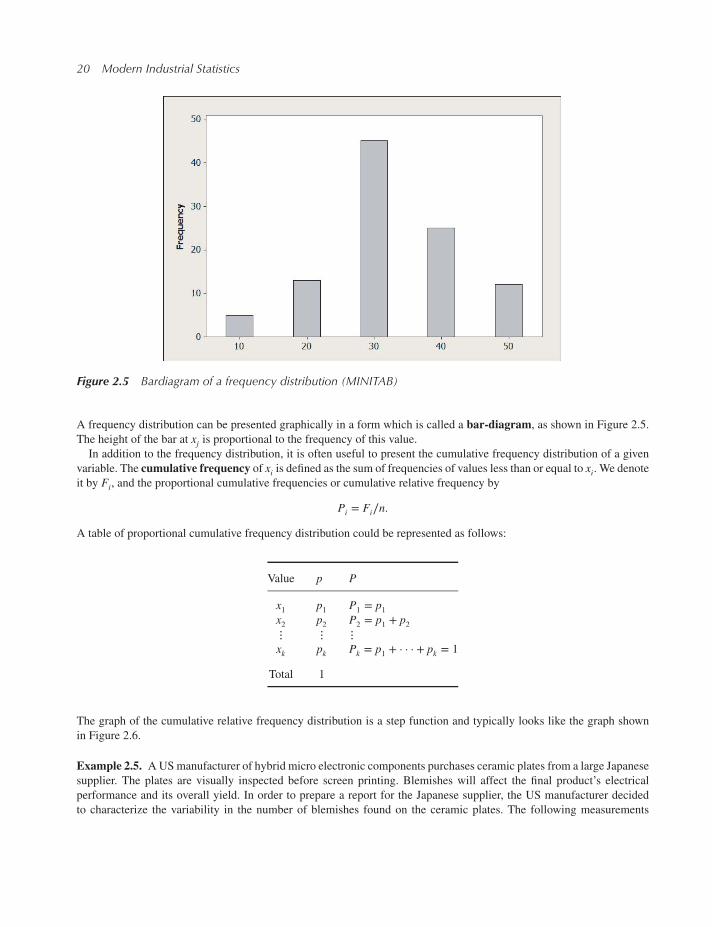
20 Modern Industrial Statistics
Figure 2.5 Bardiagram of a frequency distribution (MINITAB)
A frequency distribution can be presented graphically in a form which is called a bar-diagram, as shown in Figure 2.5.
The height of the bar at xj is proportional to the frequency of this value.
In addition to the frequency distribution, it is often useful to present the cumulative frequency distribution of a given
variable. The cumulative frequency of xi is defined as the sum of frequencies of values less than or equal to xi. We denote
it by Fi, and the proportional cumulative frequencies or cumulative relative frequency by
Pi = Fi∕n.
A table of proportional cumulative frequency distribution could be represented as follows:
Value p P
x1 p1 P1 = p1x2 p2 P2 = p1 + p2⋮ ⋮ ⋮xk pk Pk = p1 + · · · + pk = 1
Total 1
The graph of the cumulative relative frequency distribution is a step function and typically looks like the graph shown
in Figure 2.6.
Example 2.5. AUSmanufacturer of hybrid micro electronic components purchases ceramic plates from a large Japanese
supplier. The plates are visually inspected before screen printing. Blemishes will affect the final product’s electrical
performance and its overall yield. In order to prepare a report for the Japanese supplier, the US manufacturer decided
to characterize the variability in the number of blemishes found on the ceramic plates. The following measurements

Analyzing Variability: Descriptive Statistics 21
Figure 2.6 Step function of a cumulative relative frequency distribution (MINITAB)
representing the number of blemishes found on each of 30 ceramic plates:
0, 2, 0, 0, 1, 3, 0, 3, 1, 1, 0, 0, 1, 2, 0
0, 0, 1, 1, 3, 0, 1, 0, 0, 0, 5, 1, 0, 2, 0.
Here the variable X assumes the values 0, 1, 2, 3 and 5. The frequency distribution of X is displayed in Table 2.2.
Table 2.2 Frequency distribution ofblemishes on ceramic plates
x f p P
0 15 .50 .501 8 .27 .772 3 .10 .873 3 .10 .974 0 .00 .975 1 .03 1.00
Total 30 1.00
We did not observe the value x = 4, but since it seems likely to occur in future samples we include it in the frequency
distribution, with frequency f = 0. For pedagogical purposes We show next how to calculate a frequency distribution and
how to generate a bar diagram in R:
> data(BLEMISHES) # BLEMISHES is a matrix-like structure

22 Modern Industrial Statistics
The object BLEMISHES is not a simple vector like CYCLT–it is called a data frame, that is, a matrix-like structure whose
columns (variables) may be of differing types. Because of this, we access this object with the subsetting operator square
brackets [i, j] specifying elements to extract. Square brackets can be used also on vectors. Type help("[") at the
command prompt for additional information. Below are the first few rows of the object BLEMISHES.
> BLEMISHES[1:3, ] # Return rows 1 to 3, all columns
plateID countPlate 1 1 0Plate 2 2 2Plate 3 3 0
> head(BLEMISHES, # Equivalently head returns part of an objectn=3) # set number of elements
Like the previously introduced subsetting operator [i,j] the $ operator extracts a whole column by name.
> X <- factor(BLEMISHES$count, # Encode count vector as a factorlevels=0:5) # specify labels for the levels
> #> X <- table(X # Reassign to X a frequency table
) # of encoded variable count> #> X <- prop.table(X) # Reassign with proportional table> #> barplot(X, # Plot a Bar diagram
width=1, # set width of barsspace=4, # set space between barscol="grey50",ylab="Proportional Frequency")
The bar-diagram and cumulative frequency step-function are shown in Figures 2.7 and 2.8 respectively. Figure 2.8 is
obtained in MINITAB by going to the Graph > Empirical CDF window.
0 1 2 3 4 5
Pro
port
ional F
requency
0.0
0.1
0.2
0.3
0.4
0.5
Figure 2.7 Bardiagram for number of blemishes on ceramic plates

Analyzing Variability: Descriptive Statistics 23
2
Figure 2.8 Cumulative relative frequency distribution for number of blemishes on ceramic plates (MINITAB)◾
2.4.2 Frequency distributions of continuous random variables
For the case of a continuous random variable, we partition the possible range of variation of the observed variable into
k subintervals. Generally speaking, if the possible range of X is between L and H, we specify numbers b0, b1, br, · · · , bksuch that L = b0 < b1 < b2 < · · · < bk−1 < bk = H. The values b0, b1, · · · , bk are called the limits of the k subintervals.We then classify the X values into the interval (bi−1, bi) if bi−1 < X ≤ bi (i = 1, · · · , k). (If X = b0, we assign it to the firstsubinterval.) Subintervals are also called bins, classes or class-intervals.
In order to construct a frequency distribution we must consider the following two questions:
(i) How many sub-intervals should we choose?
and
(ii) How large should the width of the subintervals be?
In general, it is difficult to give to these important questions exact answers which apply in all cases. However, the
general recommendation is to use between 10 and 15 subintervals in large samples, and apply equal width subinter-
vals. The frequency distribution is given then for the subintervals, where the mid-point of each subinterval provides
a numerical representation for that interval. A typical frequency distribution table might look like the following:
Subintervals Mid-Point Freq. Cum. Freq.
b0 − b1 b1 f1 F1 = f1b1 − b2 b2 f2 F2 = f1 + f2⋮bk−1 − bk bk fk Fk = n

24 Modern Industrial Statistics
Example 2.6. Nili, a large fiber supplier to US, South American and European textile manufacturers, has tight control
over its yarn strength. This critical dimension is typically analyzed on a logarithmic scale. This logarithmic transformation
produces data that is more symmetrically distributed. Consider n = 100 values of Y = ln (X) where X is the yarn-strength
[lb./22 yarns] of woolen fibers. The data is stored in file YARNSTRG.csv and shown in Table 2.3.
The smallest value in Table 2.3 is Y = 1.1514 and the largest value is Y = 5.7978. This represents a range of 5.7978 −1.1514 = 4.6464. To obtain approximately 15 subintervals we need thewidth of each interval to be about 4.6464∕15 = .31.A more convenient choice for this class of width might be 0.50. The first subinterval would start at b0 = 0.75 and the lastsubinterval would end with bk = 6.25. The frequency distribution for this data is presented in Table 2.4.
A graphical representation of the distribution is given by a histogram as shown in Figure 2.9. Each rectangle has a
height equal to the frequency (f ) or relative frequency (p) of the corresponding subinterval. In either case the area of the
Table 2.3 A sample of 100 log (yarn strength)
2.4016 1.1514 4.0017 2.1381 2.53642.5813 3.6152 2.5800 2.7243 2.40642.1232 2.5654 1.3436 4.3215 2.52643.0164 3.7043 2.2671 1.1535 2.34834.4382 1.4328 3.4603 3.6162 2.48223.3077 2.0968 2.5724 3.4217 4.45633.0693 2.6537 2.5000 3.1860 3.50171.5219 2.6745 2.3459 4.3389 4.52345.0904 2.5326 2.4240 4.8444 1.78373.0027 3.7071 3.1412 1.7902 1.53052.9908 2.3018 3.4002 1.6787 2.17713.1166 1.4570 4.0022 1.5059 3.98213.7782 3.3770 2.6266 3.6398 2.27621.8952 2.9394 2.8243 2.9382 5.79782.5238 1.7261 1.6438 2.2872 4.64263.4866 3.4743 3.5272 2.7317 3.65614.6315 2.5453 2.2364 3.6394 3.58861.8926 3.1860 3.2217 2.8418 4.12513.8849 2.1306 2.2163 3.2108 3.21772.0813 3.0722 4.0126 2.8732 2.4190
Table 2.4 Frequency distribution for log yarn-strength data
bi−1 − bi bi fi pi Fi Pi
0.75–1.25 1.0 2 .02 2 .021.25–1.75 1.5 9 .09 11 .111.75–2.25 2.0 12 .12 23 .232.25–2.75 2.5 26 .26 49 .492.75–3.25 3.0 17 .17 66 .663.25–3.75 3.5 17 .17 83 .833.75–4.25 4.0 7 .07 90 .904.25–4.75 4.5 7 .07 97 .974.75–5.25 5.0 2 .02 99 .995.25–5.75 5.5 0 .00 99 .995.75–6.25 6.0 1 .01 100 1.00

Analyzing Variability: Descriptive Statistics 25
Log Yarn Strength
Fre
quency
1 2 3 4 5 6
010
20
30
40
Figure 2.9 Histogram of log yarn strength (Table 2.4)
1 2 3 4 5 6
0.0
0.2
0.4
0.6
0.8
1.0
Log Yarn Strength
Fn(x
)
Figure 2.10 Cumulative relative distribution of log yarn strength

26 Modern Industrial Statistics
rectangle is proportional to the frequency of the interval along the base. The cumulative frequency distribution is presented
in Figure 2.10.
Computer programs select a default midpoint andwidth of class intervals but provide the option to change these choices.
The shape of the histogram depends on the number of class intervals chosen. You can experiment with the data set
YARNSTRG.csv, by choosing a different number of class intervals, starting with the default value.
Apply the following R commands:
> data(YARNSTRG) # YARNSTRG is a vector of values> #> hist(YARNSTRG) # Plot a histogram of the given data values
This produces a histogram with 10 class intervals. The commands below produced the histogram presented in Figure 2.9
and Figure 2.10.
> hist(YARNSTRG, # Plot a histogram of the given data valuesbreaks=6, # set the number of cells for the histogrammain="", # set the main title to voidxlab = "Log yarn strength")
> #> plot.ecdf(YARNSTRG, # Plot empirical cumulative distribution
pch=NA, # set no symbol in stepsmain="",xlab="Log Yarn Strength")
◾
2.4.3 Statistics of the ordered sample
In this section we identify some characteristic values of a sample of observations that have been sorted from smallest to
largest. Such sample characteristics are called order statistics. In general, statistics are computed from observations and
are used to make an inference on characteristics of the population from where the sample was drawn. Statistics that do
not require to sort observations are discussed in Section 2.4.4.
Let X1,X2, · · · ,Xn be the observed values of some random variable, as obtained by a random sampling process. For
example, consider the following ten values of the shear strength of welds of stainless steel (lb./weld): 2385, 2400, 2285,
2765, 2410, 2360, 2750, 2200, 2500, 2550. What can we do to characterize the variability and location of these values?
The first step is to sort the sample values in increasing order. That is, we rewrite the list of sample values as: 2200,
2285, 2360, 2385, 2400, 2410, 2500, 2550, 2750, 2765. These ordered values are denoted by X(1),X(2), · · · ,X(n), where
X(1) = 2200 is the smallest value in the sample, X(2) = 2285 is the second smallest, and so on. We call X(i) the i-the orderstatistic of the sample. For convenience, we can also denote the average of consecutive order statistics by
X(i.5) = (X(i) + X(i+1))∕2 = X(i) + .5(X(i+1) − X(i)). (2.1)
For example, X(2.5) = (X(2) + X(3))∕2. We now identify some characteristic values that depend on these order statistics,
namely: the sample minimum, the sample maximum, the sample range, the sample median and the sample quartiles. The
sample minimum is X(1) and the sample maximum is X(n). In our example X(1) = 2200 and X(n) = X(10) = 2765. The
sample range is the difference R = X(n) − X(1) = 2765 − 2200 = 565. The “middle” value in the ordered sample is called
the sample median, denoted by Me. The sample median is defined as Me = X(m) where m = (n + 1)∕2. In our example
n = 10, so m = (10 + 1)∕2 = 5.5. Thus
Me = X(5.5) = (X(5) + X(6))∕2 = X(5) + .5(X(6) − X(5))
= (2400 + 2410)∕2
= 2405.
The median characterizes the center of dispersion of the sample values, and is therefore called a statistic of centraltendency, or location statistic. Approximately 50% of the sample values are smaller than the median. Finally, we define

Analyzing Variability: Descriptive Statistics 27
1 2 3 4 5 6
0.0
0.2
0.4
0.6
0.8
1.0
x
Fn(x
)
Q1 Q2 Q3
Figure 2.11 Cumulative relative distribution function with linear interpolation lines at quartiles
the sample quartiles as Q1 = X(q1) and Q3 = X(q3) where
q1 =(n + 1)
4
and (2.2)
q3 =3(n + 1)
4.
Q1 is called the lower quartile and Q3 is called the upper quartile. These quartiles divide the sample so that approxi-
mately one-fourth of the values are smaller than Q1, one half are between Q1 and Q3 and one-fourth are greater than Q3.
In our example n = 10 so
q1 =11
4= 2.75
and
q3 =33
4= 8.25.
Thus Q1 = X(2.75) = X(2) + .75 × (X(3) − X(2)) = 2341.25 and Q3 = X(8.25) = X(8) + .25 × (X(9) − X(8)) = 2600.
These sample statistics can be obtained from a frequency distribution using the cumulative relative frequency as shown
in Figure 2.11 which is based on the log yarn-strength data of Table 2.3.
Using linear interpolation within the subintervals we obtainQ1 = 2.3,Q3 = 3.6 andMe = 2.9. These estimates are only
slightly different from the exact values Q1 = X(.25) = 2.2789, Q3 = X(.75) = 3.5425 andMe = X(.5) = 2.8331.The sample median and quartiles are specific forms of a class of statistics known as sample quantiles. The p-th sample
quantile is a number that exceeds exactly 100p% of the sample values. Hence, the median is the .5 sample quantile, Q1 is
the .25th quantile andQ3 is the .75th sample quantile. We may be interested, for example, in the .9 sample quantile. Using
linear interpolation in Figure 2.11 we obtain the value 4.5, while the value of X(.9) = 4.2233. The p-th sample quantile is
also called the 100p-th sample percentile. The R commands

28 Modern Industrial Statistics
> quantile(CYCLT, # Sample quantilesprobs = seq(from=0, # set given probabilities
to=1, #by=0.25), #
type=6 # set algorithm to be used:) # 6 for MINITAB like one
0% 25% 50% 75% 100%0.17500 0.29825 0.54550 1.07175 1.14100
> #> mean(CYCLT, # Arithmetic mean
trim=0.0, # set fraction of observations# to be trimmed from each end
na.rm=TRUE # set whether NA values should) # be stripped out
[1] 0.65246
> #> # summary(CYCLT) # As above but uses R default> # type algorithm
yield the following statistics of the data: Median, Min, Max, Q1 and Q3. Applying this command on the piston cycle time
of file CYCLT.csv, we find X(1) = 0.1750, Q1 = 0.2982,Me = 0.5455, X = 0.6525, Q3 = 1.0718 and X(50) = 1.1410.
2.4.4 Statistics of location and dispersion
Given a sample of nmeasurements, X1, · · · ,Xn, we can compute various statistics to describe the distribution. The samplemean is determined by the formula
X = 1
n
n∑i=1
Xi. (2.3)
Like the sample median, X is a measure of central tendency. In physics the sample mean represents the “center of gravity”
for a system consisting of n equal-mass particles located on the points Xi on the line.As an example, consider the following measurements, representing component failure times in hours since initial
operation
45, 60, 21, 19, 4, 31.
The sample mean is
X = (45 + 60 + 21 + 19 + 4 + 31)∕6 = 30.
To measure the spread of data about the mean, we typically use the sample variance defined by
S2 = 1
n − 1
n∑i=1
(Xi − X)2, (2.4)
or the sample standard deviation, given by
S =√S2.
The sample standard deviation is used more often since its units (cm., lb.) are the same as those of the original measure-
ments. In the next section we will discuss some ways of interpreting the sample standard deviation. Presently we remark
only that data sets with greater dispersion about the mean will have larger standard deviations. The computation of S2 isillustrated in Table 2.5 using the failure time data.

Analyzing Variability: Descriptive Statistics 29
Table 2.5 Computing the sample variance
X (X − X) (X − X)2
45 15 22560 30 90021 −9 8119 −11 1214 −26 676
31 1 1
Sum 180 0 2004
X = 180∕6 = 30S2 = 2004∕5 = 400.8
The sample standard deviation and sample mean provide information on the variability and central tendency of obser-
vation. For the data set (number of blemishes on ceramic plates) in Table 2.2, one finds that X = 0.933 and S = 1.258.Looking at the histogram in Figure 2.7, one notes a marked asymmetry in the data. In 50% of the ceramic plates there were
no blemishes and in 3% there were 5 blemishes. In contrast, consider the histogram of Log Yarn-Strength which shows
remarkable symmetry with X = 2.9238 and S = 0.93776. The difference in shape is obviously not reflected by X and S.Additional information pertaining to the shape of a distribution of observations is derived from the sample skewness andsample kurtosis. The sample skewness is defined as the index
𝛽3 =1
n
n∑i=1
(Xi − X)3∕S3. (2.5)
The sample kurtosis (steepness) is defined as
𝛽4 =1
n
n∑i=1
(Xi − X)4∕S4. (2.6)
These indices can be computed in R using package e1071 and in MINITAB with Stat > Basic Statistics > DisplayDescriptive Statistics.
In JMP the output from the Analyze Distribution window looks like Figure 2.12.
Skewness and kurtosis are provided by most statistical computer packages. If a distribution is symmetric (around its
mean), then skewness = 0. If skewness > 0, we say that the distribution is positively skewed or skewed to the right. If
skewness< 0, then the distribution is negatively skewed or skewed to the left.We should also comment that in distributions
which are positively skewed X > Me, while in those which are negatively skewed X < Me. In symmetric distributions
X = Me.The steepness of a distribution is determined relative to that of the normal (Gaussian) distribution, which is described
in the next section and specified in Section 3.4.2.1. In a normal distribution, kurtosis = 3. Thus, if kurtosis > 3, thedistribution is called steep. If kurtosis < 3, the distribution is called flat. A schematic representation of shapes is given in
Figures 2.12–2.14.
To illustrate these statistics, we computed X, S2, S, skewness and kurtosis for the log yarn-strength data of Table 2.3.
We obtained
X = 2.9238
S2 = .8794 S = .93776
Skewness = .4040 Kurtosis = 2.8747.

30 Modern Industrial Statistics
Figure 2.12 Output from the analyze distribution window
0.0 0.2 0.4 0.6 0.8 1.0
01
23
4
x
y
PositiveSkewness
SymmetricNegative
Skewness
Figure 2.13 Symmetric and asymmetric distributions

Analyzing Variability: Descriptive Statistics 31
−3 −2 −1 0 1 2 3
0.0
0.1
0.2
0.3
0.4
0.5
x
y
Steep
Normal
Flat
Figure 2.14 Normal, steep, and flat distribution
The sample mean is X = 2.9238, for values on a logarithmic scale. To return to the original scale [lb/22 yarns] we can use
the measure
G = exp {X}
=
(n∏i=1
Yi
)1∕n
= 18.6119, (2.7)
where Yi = exp (Xi), i = 1, . . . , n. The measure G is called the geometric mean of Y . The geometric mean, G, is definedonly for positive valued variables. It is used as a measure of central tendency for rates or change and index numbers such
as the desirability function implemented in MINITAB and JMP. One can prove the following general result:
G ≤ X.
Equality holds only if all values in the sample are the same. Additional statistics to measure the dispersion are:
(i) The Interquartile Range IQR = Q3 − Q1, (2.8)
and
(ii) The coefficient of variation 𝛾 = S|X| . (2.9)
The interquartile range, IQR, is a useful measure of dispersion when there are extreme values (outliers) in the sample.
It is easy to compute and can yield an estimate of S, for more details, see Section 2.6.4. The coefficient of variation is
a dimensionless index, used to compare the variability of different data sets, when the standard deviation tends to grow
with the mean. The coefficient of variation of the log-yarn strength data is 𝛾 = 0.938
2.924= 0.321.

32 Modern Industrial Statistics
2.5 Prediction intervals
When the data X1, · · · ,Xn represents a sample of observations from some population, we can use the sample statistics
discussed in the previous sections to predict how future measurements will behave. Of course, our ability to predict
accurately depends on the size of the sample.
Prediction using order statistics is very simple and is valid for any type of distribution. Since the ordered measurements
partition the real line into n + 1 subintervals,
(−∞,X(1)), (X(1),X(2)), · · · , (X(n),∞),
we can predict that 100∕(n + 1)%of all future observations will fall in any one of these subintervals; hence 100i∕(n + 1)%of future sample values are expected to be less than the i-th order statistic X(i). It is interesting to note that the sample
minimum, X(1), is not the smallest possible value. Instead we expect to see one out of every n + 1 future measurements to
be less than X(1). Similarly one out of every n + 1 future measurements is expected to be greater than X(n). Predicting future
measurements using sample skewness and kurtosis is a bit more difficult because it depends on the type of distribution
that the data follow. If the distribution is symmetric (skewness ≈ 0) and somewhat “bell-shaped” or “normal”1 (kurtosis
≈ 3) as in Figure 2.9, for the log yarn strength data, we can make the following statements:
1. Approximately 68% of all future measurements will lie within one standard deviation of the mean.
2. Approximately 95% of all future measurements will lie within two standard deviations of the mean.
3. Approximately 99.7% of all future measurements will lie within three standard deviations of the mean.
The sample mean and standard deviation for the log yarn strength measurement are X = 2.92 and S = 0.94. Hencewe predict that 68% of all future measurements will lie between X − S = 1.98 and X + S = 3.86; 95% of all future
observations will be between X − 2S = 1.04 and X + 2S = 4.80; and 99.7% of all future observations will be between
X − 3S = 0.10 and X + 3S = 5.74. For the data in Table 2.3 there are exactly 69, 97 and 99 of the 100 values in the aboveintervals respectively.
When the data does not follow a normal distribution, we may use the following result: Chebyshev’s Inequality.For any number k > 1 the percentage of future measurements within k standard deviations of the mean will be at
least 100(1 − 1∕k2)%.
This means that at least 75% of all future measurements will fall within 2 standard deviations (k = 2). Similarly, at least
89% will fall within 3 standard deviations (k = 3). These statements are true for any distribution; however, the actual per-
centages may be considerably larger. Notice that for data which is normally distributed, 95% of the values fall in the inter-
val [X − 2S,X + 2S]. The Chebyshev inequality gives only the lower bound of 75%, and is therefore very conservative.
Any prediction statements, using the order statistics or the sample mean and standard deviation, can only be made
with the understanding that they are based on a sample of data. They are accurate only to the degree that the sample is
representative of the entire population. When the sample size is small, we cannot be very confident in our prediction.
For example, if based on a sample of size n = 10 we find X = 20 and S = 0.1, then we might make the statement that
95% of all future values will be between 19.8 = 20 − 2(.1) and 20.2 = 20 + 2(.1). However, it would not be too unlikelyto find that a second sample produced X = 20.1 and S = .15. The new prediction interval would be wider than 19.8 to
20.4; a considerable change. Also, a sample of size 10 does not provide sufficient evidence that the data has a “normal”
distribution. With larger samples, say, n > 100, we may be able to draw this conclusion with greater confidence.
In Chapter 4 we will discuss theoretical and computerized statistical inference whereby we assign a “confidence level”
to such statements. This confidence level will depend on the sample size. Prediction intervals which are correct with high
confidence are called tolerance intervals.
2.6 Additional techniques of exploratory data analysis
In the present section we present additional modern graphical techniques, which are quite common today in exploratory
data analysis. These techniques are the Box and Whiskers Plot, the Quantile Plot and Stem-and-Leaf Diagram. We
1The normal or Gaussian distribution will be defined in Chapter 3.

Analyzing Variability: Descriptive Statistics 33
Boxplot of Log Yarn Strength
Lo
g Y
arn
Str
en
gth
Figure 2.15 Box whiskers plot of log yarn-strength data (MINITAB)
also discuss the problem of sensitivity of the sample mean and standard deviation to outlying observations, and introduce
some robust statistics.
2.6.1 Box and whiskers plot
The Box and Whiskers Plot is a graphical presentation of the data, which provides an efficient display of various features,
like location, dispersion and skewness. A box is plotted, with its lower hinge at the first quartile Q1 = X(q1), and its upper
hinge at the third quartile Q3 = X(q3). Inside the box a line is drawn at the median,Me, and a cross is marked at the sample
mean, Xn, to mark the statistics of central location. The interquartile range, Q3 − Q1, which is the length of the box, is
a measure of dispersion. Two whiskers are extended from the box. The lower whisker is extended toward the minimum
X(1), but not lower than one and half of the interquartile range, i.e.,
Lower whisker starts = max{X(1),Q1 − 1.5(Q3 − Q1)}. (2.10)
Similarly,
Upper whisker ends = min{X(n),Q3 + 1.5(Q3 − Q1)}. (2.11)
Data points beyond the lower or upper whiskers are considered outliers. Figure 2.14 presents such a plot derived with
MINITAB. The commands below generate a similar plot in R.
> boxplot(YARNSTRG, # Produce box-and-whisker plotylab="Log Yarn Strength")
Example 2.7. In Figure 2.15 we present the box-whiskers plot of the yarn log-strength data, of Table 2.3. For this data
we find the following summarizing statistic
X(1) = 1.1514

34 Modern Industrial Statistics
Q1 = 2.2790
Me = 2.8331, X100 = 2.925
Q3 = 3.5733
X(100) = 5.7978
Q3 − Q1 = 1.2760, S(100) = 0.937.
In the box-whiskers plot, the end point of the lower whisker is at max{1.151, 0.367} = X(1). The upper whisker ends at
min{5.798, 5.51475} = 5.51475. Thus X(100) is an outlier. We conclude that the one measurement of yarn strength, which
seems to be exceedingly large, is an outlier (could have been an error of measurement). ◾
2.6.2 Quantile plots
The quantile plot is a plot of the sample quantiles xp against p, 0 < p < 1 where xp = X(p(n+1)). In Figure 2.16 we see
the quantile plot of the log yarn-strength. From such a plot one can obtain graphical estimates of the quantiles of the
distribution. For example, from Figure 2.15 we immediately obtain the estimate 2.8 for the median, 2.23 for the first
quartile and 3.58 for the third quartile. These are close to the values presented earlier. We see also in Figure 2.15 that the
maximal point of this data set is an outlier. Tracing a straight line, beginning at the median, we can also see that from x.4to x.9 (50% of the data points) are almost uniformly distributed, while the data between x.1 to x.4 tend to be larger (closerto the Me) than those of a uniform distribution, while the largest 10% of the data values tend to be again larger (further
away from the Me) than those of a uniform distribution. This explains the slight positive skewness of the data, as seen in
Figure 2.14.
2.6.3 Stem-and-leaf diagrams
Figure 2.17 is a stem-and-leaf display of the log yarn-strength data.
0.0 0.2 0.4 0.6 0.8 1.0
12
34
5
Fraction of Sample
Sam
ple
Quantile
s
Figure 2.16 Quantile plot of log yarn-strength data
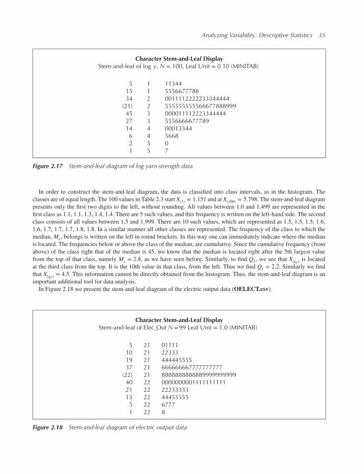
Analyzing Variability: Descriptive Statistics 35
Character Stem-and-Leaf DisplayStem-and-leaf of log y, N = 100, Leaf Unit = 0.10 (MINITAB)
5 1 1134415 1 555667778834 2 0011112222233344444
(21) 2 55555555556667788899945 3 00001111222334444427 3 555666667778914 4 000133446 4 56682 5 01 5 7
Figure 2.17 Stem-and-leaf diagram of log yarn-strength data
In order to construct the stem-and-leaf diagram, the data is classified into class intervals, as in the histogram. The
classes are of equal length. The 100 values in Table 2.3 start X(1) = 1.151 and at X(100) = 5.798. The stem-and-leaf diagram
presents only the first two digits to the left, without rounding. All values between 1.0 and 1.499 are represented in the
first class as 1.1, 1.1, 1.3, 1.4, 1.4. There are 5 such values, and this frequency is written on the left-hand side. The second
class consists of all values between 1.5 and 1.999. There are 10 such values, which are represented as 1.5, 1.5, 1.5, 1.6,
1.6, 1.7, 1.7, 1.7, 1.8, 1.8. In a similar manner all other classes are represented. The frequency of the class to which the
median, Me, belongs is written on the left in round brackets. In this way one can immediately indicate where the median
is located. The frequencies below or above the class of the median, are cumulative. Since the cumulative frequency (from
above) of the class right that of the median is 45, we know that the median is located right after the 5th largest value
from the top of that class, namely Me = 2.8, as we have seen before. Similarly, to find Q1, we see that X(q1) is located
at the third class from the top. It is the 10th value in that class, from the left. Thus we find Q1 = 2.2. Similarly we find
that X(q3) = 4.5. This information cannot be directly obtained from the histogram. Thus, the stem-and-leaf diagram is an
important additional tool for data analysis.
In Figure 2.18 we present the stem-and-leaf diagram of the electric output data (OELECT.csv).
Character Stem-and-Leaf DisplayStem-and-leaf of Elec_Out N=99 Leaf Unit = 1.0 (MINITAB)
5 21 0111110 21 2233319 21 44444555537 21 666666667777777777
(22) 21 888888888888999999999940 22 000000000111111111121 22 2223333313 22 444555555 22 67771 22 8
Figure 2.18 Stem-and-leaf diagram of electric output data

36 Modern Industrial Statistics
2.6.4 Robust statistics for location and dispersion
The sample mean Xn and the sample standard deviation are both sensitive statistics to extreme deviations. Let us illustrate
this point. Suppose we have made three observations on the sheer weld strength of steel and obtained the values 2350,
2400, 2500. The sample mean is X3 = 2416.67. What happens if the technician by mistake punches into the computer
the value 25000, instead of 2500. The sample mean would come out as 9916.67. If the result is checked on the spot, the
mistake would likely be discovered and corrected. However, if there is no immediate checking, that absurd result would
have remained and cause all kinds of difficulties later. Also, the standard deviations would have been recorded wrongly
as 13063 rather than the correct value of 76.376. This simple example shows how sensitive are the mean and the standard
deviation to extreme deviations (outliers) in the data.
To avoid such complexities, a more robust statistic can be used, instead of the sample mean, Xn. This statistic is the𝛂-trimmed mean. A proportion 𝛼 of the data is trimmed from the lower and from the upper end of the ordered sample.
The mean is then computed on the remaining (1 − 2𝛼) proportion of the data. Let us denote by T𝛼 the 𝛼-trimmed mean.
The formula of this statistic is
T𝛼 =1
N𝛼
[n(1−𝛼)]∑j=[n𝛼]+1
Xj, (2.12)
where [⋅] denotes the integer part of the number in brackets, for example, [7.3] = 7, and N𝛼 = [n(1 − 𝛼)] − [n𝛼]. Forexample, if n = 100 and 𝛼 = 0.05, we compute the mean of the 90 ordered values X(6), · · · ,X(95).
Example 2.8. Let us now examine the robustness of the trimmed mean. We import data file OELECT.csv in package
mistat, DatFiles directory. Function mean yields different results given specific values of the trim parameter. We use
this example to show how to set up a function in R.
> File <- paste( # Compose a string withpath.package("mistat"), # mistat package path and"/csvFiles/OELECT.csv", # /DatFiles/OELECT.csvsep = "") # separate the terms with ""
> #> Oelect <- read.csv(file=File) # Read a csv file and assign to> # Oelect> #> rm(File) #> #> mySummary <- function( # Define a new function
x, trim=0, type=6 ) # with arguments x, trim and type#
{ # The new function does:#
qq <-quantile(x, type=type) # Calculate quantiles#
qq <- c(qq[1L:3L], # Concatenate quantiles and meanmean(x, trim=trim),qq[4L:5L])
#names(qq) <- c("Min.", "1st Qu.", # Assign names to values
"Median", "Mean","3rd Qu.", "Max.")
#qq <- signif(qq) # Round to significant values
#return(qq) # Return results
#} # Function end
> #

Analyzing Variability: Descriptive Statistics 37
> mySummary(Oelect$OELECT) # Apply mySummary to Oelect data
Min. 1st Qu. Median Mean 3rd Qu. Max.210.896 216.796 219.096 219.248 221.706 228.986
> #> mySummary(Oelect$OELECT, # Apply mySummary to Oelect data
trim=0.05) # set trim to 5%
Min. 1st Qu. Median Mean 3rd Qu. Max.210.896 216.796 219.096 219.218 221.706 228.986
> #> sd(Oelect$OELECT) # Computes the standard deviation
[1] 4.003992
We see that X99 = 219.25 and T .05 = 219.22. Let us order the sample value by using the function sort() and re-assign
values to column V with assignment operator <-. The largest value in C2 is C2(99) = 228.986. Let us now change this
value to be V(99) = 2289.86 (an error in punching the data), and look at results when we apply the same commands
> OutVolt <- sort(Oelect$OELECT) # Assign a vector> # of sorted values> #> OutVolt[99] <- 2289.86 # Assign a specific value> # at position 99> #> mySummary(OutVolt) # Apply function mySummary
Min. 1st Qu. Median Mean 3rd Qu. Max.210.896 216.796 219.096 240.065 221.706 2289.860
> #> mySummary(OutVolt, # Apply mySummary with
trim=0.05) # trim = 5%
Min. 1st Qu. Median Mean 3rd Qu. Max.210.896 216.796 219.096 219.218 221.706 2289.860
> #> sd(OutVolt) # Computes the standard deviation
[1] 208.1505
We see by comparing the two outputs that X99 changed from 219.25 to 240.1, S99 (STDEV) changed dramatically from
4.00 to 208.2 (and correspondingly SEMEAN = S∕√n changed).
On the other hand, Me, T𝛼 , Q1 and Q3 did not change at all. These statistics are called robust (non-sensitive) againstextreme deviations (outliers). ◾
We have seen that the standard deviation S is very sensitive to deviations in the extremes. A robust statistic for disper-
sion is
�� =Q3 − Q1
1.3490. (2.13)
The denominator 1.3490 is the distance between Q3 and Q1 in the theoretical normal distribution (see Chapter 4). Indeed,
Q3 and Q1 are robust against outliers. Hence ��, which is about 3/4 of the IQR, is often a good statistic to replace S.Another statistic is the 𝛂-trimmed standard deviation
S𝛼 =
(1
N𝛼 − 1
[n(1−𝛼)]∑j=[n𝛼]+1
(Xj − T𝛼)2)1∕2
. (2.14)

38 Modern Industrial Statistics
For the OELECT data S𝛼 equals 3.5969. The command below calculates a robust statistic for dispersion �� from the
OELECT data.
> IQR(OutVolt)/1.349 # Robust estimate of S
[1] 3.587843
We see these two robust statistics, �� and S𝛼 yield close results. The sample standard deviation of OELECT is S = 4.00399.
2.7 Chapter highlights
The chapter focuses on statistical variability and on various methods of analyzing random data. Random results of experi-
ments are illustrated with distinction between deterministic and random components of variability. The difference between
accuracy and precision is explained. Frequency distributions are defined to represent random phenomena. Various char-
acteristics of location and dispersion of frequency distributions are defined. The elements of exploratory data analysis are
presented.
The main concepts and definitions introduced in this chapter include:
• Random Variable
• Fixed and Random Components
• Accuracy and Precision
• The Population and the Sample
• Random Sampling With Replacement (RSWR)
• Random Sampling Without Replacement (RSWOR)
• Frequency Distributions
• Discrete and Continuous Random Variables
• Quantiles
• Sample Mean and Sample Variance
• Skewness
• Kurtosis
• Prediction Intervals
• Box and Whiskers Plots
• Quantile Plots
• Stem-and-Leaf Diagrams
• Robust Statistics
2.8 Exercises
2.1 In the present problem we are required to generate at random 50 integers from the set {1, 2, 3, 4, 5, 6}. To do this
we can use the MINITAB command
MTB> RANDOM 50 C1;SUBC> INTEGER 1 6.
Use this method of simulation and count the number of times the different integers have been repeated. This
counting can be done by using the MINITAB command
MTB> TABLE C1How many times you expect each integer to appear if the process generates the numbers at random?
2.2 Construct a sequence of 50 numbers having a linear trend for deterministic components with random deviations
around it. This can be done by using the MINITAB commands
MTB> Set C1DATA> 1(1 ∶ 50∕1)1DATA> End.

Analyzing Variability: Descriptive Statistics 39
MTB> Let C2 = 5 + 2.5 ∗ C1MTB> Random 50 C3;SUBC> Uniform −10 10.
MTB> Let C4 = C2 + C3MTB> Plot C4 ∗ C1By plotting C4 versus C1, one sees the random variability around the linear trend.
2.3 Generate a sequence of 50 random binary numbers (0, 1), when the likelihood of 1 is p, by using the command
MTB> RANDOM 50 C1;SUBC> Bernoulli p.Do this for the values p = 0.1, 0.3, 0.7, 0.9. Count the number of 1’s in these random sequences, by the command
SUM(C1)2.4 The following are two sets of measurements of the weight of an object, which correspond to two different weighing
instruments. The object has a true weight of 10 kg.
Instrument 1:
[1] 9.490950 10.436813 9.681357 10.996083 10.226101 10.253741[7] 10.458926 9.247097 8.287045 10.145414 11.373981 10.144389
[13] 11.265351 7.956107 10.166610 10.800805 9.372905 10.199018[19] 9.742579 10.428091
Instrument 2:
[1] 11.771486 10.697693 10.687212 11.097567 11.676099 10.583907[7] 10.505690 9.958557 10.938350 11.718334 11.308556 10.957640
[13] 11.250546 10.195894 11.804038 11.825099 10.677206 10.249831[19] 10.729174 11.027622
Which instrument seems to be more accurate? Which instrument seems to be more precise?
2.5 The quality control department of a candy factory uses a scale to verify compliance of the weight of packages.
What could be the consequences of problems with the scale accuracy, precision and stability?
2.6 Draw a random sample with replacement (RSWR) of size n = 20 from the set of integers {1, 2, · · · , 100}.2.7 Draw a random sample without replacement (RSWOR) of size n = 10 from the set of integers {11, 12, · · · , 30}.2.8 (i) How many words of 5 letters can be composed (N = 26, n = 5)?
(ii) How many words of 5 letters can be composed, if all letters are different?
(iii) How many words of 5 letters can be written if the first and the last letters are x?(iv) An electronic signal is a binary sequence of 10 zeros or ones. How many different signals are available?
(v) How many electronic signals in a binary sequence of size 10 are there in which the number 1 appears exactly
5 times?
2.9 For each of the following variables state whether it is discrete or continuous:
(i) The number of “heads” among the results of 10 flippings of a coin.
(ii) The number of blemishes on a ceramic plate.
(iii) The thickness of ceramic plates.
(iv) The weight of an object.
2.10 Data fileFILMSP.csv contains data gathered from 217 rolls of film. The data consists of the film speed as measured
in a special lab.
(i) Prepare a histogram of the data.
2.11 Data file COAL.csv contains data on the number of yearly disasters in coal mines in England. Prepare a table of
frequency distributions of the number of coal-mine disasters. [You can use the MINITAB command TABLE C1.]2.12 Data fileCAR.csv contains information on 109 different car models. For each car there are values of five variables:
1. Number of cylinders (4, 6, 8)
2. Origin (1, 2, 3)
3. Turn Diameter [m]
4. Horsepower [HP]

40 Modern Industrial Statistics
5. Number of miles/gallon in city driving [mpg].
Prepare frequency distributions of variables 1, 2, 3, 4, 5.
2.13 Compute the following five quantities for the data in file FILMSP.csv(i) Sample minimum, X(1).
(ii) Sample first quartile, Q1.
(iii) Sample median, Me.
(iv) Sample third quartile, Q3.
(v) Sample maximum, X(217).
(vi) The .8-quantile.
(vii) The .9-quantile.
(viii) The .99-quantile.
Show how you get these statistics by using the formulae. [The order statistics of the sample can be obtained by
first ordering the values of the sample. For this use the MINITAB command
MTB> SORT C1 C2.Certain order statistics can be put into constants by the commands, e.g.
MTB> Let k1 = 1
MTB> Let k2 = C2(k1)The sample minimum is C2(1), the sample maximum is C2(217), etc.].
2.14 Compute with MINITAB the indices of skewness and kurtosis of the FILMSP.csv, by defining the constants: Forskewness:
MTB> Let k1 =mean((C1− mean(C1)) ∗∗ 3)∕(mean((C1−Mean(C1)) ∗∗ 2)) ∗∗ 1.5For kurtosis:
MTB> Let k2 = mean((C1− mean(C1)) ∗∗ 4)∕(mean((C1− mean(C1)) ∗∗ 2)) ∗∗ 2
Interpret the skewness and kurtosis of this sample in terms of the shape of the distribution of film speed.
2.15 Compare the means and standard deviations of the number of miles per gallon/city of cars by origin (1 = US; 2 =Europe; 3 = Asia) according to the data of file CAR.csv.
2.16 Compute the coefficient of variation of the Turn Diameter of US made cars (Origin = 1) in file CAR.csv.2.17 Compare the mean X and the geometric mean G of the Turn Diameter of US made and Japanese cars in CAR.csv.2.18 Compare the prediction proportions to the actual frequencies of the intervals
X ± kS, k = 1, 2, 3
for the film speed data, given in FILMSP.csv file.2.19 Present side by side the box plots of Miles per Gallon/City for cars by origin. Use data file CAR.csv.2.20 Prepare a stem-leaf diagram of the piston cycle time in file OTURB.csv. Compute the five summary statistics
(X(1),Q1,Me,Q3,X(n)) from the stem-leaf.
2.21 Compute the trimmed mean T .10 and trimmed standard deviation, S.10 of the piston cycle time of fileOTURB.csv.2.22 The following data is the time (in sec.) to get from 0 to 60 mph for a sample of 15 German cars and 20 Japanese cars
German cars Japanese cars
10.0 10.9 4.8 9.4 9.5 7.1 8.0
6.4 7.9 8.9 8.9 7.7 10.5 6.5
8.5 6.9 7.1 6.7 9.3 5.7 12.5
5.5 6.4 8.7 7.2 9.1 8.3 8.2
5.1 6.0 7.5 8.5 6.8 9.5 9.7
Compare and contrast the acceleration times of German and Japanese cars, in terms of their five summary statistics.
2.23 Summarize variables Res 3 and Res 7 in data set HADPAS.csv by computing sample statistics, histograms and
stem-and-leaf diagrams.
2.24 Are there outliers in the Res 3 data of HADPAS.csv? Show your calculations.

3Probability Models andDistribution Functions
3.1 Basic probability
3.1.1 Events and sample spaces: Formal presentation of random measurements
Experiments or trials of interest, are those which may yield different results with outcomes that are not known ahead of
timewith certainty.We have seen in the previous chapters a large number of examples in which outcomes of measurements
vary. It is of interest to find, before conducting a particular experiment, what are the chances of obtaining results in a certain
range. In order to provide a quantitative answer to such a question, we have to formalize the framework of the discussion
so that no ambiguity is left.
When we say a “trial” or “experiment,” in the general sense, we mean a well defined process of measuring certain
characteristic(s), or variable(s). For example, if the experiment is to measure the compressive strength of concrete cubes,
we must specify exactly how the concrete mixture was prepared, that is, proportions of cement, sand, aggregates and water
in the batch. Length of mixing time, dimensions of mold, number of days during which the concrete has hardened. The
temperature and humidity during preparation and storage of the concrete cubes, etc. All these factors influence the resulting
compressive strength. Well-documented protocol of an experiment enables us to replicate it as many times as needed. In
a well-controlled experiment we can assume that the variability in the measured variables is due to randomness. We can
think of the random experimental results as sample values from a hypothetical population. The set of all possible sample
values is called the sample space. In other words, the sample space is the set of all possible outcomes of a specified
experiment. The outcomes do not have to be numerical. They could be names, categorical values, functions, or collection
of items. The individual outcome of an experiment will be called an elementary event or a sample point (element). We
provide a few examples.
Example 3.1. The experiment consists of choosing ten names (without replacement) from a list of 400 undergraduate
students at a given university. The outcome of such an experiment is a list of ten names. The sample space is the collection
of all possible such sublists that can be drawn from the original list of 400 students. ◾
Example 3.2. The experiment is to produce twenty concrete cubes, under identical manufacturing conditions, and count
the number of cubes with compressive strength above 200 [kg/cm2]. The sample space is the set S = {0, 1, 2, · · · , 20}.The elementary events, or sample points, are the elements of S. ◾
Modern Industrial Statistics: with applications in R, MINITAB and JMP, Second Edition. Ron S. Kenett and Shelemyahu Zacks.© 2014 John Wiley & Sons, Ltd. Published 2014 by John Wiley & Sons, Ltd.Companion website: www.wiley.com/go/modern_industrial_statistics

42 Modern Industrial Statistics
Example 3.3. The experiment is to choose a steel bar from a specific production process, and measure its weight. The
sample space S is the interval (𝜔0, 𝜔1) of possible weights. The weight of a particular bar is a sample point. ◾
Thus, sample spaces could be finite sets of sample points, or countable or non-countable infinite sets.
Any subset of the sample space, S, is called an event. S itself is called the sure event. The empty set, ∅, is called the
null event. We will denote events by the letters A,B,C, · · · or E1,E2, · · · . All events under consideration are subsets of
the same sample space S. Thus, events are sets of sample points.
For any event A ⊆ S, we denote by Ac the complementary event, that is, the set of all points of S which are not in A.An event A is said to imply an event B, if all elements of A are elements of B. We denote this inclusion relationship
by A ⊂ B. If A ⊂ B and B ⊂ A, then the two events are equivalent, A ≡ B.
Example 3.4. The experiment is to select a sequence of 5 letters for transmission of a code in a money transfer operation.
Let A1,A2, . . . ,A5 denote the first, second, . . . , fifth letter chosen. The sample space is the set of all possible sequences
of five letters. Formally,
S = {(A1A2A3A4A5) ∶ Ai ∈ {a, b, c, · · · , z}, i = 1, · · · , 5}
This is a finite sample space containing 265 possible sequences of 5 letters. Any such sequence is a sample point.
Let E be the event that all the 5 letters in the sequence are the same. Thus
E = {aaaaa, bbbbb, · · · , zzzzz}.
This event contains 26 sample points. The complement of E, Ec, is the event that at least one letter in the sequence is
different from the other ones. ◾
3.1.2 Basic rules of operations with events: Unions, intersections
Given events A,B, · · · of a sample space S, we can generate new events, by the operations of union, intersection and
complementation.
The union of two events A and B, denoted A ∪ B, is an event having elements which belong either to A or to B.The intersection of two events, A ∩ B, is an event whose elements belong both to A and to B. By pairwise union or
intersection we immediately extend the definition to finite number of events A1,A2, · · · ,An, that is,n⋃i=1
Ai = A1 ∪ A2 ∪ · · · ∪ An
andn⋂i=1
Ai = A1 ∩ A2 ∩ · · · ∩ An.
The finite unionn⋃i=1Ai is an event whose elements belong to at least one of the n events. The finite intersection
n⋂i=1Ai is an
event whose elements belong to all the n events.Any two events, A and B, are said to be mutually exclusive or disjoint if A ∩ B = ∅, that is, they do not contain common
elements. Obviously, by definition, any event is disjoint of its complement, i.e., A ∩ Ac = ∅. The operations of union andintersection are:
1. Commutative:A ∪ B = B ∪ A,
A ∩ B = B ∩ A;

Probability Models and Distribution Functions 43
2. Associative:(A ∪ B) ∪ C = A ∪ (B ∪ C)
= A ∪ B ∪ C
(A ∩ B) ∩ C = A ∩ (B ∩ C)
= A ∩ B ∩ C
(3.1)
3. Distributive:A ∩ (B ∪ C) = (A ∩ B) ∪ (A ∩ C)
A ∪ (B ∩ C) = (A ∪ B) ∩ (A ∪ C).(3.2)
The intersection of events is sometimes denoted as a product, that is,
A1 ∩ A2 ∩ · · · ∩ An ≡ A1A2A3 · · ·An.
The following law, called the De-Morgan Rule, is fundamental to the algebra of events and yields the complement of the
union, or intersection, of two events, namely:
1. (A ∪ B)c = Ac ∩ Bc (3.3)
2. (A ∩ B)c = Ac ∪ Bc.Finally, we define the notion of partition. A collection of n events E1, · · · ,En is called a partition of the sample
space S, if(i)
⋃ni=1 Ei = S,
(ii) Ei ∩ Ej = ∅ for all i ≠ j (i, j = 1, · · · , n).
That is, the events in any partition are mutually disjoint, and their union exhaust all the sample space.
Example 3.5. The experiment is to generate on the computer a random number, U, in the interval (0, 1). A random
number in (0, 1) can be obtained as
U =∞∑j=1
Ij2−j,
where Ij is the random result of tossing a coin, that is,
Ij =
{1, if Head
0, if Tail.
To generate random numbers from a set of integers, the summation index j is bounded by a finite number N. This method
is, however, not practical for generating random numbers on a continuous interval. Computer programs generate “pseudo-
random” numbers. Methods for generating random numbers are described in various books on simulation (see Bratley,
Fox and Schrage (1983)). Most commonly applied is the linear congruential generator. This method is based on the
recursive equation
Ui = (aUi−1 + c) mod m, i = 1, 2, · · · .
The parameters a, c and m depend on the computer’s architecture. In many programs, a = 65539, c = 0 and m = 231 − 1.
The first integer X0 is called the “seed.” Different choices of the parameters a, c and m yield “pseudo-random” sequences
with different statistical properties.
The sample space of this experiment is
S = {u ∶ 0 ≤ u ≤ 1}

44 Modern Industrial Statistics
Let E1 and E2 be the events
E1 = {u ∶ 0 ≤ u ≤ 0.5},
E2 = {u ∶ 0.35 ≤ u ≤ 1}.
The union of these two events is
E3 = E1 ∪ E2 = {u ∶ 0 ≤ u ≤ 1} = S.
The intersection of these events is
E4 = E1 ∩ E2 = {u ∶ 0.35 ≤ u < 0.5}.
Thus, E1 and E2 are not disjoint.The complementary events are
Ec1= {u ∶ 0.5 ≤ u < 1} and Ec
2= {u ∶ u < 0.35}
Ec1∩ Ec
2= ∅; i.e., the complementary events are disjoint. By DeMorgan’s law
(E1 ∩ E2)c = Ec1∪ Ec
2
= {u ∶ u < 0.35 or u ≥ 0.5}.
However,
∅ = Sc = (E1 ∪ E2)c = Ec1∩ Ec
2.
Finally, the following is a partition of S:
B1 = {u ∶ u < 0.1}, B2 = {u ∶ 0.1 ≤ u < 0.2},
B3 = {u ∶ 0.2 ≤ u < 0.5}, B4 = {u ∶ 0.5 ≤ u < 1}.
Notice that B4 = Ec1. ◾
Different identities can be derived by the above rules of operations on events, a few will be given as exercises.
3.1.3 Probabilities of events
A probability function Pr{⋅} assigns to events of S real numbers, following the following basic axioms.
1. Pr{E} ≥ 0
2. Pr{S} = 1.
3. If E1, · · · ,En (n ≥ 1) are mutually disjoint events, then
Pr
{n⋃i=1
Ei
}=
n∑i=1
Pr{Ei}.
From these three basic axioms, we deduce the following results.
Result 1. If A ⊂ B thenPr{A} ≤ Pr{B}.
Indeed, since A ⊂ B, B = A ∪ (Ac ∩ B). Moreover A ∩ Ac ∩ B = ∅. Hence, by Axioms 1 and 3, Pr{B} = Pr{A} + Pr{Ac ∩B} ≥ Pr{A}.
Thus, if E, is any event, since E ⊂ S, 0 ≤ Pr{E} ≤ 1.
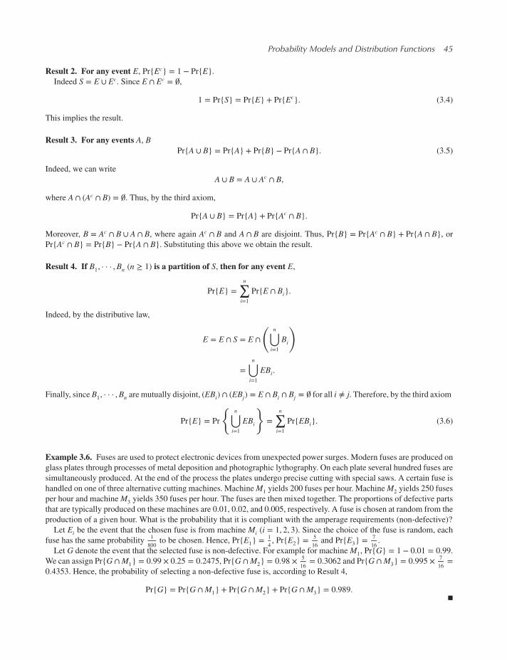
Probability Models and Distribution Functions 45
Result 2. For any event E, Pr{Ec} = 1 − Pr{E}.Indeed S = E ∪ Ec. Since E ∩ Ec = ∅,
1 = Pr{S} = Pr{E} + Pr{Ec}. (3.4)
This implies the result.
Result 3. For any events A, BPr{A ∪ B} = Pr{A} + Pr{B} − Pr{A ∩ B}. (3.5)
Indeed, we can write
A ∪ B = A ∪ Ac ∩ B,
where A ∩ (Ac ∩ B) = ∅. Thus, by the third axiom,
Pr{A ∪ B} = Pr{A} + Pr{Ac ∩ B}.
Moreover, B = Ac ∩ B ∪ A ∩ B, where again Ac ∩ B and A ∩ B are disjoint. Thus, Pr{B} = Pr{Ac ∩ B} + Pr{A ∩ B}, orPr{Ac ∩ B} = Pr{B} − Pr{A ∩ B}. Substituting this above we obtain the result.
Result 4. If B1, · · · ,Bn (n ≥ 1) is a partition of S, then for any event E,
Pr{E} =n∑i=1
Pr{E ∩ Bi}.
Indeed, by the distributive law,
E = E ∩ S = E ∩
(n⋃i=1
Bi
)
=n⋃i=1
EBi.
Finally, since B1, · · · ,Bn are mutually disjoint, (EBi) ∩ (EBj) = E ∩ Bi ∩ Bj = ∅ for all i ≠ j. Therefore, by the third axiom
Pr{E} = Pr
{n⋃i=1
EBi
}=
n∑i=1
Pr{EBi}. (3.6)
Example 3.6. Fuses are used to protect electronic devices from unexpected power surges. Modern fuses are produced on
glass plates through processes of metal deposition and photographic lythography. On each plate several hundred fuses are
simultaneously produced. At the end of the process the plates undergo precise cutting with special saws. A certain fuse is
handled on one of three alternative cutting machines. MachineM1 yields 200 fuses per hour. MachineM2 yields 250 fuses
per hour and machineM3 yields 350 fuses per hour. The fuses are then mixed together. The proportions of defective parts
that are typically produced on these machines are 0.01, 0.02, and 0.005, respectively. A fuse is chosen at random from the
production of a given hour. What is the probability that it is compliant with the amperage requirements (non-defective)?
Let Ei be the event that the chosen fuse is from machine Mi (i = 1, 2, 3). Since the choice of the fuse is random, each
fuse has the same probability1
800to be chosen. Hence, Pr{E1} = 1
4, Pr{E2} = 5
16and Pr{E3} = 7
16.
Let G denote the event that the selected fuse is non-defective. For example for machineM1, Pr{G} = 1 − 0.01 = 0.99.We can assign Pr{G ∩M1} = 0.99 × 0.25 = 0.2475, Pr{G ∩M2} = 0.98 × 5
16= 0.3062 and Pr{G ∩M3} = 0.995 × 7
16=
0.4353. Hence, the probability of selecting a non-defective fuse is, according to Result 4,
Pr{G} = Pr{G ∩M1} + Pr{G ∩M2} + Pr{G ∩M3} = 0.989.◾
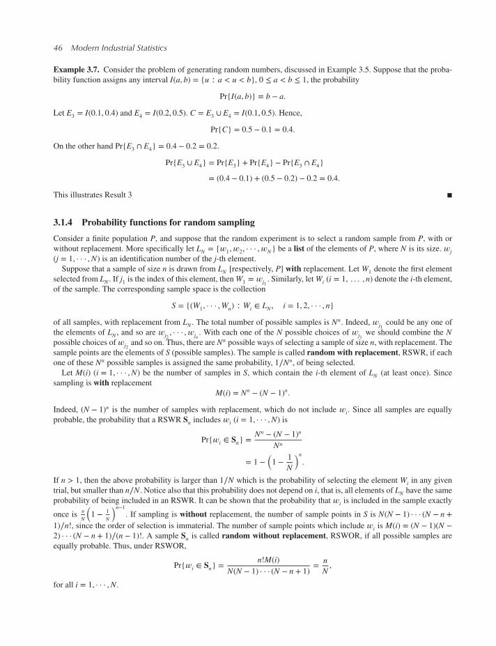
46 Modern Industrial Statistics
Example 3.7. Consider the problem of generating random numbers, discussed in Example 3.5. Suppose that the proba-
bility function assigns any interval I(a, b) = {u ∶ a < u < b}, 0 ≤ a < b ≤ 1, the probability
Pr{I(a, b)} = b − a.
Let E3 = I(0.1, 0.4) and E4 = I(0.2, 0.5). C = E3 ∪ E4 = I(0.1, 0.5). Hence,
Pr{C} = 0.5 − 0.1 = 0.4.
On the other hand Pr{E3 ∩ E4} = 0.4 − 0.2 = 0.2.
Pr{E3 ∪ E4} = Pr{E3} + Pr{E4} − Pr{E3 ∩ E4}
= (0.4 − 0.1) + (0.5 − 0.2) − 0.2 = 0.4.
This illustrates Result 3 ◾
3.1.4 Probability functions for random sampling
Consider a finite population P, and suppose that the random experiment is to select a random sample from P, with or
without replacement. More specifically let LN = {𝑤1, 𝑤2, · · · , 𝑤N} be a list of the elements of P, where N is its size. 𝑤j(j = 1, · · · ,N) is an identification number of the j-th element.
Suppose that a sample of size n is drawn from LN [respectively, P] with replacement. Let W1 denote the first element
selected from LN . If j1 is the index of this element, thenW1 = 𝑤j1 . Similarly, letWi (i = 1, . . . , n) denote the i-th element,
of the sample. The corresponding sample space is the collection
S = {(W1, · · · ,Wn) ∶ Wi ∈ LN , i = 1, 2, · · · , n}
of all samples, with replacement from LN . The total number of possible samples is Nn. Indeed, 𝑤j1 could be any one of
the elements of LN , and so are 𝑤j2 , · · · , 𝑤jn . With each one of the N possible choices of 𝑤j1 we should combine the Npossible choices of𝑤j2 and so on. Thus, there are N
n possible ways of selecting a sample of size n, with replacement. The
sample points are the elements of S (possible samples). The sample is called random with replacement, RSWR, if each
one of these Nn possible samples is assigned the same probability, 1∕Nn, of being selected.
Let M(i) (i = 1, · · · ,N) be the number of samples in S, which contain the i-th element of LN (at least once). Since
sampling is with replacement
M(i) = Nn − (N − 1)n.
Indeed, (N − 1)n is the number of samples with replacement, which do not include 𝑤i. Since all samples are equally
probable, the probability that a RSWR Sn includes 𝑤i (i = 1, · · · ,N) is
Pr{𝑤i ∈ Sn} = Nn − (N − 1)n
Nn
= 1 −(1 − 1
N
)n.
If n > 1, then the above probability is larger than 1∕N which is the probability of selecting the element Wi in any given
trial, but smaller than n∕N. Notice also that this probability does not depend on i, that is, all elements of LN have the same
probability of being included in an RSWR. It can be shown that the probability that 𝑤i is included in the sample exactly
once isn
N
(1 − 1
N
)n−1. If sampling is without replacement, the number of sample points in S is N(N − 1) · · · (N − n +
1)∕n!, since the order of selection is immaterial. The number of sample points which include 𝑤i is M(i) = (N − 1)(N −2) · · · (N − n + 1)∕(n − 1)!. A sample Sn is called random without replacement, RSWOR, if all possible samples are
equally probable. Thus, under RSWOR,
Pr{𝑤i ∈ Sn} = n!M(i)N(N − 1) · · · (N − n + 1)
= nN,
for all i = 1, · · · ,N.

Probability Models and Distribution Functions 47
We consider now events, which depend on the attributes of the elements of a population. Suppose that we sample to
obtain information on the number of defective (non-standard) elements in a population. The attribute in this case is “the
element complies to the requirements of the standard.” Suppose that M out of N elements in LN are non-defective (have
the attribute). Let Ej be the event that j out of the n elements in the sample are non-defective. Notice that E0, · · · ,En is apartition of the sample space. What is the probability, under RSWR, of Ej? Let K
nj denote the number of sample points in
which j out of n are G elements (non-defective) and (n − j) elements are D (defective). To determine Knj , we can proceed
as follows:
Choose first j G’s and (n − j) D’s from the population. This can be done inMj(N −M)n−j different ways. We have now
to assign the j G’s into j out of n components of the vector (𝑤1, · · · , 𝑤n). This can be done in n(n − 1) · · · (n − j + 1)∕j!possible ways. This is known as the number of combinations of j out of n, i.e.,(
nj
)= n!j!(n − j)!, j = 0, 1, · · · , n (3.7)
where k! = 1 ⋅ 2 ⋅ · · · ⋅ k is the product of the first k positive integers, 0! = 1. Hence, Knj =
(nj
)Mj(N −M)n−j. Since every
sample is equally probable, under RSWR,
Pr{Ej∶n} = Knj ∕N
n =(nj
)Pj(1 − P)n−j, j = 0, · · · , n (3.8)
where P = M∕N. If sampling is without replacement, then
Knj =
(Mj
)(N −Mn − j
)and
Pr{Ej} =(Mj
) (N−Mn−j)(
Nn
) . (3.9)
These results are valid since the order of selection is immaterial for the event Ej.These probabilities of Ej under RSWR and RSWOR are called, respectively, the binomial and hypergeometric prob-
abilities.
Example 3.8. The experiment consists of randomly transmitting a sequence of binary signals, 0 or 1. What is the proba-
bility that 3 out of 6 signals are 1’s? Let E3 denote this event.
The sample space of 6 signals consists of 26 points. Each point is equally probable. The probability of E3 is
Pr{E3} =(6
3
)1
26= 6 ⋅ 5 ⋅ 4
1 ⋅ 2 ⋅ 3 ⋅ 64
= 20
64= 5
16= 0.3125.
◾
Example 3.9. Two out of ten television sets are defective. A RSWOR of n = 2 sets is chosen. What is the probability that
the two sets in the sample are good (non-defective)? This is the hypergeometric probability of E0 when M = 2, N = 10,
n = 2, that is,
Pr{E0} =(82
)(102
) = 8 ⋅ 710 ⋅ 9
= 0.622.
◾
3.1.5 Conditional probabilities and independence of events
In this section we discuss the notion of conditional probabilities. When different events are related, the realization of one
event may provide us relevant information to improve our probability assessment of the other event(s). In Section 3.1.3 we

48 Modern Industrial Statistics
gave an example with three machines which manufacture the same part but with different production rates and different
proportions of defective parts in the output of those machines. The random experiment was to choose at random a part
from the mixed yield of the three machines.
We saw earlier that the probability that the chosen part is non-defective is 0.989. If we can identify, before the quality
test, from which machine the part came, the probabilities of non-defective would be conditional on this information.
The probability of choosing at random a non-defective part from machineM1, is 0.99. If we are given the information
that the machine is M2, the probability is 0.98, and given machine M3, the probability is 0.995. These probabilities are
called conditional probabilities. The information given changes our probabilities.
We define now formally the concept of conditional probability.
Let A and B be two events such that Pr{B} > 0. The conditional probability of A, given B, is
Pr{A ∣ B} = Pr{A ∩ B}Pr{B}. (3.10)
Example 3.10. The random experiment is to measure the length of a steel bar.
The sample space is S = (19.5, 20.5) [cm]. The probability function assigns any subinterval a probability equal to its
length. Let A = (19.5, 20.1) and B = (19.8, 20.5). Pr{B} = 0.7. Suppose that we are told that the length belongs to the
interval B, and we have to guess whether it belongs to A. We compute the conditional probability
Pr{A ∣ B} = Pr{A ∩ B}Pr{B}
= 0.3
0.7= 0.4286.
On the other hand, if the information that the length belongs to B is not given, then Pr{A} = 0.6. Thus, there is a differencebetween the conditional and non-conditional probabilities. This indicates that the two events A and B are dependent. ◾
Definition. Two events A, B are called independent if
Pr{A ∣ B} = Pr{A}.
If A and B are independent events, then
Pr{A} = Pr{A ∣ B} = Pr{A ∩ B}Pr{B}
or, equivalently,
Pr{A ∩ B} = Pr{A}Pr{B}.
If there are more than two events, A1,A2, · · · ,An, we say that the events are pairwise independent if
Pr{Ai ∩ Aj} = Pr{Ai}Pr{Aj} for all i ≠ j, i, j = 1, · · · , n.
The n events are said to be mutually independent if, for any subset of k events, k = 2, . . . , n, indexed by Ai1 , . . . ,Aik ,
Pr{Ai1 ∩ Ai2 · · · ∩ Aik} = Pr{Ai1} · · ·Pr{Ain}.
In particular, if n events are mutually independent, then
Pr
{n⋂i=1
Ai
}=
n∏i=1
Pr{Ai}. (3.11)
One can show examples of events which are pairwise independent but not mutually independent.
We can further show (see exercises) that if two events are independent, then the corresponding complementary events
are independent. Furthermore, if n events are mutually independent, then any pair of events is pairwise independent, every
three events are triplewise independent, etc.

Probability Models and Distribution Functions 49
Example 3.11. Five identical parts are manufactured in a given production process. LetE1, · · · ,E5 be the events that these
five parts comply with the quality specifications (non-defective). Under the model of mutual independence the probability
that all the five parts are indeed non-defective is
Pr{E1 ∩ E2 ∩ · · · ∩ E5} = Pr{E1}Pr{E2} · · ·Pr{E5}.
Since these parts come from the same production process, we can assume that Pr{Ei} = p, all i = 1, · · · , 5. Thus, theprobability that all the 5 parts are non-defective is p5.
What is the probability that one part is defective and all the other four are non-defective? Let A1 be the event that one
out of five parts is defective. In order to simplify the notation, we write the intersection of events as their product. Thus,
A1 = Ec1E2E3E4E5 ∪ E1E
c2E3E4E5 ∪ E1E2E
c3E4E5 ∪ E1E2E3E
c4E5 ∪ E1E2E3E4E
c5.
A1 is the union of five disjoint events. Therefore
Pr{A1} = Pr{Ec1E2 · · ·E5} + · · · + Pr{E1E2 · · ·Ec5}
= 5p4(1 − p).
Indeed, since E1, · · · ,E5 are mutually independent events
Pr{Ec1E2 · · ·E5} = Pr{Ec
1}Pr{E2} · · ·Pr{E5} = (1 − p)p4.
Also,
Pr{E1Ec2E3E4E5} = (1 − p)p4,
etc. Generally, if J5 denotes the number of defective parts among the five ones,
Pr{J5 = i} =(5
i
)p(5−i)(1 − p)i, i = 0, 1, 2, · · · , 5.
◾
In the context of a graph representing directed links between variables, a directed acyclic graph (DAG) represents a
qualitative causality model. The model parameters are derived by applying the Markov property, where the conditional
probability distribution at each node depends only on its parents. For discrete randomvariables, this conditional probability
is often represented by a table, listing the local probability that a child node takes on each of the feasible values for each
combination of values of its parents. The joint distribution of a collection of variables can be determined uniquely by
these local conditional probability tables. A Bayesian Network (BN) is represented by a DAG. A BN reflects a simple
conditional independence statement, namely that each variable is independent of its non-descendants in the graph given
the state of its parents. This property is used to reduce, sometimes significantly, the number of parameters that are required
to characterize the joint probability distribution of the variables. This reduction provides an efficient way to compute the
posterior probabilities given the evidence present in the data. We do not cover here BN. For examples of applications of
BN with an general introduction to this topic, see Kenett (2012).
3.1.6 Bayes formula and its application
Bayes formula, which is derived in the present section, provides us with a fundamental formula for weighing the evidence
in the data concerning unknown parameters, or some unobservable events.
Suppose that the results of a random experiment depend on some event(s) which is (are) not directly observable. The
observable event is related to the unobservable one(s) via the conditional probabilities. More specifically, suppose that
{B1, · · · ,Bm} (m ≥ 2) is a partition of the sample space. The events B1, · · · ,Bm are not directly observable, or verifiable.
The random experiment results in an event A (or its complement). The conditional probabilities Pr{A ∣ Bi}, i = 1, · · · ,mare known. The question is whether, after observing the event A, can we assign probabilities to the events B1, · · · ,Bm?

50 Modern Industrial Statistics
In order to weigh the evidence that A has on B1, · · · ,Bm, we first assume some probabilities Pr{Bi}, i = 1, · · · ,m, whichare called prior probabilities. The prior probabilities express our degree of belief in the occurrence of the events Bi (i =1, · · · ,m). After observing the event A we convert the prior probabilities of Bi (i = 1, · · · ,m) to posterior probabilitiesPr{Bi ∣ A}, i = 1, · · · ,m by using Bayes formula
Pr{Bi ∣ A} =Pr{Bi} Pr{A ∣ Bi}m∑j=1
Pr{Bj}Pr{A ∣ Bj}, i = 1, · · · ,m. (3.12)
These posterior probabilities reflect the weight of evidence that the event A has concerning B1, · · · ,Bm.Bayes formula can be obtained from the basic rules of probability. Indeed, assuming that Pr{A} > 0,
Pr{Bi ∣ A} =Pr{A ∩ Bi}Pr{A}
=Pr{Bi} Pr{A ∣ Bi}
Pr{A}.
Furthermore, since {B1, · · · ,Bm} is a partition of the sample space,
Pr = {A} =m∑j=1
Pr{Bj} Pr{A ∣ Bj}.
Substituting this expression above, we obtain Bayes formula.
The following example illustrates the applicability of Bayes formula to a problem of decision-making.
Example 3.12. Two vendors B1, B2 produce ceramic plates for a given production process of hybrid micro circuits. The
parts of vendor B1 have probability p1 = 0.10 of being defective. The parts of vendor B2 have probability p2 = 0.05 of
being defective. A delivery of n = 20 parts arrives, but the label which identifies the vendor is missing. We wish to apply
Bayes formula to assign a probability that the package came from vendor B1.
Suppose that it is a-priori equally likely that the package was mailed by vendor B1 or vendor B2. Thus, the prior
probabilities are Pr{B1} = Pr{B2} = 0.5. We inspect the twenty parts in the package, and find J20 = 3 defective items. Ais the event {J20 = 3}. The conditional probabilities of A, given Bi (i = 1, 2) are
Pr{A ∣ B1} =(20
3
)p31(1 − p1)17
= 0.1901.
Similarly
Pr{A ∣ B2} =(20
3
)p32(1 − p2)17
= 0.0596.
According to Bayes formula
Pr{B1 ∣ A} = 0.5 × 0.1901
0.5 × 0.1901 + 0.5 × 0.0596= 0.7613
Pr{B2 ∣ A} = 1 − Pr{B1 ∣ A} = 0.2387.
Thus, after observing three defective parts in a sample of n = 20 ones, we believe that the delivery came from vendor
B1. The posterior probability of B1, given A, is more than 3 times higher than that of B2 given A. The a-priori odds of B1
against B2 were 1:1. The a-posteriori odds are 19:6. ◾

Probability Models and Distribution Functions 51
3.2 Random variables and their distributions
Random variables are formally defined as real-valued functions, X(𝑤), over the sample space, S, such that, events{𝑤 ∶ X(𝑤) ≤ x} can be assigned probabilities, for all −∞ < x <∞, where 𝑤 are the elements of S.
Example 3.13. Suppose that S is the sample space of all RSWOR of size n, from a finite population, P, of size N.1 ≤ n < N. The elements 𝑤 of S are subsets of distinct elements of the population P. A random variable X(𝑤) is some
function which assigns 𝑤 a finite real number, for example, the number of “defective” elements of 𝑤. In the present
example X(𝑤) = 0, 1, · · · , n and
Pr{X(𝑤) = j} =(Mj
) (N−Mn−j)(
Nn
) , j = 0, · · · , n,
where M is the number of “defective” elements of P. ◾
Example 3.14. Another example of random variable is the compressive strength of a concrete cube of a certain dimension.
In this example, the random experiment is to manufacture a concrete cube according to a specified process. The sample
space S is the space of all cubes, 𝑤, that can be manufactured by this process. X(𝑤) is the compressive strength of 𝑤.The probability function assigns each event {𝑤 ∶ X(𝑤) ≤ 𝜉} a probability, according to some mathematical model which
satisfies the laws of probability. Any continuous non-decreasing function F(x), such that limx→−∞
F(x) = 0 and limx→∞
F(x) = 1
will do the job. For example, for the compressive strength of concrete cubes, the following model has been shown to fit
experimental results
Pr{X(𝑤) ≤ x} =
⎧⎪⎪⎨⎪⎪⎩0, x ≤ 0
1√2𝜋𝜎 ∫
x
0
1
yexp
{−(ln y − 𝜇)2
2𝜎2
}dy, 0 < x <∞.
The constants 𝜇 and 𝜎, −∞ < 𝜇 <∞ and 0 < 𝜎 <∞, are called parameters of the model. Such parameters characterize
the manufacturing process. ◾
We distinguish between two types of random variables: discrete and continuous.Discrete random variables, X(𝑤), are random variables having a finite or countable range. For example, the number
of “defective” elements in a random sample is a discrete random variable. The number of blemishes on a ceramic plate
is a discrete random variable. A continuous random variable is one whose range consists of whole intervals of pos-
sible values. The weight, length, compressive strength, tensile strength, cycle time, output voltage, etc. are continuous
random variables.
3.2.1 Discrete and continuous distributions
3.2.1.1 Discrete random variables
Suppose that a discrete random variable can assume the distinct values x0, · · · , xk (k is finite or infinite). The function
p(x) = Pr{X(𝑤) = x}, −∞ < x <∞ (3.13)
is called the probability distribution function (p.d.f.) of X.Notice that if x is not one of the values in the specified range SX = {xj; j = 0, 1, · · · , k}, then {X(𝑤) = x} = 𝜙 and
p(x) = 0. Thus, p(x) assumes positive values only on the specified sequence SX (SX is also called the sample space of X),such that
1. p(xj) ≥ 0, j = 0, · · · , k (3.14)

52 Modern Industrial Statistics
2.
k∑j=0
p(xj) = 1.
Example 3.15. Suppose that the random experiment is to cast a die once. The sample points are six possible faces of
the die, {𝑤1, · · · , 𝑤6}. Let X(𝑤j) = j, j = 1, · · · , 6, be the random variable, representing the face number. The probability
model yields
p(x) =⎧⎪⎨⎪⎩1
6, if x = 1, 2, · · · , 6
0, otherwise. ◾
Example 3.16. Consider the example of Section 3.1.5, of drawing independently n = 5 parts from a production process,
and counting the number of “defective” parts in this sample. The random variable is X(𝑤) = J5. SX = {0, 1, · · · , 5} and
the p.d.f. is
p(x) =
⎧⎪⎪⎨⎪⎪⎩
(5
x
)p5−x(1 − p)x, x = 0, 1, · · · , 5
0, otherwise. ◾
The probability of the event {X(𝑤) ≤ x}, for any −∞ < x < ∞, can be computed by summing the probabilities of the
values in SX , which belong to the interval (−∞, x]. This sum is called the cumulative distribution function (c.d.f.) of X,and denoted by
P(x) = Pr{X(𝑤) ≤ x}
=∑{xj≤x}
p(xj), (3.15)
where xj ∈ SX .The c.d.f. corresponding to Example 3.16 is
P(x) =
⎧⎪⎪⎪⎨⎪⎪⎪⎩
0, x < 0
[x]∑j=0
(5
j
)p5−j(1 − p) j, 0 ≤ x < 5
1, 5 ≤ x
where [x] denotes the integer part of x, that is, the largest integer smaller or equal to x.Generally the graph of the p.d.f. of a discrete variable is a bar-chart (see Figure 3.1). The corresponding c.d.f. is a step
function, as shown in Figure 3.2.
3.2.1.2 Continuous random variables
In the case of continuous random variables, the model assigns the variable under consideration a function F(x) which is:
(i) continuous;
(ii) non-decreasing, i.e., if x1 < x2 then F(x1) ≤ F(x2)(iii) and
(iv) limx→−∞
F(x) = 0 and limx→∞
F(x) = 1.
Such a function can serve as a cumulative distribution function (c.d.f.), for X.

Probability Models and Distribution Functions 53
0 1 2 3 4 5
0.0
50.1
00.1
50.2
00.2
50.3
0
Figure 3.1 The graph of the p.d.f. P(x) = equation random variable
0 1 2 3 4 5
0.0
0.2
0.4
0.6
0.8
1.0
Figure 3.2 The graph of the c.f.g. P(x) = equation random variable
An example of a c.d.f. for a continuous random variable which assumes non-negative values, for example, the operation
total time until a part fails, is
F(x) =⎧⎪⎨⎪⎩0, if x ≤ 0
1 − e−x, if x > 0.
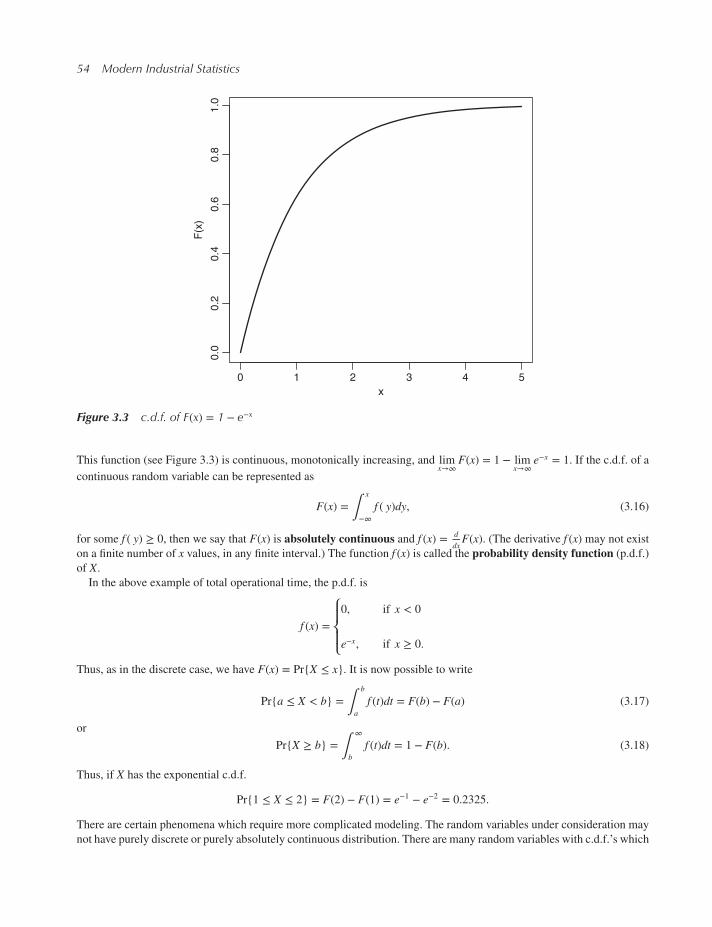
54 Modern Industrial Statistics
0 1 2 3 4 5
0.0
0.2
0.4
0.6
0.8
1.0
x
F(x
)
Figure 3.3 c.d.f. of F(x) = 1 − e−x
This function (see Figure 3.3) is continuous, monotonically increasing, and limx→∞
F(x) = 1 − limx→∞
e−x = 1. If the c.d.f. of a
continuous random variable can be represented as
F(x) = ∫x
−∞f ( y)dy, (3.16)
for some f ( y) ≥ 0, then we say that F(x) is absolutely continuous and f (x) = d
dxF(x). (The derivative f (x) may not exist
on a finite number of x values, in any finite interval.) The function f (x) is called the probability density function (p.d.f.)
of X.In the above example of total operational time, the p.d.f. is
f (x) =⎧⎪⎨⎪⎩0, if x < 0
e−x, if x ≥ 0.
Thus, as in the discrete case, we have F(x) = Pr{X ≤ x}. It is now possible to write
Pr{a ≤ X < b} = ∫b
a
f (t)dt = F(b) − F(a) (3.17)
or
Pr{X ≥ b} = ∫∞
b
f (t)dt = 1 − F(b). (3.18)
Thus, if X has the exponential c.d.f.
Pr{1 ≤ X ≤ 2} = F(2) − F(1) = e−1 − e−2 = 0.2325.
There are certain phenomena which require more complicated modeling. The random variables under consideration may
not have purely discrete or purely absolutely continuous distribution. There are many random variables with c.d.f.’s which

Probability Models and Distribution Functions 55
1.0
0.8
0.6
0.4
0.2
0 1 2 3
x
4 5
F(x
)
Figure 3.4 c.d.f. of the mixture distribution F(x) = 0.5 (1 − e−x) + 0.5 × e−1[x]∑j=0
1j!
are absolutely continuous within certain intervals, and have jump points (points of discontinuity) at the end points of the
intervals. Distributions of such random variables can be expressed as mixtures of purely discrete c.d.f., Fd(x), and of
absolutely continuous c.d.f., Fac(x), that is,
F(x) = pFd(x) + (1 − p)Fac(x), −∞ < x <∞, (3.19)
where 0 ≤ p ≤ 1 (see Figure 3.4).
Example 3.17. A distribution which is a mixture of discrete and continuous distributions is obtained, for example, when
a measuring instrument is not sensitive enough to measure small quantities or large quantities which are outside its range.
This could be the case for a weighing instrument which assigns the value 0 [mg] to any weight smaller than 1 [mg], the
value 1 [g] to any weight greater than 1 gram, and the correct weight to values in between.
Another example is the total number of minutes, within a given working hour, that a service station is busy serving
customers. In this case the c.d.f. has a jump at 0, of height p, which is the probability that the service station is idle at thebeginning of the hour, and no customer arrives during that hour. In this case,
F(x) = p + (1 − p)G(x), 0 ≤ x <∞,
where G(x) is the c.d.f. of the total service time, G(0) = 0. ◾
3.2.2 Expected values and moments of distributions
The expected value of a function g(X), under the distribution F(x), is
EF{g(X)} =
⎧⎪⎪⎨⎪⎪⎩∫ ∞−∞ g(x)f (x)dx, if X is continuous
k∑j=0g(xj)p(xj), if X is discrete.
In particular,
𝜇l(F) = EF{Xl}, l = 1, 2, · · · (3.20)
is called the l-th moment of F(x). 𝜇1(F) = EF{X} is the expected value of X, or the population mean, according to the
model F(x).
56 Modern Industrial Statistics
Moments around 𝜇1(F) are called central moments, which are
𝜇∗l (F) = E{(X − 𝜇1(F))l}, l = 1, 2, 3, · · · . (3.21)
Obviously, 𝜇∗1(F) = 0. The second central moment is called the variance of F(x), VF{X}.
In the following, the notation 𝜇l(F) will be simplified to 𝜇l, if there is no room for confusion.
Expected values of a function g(X), and in particular the moments, may not exist, since an integral ∫ ∞−∞ x
lf (x)dx may
not be well defined. An example of such a case is the distribution, called the Cauchy distribution, with p.d.f.
f (x) = 1
𝜋⋅
1
1 + x2, −∞ < x <∞.
Notice that under this model, moments do not exist for any l = 1, 2, · · · . Indeed, the integral
1
𝜋 ∫∞
−∞
x1 + x2
dx
does not exist. If the second moment exists, then
V{X} = 𝜇2 − 𝜇21 .
Example 3.18. Consider the random experiment of casting a die once. The random variable, X, is the face number. Thus
p(x) = 1
6, x = 1, · · · , 6 and
𝜇1 = E{X} = 1
6
6∑j=1
j = 6(6 + 1)2 × 6
= 7
2= 3.5
𝜇2 =1
6
6∑j=1
j2 = 6(6 + 1)(2 × 6 + 1)6 × 6
= 7 × 13
6= 91
6= 15.167.
The variance is
V{X} = 91
6−(7
2
)2
= 182 − 147
12
= 35
12.
◾
Example 3.19. X has a continuous distribution with p.d.f.
f (x) =⎧⎪⎨⎪⎩0, otherwise
1, if 1 ≤ x ≤ 2.
Thus,
𝜇1 = ∫2
1
xdx = 1
2
(x2||||21)
= 1
2(4 − 1) = 1.5
𝜇2 = ∫2
1
x2dx = 1
3
(x3||||21)
= 7
3
V{X} = 𝜇2 − 𝜇1 =7
3− 9
4= 28 − 27
12= 1
12.
◾
The following is a useful formula when X assumes only positive values, i.e., F(x) = 0 for all x ≤ 0,
𝜇1 = ∫∞
0
(1 − F(x))dx, (3.22)

Probability Models and Distribution Functions 57
for continuous c.d.f. F(x). Indeed,
𝜇1 = ∫∞
0
xf (x)dx
= ∫∞
0
(∫
x
0
dy
)f (x)dx
= ∫∞
0
(∫
∞
y
f (x)dx)dy
= ∫∞
0
(1 − F( y))dy.
For example, suppose that f (x) = 𝜇e−𝜇x, for x ≥ 0. Then F(x) = 1 − e−𝜇x and
∫∞
0
(1 − F(x))dx = ∫∞
0
e−𝜇xdx = 1
𝜇.
When X is discrete, assuming the values {1, 2, 3, . . . } then we have a similar formula
E{X} = 1 +∞∑i=1
(1 − F(i)).
3.2.3 The standard deviation, quantiles, measures of skewness and kurtosis
The standard deviation of a distribution F(x) is 𝜎 = (V{X})1∕2. The standard deviation is used as a measure of disper-
sion of a distribution. An important theorem in probability theory, called the Chebychev Theorem, relates the standard
deviation to the probability of deviation from the mean. More formally, the theorem states that, if 𝜎 exists, then
Pr{|X − 𝜇1| > 𝜆𝜎} ≤ 1
𝜆2. (3.23)
Thus, by this theorem, the probability that a random variable will deviate from its expected value by more than three
standard deviations is less than 1/9, whatever the distribution is. This theorem has important implications, which will be
highlighted later.
The p-th quantile of a distribution F(x) is the smallest value of x, 𝜉p such that F(x) ≥ p. We also write 𝜉p = F−1(p).For example, if F(x) = 1 − e−𝜆x, 0 ≤ x <∞, where 0 < 𝜆 <∞, then 𝜉p is such that
F(𝜉p) = 1 − e−𝜆𝜉p = p.
Solving for 𝜉p we get
𝜉p = − 1
𝜆⋅ ln (1 − p).
The median of F(x) is f −1(.5) = 𝜉.5. Similarly 𝜉.25 and 𝜉.75 are the first and third quartiles of F.A distribution F(x) is symmetric about the mean 𝜇1(F) if
F(𝜇1 + 𝛿) = 1 − F(𝜇1 − 𝛿)
for all 𝛿 ≥ 0.
In particular, if F is symmetric, then F(𝜇1) = 1 − F(𝜇1) or 𝜇1 = F−1(.5) = 𝜉.5. Accordingly, the mean and median of a
symmetric distribution coincide. In terms of the p.d.f., a distribution is symmetric about its mean if
f (𝜇1 + 𝛿) = f (𝜇1 − 𝛿), for all 𝛿 ≥ 0.
A commonly used index of skewness (asymmetry) is
𝛽3 =𝜇∗3
𝜎3, (3.24)

58 Modern Industrial Statistics
where 𝜇∗3is the third central moment of F. One can prove that if F(x) is symmetric, then 𝛽3 = 0. If 𝛽3 > 0, we say that
F(x) is positively skewed, otherwise it is negatively skewed.
Example 3.20. Consider the binomial distribution, with p.d.f.
p(x) =(nx
)px(1 − p)n−x, x = 0, 1, · · · , n.
In this case
𝜇1 =n∑x=0
x
(nx
)px(1 − p)n−x
= npn∑x=1
(n − 1
x − 1
)px−1(1 − p)n−1−(x−1)
= npn−1∑j=0
(n − 1
j
)pj(1 − p)n−1−j
= np.
Indeed,
x
(nx
)= x
n!x!(n − x)!
= n!(x − 1)!((n − 1) − (x − 1))!
= n
(n − 1
x − 1
).
Similarly, we can show that
𝜇2 = n2p2 + np(1 − p),
and
𝜇3 = np[n(n − 3)p2 + 3(n − 1)p + 1 + 2p2].
The third central moment is
𝜇∗3 = 𝜇3 − 3𝜇2𝜇1 + 2𝜇31
= np(1 − p)(1 − 2p).
Furthermore,
V{X} = 𝜇2 − 𝜇21= np(1 − p).
Hence,
𝜎 =√np(1 − p)
and the index of asymmetry is
𝛽3 =𝜇∗3
𝜎3=np(1 − p)(1 − 2p)(np(1 − p))3∕2
=1 − 2p√np(1 − p)
.
Thus, if p = 1
2, then 𝛽3 = 0 and the distribution is symmetric. If p < 1
2, the distribution is positively skewed, and it is
negatively skewed if p > 1
2. ◾

Probability Models and Distribution Functions 59
In Chapter 2 we mentioned also the index of kurtosis (steepness). This is given by
𝛽4 =𝜇∗4
𝜎4. (3.25)
Example 3.21. Consider the exponential c.d.f.
F(x) =⎧⎪⎨⎪⎩0, if x < 0
1 − e−x, if x ≥ 0.
The p.d.f. is f (x) = e−x, x ≥ 0. Thus, for this distribution
𝜇1 = ∫∞
0
xe−xdx = 1
𝜇2 = ∫∞
0
x2e−xdx = 2
𝜇3 = ∫∞
0
x3e−xdx = 6
𝜇4 = ∫∞
0
x4e−xdx = 24.
Therefore,
V{X} = 𝜇2 − 𝜇21 = 1,
𝜎 = 1
𝜇∗4 = 𝜇4 − 4𝜇3 ⋅ 𝜇1 + 6𝜇2𝜇21 − 3𝜇41
= 24 − 4 × 6 × 1 + 6 × 2 × 1 − 3 = 9.
Finally, the index of kurtosis is
𝛽4 = 9.◾
3.2.4 Moment generating functions
The moment generating function (m.g.f.) of a distribution of X, is defined as a function of a real variable t,
M(t) = E{etX}. (3.26)
M(0) = 1 for all distributions. M(t), however, may not exist for some t ≠ 0. To be useful, it is sufficient that M(t) willexist in some interval containing t = 0.
For example, if X has a continuous distribution with p.d.f.
f (x) =⎧⎪⎨⎪⎩
1
b−a, if a ≤ x ≤ b, a < b
0, otherwise
then
M(t) = 1
b − a ∫b
a
etxdx = 1
t(b − a)(etb − eta).
This is a differentiable function of t, for all t, −∞ < t <∞.

60 Modern Industrial Statistics
On the other hand, if for 0 < 𝜆 <∞,
f (x) =⎧⎪⎨⎪⎩𝜆e−𝜆x, 0 ≤ x <∞
0, x < 0
then
M(t) = 𝜆∫∞
0
etx−𝜆xdx
= 𝜆𝜆 − t, t < 𝜆.
This m.g.f. exists only for t < 𝜆. The m.g.f.M(t) is a transform of the distribution F(x), and the correspondence betweenM(t) and F(x) is one-to-one. In the above example,M(t) is the Laplace transform of the p.d.f. 𝜆e−𝜆x. This correspondenceis often useful in identifying the distributions of some statistics, as will be shown later.
Another useful property of the m.g.f. M(t) is that often we can obtain the moments of F(x) by differentiating M(t).More specifically, consider the r-th order derivative of M(t). Assuming that this derivative exists, and differentiation can
be interchanged with integration (or summation), then
M(r)(t) = dr
dtr ∫ etxf (x)dx = ∫( drdtr
etx)f (x)dx
= ∫ xretxf (x)dx.
Thus, if these operations are justified, then
M(r)(t)|t=0 = ∫ xrf (x)dx = 𝜇r. (3.27)
In the following sections we will illustrate the usefulness of the m.g.f.
3.3 Families of discrete distribution
In the present section we discuss several families of discrete distributions, and illustrate their possible application in
modeling industrial phenomena.
3.3.1 The binomial distribution
Consider n identical independent trials. In each trial the probability of “success” is fixed at some value p, and successiveevents of “success” or “failure” are independent. Such trials are called Bernoulli trials. The distribution of the number
of “successes,” Jn, is binomial with p.d.f.
b( j; n, p) =(nj
)pj(1 − p)n−j, j = 0, 1, · · · , n. (3.28)
This p.d.f. was derived in Example 5.11 as a special case.
A binomial random variable, with parameters (n, p) will be designated as B(n, p). n is a given integer and p belongs tothe interval (0, 1). The collection of all such binomial distributions is called the binomial family.
The binomial distribution is a proper model whenever we have a sequence of independent binary events (0 − 1, or
“Success” and “Failure”) with the same probability of “Success.”
Example 3.22. We draw a random sample of n = 10 items from a mass production line of light bulbs. Each light bulb
undergoes an inspection and if it complies with the production specifications, we say that the bulb is compliant (successful
event). Let Xi = 1 if the i-th bulb is compliant and Xi = 0 otherwise. If we can assume that the probability of {Xi = 1}

Probability Models and Distribution Functions 61
is the same, p, for all bulbs and if the n events are mutually independent, then the number of bulbs in the sample which
comply with the specifications, i.e., Jn =n∑i=1Xi, has the binomial p.d.f. b(i; n, p). Notice that if we draw a sample at random
with replacement, RSWR, from a lot of size N, which contains M compliant units, then Jn is B(n, M
N
).
Indeed, if sampling is with replacement, the probability that the i-th item selected is compliant is p = M
Nfor all i =
1, · · · , n. Furthermore, selections are independent of each other. ◾
The binomial c.d.f. will be denoted by B(i; n, p). Recall that
B(i; n, p) =i∑j=0
b( j; n, p), (3.29)
i = 0, 1, · · · , n. The m.g.f. of B(n, p) is
M(t) = E{etX}
=n∑j=0
(nj
)(pet)j(1 − p)n−j
= (pet + (1 − p))n, −∞ < t <∞. (3.30)
Notice that
M′(t) = n(pet + (1 − p))n−1pet
and
M′′(t) = n(n − 1)p2e2t(pet + (1 − p))n−2 + npet(pet + (1 − p))n−1.
The expected value and variance of B(n, p) areE{Jn} = np, (3.31)
and
V{Jn} = np(1 − p). (3.32)
This was shown in Example 3.20 and can be verified directly by the above formulae of M′(t) and M′′(t). To obtain the
values of b(i; n, p) we can use R or MINITAB. For example, suppose we wish to tabulate the values of the p.d.f. b(i; n, p),and those of the c.d.f. B(i; n, p) for n = 30 and p = .60. Below are R commands to generate a data frame with values as
illustrated in Table 3.1.
< X <- data.frame(i=0:30,b=dbinom(x=0:30, size=30, prob=0.6),B=pbinom(q=0:30, size=30, prob=0.6))
< rm(X)
In MINITABWe first put in column C1 the integers 0, 1, · · · , 30 and put the value of b(i; 30, .60) in column C2, and thoseof B(i; 30, .60) in C3. To make MINITAB commands visible in the session window, go to Editor > Enable Commands.
We then type the commands:
MTB> Set C1DATA> 1(0 : 30/1)1DATA> End.MTB> PDF C1 C2;SUBC> Binomial 30 0.60.
MTB> CDF C1 C3;SUBC> Binomial 30 0.60.
In Table 3.1 we present these values.

62 Modern Industrial Statistics
Table 3.1 Values of the p.d.f. and c.d.f. of B(30,.6)
i b(i;30, .6) B(i;30, .6)
8 0.0002 0.00029 0.0006 0.000910 0.0020 0.002911 0.0054 0.008312 0.0129 0.021213 0.0269 0.048114 0.0489 0.097115 0.0783 0.175416 0.1101 0.285517 0.1360 0.421518 0.1474 0.568919 0.1396 0.708520 0.1152 0.823721 0.0823 0.906022 0.0505 0.956523 0.0263 0.982824 0.0115 0.994325 0.0041 0.998526 0.0012 0.999727 0.0003 1.0000
An alternative option is to use the pull-down window.
After tabulating the values of the c.d.f. we can obtain the quantiles (or fractiles) of the distribution. Recall that in the
discrete case, the p-th quantile of a random variable X is
xp = smallest x such that F(x) ≥ p.
Thus, from Table 3.1 we find that the lower quartile, the median and upper quartile of B(30, .6) are Q1 = 16, Me = 18
and Q3 = 20. These values can also be obtained directly with R code
> qbinom(p=0.5, size=30, prob=0.6)
or with MINITAB commands
MTB> InvCDF .5 k1;SUBC> Binomial 30 .6.
The value of the median is stored in the constant k1.In Figure 3.5 we present the p.d.f. of three binomial distributions, with n = 50 and p = .25, .50 and .75. We see that if
p = .25, the p.d.f. is positively skewed. When p = .5, it is symmetric, and when p = .75, it is negatively skewed. This is
in accordance with the index of skewness 𝛽3, which was presented in Example 3.20.
3.3.2 The hypergeometric distribution
Let Jn denote the number of units, in a RSWOR of size n, from a population of size N, having a certain property. The
number of population units before sampling having this property isM. The distribution of Jn is called the hypergeometric

Probability Models and Distribution Functions 63
Figure 3.5 p.d.f. of B(50,p), p = .25, .50, .75 (MINITAB)
distribution. We denote a random variable having such a distribution by H(N,M, n). The p.d.f. of Jn is
h( j;N,M, n) =(Mj
) (N−Mn−j)(
Nn
) , j = 0, · · · , n. (3.33)
This formula was shown already in Section 3.1.4.
The c.d.f. ofH(N,M, n)will be designated byH( j;N,M, n). In Table 3.2 we present the p.d.f. and c.d.f. ofH(75, 15, 10).In Figure 3.6 we show the p.d.f. of H(500, 350, 100).The expected value and variance of H(N,M, n) are:
E{Jn} = n ⋅MN
(3.34)
and
V{Jn} = n ⋅MN
⋅(1 − M
N
)(1 − n − 1
N − 1
). (3.35)
Notice that when n = N, the variance of Jn is V{JN} = 0. Indeed, if n = N, JN = M, which is not a random quantity.
Derivations of these formulae are given in Section 5.2.2. There is no simple expression for the m.g.f.
Table 3.2 The p.d.f. and c.d.f. of H(75,15,10)
j h( j;75, 15, 10) H( j;75,15,10)
0 0.0910 0.09101 0.2675 0.35852 0.3241 0.68263 0.2120 0.89464 0.0824 0.97705 0.0198 0.99686 0.0029 0.99977 0.0003 1.0000

64 Modern Industrial Statistics
0 20 40 60 80 100
0.0
00.0
20.0
40.0
60.0
8
x
Hyperg
eom
etr
ic p
.d.f.
Figure 3.6 The p.d.f. h(i;500, 350,100)
Table 3.3 The p.d.f. of H(500,350,20) and B(20,0.7)
i h(i;500,350,20) b(i;20,0.7)
5 0.00003 0.000046 0.00016 0.000227 0.00082 0.001028 0.00333 0.003869 0.01093 0.0120210 0.02928 0.0308211 0.06418 0.0653712 0.11491 0.1144013 0.16715 0.1642614 0.19559 0.1916415 0.18129 0.1788616 0.12999 0.1304217 0.06949 0.0716018 0.02606 0.0278519 0.00611 0.0068420 0.00067 0.00080
If the sample size n is small relative to N, i.e., n∕N ≪ 0.1, the hypergeometric p.d.f. can be approximated by that of
the binomial B(n, M
N
). In Table 3.3 we compare the p.d.f. of H(500, 350, 20) to that of B(20, 0.7).
The expected value and variance of the binomial and the hypergeometric distributions are compared in Table 3.4.
We see that the expected values have the same formula, but that the variance formulae differ by the correction factor
(N − n)∕(N − 1) which becomes 1 when n = 1 and 0 when n = N.

Probability Models and Distribution Functions 65
Table 3.4 The expected value and variance of thehypergeometric and binomial distribution
H(a;N,M,n) B(n, M
N
)Hypergeometric Binomial
Expected nMN
nMN
Value
Variance nMN
(1 − M
N
)(1 − n − 1
N − 1
)nMN
(1 − M
N
)
Example 3.23. At the end of a production day, printed circuit boards (PCB) soldered by the wave soldering process are
subjected to sampling audit. A RSWOR of size n is drawn from the lot, which consists of all the PCB’s produced on
that day. If the sample has any defective PCB, another RSWOR of size 2n is drawn from the lot. If there are more than
three defective boards in the combined sample, the lot is sent for rectification, in which every PCB is inspected. If the
lot consists of N = 100 PCB’s, and the number of defective ones is M = 5, what is the probability that the lot will be
rectified, when n = 10?
Let J1 be the number of defective items in the first sample. If J1 > 3, then the lot is rectified without taking a second
sample. If J1 = 1, 2 or 3, a second sample is drawn. Thus, if R denotes the event “the lot is sent for rectification,”
Pr{R} = 1 − H(3; 100, 5, 10)
+3∑i=1
h(i; 100, 5, 10) ⋅ [1 − H(3 − i; 90, 5 − i, 20)
= 0.00025 + 0.33939 × 0.03313
+ 0.07022 × 0.12291
+ 0.00638 × 0.397 = 0.0227.◾
3.3.3 The Poisson distribution
A third discrete distribution that plays an important role in quality control is the Poisson distribution, denoted by P(𝜆).It is sometimes called the distribution of rare events, since it is used as an approximation to the Binomial distribution
when the sample size, n, is large and the proportion of defectives, p, is small. The parameter 𝜆 represents the “rate” atwhich defectives occur, that is, the expected number of defectives per time interval or per sample. The Poisson probability
distribution function is given by the formula
p( j; 𝜆) = e−𝜆𝜆j
j!, j = 0, 1, 2, · · · (3.36)
and the corresponding c.d.f. is
P( j; 𝜆) =j∑i=0
p(i; 𝜆), j = 0, 1, 2, · · · . (3.37)
Example 3.24. Suppose that a machine produces aluminum pins for airplanes. The probability p that a single pin emerges
defective is small, say, p = .002. In one hour, the machine makes n = 1000 pins (considered here to be a random sample
of pins). The number of defective pins produced by the machine in one hour has a Binomial distribution with a mean of
𝜇 = np = 1000(.002) = 2, so the rate of defective pins for the machine is 𝜆 = 2 pins per hour. In this case, the Binomial
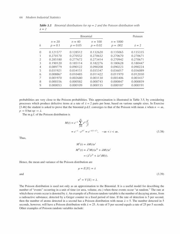
66 Modern Industrial Statistics
Table 3.5 Binomial distributions for np = 2 and the Poisson distribution with𝜆 = 2
Binomial Poisson
n = 20 n = 40 n = 100 n = 1000k p = 0.1 p = 0.05 p = 0.02 p = .002 𝜆 = 2
0 0.121577 0.128512 0.132620 0.135065 0.1353351 0.270170 0.270552 0.270652 0.270670 0.2706712 0.285180 0.277672 0.273414 0.270942 0.2706713 0.190120 0.185114 0.182276 0.180628 0.1804474 0.089779 0.090122 0.090208 0.090223 0.0902245 0.031921 0.034151 0.035347 0.036017 0.0360896 0.008867 0.010485 0.011422 0.011970 0.0120307 0.001970 0.002680 0.003130 0.003406 0.0034378 0.000356 0.000582 0.000743 0.000847 0.0008599 0.000053 0.000109 0.000155 0.000187 0.000191
probabilities are very close to the Poisson probabilities. This approximation is illustrated in Table 3.5, by considering
processes which produce defective items at a rate of 𝜆 = 2 parts per hour, based on various sample sizes. In Exercise
[3.46] the student is asked to prove that the binomial p.d.f. converges to that of the Poisson with mean 𝜆 when n → ∞,
p → 0 but np → 𝜆.The m.g.f. of the Poisson distribution is
M(t) = e−𝜆∞∑j=0
etj𝜆j
j!
= e−𝜆 ⋅ e𝜆et = e−𝜆(1−e
t), −∞ < t < ∞. (3.38)
Thus,
M′(t) = 𝜆M(t)et
M′′(t) = 𝜆2M(t)e2t + 𝜆M(t)et
= (𝜆2e2t + 𝜆et)M(t).
Hence, the mean and variance of the Poisson distribution are
𝜇 = E{X} = 𝜆
and (3.39)
𝜎2 = V{X} = 𝜆.
The Poisson distribution is used not only as an approximation to the Binomial. It is a useful model for describing the
number of “events” occurring in a unit of time (or area, volume, etc.) when those events occur “at random.” The rate at
which these events occur is denoted by 𝜆. An example of a Poisson random variable is the number of decaying atoms, from
a radioactive substance, detected by a Geiger counter in a fixed period of time. If the rate of detection is 5 per second,
then the number of atoms detected in a second has a Poisson distribution with mean 𝜆 = 5. The number detected in 5
seconds, however, will have a Poisson distribution with 𝜆 = 25. A rate of 5 per second equals a rate of 25 per 5 seconds.
Other examples of Poisson random variables include:

Probability Models and Distribution Functions 67
1. The number of blemishes found in a unit area of a finished surface (ceramic plate).
2. The number of customers arriving at a store in one hour.
3. The number of defective soldering points found on a circuit board.
The p.d.f., c.d.f. and quantiles of the Poisson distribution can be computed using R, MINITAB or JMP. In Figure 3.7 we
illustrate the p.d.f. for three values of 𝜆.
0 10 20 30 40 50
0.0
00.0
50.1
00.1
50.2
0
i
p(i,
λ)
λ = 5
λ = 10
λ = 15
Figure 3.7 Poisson p.d.f. 𝜆 = 5, 10, 15◾
3.3.4 The geometric and negative binomial distributions
Consider a sequence of independent trials, each one having the same probability for “Success,” say, p. Let N be a random
variable which counts the number of trials until the first “Success” is realized, including the successful trial.N may assume
positive integer values with probabilities
Pr{N = n} = p(1 − p)n−1, n = 1, 2, · · · . (3.40)
This probability function is the p.d.f. of the geometric distribution.Let g(n; p) designate the p.d.f. The corresponding c.d.f. is
G(n; p) = 1 − (1 − p)n, n = 1, 2, · · · .
From this we obtain that the 𝛼-quantile (0 < 𝛼 < 1) is given by
N𝛼 =[log (1 − 𝛼)log (1 − p)
]+ 1,
where [x] designates the integer part of x.

68 Modern Industrial Statistics
The expected value and variance of the geometric distribution are
E{N} = 1
p,
and (3.41)
V{N} =1 − p
p2.
Indeed, the m.g.f. of the geometric distribution is
M(t) = pet∞∑j=0
(et(1 − p))j
=pet
1 − et(1 − p), if t < − log (1 − p). (3.42)
Thus, for t < − log (1 − p),M′(t) =
pet
(1 − et(1 − p))2
and
M′′(t) =pet
(1 − et(1 − p))2+
2p(1 − p)e2t
(1 − et(1 − p))3.
Hence
𝜇1 = M′(0) = 1
p
𝜇2 = M′′(0) =2 − p
p2, (3.43)
and the above formulae of E{X} and V{X} are obtained.The geometric distribution is applicable in many problems. We illustrate one such application in the following
example.
Example 3.25. An insertion machine stops automatically if there is a failure in handling a component during an insertion
cycle. A cycle starts immediately after the insertion of a component and ends at the insertion of the next component.
Suppose that the probability of stopping is p = 10−3 per cycle. Let N be the number of cycles until the machine stops. It is
assumed that events at different cycles are mutually independent. Thus N has a geometric distribution and E{N} = 1, 000.We expect a run of 1,000 cycles between consecutive stopping. The number of cycles, N, however, is a random variable
with standard deviation of 𝜎 =(
1−pp2
)1∕2= 999.5. This high value of 𝜎 indicates that we may see very short runs and also
long ones. Indeed, for 𝛼 = 0.5 the quantiles of N are, N.05 = 52 and N.95 = 2995. ◾
The number of failures until the first success, N − 1, has a shifted geometric distribution, which is a special case of the
family of Negative-Binomial distribution.We say that a non-negative integer valued random variable X has a negative-binomial distribution, with parameters
(p, k), where 0 < p < 1 and k = 1, 2, · · · , if its p.d.f. is
g( j; p, k) =(j + k − 1
k − 1
)pk(1 − p)j, (3.44)
j = 0, 1, · · · . The shifted geometric distribution is the special case of k = 1.
Amore general version of the negative-binomial distribution can be formulated, in which k − 1 is replaced by a positive
real parameter. A random variable having the above negative-binomial will be designated by NB(p, k). The NB(p, k)

Probability Models and Distribution Functions 69
0 20 40 60 80 100
0.0
00.0
10.0
20.0
30.0
4
i
nb(i, 5, p)
p = 0.2
p = 0.1
Figure 3.8 p.d.f. of NB(p,5) with p = 0.10, 0.20
represents the number of failures observed until the k-th success. The expected value and variance of NB(p, k) are:
E{X} = k1 − p
p,
and (3.45)
V{X} = k1 − p
p2.
In Figure 3.8 we present the p.d.f. of NB(p, k). The negative binomial distributions have been applied as a model of the
distribution for the periodic demand of parts in inventory theory.
3.4 Continuous distributions
3.4.1 The uniform distribution on the interval (a, b), a < b
We denote a random variable having this distribution by U(a, b). The p.d.f. is given by
f (x; a, b) =⎧⎪⎨⎪⎩1∕(b − a), a ≤ x ≤ b
0, elsewhere,
(3.46)
and the c.d.f. is
F(x; a, b) =⎧⎪⎨⎪⎩0, if x < a
(x − a)∕(b − a), if a ≤ x < b
1, if b ≤ x
(3.47)

70 Modern Industrial Statistics
The expected value and variance of U(a, b) are
𝜇 = (a + b)∕2,
and (3.48)
𝜎2 = (b − a)2∕12.
The p-th fractile is xp = a + p(b − a).To verify the formula for 𝜇, we set
𝜇 = 1
b − a ∫b
a
xdx = 1
b − a
||||12 x2||||ba = 1
2(b − a)(b2 − a2)
= a + b2.
Similarly,
𝜇2 =1
b − a ∫b
a
x2dx = 1
b − a
||||13 x3||||ba= 1
3(b − a)(b3 − a3) = 1
3(a2 + ab + b2).
Thus,
𝜎2 = 𝜇2 − 𝜇21 =1
3(a2 + ab + b2) − 1
4(a2 + 2ab + b2)
= 1
12(4a2 + 4ab + 4b2 − 3a2 − 6ab − 3b2)
= 1
12(b − a)2.
We can get these moments also from the m.g.f., which is
M(t) = 1
t(b − a)(etb − eta), −∞ < t <∞.
Moreover, for values of t close to 0
M(t) = 1 + 1
2t(b + a) + 1
6t2(b2 + ab + a2) + · · · .
3.4.2 The normal and log-normal distributions
3.4.2.1 The normal distribution
The Normal or Gaussian distribution denoted by N(𝜇, 𝜎), occupies a central role in statistical theory. Its density function(p.d.f.) is given by the formula
n(x;𝜇, 𝜎) = 1
𝜎√2𝜋
exp{− 1
2𝜎2(x − 𝜇)2
}. (3.49)
This p.d.f. is symmetric around the location parameter, 𝜇. 𝜎 is a scale parameter. The m.g.f. of N(0, 1) is
M(t) = 1√2𝜋
etx−12x2dx
= et2∕2√2𝜋 ∫
∞
−∞e−
12(x2−2tx+t2)dx (3.50)
= et2∕2.

Probability Models and Distribution Functions 71
Indeed,1√2𝜋
exp{− 1
2(x − t)2
}is the p.d.f. of N(t, 1). Furthermore,
M′(t) = tM(t)
M′′(t) = t2M(t) +M(t) = (1 + t2)M(t)
M′′′(t) = (t + t3)M(t) + 2tM(t)
= (3t + t3)M(t)
M(4)(t) = (3 + 6t2 + t4)M(t).
Thus, by substituting t = 0 we obtain that
E{N(0, 1)} = 0,
V{N(0, 1)} = 1,
𝜇∗3 = 0,
𝜇∗4 = 3.
(3.51)
To obtain the moments in the general case of N(𝜇, 𝜎2), we write X = 𝜇 + 𝜎N(0, 1). Then
E{X} = E{𝜇 + 𝜎N(0, 1)}
= 𝜇 + 𝜎E{N(0, 1)} = 𝜇
V{X} = E{(X − 𝜇)2} = 𝜎2E{N2(0, 1)} = 𝜎2
𝜇∗3 = E{(X − 𝜇)3} = 𝜎3E{N3(0, 1)} = 0
𝜇∗4 = E{(X − 𝜇)4} = 𝜎4E{N4(0, 1)} = 3𝜎4.
Thus, the index of kurtosis in the normal case is 𝛽4 = 3.
The graph of the p.d.f. n(x;𝜇, 𝜎) is a symmetric bell-shaped curve that is centered at 𝜇 (shown in Figure 3.9). The
spread of the density is determined by the variance 𝜎2 in the sense that most of the area under the curve (in fact, 99.7% of
the area) lies between 𝜇 − 3𝜎 and 𝜇 + 3𝜎. Thus, if X has a normal distribution with mean 𝜇 = 25 and standard deviation
𝜎 = 2, the probability is .997 that the observed value of X will fall between 19 and 31.
Areas (that is, probabilities) under the normal p.d.f. are found in practice using a table or appropriate software like
MINITAB. Since it is not practical to have a table for each pair of parameters 𝜇 and 𝜎, we use the standardized form
of the normal random variable. A random variable Z is said to have a standard normal distribution if it has a normal
distribution with mean zero and variance one. The standard normal density function is 𝜙(x) = n(x; 0, 1) and the standard
cumulative distribution function is denoted by Φ(x). This function is also called the standard normal integral, that is,
Φ(x) = ∫x
−∞𝜙(t)dt = ∫
x
−∞
1√2𝜋
e−12t2dt. (3.52)
The c.d.f., Φ(x), represents the area over the x-axis under the standard normal p.d.f. to the left of the value x (see
Figure 3.10).
If we wish to determine the probability that a standard normal random variable is less than 1.5, for example, we use
R code
> pnorm(q=1.5, mean=0, sd=1)
or the MINITAB commands
MTB> CDF 1.5;
SUBC> NORMAL 0 1.

72 Modern Industrial Statistics
0 5 10 15 20
0.0
0.1
0.2
0.3
0.4
x
f(x)
σ = 1
σ = 2
σ = 3
Figure 3.9 The p.d.f. of N(𝜇, 𝜎), 𝜇 = 10, 𝜎 = 1,2,3
−3 −2 −1 0 1 2 3
0.0
0.2
0.4
0.6
0.8
1.0
x
Sta
ndard
Norm
al c.d
.f.
Figure 3.10 Standard normal c.d.f.

Probability Models and Distribution Functions 73
Figure 3.11 The symmetry of the normal distribution (MINITAB)
We find that Pr{Z ≤ 1.5} = Φ(1.5) = 0.9332. To obtain the probability that Z lies between .5 and 1.5 we first find the
probability that Z is less than 1.5, then subtract from this number the probability that Z is less than .5. This yields
Pr{.5 < Z < 1.5} = Pr{Z < 1.5} − Pr{Z < .5}
= Φ(1.5) − Φ(.5) = .9332 − .6915 = .2417.
Many tables of the normal distribution do not list values ofΦ(x) for x < 0. This is because the normal density is symmetric
about x = 0, and we have the relation
Φ(−x) = 1 − Φ(x), for all x. (3.53)
Thus, to compute the probability that Z is less than −1, for example, we write
Pr{Z < −1} = Φ(−1) = 1 − Φ(1) = 1 − .8413 = .1587 (see Figure 3.11).
The p-th quantile (percentile of fractile) of the standard normal distribution is the number zp that satisfies the statement
Φ(zp) = Pr{Z ≤ zp} = p. (3.54)
If X has a normal distribution with mean 𝜇 and standard deviation 𝜎, we denote the p-th fractile of the distribution by xp.We can show that xp is related to the standard normal quantile by
xp = 𝜇 + zp𝜎.
The p-th fractile of the normal distribution can be obtained by using R code
> qnorm(p=0.95, mean=0, sd=1)
or the MINITAB command
MTB> InvCDF 0.95;
SUBC> Normal 0.0 1.0.

74 Modern Industrial Statistics
In this command we used p = 0.95. The printed result is z.95 = 1.6449. We can use any value of 𝜇 and 𝜎 in the subcom-
mand. Thus, for 𝜇 = 10 and 𝜎 = 1.5
x.95 = 10 + z.95 × 𝜎 = 12.4673.
Now suppose that X is a random variable having a normal distribution with mean 𝜇 and variance 𝜎2. That is, X has a
N(𝜇, 𝜎) distribution. We define the standardized form of X as
Z = X − 𝜇𝜎.
By subtracting the mean from X and then dividing by the standard deviation, we transform X to a standard normal random
variable. (That is, Z has expected value zero and standard deviation one.) This will allow us to use the standard normal
table to compute probabilities involving X. Thus, to compute the probability that X is less than a, we write
Pr{X ≤ a} = Pr
{X − 𝜇𝜎<a − 𝜇𝜎
}= Pr
{Z <
a − 𝜇𝜎
}= Φ
(a − 𝜇𝜎
).
Example 3.26. Let X represent the length (with cap) of a randomly selected aluminum pin. Suppose we know that Xhas a normal distribution with mean 𝜇 = 60.02 and standard deviation 𝜎 = 0.048 [mm]. What is the probability that the
length with cap of a randomly selected pin will be less than 60.1 [mm]? Using R
> pnorm(q=60.1, mean=60.02, sd=0.048, lower.tail=TRUE)
or the MINITAB command
MTB> CDF 60.1;
SUBC> Normal 60.02 0.048.
we obtain Pr{X ≤ 60.1} = 0.9522. If we have to use the table of Φ(Z), we write
Pr{X ≤ 60.1} = Φ(60.1 − 60.02
0.048
)= Φ(1.667) = 0.9522.
Continuing with the example, consider the following question: If a pin is considered “acceptable” when its length is
between 59.9 and 60.1mm, what proportion of pins is expected to be rejected? To answer this question, we first compute
the probability of accepting a single pin. This is the probability that X lies between 59.9 and 60.1, that is,
Pr{50.9 < X < 60.1} = Φ(60.1 − 60.02
0.048
)− Φ
(59.9 − 60.02
0.048
)= Φ(1.667) − Φ(−2.5)
= .9522 − 0.0062 = 0.946.
Thus, we expect that 94.6% of the pins will be accepted, and that 5.4% of them will be rejected. ◾
3.4.2.2 The log-normal distribution
A random variable X is said to have a log-normal distribution, LN (𝜇, 𝜎2), if Y = log X has the normal distribution
N(𝜇, 𝜎2).

Probability Models and Distribution Functions 75
The log-normal distribution has been applied to model distributions of strength variables, like the tensile strength of
fibers (see Chapter 2), the compressive strength of concrete cubes, etc. It has also been used for random quantities of
pollutants in water or air, and other phenomena with skewed distributions.
The p.d.f. of LN (𝜇, 𝜎) is given by the formula
f (x;𝜇, 𝜎2) =
⎧⎪⎪⎨⎪⎪⎩
1√2𝜋𝜎x
exp{− 1
2𝜎2(ln x − 𝜇)2
}, 0 < x < ∞
0, x ≤ 0.
(3.55)
The c.d.f. is expressed in terms of the standard normal integral as
F(x) =
⎧⎪⎪⎨⎪⎪⎩0, x ≤ 0
Φ(ln x − 𝜇𝜎
), 0 < x <∞.
(3.56)
The expected value and variance of LN (𝜇, 𝜎) are
E{X} = e𝜇+𝜎2∕2
and (3.57)
V{X} = e2𝜇+𝜎2 (e𝜎2 − 1).
One can show that the third central moment of LN (𝜇, 𝜎2) is
𝜇∗3 = e3𝜇+32𝜎2 (e3𝜎2 − 3e𝜎
2 + 2).
Hence, the index of skewness of this distribution is
𝛽3 =𝜇∗3
𝜎3= e3𝜎
2 − 3e𝜎2 + 2
(e𝜎2 − 1)3∕2. (3.58)
It is interesting that the index of skewness does not depend on 𝜇, and is positive for all 𝜎2 > 0. This index of skewness
grows very fast as 𝜎2 increases. This is shown in Figure 3.12.
3.4.3 The exponential distribution
We designate this distribution by E(𝛽). The p.d.f. of E(𝛽) is given by the formula
f (x; 𝛽) =⎧⎪⎨⎪⎩0, if x < 0
(1∕𝛽)e−x∕𝛽 , if x ≥ 0,
(3.59)
where 𝛽 is a positive parameter, that is, 0 < 𝛽 <∞. In Figure 3.13 we present these p.d.f.’s for various values of 𝛽.The corresponding c.d.f. is
F(x; 𝛽) =⎧⎪⎨⎪⎩0, if x < 0
1 − e−x∕𝛽 , if x ≥ 0.
(3.60)
The expected value and the variance of E(𝛽) are𝜇 = 𝛽,

76 Modern Industrial Statistics
0.0 0.5 1.0 1.5 2.0 2.5 3.0
020
40
60
80
100
σ2
Skew
ness
Figure 3.12 The index of skewness of LN (𝜇, 𝜎)
0 2 4 6 8 10
0.0
0.2
0.4
0.6
0.8
1.0
x
f(x)
β = 1
β = 2
β = 3
Figure 3.13 The p.d.f. of E(𝛽), 𝛽 = 1,2,3

Probability Models and Distribution Functions 77
and
𝜎2 = 𝛽2.
Indeed,
𝜇 = 1
𝛽 ∫∞
0
xe−x∕𝛽dx.
Making the change of variable to y = x∕𝛽, dx = 𝛽dy, we obtain
𝜇 = 𝛽 ∫∞
0
ye−ydy
= 𝛽.
Similarly
𝜇2 =1
𝛽 ∫∞
0
x2e−x∕𝛽dx = 𝛽2 ∫∞
0
y2e−ydy
= 2𝛽2.
Hence,
𝜎2 = 𝛽2.
The p-th quantile is xp = −𝛽 ln (1 − p).The exponential distribution is related to the Poisson model in the following way: If the number of events occurring in
a period of time follows a Poisson distribution with rate 𝜆, then the time between occurrences of events has an exponential
distribution with parameter 𝛽 = 1∕𝜆. The exponential model can also be used to describe the lifetime (i.e. time to failure)
of certain electronic systems. For example, if the mean life of a system is 200 hours, then the probability that it will work
at least 300 hours without failure is
Pr{X ≥ 300} = 1 − Pr{X < 300}
= 1 − F(300) = 1 − (1 − e−300∕200) = 0.223.
The exponential distribution is positively skewed, and its index of skewness is
𝛽3 =𝜇∗3
𝜎3= 2,
irrespective of the value of 𝛽. We have seen before that the kurtosis index is 𝛽4 = 9.
3.4.4 The gamma and Weibull distributions
Two important distributions for studying the reliability and failure rates of systems are the gamma and the Weibull distri-
butions.Wewill need these distributions in our study of reliability methods (Chapter 14). These distributions are discussed
here as further examples of continuous distributions.
Suppose we use in a manufacturing process a machine which mass-produces a particular part. In a random manner, it
produces defective parts at a rate of 𝜆 per hour. The number of defective parts produced by this machine in a time period
[0, t] is a random variable X(t) having a Poisson distribution with mean 𝜆t, that is,
Pr{X(t) = j} = (𝜆t)je−(𝜆t)∕j!, j = 0, 1, 2, · · · . (3.61)
Suppose we wish to study the distribution of the time until the k-th defective part is produced. Call this continuous randomvariable Yk. We use the fact that the k-th defect will occur before time t (i.e., Yk ≤ t) if and only if at least k defects occur

78 Modern Industrial Statistics
up to time t (i.e., X(t) ≥ k). Thus the c.d.f. for Yk is
G(t; k, 𝜆) = Pr{Yk ≤ t}
= Pr{X(t) ≥ k}
= 1 −k−1∑j=0
(𝜆t)je−𝜆t∕j!.
(3.62)
The corresponding p.d.f. for Yk is
g(t; k, 𝜆) = 𝜆k
(k − 1)!tk−1e−𝜆t, for t ≥ 0. (3.63)
This p.d.f. is a member of a general family of distributions which depend on two parameters, 𝜈 and 𝛽, and are called the
gamma distributions G(𝜈, 𝛽). The p.d.f. of a gamma distribution G(𝜈, 𝛽) is
g(x; 𝜈, 𝛽) =⎧⎪⎨⎪⎩
1
𝛽𝜈Γ(𝜈)x𝜈−1e−x∕𝛽 , x ≥ 0,
0, x < 0
(3.64)
In R function pgamma computes c.d.f of a gamma distribution having 𝜈 = shape and 𝛽 = scale
> pgamma(q=1, shape=1, scale=1)
[1] 0.6321206
where 0 < 𝜈, 𝛽 < ∞, Γ(𝜈) is called the gamma function of 𝜈 and is defined as the integral
Γ(𝜈) = ∫∞
0
x𝜈−1e−xdx, 𝜈 > 0. (3.65)
The gamma function satisfies the relationship
Γ(𝜈) = (𝜈 − 1)Γ(𝜈 − 1), for all 𝜈 > 1. (3.66)
Hence, for every positive integer k, Γ(k) = (k − 1)!. Also, Γ(
1
2
)=√𝜋. We note also that the exponential distribution,
E(𝛽), is a special case of the gamma distribution with 𝜈 = 1. Some gamma p.d.f.’s are presented in Figure 3.14. The value
of Γ(𝜈) can be computed in R by the following commands which compute Γ(5). Generally, replace 5 in line 2 by 𝜈.
> gamma(5)
[1] 24
The expected value and variance of the gamma distribution G(𝜈, 𝛽) are, respectively,
𝜇 = 𝜈𝛽,
and (3.67)
𝜎2 = 𝜈𝛽2.
To verify these formulae we write
𝜇 = 1
𝛽𝜈Γ(𝜈) ∫∞
0
x ⋅ x𝜈−1e−x∕𝛽dx
= 𝛽𝜈+1
𝛽𝜈Γ(𝜈) ∫∞
0
y𝜈e−ydy
= 𝛽 Γ(𝜈 + 1)Γ(𝜈)
= 𝜈𝛽.

Probability Models and Distribution Functions 79
0 1 2 3 4 5 6
0.0
0.5
1.0
1.5
x
f(x)
β = 0.5
β = 1β = 2
Figure 3.14 The gamma densities, with 𝛽 = 1 and 𝜈 = .5, 1, 2
Similarly,
𝜇2 =1
𝛽𝜈Γ(𝜈) ∫∞
0
x2 ⋅ x𝜈−1e−x∕𝛽dx
= 𝛽𝜈+2
𝛽𝜈Γ(𝜈) ∫∞
0
y𝜈+1e−ydy
= 𝛽2 Γ(𝜈 + 2)Γ(𝜈)
= (𝜈 + 1)𝜈𝛽2.
Hence,
𝜎2 = 𝜇2 − 𝜇21 = 𝜈𝛽2.
An alternative way is to differentiate the m.g.f.
M(t) = (1 − t𝛽)−𝜈 , t <1
𝛽. (3.68)
Weibull distributions are often used in reliability models in which the system either “ages” with time or becomes
“younger” (see Chapter 14). The Weibull family of distributions will be denoted by W(𝛼, 𝛽). The parameters 𝛼 and 𝛽,𝛼, 𝛽 > 0, are called the shape and the scale parameters, respectively. The p.d.f. ofW(𝛼, 𝛽) is given by
𝑤(t; 𝛼, 𝛽) =⎧⎪⎨⎪⎩𝛼t𝛼−1
𝛽𝛼e−(t∕𝛽)
𝛼, t ≥ 0,
0, t < 0.
(3.69)
The corresponding c.d.f. is
W(t; 𝛼, 𝛽) =⎧⎪⎨⎪⎩1 − e−(t∕𝛽)
𝛼, t ≥ 0
0, t < 0.
(3.70)

80 Modern Industrial Statistics
0.0 0.5 1.0 1.5 2.0 2.5 3.0
0.0
0.2
0.4
0.6
0.8
x
w(x
, α, β
= 1
)
α = 2
α = 1.5
Figure 3.15 Weibull density functions, 𝛼 = 1.5, 2
Notice that W(1, 𝛽) = E(𝛽). The mean and variance of this distribution are
𝜇 = 𝛽 ⋅ Γ(1 + 1
𝛼
)(3.71)
and
𝜎2 = 𝛽2{Γ(1 + 2
𝛼
)− Γ2
(1 + 1
𝛼
)}(3.72)
respectively. The values of Γ(1 + (1∕𝛼)) and Γ(1 + (2∕𝛼)) can be computed by R, MINITAB or JMP. If, for example,
𝛼 = 2 then
𝜇 = 𝛽√𝜋∕2 = .8862𝛽
𝜎2 = 𝛽2(1 − 𝜋∕4) = .2145𝛽2,
since
Γ(1 + 1
2
)= 1
2⋅ Γ(1
2
)= 1
2
√𝜋,
and
Γ(1 + 2
2
)= Γ(2) = 1.
In Figure 3.15 we present three p.d.f. ofW(𝛼, 𝛽) for 𝛼 = 1.5, 2.0 and 𝛽 = 1.
3.4.5 The Beta distributions
Distributions having p.d.f. of the form
f (x; 𝜈1, 𝜈2) =⎧⎪⎨⎪⎩
1
B(𝜈1 ,𝜈2)x𝜈1−1(1 − x)𝜈2−1, 0 < x < 1,
0, otherwise
(3.73)

Probability Models and Distribution Functions 81
where, for 𝜈1, 𝜈2 positive,
B(𝜈1, 𝜈2) = ∫1
0
x𝜈1−1(1 − x)𝜈2−1dx (3.74)
are called Beta distributions. The function B(𝜈1, 𝜈2) is called the Beta integral. One can prove that
B(𝜈1, 𝜈2) =Γ(𝜈1)Γ(𝜈2)Γ(𝜈1 + 𝜈2)
. (3.75)
The parameters 𝜈1 and 𝜈2 are shape parameters. Notice that when 𝜈1 = 1 and 𝜈2 = 1, the Beta reduces to U(0, 1). We
designate distributions of this family by Beta(𝜈1, 𝜈2). The c.d.f. of Beta(𝜈1, 𝜈2) is denoted also by Ix(𝜈1, 𝜈2), which is
known as the incomplete beta function ratio, that is,
Ix(𝜈1, 𝜈2) =1
B(𝜈1, 𝜈2) ∫x
0
u𝜈1−1(1 − u)𝜈2−1du, (3.76)
for 0 ≤ x ≤ 1. Notice that Ix(𝜈1, 𝜈2) = 1 − I1−x(𝜈2, 𝜈1). The density functions of the p.d.f. Beta(2.5, 5.0) and Beta(2.5, 2.5)are plotted in Figure 3.16. Notice that if 𝜈1 = 𝜈2 then the p.d.f. is symmetric around 𝜇 = 1
2. There is no simple formula
for the m.g.f. of Beta(𝜈1, 𝜈2). However, the m-th moment is equal to
𝜇m = 1
𝛽(𝜈1, 𝜈2) ∫1
0
um+𝜈1−1(1 − u)𝜈2−1du
=B(𝜈1 + m, 𝜈2)B(𝜈1, 𝜈2)
(3.77)
=𝜈1(𝜈1 + 1) · · · (𝜈1 + m − 1)
(𝜈1 + 𝜈2)(𝜈1 + 𝜈2 + 1) · · · (𝜈1 + 𝜈2 + m − 1).
0.0 0.2 0.4 0.6 0.8 1.0
0.0
0.5
1.0
1.5
2.0
x
w(x
, v1, v2)
v1 = 2.5, v2 = 5
v1 = 2.5, v2 = 2.5
Figure 3.16 Beta densities, 𝜈1 = 2.5, 𝜈2 = 2.5; 𝜈1 = 2.5, 𝜈2 = 5.00

82 Modern Industrial Statistics
Hence,
E{Beta(𝜈1, 𝜈2)} =𝜈1𝜈1 + 𝜈2
V{Beta(𝜈1, 𝜈2)} =𝜈1𝜈2
(𝜈1 + 𝜈2)2(𝜈1 + 𝜈2 + 1).
(3.78)
The beta distribution has an important role in the theory of statistics. As will be seen later, many methods of statistical
inference are based on the order statistics (see Section 3.7). The distribution of the order statistics is related to the beta
distribution. Moreover, since the beta distribution can have a variety of shapes, it has been applied in many cases in
which the variable has a distribution on a finite domain. By introducing a location and a scale parameter, one can fit a
shifted-scaled beta distribution to various frequency distributions.
3.5 Joint, marginal and conditional distributions
3.5.1 Joint and marginal distributions
Let X1, · · · ,Xk be random variables which are jointly observed at the same experiments. In Chapter 3 we presented various
examples of bivariate and multivariate frequency distributions. In the present section we present only the fundamentals
of the theory, mainly for future reference. We make the presentation here, focusing on continuous random variables. The
theory holds generally for discrete or for a mixture of continuous and discrete random variables.
A function F(x1, . . . , xk) is called the joint c.d.f. of X1, . . . ,Xk if
F(x1, . . . , xk) = Pr{X1 ≤ x1, . . . ,Xk ≤ xk} (3.79)
for all (x1, . . . , xk) ∈ ℝk (the Euclidean k-space). By letting one or more variables tend to infinity, we obtain the joint
c.d.f. of the remaining variables. For example,
F(x1,∞) = Pr{X1 ≤ x1,X2 ≤ ∞}
= Pr{X1 ≤ x1} = F1(x1). (3.80)
The c.d.f.’s of the individual variables, are called the marginal distributions. F1(x1) is the marginal c.d.f. of X1.
A non-negative function f (x1, · · · , xk) is called the joint p.d.f. of X1, · · · ,Xk, if
(i)
f (x1, · · · , xk) ≥ 0 for all (x1, · · · , xk), where −∞ < xi < ∞ (i = 1, · · · , k)
(ii)
∫∞
−∞· · ·∫
∞
−∞f (x1, · · · , xk)dx1, · · · , dxk = 1.
and
(iii)
F(x1, . . . , xk) = ∫x1
−∞· · ·∫
xk
−∞f ( y1, . . . , yk)dy1 . . . dyk.
The marginal p.d.f. of Xi (i = 1, · · · , k) can be obtained from the joint p.d.f. f (x1, · · · , xk), by integrating the joint p.d.f.
with respect to all xj, j ≠ i. For example, if k = 2, f (x1, x2) is the joint p.d.f. of X1, X2. The marginal p.d.f. of X1 is
f1(x1) = ∫∞
−∞f (x1, x2)dx2.
Similarly, the marginal p.d.f. of X2 is
f2(x2) = ∫∞
−∞f (x1, x2)dx1.

Probability Models and Distribution Functions 83
Indeed, the marginal c.d.f. of Xi is
F(x1) = ∫x1
−∞ ∫∞
−∞f (y1, y2)dy1dy2.
Differentiating F(x1) with respect to x1 we obtain the marginal p.d.f. of X1, i.e.,
f (x1) =ddx1 ∫
x1
−∞ ∫∞
−∞f (y1, y2)dy1dy2
= ∫∞
−∞f (x1, y2)dy2.
If k = 3, we can obtain the marginal joint p.d.f. of a pair of random variables by integrating with respect to the third
variable. For example, the joint marginal p.d.f. of (X1,X2), can be obtained from that of (X1,X2,X3) as
f1,2(x1, x2) = ∫∞
−∞f (x1, x2, x3)dx3.
Similarly,
f1,3(x1, x3) = ∫∞
−∞f (x1, x2, x3)dx2,
and
f2,3(x2, x3) = ∫∞
−∞f (x1, x2, x3)dx1.
Example 3.27. The present example is theoretical and is designed to illustrate the above concepts.
Let (X,Y) be a pair of random variables having a joint uniform distribution on the region
T = {(x, y) ∶ 0 ≤ x, y, x + y ≤ 1}.
T is a triangle in the (x, y)-plane with vertices at (0, 0), (1, 0) and (0, 1). According to the assumption of uniform distribution
the joint p.d.f. of (X,Y) is
f (x, y) =⎧⎪⎨⎪⎩2, if (x, y) ∈ T
0, otherwise.
The marginal p.d.f. of X is obtained as
f1(x) = 2∫1−x
0
dy = 2(1 − x), 0 ≤ x ≤ 1.
Obviously, f1(x) = 0 for x outside the interval [0, 1]. Similarly, the marginal p.d.f. of Y is
f2( y) =⎧⎪⎨⎪⎩2(1 − y), 0 ≤ y ≤ 1
0, otherwise.
Both X and Y have the same marginal Beta (1, 2) distribution. Thus,
E{X} = E{Y} = 1
3
and
V{X} = V{Y} = 1
18.
◾

84 Modern Industrial Statistics
3.5.2 Covariance and correlation
Given any two random variables (X1,X2) having a joint distribution with p.d.f. f (x1, x2), the covariance of X1 and X2 is
defined as
Cov(X1,X2) = ∫∞
−∞ ∫∞
−∞(x1 − 𝜇1)(x2 − 𝜇2)f (x1, x2)dx1dx2, (3.81)
where
𝜇i = ∫∞
−∞xfi(x)dx, i = 1, 2,
is the expected value of Xi. Notice that
Cov(X1,X2) = E{(X1 − 𝜇1)(X2 − 𝜇2)}
= E{X1X2} − 𝜇1𝜇2.
The correlation between X1 and X2 is defined as
𝜌12 =Cov(X1,X2)𝜎1𝜎2, (3.82)
where 𝜎i (i = 1, 2) is the standard deviation of Xi.
Example 3.28. In continuation of the previous example, we compute Cov(X,Y).We have seen that E{X} = E{Y} = 1
3. We compute now the expected value of their product
E{XY} = 2∫1
0
x∫1−x
0
ydy
= 2∫1
0
x ⋅1
2(1 − x)2dx
= B(2, 3) = Γ(2)Γ(3)Γ(5)
= 1
12.
Hence,
Cov(X,Y) = E{XY} − 𝜇1𝜇2 =1
12− 1
9
= − 1
36.
Finally, the correlation between X, Y is
𝜌XY = −1∕361∕18
= −1
2.
◾
The following are some properties of the covariance
(i) |Cov(X1,X2)| ≤ 𝜎1𝜎2,where 𝜎1 and 𝜎2 are the standard deviations of X1 and X2, respectively.
(ii) If c is any constant, thenCov(X, c) = 0. (3.83)
(iii) For any constants a1 and a2,Cov(a1X1, a2X2) = a1a2Cov(X1,X2). (3.84)

Probability Models and Distribution Functions 85
(iv) For any constants a, b, c, and d,
Cov(aX1 + bX2, cX3 + dX4) = ac Cov(X1,X3) + ad Cov(X1,X4)
+ bc Cov(X2,X3) + bd Cov(X2,X4).
Property (iv) can be generalized to be
Cov
(m∑i=1
aiXi,n∑j=1
bjYj
)=
m∑i=1
n∑j=1
aibj Cov(Xi,Yj). (3.85)
From property (i) above we deduce that −1 ≤ 𝜌12 ≤ 1. The correlation obtains the values ±1 only if the two variables arelinearly dependent.
Definition of Independence.Random variables X1, · · · ,Xk are said to be mutually independent if, for every (x1, · · · , xk),
f (x1, · · · , xk) =k∏i=1
fi(xi), (3.86)
where fi(xi) is the marginal p.d.f. of Xi. The variables X, Y of Example 3.26 are dependent, since f (x, y) ≠ f1(x)f2( y).If two random variables are independent, then their correlation (or covariance) is zero. The converse is generally not
true. Zero correlation does not imply independence.
We illustrate this in the following example.
Example 3.29. Let (X,Y) be discrete random variables having the following joint p.d.f.
p(x, y) =⎧⎪⎨⎪⎩1
3, if X = −1,Y = 0 or X = 0,Y = 0 or X = 1,Y = 1
0, elsewhere.
In this case the marginal p.d.f. are
p1(x) =⎧⎪⎨⎪⎩1
3, x = −1, 0, 1
0, otherwise
p2( y) =
⎧⎪⎪⎨⎪⎪⎩1
3, y = 0
2
3, y = 1.
p(x, y) ≠ p1(x)p2( y) ifX = 1, Y = 1 for example. Thus,X and Y are dependent. On the other hand,E{X} = 0 andE{XY} =0. Hence, Cov(X,Y) = 0. ◾
The following result is very important for independent random variables.
If X1,X2, . . . ,Xk are mutually independent then, for any integrable functions g1(X1), . . . , gk(Xk),
E
{k∏i=1
gi(Xi)
}=
k∏i=1
E{gi(Xi)}. (3.87)
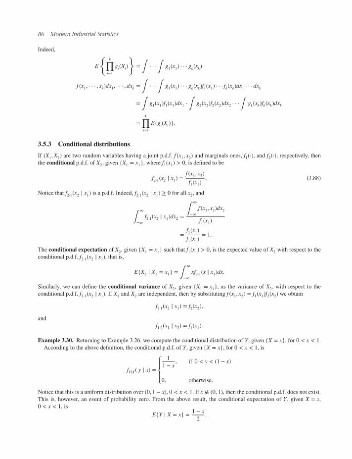
86 Modern Industrial Statistics
Indeed,
E
{k∏i=1
gi(Xi)
}= ∫ · · ·∫ g1(x1) · · · gk(xk)⋅
f (x1, · · · , xk)dx1, · · · , dxk = ∫ · · ·∫ g1(x1) · · · gk(xk)f1(x1) · · · fk(xk)dx1 · · · dxk
= ∫ g1(x1)f1(x1)dx1 ⋅ ∫ g2(x2)f2(x2)dx2 · · ·∫ gk(xk)fk(xk)dxk
=k∏i=1
E{gi(Xi)}.
3.5.3 Conditional distributions
If (X1,X2) are two random variables having a joint p.d.f. f (x1, x2) and marginals ones, f1(⋅), and f2(⋅), respectively, thenthe conditional p.d.f. of X2, given {X1 = x1}, where f1(x1) > 0, is defined to be
f2⋅1(x2 ∣ x1) =f (x1, x2)f1(x1). (3.88)
Notice that f2⋅1(x2 ∣ x1) is a p.d.f. Indeed, f2⋅1(x2 ∣ x1) ≥ 0 for all x2, and
∫∞
−∞f2⋅1(x2 ∣ x1)dx2 =
∫∞
−∞f (x1, x2)dx2
f1(x1)
=f1(x1)f1(x1)
= 1.
The conditional expectation of X2, given {X1 = x1} such that f1(x1) > 0, is the expected value of X2 with respect to the
conditional p.d.f. f2⋅1(x2 ∣ x1), that is,
E{X2 ∣ X1 = x1} = ∫∞
−∞xf2⋅1(x ∣ x1)dx.
Similarly, we can define the conditional variance of X2, given {X1 = x1}, as the variance of X2, with respect to the
conditional p.d.f. f2⋅1(x2 ∣ x1). If X1 and X2 are independent, then by substituting f (x1, x2) = f1(x1)f2(x2) we obtain
f2⋅1(x2 ∣ x1) = f2(x2),
and
f1⋅2(x1 ∣ x2) = f1(x1).
Example 3.30. Returning to Example 3.26, we compute the conditional distribution of Y , given {X = x}, for 0 < x < 1.According to the above definition, the conditional p.d.f. of Y , given {X = x}, for 0 < x < 1, is
fY∣X( y ∣ x) =⎧⎪⎨⎪⎩
1
1 − x, if 0 < y < (1 − x)
0, otherwise.
Notice that this is a uniform distribution over (0, 1 − x), 0 < x < 1. If x ∉ (0, 1), then the conditional p.d.f. does not exist.This is, however, an event of probability zero. From the above result, the conditional expectation of Y , given X = x,0 < x < 1, is
E{Y ∣ X = x} = 1 − x2.

Probability Models and Distribution Functions 87
The conditional variance is
V{Y ∣ X = x} = (1 − x)2
12.
In a similar fashion we show that the conditional distribution of X, given Y = y, 0 < y < 1, is uniform on (0, 1 − y). ◾
One can immediately prove that if X1 and X2 are independent, then the conditional distribution of X1 given {X2 = x2},when f2(x2) > 0, is just the marginal distribution of X1. Thus, X1 and X2 are independent if, and only if,
f2⋅1(x2 ∣ x1) = f2(x2) for all x2
and
f1⋅2(x1 ∣ x2) = f1(x1) for all x1,
provided that the conditional p.d.f. are well defined.
Notice that for a pair of random variables (X,Y), E{Y ∣ X = x} changes with x, as shown in Example 3.29, if X and
Y are dependent. Thus, we can consider E{Y ∣ X} to be a random variable, which is a function of X. It is interesting to
compute the expected value of this function of X, that is,
E{E{Y ∣ X}} = ∫ E{Y ∣ X = x}f1(x)dx
= ∫{∫ yfY⋅X( y ∣ x)dy
}f1(x)dx
= ∫ ∫ yf (x, y)f1(x)
f1(x)dydx.
If we can interchange the order of integration (whenever ∫ |y|f2( y)dy <∞), then
E{E{Y ∣ X}} = ∫ y
{∫ f (x, y)dx
}dy
= ∫ yf2( y)dy (3.89)
= E{Y}.
This result, known as the law of the iterated expectation, is often very useful. An example of the use of the law of the
iterated expectation is the following.
Example 3.31. Let (J,N) be a pair of random variables. The conditional distribution of J, given {N = n}, is the binomial
B(n, p). The marginal distribution of N is Poisson with mean 𝜆. What is the expected value of J?By the law of the iterated expectation,
E{J} = E{E{J ∣ N}}
= E{Np} = pE{N} = p𝜆.
One can show that the marginal distribution of J is Poisson, with mean p𝜆. ◾
Another important result relates variances and conditional variances. That is, if (X,Y) is a pair of random variables, having
finite variances then
V{Y} = E{V{Y ∣ X}} + V{E{Y ∣ X}}. (3.90)
We call this relationship the law of total variance.

88 Modern Industrial Statistics
Example 3.32. Let (X,Y) be a pair of independent random variables having finite variances 𝜎2X and 𝜎2Y and expected
values 𝜇X , 𝜇Y . Determine the variance of W = XY . By the law of total variance,
V{W} = E{V{W ∣ X}} + V{E{W ∣ X}}.
Since X and Y are independent
V{W ∣ X} = V{XY ∣ X} = X2V{Y ∣ X}
= X2𝜎2Y .
Similarly,
E{W ∣ X} = X𝜇Y .
Hence,
V{W} = 𝜎2YE{X2} + 𝜇2Y𝜎
2X
= 𝜎2Y (𝜎2X + 𝜇
2X) + 𝜇
2Y𝜎
2X
= 𝜎2X𝜎2Y + 𝜇
2X𝜎
2Y + 𝜇
2Y𝜎
2X . ◾
3.6 Some multivariate distributions
3.6.1 The multinomial distribution
The multinomial distribution is a generalization of the binomial distribution to cases of n independent trials in which theresults are classified to k possible categories (e.g. Excellent, Good, Average, Poor). The random variables (J1, J2, · · · , Jk)are the number of trials yielding results in each one of the k categories. These random variables are dependent, since J1 +
J2 + · · · + Jk = n. Furthermore, let p1, p2, · · · , pk; pi ≥ 0,k∑i=1pi = 1, be the probabilities of the k categories. The binomial
distribution is the special case of k = 2. Since Jk = n − (J1 + · · · + Jk−1), the joint probability function is written as a
function of k − 1 arguments, and its formula is
p(j1, · · · , jk−1) =(
nj1, · · · , jk−1
)pj11· · · pjk−1k−1p
jkk (3.91)
for j1, · · · , jk−1 ≥ 0 such thatk−1∑i=1ji ≤ n. In this formula,(
nj1, · · · , jk−1
)= n!j1!j2! · · · jk!
, (3.92)
and jk = n − (j1 + · · · + jk−1). For example, if n = 10, k = 3, p1 = .3, p2 = .4, p3 = .3,
p(5, 2) = 10!
5!2!3!(0.3)5(0.4)2(0.3)3
= 0.02645.
The marginal distribution of each one of the k variables is binomial, with parameters n and pi (i = 1, · · · , k). The jointmarginal distribution of (J1, J2) is trinomial, with parameters n, p1, p2 and (1 − p1 − p2). Finally, the conditional distribu-tion of (J1, · · · , Jr), 1 ≤ r < k, given {Jr+1 = jr+1, · · · , Jk = jk} is (r + 1)-nomial, with parameters nr = n − (jr+1 + · · · + jk)and p′
1, · · · , p′r, p′r+1, where
p′i =pi
(1 − pr+1 − · · · − pk), i = 1, · · · , r

Probability Models and Distribution Functions 89
and
p′r+1 = 1 −r∑i=1
p′i .
Finally, we can show that, for i ≠ j,Cov(Ji, Jj) = −npipj. (3.93)
Example 3.33. An insertion machine is designed to insert components into computer printed circuit boards. Every com-
ponent inserted on a board is scanned optically. An insertion is either error-free or its error is classified to the following
two main categories: misinsertion (broken lead, off pad, etc.) or wrong component. Thus, we have altogether three general
categories. Let
J1 = # of error-free components;
J2 = # of misinsertion;
J3 = # of wrong components.
The probabilities that an insertion belongs to one of these categories is p1 = 0.995, p2 = 0.001 and p2 = 0.004.The insertion rate of this machine is n = 3500 components per hour of operation. Thus, we expect during one hour of
operation n × (p2 + p3) = 175 insertion errors.
Given that there are 16 insertion errors during a particular hour of operation, the conditional distribution of the number
of misinsertions is binomial B(16, 0.01
0.05
).
Thus,
E{J2 ∣ J2 + J3 = 16} = 16 × 0.2 = 3.2.
On the other hand,
E{J2} = 3500 × 0.001 = 3.5.
We see that the information concerning the total number of insertion errors makes a difference.
Finally
Cov(J2, J3) = −3500 × 0.001 × 0.004
= −0.014
V{J2} = 3500 × 0.001 × 0.999 = 3.4965
and
V{J3} = 3500 × 0.004 × 0.996 = 13.944.
Hence, the correlation between J2 and J3 is
𝜌2,3 =−0.014√
3.4965 × 13.944= −0.0020.
This correlation is quite small. ◾
3.6.2 The multi-hypergeometric distribution
Suppose that we draw from a population of sizeN a RSWOR of size n. Each one of the n units in the sample is classified to
one of k categories. Let J1, J2, · · · , Jk be the number of sample units belonging to each one of these categories. J1 + · · · +Jk = n. The distribution of J1, · · · , Jk is k-variate hypergeometric. IfM1, · · · ,Mk are the number of units in the population
in these categories, before the sample is drawn, then the joint p.d.f. of J1, · · · , Jk is
p( j1, · · · , jk−1) =
(M1j1
) (M2j2
)· · ·
(Mkjk
)(Nn
) , (3.94)

90 Modern Industrial Statistics
where jk = n − (j1 + · · · + jk−1). This distribution is a generalization of the hypergeometric distribution H(N,M, n). Thehypergeometric distribution H(N,Mi, n) is the marginal distribution of Ji (i = 1, · · · , k). Thus,
E{Ji} = nMi
N, i = 1, · · · , k
V{Ji} = nMi
N
(1 −
Mi
N
)(1 − n − 1
N − 1
), i = 1, · · · , k (3.95)
and for i ≠ j
Cov(Ji, Jj) = −nMi
N⋅Mj
N
(1 − n − 1
N − 1
).
Example 3.34. A lot of 100 spark plugs contains 20 plugs from vendor V1, 50 plugs from vendor V2 and 30 plugs from
vendor V3.
A random sample of n = 20 plugs is drawn from the lot without replacement.
Let Ji be the number of plugs in the sample from the vendor Vi, i = 1, 2, 3. Accordingly,
Pr{J1 = 5, J2 = 10} =(205
) (5010
) (305
)(10020
)= 0.00096.
If we are told that 5 out of the 20 plugs in the sample are from vendor V3, then the conditional distribution of J1 is
Pr{J1 = j1 ∣ J3 = 5} =(20j1
) (50
15−j1
)(7015
) , j1 = 0, · · · , 15.
Indeed, given J3 = 5, then J1 can assume only the values 0, 1, · · · , 15. The conditional probability that j1 out of the 15remaining plugs in the sample are from vendor V1, is the same as that of choosing a RSWOR of size 15 from a lot of size
70 = 20 + 50, with 20 plugs from vendor V1. ◾
3.6.3 The bivariate normal distribution
The bivariate normal distribution is the joint distribution of two continuous random variables (X,Y) having a joint p.d.f.
f (x, y;𝜇, 𝜂, 𝜎X , 𝜎Y , 𝜌) =1
2𝜋𝜎X𝜎Y√1 − 𝜌2
⋅
exp
{− 1
2(1 − 𝜌2)
[(x − 𝜇𝜎x
)2
− 2𝜌x − 𝜇𝜎Y
⋅y − 𝜂𝜎Y
+(y − 𝜂𝜎Y
)2]},
−∞ < x, y <∞. (3.96)
𝜇, 𝜂, 𝜎X , 𝜎Y and 𝜌 are parameters of this distribution.
Integration of y yields that themarginal distribution ofX isN(𝜇, 𝜎2x ). Similarly, themarginal distribution of Y isN(𝜂, 𝜎2Y ).Furthermore, 𝜌 is the correlation between X and Y . Notice that if 𝜌 = 0, then the joint p.d.f. becomes the product of the
two marginal ones, that is,
f (x, y);𝜇, 𝜂, 𝜎X , 𝜎Y , 0) =1√2𝜋𝜎X
exp
{−1
2
(x − 𝜇𝜎X
)2}
⋅
1√2𝜋𝜎Y
exp
{−1
2
(y − 𝜂𝜎Y
)2}, for all −∞ < x, y <∞.

Probability Models and Distribution Functions 91
X
−3−2
−1
0
1
2
3
Y
−3
−2
−1
0
12
3
Density
0.05
0.10
0.15
Figure 3.17 Bivariate normal p.d.f.
Hence, if 𝜌 = 0, then X and Y are independent. On the other hand, if 𝜌 ≠ 0, then f (x, y;𝜇, 𝜂, 𝜎X , 𝜎Y , 𝜌) ≠ f1(x;𝜇, 𝜎X)f2( y; 𝜂, 𝜎Y ), and the two random variables are dependent.
In Figure 3.17 we present the bivariate p.d.f. for 𝜇 = 𝜂 = 0, 𝜎X = 𝜎Y = 1 and 𝜌 = 0.5.One can verify also that the conditional distribution of Y , given {X = x} is normal with mean
𝜇Y⋅x = 𝜂 + 𝜌𝜎Y𝜎X
(x − 𝜇) (3.97)
and variance
𝜎2Y⋅x = 𝜎2Y (1 − 𝜌
2). (3.98)
It is interesting to see that 𝜇Y⋅x is a linear function of x. We can say that 𝜇Y⋅x = E{Y ∣ X = x} is, in the bivariate normal
case, the theoretical (linear) regression of Y on X (see Chapter 5). Similarly,
𝜇X⋅y = 𝜇 + 𝜌𝜎X𝜎Y
( y − 𝜂),
and
𝜎2X⋅y = 𝜎2X(1 − 𝜌
2).
If 𝜇 = 𝜂 = 0 and 𝜎X = 𝜎Y = 1, we have the standard bivariate normal distribution. The joint c.d.f. in the standard case is
denoted by Φ2(x, y; 𝜌) and its formula is
Φ2(x, y; 𝜌) =1
2𝜋√1 − 𝜌2 ∫
x
−∞ ∫y
−∞exp
{− 1
2(1 − 𝜌2)(z21 − 2𝜌z1z2 + z2)
}dz1dz2
= ∫x
−∞𝜙(z1)Φ
(y − 𝜌z1√1 − 𝜌2
)dz1 (3.99)
values of Φ2(x, y; 𝜌) can be obtained by numerical integration. If one has to compute the bivariate c.d.f. in the general
case, the following formula is useful
F(x, y;𝜇, 𝜂, 𝜎X , 𝜎Y , 𝜌) = Φ2
(x − 𝜇𝜎X,y − 𝜂𝜎Y
; 𝜌).

92 Modern Industrial Statistics
For computing Pr{a ≤ X ≤ b, c ≤ Y ≤ d} we use the formula,
Pr{a ≤ X ≤ b, c ≤ Y ≤ d} = F(b, d; – )
− F(a, d; – ) − F(b, c; – ) + F(a, c; – ).
Example 3.35. Suppose that (X,Y) deviations in components placement on PCB by an automaticmachine have a bivariate
normal distribution with means 𝜇 = 𝜂 = 0, standard deviations 𝜎X = 0.00075 and 𝜎Y = 0.00046 [Inch] and 𝜌 = 0.160.The placement errors are within the specifications if |X| < 0.001 [Inch] and |Y| < 0.001 [Inch]. What proportion of
components are expected to have X, Y deviations compliant with the specifications? The standardized version of the spec
limits are Z1 =0.001
0.00075= 1.33 and Z2 =
0.001
0.00046= 2.174. We compute
Pr{|X| < 0.001, |Y| < 0.001} = Φ2(1.33, 2.174, .16) − Φ2(−1.33, 2.174, .16)
− Φ2(1.33,−2.174;.16) + Φ2(−1.33,−2.174;.16)
= 0.793.
This is the expected proportion of good placements. ◾
3.7 Distribution of order statistics
As defined in Chapter 2, the order statistics of the sample are the sorted data.More specifically, letX1, · · · ,Xn be identicallydistributed independent (i.i.d.) random variables. The order statistics are X(i), i = 1, · · · , n, where
X(1) ≤ X(2) ≤ · · · ≤ X(n).
In the present section we discuss the distributions of these order statistics, when F(x) is (absolutely) continuous, havinga p.d.f. f (x).
We start with the extremal statistics X(1) and X(n).
Since the random variables Xi (i = 1, · · · , n) are i.i.d., the c.d.f. of X(1) is
F(1)(x) = Pr{X(1) ≤ x}
= 1 − Pr{X(1) ≥ x} = 1 −n∏i=1
Pr{Xi ≥ x}
= 1 − (1 − F(x))n.
By differentiation we obtain that the p.d.f. of X(1) is
f(1)(x) = nf (x)[1 − F(x)]n−1. (3.100)
Similarly, the c.d.f. of the sample maximum X(n) is
F(n)(x) =n∏i=1
Pr{Xi ≤ x}
= (F(x))n.
The p.d.f. of X(n) is
f(n)(x) = nf (x)(F(x))n−1. (3.101)

Probability Models and Distribution Functions 93
Example 3.36. (i) A switching circuit consists of n modules, which operate independently and which are connected in
series (see Figure 3.18). Let Xi be the time till failure of the i-th module. The system fails when any module fails. Thus,
the time till failure of the system is X(1). If all Xi are exponentially distributed with mean life 𝛽, then the c.d.f. of X(1) is
F(1)(x) = 1 − e−nx∕𝛽 , x ≥ 0.
Thus, X(1) is distributed like E(𝛽
n
). It follows that the expected time till failure of the circuit is E{X(1)} = 𝛽
n.
Components in Series
Components in Parallel
C1 C2
C1
C2
Figure 3.18 Series and parallel systems
(ii) If the modules are connected in parallel, then the circuit fails at the instant the last of the n modules fail, which is
X(n). Thus, if Xi is E(𝛽), the c.d.f. of X(n) is
F(n)(x) = (1 − e−(x∕𝛽))n.
The expected value of X(n) is
E{X(n)} = n𝛽 ∫
∞
0
xe−x∕𝛽(1 − e−x∕𝛽)n−1dx
= n𝛽 ∫∞
0
ye−y(1 − e−y)n−1dy
= n𝛽n−1∑j=0
(−1)j(n − 1
j
)∫
∞
0
ye−(1+j)ydy
= n𝛽n∑j=1
(−1)j−1(n − 1
j − 1
)1
j2.
Furthermore, since n(n−1j−1)= j
(nj
), we obtain that
E{X(n)} = 𝛽n∑j=1
(−1)j−1(nj
)1
j.

94 Modern Industrial Statistics
One can also show that this formula is equivalent to
E{X(n)} = 𝛽n∑j=1
1
j.
Accordingly, if the parallel circuit consists of 3 modules, and the time till failure of each module is exponential with
𝛽 = 1, 000 [hr], the expected time till failure of the system is 1,833.3 [hr]. ◾
Generally, the distribution of X(i) (i = 1, · · · , n) can be obtained by the following argument. The event {X(i) ≤ x} is equiv-alent to the event that the number of Xi values in the random example which are smaller or equal to x is at least i.
Consider n independent and identical trials, in which “success” is that {Xi ≤ x} (i = 1, · · · , n). The probability of “suc-cess” is F(x). The distribution of the number of successes is B(n,F(x)). Thus, the c.d.f. of X(i) is
F(i)(x) = Pr{X(i) ≤ x} = 1 − B(i − 1; n,F(x))
=n∑j=i
(n
j
)(F(x))j(1 − F(x))n−j.
Differentiating this c.d.f. with respect to x yields the p.d.f. of X(i), namely:
f(i)(x) =n!
(i − 1)!(n − i)!f (x)(F(x))i−1(1 − F(x))n−i. (3.102)
Notice that if X has a uniform distribution on (0, 1), then the distribution of X(i) is like that of Beta(i, n − i + 1),i = 1, · · · , n. In a similar manner one can derive the joint p.d.f. of (X(i),X(j)), 1 ≤ i < j ≤ n, etc. This joint p.d.f. is givenby
f(i),(j)(x, y) =n!
(i − 1)!(j − 1 − i)!(n − j)!f (x)f ( y) ⋅
⋅ (F(x))i−1[F( y) − F(x)]j−i−1(1 − F( y))n−j, (3.103)
for −∞ < x < y < ∞.
3.8 Linear combinations of random variables
Let X1,X2, · · · ,Xn be random variables having a joint distribution, with joint p.d.f. f (x1, · · · , xn). Let 𝛼1, · · · , 𝛼n be givenconstants. Then
W =n∑i=1𝛼iXi
is a linear combination of the X’s. The p.d.f. of W can generally be derived, using various methods. We discuss in the
present section only the formulae of the expected value and variance of W.
It is straightforward to show that
E{W} =n∑i=1𝛼iE{Xi}. (3.104)
That is, the expected value of a linear combination is the same linear combination of the expectations.
The formula for the variance is somewhat more complicated, and is given by
V{W} =n∑i=1𝛼2i V{Xi} +
∑∑i≠j𝛼i𝛼jcov(Xi,Xj). (3.105)

Probability Models and Distribution Functions 95
Example 3.37. Let X1,X2, · · · ,Xn be i.i.d. random variables, with common expectations 𝜇 and common finite variances
𝜎2. The sample mean Xn =1
n
n∑i=1Xi is a particular linear combination, with
𝛼1 = 𝛼2 = · · · = 𝛼n =1
n.
Hence,
E{Xn} = 1
n
n∑i=1
E{Xi} = 𝜇
and, since X1,X2, · · · ,Xn are mutually independent, cov(Xi,Xj) = 0, all i ≠ j. Hence
V{Xn} = 1
n2
n∑i=1
V{Xi} = 𝜎2
n.
Thus, we have shown that in a random sample of n i.i.d. random variables, the sample mean has the same expectation as
that of the individual variables, but its sample variance is reduced by a factor of 1∕n.Moreover, from Chebychev’s inequality, for any 𝜖 > 0
Pr{|Xn − 𝜇| > 𝜖} < 𝜎2n𝜖2 .Therefore, since lim
n→∞𝜎2
n𝜖2= 0,
limn→∞
Pr{|Xn − 𝜇| > 𝜖} = 0.
This property is called the convergence in probability of Xn to 𝜇. ◾
Example 3.38. Let U1, U2, U3 be three i.i.d. random variables having uniform distributions on (0, 1). We consider
the statistic
W = 1
4U(1) +
1
2U(2) +
1
4U(3),
where 0 < U(1) < U(2) < U(3) < 1 are the order statistics. We have seen in Section 4.7 that the distribution of U(i) is like
that of Beta(i, n − i + 1). Hence
E{U(1)} = E{Beta(1, 3)} = 1
4
E{U(2)} = E{Beta(2, 2)} = 1
2
E{U(3)} = E{Beta(3, 1)} = 3
4.
It follows that
E{W} = 1
4⋅1
4+ 1
2⋅1
2+ 1
4⋅1
4= 1
2.
To find the variance of W we need more derivations.
First
V{U(1)} = V{Beta(1, 3)} = 3
42 × 5= 3
80
V{U(2)} = V{Beta(2, 2)} = 4
42 × 5= 1
20
V{U(3)} = V{Beta(3, 1)} = 3
42 × 5= 3
80.

96 Modern Industrial Statistics
We need to find Cov(U(1),U(2)), Cov(U(1),U(3)) and Cov(U(2),U(3)). From the joint p.d.f. formula of order statistics, the
joint p.d.f. of (U(1),U(2)) isf(1),(2)(x, y) = 6(1 − y), 0 < x ≤ y < 1.
Hence
E{U(1)U(2)} = 6∫1
0
x
(∫
1
0
y(1 − y)dy)dx
= 6
40.
Thus,
Cov(U(1),U(2)) =6
40− 1
4⋅1
2
= 1
40.
Similarly, the p.d.f. of (U(1),U(3)) is
f(1),(3)(x, y) = 6( y − x), 0 < x ≤ y < 1.
Thus,
E{U(1)U(3)} = 6∫1
0
x
(∫
1
x
y( y − x)dy)dx
= 6∫1
0
x(1
3
(1 − x3
)− x
2(1 − x2)
)dx
= 1
5,
and
Cov(U(1),U(3)) =1
5− 1
4⋅3
4= 1
80.
The p.d.f. of (U(2),U(3)) isf(2),(3)(x, y) = 6x, 0 < x ≤ y ≤ 1,
and
Cov(U(2),U(3)) =1
40.
Finally,
V{W} = 1
16⋅3
80+ 1
4⋅1
20+ 1
16⋅3
80
+ 2 ⋅1
4⋅1
2⋅1
40+ 2 ⋅
1
4⋅1
4⋅1
80
+ 2 ⋅1
2⋅1
4⋅1
40
= 1
32= 0.03125.
◾
The following is a useful result:
If X1,X2, · · · ,Xn are mutually independent, then the m.g.f. of Tn =n∑i=1Xi is
MTn(t) =
n∏i=1
MXi(t). (3.106)

Probability Models and Distribution Functions 97
Indeed, as shown in Section 4.5.2, when X1, . . . ,Xn are independent, the expected value of the product of functions is theproduct of their expectations.
Therefore,
MTn(t) = E{e
t
n∑i=1
Xi}
= E
{n∏i=1
etXi
}
=n∏i=1
E{etXi}
=n∏i=1
MXi(t).
The expected value of the product is equal to the product of the expectations, since X1, · · · ,Xn are mutually independent.
Example 3.39. In the present example we illustrate some applications of the last result.
(i) Let X1,X2, · · · ,Xk be independent random variables having binomial distributions like B(ni, p), i = 1, · · · , k, thentheir sum Tk has the binomial distribution. To show this,
MTk(t) =
k∏i=1
MXi(t)
= [etp + (1 − p)]
k∑i=1
ni.
That is, Tk is distributed like B
( k∑i=1ni, p
). This result is intuitively clear.
(ii) If X1, · · · ,Xn are independent random variables, having Poisson distributions with parameters 𝜆i (i = 1, · · · , n) then
the distribution of Tn =n∑i=1Xi is Poisson with parameter 𝜇n =
n∑i=1𝜆i. Indeed,
MTn(t) =
n∏j=1
exp {−𝜆j(1 − et)}
= exp
{−
n∑j=1𝜆j(1 − et)
}= exp {−𝜇n(1 − et)}.
(iii) Suppose X1, · · · ,Xn are independent random variables, and the distribution of Xi is normal N(𝜇i, 𝜎2i ), then the distri-
bution ofW =n∑i=1𝛼iXi is normal like that of
N
(n∑i=1𝛼i𝜇i,
n∑i=1𝛼2i 𝜎
2i
).
To verify this we recall that Xi = 𝜇i + 𝜎iZi, where Zi is N(0, 1) (i = 1, · · · , n). Thus
M𝛼iXi (t) = E{et(𝛼i𝜇i+𝛼i𝜎iZi}
= et𝛼i𝜇iMZi(𝛼i𝜎it).

98 Modern Industrial Statistics
We derived before thatMZi(u) = eu
2∕2. Hence,
M𝛼iXi (t) = exp
{𝛼i𝜇it +𝛼2i 𝜎
2i
2t2}.
Finally
MW (t) =n∏i=1
M𝛼iXi (t)
= exp
⎧⎪⎪⎨⎪⎪⎩(
n∑i=1𝛼i𝜇i
)t +
n∑i=1𝛼2i 𝜎
2i
2t2
⎫⎪⎪⎬⎪⎪⎭.
This implies that the distribution of W is normal, with
E{W} =n∑i=1𝛼i𝜇i
and
V{W} =n∑i=1𝛼2i 𝜎
2i .
(iv) If X1,X2, · · · ,Xn are independent random variables, having gamma distribution like G(𝜈i, 𝛽), respectively,
i = 1, · · · , n, then the distribution of Tn =n∑i=1Xi is gamma, like that of G
( n∑i=1𝜈i, 𝛽
). Indeed,
MTn(t) =
n∏i=1
(1 − t𝛽)−𝜈i
= (1 − t𝛽)−
n∑i=1𝜈i.
◾
3.9 Large sample approximations
3.9.1 The law of large numbers
We have shown in Example 3.36 that the mean of a random sample, Xn, converges in probability to the expected value ofX, 𝜇 (the population mean). This is the law of large numbers (L.L.N.) which states that, if X1,X2, · · · are i.i.d. random
variables and E{|X1|} < ∞, then for any 𝜖 > 0,
limn→∞
Pr{|Xn − 𝜇| > 𝜖} = 0.
We also write
limn→∞
Xn = 𝜇, in probability.
This is known as the weak L.L.N. There is a stronger law, which states that, under the above conditions,
Pr{ limn→∞
Xn = 𝜇} = 1.
It is beyond the scope of the book to discuss the meaning of the strong L.L.N.

Probability Models and Distribution Functions 99
3.9.2 The Central Limit Theorem
The Central Limit Theorem, C.L.T., is one of the most important theorems in probability theory. We formulate here the
simplest version of this theorem, which is often sufficient for applications. The theorem states that if Xn is the sample
mean of n i.i.d. random variables, then if the population variance 𝜎2 is positive and finite, the sampling distribution of Xnis approximately normal, as n → ∞. More precisely,
If X1,X2, · · · is a sequence of i.i.d. random variables, with E{X1} = 𝜇 and V{X1} = 𝜎2, 0 < 𝜎2 <∞, then
limn→∞
Pr
{(Xn − 𝜇)
√n
𝜎≤ z
}= Φ(z), (3.107)
where Φ(z) is the c.d.f. of N(0, 1).The proof of this basic version of the C.L.T. is based on a result in probability theory, stating that if X1,X2, · · · is
a sequence of random variables having m.g.f.’s, Mn(T), n = 1, 2, · · · and if limn→∞
Mn(t) = M(t) is the m.g.f. of a random
variable X∗, having a c.d.f. F∗(x), then limn→∞
Fn(x) = F∗(x), where Fn(x) is the c.d.f. of Xn.The m.g.f. of
Zn =√n(Xn − 𝜇)𝜎,
can be written as
MZn(t) = E
{exp
{t√n𝜎
n∑i=1
(Xi − 𝜇)
}}
=
(E
{exp
{t√n𝜎
(X1 − 𝜇)
}})n
,
since the random variables are independent. Furthermore, Taylor expansion of exp{
t√n𝜎(X1 − 𝜇)
}is
1 + t√n𝜎
(X1 − 𝜇) +t2
2n𝜎2(X1 − 𝜇)2 + o
(1
n
),
for n large. Hence, as n→ ∞
E
{exp
{t√n𝜎
(X1 − 𝜇)
}}= 1 + t2
2n+ o
(1
n
).
Hence,
limn→∞
MZn(t) = lim
n→∞
(1 + t2
2n+ o
(1
n
))n
= et2∕2,
which is the m.g.f. of N(0, 1). This is a sketch of the proof. For rigorous proofs and extensions, see textbooks on proba-
bility theory.
3.9.3 Some normal approximations
The C.L.T. can be applied to provide an approximation to the distribution of the sum of n i.i.d. random variables, by a
standard normal distribution, when n is large. We list below a few such useful approximations.

100 Modern Industrial Statistics
(i) Binomial DistributionWhen n is large, then the c.d.f. of B(n, p) can be approximated by
B(k; n, p) ≅ Φ
(k + 1
2− np√
np(1 − p)
). (3.108)
We add1
2to k, in the argument of Φ(⋅) to obtain a better approximation when n is not too large. This modification is
called, “correction for discontinuity.”
How large should n be to get a “good” approximation? A general rule is
n >9
p(1 − p). (3.109)
(ii) Poisson DistributionThe c.d.f. of Poisson with parameter 𝜆 can be approximated by
P(k; 𝜆) ≅ Φ
(k + 1
2− 𝜆√𝜆
), (3.110)
if 𝜆 is large (greater than 30).(iii) Gamma Distribution
The c.d.f. of G(𝜈, 𝛽) can be approximated by
G(x; 𝜈, 𝛽) ≅ Φ
(x − 𝜈𝛽𝛽√𝜈
), (3.111)
for large values of 𝜈.
Example 3.40. (i) A lot consists of n = 10, 000 screws. The probability that a screw is defective is p = 0.01. What is the
probability that there are more than 120 defective screws in the lot?
The number of defective screws in the lot, Jn, has a distribution like B(10000, 0.01). Hence,
Pr{J10000 > 120} = 1 − B(120; 10000, .01)
≅ 1 − Φ
(120.5 − 100√
99
)= 1 − Φ(2.06) = 0.0197.
(ii) In the production of industrial film, we find on the average 1 defect per 100 [ft]2 of film. What is the probability that
fewer than 100 defects will be found on 12,000 [ft]2 of film?
We assume that the number of defects per unit area of film is a Poisson random variable. Thus, our model is that the
number of defects, X, per 12,000 [ft]2 has a Poisson distribution with parameter 𝜆 = 120. Thus,
Pr{X < 100} ≅ Φ
(99.5 − 120√
120
)= 0.0306.
(iii) The time till failure, T , of radar equipment is exponentially distributed with mean time till failure (M.T.T.F.) of
𝛽 = 100 [hr].
A sample of n = 50 units is put on test. Let T50 be the sample mean. What is the probability that T50 will fail in the
interval (95, 105) [hr]?

Probability Models and Distribution Functions 101
We have seen that50∑i=1Ti is distributed like G(50, 100), since E(𝛽) is distributed like G(1, 𝛽). Hence T50 is distributed
like1
50G(50, 100) which is G(50, 2). By the normal approximation
Pr{95 < T50 < 105} ≅ Φ
(105 − 100
2√50
)
− Φ
(95 − 100
2√50
)= 2Φ(0.3536) − 1 = 0.2763.
◾
3.10 Additional distributions of statistics of normal samples
In the present section we assume that X1,X2, · · · ,Xn are i.i.d. N(𝜇, 𝜎2) random variables. In the subsections 3.10.1–3.10.3
we present the chi-squared, t- and F-distributions which play an important role in the theory of statistical inference
(Chapter 4).
3.10.1 Distribution of the sample variance
Writing Xi = 𝜇 + 𝜎Zi, where Z1, · · · ,Zn are i.i.d. N(0, 1), we obtain that the sample variance S2 is distributed like
S2 = 1
n − 1
n∑i=1
(Xi − Xn)2
= 1
n − 1
n∑i=1
(𝜇 + 𝜎Zi − (𝜇 + 𝜎Zn))2
= 𝜎2
n − 1
n∑i=1
(Zi − Zn)2.
One can show thatn∑i=1
(Zi − Zn)2 is distributed like 𝜒2[n − 1], where 𝜒2[𝜈] is called a chi-squared random variable with
𝜈 degrees of freedom. Moreover, 𝜒2[𝜈] is distributed like G(𝜈
2, 2).
The 𝛼-th quantile of 𝜒2[𝜈] is denoted by 𝜒2𝛼 [𝜈]. Accordingly, the c.d.f. of the sample variance is
HS2 (x; 𝜎2) = Pr
{𝜎2
n − 1𝜒2[n − 1] ≤ x
}= Pr
{𝜒2[n − 1] ≤ (n − 1)x
𝜎2
}= Pr
{G(n − 1
2, 2) ≤ (n − 1)x𝜎2
}= G
((n − 1)x2𝜎2
; n − 1
2, 1
).
(3.112)
The probability values of the distribution of 𝜒2[𝜈], as well as the 𝛼-quantiles, can be computed by R, MINITAB or JMP,
or read from appropriate tables.
The expected value and variance of the sample variance are
E{S2} = 𝜎2
n − 1E{𝜒2[n − 1]}

102 Modern Industrial Statistics
= 𝜎2
n − 1E{G(n − 1
2, 2)}
= 𝜎2
n − 1⋅ (n − 1) = 𝜎2.
Similarly
V{S2} = 𝜎4
(n − 1)2V{𝜒2[n − 1]}
= 𝜎4
(n − 1)2V{G(n − 1
2, 2)}
= 𝜎4
(n − 1)2⋅ 2(n − 1)
= 2𝜎4
n − 1.
(3.113)
Thus applying the Chebychev’s inequality, for any given 𝜖 > 0,
Pr{|S2 − 𝜎2| > 𝜖} < 2𝜎4
(n − 1)𝜖2.
Hence, S2 converges in probability to 𝜎2. Moreover,
limn→∞
Pr
{(S2 − 𝜎2)
𝜎2√2
√n − 1 ≤ z
}= Φ(z). (3.114)
That is, the distribution of S2 can be approximated by the normal distributions in large samples.
3.10.2 The “Student” t-statistic
We have seen that
Zn =√n(Xn − 𝜇)𝜎
has a N(0, 1) distribution. As we will see in Chapter 6, when 𝜎 is unknown, we test hypotheses concerning 𝜇 by the
statistic
t =√n(Xn − 𝜇0)
S,
where S is the sample standard deviation. If X1, · · · ,Xn are i.i.d. like N(𝜇0, 𝜎2) then the distribution of t is called the
Student t-distribution with 𝜈 = n − 1 degrees of freedom. The corresponding random variable is denoted by t[𝜈].The p.d.f. of t[𝜈] is symmetric about 0 (see Figure 3.19). Thus,
E{t[𝜈]} = 0, for 𝜈 ≥ 2 (3.115)
and
V{t[𝜈]} = 𝜈𝜈 − 2, 𝜈 ≥ 3. (3.116)
The 𝛼-quantile of t[𝜈] is denoted by t𝛼[𝜈]. It can be read from a table, or determined by R, JMP or MINITAB.
3.10.3 Distribution of the variance ratio
F =S21𝜎22
S22𝜎21
.

Probability Models and Distribution Functions 103
−4 −2 0 2 4
0.0
0.1
0.2
0.3
0.4
0.5
x
t(x,v)
v = 50
v = 5
Figure 3.19 Density Functions of t[𝜈], 𝜈 = 5,50
Consider now two independent samples of size n1 and n2, respectively, which have been taken from normal populations
having variances 𝜎21and 𝜎2
2. Let
S21 =1
n1 − 1
n1∑i=1
(X1i − X1)2
and
S22 =1
n2 − 1
n2∑i=1
(X2i − X2)2
be the variances of the two samples where X1 and X2 are the corresponding sample means. The F-ratio has a distributiondenoted by F[𝜈1, 𝜈2], with 𝜈1 = n1 − 1 and 𝜈2 = n2 − 1. This distribution is called the F-distribution with 𝜈1 and 𝜈2degrees of freedom. A graph of the densities of F[𝜈1, 𝜈2] is given in Figure 3.20.
The expected value and the variance of F[𝜈1, 𝜈2] are:
E{F[𝜈1, 𝜈2]} = 𝜈2∕(𝜈2 − 2), 𝜈2 > 2, (3.117)
and
V{F[𝜈1, 𝜈2]} =2𝜈2
2(𝜈1 + 𝜈2 − 2)
𝜈1(𝜈2 − 2)2(𝜈2 − 4), 𝜈2 > 4. (3.118)
The (1 − 𝛼)th quantile of F[𝜈1, 𝜈2], i.e. F1−𝛼[𝜈1, 𝜈2], can be computed by MINITAB. If we wish to obtain the 𝛼-th fractileF𝛼[𝜈1, 𝜈2] for values of 𝛼 < .5, we can apply the relationship:
F1−𝛼[𝜈1, 𝜈2] =1
F𝛼[𝜈2, 𝜈1]. (3.119)
Thus, for example, to compute F.05[15, 10], we write
F.05[15, 10] = 1∕F.95[10, 15] = 1∕2.54 = .3937.

104 Modern Industrial Statistics
0 1 2 3 4 5 6
0.0
0.2
0.4
0.6
x
F(v
1, v
2)
Figure 3.20 Density function of F(𝜈1, 𝜈2)
3.11 Chapter highlights
The chapter provides the basics of probability theory and of the theory of distribution functions. The probability model
for random sampling is discussed. This is fundamental for the sampling procedures to be discussed in Chapter 7. Bayes
theorem has important ramifications in statistical inference, as will be discussed in Chapter 4. The concepts and definitions
introduced are:
• Sample Space
• Elementary Events
• Operations with Events
• Disjoint Events
• Probability of Events
• Random Sampling With Replacement (RSWR)
• Random Sampling Without Replacement (RSWOR)
• Conditional Probabilities
• Independent Events
• Bayes’ Formula
• Prior Probability
• Posterior Probability
• Probability Distribution Function (p.d.f.)
• Discrete Random Variable
• Continuous Random Variable
• Cumulative Distribution Function
• Central Moments
• Expected Value
• Standard Deviation
• Chebychev’s Inequality

Probability Models and Distribution Functions 105
• Moment Generating Function
• Skewness
• Kurtosis
• Independent Trials
• P-th Quantile• Joint Distribution
• Marginal Distribution
• Conditional Distribution
• Mutual Independence
• Conditional Independence
• Law of Total Variance
• Law of Iterated Expectation
• Order Statistics
• Convergence in Probability
• Central Limit Theorem
• Law of Large Numbers
3.12 Exercises
3.1 An experiment consists of making 20 observations on the quality of chips. Each observation is recorded as Gor D.(i) What is the sample space, S, corresponding to this experiment?
(ii) How many elementary events in S?(iii) Let An, n = 0, · · · , 20, be the event that exactly n G observations are made. Write the events An formally.
How many elementary events belong to An?3.2 An experiment consists of 10 measurements 𝑤1, · · · , 𝑤10 of the weights of packages. All packages under con-
sideration have weights between 10 and 20 pounds. What is the sample space S? Let A = {(𝑤1, 𝑤2, · · · , 𝑤10) ∶𝑤1 +𝑤2 = 25}. Let B = {(𝑤1, · · · , 𝑤10) ∶ 𝑤1 +𝑤2 ≤ 25}. Describe the events A and B graphically. Show that
A ⊂ B.3.3 Strings of 30 binary (0, 1) signals are transmitted.
(i) Describe the sample space, S.(ii) Let A10 be the event that the first 10 signals transmitted are all 1’s. How many elementary events belong
to A10?
(iii) Let B10 be the event that exactly 10 signals, out of 30 transmitted, are 1’s. How many elementary events
belong to B10? Does A10 ⊂ B10?
3.4 Prove DeMorgan laws
(i) (A ∪ B)c = Ac ∩ Bc.(ii) (A ∩ B)c = Ac ∪ Bc.
3.5 Consider Exercise [3.3] Show that the events A0,A1, · · · ,A20 are a partition of the sample space S.
3.6 Let A1, · · · ,An be a partition of S. Let B be an event. Show that B =n⋃i=1AiB, where AiB = Ai ∩ B, is a union of
disjoint events.
3.7 Develop a formula for the probability Pr{A ∪ B ∪ C}, where A, B, C are arbitrary events.
3.8 Show that if A1, · · · ,An is a partition, then for any event B, P{B} =n∑i=1P{AiB}. [Use the result of [3.6].]
3.9 An unbiased die has the numbers 1, 2, · · · , 6 written on its faces. The die is thrown twice. What is the probability
that the two numbers shown on its upper face sum up to 10?
3.10 The time till failure, T , of electronic equipment is a random quantity. The event At = {T > t} is assigned the
probability Pr{At} = exp {−t∕200}, t ≥ 0. What is the probability of the event B = {150 < T < 280}?3.11 A box contains 40 parts, 10 of type A, 10 of type B, 15 of type C and 5 of type D. A random sample of 8 parts is
drawn without replacement. What is the probability of finding two parts of each type in the sample?

106 Modern Industrial Statistics
3.12 How many samples of size n = 5 can be drawn from a population of size N = 100,
(i) with replacement?
(ii) without replacement?
3.13 A lot of 1,000 items contain M = 900 “good” ones, and 100 “defective” ones. A random sample of size n = 10
is drawn from the lot. What is the probability of observing in the sample at least 8 good items,
(i) when sampling is with replacement?
(ii) when sampling is without replacement?
3.14 In continuation of the previous exercise, what is the probability of observing in an RSWR at least one defective
item?
3.15 Consider the problem of Exercise [3.10]. What is the conditional probability Pr{T > 300 ∣ T > 200}.3.16 A point (X,Y) is chosen at random within the unit square, i.e.
S = {(x, y) ∶ 0 ≤ x, y ≤ 1}.
Any set A contained in S having area given by
Area{A} = ∫ ∫Adxdyis an event, whose probability is the area of A. Define the events
B ={(x, y) ∶ x > 1
2
}C = {(x, y) ∶ x2 + y2 ≤ 1}
D = {(x, y) ∶ (x + y) ≤ 1}.
(i) Compute the conditional probability Pr{D ∣ B}.(ii) Compute the conditional probability Pr{C ∣ D}.
3.17 Show that if A and B are independent events, then Ac and Bc are also independent events.3.18 Show that if A and B are disjoint events, then A and B are dependent events.
3.19 Show that if A and B are independent events, then
Pr{A ∪ B} = Pr{A}(1 − Pr{B}) + Pr{B}
= Pr{A} + Pr{B}(1 − Pr{A}).
3.20 Amachine which tests whether a part is defective,D, or good,G, may err. The probabilities of errors are given by
Pr{A ∣ G} = .95,
Pr{A ∣ D} = .10,
where A is the event “the part is consideredG after testing.” If Pr{G} = .99 , what is the probability ofD given A?Additional problems in combinatorial and geometric probabilities
3.21 Assuming 365 days in a year, if there are 10 people in a party, what is the probability that their birthdays fall on
different days? Show that if there are more than 22 people in the party, the probability is greater than 1/2 that at
least 2 will have birthdays on the same day.
3.22 A number is constructed at random by choosing 10 digits from {0, . . . , 9} with replacement. We allow the digit
0 at any position. What is the probability that the number does not contain 3 specific digits?
3.23 A caller remembers all the 7 digits of a telephone number, but is uncertain about the order of the last four. He
keeps dialing the last four digits at random, without repeating the same number, until he reaches the right number.
What is the probability that he will dial at least ten wrong numbers?
3.24 One hundred lottery tickets are sold. There are four prizes and ten consolation prizes. If you buy 5 tickets, what
is the probability that you win:

Probability Models and Distribution Functions 107
(i) one prize?
(ii) a prize and a consolation prize?
(iii) something?
3.25 Ten PCB’s are in a bin, two of these are defectives. The boards are chosen at random, one by one, without
replacement. What is the probability that exactly five good boards will be found between the drawing of the first
and second defective PCB?
3.26 A random sample of 11 integers is drawnwithout replacement from the set {1, 2, . . . , 20}. What is the probability
that the sample median, Me, is equal to the integer k? 6 ≤ k ≤ 15.
3.27 A stick is broken at random into three pieces. What is the probability that these pieces can be the sides of a
triangle?
3.28 A particle is moving at a uniform speed on a circle of unit radius and is released at a random point on the
circumference. Draw a line segment of length 2h (h < 1) centered at a point A of distance a > 1 from the center of
the circle,O. Moreover the line segment is perpendicular to the line connectingOwith A. What is the probability
that the particle will hit the line segment? [The particle flies along a straight line tangential to the circle.]
3.29 A block of 100 bits is transmitted over a binary channel, with probability p = 10−3 of bit error. Errors occur
independently. Find the probability that the block contains at least three errors.
3.30 A coin is tossed repeatedly until 2 “heads” occur. What is the probability that 4 tosses are required?
3.31 Consider the sample space S of all sequences of 10 binary numbers (0-1 signals). Define on this sample space
two random variables and derive their probability distribution function, assuming the model that all sequences
are equally probable.
3.32 The number of blemishes on a ceramic plate is a discrete random variable. Assume the probability model,
with p.d.f.
p(x) = e−55x
x!, x = 0, 1, · · ·
(i) Show that∞∑x=0
p(x) = 1
(ii) What is the probability of at most 1 blemish on a plate?
(iii) What is the probability of no more than 7 blemishes on a plate?
3.33 Consider a distribution function of a mixed type with c.d.f.
Fx(x) =
⎧⎪⎪⎪⎪⎨⎪⎪⎪⎪⎩
0, if x < −1
.3 + .2(x + 1), if − 1 ≤ x < 0
.7 + .3x, if 0 ≤ x < 1
1, if 1 ≤ x.
(i) What is Pr{X = −1}?(ii) What is Pr{−.5 < X < 0}?(iii) What is Pr{0 ≤ X < .75}?(iv) What is Pr{X = 1}?(v) Compute the expected value, E{X} and variance, V{X}.
3.34 A random variable has the Rayleigh distribution, with c.d.f.
F(x) =⎧⎪⎨⎪⎩0, x < 0
1 − e−x2∕2𝜎2 , x ≥ 0
where 𝜎2 is a positive parameter. Find the expected value E{X}.

108 Modern Industrial Statistics
3.35 A random variable X has a discrete distribution over the integers {1, 2, . . . ,N} with equal probabilities. Find
E{X} and V{X}.3.36 A random variable has expectation 𝜇 = 10 and standard deviation 𝜎 = 0.5. Use Chebychev’s inequality to find
a lower bound to the probability
Pr{8 < X < 12}.
3.37 Consider the random variable X with c.d.f.
F(x) = 1
2+ 1
𝜋tan−1(x), −∞ < x <∞.
Find the .25th, .50th and .75th quantiles of this distribution.
3.38 Show that the central moments 𝜇∗l relate to the moments 𝜇l around the origin, by the formula
𝜇∗l =l−2∑j=0
(−1)j(lj
)𝜇l−j𝜇
j1+ (−1)l−1(l − 1)𝜇l
1.
3.39 Find the expected value 𝜇1 and the second moment 𝜇2 of the random variable whose c.d.f. is given in
Exercise [3.33].
3.40 A random variable X has a continuous uniform distribution over the interval (a, b), i.e.,
f (x) =⎧⎪⎨⎪⎩
1
b − a, if a ≤ x ≤ b
0, otherwise.
Find the moment generating function of X. Find the mean and variance by differentiating the m.g.f.
3.41 Consider the moment generating function, m.g.f. of the exponential distribution, that is,
M(t) = 𝜆𝜆 − t, t < 𝜆.
(i) Find the first four moments of the distribution, by differentiating M(t).(ii) Convert the moments to central moments.
(iii) What is the index of kurtosis 𝛽4?3.42 Using R, MINITAB or JMP prepare a table of the p.d.f. and c.d.f. of the binomial distribution B(20, .17).3.43 What are the 1st quantile, Q1, median, Me, and 3rd quantile, Q3, of B(20, .17)?3.44 Compute the mean E{X} and standard deviation, 𝜎, of B(45, .35).3.45 A PCB is populated by 50 chips which are randomly chosen from a lot. The probability that an individual chip
is non-defective is p. What should be the value of p so that no defective chip is installed on the board is 𝛾 = .99?[The answer to this question shows why the industry standards are so stringent.]
3.46 Let b( j; n, p) be the p.d.f. of the binomial distribution. Show that as n → ∞, p → 0 so that np → 𝜆, 0 < 𝜆 <∞, then
limn→∞p→0np→𝜆
b( j; n, p) = e−𝜆𝜆j
j!, j = 0, 1, . . . .
3.47 Use the result of the previous exercise to find the probability that a block of 1,000 bits, in a binary communication
channel, will have less than 4 errors, when the probability of a bit error is p = 10−3.
3.48 Compute E{X} and V{X} of the hypergeometric distribution H(500, 350, 20).3.49 A lot of sizeN = 500 items containsM = 5 defective ones. A random sample of size n = 50 is drawn from the lot
without replacement (RSWOR). What is the probability of observing more than 1 defective item in the sample?
3.50 Consider Example 3.23. What is the probability that the lot will be rectified if M = 10 and n = 20?
3.51 Use the m.g.f. to compute the third and fourth central moments of the Poisson distribution P(10). What is the
index of skewness and kurtosis of this distribution?

Probability Models and Distribution Functions 109
3.52 The number of blemishes on ceramic plates has a Poisson distribution with mean 𝜆 = 1.5. What is the probability
of observing more than 2 blemishes on a plate?
3.53 The error rate of an insertion machine is 380 PPM (per 106 parts inserted). What is the probability of observing
more than 6 insertion errors in 2 hours of operation, when the insertion rate is 4,000 parts per hour?
3.54 In continuation of the previous exercise, let N be the number of parts inserted until an error occurs. What is the
distribution of N? Compute the expected value and the standard deviation of N.3.55 What are Q1,Me and Q3 of the negative binomial N.B. (p, k) with p = 0.01 and k = 3?
3.56 Derive the m.g.f. of N.B. (p, k).3.57 Differentiate the m.g.f. of the geometric distribution, i.e.,
M(t) =pet
(1 − et(1 − p)), t < − log (1 − p),
to obtain its first four moments, and derive then the indices of skewness and kurtosis.
3.58 The proportion of defective RAM chips is p = 0.002. You have to install 50 chips on a board. Each chip is testedbefore its installation. How many chips should you order so that, with probability greater than 𝛾 = .95 you will
have at least 50 good chips to install?
3.59 The random variable X assumes the values {1, 2, . . . }with probabilities of a geometric distribution, with param-
eter p, 0 < p < 1. Prove the “memoryless” property of the geometric distribution, namely:
P[X > n + m ∣ X > m] = P[X > n],
for all n,m = 1, 2, . . . .3.60 Let X be a random variable having a continuous c.d.f. F(x). Let Y = F(X). Show that Y has a uniform distribution
on (0, 1). Conversely, if U has a uniform distribution on (0, 1) then X = F−1(U) has the c.d.f. F(x).3.61 Compute the expected value and the standard deviation of a uniform distribution U(10, 50).3.62 Show that if U is uniform on (0, 1) then X = − log (U) has an exponential distribution E(1).3.63 Use R, MINITAB or JMP to compute the probabilities, for N(100, 15), of
(i) 92 < X < 108.(ii) X > 105.(iii) 2X + 5 < 200.
3.64 The .9-quantile of N(𝜇, 𝜎) is 15 and its .99-quantile is 20. Find the mean 𝜇 and standard deviation 𝜎.3.65 A communication channel accepts an arbitrary voltage input 𝑣 and outputs a voltage 𝑣 + E, where E ∼ N(0, 1).
The channel is used to transmit binary information as follows:
to transmit 0, input − 𝑣
to transmit 1, input 𝑣
The receiver decides a 0 if the voltage Y is negative, and 1 otherwise. What should be the value of 𝑣 so that the
receiver’s probability of bit error is 𝛼 = .01?3.66 Aluminum pins manufactured for an aviation industry have a random diameter, whose distribution is (approx-
imately) normal with mean of 𝜇 = 10 [mm] and standard deviation 𝜎 = 0.02 [mm]. Holes are automatically
drilled on aluminum plates, with diameters having a normal distribution with mean 𝜇d [mm] and 𝜎 = 0.02 [mm].
What should be the value of 𝜇d so that the probability that a pin will not enter a hole (too wide) is 𝛼 = 0.01?3.67 Let X1, . . . ,Xn be a random sample (i.i.d.) from a normal distribution N(𝜇, 𝜎2). Find the expected value and
variance of Y =n∑i=1iXi.
3.68 Concrete cubes have compressive strength with log-normal distribution LN(5, 1). Find the probability that the
compressive strength X of a random concrete cube will be greater than 300 [kg/cm2].
3.69 Using the m.g.f. of N(𝜇, 𝜎), derive the expected value and variance of LN (𝜇, 𝜎). [Recall that X ∼ eN(𝜇,𝜎).]3.70 What are Q1,Me and Q3 of E(𝛽)?3.71 Show that if the life length of a chip is exponential E(𝛽), then only 36.7% of the chips will function longer than
the mean time till failure 𝛽.

110 Modern Industrial Statistics
3.72 Show that the m.g.f. of E(𝛽) is M(t) = (1 − 𝛽t)−1, for t < 1
𝛽.
3.73 Let X1, X2, X3 be independent random variables having an identical exponential distribution E(𝛽). Compute
Pr{X1 + X2 + X3 ≥ 3𝛽}.3.74 Establish the formula
G(t; k, 1𝜆) = 1 − e−𝜆t
k−1∑j=0
(𝜆t)j
j!,
by integrating in parts the p.d.f. of
G(k; 1𝜆
).
3.75 Use R to compute Γ(1.17), Γ(
1
2
), Γ(
3
2
).
3.76 Using m.g.f., show that the sum of k independent exponential random variables, E(𝛽), has the gamma distribution
G(k, 𝛽).3.77 What is the expected value and variance of the Weibull distribution W(2, 3.5)?3.78 The time till failure (days) of an electronic equipment has the Weibull distribution W(1.5, 500). What is the
probability that the failure time will not be before 600 days?
3.79 Compute the expected value and standard deviation of a random variable having the beta distribution Beta(
1
2, 32
).
3.80 Show that the index of kurtosis of Beta(𝜈, 𝜈) is 𝛽2 =3(1+2𝜈)3+2𝜈
.
3.81 The joint p.d.f. of two random variables (X,Y) is
f (x, y) =⎧⎪⎨⎪⎩1
2, if (x, y) ∈ S
0, otherwise
where S is a square of area 2, whose vertices are (1, 0), (0, 1), (−1, 0), (0,−1).(i) Find the marginal p.d.f. of X and of Y .(ii) Find E{X}, E{Y}, V{X}, V{Y}.
3.82 Let (X,Y) have a joint p.d.f.
f (x, y) =
⎧⎪⎪⎨⎪⎪⎩1
yexp
{−y − x
y
}, if 0 < x, y <∞
0, otherwise.
Find COV(X,Y) and the coefficient of correlation 𝜌XY .3.83 Show that the random variables (X,Y) whose joint distribution is defined in Example 3.26 are dependent. Find
COV(X,Y).3.84 Find the correlation coefficient of N and J of Example 3.30.
3.85 Let X and Y be independent random variables, X ∼ G(2, 100) and W(1.5, 500). Find the variance of XY .3.86 Consider the trinomial distribution of Example 3.32.
(i) What is the probability that during one hour of operation there will be no more than 20 errors?
(ii) What is the conditional distribution of wrong components, given that there are 15 misinsertions in a given
hour of operation?
(iii) Approximating the conditional distribution of (ii) by a Poisson distribution, compute the conditional prob-
ability of no more than 15 wrong components.
3.87 In continuation of Example 3.33, compute the correlation between J1 and J2.3.88 In a bivariate normal distribution, the conditional variance of Y given X is 150 and the variance of Y is 200. What
is the correlation 𝜌XY?3.89 n = 10 electronic devices start to operate at the same time. The times till failure of these devices are independent
random variables having an identical E(100) distribution.
Probability Models and Distribution Functions 111
(i) What is the expected value of the first failure?
(ii) What is the expected value of the last failure?
3.90 A factory has n = 10 machines of a certain type. At each given day, the probability is p = .95 that a machine
will be working. Let J denote the number of machines that work on a given day. The time it takes to produce an
item on a given machine is E(10), i.e., exponentially distributed with mean 𝜇 = 10 [min]. The machines operate
independently of each other. Let X(1) denote the minimal time for the first item to be produced. Determine
(i) P[J = k,X(1) ≤ x], k = 1, 2, . . .(ii) P[X(1) ≤ x ∣ J ≥ 1].Notice that when J = 0, no machine is working. The probability of this event is (0.05)10.
3.91 Let X1,X2, . . . ,X11 be a random sample of exponentially distributed random variables with p.d.f. f (x) = 𝜆e−𝜆x,x ≥ 0.
(i) What is the p.d.f. of the median Me = X(6)?
(ii) What is the expected value of Me?3.92 Let X and Y be independent random variables having an E(𝛽) distribution. Let T = X + Y andW = X − Y . Com-
pute the variance of T + 1
2W.
3.93 Let X and Y be independent random variables having a common variance 𝜎2. What is the covariance cov(X,X +Y)?
3.94 Let (X,Y) have a bivariate normal distribution. What is the variance of 𝛼X + 𝛽Y?3.95 Let X have a normal distribution N(𝜇, 𝜎). Let Φ(z) be the standard normal c.d.f. Verify that E{Φ(X)} = P{U <
X}, where U is independent of X and U ∼ N(0, 1). Show that
E{Φ(X)} = Φ
(𝜂√
1 + 𝜎2
).
3.96 Let X have a normal distribution N(𝜇, 𝜎). Show that
E{Φ2(X)} = Φ2
(𝜇√
1 + 𝜎2,𝜇√
1 + 𝜎2; 𝜎
2
1 + 𝜎2
).
3.97 X and Y are independent random variables having Poisson distributions, with means 𝜆1 = 5 and 𝜆2 = 7, respec-
tively. Compute the probability that X + Y is greater than 15.
3.98 Let X1 and X2 be independent random variables having continuous distributions with p.d.f. f1(x) and f2(x), respec-tively. Let Y = X1 + X2. Show that the p.d.f. of Y is
g( y) = ∫∞
−∞f1(x)f2( y − x)dx.
[This integral transform is called the convolution of f1(x) with f2(x). The convolution operation is denoted by
f1 ∗ f2.]3.99 Let X1 and X2 be independent random variables having the uniform distributions on (0, 1). Apply the convolution
operation to find the p.d.f. of Y = X1 + X2.
3.100 Let X1 and X2 be independent random variables having a common exponential distribution E(1). Determine the
p.d.f. of U = X1 − X2. [The distribution of U is called bi-exponential or Laplace and its p.d.f. is f (u) = 1
2e−|u|.]
3.101 Apply the central limit theorem to approximate P{X1 + · · · + X20 ≤ 50}, where X1, · · · ,X20 are independent ran-
dom variables having a common mean 𝜇 = 2 and a common standard deviation 𝜎 = 10.
3.102 Let X have a binomial distribution B(200, .15). Find the normal approximation to Pr{25 < X < 35}.3.103 Let X have a Poisson distribution with mean 𝜆 = 200. Find, approximately, Pr{190 < X < 210}.3.104 X1,X2, · · · ,X200 are 200 independent random variables have a common beta distribution B(3, 5). Approximate
the probability Pr{|X200 − .375| < 0.2282}, whereXn =
1
n
n∑i=1
Xi, n = 200.

112 Modern Industrial Statistics
3.105 Use R, MINITAB or JMP to compute the .95-quantiles of t[10], t[15], t[20].3.106 Use R, MINITAB or JMP to compute the .95-quantiles of F[10, 30], F[15, 30], F[20, 30].3.107 Show that, for each 0 < 𝛼 < 1, t2
1−𝛼∕2[n] = F1−𝛼[1, n].3.108 Verify the relationship
F1−𝛼[𝜈1, 𝜈2] =1
F𝛼[𝜈2, 𝜈1], 0 < 𝛼 < 1,
𝜈1, 𝜈2 = 1, 2, · · · .3.109 Verify the formula
V{t[𝜈]} = 𝜈𝜈 − 2, 𝜈 > 2.
3.110 Find the expected value and variance of F[3, 10].

4Statistical Inference and Bootstrapping
In this chapter we introduce basic concepts and methods of statistical inference. The focus is on estimating the parameters
of statistical distributions and of testing hypotheses about them. Problems of testing whether or not certain distributions
fit observed data are considered too. We begin with some basic problems of estimation theory.
A statistical population is represented by the distribution function(s) of the observable random variable(s) associated
with its elements. The actual distributions representing the population under consideration are generally unspecified or
only partially specified. Based on some theoretical considerations, and/or practical experience we often assume that a
distribution belongs to a particular family such as normal, Poisson,Weibull, etc. Such assumptions are called the statisticalmodel. If the model assumes a specific distribution with known parameters, there is no need to estimate the parameters.
We may, however, use sample data to test whether the hypothesis concerning the specific distribution in the model is
valid. This is a “goodness of fit” testing problem. If the model assumes only the family to which the distribution belongs,
while the specific values of the parameters are unknown, the problem is that of estimating the unknown parameters.
The present chapter presents the basic principles and methods of statistical estimation and testing hypotheses for infinite
population models.
4.1 Sampling characteristics of estimators
The means and the variances of random samples vary randomly around the true values of the parameters. In practice, we
usually take one sample of data, then construct a single estimate for each population parameter. To illustrate the concept
of error in estimation, consider what happens if we take many samples from the same population. The collection of
estimates (one from each sample) can itself be thought of as a sample taken from a hypothetical population of all possible
estimates. The distribution of all possible estimates is called the sampling distribution. The sampling distributions of the
estimates may be of a different type than the distribution of the original observations. In Figures 4.1 and 4.2 we present
the frequency distributions of X10 and of S210for 100 random samples of size n = 10, drawn from the uniform distribution
over the integers {1, · · · , 100}.We see in Figure 4.1 that the frequency distribution of sample means does not resemble a uniform distribution but
seems to be close to normal. Moreover, the spread of the sample means is from 39 to 72, rather than the original spread
from 1 to 100. We have discussed in Chapter 3 the C.L.T. which states that when the sample size is large, the sampling
distribution of the sample mean of a simple random sample, Xn, for any population having a finite positive variance 𝜎2,is approximately normal with mean
E{Xn} = 𝜇 (4.1)
Modern Industrial Statistics: with applications in R, MINITAB and JMP, Second Edition. Ron S. Kenett and Shelemyahu Zacks.© 2014 John Wiley & Sons, Ltd. Published 2014 by John Wiley & Sons, Ltd.Companion website: www.wiley.com/go/modern_industrial_statistics
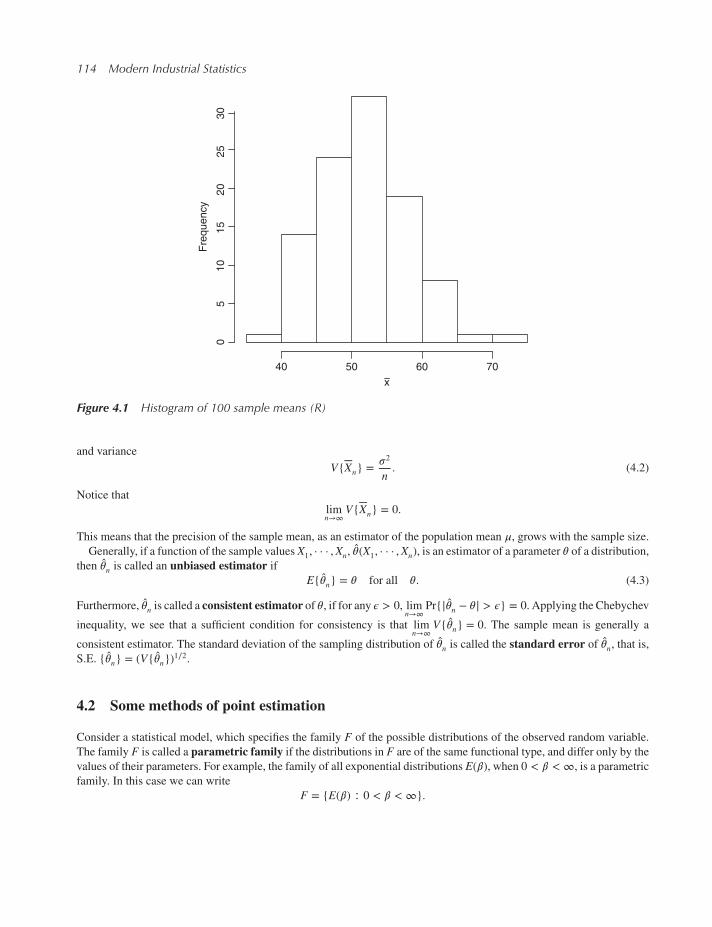
114 Modern Industrial Statistics
x
Fre
quency
40 50 60 70
05
10
15
20
25
30
Figure 4.1 Histogram of 100 sample means (R)
and variance
V{Xn} = 𝜎2
n. (4.2)
Notice that
limn→∞
V{Xn} = 0.
This means that the precision of the sample mean, as an estimator of the population mean 𝜇, grows with the sample size.
Generally, if a function of the sample values X1, · · · ,Xn, ��(X1, · · · ,Xn), is an estimator of a parameter 𝜃 of a distribution,then ��n is called an unbiased estimator if
E{��n} = 𝜃 for all 𝜃. (4.3)
Furthermore, ��n is called a consistent estimator of 𝜃, if for any 𝜖 > 0, limn→∞
Pr{|��n − 𝜃| > 𝜖} = 0. Applying the Chebychev
inequality, we see that a sufficient condition for consistency is that limn→∞
V{��n} = 0. The sample mean is generally a
consistent estimator. The standard deviation of the sampling distribution of ��n is called the standard error of ��n, that is,S.E. {��n} = (V{��n})1∕2.
4.2 Some methods of point estimation
Consider a statistical model, which specifies the family F of the possible distributions of the observed random variable.
The family F is called a parametric family if the distributions in F are of the same functional type, and differ only by the
values of their parameters. For example, the family of all exponential distributions E(𝛽), when 0 < 𝛽 <∞, is a parametric
family. In this case we can write
F = {E(𝛽) ∶ 0 < 𝛽 <∞}.

Statistical Inference and Bootstrapping 115
S2
Fre
quency
0 200 400 600 800 1000 1200 1400
05
10
15
20
25
30
35
Figure 4.2 Histogram of 100 sample variances
Another example of a parametric family is F = {N(𝜇, 𝜎); −∞ < 𝜇 <∞, 0 < 𝜎 <∞}, which is the family of all normal
distributions. The range Θ of the parameter(s) 𝛉, is called the parameter space. Thus, a parametric statistical model
specifies the parametric family F. This specification gives both the functional form of the distribution and its parameter(s)
space Θ.We observe a random sample from the infinite population, which consists of the values of i.i.d. random variables
X1,X2, · · · ,Xn, whose common distribution F(x; 𝛉) is an element of F.A function of the observable random variables is called a statistic. A statistic cannot depend on unknown parameters.
A statistic is thus a random variable, whose value can be determined from the sample values (X1, · · · ,Xn). In particular,
a statistic ��(X1, · · · ,Xn), which yields values in the parameter space is called a point estimator of 𝜃. If the distributionsin F depend on several parameters we have to determine point estimators for each parameter, or for a function of the
parameters. For example, the p-th quantile of a normal distribution is 𝜉p = 𝜇 + zp𝜎, where 𝜇 and 𝜎 are the parameters and
zp = Φ−1(p). This is a function of two parameters. An important problem in quality control is to estimate such quantiles.
In this section we discuss a few methods for deriving point estimators.
4.2.1 Moment equation estimators
If X1,X2, · · · ,Xn are i.i.d. random variables (a random sample) then the sample l-th moment (l = 1, 2, · · · ) is
Ml =1
n
n∑i=1
Xli . (4.4)
The law of large numbers (strong) says that if E{|X|l} <∞ then Ml converges with probability one to the population
l-th moment 𝜇l(F). Accordingly, we know that if the sample size n is large, then with probability close to 1, Ml is close
to 𝜇l(F). The method of moments, for parametric models, equates Ml to 𝜇l, which is a function of 𝜃, and solves for 𝜃.

116 Modern Industrial Statistics
Generally, if F(x; 𝛉) depends on k parameters 𝜃1, 𝜃2, · · · , 𝜃k then we set up k equations
M1 = 𝜇1(𝜃1, · · · , 𝜃k),
M2 = 𝜇2(𝜃11, · · · , 𝜃k),
⋮
Mk = 𝜇k(𝜃1, · · · , 𝜃k),
(4.5)
and solve for 𝜃1, · · · , 𝜃k. The solutions are functions of the sample statisticsM1, · · · ,Mk, and are therefore estimators. This
method does not always yield simple or good estimators. We give now a few examples in which the estimators obtained
by this method are reasonable.
Example 4.1. Consider the family F of Poisson distributions, i.e.,
F = {P(x; 𝜃); 0 < 𝜃 <∞}.
The parameter space is Θ = (0,∞). The distributions depend on one parameter, and
𝜇1(𝜃) = E𝜃{X} = 𝜃.
Thus, the method of moments yields the estimator
��n = Xn.
This is an unbiased estimator with V{��n} = 𝜃n. ◾
Example 4.2. Consider a random sample of X1,X2, · · · ,Xn from a log normal distribution LN(𝜇, 𝜎). The distributions
depend on k = 2 parameters.
We have seen that
𝜇1(𝜇, 𝜎2) = exp {𝜇 + 𝜎2∕2},
𝜇2(𝜇, 𝜎2) = exp {2𝜇 + 𝜎2}(e𝜎2 − 1).
Thus, let 𝜃1 = 𝜇, 𝜃2 = 𝜎2 and set the equations
exp {𝜃1 + 𝜃2∕2} = M1
exp {2𝜃1 + 𝜃2}(e𝜃2 − 1) = M2.
The solutions ��1 and ��2 of this system of equations is:
��1 = log M1 −1
2log
(1 +
M2
M21
),
and
��2 = log
(1 +
M2
M21
).
The estimators obtained are biased, but we can show that they are consistent. Simple formulae for V{��1}, V{��2} and
Cov(��1, ��2) do not exist. We can derive large sample approximations to these characteristics, or approximate them by a
method of resampling, called bootstrapping, which is discussed later. ◾
4.2.2 The method of least squares
If 𝜇 = E{X} then, the method of least squares, chooses the estimator ��, which minimizes
Q(𝜇) =n∑i=1
(Xi − 𝜇)2. (4.6)

Statistical Inference and Bootstrapping 117
It is immediate to show that the least squares estimator (L.S.E.) is the sample mean, that is,
�� = Xn.
Indeed, write
Q(𝜇) =n∑i=1
(Xi − Xn + Xn − 𝜇)2
=n∑i=1
(Xi − Xn)2 + n(Xn − 𝜇)2.
Thus, Q(��) ≥ Q(Xn) for all 𝜇 and Q(��) is minimized only if �� = Xn. This estimator is in a sense non-parametric. It is
unbiased, and consistent. Indeed,
V{��} = 𝜎2
n,
provided that 𝜎2 <∞.
The L.S.E. is more interesting in the case of linear regression (see Chapter 5).
In the simple linear regression case we have n independent random variables Y1, · · · ,Yn, with equal variances, 𝜎2, butexpected values which depend linearly on known regressors (predictors) x1, · · · , xn. That is,
E{Yi} = 𝛽0 + 𝛽1xi, i = 1, · · · , n. (4.7)
The least squares estimators of the regression coefficients 𝛽0 and 𝛽1, are the values which minimize
Q(𝛽0, 𝛽1) =n∑i=1
(Yi − 𝛽0 − 𝛽1xi)2. (4.8)
These L.S.E.’s are
𝛽0 = Yn − 𝛽1xn, (4.9)
and
𝛽1 =
n∑i=1
Yi(xi − xn)
n∑i=1
(xi − xn)2, (4.10)
where xn and Yn are the sample means of the x’s and the Y’s, respectively. Thus, 𝛽0 and 𝛽1 are linear combinations of the
Y’s, with known coefficients. From the results of Section 3.8
E{𝛽1} =n∑i=1
(xi − xn)SSx
E{Yi}
=n∑i=1
(xi − xn)SSx
(𝛽0 + 𝛽1xi)
= 𝛽0n∑i=1
(xi − xn)SSx
+ 𝛽1n∑i=1
(xi − xn)xiSSx,
where SSx =n∑i=1
(xi − xn)2. Furthermore,
n∑i=1
xi − xnSSx
= 0

118 Modern Industrial Statistics
andn∑i=1
(xi − xn)xiSSx
= 1.
Hence, E{𝛽1} = 𝛽1. Also,
E{𝛽0} = E{Yn} − xnE{𝛽1}
= (𝛽0 + 𝛽1xn) − 𝛽1xn= 𝛽0.
Thus, 𝛽0 and 𝛽1 are both unbiased. The variances of these LSE are given by
V{𝛽1} = 𝜎2
SSx,
V{𝛽0} = 𝜎2
n+𝜎2x2nSSx,
(4.11)
and
Cov(𝛽0, 𝛽1) = −𝜎2xnSSx. (4.12)
Thus, 𝛽0 and 𝛽1 are not independent. A hint for deriving these formulae is given in Problem [4.2.5].
The correlation between 𝛽0 and 𝛽1 is
𝜌 = −xn(
1
n
n∑i=1
x2i
)1∕2 . (4.13)
4.2.3 Maximum likelihood estimators
Let X1,X2, · · · ,Xn be i.i.d. random variables having a common distribution belonging to a parametric family F. Let f (x;𝜽)be the p.d.f. of X, 𝜽 ∈ Θ. This is either a density function or a probability distribution function of a discrete random
variable. Since X1, · · · ,Xn are independent, their joint p.d.f. is
f (x1, · · · , xn;𝜽) =n∏i=1
f (xi;𝜽).
The likelihood function of 𝜽 over Θ is defined as
L(𝜽; x1, · · · , xn) =n∏i=1
f (xi;𝜽). (4.14)
The likelihood of 𝜽 is thus the probability in the discrete case, or the joint density in the continuous case, of the observed
sample values under 𝜽. In the likelihood function L(𝜽; x1, . . . , xn), the sample values (x1, . . . , xn) are playing the
role of parameters. A maximum likelihood estimator (M.L.E.) of 𝜽 is a point in the parameter space, ��n, for whichL(𝜽;X1, · · · ,Xn) is maximized. The notion of maximum is taken in a general sense. For example, the function
f (x; 𝜆) =⎧⎪⎨⎪⎩𝜆e−𝜆x, x ≥ 0
0, x < 0
as a function of 𝜆, 0 < 𝜆 <∞, attains a maximum at 𝜆 = 1
x.

Statistical Inference and Bootstrapping 119
On the other hand, the function
f (x; 𝜃) =⎧⎪⎨⎪⎩1
𝜃, 0 ≤ x ≤ 𝜃
0, otherwise
as a function of 𝜃, over (0,∞) attains a lowest upper bound (supremum) at 𝜃 = x, which is 1
x. We say that it is maximized
at 𝜃 = x. Notice that it is equal to zero for 𝜃 < x. We give a few examples.
Example 4.3. Suppose that X1,X2, · · · ,Xn is a random sample from a normal distribution. Then, the likelihood function
of (𝜇, 𝜎2) is
L(𝜇, 𝜎2;X1, · · · ,Xn) =1
(2𝜋)n∕2(𝜎)nexp
{− 1
2𝜎2
n∑i=1
(Xi − 𝜇)2}
= 1
(2𝜋)n∕2(𝜎2)n∕2exp
{− 1
2𝜎2
n∑i=1
(Xi − Xn)2 −n2𝜎2
(Xn − 𝜇)2}.
Notice that the likelihood function of (𝜇, 𝜎2) depends on the sample variables only through the statistics (Xn,Qn), where
Qn =n∑i=1
(Xi − Xn)2. These statistics are called the likelihood statistics or sufficient statistics. Tomaximize the likelihood,
we can maximize the log-likelihood
l(𝜇, 𝜎2;Xn,Qn) = −n2log (2𝜋) − n
2log (𝜎2) −
Qn
2𝜎2−n(Xn − 𝜇)2
2𝜎2.
With respect to 𝜇 we maximize by ��n = Xn. With respect to 𝜎2, differentiate
l(��n, 𝜎2;Xn,Qn) = −n2log (2𝜋) − n
2log (𝜎2) −
Qn
2𝜎2.
This is𝜕
𝜕𝜎2log (��, 𝜎2;Xn,Qn) = − n
2𝜎2+Qn
2𝜎4.
Equating the derivative to zero and solving yields the M.L.E.
��2n =Qn
n.
Thus, the MLE’s are ��n = Xn and
��2n =n − 1
nS2n.
��2n is biased, but the bias goes to zero as n → ∞. ◾
Example 4.4. Let X have a negative binomial distribution N.B.(k, p). Suppose that k is known, and 0 < p < 1. The like-lihood function of p is
L(p;X, k) =(X + k − 1
k − 1
)pk(1 − p)X .
Thus, the log-likelihood is
l(p;X, k) = log
(X + k − 1
k − 1
)+ k log p + X log (1 − p).
The M.L.E. of p is
p = kX + k.

120 Modern Industrial Statistics
We can show that p has a positive bias, i.e., E{p} > p. For large values of k the bias is approximately
Bias(p; k) = E{p; k} − p
≅3p(1 − p)
2k, large k.
The variance of p for large k is approximately V{p; k} ≅ p2(1−p)k. ◾
4.3 Comparison of sample estimates
4.3.1 Basic concepts
Statistical hypotheses are statements concerning the parameters, or some characteristics, of the distribution representing a
certain random variable (or variables) in a population. For example, consider a manufacturing process. The parameter of
interest may be the proportion, p, of non-conforming items. If p ≤ p0, the process is considered to be acceptable. If p > p0the process should be corrected.
Suppose that twenty items are randomly selected from the process and inspected. Let X be the number of non-
conforming items in the sample. Then X has a binomial distribution B(20, p). On the basis of the observed value of X,we have to decide whether the process should be stopped for adjustment. In the statistical formulation of the problem we
are testing the hypothesis
H0 ∶ p ≤ p0,
against the hypothesis
H1 ∶ p > p0.
The hypothesis H0 is called the null hypothesis, while H1 is called the alternative hypothesis. Only when the data
provides significant evidence that the null hypothesis is wrong do we reject it in favor of the alternative. It may not be
justifiable to disrupt a production process unless we have ample evidence that the proportion of non-conforming items is
too high. It is important to distinguish between statistical significance and practical or technological significance. Thestatistical level of significance is the probability of rejectingH0 when it is true. If we rejectH0 at a low level of significance,
the probability of committing an error is small, and we are confident that our conclusion is correct. Rejecting H0 might
not be technologically significant, if the true value of p is not greater than p0 + 𝛿, where 𝛿 is some acceptable level of
indifference. If p0 < p < p0 + 𝛿, H1 is true, but there is no technological significance to the difference p − p0.To construct a statistical test procedure based on a test statistic, X, consider first all possible values that could be
observed. In our example X can assume the values 0, 1, 2, · · · , 20. Determine a critical region or rejection region, sothat, whenever the observed value of X belongs to this region the null hypothesis H0 is rejected. For example, if we were
testingH0 ∶ P ≤ 0.10 againstH1 ∶ P > 0.10, we might rejectH0 if X > 4. The complement of this region, X ≤ 3, is called
the acceptance region.There are two possible errors that can be committed. If the true proportion of non-conforming items, for example, were
only .05 (unknown to us) and our sample happened to produce 4 items, we would incorrectly decide to reject H0 and shut
down the process that was performing acceptably. This is called a type I error. On the other hand, if the true proportion
were .15 and only 3 non-conforming items were found in the sample, we would incorrectly allow the process to continue
with more than 10% defectives (a type II error).We denote the probability of committing a Type I error by 𝛼(p), for p ≤ p0, and the probability of committing a Type II
error by 𝛽(p), for p > p0.In most problems the critical region is constructed in such a way that the probability of committing a Type I Error will
not exceed a preassigned value called the significance level of the test. Let 𝛼 denote the significance level. In our example
the significance level is
𝛼 = Pr{X ≥ 4; p = .1} = 1 − B(3; 20, .1) = .133.
Notice that the significance level is computed with p = .10, which is the largest p value for which the null hypothesis
is true.

Statistical Inference and Bootstrapping 121
Table 4.1 The Binomial c.d.f. B(x;n,p), for n = 20, p = 0.10(0.05)0.25
x p = .10 p = .15 p = .20 p = .25
0 .1216 .0388 .0115 .00321 .3917 .1756 .0692 .02432 .6769 .4049 .2061 .09133 .8670 .6477 .4114 .22524 .9568 .8298 .6296 .41485 .9887 .9327 .8042 .61726 .9976 .9781 .9133 .78587 .9996 .9941 .9679 .89828 .9999 .9987 .9900 .95919 1.0000 .9998 .9974 .9861
10 1.0000 1.0000 .9994 .9961
To further evaluate the test procedure we would like to know the probability of accepting the null hypothesis for
various values of p. Such a function is called the operating characteristic function and is denoted by OC(p). The graphof OC(p) vs. p is called the OC curve. Ideally we would like OC(p) = 1 whenever H0 ∶ p ≤ p0 is true, and OC(p) = 0
when H1 ∶ p > p0 is true. This, however, cannot be obtained when the decision is based on a random sample of items.
In our example we can compute the OC function as
OC(p) = Pr{X ≤ 3; p} = B(3; 20, p).
From Table 4.1 we find that
OC(0.10) = 0.8670
OC(0.15) = 0.6477
OC(0.20) = 0.4114
OC(0.25) = 0.2252.
Notice that the significance level 𝛼 is the maximum probability of rejecting H0 when it is true. Accordingly, OC(p0) =1 − 𝛼. The OC curve for this example is shown in Figure 4.3.
We see that as p grows, the value of OC(p) decreases, since the probability of observing at least 4 non-conforming
items out of 20 is growing with p.Suppose that the significance level of the test is decreased, in order to reduce the probability of incorrectly interfering
with a good process. We may choose the critical region to be X ≥ 5. For this new critical region, the new OC function is
OC(0.10) = 0.9568,
OC(0.15) = 0.8298,
OC(0.20) = 0.6296,
OC(0.25) = 0.4148.
The new significance level is 𝛼 = 1 − OC(0.1) = 0.0432. Notice that, although we reduced the risk of committing a Type
I error, we increased the risk of committing a Type II error. Only with a larger sample size we can reduce simultaneously
the risks of both Type I and Type II errors.
Instead of the OC function one may consider the power function, to evaluate the sensitivity of a test procedure. The
power function, denoted by 𝜓(p), is the probability of rejecting the null hypothesis when the alternative is true. Thus,
𝜓(p) = 1 − OC(p).
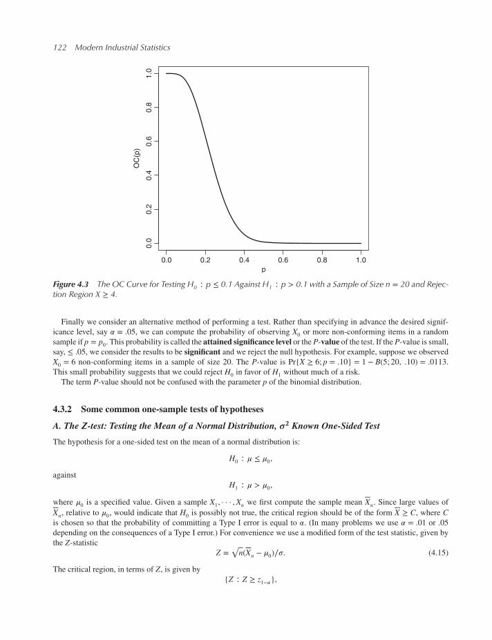
122 Modern Industrial Statistics
0.0 0.2 0.4 0.6 0.8 1.0
0.0
0.2
0.4
0.6
0.8
1.0
p
OC
(p)
Figure 4.3 The OC Curve for Testing H0 ∶ p ≤ 0.1 Against H1 ∶ p > 0.1 with a Sample of Size n = 20 and Rejec-tion Region X ≥ 4.
Finally we consider an alternative method of performing a test. Rather than specifying in advance the desired signif-
icance level, say 𝛼 = .05, we can compute the probability of observing X0 or more non-conforming items in a random
sample if p = p0. This probability is called the attained significance level or the P-value of the test. If the P-value is small,
say, ≤ .05, we consider the results to be significant and we reject the null hypothesis. For example, suppose we observed
X0 = 6 non-conforming items in a sample of size 20. The P-value is Pr{X ≥ 6; p = .10} = 1 − B(5; 20, .10) = .0113.This small probability suggests that we could reject H0 in favor of H1 without much of a risk.
The term P-value should not be confused with the parameter p of the binomial distribution.
4.3.2 Some common one-sample tests of hypotheses
A. The Z-test: Testing the Mean of a Normal Distribution, 𝝈2 Known One-Sided Test
The hypothesis for a one-sided test on the mean of a normal distribution is:
H0 ∶ 𝜇 ≤ 𝜇0,against
H1 ∶ 𝜇 > 𝜇0,
where 𝜇0 is a specified value. Given a sample X1, · · · ,Xn we first compute the sample mean Xn. Since large values of
Xn, relative to 𝜇0, would indicate that H0 is possibly not true, the critical region should be of the form X ≥ C, where Cis chosen so that the probability of committing a Type I error is equal to 𝛼. (In many problems we use 𝛼 = .01 or .05depending on the consequences of a Type I error.) For convenience we use a modified form of the test statistic, given by
the Z-statisticZ =
√n(Xn − 𝜇0)∕𝜎. (4.15)
The critical region, in terms of Z, is given by
{Z ∶ Z ≥ z1−𝛼},

Statistical Inference and Bootstrapping 123
z scale
X scale
μ0 μ0 + z1−ασ
n
0 z1−αAccept Reject
Acceptanceprobability (1 − α)
Rejectionprobability α
Figure 4.4 Critical regions for the one-sided Z-test
where z1−𝛼 is the 1 − 𝛼 quantile of the standard normal distribution. This critical region is equivalent to the region
{Xn ∶ Xn ≥ 𝜇0 + z1−𝛼𝜎∕√n}.
These regions are illustrated in Figure 4.4.
The operating characteristic function of this test is given by
OC(𝜇) = Φ(z1−𝛼 − 𝛿√n), (4.16)
where
𝛿 = (𝜇 − 𝜇0)∕𝜎. (4.17)
Example 4.5. Suppose we are testing the hypothesisH0 ∶ 𝜇 ≤ 5, againstH1 ∶ 𝜇 > 5, with a sample of size n = 100 from
a normal distribution with known standard deviation 𝜎 = .2. With a significance level of size 𝛼 = .05 we reject H0 if
Z ≥ z.95 = 1.645.
The values of the OC function are computed in Table 4.2. In this table z = z1−𝛼 − 𝛿√n and OC(𝜇) = Φ(z).
If the null hypothesis is H0 ∶ 𝜇 ≥ 𝜇0 against the alternative H1 ∶ 𝜇 < 𝜇0, we reverse the direction of the test and rejectH0 if Z ≤ −z1−𝛼 .
Table 4.2 OC values in the normal case
𝜇 𝛿√n z OC(𝜇)
5. 0 1.645 .95005.01 0.5 1.145 .87395.02 1.0 .645 .74055.03 1.5 .045 .51795.04 2.0 −.355 .36135.05 3.0 −1.355 .0877
◾

124 Modern Industrial Statistics
Two-Sided Test
The two-sided test has the form
H0 ∶ 𝜇 = 𝜇0
against
H1 ∶ 𝜇 ≠ 𝜇0.The corresponding critical region is given by
{Z ∶ Z ≥ z1−𝛼∕2} ∪ {Z ∶ Z ≤ −Z1−𝛼∕2}.
The operating characteristic function is
OC(𝜇) = Φ(z1−𝛼∕2 + 𝛿√n) − Φ(−z1−𝛼∕2 − 𝛿
√n). (4.18)
The P-value of the two-sided test can be determined in the following manner. First compute
|Z0| =√n|Xn − 𝜇0|∕𝜎,
and then compute the P-value
P = Pr{Z ≥ |Z0|} + P{Z ≤ −|Z0|}= 2(1 − Φ(|Z0|)). (4.19)
B. The t-Test: Testing the Mean of a Normal Distribution, 𝝈2 Unknown
In this case, we replace 𝜎 in the above Z-test with the sample standard deviation, S, and z1−𝛼 (or z1−𝛼∕2) with t1−𝛼[n − 1](or t1−𝛼∕2[n − 1]). Thus the critical region for the two-sided test becomes
{t ∶ |t| ≥ t1−𝛼∕2[n − 1]},
where
t = (Xn − 𝜇0)√n∕S. (4.20)
The operating characteristic function of the one-sided test is given approximately by
OC(𝜇) ≅ 1 − Φ
(𝛿√n − t1−𝛼[n − 1](1 − 1∕8(n − 1))(1 + t2
1−𝛼[n − 1]∕2(n − 1))1∕2
)(4.21)
where 𝛿 = |𝜇 − 𝜇0|∕𝜎. (This is a good approximation to the exact formula, which is based on the complicated non-central
t-distribution.)
Table 4.3 Power functions of Z and t tests
𝛿 𝜎 known 𝜎 unknown
0.0 0.050 0.0500.1 0.116 0.1110.2 0.226 0.2140.3 0.381 0.3590.4 0.557 0.5270.5 0.723 0.691

Statistical Inference and Bootstrapping 125
In Table 4.3, we present some numerical comparisons of the power of the one-sided test for the cases of 𝜎2 known and𝜎2 unknown, when n = 20 and 𝛼 = 0.05. Notice that when 𝜎 is unknown, the power of the test is somewhat smaller than
when it is known.
Example 4.6. The cooling system of a large computer consists of metal plates that are attached together, so as to create
an internal cavity, allowing for the circulation of special purpose cooling liquids. The metal plates are attached with steel
pins that are designed to measure 0.5mm in diameter. Experience with the process of manufacturing similar steel pins, has
shown that the diameters of the pins are normally distributed, with mean 𝜇 and standard deviation 𝜎. The process is aimed
at maintaining a mean of 𝜇0 = 0.5 [mm]. For controlling this process we want to test H0 ∶ 𝜇 = 0.5 against H1 ∶ 𝜇 ≠ 0.5.If we have prior information that the process standard deviation is constant at 𝜎 = 0.02 we can use the Z-test to test the
above hypotheses. If we apply a significance level of 𝛼 = 0.05, then we will reject H0 if Z ≥ z1−𝛼∕2 = 1.96.Suppose that the following data were observed:
.53, .54, .48, .50, .50, .49, .52.
The sample size is n = 7 with a sample mean of X = .509. Therefore
Z = |.509 − .5|√7∕.02 = 1.191.
Since this value of Z does not exceed the critical value of 1.96, do not reject the null hypothesis.
If there is no prior information about 𝜎, use the sample standard deviation S and perform a t-test, and reject
H0 if |t| > t1−𝛼∕2[6]. In the present example, S = .022, and t = 1.082. Since |t| < t.975[6] = 2.447, we reach the
same conclusion. ◾
C. The Chi-Squared Test: Testing the Variance of a Normal Distribution
Consider a one-sided test of the hypothesis:
H0 ∶ 𝜎2 ≤ 𝜎20 ,against
H1 ∶ 𝜎2 > 𝜎20 .
The test statistic corresponding to this hypothesis is:
Q2 = (n − 1)S2∕𝜎2, (4.22)
with a critical region
{Q2 ∶ Q2 ≥ 𝜒21−𝛼[n − 1]}.
The operating characteristic function for this test is given by
OC(𝜎2) = Pr{𝜒2[n − 1] ≤ 𝜎20
𝜎2𝜒21−𝛼[n − 1]}, (4.23)
where 𝜒2[n − 1] is a Chi-squared random variable with n − 1 degrees of freedom.
Continuing the previous example let us test the hypothesis
H0 ∶ 𝜎2 ≤ .0004,against
H1 ∶ 𝜎2 > .0004.
Since the sample standard deviation is S = .022, we find
Q2 = (7 − 1)(0.022)2∕0.0004 = 7.26.

126 Modern Industrial Statistics
Table 4.4 Power of the 𝜒2-Test, 𝛼 = .05, 𝜌 = 𝜎2∕𝜎20
n
𝜌 20 30 40
1.00 .050 .050 .0501.25 .193 .236 .2791.50 .391 .497 .5891.75 .576 .712 .8092.00 .719 .848 .920
H0 is rejected at level 𝛼 = .05 if
Q2 ≥ 𝜒20.95[6] = 12.59.
Since Q2 < 𝜒2.95[6], H0 is not rejected. Whenever n is odd, that is n = 2m + 1 (m = 0, 1, · · · ), the c.d.f. of 𝜒2[n − 1] can
be computed according to the formula:
Pr{𝜒2[2m] ≤ x} = 1 − P(m − 1; x
2
),
where P(a; 𝜆) is the c.d.f. of the Poisson distribution with mean 𝜆. For example, if n = 21, m = 10 and 𝜒2.95[20] = 31.41.
Thus, the value of the OC function at 𝜎2 = 1.5 𝜎20is
OC(1.5𝜎20 ) = Pr{𝜒2[20] ≤ 31.41
1.5
}= 1 − P(9; 10.47) = 1 − .4007
= .5993.
If n is even, that is, n = 2m, we can compute the OC values for n = 2m − 1 and for n = 2m + 1 and take the average of
these OC values. This will yield a good approximation.
The power function of the test is obtained by subtracting the OC function from 1.
In Table 4.4 we present a few numerical values of the power function for n = 20, 30, 40 and for 𝛼 = 0.05. Here wehave let 𝜎2∕𝜎2
0and have used the values 𝜒2
0.95[19] = 30.1, 𝜒2
0.95[29] = 42.6, and 𝜒2
0.95[39] = 54.6.
As illustrated in Table 4.4, the power function changes more rapidly as n grows.
D. Testing Hypotheses About the Success Probability, p, in Binomial Trials
Consider one-sided tests, for which
The Null Hypothesis is H0 ∶ p ≤ p0.The Alternative Hypothesis is H1 ∶ p > p0.The Critical Region is {X ∶ X > c𝛼(n, p0)},
where X is the number of successes among n trials and c𝛼(n, p0) is the first value of k for which the Binomial c.d.f.,
B(k; n, p0), exceeds 1 − 𝛼.The Operating Characteristic Function:
OC(p) = B(c𝛼(n, p0); n, p). (4.24)
Notice that c𝛼(n, p0) = B−1(1 − 𝛼; n, p0) is the (1 − 𝛼) quantile of the binomial distribution B(n, p0). In order to determine
c(n, p0), one can use R or MINITAB commands which, for 𝛼 = .05, n = 20 and p0 = .20 are

Statistical Inference and Bootstrapping 127
> qbinom(p=0.95, size=20, prob=0.2)
MTB> INVCDF .95;
SUBC> BINOM 20 .2.
Table 4.5 is an output for the binomial distribution with n = 20 and p = .2.The smallest value of k for which B(k; 20, .2) = Pr{X ≤ k} ≥ 0.95 is 7. Thus, we set c0.05(20, 0.20) = 7. H0 is rejected
whenever X > 7. The level of significance of this test is actually .032, which is due to the discrete nature of the binomial
distribution. The OC function of the test for n = 20 can be easily determined from the corresponding distribution of
B(20, p). For example, the B(n, p) distribution for n = 20 and p = .25 is presented in Table 4.6.
We see that B(7; 20, 0.25) = 0.8982. Hence, the probability of accepting H0 when p = .25 is OC(0.25) = 0.8982.A large sample test in the Binomial case can be based on the normal approximation to the Binomial distribution. If the
sample is indeed large, we can use the test statistic
Z =p − p0√p0q0
√n, (4.25)
with the critical region
{Z ∶ Z ≥ z1−𝛼},
where q0 = 1 − p0. Here p is the sample proportion of successes. The operating characteristic function takes the form:
OC(p) = 1 − Φ
((p − p0)
√n√
pq− z1−𝛼
√p0q0pq
), (4.26)
where q = 1 − p, and q0 = 1 − p0.For example, suppose that n = 450 and the hypotheses are H0 ∶ p ≤ .1 against H1 ∶ p > .1. The critical region, for
𝛼 = .05, is{p ∶ p ≥ .10 + 1.645
√(0.1)(0.9)∕450} = {p ∶ p ≥ .1233}.
Table 4.5 p.d.f. and c.d.f. of B(20, .2)
Binomial Distribution: n = 20 p = .2
a Pr(X = a) Pr(X ≤ a)
0 0.0115 0.01151 0.0576 0.06922 0.1369 0.20613 0.2054 0.41144 0.2182 0.62965 0.1746 0.80426 0.1091 0.91337 0.0546 0.96798 0.0222 0.99009 0.0074 0.997410 0.0020 0.999411 0.0005 0.999912 0.0001 1.0000

128 Modern Industrial Statistics
Table 4.6 p.d.f. and c.d.f. of B(20, .25)
Binomial Distribution: n = 20 p = .25
a Pr(X = a) Pr(X ≤ a)
0 0.0032 0.00321 0.0211 0.02432 0.0669 0.09133 0.1339 0.22524 0.1897 0.41485 0.2023 0.61726 0.1686 0.78587 0.1124 0.89828 0.0609 0.95919 0.0271 0.986110 0.0099 0.996111 0.0030 0.999112 0.0008 0.999813 0.0002 1.0000
Thus, H0 is rejected whenever p ≥ .1233. The OC value of this test, at p = .15 is approximately
OC(.15) ≅ 1 − Φ⎛⎜⎜⎝.05√450√
(.15)(.85)− 1.645
√(.1)(.9)(.15)(.85)
⎞⎟⎟⎠= 1 − Φ(2.970 − 1.382)
= 1 − .944 = .056.
The corresponding value of the power function is .949. Notice that the power of rejecting H0 for H1 when p = .15 is so
high because of the large sample size.
4.4 Confidence intervals
Confidence intervals for unknown parameters are intervals, determined around the sample estimates of the parameters,
having the property that, whatever the true value of the parameter is, in repetitive sampling a prescribed proportion of the
intervals, say 1 − 𝛼, will contain the true value of the parameter. The prescribed proportion, 1 − 𝛼, is called the confidencelevel of the interval. In Figure 4.5, we illustrate 50 simulated confidence intervals, which correspond to independent
samples. All of these intervals are designed to estimate the mean of the population from which the samples were drawn.
In this particular simulation, the population was normally distributed with mean 𝜇 = 10. We see from Figure 4.5 that all
of these 50 random intervals cover the true value of 𝜇.If the sampling distribution of the estimator ��n is approximately normal, one can use, as a rule of thumb, the interval
estimator with limits
��n ± 2 S.E.{��n}.
The confidence level of such an interval will be close to .95 for all 𝜃.Generally, if one has a powerful test procedure for testing the hypothesis H0 ∶ 𝜃 = 𝜃0 versus H1 ∶ 𝜃 ≠ 𝜃0, one can
obtain good confidence intervals for 𝜃 by the following method.

Statistical Inference and Bootstrapping 129
0 10 20 30 40 50
8.5
9.0
9.5
10.0
10.5
11.0
11.5
Figure 4.5 Simulated confidence intervals for the mean of a normal distribution, samples of size n = 10 fromN(10,1)
Let T = T(X) be a test statistic for testing H0 ∶ 𝜃 = 𝜃0. Suppose that H0 is rejected if T ≥ K𝛼(𝜃0) or if T ≤ K𝛼(𝜃0),where 𝛼 is the significance level. The interval (K
𝛼(𝜃0), K𝛼(𝜃0)) is the acceptance region for H0. We can now consider the
family of acceptance regions Θ = {(K𝛼(𝜃),K𝛼(𝜃)), 𝜃 ∈ Θ}, where Θ is the parameter space. The interval (L𝛼(T),U𝛼(T))
defined asL𝛼(T) = inf{𝜃 ∶ T ≤ K𝛼(𝜃)}
U𝛼(T) = sup{𝜃 ∶ T ≥ K𝛼(𝜃)},
(4.27)
is a confidence interval for 𝜃 at level of confidence 1 − 𝛼. Indeed, any hypothesisH0 with L𝛼(T) < 𝜃0 < U𝛼(T) is acceptedwith the observed value of the test statistic. By construction, the probability of accepting such hypothesis is 1 − 𝛼. Thatis, if 𝜃0 is the true value of 𝜃, the probability that H0 is accepted is (1 − 𝛼). But H0 is accepted if, and only if, 𝜃0 is coveredby the interval (L𝛼(T),U𝛼(T)).
4.4.1 Confidence intervals for 𝝁; 𝝈 known
For this case, the sample mean X is used as an estimator of 𝜇, or as a test statistic for the hypothesis H0 ∶ 𝜇 = 𝜇0. H0
is rejected, at level of significance 𝛼 if X ≥ 𝜇0 + z1−𝛼∕2𝜎√nor X ≤ 𝜇0 + z1−𝛼∕2
𝜎√n, where z1−𝛼∕2 = Φ−1(1 − 𝛼∕2). Thus,
K𝛼(𝜇) = 𝜇 + z1−𝛼∕2𝜎√nand K𝛼(𝜇) = 𝜇 − z1−𝛼∕2
𝜎√n. The limits of the confidence interval are, accordingly the roots 𝜇 of the
equation
K𝛼(𝜇) = X
and
K𝛼(𝜇) = X.
These equations yield the confidence interval for 𝜇,(X − z1−𝛼∕2
𝜎√n,X + z1−𝛼∕2
𝜎√n
). (4.28)

130 Modern Industrial Statistics
4.4.2 Confidence intervals for 𝝁; 𝝈 unknown
A confidence interval for 𝜇, at level 1 − 𝛼, when 𝜎 is unknown is obtained from the corresponding t-test. The confidenceinterval is (
X − t1−𝛼∕2[n − 1] S√n,X + t1−𝛼∕2[n − 1] S√
n
), (4.29)
where X and S are the sample mean and standard deviation, respectively. t1−𝛼∕2[n − 1] is the (1 − 𝛼∕2)th quantile of the
t-distribution with n − 1 degrees of freedom.
4.4.3 Confidence intervals for 𝝈2
We have seen that, in the normal case, the hypothesis H0 ∶ 𝜎 = 𝜎0, is rejected at level of significance 𝛼 if
S2 ≥ 𝜎20
n − 1𝜒21−𝛼∕2[n − 1]
or
S2 ≤ 𝜎20
n − 1𝜒2𝛼∕2[n − 1],
where S2 is the sample variance, and 𝜒2𝛼∕2[n − 1] and 𝜒2
1−𝛼∕2[n − 1] are the 𝛼∕2-th and (1 − 𝛼∕2)th quantiles of 𝜒2, with
(n − 1) degrees of freedom. The corresponding confidence interval for 𝜎2, at confidence level (1 − 𝛼) is((n − 1)S2
𝜒21−𝛼[n − 1]
,(n − 1)S2
𝜒2𝛼∕2[n − 1]
), (4.30)
Example 4.7. Consider a normal distribution with unknown mean 𝜇 and unknown standard deviation 𝜎. Suppose thatwe draw a random sample of size n = 16 from this population, and the sample values are:
16.16, 9.33, 12.96, 11.49,
12.31, 8.93, 6.02, 10.66,
7.75, 15.55, 3.58, 11.34,
11.38, 6.53, 9.75, 9.47.
The mean and variance of this sample are: X = 10.20, and S2 = 10.977. The sample standard deviation is S = 3.313. Fora confidence level of 1 − 𝛼 = 0.95, we find
t.975[15] = 2.131,
𝜒2.975[15] = 27.50,
𝜒2.025[15] = 6.26.
Thus, the confidence interval for 𝜇 is (8.435, 11.965). The confidence interval for 𝜎2 is (5.987, 26.303). ◾
4.4.4 Confidence intervals for p
LetX be the number of “success” in n independent trials, with unknown probability of “success,” p. The sample proportion,
p = X∕n, is an unbiased estimator of p. To construct a confidence interval for p, using p, we must find limits pL(p) andpU(p) that satisfy
Pr{pL(p) < p < pU(p)} = 1 − 𝛼.

Statistical Inference and Bootstrapping 131
The null hypothesis H0 ∶ p = p0 is rejected if p ≥ K𝛼(p0) or p ≤ K𝛼(p0) where
K𝛼(p0) =1
nB−1(1 − 𝛼∕2; n, p0)
and (4.31)
K𝛼(p0) =1
nB−1(𝛼∕2; n, p0).
B−1(𝛾; n, p) is the 𝛾-th quantile of the binomial distribution B(n, p). Thus, if X = np, the upper confidence limit for p,pU(p), is the largest value of p satisfying the equation
B(X; n, p) ≥ 𝛼∕2.The lower confidence limit for p is the smallest value of p satisfying
B(X; n, p) ≤ 1 − 𝛼∕2.
Exact solutions to this equation can be obtained using tables of the binomial distribution. This method of searching for
the solution in binomial tables is tedious. However, from the relationship between the F-distribution, the beta distribution,and the binomial distribution, the lower and upper limits are given by the formulae:
pL =X
X + (n − X + 1)F1
(4.32)
and
pU =(X + 1)F2
n − X + (X + 1)F2
, (4.33)
where
F1 = F1−𝛼∕2[2(n − X + 1), 2X] (4.34)
and
F2 = F1−𝛼∕2[2(X + 1), 2(n − X)] (4.35)
are the (1 − 𝛼∕2)th quantiles of the F-distribution with the indicated degrees of freedom.
Example 4.8. Suppose that among n = 30 Bernoulli trials we find X = 8 successes. For level of confidence 1 − 𝛼 = .95,the confidence limits are pL = .123 and pU = 0.459. Indeed,
B(7; 30, .123) = .975,
and
B(8; 30, .459) = .025.
Moreover,
F1 = F.975[46, 16] = 2.49
and
F2 = F.975[18, 44] = 2.07.
Hence,
pL = 8∕(8 + 23(2.49)) = 0.123
and
pU = 9(2.07)∕(22 + 9(2.07)) = 0.459.◾

132 Modern Industrial Statistics
When the sample size n is large we may use the normal approximation to the binomial distribution. This approximation
yields the following formula for a (1 − 𝛼) confidence interval
(p − z1−𝛼∕2√pq∕n, p + z1−𝛼∕2
√pq∕n), (4.36)
where q = 1 − p. Applying this large sample approximation to our previous example, in which n = 30, we obtain the
approximate .95-confidence interval (.108, .425). This interval is slightly different from the interval obtained with the
exact formulae. This difference is due to the inaccuracy of the normal approximation.
It is sometimes reasonable to use only a one-sided confidence interval, for example, if p is the estimated proportion
of non-conforming items in a population. Obviously, the true value of p is always greater than 0, and we may wish to
determine only an upper confidence limit. In this case we apply the formula given earlier, but replace 𝛼∕2 by 𝛼. Forexample, in the case of n = 30 and X = 8, the upper confidence limit for p, in a one-sided confidence interval, is
pU =(X + 1)F2
n − X + (X + 1)F2
where F2 = F1−𝛼[2(X + 1), 2(n − X)] = F.95[18, 44] = 1.855. Thus, the upper confidence limit of a .95 one-sided interval
is PU = .431. This limit is smaller than the upper limit of the two-sided interval.
4.5 Tolerance intervals
Technological specifications for a given characteristic X may require that a specified proportion of elements of a statistical
population satisfy certain constraints. For example, in the production of concrete wemay have the requirement that at least
90% of all concrete cubes, of a certain size, will have a compressive strength of at least 240 kg/cm2. As another example,
suppose that, in the production of washers, it is required that at least 99% of the washers produced will have a thickness
between 0.121 and 0.129 inches. In both examples we want to be able to determine whether or not the requirements are
satisfied. If the distributions of strength and thickness were completely known, we could determine if the requirements
are met without data. However, if the distributions are not completely known, we can make these determinations only
with a certain level of confidence and not with certainty.
4.5.1 Tolerance intervals for the normal distributions
In order to construct tolerance intervals we first consider what happens when the distribution of the characteristic X is
completely known. Suppose for example, that the compressive strength X of the concrete cubes is such that Y = ln X has
a normal distribution with mean 𝜇 = 5.75 and standard deviation 𝜎 = 0.2. The proportion of concrete cubes exceeding
the specification of 240 kg/cm2 is
Pr{X ≥ 240} = Pr{Y ≥ log 240}
= 1 − Φ((5.481 − 5.75)∕0.2)
= Φ(1.345) = 0.911
Since this probability is greater than the specified proportion of 90%, the requirement is satisfied.
We can also solve this problem by determining the compressive strength that is exceeded by 90% of the concrete cubes.
Since 90% of the Y values are greater than the 0.1th fractile of the N(5.75, .04) distribution,
Y0.1 = 𝜇 + z0.1𝜎
= 5.75 − 1.28(0.2)
= 5.494.
Accordingly, 90% of the compressive strength values should exceed e5.494 = 243.2 kg/cm2. Once again we see that the
requirement is satisfied, sincemore than 90% of the cubes have strength values that exceed the specification of 240 kg/cm2.

Statistical Inference and Bootstrapping 133
Notice that no sample values are required, since the distribution of X is known. Furthermore, we are certain that the
requirement is met.
Consider the situation in which we have only partial information on the distribution of Y . Suppose we know that Yis normally distributed with standard deviation 𝜎 = 0.2, but the mean 𝜇 is unknown. The 0.1th fractile of the distribu-
tion, y0.1 = 𝜇 + z0.1𝜎, cannot be determined exactly. Let Y1, · · · ,Yn be a random sample from this distribution and let Ynrepresent the sample mean. From the previous section we know that
L(Yn) = Yn − z1−𝛼𝜎∕√n
is a 1 − 𝛼 lower confidence limit for the population mean. That is
Pr{Yn − z1−𝛼𝜎∕√n < 𝜇} = 1 − 𝛼.
Substituting this lower bound for 𝜇 in the expression for the 0.1th fractile, we obtain a lower tolerance limit for 90%of the log-compressive strengths, with confidence level 1 − 𝛼. More specifically, the lower tolerance limit at level of
confidence 1 − 𝛼 isL𝛼, .1(Yn) = Yn − (z1−𝛼∕
√n + z.9)𝜎.
In general, we say that, with confidence level of 1 − 𝛼, the proportion of population values exceeding the lowertolerance limit is at least 1 − 𝛽. This lower tolerance limit is
L𝛼,𝛽(Yn) = (Yn − (z1−𝛼∕√n + z1−𝛽)𝜎. (4.37)
It can also be shown that the upper tolerance limit for a proportion 1 − 𝛽 of the values, with confidence level 1 − 𝛼, is
U𝛼,𝛽(Yn) = Yn + (z1−𝛼∕√n + z1−𝛽)𝜎 (4.38)
and a tolerance interval containing a proportion 1 − 𝛽 of the values, with confidence 1 − 𝛼, is
(Yn − (z1−𝛼∕2∕√n + z1−𝛽∕2)𝜎,Yn + (z1−𝛼∕2∕
√n + z1−𝛽∕2)𝜎).
When the standard deviation 𝜎 is unknown we should use the sample standard deviation S to construct the tolerance
limits and interval. The lower tolerance limits will be of the form Yn − kSn where the factor k = k(𝛼, 𝛽, n) is determined
so that with confidence level 1 − 𝛼 we can state that a proportion 1 − 𝛽 of the population values will exceed this limit.
The corresponding upper limit is given by Yn + kSn and the tolerance interval is given by
(Yn − k′Sn,Yn + k′Sn).
The “two-sided” factor k′ = k′(𝛼, 𝛽, n) is determined so that the interval will contain a proportion 1 − 𝛽 of the populationwith confidence 1 − 𝛼. Approximate solutions, for large values of n, are given by
k(𝛼, 𝛽, n).= t(𝛼, 𝛽, n) (4.39)
and
k′(𝛼, 𝛽, n).= t(𝛼∕2, 𝛽∕2, n), (4.40)
where
t(a, b, n) =z1−b
1 − z21−a∕2n
+z1−a(1 + z2b∕2 − z2
1−a∕2n)1∕2√
n(1 − z21−a∕2n)
. (4.41)
Example 4.9. The following data represent a sample of 20 compressive strength measurements (kg/cm2) of concrete
cubes at age of 7 days.
349.09 308.88
238.45 196.20
385.59 318.99

134 Modern Industrial Statistics
330.00 257.63
388.63 299.04
348.43 321.47
339.85 297.10
348.20 218.23
361.45 286.23
357.33 316.69
Applying the transformation Y = ln X, we find that Y20 = 5.732 and S20 = 0.184. To obtain a lower tolerance limit for
90% of the log-compressive strengths with 95% confidence we use the factor k(0.05, 0.10, 20) = 2.548. Thus the lowertolerance limit for the transformed data is
Y20 − kS20 = 5.732 − 2.548 × 0.184 = 5.263,
and the corresponding lower tolerance limit for the compressive strength is
e5.263 = 193.09 [kg/cm2].◾
If the tolerance limits are within the specification range we have a satisfactory production.
4.6 Testing for normality with probability plots
It is often assumed that a sample is drawn from a population which has a normal distribution. It is, therefore, important to
test the assumption of normality. We present here a simple test based on the normal-scores (NSCORES) of the sample
values. The normal-scores corresponding to a sample x1, x2, · · · , xn are obtained in the following manner. First we let
ri = rank of xi, i = 1, · · · , n. (4.42)
Here the rank of xi is the position of xi in a listing of the sample when it is arranged in increasing order. Thus, the rank of
the smallest value is 1, that of the second smallest is 2, etc. We then let
pi = (ri − 3∕8)∕(n + 1∕4), i = 1, · · · , n. (4.43)
Then the normal-score of xi iszi = Φ−1(pi),
i.e., the pi-th fractile of the standard normal distribution. If the sample is drawn at random from a normal distribution
N(𝜇, 𝜎2), the relationship between the normal-scores, NSCORES, and xi should be approximately linear. Accordingly,
the correlation between x1, · · · , xn and their NSCORES should be close to 1 in large samples. The graphical display of
the sample values versus their NSCORES is called a Normal Q-Q Plot.In the following example, we provide a normal probability plotting of n = 50 values simulated from N(10, 1), given
in the previous section. If the simulation is good, and the sample is indeed generated from N(10, 1) the X vs. NSCORES
should be scattered randomly around the line X = 10 +NSCORES.We see in Figure 4.6 that this is indeed the case. Also,
the correlation between the x-values and their NSCORES is .976.
The linear regression of the x values on the NSCORES, is:
X = 10.043 + 0.953 ∗ NSCORES.
We see that both the intercept and slope of the regression equation are close to the nominal values of 𝜇 and 𝜎. Chapter 5provides more details on linear regression, including testing statistical hypothesis on these coefficients.

Statistical Inference and Bootstrapping 135
−2 −1 0 1 2
89
10
11
12
Normal Q–Q Plot
Theoretical Quantiles
Sam
ple
Quantile
s
Figure 4.6 Normal Q-Q plot of simulated values from N(10,1)
In Table 4.7, we provide some critical values for testing whether the correlation between the sample values and their
NSCORES is sufficiently close to 1. If the correlation is smaller than the critical value, an indication of non-normality
has been established. In the example of Figure 4.6, the correlation is R = .976. This value is almost equal to the critical
value for 𝛼 = .05 given in the following table. The hypothesis of normality is accepted.
MINITAB provides also a graph of the Normal Probability Plot. In this graph the probabilities corresponding to the
NSCORES are plotted against x. The Normal Probability Plot of the above sample is given in Figure 4.7. Normal proba-
bility plot is obtained in MINITAB by the command.
MTB>% NormPlot C1.
To demonstrate the relationship between the sample values and their normal scores, when the sample is drawn from a
non-normal distribution, consider the following two examples.
Table 4.7 Critical values for the correlation betweensample values and their NSCORES
n\𝛼 0.10 0.05 0.01
10 0.9347 0.9180 0.880415 0.9506 0.9383 0.911020 0.9600 0.9503 0.929030 0.9707 0.9639 0.949050 0.9807 0.9764 0.9664
(adapted from Ryan, Joiner and Ryan, 1976, p. 49).

136 Modern Industrial Statistics
−2 −1 0 1 2
89
10
11
12
Norm Quantiles
X
Figure 4.7 Normal probability plot of 50 simulated N(10, 1) values
Example 4.10. Consider a sample of n = 100 observations from a log-normal distribution. The normal Q-Q plot
of this sample is shown in Figure 4.8. The correlation here is only .788. It is apparent that the relation between the
NSCORES and the sample values is not linear. We reject the hypothesis that the sample has been generated from a
normal distribution.
0 2 4 6 8 10 12
02
46
8
lnorm Quantiles
X
Figure 4.8 Normal probability plot, n = 100 random numbers generated from a log-normal distribution
◾

Statistical Inference and Bootstrapping 137
In R the package car includes the function qqPlot that can manage general distributions. It plots empirical quantiles
of a distribution against theoretical quantiles of a reference distribution for which quantiles and density functions exist in
R. Note that qqPlot does not standardize inputs automatically so that the scale needs to be properly evaluated.
< library(car)< set.seed(123)< X <- rlnorm(n=100,
meanlog=2,sdlog=0.1)
< qqPlot(X,distribution="lnorm",meanlog=2,sdlog=0.1)
Example 4.11. We consider here a sample of n = 100 values, with 50 of the values generated from N(10, 1) and 50 fromN(15, 1). Thus, the sample represents a mixture of two normal distributions. The histogram is given in Figure 4.9 and a
normal probability plot in Figure 4.10. The normal probability plot is definitely not linear. Although the correlation is
.962 the hypothesis of a normal distribution is rejected.
x
Fre
quency
8 10 12 14 16 18
05
10
15
Figure 4.9 Histogram of 100 random numbers, 50 generated from a N(10,1) and 50 from N(15,1)
◾
4.7 Tests of goodness of fit
4.7.1 The chi-square test (large samples)
The chi-square test is applied by comparing the observed frequency distribution of the sample to the expected one under the
assumption of the model. More specifically, consider a (large) sample of size N. Let 𝜉0 < 𝜉1 < · · · < 𝜉k be the limit points

138 Modern Industrial Statistics
−2 −1 0 1 2
810
12
14
16
Norm Quantiles
X
Figure 4.10 Normal probability plot of 100 random Numbers generated from a mixture of two normaldistributions
of k subintervals of the frequency distribution, and let fi be the observed frequency in the i-th subinterval. If, according tothe model, the c.d.f. is specified by the distribution function F(x), then the expected frequency ei in the i-th subinterval is
ei = N(F(𝜉i) − F(𝜉i−1)), i = 1, · · · , k.
The chi-square statistic is defined as
𝜒2 =k∑i=1
(fi − ei)2
ei.
We notice thatk∑i=1
fi =k∑i=1
ei = N,
and hence
𝜒2 =k∑i=1
f 2iei
− N.
The value of 𝜒2 is distributed approximately like 𝜒2[k − 1]. Thus, if 𝜒2 ≥ 𝜒21−𝛼[k − 1] the distribution F(x) does not fit
the observed data.
Often, the c.d.f. F(x) is specified by its family, e.g. normal or Poisson, but the values of the parameters have to be
estimated from the sample. In this case, we reduce the number of degrees of freedom of 𝜒2 by the number of estimated
parameters. For example, if F(x) is N(𝜇, 𝜎2), where both 𝜇 and 𝜎2 are unknown, we use N(X, S2) and compare 𝜒2 to
𝜒21−𝛼[k − 3].
Example 4.12. In Section 4.1, we considered the sampling distribution of sample means from the uniform distribution
over the integers {1, · · · , 100}. The frequency distribution of the means of samples of size n = 10 is given in Figure 4.1.
We test here whether the model N(50.5, 83.325) fits this data.

Statistical Inference and Bootstrapping 139
Table 4.8 Observed and expected frequenciesof 100 sample means
Interval fi ei
27.5-32.5 3 1.8432.5-37.5 11 5.2837.5-42.5 12 11.3242.5-47.5 11 18.0847.4-52.5 19 21.5552.5-57.5 24 19.757.5-62.5 14 12.7362.5-67.5 4 6.3067.5-72.5 2 2.33
TOTAL 100 99.13
Table 4.9 Observed and expected frequencies of 100cycle times
Lower Upper Observed ExpectedLimit Limit Frequency Frequency
at or below .1050 7 6.1.1050 .1100 9 7.7.1100 .1150 17 12.6.1150 .1200 12 16.8.1200 .1250 18 18.1.1250 .1300 11 15.9.1300 .1350 12 11.4
above .1350 14 11.4
The observed and expected frequencies (for N = 100) are summarized in Table 4.8.
The sum of ei here is 99.13, due to truncation of the tails of the normal distribution. The value of 𝜒2 is 12.86. The valueof 𝜒2.95[8] is 15.5. Thus, the deviation of the observed frequency distribution from the expected one is not significant at
the 𝛼 = 0.05 level. ◾
Example 4.13. We consider here a sample of 100 cycle times of a piston, which is described in detail in Chapter 8. We
make a chi-squared test whether the distribution of cycle times is normal. The estimated values of 𝜇 and 𝜎 are �� = 0.1219and �� = 0.0109.
In Table 4.9 we provide the observed and expected frequencies over k = 8 intervals.
The calculated value of 𝜒2 is 5.4036. We should consider the distribution of 𝜒2 with k − 3 = 5 degrees of freedom.
The P value of the test is 0.37. The hypothesis of normality is not rejected. ◾
4.7.2 The Kolmogorov-Smirnov test
The Kolmogorov-Smirnov (K.S.) Test is a more accurate test of goodness of fit than the chi-squared test of the previ-
ous section.

140 Modern Industrial Statistics
Table 4.10 Some critical values 𝛿∗𝛼
𝛼 0.15 0.10 0.05 0.025 0.01
𝛿∗𝛼 0.775 0.819 0.895 0.995 1.035
Suppose that the hypothesis is that the sample comes from a specified distribution with c.d.f. F0(x). The test statisticcompares the empirical distribution of the sample, Fn(x), to F0(x), and considers the maximal value, over all x values, thatthe distance |Fn(x) − F0(x)|may assume. Let x(1) ≤ x(2) ≤ · · · ≤ x(n) be the ordered sample values. Notice that Fn(x(i)) =
i
n.
The K.S. test statistic can be computed according to the formula
Dn = max1≤i≤n
{max
{ in− F0(x(i)),F0(x(i)) −
i − 1
n
}}(4.44)
We have shown earlier that U = F(X) has a uniform distribution on (0, 1).Accordingly, if the null hypothesis is correct, F0(X(i)) is distributed like the i-th order statistic U(i) from a uniform
distribution on (0, 1), irrespective of the particular functional form of F0(x). The distribution of the K.S. test statistic, Dn,
is therefore independent of F0(x), if the hypothesis,H, is correct. Tables of the critical values k𝛼 andDn are available. One
can also estimate the value of k𝛼 by the bootstrap method, discussed later.
If F0(x) is a normal distribution, i.e., F0(x) = Φ(x−𝜇𝜎
), and if the mean 𝜇 and the standard-deviation, 𝜎, are unknown,
one can consider the test statistic
D∗n = max
1≤i≤n
{max
{in− Φ
(X(i) − Xn
Sn
),Φ
(X(i) − Xn
Sn
)− i − 1
n
}}, (4.45)
where Xn and Sn are substituted for the unknown 𝜇 and 𝜎. The critical values k∗𝛼 for D
∗n are given approximately by
k∗𝛼 = 𝛿∗𝛼∕
(√n − 0.01 + 0.85√
n
), (4.46)
where 𝛿∗𝛼 is given in Table 4.10.
To compute the Kolmogorov-Smirnov statistics, in R use the function ks.test, in MINITAB use Stat > Basic Statis-tics > Normality Test and check Kolmogorov Smirnov.
For the data in Example 4.13 (file name OTURB.csv) we obtain D∗n = 0.1107. According to Table 4.10, the critical
value for 𝛼 = 0.05 is k∗.05
= 0.895∕(10 − 0.01 + 0.085) = 0.089. Thus, the hypothesis of normality for the piston cycle
time data is rejected at 𝛼 = .05.
4.8 Bayesian decision procedures
It is often the case that optimal decision depend on unknown parameters of statistical distributions. The Bayesian deci-
sion framework provides us the tools to integrate information that one may have on the unknown parameters with the
information obtained from the observed sample in such a way that the expected loss due to erroneous decisions will be
minimized. In order to illustrate an industrial decision problem of such nature consider the following example.
Example 4.14. Inventory Management. The following is the simplest inventory problem that is handled daily by orga-
nizations of all sizes world wide. One such organization is Starbread Express that supplies bread to a large community in
the Midwest. Every night, the shift manager has to decide how many loafs of bread, s, to bake for the next day consump-
tion. Let X (a random variable) be the number of units demanded during the day. If a manufactured unit is left at the end

Statistical Inference and Bootstrapping 141
of the day we lose $ c1 on that unit. On the other hand, if a unit is demanded and is not available, due to shortage, the loss
is $ c2. How many units, s, should be manufactured so that the total expected loss due to overproduction or to shortages
will be minimized?
The loss at the end of the day is
L(s,X) = c1(s − X)+ + c2(X − s)+, (4.47)
where a+ = max(a, 0). The loss function L(s,X) is a random variable. If the p.d.f. of X is f (x), x = 0, 1, · · · then the
expected loss, is a function of the quantity s, is
R(s) = c1
s∑x=0
f (x)(s − x) + c2
∞∑x=s+1
f (x)(x − s)
= c2E{X} − (c1 + c2)s∑
x=0xf (x) (4.48)
+ s(c1 + c2)F(s) − c2s,
where F(s) is the c.d.f. of X, at X = s, and E{X} is the expected demand.
The optimal value of s, s0, is the smallest integer s for which R(s + 1) − R(s) ≥ 0. Since, for s = 0, 1, · · ·
R(s + 1) − R(s) = (c1 + c2)F(s) − c2,
we find that
s0 = smallest non-negative integer s, such that F(s) ≥ c2c1 + c2. (4.49)
In other words, s0 is the c2∕(c1 + c2)th quantile of F(x). We have seen that the optimal decision is a function of F(x). Ifthis distribution is unknown, or only partially known, one cannot determine the optimal value s0.
After observing a large number, N, of X values one can consider the empirical distribution, FN(x), of the demand and
determine the level S0(FN) = smallest s value such that FN(s) ≥ c2c1+c2
. The question is what to do when N is small. ◾
4.8.1 Prior and posterior distributions
Wewill focus attention here on parametric models. Let f (x;𝜽) denote the p.d.f. of some random variable X, which dependson a parameter 𝜽. 𝜽 could be a vector of several real parameters, like in the case of a normal distribution. Let Θ denote
the set of all possible parameters 𝜽. Θ is called the parameter space. For example, the parameter space Θ of the family
of normal distribution is the set Θ = {(𝜇, 𝜎); −∞ < 𝜇 <∞, 0 < 𝜎 <∞}. In the case of Poisson distributions,
Θ = {𝜆; 0 < 𝜆 <∞}.
In a Bayesian framework we express our prior belief (based on prior information) on which 𝜽 values are plausible, by
a p.d.f. on Θ, which is called the prior probability density function. Let h(𝜽) denote the prior p.d.f. of 𝜽. For example,
suppose that X is a discrete random variable having a binomial distribution B(n, 𝜃). n is known, but 𝜃 is unknown. Theparameter space isΘ = {𝜃; 0 < 𝜃 < 1}. Suppose we believe that 𝜃 is close to 0.8, with small dispersion around this value.
In Figure 4.11 we illustrate the p.d.f. of a Beta distribution Beta(80,20), whose functional form is
h(𝜃; 80, 20) = 99!
79!19!𝜃79(1 − 𝜃)19, 0 < 𝜃 < 1.
If we wish, however, to give more weight to small values of 𝜃, we can choose the Beta(8,2) as a prior density, i.e.,
h(𝜃; 8, 2) = 72𝜃7(1 − 𝜃), 0 < 𝜃 < 1
(see Figure 4.12).

142 Modern Industrial Statistics
0.0 0.2 0.4 0.6 0.8 1.0
02
46
810
x
p.d
.f.
Figure 4.11 The p.d.f. of Beta(80, 20)
0.0 0.2 0.4 0.6 0.8 1.0
0.0
0.5
1.0
1.5
2.0
2.5
3.0
3.5
x
p.d
.f.
Figure 4.12 The p.d.f. of Beta(8, 2)

Statistical Inference and Bootstrapping 143
The average p.d.f. of X, with respect to the prior p.d.f. h(𝜽) is called the predictive p.d.f. of X. This is given by
fh(x) = ∫Θf (x;𝜽)h(𝜽)d𝜽. (4.50)
For the example above, the predictive p.d.f. is
fh(x) = 72
(nx
)∫
1
0
𝜃7+x(1 − 𝜃)n−x+1d𝜃
= 72
(nx
)(7 + x)!(n + 1) − x)!
(n + 9 − x)!, x = 0, 1, · · · , n.
Before taking observations on X, we use the predictive p.d.f. fh(x), to predict the possible outcomes of observations on X.After observing the outcome of X, say x, we convert the prior p.d.f. to a posterior p.d.f., by employing Bayes formula.If h(𝜽 ∣ x) denotes the posterior p.d.f. of 𝜽, given that {X = x}, Bayes formula yields
h(𝜽 ∣ x) =f (x ∣ 𝜃)h(𝜽)
fh(x). (4.51)
In the example above,
f (x ∣ 𝜃) =(nx
)𝜃x(1 − 𝜃)n−x, x = 0, 1, · · · , n,
h(𝜃) = 72𝜃7(1 − 𝜃), 0 < 𝜃 < 1,
and hence
h(𝜃 ∣ x) = (n + 9)!(7 + x)!(n + 1 − x)!
𝜃7+x(1 − 𝜃)n+1−x, 0 < 𝜃 < 1.
This is again the p.d.f. of a Beta distribution Beta(8 + x, n − x + 2).In Figure 4.13 we present some of these posterior p.d.f. for the case of n = 10, x = 6, 7, 8. Notice that the posterior p.d.f.
h(𝜽 ∣ x) is the conditional p.d.f. of 𝜽, given {X = x}. If we observe a random sample of n independent and identically
distributed (i.i.d.) random variables, and the observed values of X1, · · · ,Xn are x1, · · · , xn then the posterior p.d.f. of 𝜽 is
h(𝜽 ∣ x1, · · · , xn) =
n∏i=1
f (xi,𝜽)h(𝜽)
fh(x1, · · · , xn), (4.52)
where
fh(x1, · · · , xn) = ∫Θ
n∏i=1
f (xi,𝜽)h(𝜽)d𝜽) (4.53)
is the joint predictive p.d.f. of X1, · · · ,Xn. If the i.i.d. random variables X1,X2, . . . are observed sequentially (timewise)
then the posterior p.d.f. of 𝜽, given x1, · · · , xn, n ≥ 2 can be determined recursively, by the formula
H(𝜽 ∣ x1, · · · , xn) =f (xn;𝜽)h(𝜽 ∣ x1, · · · , xn−1)
∫Θf (xn;𝜽′)h(𝜽′ ∣ x1, · · · , xn−1)d𝜽′ .
The function
fh(xn ∣ x1, · · · , xn−1) = ∫Θf (xn;𝜽)h(𝜽 ∣ x1, · · · , xn−1)d𝜽
is called the conditional predictive p.d.f. of Xn, given X1 = x1, · · · ,Xn−1 = xn−1. Notice that
fh(xn ∣ x1, · · · , xn−1) =fh(x1, · · · , xn)fh(x1, · · · , xn−1)
. (4.54)

144 Modern Industrial Statistics
0.0 0.2 0.4 0.6 0.8 1.0
01
23
4
x
p.d
.f.
X = 8
X = 7
X = 6
Figure 4.13 The posterior p.d.f. of 𝜃, n = 10, X = 6,7,8
4.8.2 Bayesian testing and estimation
4.8.2.1 Bayesian Testing
We discuss here the problem of testing hypotheses as a Bayesian decision problem. Suppose that we consider a null
hypothesis H0 concerning a parameter 𝜽 of the p.d.f. of X. Suppose also that the parameter space Θ is partitioned to two
setsΘ0 andΘ1.Θ0 is the set of 𝜽 values corresponding toH0, andΘ1 is the complementary set of elements ofΘwhich are
not in Θ0. If h(𝜽) is a prior p.d.f. of 𝜽 then the prior probability that H0 is true is 𝜋 = ∫Θ0h(𝜽)d𝜽. The prior probability
that H1 is true is 𝜋 = 1 − 𝜋.The statistician has to make a decision whether H0 is true or H1 is true. Let d(𝜋) be a decision function, assuming the
values 0 and 1, i.e.,
d(𝜋) =⎧⎪⎨⎪⎩0, decision to accept H0(H0 is true)
1, decision to reject H0(H1 is true).
Let 𝑤 be an indicator of the true situation, i.e.,
𝑤 =⎧⎪⎨⎪⎩0, if H0 is true.
1, if H1 is true.
We also impose a loss function for erroneous decision
L(d(𝜋), 𝑤) =
⎧⎪⎪⎨⎪⎪⎩0, if d(𝜋) = 𝑤
r0, if d(𝜋) = 0, 𝑤 = 1
r1, if d(𝜋) = 1, 𝑤 = 0,
(4.55)

Statistical Inference and Bootstrapping 145
where r0 and r1 are finite positive constants. The prior risk associated with the decision function d(𝜋) is
R(d(𝜋), 𝜋) = d(𝜋)r1𝜋 + (1 − d(𝜋))r0(1 − 𝜋)
= r0(1 − 𝜋) + d(𝜋)[𝜋(r0 + r1) − r0]. (4.56)
We wish to choose a decision function which minimizes the prior risk R(d(𝜋), 𝜋). Such a decision function is called the
Bayes decision function, and the prior risk associatedwith the Bayes decision function is called theBayes risk. Accordingto the above formula of R(d(𝜋), 𝜋), we should choose d(𝜋) to be 1 if, and only if, 𝜋(r0 + r1) − r0 < 0. Accordingly, theBayes decision function is
d0(𝜋) =
⎧⎪⎪⎨⎪⎪⎩0, if 𝜋 ≥ r0
r0 + r1
1, if 𝜋 <r0
r0 + r1
(4.57)
Let 𝜋∗ = r0∕(r0 + r1), and define the indicator function
I(𝜋;𝜋∗) =⎧⎪⎨⎪⎩1, if 𝜋 ≥ 𝜋∗
0, if 𝜋 < 𝜋∗
then, the Bayes risk is
R0(𝜋) = r0(1 − 𝜋)I(𝜋;𝜋∗) + 𝜋r1(1 − I(𝜋;𝜋∗)). (4.58)
In Figure 4.14 we present the graph of the Bayes risk function R0(𝜋), for r0 = 1 and r1 = 5. We see that the function R0(𝜋)attains its maximum at 𝜋 = 𝜋∗. The maximal Bayes risk is R0(𝜋∗) = r0r1∕(r0 + r1) = 5∕6. If the value of 𝜋 is close to 𝜋∗the Bayes risk is close to R0(𝜋∗).
0.0 0.2 0.4 0.6 0.8 1.0
01
23
45
π
Ris
k
r0
r1
π*
Figure 4.14 The Bayes risk function

146 Modern Industrial Statistics
The analysis above can be performed even before observations commenced. If 𝜋 is close to 0 or to 1 the Bayes riskR0(𝜋)is small we may reach decision concerning the hypotheses without even making observations. Recall that observations
cost money, and it might not be justifiable to spend this money. On the other hand, if the cost of observations is negligible
compared to the loss due to erroneous decision, it might be prudent to take as many observations as required to reduce
the Bayes risk.
After observing a random sample, x1, · · · , xn, we convert the prior p.d.f. of 𝜽 to posterior, and determine the posterior
probability of H0, namely
𝜋n = ∫Θh(𝜽 ∣ x1, · · · , xn)d𝜽.
The analysis then proceeds as before, replacing 𝜋 with the posterior probability 𝜋n.Accordingly, the Bayes decision function is
d0(x1, · · · , xn) =
{0, if 𝜋n ≥ 𝜋∗1, if 𝜋n < 𝜋
∗
and the Bayes posterior risk is
R0(𝜋n) = r0(1 − 𝜋n)I(𝜋n;𝜋∗) + 𝜋nr1(1 − I(𝜋n;𝜋∗)).
Under certain regularity conditions, limn→∞𝜋n = 1 or 0, according to whether H0 is true or false. We illustrate this with a
simple example.
Example 4.15. Suppose that X has a normal distribution, with known 𝜎2 = 1. The mean 𝜇 is unknown. We wish to
test H0 ∶ 𝜇 ≤ 𝜇0 against H1 ∶ 𝜇 > 𝜇0. Suppose that the prior distribution of 𝜇 is also normal, N(𝜇∗, 𝜏2). The posterior
distribution of 𝜇, given X1, · · · ,Xn, is normal with mean
E{𝜇 ∣ X1, · · · ,Xn} = 𝜇∗ 1
(1 + n𝜏2)+ n𝜏2
1 + n𝜏2Xn
and posterior variance
V{𝜇 ∣ X1, · · · ,Xn} = 𝜏2
1 + n𝜏2.
Accordingly, the posterior probability of H0 is
𝜋n = Φ⎛⎜⎜⎜⎝𝜇0 −𝜇∗
1 + n𝜏2− n𝜏2
1 + n𝜏2Xn√
𝜏2∕(1 + n𝜏2)
⎞⎟⎟⎟⎠ .According to the Law of Large Numbers, Xn → 𝜇 (the true mean), as n→ ∞, with probability one. Hence,
limn→∞𝜋n =
⎧⎪⎪⎨⎪⎪⎩1, if 𝜇 < 𝜇01
2, if 𝜇 = 𝜇0
0, if 𝜇 > 𝜇0.
Notice that the prior probability that 𝜇 = 𝜇0 is zero. Thus, if 𝜇 < 𝜇0 or 𝜇 > 𝜇0, limn→∞R0(𝜋n) = 0, with probability one. That
is, if n is sufficiently large, the Bayes risk is, with probability close to one, smaller than some threshold r∗. This suggeststo continue, stepwise or sequentially, collecting observations, until the Bayes risk R0(𝜋n) is, for the first time, smaller than
r∗. At stopping, 𝜋n ≥ 1 − r∗
r0or 𝜋n ≤ r∗
r1. We obviously choose r∗ < r0r1
r0+r1. ◾

Statistical Inference and Bootstrapping 147
4.8.2.2 Bayesian Estimation
In an estimation problem, the decision function is an estimator ��(x1, · · · , xn), which yields a point in the parameter space
Θ. Let L(��(x1, · · · , xn),𝜽) be a loss function which is non-negative, and L(��,𝜽) = 0. The posterior risk of an estimator
��(x1, · · · , xn) is the expected loss, with respect to the posterior distribution of 𝜽, given (x1, · · · , xn), i.e.,
Rh(��, xn) = ∫ΘL(��(xn),𝜽)h(𝜽 ∣ xn)d𝜽, (4.59)
where xn = (x1, · · · , xn). We choose an estimator whichminimizes the posterior risk. Such an estimator is called aBayesestimator, and designated by ��B(xn). We present here a few cases of importance.
Case A. 𝜃 real, L(��, 𝜃) = (�� − 𝜃)2.In this case, the Bayes estimator of 𝜃, is posterior expectation of 𝜃, that is,
��B(xn) = Eh{𝜃 ∣ xn}. (4.60)
The Bayes risk is the expected posterior variance, that is,
R0h = ∫ Vh{𝜃 ∣ xn}fh(x1, · · · , xn)dx1, · · · , dxn.
Case B. 𝜃 real, L(��, 𝜃) = c1(�� − 𝜃)+ + c2(𝜃 − ��)+, with c1, c2 > 0, and (a)+ = max(a, 0).As shown in the inventory example, at the beginning of the section, the Bayes estimator is
��B(xn) =c2
c1 + c2th quantile of the posterior distribution of 𝜃, given xn.
When c1 = c2 we obtain the posterior median.
4.8.3 Credibility intervals for real parameters
We restrict attention here to the case of a real parameter, 𝜃. Given the values x1, · · · , xn of a random sample, let h(𝜃 ∣ xn)be the posterior p.d.f. of 𝜃. An interval C1−𝛼(xn) such that
∫C1−𝛼 (xn)h(𝜃 ∣ xn)d𝜃 ≥ 1 − 𝛼 (4.61)
is called a credibility interval for 𝜃. A credibility intervalC1−𝛼(xn) is called aHighest Posterior Density (HPD) intervalif for any 𝜃 ∈ C1−𝛼(xn) and 𝜃′ ∉ C1−𝛼(xn), h(𝜃 ∣ xn) > h(𝜃′ ∣ xn).
Example 4.16. Let x1, · · · , xn be the values of a random sample from a Poisson distribution P(𝜆), 0 < 𝜆 < ∞. We assign
𝜆 a Gamma distribution G(𝜈, 𝜏). The posterior p.d.f. of 𝜆, given xn = (x1, · · · , xn) is
h(𝜆 ∣ xn) =(1 + n𝜏)𝜈+Σxi
Γ(𝜈 + Σxi)𝜏𝜈+Σxi⋅ 𝜆𝜈+Σxi−1e−𝜆
1+n𝜏𝜏 .
In other words, the posterior distribution is a Gamma distribution G
(𝜈 +
n∑i=1xi,𝜏
1+n𝜏
). From the relationship between the
Gamma and the 𝜒2-distributions, we can express the limits of a credibility interval for 𝜆, at level (1 − 𝛼) as𝜏
2(1 + n𝜏)𝜒2𝛼∕2[𝜙] and
𝜏
2(1 + n𝜏)𝜒21−𝛼∕2[𝜙]
where 𝜙 = 2𝜈 + 2n∑i=1xi. This interval is called an equal tail credibility interval. However, it is not an HPD credibility
interval. In Figure 4.15 we present the posterior density for the special case of n = 10, 𝜈 = 2, 𝜏 = 1, and10∑i=1xi = 15.
For these values the limits of the credibility interval for 𝜆, at level 0.95, are 0.9 and 2.364. As we see in Figure 4.15,

148 Modern Industrial Statistics
0 1 2 3 4 5 6
0.0
0.1
0.2
0.3
0.4
0.5
x
h
Figure 4.15 The posterior p.d.f. and Credibility Intervals
h(0.9 ∣ xn) > h(2.364 ∣ xn). Thus, the equal-tail credibility interval is not an HPD interval. The limits of the HPD
interval can be determined by trial and error. In the present case they are approximately 0.86 and 2.29, as shown in
Figure 4.15. ◾
4.9 Random sampling from reference distributions
We have seen in Section 2.4.1 an example of blemishes on ceramic plates. In that example (Table 2.2) the proportion of
plates having more than one blemish is 0.23. Suppose that we decide to improve the manufacturing process and reduce
this proportion. How can we test whether an alternative production process with new operating procedures and machine
settings is indeed better so that the proportion of plates with more than one blemish is significantly smaller? The objective
is to operate a process with a proportion of defective units (i.e. with more than one blemish) which is smaller than 0.10.
After various technological modifications we are ready to test whether the modified process conforms with the new
requirement. Suppose that a random sample of ceramic plates is drawn from the modified manufacturing process. One
has to test whether the proportion of defective plates in the sample is not significantly larger than 0.10. In the parametric
model it was assumed that the number of plates having more than 1 defect, in a random sample of n plates, has a binomial
distribution B(n, p). For testing H0 ∶ p ≤ 0.1 a test was constructed based on the reference distribution B(n, .1).One can create, artificially on a computer, a population having 90 zeros and 10 ones. In this population the proportion of
ones is p0 = 0.10. From this population one can draw a large number,M, of random samples with replacement (RSWR) of
a given size n. In each sample, the sample mean Xn is the proportion of 1’s in the sample. The sampling distribution of the
M sample means is our empirical reference distribution for the hypothesis that the proportion of defective plates is
p ≤ p0. We pick a value 𝛼 close to zero, and determine the (1 − 𝛼)th quantile of the empirical reference distribution. If
the observed proportion in the real sample is greater than this quantile, the hypothesis H ∶ p ≤ p0 is rejected.
Example 4.17. To illustrate, we created, using MINITAB, an empirical reference distribution ofM = 1, 000 proportionsof 1’s in RSWR of size n = 50. This was done by executing 1,000 times the MACRO:

Statistical Inference and Bootstrapping 149
Sample 50 C1 C2;Replace.
Let k1 = mean (C2)stack C3 k1 C3end
It was assumed that column C1 contained 90 zeros and 10 ones. The frequency distribution of column C3 represents thereference distribution. This is given in Table 4.11.
Table 4.11 Frequency distributionof M = 1, 000 means of RSWR from aset with 90 zeros and 10 ones
x f x f
0.03 10 0.11 1100.04 17 0.12 1000.05 32 0.13 710.06 61 0.14 500.07 93 0.15 280.08 128 0.16 240.09 124 0.17 90.10 133 >0.17 10
For 𝛼 = 0.05, the .95-quantile of the empirical reference distribution is 0.15, since at least 50 out of 1000 observations
are greater than .15. Thus, if in a real sample, of size n = 50, the proportion defectives is greater than 0.15, the null
hypothesis is rejected. ◾
Example 4.18. Consider a hypothesis on the length of aluminum pins (with cap),H0 ∶ 𝜇 ≥ 60.1 [mm]. We create now an
empirical reference distribution for this hypothesis. In the data set ALMPIN.csv we have the actual sample values. The
mean of the variable lenWcp is X70 = 60.028. Since the hypothesis states that the process mean is 𝜇 ≥ 60.1 we transformthe sample values to Y = X − 60.028 + 60.1. This transformed sample has mean of 60.1. We now create a reference
distribution of sample means, by drawing M RSWR of size n = 70 from the transformed sample. We can perform this
using the following MINITAB’s MACRO.
Sample 70 C7 C8;Replace.
let k1 = mean(C8)stack k1 C9 C9end
Executing this MACROM = 1, 000 times, we obtain an empirical reference distribution whose frequency distribution is
given in Table 4.12.
In the data set ALMPIN.csv there are six variables, measuring various dimensions of aluminum pins. The data are
stored in columns C1-C6. Column C7 contains the values of the transformed variable Y .

150 Modern Industrial Statistics
Table 4.12 Frequency distributionof 1000 RSWR of size 70 fromlengthwcp
Midpoint Count
60.080 360.085 960.090 9160.095 26860.100 32060.105 21760.110 8060.115 1160.120 1
SinceX70 = 60.028 is smaller than 60.1, we consider as a test criterion the 𝛼-quantile of the reference distribution. IfX70
is smaller than this quantile, we reject the hypothesis. For 𝛼 = 0.01, the 0.01-quantile in the above reference distributionis 60.0869. Accordingly we reject the hypothesis, since it is very implausible (less than one chance in a hundred) that
𝜇 ≥ 60.1. The estimated P-value is less than 10−3, since the smallest value in the reference distribution is 60.0803. ◾
4.10 Bootstrap sampling
4.10.1 The bootstrap method
The bootstrap methodology was introduced in 1979 by B. Efron, as an elegant method of performing statistical inference
by harnessing the power of the computer, and without the need for extensive assumptions and intricate theory. Some of
the ideas of statistical inference with the aid of computer sampling, were presented in the previous sections. In the present
section we introduce the bootstrap method in more detail.
Given a sample of size n, Sn = {x1, · · · , xn}, let tn denote the value of some specified sample statistic T . The bootstrapmethod draws M random samples with replacement (RSWR) of size n from Sn. For each such sample the statistic T is
computed. Let {t∗1, t∗
2, · · · , t∗M} be the collection of these sample statistics. The distribution of theseM values of T , is called
theEmpirical Bootstrap Distribution (EBD). It provides an approximation, ifM is large, to theBootstrap Distribution,of all possible values of the statistic T , that can be generated by repeatedly sampling from Sn.
General Properties of the (EBD)
1. The EBD is centered at the sample statistic tn.2. The mean of the EBD is an estimate of the mean of the sampling distribution of the statistic T , over all possible
samples.
3. The standard deviation of the EBD, is the bootstrap estimate of the standard-error of T .4. The 𝛼∕2-th and (1 − 𝛼∕2)th quantiles of the EBD are bootstrap confidence limits for the parameter which is esti-
mated by tn, at level of confidence (1 − 𝛼).
Example 4.19. We illustrate the bootstrap method with data set ETCHRATE.csv in which we want to test if
the sample is derived from a population with a specific mean. After installing JMP download the addin file
com.jmp.cox.ian.bootstrapCI.jmpaddin from the book website and click on it. This will open and “Add-Ins”
window within JMP. Opening “Bootstrap Confidence Intervals” will make available to you the etchrate data set and
options to run bootstrap studentized tests for one and two samples. If you open other data sets, the same procedures

Statistical Inference and Bootstrapping 151
Figure 4.16 Output of a bootstrap studentized test for the mean (JMP)
will also work. As an example consider running a Studentized Test for the Mean (One Sample) for testing if the mean
ETCHRATE has dropped below 𝜇 = 550 and with a confidence level of (1 − 𝛼 = 0.95). As shown in Figure 4.16, we
reject the null hypothesis. The red line in Figure 4.16 indicates the position of the studentized tested mean.
The JMP PRO version of JMP includes a bootstrap analysis of most statistical reports. It is activated by right-clicking
on the JMP report itself. ◾
Using the MINITAB BOOTMEAN.MTBMACRO, we can perform the same calculation by drawing from the originalsample 1000 RSWR samples. For each such sample we compute the bootstrap means.
Sample 1000 C1 C2;Replace.
let k1 = mean(C2)stack C3 k1 C3end
The column C3 contains the 1000 bootstrap means. The standard deviation ofC3 is the bootstrap estimate of the standard-
error of X1000. We denote it by S.E.∗{X1000}. To obtain the bootstrap confidence limits, at confidence level (1 − 𝛼) = 0.95,
we sort the values in C3. The 0.025-quantile of X∗1000 is 475.817 the .975-quantile of X
∗1000 is 539.139. The bootstrap
interval (475.817,539.139) is called a bootstrap confidence interval for 𝜇. We see that this interval does not cover the
tested mean of 550.
4.10.2 Examining the bootstrap method
In the previous section we introduced the bootstrap method as a computer intensive technique for making statistical
inference. In this section some of the properties of the bootstrap methods are examined in light of the theory of sampling
from finite populations. As we recall, the bootstrap method is based on drawing repeatedly M simple RSWR from the
original sample.

152 Modern Industrial Statistics
Let SX = {x1, · · · , xn} be the values of the n original observations on X. We can consider SX as a finite population P of
size n. Thus, the mean of this population 𝜇n, is the sample mean Xn, and the variance of this population is 𝜎2n =n−1nS2n,
where S2n is the sample variance, S2n =1
n−1
n∑i=1
(xi − Xn)2. Let S∗X = {X∗1, · · · ,X∗
n} denote a simple RSWR from SX . S∗X is the
bootstrap sample. Let X ∗n denote the mean of the bootstrap sample.
We have shown in Chapter 3 that the mean of a simple RSWR is an unbiased estimator of the corresponding sample
mean. Thus,
E∗{X ∗n} = Xn, (4.62)
where E∗{⋅} is the expected value with respect to the bootstrap sampling. Moreover, the bootstrap variance of X ∗n is
V∗{X ∗n} =
n − 1
nS2n
n
=S2nn
(1 − 1
n
).
(4.63)
Thus, in large sample
V∗{X ∗n} ≅
S2nn. (4.64)
If the original sample SX is a realization of n i.i.d. random variables, having a c.d.f. F(x), with finite expected value 𝜇Fand a finite variance 𝜎2F then, as shown in Section 4.8, the variance of Xn is 𝜎
2F∕n. The sample variance S2n is an unbiased
estimator of 𝜎2F . ThusS2nnis an unbiased estimator of 𝜎2F∕n. Finally, the variance of the EBD of X ∗
1, · · · ,X ∗
M obtained by
repeating the bootstrap sampling M times independently, is an unbiased estimator ofS2nn
(1 − 1
n
). Thus, the variance of
the EBD is an approximation to the variance of Xn.We remark that this estimation problem is a simple one, and there is no need for bootstrapping in order to estimate the
variance, or standard error of the estimator Xn.
4.10.3 Harnessing the bootstrap method
The effectiveness of the bootstrap methodmanifests itself when formula for the variance of an estimator are hard to obtain.
In Section 3.2.3 we provided a formula for the variance of the estimator S2n, in simple RSWR. By bootstrapping from the
sample SX we obtain an EBD of S2n. The variance of this EBD is an approximation to the true variance of S2n. Thus, forexample, when P = {1, 2, · · · , 100} and n = 20, the true variance of S2n is 31,131.2, while the bootstrap approximation, for
a particular sample is 33,642.9. Another EBD of sizeM = 1000 will yield a different approximation. The approximation
obtained by the bootstrap method becomes more precise as the sample size grows. For the above problem, if n = 100,
V{Sn} = 5, 693.47 and the bootstrap approximation is distributed around this value.
The following are values of four approximations of V{Sn} for n = 100, when M = 100. Each approximation is based
on different random samples from P:
6293.28, 5592.07, 5511.71, 5965.89.
Each bootstrap approximation is an estimate of the true value of V{Sn} according to equation (6.8).
4.11 Bootstrap testing of hypotheses
In this section we present some of the theory and the methods of testing hypotheses by bootstrapping. Given a test
statistic T = T(X1, · · · ,Xn), the critical level for the test, k𝛼 , is determined according to the distribution of T under the
null hypothesis, which is the reference distribution.

Statistical Inference and Bootstrapping 153
The bootstrapping method, as explained before, is a randomization method which resamples the sample values, and
thus constructs a reference distribution for T, independently of the unknown distribution F of X. For each bootstrap
sample we compute the value of the test statistic T∗ = T(x∗1, · · · , x∗n). Let T∗
1, · · · ,T∗
M be the M values of the test statistic
obtained from the M samples from BP. Let F∗M(t) denote the empirical c.d.f. of these values. F∗
M(t) is an estimator of
the bootstrap distribution F∗(t), from which we can estimate the critical value k∗. Specific procedures are given in the
following subsections.
4.11.1 Bootstrap testing and confidence intervals for the mean
Suppose that {x1, · · · , xn} is a random sample from a parent population, having an unknown distribution, F, with mean 𝜇and a finite variance 𝜎2.
We wish to test the hypothesis
H0 ∶ 𝜇 ≤ 𝜇0 against H1 ∶ 𝜇 > 𝜇0.
Let Xn and Sn be the sample mean and sample standard-deviation. Suppose that we draw from the original sample Mbootstrap samples. Let X ∗
1, · · · ,X ∗
M be the means of the bootstrap samples. Recall that, since the bootstrap samples are
RSWR,E∗{X ∗j } = Xn for j = 1, · · · ,M, whereE∗{⋅} designates the expected value, with respect to the bootstrap sampling.
Moreover, for large n,
S.E.∗{X ∗j } ≅
Sn√n, j = 1, · · · ,M.
Thus, if n is not too small, the Central Limit Theorem implies that F∗M(X
∗) is approximatelyΦ
(X∗−Xn
Sn∕√n
), i.e., the bootstrap
means X ∗1, · · · ,X ∗
m are distributed approximately normally around 𝜇∗ = Xn. We wish to reject H0 if Xn is significantly
larger than 𝜇0. According to this normal approximation to F∗M(X
∗), we should reject H0, at level of significance 𝛼, if
𝜇0−XnSn∕
√n≤ z𝛼 or Xn ≥ 𝜇0 + z1−𝛼
Sn√n. This is approximately the t-test of Section 4.5.2.B.
Notice that the reference distribution can be obtained from the EBD by subtracting Δ = Xn − 𝜇0 from X ∗j
(j = 1, . . . ,M). The reference distribution is centered at 𝜇0. The (1 − 𝛼∕2)th quantile of the reference distribution is
𝜇0 + z1−𝛼∕2Sn√n. Thus, if Xn ≥ 𝜇0 + z1−𝛼∕2
Sn√nwe reject the null hypothesis H0 ∶ 𝜇 ≤ 𝜇0.
If the sample size n is not large, it might not be justified to use the normal approximation. We use bootstrap procedures
in the following sections.
4.11.2 Studentized test for the mean
A studentized test statistic, for testing the hypothesis H0 ∶ 𝜇 ≤ 𝜇0, is
tn =Xn − 𝜇0Sn∕
√n. (4.65)
H is rejected if tn is significantly greater than zero. To determine what is the rejection criterion we construct an EBD by
following procedure:
1. Draw a RSWR, of size n, from the original sample.
2. Compute X ∗n and S
∗n of the bootstrap sample.
3. Compute the studentized statistic
t∗n =X ∗n − Xn
S∗n∕√n. (4.66)
4. Repeat this procedure M times.
Let t∗p denote the p-th quantile of the EBD.

154 Modern Industrial Statistics
Case I. H ∶ 𝜇 ≤ 𝜇0.The hypothesis H is rejected if
tn ≥ t∗1−𝛼.
Case II. H ∶ 𝜇 ≥ 𝜇0.We reject H if
tn ≤ t∗𝛼.
Case III. H ∶ 𝜇 = 𝜇0.We reject H if |tn| ≥ t∗
1−𝛼∕2.
The corresponding P∗-levels are:
For Case I: The proportions of t∗n values greater than tn.For Case II: The proportions of t∗n values smaller than tn.For Case III: The proportion of t∗n values greater than |tn| or smaller than −|tn|. H is rejected if P∗ is small.
Notice the difference in definition between tn and t∗n . tn is centered around 𝜇0 while t
∗n around Xn.
Example 4.20. In data file HYBRID1.csv we find the resistance (in ohms) of Res3 in a hybrid microcircuit labeled
hybrid 1 on n = 32 boards. The mean of Res 3 in hybrid 1 is X32 = 2143.4. The question is whether Res 3 in hybrid 1 is
significantly different from 𝜇0 = 2150. We consider the hypothesis
H ∶ 𝜇 = 2150 (Case III).
WithM = 500, we obtain with the R commands below the following .95-confidence level bootstrap interval (2109,2178).
We see that 𝜇0 = 2150 is covered by this interval. We therefore infer that X32 is not significantly different than 𝜇0. Thehypothesis H is not rejected. With R, JMP PRO or the JMP bootstrap studentized test add-in, we see that the studentized
difference between the sample mean X32 and 𝜇0 is tn = −0.374. M = 500 bootstrap replicas yield the value P∗ = 0.708.The hypothesis is not rejected.
The commands in R are:
< library(boot)< data(HYBRID1)< set.seed(123)< boot.ci(boot(data=HYBRID1,
statistic=function(x, i)mean(x[i]),
R=500),type = "perc")
BOOTSTRAP CONFIDENCE INTERVAL CALCULATIONSBased on 500 bootstrap replicates
CALL :boot.ci(boot.out = boot(data = HYBRID1, statistic = function(x,
i) mean(x[i]), R = 500), type = "perc")
Intervals :Level Percentile95% (2109, 2178 )Calculations and Intervals on Original Scale

Statistical Inference and Bootstrapping 155
< t.test(HYBRID1, mu=2150)
One Sample t-test
data: HYBRID1t = -0.3743, df = 31, p-value = 0.7107alternative hypothesis: true mean is not equal to 215095 percent confidence interval:2107.480 2179.333
sample estimates:mean of x2143.406
< set.seed(123)< B <- boot(data=HYBRID1,
statistic=function(x, i, mu)t.test(x[i],
mu=mu)$p.value,R=500,mu=2150)
< sum(B$t <t.test(HYBRID1,
mu=2150)$p.value) /nrow(B$t)
[1] 0.718◾
4.11.3 Studentized test for the difference of two means
The problem is whether two population means 𝜇1 and 𝜇2 are the same. This problem is important in many branches of
science and engineering, when two “treatments” are compared.
Suppose that one observes a random sample X1, · · · ,Xn from population 1 and another random sample Y1, · · · ,Yn2 frompopulation 2. Let Xn1 , Yn2 , Sn1 and Sn2 be the means and standard deviations of these two samples, respectively. Compute
the studentized difference of the two sample means as
t =Xn1 − Yn2 − 𝛿0(S2n1n1
+S2n2n2
)1∕2 , (4.67)
where 𝛿 = 𝜇1 − 𝜇2. The question is whether this value is significantly different from zero. The hypothesis under consid-
eration is
H ∶ 𝜇1 = 𝜇2, or 𝛿0 = 0.
By the bootstrap method, we draw RSWR of size n1 from the x-sample, and an RSWR of size n2 from the y-sample. Let
X∗1, · · · ,X∗
n1and Y∗
1, · · · ,Y∗
n2be these two bootstrap samples, with means and standard deviations X ∗
n1, Y ∗
n2and S∗n1 , S
∗n2.
We compute then the studentized difference
t∗ =X ∗n1− Y ∗
n2− (Xn1 − Yn2 )(
S∗2n1n1
+S∗2n2n2
)1∕2 . (4.68)
This procedure is repeated independently M times, to generate an EBD of t∗1, · · · , t∗M .

156 Modern Industrial Statistics
Let (D∗𝛼∕2,D
∗1−𝛼∕2) be a (1 − 𝛼) level confidence interval for 𝛿, based on the EBD. If t∗
𝛼∕2 is the 𝛼∕2-quantile of t∗ and
t∗1−𝛼∕2 is its (1 − 𝛼∕2)-quantile, then
D∗𝛼∕2 = (Xn1 − Yn2 ) + t∗𝛼∕2
(S2n1n1
+S2n2n2
)1∕2
D∗1−𝛼∕2 = (Xn1 − Yn2 ) + t∗
1−𝛼∕2
(S2n1n1
+S2n2n2
)1∕2
.
(4.69)
If this interval does not cover the value 𝛿0 = 0 we reject the hypothesis H ∶ 𝜇1 = 𝜇2. The P∗-value of the test is the
proportion of t∗i values which are either smaller than −|t| or greater than |t|.Example 4.21. We compare the resistance coverage of Res 3 in hybrid 1 and in hybrid 2. The data file HYBRID2.csvconsists of two columns. The first represents the sample of n1 = 32 observations on hybrid 1 and the second column
consists of n2 = 32 observations on hybrid 2. The output file consists ofM = 500 values of t∗i (i = 1, · · · ,M).We see that Xn1 = 2143.41, Yn2 = 1902.81, Sn1 = 99.647 and Sn2 = 129.028. The studentized difference between the
means is t = 8.348. The bootstrap (1 − 𝛼)-level confidence interval for 𝛿∕(
S2n1n1
+S2n2n2
)1∕2
is (6.326,10.297). The hypoth-
esis that 𝜇1 = 𝜇2 or 𝛿 = 0 is rejected with P∗ ≈ 0. In Figure 4.17 we present the histogram of the EBD of t∗.
Studentized differences
Fre
quency
6 7 8 9 10 11 12 13
020
40
60
80
100
Figure 4.17 Histogram of the EBD of M = 500 studentized differences
In R
< data(HYBRID2)< t.test(HYBRID2$hyb1, HYBRID2$hyb2)
Welch Two Sample t-test

Statistical Inference and Bootstrapping 157
data: HYBRID2$hyb1 and HYBRID2$hyb2t = 8.3483, df = 58.276, p-value = 1.546e-11alternative hypothesis: true difference in means is not equal to 095 percent confidence interval:182.9112 298.2763
sample estimates:mean of x mean of y2143.406 1902.812
< set.seed(123)< boot(data=HYBRID2,
statistic=function(x, i)t.test(x=x[i,1],
y=x[i,2])$p.value,R=500)
ORDINARY NONPARAMETRIC BOOTSTRAP
Call:boot(data = HYBRID2, statistic = function(x, i) t.test(x = x[i,
1], y = x[i, 2])$p.value, R = 500)
Bootstrap Statistics :original bias std. error
t1* 1.546468e-11 0.000000000365478 0.000000001730513◾
4.11.4 Bootstrap tests and confidence intervals for the variance
Let S∗21, · · · , S∗2M be the variances of M bootstrap samples. These statistics are distributed around the sample variance S2n.
Consider the problem of testing the hypothesesH0 ∶ 𝜎2 ≤ 𝜎20 againstH1 ∶ 𝜎2 > 𝜎20 , where 𝜎2 is the variance of the parent
population. As in Section 4.4.2.C, H0 is rejected if S2∕𝜎20is sufficiently large.
Let G∗M(x) be the bootstrap empirical c.d.f. of S∗2
1, · · · , S∗2M . The bootstrap P∗ value for testing H0 is
P∗ = 1 − G∗M
(S4
𝜎20
). (4.70)
If P∗ is sufficiently small we reject H0. For example, in a random sample of size n = 20 the sample standard devia-
tion is S20 = 24.812. Suppose that we wish to test whether it is significantly larger than 𝜎0 = 20. We can run M = 500
bootstrapped samples with the JMP Bootstrap add-in. The P∗ value for testing the hypothesis H0 is the proportion of
bootstrap standard deviations greater than S220∕𝜎0 = 30.781. Running the program we obtain P∗ = 0.028. The hypothesis
H0 is rejected. S20 is significantly greater than 𝜎0 = 20. In a similar manner we test the hypotheses H0 ∶ 𝜎2 ≥ 𝜎2 againstH1 ∶ 𝜎2 < 𝜎2, or the two sided hypothesis H0 ∶ 𝜎2 = 𝜎20 against H0 ∶ 𝜎2 ≠ 𝜎20 . Percentile bootstrap confidence limits for
𝜎2, at level 1 − 𝛼, are given by𝛼
2th and
(1 − 𝛼
2
)th quantiles of G∗
M(x), or
S∗2(j𝛼∕2) and S∗2(1+j1−𝛼∕2).
These bootstrap confidence limits for 𝜎2 at level 0.95, are 210.914 and 1,024.315. The corresponding chi-squared con-
fidence limits (see Section 4.4.3) are 355.53 and 1,312.80. Another type of bootstrap confidence interval is given by
the limitsS4n
S∗2(j1−𝛼∕2),S4n
S∗2(j𝛼∕2).

158 Modern Industrial Statistics
These limits are similar to the chi-squared confidence interval limits, but use the quantiles of S∗2n ∕Sn instead of those of
𝜒2[n − 1]. For the sample of size n = 20 with S20 = 24.812 the above confidence interval for 𝜎2 is (370.01, 1066.033).
4.11.5 Comparing statistics of several samples
It is often the case that we have to test whether the means or the variances of three or more populations are equal. In
Chapters 11, 12 and 13 we discuss the design and analysis of experiments where we study the effect of changing levels
of different factors. Typically we perform observations at different experimental conditions. The question is whether the
observed differences between the means and variances of the samples observed under different factor level combina-
tions are significant. The test statistic which we will introduce to test differences between means, might be effected also
by differences between variances. It is therefore prudent to test first whether the population variances are the same. If
this hypothesis is rejected one should not use the test for means, which is discussed below, but refer to a different type
of analysis.
4.11.5.1 Comparing Variances of Several Samples
Suppose we have k samples, k ≥ 2. Let S2n1 , S2n2, · · · , S2nk denote the variances of these samples. Let S2max =
max{S2n1 , · · · , S2nk} and S2
min= min{S2n1 , · · · , S
2nk}. The test statistic which we consider is the ratio of the maximal
to the minimal variances, i.e.,
F = S2max∕S2min. (4.71)
The hypothesis under consideration is
H ∶ 𝜎21 = 𝜎22 = · · · = 𝜎2k .
To test this hypothesis we construct the following EBD.
• Step 1. Sample independently RSWR of sizes n1, · · · , nk respectively, from the given samples. Let S∗2n1 , · · · , S∗2nkbe the
sample variances of these bootstrap samples.
• Step 2. Compute W∗2i =
S∗2niS2ni
, i = 1, · · · , k.• Step 3. Compute F∗ = max
1≤i≤k{W∗2i }∕ min
1≤i≤k{W∗2i }.
Repeat these steps M times to obtain the EBD of F∗1, · · · , F∗
M .
Let F∗1−𝛼 denote the (1 − 𝛼)th quantile of this EBD distribution. The hypothesis H is rejected with level of signifi-
cance 𝛼, if F > F∗1−𝛼 . The corresponding P
∗ level is the proportion of F∗ values which are greater than F.
Example 4.22. We compare now the variances of the resistance Res 3 in three hybrids. The data file is HYBRID.csv.In the present example, n1 = n2 = n3 = 32. We find that S2n1 = 9929.54, S2n2 = 16648.35 and S2n3 = 21001.01. The ratio of
the maximal to minimal variance is F = 2.11. WithM = 500 bootstrap samples, we find that P∗ = 0.582. For 𝛼 = .05 wefind that F∗
.95= 2.515. The sample F is smaller than F∗
.95. The hypothesis of equal variances cannot be rejected at a level
of significance of 𝛼 = 0.05.In R
< data(HYBRID)< set.seed(123)< B <- apply(HYBRID, MARGIN=2,
FUN=boot,statistic=function(x, i){
var(x[i])},

Statistical Inference and Bootstrapping 159
R = 500)< Bt0 <- sapply(B,
FUN=function(x) x$t0)< Bt <- sapply(B,
FUN=function(x) x$t)< Bf <- max(Bt0)/min(Bt0)< FBoot <- apply(Bt, MARGIN=1,
FUN=function(x){max(x)/min(x)
{)< Bf
[1] 2.115003
< quantile(FBoot, 0.95)
95%4.232649
< sum(FBoot >= Bf)/length(FBoot)
[1] 0.618
< rm(Bt0, Bt, Bf, FBoot)◾
4.11.5.2 Comparing Several Means: The One-Way Analysis of Variance
The One-Way Analysis of Variance, ANOVA, is a procedure of testing the equality of means, assuming that the variances
of the populations are all equal. The hypothesis under test is
H ∶ 𝜇1 = 𝜇2 · · · = 𝜇k.
Let Xn1 , S2n1, · · · ,Xnk , S
2nkbe the means and variances of the k samples. We compute the test statistic
F =
k∑i=1
ni(Xni − X)2∕(k − 1)
k∑i=1
(ni − 1)S2ni∕(N − k)
, (4.72)
where
X = 1
N
k∑i=1
niXni (4.73)
is the weighted average of the sample means, called the grand mean, and N =k∑i=1ni is the total number of observations.
According to the bootstrap method, we repeat the following procedure M times:
• Step 1: Draw k RSWR of sizes n1, · · · , nk from the k given samples.
• Step 2: For each bootstrap sample, compute the mean and variance X ∗niand S∗2ni , i = 1, · · · , k.
• Step 3: For each i = 1, · · · , k compute
Y∗i = X ∗
ni− (Xni − X).
[Notice that Y ∗ = 1
N
k∑i=1niY
∗i = X ∗, which is the grand mean of the k bootstrap samples.]

160 Modern Industrial Statistics
• Step 4: Compute
F∗ =∑k
i=1 ni(Y ∗i − Y ∗)2∕(k − 1)∑k
i=1(ni − 1)S∗2ni ∕(N − k)
=
[∑ki=1 ni(X ∗
ni− Xni )
2 − N(X − X ∗)2]∕(k − 1)∑k
i=1(ni − 1)S∗2ni ∕(N − k).
(4.74)
After M repetitions we obtain the EBD of F∗1, · · · ,F∗
M .
Let F∗1−𝛼 be the (1 − 𝛼)th quantile of this EBD. The hypothesis H is rejected, at level of significance 𝛼, if F > F∗
1−𝛼 .
Alternatively H is rejected if the P∗-level is small, where
P∗ = proportion of F∗ values greater than F
Example 4.23. Testing the equality of the means in theHYBRID.csv file, we obtain, usingM = 500 bootstrap replicates,
the following statistics:
Hybrid1: X32 = 2143.406, S232 = 9929.539.
Hybrid2: X32 = 1902.813, S232 = 16648.351.
Hybrid3: X32 = 1850.344, S232 = 21001.007.
The test statistic is F = 49.274. The P∗ level for this F is 0.0000. Thus, the hypothesis H is rejected. The histogram of
the EBD of the F∗ values is presented in Figure 4.18.
F* values
Fre
quency
40 60 80 100
050
100
150
Figure 4.18 Histogram of the EBD of M = 500 F∗ values

Statistical Inference and Bootstrapping 161
In R
< onewayTestBoot <- function(x, i){x <- x[i,]y <- stack(x)names(y) <- c("v", "g")oneway.test(v ∼ g,
data=y,var.equal=TRUE)$statistic
}< set.seed(123)< B <- boot(data=HYBRID,
statistic=onewayTestBoot,R=500)
< B$t0
F49.27359
< sum(B$t > B$t0)/nrow(B$t)
[1] 0.618◾
4.12 Bootstrap tolerance intervals
4.12.1 Bootstrap tolerance intervals for Bernoulli samples
Trials (experiments) are calledBernoulli trials, if the results of the trials are either 0 or 1 (Head or Tail; Good or Defective,etc.); the trials are independently performed, and the probability for 1 in a trial is a fixed constant p, 0 < p < 1. A random
sample (RSWR) of size n, from a population of 0’s and 1’s, whose mean is p (proportion of 1’s) will be called a BernoulliSample. The number of 1’s in such a sample has a binomial distribution. This is the sampling distribution of the number
of 1’s in all possible Bernoulli sample of size n, and population mean p. p is the probability that in a random drawing of
an element from the population, the outcome is 1.
Let X be the number of 1’s in a RSWR of size n from such a population. If p is known, we can determine two inte-
gers I𝛽∕2(p) and I1−𝛽∕2(p) such that, the proportion of Bernoulli samples for which I𝛽∕2(p) ≤ X ≤ I1−𝛽∕2(p) is (1 − 𝛽).Using R
< qbinom(p=c(0.025, 0.975), size=50, prob=0.1)
[1] 1 9
Using MINITAB, we obtain these integers with the command
MTB> let k1 = pMTB> Inv_CDF 𝜷∕2 k2;SUBC> Binomial n p.
For example, if n = 50, if p = 0.1, 𝛽 = 0.05 we obtain I.025(0.1) = 1 (= k2), and I.975(0.1) = 9.
If p is unknown, and has to be estimated from a given Bernoulli sample of size n, we determine first the boot-
strap (1 − 𝛼) level confidence interval for p. If the limits for this interval are (p∗𝛼∕2, p
∗1−𝛼∕2) then the prediction interval
(I𝛽∕2(p∗𝛼∕2), I1−𝛽∕2(p∗1−𝛼∕2)) is a Bootstrap tolerance interval of confidence (1 − 𝛼) and content (1 − 𝛽). The MACRO

162 Modern Industrial Statistics
BINOPRED.MTB can be executed to obtain tolerance intervals. In this macro, k1 is the future Bernoulli sample size, n,k3 is 𝛽∕2 and k4 is 1 − 𝛽∕2. k7 is the size of the given Bernoulli sample, which is stored in columnC1. InitiateC3(1) = k1,C(4)(1) = k1.
Example 4.24. Consider the n = 99 electric voltage outputs of circuits, which is in data fileOELECT.csv. Suppose thatit is required that the output X will be between 216 and 224 volts. We create a Bernoulli sample in which, we give a circuit
the value 1 if its electric output is in the interval (216, 224) and the value 0 otherwise. This Bernoulli sample is stored in
file ELECINDX.csv.The objective is to determine a (.95, .95) tolerance interval for a future batch of n = 100 circuits from this production
process. Using MINITAB we import file ELECINDX.csv to column C1. We set k7 = 99, k1 = 100, k3 = 0.025 and
k4 = 0.975, and then apply MACRO BINOPRED.MTB M = 500 times. The next step is to order the columns C3 and
C4, by the commands
MTB> SORT C3 C5MTB> SORT C4 C6
Since M𝛽∕2 = 500 × 0.025 = 12.5,
I.025(p∗.025) = (C5(12) + C5(13))∕2 = 48
and
I.975(p∗.975) = (C6(487) + C6(488))∕2 = 84.
< data(OELECT)< ELECINDX <- ifelse(
test=OELECT >= 216 &OELECT <= 224,
yes=1, no=0)< qbinomBoot <- function(x, i,
size,probs=c(0.025,
0.975)){qbinom(p=probs,
size=size,prob=mean(x[i]))
}< set.seed(123)< B <- boot(data=ELECINDX,
statistic=qbinomBoot,R = 500, size = 100)
< quantile(x=B$t[,1],probs=c(0.025, 0.975))
2.5% 97.5%48 67
The bootstrap tolerance interval is (48,84). In other words, with confidence level of 0.95 we predict that 95% of future
batches of n = 100 circuits, will have between 48 and 84 circuits which comply to the standard. The exact tolerance
intervals are given by:
Lower = B−1(𝛽
2; n, p𝛼
)Upper = B−1
(1 − 𝛽
2; n, p𝛼
) (4.75)

Statistical Inference and Bootstrapping 163
where (p𝛼, p𝛼) is a (1 − 𝛼) confidence interval for p. In the present data, the .95-confidence interval for p is (.585,.769).
Thus, the (.95,.95) tolerance interval is (48,84), which is equal to the bootstrap interval. ◾
4.12.2 Tolerance interval for continuous variables
In a RSWR of size n, the p-th quantile, i.e., X(np), is an estimator of the pth quantile of the distribution. Thus, we expect thatthe proportion of X-values in the population, falling in the interval (X(n𝛽∕2),X(n(1−𝛽∕2))) is approximately (1 − 𝛽) in large
samples. As was explained in Chapter 2, X(j), (j = 1, · · · , n) is the j-th order statistic of the sample, and for 0 < p < 1,X(j.p) = X(j) + p(X(j+1) − X(j)). By the bootstrap method, we generate M replicas of the statistics X∗
(n𝛽∕2) and X∗(n(1−𝛽∕2)). The
(1 − 𝛼, 1 − 𝛽)-tolerance interval is given by (Y∗(M𝛼∕2),Y
∗∗(M(1−𝛼∕2))), where Y
∗(M𝛼∕2) is the 𝛼∕2-quantile of the EBD of X∗
(n𝛽∕2)and Y∗∗
(M(1−𝛼∕2)) is the (1 − 𝛼∕2)-quantile of the EBD of X∗(n(1−𝛽∕2)). MacroCONTPRED.MTB providesM bootstrap copies
of X∗(n𝛽∕2) and X
∗(n(1−𝛽∕2)), from which we determine the tolerance limits.
Example 4.25. Let us determine (0.95,0.95)-tolerance interval for samples of size n = 100, of piston cycle times. Use the
sample in the data file CYCLT.csv. The original sample is of size n0 = 50. Since future samples are of size n = 100, we
draw from the original sample RSWR of size n = 100. This bootstrap sample is put into column C2, and the ordered boot-strap sample is put in columnC3. Since n𝛽∕2 = 2.5, X∗
(2.5) = (C3(2) + C2(3))∕2. Similarly X∗(97.5) = (C3(97) + C3(98))∕2.
M replicas of X∗(2.5) and X
∗(97.5) are put, respectively, in columns C4 and C5, M = 500. Finally we sort column C4 and put
it in C6, and sort C5 and put it in C7. Y∗(M𝛼∕2) = (C6(12) + C6(13))∕2 and Y∗∗
(M(1−𝛼∕2)) = (C7(487) + C7(488))∕2. A copy
of this MINITAB session is given in the following window where we first opened a folder called MISTAT.
MTB> store ‘C:\MISTAT\CONTPRED.MTB’
Storing in file: C:\MISTAT\CONTPRED.MTB
STOR> sample 100 C1 C2;STOR> replace.STOR> sort C2 C3STOR> let k1 = (C3(2) + C3(3))∕2STOR> let k2 = (C3(97) + C3(98))∕2STOR> stack C4 k1 C4STOR> stack C5 k2 C5STOR> endMTB> exec ‘C:\MISTAT\CONTPRED.MTB’ 500
Executing from file: C:\MISTAT\CONTPRED.MTB
MTB> sort C4 C6MTB> sort C5 C7MTB> let k3 = (C6(12) + C6(13))∕2MTB> let k4 = (C7(487) + C7(488))∕2
To use MACRO CONTPRED.MTB on samples of size n ≠ 100 and for 𝛽 ≠ 0.05 we need to edit it first. Change the
sample size 100 in row 1 to the new n, and correspondingly modify k1 and k2. The bootstrap (.95,.95)-tolerance intervalfor n = 100 piston cycle times was estimated as (0.175,1.141).
In R the calculations from Example 4.24 are straightforward:
< data(CYCLT)< set.seed(123)< B <- boot(CYCLT,
statistic=function(x, i){quantile(x[i],
probs=c(0.025, 0.975))},R=500)

164 Modern Industrial Statistics
< quantile(x=B$t[,1], probs=0.025)
2.5%0.175
< quantile(x=B$t[,2], probs=0.975)
97.5%1.141
◾
4.12.3 Distribution-free tolerance intervals
The tolerance limits described above are based on the model of normal distribution. Distribution-free tolerance limits
for (1 − 𝛽) proportion of the population, at confidence level (1 − 𝛼), can be obtained for any model of continuous c.d.f.
F(x). As we will show below, if the sample size n is large enough, so the following inequality is satisfied, that is,(1 − 𝛽
2
)n
− 1
2(1 − 𝛽)n ≤ 𝛼
2(4.76)
then the order statisticsX(1) andX(n) are lower and upper tolerance limits. This is based on the following important property:
If X is a random variable having a continuous c.d.f. F(x), then U = F(x) has a uniform distribution on (0, 1).
Indeed
Pr{F(X) ≤ 𝜂} = Pr{X ≤ F−1(𝜂)}
= F(F−1(𝜂)) = 𝜂, 0 < 𝜂 < 1.
If X(i) is the i-th order statistic of a sample of n i.i.d. random variables having a common c.d.f. F(x), then U(i) = F(X(i)) isthe i-th order statistic of n i.i.d. random having a uniform distribution.
Now, the interval (X(1),X(n)) contains at least a proportion (1 − 𝛽) of the population if X(1) ≤ 𝜉𝛽∕2 and X(n) ≥ 𝜉1−𝛽∕2,where 𝜉𝛽∕2 and 𝜉1−𝛽∕2 are the 𝛽∕2 and
(1 − 𝛽
2
)quantiles of F(x).
Equivalently, (X(1),X(n)) contains at least a proportion (1 − 𝛽) if
U(1) ≤ F(𝜉𝛽∕2) =𝛽
2
U(n) ≥ F(𝜉1−𝛽∕2) = 1 − 𝛽∕2.
By using the joint p.d.f. of (U(1),U(n)) we show that
Pr
{U(1) ≤ 𝛽2 ,U(n) ≥ 1 − 𝛽
2
}= 1 − 2
(1 − 𝛽
2
)n
+ (1 − 𝛽)n. (4.77)
This probability is the confidence that the interval (X(1),X(n)) covers the interval (𝜉𝛽∕2, 𝜉1−𝛽∕2). By finding nwhich satisfies
1 − 2
(1 − 𝛽
2
)n
+ (1 − 𝛽)n ≥ 1 − 𝛼. (4.78)
we can assure that the confidence level is at least (1 − 𝛼).In Table 4.13 we give the values of n for some 𝛼 and 𝛽 values.Table 4.13 can also be used to obtain the confidence level associated with fixed values of 𝛽 and n. We see that with a
sample of size 104, (X(1),X(n)) is a tolerance interval for at least 90% of the population with approximately 99% confidence
level or a tolerance interval for at least 95% of the population with with slightly less than 90% confidence.
Other order statistics can be used to construct distribution-free tolerance intervals. That is, we can choose any integers
j and k, where 1 ≤ j, k ≤ n∕2 and form the interval (X(j),X(n−k+1)). When j > 1 and k > 1, the interval will be shorter thanthe interval (X(1),X(n)), but its confidence level will be reduced.

Statistical Inference and Bootstrapping 165
Table 4.13 Sample Size Requiredfor (X(1),X(n)) to be a (1 − 𝛼, 1 − 𝛽)Level Tolerance Interval
𝛽 𝛼 n
0.10 0.10 580.05 720.01 104
0.05 0.10 1180.05 1460.01 210
0.01 0.10 5930.05 7340.01 1057
4.13 Non-parametric tests
Testing methods like the Z-tests, t-tests etc. presented in this chapter, were designed for specific distributions. The Z-and t-tests are based on the assumption that the parent population is normally distributed. What would be the effect on
the characteristics of the test if this basic assumption is wrong? This is an important question, which deserves special
investigation. We remark that if the population variance 𝜎2 is finite and the sample is large then the t-test for the mean
has approximately the required properties even if the parent population is not normal. In small samples, if it is doubtful
whether the distribution of the parent population, we should perform a distribution-free test, or compute the P-value ofthe test statistic by the bootstrapping method. In the present section we present three non-parametric tests, the so-called
sign test, the randomization test and theWilcoxon signed rank test.
4.13.1 The sign test
Suppose that X1, · · · ,Xn is a random sample from some continuous distribution, F, and has a positive p.d.f. throughout
the range of X. Let 𝜉p, for some 0 < p < 1, be the p-th quantile of F. We wish to test the hypothesis that 𝜉p does not exceeda specified value 𝜉∗, i.e.,
H0 ∶ 𝜉p ≤ 𝜉∗against the alternative
H1 ∶ 𝜉p > 𝜉∗.
If the null hypothesis H0 is true, the probability of observing an X-value smaller than 𝜉∗ is greater or equal to p; and if
H1 is true then this probability is smaller than p. The sign test of H0 versus H1 reduces the problem to a test for p in a
binomial model. The test statistic is Kn = #{Xi ≤ 𝜉∗}, i.e., the number of observed X-values in the sample which do not
exceed 𝜉∗. Kn has a binomial distribution B(n, 𝜃), irrespective of the parent distribution F. According to H0, 𝜃 ≥ p, andaccording to H1, 𝜃 < p. The test proceeds then as in Section 4.5.2.
Example 4.26. In continuation of Example XX(was 7.8)XX, we wish to test whether the median, 𝜉.5, of the distributionof piston cycle times, is greater than 0.50 [min]. The sample data is in file CYCLT.csv. The sample size is n = 50. Let
K50 =50∑i=1I{Xi ≤ 50}. The null hypothesis is H0 ∶ p ≤ 1
2vs. H1 ∶ p >
1
2. From the sample values we find K50 = 24. The
P-value is 1 − B(23; 50, .5) = 0.664. The null hypothesis H0 is not rejected. The sample median is Me = 0.546. This is,however, not significantly greater than 0.5. ◾

166 Modern Industrial Statistics
The sign test can be applied also to test whether tolerance specifications hold. Suppose that the standard specifications
require that at least (1 − 𝛽) proportion of products will have an X value in the interval (𝜉∗, 𝜉∗∗). If we wish to test this,
with level of significance 𝛼, we can determine the (1 − 𝛼, 1 − 𝛽) tolerance interval for X, based on the observed random
sample, and accept the hypothesis
H0 ∶ 𝜉∗ ≤ 𝜉𝛽∕2 and 𝜉1−𝛽∕2 ≤ 𝜉∗∗if the tolerance interval is included in (𝜉∗, 𝜉∗∗).
We can also use the sign test. Given the random sample X1, . . . ,Xn, we compute
Kn =n∑i=1
I{𝜉∗ ≤ Xi ≤ 𝜉∗∗}.The null hypothesis H0 above, is equivalent to the hypothesis
H∗0 ∶ p ≥ 1 − 𝛽
in the binomial test. H∗0is rejected, with level of significance 𝛼, if
Kn < B−1(𝛼; n, 1 − 𝛽),
where B−1(𝛼; n, 1 − 𝛽) is the 𝛼-quantile of the binomial distribution B(n, 1 − 𝛽).
Example 4.27. In Example 4.25 we have found that the bootstrap (0.95, 0.95) tolerance interval for the CYCLT.csvsample is (0.175, 1.141). Suppose that the specification requires that the piston cycle time in 95% of the cases will be in
the interval (0.2,1.1) [min]. Can we accept the hypothesis
H∗0 ∶ 0.2 ≤ 𝜉.025 and 𝜉.975 ≤ 1.1
with level of significance 𝛼 = .05? For the data CYCLT.csv we find
K50 =50∑i=1
I{.2 ≤ Xi ≤ 1.1} = 41.
Also B−1(.05, 50, .95) = 45. Thus, since K50 < 45 H∗0is rejected. This is in accord with the bootstrap tolerance interval,
since (0.175, 1.141) contains the interval (0.2, 1.1). ◾
4.13.2 The randomization test
The randomization test described here can be applied to test whether two random samples come from the same distribution,
F, without specifying the distribution F.The null hypothesis, H0, is that the two distributions, from which the samples are generated, are the same. The ran-
domization test constructs a reference distribution for a specified test statistic, by randomly assigning to the observations
the labels of the samples. For example, let us consider two samples, which are denoted by A1 and A2. Each sample is of
size n = 3. Suppose that we observed
A2 A2 A2 A1 A1 A1
1.5 1.1 1.8 .75 .60 .80.
The sum of the values in A2 is T2 = 4.4 and that of A1 is T1 = 2.15. Is there an indication that the two samples are generated
from different distributions? Let us consider the test statistic D = (T2 − T1)∕3 and reject H0 if D is sufficiently large. For
the given samples D = .75. We construct now the reference distribution for D under H0.
There are
(6
3
)= 20 possible assignments of the letters A1 and A2 to the 6 values. Each such assignment yields a value
for D. The reference distribution assigns each such value of D an equal probability of 1/20. The 20 assignments of letters
and the corresponding D values are given in Table 4.14.

Statistical Inference and Bootstrapping 167
Table 4.14 Assignments for the randomized test
Yij Assignments
0.75 1 1 1 1 1 1 1 1 1 10.60 1 1 1 1 2 2 2 2 2 20.80 1 2 2 2 1 1 1 2 2 21.5 2 1 2 2 1 2 2 1 1 21.1 2 2 1 2 2 1 2 1 2 11.8 2 2 2 1 2 2 1 2 1 1
D 0.750 0.283 0.550 0.083 0.150 0.417 −0.05 −0.050 −0.517 −0.250
Yij Assignments
0.75 2 2 2 2 2 2 2 2 2 20.60 1 1 1 1 1 1 2 2 2 20.80 1 1 1 2 2 2 1 1 1 21.5 1 2 2 1 1 2 1 1 2 11.1 2 1 2 1 2 1 1 2 1 11.8 2 2 1 2 1 1 2 1 1 1
D 0.250 0.517 0.050 0.050 −0.417 −0.150 −0.083 −0.550 −0.283 −0.750
Under the reference distribution, each one of these values of D is equally probable, and the P-value of the observedvalue of the observed D is P = 1
20= 0.05. The null hypothesis is rejected at the 𝛼 = 0.05 level. If n is large, it becomes
impractical to construct the reference distribution in this manner. For example, if t = 2 and n1 = n2 = 10, we have
(20
10
)=
184, 756 assignments.
We can, however, estimate the P-value, by sampling, without replacement, from this reference distribution. This can be
attained byMINITAB, using the macroRANDTES2.MTB. Before executingRANDTES2.MTBwe make the following
preparation. We import the data file containing the two samples into column C1. In this column sample A occupies the
first n1 rows, and sample B the last n2 rows. After this we perform the following MINITAB commands
MTB> LET K1 = (n1).MTB> LET K2 = (n2)MTB> LET K3 = K1 + 1
MTB> LET K4 = K1 + K2MTB> COPY C1 C3;SUBC> USE(1 ∶ K1).MTB> COPY C1 C4;SUBC> USE(K3 ∶ K4).MTB> LET K5 =MEAN(C3)−MEAN(C4)MTB> LET C5(1) = K5.
After this we can execute macro RANDTES2.MTB. The first value in column C5 is the actual observed value of the teststatistic.

168 Modern Industrial Statistics
Example 4.28. File OELECT.csv contains n1 = 99 random values of the output in volts of a rectifying circuit. File
OELECT1.csv contains n2 = 25 values of outputs of another rectifying circuit. The question is whether the differences
between the means of these two samples is significant. Let X be the mean of OELECT and Y be that of OELECT1. We
find that D = X − Y = −10.7219. Executing macro RANDTES2.MTB 500 times yields results which, together with the
original D are described by the following sample statistics.
Descriptive Statistics
Variable N Mean Median TrMEAN StDev SEMean
C5 501 −0.816 −0.0192 −0.0450 1.6734 0.0748
Variable Min Max Q1 Q3C5 −10.7219 4.3893 −1.1883 1.0578
Thus, the original mean −10.721 is the minimum, and the test rejects the hypothesis of equal means with a P-valueP = 1
501.
In R we use the function randomizationTest that is included in mistat package.
< data(OELECT1)< randomizationTest(list(a=OELECT, b=OELECT1),
R=500, calc=mean,fun=function(x) x[1]-x[2],seed=123)
Original stat is at quantile 1 over 501 (0.2 %)Original stat is -10.72198
◾
4.13.3 The Wilcoxon Signed Rank test
In Section 4.13.1 we discussed the sign test. The Wilcoxon Signed Rank (WSR) test is a modification of the sign test,
which brings into consideration not only the signs of the sample values, but also their magnitudes. We construct the
test statistic in two steps. First, we rank the magnitudes (absolute values) of the sample values, giving the rank 1 to the
value with smallest magnitude, and the rank n to that with the maximal magnitude. In the second step we sum the ranks
multiplied by the signs of the values. For example, suppose that a sample of n = 5 is −1.22, −.53, 0.27, 2.25, 0.89. Theranks of the magnitudes of these values are, respectively, 4, 2, 1, 5, 3. The signed rank statistic is
W5 = 0 × 4 + 0 × 2 + 1 + 5 + 3 = 9.
Here we assigned each negative value the weight 0 and each positive value the weight 1.
The WSR test can be used for a variety of testing problems. If we wish to test whether the distribution median, 𝜉.5, issmaller or greater than some specified value 𝜉∗ we can use the statistics
Wn =n∑i=1
I{Xi > 𝜉∗}Ri, (4.79)
where
I{Xi > 𝜉∗} =⎧⎪⎨⎪⎩1, if Xi > 𝜉
∗
0, otherwise.
Ri = rank(|Xi|).

Statistical Inference and Bootstrapping 169
The WSR test can be applied to test whether two random samples are generated from the same distribution against
the alternative that one comes from a distribution having a larger location parameter (median) than the other. In this case
we can give the weight 1 to elements of sample 1 and the weight 0 to the elements of sample 2. The ranks of the values
are determined by combining the two samples. For example, consider two random samples X1, . . . ,X5 and Y1, . . . ,Y5generated from N(0, 1) and N(2, 1). These are
X 0.188 0.353 −0.257 0.220 0.168
Y 1.240 1.821 2.500 2.319 2.190
The ranks of the magnitudes of these values are
X 2 5 4 3 1
Y 6 7 10 9 8
The value of the WSR statistic is
W10 = 6 + 7 + 10 + 9 + 8 = 40.
Notice that all the ranks of the Y values are greater than those of the X values. This yields a relatively large value ofW10.
Under the null hypothesis that the two samples are from the same distribution, the probability that the sign of a given rank
is 1 is 1/2. Thus, the reference distribution, for testing the significance of Wn, is like that of
W0n =
n∑j=1
jBj
(1,
1
2
), (4.80)
where B1
(1, 1
2
), . . . ,Bn
(1, 1
2
)are mutually independent B
(1, 1
2
)random variables. The distribution of W0
n can be
determined exactly.W0n can assume the values 0, 1, . . . , n(n+1)
2with probabilities which are the coefficients of the polyno-
mial in t
P(t) = 1
2n
n∏j=1
(1 + t j).
These probabilities can be computed exactly. For large values of n W0n is approximately normal with mean
E{W0n} = 1
2
n∑j=1
j = n(n + 1)4
(4.81)
and variance
V{W0n} = 1
4
n∑j=1
j2 = n(n + 1)(2n + 1)24
. (4.82)
This can yield a large sample approximation to the P-value of the test. The WSR test, to test whether the median of a
symmetric continuous distribution F is equal to 𝜉∗ or not can be performed in R
< X <- c(0.188, 0.353, -0.257, 0.220, 0.168)< Y <- c(1.240, 1.821, 2.500, 2.319, 2.190)< wilcox.test(x=X, y=Y,
conf.int = TRUE)
Wilcoxon rank sum test
data: X and YW = 0, p-value = 0.007937alternative hypothesis: true location shift is not equal to 095 percent confidence interval:

170 Modern Industrial Statistics
-2.447 -1.052sample estimates:difference in location
-2.002
< rm(X, Y)
and in MINITAB, by using the command
MTB>WTest k1 C1
where k1 is the value of 𝜉∗ and C1 is the column in which the sample resides.
4.14 Description of MINITAB macros (available for download from Appendix VIof the book website)
CONFINT.MTB: Computes 2-sigma confidence intervals for a sample of size k1 to demonstrate the coverage probability
of a confidence interval.
BOOT1SMP.MTB: Computes the mean and standard deviation of bootstrap distributions from a single sample. (Note:
Columns where stacking occurs have to be initiated.)
BOOTPERC.MTB: Computes the 1st quartile, the mean and the 3rd quartile of bootstrap distributions from a single
sample.
BOOTREGR.MTB: Computes the least squares coefficients of a simple linear regression and their standard errors from
bootstrap distributions from a single sample with two variables measured simultaneously.
BINOPRED.MTB: Computes bootstrapped tolerance intervals from Bernoulli samples.
CONTPRED.MTB: Computes bootstrapped 95% tolerance intervals for means from one sample.
RANDTEST.MTB: Computer randomization distribution for one sample means.
RANDTES2.MTB: Computer randomization distribution for comparison of two sample means.
RANDTES3.MTB: Computer randomization distribution for comparison of three sample means.
4.15 Chapter highlights
This chapter provides theoretical foundations for statistical inference. Inference on parameters of infinite populations is
discussed using classical point estimation, confidence intervals, tolerance intervals and hypothesis testing. Properties of
point estimators such asmoment equation estimators andmaximum likelihood estimators are discussed in detail. Formulas
for parametric confidence intervals and distribution free tolerance intervals are provided. Statistical tests of hypothesis are
presented with examples, including tests for normality with probability plots and the chi-square and Kolmogorov-Smirnov
tests of goodness of fit. The chapter includes a section on Bayesian testing and estimation.
Statistical inference is introduced by exploiting the power of the personal computer. Reference distributions are con-
structed through bootstrapping methods. Testing for statistical significance and the significance of least square methods in
simple linear regression using bootstrapping is demonstrated. Industrial applications are used throughout with specially
written software simulations. Through this analysis, confidence intervals and reference distributions are derived and used
to test statistical hypothesis. Bootstrap analysis of variance is developed for testing the equality of several population
means. Construction of tolerance intervals with bootstrapping is also presented. Three non-parametric procedures for
testing are given: the sign test, randomization test and the Wilcoxon Signed Rank Test.
The main concepts and definitions introduced in this chapter include:
• Statistical Inference
• Sampling Distribution

Statistical Inference and Bootstrapping 171
• Unbiased Estimators
• Consistent Estimators
• Standard Error
• Parameter Space
• Statistic
• Point Estimator
• Least Squares Estimators
• Maximum Likelihood Estimators
• Likelihood Function
• Confidence Intervals
• Tolerance Intervals
• Testing Statistical Hypotheses
• Operating Characteristic Function
• Rejection Region
• Acceptance Region
• Type I Error
• Type II Error
• Power Function
• OC Curve
• Significance Level
• P-Value
• Normal Scores
• Normal Probability Plot
• Chi-Squared Test
• Kolmogorov-Smirnov Test
• Bayesian Decision Procedures
• Statistical Inference
• The Bootstrap Method
• Sampling Distribution of an Estimate
• Reference Distribution
• Bootstrap Confidence Intervals
• Bootstrap Tolerance Interval
• Bootstrap ANOVA
• Non-parametric Tests
4.16 Exercises
4.1 The consistency of the sample mean, Xn, in RSWR, is guaranteed by the WLLN, whenever the mean exists. Let
Ml =1
n
n∑i=1Xli be the sample estimate of the l-th moment, which is assumed to exist (l = 1, 2, · · · ). Show thatMr is
a consistent estimator of 𝜇r.4.2 Consider a population with mean 𝜇 and standard deviation 𝜎 = 10.5. Use the CLT to find, approximately how large
should the sample size, n, be so that Pr{|Xn − 𝜇| < 1} = .95.4.3 Let X1, · · · ,Xn be a random sample from a normal distribution N(𝜇, 𝜎). What is the moments equation estimator
of the p-th quantile 𝜉p = 𝜇 + zp𝜎?4.4 Let (X1,Y1), · · · , (Xn,Yn) be a random sample from a bivariate normal distribution. What is the moments equations
estimator of the correlation 𝜌?4.5 Let X1,X2, . . . ,Xn be a sample from a beta distribution Beta(𝜈1, 𝜈2); 0 < 𝜈1, 𝜈2 <∞. Find the moment-equation
estimators of 𝜈1 and 𝜈2.

172 Modern Industrial Statistics
4.6 Let Y1, · · · ,Yk be the means of k independent RSWR from normal distributions, N(𝜇, 𝜎i), i = 1, · · · , k, with com-
mon means and variances 𝜎2i known. Let n1, · · · , nk be the sizes of these samples. Consider a weighted average
Y𝑤 =
k∑i=1𝑤iYi
k∑i=1𝑤i
, with 𝑤i > 0. Show that for the estimator Y𝑤 having smallest variance, the required weights are
𝑤i =ni𝜎2i
.
4.7 Using the formula
𝛽1 =n∑i=1𝑤iYi,
with 𝑤i =xi−xnSSx
, i = 1, . . . , n, for the LSE of the slope 𝛽 in a simple linear regression, derive the formula for
V{𝛽1}. We assume that V{Yi} = 𝜎2 for all i = 1, · · · , n. You can refer to Chapter 5 for a detailed exposition of
linear regression.
4.8 In continuation of the previous exercise, derive the formula for the variance of the LSE of the intercept 𝛽0 and
Cov(𝛽0, 𝛽1).4.9 Show that the correlation between the LSE’s, 𝛽0 and 𝛽1 in the simple linear regression is
𝜌 = −xn(
1
n
∑x2i
)1∕2 .
4.10 Let X1, · · · ,Xn be i.i.d. random variables having a Poisson distribution P(𝜆), 0 < 𝜆 <∞. Show that the MLE of 𝜆
is the sample mean Xn.4.11 Let X1, · · · ,Xn be i.i.d. random variables from a gamma distribution, G(𝜈, 𝛽), with known 𝜈. Show that the MLE
of 𝛽 is 𝛽n =1
𝜈Xn, where Xn is the sample mean. What is the variance of 𝛽n?
4.12 Consider Example 4.4. Let X1, · · · ,Xn be a random sample from a negative-binomial distribution, N.B.(2, p). Showthat the MLE of p is
pn =2
Xn + 2,
where Xn is the sample mean.
(i) On the basis of the WLLN show that pn is a consistent estimator of p [Hint: Xn → E{X} = (2 − p)∕p in prob-ability as n → ∞].
(ii) Using the fact that if X1, · · · ,Xn are i.i.d. like N.B.(k, p) then Tn =n∑i=1Xi is distributed like N.B.(nk, p), and the
results of Example 4.4, show that for large values of n,
Bias(pn) ≅3p(1 − p)
4nand
V{pn} ≅p2(1 − p)
2n.
4.13 Let X1, . . . ,Xn be a random sample from a shifted exponential distribution
f (x;𝜇, 𝛽) = 1
𝛽exp
{−x − 𝜇𝛽
}, x ≥ 𝜇,
where 0 < 𝜇, 𝛽 <∞.
(i) Show that the sample minimum X(1) is an MLE of 𝜇.(ii) Find the MLE of 𝛽.(iii) What are the variances of these MLE’s?

Statistical Inference and Bootstrapping 173
4.14 We wish to test that the proportion of defective items in a given lot is smaller than P0 = 0.03. The alternative is thatP > P0. A random sample of n = 20 is drawn from the lot with replacement (RSWR). The number of observed
defective items in the sample is X = 2. Is there sufficient evidence to reject the null hypothesis that P ≤ P0?
4.15 Compute and plot the operating characteristic curve OC(p), for binomial testing of H0 ∶ P ≤ P0 versus H1 ∶ P >P0, when the hypothesis is accepted if 2 or less defective items are found in a RSWR of size n = 30.
4.16 For testing the hypothesisH0 ∶ P = 0.01 versusH1 ∶ P = 0.03, concerning the parameter P of a binomial distribu-
tion, how large should the sample be, n, and what should be the critical value, k, if we wish that error probabilitieswill be 𝛼 = 0.05 and 𝛽 = 0.05? [Use the normal approximation to the binomial.]
4.17 As will be discussed in Chapter 10, the Shewhart 3 − 𝜎 control charts, for statistical process control provide
repeated tests of the hypothesis that the process mean is equal to the nominal one, 𝜇0. If a sample mean Xn fallsoutside the limits 𝜇0 ± 3
𝜎√n, the hypothesis is rejected.
(i) What is the probability that Xn will fall outside the control limits when 𝜇 = 𝜇0?(ii) What is the probability that when the process is in control, 𝜇 = 𝜇0, all sample means of 20 consecutive inde-
pendent samples, will be within the control limits?
(iii) What is the probability that a sample mean will fall outside the control limits when 𝜇 changes from 𝜇0 to
𝜇1 = 𝜇0 + 2𝜎√n?
(iv) What is the probability that, a change from 𝜇0 to 𝜇1 = 𝜇0 + 2𝜎√n, will not be detected by the next 10 sample
means?
4.18 Consider the data in file SOCELL.csv. Use R, MINITAB or JMP to test whether the mean ISC at time t1 is
significantly smaller than 4 (Amp). [Use 1-sample t-test.]4.19 Is the mean of ISC for time t2 significantly larger than 4 (Amp)?
4.20 Consider a one-sided t-test based on a sample of size n = 30, with 𝛼 = 0.01. Compute the OC(𝛿) as a function of
𝛿 = (𝜇 − 𝜇0)∕𝜎, 𝜇 > 𝜇0.4.21 Compute the OC function for testing the hypothesisH0 ∶ 𝜎2 ≤ 𝜎20 versusH1 ∶ 𝜎2 > 𝜎20 , when n = 31 and 𝛼 = 0.10.4.22 Compute the OC function in testing H0 ∶ p ≤ p0 versus H1 ∶ p > p0 in the binomial case, when n = 100 and 𝛼 =
0.05.4.23 Let X1, . . . ,Xn be a random sample from a normal distribution N(𝜇, 𝜎). For testing H0 ∶ 𝜎2 ≤ 𝜎20 against H1 ∶𝜎2 > 𝜎2
0we use the test which rejectH0 if S
2n ≥ 𝜎
20
n−1𝜒21−𝛼[n − 1], where S2n is the sample variance. What is the power
function of this test?
4.24 Let S2n1 and S2n2be the variances of two independent samples from normal distributionsN(𝜇i, 𝜎i), i = 1, 2. For testing
H0 ∶𝜎21
𝜎22
≤ 1 against H1 ∶𝜎21
𝜎22
> 1, we use the F-test, which rejects H0 when F =S2n1S2n2> F1−𝛼[n1 − 1, n2 − 1]. What
is the power of this test, as a function of 𝜌 = 𝜎21∕𝜎2
2?
4.25 A random sample of size n = 20 from a normal distribution gave the following values: 20.74, 20.85, 20.54, 20.05,
20.08, 22.55, 19.61, 19.72, 20.34, 20.37, 22.69, 20.79, 21.76, 21.94, 20.31, 21.38, 20.42, 20.86, 18.80, 21.41.
Compute
(i) The confidence interval for the mean 𝜇, at level of confidence 1 − 𝛼 = .99.(ii) The confidence interval for the variance 𝜎2, at confidence level 1 − 𝛼 = .99.(iii) A confidence interval for 𝜎, at level of confidence 1 − 𝛼 = .99.
4.26 Let C1 be the event that a confidence interval for the mean, 𝜇, covers it. Let C2 be the event that a confidence
interval for the standard deviation 𝜎 covers it. The probability that both 𝜇 and 𝜎 are simultaneously covered is
Pr{C1 ∩ C2} = 1 − Pr{C1 ∩ C2}
= 1 − Pr{C1 ∪ C2} ≥ 1 − Pr{C1} − Pr{C2}.
This inequality is called the Bonferroni inequality. Apply this inequality and the results of the previous exercise
to determine the confidence interval for 𝜇 + 2𝜎, at level of confidence not smaller than 0.98.

174 Modern Industrial Statistics
4.27 20 independent trials yielded X = 17 successes. Assuming that the probability for success in each trial is the same,
𝜃, determine the confidence interval for 𝜃 at level of confidence 0.95.
4.28 Let X1, · · · ,Xn be a random sample from a Poisson distribution with mean 𝜆. Let Tn =n∑i=1Xi. Using the relationship
between the Poisson and the gamma c.d.f. we can show that a confidence interval for the mean 𝜆, at level 1 − 𝛼,has lower and upper limits, 𝜆L and 𝜆U , where
𝜆L =1
2n𝜒2𝛼∕2[2Tn + 2], and
𝜆U = 1
2n𝜒21−𝛼∕2[2Tn + 2].
The following is a random sample of size n = 10 from a Poisson distribution 14, 16, 11, 19, 11, 9, 12, 15, 14, 13.
Determine a confidence interval for 𝜆 at level of confidence 0.95. [Hint: for large number of degrees of freedom
𝜒2p [𝜈] ≈ 𝜈 + zp√2𝜈, where zp is the p-th quantile of the standard normal distribution.]
4.29 The mean of a random sample of size n = 20, from a normal distribution with 𝜎 = 5, is Y20 = 13.75. Determine a
1 − 𝛽 = .90 content tolerance interval with confidence level 1 − 𝛼 = .95.4.30 Use the YARNSTRG.csv data file to determine a (.95,.95) tolerance interval for log-yarn strength. [Hint: Notice
that the interval is Y100 ± kS100, where k = t(.025, .025, 100).]4.31 Use the minimum and maximum of the log-yarn strength (see previous problem) to determine a distribution free
tolerance interval. What are the values of 𝛼 and 𝛽 for your interval? How does it compare with the interval of the
previous problem?
4.32 Make a normal Q-Q plot to test, graphically, whether the ISC-t1 of data file SOCELL.csv, is normally distributed.
4.33 Using R, MINITAB or JMP and data file CAR.csv.(i) Test graphically whether the turn diameter is normally distributed.
(ii) Test graphically whether the log (horse-power) is normally distributed.
4.34 Use the CAR.csv file. Make a frequency distribution of turn-diameter, with k = 11 intervals. Fit a normal distri-
bution to the data and make a chi-squared test of the goodness of fit.
4.35 Using R, MINITAB or JMP and the CAR.csv data file. Compute the K.S. test statistic D∗n for the turn-diameter
variable, testing for normality. Compute k∗𝛼 for 𝛼 = .05. Is D∗n significant?
4.36 The daily demand (loaves) for whole wheat bread at a certain bakery has a Poisson distribution with mean 𝜆 = 100.
The loss to the bakery for unwanted units at the end of the day is C1 = $0.10. On the other hand the penalty for a
shortage of a unit is C2 = $0.20. How many loaves of wholewheat bread should be baked every day?
4.37 A random variable X has the binomial distribution B(10, p). The parameter p has a beta prior distribution Beta(3, 7).What is the posterior distribution of p, given X = 6?
4.38 In continuation to the previous exercise, find the posterior expectation and posterior standard deviation of p.4.39 A random variable X has a Poisson distribution with mean 𝜆. The parameter 𝜆 has a gamma, G(2, 50), prior distri-
bution.
(i) Find the posterior distribution of 𝜆 given X = 82.
(ii) Find the .025-th and .975th quantiles of this posterior distribution.
4.40 A random variable X has a Poisson distribution with mean which is either 𝜆0 = 70 or 𝜆1 = 90. The prior probability
of 𝜆0 is 1∕3. The losses due to wrong actions are r1 = $100 and r2 = $150. Observing X = 72, which decision
would you take?
4.41 A random variable X is normally distributed, with mean 𝜇 and standard deviation 𝜎 = 10. The mean 𝜇 is assigneda prior normal distribution with mean 𝜇0 = 50 and standard deviation 𝜏 = 5. Determine a credibility interval for
𝜇, at level 0.95. Is this credibility interval also a HPD interval?
4.42 Read fileCAR.csv intoMINITAB. There are five variables stored in columnsC1-C5.Write a macro which samples
64 values from columnC5 (MPG/City), with replacement, and puts the sample in columnC6. Let k1 be the mean of
C6, and stack k1 in column C7. Execute this macroM = 200 times to obtain a sampling distribution of the sample
means. Check graphically whether this sampling distribution is approximately normal. Also check whether the
standard deviation of the sampling distribution is approximately S∕8, where S is the standard deviation of C5.

Statistical Inference and Bootstrapping 175
4.43 Read file YARNSTRG.csv into column C1 of MINITAB. Execute macro CONFINT.MTB M = 500 times, to
obtain confidence intervals for the mean of C1. Use samples of size n = 30. Check in what proportion of samples
the confidence intervals cover the mean of C1.4.44 The average turn diameter of 58 US made cars, in data file CAR.csv, is X = 37.203 [m]. Is this mean significantly
larger than 37 [m]? In order to check this, use MINITAB with the following commands (assuming you stored the
CSV data files in a folder called MISTAT):
MTB> READ ‘C: MISTAT\CAR.csv’ C1-C5MTB> SORT C2 C3 C6 C7;SUBC> BY C2.MTB> COPY C7 C8;SUBC> USE (1:58).
Column C8 contains the turn diameter of the 58 US made cars. Write a macro which samples with replacement
from C8 58 values, and put them in C9. Stack the means of C9 in C10. Execute this macro 100 times. An estimate
of the P-value is the proportion of means in C10 smaller than 36, greater than 2 × 37.203 − 37 = 37.406. What is
your estimate of the P-value?4.45 You have to test whether the proportion of non-conforming units in a sample of size n = 50 from a production
process is significantly greater than p = 0.03. Use R, MINITAB or JMP to determine when should we reject the
hypothesis that p ≤ 0.03 with 𝛼 = 0.05.4.46 Generate 1000 bootstrap samples of the sample mean and sample standard deviation of the data in CYCLT.csv on
50 piston cycle times.
(i) Compute 95% confidence intervals for the sample mean and sample standard deviation.
(ii) Draw histograms of the EBD of the sample mean and sample standard deviation.
4.47 Use BOOTPERC.MTB to generate 1000 bootstrapped quartiles of the data in CYCLT.csv.(i) Compute 95% confidence intervals for the 1st quartile, the median and the 3rd quartile.
(ii) Draw histograms of the bootstrap quartiles.
4.48 Generate the EBD of size M = 1, 000, for the sample correlation 𝜌XY between ISC1 and ISC2 in data file
SOCELL.csv. [To run the program, you have to prepare a temporary data file containing only the first 2 columns
of SOCELL.csv.] Compute the bootstrap confidence interval for 𝜌XY , at confidence level of 0.95.4.49 Generate the EBD of the regression coefficients (a, b) of Miles per Gallon/City, Y , versus Horsepower, X, in data
file CAR.csv. See that X is in column C1, Y is in column C2. Run a simple regression with the command
MTB> Regr C2 1 C1 C3 C4The residuals are stored in C3. Let k9 be the sample size (109). Let k1 be the intercept a and k2 the slope b. Usethe commands
MTB> Let k9 = 109
MTB> Let k1 = 30.7MTB> Let k2 = −0.0736MTB> Let C7(1) = k1MTB> Let C8(1) = k2
Execute macro BOOTREGR.MTBM = 100 times.
(i) Determine a bootstrap confidence interval for the intercept a, at level 0.95.(ii) Determine a bootstrap confidence interval for the slope b, at level 0.95.(iii) Compare the bootstrap standard errors of a and b to those obtained from the formulae of Section 3.4.2.1.

176 Modern Industrial Statistics
4.50 Test the hypothesis that the data in CYCLT.csv comes from a distribution with mean 𝜇0 = 0.55 sec.(i) What is the P-value?(ii) Does the confidence interval derived in Exercise 4.46 include 𝜇0 = 0.55?(iii) Could we have guessed the answer of part (ii) after completing part (i)?
4.51 Compare the variances of the two measurements recorded in data file ALMPIN2.csv(i) What is the P-value?(ii) Draw box plots of the two measurements.
4.52 Compare the means of the two measurements on the two variables Diameter1 and Diameter2 in ALMPIN2.csv.(i) What is the bootstrap estimate of the P-values for the means and variances?
4.53 Compare the variances of the gasoline consumption (MPG/City) of cars by origin. The data is saved in file
MPG.csv. There are k = 3 samples of sizes n1 = 58, n2 = 14 and n3 = 37. Do you accept the null hypothesis of
equal variances?
4.54 Test the equality of mean gas consumption (MPG/City) of cars by origin. The data file to use is MPG.csv. Thesample sizes are n1 = 58, n2 = 14 and n3 = 37. The number of samples is k = 3. Do you accept the null hypothesis
of equal means?
4.55 Use MINITAB to generate 50 random Bernoulli numbers, with p = 0.2 into C1. Use macro BINOPRED.MTB to
obtain tolerance limits with 𝛼 = 0.05 and 𝛽 = 0.05, for the number of non-conforming items in future batches of
50 items, when the process proportion defectives is p = 0.2. Repeat this for p = 0.1 and p = 0.05.4.56 Use macro CONTPRED.MTB to construct a (.95, .95) tolerance interval for the piston cycle time from the data
in OTURB.csv.4.57 Using macro CONTPRED.MTB and data file OTURB.csv, determine (.95, .95) tolerance interval for the piston
cycle times.
4.58 Using the sign test, test the hypothesis that the median, 𝜉.5, of the distribution of cycle time of the piston, is not
exceeding 𝜉∗ = .7 [min]. The sample data is in file CYCLT.csv. Use 𝛼 = 0.10 for level of significance.4.59 Use the WSR Test on the data of file OELECT.csv to test whether the median of the distribution 𝜉.5 = 220 [Volt].
4.60 Apply the randomization test on the CAR.csv file to test whether the turn diameter of foreign cars, having four
cylinders, is different from that of US cars with four cylinders.

5Variability in Several Dimensions
and Regression Models
When surveys or experiments are performed, measurements are usually taken on several characteristics of the observation
elements in the sample. In such cases we have multi-variate observations, and the statistical methods which are used to
analyze the relationships between the values observed on different variables are calledmultivariatemethods. In this chapter
we introduce some of these methods. In particular, we focus attention on graphical methods, linear regression methods
and the analysis of contingency tables. The linear regression methods explore the linear relationship between a variable of
interest and a set of variables, by which we try to predict the values of the variable of interest. Contingency tables analysis
studies the association between qualitative (categorical) variables, onwhichwe cannot apply the usual regressionmethods.
We start the chapter with multivariate graphical analysis, using methods available in modern statistical software packages.
We then introduce the concepts of multivariate frequency distributions, marginal and conditional frequency distributions.
Following this, we present the most common methods of correlation and regression analysis, and end with the analysis
of contingency tables. Several industrial data sets are analyzed.
5.1 Graphical display and analysis
5.1.1 Scatterplots
Suppose we are given a data set consisting of N records (elements). Each record contains observed values on k variables.Some of these variablesmight be qualitative (categorical) and some quantitative. Scatterplots display the values of pairwise
quantitative variables, in two-dimensional plots.
Example 5.1. Consider the data set PLACE.csv. The observations are the displacements (position errors) of electronic
components on printed circuit boards. The data was collected by a large USmanufacturer of automatic insertion machines
used in mass production of electronic devices. The components are fed to the machine on reals. A robot arm picks the
components and places them in a prescribed location on a printed circuit board. The placement of the component is
controlled by a computer built into the insertion machine. There are 26 boards. 16 components are placed on each board.
Each component has to be placed at a specific location (x, y) on a board and with correct orientation 𝜃 (theta). Dueto mechanical and other design or environmental factors some errors are committed in placement. It is interesting to
analyze whether these errors are within the specified tolerances. There are k = 4 variables in the data set. The first one is
categorical, and gives the board number. The three other variables are continuous. The variable ‘x-dev’ provides the error
Modern Industrial Statistics: with applications in R, MINITAB and JMP, Second Edition. Ron S. Kenett and Shelemyahu Zacks.© 2014 John Wiley & Sons, Ltd. Published 2014 by John Wiley & Sons, Ltd.Companion website: www.wiley.com/go/modern_industrial_statistics

178 Modern Industrial Statistics
−0.002 0.000 0.002 0.004
−0.0
03
−0.0
01
0.0
00
0.0
01
0.0
02
0.0
03
xDev
yD
ev
Figure 5.1 Scatterplots of y-dev vs. x-dev
Figure 5.2 Scatterplot matrix (JMP)

Variability in Several Dimensions and Regression Models 179
in placement along the x-axis of the system. The variable ‘y-dev’ presents the error in placement along the y-axis. Thevariable ‘theta-dev’ is the error in angular orientation.
In Figure 5.1 we present a scatterplot of y-dev versus x-dev of each record. The picture reveals immediately certain
unexpected clustering of the data points. The y-dev of placements should not depend on their x-dev. The scatterplot ofFigure 5.1 shows three distinct clusters of points, which will be investigated later.
In a similar manner we can plot the values of theta-dev against those of x-dev or y-dev. This can be accomplished by
performing what is called amultiple scatterplot, or a scatterplot matrix. In Figure 5.2 we present the scatterplot matrix
of x-dev, y-dev and theta-dev.
The multiple (matrix) scatterplot gives us a general picture of the relationships between the three variables. Figure 5.1
is the middle left box in Figure 5.2. Figure 5.2 directs us into further investigations. For example, we see in Figure 5.2,
that the variable theta-dev has high concentration around zero with many observations to bigger than zero, indicating a
tilting of the components to the right. The frequency distribution of theta-dev, which is presented in Figure 5.3, reinforces
this conclusion. Indeed, close to 50% of the theta-dev values are close to zero. The other values tend to be positive. The
histogram in Figure 5.3 is skewed towards positive values.
Figure 5.3 Histogram of theta-dev (JMP)
An additional scatterplot can present the three-dimensional variability simultaneously. This graph is called a
3D-scatterplot. In Figure 5.4 we present this scatterplot for the three variables x-dev (X direction), y-dev (Y direction)
and ‘theta-dev’ (Z direction). ◾
This plot expands the two-dimensional scatter plot by adding horizontally a third variable.
5.1.2 Multiple boxplots
Multiple boxplot or side-by-side boxplot, is another graphical technique through which we present distributions of a
quantitative variable at different categories of a categorical variable.
Example 5.2. Returning to the data set PLACE.csv, we wish to further investigate the apparent clusters, indicated in
Figure 5.1. As mentioned before, the data was collected in an experiment in which components were placed on 26 boards
in a successive manner. The board number ‘board_n’ is in the first column of the data set. We would like to examine
whether the deviations in x, y or 𝜃 tend to change with time. We can, for this purpose, plot the x-dev, y-dev or theta-dev
against board_n. A more concise presentation is to graph multiple boxplots, by board number. In Figure 5.5 we present
these multiple boxplots of the x-dev against board #. We see in Figure 5.5 an interesting picture. Boards 1–9 yield similar
boxplots, while those of boards 10–12 are significantly above those of the first group, and those of boards 13–26 constitute
a third group. These groups seem to be connected with the three clusters seen in Figure 5.1. To verify it, we introduce a
code variable to the data set, which assumes the value 1 if board # ≤ 9, the value 2 if 10 ≤ board# ≤ 12 and the value

180 Modern Industrial Statistics
Figure 5.4 3D scatterplot (JMP)
X-D
ev
Figure 5.5 Multiple boxplots of x versus board number (MINITAB)

Variability in Several Dimensions and Regression Models 181
3 if board # ≥ 13. We then plot again y-dev against x-dev, denoting the points in the scatterplot by the code variable
symbols 0, +, ×.In Figure 5.6 we see this coded scatterplot. It is clear now that the three cluster are formed by these three groups of
boards. The differences between these groups might be due to some deficiency in the placement machine, which caused
the apparent time- related drift in the errors. Other possible reasons could be the printed circuit board composition or
different batches of raw material, such as the glue used for placing the components.
–0.002 0.000 0.002 0.004
–0.0
03
–0.0
01
0.0
00
0.0
01
0.0
02
0.0
03
x-Dev
y-D
ev
Figure 5.6 Scatterplot of y-dev vs. x-dev by code variables◾
5.2 Frequency distributions in several dimensions
In Chapter 2 we studied how to construct frequency distributions of single variables, categorical or continuous. In the
present section we extend those concepts to several variables simultaneously. For the sake of simplification we restrict
the discussion to the case of two variables. The methods of this section can be generalized to larger numbers of variables
in a straightforward manner.
In order to enrich the examples, we introduce here two additional data sets. One is called ALMPIN.csv and the other
one is called HADPAS.csv. The ALMPIN.csv set consists of 70 records on 6 variables measured on aluminum pins
used in airplanes. The aluminum pins are inserted with air-guns in pre-drilled holes in order to combine critical airplane
parts such as wings, engine supports and doors. Typical lot sizes consist of at least 1000 units providing a prime example
of the discrete mass production operations mentioned in Section 1.1. The main role of the aluminum pins is to reliably
secure the connection of two metal parts. The surface area where contact is established between the aluminum pins and
the connected part determines the strength required to disconnect the part. A critical feature of the aluminum pin is that
it fits perfectly the pre-drilled holes. Parallelism of the aluminum pin is therefore essential and the parts diameter is
measured in three different locations producing three measurements of the parts width. Diameters 1, 2 and 3 should be
all equal. Any deviation indicates lack of parallelism and therefore potential reliability problems since the surface area

182 Modern Industrial Statistics
with actual contact is not uniform. The measurements were taken in a computerized numerically controlled (CNC) metal
cutting operation. The six variables are Diameter 1, Diameter 2, Diameter 3, Cap Diameter, Lengthncp and Lengthwcp.
All the measurements are in millimeters. The first three variables give the pin diameter at three specified locations. Cap
Diameter is the diameter of the cap on top of the pin. The last two variables are the length of the pin, without and with the
cap, respectively. Data set HADPAS.csv provides several resistance measurements (ohms) of five types of resistances
(Res 3, Res 18, Res 14, Res 7 and Res 20), which are located in six hybrid micro circuits (3 rows and 2 columns)
simultaneously manufactured on ceramic substrates. There are altogether 192 records for 32 ceramic plates.
5.2.1 Bivariate joint frequency distributions
A joint frequency distribution is a function which provides the frequencies in the data set of elements (records) having
values in specified intervals. More specifically, consider two variables X and Y . We assume that both variables are con-
tinuous. We partition the X-axis to k subintervals (𝜉i−1, 𝜉i), i = 1, · · · , k1. We then partition the Y-axis to k2 subintervals(𝜂j−1, 𝜂j), j = 1, · · · , k2. We denote by fij the number (count) of elements in the data set (sample) having X values in
(𝜉i−1, 𝜉i) and Y values in (𝜂j−1, 𝜂j), simultaneously. fij is called the joint frequency of the rectangle (𝜉i−1, 𝜉i) × (𝜂j−1, 𝜂j). IfN denotes the total number of elements in the data set, then obviously∑
i
∑j
fij = N. (5.1)
The frequencies fij can be represented in a table, called a table of the frequency distribution. The column totals provide
the frequency distribution of the variable Lengthwcp. These row and column totals are called marginal frequencies.Generally, the marginal frequencies are
fi. =k2∑j=1
fij, i = 1, · · · , k1 (5.2)
and
f.j =k1∑i=1
fij, j = 1, · · · , k2. (5.3)
These are the sums of the frequencies in a given row or in a given column.
Example 5.3. In Table 5.1 we present the joint frequency distribution of Lengthncp and Lengthwcp of the data set
ALMPIN.csv
Table 5.1 Joint frequency distribution
Lengthncp\Lenthwcp 59.9–60.0 60.0–60.1 60.1–60.2 Row Total
49.8–49.9 16 17 0 3349.9–50.0 5 27 2 3450.0–50.1 0 0 3 3Column Total 21 44 5 70
The row totals provide the frequency distribution of Lengthncp. We can visualize this table using a mosaic plot where
the table entries are proportional to the size of the rectangles in the plot. Figures 5.7 presents a mosaic plot of the data
in Table 5.1. Figure 5.8 is a MINITAB output of the cross-tabulation feature with the cell values also represented as a
percent of rows, columns and total. Similar tabulation can be done of the frequency distributions of resistances, in data
set HADPAS.csv. In Table 5.2 we provide the joint frequency distribution of Res 3 and Res 7.
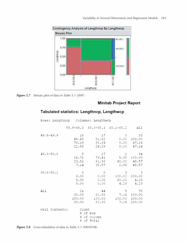
Variability in Several Dimensions and Regression Models 183
Figure 5.7 Mosaic plot of data in Table 5.1 (JMP)
Figure 5.8 Cross-tabulation of data in Table 5.1 (MINITAB)

184 Modern Industrial Statistics
Table 5.2 Joint frequency distribution of Res 3 and Res 7 (in ohms)
Res 3\Res 7 1300–1500 1500–1700 1700–1900 1900–2100 2100–2300 Row Totals
1500–1700 1 13 1 0 0 151700–1900 0 15 31 1 0 471900–2100 0 1 44 40 2 872100–2300 0 0 5 31 6 422300–2500 0 0 0 0 1 1Column Total 1 29 81 72 9 192
◾
The bivariate frequency distribution provides us also information on the association, or dependence between the two
variables. In Table 5.2 we see that resistance values of Res 3 tend to be similar to those of Res 7. For example, if the
resistance value of Res 3 is in the interval (1500, 1700), 13 out of 15 resistance values of Res 7 are in the same interval.
This association can be illustrated by plotting the Box andWhiskers plots of the variable Res 3 by the categories (intervals)
of the variable Res 7. In order to obtain these plots, we partition first the 192 cases to five subgroups, according to the
Table 5.3 Means and standard deviations of Res 3
Subgroup Interval of Res 7 Sample Size Mean Standard Deviation
1 1300–1500 1 1600.0 –2 1500–1700 29 1718.9 80.273 1700–1900 77 1932.9 101.174 1900–2100 76 2068.5 99.735 2100–2300 9 2204.0 115.49
(1300, 1500] (1700, 1900] (2100, 2300]
1600
1800
2000
2200
2400
Figure 5.9 Boxplots of Res 3 by intervals of Res 7

Variability in Several Dimensions and Regression Models 185
resistance values of Res 7. The single case having Res 7 in the interval (1300, 1500) belongs to subgroup 1. The 29 cases
having Res 7 values in (1500, 1700) belong to subgroup 2, and so on. We can then perform, an analysis by subgroups.
Such an analysis yields Table 5.3.
We see in Table 5.3 that the subgroup means grow steadily with the values of Res 7. The standard deviations do not
change much. (There is no estimate of the standard deviation of subgroup 1.) A better picture of the dependence of Res 3
on the intervals of Res 7 is given by Figure 5.9, in which the boxplots of the Res 3 values are presented by subgroup.
5.2.2 Conditional distributions
Consider a population (or a sample) of elements. Each element assumes random values of two (or more) variables
X,Y ,Z, · · · . The distribution of X, over elements whose Y value is restricted to a given interval (or set) A, is called
the conditional distribution of X, given Y is in A. If the conditional distributions of X given Y are different from the
marginal distribution of X, we say that the variables X and Y are statistically dependent. We will learn later how to test
whether the differences between the conditional distributions and the marginal ones are significant, and not due just to
randomness in small samples.
Example 5.4. If we divide the frequencies in Table 5.2 by their column sums we obtain the proportional frequency
distributions of Res 3, given the intervals of Res 7. In Table 5.4 we compare these conditional frequency distributions,
with the marginal frequency distribution of Res 3. We see in Table 5.4 that the proportional frequencies of the conditional
distributions of Res 3 depend strongly on the intervals of Res 7 to which they are restricted.
Table 5.4 Conditional and marginal frequency distributions of Res 3
Res 3\Res7 1300–1500 1500–1700 1700–1900 1900–2100 2100–2300 Marginal Distrib.
1500–1700 100.0 44.8 1.2 0 0 7.81700–1900 0 51.7 38.3 1.4 0 24.51900–2100 0 3.4 54.3 55.6 22.2 45.32100–2300 0 0 6.2 43.0 66.7 21.92300–2500 0 0 0 0 11.1 0.5Column Sums 100.0 100.0 100.0 100.0 100.0 100.0
◾
5.3 Correlation and regression analysis
In the previous sections we presented various graphical procedures for analyzing multivariate data. In particular, we
showed the multivariate scatterplots, 3-dimensional histograms, conditional boxplots, etc. In the present section we start
with numerical analysis of multivariate data.
5.3.1 Covariances and correlations
We introduce now a statistic which summarizes the simultaneous variability of two variables. The statistic is called the
sample covariance. It is a generalization of the sample variance statistics, S2x , of one variable, X. We will denote the
sample covariance of two variables, X and Y by Sxy. The formula of Sxy is
Sxy =1
n − 1
n∑i=1
(Xi − X)(Yi − Y), (5.4)
where X and Y are the sample means of X and Y , respectively. Notice that Sxx is the sample variance S2x and Syy is S2y . The
sample covariance can assume positive or negative values. If one of the variables, say, X, assumes a constant value c, forall Xi (i = 1, · · · , n), then Sxy = 0. This can be immediately verified, since X = c and Xi − X = 0 for all i = 1, · · · , n.

186 Modern Industrial Statistics
Table 5.5 Sample covariances of aluminum pins variables
X\Y Diameter 1 Diameter 2 Diameter 3 Cap Diameter Length nocp Length wcp
Diameter 1 0.0270Diameter 2 0.0285 0.0329Diameter 3 0.0255 0.0286 0.0276Cap Diameter 0.0290 0.0314 0.0285 0.0358Lengthnocp −0.0139 −0.0177 −0.0120 −0.0110 0.1962Lengthwcp −0.0326 −0.0418 −0.0333 −0.0319 0.1503 0.2307
It can be proven that, for any variables X and Y ,
S2xy ≤ S2x ⋅ S2y . (5.5)
This inequality is the celebrated Schwarz inequality. By dividing Sxy by Sx ⋅ Sy we obtain a standardized index of depen-dence, which is called the sample correlation (Pearson’s product-moment correlation), namely
Rxy =Sxy
Sx ⋅ Sy. (5.6)
From the Schwarz inequality, the sample correlation always assumes values between −1 and +1. In Table 5.5 we presentthe sample covariances of the six variables measured on the aluminum pins. Since Sxy = Syx (Covariances and correlationsare symmetric statistics), it is sufficient to present the values at the bottom half of Table 5.5 (on and below the diagonal).
Example 5.5. In Tables 5.5 and 5.6 we present the sample covariances and sample correlations in the data file
ALMPIN.csv.
Table 5.6 Sample correlations of aluminum pins variables
X\Y Diameter 1 Diameter 2 Diameter 3 Cap Diameter Length nocp Length wcp
Diameter 1 1.000Diameter 2 0.958 1.000Diameter 3 0.935 0.949 1.000Cap Diameter 0.933 0.914 0.908 1.000Lengthnocp −0.191 −0.220 −0.163 −0.132 1.000Lengthwcp −0.413 −0.480 −0.417 −0.351 0.707 1.000
We see in Table 5.6 that the sample correlations between Diameter 1, Diameter 2 and Diameter 3 and Cap Diameter
are all greater than 0.9. As we see in Figure 5.10 (the multivariate scatterplots) the points of these variables are scattered
close to straight lines. On the other hand, no clear relationship is evident between the first four variables and the length
of the pin (with or without the cap). The negative correlations, usually indicate that the points are scattered around a
straight line having a negative slope. In the present case it seems that the magnitude of these negative correlations are
due to the one outlier (pin # 66). If we delete it from the data sets, the correlations are reduced in magnitude, as shown in
the Table 5.7.
We see that the correlations between the four diameter variables and the lengthnocp are much closer to zero after
excluding the outlier. Moreover, the correlation with the Cap Diameter changed its sign. This shows that the sample
correlation, as defined above, is sensitive to the influence of extreme observations (outliers).

Variability in Several Dimensions and Regression Models 187
Figure 5.10 Multiple scatterplots of the aluminum pins measurements (MINITAB)
Table 5.7 Sample correlations of aluminum pins variables, after excluding outlyingobservation #66
X\Y Diameter 1 Diameter 2 Diameter 3 Cap Diameter Length nocp
Diameter 2 0.925Diameter 3 0.922 0.936Cap Diameter 0.876 0.848 0.876Lengthnocp −0.056 −0.103 −0.054 0.022Lengthwcp −0.313 −0.407 −0.328 −0.227 0.689
◾
An important question to ask is, how significant is the value of the correlation statistic? In other words, what is the
effect on the correlation of the random components of the measurements? If Xi = 𝜉i + ei, i = 1, · · · , n, where 𝜉i aredeterministic components and ei are random, and if Yi = 𝛼 + 𝛽𝜉i + fi, i = 1, · · · , n, where 𝛼 and 𝛽 are constants and fi arerandom components, how large could be the correlation between X and Y if 𝛽 = 0?
Questions which deal with assessing the significance of the results will be discussed later.
5.3.2 Fitting simple regression lines to data
We have seen examples before in which the relationship between two variables X and Y is close to linear. This is the case
when the (x, y) points scatter along a straight line. Suppose that we are given n pairs of observations {(xi, yi), i = 1, · · · , n}.If the Y observations are related to those on X, according to the linear model
yi = 𝛼 + 𝛽xi + ei, i = 1, · · · , n (5.7)

188 Modern Industrial Statistics
where 𝛼 and 𝛽 are constant coefficients, and ei are random components, with zero mean and constant variance, we say that
Y relates to X according to a simple linear regression. The coefficients 𝛼 and 𝛽, are called the regression coefficients. 𝛼is the intercept and 𝛽 is the slope coefficient. Generally, the coefficients 𝛼 and 𝛽 are unknown. We fit to the data points
a straight line, which is called the estimated regression line, or prediction line.
5.3.2.1 The least squares method
The most common method of fitting a regression line is the method of least squares.Suppose that y = a + bx is the straight line fitted to the data. The principle of least squares requires one to determine
estimates of 𝛼 and 𝛽, a and b, which minimize the sum of squares of residuals around the line, that is,
SSE =n∑i=1
(yi − a − bxi)2. (5.8)
If we require the regression line to pass through the point (x, y), where x, y are the sample means of the x’s and y’s, then
y = a + bx,
or the coefficient a should be determined by the equation
a = y − bx. (5.9)
Substituting this equation above we obtain that
SSE =n∑i=1
(yi − y − b(xi − x))2
=n∑i=1
(yi − y)2 − 2bn∑i=1
(xi − x)(yi − y) + b2n∑i=1
(xi − x)2.
Dividing the two sides of the equation by (n − 1) we obtain
SSEn − 1
= S2y − 2bSxy + b2S2x .
The coefficient b should be determined to minimize this quantity. One can write
SSEn − 1
= S2y + S2x
(b2 − 2b
Sxy
S2x+S2xy
S4x
)−S2xy
S2x
= S2y (1 − R2xy) + S2x
(b −
Sxy
S2x
)2
.
It is now clear that the least squares estimate of 𝛽 is
b =Sxy
S2x= Rxy
SySx. (5.10)
The value of SSE∕(n − 1), corresponding to the least squares estimate is
S2y|x = S2y (1 − R2xy). (5.11)
S2y|x is the sample variance of the residuals around the least squares regression line. By definition, S2y|x ≥ 0, and hence
R2xy ≤ 1, or −1 ≤ Rxy ≤ 1. Rxy = ±1 only if S2y|x = 0. This is the case when all the points (xi, yi), i = 1, · · · , n, lie on a
straight line. If Rxy = 0, then the slope of the regression line is b = 0 and S2y|x = S2y .

Variability in Several Dimensions and Regression Models 189
Notice that
R2xy =
(1 −
S2y|xS2y
). (5.12)
Thus, R2xy is the proportion of variability in Y , which is explainable by the linear relationship y = a + bx. For this reason,
R2xy is also called the coefficient of determination. The coefficient of correlation (squared) measures the extent of linear
relationship in the data. The linear regression line, or prediction line, could be used to predict the values of Y corresponding
to X values, when R2xy is not too small. To interpret the coefficient of determination–particularly when dealing with
multiple regression models (see Section 5.4), it is sometimes useful to consider an “adjusted” R2. The adjustment accounts
for the number of predictor or explanatory variables in themodel and the sample size. In simple linear regressionwe define
R2xy(adjusted) = 1 −
[(1 − R2
xy)n − 1
n − 2
]. (5.13)
Example 5.6. Telecommunication satellites are powered while in orbit by solar cells. Tadicell, a solar cells producer
that supplies several satellite manufacturers, was requested to provide data on the degradation of its solar cells over time.
Tadicell engineers performed a simulated experiment in which solar cells were subjected to temperature and illumination
changes similar to those in orbit and measured the short circuit current ISC (amperes) of solar cells at three different
time periods, in order to determine their rate of degradation. In Table 5.8 we present the ISC values of n = 16 solar cells,
measured at three time epochs, one month apart. The data is given in file SOCELL.csv. In Figure 5.11 we see the scatterof the ISC values at t1, and at t2
Table 5.8 ISC Values of solar cells atthree time epochs
cell\time t1 t2 t3
1 4.18 4.42 4.552 3.48 3.70 3.863 4.08 4.39 4.454 4.03 4.19 4.285 3.77 4.15 4.226 4.01 4.12 4.167 4.49 4.56 4.528 3.70 3.89 3.999 5.11 5.37 5.4410 3.51 3.81 3.7611 3.92 4.23 4.1412 3.33 3.62 3.6613 4.06 4.36 4.4314 4.22 4.47 4.4515 3.91 4.17 4.1416 3.49 3.90 3.81
We now make a regression analysis of ISC at time t2, Y , versus ISC at time t1, X. The computations can be easily
performed by R.
> data(SOCELL)> LmISC <- lm(t2 ~ 1 + t1,
data=SOCELL)> summary(LmISC)

190 Modern Industrial Statistics
Figure 5.11 Relationship of ISC values at t1 and t2 (MINITAB)
Call:lm(formula = t2 ~ 1 + t1, data = SOCELL)
Residuals:Min 1Q Median 3Q Max
-0.145649 -0.071240 0.008737 0.056562 0.123051
Coefficients:Estimate Std. Error t value Pr(>|t|)
(Intercept) 0.53578 0.20314 2.638 0.0195 *t1 0.92870 0.05106 18.189 3.88e-11 ***
---Signif. codes: 0 ‘***’ 0.001 ‘**’ 0.01 ‘*’ 0.05 ‘.’ 0.1 ‘ ’ 1Residual standard error: 0.08709 on 14 degrees of freedomMultiple R-squared: 0.9594, Adjusted R-squared: 0.9565F-statistic: 330.8 on 1 and 14 DF, p-value: 3.877e-11
And in MINITAB, as shown in the following exhibit.
MTB > regress c2 on 1 pred in c1
The regression equation is
C2 = 0.536 + 0.929C1
Predictor Coef Stdev t-ratio P
Constant 0.5358 0.2031 2.64 0.019
C1 0.92870 0.05106 18.19 0.0000
s = 0.08709 R-sq = 95.9% R-sq(adj) = 95.7%

Variability in Several Dimensions and Regression Models 191
We see in the exhibit of the MINITAB analysis that the least squares regression (prediction) line is y = 0.536 + 0.929x.We read also that the coefficient of determination is R2
xy = 0.959. This means that only 4% of the variability in the ISC
values, at time period t2, are not explained by the linear regression on the ISC values at time t1. Observation #9 is an
“unusual observation.” It has relatively a lot of influence on the regression line, as can be seen in Figure 5.11.
The MINITAB output provides also additional analysis. The Stdev corresponding to the least squares regression coef-
ficients are the square-roots of the variances of these estimates, which are given by the formulae:
S2a = S2e
⎡⎢⎢⎢⎢⎣1
n+ x2
n∑i=1
(xi − x)2
⎤⎥⎥⎥⎥⎦(5.14)
and
S2b = S2e∕n∑i=1
(xi − x)2, (5.15)
where
S2e =(1 − R2
xy)n − 2
n∑i=1
(yi − y)2. (5.16)
We see here that S2e =n−1n−2
S2y|x. The reason for this modification is for testing purposes. The value of S2e in the above analysisis 0.0076. The standard deviation of y is Sy = 0.4175. The standard deviation of the residuals around the regression line
is Se = 0.08709. This explains the high value of R2y|x.
In Table 5.9 we present the values of ISC at time t2, y, and their predicted values, according to those at time t1, y. We
present also a graph (Figure 5.12) of the residuals, e = y − y, versus the predicted values y. If the simple linear regression
explains the variability adequately, the residuals should be randomly distributed around zero, without any additional
relationship to the regression x.
Table 5.9 Observed and predictedvalues of ISC at time t2
i yi yi ei
1 4.42 4.419 0.00082 3.70 3.769 −0.06893 4.39 4.326 0.06374 4.19 4.280 −0.08995 4.15 4.038 0.11176 4.12 4.261 −0.14137 4.56 4.707 −0.14728 3.89 3.973 −0.08339 5.37 5.283 0.086810 3.81 3.797 0.013211 4.23 4.178 0.052312 3.62 3.630 −0.009613 4.36 4.308 0.052314 4.47 4.456 0.013615 4.17 4.168 0.001616 3.90 3.778 0.1218

192 Modern Industrial Statistics
4.0 4.5 5.0
−0.1
5−0
.10
−0.0
50.0
00.0
50.1
00.1
5
Fitted valueslm(t2 ~ 1 + t1)
Resid
uals
Residuals vs Fitted
76
16
Figure 5.12 Residual vs. predicted ISC values
In Figure 5.12 we plot the residuals e = y − y, versus the predicted values y, of the ISC values for time t2. It seems
that the residuals are randomly dispersed around zero. Later we will learn how to test whether this dispersion is indeed
random. ◾
5.3.2.2 Regression and prediction intervals
Suppose that we wish to predict the possible outcomes of the Y for some specific value of X, say, x0. If the true regressioncoefficients 𝛼 and 𝛽 are known, then the predicted value of Y is 𝛼 + 𝛽x0. However, when 𝛼 and 𝛽 are unknown, we predictthe outcome at x0 to be y(x0) = a + bx0. We know, however, that the actual value of Y to be observed will not be exactly
equal to y(x0). We can determine a prediction interval around y(x0) such that, the likelihood of obtaining a Y value within
this interval will be high. Generally, the prediction interval limits, given by the formula
y(x0) ± 3 ⋅⎡⎢⎢⎣1 + 1
n+
(x0 − x)2∑i(xi − x)2
⎤⎥⎥⎦1∕2
. (5.17)
will yield good predictions. In Table 5.10 we present the prediction intervals for the ISC values at time t2, for selected ISCvalues at time t1. In Figure 5.13 we present the scatterplot, regression line and prediction limits for Res 3 versus Res 7,
of the HADPAS.csv set.
5.4 Multiple regression
In the present sectionwe generalize the regression to cases where the variability of a variable Y of interest can be explained,
to a large extent, by the linear relationship between Y and k predicting or explaining variables X1, . . . ,Xk. The number of

Variability in Several Dimensions and Regression Models 193
Table 5.10 Prediction intervals for ISC valuesat time t2
x0 y(x0) Lower Limit Upper Limit
4.0 4.251 3.987 4.5144.4 4.622 4.350 4.8934.8 4.993 4.701 5.2855.2 5.364 5.042 5.687
1400 1600 1800 2000 2200
1600
1800
2000
2200
2400
res7
res3
Figure 5.13 Prediction intervals for Res 3 values, given the Res 7 values
explaining variables is k ≥ 2. All the k variables X1, . . . ,Xk are continuous ones. The regression analysis of Y on several
predictors is calledmultiple regression, and multiple regression analysis is an important statistical tool for exploring the
relationship between the dependence of one variable Y on a set of other variables. Applications of multiple regression
analysis can be found in all areas of science and engineering. This method plays an important role in the statistical planning
and control of industrial processes.
The statistical linear model for multiple regression is
yi = 𝛽0 +k∑j=1𝛽jxij + ei, i = 1, · · · , n,
where 𝛽0, 𝛽1, · · · , 𝛽k are the linear regression coefficients, and ei are random components. The commonly used method of
estimating the regression coefficients, and testing their significance, is called multiple regression analysis. The method
is based on the principle of least squares, according to which the regression coefficients are estimated by choosing
b0, b1, · · · , bk to minimize the sum of residuals
SSE =n∑i=1
(yi − (b0 + b1xi + · · · + bkxik))2.

194 Modern Industrial Statistics
The first subsections of the present chapter are devoted to the methods of regression analysis, when both the regressant Yand the regressors x1, . . . , xk are quantitative variables. In Section 5.4.7 we present quantal response regression, in whichthe regressant is qualitative (binary) variable and the regressors x1, . . . , xk are quantitative. In particular we present the
logistic model and the logistic regression. In Sections 5.5.8–5.5.9 we discuss the analysis of variance, for the comparison
of sample means, when the regressant is quantitative but the regressors are categorical variables.
5.4.1 Regression on two variables
The multiple regression linear model, in the case of two predictors, assumes the form
yi = 𝛽0 + 𝛽1x1i + 𝛽2x2i + ei, i = 1, · · · , n. (5.18)
e1, . . . , en are independent r.v.’s, with E{ei} = 0 and V{ei} = 𝜎2, i = 1, . . . , n. The principle of least-squares calls for theminimization of SSE. One can differentiate SSE with respect to the unknown parameters. This yields the least squares
estimators, b0, b1 and b2 of the regression coefficients, 𝛽0, 𝛽1, 𝛽2. The formula for these estimators is:
b0 = Y − b1X1 − b2X2; (5.19)
and b1 and b2 are obtained by solving the set of linear equations
S2x1b1 + Sx1x2b2 = Sx1ySx1x2b1 + S2x2b2 = Sx2y
}. (5.20)
As before, S2x1 , Sx1x2 , S2x2, Sx1y and Sx2y denote the sample variances and covariances of x1, x2 and y.
By simple substitution we obtain, for b1 and b2 the explicit formulae:
b1 =S2x2Sx1y − Sx1x2Sx2y
S2x1S2x2− S2x1x2, (5.21)
and
b2 =S2x1Sx2y − Sx1x2Sx1y
S2x1S2x2 − S2x1x2
. (5.22)
The values yi = b0 + b1x1i + b2x2i (i = 1, · · · , n) are called the predicted values of the regression, and the residuals
around the regression plane are
ei = yi − yi
= yi − (b0 + b1x1i + b2x2i), i = 1, · · · , n.
The mean-square of the residuals around the regression plane is
S2y|(x1 , x2) = S2y
(1 − R2
y|(x1 , x2)), (5.23)
where
R2y|(x1 , x2) = 1
S2y
(b1Sx1y + b2Sx2y
), (5.24)
is themultiple squared-correlation (multiple-R2), and S2y is the sample variance of y. The interpretation of themultiple-R2
is as before, that is, the proportion of the variability of y which is explainable by the predictors (regressors) x1 and x2.

Variability in Several Dimensions and Regression Models 195
Example 5.7. We illustrate the fitting of a multiple regression on the following data, labelled GASOL.csv. The data setconsists of 32 measurements of distillation properties of crude oils (see Daniel and Wood, 1971, pp. 165). There are five
variables, x1, · · · , x4 and y. These are
x1 ∶ crude oil gravity, ∘API;
x2 ∶ crude oil vapour pressure, psi;
x3 ∶ crude oil ASTM 10% point,∘F;
x4 ∶ gasoline ASTM endpoint, ∘F;
y ∶ yield of gasoline (in percentage of crude oil).
The measurements of crude oil, and gasoline volatility indicate the temperatures at which a given amount of liquid has
been evaporized.
The sample correlations between these five variables are
x2 x3 x4 y
x1 0.621 −0.700 −0.322 0.246
x2 −0.906 −0.298 0.384
x3 0.412 −0.315x4 0.712
We see that the yield y is highly correlated with x4 and with x2 (or x3).The following is an R output of the regression of y on x3 and x4:
> data(GASOL)> LmYield <- lm(yield ~ 1 + astm + endPt,
data=GASOL)> summary(LmYield)
Call:lm(formula = yield ~ 1 + astm + endPt, data = GASOL)
Residuals:Min 1Q Median 3Q Max
-3.9593 -1.9063 -0.3711 1.6242 4.3802
Coefficients:Estimate Std. Error t value Pr(>|t|)
(Intercept) 18.467633 3.009009 6.137 1.09e-06 ***astm -0.209329 0.012737 -16.435 3.11e-16 ***endPt 0.155813 0.006855 22.731 < 2e-16 ***—Signif. codes: 0 ‘***’ 0.001 ‘**’ 0.01 ‘*’ 0.05 ‘.’ 0.1 ‘ ’ 1
Residual standard error: 2.426 on 29 degrees of freedomMultiple R-squared: 0.9521, Adjusted R-squared: 0.9488F-statistic: 288.4 on 2 and 29 DF, p-value: < 2.2e-16

196 Modern Industrial Statistics
The following is a MINITAB output of the regression of y on x3 and x4:
The regression equation is
Yield = 18.5 - 0.209 ASTM + 0.156 End_pt
Predictor Coef Stdev t-ratioConstant 18.468 3.009 6.14
ASTM −0.20933 0.01274 −16.43End_pt 0.155813 0.006855 22.73
s = 2.426 R-sq = 95.2%
We compute now these estimates of the regression coefficients using the above formulae. The variances and covariances
of x3, x4 and y are (as derived from MINITAB)
ASTM End_pt Yield
ASTM 1409.355
End_pt 1079.565 4865.894
Yield −126.808 532.188 114.970
The means of these variables are X3 = 241.500, X4 = 332.094, Y = 19.6594. Thus, the least-squares estimators of b1 andb2 are obtained by solving the equations
1409.355b1 + 1079.565b2 = −126.808
1079.565b1 + 4865.894b2 = 532.188.
The solution is
b1 = −0.20933,
and
b2 = 0.15581.
Finally, the estimate of 𝛽0 is
b0 = 19.6594 + 0.20933 × 241.5 − 0.15581 × 332.094
= 18.469.
These are the same results as in the MINITAB output. Moreover, the multiple R2 is
R2y|(x3 , x4) = 1
114.970[0.20932 × 126.808 + 0.15581 × 532.88]
= 0.9530.
In addition,
S2y|(x1 , x2) = S2y (1 − R2y|(x1 ,x2))
= 114.97(1 − .9530)
= 5.4036.

Variability in Several Dimensions and Regression Models 197
0 10 20 30 40
−4−2
02
4
Fitted valueslm(yield ~ 1 + astm + endPt)
Resid
uals
Residuals vs Fitted
17
1910
Figure 5.14 Scatterplot of e vs. Y
In Figure 5.14 we present a scatterplot of the residuals ei (i = 1, · · · , n) against the predicted values yi (i = 1, · · · , n).This scatterplot does not reveal any pattern different than random. It can be concluded that the regression of y on x3 andx4 accounts for all the systematic variability in the yield, y. Indeed, R2 = .952, and no more than 4.8% of the variability
in y is unaccounted by the regression. ◾
The following are formulae for the variances of the least squares coefficients. First we convert S2y|(x1 ,x2) to S2e , that is,S2e =
n − 1
n − 3S2y|x. (5.25)
S2e is an unbiased estimator of 𝜎2. The variance formulae are:
S2b0 =S2en
+ x21S2b1+ x22S
2b2+ 2x1x2Sb1b2 ,
S2b1 =S2e
n − 1⋅S2x2D,
S2b2 =S2e
n − 1⋅S2x1D,
Sb1b2 = −S2e
n − 1⋅Sx1x2D,
(5.26)
where
D = S2x1S2x2− (Sx1x2 )
2.

198 Modern Industrial Statistics
Example 5.8. Using the numerical Example 5.8 on the GASOL.csv data, we find that
S2e = 5.8869,
D = 5, 692, 311.4,
S2b1 = 0.0001624,
S2b2 = 0.0000470,
Sb1 ,b2 = −0.0000332,
and
S2b0 = 9.056295
The squared roots of these variance estimates are the ‘Stdev’ values printed in the MINITAB output, and s = Se. ◾
5.5 Partial regression and correlation
In performing the multiple least squares regression one can study the effect of the predictors on the response in stages. This
more pedestrian approach does not simultaneously provide all regression coefficients but studies the effect of predictors
in more detail.
In Stage I we perform a simple linear regression of the yield y on one of the predictors, x1 say. Let a(1)0
and a(1)1
be the
intercept and slope coefficients of this simple linear regression. Let e(1) be the vector of residuals
e(1)i = yi − (a(1)0
+ a(1)1x1i), i = 1, · · · , n. (5.27)
In Stage II we perform a simple linear regression of the second predictor, x2, on the first predictor x1. Let c(2)0
and c(2)1
be
the intercept and slope coefficients of this regression. Let e(2) be the vector of residuals,
e(2)i = x2i − (c(2)0
+ c(2)1x1i), i = 1, · · · , n. (5.28)
In Stage III we perform a simple linear regression of e(1) on e(2). It can be shown that this linear regression must pass
through the origin, that is, it has a zero intercept. Let d(3) be the slope coefficient.The simple linear regression of e(1) on e(2) is called the partial regression. The correlation between e(1) and e(2) is called
the partial correlation of y and x2, given x1, and is denoted by ryx2⋅x1 .From the regression coefficients obtained in the three stages one can determine the multiple regression coefficients of
y on x1 and x2, according to the formulae:
b0 = a(1)0
− d(3)c(2)0,
b1 = a(1)1
− d(3)c(2)1, (5.29)
b2 = d(3).
Example 5.9. For the GASOL data, let us determine the multiple regression of the yield (y) on the ASTM (x3) and the
End_pt (x4) in stages.In Stage I, the simple linear regression of y on ASTM is
y = 41.4 − 0.08998 ⋅ x3.
The residuals of this regression are e(1). Also R2yx3
= 0.099. In Stage II, the simple linear regression of x4 on x3 is
x4 = 147 + 0.766 ⋅ x3.

Variability in Several Dimensions and Regression Models 199
Figure 5.15 Scatterplot of e1 vs. e2 (MINITAB)
The residuals of this regression are e(2). In Figure 5.15 we see the scatterplot of e(1) versus e(2). The partial correlation is
ryx4⋅x3 = 0.973. This high partial correlation means that, after adjusting the variability of y for the variability of x3, and the
variability of x4 for that of x3, the adjusted x4 values, namely e(2)i (i = 1, · · · , n), are still good predictors for the adjustedy values, namely e(1)i (i = 1, · · · , n). The regression of e(1) on e(2), determined in Stage III, is
e(1)
= 0.156 ⋅ e(2).
We have found the following estimates:
a(1)0
= 41.4, a(1)1
= −0.08998
c(2) = 147.0, c(2)1
= 0.766
d(3) = 0.156.
From the above formulae we get
b0 = 41.4 − 0.156 × 147.0 = 18.468,
b1 = −0.0900 − 0.156 × 0.766 = −0.2095
b2 = 0.156.
These values coincide with the previously determined coefficients. Finally, the relationship between the multiple and the
partial correlations is
R2y|(x1 ,x2) = 1 − (1 − R2
yx1)(1 − r2yx2⋅x1 ). (5.30)
In the present example
R2y|(x3 ,x4) = 1 − (1 − 0.099)(1 − .94673) = 0.9520.

200 Modern Industrial Statistics
In R:
> summary(LmYield <-update(object=LmYield,
formula.=. ~ 1 + astm))
Call:lm(formula = yield ~ astm, data = GASOL)
Residuals:Min 1Q Median 3Q Max
-14.6939 -9.5838 -0.2001 7.6575 21.4069
Coefficients:Estimate Std. Error t value Pr(>|t|)
(Intercept) 41.38857 12.09117 3.423 0.00181 **astm -0.08998 0.04949 -1.818 0.07906 .—Signif. codes: 0 ‘***’ 0.001 ‘**’ 0.01 ‘*’ 0.05 ‘.’ 0.1 ‘ ’ 1
Residual standard error: 10.34 on 30 degrees of freedomMultiple R-squared: 0.09924, Adjusted R-squared: 0.06921F-statistic: 3.305 on 1 and 30 DF, p-value: 0.07906
< summary(LmYield2 <-lm(endPt ~ 1 + astm,
data=GASOL))
Call:lm(formula = endPt ~ 1 + astm, data = GASOL)
Residuals:Min 1Q Median 3Q Max
-116.627 -46.215 -1.894 50.120 114.355
Coefficients:Estimate Std. Error t value Pr(<|t|)
(Intercept) 147.1050 75.5101 1.948 0.0608 .astm 0.7660 0.3091 2.478 0.0190 *—Signif. codes: 0 ‘***’ 0.001 ‘**’ 0.01 ‘*’ 0.05 ‘.’ 0.1 ‘ ’ 1
Residual standard error: 64.6 on 30 degrees of freedomMultiple R-squared: 0.1699, Adjusted R-squared: 0.1423F-statistic: 6.142 on 1 and 30 DF, p-value: 0.01905
◾
5.6 Multiple linear regression
In the general case, we have k predictors (k ≥ 1). Let (X) denote an array of n rows and (k + 1) columns, in which the first
column consists of the value 1 in all entries, and the second to (k + 1)st columns consist of the values of the predictors
x1, · · · , xk. (X) is called the predictors matrix. Let Y be an array of n rows and 1 column, consisting of the values of the
regressant. The linear regression model can be written in matrix notation as
Y = (X)𝜷 + e, (5.31)
where 𝜷 ′ = (𝛽0, 𝛽1, · · · , 𝛽k) is the vector of regression coefficients, and e is a vector of random residuals.

Variability in Several Dimensions and Regression Models 201
The sum of squares of residuals, can be written as
SSE = (Y − (X)𝜷)′(Y − (X)𝜷) (5.32)
( )′ denotes the transpose of the vector of residuals. Differentiating SSE partially with respect to the components of 𝜷,
and equating the partial derivatives to zero, we obtain a set of linear equations in the LSE b, namely
(X)′(X)b = (X)′Y . (5.33)
(X)′ is the transpose of the matrix (X). These linear equations are called the normal equations.If we define the matrix
B = [(X)′(X)]−1(X)′, (5.34)
where [ ]−1 is the inverse of [ ], then the general formula of the least-squares regression coefficients vector b′ =(b0, · · · , bk), is given in matrix notation as
b = (B)Y. (5.35)
The vector of predicted y values, or FITS, is given by y = (H)y, where (H) = (X)(B). The vector of residuals e = y − y isgiven by
e = (I − H)y, (5.36)
where (I) is the n × n identity matrix. The variance of e, around the regression surface, is
S2e =1
n − k − 1
n∑i=1
e2i
= 1
n − k − 1Y′(I − H)Y.
The sum of squares of ei (i = 1, · · · , n) is divided by (n − k − 1) to attain an unbiased estimator of 𝜎2. The multiple-R2
is given by
R2y|(x) = 1
(n − 1)S2y(b′(X)′Y − ny2) (5.37)
where xi0 = 1 for all i = 1, · · · , n, and S2y is the sample variance of y. Finally, an estimate of the variance-covariance
matrix of the regression coefficients b0, · · · , bk is
(Sb) = S2e [(X)′(X)]−1. (5.38)
Example 5.10. We use again theALMPIN data set, and regress the Cap Diameter (y) on Diameter 1 (x1), Diameter 2 (x2)and Diameter 3 (x3). The ‘stdev’ of the regression coefficients are the squared-roots of the diagonal elements of the (Sb)matrix. To see this we present first the inverse of the (X)′(X) matrix, which is given by the following symmetric matrix
[(X)′(X)]−1 =⎡⎢⎢⎢⎣5907.11 −658.57 557.99 −490.80
⋅ 695.56 −448.14 −181.94⋅ ⋅ 739.76 −347.37⋅ ⋅ ⋅ 578.75
⎤⎥⎥⎥⎦The value of S2e is the square of the printed s value, i.e., S2e = 0.0000457. Thus, the variances of the regression coeffi-
cients are:
S2b0 = 0.0000457 × 5907.11 = 0.2700206
S2b1 = 0.0000457 × 695.56 = 0.0317871

202 Modern Industrial Statistics
S2b2 = 0.0000457 × 739.76 = 0.033807
S2b3 = 0.0000457 × 578.75 = 0.0264489.
Thus, Sbi (i = 0, · · · 3) are the ‘Stdev’ in the printout. The t-ratios are given by
ti =biSbi, i = 0, · · · , 3.
The t-ratios should be large to be considered significant. The significance criterion is given by the P-value. A large value
of P indicates that the regression coefficient is not significantly different from zero. In the above table, we see that b2 isnot significant. Notice that Diameter 2 by itself, as the sole predictor of Cap Diameter, is very significant. This can be
verified by running a simple regression of y on x2. However, in the presence of x1 and x3, x2 loses its significance. Thisanalysis can be done in R as shown below.
Call:lm(formula = capDiam ~ 1 + diam1 + diam2 + diam3, data = ALMPIN)
Residuals:Min 1Q Median 3Q Max
-0.013216 -0.004185 -0.002089 0.007543 0.015466
Coefficients:Estimate Std. Error t value Pr(>|t|)
(Intercept) 4.04111 0.51961 7.777 6.63e-11 ***diam1 0.75549 0.17830 4.237 7.18e-05 ***diam2 0.01727 0.18388 0.094 0.9255diam3 0.32269 0.16265 1.984 0.0514 .—Signif. codes: 0 ‘***’ 0.001 ‘**’ 0.01 ‘*’ 0.05 ‘.’ 0.1 ‘ ’ 1
Residual standard error: 0.006761 on 66 degrees of freedomMultiple R-squared: 0.879, Adjusted R-squared: 0.8735F-statistic: 159.9 on 3 and 66 DF, p-value: < 2.2e-16
Df Sum Sq Mean Sq F value Pr(>F)diam1 1 0.021657 0.021657 473.823 <2e-16 ***diam2 1 0.000084 0.000084 1.832 0.1805diam3 1 0.000180 0.000180 3.936 0.0514 .Residuals 66 0.003017 0.000046—Signif. codes: 0 ‘***’ 0.001 ‘**’ 0.01 ‘*’ 0.05 ‘.’ 0.1 ‘ ’ 1
If we perform this analysis with MINITAB we get the following output.
MINITAB Output of the Multiple Regression
The regression equation is
CapDiam = 4.04 + 0.755 Diam 1 + 0.017 Diam2 + 0.323 Diam3
Predictor Coef Stdev t-ratio PConstant 4.0411 0.5196 7.78 0.000
Diam1 0.7555 0.1783 4.24 0.000
Diam2 0.0172 0.1839 0.09 0.926
Diam3 0.3227 0.1626 1.98 0.051
s = 0.006761 R-sq = 87.9% R-sq(adj) = 87.4%

Variability in Several Dimensions and Regression Models 203
Analysis of Variance
SOURCE DF SS MS F PRegression 3 0.0219204 0.0073068 159.86 0.000
Error 66 0.0030167 0.0000457
Total 69 0.0249371
The ‘Analysis of Variance’ table provides a global summary of the contribution of the various factors to the variability
of y. The total sum of squares of y, around its mean is
SST = (n − 1)S2y =n∑i=1
(yi − y)2 = .0249371.
This value of SST is partitioned into the sum of the variability explainable by the regression (SSR) and that due to the
residuals around the regression (Error, SSE). These are given by
SSE = (n − k − 1)S2eSSR = SST − SSE
= b′(X)′y − nY2
n
=k∑j=0
bj ⋅n∑i=1
Xijyi −
(n∑i=1
y(i)
)2
∕n.
We present in Figure 5.16 the scatterplot of the residuals, ei, versus the predicted values (FITS), yi. We see in this figure
one point, corresponding to element # 66 in the data set, whose x-values have strong influence on the regression. ◾
The multiple regression can be used to test whether two or more simple linear regressions are parallel (same slopes) or
have the same intercepts. We will show this by comparing two simple linear regressions.
Let (x(1)i ,Y(1)i ), i = 1, . . . , n, be data set of one simple linear regression of Y on x, and let (x(2)j ,Y
(2)j ), j = 1, . . . , n2 be
that of the second regression. By combining the data on the regression x from the two sets, we get the x vector
x = (x(1)1, . . . , x(1)n1 , x
(2)1, . . . , x(2)n2 )
′.
In a similar fashion we combine the Y values and set
Y = (Y (1)1, . . . ,Y (1)
n1 , Y(2)1, . . . , Y (2)
n2 )′.
Introduce a dummy variable z. The vector z has n1 zeros at the beginning followed by n2 ones. Consider now the multiple
regression
Y = b01 + b1x + b2z + b3w + e, (5.39)
where 1 is a vector of (n1 + n2) ones, and w is a vector of length (n1 + n2) whose i-th component is the product of the
corresponding components of x and z, i.e.,𝑤i = xizi (i = 1, . . . , n1 + n2). Perform the regression analysis ofY on (x, z,w).If b2 is significantly different than 0, we conclude that the two simple regression lines have different intercepts. If b3 issignificantly different from zero, we conclude that the two lines have different slopes.
Example 5.11. In the present example we compare the simple linear regressions of Turndiameter (Y) on MPG/City(x)of US cars and of Japanese cars. The data is in the file CAR.csv. The simple linear regression for US cars is
Y = 49.0769 − 0.7565x
with R2 = 0.432, Se = 2.735 [56 degrees of freedom]. The simple linear regression for Japanese cars is
Y = 42.0860 − 0.5743x,

204 Modern Industrial Statistics
14.90 14.92 14.94 14.96 14.98 15.00
−0.0
15
−0.0
05
0.0
05
0.0
10
0.0
15
Fitted valueslm(capDiam ~ 1 + diam1 + diam2 + diam3)
Resid
uals
Residuals vs Fitted
61
54
23
Figure 5.16 A Scatterplot of the residual versus the predicted values of CapDiam
with R2 = 0.0854, Se = 3.268 [35 degrees of freedom]. The combined multiple regression of Y on x, z, w yields the
following table of P-values of the coefficients
Coefficients:
Value Std. Error t value Pr(> |t|)(Intercept) 49.0769 5.3023 9.2557 0.0000
mpgc −0.7565 0.1420 −5.3266 0.0000
z −6.9909 10.0122 −0.6982 0.4868
𝑤 0.1823 0.2932 0.6217 0.5357
We see in this table that the P-values corresponding to z and w are 0.4868 and 0.5357 respectively. Accordingly, both
b2 and b3 are not significantly different than zero. We can conclude that the two regression lines are not significantly
different. We can combine the data and have one regression line for both US and Japanese cars, namely:
Y = 44.8152 − 0.6474x
with R2 = .3115, Se = 3.337 [93 degrees of freedom]. ◾
5.7 Partial F-tests and the sequential SS
In the MINITAB output for multiple regression a column entitled SEQ SS provides a partition of the regression sum of
squares, SSR, to additive components of variance, each one with 1 degree of freedom. We have seen that the multiple R2,

Variability in Several Dimensions and Regression Models 205
R2y|(x1 , ... ,xk) = SSR∕SST , is the proportion of the total variability which is explainable by the linear dependence of Y on all
the k regressors. A simple linear regression on the 1st variable x1 yields a smaller R2y|x1 . The first component of the SEQ
SS is SSRy|(x1) = SST ⋅ R2y|(x1). If we determine the multiple regression of Y on x1 and x2, then SSRy|(x1 ,x2) = SSTR2
y|(x1 ,x2) isthe amount of variability explained by the linear relationship with the two variables. The difference
DSSx2|x1 = SST(R2y|(x1x2) − R2
y|(x1)) (5.40)
is the additional amount of variability explainable by x2, after accounting for x1. Generally, for i = 2, . . . , k
DSSxi|x1 ... ,xi−1 = SST(R2y|(x1 , ... ,xi) − R2
y|(x1 , ... ,xi−1)) (5.41)
is the additional contribution of the i-th variable after controlling for the first (i − 1) variables.Let
s2e(i) =SST
n − i − 1(1 − R2
y|(x1 , ... ,xi)), i = 1, . . . , k (5.42)
then
F(i) =DSSxi|x1 , ... ,xi−1
S2e(i), i = 1, . . . , k (5.43)
is called the partial-F for testing the significance of the contribution of the variable xi, after controlling for x1, . . . , xi−1.If F(i) is greater than the (1 − 𝛼)th quantile F1−𝛼[1, n − i − 1] of the F distribution, the additional contribution of Xi issignificant. The partial F-test is used to assess whether the addition of the i-th regression significantly improves the
prediction of Y , given that the first (i − 1) regressors have already been included.
Example 5.12. In the previous example we have examined the multiple regression of CapDiam, Y , on Diam1, Diam2,
and Diam3 in the ALMPIN.csv file. We compute here the partial F statistics corresponding to the SEQ SS values.
Variable SEQ SS SSE d.f. Partial-F P-value
Diam1 .0216567 .003280 68 448.98 0
Diam2 .0000837 .003197 67 1.75 0.190
Diam3 .0001799 .003167 66 3.93 0.052
We see from these partial-F values, and their corresponding P-values, that after using Diam1 as a predictor, the additional
contribution of Diam2 is insignificant. Diam3, however, in addition to the regressor Diam1, significantly decreases the
variability which is left unexplained. ◾
The partial-F test is called sometimes sequential-F test (Draper and Smith, 1981, p. 612). We use the terminology Partial-
F statistic because of the following relationship between the partial-F and the partial correlation. In Section 5.5 we defined
the partial correlation ryx2⋅x1 , as the correlation between e(1), which is the vector of residuals around the regression of Yon x1, and the vector of residuals e(2), of x2 around its regression on x1. Generally, suppose that we have determined
the multiple regression of Y on (x1, . . . , xi−1). Let e(y|x1, . . . , xi−1) be the vector of residuals around this regression. Let
e(xi|x1, . . . , xi−1) be the vector of residuals around the multiple regression of xi on x1, . . . , xi−1 (i ≥ 2). The correla-tion between e(y|x1, . . . , xi−1) and e(xi|x1, . . . , xi−1) is the partial correlation between Y and xi, given x1, . . . , xi−1. We
denote this partial correlation by ryxi⋅x1 , ... ,xi−1 . The following relationship holds between the partial-F, F(i), and the partial
correlation
F(i) = (n − i − 1)r2yxi⋅x1 , ... ,xi−1
1 − r2yxi⋅x1 , ... ,xi−1, i ≥ 2. (5.44)
This relationship is used to test whether ryxi⋅x1 , ... ,xi−1 is significantly different than zero. F(i) should be larger than
F1−𝛼[1, n − i − 1].

206 Modern Industrial Statistics
5.8 Model construction: Step-wise regression
It is often the case that data can be collected on a large number of regressors, which might help us predict the outcomes
of a certain variable, Y . However, the different regressors vary generally with respect to the amount of variability in Ywhich they can explain. Moreover, different regressors or predictors are sometimes highly correlated and therefore not all
of them might be needed to explain the variability in Y , and to be used as predictors.
The following example is given by Draper and Smith (1981, p. 615). The amount of steam [Pds] which is used monthly,
Y , in a plant may depend on nine regressors:
x1 = Pounds of real fatty acid in storage per month
x2 = Pounds of crude glycerine made in a month
x3 = Monthly average wind velocity [Miles/hour]
x4 = Plant operating days per month
x5 = Number of days per month with temperature below 32∘F
x6 = Monthly average atmospheric temperature [F].
Are all these six regressors required to be able to predict Y? If not, which variables should be used? This is the problem
of model construction.
There are several techniques for constructing a regression model. R, MINITAB and JMP use a step-wise method which
is based on forward selection, backward elimination and user intervention, which can force certain variables to be included.
We present only the forward selection procedure.
In the first step we select the variable xj (j = 1, . . . , k) whose correlation with Y has maximal magnitude, provided it
is significantly different than zero.
At each step the procedure computes a partial-F, or partial correlation, for each variable, xl, which has not been selectedin the previous steps. A variable having the largest significant partial-F is selected. The procedure stops when no addi-
tional variables can be selected. We illustrate the forward step-wise regression in the following example.
Example 5.13. In Example 5.8 we introduced the data file GASOL.csv and performed a multiple regression of Y on x3and x4. In the present example we apply the MINITAB step-wise regression procedure to arrive at a linear model, which
includes all variables which contributes significantly to the prediction. In R.
> LmYield <- lm(yield ~ 1 , data=GASOL)> Step <- step(LmYield, direction="both",
scope=list(lower= ~ 1,upper= ~ endPt + astm + x1 + x2),
trace=FALSE)> Step$anova
Step Df Deviance Resid. Df Resid. Dev AIC1 NA NA 31 3564.0772 152.813592 + endPt -1 1804.38359 30 1759.6936 132.229093 + astm -1 1589.08205 29 170.6115 59.556914 + x1 -1 24.61041 28 146.0011 56.572115 + x2 -1 11.19717 27 134.8040 56.01874

Variability in Several Dimensions and Regression Models 207
The MINITAB output is given in the following
MINITAB Output for Step-wise Regression
Step-wise RegressionF-to-Enter: 4.00 F-to-Remove: 4.00
Response is gasy on 4 predictors, with N = 32
Step 1 2 3
Constant −16.662 18.468 4.032
gasx4 0.1094 0.1558 0.1565
T-Ratio 5.55 22.73 24.22
gasx3 −0.209 −0.187T-Ratio −16.43 −11.72gasx1 0.22
T-Ratio 2.17
S 7.66 2.43 2.28
R − Sq(%) 50.63 95.21 95.90
More? (Yes, No, Subcommand, or Help)
SUBC> No.
The MINITAB procedure includes at each stage the variable whose partial-F value is maximal, but greater than “F-to-enter,” which is 4.00. Since each partial-F statistic has 1 degree of freedom in the denominator, and since
(F1−𝛼[1, 𝜈])1∕2 = t1−𝛼∕2[𝜈],
the output prints the corresponding values of t. Thus, in Step 1, variable x4 is selected (gasx4). The fitted regression
equation is
Y = −16.662 + 0.1094x4
with R2y|(x4) = .5063. The partial-F for x4 is F = (5.55)2 = 30.8025. Since this value is greater than “F-to-remove,” which
is 4.00, x4 remains in the model. In Step 2 the maximal partial correlation of Y and x1, x2, x3 given x4, is that of x3, with apartial-F = 269.9449. Variable x3 is selected, and the new regression equation is
Y = 18.468 + .1558x4 − .2090x3,
with R2y|(x4 ,x3) = .9521. Since the partial-F of x4 is (22.73)2 = 516.6529, the two variables remain in the model. In Step 3
the variable x1 is chosen. Since its partial-F is (2.17)2 = 4.7089, it is included too. The final regression equation is
Y = 4.032 + .1565x4 − .1870x3 + .2200x1
with R2y|(x4 , x3 , x1) = .959. Only 4.1% of the variability in Y is left unexplained.
To conclude the example we provide the three regression analyses, from the MINITAB. One can compute the partial-Fvalues from these tables.

208 Modern Industrial Statistics
MTB> Regress ‘gasy’ 1 ‘gasx4’;SUBC> Constant.Regression AnalysisThe regression equation is gasy = −16.7 + 0.109 gasx4
Predictor Coef Stdev t-ratio pConstant −16.662 6.687 −2.49 0.018
gasx4 0.10937 0.01972 5.55 0.000
s = 7.659 R − sq = 50.6% R − sq(adj) = 49.0%
Analysis of Variance
SOURCE DF SS MS F pRegression 1 1804.4 1804.4 30.76 0.000
Error 30 1759.7 58.7
Total 31 3564.1
Unusual observations
Obs. gasx4 gasy Fit Stdev.Fit Residual St.Resid
4 407 45.70 27.85 2.00 17.85 2.41R
R denotes an obs. with a large st. resid.
MTB> Regress ‘gasy’ 2 ‘gasx4’ ‘gasx3’;SUBC> Constant.Regression AnalysisThe regression equation is gasy = 18.5 + 0.156 gasx4 - 0.209 gasx3
Predictor Coef Stdev t-ratio pConstant 18.468 3.009 6.14 0.000
gasx4 0.155813 0.006855 22.73 0.000
gasx3 −0.20933 0.01274 −16.43 0.000
s = 2.426 R − sq = 95.2% R − sq(adj) = 94.9%
Analysis of Variance
SOURCE DF SS MS F pRegression 2 3393.5 1696.7 288.41 0.000
Error 29 170.6 5.9
Total 31 3564.1
SOURCE DF SEQ SS
gasx4 1 1804.4
gasx3 1 1589.1

Variability in Several Dimensions and Regression Models 209
MTB> Regress ‘gasy’ 3 ‘gasx4’ ‘gasx3’ ‘gasx1’;SUBC> Constant.Regression AnalysisThe regression equation is gasy = 4.03 + 0.157 gasx4 - 0.187 gasx3 + 0.222 gasx1
Predictor Coef Stdev t-ratio pConstant 4.032 7.223 0.56 0.581
gasx4 0.156527 0.006462 24.22 0.000
gasx3 −0.18657 0.01592 −11.72 0.000
gasx1 0.2217 0.1021 2.17 0.038
s = 2.283 R − sq = 95.9% R − sq(adj) = 95.5%
Analysis of Variance
SOURCE DF SS MS F pRegression 3 3418.1 1139.4 218.51 0.000
Error 28 146.0 5.2
Total 31 3564.1
SOURCE DF SEQ SS
gasx4 1 1804.4
gasx3 1 1589.1
gasx1 1 24.6
Unusual Observations
Obs. gasx4 gasy Fit Stdev.Fit Residual St.Resid
17 340 30.400 25.634 0.544 4.766 2.15R
R denotes an obs. with a large st. resid.
MTB>
◾
5.9 Regression diagnostics
As mentioned earlier, the least-squares regression line is sensitive to extreme x or y values of the sample elements. Some-
times even one point may change the characteristics of the regression line substantially. We illustrate this in the following
example.
Example 5.14. Consider again the SOCELL data. We have seen earlier that the regression line (L1) of ISC at time t2 onISC at time t1 is y = 0.536 + 0.929x, with R2 = .959.
The point having the largest x-value has a y-value of 5.37. If the y-value of this point is changed to 4.37, we obtain a
different regression line (L2), given by y = 2.04 + 0.532x, with R2 = .668. In R
< print(influence.measures(LmISC), digits=2)
Influence measures oflm(formula = t2 ~ 1 + t1, data = SOCELL) :
dfb.1_ dfb.t1 dffit cov.r cook.d hat inf1 -0.0028 0.00356 0.0076 1.26 0.000031 0.0802 -0.2716 0.24914 -0.3346 1.22 0.057266 0.140

210 Modern Industrial Statistics
3 -0.0361 0.05761 0.2057 1.14 0.021816 0.0684 0.0180 -0.04752 -0.2766 1.05 0.037942 0.0645 0.1955 -0.15761 0.3949 0.95 0.073055 0.0746 0.0090 -0.05878 -0.4647 0.80 0.093409 0.0647 0.6262 -0.68909 -0.8816 0.80 0.318895 0.1618 -0.1806 0.15398 -0.2995 1.10 0.044951 0.0859 -1.4355 1.50371 1.6030 1.73 1.170543 0.521 *10 0.0529 -0.04820 0.0667 1.33 0.002391 0.13111 0.0306 -0.01344 0.1615 1.17 0.013630 0.06312 -0.0451 0.04225 -0.0511 1.44 0.001407 0.197 *13 -0.0220 0.03951 0.1662 1.17 0.014439 0.06614 -0.0233 0.02838 0.0539 1.26 0.001559 0.08715 0.0019 -0.00095 0.0089 1.24 0.000043 0.06316 0.5149 -0.47139 0.6392 0.94 0.183649 0.137
The MINITAB diagnostics singles out this point as an unusual point, as seen in the following box.
Unusual Observations
Obs. ISC1 ISC2 Fit Stdev.Fit Residual St.Resid
9 5.11 4.3700 4.7609 0.1232 −0.3909 −3.30RX
◾
In the present section we present the diagnostic tools which are commonly used. The objective is to measure the degree
of influence the points have on the regression line.
We start with the notion of the x-leverage of a point.Consider the matrix (H) defined in Section 5.6. The vector of predicted values, y, is obtained as (H)y. The x-leverage
of the i-th point is measured by the i-th diagonal element of (H), which is
hi = x′i((X)′(X))−1xi, i = 1, · · · , n. (5.45)
Here x′i denotes the i-th row of the predictors matrix (X), that is,
x′i = (1, xi1, · · · , xik).
In the special case of simple linear regression (k = 1) we obtain the formula
hi =1
n+
(xi − x)2n∑j=1
(xj − x)2, i = 1, · · · , n. (5.46)
Notice that Se√hii is the standard-error (squared root of variance) of the predicted value yi. This interpretation holds
also in the multiple regression case (k > 1). In Figure 5.17 we present the x-leverage values of the various points in the
SOCELL example.
From the above formula we deduce that, when k = 1,n∑i=1hi = 2. Generally, for any k,
n∑i=1hi = k + 1. Thus, the average
x-leverage is h = k+1n. In the above solar cells example, the average x-leverage of the 16 points is
2
16= 0.125. Point #9,
(5.21,4.37), has a leverage value of h9 = .521. This is indeed a high x-leverage.The standard-error of the i-th residual, ei, is given by
S{ei} = Se√1 − hi. (5.47)
The standardized residuals are therefore given by
e∗i =ei
S{ei}=
ei
Se√1 − hi, (5.48)

Variability in Several Dimensions and Regression Models 211
0.0 0.1 0.2 0.3 0.4 0.5
−2−1
01
Leveragelm(t2 ~ 1 + t1)
Sta
ndard
ized r
esid
uals
Cook's distance
1
0.5
0.5
1
Residuals vs Leverage
9
7
16
Figure 5.17 x-leverage of ISC values
i = 1, · · · , n. There are several additional indices, which measure the effects of the points on the regression. We mention
here two such measures, the Cook distance and the fits distance.If we delete the i-th point from the data set and recompute the regression, we obtain a vector of regression coefficients
b(i) and standard deviation of residuals S(i)e . The standardized difference
Di =(b(i) − b)′((X)′(X))(b(i) − b)
(k + 1)Se(5.49)
is the so-called Cook’s distance.The influence of the fitted values, denoted by DFIT, is defined as
DFITi =Yi − Y (i)
i
S(i)e√hi, i = 1, · · · , n (5.50)
where Y (i)i = b(i)
0+
k∑j=1b(i)j xij are the predicted values of Y , at (1, xi1, · · · , xik), when the regression coefficients are b(i).
In Figure 5.18 we present the Cook’s Distance, for the ALMPIN data set.
5.10 Quantal response analysis: Logistic regression
We consider the case where the regressant Y is a binary random variable, and the regressors are quantitative. The distri-
bution of Y at a given combination of x values x = (x1, . . . , xk) is binomial B(n, p(x)), where n is the number of identical
and independent repetitions of the experiment at x. p(x) = P{Y = 1|x}. The question is how to model the function p(x).An important class of models is the so-called quantal response models, according to which
p(x) = F(𝜷 ′x), (5.51)

212 Modern Industrial Statistics
0.0
0.5
1.0
1.5
Leverage hiilm(capDiam ~ 1 + diam1 + diam2 + diam3)
Cook's
dis
tance
0 0.1 0.2 0.3 0.4 0.5 0.6
0
0.5
1
1.522.5
Cook's dist vs Leverage hii(1−hii)
66
2361
Figure 5.18 Cook’s distance for aluminum pins data
where F(⋅) is a c.d.f., and
𝜷 ′x = 𝛽0 + 𝛽1x1 + · · · + 𝛽kxk. (5.52)
The logistic regression is a method of estimating the regression coefficients 𝜷, in which
F(z) = ez∕(1 + ez), −∞ < z <∞, (5.53)
is the logistic c.d.f.
The experiment is conducted at m different, and linearly independent, combinations of x values. Thus, let
(X) = (1, x1, x2, . . . , xk)
be the predictors matrix of m rows and (k + 1) columns. We assumed that m > (k + 1) and the rank of (X) is (k + 1). Letx(i), i = 1, . . . ,m, denote the i-th row vector of (X).
As mentioned above, we replicate the experiment at each x(i) n times. Let pi (i = 1, . . . ,m) be the proportion of 1’s
observed at x(i), i.e., pi,n =1
n
n∑j=1Yij, i = 1, . . . ,m; where Yij = 0, 1, is the observed value of the regressant at the j-th
replication (j = 1, . . . , n).We have proved before that E{pi,n} = p(x(i)), and V{pi,n} = 1
np(x(i))(1 − p(x(i))), i = 1, . . . ,m. Also, the estimators pi
(i = 1, . . . ,m) are independent. According to the logistic model
p(x(i)) = e𝜷′x(i)
1 + e𝜷′x(i), i = 1, . . . ,m. (5.54)
The problem is to estimate the regression coefficients 𝜷. Notice that the log-odds at x(i) is
logp(x(i))
1 − p(x(i))= 𝜷 ′x(i), i = 1, . . . ,m. (5.55)

Variability in Several Dimensions and Regression Models 213
Define Yi,n = logpi,n
1−pi,n, i = 1, . . . ,m. Yi,n is finite if n is sufficiently large. Since pi,n → p(x(i)) in probability, as n → ∞
(WLLN), and since logx
1−xis a continuous function of x on (0, 1), Yi,n is a consistent estimator of 𝜷 ′x(i). For large values
of n we can write the regression model
Yi,n = 𝜷 ′x(i) + ei,n + e∗i,n, i = 1, . . . ,m (5.56)
where
ei,n = (pi,n − p(x(i)))∕[p(x(i))(1 − p(x(i)))] (5.57)
e∗i,n is a negligible remainder term if n is large. e∗i,n → 0 in probability at the rate of1
n. If we omit the remainder term e∗i,n
we have the approximate regression model
Yi,n ≅ 𝜷 ′x(i) + ei,n, i = 1, . . . ,m (5.58)
where
E{ei,n} = 0,
V{ei,n} = 1
n⋅
1
p(x(i))(1 − p(x(i)))(5.59)
= (1 + e𝜷′x(i) )2
n ⋅ e𝜷′x(i),
i = 1, . . . ,m. The problem here is that V{ei,n} depends on the unknown 𝜷 and varies from one x(i) to another. An ordi-
nary LSE of 𝜷 is given by �� = [(X)′(X)]−1(X)′Y , where Y′ = (Y1,n, . . . ,Ym,n). Since the variances of ei,n are different, anestimator having smaller variances is the weighted LSE
��𝑤 = [(X)′W(𝜷)(X)]−1(X)′W(𝜷)Y , (5.60)
where W(𝜷) is a diagonal matrix, whose i-th term is
Wi(𝜷) =ne𝜷
′x(i)
(1 + e𝜷′x(i) )2, i = 1, . . . ,m. (5.61)
The problem is that the weightsWi(𝜷) depend on the unknown vector 𝜷. An iterative approach to obtain ��𝑤 is to substituteon the r.h.s. the value of �� obtained in the previous iteration, startingwith the ordinary LSE, ��. Othermethods of estimating
the coefficients 𝜷 of the logistic regression are based on the maximum likelihood method. For additional information, see
S. Kotz and N.L. Johnson, Encyclopedia of Statistical Sciences (1985) and F. Ruggeri, R. Kenett and F. Faltin, Encyclo-pedia of Statistics in Quality and Reliability (2007).
5.11 The analysis of variance: The comparison of means
5.11.1 The statistical model
When the regressors x1, x2, . . . , xk are qualitative (categorical) variables and the variable of interest Y is quantitative,
the previously discussed methods of multiple regression are invalid. The different values that the regressors obtain are
different categories of the variables. For example, suppose that we study the relationship between film speed (Y) and thetype of gelatine x used in the preparation of the chemical emulsion for coating the film, the regressor is a categorical
variable. The values it obtains are the various types of gelatine, as classified according to manufacturers.
When we have k, k ≥ 1, such qualitative variables, the combination of categorical levels of the k variables are calledtreatment combinations (a term introduced by experimentalists). Several observations, ni, can be performed at the i-th

214 Modern Industrial Statistics
treatment combination. These observations are considered a random sample from the (infinite) population of all possible
observations under the specified treatment combination. The statistical model for the j-th observation is
Yij = 𝜇i + eij, i = 1, . . . t j = 1, . . . , ni
where 𝜇i is the population mean for the i-th treatment combination, t is the number of treatment combinations, eij (i =1, . . . , t; j = 1, . . . , ni) are assumed to be independent random variables (experimental errors) with E{eij} = 0 for all (i, j)and 𝑣{eij} = 𝜎2 for all (i, j). The comparison of the means 𝜇i (i = 1, . . . , t) provides information on the various effects of
the different treatment combinations. The method used to do this analysis is called Analysis of Variance (ANOVA).
5.11.2 The one-way analysis of variance (ANOVA)
In Section 4.11.5.2 we introduced the ANOVA F-test statistics, and presented the algorithm for bootstrap ANOVA for
comparing the means of k populations. In the present section we develop the rationale for the ANOVA. We assume here
that the errors eij are independent and normally distributed. For the i-th treatment combination (sample) let
Yi =1
ni
ni∑j=1
Yij, i = 1, · · · , t (5.62)
and
SSDi =ni∑j=1
(Yij − Yi)2, i = 1, · · · , t. (5.63)
Let Y = 1
N
t∑i=1niYi be the grand mean of all the observations.
The One-Way ANOVA is based on the following partition of the total sum of squares of deviations around Y ,t∑i=1
ni∑j=1
(Yij − Y)2 =t∑i=1
SSDi +t∑i=1
ni(Yi − Y)2. (5.64)
We denote the l.h.s. by SST and the r.h.s. by SSW and SSB, i.e.,
SST = SSW + SSB. (5.65)
SST , SSW and SSB are symmetric quadratic form in deviations like Yij − Y , Yij − Yi and Yi − Y . Since∑
i
∑j(Yij − Y) = 0,
only N − 1, linear functions Yij − Y =∑
i′∑
j′ci′j′Yi′j′ , with
ci′j′ =⎧⎪⎨⎪⎩1 − 1
N, i′ = i, j′ = j
− 1
N, otherwise
are linearly independent, where N =t∑i=1ni. For this reason we say that the quadratic form SST has (N − 1) degrees of free-
dom (d.f.). Similarly, SSW has (N − t) degrees of freedom, since SSW =t∑i=1SSDi, and the number of degrees of freedom
of SSDi is (ni − 1). Finally, SSB has (t − 1) degrees of freedom. Notice that SSW is the total sum of squares of deviations
within the t samples, and SSB is the sum of squares of deviations between the t sample means.
Dividing a quadratic form by its number of degrees of freedom we obtain the mean-squared statistic. We summarize all
these statistics in a table called the ANOVA table. The ANOVA table for comparing t treatments is given in Table 5.11.
Generally, in an ANOVA table, D.F. designates degrees of freedom, S.S. designates the sum of squares of deviations,
and M.S. designates the mean-squared. In all tables,
M.S. = S.S.
D.F.(5.66)
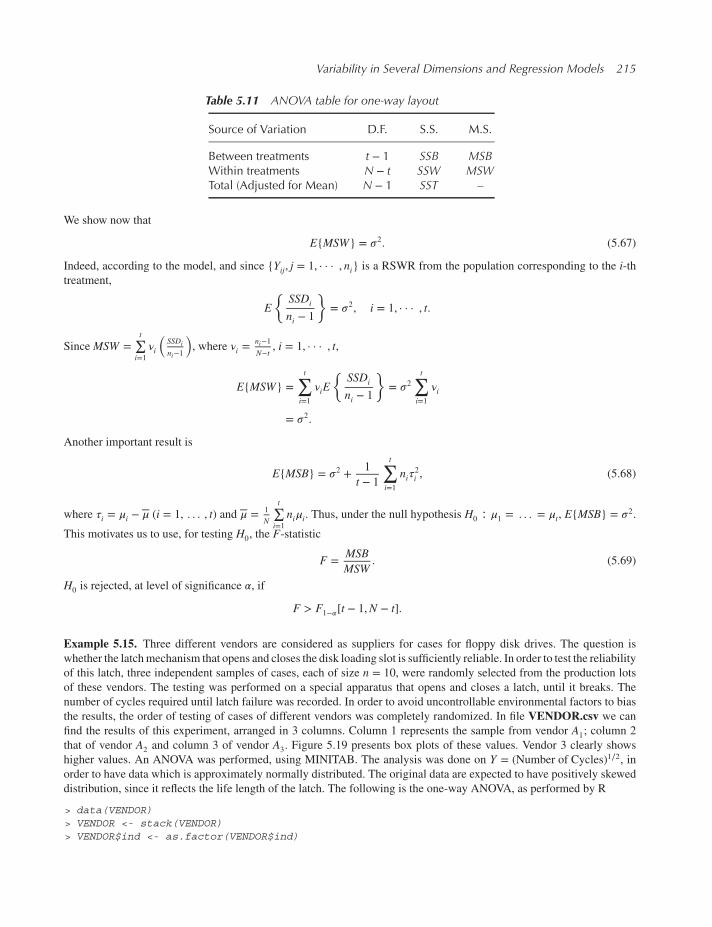
Variability in Several Dimensions and Regression Models 215
Table 5.11 ANOVA table for one-way layout
Source of Variation D.F. S.S. M.S.
Between treatments t − 1 SSB MSBWithin treatments N − t SSW MSWTotal (Adjusted for Mean) N − 1 SST –
We show now that
E{MSW} = 𝜎2. (5.67)
Indeed, according to the model, and since {Yij, j = 1, · · · , ni} is a RSWR from the population corresponding to the i-thtreatment,
E
{SSDi
ni − 1
}= 𝜎2, i = 1, · · · , t.
Since MSW =t∑i=1𝜈i
(SSDini−1
), where 𝜈i =
ni−1N−t
, i = 1, · · · , t,
E{MSW} =t∑i=1𝜈iE
{SSDi
ni − 1
}= 𝜎2
t∑i=1𝜈i
= 𝜎2.
Another important result is
E{MSB} = 𝜎2 + 1
t − 1
t∑i=1
ni𝜏2i , (5.68)
where 𝜏i = 𝜇i − 𝜇 (i = 1, . . . , t) and 𝜇 = 1
N
t∑i=1ni𝜇i. Thus, under the null hypothesis H0 ∶ 𝜇1 = . . . = 𝜇t, E{MSB} = 𝜎2.
This motivates us to use, for testing H0, the F-statistic
F = MSBMSW. (5.69)
H0 is rejected, at level of significance 𝛼, if
F > F1−𝛼[t − 1,N − t].
Example 5.15. Three different vendors are considered as suppliers for cases for floppy disk drives. The question is
whether the latchmechanism that opens and closes the disk loading slot is sufficiently reliable. In order to test the reliability
of this latch, three independent samples of cases, each of size n = 10, were randomly selected from the production lots
of these vendors. The testing was performed on a special apparatus that opens and closes a latch, until it breaks. The
number of cycles required until latch failure was recorded. In order to avoid uncontrollable environmental factors to bias
the results, the order of testing of cases of different vendors was completely randomized. In file VENDOR.csv we can
find the results of this experiment, arranged in 3 columns. Column 1 represents the sample from vendor A1; column 2
that of vendor A2 and column 3 of vendor A3. Figure 5.19 presents box plots of these values. Vendor 3 clearly shows
higher values. An ANOVA was performed, using MINITAB. The analysis was done on Y = (Number of Cycles)1∕2, inorder to have data which is approximately normally distributed. The original data are expected to have positively skewed
distribution, since it reflects the life length of the latch. The following is the one-way ANOVA, as performed by R
> data(VENDOR)> VENDOR <- stack(VENDOR)> VENDOR$ind <- as.factor(VENDOR$ind)
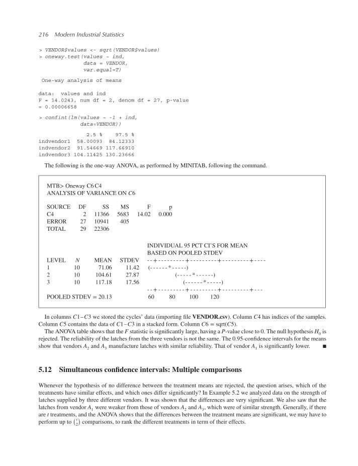
216 Modern Industrial Statistics
> VENDOR$values <- sqrt(VENDOR$values)> oneway.test(values ~ ind,
data = VENDOR,var.equal=T)
One-way analysis of means
data: values and indF = 14.0243, num df = 2, denom df = 27, p-value= 0.00006658
> confint(lm(values ~ -1 + ind,data=VENDOR))
2.5 % 97.5 %indvendor1 58.00093 84.12333indvendor2 91.54669 117.66910indvendor3 104.11425 130.23666
The following is the one-way ANOVA, as performed by MINITAB, following the command.
MTB> Oneway C6C4
ANALYSIS OF VARIANCE ON C6
SOURCE DF SS MS F p
C4 2 11366 5683 14.02 0.000
ERROR 27 10941 405
TOTAL 29 22306
INDIVIDUAL 95 PCT CI’S FOR MEAN
BASED ON POOLED STDEV
LEVEL N MEAN STDEV - -+ - - - - - - - - -+ - - - - - - - - -+ - - - - - - - - -+ - - - -
1 10 71.06 11.42 (- - - - - - * - - - - -)
2 10 104.61 27.87 (- - - - - * - - - - - -)
3 10 117.18 17.56 (- - - - - - * - - - - -)
- -+ - - - - - - - - -+ - - - - - - - - -+ - - - - - - - - -+ - - -
POOLED STDEV = 20.13 60 80 100 120
In columns C1–C3 we stored the cycles’ data (importing file VENDOR.csv). Column C4 has indices of the samples.
Column C5 contains the data of C1–C3 in a stacked form. Column C6 = sqrt(C5).The ANOVA table shows that the F statistic is significantly large, having a P-value close to 0. The null hypothesisH0 is
rejected. The reliability of the latches from the three vendors is not the same. The 0.95-confidence intervals for the means
show that vendors A2 and A3 manufacture latches with similar reliability. That of vendor A1 is significantly lower. ◾
5.12 Simultaneous confidence intervals: Multiple comparisons
Whenever the hypothesis of no difference between the treatment means are rejected, the question arises, which of the
treatments have similar effects, and which ones differ significantly? In Example 5.2 we analyzed data on the strength of
latches supplied by three different vendors. It was shown that the differences are very significant. We also saw that the
latches from vendor A1 were weaker from those of vendors A2 and A3, which were of similar strength. Generally, if there
are t treatments, and the ANOVA shows that the differences between the treatment means are significant, we may have to
perform up to( t2
)comparisons, to rank the different treatments in term of their effects.

Variability in Several Dimensions and Regression Models 217
Figure 5.19 Boxplots of Y by vendor (MINITAB)
If we compare the means of all pairs of treatments, we wish to determine( t2
)= t(t−1)
2confidence intervals to the true
differences between the treatment means. If each confidence interval has confidence level (1 − 𝛼), the probability that all( t2
)confidence intervals cover the true differences simultaneously is smaller than (1 − 𝛼). The simultaneous confidence
level might be as low as (1 − t𝛼).There are different types of simultaneous confidence intervals. We present here the method of Scheffé, for simultaneous
confidence intervals for any number of contrasts (Scheffé, 1959, pp. 66). A contrast between t means Y1, · · · , Yt, is a
linear combinationt∑i=1ciYi, such that
t∑i=1ci = 0. Thus, any difference between two means is a contrast, e.g. Y2 − Y1. Any
second order difference, for example,
(Y3 − Y2) − (Y2 − Y1) = Y3 − 2Y2 + Y1,
is a contrast. The space of all possible linear contrasts has dimension (t − 1). For this reason, the coefficient we use,
according to Scheffé’s method, to obtain simultaneous confidence intervals of level (1 − 𝛼) is
S𝛼 = ((t − 1)F1−𝛼[t − 1, t(n − 1)])1∕2 (5.70)
where F1−𝛼[t − 1, t(n − 1)] is the (1 − 𝛼)th quantile of the F-distribution. It is assumed that all the t samples are of equal
size n. Let ��2p denote the pooled estimator of 𝜎2, that is,
��2p =1
t(n − 1)
t∑i=1
SSDi, (5.71)
then the simultaneous confidence intervals for all contrasts of the formt∑i=1ci𝜇i, have limits
t∑i=1
ciYi ± S𝛼��p√n
(t∑i=1
c2i
)1∕2
. (5.72)

218 Modern Industrial Statistics
Example 5.16. In data fileHADPAS.csv we have the resistance values (ohms) of several resistors on 6 different hybrids
at 32 cards.We analyze here the differences between the means of the n = 32 resistance values of resistor RES3, where the
treatments are the t = 6 hybrids. The boxplots of the samples corresponding to the 6 hybrids are presented in Figure 5.20.
In Table 5.12 we present the means and standard deviations of these six samples (treatments).
The pooled estimator of 𝜎 is
��p = 133.74.
The Scheffé coefficient, for 𝛼 = .05 is
S.05 = (5F.95[5, 186])1∕2 = 3.332.
Upper and lower simultaneous confidence limits, with 0.95 level of significance, are obtained by adding to the differ-
ences between means ±S𝛼��p√16
= ±111.405. Differences which are smaller in magnitude than 111.405 are considered
insignificant.
Figure 5.20 Boxplots of six hybrids (MINITAB)
Table 5.12 Means and std. of resistanceRES3 by hybrid
Hybrid Y Sy
1 2143.41 99.6472 1902.81 129.0283 1850.34 144.9174 1900.41 136.4905 1980.56 146.8396 2013.91 139.816

Variability in Several Dimensions and Regression Models 219
Thus, if we order the sample means, we obtain
Hybrid Mean Group Mean
1 2143.41 2143.41
6 2013.91 1997.235
5 1980.56
2 1902.81 1884.52
4 1900.41
3 1850.34
Thus, the difference between the means of Hybrid 1 and all the others is significant. The mean of Hybrid 6 is significantly
different than those of 2, 4 and 3. The mean of Hybrid 5 is significantly larger than that of Hybrid 3. We suggest therefore
the following homogeneous group of treatments (all treatments within the same homogeneous group have means which
are not significantly different).
Homog Means
Group of Groups
{1} 2143.41
{5,6} 1997.24
{2,3,4} 1884.52
The difference between the means of {5, 6} and {2, 3, 4} is the contrast
−1
3Y2 −
1
3Y3 −
1
3Y4 +
1
2Y5 +
1
2Y6.
This contrast is significant, if it is greater than
S𝛼��p√32
√(1
2
)2
+(1
2
)2
+(1
3
)2
+(1
3
)2
+(1
3
)2
= 71.912.
The above difference is thus significant.
> HADPAS$hyb <- factor(HADPAS$hyb)> TukeyHSD(aov(res3 ~ hyb, data=HADPAS))
Tukey multiple comparisons of means95% family-wise confidence level
Fit: aov(formula = res3 ~ hyb, data = HADPAS)
$hybdiff lwr upr p adj
2-1 -240.59375 -336.87544 -144.31206 0.00000003-1 -293.06250 -389.34419 -196.78081 0.00000004-1 -243.00000 -339.28169 -146.71831 0.00000005-1 -162.84375 -259.12544 -66.56206 0.00003476-1 -129.50000 -225.78169 -33.21831 0.00203593-2 -52.46875 -148.75044 43.81294 0.61979394-2 -2.40625 -98.68794 93.87544 0.99999975-2 77.75000 -18.53169 174.03169 0.18917886-2 111.09375 14.81206 207.37544 0.01351014-3 50.06250 -46.21919 146.34419 0.6664332

220 Modern Industrial Statistics
5-3 130.21875 33.93706 226.50044 0.00188056-3 163.56250 67.28081 259.84419 0.00003155-4 80.15625 -16.12544 176.43794 0.16250166-4 113.50000 17.21831 209.78169 0.01071986-5 33.34375 -62.93794 129.62544 0.9183436
◾
5.13 Contingency tables
5.13.1 The structure of contingency tables
When the data is categorical we generally summarize it in a table which presents the frequency of each category, by
variable, in the data. Such a table is called a contingency table.
Example 5.17. Consider a test of a machine which inserts components into a board. The displacement errors of such a
machine were analyzed in Example 5.1. In this test we perform a large number of insertions with k = 9 different compo-
nents. The result of each trial (insertion) is either Success (no insertion error) or Failure (insertion error). In the present
test there are two categorical variables: Component type and Insertion Result. The first variable has nine categories:
C1: Diode
C2: 1/2 Watt Canister
C3: Jump Wire
C4: Small Corning
C5: Large Corning
C6: Small Bullet
C7: 1/8 Watt Dogbone
C8: 1/4 Watt Dogbone
C9: 1/2 Watt Dogbone
The second variable, Insertion Result, has two categories only (Success, Failure). The contingency table (Table 5.13)
presents the frequencies of the various insertion results by component type.
Table 5.13 Contingency table of insertion results bycomponent type
Component Type Insertion Result Row Total
Failure Success
C1 61 108058 108119C2 34 136606 136640C3 10 107328 107338C4 23 105042 105065C5 25 108829 108854C6 9 96864 96873C7 12 107379 107391C8 3 105851 105854C9 13 180617 180630Column Total 190 1,056,574 1,056,764
Table 5.13 shows that the proportional frequency of errors in insertions is very small (190∕1, 056, 764 = 0.0001798),which is about 180 FPM (failures per million). This may be judged to be in conformity with the industry standard. We
see, however, that there are apparent differences between the failure proportions, by component types. In Figure 5.21
we present the FPMs of the insertion failures, by component type. The largest one is that of C1 (Diode), followed by
components {C2,C4,C5}. Smaller proportions are those of {C3,C6,C9}. The smallest error rate is that of C8.

Variability in Several Dimensions and Regression Models 221
C1 C2 C3 C4 C5 C6 C7 C8 C9
%
0.0
00.0
10.0
20.0
30.0
40.0
5
Figure 5.21 Bar chart of components error rates
The differences in the components error rates can be shown to be very significant.
The structure of the contingency table might be considerably more complicated than that of Table 5.13. We illustrate
here a contingency table with three variables. ◾
Example 5.18. The data are the placement errors of an OMNI 4621 automatic insertion machine. The variables are:
(i) Machine Structure: Basic, EMI1, EMI2, EMI4;
(ii) Components: 805, 1206, SOT_23;
(iii) Placement Result: Error, No_Error.
The contingency table is given in Table 5.14, and summarizes the results of 436,431 placements.
Table 5.14 Contingency Table of Placement Errors
Comp. 805 1206 SOT_23 Total Comp Total Rows
Structure Err N_Err Er N_Err Er N_Err Er N_Err
Basic 11 40,279 7 40,283 16 40,274 34 120,836 120,870EMI1 11 25,423 8 25,426 2 25,432 21 76,281 76,302EMI2 19 54,526 15 54,530 12 54,533 46 163,589 163,635EMI4 14 25,194 4 25,204 5 25,203 23 75,601 75,624Total 55 145,422 34 145,443 35 145,442 124 436,307 436,431
We see in Table 5.14 that the total failure rate of this machine type is 124∕436, 307 = 284 (FPM). The failure rates, by
machine structure, in FPM’s, are 281, 275, 281 and 304, respectively. The first three structural types have almost the same
FPM’s, while the fourth one is slightly larger. The components failure rates are 378, 234 and 241 FPM, respectively. It
remains to check the failure rates according to Structure × Component. These are given in Table 5.15.
We see that the effect of the structure is different on different components. Again, one should test whether the observed
differences are statistically significant or due only to chance variability. Methods for testing this will be discussed in
Chapter 10.

222 Modern Industrial Statistics
Table 5.15 Failure rates (FPM) by structureand component type
Component
Structure 805 1206 SOT_23
Basic 273 174 397EMI1 433 315 79EMI2 348 275 220EMI4 555 159 198
◾
The construction of contingency tables can be done in R or by using MINITAB or JMP. We illustrate this on the data in
fileCAR.csv. This file consists of information on 109 car models from 1989. The file contains 109 records on 5 variables:
Number of cylinders (4,6,8), origin (US = 1, Europe = 2, ASIA = 3), turn diameter [meters], horsepower and number
of miles per gallon in city driving. One variable, Origin, is categorical, while the other four are interval scaled variables.
One discrete (number of cylinders) and the other three are continuous.
In R
> data(CAR)> with(data=CAR,
expr=table(cyl, origin))
origincyl 1 2 3
4 33 7 266 13 7 108 12 0 1
and in MINITAB by using the command
MTB> Table C1-C2;SUBC> Counts.
we obtain the contingency table, which is illustrated in Table 5.16.
One can prepare a contingency table also from continuous data, by selecting the number and length of intervals for
each variable, and counting the frequencies of each cell in the table.
For example, for the car data, if we wish to construct a contingency table of turn diameter versus miles/gallon, we
obtain the contingency table presented in Table 5.17.
Table 5.16 Contingency table of number ofcylinders and origin
Origin
Num. Cyc. 1 2 3 Total
4 33 7 26 666 13 7 10 308 12 0 1 13Total 58 14 37 109

Variability in Several Dimensions and Regression Models 223
Table 5.17 Contingency table of turn diameter versusmiles/gallon city
Miles/Gallon City
Turn Diameter 12–18 19–24 25– Total
27–30.6 2 0 4 630.7–34.2 4 12 15 3134.3–37.8 10 26 6 4237.9– 15 15 0 30Total 31 53 25 109
5.13.2 Indices of association for contingency tables
In the present section we construct several indices of association, which reflect the degree of dependence, or association
between variables. For the sake of simplicity, we consider here indices for two-way tables, i.e., association between two
variables.
5.13.2.1 Two interval scaled variables
If the two variables are continuous ones, measured on an interval scale, or some transformation of it, we can use some of
the dependence indices discussed earlier. For example, we can represent each interval by its mid-point, and compute the
correlation coefficient between these mid-points. As in Section 5.2, if variable X is classified into k intervals,
(𝜉0, 𝜉1), (𝜉1, 𝜉2), · · · , (𝜉k−1, 𝜉k)
and variable Y is classified into m intervals (𝜂0, 𝜂1), · · · , (𝜂m−1, 𝜂m), let
𝜉i =1
2(𝜉i−1 + 𝜉i), i = 1, · · · , k
��j =1
2(𝜂j−1 + 𝜂j), j = 1, · · · ,m.
Let pij = fij∕N denote the proportional frequency of the (i, j)-th cell, i.e., X values in (𝜉i−1, 𝜉i) and Y values in (𝜂j−1, 𝜂j).Then, an estimate of the coefficient of correlation obtained from the contingency table is
��XY =
k∑i=1
m∑j=1pij(𝜉i − 𝜉)(��j − 𝜂)[ k∑
i=1pi.(𝜉i − 𝜉)2
]1∕2[ m∑j=1p.j(��j − 𝜂)2
]1∕2 , (5.73)
where
pi. =m∑j=1
pij, i = 1, · · · , k,
p.j =k∑i=1
pij, j = 1, · · · ,m,
𝜉 =k∑i=1
pi.𝜉i,
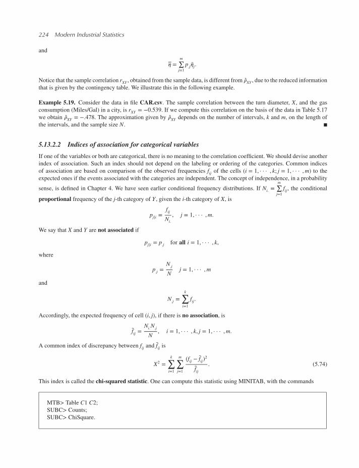
224 Modern Industrial Statistics
and
𝜂 =m∑j=1p.j��j.
Notice that the sample correlation rXY , obtained from the sample data, is different from ��XY , due to the reduced information
that is given by the contingency table. We illustrate this in the following example.
Example 5.19. Consider the data in file CAR.csv. The sample correlation between the turn diameter, X, and the gas
consumption (Miles/Gal) in a city, is rXY = −0.539. If we compute this correlation on the basis of the data in Table 5.17
we obtain ��XY = −.478. The approximation given by ��XY depends on the number of intervals, k and m, on the length of
the intervals, and the sample size N. ◾
5.13.2.2 Indices of association for categorical variables
If one of the variables or both are categorical, there is no meaning to the correlation coefficient. We should devise another
index of association. Such an index should not depend on the labeling or ordering of the categories. Common indices
of association are based on comparison of the observed frequencies fij of the cells (i = 1, · · · , k; j = 1, · · · ,m) to the
expected ones if the events associated with the categories are independent. The concept of independence, in a probability
sense, is defined in Chapter 4. We have seen earlier conditional frequency distributions. If Ni. =m∑j=1fij, the conditional
proportional frequency of the j-th category of Y , given the i-th category of X, is
pj|i = fijNi.
, j = 1, · · · ,m.
We say that X and Y are not associated if
pj|i = p.j for all i = 1, · · · , k,
where
p.j =N.jN
j = 1, · · · ,m
and
N.j =k∑i=1
fij.
Accordingly, the expected frequency of cell (i, j), if there is no association, is
fij =Ni.N.jN, i = 1, · · · , k, j = 1, · · · ,m.
A common index of discrepancy between fij and fij is
X2 =k∑i=1
m∑j=1
(fij − fij)2
fij. (5.74)
This index is called the chi-squared statistic. One can compute this statistic using MINITAB, with the commands
MTB> Table C1 C2;SUBC> Counts;SUBC> ChiSquare.

Variability in Several Dimensions and Regression Models 225
Example 5.20. For the CAR.csv data, the chi-squared statistic for the association between Origin and Num Cycl is
X2 = 12.13. In Chapter 10 we will study how to assess the statistical significance of such a magnitude of X2.
In R
> chisq.test(x=CAR$origin, y=CAR$cyl)
Another option inMINITAB is to set the observed frequencies of the contingency table into columns, and use the command
MTB> ChiSquare C− − C−.
For example, let us set the frequencies of Table 5.17 into 3 columns, say, C6–C8. The above command yields Table 5.18
in which the expected frequencies fij are printed below the observed ones.
Table 5.18 Observed and expected frequencies of turn diameterby miles/gallon, CAR.csv (fij under fij)
Miles/Gallon City
Turn Diameter 12–18 18–24 24– Total
27–30.6 2 0 4 61.71 2.92 1.38
30.6–34.2 4 12 15 318.82 15.07 7.11
34.2–37.8 10 26 6 4211.94 20.42 9.63
37.8– 15 15 0 308.53 14.59 6.88
Total 31 53 25 109
The chi-squared statistic is
X2 = (2 − 1.71)2
1.71+ · · · + 6.882
6.88= 34.99.
◾
There are several association indices in the literature, based on the X2. Three popular indices are:
Mean Squared Contingency
Φ2 = X2
N(5.75)
Tschuprow’s Index
T = Φ∕√(k − 1)(m − 1) (5.76)
Cramér’s Index
C = Φ∕√min(k − 1,m − 1) (5.77)
No association corresponds to Φ2 = T = C = 0. The larger the index the stronger the association. For the data of
Table 3.16,
Φ2 = 34.99
109= 0.321
T = 0.283
C = 0.401.
We provide an additional example of contingency tables analysis, using the Cramér Index.

226 Modern Industrial Statistics
Example 5.21. Compu Star, a service company providing technical support and sales of personal computers and print-
ers, decided to investigate the various components of customer satisfaction that are specific to the company. A special
questionnaire with 13 questions was designed and, after a pilot run, was mailed to a large sample of customers with a
self- addressed stamped envelope and a prize incentive. The prize was to be awarded by lottery among the customers who
returned the questionnaire.
The customers were asked to rate, on a 1–6 ranking order, various aspects of the service. The rating of 1 corresponding
to VERY POOR and the rating of 6 to VERY GOOD. These questions include:
Q1: First impression of service representative.
Q2: Friendliness of service representative.
Q3: Speed in responding to service request.
Q4: Technical knowledge of service representative.
Q5: Professional level of service provided.
Q6: Helpfulness of service representative.
Q7: Additional information provided by service representative.
Q8: Clarity of questions asked by service representative.
Q9: Clarity of answers provided by service representative.
Q10: Efficient use of time by service representative.
Q11: Overall satisfaction with service.
Q12: Overall satisfaction with product.
Q13: Overall satisfaction with company.
The response ranks are:
1. very poor
2. poor
3. below average
4. above average
5. good
6. very good.
The responses were tallied and contingency tables were computed linking the questions on overall satisfaction with ques-
tions on specific service dimensions. For example, Table 5.19 is a contingency table of responses to Q13 versus Q3.
Table 5.19 Two by two contingency table of customerresponses, for Q3 and Q13
Q3\Q13 1 2 3 4 5 6
1 0 1 0 0 3 12 0 2 0 1 0 03 0 0 4 2 3 04 0 1 1 10 7 55 0 0 0 10 71 386 0 0 0 1 30 134
Cramer’s Index for Table 5.19 is:
C = 1.07
2.23= 0.478.
There were 10 detailed questions (Q1–Q10) and 3 questions on overall customer satisfaction (Q11–Q13). A table was
constructed for every combination of the 3 overall customer satisfaction questions and the 10 specific questions. For each

Variability in Several Dimensions and Regression Models 227
of these 30 tables Cramer’s Index was computed and using a code of graphical symbols, we present these indices in
Table 5.20.
Table 5.20 Cramer’s Indices of Q1–Q10 by Q11–Q13
Q1 Q2 Q3 Q4 Q5 Q6 Q7 Q8 Q9 Q10
Q11: Overall satisfaction with Service • ++ • + •Q12: Overall satisfaction with Product + • • ++ • •Q13: Overall satisfaction with Company • ++ + ++ • •
The indices are coded according to the following key:
Cramer’s Index Code
0–0.2
0.2–0.3 •0.3–0.4 +0.4–0.5 ++0.5– + + +
We can see fromTable 5.20 that “Overall satisfaction with company” (Q13) is highly correlated with “Speed in respond-
ing to service requests” (Q3). However, the “Efficient use of time” (Q10) was not associated with overall satisfaction.
On the other hand we also notice that questions Q1, Q5, Q10 show no correlation with overall satisfaction.Manymodels
have been proposed in the literature for the analysis of customer satisfaction surveys. For a comprehensive review with
applications using R, see Kenett and Salini (2012). For more examples of indices of association and graphical analysis of
contingency tables, see Kenett (1983). Contingency tables are closely related to the data mining techniques of Association
Rules. For more on this, see Kenett and Salini (2008). ◾
5.14 Categorical data analysis
If all variables x1, . . . , xk and Y are categorical, we cannot perform the ANOVA without special modifications. In the
present section we discuss the analysis appropriate for such cases.
5.14.1 Comparison of binomial experiments
Suppose that we have performed t independent binomial experiments, each one corresponding to a treatment combination.
In the i-th experiment we ran ni independent trials. The yield variable, Ji, is the number of successes among the ni trials(i = 1, · · · , t). We further assume that in each experiment, the ni trials are independent and have the same, unknown,
probability for success, 𝜃i; i.e., Ji has a binomial distribution B(ni, 𝜃i), i = 1, · · · , t. We wish to compare the probabilities
of success, 𝜃i (i = 1, · · · , k). Accordingly, the null hypothesis is of equal success probabilities, that is,
H0 ∶ 𝜃1 = 𝜃2 = · · · = 𝜃k.

228 Modern Industrial Statistics
We describe here a test, which is good for large samples. Since by the C.L.T., pi =Jinihas a distribution which is approx-
imately normal for large ni, with mean 𝜃i and variance𝜃i(1−𝜃i)
ni, one can show that, the large sample distribution of
Yi = 2 arcsin
⎛⎜⎜⎝√
Ji + 3∕8ni + 3∕4
⎞⎟⎟⎠ (5.78)
(in radians) is approximately normal, with mean 𝜂i = 2 arcsin(√𝜃i) and variance V{Yi} = 1
ni, i = 1, · · · , t.
Using this result, we obtain that under the assumption of H0 the sampling distribution of the test statistic
Q =k∑i=1
ni(Yi − Y)2, (5.79)
where
Y =
k∑i=1niYi
k∑i=1ni
, (5.80)
is approximately chi-squared with k − 1 D.F., 𝜒2[k − 1]. In this test, we reject H0, at level of significance 𝛼, if Q >𝜒21−𝛼[k − 1].Another test statistic for general use in contingency tables will be given in the following section.
Example 5.22. In Table 5.13 we presented the frequency of failures of 9 different components in inserting a large number
of components automatically. In the present example we test the hypothesis that the failure probabilities, 𝜃i, are the same
for all components. In Table 5.21 we present the values of Ji (# of failures), ni and Yi = 2 arcsin(√
Ji+3∕8ni+3∕4
), for each
component. Using MINITAB, if the values of Ji are stored in C1 and those of ni in C2 we compute Yi (stored in C3) withthe command
MTB> let C3 = 2 ∗ asin(sqrt((C1 + .375)∕(C2 + .75))).
Table 5.21 The Arcsin transformation
i Ji ni Yi
1 61 108119 0.04765562 34 136640 0.03172343 10 107338 0.01966314 23 105065 0.02983265 25 108854 0.03053706 9 96873 0.01967527 12 107391 0.02146978 3 105854 0.01129319 13 180630 0.0172102
The test statistic Q can be computed by the MINITAB command (the constant k1 stands for Q).
MTB> let k1 = sum(C2 ∗ C3 ∗∗ 2)− sum(C2 ∗ C3) ∗∗ 2∕sum(C2).

Variability in Several Dimensions and Regression Models 229
The value ofQ is 105.43. The P-value of this statistic is 0. The null hypothesis is rejected. To determine this P value using
MINITAB, since the distribution of Q under H0 is 𝜒2[8], we use the commands:
MTB> CDF 105.43;
SUBC> Chisquare 8.
We find that Pr{𝜒2[8] ≤ 105.43}.= 1. This implies that P = 0. ◾
5.15 Chapter highlights
Several techniques for graphical analysis of data in several dimensions are introduced and demonstrated using case studies.
These includematrix scatterplots, 3D-scatterplots, multiple boxplots. Topics covered also include simple linear regression,
multiple regression models and contingency tables. Prediction intervals are constructed for currents of solar cells and
resistances on hybrid circuits. Robust regression is used to analyze data on placement errors of components on circuit
boards. A special section on indices of association for categorical variables includes an analysis of a customer satisfaction
survey designed to identify the main components of customer satisfaction and dissatisfaction. The material covered by
this chapter can be best studied in front of a personal computer so that the reader can reproduce and even expand the data
analysis offered in the text.
The chapter provides an introduction to multiple regression methods, in which the relationship of k explanatory (pre-
dicting) quantitative variables to a variable of interest is explored. In particular, the least squares estimation procedure
is presented in detail for regression on two variables. Partial regression and correlation are discussed. The least squares
estimation of the regression coefficients for multiple regressions (k > 2) is presented with matrix formulae. The contribu-
tions of the individual regressors is tested by the partial-F test. The sequential SS partition of the total sum of squares due
to the departure on the regressors is defined and explained. The partial correlation, given a set of predictors, is defined
and its relationship to the partial-F statistic is given.
The analysis of variance (ANOVA) for testing the significance of differences between several sample means is intro-
duced, as well as the method of multiple comparisons, which protects the overall level of significance. The comparisons
of proportions for categorical data (binomial or multinomial) is also discussed. The chapter contains also a section on
regression diagnostics, in which the influence of individual points on the regression is studied. In particular, one wishes
to measure the effects of points which seem to deviate considerably from the rest of the sample.
The main concepts and tools introduced in this chapter include:
• Matrix Scatterplots
• 3D-Scatterplots
• Multiple Boxplots
• Code Variables
• Joint, Marginal and Conditional Frequency Distributions
• Sample Correlation
• Coefficient of Determination
• Simple Linear Regression
• Multiple Regression
• Predicted Values, FITS
• Residuals Around the Regression
• Multiple Squared Correlation
• Partial Regression
• Partial Correlation
• Partial-F Test
• Sequential SS

230 Modern Industrial Statistics
• Step-Wise Regression
• Regression Diagnostics
• x-Leverage of a Point• Standard Error of Predicted Value
• Standardized Residual
• Cook Distance
• Fits Distance, DFIT
• Analysis of Variance
• Treatment Combinations
• Simultaneous Confidence Intervals
• Multiple Comparisons
• Contrasts
• Scheffé’s Method
• Contingency Tables Analysis
• Categorical Data Analysis
• Arcsin Transformation
• Chi-Squared Test for Contingency Tables
5.16 Exercises
5.1 Use fileCAR.csv to prepare multiple or matrix scatter plots of Turn Diameter versus Horsepower versus Miles per
Gallon. What can you learn from these plots?
5.2 Make a multiple (side by side) boxplot of the Turn Diameter by Car Origin, for the data in file CAR.csv. Can youinfer that Turn Diameter depends on the Car Origin?
5.3 Data file HADPAS.csv contains the resistance values (Ohms) of five resistors placed in six hybrids on 32 ceramic
substrates. The file contains eight columns. The variables in these columns are:
1. Record Number.
2. Substrate Number.
3. Hybrid Number.
4. Res 3.
5. Res 18.
6. Res 14.
7. Res 7.
8. Res 20.
(i) Make a multiple boxplot of the resistance in Res 3, by hybrid.
(ii) Make a matrix plot of all the Res variables. What can you learn from the plots?
5.4 Construct a joint frequency distribution of the variables Horsepower and MPG/City for the data in file CAR.csv.5.5 Construct a joint frequency distribution for the resistance values of RES 3 and RES 14, in data file HADPAS.csv.
[Code the variables first, see instructions in Problem [3.45].]
5.6 Construct the conditional frequency distribution of RES 3, given that the resistance values of RES 14 is between
1300 and 1500 (Ohms).
5.7 In the present exercise we compute the conditional means and standard deviations of one variable given another
one. Use file HADPAS.csv. We classify the data according to the values of Res 14 (Column C5) to 5 subgroups.
This is done by using the CODE command in MINITAB, which is:
MTB> CODE(900:1200)1 (1201:1500)2 (1501:1800)3 (1801:2100)4 (2101:2700)5 C5 C8We use then the command
MTB> DESC C3;SUBC> By C8.In this way we can obtain the conditional means and stand-deviations of Res 3 given the subgroups of Res 7. Use
these commands and write a report on the obtained results.

Variability in Several Dimensions and Regression Models 231
5.8 Given below are four data sets of (X,Y) observations(i) Compute the least squares regression coefficients of Y on X, for the four data sets.(ii) Compute the coefficient of determination, R2, for each set.
Data Set 1 Data Set 2 Data Set 3 Data Set 4
X(1) Y (1) X(2) Y (2) X(3) Y (3) X(4) Y (4)
10.0 8.04 10.0 9.14 10.0 7.46 8.0 6.68
8.0 6.95 8.0 8.14 8.0 6.67 8.0 5.76
13.0 7.58 13.0 8.74 13.0 12.74 8.0 7.71
9.0 8.81 9.0 8.77 9.0 7.11 8.0 8.84
11.0 8.33 11.0 9.26 11.0 7.81 8.0 8.47
14.0 9.96 14.0 8.1 14.0 8.84 8.0 7.04
6.0 7.24 6.0 6.13 6.0 6.08 8.0 5.25
4.0 4.26 4.0 3.1 4.0 5.39 19.0 12.5
12.0 10.84 11.0 9.13 12.0 8.16 8.0 5.56
7.0 4.82 7.0 7.26 7.0 6.42 8.0 7.91
5.0 5.68 5.0 4.74 5.0 5.73 8.0 6.89
5.9 Compute the correlation matrix of the variables Turn Diameter, Horsepower and Miles per Gallon/City for the data
in file CAR.csv.5.10 (i) Differentiate partially the quadratic function
SSE =n∑i=1
(Yi − 𝛽0 − 𝛽1Xi1 − 𝛽2Xi2)2
with respect to 𝛽0, 𝛽1 and 𝛽2 to obtain the linear equations in the least squares estimates b0, b1, b2. These linearequations are called the normal equations.
(ii) Obtain the formulae for b0, b1 and b2 from the normal equations.
5.11 Consider the variables Miles per Gallon, Horsepower, and Turn Diameter in the data set CAR.csv. Find the least
squares regression line of MPG (y) on Horsepower (x1) and Turn Diameter (x2). For this purpose use first the
equations in Section 5.4 and then verify your computations by using the MINITAB command “regress.”
5.12 Compute the partial correlation between Miles per Gallon and Horsepower, give the Number of Cylinders, in data
file CAR.csv.5.13 Compute the partial regression of Miles per Gallon and Turn Diameter, Given Horsepower, in data file CAR.csv.5.14 Use the three-stage algorithm of Section 5.5 to obtain the multiple regression of Exercise [5.2] from the results of
[5.5].
5.15 Consider Example 5.4. From the MINITAB output we see that, when regression Cap Diam on Diam1, Diam2 and
Diam3, the regression coefficient of Diam2 is not significant (P value = .926), and this variable can be omitted.
Perform a regression of Cap Diam on Diam2 and Diam3. Is the regression coefficient for Diam2 significant? How
can you explain the difference between the results of the two regressions?
5.16 Regress the yield in GASOL.csv on all the four variables x1, x2, x3, x4.(i) What is the regression equation?
(ii) What is the value of R2?
(iii) Which regression coefficient(s) is (are) non-significant?
(iv) Which factors are important to control the yield?
(v) Are the residuals from the regression distributed normally? Make a graphical test.
5.17 (i) Show that the matrix (H) = (X)(B) is idempotent, i.e., (H)2 = (H).(ii) Show that the matrix (Q) = (I − H) is idempotent, and therefore s2e = y′(Q)y∕(n − k − 1).

232 Modern Industrial Statistics
5.18 Show that the vectors of fitted values, ‚y, and of the residuals, e, are orthogonal, i.e., y′e = 0.
5.19 Show that the 1 − R2y|(x) is proportional to ||e||2, which is the squared Euclidean norm of e.
5.20 In Section 5.4 we presented properties of the cov(X,Y) operator. Prove the following generalization of property
(iv). Let X′ = (X1, . . . ,Xn) be a vector of n random variables. Let (𝚺|) be an n × n matrix whose (i, j)th element
is 𝚺| ij = cov(Xi,Xj), i, j = 1, . . . , n. Notice that the diagonal elements of (𝚺|) are the variances of the components
of X. Let 𝜷 and 𝛄 be two n-dimensional vectors. Prove that cov(𝜷 ′X, 𝛄′X) = 𝜷 ′(𝚺|)𝛄. [The matrix (𝚺|) is called the
variance-covariance matrix of X.]5.21 Let X be an n-dimensional random vector, having a variance-covariance matrix (𝚺|). Let W = (B)X, where (B) is
an m × n matrix. Show that the variance-covariance matrix of W is (B)(𝚺|)(B)′.5.22 Consider the linear regression model y = (X)𝜷 + e. e is a vector of random variables, such that E{ei} = 0 for
alli = 1, . . . , n and
cov(ei, ej) =
{𝜎2, if i = j
0, if i ≠ j
i, j = 1, . . . , n. Show that the variance-covariance matrix of the LSE b = (B)y is 𝜎2[(X)′(X)]−1.5.23 Conider SOCELL.csv data file. Compare the slopes and intercepts of the two simple regressions of ISC at time t3
on that at time t1, and ISC at t3 on that at t2.5.24 The following data (see Draper and Smith, 1981, pp. 629) gives the amount of heat evolved in hardening of element
(in calories per gram of cement), and the percentage of four various chemicals in the cement (relative to the weight
of clinkers from which the cement was made). The four regressors are
x1 ∶amount of tricalcium aluminate;
x2 ∶amount of tricalcium silicate;
x3 ∶amount of tetracalcium alumino ferrite;
x4 ∶amount of dicalcium silicate.
The regressant Y is the amount of heat evolved. The data are given in the following table.
X1 X2 X3 X4 Y
7 26 6 60 78
1 29 15 52 74
11 56 8 20 104
11 31 8 47 87
7 52 6 33 95
11 55 9 22 109
3 71 17 6 102
1 31 22 44 72
2 54 18 22 93
21 47 4 26 115
1 40 23 34 83
11 66 9 12 113
10 68 8 12 109
Compute in a sequence the regressions of Y on X1; of Y on X1,X2; of Y on X1,X2,X3; of Y on X1,X2,X3,X4. For
each regression compute the partial-F of the new regression added, the corresponding partial correlation with Y ,and the sequential SS.

Variability in Several Dimensions and Regression Models 233
5.25 For the data of Exercise [5.24], construct a linear model of the relationship between Y and X1, . . . ,X4, by the
forward step-wise regression method.
5.26 Consider the linear regression of Miles per Gallon on Horsepower for the cars in data file CAR.csv, with Origin
= 3. Compute for each car the residuals, RESI, the standardized residuals, SRES, the leverage HI and the Cook
distance, D.5.27 A simulation of the operation of a piston is available as the R piston simulator function pistonSimulation and
with a JMP addin. In order to test whether changing the piston weight from 30 to 60 [kg] effects the cycle time
significantly, run the simulation program four times at weight 30, 40, 50, 60 [kg], keeping all other factors at
their low level. In each run make n = 5 observations. Perform a one-way ANOVA of the results, and state your
conclusions. [You can use R, MINITAB or JMP.]
5.28 In experiments performed to study the effects of some factors on the integrated circuits fabrication process, the
following results were obtained, on the pre-etch line width (𝜇m)
Exp. 1 Exp. 2 Exp. 3
2.58 2.62 2.22
2.48 2.77 1.73
2.52 2.69 2.00
2.50 2.80 1.86
2.53 2.87 2.04
2.46 2.67 2.15
2.52 2.71 2.18
2.49 2.77 1.86
2.58 2.87 1.84
2.51 2.97 1.86
Perform an ANOVA to find whether the results of the three experiments are significantly different by using
MINITAB and R. Do the two test procedures yield similar results?
5.29 In manufacturing film for industrial use, samples from two different batches gave the following film speed:
Batch A: 103, 107, 104, 102, 95, 91, 107, 99, 105, 105
Batch B: 104, 103, 106, 103, 107, 108, 104, 105, 105, 97
Test whether the differences between the two batches are significant, by using (i) a randomization test; (ii) an
ANOVA.
5.30 Use the MINITAB macro RANDTES3.MTB to test the significance of the differences between the results of the
three experiments in Exercise [5.11.2].
5.31 In data file PLACE.csv we have 26 samples, each one of size n = 16, of x-, y-, 𝜃-deviations of components place-
ments. Make an ANOVA, to test the significance of the sample means in the x-deviation. Classify the samples into
homogeneous groups such that the differences between sample means in the same group are not significant, and
those in different groups are significant. Use the Scheffé coefficient S𝛼 for 𝛼 = .05.5.32 The frequency distribution of cars by origin and number of cylinders is given in the following table.
Num. Cylinders US Europe Asia Total
4 33 7 26 66
6 or more 25 7 11 43
Total 58 14 37 109
Perform a chi-squared test of the dependence of number of cylinders and the origin of car.

234 Modern Industrial Statistics
5.33 Perform a chi-squared test of the association between turn diameter and miles/gallon based on Table 5.17.
5.34 In a customer satisfaction survey several questions were asked regarding–specific services and products provided
to customers. The answers were on a 1–5 scale, where 5 means “very satisfied with the service or product” and 1
means “very dissatisfied.” Compute the Mean Squared Contingency, Tschuprow’s Index and Cramer’s Index for
both contingency tables.
Question 3 Question 1
1 2 3 4 5
1 0 0 0 1 0
2 1 0 2 0 0
3 1 2 6 5 1
4 2 1 10 23 13
5 0 1 1 15 100
Question 3 Question 2
1 2 3 4 5
1 1 0 0 3 1
2 2 0 1 0 0
3 0 4 2 3 0
4 1 1 10 7 5
5 0 0 1 30 134

Part IIAcceptance Sampling
In following the Quality Ladder discussed in Chapter 1, one finds that the next step, after reactive fire-fighting, is a focus
on inspection. Part II shows how proper sampling can alleviate the burden of inspecting every work output and improve
decision-making processes. In-process inspection (IPI) is sometimes implemented as an integral part of the production
processes and performs tests for 100% of the products. Such screening processes are reactive and tend to contain problems
and not challenge the level of chronic problems. IPI data provides a sample of the process capability. Understanding the
process characteristics, requires statistical inference. In this part we cover sampling plans that provide decision-makers
with information on characteristics of batches of material or production processes, using sample data.
Chapter 6 presents the foundations for the estimation of finite population quantities using samples. It shows how to
account for stratified data and known covariates to derive efficient population estimates.
Chapter 7 deals with sampling plans for product inspection using attribute or variable data. The chapter covers simple
acceptance sampling plans, double sampling plans and sequential sampling. The chapter takes the reader an extra step
and discusses skip-lot sampling where consistent good performance leads to skipping some lots that are accepted without
inspection. A concluding section presents the model underlying Deming’s inspection criteria that provides economic
justification for an approach based on either 100% inspection or on statistical process control (SPC). SPC is covered
in Part III.
Modern Industrial Statistics: with applications in R, MINITAB and JMP, Second Edition. Ron S. Kenett and Shelemyahu Zacks.© 2014 John Wiley & Sons, Ltd. Published 2014 by John Wiley & Sons, Ltd.Companion website: www.wiley.com/go/modern_industrial_statistics


6Sampling for Estimation of Finite
Population Quantities
6.1 Sampling and the estimation problem
6.1.1 Basic definitions
In the present chapter we consider the problem of estimating quantities (parameters) of a finite population. The problem of
testing hypotheses concerning such quantities, in the context of sampling inspection of product quality, will be studied in
Chapter 7. Estimation and testing the parameters of statistical models for infinite populations were discussed in Chapter 4.
Let P designate a finite population of N units. It is assumed that the population size, N, is known. Also assume that a
list (or a frame) of the population units LN = {u1, · · · , uN} is available.Let X be a variable of interest and xi = X(ui), i = 1, · · · ,N the value ascribed by X to the i-th unit, ui, of P.The population mean and population variance, for the variable X, i.e.,
𝜇N = 1
N
N∑i=1
xi
and (6.1)𝜎2N = 1
N
N∑i=1
(xi − 𝜇N)2,
are called population quantities. In some books (Cochran, 1977) these quantities are called “population parameters.”
We distinguish between population quantities and parameters of distributions, which represent variables in infinite pop-
ulations. Parameters are not directly observable and can only be estimated, while finite population quantities can be
determined exactly if the whole population is observed.
The population quantity 𝜇N is the expected value of the distribution of X in the population, whose c.d.f. is
FN(x) =1
N
N∑i=1
I(x; xi),
where (6.2)I(x; xi) =
{1, if xi ≤ x
0, if xi > x.
𝜎2N is the variance of FN(x).
Modern Industrial Statistics: with applications in R, MINITAB and JMP, Second Edition. Ron S. Kenett and Shelemyahu Zacks.© 2014 John Wiley & Sons, Ltd. Published 2014 by John Wiley & Sons, Ltd.Companion website: www.wiley.com/go/modern_industrial_statistics

238 Modern Industrial Statistics
In this chapter we focus attention on estimating the population mean, 𝜇N , when a sample of size n, n < N, is observed.The problem of estimating the population variance 𝜎2N will be discussed in the context of estimating the standard errors
of estimators of 𝜇N .Two types of sampling strategies will be considered. One type consists of random samples (with or without replacement)
from the whole population. Such samples are called simple random samples. The other type of sampling strategy is that
of stratified random sampling. In stratified random sampling the population is first partitioned to strata (blocks) and
then a simple random sample is drawn from each stratum independently. If the strata are determined so that the variability
within strata is smaller relative to the general variability in the population, the precision in estimating the population mean
𝜇N , using a stratified random sampling will generally be higher than that in simple random sampling. This will be shown
in Section 6.3.
As an example of a case where stratification could be helpful, consider the following. At the end of each production
day we draw a random sample from the lot of products of that day to estimate the proportion of defective item. Suppose
that several machines operate in parallel, and manufacture the same item. Stratification by machine will provide higher
precision for the global estimate, as well as information on the level of quality of each machine. Similarly, if we can
stratify by shift, by vendor or by other factors that might contribute to the variability, we may increase the precision of
our estimates.
6.1.2 Drawing a random sample from a finite population
Given a finite population consisting ofN distinct elements, we first make a list of all the elements of the population, which
are all labeled for identification purposes. Suppose we wish to draw a random sample of size n from this population, where
1 ≤ n ≤ N. We distinguish between two methods of random sampling: (a) sampling with replacement and (b) samplingwithout replacement. A sample drawn with replacement is obtained by returning the selected element, after each choice,
to the population before the next item is selected. In this method of sampling, there are altogether Nn possible samples.
A sample is called random sample with replacement (RSWR) if it is drawn by a method which gives every possible
sample the same probability to be drawn. A sample iswithout replacement if an element drawn is not replaced and hence
cannot be drawn again. There are N(N − 1) · · · (N − n + 1) such possible samples of size n from a population of size N.If each of these has the same probability of being drawn, the sample is called random sample without replacement(RSWOR). Bootstrapping discussed in Chapter 4 is an application of RSWR.
Practically speaking, the choice of a particular random sample is accomplished with the aid of random numbers.Random numbers can be generated by various methods. For example, an integer has to be drawn at random from the set
0, 1, · · · , 99. If we had a ten-faced die, we could label its faces with the numbers 0, · · · , 9 and cast it twice. The results ofthese 2 drawings would yield a two-digit integer, e.g. 13. Since in general we do not have such a die, we could, instead, use
a coin and, flipping it seven times, generate a random number between 0 and 99 in the following way. Let Xj (j = 1, · · · , 7)be 0 or 1, corresponding to whether a head or tail appeared on the j-th flip of the coin. We then compute the integer I,which can assume one of the values 0, 1, · · · , 127, according to the formula
I = X1 + 2X2 + 4X3 + 8X4 + 16X5 + 32X6 + 64X7.
If we obtain a value greater than 99, we disregard this number and flip the coin again seven times. Adding 1 to the outcome
produces random numbers between 1 and 100. In a similar manner, a roulette wheel could also be used to construct
random numbers. A computer algorithm for generating pseudo random numbers was described in Example 3.5. In actual
applications, we use ready-made tables of random numbers or computer routines for generating random numbers.
Example 6.1. The following 10 numbers were drawn by using a random number generator on a computer: 76, 49, 95, 23,
31, 52, 65, 16, 61, 24. These numbers form a random sample of size 10 from the set 1, · · · , 100. If by chance two or more
numbers are the same, the sample would be acceptable if the method is RSWR. If the method is RSWOR any number
that was already selected would be discarded. In R to draw a RSWOR of 10 integers from the set {1, · · · , 100} use
> set.seed(123)> sample(x=100, size=10)
MINITAB commands for drawing a RSWOR of 10 integers from the set {1, · · · , 100} and storing them in column C1 are:

Sampling for Estimation of Finite Population Quantities 239
MTB> Random 10 C1;SUBC> Integer 1 100.
◾
6.1.3 Sample estimates of population quantities and their sampling distribution
So far we have discussed the nature of variable phenomena, and presented some methods of exploring and presenting the
results of experiments. More specifically, the methods of analysis described in Chapter 2 explore the given data, but do
not provide an assessment of what might happen in future experiments.
If we draw from the same population several different random samples, of the same size, we will find generally that
statistics of interest assume different values at the different samples.
This can be illustrated in R we draw samples, with or without replacement, from a collection of numbers (population)
which is stored in a vector. To show it, let us store in X the integers 1,2,· · · ,100. To sample at random with replacement
(RSWR) a sample of size n = 20 from X, and put the random sample in a vector XSample, we use
> X <- 1:100> XSample <- sample(X, size=20, replace=TRUE)
This can be repeated four times, each time we put the sample in a new column with cbind. In Table 6.1 we present the
results of this sampling, and for each sample we present its mean and standard deviation.
Notice that the “population” mean (that of column C1) is 50.5 and its standard deviation is 29.011. The sample means
and standard deviations are estimates of these population parameters, and as seen above, they vary around the parameters.
The distribution of sample estimates of a parameter is called the sampling distribution of an estimate.Theoretically (hypothetically) the number of possible different random samples, with replacement, is either infinite,
if the population is infinite, or of magnitude Nn, if the population is finite (n is the sample size and N is the population
size). This number is practically too large even if the population is finite (10020 in the above example). We can, however,
approximate this distribution by drawing a large number, M, of such samples. In Figure 6.1 we present the histogram of
the sampling distribution of Xn, for M = 1, 000 random samples with replacement of size n = 20, from the population
{1, 2, · · · , 100} of the previous example.
This can be effectively done in R with the function boot, defining a simple function to calculate a statistic over a
sample of size n and looking at the returning object, component t:
> library(boot)> set.seed(123)> B <- boot(data=X,
statistic=function(x, i, n){mean(x[i[1:n]])},
R=1000, n=20)> head(B$t, 3)
[,1][1,] 45.10[2,] 47.45[3,] 49.05
> table(cut(B$t, 12))
(31.3,34.7] (34.7,38.2] (38.2,41.6] (41.6,45.1]6 21 61 119
(45.1,48.5] (48.5,52] (52,55.4] (55.4,58.8]189 236 169 109
(58.8,62.3] (62.3,65.7] (65.7,69.2] (69.2,72.6]52 32 3 3
Consider data with the following frequency distribution

240 Modern Industrial Statistics
Mid-point Frequency
28 1
32 10
36 19
40 55
44 153
48 224
52 251
56 168
60 86
64 26
68 6
72 1
This data will be the basis of the bootstrapped data presented in Figure 6.1.
Table 6.1 Four random samples withreplacement of size 20, from {1,2, · · · , 100}
Sample
1 2 3 4
26 54 4 1556 59 81 5263 73 87 4646 62 85 981 57 5 444 2 52 1
31 33 6 2779 54 47 921 97 68 285 6 50 52
94 62 89 3952 70 18 3479 40 4 3033 70 53 586 45 70 18
33 74 7 1467 29 68 1433 40 49 3221 21 70 108 43 15 52
Means
37.9 49.6 46.4 33.6
Stand. Dev.
28.0 23.7 31.3 22.6

Sampling for Estimation of Finite Population Quantities 241
Frequency
30 40 50 60 70
050
100
150
200
250
Figure 6.1 Histogram of 1,000 sample means
This frequency distribution is an approximation of the sampling distribution of X20. It is interesting to notice that this
distribution has mean X = 50.42 and standard deviation S = 6.412. X is quite close to the population mean 50.5, and S isapproximately 𝜎∕
√20, where 𝜎 is the population standard deviation. A proof of this is given in the following section.
Our computer sampling procedure provided a very close estimate of this standard error. Very often we are interested in
properties of statistics for which it is difficult to derive formulae for their standard errors. Computer sampling techniques,
like bootstrapping discussed in Chapter 4, provide good approximations to the standard errors of sample statistics.
6.2 Estimation with simple random samples
In the present section we investigate the properties of estimators of the population quantities when sampling is
simple random.
The probability structure for simple random samples with or without replacements, RSWR and RSWOR, was studied
in Section 3.1.4.
LetX1, · · · ,Xn denote the values of the variableX(u) of the n elements in the random samples. Themarginal distributions
of Xi (i = 1, · · · , n) if the sample is random, with or without replacement, is the distribution FN(x). If the sample is random
with replacement then X1, · · · ,Xn are independent. If the sample is random without replacement then X1, · · · ,Xn arecorrelated (dependent).
For an estimator of 𝜇N we use the sample mean
Xn =1
n
n∑j=1
Xj.
For an estimator of 𝜎2N we use the sample variance
S2n =1
n − 1
n∑j=1
(Xj − Xn)2.
Both estimators are random variables, which may change their values from one sample to another.

242 Modern Industrial Statistics
An estimator is called unbiased if its expected value is equal to the population value of the quantity it estimates. The
precision of an estimator is the inverse of its sampling variance.
Example 6.2. We illustrate the above with the following numerical example. The population is of size N = 100. For
simplicity we take X(ui) = i (i = 1, · · · , 100). For this simple population, 𝜇100 = 50.5 and 𝜎2100
= 833.25.Draw from this population 100 independent samples, of size n = 10, with and without replacement.
This can be done in R by using the function boot as in the previous section and modifying the function arguments.
The means and standard deviations (Std.) of the 100 sample estimates are listed in Table 6.2:
Table 6.2 Statistics of sampling distributions
RSWR RSWOR
Estimate Mean Std. Mean Std.
X10 49.85 9.2325 50.12 9.0919
S210 774.47 257.96 782.90 244.36
As will be shown in the following section, the theoretical expected value of X10, both in RSWR and RSWOR, is
𝜇 = 50.5. We see above that the means of the sample estimates are close to the value of 𝜇. The theoretical standard
deviation of X10 is 9.128 for RSWR and 8.703 for RSWOR. The empirical standard deviations are also close to these
values. The empirical means of S210are somewhat lower than their expected values of 833.25 and 841.67, for RSWR and
RSWOR, respectively. But, as will be shown later, they are not significantly smaller than 𝜎2. ◾
6.2.1 Properties of Xn and S2n under RSWR
If the sampling is RSWR, the random variables X1, · · · ,Xn are independent, having the same c.d.f. FN(x). The correspond-ing p.d.f. is
pN(x) =⎧⎪⎨⎪⎩1
N, if x = xj, j = 1, · · · ,N
0, otherwise.
(6.3)
Accordingly,
E{Xj} = 1
N
N∑j=1
xj = 𝜇N , all j = 1, · · · ,N. (6.4)
It follows from the results of Section 3.8 that
E{Xn} = 1
n
n∑j=1
E{Xj}
= 𝜇N .(6.5)
Thus, the sample mean is an unbiased estimator of the population mean.

Sampling for Estimation of Finite Population Quantities 243
The variance of Xj, is the variance associated with FN(x), that is,
V{Xj} =1
N
N∑j=1
x2j − 𝜇2N
= 1
N
N∑j=1
(xj − 𝜇N)2
= 𝜎2N .
Moreover, since X1,X2, · · · ,Xn are i.i.d,
V{Xn} =𝜎2Nn. (6.6)
Thus, as explained in Section 3.8, the sample mean converges in probability to the population mean, as n → ∞. An
estimator having such a property is called consistent.We show now that S2n is an unbiased estimator of 𝜎2N .Indeed, if we write
S2n =1
n − 1
n∑j=1
(Xj − Xn)2
= 1
n − 1
(n∑j=1
X2j − nX
2
n
)we obtain
E{S2n} = 1
n − 1
(n∑j=1
E{X2j } − nE{X
2
n}
).
Moreover, since X1, · · · ,Xn are i.i.d.,
E{X2j } = 𝜎2N + 𝜇2n , j = 1, · · · , n
and
E{X2
n} =𝜎2Nn
+ 𝜇2N .
Substituting these in the expression for E{S2n} we obtain
E{S2n} =1
n − 1
(n(𝜎2N + 𝜇2N) − n
(𝜎2Nn
+ 𝜇2N
))= 𝜎2N . (6.7)
An estimator of the standard error of Xn isSn√n. This estimator is slightly biased.
In large samples, the distribution of Xn is approximately normal, like N
(𝜇N ,𝜎2N
n
), as implied by the C.L.T. Therefore,
the interval (Xn − z1−𝛼∕2
Sn√n,Xn + z1−𝛼∕2
Sn√n
)

244 Modern Industrial Statistics
has, in large samples the property that Pr{Xn − z1−𝛼∕2
Sn√n< 𝜇N < Xn + z1−𝛼∕2
Sn√n
}≅ 1 − 𝛼. An interval having this prop-
erty is called a confidence interval for 𝜇N , with an approximate confidence level (1 − 𝛼). In the above formula, z1−𝛼∕2 =Φ−1
(1 − 𝛼
2
).
It is considerably more complicated to derive the formula for V{S2n}. An approximation for large samples is
V{S2n} ≅𝜇4,N − (𝜎2N)
2
n+
2(𝜎N)2 − 𝜇3,Nn2
+𝜇4,N − 3(𝜎2N)
2
n3(6.8)
where
𝜇3,N = 1
N
N∑j=1
(xj − 𝜇N)3, (6.9)
and
𝜇4,N = 1
N
N∑j=1
(xj − 𝜇N)4. (6.10)
Example 6.3. In file PLACE.csv we have data on x, y and 𝜃 deviations of N = 416 placements of components by auto-
matic insertion in 26 PCB’s.
Let us consider this record as a finite population. Suppose that we are interested in the population quantities of the
variable x-dev. Using R or MINITAB we find that the population mean, variance, third and fourth central moments are
𝜇N = 0.9124
𝜎2N = 2.91999
𝜇3,N = −0.98326
𝜇4,N = 14.655.
The unit of measurements of the x-dev is 10−3 [Inch].
Thus, if we draw a simple RSWR, of size n = 50, the variance of Xn will be V{X50} = 𝜎2N
50= 0.0584. The variance of
S250will be
V{S250} ≅14.655 − (2.9199)2
50+ 2(2.9199)2 + 0.9833
2500+ 14.655 − 3(2.9199)2
125000
= 0.1297.◾
6.2.2 Properties of Xn and S2n under RSWOR
We show first that Xn is an unbiased estimator of 𝜇N , under RSWOR.
Let Ij be an indicator variable, which assumes the value 1 if uj belongs to the selected sample, sn, and equal to zero
otherwise. Then we can write
Xn =1
n
N∑j=1
Ijxj. (6.11)
Accordingly
E{Xn} =1
n
N∑j=1
xjE{Ij}
= 1
n
N∑j=1
xj Pr{Ij = 1}.

Sampling for Estimation of Finite Population Quantities 245
As shown in Section 4.1.4,
Pr{Ij = 1} = nN, all j = 1, · · · ,N.
Substituting this above yields that
E{Xn} = 𝜇N . (6.12)
It is shown below that
V{Xn} =𝜎2Nn
(1 − n − 1
N − 1
). (6.13)
To derive the formula for the variance of Xn, under RSWOR, we use the result of Section 4.8 on the variance of linear
combinations of random variables. Write first,
V{Xn} = V
{1
n
N∑i=1
xiIi
}
= 1
n2V
{N∑i=1
xiIi
}.
N∑i=1xiIi is a linear combination of the random variables I1, · · · , IN .First we show that
V{Ii} = nN
(1 − n
N
), i = 1, · · · ,N.
Indeed, since I2i = Ii,
V{Ii} = E{I2i } − (E{Ii})2
= E{Ii}(1 − E{Ii})
= nN
(1 − n
N
), i = 1, · · · ,N.
Moreover, for i ≠ j,
Cov(Ii, Ij) = E{IiIj} − E{Ii}E{Ij}.
But,
E{IiIj} = Pr{Ii = 1, Ij = 1}
= n(n − 1)N(N − 1)
.
Hence, for i ≠ j,
Cov(Ii, Ij) = − nN2
⋅N − nN − 1.
Finally,
V
{N∑i=1
xiIi
}=
N∑i=1
x2i V{Ii} +∑∑
i≠jxixjCov(Xi,Xj).

246 Modern Industrial Statistics
Substituting these expressions in
V{Xn} = 1
n2V
{N∑i=1
xiIi
},
we obtain
V{Xn} = 1
n2
{nN
(1 − n
N
) N∑i=1
x2i −n(N − n)N2(N − 1)
∑∑i≠j
xixj
}.
But,∑∑i≠j
xixj =( N∑i=1xi
)2
−N∑i=1x2i . Hence,
V{Xn} =N − nnN2
⎧⎪⎨⎪⎩N
N − 1
N∑i=1
x2i −1
N − 1
(N∑i=1
xi
)2⎫⎪⎬⎪⎭= N − nn ⋅ (N − 1) ⋅ N
N∑i=1
(xi − 𝜇N)2
=𝜎2Nn
(1 − n − 1
N − 1
).
We see that the variance of Xn is smaller under RSWOR than under RSWR, by a factor of(1 − n−1
N−1
). This factor is called
the finite population multiplier.The formula we have in Section 3.3.2 for the variance of the hypergeometric distribution can be obtained from the
above formula. In the hypergeometric model, we have a finite population of size N. M elements have a certain attribute.
Let
xi =
{1, if 𝑤i has the attribute
0, if 𝑤i does not have it.
SinceN∑i=1xi = M and x2i = xi,
𝜎2N = MN
(1 − M
N
).
If Jn =n∑i=1Xi, we have
V{Jn} = n2V{Xn}
= nMN
(1 − M
N
)(1 − n − 1
N − 1
). (6.14)
To estimate 𝜎2N we can again use the sample variance S2n. The sample variance has, however, a slight positive bias. Indeed,
E{S2n} =1
n − 1E
{n∑j=1
X2j − nX
2
n
}
= 1
n − 1
(n(𝜎2N + 𝜇2N) − n
(𝜇2N + 𝜎
2
n
(1 − n − 1
N − 1
)))= 𝜎2N
(1 + 1
N − 1
).

Sampling for Estimation of Finite Population Quantities 247
This bias is negligible if 𝜎2N∕N is small. Thus, the standard-error of Xn can be estimated by
S.E.{Xn} =Sn√n
(1 − n − 1
N − 1
)1∕2. (6.15)
When sampling is RSWOR, the random variables X1, · · · ,Xn are not independent, and we cannot justify theoretically theusage of the normal approximation to the sampling distribution of Xn. However, if n∕N is small, the normal approximation
is expected to yield good results. Thus, ifn
N< 0.1 we can approximate the confidence interval, of level (1 − 𝛼), for 𝜇N ,
by the interval with limits
Xn ± z1−𝛼∕2 ⋅ S.E.{Xn}.
In order to estimate the coverage probability of this interval estimator, whenn
N= 0.3, we perform the following simulation
example.
Example 6.4. We can use MINITAB or R to select RSWOR of size n = 30 from the population P = {1, 2, · · · , 100} ofN = 100 units, whose values are xi = i.
For this purpose, set the integers 1, · · · , 100 into object X. Notice that, when n = 30, N = 100, 𝛼 = 0.05, z1−𝛼∕2 = 1.96,
and1.96√n
(1 − n−1
N−1
)1∕2= 0.301.
Sample 30 C1 C4let k1 = mean(C4) − .301 ∗ stan(C4)let k2 = mean(C4) + .301 ∗ stan(C4)stack C2 k1 C2stack C3 k2 C3end
> X <- 1:100> set.seed(123)> XSmp <- replicate(1000, sample(X,
size=30,replace=FALSE))
> Confint <- function(x, p, n=length(x), N){p <- if(p >= 0.5)1-((1-p)/2)
else1-(p/2)
m <- mean(x)z <- qnorm(p=p)/sqrt(n)*(1-((n-1)/(N-1)))ˆ(1/2)s <- sd(x)res <- m - z*sres <- c(res, m + z*s)names(res) <- c("lower", "upper")return(res)
}> XSmpCnf <- t(apply(XSmp, MARGIN=2,
FUN=Confint,p=0.95,N=100))
> head(XSmpCnf, 3)
lower upper[1,] 50.24186 68.22481

248 Modern Industrial Statistics
[2,] 35.86552 53.46781[3,] 42.37065 58.36269
> sum(apply(XSmpCnf, MARGIN=1,FUN=function(x, m){x[1]< m && x[2] > m},
m =50.5))/nrow(XSmpCnf)
[1] 0.94
The true population mean is 𝜇N = 50.5. The estimated coverage probability is the proportion of cases for which k1 ≤𝜇N ≤ k2. In the present simulation the proportion of coverage is 0.947. The nominal confidence level is 1 − 𝛼 = 0.95.The estimated coverage probability is 0.947. Thus, the present example shows that even in cases where n∕N > 0.1 the
approximate confidence limits are quite effective. ◾
6.3 Estimating the mean with stratified RSWOR
We consider now the problem of estimating the population mean, 𝜇N , with stratified RSWOR. Thus, suppose that the
population P is partitioned into k strata (subpopulations) P1,P2, · · · ,Pk, k ≥ 2.
Let N1,N2, · · · ,Nk denote the sizes; 𝜇N1 , · · · , 𝜇Nk the means and 𝜎2N1, · · · , 𝜎2Nk the variances of these strata, respectively.
Notice that the population mean is
𝜇N = 1
N
k∑i=1
Ni𝜇Ni (6.16)
and according to the formula of total variance (see Section 4.8), the population variance is
𝜎2N = 1
N
k∑i=1
Ni𝜎2Ni+ 1
N
k∑i=1
Ni(𝜇Ni − 𝜇N)2. (6.17)
We see that if the means of the strata are not the same, the population variance is greater than the weighted average of the
within strata variances, 𝜎2Ni(i = 1, · · · , k).
A stratified RSWOR is a sampling procedure in which k independent random samples without replacement are drawn
from the strata. Let ni, Xni and S2nibe the size, mean and variance of the RSWOR from the i-th stratum, Pi (i = 1, · · · , k).
We have shown in the previous section that Xni is an unbiased estimator of 𝜇Ni . Thus, an unbiased estimator of 𝜇N is
the weighted average
��N =k∑i=1
WiXni , (6.18)
where Wi =NiN, i = 1, · · · , k. Indeed,
E{��N} =k∑i=1
WiE{Xni}
=k∑i=1
Wi𝜇Ni
= 𝜇N .
(6.19)

Sampling for Estimation of Finite Population Quantities 249
Since Xn1 ,Xn2 , · · · ,Xnk are independent random variables, the variance of ��N is
V{��N} =k∑i=1
W2i V{Xni}
=k∑i=1
W2i
𝜎2nini
(1 −
ni − 1
Ni − 1
)(6.20)
=k∑i=1
W2i
��2Nini
(1 −
niNi
),
where
��2Ni =Ni
Ni − 1𝜎2Ni .
Example 6.5. Returning to the data of Example 6.3, on deviations in the x-direction of automatically inserted components,
the units are partitioned to k = 3 strata. Boards 1–10 in stratum 1, boards 11–13 in stratum 2 and boards 14–26 in
stratum 3. The population characteristics of these strata are:
Stratum Size Mean Variance
1 160 −0.966 0.4189
2 48 0.714 1.0161
3 208 2.403 0.3483.
The relative sizes of the strata areW1 = .385,W2 = .115 andW3 = 0.5. If we select a stratified RSWOR of sizes n1 = 19,
n2 = 6 and n3 = 25 the variance of ��N will be
V{��N} = (0.385)2 0.418919
(1 − 18
159
)+ (0.115)2 1.0161
6
(1 − 5
47
)+(0.5)2 0.3483
25
(1 − 24
207
)= 0.00798.
This variance is considerably smaller than the variance of X50 in a simple RSWOR, which is
V{X50} =2.9199
50
(1 − 49
415
)= 0.0515.
◾
6.4 Proportional and optimal allocation
An important question in designing the stratified RSWOR is how to allocate the total number of observations, n, to the
different strata, that is, the determination of ni ≥ 0 (i = 1, · · · , k) so thatk∑i=1ni = n, for a given n. This is called the sample
allocation. One type of sample allocation is the so-called proportional allocation, that is,
ni = nWi, i = 1, · · · , k. (6.21)

250 Modern Industrial Statistics
The variance of the estimator ��N under proportional allocation is
Vprop{��N} = 1
n
k∑i=1
Wi��2Ni
(1 − n
N
)=𝜎2
N
n
(1 − n
N
),
(6.22)
where
𝜎2
N =k∑i=1
Wi��2Ni,
is the weighted average of the within strata variances.
We have shown in the previous section that if we take a simple RSWOR, the variance of Xn is
Vsimple{Xn} =𝜎2Nn
(1 − n − 1
N − 1
)=��2Nn
(1 − n
N
),
where
��2N = NN − 1𝜎2N .
In large populations, 𝜎2N and ��2N are very close, and we can write
Vsimple{Xn} ≅𝜎2NN
(1 − n
N
)= 1
n
(1 − n
N
){ k∑i=1
Wi𝜎2Ni+
k∑i=1
Wi(𝜇Ni − 𝜇N)2
}
≅ Vprop{��N} +1
n
(1 − n
N
) k∑i=1
Wi(𝜇Ni − 𝜇N)2.
This shows that Vsimple{Xn} > Vprop{��N}; i.e., the estimator of the population mean, 𝜇N , under stratified RSWOR, with
proportional allocation, generally has smaller variance (more precise) than the estimator under a simple RSWOR. The
difference grows with the variance between the strata means,k∑i=1Wi(𝜇Ni − 𝜇N)
2. Thus effective stratification is one which
partitions the population to strata which are homogeneous within (small values of 𝜎2Ni) and heterogeneous between (large
value ofk∑i=1Wi(𝜇Ni − 𝜇N)
2). If sampling is stratified RSWR, then the variance ��N , under proportional allocation is
Vprop{��N} = 1
n
k∑i=1
Wi𝜎2Ni. (6.23)
This is strictly smaller than the variance of Xn in a simple RSWR. Indeed
Vsimple{Xn} =𝜎2Nn
= Vprop{��N} +1
n
k∑i=1
Wi(𝜇Ni − 𝜇N)2.

Sampling for Estimation of Finite Population Quantities 251
Example 6.6. Defective circuit breakers are a serious hazard since their function is to protect electronic systems from
power surges or power drops. Variability in power supply voltage levels can cause major damage to electronic systems.
Circuit breakers are used to shield electronic systems from such events. The proportion of potentially defective circuit
breakers is a key parameter in designing redundancy levels of protection devices and preventive maintenance programs. A
lot of N = 10, 000 circuit breakers was put together by purchasing the products from k = 3 different vendors. We want to
estimate the proportion of defective breakers, by sampling and testing n = 500 breakers. Stratifying the lot by vendor, we
have 3 strata of sizes N1 = 3, 000, N2 = 5, 000 and N3 = 2, 000. Before installing the circuit breakers, we drew from the
lot a stratified RSWOR, with proportional allocation, that is, n1 = 150, n2 = 250 and n3 = 100. After testing we found in
the first sample J1 = 3 defective circuit breakers. In the second sample J2 = 10 and in the third sample J3 = 2 defectives.
Testing is done with a special purpose device, simulating intensive usage of the product.
In the present case we set X = 1 if the item is defective and X = 0 otherwise. Then 𝜇N is the proportion of defective
items in the lot. 𝜇Ni (i = 1, 2, 3) is the proportion defectives in the i-th stratum.
The unbiased estimator of 𝜇N is
��N = 0.3 ×J1150
+ 0.5 ×J2250
+ 0.2 ×J3100
= 0.03.
The variance within each stratum is 𝜎2Ni= PNi (1 − PNi ), i = 1, 2, 3, where PNi is the proportion in the i-th stratum. Thus,
the variance of ��N is
Vprop{��N} = 1
500𝜎2
N
(1 − 500
10, 000
)where
𝜎2
N = 0.3��2N1 + 0.5��2N2 + 0.2��N3 ,
or
𝜎2
N = 0.3 × 3000
2999PN1 (1 − PN1 ) + 0.5
5000
4999PN2 (1 − PN2 ) + 0.2
2000
1999PN3 (1 − PN3 ).
Substituting3
150for an estimate of PN1 ,
10
250for that of PN2 and
2
100for PN3 we obtain the estimate of 𝜎
2
N ,
𝜎2
N = 0.029008.
Finally, an estimate of Vprop{��N} is
Vprop{��N} =0.029008
500
(1 − 500
10, 000
)= 0.00005511.
The standard error of the estimator is 0.00742.
Confidence limits for 𝜇N , at level 1 − 𝛼 = .95, are given by
��N ± 1.96 × S.E.{��N} =
{0.0446
0.0154.
These limits can be used for spare parts policy. ◾
When the variances ��2N within strata are known, we can further reduce the variance of 𝜇N by an allocation, which is called
optimal allocation.

252 Modern Industrial Statistics
We wish to minimizek∑i=1
W2i
��2Nini
(1 −
niNi
)subject to the constraint:
n1 + n2 + · · · + nk = n.
This can be done by minimizing
L(n1, · · · , nk, 𝜆) =k∑i=1
W2i
��2Nini
− 𝜆
(n −
k∑i=1
ni
),
with respect to n1, · · · , nk and 𝜆. This function is called the Lagrangian and 𝜆 is called the Lagrange multiplier.The result is
n0i = nWi��Nik∑j=1Wj��j
, i = 1, · · · , k. (6.24)
We see that the proportional allocation is optimal when all ��2Niare equal.
The variance of ��N , corresponding to the optimal allocation is
Vopt{��N} = 1
N
(k∑i=1
Wi��Ni
)2
− 1
N
k∑i=1
Wi��2Ni. (6.25)
6.5 Prediction models with known covariates
In some problems of estimating the mean 𝜇N of a variable Y in a finite population, we may have information on variables
X1,X2, · · · ,Xk which are related to Y . The variables X1, · · · ,Xk are called covariates. The model relating Y to X1, · · · ,Xk iscalled a prediction model. If the values of Y are known only for the units in the sample, while the values of the covariates
are known for all the units of the population, we can utilize the prediction model to improve the precision of the estimator.
The method can be useful, for example, when the measurements of Y are destructive, while the covariates can be measured
without destroying the units. There are many such examples, like the case of measuring the compressive strength of a
concrete cube. The measurement is destructive. The compressive strength Y is related to the ratio of cement to water in
the mix, which is a covariate that can be known for all units. We will develop the ideas with a simple prediction model.
Let {u1, u2, · · · , uN} be a finite population, P. The values of xi = X(ui), i = 1, · · · ,N are known for all the units of P.Suppose that Y(ui) is related linearly to X(ui) according to the prediction model
yi = 𝛽xi + ei, i = 1, · · · ,N, (6.26)
where 𝛽 is an unknown regression coefficient, and e1, · · · , eN are i.i.d. random variables such that
E{ei} = 0, i = 1, · · · ,N
V{ei} = 𝜎2, i = 1, · · · ,N.
The random variable ei in the prediction model is due to the fact that the linear relationship between Y and X is not perfect,
but subject to random deviations.
We are interested in the population quantity yN = 1
N
N∑i=1yi. We cannot, however, measure all the Y values. Even if we
know the regression coefficient 𝛽, we can only predict yN by 𝛽xN , where xN = 1
N
N∑j=1xj. Indeed, according to the prediction

Sampling for Estimation of Finite Population Quantities 253
model, yN = 𝛽xN + eN , and eN is a random variable with
E{eN} = 0, V{eN} = 𝜎2
N. (6.27)
Thus, since yN has a random component, and since E{yN} = 𝛽xN , we say that a predictor of yN , say, yN , is unbiased, ifE{YN} = 𝛽xN . Generally, 𝛽 is unknown. Thus, we draw a sample of units from P and measure their Y values, in order to
estimate 𝛽. To estimate 𝛽 we draw a simple RSWOR from P of size n, 1 < n < N.Let (X1,Y1), · · · , (Xn,Yn) be the values of X and Y in the random sample. A predictor of yN is some function of the
observed sample values. Notice that after drawing a random sample we have two sources of variability. One due to the
random error components e1, · · · , en, associated with the sample values, and the other one is due to the random sampling
of the n units of P. Notice that the error variables e1, · · · , en are independent of the X values, and thus, independent of
X1,X2, · · · ,Xn, randomly chosen to the sample. In the following, expectation and variances are taken with respect to the
errors model and with respect to the sampling procedure. We will examine now a few alternative predictors of yN .
(i) The sample mean, Yn.Since
Yn = 𝛽Xn + en,
we obtain that
E{Yn} = 𝛽E{Xn} + E{en}
E{en} = 0 and since the sampling is RSWOR, E{Xn} = xN . Thus E{Yn} = 𝛽xN , and the predictor is unbiased. Thevariance of the predictor is, since en is independent of Xn,
V{Yn} = 𝛽2V{Xn} +𝜎2
n
= 𝜎2
n+𝛽2𝜎2xn
(1 − n − 1
N − 1
).
(6.28)
where
𝜎2x =1
N
N∑j=1
(xj − xN)2.
(ii) The ratio predictor,
YR = xNYn
Xn. (6.29)
The ratio predictor will be used when all xi > 0. In this case Xn > 0 in every possible sample. Substituting Yn = 𝛽Xn + enwe obtain
E{YR} = 𝛽xN + xNE
{en
Xn
}.
Again, since en and Xn are independent, E{
enXn
}= 0 and YR is an unbiased predictor. The variance of YR is
V{YR} = (xN)2V
{en
Xn
}.

254 Modern Industrial Statistics
Since en and Xn are independent, and E{en} = 0, the law of the total variance implies that
V{YR} = 𝜎2
nx2NE
⎧⎪⎨⎪⎩1
X2
n
⎫⎪⎬⎪⎭= 𝜎
2
nE
⎧⎪⎨⎪⎩(1 +
(Xn − xN)xN
)−2⎫⎪⎬⎪⎭= 𝜎
2
nE
{1 − 2
xN(Xn − xN) +
3
x2N(Xn − xN)2 + · · ·
}≅ 𝜎
2
n
(1 +
3𝛾2xn
(1 − n − 1
N − 1
))
(6.30)
where 𝛾x = 𝜎x∕xN is the coefficient of variation of X. The above approximation is effective in large samples.
Using the large sample approximation, we see that the ratio predictor YR has a smaller variance than Yn if
3𝜎2𝛾2xn2
(1 − n − 1
N − 1
)<𝛽2𝜎2xn
(1 − n − 1
N − 1
)or, if
n >3𝜎2
(𝛽xN)2.
Other possible predictors for this model are
YRA = xN ⋅1
N
n∑i=1
YiXi
(6.31)
and
YRG = xN ⋅
n∑i=1YiXi
N∑i=1X2i
. (6.32)
We leave it as an exercise to prove that both YRA and YRG are unbiased predictors, and to derive their variances.
What happens, under the above prediction model, if the sample drawn is not random, but the units are chosen to the
sample by some non-random fashion?
Suppose that a non-random sample (x1, y1), · · · , (xn, yn) is chosen. Then
E{yn} = 𝛽xn
and
V{yn} = 𝜎2
n.
The predictor yn is biased, unless xn = xN . A sample which satisfies this property is called a balanced samplewith respectto X. Generally, themean squared error (MSE) of yn, under non-random sampling is
MSE{yn} = E{(yn − 𝛽xN)2}
= 𝜎2
n+ 𝛽2(xn − xN)2. (6.33)
Thus, if the sample is balanced with respect to X then yn is a more precise predictor than all the above, which are based
on simple random samples.

Sampling for Estimation of Finite Population Quantities 255
Example 6.7. Electronic systems such as television sets, radios or computers contain printed circuit boards with elec-
tronic components positioned in patterns determined by design engineers. After assembly (either by automatic insertion
machines or manually) the components are soldered to the board. In the relatively new SurfaceMount Technology, minute
components are simultaneously positioned and soldered to the boards. The occurrence of defective soldering points
impacts the assembly plant productivity and is therefore closely monitored. In file PRED.csv we find 1,000 records
on variable X and Y . X is the number of soldering points on a board, and Y is the number of defective soldering points.
The mean of Y is y1000 = 7.495 and that of X is x1000 = 148.58. Moreover, 𝜎2x = 824.562 and the coefficient of variation
is 𝛾x = .19326. The relationship between X and Y is yi = 𝛽xi + ei, where E{ei} = 0 and V{ei} = 7.5, 𝛽 = 0.05. Thus, if
we have to predict y1000 by a predictor based on a RSWR, of size n = 100, the variances of Y100 and YR = x1000Y100X100
are
V{Y100} = 7.5
100+ 0.0025 × 824.562
100= 0.0956.
On the other hand, the large sample approximation yields,
V{YR} =7.5
100
(1 + 3 × 0.037351
100
)= 0.07508.
We see that, if we have to predict y1000 on the basis of an RSWR of size n = 100, the ratio predictor, YR, is more precise.
◾
In Figures 6.2 and 6.3 we present the histograms of 500 predictors Y100 and 500 YR based on RSWR of size 100 from this
population.
6.6 Chapter highlights
Techniques for sampling finite populations and estimating population parameters are presented. Formulas are given for
the expected value and variance of the sample mean and sample variance of simple random samples with and without
Frequency
7.0 7.2 7.4 7.6 7.8 8.0
050
100
150
200
250
Figure 6.2 Sampling distribution of Y

256 Modern Industrial Statistics
Frequency
7.0 7.2 7.4 7.6 7.8 8.0
050
100
150
200
250
Figure 6.3 Sampling distribution of YR
replacement. Stratification is studied as a method to increase the precision of estimators. Formulas for proportional and
optimal allocation are provided and demonstrated with case studies. The chapter is concluded with a section on prediction
models with known covariates.
The main concepts and definitions introduced in this chapter include:
• Population Quantiles
• Simple Random Samples
• Stratified Random Samples
• Unbiased Estimators
• Precision of an Estimator
• Finite Population Multiplier
• Sample Allocation
• Proportional Allocation
• Optimal Allocation
• Prediction Models
• Covariates
• Ratio Predictor
• Prediction Unbiasedness
• Prediction MSE
6.7 Exercises
6.1 Consider a finite population of size N, whose elements have values x1, · · · , xN . Let FN(x) be the c.d.f., that is,
FN(x) =1
N
N∑i=1
I{xi ≤ x}.

Sampling for Estimation of Finite Population Quantities 257
Let X1, · · · ,Xn be the values of a RSWR. Show that X1, · · · ,Xn are independent having a common distribution
FN(x).6.2 Show that if Xn is the mean of a RSWR, then Xn → 𝜇N as n → ∞ in probability (WLLN).
6.3 What is the large sample approximation to Pr{√n|Xn − 𝜇N| < 𝛿} in RSWR?
6.4 Use MINITAB to draw random samples with or without replacement from data file PLACE.csv. Write a MACRO
which computes the sample correlation between the x-dev and y-dev in the sample values. Execute this MACRO
100 times and make a histogram of the sample correlations.
6.5 Use fileCAR.csv andMINITAB. Construct a MACROwhich samples at random, without replacement (RSWOR),
50 records. Stack the medians of the variables turn-diameter, horsepower and mpg (3, 4, 5). Execute the MACRO
200 times and present the histograms of the sampling distributions of the medians.
6.6 In continuation of Example 5.4, how large should the sample be from the three strata, so that the S.E. {Xi}(i = 1, . . . , 3) will be smaller than 𝛿 = 0.005?
6.7 The proportion of defective chips in a lot of N = 10, 000 chips is P = 5 × 10⁻⁴. How large should a RSWOR be
so that the width of the confidence interval for P, with coverage probability 1 − 𝛼 = .95, will be 0.002?6.8 UseMINITAB to perform stratified random samples from the three strata of the data file PLACE.csv (see Example
5.4). Allocate 500 observations to the three samples proportionally. Estimate the population mean (of x-dev).Repeat this 100 times and estimate the standard-error or your estimates. Compare the estimated standard error
to the exact one.
6.9 Derive the formula for n0i (i = 1, · · · , k) in the optimal allocation, by differentiating L(n1, · · · , nk, 𝜆) and solving
the equations.
6.10 Consider the prediction model
yi = 𝛽 + ei, i = 1, . . . ,N
where E{ei} = 0, V{ei} = 𝜎2 and COV(ei, ej) = 0 for i ≠ j. We wish to predict the population mean 𝜇N = 1
N
N∑i=1yi.
Show that the sample mean Yn is prediction unbiased. What is the prediction MSE of Yn?6.11 Consider the prediction model
yi = 𝛽0 + 𝛽1xi + ei, i = 1, . . . ,N,
where e1, . . . , eN are independent r.v.’s with E{ei} = 0, V{ei} = 𝜎2xi (i = 1, . . . , n). We wish to predict 𝜇N =1
N
N∑i=1yi. What should be a good predictor for 𝜇N?
6.12 Prove that YRA and YRG are unbiased predictors and derive their prediction variances.

7Sampling Plans for Product Inspection
7.1 General discussion
Sampling plans for product inspection are quality assurance schemes, designed to test whether the quality level of a
product conformswith the required standards. Thesemethods of quality inspection are especially important when products
are received from suppliers or vendors for whom we have no other assessment of the quality level of their production
processes. Generally, if a supplier has established procedures of statistical process control which assure the required
quality standards are met (see Chapters 8, 9 and 10), then sampling inspection of his shipments may not be necessary.
However, periodic auditing of the quality level of certified suppliers might be prudent to ensure that these do not drop
below the acceptable standards. Quality auditing or inspection by sampling techniques can also be applied within the
plant, at various stages of the production process, for example, when lots are transferred from one department to another.
In the present chapter we discuss various sampling and testing procedures, designed to maintain quality standards. In
particular, single, double and sequential sampling plans for attributes, and single sampling plans for continuous measure-
ments are studied. We discuss also testing via tolerance limits. The chapter is concluded with a section describing some
of the established standards, and in particular the Skip Lot procedure, which appears in modern standards.
We present here a range of concepts and tools associated with sampling inspection schemes. The methods presented
below can be implemented with R applications or the MINITAB Acceptance Sampling By Attributes features availablein the Stat Quality Tools window. Modern nomenclature is different from the one which was established for almost fifty
years. A product unit which did not meet the quality specifications or requirements was called defective. This term has
been changed recently to nonconforming. Thus, in early standards, like MIL-STD 105E and others, we find the term
“defective items” and “number of defects.” In modern standards like ANSI/ASQC Z1.4 and the international standard
ISO 2859, the term used is nonconforming. We will use the two terms interchangeably. Similarly, the terms LTPD and
LQL, which will be explained later, will be used interchangeably.
A lot is a collection of N elements which are subject to quality inspection. Accordingly, a lot is a finite real population
of products. Acceptance of a lot is a quality approval, providing the “green light” for subsequent use of the elements of
the lot. Generally, we refer to lots of raw material, of semi-finished or finished products, etc., which are purchased from
vendors or produced by subcontractors. Before acceptance, a lot is typically subjected to quality inspection unless the
vendor has been certified and its products are delivered directly, without inspection, to the production line. The purchase
contracts typically specify the acceptable quality level and the method of inspection.
In general, it is expected that a lot contains no more than a certain percentage of nonconforming (defective) items,
where the test conditions which classify an item as defective are usually well specified. One should decide if a lot has to
be subjected to a complete inspection, item by item, or whether it is sufficient to determine acceptance using a sample
from the lot. If we decide to inspect a sample, we must determine how large it is and what is the criterion for accepting
or rejecting the lot. Furthermore, the performance characteristics of the procedures in use should be understood.
Modern Industrial Statistics: with applications in R, MINITAB and JMP, Second Edition. Ron S. Kenett and Shelemyahu Zacks.© 2014 John Wiley & Sons, Ltd. Published 2014 by John Wiley & Sons, Ltd.Companion website: www.wiley.com/go/modern_industrial_statistics

Sampling Plans for Product Inspection 259
The proportion of nonconforming items in a lot is the ratio p = M∕N, where M is the number of defective items in
the whole lot and N is the size of the lot. If we choose to accept only lots with zero defectives, we have to inspect each lot
completely, item by item. This approach is called 100% inspection. This is the case, for example, when the items of the
lots are used in a critical or very expensive system. A communication satellite is an example of such a system. In such
cases, the cost of inspection is negligible compared to the cost of failure. On the other hand, there are many situations in
which complete inspection is impossible (e.g. destructive testing) or impractical (because of the large expense involved).
In this situation, the two parties involved, the customer and its supplier, specify an acceptable quality level (AQL) and alimiting quality level (LQL). When the proportion defectives, p, in the lot is not larger than the AQL, the lot is consideredgood and should be accepted with high probability. If, on the other hand, the proportion defectives in the lot is greater than
the LQL, the lot should be rejected with high probability. If p is between the AQL and the LQL, then either acceptance
or rejection of the lot can happen with various probability levels.
How should the parties specify the AQL and LQL levels? Usually, the AQL is determined by the quality requirements
of the customer, who is going to use the product. The producer of the product, which is the supplier, tries generally to
demonstrate to the customer that his production processes maintain a capability level in accordance with the customer’s
or consumer’s requirements. Both the AQL and LQL are specified in terms of proportions p0 and pt of nonconforming in
the process.
The risk of rejecting a good lot, i.e. a lot with p ≤ AQL, is called the producer’s risk, while the risk of accepting a badlot, i.e. a lot for which p ≥ LQL, is called the consumer’s risk. Thus, the problem of designing an acceptance sampling
plan is that of choosing:
1. the method of sampling,
2. the sample size, and
3. the acceptance criteria for testing the hypothesis
H0 ∶ p ≤ AQL,
against the alternative
H1 ∶ p ≥ LQL,
so that the probability of rejecting a good lot will not exceed a value 𝛼 (the level of significance) and the probabilityof accepting a bad lot will not exceed 𝛽. In this context, 𝛼 and 𝛽 are called the producer’s risk and the consumer’srisk, respectively.
7.2 Single-stage sampling plans for attributes
A single-stage sampling plan for an attribute is an acceptance/rejection procedure for a lot of size N, according to whicha random sample of size n is drawn from the lot, without replacement. LetM be the number of defective items (elements)
in the lot, and let X be the number of defective items in the sample. Obviously, X is a random variable whose range is
{0, 1, 2, · · · , n∗}, where n∗ = min(n,M). The distribution function of X is the hypergeometric distribution H(N,M, n),(see Section 3.3.2) with the probability distribution function (p.d.f.)
h(x;N,M, n) =
(M
x
)(N−Mn−x
)(N
n
) , x = 0, · · · , n∗ (7.1)
and the cumulative distribution function (c.d.f.)
H(x;N,M, n) =x∑j=0
h(j;N,M, n). (7.2)
Suppose we consider a lot of N = 100 items to be acceptable if it has no more than M = 5 nonconforming items, and
nonacceptable if it has more thanM = 10 nonconforming items. For a sample of size n = 10 we derive the hypergeometric
distribution H(100, 5, 10) and H(100, 10, 10):

260 Modern Industrial Statistics
Table 7.1a The p.d.f. and c.d.f. ofH(100,5,10)
j h(j;100, 5,10) H(j;100,5,10)
0 0.5838 0.58381 0.3394 0.92312 0.0702 0.99343 0.0064 0.99974 0.0003 1.0000
Table 7.1b The p.d.f. and c.d.f. of H(100,10,10)
j h(j;100,10,10) H(j;100,10,10)
0 0.3305 0.33051 0.4080 0.73852 0.2015 0.94003 0.0518 0.99184 0.0076 0.99935 0.0006 1.0000
From Tables 7.1a. and 7.1b. we see that, if such a lot is accepted whenever X = 0, the consumer’s risk of accepting a lot
which should be rejected is
𝛽 = H(0; 100, 10, 10) = 0.3305.
The producer’s risk of rejecting an acceptable lot is
𝛼 = 1 − H(0; 100, 5, 10) = 0.4162.
As before, let p0 denote the AQL and pt the LQL. Obviously, 0 < p0 < pt < 1. Suppose that the decision is to accept a
lot whenever the number of nonconforming X is not greater than c, i.e., X ≤ c. c is called the acceptance number. Forspecified values of p0, pt, 𝛼 and 𝛽 we can determine n and c so that
Pr{X ≤ c ∣ p0} ≥ 1 − 𝛼 (7.3)
and
Pr{X ≤ c ∣ pt} ≤ 𝛽. (7.4)
Notice that n and c should satisfy the inequalities
H(c;N,M0, n) ≥ 1 − 𝛼 (7.5)
H(c;N,Mt, n) ≤ 𝛽 (7.6)
where M0 = [Np0] and Mt = [Npt] and [a] is the integer part of a. In Table 7.2 a few numerical results show how n andc depend on p0 and pt, when the lot is of size n = 100 and 𝛼 = 𝛽 = 0.05. To achieve this in R, we apply the following
commands:
> library(AcceptanceSampling)> as.data.frame(
find.plan(PRP=c(0.01, 0.05),

Sampling Plans for Product Inspection 261
CRP=c(0.08, 0.05),type="hypergeom", N=100))
n c r1 31 0 1
We see that, even if the requirements are not very stringent, for example, when p0 = .01 and pt = .05, the required sample
size is n = 65. If in such a sample there is more than one defective item, then the entire lot is rejected. Similarly, if p0 = .03and pt = .05, then the required sample size is n = 92, which is almost the entire lot. On the other hand, if p0 = .01 and
pt is greater than .20, we need no more than 20 items in the sample. If we relax the requirement concerning 𝛼 and 𝛽 andallow higher producer’s and consumer’s risks, the required sample size will be smaller, as shown Table 7.3.
An important characterization of an acceptance sampling plan is given by its operating-characteristic (OC) function.This function, denoted by OC(p), yields the probability of accepting a lot having proportion p of defective items. If we
let Mp = [Np], then we can calculate the OC function by
OC(p) = H(c;N,Mp, n). (7.7)
In Table 7.4, we present a few values of the OC function for single stage acceptance sampling, when the lot is of size
N = 100; based on sample size n = 50 and acceptance number c = 1.
In Figure 7.1 we present the graph of the OC function, corresponding to Table 7.4.
Table 7.2 Sample size, n, and critical level, c, for single-stageacceptance sampling with N = 100, and 𝛼 = 𝛽 = .05
p0 pt n c p0 pt n c
.01 .05 45 0 .03 .05 45 0
.01 .08 31 0 .03 .08 31 0
.01 .11 23 0 .03 .11 23 0
.01 .14 18 0 .03 .14 18 0
.01 .17 15 0 .03 .17 15 0
.01 .20 13 0 .03 .20 13 0
.01 .23 11 0 .03 .23 11 0
.01 .26 10 0 .03 .26 10 0
.01 .29 9 0 .03 .29 9 0
.01 .32 8 0 .03 .32 8 0
Table 7.3 Sample size, n, and critical level, c, for single-stageacceptance sampling, N = 100, 𝛼 = .10, 𝛽 = .20
p0 pt n c p0 pt n c
.01 .05 37 0 .03 .05 27 0
.01 .08 18 0 .03 .08 18 0
.01 .11 13 0 .03 .11 13 0
.01 .14 11 0 .03 .14 11 0
.01 .17 9 0 .03 .17 9 0
.01 .20 7 0 .03 .20 7 0
.01 .23 6 0 .03 .23 6 0
.01 .26 6 0 .03 .26 6 0
.01 .29 5 0 .03 .29 5 0
.01 .32 5 0 .03 .32 5 0

262 Modern Industrial Statistics
Table 7.4 The OC function of a single-stageacceptance sampling plan N = 100, n = 50, c = 1.
p OC(p) p OC(p)
0.000 1.0000 0.079 0.02970.008 1.0000 0.086 0.01540.015 0.7525 0.094 0.01540.023 0.7525 0.102 0.00780.030 0.5000 0.109 0.00390.039 0.3087 0.118 0.00190.047 0.1811 0.126 0.00090.055 0.1811 0.133 0.00090.062 0.1022 0.141 0.00040.070 0.0559 0.150 0.0002
Figure 7.1 Operating characteristics curve for a single stage (MINITAB) acceptance sampling plan, N = 100,n = 50, c = 1
7.3 Approximate determination of the sampling plan
If the sample size, n, is not too small, the c.d.f. of the hypergeometric distribution can be approximated by the normal
distribution. More specifically, for large values of n we have the following approximation
H(a;N,M, n).= Φ
⎛⎜⎜⎜⎝a + .5 − nP(
nPQ(1 − n
N
))1∕2
⎞⎟⎟⎟⎠ , (7.8)
where P = M∕N and Q = 1 − P.

Sampling Plans for Product Inspection 263
The first question to ask is: how large should n be? The answer to this question depends on how close we wish the
approximation to be. Generally, if .2 < P < .8, n = 20 is large enough to yield a good approximation, as illustrated in
Table 7.5.
If P < .2 or P > .8 we usually need larger sample sizes to attain good approximation. We show now how the constants
(n, c) can be determined. The two requirements to satisfy are OC(p0) = 1 − 𝛼 and OC(pt) = 𝛽. These requirements are
expressed approximately by the following two equations:
c + 1
2− np0 = z1−𝛼
(np0q0
(1 − n
N
))1∕2
c + 1
2− npt = −z1−𝛽
(nptqt
(1 − n
N
))1∕2. (7.9)
Approximate solutions to n and c, n∗ and c∗ respectively, are:
n∗ ≅n0
1 + n0∕N, (7.10)
where
n0 =(z1−𝛼
√p0q0 + z1−𝛽
√ptqt)2
(pt − p0)2, (7.11)
and
c∗ ≅ n∗p0 −1
2+ z1−𝛼
√n∗p0q0(1 − n∗∕N). (7.12)
Table 7.5 Hypergeometric c.d.f.’s and their normal approximations
N = 100, M = 30, n = 20 N = 100, M = 50, n = 20 N = 100, M = 80, n = 20
a Hypergeometric Normal Hypergeometric Normal Hypergeometric Normal
0 0.00030 0.00140 0.00000 0.00000 0.00000 0.000001 0.00390 0.00730 0.00000 0.00000 0.00000 0.000002 0.02270 0.02870 0.00000 0.00000 0.00000 0.000003 0.08240 0.08740 0.00040 0.00060 0.00000 0.000004 0.20920 0.20780 0.00250 0.00310 0.00000 0.000005 0.40100 0.39300 0.01140 0.01260 0.00000 0.000006 0.61510 0.60700 0.03920 0.04080 0.00000 0.000007 0.79540 0.79220 0.10540 0.10680 0.00000 0.000008 0.91150 0.91260 0.22700 0.22780 0.00000 0.000009 0.96930 0.97130 0.40160 0.40180 0.00000 0.0000010 0.99150 0.99270 0.59840 0.59820 0.00060 0.0003011 0.99820 0.99860 0.77300 0.77220 0.00390 0.0026012 0.99970 0.99980 0.89460 0.89320 0.01810 0.0148013 1.00000 1.00000 0.96080 0.95920 0.06370 0.0600014 0.98860 0.98740 0.17270 0.1755015 0.99750 0.99690 0.36470 0.3779016 0.99960 0.99940 0.60840 0.6221017 1.00000 0.99990 0.82420 0.8245018 0.95020 0.9400019 0.99340 0.98520

264 Modern Industrial Statistics
Table 7.6 Exact and approximate single stage sampling plans for 𝛼 = 𝛽 = .05,N = 500, 1000, 2000, p0 = .01, pt = .03, .05
p0 = .01, pt = .03 p0 = .01, pt = .05
N Method n c �� 𝛽 n c �� 𝛽
500 Exact 254 4 .033 .050 139 3 .023 .050Approx. 248 4 .029 .060 127 2 .107 .026
1000 Exact 355 6 .028 .050 146 3 .045 .049Approx. 330 5 .072 .036 146 3 .045 .049
2000 Exact 453 8 .022 .050 176 4 .026 .050Approx. 396 6 .082 .032 157 3 .066 .037
In Table 7.6 we present several single-stage sampling plans, (n, c), and their approximations (n∗, c∗). We provide also the
corresponding attained risk levels �� and 𝛽. We see that the approximation provided for n and c yields risk levels which
are generally close to the nominal ones.
7.4 Double-sampling plans for attributes
A double-sampling plan for attributes is a two-stage procedure. In the first stage, a random sample of size n1 is drawn,without replacement, from the lot. Let X1 denote the number of defective items in this first stage sample. Then the rules
for the second stage are the following: if X1 ≤ c1, sampling terminates and the lot is accepted; if X1 ≥ c2, sampling
terminates and the lot is rejected; if X1 is between c1 and c2, a second stage random sample, of size n2, is drawn, withoutreplacement, from the remaining items in the lot. Let X2 be the number of defective items in this second-stage sample.
Then, if X1 + X2 ≤ c3, the lot is accepted and if X1 + X2 > c3 the lot is rejected.Generally, if there are very few (or very many) defective items in the lot, the decision to accept or reject the lot can
be reached after the first stage of sampling. Since the first stage samples are smaller than those needed in a single stage
sampling, a considerable saving in inspection cost may be attained.
In this type of sampling plan, there are five parameters to select, namely, n1, n2, c1, c2 and c3. Variations in the values
of these parameters affect the operating characteristics of the procedure, as well as the expected number of observations
required (i.e. the total sample size). Theoretically, we could determine the optimal values of these five parameters by
imposing five independent requirements on the OC function and the function of expected total sample size, called the
Average Sample Number or ASN-function, at various values of p. However, to simplify this procedure, it is common
practice to set n2 = 2n1 and c2 = c3 = 3c1. This reduces the problem to that of selecting just n1 and c1. Every such selectionwill specify a particular double-sampling plan. For example, if the lot consists of N = 150 items, and we choose a plan
with n1 = 20, n2 = 40, c1 = 2, c2 = c3 = 6, we will achieve certain properties. On the other hand, if we set n1 = 20,
n2 = 40, c1 = 1, c2 = c3 = 3, the plan will have different properties.
The formula of the OC function associated with a double-sampling plan (n1, n2, c1, c2, c3) is
OC(p) =H(c1;N,Mp, n1)
+c2−1∑j=c1+1
h(j;N,Mp, n1)H(c3 − j;N − n1,Mp − j, n2) (7.13)
where Mp = [Np]. Obviously, we must have c2 ≥ c1 + 2, for otherwise the plan is a single-stage plan. The probability
Π(p) of stopping after the first stage of sampling is
Π(p) = H(c1;N,Mp, n1) + 1 − H(c2 − 1;N,Mp, n1)
= 1 − [H(c2 − 1;N,Mp, n1) − H(c1;N,Mp, n1)]. (7.14)
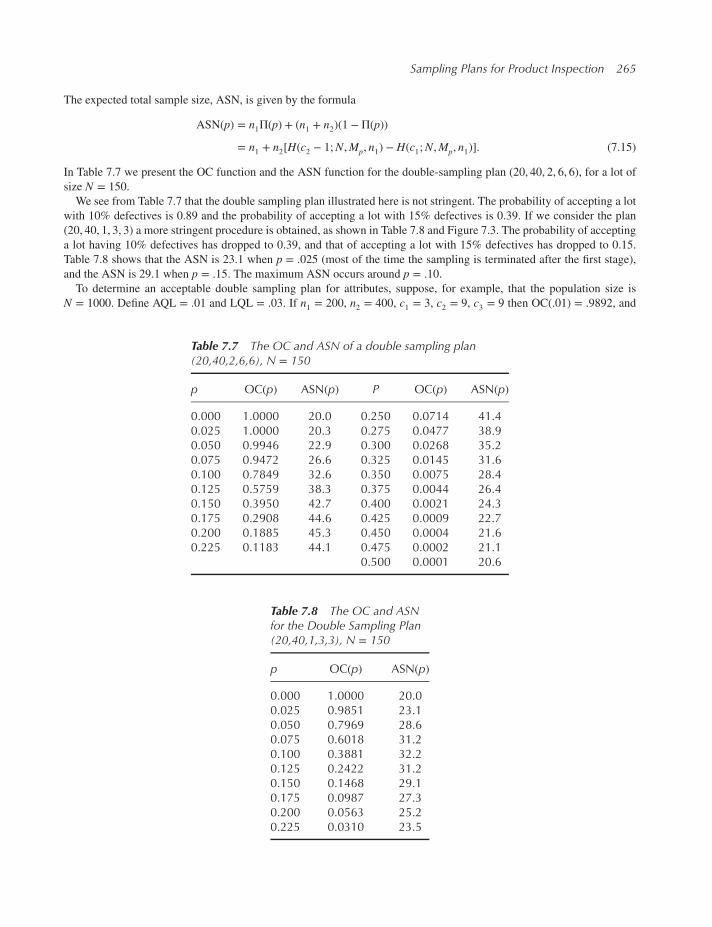
Sampling Plans for Product Inspection 265
The expected total sample size, ASN, is given by the formula
ASN(p) = n1Π(p) + (n1 + n2)(1 − Π(p))
= n1 + n2[H(c2 − 1;N,Mp, n1) − H(c1;N,Mp, n1)]. (7.15)
In Table 7.7 we present the OC function and the ASN function for the double-sampling plan (20, 40, 2, 6, 6), for a lot ofsize N = 150.
We see from Table 7.7 that the double sampling plan illustrated here is not stringent. The probability of accepting a lot
with 10% defectives is 0.89 and the probability of accepting a lot with 15% defectives is 0.39. If we consider the plan
(20, 40, 1, 3, 3) a more stringent procedure is obtained, as shown in Table 7.8 and Figure 7.3. The probability of accepting
a lot having 10% defectives has dropped to 0.39, and that of accepting a lot with 15% defectives has dropped to 0.15.
Table 7.8 shows that the ASN is 23.1 when p = .025 (most of the time the sampling is terminated after the first stage),
and the ASN is 29.1 when p = .15. The maximum ASN occurs around p = .10.To determine an acceptable double sampling plan for attributes, suppose, for example, that the population size is
N = 1000. Define AQL = .01 and LQL = .03. If n1 = 200, n2 = 400, c1 = 3, c2 = 9, c3 = 9 then OC(.01) = .9892, and
Table 7.7 The OC and ASN of a double sampling plan(20,40,2,6,6), N = 150
p OC(p) ASN(p) P OC(p) ASN(p)
0.000 1.0000 20.0 0.250 0.0714 41.40.025 1.0000 20.3 0.275 0.0477 38.90.050 0.9946 22.9 0.300 0.0268 35.20.075 0.9472 26.6 0.325 0.0145 31.60.100 0.7849 32.6 0.350 0.0075 28.40.125 0.5759 38.3 0.375 0.0044 26.40.150 0.3950 42.7 0.400 0.0021 24.30.175 0.2908 44.6 0.425 0.0009 22.70.200 0.1885 45.3 0.450 0.0004 21.60.225 0.1183 44.1 0.475 0.0002 21.1
0.500 0.0001 20.6
Table 7.8 The OC and ASNfor the Double Sampling Plan(20,40,1,3,3), N = 150
p OC(p) ASN(p)
0.000 1.0000 20.00.025 0.9851 23.10.050 0.7969 28.60.075 0.6018 31.20.100 0.3881 32.20.125 0.2422 31.20.150 0.1468 29.10.175 0.0987 27.30.200 0.0563 25.20.225 0.0310 23.5

266 Modern Industrial Statistics
OC(.03) = .1191. Thus, 𝛼 = .011 and 𝛽 = .119. The double-sampling plan with n1 = 120, n2 = 240, c1 = 0, c2 = c3 = 7
yields 𝛼 = .044 and 𝛽 = .084. For the last plan, the expected sample sizes are ASN(.01) = 294 and ASN(.03) = 341.
These expected sample sizes are smaller than the required sample size of n = 355 in a single-stage plan. Moreover, with
high probability, if p ≤ p0 or p ≥ pt, the sampling will terminate after the first stage with only n1 = 120 observations. This
is a factor of threefold decrease in the sample size, over the single sampling plan. There are other double-sampling plans
which can do even better.
If the lot is very large, and we use large samples in stage one and stage two, the formulae for the OC and ASN function
can be approximated by
OC(p) ≅ Φ(
c1 + 1∕2 − n1p
(n1pq(n1 − n1∕N))1∕2
)+
c2−1∑j=c1+1
[Φ(
j + 1∕2 − n1p
(n1pq(1 − n1∕N))1∕2
)
− Φ(
j − 1∕2 − n1p
(n1pq(1 − n1∕N))1∕2
)]⋅Φ
⎛⎜⎜⎜⎜⎝c3 − j + 1∕2 − n2p(n2pq
(1 −
n2Nn1
))1∕2
⎞⎟⎟⎟⎟⎠; (7.16)
and
ASN(p) = n1 + n2
[Φ(
c2 − 1∕2 − n1p
n1pq(1 − n1∕N))1∕2
)− Φ
(c1 + 1∕2 − n1p
(n1pq(1 − n1∕N))1∕2
)]. (7.17)
In Table 7.9 we present the OC and the ASN functions for double sampling from a population of size N = 1, 000, whenthe parameters of the plan are (100, 200, 3, 6, 6). The exact values thus obtained are compared to the values obtained from
the large sample approximation formulae. In the next section the idea of double sampling is generalized in an attempt to
reach acceptance decisions quicker and therefore at reduced costs.
Table 7.9 The exact and approximate OC andASN functions for the double sampling plan (100,200, 3, 6, 6) N = 1000
OC ASN
p Exact Approx. Exact Approx.
.01 .998 .996 102.4 100.8
.02 .896 .871 112.1 125.1
.03 .657 .621 156.4 163.5
.04 .421 .394 175.6 179.2
.05 .243 .234 174.7 172.2
.06 .130 .134 160.6 155.7
.07 .064 .074 142.7 138.7
.08 .030 .040 127.1 125.1
.09 .014 .021 115.8 115.5

Sampling Plans for Product Inspection 267
7.5 Sequential sampling
Sometimes it is possible to subject a selected item to immediate testing before selecting the next item. Such an on-
line testing environment allows for considerable savings in acceptance sampling procedures. In this situation one can
decide, after each observation, whether sufficient information is available for accepting or rejecting the lot, or whether
an additional item (or items) should be randomly selected and tested. This approach may lead to substantial reductions
in the number of required observations, especially when the proportion of nonconforming items in the lot is very small
or substantially high. For example, from a lot of size N = 5000, a single sampling plan, for 𝛼 = 𝛽 = .05, AQL = .01 andLQL = .05 is (179, 4). Under this plan, if one finds in the sample at least 5 defective items, the lot is rejected. Suppose
that the lot under inspection contains more than 10% defective items. In such a case 5 defective items are expected in
50 observations. We can reject such a lot as soon as we observe 5 defective items and avoid observing all other items.
Sequential sampling procedures allow us to decide, after each observation, whether to continue or terminate sampling.
When stopping occurs, we decide whether to accept or reject the lot.
We present here sequential acceptance sampling by attributes, also known as the Wald sequential probability ratiotest (SPRT), which can guarantee that the sum of the producer’s and consumer’s risks does not exceed the sum of the
preassigned values, 𝛼 and 𝛽. Furthermore, this procedure has the property that, compared to all other procedures with
producer’s and consumer’s risks not greater than 𝛼 and 𝛽, the SPRT has the smallest ASN values at p0 and pt. This isknown as the optimality of the SPRT. For simplicity, we present here the SPRT method for binomial distributions, rather
than the hypergeometric ones. This is valid, when the lot is very large compared to the sample size.
Given n observations, with Xn defectives, the likelihood ratio is defined as the ratio of the binomial p.d.f. b(Xn; n, pt)to b(Xn; n, p0), i.e.,
Λ(Xn; n, p0, pt) =(ptp0
)Xn( 1 − pt1 − p0
)n−Xn. (7.18)
Two critical values, A and B, satisfying 0 < A < B <∞, are selected. The SPRT, with limits (A,B), is a procedure whichterminates sampling at the first n ≥ 1 for which either Λ(Xn; n, p0, pt) ≥ B or Λ(Xn; n, p0, pt) ≤ A. In the first case, the
lot is rejected, while in the second case the lot is accepted. If A < Λ(Xn; n, p0, pt) < B, an additional item is randomly
sampled from the lot. Any specified values of A and B yield risk values 𝛼∗(A,B) and 𝛽∗(A,B), which are the actual
producer’s and consumer’s risks. We can show that if A = 𝛽∕(1 − 𝛼) and B = (1 − 𝛽)∕𝛼 (with both 𝛼 and 𝛽 smaller than
1∕2), then 𝛼∗(A,B) + 𝛽∗(A,B) ≤ 𝛼 + 𝛽. Therefore, it is customary to use these particular critical values. Thus, the SPRT,
with A = 𝛽∕(1 − 𝛼) and B = (1 − 𝛽)∕𝛼, reduces to the following set of rules:
1. Stop sampling and reject the lot if Xn ≥ h2 + sn.2. Stop sampling and accept the lot if Xn ≤ −h1 + sn.3. Continue sampling if −h1 + sn < Xn < h2 + sn.
where
h1 = log
(1 − 𝛼𝛽
)∕ log
pt(1 − p0)p0(1 − pt)
,
h2 = log
(1 − 𝛽𝛼
)∕ log
pt(1 − p0)p0(1 − pt)
, (7.19)
and
s =log
1 − p01 − pt
log
(pt
1 − pt⋅1 − p0p0
) . (7.20)
For example, if p0 = .01, pt = .05, and 𝛼 = 𝛽 = .05, we obtain
h1 = 1.78377

268 Modern Industrial Statistics
h2 = h1, ands = 0.02499.
The SPRT can be performed graphically, by plotting the two boundary lines,
an = −1.78 + .025n
and
rn = 1.78 + .025n.
After each observation, the point (n,Xn) is plotted. As long as the points lie between the parallel lines an and rn sampling
continues. As soon as Xn ≥ rn or Xn ≤ an sampling stops and the proper action is taken. Notice that the smallest number
of observations required for reaching the acceptance region is n0 = [h1∕s] + 1 and the smallest number needed to reach
the rejection region is
n1 = [h2∕(1 − s)] + 1. (7.21)
In the present example n0 = 72 and n1 = 2. This shows that if the first two observations are defectives the lot is immediately
rejected. On the other hand, the lot cannot be accepted before 72 observations, which must be all on conforming items.
To illustrate the use of the SPRT we first determine the acceptance numbers an and the rejection numbers rnWe can illustrate the sequential decision process by simulation. Using R orMINITABwe generate a random sequence of
Bernoulli trials (0’s and 1’s) with a specified probability of 1 (which corresponds to a defective item). The total number of
defects among the first n items in the sample, Xn are then computed. In the following example we illustrate the simulation
of 100 binomial outcomes, with P = .01, and print from left to right the partial sums, Xn.We see that there are no 1’s (defective items) among the first 100 numbers generated at randomwith P = .01. According
to Table 7.10, the SPRT would have stopped sampling after the 72nd observation and accepted the lot.
We now simulate binomial variables with P = .05. The result is given in Table 7.12.
Table 7.10 Acceptance and rejectionboundaries for an SPRT with AQL = .01,LQL = .05, 𝛼 = 𝛽 = .05
sample size (n) accept (an) reject (rn)
1 – 8 – 29 – 48 – 349 – 71 – 472 – 88 0 488 – 111 0 5112 – 128 1 5129 – 151 1 6152 – 168 2 6169 – 191 2 7
Table 7.11 Simulated results of 100 binomial experiments, with n = 1, p = 0.01
0 0 0 0 0 0 0 0 0 0 0 0 0 0 0 0 0 0 0 00 0 0 0 0 0 0 0 0 0 0 0 0 0 0 0 0 0 0 00 0 0 0 0 0 0 0 0 0 0 0 0 0 0 0 0 0 0 00 0 0 0 0 0 0 0 0 0 0 0 0 0 0 0 0 0 0 00 0 0 0 0 0 0 0 0 0 0 0 0 0 0 0 0 0 0 0

Sampling Plans for Product Inspection 269
Table 7.12 Simulated results of 100 binomialexperiments, with n = 1, p = 0.05
Partial Sums, Xn (Count)
0 0 0 0 0 (5)0 0 0 0 0 (10)0 0 0 0 0 (15)0 1 1 1 1 (20)1 1 1 1 1 (25)1 1 1 1 1 (30)1 2 2 2 2 (35)2 2 3 3 3 (40)3 3 3 3 3 (45)3 4 4 4 4 (50)4 4 4 4 4 (55)4 4 4 4 4 (60)4 5 5 5 5 (65)5 5 5 5 5 (70)5 5 5 5 5 (75)5 5 5 5 5 (80)5 5 5 5 5 (85)5 5 5 5 5 (90)5 5 5 5 5 (95)5 5 5 5 5 (100)
Here we see that Xn = rn for the first time at n = 38. Accordingly, the SPRT would have stopped sampling and rejected
the lot after 38 observations. It can be proven theoretically that every SPRT stops, sooner or later, and a decision is reached.
An SPRT can be characterized by computing its OC and ASN functions. The OC function provides the points
(p, OC(p)). We can express these points as functions of a parameter 𝜏, according to the following two formulas:
p(𝜏) =1 −
(1 − pt1 − p0
)𝜏(ptp0
)𝜏−(1 − pt1 − p0
)𝜏 , (7.22)
and
OC(p(𝜏)) =
(1 − 𝛽𝛼
)𝜏− 1(
1 − 𝛽𝛼
)𝜏−(𝛽
1 − 𝛼
)𝜏 . (7.23)
For 𝜏 = 1 we obtain p(1) = p0 and for 𝜏 = −1 we obtain p(−1) = pt. We can also show that for 𝜏 = 0, p(0) = s. InTable 7.13, we provide the OC function, computed according to the two formulas above for the SPRT, with p0 = 0.01,pt = 0.05, and 𝛼 = 𝛽 = 0.05.
The ASN function of an SPRT is given by the formula
ASN(p) =OC(p) log
(𝛽
1 − 𝛼
)+ (1 − OC(p)) log
(1 − 𝛽𝛼
)p log (pt∕p0) + (1 − p) log ((1 − pt)∕(1 − p0))
, (7.24)
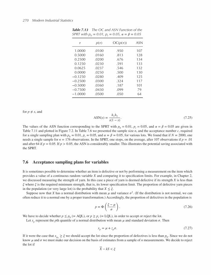
270 Modern Industrial Statistics
Table 7.13 The OC and ASN Function of theSPRT with p0 = 0.01, pt = 0.05, 𝛼 = 𝛽 = 0.05
𝜏 p(𝜏) OC(p(𝜏)) ASN
1.0000 .0100 .950 1070.5000 .0160 .813 1280.2500 .0200 .676 1340.1250 .0230 .591 1330.0625 .0237 .546 1320.0000 .0250 .500 130
−0.1250 .0280 .409 125−0.2500 .0300 .324 117−0.5000 .0360 .187 101−0.7500 .0430 .099 79−1.0000 .0500 .050 64
for p ≠ s, and
ASN(s) =h1h2
s(1 − s). (7.25)
The values of the ASN function corresponding to the SPRT with p0 = 0.01, pt = 0.05, and 𝛼 = 𝛽 = 0.05 are given in
Table 7.11 and plotted in Figure 7.2. In Table 7.6 we presented the sample size n, and the acceptance number c, requiredfor a single sampling plan with p0 = 0.01, pt = 0.05, and 𝛼 = 𝛽 = 0.05, for various lots. We found that if N = 2000, one
needs a single sample for n = 176 observations. In the SPRT, one stops, on the average, after 107 observations if p = .01and after 64 if p = 0.05. If p > 0.05, the ASN is considerably smaller. This illustrates the potential saving associated with
the SPRT.
7.6 Acceptance sampling plans for variables
It is sometimes possible to determine whether an item is defective or not by performing a measurement on the item which
provides a value of a continuous random variable X and comparing it to specification limits. For example, in Chapter 2,
we discussed measuring the strength of yarn. In this case a piece of yarn is deemed defective if its strength X is less than
𝜉 where 𝜉 is the required minimum strength, that is, its lower specification limit. The proportion of defective yarn pieces
in the population (or very large lot) is the probability that X ≤ 𝜉.Suppose now that X has a normal distribution with mean 𝜇 and variance 𝜎2. (If the distribution is not normal, we can
often reduce it to a normal one by a proper transformation.) Accordingly, the proportion of defectives in the population is
p = Φ(𝜉 − 𝜇𝜎
). (7.26)
We have to decide whether p ≤ p0 (= AQL), or p ≥ pt (= LQL), in order to accept or reject the lot.
Let xp represent the pth quantile of a normal distribution with mean 𝜇 and standard deviation 𝜎. Then
xp = 𝜇 + zp𝜎. (7.27)
If it were the case that xp0 ≥ 𝜉 we should accept the lot since the proportion of defectives is less than p0. Since we do notknow 𝜇 and 𝜎 we must make our decision on the basis of estimates from a sample of nmeasurements. We decide to reject
the lot if
X − kS < 𝜉

Sampling Plans for Product Inspection 271
0.00 0.10 0.20
0.0
0.4
0.8
Fraction Nonconforming p
Pro
ba
bili
ty o
f A
cce
pta
nce
OC Curve
0.00 0.10 0.20
20
60
10
0
Fraction Nonconforming p
Ave
rag
e s
am
ple
siz
e
Maximum ASN = 134
0.00 0.10 0.20
0.0
00
0.0
06
0.0
12
Fraction Nonconforming p
AO
Q
AOQL = 0.01375
Figure 7.2 The OC curve and the ASN curve of the SPRT with p0 = 0.01, pt = 0.05, and 𝛼 = 𝛽 = 0.05
and accept the lot if
X − kS ≥ 𝜉.Here, X and S are the usual sample mean and standard deviation, respectively. The factor k is chosen so that the producer’srisk (the risk of rejecting a good lot) does not exceed 𝛼. Values of the factor k are given approximately by the formula
k.= t1−𝛼,p0 ,n
where
t1−a,b,n =z1−b
1 − z21−a∕2n
+
z1−a
(1 +
z2b2−z21−a
2n
)1∕2
√n(1 − z2
1−a∕2n). (7.28)
The OC function of such a test is given approximately (for large samples), by
OC(p) ≈ 1 − Φ
((zp + k)∕
√n
(1 + k2∕2)1∕2
), (7.29)
where k = t1−𝛼,p,n. We can thus determine n and k so that
OC(p0) = 1 − 𝛼
and
OC(pt) = 𝛽.

272 Modern Industrial Statistics
These two conditions yield the equations (zpt + k
)√n = z1−𝛽
(1 + k2∕2
)1∕2and (7.30)(
zp0 + k)√
n = z𝛼(1 + k2∕2
)1∕2.
The solution for n and k yields:
n =(z1−𝛼 + z1−𝛽
)2(1 + k2∕2)(zpt − zp0
)2, (7.31)
and
k =(zpt z𝛼 + zp0z𝛽
)∕(z1−𝛼 + z1−𝛽
). (7.32)
In other words, if the sample size n is given by the above formula, we can replace t1−𝛼,p,n by the simpler term k, and acceptthe lot if
X − kS ≥ 𝜉.The statistic X − kS is called a lower tolerance limit.
Example 7.1. Consider the example of testing the compressive strength of concrete cubes presented in Chapter 2. It is
required that the compressive strength be larger than 240[kg/cm2]. We found that Y = ln X had an approximately normal
distribution. Suppose that it is required to decide whether to accept or reject this lot with the following specifications:
p0 = 0.01, pt = 0.05, and 𝛼 = 𝛽 = 0.05. According to the normal distribution
zp0 = −2.326, zpt = −1.645
and
z1−𝛼 = z1−𝛽 = 1.645.
Thus, according to the above formulas, we find k = 1.9855 and n = 70. Hence with a sample size of 70, we can accept
the lot if Y − 1.9855S ≥ 𝜉 where 𝜉 = ln (240) = 5.48. ◾
The sample size required in this single-stage sampling plan for variables is substantially smaller than the one we deter-
mined for the single-stage sampling plan for attributes (which was n = 176). However, the sampling plan for attributes is
free of any assumption about the distribution of X, while in the above example we had to assume that Y = ln X is normally
distributed. Thus, there is a certain trade-off between the two approaches. In particular, if our assumptions concerning the
distribution of X are erroneous, we may not have the desired producer’s and consumer’s risks.
The above procedure of acceptance sampling for variables can be generalized to upper and lower tolerance limits,double sampling, and sequential sampling. The interested reader can find more information on the subject in Duncan
(1986, Chapters 12–15). Fuchs and Kenett (1988) applied tolerance limits for the appraisal of ceramic substrates in the
multivariate case.
7.7 Rectifying inspection of lots
Rectifying inspection plans are those plans which call for a complete inspection of a rejected lot for the purpose of
replacing the defectives by non-defective items. (Lots which are accepted are not subjected to rectification.) We shall
assume that the tests are non-destructive, that all the defective items in the sample are replaced by good ones, and that the
sample is replaced in the lot.

Sampling Plans for Product Inspection 273
If a lot contains N items and has a proportion p of defectives before the inspection, the proportion of defectives in the
lot after inspection is
p′ =
{0, if lot is rejected,
p(N − X)∕N, if lot is accepted,(7.33)
where X is the number of defectives in the sample. If the probability of accepting a lot by a given sampling plan, is OC(p),then the expected proportion of outgoing defectives is, when sampling is single stage by attribute,
E{p′} = pOC(p)(1 − n
NR∗s
), (7.34)
where
R∗s =
H(c − 1;N − 1, [Np] − 1, n − 1)H(c;N, [Np], n)
. (7.35)
If n∕N is small, then
E{p′} ≅ pOC(p). (7.36)
The expected value of p′ is called the Average Outgoing Quality, and is denoted by AOQ.
The formula for R∗s depends on the method of sampling inspection. If the inspection is by double sampling, the formula
is considerably more complicated. In Table 7.14 we present the AOQ values corresponding to a rectifying plan, when
N = 1000, n = 250 and c = 5.
The AOQL (Average Outgoing Quality Limit) of a rectifying plan is defined as the maximal value of AOQ. Thus the
AOQL corresponding to the plan of Table 7.14 is approximately .01. TheAOQgiven is presented graphically in Figure 7.3.
We also characterize a rectifying plan by the average total inspection (ATI) associated with a given value of p. If alot is accepted, only n items (the sample size) have been inspected, while if it is rejected, the number of items inspected
is N. Thus,
ATI(p) = nOC(p) + N(1 − OC(p))
= n + (N − n)(1 − OC(p)). (7.37)
This function increases from n (when p = 0) to N (when p = 1).
In our example, the lot contains N = 1000 items and the sample size is n = 250. The graph of the ATI function is
presented in Figure 7.4.
Dodge and Romig (1959) published tables for the design of single and double sampling plans for attributes, for which
the AOQL is specified and the ATI is minimized at a specified value of p. Table 7.15, we provide a few values of n and cfor such a single sampling plan, for which the AOQL = .01.
According to Table 7.15, for a lot of size 2000, to guarantee an AOQL of 1% and minimal ATI at p = .01 one needs a
sample of size n = 180, with c = 3. For another method of determining n and c, see Duncan (1986, Chapter 16).
Rectifying sampling plans with less than 100% inspection of rejected lots have been developed and are available in the
literature.
Table 7.14 AOQ values for rectifying planN = 1000, n = 250, c = 5
p OC(p) R∗s AOQ
.005 1.000 1.0000 .004
.010 .981 .9710 .007
.015 .853 .8730 .010
.020 .618 .7568 .010
.025 .376 .6546 .008
.030 .199 .5715 .005
.035 .094 .5053 .003
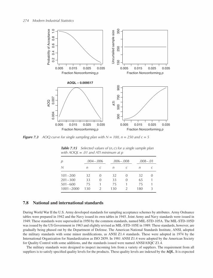
274 Modern Industrial Statistics
0.005 0.015 0.025 0.035
0.2
0.4
0.6
0.8
1.0
Fraction Nonconforming p
Pro
ba
bili
ty o
f A
cce
pta
nce
0.005 0.015 0.025 0.035
15
02
50
35
0
Fraction Nonconforming p
Un
cu
rta
iled
sa
mp
le s
ize
0.005 0.015 0.025 0.035
0.0
04
0.0
07
Fraction Nonconforming p
AO
Q
AOQL = 0.009517
0.005 0.015 0.025 0.035
30
05
00
70
09
00
Fraction Nonconforming p
AT
I
Figure 7.3 AOQ curve for single sampling plan with N = 100, n = 250 and c = 5
Table 7.15 Selected values of (n, c) for a single sample planwith AOQL = .01 and ATI minimum at p
p .004–.006 .006–.008 .008–.01
N n c n c n c
101–200 32 0 32 0 32 0201–300 33 0 33 0 65 1501–600 75 1 75 1 75 11001–2000 130 2 130 2 180 3
7.8 National and international standards
During World War II the U.S. Army developed standards for sampling acceptance schemes by attributes. Army Ordnance
tables were prepared in 1942 and the Navy issued its own tables in 1945. Joint Army and Navy standards were issued in
1949. These standards were superseded in 1950 by the common standards, named MIL-STD-105A. The MIL-STD-105D
was issued by the US Government in 1963 and slightly revised as MIL-STD-105E in 1989. These standards, however, are
gradually being phased out by the Department of Defense. The American National Standards Institute, ANSI, adopted
the military standards with some minor modifications, as ANSI Z1.4 standards. These were adopted in 1974 by the
International Organization for Standardization as ISO 2859. In 1981 ANSI Z1.4 were adopted by the American Society
for Quality Control with some additions, and the standards issued were named ANSI/ASQC Z1.4.
The military standards were designed to inspect incoming lots from a variety of suppliers. The requirement from all
suppliers is to satisfy specified quality levels for the products. These quality levels are indexed by the AQL. It is expected

Sampling Plans for Product Inspection 275
Figure 7.4 ATI curve for single sampling plan with N = 100, n = 250 and c = 5 (MINITAB)
that a supplier sends in continuously series of lots (shipments). All these lots are subjected to quality inspection. At the
beginning an AQL value is specified for the product. The type of sampling plan is decided (single, double, sequential,
etc.). For a given lot size and type of sampling, the parameters of the sampling procedure are determined. For example,
if the sampling is single stage by attribute, the parameter (n, c) are read from the tables. The special feature of the MIL-
STD-105E is that lots can be subjected to normal, tightened or reduced inspection. Inspection starts at a normal level. If
two out of five consecutive lots have been rejected, a switch to tightened inspection level takes place. Normal inspection
is reinstituted if five consecutive lots have been accepted. If ten consecutive lots remain under tightened inspection an
action may take place to discontinue the contract with the supplier. On the other hand, if the last ten lots have all been
accepted at a normal inspection level, and the total number of defective units found in the samples from these ten lots is
less than a specified value, then a switch from normal to reduced inspection level can take place.
We do not reproduce here the MIL-STD-105 tables. The reader can find detailed explanation and examples in Duncan
(1986, Chapter 10). We conclude with the following example.
Suppose that for a given product AQL= 0.01 (1%). The size of the lots isN = 1, 000. Themilitary standard specifies that
a single stage sampling for attributes, under normal inspection, has the parameters n = 80 and c = 2. Applying MINITAB
yields the following OC values for this plan.
p 0.01 0.02 0.03 0.04 0.05
OC(p) 0.961 0.789 0.564 0.365 0.219
Thus, if the proportion of nonconforming, p, of the supplier is less than AQL, the probability of accepting a lot is larger
than 0.961. A supplier which continues to ship lots with p = 0.01, has a probability of (0.961)10 = 0.672 that all the 10
lots will be accepted, and the inspection level will be switched to a reduced one. Under the reduced level, the sample size
from the lot is reduced to n = 32. The corresponding acceptance number is c = 1. Thus, despite the fact that the level of
quality of the supplier remains good, there is a probability of 0.33 that there will be no switch to reduced inspection level
after the tenth lot. On the other hand, the probability that there will be no switch to tightened level of inspection before the

276 Modern Industrial Statistics
sixth lot is inspected is 0.9859. This is the probability that after each inspection the next lot will continue to be inspected
under normal level. If there is no deterioration in the quality level of the supplier, and p = 0.03, the probability that the
inspection level will be switched to “tightened” after five inspections is 0.722.
7.9 Skip-lot sampling plans for attributes
We have seen in the previous section that according to the MIL-STD-105E, if a supplier keeps shipping high quality
lots, then after a while his lots are subjected to inspection under reduced level. All lots are inspected under a reduced
level inspection scheme, as long as their quality level remains high. The Skip-Lot Sampling Plans (SLSP), which was
proposed by Liebesman and Saperstein (1983), introduces a new element of savings if lots continue to have very low
proportions of nonconforming items. As we will see below, instead of just reduced level of inspection of high quality
lots, the SLSP plans do not necessarily inspect such lots. If the lots coming in from a given supplier qualify for skipping,
then they are inspected only with probability 0.5. This probability is later reduced to 0.33 and to 0.2, if the inspected lots
continue to be almost free of nonconforming items. Thus, suppliers which continue to manufacture their product, with
proportion defectives p, considerably smaller than the specified AQL stand a good chance of having only a small fraction
of their lots inspected. The SLSP which will be specified below was adopted as the ISO2859/3 Standard in 1986.
7.9.1 The ISO 2859 skip-lot sampling procedures
A SLSP has to address three main issues:
1. What are the conditions for beginning or reinstating the Skip-Lot (SL) state?
2. What is the fraction of lots to be skipped?
3. Under what conditions should one stop skipping lots, on a temporary or permanent basis?
The fraction of lots to be skipped is the probability that a given lot will not be inspected. If this probability for example
is 0.8, we generate a random number, U, with uniform distribution on (0, 1). If U < 0.8, inspection is skipped; otherwisethe lot is inspected.
We define three states:
State 1. Every lot is inspected.
State 2. Some lots are skipped and not inspected.
State 3. All lots are inspected, pending a decision of disqualification (back to state 1) or resumption of SL (back to state 2).
Lot by lot inspection is performed during state 3, but the requirements to requalify for skip lot inspection are less stringent
than the initial qualification requirements.
Switching rules apply to 4 transitions between states: Qualification (State 1 to State 2), Interruption (State 2 to State 3),
Resumption (State 3 to State 2), Disqualification (State 3 to State 1).
The switching rules for the SLSP procedure are listed below.
7.9.1.1 Skip-Lot Switching Rules
We specify here the rules appropriate for single sampling by attributes. Other rules are available for other sampling
schemes.
A. Qualification. (State 1→ State 2).
1. Ten consecutive lots are accepted.
2. Total number of defective items in the samples from the ten lots is smaller than critical level given in Table 7.16.

Sampling Plans for Product Inspection 277
3. Number of defective items in each one of the last two lots is smaller than the values specified in Table 7.17.
4. Supplier has a stable manufacturing organization, continuous production and other traits which qualify him to be
high quality stable manufacturer.
B. Interruption. (State 2→ State 3)
1. An inspected lot has in the sample more defectives than specified in Table 7.17.
C. Resumption. (State 3→ State 2)
1. Four consecutive lots are accepted.
2. The last two lots satisfy the requirements of Table 7.17.
D. Disqualifications. (State 3→ State 1)
1. Two lots are rejected within ten consecutively inspected lots; or
2. Violation of the supplier qualification criteria (item A4 above).
We have seen in the previous section that, under normal inspection, MIL-STD-105E specifies that, for AQL = 0.01 and
lots of size N = 1, 000 random samples of size n = 80 should be drawn. The critical level was c = 2. If 10 lots have been
accepted consecutively, the total number of observed defectives is S10 ≤ 20. The total sample size is 800 and according
to Table 7.16, S10 should not exceed 3 to qualify for a switch to State 2. Moreover, according to Table 7.17, the last two
samples should each have less than 1 defective item. Thus, the probability to qualify for State 2, on the basis of the last
10 samples, when p = AQL = 0.01 is
QP = b2(0; 80, 0.01) B(3; 640, 0.01)
= (0.4475)2 × 0.1177 = 0.0236.
Table 7.16 Minimum cumulative sample size in ten lots for skip-lot qualifications
Cumulative No.of Defectives
AQL(%)
0.65 1.0 1.5 2.5 4.0 6.5 10.0
0 400 260 174 104 65 40 261 654 425 284 170 107 65 432 883 574 383 230 144 88 573 1098 714 476 286 179 110 714 1306 849 566 340 212 131 855 1508 980 653 392 245 151 986 1706 1109 739 444 277 171 1117 1902 1236 824 494 309 190 1248 2094 1361 907 544 340 209 1369 2285 1485 990 594 371 229 14910 2474 1608 1072 643 402 247 16111 2660 1729 1153 692 432 266 17312 2846 1850 1233 740 463 285 18513 3031 1970 1313 788 493 303 19714 3214 2089 1393 836 522 321 20915 3397 2208 1472 883 552 340 22116 3578 2326 1550 930 582 358 23317 3758 2443 1629 977 611 376 24418 3938 2560 1707 1024 640 394 25619 4117 2676 1784 1070 669 412 26820 4297 2793 1862 1117 698 430 279

278 Modern Industrial Statistics
Table 7.17 Individual lot acceptance numbers for skip-lot qualification
Sample Size AQL(%)
0.65 1.0 1.5 2.5 4.0 6.5 10.0
2 – – – – – 0 03 – – – – 0 0 05 – – – 0 0 0 18 – – 0 0 0 1 1
13 – 0 0 0 1 1 220 0 0 0 1 1 2 332 0 0 1 1 2 3 550 0 1 1 2 3 5 780 1 1 2 3 5 7 11
125 1 2 3 4 7 11 16200 2 3 4 7 11 17 25315 3 4 7 11 16 25 38500 5 7 10 16 25 39 58800 7 11 16 25 38 60 91
1250 11 16 23 38 58 92 1382000 17 25 36 58 91 144 217
Thus, if the fraction defectives level is exactly at the AQL value, the probability for qualification is only 0.02. On the other
hand, if the supplier maintains the production at fraction defective of p = 0.001, then the qualification probability is
QP = b2(0; 80, 0.001) B(3; 640, 0.001)
= (0.9231)2 × 0.9958 = 0.849.
Thus, a supplier who maintains a level of p = 0.001, when the AQL = 0.01, will probably be qualified after the first
ten inspections and will switch to State 2 of skipping lots. Eventually only 20% of his lots will be inspected, under this
SLSP standard, with high savings to both producer and consumer. This illustrates the importance of maintaining high
quality production processes. In Chapters 10 and 11 we will study how to statistically control the production processes,
to maintain stable processes of high quality. Generally, for the SLSP to be effective, the fraction defectives level of the
supplier should be smaller than half of the AQL. For p level close to the AQL, the SLSP and the MIL-STD 105E are very
similar in performance characteristics.
7.10 The Deming inspection criterion
Deming (1982) has derived a formula to express the expected cost to the firm caused by sampling of lots of incoming
material. Let us define
N = number of items in a lot
k1 = cost of inspecting one item at the beginning of the process
q = probability of a conforming item
p = probability of a nonconforming item
Q = OC(p) = probability of accepting a lot
k2 = cost to the firm when one nonconforming item is moved downstream to a customer or to the next stage of
the production process
p′′ = the probability of nonconforming items being in an accepted lot
n = the sample size inspected from a lot of size N.

Sampling Plans for Product Inspection 279
Thus, the total expected cost per lot is
EC = (Nk1∕q)[1 + Qq{(k2∕k1)p′′ − 1}{1 − n∕N}] (7.38)
If (k2∕k1)p′′ > 1 then any sampling plan increases the cost to the firm and n = N (100% inspection) becomes the least
costly alternative.
If (k2∕k1)p′′ < 1 then the value n = 0 yields the minimum value of EC so that no inspection is the alternative of choice.
Now p′′ can be only somewhat smaller than p. For example if N = 50, n = 10, c = 0 and p = 0.04 then p′′ = 0.0345.Substituting p for p′′ gives us the following rule
If(k2∕k1)p > 1 inspect every item in the lot
If(k2∕k1)p < 1 accept the lot without inspection.
The Deming assumption is that the process is under control and that p is known. Sampling plans such as MIL-STD-105D
do not make such assumptions and, in fact, are designed for catching shifts in process levels.
To keep the process under control Deming suggests the use of control charts and Statistical Process Control (SPC)
procedures which are discussed in Chapters 10 and 11.
The assumption that a process is under control means that the firm has absorbed the cost of SPC as internal overhead
or as a piece-cost. Deming’s assertion then is that assuming upfront the cost of SPC implementation is cheaper, in the
long run, than doing business in a regime where a process may go out of control undetected until its output undergoes
acceptance sampling.
The next chapter will introduce the reader to basic tools and principles of Statistical Process Control.
7.11 Published tables for acceptance sampling
In this section we list some information on published tables and schemes for sampling inspection by attribute and by vari-
ables. The material given here follows Chapters 24–25 of Juran (1979). We shall not provide explanation here concerning
the usage of these tables. The interested practitioner can use the instructions attached to the tables and/or read more about
the tables in Juran (1979), Chapters 24–25, or in Duncan (1982).
I. Sampling by Attributes
1.MIL-STD-105E (reproduced as ANSI/ISO Z1.4)Type of sampling: Single, double and multiple.
Type of application: General.
Key features: Maintains average quality at a specified level. Aims to minimize rejection of good lots. Provides single
sampling plans for specified AQL and producer’s risk.
Reference: MIL-STD-105E, Sampling Procedures and Tables for Inspection by Attributes, Government Printing
Office, Washington, D.C.
2. Dodge-RomigType of sampling: Single and double.
Type of application: Where 100% rectifying of lots is applicable.
Key features: One type of plan uses a consumer’s risk of 𝛽 = 0.10. Another type limits the AOQL. Protection is
provided with minimum inspection per lot.
Reference: Dodge, H.F. and Romig, H.G. (1959).
3. H107Type of sampling: Continuous single stage.
Type of application: When production is continuous and inspection is non-destructive.
Key features: Plans are indexed byAQL, which generally start with 100% inspection until some consecutive number of
units free of defects are found. Then inspection continues on a sampling basis until a specified number of defectives
are found.

280 Modern Industrial Statistics
Reference: H-107, Single-Level Continuous Sampling Procedures and Tables For Inspection by Attribute, Government
Printing Office, Washington, D.C.
II. Sampling by Variables1.MIL-STD-414 (reproduced as ANSI/ISO Z1.9)Assumed distribution: Normal.
Criteria specified: AQL.
Features: Lot evaluation by AQL. Includes tightened and reduced inspection.
Reference: MIL-STD-414, Sampling Procedures and Tables for Inspection by Variables for Percent Defectives, Gov-ernment Printing Office, Washington, D.C.
2. H-108Assumed distribution: Exponential.
Criteria specified: Mean Life (MTBF).
Features: Life testing for reliability specifications.
Reference: H-108, Sampling Procedures and Tables for Life and Reliability Testing (Based on Exponential Distri-bution), U.S. Department of Defense, Quality Control and Reliability Handbook, Government Printing Office,
Washington, D.C.
7.12 Chapter highlights
Traditional supervision consists of keeping close control of operations and progress. The focus of attention is the product
or process outputs. A direct implication of this approach is to guarantee product quality through inspection screening. The
chapter discusses sampling techniques and measures of inspection effectiveness. Performance characteristics of sampling
plans are discussed and guidelines for choosing economic sampling plans are presented. The basic theory of single-
stage acceptance sampling plans for attributes is first presented including the concepts of Acceptable Quality Level and
Limiting Quality Level. Formulas for determining sample size, acceptance levels and Operating Characteristic functions
are provided. Moving on from single-stage sampling the chapter covers double-sampling and sequential sampling using
Wald’s sequential probability ratio test. One section deals with acceptance sampling for variable data. Other topics covered
include computations of Average Sample Numbers and Average Total Inspection for rectifying inspection plans. Modern
Skip-Lot sampling procedures are introduced and compared to the standard application of sampling plans where every
lot is inspected. The Deming “all or nothing” inspection criterion is presented and the connection between sampling
inspection and statistical process control is made. Throughout the chapter we refer to MINITAB and R applications which
are used to perform various calculations and generate appropriate tables and graphs. The main concepts and definitions
introduced in this chapter include:
• Lot
• Acceptable Quality Level
• Limiting Quality Level
• Producer’s Risk
• Consumer’s Risk
• Single Stage Sampling
• Acceptance Number
• Operating Characteristic
• Double Sampling Plan
• ASN Function
• Sequential Sampling
• Sequential Probability Ratio Test (SPRT)
• Rectifying Inspection
• Average Outgoing Quality (AOQ)

Sampling Plans for Product Inspection 281
• Average Total Inspection (ATI)
• Tightened, Normal or Reduced Inspection Levels
• Skip-Lot Sampling Plans
7.13 Exercises
7.1 Determine single sampling plans for attributes, when the lot is N = 2, 500, 𝛼 = 𝛽 = 0.01, and(i) AQL = 0.005, LQL = 0.01(ii) AQL = 0.01, LQL = 0.03(iii) AQL = 0.01, LQL = 0.05
7.2 Investigate how the lot size,N, influences the single sampling plans for attributes, when 𝛼 = 𝛽 = 0.05, AQL = 0.01,LQL = 0.03, by computing the plans for N = 100, N = 500, N = 1, 000, N = 2, 000.
7.3 Compute the OC(p) function for the sampling plan computed in Exercise 7.1 (iii). What is the probability of
accepting a lot having 2.5% of nonconforming items?
7.4 Compute the large sample approximation to a single sample plan for attributes (n∗, c∗), with 𝛼 = 𝛽 = .05 and
AQL = .025, LQL = .06. Compare these to the exact results. The lot size is N = 2, 000.7.5 Repeat the previous exercise with N = 3, 000, 𝛼 = 𝛽 = 0.10, AQL = .01 and LQL = .06.7.6 Obtain the OC and ASN functions of the double sampling plan, with n1 = 200, n2 = 2n1 and c1 = 5, c2 = c3 = 15,
when N = 2, 000.(i) What are the attained 𝛼 and 𝛽 when AQL = 0.015 and LQL = 0.05?(ii) What is the ASN when p = AQL?(iii) What is a single sampling plan having the same 𝛼 and 𝛽? How many observations do we expect to save if
p = AQL? Notice that if p = LQL the present double sampling plan is less efficient than the corresponding
single sampling plan.
7.7 Compute the OC and ASN values for a double sampling plan with n1 = 150, n2 = 200, c1 = 5, c2 = c3 = 10, when
N = 2, 000. Notice how high 𝛽 is when LQL = 0.05. The present plan is reasonable if LQL = 0.06. Compare this
plan to a single sampling one for 𝛼 = 0.02 and 𝛽 = 0.10, AQL = 0.02, LQL = 0.06.7.8 Determine a sequential plan for the case of AQL = 0.02, LQL = 0.06, 𝛼 = 𝛽 = .05. Compute the OC and ASN
functions of this plan. What are the ASN values when p = AQL, p = LQL and p = 0.035?7.9 Compare the single sampling plan and the sequential one when AQL = 0.01, LQL = 0.05, 𝛼 = 𝛽 = 0.01 and N =
10, 000. What are the expected savings in sampling cost, if each observation costs $1, and p = AQL?7.10 Determine n and k for a continuous variable size sampling plan, when (p0) = AQL = .01 and (pt) = LQL = .05,𝛼 = 𝛽 = 0.05.
7.11 Consider data file ALMPIN.csv. An aluminum pin is considered as defective if its cap diameter is smaller than
14.9 [mm]. For the parameters p0 = 0.01, 𝛼 = 0.05, compute k and decide whether to accept or reject the lot, on
the basis of the sample of n = 70 pins. What is the probability of accepting a lot with proportion defectives of
p = 0.03?7.12 Determine the sample size and k for a single sampling plan by a normal variable, with the parameters AQL = 0.02,
LQL = 0.04, 𝛼 = 𝛽 = 0.10.7.13 A single sampling plan for attributes, from a lot of size N = 500, is given by n = 139 and c = 3. Each lot which
is not accepted is rectified. Compute the AOQ, when p = 0.01, p = 0.02, p = 0.03 and p = 0.05. What are the
corresponding ATI values?7.14 A single sampling plan, under normal inspection has probability 𝛼 = 0.05 of rejection, when p = AQL. What is
the probability, when p = AQL in 5 consecutive lots, that there will be a switch to tightened inspection? What is
the probability of switching to a tightened inspection if p increases so that OC(p) = .7?7.15 Compute the probability for qualifying for State 2, in a SKLP, when n = 100, c = 1. What is the upper bound on
S10, in order to qualify for State 2, when AQL = 0.01? Compute the probability QP for State 2 qualification.


Part IIIStatistical Process Control
Statistical Process Control is not new. Implementing it requires, however, a management maturity level that identifies
the opportunities embedded in processes in terms of quality, cost and delivery. Processes are relatively abstract entities,
especially in service industries. Getting management to the third step on the Quality Ladder is not a trivial task and
requires a combination of skills. Deming and Juran have gained the status of quality gurus by convincing management
teams, all over the world, that this makes sense from a business and management point of view. In any case, the tools and
methods described in Part III build on the identification of processes for both control and improvement.
Chapter 8 covers basic issues in statistical process control. After establishing the motivation for statistical process
control, the chapter introduces the reader to process capability studies, process capability indices, the seven tools for
process improvement and the basic Shewhart charts.
Chapter 9 includes more advanced topics such as the economic design of Shewhart control charts and CUSUM proce-
dures. The chapter concludes with special sections on Bayesian detection, process tracking and automatic process control.
Chapter 10 is dedicated to multivariate statistical process control techniques, including multivariate analogues to pro-
cess capability indices.
Modern Industrial Statistics: with applications in R, MINITAB and JMP, Second Edition. Ron S. Kenett and Shelemyahu Zacks.© 2014 John Wiley & Sons, Ltd. Published 2014 by John Wiley & Sons, Ltd.Companion website: www.wiley.com/go/modern_industrial_statistics


8Basic Tools and Principles
of Process Control
8.1 Basic concepts of statistical process control
In this chapter we present the basics of Statistical Process Control (SPC). The general approach is prescriptive and
descriptive rather than analytical. With SPC we do not aim to model the distribution of data collected from a given
process. Our goal is to control the process with the aid of decision rules for signaling significant discrepancies between
the observed data and the standards of a process under control.We demonstrate the application of SPC to various processes
by referring to the examples of piston cycle time and strength of fibers, which were discussed in Chapter 2. Other examples
used include data on power failures in a computer center and office procedures for scheduling appointments of a university
dean. The data on the piston cycle time is generated by the R piston simulator function pistonSimulation or the
JMP addin available for download on the book’s website. In order to study the causes for variability in the piston cycle
time, we present, in Figure 8.1, a sketch of a piston, and, in Table 8.1, seven factors which can be controlled to change
the cycle time of a piston.
Figure 8.2 is a run chart, (also called a “connected line plot”), and Figure 8.3 is a histogram, of 50 piston cycle times
(seconds) measured under stable operating conditions. Throughout the measurement time frame the piston operating
factors remained fixed at their maximum levels. The data can be found in file OTURB1.csv.The average cycle time of the 50 cycles is 0.392 [sec] with a standard deviation of 0.114 [sec].
Even though no changes occurred in the operating conditions of the piston we observe variability in the cycle times.
From Figure 8.2 we note that cycle times vary between 0.22 and 0.69 seconds. The histogram in Figure 8.3 indicates some
skewness in the data. The normal probability plot of the 50 cycle times (Figure 8.4) also leads to the conclusion that the
cycle time distribution is not normal, but skewed.
Another example of variability is provided by the yarn strength data presented in Chapter 2. The yarn strength test
results indicate that there is variability in the properties of the product. High yarn strength indicates good spinning and
weaving performance. Yarn strength is considered a function of the fiber length, fiber fineness and fiber tensile strength.
As a general rule, longer cottons are fine-fibered and shorter cottons coarse-fibered. Very fine fibers, however, tend to
reduce the rate of processing, so that the degree of fiber fineness depends upon the specific end-product use. Variability
in fiber fineness is a major cause of variability in yarn strength and processing time.
Modern Industrial Statistics: with applications in R, MINITAB and JMP, Second Edition. Ron S. Kenett and Shelemyahu Zacks.© 2014 John Wiley & Sons, Ltd. Published 2014 by John Wiley & Sons, Ltd.Companion website: www.wiley.com/go/modern_industrial_statistics

286 Modern Industrial Statistics
Table 8.1 Operating factors of the piston simulator and theiroperational levels
Factor units Minimum Maximum
Piston weight M[Kg] 30 60Piston surface area S[m2] 0.005 .020Initial gas volume V0[m
3] 0.002 .010Spring coeff. K[N/m] 1000 5000Atmosph. pressure P0[N/m2] 9 × 10⁴ 11 × 104
Ambient temperat. T[0K] 290 296Filling gas temperat. T0[
0K] 340 360
Spark Plug
Inlet Valve
Cylinder Head
Cooling Water
Valve Spring
Exhaust Valve
Piston
Connecting Rod
Crankshaft
Figure 8.1 A sketch of the piston
Figure 8.2 Run chart or connected line plot (JMP)) of 50 piston cycle times, [sec]
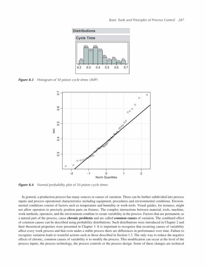
Basic Tools and Principles of Process Control 287
Figure 8.3 Histogram of 50 piston cycle times (JMP)
−2 −1 0 1 2
0.3
0.4
0.5
0.6
0.7
Norm Quantiles
sec.
Figure 8.4 Normal probability plot of 50 piston cycle times
In general, a production process has many sources or causes of variation. These can be further subdivided into process
inputs and process operational characteristics including equipment, procedures and environmental conditions. Environ-
mental conditions consist of factors such as temperature and humidity or work-tools. Visual guides, for instance, might
not allow operators to precisely position parts on fixtures. The complex interactions between material, tools, machine,
work methods, operators, and the environment combine to create variability in the process. Factors that are permanent, as
a natural part of the process, cause chronic problems and are called common causes of variation. The combined effect
of common causes can be described using probability distributions. Such distributions were introduced in Chapter 2 and
their theoretical properties were presented in Chapter 3. It is important to recognize that recurring causes of variability
affect every work process and that even under a stable process there are differences in performance over time. Failure to
recognize variation leads to wasteful actions such as those described in Section 1.3. The only way to reduce the negative
effects of chronic, common causes of variability is to modify the process. This modification can occur at the level of the
process inputs, the process technology, the process controls or the process design. Some of these changes are technical

288 Modern Industrial Statistics
X-bar Chartfor Cycle Time
Group
Gro
up S
um
mary
Sta
tistics
1 2 3 4 5 6 7 8 9 11 13 15 17 19
0.2
50.3
50.4
50.5
5
LCL
UCL
CL
Number of groups = 20
Center = 0.4346598
StdDev = 0.1313959
LCL = 0.2583737
UCL = 0.6109459
Number beyond limits = 0
Number violating runs = 0
Figure 8.5 X-bar chart of cycle times under stable operating conditions
S-Chartfor Cycle Time
Group
Gro
up S
um
mary
Sta
tistics
1 2 3 4 5 6 7 8 9 11 13 15 17 19
0.0
00.0
50.1
00.1
50.2
00.2
5
LCL
UCL
CL
Number of groups = 20Center = 0.1288128StdDev = 0.137037
LCL = 0UCL = 0.2690896
Number beyond limits = 0Number violating runs = 0
Figure 8.6 S-chart of cycle times under stable operating conditions

Basic Tools and Principles of Process Control 289
(e.g. different process settings), some are strategic (e.g. different product specifications) and some are related to human
resources management (e.g. training of operators). Special causes, assignable causes, or sporadic spikes arise from
external temporary sources that are not inherent to the process. These terms are used here interchangeably. For example,
an increase in temperature can potentially affect the piston’s performance. The impact can be both in terms of changes in
the average cycle times and/or the variability in cycle times.
In order to signal the occurrence of special causes we need a control mechanism. Specifically in the case of the piston,
such a mechanism can consist of taking samples or subgroups of 5 consecutive piston cycle times. Within each subgroup
we compute the subgroup average and standard deviation.
Figures 8.5 and 8.6 display charts of the average and standard deviations of 20 samples of 5 cycle time measurements.
To generate these charts with R we use:
> Ps <- pistonSimulation(seed=123)> Ps <- simulationGroup(Ps, 5)> head(Ps, 3)
m s v0 k p0 t t0 seconds group1 60 0.02 0.01 5000 110000 296 360 0.3503785 12 60 0.02 0.01 5000 110000 296 360 0.3901446 1
Z3 60 0.02 0.01 5000 110000 296 360 0.3907803 1
> aggregate(x=Ps["seconds"],by=Ps["group"],FUN=mean)
group seconds1 1 0.36204242 2 0.39381723 3 0.48242214 4 0.31557645 5 0.49289296 6 0.42041127 7 0.38060728 8 0.33660849 9 0.342529310 10 0.3949534
The chart of averages is called an X-bar chart, the chart of standard deviations is called an S-chart. All 100 measurements
were taken under fixed operating conditions of the piston (all factors set at the maximum levels). We note that the average
of cycle time averages is 0.414 seconds and that the average of the standard deviations of the 20 subgroups is 0.12 seconds.
All these numbers were generated by the piston computer simulation model that allows us to change the factors affecting
the operating conditions of the piston. Again we know that no changes were made to the control factors. The observed
variability is due to common causes only, such as variability in atmospheric pressure or filling gas temperature.
We now rerun the piston simulator introducing a forced change in the piston ambient temperature. At the beginning of
the 8th sample, the temperature begins to rise at a rate of 10% per cycle. Can we flag this special cause? The X-bar chart ofthis new simulated data is presented in Figure 8.7. Up to the 7th sample the chart is identical to that of Figure 8.5. At the
8th sample we note a small increase in cycle time. As of the 11th sample, the subgroup averages are consistently above
0.414 seconds. This run persists until the 21st sample when we stopped the simulation. To have 10 points in a row above
the average is unlikely to occur by chance alone. The probability of such an event is (1∕2)10 = 0.00098. The implication
of the 10 points run is that common causes are no longer the only causes of variation, and that a special factor has begun
to affect the piston’s performance. In this particular case we know that it is an increase in ambient temperature. The
S-chart of the same data (Figure 8.8) shows a run below the average of 0.12 beginning at the 8th sample. This indication
occurs earlier than that in the X-bar chart. The information obtained from both charts indicates that a special cause has
been in effect from the 8th sample onward. Its effect has been to increase cycle times and reduce variability. The new
average cycle time appears to be around 0.49 seconds. The Piston Simulator allows us to try other types of changes in the

290 Modern Industrial Statistics
X-bar Chartfor Cycle Time
Group
Gro
up S
um
mary
Sta
tistics
1 3 5 7 9 11 13 15 17 19 21
0.2
50.3
50.4
50.5
5
LCL
UCL
CL
Number of groups = 21
Center = 0.4346598
StdDev = 0.08894158
LCL = 0.2583737
UCL = 0.6109459
Number beyond limits = 0
Number violating runs = 2
Figure 8.7 X-bar chart of cycle times with a trend in ambient temperature
S-Chartfor Cycle Time
Group
Gro
up S
um
mary
Sta
tistics
1 3 5 7 9 11 13 15 17 19 21
0.0
00.0
50.1
00.1
50.2
00.2
5
LCL
UCL
CL
Number of groups = 21
Center = 0.1288128
StdDev = 0.09300534
LCL = 0
UCL = 0.2690896
Number beyond limits = 0
Number violating runs = 6
Figure 8.8 S-chart of cycle times with a trend in ambient temperature

Basic Tools and Principles of Process Control 291
X-bar Chartfor Cycle Time
Group
Gro
up S
um
mary
Sta
tistics
1 3 5 7 9 11 13 15 17 19 21
0.2
50.3
50.4
50.5
5
LCL
UCL
CL
Number of groups = 21
Center = 0.4346598
StdDev = 0.1486899
LCL = 0.2583737
UCL = 0.6109459
Number beyond limits = 0
Number violating runs = 0
Figure 8.9 X-bar chart of cycle times with a trend in spring coefficient precision
operational parameters of the piston. For example, we can change the spring that controls the intake-valve in the piston
gas chamber. In the next simulation, the standard deviation of the spring coefficient is increasing at a 5% rate past the 8th
sample. Figures 8.9 and 8.10 are X-bar and S-charts corresponding to this scenario. Until the 8th sample these charts are
identical to those in Figures 8.5 and 8.6. After the 8th samplechanges appear in the chart. Points 14 and 18 fall outside
the control limits, and it seems that the variability has increased. This is seen also in Figure 8.10. We see that after the 9th
sample, there is a run upward of six points, and points 18 and 19 are way above the upper control limit.
Control charts have wide applicability throughout an organization. Top managers can use a control chart to study varia-
tion in sales and decide on new marketing strategies. Operators can use the same tool to determine if and when to adjust a
manufacturing process. An example with universal applicability comes from the scheduling process of daily appointments
in a university dean’s office. At the end of each working day the various meetings and appointment coordinated by the
office of the dean were classified as being “on time” or with a problem such as “late beginning,” “did not end on time,”
“was interrupted” etc. . . .The ratio of problem appointments to the total number of daily appointments was tracked and
control limits computed. Figure 8.11 is the dean’s control chart (see Kelly, Kenett, Newton, Roodman and Wowk, 1991).
Another example of a special cause is the miscalibration of spinning equipment. Miscalibration can be identified by
ongoing monitoring of yarn strength. Process operators analyzing X-bar and S-charts can stop and adjust the process as
trends develop or sporadic spikes appear. Timely indication of a sporadic spike is crucial to the effectiveness of process
control mechanisms. Ongoing chronic problems, however, cannot be resolved by using local operator adjustments. The
statistical approach to process control allows us to distinguish between chronic problems and sporadic spikes. This is
crucial since these two different types of problems require different approaches. Process control ensures that a process
performs at a level determined “doable” by a process capability study. Section 8.3 discusses how to conduct such studies
and how to set control limits.
So far, we have focused on the analysis of data for process control. Another essential component of process control
is the generation and routing of relevant and timely data through proper feedback loops. We distinguish between two

292 Modern Industrial Statistics
S-Chartfor Cycle Time
Group
Gro
up S
um
mary
Sta
tistics
1197531 13 15 17 19 21
0.0
00.0
50.1
00.1
50.2
00.2
5
LCL
UCL
CL
Number of groups = 21Center = 0.1288128StdDev = 0.1544407
LCL = 0UCL = 0.2690896
Number beyond limits = 0Number violating runs = 0
Figure 8.10 S-chart of cycle times with a trend in spring coefficient precision
Canceletions due to illness
1.5
1.0
0.5
0.0
0 10
Working Days (2/21–5/14/1991)
20 30 40 50
UCL
Figure 8.11 Control chart for proportion of appointments with scheduling problems. Based on a chart preparedby the Dean of the School of Management at SUNY Binghamton
types of feedback loops: External feedback loops and internal feedback loops. An external feedback loop consists of
information gathered at a subsequent downstream process or by direct inspection of the process outputs.
To illustrate these concepts and ideas let us look at the process of driving to work. The time it takes you to get to work
is a variable that depends on various factors such as, how many other cars are on the road, how you happen to catch
the traffic lights, your mood that morning, etc. These are factors that are part of the process, and you have little or no
control over them. Such common causes create variation in the time it takes you to reach work. One day it may take you

Basic Tools and Principles of Process Control 293
15 minutes and the next day 12 minutes. If you are particularly unlucky and had to stop at all the red lights it might take
you 18 minutes. Suppose, however, that on one particular day it took you 45 minutes to reach work. Such a long trip is
outside the normal range of variation and is probably associated with a special cause such as a flat tire, a traffic jam or
road constructions.
External feedback loops rely on measurements of the process outcome. They provide information like looking in a
rear-view mirror. The previous example consisted of monitoring time after you reached work. In most cases identifying
a special cause at that point in time is too late. Suppose that we had a local radio station that provided its listener live
coverage of the traffic conditions. If we monitor, on a daily basis, the volume of traffic reported by the radio, we can avoid
traffic jams, road constructions and other unexpected delays. Such information will help us eliminate certain special
causes of variation. Moreover, if we institute a preventive maintenance program for our car we can eliminate many types
of engine problems, further reducing the impact of special causes. To eliminate the occasional flat tire would involve
improvements in road maintenance–a much larger task. The radio station is a source of internal feedback that provides
information that can be used to correct your route, and thus arrive at work on time almost every day. This is equivalent to
driving the process while looking ahead. Most drivers are able to avoid getting off the road, even when obstacles present
themselves unexpectedly. We now proceed to describe how control charts are used for “staying on course.”
Manufacturing examples consist of physical dimensions of holes drilled by a numerically controlled CNC machine,
piston cycle times or yarn strength. The finished part leaving a CNC machine can be inspected immediately after the
drilling operation or later, when the part is assembled into another part. Piston cycle times can be recorded on-line or
stored for off-line analysis. Another example is the testing of electrical parameters at final assembly of an electronic
product. The test data reflect, among other things, the performance of the components’ assembly process. Information on
defects such as missing components, wrong or misaligned components should be fed back, through an external feedback
loop, to the assembly operators. Data collected on process variables, measured internally to the process, are the basis of
an internal feedback loop information flow. An example of such data is the air pressure in the hydraulic system of a CNC
machine. Air pressure can be measured so that trends or deviations in pressure are detected early enough to allow for
corrective action to take place. Another example consists of the tracking of temperature in the surroundings of a piston.
Such information will directly point out the trend in temperature which was indirectly observed in Figure 8.7 and 8.8.
Moreover, routine direct measurements of the precision of the spring coefficient will exhibit the trend that went unnoticed
in Figures 8.9 and 8.10. The relationship between a process, its suppliers, and its customers, is presented in Figure 8.12.
Internal and external feedback loops depend on a coherent structure of suppliers, processes and customers. It is in this
context that one can achieve effective statistical process control.
We discussed in this section the concepts of feedback loops, chronic problems (common causes) and sporadic spikes
(special causes). Data funneled through feedback loops are used to indicate what the type of forces are that affect the
measured process. Statistical process control is “a rule of behavior that will strike a balance for the net economic loss from
two sources of mistake: (1) looking for special causes too often, or overadjusting; (2) not looking often enough” (excerpt
from W. Edwards Deming (1967)). In the implementation of statistical process control one distinguishes between two
phases: (1) achieving control and (2) maintaining control. Achieving control consists of a study of the causes of variation
Supplier CustomerProcess
External loop External loop
Input Output
Internal loop
Figure 8.12 The supplier-process-customer structure and its feedback loops

294 Modern Industrial Statistics
followed by an effort to eliminate the special causes and a thorough understanding of the remaining permanent factors
affecting the process, the common causes. Tools such as graphic displays (Chapters 2 and 5), correlation and regression
analysis (Section 5.3), control charts (Sections 5.3 and 5.6 and Chapter 9) and designed experiments (Chapters 11 and 12)
are typically used in a process capability study whose objective is to achieve control. Section 8.3 will discuss the major
steps of a process capability study and the determination of control limits on the control charts. Once control is achieved
one has to maintain it. The next section describes how control is maintained with the help of control limits.
8.2 Driving a process with control charts
Control charts allow us to determine when to take action in order to adjust a process that has been affected by a special
cause. Control charts also tell us when to leave a process alone and not misinterpret variations due to common causes.
Special causes need to be addressed by corrective action. Common causes are the focus of ongoing efforts aimed at
improving the process.
We distinguish between control charts for variable data and control charts for attribute data. Attribute data requiresan operational definition of what constitutes a problem or defect. When the observation unit is classified into one of
two categories (e.g. “pass” vs. “fail” or conforming vs. nonconforming), we can track the proportion of nonconforming
units in the observation sample. Such a chart is called a p-chart. If the size of the observation sample is fixed, we can
simply track the number of nonconforming units and derive an np-chart. When an observation consists of the number of
nonconformities per unit of observation, we track either number of nonconformities (c-charts) or rates of nonconformities
(u-charts). Rates are computed by dividing the number of nonconformities by the number of opportunities for errors or
problems. For variable data we distinguish between processes that can be repeatedly sampled under uniform conditions,
and processes where measurements are derived one at a time (e.g., monthly sales). In the latter case we will use control
charts for individual data also called moving range charts. When data can be grouped, we can use a variety of charts
such as the X-bar chart or the median chart discussed in detail in Chapter 9. We proceed to demonstrate how X-bar
control charts actually work using the piston cycle times discussed earlier. An X-bar control chart for the piston’s cycle
time is constructed by first grouping observations by time period, and then summarizing the location and variability in
these subgroups. An example of this was provided in Figures 8.5 and 8.6 where the average and standard deviations of 5
consecutive cycle times were tracked over 20 such subgroups. The three lines that are added to the simple run charts are
the center line, positioned at the grand average, theLower Control Limits (LCL) and theUpper Control Limits (UCL).The UCL and LCL indicate the range of variability we expect to observe around the center line, under stable operating
conditions. Figure 8.5 shows averages of 20 subgroups of 5 consecutive cycle times each. The center line and control
limits are computed from the average of the 20 subgroup averages and the estimated standard deviation for averages of
samples of size 5. The center line is at 0.414 seconds. When using the classical 3-sigma charts developed by Shewhart,
the control limits are positioned at three standard deviations of X, namely 3𝜎∕√n, away from the center line. Using R,
MINITAB or JMP, we find that UCL= 0.585 seconds and LCL= 0.243 seconds. Under stable operating conditions, with
only common causes affecting performance, the chart will typically have all points within the control limits. Specifically
with 3-sigma control limits we expect to have, on average, only one out of 370 points (1/.0027), outside these limits,
a rather rare event. Therefore, when a point falls beyond the control limits, we can safely question the stability of the
process. The risk that such an alarm will turn to be false is 0.0027. A false alarm occurs when the sample mean falls
outside the control limits and we suspect an assignable cause, but only common causes are operating. Moreover, stable
random variation does not exhibit patterns such as upward or downwards trends, or consecutive runs of points above or
below the center line. We saw earlier how a control chart was used to detect an increase in ambient temperature of a piston
from the cycle times. The X-bar chart (Figure 8.7) drawn with R indicates a run of six or more points above the center
line. Figure 8.13 shows several patterns that indicate non-randomness. In general, these patterns are:
1. A single point outside the control limits.
2. A run of nine or more points in a row above (or below) the centerline.
3. Six consecutive points increasing (trend up) or decreasing (trend down).
4. Two out of three points in a region between 𝜇 ± 2𝜎∕√n and 𝜇 ± 3𝜎∕
√n.

Basic Tools and Principles of Process Control 295
Figure 8.13 Patterns to detect special causes: top chart with special cause at 11th observation. Bottom chartrepresenting stable process (MINITAB)

296 Modern Industrial Statistics
X-bar Chartfor Process
Group
Gro
up S
um
mary
Sta
tistics
1 2 3 4 5 6 7 8 9 11 13 15 17 19
78
910
11
12
13
LCL
UCL
CL
Number of groups = 20
Center = 10
StdDev = 2.236071
LCL = 6.999996
UCL = 13
Number beyond limits = 0
Number violating runs = 1
X-bar Chartfor Process
Group
Gro
up S
um
mary
Sta
tistics
1 2 3 4 5 6 7 8 9 11 13 15 17 19
78
910
11
12
13
LCL
UCL
CL
Number of groups = 20
Center = 10
StdDev = 2.236071
LCL = 6.999996
UCL = 13
Number beyond limits = 0
Number violating runs = 0
Figure 8.13 (continued)

Basic Tools and Principles of Process Control 297
A comprehensive discussion of detection rules and properties of the classical 3-sigma control charts and of other modern
control chart techniques is presented in Chapter 9.
As we saw earlier, there are many types of control charts. Selection of the correct control chart to use in a particular
application primarily depends on the type of data that will flow through the feedback loops. The piston provided us with
an example of variable data and we used an X-bar and a S-chart to monitor the piston’s performance. Examples of attribute
data are blemishes on a given surface, wave solder defects, friendly service at the bank, missed shipping dates. Each type
of data leads to a different type of control chart. All control charts have a center line, upper and lower control limits (UCL
and LCL). In general, the rule for flagging special causes are the same in every type of control chart. Figure 8.14 presents a
classification of the various control charts. Properties of the different types of charts, including the more advanced EWMA
and CUSUM charts are presented in Chapter 9.
We discussed earlier several examples of control charts and introduced different types of control charts. The block
diagram in Figure 8.14 organizes control charts by the type of data flowing through feedback loops. External feedback
loops typically rely on properties of the process’s products and lead to control charts based on counts or classification.
If products are classified using “pass” versus “fail” criteria, one will use np-charts or p-charts depending on whether the
products are tested in fixed or variable subgroups. The advantage of such charts is that several criteria can be combined
to produce a definition of what constitutes a “fail” or defective product. When counting nonconformities or incidences of
a certain event or phenomenon, one is directed to use c-charts or u-charts. These charts provide more information than
p-charts or np-charts since the actual number of nonconformities in a product is accounted for. The drawback is that several
criteria cannot be combined without weighing the different types of nonconformities. C-charts assume a fixed likelihood
of incidence, u-charts are used in cases of varying likelihood levels. For large subgroups (subgroup sizes larger than 1000)
the number of incidences, incidences per unit, number of defectives or percent defectives can be considered as individual
measurements and an X chart for subgroups of size 1 can be used. Internal feedback loops and, in some cases, also
external feedback loops rely on variable data derived from measuring product or process characteristics. If measurements
are grouped in samples, one can combine X-bar charts with R charts or S charts. Such combinations provide a mechanism
to control stability of a process with respect to both location and variability. X-bar charts track the sample averages, R-
charts track sample ranges (Maximum–minimum) and S charts are based on sample standard deviations. For samples
larger than 10, S-charts are recommended over R-charts. For small samples and manual maintenance of control charts
R-charts are preferred. When sample sizes vary, only S-charts should be used to track variability.
n> = 10 or
computerized?
constant
sample
size?
constant
sampling
unit?
What type of data?
Variable data Attribute data
I and MR chart
X and R chart
p orNp chart
c chart u chartp-chart withvariable sample size
n>1?
Defective ornonconforming
Defect ornonconformance
no
no
noyesno
yesyes
yes
X and S chart
Figure 8.14 Classification of control charts

298 Modern Industrial Statistics
8.3 Setting up a control chart: Process capability studies
Setting up control limits of a control chart requires a detailed study of process variability and of the causes creating
this variability. Control charts are used to detect, occurrence of special, sporadic causes while minimizing the risk of
misinterpreting special causes as common causes. In order to achieve this objective one needs to assess the effect of
chronic, common causes, and then set up control limits that reflect the variability resulting from such common causes.
The study of process variability that precedes the setting up of control charts is called a Process Capability Study. We
distinguish between attribute process capability studies and variable process capability studies.
Attribute process capability studies determine a process capability in terms of fraction of defective or nonconforming
output. Such studies begin with data collected over several time periods. A rule of thumb is to use three time periods
with 20 to 25 samples of size 50 to 100 units each. For each sample the control chart statistic is computed and a control
chart is drawn. This will lead to a p, np, c or u-chart and investigation patterns flagging special causes such as those
in Figure 8.14. Special causes are then investigated and possibly removed. This requires changes to the process that
justify removal of the measurements corresponding to the time periods when those special causes were active. The new
control charts, computed without these points, indicate the capability of the process. Its center line is typically used as a
measure of process capability. For example, in Figure 8.13 one can see that the process capability of the scheduling of
appointments at the dean’s office improved from 25% of appointments with problems to 15% after introducing a change
in the process. The change consisted of acknowledging appointments with a confirmation note spelling out, time, date
and topic of appointment, a brief agenda and a scheduled ending time. On the 25th working day there was one sporadic
spike caused by illness. The Dean had to end early that day and several appointments were canceled. When sample sizes
are large (over 1000 units), control charts for attribute data become ineffective because of very narrow control limits and
X-charts for individual measurements are used.
Variable process capability studies determine a process capability in terms of the distribution of measurements on
product or process characteristics. Setting up of control charts for variable data requires far less data than attribute data
control charts. Data are collected in samples, called rational subgroups, selected from a time frame so that relatively
homogeneous conditions exist within each subgroup. The design strategy of rational subgroups is aimed at measuring
variability due to common causes only. Control limits are then determined from measures of location and variability in
each rational subgroup. The control limits are set to account for variability due to these common causes. Any deviation
from stable patterns relative to the control limits (see Figure 8.13) indicates a special cause. For example, in the piston case
study, a rational subgroup consists of 5 consecutive cycle times. The statistics used are the average and standard deviation
of the subgroups. The 3-sigma control limits are computed to be UCL= 0.585 and LCL= 0.243. From an analysis of
Figure 8.5 we conclude that the X-bar chart, based on a connected time plot of 20 consecutive averages, exhibits a pattern
that is consistent with a stable process. We can now determine the process capability of the piston movement within
the cylinder.
Process capability for variable data is a characteristic which reflects the probability of the individual outcomes of a
process to be within the engineering specification limits. Assume that the piston engineering specifications stipulate a
nominal value of 0.3 seconds and maximum and minimum values of 0.5 and 0.1 seconds respectively. Table 8.2 shows
the output from the process capability analysis storage option included in the SPCwindow ofMINITAB.With R we apply
the following commands:
> Ps <- pistonSimulation(seed=123)> Ps <- simulationGroup(Ps, 5)> CycleTime <- qcc.groups(data=Ps$seconds,
sample=Ps$group)> PsXbar <- qcc(CycleTime,
type="xbar",nsigmas=3,plot=FALSE)
> process.capability(PsXbar,spec.limits=c(0.1, 0.5))
Process Capability Analysis

Basic Tools and Principles of Process Control 299
Call:process.capability(object=PsXbar, spec.limits=c(0.1, 0.5))
Number of obs=50 Target=0.3Center=0.392186 LSL=0.1StdDev=0.1117343 USL=0.5
Capability indices:
Value 2.5% 97.5%Cp 0.5967 0.4788 0.7143Cp_l 0.8717 0.7074 1.0360Cp_u 0.3216 0.2275 0.4158Cp_k 0.3216 0.2094 0.4339Cpm 0.4602 0.3537 0.5666
Exp<LSL 0.45% Obs<LSL 0%Exp>USL 17% Obs>USL 16%
The 50 measurements that were produced under stable conditions have a mean (average) of 0.414 seconds and a standard
deviation of 0.127 seconds. The predicted proportion of cycle times beyond the specification limits is computed using
the normal distribution as an approximation. The computations yield that, under stable operating conditions, an estimated
25% of future cycle times will be above 0.5 seconds, and that 0.6% will be below below 0.1 seconds. We clearly see
that the nominal value of 0.3 seconds is slightly lower than the process average, having a Z-score of −0.90 and that the
upper limit, or maximum specification limit, is 0.67 standard deviations above the average. The probability that a standard
normal random variable is larger than 0.67 is 0.251. This is an estimate of the future percentage of cycle times above the
upper limit of 0.5 seconds, provided stable conditions prevail. It is obvious from this analysis that the piston process is
incapable of complying with the engineering specifications. The lower right-hand side Table 8.2 presents two tests for
Table 8.2 MINITAB output from storage option of process capability analysis of piston cycletime
Process Capability Analysis for OTRUB1.Cyclet
Sample size = 100Sample mean = 0.392186
Sample standarddeviation = 0.11368
Observed EstimatedSpecification Beyond Spec. z-score Beyond Spec.
Upper limit: 0.5 16.000% 0.96 17.02%Nominal: 0.3 −0.82
Lower limit: 0.1 0.00% −2.61 0.49%
16.000% 17.51%
Goodness-of-Capability Indices Fit Tests
CP: 0.597 Shapiro-Wilk’s W: 0.908685CPK: 0.322 P value: 0.000000(upper): 0.21 Chi-square test: 40.160000(lower): 0.43 P value: 0.007100

300 Modern Industrial Statistics
normality. Both tests reject the hypothesis of normality so that the estimates of non-conforming observations need to be
taken with caution.
8.4 Process capability indices
In assessing the process capability for variable data two indices have recently gained popularity: Cp and Cpk. The first
index is an indicator of the potential of a process to meet two-sided specifications with as few defects as possible. For
symmetric specification limits, the full potential is actually achieved when the process is centered at the midpoint between
the specification limits. In order to compute Cp one simply divides the process tolerance by six standard deviations that is,
Cp = (Upper Limit - Lower Limit)∕(6 ∗ Standard Deviation) (8.1)
The numerator indicates how wide the specifications are, the denominator measures the width of the process. Under
normal assumptions, the denominator is a range of values that accounts for 99.73% of the observations from a centered
process, operating under stable conditions with variability only due to common causes. When Cp = 1, we expect that
0.27% of the observations will fall outside the specification limits. A target for many modern industries is to reach, on
critical dimensions, a level of Cp = 2, which practically guarantees that under stable conditions, and for processes kept
under control around the process nominal values, there will be no defective products (“zero defects”). With Cp = 2 the
theoretical estimate under normal assumptions, allowing for a possible shift in the location of the process mean by as
much as 1.5 standard deviations, is 3.4 cases per million observations outside specification limits.
Another measure of process capability is:
Cpk = minimum(Cpu,Cpl) (8.2)
where
Cpu = (Upper limit - Process Mean)∕(3 ∗ Standard Deviation)
and (8.3)
Cpl = (Process Mean - Lower limit)∕(3 ∗ Standard Deviation).
When the process mean is not centered midway between the specification limits Cpk is different from Cp. Non-centered
processes have their potential capability measured by Cp, and their actual capability measured by Cpk. As shown in
Table 8.2, for the piston data, estimates of Cp and Cpk are Cp = 0.56 and Cpk = 0.24. This indicates that something could
be gained by centering the piston cycle times around 0.3 seconds. Even if this is possible to achieve, there will still be
observations outside the upper and lower limits, since the standard deviation is too large. The validity of the Cp and Cpk
indices is questionable in cases where the measurements on X are not normally distributed, but have skewed distributions.
The proper form of a capability index under non-normal conditions is yet to be developed (Kotz and Johnson, 1994).
It is common practice to estimate Cp or Cpk, by substituting the sample mean, X, and the sample standard deviation S,for the process mean, 𝜇, and the process standard deviation 𝜎, i.e,
Cpu =𝜉U − X
3S, Cpl =
X − 𝜉L3S
(8.4)
and Cpk = min(Cpu, Cpl), where 𝜉L and 𝜉U are the lower and upper specification limits. The question is, how close is Cpk
to the true process capability value? We develop below confidence intervals for Cpk, which have confidence levels close
to the nominal (1 − 𝛼) in large samples. The derivation of these intervals depends on the following results:
1. In a large random sample from a normal distribution, the sampling distribution of S is approximately normal, with
mean 𝜎 and variance 𝜎2∕2n.2. In a random sample from a normal distribution, the sample mean, X, and the sample standard deviation S are
independent.

Basic Tools and Principles of Process Control 301
3. If A and B are events such that Pr{A} = 1 − 𝛼∕2 and Pr{B} = 1 − 𝛼∕2 then Pr{A ∩ B} ≥ 1 − 𝛼. [This inequality is
called the Bonferroni inequality.]
In order to simplify notation, let
𝜌1 = Cpl, 𝜌2 = Cpu and 𝜔 = Cpk.
Notice that since X is distributed like N(𝜇, 𝜎
2
n
), X − 𝜉L is distributed like N
(𝜇 − 𝜉L,
𝜎2
n
). Furthermore, by the above
results 1 and 2, the distribution of X − 𝜉L − 3S𝜌1 in large samples is like that of N(0, 𝜎
2
n
(1 + 9
2𝜌21
)). It follows that, in
large samples
(X − 𝜉L − 3S𝜌1)2
S2
n
(1 + 9
2𝜌21
)is distributed like F[1, n − 1]. Or,
Pr
⎧⎪⎨⎪⎩(X − 𝜉L − 3S𝜌1)2
S2
n
(1 + 9
2𝜌21
) ≤ F1−𝛼∕2[1, n − 1]⎫⎪⎬⎪⎭ = 1 − 𝛼∕2. (8.5)
Thus, let 𝜌(L)1,𝛼
and 𝜌(U)1,𝛼
be the two real roots (if they exist) of the quadratic equation in 𝜌1
(X − 𝜉L)2 − 6S𝜌1(X − 𝜉L) + 9S2𝜌21 = F1−𝛼∕2[1, n − 1]S2
n
(1 + 9
2𝜌21
). (8.6)
Equivalently, 𝜌(L)1,𝛼
and 𝜌(U)1,𝛼
are the two real roots (𝜌(L)1,𝛼
≤ 𝜌(U)1,𝛼
) of the quadratic equation
9S2(1 −
F1−𝛼∕2[1, n − 1]2n
)𝜌21 − 6S(X − 𝜉L)𝜌1 +
((X − 𝜉L)2 −
F1−𝛼∕2[1, n − 1]S2n
)= 0. (8.7)
Substituting in this equation (X − 𝜉L) = 3SCpl, we obtain the equation(1 −
F1−𝛼∕2[1, n − 1]2n
)𝜌21 − 2Cpl𝜌1 +
(C2pl −
F1−𝛼∕2[1, n − 1]9n
)= 0. (8.8)
We assume that n satisfies n > F1−𝛼 [1, n−1]2
. Under this condition 1 − F1−𝛼∕2[1, n−1]2n> 0 and the two real roots of the quadratic
equation are
𝜌(U,L)1,𝛼
=
Cpl ±√
F1−𝛼∕2[1, n − 1]n
(C2pl
2+ 1
9
(1 −
F21−𝛼∕2[1, n − 1]
2n
))1∕2
(1 − F1−𝛼∕2 [1, n − 1]∕2n). (8.9)
From the above inequalities it follows that (𝜌(L)1,𝛼, 𝜌(U)
1,𝛼) is a confidence interval for 𝜌1 at confidence level 1 − 𝛼∕2.
Similarly, (𝜌(L)2,𝛼, 𝜌(U)
2,𝛼) is a confidence interval for 𝜌2, at confidence level 1 − 𝛼∕2, where 𝜌
(U,L)2,𝛼
are obtained by replacing
Cpl by Cpu in the above formula of 𝜌(U,L)1,𝛼
. Finally, from the Bonferroni inequality and the fact that Cpk = min{Cpl,Cpu},we obtain that the confidence limits for Cpk, at level of confidence (1 − 𝛼) are given in Table 8.3.
Example 8.1. In the present example we illustrate the computation of the confidence interval for Cpk. Suppose that
the specification limits are 𝜉L = −1 and 𝜉U = 1. Suppose that 𝜇 = 0 and 𝜎 = 1∕3. In this case Cpk = 1. We simulate
now, using R, MINITAB or JMP a sample of size n = 20, from a normal distribution with mean 𝜇 = 0 and standard
deviation 𝜎 = 1∕3. We obtain a random sample with X = 0.01366 and standard deviation S = 0.3757. For this sample,
Cpl = 0.8994 and Cpu = 0.8752. Thus, the estimate of Cpk is Cpk = 0.8752. For 𝛼 = .05, F.975[1, 19] = 5.9216. Obviously

302 Modern Industrial Statistics
n = 20 >F.975[1,19]
2= 2.9608. According to the formula,
𝜌(U,L)1,.05
=0.894 ±
√5.9216
20
((.8994)2
2+ 1− 5.9216
40
9
)1∕2
1 − 5.9216
40
.
Thus, 𝜌(L)1,.05
= 0.6845 and 𝜌(U)1,.05
= 1.5060. Similarly, 𝜌(L)2,.05
= 0.5859 and 𝜌(U)2,.05
= 1.4687. Therefore, the confidence interval,at level 0.95, for Cpk is (0.5859, 1.4687). ◾
Table 8.3 Confidence limits for Cpk, at level (1 − 𝛼)
Lower Limit Upper Limit Condition
𝜌(L)1,𝛼 𝜌(U)1,𝛼 𝜌(U)
1,𝛼 < 𝜌(L)2,𝛼
𝜌(L)1,𝛼 𝜌(U)1,𝛼 𝜌(L)1,𝛼 < 𝜌
(L)2,𝛼 < 𝜌
(U)1, alpha< 𝜌(U)
2,𝛼
𝜌(L)1,𝛼 𝜌(U)2,𝛼 𝜌(L)1,𝛼 < 𝜌
(L)2,𝛼 < 𝜌
(U)2,𝛼 < 𝜌
(U)1,𝛼
𝜌(L)2,𝛼 𝜌(U)1,𝛼 𝜌(L)2,𝛼 < 𝜌
(L)1,𝛼 < 𝜌
(U)1,𝛼 < 𝜌
(U)2,𝛼
𝜌(L)2,𝛼 𝜌(U)2,𝛼 𝜌(L)2,𝛼 < 𝜌
(L)1,𝛼 < 𝜌
(U)2,𝛼 < 𝜌
(U)1,𝛼
𝜌(L)2,𝛼 𝜌(U)2,𝛼 𝜌(U)
2,𝛼 < 𝜌(L)1,𝛼
8.5 Seven tools for process control and process improvement
In this section we review seven tools that have proven extremely effective in helping organizations to control processes and
implement process improvement projects. Some of these tools were presented in the preceding chapters. For completeness,
all the tools are briefly reviewed with references given to earlier chapters.
The Preface to the English edition of the famous text by Kaoru Ishikawa (1986) on Quality Control states: “The book
was written to introduce quality control practices in Japan which contributed tremendously to the country’s economic and
industrial development.” The Japanese workforce did indeed master an elementary set of tools that helped them improve
processes. Seven of the tools were nicknamed the “magnificent seven” and they are: The flow chart, the check sheet, the
run chart, the histogram, the Pareto chart, the scatterplot and the cause and effect diagram.
1 Flow charts
Flow charts are used to describe a process being studied or to describe a desired sequence of a new, improved process.
Often this is the first step taken by a team looking for ways to improve a process. The differences between how a process
could work and how it actually does work exposes redundancies, misunderstandings and general inefficiencies.
2 Check sheets
Check sheets are basic manual data collection mechanisms. They consist of forms designed to tally the total number of
occurrences of certain events by category. They are usually the starting point of data collection efforts. In setting up a
check sheet, one needs to agree on the categories’ definitions, the data collection time frame and the actual data collection
method. An example of a check sheet is provided in Figure 8.15.

Basic Tools and Principles of Process Control 303
DEFECTPeriod 7 Period 8 Total
Contamination
Mixed Product
Wrong Product
Electrical
Bent Leads
Chips
Permanency
Total
Wk 1 Wk 2 Wk 3 Wk 4 Wk 1 Wk 2 Wk 3 Wk 4
9 9 9 911 70
4
2
6
22
12
7
17
7106
Figure 8.15 A typical check sheet
3 Run charts
Run charts are employed to visually represent data collected over time. They are also called Connected Time Plots. Trends
and consistent patterns are easily identified on run charts. Example of a run chart is given in Figure 8.2.
4 Histograms
The histogram was presented in Section 2.4 as a graphical display of the distribution of measurements collected as a
sample. It shows the frequency or number of observations of a particular value or within a specified group. Histograms
are used extensively in process capability studies to provide clues about the characteristics of the process generating
the data.
5 Pareto charts
Pareto charts are used extensively in modern organizations. These charts help to focus on the important few causes for
trouble. When observations are collected and classified into different categories using valid and clear criteria, one can con-
struct a Pareto chart. The Pareto chart is a display, using bar graphs sorted in descending order, of the relative importance
of events such as errors, by category. The importance can be determined by the frequency of occurrence or weighted,
for example, by considering the product of occurrence and cost. Superimposed on the bars is a cumulative curve that
helps point out the important few categories that contain most of cases. Pareto charts are used to choose the starting
point for problem solving, monitor changes, or identify the basic cause of a problem. Their usefulness stems from the
Pareto principle which states that in any group of factors contributing to a common effect, a relative few (20%) account
for most of the effect (80%). A Pareto chart of software errors found in testing a PBX electronic switch is presented in
Figure 8.16. Errors are labeled according to the software unit where they occurred. For example, the “EKT” (Electronic
Key Telephone) category makes up 6.5% of the errors. What can we learn from this about the software development
process? The “GEN”, “VHS” and “HI” categories account for over 80% of the errors. These are the causes of problems
on which major improvements efforts should initially concentrate. Section 8.4.2 discusses a statistical test for comparing

304 Modern Industrial Statistics
1000
Figure 8.16 Pareto chart of software errors (MINITAB)
Pareto charts. Such tests are necessary if one wants to distinguish between differences that can be attributed to random
noise and significant differences that should be investigated for identifying an assignable cause.
6 Scatterplots
Scatterplots are used to exhibit what happens to one variable, when another variable changes. Such information is needed
in order to test a theory or make forecasts. For example, one might want to verify the theory that the relative number of
errors found in engineering drawings declines with increasing drawing sizes.
7 Cause and effect diagrams
Cause and effect diagrams (also called fishbone charts or Ishikawa diagrams) are used to identify, explore and display allthe possible causes of a problem or event. The diagram is usually completed in ameeting of individuals who have first-hand
knowledge of the problem investigated. Figure 8.17 shows a cause and effect diagram listing causes for falls of hospitalized
patients. An typical group to convene for completing such a diagram consists of nurses, physicians, administrative staff,
housekeeping personnel and physiotherapists. It is standard practice to weight the causes by impact on the problem
investigated and then initiate projects to reduce the harmful effects of the main causes. Cause and effect diagrams can be
derived after data have been collected and presented, for example, using a Pareto chart, or be entirely based on collective
experience without supporting data.
The successful efforts of previous improvement are data-driven. In attempting to reduce levels of defects, or output
variability, a team will typically begin by collecting data and charting the process. Flow charts and check sheets are used
in these early stages. Run charts, histograms and Pareto charts can then be prepared from the data collected on check sheets
or otherwise. Diagnosing the current process is carried out, using in addition scatterplots and cause and effect diagrams.
Once solutions for improvement have been implemented, their impact can be assessed using run charts, histograms and
Pareto charts. A statistical test for comparing Pareto charts is presented next.

Basic Tools and Principles of Process Control 305
Patient conditions
Sensory depravation
Patient's anatomy In bad mental state
Not cooperating with staff Unfit wheelchair
Damaged wheelchair
Bell not working
Drop of sugar level
Awareness to disability Orientation difficulty
Opens another patients restrainst Opens restraints
Muscoloskletal disorder
Furniture not suitable
Damaged walking aides
Falls from lift Open shoes
Usafe shoes
Walking on socks
Clothing
Environement
Unsuitable walking aides Unfitclothes Shoes wrong size
Patients falls
Wrong use of equipment
Equipment
Staff distracted during treatment
Alone in lobby
Staff
Alone in smoking area
Alone in dinning room
Staff unaware of dissability
Staff unaware of procedure
Alone in yard
Cannot hold patient
Patient is dizzy Patient is sleepy Obstacles
Medication
Drop of blood pressure Medication effect Wet floor Lighting
Neorological disorder
Figure 8.17 A cause and effect diagram of patient falls during hospitalization (JMP)
8.6 Statistical analysis of Pareto charts
Pareto charts are often compared over time or across processes. In such comparisons one needs to know whether
differences between two Pareto charts should be attributed to random variation or to special significant causes. In this
section we present a statistical test that is used to flag statistically significant differences between two Pareto charts
(Kenett, 1991). Once the classification of observations into different categories is complete, we have the actual number
of observations, per category. The reference Pareto chart is a Pareto chart constructed in an earlier time period or on a
different, but comparable, process. Other terms for the reference Pareto chart are the benchmark or standard Pareto chart.
The proportion of observations in each category of the reference Pareto chart is the expected proportion. We expect to
find these proportions in Pareto charts of data collected under the conditions of the reference Pareto chart. The expected
number of observations in the different categories of the Pareto chart is computed by multiplying the total number of
observations in a Pareto chart by the corresponding expected proportion. The standardized residuals are assessing the
significance of the deviations between the new Pareto chart and the reference Pareto chart. The statistical test relies on
computation of standardized residuals:
Zi = (ni − Npi)∕[Npi(1 − pi)]1∕2, i = 1, · · · ,K. (8.10)
where
N = the total number of observations in Pareto chart
pi = the proportion of observations in category i, in reference Pareto chart
Npi = the expected number of observations in category i, given a total of N observations
ni = the actual number of observations in category i.
In performing the statistical test, one assumes that observations are independently classified into distinct categories. The
actual classification into categories might depend on the data gathering protocol. Typically the classification relies on
the first error-cause encountered. A different test procedure could therefore produce different data. The statistical test
presented here is more powerful than the standard chi-squared test. It will therefore recognize differences between a
reference Pareto chart and a current Pareto chart that will not be determined significant by the chi-squared test.
In order to perform the statistical analysis we first list the error categories in a fixed–unsorted order. The natural order
to use is the alphabetic order of the categories’ names. This organization of the data is necessary in order to permit
meaningful comparisons. The test itself consists of seven steps. The last step being an interpretation of the results. To
demonstrate these steps we use data on timecard errors presented in Table 8.4.
The data come from a monitoring system of timecard entries in a medium-sized company with 15 departments. During
a management meeting, the human resources manager of the company was asked to initiate an improvement project
aimed at reducing timecard errors. The manager asked to see a reference Pareto chart of last months’ timecard errors by
department. Departments # 6, 7, 8 and 12 were responsible for 46% of timecard errors. The manager appointed a special
improvement team to learn the causes for these errors. The team recommended changing the format of the time card.
The new format was implemented throughout the company. Three weeks later, a new Pareto chart was prepared from

306 Modern Industrial Statistics
Table 8.4 Timecard errors data in 15 departments
Department # Reference Pareto Current Pareto
1 23 142 42 73 37 854 36 195 17 236 50 137 60 488 74 599 30 210 25 011 10 1212 54 1413 23 3014 24 2015 11 0
346 newly reported timecard errors. A statistical analysis of the new Pareto chart was performed in order to determine
what department had a significant change in its relative contribution of timecard errors.
The steps in applying the statistical test are:
1. Compute for each department its proportion of observations in the reference Pareto chart:
p1 = 23∕516 = 0.04457
⋮
p15 = 11∕516 = 0.0213
2. Compute the total number of observations in the new Pareto chart:
N = 14 + 7 + 85 + · · · + 20 = 346.
3. Compute the expected number of observations in department # i, Ei = Npi, i = 1, · · · , 15.
E1 = 346 × 0.04457 = 15.42
⋮
E15 = 346 × 0.0213 = 7.38
4. Compute the standardized residuals: Zi = (Ni − Npi)∕(Npi(1 − pi))1∕2, i = 1, . . . , 15.
Z1 = (14 − 15.42)∕[15.42(1 − 0.04457)]1∕2 = −0.37
⋮
Z15 = (0 − 7.38)∕[7.38(1 − 0.0213)]1∕2 = −2.75
5. Look up Table 8.5 for K = 15. Interpolate between K = 10 and K = 20. For 𝛼 = .01 significance level, the critical
value is approximately (3.10 + 3.30)∕2 = 3.20.

Basic Tools and Principles of Process Control 307
Table 8.5 Critical values for standardized residuals
Significance Level
K 10% 5% 1%
4 1.95 2.24 2.815 2.05 2.32 2.886 2.12 2.39 2.937 2.18 2.44 2.998 2.23 2.49 3.049 2.28 2.53 3.0710 2.32 2.57 3.1020 2.67 2.81 3.3030 2.71 2.94 3.46
Table 8.6 Table of standardized residuals for the timecardserror data
Department # Pareto Ei Zi
1 14 5.42 −0.372 7 5.09 −4.16*3 85 4.80 12.54*4 19 4.74 −1.085 23 3.32 3.49*6 13 5.50 −3.73*7 48 5.96 1.308 59 6.52 1.449 2 4.35 −4.16*10 0 3.99 −4.20*11 12 2.56 2.0612 14 5.69 −3.90*13 30 3.84 3.80*14 20 3.92 1.0015 0 2.69 −2.75
6. Identify categories with standardized residuals larger, in absolute value, than 3.20. Table 8.6 indicates with a star the
departments where the proportion of errors was significantly different from that in the reference Pareto.
7. Departments # 2, 3, 5, 6, 9, 10, 13 and 14 are flagged with a ∗ that indicates significant changes between the new
Pareto data from the reference Pareto chart. In category 3 we expected 24.81 occurrences, a much smaller number
than the actual 85.
The statistical test enables us to systematically compare two Pareto charts with the same categories. Focusing on the
differences between Pareto charts complements the analysis of trends and changes in overall process error levels. Increases
or decreases in such error levels may result from changes across all error categories. On the other hand, there may be no
changes in error levels but significant changes in the mix of errors across categories. The statistical analysis reveals such

308 Modern Industrial Statistics
changes. Another advantage of the statistical procedure is that it can apply to different time frames. For example, the
reference Pareto can cover a period of one year and the current Pareto can span a period of three weeks.
The critical values are computed on the basis of the Bonferroni Inequality approximation. This inequality states that,
since we are examining simultaneously K standardized residuals, the overall significance level is not more than K times
the significance level of an individual comparison. Dividing the overall significance level of choice by K, and using the
normal approximation produces the critical values in Table 8.5. For more details on this procedure, see Kenett (1991).
8.7 The Shewhart control charts
The Shewhart Control Charts is a detection procedure in which every h units of time a sample of size n is drawn from
the process. Let 𝜃 denote a parameter of the distribution of the observed random sample x1, · · · , xn. Let ��n denote an
appropriate estimate of 𝜃. If 𝜃0 is a desired operation level for the process, we construct around 𝜃0 two limits UCL and
LCL. As long as LCL ≤ ��n ≤ UCL, we say that the process is under statistical control.
More specifically, suppose that x1, x2, · · · are normally distributed and independent. Every h hours (time units) a sample
of n observations is taken.Suppose that when the process is under control xi ∼ N(𝜃0, 𝜎2). Suppose that 𝜎2 is known. We set ��n ≡ xn =
1
n
∑nj=1 xj.
The control limits are
UCL = 𝜃0 + 3𝜎√n
LCL = 𝜃0 − 3𝜎√n
(8.11)
The warning limits are set at
UWL = 𝜃0 + 2𝜎√n
LWL = 𝜃0 − 2𝜎√n
(8.12)
Figure 8.18 presents a control chart of the piston cycle time under stable conditions with control limits and warning limits.
Notice that:
(i) The samples are independent.
(ii) All xn are identically N(𝜃0,𝜎2
n
)as long as the process is under control.
(iii) If 𝛼 is the probability of observing xn outside the control limits, when 𝜃 = 𝜃0, then 𝛼 = .0027. We expect once every
N = 370 samples to yield a value of xn outside the control limits.
(iv) We expect about 5% of the xn points to lie outside the warning limits, when the process is under control. Thus,
though for testing once the null hypothesis H0 ∶ 𝜃 = 𝜃0 against H1 ∶ 𝜃 ≠ 𝜃0, we may choose a level of significance
𝛼 = .05 and use the limits UWL, LWL as rejection limits, in the control case the situation is equivalent to that of
simultaneously (or repeatedly) testing many hypotheses. For this reason we have to consider a much smaller 𝛼, like𝛼 = .0027, of the 3-sigma limits.
(v) In most of the practical applications of the Shewhart 3-sigma control charts, the samples taken are of small size,
n = 4 or n = 5, and the frequency of samples is high (h small). Shewhart recommended such small samples in order
to reduce the possibility that a shift in 𝜃 will happen during sampling. On the other hand, if the samples are picked
very frequently, there is a higher chance of detecting a shift early. The question of how frequently to sample, and what
should be the sample size is related to the idea of rational subgroups discussed earlier in Section 8.3. An economic
approach to the determination of rational subgroups will be presented in Section 9.3.1.
We now provide formulae for the control limits of certain Shewhart-type control charts.

Basic Tools and Principles of Process Control 309
X-bar Chartfor PISTON
Group
Gro
up S
um
mary
Sta
tistics
1 3 5 7 9 11 13 15 17 19 21 23 25
0.4
00.4
20.4
40.4
60.4
80.5
0
LCL
UCL
CL
Number of groups = 25
Center = 0.4508481
StdDev = 0.04601819
LCL = 0.3891083
UCL = 0.512588
Number beyond limits = 0
Number violating runs = 0
Figure 8.18 Shewhart Control Chart
8.7.1 Control charts for attributes
We consider here control charts when the control statistic is the sample fraction defectives pi =xinii = 1, · · · ,N. Here ni
is the size of the i-th sample and xi is the number of defective items in the i-th sample. It is desired that the sample size,
ni, will be the same over the samples.
Given N samples, we estimate the common parameter 𝜃 by �� =
N∑i=1
xi
N∑i=1
ni
. The upper and lower control limits are
LCL = �� − 3
√��(1 − ��)
n
UCL = �� + 3
√��(1 − ��)
n.
(8.13)
In Table 8.7 we present, for example, the number of defective items found in random samples of size n = 100, drawn
daily from a production line.
In Figure 8.19 we present the control chart for the data of Table 8.7. We see that there is indication that the fraction
defectives in two days were significantly high, but the process on the whole remained under control during the month.
Deleting these two days we can revise the control chart, by computing a modified estimate of 𝜃. We obtain a new value
of �� = 139∕2900 = .048. This new estimator yields a revised upper control limit
UCL′ = .112.

310 Modern Industrial Statistics
Table 8.7 Number of defects in daily samples (sample size isn = 100)
Sample/ # of Sample/ # ofDay Defects Day Defects
i xi i xi
1 6 16 62 8 17 43 8 18 64 13 19 85 6 20 26 6 21 77 9 22 48 7 23 49 1 24 210 8 25 111 5 26 512 2 27 1513 4 28 114 5 29 415 4 30 1
31 5
Figure 8.19 p-chart for January data (MINITAB)

Basic Tools and Principles of Process Control 311
Table 8.8 Factors c(n) and d(n) for estimating 𝜎
n c(n) d(n)
2 0.7979 1.28383 0.8862 1.69264 0.9213 2.05875 0.9400 2.32596 0.9515 2.53437 0.9594 2.70448 0.9650 2.84719 0.9693 2.969910 0.9727 3.0774
8.7.2 Control charts for variables
8.7.2.1 X-Charts
After the process has been observed for k sampling periods, we can compute estimates of the process mean and standard
deviation. The estimate of the process mean is
X = 1
k
k∑i=1
Xi.
This will be the center line for the control chart. The process standard deviation can be estimated either using the average
sample standard deviation
�� = S∕c(n) (8.14)
where
S = 1
k
k∑i=1
Si,
or the average sample range,𝜎 = R∕d(n) (8.15)
where
R = 1
k
k∑i=1
Ri.
The factors c(n) and d(n) guarantee that we obtain unbiased estimates of 𝜎. We can show, for example, that E(S) = 𝜎c(n),where
c(n) =[Γ(n∕2)∕Γ
(n − 1
2
)]√2∕(n − 1). (8.16)
Moreover E{Rn} = 𝜎d(n), where from the theory of order statistics (see Section 3.7) we obtain that
d(n) = n(n − 1)2𝜋 ∫
∞
0
y∫∞
−∞exp
{−x2 + (y + x)2
2
}[Φ(x + y) − Φ(x)]n−2dxdy. (8.17)
In Table 8.8 we present the factors c(n) and d(n) for n = 2, 3, · · · , 10.

312 Modern Industrial Statistics
The control limits are now computed as
UCL = X + 3��∕√n
and (8.18)
LCL = X − 3��∕√n.
Despite the wide use of the sample ranges to estimate the process standard deviation, this method is neither very efficient
nor robust. It is popular only because the sample range is easier to compute than the sample standard deviation. However,
since many hand calculators now have built-in programs for computing the sample standard deviation, the computational
advantage of the range should not be considered. In any case, the sample ranges should not be used when the sample size
is greater than 10.
We illustrate the construction of an X chart for the data in Table 8.9.
These measurements represent the length (in cm) of the electrical contacts of relays in samples of size five, taken
hourly from the running process. Both the sample standard deviation and the sample range are computed for each sample,
for the purposes of illustration. The center line for the control chart is X = 2.005. From Table 8.8 we find for n = 5,
c(5) = 0.9400. Let
A1 = 3∕(c(5)√n) = 1.427.
The control limits are given by
UCL = X + A1S = 2.186
Table 8.9 Samples of five electric contact lengths
Houri x1 x2 x3 x4 x5 X S R
1 1.9890 2.1080 2.0590 2.0110 2.0070 2.0348 0.04843 0.119002 1.8410 1.8900 2.0590 1.9160 1.9800 1.9372 0.08456 0.218003 2.0070 2.0970 2.0440 2.0810 2.0510 2.0560 0.03491 0.090004 2.0940 2.2690 2.0910 2.0970 1.9670 2.1036 0.10760 0.302005 1.9970 1.8140 1.9780 1.9960 1.9830 1.9536 0.07847 0.183006 2.0540 1.9700 2.1780 2.1010 1.9150 2.0436 0.10419 0.263007 2.0920 2.0300 1.8560 1.9060 1.9750 1.9718 0.09432 0.236008 2.0330 1.8500 2.1680 2.0850 2.0230 2.0318 0.11674 0.318009 2.0960 2.0960 1.8840 1.7800 2.0050 1.9722 0.13825 0.3160010 2.0510 2.0380 1.7390 1.9530 1.9170 1.9396 0.12552 0.3120011 1.9520 1.7930 1.8780 2.2310 1.9850 1.9678 0.16465 0.4380012 2.0060 2.1410 1.9000 1.9430 1.8410 1.9662 0.11482 0.3000013 2.1480 2.0130 2.0660 2.0050 2.0100 2.0484 0.06091 0.1430014 1.8910 2.0890 2.0920 2.0230 1.9750 2.0140 0.08432 0.2010015 2.0930 1.9230 1.9750 2.0140 2.0020 2.0014 0.06203 0.1700016 2.2300 2.0580 2.0660 2.1990 2.1720 2.1450 0.07855 0.1720017 1.8620 2.1710 1.9210 1.9800 1.7900 1.9448 0.14473 0.3810018 2.0560 2.1250 1.9210 1.9200 1.9340 1.9912 0.09404 0.2050019 1.8980 2.0000 2.0890 1.9020 2.0820 1.9942 0.09285 0.1910020 2.0490 1.8790 2.0540 1.9260 2.0080 1.9832 0.07760 0.17500
Average: 2.0050 0.09537 0.23665

Basic Tools and Principles of Process Control 313
X-bar Chartfor CONTACTLEN
Group
Gro
up S
um
mary
Sta
tistics
1 2 3 4 5 6 7 8 9 11 13 15 17 19
1.9
01.9
52.0
02.0
52.1
02.1
5
LCL
UCL
CL
Number of groups = 20
Center = 2.00502
StdDev = 0.1017412
LCL = 1.86852
UCL = 2.14152
Number beyond limits = 1
Number violating runs = 0
Figure 8.20 X-control chart for contact data
and
LCL = X − A1S = 1.824.
The resulting control chart is shown in Figure 8.20. If we use the sample ranges to determine the control limits, we first
find that d(5) = 2.326 andA2 = 3∕(d(5)
√n) = .577.
This gives us control limits of
UCL′ = X + A2R = 2.142
LCL′ = X − A2R = 1.868.
8.7.2.2 S-charts and R-charts
As discussed earlier, control of the process variability can be as important as control of the process mean. Two types of
control charts are commonly used for this purpose: an R-chart, based on sample ranges, and an S-chart, based on sample
standard deviations. Since ranges are easier to compute than standard deviations, R-charts are probably more common
in practice. The R-chart is not very efficient. In fact, its efficiency declines rapidly as the sample size increases and the
sample range should not be used for a sample size greater than 5. However, we shall discuss both types of charts.
To construct control limits for the S-chart, we will use a normal approximation to the sampling distribution of the
sample standard deviation, S. This means that we will use control limits
LCL = S − 3��sand (8.19)
UCL = S + 3��s,

314 Modern Industrial Statistics
where ��s represents an estimate of the standard deviation of S. This standard deviation is
𝜎s = 𝜎∕√2(n − 1). (8.20)
Using the unbiased estimate �� = S∕c(n) we obtain
��s = S∕(c(n)√2(n − 1)) (8.21)
and hence the control limits
LCL = S − 3S∕(c(n)√2(n − 1)) = B3S
and (8.22)
UCL = S + 3S∕(c(n)√2(n − 1)) = B4S.
The factors B3 and B4 can be determined from Table 8.8.
Using the electrical contact data in Table 8.9 we find
center line = S = 0.095,
LCL = B3S = 0,
and
UCL = B4S = 2.089(.095) = .199.
The S-chart is given in Figure 8.21.
S-Chartfor CONTACTLEN
Group
Gro
up S
um
mary
Sta
tistics
1 2 3 4 5 6 7 8 9 11 13 15 17 19
0.0
00.0
50.1
00.1
50.2
0
LCL
UCL
CL
Number of groups = 20
Center = 0.09537438
StdDev = 0.1014637
LCL = 0
UCL = 0.1992369
Number beyond limits = 0
Number violating runs = 0
Figure 8.21 S-chart for contact data

Basic Tools and Principles of Process Control 315
An R-chart is constructed using similar techniques, with a center line = R, and control limits:
LCL = D3R, (8.23)
and
UCL = D4R, (8.24)
where
D3 =
(1 − 3
d(n)√2(n − 1)
)+
and D4 =
(1 + 3
d(n)√2(n − 1)
). (8.25)
Using the data of Table 8.9 we find
centerline = R = 0.237,
LCL = D3R = 0,
and
UCL = D4R = (2.114)(.237) = 0.501.
The R-chart is shown in Figure 8.22.
The decision of whether to use an R-chart or S-chart to control variability ultimately depends on which method works
best in a given situation. Both methods are based on several approximations. There is, however, one additional point that
should be considered. The average value of the range of n variables depends to a great extent on the sample size n. As nincreases, the range increases. The R-chart based on 5 observations per sample will look quite different from an R-chartbased on 10 observations. For this reason, it is difficult to visualize the variability characteristics of the process directly
R-Chartfor CONTACTLEN
Group
Gro
up S
um
mary
Sta
tistics
1 2 3 4 5 6 7 8 9 11 13 15 17 19
0.0
0.1
0.2
0.3
0.4
0.5
LCL
UCL
CL
Number of groups = 20
Center = 0.23665
StdDev = 0.1017412
LCL = 0
UCL = 0.5003893
Number beyond limits = 0
Number violating runs = 0
Figure 8.22 R-chart for contact data

316 Modern Industrial Statistics
from the data. On the other hand, the sample standard deviation, S, used in the S-chart, is a good estimate of the process
standard deviation 𝜎. As the sample size increases, Swill tend to be even closer to the true value of 𝜎. The process standarddeviation is the key to understanding the variability of the process.
8.8 Chapter highlights
Competitive pressures are forcing many management teams to focus on process control and process improvement, as an
alternative to screening and inspection. This chapter discusses techniques used effectively in industrial organizations that
have adopted such ideas as concepts. Classical control charts, quality control and quality planning tools are presented
along with modern statistical process control procedures including new statistical techniques for constructing confidence
intervals of process capability indices and analyzing Pareto charts. Throughout the chapter a software piston simulator is
used to demonstrate how control charts are set up and used in real life applications. The main concepts and definitions
introduced in this chapter include:
• Statistical Process Control
• Chronic Problems
• Common Causes
• Special Causes
• Assignable Causes
• Sporadic Spikes
• External Feedback Loops
• Internal Feedback Loops
• Control Charts
• Lower Control Limit (LCL)
• Upper Control Limit (UCL)
• Upper Warning Limit (UWL)
• Lower Warning Limit (LWL)
• Process Capability Study
• Rational Subgroups
• Process Capability Indexes
• Flow Charts
• Check Sheets
• Run Charts
• Histograms
• Pareto Charts
• Scatterplots
• Cause and Effect Diagrams
• Control Charts for Attributes
• Control Charts for Variables
• Cumulative Sum Control Charts
• Average Run Length
8.9 Exercises
8.1 Use R, MINITAB or JMP and file OELECT.csv to chart the individual electrical outputs of the 99 circuits. Do
you observe any trend or non-random pattern in the data? [Use under SPC the option of Individual chart. For Mu
and Sigma use “historical” values, which are X and S.]

Basic Tools and Principles of Process Control 317
8.2 Chart the individual variability of the length of steel rods, in STEELROD.csv file. Is there any perceived
assignable cause of non-randomness?
8.3 Examine the chart of the previous exercise for possible patterns of non-randomness.
8.4 Test the dat a in file OTURB2.csv for lack of randomness. In this file we have three columns. In the first we have
the sample size. In the second and third we have the sample means and standard deviation. If you use MINITAB,
you can chart the individual means. For the historical mean use the mean of column c2. For historical standarddeviation use (��2∕5)1∕2, where ��2 is the pooled sample variance.
8.5 A sudden change in a process lowers the process mean by one standard deviation. It has been determined that the
quality characteristic being measured is approximately normally distributed and that the change had no effect on
the process variance.
(a) What percentage of points are expected to fall outside the control limits on the X chart if the subgroup size is
4?
(b) Answer the same question for subgroups of size 6.
(c) Answer the same question for subgroups of size 9.
8.6 Make a capability analysis of the electric output (volts) of 99 circuits in data file OELECT.csv, with target valueof 𝜇0 = 220 and LSL = 210, USL = 230.
8.7 Estimate the capability index Cpk for the output of the electronic circuits, based on data file OELECT.csv when
LSL = 210 and USL = 230. Determine the point estimate as well as its confidence interval, with confidence level
0.95.
8.8 Estimate the capability index for the steel rods, given in data file STEELROD.csv, when the length specificationsare 𝜉L = 19 and 𝜉U = 21 [cm] and the level of confidence is 1 − 𝛼 = 0.95.
8.9 The specification limits of the piston cycle times are 0.3 ± 0.2 seconds. Generate 20 cycle times at the lower level
of the 7 control parameters.
(a) Compute Cp and Cpk.
(b) Compute a 95% confidence interval for Cpk.
(c) Generate 20 cycle times at the upper level of the 7 control factors.
(d) Recompute Cp and Cpk.
(e) Recompute a 95% confidence interval for Cpk.
(f) Is there a significant difference in process capability between lower and upper operating levels in the piston
simulator?
8.10 A fiber manufacturer has a large contract which stipulates that its fiber, among other properties, must have a tensile
strength greater than 1.800 [grams/fiber] in 95% of the fiber used. The manufacturer states the standard deviation
of the process is 0.015 grams.
(a) Assuming a process under statistical control, what is the smallest nominal value of the mean that will assure
compliance with the contract?
(b) Given the nominal value in part a) what are the control limits of X and S charts for subgroups of size 6?(c) What is the process capability, if the process mean is 𝜇 = 1.82?
8.11 The output voltage of a power supply is specified as 350 ± 5 volts DC. Subgroups of four units are drawn from
every batch and submitted to special quality control tests. The data from 30 subgroups on output voltage produced∑30
i=1 X = 10, 500.00 and∑30
i=1 Ri = 86.5
(a) Compute the control limits for X and R.(b) Assuming statistical control and a normal distribution of output voltage, what properties of defective product
is being made?
(c) If the power supplies are set to a nominal value of 350 volts, what is now the proportion of defective products?
(d) Compute the new control limits for X and R.(e) If these new control limits are used but the adjustment to 350 volts is not carried out, what is the probability
that this fact will not be detected on the first subgroup?
(f) What is the process capability before and after the adjustment of the nominal value to 350 volts? Compute
both Cp and Cpk.
8.12 The following data were collected in a circuit pack production plant during October

318 Modern Industrial Statistics
Number of
Nonconformities
Missing component 293
Wrong component 431
Too much solder 120
Insufficient solder 132
Failed component 183
An improvement team recommended several changes that were implemented in the first week of November. The
following data were collected in the second week of November.
Number of
Nonconformities
Missing component 34
Wrong component 52
Too much solder 25
Insufficient solder 34
Failed component 18
(a) Construct Pareto charts of the nonconformities in October and the second week of November.
(b) Has the improvement team produced significant differences in the type of nonconformities?
8.13 Control charts for X and R are maintained on total soluble solids produced at 20∘C in parts per million (ppm).
Samples are drawn from production containers every hour and tested in a special test device. The test results are
organized into subgroups of n = 5 measurements, corresponding to 5 hours of production. After 125 hours of
production we find that∑25
i=1 Xi = 390.8 and∑25
i=1 Ri = 84. The specification on the process states that containers
with more than 18 ppm of total soluble solids should be reprocessed.
(a) Compute an appropriate capability index.
(b) Assuming a normal distribution and statistical control, what proportion of the sample measurements are
expected to be out of spec?
(c) Compute the control limits for X and R.8.14 Part I: Run the piston simulator at the lower levels of the 7 piston parameters and generate 100 cycle times. Add
2.0 to the last 50 cycle times.
(a) Compute control limits of X and R by constructing subgroups of size 5, and analyze the control charts.
(b) Part II: Assign a random number, Ri, from U(0, 1), to each cycle time. Sort the 100 cycle times by Ri, i =1, · · · , 100.
(c) Recompute the control limits of X and R and reanalyze the control charts.
(d) Explain the differences between a) and b).
8.15 Part I: Run the piston simulator by specifying the 7 piston parameters within their acceptable range. Record the 7
operating levels you used and generate 20 subgroups of size 5.
(a) Compute the control limits for X and S.Part II: Rerun the piston simulator at the same operating conditions and generate 20 subgroups of size 10.
(b) Recompute the control limits for X and S.(c) Explain the differences between a) and b).

9Advanced Methods of Statistical
Process Control
Following Chapter 8, we present in this chapter more advanced methods of statistical process control. We start with testing
whether data collected over time is randomly distributed around a mean level, or whether there is a trend or a shift in the
data. The tests which we consider are non-parametric run tests. This is followed with a section on modified Shewhart
type control charts for the mean. Modifications of Shewhart charts were introduced as SPC tools, in order to increase
the power of sequential procedures to detect change. Section 9.3 is devoted to the problem of determining the size and
frequency of samples for proper statistical control of processes by Shewhart control charts. In Section 9.4 we introduce
an alternative control tool, based on cumulative sums we develop and study the famous CUSUM procedures based on
Page’s control schemes. In Section 9.5 Bayesian detection procedures are presented. Section 9.6 is devoted to procedures
of process control which track the process level. The final section introduces tools from engineering control theory, which
are useful in automatically controlled processes.
9.1 Tests of randomness
In performing process capability analysis (see Chapter 8) or analyzing retroactively data for constructing a control chart,
the first thing we would like to test is whether these data are randomly distributed around their mean. This means that
the process is statistically stable and only common causes affect the variability. In this section we discuss such tests of
randomness.
Consider a sample x1, x2, · · · , xn, where the index of the values of x indicates some kind of ordering. For example, x1 isthe first observed value ofX, x2 is the second observed value, etc., while xn is the value observed last. If the sample is indeed
random, there should be no significant relationship between the values of X and their position in the sample. Thus, tests of
randomness usually test the hypothesis that all possible configurations of the x’s are equally probable, against the alterna-tive hypothesis that some significant clustering of members takes place. For example, suppose that we have sequences of
5 0’s and 5 1’s. The ordering 0, 1, 1, 0, 0, 0, 1, 1, 0, 1 seems to be random, while the ordering 0, 0, 0, 0, 0, 1, 1, 1, 1, 1 seems,
conspicuously, not to be random.
9.1.1 Testing the number of runs
In a sequence of m1 0’s and m2 1’s, we distinguish between runs of 0’s, that is, an uninterrupted string of 0’s, and runsof 1’s. Accordingly, in the sequence 0 1 1 1 0 0 1 0 1 1, there are 4 0’s and 6 1’s and there are 3 runs of 0’s and 3 runs
Modern Industrial Statistics: with applications in R, MINITAB and JMP, Second Edition. Ron S. Kenett and Shelemyahu Zacks.© 2014 John Wiley & Sons, Ltd. Published 2014 by John Wiley & Sons, Ltd.Companion website: www.wiley.com/go/modern_industrial_statistics

320 Modern Industrial Statistics
of 1’s, i.e. a total of 6 runs. We denote the total number of runs by R. The probability distribution of the total number of
runs, R, is determined under the model of randomness. It can be shown that, if there are m1 0’s and m2 1’s, then
Pr{R = 2k} =2
(m1 − 1
k − 1
)(m2 − 1
k − 1
)(nm2
) (9.1)
and
Pr{R = 2k + 1} =
(m1 − 1
k − 1
)(m2 − 1
k
)+(m1 − 1
k
)(m2 − 1
k − 1
)(nm2
) . (9.2)
Here n is the sample size, m1 + m2 = n.One alternative to the hypothesis of randomness is that there is a tendency for clustering of the 0’s (or 1’s). In such
a case, we expect to observe longer runs of 0’s (or 1’s) and, consequently, a smaller number of total runs. In this case,
the hypothesis of randomness is rejected if the total number of runs, R, is too small. On the other hand, there could be
an alternative to randomness which is the reverse of clustering. This alternative is called “mixing.” For example, the
following sequence of 10 0’s and 10 1’s is completely mixed, and is obviously not random:
0, 1, 0, 1, 0, 1, 0, 1, 0, 1, 0, 1, 0, 1, 0, 1, 0, 1, 0, 1.
The total number of runs here is R = 20. Thus, if there are too many runs, one should also reject the hypothesis of
randomness. Consequently, if we consider the null hypothesis H0 of randomness against the alternative H1 of clustering,
the lower (left) tail of the distribution should be used for the rejection region. If the alternative, H1, is the hypothesis of
mixing, then the upper (right) tail of the distribution should be used. If the alternative is either clustering or mixing, the
test should be two-sided.
We test the hypothesis of randomness by using the test statistic R, which is the total number of runs. The critical region
for the one-sided alternative that there is clustering, is of the form:
R ≤ R𝛼,
where Rp is the pth-quantile of the null distribution of R. For the one-sided alternative of mixing, we rejectH0 if R ≥ R1−𝛼 .
In cases of large samples we can use the normal approximations
R𝛼 = 𝜇R − z1−𝛼𝜎R
and
R1−𝛼 = 𝜇R + z1−𝛼𝜎R,
where
𝜇R = 1 + 2m1m2∕n (9.3)
and
𝜎R = [2m1m2(2m1m2 − n)∕n2(n − 1)]1∕2, (9.4)
are the mean and standard deviation, respectively, of R under the hypothesis of randomness. We can also use the normal
distribution to approximate the P-value of the test. For one-sided tests we have
𝛼L = Pr{R ≤ r} ≅ Φ((r − 𝜇R)∕𝜎R) (9.5)
and
𝛼U = Pr{R ≥ r} ≅ 1 − Φ((r − 𝜇R)∕𝜎R), (9.6)

Advanced Methods of Statistical Process Control 321
where r is the observed number of runs. For the two-sided alternative, the P-value of the test is approximated by
𝛼′ =
{2𝛼L, if R < 𝜇R2𝛼U , if R > 𝜇R.
(9.7)
9.1.2 Runs above and below a specified level
The runs test for the randomness of a sequence of 0’s and 1’s can be applied to test whether the values in a sequence,
which are continuous in nature, are randomly distributed. We can consider whether the values are above or below the
sample average or the sample median. In such a case, every value above the specified level will be assigned the value 1,
while all the others will be assigned the value 0. Once this is done, the previous runs test can be applied.
For example, suppose that we are given a sequence of n = 30 observations and we wish to test for randomness using
the number of runs, R, above and below the median, Me. There are 15 observations below and 15 above the median. In
this case, we take m1 = 15, m2 = 15, and n = 30. In Table 9.1 we present the p.d.f. and c.d.f. of the number of runs, R,below and above the median, of a random sample of size n = 30.
Table 9.1 Distribution of R in arandom sample of size n = 30, m1 = 15
R p.d.f. c.d.f.
2 0.00000 0.000003 0.00000 0.000004 0.00000 0.000005 0.00002 0.000026 0.00011 0.000137 0.00043 0.000558 0.00171 0.002269 0.00470 0.0069610 0.01292 0.0198811 0.02584 0.0457212 0.05168 0.0973913 0.07752 0.1749114 0.11627 0.2911815 0.13288 0.4240716 0.15187 0.5759317 0.13288 0.7088218 0.11627 0.8250919 0.07752 0.9026120 0.05168 0.9542821 0.02584 0.9801222 0.01292 0.9930423 0.00470 0.9977424 0.00171 0.9994525 0.00043 0.9998726 0.00011 0.9999827 0.00002 1.0000028 0.00000 1.0000029 0.00000 1.0000030 0.00000 1.00000

322 Modern Industrial Statistics
0 5 10 15 20 25
8.5
9.0
9.5
10.0
10.5
11.0
Index
Sam
ple
Figure 9.1 Random normal sequence and the runs above and below the level 10
For a level of significance of 𝛼 = .05 if R ≤ 10 or R ≥ 21 the two-sided test rejects the hypothesis of randomness. Criti-
cal values for a two-sided runs test, above and below the median, can be obtained also by the large sample approximation
R𝛼∕2 = 𝜇R − z1−𝛼∕2𝜎R
R1−𝛼∕2 = 𝜇R + z1−𝛼∕2𝜎R (9.8)
Substituting m = m1 = m2 = 15 and 𝛼 = .05, we have 𝜇R = 16, 𝜎R = 2.69, z.975 = 1.96. Hence R𝛼∕2 = 10.7 and R1−𝛼∕2 =21.3. Thus, according to the large sample approximation, if R ≤ 10 or R ≥ 22, the hypothesis of randomness is rejected.
This test of the total number of runs, R, above and below a given level (e.g., the mean or the median of a sequence) can
be performed by using R, MINITAB or JMP.
Example 9.1. In the present example we have used MINITAB to perform a run test on a simulated random sample of
size n = 28 from the normal distribution N(10, 1). The test is of runs above and below the distribution mean 10. We obtain
a total of R = 14 with m1 = 13 values below and m2 = 15 values above the mean. In Figure 9.1, we present this random
sequence. The MINITAB analysis given below shows that one can accept the hypothesis of randomness.
MTB > print C1C1
Count
10.917 10.751 9.262 11.171 10.807 8.630 10.097 9.638 08
10.785 10.256 10.493 8.712 8.765 10.613 10.943 8.727 16
11.154 9.504 9.477 10.326 10.735 9.707 9.228 9.879 24
9.976 9.699 8.266 9.139 28

Advanced Methods of Statistical Process Control 323
MTB > Runs 10.0 c1.C1
K = 10.0000THE OBSERVED NO. OF RUNS = 14
THE EXPECTED NO. OF RUNS = 14.928613 OBSERVATIONS ABOVE K 15 BELOW
THE TEST IS SIGNIFICANT AT 0.7193
CANNOT REJECT AT ALPHA = 0.05
The MINITAB test is one-sided. H0 is rejected if R is large.
In R we use the following commands:
> data(RNORM10)> X <- ifelse(RNORM10 <= 10,
yes="l",no="u")
> X <- as.factor(X)> library(tseries)> runs.test(X,
alternative="less")
Runs Test
data: XStandard Normal = -0.3596, p-value = 0.3596alternative hypothesis: less
> rm(X)◾
9.1.3 Runs up and down
Tests of the total number of runs above or below a specified level may not be sufficient in cases where the alternative
hypothesis to randomness is cyclical fluctuations in the level of the process. For example, a sequence may show consistent
fluctuations up and down, as in the following example:
−1, −.75, −.50, −.25, 0, .5, 1, .5, .25, −.75, · · · .
Here we see a steady increase from −1 to 1 and then a steady decrease. This sequence is obviously not random, and
even the previous test of the total number of runs above and below 0 will reject the hypothesis of randomness. If the
development of the sequence is not as conspicuous as that above, as, for example, in the sequence
−1, −.75, −.50, 1, .5, −.25, 0, .25, −.25, 1, .5, .25, −.75, · · · ,
the runs test above and below 0 may not reject the hypothesis of randomness. Indeed, in the present case, if we replace
every negative number by 0 and every non-negative number by +1, we find that m1 = 6, m2 = 7, and R = 7. In this case,
the exact value of 𝛼L is .5 and the hypothesis of randomness is not rejected.
To test for possible cyclical effects, we use a test of runs up and down. Let x1, x2, · · · , xn be a given sequence, and letus define
yi =
{+1, if xi < xi+1−1, if xi ≥ xi+1
for i = 1, · · · , n − 1. We count, then, the total number of runs, R, up and down. A run up is a string of +1’s, while a rundown is a string of −1’s. In the previous sequence, we have the following values of xi and yi:

324 Modern Industrial Statistics
xi −1.00 −0.75 −0.50 1.00 .050 −0.25 0.00 0.25 −0.25 1.00 0.50 0.25 −0.75yi 1 1 1 −1 −1 1 1 −1 1 −1 −1 −1
We thus have a total of R∗ = 6 runs, 3 up and 3 down, with n = 13.
To test the hypothesis of randomness based on the number of runs up and down we need the null distribution of R∗.
When the sample size is sufficiently large, we can use the normal approximation
R∗𝛼 = 𝜇R∗ − z1−𝛼𝜎R∗
and
R∗1−𝛼 = 𝜇R∗ + z1−𝛼𝜎R∗ ,
where
𝜇R∗ = (2n − 1)∕3 (9.9)
and
𝜎R∗ = [(16n − 29)∕90]1∕2. (9.10)
The attained significance levels are approximated by
𝛼∗L = Φ((r∗ − 𝜇R∗ )∕𝜎R∗ ) (9.11)
and
𝛼∗U = 1 − Φ((r∗ − 𝜇R∗ )∕𝜎R∗ ). (9.12)
Example 9.2. The sample in data fileYARNSTRG.csv contains 100 values of log-yarn strength. In this sample there are
R∗ = 64 runs up or down, 32 runs up and 32 runs down. The expected value of R∗ is
𝜇R∗ =199
3= 66.33,
and its standard deviation is
𝜎R∗ =(1600 − 29
90
)1∕2= 4.178.
The attained level of significance is
𝛼L = Φ(64 − 66.33
4.178
)= 0.289.
The hypothesis of randomness is not rejected. ◾
9.1.4 Testing the length of runs up and down
In the previous sections, we have considered tests of randomness based on the total number of runs. If the number of
runs is small relative to the size of the sequence, n, we obviously expect some of the runs to be rather long. We shall now
consider the question of just how long the runs can be under a state of randomness.
Consider runs up and down, and let Rk (k = 1, 2, · · ·) be the total number of runs, up or down, of length greater than or
equal to k. Thus, R1 = R∗, R2 is the total number of runs, up or down, of length 2 or more, etc. The following are formulas
for the expected values of each Rk, i.e. E{Rk}, under the assumption of randomness. Each expected value is expressed as
a function of the size n of the sequence (see Table 9.2).In general we have
E{Rk} = 2[n(k + 1) − k2 − k + 1](k + 2)!
, 1 ≤ k ≤ n − 1. (9.13)

Advanced Methods of Statistical Process Control 325
Table 9.2 Expected valuesof Rk as a function of n
k E{Rk}
1 (2n − 1)∕32 (3n − 5)∕123 (4n − 11)∕604 (5n − 19)∕3605 (6n − 29)∕25206 (7n − 41)∕201607 (8n − 55)∕181440
If k ≥ 5, we have E{Rk}.= V{Rk} and the Poisson approximation to the probability distribution of Rk is considered good,
provided n > 20. Thus, if k ≥ 5, according to the Poisson approximation, we find
Pr{Rk ≥ 1}.= 1 − exp (−E{Rk}). (9.14)
For example, if n = 50, we present E{Rk} and Pr{Rk ≥ 1} in the following table.
k E{Rk} Pr{Rk ≥ 1}
5 0.1075 0.1020
6 0.0153 0.0152
7 0.0019 0.0019
We see in the above table that the probability to observe even 1 run, up or down, of length 6 or more is quite small. This
is the reason for the rule of thumb, to reject the hypothesis of randomness if a run is of length 6 or more. This andother rules of thumb were presented in Chapter 10 for ongoing process control.
9.2 Modified Shewhart control charts for X
The modified Shewhart control chart for X, to detect possible shifts in the means of the parent distributions gives a signal
to stop, whenever the sample means X fall outside the control limits 𝜃0 ± a 𝜎√n, or whenever a run of r sample means fall
outside the warning limits (all on the same side) 𝜃0 ±𝑤𝜎√n.
We denote the modified scheme by (a, 𝑤, r). For example, 3-𝜎 control charts, with warning lines at 2-𝜎 and a run of
r = 4 is denoted by (3, 2, 4). If r = ∞ the scheme (3, 0,∞) is reduced to the common Shewhart 3-𝜎 procedure. Similarly,
the scheme (a, 3, 1) for a > 3, is equivalent to the Shewhart 3-𝜎 control charts. A control chart for a (3, 1.5, 2) procedureis shown in Figure 9.2. The means are of samples of size 5. There is no run of length 2 or more between the warning and
action limits.
The run length, of a control chart, is the number of samples taken until an “out of control” alarm is given. The averagerun length, ARL, of an (a, 𝑤, r) plan is smaller than that of the simple Shewhart a-𝜎 procedure. We denote the average
run length of an (a, 𝑤, r) procedure by ARL (a, 𝑤, r). Obviously, if 𝑤 and r are small we will tend to stop too soon, even
when the process is under control. For example, if r = 1,𝑤 = 2 then any procedure (a, 2, 1) is equivalent to Shewhart 2-𝜎procedure, which stops on the average every 20 samples, when the process is under control. Weindling (1967) and Page
(1962) derived the formula for the average run length ARL(a, 𝑤, r). Page used the theory of runs, while Weindling used

326 Modern Industrial Statistics
X-bar Chartfor Cycle Time
Group
Gro
up s
um
mary
sta
tistics
1 2 3 4 5 6 7 8 9 11 13 15 17 19
0.2
50.3
50.4
50.5
5
LCL
UCL
CL
Number of groups = 20
Center = 0.4346598
StdDev = 0.1313959
LCL = 0.2583737
UCL = 0.6109459
Number beyond limits = 0
Number violating runs = 0
Figure 9.2 A modified Shewhart X-chart
another theory (Markov chains theory). An excellent expository paper discussing the results was published byWeindling,
Littauer and de Oliviera (1970).
The basic formula for the determination of the average run length is
ARL𝜃(a, 𝑤, r) =[P𝜃(a) + Hr
𝜃(a, 𝑤)1 − H𝜃(a, 𝑤)1 − Hr𝜃(a, 𝑤)
+ Lr𝜃(a, 𝑤)1 − L𝜃(a, 𝑤)1 − Lr𝜃(a, 𝑤)
]−1, (9.15)
where:
P𝜃(a) = P𝜃
{X ≤ 𝜃0 − a
𝜎√n
}+ P𝜃
{X ≥ 𝜃0 + a
𝜎√n
}
H𝜃(a, 𝑤) = P𝜃
{𝜃0 +𝑤𝜎√n≤ X ≤ 𝜃0 + a
𝜎√n
}
L𝜃(a, 𝑤) = P𝜃
{𝜃0 − a𝜎√n≤ X ≤ 𝜃0 −𝑤 𝜎√
n
}. (9.16)
In Table 9.3 we present some values of ARL(a, 𝑤, r) for a = 3, 𝑤 = 1(.5)2.5, r = 2(1)7, when the samples are of size
n = 5 from a normal distribution, and the shift in the mean is of size 𝛿𝜎. We see in Table 9.3 that the procedures (3, 1, 7),(3, 1.5, 5), (3, 2, 3) and (3, 2.5, 2) yield similar ARL functions. However, these modified procedures are more efficient
than the Shewhart 3-𝜎 procedure. They all have close ARL values when 𝛿 = 0, but when 𝛿 > 0 their ARL values are
considerably smaller than the Shewhart’s procedure.

Advanced Methods of Statistical Process Control 327
Table 9.3 Values of ARL(a, 𝑤, r) a = 3.00 against 𝛿 = (𝜇1 − 𝜇0)∕𝜎, n = 5
𝑤 𝛿\r 2 3 4 5 6 7
1.0 0.00 22.0 107.7 267.9 349.4 366.9 369.80.25 5.1 15.7 39.7 76.0 107.2 123.50.50 1.8 3.8 7.0 11.6 17.1 22.40.75 0.9 1.6 2.5 3.6 4.7 5.91.00 0.8 1.3 1.8 2.3 2.8 3.31.25 1.0 1.4 1.8 2.0 2.2 2.31.50 1.1 1.4 1.5 1.5 1.6 1.61.75 1.1 1.2 1.2 1.2 1.2 1.22.00 1.1 1.1 1.1 1.1 1.1 1.12.25 1.0 1.0 1.0 1.0 1.0 1.0
1.5 0.00 93.1 310.1 365.7 370.1 370.4 370.40.25 17.0 63.1 112.5 129.2 132.5 133.00.50 4.5 11.4 20.3 28.0 31.5 32.30.75 1.8 3.6 5.7 7.6 9.0 9.31.00 1.2 2.0 2.7 3.4 3.8 4.11.25 1.1 1.6 2.0 2.2 2.3 2.31.50 1.2 1.4 1.5 1.6 1.6 1.61.75 1.1 1.2 1.2 1.2 1.2 1.22.00 1.1 1.1 1.1 1.1 1.1 1.12.25 1.0 1.0 1.0 1.0 1.0 1.0
2.0 0.00 278.0 367.8 370.3 370.4 370.4 370.40.25 61.3 123.4 132.5 133.1 133.2 133.20.50 12.9 26.3 32.1 33.2 33.4 33.40.75 4.2 7.6 9.6 10.4 10.7 10.71.00 2.1 3.2 3.9 4.3 4.4 4.51.25 1.5 2.0 2.2 2.3 2.4 2.41.50 1.3 1.5 1.5 1.6 1.6 1.61.75 1.2 1.2 1.2 1.2 1.2 1.22.00 1.1 1.1 1.1 1.1 1.1 1.12.25 1.0 1.0 1.0 1.0 1.0 1.0
2.5 0.00 364.0 370.3 370.4 370.4 370.4 370.40.25 121.3 132.9 133.2 133.2 133.2 133.20.50 23.1 33.1 33.4 33.4 33.4 33.40.75 8.5 10.5 10.7 10.3 10.3 10.31.00 3.6 4.3 4.5 4.5 4.5 4.51.25 2.0 2.3 2.4 2.4 2.4 2.41.50 1.4 1.5 1.6 1.6 1.6 1.61.75 1.2 1.2 1.2 1.2 1.2 1.22.00 1.1 1.1 1.1 1.1 1.1 1.12.25 1.0 1.0 1.0 1.0 1.0 1.0

328 Modern Industrial Statistics
9.3 The size and frequency of sampling for Shewhart control charts
In the present section we discuss the importance of designing the sampling procedure for Shewhart control charts. We
start with the problem of the economic design of sampling for X charts.
9.3.1 The economic design for X-charts
Duncan (1956, 1971, 1978) studied the question of optimally designing the X control charts. We show here, in a somewhat
simpler fashion, how this problem can be approached.More specifically, assume that we sample from a normal population,
and that 𝜎2 is known. A shift of size 𝛿 = (𝜃1 − 𝜃0)∕𝜎 or larger should be detected with high probability.
Let c [$/hour] be the hourly cost of a shift in the mean of size 𝛿. Let d[$] be the cost of sampling (and testing the items).
Assuming that the time of shift from 𝜃0 to 𝜃1 = 𝜃0 + 𝛿𝜎 is exponentially distributed with mean 1∕𝜆 [hr], and that a penaltyof 1[$] is incurred for every unneeded inspection, the total expected cost is
K(h, n).= ch + dn
1 − Φ(3 − 𝛿√n)
+ 1 + dn𝜆h. (9.17)
This function can be minimized with respect to h and n, to determine the optimal sample size and frequency of sam-
pling. Differentiating partially with respect to h and equating to zero, we obtain the formula of the optimal h, for a givenn, namely
h0 =(1 + d ⋅ nc𝜆
)1∕2(1 − Φ(3 − 𝛿
√n))1∕2. (9.18)
However, the function K(h, n) is increasing with n, due to the contribution of the second term on the RHS. Thus, for this
expected cost function we take every h0 hours a sample of size n = 4. Some values of h0 are:
𝛿 d c 𝜆 h0
2 .5 3.0 .0027 14.4
1 .1 30.0 .0027 1.5
For additional reading on this subject, see Gibra (1971).
9.3.2 Increasing the sensitivity of p-charts
The operating characteristic function for a Shewhart p-chart, is the probability, as a function of p, that the statistic
pn falls between the lower and upper control limits. Thus, the operating characteristic of a p-chart, with control limits
p0 ± 3√
p0(1−p0)n
is
OC(p) = Prp
{p0 − 3
√p0(1 − p0)
n< pn < p0 + 3
√p0(1 − p0)
n
}, (9.19)
where pn is the proportion of defective items in the sample. n × pn has the binomial distribution, with c.d.f.
B(j; n, p). Accordingly,
OC(p) = B(np0 + 3√np0(1 − p0); n, p)
− B (np0 − 3√np0(1 − p0); n, p). (9.20)
For large samples we can use the normal approximation to B(j; n, p) and obtain
OC(p) ≅ Φ
((UCL − p)
√n√
p(1 − p)
)− Φ
((LCL − p)
√n√
p(1 − p)
). (9.21)

Advanced Methods of Statistical Process Control 329
0.0 0.2 0.4 0.6 0.8 1.0
0.0
0.2
0.4
0.6
0.8
1.0
OC curves for p-chart
p
Pro
b. ty
pe II err
or
Figure 9.3 Typical OC curve for a p-chart
The value of the OC(p) at p = p0 is 2Φ(3) − 1 = .997. The values of OC(p) for p ≠ p0 are smaller. A typical OC(p)function looks as in Figure 9.3.
When the process is in control with process fraction defective p0, we have OC(p0) = .997; otherwise OC(p) < .997.The probability that we will detect a change in quality to level p1, with a single point outside the control limits, is
1 − OC(p1). As an example, suppose we have estimated p0 as p = .15 from past data. With a sample of size n = 100, our
control limits are
UCL = 0.15 + 3((.15)(.85)∕100)1∕2 = 0.257
and
LCL = 0.15 − 3((.15)(.85)∕100)1∕2 = 0.043.
In Table 9.4 we see that it is almost certain that a single point will fall outside the control limits when p = .40, but it isunlikely that it will fall there when p = .20. However, if the process fraction defective remains at the p = .20 level for
several measurement periods, the probability of detecting the shift increases. The probability that at least one point falls
outside the control limits when p = .20 for 5 consecutive periods is
1 − [OC(.20)]5 = .3279.
The probability of detecting shifts in the fraction defective is even greater than .33 if we apply run tests on the data.
The OC curve can also be useful for determining the required sample size for detecting, with high probability, a change
in the process fraction defective in a single measurement period. To see this, suppose that the system is in control at level
p0, and we wish to detect a shift to level pt with specified probability, 1 − 𝛽. For example, to be 90% confident that the
sample proportion will be outside the control limits immediately after the process fraction defective changes to pt, werequire that
1 − OC(pt) = .90.

330 Modern Industrial Statistics
Table 9.4 Operating characteristic values for p-chartwith p = .15 and n = 100
p OC(p) 1 −OC(p) 1 − [OC(p)]5
.05 .6255 .3745 .9043
.10 .9713 .0287 .1355
.15 .9974 .0026 .0130
.20 .9236 .0764 .3280
.25 .5636 .4364 .9432
.30 .1736 .8264 .9998
.40 .0018 .9982 1.0000
Table 9.5 Sample size required forprobability 0.9 of detecting a shift tolevel pt from level p0 = .15 (in oneperiod and within five periods)
pt one period 5 periods
.05 183 69
.10 847 217
.20 1003 156
.25 265 35
.30 122 14
.40 46 5
We can solve this equation to find that the required sample size is
n.=
(3√p0(1 − p0) + z1−𝛽
√pt(1 − pt))2
(pt − p0)2. (9.22)
If we wish that with probability (1 − 𝛽) the sample proportion will be outside the limits at least once within k sampling
periods, when the precise fraction defective is pt, the required sample size is
n.=
(3√p0(1 − p0) + z1−b
√(pt(1 − pt))2
(pt − p0)2(9.23)
where b = 𝛽1∕k.These results are illustrated in Table 9.5 for a process with p0 = .15.It is practical to take at each period a small sample of n = 5. We see in Table 9.5 that in this case, a change from 0.15
to 0.40 would be detected within 5 periods with probability of 0.9. To detect smaller changes requires larger samples.
9.4 Cumulative sum control charts
9.4.1 Upper Page’s scheme
When the process level changes from a past or specified level, we expect that a control procedure will trigger an “alarm.”
Depending on the size of the change and the size of the sample, it may take several sampling periods before the alarm

Advanced Methods of Statistical Process Control 331
occurs. Amethod that has a smaller ARL than the standard Shewhart control charts, for detecting certain types of changes,
is the cumulative sum (or CUSUM) control chart which was introduced by Barnard (1959) and Page (1954).
CUSUM charts differ from the common Shewhart control chart in several respects. The main difference is that instead
of plotting the individual value of the statistic of interest, such as X, X, S, R, p or c, a statistic based on the cumulative
sums is computed and tracked. By summing deviations of the individual statistic from a target value, T, we get a consistent
increase, or decrease, of the cumulative sum when the process is above, or below, the target. In Figure 9.4 we show the
behavior of the cumulative sums
St =t∑i=1
(Xi − 10) (9.24)
of data simulated from a normal distribution with mean
𝜇t =
{10, if t ≤ 20
13, if t > 20
and 𝜎t = 1 for all t.We see that as soon as the shift in the mean of the data occurred, a pronounced drift in St started. Page (1954) suggested
to detect an upward shift in the mean by considering the sequence
S+t = max{S+t−1 + (Xk − K+), 0
}, t = 1, 2, · · · (9.25)
where S+0≡ 0, and decide that a shift has occurred, as soon as S+t > h
+. The statistics Xt, t = 1, 2, · · ·, upon which the
(truncated) cumulative sums are constructed, could be means of samples of n observations, standard deviations, sample
proportions, or individual observations. In the following section wewill see how the parametersK+ and h+ are determined.
We will see that if Xt are means of samples of size n, with process variance 𝜎2, and if the desired process mean is 𝜃0 whilethe maximal tolerated process mean is 𝜃1, 𝜃1 − 𝜃0 > 0, then
K+ =𝜃0 + 𝜃1
2and h+ = −
𝜎2 log 𝛼
n(𝜃1 − 𝜃0). (9.26)
0 < 𝛼 < 1.
0 10 20 30 40
010
20
30
40
50
Group
Cum
ula
tive S
um
Figure 9.4 A plot of cumulative sums with drift after t = 20

332 Modern Industrial Statistics
Table 9.6 Number of monthly computercrashes due to power failure
t Xt t Xt t Xt
1 0 11 0 21 02 2 12 0 22 13 0 13 0 23 34 0 14 0 24 25 3 15 0 25 16 3 16 2 26 17 0 17 2 27 38 0 18 1 28 59 2 19 010 1 20 0
Table 9.7 The S+t statistics for theIPL data
t Xt Xt − 1.07 S+t
1 0 −1.07 02 2 0.93 0.933 0 −1.07 04 0 −1.07 05 3 1.93 1.936 3 1.93 3.867 0 −1.07 2.798 0 −1.07 1.729 2 0.93 2.6510 1 −0.07 2.5811 0 −1.07 1.5112 0 −1.07 0.4413 0 −1.07 014 0 −1.07 015 0 −1.07 016 2 0.93 0.9317 2 0.93 1.8618 1 −0.07 1.7919 0 −1.07 0.7220 0 −1.07 021 0 −1.07 022 1 −0.07 023 3 1.93 1.9324 2 0.93 2.8625 1 −0.07 2.7926 1 −0.07 2.7227 3 1.93 4.6528 5 3.93 8.58

Advanced Methods of Statistical Process Control 333
Example 9.3. The above procedure of Page, is now illustrated. The data in Table 9.6 represents the number of computer
crashes per month, due to power failures experienced at a computer center, over a period of 28 months. After a crash, the
computers are made operational with an “Initial Program Load.” We refer to the data as the IPL data set.
Power failures are potentially very harmful. A computer center might be able to tolerate such failures when they are
far enough apart. If they become too frequent one might decide to invest in an uninterruptable power supply. It seems
intuitively clear from Table 9.6 that computer crashes due to power failures become more frequent. Is the variability in
failure rates due to chance alone (common causes) or can it be attributed to special causes that should be investigated?
Suppose that the computer center can tolerate, at the most, an average of one power failure in three weeks (21 days) or
30/21 = 1.43 crashes per month. It is desirable that there will be less than 1 failure per six weeks, or 0.71 per month. In
Table 9.7 we show the computation of Page’s statistics S+t , with K+ = 1
2(0.71 + 1.43) = 1.07.
For 𝛼 = 0.05, 𝜎 = 1, n = 1 we obtain the critical level h+ = 4.16. Thus we see that the first time an alarm is triggered
is after the 27-th month. In Figure 9.5 we present the graph of S+t versus t. This graph is called a CUSUM Chart.We see in Figure 9.5 that although S+
6is close to 4, the graph falls back towards zero and there is no alarm triggered
until the 27th month.
0 5 10 15 20 25 30
02
46
8
Group
Cum
ula
tive S
um
Figure 9.5 Page’s CUSUM chart of IPL data◾
9.4.2 Some theoretical background
In Section 7.5 we discussed the Wald Sequential Probability Ratio Test (SPRT) for the special case of testing hypotheses
about the parameter 𝜃 of a binomial distribution. Generally, if X1,X2, · · · is a sequence of i.i.d. random variables (con-
tinuous or discrete), having a p.d.f. f (x; 𝜃), and we wish to test two simple hypotheses: H0 ∶ 𝜃 = 𝜃0 versus H1 ∶ 𝜃 = 𝜃1,with Type I and Type II error probabilities 𝛼 and 𝛽, respectively, the Wald SPRT is a sequential procedure which, after tobservations, t ≥ 1, considers the likelihood ratio
Λ(X1, · · · ,Xt) =t∏i=1
f (Xi; 𝜃1)f (Xi; 𝜃0). (9.27)
If𝛽
1−𝛼< Λ(X1, · · · ,Xt) <
1−𝛽𝛼
then another observation is taken; otherwise, sampling terminates. If Λ(X1, · · · ,Xt) <𝛽
1−𝛼then H0 is accepted; and if Λ(X1, · · · ,Xt) >
1−𝛽𝛼, H0 is rejected.

334 Modern Industrial Statistics
In an upper control scheme we can consider only the upper boundary, by setting 𝛽 = 0. Thus, we can decide that the
true hypothesis is H1, as soon ast∑i=1
logf (Xi; 𝜃1)f (Xi; 𝜃0)
≥ − log 𝛼.
We will examine now the structure of this testing rule in a few special cases.
9.4.2.1 A. Normal Distribution
We consider Xi to be normally distributed with known variance 𝜎2 and mean 𝜃0 or 𝜃1. In this case
logf (Xi; 𝜃1)f (Xi; 𝜃0)
= − 1
2𝜎2{(Xi − 𝜃1)2 − (Xi − 𝜃0)2}
=𝜃1 − 𝜃0𝜎2
(Xi −𝜃0 + 𝜃1
2
). (9.28)
Thus, the criteriont∑i=1
logf (Xi; 𝜃1)f (Xi; 𝜃0)
≥ − log 𝛼
is equivalent tot∑i=1
(Xi −𝜃0 + 𝜃1
2
)≥ −𝜎2 log 𝛼
𝜃1 − 𝜃0.
For this reasonwe use in the upper Page control schemeK+ = 𝜃0+𝜃12
, and h+ = − 𝜎2 log 𝛼
𝜃1−𝜃0. IfXt is an average of n independent
observations, then we replace 𝜎2 by 𝜎2∕n.
9.4.2.2 B. Binomial Distributions
Suppose that Xt has a binomial distribution B(n, 𝜃). If 𝜃 ≤ 𝜃0 the process level is under control. If 𝜃 ≥ 𝜃1 the process levelis out of control (𝜃1 > 𝜃0). Since
f (x; 𝜃) =(nx
)(𝜃
1 − 𝜃
)x(1 − 𝜃)n,
t∑i=1
logf (Xi; 𝜃1)f (Xi; 𝜃0)
≥ − log 𝛼 if,
t∑i=1
⎛⎜⎜⎜⎜⎝Xi −
n log
(1 − 𝜃01 − 𝜃1
)log
(𝜃1
1 − 𝜃1⋅1 − 𝜃0𝜃0
)⎞⎟⎟⎟⎟⎠≥ −
log 𝛼
log
(𝜃1
1 − 𝜃1⋅1 − 𝜃0𝜃0
) . (9.29)
Accordingly, in an upper Page’s control scheme, with binomial data, we use
K+ =n log
(1 − 𝜃01 − 𝜃1
)log
(𝜃1
1 − 𝜃1⋅1 − 𝜃0𝜃0
) , (9.30)
and
h+ = −log 𝛼
log
(𝜃1
1 − 𝜃1⋅1 − 𝜃0𝜃0
) . (9.31)

Advanced Methods of Statistical Process Control 335
9.4.2.3 C. Poisson Distributions
When the statistics Xt have Poisson distribution with mean 𝜆, then for specified levels 𝜆0 and 𝜆1, 0 < 𝜆0 < 𝜆1 <∞,
t∑i=1
logf (Xi; 𝜆1)f (Xi; 𝜆0)
= log
(𝜆1𝜆0
) t∑i=1
Xi − t(𝜆1 − 𝜆0). (9.32)
It follows that the control parameters are
K+ =𝜆1 − 𝜆0
log (𝜆1∕𝜆0), (9.33)
and
h+ = −log 𝛼
log (𝜆1∕𝜆0). (9.34)
9.4.3 Lower and two-sided Page’s scheme
In order to test whether a significant drop occurred in the process level (mean) we can use a lower page scheme. According
to this scheme, we set S−0≡ 0 and
S−t = min{−St−1
+(Xt − K−), 0}, t = 1, 2, · · · . (9.35)
Here the CUSUM values S−t are either zero or negative. We decide that a shift down in the process level, from 𝜃0 to 𝜃1,𝜃1 < 𝜃0, occurred as soon as S−t < h
−. The control parameters K− and h− are determined by the formula of the previous
section by setting 𝜃1 < 𝜃0.
Example 9.4. In fileCOAL.csv one can find data on the number of coal mine disasters (explosions) in England, per year,
for the period 1850 to 1961. These data are plotted in Figure 9.6. It seems that the average number of disasters per year
dropped after 40 years from 3 to 2 and later settled around an average of one per year. We apply here the lower Page’s
Figure 9.6 Number of yearly coal mine disasters in England (MINITAB)

336 Modern Industrial Statistics
Table 9.8 Page’s lower control scheme forthe coal mine disasters data
t Xt Xt − K− S−t
1 3 1.179 02 6 4.179 03 4 2.179 04 0 −1.820 −1.8205 0 −1.820 −3.6406 5 3.179 −0.4617 4 2.179 08 2 0.179 09 2 0.179 010 5 3.179 011 3 1.179 012 3 1.179 013 3 1.179 014 0 −1.820 −1.82015 3 1.179 −0.64016 5 3.179 017 3 1.179 018 3 1.179 019 6 4.179 020 6 4.179 021 3 1.179 022 3 1.179 023 0 −1.820 −1.82024 4 2.179 025 4 2.179 026 3 1.179 027 3 1.179 028 7 5.179 029 2 0.179 030 4 2.179 031 2 0.179 032 4 2.179 033 3 1.179 034 2 0.179 035 2 0.179 036 5 3.179 037 1 −0.820 −0.82038 2 0.179 −0.64039 3 1.179 040 1 −0.820 −0.82041 2 0.179 −0.64042 1 −0.820 −1.46143 1 −0.820 −2.28144 1 −0.820 −3.10245 2 0.179 −2.92246 2 0.179 −2.74347 0 −1.820 −4.56348 0 −1.820 −6.38449 1 −0.820 −7.20450 0 −1.820 −9.025

Advanced Methods of Statistical Process Control 337
0 10 20 30 40 50
−8−6
−4−2
0
Group
Cum
ula
tive
Figure 9.7 Page’s lower CUSUM control chart
scheme to seewhen dowe detect this change for the first time. It is plausible to assume that the number of disasters per year,
Xt, is a random variable having a Poisson distribution. We therefore set 𝜆0 = 3 and 𝜆1 = 1. The formula of the previous
section, with K+ and h+ replaced by K− and h− yield, for 𝛼 = 0.01, K− = 𝜆1−𝜆0log (𝜆1∕𝜆0)
= 1.82 and h− = − log (0.01)log (1∕3)
= −4.19.In Table 9.8 we find the values of Xt Xt − K− and S−t for t = 1, · · · , 50. We see that S−t < h
− for the first time at t = 47.
The graph of S−t versus t is plotted in Figure 9.7. ◾
If we wish to control simultaneously against changes in the process level in either upwards or downwards directions
we use an upper and lower Page’s schemes together, and trigger an alarm as soon as either S+t > h+ or S−t < h
−. Such a
two-sided scheme is denoted by the four control parameters (K+, h+,K−, h−).
Example 9.5. Yashchin (1991) illustrates the use of a two-sided Page’s control scheme on data, which are the difference
between the thickness of the grown silicon layer and its target value. He applied the control scheme (K+ = 3, h+ = 9,
K− = −2, h− = −5). We present the values of Xt, S+t and S−t in Table 9.9. We see in this table that S+t > h
+ for the first
time at t = 40. There is an indication that a significant drift upwards in the level of thickness occurred.
In Figure 9.8 we present the two-sided control chart for the data of Table 9.9. ◾
The two-sided Page’s control scheme can be boosted by changing the values of S+0and S−
0to non-zero. These are called
headstart values. The introduction of non-zero headstarts was suggested by Lucas and Crosier (1982), in order to bring
the history of the process into consideration, and accelerate the initial response of the scheme. Lucas (1982) suggested
also combining the CUSUM scheme with the Shewhart Control Chart. If any Xt value exceeds an upper limit UCL, or
falls below a lower limit LCL, an alarm should be triggered.

338 Modern Industrial Statistics
Table 9.9 Computation of (S+t , S−t ) in a two-sided control scheme
t Xt Xt − K+ Xt − K− S+t S−t
1 −4 −7 −2 0 −22 −1 −4 1 0 −13 3 0 5 0 04 −2 −5 0 0 05 −2.5 −5.5 −0.5 0 −0.56 −0.5 −3.5 1.5 0 07 1.5 −1.5 3.5 0 08 −3 −6 −1 0 −19 4 1 6 1 010 3.5 0.5 5.5 1.5 011 −2.5 −5.5 −0.5 0 −0.512 −3 −6 −1 0 −1.513 −3 −6 −1 0 −2.514 −0.5 −3.5 1.5 0 −115 −2.5 −5.5 −0.5 0 −1.516 1 −2 3 0 017 −1 −4 1 0 018 −3 −6 −1 0 −119 1 −2 3 0 020 4.5 −2 6.5 1.5 021 −3.5 −6.5 −1.5 0 −1.522 −3 −6 −1 0 −2.523 −1 −4 1 0 −1.524 4 1 6 1 025 −0.5 −3.5 1.5 0 026 −2.5 −5.5 −0.5 0 −0.527 4 1 6 1 028 −2 −5 0 0 029 −3 −6 −1 0 −130 −1.5 −4.5 0.5 0 −0.531 4 1 6 1 032 2.5 −0.5 4.5 0.5 033 −0.5 −3.5 1.5 0 034 7 4 9 4 035 5 2 7 6 036 4 1 6 7 037 4.5 1.5 6.5 8.5 038 2.5 −0.5 4.5 8 039 2.5 −0.5 4.5 7.5 040 5 2 3 9.5 0

Advanced Methods of Statistical Process Control 339
CUSUM Chartfor THICKDIFF
Group
1 4 7 10 13 16 19 22 25 28 31 34 37 40
−50
510
Cum
ula
tive S
um
Above targ
et
Belo
w targ
et
LDB
UDB
Number of groups = 40
Center = 0
StdDev = 1
Decision interval (std. err.) = 9
Shift detection (std. err.) = 6
No. of points beyond boundaries
Figure 9.8 CUSUM two-sided control chart for thickness difference, control parameters (K+ = 3, h+ = 9,K− = −2, h− = −5)
9.4.4 Average run length, probability of false alarm and conditional expected delay
The run length (RL) is defined as the number of time units until either S+t > h+t or S−t < h
−, for the first time. We have
seen already that the average run length (ARL) is an important characteristic of a control procedure, when there is either
no change in the mean level (ARL(0)), or the mean level has shifted to 𝜇1 = 𝜇0 + 𝛿𝜎, before the control procedure started(ARL(𝛿)). When the shift from 𝜇0 to 𝜇1 occurs at some change point 𝜏, 𝜏 > 0, then we would like to know what is the
probability of false alarm, i.e., that the run length is smaller than 𝜏, and the conditional expected run length, given that
RL > 𝜏. It is difficult to compute these characteristics of the Page control scheme analytically. The theory required for
such an analysis is quite complicated (see Yashchin, 1985). We provide computer programs which approximate these
characteristics numerically, by simulation.
Programs cusumArl, cusumPfaCedNorm, cusumPfaCedBinom and cusumPfaCedPois compute the average run
length, ARL, probability of false alarm, FPA, and conditional expected delay, CED, for normal, binomial and Poisson
distributions, respectively.
In Table 9.10 we present estimates of the ARL(𝛿) for the normal distribution, with NR = 100 runs. S.E. = standard-
deviation(RL)/√NR.
Table 9.10 ARL(𝛿) estimates for the normaldistribution, 𝜇 = 𝛿, 𝜎 = 1 NR = 100, (K+ = 1,h+ = 3, K− = −1, h− = −3)
𝛿 ARL 2 ∗S.E.
0 1225.0 230.8750.5 108.0 22.4601.0 18.7 3.3931.5 7.1 0.748

340 Modern Industrial Statistics
> cusumArl(mean= 0.0,N=100,limit=5000,seed=123)
ARL Std. Error930.5500 125.8908
> cusumArl(mean= 0.5,N=100,limit=5000,seed=123)
ARL Std. Error101.67000 14.01848
> cusumArl(mean= 1.0,N=100,limit=5000,seed=123)
ARL Std. Error18.190000 2.313439
> cusumArl(mean= 1.5,N=100,limit=5000,seed=123)
ARL Std. Error6.4500000 0.6968501
In Figure 9.9 we present the histogram of the run lengths corresponding to the two sided control scheme. The distribution
of RL is very skewed.
Run Length
Fre
quency
0 500 1000 1500 2000 2500 3000
020
40
60
80
100
Figure 9.9 Histogram of RL for 𝜇 = 10, 𝜎 = 5, K+ = 12, h+ = 29, K− = 8, h− = −29

Advanced Methods of Statistical Process Control 341
Program cusumArl can be used also to determine the values of the control parameters h+ and h− so that a certainARL(0)is attained (see Table 9.11). For example, if we use the Shewhart 3-sigma control charts for the sample means in the normal
case, the probability that, under no shift in the process level, a point will fall outside the control limits is 0.0026, and
ARL(0) = 385. Suppose we wish to devise a two-sided CUSUM control scheme, when 𝜇0 = 10, 𝜎 = 5, 𝜇+1= 14, 𝜇−
1= 6.
We obtain K+ = 12, K− = 8. If we take 𝛼 = 0.01 we obtain h+ = −25×log (0.01)4
= 28.78. Program cusumArl yields, for theparameters 𝜇 = 10, 𝜎 = 5, K+ = 12, h+ = 29, K− = 8, h− = −29 the estimate ARL(0) = 464 ± 99.3. If we use 𝛼 = .05we obtain h+ = 18.72. Under the control parameters (12,18.7,8,−18.7) we obtain ARL(0) = 67.86 ± 13.373. We can now
run the program for several h+ = −h− values to obtain an ARL(0) estimate close to 385 (see Table 9.11). The value in
Figure 9.9 ARL is 398.84 with SE of 32.599.
Thus, h+ = 29 would yield a control scheme having an ARL(0) close to that of a Shewhart 3𝜎 scheme.
Program cusumArl computes the estimates of the ARL(𝛿) for the binomial distribution. To illustrate, consider the case
of the binomial distribution B(n, 𝜃) with n = 100, 𝜃 = 0.05. A two-sided Page’s control scheme, protecting against a shift
above 𝜃+1= 0.07 or below 𝜃−
1= .03, can use the control parameters K+ = 5.95, h+ = 12.87, K− = 3.92, h− = −8.66.
> cusumArl(size=100,prob=0.05,kp=5.95,km=3.92,hp=12.87,hm=-8.66,randFunc=rbinom,N=100,limit=2000,seed=123)
ARL Std. Error347.6700 47.0467
The program cusumArl yields, for NR= 100 runs, the estimate ARL(0)= 371.2± 63.884. Furthermore, for 𝛿 = 𝜃1∕𝜃0,we obtain for the same control scheme
ARL(6
5
)= 40.5 ± 7.676, ARL
(7
5
)= 11.4 ± 1.303.
Similarly, program cusumArl can be used to estimate the ARL(𝛿) in the Poisson case. For example, suppose that Xt has aPoisson distribution with mean 𝜆0 = 10. We wish to control the process against shifts in 𝜆 greater than 𝜆+
1= 15 or smaller
than 𝜆−1= 7. We use the control parameters K+ = 12.33, h+ = 11.36, K− = 8.41, h− = −12.91. The obtained estimate is
ARL(0) = 284.2 ± 54.648.
> cusumArl(lambda=10,kp=12.33,km=8.41,hp=11.36,hm=-12.91,randFunc=rpois,N=100,limit=2000,seed=123)
ARL Std. Error300.92000 40.54301
Table 9.11 ARL(0) estimates For 𝜇 = 10, 𝜎 = 5, K+ = 12, K− = 8, h+ = −h−
h+ 18.72 25 27.5 30ARL(0) 67.86 ± 13.37 186 ± 35.22 319 ± 65.16 412.96 ± 74.65

342 Modern Industrial Statistics
Table 9.12 Estimates of PFA and CED,normal distribution 𝜇0 = 0, 𝜎 = 1, controlparameters (K+ = 1, h+ = 3, K− = −1,h− = −3), 𝜏 = 100, NR = 500
𝛿 PFA CED
0.5 0.07 15.5 ± 19.821 0.07 16.23 ± 10.871.5 0.06 6.57 ± 9.86
We can use now program cusumPfaCedNorm to estimate the probability of false alarm, PFA, and the conditional
expected delay if a change in the mean of magnitude 𝛿𝜎 occurs at time 𝜏. In Table 9.12 we present some estimates
obtained from this program.
> cusumPfaCedNorm(mean1=0.5,tau=100,N=100,limit=1000,seed=123)
PFA CED Std. Error0.0700 107.8495 20.7520
> cusumPfaCedNorm(mean1=1.0,tau=100,N=100,limit=1000,seed=123)
PFA CED Std. Error0.07000 15.40860 11.94727
> cusumPfaCedNorm(mean1=1.5,tau=100,N=100,limit=1000,seed=123)
PFA CED Std. Error0.070000 6.021505 10.982638
9.5 Bayesian detection
The Bayesian approach to the problem of detecting changes in distributions, can be described in the following terms.
Suppose that we decide to monitor the stability of a process with a statistic T , having a distribution with p.d.f. fT (t;𝜽),where 𝜽 designates the parameters on which the distribution depends (process mean, variance, etc.). The statistic T could
be the mean, X, of a random sample of size n; the sample standard-deviation, S, or the proportion defectives in the sample.
A sample of size n is drawn from the process at predetermined epochs. Let Ti (i = 1, 2, · · ·) denote the monitoring statistic
at the i-th epoch. Suppose that m such samples were drawn and that the statistics T1,T2, · · · ,Tm are independent. Let
𝜏 = 0, 1, 2, · · · denote the location of the point of change in the process parameter 𝜽0, to 𝜽1 = 𝜽0 + 𝚫. 𝜏 is called the
change-point of 𝜽0. The event {𝜏 = 0} signifies that all the n samples have been drawn after the change-point. The event
{𝜏 = i}, for i = 1, · · · ,m − 1, signifies that the change-point occurred between the i-th and (i + 1)st sampling epoch.
Finally, the event {𝜏 = m+} signifies that the change-point has not occurred before the first m sampling epochs.

Advanced Methods of Statistical Process Control 343
Given T1, · · · ,Tm, the likelihood function of 𝜏, for specified values of 𝜽0 and 𝜽1, is defined as
Lm(𝜏;T1, · · · ,Tm) =
⎧⎪⎪⎪⎪⎨⎪⎪⎪⎪⎩
m∏i=1
f (Ti;𝜽1), 𝜏 = 0
𝜏∏i=1
f (Ti,𝜽0)m∏
j=𝜏+1f (Tj;𝜽1), 1 ≤ 𝜏 ≤ m − 1
m∏i=1
f (Ti;𝜽0), 𝜏 = m+
(9.36)
A maximum likelihood estimator of 𝜏, given T1, · · · ,Tm, is the argument maximizing Lm(𝜏;T1, · · · ,Tm).In the Bayesian framework, the statistician gives the various possible values of 𝜏 non-negative weights, which reflect
his belief where the change-point could occur. High weight expresses higher confidence. In order to standardize the
approach, we will assume that the sum of all weights is one, and we call these weights, the prior probabilities of 𝜏.Let 𝜋(𝜏), 𝜏 = 0, 1, 2, · · · denote the prior probabilities of 𝜏. If the occurrence of the change-point is a realization of some
random process, the following modified-geometric prior distribution could be used
𝜋m(𝜏) =
⎧⎪⎪⎨⎪⎪⎩𝜋, if 𝜏 = 0
(1 − 𝜋)p(1 − p)i−1, if 𝜏 = i, (i = 1, · · · ,m − 1)
(1 − 𝜋)(1 − p)m−1, if 𝜏 = m+,
(9.37)
where 0 < 𝜋 < 1, 0 < p < 1 are prior parameters. Applying Bayes formula we convert the prior probabilities 𝜋(t) afterobserving T1, · · · ,Tm to posterior probabilities. Let 𝜋m denote the posterior probability of the event {𝜏 ≤ m}, givenT1, · · · ,Tm. Using the above modified-geometric prior distribution, and employing Bayes theorem, we obtain the formula
𝜋m =
𝜋
(1 − 𝜋)(1 − p)m−1
m∏j=1
Rj +p
(1 − p)m−1
m−1∑i=1
(1 − p)i−1m∏
j=i+1Rj
𝜋
(1 − 𝜋)(1 − p)m−1
m∏j=1
Rj +p
(1 − p)m−1
m−1∑i=1
(1 − p)i−1m∏
j=i+1Rj + 1
, (9.38)
where
Rj =f (Tj;𝜽1)f (Tj;𝜽0), j = 1, 2, · · · (9.39)
A Bayesian detection of a change-point is a procedure which detects a change as soon as 𝜋m ≥ 𝜋∗, where 𝜋∗ is a value in(0, 1), close to 1.
The above procedure can be simplified, if we believe that the monitoring starts when 𝜽 = 𝜽0 (i.e., 𝜋 = 0) and p is verysmall, we can represent 𝜋m then, approximately, by
��m =
m−1∑i=1
m∏j=i+1
Rj
m−1∑i=1
m∏j=i+1
Rj + 1
. (9.40)
The statistic
Wm =m−1∑i=1
m∏j=i+1
Rj (9.41)

344 Modern Industrial Statistics
is called the Shiryayev-Roberts (S.R.) statistic. Notice that ��m ≥ 𝜋∗ if,Wm ≥ 𝜋∗1−𝜋∗
.𝜋∗
1−𝜋∗is called the stopping threshold.
Thus, for example, if the Bayes procedure is to “flag” a change as soon as ��m ≥ 0.95, the procedure which “flags” as soonas Wm ≥ 19, is equivalent.
We illustrate now the use of the S.R. statistic in the special case of monitoring the mean 𝜃0 of a process. The statistic T is
the sample mean, Xn, based on a sample of n observations. We will assume that Xn has a normal distribution N(𝜃0,𝜎√n
),
and at the change-point, 𝜃0 shifts to 𝜃1 = 𝜃0 + 𝛿𝜎. It is straightforward to verify that the likelihood ratio is
Rj = exp
{− n𝛿
2
2𝜎2+ n𝛿𝜎2
(Xj − 𝜃0)}, j = 1, 2, · · · . (9.42)
Accordingly, the S.R. statistic is
Wm =m−1∑i=1
exp
{n𝛿𝜎2
m∑j=i+1
(Xj − 𝜃0) −n𝛿2(m − i)
2𝜎2
}(9.43)
Example 9.6. We illustrate the procedure numerically. Suppose that 𝜃0 = 10, n = 5, 𝛿 = 2, 𝜋∗ = .95 and 𝜎 = 3. The
stopping threshold is 19. Suppose that 𝜏 = 10. The values of Xj have the normal distribution N(10, 3√
5
)for j = 1, · · · , 10
and N(10 + 𝛿𝜎, 3√
5
)for j = 11, 12, · · ·. In Table 9.13 we present the values of Wm.
Table 9.13 Values of Wm for 𝛿 = .5(.5)2.0, n = 5, 𝜏 = 10,𝜎 = 3, 𝜋∗ = .95
m 𝛿 = 0.5 𝛿 = 1.0 𝛿 = 1.5 𝛿 = 2.0
2 0.3649 0.0773 0.0361 0.01123 3.1106 0.1311 0.0006 0.00024 3.2748 0.0144 0.0562 0.00005 1.1788 0.0069 0.0020 0.00006 10.1346 0.2046 0.0000 0.02917 14.4176 0.0021 0.0527 0.00008 2.5980 0.0021 0.0015 0.00009 0.5953 0.6909 0.0167 0.000010 0.4752 0.0616 0.0007 0.000111 1.7219 5.6838 848.6259 1538.094312 2.2177 73.834513 16.343214 74.9618
We see that the S.R. statistic detects the change-point quickly if 𝛿 is large. ◾
The larger is the critical level𝑤∗ = 𝜋∗∕(1 − 𝜋∗), the smaller will be the frequency of detecting the change-point before
it happens (false alarm). Two characteristics of the procedure are of interest:
(i) the probability of false alarm (PFA); and
(ii) the conditional expected delay, (CED) given that the alarm is given after the change-point.
Programs shroArlPfaCedNorm and shroArlPfaCedPois estimate the ARL(0) of the procedure for the normal and Pois-
son cases. Programs shroArlPfaCedNorm and shroArlPfaCedPois estimate the PFA and CED of these procedures.

Advanced Methods of Statistical Process Control 345
Table 9.14 Estimates of PFA and CED for 𝜇0 = 10, 𝜎 = 3,n = 5, 𝜏 = 10, stopping threshold = 99
𝛿 = 0.5 𝛿 = 1.0 𝛿 = 1.5 𝛿 = 2.0
PFA 0.00 0.04 0.05 0.04CED 21.02 7.19 4.47 3.41
In Table 9.14 we present simulation estimates of the PFA and CED for several values of 𝛿. The estimates are based on
100 simulation runs.
> shroArlPfaCedNorm(mean0=10,sd=3,n=5,delta=0.5,tau=10,w=99,seed=123)
ARL Std. Error PFA16.970000 0.267378 0.000000
CED CED-Std. Error6.970000 1.570188
> shroArlPfaCedNorm(mean0=10,sd=3,n=5,delta=1.0,tau=10,w=99,seed=123)
ARL Std. Error PFA12.6700000 0.1183681 0.0100000
CED CED-Std. Error2.7070707 1.2529530
> shroArlPfaCedNorm(mean0=10,sd=3,n=5,delta=1.5,tau=10,w=99,seed=123)
ARL Std. Error PFA11.45000000 0.09420722 0.03000000
CED CED-Std. Error1.57731959 1.16579980
> shroArlPfaCedNorm(mean0=10,sd=3,n=5,delta=2.0,tau=10,w=99,seed=123)

346 Modern Industrial Statistics
ARL Std. Error PFA11.0000000 0.1048809 0.0300000
CED CED-Std. Error1.1649485 1.1280707
We see that if the amount of shift 𝛿 is large (𝛿 > 1), then the conditional expected delay (CED) is small. The estimates of
PFA are small due to the large threshold value. Another question of interest is, what is the average run length (ARL) when
there is no change in the mean. We estimated the ARL(0), for the same example of normally distributed sample means
using function shroArlPfaCedNorm. 100 independent simulation runs were performed. In Table 9.15 we present the
estimated values of ARL(0), as a function of the stopping threshold.
> shroArlPfaCedNorm(mean0=10,sd=3,n=5,delta=2.0,w=19,seed=123)
> shroArlPfaCedNorm(mean0=10,sd=3,n=5,delta=2.0,w=50,seed=123)
> shroArlPfaCedNorm(mean0=10,sd=3,n=5,delta=2.0,w=99,seed=123)
Thus, the procedure based on the Shiryayev-Roberts detection is sensitive to changes, while in a stable situation (no
changes) it is expected to run long till an alarm is given. Figure 9.10 shows a boxplot of the run length with stopping
threshold of 99, when there is no change. For more details on data analytic aspects of the Shiryayev-Roberts procedure,
see Kenett and Pollak (1996).
9.6 Process tracking
Process tracking is a procedurewhich repeatedly estimates certain characteristics of the process which is beingmonitored.
The CUSUM detection procedure, as well as that of Shiryayev-Roberts, are designed to provide warning quickly after
changes occur. However, at times of stopping, these procedures do not provide direct information on the current location
of the process mean (or the process variance). In the Shewhart X-bar control chart, each point provides an estimate of the
Table 9.15 Average run length ofShiryayev-Roberts procedure, 𝜇0 = 10,𝛿 = 2, 𝜎 = 3, n = 5
Stopping Threshold ARL(0)
19 49.37 ± 10.6050 100.81 ± 19.0699 224.92 ± 41.11

Advanced Methods of Statistical Process Control 347
1000
900
800
700
600
Ru
n L
en
g500
400
300
200
100
0
Figure 9.10 Box and whisker plot of 100 run lengths of the Shiryayev-Roberts procedure normal distribution𝜇0 = 10, 𝛿 = 2, 𝜎 = 3, n = 5, stopping threshold 99
process mean at that specific time. The precision of these estimates is generally low, since they are based on small samples.
One may suggest that, as long as there is no evidence that a change in the process mean has occurred, an average of all
previous sample means can serve as an estimator of the current value of the process mean. Indeed, if after observing m
samples, each of size n, the grand average Xm = 1
m(X1 + · · · + Xm) has the standard error
𝜎√nm, while the standard error of
the last mean, Xm, is only 𝜎∕√n. It is well established by statistical estimation theory that, as long as the process mean 𝜇0
does not change, Xm is the best (minimum variance) unbiased estimator of 𝜇m = 𝜇0. On the other hand, if 𝜇0 has changedto 𝜇1 = 𝜇0 + 𝛿𝜎, between the 𝜏-th and the (𝜏 + 1)-st sample, where 𝜏 < m, the grand mean Xm is a biased estimator of 𝜇1
(the current mean). The expected value of Xm is1
m(𝜏𝜇0 + (m − 𝜏)𝜇1) = 𝜇1 −
𝜏
m𝛿𝜎. Thus, if the change-point, 𝜏, is close
to m, the bias of X can be considerable. The bias of the estimator of the current mean, when 1 < 𝜏 < m, can be reduced
by considering different types of estimators. In the present chapter we focus attention on three procedures for tracking
and monitoring the process mean. The exponentially weight moving average procedure (EWMA), the Bayes estimation
of the current mean (BECM) and the Kalman Filter.
9.6.1 The EWMA procedure
The exponentially weighted moving averages chart is a control chart for the process mean which at time t (t = 1, 2, · · ·)plots the statistic
��t = (1 − 𝜆)��t−1 + 𝜆Xt, (9.44)
where 0 < 𝜆 < 1, and ��0 = 𝜇0 is the initial process mean. The Shewhart X-chart is the limiting case of 𝜆 = 1. Small values
of 𝜆 give high weight to the past data. It is customary to use the values of 𝜆 = 0.2 or 𝜆 = 0.3.By repeated application of the recursive formula we obtain
��t = (1 − 𝜆)2��t−2 + 𝜆(1 − 𝜆)Xt−1 + 𝜆Xt= · · ·
= (1 − 𝜆)t𝜇0 + 𝜆t∑i=1
(1 − 𝜆)t−iXi. (9.45)
We see in this formula that ��t is a weighted average of the first t means X1, · · · ,Xt and 𝜇0, with weights which decrease
geometrically, as t − i grows.

348 Modern Industrial Statistics
Let 𝜏 denote the epoch of change from 𝜇0 to 𝜇1 = 𝜇0 + 𝛿𝜎. As in the previous section, {𝜏 = i} implies that
E{Xj} =
{𝜇0, for j = 1, · · · , i𝜇1, for j = i + 1, i + 2, · · ·
(9.46)
Accordingly, the expected value of the statistic ��t (an estimator of the current mean 𝜇t) is
E{��t} =
{𝜇0, if t ≤ 𝜏𝜇1 − 𝛿𝜎(1 − 𝜆)t−𝜏 , if t > 𝜏.
(9.47)
We see that the bias of ��t, −𝛿𝜎(1 − 𝜆)t−𝜏 , decreases to zero geometrically fast as t grows above 𝜏. This is a faster decrease
in bias than that of the grand mean, Xt, which was discussed earlier.
The variance of ��t can be easily determined, since X1,X2, · · · ,Xt are independent and Var{Xj} = 𝜎2
n, j = 1, 2, · · ·.
Hence,
Var{��t} =𝜎2
n𝜆2
t∑i=1
(1 − 𝜆)2(t−i)
= 𝜎2
n𝜆2
1 − (1 − 𝜆)2t
1 − (1 − 𝜆)2. (9.48)
This variance converges to
A var{��t} = 𝜎2
n𝜆
2 − 𝜆, (9.49)
as t → ∞. An EWMA-Control chart for monitoring shifts in the mean is constructed in the following manner. Starting
at ��0 = 𝜇0, the points (t, ��t), t = 1, 2, · · · are plotted. As soon as these points cross either one of the control limits
CL = 𝜇0 ± L𝜎√n
√𝜆
2 − 𝜆, (9.50)
an alarm is given that the process mean has shifted.
In Figure 9.11 we present an EWMA-chart with 𝜇0 = 10, 𝜎 = 3, n = 5, 𝜆 = .2 and L = 2. The values of ��t indicatethat a shift in the mean took place after the eleventh sampling epoch. An alarm for change is given after the fourteenth
sample.
As in the previous sections, we have to characterize the efficacy of the EWMA-chart in terms of PFA and CED when
a shift occurs, and the ARL when there is no shift. In Table 9.16 we present estimates of PFA and CED based on 1000
simulation runs. The simulations were from normal distributions, with 𝜇0 = 10, 𝜎 = 3, n = 5. The change-point was at
𝜏 = 10. The shift was from 𝜇0 to 𝜇1 = 𝜇0 + 𝛿𝜎. The estimates ��t were determined with 𝜆 = 0.2. We see in this table that
if we construct the control limits with the value of L = 3 then the PFA is very small, and the CED is not large.
The estimated ARL values for this example are
L 2 2.5 3.0
ARL 48.7 151.36 660.9
9.6.2 The BECM procedure
In the present section we present a Bayesian procedure for estimating the current mean 𝜇t (t = 1, 2, · · ·). LetX1,X2, · · · ,Xt,t = 1, 2, · · · be means of samples of size n. The distribution of Xi is N
(𝜇i,𝜎√n
), where 𝜎 is the process standard deviation.
We will assume here that 𝜎 is known and fixed throughout all sampling epochs. This assumption is made in order to
simplify the exposition. In actual cases one has to monitor also whether 𝜎 changes with time.

Advanced Methods of Statistical Process Control 349
EWMA Chartfor Length
Group
Gro
up S
um
mary
Sta
tistics
1 2 3 4 5 6 7 8 9 11 13 15 17 19
89
10
11
12
13
14
15
LCL
UCL
Number of groups = 20
Center = 10
StdDev = 3
Smoothing parameter = 0.2
Control limits at 3*sigma
No. of points beyond limits = 8
Figure 9.11 EWMA-chart, 𝜇0 = 10, 𝜎 = 3, 𝛿 = 0, n = 5, 𝜆 = .2 and L = 2
Table 9.16 Simulation estimates of PFA and CED of anEWMA chart
CED
L PFA 𝛿 = .5 𝛿 = 1.0 𝛿 = 1.5 𝛿 = 2.0
2 0.168 3.93 2.21 1.20 1.002.5 0.043 4.35 2.67 1.41 1.033 0.002 4.13 3.36 1.63 1.06
If the process mean stays stable throughout the sampling periods, then
𝜇1 = 𝜇2 = · · · = 𝜇t = 𝜇0.
Let us consider this case first and present the Bayes estimator of 𝜇0. In the Bayesian approach the model assumes that 𝜇0itself is random, with some prior distribution. If we assume that the prior distribution of 𝜇0 is normal, say N(𝜇∗, 𝜏), thenusing Bayes theorem one can show that the posterior distribution of 𝜇0, given the t sample means, is normal with mean
��B,t =(1 − nt𝜏2
𝜎2 + nt𝜏2
)𝜇∗ + nt𝜏2
𝜎2 + nt𝜏2Xt (9.51)
and variance
𝑤2t = 𝜏2(1 − nt𝜏2
𝜎2 + nt𝜏2
), (9.52)

350 Modern Industrial Statistics
where Xt =1
t
t∑i=1
Xi. The mean ��B,t of the posterior distribution is commonly taken as the Bayes estimator of 𝜇0 (see
Chapter 4).
It is interesting to notice that ��B,t, t = 1, 2, · · · can be determined recursively by the formula
��B,t =
(1 −
n𝑤2t−1𝜎2 + n𝑤2t−1
)��B,t−1 +
n𝑤2t−1𝜎2 + n𝑤2t−1
Xt, (9.53)
where ��B,0 = 𝜇∗, 𝑤20 = 𝜏2 and
𝑤2t =𝜎2𝑤2t−1
𝜎2 + n𝑤2t−1. (9.54)
This recursive formula resembles that of the EWMA estimator. The difference here is that the weight 𝜆 is a function of
time, that is,
𝜆t =n𝑤2t−1𝜎2 + n𝑤2t−1
. (9.55)
From the above recursive formula for 𝑤2t we obtain that 𝑤2t = 𝜆t𝜎2
n, or 𝜆t = 𝜆t−1∕(1 + 𝜆t−1), t = 2, 3, · · · where 𝜆1 =
n𝜏2∕(𝜎2 + n𝜏2). The procedures become more complicated if change points are introduced. We discuss in the following
section a dynamic model of change.
9.6.3 The Kalman filter
In the present section we present a model of dynamic changes in the observed sequence of random variables, and a
Bayesian estimator of the current mean, called the Kalman filter.At time t, let Yt denote an observable random variable, having mean 𝜇t. We assume that 𝜇t may change at random from
one time epoch to another, according to the model
𝜇t = 𝜇t−1 + Δt, t = 1, 2, · · ·
where Δt, t = 1, 2, · · · is a sequence of i.i.d. random variables having a normal distribution N(𝛿, 𝜎2). Furthermore we
assume that 𝜇0 ∼ N(𝜇∗0, 𝑤0), and the observation equation is
Yt = 𝜇t + 𝜖t, t = 1, 2, · · ·
where 𝜖t are i.i.d. N(0, 𝜎𝜖). According to this dynamic model, the mean at time t (the current mean) is normally distributed
with mean
��t = Bt(��t−1 + 𝛿) + (1 − Bt)Yt, (9.56)
where
Bt =𝜎2e
𝜎2𝜖 + 𝜎22 +𝑤2t−1
, (9.57)
𝑤2t = Bt(𝜎22 +𝑤2t−1). (9.58)
The posterior variance of 𝜇t is 𝑤2t . ��t is the Kalman Filter.
If the prior parameters 𝜎2𝜖 , 𝜎22and 𝛿 are unknown, we could use a small portion of the data to estimate these parameters.
According to the dynamic model, we can write
yt = 𝜇0 + 𝛿t + 𝜖∗t , t = 1, 2, · · ·
where 𝜖∗t =t∑i=1[(Δi − 𝛿) + 𝜖i]. Notice that E{𝜖∗t } = 0 for all t and V{𝜖∗t } = t(𝜎2
2+ 𝜎2𝜖 ). Let Ut = yt∕
√t, t = 1, 2, · · ·, then
we can write the regression model
Ut = 𝜇0x1t + 𝛿x2t + 𝜂t, t = 1, 2, · · ·

Advanced Methods of Statistical Process Control 351
where x1t = 1∕√t, and x2t =
√t and 𝜂t, t = 1, 2 · · · are independent random variables, with E{𝜂t} = 0 and V{𝜂t} = (𝜎2
2+
𝜎2e ).Using the first m points of (t, yt) and fitting, by the method of least squares (see Chapter 3), the regression equation of
Ut against (x1t, x2t), we obtain estimates of 𝜇0, 𝛿 and of (𝜎22 + 𝜎2𝜖 ). Estimate of 𝜎2e can be obtained, if yt are group means, by
estimating within groups variance, otherwise we assume a value for 𝜎2𝜖 , smaller than the least squares estimate of 𝜎22+ 𝜎2𝜖 .
We illustrate this now by example.
Example 9.7. In Figure 9.12 we present the Dow-Jones financial index for the 300 business days of 1935 (file
DOJO1935.csv). The Kalman Filter estimates of the current means are plotted in this figure too. These estimates were
determined by the formula
��t = Bt(��t−1 + 𝛿) + (1 − Bt)yt, (9.59)
where the prior parameters were computed as suggested above, on the basis of the first m = 20 data points. The least
squares estimates of 𝜇0, 𝛿 and 𝜎22+ 𝜎2𝜖 are, respectively, ��0 = 127.484, 𝛿 = 0.656 and ��2
2+ ��2𝜖 = 0.0731. For ��2𝜖 we have
chosen the value 0.0597 and for 𝑤20the value 0.0015. The first 50 values of the data, yt, and the estimate ��t, are given in
Table 9.17.
0 50 100 150 200 250 300
130
140
150
160
170
Index
Dow
Jones
Figure 9.12 The daily Dow-Jones financial index for 1935◾
9.6.4 Hoadley’s QMP
B. Hoadley (1981) introduced at Bell Laboratories a quality measurement plan (QMP), which employs Bayesian meth-
ods of estimating the current mean of a process. This QMP provides reporting capabilities of large data sets and, in a
certain sense, is an improvement over the Shewhart 3-sigma control. These plans were implemented throughout Western
Electric Co. in the late 1980s. The main idea is that the process mean does not remain at a constant level, but changes
at random every time period according to some distribution. This framework is similar to that of the Kalman filter, but
was developed for observations Xt having Poisson distributions with means 𝜆t (t = 1, 2, · · ·), and where 𝜆1, 𝜆2, · · · areindependent random variables having a common gamma distribution G(𝜈,Λ). The parameters 𝜈 and Λ are unknown, andare estimated from the data. At the end of each period a boxplot is put on a chart (see Figure 9.12). The center line of the

352 Modern Industrial Statistics
Table 9.17 The Dow-Jones index for the first 50 days of 1935, andthe K.F. estimates
t yt ��t t yt ��t
1 128.06 128.0875 26 141.31 141.54132 129.05 128.8869 27 141.2 141.82363 129.76 129.6317 28 141.07 141.95154 130.35 130.3119 29 142.9 142.71715 130.77 130.8927 30 143.4 143.38316 130.06 130.9880 31 144.25 144.11817 130.59 131.2483 32 144.36 144.61898 132.99 132.3113 33 142.56 144.25789 133.56 133.1894 34 143.59 144.417810 135.03 134.2893 35 145.59 145.267211 136.26 135.4378 36 146.32 146.071812 135.68 135.9388 37 147.31 146.945913 135.57 136.2108 38 147.06 147.398914 135.13 136.2161 39 148.44 148.199115 137.09 136.9537 40 146.65 148.029016 138.96 138.1156 41 147.37 148.192317 138.77 138.7710 42 144.61 147.260418 139.58 139.4843 43 146.12 147.243419 139.42 139.8704 44 144.72 146.708220 140.68 140.5839 45 142.59 145.575521 141.47 141.3261 46 143.38 145.163222 140.78 141.5317 47 142.34 144.515723 140.49 141.5516 48 142.35 144.114524 139.35 141.1370 49 140.72 143.253025 139.74 141.0238 50 143.58 143.7857
boxplot represents the posterior mean of 𝜆t, given past observations. The lower and upper sides of the box represent the
.05th and .95th quantiles of the posterior distribution of 𝜆t. The lower whisker starts at the .01th quantile of the posteriordistribution and the upper whisker ends at the .99th quantile of that distribution. These boxplots are compared to a desired
quality level.
We have seen in Section 6.8.3 that if Xt has a Poisson distribution P(𝜆t), and 𝜆t has a gamma distribution G(𝜈,Λ) thenthe posterior distribution of 𝜆t, given Xt, is the gamma distribution G
(𝜈 + Xt,
Λ1+Λ
). Thus, the Bayes estimate of 𝜆t, for a
squared error loss, is the posterior expectation
��t = (𝜈 + Xt)Λ
1 + Λ. (9.60)
Similarly, the p-th quantile of the posterior distribution is
𝜆t,p =Λ
1 + ΛGp(𝜈 + Xt, 1), (9.61)
where Gp(𝜈 + Xt, 1) is the p-th quantile of the standard gamma distribution G(𝜈 + Xt, 1). We remark that if 𝜈 is an integerthen
Gp(𝜈 + Xt, 1) =1
2𝜒2p [2(𝜈 + Xt)]. (9.62)

Advanced Methods of Statistical Process Control 353
We assumed that 𝜆1, 𝜆2, · · · are independent and identically distributed. This implies that X1,X2, · · · are independent,
having the same negative-binomial predictive distribution, with predictive expectation
E{Xt} = 𝜈Λ (9.63)
and predictive variance
V{Xt} = 𝜈Λ(1 + Λ). (9.64)
We therefore can estimate the prior parameters 𝜈 and Λ by the consistent estimators
ΛT =
(S2T
XT− 1
)+
(9.65)
and
��T =XTΛT
, (9.66)
where XT and S2T are the sample mean and sample variance of X1,X2, · · · ,XT . For determining ��t and 𝜆t,p we can substitute
ΛT and ��T in the above equations, with T = t − 1. We illustrate this estimation method, called parametric empiricalBayes method, in the following example.
Example 9.8. In file SOLDEF.csvwe present results of testing batches of circuit boards for defects in solder points, afterwave soldering. The batches includes boards of similar design. There were close to 1,000 solder points on each board.
The results Xt are number of defects per 106 points (PPM). The quality standard is 𝜆0 = 100 (PPM). 𝜆t values below 𝜆0
represent high quality soldering. In this data file there are N = 380 test results. Only 78 batches had an Xt value greater
than 𝜆0 = 100. If we take UCL = 𝜆0 + 3√𝜆0 = 130 we see that only 56 batches had Xt values greater than the UCL. All
runs of consecutive Xt values greater than 130 are of length not greater than 3. We conclude therefore that the occurrence
of low quality batches is sporadic, caused by common causes. These batches are excluded from the analysis. In Table 9.18
we present the Xt values and the associated values of Xt−1, S2t−1, Λt−1 and ��t−1, associated with t = 10, · · · , 20. The statistics
Xt−1 etc. are functions of X1, · · · ,Xt−1.
Table 9.18 Number of defects (PPM) and associated statistics for the SOLDEF data
t Xt Xt−1 S2t−1 Λt−1 ��t−1
10 29 23.66666 75.55555 2.192488 10.7944311 16 24.20000 70.56000 1.915702 12.6324412 31 23.45454 69.70247 1.971811 11.8949213 19 24.08333 68.24305 1.833621 13.1342914 18 23.69230 64.82840 1.736263 13.6455615 20 23.28571 62.34693 1.677475 13.8814016 103 23.06666 58.86222 1.551830 14.8641617 31 28.06250 429.5585 14.30721 1.96142318 33 28.23529 404.7681 13.33553 2.11729619 12 28.50000 383.4722 12.45516 2.28820720 46 27.63157 376.8642 12.63889 2.186233
In Table 9.19 we present the values of ��t and the quantiles 𝜆t,.01 for p = .01, .05, .95 and .99.

354 Modern Industrial Statistics
Table 9.19 Empirical Bayes estimates of 𝜆t and 𝜆t,p, p = .01, .05, .95, .99
Quantiles of Posterior Distributions
t ��t .01 .05 .95 .91
10 27.32941 18.40781 21.01985 34.45605 37.4063511 18.81235 12.34374 14.23760 24.59571 26.9899112 28.46099 19.59912 22.19367 35.60945 38.5687913 20.79393 13.92388 15.93527 26.82811 29.3261514 20.08032 13.52340 15.44311 25.95224 28.3831015 21.22716 14.44224 16.42871 27.22614 29.7096116 71.67607 57.21276 61.44729 82.53656 87.0326017 30.80809 16.17445 20.45885 39.63539 43.2897318 32.66762 17.93896 22.25118 41.73586 45.4899519 13.22629 2.578602 5.696005 18.98222 21.3650620 44.65323 28.14758 32.98006 55.23497 59.61562
◾
9.7 Automatic process control
Certain production lines are fully automated, as in chemical industries, paper industries, automobile industry, etc. In such
production lines it is often possible to build in feedback and controlmechanism, so that if there is indication that the process
mean or standard deviation change significantly, then a correction is made automatically via the control mechanism. If 𝜇tdenotes the level of the process mean at time t, and ut denotes the control level at time t, the dynamic liner model (DLM)
of the process mean is
𝜇t = 𝜇t−1 + Δt + but−1, t = 1, 2, · · · (9.67)
and the observations equation, is as before
Yt = 𝜇t + 𝜖t, t = 1, 2, · · · (9.68)
Δt is a random disturbance in the process evolution. The recursive equation of the DLM is linear, in the sense that the
effect on 𝜇t of ut−1, is proportional to ut−1. The control could be on a vector of several variables, whose level at time tis given by a vector ut. The question is, how to determine the levels of the control variables? This question of optimal
control of systems, when the true level 𝜇t of the process mean is not known exactly, but only estimated from the observed
values of Yt, is a subject of studies in the field of stochastic control. We refer the reader to the book by Aoki (1989). The
reader is referred also to the paper by Box and Kramer (1992).
It is common practice, in many industries, to use the proportional rule for control. That is, if the process level (mean)
is targeted at 𝜇0, and the estimated level at time t is ��t, then
ut = −p(��t − 𝜇0), (9.69)
where p is some factor, which is determined by the DLM, by cost factors, etc. This rule is not necessarily optimal. It
depends on the objectives of the optimization. For example, suppose that the DLM with control is
𝜇t = 𝜇t−1 + but−1 + Δt, t = 1, 2, · · · (9.70)
where the process mean is set at 𝜇0 at time t = 0. ΔT is a random disturbance, having a normal distribution N(𝛿, 𝜎). Theprocess level 𝜇t, is estimated by the Kalman filter, which was described in the previous section. We have the option to
adjust the mean, at each time period, at a cost of cAu2 [$]. On the other hand, at the end of T periods we pay a penalty of $
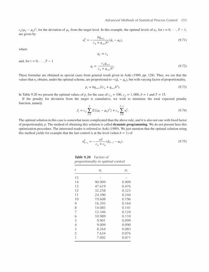
Advanced Methods of Statistical Process Control 355
cd(𝜇T − 𝜇0)2, for the deviation of 𝜇T from the target level. In this example, the optimal levels of ut, for t = 0, · · · ,T − 1,
are given by
u0t = −bqt+1
cA + qt+1b2(��t − 𝜇0), (9.71)
where
qT = cd
and, for t = 0, · · · ,T − 1
qt =cAqt+1
cA + qt+1b2. (9.72)
These formulae are obtained as special cases from general result given in Aoki (1989, pp. 128). Thus, we see that the
values that ut obtains, under the optimal scheme, are proportional to−(��t − 𝜇0), but with varying factor of proportionality,
pt = bqt+1∕(cA + qt+1b2). (9.73)
In Table 9.20 we present the optimal values of pt for the case of cA = 100, cd = 1, 000, b = 1 and T = 15.
If the penalty for deviation from the target is cumulative, we wish to minimize the total expected penalty
function, namely
Jt = cd
T∑t=1
E{(𝜇t − 𝜇0)2} + cA
T−1∑t=0
u2t . (9.74)
The optimal solution in this case is somewhat more complicated than the above rule, and it is also not one with fixed factor
of proportionality p. The method of obtaining this solution is called dynamic programming. We do not present here this
optimization procedure. The interested reader is referred to Aoki (1989). We just mention that the optimal solution using
this method yields for example that the last control is at the level (when b = 1) of
u0T−1 = − cdcA + cd
(��T−1 − 𝜇0). (9.75)
Table 9.20 Factors ofproportionality in optimal control
t qt pt
15 – –14 90.909 0.90913 47.619 0.47612 32.258 0.32311 24.390 0.24410 19.608 0.1969 16.393 0.1648 14.085 0.1417 12.346 0.1246 10.989 0.1105 9.901 0.0994 9.009 0.0903 8.264 0.0832 7.634 0.0761 7.092 0.071

356 Modern Industrial Statistics
EWMA Chartfor Speed
Group
Gro
up S
um
mary
Sta
tistics
1 4 7 10 14 18 22 26 30 34 38 42
95
100
105
110
LCL
UCL
Number of groups = 43
Center = 105
StdDev = 6.53
Smoothing parameter = 0.2
Control limits at 2*sigma
No. of points beyond limits = 11
Figure 9.13 EWMA chart for average film speed in subgroups of n = 5 film rolls, 𝜇0 = 105, 𝜎 = 6.53, 𝜆 = 0.2
The optimal control at t = T − 2 is
u0T−2 = − cdcA + 2cd
(��T−2 − 𝜇0), (9.76)
and so on.
We conclude this section mentioning that a simple but reasonable method of automatic process control is to use the
EWMA-Chart, and whenever the trend estimates, ��t, are above or below the upper or lower control limits then a control
is applied of size
u = −(��t − 𝜇0). (9.77)
In Figure 9.13 we present the results of such a control procedure on the film speed (file FILMSP.csv) in a production
process of coating film rolls. This EWMA-Chart was constructed with 𝜇0 = 105, 𝜎 = 6.53, 𝜆 = 0.2, L = 2, n = 5. Notice
that at the beginning the process was out of control. After a remedial action the process returned to a state of control. At
time 30 it drifted downward, but was corrected again.
9.8 Chapter highlights
Tests of randomness, called the run tests, are discussed. These tests are required as a first step in checking the statistical
stability of a process. Modifications of the 3-sigma control limits that include warning limits are presented as well as
control limits based on economic considerations. Particular attention is given to the determination of frequency and size
of subgroups used in the process control system. The theory of cumulative sum control charts, CUSUM, is introduced

Advanced Methods of Statistical Process Control 357
and the main results are given. Special computer programs are given for the estimation of the probability of false alarm,
conditional expected delay and expected run length. Special sections on modern topics including Bayesian detection, pro-
cess tracking, multivariate control charts and automatic process control introduce the readers to non-standard techniques
and applications.
The main concepts and definitions introduced in this chapter include:
• Run Tests
• Average Run Length
• Operating Characteristic Functions
• Multivariate Control Charts
• Cumulative Sum Control Charts
• Bayesian Detection
• Shiryayev-Roberts Statistic
• Probability of False Alarm
• Conditional Expected Delay
• Process Tracking
• Exponentially Weighted Moving Average
• Kalman Filter
• Quality Measurement Plan
• Automatic Process Control
• Dynamic Programming
9.9 Exercises
9.1 Generate the distribution of the number of runs in a sample of size n = 25, if the number of elements above the
sample mean is m2 = 10.
(i) What are Q1,Me and Q3 of this distribution?
(ii) Compute the expected value, 𝜇R, and the standard deviation 𝜎R.(iii) What is Pr{10 ≤ R ≤ 16}?(iv) Determine the normal approximation to Pr{10 ≤ R ≤ 16}.
9.2 Use MINITAB to perform a run test on the simulated cycle times from the pistons, which are in data file
CYCLT.csv. Is the number of runs above the mean cycle time significantly different than its expected value?
9.3 (i) What is the expected number of runs up or down, in a sample of size 50?
(ii) Compute the number of runs up or down in the cycle time data (CYCLT.csv).(iii) Is this number significantly different than expected?
(iv) What is the probability that a random sample of size 50 will have at least one run of size greater or equal to 5?
9.4 Analyze the observations in YARNSTRG.csv for runs.
9.5 Run the piston simulator at the upper level of the seven control parameters and generate 50 samples of size 5.
Analyze the output for runs in both X- and S-charts.9.6 (i) Run the piston simulator at the upper level of the seven control parameters and generate 50 samples of size 5
(both X- and S-charts).(ii) Repeat the exercise allowing T to change over time (mark radio-button as YES).
(iii) Compare the results in (i) and (ii) with those of Exercise 9.4.
9.7 Construct a p-chart for the fraction of defective substrates received at a particular point in the production line. Onethousand (n = 1000) substrates are sampled each week. Remove data for any week for which the process is not in
control. Be sure to check for runs as well as points outside the control limits. Construct the revised p-chart and besure to check for runs again.
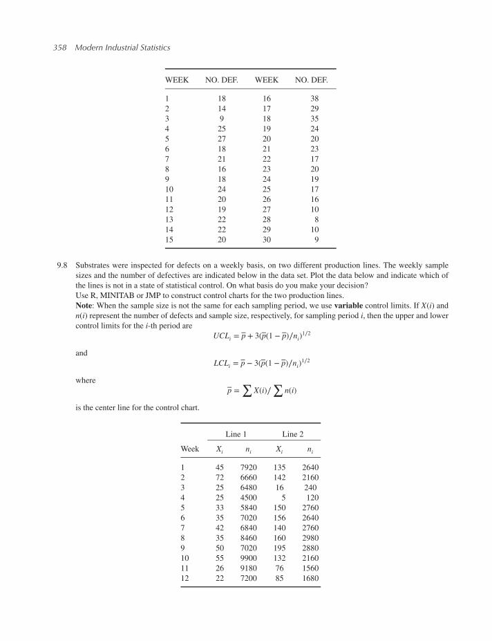
358 Modern Industrial Statistics
WEEK NO. DEF. WEEK NO. DEF.
1 18 16 38
2 14 17 29
3 9 18 35
4 25 19 24
5 27 20 20
6 18 21 23
7 21 22 17
8 16 23 20
9 18 24 19
10 24 25 17
11 20 26 16
12 19 27 10
13 22 28 8
14 22 29 10
15 20 30 9
9.8 Substrates were inspected for defects on a weekly basis, on two different production lines. The weekly sample
sizes and the number of defectives are indicated below in the data set. Plot the data below and indicate which of
the lines is not in a state of statistical control. On what basis do you make your decision?
Use R, MINITAB or JMP to construct control charts for the two production lines.
Note: When the sample size is not the same for each sampling period, we use variable control limits. If X(i) andn(i) represent the number of defects and sample size, respectively, for sampling period i, then the upper and lowercontrol limits for the i-th period are
UCLi = p + 3(p(1 − p)∕ni)1∕2
and
LCLi = p − 3(p(1 − p)∕ni)1∕2
where
p =∑
X(i)∕∑
n(i)
is the center line for the control chart.
Line 1 Line 2
Week Xi ni Xi ni
1 45 7920 135 2640
2 72 6660 142 2160
3 25 6480 16 240
4 25 4500 5 120
5 33 5840 150 2760
6 35 7020 156 2640
7 42 6840 140 2760
8 35 8460 160 2980
9 50 7020 195 2880
10 55 9900 132 2160
11 26 9180 76 1560
12 22 7200 85 1680

Advanced Methods of Statistical Process Control 359
9.9 In designing a control chart for the fraction defectives p, a random sample of size n is drawn from the productions
of each day (very large lot). How large should n be so that the probability of detecting a shift from p0 = .01 to
pt = .05, within a 5-day period, will not be smaller than .8?
9.10 The following data represent dock-to-stock cycle times for a certain type of shipment (classD). Incoming shipments
are classified according to their “type”, which is determined by the size of the item and the shipment, the type of
handling required, and the destination of the shipment. Samples of five shipments per day are tracked from their
initial arrival to their final destination, and the time it takes for this cycle to be complete is noted. The samples are
selected as follows: at five preselected times during the day, the next class D shipment to arrive is tagged and the
arrival time and identity of the shipment are recorded. When the shipment reaches its final destination, the time
is again recorded. The difference between these times is the cycle time. The cycle time is always recorded for the
day of arrival.
Dock to Stock Cycle Times
Day Times
1 27 43 49 32 36
2 34 29 34 31 41
3 36 32 48 35 33
4 31 41 51 51 34
5 43 35 30 32 31
6 28 42 35 40 37
7 38 37 41 34 44
8 28 44 44 34 50
9 44 36 38 44 35
10 30 43 37 29 32
11 36 40 50 37 43
12 35 36 44 34 32
13 48 49 44 27 32
14 45 46 40 35 33
15 38 36 43 38 34
16 42 37 40 42 42
17 44 31 36 42 39
18 32 28 42 39 27
19 41 41 35 41 44
20 44 34 39 30 37
21 51 43 36 50 54
22 52 50 50 44 49
23 52 34 38 41 37
24 40 41 40 23 30
25 34 38 39 35 33
(i) Construct X and S-charts from the data. Are any points out of control? Are there any trends in the data? If
there are points beyond the control limits, assume that we can determine special causes for the points, and
recalculate the control limits, excluding those points which are outside the control limits.
(ii) Use a t-test to decide whether the mean cycle time for days 21 and 22 was significantly greater than 45.
(iii) Make some conjectures about possible causes of unusually long cycle times. Can you think of other appropri-
ate data that might have been collected, such as the times at which the shipments reached intermediate points
in the cycle? Why would such data be useful?
9.11 Consider the modified Shewhart control chart for sample means, with a = 3, 𝑤 = 2 and r = 4. What is the ARL
of this procedure when 𝛿 = 0, 1, 2 and the sample size is n = 10?

360 Modern Industrial Statistics
9.12 Repeat the previous exercise for a = 3, 𝑤 = 1, r = 15; when n = 5 and 𝛿 = 0.5.9.13 Suppose that a shift in the mean is occurring at random, according to an exponential distribution with mean of 1
hour. The hourly cost is $100 per shift of size 𝛿 = 𝜇1−𝜇0𝜎
. The cost of sampling and testing is d = $10 per item.
How often should samples of size n = 5 be taken, when lifts of size 𝛿 ≥ 1.5 should be detected?
9.14 Compute the OC(p) function, for a Shewhart 3-sigma control chart for p, based on samples of size n = 20, when
p0 = 0.10. [Use the formula for exact computations.]
9.15 How large should the sample size n be, for a 3-sigma control chart for p, if we wish that the probability of detectinga shift from p0 = 0.01 to pt = 0.05 be 1 − 𝛽 = 0.90?
9.16 Suppose that a measurement X, of hardness of brackets after heat treatment, has a normal distribution. Every hour
a sample of n units is drawn and a X chart with control limits 𝜇0 ± 3𝜎∕√n is used. Here 𝜇0 and 𝜎 are the assumed
process mean and standard deviation. The OC function is
OC(𝛿) = Φ(3 − 𝛿√n) + Φ(3 + 𝛿
√n) − 1
where 𝛿 = (𝜇 − 𝜇0)∕𝜎 is the standardized deviation of the true process mean from the assumed one.
(i) How many hours, on average, would it take to detect a shift in the process mean of size 𝛿 = 1, when n = 5?
(ii) What should be the smallest sample size, n, so that a shift in the mean of size 𝛿 = 1 would be on average
detected in less than 3 hours?
(iii) One has two options: to sample n1 = 5 elements every hour or to sample n2 = 10 elements every two hours.
Which one would you choose? State your criterion for choosing between the two options and make the nec-
essary computations.
9.17 Electric circuits are designed to have an output of 220 (volts, DC). If the mean output is above 222 (volts DC) you
wish to detect such a shift as soon as possible. Examine the sample of data file OELECT.csv for such a shift. Forthis purpose construct a CUSUM upward scheme with K+ and h+ properly designed (consider for h+ the value
𝛼 = .001). Each observation is of sample of size n = 1. Is there an indication of a shift in the mean?
9.18 Estimate the probability of false alarm and the conditional expected delay in the Poisson case, with a CUSUM
scheme. The parameters are 𝜆0 = 15 and 𝜆1 = 25. Use 𝛼 = .001, 𝜏 = 30.
9.19 A CUSUM control scheme is based on sample means.
(i) Determine the control parameters K+, h+, K−, h−, when 𝜇0 = 100, 𝜇1 = 110, 𝜎 = 20, n = 5, 𝛼 = 0.001.(ii) Estimate the PFA and CED, when the change point is at 𝜏 = 10, 20, 30.
(iii) How would the properties of the CUSUM change if each sample size is increased from 5 to 20?
9.20 Show that the Shiryayev-Roberts statistic Wn, for detecting a shift in a Poisson distribution from a mean 𝜆0 to a
mean 𝜆1 = 𝜆0 + 𝛿 isWm = (1 +Wm−1)Rm
where W0 ≡ 0, Rm = exp {−𝛿 + xm log (𝜌)}, and 𝜌 = 𝜆1∕𝜆0.9.21 Analyze the data in file OELECT1.csv, with an EWMA control chart with 𝜆 = .2.9.22 Analyze the variable diameters in the data file ALMPIN.csv with an EWMA control chart with 𝜆 = .2. Explain
how you would apply the automatic process control technique described at the end of Section 9.7.
9.23 Construct the Kalman filter for the Dow-Jones daily index, which is given in the data file DOW1941.csv.

10Multivariate Statistical Process Control
10.1 Introduction
Univariate control charts track observations on one dimension. Multivariate data is much more informative than a collec-
tion of one dimensional variables. Simultaneously accounting for variation in several variables requires both an overall
measure of departure of the observation from the targets as well as an assessment of the data covariance structure. Mul-
tivariate control charts were developed for that purpose. We present here the construction of multivariate control charts
with the multivariate data on aluminum pins, which were introduced in Chapter 5, file ALMPIN.csv.The following is the methodology for constructing a multivariate control chart. We first use the first 30 cases of the
data file as a base sample. The other 40 observations will be used as observations on a production process which we wish
to control.
The observations in the base sample provide estimates of the means, variance and covariances of the six variables being
measured. Let Xi denote the mean of variable Xi (i = 1, · · · , p) in the base sample.
Let Sij denote the covariance between Xi and Xj (i, j = 1, · · · , p), namely,
Sij =1
n − 1
n∑l=1
(Xil − Xi⋅)(Xjl − Xj⋅). (10.1)
Notice that Sii is the sample variance of Xi (i = 1, · · · , p). Let S denote the p × p covariance matrix, i.e.,
S =⎡⎢⎢⎢⎣S11 S12 · · · S1pS21 S22 · · · S2p⋮Sp1 Sp2 · · · Spp
⎤⎥⎥⎥⎦ (10.2)
Notice that Sij = Sji for every i, j. Thus, S is a symmetric matrix.
LetM denote the (p × 1) vector of sample means, whose transpose is
M′ = (X1⋅, · · · ,Xp⋅).
Finally, we compute the inverse of S, namely S−1. This inverse exists, unless one (or some) of the variable(s) is (are) linear
combinations of the others. Such variables should be excluded.
Suppose now that every time unit we draw a sample of size m (m ≥ 1) from the production process, and observe on
each element the p variables of interest. In order to distinguish between the sample means from the production process
to those of the base sample, we will denote by Yi⋅(t), t = 1, 2, · · · the sample mean of variable Xi from the sample at
Modern Industrial Statistics: with applications in R, MINITAB and JMP, Second Edition. Ron S. Kenett and Shelemyahu Zacks.© 2014 John Wiley & Sons, Ltd. Published 2014 by John Wiley & Sons, Ltd.Companion website: www.wiley.com/go/modern_industrial_statistics

362 Modern Industrial Statistics
time t. Let Y(t) be the vector of these p means, i.e., Y′(t) = (Y1⋅(t), · · · ,Yp⋅(t)). We construct now a control chart, called
the T2-Chart. The objective is to monitor the means Y(t), of the samples from the production process, to detect when
a significant change from M occurs. We assume that the covariances do not change in the production process. Thus, for
every time period t, t = 1, 2, · · · we compute the T2 statistics
T2t = (Y(t) −M)′S−1(Y(t) −M). (10.3)
It can be shown that as long as the process mean and covariance matrix are the same as those of the base sample,
T2 ∼(n − 1)pn − p
F[p, n − p]. (10.4)
Accordingly, we set up the (upper) control limit for T2 at
UCL =(n − 1)pn − p
F.997[p, n − p]. (10.5)
If a point T(t) falls above this control limit, there is an indication of a significant change in the mean vector.
Example 10.1. The base sample consists of the first 30 rows of data file ALMPIN.csv. The mean vector of the base
sample is
M′ = (9.99, 9.98, 9.97, 14.98, 49.91, 60.05).
The covariance matrix of the base sample is S, where 103S is
⎡⎢⎢⎢⎢⎢⎢⎣
0.1826 0.1708 0.1820 0.1826 −0.0756 −0.00540.1844 0.1853 0.1846 −0.1002 −0.0377
0.2116 0.1957 −0.0846 0.00010.2309 −0.0687 −0.0054
1.3179 1.00391.4047
⎤⎥⎥⎥⎥⎥⎥⎦(Since S is symmetric we show only the upper matrix). The inverse of S is
S−1 =
⎡⎢⎢⎢⎢⎢⎢⎣
53191.3 −22791.0 −17079.7 −9343.4 145.0 −545.366324.2 −28342.7 −10877.9 182.0 1522.8
50553.9 −6467.9 853.1 −1465.125745.6 −527.5 148.6
1622.3 −1156.11577.6
⎤⎥⎥⎥⎥⎥⎥⎦We compute now for the last 40 rows of this data file the T2
t values. We consider as though each one of these rows is a
vector of a sample of size one taken every 10 minutes. In Table 10.1 we present these 40 vectors and their corresponding
T2 values.
For example T21of the table is computed according to the formula
T21 = (Y(1) −M)′S−1(Y(1) −M) = 3.523.
The 40 values of T2t of Table 10.1 are plotted in Figure 10.1. The UCL in this chart is UCL = 13.707.
We remark here that the computations can be performed by the following R-program.
> data(ALMPIN)> Base <- ALMPIN[1:30,]> MeansBase <- colMeans(Base)> CovBase <- cov(Base)> AlmpinSubset <- ALMPIN[-(1:30),]> library(qcc)

Multivariate Statistical Process Control 363
> Mqcc <- mqcc(data=AlmpinSubset,type="T2.single",center=MeansBase,cov=CovBase,plot=T)
> summary(Mqcc)
Call:mqcc(data = AlmpinSubset, type = "T2.single", center = MeansBase,
cov = CovBase, plot = T)
T2.single chart for AlmpinSubset
Summary of group statistics:Min. 1st Qu. Median Mean 3rd Qu. Max.3.421 5.900 9.718 12.520 13.840 82.630
Number of variables: 6Number of groups: 40Group sample size: 1
Center:diam1 diam2 diam3 capDiam lenNocp
9.986333 9.978667 9.974333 14.976333 49.907333lenWcp
60.047667
Covariance matrix:diam1 diam2
diam1 0.000182643678 0.00017080460diam2 0.000170804598 0.00018436782diam3 0.000181954023 0.00018528736capDiam 0.000182643678 0.00018459770lenNocp -0.000075632184 -0.00010022989lenWcp -0.000005402299 -0.00003770115
diam3 capDiamdiam1 0.0001819540230 0.000182643678diam2 0.0001852873563 0.000184597701diam3 0.0002116091954 0.000195747126capDiam 0.0001957471264 0.000230919540lenNocp -0.0000845977011 -0.000068735632lenWcp 0.0000001149425 -0.000005402299
lenNocp lenWcpdiam1 -0.00007563218 -0.0000054022989diam2 -0.00010022989 -0.0000377011494diam3 -0.00008459770 0.0000001149425capDiam -0.00006873563 -0.0000054022989lenNocp 0.00137195402 0.0010039080460lenWcp 0.00100390805 0.0014047126437|S|: 3.037256e-24
Control limits:LCL UCL0 13.70763
◾
For a comprehensive treatment of Multivariate Quality Control with MINITAB applications and detailed listing of
MINITAB macros, the reader is referred to Fuchs and Kenett (1998).

364 Modern Industrial Statistics
Table 10.1 Dimensions of aluminum pins in a production process and their T2 value
X1 X2 X3 X4 X5 X6 T2
10.00 9.99 9.99 14.99 49.92 60.03 3.52310.00 9.99 9.99 15.00 49.93 60.03 6.98310.00 10.00 9.99 14.99 49.91 60.02 6.41110.00 9.99 9.99 14.99 49.92 60.02 4.75410.00 9.99 9.99 14.99 49.92 60.00 8.16110.00 10.00 9.99 15.00 49.94 60.05 7.60510.00 9.99 9.99 15.00 49.89 59.98 10.29910.00 10.00 9.99 14.99 49.93 60.01 10.46510.00 10.00 9.99 14.99 49.94 60.02 10.77110.00 10.00 9.99 15.00 49.86 59.96 10.11910.00 9.99 9.99 14.99 49.90 59.97 11.46510.00 10.00 10.00 14.99 49.92 60.00 14.31710.00 10.00 9.99 14.98 49.91 60.00 13.67510.00 10.00 10.00 15.00 49.93 59.98 20.16810.00 9.99 9.98 14.98 49.90 59.98 8.9859.99 9.99 9.99 14.99 49.88 59.98 9.901
10.01 10.01 10.01 15.01 49.87 59.97 14.42010.00 10.00 9.99 14.99 49.81 59.91 15.99810.01 10.00 10.00 15.01 50.07 60.13 30.20410.01 10.00 10.00 15.00 49.93 60.00 12.64810.00 10.00 10.00 14.99 49.90 59.96 19.82210.01 10.01 10.01 15.00 49.85 59.93 21.88410.00 9.99 9.99 15.00 49.83 59.98 9.53510.01 10.01 10.00 14.99 49.90 59.98 18.90110.01 10.01 10.00 15.00 49.87 59.96 13.34210.00 9.99 9.99 15.00 49.87 60.02 5.4139.99 9.99 9.99 14.98 49.92 60.03 8.0479.99 9.98 9.98 14.99 49.93 60.03 5.9699.99 9.99 9.98 14.99 49.89 60.01 4.645
10.00 10.00 9.99 14.99 49.89 60.01 5.6749.99 9.99 9.99 15.00 50.04 60.15 23.639
10.00 10.00 10.00 14.99 49.84 60.03 10.25310.00 10.00 9.99 14.99 49.89 60.01 5.67410.00 9.99 9.99 15.00 49.88 60.01 5.69410.00 10.00 9.99 14.99 49.90 60.04 4.9959.90 9.89 9.91 14.88 49.99 60.14 82.628
10.00 9.99 9.99 15.00 49.91 60.04 4.4939.99 9.99 9.99 14.98 49.92 60.04 7.211
10.01 10.01 10.00 15.00 49.88 60.00 8.73710.00 9.99 9.99 14.99 49.95 60.10 3.421

Multivariate Statistical Process Control 365
T2.single Chartfor AlmpinSubset
Group
Gro
up s
um
mary
sta
tistics
1 4 7 10 13 16 19 22 25 28 31 34 37 40
020
40
60
80
LCL
UCL
Number of groups = 40
Sample size = 1
|S| = 3.037256e-24
LCL = 0
UCL = 13.70763
Num. beyond limits = 10
Figure 10.1 T2-chart for aluminum pins
10.2 A review of multivariate data analysis
The first two chapters in Part III present applications of statistical process control (SPC) to measurements in one dimen-
sion. To extend the approach to measurements consisting of several dimensions leads us to multivariate statistical process
control (MSPC), as introduced in Section 10.1. MSPC requires applications of methods and tools of multivariate data
analysis presented in Chapter 5. In this section we expand on the material presented in Chapter 5 and use the compo-
nents placement data of Examples 5.1 and 5.2. The case study consists of displacement coordinates of 16 components
placed by a robot on a printed circuit board. Overall, there are 26 printed circuit boards and therefore a total of 416 placed
components (see PLACE.csv). The components’ coordinates are measured in three dimensions, representing deviations
with respect to the target in the horizontal, vertical and angular dimensions. The measured variables are labeled x-dev,y-dev and theta-dev. The placement of components on the 26 boards was part of a validation test designed to fine tune the
placement software in order to minimize the placement deviations.
Figure 10.2 presents a scatterplot matrix of x-dev, y-dev and theta-dev with nonparametric densities providing a visual
display of the two dimensional distribution densities. On the y-dev x-dev scatterplot there are clearly three groups of
boards. In Section 5.1.2 we identified them with boxplots and confirmed the classification with coding and redrawing the
scatterplot (Figure 5.6).
Figure 10.3 presents the histograms of x-dev, y-dev and theta-dev with the low values of x-dev highlighted. Through
dynamic linking, Figure 10.3 highlights, the corresponding values for y-dev and theta-dev. We can see that components
position on the left of the target tend to be also placed below the target, with some components in this group being
positioned on target in the vertical direction (the group of y-dev between −0.001 and 0.002).To further characterize the components placed on the left of the target (negative x-dev) we draw a plot of x-dev and
y-dev versus the board number (Figure 10.4). On each board we get 16 measurements of x-dev (circle) and y-dev (cross).The highlighted points correspond to the highlighted values in Figure 10.3. One can see from Figure 10.4 that up to

366 Modern Industrial Statistics
−0.002
0.000
0.002
−0.0025 0.0000 0.0025
xDev
yD
ev
−0.05
0.00
0.05
0.10
−0.002 0.000 0.002
yDev
tDev
−0.05
0.00
0.05
0.10
−0.0025 0.0000 0.0025
xDev
tDev
Figure 10.2 Scatterplot matrix of placement data with nonparametric densities
Figure 10.3 Histograms of x-dev, y-dev and theta-dev, with dynamic linking (JMP)

Multivariate Statistical Process Control 367
Figure 10.4 Plot of x-dev and y-dev versus circuit board number (JMP)
board number 9 we have components placed to the right and below the target. In boards 10, 11 and 12 there has been a
correction in component placement which resulted in components being placed above the target in the vertical direction
and on target in the horizontal direction. These are the components in the histogram of y-dev in Figure 10.2 with the hightrailing values between −0.001 and 0.002 mentioned above. For these first 12 circuit boards we do not notice any specific
pattern in theta-dev.
Software such as R, MINITAB and JMP provide visualization and exploration technologies that complement the appli-
cation of MSPC. We will use the placement data example again in Section 10.4 to demonstrate the application of a
multivariate control chart.
10.3 Multivariate process capability indices
Chapter 8 introduced process capability studies that are a prerequisite to the set up of control limits in control charts.
Section 8.3 presented several univariate process capability indices such as Cp and Cpk that are used to characterize the
performance of a process by comparing the quality attributes specifications to the process variability. These indices map
processes in terms of their ability to deliver high critical quality parameters. In this section we focus on multivariate data
and develop several multivariate process capability indices.
As in the univariate case, the multivariate capability indices are based on the multivariate normal distribution. In
Chapter 3 we introduced the bivariate normal distribution, whose p.d.f. is given in (3.6.3). We introduce first them-variatenormal distribution as a joint distribution of a vectorX′ = (X1, . . . ,Xm) ofm random variable. The expected value of such
a vector is the vector 𝜇′ = (E{X1}, . . . ,E{Xm}). The covariance matrix of this vector is an m × m, symmetric, positive
definite matrix Σ| = (𝜎ij; i, j = 1, . . . ,m), where 𝜎ij = Cov(Xi,Xj). The multivariate normal vector is denoted by N(𝜇,Σ|).The joint p.d.f. of X is
f (x;𝜇,Σ| ) = 1
(2𝜋)m∕2|Σ| |1∕2 exp {−1
2(x − 𝜇)′Σ| −1(x − 𝜇)
}. (10.6)
In the multivariate normal distribution, the marginal distribution of Xi is normal N(𝜇i, 𝜎2i ), i = 1, . . . ,m.We describe now some of the multivariate capability indices. The reader is referred to papers by Chen (1994), Haridy,
Wu and Castagliola (2011) and Jalili, Bashiri and Amiri (2012).

368 Modern Industrial Statistics
A tolerance region, TR, is a region around a target point, T. We will consider here two possible regions: (i) a hyper-
rectangular, RTR, and (ii) a sphere, CTR. In case (i) the region is specified by parameters (𝛿1, . . . , 𝛿m), and is the set
RTR = {x ∶ |xi − Ti| ≤ 𝛿i, i = 1, . . . ,m}. (10.7)
In case (ii) the tolerance region is
CTR = {x ∶ |X − T| ≤ r}, (10.8)
where r is the radius of a sphere centered at T.In the paper by Jalili et al. (2012) a tolerance region, which is the largest ellipsoidal region in the RTR (10.7), is
considered. In the present section we will confine attention to (10.7) and (10.8). Chen (1994) suggested the following
multivariate capability index (MCp). Suppose that the TR is CTR, with a specified radius r. Let r𝛼 be the value of r, forwhich P{|X − T| ≤ r𝛼} = 1 − 𝛼, with 𝛼 = 0.0027. Then the MCp index is
MCp =rr𝛼. (10.9)
In the case of a RTR, Chen suggested the index
MCp =𝛿s𝛿𝛼
(10.10)
where 𝛿𝛼 is the value for which
P
{max
{|Xi − Ti|𝛿i, i = 1, . . . ,m
}≤ 𝛿𝛼
}= 1 − 𝛼.
𝛿s = max{𝛿i, i = 1, . . . ,m}. We will show later how to compute these indices in the case of m = 2. In the special case
where X ∼ N(T, 𝜎2I), i.e., all the m components of X are independent with 𝜇i = Ti and 𝜎2i = 𝜎
2 we have a simple
solution. If 𝛿i = 𝛿 for all i, then max{|Xi−Ti|𝛿, i = 1, . . . ,m
}∼(𝜎
𝛿
) |Z|(m), where |Z|(m) = max{|Zi|, i = 1, . . . ,m} and
Z ∼ N(0, 1). Thus
P{𝜎
𝛿|Z|(m) ≤ y
}= P{|Z| ≤ y𝛿∕𝜎}m
=(2Φ
(y𝛿
𝜎
)− 1
)m
.
Hence, 𝛿𝛼 is a solution of(2Φ
(𝛿𝛼𝛿
𝜎
)− 1
)m= 1 − 𝛼, or
𝛿𝛼 =𝜎
𝛿Φ−1
(1
2+ 1
2(1 − 𝛼)1∕m
). (10.11)
Haridy, Wu and Castagliola (2011) suggested a different type of index, based on the principal components of Σ| .LetH′ be an orthogonal matrix, whose column vectors are the orthogonal eigenvectors of Σ| . Let 𝜆1 ≥ 𝜆2 ≥ · · · ≥ 𝜆m >
0 be the corresponding eigenvalues. Recall that
HΣ| H′ =⎛⎜⎜⎝𝜆1 0
⋱0 𝜆m
⎞⎟⎟⎠ . (10.12)
The transformed vector
Y = H(X − 𝜇), (10.13)
is called the principal components vector.The distribution of Y is that of N(𝟎,Λ), where Λ = diag{𝜆i, i = 1, . . . ,m}. Here 𝜆i is the variance of Yi. Also,
Y1, . . . ,Ym are independent.
The vector of upper specification limits in the RTR isU = T + 𝛿. The corresponding vector of lower specification limits
is L = T − 𝛿. These vectors are transformed into U∗ = H𝛿 and L∗ = −H𝛿.

Multivariate Statistical Process Control 369
Suppose that X1, . . . ,Xn is a random sample from the process. These n vectors are independent and identically dis-
tributed. The maximum likelihood estimator of 𝜇 is M = 1
n
n∑i=1
Xi. An estimator of Σ| is the sample covariance matrix S
(see (10.1)). Let H′ and Λ be the corresponding matrices of eigenvectors and eigenvalues of S. The estimated vectors of
the principal components are
Yi = H(Xi −M), i = 1, . . . , n. (10.14)
Let {Y1j, · · · , Yn,j} be the sample of the j-th (j = 1, . . . ,m) principal components. Let
Cp,pcj= U∗ − L∗
6��yj, j = 1, . . . ,m, (10.15)
where ��2yj =1
n−1
n∑i=1
(Yij − Yj)2. The MCp index, based on the principal components is
MCp =
(m∏j=1
Cp,pcj
)1∕m
. (10.16)
We derive now explicit formula for a RTR, when m = 2 (bivariate normal distribution). The distribution of X is
N
([𝜉𝜂
],
[𝜎21𝜌𝜎1𝜎2
• 𝜎22
]). The conditional distribution of X2, given X1, is N
(𝜂 + 𝜌 𝜎2𝜎1(X1 − 𝜉), 𝜎22 (1 − 𝜌
2)). Accordingly,
the probability that X belongs to the rectangular tolerance region, RTR, with specified 𝛿 = (𝛿1, 𝛿2)′, is
P{X ∈ RTR(𝛿)} = ∫(T1+𝛿1−𝜉1)∕𝜎1
T1−𝛿1−𝜉1∕𝜎1𝜙(z)
[Φ
(T2 + 𝛿2 − (𝜂 + 𝜌 𝜎2
𝜎1(z − (𝜉 − T1)))
𝜎2(1 − 𝜌2)1∕2
)
−Φ
(T2 − 𝛿2 − (𝜂 + 𝜌 𝜎2
𝜎1(z − (𝜉 − T1))
𝜎2(1 − 𝜌2)1∕2
)]dz. (10.17)
In particular, if T1 = 𝜉 and T2 = 𝜂, then
P{X ∈ RTR(𝛿)} = ∫𝛿1𝜎1
− 𝛿1𝜎1
𝜙(z)[Φ(𝜎1𝛿2 − 𝜌𝜎2z𝜎1𝜎2(1 − 𝜌2)1∕2
)
−Φ( −𝜎1𝛿2 − 𝜌𝜎2z𝜎1𝜎2(1 − 𝜌2)1∕2
)]dz. (10.18)
𝜙(z) = 1√2𝜋
exp (− 1
2z2) is the standard normal density.
If the tolerance region is circular, CRC(r), with radius r, (𝜉, 𝜂) = (T1,T2) = 𝟎, then
P{X ∈ CRC(r)} = P{𝜆−11 Y21 + 𝜆
−12 Y
22 ≤ r2}, (10.19)
where 𝜆1 and 𝜆2 are the eigenvalues of Σ| =(𝜎21𝜌𝜎1𝜎2
• 𝜎22
), and Y2
1, Y2
2are independent, having a 𝜒2[1] distribution.
Thus,
P{X ∈ CRC(r)} = P{𝜒2[2] ≤ r2}; r𝛼 =√
(𝜒21−𝛼[2]) (10.20)
We compute now the capability indexMCp according to (10.10), for theALMPIN.csv data.We restrict attention to the last
two variables in the data set, that is, Lengthncp and Lengthwcp. The sample consists of the first 30 data vectors, described
in Section 10.1. We use equation (10.18) with the r = 0.7377, 𝜎21= 1.3179, 𝜎2
2= 1.4047. We assume that T1 = 𝜉 = 49.91
and T2 = 𝜂 = 60.05. From equation (10.18) we find that for 𝛿 = (3.5, 3.5)′ PX ∈ RTR(𝛿)} = 0.9964. If the tolerance
region is specified by 𝛿s = (1.5, 1.5)′ then we get index MCp =1.5
3.5= 0.4286.

370 Modern Industrial Statistics
If the tolerance region is circular, we get according to (10.20) r.0027 = 3.4086. Thus,MCp =1.5
3.4086= 0.44. We compute
now the MCp index (10.16), for the 6-dimensional vector of the ALMPIN.csv data. We base the estimation on the last
37 vectors of the data set. Notice that the expected value of the principal components Y is zero. Hence, we consider the
upper tolerance limit for Y to be USL = 0.015 and the lower tolerance limit to be LSL = −0.015. For these specificationswe get MCp = 0.4078. If we increase the tolerance limits to ±0.03, we obtain MCp = 0.8137.
10.4 Advanced applications of multivariate control charts
10.4.1 Multivariate control charts scenarios
The Hotelling T2 chart introduced in Section 10.2 plots the T2 statistic, which is the squared standardized distance of a
vector from a target point (see equation 10.3). Values of T2 represent equidistant vectors along a multidimensional ellipse
centered at the target vector point. The chart has an upper control limit (UCL) determined by the F distribution (see
equation 10.4). Points exceeding UCL are regarded as an out-of-control signal. The charted T2 statistic is a function that
reduces multivariate observations into a single value while accounting for the covariance matrix. Out-of-control signals
on the T2 chart trigger an investigation to uncover the causes for the signal.
The setup of an MSPC chart is performed by a process capability study. The process capability study period is some-
times referred to as phase I. The ongoing control using control limits determined in phase I is then called phase II. Thedistinction between these two phases is important.
In setting MSPC charts, one meets several alternative scenarios derived from the characteristics of the reference sample
and the appropriate control procedure. These include:
1. internally derived targets
2. using an external reference sample
3. externally assigned targets
4. measurements units considered as batches.
We proceed to discuss these four scenarios.
10.4.2 Internally derived targets
Internally derived targets are a typical scenario for process capability studies. The parameters to be estimated include the
vector of process means, the process covariance matrix, and the control limit for the control chart. Consider a process
capability studywith a base sample of size n of p-dimensional observations,X1,X2, . . . ,Xn.When the data are grouped and
k subgroups of observations of size m are being monitored, n = km, the covariance matrix estimator, Sp can be calculatedas the pooled covariances of the subgroups. In that case, for the jth subgroup, the Hotelling T2 statistic is then given by:
T2 = m(Xj − X)′S−1p (Xj − X) (10.21)
where Xj is the mean of the jth subgroup, X is the overall mean, and S1p is the inverse of the pooled estimated covariance
matrix. The UCL for this case is
UCL =p(k − 1)(m − 1)k(m − 1) − p + 1
F𝛼[p, k(m − 1) − p + 1]. (10.22)
When the data is ungrouped, and individual observations are analyzed, the estimation of the proper covariance matrix and
control limits requires further consideration. Typically in this case, the covariance matrix is estimated from the pooled
individual observations as S = 1
n−1
n∑i=1(Xi − X)(Xi − X)′, where X is the mean of the n observations. The corresponding T2

Multivariate Statistical Process Control 371
statistic for the ith observation, i = 1, . . . , n is given by T2 = (Xi − X)′S−1(Xi − X). In this case, (Xi − X) and S are not
independently distributed and the appropriate upper control for T2 is based on the beta distribution with
UCL = (n − 1)2
nB𝛼∕2
(p
2,n − p − 1
2
)(10.23)
and
LCL = (n − 1)2
nB1−𝛼∕2
(p
2,n − p − 1
2
)(10.24)
where B𝛼(𝜈1, 𝜈2) is the (1 − 𝛼)th quantile of the beta distribution with 𝜈1 and 𝜈2 as parameters. While theoretically the
lower control limit (LCL) can be calculated as above, in most circumstances LCL is set to zero. Figure 10.5 presents the
T2 Hotelling Control Chart for the placement data used in Figure 10.2.
In Figure 10.5, phase I was conducted over the first 9 printed circuit boards. The implication is that the first 144
observations are used to derive estimates of the means and covariances of x-dev, y-dev and theta-dev and, with these
estimates, the Upper Control Limit is determined.
The chart in Figure 10.5 indicates an out of control point at observations 55 from board 4 due to very low horizontal and
vertical deviations (x-dev = −0.0005200, y-dev = 0.0002500) and an extreme deviations in theta (theta-dev = 0.129810).In the components inserted on the first 9 boards, the average and standard deviations (in bracket) of x-dev, y-dev and
theta-dev are, respectively: −0.001062 (0.000602), −0.001816 (0.000573), +0.01392 (0.02665).
Referring again to Figure 10.5, we see a deviation in performance after board 9 with a significant jump past after
board 12. We already studied what happened on boards 10-12 and know that the shift is due to a correction in the vertical
direction, increasing the values of y-dev to be around zero (see Section 10.2).
10.4.3 Using an external reference sample
Consider again a process yielding independent observations X1,X2, . . . of a p-dimensional random variable X, such as
the quality characteristics of a manufactured item or process measurements. Initially, when the process is “in control,” the
Figure 10.5 T2 control chart of x-dev, y-dev and theta-dev with control limits and correlation structure set upwith data from first 9 printed circuit boards (MINITAB)

372 Modern Industrial Statistics
observations follow a distribution F, with density f . We now assume that we have a “reference” sample X1, . . . ,Xn of Ffrom an in-control period. To control the quality of the produced items, multivariate data is monitored for potential change
in the distribution of X, by sequentially collecting and analyzing the observations Xi. At some time t = n + k, k time units
after n, the process may run out of control and the distribution of the Xi’s changes to G. Our aim is to detect, in phase II,
the change in the distribution of subsequent observations Xn+k, k ≥ 1, as quickly as possible, subject to a bound 𝛼 ∈ (0, 1)on the probability of raising a false alarm at each time point t = n + k (that is, the probability of erroneously deciding thatthe distribution of Xn+k is not F). The reference sample X1, . . . ,Xn does not incorporate the observations Xn+k taken afterthe “reference” stage, even if no alarm is raised, so that the rule is conditional only on the reference sample.
When the data in phase II is grouped, and the reference sample from historical data includes k subgroups of observationsof size m, n = km, with the covariance matrix estimator Sp calculated as the pooled covariances of the subgroups, the T2
for a new subgroup of size m with mean Y is given by T2 = m(Y − X)′S−1p (Y − X), and the UCL is given by UCL =p(k+1)(m−1)k(m−1)−p+1
F𝛼[p, k(m − 1) − p + 1]. Furthermore, if in phase I, l subgroups were outside the control limits and assignable
causes were determined, those subgroups are omitted from the computation of X and S−1p , and the control limits for this
case areUCL = p(k−l+1)(m−1)(k−l)m−1)−p+1
F𝛼[p, (k − l∕(m − 1) − p + 1]. The T2 Control Charts constructed in phase I, and used both in
phase I and in phase II, are the multivariate equivalent of the Shewhart Control Chart. Those charts, as well as some more
advanced ones, simplify the calculations down to single-number criteria and produce a desired Type I error or in-control
run length.
While we focused on the reference sample provided by phase I of the multivariate process control, other possibilities
can occur as well. In principle, the reference in-control sample can also originate from historical data. In this case, the
statistical analysis will be the same but this situation has to be treated with precaution since both the control limits and
the possible correlations between observations may shift.
10.4.4 Externally assigned targets
If all parameters of the underlying multivariate distribution are known and externally assigned, the T2 value for a single
multivariate observation of dimension p is computed as
T2 = (Y − 𝜇)′Σ−1(Y − 𝜇) (10.25)
where 𝜇 and Σ are the expected value and covariance matrix, respectively.
The probability distribution of the T2 statistic is a 𝜒2 distribution with p degrees of freedom. Accordingly, the 0.95
UCL for T2 is UCL = 𝜒2𝜈,.95
. When the data are grouped in subgroups of size m, and both 𝜇 and Σ are known, the T2 value
of the mean vector Y is T2 = m(Y − 𝜇)′Σ−1(Y − 𝜇) with the same UCL as above.
If only the expected value of the underlying multivariate distribution, 𝜇, is known and externally assigned, the covari-
ance matrix has to be estimated from the tested sample. The T2 value for a single multivariate observation of dimension pis computed as T2 = (Y − 𝜇)′S−1(Y − 𝜇), where 𝜇 is the expected value and S is the estimate of the covariance matrix Σ,estimated either as the pooled contribution of the individual observations, i.e. S = 1
n−1
n∑i=1(Xi − X)(Xi − X)′, or by a method
which accounts for possible lack of independence between observations.
In this case, the 0.95 UCL for T2 is UCL = p(n−1)n(n−p)
F.95[p, n − p].When the tested observations are grouped, the mean vector of a subgroup with m observations (a rational sample) will
have the same expected value as the individual observations, 𝜇, and a covariance matrix Σ∕m. The covariance matrix Σcan be estimated by S or as Sp obtained by pooling the covariances of the k subgroups.
When Σ is estimated by S, the T2 value of the mean vector Y of m tested observations is T2 = m(Y − 𝜇)′S−1(Y − 𝜇)and the 0.95 UCL is
UCL =p(m − 1)m − p
F.95[p,m − p]. (10.26)
When Σ is estimated by Sp, the 0.95 UCL of T2 = m(Y − 𝜇)′S−1p (Y − 𝜇) is
UCL =pk(m − 1)
k(m − 1) − p + 1F.95[p, k(m − 1) − p + 1]. (10.27)

Multivariate Statistical Process Control 373
10.4.5 Measurement units considered as batches
In the semiconductor industry, production is typically organized in batches or production lots. In such cases, the quality-
control process can be performed either at the completion of the batch or sequentially, in a curtailed inspection, aiming at
reaching a decision as soon as possible. When the quality-control method used is reaching a decision at the completion
of the process, the possible outcomes are (a) determine the production process to be in statistical control and accept the
batch or (b) stop the production flow because of a signal that the process is out of control. On the other hand, in a curtailed
inspection, based on a statistical stopping rule, the results from the first few items tested may suffice to stop the process
prior to the batch completion.
Consider a batch of size n, with the tested items Y1, . . . ,Yn. The curtailed inspection tests the items sequentially.
Assume that the targets are specified, either externally assigned, or from a reference sample or batch. With respect to
those targets, let Vi = 1 if the T2 of the ordered ith observation exceeds the critical value 𝜅 and Vi = 0, otherwise. For the
ith observation, the process is considered to be in control if for a prespecified P, say P = 0.95, Pr(Vi = 0) ≥ P. Obviously,the inspection will be curtailed only at an observation i for which Vi = 1 (not necessarily the first).
Let N(g) =g∑i=1Vi be the number of rejection up to the gth tested item. For each number of individual rejections U (out
of n), R(U) denotes the minimal number of observations allowed up to theUth rejection, without rejecting the overall null
hypothesis. Thus, for eachU,R(U) is theminimal integer value such that under the null hypothesis, Pr
(R(U)∑i=1
Vi ≤ U
)≥ 𝛼.
For fixedU, the random variableU∑i=1Vi has a negative binomial distribution, and we can compute R(N(g)) from the inverse
of the negative binomial distribution. For example when n = 13, P = 0.95, and 𝛼 = 0.01, the null hypothesis is rejected
if the second rejection occurred at or before the third observation, or if the third rejection occurred at or before the ninth
observation, and so on.
10.4.6 Variable decomposition and monitoring indices
Data in batches is naturally grouped, but even if quality control is performed on individual items, grouping the data
into rational consequent subgroups may yield relevant information on within subgroups variability, in addition to devi-
ations from targets. In the jth subgroup (or batch) of size nj, the individual T2ij values, i = 1, . . . , nj are given by T2
ij =(Yij − 𝜃)′G−1(Yij − 𝜃). When the targets are externally assigned then 𝜃 = 𝜇. If the covariance matrix is also externally
assigned then G = Σ, otherwise G is the covariance matrix estimated either from the tested or from the reference sample.
In the case of targets derived from an external reference sample 𝜃 = m and G = S, where m and S are the mean and
the covariance matrix of a reference sample of size n. Within the jth subgroup, let us denote the mean of the subgroup
observations by Yj and the mean of the target values in the jth subgroup by 𝜃j.
The sum of the individual T2ij values, T
20j =
n∑i=1T2ij can be decomposed into two measurements of variability, one rep-
resenting the deviation of the subgroup mean from the multivariate target denoted by T2Mj, and the other measuring the
internal variability within the subgroup, denoted by T2Dj. The deviation of the subgroup mean from the multivariate target
is estimated by T2Mj = (Yj − 𝜃j)′G−1(Yj − 𝜃j), while the internal variability within the subgroup is estimated by
T2Dj + (Yij − Yj)′G−1(Yij − Yj), with T2
0j = T2Mj + T2
Dj. (10.28)
Since asymptotically, T2Mj and T
2Dj have a 𝜒
2 distribution with p and (n − 1)p degrees of freedom, respectively, one can
further compute two indices, I1 and I2, to determine whether the overall variability is mainly due to the distances between
the means of the tested subgroup from targets or to the within subgroup variability. The indices are relative ratios of
the normalized versions of the two components of T20j, i.e., I1 = I∗
1∕(I∗
1+ I∗
2), and I2 = I∗
2∕(I∗
1+ I∗
2), where I∗
1= T2
Mj∕p and
I∗2= T2
Dj∕[(n − 1)p]. We can express the indices in terms of the original T2 statistics as, I1 = (n − 1)T2Mj∕[(n − 1)T2
Mj + T2Dj]
and I2 = T2Dj∕[(n − 1)T2
Mj + T2Dj]. Tracking these indices provides powerful monitoring capabilities.

374 Modern Industrial Statistics
10.5 Multivariate tolerance specifications
Multivariate tolerance regions are based on estimates of quantiles from a multivariate distribution with parameters either
known or estimated from the data (John, 1963). Setting up a process control scheme, on the basis of tolerance regions,
involves estimating the level set {f ≥ c} of the density f which generates the data, with a pre-specified probability content1 − 𝛼. With this approach, originally proposed in Fuchs and Kenett (1987), the rejecting region is Xn+1 ∈ {f ≥ c}. Thismethod provides an exact false alarm probability of 𝛼. Since f is usually unknown, the population tolerance region {f ≥ c}needs to be estimated by an estimator of f . A similar approach was adopted by the Food and Drug Administration to
determine equivalence of a drug product tablet before and after a change in manufacturing processes such as introduction
of new equipment, a transfer of operations to another site or the scaling up of production to larger vessels. The equivalence
is evaluated by comparing tablet dissolution profiles of a batch under test with dissolution profiles of tablets from a
reference batch and allowing for at most a 15% difference. We expand on this example using the procedure proposed by
Tsong et al. (1996).
When comparing the dissolution data of a new product and a reference approved product, the goal is to assess the
similarity between the mean dissolution values at several observed sample time points. The decision to accept or reject
the hypothesis that the two batches have similar dissolution profiles, that is, are bioequivalent, is based on determining if
the difference in mean dissolution values between the test and reference products is no larger than the maximum expected
difference between any two batches of the approval product. When dissolution value is measured at a single time point,
the confidence interval of the true difference between the two batches is compared with prespecified similarity limits.
When dissolution values are measured at several time points, the Mahalanobis D2M defined above can be used to compare
the overall dissolution profiles.
The important property of the Mahalanobis D2, is that differences at points with low variability are given a higher
weight than differences at points with higher variability. This ensures that the experimental noise is properly addressed.
Let X1 = (x11x12, . . . , x1p) and X2 = (x21, x22, . . . , x2p) represent the mean dissolution values at p time instances of the
reference and the batch under test, respectively. These means can correspond to a different number of replicates, say nand m.
The Mahalanobis distance between any two vectors X1 and X2, having the same dispersion matrix Σ| isDM(X1,X2) = ((X1 − X2)′Σ| −1(X1 − X2))1∕2. (10.29)
If we estimate Σ| by covariance matrices S1 and S2, we substitute for Σ| in (10.29) the pooled estimator, Spooled. A confidence
region for the differenceΔ = 𝜇1 − 𝜇2, between the expected value of the batch and the reference populations, at confidence
Table 10.2 Dissolution data of reference and batch under test
Batch Tablet 15 90
1 REF 1 65.58 93.142 REF 2 67.17 88.013 REF 3 65.56 86.834 REF 4 66.51 88.005 REF 5 69.06 89.706 REF 6 69.77 88.887 TEST 1 47.77 92.398 TEST 2 49.46 89.939 TEST 3 47.76 90.1910 TEST 4 49.72 94.1211 TEST 5 52.68 93.8012 TEST 6 51.01 94.45
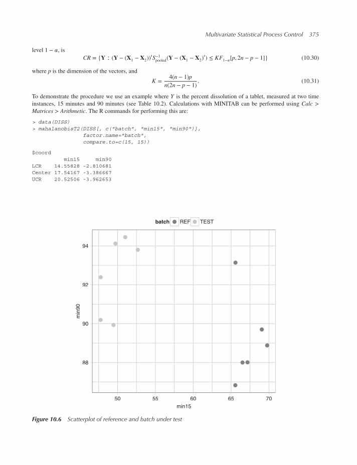
Multivariate Statistical Process Control 375
level 1 − 𝛼, isCR = {Y ∶ (Y − (X1 − X2))′S−1pooled(Y − (X1 − X2)′) ≤ KF1−𝛼[p, 2n − p − 1]} (10.30)
where p is the dimension of the vectors, and
K =4(n − 1)p
n(2n − p − 1). (10.31)
To demonstrate the procedure we use an example where Y is the percent dissolution of a tablet, measured at two time
instances, 15 minutes and 90 minutes (see Table 10.2). Calculations with MINITAB can be performed using Calc >Matrices > Arithmetic. The R commands for performing this are:
> data(DISS)> mahalanobisT2(DISS[, c("batch", "min15", "min90")],
factor.name="batch",compare.to=c(15, 15))
$coordmin15 min90
LCR 14.55828 -2.810681Center 17.54167 -3.386667UCR 20.52506 -3.962653
88
90
92
94
50 55 60 65 70
min15
min
90
batch REF TEST
Figure 10.6 Scatterplot of reference and batch under test

376 Modern Industrial Statistics
Figure 10.7 Difference between dissolution of batch under test and reference at 15 and 90min (MINITAB)
$mahalanobisLCR Center UCR
8.664794 10.440449 12.216104
$mahalanobis.compare[,1]
[1,] 9.630777
A scatter plot of the data shows the difference between test and reference. At 15 minutes dissolution is lower in the tested
batch than the reference, at 90 minutes this is reversed (see Figure 10.6). Our tested material therefore starts dissolving
than the reference but then things change and it reaches high dissolution levels faster than the reference.
For this data, n = 6, p = 2, K = 1.35, F2,19,.90 = 3.01, (X2 − X1) = (17.54,−3.39) andDM = 10.44. A contour plot with
the limits of CR set at 3.01 is presented in Figure 10.7.
The center of the ellipsoid is set at (17.54,−3.39) and, as mentioned above, at that point, DM = 10.44. The line fromthe origin connecting to this point is Y = −.193X. It crosses the ellipse first at (15.03,−2.9) labeled as “1” on Figure 10.7and then at (20.05,−3.87) labeled as “2” with DM values of Dl
M = 8.95 and DuM = 11.93 respectively.
To determine equivalence, with a 15% buffer, we consider the contour corresponding to results within this buffer. The
DM value for these point RD = Sqrt[(15, 15)′S−1pooled
(15, 15)] = 9.63.Since Du
M > RD we have a confidence region for the true difference in mean dissolution that exceeds the 15% buffer.
We therefore declare the batch under test not to be equivalent to the reference.
An index that can be used to assess process capability in terms of equivalence between reference and batch under test
is Ceq = RD∕DuM . To determine the batch under test equivalent to the reference we need to show that Ceq > 1.
10.6 Chapter highlights
As was discussed in Chapter 5, multivariate observations require special techniques for visualization and analysis.
Chapter 10 expands Chapter 5 and presents techniques for multivariate statistical process control (MSPC) based on
the Mahalanobis T2 chart. As in previous chapters, examples of MSPC using R, MINITAB and JMP are provided.

Multivariate Statistical Process Control 377
Section 10.3 introduces the reader to multivariate extensions of process capability indices. These are expansions of
the capability indices presented in Chapter 8 that are not available in MINITAB or JMP. A special role is played in
this context by the concept of multivariate tolerance regions (TR) which extends the tolerance intervals introduced in
Section 4.5. Section 10.4 considers four scenarios for setting up and running MSPC: 1) internally derived targets, 2)
using an external reference sample, 3) externally assigned targets and 4) measurements units considered as batches.
These four cases cover most practical applications of MSPC. Two subsections cover the special cases of measurement
units considered as batches and a variable decomposition of indices used for process monitoring. Section 10.5 is a special
application of MSPC to the monitoring of bioequivalence of drug product dissolution profiles. In this application tablets
manufactured by a generic drug company are compared to the original product at several dissolution times. The Food
and Drug Administration allows for a gap of at most 15%, a requirement that define multivariate specification limits. We
show how TR are used in such cases. More on multivariate applications in pharmaceuticals will be discussed in Chapter
13 on Quality by Design.
The main concepts and tools introduced in this chapter include:
• Mean Vector
• Covariance Matrix
• Mahalanobis T2
• Multivariate Statistical Process Control
• Multivariate Process Capability Indices
• Multivariate Tolerance Region
• Hyper-Rectangular Tolerance Regions
• Circular Tolerance Regions
• Principal Components
• Internal Targets
• Reference Sample
• External Targets
• Batches
• Monitoring Indices
10.7 Exercises
10.1 In data file TSQ.csv we find 368 T2 values corresponding to the vectors (x, y, 𝜃) in the PLACE.csv file. The first
n = 48 vectors inPLACE.csv file were used as a base sample, to compute the vector of meansm and the covariance
matrix S. The T2 values are for the other individual vectors (m = 1). Plot the T2 values in the fileTSQ.csv. Compute
the UCL and describe from the plot what might have happened in the placement process generating the (x, y, 𝜃)values.
10.2 Prove that if X has a multivariate normal distribution, (N𝑣(𝜇, 𝜎), then (X − 𝜇)′Σ−1(X − 𝜇) has a 𝜒2 distributionwith 𝑣 degrees of freedom where R = 𝜒2
1−p[𝑣] is the corresponding (1 − p) quantile of the 𝜒2 distribution with 𝑣degrees of freedom.
10.3 Sort the dataset CAR.csv by variable cyl, indicating the number of cylinders in a car, and run a T2 chart with inter-
nally derived targets for the variables turn, hp,mpg, with separate computations for cars with 4, 6 and 8 cylinders.
If you use MINITAB use the option Stages. How does the number of cylinders affect the overall performance of
the cars?
10.4 Sort the dataset CAR.csv by variable origin, indicating the country of origin, and run a T2 chart with internally
derived targets for the variables turn, hp, mpg, with separate computations for cars from 1 = US; 2 = Europe; 3
= Asia. If you use MINITAB use the option Stages. How does the country of origin affect the overall performance
of the cars?
10.5 Load the dataset GASOL.csv and compute a T2 chart for x1, x2, astm, endPt, yield. Design the chart with an
external assigned target based on observations 12–24. Compare the charts. Explain the differences.
10.6 Repeat exercise 10.4, but this time design the chart with an externally assigned target based on observations 25–32.
Explain the computational difficulty.

378 Modern Industrial Statistics
10.7 Calculate control limits for grouped data with 20 subgroups of size 5 and 6 dimensions, with internally derived
targets (equation (10.21). How will the control limits change if you start monitoring a process with similar data?
10.8 Let X1 = (x11, x12, . . . , x1p) and X2 = (x21, x22, . . . , x2p) represent the mean dissolution values of tablets at p time
instances of a reference product and a batch under test, respectively. The Mahalanobis distance T2, between X1
and X2, is defined here as DM = Sqrt[(X2 − X1)′S−1pooled(X2 − X1)], where Spooled = (Sreference + Stest)∕2, is the pooledcovariance matrix of the reference and test samples. The confidence region, CR, of the difference between batch
and reference consists of all vectors Y satisfying: K[(Y − (X2 − X1)′S−1pooled(Y − (X2 − X1)] ≤ F0.90[p, 2n − p − 1]where F0.90[p, 2n − p − 1] is the 90th quantile of the F-distribution with degrees of freedom p and (2n − p − 1).Prove that for measurements conducted at one time instance (p = 1) these formulae correspond to the confidence
intervals presented in Chapter 4.

Part IVDesign and Analysis of Experiments
Statistically designed experiments have been used to accelerate learning since their introduction by R.A. Fisher in the first
half of the twentieth century. One of Fisher’s major contributions was the development of factorial experiments, which
can simultaneously study several factors. Such experiments ran completely counter to the common wisdom of isolating
one factor at a time, with all other factors held constant. Quoting Fisher:
No aphorism is more frequently repeated in connection with field trials, than that we must ask Nature few questions, or, ideally,
one question, at a time. The writer is convinced that this view is wholly mistaken. Nature, he suggests, will best respond to a logical
and carefully thought out questionnaire. A factorial design allows the effect of several factors and interactions between them, to
be determined with the same number of trials as are necessary to determine any one of the effects by itself with the same degree
of accuracy.
(quoted from R.A. Fisher, The arrangement of field experiments, Journal of the Ministry of Agriculture of Great Britain 33,pp. 503–513, 1926).
New challenges and opportunities arose when Fisher’s ideas were applied in the industrial environment. The opportunity
for rapid feedback led G.E.P. Box to develop response surface methodology, with new families of designs and a new strat-
egy of sequential experimentation. Box’s contributions were stimulated by problems that arose during his 8 years of work
as a statistician for Imperial Chemical Industries (ICI). The book by G.E.P. Box, W.G. Hunter and J.S. Hunter, Statis-tics for Experimenters (Wiley, 1978) has become a classic in the area of design of experiments. The Japanese G. Taguchi
applied such methods in the 1950s in Japan’s industry and in the 1980s also in the US and elsewhere. Statistically designed
experiments are now recognized as essential for rapid learning and thereby, for reducing time-to-market, while preserving
high quality and peak performance. In recent years, computer simulators have become an increasingly popular platform
for running experiments in the product and/or process development process. Some of the issues involved in computer
experiments are common to physical experiments such as the need to study many factors, to make effective local approx-
imations to input-output relationships and to exploit sequential methods. New issues have also arisen: the ability to use a
very large number of factor settings, the lack of “experimental error,” the need to combine computer and lab or field data,
to name a few. These new issues have stimulated the development of new statistical methods, which are often given the
acronym DACE, for the design and analysis of computer experiments. In this part of the book we cover these topics in
three focused chapters.
Modern Industrial Statistics: with applications in R, MINITAB and JMP, Second Edition. Ron S. Kenett and Shelemyahu Zacks.© 2014 John Wiley & Sons, Ltd. Published 2014 by John Wiley & Sons, Ltd.Companion website: www.wiley.com/go/modern_industrial_statistics

380 Modern Industrial Statistics
Chapter 11 presents the classical approach to the design and analysis of experiments, including factorial and fractional
factorial designs and blocking and randomization principles.
Chapter 12 introduces the concepts of quality by design developed by Genichi Taguchi, including parameter and toler-
ance industrial designs. A special section covers the implementation of quality by design in the pharmaceutical industry
which has expanded the approach in the context of drug development and drug manufacturing industries.
Chapter 13 covers methods for designing and analyzing computer experiments.

11Classical Design and Analysis
of Experiments
Experiments are used in industry to improve productivity, reduce variability and obtain robust products and manufacturing
processes. In this chapter we study how to design and analyze experiments which are aimed at testing scientific or tech-
nological hypotheses. These hypotheses are concerned with the effects of procedures or treatments on the yield; the
relationship between variables; the conditions under which a production process yields maximum output or other opti-
mum results, etc. The chapter presents the classical methods of design of experiments. We start with an introductory
section, which provides some examples and discusses the guiding principles in designing experiments.
11.1 Basic steps and guiding principles
The following are guiding principles which we follow in designing experiments. They are designed to ensure high infor-
mation quality (InfoQ) of the study, as introduced in Chapter 1.
1. The objectives of the study should be well stated, and criteria established to test whether these objectives have beenmet.
2. The response variable(s) should be clearly defined so that the study objectives are properly translated. At this stagemeasurement uncertainty should be established (see Chapter 2).
3. All factors which might affect the response variable(s) should be listed, and specified. We call these the controllablefactors. This requires interactive brainstorming with content experts.
4. The type of measurements or observations on all variables should be specified.
5. The levels of the controllable factors to be tested should be determined.
6. A statisticalmodel should be formulated concerning the relationship between the pertinent variables, and their error
distributions. This can rely on prior knowledge or literature search.
7. An experimental layout or experimental array should be designed so that the inference from the gathered data
will be:
(a) valid;(b) precise;(c) generalizable;(d) easy to obtain.
Modern Industrial Statistics: with applications in R, MINITAB and JMP, Second Edition. Ron S. Kenett and Shelemyahu Zacks.© 2014 John Wiley & Sons, Ltd. Published 2014 by John Wiley & Sons, Ltd.Companion website: www.wiley.com/go/modern_industrial_statistics

382 Modern Industrial Statistics
8. The trials should be performed if possible in a random order, to avoid bias by factors which are not taken into
consideration.
9. A protocol of execution should be prepared, as well as the method of analysis. The method of analysis and data
collection depends on the design.
10. The execution of the experiment should carefully follow the protocol with proper documentation.
11. The results of the experiments should be carefully analyzed and reported ensuring proper documentation and
traceability. Modern technology (like sweave) ensures that data, analysis and conclusions are fully integrated and
reproducible.
12. Confirmatory experiments should be conducted to validate the inference (conclusions) of the main experiments.
We illustrate the above principles with two examples.
Example 11.1. The first example deals with a problem of measuring weights of objects and is meant to illustrate what
an experimental layout (design) is and why an optimal one should be chosen.
Step 1: Formulation of ObjectivesThe objective is to devise a measurement plan that will yield weight estimates of chemicals with maximal precision,
under a fixed number of four weighing operations.
Step 2: Description of ResponseThe weight measurement device is a chemical balance, which has right and left pans. One or more objects can be
put on either pan. The response variable Y , is the measurement read on the scale of the chemical balance. This is
equal to the total weight of objects on the right pan (+) minus the total weight of objects on the left pan (−), plus ameasurement error.
Step 3: Controllable VariablesSuppose we have four objectsO1,O2,O3,O4, having unknown weights𝑤1,𝑤2,𝑤3,𝑤4. The controllable (influencing)variables are
Xij =
⎧⎪⎪⎨⎪⎪⎩
1, if j-th object is put on + pan
in the i-th measurement
−1, if j-th object is put on − pan
in the i-th measurement.
i, j = 1, 2, 3, 4.Step 4: Type of measurements
The response Y is measured on a continuous scale in an interval (y∗, y∗∗). The observations are a realization of contin-uous random variables.
Step 5: Levels of Controllable VariablesXij = ±1, as above.
Step 6: A Statistical ModelThe measurement model is linear, that is,
Yi = 𝑤1Xi1 +𝑤2Xi2 +𝑤3Xi3 +𝑤4Xi4 + ei
i = 1, · · · , 4, where e1, e2, e3, e4 are independent random variables, with E{ei} = 0 and V{ei} = 𝜎2, i = 1, 2, · · · , 4.Step 7: Experimental Layout
An experimental layout is represented by a 4 × 4 matrix
(X) = (Xij; i, j = 1, · · · , 4).
Such a matrix is called a design matrix.

Classical Design and Analysis of Experiments 383
Given a design matrix (X), and a vector of measurements Y = (Y1, · · · ,Y4)′, we estimate w = (𝑤1, · · · , 𝑤4)′ by
W = (L)Y
where (L) is a 4 × 4 matrix. We say that the design is valid, if there exists a matrix L such that E{W} = w. Any non-singular design matrix (X) represents a valid design with (L) = (X)−1.
Indeed, E{Y} = (X)w. HenceE{W} = (X)−1E{Y} = w.
The precision of the design matrix (X) is measured by
(4∑i=1V{Wi}
)−1
. The problem is to find a design matrix (X)0 whichmaximizes the precision.
It can be shown that an optimal design is given by the orthogonal array
(X)0 =⎡⎢⎢⎢⎣
1 −1 −1 1
1 1 −1 −11 −1 1 −11 1 1 1
⎤⎥⎥⎥⎦or any row (or column) permutation of this matrix. Notice that in this design, in each one of the first three weighing
operations (row) two objects are put on the left pan (−) and two on the right. Also, each object, excluding the first, is puttwice on (−) and twice on (+). The weight estimates under this design are
W = 1
4
⎡⎢⎢⎢⎣1 1 1 1
−1 1 −1 1
−1 −1 1 1
1 −1 −1 1
⎤⎥⎥⎥⎦⎡⎢⎢⎢⎣Y1Y2Y3Y4
⎤⎥⎥⎥⎦ .Moreover,
4∑i=1
V{Wi} = 𝜎2.
The order of measurements is random. ◾
Example 11.2. The second example illustrates a complex process, with a large number of factors which may affect the
yield variables.
Wave soldering of circuit pack assemblies (CPA) is an automated process of soldering which, if done in an optimal
fashion, can raise quality and productivity. The process, however, involves three phases and many variables. We analyze
here the various steps required for designing an experiment to learn the effects of the various factors on the process. We
follow the process description of Lin and Kacker (1989).
If the soldering process yields good results, the CPA’s can proceed directly to automatic testing. This is a big savings
in direct labor cost and increase in productivity. The wave soldering process (WSP) is in three phases. In Phase I, called
fluxing, the solder joint surfaces are cleaned by the soldering flux, which also protects it against reoxidation. The fluxinglowers the surface tension for better solder wetting and solder joint formation.
Phase II of the WSP is the soldering assembly. This is performed in a cascade of wave soldering machines. After
preheating the solution, the non-component side of the assembly is immersed in a solder wave for 1 to 2 seconds. All
solder points are completed when the CPA exits the wave. Preheating must be gradual. The correct heating is essential
to effective soldering. Also important is the conveyor speed and the conveyor’s angle. The last phase, Phase III, of the
process is that of detergent cleaning. The assembly is first washed in detergent solution, then rinsed in water and finally
dried with hot air. The temperature of the detergent solution is raised to achieve effective cleaning and prevent excessive
foaming. The rinse water is heated to obtain effective rinsing.

384 Modern Industrial Statistics
We list now the design steps:
1. Objectives. To find the effects of the various factors on the quality of wave soldering, and optimize the process.
2. Response Variables. There are four yield variables(a) Insulation resistance
(b) Cleaning characterization
(c) Soldering efficiency
(d) Solder mask cracking.
3. Controllable Variables. There are 17 variables (factors) associated with the three phases of the process.
I. Flux formulation II.Wave Soldering III. Detergent cleaningA. Type of activator H. Amount of Flux N. Detergent concentration
B. Amount of activator I. Preheat time O. Detergent temperature
C. Type of surfactant J. Solder temperature P. Cleaning conveyor speed
D. Amount of surfactant K. Conveyor speed Q. Rinse water temperature
E. Amount of antioxidant L. Conveyor angle
F. Type of solvent M. Wave height setting
G. Amount of solvent
4. Measurements(a) Insulation resistance test at 30 minutes, 1 and 4 days after soldering at
• −35C, 90% RN, no bias voltage
• −65C, 90% RH, no bias voltage
• (continuous variable).
(b) Cleaning characterization: The amounts of residues on the board (continuous variable).
(c) Soldering efficiency: Visual inspection of no solder, insufficient solder, good solder, excess solder and other
defects (discrete variables).
(d) Solder mask cracking: Visual inspection of cracked spots on the solder mask (discrete variables).
5. Levels of Controllable Factors
Factor # Levels Factor # Levels
A 2 J 3
B 3 K 3
C 2 L 3
D 3 M 2
E 3 N 2
F 2 O 2
G 3 P 3
H 3 Q 2
I 3
6. The StatisticalModel. The response variables are related to the controllable variables by linear models having “main
effects” and “interaction” parameters, as will be explained in Section 13.3.
7. The Experiment Layout. A fractional factorial experiment, as explained in Section 11.8, is designed. Such a design
is needed, because a full factorial design contains 31027 = 7, 558, 272 possible combinations of factor levels. A frac-
tional replication design chooses a manageable fraction of the full factorial in a manner that allows valid inference,
and precise estimates of the parameters of interest.
8. Protocol of Execution. Suppose that it is decided to perform a fraction of 3322 = 108 trials at certain levels of the 17
factors. However, the set-up of the factors takes time and one cannot performmore than 4 trials a day. The experiment

Classical Design and Analysis of Experiments 385
will last 27 days. It is important to construct the design so that the important effects, to be estimated, will not be
confounded with possible differences between days (blocks). The order of the trials within each day is random-
ized as well as, the trials which are assigned to different days. Randomization is an important component of the
design, which comes to enhance its validity. The execution protocol should clearly specify the order of execution of
the trials.
◾
11.2 Blocking and randomization
Blocking and randomization are devices in planning of experiments, which are aimed at increasing the precision of the
outcome and ensuring the validity of the inference. Blocking is used to reduce errors. A block is a portion of the exper-
imental material that is expected to be more homogeneous than the whole aggregate. For example, if the experiment is
designed to test the effect of polyester coating of electronic circuits on their current output, the variability between circuits
could be considerably bigger than the effect of the coating on the current output. In order to reduce this component of
variance, one can block by circuit. Each circuit will be tested under two treatments: no-coating and coating. We first test
the current output of a circuit without coating. Later we coat the circuit, and test again. Such a comparison of before and
after a treatment, of the same units, is called paired-comparison.Another example of blocking is the famous boy’s shoes examples of Box, Hunter and Hunter (1978, pp. 97). Two kinds
of shoe soles’ materials are to be tested by fixing the soles on n pairs of boys’ shoes, and measuring the amount of wear
of the soles after a period of actively wearing the shoes. Since there is high variability between activity of boys, if m pairs
will be with soles of one type and the rest of the other, it will not be clear whether any difference that might be observed
in the degree of wearout is due to differences between the characteristics of the sole material or to the differences between
the boys. By blocking by pair of shoes, we can reduce much of the variability. Each pair of shoes is assigned the two types
of soles. The comparison within each block is free of the variability between boys. Furthermore, since boys use their right
or left foot differently, one should assign the type of soles to the left or right shoes at random. Thus, the treatments (two
types of soles) are assigned within each block at random.
Other examples of blocks could be machines, shifts of production, days of the week, operators, etc.
Generally, if there are t treatments to compare, and b blocks, and if all t treatments can be performed within a single
block, we assign all the t treatments to each block. The order of applying the treatments within each block should be
randomized. Such a design is called a randomized complete block design. We will see later how a proper analysis of
the yield can validly test for the effects of the treatments.
If not all treatments can be applied within each block, it is desirable to assign treatments to blocks in some balanced
fashion. Such designs, to be discussed later, are called balanced incomplete block designs (BIBD).Randomization within each block is important also to validate the assumption that the error components in the statistical
model are independent. This assumption may not be valid if treatments are not assigned at random to the experimental
units within each block.
11.3 Additive and non-additive linear models
Seventeen factors which might influence the outcome in WSP are listed in Example 11.2. Some of these factors, like type
of activator (A), or type of surfactant (C) are categorical variables. The number of levels listed for these factors was 2.
That is, the study compares the effects of two types of activators and two types of surfactants.
If the variables are continuous, like amount of activator (B), we can use a regression linear model to represent the
effects of the factors on the yield variables. Such models will be discussed later (Section 11.7). In the present section
linear models which are valid for both categorical or continuous variables are presented.
For the sake of explanation, let us start first with a simple case, in which the response depends on one factor only. Thus,
let A designate some factor, which is applied at different levels, A1, · · · ,Aa. These could be a categories. The levels of Aare also called “treatments.”

386 Modern Industrial Statistics
Suppose that at each level of A we make n independent repetitions (replicas) of the experiment. Let Yij, i = 1, · · · , aand j = 1, · · · , n denote the observed yield at the j-th replication of level Ai. We model the random variables Yij as
Yij = 𝜇 + 𝜏Ai + eij, i = 1, · · · , a, j = 1, · · · , n, (11.1)
where 𝜇 and 𝜏A1, · · · , 𝜏Aa are unknown parameters, satisfying
a∑i=1𝜏Ai = 0. (11.2)
eij, i = 1, · · · , a, j = 1, · · · , n, are independent random variables such that,
E{eij} = 0 and V{eij} = 𝜎2, (11.3)
for all i = 1, · · · , a; j = 1, · · · , n.Let
Yi =1
n
n∑j=1
Yij, i = 1, · · · , a.
The expected values of these means are
E{Yi} = 𝜇 + 𝜏Ai , i = 1, · · · , a. (11.4)
Let
Y = 1
a
a∑i=1, Yi. (11.5)
This is the mean of all N = a × n observations (the grand mean), sincea∑i=1𝜏Ai = 0, we obtain that
E{Y} = 𝜇. (11.6)
The parameter 𝜏Ai is called themain effect of A at level i.If there are two factors, A and B, at a and b levels respectively, there are a × b treatment combinations (Ai,Bj),
i = 1, · · · , a, j = 1, · · · , b. Suppose also that n independent replicas are made at each one of the treatment combinations.
The yield at the k-th replication of treatment combination (Ai,Bj) is given by
Yijk = 𝜇 + 𝜏Ai + 𝜏Bj + 𝜏ABij + eijk. (11.7)
The error terms eijk are independent random variables satisfying
E{eijl} = 0, V{eijl} = 𝜎2, (11.8)
for all i = 1, · · · , a, j = 1, · · · , b, k = 1, · · · , n.We further assume that
b∑j=1𝜏ABij = 0, i = 1, · · · , a
a∑i=1𝜏ABij = 0, j = 1, · · · , b.
a∑i=1𝜏Ai = 0,
b∑j=1𝜏Bj = 0.
(11.9)
𝜏Ai is the main effect of A at level i, 𝜏Bj is the main effect of B at level j, and 𝜏ABij is the interaction effect at (Ai,Bj).
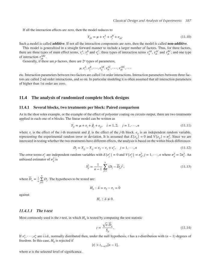
Classical Design and Analysis of Experiments 387
If all the interaction effects are zero, then the model reduces to
Yijk = 𝜇 + 𝜏Ai + 𝜏Bj + eijk. (11.10)
Such a model is called additive. If not all the interaction components are zero, then the model is called non-additive.This model is generalized in a straight forward manner to include a larger number of factors. Thus, for three factors,
there are three types of main effect terms, 𝜏Ai , 𝜏Bj and 𝜏Ck ; three types of interaction terms 𝜏ABij , 𝜏ACik and 𝜏BCjk ; and one type
of interaction 𝜏ABCijk .
Generally, if there are p factors, there are 2p types of parameters,
𝜇, 𝜏Ai , 𝜏Bj , · · · , 𝜏
ABij , 𝜏
ACik , · · · , 𝜏
ABCijk , · · ·
etc. Interaction parameters between two factors are called 1st order interactions. Interaction parameters between three fac-
tors are called 2-nd order interactions, and so on. In particular modeling it is often assumed that all interaction parameters
of higher than 1st order are zero.
11.4 The analysis of randomized complete block designs
11.4.1 Several blocks, two treatments per block: Paired comparison
As in the shoe soles example, or the example of the effect of polyester coating on circuits output, there are two treatments
applied in each one of n blocks. The linear model can be written as
Yij = 𝜇 + 𝜏i + 𝛽j + eij, i = 1, 2; j = 1, · · · , n (11.11)
where 𝜏i is the effect of the i-th treatment and 𝛽j is the effect of the j-th block. eij is an independent random variable,
representing the experimental random error or deviation. It is assumed that E{eij} = 0 and V{eij} = 𝜎2e . Since we are
interested in testing whether the two treatments have different effects, the analysis is based on the within block differences
Dj = Y2j − Y1j = 𝜏2 − 𝜏1 + e∗j , j = 1, · · · , n (11.12)
The error terms e∗j are independent random variables with E{e∗j } = 0 and V{e∗j } = 𝜎2d , j = 1, · · · , n where 𝜎2d = 2𝜎2e . An
unbiased estimator of 𝜎2d is
S2d =1
n − 1
n∑j=1
(Dj − Dn)2, (11.13)
where Dn =1
n
n∑j=1Dj. The hypotheses to be tested are:
H0 ∶ 𝛿 = 𝜏2 − 𝜏1 = 0
against
H1 ∶ 𝛿 ≠ 0.
11.4.1.1 The t-test
Most commonly used is the t-test, in which H0 is tested by computing the test statistic
t =√n Dn
Sd. (11.14)
If e∗1, · · · , e∗n are i.i.d., normally distributed then, under the null hypothesis, t has a t-distribution with (n − 1) degrees of
freedom. In this case, H0 is rejected if |t| > t1−𝛼∕2[n − 1],
where 𝛼 is the selected level of significance.

388 Modern Industrial Statistics
Table 11.1 Sign assignments and values of Y
Signs D
−1 −1 −1 −1 −0.551 −1 −1 −1 0
−1 1 −1 −1 −0.41 1 −1 −1 0.15
−1 −1 1 −1 −0.201 −1 1 −1 0.35
−1 1 1 −1 −0.051 1 1 −1 0.50
−1 −1 −1 1 −0.501 −1 −1 1 0.05
−1 1 −1 1 −0.351 1 −1 1 0.2
−1 −1 1 1 −0.151 −1 1 1 0.40
−1 1 1 1 01 1 1 1 0.55
11.4.1.2 Randomization tests
A randomization test for paired comparison, constructs a reference distribution of all possible averages of the differencesthat can be obtained by randomly assigning the sign + or − to the value of Di. It computes then an average difference Dfor each one of the 2n sign assignments.
The P-value of the test, for the two sided alternative, is determined according to this reference distribution, by
P = Pr{|D| ≥ |Observed D|}.For example, suppose we have four differences, with values 1.1, 0.3, −0.7, −0.1. The mean is D4 = 0.15. There are
24 = 16 possible ways of assigning a sign to |Di| (see Table 11.1).Under the reference distribution, all these possible means are equally probable. The P-value associated with the
observed D = 0.15 is P = 12
16= 0.75. If the number of pairs (blocks) n is large the procedure becomes cumbersome,
since we have to determine all the 2n sign assignments. If n = 20 there are 220 = 1, 048, 576 such assignments. We can
however estimate the P-value by taking a RSWR from this reference distribution. This can be easily done by using the
MINITAB macro listed below (type it and save it as RPCOMP.MTB):
Random k1 C2;Integer 1 2.
Let C3 = 2 ∗ (C2 − 1.5)Let k2 = mean(C1 ∗ C3)stack C4 k2 C4end

Classical Design and Analysis of Experiments 389
In order to execute it, we first set k1 = n, by the command
MTB> Let k1 = n
where n is the sample size. In column C1 we set the n values of the observed differences, D1, · · · ,Dn. Initiate column
C4 by
MTB> Let C4(1) = mean(C1).
After executing this macro M times we estimate the P-value by the proportion of cases in C4, whose value is greater orequal to that of mean (C1). In R this is performed with the following commands:
> X <- c(1.1, 0.3, -0.7, -0.1)> M <- 200> set.seed(123)> Di <- matrix(sample(x=c(-1,1),
size=length(X)*M,replace=TRUE),
nrow=M)> Xi <- matrix(X,
nrow=M,ncol=length(X),byrow=TRUE)
> sum(rowMeans(Di*Xi) >= mean(X))/M
[1] 0.355
> rm(X, M, Di, Xi)
Example 11.3. We analyze here the results of the shoe soles experiment, as reported in Box, Hunter and Hunter (1978,
p. 100). The observed differences in the wear of the soles, between type B and type A, for n = 10 children, are:
0.8, 0.6, 0.3, −0.1, 1.1, −0.2, 0.3, 0.5, 0.5, 0.3.
The average difference is D10 = 0.41.A t-test of H0, after setting the differences in column C3, is obtained by the MINITAB command,
MTB> T Test 0.0 C3;SUBC> Alternative 0.
The result of this t-test is
TEST OF MU = 0.000 VS MU N.E. 0.000
N MEAN STDEV SE MEAN T P VALUE
C3 10 0.410 0.387 0.122 3.35 0.0086
Executing macro RPCOMP.MTBM = 200 times on the data in column C1, gave 200 values of D, whose stem and leaf
plot is displayed in Figure 11.1.

390 Modern Industrial Statistics
Character Stem-and-Leaf DisplayStem-and-leaf of C4 N = 200
Leaf Unit=0.0103 −3 9556 −3 111
17 −2 9975555555522 −2 3331144 −1 999999999777777555555563 −1 333333333311111111188 −0 9999999997777777775555555
(17) −0 3333333333331111095 0 1111111111133333333375 0 555555555777777779999999950 1 11113333341 1 555555557777999999999919 2 11316 2 55577710 3 111335 3 7792 4 13
Figure 11.1 Stem-and-leaf plot of 200 random difference averages
According to this, the P-value is estimated by
P = 2
200= 0.01.
This estimate is almost the same as the P-value of the t-test. An equivalent analysis in R is performed using:
> X <- c(0.8, 0.6, 0.3, -0.1, 1.1, -0.2, 0.3, 0.5, 0.5, 0.3)> M <- 200> set.seed(123)> Di <- matrix(sample(x=c(-1,1),
size=length(X)*M,replace=TRUE),
nrow=M)> Xi <- matrix(X,
nrow=M,ncol=length(X),byrow=TRUE)
> Means <- rowMeans(Di*Xi)> sum(rowMeans(Di*Xi) >= mean(X))/M
[1] 0.025
> stem(Means)
The decimal point is 1 digit(s) to the left of the |
-4 | 311-3 | 5-3 | 3111-2 | 9977555

Classical Design and Analysis of Experiments 391
-2 | 333311111-1 | 9999999977777555555555-1 | 33333333331111-0 | 9999999999777777775555555555-0 | 3333333333111110 | 1111113333333333333330 | 5555577777777799999991 | 11111113333331 | 555577777999999992 | 113332 | 5555577793 | 133 | 55774 | 11134 | 7
> rm(Di, Xi, M, X, Means)◾
11.4.2 Several blocks, t treatments per block
As said earlier, the randomized complete block designs (RCBD) are those in which each block contains all the t treatments.
The treatments are assigned to the experimental units in each block at random. Let b denote the number of blocks. The
linear model for these designs is
Yij = 𝜇 + 𝜏i + 𝛽j + eij, i = 1, · · · , t j = 1, · · · , b (11.15)
where Yij is the yield of the i-th treatment in the jth block. The main effect of the i-th treatment is 𝜏i, and the main effect
of the j-th block is 𝛽j. It is assumed that the effects are additive (no interaction). Under this assumption, each treatment is
tried only once in each block. The different blocks serve the role of replicas. However, since the blocks may have additive
effects, 𝛽j, we have to adjust for the effects of blocks in estimating 𝜎2. This is done as shown in the ANOVA Table 11.2.
Further assume that, eij are the error random variables with E{eij} = 0 and V{eij} = 𝜎2 for all (i, j). The ANOVA for
this model is presented in the following table.
Table 11.2 ANOVA table for RCBD
Source DF SS MS E{MS}of Variation
Treatments t − 1 SSTR MSTR 𝜎2 + bt − 1
t∑i=1𝜏2i
Blocks b − 1 SSBL MSBL 𝜎2 + tb − 1
b∑j=1𝛽2j
Error (t − 1)(b − 1) SSE MSE 𝜎2
Total tb − 1 SST –
Here,
SST =t∑i=1
b∑j=1
(Yij − Y)2, (11.16)

392 Modern Industrial Statistics
SSTR = bt∑i=1
(Yi. − Y)2, (11.17)
SSBL = tb∑j=1
(Y .j − Y)2, (11.18)
and
SSE = SST − SSTR − SSBL. (11.19)
Yi. =1
b
b∑j=1
Yij, Y .j =1
t
t∑i=1
Yij (11.20)
and Y is the grand mean.
The significance of the treatment effects is tested by the F-statistic
Ft =MSTRMSE. (11.21)
The significance of the block effects is tested by
Fb =MSBLMSE. (11.22)
These statistics are compared with the corresponding (1 − 𝛼)th fractiles of the F-distribution. Under the assumption thatt∑i=1𝜏i = 0, the main effects of the treatments are estimated by
𝜏i = Yi. − Y , i = 1, · · · , t. (11.23)
These are least squares estimates. Each such estimation is a linear contrast
𝜏i =t∑
i′=1cii′Yi′ ., (11.24)
where
cii′ =
⎧⎪⎪⎨⎪⎪⎩1 − 1
t, if i = i′
−1
t, if i ≠ i′.
(11.25)
Hence,
V{𝜏i} = 𝜎2
b
t∑i′=1
c2ii′
= 𝜎2
b
(1 − 1
t
), i = 1, · · · , t.
(11.26)
An unbiased estimator of 𝜎2 is given by MSE. Thus, simultaneous confidence intervals for 𝜏i (i = 1, · · · , t), according to
the Scheffé method, are
𝜏i ± S𝛼
(MSEb
(1 − 1
t
))1∕2, i = 1, · · · , t (11.27)
where
S𝛼 = ((t − 1)F1−𝛼[t − 1, (t − 1)(b − 1)])1∕2.

Classical Design and Analysis of Experiments 393
Example 11.4. In Example 5.17 we estimated the effects of hybrids on the resistance in cards called “diska”. We have
t = 6 hybrids (treatments) on a card, and 32 cards. We can test now whether there are significant differences between the
values of Res3 by considering the cards as blocks, and using the ANOVA for RCBD. In this case, b = 32. Using Two-Way
Anova in MINITAB and data file HADPAS.csv. The ANOVA is presented in Table 11.3.
Table 11.3 ANOVA for hybrid data
Source DF SS MS F
Hybrids 5 1,780,741 356148 105.7Cards 31 2,804,823 90478 26.9Error 155 522,055 3368 –
Total 191 5,107,619 – –
Since F.99[5, 155] = 3.14 and F.99[31, 155] = 1.81, both the treatment effects and the card effects are significant.
The estimator of 𝜎, ��p = (MSE)1∕2, according to the above ANOVA, is ��p = 58.03. Notice that this estimator is con-
siderably smaller than the one of Example 5.17. This is due to the variance reduction effect of the blocking.
The Scheffé simultaneous confidence intervals, at level of confidence 0.95, for the treatment effects (the average hybrid
measurements minus the grand average of 1965.2) are:
Hybrid 1∶ 178.21 ± 31.05;
Hybrid 6∶ 48.71 ± 31.05;
Hybrid 5∶ 15.36 ± 31.05;
Hybrid 2∶ − 62.39 ± 31.05;
Hybrid 4∶ − 64.79 ± 31.05;
Hybrid 3∶ − 114.86 ± 31.05.
Accordingly, the effects of Hybrid 2 and Hybrid 4 are not significantly different, and that of Hybrid 5 is not significantly
different from zero. In R we obtain:
> data(HADPAS)> HADPAS$diska <- as.factor(HADPAS$diska)> HADPAS$hyb <- as.factor(HADPAS$hyb)> AovH <- aov(res3 ~ diska + hyb,
data=HADPAS)> summary(AovH)
Df Sum Sq Mean Sq F value Pr(>F)diska 31 2804823 90478 26.86 <2e-16 ***hyb 5 1780741 356148 105.74 <2e-16 ***Residuals 155 522055 3368---Signif. codes: 0 ‘***’ 0.001 ‘**’ 0.01 ‘*’ 0.05 ‘.’ 0.1 ‘ ’ 1
> tail(confint(AovH), 5)
2.5 % 97.5 %hyb2 -269.2543 -211.9332hyb3 -321.7231 -264.4019hyb4 -271.6606 -214.3394hyb5 -191.5043 -134.1832

394 Modern Industrial Statistics
hyb6 -158.1606 -100.8394
> rm(AovH)◾
11.5 Balanced incomplete block designs
As mentioned before, it is often the case that the blocks are not sufficiently large to accommodate all the t treatments. For
example, in testing the wearout of fabric one uses a special machine (Martindale wear tester) which can accommodate
only four pieces of clothes simultaneously. Here the block size is fixed at k = 4, while the number of treatments t, isthe number of types of cloths to be compared. Balanced Incomplete Block Designs (BIBD) are designs which assign ttreatment to b blocks of size k (k < t) in the following manner.
1. Each treatment is assigned only once to any one block.
2. Each treatment appears in r blocks. r is the number of replicas.
3. Every pair of two different treatments appears in 𝜆 blocks.4. The order of treatments within each block is randomized.
5. The order of blocks is randomized.
According to these requirements there are, altogether, N = tr = bk trials. Moreover, the following equality should hold
𝜆(t − 1) = r(k − 1). (11.28)
The question is how to design a BIBD, for a given t and k. One can obtain a BIBD by the complete combinatorial listing
of the(tk
)selections without replacements of k out of t letters. In this case, the number of blocks is
b =(tk
). (11.29)
The number of replicas is r =(t−1k−1
), and 𝜆 =
(t−2k−2
). The total number of trials is
N = tr = t
(t − 1
k − 1
)= t!
(k − 1)!(t − k)!= k
(tk
)= kb. (11.30)
Such designs of BIBD are called combinatoric designs. They might, however, be too big. For example, if t = 8 and
k = 4 we are required to have(8
4
)= 70 blocks. Thus, the total number of trials is N = 70 × 4 = 280 and r =
(7
3
)= 35.
Here 𝜆 =(6
2
)= 15.
There are advanced algebraic methods which can yield smaller designs for t = 8 and k = 4. Box, Hunter and Hunter
(1978, pp. 272) list a BIBD of t = 8, k = 4 in b = 14 blocks. Here N = 14 × 4 = 56, r = 7 and 𝜆 = 3.
It is not always possible to have a BIBD smaller in size than a complete combinatoric design. Such a case is t = 8 and
k = 5. Here the smallest number of blocks possible is(8
5
)= 56, and N = 56 × 5 = 280.
The reader is referred to Box, Hunter and Hunter (1978, pp. 270–274) for a list of some useful BIBD’s for k = 2, · · · , 6,t = k, · · · , 10. Let Bi denote the set of treatments in the i-th block. For example, if block 1 contains the treatments 1, 2,
3, 4, then B1 = {1, 2, 3, 4}. Let Yij be the yield of treatment j ∈ Bi. The effects model is
Yij = 𝜇 + 𝛽i + 𝜏j + eij, i = 1, · · · , b j ∈ Bi (11.31)
{eij} are random experimental errors, with E{eij} = 0 and V{eij} = 𝜎2 all (i, j). The block and treatment effects, 𝛽1, · · · , 𝛽b
and 𝜏1, · · · , 𝜏t satisfy the constraintst∑j=1𝜏j = 0 and
b∑i=1𝛽i = 0.
Let Tj be the set of all indices of blocks containing the j-th treatment. The least squares estimates of the treatment
effects are obtained in the following manner.

Classical Design and Analysis of Experiments 395
Table 11.4 ANOVA for a BIBD
Source of DF SS MS E{MS}Variation
blocks b − 1 SSBL MSBL 𝜎2 + tb − 1
b∑i=1𝛽2i
Treatments Adjusted t − 1 SSTR MSTR 𝜎2 + bt − 1
t∑j=1𝜏2j
Error N − t − b + 1 SSE MSE 𝜎2
Total N − 1 SST – –
LetWj =∑i∈Tj
Yij be the sum of all Y values under the j-th treatment. LetW∗j be the sum of the values in all the r blocks
which contain the j-th treatment, that is,W∗j =
∑i∈Tj
∑l∈Bi
Yil. Compute
Qj = kWj −W∗j , j = 1, · · · , t. (11.32)
The LSE of 𝜏j is
𝜏j =Qj
t𝜆, j = 1, · · · , t. (11.33)
Notice thatt∑j=1Qj = 0. Thus,
t∑j=1𝜏j = 0. Let Y = 1
N
b∑i=1
∑l∈Bi
Yil. The adjusted treatment average is defined as Y ∗j = Y + 𝜏j,
j = 1, · · · , t. The ANOVA for a BIBD is given in Table 11.4.
Here,
SST =b∑i=1
∑l∈Bi
Y2il −
(b∑i=1
∑l∈Bi
Yil
)2
∕N; (11.34)
SSBL = 1
k
b∑i=1
(∑l∈Bi
Yil
)2
− NY 2; (11.35)
SSTR = 1
𝜆kt
t∑j=1
Q2j (11.36)
and
SSE = SST − SSBL − SSTR. (11.37)
The significance of the treatments effects is tested by the statistic
F = MSTRMSE. (11.38)
Example 11.5. Six different adhesives (t = 6) are tested for the bond strength in a lamination process, under curing
pressure of 200 [psi]. Lamination can be done in blocks of size k = 4.
A combinatoric design (listed in Table 11.5) will have(6
4
)= 15 blocks, with r =
(5
3
)= 10, 𝜆 =
(4
2
)= 6 and N = 60.
The treatment indices of the 15 blocks are

396 Modern Industrial Statistics
Table 11.5 Block sets
i Bi i Bi
1 1, 2, 3, 4 9 1, 3, 5, 62 1, 2, 3, 5 10 1, 4, 5, 63 1, 2, 3, 6 11 2, 3, 4, 54 1, 2, 4, 5 12 2, 3, 4, 65 1, 2, 4, 6 13 2, 3, 5, 66 1, 2, 5, 6 14 2, 4, 5, 67 1, 3, 4, 5 15 3, 4, 5, 68 1, 3, 4, 6
The observed bond strength in these trials, listed in Table 11.6 are:
Table 11.6 Values of Yil, i ∈ Bi
i Yil i Yil
1 24.7, 20.8, 29.4, 24.9 8 23.1, 29.3, 27.1, 34.42 24.1, 20.4, 29.8, 30.3 9 22.0, 29.8, 31.9, 36.13 23.4, 20.6, 29.2, 34.4 10 22.8, 22.6, 33.2, 34.84 23.2, 20.7, 26.0, 30.8 11 21.4, 29.6, 24.8, 31.25 21.5, 22.1, 25.3, 35.4 12 21.3, 28.9, 25.3, 35.16 21.4, 20.1, 30.1, 34.1 13 21.6, 29.5, 30.4, 33.67 23.2, 28.7, 24.9, 31.0 14 20.1, 25.1, 32.9, 33.9
15 30.1, 24.0, 30.8, 36.5
The grand mean of the bond strength is Y = 27.389. The sets Tj and the sums Wj, W∗j are in Table 11.7
Table 11.7 The set Tj and the statistics Wj, W∗j , Qj
j Tj Wj W∗j Qj
1 1, 2, 3, 4, 5, 6, 7, 8, 9, 10 229.536 1077.7 −159.562 1, 2, 3, 4, 5, 6, 11, 12, 13, 14 209.023 1067.4 −231.313 1, 2, 3, 7, 8, 9, 11, 12, 13, 15 294.125 1107.60 68.904 1, 4, 5, 7, 8, 10, 11, 12, 14, 15 249.999 1090.90 −90.905 2, 4, 6, 7, 9, 10, 11, 13, 14, 15 312.492 1107.50 142.476 3, 5, 6, 8, 9, 10, 12, 13, 14, 15 348.176 1123.80 268.90
The ANOVA table is presented in Table 11.8.
The adjusted mean effects of the adhesives are in Table 11.9.
The variance of each adjusted mean effect is
V{Y ∗j } = k𝜎2
t𝜆, j = 1, · · · , t. (11.39)
Thus, the S.E. of Y ∗j is
S.E.{Y ∗j } =
( k MSEt𝜆
)1∕2, j = 1, · · · , t. (11.40)
It seems that there are two homogeneous groups of treatments {1, 2, 4} and {3, 5, 6}.
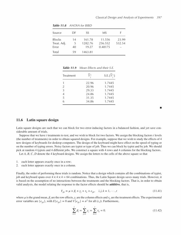
Classical Design and Analysis of Experiments 397
Table 11.8 ANOVA for BIBD
Source DF SS MS F
Blocks 14 161.78 11.556 23.99Treat. Adj. 5 1282.76 256.552 532.54Error 40 19.27 0.48175 –
Total 59 1463.81
Table 11.9 Mean Effects and their S.E.
Treatment Y ∗j S.E.{Y ∗
j }
1 22.96 1.74452 20.96 1.74453 29.33 1.74454 24.86 1.74455 31.35 1.74456 34.86 1.7445
◾
11.6 Latin square design
Latin square designs are such that we can block for two error-inducing factors in a balanced fashion, and yet save con-
siderable amount of trials.
Suppose that we have t treatments to test, and we wish to block for two factors. We assign the blocking factors t levels(the number of treatments) in order to obtain squared designs. For example, suppose that we wish to study the effects of 4
new designs of keyboards for desktop computers. The design of the keyboard might have effect on the speed of typing or
on the number of typing errors. Noisy factors are typist or type of job. Thus we can block by typist and by job. We should
pick at random 4 typists and 4 different jobs. We construct a square with 4 rows and 4 columns for the blocking factors.
Let A, B, C, D denote the 4 keyboard designs. We assign the letters to the cells of the above square so that
1. each letter appears exactly once in a row;
2. each letter appears exactly once in a column.
Finally, the order of performing these trials is random. Notice that a design which contains all the combinations of typist,
job and keyboard spans over 4 × 4 × 4 = 64 combinations. Thus, the Latin Square design saves many trials. However, it
is based on the assumption of no interactions between the treatments and the blocking factors. That is, in order to obtain
valid analysis, the model relating the response to the factor effects should be additive, that is,
Yijk = 𝜇 + 𝛽i + 𝛾j + 𝜏k + eijk, i, j, k = 1, · · · , t (11.41)
where𝜇 is the grandmean, 𝛽i are the row effects, 𝛾j are the column effects and 𝜏k are the treatment effects. The experimental
error variables are {eijk}, with E{eijk} = 0 and V{eijk} = 𝜎2 for all (i, j). Furthermore,
t∑i=1𝛽i =
t∑j=1𝛾j =
t∑k=1𝜏k = 0. (11.42)

398 Modern Industrial Statistics
Table 11.10 A 4 × 4 Latin square
Job 1 Job 2 Job 3 Job 4
Typist 1 A B C DTypist 2 B A D CTypist 3 C D A BTypist 4 D C B A
The Latin square presented in Table 11.10 is not unique. There are other 4 × 4 Latin squares. For example,
A B C DD C B AB A D CC D A B
A B C DC D A BD C B AB A D C
.
A few Latin square designs, for t = 3, · · · , 9 are given in Box, Hunter and Hunter (1978, pp. 261–262).
If we perform only 1 replication of the Latin square, the ANOVA for testing the main effects is presented in Table 11.11.
Table 11.11 ANOVA for a Latin square, one replication
Source DF SS MS F
Treatments t − 1 SSTR MSTR MSTR∕MSERows t − 1 SSR MSR MSR∕MSEColumns t − 1 SSC MSC MSC∕MSEError (t − 1)(t − 2) SSE MSE –
Total t2 − 1 SST – –
Formulae for the various SS termswill be given below. At this timewewish to emphasize that if t is small, say t = 3, then
the number of DF for SSE is only 2. This is too small. The number of DF for the error SS can be increased by performing
replicas. One possibility is to perform the same Latin square r times independently, and as similarly as possible. However,
significant differences between replicas may emerge. The ANOVA, for r identical replicas is as in Table 11.12.
Table 11.12 ANOVA for a replicated Latin square
Source D.F. SS MS F
Treatments t − 1 SSTR MSTR MSTR∕MSERows t − 1 SSR MSR MSR/MSEColumns t − 1 SSC MSC MSC/MSEReplicas r − 1 SSREP MSREP MSREP/MSEError (t − 1)[r(t + 1) − 3]) SSE MSE –
Total r(t2 − 1) SST – –

Classical Design and Analysis of Experiments 399
Notice that now we have rt2 observations. Let T ... . and Q ... . be the sum and sum of squares of all observations. Then,
SST = Q ... . − T2... .∕rt2. (11.43)
Let Ti ... denote the sum of rt observations in the i-th row of all r replications. Then
SSR = 1
tr
t∑i=1
T2i ... −
T2... .
rt2. (11.44)
Similarly, let T.j.. and T..k. be the sums of all rt observations in column j of all replicas, and treatment k of all r replicas,then
SSC = 1
rt
t∑j=1
T2.j.. −
T2....
rt2(11.45)
and
SSTR = 1
rt
t∑k=1
T2..k. −
T2....
rt2. (11.46)
Finally, let T ... l (l = 1, · · · , r) denote the sum of all t2 observations in the lth replication. Then,
SSREP = 1
t2
r∑l=1
t2... l −T2....
rt2. (11.47)
The pooled sum of squares for error is obtained by
SSE = SSD − SSR − SSC − SSTR − SSREP. (11.48)
Notice that if t = 3 and r = 3, the number of DF for SSE increases from 2 (when r = 1) to 18 (when r = 3).
The most important hypothesis is that connected with the main effects of the treatments. This we test with the statistic
F = MSTR∕MSE. (11.49)
Example 11.6. Five models of keyboards (treatments) were tested in a latin square design in which the blocking factors
are typist and job. Five typists were randomly selected from a pool of typists of similar capabilities. Five typing jobs were
selected. Each typing job had 4000 characters. The yield, Yijk, is the number of typing errors found at the i-th typist, j-thjob under the k-th keyboard. The Latin square design used is presented in Table 11.13.
Table 11.13 Latin square design, t = 5
Job
Typist 1 2 3 4 5
1 A B C D E2 B C D E A3 C D E A B4 D E A B C5 E A B C D
The five keyboards are denoted by the letters A, B, C, D, E. The experiment spanned over 5 days. In each day a typist
was assigned a job at random (from those not yet tried). The keyboard used is the one associated with the job. Only one
job was tried in a given day. The observed number of typing errors (per 4,000 characters) are listed in Table 11.14:

400 Modern Industrial Statistics
Table 11.14 Number of typing errors
Job Row
Typist 1 2 3 4 5 Sums
A B C D E1 20 18 25 17 20 100
B C D E A2 65 40 55 58 59 277
C D E A B3 30 27 35 21 27 140
D E A B C4 21 15 24 16 18 94
E A B C D5 42 38 40 35 32 187ColumnSum 178 138 179 147 156 798
Sums A B C D EKeyboard 162 166 148 152 170
Figures 11.2–11.4 present boxplots of the error rates for the three different factors. The only influencing factor is the
typist effect, as shown in Figure 11.4.
The total sum of squares is
Q = 30636.
Thus,
SST = 30636 − 7982
25= 5163.84.
Figure 11.2 Effect of keyboard on error rate (MINITAB)

Classical Design and Analysis of Experiments 401
Figure 11.3 Effect of job type on error rate (MINITAB)
1 2 3 4 5
20
30
40
50
60
Err
ors
Figure 11.4 Effect of typist on error rate (numbers indicate typist number)
Similarly,
SSR = 1
5(1002 + 2772 + · · · + 1872) − 7982
25
= 4554.64
SSC = 1
5(1782 + 1382 + · · · + 1562) − 7982
25
= 270.641

402 Modern Industrial Statistics
and
SSTR = 1
5(1622 + 1662 + · · · + 1702) − 7982
25
= 69.4395.
The analysis of variance, following Table 11.12, is Table 11.15.
Table 11.15 ANOVA for keyboard Latin square experiment
Source DF SS MS F
Typist 4 4554.640 1138.66 50.772Job 4 270.641 67.66 3.017Keyboard 4 69.439 17.3598 0.774Error 12 269.120 22.4267 –Total 24 5163.840 – –
The null hypothesis that the main effects of the keyboards are zero cannot be rejected. The largest source of variability
in this experiment were the typists. The different jobs contributed also to the variability. The P-value for the F test of jobs
is 0.062. ◾
11.7 Full factorial experiments
11.7.1 The structure of factorial experiments
Full factorial experiments are those in which complete trials are performed of all the combinations of the various factors at
all their levels. For example, if there are five factors, each one tested at three levels, there are altogether 35 = 243 treatment
combinations. All these 243 treatment combinations are tested. The full factorial experiment may also be replicated several
times. The order of performing the trials is random.
In full factorial experiments, the number of levels of different factors do not have to be the same. Some factors might be
tested at two levels and others at three or four levels. Full factorial, or certain fractional factorials which will be discussed
later, are necessary, if the statistical model is not additive. In order to estimate or test the effects of interactions, one needsto perform factorial experiments, full or fractional. In a full factorial experiment, all the main effects and interactions can
be tested or estimated. Recall that if there are p factors A,B,C, · · · there are p types of main effects,(p2
)types of pairwise
interactions AB,AC,BC, · · · ,(p3
)interactions between three factors, ABC,ABD, · · · and so on. On the whole there are,
together with the grand mean 𝜇, 2p parameters.
In the following section we discuss the structure of the ANOVA for testing the significance of main effects and inter-
actions. This is followed by a section on the estimation problem. In Sections 11.7.4 and 11.7.5 we discuss the structure
of full factorial experiments with 2 and 3 levels per factor, respectively.
11.7.2 The ANOVA for full factorial designs
The analysis of variance for full factorial designs is done to test the hypotheses that main-effects or interaction parameters
are equal to zero.We present the ANOVA for a two factor situation, factor A at a levels and factor B at b levels. The method
can be generalized to any number of factors.
The structure of the experiment is such that all a × b treatment combinations are tested. Each treatment combination is
repeated n times. The model is
Yijk = 𝜇 + 𝜏Ai + 𝜏Bj + 𝜏ABij + eijk, (11.50)

Classical Design and Analysis of Experiments 403
i = 1, · · · , a; j = 1, · · · , b; k = 1, · · · , n. eijk are independent random variables E{eijk} = 0 and V{eijk} = 𝜎2 for all
i, j, k. Let
Yij =1
n
n∑k=1
Yijk (11.51)
Yi. =1
b
b∑j=1
Yij, i = 1, · · · , a (11.52)
Y .j =1
a
a∑i=1
Yij, j = 1, · · · , b (11.53)
and
Y = 1
ab
a∑i=1
b∑j=1
Yij. (11.54)
The ANOVA partitions first the total sum of squares of deviations from Y , i.e.,
SST =a∑i=1
b∑j=1
n∑k=1
(Yijk − Y)2 (11.55)
to two components
SSW =a∑i=1
b∑j=1
n∑k=1
(Yijk − Yij)2 (11.56)
and
SSB = na∑i=1
b∑j=1
(Yij − Y)2. (11.57)
It is straightforward to show that
SST = SSW + SSB. (11.58)
In the second stage, the sum of squares of deviations SSB is partitioned to three components SSI, SSMA, SSMB, where
SSI = na∑i=1
b∑j=1
(Yij − Yi. − Y .j + Y)2, (11.59)
SSMA = nba∑i=1
(Yi. − Y)2 (11.60)
and
SSMB = nab∑j=1
(Y .j − Y)2, (11.61)
that is,
SSB = SSI + SSMA + SSMB. (11.62)
All these terms are collected in a table of ANOVA (Table 11.16).
Thus,
MSA = SSMAa − 1, (11.63)
MSB = SSMBb − 1, (11.64)

404 Modern Industrial Statistics
Table 11.16 Table of ANOVA for a 2-factor factorial experiment
Source of DF SS MS FVariation
A a − 1 SSMA MSA FAB b − 1 SSMB MSB FBAB (a − 1)(b − 1) SSI MSAB FABBetween ab − 1 SSB – –Within ab(n − 1) SSW MSW –Total N − 1 SST – –
and
MSAB = SSI(a − 1)(b − 1)
, (11.65)
MSW = SSWab(n − 1)
. (11.66)
Finally, we compute the F-statistics
FA = MSAMSW, (11.67)
FB = MSBMSW
(11.68)
and
FAB = MSABMSW. (11.69)
FA, FB and FAB are test statistics to test, respectively, the significance of the main effects of A, the main effects of B and
the interactions AB.If FA < F1−𝛼[a − 1, ab(n − 1)] the null hypothesis
HA0 ∶ 𝜏A1 = · · · = 𝜏Aa = 0.
cannot be rejected.
If FB < F1−𝛼[b − 1, ab(n − 1)] the null hypothesis
HB0 ∶ 𝜏B1 = · · · = 𝜏Bb = 0.
cannot be rejected.
Also, if
FAB < F1−𝛼[(a − 1)(b − 1), ab(n − 1)],
we cannot reject the null hypothesis
HAB0 ∶ 𝜏AB11 = · · · = 𝜏ABab = 0.
The ANOVA for two factors can be performed by MINITAB. We illustrate this estimation and testing in the following
example.
Example 11.7. In Chapter 8 we have introduced the piston example. Seven prediction factors for the piston cycle time
were listed. These are
A: Piston weight, 30–60 [kg]

Classical Design and Analysis of Experiments 405
B: Piston surface area, 0.005–0.020 [m2]
C: Initial gas volume, 0.002 - 0.010 [m3]
D: Spring coefficient, 1,000–5,000 [N/m]
E: Atmospheric pressure, 90,000–100,000 [N/m2]
F: Ambient temperature, 290–296 [∘K]G: Filling gas temperature, 340–360 [∘K].
We are interested to test the effects of the piston weight (A) and the spring coefficient (D) on the cycle time (seconds).
For this purpose we designed a factorial experiment at three levels of A, and three levels of D. The levels are
A1 = 30 [kg], A2 = 45 [kg] and A3 = 60 [kg].
The levels of factorD (spring coefficient) areD1 = 1, 500 [N/m],D2 = 3, 000 [N/m] andD3 = 4, 500 [N/m]. Five replicas
were performed at each treatment combination (n = 5).The data can be obtained by using the JMP or R piston simulator. The five factors which were not under study were
kept at the levels B = 0.01 [m2], C = 0.005 [m3], E = 95, 000 [N/m2], F = 293 [∘K] and G = 350 [∘K].
> library(DoE.base)> Factors <- list(
m=c(30, 45, 60),k=c(1500, 3000, 4500))
> FacDesign <- fac.design(factor.names=Factors,randomize=TRUE,replications=5,repeat.only=TRUE)
creating full factorial with 9 runs ...
> Levels <- data.frame(lapply(lapply(FacDesign,
as.character),as.numeric),
s=0.01,v0=0.005,p0=95000,t=293,t0=350)
> Ps <- pistonSimulation(m=Levels$m,s=Levels$s,v0=Levels$v0,k=Levels$k,p0=Levels$p0,t=Levels$t,t0=Levels$t0,each=1,seed=123)
> FacDesign <- add.response(design=FacDesign,response=Ps$seconds)
> summary(aov(Ps.seconds ~ m*k,
data=FacDesign))
Df Sum Sq Mean Sq F value Pr(>F)m 2 0.1896 0.09482 3.541 0.0395 *

406 Modern Industrial Statistics
k 2 0.2467 0.12335 4.607 0.0165 *m:k 4 0.1943 0.04857 1.814 0.1475Residuals 36 0.9640 0.02678---Signif. codes: 0 ‘***’ 0.001 ‘**’ 0.01 ‘*’ 0.05 ‘.’ 0.1 ‘ ’ 1
> rm(Levels, Factors)
We start with the two-way ANOVA presented in Table 11.17.
Table 11.17 Two-way ANOVA for cycle time
Source DF SS MS F p
Spr_Cof 2 1.01506 0.50753 8.66 0.001Pist_Wg 2 0.09440 0.04720 0.81 0.455Spr_Cof∗Pist_Wg 4 0.06646 0.01662 0.28 0.887Error 36 2.11027 0.05862Total 44 3.28619
Figure 11.5 shows the effect of the factor spring coefficient on cycle time. Spring coefficient at 4500 [N∕m] reducesthe mean cycle time and its variability.
1500 3000 4500
0.2
0.4
0.6
0.8
1.0
Figure 11.5 Effect of spring coefficient on cycle time. (The y axis corresponds to cycle time in minutes)
Figure 11.6 is an interaction-plot showing the effect of piston weight on the mean cycle time, at each level of the
spring coefficient.

Classical Design and Analysis of Experiments 407
0.4
0.5
0.6
0.7
Piston weight (m)
Mean o
f cycle
tim
e
30 45 60
Spring coefficient
1500
4500
3000
Figure 11.6 Interaction plot of piston weight with spring coefficient
The P-values are computed with the appropriate F-distributions. We see in the ANOVA table that only the main effects
of the spring coefficient (D) are significant. Since the effects of the piston weight (A) and that of the interaction are not
significant, we can estimate 𝜎2 by a pooled estimator, which is
��2 = SSW + SSI + SSMA36 + 4 + 2
= 2.2711
42
= 0.0541.
To estimate the main effects of D we pool all data from samples having the same level of D together. We obtain pooled
samples of size np = 15. The means of the cycle time for these samples are
D1 D2 D3 Grand
Y 0.743 0.509 0.380 0.544
Main Effects 0.199 −0.035 −0.164 –
The standard error of these main effects is S.E.{𝜏Dj } = 0.23259√15
√1
2= 0.0425.
Since we estimate on the basis of the pooled samples, and the main effects 𝜏Dj (j = 1, 2, 3) are contrasts of 3 means, the
coefficient S𝛼 for the simultaneous confidence intervals has the formula
S𝛼 = (2F.95[2, 42])1∕2
=√2 × 3.22 = 2.538.

408 Modern Industrial Statistics
The simultaneous confidence intervals for 𝜏Dj , at 𝛼 = .05, are
Lower Upper
Limit Limit
𝜏D1: 0.0911 0.3069
𝜏D2: −0.1429 0.0729
𝜏D3: −0.2619 −0.0561
We see that the confidence interval for 𝜏D2covers zero. Thus, 𝜏D
2is not significant. The significant main effects are 𝜏D
1
and 𝜏D3. ◾
11.7.3 Estimating main effects and interactions
In the present section we discuss the estimation of themain effects and interaction parameters. Our presentation is confined
to the case of two factors A and B, which are at a and b levels, respectively. The number of replicas of each treatment
combination is n. We further assume that the errors {eijk} are i.i.d., having a normal distribution N(0, 𝜎2).Let
Yij =1
n
n∑l=1
Yijl (11.70)
and
Qij =n∑l=1
(Yijl − Yij)2, (11.71)
i = 1, · · · , a; j = 1, · · · , b. It can be shown that the least squares estimators of 𝜏Ai , 𝜏Bj and 𝜏ABij are, respectively,
𝜏Ai. = Yi. − Y , i = 1, · · · , a
𝜏B.j = Y .j − Y , j = 1, · · · , b(11.72)
and
𝜏ABij = Yij − Yi. − Y .j + Y , (11.73)
where
Yi. =1
b
b∑j=1
Yij, (11.74)
and
Y .j =1
a
a∑i=1
Yij. (11.75)
Furthermore, an unbiased estimator of 𝜎2 is
��2 =
a∑i=1
b∑j=1
Qij
ab(n − 1). (11.76)
The standard errors of the estimators of the interactions are
S.E.{𝜏ABij } = ��√n
((1 − 1
a
)(1 − 1
b
))1∕2, (11.77)

Classical Design and Analysis of Experiments 409
for i = 1, · · · , a; j = 1, · · · , b. The standard errors of the estimators of the main effects are
S.E.{𝜏Ai } = ��√nb
(1 − 1
a
)1∕2, i = 1, · · · , a (11.78)
and
S.E.{𝜏Bj } = ��√na
(1 − 1
b
)1∕2, j = 1, · · · , b. (11.79)
Confidence limits at level (1 − 𝛼) for such a parameter are obtained by
𝜏Ai ± S𝛼 ⋅ S.E.{𝜏Ai }𝜏Bj ± S𝛼 ⋅ S.E.{𝜏Bj }
(11.80)
and
𝜏ABij ± S𝛼S.E.{𝜏ABij } (11.81)
where
S𝛼 = ((ab − 1)F1−𝛼[ab − 1, ab(n − 1)])1∕2.
Multiplying the S𝛼 guarantees that all the confidence intervals are simultaneously covering the true parameters with
probability (1 − 𝛼). Any confidence interval which covers the value zero implies that the corresponding parameter is
not significantly different than zero.
11.7.4 2m factorial designs
2m factorial designs are full factorials of m factors, each one at two levels. The levels of the factors are labelled as “Low”
and “High” or 1 and 2. If the factors are categorical then the labelling of the levels is arbitrary and the ordering of values of
the main effects and interaction parameters depend on this arbitrary labeling. We will discuss here experiments in which
the levels of the factors are measured on a continuous scale, like in the case of the factors effecting the piston cycle time.
The levels of the i-th factor (i = 1, · · · ,m) are fixed at xi1 and xi2, where xi1 < xi2.By simple transformation all factor levels can be reduced to
ci =⎧⎪⎨⎪⎩+1, if x = xi2
−1, if x = xi1
, i = 1, · · · ,m.
In such a factorial experiment there are 2m possible treatment combinations. Let (i1, · · · , im) denote a treatment combina-
tion, where i1, · · · , im are indices, such that
ii =⎧⎪⎨⎪⎩0, if ci = −1
1, if ci = 1.
Thus, if there are m = 3 factors, the number of possible treatment combinations is 23 = 8. These are given in Table 11.18.
The index 𝜈 of the standard order, is given by the formula
𝜈 =m∑j=1
ij2j−1. (11.82)
Notice that 𝜈 ranges from 0 to 2m − 1. This produces tables of the treatment combinations for a 2m factorial design,
arranged in a standard order (see Table 11.19). A full factorial experiment is a combination of fractional factorial designs.

410 Modern Industrial Statistics
Table 11.18 Treatmentcombinations of a 23 experiment
𝜈 i1 i2 i3
0 0 0 01 1 0 02 0 1 03 1 1 04 0 0 15 1 0 16 0 1 17 1 1 1
Table 11.19 The labels in standard order for a 25 factorial design
𝜈 l1 l2 l3 l4 l5 𝜈 l1 l2 l3 l4 l5
0 1 1 1 1 1 16 1 1 1 1 21 2 1 1 1 1 17 2 1 1 1 22 1 2 1 1 1 18 1 2 1 1 23 2 2 1 1 1 19 2 2 1 1 24 1 1 2 1 1 20 1 1 2 1 25 2 1 2 1 1 21 2 1 2 1 26 1 2 2 1 1 22 1 2 2 1 27 2 2 2 1 1 23 2 2 2 1 28 1 1 1 2 1 24 1 1 1 2 29 2 1 1 2 1 25 2 1 1 2 2
10 1 2 1 2 1 26 1 2 1 2 211 2 2 1 2 1 27 2 2 1 2 212 1 1 2 2 1 28 1 1 2 2 213 2 1 2 2 1 29 2 1 2 2 214 1 2 2 2 1 30 1 2 2 2 215 2 2 2 2 1 31 2 2 2 2 2
In R we obtain a fraction of a full factorial design with:
> library(FrF2)> FrF2(nfactors=5, resolution=5)
A B C D E1 -1 -1 1 1 12 1 1 1 1 13 -1 1 1 -1 14 1 -1 -1 1 15 1 -1 -1 -1 -16 -1 1 -1 -1 -17 -1 1 1 1 -18 1 -1 1 1 -19 -1 -1 -1 1 -1

Classical Design and Analysis of Experiments 411
10 -1 1 -1 1 111 1 1 -1 -1 112 1 -1 1 -1 113 -1 -1 1 -1 -114 1 1 -1 1 -115 -1 -1 -1 -1 116 1 1 1 -1 -1class=design, type= FrF2
which is a half-fractional replication of a 25 design as will be explained in Section 11.8. In Table 11.19 we present the
design of a 25 full factorial experiment derived from the R application:
> Design <- fac.design(nlevels=2,nfactors=5)
creating full factorial with 32 runs ...
> head(Design, 3)
A B C D E1 2 2 2 1 22 1 2 1 1 13 2 1 1 2 1
> tail(Design, 3)
A B C D E30 2 1 2 2 231 1 2 2 2 232 2 1 2 1 1
> rm(Design)
Let Y𝜈 , 𝜈 = 0, 1, · · · , 2m − 1, denote the yield of the 𝜈-th treatment combination.We discuss now the estimation of the main
effects and interaction parameters. Starting with the simple case of 2 factors, the variables are presented schematically, in
Table 11.20.
Table 11.20 Treatment means in a 22 design
Factor B Factor A Row1 2 Means
1 Y0 Y1 Y1.
2 Y2 Y3 Y2.Column
Means Y .1 Y .2 Y
According to our previous definition there are four main effects 𝜏A1, 𝜏A
2, 𝜏B
1, 𝜏B
2and four interaction effects 𝜏AB
11, 𝜏AB
12, 𝜏AB
21,
𝜏AB22. But since 𝜏A
1+ 𝜏A
2= 𝜏B
1+ 𝜏B
2= 0, it is sufficient to represent the main effects of A and B by 𝜏A
2and 𝜏B
2. Similarly, since
𝜏AB11
+ 𝜏AB12
= 0 = 𝜏AB11
+ 𝜏AB21
and 𝜏AB12
+ 𝜏AB22
= 0 = 𝜏AB21
+ 𝜏AB22, it is sufficient to represent the interaction effects by 𝜏AB
22.
The main effect 𝜏A2is estimated by
𝜏A2 = Y .2 − Y =
= 1
2(Y1 + Y3) −
1
4(Y0 + Y1 + Y2 + Y3)
= 1
4(−Y0 + Y1 − Y2 + Y3).

412 Modern Industrial Statistics
The estimator of 𝜏B2is
𝜏B2 = Y2. − Y
= 1
2(Y2 + Y3) −
1
4(Y0 + Y1 + Y2 + Y3)
= 1
4(−Y0 − Y1 + Y2 + Y3).
Finally, the estimator of 𝜏AB22
is
𝜏AB22 = Y3 − Y2. − Y .2 + Y
= Y3 −1
2(Y2 + Y3) −
1
2(Y1 + Y3)
+ 1
4(Y0 + Y1 + Y2 + Y3)
= 1
4(Y0 − Y1 − Y2 + Y3).
The parameter 𝜇 is estimated by the grand mean Y = 1
4(Y0 + Y1 + Y2 + Y3). All these estimators can be presented in a
matrix form as ⎡⎢⎢⎢⎢⎣��
𝜏A2
𝜏B2
𝜏AB22
⎤⎥⎥⎥⎥⎦= 1
4
⎡⎢⎢⎢⎢⎣1 1 1 1
−1 1 −1 1
−1 −1 1 1
1 −1 −1 1
⎤⎥⎥⎥⎥⎦⋅
⎡⎢⎢⎢⎢⎢⎣
Y0
Y1
Y2
Y3
⎤⎥⎥⎥⎥⎥⎦.
The indices in a 22 design are given in the following 4 × 2 matrix
D22 =⎡⎢⎢⎢⎣1 1
2 1
1 2
2 2
⎤⎥⎥⎥⎦ .The corresponding C coefficients are the 2nd and 3rd columns in the matrix
C22 =⎡⎢⎢⎢⎣
1 −1 −1 1
1 1 −1 −11 −1 1 −11 1 1 1
⎤⎥⎥⎥⎦ .The 4th column of this matrix is the product of the elements in the 2nd and 3rd columns. Notice also that the linear model
for the yield vector is ⎡⎢⎢⎢⎢⎣Y0Y1Y2Y3
⎤⎥⎥⎥⎥⎦=
⎡⎢⎢⎢⎢⎣1 −1 −1 1
1 1 −1 −11 −1 1 −11 1 1 1
⎤⎥⎥⎥⎥⎦⎡⎢⎢⎢⎢⎣𝜇
𝜏A2
𝜏B2
𝜏AB22
⎤⎥⎥⎥⎥⎦+
⎡⎢⎢⎢⎢⎣e1e2e2e4
⎤⎥⎥⎥⎥⎦where e1, e2, e3 and e4 are independent random variables, with E{ei} = 0 and V{ei} = 𝜎2, i = 1, 2, · · · , 4.
Let Y(4) = (Y0,Y1, Y2,Y3)′, 𝜃(4) = (𝜇, 𝜏A2, 𝜏B
2, 𝜏AB
22)′ and e(4) = (e1, e2, e3, e4)′ then the model is
Y(4) = C22𝜃(4) + e(4).
This is the usual linear model for multiple regression. The least squares estimator of 𝜃(4) is
��(4) = [C′22C22 ]−1C′
22Y(4).

Classical Design and Analysis of Experiments 413
The matrix C22 has orthogonal column (row) vectors and
C′22C22 = 4I4,
where I4 is the identity matrix of rank 4. Therefore,
��(4) = 1
4C′
22Y(4)
= 1
4
⎡⎢⎢⎢⎣1 1 1 1
−1 1 −1 1
−1 −1 1 1
1 −1 −1 1
⎤⎥⎥⎥⎦⎡⎢⎢⎢⎢⎣Y0
Y1
Y2
Y3
⎤⎥⎥⎥⎥⎦.
This is identical with the solution obtained earlier.
The estimators of the main effects and interactions are the least squares estimators, as has been mentioned before.
This can now be generalized to the case of m factors. For a model with m factors there are 2m parameters. The mean 𝜇,m main effects 𝜏1, · · · , 𝜏m,
(m2
)first order interactions 𝜏 ij, i ≠ j = 1, · · · ,m,
(m3
)second order interactions 𝜏 ijk, i ≠ j ≠ k,
etc. We can now order the parameters in a standard manner in the following manner. Each one of the 2m parameters
can be represented by a binary vector (j1, · · · , jm), where ji = 0, 1 (i = 1, · · · ,m). The vector (0, 0, · · · , 0) represents thegrand mean 𝜇. A vector (0, 0, · · · , 1, 0, · · · , 0) where the 1 is the ith component, represents the main effect of the ith factor(i = 1, · · · ,m). A vector with two ones, at the i-th and j-th component (i = 1, · · · ,m − 1; j = i + 1, · · · ,m) represent thefirst order interaction between factor i and factor j. A vector with three ones, at i, j, k components, represent the second
order interaction between factors i, j, k, etc.Let 𝜔 =
∑mi=1 ji2
i−1 and 𝛽𝜔 be the parameter represented by the vector with index 𝜔. For example 𝛽3 corresponds to(1, 1, 0, · · · , 0), which represents the first order interaction between factors 1 and 2.
Let Y(2m) be the yield vector, whose components are arranged in the standard order, with index 𝜈 = 0, 1, 2, · · · , 2m − 1.
Let C2m be the matrix of coefficients, that is obtained recursively by the equations
C2 =[
1 −11 1
], (11.83)
and
C2l =[C2l−1 −C2l−1
C2l−1 C2l−1
], (11.84)
l = 2, 3, · · · ,m. Then, the linear model relating Y(2m) to 𝛽(2m) is
Y(2m) = C2m ⋅ 𝛽(2m) + e(2
m), (11.85)
where
𝛽(2m) = (𝛽0, 𝛽1, · · · , 𝛽2m−1 )′.
Since the column vectors of C2m are orthogonal, (C2m )′C2m = 2mI2m , the least squares estimator (LSE) of 𝛽(2m) is
𝛽(2m) = 1
2m(C2m )′Y(2m). (11.86)
Accordingly, the LSE of 𝛽𝜔 is
𝛽𝜔 =1
2m
2m−1∑𝜈=0
c(2m)
(𝜈+1),(𝜔+1)Y𝜈 , (11.87)
where c(2m)
ij is the i-th row and j-th column element of C2m , i.e., multiply the components of Y(2m) by those of the column
of C2m , corresponding to the parameter 𝛽𝜔, and divide the sum of products by 2m.
We do not have to estimate all the 2m parameters, but can restrict attention only to parameters of interest, as will be
shown in the following example.

414 Modern Industrial Statistics
Since c(2m)
ij = ±1, the variance of 𝛽𝜔 is
V{𝛽𝜔} = 𝜎2
2m, for all 𝜔 = 0, · · · , 2m − 1. (11.88)
Finally, if every treatment combination is repeated n times, the estimation of the parameters is based on the means Y𝜈 ofthe n replications. The variance of 𝛽𝜔 becomes
V{𝛽𝜔} = 𝜎2
n2m. (11.89)
The variance 𝜎2 can be estimated by the pooled variance estimator, obtained from the between replication variance within
each treatment combinations. That is, if Y𝜈j, j = 1, · · · , n, are the observed values at the 𝜈-th treatment combination then
��2 = 1
(n − 1)2m2m∑𝜈=1
n∑j=1
(Y𝜈j − Y𝜈)2. (11.90)
Table 11.21 Labels of treatment combinations and average response
A B C D F Y
1 1 1 1 1 0.9292 1 1 1 1 1.1111 2 1 1 1 0.1912 2 1 1 1 0.3051 1 2 1 1 1.0722 1 2 1 1 1.4661 2 2 1 1 0.8622 2 2 1 1 1.3181 1 1 2 1 0.2092 1 1 2 1 0.3401 2 1 2 1 0.1232 2 1 2 1 0.1671 1 2 2 1 0.4842 1 2 2 1 0.6901 2 2 2 1 0.4642 2 2 2 1 0.6671 1 1 1 2 0.4462 1 1 1 2 0.3241 2 1 1 2 0.2242 2 1 1 2 0.2941 1 2 1 2 1.0672 1 2 1 2 1.3901 2 2 1 2 0.9172 2 2 1 2 1.3411 1 1 2 2 0.4262 1 1 2 2 0.4941 2 1 2 2 0.2712 2 1 2 2 0.2021 1 2 2 2 0.4822 1 2 2 2 0.6811 2 2 2 2 0.4622 2 2 2 2 0.649

Classical Design and Analysis of Experiments 415
Example 11.8. In Example 11.7 we studied the effects of two factors on the cycle time of a piston, keeping all the other
five factors fixed. In the present example we perform a 25 experiment with the piston varying factors A, B, C, D and F at
two levels, keeping the atmospheric pressure (factor E) fixed at 90,000 [N/m2] and the filling gas temperature (factorG) at340 [∘K]. The two levels of each factor are those specified, in Example 11.7, as the limits of the experimental range. Thus,
for example, the low level of piston weight (factor A) is 30 [kg] and its high level is 60 [kg]. The treatment combinations
are listed in Table 11.21.
The number of replications is n = 5. Denote the means Y𝜈 and the standard deviations, S𝜈 , of the five observations ineach treatment combination. We obtain the value ��2 = 0.02898 and the estimated variance of all LSE of the parameters is
V{𝛽𝜔} = ��2
5 × 32= 0.0001811,
or standard error of S.E.{𝛽𝜔} = 0.01346. As an estimate of the main effect of A we obtain the value 𝛽1 = 0.0871. In the
following tables derived using R we present the LSE’s of all the 5 main effects and 10 first order interactions. The SE
values in Table 11.22 are the standard errors of the estimates and the t values are t = LSE
SE.
> Factors <- list(m=c(30, 60),s=c(0.005, 0.02),v0=c(0.002, 0.01),k=c(1000, 5000),t=c(290, 296))
> FacDesign <- fac.design(factor.names=Factors,randomize=TRUE,replications=5,repeat.only=TRUE)
creating full factorial with 32 runs ...
> Levels <- data.frame(lapply(lapply(FacDesign, as.character),as.numeric),
p0=90000,t0=340, stringsAsFactors=F)
> Ps <- pistonSimulation(m=Levels$m,s=Levels$s,v0=Levels$v0,k=Levels$k,p0=Levels$p0,t=Levels$t,t0=Levels$t0,each=1,seed=123)
> FacDesign <- add.response(design=FacDesign,response=Ps$seconds)
> summary(aov(Ps.seconds ~ (m+s+v0+k+t)ˆ2,
data=FacDesign))
Df Sum Sq Mean Sq F value Pr(>F)m 1 0.775 0.775 11.763 0.000788 ***s 1 3.786 3.786 57.438 3.90e-12 ***v0 1 2.310 2.310 35.041 2.26e-08 ***k 1 3.866 3.866 58.659 2.51e-12 ***t 1 0.001 0.001 0.018 0.894142

416 Modern Industrial Statistics
m:s 1 0.004 0.004 0.054 0.817010m:v0 1 0.340 0.340 5.165 0.024533 *m:k 1 0.038 0.038 0.580 0.447406m:t 1 0.129 0.129 1.960 0.163671s:v0 1 0.009 0.009 0.132 0.716490s:k 1 0.546 0.546 8.287 0.004603 **s:t 1 0.024 0.024 0.371 0.543429v0:k 1 0.311 0.311 4.713 0.031577 *v0:t 1 0.014 0.014 0.208 0.649122k:t 1 0.002 0.002 0.033 0.855490Residuals 144 9.492 0.066---Signif. codes: 0 ‘***’ 0.001 ‘**’ 0.01 ‘*’ 0.05 ‘.’ 0.1 ‘ ’ 1
> rm(Levels, Ps, Factors)
Values of t which are greater in magnitude than 2.6 are significant at 𝛼 = 0.02. If we wish, however, that all 15
tests have simultaneously a level of significance of 𝛼 = 0.05 we should use as critical value the Scheffé coefficient√31 × F.95[31, 128] = 7.01, since all the LSE are contrasts of 32 means. In Table 11.22 we marked with one * the t
values greater in magnitude than 2.6, and with ** those greater than 7. The above estimates of the main effects and
first order interactions can be also obtained by running a multiple regression of C11 on 15 predictors, in C6–C10 and
C13–C22.
Table 11.22 LSE of main effects and interactions
Effect LSE S.E. t
A(m) 0.08781 0.01346 6.52*B(s) −0.09856 0.01346 −7.32**C(v0) 0.24862 0.01346 18.47**D(k) −0.20144 0.01346 −14.97F(t) −0.02275 0.01346 −1.69AB 0.00150 0.01346 0.11AC 0.06169 0.01346 4.58*AD −0.02725 0.01346 −2.02AF −0.02031 0.01346 −1.51BC 0.05781 0.01346 4.29*BD 0.04850 0.01346 3.60*BF 0.03919 0.01346 2.91*CD −0.10194 0.01346 −7.57**CF 0.02063 0.01346 1.53DF 0.05544 0.01346 4.12*
When we execute this regression, we obtain R2 = .934. The variance around the regression surface is s2y∣x = 0.02053.
This is significantly greater than ��2∕5 = 0.005795. This means that there might be significant high order interactions,
which have not been estimated.
Figure 11.7 is a graphical display of the main effects of factors A, B, C, D and F. The left limit of a line shows the
average response at a low level and the right limit that at a high level. Factors C and D seem to have the highest effect,
as is shown by the t-values in Table 11.22. Figure 11.8 shows the two-way interactions of the various factors. InteractionC ∗ D is the most pronounced. ◾

Classical Design and Analysis of Experiments 417
Figure 11.7 Main effects plot (MINITAB)
11.7.5 3m factorial designs
We discuss in the present section estimation and testing of model parameters, when the design is full factorial, of mfactors each one at p = 3 levels. We assume that the levels are measured on a continuous scale, and are labelled Low,
Medium and High. We introduce the indices ij (j = 1, · · · ,m), which assume the values 0, 1, 2 for the Low, Medium and
High levels, correspondingly, of each factor. Thus, we have 3m treatment combinations, represented by vectors of indices
(i1, i2, · · · , im). The index 𝜈 of the standard order of treatment combination is
𝜈 =m∑j=1
ij3j−1. (11.91)
This index ranges from 0 to 3m − 1. Let Y𝜈 denote the mean yield of n replicas of the 𝜈-th treatment combination, n ≥ 1.
Since we obtain the yield at three levels of each factor we can, in addition to the linear effects, estimate also the quadratic
effects of each factor. For example, if we have m = 2 factors, we can use a multiple regression method to fit the model
Y = 𝛽0 + 𝛽1x1 + 𝛽2x21 + 𝛽3x2 + 𝛽4x1x2+
𝛽5x21x2 + 𝛽6x
22 + 𝛽7x1x
22 + 𝛽8x
21x
22 + e. (11.92)
This is a quadratic model in two variables. 𝛽1 and 𝛽3 represent the linear effects of x1 and x2. 𝛽2 and 𝛽6 represent the
quadratic effects of x1 and x2. The other coefficients represent interaction effects. 𝛽4 represents the linear × linear interac-
tion, 𝛽5 represents the quadratic × linear interaction, etc. We have two main effects for each factor (linear and quadratic)
and 4 interaction effects.

418 Modern Industrial Statistics
Figure 11.8 Two-way interaction plots (MINITAB)
Generally, if there are m factors we have, in addition to 𝛽0, 2m parameters for main effects (linear and quadratic)
22(m2
)parameters for interactions between 2 factors, 23
(m3
)interactions between 3 factors, etc. Generally, we have 3m
parameters, where
3m =m∑j=0
2j(mj
).
As in the case of 2m models, each parameter in a 3m model is represented by a vector of m indices (𝜆1, 𝜆2, · · · , 𝜆m) where𝜆j = 0, 1, 2. Thus, for example the vector (0, 0, · · · , 0) represent the grand mean 𝜇 = 𝛾0. A vector (0, · · · , 0, 1, 0, · · · , 0)with 1 at the i-th component represents the linear effect of the i-th factor. Similarly, (0, 0, · · · , 0, 2, 0, · · · , 0) represents thequadratic effect of the i-th factor. Two indices equal to 1 and all the rest zero, represent the linear × linear interaction of
the i-th and j-th factor, etc. The standard order of the parameters is
𝜔 =m∑j=1𝜆j3
j−1, 𝜔 = 0, · · · , 3m − 1.
Ifm is not too large, it is also customary to label the factors by the lettersA,B,C, · · · and the parameters by A𝜆1B𝜆2C𝜆3 · · · .In this notation a letter to the zero power is omitted. In Table 11.23 we list the parameters of a 33 system.
It is simple to transform the x-values of each factor to
Xj =
⎧⎪⎪⎨⎪⎪⎩
−1, if ij = 0
0, if ij = 1
1, if ij = 2.

Classical Design and Analysis of Experiments 419
However, the matrix of coefficients X that is obtained, when we have quadratic and interaction parameters, is not orthog-
onal. This requires then the use of the computer to obtain the least squares estimators, with the usual multiple regression
program. Another approach is to redefine the effects so that the statistical model will be linear with a matrix having
coefficients obtained by the method of orthogonal polynomials (see Draper and Smith (1981), p. 166). Thus, consider
the model
Y(3m) = Ψ(3m)𝛾(3m) + e(3
m), (11.93)
where
Y(3m) = (Y0, · · · ,Y3m−1)′,
and e(3m) = (e0, · · · , e3m−1)′ is a vector of random variables with
E{e𝜈} = 0, V{e𝜈} = 𝜎2 all 𝜈 = 0, · · · , 3m − 1.
Moreover
Ψ(3) =⎡⎢⎢⎢⎣
1 −1 1
1 0 −21 1 1,
⎤⎥⎥⎥⎦ (11.94)
and for m ≥ 2,
Ψ(3m) =⎡⎢⎢⎢⎣Ψ(3m−1) −Ψ(3m−1) Ψ(3m−1)
Ψ(3m−1) 0 −2Ψ(3m−1)
Ψ(3m−1) Ψ(3m−1) Ψ(3m−1)
⎤⎥⎥⎥⎦ . (11.95)
The matrices Ψ(3m) have orthogonal column vectors and
(Ψ(3m))′(Ψ(3m)) = Δ(3m) (11.96)
Table 11.23 The main effects and interactions of a 33 factorial
𝜔 Parameter Indices 𝜔 Parameter Indices
0 Mean (0,0,0) 15 B2C (0,2,1)1 A (1,0,0) 16 AB2C (1,2,1)2 A2 (2,0,0) 17 A2B2C (2,2,1)3 B (0,1,0) 18 C2 (0,0,2)4 AB (1,1,0) 19 AC2 (1,0,2)5 A2B (2,1,0) 20 A2C2 (2,0,2)6 B2 (0,2,0) 21 BC2 (0,1,2)7 AB2 (1,2,0) 22 ABC2 (1,1,2)8 A2B2 (2,2,0) 23 A2BC2 (2,1,2)9 C (0,0,1) 24 B2C2 (0,2,2)10 AC (1,0,1) 25 AB2C2 (1,2,2)11 A2C (2,0,1) 26 A2B2C2 (2,2,2)12 BC (0,1,1)13 ABC (1,1,1)14 A2BC (2,1,1)

420 Modern Industrial Statistics
where Δ(3m) is a diagonal matrix whose diagonal elements are equal to the sum of squares of the elements in the corre-
sponding column of Ψ(3m). For example, for m = 1,
Δ(3) =⎛⎜⎜⎝3 0 0
0 2 0
0 0 6
⎞⎟⎟⎠ .For m = 2 we obtain
Ψ(9) =
⎡⎢⎢⎢⎢⎢⎢⎢⎢⎢⎢⎣
1 −1 1 −1 1 −1 1 −1 1
1 0 −2 −1 0 2 1 0 −21 1 1 −1 −1 −1 1 1 1
1 −1 1 0 0 0 −2 2 −21 0 −2 0 0 0 −2 0 4
1 1 1 0 0 0 −2 −2 −21 −1 1 1 −1 1 1 −1 1
1 0 −2 1 0 −2 1 0 −21 1 1 1 1 1 1 1 1
⎤⎥⎥⎥⎥⎥⎥⎥⎥⎥⎥⎦and
Δ(9) =
⎡⎢⎢⎢⎢⎢⎢⎢⎢⎢⎢⎣
9
6
18 0
6
4
12
0 18
12
36
⎤⎥⎥⎥⎥⎥⎥⎥⎥⎥⎥⎦
.
Thus, the LSE of 𝛾 (3m) is
�� (3m) = Δ−1
(3m)(Ψ(3m))′Y(3m). (11.97)
These LSE are best linear unbiased estimators and
V{��𝜔} = 𝜎2
n3m∑i=1
(Ψ(3m)i,𝜔+1)
2
. (11.98)
If the number of replicas, n, is greater than 1 then 𝜎2 can be estimated by
��2 = 1
3m(n − 1)
3m−1∑𝜈=0
n∑l=1
(Y𝜈l − Y𝜈)2. (11.99)
If n = 1 we can estimate 𝜎2 if it is known a-priori that some parameters 𝛾𝜔 are zero. Let Λ0 be the set of all parameters
which can be assumed to be negligible. Let K0 be the number of elements of Λ0. If 𝜔 ∈ Λ0 then ��2𝜔
(3m∑j=1
(Ψ(3m)j,𝜔+1)
2
)is
distributed like 𝜎2𝜒2[1]. Therefore, an unbiased estimator of 𝜎2 is
𝜎 2 = 1
k0
∑𝜔∈Λ0
��2𝜔
(3m∑j=1
(Ψ(3m)j,𝜔+1)
2
). (11.100)

Classical Design and Analysis of Experiments 421
Example 11.9. Oikawa and Oka (1987) reported the results of a 33 experiment to investigate the effects of three factors
A, B, C on the stress levels of a membrane Y . The data is given in file STRESS.csv. The first three columns of the data
file provide the levels of the three factors, and column 4 presents the stress values. To analyze this data with R we apply:
> data(STRESS)> summary(
lm(stress ~ (A+B+C+I(Aˆ2)+I(Bˆ2)+I(Cˆ2))ˆ3,data=STRESS))
Call:lm.default(formula = stress ~ (A + B + C + I(Aˆ2) + I(Bˆ2) +
I(Cˆ2))ˆ3, data = STRESS)
Residuals:ALL 27 residuals are 0: no residual degrees of freedom!
Coefficients: (15 not defined because of singularities)Estimate Std. Error t value
(Intercept) 191.8000 NA NAA 38.5000 NA NAB -46.5000 NA NAC 63.0000 NA NAI(Aˆ2) 0.2000 NA NAI(Bˆ2) 14.0000 NA NAI(Cˆ2) -27.3000 NA NAA:B -32.7500 NA NAA:C 26.4500 NA NAA:I(Aˆ2) NA NA NAA:I(Bˆ2) 13.1500 NA NAA:I(Cˆ2) -0.5000 NA NAB:C -44.0000 NA NAB:I(Aˆ2) 0.7000 NA NAB:I(Bˆ2) NA NA NAB:I(Cˆ2) 21.6000 NA NAC:I(Aˆ2) 8.2000 NA NAC:I(Bˆ2) 6.0000 NA NAC:I(Cˆ2) NA NA NAI(Aˆ2):I(Bˆ2) -3.6000 NA NAI(Aˆ2):I(Cˆ2) -5.2500 NA NAI(Bˆ2):I(Cˆ2) -4.0000 NA NAA:B:C 37.7375 NA NAA:B:I(Aˆ2) NA NA NAA:B:I(Bˆ2) NA NA NAA:B:I(Cˆ2) -16.7875 NA NAA:C:I(Aˆ2) NA NA NAA:C:I(Bˆ2) -3.2625 NA NAA:C:I(Cˆ2) NA NA NAA:I(Aˆ2):I(Bˆ2) NA NA NAA:I(Aˆ2):I(Cˆ2) NA NA NAA:I(Bˆ2):I(Cˆ2) -0.5875 NA NAB:C:I(Aˆ2) -10.7875 NA NAB:C:I(Bˆ2) NA NA NAB:C:I(Cˆ2) NA NA NAB:I(Aˆ2):I(Bˆ2) NA NA NAB:I(Aˆ2):I(Cˆ2) 4.4875 NA NA

422 Modern Industrial Statistics
B:I(Bˆ2):I(Cˆ2) NA NA NAC:I(Aˆ2):I(Bˆ2) -0.5875 NA NAC:I(Aˆ2):I(Cˆ2) NA NA NAC:I(Bˆ2):I(Cˆ2) NA NA NAI(Aˆ2):I(Bˆ2):I(Cˆ2) 1.5875 NA NA
Pr(>|t|)(Intercept) NAA NAB NAC NAI(Aˆ2) NAI(Bˆ2) NAI(Cˆ2) NAA:B NAA:C NAA:I(Aˆ2) NAA:I(Bˆ2) NAA:I(Cˆ2) NAB:C NAB:I(Aˆ2) NAB:I(Bˆ2) NAB:I(Cˆ2) NAC:I(Aˆ2) NAC:I(Bˆ2) NAC:I(Cˆ2) NAI(Aˆ2):I(Bˆ2) NAI(Aˆ2):I(Cˆ2) NAI(Bˆ2):I(Cˆ2) NAA:B:C NAA:B:I(Aˆ2) NAA:B:I(Bˆ2) NAA:B:I(Cˆ2) NAA:C:I(Aˆ2) NAA:C:I(Bˆ2) NAA:C:I(Cˆ2) NAA:I(Aˆ2):I(Bˆ2) NAA:I(Aˆ2):I(Cˆ2) NAA:I(Bˆ2):I(Cˆ2) NAB:C:I(Aˆ2) NAB:C:I(Bˆ2) NAB:C:I(Cˆ2) NAB:I(Aˆ2):I(Bˆ2) NAB:I(Aˆ2):I(Cˆ2) NAB:I(Bˆ2):I(Cˆ2) NAC:I(Aˆ2):I(Bˆ2) NAC:I(Aˆ2):I(Cˆ2) NAC:I(Bˆ2):I(Cˆ2) NAI(Aˆ2):I(Bˆ2):I(Cˆ2) NA
Residual standard error: NaN on 0 degrees of freedomMultiple R-squared: 1, Adjusted R-squared: NaNF-statistic: NaN on 26 and 0 DF, p-value: NA
> summary(aov(stress ~ (A+B+C)ˆ3 +I(Aˆ2)+I(Bˆ2)+I(Cˆ2),
data=STRESS))

Classical Design and Analysis of Experiments 423
Df Sum Sq Mean Sq F value Pr(>F)A 1 36315 36315 378.470 1.47e-12 ***B 1 32504 32504 338.751 3.43e-12 ***C 1 12944 12944 134.904 3.30e-09 ***I(Aˆ2) 1 183 183 1.911 0.185877I(Bˆ2) 1 2322 2322 24.199 0.000154 ***I(Cˆ2) 1 4536 4536 47.270 3.73e-06 ***A:B 1 3290 3290 34.289 2.44e-05 ***A:C 1 6138 6138 63.971 5.56e-07 ***B:C 1 183 183 1.910 0.185919A:B:C 1 32 32 0.338 0.569268Residuals 16 1535 96---Signif. codes: 0 ‘***’ 0.001 ‘**’ 0.01 ‘*’ 0.05 ‘.’ 0.1 ‘ ’ 1
The values of the LSE and their standard errors are given in Table 11.24. The formula for the variance of an LSE is
V{��𝜔} = 𝜎2∕n⎛⎜⎜⎝
33∑i=1
(Ψ(33)i,𝜔+1)
2
⎞⎟⎟⎠ , (11.101)
where 𝜓 (33)
i, j is the coefficient of Ψ(33) in the i-th row and j-th column.
Table 11.24 The LSE of the parameters of the 33 system
Parameter LSE S.E. Significance
A 44.917 2.309A2 −1.843 1.333 n.s.B −42.494 2.309AB −16.558 2.828A2B −1.897 1.633 n.s.B2 6.557 1.333AB2 1.942 1.633 n.s.A2B2 −0.171 0.943 n.s.C 26.817 2.309AC 22.617 2.828A2C 0.067 1.633 n.s.BC −3.908 2.828 n.s.ABC 2.013 3.463 n.s.A2BC 1.121 1.999 n.s.B2C −0.708 1.633 n.s.AB2C 0.246 1.099 n.s.A2B2C 0.287 1.154 n.s.C2 −9.165 1.333AC2 −4.833 1.633A2C2 0.209 0.943 n.s.BC2 2.803 1.633 n.s.ABC2 −0.879 1.999 n.s.A2BC2 0.851 1.154 n.s.B2C2 −0.216 0.943 n.s.AB2C2 0.287 1.154 n.s.A2B2C2 0.059 0.666 n.s.
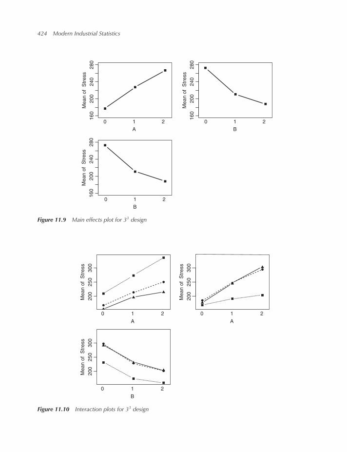
424 Modern Industrial Statistics
B
0 1 2
B
0 1 2
A
0 1 2
160
200
240
280
Mean o
f S
tress
160
200
240
280
Mean o
f S
tress
160
200
240
280
Mean o
f S
tress
Figure 11.9 Main effects plot for 33 design
200
250
300
A
Mean o
f S
tress
200
250
300
Me
an o
f S
tress
200
250
300
Mean o
f S
tress
0 1 2
B
0 1 2
A
0 1 2
Figure 11.10 Interaction plots for 33 design

Classical Design and Analysis of Experiments 425
Suppose that from technological considerations we decide that all interaction parameters involving quadratic compo-
nents are negligible (zero). In this case we can estimate 𝜎2 by 𝜎 2. In the present example the setΛ0 contains 16 parameters,
that is,
Λ0 = {A2B,AB2,A2B2,A2C,A2BC,B2C,AB2C,A2B2C,AC2,
A2C2,BC2,ABC2,A2BC2,B2C2,AB2C2,A2B2C2}.
ThusK0 = 16 and the estimator 𝜎 2 has 16 degrees of freedom. The estimate of 𝜎2 is 𝜎 2 = 95.95. The estimates of the stan-
dard errors (S.E.) in Table 11.24 use this estimate. All the non-significant parameters are denoted by n.s. In Figures 11.9
and 11.10 we present the main effects and interaction plots. ◾
11.8 Blocking and fractional replications of 2m factorial designs
Full factorial experiments with large number of factors might be impractical. For example, if there are m = 12 factors,
even at p = 2 levels, the total number of treatment combinations is 212 = 4096. This size of an experiment is generally
not necessary, because most of the high order interactions might be negligible and there is no need to estimate 4096
parameters. If only main effects and first order interactions are considered, a priori of importance, while all the rest are
believed to be negligible, we have to estimate and test only 1 + 12 +(12
2
)= 79 parameters. A fraction of the experiment, of
size 27 = 128 would be sufficient. Such a fraction can be even replicated several times. The question is, how do we choose
the fraction of the full factorial in such a way that desirable properties of orthogonality, equal variances of estimators, etc.
will be kept, and the parameters of interest will be estimable unbiasedly?
The problem of fractioning the full factorial experiment arises also when the full factorial cannot be performed in
one block, but several blocks are required to accommodate all the treatment conditions. For example, a 25 experiment is
designed, but only 8 = 23 treatment combinations can be performed in any given block (day, machine, etc.). We have to
design the fractions that will be assigned to each block in such a way that, if there are significant differences between the
blocks, the block effects will not confound or obscure parameters of interest. We start with a simple illustration of the
fractionization procedure, and the properties of the ensuing estimators.
Consider 3 factors A, B, C at 2 levels. We wish to partition the 23 = 8 treatment combinations to two fractions of size
22 = 4. Let 𝜆i = 0, 1 (i = 1, 2, 3) and let A𝜆1B𝜆2C𝜆3 represent the 8 parameters. One way of representing the treatment
combinations, when the number of factors is not large, is by using low case letters a, b, c, · · · . The letter a indicates thatfactor A is at the High level (i1 = 1), similarly about other factors. The absence of a letter indicates that the corresponding
factor is at Low level. The symbol (1) indicates that all levels are Low. Thus, the treatment combinations and the associated
coefficients c(23)
ij are shown in Table 11.25.
Table 11.25 A 23 factorial
Treatments Main Effects Defining Parameter
A B C ABC
(1) −1 −1 −1 −1a 1 −1 −1 1b −1 1 −1 1ab 1 1 −1 −1c −1 −1 1 1ac 1 −1 1 −1bc −1 1 1 −1abc 1 1 1 1

426 Modern Industrial Statistics
Table 11.26 Coefficients and response for several treatmentcombinations
t.c. A B C AB AC BC Y
(1) −1 −1 −1 1 1 1 Y(1)ab 1 1 −1 1 −1 −1 Y(ab)ac 1 −1 1 −1 1 −1 Y(ac)bc −1 1 1 −1 −1 1 Y(bc)
Suppose now that the treatment combinations should be partitioned to two fractional replications (blocks) of size 4.
We have to choose a parameter, called a defining parameter, according to which the partition will be done. This definingparameter is in a sense sacrificed. Since its effects will be either confounded with the block effects, or unestimable if only
one block of trials is performed. Thus, let us choose the parameter ABC, as a defining parameter. Partition the treatment
combinations to two blocks, according to the signs of the coefficients corresponding to ABC. These are the products ofthe coefficients in the A, B and C columns. Thus, two blocks are obtained
B− = {(1), ab, ac, bc},
B+ = {a, b, c, abc}.
If 2m treatment combinations are partitioned to 2k = 2 blocks, we say that the degree of fractionation is k = 1, the
fractional replication is of size 2m−k, and the design is 1∕2k fraction of a full factorial. If, for example, m = 5 factors and
we wish to partition to 4 blocks of 8, the degree of fractionization is k = 2. Select k = 2 parameters to serve as defining
parameters, e.g. ACE and BDE, and partition the treatment combinations according to the signs ±1 of the coefficients in
the ACE and BDE columns. This becomes very cumbersome if m and k are large. Function fac.design performs this
partitioning and prints into a file the block which is requested. We will return to this later. It is interesting to check now
what are the properties of estimators in the 23−1 fractional replication, if only the block B− was performed. The defining
parameter was ABC (see Table 11.26).
Let Y(1) be the response of treatment combination (1), this is Y0 in the standard order notation, let Y(a) be the responseof ‘a’, etc. The results of performing B−, with the associated coefficients of parameters of interest can be presented in the
following manner.
We see that the six columns of coefficients are orthogonal to each other, and each column has 2 −1’s and 2 +1’s. TheLSE of the above parameters are orthogonal contrasts, given by
A = 1
4(−Y(1) + Y(ab) + Y(ac) − Y(bc)),
B = 1
4(−Y(1) + Y(ab) − Y(ac) + Y(bc)),
etc. The variances of all these estimators, when n = 1, are equal to𝜎2
4. However, the estimators might be biased. The
expected value of the first estimator is
E{A} = 1
4(−E{Y(1)} + E{Y(ab)} + E{Y(ac)} − E{Y(bc)}).
Now,
E{Y(1)} = 𝜇 − A − B − C + AB + AC + BC − ABC,
E{Y(ab)} = 𝜇 + A + B − C + AB − AC − BC − ABC,
E{Y(ac)} = 𝜇 + A − B + C − AB + AC − BC − ABC,

Classical Design and Analysis of Experiments 427
and
E{Y(bc)} = 𝜇 − A + B + C − AB − AC + BC − ABC.
Collecting all these terms, the result is
E{A} = A − BC.
Similarly, one can show that
E{B} = B − AC,
E{C} = C − AB,
E{AB} = AB − C,
etc. The LSE of all the parameters are biased, unless AB = AC = BC = 0. The bias terms are called aliases. The aliasesare obtained by multiplying the parameter of interest by the defining parameter, when any letter raised to the power 2 is
eliminated, e.g.,
A⊗ ABC = A2BC = BC.
The sign of the alias is the sign of the block. Since we have used the block B−, all the aliases appear above with a negative
sign. The general rules for finding the aliases in 2m−k designs is as follows.
To obtain a 2m−k fractional replication one needs k defining parameters. The multiplication operation of parameters
was illustrated above. The k defining parameters should be independent, in the sense that none can be obtained as a
product of the other ones. Such independent defining parameters are called generators. For example, to choose 4 defining
parameters, when the factors are A, B, C, D, E, F, G, H, choose first two parameters, like ABCH and ABEFG. Theproduct of these two is CEFGH. In the next step choose, for the third defining parameter, any one which is different
than {ABCH,ABEFG,CEFGH}. Suppose one chooses BDEFH. The three independent parameters ABCH, ABEFG and
BDEFH generate a subgroup of eight parameters, including the mean 𝜇. These are:
𝜇 BDEFHABCH ACDEFABEFG ADGHCEFGH BCDG
Finally, to choose a 4th independent defining parameter, one can choose any parameter which is not among the eight
listed above. Suppose that the parameter BCEFH is chosen. Now we obtain a subgroup of 24 = 16 defining parameter, by
adding to the eight listed above their products with BCEFH. Thus, this subgroup is
𝜇 BCEFHABCH AEFABEFG ACGHCEFGH BGBDEFH CDACDEF ABDHADGH ABCDEFGBCDG DEFGH
Notice that this subgroup includes, excluding the mean, two first order interactionsCD and BG. This shows that the choiceof defining parameters was not a good one. The aliases created by these defining parameters include main effects and other
low order interactions.
Given a subgroup of defining parameters, the aliases of a given parameter are obtained by multiplying the parameter
by the defining parameters. In Table 11.27 we list the aliases of the eight main effects, with respect to the above subgroup
of 24 defining parameters.
We see in this table that most of the aliases to the main effects are high order interactions (that are generally negligible).
However, among the aliases of A there is EF. Among the aliases to B there is the main effect G. Among the aliases to C

428 Modern Industrial Statistics
Table 11.27 The aliases to the main effects in a 28−4 Design, Thegenerators are ABCH, ABEFG, BDEFH, and BCEFH
MainEffects Aliases
A BCH,BEFG,ACEFGH,ABDEFH,CDEF,DGH,ABCDG,ABCEFH, EF,CGH,ABG,ACD,BDH,BCDEFG,ADEFGH
B ACH,AEFG,BCEFGH,DEFH,ABCDEF,ABDGH,CDG,CEFH,ABEF,ABCGH,G,BCD,ADH,ACDEFG,BDEFGH
C ABH,ABCEFG, EFGH,BCDEFH,ADEF,ACDGH,BDG,BEFH,ACEF,AGH,BCG,D,ABCDH,ABDEFG,CDEFGH
D ABCDH,ABDEFG,CDEFGH,BEFH,ACEF,AGH,BCG,BCDEFH,ADEF,ACDGH,BDG,C,ABH,ABCEFG, EFGH
E ABCEH,ABFG,CFGH,BDFH,ACDF,ADEGH,BCDEG,BCFH,AF,ACEGH,BEG,CDE,ABDEH,ABCDFG,DFGH
F ABCFH,ABEG,CEGH,BDEH,ACDE,ADFGH,BCDFG,BCEH,AE,ACFGH,BFG,CDF,ABDFH,ABCDEG,DEGH
G ABCGH,ABEF,CEFH,BDEFGH,ACDEFG,ADH,BCD,BCEFGH,AEFG,ACH,B,CDG,ABDGH,ABCDEF,DEFH
H ABC,ABEFGH,CEFG,BDEF,ACDEFH,ADG,BCDGH,BCEF,AEFH,ACG,BGH,CDH,ABD,ABCDEFGH,DEFG
there is D, etc. This design is not good since it may yield strongly biased estimators. The resolution of a 2m−k design isthe length of the smallest word (excluding 𝜇) in the subgroup of defining parameters. For example, if in a 28−4 design
we use the following four generators BCDE, ACDF, ABCG and ABDH, we obtain the 16 defining parameters {𝜇,BCDE,ACDF,ABEF,ABCG,ADEG,BDFG,CEFG,ABDH,ACEH,BDFH,DEFH,CDGH,BEGH,AFGH,ABCDEFGH}. The
length of the smallest word, excluding 𝜇, among these defining parameters is four. Thus the present 28−4 design is a
resolution IV design. In this design, all aliases of main effects are second order interactions or higher (words of length
greater or equal to three). Aliases to first order interactions are interactions of first order or higher. The present design is
obviously better, in terms of resolution, than the previous one (which is of resolution II). We should always try to get
resolution IV or higher. If the degree of fractionation is too high there may not exist resolution IV designs. For example,
in 26−3 and 27−4, 29−5, 210−6 and 211−7 we have only resolution III designs. One way to reduce the bias is to choose
several fractions at random. For example in a 211−7 we have 27 = 128 blocks of size 24 = 16. If we execute only one
block, the best we can have is a resolution III. In this case some main effects are biased (confounded) with some first
order interactions. If one chooses n blocks at random (RSWOR) out of the 128 possible ones, and compute the average
estimate of the effects, the bias is reduced to zero, but the variance of the estimators is increased.
To illustrate this, suppose that we have a 26−2 design with generators ABCE and BCDF. This will yield a resolution IVdesign. There are 4 blocks and the corresponding bias terms of the LSE of A are
block
0 −BCE − ABCDF + DEF1 BCE − ABCDF − DEF2 −BCE + ABCDF − DEF3 BCE + ABCDF + DEF
If we choose one block at random, the expected bias is the average of the four terms above, which is zero. The total
variance of A is𝜎2
16+ Variance of conditional bias = 𝜎
2
16+ [(BCE)2 + (ABCDF)2 + (DEF)2]∕4.

Classical Design and Analysis of Experiments 429
Table 11.28 Blocks of 28−4 designs
Block 0 Block 1
1 1 1 1 1 1 1 1 1 2 2 2 1 1 1 11 2 2 2 2 1 1 1 1 1 1 1 2 1 1 12 1 2 2 1 2 1 1 2 2 1 1 1 2 1 12 2 1 1 2 2 1 1 2 1 2 2 2 2 1 12 2 2 1 1 1 2 1 2 1 1 2 1 1 2 12 1 1 2 2 1 2 1 2 2 2 1 2 1 2 11 2 1 2 1 2 2 1 1 1 2 1 1 2 2 11 1 2 1 2 2 2 1 1 2 1 2 2 2 2 12 2 1 2 1 1 1 2 2 1 2 1 1 1 1 22 1 2 1 2 1 1 2 2 2 1 2 2 1 1 21 2 2 1 1 2 1 2 1 1 1 2 1 2 1 21 1 1 2 2 2 1 2 1 2 2 1 2 2 1 21 1 2 2 1 1 2 2 1 2 1 1 1 1 2 21 2 1 1 2 1 2 2 1 1 2 2 2 1 2 22 1 1 1 1 2 2 2 2 2 2 2 1 2 2 22 2 2 2 2 2 2 2 2 1 1 1 2 2 2 2
Example 11.10. In the present example we illustrate the construction of fractional replications. The case that is illustrated
is a 28−4 design presented in Table 11.28. Here we can construct 16 fractions, each one of size 16. As discussed before,
four generating parameters should be specified. Let these be BCDE, ACDF, ABCG, ABDH. These parameters generate
resolution IV design where the degree of fractionation is k = 4. The blocks can be indexed 0, 1, · · · , 15. Each index is
determined by the signs of the four generators, which determine the block. Thus, the signs (−1,−1, 1, 1) correspond to
(0, 0, 1, 1) which yields the index4∑j=1ij2
j−1 = 12.
The index of generator 1 (BCDE = A0B1C1D1E1F0G0H0) is 0, 1, 1, 1, 1, 0, 0, 0, for generator 2: 1, 0, 1, 1, 0, 1, 0, 0; forgenerator 3: 1, 1, 1, 0, 0, 0, 1, 0 and for generator 4: 1, 1, 0, 1, 0, 0, 0, 1.
In the following table two blocks derived with R are printed.
> Gen <- matrix(c(0,1,1,1,1,0,0,0,1,0,1,1,0,1,0,0),
nrow=2,byrow=TRUE)
> head(fac.design(nlevels=2,
nfactors=8,blocks=4,block.gen=Gen))
creating full factorial with 256 runs ...Blocks A B C D E F G H
1 1 1 1 1 1 1 1 2 12 1 1 2 2 1 1 2 1 23 1 1 2 1 1 2 1 1 14 1 2 1 2 2 1 2 2 25 1 1 2 2 2 2 1 2 26 1 1 1 2 2 1 1 2 2
> rm(Gen)◾

430 Modern Industrial Statistics
Table 11.29 Some generators for 2m−k designs
m
k 5 6 7 8
1 ABCDE ABCDEF ABCDEFGH ABCDEFGH2 ABD ABCE ABCDF ABCDG
ACE BCDF ABDEG ABEFH3 ABD ABCE ABCF
ACD BCDF ABDGBCF ACDG BCDEH
4 ABD BCDEACE ACDFBCF ABCGABCG ABDH
In Box, Hunter and Hunter (1978, pp. 410) there are recommended generators for 2m−k designs. Some of these gener-
ators are given in Table 11.29.
The LSE of the parameters is performed by writing first the columns of coefficients ci,j = ±1 corresponding to the
design, multiplying the coefficients by the Y values, adding the results and dividing by 2m−k.
11.9 Exploration of response surfaces
The functional relationship between the yield variable Y and the experimental variables (x1, · · · , xk) is modeled as
Y = f (x1, · · · , xk) + e,
where e is a random variable with zero mean and a finite variance, 𝜎2. The set of points {f (x1, · · · , xk), xi ∈ Di, i =1, · · · , k}, where (D1, · · · ,Dk) is the experimental domain of the x-variables, is called a response surface. Two types of
response surfaces were discussed before, the linear
f (x1, · · · , xk) = 𝛽0 +k∑i=1𝛽ixi (11.102)
and the quadratic
f (x1, · · · , xk) = 𝛽0 +k∑i=1𝛽ixi +
k∑i=1𝛽iix
2i +
∑∑i≠j𝛽ijxixj. (11.103)
Response surfaces may be of complicated functional form. We assume here that in local domains of interest, they can be
approximated by linear or quadratic models.
Researchers are interested in studying, or exploring, the nature of response surfaces, in certain domains of interest, for
the purpose of predicting future yield, and in particular for optimizing a process, by choosing the x-values to maximize (or
minimize) the expected yield (or the expected loss). In the present section we present special designs for the exploration
of quadratic surfaces, and for the determination of optimal domains (conditions). Designs for quadratic models are called
second order designs. We start with the theory of second order designs, and conclude with the optimization process.

Classical Design and Analysis of Experiments 431
11.9.1 Second order designs
Second order designs are constructed in order to estimate the parameters of the quadratic response function
E{Y} = 𝛽0 +k∑i=1𝛽ixi +
k∑i=1𝛽iix
2i +
k−1∑i=1
k∑j=i+1𝛽ijxixj. (11.104)
In this case the number of regression coefficients is p = 1 + 2k +(k2
). We will arrange the vector 𝜷 in the form
𝜷 ′ = (𝛽0, 𝛽11, · · · , 𝛽kk, 𝛽1, · · · , 𝛽k, 𝛽12, · · · , 𝛽1k, 𝛽23, · · · , 𝛽2k, · · · , 𝛽k−1,k).
Let N be the number of x-points. The design matrix takes the form
(X) =
⎡⎢⎢⎢⎢⎢⎣
1 x211
· · · x21k x11 · · · x1k x11x12 · · · x1,k−1x1,k
1 x221
x22k x21 x2k x21x22
1 x231
x23k x31 x3k
⋮ ⋮ ⋮ ⋮ ⋮ ⋮ ⋮1 x2N1 x2Nk xN1 · · · xNk xN1xN2 · · · xN,k−1xN,k
⎤⎥⎥⎥⎥⎥⎦Impose on the x-values the conditions:
(i)N∑j=1xji = 0, i = 1, · · · , k
(ii)N∑j=1x3ji = 0, i = 1, · · · , k
(iii)N∑j=1x2jixjl = 0, i ≠ l
(iv)N∑j=1x2ji = b, i = 1, · · · , k (11.105)
(v)N∑j=1x2jix
2jl = c, i ≠ l
(vi)N∑j=1x4ji = c + d.
The matrix (S) = (X)′(X) can be written in the form
(S) =[(U) 0
0 (B)
](11.106)
where (U) is the (k + 1) × (k + 1) matrix
(U) =[N b1′kb1k dIk + cJk
](11.107)
and (B) is a diagonal matrix of orderk(k+1)
2
(B) =
⎡⎢⎢⎢⎢⎣b
⋱b 0
cc
0 ⋱c
⎤⎥⎥⎥⎥⎦. (11.108)

432 Modern Industrial Statistics
One can verify that
(U)−1 =[p q1′kq1k tIk + sJk
], (11.109)
where
p = d + kcN(d + kc) − b2k
,
q = − bN(d + kc) − b2k
,
t = 1
d
s = b2 − Ncd[N(d + kc) − b2k]
.
(11.110)
Notice that U is singular if N(d + kc) = b2k. We therefore say that the design is non-singular if
N ≠ b2kd + kc.
Furthermore, if N = b2∕c then s = 0. In this case the design is called orthogonal.Let x𝟎′ = (x0
1, · · · , x0k) be a point in the experimental domain, and
𝝃0′ = (1, (x0
1)2, · · · , (x0k)
2, x01, · · · , x0k , x
01x02, x0
1x03, · · · , x0k−1x
0k).
The variance of the predicted response at x0 is
V{Y(x0)} = 𝜎2𝝃0′
⎡⎢⎢⎢⎢⎢⎢⎢⎢⎢⎣
(U)−1−−
0
|||||||||||||||||
0
−− −− −− −− −− −−b−1 0
⋱b−1
c−1
0 ⋱c−1
⎤⎥⎥⎥⎥⎥⎥⎥⎥⎥⎦𝝃0
= 𝜎2[p + 1
b
k∑i=1
(x0i )2 + (t + s)
k∑i=1
(x0i )4
+ 1
c
∑∑h<j
(x0h)2(x0j )
2 + 2bk∑i=1
(x0i )2
+ 2s∑∑
h<j
(x0h)2(x0j )
2
]
= 𝜎2[p + 𝜌2
(2b + 1
b
)+ (t + s)
k∑i=1
(x0i )4
+ 2(s + 1
2c
)∑∑h<j
(x0n)2(x0j )2
], (11.111)
where 𝜌2 =∑k
i=1 (x0i )2. Notice that
𝜌4 =
(k∑i=1
(x0i )2
)2
=k∑i=1
(x0i )4 + 2
∑∑h<j
(x0h)2(x0j )
2.

Classical Design and Analysis of Experiments 433
Thus, if d = 2c then t + s = s + 1
2cand
V{Y(x0)} = 𝜎2[p + 𝜌2
(2b + 1
b
)+ (t + s)𝜌4
]. (11.112)
Such a design (d = 2c) is called rotatable, since V{Y(x0)} is constant for all points x0 on the circumference of a circle of
radius 𝜌, centered at the origin.
11.9.2 Some specific second order designs
11.9.2.1 3k-designs
Consider a factorial design of k factors, each one at three levels −1, 0, 1. In this case the number of points is N = 3k.
Obviously3k∑j=1xji = 0 for all i = 1, · · · , k. Also
3k∑j=1x3ji = 0 and
3k∑j=1x2jixjk = 0, i ≠ k.
b =3k∑j=1
x2ji =2
33k = 2 ⋅ 3k−1.
c =3k∑j=1
x2jix2jl =
2
3b = 4 ⋅ 3k−2⋅
d = b − c.
(11.113)
Hence
d = 2 ⋅ 3k−1 − 4 ⋅ 3k−2 = 2 ⋅ 3k−2. (11.114)
b2 = 4 ⋅ 32k−2 and N ⋅ c = 3k ⋅ 4 ⋅ 3k−2 = 4 ⋅ 32k−2. Thus, Nc = b2. The design is orthogonal. However, d ≠ 2 ⋅ c. Thus, thedesign is not rotatable.
11.9.2.2 Central composite designs
A Central Composite Design is one in which we start with nc = 2k points of a factorial design, in which each factor is at
levels −1 and +1. To these points we add na = 2k axial points which are at a fixed distance 𝛼 from the origin. These are
the points
(±𝛼, 0, · · · , 0), (0,±𝛼, 0, · · · , 0), · · · , (0, 0, · · · , 0,±𝛼).
Finally, put n0 points at the origin. These n0 observations yield an estimate of the variance 𝜎2. Thus, the total number of
points is N = 2k + 2k + n0. In such a design,
b = 2k + 2𝛼2,
c = 2k,
c + d = 2k + 2𝛼4, or
d = 2𝛼4.
(11.115)
The rotatability condition is d = 2c. Thus, the design is rotatable if
𝛼4 = 2k, or
𝛼 = 2k∕4.(11.116)
For this reason, in central composite designs, with k = 2 factors we use 𝛼 =√2 = 1.414. For k = 3 factors we use 𝛼 =
23∕4 = 1.6818. For rotatability and orthogonality, the following should be satisfied
n0 + 2k = 4𝛼2(2k + 𝛼2)2k, (11.117)

434 Modern Industrial Statistics
Table 11.30 Factors and level in piston simulator experiment
Factor Levels
Piston Surface Area .0075 .01 .0125 .015 .0175Initial Gas Volume .0050 .00625 .0075 .00875 .0100Spring Coefficient 1000 2000 3000 4000 5000Filling Gas Temperature 340 345 350 355 360
Code −2 −1 0 1 2
Table 11.31 The central composite design and the mean andstandard-deviations of cycle time
CODE LEVELS
B C D G Y STD.
−1.00 −1.00 −1.00 −1.00 0.671 0.23281.00 −1.00 −1.00 −1.00 0.445 0.1771
−1.00 1.00 −1.00 −1.00 0.650 0.22981.00 1.00 −1.00 −1.00 0.546 0.2228
−1.00 −1.00 1.00 −1.00 0.534 0.16501.00 −1.00 1.00 −1.00 0.410 0.1688
−1.00 1.00 1.00 −1.00 0.534 0.12571.00 1.00 1.00 −1.00 0.495 0.1388
−1.00 −1.00 −1.00 1.00 0.593 0.24531.00 −1.00 −1.00 1.00 0.542 0.2266
−1.00 1.00 −1.00 1.00 0.602 0.21851.00 1.00 −1.00 1.00 0.509 0.1977
−1.00 −1.00 1.00 1.00 0.480 0.17131.00 −1.00 1.00 1.00 0.411 0.1658
−1.00 1.00 1.00 1.00 0.435 0.13891.00 1.00 1.00 1.00 0.438 0.14822.00 0.00 0.00 0.00 0.458 0.1732
−2.00 0.00 0.00 0.00 0.635 0.16770.00 2.00 0.00 0.00 0.570 0.15690.00 −2.00 0.00 0.00 0.481 0.17570.00 0.00 2.00 0.00 0.428 0.10640.00 0.00 −2.00 0.00 0.742 0.32700.00 0.00 0.00 2.00 0.496 0.20290.00 0.00 0.00 −2.00 0.549 0.17650.00 0.00 0.00 0.00 0.490 0.18020.00 0.00 0.00 0.00 0.468 0.14800.00 0.00 0.00 0.00 0.481 0.16360.00 0.00 0.00 0.00 0.557 0.1869
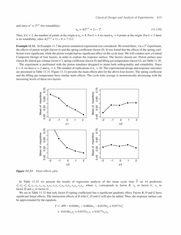
Classical Design and Analysis of Experiments 435
and since 𝛼2 = 2k∕2 (for rotatability)
n0 = 4(2k∕2 + 1) − 2k. (11.118)
Thus, if k = 2, the number of points at the origin is n0 = 8. For k = 4 we need n0 = 4 points at the origin. For k = 3 there
is no rotatability, since 4(23∕2 + 1) − 8 = 7.313.
Example 11.11. In Example 11.7 the piston simulation experiment was considered. We tested there, via a 32 experiment,
the effects of piston weight (factor A) and the spring coefficient (factorD). It was found that the effects of the spring coef-ficient were significant, while the piston weight had no significant effect on the cycle time. We will conduct now a Central
Composite Design of four factors, in order to explore the response surface. The factors chosen are: Piston surface area
(factorB); Initial gas volume (factorC); spring coefficient (factorD) and filling gas temperature (factorG), see Table 11.30.The experiment is performed with the piston simulator designed to attain both orthogonality and rotatability. Since
k = 4, we have 𝛼 = 2 and n0 = 4. The number of replications is nr = 30. The experimental design and response outcomes
are presented in Table 11.31. Figure 11.11 presents the main effects plot for the above four factors. The spring coefficient
and the filling gas temperature have similar main effects. The cycle time average is monotonically decreasing with the
increasing levels of these two factors.
0.4
50.5
50.6
50.7
5
x2
Mean o
f m
eantim
e
0.4
50.5
50.6
50.7
5
Mean o
f m
eantim
e
0.4
50.5
50.6
50.7
5
Mean o
f m
eantim
e
0.4
50.5
50.6
50.7
5
Mean o
f m
eantim
e
−2 −1 0 1 2
x4
−2 −1 0 1 2
x3
−2 −1 0 1 2
x1
−2 −1 0 1 2
Figure 11.11 Main effects plot
In Table 11.32 we present the results of regression analysis of the mean cycle time Y on 14 predictors
x21, x2
2, x2
3, x2
4, x1, x2, x3, x4, x1x2, x1x3, x1x4, x2x3, x2x4, x3x4, where x1 corresponds to factor B, x2 to factor C, x3 to
factor D and x4 to factor G.We see in Table 11.32 that only factor D (spring coefficient) has a significant quadratic effect. Factor B, D and G have
significant linear effects. The interaction effects of B with C, D and G will also be added. Thus, the response surface can
be approximated by the equation,
Y = .499 − 0.0440x1 − 0.0604x3 − 0.0159x4 + 0.0171x23
+ 0.0148x1x2 + 0.0153x1x3 + 0.0177x1x4.

436 Modern Industrial Statistics
The contour lines for the mean cycle time, corresponding to x2 = x4 = 0 are shown in Figure 11.12.
> library(rsm)> s <- c(0.0075, 0.01, 0.0125, 0.015, 0.0175)> v0 <- c(0.0050, 0.00625, 0.0075, 0.00875, 0.0100)> k <- c(1000, 2000, 3000, 4000, 5000)> t0 <- c(340, 345, 350, 355, 360)> Ccd <- ccd(basis=4,
n0=4,alpha=2,coding=list(x1 ~ -5 + s*400,
x2 ~ -6 + v0*800,x3 ~ -3 + k*0.001,x4 ~ -70 + t0*0.2),
randomize=FALSE)> head(Ccd)
run.order std.order s v0 k t0 Block1 1 1 0.010 0.00625 2000 345 12 2 2 0.015 0.00625 2000 345 13 3 3 0.010 0.00875 2000 345 14 4 4 0.015 0.00875 2000 345 15 5 5 0.010 0.00625 4000 345 16 6 6 0.015 0.00625 4000 345 1
Data are stored in coded form using these coding formulas ...x1 ~ -5 + s * 400x2 ~ -6 + v0 * 800x3 ~ -3 + k * 0.001x4 ~ -70 + t0 * 0.2
> Levels <- as.data.frame(decode.data(Ccd))[, c("s", "v0", "k", "t0")]
> Ps <- pistonSimulation(m=rep(60, nrow(Levels)),s=Levels$s,v0=Levels$v0,k=Levels$k,p0=rep(110000, nrow(Levels)),t=rep(296, nrow(Levels)),t0=Levels$t0,each=30,seed=123)
> Ps <- simulationGroup(Ps, 30)> Ccd$meantime <- aggregate(Ps["seconds"],
by=Ps["group"],FUN=mean)$seconds
> Rsm <- rsm(meantime ~ SO(x1, x2, x3, x4),data= Ccd)
> summary(Rsm)
Call:rsm(formula = meantime ~ SO(x1, x2, x3, x4), data = Ccd)
Estimate Std. Error t value Pr(>|t|)(Intercept) 0.55651498 0.00895672 62.1338 < 2.2e-16x1 -0.06273744 0.00517116 -12.1322 8.508e-10x2 0.01732095 0.00517116 3.3495 0.003801x3 -0.07605865 0.00517116 -14.7082 4.227e-11

Classical Design and Analysis of Experiments 437
x4 -0.00086087 0.00517116 -0.1665 0.869748x1:x2 0.01063617 0.00633336 1.6794 0.111360x1:x3 0.01540720 0.00633336 2.4327 0.026322x1:x4 -0.00398071 0.00633336 -0.6285 0.538010x2:x3 0.00097643 0.00633336 0.1542 0.879289x2:x4 -0.00634481 0.00633336 -1.0018 0.330483x3:x4 -0.00099975 0.00633336 -0.1579 0.876431x1ˆ2 0.00780867 0.00466122 1.6752 0.112182x2ˆ2 -0.00124712 0.00466122 -0.2676 0.792262x3ˆ2 0.02990712 0.00466122 6.4161 6.389e-06x4ˆ2 0.00155039 0.00466122 0.3326 0.743492
(Intercept) ***x1 ***x2 **x3 ***x4x1:x2x1:x3 *x1:x4x2:x3x2:x4x3:x4x1ˆ2x2ˆ2x3ˆ2 ***x4ˆ2---Signif. codes: 0 ‘***’ 0.001 ‘**’ 0.01 ‘*’ 0.05 ‘.’ 0.1 ‘ ’ 1
Analysis of Variance Table
Response: meantimeDf Sum Sq Mean Sq F value
FO(x1, x2, x3, x4) 4 0.240520 0.060130 93.6921TWI(x1, x2, x3, x4) 6 0.006537 0.001090 1.6976PQ(x1, x2, x3, x4) 4 0.027809 0.006952 10.8327Residuals 17 0.010910 0.000642Lack of fit 10 0.006863 0.000686 1.1871Pure error 7 0.004047 0.000578
Pr(>F)FO(x1, x2, x3, x4) 2.391e-11TWI(x1, x2, x3, x4) 0.1821633PQ(x1, x2, x3, x4) 0.0001499ResidualsLack of fit 0.4223317Pure error
Stationary point of response surface:x1 x2 x3 x4
5.65531833 1.91720834 -0.02501298 11.45274099
Stationary point in original units:s v0 k
0.02663830 0.00989651 2974.98701820t0
407.26370496

438 Modern Industrial Statistics
Eigenanalysis:$values[1] 0.0325114175 0.0091700709 0.0009851376[4] -0.0046475718
$vectors[,1] [,2] [,3] [,4]
x1 -0.31297494 0.7394155 0.4733013 -0.36234958x2 -0.06696307 0.4770755 -0.1256402 0.86725401x3 -0.94645473 -0.2948946 -0.1089955 0.07335251x4 0.04226194 -0.3724256 0.8650552 0.33345567
> rm(k, s, t0, v0)
Table 11.32 Regression analysis of piston experiment with four factors
Predictor Coef Stdev t-ratio p
𝜇 Constant 0.499000 0.018530 26.92 0.000𝛽11 x21 0.007469 0.007567 0.99 0.342𝛽22 x22 0.002219 0.007567 0.29 0.774𝛽33 x23 0.017094 0.007567 2.26 0.042𝛽44 x24 0.001469 0.007567 0.19 0.849𝛽1 x1(s) −0.044042 0.007567 −5.82 0.000𝛽2 x2(v0) 0.012542 0.007567 1.66 0.121𝛽3 x3(k) −0.060375 0.007567 −7.98 0.000𝛽4 x4(t0) −0.015875 0.007567 −2.10 0.056𝛽12 x1x2 0.014813 0.009267 1.60 0.134𝛽13 x1x3 0.015313 0.009267 1.65 0.122𝛽14 x1x4 0.017687 0.009267 1.91 0.079𝛽23 x2x3 0.000688 0.009267 0.07 0.942𝛽24 x2x4 −0.012937 0.009267 −1.40 0.186𝛽34 x3x4 −0.008937 0.009267 −0.96 0.352
s = 0.03707 R − sq = 90.4% R − sq(adj) = 80.0%
◾
11.9.3 Approaching the region of the optimal yield
Very often, the purpose for fitting a response surface is to locate the levels of the factors, which yield optimal results.
Initially one might be far from the optimal regions. A series of small experiments may be performed, in order to move
towards the optimal region. Thus, we start with simple first order experiments, like 2k factorial, and fit to the results a
linear model of the form
Y = b0 + b1x1 + · · · + bkxk.
We wish to determine now a new point, 𝝃∗ say, whose distance from the center of the 1st stage experiment (say 0) is R,and with maximal (or minimal) predicted yield. The predicted yield at 𝝃∗( is
y∗ = b0 +k∑i=1
bi𝜉∗i .
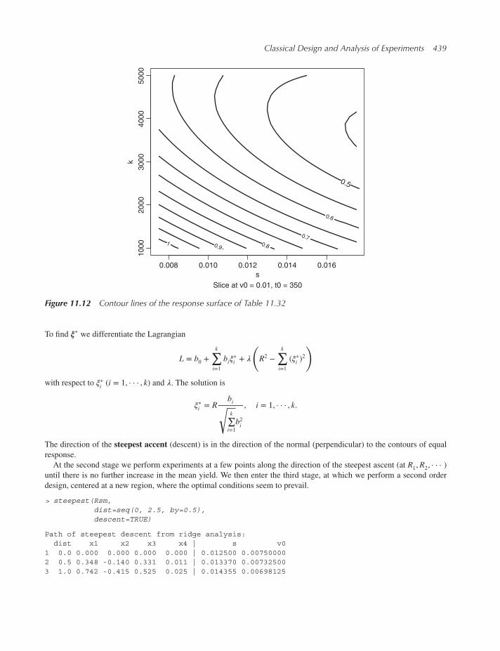
Classical Design and Analysis of Experiments 439
s
Slice at v0 = 0.01, t0 = 350
k
0.5
0.6
0.70.80.9
1
0.008 0.010 0.012 0.014 0.016
1000
2000
3000
4000
5000
Figure 11.12 Contour lines of the response surface of Table 11.32
To find 𝝃∗ we differentiate the Lagrangian
L = b0 +k∑i=1
bi𝜉∗i + 𝜆
(R2 −
k∑i=1
(𝜉∗i )2
)with respect to 𝜉∗i (i = 1, · · · , k) and 𝜆. The solution is
𝜉∗i = Rbi√k∑i=1b2i
, i = 1, · · · , k.
The direction of the steepest accent (descent) is in the direction of the normal (perpendicular) to the contours of equal
response.
At the second stage we perform experiments at a few points along the direction of the steepest ascent (at R1,R2, · · · )until there is no further increase in the mean yield. We then enter the third stage, at which we perform a second order
design, centered at a new region, where the optimal conditions seem to prevail.
> steepest(Rsm,dist=seq(0, 2.5, by=0.5),descent=TRUE)
Path of steepest descent from ridge analysis:dist x1 x2 x3 x4 | s v0
1 0.0 0.000 0.000 0.000 0.000 | 0.012500 0.007500002 0.5 0.348 -0.140 0.331 0.011 | 0.013370 0.007325003 1.0 0.742 -0.415 0.525 0.025 | 0.014355 0.00698125

440 Modern Industrial Statistics
4 1.5 1.120 -0.795 0.598 0.020 | 0.015300 0.006506255 2.0 1.460 -1.228 0.611 -0.015 | 0.016150 0.005965006 2.5 1.762 -1.673 0.597 -0.077 | 0.016905 0.00540875
k t0 | yhat1 3000 350.000 | 0.5572 3331 350.055 | 0.5123 3525 350.125 | 0.4784 3598 350.100 | 0.4475 3611 349.925 | 0.4176 3597 349.615 | 0.387
11.9.4 Canonical representation
The quadratic response function
Y = b0 +k∑i=1
bixi +k∑i=1
biix2i + 2
∑∑i<j
bijxixj, (11.119)
can be written in the matrix form
Y = b0 + b′x + x′Bx, (11.120)
where x′ = (x1, · · · , xk), b′ = (b1, · · · , bk) and
B =⎡⎢⎢⎢⎣b11 b12 · · · b1kb12 ⋱ ⋮⋮ ⋱ ⋮b1k · · · · · · bkk
⎤⎥⎥⎥⎦ .Let 𝛁Y be the gradient of Y , i.e.,
𝛁Y = 𝜕𝜕xY = b + 2Bx.
Let x0 be a point at which the gradient is zero, namely
x0 = −1
2B−1b, (11.121)
assuming that the matrix B is non-singular. Making the transformation (change of origin to x0) z = x − x0, we obtain
Y = b0 + (x0 + z)′b + (x0 + z)′B(x0 + z)
= Y0 + z′Bz,(11.122)
where Y0 = b0 + b′x0.The matrix B is real symmetric. Thus, there exists an orthogonal matrix H (see Appendix I), which consists of the
normalized eigenvectors of B, such that
HBH′ =⎛⎜⎜⎝𝜆
0 ⋱ 0
𝜆k
⎞⎟⎟⎠ ,where 𝜆i (i = 1, · · · , k) are the eigenvalues of B. We make now a new transformation (rotation), namely,
w = Hz.
Since H is orthogonal, z = H′w and
z′Bz = w′HBH′w
=k∑i=1𝜆i𝑤
2i .

Classical Design and Analysis of Experiments 441
In these new coordinates,
Y = Y0 +k∑i=1𝜆i𝑤
2i . (11.123)
This representation of the quadratic surface is called the canonical form. We see immediately that if 𝜆i > 0 for all i =1, · · · , k, then Y0 is aminimum. If 𝜆i < 0 for all i = 1, · · · , k then Y0 is amaximum. If some eigenvalues are positive and
some are negative, then Y0 is a saddle point.The following examples of second order equations are taken from Box, Hunter and Hunter (1978, pp. 527–530).
1. Simple maximum:
Y = 83.57 + 9.39x1 + 7.12x2 − 7.44x21 − 3.71x22 − 5.80x1x2
= 87.69 − 902𝑤21 − 2.13𝑤22.
2. Minimax:
Y = 84.29 + 11.06x1 + 4.05x2 − 6.46x21 − 0.43x22 − 9.38x1x2
= 87.69 − 9.02𝑤21 + 2.13𝑤22.
3. Stationary ridge:
Y = 83.93 + 10.23x1 + 5.59x2 − 6.95x21 − 2.07x22 − 7.59x1x2
= 87.69 − 9.02𝑤21 + 0.00𝑤22.
4. Rising ridge:
Y = 82.71 + 8.80x1 + 8.19x2 − 6.95x21 − 2.07x22 − 7.59x1x2
= 87.69 − 9.02𝑤21 + 2.97𝑤2.
> canonical.path(Rsm,dist=seq(0, 2.5, by=0.5),descent=TRUE)
dist x1 x2 x3 x4 | s1 0.0 5.655 1.917 -0.025 11.453 | 0.02663752 0.5 5.474 2.351 0.012 11.619 | 0.02618503 1.0 5.293 2.784 0.048 11.786 | 0.02573254 1.5 5.112 3.218 0.085 11.953 | 0.02528005 2.0 4.931 3.652 0.122 12.120 | 0.02482756 2.5 4.749 4.085 0.158 12.286 | 0.0243725
v0 k t0 | yhat1 0.00989625 2975 407.265 | 0.3922 0.01043875 3012 408.095 | 0.3913 0.01098000 3048 408.930 | 0.3874 0.01152250 3085 409.765 | 0.3815 0.01206500 3122 410.600 | 0.3736 0.01260625 3158 411.430 | 0.363
11.10 Chapter highlights
The chapter covers the range of classical experimental designs including complete block designs, Latin squares, full and
fractional factorial designs with factors at two and three levels. The basic approach to the analysis is through modeling the
response variable and computing ANOVA tables. Particular attention is also given to the generation of designs using R.

442 Modern Industrial Statistics
The main concepts and definitions introduced in this chapter include:
• Response Variable
• Controllable Factor
• Factor Level
• Statistical Model
• Experimental Array
• Blocking
• Randomization
• Block Designs
• Main Effects
• Interactions
• Analysis of Variance
• Latin Squares
• Factorial Designs
• Fractional Factorial Designs
11.11 Exercises
11.1 Describe a production process familiar to you, like baking of cakes, or manufacturing concrete. List the pertinent
variables.What is (are) the response variable(s)? Classify the variables which affect the response to noise variables
and control variables. How many levels would you consider for each variable?
11.2 Different types of adhesive are used in a lamination process, in manufacturing a computer card. The card is tested
for bond strength. In addition to the type of adhesive, a factor which might influence the bond strength is the
curing pressure (currently at 200 psi). Follow the basic steps of experimental design to set a possible experiment
for testing the effects of adhesives and curing pressure on the bond strength.
11.3 Provide an example where blocking can reduce the variability of a product.
11.4 Three factors A, B, C are tested in a given experiment, designed to assess their effects on the response variable.
Each factor is tested at 3 levels. List all the main effects and interactions.
11.5 Let x1, x2 be two quantitative factors and Y a response variable. A regression model Y = 𝛽0 + 𝛽1x1 + 𝛽2x2 +𝛽12x1x2 + e is fitted to the data. Explain why 𝛽12 can be used as an interaction parameter.
11.6 Consider the ISC values for times t1, t2 and t3 in data file SOCELL.csv. Make a paired comparison for testing
whether the mean ISC in time t2 is different from that in time t1, by using a t-test.11.7 Use macro RPCOMP.MTB to perform a randomization test for the differences in the ISC values of the solar
cells in times t2 and t3 (data file SOCELL.csv).11.8 Box, Hunter and Hunter (1978, p. 209) give the following results of four treatments A, B, C, D in penicillin
manufacturing in five different blends (align).
Treatments
Blends A B C D
1 89 88 97 94
2 84 77 92 79
3 81 87 87 85
4 87 92 89 84
5 79 81 80 88
Perform an ANOVA to test whether there are significant differences between the treatments or between the blends.

Classical Design and Analysis of Experiments 443
11.9 Eight treatments A,B,C, · · · ,H were tested in a BIBD of 28 blocks, k = 2 treatments per block, r = 7 and 𝜆 = 1.
The results of the experiments are
Block Treatments Block Treatments
1 A 38 B 30 15 D 11 G 24
2 C 50 D 27 16 F 37 H 39
3 E 33 F 28 17 A 23 F 40
4 G 62 H 30 18 B 20 D 14
5 A 37 C 25 19 C 18 H 10
6 B 38 H 52 20 E 22 G 52
7 D 89 E 89 21 A 66 G 67
8 F 27 G 75 22 B 23 F 46
9 A 17 D 25 23 C 22 E 28
10 B 47 G 63 24 D 20 H 40
11 C 32 F 39 25 A 27 H 32
12 E 20 H 18 26 B 10 E 40
13 A 5 E 15 27 C 32 G 33
14 B 45 C 38 28 D 18 F 23
Make an ANOVA to test the significance of the block effects and treatment effects. If the treatment effects are
significant, make multiple comparisons of the treatments.
11.10 Four different methods of preparing concrete mixtures A, B, C, D were tested, these methods consist of two
different mixture ratios of cement towater and two blending duration. The fourmethods (treatments) were blocked
in four batches and four days, according to a Latin square design. The concrete was poured to cubes and tested for
compressive strength [kg/cm2] after 7 days of storage in special rooms with 20∘C temperature and 50% relative
humidity. The results are:
batches
Days 1 2 3 4
A B C D1 312 299 315 290
C A D B2 295 317 313 300
B D A C3 295 298 312 315
D C B A4 313 314 299 300
Are the differences between the strength values of different treatments significant? [Perform the ANOVA.]
11.11 Repeat the experiments described in Example 11.7 at the low levels of factors B, C, E, F, and G. Perform the
ANOVA for the main effects and interaction of spring coefficient and piston weight on the cycle time. Are your
results different from those obtained in the example?
11.12 For the data in Example 11.7 compute the least squares estimates of the main effects on the means and on the
standard deviations.

444 Modern Industrial Statistics
11.13 A 24 factorial experiment gave the following response values, arranged in standard order: 72, 60, 90, 80, 65, 60,
85, 80, 60, 50, 88, 82, 58, 50, 84, 75.
(i) Estimate all possible main effects.
(ii) Estimate 𝜎2 under the assumption that all the interaction parameters are zero.
(iii) Determine a confidence interval for 𝜎2 at level of confidence 0.99.11.14 A 32 factorial experiment, with n = 3 replications, gave the following observations:
A1 A2 A3
18.3 17.9 19.1
B1 17.9 17.6 19.0
18.5 16.2 18.9
20.5 18.2 22.1
B2 21.1 19.5 23.5
20.7 18.9 22.9
21.5 20.1 22.3
B3 21.7 19.5 23.5
21.9 18.9 23.3
Perform an ANOVA to test the main effects and interactions. Break the between treatments sum of squares to one
degree of freedom components. Use the Scheffé S𝛼 coefficient to determine which effects are significant.
11.15 Construct a 28−2 fractional replication, using the generators ABCDG and ABEFH. What is the resolution of this
design? Write the aliases to the main effects, and to the first order interactions with the factor A.11.16 Consider a full factorial experiment of 26 = 64 runs. It is required to partition the runs to 8 blocks of 8. The
parameters in the group of defining parameters are confounded with the effects of blocks, and are not estimable.
Show which parameters are not estimable if the blocks are generated by ACE, ABEF and ABCD.11.17 A 22 factorial design is expanded by using 4 observations at 0. The design matrix and the response are:
X1 X2 Y
−1 −1 55.8
−1 −1 54.4
1 −1 60.3
1 −1 60.9
−1 1 63.9
−1 1 64.4
1 1 67.9
1 1 68.5
0 0 61.5
0 0 62.0
0 0 61.9
0 0 62.4
(i) Fit a response function of the form: Y = 𝛽0 + 𝛽1X1 + 𝛽2X2 + 𝛽12X1X2 + e, and plot its contour lines.
(ii) Estimate the variance 𝜎2 and test the goodness of fit of this model.

Classical Design and Analysis of Experiments 445
11.18 The following represents a design matrix and the response for a central composite design
X1 X2 Y
1.0 0.000 95.6
0.5 0.866 77.9
−0.5 0.866 76.2
−1.0 0 54.5
−0.5 −0.866 63.9
0.5 −0.866 79.1
0 0 96.8
0 0 94.8
0 0 94.4
(i) Estimate the response function and its stationary point.
(ii) Plot contours of equal response, in two dimensions.
(iii) Conduct an ANOVA.

12Quality by Design
Factorial designs discussed in the previous chapter, were developed in the 1930s by R.A. Fisher and F. Yates
in Rothamsted agricultural station in Britain. Fractional replications were developed in the 1940s by D. Finney, also in
Rothamsted. After World War II these experimental design methods were applied to industrial problems in the Imperial
Chemical Laboratories (ICL) in Britain. The objective of agronomists is to find treatment combinations which lead to
maximal yield in agricultural product growth. The chemical engineer wishes to find the right combinations of pressure,
temperature and other factors, which lead to a maximal amount of the product coming out of a reactor. The objective in
manufacturing engineering is, on the other hand, to design the process so that the products will be as close as possible to
some specified target, without much fluctuation over time.
The following is a specific example of a flaw in engineering design, which caused severe problems over time. A small
British electronics company called Encrypta designed an ingenious electronic seal for lorries and storerooms. Industrial
versions of D-size batteries were used to drive the circuit and numeric display. Encrypta started to receive defective seals
returned by customers. A failure mode analysis revealed that, when dropped on a hard surface, the batteries would heat up
and cause a short circuit. Encrypta won Ł30000 in compensations from the batteries manufacturer and switched to Vidor
batteries made by Fuji who passed the test. Encrypta found that the D-batteries failed on dropping because a cloth-like
separation inside ruptures. This produced an active chemicals mix that discharged the battery. Fuji uses a tough, rolled
separator which eliminates the problem (New Scientist, 119, September 15, 1988, p. 39).
In the present chapter we discuss methods and tools compatible with the top of the Quality Ladder mentioned in
Chapter 1. At that level the organization has adopted a Quality by Design approach which represents high organizational
maturity. An example of Quality by Design is the comprehensive quality engineering approach developed in the 1950s
by the Japanese Genichi Taguchi. Taguchi labeled his methodology off-line quality control. The basic ideas of off-linequality control originated while Taguchi was working at the Electrical Communications Laboratory (ECL) of the Nippon
Telephone and Telegraph Company (NTT). Taguchi’s task was to help Japanese engineers develop high-quality products
with raw materials of poor quality, outdated manufacturing equipment and an acute shortage of skilled engineers. Central
to his approach is the application of statistically designed experiments. Taguchi’s impact on Japan has expanded to a wide
range of industries. He won the 1960 Deming Prize for application of quality as well as three Deming Prizes for literature
on quality in 1951, 1953 and 1984. In 1959 the Japanese company NEC followed Taguchi’s methods and ran 402 such
experiments. In 1976 Nippon Denso, a 20,000-employee company producing electrical parts for automobiles, is reported
to have run 2,700 experiments using the Taguchi off-line quality control method. Off-line quality control was first applied
in the West to Integrated Circuit manufacturing (see Phadke et al. (1983)). Applications of off-line quality control range
now from the design of automobiles, copiers and electronic systems to cash-flow optimization in banking, improvements
in computer response times and runway utilization in an airport. Another industry that has adopted Quality by Design
Modern Industrial Statistics: with applications in R, MINITAB and JMP, Second Edition. Ron S. Kenett and Shelemyahu Zacks.© 2014 John Wiley & Sons, Ltd. Published 2014 by John Wiley & Sons, Ltd.Companion website: www.wiley.com/go/modern_industrial_statistics

Quality by Design 447
to ensure high quality and reduced inefficiencies is the pharmaceutical industry. The chapter will cover both the Taguchi
methods and the application of Quality by Design in pharmaceutical companies.
12.1 Off-line quality control, parameter design and the Taguchi method
Kacker (1985), Dehand (1989), Phadke (1989), John (1990), Box, Bisgaard and Fung (1988) and others explain the
Taguchi methodology for off-line experimentation. We provide here a concise summary of this approach.
The performance of products or processes is typically quantified by performance measures. Examples include measures
such as piston cycle time, yield of a production process, output voltage of an electronic circuit, noise level of a compressor
or response times of a computer system. These performance measures are affected by several factors that have to be set at
specific levels to get desired results. For example, the piston simulator introduced in previous chapters has seven factors
that can be used to control the piston cycle time. The aim of off-line quality control is to determine the factor-level
combination that gives the least variability to the appropriate performance measure, while keeping the mean value of the
measure on target. The goal is to control both accuracy and variability. In the next section we discuss an optimization
strategy that solves this problem by minimizing various loss functions.
12.1.1 Product and process optimization using loss functions
Optimization problems of products or processes can take many forms that depend on the objectives to be reached. These
objectives are typically derived from customer requirements. Performance parameters such as dimensions, pressure or
velocity usually have a target or nominal value. The objective is to reach the target within a range bounded by upper
and lower specification limits. We call such cases “nominal is best.” Noise levels, shrinkage factors, amount of wear
and deterioration are usually required to be as low as possible. We call such cases “the smaller the better.” When we
measure strength, efficiency, yields or time to failure our goal is, in most cases, to reach the maximum possible levels.
Such cases are called “the larger the better.” These three types of cases require different objective (target) functions tooptimize. Taguchi introduced the concept of loss function to help determine the appropriate optimization procedure.
When “nominal is best” is considered, specification limits are typically two-sided with an upper specification limit
(USL) and a lower specification limit (LSL). These limits are used to differentiate between conforming and nonconforming
products. Nonconforming products are usually repaired, retested and sometimes downgraded or simply scrapped. In all
cases defective products carry a loss to the manufacturer. Taguchi argues that only products right on target should carry
no loss. Any deviation carries a loss which is not always immediately perceived by the customer or production personnel.
Taguchi proposes a quadratic function as a simple approximation to a graduated loss function that measures loss on a
continuous scale. A quadratic loss function has the form
L(y,M) = K(y −M)2, (12.1)
where y is the value of the performance characteristic of a product,M is the target value of this characteristic andK is a posi-
tive constant, which yieldsmonetary or other utility value to the loss. For example, suppose that (M − Δ,M + Δ) is the cus-tomer’s tolerance interval around the target (note that this is different from the statistical tolerance interval introduced in
Chapter 4).When y falls out of this interval the product has to be repaired or replaced at a cost of $A. Then, for this product,
A = KΔ2 (12.2)
or
K = A∕Δ2. (12.3)
The manufacturer’s tolerance interval is generally tighter than that of the customer, namely (M − 𝛿,M + 𝛿), where𝛿 < Δ. One can obtain the value of 𝛿 in the following manner. Suppose the cost to the manufacturer to repair a product
that exceeds the customer’s tolerance, before shipping the product, is $ B, B < A. Then
B =( AΔ2
)(Y −M)2,
orY = M ± Δ
(BA
)1∕2. (12.4)

448 Modern Industrial Statistics
ManufacturerTolerance
Target
$ A
$ BLO
SS
M − Δ M + ΔM − δ M + δM
Customer Tolerance
Figure 12.1 Quadratic loss and tolerance intervals
Thus,
𝛿 = Δ(BA
)1∕2. (12.5)
The manufacturer should reduce the variability in the product performance characteristic so that process capability Cpk
relative to the tolerance interval (M − 𝛿,M + 𝛿) should be high. See Figure 12.1 for a schematic presentation of these
relationships.
Notice that the expected loss is
E{L(Y ,M)} = K(Bias2 + Variance) (12.6)
where Bias = 𝜇 −M, 𝜇 = E{Y} and Variance = E{(Y − 𝜇)2}. Thus, the objective is to have a manufacturing process
with 𝜇 as close as possible to the target M, and variance, 𝜎2, as small as possible (𝜎 < 𝛿3so that Cpk > 1). Recall that
Variance+Bias2 is the Mean Squared Error, MSE. Thus, when “normal is best” the objective should be to minimize the
MSE.
Objective functions for cases of “the bigger the better” or “the smaller the better” depend on the case under considera-
tion. In cases where the performance measure is the life length of a product, the objective might be to design the product to
maximize the expected life length. In the literature we may find the objective of minimizing1
n
∑ 1
yj, which is an estimator
of E{
1
Y
}. This parameter, however, may not always exist (e.g. when Y has an exponential distribution), and this objective
function might be senseless.
12.1.2 Major stages in product and process design
Amajor challenge to industry is to reduce variability in products and processes. The previous section dealt with measuring
the impact of such variability. In this section we discuss methods for actually reducing variability. Design of products or
processes involves two main steps: designing the engineering characteristics and setting tolerances. System design is the
stage where engineering skills, innovation, and technology are pooled together to create a basic design. Once the design
is ready to go into production, one has to specify tolerances of parts and sub-assemblies so that the product or process
meets its requirements. Loose tolerances are typically less expensive than tight tolerances. Taguchi proposed changing
the classical approach to the design of products and processes and add an intermediate stage of parameter design. Thus,the three major stages in designing a product or a process are:
I. System Design – This is when the product architecture and technology are determined.
II. Parameter Design – At this stage a planned optimization program is carried out in order to minimize variability
and costs.
III. Tolerance Design – Once the optimum performance is determined tolerances should be specified, so that the product
or process stays within specifications. The setting of optimum values of the tolerance factors is called tolerance design.

Quality by Design 449
Table 12.1 Noise factors and design phases
Leverage on Noise Factors
Activity Design Phase External Manufacturingimperf
NaturalDeterioration
Comments
Product design a) System design High High High Involves innovation to reducesensitivity to all noisefactors.
b) Parameterdesign
High High High Most important step forreducing sensitivity to allnoise factors.
c) Tolerancedesign
High High High Method for selecting mosteconomical grades ofmaterials, components andmanufacturing equipment,and operating environmentfor the product.
Manufacturingprocessdesign
a) Concept design Low High Low Involves innovation to reducethe effect of manufacturingimperfections.
b) Parameterdesign
Low High Low Important for reducingsensitivity of unit-to-unitvariation to manufacturingvariations.
c) Tolerancedesign
Low High Low Method for determiningtolerance on manufacturingprocess parameters.
Manufacturing a) Concept design Low High Low Method of detecting problemswhen they occur andcorrecting them.
b) Parameterdesign
Low High Low Method of compensating forknown problems.
c) Tolerancedesign
Low High Low Last alternative, useful whenprocess capability is poor.
Customerusage
Warranty andRepair
Low Low Low
Table 12.1 (adapted from Phadke, 1989) shows the relationships between the type of problems experienced in industrial
products and processes and the various design phases.
12.1.3 Design parameters and noise factors
Taguchi classifies the variables which affect the performance characteristics into two categories: design parameters andsource of noise. All factors which cause variability are included in the source of noise. Sources of noise are classified
into two categories: external sources and internal sources. External sources are those external to the product, like envi-ronmental conditions (temperature, humidity, dust, etc.); human variations in operating the product and other similar
factors. Internal sources of variability are those connected with manufacturing imperfections and product degradation or
natural deterioration.

450 Modern Industrial Statistics
The design parameters, on the other hand, are controllable factors which can be set at predetermined values (level). The
product designer has to specify the values of the design parameters to achieve the objectives. This is done by running an
experiment which is called parameter design. In manufacturing conditions the values of these parameters may slightly
vary from values determined in the parameter design stage (the nominal ones). In tolerance designs we test the effectsof such variability and determine tolerances which yield the desired results at lower cost.
Example 12.1. An R,L circuit is an electrical circuit of alternating current which obtains an input of voltage 100 [V] AC
and frequency 55 [HZ]. The output current of the circuit is aimed at 10 [A], with tolerances of Δ = ±4 [A]. There are
four factors which influence the output y.
1. V: Input voltage [V];2. f : Input frequency [HZ];
3. R: Resistance [Ohm];
4. L: Self-Inductance [H].
R and L are controllable factors, while V and f are noise factors. Assuming that V has a distribution between 90–110 [V]
and f has a distribution between 55–65 [HZ]. R and L are design parameters. What should be values of R [Ω] and L [H]
to obtain an output y distributed around the target of M = 10 [A], with minimal mean-squared error and lowest cost? In
the next section we study how one can take advantage of the non-linear relationship between the above factors to attain
lower variability and high accuracy. ◾
12.1.4 Parameter design experiments
In a parameter design experiment we test the effects of the controllable factors and the noise factors on the performance
characteristics of the product, in order to:
(a) make the product robust (insensitive) to environmental conditions;
(b) make the product insensitive to components variation;
(c) minimize the mean-squared-error about a target value.
We distinguish between two types of experiments, physical experiments and computer based simulation experiments.
In Chapter 13 we discuss how to design and analyze computer based simulation experiments. Let 𝜽 = (𝜃1, · · · , 𝜃k) be thevector of design parameters. The vector of noise variables is denoted by x = (x1, · · · , xm).
The response function y ∈ f (𝜽, x) involves in many situations the factors 𝜽 and x in a non-linear fashion. The RLcircuit described in Example 12.1 involves the four factors V , f , R, L and the output y according to the non-linear
response function
y = V(R2 + (2𝜋fL)2)1∕2
.
If the noise factors V and f had no variability, one could determine the values of R and L to always obtain a target value
y0 = M. The variability of V and f around their nominal values turns y to be a random variable, Y , with expected value 𝜇and variance 𝜎2, which depend on the setting of the design parameterR and L and on the variances ofV and f . The effects ofthe non-linearity on the distribution of Y will be studied in Section 12.2. The objective of parameter design experiments
is to take advantage of the effects of the non-linear relationship. The strategy is to perform a factorial experiment to
investigate the effects of the design parameters (controllable factors). If we learn from the experiments that certain design
parameters effect the mean of Y but not its variance and, on the other hand, other design factors effect the variance but
not the mean, we can use the latter group to reduce the variance of Y as much as possible, and then adjust the levels of
the parameters in the first group to set 𝜇 close to the target M. We illustrate this approach in the following example.
Example 12.2. The data for the present example is taken from P.W.M. John (1990, p. 335). Three factors A,B,C (con-
trollable) effect the output, Y , of a system. In order to estimate the main effects of A,B,C, a 23 factorial experiment was

Quality by Design 451
Table 12.2 Response at a 23 factorial experiment
Factor Levels Response
A B C y1 y2 y3 y4
−1 −1 −1 60.5 61.7 60.5 60.81 −1 −1 47.0 46.3 46.7 47.2
−1 1 −1 92.1 91.0 92.0 91.61 1 −1 71.0 71.7 71.1 70.0
−1 −1 1 65.2 66.8 64.3 65.21 −1 1 49.5 50.6 49.5 50.5
−1 1 1 91.2 90.5 91.5 88.71 1 1 76.0 76.0 78.3 76.4
conducted. Each treatment combination was repeated 4 times, at the “low” and “high” levels of two noise factors. The
results are given in Table 12.2.
The mean, Y , and standard deviation, S, of Y at the 8 treatment combinations are:
𝜈 Y S
0 60.875 0.4918
1 46.800 0.3391
2 91.675 0.4323
3 70.950 0.6103
4 65.375 0.9010
5 50.025 0.5262
6 90.475 1.0871
7 76.675 0.9523
Regressing the column Y on the 3 orthogonal columns under A,B,C in Table 12.2, we obtain
Mean = 69.1 − 7.99A + 13.3B + 1.53C
with R2 = .991. Moreover, the coefficient 1.53 of C is not significant (P value of .103). Thus, the significant main effects
on the mean yield are of factors A and B only. Regressing the column of S on A,B,C we obtain the equation
STD = 0.655 − 0.073A + 0.095B + 0.187C,
with R2 = .805. Only the main effect of C is significant. Factors A and B have no effects on the standard deviation. The
strategy is therefore to set the value of C at −1 (as small as possible) and the values of A and B to adjust the mean response
to be equal to the target value M. If M = 85, we find A and B to solve the equation
69.1 − 7.99A + 13.3B = 85.
Letting B = 0.75 then A = −0.742. The optimal setting of the design parameters A,B,C is at A = −.742, B = .75 and
C = −1. ◾

452 Modern Industrial Statistics
12.1.5 Performance statistics
As we have seen in the previous example, the performance characteristic y, at various combinations of the design
parameters, is represented by the mean, Y , and standard deviation, S, of the y values observed at various combinations
of the noise factors. We performed the analysis first on Y and then on S to detect which design parameters influence
Y but not S, and which influence S but not Y . Let 𝜂(𝜽) denote the expected value of Y , as a function of the design
parameters 𝜃1, · · · , 𝜃k. Let 𝜎2(𝜽) denote the variance of Y as a function of 𝜽. The situation described above corresponds
to the case that 𝜂(𝜽) and 𝜎2(𝜽) are independent. The objective in setting the values of 𝜃1, · · · , 𝜃k, is to minimize the mean
squared error
MSE(𝜽) = B2(𝜽) + 𝜎2(𝜽), (12.7)
where B(𝜽) = 𝜂(𝜽) −M. The performance statistic is an estimator of MSE(𝜽), namely,
MSE(𝜽) = (Y(𝜽) −M)2 + S2(𝜽). (12.8)
If Y(𝜽) and S2(𝜽) depend on different design parameters, we perform the minimization in two steps. First, we minimize
S2(𝜽) and then B2(𝜽) = (Y(𝜃) −M)2. If 𝜂(𝜽) and 𝜎2(𝜽) are not independent, the problem is more complicated.
Taguchi recommends to consider a function of 𝜂(𝜽) and 𝜎(𝜽), which is called a signal to noise ratio (SN) and maximize
an estimator of this SN function. Taguchi devised a large number of such performance statistics. In particular, Taguchi
recommended to maximize the performance statistic
𝜂 = 10 log
(Y2
S2− 1
n
), (12.9)
which is being used in many studies. As can be shown by the method of the next section, the variance of log (Y), in largesamples, is approximately
V{log (Y)} ≅ 𝜎2
n𝜇2. (12.10)
Thus,
− log V{log (Y)} = log
(𝜇2
𝜎2
)+ log n.
In the case of a normal distribution of Y , Y2
S2− 1
nis an unbiased estimator of
𝜇2
𝜎2. Thus,
10 log
(Y2
S2− 1
n
)(12.11)
is an estimator of −10 log (nV{log (Y)}), although not an unbiased one. It is difficult to give any other justification to theperformance statistic 𝜂(SN ratio). One has to be careful, since maximizing this SN might achieve bad results if 𝜂(𝜽) is farfrom the target M. Thus, if the objective is to set the design parameters to obtain means close to M and small standard
deviations, one should minimize the mean-square-error and not necessarily maximize the above SN ratio.
12.2 The effects of non-linearity
As mentioned in the previous section, the response function f (𝜽, x)might be non-linear in 𝜽 and x. An example was given
for the case of output current of an RL circuit, namely
Y = V(R2 + (2𝜋fL)2)1∕2
.
This is a non-linear function of the design parameters R and L and the noise factor f . We have assumed that V and f arerandom variables, R and L are constant parameters. The output current is the random variable Y . What is the expected

Quality by Design 453
value and variance of Y? Generally, one can estimate the expected value of Y and its variance by simulation, using the
function f (𝜽,X), and the assumed joint distribution of X. An approximation to the expected value and the variance of Ycan be obtained by the following method.
Let the random variables X1, · · · ,Xk have expected values 𝜉1, · · · , 𝜉k and variance covariance matrix
V =
⎡⎢⎢⎢⎢⎣𝜎21𝜎12 · · · 𝜎1k
𝜎21
⋮ ⋱ ⋮
𝜎k1 𝜎k2 · · · 𝜎2k
⎤⎥⎥⎥⎥⎦.
Assuming that f (𝜽,X) can be expanded into a Taylor series around the means 𝝃1 = (𝜉1, · · · , 𝜉k) we obtain the
approximation
f (𝜽,X) ≅ f (𝜽, 𝝃) +k∑i=1
(xi − 𝜉i)𝜕
𝜕xif (𝜽, 𝝃) + 1
2(X − 𝝃)′H(𝜽, 𝝃)(X − 𝝃), (12.12)
where H(𝜽, 𝝃) is a k × k matrix of second order partial derivatives, evaluated at 𝝃i with (i, j)th element equal to
Hij(𝜽, 𝝃) =𝜕2
𝜕xi𝜕xjf (𝜽, 𝝃), i, j = 1, · · · , k. (12.13)
Thus, the expected value of f (𝜽,X) is approximated by
E{f (𝜽,X)} ≅ f (𝜽, 𝝃) + 1
2
k∑i=1
i∑j=1𝜎ijHij(𝜽, 𝝃), (12.14)
and the variance of f (𝜽,X) is approximated by
V{f (𝜽,X)} ≅k∑i=1
k∑j=1𝜎ij𝜕
𝜕xif (𝜽, 𝝃) 𝜕𝜕xj
f (𝜽, 𝝃). (12.15)
As seen in these approximations, if the response variable Y is a non-linear function of the random variables X1, · · · ,Xmits expected value depends also on the variances and covariances of the X’s. This is not the case if Y is a linear function
of the x’s. Moreover, in the linear case the formula for V{Y} is exact.
Example 12.3. Consider the function
Y = V(R2 + (2𝜋fL)2)1∕2
,
where R = 5.0 [Ω] and L = 0.02 [H]. V and f are independent random variables having normal distributions:
V ∼ N(100, 9)
f ∼ N(55, 25∕9).
Notice that
𝜕y
𝜕𝑣= 1
(R2 + (2𝜋fL)2)1∕2
𝜕y
𝜕f= −4V(R2 + (2𝜋fL)2)−3∕2𝜋2L2f
𝜕2y
𝜕𝑣2= 0
𝜕2y
𝜕𝑣𝜕f= −4(R2 + (2𝜋fL)2)−3∕2𝜋2L2f .

454 Modern Industrial Statistics
Also,
𝜕2y
𝜕f 2= −4V(R2 + (2𝜋fL)2)−3∕2𝜋2L2
+ 48V(R2 + (2𝜋fL)2)−5∕2𝜋4L4f 2.
Substituting in these derivatives the value, of R and L, and the expected values of V and f , we obtain
𝜕y
𝜕𝑣= 1
8.5304681= 0.11723
𝜕y
𝜕f= −0.13991
𝜕2y
𝜕𝑣2= 0
𝜕2y
𝜕𝑣𝜕f= −0.0013991
𝜕2y
𝜕f 2= −0.0025438 + 0.0050098
= 0.002466.
Accordingly, an approximation for E{Y} is given by
E{Y} ≅ 11.722686 + 1
2(9 × 0 + 2.7778 × 0.002466) = 11.7261.
The variance of Y is approximated by
V{Y} ≅ 9 × (0.11723)2 + 25
9× (−0.13991)2 = 0.17806.
To check the goodness of these approximations we do the following simulation using MINITAB and R.
With MINITAB we simulate N = 500 normal random variables having mean 100 and standard deviation 3 into C1.Similarly, 500 normal random variables having mean 55 and standard deviation 1.67 are simulated into C2. In C3 we putthe values of Y . This is done by the program
MTB> Random 500 C1;SUBC> Normal 100 3.
MTB> Random 500 C2;SUBC> Normal 55 1.67.
MTB> let k1 = 8 ∗ ATAN(1)
MTB> let C3 = C1∕sqrt(25 + (k1 ∗ 0.02 ∗ C2) ∗∗ 2)MTB> mean C3MTB> stan C3
With R we perform the following commands:
> set.seed(123)> X1 <- rnorm(500,
mean=100,sd=3)

Quality by Design 455
> X2 <- rnorm(500,mean=55,sd=1.67)
> K <- 8 * atan(1)> Y <- X1/sqrt(25 + (K * 0.02 * X2)ˆ2)> mean(Y)
[1] 11.73927
> var(Y)
[1] 0.1822364
> rm(X1, X2, K, Y)
The results obtained are Y500 = 11.687 and S2500
= 0.17123. The analytical approximations are very close to the simulation
estimates. Actually, a .95 confidence interval for E{Y} is given by Y500 ± 2S500√500
, which is (11.650, 11.724). The result ofthe analytical approximation, 11.7261, is only slightly above the upper confidence limit. The approximation is quite good.
It is interesting to estimate the effects of the design parameters R and L on E{Y} and V{Y}. We conduct a small experi-
ment on the computer for estimating E{Y} and V{Y} by a 32 factorial experiment. The levels of R and L as recommended
by G. Taguchi, in his review paper (see Ghosh (1990), pp. 1–34) are
0 1 2
R 0.05 5.00 9.50
L 0.01 0.02 0.03
In each treatment combination we simulate 500 y-values. The results are given in Table 12.3.
Table 12.3 The means, variances and MSE of Yin a 32 experiment
R L Y500 S2500 MSE
0 0 28.943 1.436 360.270 1 14.556 0.387 21.140 2 9.628 0.166 0.301 0 16.441 0.286 41.771 1 11.744 0.171 3.211 2 8.607 0.109 1.882 0 9.891 0.087 0.102 1 8.529 0.078 2.242 2 7.119 0.064 8.36
The objective is to find the combinations of R and L which yield minimum MSE = (E{Y} −M)2 + V{Y}, whereM is the target of 10 [Ω]. It seems that the best setting of the design parameters is R = 9.5 [Ω] and L = 0.01[H]. The combination R = 0.05 [Ω] and L = 0.03 [H] also yields very small MSE. One should choose the least
expensive setting. ◾

456 Modern Industrial Statistics
12.3 Taguchi’s designs
In order to simulate the effect of noise factors Taguchi advocates the combination of two experimental arrays, an innerarray and an outer array. The inner array is used to determine factor-level combinations of factors that can be controlled
by the designer of the product or process. The outer array is used to generate the variability due to noise factors that is
experienced by the product or process under optimization, in its day to day operation.
The experimental arrays used by Taguchi are Orthogonal Array designs. An example of a design with 15 factors at
two levels each, using 16 experiments is given in Table 12.4. The levels are indicated by 1 and 2 and the first row consists
of all factors at level 1. This experimental array was introduced in Chapter 12 as a 215−11 fractional factorial design which
is a fully saturated design with 15 factors and 16 experimental runs. The corresponding full factorial design consists of
215 = 32768 experiments. Taguchi labeled several experimental arrays using a convenient notation and reproduced them
in tables that were widely distributed among engineers (see Taguchi, G. and Taguchi, S. (1987)). The availability of these
tables made it convenient for practitioners to design and run such experiments.
One can note from Table 12.4 that if we run the experiment using the order of the experiment array we will find it
convenient to assign to column 1 a factor which is difficult to change from level 1 to level 2. For example if changing the
temperature of a solder bath requires 5 hours the assignment of temperature to column 1 would require one change only.
Column 15 on the other hand has 9 changes between levels. Taguchi recommends that in some cases randomization be
abandoned for the benefit of simplicity and cost. If we choose to run the experiment in the order of the experimental array
we can reduce the practical difficulties in running the experiment by proper assignment of factors to columns. An easily
changed factor can get assigned to column 15 with low penalty. However, assigning a factor that is difficult to change to
column 15 might make the whole experiment impractical.
In order to simulate the noise factors we can design a second experiment using an external array. In some cases noise
cannot be directly simulated and the external array consists of replicating the internal array experiments over a specified
length of time or amount of material. In Section 12.6 we describe two such experiments. The first experiment deals with a
speedometer cable where the percentage of shrinkage is measured on several pieces of cable taken from various parts of a
spool and running a heat test. The external array simply consists of the sampled parts of the spool. The second experiment
Table 12.4 Factor level combinations of 15 factors at two levels each in an L10(215) orthogonal array
Columns
Trial 1 2 3 4 5 6 7 8 9 10 11 12 13 14 15
1 1 1 1 1 1 1 1 1 1 1 1 1 1 1 12 1 1 1 1 1 1 1 2 2 2 2 2 2 2 23 1 1 1 2 2 2 2 1 1 1 1 2 2 2 24 1 1 1 2 2 2 2 2 2 2 2 1 1 1 15 1 2 2 1 1 2 2 1 1 2 2 1 1 2 26 1 2 2 1 1 2 2 2 2 1 1 2 2 1 17 1 2 2 2 2 1 1 1 1 2 2 2 2 1 18 1 2 2 2 2 1 1 2 2 1 1 1 1 2 29 2 1 2 1 2 1 2 1 2 1 2 1 2 1 210 2 1 2 1 2 1 2 2 1 2 1 2 1 2 111 2 1 2 2 1 2 1 1 2 1 2 2 1 2 112 2 1 2 2 1 2 1 2 1 2 1 1 2 1 213 2 2 1 1 2 2 1 1 2 2 1 1 2 2 114 2 2 1 1 2 2 1 2 1 1 2 2 1 1 215 2 2 1 2 1 1 2 1 2 2 1 2 1 1 216 2 2 1 2 1 1 2 2 1 1 2 1 2 2 1

Quality by Design 457
2 2
6
6
4
4
12
12
8
8
LG1 LG2
7711
1199
1313
5
510
1015
15
14
14
1
1
3
Figure 12.2 Two linear graphs for L10(215)
deals with optimizing the response time of a computer system. Here the inner array experiment was carried out on an
operational system so that the variability induced by various users were not specifically simulated. A retrospective study
verified that there was no bias in user methods.
The design given in Table 12.4 can be used for up to 15 factors. It allows us to compute estimates of main effects,
provided there are no interactions of any order between them. If, on the other hand, all first order interactions can be
potentially significant, this design cannot be used with more than 5 factors. (The resolution of the above design is III.)
In order to assist the engineer with the correct choice of columns from the table of orthogonal arrays, Taguchi devised a
graphical method of presenting the columns of an orthogonal array table which are confounded with first order interactions
of some factors. These graphs are called linear graphs.In Figure 12.2 we present two linear graphs associated with Table 12.4. Linear graph LG1 corresponds to the case
where all interactions might be significant. The graph has five vertices and 10 lines connecting the vertices. The factors
A, B, C, D, E are assigned to the columns with numbers at the vertices. Thus, the assignment of the factors to columns
are, according to this linear graph.
Factor A B C D E
Column 1 2 4 8 15
We also see that column 3 can be used to estimate the interaction AB. Column 6 for the interaction BC, column 5 for the
interaction AC etc.
The second linear graph, LG2, represents the case where only some interactions are significant. These are: AB, AC, AD,AE FG, FH. In this case we can perform the 16 trials experiment with 8 factors and assign them to columns
Factor A B C D E F G H
Column 1 8 10 12 14 2 4 5
The columns that can be used to estimate the interactions are 3, 6, 7, 9, 11, 13, 15.
Although the emphasis in Taguchi’s methodology is on estimating main effects, one should not forget that interactions
might exist. It is better to be cautious and not to over-saturate a small design with too many factors. Recall that when
fractional replications are used the estimates of main effects might be confounded. We should choose a design with
sufficient resolution (see Chapter 11), and this may require sufficiently large fractions. The table that we presented (Table
12.4) is a 2−11 fraction of a 215 factorial experiment. Taguchi also prepared tables of orthogonal arrays for 3n factorial
experiments, and for mixtures of factors with 2 and 3 levels (2m × 3k factorials). The reader is referred to the tables of
Taguchi and Taguchi (1987) and also Appendix C of Phadke (1989).

458 Modern Industrial Statistics
12.4 Quality by design in the pharmaceutical industry
12.4.1 Introduction to quality by design
A product or process in the pharmaceutical industry is well understood when all critical sources of variability are identified
and explained, variability is proactively managed, and product quality attributes can be accurately and reliably predicted.
Drugmanufacturing processes must meet current goodmanufacturing practices (cGMP) to ensure that drug products meet
safety and efficacy requirements. Traditionally, the pharmaceutical industry has performed process validation studies on
three batches. This approach, however, does not represent routine manufacturing and therefore is unlikely to cover all
potential sources of variability (e.g., raw materials, operators, shifts, reactor vessels). The Office of New Drug Quality
Assessment at the Food and Drug Administration, has identified this issue as a challenge to the regulatory process and
launched a Quality by Design initiative with a focus on product and process understanding (Nasr, 2007).
Quality by Design (QbD) in the pharmaceutical industry is a systematic approach to development of drug products and
drug manufacturing processes that begins with predefined objectives, emphasizes product and process understanding and
sets up process control based on sound science and quality risk management. In the traditional approach, product quality
and performance are achieved predominantly by restricting flexibility in the manufacturing process and by end product
testing. Under the QbD paradigm, pharmaceutical quality is assured by understanding and controlling manufacturing
and formulation variables. End product testing is used to confirm the quality of the product and is not part of the ongoing
consistency assurance and/or process control. The Food and Drug Administration (FDA) and the International Conference
on Harmonization of Technical Requirements for Registration of Pharmaceuticals for Human Use (ICH) are promoting
QbD in an attempt to curb rising development costs and regulatory barriers to innovation and creativity (Kenett and Kenett,
2008). ICHGuidelines published several texts that defineQbD for both the pharmaceutical and biopharmaceutical industry
(ICHQ8-Q11). The implementation of QbD involves the application of statistical Design of Experiments (DoE) described
in Chapter 11 in the development of products, processes, analytical methods and pharmaceutical formulations (Rathore
andMahtre, 2009; Faltin et al., 2012). This section introduces QbDwith a focus on the application of statistically designed
experiments in this context.
Under QbD, statistically designed experiments are used for efficiently and effectively investigating potential main
effects and interactions among process and product factors. The mathematical model derived from such designed exper-
iments are then used together with the acceptable boundaries of critical quality attributes to define a design space for a
given process step. The normal operating range which is embedded within the design space yields quality attribute mea-
surements that fall within the lower and upper control limits (LCL and UCL) representing the process performance (see
Chapters 8–10 in Part III). When the LCL and UCL fall well within the lower and upper specification limits (LSL and
USL), the process is predicted to be highly capable of delivering product that meets the requirements of subsequent steps
in the process. Excursions outside the normal operating range are expected to deliver product with quality attributes that
are acceptable for further processing, as long as the operating parameters are held to limits defined by the design space.
When operations are affected by several quality attributes the design space for the unit operation is obtained from overlays
of the design spaces derived from analyses of multiple attributes, or from a multivariate analysis of the system.
The ICH Q10 guideline for Quality Systems indicates that controls for a product consist not only of process controls
and final specifications for drug substance and drug product but also controls associated with the rawmaterials, excipients,
container and closure, manufacturing equipment, and facility. It is a state of control in which all of the “planned controls”
work together to ensure that the product delivered to the patient meets the patient’s needs. Design space boundaries, as
described above, are an integral part of a comprehensive control strategy. The control strategy for a product is expected
to evolve through the product lifecycle. The purpose of a control strategy for a product is to ensure that sufficient controls
are in place to maintain the risks associated with the product at a tolerable level. Risk management and control strategy
principles are described in ICHQ9 (For a comprehensive treatment of operational risks, see Kenett and Raanan (2010)). A
well-designed control strategy that results from appropriate leveraging of QbD principles, then, leads to reliable product
quality and patient safety profiles. The steps to develop a QbD drug application consist of: 1) Determine the quality target
product profile, 2) define the critical quality attributes (CQA), 3) conduct a risk assessment to identify potential critical
process parameters, 4) conduct statistically designed experiments (DoE) to identify actual critical process parameters, 5)
determine an appropriate control strategy and 6) revise the risk assessment. In the next section we present a QbD case
study focusing on the setting up of a design space.

Quality by Design 459
12.4.2 A quality by design case study – the full factorial design
The case study is a steroid lotion formulation of a generic product designed to match the properties of an existing brand
using in vitro tests. In vitro release is one of several standard methods which can be used to characterize performance
characteristics of a finished topical dosage form. Important changes in the characteristics of a drug product formula
or the chemical and physical properties of the drug it contains, should show up as a difference in drug release profile.
Release is theoretically proportional to the square root of time when the formulation in question is in control of the release
process because the release is from a receding boundary. The in vitro release method for topical dosage forms described
in SUPAC (1997) is based on an open chamber diffusion cell system such as a Franz cell system, fitted usually with a
synthetic membrane. The test product is placed on the upper side of the membrane in the open donor chamber of the
diffusion cell and a sampling fluid is placed on the other side of the membrane in a receptor cell. Diffusion of drug from
the topical product to and across the membrane is monitored by assay of sequentially collected samples of the receptor
fluid. A plot of the amount of drug released per unit area (mcg/cm2) against the square root of time yields a straight line,
the slope of which represents the release rate. This release rate measure is formulation-specific and can be used to monitor
product quality. The typical in vitro release testing apparatus has six cells where the tested and brand products are being
compared. A 90% confidence interval for the ratio of the median in vitro release rate in the tested and brand products
are computed, and expressed in percentage terms. If the interval falls within the limits of 75% to 133.33% the tested and
brand products are considered equivalent.
An initial risk assessment maps risks in meeting specifications of critical quality attributes (CQA). Table 12.5 presents
expert opinions on the impact of manufacturing process variables on various CQAs. Cooling temperature was considered
to have low impact and the order of ingredient addition was determined using risk contamination considerations. Later,
both these factors were not studied in setting up the process design space.
The responses that will be considered in setting up the process design space include 8 quality attributes: 1) Assay of
active ingredient, 2) In vitro permeability lower confidence interval, 3) In vitro permeability upper confidence interval,
4) 90th percentile of particle size, 5) Assay of material A, 6) Assay of material B, 7) Viscosity and 8) pH values. Three
process factors are considered: A) Temperature of reaction, B) Blending time and C) Cooling time.
In order to elicit the effect of the three factors on the eight responses, we will use a full factorial experiment with two
center points (see Table 12.6 which presents the experimental array in standard order). In order to study the performance of
this design we use the JMP Prediction Variance Profile that shows the ratio of the prediction variance to the error variance,
also called the relative variance of prediction, at various factor level combinations. Relative variance is minimized at the
center of the design. As expected, if we choose to use a half fraction replication with 4 experimental runs on the edge of
the cube, instead of the 8 points full factorial, our variance will double (see Figure 12.3).
The two center points in the experimental array allow us to test for nonlinearity in the response surface by comparing
the average responses at the center points, e.g. for viscosity (4135.5) with the average of the responses on the corners of
the cube (4851.6). For a visual display of viscosity responses at the corners of the cube, see Figure 12.4. From this figure
we can see that increasing temperature clearly increases viscosity. The difference between the averages of 716.1, in an
analysis considering third order interactions as noise, is not found significant at the 1% level of significance (Table 12.7).
None of the other effects were found significant at that level. The bottom part of Table 12.7 repeats the analysis without
the test for non linearity. Table 12.8 is an identical analysis of Viscosity with JMP.
Table 12.5 Risk assessment of manufacturing process variables
Manufacturing Process Variables
CQATemperatureof reaction
Blendingtime
Coolingtemperature
Coolingtime
Order ofingredientaddition
Appreance High High Low Low HighViscosity High High Low High HighAssay Low Low Low Low LowIn-Vitro Permeability High High Low High High

460 Modern Industrial Statistics
Table 12.6 Full factorial design with two center points (JMP)
Temp67.5
0
0.125
0.25 0.5
0
0.2
0.4
1
0.8
0.6
Variance
Variance
1
BlendingTime
3.5Cooling
Time
105
60
65
70
75 2
2.5 3
3.5 4
4.5 5
50
100
150
Temp67.5
BlendingTime
3.5Cooling
Time
105
60
65
70
75 2
2.5 3
3.5 4
4.5 5
50
100
150
Figure 12.3 Prediction variance profile for full factorial design of Table 12.6 (top) and half fraction design (bot-tom) (JMP)

Quality by Design 461
4140.4
5553.4
4661.4
4478.4
4656.15
4910.15
Temp60
25
7530
180
Cooling TimeB
lendin
g T
ime
4652.15
4615.15
Figure 12.4 Cube display of viscosity responses(JMP)
Table 12.7 Analysis of viscosity using second order interaction model with andwithout test for nonlinearity (MINITAB)
Term Effect Coef4851.6
CoefSE T P
Effect Coef CoefSE T PTerm
Temp
Ct
Constant
Pt
TEMPBlending Time
Blending Time
Blending Time*Cooling Time
Blending Time*Cooling Time
Cooling Time
Cooling Time
TEMP* Blending Time
Temp* Blending TimeTemp* Cooling Time
TEMP* Cooling Time
Constant473.765.8
–361.8
–211.2–324.2
253.3
236.932.9
–180.9
–105.6–162.1–716.1
126.6
72.1372.1372.1372.13
72.1372.13161.28
72.13
67.273.280.46-2.51
-1.46-2.25-4.44
1.76
0.0000.0820.6930.129
0.2810.1540.047
0.221
4708.4473.765.8
–361.8
–211.2–324.2
253.3
236.932.9
–180.9
–105.6–162.1
126.6
173.6194.1194.1194.1
194.1194.1
194.1
27.131.220.17-0.93
-0.54-0.84
0.65
0.0000.3090.8760.420
0.6240.465
0.561
Table 12.8 Analysis of viscosity using second order interaction model (JMP)

462 Modern Industrial Statistics
12.4.3 A quality by design case study – the profiler and desirability function
The design space we are seeking is simultaneously addressing requirements on 8 responses named: 1) Active Assay, 2) In-
Vitro Lower, 3) In-Vitro Upper, 4) D90, 5) A Assay, 6) B Assay, 7) Viscosity and 8) pH. Our goal is to identify operating
ranges of temperature, blending time and cooling time that guarantee that all 8 responses are within specification limits.
To achieve this objective we apply a popular solution called the desirability function (Derringer and Suich, 1980). Other
techniques exist such as principal components analysis and non-linear principal components (see Figini et al., 2010).
In order to combine the 8 responses simultaneously we first compute a desirability function using the characteristics
of each response Yi(x), i = 1, . . . , 8. For each response, Yi(x), the univariate desirability function di(Yi) assigns numbers
between 0 and 1 to the possible values of Yi, with di(Yi) = 0 representing a completely undesirable value of Yi and di(Yi) =1 representing a completely desirable or ideal response value. The desirability functions for the 8 responses are presented
graphically in Figure 12.5. For Active Assay we want to be above 95% and up to 105%. Assay values below 95% yield
desirability of zero, assay above 105% yield desirability of 1. For In-Vitro Upper we do not want to be above 133%. Our
target for D90 is 1.5 with results above 2 and below 1 having zero desirability. The desirability functions scale the various
responses to a value between 0 and 1. The design space can be assessed by an overall desirability index using the geometric
mean of the individual desirabilities: Desirability Index = [d1(Y1) ∗ d2(Y2) ∗ . . . dk(Yk)]1k with k denoting the number of
measures (In our case k = 8). Notice that if any response Yi is completely undesirable (di(Yi) = 0), then the overall
desirability is zero. From Figure 12.5 we can see that setting Temp= 65, Blending Time= 2.5 and Cooling Time= 150
gives us an overall Desirability Index= 0.31. The JMP software allows you to introduce variability in the factor levels,
as implemented in the Piston Simulator. In Figure 12.5 we apply three normal distributions for inducing variability in
the settings of Temp, Blending Time and Cooling Time. This variability is then transferred to the 8 responses and to the
overall desirability index. The JMP output allows us to simulate responses and visualize the impact of variability in factor
level combinations to variability in response. Viscosity and In-Vitro Upper show the smallest variability relative to the
experimental range.
12.4.4 A quality by design case study – the design space
To conclude the analysis we apply the JMP Contour Profiler to the experimental data fitting a model with main effects
and two way interactions. The overlay surface is limited by the area with In-Vitro Upper being above 133, which is not
acceptable. As a design space we identify operating regions with blending time below 2.5 minutes, cooling time above
150 minutes and temperature ranging from 60 to 75 degrees Celsius. Once approved by the regulator, these areas of
operations are defined as the normal range of operation. Under QbD any changes within these regions do not require
pre-approval, only post change notification. This change in regulatory strategy is considered a breakthrough in traditional
inspection doctrines and provide a significant regulatory relief.
An essential component of QbD submissions to the FDA is the design of a control strategy. Control is established by
determining expected results and tracking actual results in the context of expected results. The expected results are used
to set up upper and control limits. The use of simulations, as presented in Figure 12.6 can be used for this purpose. A
final step in a QbD submission is to revise the risk assessment analysis. At this stage the experts agreed that with the
defined design space and an effective control strategy accounting for the variability presented in Figure 12.5, all risks in
Table 12.5 have been reset as low.
In this section we covered the essential steps in preparing a QbD submission. We focused on the application of sta-
tistically designed experiments and show how they can be used to achieve robust and optimized process design standard
operating procedures. The next section covers the tolerance designs proposed by Taguchi.
12.5 Tolerance designs
Usually parts which are installed in systems, like resistors, capacitors, transistors, and other parts of mechanical nature,
have some deviations in their characteristics from the nominal ones. For example, a resistor with a nominal resistance of
8200 [Ohm] will have an actual resistance value which is a random deviate around the nominal value. Parts are classified
according to their tolerances. Grade A could be with a tolerance interval ±1% of the nominal value. Grade B of ±5%,

Quality by Design 463
Figure 12.5 Prediction profiler with individual and overall desirability function and variability in factor levels:(JMP) temp=65, blending time −2.5 and cooling time −150

464 Modern Industrial Statistics
Figure 12.6 Contour profiler with overlap of eight responses (JMP)
grade C of ±10%, etc. Parts with high grade tolerances are more expensive than low grade ones. Due to the non-linear
dependence of the system output (performance characteristic) on the input values of its components, not all component
variances contribute equally to the variance of the output. We have also seen that the variances of the components effect
the means of the output characteristics. It is therefore important to perform experiments to determine which tolerance
grade should be assigned to each component. We illustrate such a problem in the following example.
Example 12.4. Taguchi (1987, Vol. 1, pp. 379) describes a tolerance design for a circuit which converts alternating current
of 100 [V] AC to a direct current of 220 [V] DC. This example is based on an experiment performed in 1974 at the Shin
Nippon Denki Company.
The output of the system, Y , depends in a complicated manner on 17 factors. The R simulator powerCircuitSim-ulation was designed to experiment with this system.
In this example we use powerCircuitSimulation to execute a fractional replication of 213−8 to investigate the
effects of two tolerance grades of 13 components, 10 resistors and 3 transistors, on the output of the system. The two
design levels for each factor are the two tolerance grades. For example, if we specify for a given factor a tolerance of
10%, then the experiment at level 1 will use at level 1 a tolerance of 5% and at level 2 a tolerance of 10%. The value of
a given factor is simulated according to a normal distribution with mean at the nominal value of that factor. The standard
deviation is 1/6 of the length of the tolerance interval. For example, if the nominal value for factor A is 8200 [Ohm], and
the tolerance level is 10%, the standard deviation for level 1 is 136.67 [Ohm] and for level 2 is 273.33 [Ohm].
As mentioned earlier, the control factors are 10 resistors, labeled A − J and 3 transistors labeled K–M. The nominal
levels of these factors are:
A = 8200, B = 220000, C = 1000, D = 33000, E = 56000, F = 5600,
G = 3300, H = 58.5, I = 1000, J = 120, K = 130, L = 100, M = 130
The levels of the 13 factors in the 213−8 fractional replicate are given in Table 12.9.
We perform this experiment on the computer, using program powerCircuitSimulation. We wish to find a treat-
ment combination (run) which yields a smallMSE at low cost per circuit.Wewill assume that grade B parts (5% tolerance)

Quality by Design 465
Table 12.9 Factor levels for the 213−8 design
Run A B C D E F G H I J K L M
1 1 1 1 1 1 1 1 1 1 1 1 1 12 2 2 2 2 2 2 2 2 1 1 1 1 13 2 1 2 2 1 1 2 1 2 2 1 1 14 1 2 1 1 2 2 1 2 2 2 1 1 15 1 1 2 1 2 2 2 1 2 1 2 1 16 2 2 1 2 1 1 1 2 2 1 2 1 17 2 1 1 2 2 2 1 1 1 2 2 1 18 1 2 2 1 1 1 2 2 1 2 2 1 19 2 2 2 1 2 1 1 1 2 1 1 2 110 1 1 1 2 1 2 2 2 2 1 1 2 111 1 2 1 2 2 1 2 1 1 2 1 2 112 2 1 2 1 1 2 1 2 1 2 1 2 113 2 2 1 1 1 2 2 1 1 1 2 2 114 1 1 2 2 2 1 1 2 1 1 2 2 115 1 2 2 2 1 2 1 1 2 2 2 2 116 2 1 1 1 2 1 2 2 2 2 2 2 117 2 2 2 1 2 1 1 1 2 1 1 1 218 1 1 1 2 1 2 2 2 2 1 1 1 219 1 2 1 2 2 1 2 1 1 2 1 1 220 2 1 2 1 1 2 1 2 1 2 1 1 221 2 2 1 1 1 2 2 1 1 1 2 1 222 1 1 2 2 2 1 1 2 1 1 2 1 223 1 2 2 2 1 2 1 1 2 2 2 1 224 2 1 1 1 2 1 2 2 2 2 2 1 225 1 1 1 1 1 1 1 1 1 1 1 2 226 2 2 2 2 2 2 2 2 1 1 1 2 227 2 1 2 2 1 1 2 1 2 2 1 2 228 1 2 1 1 2 2 1 2 2 2 1 2 229 1 1 2 1 2 2 2 1 2 1 2 2 230 2 2 1 2 1 1 1 2 2 1 2 2 231 2 1 1 2 2 2 1 1 1 2 2 2 232 1 2 2 1 1 1 2 2 1 2 2 2 2
cost $1 and grade C parts (10% tolerance) cost $0.5. In order to obtain sufficiently precise estimates of the MSE, we
perform at each run a simulated sample of size n = 100. The results of this experiment are given in Table 12.9.
> library(FrF2)> Factors <- list(
tlA = c(5, 10), tlB = c(5, 10), tlC = c(5, 10),tlD = c(5, 10), tlE = c(5, 10), tlF = c(5, 10),tlG = c(5, 10), tlH = c(5, 10), tlI = c(5, 10),tlJ = c(5, 10), tlK = c(5, 10), tlL = c(5, 10),tlM = c(5, 10))

466 Modern Industrial Statistics
> FrDesign <- FrF2(nruns=32,factor.names=Factors,randomize=TRUE,replications=100,repeat.only=TRUE)
> head(unique(FrDesign), 3)
tlA tlB tlC tlD tlE tlF tlG tlH tlI tlJ tlK tlL1 10 5 10 5 5 5 10 5 10 10 5 10101 5 5 10 5 5 10 5 10 10 5 10 10201 5 10 10 10 10 5 5 5 10 5 5 10
tlM1 10101 5201 5
> Levels <- data.frame(rsA = 8200, rsB = 220000, rsC = 1000,rsD = 33000, rsE = 56000, rsF = 5600,rsG = 3300, rsH = 58.5, rsI = 1000,rsJ = 120, trK = 130, trL = 100, trM = 130,lapply(
lapply(FrDesign,as.character),
as.numeric))> Ps <- powerCircuitSimulation(
rsA = Levels$rsA, rsB = Levels$rsB, rsC = Levels$rsC,rsD = Levels$rsD, rsE = Levels$rsE, rsF = Levels$rsF,rsG = Levels$rsG, rsH = Levels$rsH, rsI = Levels$rsI,rsJ = Levels$rsJ, trK = Levels$trK, trL = Levels$trL,trM = Levels$trM, tlA = Levels$tlA, tlB = Levels$tlB,tlC = Levels$tlC, tlD = Levels$tlD, tlE = Levels$tlE,tlF = Levels$tlF, tlG = Levels$tlG, tlH = Levels$tlH,tlI = Levels$tlI, tlJ = Levels$tlJ, tlK = Levels$tlK,tlL = Levels$tlL, tlM = Levels$tlM,each=1,seed=123)
> FrDesign <- add.response(design=FrDesign,response=Ps$volts)
> Ps <- simulationGroup(Ps, 100)> X <- aggregate(x=Ps["volts"],
by=Ps["group"],FUN=mean)
> names(X) <- c("run", "mean")> X2 <- aggregate(x=Ps["volts"],
by=Ps["group"],FUN=sd)
> names(X2) <- c("run", "sd")> X <- merge(X, X2, by="run")> X2 <- aggregate(
rowSums(ifelse(Ps[,14:26] == 10,yes=0.5,no=1)),
by=Ps["group"],FUN=mean)

Quality by Design 467
> names(X2) <- c("run", "tc")> X <- merge(X, X2)> rownames(X) <- X$run> head(X[order(X$sd),], 6)
run mean sd tc9 9 230.3657 3.481009 13.022 22 229.3033 4.420821 9.56 6 230.2795 4.425876 10.57 7 229.2121 4.547469 10.01 1 230.5765 4.742479 9.532 32 229.2845 4.764728 10.5
> rm(Levels, Factors, FrDesign, Ps, X, X2)
We see that the runs having small mean square errors (MSE) are 1, 11, 19, and 25. Among these, the runs with the smallest
total cost (TC) are 11 and 19. The MSE of run 11 is somewhat smaller than that of run 19. The difference, however, is
not significant. We can choose either combination of tolerance levels for the manufacturing of the circuits. ◾
12.6 More case studies
12.6.1 The Quinlan experiment at Flex Products, Inc.
This experiment was carried out at Flex Products in Midvale Ohio. Flex Products is a subcontractor of General Motors,
manufacturing mechanical speedometer cables (Quinlan, 1985). The basic cable design has not changed for fifteen years
and General Motors had experienced many disappointing attempts at reducing the speedometer noise level. Flex products
decided to apply the off-line quality control and involve in the project customers, production personnel and engineers
with experience in the product and manufacturing process. A large experiment involving 15 factors was designed and
completed. The data showed that much improvement could be gained by few simple changes. The results were dramatic
and the loss per unit was reduced from $2.12 to $0.13 by changing the braid type, the linear material and the braiding
tension.
We proceed to describe the experiment using an eight points template:
1. Problem Definition. The product under investigation is an extruded thermoplastic speedometer casing used to cover
the mechanical speedometer cable on automobiles. Excessive shrinkage of the casing is causing noise in the mechan-
ical speedometer cable assembly.
2. Response variable. The performance characteristic in this problem is the post extrusion shrinkage of the casing. The
percent shrinkage is obtained by measuring approximately 600mm of casing that has been properly conditioned (A),placing that casing in a two-hour heat soak in an air circulating oven, reconditioning the sample and measuring the
length (B). Shrinkage is computed as: Shrinkage = 100 × (A − B)∕A.3. Control factors:
Liner Process:
A: Liner O.D.B: Liner DieC: Liner Material
D: Liner Line SpeedWire Braiding:
E: Wire Braid Type
F: Braiding TensionG: Wire Diameter
H: Liner TensionI: Liner Temperature

468 Modern Industrial Statistics
Coating Process:
J: Coating Material
K: Coating Dye TypeL: Melt Temperature
M: Screen Pack
N: Cooling Method
O: Line Speed
4. Factor Levels. Existing (1)–Changed (2)
5. Experimental Array. L16(215) Orthogonal Array.6. Number of Replications. Four random samples of 600mm from the 3000 feet manufactured at each experimental run.
7. Data Analysis. Signal to noise ratios (SN) are computed for each experimental run and analyzed using main effect
plots and an ANOVA. Savings are derived from Loss function computations.
The signal to noise formula used by Quinlan is 𝜂 = −10log 10
(1
n
n∑i=1y2i
).
For example, experimental run number 1 produced shrinkage factors of: 0.49, 0.54, 0.46, 0.45. The SN is 6.26. The
objective is to maximize the SN by proper setup of the 15 controllable factors. Table 12.11 shows the factor levels
and the SN values, for all 16 experimental runs.
Notice that Quinlan, by using the orthogonal array L16(215) for all the fifteen factors, assumes that there are no
significant interactions. If this assumption is correct then, the main effects of the fifteen factors are:
Factor A B C D E F G H
Main Effect −1.145 0.29 1.14 −0.86 3.60 1.11 2.37 −0.82
Factor I J K L M N O
Main Effect 0.49 −0.34 −1.19 0.41 0.22 0.28 0.22
Figure 12.7 presents the main effects plot for this experiment. Factors E and G seem to be most influential. These
main effects, as defined in Ch. 11, are the regression coefficients of SN on the design coefficients ±1. As mentioned
in Chapter 12, these are sometimes called “half effects.” Only the effects of factors E and G are significant. If the
assumption of no-interaction is wrong, and all the first order interactions are significant then, as shown in the linear
graph LG1 in Figure 12.2, only the effects of factors A, B, D, H and O are not confounded. The effects of the other
factors are confounded with first order interactions. The main effect of factor E is confounded with the interaction
AD, that of G is confounded with HO. In order to confirm the first hypothesis, that all interactions are negligible,
an additional experiment should be performed, in which factors E and G will be assigned columns which do not
represent possible interactions (like columns 1 and 2 of Table 12.4). The results of the additional experiment should
reconfirm the conclusions of the original experiment.
8. Results. As a result of Quinlan’s analysis, factors E andGwere properly changed. This reduced the average shrinkage
index from 26% to 5%. The shrinkage standard deviation was also reduced, from 0.05 to 0.025. This was considered
a substantial success in quality improvement.

Quality by Design 469
Table 12.10 Performance characteristics of tolerance designexperiment
Run Y STD MSE TC
1 219.91 3.6420 13.2723 132 219.60 7.5026 56.4490 93 220.21 5.9314 35.2256 104 220.48 7.3349 54.0312 105 219.48 4.8595 23.8851 106 219.82 6.3183 39.9533 107 219.61 6.0647 36.9327 108 219.40 5.2205 27.6136 109 220.29 5.6093 31.5483 1010 218.52 6.5635 45.2699 1011 219.71 4.0752 16.6914 1012 220.27 5.6723 32.2479 1013 220.74 5.8068 34.2665 1014 219.93 5.4065 29.2351 1015 219.92 5.6605 32.0477 916 219.71 6.9693 48.6552 917 219.93 5.1390 26.4142 1018 221.49 6.6135 45.9585 1019 219.98 4.1369 17.1143 1020 220.10 6.5837 43.3551 1021 220.65 6.0391 36.8932 1022 219.38 5.7089 32.9759 1023 220.26 6.2068 38.5920 924 219.97 6.3469 40.2840 925 220.53 4.0378 16.5847 1226 220.20 6.6526 44.2971 827 220.22 5.4881 30.1676 928 219.48 6.1564 38.1717 929 219.60 5.1583 26.7681 930 220.50 6.3103 40.0699 931 221.43 5.8592 36.3751 932 220.22 5.2319 27.4212 9
12.6.2 Computer response time optimization
The experiment described here was part of an extensive effort to optimize a UNIX operating system running on a VAX
11-780 machine (Pao, Phadke and Sherrerd, 1985). The machine had 48 user terminal ports, two remote job entry links,
four megabytes of memory, and five disk drives. The typical number of users logged on at a given time was between 20
to 30.
1. Problem Definition. Users complained that the system performance was very poor, especially in the afternoon. The
objective of the improvement effort was to both minimize response time and reduce variability in response.

470 Modern Industrial Statistics
Table 12.11 Factor levels and SN values
Factor
run A B C D E F G H I J K L M N O SN
1 1 1 1 1 1 1 1 1 1 1 1 1 1 1 1 6.262 1 1 1 1 1 1 1 2 2 2 2 2 2 2 2 4.803 1 1 1 2 2 2 2 1 1 1 1 2 2 2 2 21.044 1 1 1 2 2 2 2 2 2 2 2 1 1 1 1 15.115 1 2 2 1 1 2 2 1 1 2 2 1 1 2 2 14.036 1 2 2 1 1 2 2 2 2 1 1 2 2 1 1 16.697 1 2 2 2 2 1 1 1 1 2 2 2 2 1 1 12.918 1 2 2 2 2 1 1 2 2 1 1 1 1 2 2 15.059 2 1 2 1 2 1 2 1 2 1 2 1 2 1 2 17.6710 2 1 2 1 2 1 2 2 1 2 1 2 1 2 1 17.2711 2 1 2 2 1 2 1 1 2 1 2 2 1 2 1 6.8212 2 1 2 2 1 2 1 2 1 2 1 1 2 1 2 5.4313 2 2 1 1 2 2 1 1 2 2 1 1 2 2 1 15.2714 2 2 1 1 2 2 1 2 1 1 2 2 1 1 2 11.215 2 2 1 2 1 1 2 1 2 2 1 2 1 1 2 9.2416 2 2 1 2 1 1 2 2 1 1 2 1 2 2 1 4.68
2. Response variable. In order to get an objective measurement of the response time two specific representative com-
mands called standard and trivial were used. The standard command consisted of creating, editing and removing
a file. The trivial command was the UNIX system “date” command. Response times were measured by submitting
these commands every 10 minutes and clocking the time taken for the system to complete their execution.
3. Control factors:A: Disk Drives
B: File Distribution
C: Memory Size
D: System Buffers
E: Sticky Bits
F: KMCs used
G: INODE Table Entries
H: Other System Tables
4. Factor Levels.
Factor Levels
A: RM05 & RP06 4& 1 4 & 2
B: File distribution a b c
C: Memory Size (MB) 4 3 3.5
D: System Buffers 1/5 1/4 1/3
E: Sticky Bits 0 3 8
F: KMCs used 2 0
G: INODE table entries 400 500 600
H: Other system tables a b c

Quality by Design 471
A
SN
1 2
810
12
14
16
B
1 2
C
1 2
D
1 2
E
1 2
F
1 2
G
1 2
H
1 2
I
SN
1 2
10.5
11
11.5
12
12.5
13
13.5
J
1 2
K
1 2
L
1 2
M
1 2
N
1 2
O
1 2
Figure 12.7 Main effects plot for quinlan experiment

472 Modern Industrial Statistics
Table 12.12 Factor levels and mean response *
F B C D E A G H Mean (sec) SN
1 1 1 1 1 1 1 1 1 4.65 −14.662 1 1 2 2 2 2 2 2 5.28 −16.373 1 1 3 3 3 3 3 3 3.06 −10.494 1 2 1 1 2 2 3 3 4.53 −14.855 1 2 2 2 3 3 1 1 3.26 −10.946 1 2 3 3 1 1 2 2 4.55 −14.967 1 3 1 2 1 3 2 3 3.37 −11.778 1 3 2 3 2 1 3 1 5.62 −16.729 1 3 3 1 3 2 1 2 4.87 −14.6710 2 1 1 3 3 2 2 1 4.13 −13.5211 2 1 2 1 1 3 3 2 4.08 −13.7912 2 1 3 2 2 1 1 3 4.45 −14.1913 2 2 1 2 3 1 3 2 3.81 −12.8914 2 2 2 3 1 2 1 3 5.87 −16.7515 2 2 3 1 2 3 2 1 3.42 −11.6516 2 3 1 3 2 3 1 2 3.66 −12.2317 2 3 2 1 3 1 2 3 3.92 −12.8118 2 3 3 2 1 2 3 1 4.42 −13.71
*Factor A had only 2 levels. All levels 3 in the table were changed to level 2. Each mean response in Table 12.10 is over n = 96 measurements.
7. Experimental Array. The design was an orthogonal array L18(38). This and the mean response are given in
Table 12.12.
8. Data Analysis. The measure of performance characteristic used was the S∕N ratio
𝜂 = −10log 10
(1
n
n∑i=1
y2i
),
where yi is the i-th response time. Figure 12.8 is the main effects plot of these eight factors. The linear and quadratic
effects of the factors were found to be
Factor Linear Quadratic
A 0.97 –
B 0.19 −0.15C −1.24 −1.32D −0.37 −1.23E 1.72 1.86
F 0.44 –
G 0.17 −0.63H 0.05 1.29
We see that factors having substantial effects are A,C,D, E andH. As a result the number of disk drives were changed
to 4 and 2. The system buffers were changed from 1/3 to 1/4. Number of sticky bits were changed from 0 to 8. After

Quality by Design 473
–17
–15
–13
–11
F
mean o
f S
N
1 2
–17
–15
–13
–11
B
mean o
f S
N
1 2 3
–17
–15
–13
–11
C
mean o
f S
N
1 2 3
–17
–15
–13
–11
D
mean o
f S
N
1 2 3
–17
–15
–13
–11
E
mean o
f S
N
1 2 3
–17
–15
–13
–11
A
mean o
f S
N
1 2 3
–17
–15
–13
–11
G
mean o
f S
N
1 2 3
–17
–15
–13
–11
H
mean o
f S
N
1 2 3
Figure 12.8 Main effects plot

474 Modern Industrial Statistics
introducing these changes, the average response time dropped from 6.15 (s) to 2.37 (s) with a substantial reduction
in response times variability.
12.7 Chapter highlights
Quality is largely determined by decisions made in the early planning phases of products and processes. A particularly
powerful technique for making optimal design decisions is the statistically designed experiment. The chapter covers the
basics of experimental designs in the context of engineering and economic optimization problems. Taguchi’s loss function,
signal to noise ratios, factorial models and orthogonal arrays are discussed using case studies and simple examples.
A special section is dedicated to the application of Quality by Design (QbD) in the pharamceutical industry. QbD is
supported internationally by the International Conference on Harmonization of Technical Requirements for Registration
of Pharmaceuticals for Human Use (ICH) and by the Food and Drug administration (FDA).
The main concepts and definitions introduced in this chapter include:
• Design of Experiments
• Robust Design
• Quality Planning
• Quality Engineering
• Off-Line Quality Control
• Loss Functions
• Parameter Design
• Tolerance Design
• Response Surfaces
• Mixture Designs
• Inner Array
• Outer Array
• Linear Graph
• Signal to Noise
• Performance Measures
• Quality by Design (QbD)
• Design Space
• Control Strategy
• Risk Management
• Critical Quality Attributes (CQA)
• ICH Guidelines Q8-Q11
• Desirability Function
• Current Good Manufactirung Practices (cGMP)
• Prediction Profiler
• Desirability Function
12.8 Exercises
12.1 The objective is to find the levels of the factors of the turbo piston, which yield average cycle time of 0.45 [sec].
Execute program pistonSimulation or the JMP addin, with sample size n = 100.
(i) Determine which treatment combination yields the smallest MSE = (Y − 0.45)2 + S2.
(ii) Determine which treatment combination yields the largest SN ratio, 𝜂 = 10 log 10
(Y2
S2− 1
100
)? What is the
MSE at this treatment combination?

Quality by Design 475
The five factors which are varied are: piston weight; piston surface area; initial gas volume; spring coefficient
and ambient temperature. The factors atmospheric pressure and filling gas temperature are kept constant at the
midrange level.
12.2 Run program pistonSimulation or the JMP addin with sample size of n = 100 and generate the sample
means and standard deviation of the 27 = 128 treatment combinations of a full factorial experiment, for the effects
on the piston cycle time. Perform regression analysis to find which factors have significant effects on the signal
to noise ratio SN = log ((X∕S)2).12.3 Let (X1,X2) have joint distribution with means (𝜉1, 𝜉2) and covariance matrix
V =(𝜎21𝜎12
𝜎12 𝜎22
).
Find approximations to the expected values and variances of:
(i) Y = X1∕X2;
(ii) Y = log (X21∕X2
2);
(iii) Y = (X21+ X2
2)1∕2.
12.4 The relationship between the absorption ratio Y of a solid image in a copied paper and the light intensity X is
given by the function
Y = 0.0782 + 0.90258
1 + 0.6969X−1.4258 .
Assuming that X has the gamma distribution G(1, 1.5), approximate the expected value and variance of Y .12.5 Let Xn and S
2n be the mean and variance of a random sample of size n from a normal distributionN(𝜇, 𝜎). We know
that Xn and S2n are independent, Xn ∼ N
(𝜇, 𝜎√
n
)and S2n ∼
𝜎2
n−1𝜒2[n − 1]. Find an approximation to the expected
value and variance of Y = log
(X2
n
S2n
).
12.6 An experiment based on an L18 orthogonal array involving eight factors, gave the following results (see Phadke
et al., 1983). Each run had n = 5 replications.
Factors
run 1 2 3 4 5 6 7 8 X S
1 1 1 1 1 1 1 1 1 2.500 0.0827
2 1 1 2 2 2 2 2 2 2.684 0.1196
3 1 1 3 3 3 3 3 3 2.660 0.1722
4 1 2 1 1 2 2 3 3 1.962 0.1696
5 1 2 2 2 3 3 1 1 1.870 0.1168
6 1 2 3 3 1 1 2 2 2.584 0.1106
7 1 3 1 2 1 3 2 3 2.032 0.0718
8 1 3 2 3 2 1 3 1 3.267 0.2101
9 1 3 3 1 3 2 1 2 2.829 0.1516
10 2 1 1 3 3 2 2 1 2.660 0.1912
11 2 1 2 1 1 3 3 2 3.166 0.0674
12 2 1 3 2 2 1 1 3 3.323 0.1274
13 2 2 1 2 3 1 3 2 2.576 0.0850
14 2 2 2 3 1 2 1 3 2.308 0.0964
15 2 2 3 1 2 3 2 1 2.464 0.0385
16 2 3 1 3 2 3 1 2 2.667 0.0706
17 2 3 2 1 3 1 2 3 3.156 0.1569
18 2 3 3 2 1 2 3 1 3.494 0.0473
Analyze the effects of the factors of the SN ratio 𝜂 = log (X∕S).

476 Modern Industrial Statistics
12.7 Using pistonSimulation or the JMP addin perform a full factorial (27), a 1∕8 (27−3), 1∕4 (27−2) and 1∕2(27−1) fractional replications of the cycle time experiment. Estimate the main-effects of the seven factors with
respect to SN = log (X∕S) and compare the results obtained from these experiments.
12.8 To see the effect of the variances of the random variables on the expected response, in non-linear cases, execute
pistonSimulation or the JMP addin, with n = 20, and compare the output means to the values in Table 12.5.
12.9 Run program powerCircuitSimulation with 1% and 2% tolerances, and compare the results to those of
Table 12.10.

13Computer Experiments
13.1 Introduction to computer experiments
Experimentation via computer modeling has become very common in many areas of science and technology. In computer
experiments, physical processes are simulated by running a computer code that generates output data for given input
values. In physical experiments, data is generated directly from a physical process. In both physical and computer experi-
ments, a study is designed to answer specific research questions, and appropriate statistical methods are needed to design
the experiment and to analyze the resulting data. Chapters 11 and 12 present such methods and many examples. In this
chapter we focus on computer experiments and specific design and analysis methods relevant to such experiments.
Because of experimental error, a physical experiment will produce a different output for different runs at the same input
settings. On the other hand computer experiments are deterministic and the same inputs will always result in the same
output. Thus, none of the traditional principles of blocking, randomization and replication can be used in the design and
analysis of computer experiments data.
Computer experiments consist of a number of runs of a simulation code and factors level combinations correspond to
a subset of code inputs. By considering computer runs as a realization of a stochastic process, a statistical framework is
available both to design the position of the experimental points and to analyze the responses. Themajor difference between
computer numerical experiments and physical experiments is the logical difficulty in specifying a source of randomness
for computer experiments.
The complexity of the mathematical models implemented in the computer programs can, by themselves, build equiva-
lent sources of random noise. In complex code, a number of parameters and model choices give the user many degrees of
freedom that provide potential variability to the outputs of the simulation. Examples include different solution algorithms
(i.e., implicit or explicit methods for solving differential equations), approach to discretization intervals and convergence
thresholds for iterative techniques. In this very sense, an experimental error can be considered in the statistical analysis
of computer experiments. The nature of the experimental error in both physical and simulated experiments, is our igno-
rance about the phenomena and the intrinsic error of the measurements. Real-world phenomena are, often, too complex
for the experimenter to keep under control by specifying all the factors affecting the response of the experiment. Even
if it were possible, the physical measuring instruments, being not ideal, introduce problems of accuracy and precision
(see Section 2.2). Perfect knowledge would be achieved in physical experiments only if all experimental factors could
be controlled and measured without any error. Similar phenomena occur in computer experiments. A complex code has
several degrees of freedom in its implementation that are often not controllable.
A specific case where randomness is introduced into computer experiments consists of the popular Finite Element
Method (FEM) programs. These models are applied in a variety of technical sectors such as electromagnetics, fluid-
dynamics, mechanical design, and civil design. The FEMmathematical models are based on a system of partial differential
Modern Industrial Statistics: with applications in R, MINITAB and JMP, Second Edition. Ron S. Kenett and Shelemyahu Zacks.© 2014 John Wiley & Sons, Ltd. Published 2014 by John Wiley & Sons, Ltd.Companion website: www.wiley.com/go/modern_industrial_statistics

478 Modern Industrial Statistics
equations defined on a time-space domain for handling linear or non-linear, steady-state or dynamic problems. FEM
software can deal with very complex shapes as well as with a variety of material properties, boundary conditions and
loads. Applications of FEM simulations require subdivision of the space-domain into a finite number of subdomains,
named finite elements, and solving the partial differential system within each subdomain, letting the field-function to be
continuous on its border.
Experienced FEM practitioners are aware that the results of complex simulations (complex shapes, non-linear constitu-
tive equations, dynamic problems, contacts among different bodies, etc.) can be sensitive to the choice of manifold model
parameters. Reliability of FEM results is a critical issue for the single simulation and even more for a series of computer
experiments. The model parameters used in the discretization of the geometry are likely to be the most critical. Discretiza-
tion of the model geometry consists of a set of points (nodes of the mesh) and a set of elements (two-dimensional patches
or three-dimensional volumes) defined through a connectivity matrix whose rows list the nodes enclosing the elements.
Many degrees of freedom are available to the analyst when defining a mesh on a given model. By changing the location
and the number of nodes, the shape and the number of elements, an infinity of meshes are obtained. Any of them will
produce different results. How can we model the effects of different meshes on the experimental response? In principle,
the finer the discretization, the better the approximation of numerical solution, even if numerical instabilities may occur
using very refined meshes. Within a reasonable approximation, a systematical effect can be assigned to mesh density;
it would be a fixed-effect factor if it is included in the experiment. A number of topological features (node locations,
element shape), to which the analyst has no meaningful effect to assign, are generators of random variability. One can
assume that they are randomized along the experiment or random-effect factors with nuisance variance components if
they are included as experimental factors.
Mesh selection has also a direct economical impact as computational complexity grows with the power of the number
of the elements. In the case of computer experiments, the problem of balancing reliability and cost of the experiment needs
to be carefully addressed. In principle, for any output of a numerical code, the following deterministic model holds:
y = f (x) + g(x;u) (13.1)
where the function f represents the dependence of the output y on the vector x of experimental factors, and g describes thecontribution of parameters, u, which are necessary for the setup of the computer model. Since the function g may have
interactions with engineering parameters, x is also an argument of function g. Generally an engineer is interested in the
estimation of function f while he considers g as a disturbance. In general, two options are available to analyze computer
experiments: (1) considering the model parameters as additional experimental factors or (2) fixing them along the whole
experiment. The first option allows the estimation of the deterministic model written in Equation 13.5. This is a good
choice since the influence of both engineering and model parameters on the experimental response can be evaluated. This
requires, however, an experimental effort that cannot be often affordable. Keeping every model parameter at a fixed value
in the experiment, only the first term f of model (13.1) can be estimated. This results in a less expensive experiment but
has two dangerous drawbacks: (1) the presence of effects of model parameters on the function g in (13.1) can cause a biasin the response, and (2) the estimates of the effects of engineering parameters are distorted by the interactions between
model and engineering parameters according to the function g. A different approach is to randomize along the experiment
those model parameters whose effects can reasonably be assumed to be normal random variables with zero average. In
this case, the underlying model becomes a stochastic one:
y = f (x) + g∗(x;u) + 𝝐 (13.2)
where g∗ in (13.2) is a function that represents the mixed contribution between engineering and fixed-effects model
parameters, after random-effects model parameters have been accounted for in building the experimental error. Anymodel
parameter that is suspected to have a substantial interaction with some engineering parameters should be included as an
experimental factor so that the systematic deviation of effects of such engineering parameters is prevented. Randomization
of model parameters yields two simultaneous benefits. On the one hand, the model has acquired a random component
equivalent to the experimental error of physical experiments; and in this way, the rationale of replications is again justified
so that a natural measurement scale for effects is introduced and usual statistical significance tests can be adopted. On
the other hand, without any increase of experimental effort, possible interactions between randomized model parameters
and engineering parameters do not give rise to the distortion of effects of engineering parameters or experimental factors.
Moreover it becomes possible to tune the experimental error of the computer experiment to that of the experimental

Computer Experiments 479
Table 13.1 Different models for computer experiments
Option Model Model nature Advantages Disadvantages
Fixed model factors y = f (x) Deterministic Inexpensive Possible bias anddistortion of effectsof engineeringparameters
Model of factoreffects is includedin the experiment
y = f (x) + g(x;u) Deterministic More accurate.Systematic effectof u can bediscovered
More programming isrequired
Randomizing modelparameters withrandom effects
y = f (x) + g∗(x;u) + 𝜖 Stochastic Possibility ofcalibratingexperimental error.
Even moreprogramming isrequired.
error of a related physical experiment. In the case where several u parameters are present, it is likely that the normality
assumption for random errors is reasonable. Table 13.1, adapted from Romano and Vicario (2002), summarizes a variety
of approaches to computer experiments that are presented below in some detail.
One of the modeling methods applied to computer experiments data is Kriging also called Gaussian Process models.
Section 13.3 is dedicated to Kriging methods for data analysis. Throughout this chapter we refer to the piston simulator
of Example 2.1 and later as Examples 4.13, 4.23, 4.24, 4.25, in Chapter 8 and in Chapter 11. A JMP script implement-
ing this simulator is available for download from the book’s website as Appendix VII. An R version of this simulator,
pistonSimulation, is included in the mistat package. We describe next the mathematical foundation of the piston
simulator.
Example 13.1. The piston cycle time data introduced in Example 2.1 is generated by software simulating a piston moving
within a cylinder. The piston’s linear motion is transformed into circular motion by connecting a linear rod to a disk. The
faster the piston moves inside the cylinder, the quicker the disk rotation and therefore the faster the engine will run. The
piston’s performance is measured by the time it takes to complete one cycle, in seconds. The purpose of the simulator
is to study the causes of variability in piston cycle time. The following factors (listed below with their units and ranges)
affect the piston’s performance:
• M = Piston weight (Kg), 30–60
• S = Piston surface area (m2), 0.005–0.020
• V0 = Initial gas volume (m3), 0.002–0.010
• k = Spring coefficient (N∕m), 1000–5000• P0 = Atmospheric pressure (N∕m2), 9 × 10⁴ − 11 × 104
• T = Ambient temperature (K), 290–296• T0 = Filling gas temperature (K), 340–360
These factors affect the Cycle Time via a chain of nonlinear equations:
Cycle Time = 2𝜋
√√√√ M
k + S2 P0V0T0
T
V2
(13.3)
where
V = S2k
(√A2 + 4k
P0V0
T0T − A
)and A = P0S + 19.62M −
kV0
S. (13.4)

480 Modern Industrial Statistics
Figure 13.1 Operating panel of the piston simulator add-in within the JMP application (JMP). Note that if theseed of the random number generator is not reset, every run produces different numbers. Also note that the levelsof atmospheric pressure on display are in units of 10−8.
Randomness in Cycle Time is induced by generating observations for factors set up around design points with noise added
to the nominal values. Figure 13.1 shows the operating panel of the piston simulator add-in within the JMP application.
To change the factor level combinations, simply move the sliders left or right. To install it, after installing JMP, download
the file com.jmp.cox.ian.piston.jmpaddin from the book’s website and double click on it. This will open up a “Piston
Simulator” Add-In on the JMP top ruler.
We can run the simulator by manually setting up the factor level combinations or by using statistically designed exper-
imental arrays. In this chapter the arrays we will refer to are called, in general, space filling experiments. The simulator
was used in the context of Statistical Process Control (Chapter 8). We use it here in the context of statistically designed
computer experiments. The next section deals with designing computer experiments. We will discuss there space filling
designs that are specific to computer experiments where the factor level combinations can be set freely, without physical
constraints at specific levels. The section after that, 13.3, deals with models used in the analysis of computer experiments.
These models are called Kriging, Dace or Gaussian process models. They will be introduced at a general level designed
to provide a basic understanding of their properties, without going into their theoretical development. The JMP piston
simulator is fully integrated with the JMP DOE experimental design features. ◾

Computer Experiments 481
13.2 Designing computer experiments
Experimentation via computer modeling has become very common. We introduce here two popular designs for such
experiments: the uniform design and the Latin hypercube design.
Suppose that the experimenter wants to estimate 𝜇, the overall mean of the response y on the experimental domain X.The best design for this purpose is one whose empirical distribution approximates the uniform distribution. This idea
arose first in numerical integration methods for high-dimensional problems, called quasi-Monte Carlo methods that were
proposed in the early 1960s.
The discrepancy function, D(⋅), or measure of uniformity, quantifies the difference between the uniform distribution
and the empirical distribution of the design. Designs with minimum discrepancy are called uniform designs. There are
different possible forms of discrepancy functions, depending on the norm used to measure the difference between the
uniform distribution and the empirical distribution of the design.
In general, the discrepancy function is a Kolmogorov-Smirnov type goodness-of-fit statistic. To estimate 𝜇 in the
overall mean model the uniform design has optimal average mean-square error assuming random h and optimal max-
imum mean-square error assuming deterministic h. This implies that the uniform design is a kind of robust design (see
Chapter 12).
Latin hypercube designs are easy to generate. They achieve maximum uniformity in each of the univariate margins of
the design region, thus allowing the experimenter to use models that are capable of capturing the complex dependence of
the response variable on the input variables. Another reason that contributes to the popularity of Latin hypercube designs
is that they have no repeated runs.
In computer experiments, repeated runs do not provide additional information since running a deterministic computer
code twice yields the identical output. Latin hypercube designs are a very large class of designs that, however, do not
necessarily perform well in terms of criteria such as orthogonality or space filling.
An n × mmatrixD = (dij) is called a Latin hypercube design of n runs form factors if each column ofD is a permutation
of 1, . . . , n. What makes Latin hypercube designs distinctly different from other designs is that every factor in a Latin
hypercube design has the same number of levels as the run size.
Let y = f (x1, . . . , xm) be a real-valued function with m variables defined on the region given by 0 ≤ xj ≤ 1 for j =1, . . . ,m. The function represents the deterministic computer model in the case of computer experiments or the integrand
in the case of numerical integration. There are two natural ways of generating design points based on a given Latin
hypercube. The first is through
xij = (dij − 0.5)∕n,
with the n points given by (xi1, . . . , xim) with i = 1, . . . , n. The other is through
xij = (dij − uij)∕n,
with the n points given by (xi1, . . . , xim) with i = 1, . . . , n, where uij are independent random variables with a common
uniform distribution on (0, 1]. The difference between the two methods can be seen as follows. When projected onto each
of the m variables, both methods have the property that one and only one of the n design points falls within each of the nsmall intervals defined by [0, 1∕n), [1∕n, 2∕n), . . . , [(n − 1)∕n, 1]. The first method gives the mid-points of these intervals
while the second gives the points that uniformly are distributed in their corresponding intervals. Figure 13.2 presents two
Latin hypercube designs of n = 5 runs for m = 2 factors.
Although they are both Latin hypercube designs, design D2 provides a higher coverage of the design region than
design D1. This raises the need to develop specific methods for selecting better Latin hypercube designs. Basic Latin
hypercube designs are very easy to generate. By simply combining several permutations of 1, . . . , n, one obtains a Latinhypercube design. There is no restrictionwhatsoever on the run size n and the numberm of factors. Since a Latin hypercube
design has n distinct levels in each of its factors, it achieves the maximum uniformity in each univariate margin. Two useful
properties follow from this simple fact: (1) a Latin hypercube design presents the experimenter with the opportunity of
modeling the complex dependence of the response variable on each of the input variables; and (2) there are no repeated
levels in each factor.

482 Modern Industrial Statistics
Figure 13.2 Two Latin hypercube designs (D1 left and D2 right) with 5 runs and 2 factors (MINITAB)
By definition, a Latin hypercube does not guarantee any property in two or higher dimensional margins. It is therefore
up to the user to find the “right permutations” so that the resulting design has certain desirable properties in two or
higher dimensions. One simple strategy is to use a random Latin hypercube design in which the permutations are selected
randomly. This helps eliminate the possible systematic patterns in the resulting design but there is no guarantee that the
design will perform well in terms of other useful design criteria. A Latin hypercube design will provide a good coverage
of the design region if all the points are farther apart, that is, no two points are too close to each other. This idea can be
formally developed using the maximin distance criterion, according to which designs should be selected by maximizing
mini=jd(pi, pj), where d(pi, pj) denotes the distance between design points pi and pj. Euclidean distance is commonly used
but other distance measures are also useful.
Example 13.2. To design a space filling experiment with the piston simulator, one needs to click the “Make Table of
Inputs” in the Piston Simulator JMP add-in and load factors in the DOE “Space Filling Design” window. This leads us to
Figure 13.3. In that window the response Cycle time (Y) has been set to a target of 0.5 seconds and specification limits of
0.4 and 0.6 seconds. In R, a Latin hypercube design for the piston simulator is achieved with the following code:
> library(lhs)> set.seed(123)> Des <- maximinLHS(n=14, k=7)> Des[, 1] <- Des[, 1] * (60-30) + 30> Des[, 2] <- Des[, 2] * (0.02-0.005) + 0.005> Des[, 3] <- Des[, 3] * (0.01-0.002) + 0.002> Des[, 4] <- Des[, 4] * (5000-1000) + 1000> Des[, 5] <- Des[, 5] * (110000-90000) + 90000> Des[, 6] <- Des[, 6] * (296-290) + 290> Des[, 7] <- Des[, 7] * (360-340) + 340> Ps <- pistonSimulation(m=Des[,1],
s=Des[,2],

Computer Experiments 483
v0=Des[,3],k=Des[,4],p0=Des[,5],t=Des[,6],t0=Des[,7],each=50, seed = 123)
> Ps <- simulationGroup(Ps, 50)> aggregate(Ps[, !names(Ps) %in% "group"], by=Ps["group"], mean)
group m s v0 k1 1 36.62212 0.007813297 0.007568935 3595.8222 2 49.10798 0.011938304 0.008609783 3496.1773 3 35.36337 0.009661298 0.004197461 1801.8394 4 49.44634 0.013502478 0.006661239 2613.4455 5 30.18488 0.014946074 0.006240249 3167.7946 6 56.67459 0.018643301 0.002408431 2951.7787 7 41.83358 0.019111462 0.007988155 1929.6638 8 43.15736 0.008518263 0.009761732 3904.2939 9 55.38200 0.013850142 0.003156083 2389.25710 10 45.80667 0.015913435 0.009102252 4894.50711 11 52.47176 0.005411918 0.005432476 1286.76712 12 33.68118 0.006867006 0.004783999 4316.53413 13 59.55691 0.010381630 0.002809665 1249.96614 14 39.24817 0.017647417 0.005422265 4520.682
p0 t t0 seconds1 94715.03 291.1205 352.5042 0.45980972 98367.78 295.1039 345.7948 0.51975133 105881.90 292.8769 348.9075 0.51509904 91676.45 291.7229 347.8876 0.50850845 101152.42 293.0866 344.9420 0.34399246 104123.67 290.8368 355.0723 0.30817487 98628.26 294.1292 356.4851 0.43487598 104423.29 292.3265 359.0797 0.52180619 101906.55 295.4136 340.7806 0.447106210 90744.06 293.7113 343.8991 0.416906111 108564.19 294.3320 353.4552 0.917692212 96794.58 295.9345 358.0183 0.391753313 93781.92 291.6819 341.6746 0.765833614 108573.13 290.4252 350.2119 0.3008740
Clicking on “Continue” in JMP opens a new window with several experimental designs (Figure 13.4). Clicking on the
Latin hypercube produces the design shown in Figure 13.5. A graphical display of this space filing design with seven
factors is presented in Figure 13.6. As seen in Figure 13.4, other designs are also available. In Section 13.3 we will run
the piston simulator at each one of the 14 experimental runs.
The next section is focused on models used for analyzing computer experiments. ◾
13.3 Analyzing computer experiments
As already mentioned in Section 13.1, Kriging was developed for modeling spatial data in Geostatistics. Matheron (1963)
named this method after D. G. Krige, a South African mining engineer who in the 1950s developed empirical methods for
estimating true ore grade distributions based on sample ore grades. At the same time the same ideas were being developed
in meteorology under L. S. Gandin (1963) in the Soviet Union. Gandin named the method Optimal Interpolation. The
central feature of Kriging models is that spatial trends can be modeled using spatial correlation structures, similar to time
series models, in which observations are assumed to be dependent. Spatial models, however, need to be more flexible than

484 Modern Industrial Statistics
Figure 13.3 Setting of responses and factors in space filling design panel for piston simulator (JMP)
Figure 13.4 Specifying design in space filling design panel for piston simulator (JMP)

Computer Experiments 485
Figure 13.5 Latin hypercube design for piston simulator (JMP)
Figure 13.6 Latin hypercube design for piston simulator (MINITAB)

486 Modern Industrial Statistics
time series models, as there is dependence in a multitude of directions. In general, the approach is a method of optimal
spatial linear prediction based on minimum-mean-squared-error. The use of Kriging for modeling data from computer
experiments was originally labeledDACE (Design andAnalysis of Computer Experiments) by Sacks et al. (1989). Kriging
models are also known as Gaussian Process models (e.g. in JMP). Computer experiments may have many input variables
whereas spatial models have just two or three. The DACE algorithm uses a model that treats the deterministic output of
a computer code as the realization of a stochastic process. This nonparametric model simultaneously identifies important
variables and builds a predictor that adapts to nonlinear and interaction effects in the data.
Assume there is a single scalar output y(x), which is a function of a d-dimensional vector of inputs, x. The deterministic
response y(x) is treated as a realization of a random function
Y(x) = 𝛽 + Z(x). (13.5)
The random process Z(x) is assumed to have mean 0 and covariance function
Cov(Z(xi),Z(xj)) = 𝝈2R(xi, xj) (13.6)
between Z(xi) and Z(xj) at two vector-valued inputs xi and xj, where 𝜎2 is the process variance and R(xi, xj) is the corre-
lation.
DACE is using the correlation function:
R(xi, xj) =d∏k=1
exp (−𝜃k|xik − xjk|pk ), (13.7)
where 𝜃k ≥ 0 and 0 ≤ pk ≤ 2.
The basic idea behind this covariance is that values of Y for points “near” each other in the design space should be
more highly correlated than for points “far” from each other. Thus, we should be able to estimate the value of Y(x) at anew site by taking advantage of observed values at sites that have a high correlation with the new site. The parameters
in the correlation function determine which of the input variables are important in measuring the distance between two
points. For example, a large value of 𝜃k means that only a small neighborhood of values on this variable is considered to
be “close” to a given input site and will typically correspond to an input with a strong effect. In this model the covariance
structure is specified via R rather than by the variogram, as is traditionally done in Geostatistics.
All the unknown parameters are estimated using maximum likelihood estimation (MLEs). Since the global maximiza-
tion is very problematic from a computational perspective, a pseudo maximization algorithm is applied using a “stepwise”
approach, where at each step the parameters for one input factor are “free” and all the rest are equal.
Given the correlation parameters 𝜃 and p, the MLE of 𝛽 is
�� = (JTR−1D J)−1(JTR−1
D y). (13.8)
where J is a vector of ones and RD is the n × n matrix of correlations R(xi, xj).The generalized least squares estimator, and the MLE, of 𝝈2 is
��2 = (y − J𝛽)TR−1
D (y − J𝛽)∕n. (13.9)
The best linear unbiased predictor (BLUP) at an untried x is
y(x) = 𝛽 + rT (x)R−1D (y − J𝛽) (13.10)
where r(x) = [R(x1, x), . . . ,R(xn, x)]T is the vector of correlations between Zs at the design points and at the new point x.The BLUP interpolates the observed output at sites x that are in the training data.
Example 13.3. We invoke again the piston simulator by applying the JMP add-in application. On the Latin hypercube
design of Figure 13.5 we run the simulator by clicking the “Run Simulator” add-in. This adds a column Y of cycle times
to the JMP table for values of the factors determined by the experimental array. The box on the top right in JMP now

Computer Experiments 487
includes two models, a screening model and a Gaussian (Kriging) model. Clicking on the red arrows we can edit these
models or simply run them. In R an application of a Gaussian model looks as follows:
> library(DiceEval)> data(LATHYPPISTON)> Dice <- modelFit(LATHYPPISTON[, !names(LATHYPPISTON) %in% "seconds"],
LATHYPPISTON[,"seconds"],type = "Kriging",formula=~ .,control=list(trace=FALSE))
> Dice$model
Call:km(formula = ..1, design = data[, 1:f], response = data[, f +
1], control = ..2)
Trend coeff.:Estimate
(Intercept) -5.5479m 0.0047s -18.7901v0 120.7077k 0.0001p0 675.7679t 0.0303t0 -0.0129
Covar. type : matern5_2Covar. coeff.:
Estimatetheta(m) 18.6575theta(s) 0.0200
theta(v0) 0.0024theta(k) 6516.2661
theta(p0) 0.0000theta(t) 3.6451
theta(t0) 5.0568
Variance estimate: 0.01418025
> Dice <- modelFit(scale(x=LATHYPPISTON[, !names(LATHYPPISTON) %in% "seconds"]),LATHYPPISTON[,"seconds"],type = "Kriging",formula= ~ .,control=list(trace=FALSE))
> Dice$model
Call:km(formula = ..1, design = data[, 1:f], response = data[, f +
1], control = ..2)
Trend coeff.:Estimate
(Intercept) 0.4910m 0.0363s -0.0795

488 Modern Industrial Statistics
v0 0.3178k 0.1405p0 0.0256t 0.0712t0 -0.0738
Covar. type : matern5_2Covar. coeff.:
Estimatetheta(m) 6.2152theta(s) 0.8028theta(v0) 0.7725theta(k) 6.2152theta(p0) 6.2152theta(t) 6.2152theta(t0) 6.2152
Variance estimate: 0.01488352◾
Running the screening model produces Figure 13.7. We can see that the initial gas volume, Vo, and the spring coefficient,K, are the only two significant factors. This was determined by fitting a screening design polynomial model of main effects
and two-way interactions. The half normal plot of the effects and their interactions confirms this finding. Clicking “Run
mode” will produce a marginal regression analysis of the factors highlighted by the color bar. In the setup of Figure 13.7
this produces an analysis of the quadratic effect of S, the piston surface area.Running the Gaussian model produces Figure 13.8 which presents the estimated model parameters and an assessment
of the goodness of fit using the jackknife, a technique very similar to the bootstrapping presented in Chapter 4. The
jacknife considers parameter estimates for the full data set without one observation, for all observations. In this approach
one can compare the observed value with the value predicted from the model as shown in the top of Figure 13.8. Points
lying on the line of equality (Y = X) indicate a good fit of the model since the observed data points are well predicted by
the model.
In Figure 13.9 we show the JMP profiler which, again, confirms that only V0 and K have an effect on the average
cycle time.
13.4 Stochastic emulators
Traditional engineering practice augments deterministic design system predictions with factors of safety or designmargins
to provide some assurance of meeting requirements in the presence of uncertainty and variability in modeling assump-
tions, boundary conditions, manufacturing, materials, and customer usage. Modern engineering practice is implementing
Quality by Design methods to account for probability distributions of component or system performance characteristics.
Chapter 12 provided several such examples, including the robust design approach developed by Genichi Taguchi in Japan.
At Pratt andWhitney, in the US, Grant Reinman and his team developed amethodology labeled design for variation (DFV)
that incorporates the same principles (Reinman et al., 2012). In this chapter we focus on an essential element of modern
Quality by Design engineering, computer experiments.
The new experimental framework of computer simulators has stimulated the development of new types of experimental
designs and methods of analysis that are tailored to these studies. The guiding idea in computer simulation experimental
design has been to achieve nearly uniform coverage of the experimental region. The most commonly used design has been
the so-called Latin hypercube presented in Section 13.2. In Latin hypercube designs, each factor is given a large number
of levels, an option that is virtually impossible in physical experiments but very easy when experimenting on a simulator.
In using computer experiments for robust design problems, outcome variation is induced via uncertainty in the inputs.
The most direct way to assess such variation is to generate simulator output for a moderate to large sample of input settings
(see Section 13.1). However, if the simulator is slow and/or expensive, such a scheme may not be practical. The stochastic

Computer Experiments 489
Figure 13.7 Main effects and interactions of factors in cycle time piston simulator latin hypercube experiment(JMP)

490 Modern Industrial Statistics
Figure 13.8 Estimates of DACE parameters in cycle time piston simulator Latin hypercube experiment (JMP)
Figure 13.9 JMP profiler showing marginal effect of factors in cycle time piston simulator Latin hypercube exper-iment (JMP)
emulator paradigm, also called a metamodel, provides a simple solution by replacing the simulator with an emulator for
the bulk of the computations. The key steps of the stochastic emulator approach are as follows:
1. Begin with a Latin hypercube (or other space-filling) design of moderate size.
2. Use the simulator to generate data at points in the design.
3. Model the simulator data to create an emulator, called the stochastic emulator.
4. Use cross-validation to verify that the emulator accurately represents the simulator.
5. Generate a new space-filling design. Each configuration in this design is a potential nominal setting at which we will
assess properties of the output distribution.
6. At each configuration in the new design, sample a large number of points from the noise factors and compute output
data from the stochastic emulator.
7. Construct statistical models that relate features of the output distribution to the design factor settings. These models
might themselves be emulators.

Computer Experiments 491
This approach can dramatically reduce the overall computational burden by using the stochastic emulator, rather than the
simulator, to compute the results in step 6. Stochastic emulators are a primary Quality by Design tools in organizations that
have successfully incorporated simulation experiments in the design of drug products, analytical methods and scale-up
processes.
13.5 Integrating physical and computer experiments
Information from expert opinion, computer experiments and physical experiments can be combined in a simple regression
model of the form:
Y = f (X, 𝜷) + 𝝐. (13.11)
In this model X represents the design space corresponding, and the vector 𝜷 represents the values of the model coeffi-
cients, and Y represents the k observations, for example, of method resolution. This is achieved by modeling physical
experimental data as:
Yp ∼ N(Xp𝜷,𝝈2I) (13.12)
where 𝝈2 is the experimental variance representing the uncertainty of responses due to experimental conditions and mea-
surement system.
Instead of relying solely on the physical experiments to establish the distribution of the response in the design space,
we start by first eliciting estimates from expert opinion and, later, add results from computer experiments. Results from
physical experiments are then superimposed on these two sources of information. Suppose there are e expert opinions.Expert opinions on the values of 𝜷 can be described as quantiles of:
Y0 ∼ N(X0𝜷 + 𝜹0,𝝈2𝚺0) (13.13)
where 𝜹0 is the expert specific location bias.
Assuming the following prior distributions for the unknown parameters 𝜷 and 𝜎2:
𝜷|𝝈2 ∼ N(𝝁0,𝝈2C0) (13.14)
𝝈2 ∼ IG(𝛼0, 𝛾0) (13.15)
where N(𝝁,𝝈2) stands for a normal distribution and IG(𝜶, 𝜸) is the inverse gamma distribution. Using Bayes theorem, the
resulting posterior distribution of 𝜷 becomes:
𝜋(𝜷|𝝈2,𝛈, y0) ∼ N((X′0𝚺
−10 X0 + C−1
0 )−1z,𝝈2(X′0𝚺
−10 X0 + C−1
0 )−1) (13.16)
with
z = X′0𝚺
′0(y0 − 𝜹0) + C−1
0 𝝁. (13.17)
The computer experimental data can be described as:
Yc ∼ N(Xc𝜷 + 𝜹c, 𝜎2𝝈c). (13.18)
Combining these results with the expert opinion posteriors we derive a second posterior distribution and then adding
estimates from physical experiments through Markov Chain Monte Carlo we calculate the final distribution for 𝜷.
Stage 1(Y0) → Stage 2(Y0 + Yc) → Stage 3(Y0 + Yc + Yp). (13.19)
A related approach called “variable fidelity experiments” has been proposed in Huang and Allen (2005) to combine results
from experiments conducted at various levels of sophistication.
Consider, for example, combining simple calculations in Excel, to results from a mixing simulation software and actual
physical mixing experiments.
The combined model is:
Y(x, l) = f1(x)′𝜷1 + f1(x)′𝜷2 + Zsys(x, l) + 𝜖means(l) (13.20)

492 Modern Industrial Statistics
where l = 1, . . . ,m is the fidelity level of the experimental system, Zsys(x, l), is the systematic error and 𝜖means(l) is therandom error (l = 1 corresponds to the real system). There are also primary terms and potential terms, only the primary
terms, f1(x), are included in the regression model.
Assuming that the covariance matrix V is is known and Y is a vector that contains data from n experiments, the GLS
estimator of 𝛽1 is:𝛽1 = (X′
1V−1X1)−1X′
1V−1Y. (13.21)
Both the integrated model, combining expert opinion with simulation and physical experiments and the variable fidelity
level experiments have proven useful in practical applications where experiments are conducted in different conditions
and prior experience has been accumulated. For more on computer experiments, integrating computer and physical exper-
iments and stochastic emulators see Ruggeri et al, 2007.
13.6 Chapter highlights
Computer experiments are integrated in modern product and service development activities, Technology provides
advanced digital platforms to study various properties of suggested designs, without the need to physically concretize
them. This chapter is about computer experiments and the special techniques required when designing such experiments
and analyzing their outcomes. A specific example of such experiments is the piston simulator used throughout the
book to demonstrate statistical concepts and tools. In this simulator random noise is induced on the control variables
themselves, a non-standard approach in modeling physical phenomena. The experiments covered include space filling
designs and Latin hypercubes. The analysis of the experimental outputs is based on Kriging or DACE models. The
chapter discusses the concept of a stochastic emulator where a model derived from the simulation outputs is used to
optimize the design in a robust way. A special section discusses several approaches to integrate the analysis of computer
and physical experiments.
The main concepts and tools introduced in this chapter include:
• Simulation
• Space Filling Designs
• Latin Hypercubes
• Kriging
• Metamodel
• Emulator
• Stochastic Emulator
• Physical Experiments
• Bayesian Hierarchical Model
• Fidelity Level
13.7 Exercises
13.1 Exercise [3.21] is called the birthday problem. We will revisit it using a computer simulation. The JAVA applet is
available at http://www-stat.stanford.edu/susan/surprise/Birthday.html simulates the birthday problem. Show that
if there are more than 22 people in the party, the probability is greater than1
2that at least 2 will have birthdays on
the same day.
13.2 The Deming funnel experiment was designed to show that an inappropriate reaction to common cause variation
will make matters worse. Common cause and special causes affecting processes over time were discussed in
Part III. In the actual demonstration, a funnel is placed above a circular target. The objective is to drop a marble
through the funnel as close to the target as possible. A pen or pencil is used to mark the spot where the marble
actually hits. Usually, 20 or more drops are performed in order to establish the pattern and extent of variation
about the target. The funnel represents common causes affecting a system. Despite the operator’s best efforts, the
marble will not land exactly on the target each time. The operator can react to this variability in one of four ways:

Computer Experiments 493
(1) not moving the funnel; (2) measuring the distance the hit is from the target and moving the funnel an equal
distance, but in the opposite direction (error relative to the previous position); (3) measuring the distance the hit
is from the target and moving the funnel this distance in the opposite direction, starting at the target (error relative
to the target); and (4) moving the funnel to be exactly over the location of the last hit. Use R, MINITAB or JMP to
compare these four strategies using simulation data. A MINITAB macro simulating the funnel is available from
http://www.minitab.com/enAU/support/macros/default.aspx?action=code&id=25.13.3 Design a 50 runs experimental array for running the piston simulator using the six options available in JMP (Sphere
Packing, Latin Hypercube, Uniform Design, Maximum Potential, Maximum Entropy and Gaussian Process IMSE
Optimal). Compare the designs.
13.4 Fit a Gaussian Process model to data generated by the six designs listed in Exercise [13.3] and compare the MSE
of the model fits.
13.5 Using a Uniform Design, generate a Stochastic Emulator for the piston simulator in order to get 0.2 seconds cycle
time with minimal variability.
13.6 Using a Latin Hypercube Design, generate a Stochastic Emulator for the piston simulator in order to a 0.2 seconds
cycle time with minimal variability. Compare your results to what you found in Exercise [13.5].


Part VReliability and Survival Analysis
Reliability is the probability that a unit will perform its intended function until a given point in time under specified useconditions. For reliability analysis to have practical statistical efficiency (PSE), as defined in Chapter 1, the specified
use conditions should overlap encountered use conditions. Alternatively one could define reliability as quality over time.Design for reliability requires detailed consideration of product and process failure modes. Manufacturers typically have
formal or informal reliability goals for their products. Such goals are generally derived from past experience with similar
products, industry standards, customer requirements, or a desire to improve the existing reliability of a product. This final
part of the book includes two chapters dedicated to reliability models and methods.
Chapter 14 deals with classical reliability methods including system reliability, availability models, reliability demon-
stration tests and accelerated life testing.
Chapter 15 presents state-of-the-art Bayesian reliability estimation and prediction methods that are implemented using
applications in R.
Modern Industrial Statistics: with applications in R, MINITAB and JMP, Second Edition. Ron S. Kenett and Shelemyahu Zacks.© 2014 John Wiley & Sons, Ltd. Published 2014 by John Wiley & Sons, Ltd.Companion website: www.wiley.com/go/modern_industrial_statistics


14Reliability Analysis
Industrial products are considered to be of high quality, if they conform to their design specifications and appeal to the
customer. However, products can fail after a while, due to degradation over time or to some instantaneous shock. A system
or a component of a system is said to be reliable if it continues to function, according to specifications, for a long time.
Reliability of a product is a dynamic notion, over time. We say that a product is highly reliable if the probability that it
will function properly for a specified long period, is close to 1. As will be defined later, the reliability function, R(t), isthe probability that a product will continue functioning at least t units of time.
We distinguish between the reliability of systems which are unrepairable and that of repairable systems. A repairable
system, after failure, goes through a period of repair and then returns to function normally. Highly reliable systems need
less repair. Repairable systems which need less repair are more available to operate, and are therefore more desirable.
Availability of a system at time t is the probability that the system will be up and running at time t. To increase the
availability of repairable systems, maintenance procedures are devised. Maintenance is designed to prevent failures of a
system by periodic replacement of parts, tuning, cleaning, etc. It is very important to develop maintenance procedures,
based on the reliability properties of the components of systems, which are cost effective and helpful to the availability
of the systems.
One of the intriguing features of failure of components and systems is their random nature. We consider therefore the
length of time that a part functions till failure as a random variable, called the life length of the component or the system.
The distribution functions of life length variables are called life distributions. The role of statistical reliability theory is todevelop methods of estimating the characteristics of life distributions from failure data, and to design experiments called
life tests. An interesting subject connected to life testing is accelerated life testing. Highly reliable systems may take a
long time till failure. In accelerated life tests early failures are induced by subjecting the systems to higher than normal
stress. In analyzing the results of such experiments one has to know how to relate failure distributions under stressful
conditions to those under normal operating conditions. The present chapter provides the foundations to the theoretical
and practical treatment of the subjects mentioned above. For additional readings, see Zacks (1992).
The following examples illustrate the importance of reliability analysis and modifications (improvements) for industry.
1. Florida Power and Light:A reduction of power plant outage rate from 14% to less than 4% has generated $300 million savings to the consumer,
on an investment of $5 million for training and consulting. Customer service interruptions dropped from 100 minutes
per year to 42 minutes per year.
2. Tennessee Valley Authority (TVA):The Athens Utilities Board is one of 160 power distributors supplied by TVA with a service region of 100 square
miles, 10000 customers and a peak load of 80MW. One year’s worth of trouble service data was examined in three
Modern Industrial Statistics: with applications in R, MINITAB and JMP, Second Edition. Ron S. Kenett and Shelemyahu Zacks.© 2014 John Wiley & Sons, Ltd. Published 2014 by John Wiley & Sons, Ltd.Companion website: www.wiley.com/go/modern_industrial_statistics

498 Modern Industrial Statistics
South Athens feeders. The primary circuit failure rate was 15.3 failures/year/mile, restoring service using automatic
equipment took, on average, 3 minutes per switch, while manual switching requires approximately 20 minutes. Line
repair generally takes 45 minutes. The average outage cost for an industrial customer in the US is $11.87/kWh.
Without automation the yearly outage cost for a 6000 kW load per year is, on average, $540K. The automation
required to restore service in 3 minutes in South Athens costs about $35K. Automation has reduced outage costs
to $340K. These improvements in reliability of the power supply have therefore produced an average return on
investment of $9.7 for every dollar invested in automation.
3. AT&T:An original plan for a transatlantic telephone cable called for three spares to back up each transmitter in the 200
repeaters that would relay calls across the seabed. A detailed reliability analysis with SUPER (System Used for
Prediction and Evaluation of Reliability) indicated that one spare is enough. This reduced the cost of the project by
10%–and AT&T won the job with a bid just 5% less than that of its nearest competitor.
4. AVX:The levels of reliability now achieved by tantalum capacitors, along with their small size and high stability are pro-
moting their use in many applications that are electrically and environmentally more aggressive than in the past. The
failure rates are 0.67 FIT (failures in 109 component hours) with shorts contributing approximately 67% of the total.
5. Siemens:Broadband transmission systems use a significant number of microwave components and these are expected to work
without failure from first switch-on. The 565 Mbit coaxial repeater uses 30 diodes and transistor functions in each
repeater which adds up to 7000 SP87-11 transistors along the 250km link. The link must not fail within 15 years and
redundant circuits are not possible because of the complex circuitry. Accelerated life testing has demonstrated that
the expected failure rate of the SP87-11 transistor is less than 1 FIT, thus meeting the 15 years requirement.
6. National Semiconductor:A single-bit error inmicroelectronic device can cause an entire system crash. In developing the BiCmos III component
one-third of the design team were assigned the job of improving the component’s reliability. Accelerated life tests
under high temperature and high humidity (145∘C, 85% relative humidity and under bias) proved the improved
device to have a failure rate below 100 FIT. In a system using 256-kbit BiCmos III static random-access memories,
this translates to less than one failure in 18 years.
7. Lockheed:Some 60% of the cost of military aircraft now goes into its electronic systems, and many military contracts require the
manufacturer to provide service at a fixed price for product defects that occur during the warranty period. Lockheed
Corporation produces switching logic units used in the US Navy S-3A antisubmarine aircraft to distribute communi-
cations within and outside the aircraft. These units were high on the Pareto of component failures. Theywere therefore
often removed for maintenance, thereby damaging the chassis. Themean time between failures for the switching logic
units was approximately 100 hours. Changes in the design and improved screening procedures increased the mean
time between failures to 500 hours. The average number of units removed each week from nine aircraft dropped from
1.8 to 0.14.
14.1 Basic notions
14.1.1 Time categories
The following time categories play an important role in the theory of reliability, availability and maintainability
of systems.
I. Usage-Related Time Categories1. Operating Time is the time interval during which the system is in actual operation.
2. Scheduled operating time is the time interval during which the system is required to properly operate.
3. Free time is the time interval during which the system is scheduled to be off duty.
4. Storage time is the time interval during which a system is stored as a spare part.

Reliability Analysis 499
II. Equipment Condition Time Categories1. Up time is the time interval during which the system is operating or ready for operation.
2. Down time is the time interval out of the scheduled operating time during which the system is in state of failure
(inoperable).
3. Down time is the sum of
(i) administrative time
(ii) active repair time
(iii) logistic time (repair suspension due to lack of parts).
III. Indices
Scheduled Operating Time = operating time + down time
Intrinsic Availability =operating time
operating time + active repair time
Availability =operating time
operating time + down time
Operational Readiness =Up time
total calendar time
Example 14.1. A machine is scheduled to operate for two shifts a day (8 hours each shift), five days a week. During the
last 48 weeks, the machine was “down” five times. The average down time is partitioned into
1. Average administrative time = 9 [hr]
2. Average repair time = 30 [hr]
3. Average logistic time = 7.6 [hr].
Thus, the total down time in the 48 weeks is
down time = 5 × (9 + 30 + 7.6) = 233 [hr].
The total scheduled operating time is 48 × 16 × 5 = 3, 840 [hr]. Thus, total operating time = 3, 607 [hr]. The indices
of availability and intrinsic availability are
Availability = 3, 607
3, 840= 0.9393.
Intrinsic Availability = 3, 607
3, 607 + 150= 0.9601.
Finally the operational readiness of the machine is
Operational Readiness = 8, 064 − 233
8, 064= 0.9711.
◾
14.1.2 Reliability and related functions
The length of life (lifetime) of a (product) system is the length of the time interval, T , from the initial activation of it till its
failure. If a system is switched on and off, we consider the total active time of the system till its failure. T is a non-negative
random variable. The distribution of T is called a life distribution. We generally assume that T is a continuous random
variable, having a p.d.f. fT (t) and c.d.f. FT (t). The reliability function of a (product system) is defined as
R(t) = Pr{T ≥ t}
= 1 − FT (t), t ≥ 0.(14.1)

500 Modern Industrial Statistics
The expected life length of a product is called the mean time till failure (MTTF). This quantity is given by
𝜇 = ∫∞
0
tfT (t)dt
= ∫∞
0
R(t)dt.(14.2)
The instantaneous hazard function of a product, also called the failure rate function, is defined as
h(t) =f (t)R(t), t ≥ 0. (14.3)
Notice that h(t) and f (t) have the dimension of 1∕T . That is, if T is measured in hours, the dimension of h(t) is [1/hr].Notice that h(t) = d
dtlog (R(t)). Accordingly,
R(t) = exp
{−∫
t
0
h(u)du}. (14.4)
The function
H(t) = ∫t
0
h(u)du (14.5)
is called the cumulative hazard rate function.
Example 14.2. In many applications of reliability theory the exponential distribution with mean 𝜇 is used for T . Inthis case
fT (t) =1
𝜇exp {−t∕𝜇}, t ≥ 0
and
R(t) = exp {−t∕𝜇}, t ≥ 0.
In this model the reliability function diminishes from 1 to 0 exponentially fast, relative to 𝜇.The hazard rate function is
h(t) =1
𝜇⋅ exp {−t∕𝜇}
exp {−t∕𝜇}= 1
𝜇, t ≥ 0.
That is, the exponential model is valid for cases where the hazard rate function is a constant independent of time. If the
MTTF is 𝜇 = 100 [hr] we expect 1 failure per 100 [hr], i.e., h(t) = 1
100
[1
hr
]. ◾
14.2 System reliability
In the present section we will learn how to compute the reliability function of a system, as a function of the reliability
of its components (modules). Thus, if we have a system comprised of k subsystems (components or modules), having
reliability functions R1(t), · · · ,Rk(t), the reliability of the system is given by
Rsys(t) = 𝜓(R1(t), · · · ,Rk(t)); t ≥ 0. (14.6)
The function 𝜓(⋅) is called a structure function. It reflects the functional relationship between the subsystems and the
system. In the present section we discuss some structure functions of simple systems.We will also assume that the random
variables T1, · · · ,Tk, representing the life length of the subsystems, are independent.Consider a system having two subsystems (modules) C1 and C2. We say that the subsystems are connected in series, if
a failure of either one of the subsystems causes immediate failure of the system. We represent this series connection by a
block diagram, as in Figure 14.1. Let Ii (i = 1, · · · , k) be indicator variables, assuming the value 1 if the component Ci
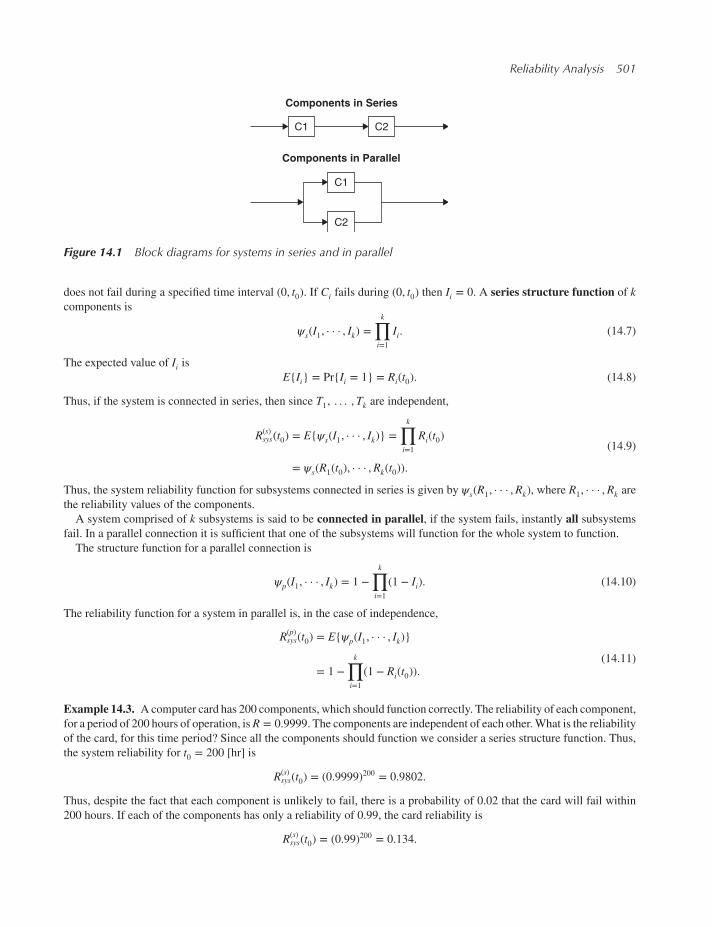
Reliability Analysis 501
C1
C1
C2
C2
Components in Series
Components in Parallel
Figure 14.1 Block diagrams for systems in series and in parallel
does not fail during a specified time interval (0, t0). If Ci fails during (0, t0) then Ii = 0. A series structure function of kcomponents is
𝜓s(I1, · · · , Ik) =k∏i=1
Ii. (14.7)
The expected value of Ii isE{Ii} = Pr{Ii = 1} = Ri(t0). (14.8)
Thus, if the system is connected in series, then since T1, . . . ,Tk are independent,
R(s)sys(t0) = E{𝜓s(I1, · · · , Ik)} =
k∏i=1
Ri(t0)
= 𝜓s(R1(t0), · · · ,Rk(t0)).
(14.9)
Thus, the system reliability function for subsystems connected in series is given by 𝜓s(R1, · · · ,Rk), where R1, · · · ,Rk arethe reliability values of the components.
A system comprised of k subsystems is said to be connected in parallel, if the system fails, instantly all subsystems
fail. In a parallel connection it is sufficient that one of the subsystems will function for the whole system to function.
The structure function for a parallel connection is
𝜓p(I1, · · · , Ik) = 1 −k∏i=1
(1 − Ii). (14.10)
The reliability function for a system in parallel is, in the case of independence,
R(p)sys(t0) = E{𝜓p(I1, · · · , Ik)}
= 1 −k∏i=1
(1 − Ri(t0)).(14.11)
Example 14.3. Acomputer card has 200 components, which should function correctly. The reliability of each component,
for a period of 200 hours of operation, isR = 0.9999. The components are independent of each other.What is the reliability
of the card, for this time period? Since all the components should function we consider a series structure function. Thus,
the system reliability for t0 = 200 [hr] is
R(s)sys(t0) = (0.9999)200 = 0.9802.
Thus, despite the fact that each component is unlikely to fail, there is a probability of 0.02 that the card will fail within
200 hours. If each of the components has only a reliability of 0.99, the card reliability is
R(s)sys(t0) = (0.99)200 = 0.134.

502 Modern Industrial Statistics
This shows why it is so essential in the electronic industry to demand from the vendors of the components most reli-
able products.
Suppose that there is on the card room for some redundancy. It is therefore decided to use the parts having reliability
of R = 0.99 and duplicate each component in a parallel structure. The parallel structure of duplicated components is
considered amodule. The reliability of eachmodule isRM = 1 − (1 − 0.99)2 = 0.9999. The reliability of the whole systemis again
R(s)sys = (RM)200 = 0.9802.
Thus, by changing the structure of the card we can achieve the .98 reliability with 200 pairs of components, each with
reliability value of 0.99. ◾
Systems may have more complicated structures. In Figure 14.2 we see the block diagram of a system consisting of
five components. Let R1,R2, · · · ,R5 denote the reliability values of the five components C1, · · · ,C5, respectively. LetM1
be the module consisting of components C1 and C2, and let M2 be the module consisting of the other components. The
reliability of M1 for some specified time interval is
RM1= R1R2.
The reliability of M2 is
RM2= R3(1 − (1 − R4)(1 − R5))
= R3(R4 + R5 − R4R5)
= R3R4 + R3R5 − R3R4R5.
Finally, the system reliability for that block diagram is
Rsys = 1 − (1 − RM1)(1 − RM2
)
= RM1+ RM2
− RM1RM2
= R1R2 + R3R4 + R3R5 − R3R4R5
− R1R2R3R4 − R1R2R3R5 + R1R2R3R4R5.
Another important structure function is that of k out of n subsystems. In other words, if a system consists of n subsystems,
it is required that at least k, 1 ≤ k < n subsystems will function, throughout the specified time period, in order that the
system will function. Assuming independence of the lifetimes of the subsystems, we can construct the reliability function
of the system, by simple probabilistic considerations. For example, if we have three subsystems having reliability values,
for the given time period, of R1,R2,R3 and at least 2 out of the 3 should function, then the system reliability is
R2(3)sys = 1 − (1 − R1)(1 − R2)(1 − R3) − R1(1 − R2)(1 − R3)
− R2(1 − R1)(1 − R3) − R3(1 − R1)(1 − R2)
= R1R2 + R1R3 + R2R3 − 2R1R2R3.
A Parallel Series System
C1 C2
C4
C3
C5
Figure 14.2 A parallel series structure

Reliability Analysis 503
If all the subsystems have the same reliability value R, for a specified time period, then the reliability function of the
system, in a k out of n structure, can be computed by using the binomial c.d.f. B(j; n,R), that is,
Rk(n)sys = 1 − B(k − 1; n,R). (14.12)
Example 14.4. A cooling system for a reactor has three identical cooling loops. Each cooling loop has two identical
pumps connected in parallel. The cooling system requires that 2 out of the 3 cooling loops operate successfully. The
reliability of a pump over the life span of the plant is R = .6. We compute the reliability of the cooling system.
First, the reliability of a cooling loop is
Rcl = 1 − (1 − R)2 = 2R − R2
= 1.2 − .36 = 0.84.
Finally, the system reliability is
R2(3)sys = 1 − B(1; 3, 0.84) = 0.9314.
This reliability can be increased by choosing pumps with higher reliability. If the pump reliability is 0.9, the loop’s
reliability is .99 and the system’s reliability is 0.9997. ◾
The reader is referred to Zacks (1992, Ch. 3) for additional methods of computing systems reliability.
14.3 Availability of repairable systems
Repairable systems alternate during their functional life through cycles of up phase and down phase. During the up phase
the system functions as required, till it fails. At the moment of failure the system enters the down phase. The system
remains in this down phase until it is repaired and activated again. The length of time the system is in the up phase is
called the time till failure (TTF). The length of time the system is in the down phase is called the time till repair (TTR).Both TTF and TTR are modeled as random variables, T and S, respectively. We assume here that T and S are independent.The cycle time is the random variable C = T + S.
The process in which the system goes through these cycles is called a renewal process. LetC1,C2,C3, · · · be a sequenceof cycles of a repairable system. We assume that C1,C2, · · · are i.i.d. random variables.
Let F(t) be the c.d.f. of the TTF, and G(t) the c.d.f. of the TTR. Let f (t) and g(t) be the corresponding p.d.f. Let K(t)denote the c.d.f. of C. Since T and S are independent random variables,
K(t) = Pr{C ≤ t}
= ∫t
0
f (x)P{S ≤ t − x}dx (14.13)
= ∫t
0
f (x)G(t − x)dx.
Assuming that G(0) = 0, differentiation of K(t) yields the p.d.f. of the cycle time, k(t), namely
k(t) = ∫t
0
f (x)g(t − x)dx. (14.14)
The operation of getting k(t) from f (t) and g(t) is called a convolution.The Laplace transform of an integrable function f (t), on 0 < t <∞, is defined as
f ∗(s) = ∫∞
0
e−tsf (t)dt, s ≥ 0. (14.15)

504 Modern Industrial Statistics
Notice that if f (t) is a p.d.f. of a non-negative continuous random variable, then f ∗(s) is its moment generating function
(m.g.f.) at −s. Since C = T + S, and T , S are independent, the m.g.f. of C isMC(u) = MT (u)MS(u), for all u ≤ u∗ at whichthese m.g.f. exist. In particular, if k∗(s) is the Laplace Transform of k(t),
k∗(s) = f ∗(s)g∗(s), s ≥ 0. (14.16)
Example 14.5. Suppose that T is exponentially distributed like E(𝛽), and S is exponentially distributed like E(𝛾); 0 < 𝛽,𝛾 <∞, that is,
f (t) = 1
𝛽exp {−t∕𝛽},
g(t) = 1
𝛾exp {−t∕𝛾}.
The p.d.f. of C is
k(t) = ∫t
0
f (x)g(t − x)dx
=⎧⎪⎨⎪⎩
1
𝛽 − 𝛾(e−t∕𝛽 − e−t∕𝛾 ), if 𝛽 ≠ 𝛾
t𝛽2e−t∕𝛽 , if 𝛽 = 𝛾.
The corresponding Laplace transforms are
f ∗(s) = (1 + s𝛽)−1,
g∗(s) = (1 + s𝛾)−1,
k∗(s) = (1 + s𝛽)−1(1 + s𝛾)−1.◾
Let NF(t) denote the number of failures of a system during the time interval (0, t]. Let W(t) = E{NF(t)}. Similarly, let
NR(t) be the number of repairs during (0, t] and V(t) = E{NR(t)}. Obviously NR(t) ≤ NF(t) for all 0 < t <∞.
Let A(t) denote the probability that the system is up at time t. A(t) is the availability function of the system. In unre-
pairable systems, A(t) = R(t).Let us assume thatW(t) and V(t) are differentiable, and let 𝑤(t) = W ′(t), 𝑣(t) = V ′(t).The failure intensity function of repairable systems is defined as
𝜆(t) = 𝑤(t)A(t), t ≥ 0. (14.17)
Notice that if the system is unrepairable, then W(t) = F(t), 𝑤(t) = f (t), A(t) = R(t) and 𝜆(t) is the hazard function h(t).Let Q(t) = 1 − A(t) and 𝑣(t) = V ′(t). The repair intensity function is
𝜇(t) = 𝑣(t)Q(t), t ≥ 0. (14.18)
The function V(t) = E{NR(t)} is called the renewal function. Notice that
Pr{NR(t) ≥ n} = Pr{C1 + · · · + Cn ≤ t}
= Kn(t), t ≥ 0(14.19)
where Kn(t) is the c.d.f. of C1 + · · · + Cn.

Reliability Analysis 505
The renewal function is, since NR(t) is a non-negative random variable,
V(t) =∞∑n=1
Pr{Nr(t) ≥ n}
=∞∑n=1
Kn(t).
(14.20)
Example 14.6. Suppose that TTF ∼ E(𝛽) and that the repair is instantaneous. Then, C is distributed like E(𝛽) and Kn(t)is the c.d.f. of G(n, 𝛽), that is,
Kn(t) = 1 − P
(n − 1; t𝛽
), n = 1, 2, · · ·
where P(j; 𝜆) is the c.d.f. of a Poisson random variable with mean 𝜆. Thus, in the present case,
V(t) =∞∑n=1
(1 − P
(n − 1; t𝛽
))= E
{Pois
(t𝛽
)}= t𝛽, t ≥ 0.
Here Pois(t
𝛽
)designates a random variable having a Poisson distribution with mean t∕𝛽. ◾
At time t, 0 < t <∞, there are two possible events:
E1: The first cycle is not yet terminated;
E2: The first cycle has terminated at some time before t.
Accordingly, V(t) can be written as
V(t) = K(t) + ∫t
0
k(x)V(t − x)dx. (14.21)
The derivative of V(t) is called the renewal density. Let 𝑣(t) = V ′(t). Since V(0) = 0, we obtain by differentiating this
equation, that
𝑣(t) = k(t) + ∫t
0
k(x)𝑣(t − x)dx. (14.22)
Let 𝑣∗(s) and k∗(s) denote the Laplace transforms of 𝑣(t) and k(t), respectively. Then, from the above equation
𝑣∗(s) = k∗(s) + k∗(s)𝑣∗(s), (14.23)
or, since k∗(s) = f ∗(s)g∗(s),𝑣∗(s) =
f ∗(s)g∗(s)1 − f ∗(s)g∗(s)
. (14.24)
The renewal density 𝑣(t) can be obtained by inverting 𝑣∗(s).
Example 14.7. As before, suppose that the TTF is E(𝛽) and that the TTR is E(𝛾). Let 𝜆 = 1
𝛽and 𝜇 = 1
𝛾
f ∗(s) = 𝜆𝜆 + s,
and
g∗(s) = 𝜇𝜇 + s.

506 Modern Industrial Statistics
Then
𝑣∗(s) = 𝜆𝜇
s2 + (𝜆 + 𝜇)s
= 𝜆𝜇𝜆 + 𝜇
(1
s− 1
s + 𝜆 + 𝜇
).
1
sis the Laplace transform of 1, and
𝜆+𝜇s+𝜆+𝜇
is the Laplace transform of E(
1
𝜆+𝜇
). Hence
𝑣(t) = 𝜆𝜇𝜆 + 𝜇
− 𝜆𝜇𝜆 + 𝜇
e−t(𝜆+𝜇), t ≥ 0.
Integrating 𝑣(t) we obtain the renewal function
V(t) = 𝜆𝜇𝜆 + 𝜇
t − 𝜆𝜇(𝜆 + 𝜇)2
(1 − e−t(𝜆+𝜇)),
0 ≤ t <∞.
In a similar fashion we can show that
W(t) = 𝜆𝜇𝜆 + 𝜇
t + 𝜆2
(𝜆 + 𝜇)2(1 − e−t(𝜆+𝜇)),
0 ≤ t <∞.
Since W(t) > V(t) if, and only if, the last cycle is still incomplete, and the system is down, the probability, Q(t), thatthe system is down at time t is
Q(t) = W(t) − V(t)
= 𝜆𝜆 + 𝜇
− 𝜆𝜆 + 𝜇
e−t(𝜆+𝜇), t ≥ 0.
Thus, the availability function is
A(t) = 1 − Q(t)
= 𝜇𝜆 + 𝜇
+ 𝜆𝜆 + 𝜇
e−t(𝜆+𝜇), t ≥ 0.
Notice that the availability at large values of t is approximately
limt→∞
A(t) = 𝜇𝜆 + 𝜇
= 𝛽𝛽 + 𝛾.
◾
The availability function A(t) can be determined from R(t) and 𝑣(t) by solving the equation
A(t) = R(t) + ∫t
0
𝑣(x)R(t − x)dx. (14.25)
The Laplace transform of this equation is
A∗(s) = R∗(s)1 − f ∗(s)g∗(s)
, 0 < s <∞. (14.26)
This theory can be useful in assessing different system structures, with respect to their availability. The following asymp-
totic (large t approximations) results are very useful. Let 𝜇 and 𝜎2 be the mean and variance of the cycle time.
1. limt→∞
V(t)t
= 1
𝜇(14.27)

Reliability Analysis 507
2. limt→∞
(V(t + a) − V(t)) = a𝜇, a > 0 (14.28)
3. limt→∞
(V(t) − t𝜇
)= 𝜎
2
2𝜇2− 1
2(14.29)
If the p.d.f of C, k(t), is continuous, then
4. limt→∞𝑣(t) = 1
𝜇. (14.30)
5. limt→∞
Pr
{NR(t) − t∕𝜇(𝜎2t∕𝜇3)1∕2
≤ z
}= Φ(z). (14.31)
6. A∞ = limT→∞
1
T ∫T
0
A(t)dt = E{TTF}E{TTF} + E{TTR}
. (14.32)
According to (1), the expected number of renewals, V(t), is approximately t∕𝜇, for large t. According to (2), we expect
approximately a∕𝜇 renewals in a time interval of length (t, t + a), when t is large. The third result (3) says that t∕𝜇 is anunder-over-estimate, for large t, if the squared coefficient of variation 𝜎2∕𝜇2, of the cycle time is larger (smaller) than 1.
The last three properties can be interpreted in a similar fashion. We illustrate these asymptotic properties with examples.
Example 14.8. Consider a repairable system. The TTF [hr] has a gamma distribution like G(2, 100). The TTR [hr] has
a Weibull distribution W(2, 2.5). Thus, the expected TTF is 𝜇T = 200 [hr], and the expected TTR is 𝜇s = 2.5 × Γ(
3
2
)=
1.25√𝜋 = 2.2 [hr]. The asymptotic availability is
A∞ = 200
202.2= 0.989.
That is, in the long run, the proportion of total availability time is 98.9%.
The expected cycle time is 𝜇c = 222.2 and the variance of the cycle time is
𝜎2c = 2 × 1002 + 6.25[Γ(2) − Γ2
(3
2
)]= 20, 000 + 1.34126 = 20, 001.34126.
Thus, during 2,000 [hr] of scheduled operation, we expect close to2,000
202.2≅ 10 renewal cycles. The probability that
NR(2, 000) will be less than 11 is
Pr{NR(2000) ≤ 11} ≅ Φ(
2
1.91
)= Φ(1.047) = 0.8525.
◾
An important question is, what is the probability, for large values of t, that we will find the system operating, and will
continue to operate without a failure for at least u additional time units? This function is called the asymptotic operationalreliability, and is given by
R∞(u) = A∞ ⋅∫
∞
u
R(u)du
𝜇T, 0 ≤ u (14.33)
where R(u) = 1 − FT (u).

508 Modern Industrial Statistics
Example 14.9. We continue discussing the case of Example 14.8. In this case
FT (u) = Pr{G(2, 100) ≤ u}
= Pr{G(2, 1) ≤ u
100
}= 1 − P
(1; u
100
)= 1 − e−u∕100 − u
100e−u∕100,
and
R(u) = e−u∕100 + u100
e−u∕100.
Furthermore, 𝜇T = 200 and A∞ = 0.989. Hence
R∞(u) = 0.989 ⋅∫ ∞u
(1 + x
100
)e−x∕100dx
200
= 98.9
200
(2 + u
100
)e−u∕100.
Thus, R∞(0) = 0.989, R∞(100) = 0.546 and R∞(200) = 0.268. ◾
Before concluding the present section we introduce two R applications, availDis and renewDis which provide the
bootstrap EBD of the number of renewals in a specified time interval and the EBD of the asymptotic availability index
A∞, based on observed samples of failure times and repair times. These programs provide computer aided estimates of
the renewal distribution and of the precision of A∞. We illustrate this in the following example.
Example 14.10. Consider again the renewal process described in Example 14.8. Consider n = 50 observed values of i.i.d.
TTF fromG(2, 100) and n = 50 observed repair times. We run renewDis 1,000 times to obtain an EBD of the number of
renewals in 1,000 [hr]. The program yields that the mean number of renewals for 1,000 hours of operation is 6.128. This
is the bootstrap estimate of V(1, 000). The asymptotic approximation is 1, 000∕202.2 = 4.946. The bootstrap confidenceinterval for V(1, 000) at 0.95 level of confidence is (4,9). This confidence interval covers the asymptotic approximation.
Accordingly, the bootstrap estimate of 6.13 is not significantly different from the asymptotic approximation. ◾
> set.seed(123)> Ttf <- rgamma(50,
shape=2,scale=100)
> Ttr <- rgamma(50,shape=2,scale=1)
> AvailEbd <- availDis(ttf=Ttf,ttr=Ttr,n=1000,seed=123)
The estimated MTTF from ttf is 153.01The estimated MTTR from ttr is 1.91The estimated asymptotic availability is 0.9877availability EBDMin. :0.98151st Qu.:0.9865Median :0.9877Mean :0.98763rd Qu.:0.9887Max. :0.9921

Reliability Analysis 509
> RenewEbd <- renewDis(ttf=Ttf,ttr=Ttr,time=1000,n=1000)
The estimated MEAN NUMBER Of RENEWALS is 8.19number of renewals EBD
Min. 1st Qu. Median Mean 3rd Qu. Max.3.000 7.000 8.000 8.185 9.000 15.000
> rm(AvailEbd, RenewEbd, Ttf, Ttr)
Additional topics of interest are maintenance, repairability and availability. The objective is to increase the availability
by instituting maintenance procedures and by adding stand-by systems and repairmen. The question is what is the opti-
mal maintenance period, how many stand-by systems and repairmen to add. The interested reader is referred to Zacks
(1992, Ch. 4) and Gerstbakh (1989). In the following sections we discuss statistical problems associated with reliability
assessment, when one does not know definitely the model and the values of its parameters.
14.4 Types of observations on TTF
The proper analysis of data depends on the type of observations available. Dealing with TTF and TTR random variables we
wish to have observations which give us the exact length of time interval from activation (failure) of a system (component)
till its failure (repair). However, one can find that proper records have not been kept, and instead one can find only the
number of failures (repairs) in a given period of time. These are discrete random variables rather than the continuous
ones under investigation. Another type of problem typical to reliability studies is that some observations are censored.For example, if it is decided to put n identical systems on test for a specified length of time t∗, we may observe only a
random number, Kn, of failures in the time interval (0, t∗]. On the other n − Kn systems which did not fail we have only
partial information, that is, their TTF is greater than t∗. The observations on these systems are called right censored. Inthe above example n units are put on test at the same time. The censoring time t∗ is a fixed time. Sometimes we have
observations with random censoring. This is the case when we carry a study for a fixed length of time t∗ [years] but theunits (systems) enter the study at random times between 0 and t∗, according to some distribution.
Suppose that a unit enters the study at the random time 𝜏, 0 < 𝜏 < t∗, and its TTF is T . We can observe only W =min(T , t∗ − 𝜏). Here the censoring time is the random variable t∗ − 𝜏. An example of such a situation is when we sell a
product under warranty. The units of this product are sold to different customers at random times during the study period
(0, t∗). Products which fail are brought back for repair. If this happens during the study period, we have an uncensored
observation on the TTF of that unit; otherwise the observation is censored, i.e.,W = t∗ − 𝜏.The censored observations described above are time censored. Another type of censoring is frequency censoring.
This is done when n units are put on test at the same time, but the test is terminated the instant the r-th failure occurs. In
this case the length of the test is the r-th order statistic of failure times Tn,r (r = 1, · · · , n). Notice that Tn,r = T(r), whereT(1) < T(2) < · · · < T(n) are the order statistics of n i.i.d. TTF’s. If T is distributed exponentially, E(𝛽), for example, the
expected length of the experiment is
E{Tn,r} = 𝛽(1
n+ 1
n − 1+ · · · + 1
n − r + 1
).
There may be substantial time saving if we terminate the study at the r-th failure, when r < n. For example, in the expo-
nential case, with E{T} = 𝛽 = 1, 000 [hr] and n = 20,
E{T20,20} = 1, 000 ×(1 + 1
2+ 1
3+ · · · + 1
20
)= 3597.7 [hr].
On the other hand, for r = 10 we have E{T20,10} = 668.8 [hr]. Thus, a frequency censored experiment, with r = 10 and
n = 20, 𝛽 = 1, 000 lasts on average only 19% of the time length of an uncensored experiment. We will see later how one
can determine the optimal n and r to estimate the mean TTF (MTTF) in the exponential case.

510 Modern Industrial Statistics
14.5 Graphical analysis of life data
In the present section we discuss some graphical procedures to fit a life distribution to failure data, and obtain estimates
of the parameters from the graphs.
Let t1, t2, · · · , tn be n uncensored observation on i.i.d. random variables T1, · · · , Tn, having some life distribution F(t).The empirical c.d.f., given t1, · · · , tn, is defined as
Fn(t) =1
n
n∑i=1
I{ti ≤ t}, (14.34)
where I{ti ≤ t} is the indicator variable, assuming the value 1 if ti ≤ t, and the value 0 otherwise. A theorem in probability
theory states that the empirical c.d.f. Fn(t) converges to F(t), as n → ∞.
In Figure 14.3 we present the empirical c.d.f. of a random sample of 100 variables having the Weibull distribution
W(1.5, 100). Since Fn(t(i)) =i
nfor i = 1, 2, · · · , n, the i
n-th quantile of Fn(t) is the ordered statistic t(i). Accordingly, if
F(t) has some specific distribution, the scattergram of(F−1
(i
n
), t(i)
)(i = 1, · · · , n) should be around a straight line with
slope 1. The plot of t(i) versus F−1(i
n
)is called a Q-Q Plot (quantile versus quantile). TheQ-Q plot is the basic graphical
procedure to test whether a given sample of failure times is generated by a specific life distribution. Since F−1(1) = ∞ for
the interesting life distribution, the quantile of F is taken ati
n+1or at some other
i+𝛼n+𝛽
, which give better plotting positions
for a specific distribution. For the normal distribution,i−3∕8n+1∕4
is used.
If the distribution depends on location and scale parameters, we plot t(i) against the quantiles of the standard distribution.The intercept and the slope of the line fitted through the points yield estimates of these location and scale parameters. For
example, suppose that t1, · · · , tn are values of a sample from a N(𝜇, 𝜎2) distribution. Thus, t(i) ≈ 𝜇 + 𝜎Φ−1(i
n
). Thus, if
we plot t(i) against Φ−1(i
n
)we should have points around a straight line whose slope is an estimate of 𝜎 and intercept an
estimate of 𝜇.
0 100 200 300 400
0.0
0.2
0.4
0.6
0.8
1.0
x
Fn(x
)
Figure 14.3 The empirical c.d.f. of a random sample of 100 variables from W(1.5,100)

Reliability Analysis 511
We focus attention here on three families of life distributions.
1. The exponential or shifted exponential.
2. The Weibull.
3. The log normal.
The shifted-exponential c.d.f. has the form
F(t;𝜇, 𝛽) =⎧⎪⎨⎪⎩1 − exp
{t − 𝜇𝛽
}, t ≥ 𝜇
0, t < 𝜇.(14.35)
The starting point of the exponential distributionE(𝛽) is shifted to a point 𝜇. Location parameters of interest in reliability
studies are 𝜇 ≥ 0. Notice that the p-th quantile, 0 < p <∞, of the shifted exponential is
tp = 𝜇 + 𝛽(− log (1 − p)). (14.36)
Accordingly, for exponential Q-Q plots we plot t(i) versus Ei,n = − log(1 − i
n+1
). Notice that in this plot, the intercept
estimates the location parameter 𝜇, and the slope estimates 𝛽. In the Weibull case, W(𝜈, 𝛽), the c.d.f. is
F(t; 𝜈, 𝛽) = 1 − exp
{−(t𝛽
)𝜈}, t ≥ 0. (14.37)
Thus, if tp is the p-th quantile,
log tp = log 𝛽 + 1
𝜈log (− log (1 − p)). (14.38)
For this reason, we plot log t(i) versus
Wi,n = log(− log
(1 − i
n + 1
)), i = 1, · · · , n. (14.39)
The slope of the straight line estimates 1∕𝜈 and the intercept estimates log 𝛽. In the log normal case we plot log t(i) against
Φ−1(i−3∕8n+1∕4
).
Example 14.11. In Figure 14.4 we present the Q-Q plot of 100 values generated at random from an exponential distribu-
tion E(5). We fit a straight line through the origin to the points by the method of least-squares. A linear regression routine
provides the line
x = 5.94 ∗ E.
Accordingly, the slope of a straight line fitted to the points provides an estimate of the true mean and standard deviation,
𝛽 = 5. An estimate of the median is
x(.693) = 0.693 × 5.9413 = 4.117.
The true median is Me = 3.465.In Figure 14.5 we provide a probability plot of n = 100 values generated from a Weibull distribution with parameters
𝜈 = 2 and 𝛽 = 2.5.Least-squares fitting of a straight line to these points yields the line
y = .856 + .479W.
Accordingly, we obtain the following estimates:
�� = 1∕.479 = 2.087
𝛽 = exp (.856) = 2.354
Median = exp (.856 − (.3665)(.479))
= 1.975.

512 Modern Industrial Statistics
0 1 2 3 4 5
010
20
30
exp quantiles
rexp(n
= 1
00, ra
te =
1/5
)
Figure 14.4 Q-Q plot of a sample of 100 values from E(5)
0 1 2 3 4 5
01
23
45
67
Weibull quantiles
rweib
ull(
n =
100, shape =
2, scale
= 2
.5)
Figure 14.5 Q-Q plot of a sample of 100 from W(2,2.5)

Reliability Analysis 513
The true median is equal to 𝛽(ln 2)1∕2 = 2.081. The estimate of the mean is
�� = 𝛽Γ(1 + .479)
= 𝛽 × .479 × Γ(.479) = 2.080.
The true mean is 𝜇 = 𝛽Γ(1.5) = 2.216. Finally, an estimate of the standard deviation is
�� = 𝛽(Γ(1.958) − Γ2(1.479))1∕2
= 𝛽[.958 × Γ(.958) − (.479 × Γ(.479))2]1∕2 = 1.054.
The true value is 𝜎 = 𝛽(Γ(2) − Γ2(1.5))1∕2 = 1.158. ◾
If observations are censored from the left or from the right, we plot the quantiles only from the uncensored part of the
sample. The plotting positions take into consideration the number of censored values from the left and from the right. For
example, if n = 20 and the 2 smallest observations are censored, the plotting positions are
i t(i)i
n + 1
1 – –
2 – –
3 t(3)3
21⋮
20 t2020
21
14.6 Non-parametric estimation of reliability
A non-parametric method called the Kaplan-Meier method yields an estimate, called the Product Limit (PL) estimate
of the reliability function, without an explicit reference to the life distribution. The estimator of the reliability function at
time t will be denoted by Rn(t), when n is the number of units put on test at time t = 0. If all the failure times 0 < t1 <t2 < · · · < tn <∞ are known, then the PL estimator is equivalent to
Rn(t) = 1 − Fn(t), (14.40)
where Fn(t) is the empirical CDF defined earlier.
In some cases either random or non-random censoring or withdrawals occur and we do not have complete information
on the exact failure times. Suppose that 0 < t1 < t2 < · · · < tk <∞, k ≤ n, are the failure times and𝑤 = n − k is the totalnumber of withdrawals.
Let Ij = (tj−1, tj), j = 1, · · · , k + 1, with t0 = 0, tk+1 = ∞, be the time intervals between recorded failures. LetWj be the
number of withdrawals during the time interval Ij. The PL estimator of the reliability function is then
Rn(t) = I{t < t1} +k+1∑i=2
I{ti−1 ≤ t ≤ ti}i−1∏j=1
(1 − 1
nj−1 −𝑤j∕2
), (14.41)
where n0 = n, and nl is the number of operating units just prior to the failure time tl.Usually, when units are tested in the laboratory under controlled conditions, there may be no withdrawals. This is not
the case, however, if tests are conducted in field conditions, and units on test may be lost, withdrawn or destroyed for
reasons different than the failure phenomenon under study.

514 Modern Industrial Statistics
Suppose now that systems are installed in the field as they are purchased (random times). We decide to make a follow-
up study of the systems for a period of two years. The time till failure of systems participating in the study is recorded.
We assume that each system operates continuously from the time of installment until its failure. If a system has not failed
by the end of the study period, the only information available is the length of time it has been operating. This is a case
of multiple censoring. At the end of the study period we have the following observations {(Ti, 𝛿i), i = 1, · · · , n}, wheren is the number of systems participating in the study; Ti is the length of operation of the i-th system (TTF or time till
censoring); 𝛿i = 1 if i-th observation is not censored and 𝛿i = 0 otherwise.
Let T(1) ≤ T(2) ≤ · · · ≤ T(n) be the order statistic of the operation times and let 𝛿j1 , 𝛿j2 , · · · , 𝛿jn be the 𝛿-values corre-sponding to the ordered T values where ji is the index of the i-th order statistic T(i), i.e., T(i) = Tj, (i = 1, · · · , n).
The PL estimator of R(t) is given by
Rn(t) = I{t < T(1)}
+n∑i=1
I{T(i) ≤ T(i+1)}i∏j=1
(1 −𝛿j
n − j + 1
).
(14.42)
Another situation prevails in the laboratory or in field studies when the exact failure times cannot be recorded. Let 0 <t1 < t2 < · · · < tk <∞ be fixed inspection times. Let𝑤i be the number of withdrawals and fi the number of failures in the
time interval Ii (i = 1, · · · , k + 1). In this case the formula is modified to be
Rn(t) = I{t < t1}
+k+1∑i=2
I{ti ≤ t < ti+1}i−1∏j=1
(1 −
fj
nj−1 −𝑤j
2
).
(14.43)
This version of the estimator of R(t), when the inspection times are fixed (not random failure times), is called the actuar-ial estimator.
In the following examples we illustrate these estimators of the reliability function.
Example 14.12. A machine is tested before shipping it to the customer for a one-week period (120 [hr]) or till its first
failure, whichever comes first. Twenty such machines were tested consecutively. In Table 14.1 we present the ordered
time till failure or time till censor (TTF/TTC) of the 20 machines, the factors (1 − 𝛿i∕(n − i + 1)) and the PL estimator
R(ti), i = 1, · · · , 20. ◾
14.7 Estimation of life characteristics
In Chapter 8 we studied the estimation of parameters of distributions, and of functions of these parameters. We discussed
point estimators and confidence intervals. In particular, we discussed unbiased estimators, least-squares estimators, maxi-
mum likelihood estimators and Bayes estimators. All these methods of estimation can be applied in reliability studies. We
will discuss in the present section themaximum likelihood estimation of the parameters of some common life distributions,
like the exponential and the Weibull, and some non-parametric techniques, for censored and uncensored data.
14.7.1 Maximum likelihood estimators for exponential TTF distribution
We start with the case of uncensored observations. Thus, let T1,T2, · · · ,Tn be i.i.d. random variables distributed like
E(𝛽). Let t1, · · · , tn be their sample realization (random sample). The likelihood function of 𝛽, 0 < 𝛽 <∞, is
L(𝛽; t) = 1
𝛽nexp
{− 1
𝛽
n∑i=1
ti
}. (14.44)

Reliability Analysis 515
Table 14.1 Failure times [hr] and PL estimates
i T(i)
(1 −𝛿i
n − i + 1
)R(Ti)
1 4.787715 .95 .952 8.378821 .9473684 .93 8.763973 .9444444 .854 13.77360 .9411765 .85 29.20548 .9375 .756 30.53487 .9333333 .77 47.96504 .9285714 .658 59.22675 .9230769 .69 60.66661 .9166667 .5510 62.12246 .9090909 .511 67.06873 .9 .4512 92.15673 .8888889 .413 98.09076 .875 .3514 107.6014 .8571429 .315 120 1 .316 120 1 .317 120 1 .318 120 1 .319 120 1 .320 120 1 .3
It is easy to check that the maximum likelihood estimator (MLE) of 𝛽 is the sample mean
𝛽n = Tn =1
n
n∑i=1
Ti. (14.45)
Tn is distributed like G(n, 𝛽
n
). Thus, E{𝛽n} = 𝛽 and V{𝛽n} = 𝛽
2
n. From the relationship between the Gamma and the 𝜒2
distributions we have that 𝛽n ∼𝛽
2n𝜒2[2n]. Thus, a (1 − 𝛼) level confidence interval for 𝛽, based on the MLE 𝛽n is(
2n𝛽n𝜒21−𝛼∕2[2n],
2n𝛽n𝜒2𝛼∕2[2n]
). (14.46)
For large samples we can use the normal approximation 𝛽n ± z1−𝛼∕2𝛽n√n.
Example 14.13. The failure times of 20 electric generators (in [hr]) are:
121.5 1425.5 2951.2 5637.91657.2 592.1 10609.7 9068.5848.2 5296.6 7.5 2311.1279.8 7201.9 6853.7 6054.3
1883.6 6303.9 1051.7 711.5.
Exponential probability plotting of these data yields a scatter around the line with slope of 3866.17 and R2 = .95. Theexponential model fits the failure times quite well. The MLE estimator of the MTTF, 𝛽, yields 𝛽20 = 3543.4 [hr]. Notice

516 Modern Industrial Statistics
that the MLE is different, but not significantly from the above graphical estimate of 𝛽. Indeed, the standard error of 𝛽20 is
S.E. = 𝛽20∕√20 = 792.328.
> data(FAILTIME)> library(survival)> SuRe <- survreg(
Surv(time=FAILTIME) ~ 1 ,dist = "exponential")
> summary(SuRe)
Call:survreg(formula = Surv(time = FAILTIME) ~ 1, dist = "exponential")
Value Std. Error z p(Intercept) 8.17 0.224 36.6 1.78e-292
Scale fixed at 1
Exponential distributionLoglik(model)= -183.5 Loglik(intercept only)= -183.5Number of Newton-Raphson Iterations: 5n= 20
> confint(SuRe)
2.5 % 97.5 %(Intercept) 7.734572 8.611095
Confidence interval, at level of 0.95, for 𝛽 is given by (2388.6,5801.8). The normal approximation to the confidence
interval is (1990.4,5096.4). The sample size is not sufficiently large for the normal approximation to be effective. ◾
When the observations are time censored by a fixed constant t∗, let Kn denote the number of uncensored observations.
Kn is a random variable having the binomial distribution B(n, 1 − exp {−t∗∕𝛽}). Let pn =Knn. pn is a consistent estimator
of 1 − exp {−t∗∕𝛽}. Hence, a consistent estimator of 𝛽 is
𝛽n = −t∗∕ log (1 − pn). (14.47)
This estimator is not an efficient one, since it is not based on observed failures. Moreover, if Kn = 0, 𝛽n = 0. Using the
expansion method shown in Section 13.2 we obtain that the asymptotic variance of 𝛽n is
AV{𝛽n} ≅ 𝛽4
nt∗2⋅1 − e−t
∗∕𝛽
e−t∗∕𝛽. (14.48)
The likelihood function of 𝛽 in this time-censoring case is
L(𝛽;Kn,Tn) =1
𝛽Knexp
{− 1
𝛽
(Kn∑i=1
Ti + t∗(n − Kn)
)}. (14.49)
Also here, if Kn = 0, the MLE of 𝛽 does not exist. If Kn ≥ 1, the MLE is
𝛽n =Sn,KnKn
, (14.50)
where Sn,Kn =Kn∑i=1Ti + (n − Kn)t∗, is the total time on test of the n units.
The theoretical evaluation of the properties of the MLE 𝛽n is complicated. We can, however, get information on its
behavior by simulation.

Reliability Analysis 517
Example 14.14. For a sample of size n = 50, with 𝛽 = 1, 000 and t∗ = 2, 000, Pr{K50 = 0} = exp {−100}.= 0. Thus, we
expect that 𝛽n will exist in all the simulation runs. For 100 MLE’s of 𝛽, obtained by this simulation we have a mean =1, 025.5, a median = 996.7 and a standard deviation = 156.9. The standard deviation of 𝛽n, according to the previous
formula, with the above values of n, 𝛽 and t∗, is 178.7. ◾
> library(boot)> FAILTIME[FAILTIME >= 7000] <- 7000 # Censor data at 7000> X <- data.frame(
time= FAILTIME,event=ifelse(FAILTIME < 7000,
yes=1,no=0))
> head(X, 8)
time event1 121.5 12 1425.5 13 2951.2 14 5637.9 15 1657.2 16 592.1 17 7000.0 08 7000.0 0
> B <- boot(data=X,statistic=function(x, i){coefficients(
survreg(Surv(time=x[i,1],event=x[i,2]) ~ 1 ,
dist = "exponential"))},R = 100)
> boot.ci(B,conf=0.95,type="perc")
BOOTSTRAP CONFIDENCE INTERVAL CALCULATIONSBased on 100 bootstrap replicates
CALL :boot.ci(boot.out = B, conf = 0.95, type = "perc")
Intervals :Level Percentile95% ( 7.692, 8.806 )Calculations and Intervals on Original ScaleSome percentile intervals may be unstable
> rm(B)
For further reading on the properties of MLE under time censoring, see Zacks (1992, pp. 125).
Under frequency censoring the situation is simpler. Suppose that the censoring is at the r-th failure. The total time on
test is Sn,r =r∑i=1T(i) + (n − r)T(r). In this case,
Sn,r ∼𝛽
2𝜒2[2r] (14.51)

518 Modern Industrial Statistics
and the MLE 𝛽n,r =Sn,rr
is an unbiased estimator of 𝛽, with variance
V{𝛽n,r} = 𝛽2
r.
Or, (14.52)
S.E.{𝛽n,r} = 𝛽√r.
If we wish to have a certain precision, so that S.E.{𝛽n,r} = 𝛾𝛽 then r = 1
𝛾2. Obviously n ≥ r.
Suppose that we pay for the test c2 $ per unit and c1 $ per time unit, for the duration of the test. Then, the total cost of
the test is
TKn,r = c1Tn,r + c2n. (14.53)
For a given r, we choose n to minimize the expected total cost. The resulting formula is
n0.= r
2
(1 +
(1 +
4c1rc2𝛽
)1∕2). (14.54)
The problem is that the optimal sample size n0 depends on the unknown 𝛽. If one has some prior estimate of 𝛽, it couldbe used to determine a good starting value for n.
Example 14.15. Consider a design of a life testing experiment with frequency censoring and exponential distribution of
the TTF. We require that S.E.{𝛽n,r} = 0.2𝛽. Accordingly, r =(
1
0.2
)2
= 25. Suppose that we wish to minimize the total
expected cost, at 𝛽 = 100 [hr], where c1 = c2 = 2 $. Then,
n0.= 25
2
(1 +
(1 + 4
25100
)1∕2)= 64.
The expected duration of this test is
E{T64,25} = 100
25∑i=1
1
65 − i= 49.0 [hr].
◾
14.7.2 Maximum likelihood estimation of the Weibull parameters
Let t1, · · · , tn be uncensored failure times of n random variables having a Weibull distribution W(𝜈, 𝛽). The likelihood
function of (𝜈, 𝛽) is
L(𝜈, 𝛽; t) = 𝜈n
𝛽n𝜈
(n∏i=1
ti
)𝜈−1exp
{−
n∑i=1
(ti𝛽
)𝜈}, (14.55)
0 < 𝛽, 𝜈 < ∞. The MLE of 𝜈 and 𝛽 are the solutions 𝛽n, ��n of the equations
𝛽n =
(1
n
n∑i=1
t��ni
)1∕��n
, (14.56)
and
��n =
⎡⎢⎢⎢⎢⎢⎣
n∑i=1
t��ni log ti
n∑i=1
t��ni
− 1
n
n∑i=1
log (ti)
⎤⎥⎥⎥⎥⎥⎦
−1
. (14.57)
All logarithms are on base e (ln ).

Reliability Analysis 519
The equation for ��n is solved iteratively by the recursive equation
��(j+1) =
⎡⎢⎢⎢⎢⎢⎣
n∑i=1
t��(i)i log (ti)
n∑i=1
t��(j)i
− 1
n
n∑i=1
log (ti)
⎤⎥⎥⎥⎥⎥⎦
−1
, j = 0, 1, · · · . (14.58)
where ��(0) = 1.
To illustrate, we simulated a sample of n = 50 failure times from W(2.5, 10). In order to obtain the MLE, we have to
continue the iterative process until the results converge. We show here the obtained values, as functions of the number of
iterations.
# iter 𝛽 ��
10 11.437 2.314
20 9.959 2.367
30 9.926 2.368
40 9.925 2.368
It seems that 40 iterations yield sufficiently accurate solutions.
Confidence intervals for ��n, 𝛽n can be determined, for large samples, by using large sample approximation formulae
for the standard errors of the MLE, which are found in Zacks (1992, p. 147).
SE{𝛽n} ≅𝛽n√n ��n
⋅ 1.053 (14.59)
and
SE{��n} ≅ .780��n√n. (14.60)
The large sample confidence limits are
𝛽n ± z1−𝛼∕2S.E.{𝛽n}, (14.61)
and
��n ± z1−𝛼∕2S.E.{��n}. (14.62)
In the above numerical example we obtained the MLE 𝛽50 = 9.925 and ��50 = 2.368. Using these values we obtain the
large sample approximate confidence intervals, with level of confidence 1 − 𝛼 = .95, to be (8.898, 11.148) for 𝛽 and(1.880, 2.856) for 𝜈.
We can obtain bootstrapping confidence intervals. The bootstrap confidence limits are the 𝛼∕2th and (1 − 𝛼∕2)th quan-tile of the simulated values which produced confidence intervals (8.378, 11.201) for 𝛽 and (1.914, 3.046) for 𝜈. Thedifference between these confidence intervals and the large sample approximation ones is not significant.
Maximum likelihood estimation in censored cases is more complicated and will not be discussed here. Estimates of 𝜈and 𝛽 in the censored case can be obtained from the intercept and slope of the regression line in the Q-Q plot.
> B <- boot(data=X,statistic=function(x, i){coefficients(
survreg(Surv(
time=x[i,1],

520 Modern Industrial Statistics
event=x[i,2]) ~ 1 ,dist="weibull"))
},R = 100)
> boot.ci(B,conf=0.95,type="perc")
BOOTSTRAP CONFIDENCE INTERVAL CALCULATIONSBased on 100 bootstrap replicates
CALL :boot.ci(boot.out = B, conf = 0.95, type = "perc")
Intervals :Level Percentile95% ( 7.555, 8.776 )Calculations and Intervals on Original ScaleSome percentile intervals may be unstable
> rm(B)
14.8 Reliability demonstration
Reliability demonstration is a procedure for testing whether the reliability of a given device (system) at a certain age is
sufficiently high. More precisely, a time point t0 and a desired reliability R0 are specified, and we wish to test whether the
reliability of the device at age t0, R(t0), satisfies the requirement that R(t0) ≥ R0. If the life distribution of the device is
completely known, including all parameters, there is no problem of reliability demonstration–one computes R(t0) exactlyand determines whether R(t0) ≥ R0. If, as is generally the case, either the life distribution or its parameters are unknown,
then the problem of reliability demonstration is that of obtaining suitable data and using them to test the statistical hypoth-
esis that R(t0) ≥ R0 versus the alternative that R(t0) < R0. Thus, the theory of testing statistical hypotheses provides the
tools for reliability demonstration. In the present section we review some of the basic notions of hypothesis testing as they
pertain to reliability demonstration.
In the following subsections we develop several tests of interest in reliability demonstration. We remark here that
procedures for obtaining confidence intervals for R(t0), which were discussed in the previous sections, can be used to
test hypotheses. Specifically, the procedure involves computing the upper confidence limit of a (1 − 2𝛼)-level confidenceinterval for R(t0) and comparing it with the value R0. If the upper confidence limit exceeds R0, then the null hypothesis
H0 ∶ R(t0) > R0 is accepted, otherwise it is rejected. This test will have a significance level of 𝛼.For example, if the specification of the reliability at age t = t0 is R = .75 and the confidence interval for R(t0), at
level of confidence 𝛾 = .90, is (.80, .85), the hypothesis H0 can be immediately accepted at a level of significance of
𝛼 = (1 − 𝛾)∕2 = .05. There is a duality between procedures for testing hypotheses and for confidence intervals.
14.8.1 Binomial testing
A random sample of n devices is put on life test simultaneously. Let Jn be the number of failures in the time interval [0, t0),and Kn = n − Jn. We have seen that Kn ∼ B(n,R(t0)). Thus, if H0 is true, i.e., R(t0) ≥ R0, the values of Kn will tend to be
larger, in a probabilistic sense. Thus, one tests H0 by specifying a critical value C𝛼 and rejecting H0 whenever Kn ≤ C𝛼 .The critical value C𝛼 is chosen as the largest value satisfying
FB(C𝛼; n,R0) ≤ 𝛼.

Reliability Analysis 521
The OC function of this test, as a function of the true reliability R, is
OC(R) = Pr{Kn > C𝛼|R(t0) = R}
= 1 − FB(C𝛼; n,R).(14.63)
If n is large, then one can apply the normal approximation to the Binomial CDF. In these cases we can determine C𝛼 tobe the integer most closely satisfying
Φ(C𝛼 + 1∕2 − nR0
(nR0(1 − R0))1∕2
)= 𝛼. (14.64)
Generally, this will be given by
C𝛼 = integer closest to{nR0 − 1∕2 − z1−𝛼(nR0(1 − R0))1∕2}, (14.65)
where z1−𝛼 = Φ−1(1 − 𝛼). The OC function of this test in the large sample case is approximated by
OC(R) ≅ Φ(nR − C𝛼 − 1∕2(nR(1 − R))1∕2
). (14.66)
The normal approximation is quite accurate whenever n > 9∕(R(1 − R)).If in addition to specifying 𝛼, we specify that the test have Type II error probability 𝛽, when R(t0) = R1, then the normal
approximation provides us with a formula for the necessary sample size:
n.=
(z1−𝛼𝜎0 + z1−𝛽𝜎1)2
(R1 − R0)2, (14.67)
where 𝜎2i = Ri(1 − Ri), i = 0, 1.
Example 14.16. Suppose that we wish to test at significance level 𝛼 = .05 the null hypothesis that the reliability at age
1000 [hr] of a particular system is at least 85%. If the reliability is 80% or less, we want to limit the probability of accepting
the null hypothesis to 𝛽 = .10. Our test is to be based onKn, the number of systems, out of a random sample of n, survivingat least 1000 hours of operation. Setting R0 = .85 and R1 = .80, we have 𝜎0 = .357, 𝜎1 = .4, z.95 = 1.645, z.90 = 1.282.Substituting above, we obtain that the necessary sample size is n = 483. The critical value is C.05 = 397.
We see that in binomial testing one may need very large samples to satisfy the specifications of the test. If in the
above problem we reduce the sample size to n = 100, then C.05 = 79. However, now the probability of accepting the null
hypothesis when R = .80 is OC(.8) = Φ(.125) = .55, which is considerably higher than the corresponding probability of.10 under n = 483. ◾
14.8.2 Exponential distributions
Suppose that we know that the life distribution is exponential E(𝛽), but 𝛽 is unknown. The hypotheses
H0 ∶ R(t0) ≥ R0
versus
H1 ∶ R(t0) < R0
can be rephrased in terms of the unknown parameter, 𝛽, as
H0 ∶ 𝛽 ≥ 𝛽0versus
H1 ∶ 𝛽 < 𝛽0

522 Modern Industrial Statistics
where 𝛽0 = −t0∕ ln R0. Let t1, · · · , tn be the values of a (complete) random sample of size n. Let tn =1
n
n∑i=1ti. The hypothesis
H0 is rejected if tn < C𝛼 , where
C𝛼 =𝛽02n𝜒2𝛼 [2n]. (14.68)
The OC function of this test, as a function of 𝛽, is
OC(𝛽) = Pr{tn > C𝛼|𝛽}= Pr{𝜒2[2n] >
𝛽0𝛽𝜒2𝛼 [2n]}. (14.69)
If we require that at 𝛽 = 𝛽1 the OC function of the test will assume the value 𝛾 , then the sample size n should satisfy
𝛽0𝛽1𝜒2𝛼 [2n] ≥ 𝜒21−𝛾 [2n].
The quantiles of 𝜒2[2n], for n ≥ 15, can be approximated by the formula
𝜒2p [2n] ≅1
2(√4n + zp)2. (14.70)
Substituting this approximation and solving for n, we obtain the approximation
n ≅ 1
4
(z1−𝛾 + z1−𝛼√𝜁 )2
(√𝜁 − 1)2
, (14.71)
where 𝜁 = 𝛽0∕𝛽1.
Example 14.17. Suppose that in Example 14.16, we know that the system lifetimes are exponentially distributed. It is
interesting to examine how many systems would have to be tested in order to achieve the same error probabilities as
before, if our decision were now based on tn.Since 𝛽 = −t∕ ln R(t), the value of the parameter 𝛽 under R(t0) = R(1000) = .85 is 𝛽0 = −1000∕ ln (.85) = 6153 [hr],
while its value under R(t0) = .80 is 𝛽1 = −1000∕ ln (.80) = 4481 [hr]. Substituting these values into (9.3.5), along with
𝛼 = .05 and 𝛾 = .10 (𝛾 was denoted by 𝛽 in Example 14.16), we obtain the necessary sample size n ≅ 87.
Thus we see that the additional knowledge that the lifetime distribution is exponential, along with the use of complete
lifetime data on the sample, allows us to achieve a greater than five-fold increase in efficiency in terms of the sample size
necessary to achieve the desired error probabilities. ◾
We remark that if the sample is censored at the r-th failure then all the formulae developed above apply after replacing nby r, and tn by 𝛽n,r = Tn,r∕r.
Example 14.18. Suppose that the reliability at age t = 250 [hr] should be at least R0 = .85. Let R1 = .75. The corre-
sponding values of 𝛽0 and 𝛽1 are 1538 [hr] and 869 [hr], respectively. Suppose that the sample is censored at the r = 25-th
failure. Let 𝛽n,r = Tn,r∕25 be the MLE of 𝛽. H0 is rejected, with level of significance 𝛼 = .05, if
𝛽n,r ≤ 1538
50𝜒2.05[50] = 1069 [hr].
The Type II error probability of this test, at 𝛽 = 869, is
OC(869) = Pr{𝜒2[50] > 1538869𝜒2.05[50]}
= Pr{𝜒2[50] > 61.5}
.= 1 − Φ
(61.5 − 50√
100
)= .125. ◾

Reliability Analysis 523
Sometimes in reliability demonstration an overriding concern is keeping the number of items tested to a minimum,
subject to whatever accuracy requirements are imposed. This could be the case, for example, when testing very complex
and expensive systems. In such cases, it may be worthwhile applying a sequential testing procedure, where items are
tested one at a time in sequence until the procedure indicates that testing can stop and a decision be made. Such, an
approach would also be appropriate when testing prototypes of some new design, which are being produced one at a time
at a relatively slow rate.
In Section 7.5 (page 267) and Section 9.4.2 (page 333) we introduced the Wald SPRT for testing hypotheses with
binomial data. Here we reformulate this test for reliability testing.
14.8.2.1 The SPRT for Binomial Data
Without any assumptions about the lifetime distribution of a device, we can test hypotheses concerning R(t0) by simply
observing whether or not a device survives to age t0. Letting Kn represent the number of devices among n randomly
selected ones surviving to age t0, we have Kn ∼ B(n,R(t0)). The likelihood ratio is given by
𝜆n =(1 − R1
1 − R0
)n(R1(1 − R0)R0(1 − R1)
)Kn
. (14.72)
Thus,
ln 𝜆n = n ln
(1 − R1
1 − R0
)− Kn ln
(R0(1 − R1)R1(1 − R0)
).
It follows that the SPRT can be expressed in terms of Kn as follows:
Continue sampling if − h1 + sn < Kn < h2 + sn,
Accept H0 if Kn ≥ h2 + sn,
Reject H0 if Kn ≤ −h1 + sn,
where ⎧⎪⎪⎪⎪⎨⎪⎪⎪⎪⎩
s = ln
(1 − R1
1 − R0
)/ln
(R0(1 − R1)R1(1 − R0)
),
h1 = ln
(1 − 𝛾𝛼
)/ln
(R0(1 − R1)R1(1 − R0)
),
h2 = ln
(1 − 𝛼𝛾
)/ln
(R0(1 − R1)R1(1 − R0)
).
(14.73)
𝛼 and 𝛾 are the prescribed probabilities of Type I and Type II errors. Note that if we plot Kn vs. n, the accept and reject
boundaries are parallel straight lines with common slope s and intercepts h2 and −h1, respectively.The OC function of this test is expressible (approximately) in terms of an implicit parameter 𝜓 . Letting
R(𝜓) =
⎧⎪⎪⎪⎪⎨⎪⎪⎪⎪⎩
1 −(1 − R1
1 − R0
)𝜓(R1
R0
)𝜓−(1 − R1
1 − R0
)𝜓 , 𝜓 ≠ 0
s, 𝜓 = 0
(14.74)

524 Modern Industrial Statistics
we have that the OC function at R(t0) = R(𝜓) is given by
OC(R(𝜓)) ≈
⎧⎪⎪⎪⎪⎪⎨⎪⎪⎪⎪⎪⎩
(1 − 𝛾𝛼
)𝜓− 1(
1 − 𝛾𝛼
)𝜓−( 𝛾1 − 𝛼
)𝜓 , 𝜓 ≠ 0
ln
(1 − 𝛾𝛼
)ln
((1 − 𝛼)(1 − 𝛾)𝛼𝛾
) , 𝜓 = 0.
(14.75)
It is easily verified that for 𝜓 = 1, R(𝜓) equals R0 and OC(R(𝜓)) equals 1 − 𝛼, while for 𝜓 = −1, R(𝜓) equals R1 and
OC(R(𝜓)) equals 𝛾 .The expected sample size, or average sample number (ASN), as a function of R(𝜓), is given by
ASN(R(𝜓)) ≈
⎧⎪⎪⎪⎨⎪⎪⎪⎩
ln1 − 𝛾𝛼
− OC(R(𝜓)) ln((1 − 𝛼)(1 − 𝛾)𝛼𝛾
)ln
1 − R1
1 − R0
− R(𝜓) ln
(R0(1 − R1)R1(1 − R0)
) , 𝜓 ≠ 0
h1h2s(1 − s), 𝜓 = 0.
(14.76)
The ASN function will typically have a maximum at some value of R between R0 and R1, and decrease as R moves away
from the point of maximum in either direction.
Example 14.19. Consider Example 14.17, where we had t = 1000 [hr], R0 = .85, R1 = .80, 𝛼 = .05, 𝛾 = .10. Supposenow that systems are tested sequentially, and we apply the SPRT based on the number of systems still functioning at 1000
[hr]. The parameters of the boundary lines are s = .826, h1 = 8.30, and h2 = 6.46.The OC and ASN functions of the test are given in Table 14.2, for selected values of 𝜓 .Compare the values in the ASN column to the sample size required for the corresponding fixed-sample test, n = 483. It
is clear that the SPRT effects a considerable saving in sample size, particularly when R(t0) is less than R1 or greater than
R0. Note also that the maximum ASN value occurs when R(t0) is near s. ◾
14.8.2.2 The SPRT for Exponential Lifetimes
When the lifetime distribution is known to be exponential, we have seen the increase in efficiency gained by measuring
the actual failure times of the parts being tested. By using a sequential procedure based on these failure times, further
gains in efficiency can be achieved.
Expressing the hypotheses in terms of the parameter 𝛽 of the lifetime distribution E(𝛽), we wish to test H0 ∶ 𝛽 ≥ 𝛽0 vs.H1 ∶ 𝛽 < 𝛽0, with significance level 𝛼 and Type II error probability 𝛾 , when 𝛽 = 𝛽1, where 𝛽1 < 𝛽0. Letting tn = (t1, · · · , tn)be the times till failure of the first n parts tested, the likelihood ratio statistic is given by
𝜆n(tn) =(𝛽0𝛽1
)n
exp
(−(
1
𝛽1− 1
𝛽0
) n∑i=1
ti
). (14.77)
Thus,
ln 𝜆n(tn) = n ln (𝛽0∕𝛽1) −(
1
𝛽1− 1
𝛽0
) n∑i=1
ti.

Reliability Analysis 525
Table 14.2 OC and ASN values for the SPRT
𝜓 R(𝜓) OC(R(𝜓)) ASN(R(𝜓))
−2.0 .7724 .0110 152.0−1.8 .7780 .0173 167.9−1.6 .7836 .0270 186.7−1.4 .7891 .0421 208.6−1.2 .7946 .0651 234.1−1.0 .8000 .1000 263.0−0.8 .8053 .1512 294.2−0.6 .8106 .2235 325.5−0.4 .8158 .3193 352.7−0.2 .8209 .4357 370.20.0 .8259 .5621 373.10.2 .8309 .6834 360.20.4 .8358 .7858 334.80.6 .8406 .8629 302.60.8 .8453 .9159 269.11.0 .8500 .9500 238.01.2 .8546 .9709 210.81.4 .8590 .9833 187.81.6 .8634 .9905 168.61.8 .8678 .9946 152.72.0 .8720 .9969 139.4
The SPRT rules are accordingly,
Continue sampling if − h1 + sn <n∑i=1
ti < h2 + sn,
Accept H0 if
n∑i=1
ti ≥ h2 + sn,
Reject H0 if
n∑i=1
ti ≤ −h1 + sn
where
s = ln (𝛽0∕𝛽1)/(
1
𝛽1− 1
𝛽0
),
h1 = ln ((1 − 𝛾)∕𝛼)/(
1
𝛽1− 1
𝛽0
),
h2 = ln ((1 − 𝛼)∕𝛾)/(
1
𝛽1− 1
𝛽0
). (14.78)
Thus, if we plotn∑i=1ti vs. n, the accept and reject boundaries are again parallel straight lines.

526 Modern Industrial Statistics
As before, let 𝜓 be an implicit parameter, and define
𝛽(𝜓) =
⎧⎪⎪⎪⎨⎪⎪⎪⎩
(𝛽0∕𝛽1)𝜓 − 1
𝜓
(1
𝛽1− 1
𝛽0
) , 𝜓 ≠ 0
ln (𝛽0∕𝛽1)1
𝛽1− 1
𝛽0
, 𝜓 = 0.
(14.79)
Then the OC and ASN functions are approximately given by
OC(𝛽(𝜓)) ≈
⎧⎪⎪⎨⎪⎪⎩((1 − 𝛾)∕𝛼)𝜓 − 1
((1 − 𝛾)∕𝛼)𝜓 − (𝛾∕(1 − 𝛼))𝜓, 𝜓 ≠ 0
ln ((1 − 𝛾)∕𝛼)ln ((1 − 𝛼)(1 − 𝛾)∕𝛼𝛾)
, 𝜓 = 0
(14.80)
and
ASN(𝛽(𝜓)) ≈
⎧⎪⎪⎨⎪⎪⎩
ln ((1 − 𝛾)∕𝛼) − OC(𝛽(𝜓)) ln ((1 − 𝛼)(1 − 𝛾)∕𝛼𝛾)
ln (𝛽0∕𝛽1) − 𝛽(𝜓)(
1
𝛽1− 1
𝛽0
) , 𝜓 ≠ 0
h1h2s2, 𝜓 = 0
(14.81)
Note that when 𝜓 = 1, 𝛽(𝜓) equals 𝛽0, while when 𝜓 = −1, 𝛽(𝜓) equals 𝛽1.
Example 14.20. Continuing Example 14.17, recall we had 𝛼 = .05, 𝛾 = .10, 𝛽0 = 6153, 𝛽1 = 4481. The parameters of
the boundaries of the SPRT are s = 5229, h1 = 47662, h2 = 37124. The OC and ASN functions, for selected values of 𝜓 ,are given in Table 14.3.
Table 14.3 OC and ASN values for the SPRT
𝜓 𝛽(𝜓) OC(𝛽(𝜓)) ASN(𝛽(𝜓))
−2.0 3872 .0110 34.3−1.8 3984 .0173 37.1−1.6 4101 .0270 40.2−1.4 4223 .0421 43.8−1.2 4349 .0651 47.9−1.0 4481 .1000 52.4−0.8 4618 .1512 57.1−0.6 4762 .2235 61.4−0.4 4911 .3193 64.7−0.2 5067 .4357 66.10.0 5229 .5621 64.70.2 5398 .6834 60.70.4 5575 .7858 54.80.6 5759 .8629 48.10.8 5952 .9159 41.51.0 6153 .9500 35.61.2 6363 .9709 30.61.4 6582 .9833 26.41.6 6811 .9905 22.91.8 7051 .9946 20.12.0 7301 .9969 17.8

Reliability Analysis 527
In Example 14.17, we saw that the fixed-sample test with the same 𝛼 and 𝛾 requires a sample size of n = 87. Thus, in
the exponential case as well, we see that the SPRT can result in substantial savings in sample size. ◾
It is obviously impractical to perform a sequential test, like the one described in the above example by running one
system, waiting till it fails, renewing it and running it again and again until a decision can be made. In the above example,
if the MTTF of the system is close to the value of 𝛽0 = 6153 [hr], it takes on average about 256 days between failures, and
on average about 36 failures till decision is reached. This trial may take over 25 years. There are three ways to overcome
this problem. The first is to test several systems simultaneously. Thus, if in the trial described in the above example 25
systems are tested simultaneously, the expected duration of the test will be reduced to one year. Another way is to consider
a test based on a continuous time process, not on discrete samples of failure times. The third possibility of reducing the
expected test duration is to perform accelerated life testing. In the following sections we discuss these alternatives.
14.8.2.3 The SPRT for Poisson Processes
Suppose that we put n systems on test starting at t = 0. Suppose also that any system which fails is instantaneously
renewed, and at the renewal time it is as good as new. In addition we assume that the life characteristics of the systems
are identical, the TTF of each system is exponential (with the same 𝛽) and failures of different systems are independentof each other.
Under these assumptions, the number of failures in each system, in the time interval (0, t] is a Poisson random variable
with mean 𝜆t, where 𝜆 = 1∕𝛽.Let Xn(t) = total number of failures among all the n systems during the time interval (0, t]. Xn(t) ∼ Pos(n𝜆t), and the
collection {Xn(t); 0 < t < ∞} is called a Poisson process. We add the initial condition that Xn(0) = 0.
The random function Xn(t), 0 < t < ∞, is a non-decreasing step function which jumps one unit at each random failure
time of the system. The random functions Xn(t) satisfy:
(i) Xn(t),∼ Pos(n𝜆t), all 0 < t <∞;
(ii) For any t1 < t2, Xn(t2) − Xn(t1) is independent of Xn(t1);(iii) For any t1, t2, 0 < t1 < t2 <∞, Xn(t2) − Xn(t1) ∼ Pos(n𝜆(t2 − t1)).
We develop now the SPRT based on the random functions Xn(t).The hypotheses H0 ∶ 𝛽 ≥ 𝛽0 versus H1 ∶ 𝛽 ≤ 𝛽1, for 0 < 𝛽1 < 𝛽0 <∞, are translated to the hypotheses H0 ∶ 𝜆 ≤ 𝜆0
versus H1 ∶ 𝜆 ≥ 𝜆1 where 𝜆 = 1∕𝛽. The likelihood ratio at time t is
Λ(t;Xn(t)) =(𝜆1𝜆0
)Xn(t)
exp {−nt(𝜆1 − 𝜆0)}. (14.82)
The test continues as long as the random graph of (Tn(t),Xn(t)) is between the two linear boundaries
bU(t) = h2 + sTn(t), 0 ≤ t <∞
and
bL(t) = −h1 + sTn(t), 0 ≤ t <∞,
where Tn(t) = nt is the total time on test at t,
h1 =ln
(1 − 𝛼𝛾
)ln(𝜆1𝜆0
) ,h2 =
ln(
1−𝛾𝛼
)ln(𝜆1𝜆0
) , (14.83)

528 Modern Industrial Statistics
and
s =𝜆1 − 𝜆0
ln
(𝜆1𝜆0
) .The instant Xn(t) jumps above bU(t) the test terminates and H0 is rejected; on the other hand, the instant Xn(t) = bL(t) thetest terminates andH0 is accepted. Acceptance ofH0 entails that the reliability meets the specified requirement. Rejection
of H0 may lead to additional engineering modification to improve the reliability of the system.
The OC function of this sequential test is the same as that in the exponential case. Let 𝜏 denote the random time
of termination. It can be shown that Pr𝜆{𝜏 <∞} = 1 for all 0 < 𝜆 <∞. The expected deviation of the test is given
approximately by
E𝜆{𝜏} = 1
𝜆nE𝜆{Xn(𝜏)}, (14.84)
where
E𝜆{Xn(𝜏)} ≅⎧⎪⎨⎪⎩h2 − OC(𝜆)(h1 + h2)
1 − s∕𝜆, if 𝜆 ≠ s
h1h2, if 𝜆 = s.
(14.85)
It should be noticed that the last formula yields the same values as the formula in the exponential case for 𝜆 = 1∕𝛽(𝜓).The SPRT of the previous section can terminate only after a failure, while the SPRT based on Xn(t) may terminate while
crossing the lower boundary bL(t), before a failure occurs.The minimal time required to accept H0 is 𝜏0 = h1∕ns. In the case of Example 14.20, with n = 20, 𝜏0 = 9.11536∕(20 ×.0001912) = 2383.2 [hr]. That is, over 99 days of testing without any failure. The SPRT may be, in addition, frequency
censored by fixing a value x∗ so that, as soon as Xn(t) ≥ x∗, the test terminates and H0 is rejected. In Example 14.20 we
see that the expected number of failures at termination may be as large as 66. We can censor the test at x∗ = 50. This will
reduce the expected duration of the test, but will increase the probability of a Type I error, 𝛼. Special programs are available
for computing the operating characteristics of such censored tests, but these are beyond the scope of the present text.
14.9 Accelerated life testing
It is often impractical to test highly reliable systems, or components, under normal operating conditions, because no
failures may be observed during long periods of time. In accelerated life testing, the systems are subjected to higher than
normal stress conditions in order to generate failures. The question is how to relate failure distributions, under higher than
normal stress conditions, to those under normal conditions?
Accelerated life testing is used by engineers in testing materials like food and drugs, lubricants, concrete and cement,
building materials and nuclear reactor materials. The stress conditions are generally, mechanical load, vibrations, high
temperatures, high humidity, high contamination, etc. Accelerated testing is used for semiconductors including transistors,
electronic devices such as diodes, random access memories, plastic encumpsulants etc. The reader is referred to Nelson
(1992) for a survey of methods and applications. The statistical methodology of accelerated life testing is similar to the
methods described earlier in this chapter, including graphical analysis and maximum likelihood estimation. The reader is
referred to Nelson (1992), Mann, Schaffer and Singpurwalla (1974), for details. We describe below some of the models
used to relate failures under various stress conditions.
14.9.1 The Arrhenius temperature model
This model is widely used when the product failure time is sensitive to high temperature. Applications include electri-
cal insulations and dielectric (see Goba (1969)); solid state and semiconductors (Peck and Trapp (1978)); battery cells;
lubricants and greases; plastics; incandescent light filaments.
The Arrhenius law states that the rate of simple chemical reaction depends on temperature as follows:
𝜆 = A exp {−E∕(kT)}, (14.86)

Reliability Analysis 529
where E is the activation energy (in electron volts; k is the Boltzman constant, 8.6171 × 10⁻⁵ electron volts per ∘C; Tis the absolute Kelvin temperature (−273.16 + ∘C); A is a product parameter, which depends on the test conditions and
failure characteristics. In applying the Arrhenius model to failure times distribution we find the Weibull-Arrhenius life
distribution, in which the scale parameter 𝛽 of the Weibull distribution is related to temperature, T , according to the
function
𝛽(T) = 𝜆 exp{A + B
T
}, B > 0, (14.87)
where 𝜆, A and B are fitted empirically to the data.
14.9.2 Other models
Another model is called the log normal Arrheniusmodel, in which the log failure time is normally distributed with mean
A + B∕T and variance 𝜎2. According to this model, the expected failure time is exp {A + B∕T + 𝜎2∕2}. Another model
prevalent in the literature, relates the expected failure time to a stress level V according to the inverse power model
MTTF(V) = CVp, C > 0. (14.88)
The statistical data analysis methodology is to fit an appropriate model to the data, usually by maximum likelihood
estimation, and then predict the MTTF of the system under normal conditions, or some reliability or availability function.
Tolerance intervals, for the predicted value should be determined.
14.10 Burn-in procedures
Many products show relatively high frequency of early failures. For example, if a product has an exponential distribution
of the TTF with MTTF of 𝛽 = 10, 000 [hr], we do not expect more than 2% of the product to fail within the first 200 [hr].
Nevertheless, many products designed for high value of MTTF show a higher than expected number of early failures.
This phenomenon led to the theory that the hazard rate function of products is typically a U-shaped function. In its earlylife the product is within a phase with monotone decreasing hazard rate. This phase is called the “infant mortality” phase.
After this phase the product enters a phase of “maturity” in which the hazard rate function is almost constant. Burn-in
procedures are designed to screen (burn) the weak products within the plant, by setting the product to operate for several
days, in order to give the product a chance to fail in the plant and not in the field, where the loss due to failure is high.
How long should a burn-in procedure last? Jensen and Petersen (1982) discuss this and other issues, in designing burn-in
procedures. We refer the reader to this book for more details. We present here only some basic ideas.
Burn-in procedures discussed by Jensen and Petersen are based on a model of a mixed life distribution. For example,
suppose that experience shows that the life distribution of a product is Weibull, W(𝜈, 𝛽1). A small proportion of units
manufactured may have generally short life, due to various reasons, which is given by another Weibull distribution, say,
W(𝜈, 𝛽0), with 𝛽0 < 𝛽1. Thus, the life distribution of a randomly chosen product has a distribution which is a mixture of
W(𝜈, 𝛽0) and W(𝜈, 𝛽1) that is,
F(t) = 1 −[p exp
{−(t𝛽0
)𝜈}+ (1 − p) exp
{−(t𝛽1
)𝜈}], (14.89)
for t > 0. The objective of the burn-in is to let units with the W(𝜈, 𝛽0) distribution have an opportunity to fail in the
plant. The units which do not fail during the burn-in have, for their remaining life, a life distribution closer to the desired
W(𝜈, 𝛽1).Suppose that a burn-in continues for t∗ time units. The conditional distribution of the time till failure T , given that
{T > t∗} is
F∗(t) =∫ t
t∗ f (u)du1 − F(t∗)
, t ≥ t∗. (14.90)
530 Modern Industrial Statistics
The c.d.f. F∗(t), of units surviving the burn-in, start at t∗, i.e., F∗(t∗) = 0 and has MTTF
𝛽∗ = t∗ + ∫∞
t∗(1 − F∗(t))dt. (14.91)
We illustrate this in the following example on mixtures of exponential life times.
Example 14.21. Suppose that a product is designed to have an exponential life distribution, with mean of 𝛽 = 10, 000[hr]. A proportion p = .05 of the products comes out of the production process with a short MTTF of 𝛾 = 100 [hr].
Suppose that all products go through a burn-in for t∗ [hr].The c.d.f. of the TTF of units which did not fail during the burn-in is
F∗(t) = 1 −0.05 exp
{− t100
}+ 0.95 exp
{− t10, 000
}0.05 exp
{−200
100
}+ .95 exp
{− 200
10, 000
}= 1 − 1
0.93796
[0.05 exp
{− t100
}+ 0.95 exp
{− t10, 000
}]for t ≥ 200. The mean time till failure, for units surviving the burn-in is thus
𝛽∗ = 200 + 1
0.93796 ∫∞
200
(0.05 exp
{− t100
}+ 0.95 exp
{− t10, 000
})dt
= 200 + 5
0.93796exp
{−200
100
}+ 9500
0.93796exp
{− 200
10, 000
}= 10, 128.53 [hr].
A unit surviving 200 hours of burn-in, is expected to operate an additional 9,928.53 hours in the field. The expected life
of these units without the burn-in is 0.05 × 200 + 0.95 × 10, 000 = 9, 510 [hr]. The burn-in of 200 hours in the plant, is
expected to increase the mean life of the product in the field by 418 hours. Whether this increase in the MTTF justifies the
burn-in depends on the relative cost of burn-in in the plant to the cost of failures in the field. The proportion p of “shortlife” units plays also an important role. If this proportion is p = 0.1 rather than 0.05, the burn-in increases the MTTF in
the field from 9,020 hours to 9,848.95 hours. One can easily verify that for p = 0.2, if the income for an hour of operation
of one unit in the field is Cp = 5$ and the cost of the burn-in per unit is 0.15$ per hour, then the length of burn-in which
maximizes the expected profit is about 700 hours. ◾
14.11 Chapter highlights
Chapter 13 dwelled on design decisions of product and process developers that are aimed at optimizing the quality
and robustness of products and processes. This chapter looks at performance over time and discusses basic notions of
repairable and non-repairable systems. Graphical and non-parametric techniques are presented together with classical
parametric techniques for estimating life distributions. Special sections cover the reliability of demonstrational proce-
dures, sequential reliability testing, burn-in procedures and accelerated life testing. Design and testing of reliability are
crucial activities for organizations at the top of the Quality Ladder.
The main concepts and definitions introduced in this chapter include:
• Life Distributions
• Accelerated Life Testing
• Availability

Reliability Analysis 531
• Time Categories
• Up Time
• Down Time
• Intrinsic Availability
• Operational Readiness
• Mean Time To Failure (MTTF)
• Reliability Function
• Failure Rate
• Structure Function
• Time Till Failure (TTF)
• Time Till Repair (TTR)
• Cycle Time
• Renewal Function
• Censored Data
• Product Limit (PL) estimator
• Average Sample Number (ASN)
• Sequential Probability Ratio Test (SPRT)
• Burn-In Procedure
14.12 Exercises
14.1 During 600 hours of manufacturing time a machine was up 510 hours. It had 100 failures which required a total
of 11 hours of repair time. What is the MTTF of this machine? What is its mean time till repair, MTTR? What is
the intrinsic availability?
14.2 The frequency distribution of the lifetime in a random sample of n = 2, 000 solar cells, under accelerated life
testing is the following:
t[103 [hr] 0–1 1–2 2–3 3–4 4–5 5–
prof. freq. 0.15 0.25 0.25 0.10 0.10 0.15
The relationship of the scale parameters of the life distributions, between normal and accelerated conditions
is 10:1.
(i) Estimate the reliability of the solar cells at age t = 4.0 [yr].
(ii) What proportion of solar cells are expected to survive 40,000 [hr] among those which survived 20,000 [hr]?
14.3 The CDF of the lifetime [months] of a piece of equipment is
F(t) =
{t4∕20736, 0 ≤ t < 12
1, 12 ≤ t
1. What is the failure rate function of this equipment?
2. What is the MTTF?
3. What is the reliability of the equipment at 4 months?
14.4 The reliability of a system is
R(t) = exp {−2t − 3t2}, 0 ≤ t <∞.
1. What is the failure rate of this system at age t = 3?
2. Given that the system reached the age of t = 3, what is its reliability for two additional time units?

532 Modern Industrial Statistics
14.5 An aircraft has four engines but can land using only two engines.
(i) Assuming that the reliability of each engine, for the duration of a mission, is R = .95, and that engine failuresare independent, compute the mission reliability of the aircraft.
(ii) What is the mission reliability of the aircraft if at least one functioning engine must be on each wing?
14.6 (i) Draw a block diagram of a system having the structure function
Rsys = 𝜓s(𝜓p(𝜓M1, 𝜓M2
),R6), 𝜓M1= 𝜓p(R1,R2R3), 𝜓M2
= 𝜓2(R4,R5)
(ii) Determine Rsys if all the components act independently, and have the same reliability R = .8.14.7 Consider a system of n components in a series structure. Let R1, · · · ,Rn be the reliabilities of the components.
Show that
Rsys ≥ 1 −n∑i=1
(1 − Ri).
14.8 A 4 out of 8 system has identical components whose life lengths T [weeks] are independent and identically
distributed like a Weibull W(
1
2, 100
). What is the reliability of the system at t0 = 5 weeks?
14.9 A system consists of a main unit and two standby units. The lifetimes of these units are exponential with mean
𝛽 = 100 [hr]. The standby units undergo no failure while idle. Switching will take place when required. What is
the MTTF of the system? What is the reliability function of this system?
14.10 Suppose that the TTF in a renewal cycle has aW(𝛼, 𝛽) distribution and that the TTR has a lognormal distribution
LN(𝜇, 𝜎). Assume further that TTF and TTR are independent. What are the mean and standard deviation of a
renewal cycle?
14.11 Suppose that a renewal cycle has the normal distribution N(100, 10). Determine the p.d.f of NR(200).14.12 Let the renewal cycle C be distributed like N(100, 10). Approximate V(1000).14.13 Derive the renewal density 𝑣(t) for a renewal process with C ∼ N(100, 10).14.14 Two identical components are connected in parallel. The system is not repaired until both components fail. Assum-
ing that the TTF of each component is exponentially distributed, E(𝛽), and the total repair time is G(2, 𝛾), derivethe Laplace transform of the availability function A(t) of the system.
14.15 Simulate a sample of 100 TTF of a system comprised of two components connected in parallel, where the life
distribution of each component (in hours) is E(100). Similarly, simulate a sample of 100 repair times (in hours),
having a G(2, 1) distribution. Estimate the expected value and variance of the number of renewals in 2,000 [hr].
14.16 In a given life test, n = 15 units are placed to operate independently. The time till failure of each unit has an
exponential distribution with mean 2,000 [hr]. The life test terminates immediately after the 10th failure. How
long is the test expected to last?
14.17 If n units are put on test and their TTF are exponentially distributed with mean 𝛽, the time elapsed between the r-thand (r + 1)st failure, i.e.,Δn,r = Tn,r+1 − Tn,r, is exponentially distributedwithmean 𝛽∕(n − r), r = 0, 1, · · · , n − 1.
Also, Δn,0,Δn,2, · · · ,Δn,n−1 are independent. What is the variance of Tn,r? Use this result to compute the variance
of the test length in the previous exercise.
14.18 Consider again the previous exercise. How would you estimate unbiasedly the scale parameter 𝛽, if the r failuretimes, Tn,1,Tn,2, · · · ,Tn,r are given? What is the variance of this unbiased estimator?
14.19 Simulate a random sample of 100 failure times, following the Weibull distribution W(2.5, 10). Draw a Weibull
probability plot of the data. Estimate the parameters of the distribution from the parameters of the linear regression
fitted to the Q-Q plot.
14.20 The following is a random sample of the compressive strength of 20 concrete cubes [kg/cm2].
94.9, 106.9, 229.7, 275.7, 144.5, 112.8, 159.3, 153.1, 270.6, 322.0,
216.4, 544.6, 266.2, 263.6, 138.5, 79.0, 114.6, 66.1, 131.2, 91.1
Make a lognormal Q-Q plot of these data and estimate the mean and standard deviation of this distribution.
14.21 The following data represent the time till first failure [days] of electrical equipment. The data were censored after
400 days.
13, 157, 172, 176, 249, 303, 350, 400+, 400+.
(Censored values appear as x+.) Make aWeibullQ-Q plot of these data and estimate the median of the distribution.

Reliability Analysis 533
14.22 Make a PL (Kaplan-Meir) estimate of the reliability function of an electronic device, based on 50 failure times
in file ELECFAIL.csv.14.23 Assuming that the failure times in file ELECFAIL.csv come from an exponential distribution E(𝛽), compute the
MLE of 𝛽 and of R(50; 𝛽) = exp {−50∕𝛽}. [The MLE of a function of a parameter is obtained by substituting
the MLE of the parameter in the function.] Determine confidence intervals for 𝛽 and for R(50; 𝛽) at level ofconfidence 0.95.
14.24 The following are values of 20 random variables having an exponential distribution E(𝛽). The values are censoredat t∗ = 200.
96.88, 154.24, 67.44, 191.72, 173.36, 200, 140.81, 200, 154.71, 120.73,
24.29, 10.95, 2.36, 186.93, 57.61, 99.13, 32.74, 200, 39.77, 39.52.
Determine the MLE of 𝛽. Use 𝛽 equal to the MLE, to estimate the standard deviation of the MLE, and to obtain
confidence interval for 𝛽, at level 1 − 𝛼 = .95. [This simulation is called an empirical bootstrap.]
14.25 Determine n0 and r for a frequency censoring test for the exponential distribution, where the cost of a unit is 10
times bigger than the cost per time unit of testing. We want that S.E.{𝛽n} = 0.1𝛽, and the expected cost to be
minimized at 𝛽 = 100 [hr]. What is the expected cost of this test, at 𝛽 = 100, when c1 = $1 [hr]?
14.26 File WEIBUL.csv contains the values of a random sample of size n = 50 from a Weibull distribution.
1. Obtain MLE of the scale and shape parameters 𝛽 and 𝜈.2. Use theMLE estimates of 𝛽 and 𝜈, to obtain parametric bootstrap EBD of the distribution of 𝛽, ��, withM = 500
runs. Estimate from this distribution the standard deviations of 𝛽 and ��. Compare these estimates to the large
sample approximations.
14.27 In binomial life testing by a fixed size sample, how large should the sample be in order to discriminate between
R0 = 0.99 and R1 = 0.90, with 𝛼 = 𝛽 = 0.01? [𝛼 and 𝛽 denote the probabilities of error of Type I and II.]14.28 Design the Wald SPRT for binomial life testing, in order to discriminate between R0 = 0.99 and R1 = 0.90, with𝛼 = 𝛽 = 0.01. What is the expected sample size, ASN, if R = 0.9?
14.29 Design a Wald SPRT for exponential life distribution, to discriminate between R0 = 0.99 and R1 = 0.90, with𝛼 = 𝛽 = 0.01. What is the expected sample size, ASN, when R = 0.90?
14.30 n = 20 computer monitors are put on accelerated life testing. The test is an SPRT for Poisson processes, based
on the assumption that the TTF of a monitor, in those conditions, is exponentially distributed. The monitors are
considered to be satisfactory if their MTBF is 𝛽 ≥ 2, 000 [hr] and considered to be unsatisfactory if 𝛽 ≤ 1, 500[hr]. What is the expected length of the test if 𝛽 = 2, 000 [hr]?
14.31 A product has an exponential life time with MTTF 𝛽 = 1, 000 [hr]. 1% of the products come out of production
with MTTF of 𝛾 = 500 [hr]. A burn-in of t∗ = 300 [hr] takes place. What is the expected life of units surviving
the burn-in? Is such a long burn-in justified?

15Bayesian Reliability Estimation
and Prediction
It is often the case that some information is available on the parameters of the life distributions from prior experiments
or prior analysis of failure data. The Bayesian approach provides the methodology for formal incorporation of prior
information with the current data.
15.1 Prior and posterior distributions
Let X1, · · · ,Xn be a random sample from a distribution with a p.d.f. f (x;𝜽), where 𝜽 = (𝜃1, · · · , 𝜃k) is a vector of k param-
eters, belonging to a parameter space Θ. So far we have assumed that the point 𝜽 is an unknown constant. In the Bayesian
approach, 𝜽 is considered a random vector having some specified distribution. The distribution of 𝜽 is called a priordistribution. The problem of which prior distribution to adopt for the Bayesian model is not easily resolvable, since the
values of 𝜽 are not directly observable. The discussion of this problem is beyond the scope of the book.
Let h(𝜃1, · · · , 𝜃k) denote the joint p.d.f. of (𝜃1, · · · , 𝜃k), corresponding to the prior distribution. This p.d.f. is called the
prior p.d.f. of 𝜽. The joint p.d.f. of X and 𝜽 is
g(x,𝜽) = f (x;𝜽)h(𝜽). (15.1)
The marginal p.d.f. of X, which is called the predictive p.d.f., is
f ∗(x) = ∫ · · ·Θ ∫ f (x;𝜽)h(𝜽)d𝜃1 · · · d𝜃k. (15.2)
Furthermore, the conditional p.d.f. of 𝜽 given X = x is
L(𝜽|x) = g(x,𝜽)∕f ∗(x). (15.3)
This conditional p.d.f. is called the posterior p.d.f. of 𝜽, given x. Thus, starting with a prior p.d.f., h(𝜽), we convert it,after observing the value of x, to the posterior p.d.f. of 𝜽 given x.
Modern Industrial Statistics: with applications in R, MINITAB and JMP, Second Edition. Ron S. Kenett and Shelemyahu Zacks.© 2014 John Wiley & Sons, Ltd. Published 2014 by John Wiley & Sons, Ltd.Companion website: www.wiley.com/go/modern_industrial_statistics

Bayesian Reliability Estimation and Prediction 535
If x1, · · · , xn is a random sample from a distribution with a p.d.f. f (x;𝜽) then the posterior p.d.f. of 𝜽, corresponding to
the prior p.d.f. h(𝜽), is
h(𝜽|x) =n∏i=1
f (xi;𝜽)h(𝜽)
∫ · · ·Θ
∫n∏i=1
f (xi; 𝜃)h(𝜽)d𝜃1 · · · d𝜃k
. (15.4)
For a given sample, x, the posterior p.d.f. h(𝜽|x) is the basis for most types of Bayesian inference.
Example 15.1.I. Binomial DistributionsX ∼ B(n; 𝜃), 0 < 𝜃 < 1.The p.d.f. of X is
f (x; 𝜃) =(nx
)𝜃x(1 − 𝜃)n−x, x = 0, · · · , n.
Suppose that 𝜃 has a prior beta distribution, with p.d.f.
h(𝜃; 𝜈1, 𝜈2) =1
B(𝜈1, 𝜈2)𝜃𝜈1−1(1 − 𝜃)𝜈2−1, (15.5)
0 < 𝜃 < 1, 0 < 𝜈1, 𝜈2 <∞, where B(a, b) is the complete beta function
B(a, b) = ∫1
0
xa−1(1 − x)b−1dx
= Γ(a)Γ(b)Γ(a + b).
The posterior p.d.f. of 𝜃, given X = x, is
h(𝜃|x) = 1
B(𝜈1 + x, 𝜈2 + x)𝜃𝜈1+x−1(1 − 𝜃)𝜈2+n−x−1, 0 < 𝜃 < 1. (15.6)
Notice that the posterior p.d.f. is also that of a beta distribution, with parameters 𝜈1 + x and 𝜈2 + n − x. The expected valueof the posterior distribution of 𝜃, given X = x, is
E{𝜃|x} = 1
B(𝜈1 + x, 𝜈2 + n − x) ∫1
0
𝜃𝜈1+x(1 − 𝜃)𝜈2+n−x−1d𝜃
=B(𝜈1 + x + 1, 𝜈2 + n − x)B(𝜈1 + x, 𝜈2 + n − x)
=𝜈1 + x
𝜈1 + 𝜈2 + n.
(15.7)
> library(LearnBayes)> Probs <- c(0.5, 0.5)> BetaPar1<- c(1, 1)> BetaPar2 <- c(15, 2)> Betapar <- rbind(BetaPar1, BetaPar2)> Data<- c(10, 2)> binomial.beta.mix(probs=Probs,
betapar=Betapar,data=Data)
$probsBetaPar1 BetaPar2
0.2845528 0.7154472
$betapar

536 Modern Industrial Statistics
[,1] [,2]BetaPar1 11 3BetaPar2 25 4
II. Poisson DistributionsX ∼ P(𝜆), 0 < 𝜆 <∞.
The p.d.f. of X is
f (x; 𝜆) = e−𝜆𝜆x
x!, x = 0, 1, · · · .
Suppose that the prior distribution of 𝜆 is the gamma distribution, G(𝜈, 𝜏). The prior p.d.f. is thus
h(𝜆; 𝜈, 𝜏) = 1
𝜏𝜈Γ(𝜈)𝜆𝜈−1e−𝜆∕𝜏 . (15.8)
The posterior p.d.f. of 𝜆, given X = x, is
h(𝜆|x) = 𝜆𝜈+x−1(𝜏
1 + 𝜏
)𝜈+xΓ(𝜈 + x)
e−𝜆(1+𝜏)∕𝜏 . (15.9)
That is, the posterior distribution of 𝜆, given X = x, is G(𝜈 + x, 𝜏
1+𝜏
). The posterior expectation of 𝜆, given X = x, is
(𝜈 + x)𝜏∕(1 + 𝜏).
> Probs <- c(0.5, 0.5)> GammaPar1 <- c(1, 1) # Gamma parameters are expressed as> # shape and rate> # scale is 1/rate> GammaPar2 <- c(15, 2)> Gammapar <- rbind(GammaPar1, GammaPar2)> Data<- list(
y=c(5),t=c(1))
> poisson.gamma.mix(probs=Probs,gammapar=Gammapar,data=Data)
$probsGammaPar1 GammaPar20.1250978 0.8749022
$gammapar[,1] [,2]
GammaPar1 6 2GammaPar2 20 3
III. Exponential DistributionsX ∼ E(𝛽).
The p.d.f. of X is
f (x; 𝛽) = 1
𝛽e−x∕𝛽 .
Let 𝛽 have an inverse-gamma prior distribution, IG(𝜈, 𝜏). That is, 1
𝛽∼ G(𝜈, 𝜏). The prior p.d.f. is
h(𝛽; 𝜈, 𝜏) = 1
𝜏𝜈Γ(𝜈)𝛽𝜈+1e−1∕𝛽𝜏 . (15.10)
Then, the posterior p.d.f. of 𝛽, given X = x, is
h(𝛽|x) = (1 + x𝜏)𝜈+1
𝜏𝜈+1Γ(𝜈 + 1)𝛽𝜈+2e−(x+1∕𝜏)∕𝛽 . (15.11)

Bayesian Reliability Estimation and Prediction 537
That is, the posterior distribution of 𝛽, given X = x, is IG(𝜈 + 1, 𝜏1+x𝜏
). The posterior expectation of 𝛽, given X = x, is(x + 1∕𝜏)∕𝜈.
The likelihood function L(𝜽; x), is a function over a parameter space Θ. In the definition of the posterior p.d.f. of 𝜽,
given x, we see that any factor of L(𝜽; x)which does not depend on 𝜽 is irrelevant. For example, the binomial p.d.f., under
𝜃 is
f (x; 𝜃) =(nx
)𝜃x(1 − 𝜃)n−x, x = 0, 1, · · · , n,
0 < 𝜃 < 1. The factor (nx) can be omitted from the likelihood function in Bayesian calculations. The factor of the likelihood
which depends on 𝜃 is called the kernel of the likelihood. In the above binomial example, 𝜃x(1 − 𝜃)n−x, is the kernel ofthe binomial likelihood. If the prior p.d.f. of 𝜃, h(𝜃), is of the same functional form (up to a proportionality factor which
does not depend on 𝜃) as that of the likelihood kernel, we call that prior p.d.f. a conjugate distribution. As shown in
Example 15.1, the beta prior distributions are conjugate to the binomial model, the gamma prior distributions are conjugate
to the Poisson model and the inverse-gamma priors are conjugate to the exponential model.
If a conjugate prior distribution is applied, the posterior distribution belongs to the conjugate family.
One of the fundamental problems in Bayesian analysis is that of the choice of a prior distribution of 𝜃. From a Bayesian
point of view, the prior distribution should reflect the prior knowledge of the analyst on the parameter of interest. It
is often difficult to express the prior belief about the value of 𝜽 in a p.d.f. form. We find that analysts apply, whenever
possible, conjugate priors whose means and standard deviations may reflect the prior beliefs. Another common approach
is to use a “diffused,” “vague” or Jeffrey’s prior, which is proportional to |I(𝜃)|1∕2, where I(𝜃) is the Fisher information
function (matrix). Bayes decision procedures were already introduced in Section 4.8 (page 140). For further reading on
this subject, the reader is referred to Box and Tiao (1973), Good (1965) and Press (1989). ◾
15.2 Loss functions and Bayes estimators
In order to define Bayes estimators we must first specify a loss function, L(��,𝜽), which represents the cost involved in
using the estimate �� when the true value is 𝜽. Often this loss is taken to be a function of the distance between the estimate
and the true value, i.e., |�� − 𝜽|. In such cases, the loss function is written as
L(��,𝜽) = W(|�� − 𝜽|).Examples of such loss functions are
Squared-error loss: W(|�� − 𝜽|) = (�� − 𝜽)2,
Absolute-error loss: W(|�� − 𝜽|) = |�� − 𝜽|.The loss function does not have to be symmetric. For example, we may consider the function
L(��, 𝜃) =
{𝛼(𝜃 − ��), if �� ≤ 𝜃𝛽(�� − 𝜃), if �� > 𝜃
where 𝛼 and 𝛽 are some positive constants.
As already introduced in Section 4.8.2.2, the Bayes estimator of 𝜽, with respect to a loss function L(��,𝜽), is definedas the value of �� which minimizes the posterior risk, given x, where the posterior risk is the expected loss with respect
to the posterior distribution. For example, suppose that the p.d.f. of X depends on several parameters 𝜃1, · · · , 𝜃k, but wewish to derive a Bayes estimator of 𝜃1 with respect to the squared-error loss function. We consider the marginal posterior
p.d.f. of 𝜃1, given x, h(𝜃1|x). The posterior risk isR(��1, x) = ∫ (��1 − 𝜃1)2h(𝜃1|x)d𝜃1.
It is easily shown that the value of ��1 which minimizes the posterior risk R(��1, x) is the posterior expectation of 𝜃1:
E{𝜃1|x} = ∫ 𝜃1h(𝜃1|x)d𝜃1.

538 Modern Industrial Statistics
If the loss function is L(��1, ��) = |��1 − 𝜃1|, the Bayes estimator of 𝜃1 is the median of the posterior distribution of 𝜃1given x.
15.2.1 Distribution-free Bayes estimator of reliability
Let Jn denote the number of failures in a random sample of size n, during the period [0, t). The reliability of the device
on test at age t is R(t) = 1 − F(t), where F(t) is the CDF of the life distribution. Let Kn = n − Jn. The distribution of Kn is
the binomial B(n,R(t)). Suppose that the prior distribution of R(t) is uniform on (0, 1). This prior distribution reflects ourinitial state of ignorance concerning the actual value of R(t).
The uniform distribution is a special case of the beta distribution with 𝜈1 = 1 and 𝜈2 = 1. Hence, according to Part
I of Example 15.1, the posterior distribution of R(t), given Kn, is a beta distribution with parameters 𝜈1 = Kn + 1 and
𝜈2 = 1 + n − Kn. Hence, the Bayes estimator of R(t), with respect to the squared-error loss function, is
R(t;Kn) = E{R(t)|Kn}
=Kn + 1
n + 2.
(15.12)
If the sample size is n = 50, and K50 = 27, the Bayes estimator of R(t) is R(t; 27) = 28∕52 = .538. Notice that the MLE of
R(t) is R50 = 27∕50 = .540. The sample size is sufficiently large for the MLE and the Bayes estimator to be numerically
close. If the loss function is |R − R|, the Bayes estimator of R is the median of the posterior distribution of R(t) given Kn,
that is, the median of the beta distribution with parameters 𝜈1 = Kn + 1 and 𝜈2 = n − Kn + 1.
Generally, if 𝜈1 and 𝜈2 are integers, then the median of the beta distribution is
Me =𝜈1F.5[2𝜈1, 2𝜈2]𝜈2 + 𝜈1F.5[2𝜈1, 2𝜈2]
, (15.13)
where F.5[j1, j2] is the median of the F[j1, j2] distribution. Substituting 𝜈1 = Kn + 1 and 𝜈2 = n − Kn + 1 in (15.13), we
obtain that the Bayes estimator of R(t) with respect to the absolute error loss is
R(t) =(Kn + 1)F.5[2Kn + 2, 2n + 2 − 2Kn]
n + 1 − Kn + (Kn + 1)F.5[2Kn + 2, 2n + 2 − 2Kn]. (15.14)
Numerically, for n = 50, Kn = 27, F.5[56, 48] = 1.002, and R(t) = .539. The two Bayes estimates are very close.
15.2.2 Bayes estimator of reliability for exponential life distributions
Consider a Type II censored sample of size n from an exponential distribution, E(𝛽), with censoring at the r-th fail-
ure. Let t(1) ≤ t(2) ≤ · · · ≤ t(r) be the ordered failure times. For squared-error loss, the Bayes estimator of R(t) = e−t∕𝛽 isgiven by
R(t) = E{R(t)|t(1), · · · , t(r)}= E{e−t∕𝛽 |t(1), · · · , t(r)}. (15.15)
This conditional expectation can be computed by integrating e−t∕𝛽 with respect to the posterior distribution of 𝛽, givent(1), · · · , t(r).
Suppose that the prior distribution of 𝛽 is IG(𝜈, 𝜏). One can easily verify that the posterior distribution of 𝛽 given
t(1), · · · , t(r) is the inverted-gamma IG(𝜈 + r, 𝜏
1+Tn,r𝜏
)where Tn,r =
r∑i=1t(i) + (n − r)t(r). Hence, the Bayes estimator of R(t) =
exp (−t∕𝛽) is, for squared-error loss,
R(t) =(1 + Tn,r𝜏)r+𝜈
𝜏r+𝜈Γ(r + 𝜈) ∫∞
0
1
𝛽r+𝜈+1

Bayesian Reliability Estimation and Prediction 539
⋅ exp
(− 1
𝛽
(Tn,r +
1
𝜏+ t))
d𝛽
=(
1 + Tn,r𝜏
1 + (Tn,r + t)𝜏
)r+𝜈
. (15.16)
Note that the estimator only depends on n through Tn,r.In the following table we provide a few values of the Bayes estimator R(t) for selected values of t, when 𝜈 = 3, r = 23,
Tn,r = 2242 and 𝜏 = 10−2, along with the corresponding MLE, which is
MLE = e−t∕𝛽n,r = e−rt∕Tn,r .
t 50 100 150 200
R(t) .577 .337 .199 .119
MLE .599 .359 .215 .129
If we have a series structure of k modules, and the TTF of each module is exponentially distributed, then formula (15.15)
is extended to
Rsys(t) =k∏i=1
(1 −
t𝜏i
1 + T (i)n,ri𝜏i + t𝜏i
)𝛾i+𝜈i(15.17)
where T (i)n,ri
is the total time on test statistic for the i-th module, ri is the censoring frequency of the observations on the
i-th module, 𝜏i and 𝜈i are the prior parameters for the i-th module. As in (15.15), (15.16) is the Bayes estimator for the
squared-error loss, under the assumption that the MTTFs of the various modules are priorly independent. In a similar
manner one can write a formula for the Bayes estimator of the reliability of a system having a parallel structure.
15.3 Bayesian credibility and prediction intervals
Bayesian credibility intervals at level 𝛾 are intervals C𝛾 (x) in the parameter space Θ, for which the posterior probability
that 𝜽 ∈ C𝛾 (x) is at least 𝛾 , that is,Pr{𝜃 ∈ C𝛾 (x)|x} ≥ 𝛾. (15.18)
Pr{E|x} denotes the posterior probability of the event E, given x. The Bayesian credibility interval for 𝜃, given x, hasan entirely different interpretation than that of the confidence intervals discussed in the previous sections. While the
confidence level of the classical confidence interval is based on the sample-to-sample variability of the interval, for fixed 𝜃,the credibility level of the Bayesian credibility interval is based on the presumed variability of 𝜃, for a fixed sample.
15.3.1 Distribution-free reliability estimation
In Section 15.2.1 we developed the Bayes estimator, with respect to squared-error loss, of the reliability at age t, R(t),when the data available are the number of sample units which survive at age t, namely Kn. We have seen that the pos-
terior distribution of R(t), given Kn, for a uniform prior is the beta distribution with 𝜈1 = Kn + 1 and 𝜈2 = n − Kn + 1.
The Bayesian credibility interval at level 𝛾 is the interval whose limits are the 𝜖1- and 𝜖2-quantiles of the posterior dis-tribution, where 𝜖1 = (1 − 𝛾)∕2, 𝜖2 = (1 + 𝛾)∕2. These limits can be determined with aid of R, getting the quantile of theF-distribution, according to the formulae
Lower limit =(Kn + 1)
(Kn + 1) + (n − Kn + 1)F𝜖2 [2n + 2 − 2Kn, 2Kn + 2](15.19)

540 Modern Industrial Statistics
and
Upper limit =(Kn + 1)F𝜖2 [2Kn + 2, 2n + 2 − 2Kn]
(n − Kn + 1) + (Kn + 1)F𝜖2 [2Kn + 2, 2n + 2 − 2Kn]. (15.20)
In Section 15.2.1 we considered the case of n = 50 and Kn = 27. For 𝛾 = .95 we need
F.975[48, 56] = 1.735
and
F.975[56, 48] = 1.746.
Thus, the Bayesian credibility limits obtained for R(t) are .402 and .671. Recall the Bayes estimator was .538.
15.3.2 Exponential reliability estimation
In Section 15.2.2 we developed a formula for the Bayes estimator of the reliability function R(t) = exp (−t∕𝛽) forType II censored data. We saw that if the prior on 𝛽 is IG(𝜈, 𝜏) then the posterior distribution of 𝛽, given the data,
is IG(𝜈 + r, 𝜏∕(1 + 𝜏Tn,r). Thus, 𝛾 level Bayes credibility limits for 𝛽 are given by 𝛽L,𝛾 (lower limit) and BU,𝛾 (upperlimit), where
𝛽L,𝛾 =Tn,r + 1∕𝜏G𝜖2 (𝜈 + r, 1)
(15.21)
and
𝛽U,𝛾 =Tn,r + 1∕𝜏G𝜖1 (𝜈 + r, 1)
. (15.22)
Moreover, if 𝜈 is an integer then we can replace Gp(𝜈 + r, 1) by 1
2𝜒2p [2𝜈 + 2r]. Finally, since R(t) = exp (−t∕𝛽) is an
increasing function of 𝛽, the 𝛾-level Bayes credibility limits for R(t) are
RL,𝛾 (t) = exp (−t∕𝛽L,𝛾 ) (15.23)
and
RU,𝛾 (t) = exp (−t∕𝛽U,𝛾 ). (15.24)
If we consider the values 𝜈 = 3, r = 23, Tn,r = 2242 and 𝜏 = 10−2 we need for 𝛾 = .95, 𝜒2.025
[52] = 33.53 and 𝜒2.975
[52] =73.31. Thus,
𝛽L,.95 = 63.91 and 𝛽U,.95 = 139.73.
The corresponding Bayesian credibility limits for R(t), at t = 50, are RL,.95(50) = .457 and RU,.95(50) = .699.
15.3.3 Prediction intervals
In Section 15.3.2, we introduced the notion of prediction intervals of level 𝛾 . This notion can be adapted to the Bayesianframework in the following manner.
Let X be a sample from a distribution governed by a parameter 𝜃; we assume that 𝜃 has a prior distribution. Let
h(𝜃|x) denote the posterior p.d.f. of 𝜃, given X = x. x represents the values of a random sample already observed. We are
interested in predicting the value of some statistic T(Y) based on a future sample Y from the same distribution. Let g(t; 𝜃)denote the p.d.f. of T(Y) under 𝜃. Then the predictive distribution of T(Y), given x, is
g∗(t|x) = ∫Θg(t; 𝜃)h(𝜃|x)d𝜃. (15.25)
A Bayesian prediction interval of level 𝛾 for T(Y), given x, is an interval (TL(x),TU(x)) which contains a proportion 𝛾of the predictive distribution, that is, satisfying
∫TU (x)
TL(x)g∗(t|x)dt = 𝛾. (15.26)

Bayesian Reliability Estimation and Prediction 541
Generally, the limits are chosen so that the tail areas are each (1 − 𝛾∕2). We illustrate the derivation of a Bayesian pre-
diction interval in the following example.
Example 15.2. Consider a device with an exponential lifetime distribution E(𝛽). We test a random sample of n of these,stopping at the r-th failure. Suppose the prior distribution of 𝛽 is IG(𝜈, 𝜏). Then, as seen in Section 15.2.2, the posterior
distribution of 𝛽 given the ordered failure times t(1), · · · , t(r) is IG(𝜈 + r, 𝜏
1+Tn,r𝜏
), where Tn,r =
r∑i=1t(i) + (n − r)t(r).
Suppose we have an additional s such devices, to be used one at a time in some system, replacing each one immediately
upon failure by another.We are interested in a prediction interval of level 𝛾 for T , the time until all s devices have been used
up. Letting Y = (Y1, · · · ,Ys) be the lifetimes of the devices, we have T(Y) =s∑i=1Yi. Thus, T(y) has a G(s, 𝛽) distribution.
Substituting in (15.24), it is easily shown that the predictive p.d.f. of T(Y), given t(1), · · · , t(r), is
g∗(t|t(1), · · · , t(r)) = (B(s, 𝜈 + r)(Tn,r + 1∕𝜏))−1
⋅(𝜏
t + Tn,r + 1∕𝜏
)s−1( Tn,r + 1∕𝜏t + Tn,r + 1∕𝜏
)r+𝜈+1
.(15.27)
Making the transformation
U = (Tn,r + 1∕𝜏)∕(T(Y) + Tn,r + 1∕𝜏)
one can show that the predictive distribution ofU given t(1), · · · , t(r) is the Beta(r + 𝜈, s) distribution. If we let Be𝜖1 (r + 𝜈, s)and Be𝜖2 (r + 𝜈, s) be the 𝜖1- and 𝜖2-quantiles of Beta (r + 𝜈, s), where 𝜖1 = (1 − 𝛾)∕2 and 𝜖2 = (1 + 𝛾)∕2, then the lower
and upper Bayesian prediction limits for T(Y) are
TL =(Tn,r +
1
𝜏
)(1
Be𝜖2 (𝜈 + r, s)− 1
)(15.28)
and
TU =(Tn,r +
1
𝜏
)(1
Be𝜖1 (𝜈 + r, s)− 1
). (15.29)
If 𝜈 is an integer, the prediction limits can be expressed as
TL =(Tn,r +
1
𝜏
) s𝜈 + r
F𝜖1 [2s, 2𝜈 + 2r] (15.30)
and
TU =(Tn,r +
1
𝜏
) s𝜈 + r
F𝜖2 [2s, 2𝜈 + 2r].
Formulae (15.28) and (15.29) have been applied in the following context.
Twenty computer monitors have been put on test at time t0 = 0. The test was terminated at the sixth failure (r = 6). Thetotal time on test was T20,6 = 75, 805.6 [hr]. We wish to predict the time till failure [hr] of monitors which are shipped to
customers. Assuming that TTF ∼ E(𝛽) and ascribing 𝛽 a prior IG(5, 10−3) distribution, we compute the prediction limits
TL and TU for s = 1, at level 𝛾 = .95.In the present case 2𝜈 + 2r = 22 and F.025[2, 22] = 1∕F.975[22, 2] = 1∕39.45 = .0253. Moreover, F.975[2, 22] =
4.38. Thus,
TL = 76805.61
11× .0253 = 176.7 [hr]
and
TU = 76805.61
11× 4.38 = 30, 582.6 [hr].
We have high prediction confidence that a monitor in the field will not fail before 175 hours of operation. ◾

542 Modern Industrial Statistics
15.4 Credibility intervals for the asymptotic availability of repairable systems:The exponential case
Consider a repairable system. We take observations on n consecutive renewal cycles. It is assumed that in each renewal
cycle, TTF ∼ E(𝛽) and TTR ∼ E(𝛾). Let t1, · · · , tn be the values of TTF in the n cycles and s1, · · · , sn be the values of
TTR. One can readily verify that the likelihood function of 𝛽 depends on the statistic U =n∑i=1ti and that of 𝛾 depends on
V =n∑i=1si.U and V are called the likelihood (orminimal sufficient) statistics. Let 𝜆 = 1∕𝛽 and 𝜇 = 1∕𝛾 . The asymptotic
availability is A∞ = 𝜇∕(𝜇 + 𝜆).In the Bayesian framework we assume that 𝜆 and 𝜇 are priorly independent, having prior gamma distributions G(𝜈, 𝜏)
and G(𝜔, 𝜁 ), respectively. One can verify that the posterior distributions of 𝜆 and 𝜇, given U and V , are G(n + 𝜈,U + 𝜏)and G(n + 𝜔,V + 𝜁 ), respectively. Moreover, 𝜆 and 𝜇 are posteriorly independent. Routine calculations yield that
1 − A∞
A∞(U + 𝜏)
1 − A∞
A∞(U + 𝜏) + (V + 𝜁 )
∼ Beta(n + 𝜈, n + 𝜔),
where Beta(p, q) denotes a random variable having a beta distribution, with parameters p and q, 0 < p, q <∞. Let 𝜖1 =(1 − 𝛾)∕2 and 𝜖2 = (1 + 𝛾)∕2. We obtain that the lower and upper limits of the 𝛾-level credibility interval for A∞ are A∞,𝜖1and A∞,𝜖2 where
A∞,𝜖1 =
[1 + V + 𝜁
U + 𝜏⋅Be𝜖2 (n + 𝜈, n + 𝜔)Be𝜖1 (n + 𝜔, n + 𝜈)
]−1
(15.31)
and
A∞,𝜖2 =
[1 + V + 𝜁
U + 𝜏⋅Be𝜖1 (n + 𝜈, n + 𝜔)Be𝜖2 (n + 𝜔, n + 𝜈)
]−1
. (15.32)
where Beta𝜖(p, q) is the 𝜖-th quantile of Beta(p, q). Moreover, the quantiles of the beta distribution are related to those of
the F-distribution according to the following formulae:
Be𝜖2 (a1, a2) =a1a2F𝜖2 [a1, a2]
1 + a1a2F𝜖2 [a1, a2]
(15.33)
and
Be𝜖1 (a1, a2) =1
1 + a2a1F𝜖2 [a2, a1]
. (15.34)
We illustrate these results in the following example.
Example 15.3. Observations were taken on n = 72 renewal cycles of an insertion machine. It is assumed that TTF∼ E(𝛽)and TTR ∼ E(𝛾) in each cycle. The observations gave the values U = 496.9 [min] and V = 126.3 [min]. According to
these values, the MLE of A∞ is ⅄∞ = 496.9∕(496.9 + 126.3) = .797. Assume the gamma prior distributions for 𝜆 and 𝜇,with 𝜈 = 2, 𝜏 = .001, 𝜔 = 2 and 𝜁 = .005. We obtain from (15.33) and (15.34) for 𝛾 = .95,
Be.025(74, 74) = .3802, Be.975(74, 74) = .6198.
Finally, the credibility limits obtained from (15.31) and (15.32) are A∞,.025 = .707, and A∞,.975 = .865. To conclude this
example we remark that the Bayes estimator of A∞, for the absolute deviation loss function, is the median of the posterior
distribution of A∞, given (U,V), namely A∞,.5.

Bayesian Reliability Estimation and Prediction 543
In the present example n + 𝜈 = n + 𝜔 = 74. The Beta(74, 74) distribution is symmetric. Hence Be0.5(74, 74) = .5. Toobtain the A∞,.5 we solve the equation
1 − A∞,.5
A∞,.5
(U + 𝜏)
1 − A∞,.5
A∞,.5
(U + 𝜏) + (V + 𝜁 )= Be.5(n + 𝜈, n + 𝜔).
In the present case we get
A∞,.5 =(1 + V + 𝜁
U + 𝜏
)−1
= 1
1 + 126.305
496.901
= .797.
This is equal to the value of the MLE. ◾
15.5 Empirical Bayes method
Empirical Bayes estimation is designed to utilize the information in large samples to estimate the Bayes estimator, without
specifying the prior distribution. We introduce the idea in relation to estimating the parameter, 𝜆, of a Poisson distribution.Suppose that we have a sequence of independent trials, in each trial, a value of 𝜆 (failure rate) is chosen from some prior
distribution H(𝜆), and then a value of X is chosen from the Poisson distribution (𝜆). If this is repeated n times, we have
n pairs (𝜆1, x1), · · · , (𝜆n, xn). The statistician, however, can observe only the values x1, x2, · · · , xn. Let fn(i), i = 0, 1, 2, · · ·,
be the empirical p.d.f. of the observed variable X, i.e., fn(i) =1
n
n∑j=1I{xj = i}.
A new trial is to be performed. Let Y be the observed variable in the new trial. It is assumed that Y has a Poisson
distribution with mean 𝜆 which will be randomly chosen from the prior distribution H(𝜆). The statistician has to estimate
the new value of 𝜆 from the observed value y of Y . Suppose that the loss function for erroneous estimation is the squared-
error loss, (�� − 𝜆)2. The Bayes estimator, if H(𝜆) is known, is
EH{𝜆|y} =∫
∞
0
𝜆y+1e−𝜆h(𝜆)d𝜆
∫∞
0
𝜆ye−𝜆h(𝜆)d𝜆, (15.35)
where h(𝜆) is the prior p.d.f. of 𝜆.The predictive p.d.f. of Y , under H, is
fH(y) =1
y! ∫∞
0
𝜆ye−𝜆h(𝜆)d𝜆. (15.36)
The Bayes estimator of 𝜆 (15.35) can be written in the form
EH{𝜆|y} = (y + 1)fH(y + 1)fH(y), y = 0, 1, · · · . (15.37)
The empirical p.d.f. fn(y) converges (by the Strong Law of Large Numbers) in a probabilistic sense, as n → ∞, to fH(y).Accordingly, replacing fH(y) in (15.37) with fn(y) we obtain an estimator of EH{𝜆|y} based on the past n trials. This
estimator is called an empirical Bayes estimator (EBE) of 𝜆:
��n(y) = (y + 1)fn(y + 1)fn(y), y = 0, 1, · · · . (15.38)
In the following example we illustrate this estimation method.

544 Modern Industrial Statistics
Example 15.4. n = 188 batches of circuit boards were inspected for soldering defects. Each board has typically several
hundred soldering points, and each batch contained several hundred boards. It is assumed that the number of soldering
defects, X (per 105 points), has a Poisson distribution. In the following table we present the frequency distribution of Xamong the 188 observed batches.
Table 15.1 Empirical distribution of number of soldering defects (per100,000 points)
x 0 1 2 3 4 5 6 7 8f (x) 4 21 29 32 19 14 13 5 8
x 9 10 11 12 13 14 15 16 17 18f (x) 5 9 1 2 4 4 1 4 2 1
x 19 20 21 22 23 24 25 26 Totalf (x) 1 1 1 1 2 1 2 1 188
Accordingly, if in a new batch the number of defects (per 105 points) is y = 8, the EBE of 𝜆 is ��188(8) = 9 × 5
8= 5.625
(per 105), or 56.25 (per 106 points), i.e., 56.25 PPM. After observing y189 = 8 we can increase f188(8) by 1, i.e., f189(8) =f188(8) + 1, and observe the next batch. ◾
The above method of deriving an EBE can be employed for any p.d.f. f (x; 𝜃) of a discrete distribution, such that
f (x + 1; 𝜃)f (x; 𝜃)
= a(x) + b(x)𝜃.
In such a case, the EBE of 𝜃 is
��n(x) =fn(x + 1)fn(x)b(x)
− a(x)b(x). (15.39)
Generally, however, it is difficult to obtain an estimator which converges, as n increases, to the value of the Bayes estimator.
A parametric EB procedure is one in which, as part of the model, we assume that the prior distribution belongs to a
parametric family, but the parameter of the prior distribution is consistently estimated from the past data. For example, if
the model assumes that the observed TTF is E(𝛽) and that 𝛽 ∼ IG(𝜈, 𝜏), instead of specifying the values of 𝜈 and 𝜏, weuse the past data to estimate. We may obtain an estimator of E{𝜃|T , 𝜈, 𝜏) which converges in a probabilistic sense, as nincreases, to the Bayes estimator. An example of such a parametric EBE is given below.
Example 15.5. Suppose that T ∼ E(𝛽) and 𝛽 has a prior IG(𝜈, 𝜏). The Bayes estimator of the reliability function is given
by (15.16).
Let t1, t2, · · · , tn be past independent observations on T .The expected value of T under the predictive p.d.f. is
E𝜏,𝜈{T} = 1
𝜏(𝜈 − 1), (15.40)
provided 𝜈 > 1. The second moment of T is
E𝜏,𝜈{T2} = 2
𝜏2(𝜈 − 1)(𝜈 − 2), (15.41)
provided 𝜈 > 2.

Bayesian Reliability Estimation and Prediction 545
Let M1,n =1
n
n∑i=1ti and M2,n =
1
n
n∑i=1
2
ti. M1,n and M2,n converge in a probabilistic sense to E𝜏,𝜈{T} and E𝜏,𝜈{T2}, respec-
tively. We estimate 𝜏 and 𝜈 by themethod of moment equations, by solving
M1,n =1
𝜏(�� − 1)(15.42)
and
M2,n =2
𝜏2(�� − 1)(�� − 2). (15.43)
Let D2n = M2,n −M2
1,n be the sample variance. Simple algebraic manipulations yield the estimators
𝜏n =(D2
n −M21,n)
[M1,n(D2n +M2
1,n)], (15.44)
��n =2D2
n
D2n −M2
1,n
, (15.45)
provided D2n > M
21,n. It can be shown that for large values of n, D2
n > M21,n with high probability.
Substituting the empirical estimates 𝜏n and ��n in (15.16) we obtain a parametric EBE of the reliability function. ◾
For additional results on the EBE of reliability functions, see Martz and Waller (1982) and Tsokos and Shimi (1977).
15.6 Chapter highlights
This advance chapter presents reliability estimation and prediction from a Bayesian perspective. It introduces the reader
to prior and posterior distributions used in Bayesian reliability inference, discusses loss functions and Bayesian estimators
and distribution-free Bayes estimators of reliability. A special section is dedicated to Bayesian credibility and prediction
intervals. A final section covers empirical Bayes methods.
The main concepts and definitions introduced in this chapter include:
• Prior Distribution
• Predictive Distribution
• Posterior Distribution
• Beta Function
• Conjugate Distributions
• Bayes Estimator
• Posterior Risk
• Posterior Expectation
• Distribution-Free Estimators
• Credibility Intervals
• Minimal Sufficient Statistics
• Empirical Bayes Method
15.7 Exercises
15.1 Suppose that the TTF of a system is a random variable having exponential distribution, E(𝛽). Suppose also that
the prior distribution of 𝜆 = 1∕𝛽 is G(2.25,.01).

546 Modern Industrial Statistics
(i) What is the posterior distribution of 𝜆, given T = 150 [hr]?
(ii) What is the Bayes estimator of 𝛽, for the squared-error loss?(iii) What is the posterior SD of 𝛽?
15.2 Let J(t) denote the number of failures of a device in the time interval (0, t]. After each failure the device is
instantaneously renewed. Let J(t) have a Poisson distribution with mean 𝜆t. Suppose that 𝜆 has a gamma prior
distribution, with parameters 𝜈 = 2 and 𝜏 = .05.(i) What is the predictive distribution of J(t)?(ii) Given that J(t)∕t = 10, how many failures are expected in the next time unit?
(iii) What is the Bayes estimator of 𝜆, for the squared-error loss?(iv) What is the posterior SD of 𝜆?
15.3 The proportion of defectives, 𝜃, in a production process has a uniform prior distribution on (0, 1). A random
sample of n = 10 items from this process yields K10 = 3 defectives.
(i) What is the posterior distribution of 𝜃?(ii) What is the Bayes estimator of 𝜃 for the absolute error loss?
15.4 LetX ∼ (𝜆) and suppose that 𝜆 has the Jeffrey’s improper prior h(𝜆) = 1√𝜆. Find the Bayes estimator for squared-
error loss and its posterior SD.
15.5 Apply formula (15.14) to determine the Bayes estimator of the reliability when n = 50 and K50 = 49.
15.6 A system has three modules, M1, M2, M3. M1 and M2 are connected in series and these two are connected in
parallel toM3, i.e.,
Rsys = 𝜓p(R3, 𝜓s(R1,R2)) = R3 + R1R2 − R1R2R3,
where Ri is the reliability of moduleMi. The TTFs of the three modules are independent random variables having
exponential distributions with prior IG(𝜈i, 𝜏i) distributions of their MTTF. Moreover, 𝜈1 = 2.5, 𝜈2 = 2.75, 𝜈3 = 3,
𝜏1 = 𝜏2 = 𝜏3 = 1∕1000. In separate independent trials of the TTF of each module, we obtained the statistics
T (1)n = 4565 [hr], T (2)
n = 5720 [hr] and T (3)n = 7505 [hr], where in all three experiments n = r = 10. Determine the
Bayes estimator of Rsys, for the squared-error loss.
15.7 n = 30 computer monitors were put on test at a temperature of 100∘F and relative humidity of 90% for 240 [hr].
The number of monitors which survived this test is K30 = 28. Determine the Bayes credibility interval for R(240),at level 𝛾 = .95, with respect to a uniform prior on (0, 1).
15.8 Determine a 𝛾 = .95 level credibility interval for R(t) at t = 25 [hr] when TTF ∼ E(𝛽), 𝛽 ∼ IG(3,.01), r = 27,
Tn,r = 3500 [hr].
15.9 Under the conditions of Exercise 15.8 determine a Bayes prediction interval for the total life of s = 2 devices.
15.10 A repairable system has exponential TTF and exponential TTR, which are independent of each other. n = 100
renewal cycles were observed. The total times till failure were 10,050 [hr] and the total repair times were 500
[min]. Assuming gamma prior distributions for 𝜆 and 𝜇 with 𝜈 = 𝜔 = 4 and 𝜏 = .0004 [hr], 𝜁 = .01 [min], find a
𝛾 = .95 level credibility interval for A∞.
15.11 In reference to Example 15.4, suppose that the data of Table 15.1 were obtained for a Poisson random variable
where 𝜆1, · · · , 𝜆188 have a gamma (𝜈, 𝜏) prior distribution.(i) What is the predictive distribution of the number of defects per batch?
(ii) Find the formulae for the first two moments of the predictive distribution.
(iii) Find, from the empirical frequency distribution of Table 15.1, the first two sample moments.
(iv) Use the method of moment equations to estimate the prior parameters 𝜈 and 𝜏.(v) What is the Bayes estimator of 𝜆 if X189 = 8?

List of R packages
AcceptanceSampling Kiermeier A (2008). “Visualizing and Assessing Acceptance Sampling Plans: The R Pack-
age AcceptanceSampling.” Journal of Statistical Software, 26(6), http://www.jstatsoft.org/v26/i06/.
boot Canty A and Ripley BD (2012). boot: Bootstrap R (S-Plus) Functions. R package version 1.3-7.
Davison AC and Hinkley DV (1997). Bootstrap Methods and Their Applications. Cambridge University Press,
Cambridge. ISBN 0-521-57391-2, http://statwww.epfl.ch/davison/BMA/.
car Fox J and Weisberg S (2011). An R Companion to Applied Regression, Second edition. Sage, Thousand Oaks,
CA, http://socserv.socsci.mcmaster.ca/jfox/Books/Companion.
DiceDesign Franco J, Dupuy D, Roustant O, Damblin G and Iooss B (2013). DiceDesign: Designs of ComputerExperiments. R package version 1.3, http://CRAN.R-project.org/package=DiceDesign.
DiceEval Dupuy D and Helbert C (2011). DiceEval: Construction and Evaluation of Meta-models. R package ver-
sion 1.1, http://CRAN.R-project.org/package=DiceEval.
DiceKriging “DiceKriging, DiceOptim: Two R Packages for the Analysis of Computer Experiments by Kriging-
Based Metamodeling and Optimization.” Journal of Statistical Software, 51(1), pp. 1–55, http://www.jstatsoft.org/v51/i01/.
DiceView Richet Y, Deville Y and Chevalier C (2012). DiceView: Plot Methods for Computer Experiments Designand Surrogate. R package version 1.3-0, http://CRAN.R-project.org/package=DiceView.
Dodge Godfrey AJR and Govindaraju K (2012).Dodge: Functions for Acceptance Sampling Ideas Originated by H.F.Dodge. R package version 0.7, http://CRAN.R-project.org/package=Dodge.
DoE.base Groemping U and Amarov B. (2013). DoE.base: Full Factorials, Orthogonal Arrays and Base Utilitiesfor DoE Packages. R package version 0.23-4, http://CRAN.R-project.org/package=DoE.base.
e1071 Meyer D, Dimitriadou E, Hornik K, Weingessel A and Leisch F (2012). e1071: Misc Functions of the Depart-ment of Statistics (e1071), TU, Vienna. R package version 1.6-1, http://CRAN.R-project.org/package=e1071.
FrF2 Groemping U (2013). FrF2: Fractional Factorial Designs with 2-Level Factors. R package version 1.6-6,
http://CRAN.R-project.org/package=FrF2.
ggplot2 Wickham H (2009). ggplot2: Elegant Graphics for Data Analysis. Springer, New York. ISBN 978-0-387-
98140-6, http://had.co.nz/ggplot2/book.
grid R Core Team (2013). R: A Language and Environment for Statistical Computing. R Foundation for Statistical
Computing, Vienna, Austria. ISBN 3-900051-07-0, http://www.R-project.org/.
lattice Sarkar D (2008). Lattice: Multivariate Data Visualization with R. Springer, New York. ISBN 978-0-387-
75968-5, http://lmdvr.r-forge.r-project.org.
Modern Industrial Statistics: with applications in R, MINITAB and JMP, Second Edition. Ron S. Kenett and Shelemyahu Zacks.© 2014 John Wiley & Sons, Ltd. Published 2014 by John Wiley & Sons, Ltd.Companion website: www.wiley.com/go/modern_industrial_statistics

548 List of R packages
LearnBayes Albert J (2012). LearnBayes: Functions for Learning Bayesian Inference. R package version 2.12,
http://CRAN.R-project.org/package=LearnBayes.
lhs Carnell R (2012). lhs: Latin Hypercube Samples. R package version 0.10, http://CRAN.R-project.org/package
=lhs.
mistat Amberti D (2012). mistat: Data sets, functions and examples from the book: “Modern Industrial Statistics”by Kenett, Zacks and Amberti. R package version 1.01.
mvtnorm Genz A, Bretz F, Miwa T, Mi X, Leisch F, Scheipl F and Hothorn T (2012). mvtnorm: Multivariate Normaland t Distributions. R package version 0.9-9994, http://CRAN.R-project.org/package=mvtnorm.
Genz A and Bretz F (2009). Computation of Multivariate Normal and t Probabilities, series Lecture Notes in Statistics.Springer-Verlag, Heidelberg. ISBN 978-3-642-01688-2.
qcc Scrucca L (2004). “qcc: an R package for quality control charting and statistical process control.” R News, 4/1,pp. 11–17. http://CRAN.R-project.org/doc/Rnews/.
rsm Lenth RV (2009). “Response-Surface Methods in R, Using rsm.” Journal of Statistical Software, 32(7), pp. 1–17,http://www.jstatsoft.org/v32/i07/.
survival Therneau T (2013). A Package for Survival Analysis in S. R package version 2.37-4, http://CRAN.R-
project.org/package=survival.
Therneau, T. and Grambsch, P.M. (2000). Modeling Survival Data: Extending the Cox Model. Springer, New York.
ISBN 0-387-98784-3.
tseries Trapletti A and Hornik K (2013). tseries: Time Series Analysis and Computational Finance. R package
version 0.10-31., http://CRAN.R-project.org/package=tseries.

References and Further Reading
Adams, B.M. (2008) Selection of Control Charts, in Encyclopedia of Statistics in Quality and Reliability, Ruggeri,F., Kenett, R.S. and Faltin, F. (Editors in Chief), John Wiley, Chichester, and WileyInterscience.
Aoki, M. (1989) Optimization Of Stochastic Systems: Topics in Discrete-Time Dynamics, (Second Edition), Academic
Press, New York.
Barnard, G. A. (1959) Control Charts and Stochastic Processes, Journal of the Royal Statistical Society, Series B, 21,239–271.
Bayarri,M., Berger, J., Paulo, R., Sacks, J., Cafeo, J., Cavendish, J., Lin, C-H and Tu, J. (2007)AFramework forValidation
of Computer Models, Technometrics, 49(2), 138–154.Box, G.E.P, Bisgaard, S. and Fung, C. (1988) An Explanation and Critique of Taguchi’s Contributions to Quality
Engineering, Quality and Reliability Engineering International, 4(2), 123–131.Box, G.E.P. and Draper, N.R. (1987) Empirical Model-Building and Response Surfaces, John Wiley & Sons, Inc., New
York.
Box, G.E.P., Hunter, W.G. and Hunter, S.J. (1978) Statistics for Experimenters, John Wiley & Sons, Inc., New York.
Box, G.E.P. and Kramer, T. (1992) Statistical Process Monitoring and Feedback Adjustment: A Discussion, Technomet-rics, 34, 251–285.
Box, G.E.P and Tiao, G. (1973) Bayesian Inference in Statistical Analysis, Addison-Wesley, Reading, MA.
Bratley, P., Fox, B.L. and Schrage, L.E. (1983) A Guide to Simulation, Springer-Verlag, New York.
Castagliola, P. and Castellanos, J.V. (2005) Capability Indices Dedicated to the TwoQuality Characteristics Cases, Journalof Quality Technology and Quantitative Management, 2(2), 201–220.
Chan, L.K., Cheng, S.W., and Spiring, F.A. (1991) A Multivariate Measure of Process Capability, International Journalof Modelling and Simulation, 11, 1–6.
Chen, H. (1994) A Multivariate Process Capability Index Over a Rectangular Solid Tolerance Zone, Statistics Sinica, 4,749–758.
Cochran, W.G. (1977) Sampling Techniques, John Wiley & Sons, Inc., New York.
Colosimo, B.M. (2008) Bayesian Control Charts, in Encyclopedia of Statistics in Quality and Reliability, Ruggeri, F.,Kenett, R.S. and Faltin F. (Editors in Chief), John Wiley & Sons, Ltd, Chichester, and WileyInterscience, 2008.
Craven, P. andWahba, G. (1979) Smoothing Noisy Data with Spline Functions: Estimating the Correct Degree of Smooth-
ing by the Method of Generalized Cross-Validation, Numerische Mathematique, 31, 377–403.Daniel, C. and Wood, F.S. (1971) Fitting Equations to Data: Computer Analysis of Multifactor Data for Scientists andEngineers. John Wiley & Sons, Inc., New York.
Dehand, K. (1989) Quality Control, Robust Design, and the Taguchi Method, Wadsworth and Brooks/Cole, Pacific
Grove, CA.
Deming, W.E. (1967) A Tribute to Walter A. Shewhart, The American Statistician, 21(2), 39–40.Deming, W.E. (1982) Quality, Productivity and the Competitive Position, Center for Advanced Engineering Studies,
Cambridge, MA.
Deming, W.E. (1991) Out of the Crisis, MIT Press, Boston, MA.
Derringer, G. and Suich, R. (1980) Simultaneous Optimization of Several Response Variables, Journal of Quality Tech-nology, 12(4), 214–219.
Dodge, H.F. and Romig, H.G. (1929) A Method of Sampling Inspection, Bell System Technical Journal, 8, 613–631.
Modern Industrial Statistics: with applications in R, MINITAB and JMP, Second Edition. Ron S. Kenett and Shelemyahu Zacks.© 2014 John Wiley & Sons, Ltd. Published 2014 by John Wiley & Sons, Ltd.Companion website: www.wiley.com/go/modern_industrial_statistics

550 References and Further Reading
Dodge, H.F. and Romig, H.G. (1959) Sampling Inspection Tables (Second Edition), John Wiley & Sons, Inc.,
New York.
Draper, N.R. and Smith, H. (1981) Applied Regression Analysis (Second Edition), John Wiley & Sons, Inc., New York.
Duncan, A.J. (1956) The Economic Design of X Charts Used to Maintain Current Control of a Process, Journal ofAmerican Statistical Association, 51, 228–242.
Duncan, A.J. (1971) The Economic Design of X Charts When There Is a Multiplicity of Assignable Causes, Journal ofAmerican Statistical Association, 66, 107–121.
Duncan, A.J. (1978) The EconomicDesign of p-Charts toMaintain Current Control of a Process: SomeNumerical Results,
Technometrics, 20, 235–243.Duncan, A.J. (1986) Quality Control and Industrial Statistics (5th Edition), Irwin, Homewood, IL.
Faltin, F., Kenett, R.S. and Ruggeri, F. (2012) Statistical Methods in Healthcare, John Wiley & Sons, Ltd, Chichester.
Fang, K.T., Lin, D.K., Winker, J.P. and Zhang, Y. (2000) Uniform Design: Theory and Application, Technometrics, 42,237–248.
Figini, S., Kenett, R.S. and Salini, S. (2010) Integrating Operational and Financial Risk Assessments, Quality and Relia-bility Engineering International, 26(8), 887–897.
Friedman, J.H. (1991) Multivariate Adaptive Regression Splines, Annals of Statistics, 19, 1–67.Friedman, J.H. and Stuetzle, W. (1981) Projection Pursuit Regression, Journal of the American Statistical Association,
76, 817–823.Fuchs, C. and Kenett, R.S. (1987) Multivariate Tolerance Regions and F-tests, Journal of Quality Technology, 19,
122–131.
Fuchs, C. and Kenett, R.S. (1988) Appraisal of Ceramic Substrates by Multivariate Tolerance Regions, Journal of theRoyal Statistical Society, Series D, 37, 401–411.
Fuchs, C. and Kenett, R.S. (1998)Multivariate Quality Control: Theory and Application, Quality and Reliability Series,Vol. 54, Marcel Dekker, New York.
Gandin, L.S. (1963) Objective Analysis of Meteorological Fields. GIMIZ, Leningrad.
Gertsbakh, I.B. (1989) Statistical Reliability Theory, Marcel Dekker, New York.
Ghosh, S. (1990) Statistical Design and Analysis of Industrial Experiments, Marcel Dekker, New York.
Gibra, I.N. (1971) Economically Optimal Determination of the Parameters of X-Bar Control Chart,Management Science,17, 635–646.
Goba, F.A. (1969) Biography on Thermal Aging of Electrical Insulation, IEEE Transactions on Electrical Insulation,EI-4, 31–58.
Godfrey, A.B. (1986) The History and Evolution of Quality in AT&T, AT&T Technical Journal, 65, 9–20.Godfrey, B.L. and Kenett, R.S. (2007) Joseph M. Juran: A Perspective on Past Contributions and Future Impact, Qualityand Reliability Engineering International, 23, 653–663.
Good, I.J. (1965) The Estimation of Probabilities: An Essay on Modern Bayesian Methods, MIT Press, Cambridge, MA.
H-107 (1959) Single Level Continuous Sampling Procedures and Tables for Inspection by Attribute, Government Printing
Office, Washington, DC.
H-108 (1959) Sampling Procedures and Tables for Life and Reliability Testing (Based on the Exponential Distribution),U.S. Department of Defense, Quality Control and Reliability Handbook, Government PrintingOffice,Washington, DC.
Haridy, S., Wu, Z. and Castagliola, P. (2011) Univariate and Multivariate Approaches for Evaluating the Capability of
Dynamic-Behavior Processes (Case Study), Statistical Methodology, 8, 185–203.Hoadley, B. (1981) The Quality Measurement Plan, Bell System Technical Journal, 60, 215–271.Hoadley, B. (1986) Quality Measurement Plan, in Encyclopedia of Statistical Sciences, Vol. 7, John Wiley & Sons, Inc.,
New York.
Hoadley, B. (1988) QMP/USP: A Modern Approach to Statistical Quality Auditing, in Handbook of Statistics, Vol. 7,Krishnaiah, P.R. (Ed.), Elsevier Science Publishers, Oxford, pp. 353–373.
Hotelling, H. (1931) The Generalization of Student’s Ratio, Annals of Mathematical Statistics, 2, 360–378.Hotelling, H. (1947) Multivariate Quality Control, Illustrated by the Air Testing of Sample Bombsights, in Techniques ofStatistical Analysis, O. Eisenhart, M. Hastay and W.A. Wallis (Editors), McGraw-Hill, New York.
Huang, D. and Allen, T. (2005), Design and Analysis of Variable Fidelity Experimentation Applied to Engine Valve Heat
Treatment Process Design, Journal of the Royal Statistical Society, Series C, 54(2), 443–463.

References and Further Reading 551
ICH Guidelines Q8-Q11, http://www.ich.org/products/guidelines/quality/article/quality-guidelines.html, retrieved
15-8-2012.
Ishikawa, K. (1986) Guide to Quality Control (Second Edition), Asian Productivity Organization, UNIPAB Kraus
International Publications.
Jackson, J.E. (1985) Multivariate Quality Control, Communications in Statistics: Theory and Methods, 14, 2657–2688.Jalili, M., Bashiri, M. and Amiri, A. (2012) A New Multivariate Process Capability Index Under Both Unilateral and
Bilateral Quality Characteristics, Wileylibrary.com, DOI: 10.1002/qre.1284.
Jensen, F. and Petersen, N.E. (1982)Burn-In: An Engineering Approach to theDesign and Analysis of Burn-In Procedures,John Wiley & Sons, Inc., New York.
John, P.W.M. (1990) Statistical Methods in Engineering and Quality Assurance, John Wiley & Sons, Inc., New York.
John, S. (1963) A Tolerance Region for Multivariate Normal Distributions, Sankhya; Series A, 25, 363–368.Juran, J.M. (Ed.) (1979) Quality Control Handbook (Third Edition), McGraw-Hill, New York.
Juran, J.M. (Ed.) (1995) A History of Managing for Quality, ASQ Quality Press, Milwaukee, WI.
Juran, J.M. and Gryna, F.M. (1988) Juran’s Quality Control Handbook (Fourth Edition), McGraw-Hill, New York.
Kacker, R.N. (1985) Off-line Quality Control, Parameter Design, and the Taguchi Method (with Discussion), Journal ofQuality Technology, 17, 176–209.
Kelly, T., Kenett, R.S., Newton, E., Roodman, G. and Wowk, A. (1991) Total Quality Management Also Applies to a
School of Management, in Proceedings of the 9th IMPRO Conference, Atlanta, GA.Kenett, R.S. (1983) On an Exploratory Analysis of Contingency Tables, Journal of the Royal Statistical Society, Series
D, 32, 395–403.Kenett, R.S. (1991) Two Methods for Comparing Pareto Charts, Journal of Quality Technology, 23, 27–31.Kenett, R.S. (2012) Applications of Bayesian Networks, http://ssrn.com/abstract=2172713.Kenett, R.S. and Baker, E. (2010) Process Improvement and CMMI for Systems and Software, Taylor & Francis, Auerbach
CRC Publications, Boca Raton, FL.
Kenett, R.S., Coleman, S. and Stewardson, D. (2003) Statistical Efficiency: The Practical Perspective, Quality andReliability Engineering International, 19, 265–272.
Kenett, R.S. and Kenett D.A. (2008) Quality by Design Applications in Biosimilar Technological Products, ACQUAL,
Accreditation and Quality Assurance, 13(12), 681–690.Kenett, R.S. and Pollak, M. (1996) Data Analytic Aspects of the Shiryayev-Roberts Control Chart, Journal of AppliedStatistics, 23, 125–137.
Kenett, R.S. and Raanan, Y. (2010) Operational Risk Management: A Practical Approach to Intelligent Data Analysis,John Wiley & Sons, Ltd, Chichester, Kindle Edition, 2011.
Kenett, R.S. and Salini, S. (2008) Relative Linkage Disequilibrium Applications to Aircraft Accidents and Operational
Risks, Transactions on Machine Learning and Data Mining, 1(2): 83–96. The procedure is implemented in a rules RPackage. Version 0.6–6, Mining Association Rules and Frequent Itemsets.
Kenett, R.S. and Salini, S. (2012)Modern Analysis of Customer Surveys: With Applications Using R, John Wiley & Sons,
Ltd, Chichester.
Kenett, R.S. and Shmueli, G. (2013) On Information Quality, Journal of the Royal Statistical Society, Series A (with
discussion), 176(4), http://ssrn.com/abstract=1464444.Kenett, R.S. and Zacks, S. (1992) Process Tracking Under Random Changes in the Mean, Technical Report School of
Management, State University of New York, Binghamton.
Kenett, R.S. and Zacks, S. (1998)Modern Industrial Statistics: Design and Control of Quality and Reliability, Duxbury,Belmont, CA.
Kotz, S. and Johnson, N.L. (1985) Enclyclopedia of Statistical Sciences, John Wiley & Sons, Inc., New York.
Kotz, S. and Johnson, N.L. (1994) Process Capability Indices, Chapman and Hall, New York.
Liebesman, B.S. and Saperstein, B. (1983) A Proposed Attribute Skip-Lot Sampling Program, Journal of Quality Tech-nology, 15, 130–140.
Lin, K.M. and Kacker, R.N. (1989) Optimizing the Wave Soldering Process, in Quality Control Robust Design, and TheTaguchi Method, Khorsrow Dehand (Ed.), Wadsworth BrooksCole, Pacific Grove, CA, pp. 143–157.
Lucas, J.M. (1982) Combined Shewhart: CUSUM Quality Control Schemes, Journal of Quality Technology, 14,51–59.

552 References and Further Reading
Lucas, J.M. and Crosier, R.B. (1982) Fast Initial Response for CUSUM Quality Control Scheme: Give Your CUSUM a
Headstart, Technometrics, 24, 199–205.Mann, N.R., Schaffer, R.E. and Singpurwala, N.D. (1974) Methods for Statistical Analysis of Reliability and Life Data,
John Wiley & Sons, Inc., New York.
Martz, H. and Walker, R. (1982) Bayesian Reliability Analysis, John Wiley & Sons, Inc., New York.
Matheron, G. (1963) Principles of Geostatistics, Economic Geology, 58, 1246–1266.McKay, M.D., Beckman, R.J. and Conover, W.J. (1979) A Comparison of Three Methods for Selecting Values of Input
Variables in the Analysis of Output from a Computer Code, Technometrics, 21, 239–245.MIL-STD-105E (1989) Sampling Procedures and Tables for Inspection by Attributes, Government Printing Office,
Washington, DC.
MIL-STD-414 (1957) Sampling Procedures and Tables for Inspection by Variables for Percent Defectives, Government
Printing Office, Washington, DC.
Myers, M.D., A.I. Khuri and W.H. Carter (1989) Response surface methodology: 1966–1988, Technometrics,31(3), 137–157.
Nasr, M. (2007) Quality by Design (QbD) – A Modern System Approach to Pharmaceutical Development andManufacturing – FDA Perspective, FDA Quality Initiatives Workshop, Maryland, USA.
Nelson, W. (1992) Accelerated Testing: Statistical Models, Test Plans and Data Analysis, John Wiley & Sons, Inc.,
New York.
Oikawa, T. and Oka, T. (1987) New Techniques for Approximating the Stress in Pad-Type Nozzles Attached to a Spherical
Shell, Transactions of the American Society of Mechanical Engineers, May, 188–192.
Page, E.S. (1954) Continuous Inspection Schemes, Biometrika, 41, 100–114.Page, E.S. (1962) A Modified Control Chart with Warning Limits, Biometrika, 49, 171–176.Pao, T.W., Phadke, M.S. and Sherrerd, C.S. (1985) Computer Response Time Optimization Using Orthogonal Array
Experiments, IEEE International Communication Conference, Chicago, Conference Record, 2, 890–895.Peck, D.S. and Trapp, O. (1978) Accelerated Testing Handbook, Portola Valley, CA: Technology Associations.
Phadke, M.S. (1989) Quality Engineering Using Robust Design, Prentice-Hall, Englewood Cliffs, NJ.
Phadke, M.S., Kacker, R.N., Speeney, D.V. and Grieco, M.J. (1983) Quality Control in Integrated Circuits Using Exper-
imental Design, Bell System Technical Journal, 62, 1275–1309.Press, S. (1989) Bayesian Statistics: Principles, Models and Applications, John Wiley & Sons, Inc., New York.
Quinlan, J. (1985) Product Improvement by Application of Taguchi Methods, in Third Supplier Symposium on Taguchi
Methods, American Supplier Institute, Inc., Dearborn, MI.
Rathore, A.S. andMhatre, R. (2009)Quality by Design for Biopharmaceuticals, JohnWiley and Sons, Inc., Hoboken, NJ.
Reinman, G. et al. (2012) Design for Variation, Quality Engineering, 24, 317–345.Roberts, S.W. (1966) A Comparison of Some Control Chart Procedures, Technometrics, 8, 411–430.Romano, D. and Vicario, G. (2002) Reliable Estimation in Computer Experiments on Finite Element Codes, QualityEngineering, 14(2), 195–204.
Ruggeri, F., Kenett, R. and Faltin, F. (2007) Encyclopedia of Statistics in Quality and Reliability, John Wiley & Sons,
Inc., New York.
Ryan, B.F., Joiner, B.L. and Ryan, T.P. (1976)Minitab Handbook, Duxbury Press, Belmont, CA.
Sacks J., Welch W.J., Mitchell T.J., and Wynn H.P. (1989) Design and Analysis of Computer Experiments, StatisticalScience, 4(4), 409–435.
Scheffé, H. (1959) The Analysis of Variance, John Wiley & Sons, Inc., New York.
Shewhart, W.A. (1926) Quality Control Charts, Bell System Technical Journal, 5, 593–603.SUPAC (1997) Food and Drug Administration, Center for Drug Evaluation and Research (CDER) Scale-Up and
Postapproval Changes: Chemistry, Manufacturing, and Controls; In Vitro Release Testing and In Vivo Bioequivalence
Documentation, Rockville, MD, USA.
Taguchi, G. (1987) Systems of Experimental Design, D. Clausing (Ed.), Vols 1–2, UNIPUB/Kraus International
Publications, New York.
Taguchi, G. and Taguchi, S. (1987) TaguchiMethods: Orthogonal Arrays and Linear Graphs, American Supplier Institute,
Dearborn, MI.

References and Further Reading 553
Tsiamyrtzis, P. and Hawkins, D.M. (2008) Bayesian Statistical Process Control, in Encyclopedia of Statistics in Qualityand Reliability, Ruggeri, F., Kenett, R.S. and Faltin F. (Editors in Chief), John Wiley and Sons, New York, and
WileyInterscience.
Tsokos, C. and Shimi, I. (1977) The Theory and Applications of Reliability with Emphasis on Bayesian andNon-Parametric Methods, Academic Press, New York.
Tsong, Y., Hammerstrom, T., Sathe P., and Shah, V. (1996) Statistical Assessment of Mean Differences Between Two
Dissolution Data Sets, Drug Information Journal, 30, 1105–1112.Wang, F.K. and Chen, J.C. (1998) Capability Index Using Principal Components Analysis, Quality Engineering, 11(1),
21–27.
Weindling, J.I. (1967) Statistical Properties of a General Class of Control Charts Treated as a Markov Process, Ph.D.
Dissertation, Columbia University, New York.
Weindling, J.I., Littauer, S.B. and S.E. Olivera, J. (1970) Mean Action Time of the X-Bar Control Chart with Warning
Limits, Journal of Quality Technology, 2, 79–85.Welch, W.J., Yi, T.K, Kang, S.M. and Sacks, J. (1990) Computer Experiments for Quality Control by Parameter Design,
Journal of Quality Technology, 22, 15–22.Woodall, W.H. and Montgomery, D.C.R. (1999) Research Issues and Ideas in Statistical Process Control, Journal ofQuality Technology, 31, 376–386.
Yashchin, E. (1985) On a Unified Approach to the Analysis of Two-Sided Cumulative Sum Control Schemes with Head-
starts, Advances in Applied Probability, 17, 562–593.Yashchin, E. (1991) Some Aspects of the Theory of Statistical Control Schemes, IBM Journal of Research Development,
31, 199–205.Zacks, S. (1992) Introduction to Reliability Analysis: Probability Models and Statistical Methods, Springer-Verlag,
New York.


Author Index
Allen, T. 491
Amiri, A. 367
Aoki, M. 354, 355
Baker, E. 9
Barnard, G. A. 331
Bashiri, M. 367
Bisgaard, S. 447
Box, G. E. P. 354, 385, 389, 394, 398, 431,
442, 443, 447, 537
Bratley, P. 43
Castagliola, P. 367, 368
Chen, H. 367, 368
Cochran, W. G. 237
Coleman, S. 10
Crosier, R. B. 337
Daniel, C. 195
Dehand, K. 447
Deming, W. E. 278, 293
Derringer, G. 462
Dodge, H. F. 7, 273, 279
Draper, N. R. 205, 206, 232, 420
Duncan, A. J. 272, 275, 328
Faltin, F. 49, 458, 492
Figini, S. 462
Fox, B. L. 43
Fuchs, C. 272, 363, 374
Fung, C. 447
Gandin, L. S. 483
Ghosh, S. 455
Gibra, I. N. 328
Goba, F. A. 528
Godfrey, A. B. 7
Godfrey, B. L. 7
Good, I. J. 537
Grieco, M. J. 446, 475
Gryna, F. M. 9
Modern Industrial Statistics: with applications in R, MINITAB and JMP, Second Edition. Ron S. Kenett and Shelemyahu Zacks.© 2014 John Wiley & Sons, Ltd. Published 2014 by John Wiley & Sons, Ltd.Companion website: www.wiley.com/go/modern_industrial_statistics
Hammerstrom, T. 374
Haridy, S. 367, 368
Hoadley, B. 351
Huang, D. 491
Hunter, S. J. 385, 389, 394, 398, 431, 442, 443
Hunter, W. G. 385, 389, 394, 398, 431, 442, 443
Ishikawa, K. 302
Jalili, M. 367, 368
Jensen, F. 529
John, P. W. M. 447, 450
John, S. 374
Johnson, N. L. 300
Juran, J. M. 7, 9, 279
Kacker, R. N. 383, 446, 447, 475
Kelly, T. 291, 305, 308
Kenett, D. A. 458
Kenett, R. S. 5, 7, 9, 10, 49, 227, 272, 291, 305, 308, 346, 363,
374, 458, 492, 497, 503, 509, 517, 519
Kotz, S. 300
Kramer, T. 354
Liebesman, B. S. 276
Lin, K. M. 383
Lucas, J. M. 337
Martz, H. 545
Matheron, G. 483
Mitchell, T. J. 486
Nasr, M. 458
Nelson, W. 528
Newton, E. 291, 305, 308
Oikawa, T. 422
Oka, T. 422
Page, E. S. 325, 331
Pao, T. W. 469

556 Author Index
Peck, D. S. 528
Petersen, N. E. 529
Phadke, M. S. 446, 447, 449, 457, 469, 475
Pollak, M. 346
Press, S. 537
Quinlan, J. 467
Raanan, Y. 458
Reinman, G. 488
Romano, D. 479
Romig, H. G. 7, 273, 279
Roodman, G. 291, 305, 308
Ruggeri, F. 49, 458, 492
Sacks, J. 486
Salini, S. 227, 462
Saperstein, B. 276
Sathe, P. 374
Scheffé, H. 217
Schrage, L. E. 43
Shah, V. 374
Sherrerd, C. S. 469
Shewhart, W. A. 7
Shimi, I. 545
Shmueli, G. 9, 10
Smith, H. 205, 206, 232, 420
Speeney, D. V. 446, 475
Stewardson, D. 10
Suich, R. 462
Taguchi, G. 457, 464
Tiao, G. 537
Trapp, O. 528
Tsokos, C. 545
Tsong, Y. 374
Vicario, G. 479
Walker, R. 545
Weindling, J. I. 325
Welch, W. J. 486
Wood, F. S. 195
Wowk, A. 291, 305, 308
Wu, Z. 367, 368
Wynn, H. P. 486
Yashchin, E. 337, 339
Zacks, S. 5, 497, 503, 509, 517, 519

Subject Index
accelerated life testing 495, 497–8, 527–30
acceptable quality level (AQL) 259
acceptance 258–9, 268
acceptance number 260, 268
acceptance region 120
acceptance sampling 19, 258–9, 261–2, 270–72, 279–80
accuracy 17–18
actuarial estimator 514
additive linear models 385–7
alfa-trimmed mean 36
alfa-trimmed standard deviation 37
aliases 427–8
alternative hypothesis 120
American National Standard Institute (ANSI) 274
American Society for Quality (ASQ) 10, 274
analysis of variance (ANOVA) 159–61, 203, 214–16, 229,
402–8
ANOVA table 214–16
arcsine transformation 228
Arrhenius law 528
assignable causes 289
attributes 259–62, 264–6
attained significance level 122
automatic process control 354–6
availability 497, 499, 503–9
availability function 504, 506
average outgoing quality (AOQ) 273
average run length (ARL) 325–6, 339–42, 346
average sample number (ASN) 264, 524
ASN function 264–6, 269–70
average total inspection (ATI) 273
balanced incomplete block designs (BIBD) 385, 394–7
balanced sample 254
bar diagram 20
basic probability results 41–50
batches 373–5
Bayes decision function 145–6
Bayes estimation of current mean (BECM) 347–50
Bayes estimator 537–9
Bayes’ formula 49–50, 143
Bayes risk 145–6
Bayesian decisions 140–48
Modern Industrial Statistics: with applications in R, MINITAB and JMP, Second Edition. Ron S. Kenett and Shelemyahu Zacks.© 2014 John Wiley & Sons, Ltd. Published 2014 by John Wiley & Sons, Ltd.Companion website: www.wiley.com/go/modern_industrial_statistics
Bayesian detection 342–6
Bayesian hierarchical model 534
BECM procedure, see Bayes estimation of current mean
(BECM)
Bernoulli trials 60, 161
beta distribution 80–82
beta function 81, 535
binomial distribution 58, 60–62, 67–9, 100, 334,
535
binomial experiments 227–9
binomial testing 520–21
bivariate frequency distribution 82, 182–5
bivariate normal distribution 90–92
block designs 387–97
block diagram 500
blocking 385, 425–30
Bonferroni’s inequality 301, 308
Bootstrap 113–76
bootstrap ANOVA 214
bootstrap confidence intervals 150, 153
bootstrap confidence limits 150
bootstrap distribution 150
bootstrap estimate 150
bootstrap linear regression 170
bootstrap method 150–52
bootstrap population 153
bootstrap quantiles 150
bootstrap sampling 150–61
bootstrap standard errors 150, 170
bootstrap testing 152–61
bootstrap tolerance interval 161–5
box and whiskers plot 33–4
boxplot, multiple 179–81
burn-in procedure 529–30
canonical form 441
canonical representation 440–41
categorical data analysis 227–9
Cauchy distribution 56
cause and effect diagrams 304
c-chart 294, 297
censored observations 509
center line 294

558 Subject Index
central limit theorem 99
central moments 56
change point 342–4
Chebyshev’s inequality 32
check sheets 302, 304
chi-squared distribution 101, 125–6
chi-squared statistic 224
chi-squared test 125–6
for contingency tables 225
for goodness of fit 137–9
chronic problems 287, 291
circular tolerance regions 369–70
class intervals 23
clustering 320
coal mines disasters 335
code variables 181
coding 18, 365
coefficient of determination 189
coefficient of variation 31
combinatoric designs 394
common causes 287, 292
comparison of treatments 155, 385, 387
complementary event 42
computer aided design (CAD) 4
computer aided drawing and drafting (CADD) 4
computer based experiments 477–93, 450
analyzing 483–8
designing 481–3
integrating 491–2
introduction 477–80
stochastic emulators 489–91
computer integrated manufacturing (CIM) 4
conditional distribution 82–8, 185
conditional expectation 86
conditional expected delay (CED) 339, 344, 346
conditional frequency distribution 185
conditional independence 49
conditional probabilities 47–9
conditional variance 86
confidence intervals 128–32
confidence level 32, 128
conjugate distributions 537
consistent estimator 114
consumer’s risk 259
contingency tables 220–27
indices of association 223–7
structure 220–23
contingency tables analysis 225
continuous flow production 3
continuous random variable 51–5
continuous variable 19
contrasts 217
control charts 294, 297–8, see also cumulative sum control
chart; multivariate control charts; Shewhart control charts
for attributes 309–11
for variables 311–13
control strategy 458
controllable factors 381
convergence in probability 95
convolution 111, 503
Cook distance 211
Correlation, see multiple squared correlation; partial correlation;
sample correlation
Covariance 84, see also sample covariance
covariance matrix 372–3
covariates 252
Cramer’s index 225–7
credibility intervals 147
for asymptotic availability 542–3
Bayesian 539–40
critical quality attributes (CQA) 458–9
critical region 120
cumulative distribution function 52, 71
cumulative frequency distribution 20
cumulative hazard rate 500
cumulative sum control chart (CUSUM) 319, 330–342, seealso binomial distribution; normal distribution; Page’s
control scheme
CUSUM for binomial distributions 334
CUSUM for normal distributions 334
CUSUM for Poisson distributions 335
current good manufacturing practices (cGMP) 9, 458
customer requirement 447
customer’s tolerance interval 447
CUSUM, see cumulative sum control chart
cycle time 13–14
3D-scatterplots 179
defining parameters 427–8
degree of fractionation 426
degrees of freedom 101–3
De-Morgan Rule 43
design of experiments (DoE) 4, 6, 381,
458
design parameters 449–52
design space 458–9, 462
desirability function 462
deterministic component 187
discrete random variables 51–2
discrete variable 19
disjoint events 44, 49
disqualification 277
distribution free estimators 538–9
distribution-free tolerance limits 164–5
distribution median 168
distribution of F-ratio 103
distribution quantiles 67, 137, 542
double-sampling plan 264–6
Dow-Jones financial index 351
down time 499
drift in the mean 331
dynamic linear models 354
dynamic programming 355

Subject Index 559
economic design 328
for control charts 328
elementary events 41
empirical Bayes method 543–5
empirical bootstrap distribution (EBD) 150
emulator 490, see also stochastic emulator
equivalent events 42
estimator 113–14
European Quality Award (EFQM) 8
event 41–2, see also complementary event; disjoint events;
elementary events; independent events; null event; sure
event
EWMA control charts 348
EWMA control procedure 347–8
expected frequency 138, 224
expected loss 141
expected value 55–57
experiment 41
analysis of 381–45
experimental array 381, 456, 468, 472
experimental layout 381–2
explainable 194
exponential distribution 75–7
exponentially weighted moving averages (EWMA)
347
external feedback loop 292
external sources 449
external targets 372
factor levels 468, 470
factorial designs 402
2m 409–17
3m 417–25
factorial experiments 402
failure intensity function 504
failure rate 221–2, 500
fidelity level 492
finite population 237–57
finite population multiplier 246
fire fighting 6–7
fishbone charts 304
fits distance (DFIT) 211
flow charts 302
fractional factorial designs 409
fractional replications 425–30
free time 498
frequency censoring 509, 517
frequency distribution 19–26
several dimensions 181–5, see also continuous variable;discrete random variables
F-statistic 215, 392, 404
gage repeatability and reproducibility (GR&R) 17
gamma distribution 78, 100
Gaussian distribution 32n1, 70
generators 427, 448
geometric distribution 62–5
multi-geometric distribution 89–90
geometric mean 31
guiding principles for experimental designs 488
hazard function 500
headstart values 337
histograms 303–4
homogeneous groups 219
hypergeometric distribution 62–5
multi-geometric distribution 89–90
hyper-rectangular tolerance regions 369
ICH guidelines Q8-Q11 458, 474
idempotent matrix 231
inclusion relationship 42
incomplete beta function ratio 81
independence of categorical variables 224–7
independent events 48
independent random variables 85, 249, 351, 386, 387, 503
independent trials 60–61, 67, 88, 227, 543
indices of association 223–7
Information Quality (InfoQ) 1, 3–11, 381
inner array 456–7
inspection 7
inspection-normal 275–8
inspection-reduced 275–6
inspection-tightened 276
interactions 379, 402, 408–9, 416, 462
intercept coefficient 188, 198
internal feedback loop 292–3, 297
internal sources 449
internal targets 377
interquartile range 31, 33
interruption 276–7
intersection of events 43, 49
interval estimator 128, 247
intrinsic availability 499
inventory management 140–41
Ishikawa diagrams 304
JMP software 13–14, 16, 29, 31, 67, 80, 101–2, 150–51, 154,
178–80, 183, 206, 222, 285–7, 294, 301, 305, 322,
366–7, 460–62, 464, 480, 482, 484–6, 488–90
job shop 3–4
joint distribution 49, 84, 90, 94
joint frequency distribution 182–5
joint probability density function 49, 54, 88, 141
just in time 7
k out of n system 502–3, 527
Kalman Filter 350–51
Kaplan-Meier survival function 513
Kolmogorov-Smirnov test 139–40
Kriging 479, 483, 486
Kurtosis 29, 59

560 Subject Index
Lagrange multiplier 252
Lagrangian 252
Laplace transform 503
Latin hypercubes 481–5
Latin squares 397–402
law of iterated expectation 87
law of large numbers (LLN) 98, 543
law of total variance 87
least squares 116–18, 188–92
estimator 113–16, 118–20
method of 116–18, 188, 238, 545
principle of 188, 193
length of runs 324–5
level of significance 120, 129–30
life distribution 497, 499, 520–21
Bayes estimator of reliability 538–9
life length 497, 500
likelihood function 118, 343, 518, 542
likelihood ratio 267
likelihood statistic 119
limiting quality level (LQL) 259
linear congruential generator 43
linear combination 94–8
linear graph 457
linear model 194, 385–7
linearity 17
non-linearity 450, 452–5
log-normal distribution 70–75
loss function 144, 147, 447–8, 537–9
product and process optimization 447–8
lot 258–67, 272–4
lower control limit (LCL) 294–7, 371–2
lower tolerance limit 133–4, 272
lower warning limit (LWL) 308
macro binopred.mtb 162, 170
macro bootperc.mtb 170, 175
macro bootregr.mtb 175
Mahalanobis T2 374–5
main effects 384, 402
estimation of 408–9
manufacturer’s tolerance 447
marginal distribution 82–3
marginal frequencies 182
marginal probability density function 82
mass production systems 4
matrix scatterplot 179
maximum likelihood estimator 118–20, 343, 514–18
mean squared contingency 225
mean squared error 254
mean squares of deviations 214
mean time to failure (MTTF) 500, 509
mean vector 362, 372
measurements 17–18, 373, 381
metamodel 490
MIL-STD-414 280
MIL-STD-105 7, 274, 279
minimal sufficient statistic 542
MINITAB 17, 29, 31, 67, 102, 135, 206–7, 322, 438
mixing 320
mixture design 474
mixtures of distributions 55
model 41–112, 381, 529
moment equation estimator 115–16
moment generating function 59–60
moments 55, 59–60, 115–16
monitoring indices 373
multi-hypergeometric distribution 89–90
multinomial distribution 88–9
multiple box-plot 179–81
multiple comparisons 216–20
multiple regression 192–8
for two variables 194–8
multiple squared correlation 194
multivariate control charts 370–73
multivariate process capability indices 367–70
multivariate statistical process control 361–77
multivariate tolerance region 374
mutual independence 49
negative-binomial distribution 68
nonconforming item 259
non-parametric test 32, 70–74, 165–70
normal approximation 99–101
normal distribution 32, 70–74
normal equations 201, 231
normal inspection level 275
normal probability plot 135–7
normal scores 134
np-chart 294, 297
null event 42
null hypothesis 44, 120
objectives 381, 384
observed frequency 137–9
OC curve 121
off-line quality control 446–52, see also design parameters and
noise factors; parameter design experiments; performance
statistics; product and process design; product and process
optimization
one way layout ANOVA 214–16
ongoing chronic problems 291
operating characteristic 264, 328, 528
operating characteristic curve 121
operating characteristic function 121, 328
operating time 498–9
operational readiness 499
operational risk 458
optimal allocation 249–52
order statistics 26, 32, 40, 82, 92–4
orthogonal array 383, 456–7, 468
outer array 456
outliers 33

Subject Index 561
Page’s control schemes 319, 334, 336–41
paired comparisons 385, 387–91
parallel connection 501
parameter design 447–52
parameter space 115, 141
parameters 51
parametric empirical Bayes 353
parametric family 114–15
Pareto chart 303–8
statistical analysis of 305
partial correlation 198–9, 205–7
partial-F test 205
partial regression 198–200
partition of sample space 43–5, 47, 49
p-chart 294, 297, 328–30
performance measures 8, 13, 447
physical experiments 379, 450, 477–9, 491–2
point estimator 115, 170
Poisson distribution 65–7, 100, 335
Poisson process 527–8
population 18–19, 26, 47, 113–14, 132–3, 156–7, 161, 164
finite population quantities 237–57
and the sample 18–19
population mean 55
population quantiles 256
population quantities 237, 239–41, 244
posterior distribution 141–3, 147, 349–52, 534–9, 545
posterior expectation 537
posterior probabilities 50, 343
posterior risk 147, 537
power function 121, 126
practical statistical efficiency (PSE) 1, 9–11, 495
precision 17, 242, 383
precision of an estimator 242
predicted values, FITS 194, 201
prediction intervals 32, 192, 539–41
prediction model 252–5
prediction MSE 256
prediction profiler 463
prediction unbiased 254
predictive distribution 540
principal components 368
principle of least squares 188, 193
prior distribution 534
prior probability 141, 144
prior risk 145
probability axioms 44
probability distribution function (p.d.f) 51, 54, 259
probability function 46–7
probability of events 44–6
probability of false alarm (PFA) 339–342, 344
process improvement 302–4
process capability 298–300
process capability indices 300–302
process capability study 298
process control 7–8, 285–318
process tracking 346–54
producer’s risk 259
product limit (PL) estimator 513
proportional allocation 249
proportional rule 354
protocol 382, 384
P-th quantile 57, 73
P-value 122
Q-Q plot 134, 510
quadratic model 417
qualification 276–8
quality by design (QbD) 8–9, 11, 446–476, 488
quality engineering 446
quality ladder 1, 5–6, 9, 11
quality management 5
quality measurement plan (QMP) 351
quality planning 9
quality productivity dilemma 5–6
quantile plot 32, 34
quantiles 57–9
random censoring 509
random component 17
random measurements 41–2
random numbers 238
random numbers generation 14, 43, 238
random sample 19
random sampling with replacement (RSWR) 19, 46, 61, 148,
150, 161, 238–9
random sampling without replacement (RSWOR) 19, 46, 238
random variable 14, 51–60
randomization 385
randomization test 165–8, 388–90
randomness 41
ratio predictor 253
rational subgroups 298
R-charts 313–16
rectifying inspection 272–4
reduced inspection level 275
reference distribution 148–50, 152, 388
reference sample 370, 373
regression coefficients 188
regression diagnostics 209–11
rejection region 120
reliability function 499
reliable 497
renewal density 505
renewal function 504
renewal process 503
repair intensity function 504
repeatability 17
reproducibility 17
residuals around the regression 194
resistant regression 182, 450
resolution 428
response surface 430–41

562 Subject Index
response variable 381, 384, 467, 470
resumption 277
right censoring 509
risk management 9, 458
robust design 488
robust statistics 36–8
run charts 303
run length 325, 339–42
run test 319
runs 319–321
runs above or below 321–3
runs up and down 323–5
saddle point 441
sample allocation 249
sample correlation 186–7
sample covariance 185–6
sample kurtosis 29
sample maximum 26
sample mean 28, 253
sample median 26
sample minimum 26
sample percentile 27
sample quantiles 27
sample quartiles 27
sample range 26, 313
sample realization 514
sample skewness 29
sample space 41–2
sample standard deviation 28
sample variance 28, 101–2
sampling distribution 113
sampling distribution of an estimate 239
sampling inspection 7
sampling with replacement 238
sampling without replacement 238
scatterplots 177–9, 187, 304
S-charts 289–92, 297, 313–16
scheduled operating time 498–9
Scheffe’s method 217–18
Schwarz inequality 186
second order designs 430–33
sequential probability ratio test (SPRT) 267, 333
sequential sampling 267–70
sequential SS 204–5
series structure function 501
Shewhart control charts 308–16, 325–7, 328–30, see alsoattributes; R-charts; S-Charts
shift in the mean 326, 328, 331
shifted exponential distribution 172
Shiryayev-Roberts procedure 346–7
Shiryayev-Roberts statistic 344
sign test 165–6
signal to noise ratio 452, 468
significance level 120–22
simple linear regression 188, 198, 203
simple random sample 113, 238, 241–3
simultaneous confidence interval 216–20
single stage sampling 259–62
single-stage sampling plan 259–62, 272
skewness 29, 33, 57–9
skip lot sampling plans 276–8
skip lot switching rules 276–8
slope coefficient 188
source of noise 449
space filling designs 496
special causes 289, 293
sporadic spikes 289
stability 17, 297, 342
standard deviation 57–9
standard error 114, 241
standard error mean 347
standard error of predicted value 210
standardized residual 210, 307–8
statistic 10, 26, 31
statistic of central tendency 26
statistical hypotheses 120
statistical inference 113–75
statistical model 113, 213–14, 381–2
statistical process control (SPC) 4–7, 235, 258, 279, 285, 365
steepest ascent 439
stem and leaf diagram 32, 34–5
step-wise regression 206–9
stochastic control 354
stochastic emulator 488–91
stopping threshold 344–7
storage time 498
stratified random sample 238
structure function 500–502
studentized difference of means 155–7
studentized test for the mean 151, 153–5
studentized test statistic 153
Student’s t-distribution 102
sufficient statistic 119
sum of squares of deviations (SSD) 214, 403
sure event 42
symmetric matrix 201, 361
symmetry of distribution 73
system design 448, 449
system reliability 500–503
T2 chart 362
Taguchi method 447–52
Taylor approach 5
Tschuprow’s Index 225
testing hypotheses 126–8
testing statistical hypotheses 520
tightened inspection level 275
time categories 498–9
time censored observations 509, 516
time till failure (TTF) 503, 509
time till repair (TTR) 503, 509
tolerance design 448–9

Subject Index 563
tolerance interval 132–4, 161, 163–4, 170, see also normal
distribution
total time on test 516
treatment combinations 213, 386, 425–6
treatments 155, 384–5, 387
trial 41, 60, 67, 148, 543
t-test 124–5, 387–8
two-sided test 124
type I error 120
type II error 120
u-chart 294
unbiased coin 14
unbiased estimator 114, 243, 452
unbiased predictor 253
union of events 42–4
up time 499
upper control limit (UCL) 294, 370–71, 458
upper Page’s control scheme 330–33
upper tolerance limit 133
upper warning limit (UWL) 308
US National Quality Award (MBNQA) 8
validity 300, 385
variance, see sample variance
Wald SPRT 267, 333
Weibull distribution 77–82
Wilcoxon signed rank test 165, 168–70
x-bar chart 289–1, 294
x-leverage 210
x-leverage of a point 210
z-test 122–4

Statistics in Practice
Human and Biological Sciences
Berger – Selection Bias and Covariate Imbalances in Randomized Clinical Trials
Berger and Wong – An Introduction to Optimal Designs for Social and Biomedical Research
Brown and Prescott – Applied Mixed Models in Medicine, Second Edition
Carpenter and Kenward – Multiple Imputation and its Application
Carstensen – Comparing Clinical Measurement Methods
Chevret (Ed.) – Statistical Methods for Dose-Finding Experiments
Ellenberg, Fleming and DeMets – DataMonitoring Committees in Clinical Trials: A Practical Perspective
Hauschke, Steinijans and Pigeot – Bioequivalence Studies in Drug Development: Methods and Applications
Källén – Understanding Biostatistics
Lawson, Browne and Vidal Rodeiro – Disease Mapping with Win-BUGS and MLwiN
Lesaffre, Feine, Leroux and Declerck – Statistical and Methodological Aspects of Oral Health Research
Lui – Statistical Estimation of Epidemiological Risk
Marubini and Valsecchi – Analysing Survival Data from Clinical Trials and Observation Studies
Millar – Maximum Likelihood Estimation and Inference:With Examples in R, SAS and ADMB
Molenberghs and Kenward – Missing Data in Clinical Studies
Morton, Mengersen, Playford and Whitby – Statistical Methods for Hospital Monitoring with R
O’Hagan, Buck, Daneshkhah, Eiser, Garthwaite, Jenkinson, Oakley and Rakow Uncertain Judgements: Eliciting Expert’s
Probabilities
Parmigiani – Modeling in Medical Decision Making: A Bayesian Approach
Pintilie – Competing Risks: A Practical Perspective
Senn – Cross-over Trials in Clinical Research, Second Edition
Senn – Statistical Issues in Drug Development, Second Edition
Spiegelhalter, Abrams and Myles – Bayesian Approaches to Clinical Trials and Health-Care Evaluation
Walters – Quality of Life Outcomes in Clinical Trials and Health-Care Evaluation Welton, Sutton, Cooper and
Ades – Evidence Synthesis for Decision Making in Healthcare
Whitehead – Design and Analysis of Sequential Clinical Trials, Revised Second Edition
Whitehead – Meta-Analysis of Controlled Clinical Trials
Willan and Briggs – Statistical Analysis of Cost Effectiveness Data
Winkel and Zhang – Statistical Development of Quality in Medicine
Earth and Environmental Sciences
Buck, Cavanagh and Litton – Bayesian Approach to Interpreting Archaeological Data
Chandler and Scott – Statistical Methods for Trend Detection and Analysis in the Environmental Statistics
Glasbey and Horgan – Image Analysis in the Biological Sciences
Haas – Improving Natural Resource Management: Ecological and Political Models
Haas – Introduction to Probability and Statistics for Ecosystem Managers
Helsel – Nondetects and Data Analysis: Statistics for Censored Environmental Data Illian, Penttinen, Stoyan and
Stoyan – Statistical Analysis and Modelling of Spatial Point Patterns

Mateu and Muller (Eds) – Spatio-Temporal Design: Advances in Efficient Data Acquisition
McBride – Using Statistical Methods for Water Quality Management
Webster and Oliver – Geostatistics for Environmental Scientists, Second Edition
Wymer (Ed.) – Statistical Framework for RecreationalWater Quality Criteria and Monitoring
Industry, Commerce and Finance
Aitken – Statistics and the Evaluation of Evidence for Forensic Scientists, Second Edition
Balding – Weight-of-evidence for Forensic DNA Profiles
Brandimarte – Numerical Methods in Finance and Economics: AMATLAB-Based Introduction, Second Edition
Brandimarte and Zotteri – Introduction to Distribution Logistics
Chan – Simulation Techniques in Financial Risk Management
Coleman, Greenfield, Stewardson and Montgomery (Eds) – Statistical Practice in Business and Industry
Frisen (Ed.) – Financial Surveillance
Fung and Hu – Statistical DNA Forensics
Gusti Ngurah Agung – Time Series Data Analysis Using EViews
Jank and Shmueli (Ed.) – Statistical Methods in e-Commerce Research
Kenett (Ed.) – Operational Risk Management: A Practical Approach to Intelligent Data Analysis
Kenett (Ed.) – Modern Analysis of Customer Surveys: With Applications using R
Kenett and Zacks – Modern Industrial Statistics: With Applications in R, MINITAB and JMP, Second Edition
Kruger and Xie – Statistical Monitoring of Complex Multivariate Processes: With Applications in Industrial Process
Control
Lehtonen and Pahkinen – Practical Methods for Design and Analysis of Complex Surveys, Second Edition
Ohser and Mücklich – Statistical Analysis of Microstructures in Materials Science
Pasiouras (Ed.) – Efficiency and Productivity Growth: Modelling in the Financial Services Industry
Pourret, Naim and Marcot (Eds) – Bayesian Networks: A Practical Guide to Applications
Ruggeri, Kenett and Faltin – Encyclopedia of Statistics and Reliability
Taroni, Aitken, Garbolino and Biedermann – Bayesian Networks and Probabilistic Inference in Forensic Science
Taroni, Bozza, Biedermann, Garbolino and Aitken – Data Analysis in Forensic Science