arX

iv:a

stro

-ph/

0207

189v

1 9

Jul

200

2

The Sloan Digital Sky Survey

Jon Loveday, for the SDSS collaboration

Astronomy Centre, University of Sussex, Falmer, Brighton, BN1 9QJ, England

January 14, 2014

Abstract

The Sloan Digital Sky Survey (SDSS) is making a multi-colour, three dimensional map of thenearby Universe. The survey is in two parts. The first part is imaging one quarter of the sky infive colours from the near ultraviolet to the near infrared. In this imaging survey we expect todetect around 50 million galaxies to a magnitude limit g ∼ 23. The second part of the survey,taking place concurrently with the imaging, is obtaining spectra for up to 1 million galaxies and100,000 quasars. From these spectra we obtain redshifts and hence distances, in order to map outthe three-dimensional distribution of galaxies and quasars in the Universe. These observationswill be used to constrain models of cosmology and of galaxy formation and evolution.

This article describes the goals and methods used by the SDSS, the current status of thesurvey, and highlights some exciting discoveries made from data obtained in the first two yearsof survey operations.

1 Introduction

What is the Universe made of? How did the Universe begin? How will it end?

These are some of the fundamental questions which can be addressed by studying the large scaledistribution of galaxies in the Universe. It is widely believed that the galaxies we see today formedat the sites of tiny (∼ 1 part in 105) density fluctuations in the early Universe. The form of thesedensity fluctuations (which, if Gaussian in nature, may be fully described by their power spectrum)are predicted by cosmological models, and depend on such parameters as the mean matter densityΩm, the fraction of baryonic matter Ωb/Ωm and any contribution to the cosmological density fromvacuum energy, also known as the cosmological constant ΩΛ. On large scales, the clustering ofgalaxies can be predicted from the primordial density fluctuations using linear perturbation theory.By measuring this large-scale clustering, we can thus obtain important constraints on cosmologicalmodels. By studying the intrinsic properties of the galaxies themselves, such as luminosity, colourand morphology, we can test theories for how galaxies are born and evolve.

In order to measure the clustering of galaxies reliably, it is important to use a systematic andwell-defined catalogue. Systematic surveys date back to that of Messier, published in three parts inthe 1770s and 1780s, although it was not realized at the time that some of the nebulae cataloguedby Messier were other galaxies outside our own Milky Way. It was only in 1923, by a carefulmeasurement of the distance to the Andromeda Nebula (M31 in Messier’s catalogue), that Edwin

1

Hubble proved definitively that M31 was a large galaxy separate from our own. Hubble laterdiscovered the expansion of the Universe, and found that the recession velocity of a galaxy is indirect proportion to its distance from us, the Hubble law. Since then, a number of galaxy surveyshave been published, starting with that of Shapley and Ames in 1932 [33], and including morerecently the APM Galaxy Survey [24], which contains positions and magnitudes for about threemillion galaxies. Most of these surveys are based on photographic plates, and there is concern thatsuch surveys could be missing a substantial fraction of low surface-brightness galaxies, eg. [8]. Thereis also apprehension that uncertainties in the photometric calibration of these surveys could lead tospurious measurement of galaxy clustering on large scales [12, 23].

Smaller surveys have been made using charge coupled device (CCD) detectors. These solid statedevices, unlike photographic plates, have a linear response to light and ∼ 50 times higher quantumefficiency, but the limited size of these detectors has before now precluded the construction ofwide-area galaxy surveys.

In order to map out the three-dimensional distribution of galaxies, as opposed to just their two-dimensional projection on the celestial sphere, one needs the distance to each galaxy. This may beobtained by measuring the spectrum of light emitted by a galaxy. The Doppler shift in featurestowards the red end of the spectrum (the redshift) may be used to infer a galaxy’s recession velocityand hence its distance from the Hubble relation. Until recently, galaxy spectra were painstakinglymeasured one-by-one, and it is only in the last few years that optical fibre multiplexing has beenused to measure redshifts for many thousands of galaxies.

The largest redshift survey to date is the nearly-completed Two Degree Field (2dF) Galaxy RedshiftSurvey carried out on the Anglo-Australian Telescope [6]. While containing redshifts for more than200,000 galaxies, the 2dF survey is based on the photographic APM Galaxy Survey, with thepotential problems mentioned above.

The Sloan Digital Sky Survey (SDSS) collaboration was therefore formed in 1988 with the aim ofconstructing a definitive map of the local universe, incorporating CCD imaging in several passbandsover a large area of sky, and measurement of redshifts for around one million galaxies. In order tocomplete such an ambitious project over a reasonable timescale, it was decided to build a dedicated2.5-metre telescope equipped with a large CCD array imaging camera and multi-fibre spectrographs.The survey itself began in April 2000, and observations are scheduled to finish in June 2005. In thisarticle I review some important aspects of the survey, including an overview of survey operations(§2), a description of the preliminary public data release (§3), and a selection of some early scienceresults (§4).

2 Survey Overview

2.1 Goals

The basic goal of the survey is to make a definitive map of the local Universe, which can then beused to constrain cosmological models and models for the formation and evolution of galaxies. Thismap will consist of 5-colour imaging to a g-band limiting magnitude m ≈ 23 over a contiguous areaof π steradians (10,000 square degrees) in the northern sky and three, non-contiguous stripes withtotal area 740 square degrees in the southern sky. (Magnitudes measure flux on a logarithmic scale,

2

where smaller magnitudes correspond to larger flux. The magnitude difference between two starsof flux f1 and f2 is defined to be m1 − m2 = −2.5 lg(f1/f2). The brightest stars have magnitudem ≈ 1, the faintest stars visible to the naked eye have m ≈ 6, ie. 100 times fainter. A magnitudem ≈ 23 thus corresponds to an observed flux which is roughly six million times fainter than thatof the dimmest naked-eye stars.) From this imaging data we can map out the two-dimensionaldistribution of galaxies and quasars as projected on the celestial sphere. Distances to a subset ofthese objects will be determined by observing spectra of roughly one million galaxies and 100,000quasars. The spectrum of a galaxy or quasar enables one to measure its recession velocity v fromthe Doppler redshift of spectral features. Distances d may then be estimated from the Hubblelaw: v = H0d, where H0 ≈ 70 km/s/Mpc is the Hubble parameter. In this way, we can map outthe three-dimensional distribution of objects in space. (Astronomers often measure extragalacticdistances in units of Mpc where 1 Mpc = 106 parsecs, and 1 parsec ≈ 3.09× 1016m. Uncertainty inthe value of H0 leads to a corresponding uncertainty in distances derived from the Hubble relation.To reflect this, distances are often written in units of h−1Mpc, where H0 = 100h km/s/Mpc.)

2.2 Hardware and operations

The SDSS consists of two concurrent surveys, one photometric and one spectroscopic. To complete adigital survey over a large fraction of the sky within a reasonable timescale, it is necessary to conductwide-field imaging and multi-object spectroscopy. To meet this need, a wide-field telescope, imagingcamera and multi-fibre spectrographs were designed and built specifically for this purpose, which Idescribe very briefly below.

The survey hardware comprises the 2.5-metre survey telescope, a 0.5-metre photometric telescope(called the monitor telescope in its previous incarnation), a state-of-the-art imaging camera [14]that observes near-simultaneously in five passbands covering the near-ultraviolet to near-infrared,and a pair of dual beam spectrographs, each capable of observing 320 fibre-fed spectra. The siteis also equipped with a 10-micron all-sky camera [17], which provides rapid warning of any cloudcover. The data are reduced by a series of automated pipelines and the resulting data productsstored in an object-oriented database.

The main survey telescope is of modified Ritchey-Chretien design [39], with a primary apertureof 2.5m and a focal ratio of f/5 to produce a flat field of 3 with a plate scale of 16.51 arc-sec/mm. It is situated at Apache Point Observatory, near Sunspot, New Mexico, at a heightof 2,800m. The telescope is housed in an enclosure which rolls off for observing, and is encasedin a co-rotating baffle which protects it from wind disturbances and stray light. This unique de-sign allows the telescope to remain free of dome-induced seeing. Photographs of the site andtelescope can be found at http://www.sdss.org/. A technical overview of the survey has beengiven by York et al. [40] and further details are available online in the SDSS Project Book athttp://astro.princeton.edu/PBOOK/welcome.htm.

2.3 Imaging Survey

The photometric imaging survey will produce a database of roughly 108 galaxies and 108 stellarobjects, with accurate (≤ 0.10 arcsec) astrometry, 5-colour photometry, and object classificationparameters. This database will become a public archive.

3

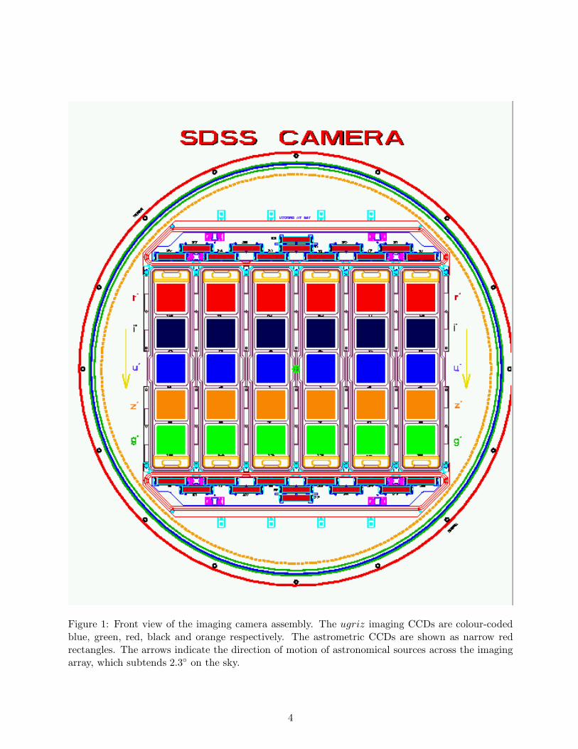
Figure 1: Front view of the imaging camera assembly. The ugriz imaging CCDs are colour-codedblue, green, red, black and orange respectively. The astrometric CCDs are shown as narrow redrectangles. The arrows indicate the direction of motion of astronomical sources across the imagingarray, which subtends 2.3 on the sky.

4

The imaging camera [14] (Figure 1) consists of 54 CCDs in eight dewars and spans 2.3 on the sky.Thirty of these CCDs are the main imaging/photometric devices, each a SITe (Scientific ImagingTechnologies, formerly Tektronix) device with 2048 × 2048 24µ pixels. They are arranged in sixdewars aligned with the scan direction and holding 5 CCDs each, one CCD for each filter bandpass.The camera operates in TDI (Time Delay and Integrate), or scanning, mode for which the telescopeis driven at a rate synchronous with the charge transfer rate of the CCDs. Objects on the sky driftdown the CCD array so that nearly simultaneous 5-colour photometry is obtained. The effectiveintegration time, i.e. the time any part of the sky spends on each detector, is 55 seconds at thechosen (sidereal) scanning rate, which results in a limiting magnitude of g ∼ 23.

The SDSS photometric system u′g′r′i′z′ [13] (Figure 2) has been specifically designed for this surveyand covers the near-UV to near-IR range (∼ 3000–10, 000A) in five essentially non-overlappingpassbands. The u filter response peaks in the near ultra-violet at 3500A, g is a blue-green bandcentred at 4800A, r is a red band centred at 6250A, i is a far-red filter centred at 7700A and z isa near-infrared passband centred at 9100A. The standard stars that define this system have beenpresented by Smith et al. [34]. The photometric data are not yet finally calibrated, so the currentmagnitudes are indicated with asterisks, u∗g∗r∗i∗z∗, to denote their preliminary nature. The SDSSfilters themselves are referred to simply as ugriz, without primes or asterisks.

In order to provide photometric calibration while the imaging camera is scanning, a second, dedi-cated Photometric Telescope operates concurrently, observing photometric standard stars and cre-ating photometrically calibrated “secondary patches” which lie within the main telescope’s scan.These calibration patches are then used to transfer the primary photometric calibration to objectsdetected with the 2.5m telescope and imaging camera. The photometric quality of the data ismonitored by a software “robot” that automatically rejects data observed during cloudy periods[16].

The other 24 CCDs in two additional dewars are also SITe chips of width 2048 24µ pixels, butthey have only 400 rows in the scanning direction. These dewars are oriented perpendicular tothe photometric dewars, with one at the top and one at the bottom of the imaging array. Two ofthese CCDs (one in each dewar) are used to determine changes in focus. The remaining 22 CCDsreach brighter magnitudes before saturating and are used to tie our observations to an astrometricreference frame defined by bright stars which saturate our imaging detectors [28].

The location of the survey imaging area is shown in Figure 3. The northern survey area is centrednear the North Galactic Pole and it lies within a nearly elliptical shape 130 E-W by 110 N-Schosen to minimize Galactic foreground extinction. All scans are conducted along great circles inorder to minimize the transit time differences across the camera array. There are 45 great circles(“stripes”) in the northern survey region separated by 2.5. We observe three non-contiguousstripes in the Southern Galactic Hemisphere, at declinations of 0, +15 and −10, during partsof the autumn season when the northern sky is unobservable. Each stripe is scanned twice, withan offset perpendicular to the scan direction in order to interlace the photometric columns. Acompleted stripe slightly exceeds 2.5 in width and thus there is a small amount of overlap to allowfor telescope mis-tracking and to provide multiple observations of some fraction of the sky for qualityassurance purposes. The total stripe length for the 45 northern stripes will require a minimum of650 hours of pristine photometric and seeing conditions to scan at a sidereal rate. Based upon ourcurrent experience of observing conditions at APO, it seems likely that we will only complete about75% of this imaging after 5 years of survey operations.

5

Figure 2: SDSS photometric system response as a function of wavelength in Angstroms. Theupper curve is without atmospheric extinction, the lower curve includes the effects of atmosphericextinction when observing at a typical altitude of 56.

6

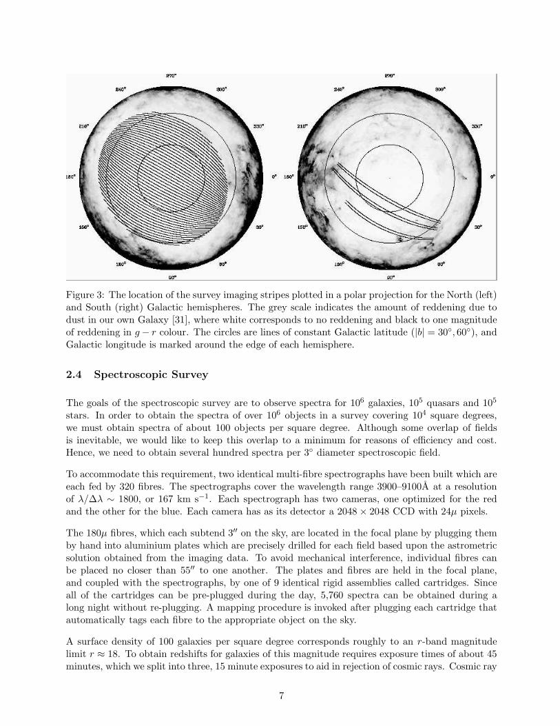
Figure 3: The location of the survey imaging stripes plotted in a polar projection for the North (left)and South (right) Galactic hemispheres. The grey scale indicates the amount of reddening due todust in our own Galaxy [31], where white corresponds to no reddening and black to one magnitudeof reddening in g − r colour. The circles are lines of constant Galactic latitude (|b| = 30, 60), andGalactic longitude is marked around the edge of each hemisphere.

2.4 Spectroscopic Survey

The goals of the spectroscopic survey are to observe spectra for 106 galaxies, 105 quasars and 105

stars. In order to obtain the spectra of over 106 objects in a survey covering 104 square degrees,we must obtain spectra of about 100 objects per square degree. Although some overlap of fieldsis inevitable, we would like to keep this overlap to a minimum for reasons of efficiency and cost.Hence, we need to obtain several hundred spectra per 3 diameter spectroscopic field.

To accommodate this requirement, two identical multi-fibre spectrographs have been built which areeach fed by 320 fibres. The spectrographs cover the wavelength range 3900–9100A at a resolutionof λ/∆λ ∼ 1800, or 167 km s−1. Each spectrograph has two cameras, one optimized for the redand the other for the blue. Each camera has as its detector a 2048 × 2048 CCD with 24µ pixels.

The 180µ fibres, which each subtend 3′′ on the sky, are located in the focal plane by plugging themby hand into aluminium plates which are precisely drilled for each field based upon the astrometricsolution obtained from the imaging data. To avoid mechanical interference, individual fibres canbe placed no closer than 55′′ to one another. The plates and fibres are held in the focal plane,and coupled with the spectrographs, by one of 9 identical rigid assemblies called cartridges. Sinceall of the cartridges can be pre-plugged during the day, 5,760 spectra can be obtained during along night without re-plugging. A mapping procedure is invoked after plugging each cartridge thatautomatically tags each fibre to the appropriate object on the sky.

A surface density of 100 galaxies per square degree corresponds roughly to an r-band magnitudelimit r ≈ 18. To obtain redshifts for galaxies of this magnitude requires exposure times of about 45minutes, which we split into three, 15 minute exposures to aid in rejection of cosmic rays. Cosmic ray

7

events occur at essentially random locations on our detectors, and so are very unlikely to appearat the same place in all three exposures. Each field takes about one hour, including calibration(flat field and comparison lamp) exposures and allowing for telescope pointing and the exchange offibre cartridges. Spectroscopic observations are carried out whenever observing conditions are notadequate for imaging, ie. when seeing exceeds 1.5 arcsec or when skies are non-photometric.

2.5 Data Processing

All of the raw data from the photometric CCDs are archived. The frames are first read to disk,then written to DLT tape. Over 16 Gb per hour are generated from the photometric chips. Whenobserving in spectroscopic mode, the amount of data generated seems trivial in comparison (about6 exposures per hour for each of two cameras for each of two spectrographs, or 24 8Mb frames perhour).

All data tapes are shipped by overnight express courier to Fermi National Accelerator Laboratory,near Chicago, where the data reduction pipelines are run. The goal is to turn the imaging dataaround within a few days, so that one dark run’s worth of imaging data will be processed before thenext dark run begins, allowing objects to be targeted for spectroscopy. The data flow serially throughseveral pipelines to identify, measure and extract astronomical images and to apply photometricand astrometric calibrations. Once a significant area of sky has been imaged, a target selection

procedure is then run in order to select objects for followup spectroscopy. Next, an adaptive tiling

algorithm assigns targets to spectroscopic plates and chooses plate centres in order to maximizeobserving efficiency [4]. Since galaxies are clustered on the sky, the target density varies from placeto place. In regions of high target density, the adaptive tiling algorithm allows the plates to moveslightly closer together so that all targets can be observed. The plates are then manufactured andshipped to the site.

Spectroscopic reduction is also automated. We are able to obtain correct redshifts for 99% oftargeted objects, without human intervention. The pipelines are integrated into a specially-writtenenvironment known as Dervish, and the reduced data are stored in an object-oriented database.

2.6 Spectroscopic Samples

There are several distinct spectroscopic samples observed by the survey. In a survey of this magni-tude, it is important that the selection criteria for each sample remain fixed throughout the durationof the survey. Therefore, we spent a whole year obtaining test data with the survey instruments andrefining the spectroscopic selection criteria in light of our test data. Now that the survey proper isunderway, these criteria have been “frozen in” for the duration of the survey.

The main galaxy sample [36] consists of ∼ 900, 000 galaxies selected by r band magnitude,r∗ < 17.77. This magnitude limit was chosen as test year data demonstrated that it correspondsclosely to the desired target density of 90 objects per square degree. Since galaxies are fuzzy,extended sources, there is no easy way to measure their total magnitude. Most previous surveyshave measured the light within an isophote of constant surface brightness, but these isophotalmagnitudes will systematically underestimate the flux of galaxies of low intrinsic surface brightnessand at high redshift z, since observed surface brightness scales as (1 + z)4. Simulations have shown

8

that the Petrosian magnitude [27], which is based on an aperture defined by the ratio of light withinan annulus to total light inside that radius, provides probably the least biased and most stableestimate of total magnitude. We therefore select galaxies according to their Petrosian magnitude.We also apply a surface-brightness limit, µr∗ < 24.5 mag arcsec−2, so that we do not waste fibreson galaxies of too low surface brightness to give a reasonable spectrum. This surface brightness cuteliminates just 0.1% of galaxies that would otherwise be selected for observation. Galaxies in thissample have a median redshift 〈z〉 ≈ 0.104.

We will observe an additional ∼ 100, 000 luminous red galaxies [10]. Given photometry in thefive survey bands, redshifts can be estimated for the reddest galaxies to ∆z ≈ 0.02 or better, andso one can also predict their intrinsic luminosities quite accurately. The luminous red galaxies,many of which will be so-called central dominant (cD) galaxies in cluster cores, provide a valuablesupplement to the main galaxy sample since 1) they have distinctive spectral features, allowing aredshift to be measured for objects to a flux limit around 1.5 magnitudes fainter than the mainsample, and 2) they form a volume-limited sample, ie. a sample of uniform density, out to redshiftz = 0.38. This sample will thus be extremely powerful for studying clustering on the largest scalesand for investigating galaxy evolution.

Quasar candidates [29] are selected from cuts in multi-colour space and by identifying sourcesfrom the FIRST radio catalogue [2], with the aim of observing ∼ 100, 000 quasars. This samplewill be orders of magnitude larger than any existing quasar catalogue, and will be invaluable forquasar luminosity function, evolution and clustering studies as well as providing sources for followupabsorption-line observations.

In addition to the above three classes of spectroscopic sources, which are designed to provide statis-

tically complete samples, we are also obtaining spectra for many thousands of stars and for variousserendipitous objects. The latter class includes objects of unusual colour or morphology which donot fit into the earlier classes, plus unusual objects found by other surveys and in other wavebands.

2.7 Survey Status

First light with the imaging camera was obtained on 9 May 1998 and the first extra-galactic spectrawere obtained in June 1999. The survey officially began on 1 April 2000, and observing is scheduledto end on 30 June 2005. At the time of writing (June 2002), we have imaged 4278 square degrees(40% of the total survey area) and obtained spectra for 621 plug-plates, yielding spectra for 264,995galaxies, 37,612 quasars and 50,023 stars, including some repeated observations. The spectrographsare performing extremely efficiently, with an overall throughput, including telescope optics butexcluding the atmosphere, of 20% in the blue (3900–6000 A) and 25% in the red (6000–9100 A).Automated spectral reduction pipelines classify these spectra and measure redshifts. Conservatively,we inspect the spectra of roughly 8% of sources, whenever there is any doubt about the reliabilityof the automated redshift measurement. In seven-eighths of these cases, the automated redshiftmeasurement is in fact confirmed to be correct. The remaining eighth of these spectra (1% overall)have their redshifts manually corrected. Based on manual inspection of all ≈ 23, 000 spectra from39 plugplates, this procedure correctly measures redshifts for 99.7% of galaxies, 98.0% of quasarsand 99.6% of stars.

9

3 The Early Data Release

The first public release of SDSS data (hereafter EDR) took place on 5 June 2001, and consists ofimages covering 460 square degrees of sky, photometric parameters for 10 million objects and spectrafor 54,000 objects. The main access point to the data is through the website http://www.sdss.org/and the EDR is described in [35].

There are presently three ways to access the data, the choice of which depends on the nature of thedata required and the experience of the user.

The SkyServer (http://skyserver.fnal.gov) provides a graphical user interface to images ofthe sky and also enables one to download spectra of specified objects. It was primarily intended asan interface for the general public and for educational purposes, but new features are being added,making it also useful for professional astronomers. Public interest in the SDSS is illustrated by thefact that this web site has been receiving around half a million hits per month.

The MAST interface (http://archive.stsci.edu/sdss/) allows simple web-based searches aroundspecified objects or positions on the sky. It is a useful way of retrieving SDSS observations for mod-erate numbers of objects in a small region of the sky.

For accessing SDSS data on large numbers of objects, and over larger areas, the SDSS query toolsdssQT is recommended. This tool allows one to query the EDR database on any measuredparameters and to specify which parameters, such as position and magnitude, are to be returned.Documentation on the query tool is available from http://archive.stsci.edu/sdss/software/.

The distribution of equatorial galaxies in the EDR is shown in right ascension (RA) versus redshiftwedge plots in Figure 4. The main galaxy sample is flux-limited (r∗ < 17.6) and has a medianredshift z ≈ 0.11. The clustering of galaxies is clearly visible in this plot: the galaxies appear to liewithin filamentary structures enclosing regions of substantially lower density. The drop in galaxydensity with redshift (distance from the centre of the plot) is entirely due to the fact that thissample is limited by apparent flux: only the most luminous galaxies, which are rare, can be seenbeyond a redshift z & 0.15.

By contrast, the luminous red galaxy (LRG) sample is designed to be volume-limited, ie. to be ofuniform density, out to redshift z = 0.38. This sample also includes additional galaxies to z ∼ 0.5,although these high redshift galaxies do not form a complete subsample. At z < 0.15, the simplelinear colour cut used allows less luminous galaxies to enter the sample, hence the increase in galaxydensity at these low redshifts.

The EDR includes some engineering data of sub-survey standard, and will be superseded by thefirst official data release, DR1, in January 2003. This release will include spectra of more than200,000 objects over 2800 square degrees of sky. Subsequent data releases will follow at roughlyyearly intervals.

10

Figure 4: Distribution of EDR galaxies in right ascension (RA) and redshift around the equator(declination |δ| < 1.25 deg). The left plot shows 24,915 galaxies from the main flux-limited galaxysample within a redshift z = 0.2. The right plot shows 8025 galaxies from the luminous red galaxysample to z = 0.5.

4 Early Science Results

Although the primary science driver behind the Sloan Digital Sky Survey is characterization ofthe large scale structure of the Universe, the survey has already had a significant impact on severalbranches of astrophysics, from the investigation of asteroids in our own Solar System to the discoveryof the most distant known objects in the Universe. Here I very briefly highlight some interestingresults which have come out of the commissioning phase of the survey. For further details, pleasesee the original articles as referenced.

4.1 Asteroids

Asteroids are easily detected in SDSS imaging data since they are fast-moving and very nearby(within the Solar System), leading to a significant motion relative to the background stars during the55 s integration time. They thus appear on SDSS images as trails, the length and orientation of whichenable the asteroid’s orbit to be determined. Around 13,000 asteroids have been detected in 500deg2 of SDSS commissioning data [18]. These observations have enabled an accurate determinationof the size distribution of asteroids to r∗ < 21.5 over the range 0.4–40 km. The total numberof predicted asteroids with r∗ < 21.5 is about a factor of ten smaller than that predicted by anextrapolation from previous observations of brighter asteroids (r∗ . 18), and the number of “killer”asteroids with diameter D > 1 km is a factor of about three smaller than previously thought, witha new estimate of roughly one impact per 500,000 years. By completion, we estimate that the SDSSwill have observed roughly 100,000 asteroids in five colours, enabling their approximate chemical

11

composition to be determined. There is already clear evidence for chemical segregation in the beltof asteroids between Mars and Jupiter. Asteroids in the inner part of the belt are composed mostlyof rocky silicates, whereas the outer belt asteroids are primarily carbonaceous. These observationshave important implications for the formation history of the Solar System.

4.2 Brown Dwarfs and Methane Dwarfs

Moving slightly further afield than the Solar System, the SDSS has also been very successful atfinding brown dwarfs in the vicinity of the Sun. Brown dwarfs are sub-stellar objects which aretoo small to sustain thermonuclear reactions in their cores, and are thus not true stars, but arelarger than planets (they are thought to be 10–70 times the mass of Jupiter). They are thus cool,below 2,500 K, and hence very red, enabling them to be easily distinguished from true stars bytheir colours in the SDSS filters. To date [15], SDSS has discovered around fifty new brown dwarfs,including four T-dwarfs, also known as methane dwarfs. The methane dwarfs are so cool, below1,300 K, that their spectra are dominated by the presence of molecules such as water vapour andmethane. While a methane dwarf, Gliese 229B, had already been discovered in orbit around abrighter star, the SDSS was the first survey to discover free-floating methane dwarfs. Using thediscovery technique pioneered by SDSS, the Two Micron All Sky Survey (2MASS) has since foundmore than a dozen methane dwarfs [5]. Although very low in mass, these elusive objects may be verycommon, and thus may provide a significant fraction of the “dark matter” that is known to existin the Milky Way. To understand their contribution to the total mass of the Milky Way requiresdetermining both their abundance and their mass. The SDSS will be important in addressing boththese questions, due to its capability of obtaining precision five-colour photometry over a very largearea of sky.

4.3 Star Structures in the Galaxy

The SDSS has discovered an unexpectedly large number of blue stars within 20 degrees of theGalactic plane. It is thought that these stars could be part of a disrupted dwarf galaxy, or a disk-like distribution of stars that is puffier than accepted models of the stellar disk of the Galaxy, andflatter than the spherical distribution in the halo [26]. These observations suggest that the modelfor our Galaxy needs to be reconsidered. One possible explanation is that these star structures camefrom tidal disruption of nearby dwarf galaxies such as Sagittarius, since the ages and metallicitiesof the stars are consistent with the stellar populations in Sagittarius.

4.4 Galaxy luminosity function

The distance to a galaxy can be obtained from its spectroscopic redshift using Hubble’s law, whichsays that the recession velocity of a galaxy is linearly proportional to its distance. Knowing thedistance to a galaxy, its intrinsic luminosity may be determined from its apparent magnitude usingthe inverse-square law. By calculating the maximum distance to which a galaxy of given luminositymay be seen, one can find the galaxy luminosity function, φ(L), the number density of galaxies asa function of intrinsic luminosity. It has long been known that the galaxy LF is well fit by the

12

Schechter function [30],

φ(L) dL = φ∗

(

L

L∗

)α

exp

(

−L

L∗

)

d

(

L

L∗

)

,

in which the number density of faint galaxies is described by a power law with index α ≈ −1.2. Forgalaxies brighter than a characteristic luminosity L∗, the number density drops exponentially.

We have determined the luminosity function from a sample of 11,275 galaxies in the SDSS com-missioning data [3], and find that the LF is extremely well fit by a Schechter function over a rangeof 8 magnitudes. The use of Petrosian magnitudes by the SDSS means that a larger fraction of agalaxy’s light is being measured than is the case with most previous surveys. The integrated lu-

minosity density of the Universe determined from SDSS measurements is thus a factor 1.5–2 timeslarger than previously thought. This improves the agreement with most models of galaxy formation,which predict a higher density of stellar matter than previous observational estimates.

4.5 Galaxy clustering

The clustering of galaxies provides a powerful probe of the initial density perturbations in the earlyUniverse, the power spectrum of which is determined by cosmological parameters such as the matterdensity and Hubble parameters, Ωm and h respectively. On large scales, r & 20 Mpc, the clusteringof galaxies is related to the primordial density fluctuations by linear perturbation theory, but onsmaller scales, non-linear effects can change the shape of the observed clustering pattern.

The clustering of galaxies is most frequently measured with the two-point correlation function ξ(r),which gives the excess probability above random of finding two galaxies at separation r, or itsFourier inverse, the power spectrum P (k). The huge volume of the completed SDSS redshift surveywill enable estimates of the galaxy power spectrum to ∼ 1000h−1Mpc scales. Figure 5a shows thepower spectrum P (k) we would expect to measure from a volume-limited sample of galaxies fromthe SDSS northern redshift survey, assuming Gaussian fluctuations and a Ωmh = 0.3 cold darkmatter (CDM) model. The error bars include cosmic variance and shot noise, but not systematicerrors, due, for example, to Galactic obscuration. Provided such errors can be corrected for, wecan easily distinguish between Ωmh = 0.2, as indicated by a recent study of the masses of SDSSgalaxy clusters [1], and Ωmh = 0.3, favoured by previous studies, as Figure 5a demonstrates. Thenoted systematic effects of Galactic obscuration will be minimized by SDSS observations of distantF stars, far from the Galactic centre. These stars, three of which are observed on each spectroscopicplate, have well-understood intrinsic colours, and so can be used as reliable reddening indicators.Adding the luminous red galaxy sample (Fig. 5b), will further decrease measurement errors on thelargest scales, and so we also expect to be able to easily distinguish between low-density CDM andmixed dark matter (MDM) models, and models with differing shapes of the primordial fluctuationspectrum.

Given the relatively small sky coverage of our existing data, we are not yet able to place reliableconstraints on cosmological parameters. We can however use observations of galaxy clustering to testthe quality of our photometry and star-galaxy separation, and to investigate the relative clusteringstrength of different types of galaxies on small scales.

13

Figure 5: Left: (a) Expected 1σ uncertainty in the galaxy power spectrum P (k) we would measurefrom a volume-limited sample from the completed SDSS northern survey, along with predictions ofP (k) from four variants of the low-density CDM model. Note that the models have been arbitrarilynormalized to agree on small scales (k = 0.4); in practice the COBE observations of CMB fluctu-ations fix the amplitude of P (k) on very large scales. Right: (b) Power spectrum expected fromthe luminous red galaxy sample (BRGs), assuming that these galaxies are four times as stronglyclustered as the main sample galaxies.

4.5.1 Angular clustering

A series of papers [7, 9, 32, 37, 38] have studied the angular clustering of galaxies in SDSS commis-sioning data. These papers are based on a single survey stripe (runs 752/756 observed in March1999) measuring 2.5 × 90 degrees and containing some 3 million galaxies to r∗ = 22. Star-galaxyseparation is performed using a Bayesian likelihood and approximately 30% of the area is maskedout due to poor seeing [32]. The angular correlation function, w(θ), which describes the excessprobability over random of finding two galaxies at angular separation θ, is consistent with thatmeasured from the APM Galaxy Survey [22] when scaled to the same depth [7].

An important test of the star-galaxy separation and of the photometric calibration is to check thatw(θ) scales as expected with apparent magnitude. (We expect w(θ) to shift to smaller angularscales and a lower amplitude as we look at more distant, and hence apparently fainter, galaxies.This scaling is quantified by Limber’s equation [19].) Figure 6 shows that the scaling of w(θ) iswell-described by Limber’s equation, particularly when a vacuum-dominated (Ωm = 0.3, ΩΛ = 0.7)cosmology is assumed. Further tests for possible sources of systematic errors in the SDSS data aredescribed in detail in [32] and the angular clustering results are summarized in [7].

14

0.01 0.1 1

θ (degrees)

0.001

0.01

0.1

1

18 < r’ < 1919 < r’ < 2020 < r’ < 2121 < r’ < 22

0.01 0.1 1

θ (degrees)

0.001

0.01

0.1

1

18 < r’ < 1919 < r’ < 2020 < r’ < 2121 < r’ < 22

Figure 6: Scaling of the angular correlation function w(θ) measured in four magnitude slices ac-cording to Limber’s equation (see text) and assuming a selection function assumed based on theCNOC2 galaxy redshift survey [20]. The left plot assumes a Ωm = 1, ΩΛ = 0 cosmology, the rightplot a Ωm = 0.3, ΩΛ = 0.7 cosmology. Assuming the latter cosmology improves the scaling of thefaintest (21 < r′ < 22) slice, since the volume per unit redshift is larger at high redshifts in theΛ-dominated cosmology. From [32].

4.5.2 Spatial clustering

A preliminary estimate of the spatial clustering of galaxies has been made using redshift information[41]. This sample consists of 29,300 galaxies with r∗ < 17.6 and within ±1.5 magnitudes of thecharacteristic magnitude M∗

r (corresponding to the characteristic luminosity L∗ in the Schechterfunction fit to the luminosity function, see §4.4), distributed non-contiguously over 690 squaredegrees.

When using redshifts to infer distances, one relies on the Hubble relation, ie. that distance isproportional to recession velocity. In fact, galaxies have peculiar velocities relative to the Hubbleexpansion, leading to an error in estimated distances. It is important to take these distance errors,or redshift-space distortions, into account when measuring galaxy clustering. One way of doingthis is to estimate galaxy clustering as a function ξ2(rp, π) of two components of the separationvector: the line of sight separation π, which is affected by peculiar velocities, and the sky-projectedseparation rp, which is not. In the absence of redshift-space distortions, the contours of ξ2(rp, π)would be symmetric about the origin, but small-scale peculiar velocities cause an elongation of thecontours along the line of sight direction π, the so-called “finger of God” effect. One can estimate aprojected correlation function wp(rp) that is unaffected by redshift-space distortions by integratingξ2(rp, π) along the line of sight π,

wp(rp) = 2

∫

∞

0

dπξ2(rp, π) = 2

∫

∞

0

dyξ(√

r2p + y2),

where the second integral relates wp(rp) to the spatial correlation function ξ(r).

15

Figure 7: Projected correlation functions wp(rp) against projected separation rp for redshift surveygalaxies subdivided by colour (left plot) and luminosity (right plot). Note that the slope of wp(rp)increases from blue to red colour, but remains approximately constant with luminosity. From [41].

Table 1: Power-law parameters for the real-space correlation function ξ(r) = (r/r0)−γ . Units for

the correlation length r0 are h−1Mpc. From [41].

Sample r0 γ

All 6.14 ± 0.18 1.75 ± 0.03Red 6.78 ± 0.23 1.86 ± 0.03Blue 4.02 ± 0.25 1.41 ± 0.04M∗ − 1.5 7.42 ± 0.33 1.76 ± 0.04M∗ 6.28 ± 0.77 1.80 ± 0.09M∗ + 1.5 4.72 ± 0.44 1.86 ± 0.06

We find that ξ(r) is well-fit over the range 0.1 < r < 30h−1Mpc by a power law ξ(r) = (r/r0)−γ

with parameters given in Table 1. The correlation length r0 = 6.14 ± 0.18h−1Mpc is larger thanr0 = 5.1 ± 0.2h−1Mpc found by an earlier study [21], presumably because dwarf galaxies withM > M∗ + 1.5 have been excluded from the SDSS analysis. The index γ = 1.75 ± 0.03 is in verygood agreement with the earlier result (γ = 1.71 ± 0.05).

This analysis also allows one to explore the dynamics of galaxies. We find that for close pairs ofgalaxies, at a projected separation rp < 5h−1Mpc, the rms relative velocity of galaxies σ ≈ 600km/s.

16

0

200

400

600

800u′

Luminosity

02

4

68

Mas

s

0 1 2 3 4

g′

Luminosity

Mas

s

0.5 1 2 2 30

2

4

6

0

200

400

600

800r′

Luminosity

05

10

1520

Mas

s

0 2 4 6 8 10

β

0.5 1.0 1.5 2.0

i′

Luminosity

Mas

s

0 2 4 605

10152025

0.0 0.5 1.0 1.5 2.0β

0

200

400

600

800

ϒ (h

MO • /L

O •)

z′

0 5 10 15 20Luminosity

05

10152025

Mas

s

Figure 8: Mass-luminosity relation in thefive SDSS bands estimated from weaklensing. The inset in each panel plotsestimated mass within 260h−1kpc (M260)as a function of lens luminosity. Thecontours show 1, 2 and 3 sigma confi-dence limits on the scale factor Υ and thepower-law index β in the relation M260 =Υ(L/1010L⊙)β. Note that inferred masshas only very weak dependence on u-bandluminosity, but in the redder survey bandsgriz, the mass-luminosity relation appearsto be linear. From [25].

Figure 7 shows the clustering properties for two subsamples of the galaxy population selected byrestframe u − r colour at (u∗ − r∗)0 = 1.8, corresponding roughly to bulge (red) and disk (blue)dominated galaxies. The red galaxies exhibit a steeper power-law slope and longer correlation lengththan the blue galaxies, as indicated by the power-law fit parameters in Table 1. Also shown inFigure 7 are the correlation functions for three, volume-limited samples, with luminosities centeredon M∗− 1.5, M∗ and M∗ +1.5 (bright, medium and faint). The power-law slopes for these samplesare all consistent with γ = 1.8, although the correlation length r0 decreases as expected from brightto faint luminosities.

4.6 Galaxy-mass correlation function

So far, I have summarized recent SDSS results concerning the distribution of luminous matter inthe Universe. Direct constraints on the dark matter distribution may be obtained from gravita-tional lensing, in which the images of background sources are distorted by the gravitational fieldof foreground masses. McKay et al. [25] have made weak lensing measurements of the surfacemass density contrast around foreground galaxies of known redshift. Although the lensing signal istoo weak to detect about any single lens, by stacking together around 31,000 lens galaxies a clearlensing signal is detected. The galaxy-mass correlation function is well fit by a power-law of the

17

form ∆Σ+ = 2.5(r/Mpc)−0.8hM⊙ pc−2, where M⊙ represents the mass of the Sun. The strength ofcorrelation is found to increase with the following properties of the lensing galaxy: late → early-typemorphology, local density and luminosity in all bands apart from u′. Figure 8 shows the relationshipbetween inferred mass within a 260h−1kpc radius and luminosity in each of the survey bands.

4.7 High-redshift quasars

The SDSS has broken the z = 6 redshift barrier, with the discovery of a quasar at a redshift z = 6.28,along with two new quasars at redshifts z = 5.82 and z = 5.99 [11]. These objects were selectedas i-dropouts: i∗ − z∗ > 2.2 and z∗ < 20.2. Contaminating L and T dwarfs were eliminated withfollowup near-IR photometry and confirming spectra were obtained with the ARC 3.5m telescope.The SDSS has now observed a well-defined sample of four luminous quasars at redshift z > 5.8.The Eddington luminosities of these quasars are consistent with a central black hole of mass severaltimes 109 M⊙, and with host dark matter halos of mass ∼ 1013 M⊙. The existence of such massconcentrations at redshifts z ≈ 6, when the Universe was less than 1Gyr old, provides importantconstraints on models of formation of massive black holes. We expect to discover ∼ 27 z > 5.8quasars and one z ≈ 6.6 quasar by the time the survey is complete. Such observations will setstrong constraints on cosmological models for galaxy and quasar formation.

5 Conclusions and Acknowledgments

The Sloan Digital Sky Survey is now fully operational and is producing high quality data at aprodigious rate. We have imaged 4278 deg2 of sky in five colours and have obtained more than350,000 spectra. Much exciting science has already come out of just a small fraction of the finaldataset and we look forward to many more exciting discoveries in the coming years.

Funding for the creation and distribution of the SDSS Archive has been provided by the AlfredP. Sloan Foundation, the Participating Institutions, the National Aeronautics and Space Adminis-tration, the National Science Foundation, the U.S. Department of Energy, the Japanese Monbuka-gakusho, and the Max Planck Society. The SDSS Web site is http://www.sdss.org/.

The SDSS is managed by the Astrophysical Research Consortium (ARC) for the ParticipatingInstitutions. The Participating Institutions are The University of Chicago, Fermilab, the Institutefor Advanced Study, the Japan Participation Group, The Johns Hopkins University, Los AlamosNational Laboratory, the Max-Planck-Institute for Astronomy (MPIA), the Max-Planck-Institutefor Astrophysics (MPA), New Mexico State University, Princeton University, the United StatesNaval Observatory, and the University of Washington.

It is a pleasure to thank SDSS colleagues for supplying some of the figures. I would particularlylike to thank Donald York for his careful reading of the manuscript.

18

References

[1] Bahcall N.A. et al., 2002, submitted to ApJ (astro-ph/0205490)

[2] Becker, R.H., White, R.L. & Helfand, D.J., 1995, ApJ, 450, 559

[3] Blanton M., et al., 2001, AJ, 121, 2358

[4] Blanton M.R., Lupton R.H., Maley F.M., Young N., Zehavi I., Loveday J, 2001, submitted toAJ

[5] Burgasser A.J., 2001, astro-ph/0101242

[6] Colless M., et al., 2001, MNRAS, 328, 1039

[7] Connolly A., et al., 2001, submitted to ApJ (astro-ph/0107417)

[8] Disney, M.J., 1976, Nature, 263, 573

[9] Dodelson, S., et al., 2001, submitted to ApJ (astro-ph/0107421)

[10] Eisenstein, D.J., et al., 2001, AJ, 122, 2267

[11] Fan, X. et al., 2001, AJ, 122, 2833

[12] Fong, R., Hale-Sutton, D. & Shanks, T., 1992, MNRAS, 257, 650

[13] Fukugita, M., et al, 1996, AJ, 111, 1748

[14] Gunn J.E., et al, 1998, AJ, 116, 3040

[15] Hawley L.S. et al., 2002, AJ, 123, 3409

[16] Hogg D.W., Finkbeiner D.P., Schlegel D.J., Gunn J.E., 2001, AJ, 122, 2129

[17] Hull C.L., Limmongkol S., Siegmund W.A., 1994, Proc. SPIE, 2199, 852

[18] Ivezic Z., et al., 2001, AJ, 122, 2749

[19] Limber, D.N., 1953, ApJ, 117, 134

[20] Lin, H., et al., 1999, ApJ, 518, 533

[21] Loveday, J., Maddox, S.J., Efstathiou, G., & Peterson, B.A., 1995, ApJ, 442, 457

[22] Maddox, S.J., Efstathiou, G., Sutherland, W.J. & Loveday, J., 1990, MNRAS, 242, 43P

[23] Maddox, S.J., Efstathiou, G., & Sutherland, W.J., 1996, MNRAS, 283, 1227

[24] Maddox, S.J., Sutherland, W.J. Efstathiou, G., & Loveday, J., 1990, MNRAS, 243, 692

[25] McKay T.A., et al., 2001, astro-ph/0108013

[26] Newberg H.J. et al., 2002, ApJ, 569, 245

[27] Petrosian, V., 1976, ApJ, 209, L1

[28] Pier J.R. et al., 2002, submitted to AJ

[29] Richards G.T. et al., 2002, AJ, in press

[30] Schechter, P.L., 1976, ApJ, 203, 297

[31] Schlegel, D.J., Finkbeiner, D.P. & Davis, M., 1998, ApJ, 500, 525

[32] Scranton R., et al., 2001, submitted to ApJ (astro-ph/0107416)

[33] Shapley, H. & Ames, A., 1932, Annals of the Harvard College Observatory, 88, No. 2

[34] Smith J.A., et al, 2002, AJ, 123, 2121

19

[35] Stoughton C. et al., 2002, AJ, 123, 485

[36] Strauss M.A. et al., 2002, AJ, in press (astro-ph/0206225)

[37] Szalay A.S. et al., 2001, submitted to ApJ (astro-ph/0107419)

[38] Tegmark M., et al., 2002, ApJ, 571, 191

[39] Waddell, P., Mannery, E. J., Gunn, J., Kent, S., 1998, Proc. SPIE, Vol. 3352

[40] York D.G., et al., 2000, AJ, 120, 1579

[41] Zehavi I., et al., 2002, ApJ, 571, 172

Jon Loveday is a Lecturer in the Astronomy Centre, University of Sussex. He has been interestedin galaxy surveys and observational cosmology since studying for his PhD in Astronomy at theUniversity of Cambridge. After spending three years in Australia, he became one of the first SDSSparticipants while at Fermilab and then the University of Chicago. He is still occasionally seencarrying a violin case.

20