
Planck Early Results: The Galactic Cold Core Population revealed by the first all-sky survey
28
arXiv:1101.2035v1 [astro-ph.GA] 11 Jan 2011 Astronomy & Astrophysics manuscript no. Planck˙Early˙Paper˙1˙v3.1 c ESO 2011 January 12, 2011 Planck Early Results: The Galactic Cold Core Population revealed by the first all-sky survey Planck Collaboration: P. A. R. Ade 68 , N. Aghanim 45 , M. Arnaud 55 , M. Ashdown 53,74 , J. Aumont 45 , C. Baccigalupi 66 , A. Balbi 27 , A. J. Banday 72,6,60 , R. B. Barreiro 50 , J. G. Bartlett 3,51 , E. Battaner 76 , K. Benabed 46 , A. Benoˆ ıt 46 , J.-P. Bernard 72,6 , M. Bersanelli 25,40 , R. Bhatia 33 , J. J. Bock 51,7 , A. Bonaldi 36 , J. R. Bond 5 , J. Borrill 59,69 , F. R. Bouchet 46 , F. Boulanger 45 , M. Bucher 3 , C. Burigana 39 , P. Cabella 27 , C. M. Cantalupo 59 , J.-F. Cardoso 56,3,46 , A. Catalano 3,54 , L. Cay´ on 18 , A. Challinor 75,53,8 , A. Chamballu 43 , R.-R. Chary 44 , L.-Y Chiang 47 , P. R. Christensen 63,28 , D. L. Clements 43 , S. Colombi 46 , F. Couchot 58 , A. Coulais 54 , B. P. Crill 51,64 , F. Cuttaia 39 , L. Danese 66 , R. D. Davies 52 , R. J. Davis 52 , P. de Bernardis 24 , G. de Gasperis 27 , A. de Rosa 39 , G. de Zotti 36,66 , J. Delabrouille 3 , J.-M. Delouis 46 , F.-X. D´ esert 42 , C. Dickinson 52 , K. Dobashi 14 , S. Donzelli 40,48 , O. Dor´ e 51,7 , U. D ¨ orl 60 , M. Douspis 45 , X. Dupac 32 , G. Efstathiou 75 , T. A. Enßlin 60 , E. Falgarone 54 , F. Finelli 39 , O. Forni 72,6 , M. Frailis 38 , E. Franceschi 39 , S. Galeotta 38 , K. Ganga 3,44 , M. Giard 72,6 , G. Giardino 33 , Y. Giraud-H´ eraud 3 , J. Gonz´ alez-Nuevo 66 , K. M. G ´ orski 51,78 , S. Gratton 53,75 , A. Gregorio 26 , A. Gruppuso 39 , F. K. Hansen 48 , D. Harrison 75,53 , G. Helou 7 , S. Henrot-Versill´ e 58 , D. Herranz 50 , S. R. Hildebrandt 7,57,49 , E. Hivon 46 , M. Hobson 74 , W. A. Holmes 51 , W. Hovest 60 , R. J. Hoyland 49 , K. M. Huffenberger 77 , A. H. Jaffe 43 , G. Joncas 11 , W. C. Jones 17 , M. Juvela 16 , E. Keih¨ anen 16 , R. Keskitalo 51,16 , T. S. Kisner 59 , R. Kneissl 31,4 , L. Knox 20 , H. Kurki-Suonio 16,34 , G. Lagache 45 , J.-M. Lamarre 54 , A. Lasenby 74,53 , R. J. Laureijs 33 , C. R. Lawrence 51 , S. Leach 66 , R. Leonardi 32,33,21 , C. Leroy 45,72,6 , M. Linden-Vørnle 10 , M. L´ opez-Caniego 50 , P. M. Lubin 21 , J. F. Mac´ ıas-P´ erez 57 , C. J. MacTavish 53 , B. Maffei 52 , N. Mandolesi 39 , R. Mann 67 , M. Maris 38 , D. J. Marshall 72,6 , P. Martin 5 , E. Mart´ ınez-Gonz´ alez 50 , G. Marton 30 , S. Masi 24 , S. Matarrese 23 , F. Matthai 60 , P. Mazzotta 27 , P. McGehee 44 , A. Melchiorri 24 , L. Mendes 32 , A. Mennella 25,38 , S. Mitra 51 , M.-A. Miville-Deschˆ enes 45,5 , A. Moneti 46 , L. Montier 72,6 ⋆ , G. Morgante 39 , D. Mortlock 43 , D. Munshi 68,75 , A. Murphy 62 , P. Naselsky 63,28 , F. Nati 24 , P. Natoli 27,2,39 , C. B. Netterfield 13 , H. U. Nørgaard-Nielsen 10 , F. Noviello 45 , D. Novikov 43 , I. Novikov 63 , S. Osborne 71 , F. Pajot 45 , R. Paladini 70,7 , F. Pasian 38 , G. Patanchon 3 , T. J. Pearson 7,44 , V.-M. Pelkonen 44 , O. Perdereau 58 , L. Perotto 57 , F. Perrotta 66 , F. Piacentini 24 , M. Piat 3 , S. Plaszczynski 58 , E. Pointecouteau 72,6 , G. Polenta 2,37 , N. Ponthieu 45 , T. Poutanen 34,16,1 , G. Pr´ ezeau 7,51 , S. Prunet 46 , J.-L. Puget 45 , W. T. Reach 73 , R. Rebolo 49,29 , M. Reinecke 60 , C. Renault 57 , S. Ricciardi 39 , T. Riller 60 , I. Ristorcelli 72,6 , G. Rocha 51,7 , C. Rosset 3 , M. Rowan-Robinson 43 , J. A. Rubi ˜ no-Mart´ ın 49,29 , B. Rusholme 44 , M. Sandri 39 , D. Santos 57 , G. Savini 65 , D. Scott 15 , M. D. Seiffert 51,7 , G. F. Smoot 19,59,3 , J.-L. Starck 55,9 , F. Stivoli 41 , V. Stolyarov 74 , R. Sudiwala 68 , J.-F. Sygnet 46 , J. A. Tauber 33 , L. Terenzi 39 , L. Toffolatti 12 , M. Tomasi 25,40 , J.-P. Torre 45 , V. Toth 30 , M. Tristram 58 , J. Tuovinen 61 , G. Umana 35 , L. Valenziano 39 , P. Vielva 50 , F. Villa 39 , N. Vittorio 27 , L. A. Wade 51 , B. D. Wandelt 46,22 , N. Ysard 16 , D. Yvon 9 , A. Zacchei 38 , S. Zahorecz 30 , and A. Zonca 21 (Affiliations can be found after the references) Preprint online version: January 12, 2011 ABSTRACT We present the statistical properties of the first version of the Cold Core Catalogue of Planck Objects (C3PO), in terms of their spatial distribution, temperature, distance, mass, and morphology. We also describe the statistics of the Early Cold Core Catalogue (ECC) that is a subset of the complete catalogue, and that contains only the 915 most reliable detections. ECC is delivered as a part of the Early Release Compact Source Catalogue (ERCSC). We have used the CoCoCoDeT algorithm to extract about 10 thousand cold sources. The method uses the IRAS 100μm data as a warm template that is extrapolated to the Planck bands and subtracted from the signal, leading to a detection of the cold residual emission. We have used cross-correlation with ancillary data to increase the reliability of our sample, and to derive other key properties such as distance and mass. Temperature and dust emission spectral index values are derived using the fluxes in the IRAS 100 μm band and the three highest frequency Planck bands. The range of temperatures explored by the catalogue spans from 7 K to 17 K, and peaks around 13 K. Data are not consistent with a constant value of the associated spectral index β over the all temperature range. β ranges from 1.4 to 2.8 with a mean value around 2.1, and several possible scenarios are possible, including β(T ) and the effect of multiple temperature components folded into the measurements. For one third of the objects the distances are obtained using various methods such as the extinction signature, or the association with known molecular complexes or Infra-Red Dark Clouds. Most of the detections are within 2 kpc in the Solar neighbourhood, but a few are at distances greater than 4 kpc. The cores are distributed over the whole range of longitude and latitude, from the deep Galactic plane, despite the confusion, to high latitudes (> 30 ◦ ). The associated mass estimates derived from dust emission range from 1 to 10 5 solar masses. Using their physical properties such as temperature, mass, luminosity, density and size, these cold sources are shown to be cold clumps, defined as the intermediate cold sub- structures between clouds and cores. These cold clumps are not isolated but mostly organized in filaments associated with molecular clouds. The Cold Core Catalogue of Planck Objects (C3PO) is the first unbiased all-sky catalogue of cold compact objects and contains 10783 objects. It gives an unprecedented statistical view to the properties of these potential pre-stellar clumps and offers a unique possibility for their classification in terms of their intrinsic properties and environment. Key words. Cold Cores, Galaxy, Source extraction ⋆ Corresponding author = [email protected] 1. Introduction The main difficulty in understanding star formation lies in the vast range of scales involved in the process. If star formation it-
-
Upload
independent -
Category
Documents
-
view
5 -
download
0
Transcript of Planck Early Results: The Galactic Cold Core Population revealed by the first all-sky survey

arX
iv:1
101.
2035
v1 [
astr
o-ph
.GA
] 11
Jan
201
1Astronomy & Astrophysicsmanuscript no. Planck˙Early˙Paper˙1˙v3.1 c© ESO 2011January 12, 2011
Planck Early Results: The Galactic Cold Core Population revealedby the first all-sky survey
Planck Collaboration: P. A. R. Ade68, N. Aghanim45, M. Arnaud55, M. Ashdown53,74, J. Aumont45, C. Baccigalupi66, A. Balbi27,A. J. Banday72,6,60, R. B. Barreiro50, J. G. Bartlett3,51, E. Battaner76, K. Benabed46, A. Benoıt46, J.-P. Bernard72,6, M. Bersanelli25,40, R. Bhatia33,
J. J. Bock51,7, A. Bonaldi36, J. R. Bond5, J. Borrill59,69, F. R. Bouchet46, F. Boulanger45, M. Bucher3, C. Burigana39, P. Cabella27,C. M. Cantalupo59, J.-F. Cardoso56,3,46, A. Catalano3,54, L. Cayon18, A. Challinor75,53,8, A. Chamballu43, R.-R. Chary44, L.-Y Chiang47,
P. R. Christensen63,28, D. L. Clements43, S. Colombi46, F. Couchot58, A. Coulais54, B. P. Crill51,64, F. Cuttaia39, L. Danese66, R. D. Davies52,R. J. Davis52, P. de Bernardis24, G. de Gasperis27, A. de Rosa39, G. de Zotti36,66, J. Delabrouille3, J.-M. Delouis46, F.-X. Desert42, C. Dickinson52,
K. Dobashi14, S. Donzelli40,48, O. Dore51,7, U. Dorl60, M. Douspis45, X. Dupac32, G. Efstathiou75, T. A. Enßlin60, E. Falgarone54, F. Finelli39,O. Forni72,6, M. Frailis38, E. Franceschi39, S. Galeotta38, K. Ganga3,44, M. Giard72,6, G. Giardino33, Y. Giraud-Heraud3, J. Gonzalez-Nuevo66,
K. M. Gorski51,78, S. Gratton53,75, A. Gregorio26, A. Gruppuso39, F. K. Hansen48, D. Harrison75,53, G. Helou7, S. Henrot-Versille58, D. Herranz50,S. R. Hildebrandt7,57,49, E. Hivon46, M. Hobson74, W. A. Holmes51, W. Hovest60, R. J. Hoyland49, K. M. Huffenberger77, A. H. Jaffe43, G. Joncas11,
W. C. Jones17, M. Juvela16, E. Keihanen16, R. Keskitalo51,16, T. S. Kisner59, R. Kneissl31,4, L. Knox20, H. Kurki-Suonio16,34, G. Lagache45,J.-M. Lamarre54, A. Lasenby74,53, R. J. Laureijs33, C. R. Lawrence51, S. Leach66, R. Leonardi32,33,21, C. Leroy45,72,6, M. Linden-Vørnle10,
M. Lopez-Caniego50, P. M. Lubin21, J. F. Macıas-Perez57, C. J. MacTavish53, B. Maffei52, N. Mandolesi39, R. Mann67, M. Maris38,D. J. Marshall72,6, P. Martin5, E. Martınez-Gonzalez50, G. Marton30, S. Masi24, S. Matarrese23, F. Matthai60, P. Mazzotta27, P. McGehee44,A. Melchiorri24, L. Mendes32, A. Mennella25,38, S. Mitra51, M.-A. Miville-Deschenes45,5, A. Moneti46, L. Montier72,6 ⋆, G. Morgante39,D. Mortlock43, D. Munshi68,75, A. Murphy62, P. Naselsky63,28, F. Nati24, P. Natoli27,2,39, C. B. Netterfield13, H. U. Nørgaard-Nielsen10,
F. Noviello45, D. Novikov43, I. Novikov63, S. Osborne71, F. Pajot45, R. Paladini70,7, F. Pasian38, G. Patanchon3, T. J. Pearson7,44, V.-M. Pelkonen44,O. Perdereau58, L. Perotto57, F. Perrotta66, F. Piacentini24, M. Piat3, S. Plaszczynski58, E. Pointecouteau72,6, G. Polenta2,37, N. Ponthieu45,
T. Poutanen34,16,1, G. Prezeau7,51, S. Prunet46, J.-L. Puget45, W. T. Reach73, R. Rebolo49,29, M. Reinecke60, C. Renault57, S. Ricciardi39, T. Riller60,I. Ristorcelli72,6, G. Rocha51,7, C. Rosset3, M. Rowan-Robinson43, J. A. Rubino-Martın49,29, B. Rusholme44, M. Sandri39, D. Santos57, G. Savini65,
D. Scott15, M. D. Seiffert51,7, G. F. Smoot19,59,3, J.-L. Starck55,9, F. Stivoli41, V. Stolyarov74, R. Sudiwala68, J.-F. Sygnet46, J. A. Tauber33,L. Terenzi39, L. Toffolatti12, M. Tomasi25,40, J.-P. Torre45, V. Toth30, M. Tristram58, J. Tuovinen61, G. Umana35, L. Valenziano39, P. Vielva50,
F. Villa39, N. Vittorio27, L. A. Wade51, B. D. Wandelt46,22, N. Ysard16, D. Yvon9, A. Zacchei38, S. Zahorecz30, and A. Zonca21
(Affiliations can be found after the references)
Preprint online version: January 12, 2011
ABSTRACT
We present the statistical properties of the first version ofthe Cold Core Catalogue of Planck Objects (C3PO), in terms oftheir spatial distribution,temperature, distance, mass, and morphology. We also describe the statistics of the Early Cold Core Catalogue (ECC) that is a subset of thecomplete catalogue, and that contains only the 915 most reliable detections. ECC is delivered as a part of the Early Release Compact SourceCatalogue (ERCSC). We have used the CoCoCoDeT algorithm to extract about 10 thousand cold sources. The method uses the IRAS 100µm dataas a warm template that is extrapolated to thePlanckbands and subtracted from the signal, leading to a detectionof the cold residual emission.We have used cross-correlation with ancillary data to increase the reliability of our sample, and to derive other key properties such as distance andmass.Temperature and dust emission spectral index values are derived using the fluxes in the IRAS 100µmband and the three highest frequencyPlanckbands. The range of temperatures explored by the catalogue spans from 7 K to 17 K, and peaks around 13 K. Data are not consistent with a constantvalue of the associated spectral indexβ over the all temperature range.β ranges from 1.4 to 2.8 with a mean value around 2.1, and several possiblescenarios are possible, includingβ(T) and the effect of multiple temperature components folded into the measurements.For one third of the objects the distances are obtained usingvarious methods such as the extinction signature, or the association with knownmolecular complexes or Infra-Red Dark Clouds. Most of the detections are within 2 kpc in the Solar neighbourhood, but a few are at distancesgreater than 4 kpc. The cores are distributed over the whole range of longitude and latitude, from the deep Galactic plane, despite the confusion, tohigh latitudes (> 30). The associated mass estimates derived from dust emissionrange from 1 to 105 solar masses. Using their physical propertiessuch as temperature, mass, luminosity, density and size, these cold sources are shown to be cold clumps, defined as the intermediate cold sub-structures between clouds and cores. These cold clumps are not isolated but mostly organized in filaments associated with molecular clouds. TheCold Core Catalogue of Planck Objects (C3PO) is the first unbiased all-sky catalogue of cold compact objects and contains10783 objects. It givesan unprecedented statistical view to the properties of these potential pre-stellar clumps and offers a unique possibility for their classification interms of their intrinsic properties and environment.
Key words. Cold Cores, Galaxy, Source extraction
⋆ Corresponding author= [email protected]
1. Introduction
The main difficulty in understanding star formation lies in thevast range of scales involved in the process. If star formation it-
2 Planck Collaboration: The Galactic Cold Core Population revealed by the firstPlanckall-sky survey
self is the outcome of gravitational instability occurringin coldand dense structures at sub-parsec scales, the characteristics ofthese structures (usually called pre-stellar cores) depend on theirlarge-scale environment, up to Galactic scales because their for-mation and evolution is driven by a complex coupling of self-gravity with cooling processes, turbulence and magnetic fields,to name a few. To progress in the understanding of star forma-tion pre-stellar cores need to be observed, in a variety of environ-ments. More importantly, broad surveys are required to addressstatistical issues, and probe theoretical predictions regarding theinitial mass function (IMF) largely determined at the stageoffragmentation of pre-stellar cores.
Unfortunately, the properties of the pre-stellar cores arestillpoorly known mostly because of observational difficulties. Thetotal number of Galactic pre-stellar cores is estimated to bearound 3×10⁵ (Clemens et al. 1991) but most of them have so farescaped detection, simply because they are cold and immersedin warmer (therefore brighter) environments.
The thermal dust emission of nearby molecular clouds hasbeen mapped from the ground in the millimeter and submillime-ter ranges with instruments such as SCUBA, MAMBO, SIMBA,and Laboca. Because of limited sensitivity, but also the presenceof the atmospheric fluctuations that call for beam-throw of atmost a few arcmin, the studies have concentrated on the bright-est and most compact regions that are already in an active phaseof star formation. Thanks to sub-arcminute resolution, these ob-servations (together with dedicated molecular line studies) havebeen the main source of information also on the structure ofthe pre-stellar cores (Motte et al. 1998; Curtis & Richer 2010;Hatchell et al. 2005; Enoch et al. 2006; Kauffmann et al. 2008).
Many compactclouds were detected as absorption featureson photographic plates. A new population of thousands of colddark clouds was discovered by observations of mid-infraredabsorption towards the bright Galactic background (MSX andISOGAL surveys; seeEgan et al. 1998; Perault et al. 1996). Theabsorption studies are, however, strongly biased towards the lowlatitudes and do not directly provide information on the tem-perature of the detected sources. For a definitive study of thecold cloud cores, one must turn to high resolution observationsin the submillimetre or millimetre range (Andre et al. 2000). TheBolocam Galactic Plane Survey (BGPS) is producing mm datafor the central part of the Galactic plane (Aguirre et al. 2010).The first results suggest that at kpc distances, even with a half ar-cmin resolution, one is detecting mainly cluster formingclumpsrather than cores that would produce, at most, a small multiplesystem (Dunham et al. 2010).
Balloon borne experiments have provided larger blind sur-veys of higher latitudes. PRONAOS discovered cold condensa-tions also in cirrus-type clouds (Bernard et al. 1999; Dupac et al.2003) Similarly, Archeops (Desert et al. 2008) detected hundredsof sources with temperatures down to 7 K. The latest additionto the balloon borne surveys is the BLAST experiment whichhas located several hundred submillimetre sources in Vulpecula(Chapin et al. 2008) and Vela (Netterfield et al. 2009; Olmi et al.2009), including a number of cold and probably pre-stellar cores.
Since its launch in May 2009, the Herschel satellite has al-ready provided hundreds of new detections of both starless andprotostellar cores (Andre et al. 2010; Bontemps et al. 2010;Konyves et al. 2010; Molinari et al. 2010; Ward-Thompson et al.2010). There is an intriguing similarity between the core massfunction (CMF) derived from these data, and the IMF that needto be investigated in different environments, towards the innerGalaxy in particular.The Herschel studies will eventuallycovera significant fraction of the Galactic mid-plane and the central
parts of the nearby star-forming clouds but cannot cover highGalactic latitudes where star formation is known to occur. In thisendeavor the main challenge is how to locate the cores because,even with Herschel, detailed studies must be limited to a smallfraction of the whole sky.
The Planck 1 satellite (Tauber et al. 2010) improvesover the previous studies by providing anall-sky submillime-tre/millimetre survey that has both the sensitivity and resolutionneeded for the detection of compact sources. The shortest wave-length channels ofPlanck cover the wavelengths around andlongwards of the intensity maximum of the cold dust emission:ν2Bν(T = 10K) peaks close to 300µm while, with a temperatureof T ∼ 6 K, the coldest dust inside the cores has its maximumclose to 500µm. Combined with far-infrared data such as theIRAS survey, the data enable accurate determination of boththedust temperature and the spectral index. We use thePlanckob-servations to search for Galactic cold cores, i.e. compact cloudcores with colour temperatures below 14 K. Because of the lim-ited resolution, we are likely to detect mainly larger clumps in-side which the cores are located. The cores will be pre-stellarobjects before (or at the very initial stages) of the protostel-lar collapse, or possibly more evolved sources that still containsignificant amounts of cold dust. The Cold Core Catalogue ofPlanck Objects (C3PO) which will be made public at the endof the Planck proprietary period, will be the first all-sky cat-alogue of cold cloud cores and clumps. It will reveal the lo-cations where the next generations of stars will be born andwill provide an opportunity to address a number of key ques-tions related to Galactic star formation: What are the character-istics of this source population? How does the distributionof thecores/clumps correlate with the current star formation activityand the location of the molecular cloud rings and the spiral arms?How are the sources related to large-scale structures like the FIRloops, bubbles, shells, and filaments? Are there pre-stellar coresat high latitudes? How much do the core properties depend ontheir environment? Investigations such as these will help us un-derstand the origin of the pre-stellar cores, the instabilities thatinitiate the collapse, and the roles of turbulence and magneticfields. The catalogue will prove invaluable for follow-up studiesto investigate in detail the internal properties of the individualsources.
In this paper we describe the general properties of thecurrent cold cores catalogue that is based on data that thePlanck satellite has gathered during its first two scans of thefull sky. In particular, we will describe the statistics of theEarly Cold Cores Catalogue (ECC) that is part of the recentlypublished Planck Early Release Compact Source Catalogue(ERCSCPlanck Collaboration 2011c). ECC forms a subset ofthe full C3PO and contains only the most secure detections ofallthe sources with colour temperatures below 14 K. The final ver-sion of C3PO will be published in 2013. For historical reasons,we use ”Cold Cores” to designate the entries in the C3PO and inthe ECC, and similarly in much of this paper. However, as thispaper and the companion paper (Planck Collaboration 2011r,hereafter Paper II) demonstrate, most of these are more correctlydescribed as ”cold clumps”, intermediate in their structure and
1 Planck (http://www.esa.int/Planck) is a project of the EuropeanSpace Agency (ESA) with instruments provided by two scientific con-sortia funded by ESA member states (in particular the lead countriesFrance and Italy), with contributions from NASA (USA) and telescopereflectors provided by a collaboration between ESA and a scientific con-sortium led and funded by Denmark.

Planck Collaboration: The Galactic Cold Core Population revealed by the firstPlanckall-sky survey 3
physical scale between a true pre-stellar core and a molecularcloud.
Planck (Tauber et al. 2010; Planck Collaboration 2011a) isthe third generation space mission to measure the anisotropy ofthe cosmic microwave background (CMB). It observes the skyin nine frequency bands covering 30–857GHz with high sensi-tivity and angular resolution from 31′ to 5′. The Low FrequencyInstrument LFI; (Mandolesi et al. 2010; Bersanelli et al. 2010;Mennella et al. 2011) covers the 30, 44, and 70 GHz bands withamplifiers cooled to 20 K. The High Frequency Instrument (HFI;Lamarre et al. 2010; Planck HFI Core Team 2011a) covers the100, 143, 217, 353, 545, and 857 GHz bands with bolometerscooled to 0.1 K. Polarization is measured in all but the highesttwo bands (Leahy et al. 2010; Rosset et al. 2010). A combina-tion of radiative cooling and three mechanical coolers producesthe temperatures needed for the detectors and optics (PlanckCollaboration 2011b). Two Data Processing Centers (DPCs)check and calibrate the data and make maps of the sky (PlanckHFI Core Team 2011b; Zacchei et al. 2011). Planck’s sensitiv-ity, angular resolution, and frequency coverage make it a pow-erful instrument for galactic and extragalactic astrophysics aswell as cosmology. Early astrophysics results are given inPlanckCollaboration, 2011h–z.
2. Source Extraction
2.1. Data Set
As cold cores are traced by their cold dust emission in thesubmillimetric bands, we usePlanckchannel maps of the HFIat 3 frequencies : 353, 545 and 857 GHz as described in de-tail in Planck HFI Core Team(2011b). The temperature mapsat these frequencies are based on the first two sky surveysof Planck, provided in Healpix format (Gorski et al. 2005) atnside=2048. We give here a very brief summary of the data re-duction, cfPlanck HFI Core Team(2011b) for further details.Raw data are first processed to produce cleaned timelines (TOI)and associated flags identifying various systematic effects. Thedata analysis includes application of a low-pass filter, removaland correction of glitches, conversion to absorbed power anddecorrelation of thermal stage fluctuations. For the cold core de-tection, and more generally for source detection, Solar Systemobjects (SSO) are identified in the TOI data using the publiclyavailable Horizon ephemerides and an SSO flag is created to en-sure that they are not projected onto the sky.
Focal plane reconstruction and beam-shape estimates are ob-tained using observations of Mars. Beams are described by anelliptical Gaussian parameterisation leading to FWHMθS givenin Table 2 ofPlanck HFI Core Team(2011b). The attitude ofthe satellite as a function of time is provided by the two startrackers installed on thePlanckspacecraft. The pointing for eachbolometer is computed by combining the attitude with the loca-tion of the bolometer in the focal plane reconstructed from Marsobservations.
From the cleaned TOI and the pointing, channel maps havebeen made using bolometers at a given frequency. The path fromTOI to maps in the HFI DPC is schematically divided into threesteps, ring-making, destriping and map-making. The first stepaverages circles within a pointing period to make rings withhigher signal-to-noise ratio taking advantage of the redundancyof observations provided by thePlanckscanning strategy. Thelow amplitude 1/ f component is accounted for in a second stepusing a destriping technique. Finally, cleaned maps are producedusing a simple co-addition of the rings.
The noise in the channel maps is essentially white witha mean standard deviation of 1.4 × 10⁻³, 4.1 × 10⁻³, 1.4 ×10⁻³ MJy/sr at 353, 545 and 857 GHz respectively (Planck HFICore Team 2011b). The photometric calibration is performed ei-ther at the ring level using the CMB dipole, for the lower fre-quency channels, or at the map level using FIRAS data, for thehigher frequency channels at 545 and 857 GHz. The absolutegain calibration of HFIPlanckmaps is known to better than 2%at 353 GHz and 7% at 545 and 857 GHz (see Table 2 inPlanckHFI Core Team 2011b).
The detection algorithm requires the use of ancillary data totrace the warm component of the gas. Thus we combinePlanckdata with the IRIS all-sky data (Miville-Deschenes & Lagache2005). The choice of the IRIS 100µm as thewarm templateismotivated by the following: (i) 100µm is very close to the peakfrequency of a black body at 20 K, and traces the warm compo-nent of the Galaxy; (ii) the fraction of small grains at this wave-length remains very small and does not significantly the estimateof the emission from large grains that is extrapolated to longerwavelengths; (iii) the IRAS survey covers almost the entiresky(only 2 bands of∼2% of the whole sky are missing); (iv) theresolution of the IRIS maps is similar to the resolution ofPlanckin the high frequency bands, i.e. around 4.5′. Using the map at100µm as thewarm templateis, of course, not perfect, becausea non-negligible fraction of the cold emission is still present atthis frequency. This lowers the intensity in thePlanckbands af-ter removal of the extrapolated background. We will describe indetail, especially in Sect.2.3, how we deal with this issue for thephotometry of the detected cores.
All Planckand IRIS maps have been smoothed at the sameresolution 4.5′ before source extraction and photometry process-ing.
2.2. Source Extraction Method
We have applied the detection method described in Montier etal. 2010, known asCoCoCoDeT(standing for Cold Core ColourDetection Tool), on the combined IRIS plusPlanckdata set de-scribed in Sect.2.1. This algorithm uses the colour properties ofthe objects to be detected to separate them from the background.In the case of cold cores, the method selects compact sourcescolder than the surrounding envelope and the diffuse Galacticbackground, that is at about 17 K (Boulanger et al. 1996) butcan largely vary from one place to the other across the Galacticplane or at higher latitudes. ThisWarm Background Subtractionmethod is applied on each one of the threePlanck maps, andconsists of 6 steps:
1. for each pixel, the background colour is estimated as the me-dian value of thePlanck map divided by the 100µm mapwithin a disc of radius 15′ around the central pixel;
2. thewarm componentin a pixel at thePlanckfrequency is ob-tained by multiplying the estimate of the background colourwith the value of the pixel in the 100µmmap;
3. thecold residualmap is computed by subtracting thewarmcomponentfrom thePlanckmap;
4. the local standard deviation around each pixel in thecoldresidualmap is estimated in a radius of 30′ using the so-called Median Absolute Deviation that ensures robustnessagainst a high confusion level of the background and pres-ence of other point sources within the same area;
5. a thresholding detection method is applied in thecold resid-ual map to detect sources at a signal-to-noise ratio SNR>4;

4 Planck Collaboration: The Galactic Cold Core Population revealed by the firstPlanckall-sky survey
6. final detections are defined as local maxima of the SNR con-strained so that there is a minimum distance of 5′ betweenthem.
This process is performed at eachPlanckband yielding in-dividual catalogues at 857 GHz, 545 GHz and 353 GHz. Thelast step of the source extraction consists in merging thesethreeindependent catalogues requiring a detection in all three bandsat SNR>4. This step rejects spurious detections that are due tomap artifacts associated with a single frequency (e.g. stripes orunder-sampled features). It increases the robustness of the finalcatalogue, which contains 10783 objects.
We stress that no any other a-priori constraints are imposedon the size of the expected sources, other than the limited areaon which the background colour is estimated. Thus the maxi-mum scale of the C3PO objects is about 12′. Note also that thisWarm Background Subtractionmethod uses local estimates ofthe colour, identifying a relative rather than an absolute colourexcess. Thus cold condensations embedded in cold regions canbe missed, while in hot regions condensations may be detectedthat are not actually cold. A more detailed analysis in tempera-ture is required to assess the nature of the objects.
2.3. Photometry
We have developed a dedicated algorithm to derive the photom-etry of the clump itself. The fluxes are estimated from thecoldresidualmaps, instead of working on the initial maps where theclumps are embedded in their warm surrounding envelope. Asalready stressed above, the main issue is to perform the photom-etry on the IRIS 100µm maps that also include a fraction of thecold emission. The flux of the source at 100µm has to be welldetermined for two reasons: (1) an accurate estimate of the fluxat this frequency is required because it is constrains significantlythe rest of the analysis (in terms of spectral density distribution(SED) and temperature); (2) an incorrect estimate of the fluxat100µm will propagate through thePlanckbands after removalof the extrapolatedwarm component. The main steps of the pho-tometry processing are described in the following subsections.An illustration of this process is provided in Fig. B.5 of theasso-ciated Planck Early Paper on Cold Clumps describing in detail asample of 10 sources (Planck Collaboration 2011r).
2.3.1. Step1: Elliptical Gaussian fit
An elliptical Gaussian fit is performed on the 1 ×1 colour map857 GHz divided by 100µm centered on each C3PO object. Thisresults in estimates of three parameters: major axis extensionσMaj, minor axis extensionσMin and position angleψ. The re-lation between the extensionσ and the FWHMθ of a Gaussianis given by :
σ = θ/√
8 ln(2) (1)
If the elliptical Gaussian fit is indeterminate, a symmetricalGaussian is assumed with a FWHM fixed toθ = 4.5′, and theflagAper Forcedis set to on. In these cases, the source fluxes areseverely underestimated at all frequencies. This flagged popula-tion contains 978 sources which are rejected from the physicalanalysis of Sect.4, but not from the entire catalogue, which isused to assess the association with ancillary data (cf Sect.3) andto study morphology at large scale (cf Sect.5).
2.3.2. Step2: 100µm photometry
The photometry on the 100µm map is obtained by surface fit-ting, performed on local maps of 1 × 1 centered on each can-didate. All components of the map are fitted as a whole: a poly-nomial surface of an order between three and six for the back-ground; a set of elliptical Gaussians when other point sources aredetected inside the local map; and a central elliptical Gaussiancorresponding to the cold core candidate for which the ellipticalshape is set by the parameters obtained during step 1. When thefit of the background is poor, i.e. a clear degeneracy is observedbetween the polynomial fit and the central Gaussian, we switchto a simple aperture photometry on the local map. Note that theaperture photometry is performed taking into account the ellipti-cal shape of the cold core provided by step 1. In such cases (140sources), the flagBad Sfit 100µm is set to on. Occasionally nocounterpart at all is observed at 100µm, when the cold core can-didate is too faint or very cold, or the confusion of the Galacticbackground is too high. In such case, we are not able to deriveany reliable estimate of the 100µm flux of the core, so only anupper-limit can be provided. This upper limit is defined as threetimes the standard deviation of thecold residualmap within a25′ radius circle, and the flagUpper 100µm is set to on. Thereare 2356 objects for which only an upper limit of the temper-ature is derived. This population represents a very interestingsub-sample of the whole catalogue, probably the coldest objects,but we do not have confidence in the physical properties derivedfrom the Planck data and so it is excluded from the physicalanalysis.
2.3.3. Step 3: 100µm correction
Once an estimate of the flux at 100µm has been provided bysteps 1 and 2, thewarm templateat 100µm is corrected by re-moving an elliptical Gaussian corresponding to the flux of thecentral clump. This newwarm template is then extrapolated andsubtracted from thePlanckmaps to build thecold residualmaps.When only an upper limit has been obtained at 100µm, thewarmtemplateis not changed.
2.3.4. Step 4: Planckbands photometry
Aperture photometry is performed on localcold residualmapscentered on each candidate in thePlanck bands, at 857 GHz,545 GHz and 353 GHz. This aperture photometry takes into ac-count the real extension of each object by integrating the sig-nal inside the elliptical Gaussian constrained by the parametersobtained at step 1. The background is estimated by taking themedian value on an annulus around the source. Nevertheless,in229 cases, no positive estimate of the flux has been obtained,be-cause of the presence of cold point sources that are too closeorbecause the background is highly confused. These sources (forwhich the flagPS Negis set to on) are simply removed from thephysical analysis described in this paper.
2.4. Monte-Carlo Quality Assessment
To assess the quality of our photometry algorithm, we haveperformed a Monte-Carlo analysis. A total of 10000 simulatedsources are randomly distributed over the whole sky in the IRISandPlanckmaps. The sources are assumed to follow the emis-sion of a modified black body with a temperature randomly,T,distributed between 6 K and 20 K, and an associated spectral in-dex given byβ = 11.5 × T−0.66 within a 20% error bar, based

Planck Collaboration: The Galactic Cold Core Population revealed by the firstPlanckall-sky survey 5
Normal Bad Sfit100µm Aper Forced Upper 100µmQuantity Bias (%) 1σ(%) Bias(%) 1σ(%) Bias(%) 1σ(%) Bias (%) 1σ(%)
Flux at 100µm 1.4 31.7 1.0 4.7 -58.1 14.1 117.1 190.0Flux at 857 GHz -5.0 6.2 3.9 3.2 -56.3 13.8 -11.0 6.0Flux at 545 GHz -3.6 6.4 3.7 3.7 -55.8 14.4 -9.0 6.0Flux at 353 GHz -5.0 7.3 2.4 4.7 -58.9 14.8 -10.0 6.7FWHM -0.6 16.2 30.9 27.7 -25.2 16.3 -6.7 15.3Ellipticity 0.0 8.2 0.0 9.5 - - 0.0 9.0T -4.2 5.2 -4.1 1.6 -6.5 3.8 0.4 16.0β 9.8 7.3 10.5 2.4 11.2 6.7 2.7 18.7
Table 1. Statistics of the Monte-Carlo analysis performed to estimate the robustness of the photometry algorithm. The bias (ex-pressed in %) is defined as the relative error between the median of the output distribution of the photometry algorithm and theinjected input. The 1σ (expressed in %) represents the discrepancy around the mostprobable value of the output distribution. Thosequantities are given in the various cases corresponding to the output flags provided by the algorithm. Statistics of the temperatureand spectral index is also given here to show the impact of theobserved error on fluxes.
Normal Bad Sfit100µm Aper Forced Upper 100µmQuantity Bias (%) 1σ(%) Bias(%) 1σ(%) Bias(%) 1σ(%) Bias (%) 1σ(%)
Flux at 100µm 11.5 44.3 0.8 8.4 -51.6 21.1 204.5 278.2Flux at 857 GHz -4.0 8.1 2.1 4.7 -58.3 20.1 -10.4 7.1Flux at 545 GHz -2.5 8.0 2.4 4.9 -57.4 21.3 -7.8 7.0Flux at 353 GHz -3.4 8.7 1.9 5.5 -59.3 21.3 -8.7 7.4FWHM 0.0 18.1 31.0 31.1 -24.4 16.9 -5.2 17.6Ellipticity 0.0 9.3 -0.5 9.2 - - 0.1 10.4T -2.1 6.3 -3.2 1.8 -4.4 6.2 6.8 20.6β 7.1 8.2 9.3 2.6 5.6 12.3 -4.9 20.4
Table 2. Same as Table1 in the Galactic plane (|b| < 25).
on the work done on Archeops data byDesert et al.(2008). TheFHWM of the simulated sources spans from 4.5′ to 7′ with anellipticity ranging from 0 to 0.87. The flux at 857 GHz is takenfrom 10 to 500 Jy following a logarithmic random distribution.The derived fluxes in all IRAS andPlanckbands take into ac-count the colour correction. We apply our complete process ofphotometry on this set of simulated data, and retrieve an esti-mate of all quantities (fluxes, FWHM, ellipticity) in the variouscases described by the flags listed before (cf Fig.A.1). Statisticalbias and 1σ errors are derived for all quantities and cases, andare listed in Table1 and2 for all-sky and|b| < 25 respectively.We the temperature and spectral index estimates recovered at theend of the processing are also listed to illustrate the impact of theerrors on the fluxes.
This Monte-Carlo analysis confirms, firstly, why sourceswith Aper forcedset to on should be rejected from the physicalstudy, since for these sources fluxes are systematically under-estimated by about 60%. Sources withUpper100µm set to on,for which only an upper limit at 100µm has been provided bythe algorithm, the flux at 100µm is over-estimated by a factorof two, with an associated discrepancy that can reach a factor ofthree times the input value in regions close to the Galactic plane.Moreover the fluxes in thePlanckbands are significantly biasedto lower values, with a bias greater than the 1σ discrepancy. Theresulting temperature estimate is, as expected, greater than theinjected value and the uncertainties in the temperature andspec-tral index are around 20%. This illustrates the limitationson anyphysical conclusions that could be drawn from this populationof sources. When a bad fit of the 100µm background has beenobtained,Bad Sfit100µm flag set to on, the main error comesfrom the highly biased estimate of the FWHM (∼31%), leadingto an over-estimate of the fluxes in all bands. This happens when
a strong source is embedded in a faint background (e.g. at highlatitude), introducing a degeneracy between the fit of the centralelliptical Gaussian and the polynomial fit of the backgroundsur-face at 100µm. Although bias and 1-σ values are smaller thanin thenormalcase due to the strong signal of these sources, wereject this population from the physical analysis, becausetheycould introduce wrong estimates of the physical propertiesbasedon a highly biased extension.
If we focus now on thenormal case, when the photometryalgorithm has performed well, we first observe a slight bias ofall fluxes estimates. The bias at 100µm becomes larger whenlooking into the Galactic plane (11.5% for|b| < 25 comparedto 1.4% over the whole sky). The fluxesPlanckbands, however,are less under-estimated when looking inside the Galactic plane,with biases spanning from 2.5% to 5%. The associated 1σ er-rors are about 6 to 7% on all-sky and 8-9% in the Galactic plane.The impact of such a biased estimate of the fluxes will be dis-cussed together with the study on the calibration uncertainty inSect.4.1. On the other hand, the FWHM estimate are typicallybiased by less than 1% and have an accuracy of∼18%, when theellipticity presents no bias and an accuracy of∼9%. Finally thetemperature and spectral index are derived using the methodde-scribed in Sect.4.1. Whereas the temperature is slightly under-estimated (∼2% in the Galactic plane), the associated spectralindex is over-estimated by∼7%. The statistical 1-σ uncertain-ties are about 6% and 8% forT andβ respectively. These resultswill be taken into account in detail when discussing the physicalproperties of these cold sources in Sect.4.1.
The Monte-Carlo simulations described here demonstratethe robustness of our photometry algorithm, and justify there-jection of entire categories of objects using the photometry flags,such as theAper Forced, PS NegandBad Sfit 100µm. The re-

6 Planck Collaboration: The Galactic Cold Core Population revealed by the firstPlanckall-sky survey
Fig. 1. Colour-Colour diagram of the catalogue. The over-plottedsymbols stand for the positive cross-matches with non ISM ob-jects. The red contours give the domain of the diagram filled byArcheops cold cores assumed to follow a grey-body law, with atemperature ranging from 6 K< T < 25 K, and a spectral indexβ given byDesert et al.(2008).
maining sample consists of 9465 objects, divided into two cat-egories: 1840 objects have only an upper limit estimate of theflux at 100µm and 7625 have well defined photometry in IRASandPlanckbands. We will focus on this last category of 7625sources for the rest of the analysis on the physical properties.Based on this Monte-Carlo analysis, we will adopt the followingestimate of the 1σ uncertainty on fluxes: 40% on IRAS 100µm,and 8% onPlanckbands. This error is much larger than the in-trinsic pixel noise and so instrumental errors are neglected.
2.5. Cross-Correlation with existing catalogues
As one step of the validation of our detections, we have per-formed an astrometric search on the Simbad database2 for allknown sources within a 5′ radius of our sources. There are alarge number of objects in the Simbad database which raisesthe question of chance alignments. This is especially true forextragalactic objects which have a reasonably isotropic sky dis-tribution. To judge the number of chance alignments that canbe expected by performing this kind of search, we have alsoconducted a Simbad cross check on the positions of a set of100 Monte-Carlo simulated catalogues presented in Sect.5.1.1.These Monte-Carlo realizations reproduce the object density ofthe Planckcatalogue per bin of longitude and latitude. The re-sults presented in Table3 show that the number of coincidencesin the ISM category is greater in the C3PO catalogue than theprobability of chance alignment estimated from the Monte-Carlosimulations. On the contrary, the fraction of contaminants(i.e.Galaxies, QSO, Radio Sources, stars) is always lower in C3POthan in the Monte-Carlo realizations. Thus extragalactic objectsand Galactic non-dusty objects are mostly rejected by the de-tection algorithm, whereas actual ISM structures are preferen-tially detected. A more detailed comparison between C3PO andIRDCs catalogues is presented in Sect.7.1.
Nevertheless the association with probable contaminants inC3PO is quite high (∼10%) and not all are necessarily the resultof chance alignments. To disentangle between chance alignmentand real matches, we use colour-colour information as shownin Fig. 1. Mostly objects are distributed in the bottom-left cor-ner of the diagram, typical of dust-dominated emitters. Thered
2 http://simbad.u-strasbg.fr/simbad/
Fig. 2. Signal-to-noise ratio (SNR) of new sources (dash line)overlaid on the SNR of all sources (solid line).
Simbad type C3PO < MC >
[%] [%]ISM 49.0 21.7Star 2.3 4.9Gal 2.1 7.4Radio 5.3 7.7QSO 0.1 0.3Others 0.3 0.2New detections 40.9 57.8
Table 3. Cross match with Simbad database for C3PO and simu-lated catalogues, for each category of Simbad type. The< MC >
column gives an estimate of the probability of chance alignmentfor each Simbad type.
contours of this figure show the domain filled by dusty objectsassuming a grey-body emission law, with 6 K< T < 25 K, anda spectral indexβ given byDesert et al.(2008). The match be-tweenPlanckdetections and this colour-colour domain is strong.Only a few objects (17) show the colour-colour properties ofradio emitters, located in the top-right corner, indicating realmatches with extragalactic objects. For the rest of the sample,the probability of chance alignment is high. Concerning theas-sociation withstars, except for a few X-ray emitters, mostly allSimbad matches seem associated with dusty emission, and thusrepresent chance alignment.
We finally reject only the obvious extragalactic matches, lo-cated in the top-right corner of the colour-colour diagram,lead-ing to 7608 objects.
Out of the 7608 sources in the photometric reliable cata-logue, 40 % have no counterpart in the Simbad database. In ad-dition, thesenewdetections have a similar SNR distribution asthe entire catalogue as shown in Fig.2, and can be considered asreliable as the entire catalogue.
3. Spatial Distribution
3.1. Association with Galactic structures
The all-sky distribution of the 10783 C3PO sources is presentedin the upper panel of Fig.3. Mostly concentrated in the Galacticplane, the distribution clearly follows Galactic structures be-tween latitudes of−20 and+20. A few detections are observedat high Galactic latitude (|b| > 30) and after cross-correlationwith external catalogues have been confirmed not to be extra-galactic objects (see Sect.2.5).

Planck Collaboration: The Galactic Cold Core Population revealed by the firstPlanckall-sky survey 7
Cold Core Density Map
CO contours on Cold Core Density Map
Av contours on Cold Core Density Map
Fig. 3. Upper panel: All-sky map of the number of C3POPlanckcold clumps per sky area, smoothed at 3. Middle panel: COcontours are over-plotted on the C3PO density map which is set to 0 where CO map is not defined. Lower panel: Av contours areover-plotted on the C3PO density map which is set to 0 where Avmap is lower than 0.1 Av.

8 Planck Collaboration: The Galactic Cold Core Population revealed by the firstPlanckall-sky survey
In the middle panel of Fig.3, contours of the integrated in-tensity map of the CO J1-0 line are overlaid on thePlanckcoldclumps density all-sky map. This CO map is a combination ofCO data fromDame et al.(2001) and NANTEN data (Fukui et al.1999; Matsunaga et al. 2001; Mizuno & Fukui 2004), as definedin Planck Collaboration(2011o). The correlation between COand C3PO Cold Clumps is quite impressive and demonstratesonce again the robustness of the detection process and the con-sistency of the physical nature of thesePlanckcold objects. Adetailed analysis shows that more than 95% of the clumps areassociated with CO structures.
The lower panel shows the same kind of spatial correlationwith the all-sky Av map (Dobashi 2011 in preparation). The Avmap traces more diffuse regions of the Galaxy and extents tohigher latitude, where cold clumps are also present. About 75%of the C3PO objects are associated with an Av signature greaterthan 1.
3.2. Distance Estimation
Distance estimates are essential to properly analyse the popula-tion of detected cold clumps. We have used four different meth-ods: association with IRDCs, association with known molecularcomplexes, three dimensional extinction method using 2MASSdata, and extinction method using SDSS data.
3.2.1. Distances to IRDCs
Simon et al.(2006b) andJackson et al.(2008) provide kinematicdistance estimates for a total of 497 IRDCs extracted from theMSX catalogue (Simon et al. 2006a) that consists of 10931 ob-jects. Kinematic distances are obtained via the observed radialvelocity of gas tracers in the plane of the Galaxy. By assum-ing that the Galactic gas follows circular orbits and a Galacticrotation curve, an observed radial velocity at a given longitudecorresponds to a unique Galactocentric radius. Of course, thismeans that in the inner Galaxy, two heliocentric distances arepossible. This technique is only applicable in the plane andre-quires the availability of appropriate molecular data. We find127 Planck cold clumps, over the complete catalogue, associ-ated with IRDCs that already have a kinematic distance estimate.This number decreases to 32 associations over the 7608 objectsof thephotometric reliableC3PO catalogue.
A more recent work byMarshall et al.(2009) uses an extinc-tion method, detailed in Sect.3.2.3, on the same MSX catalogueof IRDCs to derive the distance of 1259 objects. This yields 188associations with C3PO clumps over the entire catalogue, and47 over thephotometric reliableC3PO catalogue.
3.2.2. Distances to known molecular complexes
The all-sky distribution of cold clumps follows known molec-ular complexes. Many of these have distances estimates in thelitterature. To assign the distance of a complex to a particularcold clump we use the CO map ofDame et al.(2001) to tracethe structure of the molecular cloud above a given threshold, andtest for the presence of cold clumps inside this region. The as-sociation has been performed on 14 molecular complexes (seeTable4), leading to 1152 distance estimates over the entire cat-alogue and 947 on the photometrically reliable catalogue. cata-logue.
Name Lon Lat Area Distance Nb[deg] [deg] [deg2] [pc]
Aquila Serpens 3 28 30 260 59Polaris Flare 24 123 134 150 55Camelopardalis 20 148 159 240 11Ursa Major 35 148 44 240 13Taurus -15 170 883 140 393Taurus Perseus -15 170 883 350 227λ Ori -13 196 113 400 66Orion -9 212 443 450 353Chamaeleon -16 300 27 150 114Ophiuchus 17 355 422 150 311Hercules 9 45 35 300 16
Table 4. Molecular complexes used to associate C3PO coldclumps to Galactic well-known structures, for which an estimateof the distance is available.
3.2.3. Distances from extinction signature
Genetic forward modelling (using the PIKAIA codeCharbonneau 1995) is used along with the Two MicronAll Sky Survey (Skrutskie et al. 2006) and the BesanconGalactic model (Robin et al. 2003) to deduce the three di-mensional distribution of interstellar extinction towards thecold clump detections. The derived dust distribution can thenbe used to determine the distance and mass of the sources,independently of kinematic models of the Milky Way. Alonga line of sight that crosses a cold clump, the extinction is seento rise sharply at the distance of the cloud. The method is fullyexplained inMarshall et al.(2006) andMarshall et al.(2009).
The distance, as determined by this technique, provides lineof sight information on the dust distribution. However, it doesnot have sufficient angular resolution to perform morphologi-cal matches on the cold clumps. To ensure that the extinctionrise detected along the line of sight is indeed related to theinnerstructure we perform a consistency check on the column densityderived from the extinction and from the source flux, correctedfor its temperature. Only detections where the two column den-sities are in agreement within a factor of two are retained. Thisleads to distance estimates for 978 objects of the entire andpho-tometric reliablecatalogue.
3.2.4. Distances from SDSS
Distances to cold clumps within 1 kpc are obtained by analysisof distance-reddening relations for late spectral type stars withinthe line of sight to each source (Mc Gehee 2011 in preparation).Specifically, we use Sloan Digital Sky Survey photometry of M1to M5 dwarfs colour-selected by the reddening-invariant index
Qgri = (g− r) − E(g− r)Er − i
(r − i). (2)
The updatedugrizreddening coefficients ofSchlafly et al.(2010)are used. The median stellar locus ofCovey et al.(2007) formsthe basis of a calibration betweenQgri and the intrinsicg − icolour. After dereddening, the distance to each star is determinedincluding corrections for Galactic metallicity variationfollowingBochanski et al.(2010).
The distance-reddening profile is constructed by computingthe median reddening for stars within a circular patch centeredon the core location for 25 pc wide distance bins spanning 0to 2000 pc. We fit the observed reddening profile to the model

Planck Collaboration: The Galactic Cold Core Population revealed by the firstPlanckall-sky survey 9
Fig. 4. Distribution of C3PO cold clumps as seen from the NorthGalactic Pole. Colours stand for methods used to estimate dis-tance: Molecular Complex association (green), SDSS extinc-tion (light blue), 2MASS extinction (dark blue), IRDCs extinc-tion (orange) and IRDCs kinematic (red). The red dashed circleshows the 1 kpc radius around the sun. Black dashed lines rep-resent the spiral arms and local bar. The black circles give thelimits of the molecular ring.
defined by convolution of the near-field plus single cloud profilewith a Gaussian (in distance modulus), this function is:
E(B− V)obs= a+ c∫ x−x0
−∞
1√
2πσ2exp
(
−t2
2σ2
)
dt (3)
wherex is the independent variable (distance modulus),x0 is thelocation of the single cloud,a is the near-field reddening,c is thereddening associated with the cloud, andσ is the width of theGaussian. The fittedσ values are typically 0.4 to 0.5 magnitudesin m− M, as expected from the standard deviation of the (r −z,Mr ) used to assign absolute magnitudes.
Analysis of calibration fields containing well-studied molec-ular cloud complexes, e.g. the Orion B Cloud, reveal that therecovered distance moduli are underestimated by 0.2 to 0.3 mag-nitudes, consistent with the bias expected from the M dwarf mul-tiplicity fraction.
This processing leads to 1452 distance estimates over the en-tire catalogue and 1004 over thephotometric reliableone.
3.2.5. Combined results
The number of sources for which distances could be recovereddepends on the method used (cf Table5). There is some over-lap but each method has its distinct advantages according tothedistance range being considered. The 2MASS extinction methodis not very sensitive nearby (D<1 kpc), as there are not enoughstars to determine accurately the line of sight information. Incontrast, the extinction method using SDSS is especially de-signed for nearby objects. For objects with 1 kpc, we have usedSDSS distances when availble or molecular complex distances.
Method Entire C3PO Reduced C3PO(10783) (7608)
IRDCs (Kinematic) 127 32IRDCs (Extinction) 188 472MASS Extinction 978 978SDSS Extinction 1452 1004
Molecular Complexes 1152 947Total 3411 2619
Table 5. Number of distance estimates available of the C3POsources for each method. Notice that the total numbers are notequal to the sum of all methods, due to overlap between them.
Fig. 5. Distance distribution of the MSX IRDCs (Simon et al.2006b) (solid line) and of the subset associated to the coldclumps of the entire C3PO catalogue (dot-dash-dash line) andthephotometric reliablesubset of C3PO (dotted line).
The number of objects for which we have a distance estimateis 2619 out of a total of 7608 objects in ourphotometric reli-able subset, i.e.∼34%. The distances of the cold clumps spanfrom 0.1 to 7 kpc, but they mainly concentrated in the nearbySolar neighbourhood as shown on Fig.4. This type of distri-bution has been already demonstrated using simulations, seeFig. 10 ofMontier et al.(2010). The lack of detections at largedistances is mainly caused by the effects of confusion withinthe Galactic plane, from which suffers the detection method.Nevertheless, when comparing the distance distribution oftheC3PO cold clumps associated to MSX IRDCs with the total sam-ple of Simon et al.(2006b) in Fig. 5, we notice that the fractionof C3PO - IRDCs matches does not depend on distance and ex-tends to 8 kpc.
Because the subset of C3PO cold clumps with a distance es-timate has been obtained using different methods, exploring var-ious regions and distances over the sky, this sample appearshet-erogeneous. The completeness of the catalogue with distances isquite difficult to assess. Thus we define two subsets for furtheranalysis, especially when looking at number counts, for whichwe know that the sample is more homogeneous: the first subset(1790 objects) deals with the local objects (D < 1 kpc) and usesonly estimates from molecular complexes association and SDSSextinction; the second subset (674 objects) focuses on distant ob-jects (D > 1 kpc) and uses only 2MASS extinction estimates andIRDCs associations.

10 Planck Collaboration: The Galactic Cold Core Populationrevealed by the firstPlanckall-sky survey
Fig. 6. Distribution of the temperature of the cold clumps (blue),of the warm envelope (red) and of the total (green) estimatedinside the elliptical Gaussian of the clump itself. The averagedtemperature of the local background is plotted in red dot-dashline.
4. Physical Properties
4.1. Temperature
The temperature of the sources is estimated from SEDs using 4bands: the IRAS 100µm and the three highest frequencyPlanckbands 857 GHz, 545 GHz and 353 GHz. The assumed emissionmodel is a modified black-body law, defined as:
Sν = ABν (T) νβ, (4)
where Sν is the flux integrated over the solid angleΩC = πσMajσMin , A is the amplitude,T is the temperature,β is the spectral index andBν is the Planck function.
For each source, a set of four temperatures is measured: (1)the temperature of the clumpTC is defined as the temperaturebased on the SEDs of thecold residualas described in Sect.2.3;(2) the temperature of the warm envelopeTenv is obtained fromaperture photometry over the same region but performed on thewarm component; (3) the total temperatureTtot is defined as thetemperature of the source in the initial map, i.e. without remov-ing any warm component; (4) the temperature of the local back-groundTbkg is defined as the temperature of the average surfacebrightness around the source.
We have first fixed the spectral index toβ = 2 (Boulangeret al. 1996). A χ2 fit is performed on the SEDs to derive all es-timates of temperatures and associated 1-σ errors. The distribu-tion of these temperatures is shown on the upper panel of Fig.6.The temperature of the coresTC (blue line) peaks at 13.4 K andspans from 9 K to 16 K. The temperature of the totalTtot (green
Fig. 7. Reducedχ2 obtained in the caseβ = 2 as a function ofthe temperature obtained withβ free. When T becomes lower,theχ2 becomes larger.
line), of the warm envelopeTenv (red line), and of the local back-groundTbkg (red dot dash line) distributions peak respectively at13.9 K, 15.1 K and 16.1 K. The uncertainty on the temperatureestimates is about 7%. These results are in good agreement withthe expected values of cold cores (e.g.Bergin & Tafalla 2007)and consistent with the results of our Monte-Carlo simulationsdemonstrating that our source extraction method accurately re-covers the cold source parameters in the presence of a warmerbackground.
In a second analysis, we performed a three parameter (A, Tandβ) χ2 fit leading to the temperature distributions shown inthe lower panel of Fig.6. Theχ2 fit is performed on a grid tak-ing into account the colour correction as defined inPlanck HFICore Team(2011b) and gives the exact minimum of theχ2 inthe (A,T,β) space and providing the associated 1-σ uncertainty.Evaluating theχ2 obtained withβ = 2 as a function of the best fittemperature obtained from the full three parameter fits, we seethat a modelβ = 2 is reasonable for temperatures in the range10 K < T < 18 K (for which theχ2 < 1), but does not providea good fit at lower temperatureT < 10 K (see Fig.7). In fact,the lower the temperature, the worse the fit. Usingβ as a freeparameter, the temperature distributions peak at 13 K, 13.9K,15.5 K and 17 K forTC, Ttot, Tenv andTbkg respectively, with anerror of about 7%. The associated spectral indexβ varies from1.5 to 3, with an uncertainty of 21% and a mean value of 2.1 forcold clumps and 1.8 for the total emission, consistent with otherstudies based onPlanckdata (Planck Collaboration 2011o,t,u).The temperature of the cold clumps span the range 7 K to 17 K.
The bias and the uncertainty of the temperature and spectralindex have to be adjusted, taking into account the Monte-Carloanalysis of the photometry algorithm (see Sect.2.4), and the im-pact of the calibration uncertainty detailed in Sect.B. We recallthat a bias of∼ -2% on T and∼7% onβ is induced by the pho-tometry itself. On the other hand, the calibration uncertainty offluxes does not introduced any bias on T orβ, but generates anerror of∼8% onβ and from 3% to 5% on T, that should be addedquadratically to the uncertainty due to statistical errors. All theseconsiderations lead to a final range of temperature spanningtherange 7 K to 17 K with an uncertainty of about 9%, and a spec-tral indexβ varying from 1.4 to 2.8 with an uncertainty of about23%.

Planck Collaboration: The Galactic Cold Core Population revealed by the firstPlanckall-sky survey 11
Fig. 8. Upper panel: distribution of the FWHM of thePlanckde-tections compared to the distribution of the local PSF at 857GHz(dashed line). Middle panel: distribution of the ellipticity of thecold clumps (solid line) and of the local PSF (dashed line).Lower panel: distribution of the position angle of the ellipticalGaussian of the clumps (solid line), of the local PSF (dashedline), and difference between both (dotted line).
4.2. Extension and ellipticity
The extension and ellipticity of the sources derived duringstep1 of the photometry algorithm described in Sect.2.3 have beencompared with the local Point Spread Function (hereafter PSF)provided by the FEBeCoP tool (Mitra et al. 2010) at 857 GHz.This PSF takes into account the scanning strategy and the pix-elization of the maps at each location of the sky. Thus for eachsource, an elliptical Gaussian fit is applied on the PSF smoothedat 4.5′ to get the local FWHMθPSF, ellipticity ǫPSF and positionangleψPSFof the effective beam. The FWHMθ is defined as thegeometric mean of the major and minor axis widths:
θ =
√
(
θMaj · θMin
)
, (5)
and the ellipticity is given by:
ǫ =
√
1−(
θMin
θMaj
)2
. (6)
A few examples of FEBeCoP beams forPlanck HFI detec-tors are given in Fig. B.5 ofPlanck Collaboration(2011r).Fig. 8 compares the statistical distributions of the FWHM (up-per panel), ellipticity (middle) and position angle (lowerpanel)between C3PO sources (solid line) and the local PSF at 857 GHz(dashed line).
Cold clumps are clearly extended, with an average value ofθC of 7.7′ compared to the 4.3′ of the average PSF over the sky.Assuming that these compact sources are resolved by thePlanckbeam, we can deconvolve them to derive the inferred intrinsicsource sizeθi (dot-dash line in Fig.8):
θi =
√
θ2C − θ
2PS F, (7)
whereθC is the extension of the source andθPS F is the PSF ex-tension. We find thatθi/θPS F ≈ 1.4, and could conclude that wehave resolved the sources. Nevertheless, as pointed out byEnochet al. (2007) andNetterfield et al.(2009), the fact that the coldsources are mostly extended compared to the PSF is an indica-tor of the hierarchical structure of these objects.Netterfield et al.(2009) show that the BLAST sources present the same behav-ior with a ratio between the inferred source size and the BLASTbeam equal to 1.1.Enoch et al.(2007) obtained a value of 1.5for cold cores in Serpens, Perseus and Ophiucus observed withBolocam. Indeed these compact sources are associated to largerenvelopes presenting radial density profiles in power law with anexponent equal to -2 to -1 (Young et al. 2003).
Cold clumps are also mostly elongated, with a distributionof axial ratios extending to values as large as 5 and peaking ataround 1.5, compared to the mean value of 1.3 for the local PSF.Note that the C3PO cold clumps are not preferentially alignedwith the major axis of the PSF, the position angles of the ellip-tical clumps and of the PSF are uncorrelated. As also stressedby Planck Collaboration(2011r), cold cores are often associ-ated with filaments and parts of larger elongated cold structureswhere star formation occurs. This was noted a long time ago byBarnard(1907) for Taurus, and it has more recently been inves-tigated by Herschel observations in Polaris (Men’shchikov et al.2010) and Aquila (Konyves et al. 2010). This characteristic ofthe cold core population can now addressed more generally us-ing thePlanckall-sky data and is discussed in detail in Sect.5.
When distances are available (see Sect.3.2), we can derivethe physical size of the sources, defined as the FWHM in pc.Fig. 9 presents the statistical distribution of the size obtainedfor2619 sources. A distinction is made between local (D < 1kpc,dashed line ) and distant (D > 1kpc, dot-dash line) sources asdefined in Sect.3.2.5. The relation ofElmegreen & Falgarone(1996) andHeyer et al.(2001), a size spectral index of -2.3 typi-cal of dust clouds, is over-plotted on the distributions of the twosubsets.
4.3. Column Densities
The column density values averaged over the clump solid anglecan be derived from the integrated flux using :
NH2 =Sν0
ΩCµmHκν0 × Bν0(T), (8)
whereΩC = πσMajσMin is the solid angle,µ = 2.33 is the meanmolecular weight,mH is the mass of atomic hydrogen,κν0 is thedust opacity (or mass absorption coefficient), andBν0(T) is thePlanck function for dust temperature atT. We compute two dif-ferent column densities, one for the coreNC
H2(with TC andSC
ν0)and the second for the total integrated flux along the line of siteNfull
H2(with Tfull and Sfull
ν0) to give an indication of the density
of the surrounding environment. The main source of uncertaintyhere comes from the value adopted forκν. Large variations arisefrom one dust model to another, depending on the dust prop-erties considered : composition (with or without ice mantles),

12 Planck Collaboration: The Galactic Cold Core Populationrevealed by the firstPlanckall-sky survey
Fig. 9. Distribution of the physical size of the cold clumps in pc.The distinction is done between the local sample (D < 1kpc,dashed line ) and the distant sample (D > 1kpc, dot-dash line).A power law withα = −2.3 is overlaid in dotted line over the 2subsets.
structure (compact or fluffy aggregates), size... (see reviews fromBeckwith et al. 1990; Henning et al. 1995). Dust models and ob-servations show thatκν values can vary by a factor of 3-4 (orhigher) from diffuse to dense and cold regions (Ossenkopf &Henning 1994; Kruegel & Siebenmorgen 1994; Stepnik et al.2003; Juvela et al. 2010).
For this study, we have adopted the dust opacity fromBeckwith et al.(1990) in agreement with the recommendationfor dense clouds at intermediate densities (nH2 ≤ 105) (Preibischet al. 1993; Henning et al. 1995; Motte et al. 1998):
κν = 0.1(ν/1000GHz)β cm2g−1, (9)
where we take a standard emissivity spectral indexβ = 2. Asν0is set to 857 GHz that is close to the 1000 GHz of the formula,the impact of variability of the spectral indexβ remains smallcompared to the uncertainty ofκν. For β varying from 1 to 3,κν0 varies of a maximum of 15% around the value obtained withβ = 2.
For the clumps for which the distance could be estimated, wehave also determined an approximate averaged volume densityvalue with :
nCH2= NC
H2/σMin , (10)
where the third size dimension of the object is taken as equaltothe minimum value of the clump 2D sizeσMin .
Fig. 10 shows the column densitiesNfullH2
(lower panel) andNC
H2(upper panel) . The column density associated with the in-
ner clump are systematically higher than the full column density,because it is tracing the colder and denser phase of the medium.We also compare the observed column density of the clump withBonnor-Ebert models of cold cores (Bonnor 1956; Ebert 1955;Fischera & Dopita 2008) placed at 200 pc and for masses span-ning from 0.2 M⊙ (blue) to 12M⊙ (red): The triangles corre-spond to a normal radiation field (Mathis et al. 1983) around thecold core, while the diamond correspond to the case of a radi-ation field already attenuated by external dust with Av=2. Thismodeling does not match well with the observations. One expla-nation is first that the Bonnor Ebert sphere modeling is only validuntil M = 20M⊙ as stressed inMontier et al.(2010), whereasthe mass range of the C3PO catalogue is much larger as detailedin Sect.4.4. Moreover it does not take into account the dilutioninside the beam. This comparison shows also that thePlanck
Fig. 10. Molecular column density of the clump itselfNCH2
(up-per panel) and molecular column density of the total line ofsightN f ull
H2(lower panel) as a function of the temperature of the
cold clumpTC. Modeling of Bonnor-Ebert spheres provides thetemperature and column densities over-plotted in colouredsym-bols (triangle and diamond) for mass spanning from 0.4 (blue)to 12 (red) solar masses. The triangles correspond to a normalradiation field (Mathis et al. 1983) around the cold core, whenthe diamond correspond to the case of a radiation field alreadyattenuated by external dust with Av=2. The square, cross andplus green symbols are respectively the very cold core in L134N(Pagani et al. 2004), the Pronaos core in Taurus (Stepnik et al.2003), and the starless cores of Herschel in Polaris Flare (Ward-Thompson et al. 2010). The dashed red box gives the limits ofthe domain occupied by the IRDCs ofRathborne et al.(2010).
cold detections cannot be modeled in such a simple way and areprobably more complex and extended objects.
We have also over-plotted a few other reference points ofstarless cores (see caption of Fig.10). These few objects iden-tified as cold cores are located in the upper distribution of theC3PO catalogue, in the coldest and densest part of the diagram.This underlines again the statistical property of thePlanckob-jects that have a mean column density around a few 1021 hydro-gen atoms per square cm. This can be explained by thePlanckresolution that preferentially selects quite extended objects, di-luting objects smaller than the 5′ beam. This will be discussed indetail in Sect.7.1. Nevertheless, we observe a few objects withcolumn density greater than 1023, even at thePlanckresolution.These few objects could be precursors of massive stars, or highmass formation regions. Moreover, the locus of the IRDCs stud-ied byRathborne et al.(2010) is shown as a red dashed box inFig.10. This underlies the fact thatPlanckdetects clumps having

Planck Collaboration: The Galactic Cold Core Population revealed by the firstPlanckall-sky survey 13
Fig. 11. Mass spectrum for total sample (solid line), close sample(D < 1 kpc, dashed line) and far sample (D > 1 kpc, dot-dashline). A power lawM−2 (dotted line) is overlaid for both subsets.
the same column density but significantly colder temperaturesthan the IRDCs.
Finally, we observe that even the densest clumps (with highcolumn densities) cannot reach temperature lower than 7 K. Thisis in excellent agreement with recent observations of cold coreswith Herschel (private communication).
4.4. Mass Distribution
The integrated mass over the clump is defined by:
M =Sν0D
2
κν0 Bν0(T), (11)
whereSν0 is the integrated flux at the frequencyν0 = 857GHz,Dis the distance,κν0 is the dust opacity (or mass absorption coef-ficient) as defined in Sect.4.3, andBν0(T) is the Planck functionfor dust temperature atT. The range of masses of the detectedcold clumps spans from 0.3 M⊙ up to 2.5× 10⁴ M⊙, with a me-dian mass of 88 M⊙. The mass spectrum of the cold clumps isestimated by binning the mass distribution into logarithmicallyspaced bins in mass. The mass spectrum is then calculated from
f (M) =dNdM≈ Ni
∆Mi, (12)
whereNi is the number of clouds in bini and∆Mi is the widthof the ith mass bin.
As already stressed in Sect.3.2.5, it is very difficult to char-acterize the completeness of the catalogue over the all-sky. Thebias induced by the detection method inside the Galactic plane,due to confusion, and induced by the various methods of dis-tance estimate prevents any robust knowledge of the complete-ness of the sample. Thus the mass spectrum built here is notthe mass spectrum of the cold core population of the entireMilky Way. Fig. 11shows the mass spectrum of the total sample(solid line) and of the two subsets,D < 1 kpc (dashed line) andD > 1 kpc (dot-dash line), as defined in Sect.3.2.5. A power law,dN/dM ∝ M−α with α = 2 is overlaid (dotted line) on each massfunction. We observe that the mass function for local objects iscompatible withα ∼ 2 over the range 30M⊙ < M < 2000M⊙,and over the range 300M⊙ < M < 104 M⊙ for the distant ob-jects. This slopeα = 2 is representative of the standard valueα = 2.1 ± 0.4 derived for MSX IRDCs withM > 100M⊙ byRathborne et al.(2006) . Similar mass function have been ob-tained on the Pipe Nebula (Alves et al. 2007) (Rathborne et al.
2008), Perseus (Enoch et al. 2006), Ophiuchus (Young et al.2006), and Serpens (Enoch et al. 2007). They all derive massfunction for cold cores in a range of mass 0.5 M⊙ < M < 20M⊙with slopes spanning the rangeα = 1.6 to 2.77 and peaking ataroundα = 2.1. An excess of high mass objects is observedfor M > 104 M⊙, but the heterogeneity of our sample preventsany further interpretation at this stage of the analysis. A betterknowledge of the completeness of the C3PO catalogue and abetter consistency between the distance estimates are needed.
4.5. Luminosity
The bolometric luminosity is defined by:
L = 4πD2∫
ν
Sνdν, (13)
whereD is the distance, andSν is the integrated flux over theclump. The bolometric luminosity,L, is integrated over the fre-quency range 1 Hz< ν < 1 THz, using the modeled SEDs de-rived from temperature and spectral index fitting (see Sect.4.1).TheL − M diagram is shown in Fig.12. A large majority of theobjects is located below theL = M line (green dot-dash) over thewhole range of mass. The loci empirically derived byMolinariet al. (2008) for sources in the accretion stage (light blue) andin the nuclear burning stage (dark blue) are at least two order ofmagnitude above the domain covered by the C3PO clumps, in-dicating that accretion and nuclear burning are not dominant inthese sources.
The quantityL/M is very powerful in assessing the evolu-tionary stage of the sources, and has the advantage that it isin-dependent of distance:
LM=
4π∫
νSνdν
µmHΩCNH2
, (14)
Fig. 13 shows the histogram ofL/M for the high-reliabilityC3PO catalogue (solid line), for the subset with distances(dashed line), and for all sub-samples corresponding to differ-ent methods of distance estimate. Three domains are definedfollowing the formalism ofRoy et al.(2010): Stage E(L/M <
1L⊙/M⊙) corresponding to the ’Early’ stage in which externalheating is dominant ;Stage A(1L⊙/M⊙ < L/M < 30L⊙/M⊙)corresponding to the ’Accretion’-powered stage ; and the nu-clear burning dominant phase of the star formation (L/M >30L⊙/M⊙) . The C3PO clumps are mainly located in theL/Mdomain of Stage E for all sub-samples of the catalogue, indicat-ing that the nature of the objects in the catalogue is homogeneouswith distance. Nevertheless about 15% of the C3PO sources havea ratio L/M > 1L⊙/M⊙ and represent a candidate populationof evolved objects in which the accretion process has alreadystarted and so could already contain stars. The mean tempera-ture of this population of clumps is around 16 K and spans from13 K to 18 K, indicating an internal heating due to star forma-tion. For the other 85% of sources that fall into the early stagedomain, it is difficult to assess the presence of stars inside theclumps. The lack of angular resolution prevents us from seeinginternal sub-structures, so the presence of low-mass YSOs can-not be rejected (as discussed inRoy et al.(2010) for the BLASTpopulation in CygX).
Moreover we have overlaid on the L-M diagram of Fig.12the curves of constant surface densityΣ using the theoretical for-mula ofKrumholz(2006):
L = 390
(
Σ
1 g cm−2
M100M⊙
)0.67
L⊙, (15)

14 Planck Collaboration: The Galactic Cold Core Populationrevealed by the firstPlanckall-sky survey
Fig. 12. Bolometric luminosity as a function of mass. TheL = Mlimit is over-plotted in dot-dash green line. The loci of accretion-powered and nuclear burning phases ofMolinari et al. (2008)are shown in light and dark blue lines. The theoretical surfacedensitiesΣ of Krumholz(2006) are given in dashed red lines for3 values: 0.01 g· cm−2, 0.1 g · cm−2 and 1 g· cm−2.
Fig. 13. Histogram of theL/M ratio for the total C3PO catalogue(solid line) and the sub-sample of 2619 objects for which a dis-tance estimate has been obtained (dashed line). The distinction isalso done between the various methods used to estimate the dis-tance: Molecular Complex association (green), SDSS extinction(light blue), 2MASS extinction (dark blue), IRDCs extinction(orange) and IRDCs kinematic (red). The vertical lines indicatethe theoretical frontiers between the three stages of the star evo-lution: the early stage ’E’, the accretion-powered stage ’A’ andthe nuclear burning dominant stage.
for 3 values ofΣ=0.01, 0.1 and 1 g cm−2 (=45, 450 and 4500M⊙ pc−2). Following recent theoretical work byKrumholz &McKee(2008) suggesting that high-mass star form from cloudswith Σ > 1g cm−2, it appears that only a fewPlanckcold clumpscould be considered as precursors of high-mass stars,
5. Large and medium scale distribution
The spatial distribution of C3PO clumps is highly nonuniform;they seem to form arcs, groups and filaments (see Fig.16). Theselarge and small scale distribution anomalies were analysed. Weperformed an all-sky analysis (|b| > 5) and we show resultsfor both all-sky and Tau-Aur-Per-Ori region (hereafter TAPO),where C3PO surface density shows remarkable excess on knownlarge scale loops and shells.
Region C3PO MCNG 260 161± 9
TAPO NG4/NG 0.17 0.04± 0.016ǫ 2.67 2.55± 0.920NG 1833 988± 25
All-sky NG4/NG 0.11 0.06± 0.007ǫ 2.64 2.54± 0.130
Table 6. The number and properties of identified groups in theC3PO data and the Monte Carlo simulations for the TAPO andfor the all-sky.ǫ means the average elongation of the groups.
5.1. Medium Scale Structures
5.1.1. Groups
We identified groups in the TAPO region using the MinimumSpanning Tree (MST) method ofCartwright & Whitworth(2004) as described inGutermuth et al.(2009) andBeerer et al.(2010). A cut-off length (i.e. maximum allowed distance be-tween a group member core and a given subgraph) of 16 ar-cmins was used. It corresponds to the average distance betweenthe nearest neighbours in the C3PO all-sky data. The number ofC3PO groups,NG in the region is 260. The fraction of groupswith more than 3 elements,NG4/NG is 17% (see Fig.14). Weidentified groups in the all-sky data with the same method. Thenumber of C3PO groups is 1833 and the value ofNG4/NG is11%.
In order to assess the reliability of the statistical estimate,we performed a Monte-Carlo analysis consisting in 1000 ran-dom realizations. The same number of sources as present in theC3PO catalogue were randomly placed onto the sky, followingthe (l,b) marginal distributions of the C3PO positions, averagedin latitude and longitude bins of 5.
In the TAPO region in the simulated samples the averagenumber of groups is 161, that is∼40% less than in the C3PO,see Table6. There were at maximum 189 groups in the simulatedsamples, still 30% less then the value for C3PO. The histogramof the number of groups is shown in Fig.14, where the value forC3PO is marked with a vertical dashed line. The all sky distri-bution shows similar grouping tendencies. The random samplesshow in average 988 groups,∼47% less then in the C3PO. Wefound at maximum 1083 groups in the simulated samples, still40% less then the value for C3PO. Our result suggests that thepoint pattern unlikely has these many groups in random distribu-tions. In the 1000 Monte-Carlo simulated samples the fraction ofgroups with more than 3 elements is in average 4% in the TAPOregion and 6% in the all-sky and is never higher than 11% in theTAPO region and 9% in the all-sky. Their histogram is shownin Fig. 14, where the vertical dashed line marks again the C3POvalue. We note that the larger groups are more common in theC3PO than in an average random sample.
We also investigated the variation ofNG and NG4/NG as afunction of the cut-off length, that we varied from 10′ to 30′. Wefound thatNG andNG4/NG increase with the cut-off length. Forevery cut-off length the averageNG andNG4/NG in the simulateddata are∼25-45% less than in the C3PO data.
5.1.2. Filaments
The elongation of groups was analysed as described inSchmeja& Klessen(2006). We used theCartwright & Whitworth(2004)definition of cluster radius:Rc as the distance between the mean

Planck Collaboration: The Galactic Cold Core Population revealed by the firstPlanckall-sky survey 15
Fig. 14. Left: histogram of the number of groups,NG in theTAPO region in the Monte-Carlo simulations. Vertical dashedline shows the number of groups identified in the C3PO by us-ing the same method in the same region. Right: histogram of therelative number of groups with 4 or more elementsNG4/NG for1000 MC simulations in the TAPO region. Vertical dashed lineshows the same value for the C3PO in this region.
Fig. 15. A sample group from the C3PO in the TAPO region.Black asterisks show the clumps, black lines indicate the MST,dark dashed and dotted line indicate the convex hull and the ra-dius of the red dashed circle is (Rc).
position of all cluster members and the most distant sources. TheareaA of the cluster was estimated using the convex hull (theminimal convex set containing the set of points X in a real vec-tor space V) of the data points. The convex hull radius (Rh) isdefined as the radius of a circle with an area equal to theA areaof the convex hull of the data points.Cartwright & Whitworth(2004) define the elongation measureξ as follows:
ξ =Rc
Rh. (16)
Fig. 15 shows a sample group from the C3PO in the TAPO re-gion with an elongation measure ofξ = 3.4.
We calculated the elongation measure for all the 205 largergroups (i.e. with more than 3 members) in the C3PO all-sky data.We found a mean elongation of∼2.7 in the TAPO region and∼2.6 in the all-sky, see Table6. The mean elongation of the fila-ments in the Monte-Carlo simulated samples (see Sect.5.1.1)does not differ from that in the C3PO in these regions, seeTable6. We note here the very low value ofNG4 in the simu-lated samples. We also investigated the mean elongation in theC3PO data for different cut-off lengths and found that the aver-aged elongation of the groups is insensitive to the cut-off lengthand is always around∼2.6,
Region C3PO MCIN 0.764 0.756± 0.022
TAPO ON 0.912 0.853± 0.023OFF 0.792 1.058± 0.054IN 0.184 0.175± 0.002
All-sky ON 0.322 0.238± 0.005OFF 0.056 0.097± 0.002
Table 7. Surface density of C3PO sources and Monte-Carlo sim-ulations for HI supershells in the 3 cases: IN shell, ON shellandOFF areas. Values for both TAPO region and all-sky are pre-sented. For Monte-Carlo simulations, the mean value of the dis-tribution is given with the 1-σ discrepancy.
Region C3PO MCIN 0.652 1.024± 0.033
TAPO ON 1.212 0.906± 0.027OFF 0.557 0.600± 0.023IN 0.119 0.135± 0.004
All-sky ON 0.193 0.122± 0.003OFF 0.144 0.173± 0.002
Table 8. Same as Table7 for IRAS Loops
5.2. HI shells and superloops
A first look at the all-sky distribution of the C3PO sourcesreveals loop-like structures at medium and large scales. Herewe quantify this impression and study the associations betweenthese loops and known shells and supershells, already stressedto be locations of star formation. The link between the cold sub-structures detected byPlanckand the star formation regions isalso discussed within the framework of the triggering scenario(e.g. Deharveng et al. 2005; Zavagno et al. 2010a,b).
5.2.1. HI shells
Initially we compared the distribution of C3PO sources and theHI supershells fromHeiles (1984). This list of shells containsHI shells, supershells and also shell-like objects and ‘worms’,restricted to shells crossing|b| = 10 or located entirely outside|b| = 10. These objects were originally derived from two 21 cmline surveys (Weaver & Williams 1973; Heiles & Habing 1974)exhibiting filamentary structure associated with high-velocitygas and radio continuum loops.Heiles(1979) observed that HIshells do not seem to be significantly correlated with any othertypes of object, except perhaps young stellar clusters.
The comparison of HI shells and C3PO distribution gives thefollowing results: For the TAPO region, 682 (46%) of the clumpsare found on the shells, 635 (43%) within them and 153 (11%)outside the shells. For the all-sky sample the corresponding val-ues are as follows: 1869 (33%), 2985 (52%), 873 (15%).
To assess the statistical reliability of these numbers, we per-formed an equivalent analysis on the 1000 Monte-Carlo simu-lations introduced in Sect.5.1.1. The simulated surface densityof clumps on the shells is slightly lower ( 3σ) than in the realsample, see Table7.
5.2.2. IRAS loops
We also compared the distribution ofPlanckcold clumps to theFIR loops in the IRAS Galactic Infrared Loops of Konyves et al.

16 Planck Collaboration: The Galactic Cold Core Populationrevealed by the firstPlanckall-sky survey
Fig. 16. Left: Surface density grayscale map of the C3PO sources withthe inner and outer boundaries of FIR loops (Konyves et al.2006) overlaid. Right: Histogram of the surface density of 1000 Monte-Carlo simulated sources for ON (solid line), IN (dashedline) and OFF (dotted line) areas. Vertical lines show the same for the C3PO clumps, respectively.
(2006). These IRAS loops were identified in an investigationofthe large-scale structure of the diffuse interstellar medium (Kisset al. 2004) based on 60 and 100µm ISSA plates (IRAS SkySurvey AtlasWheelock et al. 1994). They have been identifiedin the Galaxy as surfaces of high and low density ISM (Toth &Kiss 2007), and have been proposed as locations for star forma-tion (Kiss et al. 2006). These loops by definition must show anexcess FIR intensity confined to an arc-like feature extending toat least 60% of a complete ellipse-shaped ring. Dust IR emis-sion maps bySchlegel et al.(1998) were investigated to derivethe parameters describing the loop features (Kiss et al. 2004).Comparing the distribution of IRAS loops and the C3PO clumpsgives a hint of the correlation between star formation sitesandthe cold sub-structures of the ISM.
Fig. 16 shows the surface density map of C3PO in TAPOwith the FIR loop boundaries overlaid. We found 810 (55%),312 (21%) and 348 clumps (24%) on the FIR loop shells, insidethe loops and in the area between the FIR loops, respectively.Values for the all-sky study are as follows: 1928 (34%), 877(15%), 2922 (51%). We performed the same analysis as withthe Heiles supershells using the Monte-Carlo simulations as de-scribed in Sect.5.1.1, see Table8. We present the histogram ofsurface density distribution of the Monte-Carlo realizations forthe IN, ON and OFF (between loops) areas in Fig.16b. The ver-tical lines give the C3PO observations. A significant (> 30%) ex-cess of C3PO clumps on the FIR loop shells in the TAPO regionis found in compared to the simulations. The same behaviour isobserved on the all-sky analysis (see Table8).
This analysis shows that the all-sky distribution of the C3POcold clumps shows a significant correlation with known largescale loops, identified to be star formation regions. It is evenmore reliable in the case of IRAS loops for which this correlationis detected at 23σ compared to Monte-Carlo simulations. It isdetected at 15σ for HI supershells on the all-sky data, but onlyat 2.6σ in the TAPO region.
5.3. Triggering
In this subsection, we explore, from a qualitative point of view,correlations between the spatial location ofPlanckcold clumpsand that of candidate sources of star formation triggering.A sig-
nificant body of evidence (e.g.Deharveng et al. 2005; Zavagnoet al. 2010a,b) has recently been found to support the so-calledcollect and collapsescenario, in which the swept up shell gener-ated by the radiation pressure associated with newly born stars isthe preferential location for the formation of a second generationof stars. Alternatively, triggered star formation may occur withinthe swept up shell itself, as discussed byElmegreen(1998).
In this study we consider, in addition to thePlanck coldclumps, three classes of objects, namely: the 13 most luminoussources recently identified byMurray & Rahman(2010) in theWMAP (Wilkinson Microwave Anisotropy Probe,Bennett et al.2003) free-free map and thought to be responsible for the bulkof the ionizing luminosity of the Galaxy; the 41 very massivestar formation complexes (SFCs) found byRahman & Murray(2010) to be associated with the WMAP sources; the catalogueof bubbles byChurchwell et al.(2006), the majority of whichare thought to be signposts of HII regions. The ensemble ofthese three classes of objects might be representative, on dif-ferent angular scales, of different stages of a triggering scenario,with the WMAP sources being thesuper-giantbubbles (scale ofmultiple supermassive star formation complexes), the Rahman &Murray’s SFCs acting as thesuperbubbles (scale of a supermas-sive star formation complex), and the Churchwell et al.’s sourcesrepresenting thecommonbubbles (scale of a typical OB asso-ciation). Given the preliminary nature of the analysis herede-scribed, and due to the relatively lowPlanckangular resolution,we do not take into account smaller star formation complexes,such as compact and ultra-compact HII regions.
The 13 WMAP sources are all located along the GalacticPlane. As for the SFCs ofRahman & Murray(2010) andthe bubbles in the catalogue byChurchwell et al.(2006),these have been mostly identified using the data from theSpitzer GLIMPSE (Galactic Legacy Infrared Mid-Plane SurveyExtraordinaireBenjamin et al. 2003) survey, which only coversthe inner Galactic Plane (first and fourth quadrant). Takingintoaccount the size of the WMAP sources and the coverage of theGLIMPSE survey, we restrict our analysis to the longitude range10 < l < 65 and 295 < l < 350, |b| < 2. Despite the lim-ited area, this is where the bulk of the Galactic star formationtakes place. At the same time, it is important to bear in mind that

Planck Collaboration: The Galactic Cold Core Population revealed by the firstPlanckall-sky survey 17
Fig. 17. Spatial location of:Planckclumps (white solid line), Churchwell’s bubbles (white dashed line), SFCs fromRahman &Murray(2010) (green dashed line), WMAP sources fromMurray & Rahman(2010), red dashed line). Plain numbers correspond toentries in the C3PO catalogue, while N are names of bubbles inChurchwell’s compilation. Background data are from GLIMPSE8µm.

18 Planck Collaboration: The Galactic Cold Core Populationrevealed by the firstPlanckall-sky survey
Fig. 18. Distribution of the ECC objects (blue squares) over-plotted on the C3PO density all-sky map.
nearby molecular clouds such as Perseus and Taurus, have notbeen included in this study.
In the restricted coordinate region defined about, there are802Planckcandidate prestellar clumps. We compare the spatiallocation of these objects using, for the C3PO clumps, the size ofthe major and minor axis, and the position angles, derived fromthe fits, as described in Sect.2.3.1. Likewise, we make use of thesame type of information, when provided by the authors, for therest of the sources. Since at this stage we are only interested ina qualitative, rather than quantitative, analysis, to assess a spa-tial correlation we simply overlay the positions of thePlancksources with those of the other classes of object and count thenumber of (partial or complete) overlaps between them. In total,we find that 147Plancksources (∼18%) appear to be spatiallycorrelated with either the WMAP sources or the SFCs (Fig.17).Of these, 50 (∼35%) candidate cold clumps are located at theedges of thesuper-giantor giantshells, while the remaining ob-jects lie within the area delineated by the shells. The relativelylow correlation might appear surprising. However, three poten-tially important caveats should be noted: (1) the WMAP sourcesare visually identified in the free-free map, hence the complete-ness of the sample is highly uncertain; (2) likewise for the SFCs,given that they have been extracted with the same technique.In particular, the completeness will be non-uniform acrosstheGalactic plane, with the more confused lines of sight being themost affected by incompleteness; (3) the thickness of the shellstraced by the WMAP sources and the SFCs is not provided bythe authors. As a consequence, many C3PO clumps which arecurrently near but not close enough to overlap with the otherob-jects, might actually be found to overlap when the thicknessofthesuper-giantandgiantbubbles is taken into account.
We also do not find a significant spatial correlation withChurchwell et al.’s bubbles. However, in this case, the lackofcorrelation can be explained by the fact these bubbles and theC3PO sources typically have comparable angular sizes. In fact,often Churchwell et al.’s bubbles are smaller than the Planck can-didate clumps, suggesting that a triggering scenario in which theformation of a Planck clump is induced by the expansion of aGLIMPSE bubble is not very likely.
We strongly emphasize that these results will have to be con-firmed by a more detailed and quantitative analysis. In particular,effects due to incompleteness, chance superposition and fore-
ground/background sources along the line of sight will be inves-tigated using Monte Carlo simulations, and information on thedistances of all the objects, where available.
6. The Early Release Compact Source Cataloguesubsample
6.1. Selection Criteria
The Early Release Compact Source Catalogue (PlanckCollaboration 2011c) subsample, called the Early Cold Cores(ECC) catalogue, is a subsample of the full C3PO legacy cata-logue. It is obtained by applying the following two criteria:
1. SNR> 15,2. TECC< 14 K,
where SNR is the signal-to-noise ratio of the detection, andTECCis the temperature derived from aperture photometry. However,this temperatureTECC is derived differently from the C3PO. Inthe ECC, the photometry is done on the originalPlanckmaps,i.e. maps that still retain the warm component of the diffuse dustemission, by placing an aperture of 5′ radius on top of the de-tection. The background is estimated from an annulus aroundthe aperture with an inner radius of 5′ and an outer radius of 10′.Temperature is derived from a fit to all four bands used in the de-tection. While the annulus is efficient in subtracting the diffusewarm background, any warmer surrounding envelope associatedwith the cold clump remains. This estimate of the temperaturedoes not take into account the real shape of the sources nor thesubtraction of the warm envelope linked to the clump. It does,however, provide a simple and straightforward estimate of thetemperature that is used only for the selection process.
The signal-to-noise cut at SNR= 15 was chosen based onthe Monte Carlo Quality Assessment (MCQA) results. a relia-bility of 90% was required, where the reliability is defined as thefraction of sources that have a recovered flux within 30% of thatof the injected sources. The MCQA analysis has shown that thechoice of SNR= 15 ensures a reliability of 90% over the tem-perature rangeTECC < 14 K in all three Planck wavelengths (cfFig. 23 of Planck Collaboration 2011v). Hence, the ECC is 90%reliable, where the reliability is based on flux.
These selection criteria lead to a sub-sample of 915 objectsover the sky and is distributed as shown in Fig.18. Of these

Planck Collaboration: The Galactic Cold Core Population revealed by the firstPlanckall-sky survey 19
Fig. 19. Statistical comparison between ECC and C3PO.
objects 118 have no Simbad entry and are new detections. Thusat least 13% are new detections, as discussed in Sect.2.5.
6.2. Comparison with C3PO catalogue
Fig. 19 shows the histograms of various properties of the C3POand ECC catalogues, normalized to the integral of each his-togram. The selection criteria (high SNR, low temperature)ex-plain the differences between the two catalogues. Because of theSNR selection criteria, the ECC is largely the high SNR tail ofC3PO. The clear suppression of objects in the Galactic planeasshown by the latitude histogram is explained by two characteris-tics of the detections in this region: (1) the plane is warmerandhence CoCoCoDet is able to find less cold objects in the plane;(2) the plane is a confused region, and the SNR tends to be lowerthan for more isolated sources. The temperature shown in Fig. 19is notTECC used in the selection criteria, but the derived temper-ature of the clump itselfTC. The ECC sources are clearly colderthan 14 K as a rule, and even colder than the bulk of the C3PO.
The ECC is clearly weighted towards smaller distances,where SNR is higher due to the flux of the cold clump, whilemore distant sources have lower SNR. Similar reasons explainthe differences in the mass histograms; while the peak is inthe same place, the ECC misses very low mass clumps, whichhave a poor SNR since they are faint, and misses very mas-sive clumps, which tend to be farther away and hence harderto detect. The histograms of hydrogen column density show thatECC is weighted towards sight-lines with higher column density,again due to the temperature. The longitude histograms are com-plex, but the peak in the direction of the anti-center is caused bythe Taurus-Perseus-Aurigae Complex, as also seen on Fig.18.
Finally, the extent of the clumps, measured here by the fullwidth half maximum of the fitted Gaussian profile, shows thatthe ECC sources are shifted slightly towards smaller sizes.Thiscan be partly explained by the method of photometry used, butalso by the fact that the smaller clumps tend to be colder.
The ECC is not intended to be a complete catalogue, but asubset of high SNR, reliable detections of cold clumps. It isbi-ased towards local, cold objects which have angular sizes com-parable to or smaller than the Planck beam.
7. Discussion
7.1. Nature of the C3PO objects
The C3PO sources have been selected by their colour propertiesas the relatively coldest Galactic sources over the sky. Howevertheir nature is still uncertain: are they cold clouds, clumps orcores? Are they really starless? The low resolution ofPlanckdoes not allow us to probe the inner structures of these objects toanswer these questions. Here we will use the statistical proper-ties discussed in the preceeding sections to constrain the natureof the CP3O objects.
The analysis of the mass-luminosity relation (see Sect.4.5)has shown that 85% of the catalogue display properties of anearly stage population, whereas the remaining 15% could beassociated with objects that have already started the accretion-powered phase. Thus C3PO sources are mainly pre-stellar ob-jects, but not systematically pre-stellar cores. Table9 summa-rizes the properties of the C3PO population in term of tem-perature, mass, physical size, molecular column density anddensity. Following the categorization ofWilliams et al.(2000)and Bergin & Tafalla (2007) into three populations (clouds,clumps and cores), thePlanck detections seem mostly associ-ated to clumps and clouds, but not to cores that are defined tobe smaller than 0.2 pc, with a densityn > 104cm−3 and massM < 5 M⊙. Indeed a first study based on the prestellar core pop-ulation revealed by Herschel in Aquila (Konyves et al. 2010)and thePlanckdetections in the same region underlies the factthat Planckcold clumps are often associated with at least twoHerschel cores. The same question is addressed in more detailin Paper II (Planck Collaboration 2011r), in which a comparisonbetweenPlanckcold clumps maps and higher resolution mapsobtained with Herschel follow-up has been performed.
As Planckcold clumps are tracing pre-stellar objects, a com-parison with IRDC properties is very instructive. A cross-matchbetween C3PO sources and the MSX catalogue of 10931 IRDCs(Simon et al. 2006a) leads to 469 (136 inn thephotometric reli-ablecatalogue)PlanckCold Clumps associated with 1007 (296respectively) MSX IRDCs. Notice also that less than 8% of thePlanckclumps inside the MSX region are not directly associ-ated with an IRDC, or are located in the border of the spatial

20 Planck Collaboration: The Galactic Cold Core Populationrevealed by the firstPlanckall-sky survey
Quantity min <> maxTC [K] 7 13 17NH[Hatom.cm−2] 1020 2 · 1021 2 · 1023
Size [pc] 0.2 1.2 18Ellipticity 0.4 0.8 1Mass [M⊙] 0.4 88 24000Mean density [cm−3] 102 2 · 103 105
Table 9. Statistical physical properties of thePlanckC3PO cat-alogue of cold clumps.
Fig. 20. Ratio of the angular extension of C3PO clumps andMSX IRDCs
domain covered by the MSX survey. A comparison of the an-gular size of these objects is presented on Fig.20 and clearlyshows that the C3PO objects are more extended than the IRDCs,confirming their nature as clumps and not cores. Moreover thefact that most of the IRDCs ofSimon et al.(2006a) are them-selves divided into cores, gives further evidence of the nature ofthePlanckdetections that are only extended clumps.
We also perform a cross-match with the Spitzer catalogue ofIRDCs (Peretto & Fuller 2009), leading to 321 (78 on thephoto-metric reliablecatalogue)PlanckCold Clumps associated with1382 (356 respectively) Spitzer IRDCs. As shown on Fig.21C3PO clumps could contains up to 8 MSX IRDCs and 15 SpitzerIRDCs. Moreover, as already stressed in Sect.4.2, the mean ex-tension of the C3PO sources (about 1.4 times thePlanckbeam)is an indicator of the intrinsic scaling ofr−2 for the profile ofthe extended envelope and an indicator of the physical link be-tween these clumps and the larger scale Galactic diatribution. Allthese observations favour the fragmentation scenario (Falgarone& Puget 1985; Williams et al. 2000), and place the C3PO objectsin the middle of this process, between clouds and cores, as coldsub-structures.
A detailed comparison has been performed on a smaller sam-ple of 14 objects for which a cross-match with MSX IRDCs hasbeen obtained, and providing also kinematic distance, massanddensity column estimates (Simon et al. 2006b). Fig.22shows thecomparison of the mass, column density, density and FWHM.The solid line is the ‘1:1’ relation and the dashed lines showthe ‘1:10’ and ‘1:0.1’ relations. As already stressed above, theextension of the C3PO clumps is greater than for IRDCs. TheC3PO clumps are 3 to 4 times more massive than the IRDCs,thus the mass of the cores represents only 25% to 30% of thetotal mass, as observed in the CygX cold core population (Royet al. 2010). More surprising is that the column density and thedensity of the clumps are about 2 to 3 times greater than thoseof the IRDCs. This can be interpreted as a variation of the dust
Fig. 21. Number of IRDCs found inside thePlanckCold Clumpswhen a match has been obtained with MSX catalogue (Simonet al. 2006a) and Spitzer catalogue (Peretto & Fuller 2009).
Fig. 22. Comparison of the physical properties between 14sources in common in the C3PO catalogue and the MSX IRDCs,and for which a distance estimate is available.
opacity κν, as discussed in Sect.4.3. We adopted the value ofBeckwith et al.(1990) whereas it has been shown that it canvary by a factor of 3 or more from diffuse to dense, cold re-gions (Ossenkopf & Henning 1994; Kruegel & Siebenmorgen1994; Stepnik et al. 2003; Juvela et al. 2010). This could par-tially explain the discrepancy observed here. As an example, theOssenkopf & Henning(1994) value ofκν is about twice the es-timate of Beckwith et al.(1990) and would tend to lower theobserved bias between the column densities of C3PO clumpsand MSX IRDCs. HoweverSimon et al.(2001) gave limita-tions on the column density estimates derived from CO linesthat are known to be upper limits and to have an uncertaintyof a few. This would then result in acceptable compatibilitybe-tween C3PO and MSX estimates inside the error bars, withoutexploring changes of the dust opacity values.
7.2. T, β relation
The variability of the dust spectral indexβ is still a contentiousissue. Using Pronaos dataDupac et al.(2003) claimed to findan anti-correlation of the dust spectral index with tempera-ture. Since then, many investigations have been carried outon Archeops cold cores (Desert et al. 2008), on Boomerangdata (Veneziani et al. 2010) and recently on Herschel data

Planck Collaboration: The Galactic Cold Core Population revealed by the firstPlanckall-sky survey 21
Fig. 23. The relation between the temperature and spectral indexin the catalogue and the fittedβ(T) relations. The estimates arebased on bias corrected flux values. The relation estimated fromIRAS and the three highest frequency HFI channels is shownin blue line (with 1σ error in dashed line), when the red lineis the relation obtained using only IRAS and two highest fre-quency HFI channels. The relation obtained on Archeops coldcores (Desert et al. 2008) is shown in orange.
Fig. 24. Monte Carlo analysis of the noise effects on theβ(T)relation. The black dots correspond to a synthetic sample wherethe source fluxes have been scaled to be consistent with a con-stant β value. The green points show the same sources afteradding the estimated noise in the flux values, and the red lineis the fit to these points. The observed relation (blue line) is sig-nificantly steeper.
(Paradis et al. 2010), in which the same behaviour was found.Nevertheless, the issue is not straightforward because thein-ferred T-β relation suffers from a strong degeneracy between thetwo parameters.
In the analysis described in this paper, flux values were firstcorrected for small biases estimated form Monte Carlo simula-tion. The derived (T, β) values were fitted with a formula
β = (δ + ωT)−1, (17)
(seeDupac et al. 2003). Using the IRAS 100µm data and thethree highest HFI frequency bands, the least squares fit gavepa-rametersδ = 0.020 andω = 0.035 (see Fig.23). When theanalysis was repeated without the 353 GHz band, the fit give pa-rametersδ = 0.053 andω = 0.032. In particular, the presence ofthe 353 GHz band has only little effect onω, i.e. on the magni-tude of the temperature dependence.
To estimate the uncertainty of the parameters, we carried outMonte Carlo simulations starting with the source fluxes. Theun-certainties of the flux values were assumed to be 40% for theIRAS 100µm and 8% for the threePlanckbands. In addition,for each Monte Carlo realization of the catalogue, we includedvariations in the calibration. The calibration factors were gen-erated from normal distribution and were assumed to be 13.5%for the IRAS observations, 7% for the 545 GHz and 857 GHzand 2% for the 353 GHzPlanckbands, the same scaling beingalways applied to the two highest frequencyPlanck bands, astheir calibration is based on the correlation with the same FIRAStemplate (seeB). With the estimated statistical uncertainties, theresult for the analysis of the four bands isδ = 0.020± 0.001 andω = 0.035± 0.001.
In addition, we used Monte Carlo simulations to determine towhat extent noise could produce an apparent correlation betweenT andβ. We started with the fluxes, temperatures, and spectralindices listed in the catalogue. For each source, the fluxes werescaled withν2.2−β to produce a synthetic sample in which thespectral index is approximately constant but where the devia-tions from the grey body curve are still consistent with the ob-served sample. The resulting (T, β) points are plotted in Fig.24as black dots. In the Monte-Carlo study, noise is added to thefluxes, and the observed relation is no longer flat (green pointsand the red least squares line). The scatter of the points is largerthan for the observed points (Fig.23), suggesting that the noisehas not been underestimated. Nevertheless, the fittedβ(T) curveis still flat compared to the relation observed in the catalogue(blue curve) and the hypothesis of a flatβ(T) relation can beexcluded with more than 99% confidence.
The recovered temperature dependence of the spectral indexis much stronger than the one found in PRONAOS data (Dupacet al. 2003). It is also slightly steeper than the relation reportedfor Archeops cores (see Fig.24; Desert et al. 2008) although theArcheops relations is clearly compatible with our results giventhe uncertainties of the Archeops relation.
This kind of aβ(T) relation is expected for amorphous grainswith disordered structure (Meny et al. 2007; Boudet et al. 2005).Moreover recent laboratory experiments on silica and silicateshave shown a dependence of the spectral index on temperatureand wavelength (Coupeaud et al. 2011a,b). As pointed out byDesert et al.(2008), the spectral index is expected to vary alsowith wavelength and this could have explained part of the dif-ference between PRONAOS at 200− 500µm and Archeops atlonger wavelengths, 500µm–2mm. However, with data cover-ing wavelengths from 100µm to 850µm, we also find a verysteepβ(T) relation. When the spectral index is estimated with-out our longest wavelength band (353 GHz or 850µm) theβ(T)dependence becomes marginally steeper (see Fig.23). Althoughthe effect is only slight, it does suggest some flattening of theemission spectrum beyond 500µm.
The observed colour temperatureTC and spectral index arenot identical to the corresponding mass averaged quantitiesalong the line of sight. In the presence of any observationaler-rors, theT andβ parameters become anticorrelated (Schwartz1982; Dupac et al. 2003). Shetty et al.(2009b,a) studied theeffects of both observational noise and line of sight tempera-ture variations on these parameters. The colour temperature isbiased towards the warmest regions that emit more radiation.Therefore,TC overestimates the real dust temperature and thespectral indices are correspondinglyunderestimated. With a sim-ple model of two dust layersShetty et al.(2009a) showed thatTC may rise above the real dust temperature anywhere alongthe line of sight. Similar results were obtained byMalinen et al.

22 Planck Collaboration: The Galactic Cold Core Populationrevealed by the firstPlanckall-sky survey
(2010) in connection with more complex models that combinedmagneto-hydrodynamicsimulations with radiative transfer mod-eling. Malinen et al.(2010) concluded that the spectral indicesbecome more biased close to local radiation sources and thiscould affect the derivedβ–T relation when the sample also in-cludes star forming clouds. Because of all these effects, somecaution is needed when interpreting the value and variationofthe observed spectral index. However we see observationallythe dust emission spectral indexβ increasing towards the coldclumps and, because temperature variations tend to decrease βespecially towards the clump where the temperature variationsare the largest, the actual variations in dust properties may beeven more pronounced.
8. Conclusion
We have applied a dedicated source extraction algorithm,CoCoCoDeT(Montier et al. 2010), to the Planck data com-bined with the IRAS 100µm, to build a robust catalogue of coldsources over the whole sky. This Cold Core Catalogue ofPlanckObjects (C3PO) is the first objectively selected all-sky catalogueof cold objects. It has been built using the local colour signatureof relative colder objects embedded in a warmer background.We stress that this method could lead to missing sources due toan already cold background or spurious warm detections due tovery hot backgrounds. The catalogue consists of 10783 objects,from which we have selected the 7608 sources with a completeset of robust physical characteristics such as fluxes, temperature,angular extension, ellipticity and column density. A second sub-sample has been constructed with 2619 sources with distanceestimates, physical sizes, masses, and densities. In this paper wehave performed a statistical analysis of this complete sample ofcold objects and analysed their physical properties.
A dedicated method has been applied to derive the photome-try of the clumps themselves, and to look at their local propertiesinside the warmer envelopes embedded in the Galactic environ-ment. The temperature of thePlanck cold clumps spans from7 K to 17 K and peaks at around 13 K, in agreement with pre-vious studies. The advantage of the C3PO catalogue is that itprovides a high number of very cold objects, about 600 objectshave a temperatureTC < 10 K. It has been shown that the dataare not consistent with a constant value of the dust spectralindexβ over the whole range of temperature. Several possible scenarioare possible, such as the effect of multiple temperature compo-nents folded into the measurements, and alsoβ(T). The questionof the dependence of the dust spectral indexβ with tempera-ture has been discussed here and constrained, especially usingthis low temperature sample. The mean value ofβ is around 2.1andβ(T) follows a function of the temperature:β = (δ + ωT)−1
with δ = 0.020 andω = 0.035. Monte-Carlo simulations havedemonstrated that such an anti-correlation can not be explainedby a fitting degeneracy given our error bars.
The mean density of these objects varies between 30 cm−3
and 105cm−3 with an averaged value of 2× 103cm−3. Followingthe prescription ofWilliams et al.(2000), such objects are clas-sified as clumps, but not cores. The mass range of the catalogueobjects varies between 0.3 and 2.5× 10⁴ M⊙, the physical sizesspan from 0.2 to 18 pc. These parameters of temperature, mass,density and size match well the definition of clumps given byWilliams et al. (2000). A cross-match between C3PO sourcesand IRDCs from MSX and Spitzer has shown that each C3POcold clump could contain up to 15 IRDCs, and that the C3POsources are statistically more extended. ThusPlanckcold detec-tions appear to be mainly cold clumps, intermediate structures of
the fragmentation scenario (Falgarone & Puget 1985), betweenlarge clouds and very dense cold cores. Moreover, the fact thatthey are significantly extended (by a factor of almost 1.4, com-pared to the PSF of thePlanck-HFI instrument) indicates thatthese compact sources are linked to larger envelopes followinga power-law profile with index in the range−2 to−1. These as-pects are investigated in further detail inPlanck Collaboration(2011r), which analyses Herschel observations of a fewPlancksources.
The Planck cold clump population is strongly associatedwith Galactic structures, especially the molecular component,and is mainly distributed within the Galactic plane. Nevertheless,as the detection of cold sources inside the thin Galactic planeis difficult due to the high confusion level, most of the de-tections are located in the Solar neighbourhood, within a dis-tance of 7 kpc. By studying the correlation between the coldclumps and the large scale structures such as the IRAS loops(Konyves et al. 2007) or the WMAP triggering features (Murray& Rahman 2010), it has been shown in this paper that the coldclump population is preferably distributed on the borders ofthese large shells, where star formation is very active. Anotherinteresting aspect of the C3PO is the filamentary structure ofthe clumps. This has been statistically quantified over the wholesky and is also apparent in the high degree of ellipticity of thesources. The large variety of objects covered by this all-sky cat-alogue gives the opportunity to perform a tentative classifica-tion using the physical properties, environment, and the evo-lution stage of these objects. In that perspective, the Herschelfollow-up key program Galactic Cold Cores is a unique toolto select a representative sample of cold clumps inside thislarge C3PO catalogue, and then obtain high resolution infor-mation with Herschel-SPIRE/PACS. Such an analysis has al-ready been carried out byJuvela et al.(2010) on HerschelScience Demonstration Phase Data, and is continued inPlanckCollaboration(2011r).
Finally, we stress that a robust sub-sample of this large C3POcatalogue has been delivered to the community: the Early ColdCore Catalogue (ECC). It provides a list of 915 objects over thewhole sky, with similar statistics at high fluxes to the C3PO,andprovides opportunities for ground-based or Herschel follow-upof cold clumps. The final legacy catalogue C3PO will benefitfrom two furtherPlancksky surveys. It will increase its robust-ness, via increased redundancy over the sky, and also increasethe number of detections because of the reduction of the noiselevel. The polarization information will be also availablein thisfinal version of the catalogue. A special effort will be made toimprove the distance estimates and so increase the volume ofGalaxy explored, and also to improve the completeness of thestatistical analysis.
Appendix A: Photometry Monte-Carlo QualityAssessment
As presented in Sect.2.4, we have performed a Monte-carloAnalysis to assess the robustness of the photometry algorithmdescribed in Sect.2.3. A set of 10000 sources have been injectedin Planckall-sky maps following a distribution of temperature,dust spectral index and flux in agreement with the observations.Fig. A.1 compiles the relative errors between output and inputquantities (fluxes, FWHM, Ellipticity, temperature and spectralindex) for the complete set of simulated sources as a function ofthe flags raised during the photometry estimate. Three flags havebeen introduced:Aper Forced(blue),Bad Sfit 100µm (red) andUpper 100µm (green).

Planck Collaboration: The Galactic Cold Core Population revealed by the firstPlanckall-sky survey 23
Fig. A.1. Comparison of the output and injected values of the Monte-Carlo simulations performed to assess the quality of thephotometry algorithm. Black dots refer to thenominalcase, when red, blue and green dots stand for various flags of the photometryalgorithm:Bad Sfit 100µm, Aper ForcedandUpper 100µm respectively.
Appendix B: Impact of Calibration Uncertainty
The calibration uncertainty is known to be 13.5% for the IRIS100µm (Miville-Deschenes & Lagache 2005), and about 7% forthePlanckhigh frequency bands at 857 GHz and 545 GHz, and2% at 353 GHz (Planck HFI Core Team 2011a). We investigatehere what is the impact of this error on temperature and spec-tral index measurements, considering that it is not independentfrom one band to the others. The principle is to constrain the2topPlanckbands (545 and 857 GHz) to follow the same relative
calibration error, when the 100µm and the 353 GHz remain in-dependent. For a given temperatureT and a dust spectral indexβ, SEDs are simulated using a modified black-body modeling,including colour correction. A 13.5% relative noise is added onthe 100µm fluxes, when another 7% noise realization is addedat 545 Ghz and 857 GHz simultaneously, and a 2% noise realiza-tion is added on the 353 GHz fluxes. We also study the combi-nation of a calibration error plus an independent error bandperband, set to 20% and 10% for 100µm andPlanckbands respec-tively. A third set of data is defined as our reference case and
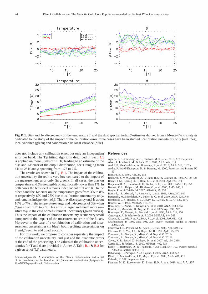
24 Planck Collaboration: The Galactic Cold Core Populationrevealed by the firstPlanckall-sky survey
Fig. B.1. Bias and 1σ discrepancy of the temperatureT and the dust spectral indexβ estimates derived from a Monte-Carlo analysisdedicated to the study of the impact of the calibration error. three cases have been studied : calibration uncertainty only (red lines),local variance (green) and calibration plus local variance(blue).
does not include any calibration error, but only an independenterror per band. The T,β fitting algorithm described in Sect.4.1is applied on these 3 sets of SEDs, leading to an estimate of thebias and 1σ error of the output distribution, for T ranging from6 K to 25 K andβ spanning from 1.75 to 2.5.
The results are shown in Fig.B.1. The impact of the calibra-tion uncertainty (in red) is very low compared to the impact ofthe measurement error only (in green). In all cases, the biasontemperature andβ is negligible or significantly lower than 1%. Inboth cases the bias level remains independent of T andβ. On theother hand the 1σ error on the temperature goes from 3% to 8%at respectively 6 K and 25K due to calibration uncertainty only,and remains independent ofβ. The 1-σ discrepancy onβ is about10% to 7% in the temperature range and it decreases of 3% whenβ goes from 1.75 to 2.5. This error is larger and much more sen-sitive toβ in the case of measurement uncertainty (green curves).Thus the impact of the calibration uncertainty seems very smallcompared to the impact of the measurement error of the fluxes.Moreover in the case of a combination of calibration and mea-surement uncertainties (in blue), both resulting uncertainties onT andβ seem to add quadratically.
For this work, we propose to consider separately the impactof the calibration uncertainty, and just add the quadratic errorsat the end of the processing. The values of the calibration uncer-tainties for T andβ are provided in Annex A TableB.1& B.2 fora given set of T,β parameters.
Acknowledgements.A description of the Planck Collaboration and a listof its members can be found at http://www.rssd.esa.int/index.php?project=PLANCK&page=PlanckCollaboration
ReferencesAguirre, J. E., Ginsburg, A. G., Dunham, M. K., et al. 2010, ArXiv e-printsAlves, J., Lombardi, M., & Lada, C. J. 2007, A&A, 462, L17Andre, P., Men’shchikov, A., Bontemps, S., et al. 2010, A&A, 518, L102+Andre, P., Ward-Thompson, D., & Barsony, M. 2000, Protostars and Planets IV,
59Barnard, E. E. 1907, ApJ, 25, 218Beckwith, S. V. W., Sargent, A. I., Chini, R. S., & Guesten, R.1990, AJ, 99, 924Beerer, I. M., Koenig, X. P., Hora, J. L., et al. 2010, ApJ, 720, 679Benjamin, R. A., Churchwell, E., Babler, B. L., et al. 2003, PASP, 115, 953Bennett, C. L., Halpern, M., Hinshaw, G., et al. 2003, ApJS, 148, 1Bergin, E. A. & Tafalla, M. 2007, ARA&A, 45, 339Bernard, J. P., Abergel, A., Ristorcelli, I., et al. 1999, A&A, 347, 640Bersanelli, M., Mandolesi, N., Butler, R. C., et al. 2010, A&A, 520, A4+Bochanski, J. J., Hawley, S. L., Covey, K. R., et al. 2010, AJ,139, 2679Bonnor, W. B. 1956, MNRAS, 116, 351Bontemps, S., Andre, P., Konyves, V., et al. 2010, A&A, 518, L85+Boudet, N., Mutschke, H., Nayral, C., et al. 2005, ApJ, 633, 272Boulanger, F., Abergel, A., Bernard, J., et al. 1996, A&A, 312, 256Cartwright, A. & Whitworth, A. P. 2004, MNRAS, 348, 589Chapin, E. L., Ade, P. A. R., Bock, J. J., et al. 2008, ApJ, 681,428Charbonneau, P. 1995, apjs, 101, 309, owner: marshall Addedto JabRef:
2008.07.29Churchwell, E., Povich, M. S., Allen, D., et al. 2006, ApJ, 649, 759Clemens, D. P., Yun, J. L., & Heyer, M. H. 1991, ApJS, 75, 877Coupeaud, A., Demyk, K., Meny, C., & Nayral, C. 2011aCoupeaud, A., Demyk, K., Meny, C., & Nayral, C. 2011bCovey, K. R., Ivezic,Z., Schlegel, D., et al. 2007, AJ, 134, 2398Curtis, E. I. & Richer, J. S. 2010, MNRAS, 402, 603Dame, T., Hartmann, D., & Thaddeus, P. 2001, apj, 547, 792, owner: marshall
Added to JabRef: 2008.11.12Deharveng, L., Zavagno, A., & Caplan, J. 2005, A&A, 433, 565Desert, F., Macıas-Perez, J. F., Mayet, F., et al. 2008, A&A, 481, 411Dobashi, K. 2011 in preparationDunham, M. K., Rosolowsky, E., Evans, II, N. J., et al. 2010, ApJ, 717, 1157

Planck Collaboration: The Galactic Cold Core Population revealed by the firstPlanckall-sky survey 25
β = 1.75 β = 2.00 β = 2.25 β = 2.50T [K] Bias [%] 1− σ [%] Bias [%] 1− σ [%] Bias [%] 1− σ [%] Bias [%] 1− σ [%]6 -0.15 2.68 -0.01 2.59 0.03 2.70 0.36 2.687 0.23 3.19 0.34 2.94 -0.01 3.04 -0.08 2.958 0.21 3.25 0.24 3.16 -0.00 3.25 0.31 3.299 0.32 3.72 0.04 3.41 -0.07 3.44 0.25 3.33
10 -0.15 3.81 0.29 3.92 0.02 4.08 -0.15 3.7811 0.28 4.25 -0.06 4.17 -0.35 4.04 0.22 4.0912 -0.03 4.15 -0.31 4.32 0.09 4.32 0.11 4.2713 -0.08 4.89 0.58 4.69 0.58 4.28 0.06 4.5214 0.34 5.22 -0.18 5.26 0.43 5.20 0.41 4.7615 -0.01 5.20 -0.06 5.46 0.25 5.66 0.24 5.5416 0.23 5.64 0.66 5.54 0.16 5.75 0.45 5.9217 0.13 5.73 -0.12 5.97 0.21 5.83 0.15 5.7418 0.16 6.12 0.58 6.64 0.08 6.24 0.31 6.2419 0.20 6.52 0.53 6.30 -0.12 6.14 -0.45 6.3520 0.31 7.22 0.40 7.04 1.00 7.05 0.22 6.6921 0.56 7.49 0.70 7.20 0.22 7.22 0.03 7.2822 0.24 7.51 0.47 7.89 0.31 7.49 0.63 7.1323 0.36 7.56 1.01 8.41 0.53 8.02 0.58 8.3324 0.18 8.48 0.55 8.30 0.87 8.17 0.47 8.5625 0.22 8.08 0.29 8.21 0.33 8.27 0.51 8.26
Table B.1. Bias and 1− σ error on the temperature due to the calibration uncertaintyon fluxes in the IRIS 100µmandPlanck857,545 and 353 GHz bands, and estimated for each couple of (T,β).
β = 1.75 β = 2.00 β = 2.25 β = 2.50T [K] Bias [%] 1− σ [%] Bias [%] 1− σ [%] Bias [%] 1− σ [%] Bias [%] 1− σ [%]6 0.72 11.45 0.07 9.79 -0.11 9.00 -0.77 8.127 -0.61 11.37 -0.97 9.24 0.15 8.77 0.21 7.618 -0.52 10.52 -0.50 8.73 -0.14 8.19 -0.60 7.539 -0.80 10.77 0.00 8.56 0.31 7.83 -0.48 6.66
10 0.32 9.91 -0.59 8.89 0.11 8.23 0.29 6.6211 -0.32 10.06 0.12 8.59 0.61 7.62 -0.18 6.7312 0.18 9.01 0.70 8.20 -0.02 7.42 0.10 6.3913 0.49 9.60 -0.95 8.19 -0.74 6.51 0.02 6.2414 -0.30 9.67 0.49 8.36 -0.53 7.42 -0.50 6.1015 0.47 8.69 0.41 8.07 -0.15 7.55 -0.04 6.5416 0.01 9.09 -0.53 7.46 0.08 7.31 -0.23 6.6117 0.22 8.58 0.43 7.76 -0.04 6.53 -0.16 6.0318 0.16 8.46 -0.21 7.86 0.29 6.90 0.03 6.1319 -0.20 8.70 -0.27 7.45 0.30 6.36 0.75 6.0120 0.12 9.00 -0.04 7.68 -0.78 6.84 0.14 6.0121 -0.25 8.88 -0.21 7.34 -0.04 6.55 0.30 5.9822 0.32 8.66 -0.12 7.73 -0.02 6.51 -0.19 5.6323 0.09 8.12 -0.39 7.62 0.05 6.55 -0.06 6.1424 0.65 8.71 -0.03 7.27 -0.23 6.44 0.11 5.9725 0.28 7.95 0.03 6.80 0.06 6.17 0.14 5.81
Table B.2. Bias and 1− σ error on the spectral indexβ due to the calibration uncertainty on fluxes in the IRIS 100µm andPlanck857, 545 and 353 GHz bands, and estimated for each couple of (T,β).
Dupac, X., Bernard, J., Boudet, N., et al. 2003, A&A, 404, L11Ebert, R. 1955, Zeitschrift fur Astrophysik, 37, 217Egan, M. P., Shipman, R. F., Price, S. D., et al. 1998, ApJ, 494, L199+Elmegreen, B. G. 1998, in Astronomical Society of the PacificConference
Series, Vol. 148, Origins, ed. C. E. Woodward, J. M. Shull, & H. A. ThronsonJr., 150–+
Elmegreen, B. G. & Falgarone, E. 1996, ApJ, 471, 816Enoch, M. L., Glenn, J., Evans, II, N. J., et al. 2007, ApJ, 666, 982Enoch, M. L., Young, K. E., Glenn, J., et al. 2006, ApJ, 638, 293Falgarone, E. & Puget, J. L. 1985, A&A, 142, 157Fischera, J. & Dopita, M. A. 2008, ApJS, 176, 164Fukui, Y., Mizuno, N., Yamaguchi, R., et al. 1999, PASJ, 51, 745Gorski, K. M., Hivon, E., Banday, A. J., et al. 2005, ApJ, 622, 759Gutermuth, R. A., Megeath, S. T., Myers, P. C., et al. 2009, ApJS, 184, 18Hatchell, J., Richer, J. S., Fuller, G. A., et al. 2005, A&A, 440, 151
Heiles, C. 1979, ApJ, 229, 533Heiles, C. 1984, ApJS, 55, 585Heiles, C. & Habing, H. J. 1974, A&AS, 14, 1Henning, T., Michel, B., & Stognienko, R. 1995, Planet. Space Sci., 43, 1333Heyer, M. H., Carpenter, J. M., & Snell, R. L. 2001, ApJ, 551, 852Jackson, J., Finn, S., Rathborne, J., Chambers, E., & Simon,R. 2008, apj, 680,
349, owner: marshall Added to JabRef: 2008.07.31Juvela, M., Ristorcelli, I., Montier, L. A., et al. 2010, A&A, 518, L93+Kauffmann, J., Bertoldi, F., Bourke, T. L., Evans, II, N. J., & Lee,C. W. 2008,
A&A, 487, 993Kiss, C., Moor, A., & Toth, L. V. 2004, A&A, 418, 131Kiss, Z. T., Toth, L. V., Balazs, L. G., & Konyves, V. 2006,Publications of the
Astronomy Deparment of the Eotvos Lorand University, 17, 173Konyves, V., Andre, P., Men’shchikov, A., et al. 2010, A&A, 518, L106+

26 Planck Collaboration: The Galactic Cold Core Populationrevealed by the firstPlanckall-sky survey
Konyves, V., Kiss, C., Moor, A., Kiss, Z. T., & Toth, L. V. 2006, VizieR OnlineData Catalog, 346, 31227
Konyves, V., Kiss, C., Moor, A., Kiss, Z. T., & Toth, L. V. 2007, A&A, 463,1227
Kruegel, E. & Siebenmorgen, R. 1994, A&A, 288, 929Krumholz, M. R. 2006, ApJ, 641, L45Krumholz, M. R. & McKee, C. F. 2008, Nature, 451, 1082Lamarre, J., Puget, J., Ade, P. A. R., et al. 2010, A&A, 520, A9+
Leahy, J. P., Bersanelli, M., D’Arcangelo, O., et al. 2010, A&A, 520, A8+Malinen, J., Juvela, M., Collins, D. C., Lunttila, T., & Padoan, P. 2010, ArXiv
e-printsMandolesi, N., Bersanelli, M., Butler, R. C., et al. 2010, A&A, 520, A3+Marshall, D. J., Joncas, G., & Jones, A. P. 2009, ArXiv e-printsMarshall, D. J., Robin, A. C., Reyle, C., Schultheis, M., & Picaud, S. 2006,
A&A, 453, 635Mathis, J. S., Mezger, P. G., & Panagia, N. 1983, A&A, 128, 212Matsunaga, K., Mizuno, N., Moriguchi, Y., et al. 2001, PASJ,53, 1003Mc Gehee, P. 2011 in preparationMennella et al. 2011, Planck early results 03: First assessment of the Low
Frequency Instrument in-flight performance (Submitted to A&A)Men’shchikov, A., Andre, P., Didelon, P., et al. 2010, A&A,518, L103+Meny, C., Gromov, V., Boudet, N., et al. 2007, A&A, 468, 171Mitra, S., Rocha, G., Gorski, K. M., et al. 2010, ArXiv e-printsMiville-Deschenes, M. & Lagache, G. 2005, ApJS, 157, 302Mizuno, A. & Fukui, Y. 2004, in Astronomical Society of the Pacific Conference
Series, Vol. 317, Milky Way Surveys: The Structure and Evolution of ourGalaxy, ed. D. Clemens, R. Shah, & T. Brainerd, 59–+
Molinari, S., Pezzuto, S., Cesaroni, R., et al. 2008, A&A, 481, 345Molinari, S., Swinyard, B., Bally, J., et al. 2010, A&A, 518,L100+Montier, L. A., Pelkonen, V., Juvela, M., Ristorcelli, I., &Marshall, D. J. 2010,
A&A, 522, A83+Motte, F., Andre, P., & Neri, R. 1998, A&A, 336, 150Murray, N. & Rahman, M. 2010, ApJ, 709, 424Netterfield, C. B., Ade, P. A. R., Bock, J. J., et al. 2009, ApJ,707, 1824Olmi, L., Ade, P. A. R., Angles-Alcazar, D., et al. 2009, ApJ, 707, 1836Ossenkopf, V. & Henning, T. 1994, A&A, 291, 943Pagani, L., Bacmann, A., Motte, F., et al. 2004, A&A, 417, 605Paradis, D., Veneziani, M., Noriega-Crespo, A., et al. 2010, A&A, 520, L8+Perault, M., Omont, A., Simon, G., et al. 1996, A&A, 315, L165Peretto, N. & Fuller, G. A. 2009, A&A, 505, 405Planck Collaboration. 2011a, Planck early results 01: The Planck mission
(Submitted to A&A)Planck Collaboration. 2011b, Planck early results 02: The thermal performance
of Planck (Submitted to A&A)Planck Collaboration. 2011c, Planck early results 07: The Early Release
Compact Source Catalogue (Submitted to A&A)Planck Collaboration. 2011d, Planck early results 08: The all-sky early Sunyaev-
Zeldovich cluster sample (Submitted to A&A)Planck Collaboration. 2011e, Planck early results 09: XMM-Newton follow-up
for validation of Planck cluster candidates (Submitted to A&A)Planck Collaboration. 2011f, Planck early results 10: Statistical analysis of
Sunyaev-Zeldovich scaling relations for X-ray galaxy clusters (Submitted toA&A)
Planck Collaboration. 2011g, Planck early results 11: Calibration of the localgalaxy cluster Sunyaev-Zeldovich scaling relations (Submitted to A&A)
Planck Collaboration. 2011h, Planck early results 12: Cluster Sunyaev-Zeldovich optical Scaling relations (Submitted to A&A)
Planck Collaboration. 2011i, Planck early results 13: Statistical properties ofextragalactic radio sources in the Planck Early Release Compact SourceCatalogue (Submitted to A&A)
Planck Collaboration. 2011j, Planck early results 14: Early Release CompactSource Catalogue validation and extreme radio sources (Submitted to A&A)
Planck Collaboration. 2011k, Planck early results 15: Spectral energy distri-butions and radio continuum spectra of northern extragalactic radio sources(Submitted to A&A)
Planck Collaboration. 2011l, Planck early results 16: The Planck view of nearbygalaxies (Submitted to A&A)
Planck Collaboration. 2011m, Planck early results 17: Origin of the submillime-tre excess dust emission in the Magellanic Clouds (Submitted to A&A)
Planck Collaboration. 2011n, Planck early results 18: The power spectrum ofcosmic infrared background anisotropies (Submitted to A&A)
Planck Collaboration. 2011o, Planck early results 19: All-sky temperature anddust optical depth from Planck and IRAS — constraints on the “dark gas” inour Galaxy (Submitted to A&A)
Planck Collaboration. 2011p, Planck early results 20: New light on anomalousmicrowave emission from spinning dust grains (Submitted toA&A)
Planck Collaboration. 2011q, Planck early results 21: Properties of the interstel-lar medium in the Galactic plane (Submitted to A&A)
Planck Collaboration. 2011r, Planck early results 22: The submillimetre proper-ties of a sample of Galactic cold clumps (Submitted to A&A)
Planck Collaboration. 2011s, Planck early results 23: The Galactic cold corepopulation revealed by the first all-sky survey (Submitted to A&A)
Planck Collaboration. 2011t, Planck early results 24: Dustin the diffuse inter-stellar medium and the Galactic halo (Submitted to A&A)
Planck Collaboration. 2011u, Planck early results 25: Thermal dust in nearbymolecular clouds (Submitted to A&A)
Planck Collaboration. 2011v, The Explanatory Supplement to the Planck EarlyRelease Compact Source Catalogue (ESA)
Planck HFI Core Team. 2011a, Planck early results 04: First assessment of theHigh Frequency Instrument in-flight performance (Submitted to A&A)
Planck HFI Core Team. 2011b, Planck early results 06: The High FrequencyInstrument data processing (Submitted to A&A)
Preibisch, T., Ossenkopf, V., Yorke, H. W., & Henning, T. 1993, A&A, 279, 577Rahman, M. & Murray, N. 2010, ApJ, 719, 1104Rathborne, J. M., Jackson, J. M., Chambers, E. T., et al. 2010, ApJ, 715, 310Rathborne, J. M., Jackson, J. M., & Simon, R. 2006, ApJ, 641, 389Rathborne, J. M., Lada, C. J., Muench, A. A., Alves, J. F., & Lombardi, M. 2008,
ApJS, 174, 396Robin, A., Reyle, C., Derriere, S., & Picaud, S. 2003, aap,409, 523, owner:
marshall Added to JabRef: 2008.07.29Rosset, C., Tristram, M., Ponthieu, N., et al. 2010, A&A, 520, A13+Roy, A., Ade, P. A. R., Bock, J. J., et al. 2010, ArXiv e-printsSchlafly, E. F., Finkbeiner, D. P., Schlegel, D. J., et al. 2010, ApJ, 725, 1175Schlegel, D. J., Finkbeiner, D. P., & Davis, M. 1998, ApJ, 500, 525Schmeja, S. & Klessen, R. S. 2006, A&A, 449, 151Schwartz, P. R. 1982, ApJ, 252, 589Shetty, R., Kauffmann, J., Schnee, S., & Goodman, A. A. 2009a, ApJ, 696, 676Shetty, R., Kauffmann, J., Schnee, S., Goodman, A. A., & Ercolano, B. 2009b,
ApJ, 696, 2234Simon, R., Jackson, J. M., Clemens, D. P., Bania, T. M., & Heyer, M. H. 2001,
ApJ, 551, 747Simon, R., Jackson, J. M., Rathborne, J. M., & Chambers, E. T.2006a, ApJ, 639,
227Simon, R., Rathborne, J. M., Shah, R. Y., Jackson, J. M., & Chambers, E. T.
2006b, ApJ, 653, 1325Skrutskie, M., Cutri, R., Stiening, R., et al. 2006, aj, 131,1163, owner: marshall
Added to JabRef: 2008.07.29Stepnik, B., Abergel, A., Bernard, J., et al. 2003, A&A, 398,551Tauber, J. A., Mandolesi, N., Puget, J., et al. 2010, A&A, 520, A1+Toth, L. V. & Kiss, Z. T. 2007, in IAU Symposium, Vol. 237, IAUSymposium,
ed. B. G. Elmegreen & J. Palous, 124–127Veneziani, M., Ade, P. A. R., Bock, J. J., et al. 2010, ApJ, 713, 959Ward-Thompson, D., Kirk, J. M., Andre, P., et al. 2010, A&A,518, L92+Weaver, H. & Williams, D. R. W. 1973, A&AS, 8, 1Wheelock, S. L., Gautier, T. N., Chillemi, J., et al. 1994, NASA STI/Recon
Technical Report N, 95, 22539Williams, J. P., Blitz, L., & McKee, C. F. 2000, in Protostarsand Planets IV, ed.
V. Mannings, A. P. Boss, & S.S. Russell, University of Arizona Press, 97Young, C. H., Shirley, Y. L., Evans, II, N. J., & Rawlings, J. M. C. 2003, ApJS,
145, 111Young, K. E., Enoch, M. L., Evans, II, N. J., et al. 2006, ApJ, 644, 326Zacchei et al. 2011, Planck early results 05: The Low Frequency Instrument data
processing (Submitted to A&A)Zavagno, A., Anderson, L. D., Russeil, D., et al. 2010a, A&A,518, L101+Zavagno, A., Russeil, D., Motte, F., et al. 2010b, A&A, 518, L81+
1 Aalto University Metsahovi Radio Observatory, Metsahovintie114, FIN-02540 Kylmala, Finland
2 Agenzia Spaziale Italiana Science Data Center, c/o ESRIN, viaGalileo Galilei, Frascati, Italy
3 Astroparticule et Cosmologie, CNRS (UMR7164), Universit´eDenis Diderot Paris 7, Batiment Condorcet, 10 rue A. Domon etLeonie Duquet, Paris, France
4 Atacama Large Millimeter/submillimeter Array, ALMA SantiagoCentral Offices Alonso de Cordova 3107, Vitacura, Casilla 7630355, Santiago, Chile
5 CITA, University of Toronto, 60 St. George St., Toronto, ONM5S 3H8, Canada

Planck Collaboration: The Galactic Cold Core Population revealed by the firstPlanckall-sky survey 27
6 CNRS, IRAP, 9 Av. colonel Roche, BP 44346, F-31028 Toulousecedex 4, France
7 California Institute of Technology, Pasadena, California, U.S.A.
8 DAMTP, Centre for Mathematical Sciences, Wilberforce Road,Cambridge CB3 0WA, U.K.
9 DSM/Irfu/SPP, CEA-Saclay, F-91191 Gif-sur-Yvette Cedex,France
10 DTU Space, National Space Institute, Juliane Mariesvej 30,Copenhagen, Denmark
11 Departement de physique, de genie physique et d’optique,Universite Laval, Quebec, Canada
12 Departamento de Fısica, Universidad de Oviedo, Avda. CalvoSotelo s/n, Oviedo, Spain
13 Department of Astronomy and Astrophysics, University ofToronto, 50 Saint George Street, Toronto, Ontario, Canada
14 Department of Astronomy and Earth Sciences, Tokyo GakugeiUniversity, Koganei, Tokyo 184-8501, Japan
15 Department of Physics & Astronomy, University of BritishColumbia, 6224 Agricultural Road, Vancouver, British Columbia,Canada
16 Department of Physics, Gustaf Hallstromin katu 2a, University ofHelsinki, Helsinki, Finland
17 Department of Physics, Princeton University, Princeton, NewJersey, U.S.A.
18 Department of Physics, Purdue University, 525 NorthwesternAvenue, West Lafayette, Indiana, U.S.A.
19 Department of Physics, University of California, Berkeley,California, U.S.A.
20 Department of Physics, University of California, One ShieldsAvenue, Davis, California, U.S.A.
21 Department of Physics, University of California, Santa Barbara,California, U.S.A.
22 Department of Physics, University of Illinois at Urbana-Champaign, 1110 West Green Street, Urbana, Illinois, U.S.A.
23 Dipartimento di Fisica G. Galilei, Universita degli StudidiPadova, via Marzolo 8, 35131 Padova, Italy
24 Dipartimento di Fisica, Universita La Sapienza, P. le A. Moro 2,Roma, Italy
25 Dipartimento di Fisica, Universita degli Studi di Milano,ViaCeloria, 16, Milano, Italy
26 Dipartimento di Fisica, Universita degli Studi di Trieste, via A.Valerio 2, Trieste, Italy
27 Dipartimento di Fisica, Universita di Roma Tor Vergata, Via dellaRicerca Scientifica, 1, Roma, Italy
28 Discovery Center, Niels Bohr Institute, Blegdamsvej 17,Copenhagen, Denmark
29 Dpto. Astrofısica, Universidad de La Laguna (ULL), E-38206 LaLaguna, Tenerife, Spain
30 Eotvos Lorand University, Department of Astronomy, PazmanyPeter setany 1/A, 1117 Budapest, Hungary
31 European Southern Observatory, ESO Vitacura, Alonso deCordova 3107, Vitacura, Casilla 19001, Santiago, Chile
32 European Space Agency, ESAC, Planck Science Office, Caminobajo del Castillo, s/n, Urbanizacion Villafranca del Castillo,Villanueva de la Canada, Madrid, Spain
33 European Space Agency, ESTEC, Keplerlaan 1, 2201 AZNoordwijk, The Netherlands
34 Helsinki Institute of Physics, Gustaf Hallstromin katu 2,University of Helsinki, Helsinki, Finland
35 INAF - Osservatorio Astrofisico di Catania, Via S. Sofia 78,Catania, Italy
36 INAF - Osservatorio Astronomico di Padova, Vicolodell’Osservatorio 5, Padova, Italy
37 INAF - Osservatorio Astronomico di Roma, via di Frascati 33,Monte Porzio Catone, Italy
38 INAF - Osservatorio Astronomico di Trieste, Via G.B. Tiepolo11, Trieste, Italy
39 INAF/IASF Bologna, Via Gobetti 101, Bologna, Italy
40 INAF/IASF Milano, Via E. Bassini 15, Milano, Italy
41 INRIA, Laboratoire de Recherche en Informatique, UniversiteParis-Sud 11, Batiment 490, 91405 Orsay Cedex, France
42 IPAG: Institut de Planetologie et d’Astrophysique de Grenoble,Universite Joseph Fourier, Grenoble 1/ CNRS-INSU, UMR 5274,Grenoble, F-38041, France
43 Imperial College London, Astrophysics group, BlackettLaboratory, Prince Consort Road, London, SW7 2AZ, U.K.
44 Infrared Processing and Analysis Center, California Institute ofTechnology, Pasadena, CA 91125, U.S.A.
45 Institut d’Astrophysique Spatiale, CNRS (UMR8617) UniversiteParis-Sud 11, Batiment 121, Orsay, France
46 Institut d’Astrophysique de Paris, CNRS UMR7095, UniversitePierre & Marie Curie, 98 bis boulevard Arago, Paris, France
47 Institute of Astronomy and Astrophysics, Academia Sinica,Taipei, Taiwan
48 Institute of Theoretical Astrophysics, University of Oslo,Blindern, Oslo, Norway
49 Instituto de Astrofısica de Canarias, C/Vıa Lactea s/n, La Laguna,Tenerife, Spain
50 Instituto de Fısica de Cantabria (CSIC-Universidad de Cantabria),Avda. de los Castros s/n, Santander, Spain
51 Jet Propulsion Laboratory, California Institute of Technology,4800 Oak Grove Drive, Pasadena, California, U.S.A.

28 Planck Collaboration: The Galactic Cold Core Populationrevealed by the firstPlanckall-sky survey
52 Jodrell Bank Centre for Astrophysics, Alan Turing Building,School of Physics and Astronomy, The University of Manchester,Oxford Road, Manchester, M13 9PL, U.K.
53 Kavli Institute for Cosmology Cambridge, Madingley Road,Cambridge, CB3 0HA, U.K.
54 LERMA, CNRS, Observatoire de Paris, 61 Avenue del’Observatoire, Paris, France
55 Laboratoire AIM, IRFU/Service d’Astrophysique - CEA/DSM -CNRS - Universite Paris Diderot, Bat. 709, CEA-Saclay, F-91191Gif-sur-Yvette Cedex, France
56 Laboratoire Traitement et Communication de l’Information,CNRS (UMR 5141) and Telecom ParisTech, 46 rue Barrault F-75634 Paris Cedex 13, France
57 Laboratoire de Physique Subatomique et de Cosmologie, CNRS,Universite Joseph Fourier Grenoble I, 53 rue des Martyrs, Grenoble,France
58 Laboratoire de l’Accelerateur Lineaire, Universite Paris-Sud 11,CNRS/IN2P3, Orsay, France
59 Lawrence Berkeley National Laboratory, Berkeley, California,U.S.A.
60 Max-Planck-Institut fur Astrophysik, Karl-Schwarzschild-Str. 1,85741 Garching, Germany
61 MilliLab, VTT Technical Research Centre of Finland, Tietotie 3,Espoo, Finland
62 National University of Ireland, Department of ExperimentalPhysics, Maynooth, Co. Kildare, Ireland
63 Niels Bohr Institute, Blegdamsvej 17, Copenhagen, Denmark
64 Observational Cosmology, Mail Stop 367-17, California Instituteof Technology, Pasadena, CA, 91125, U.S.A.
65 Optical Science Laboratory, University College London, GowerStreet, London, U.K.
66 SISSA, Astrophysics Sector, via Bonomea 265, 34136, Trieste,Italy
67 SUPA, Institute for Astronomy, University of Edinburgh, RoyalObservatory, Blackford Hill, Edinburgh EH9 3HJ, U.K.
68 School of Physics and Astronomy, Cardiff University, QueensBuildings, The Parade, Cardiff, CF24 3AA, U.K.
69 Space Sciences Laboratory, University of California, Berkeley,California, U.S.A.
70 Spitzer Science Center, 1200 E. California Blvd., Pasadena,California, U.S.A.
71 Stanford University, Dept of Physics, Varian Physics Bldg,382Via Pueblo Mall, Stanford, California, U.S.A.
72 Universite de Toulouse, UPS-OMP, IRAP, F-31028 Toulousecedex 4, France
73 Universities Space Research Association, StratosphericObservatory for Infrared Astronomy, MS 211-3, Moffett Field,CA 94035, U.S.A.
74 University of Cambridge, Cavendish Laboratory, Astrophysicsgroup, J J Thomson Avenue, Cambridge, U.K.
75 University of Cambridge, Institute of Astronomy, MadingleyRoad, Cambridge, U.K.
76 University of Granada, Departamento de Fısica Teorica y delCosmos, Facultad de Ciencias, Granada, Spain
77 University of Miami, Knight Physics Building, 1320 CampoSano Dr., Coral Gables, Florida, U.S.A.
78 Warsaw University Observatory, Aleje Ujazdowskie 4, 00-478Warszawa, Poland