arX

iv:a

stro

-ph/

0608

531v

2 2

4 A

pr 2

007

Mon. Not. R. Astron. Soc.000, 000–000 (0000) Printed 5 February 2008 (MN LATEX style file v2.2)

The star formation histories of galaxies in the Sloan Digital SkySurvey

Benjamin Panter1,2, Raul Jimenez3, Alan F. Heavens2 and Stephane Charlot1,4

1Max-Planck-Institut fur Astrophysik, Karl-Schwarzschild Str. 1, D-85748, Garching bei Munchen, Germany2SUPA ⋆, Institute for Astronomy, University of Edinburgh, Royal Observatory, Blackford Hill, Edinburgh EH9 3HJ, UK3Dept. of Physics and Astronomy, University of Pennsylvania, Philadelphia, PA 19104, USA4Institut d’Astrophysique de Paris, UMR 7095, 98 bis Boulevard Arago, F-75014 Paris, France

5 February 2008

ABSTRACTWe present the results of a MOPED analysis of∼ 3 × 10

5 galaxy spectra from the SloanDigital Sky Survey Data Release Three (SDSS DR3), with a number of improvements indata, modelling and analysis compared with our previous analysis of DR1. The improvementsinclude: modelling the galaxies with theoretical models ata higher spectral resolution of 3A;better calibrated data; an extended list of excluded emission lines, and a wider range of dustmodels. We present new estimates of the cosmic star formation rate, the evolution of stellarmass density and the stellar mass function from the fossil record. In contrast to our earlierwork the results show no conclusive peak in the star formation rate out to a redshift around 2but continue to show conclusive evidence for ‘downsizing’ in the SDSS fossil record. The starformation history is now in good agreement with more traditional instantaneous measures.The galaxy stellar mass function is determined over five decades of mass, and an updatedestimate of the current stellar mass density is presented. We also investigate the systematiceffects of changes in the stellar population modelling, thespectral resolution, dust modelling,sky lines, spectral resolution and the change of data set. Wefind that the main changes in theresults are due to the improvements in the calibration of theSDSS data, changes in the initialmass function and the theoretical models used.

Key words: galaxies: fundamental parameters, galaxies: statistics,galaxies: stellar content

1 INTRODUCTION

The quality of spectra of the observed light of unresolved stellarpopulations has reached enough accuracy that it is possibleto makedetailed studies of the physical properties of the stellar popula-tions in these galaxies. An excellent example of this new generationof data-sets is given by the Sloan Digital Sky Survey (Gunn etal.1998; York et al. 2000; Strauss et al. 2002) at low redshift, not onlyby the size of the spectroscopic sample (about106 spectra) but bythe quality and wavelength coverage of the spectra. At higher red-shift the DEEP2 survey (Davis et al. 2003) is providing a similardatabase, albeit with a smaller wavelength coverage. Future spec-troscopic surveys (e.g. WFMOS) will yield larger samples atevendeeper redshifts. Given the quality of the spectra, it is interestingto ask the question of whether reliable information about the stellarpopulation of these galaxies can be inferred from the spectra.

Indeed, several attempts have been made previously tostudy in detail the physical properties of the SDSS galaxiesei-ther by using selected features in the spectra (Kauffmann etal.2004; Brinchmann et al. 2004; Tremonti et al. 2004) or using the

⋆ Scottish Universities Physics Alliance

full spectrum (Panter, Heavens & Jimenez 2003; Heavens et al.2004; Panter, Heavens, & Jimenez 2004; Cid Fernandes 2005;Mathis et al. 2006; Ocvirk et al. 2006). These studies have led tointeresting conclusions about the physical properties of these galax-ies. In particular analysis of the SDSS sample (Heavens et al. 2004)and other local galaxies (Thomas et al. 2005) show very clearevi-dence for ‘downsizing’ - the process by which star formationat lowredshift takes place predominantly in low-mass galaxies, whereasmore massive galaxies have the bulk of their star-formationactivityat high redshift. also observed using other methods. In addition onecan also determine the global star formation history in the Universefrom this fossil record. Our previous study found broad agreementwith observations of contemporary star formation at large lookbacktimes, but suggested that there was a peak in star formation activityat z < 1. Agreement between the fossil record and contemporarystar formation indicators is expected if the Cosmological Principleholds; this expected agreement offers an opportunity in principle totest the assumptions in the modelling of both the fossil record andthe instantaneous star formation rates. Of most importanceis thatboth are dependent on the stellar initial mass function, butin differ-ent ways, with the instantaneous rates being determined very muchby the upper end of the IMF, while the fossil record is determined

2 Panter et al.

by a wider range of stars. This offers an opportunity in principle totest the evolution of the IMF as a function of cosmic time.

In our previous work, we have presented results from around105 galaxies from the SDSS DR1. This paper enhances the pre-vious results through the introduction of a number of improve-ments to data and analysis methods, and through an investigationof systematic effects and sensitivity to assumptions. On the dataside, we have analysed∼ 3 × 105 galaxies from the SDSS DR3sample. The extra size of this sample is not particularly important,but the calibration of the data has been improved since DR1. Onthe methods side, we no longer rebin the data to 20A resolution,but compare the data with a wider range of theoretical models, in-cluding the Bruzual & Charlot models (Bruzual & Charlot 2003)at 3A resolution. We consider two stellar initial mass functions (aSalpeter and a Chabrier IMF), and a wider range of dust models.We also make some improvements to the treatment of emissionlines, by removing additional weaker lines, since interstellar emis-sion lines are not included in the stellar modelling. Finally, we havealso explored the effect of removal of sky lines, using a PCA-basedmethod (Wild & Hewett 2005). These studies give us a reasonableestimate of the sensitivity of the results to the assumptions. As isexpected from a sample of this size, changes in the assumptionsgive rise to much larger variations in the results than the statisti-cal errors. The uncertainties in star formation rates from the stellarmodels used are typically about a factor of two, which makes itdifficult to distinguish between different IMFs, although it may bepossible to constrain extreme IMF variations.

The layout of the paper is as follows. In Section 2 we outlinethe enhancements to the method, and the improvements to the data,and describe the assumptions which are made for analysis of theDR3 sample. In Section 3 we present the new results on star for-mation history, downsizing and galaxy stellar mass function fromthe DR3 dataset. We also introduce a method to assess the partic-ular areas where current models are lacking. In Section 4 we showthe sensitivity of our results to changes in the assumptions, throughanalysis of a subset of the data, and in Section 5 we draw conclu-sions.

Throughout this work we assume a concordance cos-mology with Ωv = 0.73, Ωm = 0.27, H0 = 71kms−1Mpc−1(Spergel et al. 2003).

2 SDSS DR3 ANALYSIS

In this Section we describe briefly the SDSS DR3 dataset, andoutline the assumptions in the method, highlighting changes madesince the analysis of SDSS DR1 (Heavens et al. 2004).

2.1 SDSS DR3 data

The spectrophotometric pipeline used by the SDSS has evolvedfrom the Early Data Release (EDR) to the DR3 sample used here.According to the papers describing each release (Stoughtonet al.2002; Abazajian et al. 2003, 2004, 2005), the pipeline was changedbetween the EDR, DR1 and DR2 subsets, but remained static be-tween DR2 and DR3. Some DR1 spectra had a slight systematicoffset for wavelengths smaller than4000A. Abazajian et al. (2005)claim that this has been corrected in the DR3. There are no pub-lished plans for further improvements. The DR1 data has beenre-reduced with the new pipeline and this work considers the setofgalaxies contained in the SDSS Main Galaxy Sample (MGS) of

Table 1.Regions masked from MOPED fitting.

Wavelength Range (A) Reason

3711-3741 [OII]4087-4117 [SII], Hδ4325-4355 Hγ4846-4876 Hβ4992-5022 [OIII]4944-4974 [OIII]5870-5900 Na6535-6565 [NII]6548-6578 Hα6569-6599 [NII]6702-6732 [SII]6716-6746 [SII]

DR1-3 reduced with the DR2 version of the spectrophotometricpipeline.

We apply further cuts to this main galaxy sample based onthose of Shen et al. (2003). Our sample is determined by r bandap-parent magnitude limits of15.0 6 mr 6 17.77. The magnitudelimits are set by the SDSS target selection criteria, as discussed inAbazajian et al. (2005). The target criteria for surface brightnesswasµr < 24.5, although forµr > 23.0 galaxies are included onlyin certain atmospheric conditions. In order to remove any bias andsimplify our Vmax criteria we have cut our sample atµr < 23.0.At low redshifts a small number of Sloan galaxies are subjecttoshredding - where a nearby large galaxy is split by the targetselec-tion algorithm into several smaller sources. To eliminate this effect,for our star formation analysis we use a range of0.01 < z < 0.25.This also removes the problems of non Hubble-flow peculiar veloc-ities giving erroneous distances based on redshift, which can havea significant effect on recovered stellar mass. For samples involv-ing a very large redshift range there is a concern that afterVmax

weighting an individual galaxy at low redshift can dominatehigherredshift galaxy signals. For our criteria we have tested this, and noVmax weighted galaxy contributes more than a tenth of a percentto the final mass total in each bin. The total number of galaxies inthe DR3 Main Galaxy Catalogue is312415, while the number thatsatisfy our cuts is299571. In order to estimate the completeness ofthe survey we have used the ratio of target galaxies to those whichhave observed redshifts (P. Nordberg, Priv. Comm.). This does notallow for galaxies which are too close for the targetting algorithm,and we estimate this fraction at a6% level from the discussion inStrauss et al. (2002). As a result of both these cuts, our effectivesky coverage is2947 square degrees.

We also remove from our analysis a larger set of wavelengthswhich may be affected by emission lines than in our DR1 analy-sis. These lines are not modelled by the stellar population codes,which only consider the continuum and absorption features.Theexcluded restframe wavelength ranges due to emission or emissionline filling of features are listed in table 1. We also discount signalwith wavelength above 7800A in order to reduce the risk of skylinecontamination. Typically the rest frame wavelength range used foranalysis is 3450A - 7800A.

3

2.2 Modelling assumptions

2.2.1 Stellar population modelling

Both our EDR (Panter, Heavens & Jimenez 2003) and DR1(Heavens et al. 2004; Panter, Heavens, & Jimenez 2004) studiesused the 20A resolution models described in Jimenez et al. (2004).The field of stellar population modelling has moved on in the mean-time, and models at 3A resolution and better are available fromvarious authors. We have used those of Bruzual & Charlot (2003)as the basis for this study.

Although with 20A models the effect of velocity dispersioncan be ignored, there is possibility of significant changes in theinput spectrum when working at 3A. After extensive testing wefound that in fact there is very little effect, if any, on the recoveredstellar populations and metallicities for a wide range of galaxies.We chose to apply a uniform velocity dispersion of 170 kms−1

to the 3A models, reflecting a typical value for the Main GalaxySample.

2.2.2 Initial Mass Functions

Both the instantaneous and fossil approach to star formation de-termination require assumptions about the Initial Mass Function(IMF). The two methods probe different mass regions and deducethe complete stellar populations by assuming an IMF. For instanta-neous measures such as H-α or OII emission the presence of lowermass stars is estimated by working down the mass function from themassive stars which cause the majority of the emission. For high-redshift star formation estimated using the fossil record technique,the contribution to the spectrum from older, less massive stars isused to determine early star formation, requiring extrapolation upthe mass function.

In recent years, the choice of IMF has been the subject ofmuch debate - in particular whether a universal IMF can be as-sumed, both in space and time. Several candidates have been pro-posed for such a IMF, however single stellar population (SSP) mod-els only include a few. Although disfavoured by observations, theSalpeter IMF (Salpeter 1955) has been used as a reference duetoits simplicity; it is a power law. The most recent modification isthe Chabrier IMF (Chabrier 2003) which seems to be very success-ful at reproducing current observations in our galaxy. For the mainanalysis, we use the Chabrier IMF.

2.2.3 Dust

Our previous MOPED studies used a single foreground dust screen.In this parameterisation the strength of the extinction maybe char-acterised byE(B − V ), and the wavelength dependence of theextinction is determined by the choice of extinction model,whichmay be empirical or modelled. We used an LMC extinction law forthe main analysis, but later we will explore the difference in recov-ered SFH using the Calzetti (1997) starburst model and the LMCand SMC curves given in Gordon et al. (2003).

We have also computed results using the two-dust parametermodel of Charlot & Fall (2000). This is a more physically moti-vated model of the absorption of starlight by dust, which accountsfor the different attenuation affecting young (< 10 Myr) and oldstars in galaxies, as characterized by the typical absorption opticaldepths of dust in giant molecular clouds and in the diffuse ISM.Unfortunately, our investigations have shown that the absorption ingiant molecular clouds cannot be well constrained from the optical

continuum emission alone. This dust component would be moretightly constrained by the ultraviolet and infrared continuum emis-sion and by emission-line fluxes. We therefore do not show resultsbased on this model here.

2.3 Star formation and metallicity history parametrization

In the past, the SFH of galaxies was typically modelled by an ex-ponential decay with a single parameter - for more complex mod-els one or two bursts of formation were allowed. In fact, it wouldbe better not to put any such constraints on star formation, particu-larly considering that each galaxy may have (as a result of mergers)several distinctly different aged populations. Star formation takesplace in giant molecular clouds, which have a lifetime of around107 years. Splitting the history of the Universe into the lifetimesof these clouds give a natural unit of time for star formationanal-ysis, but unfortunately it would require several thousand of theseunits to map the age of galaxies formed 13 billion years ago, andthe (lack of) sensitivity of the final spectrum to the detailed his-tory would make any estimate of star formation history extremelydegenerate. We choose a compromise solution, where we allow11time bins in which the star formation rate (SFR) can vary indepen-dently. This allows a reasonable time resolution, whilst not beingprohibitively slow to compute. For most galaxies this parametriza-tion is a little too ambitious, so we do not recommend the useof the recovered star formation histories on an individual galaxybasis. Extensive testing (Panter, Heavens & Jimenez 2003) showsthat for large samples the average star formation history isrecov-ered with good accuracy. Future work will concentrate on recov-ering only as much detail as the data from an individual galaxydemands. The boundaries between the 11 different bins used aredetermined by considering bursts of star formation at the beginningand end of each period (at a fixed metallicity) and set the bound-aries such that the fractional difference in the final spectrum is thesame for each bin. This leads to a set of bins which are almostequally spaced in log(lookback time). Nine bins are spaced with aratio of log(lookback time) of 2.07 in this application of MOPED,plus a pair of high-redshift bins to improve resolution atz > 1.This leads to a set of bins whose central ages are 0.0139, 0.0288,0.0596, 0.123, 0.256, 0.529, 1.01, 2.27, 4.70, 8.50 and 12.0Gyr.The gas which forms stars in each time bin is also allowed to havea metallicity which can vary independently. The Bruzual & Charlot(2003) models allow metallicities between0.02 < (Z/Z⊙) < 1.5.In order to investigate metallicity evolution (Panter et al. 2007, inprep) no regularization or other constraint is applied to the metallic-ity of the populations - each different age can have whatevermetal-licity fits best. A further complexity to the parametrization to dealwith post-merger galaxies which contain gas which has followeddramatically different enrichment processes would be to have sev-eral populations with the same age but independent metallicities. Itis possible to consider a more complex parametrization, butagainone risks degeneracies in solution. With 11 ages, 11 metallicitiesand the dust parameter, the model has 23 parameters. The 23 di-mensional likelihood surface is explored by a Markov Chain MonteCarlo technique outlined in Panter, Heavens & Jimenez (2003) Fur-ther information on the MOPED algorithm is contained in Panter(2005).

2.3.1 Speed issues

MOPED (Heavens, Jimenez, & Lahav 2000) works by a massivedata compression step, forming (in this case) 23 linear combina-

4 Panter et al.

tions of the flux data. The resulting MOPED coefficients are fittedby standard minimumχ2 techniques. The data compression stepis carefully designed to give answers which are (in ideal circum-stances) as accurate as performing a full fit to the∼ 3852 flux data.One of the benefits of the MOPED algorithm is that the numberof compressed data is determined by the number of model parame-ters, not the number of data points. This has the huge advantage thatanalysis of the spectra at 3A resolution is no slower than analysis of20A spectra (except for a small increase in overheads such as pre-computing the data compression weighting vectors). The algorithmtakes around two minutes per galaxy on a fast desktop workstation,and represents a speed up of around a factor of170 over a brute-force likelihood fit.

2.4 Computing Ensemble Results

2.4.1 Common star formation time bins

MOPED determines the star formation history of each galaxy,rel-ative to the lookback time. To obtain the cosmic SFR it is neces-sary to shift these results to a common set of time bins, whichforsimplicity are chosen to be the same as those used in the galaxyanalysis. This allows direct comparison of galaxy star formationbetween galaxies at different redshifts in terms of cosmic time, andensemble conclusions to be drawn. The shifting algorithm ensuresconservation of star formation. Star formation in the oldest bin isalways assigned to the final bin with ages no greater than 13.7Gyr,the age of the Universe determined by the concordant WMAP cos-mology.

2.4.2 Inverse Vmax weighting for Fossil studies

In a magnitude-limited survey such as the SDSS the range of galaxytypes and sizes included in the survey will vary over the redshiftrange studied. Some mechanism is required to compensate forthischange and determine the overall bulk parameters for the sample.To convert from star formation rates to star formation rate density,galaxies are weighted by1/Vmax, whereVmax is the maximumvolume of the survey in which the galaxy could be observed in theSDSS sample. This gives an unbiased estimate of the space densityf of any additive propertyF of the galaxy under investigation, suchas mass, luminosity, star formation rate.

f =X

galaxies i

Fi

Vmax,i

(1)

On smaller scales the estimator is affected by source clustering,but the SDSS is deep enough that these variations should not besignificant. Any properties which change with redshift and whichcould determine inclusion in the sample must be calculated for eachgalaxy over the redshift range of the survey to determine whether ornot it would have been included. In order to calculate theVmax as-signed to each galaxy it is necessary to consider the apparent mag-nitude and surface brightness evolution over the redshift range. Inorder to compute this we use the same stellar evolution models usedin the MOPED analysis to calculate luminosity over the lifetime ofthe galaxy due to its recovered star formation history.

The magnitude of a galaxy over its lifetime depends on the lu-minosity behaviour of the various stellar populations thatmake itup - the star formation history. As young stars, the populations willhave a very high light output, which will reduce as they age. Thisinformation is encoded in the galaxy spectrum and recoveredby

MOPED, which gives the relative fractions of different agedpop-ulations. To compute the observed magnitude if the galaxy wereto be observed at higher redshifts, we need to evolve the modelsover time and track the changes in luminosity. Obviously, asthegalaxy is projected to a further redshift the younger fractions donot contribute, as galaxy is being ‘observed’ before these popula-tions were born. Since the spectral energy distribution of the lightchanges with evolution of the galaxy, it is also necessary toapplythe filters used by Sloan to determine the flux included in therband, leading to a change inci,z in the r-band magnitude as theredshift is changed:

ri,z = ri,zobs+ ci,z . (2)

These magnitude corrections can then be used to calculate cor-rections which need to be applied to the surface brightness.Thesurface brightness of the galaxy at each redshiftz is

µi,z = ri,z+ci,z+2.5 log10

ˆ

πr2

50,i(Dz/Dzobs)2

˜

+2.5 log10

2(3)

whereDz is the luminosity distance,r50 is the Petrosian halflight radius andzobs is the observed redshift of the galaxy. Thisequation assumes that the size of the galaxy does not change overthe redshift range. Although this assumption is valid for low red-shift sources, it will need to be developed if the technique is appliedto deeper surveys.

The MOPED technique gives the relative strengths of the dif-ferent spectral models. The mass originally created to makethesemasses is then calculated, and by dividing this by the maximumvolume over which the galaxy could be observed gives the starforming density,ρi. By adding all theV −1

max weighted star form-ing densities of galaxies in the sample, rebinned to a commontimeframe, the overall star forming densityρ can be found for the regionstudied.

Galaxies may only contribute to the SFR of a time bin if theyare at a lower redshift than the lower limit of that bin. This con-servative approach ensures that the star formation of a galaxy isnever extrapolated. It also means that in all but a few cases where agalaxy is almost on the boundary between bins, the youngest pop-ulations, those which are better calculated using instantaneous in-dicators from emission lines, do not contribute to estimates of theSFR. In addition, to ensure that our results are not biased bysingleerroneous SFH reconstructions we only present results frombinswhich contain contributions from greater than1000 galaxies.

3 RESULTS FROM THE DR3

3.1 Evolution of Stellar Mass Density

The simplest interpretation of the combined star formationhistoriesis a simpleV −1

max weighted addition that shows how the present daystellar mass of the Universe has built up. In Fig. 1 and Table 2weshow how the stellar mass density of the universe has changedsincez = 2. In order to compute the remaining mass (when from theMOPED algorithm we estimate the original mass of stars formed)it is necessary to invoke the recycling fraction, R. Rather than as-sume a blanket correction, we have used the detailed predictionsallowed by the Bruzual & Charlot (2003) models for each popu-lation of each galaxy, based on their determined ages and metal-licities. Although this is slightly more laborious than assuming ablanket recycling fraction it gives a more accurate determination ofpresent mass, since R is a function of both age and metallicity.

The abscissa on this plot refers to the minimum redshift of a

5

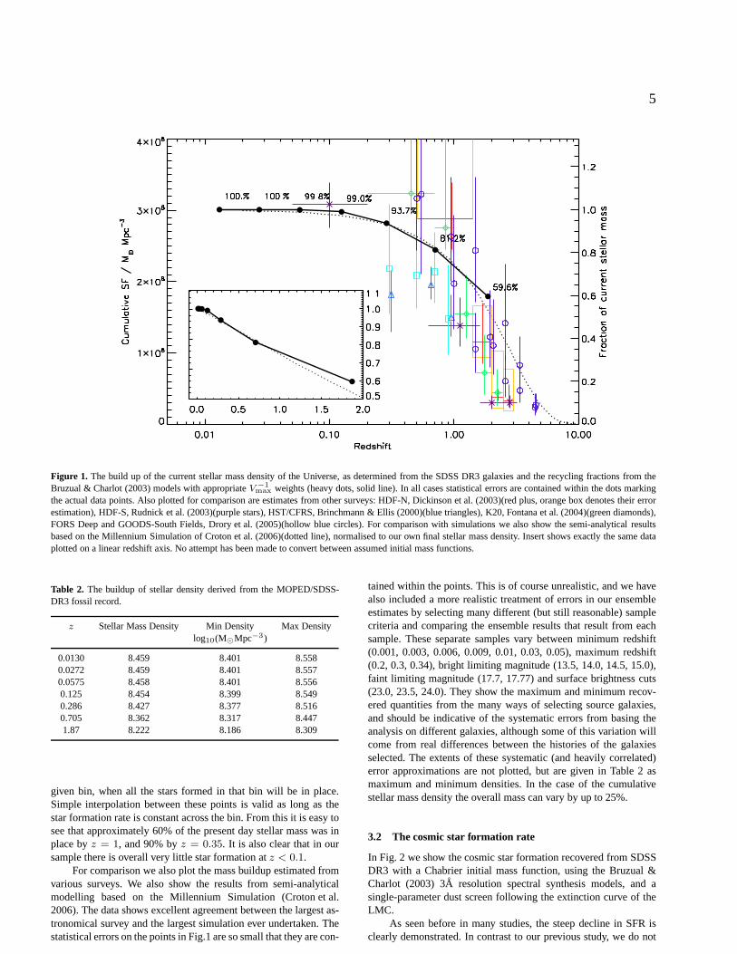
Figure 1. The build up of the current stellar mass density of the Universe, as determined from the SDSS DR3 galaxies and the recycling fractions from theBruzual & Charlot (2003) models with appropriateV −1

max weights (heavy dots, solid line). In all cases statistical errors are contained within the dots markingthe actual data points. Also plotted for comparison are estimates from other surveys: HDF-N, Dickinson et al. (2003)(red plus, orange box denotes their errorestimation), HDF-S, Rudnick et al. (2003)(purple stars), HST/CFRS, Brinchmann & Ellis (2000)(blue triangles), K20, Fontana et al. (2004)(green diamonds),FORS Deep and GOODS-South Fields, Drory et al. (2005)(hollow blue circles). For comparison with simulations we also show the semi-analytical resultsbased on the Millennium Simulation of Croton et al. (2006)(dotted line), normalised to our own final stellar mass density. Insert shows exactly the same dataplotted on a linear redshift axis. No attempt has been made toconvert between assumed initial mass functions.

Table 2. The buildup of stellar density derived from the MOPED/SDSS-DR3 fossil record.

z Stellar Mass Density Min Density Max Densitylog10(M⊙Mpc−3)

0.0130 8.459 8.401 8.5580.0272 8.459 8.401 8.5570.0575 8.458 8.401 8.5560.125 8.454 8.399 8.5490.286 8.427 8.377 8.5160.705 8.362 8.317 8.4471.87 8.222 8.186 8.309

given bin, when all the stars formed in that bin will be in place.Simple interpolation between these points is valid as long as thestar formation rate is constant across the bin. From this it is easy tosee that approximately 60% of the present day stellar mass was inplace byz = 1, and 90% byz = 0.35. It is also clear that in oursample there is overall very little star formation atz < 0.1.

For comparison we also plot the mass buildup estimated fromvarious surveys. We also show the results from semi-analyticalmodelling based on the Millennium Simulation (Croton et al.2006). The data shows excellent agreement between the largest as-tronomical survey and the largest simulation ever undertaken. Thestatistical errors on the points in Fig.1 are so small that they are con-

tained within the points. This is of course unrealistic, andwe havealso included a more realistic treatment of errors in our ensembleestimates by selecting many different (but still reasonable) samplecriteria and comparing the ensemble results that result from eachsample. These separate samples vary between minimum redshift(0.001, 0.003, 0.006, 0.009, 0.01, 0.03, 0.05), maximum redshift(0.2, 0.3, 0.34), bright limiting magnitude (13.5, 14.0, 14.5, 15.0),faint limiting magnitude (17.7, 17.77) and surface brightness cuts(23.0, 23.5, 24.0). They show the maximum and minimum recov-ered quantities from the many ways of selecting source galaxies,and should be indicative of the systematic errors from basing theanalysis on different galaxies, although some of this variation willcome from real differences between the histories of the galaxiesselected. The extents of these systematic (and heavily correlated)error approximations are not plotted, but are given in Table2 asmaximum and minimum densities. In the case of the cumulativestellar mass density the overall mass can vary by up to 25%.

3.2 The cosmic star formation rate

In Fig. 2 we show the cosmic star formation recovered from SDSSDR3 with a Chabrier initial mass function, using the Bruzual&Charlot (2003) 3A resolution spectral synthesis models, and asingle-parameter dust screen following the extinction curve of theLMC.

As seen before in many studies, the steep decline in SFR isclearly demonstrated. In contrast to our previous study, wedo not

6 Panter et al.

Figure 2. The cosmic star formation history of the Universe, as determined from the SDSS DR3 galaxies (heavy black horizontal barscover the bins, the lumi-nosity weighted age of each bin given by black dots). The vertical error bars are indicative of systematic errors arisingfrom choosing different subsets of the datafor analysis. See text for full details. Also plotted for comparison are the estimates from our DR1 work (black diamonds)(Heavens et al. 2004) and those com-piled in Hopkins (2004), using the common obscuration discussed within that paper. The points have also been corrected for the minor difference in cosmologybetween that work and this paper, and shifted downwards by 0.25 dex to convert from the Salpeter to Chabrier IMF as indicated by the arrow in the top left. TheHopkins (2004) points are coded as follows: UV indicators (dark blue): Giavalisco et al. (2004); Wilson et al. (2002); Massarotti et al. (2001); Sullivan et al.(2000); Steidel et al. (1999); Cowie et al. (1999); Treyer etal. (1998); Connolly et al. (1997); Lilly et al. (1996); Madau et al. (1996); OII, H-α and H-β emis-sion (red): Teplitz et al. (2003); Gallego et al. (2002); Hogg et al. (1998); Hammer et al. (1997); Pettini et al. (1998); Perez-Gonzalez et al. (2003); Tresse et al.(2002); Moorwood et al. (2000); Hopkins et al. (2000); Sullivan et al. (2000); Glazebrook et al. (1999); (1999); Tresse &Maddox (1998); Gallego et al.(1995); sub-mm (green)Flores et al (1999); Barger et al. (2000); Hughes et al. (1998); x-ray and radio (light blue):Condon et al. (2002); Sadler et al. (2002);Serjeant et al. (2002); Machalski & Godlowski (2000); Haarsma et al. (2000); Condon (1989); Georgakakis et al. (2003).

find a peak in SFR atz < 1. This was also found by Mathis et al.(2006), in work based on the MOPED fossil analysis approach.Ifthere is a peak, it occurs somewhere in our last bin (z >

∼2). These

new results from the fossil record are in much better agreementwith determinations based on contemporary star formation rates.Purely statistical error bars are so small to be almost invisible in allbut the lowest redshift bin. As with the previous figure, the verticalerror bars in Fig.2 are indicative only. They show the maximum andminimum recovered star formation rates from the many ways ofse-lecting source galaxies. They should be indicative of the systematicerrors from basing the analysis on different galaxies, although someof this variation will come from real differences between the histo-ries of the galaxies selected.

Although for completeness we show our results fromz ∼ 0.1,we do not present points withz ≪ 0.1 for three reasons. First,from Fig. 1 it is clear that there is much less mass in these binson which to form an estimate of the SFR, the change in mass withtime. Second, to avoid biasing, ourVmax criteria exclude galax-ies from contributing to bins with upper boundary lower thantheirredshift - hence the bulk of the galaxies, at approximatelyz = 0.1,can only contribute to bins fromz = 0.2 onwards. Third, the galax-ies contained in these bins, and the resultant SFR, are strongly de-pendent on sample criteria, as expected when sample size drops.

Table 3. The SFR density derived from the MOPED/SDSS-DR3 fossilrecord.

z zmin zmax SFRd Min SFRd Max SFRd(M⊙yr−1Mpc−3)

0.081 0.0575 0.125 0.00537 0.00276 0.01170.177 0.125 0.286 0.0166 0.0131 0.02700.416 0.286 0.705 0.0226 0.0187 0.02941.03 0.705 1.87 0.0332 0.0275 0.03883.24 1.87 6.42 0.0993 0.0850 0.113

Later in this paper we analyse a subset of the data to determinewhich changes are responsible for the modifications to the results;the main reasons for the changes are the better calibration of theSDSS DR3, the change in IMF to Chabrier (2003) and the changeto the higher-resolution Bruzual and Charlot (2003) models. Thestar formation rate density resulting from the MOPED DR3 analy-sis is presented in table 3.

7

3.3 The mass function of stellar mass andΩb∗

The galaxy stellar mass function of SDSS DR3 is shown in Fig. 3,for a range of almost 5 decades in mass (107

− 1012 M⊙). The er-rors shown are statistical based on our chosen sample criteria. Wealso compute the mass function for the alternative sample criteriato develop systematic errors. Over much of this range a Schechterfit is good, with parametersφ∗ = (2.2 ± 0.5stat ± 1sys) × 10−3

Mpc −3, M∗ = (1.005 ± 0.004stat ± 0.200sys) × 1011 M⊙,and slopeα = −1.222 ± 0.002stat ± 0.1sys calculated in the re-gion where there are more than 300 galaxies contributing to eachbin (108.5

− 1011.85M⊙). The mass function is very similar toour DR1 analysis (Panter, Heavens, & Jimenez 2004), but shiftedto lower masses as a result of the use of the Chabrier IMF ratherthan Salpeter. For further discussion of the systematic differencesin recovered galaxy mass caused by IMF variation refer to thedis-cussion in Bell & de Jong (2001).

The stellar mass function can be used to give a further con-straint on the contribution to the density parameter from baryons instars,Ωb* . By integrating the mass over the range of the mass func-tion we deduce a value ofΩb∗ = (1.82±0.03stat±0.1sys)×10−3

(systematic error). This value is in broad agreement with resultsobtained previously when the correction from Salpeter IMF istaken into account (Panter, Heavens, & Jimenez 2004; Cole etal.2001; Bell et al. 2003; Fukugita et al. 1998; Kochanek et al. 2001;Glazebrook et al. 2003; Persic et al. 1992; Salucci et al. 1999). Thestatistical errors reflect the spread of results obtained with varyingsample criteria as before.

3.4 Downsizing

One of the results of Heavens et al. (2004) was the finding of‘downsizing’ from the SDSS fossil record. Using the new modelsat higher resolution we have found that the evidence for downsizingis just as clear. In Fig. 4 we show the cosmic star formation rate forgalaxies split into different stellar mass ranges. A clear signature of‘downsizing’ is seen: the stars ending up in today’s highest-massgalaxies formed early, and show negligible recent star formation,while the lower-mass galaxies continue with star formationuntilthe present day. The lower, non-offset plot can be used to determinefor a given redshift which galaxies dominate the star formation rate.

3.5 Investigating spectral residuals

Due to the power of MOPED and the number of SSPs offered forfitting (11) excellent fits can be obtained if the models are accu-rate. By comparing the residuals of the best fitting spectrumto theraw data on a pixel by pixel basis and then averaging over manygalaxiesin the galaxy restframe it is possible to determine exactlywhich areas are not being accurately fitted for a given spectrum.By stacking the residuals of high signal to noise (SloanSPECOB-JALL .SCI SN, scienceS/N > 20 per flux measurement) galax-ies it is possible to determine to a high degree of accuracy whichwavelength ranges are failing in the models, and to what extent. Ifwe assume that MOPED can, in most cases, obtain the best pos-sible fit to a spectrum then the differences must be features notincluded in the models. These features could be things that themodels are not designed to measure (instrumental effects, inter-stellar or intergalactic medium absorption, skyline contaminationetc.) or alternatively features that are either misrepresented or notyet included in stellar modelling codes (e.g. alpha enhancement

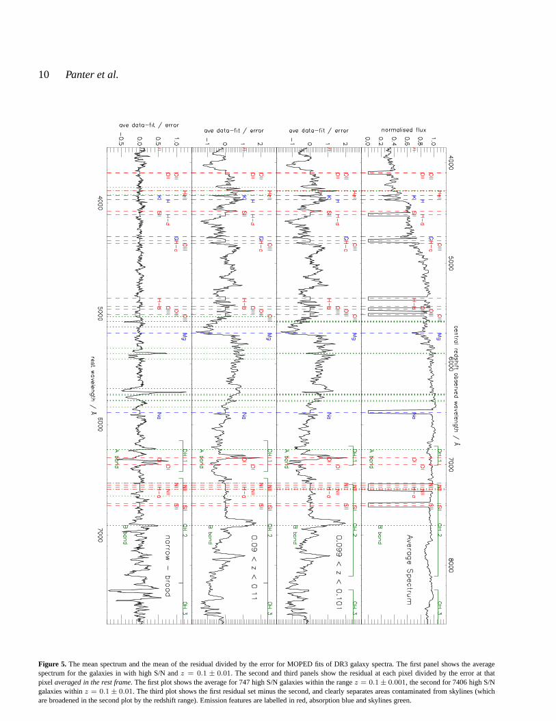
(Thomas, Maraston, & Bender 2003), emission lines, helium pro-duction ofdY/dZ ∼ 1.5− 2 (Jimenez et al. 2003) and other spec-tral features). Fig 5 provides some insight into which features in theresiduals can be identified. Since we subtract the modelled spec-trum from the data, unfitted emission will have a positive effect onthe residuals while unfitted absorption will be negative. Both ob-vious emission lines and filling of absorption features should bedetectable. The spectra used for this analysis are those which havealready had the strongest emission line regions removed, asdetailedearlier - in this case the residual is simply zero.

The first panel of Fig. 5 shows the mean spectrum. To distin-guish between galaxy features and skyline features we select tworedshift ranges with the same central redshift,z = 0.1. Since theaveraging of residuals is carried out in the galaxy restframe, in-creasing the redshift spread will act to spread any skyline features.The third panel gives the residuals for galaxies within 0.001 of thecentral redshift while the second has a range of 0.01. The fourthpanel shows the second subtracted from the first. In this case, sky-line/instrumental will create regions with large amplitude. The rel-evant skyline features (and their convolutions with the extremes ofthe particular redshift distribution) are shown and correspond ex-actly. It can be seen from the third panel that the majority ofthespectral range is remarkably clear of skyline contamination - testa-ment to the high quality of the Sloan spectroscopy.

Considering the regions which are not excluded by skylineswe begin to be able to assess the ability of the Bruzual & Charlot(2003) models to fit the data. It is clear that in all regions whereweak emission filling could be present and has not been maskedthere is a slight positive tendency in the residuals (although thisis of course not a failing of the models but a reflection of possiblesystematics affecting our fits), and many of the features in the resid-ual correspond to features that may be affected by alpha enhance-ment. A more detailed study of individual indices and their alphaenhancement, and their resolution in more advanced models includ-ing variable abundance ratios will be presented in a later paper. Al-though the vast majority of features in the residual can be directlyrelated to specific lines there is a strong signal just red of the mag-nesium line at restframe 5176A. Although tempting to attribute thisto poor fitting of the magnesium feature, it could also be interpretedas part of a broader feature between restframe 5200-5900A. It is in-teresting to compare the fitting in this region to the area around the4000A break as both are heavily dependent on metallicity. It is sur-prising that the models do so well in fitting the break but cannotsimultaneously fit this region, and taken with the excess around theCalcium Hydride band ( 6830-6900A) suggest that perhaps the bal-ance of K-M giants in the models must be improved, the resolutionof which would lead to a bluer continuum.

Converting this feature to the observed frame it coincides withthe dichroic region of the combined red and blue SDSS spectro-graphs. If this were to be the cause one would expect that the fea-ture would appear in the third panel, which it does not, and certainlyfurther work would be necessary to interpret this residual feature inthe context of the DR3 spectrophotometric calibration pipeline.

4 THE IMPACT OF MODEL CHOICE

In this section, we investigate the influence on assumptionson theresults obtained in the last section. There have been several im-provements and changes since our analysis of DR1, and the resultshave changed to some degree. The purpose of this study is to seehow the assumptions change the conclusions, and to get some idea

8 Panter et al.

Figure 3.The galaxy stellar mass function of SDSS. Also shown are those of Cole et al. (2001) (Orange) and Bell et al. (2003) (Blue),corrected for differencesin IMF. The errors quoted on the parameters are based upon thestatistical errors of the galaxy sample rather than systematics, which are discussed in the text.The red solid line is the Schechter (1976) best fit solution over the qualifying points, the dotted section is an extrapolation over the range covered by the data.

of the systematic effects introduced by choices of such things as thestellar populations used to model the spectra.

4.1 Sample studied

Although the MOPED algorithm allows rapid analysis of differentmodelling choices, to investigate a wide range of parameters it isnecessary to cut the sample down to something more manageable.We chose to operate on the main galaxy sample spectra in plates0288 and 0444. These two plates form a representative sampleof808 galaxies from two widely separated patches on the sky. Intotal767 of the 808 satisfy the criteria used in our main analysis andwould appear in our estimates of SFR.

4.2 Star Formation Fractions and Star Formation Rates

There are two places where modelling choices affect the shape ofthe recovered cosmic star formation rate - the estimation ofthe rel-ative fractions of different SSPs and the calculation of aVmax cor-rection based on that SFH. For this analysis we wish to investigatethe two stages independently. To achieve this we need to compareboth the SFF recovered using different models and the SFR thatresults.

The galaxies’ star formation fractions (SFF) and total massare calculated in their individual rest frames. This SFH is then con-verted to a common frame for all galaxies and weighted in propor-tion to 1/Vmax. Both the original SFF and the1/Vmax weightingare calculated by the models, and the mass is dependent on theIMF.Our first comparison (Fig. 6) shows the initial normalized SFF re-covered for the galaxiesaveraged in their restframes. Since it is ourintention to compare the relative fractions produced by changingmodel parameters rather than the overall mass (which has been de-scribed elsewhere, see Bell & de Jong (2001)) we present the SFFnormalized to total star formation of 1 per galaxy . This should

Table 4.A summary of models used in the analysis.

Name Reference FWHM

SPEED Jimenez et al. (2004) 20APEGASE Fioc & Rocca-Volmerange (1997) 20A

BC93 Bruzual & Charlot (1993) 20AMaraston Maraston (2005) 20A

GALAXEV Bruzual & Charlot (2003) 3A

give a clear indication of differences on recovered star formationfractions in the models.

Next we compare the cosmic SFR calculated using these var-ious modelling choices. This method allows direct comparison ofthe SFR obtained using each model, but is subject to greater errorsdue to the sensitivity of theVmax calculation on individual starformation histories and the large relative weight change this canproduce. We present this model-dependent SFR in addition totheSFF but caution that the number of galaxies present is insufficientto draw robust conclusions. Given the substantially smaller numberof galaxies, the errors are far larger than those of the complete DR3analysis presented earlier in this paper.

A summary of the models is given in table 4; unless otherwisestated a Salpeter (1955) IMF is used to calculate the SSPs.

4.3 Sample galaxies compared to full dataset

Fig 6a shows the difference in recovered SFF between our originalDR1 analysis and our subsample. The differences are due to thenumber of galaxies (120,000 in the full DR1 vs. 808 in the DR1Sample). For all further comparisons in this section the sample ofgalaxies will be 808 identified in the MGS plates 0288 and 0444.Fig 8a shows the difference in SFR.

9

Figure 4. The star formation rate of galaxies of different masses. These plots show the contribution to the overall star formationrate in the universe fromgalaxies with different masses over the redshift range we consider reliable. In the upper panel the SFR has been offset toenable easier comparison of thecurves, in the lower there has been no offset applied. It is clear that the more massive systems formed their stars earlier, although no conclusion can be drawnas to the number of objects these stars formed in.

4.4 Pipeline changes DR3 vs DR1, PCA cleaning of skylines

Fig 6b shows the impact of changing the pipeline used to reducethe original raw data. DR3 contains a more accurate calibration ofthe continuum of the spectrum and a systematic trend that devi-ated the continuum blueward of4000 A has been corrected. TheSPEED model, at a resolution of20A was used for all three sets.Except for bins 6-9 (numbered from the right), the variationthe twodatasets introduce is very small, at the few percent level. However,for these bins the deviations are as much as a factor of three.Notethat, where present, continuum discrepancies between the blue end

for DR1 and DR3 were on average 10% in the flux (at 3500A). It isremarkable that such drastic changes introduce such small changeson the average physical properties of the sample.

It is reassuring that the changes made to the spectra by PCAremoval of skyline regions have virtually no effect on our SSP fits.It is important to realise though that the majority of the regionscleaned by the Wild & Hewett (2005) code are outside of our sam-pled wavelength range.

The effect of the pipeline on the SFR shown in Fig 8b is fargreater. The mean flux of the spectra between the two releaseshaschanged by a factor of between 1.5 and 2, and the masses reflect

10 Panter et al.

Figure 5. The mean spectrum and the mean of the residual divided by the error for MOPED fits of DR3 galaxy spectra. The first panel showsthe averagespectrum for the galaxies in with high S/N andz = 0.1 ± 0.01. The second and third panels show the residual at each pixel divided by the error at thatpixel averaged in the rest frame. The first plot shows the average for 747 high S/N galaxies within the rangez = 0.1± 0.001, the second for 7406 high S/Ngalaxies withinz = 0.1 ± 0.01. The third plot shows the first residual set minus the second,and clearly separates areas contaminated from skylines (whichare broadened in the second plot by the redshift range). Emission features are labelled in red, absorption blue and skylines green.

11

Figure 6. The systematic changes in recovered SFH for various modelling choices. The labels show the various modelling choices applied to generate theSFFs, and are expanded upon in the text. It is important to note that these are the fractions of total mass formed over the lifetime of the galaxy, and not thefractions of light contributing to the recovered spectrum.The light from the youngest populations is some 300x brighter than the oldest. The fractions arenormalised, so changes in overall recovered mass for spectra are not apparent.

12 Panter et al.

Figure 7. The systematic changes in recovered rest frame star formation fractions (not rates) for various different SSPs expanded from figure 6 for clarity. Itis important to note that these are the fractions of total mass formed over the lifetime of the galaxy, and not the fractions of light contributing to the recoveredspectrum. The light from the youngest populations is some 300x brighter than the oldest

this change. Even ignoring this change in the normalizationof theSFR it is clear that the trend for a low redshift peak is no longerpresent - the SFR appears to fall monotonically to the present day.This interpretation does not exclude a peak at a higher redshift thanour eldest bin.

4.5 Stellar population models

Figs. 6c and 7 show the comparison between five different stel-lar population synthesis models: the Jimenez et al. (2004) SPEEDmodels, the Fioc & Rocca-Volmerange (1997) PEGASE mod-els, the Maraston (2005) RHB models; the Bruzual & Charlot(1993) models and the more modern 3A Bruzual & Charlot (2003)GALAXEV models rebinned to 20A. The comparison is done at20A for the Salpeter IMF and for the one-parameter dust model. Itis important to establish that this analysis cannot say which modelset is ‘right’, only assist in understanding the differences betweenmodels. The overall shape of the SFF is in reasonable agreement -although there are certainly discrepancies between the populationsthat are recovered. For the very oldest populations the differentmodels agree very well. This is not entirely unexpected of course,as the stars which contribute to this area of the age-metallicity pa-rameter space are well studied and dominate the emission at redwavelengths. The different models also predict roughly similar pro-portions of the very youngest populations, which rely on similarprescriptions for the evolution of blue massive stars and can beconstrained through the emission at the bluest wavelengths. At in-

termediate ages the agreement is not so good: this is likely to becaused, at least in part, by the difficulty in recovering the fractionof intermediate-age stars in stellar populations with declining starformation histories (see discussion by Mathis et al. (2006)). Thistends to produce an artificial step around 1 Gyr in the star formationhistory, except perhaps in the Maraston (2005) model. The differ-ent behavior of this model probably results from the different pre-scription for bright Thermally Pulsing Asymptotic Giant Branch(TP-AGB) stars. The contribution by these stars to the integratedlight is still subject to controversy in current populationsynthesismodels. Since our spectra are fitted in addition, any poorly fit com-ponent will be replaced by another.

Fig. 8c shows the difference that the various models make tothe recovered SFR. It is clear that there is a large spread - asdis-cussed earlier, this is due to the fact that the models contribute bothto the estimation of the SFH and theVmax weights attributed to thegalaxies. In all models except those of the PEGASE group the SFRdecreases monotonically from the oldest to the youngest bins.

4.6 The impact of resolution, 20A vs 3A

Fig.6d shows the impact of increasing the spectral resolution of thedata. In this case we use the BC03 at resolutions of 20A and 3Aon DR3. The differences between the two curves are very small.the maximum deviation is only of about 30% in bin 4 and smallerin bin 5. For the other bins the agreement is remarkable. Whatthiscomparison is telling us is that 20A is sufficient resolution to deter-

13

Figure 8. The systematic changes in the overall SFR for various modelling choices. The labels show the various modelling choices applied to generate theSFFs,Vmax, mass and SFR and are expanded upon in the text. We plot only those bins used for the analysis in the main section, and caution that due to thelargeVmax corrections there are insufficient galaxies in this sub-sample to draw robust conclusions

14 Panter et al.

mine the average properties of galaxies. The higher resolution doesnot add much extra information to this. More importantly, the resultis not biased at the lower resolution. This is not entirely surprisingsince the continuum certainly contains information about both ageand metallicity of a stellar population (e.g. Jimenez et al.(2004)).The shape of the SFR recovered in Fig. 8d is remarkably consistentbetween the two resolutions, with a significant variation inonly onebin.

4.7 IMF: Salpeter vs. Chabrier.

Fig.6e and 8e show the impact of changing the initial mass func-tion on the recovered SFF and SFR. In this case we have chosen towork with the BC03 models at 3A resolution. The IMF determinesthe initial distribution of the number of stars as a functionof mass.It is therefore not surprising to find changes in the recovered starformation history for dramatic changes in the IMF. The Chabrierand Salpeter IMF are very similar for masses larger than1− 2 M⊙

(they are both power laws) while they differ considerably atsmallermasses: the Salpeter IMF continues being a power law (with index−1.35) while the Chabrier IMF deviates containing a much smallernumber of small mass stars relative to the Salpeter IMF. As panel6e shows the main difference occurs at the oldest bin (bin 1),withsmaller differences in bins2−4 and virtually no differences for theyoungest bins when the bootstrap error bars are taken into account.This effect is propagated through theVmax and mass calculationto the SFR. This is more-or-less what one would expect: for theoldest bin, the Chabrier IMF has to compensate its relative lack oflow mass stars compared with the Salpeter IMF by forming moreof them. The differences then disappear as more massive stars aremore dominant at recent ages. It is interesting that although ourresults will be affected by varying the IMF, it will be in a differ-ent sense from the results from instantaneous SFRs attainedat highredshift. Where as virtually all instantaneous indicatorsestimatethe total mass of stars from the very high mass UV emitting stars,our technique uses the low mass remnants. The fact that the two ap-proaches agree suggests that the IMFs currently in vogue arealongthe right lines, and a direct comparison of sufficiently accurate indi-cators from both the instantaneous and fossil approach could allowIMF fine-tuning. This approach would also require an accurate un-derstanding of the dust in star forming regions, a subject ofsomecontroversy in the literature. This topic will be discussedin a futurepaper.

4.8 Dust modelling

One of the most difficult problems in modelling stellar populationsis how to model the attenuation of the population by dust. Forourprevious study (Heavens et al. 2004) we adopted a simplified modelwith only one parameter (the attenuation) while the spectral depen-dence of the attenuation was taken to be that of the Large Magel-lanic Cloud. Alternate formalisations for the screen are based onthe Small Magellanic Cloud, or estimated for starburst galaxies byCalzetti (1997). On the other hand, Charlot & Fall (2000) have pro-posed that a more accurate modelling of the effects of dust atten-uation in galaxies can be achieved by a two-parameter model.Inthis model one parameter accounts for dust in the giant molecularclouds surrounding young stars (of ages< 10 Myr) and the otherparameter the dust in the diffuse ISM. The combination of thetwoparameters allows a more complex extinction curve to be generated.Unfortunately, since our method does not include the contribution

to the spectrum from emission lines, it is not possible to determinethe extinction from the birth cloud from continuum alone.

Fig.6f and 8f show the differences between the LMC, SMCand Calzetti models for the BC03 models at 3A resolution. Themost significant difference occurs clearly at about0.1 Gyr.

5 RESIDUALS OF BEST FIT MODELS

The average residuals from the best-fit solutions of the differentmodels is shown in Fig. 9. This provides a more detailed look athow well the models are faring at reproducing the features intheobserved spectra and if some models do better than others. Itcan beseen that the 20A models cover essentially the same range of spec-tral features, and it would be impossible to say that one is betterthan another. The picture changes when we consider the 3A mod-els however, they are clearly superior at minimizing the residuals -even when rebinned to 20A resolution. Although there are still sev-eral regions where features are not quite correct, it is on the levelof individual lines rather than wide bands of the spectrum. Com-paring panels (a) and (b) allows us to investigate the effectof theimprovement in photometric calibration between DR1 and DR2-3on line strengths – practically none, as it should be.

This average deviation should not be confused with averagegoodness of fit however, as inspection of the relevant average χ2

of the samples shows a slightly different story. The models haveessentially infinite precision, so there is no penalty associated withrebinning. The converse is true for the spectra, as binning pixelswhile correctly propagating the error will reduce the standard devi-ation.

6 CONCLUSIONS

We have used MOPED to probe the fossil record of star formationencoded in the spectra of more than300, 000 SDSS-DR3 galax-ies to determine stellar populations, metallicity evolution and dustcontent. We have also investigated the impact of systematics onrecovering physical information from the fossil record. Our mainconclusions are:

• The main impacts on systematic variation in the estimationof SFR from the fossil record are due to the the stellar populationmodel, the calibration of the observed spectra and the choice of theIMF.• We find strong evidence for downsizing, independent of model

choice.• The overall star formation history of galaxies recovered from

the fossil record agrees well with instantaneous formationmeasure-ments.• The mass build-up recovered from our analysis is in good

agreement with that predicted from both high redshift studies andthe semi-analytic simulations of galaxy formation based onMillen-nium Run.• We have identified the cause of many of the residuals from the

spectral fits. Stellar population models that provide extrafreedomin terms of alpha enhancement should provide better fits.

The fossil record continues to provide a useful tool to unveilthe physical conditions of galaxies in the present and the past. Withimproved models that incorporate alpha-enhancement it should bepossible to constrain further models of galaxy formation and evo-lution and the initial mass function of galaxies.

15

Figure 9. Average residuals, following the method used to prepare figure 5 but instead using all the MGS spectra in the two plates. The individual panels arelabelled with the models and datasets which were used to generate them. From top to bottom, a) DR1 data, Jimenez et al. (2004) SPEED models; b) DR3 data,SPEED models; c) DR3 data, Fioc & Rocca-Volmerange (1997) PEGASE models; d) DR3 data, Maraston (2005) RHB models; e) Bruzual & Charlot (1993)models; f) DR3 data, Bruzual & Charlot (2003) GALAXEV modelsrebinned to 20A; g) DR3 data, GALAXEV models at 3A resolution using a Salpeter(1955) IMF; h) DR3 data, GALAXEV models at 3A using a Chabrier (2003) IMF; i) DR3 data cleaned using the skyline extraction method of Wild & Hewett(2005). Residuals are averaged in the rest frame.

16 Panter et al.

ACKNOWLEDGMENTS

We thank the anonymous referee for several suggestions whichhave considerably increased the scope and clarity of the paper.

BP and SC thank the Alexander von Humboldt Foundation,the Federal Ministry of Education and Research, and the Pro-gramme for Investment in the Future (ZIP) of the German Gov-ernment for funding through a Sofja Kovalevskaja award. There-search of RJ is partially supported by NSF grants AST-0408698,PIRE-0507768 and NASA grant NNG05GG01G.

BP wishes to thank Paul Hewett for considerable assistanceidentifying the source of various residuals in Fig. 5.

We acknowledge use of the public IDL routines of CraigMackwardt, David Fanning and the SDSS idlutils package, andtheprivate SDSS/Milky Way dust compensation routine of Rita To-jeiro. Much of the exploratory work that led to the results containedin this paper benefited from an SQL database created with GerardLemson as part of the GAVO project. We wish to thank Darren Cro-ton for providing the data used for comparison with the MilleniumSimulation in Figure 1 in electronic form.

Funding for the creation and distribution of the SDSS Archivehas been provided by the Alfred P. Sloan Foundation, the Partici-pating Institutions, the National Aeronautics and Space Adminis-tration, the National Science Foundation, the U.S. Department ofEnergy, the Japanese Monbukagakusho, and the Max Planck Soci-ety. The SDSS Web site ishttp://www.sdss.org/.

The SDSS is managed by the Astrophysical Research Con-sortium (ARC) for the Participating Institutions. The Participat-ing Institutions are The University of Chicago, Fermilab, the Insti-tute for Advanced Study, the Japan Participation Group, TheJohnsHopkins University, Los Alamos National Laboratory, the Max-Planck-Institute for Astronomy (MPIA), the Max-Planck-Institutefor Astrophysics (MPA), New Mexico State University, Universityof Pittsburgh, Princeton University, the United States Naval Obser-vatory and the University of Washington.

REFERENCES

Abazajian et al. K., 2003, AJ, 126, 2081Abazajian et al. K., 2004, AJ, 128, 502Abazajian et al. K., 2005, AJ, 129, 1755Barger, A. J., Cowie, L. L., Richards, E. A. 2000, AJ, 119, 2092Bell, E.F., McIntosh, D.H., Katz, N., Weinberg, M.D., ApJ, 2003,585, 117-120

Bell E. F., de Jong R. S., 2001, ApJ, 550, 212Borch A., et al., 2006, A&A, 453, 869Brinchmann J., Ellis R. S., 2000, ApJ, 536, L77Brinchmann J., Charlot S., White S. D. M., Tremonti C., Kauff-mann G., Heckman T., Brinkmann J., 2004, MNRAS, 351, 1151

Bruzual A. G., Charlot S., 1993, ApJ, 405, 538Bruzual G., Charlot S., 2003, MNRAS, 344, 1000Calzetti D., 1997, AJ, 113, 162Chabrier G., 2003, PASP, 115, 763Cid Fernandes, R., Mateus, A., Sodre, L., Stasinska, G., &Gomes,J. M. 2005, MRAS, 358, 363

Charlot S. ., Fall S. M., 2000, apj, 539, 718Cole, S., et al. 2001, MNRAS, 326, 255Condon, J. J., Cotton, W. D., Broderick, J. J. 2002, AJ, 124, 675Condon, J. J. 1989, ApJ, 338, 13Connolly, A. J., Szalay, A. S., Dickinson, M., SubbaRao, M. U.,Brunner, R. J. 1997, ApJl, 486, L11

Cowie, L. L., Songaila, A., Barger, A. J. 1999, AJ, 118, 603Croton D. J., et al., 2006, MNRAS, 365, 11Davis et al. M., 2003, in Guhathakurta P., ed., Discoveries and Re-search Prospects from 6- to 10-Meter-ClassTelescopes II. Editedby Guhathakurta, Puragra. Proceedings of the SPIE, Volume4834, pp. 161-172 (2003). Science Objectives and Early Resultsof the DEEP2 Redshift Survey. pp 161–172

Dickinson M., Papovich C., Ferguson H. C., Budavari T., 2003,ApJ, 587, 25

Drory N., Salvato M., Gabasch A., Bender R., Hopp U., FeulnerG., Pannella M., 2005, ApJ, 619, L131

Fioc M., Rocca-Volmerange B., 1997, A&A, 326, 950Flores, H., et al. 1999, ApJ, 517, 148Fontana A., et al., 2004, A&A, 424, 23Fukugita, M., Hogan, C.J., Peebles, P.J.E., 1998, ApJ, 503,518Gallego, J., Zamorano, J., Aragon-Salamanca, A., Rego, M.1995,ApJl, 455, L1

Gallego, J., Garcıa-Dabo, C. E., Zamorano, J., Aragon-Salamanca, A., Rego, M. 2002, ApJl, 570, L1

Georgakakis, A., Hopkins, A. M., Sullivan, M., Afonso, J., Geor-gantopoulos, I., Mobasher, B., Cram, L. 2003, MNRAS, 345,939

Giavalisco, M., et al. 2004, ApJl, 600, L103Glazebrook, K., Blake, C., Economou, F., Lilly, S., Colless, M.1999, MNRAS, 306, 843

Glazebrook, K., Baldry, I. K., Blanton, M. R., Brinkmann, J.,Connolly, A., Csabai, I., Fukugita, M., Ivezic, Z., Loveday, J.,Meiksin, A., Nichol, R., Peng, E., Schneider, D. P., SubbaRao,M., Tremonti, C., York, D. G., 2003, ApJ, 587, 55

Gordon, K. D., Clayton, G. C., Misselt, K. A., Landolt, A. U.,Wolff, M. J., 2003, ApJ, 594, 279

Gunn et al. J. E., 1998, AJ, 116, 3040Haarsma, D. B., Partridge, R. B., Windhorst, R. A., Richards, E.A. 2000, ApJ, 544, 641

Hammer, F., et al. 1997, ApJ, 481, 49Heavens A., Panter B., Jimenez R., Dunlop J. S., 2004, NatureHeavens A. F., Jimenez R., Lahav O.,2000, MNRAS, 317, 965Hogg, D. W., Cohen, J. G., Blandford, R., Pahre, M. A. 1998, ApJ,504, 622

Hopkins, A. M., Connolly, A. J., Szalay, A. S. 2000, AJ, 120, 2843Hopkins A. M., 2004, ApJ, 615, 209Hughes, D. H., et al. 1998, Nature, 394, 241Jimenez R., Flynn C., MacDonald J., Gibson B. K., 2003, Sci,299, 1552

Jimenez R., MacDonald J., Dunlop J. S., Padoan P., Peacock J.A.,2004, MNRAS, 349, 240

Kauffmann G., White S. D. M., Heckman T. M., Menard B.,Brinchmann J., Charlot S., Tremonti C., Brinkmann J., 2004,astro-ph/0402030

Kochanek, C.S., et al. 2001, ApJ, 560,566Lilly, S. J., Le Fevre, O., Hammer, F., Crampton, D. 1996, ApJl,460, L1

Machalski, J., Godlowski, W. 2000, A&A, 360, 463Madau, P., Ferguson, H. C., Dickinson, M. E., Giavalisco, M.,Steidel, C. C., Fruchter, A. 1996, MNRAS, 283, 1388

Maraston C., 2005, MNRAS, 362, 799Massarotti, M., Iovino, A., Buzzoni, A. 2001, ApJl, 559, L105Mathis H., Charlot S., Brinchmann J., 2006, MNRAS, 365, 385Moorwood, A. F. M., van der Werf, P. P., Cuby, J. G., Oliva, E.2000, A&A, 362, 9

Ocvirk P., Pichon C., Lancon A., Thiebaut E., 2006, MNRAS,365, 46

17

Panter B., Heavens A. F., Jimenez R., 2003, MNRAS, 343, 1145Panter B., Heavens A. F., Jimenez R., 2004,MNRAS, 355, 764Panter B., Thesis, 2005. Availiable at from the Edinburgh Re-search Archive at http://hdl.handle.net/1842/774

Persic, M., Salucci, P., 1992, MNRAS, 258, 14Pettini, M., Kellogg, M., Steidel, C. C., Dickinson, M., Adel-berger, K. L., Giavalisco, M. 1998, ApJ, 508, 539

Perez-Gonzalez, P. G., Zamorano, J., Gallego, J., Aragon-Salamanca, A., Gil de Paz, A. 2003, ApJ, 591, 827

Rudnick G. H., Rix H.-W., Franx M., Labbe I., FIRES Collabora-tion, 2003, AAS, 36, 591

Sadler, E. M., et al. 2002, MNRAS, 329, 227Salpeter E. E., 1955, ApJ, 121, 161Salucci, P., Persic, M., 1992, MNRAS, 309, 923Schechter, P. 1976, ApJ, 203, 297Serjeant, S., Gruppioni, C., Oliver, S. 2002, MNRAS, 330, 621Shen S., Mo H. J., White S. D. M., Blanton M. R., Kauffmann G.,Voges W., Brinkmann J., Csabai I., 2003, MNRAS, 343, 978

Spergel D. N., Verde L., Peiris H. V., Komatsu E., Nolta M. R.,Bennett C. L., Halpern M., Hinshaw G., Jarosik N., Kogut A.,Limon M., Meyer S. S., Page L., Tucker G. S., Weiland J. L.,Wollack E., Wright E. L., 2003, ApJS, 148, 175

Steidel, C. C., Adelberger, K. L., Giavalisco, M., Dickinson, M.,Pettini, M. 1999, ApJ, 519, 1

Stoughton et al. C., 2002, AJ, 123, 485Strauss et al. M. A., 2002, AJ, 124, 1810Sullivan, M., Treyer, M. A., Ellis, R. S., Bridges, T. J., Milliard,B., Donas, J., 2000, MNRAS, 312, 442

Sullivan, M., Mobasher, B., Chan, B., Cram, L., Ellis, R., Treyer,M., Hopkins, A. 2001, ApJ, 558, 72

Teplitz, H. I., Collins, N. R., Gardner, J. P., Hill, R. S., Rhodes, J.2003, ApJ, 589, 704

Thomas D., Maraston C., Bender R., 2003, MNRAS, 339, 897Thomas, D., Maraston, C., Bender, R., & Mendes de Oliveira, C.2005, ApJ, 621, 673

Tremonti C. A., Heckman T. M., Kauffmann G., Brinchmann J.,Charlot S., White S. D. M., Seibert M., Peng E. W., SchlegelD. J., Uomoto A., Fukugita M., Brinkmann J., 2004, ApJ, 613,898

Tresse, L., Maddox, S. J., Le Fevre, O., Cuby, J.-G. 2002, MN-RAS, 337, 369

Tresse, L., Maddox, S. J. 1998, ApJ, 495, 691Treyer, M. A., Ellis, R. S., Milliard, B., Donas, J., Bridges, T. J.1998, MNRAS, 300, 303

Wild V., Hewett P. C., 2005, MNRAS, 358, 1083Wilson, G., Cowie, L. L., Barger, A., Burke, D. J. 2002, AJ, 124,1258

Yan, L., McCarthy, P. J., Freudling, W., Teplitz, H. I., Malumuth,E. M., Weymann, R. J., Malkan, M. A. 1999, ApJL, 519, L47

York et al. D., 2000, AJ, 120, 1579