Cosmological simulations of the growth of supermassive black ...

Mon. Not. R. Astron. Soc. 398, 53–74 (2009) doi:10.1111/j.1365-2966.2009.15043.x

Cosmological simulations of the growth of supermassive black holes andfeedback from active galactic nuclei: method and tests

C. M. Booth� and Joop SchayeLeiden Observatory, Leiden University, PO Box 9513, 2300 RA Leiden, the Netherlands

Accepted 2009 May 14. Received 2009 May 14; in original form 2009 April 17

ABSTRACTWe present a method that self-consistently tracks the growth of supermassive black holes(BHs) and the feedback from active galactic nuclei (AGN) in cosmological, hydrodynamicalsimulations. Our model is a substantially modified version of the one introduced by Springel,Di Matteo & Hernquist implemented in a significantly expanded version of the GADGET III

code, which contains new prescriptions for star formation, supernova feedback, radiativecooling and chemodynamics. We simulate the growth of BHs from an initial seed state viaEddington-limited accretion of the surrounding gas, and via mergers with other BHs. Becausecosmological simulations at present lack both the resolution and the physics to model themultiphase interstellar medium, they tend to strongly underestimate the Bondi–Hoyle accretionrate. To allow low-mass BHs to grow, it is therefore necessary to increase the predictedBondi–Hoyle rates in star-forming gas by large factors, either by explicitly multiplying theaccretion rate by a numerical correction factor or by using an unresolved, subgrid model forthe gas close to the BH. We explore the physical regimes where the use of such multiplicativefactors is reasonable, and through this introduce a new prescription for gas accretion by BHs.Feedback from AGN is modelled by coupling a fraction of the rest-mass energy of the accretedgas thermally into the surrounding medium. We describe the implementation as well as thelimitations of the model in detail and motivate all the changes relative to previous work. Wedemonstrate how general physical considerations can be used to choose many of the parametersof the model and demonstrate that the fiducial model reproduces observational constraints.

We employ a large suite of cosmological simulations, in which the parameters of the BHmodel are varied away from their fiducial values, to investigate the robustness of the predictionsfor the cosmic star formation history and the redshift zero cosmic BH density, BH scalingrelations and galaxy-specific star formation rates. We find that the freedom introduced by theneed to increase the predicted accretion rates by hand, the standard procedure in the literature,is the most significant source of uncertainty. Our simulations demonstrate that supermassiveBHs are able to regulate their growth by releasing a fixed amount of energy for a given halomass, independent of the assumed efficiency of AGN feedback, which sets the normalizationof the BH scaling relations. Regardless of whether BH seeds are initially placed above orbelow the BH scaling relations, they grow on to the same scaling relations. AGN feedbackefficiently suppresses star formation in high-mass galaxies.

Key words: hydrodynamics – galaxies: active – galaxies: evolution – galaxies: formation –quasars: general – cosmology: theory.

1 IN T RO D U C T I O N

Over the past decades, a growing body of observational and theoret-ical evidence has suggested that supermassive black holes (SMBHs;

�E-mail: [email protected] CMB

mBH > 106 M�) exist in the centres of all galaxies with spheroids(e.g. Kormendy & Richstone 1995; Ferrarese & Merritt 2000) andthat the properties of these SMBHs are tightly correlated with theproperties of the spheroid in which they reside. For example, themass of the SMBH is found to be tightly correlated with the bulgestellar mass or luminosity (Magorrian et al. 1998; Laor 2001;McLure & Dunlop 2002; Haring & Rix 2004), stellar velocity

C© 2009 The Authors. Journal compilation C© 2009 RAS

Dow

nloaded from https://academ

ic.oup.com/m

nras/article/398/1/53/1092579 by guest on 11 July 2022

54 C. M. Booth and J. Schaye

dispersion (Gebhardt et al. 2000; Merritt & Ferrarese 2001;Tremaine et al. 2002) and galaxy concentration, as measured bythe Sersic index (Graham & Driver 2007a). Some recent work hasdemonstrated that these correlations may be understood in terms ofa black hole (BH) ‘fundamental plane’, relating BH mass, galaxyeffective radius, stellar velocity dispersion and stellar mass. Here,the mass of the SMBH essentially tracks the binding energy of thestellar bulge (Marconi & Hunt 2003; Feoli & Mele 2005; Aller &Richstone 2007; Hopkins et al. 2007, 2008), although other authorsargue that the appearance of a fundamental plane is actually dueto biasing caused by the presence of galaxies with bars (Graham2008).

The exact mechanisms leading to the tight observed couplingbetween galaxy spheroidal components and central active galacticnuclei (AGN) are not yet fully understood, although it has long beenrecognized that the formation mechanisms of SMBHs (e.g. Silk &Rees 1998) and stars (e.g. Dekel & Silk 1986) are most likely self-regulating. These results suggest that the same processes that shapegalaxy spheroids also act on the central BHs. Correlations betweenAGN activity and other processes provide other clues about themechanisms that lead to the buildup of the SMBH population. Thereis evidence that there exists a link between galactic star formation(SF) and accretion on to a central AGN: in a global sense, theevolution of the cosmic star formation rate (SFR; e.g. Madau et al.1996) and the luminosity density of quasars are tightly correlated(Boyle & Terlevich 1998). Additionally, on the scale of individualobjects it has been found that the most powerful narrow-line AGNare preferentially found in galaxies that appear to have undergonea recent starburst phase (Kauffmann et al. 2003).

The massive BHs present in the centres of galaxies are likely tohave started their lives as ‘seed’ BHs. The typical masses of seedBHs remain somewhat uncertain, and depend upon the mechanismby which they form. Plausible mechanisms include the collapse ofPopulation III stars, giving rise to BHs with masses in the range102 < mBH < 103 M� (e.g. Madau & Rees 2001; Schneider et al.2002; Islam, Tayloe & Silk 2003), and direct collapse of matterin high-redshift, low angular momentum haloes, which may giverise to seed BHs with masses ∼105 M� (e.g. Loeb & Rasio 1994;Bromm & Loeb 2003; Begelman, Volonteri & Rees 2006; Dijkstraet al. 2008; Volonteri & Natarajan 2009). These seed mass BHs canthen grow either by mergers with other BHs (e.g. Islam et al. 2003)or through accretion of gas and/or stars.

Accretion of matter on to central BHs, accompanied by the releaseof a fraction of the rest-mass energy of the fuel, has long beenrecognized as one of the most likely mechanisms to power AGN(Salpeter 1964), and a coupling between the accretion history ofan AGN and the gas dynamics of the bulge provides a plausiblemechanism by which AGN and bulge properties could becomestrongly correlated coupled (e.g. Silk & Rees 1998). For example,it has been suggested that the central BHs grow until they releasesufficient energy to unbind the gas that feeds them from the hostgalaxy (Fabian 1999). Bursts of AGN activity then expel gas fromgalaxies and remain quiescent until stellar mass loss replenishes thegalaxy’s gas reservoir (Ciotti & Ostriker 2001).

A theoretical link between galaxy mergers and both galaxy-scalestarburst events and active AGN phases has been well establishedand modelled. Galaxy mergers have long been recognized as amechanism by which gas can potentially be channelled to the cen-tre of a galaxy (Toomre & Toomre 1972), and N-body simulations ofgalaxy mergers confirmed and extended this picture by showing thatthe asymmetrical gravitational potential present during mergers iscapable of funnelling gas efficiently to the centre of a galaxy (Mihos

& Hernquist 1994), where it may be accreted by a SMBH. Hydrody-namical simulations of galaxy mergers (Barnes & Hernquist 1991,1996; Mihos & Hernquist 1996; Kapferer et al. 2005), and numer-ical models of AGN growth (Kapferer et al. 2005; Springel 2005),predict that these merger events are indeed responsible for the rapidgrowth of AGN. Recent numerical studies (e.g. Micic et al. 2007)have indicated that both BH mergers and gas accretion are impor-tant processes in forming the population of BHs that we observe inthe local universe.

Thus, it seems that we can paint a coherent picture in whichemission by AGN, galaxy mergers and the growth of supermas-sive BHs are closely intertwined. As such, the study of any one ofthese processes requires an understanding of all of them. For thisreason, detailed studies of the co-evolution of the AGN and galaxypopulations in a cosmological context often resort to numericaltechniques. Early theoretical studies of the galaxy–AGN connec-tion relied upon dark matter halo merger rates, without any separatetreatment of galaxy formation processes (Efstathiou & Rees 1988;Haehnelt & Rees 1993). Later work expanded upon this ground-work by incorporating AGN feedback into semi-analytic modellingof galaxy formation (e.g. Kauffmann & Haehnelt 2000; Cattaneo2001; Benson et al. 2003; Granato et al. 2004; Baugh 2006; Boweret al. 2006; Croton et al. 2006; Lagos, Cora & Padilla 2008). Semi-analytic models indicate that feedback from AGN is necessary inorder to build up a red-sequence of galaxies. Although a combina-tion of photo-heating by reionization and supernova feedback cansuppress SF in low-mass haloes – bringing the galaxy luminosityfunction in line with observations at the low-mass end – modelswithout AGN feedback face the problem that the reheated gas inmassive haloes would eventually cool, giving rise to an excessivenumber of bright galaxies (e.g. Bower et al. 2006) as compared tothe local universe.

A more computationally challenging approach is to simulategalaxies hydrodynamically, with additional subgrid modelling ofthe growth and energy feedback from AGN. Numerical hydrody-namic simulations of galaxy mergers containing AGN (e.g. Springelet al. 2005, hereafter S05; Di Matteo, Springel & Hernquist 2005;Hopkins et al. 2006; Robertson et al. 2006) have shown that thepresence of a central AGN can significantly alter the structure ofmerger remnants, particularly by expelling a hot halo of diffuse, low-angular momentum gas from the centre of the remnant. More recentnumerical studies have revealed that dissipation and dry mergers arelikely to play a fundamental role in shaping the co-evolution of BHsand galaxies (Hopkins et al. 2009). Hydrodynamic simulations offull cosmological volumes (Sijacki et al. 2007; Croft et al. 2008; DiMatteo et al. 2008; Okamoto, Nemmen & Bower 2008) have probedthe effect of AGN on a cosmologically representative set of galaxiesand showed that the inclusion of AGN physics into galaxy forma-tion simulations allows us to match many of the observed propertiesof galaxies in the local universe. The modelling of an AGN pop-ulation in this manner is both computationally very expensive andsubject to very many, as yet poorly understood, numerical effects.As such studies of this type must take care to test the robustness ofthe models to all physical and numerical parameters.

The focus of the current work is to present and test a new modelfor the co-evolution of BHs and galaxies. We note that nearly all BHmodels published thus far in the literature employ the SF and super-nova feedback models of Springel & Hernquist (2003) (hereafterSH03), and the model for BH growth and AGN feedback of S05.1

1 Although see Okamoto et al. (2008) for a different approach.

C© 2009 The Authors. Journal compilation C© 2009 RAS, MNRAS 398, 53–74

Dow


ic.oup.com/m


Simulating SMBH growth and feedback 55

Throughout this paper, we highlight similarities and differencesbetween our approach and that used previously in the literature. Theprimary difference between our models and previous work is that weemploy a different parametrization of the process of gas accretionon to BHs as well a different implementation of AGN feedback. Weshow that changes to the BH accretion model can lead to profounddifferences in galaxy properties, global SFRs and BH demograph-ics. We examine both the global properties of the simulation, such asthe integrated SFR and cosmic BH density, and consider the prop-erties of individual galaxies, including specific SFRs, and the BHfundamental plane. We quantify how uncertainties in our numericalmodel and all of our parameter choices affect the reliability of ourresults. We find that changes in the numerical model that generatesseed mass BHs, and in the model that distributes feedback energyinto the ISM do not strongly affect our results. However, the accre-tion model is found to be of crucial importance in understanding ourresults. Throughout, we assume a flat � cold dark matter cosmol-ogy with the cosmological parameters: {�m, �b, ��, σ 8, ns, h} ={0.238, 0.0418, 0.762, 0.74, 0.951, 0.73}, as determined from theWilkinson Microwave Anisotropy Probe (WMAP) 3-year data(Spergel et al. 2007) and consistent2 with the WMAP 5-year data(Komatsu et al. 2009). Where necessary, observational results havebeen scaled to our chosen cosmology, and the stellar initial massfunction (IMF) assumed in observational analyses has been scaledto the Chabrier IMF used in our simulations.

The paper is structured as follows. In Section 2, we introduce oursimulation set, and describe briefly the subgrid physics modulesthat are not directly related to BHs. In Section 3, we describe indetail our model for BH formation, growth and feedback, and wemotivate our choices for numerical parameters in Section 4. In Sec-tion 5, we present simulation results, including a comparison withredshift zero observational data and an investigation into the severityof uncertainties introduced by different parameter choices. Finally,in Section 6 we discuss and summarize our findings. In a compan-ion work, we investigate in detail the interplay between feedbackfrom AGN and other feedback processes, including winds drivenby Type 2 supernovae and mass loss from the stellar population.

2 N U M E R I C A L S I M U L AT I O N S

In this section, we introduce the numerical techniques used in oursimulations and provide a brief overview of the subgrid physicsmodules that are not directly related to BH growth or AGN feedback.

We have carried out a suite of cosmological simulationsusing smoothed particle hydrodynamics (SPH) (Gingold &Monaghan 1977; Lucy 1977; Monaghan 1992), employing a signif-icantly extended version of the parallel PMTree-SPH code GADGET

III (Springel, Yoshida & White 2001a; Springel 2005), a Lagrangiancode used to calculate gravitational and hydrodynamic forces on aparticle-by-particle basis. The initial particle positions and veloci-ties are set at z = 127 using the Zel’dovich approximation to linearlyevolve positions from an initially glass-like state. The productionsimulations used in this study are run in boxes of size 50 comovingMpc h−1, and contain 2563 particles of both gas and dark matter.Comoving gravitational softenings are set to 1/25 of the mean co-moving inter-particle separation down to z = 2.91, below which weswitch to a fixed proper scale of 2 kpc h−1. The production simu-lations have gas particle masses of 8.64 × 107 M� h−1. The boxesare evolved all the way to redshift zero.

2 Our value of σ 8 is 1.6σ lower than allowed by the WMAP 5-year data.

In addition to hydrodynamic forces, we treat SF, supernova feed-back, radiative cooling, chemodynamics, BH accretion and AGNenergy feedback in these simulations.

SF is tracked in the simulations following the prescription ofSchaye & Dalla Vecchia (2008). Gas with densities exceeding acritical density for the onset of the thermo-gravitational instability(hydrogen number densities nH = 10−2 to 10−1 cm−3) is expectedto be multiphase and to form stars (Schaye 2004). Because we lackboth the physics and the resolution to model the cold interstellar gasphase, we impose an effective equation of state (EOS) with pressureP ∝ ργeff for densities nH > n∗

H where n∗H = 0.1 cm−3, normalized

to P/k = 103 cm−3 K at the threshold. We use γ eff = 4/3 forwhich both the Jeans mass and the ratio of the Jeans length to theSPH kernel are independent of the density, thus preventing spuriousfragmentation due to a lack of numerical resolution (Schaye & DallaVecchia 2008). As described in Schaye & Dalla Vecchia (2008),gas on the effective EOS is allowed to form stars at a pressure-dependent rate that reproduces the observed Kennicutt–Schmidtlaw (Kennicutt 1998) by construction, renormalized by a factor3 of1/1.65 to account for the fact that it assumes a Salpeter IMF whereaswe use a Chabrier IMF.

Energy injection due to supernovae is included through kineticfeedback. We employ the prescription of Dalla Vecchia & Schaye(2008), which is a variation of the SH03 recipe for kinetic feedback.In this prescription, core-collapse supernovae locally inject kineticenergy and kick gas particles into winds. The feedback is specifiedby two parameters: first, the initial mass-loading η = mw/m∗, whichdescribes the initial amount of gas put into the wind, mw, as afunction of the local SFR, m∗, and secondly the wind velocity, vw.We use η = 2 and vw = 600 km s−1, which corresponds to 40 percent of the total amount of supernova energy. In contrast with themodels of SH03, the kinetic energy is injected locally to every SFevent and wind particles are not temporarily decoupled from thehydrodynamics when they are put into the wind.

As described in Wiersma et al. (2009b), we follow the timedrelease of 11 different elements from massive stars (Type II su-pernovae and stellar winds) and intermediate-mass stars (Type Iasupernovae and asymptotic giant branch stars), assuming a ChabrierIMF spanning the range 0.1 to 100 M�. Radiative cooling was im-plemented following Wiersma, Schaye & Smith (2009a).4 In brief,net radiative cooling rates are computed element-by-element in thepresence of the cosmic microwave background and a Haardt &Madau (2001) model for the UV/X-ray background radiation fromquasars and galaxies. The contributions of the 11 elements, hydro-gen, helium, carbon, nitrogen, oxygen, neon, magnesium, silicon,sulphur, calcium and iron, are interpolated as a function of density,temperature and redshift from tables that have been precomputedusing the publicly available photo-ionization package CLOUDY, lastdescribed by Ferland et al. (1998), assuming the gas to be opticallythin and in (photo-)ionization equilibrium.

3 TH E B L AC K H O L E MO D E L

We now provide a detailed description of our models for BH for-mation and accretion (Section 3.1), BH mergers (Section 3.2) and

3 This normalization factor is calculated from the asymptotic ratio of thenumbers of ionizing photons predicted from models of stellar populationswith a constant SFR (Bruzual & Charlot 2003).4 We used their equation (3) rather than (4) and CLOUDY version 05.07 ratherthan 07.02.


Dow


ic.oup.com/m



energy feedback from AGN (Section 3.3). Throughout this section,we highlight and justify the aspects of our model that differ fromprevious works. We also introduce all the relevant parameters. InSection 4, we motivate our choices for these parameters.

3.1 Black hole formation and accretion

Plausible BH seed formation mechanisms lead to the creation ofBHs with masses in the range 10−105 M�, whereas SMBHs inthe local Universe have masses of up to 109 M� (see Section 1for a discussion). To understand the origin of the redshift zeroBH population we therefore need to model how BHs can grow tothe sizes observed in present-day galaxies. Over the past decades,a picture has emerged in which SMBHs are embedded in densestellar systems in the centres of galaxies and increase their massesprimarily by the accretion of gas (e.g. Begelman & Rees 1978). BHsmay also grow by mergers with other BHs, or by the disruption andcapture of stars (e.g. Lynden-Bell 1969). The capture of stars hasbeen put forward as an explanation for ultra-luminous X-ray sources(see e.g. Fabbiano 2006, for a review). However, we neglect thisprocess in the current work, and instead focus on how BHs canaccrete gas from their surroundings.

The model presented in this section is a substantially modifiedversion of the model introduced by S05 and employed in almost allof the large-scale numerical simulations of AGN growth thus faravailable in the literature (see Table 2 for an overview).

Because cosmological simulations have neither the resolution northe necessary physics to simulate the formation of the seed BHs thateventually grow into SMBHs, it is assumed that low-mass seed BHsare produced sufficiently regularly that every halo above a certainthreshold mass contains one such object at its centre. Here, ourmodel follows that of Di Matteo et al. (2008) in that we regularlyrun a friends-of-friends group finder with linking length equal to0.2 times the initial mean inter-particle spacing (Davis et al. 1985)on all of the dark matter particles during the simulation. We doso at times spaced evenly in log expansion factor, a, such thata = 0.02a, which corresponds to a proper time of ∼250 Myr(∼70 Myr) at redshift zero (three) for our cosmology. When a halogrows above some threshold mass, mhalo,min, and does not alreadycontain a BH, then its most gravitationally bound baryonic particleis converted into a collisionless BH particle. The initial mass ofthese BHs is usually chosen to be well below the resolution limitof our cosmological simulations (see Section 4), and as such weneed to employ subgrid models to follow the BH. Although weconvert the entire particle into a ‘BH particle’, the mass of theseed BH (mseed) associated with this particle is usually initiallysignificantly less than the particle mass (mseed � mg; where mg

is the simulation gas particle mass). We therefore store the mass ofthe subgrid BH separately. For the gravitational interactions, otherthan BH accretion, the full mass of the particle (mg) is used, but forcalculating the BH-specific processes we use the subgrid BH mass(mBH). We now discuss in more detail the manner in which we trackthe growth of the BH.

BH particles are collisionless sink particles that contain a subgridBH, initially of mass mseed, chosen to be well below the observedmass of BHs in haloes of this size. From their initial seed mass, BHsmay grow via one of two processes: mergers with other BHs andaccretion of surrounding ambient gas. We now treat each of theseprocesses in turn. In our models, BHs accrete from the surroundingambient gas phase at a rate proportional to that given by the Bondi–Hoyle–Lyttleton (Bondi & Hoyle 1944; Hoyle & Lyttleton 1939)

formula

maccr = α4πG2m2

BHρ(c2

s + v2)3/2 , (1)

where mBH is the mass of the BH, cs and ρ are the sound speedand gas density of the local medium, v is the velocity of the BHrelative to the ambient medium and α is a dimensionless efficiencyparameter. The factor α did not appear in the original analysesof Bondi & Hoyle (1944) and Hoyle & Lyttleton (1939), but wasintroduced by S05 as a numerical correction factor, to compensatefor the limitations of the numerical simulations. The assumptionthat BHs grow via Bondi–Hoyle accretion is reasonable even ifthey are in reality fed by accretion discs that are far smaller thanthe resolution limit of our simulations as long as the latter growby Bondi–Hoyle accretion. However, we will see that very largefactors of α are required for low-mass BHs to grow, in which caseone cannot claim to be simulating Bondi–Hoyle accretion.

The amount of accreted mass is related to the rate of growth ofthe BH by5 mBH = maccr(1 − εr), where εr is the radiative efficiencyof a BH, which we always assume to be 10 per cent, the mean valuefor the radiatively efficient Shakura & Syunyaev (1973) accretionon to a Schwarzschild BH.

In order to resolve Bondi–Hoyle accretion on to a BH, we needto resolve the Bondi–Hoyle radius (rb), defined as (e.g. Edgar 2004)

rb = GmBH

c2s

≈ 0.042

(MBH

106 M�

)(cs

10 km s−1

)−2

kpc. (2)

Comparing this to the Jeans length,

LJ ∼√

c2s

Gρ∼ GMJ

c2s

, (3)

where M J is the Jeans mass, we see that rb ∼ LJ if mBH ∼ M J andrb LJ if mBH M J. Hence, any simulation that resolves theJeans scales will also resolve accretion on to BHs of mass mBH >

mg. We can then parametrize accretion on to a BH in two differentways.

1. Density-independent Accretion Efficiency. Most AGN modelsin the literature use a constant value of α = 102 (e.g. S05; DiMatteo et al. 2005; Sijacki et al. 2007; Bhattacharya, di Matteo& Kosowsky 2008; Colberg & di Matteo 2008; Croft et al. 2008;Di Matteo et al. 2008; Johansson, Naab & Burkert 2009, see alsoTable 2). Although most authors do not motivate or even mention6

their choice of α, we note that values much greater than unity canbe justified in one of two ways: first by noting that the Bondi–Hoyleaccretion rate depends strongly upon the local ISM sound speed.Galaxy formation simulations currently have neither the resolutionnor the physics to self-consistently track the properties of the coldphase of the ISM, and as such the temperature of the gas accreted bythe AGN may be overestimated by orders of magnitude. Hence, wecan justify very large values of α in star-forming gas. Secondly, in

5 Note that S05 neglected the (1 − εr) term and used mBH = maccr.6 S05, Di Matteo et al. (2005), Sijacki et al. (2007), Di Matteo et al. (2008),Bhattacharya et al. (2008), Colberg & di Matteo (2008) all do not discussor mention the value of α that they used, but we have been informed by V.Springel that they assumed α = 100. Khalatyan et al. (2008) state explicitlythat in their models α = 300 and justify this by noting that when the densityof the ISM is smoothed on the scale of the computational resolution, therecovered densities are much lower than would be expected on the scale ofthe Bondi radius. Using similar reasoning, Johansson et al. (2009) reach asimilar conclusion and set α = 100.


Dow


ic.oup.com/m



low-resolution simulations we do not resolve the Jeans scale, evenin single-phase gas, so the density of the gas at the Bondi radiusis underestimated, allowing us to again justify large values of α.We call models that use a fixed value of α ‘constant-α’ models.Constant-α models are parametrized by a constant multiplicativefactor in the Bondi–Hoyle accretion rate, α0. An alternative wayof increasing accretion rates is to employ a subgrid model for theunresolved ISM properties, and use this to artificially boost the ISMdensities local to the BHs. We discuss this further in the followingsections.

We will show in Section 4.1 that the use of a constant-α model hasa profound effect on the ability of BHs to grow, and that changes inthis very poorly constrained parameter can lead to large changesin the global properties of the simulation such as the global densityin BHs. We emphasize that values of α 1 imply the assumptionthat the simulation predictions for the gas density and temperatureare sufficiently wrong that the Bondi–Hoyle accretion rate is under-estimated by two orders of magnitude. Although this assumptioncan be justified for high-density gas, it does mean that the value ofα is in fact more important than the predicted densities and temper-atures. One could therefore argue that models of this kind do notreally simulate Bondi–Hoyle accretion.

Cosmological simulations can, however, already model Bondi–Hoyle accretion of low-density gas, and it hence makes sense touse an accretion model for which the ‘fudge factor’ α becomesunity in the regime where the simulations are reliable. We thereforeintroduce a new class of BH accretion models in which the valueof α depends on the local gas density, while keeping the number offree parameters fixed.

2. Density-dependent Accretion Efficiency. The assumptions usedto justify large values of α in simulations similar to ours breakdown when two conditions are satisfied: first the local gas densitymust be lower than required for the formation of a cold (i.e. T �104 K) phase, and secondly the simulation must resolve the Jeansscale of the single-phase gas. Our highest resolution simulations(as well as many published AGN simulations) do resolve the Jeansscale at the SF threshold and so in contrast to most published AGNmodels we choose to parametrize the accretion efficiency parameteras a function of density

α =⎧⎨⎩

1 if nH < n∗H(

nHn∗

H

)β

otherwise.(4)

Here, the accretion efficiency (α) becomes unity for densities lowerthan the critical value required for the formation of a cold interstellargas phase (n∗

H = 0.1 cm−3; see Section 2). As discussed above,provided the simulations resolve the Jeans scale, the Bondi radiuswill be resolved for BHs with mBH ≥ mg, which means that values ofα 1 are unphysical for such BHs. We then choose to parametrizeour lack of knowledge about both the physical properties of themultiphase ISM and the rate at which it accretes on to the centralAGN using a power law of the gas density, with slope β. Thisconstant-β model, which has the same number of free parameters(one) as the constant-α models used in previous work, allows usto correctly describe accretion in the physical regime where it isresolved by our simulations and to introduce a reasonable scalingwhen it is not. We will show in Section 5.2 that the change from aconstant-α to a constant-β model can have a profound effect on thegrowth of BHs, particularly for low-mass galaxies. We call modelsof this type ‘constant-β models’.

A second approach to boosting accretion rates, which operatesin a similar manner to the constant-β models, is to make use of a

subgrid model for the unresolved subgrid physics not encapsulatedby the simulations. For example, Pelupessy, Di Matteo & Ciardi(2007) use the SF and supernova feedback models of SH03 toestimate the amount of time that a BH spends in dense, molecularclouds, and Okamoto et al. (2008) use a subgrid model in whichdrag due to stellar radiation on a clumpy ISM can give rise tolarge accretion rates on to a central BH. We note that differingimplementations of the subgrid model can lead to large differencesin the properties of the ISM, and for the purposes of this workwe emphasize that the functional form (equation 4), as well as thevalue for β, are ad hoc. Any function for which α → 1 at gasdensities for which the simulations are reliable and for which α 1 at higher densities would do. We chose to use a simple power-law dependence because it satisfies these constraints, is continuousand uses only one free parameter. We will investigate the effectof changing β in the following sections. In the limit that β → 0the behaviour of the constant-β model will tend towards that of aconstant-α model with α0 = 1, and in the limit that β → ∞ themodel tends towards behaviour where the accretion is pure Bondi–Hoyle in non-star-forming gas, and always Eddington limited ingas with densities above the SF threshold. We caution that thisprescription is not suitable for simulations that resolve the relevantphysics at densities exceeding n∗

H.Because we have changed the density-dependence of the accre-

tion rate, we cannot claim to be simulating Bondi–Hoyle accretion.Values of α 1 are, however, motivated by the Bondi–Hoyle for-mula. Moreover, for nH > n∗

H the density should be interpretedas the mass-weighted mean density of the unresolved, multiphasemedium, smoothed on the scale of the spatial resolution of the sim-ulation, whereas the density appearing in the Bondi–Hoyle formulaapplies to a single gas phase. Since the accretion rate-weighted meandensity (which we can only compute if we know the mass distribu-tion of the multiphase gas as a function of density and temperature)is unlikely to be proportional to this effective density, there is noreason to keep the Bondi–Hoyle scaling. For this reason, and be-cause α 1 implies the assumption that the predicted densities andtemperatures are greatly in error, we argue that constant-α prescrip-tions with α 1 can no more claim to be modelling Bondi–Hoyleaccretion than constant-β prescriptions. We prefer the latter sinceit allows us to get the right answer in the regime where the simu-lations are reliable, that is, at sufficiently low densities. Finally, wenote that both accretion models use the Bondi–Hoyle scaling of theaccretion rate with the mass of the BH, maccr ∝ m2

BH.In common with the models of S05, we limit the accretion rate

to the Eddington rate:

mEdd = 4πGmBHmp

εrσTc, (5)

where mp is the proton mass and σ T is the Thomson cross-section forscattering of free electrons. Because mEdd ∝ mBH whereas maccr ∝m2

BH, Eddington-limited accretion tends to be more important formore massive BHs.

Following S05, we allow BH particles to stochastically swallowneighbouring baryonic particles with a probability

pi ={

(mBH − mpart)ρ−1W (rBH − ri , hBH) if mBH > mpart

0 otherwise,

where ρ is the local gas density, mBH is the mass of the subgridBH, mpart is the mass of the particle containing the subgrid BHand W (rBH − ri, hBH) is the SPH kernel, evaluated between thepositions of the BH and gas particle i. The BH smoothing length,hBH, is chosen such that within a distance hBH from the BH there


Dow


ic.oup.com/m



are N ngb = 48 neighbours, the same number of neighbours as weused in our SPH calculations. This process ensures that the mass ofthe BH particle always closely tracks mBH.

When the mass of the BH particle is smaller than or of the sameorder of magnitude as the simulation mass resolution, the BH doesnot dominate the local dynamics and may wander from the centreof mass of its parent halo due to numerical effects. Conservation ofmomentum from accreted ISM gas can lead to similar effects. Inorder to avoid this, we employ the same scheme as in the modelsof S05. At every time-step the gravitational potential energy iscalculated at the position of each of the BH’s neighbouring gasparticles and the BH particle is repositioned on top of the particlewith the minimum potential energy. In order to prevent the BHfrom being ‘dragged’ by a minimum-potential particle with a largerelative velocity, we only perform this process if the relative velocitybetween the BH and its most-bound gas particle neighbour is lessthan 0.25 cs, where cs is the local sound speed. This process ensuresthat the location of the BH particle always tracks the centre of massof its parent halo very closely. This procedure is halted after the massof the SMBH becomes greater than 10 times the initial gas particlemass in the simulation because by this point the BH dominates thedynamics in the centre of the halo.

3.2 Black hole mergers

Galaxy mergers are thought to be one of the major processes drivingthe evolution of galaxies. When galaxies merge, it is expected thattheir central BHs will eventually also merge. Indeed, the build-up of BHs through mergers may play an important part in thegrowth of SMBHs. Similarly to S05, we have implemented BHmerging as follows. When any two BHs pass within a distancehBH of each other with a relative velocity smaller than the circularvelocity at a distance hBH(vrel <

√GmBH/hBH, where hBH and mBH

are the smoothing length and mass of the most massive BH in thepair, respectively), then they are allowed to merge. This velocitycriterion is necessary in order to prevent BHs from merging duringa fly-through encounter of two galaxies, as this could lead to BHsbeing quickly removed from their host galaxies due to momentumconservation. This velocity scale is somewhat different from thatemployed by S05, who used the local sound speed, cs, as the relevantvelocity scale, arguing that the sound speed represents a simplemeasure of the characteristic velocity scale of the galaxies, andhence gives a simple measure of the velocity scale at which BHswill be able to merge. However, because AGN input large amountsof energy into their surroundings, it is not necessarily true that thesound speed local to the AGN reflects the depth of the potentialwell.

The BH merging rate estimated from our simulations likely rep-resents an upper limit to the true merger rate as our simulations donot have the resolution required to resolve the formation of the tightBH binaries that are a prerequisite for their eventual coalescence(Callegari et al. 2009). Since it is not yet fully understood how longit takes to harden a BH binary (Makino & Funato 2004), we assumethat the merging process is instantaneous.

3.3 Energy feedback from black holes

The precise mechanism by which energy emitted from a BH iscoupled to the surrounding medium is as yet unknown, but plausi-ble mechanisms include radiation pressure on free electrons (whichgives rise to the classical Eddington limit), Compton heating of theinfalling gas (e.g. Ciotti & Ostriker 2001; Wang, Chen & Hu 2006b),

photo-ionization pressure (Buff & McCray 1974; Cowie, Ostriker& Stark 1978) and radiation pressure on dust grains (e.g. Murray,Quataert & Thompson 2005). Regardless of the precise couplingmechanism, there is a catalogue of observational evidence indi-cating that energy output from AGN can drive galactic outflows.For example, absorbers seen in X-rays show evidence of outflow(Laor et al. 1997) and broad absorption line systems show evidenceof outflows at very high velocity (e.g. Pounds et al. 2003). Al-though these observations indicate that high-velocity outflows arepresent around some AGN, they do not tell us how much mass (andhence how much energy) is present in the outflow. Estimates of themass outflow rate in the winds are highly uncertain. Some studies(e.g. Chelouche 2008) imply that the actual rate of mass outflowis only a small fraction of the bolometric luminosity of the AGNsources, while other studies (e.g. Arav, Korista & de Kool 2002;Arav et al. 2008) suggest large mass outflow rates in quasar-drivenwinds.

In our models, BHs inject a fixed fraction of the rest-mass energyof the gas they accrete into the surrounding medium. The feed-back is implemented thermally, that is energy is deposited into thesurrounding gas by increasing its internal energy, as opposed tothe kinetic feedback used to inject supernova energy, which is de-posited by kicking the gas particles (see Section 2). The fraction ofthe accreted rest-mass energy that is injected is assumed to be inde-pendent of both the environment and the accretion rate. We thus donot differentiate between ‘quasar mode’ and ‘radio mode’ feedbackas in the models of Sijacki et al. (2007). In a future work, we willconsider how spatially distributed AGN heating mechanisms affectthe cosmological evolution of galaxies. The amount of energy re-turned by a BH to its surrounding medium in a time-step t is givenby

Efeed = εfεrmBHc2t , (6)

where εf is the efficiency with which a BH couples the radiatedenergy into its surroundings – a free parameter in our simulations –and c is the speed of light. Only the product of εr and εf is importantin calculating the amount of energy feedback in our model.

Because our subgrid model for SF relies on an effective EOSand does not include an (semi-)analytic subgrid model for the mul-tiphase ISM, our energy distribution mechanism is different fromthat in S05. In contrast, because we prefer to minimize the use ofsemi-analytic models within our hydrodynamical simulations, ourmodels rely only on an effective EOS and leave the distribution ofthe mass over unresolved gas phases undefined. We therefore needto make two changes to the EOS model of Schaye & Dalla Vecchia(2008) that was used in our simulations without AGN feedback.

First, in the original models, once gas was identified as star form-ing, it was forced to remain on the EOS, until its density droppedbelow the critical density for SF, n∗

H, it turned into a star particle,or it was kicked into the wind. It is therefore necessary that wechange this by allowing strongly heated gas to leave the EOS. Thisis implemented numerically by taking gas that is heated by morethan 0.5 dex above the EOS in a single time-step off the EOS (i.e. itis no longer star-forming and its pressure is no longer constrained tolie on the EOS). Gas is placed back on to the EOS if its temperaturefalls back below 0.5 dex above the EOS temperature correspondingto its density. By checking SFRs, both globally and for individualobjects, and by comparing gas distributions on the ρ − T planewe have verified that making this change to our EOS model hasa negligible effect on the results in a simulation that does not in-clude AGN feedback. A second possible change to the AGN modelwould have been to treat the effective EOS as a lower limit to the


Dow


ic.oup.com/m



gas temperature. We tested this and again found the differences inour results to be negligible. We choose to use the first procedurein order to facilitate direct comparisons between the simulationscontaining AGN and those run earlier in the project.

Secondly, in order to ensure that the thermal feedback from BHs isnot immediately radiated away it is necessary to impose a minimumheating temperature. BHs store feedback energy until they haveaccumulated enough energy to increase the temperature of nheat oftheir neighbours by an amount of T min, i.e.

Ecrit = nheatmgkBTmin

(γ − 1)μmH, (7)

where Ecrit is the critical energy for a heating event to be triggeredand μ is the mean molecular weight of the gas (we assume μ =0.58, appropriate for a fully ionized gas of primordial composition).The internal energy of the heated gas is instantaneously increasedby an amount Ecrit. This implementation of quasar mode feedbackis similar to the radio mode feedback introduced by Sijacki et al.(2007). If T min is set too low, then the cooling time of the AGN-heated gas will remain very short, and the energy will be efficientlyradiated away. If nheatT min is set too high, then the threshold energyfor a heating event to occur and hence the time period between AGNheating events will become very large. In particular, a time intervallarger than the Salpeter time would prevent the BH from regulatingits growth. Finally, we note that the energy is deposited into theambient gas isotropically, equally distributed to a random fractionnheat/N ngb of the BH’s neighbours. If, on a given time-step, a BHaccretes more energy than necessary to heat nheat particles to T min

then the process it repeated until the BH has distributed all of itsenergy. Individual gas particles may, therefore, be heated by anamount T min multiple times on any given time-step.

4 PA R A M E T E R C H O I C E S

Both the mechanism by which BHs grow and the efficiency of theirthermal feedback can be changed drastically by changing the valuesof the parameters of the AGN model. In this section, we discusshow parameter values are chosen to minimize unphysical numericaleffects whilst simultaneously requiring that the global properties ofthe BH distribution satisfy various observational constraints. Forquick reference, Table 1 contains a full list of the parameters thatcontrol the behaviour of the BH growth and AGN feedback model,along with their fiducial values.

Because it is difficult to discuss the effect of each parameterin isolation, we will first discuss the general properties of the BHmodel (e.g. growth mechanisms, feedback efficiency) and use eachof these general themes to motivate our fiducial choices for theparameters of the AGN model.

4.1 Black hole growth

We allow BHs to grow by two processes: mergers with other BHsand accretion of gas. The BH accretion time-scale taccr ≡ mBH/mBH

is, for Bondi–Hoyle accretion (equation 1), proportional to m−1BH.

Therefore, depending upon choices for various parameters, the ini-tial growth of BHs can proceed in one of two different ways. First,in the regime where the time-scales over which gas accretion oper-ates are very long, BHs may grow primarily by mergers with other(seed mass) BHs until mBH is large enough for the accretion rateto become appreciable. In this regime, BHs initially grow at a rategoverned by the integrated mass of seed BHs they collide with.Secondly, seed mass BHs may have accretion rates large enoughfor the BHs to experience runaway growth until their accretion rateis limited by feedback processes.

We can estimate the growth rate of BHs by noting that in ourSF model we impose an effective EOS on star-forming gas, andas such can immediately calculate the local ISM pressure, P, (andhence cs = √

γP/ρ) from

P = Pcrit

(nH

n∗H

)γeff

, (8)

where n∗H = 0.1 cm−3 and P crit are the critical threshold density

and pressure for SF, respectively (see Section 2). Fig. 1 shows BHgrowth times as a function of the ambient gas density for bothconstant-α and constant-β models, assuming here that the BH is ofmass 106 M�. For the purposes of this plot, we assume that whengas densities are below the SF threshold the EOS is isothermal,but note that in the simulations we calculate the pressure self-consistently. Following other authors, we set α0 = 100 for theconstant-α model. For the constant-β lines, we set β = [1, 2, 4].The horizontal, red line in this plot shows the growth time of a BHthat is accreting at the Eddington rate (i.e. the Salpeter time). TheSalpeter time depends only upon physical constants and the BHradiative efficiency, such that

tSalpeter ≡ mBH

mEdd= εrσTc

4πGmp= 4.5 × 105

(εr

0.1

)yr . (9)

It is immediately clear from Fig. 1 that the choice of accretionmodel strongly affects the local density at which the BH growthbecomes Eddington limited, with BHs accreting in the constant-α model becoming Eddington limited at densities 1–2 orders ofmagnitude lower than the same BH accreting in the constant-βmodel.

From the simulations we find that, for our chosen value of mhalo,min

(=100 mDM; see Section 4.3) and at high-redshift, typical birth den-sities of BHs are ∼10–100 times the SF threshold. Hence, in theregimes of interest, in constant-α models all BHs of mass > 105 M�

Table 1. Full list of parameters of the AGN model, along with the values they take in the fiducial set of simulations, and short definitions.

Parameter Fiducial value Description

mseed 0.001 mg Initial mass of the subgrid BHmhalo,min 100 mDM Minimum halo mass into which BH seeds may be placedεr 0.1 Radiative efficiency of the BH accretion discsεf 0.15 Fraction of energy emitted by BHs that couples into the ambient gasnheat 1 Number of neighbouring particles heated per feedback eventT min 108 K Amount by which BH feedback heats surrounding gas

Depending on the accretion model, one of the following parameters is used:α0 100 Normalization of the Bondi–Hoyle accretion efficiency (equation 1) in constant-α modelsβ 2 Slope of the Bondi–Hoyle accretion efficiency (equation 4) in constant-β models


Dow


ic.oup.com/m



Figure 1. BH growth times (mBH/mBH) as a function of the ambient gasdensity under various accretion models, all for a BH mass of 106 M�.The normalization of all black lines scales as m−1

BH. Lines are shown forboth a constant-α accretion model (solid, black/grey line) and constant-βaccretion models (all other black/grey lines). The solid, red line shows theSalpeter time (the growth time for a BH accreting at the Eddington rate),and represents the lower limit on the BH growth time in the simulations.The grey section of each line represents the region where the accretion rateis greater than the Eddington rate. The vertical dotted line shows the SFdensity threshold, n∗

H = 10−1 cm−3. Above this density, the gas follows theeffective EOS defined by equation (8). For lower densities, we have assumedthe gas to be isothermal (only in this figure, not in the simulations). Note thatthe constant-α accretion model predicts that a 106 M� BH will be growingat an Eddington-limited rate even in gas with density at the star formationthreshold (0.1 cm−3).

grow initially at close to the Eddington rate7 (for a seed mass of105 M� and typical initial gas densities of 101−102 cm−3 the ini-tial Eddington ratio is 0.037-0.37) until feedback effects reduce thelocal gas density to values below the threshold for SF. From Fig. 1,we can see that for a BH of mass 106 M� the accretion rate re-mains Eddington limited until the local gas density falls to nH �10−2 cm−3. Fig. 2 presents this information in a slightly differentmanner by showing the density above which a BH’s accretion rate isEddington limited as a function of BH mass for the same accretionmodels as in Fig. 1. Again, it is clear that the gas density belowwhich the accretion rate depends on the density, and can thus moreeasily be regulated by feedback from the AGN, has a strong de-pendence on the accretion model used. Take, for example, the caseof a BH of mass 108 M�, here in a constant-α model this BH willgrow at the Eddington rate until it can modulate its local density tobelow 10−3.5 cm−3, more than two orders of magnitude below theSF threshold. This is well within the regime where Bondi–Hoyleaccretion is resolved in the simulations.

In the constant-α model with α0 = 100, the growth of BHstherefore proceeds as follows: seed mass BHs (typical seed massesare in the range 103–105 M� in our simulations) grow exponen-tially by Eddington-limited accretion until feedback from the BHhas decreased the local ISM density to the point that growth is nolonger Eddington limited, and further energy output from the AGNcan decrease the accretion rate. For BHs with masses greater than

7 Note that the choice of subgrid ISM model is a significant source ofadditional uncertainty in the accretion rates. For example, the use of theSH03 subgrid multiphase ISM can give rise to differences of almost anorder of magnitude in the accretion rates of seed mass BHs due to the useof different effective equations of state.

Figure 2. The gas density above which the accretion rate on to a BHbecomes Eddington limited as a function of BH mass, assuming that gas withdensity above the critical density for SF, n∗

H = 10−1 cm−3, has propertiesgoverned by the effective EOS and that gas below the critical density followsan isothermal EOS. The thick, black line shows the behaviour of a constant-α accretion model, and all other lines show how models with a constant-βaccretion rate behave. The grey line shows the critical density for SF in oursimulations. Except for very low BH masses, the constant-α model becomesEddington limited at much lower gas densities than the constant-β models.

106 M�, self-regulation can only occur at densities orders of mag-nitude below the SF threshold (Fig. 2). In this regime, we resolveBondi–Hoyle accretion, invalidating the assumption used to justifylarge values of α in the first place.

In contrast, simulations that employ a constant-β model are notnecessarily Eddington limited from birth. Taking again the case ofa 106 M� BH, and our fiducial value of β = 2, we see that the BHcan decrease its accretion rate at a much higher gas density, and assuch the period of Eddington-limited growth will be much shorterthan for the constant-α model. The difference in the gas densitybelow which AGN accretion rates are no longer Eddington limitedcan lead to large differences in the properties of low-mass galaxiesand BH growth in small haloes.

4.2 Efficient thermal feedback

As discussed in Section 3.3, it is necessary to impose a minimumheating temperature in order to prevent BHs from heating theirsurroundings before they have generated enough energy for thermalfeedback to become efficient.

Two parameters control how efficient this feedback may be: thenumber of neighbours to heat (nheat) and the temperature to whichthe neighbours are heated (T min). Two competing effects con-trol our choices for these parameters. If T min is too low thenAGN heated gas will retain a low temperature and therefore alsoa short cooling time [an analogous problem to the ‘overcooling’of supernova heated gas in early cosmological simulations (Katz,Weinberg & Hernquist 1996), which is, however, usually attributedto an overestimate of the gas density]. In this regime, the energy willbe immediately radiated away, making AGN feedback ineffective.Conversely, if T min or nheat are set too high then the time-scale overwhich BHs accrete enough energy to heat nheat of their neighboursby an amount T min will become longer than either the dynamicaltime in the vicinity of the BH or the Salpeter time for Eddington-limited growth, leading to spurious growth as BHs are unable toself-regulate.

The choice of the minimum heating temperature, T min, is moti-vated by the fact that we wish to choose the minimum value (and so


Dow


ic.oup.com/m



Figure 3. Time between AGN heating events for Bondi–Hoyle (black and grey lines) and Eddington-limited (red lines) accretion as a function of the ratiobetween the BH mass and the simulation gas particle mass. The grey section of each line represents the region where m > mEdd. In this plot, we assume thatnheat = 1 and T min = 108 K. All lines may be shifted vertically in proportion with nheatT min. The horizontal blue line shows the Salpeter time (mBH/mEdd).Left-hand panel: a constant-α accretion model with α0 = 100. Right-hand panel: a constant-β accretion model with β = 2. The spacings between the lineschange when nH > n∗

H, because the accretion efficiency becomes proportional to nβH. For any Eddington-limited accretion and BH masses greater than 10−3 mg,

the time between heating events is shorter than the Salpeter time, enabling the BHs to self-regulate.

minimum time between heating events) for which the cooling timeof the heated gas is long enough that the energy is not immediatelyradiated away. In practice, it was found that T min = 108 K is theminimum temperature for which BH feedback has a sufficient effecton galaxy clusters. We return to this point in Section 5.2.

The second parameter, nheat, is calibrated by noting that althoughideally we would like to allow AGN to heat gas instantaneously, ourfinite resolution forces us to store energy until the feedback is effec-tive, hence introducing a delay to AGN heating. We can minimizethe effect of this delay by noting that the numerically imposed timebetween heating events should be lower than the typical time-scalesof dynamical processes that affect AGN feedback. If nheat is set toohigh then it is possible that the amount of time taken for a BH toaccrete enough energy to perform a heating event would be largeenough that we see spurious growth. We can quantify this effect bycalculating the mean time between heating events for BHs of differ-ent masses in different density environments. This is demonstratedin Fig. 3, which shows the mean time between heating events as afunction of mBH/mg for models with both constant-β and constant-α accretion rates. Plotting the heating time as a function of thismass ratio allows us to make this plot in a resolution-independentmanner. Fig. 3 assumes T min = 108 K and nheat = 1, but all linescan be shifted vertically in proportion with the quantity T min nheat.To make the time between feedback events as small as possible, weshould choose nheat as small as possible, but it is not immediatelyobvious that BHs will be able to regulate their growth if we heatonly a small number of neighbours of an AGN that it will be able toself-regulate. However, we found from numerical tests (Section 5.2)that nheat = 1 is sufficient for BH feedback to be effective, and sonheat = 1 is the parameter value used in our fiducial simulations.The dependence of our results on the two parameters T min andnheat will be discussed in Section 5.2.

The next model parameter that we consider is εf , the efficiencywith which energy radiated from the BH is coupled to the ISM(equation 6). The parameter εf sets the normalizations of the globalBH density and the BH–galaxy scaling relations. We therefore tuneεf after setting all of the other parameters in order to match the

redshift zero observations (Section 5.2, Fig. 7d) and find that avalue of εf = 0.15 provides a good match to the observations.

4.3 Black hole seed mass and minimum halo mass

Our initial choice for the halo mass into which we insert a BH ismotivated by the fact that we wish for every resolved halo withmhalo mseed to contain a seed BH. We therefore choose to placeBH seeds into haloes of a constant particle number. Using mhalo,min

= 100 mDM ensures that haloes containing BHs are always welldefined (e.g. Diemand, Kuhlen & Madau 2007). The choice of aconstant particle number halo mass also has the advantage that if wechange the simulation mass resolution, BHs will still be placed intothe smallest allowable mass of dark matter haloes without the needto tune any parameters. Note, however, that this prescription willhave to be changed for simulations that have sufficient resolutionfor 100 mDM to be comparable or smaller than the minimum halomass expected to be able to form seed mass BHs.

Given the minimum halo mass into which we place BH seeds,we must ensure that the integrated number of seed BHs generatedbetween redshifts z = ∞ and zero is much smaller than the observedcosmic BH density. We can obtain an upper limit on the cumulativecosmic density of BH seeds by taking the redshift zero dark matterhalo mass function f (m) = n(m)dm assuming that all collapsedmass was assembled through mergers of critical mass haloes:

ρseed(mhalo,min) <mseed

mhalo,min

∫ ∞

mhalo,min

mf (m) dm . (10)

This quantity is plotted for a number of values of the seed BH massin Fig. 4, where the two vertical grey lines represent the masses ofhaloes of 100 DM particles (=mhalo,min) in our fiducial simulationsrun at the mass resolution as the OWLS runs of Schaye et al. (inpreparation).

Given choices for T min and nheat, we can use Fig. 3 to place aminimum limit on the BH seed mass, mseed. Here, we show the timebetween heating events as a function of BH mass, for both constant-α and constant-β models. The time between heating events for BHs


Dow


ic.oup.com/m



Figure 4. Maximum possible contribution to the cosmic BH density fromseed mass BHs, as a function of the minimum dark matter halo mass,mhalo,min, assuming the dark matter mass function of Reed et al. (2006).Each black line corresponds to a different BH seed mass, as indicated in thelegend. The horizontal, grey shaded region shows the observed cosmic BHdensity at redshift z = 0 (Shankar et al. 2004), and the vertical line indicatesmhalo,min for our fiducial simulation, which has a DM mass resolution of8.64 × 1−7 M�. For our fiducial BH seed mass of mseed = 1.2 × 1−5 M�,we see that the maximum possible contribution of seed mass BHs to theglobal BH density is much lower than the z = 0 observations.

accreting at the Eddington accretion rate is shown as red lines in eachpanel. We now note that we require BH heating to occur regularlyin high-density environments. In particular, in order for a BH to beable to effectively self-regulate its own growth, we require that thenumerically imposed minimum duty cycle, theat, is less than theSalpeter time, the characteristic growth time for BHs accreting atthe Eddington rate. It is clear from Fig. 3 by comparing the BHSalpeter time (blue line) to the BH duty cycle that in high-densityenvironments (nH > 102 cm−3) this condition is satisfied only if theBH mass is greater than 10−3 mg. This provides a minimum allowedseed mass in our models.

However, in addition to ensuring that BHs grow in a physical man-ner and that their feedback can be effective, we must also satisfy var-ious observational constraints. Most fundamentally, it is known thatthe present-day cosmic BH density is (4.2 ± 1.1) × 105 M� Mpc−3

(Shankar et al. 2004) or (4.22+1.75−1.22) × 105 M� Mpc−3 (Marconi et al.

2004), although we caution that a more accurate consideration ofthe effects of cosmology may lead to a slightly higher determinationof the BH density (Graham & Driver 2007b). In order that we donot violate these observational constraints in the presence of sub-stantial BH growth through accretion, we require the z = 0 globalseed density to be much smaller than the observed BH mass density.We now ensure that – given all of our other parameter choices –mseed = 10−3 mg does not violate this constraint on the global BHdensity. For our simulations 10−3 mg corresponds to a BH seed massof 1.2 × 105 M�. It is clear from Fig. 4 that the maximum possiblecontribution of the seed BH mass to the cosmic density is at leasta factor of 10 less than the redshift zero observations, which weindicate by the grey, horizontal shaded region. We will see in Fig. 7that, as expected, the actual contributions of seed BHs to the totalcosmic density are much smaller than this value.

An additional observational constraint is placed by the well-defined relation between the mass of a BH and the mass of thebulge component of a galaxy, mBH ≈ 0.006 mbulge (Magorrian et al.1998). In simulations, it is more convenient to work with the rela-

tion between BH mass and dark matter halo mass, investigated byFerrarese (2002), who found that in haloes of 1012 M� the ratiomBH/mhalo ∼ 10−5. This provides a second, related constraint onthe mass of seed BHs: we wish to place them below this relation-ship so that they can subsequently grow on to the observed redshiftzero relation.8 For our parameter choices (mseed = 10−3 mg andmhalo,min = 100 mDM)

mseed

mhalo,min= 10−3

100

(�b

�m − �b

)= 2.1 × 10−6 , (11)

where the last equality assumes our chosen cosmology. This ratiois indeed much smaller than the observed value.

Finally, we note that our fiducial choice of seed mass, mseed =10−3 mg, will need to be modified for simulations that have sufficientresolution for this value to be below the expected BH seed masses.

4.4 Comparison with previous work

Through the arguments in the previous sections, we were able tospecify values for all of our model parameters. These fiducial param-eter values are summarized in Table 1. The AGN model developedin this paper is a modification of that introduced in S05, and usedthereafter in a large number of works. As such, it is instructiveto compare our parameter choices with those employed in otherstudies, as collected in Table 2.

We turn our attention first to the AGN feedback efficiency, εf .The value used in the present study (εf = 0.15) is significantlyhigher than that used in previous published studies, which all assumeεf = 0.05–0.1. We can account for this difference if we note that,unlike the other studies, we do not employ the SH03 subgrid modelfor the ISM. Use of a different subgrid model for the unresolved ISMis likely to lead to differences in the amount of radiative losses, asthe effective density and temperature of the ISM differ significantlybetween the two models.

We note that apart from differences in the ISM model and AGNheating mechanisms, the strength of the AGN feedback dependsonly on the parameter combination εf εr, and that there is significantleeway in the value of εr. All studies presented in Table 2 assumeεr = 10 per cent, but values close to εr = 20 per cent are possible forthin-disc accretion on to a Kerr BH (Thorne 1974; Yu & Tremaine2002). Recent observational determinations of εr span the full rangeof allowable values: εr = 30–35 per cent (Wang et al. 2006a),εr = 15 per cent (Elvis, Risaliti & Zamorani 2002; Yu & Lu 2008),εr = 7–8 per cent (Cao & Li 2008; Martinez-Sansigre & Taylor2009) depending upon the specific assumptions and models used ineach study.

The ratio of the minimum halo mass to the seed mass is similarin all of the cosmological studies, with the exception of the workof Khalatyan et al. (2008), who performed zoomed cosmologicalsimulations of an individual object. In order to avoid numericalissues when mBH < mg, these authors forced the BH to accrete veryquickly at early times before artificially halting its accretion untilthe stellar mass of the halo becomes large enough that the BH lieson the observed mBH–m∗ relation.

8 In some BH seed generation scenarios, for example the direct collapse ofmatter in haloes, we expect BH seeds to reside initially above the observedscaling relations. We will show in Section 5.2.2 that in our models BHsgrow on to the BH scaling relations regardless of whether they are initiallyplaced above or below the relations.


Dow


ic.oup.com/m



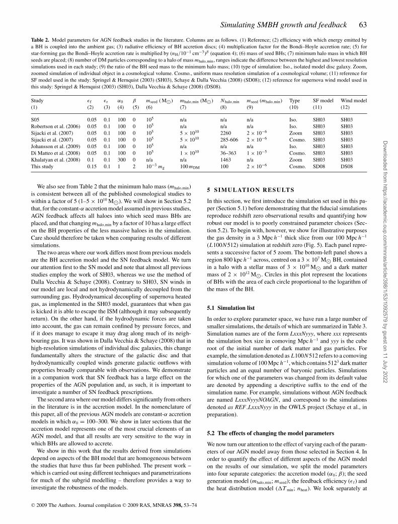
Table 2. Model parameters for AGN feedback studies in the literature. Columns are as follows. (1) Reference; (2) efficiency with which energy emitted bya BH is coupled into the ambient gas; (3) radiative efficiency of BH accretion discs; (4) multiplication factor for the Bondi–Hoyle accretion rate; (5) forstar-forming gas the Bondi–Hoyle accretion rate is multiplied by (nH/10−1 cm−3)β (equation 4); (6) mass of seed BHs; (7) minimum halo mass in which BHseeds are placed; (8) number of DM particles corresponding to a halo of mass mhalo,min, ranges indicate the difference between the highest and lowest resolutionsimulations used in each study; (9) the ratio of the BH seed mass to the minimum halo mass; (10) type of simulation: Iso., isolated model disc galaxy. Zoom,zoomed simulation of individual object in a cosmological volume. Cosmo., uniform mass resolution simulation of a cosmological volume; (11) reference forSF model used in the study: Springel & Hernquist (2003) (SH03), Schaye & Dalla Vecchia (2008) (SD08); (12) reference for supernova wind model used inthis study: Springel & Hernquist (2003) (SH03), Dalla Vecchia & Schaye (2008) (DS08).

Study εf εr α0 β mseed ( M�) mhalo,min (M�) Nhalo,min mseed (mhalo,min) Type SF model Wind model(1) (2) (3) (4) (5) (6) (7) (8) (9) (10) (11) (12)

S05 0.05 0.1 100 0 105 n/a n/a n/a Iso. SH03 SH03Robertson et al. (2006) 0.05 0.1 100 0 105 n/a n/a n/a Iso. SH03 SH03Sijacki et al. (2007) 0.05 0.1 100 0 105 5 × 1010 2260 2 × 10−6 Zoom SH03 SH03Sijacki et al. (2007) 0.05 0.1 100 0 105 5 × 1010 285-606 2 × 10−6 Cosmo. SH03 SH03Johansson et al. (2009) 0.05 0.1 100 0 105 n/a n/a n/a Iso. SH03 SH03Di Matteo et al. (2008) 0.05 0.1 100 0 105 1 × 1010 36–363 1 × 10−5 Cosmo. SH03 SH03Khalatyan et al. (2008) 0.1 0.1 300 0 n/a n/a 1463 n/a Zoom SH03 SH03This study 0.15 0.1 1 2 10−3 mg 100 mDM 100 2 × 10−6 Cosmo. SD08 DS08

We also see from Table 2 that the minimum halo mass (mhalo,min)is consistent between all of the published cosmological studies towithin a factor of 5 (1–5 × 1010 M�). We will show in Section 5.2that, for the constant-α accretion model assumed in previous studies,AGN feedback affects all haloes into which seed mass BHs areplaced, and that changing mhalo,min by a factor of 10 has a large effecton the BH properties of the less massive haloes in the simulation.Care should therefore be taken when comparing results of differentsimulations.

The two areas where our work differs most from previous modelsare the BH accretion model and the SN feedback model. We turnour attention first to the SN model and note that almost all previousstudies employ the work of SH03, whereas we use the method ofDalla Vecchia & Schaye (2008). Contrary to SH03, SN winds inour model are local and not hydrodynamically decoupled from thesurrounding gas. Hydrodynamical decoupling of supernova heatedgas, as implemented in the SH03 model, guarantees that when gasis kicked it is able to escape the ISM (although it may subsequentlyreturn). On the other hand, if the hydrodynamic forces are takeninto account, the gas can remain confined by pressure forces, andif it does manage to escape it may drag along much of its neigh-bouring gas. It was shown in Dalla Vecchia & Schaye (2008) that inhigh-resolution simulations of individual disc galaxies, this changefundamentally alters the structure of the galactic disc and thathydrodynamically coupled winds generate galactic outflows withproperties broadly comparable with observations. We demonstratein a companion work that SN feedback has a large effect on theproperties of the AGN population and, as such, it is important toinvestigate a number of SN feedback prescriptions.

The second area where our model differs significantly from othersin the literature is in the accretion model. In the nomenclature ofthis paper, all of the previous AGN models are constant-α accretionmodels in which α0 = 100–300. We show in later sections that theaccretion model represents one of the most crucial elements of anAGN model, and that all results are very sensitive to the way inwhich BHs are allowed to accrete.

We show in this work that the results derived from simulationsdepend on aspects of the BH model that are homogeneous betweenthe studies that have thus far been published. The present work –which is carried out using different techniques and parametrizationsfor much of the subgrid modelling – therefore provides a way toinvestigate the robustness of the models.

5 SI MULATI ON R ESULTS

In this section, we first introduce the simulation set used in this pa-per (Section 5.1) before demonstrating that the fiducial simulationsreproduce redshift zero observational results and quantifying howrobust our model is to poorly constrained parameter choices (Sec-tion 5.2). To begin with, however, we show for illustrative purposesthe gas density in a 3 Mpc h−1 thick slice from our 100 Mpc h−1

(L100N512) simulation at redshift zero (Fig. 5). Each panel repre-sents a successive factor of 5 zoom. The bottom-left panel shows aregion 800 kpc h−1 across, centred on a 3 × 107 M� BH, containedin a halo with a stellar mass of 3 × 1010 M� and a dark mattermass of 2 × 1012 M�. Circles in this plot represent the locationsof BHs with the area of each circle proportional to the logarithm ofthe mass of the BH.

5.1 Simulation list

In order to explore parameter space, we have run a large number ofsmaller simulations, the details of which are summarized in Table 3.Simulation names are of the form LxxxNyyy, where xxx representsthe simulation box size in comoving Mpc h−1 and yyy is the cuberoot of the initial number of dark matter and gas particles. Forexample, the simulation denoted as L100N512 refers to a comovingsimulation volume of 100 Mpc h−1, which contains 5123 dark matterparticles and an equal number of baryonic particles. Simulationsfor which one of the parameters was changed from its default valueare denoted by appending a descriptive suffix to the end of thesimulation name. For example, simulations without AGN feedbackare named LxxxNyyyNOAGN, and correspond to the simulationsdenoted as REF LxxxNyyy in the OWLS project (Schaye et al., inpreparation).

5.2 The effects of changing the model parameters

We now turn our attention to the effect of varying each of the param-eters of our AGN model away from those selected in Section 4. Inorder to quantify the effect of different aspects of the AGN modelon the results of our simulation, we split the model parametersinto four separate categories: the accretion model (α0; β); the seedgeneration model (mhalo,min; mseed); the feedback efficiency (εf ) andthe heat distribution model (T min; nheat). We look separately at


Dow


ic.oup.com/m



Figure 5. Successively zoomed projections of the gas density in a 3 Mpc h−1 thick slice from our L100N512 simulation at redshift zero. BHs are representedin this plot by open circles and the area of each circle is proportional to the logarithm of the BH mass. The largest circle in the lower-left panel represents a BHof mass 3 × 107 M�.

the effects of changes in each of these parameter sets, and addi-tionally consider two purely numerical effects: the simulation massresolution and box size. For each set of simulations, we make fourdiagnostic plots: in Fig. 6, we show the cosmic SFR density as afunction of redshift; Fig. 7 shows the evolution of the global BHdensity, and the cumulative BH density present in seed-mass BHs(grey curves); Fig. 8 shows the redshift zero mBH–M∗ and mBH–σ

relations. We associate BHs with gravitationally bound objects byidentifying bound substructures in the simulation using the algo-rithm SUBFIND (Springel et al. 2001b; Dolag et al. 2008). We notethat in this plot we show total halo stellar mass as a function ofBH mass, as opposed to the observations, where only the bulgestellar mass is calculated. This means that all curves can be shiftedslightly to the left. Finally, Fig. 9 shows the median-specific SFR(SSFR) in bins of stellar mass. In this plot, the grey lines repre-sent results from simulations that do not include AGN feedback. InFigs 8 and 9, the vertical lines represent the halo stellar masses with50 per cent and 90 per cent of haloes containing BHs massiveenough to have performed at least one heating event. It is immedi-ately clear from Fig. 8 that the mBH–σ relation is much more robustto changes in parameters than the mBH–M∗ relation.

Each set of simulations is compared to our fiducial simulation(L050N256), which uses the model parameters that were justifiedin Section 4. To aid comparison between the different simulation

sets, the fiducial simulation appears in every plot as a solid, blackcurve. Details of all the simulations discussed in this section appearin Table 3. We now discuss each simulation set in turn.

5.2.1 The effect of box size and mass resolution

We consider first the effect of changing the box size at a con-stant resolution by comparing models L100N512, L050N256 andL025N128. The size of the simulation box has a negligible effect onboth the SFR density (Fig. 6a) and, for z < 4, on the global massof BHs (Fig. 7a). Because the properties of individual BHs are setby local physical processes, increasing the box size does nothing tothe scaling relations (Fig. 8a), except for allowing us to probe themass function up to larger halo masses. The same holds true for theSSFRs of individual objects (Fig. 9a).

We now assess the impact of numerical resolution on our results.We compare simulations at three different resolutions (L100N512,L100N256 and L100N128), both with and without AGN feedback.Simulation L100N128 has a dark matter particle mass of 3.54 ×1010 M�, a factor of 64 worse than that used in L050N256, ourlowest resolution production simulation.

We concentrate first on the SF history in these simulations(Fig. 6b). At high redshift (z > 4), the SFR is governed by


Dow


ic.oup.com/m



Table 3. Summary of simulation parameters. Columns are as follows. (1) Name of simulation; (2) comoving box size; (3) number of DM and gas particles; (4)final redshift; (5) multiplication factor for the Bondi–Hoyle accretion rate (equation 1); (6) for star-forming gas the Bondi–Hoyle accretion rate is multipliedby (nH/10−1 cm−3)β (equation 4); (7) fraction of radiated energy that is coupled back into the ISM (equation 6); (8) initial mass of subgrid BH; (9) minimumhalo mass into which a seed BH is placed; (10) minimum AGN heating temperature difference; (11) number of particles heated per event. Entries in boldrepresent parameters that have been changed from the value they take in the default model.

Identifier L (Mpc h−1) Ngas zend α0 β εf mseed(mg) mhalo,min(mDM) T heat(108 K) nheat

(1) (2) (3) (4) (5) (6) (7) (8) (9) (10) (11)

Simulations for parameter studiesL050N256 50.0 2563 0 1 2 0.15 0.001 100 1 1L050N256VLOEPS 50.0 2563 0 1 2 0.0375 0.001 100 1 1L050N256LOEPS 50.0 2563 0 1 2 0.075 0.001 100 1 1L050N256HIEPS 50.0 2563 0 1 2 0.3 0.001 100 1 1L050N256VHIEPS 50.0 2563 0 1 2 0.6 0.001 100 1 1L050N256HIHALO 50.0 2563 0 1 2 0.15 0.001 1000 1 1L050N256HISEED 50.0 2563 0 1 2 0.15 0.01 100 1 1L050N256LOSEED 50.0 2563 0 1 2 0.15 0.0001 100 1 1L050N256HINHEAT 50.0 2563 0 1 2 0.15 0.001 100 1 10L050N256B0 50.0 2563 0 1 0 0.15 0.001 100 1 1L050N256B1 50.0 2563 0 1 1 0.15 0.001 100 1 1L050N256B4 50.0 2563 0 1 4 0.15 0.001 100 1 1L050N256A100B0 50.0 2563 0 100 0 0.15 0.001 100 1 1L050N256A1000B0 50.0 2563 0 1000 0 0.15 0.001 100 1 1L050N256T7 50.0 2563 0 1 2 0.15 0.001 100 0.1 1L050N256NOAGN 50.0 2563 0 – – – – – – –

Simulations for box size and resolution testsL100N128 100.0 1283 0 1 2 0.15 0.001 100 1 1L100N128NOAGN 100.0 1283 0 – – – – – – –L100N256 100.0 2563 0 1 2 0.15 0.001 100 1 1L100N256NOAGN 100.0 2563 0 – – – – – – –L100N512 100.0 5123 0 1 2 0.15 0.001 100 1 1L100N512NOAGN 100.0 5123 0 – – – – – – –L025N128 25.0 1283 0 1 2 0.15 0.001 100 1 1

numerical resolution. At low redshift (z < 2), the two highest reso-lution simulations (L100N512 and L100N256) have SFRs that differby ∼0.2 dex, indicating that this quantity is not yet fully resolved.We see by comparing simulations with and without AGN that thefactor by which AGN feedback decreases the global SFR is the samein both simulations. However, in the lowest resolution simulation(L100N128; blue, dashed line), the AGN are largely ineffective atdecreasing the global SFR.

We now turn our attention to the BH properties. The z < 1 inte-grated BH density (Fig. 7b) is virtually indistinguishable betweenruns L100N512 and L100N256. This occurs because the global BHdensity is dominated by the massive BHs, which are well resolvedin both simulations. L100N128 underpredicts the redshift zero BHdensity by a factor of 2. This is due to two reasons. First, in thissimulation seed mass BHs are placed only in objects with masseslarger than 3.54 × 1012 M�, which means that we neglect a largepopulation of important BHs. Secondly, we see that the first BHsin this simulation start growing only at low redshift (z ≈ 4), and,as such, may not have had enough time to grow on to the observedBH scaling relations.

This picture is borne out by the properties of individual BHs.Fig. 8(b) shows that for σ > 100 km s−1 the BH properties are wellconverged, whereas at the lower mass end of the scaling relationsthe resolution becomes important. The lowest resolution simulationunderpredicts the BH scaling relations at all masses.

If we now examine the SSFRs of individual objects(Fig. 9b), looking first at simulations that do not contain AGN(L100N512NOAGN and L100N256NOAGN; grey, dotted and solid

lines, respectively), we see that the SSFR is almost converged abovea stellar mass of 1010.5 M�. If we now consider the effect of addingAGN feedback to these simulations, we see that the stellar massat which the simulations with and without AGN diverge from oneanother has not yet converged, indicating that results on the scaleof individual objects in these simulations may remain affected bynumerical resolution. We note that the redshift zero global SFR isaffected by resolution to a lesser degree than the SSFR. This islikely to be because the total galaxy stellar mass is an integral overall time of the galaxy SFRs, so the strong resolution effects at highredshift (Fig. 6b) persist in the redshift zero population.

We thus conclude that, because local processes govern the sizeof individual BHs, the simulation box size is unimportant when dis-cussing BH scaling relations. However, the limited simulation massresolution means that the stellar masses in our simulated galaxiesare not yet fully resolved. We also conclude that BH properties, suchas the integrated cosmic mass density and BH scaling relations, areconverged in all of our production simulations, but decreasing themass resolution by a factor of 64 places us in the regime whereno AGN properties are resolved. Therefore, we can conclude thatthe global results we present in this paper are robust to changesin numerical resolution, but that predictions involving the stellarproperties of individual objects should be treated with caution.

5.2.2 The seed model

Two parameters control the way that seed BHs are generated: theBH seed mass (mseed) and the halo mass above which BH seeds


Dow


ic.oup.com/m



Figure 6. The dependence of the global SF history on various sets of parameters. (a) The effect of changing the simulation volume at a constant resolution.(b) The effect of changing the resolution at a constant box size. (c) Simulations with different prescriptions for the generation of seed BHs (mhalo,min, mseed).(d) Simulations with different values of the heating efficiency (εf ). (e) The effect of changing the way in which AGN feedback energy is distributed to thesurrounding gas particles (T min, nheat). (f) The effect of changing the BH accretion model (α0, β). Curves in grey represent simulations that do not includeAGN feedback and the solid black curve in each panel represents the fiducial simulation (L050N256).

are inserted into haloes (mhalo,min). For the minimum halo mass,we chose to use a fixed number of particles, mhalo,min = 100 mDM,rather than a fixed halo mass because this ensures that BHs arealways placed into well-defined haloes, regardless of the numer-ical resolution. Consideration of the AGN feedback process thenallowed us to place a minimum value on the possible mass of BHseeds (10−3 mg) such that the average time between heating eventsfor a BH accreting at the Eddington rate is shorter than the Salpetertime, making it possible for the BH to regulate its growth. We alsonoted that the requirement that the total mass in seed mass BHsgenerated in a simulation is much lower than the observed redshiftzero cosmic BH density does not allow the seed mass to be muchlarger than the minimum possible value. We thus chose mseed =10−3 mg as our fiducial value. We now examine how changes inthese two parameters affect our results.

By comparing our base model (L050N256) to a simulation inwhich BH seeds are only placed into haloes that are 10 times moremassive (L050N256HIHALO; green dot–dashed curves), we cansay that most of our results are insensitive to the choice of mhalo,min.The global SFR density in the simulations (Fig. 6c) is virtually un-affected by changing mhalo,min from 102 mDM to 103 mDM, probablybecause the SFR of galaxies is only affected by AGN in the mostmassive haloes (M∗ � 1011 M�; Fig. 9). The cosmic BH densityis also insensitive to mhalo,min. This follows because in the fiducialmodel, the cumulative seed BH mass makes up only ∼2 per cent ofthe redshift zero BH density, so removing some seeds has a negli-gible effect on the global density. We now turn our attention to theBH scaling relations (Fig. 8c), where we see that the BHs grow onto the observed scaling relations at a higher mass, but that for M∗ �1011 M� or σ > 100 km s−1 the results are almost identical to the


Dow


ic.oup.com/m



Figure 7. The dependence of the evolution of the cosmic BH density on the parameters of the AGN model. The panels are the same as in Fig. 6, the shadedgrey area represents the redshift zero BH density as measured by Shankar et al. (2004). The grey curves show the cumulative density in seed BHs. The solid,black curve in each panel represents the fiducial simulation (L050N256).

fiducial simulation. These are the BHs that are energetically impor-tant, and we can therefore conclude that results derived from ourAGN simulations are insensitive to uncertainties in the minimumhalo mass that contains a BH.

Large changes in the mass of the seed BHs (L050N256HISEED,L050N256LOSEED) can lead to more significant changes in theglobal properties of the simulation. If the initial seed mass is loweredby a factor of 10, then by redshift zero the global BH densityis slightly greater than in the fiducial case (Fig. 7c). This occursbecause initially smaller BHs take longer to grow on to the BHscaling relations both because they need to grow more and becausethey grow more slowly (see Fig. 1). As a result of this, the galaxypotential well is deeper by the time that the BH begins to heatgas, and so it requires more energy input for the BH to stop itsown growth. Because it takes longer for AGN feedback to becomeeffective, the global SFR is higher (Fig. 6c). The same argument

can be made in reverse for high seed masses and explains whyincreasing the BH seed mass slightly decreases the global SFR(Fig. 6c). We can draw the same conclusions from examining theSSFR of individual objects (Fig. 9c). Changing the seed mass hasvirtually no effect on the SFR of the most massive objects, andonly affects haloes near the threshold mass at which AGN feedbackbegins to become important.

The cumulative amount of seed BHs in the simulationL050N256HISEED is within a factor of 4 of the redshift zero BHdensity. Although this does not violate our constraint that the totalmass in seed BHs should be less than the observed redshift zerovalue, it is barely satisfied, and leaves very little room for AGN inour simulations to grow. Additionally, a large value for the initialseed mass means that we place seed BHs initially above the BHscaling relations (Fig. 8c). Nevertheless, they still grow on to thesame scaling relations.


Dow


ic.oup.com/m



Figure 8. The Magorrian relation and the mBH–σ relation for each set of simulations. Line styles and panels correspond to those in Fig. 6. The simulatedstellar velocity dispersion is calculated as the mean of the three one-dimensional velocity dispersions of the stellar particles in each halo. The pale, solid, greyline in each plot represents the redshift zero observations of Haring & Rix (2004) (left-hand panel) and Tremaine et al. (2002) (right-hand panel). The solid,black curve in each panel represents the fiducial simulation (L050N256). The horizontal, triple-dot–dashed line indicates the mass that a BH requires to beginto heat its surroundings, and the horizontal grey, dashed line indicates the BH seed mass in the fiducial simulation. The two solid vertical lines show, for thefiducial simulation, the stellar mass above which 50 per cent and 90 per cent of haloes contain a BH massive enough to have performed at least one heatingevent.

We note that all our global results are a very weak function ofthe seed mass. For example, changing the seed mass by a factor of100 changes the global SFR by no more than a factor 2.5. Other un-certainties, particularly those introduced by our lack of knowledgeabout the way in which BHs accrete, lead to us conclude that thespecifics of the seed model are relatively unimportant.

5.2.3 The feedback efficiency

The efficiency with which a BH’s radiated energy is coupled to theambient gas, εf , is treated as a free parameter in our simulations. Weshow in this section that this parameter controls the normalization

of the total mass in BHs and of the BH scaling relations (see alsoDi Matteo et al. 2005). In our simulations εf was tuned to match thez = 0 mBH − mhalo relation and the redshift zero cosmic BH density.A value of εf = 0.15 was found to work well.

Changing εf from its fiducial value has no discernible effect onthe global SFR (Fig. 6d), or on the SSFRs of individual objects(Fig. 9d), but the total redshift zero BH density is inversely pro-portional to the feedback efficiency (Fig. 7d). Most strikingly, sim-ulations L050N256VHIEPS, L050N256HIEPS, L050N256LOEPS,and L050N256VLOEPS have values of εf that differ by factorsof 4, 2, 1/2, and 1/4 from the fiducial run, and the ratio of theirz = 0 BH densities to that of the fiducial simulation are 0.24, 0.53,


Dow


ic.oup.com/m



Figure 9. The median SSFR as a function of galaxy stellar mass for each set of simulations. Line styles and panels correspond to those in Fig. 6. The pale,grey curve in each plot represents the SSFR as measured in the simulation without AGN feedback (L050N256NOAGN). The solid black curve in each panelrepresents the fiducial simulation (L050N256). The upturn in galaxy SSFR in the simulations without AGN feedback at M∗ ≈ 3 × 1010 M� is due to SNfeedback becoming inefficient. The two vertical lines in each panel indicate, for the fiducial simulation, the stellar mass above which 50 per cent and 90 percent of haloes contain a BH massive enough to have performed at least one heating event.

1.93 and 4.03 respectively. The fact that the final mass of BHs isdirectly proportional to 1/εf implies that in our models any givenBH grows until it has injected a specific amount of energy per unithalo mass, at which point it is able to reduce its local density andto effectively self-regulate its growth. This remarkable result agreesqualitatively with the ideas presented in e.g. Fabian (1999) and Silk& Rees (1998), where BHs grow until they can expel gas from thegalaxy, at which point they enter a quiescent phase.

The redshift zero global BH density (Fig. 7d) and the normal-ization of the BH scaling relations (Fig. 8d) are both directly pro-portional to 1/εf , and so we can use these observations to constrainthe value of εf that allows our model to be consistent with redshiftzero observations. We employ a value of εf = 0.15 in the presentstudy, but note that we will show elsewhere that the parameters of

the AGN model must be tuned in conjunction with the SN feedbackprescription.

5.2.4 The heating mechanism

The resolution of cosmological simulations is too poor to resolvethe scales on which AGN inject energy into the ISM and as such weare forced to make some assumptions. It is therefore important toverify that the results obtained from our simulations do not dependstrongly on the implementation of the energy coupling mechanism.

Two parameters control how energy is distributed from the AGNto its surroundings: the minimum temperature increase and the num-ber of neighbouring SPH particles to heat (T min = 108 K andnheat = 1). The fiducial value of the minimum temperature increase


Dow


ic.oup.com/m



was constrained by two competing effects. First, if T min is toolow, the cooling time of heated gas will be so short that the gaswill be able to radiate away its energy before having a dynamicaleffect. On the other hand, if T min is set too high, then the amountof energy needed to perform a heating event will be so high that thenumerically determined time between heating events exceeds theSalpeter time-scale, making it impossible for the BH to regulate itsgrowth. We found that T min = 108 K provides a good compromisebetween these two effects. Similarly, to minimize the numericallycontrolled duty cycle we set nheat = 1 in our fiducial models. Herewe assess the impact of distributing feedback energy in differentways.

If we change either the temperature to which gas is heated from108 K to 107 K (L050N256T7) or the number of BH neighbours af-fected by each feedback event from 1 to 10 (L050N256HINHEAT),we see small changes in the cosmic SF history (Fig. 6e) and inthe cosmic BH density (Fig. 7e). We note, however, that the resultsare relatively insensitive to these parameters, and that changing thevalue of either T min or nheat by an order of magnitude affects bothBH properties and SFRs by only ∼0.3 dex. We thus conclude thatas long as the feedback efficiency (εf ) is calibrated such that theredshift zero BH relations are satisfied, and that the minimum heat-ing temperature is sufficient for feedback to be effective, our otherresults are robust to the precise way in which this energy is coupledto the ISM.

5.2.5 The accretion model

Because numerical simulations cannot resolve the properties of themultiphase ISM, we can justify the use of high values for the mul-tiplicative factor, α, in the Bondi–Hoyle accretion rate (see equa-tion 1), at least for high density gas (Section 4). This provides amotivation for the constant-α accretion model – similar to thosepreviously published – where BHs accrete with a very high effi-ciency. In this paper we have introduced a new class of models thattreat accretion of low-density gas differently. By noting that theISM will not contain a cold (T � 104 K) phase at low pressures andthat we are also able to resolve Bondi–Hoyle accretion on to BHswith masses greater than the resolution limit of our simulation ifwe resolve the Jeans mass, we argue that α must asymptote to unityin low density environments. We then parametrize our ignoranceabout the state of the multiphase ISM, and the precise mechanismby which AGN accrete by introducing a parameter, β, that describesa power-law dependence of the accretion rate on the local gas den-sity (equation 4).

The growth of a BH depends upon the accretion model used. Inthe constant-α model (Bondi–Hoyle with α0 = 100) the growth isEddington limited unless the gas in the immediate surroundings ofthe BH has a density that is much lower than typical of the ISM,e.g. as a result of feedback from the BH. In the constant-β models,however, much larger densities are required for the accretion rateto become Eddington limited. Efficient growth is only possible ifthe BH’s local density is enhanced by dynamical processes. BHscan only decrease their accretion rate (and hence regulate their owngrowth) when densities are low enough that accretion rates are nolonger Eddington limited. The density at which BH accretion ratesbecome Eddington limited depends on the accretion model (Fig. 2).In the constant-α model with α0 = 100 BHs self-regulate at densitiesbelow the density at which a multiphase medium is expected toform (Fig. 2), this has a large effect on the physical properties of thegalaxy and because the simulations resolve Bondi–Hoyle accretion

in this regime it invalidates the assumptions used to justify the useof α0 = 100 in the first place.

We now consider how changes in the accretion model affect theproperties of the simulated galaxy population. Increasing β from 2to 4 (simulation L050N256B4) depresses the global SFR somewhat(Fig. 6f) because the β parameter controls the gas density at whichthe accretion rate for a given BH mass becomes Eddington limited(Fig. 2). Hence, for a given value of β there is a critical valueof the local gas density above which a BH can ‘switch on’ andbegin to grow rapidly. For larger values of β this occurs at a lowerdensity, and hence in smaller haloes. This manifests itself in the BHscaling relations by changing the minimum galaxy mass at whichthe BHs grow on to the observed scaling relations. A lower valueof β therefore increases the global SFR by allowing BHs to growonly in more massive haloes. Increasing β above 4 does not have alarge effect on any of our results, as for any large value of β, the BHaccretion model behaves in such a way as to be Eddington limited instar-forming gas (Fig. 2), and the difference in behaviour betweena β = 4 model and a β = ∞ model is very small. Any physicalprocess that is strongly dependent on the local density is affected bynumerical resolution, because higher resolution simulations allowthe formation of higher density regions. For this reason, we cautionthat the stellar mass at which BHs grow on to the observed relationis affected by numerical resolution, and so the value of β may needto be tuned to different values for simulations with mass resolutionssignificantly different to those presented here.

A comparison of the effect of different β models on the SSFR ofhaloes (Fig. 9f) supports this picture. The stellar mass above whichthe behaviour of each AGN model diverges from the behaviour ofthe simulation without AGN depends upon the value of β.

In the constant-α model with α0 = 100 (L050N256A100B0),BHs grow in an Eddington-limited manner from their birth, and assuch suppress SF in all haloes that contain a BH. This is visiblein Fig. 9(f), in which the constant-α simulation deviates from thesimulation without AGN in haloes with a low stellar mass. Theconstant-α simulations efficiently suppress SF in every halo thatcontains a BH, and as such the integrated SFR is more than an orderof magnitude lower than in the other simulations. The same effectis present in the large simulation volume, but is less pronouncedbecause seed mass BHs are placed only into larger haloes, whereboth accretion models are capable of suppressing SF. This resultimplies that in order for a simulation that employs a constant-α ac-cretion model to reproduce the observed break in galaxy propertiesat log (M∗) ∼ 10.5 (e.g. Kauffmann et al. 2003), the resolution mustbe tuned such that BH seeds are placed into haloes of the correctsize.9

Considering now reducing the value of α0 in the constant-α mod-els from 100 to 1 (L050N256A100B0 compared to L050N256B0; aconstant-β model with β = 0 is equivalent to a constant-α modelwith α0 = 1), equivalent to removing the numerical ‘fudge factor’from the BH accretion rates, we see that BHs are unable to grow inall but the very most massive haloes (Fig. 8f), and so the halo SSFRsare virtually the same as for the simulation without AGN feedbackin all haloes up to a stellar mass of 1012 M� (Fig. 9f). This, in turn,means that the global SFR density in the α0 = 1 simulation is very

9 Because the accretion rate also depends on the assumed effective EOS, thismay not be true for all constant-α models used in the literature. In the modelsof S05, which employ an EOS that is initially stiffer than our γ eff = 4/3, theBH growth time has a local minimum at nH = n∗

H which suppresses AGNgrowth relative to our constant-α model (Springel, private communication).


Dow


ic.oup.com/m



similar to that in the simulation run without AGN (Fig. 6f). Theglobal BH density at redshift zero is actually higher than that in thefiducial simulation (Fig. 7f). This occurs because the BHs that dogrow in the α0 = 1 simulation grow very late, and so find themselvesin a deeper potential well. In order to self-regulate, they then needto output more energy and hence grow even more than in the othersimulations. The global BH density is therefore by itself not a goodindicator of how efficiently AGN are able to suppress SF.

We now consider increasing α0 by an order of magnituderelative to the usual value (L050N256A1000B0 compared toL050N256A100B0). We already know that the density below whichBHs can self-regulate depends strongly on the value of α0 (Fig. 2),and it follows that the value of α0 will have a strong effect onthe physical conditions in the centres of haloes. In the case of α0 =1000, the global BH density is similar to the α0 = 100 case (Fig. 7f),whereas the global SFR and galaxy SSFRs are much lower than inany other simulation (Fig. 6f and Fig. 9f), and the mBH–mstellar

relation is shifted significantly to the left as the BHs effectivelyshut down SF in all haloes. However, the mBH–σ relation is not asstrongly affected by the very effective AGN feedback. This is likelydue to the fact that the stellar velocity dispersion tracks the depth ofthe galaxy potential well, which contains a large contribution fromdark matter, whereas the galaxy stellar mass is sensitive to the de-tails of the feedback processes operating inside the galaxy. We seethat changing the value of the free parameter α0 can have profoundeffects on the simulated galaxy population, even if the evolution inthe global mass density of BHs is barely affected by the parameterchange.

We conclude this section by noting that predictions from AGNfeedback models of this type are sensitive to the accretion modelthat is used. More generally, it is not clear that the Bondi–Hoylerate is the correct accretion rate to use in the case of a BH accretingfrom a hot halo (Krumholz, McKee & Klein 2006). We find thata different parametrization of the accretion rate leads to profounddifferences in the SF histories and speed of BH growth and thereforecaution the reader that the AGN accretion mechanism represents asignificant source of uncertainty in all our results.

6 D I S C U S S I O N A N D C O N C L U S I O N S

We have presented and tested a method to incorporate SMBHsinto cosmological, smoothed particle hydrodynamics simulations.The method, which is a substantially modified version of the oneintroduced by S05, self-consistently describes the mass growth ofBHs and feedback from AGN. Here, we consider growth throughmergers with other BHs as well as through accretion of gas. TheAGN feedback in our model is thermal and local to the BH.

Although we also use the SPH code GADGET III, our code differsfrom that of S05 in many ways, including the use of different modelsfor SF, feedback from SN, radiative cooling and stellar evolution.Particularly relevant for AGN feedback is the fact that, contrary toS05, we do not make use of a subgrid model to describe the differentphases of the ISM. Following S05, we make use of subgrid BHsto allow BH masses to be small compared with the masses of theparticles containing the BHs. We note, however, that while thisapproach allows one to significantly extend the range of BH massesin the simulation, the accretion radius will only be resolved if the BHmass exceeds the local Jeans mass. Unfortunately, this is generallynot the case if the BH mass is small compared with the particlemass.

The AGN model is specified by seven main parameters (Table 1).Two parameters describe the BH seed generation mechanism: the

BH seed mass, mseed, and the halo mass into which seed BHs areplaced, mhalo,min. Two parameters describe the amount of energy thatis coupled back to the ISM per unit accreted mass: εr, the radiativeefficiency of a BH accretion disc, is the fraction of the rest-massenergy accreted by the BH that is radiated by the AGN and εf is thefraction of the radiated energy that is coupled thermally to the ISM.For a given BH accretion rate, the rate at which energy is injectedinto the ISM depends only on the product εrεf . However, we doneed to specify the radiative efficiency εr since the mass growthof the BH is proportional to (1 − εr). A further two parameterscontrol the numerical implementation of the injection of energyinto the ISM by AGN: the number of neighbouring gas particlesheated by each BH heating event, nheat, and the minimum amountby which their temperature is increased, T min. Because we letBHs store feedback energy until they have saved enough to heatnheat particles by T min degrees kelvin, these last two parameterstogether determine the AGN duty cycle for a fixed accretion rate.Finally, we require one additional parameter that controls how BHsaccrete gas, and we describe two different models for this process.

The gas accretion rate is assumed to scale as the Bondi–Hoyleaccretion rate, evaluated at the location of the BH and on the scalesresolved by the simulation. We do not, however, allow the accretionrate to exceed the Eddington rate. The Bondi–Hoyle accretion ratepredicted by the simulation will underestimate the true rate if thedensity is underestimated or if the temperature is overestimated. Alack of numerical resolution may result in an underestimate of thegas density, which motivated S05 to multiply the Bondi–Hoyle ratepredicted by the simulation by a constant factor α0 = 100. We callmodels of this type constant-α models. We noted that cosmologicalsimulations lack not only the resolution, but also the physics tomodel the cold ISM phase. For example, our simulations use apolytropic effective EOS for densities at which the gas is expectedto be multiphase. Hence, they will miss the cold component forwhich the Bondi–Hoyle accretion rate would be highest. This willlead us to strongly underestimate the Bondi–Hoyle rate in high-density gas.

Although cosmological simulations cannot yet resolve cold, in-terstellar gas, many do resolve the Jeans scales at densities lowenough for the ambient ultraviolet radiation to suppress coolingbelow 104 K. Specifically, any simulation that resolves the Jeansscales in the gas surrounding a BH particle will also resolve theBondi–Hoyle radius if the BH mass exceeds the local Jeans mass.Hence, at sufficiently low densities the Bondi–Hoyle accretion rateis modelled correctly and multiplying it by α0 = 100 would resultin a large overestimate of the accretion rate.

We therefore introduced a second class of models in which theBondi–Hoyle accretion rate is multiplied by a factor (nH/n∗

H)β fordensities nH > n∗

H, where n∗H is the density above which the gas is

expected to be multiphase (we take n∗H = 0.1 cm−3). We refer to

this class of models as constant-β models. Note that both constant-α and constant-β models use a single free parameter. Because wehave changed the density-dependence of the accretion rate, we can-not claim to be simulating Bondi–Hoyle accretion, even thoughthe changes are motivated by the Bondi–Hoyle formula and eventhough we do retain the Bondi–Hoyle scaling with the BH mass.We argued, however, that this is also true for constant-α modelsbecause the use of values α0 1 implies that the densities andtemperatures predicted by the simulations are greatly in error.

The parameters α0 and β, used in the constant-α and constant-βmodels, respectively, control the ambient gas density at which theBH accretion rate becomes Eddington limited (Fig. 2). Because themaximum densities sampled by the simulation increase with halo


Dow


ic.oup.com/m



mass (both because more massive haloes are resolved with moreparticles and because the central pressure increases with the depth ofthe potential), these parameters effectively set the halo mass abovewhich BHs can grow efficiently. We set β = 2, which we find resultsin efficient BH growth in haloes with stellar masses � 1010.5 M� inthese simulations. Using a constant-α prescription with α0 = 100implies that, in the absence of AGN feedback, the accretion rateis essentially always Eddington limited. Because the accretion isefficient even at relatively low gas densities, AGN feedback is inthat case important in all haloes that exceed mhalo,min. For this classof models, the halo mass above which AGN can suppress SF is thusin effect a free parameter (mhalo,min). For BHs with masses greaterthan 106 M�, self-regulation can only occur at densities ordersof magnitude below the SF threshold (Fig. 2). In this regime, weresolve Bondi–Hoyle accretion, invalidating the assumption usedto justify large values of α in the first place. Constant-α modelstherefore underestimate the gas density required for self-regulationand will thus overestimate the suppression of the SFR.

Having chosen a prescription for gas accretion, we then derivevalues for the other model parameters. Because each BH stores itsfeedback energy until it suffices to heat nheat neighbours by T min,we are faced with a numerically determined duty cycle (for a givenaccretion rate). In order for the BH to be able to regulate its growth,we require the time between heating events, theat ∝ nheatT min,to be as small as possible and certainly smaller than the Salpetertime if the accretion is Eddington limited. We use T min = 108 K,which ensures the temperature of the heated gas is high enough thatthe injected thermal energy is not just radiated away, and nheat = 1,which minimizes theat. Because theat decreases with the ratio ofthe mass of the BH to that of the heated gas particle, the require-ment that theat is smaller than the Salpeter time for Eddington-limited accretion implies that the (subgrid) BH mass must exceed0.1 per cent of the gas particle mass (Fig. 3). Hence, we setmseed = 10−3 mg. We set mhalo,min = 100 mDM in order to ensurethat seed BHs are placed only into well-defined haloes. These pa-rameter values will obviously need to be increased if they resultin seed and/or minimum halo masses that are lower than expectedphysically, as may be the case for simulations that use a much higherresolution than is used here.

We assume the standard value εr = 0.1 for the radiative efficiencyand tune εf to match the redshift zero mBH–mhalo relation and cosmicBH density. A value of εf = 0.15 was found to provide a good matchto the observations.

Having specified the AGN model, we then analysed the resultsfrom a large suite of cosmological simulations chosen to investigatethe sensitivity of the predictions on the model parameters. For thispurpose, we compared the predictions for the cosmic SF history, thecosmic BH density, the redshift zero BH scaling relations (both theMBH–M∗ and the MBH–σ relations) and the redshift zero galaxy-specific star formation rates (SSFRs).

We demonstrated that the fiducial model provides good agree-ment with both the observed mass density in BHs (Fig. 7) and theBH scaling relations (Fig. 8), and that the inclusion of AGN feed-back in the simulations effectively suppresses SF in galaxies withstellar masses greater than >1010.5 M� (Fig. 9). We will discussthe comparison between the simulated global SFR density and ob-servations elsewhere, but for now we note that the SN feedbackparameters of our models were tuned such that a simulation withoutAGN feedback has a peak SFR density that is in good agreementwith observations. As such, adding an extra source of feedback en-ergy inevitably results in an underestimate of the SFR density. Inorder to achieve a good match with observations, the properties of

the SN model must be tuned in conjunction with those of the AGNmodel.

However, the focus of our study was not to match observations,but to explore the dependence of the results on the parameters ofthe model. Our main conclusions are summarized below.

(i) Regardless of whether BH seeds are initially placed above orbelow the BH scaling relations, they grow on to the same relations.

(ii) Because the global BH density is dominated by massive BHsand because AGN feedback is only important in high-mass haloes,uncertainties in the seed model employed do not lead to significantchanges to the global properties of our simulations. Changing theinitial seed mass by two orders of magnitude changes the globalSFR by only a factor of 2.5. The assumed seed generation modelcan, however, affect galaxy properties at around the galaxy masswhere AGN first begin to become energetically important. At highermasses, galaxy properties are largely insensitive to the initial distri-bution of BH seeds.

(iii) As discussed more comprehensively in Booth & Schaye(2009), the normalization of both the global BH density and the BHscaling relations is nearly exactly inversely proportional to the AGNfeedback efficiency, εrεf . Most strikingly, changing the efficiencyby a factor of 16 does not give rise to any discernible changes inthe global SF history. These results imply that the total amount ofthermal energy injected by AGN is conserved when the feedbackefficiency is changed. These results can be explained if BHs growuntil they have generated enough energy to regulate the accretionrate and if the required amount of energy depends on the depth ofthe potential well on scales that are larger than the radius on whichthe BH dominates.

(iv) Changing the way in which the thermal energy from theAGN is distributed in the gas surrounding the BH has little effecton our results, as long as the gas is heated to a temperature that ishigh enough for its cooling time to become long. Hence, thermalfeedback can be efficient in cosmological simulations that do notresolve the multiphase ISM.

(v) Cosmological simulations currently underestimate theBondi–Hoyle accretion rate in dense gas because they lack boththe resolution and the physics to model the dense, cold phase of theISM. It is therefore necessary to increase the predicted accretion rateby a fudge factor, either by explicitly multiplying the accretion rateby a numerical correction factor or by employing a subgrid modelfor the unresolved gas physics to artificially boost accretion rates instar-forming gas. Using a multiplicative factor that asymptotes tounity in the regime where the simulation is able to model the relevantphysics (our constant-β model) gives different results from using ahigh factor throughout (the constant-α model) as has been used inmost previous work. In general, the density above which BHs areable to accrete efficiently depends upon the accretion model used(Fig. 1). Because higher mass haloes contain higher density gas, theaccretion model determines the halo mass above which AGN feed-back becomes effective. Until the simulations are able to resolveBondi–Hoyle accretion in a multiphase ISM, the predictions of themodels will remain subject to significant uncertainty.

(vi) The mBH–σ relation is more robust than the mBH–M∗ relationto changes in the model parameters (Fig. 8), and so provides a testof the numerical model that is less affected by uncertainties innumerical parameters than the Magorrian relation. This is likelydue to the fact that the stellar velocity dispersion tracks the depthof the galaxy potential well, which contains a large contributionfrom dark matter, whereas the galaxy stellar mass is sensitive to thedetails of the feedback processes operating inside of the galaxy.


Dow


ic.oup.com/m



In summary, we have presented and tested a new model for theself-consistent growth of BHs and feedback from AGN in cosmo-logical simulations. In a future work, we will discuss the interactionbetween AGN feedback and other physical processes, and showthat the results obtained from an AGN model depend also on otherprocesses such as SN feedback and stellar mass loss.

AC K N OW L E D G M E N T S

We are very grateful to Volker Springel for generously providingus with a copy of his code. We would like to thank him as wellas Richard Bower, Ian McCarthy and the members of the OWLScollaboration for useful discussions. The simulations presented herewere run on the Cosmology Machine at the Institute for Compu-tational Cosmology in Durham as part of the Virgo Consortiumresearch programme, on Stella, the LOFAR BlueGene/L systemin Groningen, and on Huygens, the Dutch national supercomputer.This work was supported by Marie Curie Excellence Grant MEXT-CT-2004-014112 and by an NWO Vidi grant.

REFERENCES

Aller M. C., Richstone D., 2007, ApJ, 665, 120Arav N., Korista K. T., de Kool M., 2002, ApJ, 566, 699Arav N., Moe M., Costantini E., Korista K. T., Benn C., Ellison S., 2008,

ApJ, 681, 954Barnes J. E., Hernquist L. E., 1991, ApJ, 370, L65Barnes J. E., Hernquist L. E., 1996, ApJ, 471, 115Baugh C. M., 2006, Rep. Prog. Phys., 69, 3101Begelman M., Rees M. J., 1978, MNRAS, 185, 847Begelman M., Volonteri M., Rees M. J., 2006, MNRAS, 370, 289Benson A. J., Bower R. G., Frenk C. S., Lacey C. G., Baugh C. M., Cole S.,

2003, MNRAS, 599, 38Bhattacharya S., di Matteo T., Kosowsky A., 2008, MNRAS, 389, 34Bondi H., Hoyle F., 1944, MNRAS, 104, 273Bower R. G., Benson A. J., Malbon R., Helly J. C., Frenk C. S., Baugh

C. M., Cole S., Lacey C. G., 2006, MNRAS, 370, 645Boyle B. J., Terlevich R. J., 1998, MNRAS, 293, L49Bromm V., Loeb A., 2003, ApJ, 596, 34Bruzual G., Charlot S., 2003, MNRAS, 344, 1000Buff J., McCray R., 1974, ApJ, 189, 147Callegari S., Mayer L., Kazantzidis S., Colpi M., Governato F., Quinn T.,

Wadsley J., 2009, ApJ, 696, L89Cao X., Li F., 2008, MNRAS, 390, 561Cattaneo A., 2001, MNRAS, 324, 128Chelouche D., 2008, preprint (astro-ph/0812.3621)Ciotti L., Ostriker J. P., 2001, ApJ, 551, 131Colberg J. M., di Matteo T., 2008, MNRAS, 387, 1163Cowie L. L., Ostriker J. P., Stark A. A., 1978, ApJ, 226, 1041Croft R. A. C., Di Matteo T., Springel V., Hernquist L., 2008, preprint

(astro-ph/0803.4003)Croton D. J., 2006, MNRAS, 365, 11Dekel A., Silk J., 1986, ApJ, 303, 39Dalla Vecchia C., Schaye J., 2008, MNRAS, 387, 1431Davis M., Efstathiou G., Frenk C. S., White S. D. M., 1985, ApJ, 292,

371Diemand J., Kuhlen M., Madau P., 2007, ApJ, 667, 859Dijkstra M., Haiman Z., Mesinger A., Wyithe S., 2008, MNRAS, 391, 1961Di Matteo T., Springel V., Hernquist L., 2005, Nat, 433, 604Di Matteo T., Colberg J., Springel V., Hernquist L., 2008, ApJ, 676, 33Dolag K., Borgani S., Murante G., Springel V., 2008, MNRAS, in press

(arXiv:0808.3401)Edgar R., 2004, New Astron. Rev., 48, 843Efstathiou G., Rees M. J., 1998, MNRAS, 230, 5Elvis M., Risaliti G., Zamorani G., 2002, ApJ, 565, L75Fabbiano G., 2006, ARA&A, 44, 323

Fabian A. C., 1999, MNRAS, 308, L39Feoli A., Mele D., 2005, Int. J. Mod. Phys. D, 14, 1861Ferland G. J., Korista K. T., Verner D. A., Ferguson J. W., Kingdon J. B.,

Verner E. M., 1998, PASP, 110, 761Ferrarese L., 2002, ApJ, 578, 90Ferrarese L., Merritt D., 2000, ApJ, 539, L9Gebhardt K. et al., 2000, ApJ, 539, L13Gingold R. A., Monaghan J. J., 1977, MNRAS, 181, 375Graham A. W., 2008, ApJ, 680, 143Graham A. W., Driver S. P., 2007a, ApJ, 666, 77Graham A. W., Driver S. P., 2007b, MNRAS, 380, L15Granato G. L., De Zotti G., Silva L., Bressan A., Danese L., 2004, ApJ, 600,

580Haardt F., Madau P., 2001, in Neumann D. M., Tran J. T. V., eds, 21st

Moriond Astrophys. Meeting, Clusters of Galaxies and the High RedshiftUniverse Observed in X-rays. Editions Frontieres, Paris, p. 64

Haehnelt M. G., Rees M. J., 1993, MNRAS, 263, 168Haring N., Rix H. W., 2004, ApJ, 604, L89Hopkins P. F., Hernquist L., Cox T. J., Di Matteo T., Robertson B., Springel

V., 2006, ApJS, 163, 1Hopkins P. F., Hernquist L., Cox T. J., Robertson B., 2007, ApJ, 669, 67Hopkins P. F., Hernquist L., Cox T. J., Keres D., Stijn W., 2009, ApJ, 691,

1424Hoyle F., Lyttleton R. A., 1939, Proc. Camb. Philos. Soc., 35, 405Islam R. R., Tayloe J. E., Silk J., 2003, MNRAS, 340, 647Johansson P. H., Naab T., Burkert A., 2009, ApJ, 690, 802Kapferer W., Knapp A., Schindler S., Kimeswenger S., van Kampen E.,

2005, A&A, 438, 87Katz N., Weinberg D. H., Hernquist L., 1996, ApJS, 105, 19Kauffmann G., Haehnelt M., 2000, MNRAS, 311, 576Kauffmann G. et al., 2003, MNRAS, 346, 1055Kennicutt R. C., 1998, ApJ, 498, 541Khalatyan A., Cattaneo A., Schramm M., Gottloeber S., 2008, MNRAS,

387, 13Komatsu E. et al., 2009, ApJS, 180, 330Kormendy J., Richstone D., 1995, ARA&A, 33, 581Krumholz M. R., McKee C. F., Klein R. I., 2006, ApJ, 638, 369Lagos C. D. P., Cora S. A., Padilla N. D., 2008, MNRAS, 388, 587Laor A., 2001, ApJ, 553, 677Laor A., Fiore F., Elvis M., Wilkes B. J., 1997, ApJ, 477, 93Loeb A., Rasio F. A., 1994, ApJ, 432, 52Lucy L. B., 1977, AJ, 82, 1013Lynden-Bell D., 1969, Nat, 223, 690McLure R. J., Dunlop J. S., 2002, MNRAS, 331, 795Madau P., Rees M. J., 2001, ApJ, 551, L27Madau P., Ferguson H. C., Dickinson M. E., Giavalisco M., Steidel C. C.,

Fruchter A., 1996, MNRAS, 283, 1388Magorrian J. et al., 1998, AJ, 115, 2285Makino J., Funato Y., 2004, ApJ, 602, 93Marconi A., Hunt L. K., 2003, ApJ, 589, L21Marconi A., Risaliti G., Gilli R., Hunt L. K., Maiolino R., Salvati M., 2004,

MNRAS, 351, 169Merritt D., Ferrarrese L., 2001, ApJ, 547, 140Martinez-Sansigre A., Taylor A. M., 2009, ApJ, 692, 964Micic M., Holley-Bockelmann K., Sigurdsson S., Abel T., 2007, MNRAS,

380, 1533Mihos J. C., Hernquist L., 1994, ApJ, 425, L13Mihos J. C., Hernquist L., 1996, ApJ, 464, 641Monaghan J. J., 1992, ARA&A, 30, 543Murray N., Quataert E., Thompson T. A., 2005, ApJ, 618, 569Okamoto T., Nemmen R. S., Bower R. G., 2008, MNRAS, 385, 161Pelupessy F. I., Di Matteo T., Ciardi B., 2007, ApJ, 665, 107Pounds K. A., King A. R., Page K. L., O’Brien P. T., 2003, MNRAS, 346,

1025Reed D. S., Bower R., Frenk C. S., Jenkins A., 2006, MNRAS, 374, 2Robertson B., Hernquist L., Cox T. J., Di Matteo T., Hopkins P. F., Martini

P., Springel V., 2006, ApJ, 641, 90Salpeter E., 1964, ApJ, 140, 796


Dow


ic.oup.com/m



Schaye J., 2004, ApJ, 609, 667Schaye J., Dalla Vechia C., 2008, MNRAS, 383, 1210Schneider R., Ferrara A., Natarajan P., Omukai K., 2002, ApJ, 571, 30Shakura N. I., Syunyaev R. A., 1973, A&A, 24, 337Shankar F., Salucci P., Granato G. L., De Zotti G., Danese L., 2004, MNRAS,

354, 1020Sijacki D., Springel V., di Matteo T., Hernquist L., 2007, MNRAS, 380, 877Silk J., Rees M. J., 1998, AA, 31, L1Spergel D. N. et al., 2007, ApJS, 170, 377Springel V., 2005, MNRAS, 364, 1105Springel V., Hernquist L., 2003, MNRAS, 339, 289 (SH03)Springel V., Yoshida N., White S. D. M., 2001a, New. Astron., 6, 79Springel V., White S. D. M., Tormen G., Kauffmann G., 2001b, MNRAS,

328, 726Springel V., Di Matteo T., Hernquist L., 2005, MNRAS, 361, 776 (S05)

Thorne K., 1974, ApJ, 191, 507Toomre A., Toomre J., 1972, ApJ, 178, 623Tremaine S. et al., 2002, ApJ, 574, 740Volonteri M., Natarajan P., 2009, preprint (astro-ph/0903.2262)Wang J. M., Chen Y. M., Ho L. C., McLure R. J., 2006a, ApJ, 642, L111Wang J. M., Chen Y. M., Hu C., 2006b, ApJ, 637, L85Wiersma R. P. C., Schaye J., Smith B. D., 2009a, MNRAS, 393, 99Wiersma R. P. C., Schaye J., Theuns T., Dalla Vecchia C., Tornatore L.,

2009b, MNRAS, submitted (arXiv:0902.1535)Yu Q., Lu Y., 2008, ApJ, 689, 732Yu Q., Tremaine S., 2002, MNRAS, 335, 965

This paper has been typeset from a TEX/LATEX file prepared by the author.


Dow


ic.oup.com/m


Cosmological simulations of the growth of supermassive black ...

Documents

Transcript of Cosmological simulations of the growth of supermassive black ...