May 2014

Vacuum Energy Sequestering: The Framework and

Its Cosmological Consequences

Nemanja Kalopera,1 and Antonio Padillab,2

aDepartment of Physics, University of California, Davis, CA 95616, USA

bSchool of Physics and Astronomy, University of Nottingham, Nottingham NG7 2RD, UK

ABSTRACT

Recently we suggested a reformulation of General Relativity which completely sequestersfrom gravity all of the vacuum energy from a protected matter sector, assumed to containthe Standard Model. Here we elaborate further on the mechanism, presenting additionaldetails of how it cancels all loop corrections and renders all contributions from phase tran-sitions automatically small. We also consider cosmological consequences in more detail andshow that the mechanism is consistent with a variety of inflationary models that make auniverse big and old. We discuss in detail the underlying assumptions behind the dynamicsof our proposal, and elaborate on the relationship of the physical interpretation of divergentoperators in quantum field theory and the apparent ‘acausality’ which our mechanism seemsto entail, which we argue is completely harmless. It is merely a reflection of the fact that anyUV sensitive quantity in quantum field theory cannot be calculated from first principles, butis an input whose numerical value must be measured. We also note that since the universeshould be compact in spacetime, and so will collapse in the future, the current phase ofacceleration with wDE ≈ −1 is just a transient. This could be tested by future cosmologicalobservations.

1kaloper@physics.ucdavis.edu2antonio.padilla@nottingham.ac.uk

arX

iv:1

406.

0711

v3 [

hep-

th]

30

Oct

201

4

1 Introduction

Cosmological observations suggest that the cosmological constant is different from zero.Yet we have no clear and compelling argument which would explain the observed scale ofthe cosmological constant in quantum field theory (QFT). This fact is recognized underthe term “the cosmological constant problem” [1, 2, 3]. In a nutshell, the problem arisesbecause of the universality of gravity. The Equivalence Principle of General Relativity (GR),which controls how energy distorts geometry, posits that all forms of energy curve space-time. Since in QFT even the vacuum possesses energy density, given by the resummationof the QFT bubble diagrams, this means that the vacuum geometry generically must becurved. The scale of the curvature is Lvac ∼ (

√GNρvac)

−1. Cosmological observations thenconstrain it to be Lvac >∼ 1024 cm, implying that the energy density of the vacuum mustsatisfy ρvac <∼ (10−3eV)4. However, attempts to estimate the contributions to ρvac in QFT,using the available scales in Nature, exceed this value manyfold. An early example of thiscontradiction led Pauli to famously quip “that the radius of the world would not even reachto the Moon” (cf. 3.8 × 107 cm) after he had estimated the vacuum energy contributionsdown to the scale set by the classical radius of the electron [4]. Estimates involving higherenergy cutoffs yield energy densities of the vacuum far in excess of this value, at least ashigh as (TeV)4, and possibly as high as Planckian scales, M4

Pl.The structure of GR, namely the underlying diffeomorphism invariance, allows one to

freely add a classical contribution to the cosmological constant and tune it with tremendousprecision to cancel off the vacuum energy. This means one needs to pick the classical pieceto be the opposite of whatever the (regulated!) result of a field theory calculation of thequantum vacuum energy yields, plus an extra (10−3eV)4, once one chooses to satisfy thecosmological observations with the leftover remaining after the cancellation. However, thischoice is unstable in any perturbative scheme for the computation of vacuum energy: anychange of the matter sector parameters or inclusion of higher order loop corrections to thevacuum energy shifts its value significantly, often by O(1) in the units of the UV cutoff1.One must then retune the classical term by hand order by order in perturbation theory.This is discomforting. The classical contribution to the cosmological constant is a separatelyconserved quantity, coded in the initial conditions of the universe. So the required retuning ofits value needed to cancel the subsequent corrections the vacuum energy in quantum theorymeans that one - in reality - must choose a completely different approximate description ofthe cosmic history to attain the required smallness of the vacuum curvature at late times.

One could try to argue how this might be a red herring, by proposing to sum all thequantum contributions to the total vacuum energy right away. After that one could simplypick the required value of the classical contribution, however tuned, and be done with it.One might even wonder if the large corrections from known field theory degrees of freedomare merely a problem of perturbation theory rather than a real physical issue2. However,

1If exact, SUSY and/or conformal symmetry can enforce the vanishing of vacuum energy. There are somecases where the corrections might be smaller, of quadratic order in the cutoff [5, 6, 7]. However the correctionsare quartic in the cutoff in generic cases, with interactions; without supersymmetry and conformal symmetry,the vacuum energy is given by the fourth power of the breaking scale of these symmetries[3, 8, 9, 10, 11].

2Implausible as this might sound, given that no convincing alternatives to perturbation theory calculationsof cosmological constant have been offered to date.

1

this is clearly impossible if one does not know the full QFT up to whatever the fundamentalcutoff may be. One can merely guess the quantum contents of the universe beyond the TeVscale, and so cannot be sure just what it is that needs to be cancelled. Further, quantumcorrections to the vacuum energy coming from phase transitions at late times would not beproperly accounted for either.

In fact, the subtleties are brought into focus when one recounts how one really deals withUV-divergent quantities. In QFT they must be renormalized: after a suitable regularization,which at a technical level introduces a cutoff (that renders the divergence formally finite,but very sensitive to whatever lies beyond the cutoff) the divergence – ie the contributionwhich diverges as the cutoff is sent to infinity – must be subtracted by the bare counterterm.This is the real role of the classical contribution to the cosmological constant: it is the barecounterterm which one must keep in the theory for the purpose of renormalization. This istrue even in effective field theories with a hard cutoff [12], where one still renormalizes awaythe cutoff-dependent terms which signify the dependence on the unknown short distancephysics. The remainder is finite. However since it depends on an arbitrary subtraction scaleit cannot be computed from first principles. Thus since the vacuum energy is divergent itsfinal value cannot be predicted within QFT. It must be measured, just as, for example, aquadratically divergent mass of a scalar field. Once the measurement is performed, and theterminal numerical value obtained, predictions can be made for other observables, whichdepend on the renormalized vacuum energy, but are not divergent themselves.

Now, the measurement of the cosmological constant may seem to be a simple exercise,since, after all, it’s just one number. However, this depends on the nature of the mechanismof subtracting the UV-sensitive part from it. If the subtraction scheme involves local fields,then the leftover value could in principle vary in spacetime and needs to be measured moreprecisely. In other words, once must be able to distinguish between the cosmological constant,and the contributions which vary in the far IR very slowly, having weak dependence on verylow momenta. The problem with measuring the vacuum energy is that it is a quantity whichcharacterizes an object of co-dimension zero. To measure it, one therefore ultimately needsa detector of the same co-dimension: namely, the whole universe. Only in this way canone assure that the remainder is really a constant, being the same everywhere and at alltimes. The measurement with an arbitrary precision thus must be non-local, in space and intime, from the viewpoint of an observer of a smaller co-dimension cohabiting the universe.Remarks about the necessity of a nonlocal measurement of cosmological constant were alsonoted in [13].

Thus asking why the cosmological constant is small, large, or anything in between ulti-mately does not – really – make sense in the context of QFT coupled of gravity. To see whatit is, one must regulate it, renormalize it and measure it. The one aspect of the problemwhich remains, however, is why is the evaluation of the leftover cosmological constant radia-tively unstable? Or in other words, why do the measurements of the cosmological constantafter regularization require large modifications of the finite subtractions between consecutiveorders in perturbation theory? This issue is fully analogous to the gauge hierarchy problemin QFT, and is well defined in QFT coupled to gravity. Yet there are precious few cluesas to how to address it, in contrast to various extensions of the Standard Model beyond

2

the electroweak breaking scale designed precisely to address the gauge hierarchy problem3.Note, that this applies to any attempt to address the cosmological constant problem withinthe realm of local QFT.

At first sight, not only does this perspective invoke nonlocality, but it also resembles a‘circular argument’. There is a precedent for this logic, however. Recall how a notion of forceis defined in Newtonian mechanics. To formulate the second law, m~a = ~F , one needs to firstintroduce a standard of mass whose accelerations in response to various externally appliedagents calibrate their forces. Only after such a calibration has been completed, can one beginto make predictions for all other masses in a Newtonian universe. The mass standard mustbe taken out of the clockwork, since no predictions can be made for it: its motion defines theforces, rather than the other way around. Of course, since the mass characterizes objectswhose co-dimension is 3, the sector of the universe whose evolution cannot be predicted isa mere worldline, a set of measure zero. This is far easier to ignore. That the mass scalesin QFT of the Standard Model are all set by the Higgs, whose own mass is quadraticallydivergent, and therefore can only be determined a posteriori, by measurement, only reaffirmsthis view further. The challenge, therefore, is not to ask why the cosmological constant issmall, but why it is radiatively stable.

Motivated by this ‘vacuum’ of natural protection mechanisms of the vacuum energy, in arecent letter [14] we proposed a mechanism that ensures that all vacuum energy contributionsfrom a protected matter sector are in fact sequestered from (semi)classical gravity. Furtherthe mechanism automatically renders all the contributions to vacuum energy coming fromthe phase transitions small, and hence observationally harmless. Crucial for the mechanismis that we only consider the theory in the decoupling limit of gravity, prohibiting gravitonsas internal lines of the vacuum energy corrections4. In this paper we will expand on thatproposal, providing further details of the mechanism and its consequences. The sequesteringworks at each and every order in perturbation theory, so there is no need to retune the clas-sical cosmological constant when higher loop corrections are included. Instead, as we notedabove, one is left with a residual cosmological constant, which is automatically radiativelystable, being completely independent of the vacuum energy contributions from the protectedsector. In a universe that grows old and big, the residual cosmological constant is naturallysmall, along with any contributions from phase transitions in the early universe. To be clear,our mechanism takes care of all vacuum energy contributions from a protected matter sector,which we take to include the Standard Model of Particle Physics, but has nothing to sayabout virtual graviton loops5.

Our mechanism is based on the introduction of global constraints in the formulation ofthe action describing the matter coupled to gravity. We postulate two such constraints, bypromoting the classical contribution to the cosmological constant, Λ, and the dimensionless

3The absence of direct signatures from the LHC of any such new BSM physics to date may raise concernswhether naturalness is realized in Nature. In what follows, however, we shall ignore this.

4This limit of the problem is in fact precisely how Zeldovitch formulated it in [1].5The graviton contributions to the vacuum energy are context dependent (see eg. [15] for an exploration

of loop contributions to vacuum energy in string theory). The Standard Model contributions are not, oncewe assume QFT to describe them. The result of our protection mechanism might be de-sensitized fromgravity, for example, if we can supersymmetrize gravitational sector down to a millimeter scale, in whichcase gravitational contributions to vacuum energy in field theory would never exceed the observationalbounds. While this looks interesting, further work is needed to determine if such an extension could work.

3

parameter which controls the protected sector scales relative to a fixed Planck scale, λ ∝mphys/MPl, to global variables in the variational principle, and extend the action by addingto it a term σ(Λ, λ) outside of the intergal. Then diffeomorphism invariance guaranteesthat the vacuum energy always scales with λ in the same way, regardless of the order inthe loop expansion, and the constraints imposed by the variation with respect to the globalvariables amount to dynamically determining the value of Λ which always precisely cancelsthe vacuum energy. Since the theory remains completely diffeormorphism invariant andlocally Poincare invariant, no new local degrees of freedom appear. So locally the theorylooks just like a usual QFT coupled to gravity, but with an aposteriori cosmological constantdetermined by a non-local measurement intrinsic to the universe’s dynamics - as it should be.An alternative way of describing the mechanism is to integrate out the auxiliary variables Λand λ. Then our mechanism can be understood simply as setting all scales in the protectedmatter sector to be functionals of the 4-volume element of the universe6. This ensures thatthe vacuum energy quantum corrections consistently drop out order by order in perturbationtheory, yet the local dynamics remains the same as in the standard approach. Furthermore,the mechanism is consistent with phenomenological requirements, specifically with largehierarchies between the Planck scale, electroweak scale and vacuum curvature scale, andwith early universe cosmology including inflation. In the Letter [14] we have illustrated thelast point by showing that the mechanism is completely harmonious with the Starobinskyinflation. Here, in contrast we will show that it can also coexist with a model where the last 60efolds of inflation are driven by a quadratic potential from the protected sector. Nevertheless,the global cosmology must differ. For the protected matter scales to be nonzero, the universeshould have a finite space-time volume, being spatially compact and crunching in the future.This represents the main prediction of our theory to date. An immediate corollary is thatthe current phase of acceleration cannot last forever, which means that wDE ≈ −1 is merelya transient phase. Ergo, the dark energy cannot be everpresent cosmological constant7.In addition, since the cosmological contributions of local events are weighed down by thelarge spacetime volume of the universe, the contributions to vacuum energy from phasetransitions are automatically small. Hence in our framework the residual net cosmologicalconstant, which sources the curvature of the vacuum, is

• purely classical, set by the complete evolution of the geometry;

• a ‘cosmic average’ of the values of non-constant sources;

• automatically small in universes which grow old and big.

This paper is organized as follows. In section 2, we review the cosmological constantproblem, outlining the key features, and ending with a discussion of Weinberg’s venerableno-go theorem prohibiting a local field theory adjustment mechanism [3]. In section 3 wepresent our main proposal in detail, explaining how the cancellation of vacuum energy works,focusing on a pair of symmetries that are ultimately responsible for this cancellation. Insection 4 we study the kinematics of our theory in some detail. In particular we estimate

6An equivalent interpretation is to fix the protected field theory scales, and make the Planck scale afunctional of the world volume of the universe.

7Although it can approximate a cosmological constant very accurately for a long period.

4

the relevant historic cosmic averages, demonstrating that the residual cosmological constantwill not exceed the critical density today, and show that the contributions from (many!)astrophysical black holes in section 4.2 are small. In section 4.3 we outline the procedure forfinding general cosmological solutions which satisfy the global constraints by their selectionfrom the families of known solutions of General Relativity. The very important questionof contributions to vacuum energy from early universe phase transitions are the topic ofsection 5, where we show that after the transition they are automatically small in largeold universes. In section 6, we show how our mechanism is compatible with the observedmass scales in particle physics, and how this can be achieved without introducing any newhierarchies. Generalizations of our proposal are presented in section 7, including the effectof radiative corrections to the Planck scale. Section 8 is devoted to inflation. Commentingon consistency with Starobinsky inflation, we also show that single monomial inflationarymodels, and specifically quadratic inflation, driven by fields from the protected sector, arealso compatible with our mechanism. We further comment on the possible conflict witheternal inflation, which generically yields universes with infinite volume. Finally, in section9, we briefly summarize some key features and observational signatures of our proposal.

2 The cosmological constant problem

We begin with a brief review of the vacuum energy problem from the viewpoint of QFTcoupled to gravity. Further details can be found in many reviews of the subject, for example[3, 16, 17, 18, 19]. So: consider a QFT of matter, which – to be complete in the flat spacelimit – requires a specification of a UV regulator. By a UV regulator, we mean a procedurefor rendering the divergences in renormalizable QFTs formally finite, so that they can besystematically subtracted by the addition of bare counterterms. This could just be a hardcutoff in nonrenormalizable theories, which is really an avatar of the full renormalizationprocedure in the UV completion of the theory (assuming that one exists). Couple thistheory to a covariant semi-classical theory of gravity universally (i.e. minimally), by definingthe source of gravity to be stress-energy of the matter QFT. Then, by the EquivalencePrinciple, the vacuum energy of the QFT, which corresponds to the resummation of thebubble diagrams in the loop expansion and drops out from the expressions for the scatteringamplitudes in flat space8 couples to gravity via the covariant measure, −Vvac

∫d4x√g, where

g = | det gµν | is the determinant of the metric gµν . Hence the vacuum energy sources gravity,yielding an energy-momentum tensor Tµν = −Vvacgµν . Since Vvac is divergent, we should alsoinclude a bare cosmological constant – i.e. the ‘classical contribution’ – as a counter-term inthe action, −Λbare

∫d4x√g, so that it is actually the combination Λtotal = Λbare + Vvac that

gravitates. Cosmology then requires that this combination should not exceed the observeddark energy scale, i.e., Λtotal = Λbare + Vvac <∼ (10−3eV)4.

In practice, one computes Vvac in perturbation theory, using the loop expansion in flatspace9. This means, one truncates the infinite series of bubble diagram contributions to a

8Which is guaranteed by the fact that in flat space field theory one can freely recalibrate the zero pointenergies of any matter fields.

9Note, that the results are consistent with the UV-sensitive terms computed in curved space using co-variant regularization techniques [20, 21].

5

desired precision in the loop expansion, evaluates these diagrams and sums them up. Eg.at, say, one loop, one simply evaluates the vacuum energy to one loop, Vvac = V tree

vac +V 1-loopvac ,

and then subtracts the infinity in Vvac by

• regulating Vvac with, eg. a hard cutoff;

• adding the bare term Λbare to subtract away the UV sensitive contribution from Vvac;

• tuning the remainder in Λbare so that the observational constraint is satisfied.

Although the definition of the calculated Λtotal = Λbare + Vvac ensures that it is a constant,for it to actually be measured one must continue measuring it across the whole worldvolumeof the universe, as we explained in the introduction. This fact is obscured by the descriptionof the flat space subtraction procedure utilized here – since it is commonplace – becausethe subtraction procedure we employ is local (being imposed by an external observer who iscomputing Λtotal), and so the residual leftover Λtotal is a constant by consequence.

Note that this implies that Λtotal can be very different from either Λbare or Vvac. It is notpredicted - it is to be measured, as we stressed above, and so it can be anything. This isstandard in renormalization in QFT. So, saying that Λtotal Vvac is not a problem by itself.The problem is that the renormalization procedure sketched above is not perturbativelystable. Eg, generically, the regulated two loop correction is V 2-loop

vac ∼ V 1-loopvac , which is much

greater than Λtotal that remains after the subtraction of the UV-sensitive contribution at1-loop level. This means that the bare (‘classical’) cosmological constant Λbare, which wasselected with a high degree of precision to cancel the UV-sensitive contribution to the oneloop vacuum energy needs to be retuned by O(1) in the units of the UV cutoff, in orderto yield a new two-loop Λtotal that remains compatible with the observational bound. Oncegravity is turned on, so that we can view Λbare as a classical conserved quantity fixed bysome cosmological initial condition, this implies that the initial condition must be altereddramatically in order to readjust the two-loop value of Λtotal to satisfy the bound. Thus theobservable value of the total cosmological constant is not a reliable, stable prediction of thetheory. It is very sensitive to both the details of the UV physics, which are unknown, and tothe cosmological initial conditions, which are notoriously difficult to reconstruct. This issuerepeats at each successive order in the loop expansion, indicating the radiative instability ofthe small value of the observable Λtotal.

A simple illustrative example is provided by a massive scalar field theory with quarticself-coupling and minimal coupling to gravity. At one loop, the relevant Feynman diagramscorrespond to a single scalar loop with external graviton legs carrying zero momenta. Thesum of all such diagrams generates a term −V φ,1-loop

vac

∫d4x√g, so it suffices to calculate just

one. Perhaps the simplest contribution is the tadpole diagram, given by [18]

tadpole =1

2

∫d4k

(2π)4

[kµkν − 1

2ηµν (k2 +m2)

k2 +m2

]= − i

2ηµνV φ,1-loop

vac . (1)

Using dimensional regularization, one finds [18]

V φ,1-loopvac = − m4

(8π)2

[2

ε+ finite + ln

(M2

UV

m2

)], (2)

6

where MUV is the UV regulator scale. The bare counterterm one would add to cancel thedivergence would therefore be

Λbare =m4

(8π)2

[2

ε+ ln

(M2

UV

M2

)], (3)

where M is the subtraction point. The 1-loop renormalized cosmological constant wouldthen be

Λren = V φ,1-loopvac + Λbare =

m4

(8π)2

[ln

(m2

M2

)− finite

]. (4)

Note that the remainder depends on lnM, illustrating the dependence of the renormalizedcosmological constant on the arbitrary subtraction scale M. This is why the value of Λren

can only be fixed by a measurement. At two loops, we consider the so-called scalar “figure ofeight” with external graviton legs. Its contribution to vacuum energy is given by V φ,2-loop

vac ∼λm4. For perturbative theories without finely tuned couplings, where λ ∼ O(0.1), (as forexample the Standard Model Higgs) the higher loop corrections remain competitive with theleading order contributions.

One could try to improve the situation by designing dynamical mechanisms which cancelthe vacuum energy contributions to the total cosmological constant order by order in theloop expansion. An example is provided by either supersymmetric theories or conformal fieldtheories. In both cases, it is the underlying unbroken symmetry which automatically sets thevacuum energy at any order in the loop expansion to zero. In the case of supersymmetry, thisfollows from the cancellations of loop diagrams between bosons and fermions with degeneratemasses. For conformal theories, it is the unbroken conformal symmetry which simply scalesaway all the dimensional characteristics of the vacuum. Both examples represent technicallynatural solutions of the problem: the vacuum energy, and the total cosmological constantvanish as a consequence of the underlying symmetry. However, in the real world, both ofthese symmetries, if they exist, are broken, at least below the electroweak breaking scale.The prediction which follows from the breaking, and which is in fact technically natural, isthat the resulting vacuum energy should be at least M4

EW . Restoring either supersymmetryor conformal symmetry (or both) would render the vacuum energy to be zero, and so thesesymmetries could be protecting the cosmological constant from the corrections larger thanM4

EW . However, in our world the observed value of the cosmological constant must be muchsmaller, by at least 60 orders of magnitude.

An alternative approach could be to look for some dynamical extension of the minimalframework of QFT coupled to gravity, where a symmetry protecting a small total cosmolog-ical constant could be hidden. This was an idea behind many past attempts to address thecosmological constant problem via the adjustment mechanism. This approach is obstructedby the venerable Weinberg’s no-go theorem [3], which precludes a dynamical adjustmentmechanism of the cosmological constant in the framework of an effective QFT coupled togravity. We review it here, as it provides a very clear and important guide for the formu-lation of our mechanism of vacuum energy sequestration, to which we will turn in the nextsection.

Consider a local and locally Poincare-invariant 4D QFT describing finitely many degreesof freedom below a certain UV cutoff MUV . Imagine, for starters, that it couples minimallyto gravity described by the 4D metric gµν . Next look for a Poincare-invariant vacuum; if

7

it exists, the theory admits a vacuum with a zero cosmological constant. Clearly, the aimis to evaluate under which circumstances this can happen. Now, in the Poincare state, allthe fields, regardless of their spin are annihilated by the translation generators. Choosingthem as the coordinate basis, this implies that the fields must be Φm = const and gµν = ηµνmodulo a residual rigid GL(4) symmetry, inherited from diffeomorphisms. Hence the fieldequations for matter and gravity, respectively, reduce to

∂L∂Φm

= 0 ,∂L∂gµν

= 0 . (5)

The residual rigid GL(4) symmetry of the system is realized linearly. The metric and matterfields and the Lagrangian density transform as gµν → Jµ

αJνβgαβ, Φm → J (J)Φm and

L → det(J)L, respectively, where J (J) is some appropriate representation of GL(4). Now,since the field equations (5) are linearly independent, and the Poincare-invariant ground stateis unique, by virtue of the matter field equations in (5) and the residual GL(4) symmetry,the Lagrangian in this state is

L =√ηΛ0(Φm) , (6)

where Φm are field configurations which extremize Λ0. Here, clearly, one can think of Λ0

and Φm as the renormalized variables, computed to some fixed order in the loop expansion,and using some type of a covariant regulator and subtraction scheme to cancel the divergentcontribution and obtain a finite value. The bottomline is that the final equation of (5) thenimplies Λ0ηµν = 0, and so consistency requires setting Λ0 = 0 – by hand. And resetting itto zero – also by hand – if further loop corrections are included. Technically, the problem isthat the last Eq. of (5) is completely independent of the other equations.

What if that were not the case? Clearly, an adjustment mechanism, if it exists, would setthe value of Λ0 automatically to zero (or sufficiently close to it) once field variables attaintheir extrema. This could be enforced by requiring that the trace of the last Eq. of (5) isreplaced by an equation of the form

2gµν∂L∂gµν

=∑m

fm(Φn)∂L∂Φm

. (7)

If a theory exists such that one of the resulting gravitational equations yields (7), it wouldopen the road to constructing a successful adjustment mechanism within the domain ofeffective QFT coupled to gravity. Furthermore, to ensure the absence of fine tunings, onecan require that fm(Φn) are a set of smooth functions in field space, which only depend onthe fields Φm in order to maintain Poincare invariance. A closer look [3] reveals that thefirst order (functional) partial differential equation (7) is in fact a requirement that the totalaction describing the theory is invariant under a transformation generated by

δgµν = 2εgµν , δΦm = −εfm(Φn) . (8)

This is clearly a scaling symmetry in disguise. Now, since (1) the number of field theorydegrees of freedom is finite, and (2) the functions fm(Φn) are smooth, one can perform afield redefinition Φm → Φm = Φm(Φn), so that in terms of the new field theory degrees offreedom the transformations (8) simplify to

δgµν = 2εgµν , δΦ0 = −ε , δΦm6=0 = 0 . (9)

8

That such a transformation exists is guaranteed by a theorem of differential geometry onembeddings of hypersurfaces [22] and Poincare symmetry. The field space generator oftransformations (8) is a smooth finite-dimensional vector field X =

∑m fm(Φn) ∂

∂Φm, so that

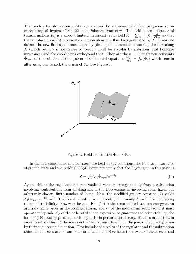
the transformation (8) represents a motion along the flow lines generated by X. Then onedefines the new field space coordinates by picking the parameter measuring the flow alongX (which being a single degree of freedom must be a scalar by unbroken local Poincareinvariance) and the coordinates orthogonal to it. They are the n − 1 integration constantsΦm 6=1 of the solution of the system of differential equations δΦm

δΦ0= fm(Φn) which remain

after using one to pick the origin of Φ0. See Figure 1.

Φm≠0

~

~

Φm

Φ0

Figure 1: Field redefinition Φm → Φm.

In the new coordinates in field space, the field theory equations, the Poincare-invarianceof ground state and the residual GL(4) symmetry imply that the Lagrangian in this state is

L =√ηΛ0(Φm 6=0)e−4Φ0 . (10)

Again, this is the regulated and renormalized vacuum energy coming from a calculationinvolving contributions from all diagrams in the loop expansion involving some fixed, butarbitrarily chosen, finite number of loops. Now, the modified gravity equation (7) yields

Λ0(Φm6=0)e−4Φ0 = 0. This could be solved while avoiding fine tuning Λ0 = 0 if one allows Φ0

to run off to infinity. However: because Eq. (10) is the renormalized vacuum energy at anarbitrary finite order in the loop expansion, and since the mechanism suppressing it mustoperate independently of the order of the loop expansion to guarantee radiative stability, theform of (10) must be preserved order-by-order in perturbation theory. But this means that inorder to satisfy this, all the scales in the theory must depend on the power of exp(−Φ0) givenby their engineering dimension. This includes the scales of the regulator and the subtractionpoint, and is necessary because the corrections to (10) come as the powers of these scales and

9

logarithms of their ratios. Only then will all the corrections, including the log-dependentterms, will scale the same way as in (10). So (10) will accomplish the task if all the matterfields and the regulator couple to the ‘rescaled’ metric gµν = exp(−2Φ0)gµν . However, aftercanonically normalizing the fields in the matter sector on the background given by solvingthe vacuum equations, one finds that all dimensional parameters in QFT must scale asmd ∝ e−dΦ0 . This means that in the limit Φ0 →∞ not only does the cosmological constantvanish, but so do all the other scales in the theory! In other words, this restores conformalsymmetry in the field theory sector. As noted this is not our world. Hence the problem.

3 Our proposal

In the attempt to evade the Weinberg’s no-go theorem, in [14] we proposed a very minimalmodification of General Relativity with minimally coupled matter. The idea was to promotethe classical cosmological constant Λ to that of a global dynamical variable, and introducea second global variable λ corresponding to scales in the matter sector. The variation withrespect to these new variables however is used to impose a global constraint on the dynamicsof the theory, similar in spirit to the constraint imposed in the classic isoperimetric problemof variational calculus [23]. To do this, we supplemented the local action with an additivefunction σ(Λ, λ) which is not integrated over the space time. Then the variations withrespect to Λ, λ select the values of these parameters. In particular, this procedure sets theboundary condition for the variable λ such that at any order of the loop expansion is takesprecisely the right value to completely absorb away the whole of vacuum energy contributionfrom the matter sector at that loop order. Our approach is a simplified hybrid of thinkingabout GR as unimodular gravity, with a variable Λ specified by arbitrary cosmological initialconditions, and the proposal of Linde [24], further considered by Tseytlin [25], of usingmodified variational procedures to fix values of global variables such as Λ. Our variationalprescription however differs from those previously considered in that it is more minimal,and that it uses a global scaling symmetry as an organizing principle for accounting for allquantum vacuum energy contributions.

The idea is to start with the action

S =

∫d4x√g

[M2

Pl

2R− Λ− λ4L(λ−2gµν ,Φ)

]+ σ

(Λ

λ4µ4

), (11)

where the matter sector described by L is minimally coupled to the metric gµν = λ2gµν . Weimagine that the Standard Model is included in it. For simplicity, we consider the matterto only belong to this sector, henceforth referred to as the ‘protected sector’. One couldalso include other matter sectors to the theory, that could couple to a different combinationof λ and gµν . However, vacuum energy contributions from such sectors would not cancelautomatically. In what follows we will focus on the matter dynamics only from the protectedsector, for simplicity’s sake. The function σ(z) is a (odd) differentiable function whichimposes the global constraints. The parameter µ is a mass scale introduced on dimensionalgrounds. The precise form of σ is determined in order to fix the particle masses in QFT inaccordance with a specific phenomenological model of physics beyond the Standard Model,as we will discuss in Sec. 6. Eg., an asymptotically exponential form of σ allows us to chooseµ to be up near the Planck scale etc.

10

The global variable λ sets the hierarchy between the matter scales and the Planck scale,since

mphys

MPl

= λm

MPl

, (12)

where mphys is a physical mass scale of a canonically normalized matter theory, and m is thebare mass in the Lagrangian. As an illustration, consider a scalar field with bare mass m,√

gLφ =1

2

√g[gµν∂µφ∂νφ+m2φ2

]=

1

2

√gλ4

[λ−2gµν∂µφ∂νφ+m2φ2

]=

1

2

√g[gµν∂µϕ∂νϕ+m2

physϕ2], (13)

where ϕ = λφ is the canonical scalar and the physical mass is mphys = λm.It is absolutely essential for our cancellation mechanism to enforce the UV regulator of

this sector to also couple to exactly the same metric as the fields from L. This is necessaryin order to ensure the correct operational form of the vacuum energy sequestration from L,and makes the effective UV cutoff MUV and the subtraction scaleM scale with λ in exactlythe same way as mass scales from L, given by Eq. (12). This can be accomplished, forexample, by regulating the theory with a system of Pauli-Villars regulators, which couple tothe metric gµν .

With this in place, the form of the (11) guarantees that all vacuum energy contributionscoming from the protected Lagrangian

√gλ4L(λ−2gµν ,Φ) must depend on λ only through an

overall scaling by λ4, even after the logarithmic corrections are included. This follows sincethe regulator of the QFT introduces contributions where the scales depend on λ in the sameway as those from the physical degrees of freedom from L. That ensures the cancellation of λin loop logarithms, and so only the powers of λ remain. This fact follows from diffeomorphisminvariance of the theory, which since λ is a global variable, is unbroken both for the metrics gµνand gµν . Diffeomorphism invariance ensures that the full effective Lagrangian computed from√gλ4L(λ−2gµν ,Φ) =

√gL(gµν ,Φ), including all quantum corrections – and the divergent

terms, as well – still couples to the exact same gµν [26]. Of course, this is true only when werestrict our attention to the vacuum energy contributions from loop diagrams involving onlyprotected sector degrees of freedom in the internal lines which are integrated over. This is,however, all of the vacuum energy in the decoupling limit of gravity, which we calculate usingstandard flat space field theory techniques in locally freely falling frames. As we stressedpreviously, we re-couple these terms to gravity by the minimal coupling procedure, takinggravity as a purely (semi) classical field which merely serves the purpose of detecting vacuumenergy. At present, this is the sharply formulated part of the cosmological constant problem,and as we discussed in the introduction we choose to focus on it alone.

The field equations that follow from varying the action (11) with respect to global aux-iliary fields Λ, λ are

σ′

λ4µ4=

∫d4x√g , 4Λ

σ′

λ4µ4=

∫d4x√g λ4 T µµ , (14)

where Tµν = − 2√gδSmδgµν

is the energy-momentum tensor defined in the ‘Jordan frame’. To go

11

to the ‘physical’ frame, in which matter sector is canonically normalized, note that

T µν = gµα[− 2√g

δSmδgαν

]= λ2gµα

[−2λ4

√g

δSmλ2δgαν

]= λ4T µν ,

where σ′ = dσ(z)dz

. As long as it is nonzero10, eliminating it from the two Eqs. (14) one finds

Λ =1

4〈T µµ〉 ,

where we defined the 4-volume average of a quantity by 〈Q〉 =∫d4x√g Q/

∫d4x√g. Note

that Λ is the bare cosmological constant, which is now however completely fixed by this con-dition. One has to define these averages meaningfully, since after regulating the divergencesthey can still be indeterminate ratios when the space-time volume is infinite [9]. We willaddress this in short order, since this issue has very important physical implications and tiesinto how our proposal evades Weinberg’s no-go theorem.

The variation of (11) with respect to gµν yields

M2PlG

µν = −Λδµν + λ4T µν , (15)

where Gµν is the standard Einstein tensor. After eliminating Λ and canonically normalizing

the matter sector, this becomes

M2PlG

µν = T µν −

1

4δµν〈Tαα〉 , (16)

This equation is one of the two key ingredients of our proposal. Note that this is the fullsystem of ten field equations, with the trace equation included. It differs from unimodulargravity [27, 28, 29, 30, 31, 32, 33, 34, 35], where although the restricted variation removesthe trace equation that involves the vacuum energy, this equation comes back along with anarbitrary integration constant, after using the Bianchi identity. Here there are no hiddenequations nor integration constants, and all the sources are automatically accounted for in(16). Crucially, however,

1

4〈Tαα〉

is subtracted from the right-hand side of (16). This means that the hard cosmological con-stant, be it a classical contribution to L in (11), or a quantum vacuum correction calculatedto any order in the loop expansion, divergent (but regulated!) or finite, never contributesto the field equations (16). To see this explicitly, we take the effective matter Lagrangian,Leff at any given order in loops, and split it into the renormalized quantum vacuum energycontributions (classical and quantum) Vvac = 〈0|Leff(gµν ,Φ)|0〉, and local excitations ∆Leff,

λ4√gLeff(λ−2gµν ,Φ) = λ4√g[Vvac + ∆Leff(λ−2gµν ,Φ)

]. (17)

It follows that T µν = Vvacδµν + τµν , where Vvac = λ4Vvac is the total regularized vacuum

energy and τµν = 2√g

δδgµν

∫d4x√gλ4∆Leff(λ−2gµν ,Φ) describes the physical excitations. By

10And non-degenerate: it can’t be the pure logarithm. In that case Eqs. (14) turn into two independentconstraints, 1

Λ =∫d4x√g, 4 =

∫d4x√g Tµ

µ, the latter placing an artificial constraint on the matter sector.

12

our definition of the historic 4-volume average, 〈Vvac〉 ≡ Vvac and so the field equations (16)become

M2PlG

µν = τµν −

1

4δµν〈ταα〉 , (18)

The regularized vacuum energy Vvac has completely dropped out from the source in (16).There is a residual effective cosmological constant coming from the historic average of thetrace of matter excitations:

Λeff =1

4〈ταα〉 . (19)

We emphasize that this residual cosmological constant has absolutely nothing to do with thevacuum energy contributions from the matter sector, including the Standard Model contri-butions. Instead, after the cancellation of the vacuum energy contributions enforced by theglobal variables Λ, λ, the residual value of 〈ταα〉 is picked as a ‘boundary condition’, resultingfrom the measurement of the finite part of the cosmological constant after it was renormal-ized. As we noted above, this measurement requires the whole history of the universe forthis one variable, in effect setting the boundary condition for it at future infinity. Obviously,it is crucial that the numerical value of Λeff is automatically small - one might hope for it,since it is the contribution coming predominantly from the IR modes in the cosmologicalevolution, but a quantitative confirmation is necessary since otherwise the proposal wouldhave failed. It turns out that indeed Λeff is automatically small enough in large old universes,as we will show in the next section. This follows from the fact that our universe is large andold, which in the very least is a consequence of extremely weak anthropic considerations.In actual fact, a large universe like ours can be formed by at least 60 efolds of inflation,which we will show is consistent with the vacuum sequestration proposal. The smallness ofΛeff is completely safe from radiative instabilities, and the required dynamics is essentiallyinsensitive of the order of perturbation theory. The apparent acausality in the determina-tion of Λeff is therefore of no consequence; a better terminology is aposteriority, that followsfrom the nature of the measuring process needed to set the numerical value of the renormal-ized cosmological constant. This has no impact on local physics and so cannot lead to anypathologies normally associated with any local acausality. One might only worry if theredo not appear some unexpected restrictions on a possible range of numerical values whichthe renormalized cosmological constant might have, that follow from the global constraintswhich we introduced. We will turn to this later, when we address how the solutions of thetheory are constructed.

The second key ingredient of our mechanism is that the field theory spectrum has anonzero gap, which can be arbitrarily large compared to |〈ταα〉|1/4. Otherwise, the mecha-nism would fail to provide a way around Weinberg’s no-go theorem - reducing yet again to aframework with at least scaling symmetry. This means that on the solutions the parameterλ must be nonzero, since λ ∝ mphys/MPl. But by virtue of the first of Eqs. (14), since σ(z)is a differentiable function, if λ is nonzero,

∫d4x√g must be finite. Fortunately this can be

accomplished in a universe with spatially compact sections, which is also temporally finite:it starts with a Bang and ends with a Crunch. In other words, the spacelike singularitiesregulate the worldvolume of the universe without destroying diffeomorphism invariance andlocal Poincare symmetry. Therefore, in our framework the universes which support non-scaleinvariant particle physics must be spatiotemporally finite. Infinite universes are solutions

13

too, however their phenomenology is not a good approximation to our world, since all scalesin the protected sector vanish. Note, that the quantity which controls the value of λ, andtherefore mphys/MPl, is the worldvolume of the universe, and not 〈ταα〉. This is essential forthe phenomenological viability of our proposal, since it separates the scales of the observedcosmological constant and masses of particle physics.

We will address these points in more detail in section 4, focussing on quantitative state-ments, demonstrating, in particular, that the residual cosmological constant is naturallysmall, never exceeding the critical density of the universe today. This is of course the finaltouche of our model, guaranteeing that the cancellations of the vacuum energy did not – inturn – necessitate large classical values to appear. Before we address these, and other phe-nomenologically important issues, let us look in more depth at just how the vacuum energycontributions get cancelled.

A holy grail of the past attempts to protect the cosmological constant from radiativecorrections, which is partially realized with supersymmetry and conformal symmetry, wasto find a symmetry which will insulate the finite term left after renormalization from higherorder loop corrections. As it turns out, a system of two symmetries is the reason why ourcancellation works. Our action (11) has approximate scale invariance, broken only by theEinstein-Hilbert term,

λ→ Ωλ , gµν → Ω−2gµν , Λ→ Ω4Λ , (20)

such that the action changes by

δS =M2

Pl

2Ω−2

∫d4x√gR =

M2Pl

2Ω−2〈R〉

∫d4x√g . (21)

The other symmetry appears as an approximate shift symmetry

L → L+ εm4 , Λ→ Λ− ελ4m4 , (22)

under which the action changes by

δS = σ

(Λ

λ4µ4− εm

4

µ4

)− σ

(Λ

λ4µ4

)' −εσ′m

4

µ4. (23)

The scaling symmetry ensures that the vacuum energy at an arbitrary order in the loop ex-pansion couples to gravitational sector exactly the same way as the classical piece. The ‘shiftsymmetry’ of the bulk action then cancels the matter vacuum energy and its quantum correc-tions. The scaling symmetry breaking by the gravitational sector is mediated to the matteronly by the cosmological evolution, through the scale dependence on

∫d4x√g, and so is weak.

This is why the residual cosmological constant is small: substituting the first of Eqs. (14)

and using λ = mphys/m, we see that δS ' −εm4λ4∫d4x√g = −ε

(mphysMPl

)4 [M4

Pl

∫d4x√g].

Holding the volume fixed, this is small when mphys/MPl 1, vanishing in the conformallimit11 λ ∝ mphys → 0. This restoration of symmetry renders a small residual curvaturetechnically natural.

11Defined by fixing∫d4x√g and taking µ→∞ in the first of Eqs. (14).

14

Let us see how this occurs at the level of the field equations (14), (16). First off, note thatthe historic average of the trace of the right hand side of (16) is zero, 〈R〉 = 0. Hence, by(21), the action (11) is in fact invariant under scaling (20) on shell. Next, the variation of thematter Lagrangian under the shift L → L+εm4 is equivalent to letting T µν → T µν−εm4δµν .Then if gµν , Λ and λ solve Eqs. (14) and (15) for a source T µν , by manipulating the constraintequations (14) one finds that

gµν = gµν , Λ = Λzσ′(z)

zσ′(z), λ4 = λ4σ

′(z)

σ′(z), (24)

are solutions with a source T µν − εm4δµν , where z = Λ/λ4µ4, and z = z(

1− 4εm4/〈T 〉)

.

Crucially, gµν remains unchanged, which means that a shift of the vacuum energy – by addinghigher order corrections in the loop expansion – is absorbed by an automatic readjustmentof the global variables, and so has no impact whatsoever on the geometry.

Finally, since the role of the two global auxiliary fields, λ and Λ is to enforce globalconstraints, they only appear algebraically in the theory and can be integrated out explic-itly. The resulting formulation of the theory provides further insight into the protectionmechanism. So using the variable z defined above, the constraints (14) are

σ′(z)

λ4µ4=

∫d4x√g , z =

〈Tαα〉4µ4

. (25)

Solving for λ,Λ yields

λ =

σ′(〈Tαα〉/4µ4

)µ4∫d4x√g

1/4

, Λ =σ′(〈Tαα〉/4µ4

)〈Tαα〉/4µ4∫

d4x√g

. (26)

Substituting these back into the action, we obtain

S =

∫d4x√g

[M2

Pl

2R− λ4L(λ−2gµν ,Φ)

]+ F

(〈Tαα〉/4µ4

), (27)

where λ is given by equation (26), and Tαα = gαβ(

2√g

δδgαβ

∫ √gL(gµν ,Φ)

). An important

point here is that the function F (z) = σ(z)− zσ′(z) is the Legendre transform of σ. This ex-plicitly shows that the independent variable z (or Λ) has been traded for the new independentvariable σ′(z) – which, by the first of Eqs. (26), is λ4µ4

∫d4x√g . Thus, the independent

variable of the theory is really not the cosmological counterterm Λ, (like in GR or in uni-modular extension of GR) but the worldvolume of the universe,

∫d4x√g. So this in fact

reveals how our mechanism operates. The cosmological system responds instead to changesin the space-time volume, rather than changes in Λ. Furthermore, in GR, when higher ordercorrections to the vacuum energy are included, Λ stays fixed forcing the space-time volume∫d4x√g to absorb the corrections (inflating a lot due to a large vacuum energy). For our

scenario it is exactly the opposite: it is the space-time volume that remains fixed, forcing Λto adjust. As a result, the cosmological system is stable against radiative corrections to thevacuum energy.

15

Indeed, let us consider the gradient expansion of the effective matter Lagrangian, includ-ing any number of loop corrections. To the lowest order, we retain only the full effectivepotential of the theory, and truncate it to the zero momentum limit, which represents thevacuum energy Vvac. We find that Leff = Vvac, 〈Tαα〉 = −4Vvac, and the action is

S =

∫d4x√g

M2Pl

2R−

σ′(−Vvac/µ4

)µ4∫ √

g

Vvac

+ F(−Vvac/µ4

)=

∫d4x√g

[M2

Pl

2R

]+ σ

(−Vvac/µ4

). (28)

We see how the choice of coupling of gµν to the Standard Model given by equation (27)guarantees that all gµν dependence is cancelled in the vacuum energy contribution to theaction. This is how the Standard Model vacuum energy is sequestered. Diffeomorphisminvariance guarantees that the full effective Lagrangian computed from

√gL(gµν ,Φ), includ-

ing all quantum corrections, still couples to the same gµν =

[σ′(〈Tαα〉/4µ4)

µ4∫ √

g

]1/2

gµν . The loop

corrections are accommodated by (small!) changes of the scaling factor

[σ′(〈Tαα〉/4µ4)

µ4∫ √

g

]1/2

,

while the metric gµν remains completely unaffected. This works to any order in the loopexpansion, as is the core element of the adjustment mechanism.

So to summarize, we see that the key point of our mechanism is a dramatically alteredrole of

∫d4x√g, which provides the way around Weinberg’s no-go theorem [3]. Instead of Λ

in GR or in its unimodular formulation, now∫d4x√g is the independent variable. Taking

all the physical scales in the protected matter sector to depend on it, automatically removesall the vacuum energy contributions to drop out. For example, if we were to take the linearfunction σ(z) = z in (11) and declare L to be literally the Standard Model, integrating Λand λ out and rewriting (11) as just Einstein-Hilbert action coupled to the Standard Model,the only modification is that the Higgs vev v is replaced by v/(µ4

∫d4x√g)1/4! Further,

in a collapsing spacetime, since∫d4x√g is finite, the protected sector QFT has a nonzero

mass gap, by virtue of (14), while the residual cosmological constant 〈ταα〉/4 6= 0, but itis completely independent of all the vacuum energy corrections, and as we will show belowis automatically small in a large old universe. The particle sector scales are affected bythe historic value of the worldvolume12. However, this dependence of field theory scales on∫d4x√g is completely invisible to any nongravitational local experiment, by diffeomorphism

invariance and local Poincare symmetry. Locally the theory looks just like standard GR,in the (semi) classical limit - but without a large cosmological constant, and without itsradiative instability, at least in the limit of (semi) classical gravity.

12In the case where σ is a linear function, they would be too sensitive to the initial conditions in the earlyuniverse. This is why the forms of σ which are asymptotically exponential are preferred, since they reducethe sensitivity to merely logarithmic corrections.

16

4 Historic integrals and quantitative considerations

We have already stated that in universe which is compact, starting in a Bang and ending in aCrunch, the worldvolume

∫d4x√g is finite. Also the residual cosmological constant given by

the historic average of the trace of stress-energy tensor −〈ταα〉/4 is automatically small in bigand large universes, as long as τµν satisfies the dominant and null energy conditions (DECand NEC, respectively). In this section we will give a proof of this statement at the classicallevel. Semiclassically, it has been shown that the integrals 〈ταα〉 are finite if NEC is valid in[36]. Then for bounded ταα our argument automatically extends to the semiclassical case,too. Further, we will consider the techniques for finding solutions of field equations in oursetup. From a practical point of view, solving the equation (18) requires a bootstrap method:allow 〈ταα〉 = C to be arbitrary to start with, find the family of solutions parameterizedby this integration constant, and finally substitute this family of solutions back into 〈ταα〉in order to show that a subset of them is compatible with the initial choice. This is akinto the gap equation in superconductivity. Here we will focus on the proof of existence ofsolutions to this procedure in the case of background FRW cosmologies. In the forthcomingwork [37] we will show that consistent solutions of this type including the current epoch of(transient) acceleration exist. Specific dynamics will resort to the earliest quintessence withlinear potential dating back to, at least, 1987 [38], as the really relevant model of transientcosmic acceleration. We will show in [37] that it has a natural embedding in our proposal.Other scenarios and aspects of transient acceleration have also been considered (see eg [39]).

4.1 Historic integrals and the cosmological background

The integrals which appear in the definition of our historic averages are∫d4x√g ⊃ Vol3

∫ tcrunch

tbang

dta3 , (29)∫d4x√gταα ⊃ Vol3

∫ tcrunch

tbang

dta3(−ρ+ 3p) , (30)

where the cosmology takes place over a finite proper time interval tbang < t < tcrunch, with ascale factor a, and finite spatial comoving volume Vol3. We will approximate the integrals forthe most part by the FRW geometry with fluids, whose energy density and pressure are ρ andp respectively. We will eventually impose DEC and NEC, which combined together require|p/ρ| ≤ 1. The integrals are regulated - ie., finite - because we assume that spatial sectionsare compact, and that the universe starts at a Bang and ends in Crunch. This guaranteesthat (29) is finite, and that the QFT spectrum has a nonzero mass gap. Further, we willsee that validity of NEC then also guarantees that (30) is also finite, and bounded by thecontributions from near the turning point, being estimated by the product of the minimalenergy density during cosmological evolution and the age of the universe. At the technicallevel, we will take the evolution to be symmetric in time for simplicity. This does not impairthe generality of our analysis because the integrals are dominated by the contributions nearthe turning point. Approximating the spatial volumes by homogeneous 3-geometries, we willfirst consider time integrals. We will briefly return to contributions from inhomogeneitieslater, when we consider the effects from black holes.

17

For starters, note that the DEC and NEC together – |p/ρ| ≤ 1 – put a very strongbound on the contributions to the integral (30) from the Bang and Crunch singularities.Namely while at the singularities the energy density and pressure diverge, the spacelikevolume which they occupy shrinks, and |p/ρ| ≤ 1 ensures that the rate of shrinking is fasterthan the divergence of ταα. Indeed, near the singularities ρ scales as ρ ∼ 1/(t − tend)

2,by virtue of the Friedman equation, where tend is either of the singular instants. Since inthis limit a3 ∼ (t − tend)2/(1+w), the integrand ∝ a3ρ ∼ (t − tend)−2w/(1+w) will not divergeprovided |w| < 1. For w = +1 the divergence is at most logarithmic, with coefficients' O(1) so that when properly cut off at the physical Planckian density surfaces thesecontributions are still much smaller than the cutoff. Hence our historic averages will alwaysbe finite in a bang/crunch universe for all realistic matter sources. Having shown that (30)is bounded, we can proceed with a more careful comparison of contributions to (30) fromdifferent cosmological epochs.

Now, to get a more accurate estimate of various contributions to (30) we can split thehistory of the universe into epochs governed by different matter sources, which we canapproximate as perfect fluids. So let us consider one such epoch, during which a fluid withequation of state wi controls the evolution of a in an interval ai < a < ai+1. The contributionof this epoch to the temporal integral in (29) is

Ii =

∫ ti+1

ti

dta3 =

∫ ai+1

ai

daa2

H=

a3i+1

Hi+1

∫ ai+1

ai

da

ai+1

(a

ai+1

)2Hi+1

H, (31)

where H = a/a and Hi, Hi+1 are the values of H at a = ai, ai+1 respectively. Using the

Friedmann equation, H2 ' H2i+1

(ai+1

a

)3(1+wi), and so

Ii =2

3(3 + wi)

(a3i+1

Hi+1

)[1−

(aiai+1

)3(3+wi)/2]. (32)

For |p/ρ| ≤ 1, this integral is always finite, even if ai → 0. Similarly, the contribution of thisepoch to the temporal integral in (30) is

Ji =

∫ ti+1

ti

dta3(−ρ+ 3p) = (3wi − 1)ρi+1a

3i+1

Hi+1

∫ ai+1

ai

da

ai+1

(a

ai+1

)2(Hi+1

H

)ρ

ρi+1

= (3wi − 1)ρi+1a

3i+1

Hi+1

∫ ai+1

ai

da

ai+1

(a

ai+1

)2(H

Hi+1

), (33)

where in the last step we have used H2 ' H2i+1

ρρi+1

. Since H2 ' H2i+1

(ai+1

a

)3(1+wi),

Ji =2(3wi − 1)

3(1− wi)

(ρi+1a

3i+1

Hi+1

)[1−

(aiai+1

)3(1−wi)/2]. (34)

Clearly these integrals describe contributions from both expanding and contracting regimes.Note, that (33) is logarithmically divergent near the singularity for a stiff fluid wi = 1,

as we noted above. But this divergence is a red herring. We cut the evolution off at a timewhen the density reaches Planck scale, lpl <∼ a <∼ a?, and so

J singularitystiff = 2

(ρ?a

3?

H?

)log(

a?lpl

) '(H?

MPl

)log(

a?lpl

) , (35)

18

where H? and ρ? are the Hubble scale and energy density when a = a?. Hence J singularitystiff ≤ 1.

For all other cases with −1 ≤ w < 1, the integral Ji is automatically finite – and small.Next we consider the contributions from the turning point at a time T . During this time,

the universe is approximately static, with the scale factor roughly a constant, a ' amax, over atime interval ∆t. The turning point happens roughly at the time given by the total age of theuniverse, T ' ∆t ' 1/Hage. The effective Hubble parameter at that time is approximatelyzero, by virtue of a cancellation between different contributions to the energy density, wheresome must be negative to trigger the collapse (eg., a positive spatial curvature or a negativepotential). But since 1/a2

max measures the characteristic curvature of the universe at thattime, |R| ∼ H2

age ∼ 1/a2max, we obtain

Iturn =

∫ T+∆t/2

T−∆t/2

dta3 ' a3max∆t ∼

a3max

Hage

∼ 1

H4age

. (36)

The contribution from the turning point to the temporal integral in (30) is

Jturn =

∫ T+∆t/2

T−∆t/2

dta3(−ρ+ 3p) ' O(1)a3maxρage∆t ∼

ρageH4age

, (37)

where ρage ∼ M2PlH

2age corresponds to the characteristic energy density of the universe at

that time.Clearly, (36) and (37) are dominant contributions to (29) and (30), respectively. To see

this, consider first two consecutive epochs away from the turning point. After simple algebra

one finds Ii/Ii−1 = O(1)(ai+1

ai

)3(3+wi)/2

, Ji/Ji−1 = O(1)(ai+1

ai

)3(1−wi)/2using the Friedmann

equation. Clearly, the epoch with larger value of the scale factor at any of its end pointsgives a dominant contribution. This means that the larger contributions to (29) and (30)come from the regimes of evolution nearer the turning point. Indeed, at the turnaround,we find that the contributions from the quasi-static interval at during the turning and the

adjacent epochs are Iturn/Ii = O(1)(Hi+1

Hage

)(a3max

a3i+1

)and Jturn/Ji = O(1)

(HageHi+1

)(a3max

a3i+1

). Now

Hage < Hi+1, and amax > ai+1. Next, as long as |wi| ≤ 1, we also have H2age

>∼ H2i+1

(ai+1

amax

)6

,

which follows from the fact that the stiff fluid yields the fastest allowed decrease of H withexpansion. From these inequalities we conclude that the contributions to (29) and (30) areindeed dominated by the evolution near the turning point. Thus we obtain[∫

d4x√g

]FRW

= O(1)Vol3H4age

, (38)[∫d4x√gταα

]FRW

= O(1)Vol3 ρageH4age

. (39)

Therefore the residual cosmological constant is

Λeff =1

4〈ταα 〉 ' O(1)ρage ' O(1)M2

PlH2age

<∼ M2PlH

20 . (40)

This is guaranteed to be bounded by the current critical density of the universe as long asthe universe lives at least H−1

age>∼ H−1

0 ∼ 1010 years. This proves the previously stated claim

19

that Λeff is automatically small enough in large old universes, which is a crucial check of ourproposal. On the other hand, this can’t – by itself – be taken as a prediction of the lateepoch of cosmic acceleration. For one, the sign of Λeff is determined by equation of state ofthe dominant fluid close to the turning point; if w > 1/3, Λeff is positive, and if w < 1/3it is negative. Secondly, if the residual cosmological constant were dominant today, futurecollapse would have been impossible as long as all other matter satisfies standard energyconditions. Thus Λeff cannot be identified with dark energy, since the universe must collapsein order to be phenomenologically acceptable within the context of our proposal. The currentcosmological acceleration must be a transient phenomenon, with the net potential turningnegative some time in the future, and/or our universe were spatially closed, with a small butnonzero positive spatial curvature. We will return to this issue in the future [37].

4.2 Historic integrals and black holes

One may worry13 that astrophysical black holes may provide a significant contribution tothe spacetime volume of the universe. The point is that the familiar black hole solutionsin GR have infinite volumes in their interiors. However, black holes in compact spacetimesare different. For simplicity let us model a small black hole in a collapsing universe asa Schwarzschild black hole on a spacetime where time is an interval limited by the totalage of the universe, ∆t <∼ 1/Hage. The analytic extension across the horizon then tradesthe radial and time coordinates, making t spacelike inside. But because t is compactified,that automatically means the internal volume is finite. Further reduction of black holecontributions may come from the fact that they evaporate, although this seems to be muchless important for astrophysical black holes which mainly gain weight in the course of theirlifetime. Properties of black holes in compactified spacetimes have been studied in [40].

Now we estimate the black hole internal volume. We will stick with the model of a smallSchwarzschild black hole with a compactified time direction. The geometry is approximatelyds2 = −(1−rH/r)dt2+(1− rH/r)−1dr2+r2dΩ2, where dΩ2 is the metric on the unit 2-sphere,and rH is the Schwarszchild radius. So the interior spacetime volume is∫

interior

d4x√g = 4π

∫ ∆t

0

dt

∫ rH

0

drr2 =4π

3r3Ht

<∼4π

3r3H/Hage . (41)

The total contribution from all black holes to the spacetime volume of the universe cannotsignificantly exceed the contribution from the largest black holes known to exist, with amass ∼ 109M [41]. Assuming there is one such black hole in all 1011 galaxies in the Hubblevolume today, and assuming that our Hubble volume is typical, we extrapolate the galaxypopulation in the whole collapsing universe to be about Ngal ∼ 1011H3

0a30, where H0 ∼ 10−33

eV is the current Hubble scale and a0 > 10/H0 the current scale factor. This yields[∫d4x√g

]galBH

<∼ 1011H30a

30

Hage

(109 M

M2Pl

)3

= 10−19

(a0

amax

)31

H4age

, (42)

as the contribution of all black hole interiors to the total spacetime volume of the universe.We have used that the scale factor near the turning point is amax ∼ 1/Hage. Since a0 < amax,

13We thank Paul Saffin and Alex Vikman for raising this question.

20

we see that galactic black hole interiors’ contribution to the spacetime volume is completelynegligibe in comparison to the background cosmology.

Estimating the contribution of their mass to 〈ταα〉 is now straightforward. Since the totalvolume integral is unaffected, and since

∫interior

d4x√gταα <∼ MBH∆t <∼ MBH/Hage, where

MBH is the total mass in all black holes, the black hole contribution to 〈ταα〉 is boundedby MBHH

3age. Again using the extrapolated number of black holes in the whole universe

to be Ngal ∼ 1011H30a

30, the total mass in black holes is MBH ∼ 1020H3

0a30M. So after a

straightforward calculation, using M ' 1039MPl, we find that the contribution to 〈ταα〉 isbounded by

〈ταα〉galBH <∼ρnow10

(a0

amax

)3

, (43)

where ρnow = M2PlH

20 is the critical density today. As a0

<∼ amax, this is clearly subleadingeven with our overestimate of the black hole population, ρBH ∼ MBH

a30∼ 0.1ρnow.

4.3 Historic integrals and FRW cosmology

So far we have been considering the implications of the historic integrals and averages on thephenomenology of solutions, assuming they exist. Do they? Now we address this question14.In principle, one should expect that such solutions should exist, on the grounds that onecould always start with a family of solutions in GR with an arbitrary value of cosmologicalconstant, construct the geometry, and then pick the specific value of the – initially arbitrary –bare cosmological constant to satisfy Λeff = 〈ταα〉/4. Equivalently, this merely means takingthe special solution from each one parameter family of solutions, parametrized by Λbare, forwhich 〈R〉 = 0. In a way, the freedom of picking Λ and the arbitrariness of initial conditionsappear to guarantee the existence of specific solutions. Nevertheless, an explicit proof is stillrequired given that the determination of Λeff = 〈ταα〉/4 involves specific future boundaryconditions which must be picked to find the self-consistent solution. This ‘bootstrapping’logic is very similar to what one encounters in BCS theory of superconductivity, where onealso has to solve a nonlocal equation – the gap equation – to decide if the solutions existin the first place. Here, we will review the conditions under which such solutions do existin the family of FRW cosmologies. In a forthcoming publication [37] we will consider therequirements to build a fully realistic model, consistent with cosmic phenomenology, thatincludes a transient phase of acceleration like the one we see today.

For simplicity we will focus on solutions which are dominated by a single fluid and theresidual effective cosmological constant. Adding more ingredients in fact makes the existenceof solutions easier to prove, by adding additional parameters. So, FRW cosmologies withspatial curvature k, a cosmological constant Λeff and a single perfect fluid with equation ofstate parameter w = p/ρ = const, which obeys DEC and NEC, |w| ≤ 1, are described bythe Friedmann equation

3M2Pl

(H2 +

k

a2

)= ρ0

(a0

a

)3(1+w)

+ Λeff . (44)

14We thank Guido D’Amico and Matt Kleban for discussions on the subject of this section.

21

The special solution of (44) which also satisfies Eq. (19), which in this case reduces to

Λeff = −(1− 3w)

4

∫dta3ρ∫dta3

, (45)

is the solution of our theory. We will assume that the spatial volume is compactified, so thatthe integral over the spatial coordinates stays finite. We will further assume that ρ0 > 0. Itis instructive to rewrite (44) in the form resembling the energy conservation equation for aparticle in one dimension,

a2 + Veff(a) = −k , Veff = − κ2

a1+3w− Ω2a2 , (46)

where κ2 =ρ0a

3(1+w)0

3M2Pl

> 0, but Ω2 = Λeff

3M2Pl

can take either sign.

Let us first consider the (simpler) case of universes with k ≤ 0. When w ≥ 1/3, by(45) Λeff and Ω2 are nonnegative. So the ‘potential’ Veff in (46) is negative definite. Forthe total conserved ‘energy’ −k ≥ 0, the solutions exist for all a 6= 0, since the lines Veff

and a2 = const > 0 never intersect. An expanding solution expands forever. Therefore thetemporal ‘volume’

∫dta3 is infinite, and so Λeff vanishes. However, this also means that∫

d4x√g diverges. Hence these solutions are all cosmologies in which field theory has no

mass gap, and are not good candidates to accommodate our universe.When −1 < w < 1/3, Λeff and Ω2 are negative. The potential Veff is a sum of two

powers, a−(1+3w) and a2, with opposite coefficients. However, since w > −1, the quadraticalways wins at large a. This means that a ‘particle’ moving from the origin (an expandinguniverse starting with a Bang) with a total energy which is nonnegative (−k ≥ 0) encountersa potential barrier at some finite a from the origin and turns around. So such configurationsalways admit a collapsing solution, and for the given ‘free parameters’ describing the solutionsof (44) in GR (Λeff and the value of a at the turning point, specified by the integrationconstant) one needs to pick the combination which solves (45), which as we see exists. Note,that this does not mean tuning the initial conditions for a to find the solution. It means, forthe given initial conditions specifying the solution, one needs to pick the right value of theaposteriori parameter Λeff. The same logic applies to all cases.

The case k > 0 is slightly more subtle. In the language of the one dimensional dynamics(46) we are now looking for states with negative conserved energies. Now, when −1 < w <−1/3, since Λeff and Ω2 are negative, and so is 1 + 3w, the potential Veff is a sum of twopositive powers of a, with opposite coefficients. This sum is negative between the origin andsome (large) value of a, beyond which it turns positive, going again as a2 at large a. Butsince we are looking for trajectories with −k < 0 now, it means that the total energy −kcan be greater than the effective potential Veff only in a finite interval of a’s. So classicalmotion is only possible between these two turning points, and it continues forever. This casecorresponds to oscillating cosmologies of [42], which have finite spatial volume, and where thenegative effective cosmological constant, needed for oscillating motion, is generated by ourconstraint. Here, even though

∫d4x√g is infinite, and so the QFT is gapless, Λeff remains

finite as can be seen readily by splitting the integration into the sum of integrals over fullperiods. Yet, such universes are not phenomenologically viable since QFT is scale invariant.

When −1/3 < w < 1/3, Λeff and Ω2 are still negative, but 1 + 3w > 0. Thus Veff is acombination of an infinite potential well at the origin and a quadratic barrier far away. So

22

solutions with −k < 0 always exist, again representing universes which start with a Bang,expand to the maximum radius and subsequently crunch. The cases w = −1/3 and w = 1/3are special limits. In the former, the barrier has finite depth, again admitting collapsingsolutions, while in the later case the barrier is pushed to infinity since Λeff = 0 by scaleinvariance. This latter case corresponds to a radiation dominated universe with vanishingcosmological constant.

Finally, when w > 1/3, Λeff and Ω2 are positive. Hence the potential Veff is negativedefinite, diverging at the origin and infinity, with a maximum in between. Since −k < 0,solutions exist if the ‘conserved energy’ −k is smaller than the value of Veff at the maximum,representing again cosmologies that start with a Bang and end with a Crunch. The solutionswould not have existed if −k were larger than the maximum. But this is not the case; thelimiting case, where −k is exactly equal to Veff(max), would have been a static Einsteinuniverse, that would have been eternal. This would require a = a = 0. Taking the derivativeof (46) one can easily check that this requires w = −1, contradicting w > 1/3. So thereforethe closed cosmologies describing Bang/Crunch always exist for w > 1/3.

Before closing this section, we should clarify the role and the implications of the constraint〈R〉 = 0 which follows from tracing and integrating Eq. (18) and using Eq. (19). On FRWgeometries with spatially compact smooth sections it reduces to

∫dta3(H + 2H2 + k

a2 ) = 0

after factoring out the finite spatial integral. Integrating the term ∝ H by parts yields

a3H∣∣∣tcrunchtbang

=

∫dta3(H2 − k

a2) . (47)

If we were to take the limits of integration to be the time intervals where the scale factorliterally vanishes, and the dominant stress-energy sources determining the behavior of Hobey NEC, the left-hand side would have vanished for precisely the same reasons as we havealready discussed in Sec. 4.1. This would appear to have ruled out spatially open and flatFRW universes, as is clear from Eq. (47) since in this case the right hand side could onlyhave vanished if H and k were exactly zero at all times. This argument is a little hasty,however. The point is that the integration must be ended at times when the curvatureR reaches the Planck scale, and not when the scale factor exactly vanishes. Thus the lefthand side does not vanish, but simply represents a boundary condition which the terminalgeometry must satisfy to ensure that 1) it is a solution of Einstein’s equations and 2) thatthe vacuum energy is sequestered. Indeed, the left hand side is merely a nonzero numberwhich represents the difference between a3H at the beginning and the end of cosmology,encoding the posterior determination of the effective cosmological constant Λeff = 〈τ〉/4,communicated to the on-shell geometry by way of Einstein’s equations. For small universes,the contributions to this term from beyond the cut-off are sufficiently important that wecan treat it as an arbitrary boundary condition allowing any value of k. However: for largeand old universes, the integrals on the right hand side are dominated by the contributionsfrom large volumes near the turning point, and thus essentially insensitive to the boundaryconditions. Since the left hand side is much smaller, the integrals on the right hand sidemust include negative contributions that yield cancellations to match the left hand side.Thus having a large old approximately FRW universe does require k = 1 (and so Ωk < 1).Small inhomogenous universes may evade this. A similar observation was made in a differentcontext in [34].

23

5 Vacuum energy sequestering and phase transitions

In the course of the cosmological evolution the field theory dynamics may go through manyphase transitions: QCD phase transition, electroweak symmetry breaking, etc. This meansthat the local vacuum of the theory changes. As a result, since after renormalization theeffective potential governing the dynamics is fixed, this implies that the net renormalizedcosmological constant may actually change in time and space. The variation is typically ofthe order of ∆V ∼ M4

PT , where MPT is the energy scale of the transition. So the questionarises, if the universe has undergone many phase transitions in its past, how come thatthe initial finite value of cosmological constant was just right to exactly cancel the phasetransitions and yield a very small value which obeys current observational bounds [8, 9, 10]?

In our framework, such contributions do not drop out from (16), (18), but they becomeautomatically small at times after the transition in a large and old universe. Let us assume,for simplicity, a single phase transition that took place in the past. If the phase transition isfirst order, it proceeds through bubble formation, which will percolate some time after thetransition. If it is second order, then it is characterized by some order parameter smoothlytransitioning from one value to another in the universe, where the onset of this rolling indifferent regimes is local. In any case the process takes some time to complete, and thereforeinvolves gradients of fields or background geometry. Either way, the energy density in thegradients will not exceed the total potential energy density change. So for simplicity we willmodel the phase transitions as a sudden jump in the potential across the whole universe. Thismeans that we ignore the gradients of fields, as they just give an O(1) correction, and modelthe transition with a simple step function potential V = Vbefore(1−Θ(t−t∗))+VafterΘ(t−t∗),where Θ(t − t∗) is the step function, and t∗ the transition time. Substituting into (18), wefind

τµν −1

4δµν〈ταα〉 =

−〈Vbefore − V 〉δµν t < t∗ ,

−〈Vafter − V 〉δµν t > t∗ .(48)

Hence, after the transition, the historic average in (48) is

〈Vafter − V 〉 = −∆V

∫ t∗tbang

dta3∫ tcrunchtbang

dta3, (49)

where ∆V = Vbefore − Vafter. The denominator is just the spacetime volume, computed insection 4.1, and is given by ∼ 1/H4

age. To estimate the numerator, we use the result ofsection 4.1, where we showed that the largest contributions to the temporal integrals duringa particular epoch come from the region where the scale factor is largest. Since we areconsidering the phase transitions in the past, as dictates by the structure of the StandardModel, the dominant contributions come from just before the transition itself. Hence∫ t∗

tbang

dta3 ∼ O(1)a3∗

H∗,

where a∗ is the scale factor and H∗ the curvature scale during the transition. Therefore

〈Vafter − V 〉 = O(1)ρage∆V

M2PlH

2∗

(H∗Hage

)(a∗amax

)3

, (50)

24

where we have used the fact that ρage ∼ M2PlH

2age, and amax ∼ 1/Hage. Assuming that the

cosmological evolution after the transition to the turning point is dominated by a single

perfect fluid with an equation of state w, so that H2age = H2

∗

(a∗amax

)3(1+w)

we then find that

〈Vafter − V 〉 = O(1)ρage∆V

M2PlH

2∗

(Hage

H∗

) 1−w1+w

. (51)

If the phase transition is followed by several different epochs dominated by different matterdistributions, the correction is merely a factor of O(1). Now assuming DEC and NEC,|w| ≤ 1, along with the fact that H∗ ∼

√Vbefore/MPl

>∼√

∆V /MPl, we conclude that

|〈Vafter − V 〉| <∼ ρage < ρnow , (52)

which means that the contributions of phase transitions to the net effective vacuum energyare automatically suppressed to below the critical energy density of the universe today. Aswe also see, the earlier they are, the more suppressed: the reason is the historic weightingof the contributions, since the ‘imbalance’ is weighted only by the spacetime volume beforethe transition. Dividing by the total spacetime volume of the universe then suppresses thecontributions from the transition more efficiently if they occur earlier. For the StandardModel all the phase transitions occur early, with H∗ H0 > Hage, and so the suppressionis considerable.

What about the period before the transition? Using similar arguments, we find that〈Vbefore−V 〉 ∼ O(1)∆V . Since ∆V ∼M2

plH2∗ , this contribution could be large, but it affects

the universe only at early times before the transition, when H >∼ H∗. This means thatthis aposteriori contribution is subdominant to the contributions from other energy sources,except at most during the period immediately before the transition. Indeed, it is consistentwith the Standard Model and a reheating scale TeV to assume that all transitions occurduring the radiation era. So this could at most yield several short bursts of inflation (of atmost a few e-folds) in the run up to a transition, as long as it is sharp. Such phases are onlya small perturbation of the radiation driven cosmology, and occurring at very short scalesin the present universe. If, however, the transition is very slow, say a second order phasetransition where the order parameter takes a long time to move from its initial position tothe new vacuum, this in fact can drive a long inflation responsible for making the universesubsequently big and old. This, in fact, is beneficial, and we will show in section 8 that it isthe key reason why our proposal is consistent with inflation, even in the protected sector.

6 Particle masses and phenomenology

So far we have shown that vacuum energy can be sequestered away from curvature yieldinga small residual net cosmological constant, while particle physics still has a mass gap as longas the universe is compact in spacetime, with a finite spacetime volume. Here we expand onthe latter point, and discuss in greater detail the properties that the function σ must havein order to ensure that the particle mass gap is phenomenologically reasonable. Since thenumerical value of the parameter λ sets the physical scales in L, setting mphys = λm, where mis the bare mass, the function σ must be carefully engineered to generate the right hierarchies

25

between the various scales in a given model of (beyond) the Standard Model physics. Thiscannot protect the hierarchy between mphys and MPl, nor the hierarchies between differentphysical masses in L, but it can help set the scale hierarchy, and it can coexist with specificmechanisms designed by model builders to protect particle physics hierarchies, by removingthe vacuum energy contributions.

Since by virtue of the equations (14)

mphys

m= λ =

σ′(〈Tαα〉/4µ4

)µ4∫ √

g

1/4

, (53)

to compute it we need to specify the cutoff for the regulated vacuum energy contributions.We will assume that the cutoff is large enough that the vacuum energy gives the dominantcontribution to Tαα. We approximate Tαα ≈ −4Vvac, where Vvac = 〈0|Leff(gµν ,Φ|0〉 is theregulated vacuum energy of the effective matter Lagrangian in the protected sector L at anygiven order in the loop expansion. It is related to the physical regulated vacuum energy viathe relation Vvac = λ4Vvac. The regulator scale, ie., the cut-off, of the protected sector isMphys

UV = λMUV , and in principle it can be as high as MPl. Depending on the model, the‘bare’ regulator, MUV , could also be as high as MPl, in which case we must ensure that thesolutions saturate λ ∼ O(1). Even in this most extreme scenario, the regulated vacuumenergy Vvac ∼ Vvac ∼ M4

Pl, is still completely sequestered from gravity by our mechanism.The scale µ needs to be chosen appropriately in order to be consistent with λ ∼ O(1), viathe condition

O(1) =

[σ′ (±O(1)M4

Pl/µ4)

µ4∫ √

g

]1/4

∼[σ′(±O(1)M4

Pl/µ4)]1/4 Hage

µ, (54)

where the ± reflects the fact that the vacuum energy may take either sign. Since we areintroducing µ buy hand, we can take it to have as natural a value as possible, and pick itclose to the cut-off in the protected sector. Note, that this parameter is entirely external -a mere normalization required for dimensional purposes - since neither it nor the function σever get explicitly renormalized. The value of the function σ can only change because theratio Λ/λ4 which appears in the argument of σ may change between different orders in theloop expansion. So setting µ ∼MPl/

√10, we now require

O(1) ∼ [σ′ (±O(100))]1/4 Hage

MPl

. (55)

Provided the lifetime of the universe, 1/Hage, does not exceed its lower bound, 10/H0, by toomuch, getting λ ∼ O(1) is will follow if σ(z) ' exp(z) for z > 1. To allow for both positiveand negative vacuum energy, we need an odd function, so we can simply take σ(z) ∼ sinh z.

We should note that the exponential form of σ, which easily sets up the required hierarchybetween the electroweak scale and the Planck scale is also highly beneficial by protectingparticle physics masses from a significant sensitivity to the cosmological initial conditions.This can be easily seen as follows. Consider Eqs. (14) and imagine, for example, thatσ(z) = z. In this case, the first of (14) translates to λ = 1/[µ(

∫d4x√g)1/4], which by Eq.

(38) implies λ ' Hage/µ. In this case, if we take the cutoff to be MUV ∼ MPl, to get

26

mphys ∼ TeV, we need λ ∼ 10−15. If Hage ∼ H0 ∼ 10−33eV, this requires µ ∼ 10−18eV.Besides having such a tiny µ, this setup is even more problematic from extreme sensitivityto the cosmological conditions that yield the terminal value of Hage. For example, if theyare changed so that one has a few more or less efolds of inflation, Hage will change by ordersof magnitude. If this happens, one must redial all the particle scales by those amounts byhand. Having an exponential form of σ reduces this sensitivity to logarithms, which are fartamer.

Of course, the Standard Model may be embedded in L via some of its BSM extensions,such as some version of supersymmetry, in which case we could get a much lower value ofthe vacuum energy. For example, the SUSY breaking scale might still be close to TeV, inwhich case Λvacuum

>∼ (TeV)4. In this case, to retain λ ∼ O(1) as the solution, and keep theexponential form for σ, which protects particle scales from sensitivity to cosmological initialconditions, we ought to rescale µ so that it is closer to TeV. Either way, in principle wecan adjust the external parameters µ and/or σ(z) to fit with a dynamical mechanism whichprotects the hierarchy within L . Then our mechanism can complement the QFT hierarchyprotection by sequestering those vacuum energy contributions which the BSM extensioncannot remove.

7 Planck mass renormalization and generalized actions

So far we have conspicuously ignored discussing the renormalization of the Planck mass.In the context of QFT coupled to (semi) classical gravity, however, we cannot avoid facingthis issue. The reason is precisely the logic we have adopted in addressing the problemof vacuum energy corrections to the cosmological constant. These are calculated in theloop expansion in QFT, and involve loops with gravitons only in external lines. However,similar loop diagrams also give rise to graviton vacuum polarization - ie., wave functionrenormalization. These are precisely the corrections to the Planck mass. For example, ifone includes one-loop corrections to the graviton wave function, one finds that each fieldtheory species contributes to the regulated Planck mass an expression of the form ∆M2

Pl 'O(1)× (Mphys

UV )2 +O(1)×m2phys ln(Mphys

UV /mphys)+O(1)×m2phys+ . . ., where Mphys

UV = λMUV

is the matter UV regulator mass and mphys = λmbare the mass of the virtual particle in theloop [20]. It is important to note that here, as well as in the corrections to the vacuumenergy, the dependence on λ is multiplicative, since λ’s in the logs cancel by virtue ofthe careful choice of the regulator. Renormalization of MPl then corresponds to picking asuitable subtraction scaleM and canceling the MUV dependent pieces, which yields M2

Pl →M2

Pl+O(1)×M2phys+O(1)×m2

phys ln(Mphys

mphys

)+O(1)×m2

phys+ . . .. But, sinceMphys = λM,

this implies that the counterterm in the renormalization of the Planck scale must also go asλ2, implying that the consistent semiclassical theory really is given by the action

S =

∫d4x√g

[M2

Pl + λ2M2

2R− Λ− λ4L(λ−2gµν ,Φ)

]+ σ

(Λ

λ4µ4

). (56)

Here, λM is the total finite renormalization of MPl which remains after subtracting theinfinities. As long as Mphys

UV = λMUV < MPl, a condition automatically satisfied by picking

27

a cutoff of the QFT below MPl and maintained by evolution in a large old universe15, thevalue of the Planck scale is radiatively stable in our original model. The change of the formof (56) relative to (11) then does not affect the dynamics of vacuum energy sequestering atall in the limit of (semi) classical gravity.

To see this, note that the field equations that follow from varying the action (56) withrespect to Λ, λ now take a slightly different form,

σ′

λ4µ4=

∫d4x√g , 4Λ

σ′

λ4µ4=

∫d4x√g(λ2M2R + λ4 T µµ

), (57)

yielding

Λ =1

4〈λ2M2R + λ4 T µµ〉 . (58)

The variation of (56) with respect to gµν gives (M2Pl + λ2M2)Gµ

ν = −Λδµν + λ4T µν . Aftereliminating Λ from this equation with the help of Eq. (58) and canonically normalizing thematter sector, this becomes(

M2Pl + λ2M2

)Gµ

ν = T µν −1

4δµν〈λ2M2R + Tαα〉 . (59)

Rewriting this as M2PlG

µν = T µν − λ2M2Gµ

ν − δµν〈Tαα − λ2M2Gαα〉/4, we see that the

right-hand side vanishes identically upon taking the trace and the space-time average. Thus,as long as M2

Pl 6= 0, we again obtain 〈R〉 = 0, and so the gravitational equations reduce to(M2

Pl + λ2M2)Gµ

ν = T µν −1

4δµν〈Tαα〉 . (60)

The theory is identical to the one described previously but with a renormalized Planck mass(M ren

Pl )2 = M2Pl + λ2M2 and everything we have said so far remains unchanged!

A curious limiting case occurs if we take the bare Planck scale to zero, M2Pl → 0, in effect

thinking of the whole theory as ‘induced gravity, [43, 44]. The action becomes

S =

∫d4x√g

[λ2M2

2R− Λ− λ4L(λ−2gµν ,Φ)

]+ σ

(Λ

λ4µ4

). (61)

Now the resulting gravitational field equations have a vanishing historic trace:

0 = T µν − λ2M2Gµν −

1

4δµν〈Tαα − λ2M2Gα

α〉 . (62)

This degeneracy of the averaged trace is an artifact of the global scale invariance (20) beingunbroken, so that the field equations no longer force the constraint 〈R〉 = 0. Nevertheless,the vacuum energy from the protected matter sector is again sequestered from gravity inthis model - all loop corrections still automatically cancel. Indeed, as above, at any givenorder in loops, we can separate off vacuum energy and local excitations by writing, T µν =Vvacδ

µν + τµν . Then the vacuum energy is seen to drop out, and the field equations become,

λ2M2Gµν = τµν −

1

4δµν〈ταα + λ2M2R〉 . (63)

15This is because the physical masses scale as λ, and λ decreases with increasing space-time volume.

28

With the vacuum energy eliminated, the theory now behaves like GR with an effective Planckmass Mphys

P l = λM , and a residual cosmological constant Λeff = 〈ταα + λ2M2R〉/4. Unlikethe generic class of theories, in this case the choice of Λeff does not impose any boundaryconditions on the matter sources. This of course is a consequence of the fact that the wholetheory now has unbroken scale invariance. Choosing Λeff breaks it spontaneously, but itdoes not fix 〈ταα〉. Thus this limit of our mechanism has more in common with unimodulargravity than the main case, in that it leaves an unspecified integration constant as theeffective residual cosmological constant. However, the vacuum energy corrections from theQFT are still completely cancelled, unlike in the standard formulation of unimodular gravity.Thus the residual cosmological constant is completely classical.

The unbroken scale invariance of the theory (61) makes it tempting to argue that thesequestering of the vacuum energy corrections from gravity may now be extended to includealso the corrections involving virtual graviton lines. This, however, does not happen. Whilesome of the loops involving internal graviton lines might indeed cancel, the presence of R inthe historic average in (63) is indicative of the problem. It will be renormalized by quantumgravity effects, both quantitatively and by the fact that other higher derivative operators willappear in the action, which implies that the radiative stability of the residual cosmologicalconstant will be lost. In general however, allowing gravitons in the loops takes us on a roadto the – as yet unexplored – realms of quantum gravity, so it is difficult to say anythingconcrete. To sequester contributions from graviton loops at each and every order we wouldpresumably need stronger symmetry requirements than just global scale invariance whichappears here. Therefore we will refrain from delving into this complex issue here, hoping toreturn to this in the future.

Note that the phenomenology of this limiting case of our mechanism also differs. Inthis case λ does not set the hierarchy between the physical matter scales and the Planckmass, since

mphys

MphysPl

= λmλM

= mM

. This implies that now the spacetime volume is allowed to be

infinite, and in particular it admits Minkowski spacetime as a solution. This immediatelyraises the specter of Weinberg’s no-go theorem, which we have evaded previously by requiringa collapsing spacetime. In the Minkowski limit, our scale invariant theory corresponds to therunaway behavior as Φ0 → −∞ discussed at the end of our review of Weinberg’s theorem inthe previous section. There we argued that such a runaway also set all QFT scales to zero, inobvious conflict with the universe we see. The caveat here is that in the case of Weinberg’sno-go, the Planck mass were held fixed. That is not the case here. The effective Planck massexperiences exactly the same runaway behavior, dependent on the volume, so that ratiosbetween masses are maintained. So it appears that at least in the limit of classical gravitywe can consistently take all bare masses to infinity such that the physical masses remainfinite. However, it’s not clear this will survive when quantum effects are in fact included onthe gravitational side, even in infrared. Again this is a question which we leave to futureconsiderations.

Finally, let us comment here on the main difference between our proposal and the sugges-tion by Tseytlin [25] which seems to be similar (for followups to Tseytlin’s work, exploringhis proposal at the classical level, see [45]). This proposal posits that the standard actionof a QFT minimally coupled to gravity should be divided by the spacetime volume of the

universe, ST =∫d4x√g[M2Pl

2R− L(gµν ,Φ)

]/[µ4∫d4x√g]. Clearly, this trick immediately

29

removes the classical and zero-point (tree-level) corrections to the cosmological constant.However it does not remove the loop corrections to vacuum energy. To see that, rewrite thetheory as

ST =

∫d4x√g

[λ4M2

Pl

2R− Λ− λ4L(gµν ,Φ)

]+

Λ

λ4µ4, (64)

with the introduction of the global variables Λ, λ. Ignoring any phenomenological problemsassociated with the linear fucntion σ, we see that the main difference between (64) and ourproposal (11) is the dependence of the bulk terms on λ. Here, the Einstein-Hilbert term hasa λ4 prefactor, and the matter sector does not have the kinetic energy scaling 1/λ2. Now, it’sconvenient to normalize the Einstein-Hlbert term canonically, by taking gµν → λ−4gµν . The

action (64) then becomes ST =∫d4x√g[M2Pl

2R− Λ

λ8 − 1λ4L (λ4gµν ,Φ)

]+ Λλ4µ4 . Now it is clear

that the tree-level vacuum energy scales like 1/λ4 and so will be automatically eliminatedfrom the dynamics once λ is integrated out. However, after canonically normalizing theQFT Lagrangian, it is straightforward see that the physical masses scale as mphys = m/λ2,and so the radiative corrections to the vacuum energy scale as ∼ 1/λ8. Thus they will notautomatically cancel, and will restore the vacuum energy radiative instability in much thesame way as in GR (or unimodular gravity). In effect, the λ dependence of (64) does notcorrectly count the engineering dimension of the vacuum energy loop corrections. Further,as already alluded in [25], the Planck mass is not radiatively stable. The reason is that thecorrections to it come as ∆M2

Pl ' O(1) ×m2phys ' O(1)m2/λ4, and so they are extremely

large in old and large universes. Therefore in a large and old universe like ours, the Planckscale would receive very large radiative corrections (unless of course the bare particle massesare incredibly small to start with). This is in complete contrast to what happens in ourmodel.

8 Inflation

So far, we have shown that in our framework the residual effective cosmological constant isautomatically small in large old universes. How does a universe become large and old? Acommon approach to answering this question is to resort to the inflationary paradigm, andpostulate that at some early epoch the universe was dominated by a transient large vacuumenergy which made it very big and smooth quickly. But, we want to get rid of vacuumenergy here. So how do we reconcile these two requirements? Is our framework compatiblewith inflation? If so, why does our mechanism not sequester away the vacuum energy duringinflation?

In [14] we noted that in principle one could add an extra sector to (11) which containsan inflaton, outside of the protected sector L. However, since inflation must end and theuniverse must reheat, this means that the inflaton must couple to the protected sector fieldsin L. Then one must worry about quantum cross-contamination between the two sectorsand how this may spoil the vacuum energy sequestration. In particular, loops involvinginflaton internal lines could spoil the scaling of the vacuum energy corrections with λ, andso they could end up yielding large corrections to the residual cosmological constant. Wenoted however that there is an easy way out: since we are already treating gravity (semi)classically, prohibiting internal graviton lines in vacuum energy loops, we could just embed

30

the inflaton in the gravitational sector, and imagine that some – yet unknown – mechanismprotects the residual vacuum corrections involving virtual inflaton lines in the same way itprotects them from corrections involving virtual gravitons.

Such a model is readily provided by the original inflation model of Starobinsky [46]. Thismodel has – until very recently – been favored by the data [47], and even post BICEP2 [48],there may still be variants in play [49]. The model can be simply embedded in our frameworkby extending the action (11) by

S =

∫d4x√g

[M2

Pl

2R + β R2 − Λ− λ4L(λ−2gµν ,Φ)

]+ σ

(Λ

λ4µ4

), (65)

where β ∼ O(106) is a dimensionless parameter. Such a large parameter is radiativelystable to the corrections from the loops of the protected sector fields, and retains its formas long as we pick the UV regulators that couple to gµν , as before. We can now go tothe axial gauge, by first extracting the Starobinsky scalaron χ by the field redefinition

gµν =(

1 + 4βM2PlR)gµν , χ =

√32MPl ln

(1 + 4β

M2PlR)

[50]. The scalaron has the potential

V =M4Pl

16β

[1− exp

(−√

23χ/MPl

)]2

and the protected matter sector couples to both gµν and

to χ, via

S =

∫d4x√g

M2Pl

2R− 1

2(∂χ)2 − V − Λe

−2√

23

χMPl − λ4e

−2√

23

χMPlL

e√ 23

χMPl

λ2gµν ,Φ

+σ

(Λ

λ4µ4

). (66)

Clearly, the sequestering of vacuum energy in the protected sector goes through unaffected,which follows from the scaling of the protected sector Lagrangian with λ. The Starobinskyinflation χ does not spoil it, since coming from the gravitational sector it is also treatedpurely classically, like the graviton. By a direct variation of (66) one could directly verifythis, noting that a substitution T µν = −Vvacδµν + τµν , where Vvac is the physical vacuumenergy computed up to any given order in loops, and τµν is the energy momentum tensordescribing local on-shell modes, still leads to a complete cancellation of Vvac.

Furthermore, we find that the deviations from the original Starobinksy scenario go like

〈ταα〉χ/V , where the χ-modified average is defined as 〈Q〉χ =∫d4x√ge−2

√23

χMPl Q∫

d4x√ge−2

√23

χMPl

. Since χ 6= 0

only during inflation, the dominant contribution to the χ-modified averages comes from thefull history of the universe, which means that 〈ταα〉χ ≈ 〈ταα〉 ∼ ρage. This is very smallcompared to the inflaton potential V ∼ M4

pl/β during inflation. We see, then, that thedynamics of Starobinsky inflation with sequestering is identical to the standard case to anaccuracy of ∼ ρage/(M

4Pl/β) <∼ 10−110.

However, if the BICEP2 claim survives the ongoing scrutiny, the inflationary mechanismwhich shaped our universe may be different from Starobinsky. In fact, BICEP2 appears tofavor large field chaotic inflation [51], which can be UV completed consistently [52, 53]. Itturns out that such inflationary models are also consistent with vacuum energy sequestering.This means, the inflaton itself resides in the protected sector - so that the exit from inflation,

31

reheating and all the usual inflationary phenomenology may proceed without spoiling thecancellation of vacuum energy loop corrections. A clue that this is the case comes from theconsideration of phase transition contributions to vacuum energy in Sec. 5. There we havenoted that while the phase transition contributions are small after the transition, they couldend up dominating before. Slow-roll large field inflation can in fact be viewed as one suchslow, second-order phase transition – very slow, in fact, to ensure that at least O(60) efoldsof accelerated expansion may occur.

To check this, the simplest way to proceed is to consider the field equations that followfrom the action

S =

∫d4x√g

[M2

Pl

2R− Λ− λ4

2

((∂ϕ)2

λ2+m2ϕ2

)− λ4L(λ−2gµν ,Φ, ϕ)

]+σ

(Λ

λ4µ4

), (67)

where ϕ is the inflaton avatar and Φ are the fields that it decays into after the end of inflation,including the Standard Model. This guarantees that the vacuum energy corrections remaincompletely sequestered even if they involve inflaton loops. Further, the inflaton sector needsto have an internal mechanism which protects the flatness of its potential (in this case, thesmallness of m in (67)), and allows for sufficient reheating, as explained, for example, in[53]. We will ignore these – important – details here, and merely focus on showing that(67) supports inflation driven by the quadratic potential of ϕ, which is sufficient to provethe consistency between vacuum sequestration and large field inflation. This means, we willfocus only on the quadratic ϕ potential in the matter sector.

For our purposes, it suffices to show that there exists an inflating FRW flat (toroidal)cosmology driven by the field ϕ in the slow roll, and including the historic average cosmo-logical term. With this, after canonically normalizing ϕ → ϕ/λ, m → m/λ, the variationalequations (14), (16) reduce to

3M2PlH

2 =1

2ϕ2+

1

2m2ϕ2+Λeff , Λeff = −

∫dta3(1

2m2ϕ2 − 1

4ϕ2)∫

dta3, ϕ+3Hϕ+m2ϕ = 0 . (68)

In slow roll approximation, the field kinetic energy and acceleration terms are negligible, sothis system simplifies to

3M2PlH

2 =1

2m2ϕ2 + Λeff , Λeff = −m

2

2

∫dta3ϕ2∫dta3

, 3Hϕ+m2ϕ = 0 . (69)

Now, it is clear that the integral for Λeff picks up significant contributions only from thetime interval during which ϕ 6= 0. In other words,

∫dta3ϕ2 '

∫ tend0

dta3ϕ2 where tend is theend of inflation. We can bound this by taking ϕ ≤ few ×MPl during the last 60 efolds,which implies that

∫dta3ϕ2 <∼ 100M2

Pl

∫ tend0

dta3 ' 100M2Ple

3N/H4 where H is the Hubble

scale during inflation, and N the number of efolds. So we find that |Λeff| <∼ 50m2M2

Pl

H4∫dta3 e

3N .

But the integral in the denominator involves the full cosmic history, and so by Eq. (36) it is' 1/H4

age. This means,

|Λeff| <∼ 50m2M2

PlH4agee

3N

H4. (70)

So relative to the scale of inflation, this gives |Λeff|M2PlH

2<∼ 50

m2H4agee

3N

H6 . Now, to have slow

roll inflation we must enforce m < H. More importantly, for inflation to solve the horizon

32

problem, we must require that H0eN/H ≤ 1. Since Hage ≤ H0, this immediately shows that

|Λeff|M2

PlH2 1 . (71)

This means that the historic average contribution to the residual cosmological constant fromthe inflationary dynamics is completely negligible during inflation. Similar considerationsalso apply to other power law potentials. Hence large field inflation proceeds as in GR.

The one remaining point of potential conflict between our proposal and inflation is theregime of eternal inflation [54]. For our proposal to work we need the spacetime volume of theuniverse to be finite. On the other hand, in eternal inflation large quantum fluctuations of theinflaton field restart inflation in various regions of space. In effect this allows the inflaton toutilize an entire ensemble of initial conditions, many of which yield neverending exponentialexpansion creating infinite spacetime volumes. Although the dynamics of eternal inflationremains a topic of debate, it is nevertheless an important ingredient of the inflationaryparadigm and hence we cannot ignore it.

The success of our mechanism in its present form precludes eternal inflation. We canimagine two ways to accomplish this. The simplest possibility is to imagine that the trueminima of the QFT have negative potential, in which case the vacuum would have been ananti-de Sitter. This is even consistent with the fact that our historic term 〈ταα〉 genericallyyields a very small negative residual cosmological constant. If this happens, then a randomobserver will eventually find herself in the global AdS minimum and experience an apoc-alyptic crunch. Of course, this does not rule out an infinite universe, as the birth-rate ofinflating bubbles could exceed the death-rate due to crunches. Whether or not this is thecase depends on the shape of the potential barrier separating inflationary vacua from theAdS minimum. A scenario in which the rate of terminal collapse of a universe exceeds theirbirth rate corresponds to the case where the barrier is neither too wide nor too steep [55, 56].One could reasonably expect to achieve this and still allow the inflaton field to explore anensemble of inflationary initial conditions. The convincing, quantitative estimates of thelikelihood of such a scenario at this point are obstructed by the ambiguities in the definitionof the cosmological measures, and dynamics of eternal inflation. Another possibility is toimagine that inflationary potential at high energies – or large displacements of the inflatonfrom the vacuum – is dramatically modified preventing inflationary slow roll altogether. Forthis, one needs to have very steep potentials away from the minimum. This does appear tobe a designer model, but it is nevertheless possible to construct such theories [55, 56, 57, 58].In such setups, one can avoid eternal inflation but then one needs a different approach foraddressing initial conditions for inflation.

9 Summary

We have proposed a mechanism for stabilizing the cosmological constant from vacuum energycorrections. The main idea behind it is to modify the dynamics by introducing two globalvariables which yields a theory with two new approximate symmetries: global scale invarianceof the matter sector, which is broken only by the Einstein-Hilbert term, and a shift symmetrythat allows us to shift the matter Lagrangian by a constant without affecting the geometry.

33

These symmetries provide the key insight into how the vacuum energy is sequestered. Ata fixed scale below the cutoff, the shift symmetry is responsible for the cancellation of thevacuum energy after it is renormalized. The scaling symmetry then guarantees that the shiftsymmetry remains operational at all scales below the cutoff. Thus, all the vacuum energycorrections coming from a sector whose dynamics is constrained by the global variablesis completely removed from the gravitational field equations. Since the two symmetries areapproximate, being broken by the gravitational sector, the net residual cosmological constantis not zero, but it is automatically small in old large universes, being given by the historicaverage 〈ταα〉 =

∫d4x√gταα/

∫d4x√g, where the trace involves only the contributions from

the fluctuating on-shell sources that affect cosmic evolution.This term is non-local. However this non-locality is not pathological, but a mere conse-

quence that the starting cosmological constant is a UV-divergent variable in the theory. Itmust be renormalized, which means that the finite leftover part is a quantity that cannot bepredicted, but must be measured. Since the cosmological constant is a global variable, a pa-rameter of a system of codimension zero, and its measurement requires carefully separatingit from all the other long-wavelength modes in the universe, it takes a detector of the sizeof the universe to measure it. Once determined, however, it is independent of any vacuumenergy corrections, and can be used to predict other, UV-insensitive, observable. Note thatthe cancellation of the UV-sensitive contributions is perfectly local in spacetime.

This aposteriority of the measurement of Λeff represents a self-consistent determinationof a single number, and does not give rise to any pathologies one typically associates withlocal violations of causality. It is interesting to note Coleman has argued that the universeshould possess a degree of what he calls precognition – it knows from the beginning that itintends to grow old and big [59].

All this follows from the modification of the gravitational sector, accomplished with theintroduction of two global variables and two global constraints. This approach, equivalentto the isoperimetric problem of variational calculus, does not affect local particle physicsat all. The theory still has diffeomorphism invariance and local Poincare symmetry, and solocal QFT behaves exactly the same as in the conventional formulation. Further, because ofthese symmetries the number of local degrees of freedom in gravity is still just two, the usualspin-2 helicities of GR. The global variables disappear from local dynamics, one cancelingthe quantum vacuum energy and the other being absorbed into the definition of physicalscales of the local QFT, without affecting particle physics. A key ingredient of the proposal,however, which allows for this disappearance of the variable λ, is that the universe should becompact in space and time. This is necessary in the present formulation in order to to havenonzero mass gap in the QFT sector. So far we have not specified the detailed mechanismwhich produces collapse, but have shown that this is consistent with the dynamics of theproposal. In a forthcoming work [37] we will return to this issue.

The main phenomenological differences of our proposal relative to the standard formu-lation of QFT coupled to gravity, and so predictions, follow from this requirement. Thiscompletely changes cosmic eschatology since we now require the universe to be spatiallyclosed and to exist for a finite proper time, starting out with a Big Bang and ending with aBig Crunch. A spatially closed universe can have observational signatures, yielding doublingof images due to nontrivial spatial topology or affecting CMB at the largest scales. Currentlythere is no direct evidence of such topology [60], but the search continues. Further, it may

34

be possible to forecast the impending collapse observationally, as noted in [61], particularlyif the impending doom is triggered by whatever is driving the current acceleration. The keyconsequence, however, is the prediction that the current epoch of cosmic acceleration withwDE ≈ −1 is a transient. So finding deviations away from this equation of state of darkenergy may indeed be a harbinger of a future cosmological collapse.

Acknowledgements

We would like to thank Guido D’Amico, Ido Ben-Dayan, Ed Copeland, Savas Dimopoulos,Kiel Howe, Justin Khoury, Matt Kleban, Albion Lawrence, Andrei Linde, Adam Moss,Fernando Quevedo, Paul Saffin, Martin Sloth, Lorenzo Sorbo, David Stefanyszyn, NataliaToro, Alex Vikman, Andrew Waldron and Alexander G. Westphal for useful discussions.NK thanks the School of Physics and Astronomy, U. of Nottingham for hospitality in thecourse of this work. NK is supported by the DOE Grant DE-FG03-91ER40674, and receivedsupport from a Leverhulme visiting professorship. AP was funded by a Royal Society URF.

References

[1] Y. B. Zeldovich, JETP Lett. 6, 316 (1967) [Pisma Zh. Eksp. Teor. Fiz. 6, 883 (1967)];Sov. Phys. Usp. 11, 381 (1968).

[2] F. Wilczek, Phys. Rept. 104, 143 (1984).

[3] S. Weinberg, Rev. Mod. Phys. 61, 1 (1989).

[4] S. E. Rugh and H. Zinkernagel, Stud. Hist. Philos. Mod. Phys. 33, 663 (2002) [hep-th/0012253].

[5] E. K. Akhmedov, hep-th/0204048.

[6] B. Bellazzini, C. Csaki, J. Hubisz, J. Serra and J. Terning, arXiv:1305.3919 [hep-th].

[7] F. Coradeschi, P. Lodone, D. Pappadopulo, R. Rattazzi and L. Vitale, JHEP 1311, 057(2013) [arXiv:1306.4601 [hep-th]].

[8] J. Dreitlein, Phys. Rev. Lett. 33, 1243 (1974).

[9] A. D. Linde, Rept. Prog. Phys. 42, 389 (1979).

[10] M. J. G. Veltman, Phys. Rev. Lett. 34, 777 (1975).

[11] G. Ossola and A. Sirlin, Eur. Phys. J. C 31, 165 (2003) [hep-ph/0305050].

[12] J. Polchinski, Nucl. Phys. B 231, 269 (1984); J. F. Donoghue, Phys. Rev. D 50, 3874(1994) [gr-qc/9405057]; C. P. Burgess, Living Rev. Rel. 7, 5 (2004) [gr-qc/0311082].

[13] N. Arkani-Hamed, S. Dimopoulos, G. Dvali and G. Gabadadze, hep-th/0209227.

35

[14] N. Kaloper and A. Padilla, Phys. Rev. Lett. 112, 091304 (2014) [arXiv:1309.6562 [hep-th]].

[15] S. Kachru and E. Silverstein, JHEP 9901, 004 (1999) [hep-th/9810129].

[16] J. ’i. Yokoyama, gr-qc/0305068.

[17] A. D. Dolgov, In *Paris 1997, Phase transitions in cosmology* 161-175 [astro-ph/9708045].

[18] J. Martin, Comptes Rendus Physique 13 (2012) 566 [arXiv:1205.3365 [astro-ph.CO]].

[19] C. P. Burgess, arXiv:1309.4133 [hep-th].

[20] J. -G. Demers, R. Lafrance and R. C. Myers, Phys. Rev. D 52, 2245 (1995).

[21] S. N. Solodukhin, Living Rev. Rel. 14, 8 (2011) [arXiv:1104.3712 [hep-th]].

[22] R. Bishop and S. Goldberg, “Tensor Analysis on Manifolds”, Dover 1980.

[23] L. Elsgolts, “Differential Equations and the Calculus of Variations”, Mir Publishers,1977.

[24] A. D. Linde, Phys. Lett. B 200, 272 (1988).

[25] A. A. Tseytlin, Phys. Rev. Lett. 66, 545 (1991).

[26] N. Arkani-Hamed, S. Dimopoulos, N. Kaloper and R. Sundrum, Phys. Lett. B 480, 193(2000); S. Kachru, M. B. Schulz and E. Silverstein, Phys. Rev. D 62, 045021 (2000)[hep-th/0001206].

[27] J. L. Anderson and D. Finkelstein, Am. J. Phys. 39, 901 (1971).

[28] W. Buchmuller and N. Dragon, Phys. Lett. B 207, 292 (1988); Phys. Lett. B 223, 313(1989).

[29] M. Henneaux and C. Teitelboim, Phys. Lett. B 222, 195 (1989).

[30] W. G. Unruh, Phys. Rev. D 40, 1048 (1989).

[31] Y. J. Ng and H. van Dam, Phys. Rev. Lett. 65, 1972 (1990).

[32] K. V. Kuchar, Phys. Rev. D 43, 3332 (1991).

[33] G. F. R. Ellis, H. van Elst, J. Murugan and J. P. Uzan, Class. Quant. Grav. 28, 225007(2011); G. F. R. Ellis, Gen. Rel. Grav. 46, 1619 (2014).

[34] J. D. Barrow and D. J. Shaw, Phys. Rev. Lett. 106, 101302 (2011); Phys. Rev. D 83,043518 (2011).

[35] I. Kimpton and A. Padilla, JHEP 1212, 031 (2012) [arXiv:1203.1040 [hep-th]].

36

[36] E. E. Flanagan and R. M. Wald, Phys. Rev. D 54, 6233 (1996) [gr-qc/9602052].

[37] N. Kaloper and A. Padilla, work in progress

[38] A. Linde, “Inflation and quantum cosmology”, p. 604, in “300 Years of Gravitation”,ed. S. Hawking and W. Israel, Cambridge Univ. Press, 1989.

[39] A. Albrecht and C. Skordis, Phys. Rev. Lett. 84, 2076 (2000); J. Barrow, R. Bean andJ. Magueijo, Mon. Not. Roy. Astron. Soc. 316, L41 (2000); S. Hellerman, N. Kaloperand L. Susskind, JHEP 0106, 003 (2001); W. Fischler, A. Kashani-Poor, R. McNeesand S. Paban, JHEP 0107, 003 (2001).

[40] B. Kol, E. Sorkin and T. Piran, Phys. Rev. D 69, 064031 (2004) [hep-th/0309190];Phys. Rev. D 69, 064032 (2004) [hep-th/0310096].

[41] M. Vika, S. P. Driver, A. W. Graham and J. Liske, arXiv:0908.2102 [astro-ph.CO].

[42] P. W. Graham, B. Horn, S. Kachru, S. Rajendran and G. Torroba, JHEP 1402, 029(2014) [arXiv:1109.0282 [hep-th]]; P. W. Graham, B. Horn, S. Rajendran and G. Tor-roba, arXiv:1405.0282 [hep-th].

[43] A. D. Sakharov, Sov. Phys. Dokl. 12, 1040 (1968); [Dokl. Akad. Nauk Ser. Fiz. 177, 70(1967)]; [Gen. Rel. Grav. 32, 365 (2000)].

[44] A. Zee, Phys. Rev. Lett. 42, 417 (1979); S. L. Adler, Rev. Mod. Phys. 54, 729 (1982)[Erratum-ibid. 55, 837 (1983)].

[45] A. Davidson and S. Rubin, Class. Quant. Grav. 26 (2009) 235019 [arXiv:0905.0661 [gr-qc]]; Phys. Rev. D 89, 024036 (2014) [arXiv:1401.8113 [gr-qc]]; J. Katz, Class. Quant.Grav. 31, 012001 (2014) [arXiv:1310.8188 [gr-qc]].

[46] A. A. Starobinsky, Phys. Lett. B 91, 99 (1980).

[47] G. Hinshaw et al. [WMAP Collaboration], arXiv:1212.5226 [astro-ph.CO]; P. A. R. Adeet al. [Planck Collaboration], arXiv:1303.5082 [astro-ph.CO].

[48] P. A. R. Ade et al. [BICEP2 Collaboration], arXiv:1403.3985 [astro-ph.CO].

[49] J. Ellis, N. E. Mavromatos and D. V. Nanopoulos, Phys. Lett. B 732, 380 (2014)[arXiv:1402.5075 [hep-th]]; S. Ferrara, A. Kehagias and A. Riotto, arXiv:1403.5531 [hep-th]; R. Kallosh, A. Linde, B. Vercnocke and W. Chemissany, arXiv:1403.7189 [hep-th];R. Kallosh, A. Linde and A. Westphal, arXiv:1405.0270 [hep-th].

[50] S. Kalara, N. Kaloper and K. A. Olive, Nucl. Phys. B 341, 252 (1990).

[51] A. D. Linde, Phys. Lett. B 129, 177 (1983).

[52] E. Silverstein and A. Westphal, Phys. Rev. D 78, 106003 (2008) [arXiv:0803.3085 [hep-th]]; L. McAllister, E. Silverstein and A. Westphal, Phys. Rev. D 82, 046003 (2010)[arXiv:0808.0706 [hep-th]]; L. McAllister, E. Silverstein, A. Westphal and T. Wrase,arXiv:1405.3652 [hep-th].

37

[53] N. Kaloper and L. Sorbo, Phys. Rev. Lett. 102, 121301 (2009) [arXiv:0811.1989 [hep-th]]; N. Kaloper, A. Lawrence and L. Sorbo, JCAP 1103, 023 (2011) [arXiv:1101.0026[hep-th]]; N. Kaloper and A. Lawrence, arXiv:1404.2912 [hep-th].

[54] A. D. Linde, Mod. Phys. Lett. A 1 (1986) 81.

[55] A. D. Linde, JCAP 0701 (2007) 022 [hep-th/0611043].

[56] N. Arkani-Hamed, S. Dubovsky, L. Senatore and G. Villadoro, JHEP 0803 (2008) 075[arXiv:0801.2399 [hep-ph]].

[57] A. Linde and M. Noorbala, JCAP 1009, 008 (2010) [arXiv:1006.2170 [hep-th]].

[58] M. Kleban and M. Schillo, JCAP 1206, 029 (2012) [arXiv:1202.5037 [astro-ph.CO]].

[59] S. R. Coleman, Nucl. Phys. B 310 (1988) 643.

[60] N. J. Cornish, D. N. Spergel and G. D. Starkman, Class. Quant. Grav. 15, 2657(1998) [astro-ph/9801212]; A. de Oliveira-Costa, M. Tegmark, M. Zaldarriaga andA. Hamilton, Phys. Rev. D 69, 063516 (2004) [astro-ph/0307282]; N. J. Cornish,D. N. Spergel, G. D. Starkman and E. Komatsu, Phys. Rev. Lett. 92, 201302 (2004)[astro-ph/0310233]; P. A. R. Ade et al. [ Planck Collaboration], arXiv:1303.5086 [astro-ph.CO].

[61] R. Kallosh, J. Kratochvil, A. D. Linde, E. V. Linder and M. Shmakova, JCAP 0310(2003) 015 [astro-ph/0307185].

38