The dependence of luminous efficiency onchromatic adaptation

Institute of Ophthalmology, University College London,London, UKAndrew Stockman

Centre for Ophthalmology, Eberhard Karls University,Tübingen, GermanyHerbert Jägle

Centre for Ophthalmology, Eberhard Karls University,Tübingen, GermanyMarkus Pirzer

Institute of Ophthalmology, University College London,London, UKLindsay T. Sharpe

We investigated the dependence of luminous efficiency on background chromaticity by measuring 25-Hz heterochromaticflicker photometry (HFP) matches in six genotyped male observers on 21 different 1000-photopic-troland adapting fields: 14spectral ones ranging from 430 to 670 nm and 7 bichromatic mixtures of 478 and 577 nm that varied in luminance ratio.Each function was analyzed in terms of the best-fitting linear combination of the long- (L) and middle- (M) wavelengthsensitive cone fundamentals of A. Stockman and L. T. Sharpe (2000). Taking into account the adapting effects of both thebackgrounds and the targets, we found that luminous efficiency between 603 and 535 nm could be predicted by a simplemodel in which the relative L- and M-cone weights are inversely proportional to the mean cone excitations produced in eachcone type multiplied by a single factor, which was roughly independent of background wavelength (and may reflect relativeL:M cone numerosity). On backgrounds shorter than 535 nm and longer than 603 nm, the M-cone contribution to luminousefficiency falls short of the proportionality prediction but most likely for different reasons in the two spectral regions.

Keywords: luminance, chromatic adaptation, cone fundamentals, heterochromatic flicker photometry (HFP),luminous efficiency, minimum flicker

Citation: Stockman, A., Jägle, H., Pirzer, M., & Sharpe, L. T. (2008). The dependence of luminous efficiency on chromaticadaptation. Journal of Vision, 8(16):1, 1–26, http://journalofvision.org/8/16/1/, doi:10.1167/8.16.1.

Introduction

Spectral luminous efficiency functions are relativeweighting functions that are used to convert physical orradiometric measures, such as radiance, to visually relevantor photometric ones, such as luminance. They define therelative visual “effectiveness” of lights of different wave-length. In 1924, the CIE established a luminous efficiencyfunction, V(1), for photopic (cone) vision, which has sincebecome the standard for business and industry. In visualscience, V(1) or its variants has been assumed tocorrespond to the spectral sensitivity of a hypotheticalhuman postreceptoral channel, the so-called “luminance”channel with additive inputs from the long-wavelengthsensitive (L-) and middle-wavelength sensitive (M-) cones(e.g., Smith & Pokorny, 1975). The widespread acceptanceof these functions, however, downplays the many difficul-ties inherent in their derivation and application (see, fordiscussion Sharpe, Stockman, Jagla, & Jagle, 2005).In an attempt to overcome some of these difficulties, we

recently determined a luminous efficiency function for 2-

photopic viewing conditions, which we called V*(1),based exclusively on HFP measurements made in 40genotyped observers (Sharpe et al., 2005). The functionwas obtained under neutral adaptation that correspondedto daylight D65 adaptation and is defined as a linearcombination of the Stockman and Sharpe (2000) L- andM- cone fundamentals. The specification of a fixedluminous efficiency function for neutral adaptation, andits definition in terms of standardized L- and M-conespectral sensitivities, is important for practical photometryand for modeling visual performance under neutral orachromatic conditions. In terms of modeling performanceunder “real world” conditions, however, it is a grossoversimplification. Photopic luminous efficiency functionsare not fixed in spectral sensitivity but change withchromatic adaptation (e.g., De Vries, 1948b; Eisner,1982; Eisner & MacLeod, 1981; Ikeda & Urakubo, 1968;King-Smith & Webb, 1974; Marks & Bornstein, 1973;Stockman, MacLeod, & Vivien, 1993; Stromeyer,Chaparro, Tolias, & Kronauer, 1997; Stromeyer, Cole, &Kronauer, 1987; Swanson, 1993). Thus, any luminousefficiency function strictly applies only to the limited

Journal of Vision (2008) 8(16):1, 1–26 http://journalofvision.org/8/16/1/ 1

doi: 10 .1167 /8 .16 .1 Received July 6, 2007; published December 15, 2008 ISSN 1534-7362 * ARVO

conditions of chromatic adaptation under which it wasmeasured. Luminous efficiency is therefore quite distinctfrom color matching functions (CMFs) or cone funda-mentals, which do not change in spectral sensitivity(unless the photopigment is bleached at high intensitylevels). Consequently, the correspondence between lumi-nous efficiency and the CIE y�(1) CMF is largely acontrivance: the former should change with chromaticadaptation, but the latter does not.Defining a photopic luminous efficiency measure that

can be generalized to changes in both backgroundluminance and background chromaticity is a dauntingproposition. Here, we focus merely on describing theeffects of changing background chromaticity. Twenty-onebackgrounds, each of 3 log photopic trolands were used:14 spectral ones ranging in wavelength from 430 to670 nm and 7 bichromatic mixtures comprising 478 and577 nm fields in different luminance ratios. Each HFPspectral sensitivity curve was analyzed as a linearcombination of the Stockman and Sharpe (2000) L- andM-cone fundamentals. Our aim was to understand andmodel how the relative contributions of the L- and M-conesto HFP depend upon background chromaticity. Theanalysis was complicated by the fact that the mean stateof adaptation depended not only on the fixed luminance ofthe background but also on the luminances of theflickering reference and variable-wavelength test lights.Nonetheless, a relatively simple predictive model wasdeveloped. The extent to which this model can be appliedto luminance levels other than 3 log trolands is funda-mentally limited, but it should at least be approximatelycorrect for conditions under which Weber’s Law appliesindependently for each cone signal (see Discussionsection).To monitor the effects of chromatic adaptation on

luminous efficiency, we measured the efficiency of targetssuperimposed on various adapting backgrounds. Conse-quently, our luminance measure is an incremental oneand, thus, only partially related to the absolute luminancesof the adapting backgrounds themselves.

Methods

Subjects

Six male observers with normal visual acuity served assubjects in this study. All had normal trichromatic colorvision as defined by standard tests, including theirRayleigh match on a Nagel Type I anomaloscope. Theywere genotyped according to the alanine/serine (ala180/ser180) photopigment polymorphism at amino-acid posi-tion 180 in the L-cone photopigment gene: S1, S2, S3, andS4 have L(ser180), while A1 and A2 have L(ala180). Theirages ranged between 18 and 53 years.

Genotyping

The classification of photopigment genes is complicatedby polymorphisms in the normal population, the mostcommon of which is the frequent replacement of serine byalanine at codon 180 in exon 3 of the X-chromosome-linked opsin gene. Approximately 56% of a large sampleof 304 Caucasian males with normal and deutan colorvision have the serine variant [identified as L(ser180)] and44% the alanine variant [identified as L(ala180)] for theirL-cone gene (summarized in Table 1 of Stockman &Sharpe, 2000). In contrast, in the M-cone pigment, theala180/ser180 polymorphism is much less frequent, 93%–94% of males having the ala180 variant (Neitz & Neitz,1998; Winderickx, Battisti, Hibiya, Motulsky, & Deeb,1993). Therefore, we only identified the genotype withrespect to the ser180/ala180 polymorphism in the first(L-cone) photopigment gene in the array of our observers.Given that we used 6 subjects, there is about a 33%chance that one of them will have the ser180 M-conevariant. This variant would cause a modest red shift in theluminous efficiency function and a corresponding increasein the estimated L-cone weight. The genotype was firstdetermined by amplification, using total genomic DNA, ofexon 3 followed by digestion with Fnu4H as previouslydescribed (Deeb, Hayashi, Winderickx, & Yamaguchi,2000).

Apparatus

Details of the design and calibration of the four-channelMaxwellian-view optical system, used to measure theHFP sensitivities, are provided elsewhere (Sharpe,Stockman, Jagle et al., 1998; Sharpe et al., 2005). Briefly,all four of the optical channels originated from a 75-Wxenon arc lamp run at constant current. In addition, thebeam path in one of the channels (Channel 4) could beinterrupted by the placement of a half-silvered mirror,allowing the source of illumination to be replaced by a12-V, 50-W tungsten halogen lamp.Two of the channels (Channels 1 and 2) provided the 2-

(diameter) flickering test and reference lights, which werealternated at 25 Hz in opposite-phase square wave. Afrequency of 25 Hz was chosen to obviate signals from therods and S-cone pathways and because it was the same asthat used to measure the flicker data guiding the derivationof the Stockman and Sharpe (2000) L- and M-conefundamentals (see Advantages of using 25-Hz flickersection). Wavelengths were selected by grating mono-chromators (Model CM110, CVI Spectral Products,Putnam, USA), with 0.6-mm entrance and exit slits, whichgenerated triangular spectral profiles having a full band-width at half-maximum (FWHM) of G5 nm. The wave-length of the reference light was always set to 560 nm,whereas that of the test light was varied from 420 to 680 nm

Journal of Vision (2008) 8(16):1, 1–26 Stockman, Jägle, Pirzer, & Sharpe 2

in 20-nm steps. At wavelengths longer than 560 nm, a glasscut-off filter (Schott OG550, Mainz, Germany), whichblocked short wavelengths but transmitted wavelengthshigher than 550 nm, was inserted after the exit slit of bothmonochromators.The other two channels (Channels 3 and 4) provided the

16- diameter neutral and chromatic adapting fields.Channel 3 provided chromatic adapting fields by meansof a grating monochromator, the properties of which wereidentical to those of the monochromators in Channels 1and 2. The wavelength was set at either 430, 444, 463,495, 517, 535, 549, 563, 577, 589, 603, 619, 645, or670 nm. The retinal illuminance of the backgroundadapting field was held constant at 3.0 log photopic td,regardless of wavelength.Channel 4 provided the second chromatic adapting field

of 478 nm in the bichromatic mixture experiments. Thebeam was rendered nearly monochromatic by inserting aninterference filter (Schott, Mainz, Germany), with a fullbandwidth at half-amplitude of 8 nm in the path of the75-W xenon arc lamp.Infrared radiation was eliminated by heat-absorbing

glass (Schott, Mainz, Germany) placed early in eachbeam. The images of the arcs or filament were less than1.5 mm in diameter at the plane of the observer’s pupil.Circular field stops placed in collimated portions of eachbeam at the focal length of the final Maxwellian lensdefined the test/reference lights and adapting fields asseen by the observer. Mechanical shutters driven by acomputer-controlled square-wave generator were posi-tioned in each channel near focal points of the xenonarc. The optical waveforms so produced were monitoredperiodically with a Pin-10 diode (United DetectorTechnology, Santa Monica, CA) and oscilloscope. Finecontrol over the luminance of the stimuli was achievedby variable 2.0-log unit linear (LINOS Photonics,formerly, Spindler and Hoyer) or 4.0-log unit circular(Rolyn Optics, Covina, California, USA) neutral densitywedges positioned at focal points of the arc lamps orfilaments and by insertion of fixed neutral density filtersin parallel portions of the beams. The position of theobserver’s head was maintained by a rigidly mounteddental wax impression.

Procedure

Corneal spectral sensitivities were measured by HFPwithin the central 2- of the fovea. The reference light of560 nm was alternated at a rate of 25 Hz, in oppositephase with a superimposed test light of one of the 14 testwavelengths. Both flickering stimuli were superimposedon a 16- diameter adapting field with a retinal illuminanceof 3.0 log trolands. The HFP task was easily explained tothe subjects who were experienced and well trained. Noneexpressed any difficulties with the technique, except onlong-wavelength fields (in particular, 645 and 670 nm) on

which the phase differences between the L- and M-conesignals are large (see Complexities section). Our reasonsfor choosing this variant of the HFP task are fullydiscussed in our previous paper (Sharpe et al., 2005).At the start of the measurement of a spectral

sensitivity curve, the radiance of the 560-nm referenceflickering light (presented alone on the backgroundwithout the test light) was adjusted by the subject to beat the threshold for just detecting flicker. Five adjust-ments were made and averaged. The reference was thenfixed at 0.2 log unit above this value for the HFPmeasurements. The test light was next added to thereference light in counterphase. The subject adjustedthe intensity of the test light until the flicker perceptproduced by the combined test and reference lightsdisappeared or was minimized. Each setting was repeatedthree times; after each setting, the intensity of theflickering test light was randomly reset to a higher orlower intensity so that the subject had to readjust theintensity to find the best setting. The test wavelength wasvaried randomly in 20-nm steps from 420 to 680 nm, andeach wavelength was presented 4 separate times, withina single run. As noted below, between one and sixcomplete runs were performed by each subject for eachof the 23 different adapting field conditions.The adapting conditions were the 14 spectral back-

grounds ranging in wavelength from 430 to 670 nm andthe 7 bichromatic mixtures of 478- and 577-nm adaptingfields. The luminance of all fields whether single orcombined was 3 log photopic trolands. The bichromaticmixtures were: (100%) 478 nm + (0%) 577 nm, (75%)478 nm + (25%) 577 nm, (62.5%) 478 nm + (37.5%)577 nm, (50%) 478 nm + (50%) 577 nm, (37.5%) 478 nm +(62.5%) 577 nm, (25%) 478 nm + (75%) 577 nm, and(0%) 478 nm + (100%) 577 nm.

Calibration

During the experiments, the quantal flux densities of thetest/reference lights and adapting fields were measured insitu at the plane of the observer’s pupil with a siliconphotodiode (Model SS0-PD50-6-BNC, Gigahertz-Optics,Munchen, Germany), which was calibrated against theGerman National Standard and a picoammeter (Model486, Keithley, Germering, Germany). The fixed andvariable neutral density filters were calibrated in situ forall test and field wavelengths. Particular care was taken incalibrating the monochromators and interference filters: aspectroradiometer (Compact Array Spectrometer CAS-140, Instrument Systems, Munchen, Germany), with aspectral resolution better than 0.2 nm, was used tomeasure the center wavelength and the bandpass (full-width at half-maximum, FWHM) at each wavelength. Theabsolute wavelength accuracy was better than 0.2 nm,whereas the resolution of the wavelength settings wasbetter than 0.15 nm (Sharpe, Stockman, Jagle et al., 1998).

Journal of Vision (2008) 8(16):1, 1–26 Stockman, Jägle, Pirzer, & Sharpe 3

The wavelengths of the two CVI monochromators wereadditionally calibrated against a low-pressure mercurysource (Model 6035, L.O.T.-Oriel, Darmstadt, Germany).Each adapting field or field mixture was set to be 3 log

td. The mean luminance level of the adapting field plusthe near-threshold 25-Hz reference and target lights,however, was slightly higher, being on average approx-imately 3.2 log td.

Curve fitting

All curve-fitting was carried out with the standardMarquardt–Levenberg algorithm implemented in Sigma-Plot (SPSS, Chicago), which was used to find thecoefficients (parameters) of the independent variable orvariables that gave the “best least squares fit” betweenour model and the data. This algorithm seeks the values ofthe parameters that minimize the sum of the squareddifferences between the values of the observed andpredicted values of the dependent variable or variables. Fitswere made to logarithmic quantal spectral sensitivity data.

Nomenclature

We call the luminous efficiency for incremental lightson a background: V2*(1). The symbol 2 in this contextrefers to the background chromaticity (which can bedefined in the model as the monochromatic wavelengththat produces the same ratio of M:L-cone excitations asthe actual background). The previously published V*(1)function (Sharpe et al., 2005) is a special case of V2*(1),which we now refer to as VD65* (1).

Advantages of using 25-Hz flicker

There are several advantages of using 25-Hz flicker.First, it eliminates the contributions of chromaticallyopponent color channels, which can disturb flicker nullsettings at lower temporal frequencies. Second, itminimizes sluggish spectrally opponent (but achromatic)L- and M-cone contributions that can be prominent inHFP at lower frequencies on some spectral fields. Theseinteractions may be especially problematical near 15 Hz,where large frequency- and intensity-dependent changes inflicker sensitivity and phase delay are found, but theydecrease as the frequency is further increased (see, e.g.,Stockman, Montag, & MacLeod, 1991; Stockman &Plummer, 1994, 2005b; Stockman, Plummer, & Montag,2005; Stromeyer et al., 1997, 2000; Swanson, Pokorny, &Smith, 1987). Third, it minimizes the small contribu-tions to HFP from the S-cones, which are found onlonger wavelength fields (e.g., Stockman, MacLeod, &

DePriest, 1991). Fourth, it minimizes any flicker contri-butions from the rods (e.g., Conner & MacLeod, 1977;Sharpe, Stockman, & MacLeod, 1989), which may not befully saturated by 3 log photopic troland long-wavelengthfields.It should be noted that the choice of task for

measuring luminous efficiency is complicated by oftencompeting requirements. The first and arguably mostimportant requirement is to yield an additive, practicablemeasure of luminous efficiency, according to which thephotometry of narrow-band and broad-band lights isconsistent (see above). The second is to yield a measurethat corresponds in some meaningful way to the visualeffectiveness of lights in the real world. The third, whichis perhaps more relevant to the needs of visual science,is that the task should depend on the so-called luminancechannel, which is more sensitive to high-frequencyflicker than the chromatic channels (see, e.g., Lennie,Pokorny, & Smith, 1993). The choice is inevitably acompromise. The use of 25-Hz HFP favors the first andthird requirements.

Results

Flicker photometric spectral sensitivity data

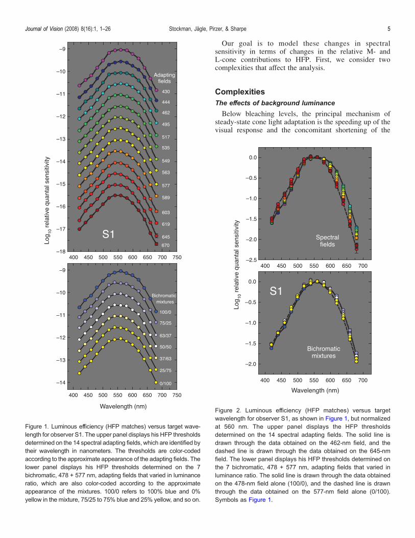
Figure 1 shows flicker photometric spectral sensitivitydata for subject S1 plotted as a function of the wavelengthof the test target. The top panel presents HFP datameasured on spectral backgrounds from 430 to 670 nm,and the bottom panel presents data measured on bichro-matic field mixtures from 100% 478 nm (100/0) to 100%577 nm (0/100). As the field wavelength increases, or thebichromatic mixture becomes more yellow, there is arelative loss of sensitivity to long-wavelength targets andan increase in sensitivity to short-wavelength targets.These effects can be seen more clearly in Figure 2, inwhich the HFP data have been normalized at a targetwavelength of 560 nm. The top panel of Figure 2 showsthe data obtained on spectral backgrounds (the solid anddashed lines join the 462- and 645-nm field data,respectively), and the lower panel shows the data obtainedon bichromatic mixtures [the solid and dashed lines jointhe 100/0 (blue field) and 0/100 (yellow field) data,respectively]. As expected, chromatic adapting fieldschange the shape of the luminous efficiency function.Longer wavelength (or more yellow) fields decrease long-wavelength sensitivity relative to short, which is consis-tent with a relative reduction in the L-cone contribution toHFP. In contrast, shorter wavelength (or more blue) fieldsincrease long-wavelength sensitivity relative to short,which is consistent with a relative reduction in theM-cone contribution.

Journal of Vision (2008) 8(16):1, 1–26 Stockman, Jägle, Pirzer, & Sharpe 4

Our goal is to model these changes in spectralsensitivity in terms of changes in the relative M- andL-cone contributions to HFP. First, we consider twocomplexities that affect the analysis.

ComplexitiesThe effects of background luminance

Below bleaching levels, the principal mechanism ofsteady-state cone light adaptation is the speeding up of thevisual response and the concomitant shortening of the

Figure 1. Luminous efficiency (HFP matches) versus target wave-length for observer S1. The upper panel displays his HFP thresholdsdetermined on the 14 spectral adapting fields, which are identified bytheir wavelength in nanometers. The thresholds are color-codedaccording to the approximate appearance of the adapting fields. Thelower panel displays his HFP thresholds determined on the 7bichromatic, 478 + 577 nm, adapting fields that varied in luminanceratio, which are also color-coded according to the approximateappearance of the mixtures. 100/0 refers to 100% blue and 0%yellow in the mixture, 75/25 to 75% blue and 25% yellow, and so on.

Figure 2. Luminous efficiency (HFP matches) versus targetwavelength for observer S1, as shown in Figure 1, but normalizedat 560 nm. The upper panel displays the HFP thresholdsdetermined on the 14 spectral adapting fields. The solid line isdrawn through the data obtained on the 462-nm field, and thedashed line is drawn through the data obtained on the 645-nmfield. The lower panel displays his HFP thresholds determined onthe 7 bichromatic, 478 + 577 nm, adapting fields that varied inluminance ratio. The solid line is drawn through the data obtainedon the 478-nm field alone (100/0), and the dashed line is drawnthrough the data obtained on the 577-nm field alone (0/100).Symbols as Figure 1.

Journal of Vision (2008) 8(16):1, 1–26 Stockman, Jägle, Pirzer, & Sharpe 5

visual integration time, so that although observers becomemore insensitive as the light level rises, they also becomerelatively more sensitive to flicker of higher temporalfrequencies (e.g., De Lange, 1958, 1961; Green, 1968;Kelly, 1961, 1974; MacLeod, 1978; Matin, 1968; Sperling& Sondhi, 1968; Stockman, Langendorfer, Smithson, &Sharpe, 2006; Tranchina, Gordon, & Shapley, 1984;Watson, 1986). As a result, the sensitivity to 25-Hz flickerdeclines at lower adaptation levels more slowly withbackground intensity than the sensitivity to lower fre-quencies. Weber’s Law is reached for 25-Hz flicker onneutral or middle-wavelength backgrounds of about 3 logtd for achromatic flicker (e.g., De Lange, 1958) and forM-cone flicker (Stockman, Langendorfer et al., 2006) andholds at luminances greater than 3 log td. Above 3 log td(or for spectral fields above a field radiance that has anequivalent effect on the M- and L-cones as a 3 log tdneutral or middle-wavelength field), therefore, the tempo-ral properties of the M- and L-cones at 25 HzVat least interms of their modulation sensitivities and phasedelaysVare roughly asymptotic and thus relativelyimmune to changes in background luminance (Stockman,Langendorfer et al., 2006). However, if the adaptive stateof one of the two cone types falls below those asymptoticlevels, then its relative contribution to 25-Hz HFPfunction will fall, and its signals will be delayed (seebelow). Such a fall occurs for the M-cones on long-wavelength fields of 3 log trolands (see red symbols,Figure 5, below) owing to the relative insensitivity of theM-cones to longer wavelengths. To avoid such difficulties,we have confined our main analysis to backgroundchromaticities on which we estimate that both cone typeshave reached Weber’s Law for 25-Hz flicker detection.We can determine which fields should be excluded from

our analysis from the relative M- and L-cone excitationsproduced by each background (Stockman & Sharpe,2000). Data obtained on fields of 589 nm or shorter canbe retained, because the M-cones are always sufficientlylight adapted [relative to equal peak quantal sensitivities,they are between 0.28 log unit less sensitive (at 589 nm) and0.23 log unit more sensitive (at 462 nm) to the fields than theL-cones]. However, on longer wavelength fields, the differ-ences in M- and L-cone excitation can be substantial. On3 log troland fields of 619, 645, and 670 nm, to which theM-cones are 0.68, 1.01, and 1.18 log units, respectively,less sensitive than the L-cones, the M-cone contribution to25-Hz HFP will drop because of low M-cone adaptationlevels (see Stockman, Langendorfer et al., 2006)Vasindeed we find (see Figure 5, below). On the 603-nmfield, on which the M-cones are 0.46 log unit less sensitivethan the L-cones, the expectations are less clear. Since thedata at 603 nm are consistent with a Weber’s Law model(see below), we have retained them in our analysis. TheM-cone adaptation data on which these predictions arebased were obtained in two protanopes and so should berelatively unaffected by second-site cone-opponent sup-pression (see Stockman, Langendorfer et al., 2006).

The problem of the M-cones being relatively unadaptedon long-wavelength fields is compounded by potentiallylarge phase delays between the M- and L-cone signals.From our recent model and data (Stockman, Langendorferet al., 2006), we estimate that the M-cone signals will bephase delayed by approximately 103- at 670 nm, 95- at645 nm, and 52- at 619 nm relative to the L-cone signals.By simple vector analysis (e.g., Equation 4 of Stockman etal., 2005) and assuming M- and L-cone signals of equalamplitude (the most extreme case for cancellation), weestimate that the resultant amplitude of the combined M-and L-cone signals would be reduced by 0.21 log unit at670 nm, 0.17 at 645 nm, and 0.05 at 619 nm. Indeed, thephase differences at 670 nm are large enough to make theadditive luminance channel weakly opponent at 25 Hz(see Drum, 1977). However, phase differences betweenthe L- and M-cone signals at 603 nm and lower wave-lengths can be safely ignored because they are no morethan 17- and, therefore, will reduce the amplitude by lessthan 0.02 log unit.Because of these complexities, we have restricted our

main analysis and model to data obtained on fields withwavelengths of 603 nm and shorter.

The flickering targets alter the mean adaptingchromaticities

Even though the flickering 25-Hz targets and referencelights are each only about 0.2 log unit above threshold,they can significantly alter the mean adapting chromatic-ities. This influence is illustrated in Figure 3 for observerS1, who set the highest reference target threshold (for theother observers, the effects are smaller). The horizontaldashed lines in each panel show the ratios of M:L-coneexcitations produced by the backgrounds or mixtures ofbackgrounds alone (M2 /L2). Ideally, the mean chromatic-ity of the combined background, target, and referencelights at the HFP null (M2,1/L2,1) should deviate very littlefrom the dashed lines. However, as the symbols show forsubject S1, the mean chromaticity at each null (plotted asM2,1/L2,1) can diverge substantially from the chromaticityof the background alone. Overall, the target and referencelights shift the mean chromaticity of both short- and long-wavelength fields: M2,1/L2,1 is increased on short-wavelength fields and decreased on long-wavelength ones.Moreover, M2,1/L2,1 also changes with target wavelength(1): M2,1/L2,1 is decreased by short-wavelength targetsand increased by long-wavelength ones. This dependenceof adapting field chromaticity on the test wavelengthoccurs on all backgrounds. Comparable effects can beseen for all six subjects in Figure 4, and Figures A1–A6 inAppendix A, in which the M2,1/L2,1 ratios produced bythe background lights alone are shown by the verticalcolored lines, and the combined values at each HFP nullare shown by the symbols.As discussed in detail in the next section, we account

for the changes in background chromaticity by finding the

Journal of Vision (2008) 8(16):1, 1–26 Stockman, Jägle, Pirzer, & Sharpe 6

best-fitting linear combinations of the Stockman andSharpe (2000) L- and M-cone fundamentals with respectto the relative M:L-cone excitation produced by thecombined test, reference, and background lights (M2,1/L2,1 in Equations 2–5, below) calculated for eachHFP setting.

Analysis of flicker photometric spectralsensitivity dataMean HFP matches for six subjects

The mean 25-Hz HFP matches for subject S1 are shownin Figure 4 plotted as a function of the M2,1/L2,1 value foreach HFP match. The matches for the other five subjectsare shown in Figures A1–A6 in Appendix A. The matcheswere made in one run, except for observer S1, who madethe bichromatic matches twice, and S2, who made thebichromatic and spectral matches twice, and observer A2,who made no bichromatic matches. The spectral matchesand bichromatic mixture matches are shown in the upperand middle panels, respectively, in each figure, with theexception of those for observer S2, whose more extensivedata span two figures: his first runs are shown in AppendixFigure A1, and his second in Appendix Figure A2.The spectral luminous efficiencies are plotted as a

function of M2,1/L2,1 instead of as a conventional functionof target wavelength, 1. This unusual scheme reveals theeffects of the test and reference lights on the adaptingchromaticity. Each spectral sensitivity curve, determined forthe different spectral and bichromatic mixture fields, com-prises the data for target wavelengths from 420 to 680 nm.Notice that the spectrum is effectively reversed in these plots.Long-wavelength backgrounds and targets produce lowerM2,1/L2,1 values and therefore plot to the left, whereas shorterwavelength backgrounds and targets produce higher valuesand plot to the right. Consequently, the target wavelengths foreach adapting condition plot from right to left.The overall quality of the data is very good. The

standard deviations within an observer are small andindependent of test and field wavelength. Data are color-coded according to the approximate appearance of theadapting field. The small open (white dots) and closed(black dots) circles in the upper and middle panels are themodel fits, which are described in the next section.

Model

In order to account for the changes in adaptingchromaticity with 2 and 1, we fit linear combinations ofthe Stockman and Sharpe (2000) L- and M-cone spectral

Figure 3. Mean M:L-cone excitation ratios elicited by thecombined reference, target, and background lights (M2,1/L2,1) ateach target wavelength for observer S1. The upper panel showsthe ratios for the spectral backgrounds, and the lower panelshows those for the bichromatic mixtures. The dashed horizontallines show the excitation ratios for the backgrounds alone (M2/L2).The backgrounds are identified by the labels to the right of eachline, indicating either the adapting wavelength for the single fieldsor the proportion of Blue (B, 478 nm) to Yellow (Y, 577 nm) for thebichromatic fields. Symbols as Figures 1 and 2. The continuouswhite line in the upper panel shows the predicted ratios for aseries of ERG 32.5-Hz flicker nulls (see Discussion section fordetails).

Journal of Vision (2008) 8(16):1, 1–26 Stockman, Jägle, Pirzer, & Sharpe 7

Journal of Vision (2008) 8(16):1, 1–26 Stockman, Jägle, Pirzer, & Sharpe 8

sensitivities for each adapting condition (2) not just as afunction of target wavelength (1) but also as a function ofthe mean adapting chromaticity at each HFP null (M2,1/L2,1). We began with

log10V2 * ð1Þ ¼ log10ða2l�ð1Þ þ m�ð1ÞÞ; ð1Þ

where a2 is the L-cone weight, V2*(1) is the predictedspectral sensitivity (luminous efficiency) function for anadapting field 2, l�(1) is either the L(ser180) or the L(ala180)variant of the Stockman and Sharpe (2000) L-conefundamentals, and m�(1) is the Stockman and Sharpe(2000) M-cone spectral sensitivity. The spectral sensitiv-ity functions, which in these formulae are quantum-based,are given in Appendix Table A1. We then set a2 = "2 �(M2,1/L2,1), where "2 is now the “L-cone bias,” and (toreiterate) M2,1/L2,1 is the relative M:L-cone excitationproduced by the combined test, reference, and backgroundlights at each HFP null. (We ignore the possibility that theM- and L-cone incremental test components might have agreater or lesser influence than expected, because ofspatial opponency or spatial integration with respect tothe surrounding background.) The excitation ratios werecalculated from the radiometric calibrations and nullsettings using the Stockman & Sharpe cone fundamentalswith unity quantal peaks. Next, the sensitivity for each 2,1, and M2,1/L2,1 is normalized relative to the referencewavelength of 560 nm (recall that M2,1/L2,1 includes theeffects of the fixed 560-nm reference), so that

log10V2 * 1ð Þ ¼ log10 "2M2;1

L2;1l� 1ð Þ þ m� 1ð Þ

� �

j log10 "2M2;1

L2;1l� 560ð Þ þ m� 560ð Þ

� �:

ð2Þ

Equation 2 defines the sensitivity difference (or relativeHFP match) between 1 and 560 nm for each combinationof background, test, and reference lights at an HFP null.The reason we have added the complexity of setting

a2 = "2 � (M2,1/L2,1) is illustrated by rearranging(Equation 2) to yield

log10V2 * 1ð Þ ¼ log10 "2l�ð1ÞL2;1

þ m�ð1ÞM2;1

� �

jlog10 "2l�ð560ÞL2;1

þ m�ð560ÞM2;1

� �:

ð3Þ

In Equation 3, the L-cone fundamental is scaled by theL-cone excitation, and the M-cone fundamental is scaledby the M-cone excitation, which is equivalent to areciprocal sensitivity adjustment of each cone signal inaccordance with Weber’s Law. Consequently, if theL-cone bias, "2, is found to be constant over a range ofM2,1/L2,1, it suggests that Weber’s Law holds over thatrange. An increase in "2 implies a decrease of the M-conecontribution relative to the Weber’s Law prediction,whereas a decrease in "2 implies a decrease of the L-conecontribution relative to the Weber’s Law prediction.Increases or decreases in "2 can be potentially due to avariety of causes including relative chromatic suppressionor facilitation, or shortfalls from Weber’s Law (seeabove).We found the best-fitting values of "2 for each spectral

and bichromatic spectral sensitivity condition (2) bysimultaneously fitting all the data for each subject with

log10V2 * 1ð Þ ¼ log10 "2M2;1

L2;1l� 1ð Þ þ m� 1ð Þ

� �þ klensdlensð1Þ þ kmacdmacð1Þ

j log10 "2M2;1

L2;1l� 560ð Þ þ m� 560ð Þ

� �

j klensdlensð560Þ j kmacdmacð560Þ:

ð4Þ

Equation 4 is the same as Equation 2, except that thedata for each subject undergo best-fitting adjustments forindividual differences in prereceptoral lens and macularpigment filtering. The constants klens and kmac are,respectively, best-fitting lens and macular pigment densitymultipliers that adjust each subject’s HFP curves to beconsistent with the mean lens [dlens(1)] and macular[dmac(1)] pigment density spectra implied by theStockman and Sharpe standard observer. The functiondlens(1) is the lens pigment density spectrum of Norren

Figure 4. Luminous efficiencies (HFP matches), in decimallogarithm, versus M:L-cone excitation ratios elicited by thecombined reference, test, and background lights (M2,1/L2,1) forobserver S1. The upper panel shows the HFP sensitivitiesdetermined on the 11 spectral adapting fields. The second andthird panels show two separate determinations of the HFPsensitivities on the 7 bichromatic, 478 nm (blue, b) + 577 nm(yellow, y) adapting fields. The small open circles (which appearas white dots), filled circles (which appear as black dots), andfilled black triangles plotted, respectively, in the upper threepanels are the best-fitting combinations of the Stockman andSharpe (2000) M- and L-cone fundamentals determined fromEquation 4. The corresponding residuals are plotted in the lowestpanel. The M:L-cone excitation ratios produced by the labeledbackground adapting fields alone (M2/L2) are identified by thevertical colored lines in the upper three panels. Symbols asFigures 1–3 (see also key).

Journal of Vision (2008) 8(16):1, 1–26 Stockman, Jägle, Pirzer, & Sharpe 9

and Vos (1974), slightly modified by Stockman, Sharpe,and Fach (1999) [dlens(400), for example, is 1.76], whilethe function dmac(1) is the mean macular density spectrumbased on measurements by Bone, Landrum, and Cairns(1992) proposed by Stockman et al. (1999) [dmac(460), forexample, is 0.35]. For further details about the fitting

procedure, see our earlier papers (Sharpe et al., 2005;Stockman & Sharpe, 2000).The appropriate L(ser180) and L(ala180) cone templates

are based on the Stockman and Sharpe (2000) L-conefundamental calculated back to an absorbance spectrum(see their Table 2, Column 9), and then shifted along a

Figure 5. The best-fitting values of the L-cone bias, "2, for each of the six observers (Panels 1–6), plotted as a function of the mean M2,1/L2,12 cone excitations for each adapting and mixture field condition (dotted, yellow circles). The standard errors of the fits are indicated.The red circles in each panel show the partial results of a separate analysis that included the three longest wavelength backgrounds of619, 645, and 670 nm, which were excluded from themain analysis. The continuous black lines indicate simple power functions (Equation 5)fitted to the dotted, yellow circles. The red continuous lines indicate best-fitting forms of the threshold power model (Equations 4 and 5)fitted simultaneously to each observer’s HFP data for all background conditions. The horizontal gray lines indicate the best-fitting fixedL-cone bias (Weber’s Law) again fitted simultaneously to each observer’s HFP data for all background conditions.

Journal of Vision (2008) 8(16):1, 1–26 Stockman, Jägle, Pirzer, & Sharpe 10

logarithmic wavelength scale by j1.51 nm at 1max for L(ala180) or by +1.19 nm for L(ser180) in accordance withthe 2.7-nm spectral shift between the L(ala180) and L(ser180) spectral sensitivities (Sharpe, Stockman, Jagleet al., 1998). Eisner and MacLeod (1981) also found a2.7-nm shift between two groups of alleged L-coneisolates but of unknown genotype. The two respectiveshifted spectra were then corrected back to cornealspectral sensitivities to generate the corneal templatesused in the fits. For further details, see Stockmanand Sharpe (2000). These two templates, which have notbeen published before, are provided in 5-nm steps inTable A1 in Appendix A. The use of the appropriateversion of the L-cone template is important for avoidingsizable errors that can arise in estimating the relativeL-cone weights with the mean L-cone template (e.g.,Bieber, Kraft, & Werner, 1998; Carroll, McMahon,Neitz, & Neitz, 2000; Sharpe et al., 2005). The functionsin Equation 4 can be downloaded from the website: http://www.cvrl.org.We used two approaches to fit Equation 4 simultane-

ously to all the data for each subject. First, we determinedthe optimal "2 for each 2. Second, we assumed that "2

varied as some function of 2 or was constant (Weber’sLaw) and determined the optimal fit for all 2.

Determination of "2 for each 2

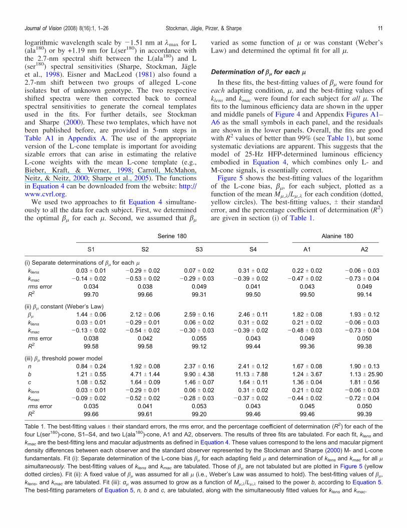
In these fits, the best-fitting values of "2 were found foreach adapting condition, 2, and the best-fitting values ofklens and kmac were found for each subject for all 2. Thefits to the luminous efficiency data are shown in the upperand middle panels of Figure 4 and Appendix Figures A1–A6 as the small symbols in each panel, and the residualsare shown in the lower panels. Overall, the fits are goodwith R2 values of better than 99% (see Table 1), but somesystematic deviations are apparent. This suggests that themodel of 25-Hz HFP-determined luminous efficiencyembodied in Equation 4, which combines only L- andM-cone signals, is essentially correct.Figure 5 shows the best-fitting values of the logarithm

of the L-cone bias, "2, for each subject, plotted as afunction of the mean M2,1/L2,1 for each condition (dotted,yellow circles). The best-fitting values, T their standarderror, and the percentage coefficient of determination (R2)are given in section (i) of Table 1.

Serine 180 Alanine 180

S1 S2 S3 S4 A1 A2

(i) Separate determinations of "2 for each 2

klens 0.03 T 0.01 j0.29 T 0.02 0.07 T 0.02 0.31 T 0.02 0.22 T 0.02 j0.06 T 0.03kmac j0.14 T 0.02 j0.53 T 0.02 j0.29 T 0.03 j0.39 T 0.02 j0.47 T 0.02 j0.73 T 0.04rms error 0.034 0.038 0.049 0.041 0.043 0.049R2 99.70 99.66 99.31 99.50 99.50 99.14

(ii) "2 constant (Weber’s Law)"2 1.44 T 0.06 2.12 T 0.06 2.59 T 0.16 2.46 T 0.11 1.82 T 0.08 1.93 T 0.12klens 0.03 T 0.01 j0.29 T 0.01 0.06 T 0.02 0.31 T 0.02 0.21 T 0.02 j0.06 T 0.03kmac j0.13 T 0.02 j0.54 T 0.02 j0.30 T 0.03 j0.39 T 0.02 j0.48 T 0.03 j0.73 T 0.04rms error 0.038 0.042 0.055 0.043 0.049 0.050R2 99.58 99.58 99.12 99.44 99.36 99.38

(iii) "2 threshold power modeln 0.84 T 0.24 1.92 T 0.08 2.37 T 0.16 2.41 T 0.12 1.67 T 0.08 1.90 T 0.13b 1.21 T 0.55 4.71 T 1.44 9.90 T 4.38 11.13 T 7.88 1.24 T 3.67 1.13 T 25.90c 1.08 T 0.52 1.64 T 0.09 1.46 T 0.07 1.64 T 0.11 1.36 T 0.04 1.81 T 0.56klens 0.03 T 0.01 j0.29 T 0.01 0.06 T 0.02 0.31 T 0.02 0.21 T 0.02 j0.06 T 0.03kmac j0.09 T 0.02 j0.52 T 0.02 j0.28 T 0.03 j0.37 T 0.02 j0.44 T 0.02 j0.72 T 0.04rms error 0.035 0.041 0.053 0.043 0.045 0.050R2 99.66 99.61 99.20 99.46 99.46 99.39

Table 1. The best-fitting values T their standard errors, the rms error, and the percentage coefficient of determination (R2) for each of thefour L(ser180)-cone, S1–S4, and two L(ala180)-cone, A1 and A2, observers. The results of three fits are tabulated. For each fit, klens andkmac are the best-fitting lens and macular adjustments as defined in Equation 4. These values correspond to the lens and macular pigmentdensity differences between each observer and the standard observer represented by the Stockman and Sharpe (2000) M- and L-conefundamentals. Fit (i): Separate determination of the L-cone bias "2 for each adapting field 2 and determination of klens and kmac for all 2simultaneously. The best-fitting values of klens and kmac are tabulated. Those of "2 are not tabulated but are plotted in Figure 5 (yellowdotted circles). Fit (ii): A fixed value of "2 was assumed for all 2 (i.e., Weber’s Law was assumed to hold). The best-fitting values of "2,klens, and kmac are tabulated. Fit (iii): α2 was assumed to grow as a function of M2,1/L2,1 raised to the power b, according to Equation 5.The best-fitting parameters of Equation 5, n, b and c, are tabulated, along with the simultaneously fitted values for klens and kmac.

Journal of Vision (2008) 8(16):1, 1–26 Stockman, Jägle, Pirzer, & Sharpe 11

In general, "2 is roughly constant at low M2,1/L2,1 (i.e.,Weber’s Law holds), but for four out of six subjects (S1,S2, S3, and A1) it increases at higher mean M2,1/L2,1(i.e., the M-cone contribution falls below the Weber’sLaw prediction). The fall in the M-cone contribution onshorter wavelength fields (lower mean M2,1/L2,1) isexpected from previous work (e.g., Eisner & MacLeod,1981). Note that although the L-cone bias, "2, is constant atlow M2,1/L2,1, the weight, a2, decreases as M2,1/L2,1decreases. In general, on shorter wavelength fields (i.e.,higher values of M2,1/L2,12), a2 increases so that thespectral luminous efficiency becomes more L-cone-like,whereas on longer wavelength fields (i.e., lower values ofM2,1/L2,12), it decreases so that the efficiency becomesmore M-cone-like (compare the red and black continuouslines in Figure 6, below).Notice that as "2 increases, so too does the standard

error of its fit. This is a general property of these fits thatarises because as "2 gets larger, its effect on spectralsensitivity gets smaller (for further discussion, see Sharpeet al., 2005). Thus, apparently large discrepancies betweenlarge values of "2, such as that between the two "2 valuesfor the repeated 462-nm adapting field measurements forS2 (i.e., the two rightmost yellow circles in the middle left panelof Figure 5), correspond to only relatively small differences inthe underlying spectral luminous efficiency functions.The mean values of klens were 0.03, j0.29, 0.07,

0.31, 0.22, and j0.05 for subjects S1–S4, A1, andA2, respectively, and the mean values of kmac were j0.14,j0.53, j0.29, j0.39, j0.47, and j0.73, respectively.These values correspond to the factor by which the pigmentdensity spectrum template in question must be adjusted tobring each subject’s luminous efficiency data into bestagreement with the linear combination of l�(1) and m�(1).Note that a negative value means that a particular subjecthas a higher pigment density than the Stockman and Sharpe(2000) mean observer, and a positive value, a lowerpigment density. Thus, our observers have on average0.05 times less lens density as the Stockman and Sharpe(2000) mean observer (so that their mean density at 400 nmis 1.67 compared with 1.76) and, on average, 0.43 timesmore macular density (so that their mean peak density is0.50 compared with 0.35). Our observers, therefore, aremore heavily macular pigmented, on average, than theStockman and Sharpe (2000) mean observer, but theirdensity values all lie within the normal range. We areconfident that these densities are not overinflated by thefitting procedure. The macular pigment density of three ofthe six subjects has been estimated before. Two of them(S2 and A2) participated in a study (Sharpe, Stockman,Knau, & Jagle, 1998) in which the actual macular densityspectra were determined. S2 was found to have a peakdensity of 0.50 (compared with 0.54 here) and A2 wasfound to have a peak density of approximately 0.60(compared with 0.61 here). S1 has carried out more limiteddeterminations but is known to be typical in having a peakdensity of ca. 0.35 (compared with 0.40 here).

The red circles in each panel of Figure 5 show the partialresults of a separate analysis that included the three longestwavelength backgrounds of 619, 645, and 670 nm, whichwere excluded from the main analysis. As the fieldwavelength lengthens, "2 becomes increasingly large,suggesting the contribution of the M-cones falls below theWeber’s Law predictions. However, this is one of thecomplexities discussed in The effects of backgroundluminance section; the lowered M-cone contribution occursprobably because the M-cones are relatively unadapted.

Determination of "2 as a function of 2

By using Equation 4 and separately determining "2, foreach 2, we have effectively assumed that local variationsof M2,1/L2,1 around the mean for each adapting conditioninduce changes in the L-cone weight that are consistentwith Weber’s Law (i.e., we assume that, locally, "2 isconstant). The goodness of the fits shown in Figure 4 andAppendix Figures A1–A6 suggests that this is a reason-able approximation. However, for the majority of subjectsthe "2 values, as shown in Figure 5, increase as M2,1/L2,1increases. In this section, we try to capture this increase byassuming that "2 increases as some function of M2,1/L2,1.In principle, this should yield a better local fit in thoseregions in which M2,1/L2,1 increases.Initially, however, we made the much simpler assump-

tion that Weber’s Law holds across all conditions, and that"2 is therefore fixed across all M2,1/L2,1. Equation 4 wasfitted simultaneously to all the data for each subject to findthe best-fitting values of "2, klens, and kmac for all 2. Thisreduced the number of fitted parameters from 20 (or morefor S1 and S2, less for A1) to just 3. Figure 5 shows thebest-fitting values of the fixed L-cone bias, "2, for eachsubject, plotted as a horizontal gray line. The best-fittingvalues, T their standard error, and the percentage coef-ficient of determination (R2) are given in section (ii) ofTable 1. Despite the large reduction in the number ofparameters, the fits are only slightly worse than theindividual fits. However, the fixed value clearly under-estimates "2 at low M2,1/L2,1 values and overestimates it athigh values, which is undesirable in any predictive model.To overcome this problem, we sought a simple continuousfunction that could be used to describe the change in "2 forall 6 subjects just by changing its parameters. We finallysettled on the following version of a power function:

"2 ¼ n 1þ M2;1=L2;1c

� �b !; ð5Þ

in which b is the power to which M2,1/L2,1 is raised, cdetermines the “threshold” level of M2,1/L2,1 after whichthe power term becomes important, and n is a multiplierthat scales the whole function.Equation 5 is shown as the continuous black lines in

Figure 5 fitted to the individual "2 estimates for each

Journal of Vision (2008) 8(16):1, 1–26 Stockman, Jägle, Pirzer, & Sharpe 12

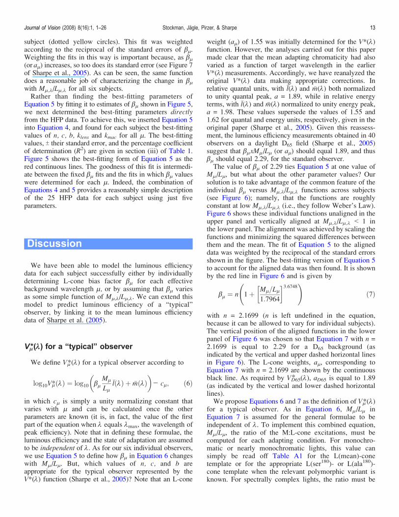
subject (dotted yellow circles). This fit was weightedaccording to the reciprocal of the standard errors of "2.Weighting the fits in this way is important because, as "2(or a2) increases, so too does its standard error (see Figure 7of Sharpe et al., 2005). As can be seen, the same functiondoes a reasonable job of characterizing the change in "2with M2,1/L2,1 for all six subjects.Rather than finding the best-fitting parameters of

Equation 5 by fitting it to estimates of "2 shown in Figure 5,we next determined the best-fitting parameters directlyfrom the HFP data. To achieve this, we inserted Equation 5into Equation 4, and found for each subject the best-fittingvalues of n, c, b, klens and kmac for all 2. The best-fittingvalues, T their standard error, and the percentage coefficientof determination (R2) are given in section (iii) of Table 1.Figure 5 shows the best-fitting form of Equation 5 as thered continuous lines. The goodness of this fit is intermedi-ate between the fixed "2 fits and the fits in which "2 valueswere determined for each 2. Indeed, the combination ofEquations 4 and 5 provides a reasonably simple descriptionof the 25 HFP data for each subject using just fiveparameters.

Discussion

We have been able to model the luminous efficiencydata for each subject successfully either by individuallydetermining L-cone bias factor "2 for each effectivebackground wavelength 2, or by assuming that "2 variesas some simple function of M2,1/L2,1. We can extend thismodel to predict luminous efficiency of a “typical”observer, by linking it to the mean luminous efficiencydata of Sharpe et al. (2005).

V2*(1) for a “typical” observer

We define V2*(1) for a typical observer according to

log10V2* 1ð Þ ¼ log10 "2M2

L2l� 1ð Þ þ m� 1ð Þ

� �j c2; ð6Þ

in which c2 is simply a unity normalizing constant thatvaries with 2 and can be calculated once the otherparameters are known (it is, in fact, the value of the firstpart of the equation when 1 equals 1max, the wavelength ofpeak efficiency). Note that in defining these formulae, theluminous efficiency and the state of adaptation are assumedto be independent of 1. As for our six individual observers,we use Equation 5 to define how "2 in Equation 6 changeswith M2/L2. But, which values of n, c, and b areappropriate for the typical observer represented by theV*(1) function (Sharpe et al., 2005)? Note that an L-cone

weight (a2) of 1.55 was initially determined for the V*(1)function. However, the analyses carried out for this papermade clear that the mean adapting chromaticity had alsovaried as a function of target wavelength in the earlierV*(1) measurements. Accordingly, we have reanalyzed theoriginal V*(1) data making appropriate corrections. Inrelative quantal units, with l�(1) and m�(1) both normalizedto unity quantal peak, a = 1.89, while in relative energyterms, with l�(1) and m�(1) normalized to unity energy peak,a = 1.98. These values supersede the values of 1.55 and1.62 for quantal and energy units, respectively, given in theoriginal paper (Sharpe et al., 2005). Given this reassess-ment, the luminous efficiency measurements obtained in 40observers on a daylight D65 field (Sharpe et al., 2005)suggest that "2xM2/L2 (or a2) should equal 1.89, and thus"2 should equal 2.29, for the standard observer.The value of "2 of 2.29 ties Equation 5 at one value of

M2/L2, but what about the other parameter values? Oursolution is to take advantage of the common feature of theindividual "2 versus M2,1/L2,1 functions across subjects(see Figure 6); namely, that the functions are roughlyconstant at low M2,1/L2,1 (i.e., they follow Weber’s Law).Figure 6 shows these individual functions unaligned in theupper panel and vertically aligned at M2,1/L2,1 G 1 inthe lower panel. The alignment was achieved by scaling thefunctions and minimizing the squared differences betweenthem and the mean. The fit of Equation 5 to the aligneddata was weighted by the reciprocal of the standard errorsshown in the figure. The best-fitting version of Equation 5to account for the aligned data was then found. It is shownby the red line in Figure 6 and is given by

"2 ¼ n 1þ M2=L21:7964

� �3:6748 !ð7Þ

with n = 2.1699 (n is left undefined in the equation,because it can be allowed to vary for individual subjects).The vertical position of the aligned functions in the lowerpanel of Figure 6 was chosen so that Equation 7 with n =2.1699 is equal to 2.29 for a D65 background (asindicated by the vertical and upper dashed horizontal linesin Figure 6). The L-cone weights, a2, corresponding toEquation 7 with n = 2.1699 are shown by the continuousblack line. As required by VD65* (1), aD65 is equal to 1.89(as indicated by the vertical and lower dashed horizontallines).We propose Equations 6 and 7 as the definition of V2*(1)

for a typical observer. As in Equation 6, M2/L2 inEquation 7 is assumed for the general formulae to beindependent of 1. To implement this combined equation,M2/L2, the ratio of the M:L-cone excitations, must becomputed for each adapting condition. For monochro-matic or nearly monochromatic lights, this value cansimply be read off Table A1 for the L(mean)-conetemplate or for the appropriate L(ser180)- or L(ala180)-cone template when the relevant polymorphic variant isknown. For spectrally complex lights, the ratio must be

Journal of Vision (2008) 8(16):1, 1–26 Stockman, Jägle, Pirzer, & Sharpe 13

calculated by cross-multiplying the spectral power distri-bution of the field in question with the Stockman andSharpe (2000) L- and M-cone spectral sensitivities (afterchoosing the appropriate L-cone polymorphic variant),separately summing the L- andM-cone cross-multiplicationsand obtaining the ratio between them. For the estimate ofV2*(1) to be more accurate for individual observers, n inEquation 7 can be individually determined.

Chromatic suppression of the cone inputs toluminance

Evidence that the luminance contribution of the L-or M-cone type more sensitive to a given chromatic

field is suppressed in excess of Weber’s Law has beenpresented before (Eisner & MacLeod, 1981; Stockmanet al., 1993), although in one study the L-cone suppressionon long-wavelength fields was found to be more pro-nounced than M-cone suppression on short-wavelengthones (Stromeyer et al., 1987). Such suppression causesluminous efficiency functions to become more M-cone-like than expected on long-wavelength adapting fields andmore L-cone-like than expected on short-wavelengthfields.Our results are consistent with a relative M-cone

suppression in excess of Weber’s Law on short-wavelength fields but with there being no comparableL<cone suppression on long-wavelength fields. The appa-rent lack of L-cone suppression (red circles, Figure 5) maysimply reflect the low levels of M-cone adaptation on3 log troland long-wavelength fields (see, e.g., De Vries,1948b; Eisner & MacLeod, 1981; Stiles, 1978; Stockmanet al., 1993; Stockman, Montag, & Plummer, 2006;Stromeyer et al., 1987).It is important to note that obedience to the Weber’s

Law prediction does not necessarily imply an absenceof chromatic suppression. For example, on longerwavelength fields, such as 603 nm, Weber’s Law forM-cone flicker detection in normal trichromats mayreflect a less-than-Weber adjustment of 25-Hz gain atthe cone level, with a later, cone-opponent suppression ofthe M-cone signal. The expected relative suppression onlong-wavelength fields is, however, of the L-cones (Eisner& MacLeod, 1981).Another complication is that the L- and M-cone

suppressions, particularly on long-wavelength fields, maybe due in part to constructive and destructive interfer-ence between the fast and slow M- and L-cone signals(Stockman, Montag et al., 2006; Stockman & Plummer,2005a, 2005b; Stockman et al., 2005). These interferenceeffects are most prominent near 15 Hz. Consequently, theuse of 25-Hz flicker would have reduced any effects ofinterference.

Luminous efficiency and relative L- andM-cone numerosity

Luminous efficiency functions have been used byseveral groups as a way of estimating the relativenumber of L- and M-cones in the retinal area withinwhich it is measured (e.g., Adam, 1969; Crone, 1959; DeVries, 1946, 1948a; Dobkins, Thiele, & Albright, 2000;Gunther & Dobkins, 2002; Kremers, Scholl, Knau,Berendschot, & Sharpe, 2000; Lutze, Cox, Smith, &Pokorny, 1990; Rushton & Baker, 1964; Smith &Pokorny, 1975; Vimal, Pokorny, Smith, & Shevell, 1989;Vos & Walraven, 1971). The assumption underlying suchestimates is that the L-cone weight a2("2xM2,1/L2,1,in our model) directly reflects the relative numbers of the

Figure 6. The L-cone bias ("2) as a function of mean M2/L2 coneexcitation for each of the six observers (different colored symbols)unaligned (top panel) and vertically aligned at M2/L2 G 1 (bottompanel). The red line denotes the V2*(1) L-cone bias “template”function (see description of Equation 7 in the text for details), andthe black line the corresponding L-cone weights. The dashed linesindicate the L-cone bias and L-cone weight template values corre-sponding to the M2,1/L2,1 cone excitation ratio for a D65 white field.

Journal of Vision (2008) 8(16):1, 1–26 Stockman, Jägle, Pirzer, & Sharpe 14

L- and M-cones contributing to luminous efficiency. Thisassumption is, however, highly questionable, because theoutputs of each cone type are modified not only byreceptoral adaptation, but also, as our results suggest onshort-wavelength fields that show M-cone suppression,by postreceptoral adaptation before the signals arecombined. Indeed, the strong dependence of a2 onchromatic adaptation begs the question of which conditionof chromatic adaptation should be considered truly“neutral”Vin the sense of not altering the relativecontributions of the M- and L-cones to luminous effi-ciency away from those due to relative numerosity. Oneway of potentially simplifying the problem is, as we havedone, to consider the effects of selective proportionalchromatic adaptation separately from other factors byconsidering the L-cone weight a2 as "2xM2,1/L2,1,where "2 is the L-cone bias. Indeed, it is temptingto conclude that the roughly constant value of "2found for low M2,1/L2,1 (where Weber’s Law approx-imately holds) actually reflects relative L- and M-conenumerosity.However, even at low M2,1/L2,1, "2 is still likely to be

influenced by factors other than numerosity, such asneural weighting differences. In principle, "2 could havelittle or nothing to do with relative L- and M-conenumbers but instead reflect the relative L- and M-conecontrast gains. This view is doubtful, however, given thatL:M-cone ratio estimates derived from luminous effi-ciency functions correlate with estimates derived in thesame subjects using other methods (e.g., Albrecht, Jagle,Hood, & Sharpe, 2002; Brainard et al., 2000; Kremerset al., 2000; Lutze et al., 1990; Rushton & Baker, 1964;Sharpe, de Luca, Hansen, Jagle, & Gegenfurtner, 2006;Vimal et al., 1989; Wesner, Pokorny, Shevell, & Smith,1991). Nevertheless, any claims that luminous efficiencycan be used to derive cone numerosity directly should betreated with extreme caution. Other workers havepointed out the problems of linking luminous efficiencywith cone numerosity (e.g., Chaparro, Stromeyer,Kronauer, & Eskew, 1994; Eskew, McLellan, & Giulianini,1999).

Backgrounds and HFP

The use of steady backgrounds mitigates against thechanges in chromaticity caused by the 25-Hz referenceand target lights. Had we not used backgrounds, thechromaticity changes would have been much larger.The problems caused by not using backgrounds forhigh-frequency HFP are nicely illustrated by the largebody of ERG work carried out using 32.5-Hz flicker(e.g., Brainard et al., 2000; Carroll et al., 2000; Carroll,Neitz, & Neitz, 2002; Hofer, Carroll, Neitz, Neitz, &

Williams, 2005; Jacobs, Neitz, & Krogh, 1996). In thesemeasurements, only two flickering fields of 59 deg indiameter were used: a flickering white (2850 K) referencefield of 2.37 log trolands that was superimposed on aflickering variable-wavelength target, the radiance ofwhich was adjusted to elicit a null in the ERG at 32.5 Hz.The white field, which was produced in Maxwellian-viewby a tungsten halide lamp, had a color temperature closeto Illuminant A. From the information provided, we canonly roughly estimate the effects of this light on theM- and L-cones. However, a comparable spectrallycalibrated white field (close to Illuminant A) of 2.37 logtrolands in our system produced M:L-cone excitationsequivalent to a monochromatic light of 578 nm and8.35 log quantaIsj1Idegj2. Given this assumption, we canuse the V2*(1) function to estimate the ERG flickermatches and then calculate from those matches thechanges in adapting chromaticity with target wavelength.The estimated chromaticities for the ERG measurementsare shown as the continuous white line in the upper panelof Figure 3. As can be seen, the changes in adaptingchromaticity are substantialVmuch larger than thechanges found when a background is used. Over thetypical range of their ERG measurements (460 to680 nm), the M/L cone excitation ratio changes from1.25 (equivalent to a background of about 520 nm) to 0.40(equivalent to a background of about 600 nm). Theseconsiderable changes in adapting chromaticity with targetwavelength will distort the ERG spectral sensitivities (seeFigure 2, above, for the expected changes betweencomparable spectral fields). The 32.5-Hz ERG measure-ments, therefore, are unlikely to reflect accuratelyrelative L- and M-cone numerosity, as the authors claim.Although the curves may still be describable as a linearcombination of the M- and L-cone spectral sensitivities(as we also found in a preliminary analysis of the HFPdata shown here), the weights will be systematicallyoffset from values that would be obtained if there hadbeen no change in chromatic adaptation with targetwavelength. Errors of this type are expected from thework of De Vries (1948b), who showed HFP additivityfailures for combined test and reference targets thatexceeded 1.7 log trolands.As we noted above, any luminous efficiency function

strictly applies only to the conditions of chromaticadaptation under which it was measured. In addition,the function will also depend on other aspects of themeasurement: for example, the stimulus size, thestimulus intensity, the retinal location probed, the flickerfrequency, the measurement task, and so on. Thesedependencies mean that any generalization of luminousefficiency will inevitably be an approximation. Indeed, ifthe measure of luminance is in any way critical, itshould be determined anew for the particular conditionsof interest.

Journal of Vision (2008) 8(16):1, 1–26 Stockman, Jägle, Pirzer, & Sharpe 15

nm log M log Lmean M/Lmean log L(ser180) M/L(ser180) log L(ala180) M/L(ala180)

390 j3.2908 j3.2186 0.8470 j3.2459 0.9018 j3.2024 0.8159395 j2.8809 j2.8202 0.8696 j2.8197 0.8686 j2.8119 0.8531400 j2.5120 j2.4660 0.8994 j2.4737 0.9155 j2.4738 0.9158405 j2.2013 j2.1688 0.9279 j2.1722 0.9352 j2.1746 0.9403410 j1.9346 j1.9178 0.9622 j1.9245 0.9771 j1.9270 0.9828415 j1.7218 j1.7371 1.0358 j1.7353 1.0316 j1.7368 1.0351420 j1.5535 j1.6029 1.1206 j1.5999 1.1129 j1.5995 1.1119425 j1.4235 j1.5136 1.2305 j1.5149 1.2342 j1.5120 1.2262430 j1.3033 j1.4290 1.3357 j1.4345 1.3527 j1.4288 1.3350435 j1.1900 j1.3513 1.4499 j1.3637 1.4921 j1.3548 1.4617440 j1.0980 j1.2842 1.5355 j1.2938 1.5698 j1.2815 1.5259445 j1.0342 j1.2414 1.6113 j1.2500 1.6436 j1.2343 1.5852450 j0.9794 j1.2010 1.6659 j1.2085 1.6946 j1.1895 1.6222455 j0.9319 j1.1606 1.6931 j1.1683 1.7234 j1.1463 1.6385460 j0.8632 j1.0974 1.7144 j1.1113 1.7702 j1.0868 1.6734465 j0.7734 j1.0062 1.7093 j1.0260 1.7889 j0.9996 1.6835470 j0.6928 j0.9200 1.6873 j0.9395 1.7647 j0.9118 1.6557475 j0.6301 j0.8475 1.6498 j0.8597 1.6968 j0.8313 1.5895480 j0.5747 j0.7803 1.6052 j0.7913 1.6464 j0.7628 1.5421485 j0.5235 j0.7166 1.5602 j0.7289 1.6050 j0.7010 1.5051490 j0.4738 j0.6535 1.5125 j0.6626 1.5446 j0.6358 1.4520495 j0.4078 j0.5730 1.4628 j0.5874 1.5120 j0.5620 1.4262500 j0.3337 j0.4837 1.4126 j0.4980 1.4597 j0.4744 1.3825505 j0.2569 j0.3929 1.3677 j0.4068 1.4122 j0.3852 1.3436510 j0.1843 j0.3061 1.3238 j0.3191 1.3640 j0.2995 1.3039515 j0.1209 j0.2279 1.2791 j0.2401 1.3157 j0.2226 1.2638520 j0.0699 j0.1633 1.2397 j0.1789 1.2851 j0.1635 1.2403525 j0.0389 j0.1178 1.1991 j0.1310 1.2363 j0.1176 1.1987530 j0.0191 j0.0830 1.1586 j0.0914 1.1811 j0.0799 1.1501535 j0.0081 j0.0571 1.1197 j0.0638 1.1369 j0.0540 1.1116540 j0.0004 j0.0330 1.0779 j0.0421 1.1007 j0.0340 1.0803545 j0.0036 j0.0187 1.0353 j0.0254 1.0516 j0.0189 1.0359550 j0.0163 j0.0128 0.9918 j0.0131 0.9925 j0.0082 0.9813555 j0.0295 j0.0050 0.9452 j0.0054 0.9460 j0.0021 0.9387560 j0.0514 j0.0019 0.8923 j0.0017 0.8919 0.0000 0.8884565 j0.0769 j0.0001 0.8379 0.0000 0.8377 0.0000 0.8377570 j0.1115 j0.0015 0.7763 j0.0014 0.7761 j0.0033 0.7795575 j0.1562 j0.0086 0.7119 j0.0062 0.7079 j0.0101 0.7143580 j0.2143 j0.0225 0.6430 j0.0146 0.6315 j0.0209 0.6406585 j0.2753 j0.0325 0.5718 j0.0282 0.5662 j0.0370 0.5778590 j0.3443 j0.0491 0.5067 j0.0462 0.5034 j0.0579 0.5171595 j0.4264 j0.0727 0.4429 j0.0693 0.4395 j0.0843 0.4549600 j0.5198 j0.1026 0.3826 j0.1000 0.3803 j0.1186 0.3970605 j0.6247 j0.1380 0.3261 j0.1357 0.3243 j0.1583 0.3416610 j0.7390 j0.1823 0.2776 j0.1790 0.2755 j0.2060 0.2931

Table A1. The L(ser180)- and L(ala180)-cone templates based on the Stockman and Sharpe (2000) cone sensitivity measurements, whichare tabulated here for the first time, as well as the L(mean)- and M-cone templates (from Stockman & Sharpe, 2000). Also tabulated arethe M:L cone sensitivity ratios as a function of wavelength for the L(mean)-, L(ser180)-, and L(ala180)-cone template variants. Please notethat all sensitivities are in quantal units.

Appendix A: Online appendix

L- and M-cone spectral sensitivities

Journal of Vision (2008) 8(16):1, 1–26 Stockman, Jägle, Pirzer, & Sharpe 16

nm log M log Lmean M/Lmean log L(ser180) M/L(ser180) log L(ala180) M/L(ala180)

615 j0.8610 j0.2346 0.2364 j0.2295 0.2336 j0.2611 0.2512620 j0.9915 j0.2943 0.2008 j0.2885 0.1982 j0.3252 0.2156625 j1.1294 j0.3603 0.1702 j0.3555 0.1683 j0.3975 0.1854630 j1.2721 j0.4421 0.1479 j0.4296 0.1437 j0.4771 0.1603635 j1.4205 j0.5327 0.1295 j0.5121 0.1235 j0.5652 0.1395640 j1.5748 j0.6273 0.1128 j0.6031 0.1067 j0.6618 0.1222645 j1.7370 j0.7262 0.0976 j0.7046 0.0928 j0.7690 0.1076650 j1.8900 j0.8407 0.0893 j0.8143 0.0840 j0.8844 0.0987655 j2.0523 j0.9658 0.0819 j0.9311 0.0756 j1.0066 0.0900660 j2.2220 j1.0966 0.0749 j1.0566 0.0683 j1.1375 0.0823665 j2.3923 j1.2327 0.0692 j1.1904 0.0628 j1.2764 0.0766670 j2.5559 j1.3739 0.0658 j1.3311 0.0596 j1.4219 0.0734675 j2.7194 j1.5208 0.0633 j1.4779 0.0573 j1.5731 0.0714680 j2.8843 j1.6736 0.0616 j1.6303 0.0557 j1.7294 0.0700685 j3.0519 j1.8328 0.0604 j1.7874 0.0544 j1.8900 0.0689690 j3.2234 j1.9992 0.0597 j1.9484 0.0531 j2.0539 0.0677695 j3.3874 j2.1596 0.0592 j2.1124 0.0531 j2.2201 0.0680700 j3.5484 j2.3200 0.0591 j2.2783 0.0537 j2.3876 0.0691705 j3.7103 j2.4819 0.0591 j2.4452 0.0543 j2.5552 0.0700710 j3.8757 j2.6490 0.0593 j2.6118 0.0545 j2.7217 0.0702715 j4.0389 j2.8165 0.0599 j2.7769 0.0547 j2.8859 0.0703720 j4.1981 j2.9801 0.0605 j2.9394 0.0551 j3.0466 0.0705725 j4.3559 j3.1432 0.0613 j3.0979 0.0552 j3.2025 0.0702730 j4.5101 j3.3032 0.0621 j3.2514 0.0551 j3.3525 0.0696D65* 0.8170 0.8200 0.8280A* 0.6590 0.6560 0.6750

Table A1. (continued)

Journal of Vision (2008) 8(16):1, 1–26 Stockman, Jägle, Pirzer, & Sharpe 17

HFP matches

Mean 25-Hz HFP matches for subjects S2–S4, A1, andA2 plotted as a function of the M2,1/L2,1 value for eachHFP match. Figures A1 and A2 show the repeatedmatches for subject S2, who made the bichromatic and

spectral matches twice. Figures A3–A6 show the matchesfor S3, S4, A1, and A2, respectively. The spectral matchesand bichromatic mixture matches are shown in the upperand middle panels, respectively, in each figure, with theexception of the figure for A2, who made no bichromaticmatches. Data for S1 are shown in Figure 4 in the maintext.

Figure A1. Luminous efficiencies (HFP matches) versus M:L-cone excitation ratios elicited by the combined reference, target, andbackground lights (M2,1/L2,1) for observer S2. First of two separate runs for this subject. The upper panel shows the HFP sensitivitiesdetermined on the spectral adapting fields, and the middle panel the sensitivities on the bichromatic adapting fields. The small open (whitedots) and filled (black dots) circles plotted in the upper and middle panels, respectively, are best-fitting version of Equation 4. Thecorresponding residuals are plotted in the bottom panel. Other details as Figure 4.

Journal of Vision (2008) 8(16):1, 1–26 Stockman, Jägle, Pirzer, & Sharpe 18

Figure A2. Luminous efficiencies (HFP matches) versus M:L-cone excitation ratios elicited by the combined reference, target, andbackground lights (M2,1/L2,1) for observer S2. Second of two separate runs. Other details as Figure 4.

Journal of Vision (2008) 8(16):1, 1–26 Stockman, Jägle, Pirzer, & Sharpe 19

Figure A3. Luminous efficiencies (HFP matches) versus M:L-cone excitation ratios elicited by the combined reference, target, andbackground lights (M2,1/L2,1) for observer S3. Other details as Figure 4.

Journal of Vision (2008) 8(16):1, 1–26 Stockman, Jägle, Pirzer, & Sharpe 20

Figure A4. Luminous efficiencies (HFP matches) versus M:L-cone excitation ratios elicited by the combined reference, target, andbackground lights (M2,1/L2,1) for observer S4. Other details as Figure 4.

Journal of Vision (2008) 8(16):1, 1–26 Stockman, Jägle, Pirzer, & Sharpe 21

Figure A5. Luminous efficiencies (HFP sensitivities) versus M:L-cone excitation ratios (M2,1/L2,1) elicited by the combined reference,target, and background lights for observer A1. Other details as Figure 4.

Journal of Vision (2008) 8(16):1, 1–26 Stockman, Jägle, Pirzer, & Sharpe 22

Acknowledgments

This work was supported by the Deutsche Forschungs-gemeinschaft (Bonn) grants SFB 325 Tp A13 and Sh23/5-1 awarded to LTS, SFB 430 Tp A6 and JA997/5-1awarded to HJ, and a Hermann- und Lilly-Schilling-Stiftung-Professur awarded to LTS, by a BBSRC and aWellcome Trust grant awarded to AS, and by Fight forSight. We thank Rhea Eskew for helpful and challengingdiscussions concerning the model and Bruce Henning forcomments on the manuscript.

Commercial relationships: none.Corresponding authors: Andrew Stockman, Herbert Jagleor Lindsay T. Sharpe.Email: a.stockman@ucl.ac.uk, herbert.jaegle@uni-tuebingen.de or ltsharpe@cvrl.org.Address: Institute of Ophthalmology, 11-43 Bath Street,London, EC1V 9EL, UK.

References

Adam, A. (1969). Foveal red–green ratios of normals,colorblinds and heterozygotes. Proceedings of theTel-Hashomer Hospital: Tel-Aviv, 8, 2–6.

Albrecht, J., Jagle, H., Hood, D. C., & Sharpe, L. T.(2002). The multifocal electroretinogram (mfERG)

and cone isolating stimuli: Variation in L- and M-cone driven signals across the retina. Journal of Vision,2(8):2, 543–558, http://journalofvision.org/2/8/2/,doi:10.1167/2.8.2. [PubMed] [Article]

Bieber, M. L., Kraft, J. M., & Werner, J. S. (1998). Effectsof known variations in photopigments on L/M coneratios estimated from luminous efficiency functions.Vision Research, 38, 1961–1966. [PubMed]

Bone, R. A., Landrum, J. T., & Cains, A. (1992). Opticaldensity spectra of the macular pigment in vivo and invitro. Vision Research, 32, 105–110. [PubMed]

Brainard, D. H., Roorda, A., Yamauchi, Y., Calderone,J. B., Metha, A., Neitz, M., et al. (2000). Functionalconsequences of the relative numbers of L andM cones. Journal of the Optical Society of America A,Optics, Image Science, and Vision, 17, 607–614.[PubMed]

Carroll, J., McMahon, C., Neitz, M., & Neitz, J. (2000).Flicker-photometric electroretinogram estimates of L:M cone photoreceptor ratio in men with photopig-ment spectra derived from genetics. Journal of theOptical Society of America A, Optics, Image Science,and Vision, 17, 499–509. [PubMed]

Carroll, J., Neitz, J., & Neitz, M. (2002). Estimates ofL:M cone ratio from ERG flicker photometry andgenetics. Journal of Vision, 2(8):1, 531–542, http://journalofvision.org/2/8/1/, doi:10.1167/2.8.1. [PubMed][Article]

Figure A6. Luminous efficiencies (HFP sensitivities) versus M:L-cone excitation ratios (M2,1/L2,1) elicited by the combined reference,target, and background lights for observer A2. This subject made no measurements on bichromatic fields. Other details as Figure 4.

Journal of Vision (2008) 8(16):1, 1–26 Stockman, Jägle, Pirzer, & Sharpe 23

Chaparro, A., Stromeyer, C. F., III, Kronauer, R. E., &Eskew, R. T., Jr. (1994). Separable red–green andluminance detectors for small flashes. VisionResearch, 34, 751–762. [PubMed]

Conner, J. D., & MacLeod, D. I. (1977). Rod photo-receptors detect rapid flicker. Science, 195, 689–699.[PubMed]

Crone, R. A. (1959). Spectral sensitivity in color-defectivesubjects and heterozygous carriers. American Journalof Ophthalmology, 48, 231–238. [PubMed]

Deeb, S. S., Hayashi, T., Winderickx, J., & Yamaguchi, T.(2000). Molecular analysis of human red/green visualpigment gene locus: Relationship to color vision. InK. Palczewski (Ed.), Vertebrate phototransductionand the visual cycle, Part B. Methods in enzymology(vol. 316, pp. 651–670). New York: Academic Press.

De Lange, H. (1958). Research into the dynamic nature ofthe human fovea–cortex systems with intermittentand modulated light. I. Attenuation characteristicswith white and colored light. Journal of the OpticalSociety of America, 48, 777–784. [PubMed]

De Lange, H. (1961). Eye’s response at flicker fusion tosquare-wave modulation of a test field surrounded bya large steady field of equal mean luminance. Journalof the Optical Society of America, 51, 415–421.

De Vries, H. (1946). Luminosity curves of trichromats.Nature, 157, 736–737.

De Vries, H. (1948a). The heredity of the relative numbersof red and green receptors in the human eye.Genetica, 24, 199–212.

De Vries, H. (1948b). The luminosity curve of the eye asdetermined by measurements with the flicker photo-meter. Physica, 14, 319–348.

Dobkins, K. R., Thiele, A., & Albright, T. D. (2000).Comparisons of red–green equiluminance points inhumans and macaques: Evidence for different L:Mcone ratios between species. Journal of the OpticalSociety of America A, Optics, Image Science, andVision, 17, 545–556. [PubMed]

Drum, B. A. (1977). Cone interactions at high flickerfrequencies: Evidence for cone latency differences?Journal of the Optical Society of America, 67,1601–1603.

Eisner, A. (1982). Comparison of flicker-photometricand flicker-threshold spectral sensitivities while theeye is adapted to colored backgrounds. Journal ofthe Optical Society of America, 72, 517–518.[PubMed]

Eisner, A., & MacLeod, D. I. (1981). Flicker photometricstudy of chromatic adaptation: Selective suppressionof cone inputs by colored backgrounds. Journal of theOptical Society of America, 71, 705–717. [PubMed]

Eskew, R. T., Jr., McLellan, J. S., & Giulianini, F.(1999). Chromatic detection and discrimination. InK. Gegenfurtner & L. T. Sharpe (Eds.), Color vision:From genes to perception. Cambridge: CambridgeUniversity Press.

Green, D. G. (1968). The contrast sensitivity of the colourmechanisms of the human eye. The Journal ofPhysiology, 196, 415–429. [PubMed] [Article]

Gunther, K. L., & Dobkins, K. R. (2002). Individualdifferences in chromatic (red/green) contrast sensitiv-ity are constrained by the relative numbers of L- versusM-cones in the eye. Vision Research, 42, 1367–1378.[PubMed]

Hofer, H., Carroll, J., Neitz, J., Neitz, M., &Williams, D. R.(2005). Organization of the human trichromatic conemosaic. Journal of Neuroscience, 25, 9669–9679.[PubMed] [Article]

Ikeda, M., & Urakubo, M. (1968). Flicker HRTF as test ofcolor vision. Journal of the Optical Society ofAmerica, 58, 27–31. [PubMed]

Jacobs, G. H., Neitz, J., & Krogh, K. (1996). Electro-retinogram flicker photometry and its applications.Journal of the Optical Society of America A, Optics,Image Science, and Vision, 13, 641–648. [PubMed]

Kelly, D. H. (1961). Visual responses to time-dependentstimuli. I. Amplitude sensitivity measurements. Jour-nal of the Optical Society of America, 51, 422–429.[PubMed]

Kelly, D. H. (1974). Spatio-temporal frequency character-istics of color-vision mechanisms. Journal of theOptical Society of America, 64, 983–990. [PubMed]

King-Smith, P. E., & Webb, J. R. (1974). The use ofphotopic saturation in determining the fundamentalspectral sensitivity curves. Vision Research, 14,421–429. [PubMed]

Kremers, J., Scholl, H. P., Knau, H., Berendschot, T. T.,& Sharpe, L. T. (2000). L/M-cone ratios in humantrichromats assessed by psychophysics, electroreti-nography and retinal densitometry. Journal of theOptical Society of America A, Optics, Image Science,and Vision, 17, 517–526. [PubMed]

Lennie, P., Pokorny, J., & Smith, V. C. (1993). Lumi-nance. Journal of the Optical Society of America A,Optics and Image Science, 10, 1283–1293. [PubMed]

Lutze, M., Cox, N. J., Smith, V. C., & Pokorny, J. (1990).Genetic studies of variation in Rayleigh and photo-metric matches in normal trichromats. VisionResearch, 30, 149–162. [PubMed]

MacLeod, D. I. (1978). Visual sensitivity. Annual Reviewof Psychology, 29, 613–645. [PubMed]

Marks, L. E., & Bornstein, M. H. (1973). Spectralsensitivity by constant CFF: Effect of chromatic

Journal of Vision (2008) 8(16):1, 1–26 Stockman, Jägle, Pirzer, & Sharpe 24

adaptation. Journal of the Optical Society of America,63, 220–226. [PubMed]

Matin, L. (1968). Critical duration, the differential lumi-nance threshold, critical flicker frequency, and visualadaptation: A theoretical treatment. Journal of theOptical Society of America, 58, 404–415. [PubMed]

Neitz, M., & Neitz, J. (1998). Molecular genetics andthe biological basis of color vision. In W. G. K.Backhaus, R. Kliegl, & J. S.Werner (Eds.),Color vision:Perspectives from different disciplines (pp. 101–119).Berlin: Walter de Gruyter.

Rushton,W. A., &Baker, H. D. (1964). Red/green sensitivityin normal vision. Vision Research, 4, 75–85. [PubMed]

Sharpe, L. T., de Luca, E., Hansen, T., Jagle, H., &Gegenfurtner, K. R. (2006). Advantages and disadvan-tages of human dichromacy. Journal of Vision, 6(3):3,213–223, http://journalofvision.org/6/3/3/, doi:10.1167/6.3.3. [PubMed] [Article]

Sharpe, L. T., Stockman, A., Jagla, W., & Jagle, H. (2005).A luminous efficiency function, V*(1), for daylightadaptation. Journal of Vision, 5(11):3, 948–968,http://journalofvision.org/5/11/3/, doi:10.1167/5.11.3.[PubMed] [Article]

Sharpe, L. T., Stockman, A., Jagle, H., Knau, H.,Klausen, G., Reitner, A., et al. (1998). Red, green,and red–green hybrid photopigments in the humanretina: Correlations between deduced protein sequen-ces and psychophysically-measured spectral sensitiv-ities. Journal of Neuroscience, 18, 10053–10069.[PubMed] [Article]

Sharpe, L. T., Stockman, A., Knau, H., & Jagle, H. (1998).Macular pigment densities derived from central andperipheral spectral sensitivity differences. VisionResearch, 38, 3233–3239. [PubMed]

Sharpe, L. T., Stockman, A., & MacLeod, D. I. (1989).Rod flicker perception: Scotopic duality, phase lagsand destructive interference. Vision Research, 29,1539–1559. [PubMed]

Smith, V. C., & Pokorny, J. (1975). Spectral sensitivity ofthe foveal cone photopigments between 400 and500 nm. Vision Research, 15, 161–171. [PubMed]

Sperling, G., & Sondhi, M. M. (1968). Model for visualluminance discrimination and flicker detection. Jour-nal of the Optical Society of America, 58, 1133–1145.[PubMed]

Stiles, W. S. (1978). Mechanisms of colour vision.London: Academic.

Stockman, A., Langendorfer, M., Smithson, H. E., &Sharpe, L. T. (2006). Human cone light adaptation:From behavioral measurements to molecular mecha-nisms. Journal of Vision, 6(11):5, 1194–1213,http://journalofvision.org/6/11/5/, doi:10.1167/6.11.5.[PubMed] [Article]

Stockman, A., MacLeod, D. I., & DePriest, D. D. (1991).The temporal properties of the human short-wavephotoreceptors and their associated pathways. VisionResearch, 31, 189–208. [PubMed]

Stockman, A., MacLeod, D. I., & Vivien, J. A. (1993).Isolation of the middle- and long-wavelength-sensi-tive cones in normal trichromats. Journal of theOptical Society of America A, Optics, Image Science,and Vision, 10, 2471–2490. [PubMed]

Stockman, A., Montag, E. D., & MacLeod, D. I. A.(1991). Large changes in phase delay on intensebleaching backgrounds. Investigative Ophthalmology& Visual Science, 32, 841.

Stockman, A., Montag, E. D., & Plummer, D. J. (2006).Paradoxical shifts in human colour sensitivity causedby constructive and destructive interference betweensignals from the same cone class. Visual Neuro-science, 23, 471–478. [PubMed]

Stockman, A., & Plummer, D. J. (1994). The luminancechannel can be opponent? Investigative Ophthalmol-ogy & Visual Science, 35, 1572.

Stockman, A., & Plummer, D. J. (2005a). Long-wavelengthadaptation reveals slow, spectrally-opponent inputsto the human luminance pathway. Journal of Vision,5(9):5, 702–716, http://journalofvision.org/5/9/5/,doi:10.1167/5.9.5. [PubMed] [Article]

Stockman, A., & Plummer, D. J. (2005b). Spectrally-opponent inputs to the human luminance pathway:Slow +L and jM cone inputs revealed by low tomoderate long-wavelength adaptation. The Journal ofPhysiology, 566, 77–91. [PubMed] [Article]

Stockman, A., Plummer, D. J., & Montag, E. D. (2005).Spectrally-opponent inputs to the human luminancepathway: Slow +M and jL cone inputs revealed byintense long-wavelength adaptation. The Journal ofPhysiology, 566, 61–76. [PubMed] [Article]

Stockman, A., & Sharpe, L. T. (2000). Spectral sensitiv-ities of the middle- and long-wavelength sensitivecones derived from measurements in observers ofknown genotype. Vision Research, 40, 1711–1737.[PubMed]

Stockman, A., Sharpe, L. T., & Fach, C. (1999). Thespectral sensitivity of the human short-wavelengthcones derived from thresholds and color matches.Vision Research, 39, 2901–2927. [PubMed]

Stromeyer, C. F., III, Chaparro, A., Tolias, A. S., &Kronauer, R. E. (1997). Colour adaptation modifiesthe long-wave versus middle-wave cone weights andtemporal phases in human luminance (but not red–green) mechanism. The Journal of Physiology, 499,227–254. [PubMed] [Article]

Stromeyer, C. F., III, Cole, G. R., & Kronauer, R. E.(1987). Chromatic suppression of cone inputs to the

Journal of Vision (2008) 8(16):1, 1–26 Stockman, Jägle, Pirzer, & Sharpe 25

luminance flicker mechanisms. Vision Research, 27,1113–1137. [PubMed]

Stromeyer, C. F., III, Gowdy, P. D., Chaparro, A.,Kladakis, S., Willen, J. D., & Kronauer, R. E.(2000). Colour adaptation modifies the temporalproperties of the long- and middle-wave cone signalsin the human luminance mechanism. The Journal ofPhysiology, 526, 177–194. [PubMed] [Article]

Swanson, W. H. (1993). Chromatic adaptation altersspectral sensitivity at high temporal frequencies.Journal of the Optical Society of America A, Opticsand Image Science, 10, 1294–1303. [PubMed]

Swanson, W. H., Pokorny, J., & Smith, V. C. (1987).Effects of temporal frequency on phase-dependentsensitivity to heterochromatic flicker. Journal of theOptical Society of America A, Optics and ImageScience, 4, 2266–2273. [PubMed]

Tranchina, D., Gordon, J., & Shapley, R. M. (1984).Retinal light adaptationVEvidence for a feedbackmechanism. Nature, 310, 314–316. [PubMed]

Norren, D., & Vos, J. J. (1974). Spectral transmissionof the human ocular media. Vision Research, 14,1237–1244. [PubMed]

Vimal, R. L., Pokorny, J., Smith, V. C., & Shevell, S. K.(1989). Foveal cone thresholds. Vision Research, 29,61–78. [PubMed]

Vos, J. J., & Walraven, P. L. (1971). On the derivation ofthe foveal receptor primaries. Vision Research, 11,799–818. [PubMed]

Watson, A. B. (1986). Temporal sensitivity. In K. Boff,L. Kaufman, & J. Thomas (Eds.),Handbook of percep-tion and human performance (vol. 1, pp. 6–1–6–43).New York: Wiley.

Wesner, M. F., Pokorny, J., Shevell, S. K., & Smith, V. C.(1991). Foveal cone detection statistics in color-normalsand dichromats. Vision Research, 31, 1021–1037.[PubMed]

Winderickx, J., Battisti, L., Hibiya, Y., Motulsky, A. G.,& Deeb, S. S. (1993). Haplotype diversity in thehuman red and green opsin genes: Evidence forfrequent sequence exchange in exon 3. HumanMolecular Genetics, 2, 1413–1421. [PubMed]

Journal of Vision (2008) 8(16):1, 1–26 Stockman, Jägle, Pirzer, & Sharpe 26