Mass profiles and c - MDM relation in X-ray luminous galaxy clusters

A&A 524, A68 (2010)DOI: 10.1051/0004-6361/201015271c© ESO 2010

Astronomy&

Astrophysics

Mass profiles and c−MDM relationin X-ray luminous galaxy clusters

S. Ettori1,2, F. Gastaldello3,5,6, A. Leccardi3,4, S. Molendi3, M. Rossetti3, D. Buote5, and M. Meneghetti1,2

1 INAF, Osservatorio Astronomico di Bologna, via Ranzani 1, 40127 Bologna, Italye-mail: [email protected]

2 INFN, Sezione di Bologna, viale Berti Pichat 6/2, 40127 Bologna, Italy3 INAF, IASF, via Bassini 15, 20133 Milano, Italy4 Università degli Studi di Milano, Dip. di Fisica, via Celoria 16, 20133 Milano, Italy5 Department of Physics and Astronomy, University of California, Irvine, CA 92697-4575, USA6 Occhialini Fellow

Received 24 June 2010 / Accepted 14 September 2010

ABSTRACT

Context. Galaxy clusters represent valuable cosmological probes using tests that mainly rely on measurements of cluster masses andbaryon fractions. X-ray observations represent one of the main tools for uncovering these quantities.Aims. We aim to constrain the cosmological parameters Ωm and σ8 using the observed distribution of the both values of the concen-trations and dark mass within R200 and of the gas mass fraction within R500.Methods. We applied two different techniques to recover the profiles the gas and dark mass, described according to the Navarro, Frenk& White (1997, ApJ, 490, 493) functional form, of a sample of 44 X-ray luminous galaxy clusters observed with XMM-Newton inthe redshift range 0.1−0.3. We made use of the spatially resolved spectroscopic data and of the PSF–deconvolved surface brightnessand assumed that hydrostatic equilibrium holds between the intracluster medium and the gravitational potential. We evaluated severalsystematic uncertainties that affect our reconstruction of the X-ray masses.Results. We measured the concentration c200, the dark mass M200 and the gas mass fraction in all the objects of our sample, providingthe largest dataset of mass parameters for galaxy clusters in the redshift range 0.1−0.3. We confirm that a tight correlation betweenc200 and M200 is present and in good agreement with the predictions from numerical simulations and previous observations. When weconsider a subsample of relaxed clusters that host a low entropy core, we measure a flatter c − M relation with a total scatter that islower by 40 per cent. We conclude, however, that the slope of the c − M relation cannot be reliably determined from the fitting over anarrow mass range as the one considered in the present work. From the distribution of the estimates of c200 and M200, with associatedstatistical (15–25%) and systematic (5–15%) errors, we used the predicted values from semi-analytic prescriptions calibrated throughN-body numerical runs and obtain σ8Ω

0.60±0.03m = 0.45± 0.01 (at 2σ level, statistical only) for the subsample of the clusters where the

mass reconstruction has been obtained more robustly and σ8Ω0.56±0.04m = 0.39 ± 0.02 for the subsample of the 11 more relaxed LEC

objects. With the further constraint from the gas mass fraction distribution in our sample, we break the degeneracy in the σ8 − Ωm

plane and obtain the best-fit values σ8 ≈ 1.0 ± 0.2 (0.83 ± 0.1 when the subsample of the more relaxed objects is considered) andΩm = 0.26 ± 0.02.Conclusions. Analysis of the distribution of the c200 −M200 − fgas values represents a mature and competitive technique in the presentera of precision cosmology, even though it needs more detailed analysis of the output of larger sets of cosmological numerical simu-lations to provide definitive and robust results.

Key words. galaxies: cluster: general – intergalactic medium – X-ray: galaxies: clusters – cosmology: observations – dark matter

1. Introduction

The distribution of the total and baryonic mass in galaxy clustersis a fundamental ingredient to validate the scenario of structureformation in a Cold Dark Matter (CDM) Universe. Within thisscenario, the massive virialized objects are powerful cosmologi-cal tools able to constrain the fundamental parameters of a givenCDM model. The N-body simulations of structure formation inCDM models indicate that dark matter halos aggregate with atypical mass density profile characterized by only 2 parameters,the concentration c and the scale radius rs (e.g. Navarro et al.1997, hereafter NFW). The product of these two quantities fixesthe radius within which the mean cluster density is 200 times thecritical value at the cluster’s redshift [i.e. R200 = c200× rs and thecluster’s volume V = 4/3πR3

200 is equal to M200/(200ρc,z), whereM200 is the cluster gravitating mass within R200]. With this pre-scription, the structural properties of DM halos from galaxies to

galaxy clusters are dependent on the halo mass, with systemsat higher masses less concentrated. Moreover, the concentrationdepends upon the assembly redshift (e.g. Bullock et al. 2001;Wechsler et al. 2002; Zhao et al. 2003; Li et al. 2007), whichhappens to be later in cosmologies with lower matter density,Ωm, and lower normalization of the linear power spectrum onscale of 8 h−1 Mpc, σ8, implying less concentrated DM halos ofgiven mass. The concentration – mass relation, and its evolutionin redshift, is therefore a strong prediction obtained from CDMsimulations of structure formation and is quite sensitive to theassumed cosmological parameters (NFW; Bullock et al. 2001;Eke et al. 2001; Dolag et al. 2004; Neto et al. 2007; Macciòet al. 2008). In this context, NFW, Bullock et al. 2001 (with re-vision after Macciò et al. 2008) and Eke et al. 2001 have pro-vided simple and powerful models that match the predictionsfrom numerical simulations and allow comparison with the ob-servational measurements.

Article published by EDP Sciences of 18

http://dx.doi.org/10.1051/0004-6361/201015271

http://www.aanda.org

http://www.edpsciences.org

A&A 524, A68 (2010)

Recent X-ray studies (Pointecouteau et al. 2005; Vikhlininet al. 2006; Voigt & Fabian 2006; Zhang et al. 2006; Buoteet al. 2007) have shown good agreement between observationalconstraints at low redshift and theoretical expectations. By fit-ting 39 systems in the mass range between early-type galaxiesup to massive galaxy clusters, Buote et al. (2007) confirm withhigh significance that the concentration decreases with increas-ing mass, as predicted from CDM models, and require a σ8, thedispersion of the mass fluctuation within spheres of comovingradius of 8 h−1 Mpc, in the range 0.76−1.07 (99% confidence)definitely in contrast to the lower constraints obtained, for in-stance, from the analysis of the WMAP 3 years data. Since it isbased upon a selection of the most relaxed systems, these re-sults assumed a 10% upward early formation bias in the concen-tration parameter for relaxed halos. Using a sample of 34 mas-sive, dynamically relaxed galaxy clusters resolved with Chandrain the redshift range 0.06−0.7, Schmidt & Allen (2007) high-light a possible tension between the observational constraintsand the numerical predictions, in the sense that either the relationis steeper than previously expected or some redshift evolutionhas to be considered. Comerford & Natarajan (2007) compiled alarge dataset of observed cluster concentration and masses, find-ing a normalization higher by at least 20 per cent than the resultsfrom simulations. In the sample, they use also strong lensingmeasurements of the concentration concluding that these are sys-tematically larger than the ones estimated in the X-ray band, and55 per cent higher, on average, than the rest of the cluster popu-lation. Recently, Wojtak & Łokas (2010) analyze kinematic dataof 41 nearby (z < 0.1) relaxed objects and find a normalizationof the concentration – mass relation fully consistent with the am-plitude of the power spectrum σ8 estimated from WMAP1 dataand within 1σ from the constraint obtained from WMAP5.

In this work, we use the results of the spectral analysis pre-sented in Leccardi & Molendi (2008a) for a sample of 44 X-rayluminous galaxy clusters located in the redshift range 0.1−0.3with the aim to (1) recover their total and gas mass profiles, (2)constraining the cosmological parameters σ8 and Ωm throughthe analysis of the measured distribution of c200, M200 and bary-onic mass fraction in the mass range above 1014 M�. We notethat this is the statistically largest sample for which this studyhas been carried on up to now between z = 0.1 and z = 0.3.

The outline of our work is the following. In Sect. 2, we de-scribe the dataset of XMM-Newton observations used in our anal-ysis to recover the gas and total mass profiles with the techniquespresented in Sect. 3. In Sect. 4, we present a detailed discus-sion of the main systematic uncertainties that affect our mea-surements. We investigate the c200 − M200 relation in Sect. 5.By using our measurements of c200 and M200, we constrain thecosmological parameters σ8 and Ωm, breaking the degeneracybetween these parameters by adding the further cosmologicalconstraints from our estimates of the cluster baryon fraction, asdiscussed in Sect. 6. We summarize our results and draw the con-clusion of the present study in Sect. 7. Throughout this work, ifnot otherwise stated, we plot and tabulate values estimated byassuming a Hubble constant H0 = 70 h−1

70 km s−1 Mpc−1 andΩm = 1 − ΩΛ = 0.3, and quote errors at the 68.3 per cent (1σ)level of confidence.

We list here in alphabetic order, with the adopted acronyms,the work to which we will refer more often in the present study:Bullock et al. (2001 – B01); Dolag et al. (2004 – D04); Eke et al.(2001 – E01); Leccardi & Molendi (2008a – LM08); Macciòet al. (2008 – M08); Navarro et al. (1997 – NFW); Neto et al.(2007 – N07).

2. The dataset

Leccardi & Molendi (2008a) have retrieved from theXMM-Newton archive all observations of clusters available atthe end of May 2007 (and performed before March 2005, whenthe CCD6 of EPIC-MOS1 was switched off) and satisfying theselection criteria to be hot (kT > 3.3 keV), at intermediate red-shift (0.1 < z < 0.3), and at high galactic latitude (|b| > 20◦).Upper and lower limits to the redshift range are determined, re-spectively, by the cosmological dimming effect and the size ofthe EPIC field of view (15′ radius). Out of 86 observations, 23were excluded because they are highly affected by soft protonflares (see Table 1 in LM08) and have cleaned exposure time lessthan 16 ks when summing MOS1 and MOS2. Furthermore, 15observations were excluded because they show evidence of re-cent and strong interactions (see Table 2 in LM08). The spectralanalysis of the remaining 48 exposures, for a total of 44 clusters,is presented in LM08 and summarized in the next subsection. InTable 1, we present the list of the clusters analyzed in the presentwork.

2.1. Spatially resolved spectral analysis

We use gas temperature profiles measured by LM08. A detaileddescription of how the profiles were obtained and tested againstsystematic uncertainties can be found in their paper. Here webriefly review some of the most important points. Unlike mosttemperature estimates the one reported in LM08 have been se-cured by performing background modelling rather than back-ground subtraction. Great care and considerable effort has goneinto building an accurate model of the EPIC background, both interms of its instrumental and cosmic components. Unfortunatelythe impossibility of performing an adequate monitoring of thepn instrumental background during source observation resultedin the exclusion of this detector from the analysis. Therefore,we adopt the measurements obtained from the two MOS instru-ments (M1 and M2, hereafter) independently in the followinganalysis.

The impact of small errors in the background estimates ontemperature and normalization estimates was tested both by per-forming Monte-Carlo simulations (a-priori tests) and by check-ing how results varied for different choices of key parameters(a-posteriori tests). The detailed analysis allowed to track sys-tematic errors and provide an error budget including both statis-tical and systematic uncertainties.

The two profiles have been analyzed both independentlyand after they were combined as described below. M1 and M2are cross-calibrated to about 5% (Mateos et al. 2009). Thelargest discrepancy appears to be in the high energy range(above 4.5 keV), leading to a general tendency where M2 re-turns slightly softer spectra than M1. Since a similar compari-son between M2 and pn shows that the latter returns even softerspectra, the M2 experiment may be viewed as returning spectrawhich are intermediate between M1 and pn in the 0.7−10 keVband. As consequence of that, a systematic shift between the M1and M2 temperature profiles is present, meaning that an highermeasurements is obtained with M1. This shift is not very sensi-tive to the value of the temperature, but instead manifests itselfas a difference between M1 and M2 in the shape of the radialtemperature profile. Using as reference the value of gas temper-ature measured with M2, we estimate the median deviation inthe different radial bins to be 4.8% in the inner bin, 8.9% inthe following 4 bins, 10% from the 5th bin upwards. The twoprofiles are then combined by a weighted mean and a further

of 18

https://www.researchgate.net/publication/1735535_Radial_metallicity_profiles_for_a_large_sample_of_galaxy_clusters_observed_with_XMM-Newton?el=1_x_8&enrichId=rgreq-67801ba8-5ac9-4738-b238-688b5858532d&enrichSource=Y292ZXJQYWdlOzI1ODM2OTk2MztBUzoxMjc4NTg0NDE3MjM5MDVAMTQwNzQ5NTIzNjQ1OA==

https://www.researchgate.net/publication/1919021_Radial_temperature_profiles_for_a_large_sample_of_galaxy_clusters_observed_with_XMM-Newton?el=1_x_8&enrichId=rgreq-67801ba8-5ac9-4738-b238-688b5858532d&enrichSource=Y292ZXJQYWdlOzI1ODM2OTk2MztBUzoxMjc4NTg0NDE3MjM5MDVAMTQwNzQ5NTIzNjQ1OA==

https://www.researchgate.net/publication/23936243_Statistical_evaluation_of_the_flux_cross-calibration_of_the_XMM-Newton_EPIC_cameras?el=1_x_8&enrichId=rgreq-67801ba8-5ac9-4738-b238-688b5858532d&enrichSource=Y292ZXJQYWdlOzI1ODM2OTk2MztBUzoxMjc4NTg0NDE3MjM5MDVAMTQwNzQ5NTIzNjQ1OA==

S. Ettori et al.: Mass profiles and c − MDM relation in X-ray luminous galaxy clusters

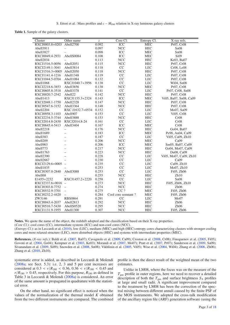
Table 1. Sample of the galaxy clusters.

Cluster Other name z Core Cl. Entropy Cl. X-ray refs.RXCJ0003.8+0203 Abell2700 0.092 ICC MEC Pr07, Cr08Abell3911 – 0.097 NCC HEC Sn08Abell3827 – 0.098 ICC MEC Sn08RXCJ0049.4-2931 AbellS0084 0.108 ICC MEC Si09Abell2034 – 0.113 NCC HEC Ke03, Ba07RXCJ1516.5-0056 Abell2051 0.115 NCC HEC Pr07, Cr08RXCJ2149.1-3041 Abell3814 0.118 CC LEC Cr08, Le08RXCJ1516.3+0005 Abell2050 0.118 NCC HEC Pr07, Cr08RXCJ1141.4-1216 Abell1348 0.119 CC LEC Pr07, Cr08RXCJ1044.5-0704 Abell1084 0.132 CC LEC Pr07, Cr08Abell1068 RXCJ1040.7+3956 0.138 CC LEC Wi04, Sn08RXCJ2218.6-3853 Abell3856 0.138 NCC MEC Pr07, Cr08RXCJ0605.8-3518 Abell3378 0.141 CC LEC Pr07, Cr08, Sn08RXCJ0020.7-2542 Abell22 0.142 NCC HEC Pr07, Cr08Abell1413 RXCJ1155.3+2324 0.143 ICC MEC Vi05, Ba07, Sn08, Ca09RXCJ2048.1-1750 Abell2328 0.147 NCC HEC Pr07, Cr08RXCJ0547.6-3152 Abell3364 0.148 NCC HEC Pr07, Cr08Abell2204 RXC J1632.7+0534 0.152 CC LEC Mo07, Sa09RXCJ0958.3-1103 Abell907 0.153 CC LEC Vi05, Cr08RXCJ2234.5-3744 Abell3888 0.153 NCC HEC Cr08RXCJ2014.8-2430 RXCJ2014.8-24 0.161 CC LEC Cr08RXCJ0645.4-5413 Abell3404 0.167 ICC MEC Cr08Abell2218 – 0.176 NCC HEC Go04, Ba07Abell1689 – 0.183 ICC MEC Pe98, An04, Ca09Abell383 – 0.187 CC LEC Vi05, Ca09, Zh10Abell209 – 0.206 NCC MEC Ca09Abell963 – 0.206 ICC MEC Sm05, Ba07, Ca09Abell773 – 0.217 NCC HEC Go04, Mo07, Ca09Abell1763 – 0.223 NCC HEC Du08, Ca09Abell2390 – 0.228 CC LEC Vi05, Mo07, Ca09, Zh10Abell2667 – 0.230 CC LEC Ca09RXCJ2129.6+0005 – 0.235 CC LEC Ca09, Zh10Abell1835 – 0.253 CC LEC Mo07, Zh10RXCJ0307.0-2840 Abell3088 0.253 CC LEC Fi05, Zh06Abell68 – 0.255 NCC HEC Zh10E1455+2232 RXCJ1457.2+2220 0.258 CC LEC Sn08RXCJ2337.6+0016 – 0.273 NCC HEC Fi05, Zh06, Zh10RXCJ0303.8-7752 – 0.274 NCC HEC Zh06RXCJ0532.9-3701 – 0.275 CC ? MEC Fi05, Zh06RXCJ0232.2-4420 – 0.284 Cool core remnant ? MEC Fi05, Zh06ZW3146 RBS0864 0.291 CC LEC Mo07RXCJ0043.4-2037 Abell2813 0.292 NCC HEC Zh06RXCJ0516.7-5430 AbellS0520 0.295 NCC HEC Zh06RXCJ1131.9-1955 Abell1300 0.307 NCC HEC Fi05, Zh06

Notes. We quote the name of the object, the redshift adopted and the classification based on their X-ray properties.(Core Cl.): cool cores (CC), intermediate systems (ICC) and non-cool cores (NCC).(Entropy Cl.): as in Leccardi et al. (2010), low (LEC), medium (MEC) and high (HEC) entropy cores characterizing clusters with stronger coolingcores and more relaxed structure (LEC), more disturbed objects (HEC) and systems with intermediate properties (MEC).

References. (X-ray refs.): Baldi et al. (2007, Ba07); Cavagnolo et al. (2009, Ca09); Croston et al. (2008, Cr08); Finoguenov et al. (2005, Fi05);Govoni et al. (2004, Go04); Kempner et al. (2003, Ke03); Morandi et al. (2007, Mo07); Pratt et al. (2007, Pr07); Sanderson et al. (2009, Sa09);Sivanandam et al. (2009, Si09); Snowden et al. (2008, Sn08); Vikhlinin et al. (2005, Vi05); Wise et al. (2004, Wi04); Zhang et al. (2006, Zh06);Zhang et al. (2010, Zh10).

systematic error is added, as described in Leccardi & Molendi(2008a; see Sect. 5.3): i.e. 2, 3 and 5 per cent increases areconsidered at 0.3 < r/R180 < 0.36, 0.36 < r/R180 < 0.45 andr/R180 > 0.45, respectively. For this purpose, R180 as defined inTable 3 in Leccardi & Molendi (2008a) is considered. An errorof the same amount is propagated in quadrature with the statisti-cal error.

On the other hand, no significant effect is noticed when thevalues of the normalization of the thermal model K obtainedfrom the two different instruments are compared. The combined

profile is then the direct result of the weighted mean of the twoestimates.

Unlike in LM08, where the focus was on the measure of theTgas profile in outer regions, here we need to recover a detaileddescription of both the Tgas and surface brightness S b profilesat large and small radii. A significant improvement comparedto the treatment by LM08 has been the correction of the spec-tral mixing between different annuli caused by the finite PSF ofthe MOS instruments. We adopted the cross-talk modificationof the ancillary region file (ARF) generation software (using the

of 18

A&A 524, A68 (2010)

Fig. 1. (Left) Surface brightness profile in the 0.7−1.2 keV band (black filled circles) of Abell1835 compared with the profiles of the backgroundcomponents. The open diamonds show the count rate predicted from the background spectral model in the annulus 10–12 arcmin and rescaledfor the mean vignetting correction of 0.472 at those radii: the instrumental component (NXB; green), the photon component (CXB + galacticforegrounds; blue) and the total background (sky + instrumental; red). The dashed lines show the background profiles that we have used in ouranalysis: the “photon” background (blue), which is constant and corresponds to the value in the outer annulus rescaled to the center, and theinstrumental background profile (green), increasing with radius in order to consider the over-correction of this component. The red dashed lineshows the total background that we have subtracted from our source plus background profile, with its associated one σ statistical error (reddotted lines) obtained with a Monte Carlo simulation. Note that the intensity of the background components and their relative contribution varysignificantly from cluster to cluster. (Right) Example of the PSF-corrected background-subtracted surface brightness profile as obtained after theanalysis outlined in Sect. 2.2. This example refers to Abell1835, one of the objects with the largest smearing effect due to the combination of thetelescope’s PSF and the centrally peaked intrinsic profile.

crossregionarf parameter of the argen task of SAS), treating thecross-talk contribution to the spectrum of a given annulus from anearby annulus as an additional model component (see Snowdenet al. 2008). This is a thermal model with parameters linked tothe thermal spectrum fitted to the nearby annulus and associatedto the appropriate ARF file of that region (i.e., the usual ARFfamiliar to X-ray astronomers). We found the correction to beimportant in particular to the first two annuli used in the analy-sis. The annuli have been therefore fitted jointly in XSPEC ver-sion 12 (Arnaud 1996), which allows to associate different mod-els to different RMF and ARF files. A comparison of the valuesobtained with this modelling and the values quoted in Snowdenet al. (2008) for the 16 clusters in common with our sample giveresults in agreement within the errors.

2.2. Analysis of the surface brightness profile

We extend the spectral analysis presented in LM08 with a spatialanalysis of the combined exposure-corrected M1-M2 images.

We extract surface brightness profiles from MOS images inthe energy band 0.7−1.2 keV, in order to keep the backgroundas low as possible with respect to the source. For this reason, weavoid the intense fluorescent instrumental lines of Al (∼1.5 keV)and Si (∼1.8 keV) (LM08). To correct for the vignetting, we di-vide the images by the corresponding exposure maps. From thesurface brightness profiles, we subtract the background that is es-timated starting from the spectral modelling of the backgroundcomponents in the external ring 10–12 arcmin (see LM08 fordetails on the adopted models). We recall here that in the proce-dure of LM08 the normalizations of the background components

are the only free parameters of the fit and that the galactic fore-ground emission, the cosmic X-ray background and the cos-mic ray induced continuum give a significant contribution inthe 0.7−1.2 keV energy range. The intensities of the backgroundcomponents in the annulus 10–12 arcmin are given by the countrates predicted by the best fit spectral model in this region. Inorder to associate errors to these count rates, we perform a sim-ulation within XSPEC: we allow the normalizations of the back-ground components to vary randomly within their errors, we ob-tain the count rates associated to this fake model and we iteratethis procedure. The error on the level of the background com-ponents is the width of the distribution of the simulated countrates. Using these values in the outer annulus, we reconstruct thebackground profile at all radii. The “photon” components (CXBand galactic foreground) are affected by vignetting in the sameway as the source photons and, therefore, dividing by the expo-sure map effectively corrects also these background componentsfor the vignetting. In order to reconstruct the “photon” back-ground profile, it is thus sufficient to rescale the count rate forthe mean vignetting in the outer annulus (constant blue profilein Fig. 1). On the contrary, the instrumental background doesnot suffer from vignetting and, therefore, dividing the imageby the exposure map “mis-corrects” this component. In orderto consider this effect, we divide the corresponding count rateby the vignetting profile (that we derive from the exposure mapin the 0.7−1.2 keV), obtaining the growing green curve in Fig. 1.The total background profile (red line in Fig. 1) is the sum of thephoton (blue) and instrumental (green) profiles.

The surface brightness profiles S b(r) have been first ex-tracted from the combined images and binned by requiring a

of 18

http://dexter.edpsciences.org/applet.php?DOI=10.1051/0004-6361/201015271&pdf_id=1


fixed number of 200 counts in each radial bin to preserve allthe spatial information available. After the background sub-traction, they have been corrected for the PSF smearing. Forthis purpose, a sum of a cusped β-model and of a β-model(Cavaliere & Fusco-Femiano 1978) with seven free parameters,

fm(r) = a0×[x−a2

1 ×(1 + x2

1

)0.5−3a3+a2/2+ a4

(1 + x2

2

)0.5−3a6]

(with

x1 = r/a1 and x2 = r/a2), is convolved with the predicted PSF(Ghizzardi 2001) and fitted to the observed profile background-subtracted S b(r) to obtain the best-fit convolved model fc(ai; r).Finally, to correct S b(r) for the PSF-convolution, we apply a cor-rection at each radius r where S b(r) is measured equal to the ra-tio fm(ai; r)/ fc(ai; r). An example of the results of the procedureis shown in Fig. 1. These corrected profiles are, finally, used inthe following analysis up to the radial limit, Rsp, beyond whichthe ratio between the profile and the error on it (including theestimated uncertainty on the measurement of the background) isbelow 2.

3. Estimates of the mass profiles

We use the profiles of the spectroscopically determined ICMtemperature and of the PSF-corrected surface brightness esti-mated, as described in the previous section, to recover the X-raygas, the dark and the total mass profiles, under the assumptionsof the spherical geometry distribution of the intracluster medium(ICM) and that the hydrostatic equilibrium holds between ICMand the underlying gravitational potential. We apply the two fol-lowing different methods:

– (Method 1) This technique is described in Ettori et al. (2002)and has been widely used to recover the mass profiles in re-cent X-ray studies of both observational (e.g. Morandi et al.2007; Donnarumma et al. 2009, 2010) and simulated datasets(e.g. Rasia et al. 2006; Meneghetti et al. 2010) against whichit has been thoroughly tested.We summarize here the algorithm adopted and how it usesthe observed measurements. Starting from the X-ray surfacebrightness profile and the radially resolved spectroscopictemperature measurements, this method puts constraints onthe parameters of the functional form describing the darkmatter MDM, defined as the total mass minus the gas mass(we neglect the marginal contribution from the mass in starsthat amounts to about 10–15% of the gas mass in massivesystems – see, e.g., discussion in Ettori et al. 2009; Andreon2010 –, and is here formally included in the MDM term). Inthe present work, we adopt a NFW profile:

MDM(<r) = Mtot(<r) − Mgas(<r) = 4π r3s ρs f (x),

ρs = ρc,z200

3c3

ln(1 + c) − c/(1 + c),

f (x) = ln(1 + x) − x1 + x

, (1)

where x = r/rs, ρc,z = 3H2z /8πG is the critical density at the

cluster’s redshift z, Hz = H0 ×[ΩΛ + Ωm(1 + z)3

]1/2is the

Hubble constant at redshift z for an assumed flat Universe(Ωm + ΩΛ = 1), and the relation R200 = c200 × rs holds.The two parameters (rs, c200) are constrained by minimizinga χ2 statistic defined as

χ2T =

∑i

(Tdata,i − Tmodel,i

)2

ε2T,i(2)

where the sum is done over the annuli of the spectral analy-sis; Tdata are the either deprojected or observed temperaturemeasurements obtained in the spectral analysis; Tmodel areeither the three-dimensional or projected values of the esti-mates of Tgas recovered from the inversion of the hydrostaticequilibrium equation (see below) for a given gas density andtotal mass profiles; εT is the error on the spectral measure-ments. The gas density profile, ngas, is estimated from the ge-ometrical deprojection (Fabian et al. 1981; Kriss et al. 1983;McLaughlin 1999; Buote 2000; Ettori et al. 2002) of eitherthe measured X-ray surface brightness or the estimated nor-malization of the thermal model fitted in the spectral analysis(see Fig. 2). In the present study, we consider the observedspectral values of the temperature and evaluate Tmodel by pro-jecting the estimates of Tgas over the annuli adopted in thespectral analysis accordingly to the recipe in Mazzotta et al.(2004) and using the gas density profile obtained from thedeprojection of the PSF-deconvolved surface brightness pro-file (see Sect. 2.2). We exclude the deprojected data of thegas density within a cutoff radius of 50 kpc because the in-fluence of the central galaxy is expected to be not negligible,in particular for strong low-entropy core systems. The valuesof Tgas are then obtained from

−GμmangasMtot(< r)

r2=

d(ngas × Tgas

)dr

, (3)

where G is the universal gravitational constant, ma is theatomic mass unit and μ = 0.61 is the mean molecular weightin atomic mass unit. To solve this differential equation, weneed to define a boundary condition that is here fixed to thevalue of the pressure measured in the outermost point of thegas density profile, Pout = Pgas(Rsp) = ngas(Rsp) × Tgas(Rsp),where Tgas(Rsp) is estimated by linear extrapolation in thelogarithmic space, if required. The systematic uncertaintiesintroduced by this assumption on Pout are discussed in thenext section. Note that by applying Method 1 the errors onthe gas density do not propagate into the estimates of theparameters of the mass profile and are used both to definethe range of the accepted values of Pout and to evaluate theuncertainties on the gas mass profiles. The allowed rangeat 1σ of the two interesting parameters, rs and c200, is de-fined from the minimum and the maximum of the valuesthat permit χ2

T to be lower or equal to min(χ2T ) + 1. The

average error on the mass is then the mean of the upperand lower limit obtained at each radius from the allowedranges at 1σ of rs and c200. Only for the purpose of esti-mating the profile of Mgas(<r), and eventually to provide theextrapolated values, the deprojected gas density profile is fit-ted with the generic functional form described in Ettori et al.(2009) and adapted from the one described in Vikhlinin et al.

(2006), ngas = ngas,0 (r/rc,0)−α0 ×(1 + (r/rc,0)2

)−1.5α1+α0/2 ×(1 + (r/rc,1)α2

)−α3/α2 .– (Method 2) The second method follows the approach de-

scribed in Humphrey et al. (2006) and Gastaldello et al.(2007) where further details of this technique (in particularin Appendix B of Gastaldello et al. 2007) are provided. Weassume parametrizations for the gas density and mass pro-files to calculate the gas temperature assuming hydrostaticequilibrium,

T (r) = T0ngas,0

ngas(r)− μmaG

kBngas(r)

∫ r

r0

ngasMtot dr

r2, (4)

of 18

https://www.researchgate.net/publication/1925781_Gravitating_mass_profiles_of_nearby_galaxy_clusters_and_relations_with_X-ray_gas_temperature_luminosity_and_mass?el=1_x_8&enrichId=rgreq-67801ba8-5ac9-4738-b238-688b5858532d&enrichSource=Y292ZXJQYWdlOzI1ODM2OTk2MztBUzoxMjc4NTg0NDE3MjM5MDVAMTQwNzQ5NTIzNjQ1OA==


A&A 524, A68 (2010)

Fig. 2. Example of the results of the two analyses adopted for the mass reconstruction. (Top and middle panels, left) Gas density profile as obtainedfrom the deprojection of the surface brightness profile compared to the one recovered from the deprojection of the normalizations of the thermalmodel in the spectral analysis; observed temperature profile with overplotted the best-fit model (from Method 1). (Top and middle panels, right)Data (diamonds) and models (dashed lines) of the projected gas density squared and temperature (from Method 2). (Bottom, left) Constraints in the

rs − c plane with the prediction (in green) obtained by imposing the relation c200 = 4.305/(1 + z) ×(M200/1014h−1

100 M�)−0.098

from M08. (Bottom,right) Gas mass fraction profile obtained from Method 1 (gray) and Method 2 (red).

where ngas is the gas density, ngas,0 and T0 are densityand temperature at some “reference” radius r0 and kB isBoltzmann’s constant. The ngas and T (r) profiles are fittedsimultaneously to the data to constrain the parameters of thegas density and mass models. The parameters of the massmodel are obtained from fitting the gas density and temper-ature data and goodness-of-fit for any mass model can beassessed directly from the residuals of the fit. The quality ofthe data, in particular of the temperature profile, motivatedthe use of this approach rather than the default approach

of parametrizing the temperature and mass profiles to cal-culate the gas density used in Gastaldello et al. (2007). Weprojected the parametrized models of the three-dimensionalquantities, n2

gas and T , and fitted these projected emission-weighted models to the results obtained from our analysis ofthe data projected on the sky. With respect to the paper citedabove, the XSPEC normalization have been derived convert-ing the XMM surface brightness in the 0.7−1.2 keV band us-ing the effective area and observed projected temperature andmetallicity obtained in the wider radial bins used for spectral

of 18



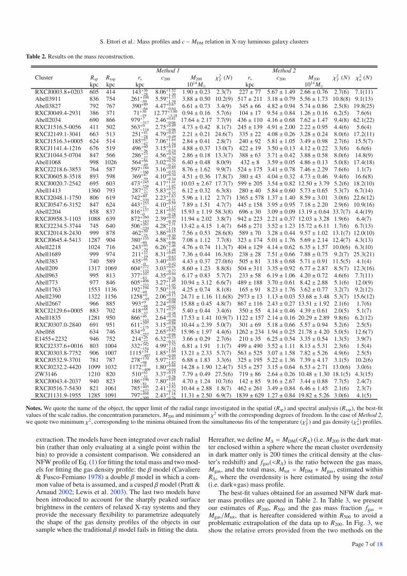
Table 2. Results on the mass reconstruction.

Method 1 Method 2Cluster Rsp Rxsp rs c200 M200 χ2

T (N) rs c200 M200 χ2T (N) χ2

n (N)kpc kpc kpc 1014 M� kpc 1014 M�

RXCJ0003.8+0203 605 414 143+36−28 8.06+1.52

−1.30 1.90 ± 0.23 2.3(7) 227 ± 77 5.67 ± 1.49 2.66 ± 0.76 2.7(6) 7.1(11)Abell3911 836 754 261+108

−59 5.59+1.33−1.39 3.88 ± 0.50 10.2(9) 517 ± 211 3.18 ± 0.79 5.56 ± 1.73 10.8(8) 9.1(13)

Abell3827 792 767 390+89−64 4.47+0.67

−0.64 6.61 ± 0.73 3.4(9) 345 ± 66 4.82 ± 0.94 5.74 ± 0.86 2.5(8) 19.8(25)RXCJ0049.4-2931 386 371 71+30

−19 12.77+3.80−3.18 0.94 ± 0.16 5.7(6) 104 ± 17 9.54 ± 0.84 1.26 ± 0.16 6.2(5) 7.6(6)

Abell2034 690 866 979+7−317 2.46+0.81

−0.06 17.64 ± 2.17 7.7(9) 436 ± 110 4.16 ± 0.68 7.62 ± 1.47 9.4(8) 62.1(22)RXCJ1516.5-0056 411 502 563+0

−114 2.75+0.49−0.06 4.73 ± 0.42 8.1(7) 245 ± 139 4.91 ± 2.00 2.22 ± 0.95 4.4(6) 5.6(4)

RXCJ2149.1-3041 663 513 251+41−28 4.79+0.43

−0.49 2.21 ± 0.21 24.6(7) 335 ± 22 4.08 ± 0.26 3.28 ± 0.24 8.0(6) 17.2(11)RXCJ1516.3+0005 624 514 185+67

−42 7.06+1.64−1.54 2.84 ± 0.41 2.8(7) 240 ± 92 5.81 ± 1.05 3.49 ± 0.98 2.7(6) 15.5(7)

RXCJ1141.4-1216 676 519 496+60−36 3.15+0.19

−0.24 4.88 ± 0.37 13.0(7) 422 ± 19 3.50 ± 0.13 4.12 ± 0.22 3.3(6) 6.6(6)RXCJ1044.5-0704 847 566 286+23

−27 4.56+0.34−0.25 2.86 ± 0.18 13.3(7) 388 ± 63 3.71 ± 0.42 3.88 ± 0.58 8.0(6) 14.8(9)

Abell1068 998 1026 564+66−49 3.02+0.20

−0.22 6.40 ± 0.48 8.0(9) 432 ± 8 3.59 ± 0.05 4.86 ± 0.13 5.0(8) 17.4(18)RXCJ2218.6-3853 764 587 597+184

−166 3.16+0.85−0.55 8.76 ± 1.62 9.9(7) 524 ± 175 3.41 ± 0.78 7.46 ± 2.29 7.6(6) 1.1(7)

RXCJ0605.8-3518 893 598 369+47−39 4.10+0.34

−0.34 4.51 ± 0.36 17.8(7) 380 ± 43 4.04 ± 0.32 4.73 ± 0.46 9.4(6) 16.6(8)RXCJ0020.7-2542 695 603 473+245

−154 4.17+1.41−1.07 10.03 ± 2.67 17.7(7) 599 ± 205 3.54 ± 0.82 12.50 ± 3.79 5.2(6) 18.2(10)

Abell1413 1360 793 287+23−32 5.83+0.57

−0.35 6.12 ± 0.32 6.3(8) 280 ± 40 5.84 ± 0.60 5.73 ± 0.65 5.3(7) 6.7(14)RXCJ2048.1-1750 806 619 742+80

−370 2.23+1.63−0.21 5.96 ± 1.12 2.7(7) 1365 ± 578 1.37 ± 1.40 8.59 ± 3.01 3.0(6) 22.6(12)

RXCJ0547.6-3152 847 624 443+253−71 4.10+0.59

−1.17 7.89 ± 1.51 4.7(7) 445 ± 158 3.95 ± 0.95 7.18 ± 2.20 2.9(6) 10.9(16)Abell2204 858 837 816+137

−0 2.81+0.02−0.28 15.93 ± 1.19 58.3(8) 696 ± 30 3.09 ± 0.09 13.19 ± 0.64 33.7(7) 4.4(19)

RXCJ0958.3-1103 1088 639 872+260−183 2.39+0.42

−0.39 11.94 ± 2.02 3.8(7) 942 ± 223 2.21 ± 0.37 12.03 ± 3.28 1.9(6) 6.4(7)RXCJ2234.5-3744 745 640 506+261

−220 4.28+2.31−1.16 13.42 ± 4.15 1.4(7) 648 ± 271 3.52 ± 1.23 15.72 ± 6.11 1.7(6) 6.7(13)

RXCJ2014.8-2430 999 878 462+59−25 3.86+0.15

−0.30 7.56 ± 0.53 28.6(8) 589 ± 70 3.28 ± 0.44 9.57 ± 1.02 13.1(7) 12.0(10)RXCJ0645.4-5413 1287 904 380+135

−89 4.58+1.06−0.96 7.08 ± 1.12 7.7(8) 323 ± 174 5.01 ± 1.76 5.69 ± 2.14 12.4(7) 4.3(13)

Abell2218 1024 716 243+95−79 6.26+2.46

−1.48 4.76 ± 0.74 11.3(7) 404 ± 129 4.14 ± 0.62 6.35 ± 1.57 10.0(6) 6.3(10)Abell1689 999 974 211+22

−19 8.31+0.64−0.63 7.36 ± 0.44 16.3(8) 238 ± 28 7.51 ± 0.66 7.88 ± 0.75 9.2(7) 25.3(21)

Abell383 740 589 435+95−0 3.40+0.03

−0.42 4.43 ± 0.37 27.0(6) 505 ± 81 3.18 ± 0.68 5.71 ± 0.91 11.5(5) 4.1(4)Abell209 1317 1069 604+272

−133 3.03+0.67−0.77 8.60 ± 1.23 8.8(8) 504 ± 311 3.35 ± 0.92 6.77 ± 2.87 8.5(7) 12.3(16)

Abell963 995 813 377+107−83 4.35+0.94

−0.76 6.17 ± 0.83 5.7(7) 233 ± 58 6.19 ± 1.06 4.20 ± 0.72 4.6(6) 7.7(11)Abell773 977 846 605+408

−233 3.27+1.49−1.05 10.94 ± 3.12 6.6(7) 489 ± 188 3.70 ± 0.61 8.42 ± 2.88 5.1(6) 12.0(9)

Abell1763 1553 1136 192+194−49 7.50+2.30

−3.41 4.25 ± 0.74 8.1(8) 165 ± 91 8.23 ± 1.76 3.62 ± 0.77 3.2(7) 9.2(12)Abell2390 1322 1156 1258+0

−95 2.06+0.12−0.04 24.71 ± 1.16 11.6(8) 2973 ± 13 1.13 ± 0.03 53.68 ± 3.48 5.3(7) 15.6(12)

Abell2667 966 885 993+0−48 2.24+0.08

−0.02 15.88 ± 0.45 4.8(7) 867 ± 116 2.43 ± 0.27 13.51 ± 1.92 2.1(6) 1.7(6)RXCJ2129.6+0005 883 702 418+68

−37 3.71+0.27−0.38 5.40 ± 0.44 3.4(6) 350 ± 55 4.14 ± 0.46 4.39 ± 0.61 2.0(5) 5.1(7)

Abell1835 1281 950 866+46−143 2.64+0.34

−0.09 17.53 ± 1.41 10.9(7) 1122 ± 157 2.14 ± 0.16 20.29 ± 2.89 9.8(6) 6.2(12)RXCJ0307.0-2840 691 951 611+297

−175 3.15+0.88−0.78 10.44 ± 2.39 5.0(7) 301 ± 69 5.18 ± 0.66 5.57 ± 0.94 5.2(6) 2.5(5)

Abell68 634 746 834+0−257 2.65+0.82

−0.06 15.96 ± 1.97 4.4(6) 1262 ± 234 1.94 ± 0.25 21.78 ± 4.20 5.0(5) 12.6(7)E1455+2232 946 752 214+26

−22 6.32+0.53−0.51 3.66 ± 0.29 2.7(6) 210 ± 35 6.25 ± 0.54 3.35 ± 0.54 1.3(5) 3.9(7)

RXCJ2337.6+0016 803 1004 332+342−154 4.99+3.52

−2.18 6.81 ± 1.91 1.1(7) 499 ± 490 3.52 ± 1.11 8.13 ± 5.31 2.3(6) 1.5(4)RXCJ0303.8-7752 906 1007 1115+14

−497 1.85+1.04−0.09 13.21 ± 2.33 5.7(7) 563 ± 525 3.07 ± 1.58 7.82 ± 5.26 4.9(6) 2.5(5)

RXCJ0532.9-3701 781 787 278+170−98 5.97+2.43

−1.82 6.88 ± 1.83 3.3(6) 325 ± 195 5.22 ± 1.36 7.39 ± 4.17 3.1(5) 10.2(6)RXCJ0232.2-4420 1099 1032 1172+0

−409 1.80+0.66−0.04 14.28 ± 1.90 12.4(7) 515 ± 257 3.15 ± 0.64 6.53 ± 2.71 13.0(6) 3.0(6)

ZW3146 1210 820 510+61−31 3.37+0.15

−0.26 7.79 ± 0.49 27.5(6) 719 ± 86 2.64 ± 0.26 10.48 ± 1.30 18.1(5) 4.3(15)RXCJ0043.4-2037 940 823 186+196

−81 7.80+5.05−3.51 4.70 ± 1.24 10.7(6) 142 ± 85 9.16 ± 2.67 3.44 ± 0.88 7.7(5) 2.4(7)

RXCJ0516.7-5430 821 1061 785+405−472 2.41+2.82

−0.75 10.44 ± 2.88 1.8(7) 462 ± 261 3.49 ± 0.84 6.46 ± 1.45 2.1(6) 2.3(7)RXCJ1131.9-1955 1285 1091 797+494

−309 2.43+1.16−0.76 11.31 ± 2.50 6.9(7) 1839 ± 629 1.27 ± 0.84 19.82 ± 5.26 3.0(6) 4.1(5)

Notes. We quote the name of the object, the upper limit of the radial range investigated in the spatial (Rsp) and spectral analysis (Rxsp), the best-fitvalues of the scale radius, the concentration parameters, M200 and minimum χ2 with the corresponding degrees of freedom. In the case of Method 2,we quote two minimum χ2, corresponding to the minima obtained from the simultaneous fits of the temperature (χ2

T ) and gas density (χ2n) profiles.

extraction. The models have been integrated over each radialbin (rather than only evaluating at a single point within thebin) to provide a consistent comparison. We considered anNFW profile of Eq. (1) for fitting the total mass and two mod-els for fitting the gas density profile: the β model (Cavaliere& Fusco-Femiano 1978) a double β model in which a com-mon value of beta is assumed, and a cusped βmodel (Pratt &Arnaud 2002; Lewis et al. 2003). The last two models havebeen introduced to account for the sharply peaked surfacebrightness in the centers of relaxed X-ray systems and theyprovide the necessary flexibility to parametrize adequatelythe shape of the gas density profiles of the objects in oursample when the traditional β model fails in fitting the data.

Hereafter, we define MΔ = MDM(<RΔ) (i.e. M200 is the dark mat-ter enclosed within a sphere where the mean cluster overdensityin dark matter only is 200 times the critical density at the clus-ter’s redshift) and fgas(<RΔ) is the ratio between the gas mass,Mgas, and the total mass, Mtot = MDM + Mgas, estimated withinRΔ, where the overdensity is here estimated by using the total(i.e. dark+gas) mass profile.

The best-fit values obtained for an assumed NFW dark mat-ter mass profiles are quoted in Table 2. In Table 3, we presentour estimates of R200, R500 and the gas mass fraction fgas =Mgas/Mtot, that is hereafter considered within R500 to avoid aproblematic extrapolation of the data up to R200. In Fig. 3, weshow the relative errors provided from the two methods on the

of 18

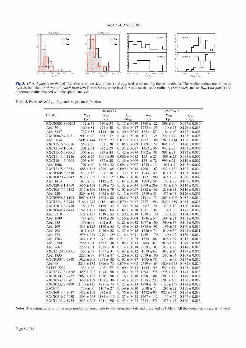
A&A 524, A68 (2010)

Fig. 3. (First 2 panels on the left) Relative errors on M200 (black) and c200 (red) estimated by the two methods. The median values are indicatedby a dashed line. (3rd and 4th panel from left) Ratios between the best-fit result on the scale radius rs (3rd panel) and on R500 (4th panel) andoutermost radius reached with the spatial analysis.

Table 3. Estimates of R200, R500 and the gas mass fraction.

Method 1 Method 2Cluster R200 R500 fgas R200 R500 fgas

kpc kpc <R500 kpc kpc <R500

RXCJ0003.8+0203 1152 ± 58 780 ± 34 0.117 ± 0.049 1360 ± 122 899 ± 50 0.097 ± 0.010Abell3911 1460 ± 81 971 ± 40 0.146 ± 0.017 1773 ± 155 1130 ± 75 0.126 ± 0.015Abell3827 1742 ± 85 1144 ± 46 0.140 ± 0.012 1823 ± 87 1184 ± 40 0.147 ± 0.008RXCJ0049.4-2931 907 ± 62 625 ± 37 0.143 ± 0.020 1071 ± 39 721 ± 29 0.123 ± 0.008Abell2034 2405 ± 144 1507 ± 77 0.073 ± 0.007 1957 ± 108 1267 ± 114 0.123 ± 0.016RXCJ1516.5-0056 1550 ± 66 981 ± 38 0.105 ± 0.009 1309 ± 159 845 ± 98 0.120 ± 0.015RXCJ2149.1-3041 1201 ± 51 792 ± 29 0.131 ± 0.027 1452 ± 36 942 ± 26 0.101 ± 0.006RXCJ1516.3+0005 1305 ± 80 879 ± 44 0.142 ± 0.074 1502 ± 107 991 ± 81 0.122 ± 0.015RXCJ1141.4-1216 1563 ± 55 1001 ± 30 0.086 ± 0.012 1551 ± 27 1003 ± 23 0.095 ± 0.005RXCJ1044.5-0704 1303 ± 36 857 ± 20 0.146 ± 0.009 1531 ± 72 996 ± 21 0.119 ± 0.007Abell1068 1701 ± 60 1085 ± 32 0.091 ± 0.007 1645 ± 13 1061 ± 7 0.105 ± 0.002RXCJ2218.6-3853 1888 ± 163 1209 ± 85 0.099 ± 0.018 1900 ± 167 1222 ± 132 0.107 ± 0.024RXCJ0605.8-3518 1512 ± 53 987 ± 30 0.133 ± 0.012 1643 ± 49 1071 ± 25 0.125 ± 0.006RXCJ0020.7-2542 1972 ± 235 1289 ± 127 0.062 ± 0.016 2182 ± 200 1415 ± 82 0.060 ± 0.009Abell1413 1673 ± 38 1115 ± 21 0.161 ± 0.010 1809 ± 58 1188 ± 28 0.167 ± 0.007RXCJ2048.1-1750 1656 ± 154 1028 ± 75 0.132 ± 0.044 2008 ± 269 1187 ± 109 0.114 ± 0.020RXCJ0547.6-3152 1817 ± 156 1186 ± 79 0.105 ± 0.057 1882 ± 168 1219 ± 81 0.116 ± 0.013Abell2204 2294 ± 82 1455 ± 45 0.115 ± 0.008 2319 ± 33 1477 ± 47 0.126 ± 0.007RXCJ0958.3-1103 2083 ± 173 1302 ± 88 0.086 ± 0.013 2191 ± 174 1363 ± 106 0.087 ± 0.014RXCJ2234.5-3744 2166 ± 298 1418 ± 164 0.079 ± 0.067 2377 ± 294 1542 ± 159 0.085 ± 0.025RXCJ2014.8-2430 1783 ± 57 1159 ± 32 0.136 ± 0.014 2067 ± 70 1323 ± 16 0.120 ± 0.004RXCJ0645.4-5413 1741 ± 122 1145 ± 64 0.161 ± 0.020 1811 ± 183 1174 ± 83 0.177 ± 0.022Abell2218 1521 ± 101 1018 ± 53 0.159 ± 0.019 1820 ± 120 1122 ± 66 0.154 ± 0.016Abell1689 1754 ± 43 1189 ± 26 0.156 ± 0.008 1946 ± 54 1304 ± 21 0.151 ± 0.005Abell383 1479 ± 58 952 ± 31 0.121 ± 0.042 1697 ± 100 1090 ± 17 0.101 ± 0.005Abell209 1833 ± 123 1170 ± 55 0.146 ± 0.015 1873 ± 197 1196 ± 54 0.160 ± 0.013Abell963 1641 ± 98 1076 ± 52 0.137 ± 0.015 1586 ± 74 1049 ± 36 0.164 ± 0.011Abell773 1978 ± 261 1270 ± 129 0.116 ± 0.041 1959 ± 170 1140 ± 92 0.156 ± 0.019Abell1763 1441 ± 105 972 ± 49 0.212 ± 0.025 1575 ± 88 1028 ± 39 0.213 ± 0.012Abell2390 2585 ± 61 1592 ± 36 0.108 ± 0.013 3484 ± 67 2026 ± 57 0.079 ± 0.005Abell2667 2229 ± 31 1385 ± 18 0.114 ± 0.018 2259 ± 103 1417 ± 72 0.118 ± 0.013RXCJ2129.6+0005 1553 ± 57 1007 ± 31 0.165 ± 0.012 1619 ± 63 1042 ± 16 0.177 ± 0.006Abell1835 2285 ± 89 1441 ± 47 0.120 ± 0.012 2539 ± 100 1583 ± 34 0.109 ± 0.006RXCJ0307.0-2840 1922 ± 205 1231 ± 105 0.105 ± 0.017 1695 ± 78 1114 ± 59 0.147 ± 0.017Abell68 2213 ± 132 1396 ± 73 0.079 ± 0.008 2549 ± 165 1489 ± 155 0.082 ± 0.020E1455+2232 1354 ± 46 906 ± 27 0.160 ± 0.013 1445 ± 59 954 ± 14 0.163 ± 0.006RXCJ2337.6+0016 1655 ± 202 1094 ± 96 0.148 ± 0.027 1894 ± 278 1225 ± 173 0.141 ± 0.033RXCJ0303.8-7752 2063 ± 187 1256 ± 96 0.116 ± 0.016 1888 ± 301 1203 ± 122 0.148 ± 0.024RXCJ0532.9-3701 1659 ± 189 1108 ± 104 0.141 ± 0.027 1835 ± 233 1207 ± 105 0.136 ± 0.019RXCJ0232.2-4420 2110 ± 145 1281 ± 74 0.123 ± 0.013 1798 ± 167 1152 ± 137 0.178 ± 0.032ZW3146 1719 ± 50 1107 ± 27 0.159 ± 0.010 2040 ± 77 1293 ± 22 0.135 ± 0.005RXCJ0043.4-2037 1452 ± 159 982 ± 81 0.176 ± 0.032 1472 ± 95 982 ± 133 0.199 ± 0.033RXCJ0516.7-5430 1893 ± 253 1184 ± 113 0.127 ± 0.022 1767 ± 112 1135 ± 57 0.157 ± 0.013RXCJ1131.9-1955 1935 ± 208 1211 ± 90 0.155 ± 0.023 2513 ± 271 1475 ± 97 0.120 ± 0.015

Notes. The estimates refer to the mass models obtained with two different methods and presented in Table 2. All the quoted errors are at 1σ level.

of 18



Fig. 4. Best-fit values of rs, c, gas mass fraction fgas at R500 and dark mass MDM within R200 as obtained from Method 1 (diamonds; the onesincluding red points indicate the objects where the condition (rs + εrs ) < Rsp is satisfied by both methods. Rsp here plotted as horizontal line in theupper panel).

estimates of c200 and M200. The distribution of the statisticaluncertainties is comparable, with median values of 15–20% onboth c200 and M200 with Method 1 and Method 2. Also the distri-butions of the measurements of c200 and M200 are very similar,with 1st–3rd quartile range of 2.70−5.29 and 4.7−11.1×1014 M�with Method 1 and 3.17−5.09 and 4.3−9.1 × 1014 M� withMethod 2.

Moreover, the two methods show a good agreement be-tween the two estimates of the gas mass fraction fgas(<R500),as shown in Fig. 5. We measure a median (1st, 3rd quartile) of0.131(0.106, 0.147), and a median relative error of 12%, with

Method 1 and 0.124(0.108, 0.155), and a relative error of 10%,with Method 2.

As shown in the last two panels of Fig. 3, we note that thelarge majority of our data is able to define a scale radius rs wellwithin the radial range investigated in the spectral and spatialanalysis, allowing a quite robust constraints of the fitted param-eters.

To rely on the best estimates of the concentration and mass,we define in the following analysis a further subsample by col-lecting the clusters that satisfy the criterion that the upper valueat 1σ of the scale radius, as estimated from the 2 methods, is

of 18


A&A 524, A68 (2010)

Fig. 5. Estimates of M200 (left), c200 (center) and fgas(<R500) (right) with the two methods. (Upper panels) The color code indicates the objects atz < 0.15 (blue), in the range 0.15 < z < 0.25 (green) and at z > 0.25 (red). (Lower panels) Distribution of Low (LEC), Medium (MEC), High(HEC) Entropy Core systems.

lower than the upper limit of the spatial extension of the detectedX-ray emission, i.e. (rs + εrs ) < Rsp. Imposing this condition, weselect the 26 clusters where a more robust (i.e. with well definedand constrained free parameters) mass reconstruction is achiev-able.

4. Systematics in the measurements of c200, M200

and fgas

The derived quantities c200, M200 and fgas(<R500) are mea-sured with a relative statistical error of about 20, 15 and 10%,respectively (see Sect. 3 and Figs. 3 and 5). Here, we investi-gate the main uncertainties affecting our techniques that will betreated as systematic effects in the following analysis.

We consider two main sources of systematic errors: (i) theanalysis of our dataset, both for what concerns the estimates ofthe gas temperature and the reconstructed gas density profile; (ii)the limitations and assumptions in the techniques adopted for themass reconstruction.

In Table 4, we summarize our findings tabulated as rela-tive median difference with respect to the estimates obtainedwith Method 1. Overall, we register systematic uncertaintiesof (−5,+1)% on c200, (−4,+3)% on M200 and (−1,+4)% onfgas(<R500), where these ranges represent the minimum and max-imum estimated in the dataset investigated and quoted in Table 4.

4.1. Systematics from the spectral analysis

The ICM properties of the present dataset have been studiedthrough spatially resolved spectroscopic measurements of thegas temperature profile and deprojected, PSF-corrected surfacebrightness profile as accessible to XMM-Newton (see Sect. 2).

To assess the systematics propagated through the temper-ature measurements, we present the results obtained with M2only, i.e. before any correction introduced from the harder spec-tra observed with M1 (see Sect. 2.1). Overall, the systematicsare in the order of a few per cent, with the largest offset of about4 per cent on the concentration and mass measurements at R500and beyond.

When the deprojected spectral values of the gas temperature,instead of the projected ones, are compared with the predictionsfrom the model, we measure differences below 5% (see datasetlabelled “T3D”).

On the gas density profile, we investigate the role playedfrom the use of a functional form instead of the values obtaineddirectly from deprojection. To this purpose, we use a revisedform of the one introduced from Vikhlinin et al. (2006) to fitthe gas density profile and, then, we adopt it as representativeof the gas density profile to be put in hydrostatic equilibriumwith the gravitational potential in Eq. (3). The measurements ob-tained are labelled “fit ngas” and show discrepancies in the orderof 1 per cent or less.

of 18



Table 4. Median deviations measured in the distribution of c200, MDM and fgas.

Dataset (c200 − c200)/c200 (MDM − MDM)/MDM ( fgas − fgas)/ fgas

Method 2 −0.013 +0.008 +0.036M2 +0.010 −0.017 +0.009T3D −0.048 −0.036 +0.024fit ngas +0.001 +0.011 +0.000Pout −0.011 +0.030 −0.014

at R200 (−0.048,+0.010) (−0.036,+0.030) (−0.014,+0.036)

Method 2 − −0.015 +0.035M2 − −0.018 +0.010T3D − −0.046 +0.025fit ngas − +0.012 −0.008Pout − +0.028 −0.013

at R500 − (−0.046,+0.028) (−0.013,+0.035)

Method 2 − −0.073 +0.032M2 − −0.013 +0.008T3D − −0.059 +0.028fit ngas − +0.004 +0.000Pout − +0.020 −0.009

at R2500 − (−0.073,+0.020) (−0.009,+0.032)

Notes. The deviations are measured with respect to the estimates obtained from the combined M1+M2 profile with the Method 1 for the wholesample of 44 clusters. Dataset: (Method 2) Method 2 is used for mass reconstruction; (M2) only the T (r) profile from M2 is used; (T3D) thedeprojected spectral measurements of T (r) are used in Method 1 instead of the projected estimates of Tmodel (see Sect. 3); (fit ngas) a model fittedto the gas density profile is used in Method 1; (Pout) the outer value of the pressure is not fixed.

4.2. Systematics from the mass reconstruction methods

With the intention to assess the the bias affecting the recon-structed mass values, we make use of the gas temperature anddensity profiles through two independent techniques (labelledMethod 1 and Method 2), as described in Sect. 3. With respect toMethod 1, Method 2 provides differences on MDM that are lowerthan 10 per cent, increasing from about 1 per cent at R200 up to7 per cent at R2500 (see Table 4). The bias on fgas remains sta-ble around 3–4 per cent, suggesting that some systematics affectalso the estimate of Mgas. This is due to the application of twodifferent functional forms in Method 1 and Method 2 over a ra-dial range that extends beyond the observational limit (see, e.g.,Fig. 3).

The mass reconstruction of Method 1 depends upon theboundary condition on the gas pressure profile. In particular, tosolve the differential Eq. (3), an outer value on the pressure isfixed to the product of the observed estimate of the gas densityprofile at the outermost radius and an extrapolated measurementof the gas temperature. Using a grid of values for the pressureobtained from the best-fit results of the gas density and tempera-ture profiles, we evaluate a systematic bias on the mass of about3 per cent, on the gas mass fraction of 1 per cent, and on c200 ofabout 1 per cent (see dataset labelled “Pout”).

5. The c200 − M200 relation

In this section, we investigate the c200 − M200 relation. We notethat our sample has not been selected to be representative ofthe cluster population in the given redshift range and, in themean time, does not include only relaxed systems. Therefore,the results here presented on the c200 − M200 relation have to be

just considered for a qualitative comparison with the predictionsfrom numerical simulations and to assess differences or simili-tude with previous work on this topic.

As we show in Fig. 6 using the measurements obtained withMethod 1, the median relation between concentration and totalmasses for CDM halos as function of redshift is represented wellfrom the analytic algorithms, as in N97, E01 and B01. Thesemodels relate the halo properties to the physical mechanism ofhalo formation. Considering the weak dependence of the haloconcentrations on the mass and redshift, Dolag et al. (2004) in-troduced a two-parameter functional form, c = c0MB/(1 + z).We consider this relation in its logarithmic form and fit linearlyto our data the expression:

log10 (c200 × (1 + z)) = A + B × log10

(M200

1015 M�

)· (5)

A minimum in the χ2 distribution is looked for by taking intoaccount the errors on both the coordinates (we use the routineFITEXY in IDL). The errors are assumed to be Gaussian inthe logarithmic space, although they are properly measured asGaussian in the linear space.

We also express our results in term of the concentration c15expected for a dark matter halo of 1015 h−1

70 M� and equal to10A once the parameters in Eq. (5) are used. We convert to c15even the results from literature obtained, for instance, at differentoverdensity, as described in the Appendix.

We measure A ≈ 0.6 and B systematically lower than −0.1,with the best-fit results obtained through Method 1 that prefer,with respect to Method 2, a relation with slightly higher normal-ization (by ∼10 per cent) and flatter (by 10−30 per cent) distri-bution in mass. In both cases, a total scatter of σlog10 c ≈ 0.13 is

of 18

A&A 524, A68 (2010)

Fig. 6. Data in the plane (c200,M200) used to constrain the cosmological parameters (Ωm, σ8). The dotted lines show the predicted relations fromEke et al. (2001) for a given ΛCDM cosmological model at z = 0 (from top to bottom: σ8 = 0.9 and σ8 = 0.7). The shaded regions show thepredictions in the redshift range 0.1−0.3 for an assumed cosmological model in agreement with WMAP-1, 5 and 3 years (from the top to thebottom, respectively) from Bullock et al. (2001; after Macciò et al. 2008). The dashed lines indicate the best-fit range at 1σ obtained for relaxedhalos in a WMAP-5 years cosmology from Duffy et al. (2008; thin lines: z = 0.1, thick lines: z = 0.3). Color codes and symbols as in Fig. 5.

measured both in the whole sample of 44 objects, where the sta-tistical scatter related to the observed uncertainties is still domi-nant, and in the subsample of 26 selected clusters.

When a slope B = −0.1 is assumed, as measured in numeri-cal simulations over one order of magnitude in mass almost in-dependently from the underlying cosmological model (see e.g.Dolag et al. 2004; Macciò et al. 2008), the measured normaliza-tions of the c200−M200 relation fall into the range of the estimatedvalues for samples of simulated clusters (see Table 5).

All the values of normalization and slope are confirmed,within the estimated errors, with both the BCES bisector method(as described in Akritas & Bershady 1996 and implementedin the routines made available from Bershady) and a Bayesianmethod that accounts for measurement errors in linear regres-sion, as implemented in the IDL routine LINMIX_ERR by Kelly(see Kelly 2007). As we quote in Table 5, with these linear re-gression methods (and after 106 bootstrap resampling of the datain BCES), we measure a typical error that is larger by a factor2−3 in normalization and up to 6 in the slope than the corre-sponding values obtained through the covariance matrix of theFITEXY method.

These values compare well with the measurements obtainedfrom numerical simulations of DM-only galaxy clusters, al-though these simulations sample, on average, mass ranges lowerthan the ones investigated here. Recent work from Shaw et al.(2006) and Macciò et al. (2008) summarize the findings. Theslope of the relation, as previously obtained from B01 and D04,lies in the range (−0.160,−0.083), with a preferred value ofabout −0.1. The normalizations for low-density Universe witha relatively higher σ8, as from WMAP-1, are more in agree-ment with the observed constraints on, e.g., c15. For instance,M08 find c15 = 4.18, 3.41, 3.56 for relaxed objects in a back-ground cosmology that matches WMAP-1, 3 and 5 year data,respectively1. Shaw et al. (2006) measure c15 = 4.64 using a flat

1 We refer to Appendix A for a detailed discussion of the conversionsadopted.

Universe with Ωm = 0.3 and σ8 = 0.95. D04 for a ΛCDM withσ8 = 0.9 require c15 = 4.29. All these values show the sensitiv-ity of the normalization to the assumed cosmology, that is furtherdiscussed in the section where constraints on the cosmologicalparameters (Ωm − σ8) will be obtained through the measuredc − M relation. Neto et al. (2007) study the statistics of the haloconcentrations at z = 0 in the Millennium Simulation (with anunderlying cosmology of Ωm = 1 − ΩΛ = 0.25, σ8 = 0.9) andfind that a power-law with B = −0.10 and c15 = 4.33 fits fairlywell the relation for relaxed objects, with an intrinsic logarithmicscatter for the most massive objects of 0.092 (see their Fig. 7).

We note, however, that, while the normalizations we mea-sure for a fixed slope B = −0.1 are well in agreement with theresults from numerical simulations, a systematic lower value ofthe slope is measured, when it is left to vary. To test the ro-bustness of this evidence, we have implemented Monte-Carloruns using the best-fit central values estimated in N-body simu-lations (see Appendix B for details). With almost no dependenceupon the input values from numerical simulations and using theFITEXY technique that provides the results with the most sig-nificant deviations from B ≈ −0.1, we measure in the 3 sam-ples here considered (i.e. all 44 objects, the selected 26 objects,and the only 11 LEC objects) a probability of about 0.5 (1), 20(42) and 26 (46) per cent, respectively, to obtain a slope lowerthan the measured 1(3)σ upper limit. These result confirm thatthe systematic uncertainties present in the measurements of theconcentration and dark mass within R200 are still affecting thesample of 44 objects, whereas they are significantly reduced inthe selected subsamples.

Our best-fit results are in good agreement also with previ-ous constraints obtained from X-ray measurements in the samecosmology. Pointecouteau et al. (2005) measure c15 ≈ 4.5 andB = −0.04 ± 0.03 in a sample of ten nearby (z < 0.15) andrelaxed objects observed with XMM-Newton in the tempera-ture range 2−9 keV. Zhang et al. (2006) measure a steeperslope of −1.5 ± 0.2, probably affected from few outliers, in

of 18



Table 5. Best-fit values of the c200 − M200 relation.

Dataset c15 A B σlog10 c

All objects (44 clusters)

Method 1 - Weighted Mean 3.60+0.05−0.05 0.556 ± 0.006 −0.1 0.193/0.116

Method 1 - FITEXY 3.62 ± 0.07 0.558 ± 0.008 −0.451 ± 0.023 0.135/0.116Method 1 - BCES 3.78 ± 0.18 0.577 ± 0.021 −0.544 ± 0.071 0.132/0.116Method 1 - LINMIX 3.79 ± 0.22 0.578 ± 0.025 −0.444 ± 0.078 0.132/0.116



Selected objects (26 clusters)





only LEC objects (11 clusters)





Simulations

B01 4.29 0.632 −0.102D04 4.01 0.603 −0.130S06 – all, relaxed 4.64, 4.86 0.667, 0.687 −0.120,−0.160N07 – all, relaxed 3.77, 4.33 0.576, 0.636 −0.110,−0.100M08 /WMAP-1 – all, relaxed 3.47, 4.18 0.540, 0.621 −0.119,−0.104M08 /WMAP-3 – all, relaxed 2.94, 3.41 0.469, 0.533 −0.088,−0.083M08 /WMAP-5 – all, relaxed 2.98, 3.56 0.474, 0.551 −0.110,−0.098

Notes. The best-fit values refer to Eq. (5) and are obtained by using (i) the linear least-squares fitting with errors in both variables (FITEXY); (ii) thelinear regression method BCES; (iii) a Bayesian linear regression method (LINMIX). In the last column, the total (σtot =

∑Ni (yi − A − Bxi)2/N)

and statistical (σstat =∑N

i ε2yi/N) scatters are quoted, where yi = log10 (c200(1 + z)), xi = log10 M200, εyi is the statistical error on yi and N is the

number of objects.

the REFLEX-DXL sample of 13 X-ray luminous and distant(z ∼ 0.3) clusters observed with XMM-Newton, that, they claim,are however not well reproduced from a NFW profile. Voigt& Fabian (2006) show a good agreement with B01 results andB ≈ −0.2 for their estimates of 12 mass profiles of X-ray lu-minous objects observed with Chandra in the redshift range0.02−0.45. A good match with the results in D04, and within thescatter found in simulations, is obtained with 13 low-redshift re-laxed systems with Tgas in the range 0.7−9 keV as measured withChandra in Vikhlinin et al. (2006). Schmidt & Allen (2007), us-ing Chandra observations of 34 massive relaxed galaxy clus-ters, measure B = −0.45 ± 0.12 (95% c.l.), significantly steeperthan the value predicted from CDM simulations. Leaving freethe redshift dependence that they estimate to be consistent withthe (1 + z)−1 expected evolution, they measure a normalizationc15 ≈ 5.4 ± 0.6 (95% c.l.), definitely higher than our best-fit pa-rameter. Buote et al. (2007) fit the c−M relation from 39 systemsin the mass range 0.06−20 × 1014 M� selected from Chandraand XMM-Newton archives to be relaxed. Analysing the tabu-lated values of the 20 galaxy clusters with M200 > 1014 M�,

that include the most massive systems from the XMM-Newtonstudy of Pointecouteau et al. (2005) and the Chandra analysisin Vikhlinin et al. (2006), we measure B = −0.08 ± 0.05 andc15 ≈ 5.16 ± 0.36.

Overall, we conclude however that the slope of the c−M rela-tion cannot be reliably determined from the fitting over a narrowmass range as the one considered in the present work and that,once the slope is fixed to the expected value of B = −0.1, thenormalization, with estimates of c15 in the range 3.8−4.6, agreeswith results of previous observations and simulations for a cal-culations in a low density Universe.

5.1. The subsample of low-entropy-core objects

Following Leccardi et al. (2010), we have employed the pseudo-entropy ratio (σ ≡ (TIN/TOUT) × (EMIN/EMOUT)−1/3, where INand OUT define regions within ≈0.05 R180 and encircled in theannulus with bounding radii 0.05–0.20 R180, respectively, and Tand EM are the cluster temperature and emission measure) to

of 18

A&A 524, A68 (2010)

classify our sample of 44 galaxy clusters accordingly to theircore properties. We identify 17 high-entropy-core (HEC), 11medium-entropy-core (MEC) and 16 low-entropy-core (LEC;see Table 1) systems. While the MEC and HEC objects are pro-gressively more disturbed (about 85 per cent of the merging clus-ters are HEC) and with a core that presents less evidence inthe literature of a temperature decrement and a peaked surfacebrightness profile (intermediate, ICC, and no cool core, NCC,systems), the LEC objects represent the prototype of a relaxedcluster with a well defined cool core (CC in Table 1) at low en-tropy (see also Cavagnolo et al. 2009). These systems are pre-dicted from numerical simulations to have higher concentrationsfor given mass, by about 10 per cent, and lower scatter, by about15–20 per cent, in the c − M relation (e.g. M08, Duffy et al.2008).

Out of 16, eleven LEC objects are selected under the condi-tion that their scale radius is within the radial coverage of ourdata. We measure their c−M relation to have slightly lower nor-malization (A ≈ 0.5−0.6, c15 ≈ 3.2−3.7) and flatter distribution(B = −0.4±0.2) than the one observed in the selected subsampleof 26 objects, with a dispersion around the logarithmic value ofthe concentration of 0.08, that is about 40 per cent lower thanthe similar value observed in the latter sample. This is consistentin a scenario where disturbed systems have an estimated con-centration through the hydrostatic equilibrium equation that isbiased higher (and with larger scatter) than in relaxed objects upto a factor of 2 due to the action of the ICM motions (mainlythe rotational term in the inner regions and the random gas termabove R500), as discussed in Lau et al. (2009; see also Fang et al.2009; Meneghetti et al. 2010) for galaxy clusters extracted fromhigh-resolution Eulerian cosmological simulations.

6. Cosmological constraints from themeasurements of c200,M200, and fgas

N-body simulations have provided theoretical fitting functionsthat are able to reproduce the distribution of the concentrationparameter of the NFW density profile as function of halo massand redshift (e.g. NFW, E01, B01, N07). Basically, all thesesemi-empirical prescriptions provide the expected values of theconcentration parameter for a given set of cosmological parame-ters (essentially, the cosmic matter density, Ωm, and the normal-ization of the power spectrum on clusters scale, σ8) for a givenmass (the estimated cluster dark mass, M200, in our case) at themeasured redshift of the analyzed object. They assume that theconcentration reflects the background density of the Universe atthe formation time of a given halo. The cosmological model in-fluences the concentration and virial mass because of the cosmicbackground density and the evolution of structure formation. Forinstance, the NFW model uses two free parameters, ( f ,C), to de-fine the collapse redshift at which half of the final mass M is con-tained in progenitors of mass ≥ f M, with C representing the ratiobetween the characteristic overdensity and the mean density ofthe Universe at the collapse redshift. We use ( f ,C) = (0.1, 3000).

B01 assume, instead, an alternative model to improve theagreement between the predicted redshift dependence of the con-centrations and the results of the numerical simulations by usingtwo free parameters, F and K, where F is still a fixed fraction(0.01 in our study) of a halo mass at given redshift and K in-dicates the concentration of the halo at the collapse redshift. Khas to be calibrated with numerical simulations and is fixed hereto be equal to 4 (see also Buote et al. 2007, for a detailed dis-cussion on the role played from the parameters F and K on theprediction of the concentrations as function of the background

cosmology and halo masses). M08 have revised this model byassuming that the characteristic density of the halo, that in B01scales as (1 + z)3, is independent of redshift. This correctionpropagates into the growth factor of the concentration parame-ter that becomes shallower with respect to the mass dependenceat masses higher than 1013 h−1 M�, permitting larger concentra-tions at the high-mass end than the original B01 formulation.

The prescription in E01 defines with the only parameter Cσ(equal to 28, in our analysis, as suggested in their original work)the collapse redshift zc through the relation D(zc)σeff(Ms) = C−1

σ ,where D(z) is the linear growth factor, σeff is the effective am-plitude of the linear power spectrum at z = 0 and Ms is the totalmass within the radius at which the circular velocity of an NFWhalo reaches its maximum and that is equal to 2.17 times thescale radius, rs.

As tested in high-resolution numerical simulations (see, e.g.,N07, M08, Duffy et al. 2008), these 3 formulations provide dif-ferent predictions over different mass range and redshift: formassive systems a z < 1, as the ones under investigation inthe present analysis, the original B01 tends to underestimate theconcentration at fixed halo mass; its revised version after M08partially compensate for this difference but still shows sometension with numerically simulated objects (see, e.g., Fig. 5 inM08); NFW overestimates the concentration, whereas E01 pro-vide good estimates (see, e.g. Fig. 2 in Duffy et al. 2008) alsoconsidering its simpler and more robust formulation, being de-pendent upon a single parameter that does not need an indepen-dent calibration from simulations evolved with a given back-ground cosmology (note, indeed, that as pointed out in M08,both NFW and B01 models have normalizations that, ideally,have to be determined empirically for each assumed cosmologywith a dedicated numerical simulation).

Hereafter, we consider E01 as the model of reference and usethe other prescriptions as estimate of the systematics affectingour constraints.

In particular, to constrain the cosmological parameters of in-terest, σ8 and Ωm, we calculate first the concentration c200,i jk =c200(Mi,Ωm,j, σ8,k) predicted from the model investigated at eachcluster redshift for a given grid of values in mass, Mi, cos-mic density parameter,Ωm,j, and power spectrum normalization,σ8,k.

Then, we proceed with the following analysis:

1. a new mass M200, j and concentration c200, j are estimatedfrom the X-ray data for given Ωm,j;

2. we perform a linear interpolation on the theoretical predic-tion of c200,i jk to associate a concentration c200, jk to the newmass M200, j for given Ωm,j and σ8,k;

3. we evaluate the merit function χ2c

χ2c = χ

2c(Ωm,j, σ8,k) =

∑data,i

(c200,i − c200, jk

)2

ε2200,i + σ2c

, (6)

where ε200,i is the 1σ uncertainty related to the measuredc200,i and σc is the scatter intrinsic to the mean predictedvalue c200, jk as evaluated in Neto et al. (2007; see theirFig. 7 and relative discussion). They estimate in the massbin 1014.25−1014.75 h−1 M� a logarithmic mean value ofthe concentration parameter of 0.663, with a dispersion of0.092, corresponding to a relative uncertainty of 0.139. Wetake into account these estimates by associating to the ex-pectation of c200, jk a scatter equals to 10log c200, jk±εc , whereεc = 0.139 × log c200, jk;

of 18


Fig. 7. Cosmological constraints in the (Ωm, σ8) plane obtained from Eqs. (6) and (7) by using predictions from the model by Eke et al. (2001). Theconfidence contours at 1, 2, 3σ on 2 parameters (solid contours) are displayed. The combined likelihood with the probability distribution providedfrom the cluster gas mass fraction method is shown in red. The dashed green line indicates the power-law fit σ8Ω

γm = Γ. The best-fit results are

quoted in Table 6. A relative logarithmic scatter of 0.139 (see Sect. 6) is considered in the models. Systematic uncertainties on c200 and fgas(<R500)as quoted in Table 4 are also propagated. (Left) From the subsample of 26 clusters satisfying the condition (rs + εrs ) < Rsp; (center) from thesubsample of the LEC objects; (right) from all the 44 clusters.

Table 6. Cosmological constraints on σ8 and Ωm.

Model N data γ Γ χ2c σ8 Ωm χ2

totadding fgas

E01 26 0.596 ± 0.030 0.449 ± 0.012 33.4 1.039+0.124−0.106 0.25+0.01

−0.01 79.3(LEC) E01 11 0.558 ± 0.042 0.388 ± 0.018 8.3 0.825+0.114

−0.083 0.26+0.02−0.01 38.3

(all) E01 44 0.569 ± 0.026 0.408 ± 0.012 64.0 0.850+0.087−0.056 0.28+0.01

−0.01 184.0B01+M08 26 0.668 ± 0.040 0.547 ± 0.014 33.4 1.260+0.040

−0.076 0.25+0.01−0.01 79.1

NFW 26 0.718 ± 0.086 0.344 ± 0.036 35.4 0.940+0.252−0.150 0.25+0.01

−0.01 81.8E01 (bc) 26 0.574 ± 0.032 0.418 ± 0.014 36.8 0.939+0.108

−0.082 0.25+0.01−0.01 82.7

E01 (bM) 26 0.591 ± 0.030 0.458 ± 0.012 33.3 1.003+0.145−0.089 0.26+0.02

−0.01 79.5E01 (bc, bM) 26 0.576 ± 0.032 0.423 ± 0.014 36.8 0.936+0.102

−0.109 0.26+0.02−0.01 82.9

E01 (Mtot) 26 0.588 ± 0.030 0.441 ± 0.012 28.7 1.006+0.116−0.081 0.25+0.01

−0.01 74.9

Notes. These cosmological contraints are obtained from Eqs. (6) and (7) corresponding to the confidence contours shown in Fig. 7. To representthe observed degeneracy, we quote the best-fit values of the power-law σ8Ω

γm = Γ. Errors at 2σ (95.4%) level of confidence are indicated.

4. a minimum in the χ2c distribution, χ2

c,min, is evaluated and theregions encompassing χ2

c,min + (2.3, 6.17, 11.8) are estimatedto constrain the best-fit values and the 1, 2, 3σ intervals in the(Ωm, σ8) plane shown in Fig. 7. To represent the observeddegeneracy in the σ8 − Ωm plane, we quote in Table 6 (andshow with a dashed line in Fig. 7) the best-fit values of thepower-law fit σ8Ω

γm = Γ, obtained by fitting this function on

a grid of values estimated, at each assigned Ωm, the best-fitresult, and associated 1σ error, of σ8.

5. A further constraint on the Ωm parameter that allows us tobreak the degeneracy in the σ8 − Ωm plane (as highlightedfrom the banana-shape of the likelihood contours plotted inFig. 7) is provided from the gas mass fraction distribution.We use our estimates of fgas(<R500) = f500 from Method 1quoted in Table 3. We follow the procedure described inEttori et al. (2009) and assume: (i) Ωbh2

70 = 0.0462± 0.0012and H0 = 70.1 ± 1.3 from the best-fit results of the jointanalysis in Komatsu et al. (2008); (ii) a depletion parame-ter at R500 b500 = 0.874 ± 0.023; (iii) a contribution of coldbaryons to the total budget fcold = 0.18(±0.05) fgas. All thequoted errors are at 1σ level. Then, we look for a minimumin the function χ2

f = χ2f (Ωm,j)

χ2f =

∑data,i

[f500,i(1 + fcold)/b500 − fbar, j

]2

ε2f ,i, (7)

where fbar, j = Ωb/Ωm, j and ε f ,i is given from the sumin quadrature of all the statistical errors, namely, onf500, fcold,H0, b500 and Ωb.

6. We combine the two χ2 distribution, χ2tot = χ

2c + χ

2f , and plot

in Fig. 7 the constraints obtained from both χ2c only and χ2

tot,quoting the best-fit results in Table 6.

7. The effect of the systematic uncertainties, assumed to be nor-mally distributed, is also considered by propagating them inquadrature to the measurements of c200 and f500, as obtainedfrom the analysis summarized in Table 4. The constraintsobtained after this further correction are indicated with label“+syst” in Table 6.

The cosmological constraints we obtain with 3 different analyticmodels (E01, B01+M08, NFW) are summarized in Table 6 andlikelihood contours for the model of reference E01 are plottedin Fig. 7. To represent the observed degeneracy, we constrainthe parameters of the power-law fit σ8 Ω

γm = Γ. As expected

from the properties of the prescriptions, E01 provides constraintson σ8, for given Ωm, that lie between the other two, with γ =0.60 ± 0.04 and Γ = 0.44 ± 0.02 (at 2σ level; statistical only).We break the degeneracy of the best-fit values in the (σ8,Ωm)plane by assuming that the cluster baryon fraction represents thecosmic value well. We obtain thatσ8 = 1.0±0.2 andΩm = 0.27±0.01 (at 2σ level). When the subsample of 11 LEC clusters, thatare expected to be more relaxed and with a well-formed central

of 18


A&A 524, A68 (2010)

cooling core, is considered, we measure γ = 0.55 ± 0.05, Γ =0.40±0.02σ8 = 0.85±0.16 andΩm = 0.27±0.01 (at 2σ level).

We confirm that, assumed correct the ones measured withE01, NFW tends to overestimate the predicted concentrationsand, therefore, requires lower normalization σ8 of the powerspectrum, whereas B01+M08 compensate with larger values ofσ8 the underestimate of c200 with respect to E01.

We assess the systematics affecting our results by comparingthe cosmological constraints obtained by assuming (i) differ-ent algorithms to relate the cosmological models to the derivedc − M relation; (ii) biases both in the concentration parameter(bc = 0.9), from the evidence in numerical simulations that re-laxed halos have an higher concentration by about 10 per cent(e.g. Duffy et al. 2008), and in the dark matter (bM = 1.1)measurements from the evidence provided from hydrodynamialsimulations that the hydrostatic equilibrium might underesti-mate the true mass by 5–20 per cent (e.g. see recent work inMeneghetti et al. 2010). As expected, lower concentrations andhigher masses push the best-fit values to lower normalizationsof the power spectrum at fixed Ωm, with an offset of about10 per cent with bc = 0.9 and of few per cent bM = 1.1 andMtot.

7. Summary and conclusions

We present the reconstruction of the dark and gas mass fromthe XMM-Newton observations of 44 massive X-ray luminousgalaxy clusters in the redshift range 0.1−0.3. We estimate a dark(Mtot −Mgas) mass within R200 in the range (1st and 3rd quartile)4−10 × 1014 M�, with a concentration c200 between 2.7 and 5.3,and a gas mass fraction within R500 between 0.11 and 0.16.

By applying the equation of the hydrostatic equilibrium tothe spatially resolved estimates of the spectral temperature andnormalization, we recover the underlying gravitational potentialof the dark matter halo, assumed to be well described from aNFW functional form, with two independent techniques.

Our dataset is able to resolve the temperature profiles up toabout 0.6−0.8R500 and the gas density profile, obtained from thegeometrical deprojection of the PSF-deconvolved surface bright-ness, up to a median radius of 0.9R500. Beyond this radial end,our estimates are the results of an extrapolation obtained by im-posing a NFW profile for the total mass and different functionalforms for Mgas.

We estimate, with a relative statistical uncertainty of15−25%, the concentration c200 and the mass M200 of thedark matter (i.e. total-gas mass) halo. We constrain the c200 −M200 relation to have a normalization c15 = c200 × (1 + z) ×(M200/1015 M�

)−Bof about 2.9−4.2 and a slope B between −0.3

and −0.7 (depending on the methods used to recover the clus-ter parameters and to fit the linear correlation in the logarithmicspace), with a relative error of about 5% and 15%, respectively.Once the slope is fixed to the expected value of B = −0.1, thenormalization, with estimates of c15 in the range 3.8−4.6, agreeswith results of previous observations and simulations for calcu-lations done assuming a low density Universe. We conclude thusthat the slope of the c200 − M200 relation cannot be reliably de-termined from the fitting over a narrow mass range as the oneconsidered in the present work, altough the steeper values mea-sured are not significantly in tension with the results for simu-lated halos when the subsamples of the most robust estimatesare considered (see Sect. 5 and Appendix B). We measure a to-tal scatter in the logarithmic space of about 0.15 at fixed mass.This value decreases to 0.08 when the subsample of LEC clusters

is considered, where a slightly lower normalization and flatterdistribution is measured. This is consistent in a scenario wheredisturbed systems have an estimated concentration through thehydrostatic equilibrium equation that is biased higher (and withlarger scatter) than in relaxed objects up to a factor of 2 due tothe action of the ICM motions (see e.g. Lau et al. 2009).

We put constraints on the cosmological parameters (σ8,Ωm)by using the measurements of c200 and M200 and by comparingthe estimated values with the predictions tuned from numericalsimulations of CDM universes. In doing that, we propagate thestatistical errors (with a relative value of about 15−25% at 1σlevel) and consider the systematic uncertainties present both inthe simulated datasets (∼20%) and in our measurements (∼10%;see Table 4). To represent the observed degeneracy, we constrainthe parameters of the power-law fit σ8Ω

γm = Γ and obtain γ =

0.60 ± 0.03 and Γ = 0.45 ± 0.02 (at 2σ level) when the E01formalism is adopted. Different formalisms (like the ones in B01,revised after M08, and NFW) induce variations in the best-fitparameters in the order of 20 per cent. A further variation ofabout 10 per cent occurs if a bias of the order of 10 per cent isconsidered on the estimates of c200 and M200.

We break the degeneracy of the best-fit values in the (σ8,Ωm)plane by assuming that the cluster baryon fraction represents thecosmic value well. We obtain that σ8 = 1.0 ± 0.2 and Ωm =0.26 ± 0.01 (at 2σ level; statistical only).

When the subsample of 11 LEC clusters, that are expectedto be more relaxed and with a well-formed central cooling core,is considered, we measure γ = 0.56 ± 0.04, Γ = 0.39 ± 0.02σ8 = 0.83 ± 0.1 and Ωm = 0.26 ± 0.02 (at 2σ level).

All these estimates agree well with similar constraints ob-tained for an assumed low-density Universe in Buote et al.(2007; 0.76 < σ8 < 1.07 at 99% confidence for a ΛCDM modelwith Ωm = 0.3) and with the results obtained by analysing themass function of rich galaxy clusters (see, e.g., Wen et al. 2010that summarizes recent results obtained by this cosmologicaltool), showing that the study of the distribution of the measure-ments in the c − MDM − fgas plane provides a valid techniquealready mature and competitive in the present era of precisioncosmology.

However, we highlight the net dependence of our results onthe models adopted to relate the properties of a DM halo tothe background cosmology. In this context, we urge the N-bodycommunity to generate cosmological simulations over a largebox to properly predict the expected concentration associated tothe massive (>1014 M�) DM halos as function of σ8, Ωm andredshift. The detailed analysis of the outputs of these datasetswill provide the needed calibration to make this technique morereliable and robust.

Acknowledgements. The anonymous referee is thanked for suggestions that haveimproved the presentation of the work. We acknowledge the financial contri-bution from contracts ASI-INAF I/023/05/0 and I/088/06/0. This research hasmade use of the X-Rays Clusters Database (BAX) which is operated by theLaboratoire d’Astrophysique de Tarbes-Toulouse (LATT), under contract withthe Centre National d’Etudes Spatiales (CNES).

Appendix A: Conversion between differentoverdensity and c − M relations

The total mass within a given overdensity Δ is defined in thepresent work as

MΔ =43πR3Δ Δρc,z, (A.1)

of 18


Fig. A.1. Numerical solution to Eq. (A.4) for an assumed c200 in therange 3–8 (from the thinnest to the thickest line).

where ρc,z = 3H2z /(8πG) is the critical density of the Universe

at the cluster’s redshift z, RΔ = cΔrs is the radius within whichthe mean cluster overdensity is Δ times ρc,z and the relation withthe concentration cΔ and the scale radius rs holds by definitionof the NFW mass profile. We assume Δ = 200. Hereafter, werefer to Δ as any other assumed overdensity. In case it is referredto the background density of the Universe, ρb = Ωm,zρc,z, it isstraightforward to correct Δ byΩm,z = Ωm(1+ z)3/H2

z to recoverthe definition in Eq. (A.1).

To convert the tabulated values to our definition of the c−Mrelation,

c200 =c15

1 + z

(M200

M15

)B

, (A.2)

where M15 = 1015 h−170 M�, we proceed as follows:

1. by definition, MΔ/(R3ΔΔ) is constant and RΔ/cΔ is fixed from

the measurement of the scale radius. Therefore, we can write

MΔc3Δ

=M200

c3200

Δ

200· (A.3)

2. cΔ and c200 are related through the assumed NFW mass den-sity profile

c200

cΔ

ln(1 + cΔ) − cΔ/(1 + cΔ)ln(1 + c200) − c200/(1 + c200)

=Δ

200· (A.4)

This function is monotonic and easily to resolve numericallyto estimate C = cΔ/c200, that is a quantity that dependsmostly on Δ and only marginally on the guessed c200, asshown in Fig. A.1. For instance, for Δ = 178Ω0.45

m,z , whichestimate the virial overdensity predicted from the sphericalcollapse model in a flat Universe with a contribution fromdark energy (Eke et al. 2001), C = 1.34 and 1.22 at z = 0 andz = 0.3, respectively, for Ωm = 0.3, with deviations within2% in the range c200 = 3−6.

3. for a given relation cΔ = c0(1+ z)−1 (MΔ/M∗)B, we substitutethe above relations to obtain after simple algebrical opera-tions:

c200 =c0C3B−1

1 + z

(Δ

200M15

M∗M200

M15

)B

, (A.5)

Fig. B.1. Distribution of the best-fit values of the normalization A andslope B after 10 000 MC realizations. The input values (in these plotsfrom M08 /WMAP-5) are indicated with vertical solid (for all the sim-ulated objects) and dashed (for the relaxed ones) lines. The red solidline represents the central value for the corresponding sample as quotedin Table 5. The red dotted lines show the 1σ uncertainties.

or

c15 = c0C3B−1

(Δ

200M15

M∗

)B

. (A.6)

Appendix B: Monte-Carlo realizationsof the c200 − M200 relation

We have run Monte-Carlo (MC) simulations to test the robust-ness of the observed deviations in the c200 − M200 relation de-scribed in Sect. 5. We have used as input values the best-fit re-sults (defined in the following analysis as c15 and B) obtainedin the numerical simulations from Neto et al. (2007; see theirEqs. (4) and (5)) and Macciò et al. (2008; see Table A1 and A2)and listed in Table 5. We have considered the results for both thecomplete sample and the relaxed objects only. To each cluster inour sample with measured mass M200,i and redshift zi, we assignthe concentration c200,i defined as

c200,i = 10li (B.1)

li = log10

[c15 ×

(M200,i/1015

)B/(1 + zi)

]+ R × εlog c,

where R is a random value extracted from a Gaussian distributionand εlog c is the scatter in the log-Normal distribution measuredin the numerical simulations (∼0.13 for samples including all thesimulated objects and ∼0.1 for the sample of the relaxed ones;the actual values are quoted in N07 and in Table A1 and A2 ofM08). We assume that (1) our LEC objects follow the distribu-tion obtained for relaxed simulated clusters; (2) all the remainingclusters follow the distribution estimated for the complete simu-lated halo sample; (3) the 3 samples considered in our analysis

of 18



A&A 524, A68 (2010)

Table B.1. Results of the 10 000 MC runs of the c − M relation fitted using the expression in Eq. (5).

Model N obj mean (rms) A mean (rms) B Bobs ± σ P1σ(Bobs) P3σ(Bobs)N07 44 0.585(0.034) −0.140(0.106) −0.451 ± 0.023 0.5 1.5N07 26 0.583(0.047) −0.130(0.136) −0.321 ± 0.050 14.5 38.2N07 11 0.570(0.051) −0.134(0.153) −0.297 ± 0.051 23.4 47.4M08 /WMAP-1 44 0.610(0.041) −0.095(0.135) −0.451 ± 0.023 0.8 1.8M08 /WMAP-1 26 0.591(0.057) −0.154(0.175) −0.321 ± 0.050 24.6 46.1M08 /WMAP-1 11 0.611(0.067) −0.140(0.206) −0.297 ± 0.051 29.9 49.3M08 /WMAP-3 44 0.524(0.040) −0.073(0.130) −0.451 ± 0.023 0.4 0.9M08 /WMAP-3 26 0.510(0.056) −0.118(0.170) −0.321 ± 0.050 18.0 37.7M08 /WMAP-3 11 0.526(0.065) −0.107(0.200) −0.297 ± 0.051 23.6 42.6M08 /WMAP-5 44 0.541(0.039) −0.087(0.125) −0.451 ± 0.023 0.4 1.1M08 /WMAP-5 26 0.525(0.054) −0.139(0.162) −0.321 ± 0.050 20.5 41.9M08 /WMAP-5 11 0.544(0.062) −0.125(0.189) −0.297 ± 0.051 26.0 45.9

Notes. Bobs is the best-fit result quoted in Table 5. P1σ(Bobs) and P3σ(Bobs) indicate the percentage of MC runs that provides an estimate of B lowerthan Bobs + 1σ and Bobs + 3σ, respectively.

with 44, 26 and 11 clusters, respectively, are built consideringwhether each object is a LEC and/or has an upper limit at 1σon the scale radius lower than Rsp, as discussed in Sect. 5. To beconservative in our approach, we fit Eq. (5) to the distribution inthe c200 −M200 with the fitexy technique that is the one that pro-vides the most significant deviations from the results obtained innumerical simulations. We repeat this process 10 000 times andobtain the plots shown in Fig. B.1 for each of the case investi-gated. In Table B.1, we summarize our finding from which weconclude that, while the best-fit values estimated for the samplesof 26 and 11 clusters are within the overall distribution expectedin numerical simulations, the sample of 44 clusters provides re-sults on the slope B that lie on the lower end of the distribution,as probable consequence of the uncertainties present both on theestimates of c200 and M200 for the 18 clusters that are indeed notselected for the further analysis and on the residual bias affectingthe measurements of c200 under the hypothesis of the hydrostaticequilibrium (see Sect. 5.1 and, e.g., Lau et al. 2009).

References

Akritas, M. G., & Bershady, M. A. 1996, ApJ, 470, 706Allen, S. W., Schmidt, R. W., & Fabian, A. C. 2001, MNRAS, 328, L37Andreon, S. 2010, MNRAS, 407, 263Arnaud, K. A. 1996, Astronomical Data Analysis Software and Systems V, ed.

G. Jacoby, & J. Barnes, ASP Conf. Ser., 101, 17Arnaud, M., Pointecouteau, E., & Pratt, G. W. 2005, A&A, 441, 893Baldi, A., Ettori, S., Mazzotta, P., Tozzi, P., & Borgani, S. 2007, ApJ, 666, 835Bullock, J. S., Kolatt, T. S., Sigad, Y., et al. 2001, MNRAS, 321, 559Buote, D. A. 2000, ApJ, 539, 172Buote, D. A., Gastaldello, F., Humphrey, P. J., et al. 2007, ApJ, 664, 123Cavaliere, A., & Fusco-Femiano, R. 1978, A&A, 70, 677Cavagnolo, K. W., Donahue, M., Voit, G. M., & Sun, M. 2009, ApJS, 182, 12Comerford, J. M., & Natarajan, P. 2007, MNRAS, 379, 190Croston, J. H., Pratt, G. W., Böhringer, H., et al. 2008, A&A, 487, 431Dickey, J. M., & Lockman, F. J. 1990, ARAA, 28, 215Dolag, K., Bartelmann, M., Perrotta, F., et al. 2004, A&A, 416, 853Donnarumma, A., Ettori, S., Meneghetti, M., & Moscardini, L. 2009, MNRAS,

398, 438Donnarumma, A., Ettori, S., Meneghetti, M., et al. 2010, A&A, in press

[arXiv:1002.1625]Duffy, A. R., Schaye, J., Kay, S. T., & Dalla Vecchia, C. 2008, MNRAS, 390,

L64Eke, V. R., Navarro, J. F., & Steinmetz, M. 2001, ApJ, 554, 114Ettori, S., De Grandi, S., & Molendi, S. 2002, A&A, 391, 841Ettori, S., Morandi, A., Tozzi, P., et al. 2009, A&A, 501, 61Fabian, A. C., Hu, E. M., Cowie, L. L., & Grindlay, J. 1981, ApJ, 248, 47

Fang, T., Humphrey, P., & Buote, D. 2009, ApJ, 691, 1648Finoguenov, A., Boehringer, H., & Zhang, Y.-Y. 2005, A&A, 442, 827Gao, L., Navarro, J. F., Cole, S., et al. 2008, MNRAS, 387, 536Gastaldello, F., Buote, D. A, Humphrey, P. J., et al. 2007, ApJ, 669, 158Ghizzardi, S. 2001, In Flight Calibration of the PSF for the MOS1 and MOS2

Cameras, EPIC-MOS-TN-11Govoni, F., Markevitch, M., Vikhlinin, A., et al. 2004, ApJ, 605, 695Humphrey, P. J., Buote, D. A, Gastaldello, F., et al. 2006, ApJ, 646, 899Kelly, B. C. 2007, ApJ, 665, 1489Kempner, J. C., Sarazin, C. L., & Markevitch, M. 2003, ApJ, 593, 291Kriss, G. A., Cioffi, D. F., & Canizares, C. R. 1983, ApJ, 272, 439Kuhlen, M., Strigari, L. E., Zentner, A. R., Bullock, J. S., & Primack, J. R. 2005,

MNRAS, 357, 387Lau, E. T., Kravtsov, A. V., & Nagai, D. 2009, ApJ, 705, 1129Leccardi, A., & Molendi, S. 2008a, A&A, 486, 359Leccardi, A., & Molendi, S. 2008b, A&A, 487, 461Leccardi, A., Rossetti, M., & Molendi, S. 2010, A&A, 510, 82Lewis, A. D., Buote, D. A., & Stocke, J. T. 2003, ApJ, 586, 135Lin, W. P., Jing, Y. P., Mao, S., Gao, L., & McCarthy, I. G. 2006, ApJ, 651, 636Macciò, A. V., Dutton, A. A., & van den Bosch, F. C. 2008, MNRAS, 391, 1940Mateos, S., Saxton, R. D., Read, A. M., & Sembay, S. 2009, A&A, 496, 879Mazzotta, P., Rasia, E., Moscardini, L., & Tormen, G. 2004, MNRAS, 354, 10Meneghetti, M., Rasia, E., Merten, J., et al. 2010, A&A, 514, 93Morandi, A., Ettori, S., & Moscardini, L. 2007, MNRAS, 379, 518McLaughlin, D. E. 1999, AJ, 117, 2398Navarro, J. F., Frenk, C. S., & White, S. D. M. 1997, ApJ, 490, 493Navarro, J. F., Hayashi, E., Power, C., et al. 2004, MNRAS, 349, 1039Neto, A. F., Gao, L., Bett, P., et al. 2007, MNRAS, 381, 1450Pointecouteau, E., Arnaud, M., & Pratt, G. W. 2005, A&A, 435, 1Pratt, G. W., & Arnaud, M. 2002, A&A, 394, 375Pratt, G. W., Böhringer, H., Croston, J. H., et al. 2007, A&A, 461, 71Press, W. H., Teukolsky, S. A., Vetterling, S. A., & Flannery, B. P. 1992,

Numerical Recipes in Fortran, 2nd edn., 660Rasia, E., Ettori, S., Moscardini, L., et al. 2006, MNRAS, 369, 2013Sanderson, A. J. R., O’Sullivan, E., & Ponman, T. J. 2009, MNRAS, 395, 764Schmidt, R. W., & Allen, S. W. 2007, MNRAS, 379, 209Shaw, L. D., Weller, J., Ostriker, J. P., & Bode, P. 2006, ApJ, 646, 815Sivanandam, S., Zabludoff, A. I., Zaritsky, D., Gonzalez, A. H., & Kelson, D. D.

2009, ApJ, 691, 1787Snowden, S. L., Mushotzky, R. F., Kuntz, K. D., & Davis, D. S. 2008, A&A,

478, 615Vikhlinin, A., Markevitch, M., Murray, S. S., et al. 2005, ApJ, 628, 655Vikhlinin, A., Kravtsov, A., Forman, W., et al. 2006, ApJ, 640, 691Voigt, L. M., & Fabian, A. C. 2006, MNRAS, 368, 518Voit, G. M. 2005, AdSpR, 36, 701Wechsler, R. H., Bullock, J. S., Primack, J. R., Kravtsov, A. V., & Dekel, A.

2002, ApJ, 568, 52Wen, Z. L., Han, J. L., & Liu, F. S. 2010, MNRAS, 407, 533Wise, M. W., McNamara, B. R., & Murray, S. S. 2004, ApJ, 601, 184Wojtak, R., & Łokas, E. L. 2010, MNRAS, 408, 2442Zhang, Y.-Y., Böhringer, H., Finoguenov, A., et al. 2006, A&A, 456, 55Zhang, Y.-Y., Okabe, N., Finoguenov, A., et al. 2010, ApJ, 711, 1033

of 18

https://www.researchgate.net/publication/1788711_The_Influence_of_Baryons_on_the_Mass_Distribution_of_Dark_Matter_Halos?el=1_x_8&enrichId=rgreq-67801ba8-5ac9-4738-b238-688b5858532d&enrichSource=Y292ZXJQYWdlOzI1ODM2OTk2MztBUzoxMjc4NTg0NDE3MjM5MDVAMTQwNzQ5NTIzNjQ1OA==


https://www.researchgate.net/publication/1735535_Radial_metallicity_profiles_for_a_large_sample_of_galaxy_clusters_observed_with_XMM-Newton?el=1_x_8&enrichId=rgreq-67801ba8-5ac9-4738-b238-688b5858532d&enrichSource=Y292ZXJQYWdlOzI1ODM2OTk2MztBUzoxMjc4NTg0NDE3MjM5MDVAMTQwNzQ5NTIzNjQ1OA==

https://www.researchgate.net/publication/1919021_Radial_temperature_profiles_for_a_large_sample_of_galaxy_clusters_observed_with_XMM-Newton?el=1_x_8&enrichId=rgreq-67801ba8-5ac9-4738-b238-688b5858532d&enrichSource=Y292ZXJQYWdlOzI1ODM2OTk2MztBUzoxMjc4NTg0NDE3MjM5MDVAMTQwNzQ5NTIzNjQ1OA==

https://www.researchgate.net/publication/23936243_Statistical_evaluation_of_the_flux_cross-calibration_of_the_XMM-Newton_EPIC_cameras?el=1_x_8&enrichId=rgreq-67801ba8-5ac9-4738-b238-688b5858532d&enrichSource=Y292ZXJQYWdlOzI1ODM2OTk2MztBUzoxMjc4NTg0NDE3MjM5MDVAMTQwNzQ5NTIzNjQ1OA==

Mass profiles and c - MDM relation in X-ray luminous galaxy clusters

Documents

Transcript of Mass profiles and c - MDM relation in X-ray luminous galaxy clusters