A bound on the chromatic number of the square of a planar graph

Journal of Combinatorial Theory, Series B 94 (2005) 189–213www.elsevier.com/locate/jctb

A bound on the chromatic number of the square of aplanar graph

Michael Molloya,1, Mohammad R. Salavatipourb,2

aDepartment of Computer Science, University of Toronto, 10 King’s College Rd., Toronto, Ontario M5S 3G4,Canada

bDepartment of Computing Science, University of Alberta, Edmonton, Albta., Canada T6G2E8

Received 7 November 2001Available online 25 February 2005

Abstract

Wegner conjectured that the chromatic number of the square of any planar graphGwith maximumdegree��8 is bounded by�(G2)��3

2 �� + 1. We prove the bound�(G2)��53 �� + 78. This is

asymptotically an improvement on the previously best-known bound. For large values of� we givethe bound of�(G2)��5

3 �� + 25. We generalize this result toL(p, q)-labeling of planar graphs,

by showing that�pq (G)�q�53 �� + 18p + 77q − 18. For each of the results, the proof provides a

quadratic time algorithm.© 2005 Elsevier Inc. All rights reserved.

Keywords:Chromatic number; Square of a graph; Planar graphs; Distance-2-coloring; Frequency channelassignment; Wegner’s conjecture

1. Introduction

In this paper bygraphwe mean a simple graph. The vertex set and edge set of a graphG are denoted byV (G) andE(G), respectively. The length of a path between two verticesis the number of edges on that path. We define the distance between two vertices to be the

E-mail addresses:[email protected](M. Molloy), [email protected](M. Salavatipour)M.R. .1 Supported by NSERC, a Sloan Research Fellowship, and a Premier’s Research Excellence Award.2 Research done while the author was a graduate student in the Department of Computer Science at University of

Toronto. Supported by Research Assistantship, Department of computer science, and University open fellowship,University of Toronto.

0095-8956/$ - see front matter © 2005 Elsevier Inc. All rights reserved.doi:10.1016/j.jctb.2004.12.005

http://www.elsevier.com/locate/jctb

mailto:[email protected]

mailto:[email protected]

190 M. Molloy, M.R. Salavatipour / Journal of Combinatorial Theory, Series B 94 (2005) 189–213

length of the shortest path between them. The square of a graphG, denoted byG2, is agraph on the same vertex set such that two vertices are adjacent inG2 iff their distance inGis at most 2. The degree of a vertexv is the number of edges incident withv and is denotedby dG(v) or simplyd(v) if it is not confusing. We denote the maximum degree of a graphG by �(G) or simply�. If the degree ofv is i, at leasti, or at mosti we call it ani-vertex, a� i-vertex, or a� i-vertex, respectively. ByNG(v), we mean the open neighborhood ofvinG, which contains all those vertices that are adjacent tov inG. The closed neighborhoodof v, which is denoted byNG[v], isNG(v)∪ {v}. We usually useN(v) andN [v] instead ofNG(v) andNG[v], respectively.

A vertex k-coloring of a graphG is a mappingC : V −→ {1, . . . , k} such that anytwo adjacent verticesu andv are mapped to different integers. The minimumk for whicha coloring exists is called the chromatic number ofG and is denoted by�(G). The wellknown result of Appel and Haken[2] states that:

Theorem 1.1(The Four Color Theorem). For every planar graph G: �(G)�4.

The question of finding the best-possible upper bound for the chromatic number of thesquare of a planar graph seems to first have been asked by Wegner[21]. He posed thefollowing conjecture:

Conjecture 1.2. For a planar graph G,

�(G2)�{

� + 5 if 4��7,�3

2 �� + 1 if ��8.

Wegner gave examples illustrating that these bounds are best possible. He also showedthat if� = 3 thenG2 can be 8-colored and conjectured that 7 colors would be enough. Veryrecently, Thomassen[18] has solved this conjecture for� = 3, by showing that the squareof every cubic planar graph is 7-colorable, but the conjecture for general planar graphsremains open.

Wegner’s conjecture is mentioned in [14, Section 2.18], followed by a brief history of it.One might think that since every planar graph has a�5-vertex then this trivially implies agreedy algorithm for(5� + 1)-coloring ofG2. See [20] why this straightforward argumentdoes not work. Jonas [13] in his Ph.D. Thesis proved�(G2)�8� − 22. This bound waslater improved by Wong [23] to�(G2)�3� + 5. Then van den Heuvel and McGuinness[20] proved�(G2)�2� + 25. For large values of�, Agnarsson and Halldórsson [1] havea better asymptotic bound. They showed that ifG is a planar graph with��749, then�(G2)��9

5 �� + 2. Recently, Borodin et al. [4,5] have been able to extend this resultfurther by proving�(G2)��9

5 �� + 1 for planar graphs with��47. We improve theseresults asymptotically by showing that:

Theorem 1.3. For a planar graph G, �(G2)��53 �� + 78.

Theorem 1.4. For a planar graph G, if ��241,then�(G2)��53 �� + 25.

M. Molloy, M.R. Salavatipour / Journal of Combinatorial Theory, Series B 94 (2005) 189–213191

Remark. The constants 78 and 25 in the above theorems can be improved. For examplewith an extra page of proof the first constant can be brought down to 61 but we do not knowhow to bring it down to a number close to 1, using this proof.

The technique we use is inspired by that used by Sanders and Zhao[17] to obtain a similarbound on the cyclic chromatic number of planar graphs.

A generalization of ordinary vertex coloring isL(p, q)-labeling. Letdist(u, v) denotethe distance betweenu andv. For integersp, q�0, anL(p, q)-labeling of a graphG is amappingL : V (G) −→ {0, . . . , k} such that

• |L(u)− L(v)|�p if dist(u, v) = 1, and• |L(u)− L(v)|�q if dist(u, v) = 2.

Thep, q-span ofG, denoted by�pq (G), is the minimumk for which anL(p, q)-labeling

exists. It is easy to see that for any graphG: �(G2) = �11(G)+1. The problem of determining

�pq (G) has been studied for some specific classes of graphs[3,6–12,15,16,19,22]. Themotivation for this problem comes from the channel assignment problem in radio and cellularphone systems, where each vertex of the graph corresponds to a transmitter location, with thelabel assigned to it determining the frequency channel on which it transmits. In applications,because of possible interference between neighboring transmitters, the channels assignedto them must have a certain distance from each other. A similar requirement arises fromtransmitters that are not neighbors but are close, i.e. at distance 2. This problem is alsoknown as the Frequency Assignment Problem. Because of the motivating application forthis problem, it is quite natural to consider it on planar graphs. Since the caseq = 0corresponds to labeling the vertices of a graph with integers such that adjacent verticesreceive labels at leastp apart, the upper bound 3p for �p0 of planar graphs follows from theFour Color Theorem (if we use colors from{0, p,2p,3p}). So let us assume thatq�1. Forany planar graphG, a straightforward argument shows that�pq (G)�q�+p−q+1. There

are planar graphsG for which�pq (G)� 32 q� +O(p, q). The best-known upper bound for

�pq (G), for a planar graphG, is proved in [20].

Theorem 1.5(van den Heuvel and McGuiness[20] ). For anyplanar graphGandpositiveintegers p and q, such thatp�q: �pq (G)�(4q − 2)� + 10p + 38q − 24.

We sharpen the gap between this result and the best-possible bound asymptotically, byshowing that:

Theorem 1.6. For any planar graph G and positive integers p and q: �pq (G)�q�53 �� +

18p + 77q − 18.

Sections2 and 3 contain the proof of Theorem 1.3. In Section 4 we show how to modify theproof of Theorem 1.3 to prove Theorem 1.4. In Section 5 we explain why any modificationsof the lemmas used in the proof of Theorem 1.3 are not sufficient to improve this theoremasymptotically, and one has to come up with a new configuration. These arguments will becleared later in the paper. We generalize the proof of Theorem 1.3 in Section 6 to prove


Theorem1.6. Finally, in Section 7 we describe anO(n2) time algorithm for finding acoloring as described in Theorems 1.3, 1.4, and 1.6.

2. Preliminaries

A vertex v is calledbig if dG(v)�47, otherwise we call it asmall vertex. From nowon we assume thatG is a counter-example to Theorem 1.3 with the minimum number ofvertices. By a coloring we mean a coloring in which vertices at distance at most two fromeach other get different colors. TriviallyG is connected.

Lemma 2.1. For every vertexv of G, if there exists a vertexu ∈ N(v), such thatdG(v)+dG(u)�� + 2 thendG2(v)��5

3 �� + 78.

Proof. Assume thatv is such a vertex. Contractv on edgeuv. The resulting graph hasmaximum degree at most� and becauseG was a minimum counter-example, the newgraph can be colored with�5

3 �� + 78 colors. Now consider this coloring induced onG, inwhich every vertex other thanv is colored. IfdG2(v) < �5

3 �� + 78 then we can assign acolor tov to extend the coloring tov, which contradicts the definition ofG. �

Observation 2.2.We can assume that��160,otherwise2� + 25��53 �� + 78.

Lemma 2.3. Every�5-vertex in G must be adjacent to at least two big vertices.

Proof. By way of contradiction assume that this is not true. Then there is a�5-vertexvwhich is adjacent to at most one big vertex and all its other neighbors are�46-vertices. Then, using Observation2.2,v along with one of these small vertices will contradictLemma 2.1. �

Corollary 2.4. Every vertex of G is a�2-vertex.

Lemma 2.5. G is2-connected.

Proof. By contradiction, letv be a cut-vertex ofG and letC1, . . . , Ct (t�2) be the con-nected components ofG−{v}. By the definition ofG, for each 1� i� t , there is a coloring�i of Gi = Ci ∪ {v} with �5

3 �� + 78 colors. We can permute the colors in each�i (ifneeded) such thatv has the same color in all�i ’s, and the sets of colors appearing inNGi (v), 1� i� t , are all disjoint. Now the union of these colorings will be a coloring ofG,a contradiction. �

The proof of Theorem1.3 becomes significantly simpler if we can assume that theunderlying graph is a triangulation, i.e. all faces are triangles, and has minimum degree atleast 4. To be able to make these assumptions, we begin by modifying the graphG in twophases.Phase1: In this phase we transformG into a (simple) triangulated graphG′, by adding

edges to every non-triangle face ofG. LetG′ be initially equal toG. Consider any non-


triangle facef = v1, v2, . . . , vk of G′. BecauseG is 2-connected, we cannot have bothv1v3 ∈ E(G′) andv2v4 ∈ E(G′) at the same time since they both have to be outsideof f. So we can add at least one of these edges toE(G′) inside f, without creating anymultiple edges. We follow this procedure to reduce the faces’ sizes as long as we have anynon-triangle face inG′. At the end we have a triangulated graphG′ which containsG asa subgraph.

Observation 2.6. For every vertexv,NG(v) ⊆ NG′(v).

Lemma 2.7. All vertices ofG′ are�3-vertices.

Proof. By Corollary2.4 and Observation 2.6 all the vertices ofG′ are�2-vertices. Supposethat we have a 2-vertexv inG′ having neighborsxandy. SinceG′ is triangulated, the faceson each side of edgevx must be triangles, call themf1 andf2. So we must havexy ∈ f1and alsoxy ∈ f2. SinceG′ has at least 4 vertices,f1 �= f2 and so we have a multiple edge.ButG′ is simple. �

Lemma 2.8. Each�4-vertexv inG′ can have atmostd(v)2 neighborswhich are3-vertices.

Proof. Let x0, x1, . . . , xdG′ (v)−1 be the sequence of neighbors ofv in G′, in clockwiseorder. We show that we cannot have two consecutive 3-vertices in this sequence. If thereare two consecutive 3-vertices, sayd(xi) = d(xi+1) = 3, where addition is in moddG′(v),then there is a face containingxi−1, xi, xi+1, xi+2. ButG′ is a triangulated graph.�

Phase2: In this phase we transform graphG′ into another triangulated graphG′′, whoseminimum degree is at least 4. InitiallyG′′ is equal toG′. As long as there is any 3-vertexv we do the followingswitchingoperation: letx, y, z be the three neighbors ofv. At leasttwo of them, sayx andy, are big inG′ by Lemma2.3 and Observation 2.6. Remove edgexy. SinceG′ (and alsoG′′) is triangulated this leaves a face of size 4, sayx, v, y, t . Addedgevt toG′′ (see Fig. 1). This way, the graph is still triangulated.

Observation 2.9. If v is not a big vertex in G thenNG(v) ⊆ NG′′(v).

Lemma 2.10. If v is a big vertex in G thendG′′(v)�24.

Proof. Follows easily from Lemma2.8 and the definition of the switching operation.�

So a big vertexv in G will not be a �23-vertex inG′′. Let v be a big vertex inG andx0, x1, . . . , xdG′′ (v)−1 be the neighbors ofv inG′′ in clockwise order. We callxa, . . . , xa+b(where addition is in moddG′′(v)) asparse segmentin G′′ iff:

• b�2,• Eachxi is a 4-vertex.

In the next two lemmas, we assume thatxa, . . . , xa+b is a maximal sparse segment ofvin G′′, which is not equal to the whole neighborhood ofv. Also, we assume thatxa−1 andxa+b+1 are the neighbors ofv right beforexa and right afterxa+b, respectively.


y

t

x

z

v

Fig. 1. The switching operation.

Lemma 2.11. There is a big vertex in G other thanv, that is connected to all the verticesof xa+1, . . . , xa+b−1, in G′′ (and in G).

Proof. Follows easily from Observation2.9, Lemma 2.3, and the definition of a sparsesegment. �

We useu to denote the big vertex, other thanv, that is connected to allxa+1, . . . , xa+b−1.

Lemma 2.12. All the verticesxa+1, . . . , xa+b−1 are connected to both u andv in G. Ifxa−1 is not big in G thenxa is connected to both u andv in G. Otherwise it is connected toat least one of them. Similarly ifxa+b+1 is not big in G, xb is connected to both u andv inG, and otherwise it is connected to at least one of them.

Proof. Since the only big neighbors ofxa+1, . . . , xa+b−1 inG′′ arev andu, by Lemma2.3they must be connected to both of them inG as well. For the same reasonxa andxa+b willbe connected tou andv in G, if xa−1 andxa+b−1 are not big. �

We callxa+1, . . . , xa+b−1 the innervertices of the sparse segment, andxa andxa+b theendvertices of the sparse segment. Consider vertexv and let us denote the maximal sparsesegments ofN(v) byQ1,Q2, . . . ,Qm in clockwise order, whereQi = qi,1, qi,2, qi,3, . . . .The next two lemmas are the key lemmas in the proofs of Theorems 1.3 and 1.4. Theyprovide two reducible configurations for a graph that is a minimum counter-example totheorem.

Lemma 2.13. |Qi |�dG(v)− �23 �� − 73, for 1� i�m.

Proof. We prove this by contradiction. Assume that for somei, |Qi | > dG(v)−�23 ��−73.

Let ui be the big vertex that is adjacent to all the inner vertices ofQi (in bothG andG′′).See Fig.2. For an inner vertex ofQi , sayqi,2, we have

dG2(qi,2) � dG(ui)+ dG(v)+ 2 − (|Qi | − 3)

� � + dG(v)− |Qi | + 5

< �53 �� + 78.


qi,2

ui

iQ

v

Fig. 2. The configuration of Lemma2.13.

w

v

ui+1

t

qi,2

ui

qi+1,2

iQ Qi+1

Fig. 3. Configuration of Lemma2.14.

If qi,2 is adjacent toqi,1 or qi,3 in G then it is contradicting Lemma2.1. Otherwise it isonly adjacent tov andui inG, therefore has degree 2, and so along withv orui contradictsLemma 2.1. �

Lemma 2.14. Consider G and suppose thatui andui+1 are the big vertices adjacent toall the inner vertices ofQi andQi+1, respectively. Furthermore, assume that t is a vertexadjacent to bothui andui+1but not adjacent tov (seeFig.3)and there is a vertexw ∈ NG(t)such thatdG(t)+ dG(w)�� + 2. LetX(t) be the set of vertices at distance at most2 of tthat are not inNG[ui] ∪NG[ui+1]. If |X(t)|�6 then:

|Qi | + |Qi+1|��13 �� − 67.

Proof. Again we use contradiction. Assume that|Qi | + |Qi+1|��13 �� − 66. Using the

argument of the proof of Lemma2.1 we can color every vertex ofG other thant. Note thatdG2(t)�dG(ui) + dG(ui+1) + |X(t)|�2� + 6. If all the colors of the inner vertices ofQi have appeared on the vertices ofNG[ui+1] ∪ X(t) −Qi+1 and all the colors of innervertices ofQi+1 have appeared on the vertices ofNG[ui] ∪ X(t) − Qi then there are atleast|Qi | − 2 + |Qi+1| − 2 repeated colors atNG2(t). So the number of colors atNG2(t)

is at most 2� + 6− |Qi | − |Qi+1| + 4��53 �� + 76 and so there is still one color available

for t, which is a contradiction.


Therefore, without loss of generality, there exists an inner vertex ofQi+1, sayqi+1,2,whose color is not inNG[ui] ∪ X(t) − Qi . If there are less than�5

3 �� + 77 colors atNG2(qi+1,2) then we could assign a new color toqi+1,2 and assign the old color of it totand get a coloring forG. So there must be�5

3 ��+77 or more different colors atNG2(qi+1,2).From the definition of a sparse segmentNG(qi+1,2) ⊆ {v, ui+1, qi+1,1, qi+1,3}. There

are at mostdG(ui+1)+7 colors, called thesmallercolors, atNG[ui+1]∪X(t)∪NG[qi+1,1]∪NG[qi+1,3] − {v} − {qi+1,2} (note thatt is not colored). So there must be at least�2

3 �� +70 different colors, called thelarger colors, atNG[v] − Qi+1. Since|NG[v]| − |Qi | −|Qi+1|�� + 1 − �1

3 �� + 66��23 �� + 67, one of thelarger colors must be on an inner

vertex ofQi , which without loss of generality, we can assume isqi,2. Becauset is notcolored, we must have all the�5

3 �� + 78 colors atNG2(t). Otherwise we could assign acolor tot. As there are at most�+6 colors, all from thesmallercolors, atNG[ui+1]∪X(t),all thelargercolors must be inNG[ui], too. LetL be the number of larger colors. Therefore,the number of forbidden colors forqi,2 that are not from the larger colors, is at mostd(ui)− L+ d(ui+1)− L�2� − 2L. By considering the vertices at distance exactly twoof qi,2 that have a larger color and noting thatqi,2 has a larger color too, the total numberof forbidden colors forqi,2 is at most 2� − L��4

3 �� − 70, and so we can assign a newcolor toqi,2 and assign the old color ofqi,2, which is one of thelarger colors and is not inNG2(t)− {qi+1,2}, to t and extend the coloring toG, a contradiction. �

3. Discharging rules

We give an initial charge ofdG′′(v) − 6 units to each vertexv. Using Euler’s formula,|V | − |E| + |F | = 2, and noting that 3|F(G′′)| = 2|E(G′′)|, it is straightforward to checkthat

∑v∈V(dG′′(v)− 6) = 2|E(G′′)| − 6|V | + 4|E(G′′)| − 6|F(G′′)| = −12. (1)

By these initial charges, the only vertices that have negative charges are 4- and 5-vertices,which have charges−2 and−1, respectively. The goal is to show that, based on the as-sumption thatG is a minimum counter-example, we can send charges from other verticesto �5-vertices such that all the vertices have non-negative charge, which is of course acontradiction since the total charge must be negative by Eq. (1).

We call a vertexv pseudo-big(inG′′) if v is big (inG) anddG′′(v)�dG(v)−11. Note thata pseudo-big vertex is also a big vertex, but a big vertex might or might not be a pseudo-bigvertex. Before explaining the discharging rules, we need a few more notations.

Suppose thatv, x1, x2, . . . , xk, u is a sequence of vertices such thatv is adjacent tox1,xi is adjacent toxi+1, 1� i < k, andxk is adjacent tou.

Definition. By “v sends c units of charge throughx1, . . . , xk tou” we meanv sendscunitsof charge tox1, it passes the charge tox2, x3, . . . , and finallyxk passes the charge tou. Inthis case, we also say “v sends c units of charge throughx1” and “u gets c units of chargethroughxk”. In order to simplify the calculations of the total charges on vertexxi , 1� i�k,we do not take into account the charges that only pass throughxi .


u3

u0

u1

u2

21

21

u0u1 u

2 u321

u0

u1

u2

u3

21

21

21

u0

u1

u4

u3

u2

u0

u1

u2 u3

u4

u5

Rule 4: 5 d(u ) 62

: 12–vertex

: Big

u0

1x

u2

u1

x2 x3

12

v

1x

x2 x3

14

v

u

v

u

u

u

u

x

u0

1

2

3

4

2

1x

Rule 3

vu0

1x u3u1

12

Rule 5

v

x

u0

2

1x

u2

u3u1

14

Rule 7

v

t

v

v

Rule 11

v

Rule 12

u2

2

x2

Rule 8: 7 d(v) 12

Rule 6: d(u ) 5

Rule 9: 7 d(v) 12

: 4–vertex

: 5–vertex

: 6–vertex

: 7–vertex

: 5–vertex

: 6–vertex

: 4–vertex

: 7–vertex

: 11–vertex

: Small

: Any degree

Fig. 4. Discharging rules.

In discharging phase, a big vertexv of G (see Fig.4):

(1) Sends 1 unit of charge to each 4-vertexu in NG′′(v).(2) Sends1

2 unit of charge to each 5-vertexu in NG′′(v).

In addition, if v is a big vertex andu0, u1, u2, u3, u4 are consecutive neighbors ofv inclockwise or counter-clockwise order, wheredG′′(u0) = 4, then:

(3) If dG′′(u1) = 5, u2 is big, dG′′(u3) = 4, dG′′(u4)�5, and the neighbors ofu1 inclockwise or counter-clockwise order arev, u0, x1, x2, u2 thenv sends1

2 to x1 throughu2, u1.

(4) If dG′′(u1) = 5, 5�dG′′(u2)�6, dG′′(u3)�7, and the neighbors ofu1 in clockwise orcounter-clockwise order arev, u0, x1, x2, u2 thenv sends1

2 to x1 throughu3, u2, u1.(5) If dG′′(u1) = 5,u2 is big,dG′′(u3)�5, and the neighbors ofu1 in clockwise or counter-

clockwise order arev, u0, x1, x2, u2 thenv sends14 to x1 throughu2, u1.


(6) If dG′′(u1) = 6, dG′′(u2)�5, dG′′(u3)�7, and the neighbors ofu1 in clockwise orcounter-clockwise order arev, u0, x1, x2, x3, u2 thenv sends1

2 to x1 throughu1.(7) If dG′′(u1) = 6,dG′′(u2)�6, and the neighbors ofu1 in clockwise or counter-clockwise

order arev, u0, x1, x2, x3, u2 thenv sends14 to x1 throughu1.

If 7�dG′′(v) < 12 then:

(8) If u is a big vertex andu0, u1, u2, v, u3, u4, u5 are consecutive neighbors ofu whereall u0, u1, u2, u3, u4, u5 are 4-vertices thenv sends1

2 to u.(9) If u0, u1, u2, u3 are consecutive neighbors ofv, such thatdG′′(u1) = dG′′(u2) = 5,u0

andu3 are big, andt is the other common neighbor ofu1 andu2 (other thanv), thenvsends1

2 to t.

Every �12-vertexv of G′′ that was not big inG:

(10) Sends12 to each of its neighbors.

A �5-vertexv sends charges as follows:

(11) If dG′′(v) = 4 and its neighbors in clockwise order areu0, u1, u2, u3, such thatu0, u1, u2 are big inG andu3 is small, thenv sends1

2 to each ofu0 andu2 throughu1.

(12) If dG′′(v) = 5 and its neighbors in clockwise order areu0, u1, u2, u3, u4, such thatdG′′(u0)�11,dG′′(u1)�12,dG′′(u2)�12,dG′′(u3)�11, andu4 is big, thenv sends12 to u4.

From now on, by “the total charge sent fromv to one of its neighborsu”, we mean thetotal charge sent fromv to u or throughu. Similarly, by “the total chargev received fromu”, we mean the total charge sent from or throughu to v.

Lemma 3.1. Every big vertexv sends at most12 to every5- or 6-vertex inNG′′(v).

Proof. For any 5- or 6-vertexu, v sends charges tou by at most one rule. �

Lemma 3.2. If v is big andu0, u1, u2, u3, u4 are consecutive neighbors ofv in counter-clockwise order,such thatdG′′(u2)�7 thenv sends atmost12 throughu2,or sends1 throughu2 anddG′′(u0) = dG′′(u4) = 5 andu1 andu3 are5- or 6-vertices.

Proof. If u2 is big and one of rules 3 or 5 applies then it is easy to verify that it is the onlyrule by whichu2 gets charge fromv. If u1 andu3 are both 5-vertices then rule 5 may applytwice, one for sending charge to a neighbor ofu1 and one for sending charge to a neighborof u3, so overallu2 gets at most12 from v. It is straightforward to check that there is noconfiguration in which we can apply rule 3 twice.

The only other way forv to send charge tou2 is by rule 4. Note that if this rule appliesthen none of the other rules apply. Also,v can send charge tou2 twice by rule 4 since itmight apply under clockwise and counter-clockwise orientations of neighbors ofv. Thishappens ifdG′′(u0) = 5, 5�dG′′(u1)�6, 5�dG′′(u3)�6, dG′′(u4) = 5, v, u1, x2, x1, x0are neighbors ofu0 in clockwise order wheredG′′(x0) = 4, andy0, y1, y2, u3, v are neigh-bors ofu4 in clockwise order wheredG′′(y0) = 4. In this casev sends1

2 to x1 through


yi

xizi

ui,1

ui,l i

xi+1 zi+1

yi+1

v

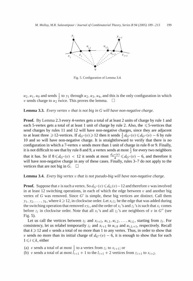
Fig. 5. Configuration of Lemma3.4.

u2, u1, u0 and sends12 to y1 throughu2, u3, u4, and this is the only configuration in whichv sends charge tou2 twice. This proves the lemma.�

Lemma 3.3. Every vertexv that is not big in G will have non-negative charge.

Proof. By Lemma2.3 every 4-vertex gets a total of at least 2 units of charge by rule 1 andeach 5-vertex gets a total of at least 1 unit of charge by rule 2. Also, the�5-vertices thatsend charges by rules 11 and 12 will have non-negative charges, since they are adjacentto at least three�12-vertices. IfdG′′(v)�12 then it sends12 dG′′(v)�dG′′(v) − 6 by rule10 and so will have non-negative charge. It is straightforward to verify that there is noconfiguration in which a 7-vertexv sends more than 1 unit of charge in rule 8 or 9. Finally,it is not difficult to see that by rule 8 and 9, a vertex sends at most1

2 for every two neighbors

that it has. So if 8�dG′′(v) < 12 it sends at mostdG′′ (v)4 �dG′′(v) − 6, and therefore it

will have non-negative charge in any of these cases. Finally, rules 3–7 do not apply to thevertices that are not big inG. �

Lemma 3.4. Every big vertexv that is not pseudo-big will have non-negative charge.

Proof. Suppose thatv is such a vertex. SodG′′(v)�dG(v)−12 and thereforevwas involvedin at least 12 switching operations, in each of which the edge betweenv and another bigvertex ofG was removed. SinceG′ is simple, these big vertices are distinct. Call themy1, y2, . . . , yk, wherek�12, in clockwise order. Letxizi be the edge that was added duringthe switching operation that removedvyi , and the order ofxi ’s andzi ’s is such thatxi comesbeforezi in clockwise order. Note that allxi ’s and allzi ’s are neighbors ofv in G′′ (seeFig. 5).

Let us call the vertices betweenzi andxi+1, ui,1, ui,2, . . . , ui,li , starting fromzi . Forconsistency, let us relabel temporarilyzi andxi+1 to ui,0 andui,li+1, respectively. Recallthatk�12 andv sends a total of no more than 1 to any vertex. Thus, in order to show thatv sends no more than its initial charge ofdG′′(v) − 6, it is enough to show that for each1� i�k, either

(a) v sends a total of at most12 to a vertex fromzi to xi+1; or

(b) v sends a total of at mostli+1 + 1 to theli+1 + 2 vertices fromzi+1 to xi+2.


First we show that there is at least one�5-vertex inui,0, . . . , ui,li+1, for each 1� i�k.If ui,0 is a 4-vertex we must haveyiui,1 ∈ G′′, becauseG′′ is a triangulation. Assumingthatui,1 is a 4-vertex we must haveyiui,2 ∈ G′′ and so on, until we haveyi+1ui,li+1 ∈ G′′and soui,li+1 will be a �5-vertex. So for every 1� i�k, there is a�5-vertex betweenziandxi+1; take any such vertex and call itui,ji . By Lemmas3.1 and 3.2 and rule 10, it canbe seen thatv sends a total of at most1

2 to ui,ji , unless 7�dG′′(ui,ji )�11.So assume that 7�dG′′(ui,ji )�11 andv sends 1 throughui,ji . By Lemma 3.2 both of

the neighbors ofv before and afterui,ji are 5- or 6-vertices and so to each of themv sendsa total of at most12. If zi �= xi+1 then at least one of these lies betweenzi andxi+1 andtherefore we satisfy (a) above.

So we can assumezi = xi+1. Thusui,ji = zi = xi+1, and so (i) 5�dG′′(zi+1)�6,and (ii) dG′′(ui+1,1) = 5 if zi+1 �= xi+2, or dG′′(zi+2) = 5 otherwise. First assume thatzi+1 = xi+2. Now if dG′′(zi+1) = 5 thenv gets back1

2 from zi+1 by rule 12 and so sendsa total of at most 0 to it. IfdG′′(zi+1) = 6 then it is easy to verify thatv sends nothing tozi+1 by any rule and so sends a total of at most 0 to it. Either way, we satisfy (b), above.

Otherwise ifzi+1 �= xi+2 then there are at least two vertices betweenzi+1, . . . , xi+2,that are 5- or 6-vertices and so to each of themv sends a total of at most12. Therefore wesatisfy (b), above. �

So the only vertices that may have negative charges are pseudo-big vertices inG′′. Assumethat v is a pseudo-big vertex ofG′′ whose neighborhood sequence in clockwise order isx1, . . . , xk. Letmbe the number of maximal sparse segments of the neighborhood ofv andcall these segmentsQ1,Q2, . . . ,Qm in clockwise order. Also, letRi be the sequence ofneighbors ofv between the last vertex ofQi and the first vertex ofQi+1, whereQm+1 = Q1.If m = 0 then we defineR1 to be equal toNG′′(v).

Lemma 3.5. LetR = xa, . . . , xb, where R is one ofR1, . . . , Rm. Thenv sends at total ofat most�5|R|

6 � to the vertices of R.

Proof. SinceRdoes not overlap with any maximal sparse segment, from every three consec-utive verticesxi, xi+1, xi+2 inR(where we consider the neighbors cyclicly ifR = NG′′(v)),at least one of them is a�5-vertex. Eitherv sends a total at most12 to this vertex, orvsends 1 and by Lemma3.2 the two vertices before that and the two vertices after that are5- or 6-vertices and sov sends to each of them a total of at most1

2. Thus in either casev sends a total of at most52 to every three consecutive vertices ofR and so sends at most

�56 (b − a + 1)� = �5|R|

6 � to the vertices ofR. �

Lemma 3.6. Suppose thatm�4.Then for every1� i�m eitherv sends at most|Ri | − 32

toRi , or v sends at most|Ri | − 1 toRi and

|Qi | + |Qi+1|��13 �� − 67. (2)

Proof. We consider different cases based on|Ri |:|Ri | = 1: Assume thatRi = u. Sinceu is the only vertex between two maximal sparse

segments,dG′′(u)�5. First letdG′′(u) = 5. SinceQi andQi+1 are sparse segments there


v

ui+1

tui

iQ Qi+1u

1w 2w

Fig. 6. The first configuration in Lemma3.6.

must be two big verticesui andui+1 that are connected to all the vertices ofQi andQi+1,respectively. Also,umust be connected to these two vertices, becauseG′′ is a triangulation(see Fig.6).

Note that by rule 12v gets back the12 charge it had sent tou. Sov is sending a total of atmost 0, so far. Lett be the other vertex that makes a triangle with edgeuiui+1. Assume thatdG′′(t) = 4, andw1, w2 are the two neighbors oft other thanui andui+1. If dG′′(w1)�4 anddG′′(w2)�4 then sinceQi andQi+1 are sparse segments andui andui+1 are big verticesinG, by Lemma 2.14 Eq. (2) holds. Otherwise, assume thatdG′′(w1)�5. Then by rule 3uiwill be sending extra12 to v throughu. So overall,v sends a total of−1

2 to u. If dG′′(t)�5then each ofui andui+1 will send an extra1

4 to v throughu by rule 5 and thereforev sendsa total of−1

2 to u.Now assumedG′′(u) = 6 and that the neighbors ofuarev, ui, ui+1, t and the end vertices

of Qi andQi+1. Note that in this casev will send nothing tou. Assume thatdG′′(t) = 4and its other neighbor isw. If dG′′(w)�6 then by Lemma 2.14 Eq. (2) holds. Otherwise,dG′′(w)�7 and so each ofui andui+1 sends an extra12 to v throughu by rule 6 and sovsends a total of−1 to u. If dG′′(t) = 5 and its other neighbors arew1 andw2 then eitherdG′′(w1)�6 anddG′′(w2)�6 and we can apply Lemma 2.14 to get Eq. (2), or at least oneof w1 andw2 has degree�7 and so one ofui or ui+1 will send an extra1

2 unit of charge tov throughu by rule 6 and sov sends a total of−1

2 to u. If dG′′(t)�6 then bothui andui+1

send an extra14 charge tov throughu by rule 7. Sov sends a total of−12 to u.

If 7�dG′′(u)�11, or 12�dG′′(u) anduwas not big inG, thenu sends12 to v by rule 8

or 10 and sov sends a total of−12 to u.

If uwas big inG then by rule 11v gets back12 throughu for each of the end vertices of

Qi andQi+1 that are adjacent tou, and sov sends a total of at most−1 tou.|Ri | = 2: Assume thatRi = v1, v2. If dG′′(v1)�6 ordG′′(v2)�6 then it is easy to check

thatv sends nothing to one ofv1, v2 and sends at most12 to the other one, or sends14 toeach, and so sends at most1

2 toRi . So let us assume thatdG′′(v1) = dG′′(v2) = 5 and lettbe the other vertex which makes a triangle withv1, v2. Note thatv sends only1

2 to each ofv1 andv2.


2v1v

w

(a)

v

ui+1

tui

iQ Qi+1

2v1v

(b)

v

ui+1

tui

iQ Qi+1

1w 2w

Fig. 7. Two other configurations for Lemma3.6.

If dG′′(t) = 4 then we can apply Lemma2.14 and get Equation (2). LetdG′′(t) = 5 andcall the other neighbor oft (other thanui, v1, v2, ui+1),w (see Fig. 7(a)). IfdG′′(w)�6 thenwe can apply Lemma 2.14 to get Eq. (2). OtherwisedG′′(w)�7 and by rule 4ui andui+1each send an extra12 to v (throughv1 andv2, respectively) and thereforev sends a total ofat most 0 toRi . Now assume thatdG′′(t) = 6 and its neighbors arew1, w2, ui, ui+1, v1, v2(see Fig. 7(b)). IfdG′′(w1)�6 anddG′′(w2)�6 then by Lemma 2.14 we have Eq. (2).Otherwise, at least one ofw1 orw2 is a �7-vertex and so one ofui or ui+1 sends an extra12 to v (throughv1 or v2) by rule 4 and thereforev sends a total of at most12 to Ri . If7�dG′′(t) < 12 thent sends1

2 to v by rule 9 and sov sends a total of at most12 to Ri . If12�dG′′(t) thenv gets back the12 it had sent to each ofv1 andv2 by rule 12 and so sendsa total of at most o toRi .

|Ri |�3: If there is no 4-vertex inRi then they are all�5-vertices and by Lemmas 3.1and 3.2v sends a total of at most|Ri | − 3

2 to Ri . If |Ri |�5, sinceRi cannot have threeconsecutive 4-vertices, we must have at least three�5-vertices and again by Lemmas 3.1and 3.2v sends a total of at most|Ri | − 3

2. So consider the case thatRi = v1, v2, v3, v4,dG′′(v1)�5, dG′′(v4)�5, anddG′′(v2) = dG′′(v3) = 4 (exactly the same argument worksfor the case that|Ri | = 3 andv2 = v3). There must be a big vertexw, other thanv,connected to all the vertices ofRi . If dG′′(v1) = 5 thenv gets back1

2 from v1 by rule 12


and so sends a total of at most 0 tov1. If dG′′(v1)�6 it can be verified thatv sends nothingto v1 by any rule. Sincev sends a total of at most12 to v2 and at most 1 to any vertex, itsends a total of at most|Ri | − 3

2 toRi .

Lemma 3.7. Every pseudo-big vertexv has non-negative charge.

Proof. Recall that the initial charge ofv wasdG′′(v)−6 and thatv sends a total of at most 1to any neighbor. We will show thatv sends a total of less than 1 to each of several neighbors,enough so that the total charge thatv loses is at mostdG′′(v) − 6. We consider differentcases based on the value ofm, the number of maximal sparse segments ofv. Recall that byObservation2.2 we can assume that��160.m = 0: Sincev is pseudo-bigdG′′(v)�dG(v)− 11�36. Using Lemma 3.5v will send

at most�56 dG′′(v)��dG′′(v)− 6 and therefore will have non-negative charge.

1�m�3: By Lemma 2.13 and definition of a pseudo-big vertex:• m = 1: Then

|R1| = dG′′(v)− |Q1|� dG′′(v)− dG(v)+ �2

3 �� + 73

� �23 × 160� + 62

� 36.

So by Lemma3.5v sends a total of at most|R1| − 6 toR1.• m = 2: Then∑

1� i�2|Ri | = dG′′(v)− ∑

1� i�2|Qi |

� dG′′(v)− 2dG(v)+ 2 × �23 �� + 146

� �13 �� + 135

� 36.

So by Lemma3.5v sends a total of at most|R1 ∪ R2| − 6 toR1 ∪ R2.• m = 3: Then∑

1� i�3|Ri | = dG′′(v)− ∑

1� i�3|Qi |

� dG′′(v)− 3dG(v)+ 3 × �23 �� + 219

� 36.

Therefore by Lemma3.5v sends at most|R1 ∪ R2 ∪ R3| − 6 toR1 ∪ R2 ∪ R3.m = 4: If v sends a total of at most|Ri | − 3

2 to eachRi then we are done. Otherwise byLemma 3.6, we can assume, without loss of generality, thatv sends a total of|R1| − 1 toR1 and that Eq. (2) holds forQ1 andQ2. Therefore using Lemma 2.13

|R2| + |R3| + |R4| � dG′′(v)− (|Q1| + |Q2|)− |Q3| − |Q4|� dG′′(v)− �1

3 �� + 67− 2(dG(v)− �23 �� − 73)

� � − 2dG(v)+ dG′′(v)+ 213

� 36.

Thus by Lemma 3.5,v sends a total of at most|R2 ∪ R3 ∪ R4| − 5 toR2 ∪ R3 ∪ R4.


m = 5: v sends a total of at most|Ri | − 1 to eachRi , by Lemma3.6. If there are atleast two values ofi such thatv sends a total of at most|Ri | − 3

2 to Ri then we are done.Otherwise there is at most oneRi , sayR5, to whichv sends a total of at most|Ri | − 3

2.Therefore Eq. (2) must hold for|Q1| + |Q2| and|Q3| + |Q4|, i.e.

|Q1| + |Q2| + |Q3| + |Q4|�2 × �13 �� − 134.

Then using Lemma2.13∑1� i�5

|Ri | � dG′′(v)− dG(v)+ �23 �� + 73− 2 × �1

3 �� + 134

� 36.

Therefore by Lemma 3.5,v sends a total of at most|R1 ∪ R2 ∪ R3 ∪ R4 ∪ R5| − 6 toR1 ∪ R2 ∪ R3 ∪ R4 ∪ R5.m�6: v sends at most|Ri | − 1 to eachRi , by Lemma 3.6. So we are done.�

Proof of Theorem 1.3. By Lemmas 3.3, 3.4, and 3.7 every vertex ofG′′ will have non-negative charge, after applying the discharging rules. Therefore the total charge over all thevertices ofG′′ will be non-negative, but this is contradicting Eq. (1). This disproves theexistence ofG, a minimum counter-example to the theorem.

Remark. Using a more careful analysis one can prove the bound�4|R|5 � in Lemma 3.5 which

in turn can be used to prove�(G2)��53 �� + 61. By being even more careful throughout

the analysis one can probably prove the bound�(G2)��53 �� + 51 or even maybe with 30

or 20 instead of 51.

4. A better bound for graphs with large �

The steps of the proof of Theorem 1.4 are very similar to those of Theorem 1.3, we onlyhave to modify a few lemmas and redo the calculations. For these lemmas, since the proofsare almost identical and do not need any new ideas, we only state the lemmas without givingfurther proofs. LetG be a minimum counter-example to Theorem 1.4 such that��241.

Lemma 4.1. For every vertexv of G, if there exists a vertexu ∈ N(v), such thatdG(v)+dG(u)�� + 2 thendG2(v)��5

3 �� + 25.

We construct the triangulated graphsG′ and thenG′′ exactly in the same way. Lemmas2.3–2.12 are still valid. The analogous of Lemmas 2.13 and 2.14 will be as follows.

Lemma 4.2. |Qi |�dG(v)− �23 �� − 20, for 1� i�m.

Lemma 4.3. Under the same assumption as in Lemma2.14,we have

|Qi | + |Qi+1|��13 �� − 14.


We apply the same initial charges and discharging rules. Again, all Lemmas3.1–3.5 hold.The analogue of Lemma 3.6 will be:

Lemma 4.4. Suppose thatm�4.Then for every1� i�m eitherv sends a total of at most|Ri | − 3

2 toRi , or v sends a total of at most|Ri | − 1 toRi and

|Qi | + |Qi+1|��13 �� − 14.

Now it is straightforward to do the calculations of Lemma3.7 with the above values tosee that it holds in this case too. This will complete the proof of Theorem 1.4.

5. On possible asymptotic improvement of Theorem 1.3

In this section, we only focus on the asymptotic order of the bounds, i.e. the coefficientof �. The results of [1,4,5] are essentially based on showing that in a planar graphG, thereexists a vertexv such thatdG2(v)��9

5 �� + O(1) ([5] actually obtains a slightly weaker,but still sufficient bound). However, as pointed out in [1], this is the best-possible bound onthe minimum degree of a vertex inG2. That is, there are 2-connected planar graphs in whichevery vertexv satisfiesdG2(v)��9

5 ��. One of these extremal graphs can be obtained froma icosahedron, by taking a perfect matching of it, addingk − 1 paths of length two parallelto each edge of the perfect matching, and replacing every other edge of the icosahedron byk parallel paths of length two (see Fig. 8).

Therefore, by only bounding the minimum degree ofG2 we cannot improve the bound�9

5 ��+O(1), asymptotically. This is the reason we introduced the reducible configurationof Lemma 2.14. We proved that any planar graphG either has a cut-vertex, or a vertexvsuch thatdG2(v)��5

3 �� +O(1), or has the configuration of Lemma 2.14.But there are graphs that are extremal for this new set of reducible configurations in

the following sense: these graphs do not have a cut-vertex, do not have a vertexv withdG2(v)��5

3 ��, and do not have the configuration of Lemma 2.14. For an odd value ofk,one of these graphs is shown in Fig. 9. To interpret this figure, we have to join the threecopies ofv8 and remove the multiple edges (we draw the graph in this way for clarity). Also,the dashed lines represent sequences of consecutive 4-vertices. Around each ofv1, . . . , v4there are 3k−6 such vertices. So,d(v1) = d(v2) = d(v3) = d(v4) = 3k, d(v5) = d(v6) =d(v7) = d(v8) = 3k + 3, � = 3k + 3, and for any vertexv ∈ G: dG2(v)�5k + 3 (withequality holding forv ∈ {v1, . . . , v4}). The minimum degree ofG2 is �5

3 �� + O(1) andit is easy to see thatG does not have the configuration of Lemma 2.14. Therefore, usingreducible configurations similar to those of Section 2 the best asymptotic bound that wecan achieve is�5

3 �� + O(1). So we need another reducible configuration to improve themultiplicative constant53.

6. Generalization toL(p, q)-labeling

In this section we prove Theorem 1.6. As we said before, the upper bound 3p for �p0 of aplanar graph follows from the Four Color Theorem (if we use colors from{0, p,2p,3p}).


Fig. 8. The icosahedron and the modified graph.

v8

v8

v6

v3

v4

v1

xk

x1

v7

v8

v5

v2

Fig. 9. The graph obtained based on a tetrahedron.

So let us assume thatq�1. We prove the following theorem:

Theorem 6.1. For any planar graph G and positive integer p:

�p1 (G)��53 �� + 18p + 59.

Assuming Theorem6.1, we can prove Theorem 1.6 as follows:

Proof of Theorem 1.6. Let c = �53 �� + 18�p

q� + 60. By Theorem 6.1, there is an

L(�pq�,1)-labeling ofG with thec colors in{0, . . . , c − 1}. Consider such a labeling and


multiply every color byq. This yields anL(p, q)-labeling ofGwith colors in{0, . . . , q(c−1)}. Noting that�p

q�� p+q−1

qyieldsq(c − 1)�q�5

3 �� + 18p + 77q − 18 which in turncompletes the proof. �

In the rest of this section we give the proof of Theorem6.1. The steps of the proof are verysimilar to those of proof of Theorem 1.3. LetGbe a planar graph which is a counter-exampleto Theorem 6.1 with the minimum number of vertices. We set

C = �53 �� + 18p + 60

and throughout this section we use colors from{0, . . . , C − 1}. Recall that a vertex is saidto be big ifdG(v)�47.

Lemma 6.2. Suppose thatv is a �5-vertex in G. If there exists a vertexu ∈ N(v), suchthatdG(v)+ dG(u)�� + 2 thendG2(v)�dG(v)+ �5

3 �� + 73.

Proof. Assume thatv is such a vertex and assume thatdG2(v) < dG(v) + �53 �� + 73.

Contractv on edgevu. The resulting graph has maximum degree at most� and becauseGwas a minimum counter-example, the new graph has anL(p,1)-labeling with at mostCcolors. Now consider such a labeling induced onG, in which every vertex other thanv iscolored. Every vertex at distance (exactly) two ofv in G forbids one color forv, and everyvertex inN(v) forbids at most 2p− 1 colors forv. So the total number of forbidden colorsfor v, i.e. the colors that we cannot assign tov, is at most

dG(v)(2p − 1)+ dG2(v)− dG(v) < 10p − 5 + �53 �� + 73

= �53 �� + 10p + 68

� C.

The last inequality follows from the assumption thatp�1. Therefore, there is still at leastone color available forv whose absolute difference from its neighbors inG2 is large enoughand so we can extend the coloring toG. �

Observation 6.3. By Theorem1.5we can assume that��162,otherwise(4q − 2)� +10p + 38q − 24�C − 1 (with q = 1).

Lemma 6.4. Every�5-vertex must be adjacent to at least2 big vertices.

Proof. By way of contradiction assume that there is a�5-vertexv which is adjacent to atmost one big vertex and so all its other neighbors are�46-vertices. Then, using Observation6.3,v along with one of these small vertices will contradict Lemma 6.2.�

Now construct graphG′ from G and thenG′′ from G′ in the same way we did in theproof of Theorem 1.3. Also, we define the sparse segments in the same way. Consider vertexv and let us call the maximal sparse segments of itQ1,Q2, . . . ,Qm in clockwise order,whereQi = qi,1, qi,2, qi,3, . . . .


Lemma 6.5. |Qi |�dG(v)− �23 �� − 69.

Proof. Analogous to the proof of Lemma2.13. �

The next lemma is analogous to Lemma 2.14. The key difference is that we require abound on the degree oft. This is because each vertex adjacent tot can forbid fort up to 2p−1colors. Thus we have to be more careful about controlling the number of such vertices.

Lemma 6.6. Suppose thatui andui+1 are the big vertices adjacent to all the vertices ofQi andQi+1, respectively. Furthermore, assume that t is a�6-vertex adjacent to bothui andui+1 but not adjacent tov (see Fig.3) and there is a vertexw ∈ N(t) such thatdG(t)+ dG(w)�� + 2.LetX(t) be the set of vertices at distance at most two of t that arenot inN [ui] ∪N [ui+1]. If |X(t)|�6 then

|Qi | + |Qi+1|��13 �� − 60. (3)

Proof. Again, by way of contradiction, assume that|Qi |+ |Qi+1|��13 ��−59. Using the

same argument as at the beginning of the proof of Lemma6.2, we can color every vertexof G other thant using colors in{0, . . . , C − 1} such that the vertices that are adjacentreceive colors that are at leastpapart and the vertices at distance two receive distinct colors.Consider such a coloring.

Note. We often focus on the inner vertices ofQi . So recall that there are exactly|Qi | − 2such vertices (similarly forQi+1). Also, for a setSof vertices each of which has a color,we sometimes use “the colors inS” to refer to the set of colors that appear on the verticesof S.

We say that a vertexu ∈ NG2(w) forbidsa color� for w if either (i) u is a distance 2fromw andu has colour� or (ii) u is adjacent tow andu has a colour that differs from� byless thanp; i.e., if an assignment of� tow would create a conflict with the colour onu. AsetSof verticesforbidsa setT of colours forw if for each colour� ∈ T , some vertex inSforbids� for w. A colour� is forbiddenfor w if someu ∈ NG2(w) forbids it forw.

Claim 1. There are at least�53 �� + 78 colors inNG2(t) andNG2(t) forbids all the C

colors for t.

Proof. Trivially, if there is a non-forbidden color fort then we can extend the coloring tot, which contradicts the minimality ofG.

If there are at most�53 �� + 77 colors inNG2(t) then (becauset is not colored and has

degree at most 6) they forbid at most�53 �� + 71+ 6(2p − 1) = �5

3 �� + 12p + 65< Ccolors fort, which contradicts what we proved in the previous paragraph.�

Claim 2. There exists an inner vertex ofQi orQi+1 whose color is distinct from the colorof every other vertex inNG2(t) and differs from the color of every vertex inN(t) by atleast p.


Proof. By way of contradiction assume the above statement is false. Let us count thenumber of forbidden colors fort. The neighbors oft forbid at mostdG(t)× (2p− 1) colorsfor t. Let us denote this set of forbidden colors byR. The vertices at distance exactly twoof t are inN(ui) ∪ N(ui+1) ∪ X(t) − N(t), and each of them forbids its own color fort.However, by assumption, at least|Qi | − 2 + |Qi+1| − 2 of these forbidden colors (fort)are counted twice. This is because we assumed the claim is false; i.e. for every color� thatappears on an inner vertex ofQi orQi+1 there is a neighbor oft whose color differs from� by less thanp (and so� ∈ R) or there is another vertex inNG2(t) with color �. SincedG(ui)+ dG(ui+1)+ |X(t)|�2� + 6, the total number of forbidden colors fort is at mostdG(t)×(2p−1)+2�+6−dG(t)−|Qi |−|Qi+1|+4��5

3 ��+6(2p−1)+63��53 ��+

12p + 57< C. This contradicts Claim 1. �

Thus, without loss of generality, we can assume there exists an inner vertex ofQi+1, sayqi+1,2, whose color is different from the color of every vertex inNG2(t) and differs fromthe color of every vertex inN(t) by at leastp.

Claim 3. There are at least�53 �� + 77 colors inNG2(qi+1,2) and they forbid forqi+1,2,

C − 1 colors(all the colors except the one that appears onqi+1,2).

Proof. First we show that the vertices inNG2(qi+1,2)must forbid all the colors (except theone that appears onqi+1,2) for qi+1,2. Otherwise, we can produce a valid labelling ofG byremoving the color ofqi+1,2 and assigning it tot, and then assigning a new color toqi+1,2(from the other colors that are not forbidden for it). Hence, the number of forbidden colorsfor qi+1,2 must beC − 1.

If there are fewer than�53 �� + 77 different colors inNG2(qi+1,2) then, sincedG(qi+1,2)

�4, the vertices inNG2(qi+1,2) forbid fewer than 4(2p − 1) + �53 �� + 73 = �5

3 �� +8p + 69�C − 1 colors for qi+1,2. This contradicts what we proved in the previousparagraph. �

From the definition of a sparse segmentN(qi+1,2) ⊆ {v, ui+1, qi+1,1, qi+1,3}. Let usdenote the set of colors on the vertices inN [ui+1] ∪N(t) ∪X(t) ∪N [qi+1,1] ∪N [qi+1,3]bySand call it the set ofsmaller colors.

Claim 4. |S|�dG(ui+1)+ 14.

Proof. Follows from the definition ofS. �

Every vertex inN [ui+1] ∪N(t)∪X(t)∪N [qi+1,1] ∪N [qi+1,3] is of distance at most 2from eithert or qi+1,2, and therefore forbids some colors fort or for qi+1,2. Let us call theset of colors that are forbidden fort orqi+1,2 by those vertices thesmaller forbiddencolors,and denote them bySF. Sinced(t)�6 andd(qi+1,2)�4 andui+1 is a common neighborof t andqi+1,2,

|SF |�9(2p − 1)+ |S| − 9 = |S| + 18p − 18. (4)


So,SFcontainsSalong with at most 18(p− 1) colors which differ from the color of someneighbor oft or some neighbor ofqi+1,2 by at mostp − 1.

Claim 5. Every color that is not in SF differs from every color inN(t) ∪ N(qi+1,2) by atleast p.

Proof. By the definition ofSF, every color which differs from the color of a vertex inN(t) ∪N(qi+1,2) by less thanp is inSF. �

We will use Claim 5 at the end of the proof of this Lemma. By Claim 3, there are at leastC − 1− |SF | colors, different from the smaller forbidden colors, inN(v)−Qi+1. We callthis set thelarger colors and denote it byL.

Claim 6. |L|��53 �� − |S| + 77��5

3 �� − dG(ui+1)+ 63.

Proof. Follows from the definition of L, Claim 4, and the bound on|SF |(Inequality4). �

Since|N(v)| − (|Qi | − 2) − |Qi+1|�� − �13 �� + 61< |L|, one of thelarger colors

must be on an inner vertex ofQi , which without loss of generality, we can assume isqi,2.

Claim 7. The vertices inN(v) −Qi+1 − {qi,2} forbid for qi,2 all the colors in L, exceptthe one that appears onqi,2.

Proof. All the larger colors appear inN(v)−Qi+1 and so they are at distance at most twoof qi,2. �

Claim 8. The number of forbidden colors forqi,2 is at most�43 �� + 8p − 68< C.

Proof. By noting thatd(qi,2)�4, neighbors ofqi,2 forbid at most 4(2p−1) colors forqi,2.Now let us count the number of forbidden colors forqi,2 by the vertices at distance exactlytwo of it.N [ui+1] ∪ N(t) ∪ X(t) forbids for t only colors that are inSF. Thus, by Claim 1, all

the larger colors must appear inN [ui] − N(t). Remember that the larger colors appear inN(v)−Qi+1, too. Therefore, the number of colors that are not inL and are forbidden forqi,2 by the vertices at distance exactly 2 ofqi,2 is at most:d(ui)− 1 − (|L| − 1)+ d(v)−1 − (|L| − 1)�2� − 2|L|. By considering the vertices at distance exactly two ofqi,2 thathave a larger color and noting thatqi,2 has a larger color too, and using Claim 6, the totalnumber of colors forbidden forqi,2 is at most

4(2p − 1)+ (2� − 2|L|)+ (|L| − 1) � �13 �� + dG(ui+1)+ 8p − 68

� �43 �� + 8p − 68. �

By Claim 8, we can produce a valid labelling ofG by assignning the color ofqi,2 to t(because it is a larger color and so it is different from the colors inX(t) and, by Claim 5,


differs from all the colors inN(t) by at leastp) and then finding a new color forqi,2 that isnot forbidden for it. This completes the proof of Lemma6.6. �

The rest of the proof is almost identical to that of Theorem 1.3. We use Lemmas 6.4, 6.5,and 6.6, instead of Lemmas 2.3, 2.13, and 2.14, respectively. The initial charges and thedischarging rules are the same. Without any modifications, Lemmas 3.1–3.5 hold in thiscase, too. In Lemma 3.6 we should replace Eq. (2) with Eq. (3) and use Lemma 6.6 insteadof Lemma 2.14. To do so, it is important to note that whenever we used Lemma 2.14 in theproof of Lemma 3.6, the degree oft was at most 6; thus, we can use Lemma 6.6, instead.After doing these modifications, the calculations for the proof of this revised version ofLemma 3.6 are fairly straightforward.

7. An O(n2) time algorithm

In this section we show how to transform the proof of Theorem 1.3 into a coloringalgorithm which uses at most�5

3 �� + 78 colors. With some minor modifications in thealgorithm, we can obtain coloring algorithms for Theorems 1.4 and 1.6.

Consider a planar graphG. We may assume that��160 since for smaller values of�it is straightforward to obtain an algorithm based on the result of [20] that uses at most�5

3 ��+78 colors. Also, we assume that the input to our algorithm is connected, since for adisconnected graph it is enough to color each connected component, separately. One iterationof the algorithm either finds a cut-vertex and breaks the graph into smaller subgraphs, orreduces the size of the problem by contracting a suitable edge ofG. Then it colors the newsmaller graph(s) recursively, and extends the coloring(s) toG. More specifically, we do thefollowing steps, as long as the graph has at least one vertex:

1. Check to see whetherG has a cut-vertex. Ifv is a cut-vertex andC1, . . . , Ck are theconnected components ofG − v then color eachGi = Ci ∪ {v}, independently. Theunion of these colorings, after permuting the colors in some of them, will be a coloringof G.

2. Else, check to see whether there is a�5-vertex adjacent to at most one big vertex. Ifsuch a vertex exists, then that vertex along with one of its small neighbours will be thesuitable edge to be contracted.

3. Else, construct the triangulated graphG′′.4. Apply the initial charges and the discharging rules.5. As the total charge is negative, we can find a vertexv with negative charge. This vertex

must be in one of the reducible configurations described in Lemma2.13 or 2.14.If we find the reducible configuration of Lemma2.13 aroundv then one of the innervertices of the sparse segment along with one of its two big neighbours will be thesuitable edge to contract. Otherwise, if we find the reducible configuration of Lemma2.14 aroundv then we can contract edgetw (recall the specification oft andw fromLemma 2.14).

6. Color the new graph (after contracting the suitable edge), recursively.7. This coloring can be easily extended toG by the arguments of proofs of Lemmas2.3,

2.13 or 2.14.


That this algorithm works follows easily from the proofs of Lemmas3.3, 3.4, and 3.7.Since in a planar graph the number of edges and faces is linear in the number of vertices wemay letn = |V | be the size of the graph. Finding a cut-vertex in a graph takes linear time.To see if there is a�5-vertex with less than 2 big neighbors we spend at mostO(n) time.Also, applying the initial charges and the discharging rules takesO(n) time. After findinga vertex with negative charge, finding the suitable edge and then contracting it can be donein O(n). Since there areO(n) iterations of the main procedure, the total running time ofthe algorithm would beO(n2).

The algorithms for Theorems 1.4 and 1.6 work almost identically.

Acknwoledgments

We would like to thank two anonymous referees whose comments greatly improved thepresentation of the paper.

References

[1] G. Agnarsson, M.M. Halldórsson, Coloring powers of planar graphs, SIAM J. Discrete Math. 16 (4) (2003)651–662.

[2] K. Appel, W. Haken, Every planar map is four colourable, Contemp. Math. 98 (1989).[3] H.L. Bodlaender, T. Kloks, R.B. Tan, J. van Leeuwen, Approximations for�-coloring of graphs, Proceedings

of 17th Annual Symposium on Theoretical Aspects of Computer Science, Lecture Notes in Computer Science1770, 2000.

[4] O. Borodin, H.J. Broersma, A. Glebov, J. van den Heuvel, Stars and bunches in planar graphs. Part I:triangulations, CDAM Research Report Series 2002-04, 2002.

[5] O. Borodin, H.J. Broersma, A. Glebov, J. van den Heuvel, Stars and bunches in planar graphs. Part II: generalplanar graphs and colourings, CDAM Research Report Series 2002-05, 2002.

[6] J. Chang, Kuo, TheL(2,1)-labeling problem on graphs, SIAM J. Discrete Math. 9 (1996) 309–316.[7] D.A. Fotakis, S.E. Nikoletseas, V.G. Papadopoulou, P.G. Spirakis, Hardness results and efficient

approximations for frequency assignment problems: radio labeling and radio coloring, J. Comput. Artif.Intell. 20 (2) (2001) 121–180.

[8] J.P. Georges, D.W. Mauro, Generalized vertex labeling with a condition at distance two, Congr. Numer. 109(1995) 141–159.

[9] J.P. Georges, D.W. Mauro, On the size of graphs labeled with a condition at distance two, J. Graph Theory22 (1996) 47–57.

[10] J.P. Georges, D.W. Mauro, Some results on�ij -numbers of the products of complete graphs, Congr. Numer.140 (1999) 141–160.

[11] J.R. Griggs, R.K. Yeh, Labeling graphs with a condition at distance 2, SIAM J. Discrete Math. 5 (1992)586–595.

[12] W.K. Hale, Frequency assignment: theory and application, Proc. IEEE 68 (1980) 1497–1514.[13] T.K. Jonas, Graph coloring analogues with a condition at distance two:L(2,1)-labelings and list�-labelings,

Ph.D. Thesis, University of South Carolina, 1993.[14] T.R. Jensen, B. Toft, Graph Coloring Problems, Wiley, New York, 1995.[15] S. Ramanathan, E.L. Lloyd, On the complexity of distance-2 coloring, in: Proceedings of the Fourth

International Conference, Computers and Information, 1992, , pp. 71–74.[16] S. Ramanathan, E.L. Lloyd, Scheduling algorithms for multi-hop radio networks, IEEE/ACM Trans.

Networking 1 (2) (1993) 166–172.[17] D.P. Sanders, Y. Zhao, A new bound on the cyclic chromatic number, J. Combin. Theory B 83 (2001)

102–111.


[18] C. Thomassen, Applications of Tutte cycles, Technical Report, Department of Mathematics, TechnicalUniversity of Denmark, September 2001.

[19] J. van den Heuvel, R.A. Leese, M.A. Shepherd, Graph labeling and radio channel assignment, J. GraphTheory 29 (1998) 263–283.

[20] J. van den Heuvel, S. McGuinness, Colouring the square of a planar graph, J. Graph Theory 42 (2003)110–124.

[21] G. Wegner, Graphs with given diameter and a coloring problem, Technical Report, University of Dortmond,1977.

[22] A. Whittlesey, J.P. Georges, D.W. Mauro, On the�-number ofQn and related graphs, SIAM J. Disc. Math.8 (1995) 499–506.

[23] S.A. Wong, Colouring graphs with respect to distance, M.Sc. Thesis, Department of Combinatorics andOptimization, University of Waterloo, 1996.

A bound on the chromatic number of the square of a planar graph

Documents

Transcript of A bound on the chromatic number of the square of a planar graph