Seediscussions,stats,andauthorprofilesforthispublicationat:https://www.researchgate.net/publication/233982130

CosmologicalBackreactionforaTestFieldObserverinaChaoticInflationaryModel

ArticleinJournalofCosmologyandAstroparticlePhysics·February2013

DOI:10.1088/1475-7516/2013/02/027·Source:arXiv

CITATIONS

15

READS

51

3authors,including:

G.Marozzi

UniversityofGeneva

45PUBLICATIONS803CITATIONS

SEEPROFILE

GianPaoloVacca

INFN-IstitutoNazionalediFisicaNucleare

91PUBLICATIONS1,441CITATIONS

SEEPROFILE

AllcontentfollowingthispagewasuploadedbyGianPaoloVaccaon02December2016.

Theuserhasrequestedenhancementofthedownloadedfile.Allin-textreferencesunderlinedinbluearelinkedtopublicationsonResearchGate,lettingyouaccessandreadthemimmediately.

Cosmological Backreaction for a Test Field Observer in a Chaotic

Inflationary Model

Giovanni Marozzi1,2∗ , Gian Paolo Vacca3† , Robert H. Brandenberger4‡

1 College de France, 11 Place M. Berthelot, 75005 Paris, France.2 Universite de Geneve, Departement de Physique Theorique and CAP,

24 quai Ernest-Ansermet, CH-1211 Geneve 4, Switzerland.3 INFN Sezione di Bologna, via Irnerio 46, I-40126 Bologna, Italy.

4 Physics Department, McGill University,3600 University Street, Montreal, QC H3A 2T8, Canada

Abstract

In an inhomogeneous universe, an observer associated with a particular matter field does notnecessarily measure the same cosmological evolution as an observer in a homogeneous and isotropicuniverse. Here we consider, in the context of a chaotic inflationary background model, a class ofobservers associated with a “clock field” for which we use a light test field. We compute the effectiveexpansion rate and fluid equation of state in a gauge invariant way, taking into account the quantumfluctuations of the long wavelength modes, and working up to second order in perturbation theoryand in the slow-roll approximation. We find that the effective expansion rate is smaller than whatwould be measured in the absence of fluctuations. Within the stochastic approach we study thebounds for which the approximations we make are consistent.

1 Introduction

The setting of this work is inflationary cosmology [1], specifically a simple large field (or “chaotic”)inflationary model [2] in which the almost constant potential of a slowly rolling scalar field Φ (the“inflaton”) leads to a phase of almost exponential expansion of space. We know, however, that theremust be other matter fields present, in particular those of the Standard Model of particle physics.These fields may play a sub-dominant role in determining the expansion of space during the periodof inflation, but they are very relevant to late-time cosmology. In such a framework it is reasonableto consider the possibility of associating to one of these extra fields a class of dynamical observers, afact which leads to the construction and study of observables which are determined by measurementsperformed by such a class of observers. In the presence of primordial cosmological fluctuations, whichare unavoidably present in the semiclassical approach of the gravity-matter dynamics, such observerswill in general not measure exactly the same physics as a canonical observer in a homogeneous universewould. Such an effect is, in general, called the cosmological backreaction.

This is a non-trivial task and we shall consider here a simple toy model setup. Following [3], wewill consider the case where the clock/observer is associated to a light test scalar field χ (as opposedto the inflaton field), and the inflaton field has the standard quadratic potential of chaotic inflation

given by V (Φ) = m2

2 Φ2. More specifically, we assume that the light field χ at the background leveldoes not affect the evolution of the space-time during the inflationary regime but only plays the roleof a clock.

∗giovanni.marozzi@unige.ch†vacca@bo.infn.it‡rhb@physics.mcgill.ca

1

arX

iv:1

212.

6029

v2 [

hep-

th]

30

Jan

2013

2

In general, the issue of backreaction of cosmological perturbations [4] can be described as follow. Ifwe start with a background cosmological solution (metric and matter) and add to it small amplitudefluctuations of relative amplitude ε 1 which satisfy the linear perturbation equations, then due to thenon-linearities in the Einstein equations these equations are not satisfied to quadratic order. Secondorder fluctuations in matter and metric build up. In particular, corrections to the background canbe induced. The calculations of [4] showed that, to leading order in spatial gradients, super-Hubblelinear fluctuation modes induce effects which grow logarithmically in time and act like a negativecontribution to the effective cosmological constant. It was then conjectured [5] that this effect mightlead to a dynamical relaxation mechanism for the cosmological constant, in analogy of the effect whichis conjectured to occur in pure quantum gravity due to two loop infrared gravitons [6]. In [4], theeffects were computed as a function of the background time variable t.

However, in [7] the challenge was raised as to whether this effect could be measured in terms ofa physical clock. Indeed, it was then shown [8] that in the case of single field matter, the infraredbackreaction is not physically measurable (see [9] for the same result obtained within a manifestlygauge invariant, and up to second order in perturbation theory, approach). The Hubble expansionrate measured by the only available physical clock (namely the value of the scalar field) has the samehistory with and without long wavelength fluctuations (see also [10]).

Now, in late time cosmology we measure time in terms of the temperature of the cosmic microwavebackground (CMB) which at late times is a sub-dominant component of matter. Hence, as said, itis reasonable to ask whether effects of cosmological fluctuations can be measured by a clock whichcorresponds to a sub-dominant field, a field which in the late time universe would represent thetemperature of the CMB. A first step in this direction was made in [3] where it was shown that aclock tied to an entropy field will indeed measure a different expansion rate of space in the presenceand absence of curvature fluctuations.

On the other hand, in order to give meaningful statements about observables - once the observershave been chosen - these must be constructed in a gauge invariant way, i.e. they should be definedcovariantly in a reparameterization invariant way, so that any other spectator (secondary) observeragrees with the definition given, computing it with its preferred reference system. Therefore some careis required since normally one is dealing with observables obtained after averaging procedures. Forexample, it is crucial to take into account the volume measure. The problem can be naturally analyzedemploying the gauge invariant method developed in [11, 12] (where the set of effective equations forthe averaged geometry given in [13] has been generalized in a covariant and gauge invariant form)and recently applied to single field inflationary models [9, 14].

Therefore, considering the gauge invariant approach just mentioned, the question we address in thispaper is the following: we compare the average expansion rate of a spatial hypersurface characterizedby a fixed value of a spectator test scalar field in two space-time manifolds, the first one which hasno curvature fluctuations, the second one which contains such perturbations 2. We find that as aconsequence of long wavelength fluctuations, the average expansion rate is smaller. This effect is atquadratic order in the amplitude of cosmological fluctuations (at one loop in quantum field theorylanguage) as opposed to the situation in pure gravity where backreaction effects of long wavelengthfluctuations occur only at two loop order [6]. The backreaction leads to a reduction of the expansionrate. Whether the effect leads to a uniform relaxation of the cosmological constant or simply to astochastic adjustment is probably difficult to be answered using only our perturbative approach.

The outline of this paper is as follows. In Section 2 we review the covariant and gauge-invariantapproach which we shall use, and introduce the “effective Hubble expansion rate” for an observer inan inhomogeneous universe. Section 3 forms the heart of this paper: we introduce our toy model,define the class of observers used (observers associated with a test scalar field χ), determine thegauge transformation into a coordinate system in which χ is constant on spatial hypersurfaces, and

1Note that ε is not the inflationary slow-roll parameter.2Let us observe that, in investigations concerning the actual dynamics of the Universe, one may imagine more

suitable choices to investigate physical phenomena based on past light-cone observations. In particular, the gaugeinvariant approach of [11, 12] has been generalized to averaging over the past light-cone of a generic observer in [15] andthis new approach has been applied in [16].

3

evaluate the effective Hubble expansion rate which our observer sees. We also discuss bounds onthe parameters of the model under which our perturbative analysis is valid, estimate the magnitudeof the terms contributing to the backreaction, and determine the equation of state as seen by ourobservers. In Section 4 we give a general discussion and provide some numerical results. The finalsection contains our conclusions.

2 Observables and gauge invariant backreaction

The issue of the backreaction on an observable induced by quantum fluctuations in an inflationaryuniverse can be cast on solid grounds using a recent covariant and gauge invariant (GI) approach [11,12]. One can construct a general non-local observable by taking quantum averages of a scalar fieldS(x) over a space-time hypersurface ΣA0 where another scalar A(x) (assumed to have a time-likegradient) has constant value A0. Given this second scalar field, we can define a particular (barred)coordinate system xµ = (t, ~x) in which the scalar A is homogeneous. A physical (and hence GI)definition of the observable is then given by the following quantity

〈S〉A0 =〈√|γ(t0, ~x)| S(t0, ~x)〉〈√|γ(t0, ~x)|〉

, (1)

where we have denoted by√|γ(t0, ~x)| the determinant of the induced three dimensional metric on

ΣA0 . The natural foliation of spacetime is then defined by the four vector

nµ = − ∂µA

(−∂νA∂νA)1/2(2)

which characterizes the class of observers.We are interested in the dynamics encoded in the effective scale factor aeff = 〈

√|γ| 〉1/3, which

satisfies the GI effective cosmological equation [12](1

aeff

∂ aeff∂A0

)2

=1

9

⟨Θ

(−∂µA∂µA)1/2

⟩2

A0

, (3)

where Θ = ∇µnµ is the expansion scalar of the timelike congruence nµ. This effective scale factordescribes the expansion of the space as seen by the class of observers sitting on the hypersurfaceΣA0 . The dynamics can be then extracted solving the Einstein and matter equations of motion inany gauge.

In order to deal with the metric components in any specific frame we employ the standard decom-position of the metric in terms of scalar, transverse vector (Bi,χi) and traceless transverse tensor (hij)fluctuations up to the second order around a homogeneous Friedmann-Lemaitre-Robertson-Walker(FLRW) zero order space-time

g00 = −1− 2α− 2α(2) , gi0 = −a2

(β,i +Bi)−a

2

(β

(2),i +B

(2)i

)gij = a2

[δij

(1−2ψ−2ψ(2)

)+Dij(E + E(2)) +

1

2(χi,j + χj,i + hij) +

1

2

(χ

(2)i,j + χ

(2)j,i + h

(2)ij

)](4)

where Dij = ∂i∂j−δij∇2/3 and for notational simplicity we have removed a superscript for first orderquantities. The Einstein equations connect these fluctuations with those in the matter fields. Forexample, an inflaton field can be written to second order as Φ(x) = φ(0)(t) + φ(1)(x) + φ(2)(x) (wherex is the space-time four vector).

These general perturbed expressions can be gauge fixed. Let us recall some common gauge fixingsof the scalar and vector part: the synchronous gauge (SG) is defined by g00 = −1 and gi0 = 0,the uniform field gauge (UFG) apart from setting Φ(x) = φ(0)(t) must be supplemented by otherconditions (one can consider gi0 = 0), finally the uniform curvature gauge (UCG) is defined by

gij = a2[δij + 1

2

(hij + h

(2)ij

)].

4

To quadratic order (in the amplitude of the fluctuations), the inhomogeneities effect the effec-tive expansion rate. This is called the “backreaction” effect. Using Eq. (3) we can now define thebackreaction on the averaged expansion rate as the one obtained with respect to a class of observersidentified by the scalar field A(t, ~x). In the long wavelength (LW) limit and neglecting the tensorperturbations, we obtain [9]

H2eff ≡ A(0) 2

(1

aeff

∂ aeff∂A0

)2

= H2

[1 +

2

H〈ψ ˙ψ〉 − 2

H〈 ˙ψ(2)〉

], (5)

Let us stress here that the choice of a particular class of observers leads to the choice of a particularobservable. The observers depend on a preferred reference frame but the associated observable isphysical, and hence gauge invariant, in the sense that every other observer associated to a differentframe agrees on its value.

In an inflationary background, the long wavelength contribution to the expectation values 〈ψ ˙ψ〉and 〈 ˙ψ(2)〉 will be increasing in time since the phase space of infrared (super-Hubble) modes is growing.The contribution of the ultraviolet (sub-Hubble) modes is constant in time since, given an ultravioletcutoff which is fixed in physical coordinates (see e.g. [17] for a discussion of this point), the phasespace of these modes is constant (in the limit of exponential inflation). In the following we will usethe stochastic approach to evaluate the above expectation values.

3 Gauge invariant backreaction in a 2-field model

The classical model from which we start is a Friedmann-Lemaitre-Robertson-Walker (FLRW) space-time with an inflaton (scalar) field Φ and a second light field χ which we study in the test fieldapproximation (i.e. neglecting its energy density and pressure in the background FLRW equations).We shall admit all possible inhomogeneous scalar quantum fluctuations of the metric and of thescalar matter fields, up to second order in perturbation theory. In particular, the inflaton model weconsider here is, for simplicity, given by a free massive scalar field which we shall treat in the slow-rollapproximation together with a second free massive (test) field χ, both minimally coupled to gravity.The action is

S =

∫d4x√−g[

R

16πG− 1

2gµν∂µΦ∂νΦ− 1

2m2Φ2 − 1

2gµν∂µχ∂νχ−

1

2m2χχ

2

]. (6)

In the rest of this work we shall make an heavy use of the results on the stochastic approach toinflationary dynamics presented in Section 5 of [18].

3.1 Perturbative dynamics of the observers

We now choose a special class of observers which will define our observables. Following [3], we considerthe average expansion rate as computed by the observers ”χ”, namely by the observers sitting onthe spacelike hypersurface defined by χ equal to a constant. This hypersurface characterizes whatwe denote the barred gauge. To proceed we need the solutions of the equation of motion in thisframe up to second order in perturbation theory (see Eq. (5)). These can be obtained with a gaugetransformation from the results in the UCG [18, 19]. As a consequence we have to find the gaugetransformation that goes from the UCG to the barred gauge, where χ(x) = χ(0)(t) +χ(1)(x) +χ(2)(x)is equal to a constant, i.e. where χ(1) = χ(2) = 0. To fix the second gauge completely we also imposethe condition β = 0. This gauge, which we denote UχFG, explicitly depends on the property of thefield χ. We stress that this is a new scenario compared to previous analysis in a single field inflationarymodel [9, 14], where the observers were defined in a geometrical way.

To find the gauge transformation, let us first consider the “infinitesimal” coordinate transformationparametrized by the first-order and second-order generators εµ(1) and εµ(2), respectively, and given by

[20]

xµ → xµ = xµ + εµ(1) +1

2

(εν(1)∂νε

µ(1) + εµ(2)

)+ . . . (7)

5

whereεµ(1) =

(ε0(1), ∂

iε(1) + εi(1)

), εµ(2) =

(ε0(2), ∂

iε(2) + εi(2)

)(8)

(we have explicitly separated the scalar part from the pure transverse vector part εi(1), εi(2)). Let us

then recall that the associated gauge transformation of a scalar field S is, to first order,

S(1) → S(1) = S(1) − ε0(1)S(0), (9)

and, to second order,

S(2) → S(2) = S(2) − ε0(1)S(1) −

(εi(1) + ∂iε(1)

)∂iS

(1)

+1

2

[ε0(1)∂t(ε

0(1)S

(0)) +(εi(1) + ∂iε(1)

)∂iε

0(1)S

(0) − ε0(2)S(0)]. (10)

On neglecting vector perturbations we can fix to zero εi(1) and with S ≡ χ the gauge conditions

χ(1) = 0 and χ(2) = 0 give the following results:

ε0(1) =χ(1)

χ(0), (11)

ε0(2) = 2χ(2)

χ(0)+

1

χ(0)

[−2(∂iε(1)∂iχ

(1) + ε0(1)χ(1))

+ ε0(1)∂t

(ε0(1)χ

(0))

+(∂iε(1)∂iε

0(1)

)χ(0)

], (12)

and using ε0(1) in ε0(2) one obtains

ε0(2) = 2χ(2)

χ(0)− 1

χ(0)∂iε(1)∂iχ

(1) − 1

χ(0) 2χ(1)χ(1) . (13)

We can now evaluate ε(1) from the second gauge condition of UχFG, namely β = 0. One obtains(from Eq. (3.8) of [21])

ε(1) =

∫dt

[1

a2

χ(1)

χ(0)− β

2a

]. (14)

Considering finally the transformation between UCG and UχFG it is straightforward to derivethe following gauge transformation for ψ and ψ(2) (from Eqs. (3.9) and (3.13) of [21]):

ψ = Hε0(1) +1

3∇2ε(1) (15)

ψ(2) =H

2ε0(2) +

1

6∇2ε(2) −

H

2ε0(1)ε

0(1) −

ε0 2(1)

2

(H + 2H2

)− H

2∂iε

0(1)∂

iε(1) −1

6Πii , (16)

where Πij is defined in Eq. (3.16) of [21]. Using the above results and working in the long wavelengthlimit (and neglecting also tensor perturbations) one explicitly obtains

ψ =H

χ(0)χ(1) , ψ(2) =

H

χ(0)χ(2) − H

χ(0) 2χ(1)χ(1) − χ(1) 2

2χ(0) 2

(2H2 + H −H χ(0)

χ(0)

). (17)

We have now almost all the ingredients needed to evaluate the different terms involved in the

backreaction equation (5). Let us begin with 〈ψ ˙ψ〉:

〈ψ ˙ψ〉 =H2

χ(0) 2

[(H

H− χ(0)

χ(0)

)〈χ(1) 2〉+ 〈χ(1)χ(1)〉

]. (18)

Following [18] we solve the background equations for our particular model and find the followingzero order solution for the test field χ

χ(0)(t) = χ(0)(ti)

(H(t)

H(ti)

)α, (19)

6

where we have defined α =m2

χ

m2 .Let us remark that, for the purpose of this work, based on a perturbative analysis, we need to

consider χ(0)(ti) 6= 0, namely, a dynamical regime such that χ has non zero vacuum expectationvalue, a condensate. In such a case we have a scalar with time-like gradient which defines a space-likehypersurface, χ(x) equal to a constant, up to when the space dependence of the scalar can be seenas a perturbative dependence over a time function χ(0)(t). Namely, when the stochastic perturbativeapproach defined in [18] is valid (see, Eqs. (29-31)). Such a configuration is compatible with adynamical phase of universe expansion such as inflation. Let us further underline as the dynamicalcut-off, present in the stochastic approach of [18] and which is used to regularize our correlator (as,for example, 〈χ(1)2〉), is defined in the way that only the super-Hubble ”classical” fluctuations of ourfields are taken in consideration. If the background value of χ were to vanish, χ would not define aphysical clock field which can be used to follow the evolution of space-time.

At this point we turn to the evaluation of the contribution of the long wavelength (super-Hubble)modes to the expectation values which appear in Eq. (18). Following [18] we obtain for our particularbackground the following stochastic solutions up to second order in perturbation theory

〈χ(1)2〉 =3H2α

8π2m2(2− α)(H4−2α

i −H4−2α)− α2

48π2

χ(0)(ti)2

M2pl

(H

Hi

)2α 1

H4

(H2 −H2

i

)3, (20)

〈χ(2)〉 =α

8π2

χ(0)(ti)

M2pl

(H

Hi

)α [−H

6i

H4

1− α/26

+H4i

H2

1− α4

+H2i

α

4−H2 1 + α

12

]. (21)

Going back to the expression of Eq.(18) we obtain by substitution the following result

〈ψ ˙ψ〉 =H2

χ(0) 2

H

H

{3H2α

8π2m2(2− α)

[(2−H H

H2

)H4−2αi −

(4− α−H H

H2

)H4−2α

]

− α2

48π2

χ(0)(ti)2

M2pl

(H

Hi

)2α 1

H4

[−H H

H2

(H2 −H2

i

)3+ 3H2

(H2 −H2

i

)2]}. (22)

Let us now consider the other term in Eq. (5) which depends on 〈 ˙ψ(2)〉. It is easy to show thatthe leading slow-roll contribution is given by the derivative of the leading term of 〈ψ(2)〉. Indeed,considering the leading part in Eq.(17), then in the slow-roll approximation, and starting from theexpression

〈ψ(2)〉 ' H

χ(0)〈χ(2)〉 − H2

χ(0) 2〈χ(1) 2〉 , (23)

one obtains that

〈 ˙ψ(2)〉 ' H

χ(0)

[(H

H− χ(0)

χ(0)

)〈χ(2)〉+ 〈χ(2)〉

]− 2〈ψ ˙ψ〉 , (24)

from which it follows that the leading value of 〈 ˙ψ(2)〉 will be given by

〈 ˙ψ(2)〉 ' H

χ(0)

[−2

H

H− H

H

]〈χ(2)〉 − 2〈ψ ˙ψ〉 . (25)

As a consequence, we can rewrite the cosmological backreaction (Eq.(5)) for the expansion rate asseen by an observer comoving with the light test field χ in the following way

H2eff ' H2

[1 +

6

H〈ψ ˙ψ〉+

2

χ(0)

(2H

H+H

H

)〈χ(2)〉

]. (26)

This equation will be the starting point of the analysis which we shall develop in Section 4.

7

3.2 Bounds

Let us now see which are the constraints that we have to take into consideration to have a consistentdescription of our problem.

Test field condition for χ. The condition that the gravitational background dynamics is notaffected by the field χ can be derived from ρχ � ρΦ using the solution in Eq. (19) and, for the wholeinflationary period, reads [18]

χ(0)(ti)2 �

[1 +

α

9

m2

H2

]−11

α

(H

Hi

)2−2α

6H2i

m2M2pl . (27)

In particular, for the case α � 1, we obtain the following limiting condition at the end of inflation(H ' m):

χ(0)(ti)2 � 6

αM2pl . (28)

Reliability of the perturbative approach. We study the quantum fluctuations of the system of fieldsΦ and χ in perturbation theory. Such an approach is valid provided that the perturbed quantitiesare smaller in amplitude than the background values. There are several conditions which need to besatisfied (

〈φ(1)2〉)1/2

φ(0)� 1 ,

〈φ(2)〉(〈φ(1)2〉

)1/2 � 1 , (29)

〈φ(1)χ(1)〉φ(0)χ(0)

� 1 , (30)(〈χ(1)2〉

)1/2χ(0)

� 1 ,〈χ(2)〉(〈χ(1)2〉

)1/2 � 1 . (31)

The first conditions given in (29) are related only to the inflaton field. For the chaotic model underinvestigation they have been already analyzed in the appendix of [22]. One finds that the perturbativetreatment up to second order of the inflaton field is reliable, for all the duration of inflation, only fora value of Hi less of nearly 130m (where we consider Mpl = 105m).

It can be shown that the last two conditions (Eq. (31)), which involve only the test field χ, arethe most stringent, and in particular stronger that the one which contains the mixed correlator inEq. (30).

In Section 4 we shall present a numerical evaluation based only on the constraints in (31), togetherwith the one in Eq.(27). We shall also introduce a bound to control the magnitude of the backreaction(see Eq. (26)). Indeed, to obtain a reliable estimate of the quantum backreaction in a perturvativeway, it is natural to study a contraint to limit its value. If the backreaction terms become comparableto the background values, then the perturbative approach will break down.

3.3 Estimates for the backreaction

Before presenting the numerical evaluation of the backreaction effect it is useful to investigate theanalytical expressions of the various contributions to the effective Hubble expansion rate in order toextract the leading behaviour in the different phases of the inflationary evolution, in particular duringthe final stages of inflation. Since the phase space of infrared modes is increasing as we approach theend of inflation, we expect the magnitude of the backreaction terms to increase.

Let us begin with the first term of the cosmological quantum backreaction terms in Eq. (26), the

one proportional to 〈ψ ˙ψ〉. At the end of inflation, the leading value of the second term in Eq. (22) isnegligible with respect to the leading value of the first one, for α < 2 which is the region of interestfor our model since we want to describe light fields, provided that

χ(0)(ti)2 � 81

α2

2

2− αM2plm

2

H2i

. (32)

8

Note that this condition is different from the condition (28). If we consider the particular case α� 1and require that (28) implies (32), we obtain the following condition on α:

α <27

2

m2

H2i

. (33)

In such a case the leading result is given by

6

H〈ψ ˙ψ〉 =

H

χ(0) 2

9H2α

2π2m2(2− α)H4−2αi . (34)

Note that the sign of this contribution is negative. Hence, this backreaction term will contribute toa decrease in the measured local expansion rate, an effect conjectured in [4, 5]. The contributionis increasing as inflation proceeds, an effect which is due to the increasing phase space of infraredmodes, before being attenuated at the end of inflation by an H2 factor (coming from the 1/(χ(0))2).Returning to the full expression of Eq. (22), let us note that at the beginning of inflation the secondterm in the square parentheses of the first line dominates over the first, and that therefore the sign isopposite, and thus the contribution to the effective Hubble expansion rate starts out positive.

We are left with the task of analyzing the magnitude of the second term in Eq. (26), proportionalto 〈χ(2)〉. Starting from Eq.(21), one can see that this term reaches its maximum value at the end ofinflation or more generally for H � Hi. Working in this limit, assuming α� 2, considering the longwavelength limit and calculating in leading slow-roll approximation, one finds

2

χ(0)

(2H

H+H

H

)〈χ(2)〉 ' − 1

12π2

(1− α

2

) H6i

M2plH

4. (35)

A first interesting observation is that this contribution (35) is always negative (as well as the fullexpression of 〈χ(2)〉 in Eq. (21)) and once again goes in the direction of decreasing the effectiveexpansion rate of the Universe given in Eq. (26), namely the expansion rate measured by the observer”sitting” on χ. Furthermore, this contribution is of the same order of magnitude of the one foundin [14] for the case of a single field model. In fact, in [14] we found, at leading order in the slow-rollapproximation and in the long wavelength limit, a backreaction effect on the expansion rate of theUniverse as seen by an isotropic observer, of the following magnitude:

H

H2

〈φ(1)2〉M2pl

' − 1

24π2

H6i

M2plH

4(36)

which is indeed of the same order as (35).We have now seen that both backreaction terms in Eq. (26) reduce the effective expansion rate

of the Universe as seen by an observer located on constant χ surfaces. We now turn to an estimateof the magnitude of the backreaction effect in the region of parameter space in which the boundspresented in the previous subsection apply. We consider only the final stage of the inflationary era(H � Hi) and, for simplicity, maintain the condition of Eq.(32).

Using Eq.(19) and the slow-roll approximation H ' −m2/3, the expression in Eq. (34) becomes

6

H〈ψ ˙ψ〉 ' − 1

χ(0)(ti)2

27

2π2

1

α2(2− α)

H2H4i

m4. (37)

If we now consider, in order to be consistent, the test field condition (28) (considering the limit (33)in the case when this implies the condition (32)) we find a lower bound to the above contribution∣∣∣∣ 6

H〈ψ ˙ψ〉

∣∣∣∣� 9

4π2

1

α(2− α)

H2H4i

M2plm

4. (38)

This is to be compared with the other contribution to the backreaction explicity given in Eq.(35) forthe case H � Hi.

9

Concerning their order of magnitude we note that, under the condition considered here, while the

contribution (37) depends, for the given model, on the zeroth order value χ(0)i and on the mass mχ

of the test field, the contribution (35) is almost independent of the features of the test field, providedthat it is light (α� 1). Furthermore, for typical values of our parameters we will have∣∣∣∣ 6

H〈ψ ˙ψ〉

∣∣∣∣�∣∣∣∣∣ 2

χ(0)(ti)

(2H

H+H

H

)〈χ(2)〉

∣∣∣∣∣ (39)

and the first contribution will be the leading one. For example, if we consider a light test field at theend of inflation, and the following typical value for a chaotic model of inflation Hi = O(10)m withm = 10−5Mpl, we obtain (at the end of inflation when H ∼ m) the following order of magnitude(from Eqs. (38) and (35)) ∣∣∣∣ 6

H〈ψ ˙ψ〉

∣∣∣∣� 1

α(2− α)O(10−6) (40)∣∣∣∣∣ 2

χ(0)(ti)

(2H

H+H

H

)〈χ(2)〉

∣∣∣∣∣ ' O(10−6) . (41)

During the early stages of inflation the behaviour of 6H 〈ψ

˙ψ〉 is more complicated, but in general it

will be larger in amplitude than 2χ(0)

(2 HH + H

H

)〈χ(2)〉. In particular, as said, looking at the dominant

contribution in the first line of (22), one can see that it is positive when the second term in the squarebracket overcomes the first one. This happens approximately up to the point where H ' 2−1/(4−2α)Hi.The ratio between the maximum positive backreaction contribution to H2

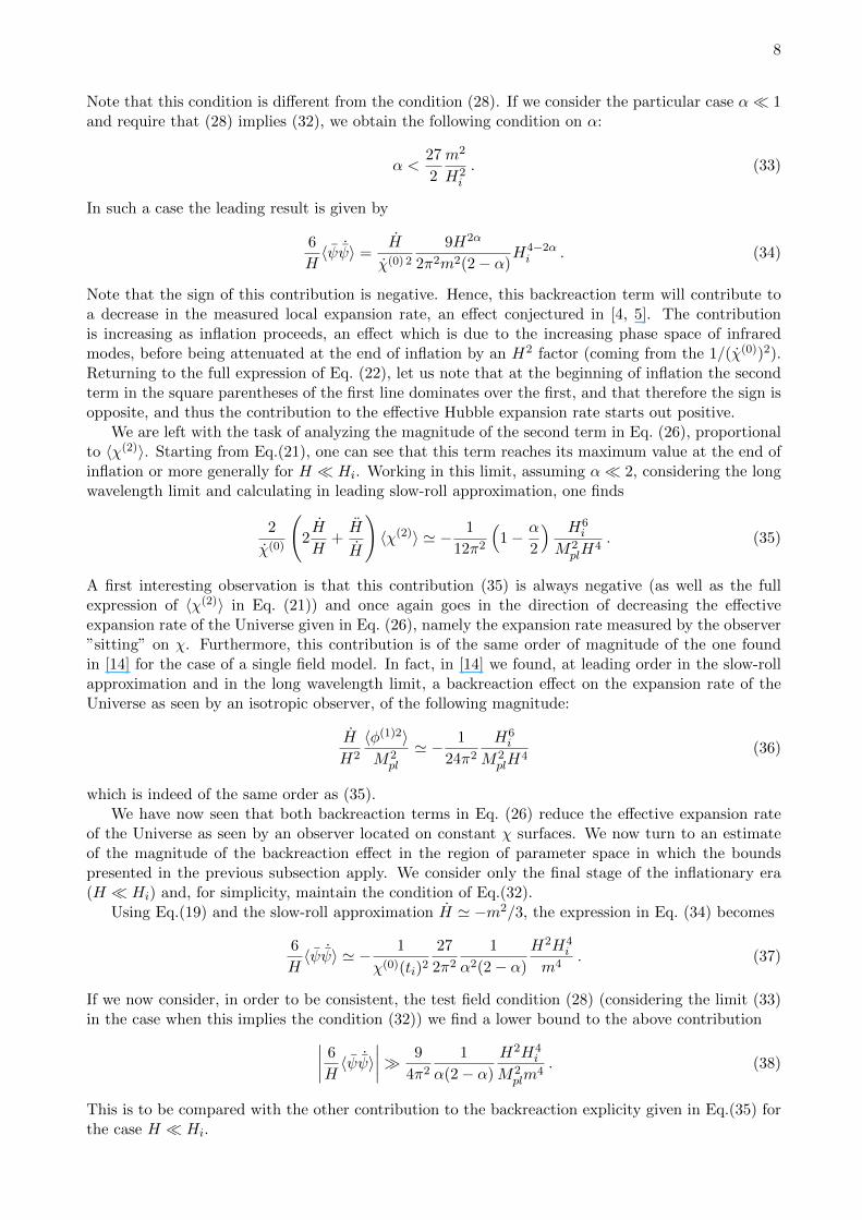
eff and the absolute value ofthe maximum negative contributions is monotonically decreasing from approximately 3.7 (α� 1) to3.2 (α = 1). In Fig. 1 we plot these two different contributions, to the effective Hubble expansion rate,without making any approximation, and for typical values of our parameter for which the backreactionis still perturbative and our results consistent.

2 4 6 8 10

-0.001

0.000

0.001

0.002

0.003

H�m2 4 6 8 10

-7. ´ 10-7

-6. ´ 10-7

-5. ´ 10-7

-4. ´ 10-7

-3. ´ 10-7

-2. ´ 10-7

-1. ´ 10-7

0

H�m

Figure 1: We show 6H 〈ψ

˙ψ〉 (left plot) and 2χ(0)

(2 HH + H

H

)〈χ(2)〉 (right plot) as functions of H/m with

Hi = 10m, α = 0.2 and χ0 = 0.7Mpl.

Furthermore, for a very light test field, the contribution of the first term ∼ 6H 〈ψ

˙ψ〉 may result

(since it contains a 1/χ(0) 2 enhancement factor (see Eq.(22))) in a value which is even greater inmagnitude than 1. This may happen even if the perturbative expansion used to study the dynamicsis still valid. But the perturbative approach to study backreaction will have broken down. We shallmake more comment on this fact in Section 4.

3.4 Gauge invariant backreaction on the effective equation of state

A valuable piece of information, which can be obtained without much effort, is given by the effectiveequation of state with respect to observers which measure the effective Hubble expansion rate discussedhere. For this purpose, we take advantage of the fact that one of the quantum contributions (thesecond one) to the effective expansion rate in Eq. (26) can be written as c (H/H2) 〈ϕ2〉/M2

pl withc = 2− α (see Eqs.(35, 36)). Let us start from the general result obtained in [14], valid for any class

10

of observers and slow-roll inflationary models, where we allow for a further second order contributionH2B in the effective expansion rate, beyond the typical terms ∼ 〈ϕ2〉,

χ(0) 2

(1

aeff

∂ aeff∂χ0

)2

≡ 8πG

3ρeff = H2

[1+

(cH

H2+ d

H2

H4+O

(H3

H6

))〈ϕ2〉M2pl

+B(t)

]. (42)

In the single field model [14], the parameters c and d encode the typical non zero backreaction effectsat first and second order in the slow-roll approximation and B(t) encodes other possible effects (in ourcase c = 2−α while d is not fixed). Since this latter quantity is of second order in perturbation theorywe have to consider only linear terms in any perturbative expression. Then, from the consistencybetween the effective equations for the averaged geometry (see [9, 14]), one obtains

− 1

aeffχ(0) ∂

∂χ0

(χ(0) ∂

∂χ0aeff

)≡ 4πG

3(ρeff + 3peff ) = −H−H2−H2

{[cH

H2+

(d− 3

2c

)H2

H4

+cH

H3+O

(H3

H6

)]〈ϕ2〉M2pl

+B(t) +H

2H2

[B(t) + B(t)

]}. (43)

From these relations it is easy to see that the effective equation of state weff = peff/ρeff , to first nontrivial order, is given by

weff =peffρeff

= −1− 2

3

H

H2+

{[5

3cH2

H4− 2

3cH

H3+O

(H3

H6

)]〈ϕ2〉M2pl

+H

3H2B(t)− 1

3HB(t)

}, (44)

where the d dependence disappears in the leading order correction. In the case under investigation

B =6

H〈ψ ˙ψ〉 . (45)

4 Discussions and numerical results

In the previous section we have defined our model, and studied the main observables in a GI way,giving their analytical expressions for the quantum corrections. Having also provided the generalcriteria for the reliability of our model within a perturbative approach, we want now to analyzenumerically the magnitude of the overall backreaction effects experienced by our observers due toquantum fluctuations.

Let us first begin with some general considerations. As seen, in the evaluation of the backreactionfrom Eq.(5), the quantities ψ and ψ(2) are connected to χ(1) and χ(2) by the gauge trasformationgiven in Eqs.(11,13,14). Therefore, the backreaction terms will be given by combinations of testfield perturbations multiplied by factors like 1/χ(0) and (1/χ(0))2. These factors replace the similarfactors 1/φ and (1/φ)2 which are present in the backreaction terms obtained in [14] for the singlefield model. On the other hand, even in comparison with the slow rolling of the background inflatonfield, the background test field χ(0) changes relatively slowly for α � 1 (see Eq.(19)) and hence theabove factors can give a strong enhancement of the backreaction compared to the effect of the factors(1/φ)2 ∼ 1/M2

pl in the case of single field inflation. So, contrary to [18], where it was shown thatfor a chaotic model the mean square gauge-invariant inflaton fluctuations grow faster than those ofany test field with nonnegative mass, the backreaction on the effective expansion rate, measured withrespect to the observer comoving with the light test field in a two field model, is at least of the sameorder, and in general bigger, than the typical backreaction that we can obtain in a single field case.

The relative magnitude of the backreaction terms in the expression for the effective Hubble ex-pansion rate has already been given in Fig. 1. We now want to numerically study the parameterspace where our analysis is under perturbative control.

Concerning the validity of the expressions for the quantum corrections (backreaction) found in

the previous section, we have a safe perturbative expansion for the observables only for 6H 〈ψ

˙ψ〉 � 1,since this appears in the leading terms both in Eq.(26) and in Eq.(44).

11

In the following we give the limit of validity of our results imposing the condition that the backreac-tion contributes a fixed maximal amount to the effective Hubble expansion rate, i.e. |H2

eff−H2|/H2 �1. In the numerical analysis we consider the condition |H2

eff −H2|/H2 < 10−2. To do this we join

the test field condition (27) (with the � sign replaced by < 10−2) and conditions on the validity ofthe perturbative expansion of the fields. The latter can be obtained by requiring the condition givenin Eq. (31) (with the � sign replaced by < 10−1), which is the most stringent one among (29)-(31).

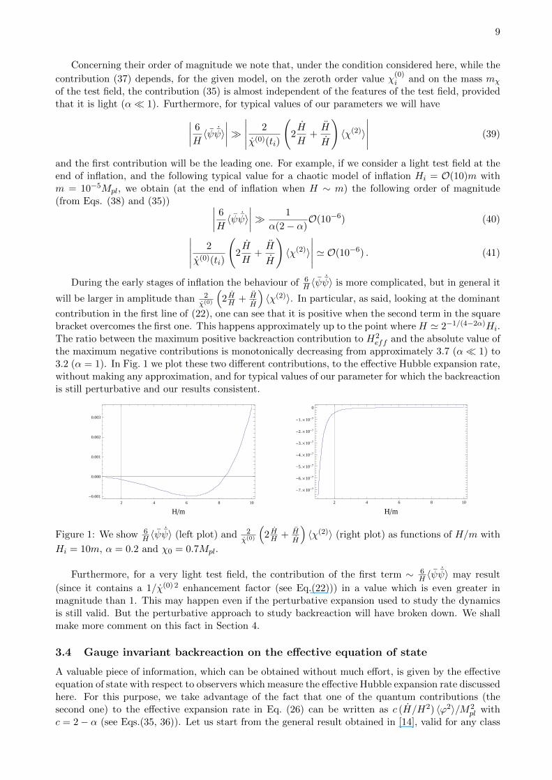
In Fig. 2 we consider the cases of Hi = 10m and Hi = 20m, and show the region in the two-dimensional parameter space labelled by α and by the initial value of the χ field for which all of theconditions are satisfied. The shaded region is the allowed one. For very small initial values of the χfield the backreaction becomes too large in amplitude, for very large values the test field condition issatisfied only for α � 1 (see also Fig 3). This leaves us with the indicated region. For higher valuesof Hi the region narrows more and more until it disappears around a value of Hi ' 50m.

0 2 4 6 8 10

0.0

0.5

1.0

1.5

2.0

Χ0�Mpl

Α

0 2 4 6 8 10

0.0

0.5

1.0

1.5

2.0

Χ0�Mpl

Α

Figure 2: We plot the region where all three conditions (validity of the perturbation theory, testfield approximation, both defined in the text, and requiring the backreaction to be at most 1%) aresatisfied, for the values Hi = 10m (left plot) and Hi = 20m (right plot). The horizontal axis denotesχ(0)(ti)/Mpl and the vertical axis α. We chose the value of m given by Mpl = 105m to be consistentwith the observed value of cosmological perturbations.

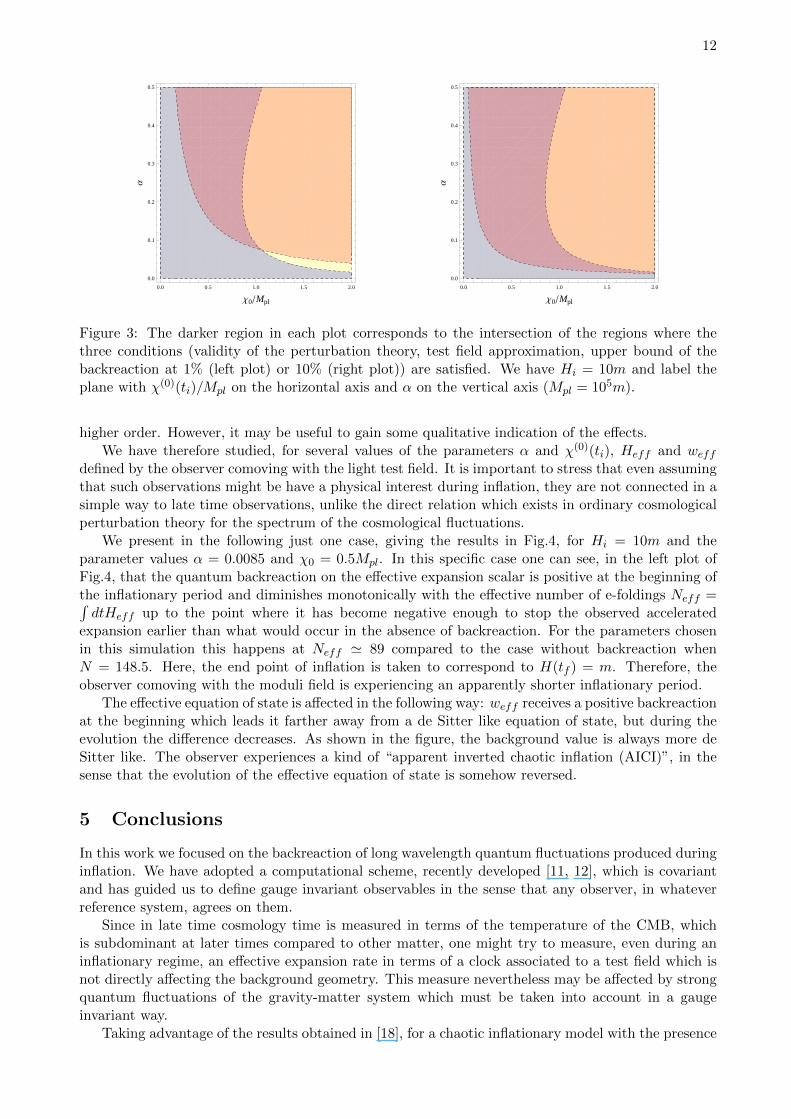
We have still not yet discussed the change in magnitude of the backreaction as our parametersvary. In the region where the backreaction is small, then for the whole duration of inflation we canstudy numerically how it depends on the free parameters of the model (initial condition χ(0)(ti) andthe mass mχ). We find it convenient to show in Fig. 3 how the constrained region in parameter space,obtained requiring a certain amount of maximum backreaction, changes as the limit on the amplitudeof backreaction is changed. In each of the plots, the right dashed line separates the region wherethe test field approximation is valid (left of the line) from the region where it is not (right of theline). The left dashed line separates the region where the backreaction effect on the observed Hubbleparameter is smaller than the limit indicated (right of the line) from that where it is not (left of theline). One can see that the relative amplitude of backreaction on the local Hubble expansion rateincreases for smaller values of the mass mχ and for smaller χ(0)(ti).

In both the two plots of Fig.3 we give also further informations related to the different bounds.Each bound is associated to a region which has a colour: yellow (perturbation theory valid), blue (testfield approximation) and light red (backreaction with an upper bound). Where two regions overlapthe colours change as follow: blue+yellow is gray, yellow + light red is orange. Where all the boundsare satisfied, all regions overlap, the colour is darker red.

It may be interesting to follow the results obtained in our perturbative analysis up to the pointwhen the backreaction effects are of the same order (positive or negative) of the background, whilemaintaining the other bounds (test field approximation and validity of the cosmological perturbationtheory for metric and matter fluctuations). We want to stress that this is of course not formally a safechoice since the backreaction on the observables might have important perturbative contributions at

12

0.0 0.5 1.0 1.5 2.0

0.0

0.1

0.2

0.3

0.4

0.5

Χ0�Mpl

Α

0.0 0.5 1.0 1.5 2.0

0.0

0.1

0.2

0.3

0.4

0.5

Χ0�Mpl

Α

Figure 3: The darker region in each plot corresponds to the intersection of the regions where thethree conditions (validity of the perturbation theory, test field approximation, upper bound of thebackreaction at 1% (left plot) or 10% (right plot)) are satisfied. We have Hi = 10m and label theplane with χ(0)(ti)/Mpl on the horizontal axis and α on the vertical axis (Mpl = 105m).

higher order. However, it may be useful to gain some qualitative indication of the effects.We have therefore studied, for several values of the parameters α and χ(0)(ti), Heff and weff

defined by the observer comoving with the light test field. It is important to stress that even assumingthat such observations might be have a physical interest during inflation, they are not connected in asimple way to late time observations, unlike the direct relation which exists in ordinary cosmologicalperturbation theory for the spectrum of the cosmological fluctuations.

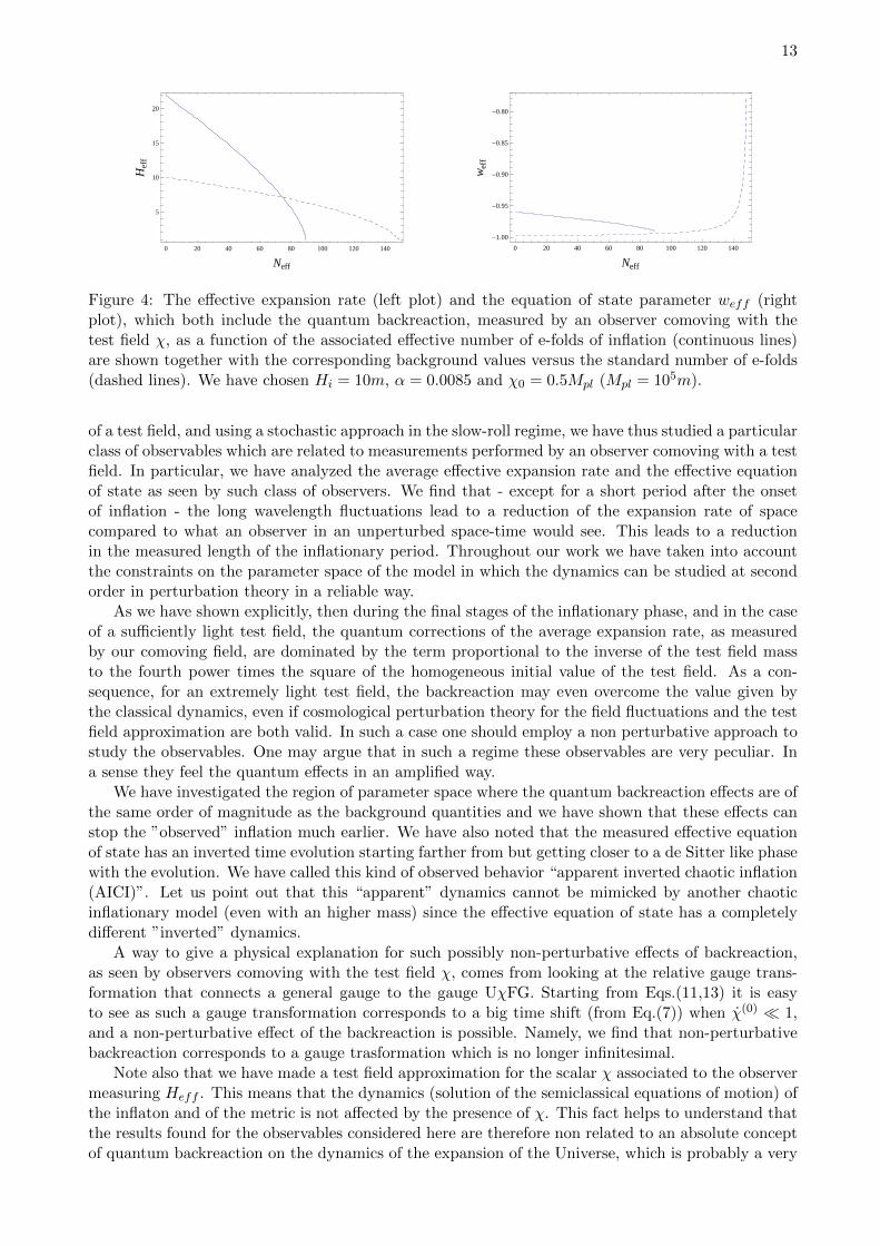
We present in the following just one case, giving the results in Fig.4, for Hi = 10m and theparameter values α = 0.0085 and χ0 = 0.5Mpl. In this specific case one can see, in the left plot ofFig.4, that the quantum backreaction on the effective expansion scalar is positive at the beginning ofthe inflationary period and diminishes monotonically with the effective number of e-foldings Neff =∫dtHeff up to the point where it has become negative enough to stop the observed accelerated

expansion earlier than what would occur in the absence of backreaction. For the parameters chosenin this simulation this happens at Neff ' 89 compared to the case without backreaction whenN = 148.5. Here, the end point of inflation is taken to correspond to H(tf ) = m. Therefore, theobserver comoving with the moduli field is experiencing an apparently shorter inflationary period.

The effective equation of state is affected in the following way: weff receives a positive backreactionat the beginning which leads it farther away from a de Sitter like equation of state, but during theevolution the difference decreases. As shown in the figure, the background value is always more deSitter like. The observer experiences a kind of “apparent inverted chaotic inflation (AICI)”, in thesense that the evolution of the effective equation of state is somehow reversed.

5 Conclusions

In this work we focused on the backreaction of long wavelength quantum fluctuations produced duringinflation. We have adopted a computational scheme, recently developed [11, 12], which is covariantand has guided us to define gauge invariant observables in the sense that any observer, in whateverreference system, agrees on them.

Since in late time cosmology time is measured in terms of the temperature of the CMB, whichis subdominant at later times compared to other matter, one might try to measure, even during aninflationary regime, an effective expansion rate in terms of a clock associated to a test field which isnot directly affecting the background geometry. This measure nevertheless may be affected by strongquantum fluctuations of the gravity-matter system which must be taken into account in a gaugeinvariant way.

Taking advantage of the results obtained in [18], for a chaotic inflationary model with the presence

13

0 20 40 60 80 100 120 140

5

10

15

20

Neff

Hef

f

0 20 40 60 80 100 120 140

-1.00

-0.95

-0.90

-0.85

-0.80

Neff

wef

f

Figure 4: The effective expansion rate (left plot) and the equation of state parameter weff (rightplot), which both include the quantum backreaction, measured by an observer comoving with thetest field χ, as a function of the associated effective number of e-folds of inflation (continuous lines)are shown together with the corresponding background values versus the standard number of e-folds(dashed lines). We have chosen Hi = 10m, α = 0.0085 and χ0 = 0.5Mpl (Mpl = 105m).

of a test field, and using a stochastic approach in the slow-roll regime, we have thus studied a particularclass of observables which are related to measurements performed by an observer comoving with a testfield. In particular, we have analyzed the average effective expansion rate and the effective equationof state as seen by such class of observers. We find that - except for a short period after the onsetof inflation - the long wavelength fluctuations lead to a reduction of the expansion rate of spacecompared to what an observer in an unperturbed space-time would see. This leads to a reductionin the measured length of the inflationary period. Throughout our work we have taken into accountthe constraints on the parameter space of the model in which the dynamics can be studied at secondorder in perturbation theory in a reliable way.

As we have shown explicitly, then during the final stages of the inflationary phase, and in the caseof a sufficiently light test field, the quantum corrections of the average expansion rate, as measuredby our comoving field, are dominated by the term proportional to the inverse of the test field massto the fourth power times the square of the homogeneous initial value of the test field. As a con-sequence, for an extremely light test field, the backreaction may even overcome the value given bythe classical dynamics, even if cosmological perturbation theory for the field fluctuations and the testfield approximation are both valid. In such a case one should employ a non perturbative approach tostudy the observables. One may argue that in such a regime these observables are very peculiar. Ina sense they feel the quantum effects in an amplified way.

We have investigated the region of parameter space where the quantum backreaction effects are ofthe same order of magnitude as the background quantities and we have shown that these effects canstop the ”observed” inflation much earlier. We have also noted that the measured effective equationof state has an inverted time evolution starting farther from but getting closer to a de Sitter like phasewith the evolution. We have called this kind of observed behavior “apparent inverted chaotic inflation(AICI)”. Let us point out that this “apparent” dynamics cannot be mimicked by another chaoticinflationary model (even with an higher mass) since the effective equation of state has a completelydifferent ”inverted” dynamics.

A way to give a physical explanation for such possibly non-perturbative effects of backreaction,as seen by observers comoving with the test field χ, comes from looking at the relative gauge trans-formation that connects a general gauge to the gauge UχFG. Starting from Eqs.(11,13) it is easyto see as such a gauge transformation corresponds to a big time shift (from Eq.(7)) when χ(0) � 1,and a non-perturbative effect of the backreaction is possible. Namely, we find that non-perturbativebackreaction corresponds to a gauge trasformation which is no longer infinitesimal.

Note also that we have made a test field approximation for the scalar χ associated to the observermeasuring Heff . This means that the dynamics (solution of the semiclassical equations of motion) ofthe inflaton and of the metric is not affected by the presence of χ. This fact helps to understand thatthe results found for the observables considered here are therefore non related to an absolute conceptof quantum backreaction on the dynamics of the expansion of the Universe, which is probably a very

14

difficult concept to define. It is related instead to observations which the specific class of dynamicalobservers can make.

Summarizing our findings, from our analysis we therefore deduce that a gedanken experiment withobservers of the kind discussed here may be useful to extract ”amplified” quantum corrections in theassociated observables. Insisting on considering such observables as physically relevant, one faces ingeneral a computability problem. If the backreaction on the GI observable associated to the effectiveexpansion rate is small then one can proceed with our perturbative approach which stops at secondorder and obtain a reasonable estimate. We have found this is possible only in a bounded parameterregion. When outside of this region, the perturbative analysis for the observer level could fail. Welack other tools to perform a different investigation. Therefore in such a case we are not sure thatthe results found can be extrapolated, at least qualitatively, to a non-perturbative region.

AcknowledgementsWe wish to thank Gabriele Veneziano for stimulating discussions. GPV thanks the Cosmology

Group of the University of Geneva for its kind hospitality. GM is supported by the Marie Curie IEF,Project NeBRiC - “Non-linear effects and backreaction in classical and quantum cosmology”. Theresearch of RB is supported by an NSERC Discovery Grant and by funds from the Canada ResearchChair program.

References

[1] A. H. Guth, “The Inflationary Universe: A Possible Solution to the Horizon and FlatnessProblems,” Phys. Rev. D 23, 347 (1981).

[2] A. D. Linde, “Chaotic Inflation,” Phys. Lett. B 129, 177 (1983).

[3] G. Geshnizjani and R. Brandenberger, “Back reaction of perturbations in two scalar field infla-tionary models,” JCAP 0504, 006 (2005) [hep-th/0310265].

[4] L. R. W. Abramo, R. H. Brandenberger and V. F. Mukhanov, “The energy-momentum tensorfor cosmological perturbations,” Phys. Rev. D 56, 3248 (1997) [arXiv:gr-qc/9704037];V. F. Mukhanov, L. R. W. Abramo and R. H. Brandenberger, “On the back reaction problemfor gravitational perturbations,” Phys. Rev. Lett. 78, 1624 (1997) [arXiv:gr-qc/9609026];L. R. W. Abramo and R. P. Woodard, “One loop back reaction on chaotic inflation,” Phys.Rev. D 60, 044010 (1999) [arXiv:astro-ph/9811430].

[5] R. H. Brandenberger, “Back reaction of cosmological perturbations and the cosmological con-stant problem,” hep-th/0210165.

[6] N. C. Tsamis and R. P. Woodard, “Relaxing The Cosmological Constant,” Phys. Lett. B 301,351 (1993);N. C. Tsamis and R. P. Woodard, “The Physical basis for infrared divergences in inflationaryquantum gravity,” Class. Quant. Grav. 11, 2969 (1994);N. C. Tsamis and R. P. Woodard, “Strong infrared effects in quantum gravity,” Annals Phys.238, 1 (1995);N. C. Tsamis and R. P. Woodard, “The quantum gravitational back-reaction on inflation,”Annals Phys. 253, 1 (1997) [arXiv:hep-ph/9602316];N. C. Tsamis and R. P. Woodard, “Quantum Gravity Slows Inflation,” Nucl. Phys. B 474, 235(1996) [arXiv:hep-ph/9602315];N. C. Tsamis and R. P. Woodard, “One Loop Graviton Self-Energy In A Locally De SitterBackground,” Phys. Rev. D 54, 2621 (1996) [arXiv:hep-ph/9602317];N. C. Tsamis and R. P. Woodard, “A Phenomenological Model for the Early Universe,” Phys.Rev. D 80, 083512 (2009) [arXiv:0904.2368 [gr-qc]].

[7] W. Unruh, “Cosmological long wavelength perturbations,” astro-ph/9802323.

15

[8] G. Geshnizjani and R. Brandenberger, “Back reaction and local cosmological expansion rate,”Phys. Rev. D 66, 123507 (2002) [arXiv:gr-qc/0204074].

[9] F. Finelli, G. Marozzi, G. P. Vacca and G. Venturi, “Backreaction during inflation: A Physicalgauge invariant formulation,” Phys. Rev. Lett. 106, 121304 (2011) [arXiv:1101.1051 [gr-qc]].

[10] L. R. Abramo and R. P. Woodard, “No one loop back-reaction in chaotic inflation,” Phys. Rev.D 65, 063515 (2002) [arXiv:astro-ph/0109272].

[11] M. Gasperini, G. Marozzi and G. Veneziano, “Gauge invariant averages for the cosmologicalbackreaction,” JCAP 0903, 011 (2009) [arXiv:0901.1303 [gr-qc]].

[12] M. Gasperini, G. Marozzi and G. Veneziano, “A Covariant and gauge invariant formulation ofthe cosmological ’backreaction’,” JCAP 1002, 009 (2010) [arXiv:0912.3244 [gr-qc]].

[13] T. Buchert, “On average properties of inhomogeneous fluids in general relativity. 1. Dust cos-mologies,” Gen. Rel. Grav. 32, 105 (2000) [gr-qc/9906015].

[14] G. Marozzi and G. P. Vacca, “Isotropic Observers and the Inflationary Backreaction Problem,”Class. Quant. Grav. 29 (2012) 115007 [arXiv:1108.1363 [gr-qc]].

[15] M. Gasperini, G. Marozzi, F. Nugier and G. Veneziano, “Light-cone averaging in cosmology:Formalism and applications,” JCAP 1107, 008 (2011) [arXiv:1104.1167 [astro-ph.CO]].

[16] I. Ben-Dayan, M. Gasperini, G. Marozzi, F. Nugier and G. Veneziano, “Backreaction on theluminosity-redshift relation from gauge invariant light-cone averaging,” JCAP 1204, 036 (2012)[arXiv:1202.1247 [astro-ph.CO]];I. Ben-Dayan, M. Gasperini, G. Marozzi, F. Nugier and G. Veneziano, “Do stochastic inho-mogeneities affect dark-energy precision measurements?,” Phys. Rev. Lett. 110, 021301 (2013)[arXiv:1207.1286 [astro-ph.CO]];I. Ben-Dayan, G. Marozzi, F. Nugier and G. Veneziano, “The second-order luminosity-redshiftrelation in a generic inhomogeneous cosmology,” JCAP 1211, 045 (2012) [arXiv:1209.4326[astro-ph.CO]].

[17] W. Xue, K. Dasgupta and R. Brandenberger, “Cosmological UV/IR Divergences and de-SitterSpacetime,” Phys. Rev. D 83, 083520 (2011) [arXiv:1103.0285 [hep-th]].

[18] F. Finelli, G. Marozzi, A. A. Starobinsky, G. P. Vacca and G. Venturi, “Stochasticgrowth of quantum fluctuations during slow-roll inflation,” Phys. Rev. D 82, 064020 (2010)[arXiv:1003.1327 [hep-th]].

[19] F. Finelli, G. Marozzi, G. P. Vacca and G. Venturi, “Energy momentum tensor of cosmologicalfluctuations during inflation,” Phys. Rev. D 69, 123508 (2004) [arXiv:gr-qc/0310086].

[20] M. Bruni, S. Matarrese, S. Mollerach and S. Sonego, “Perturbations of space-time: Gaugetransformations and gauge invariance at second order and beyond,” Class. Quant. Grav. 14,2585 (1997) [arXiv:gr-qc/9609040].

[21] G. Marozzi, “The cosmological backreaction: gauge (in)dependence, observers and scalars,”JCAP 1101, 012 (2011) [arXiv:1011.4921 [gr-qc]].

[22] F. Finelli, G. Marozzi, A. A. Starobinsky, G. P. Vacca and G. Venturi, “Generation of fluctua-tions during inflation: Comparison of stochastic and field-theoretic approaches,” Phys. Rev. D79, 044007 (2009) [arXiv:0808.1786 [hep-th]].