arX

iv:1

402.

7288

v1 [

gr-q

c] 2

8 Fe

b 20

14

Gravitomagnetic currents in the inflationary universe from WIMT

1,2 Jesus Martın Romero∗, 1,2 Mauricio Bellini †

1 Departamento de Fısica, Facultad de Ciencias Exactas y Naturales,

Universidad Nacional de Mar del Plata,

Funes 3350, C.P. 7600, Mar del Plata, Argentina.

2 Instituto de Investigaciones Fısicas de Mar del Plata (IFIMAR),

Consejo Nacional de Investigaciones Cientıficas y Tecnicas (CONICET), Argentina.

Abstract

Using the Weitzenbock representation of a Riemann-flat 5D spacetime, we study the possible

existence of primordial gravitomagnetic currents from GEMI. We found that these currents decrease

exponentially in the Weitzenbock representation, but they are null in a Levi-Civita representation

because we are dealing with a 5D Riemann-flat spacetime without structure nor torsion.

∗ E-mail address: jesusromero@conicet.gov.ar† E-mail address: mbellini@mdp.edu.ar

1

I. INTRODUCTION AND MOTIVATION

It is well known that magnetic monopoles have been elusive to be detected, despite

the efforts. Such monopoles arise as a theoretical possibility from the dual formulation of

an electrodynamic theory[1]. The fate of primordial monopoles is very closely linked to the

history of the very early universe. Preskill[2] realized that this possible monopole production

could create a crisis for cosmology, implying far more monopoles than observational limits

allow. Because the expected energy scale of grand unification is quite high, the geometrical

size of a monopole core must be quite small. Linde and Vilenkin independently pointed out

that such monopoles could expand exponentially in the context of inflationary cosmology

[3].

However, there is an even more interesting possibility, which arises from a theory that

extends and unify conceptually the electrodynamics with a theory of gravity; the gravito-

electrodynamics. This theory was first outlined in 2006[4] in a cosmological context and

later studied in greater detail[5, 6], but the dual formalization has not yet been addressed.

In this paper we shall study the dual formalism from a 5D vacuum and we will try and get

formalize their dual streams, that, in a gravito-electrodynamic context are related gravito-

magnetic currents. This formalism is inspired in the Induced Matter Theory (IMT), which

is based on the assumption that ordinary matter and physical fields that we can observe in

our 4D universe can be geometrically induced from a 5D Ricci-flat metric with a space-like

noncompact extra dimension on which we define a physical vacuum[7]. The Campbell-

Magaard theorem[8–11] serves as a ladder to go between manifolds whose dimensionality

differs by one. This theorem, which is valid in any number of dimensions, implies that

every solution of the 4D Einstein equations with arbitrary energy momentum tensor can

be embedded, at least locally, in a solution of the 5D Einstein field equations in vacuum.

Because of this, the stress-energy may be a 4D manifestation of the embedding geometry. An

extension of the IMT was realized recently using the Weitzenbock Induced Matter Theory

(WIMT)[12]. This approach makes possible a geometrical representation of a 5D vacuum

(with a zero curvature in the Weitzenbock representation), on nonzero curvature tensor (in

the sense of the Levi-Civita representation).

2

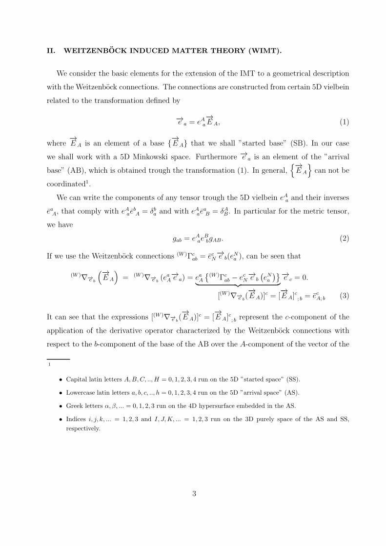
II. WEITZENBOCK INDUCED MATTER THEORY (WIMT).

We consider the basic elements for the extension of the IMT to a geometrical description

with the Weitzenbock connections. The connections are constructed from certain 5D vielbein

related to the transformation defined by

−→e a = eAa−→E A, (1)

where−→E A is an element of a base {

−→E A} that we shall ”started base” (SB). In our case

we shall work with a 5D Minkowski space. Furthermore −→e a is an element of the ”arrival

base” (AB), which is obtained trough the transformation (1). In general,{−→E A

}

can not be

coordinated1.

We can write the components of any tensor trough the 5D vielbein eAa and their inverses

eaA, that comply with eAaebA = δba and with eAae

aB = δAB. In particular for the metric tensor,

we have

gab = eAaeBbgAB. (2)

If we use the Weitzenbock connections (W )Γcab = ecN

−→e b(eNa ), can be seen that

(W )∇−→e b

(−→E A

)

= (W )∇−→e b(eaA

−→e a) = eaA{(W )Γc

ab − ecN−→e b

(eNa

)}

︸ ︷︷ ︸

−→e c = 0.

[(W )∇−→e b(−→E A)]

c = [−→E A]

c; b = ecA; b (3)

It can see that the expressions [(W )∇−→e b(−→E A)]

c = [−→E A]

c; b represent the c-component of the

application of the derivative operator characterized by the Weitzenbock connections with

respect to the b-component of the base of the AB over the A-component of the vector of the

1

• Capital latin letters A,B,C, ..,H = 0, 1, 2, 3, 4 run on the 5D ”started space” (SS).

• Lowercase latin letters a, b, c, .., h = 0, 1, 2, 3, 4 run on the 5D ”arrival space” (AS).

• Greek letters α, β, ... = 0, 1, 2, 3 run on the 4D hypersurface embedded in the AS.

• Indices i, j, k, ... = 1, 2, 3 and I, J,K, ... = 1, 2, 3 run on the 3D purely space of the AS and SS,

respectively.

3

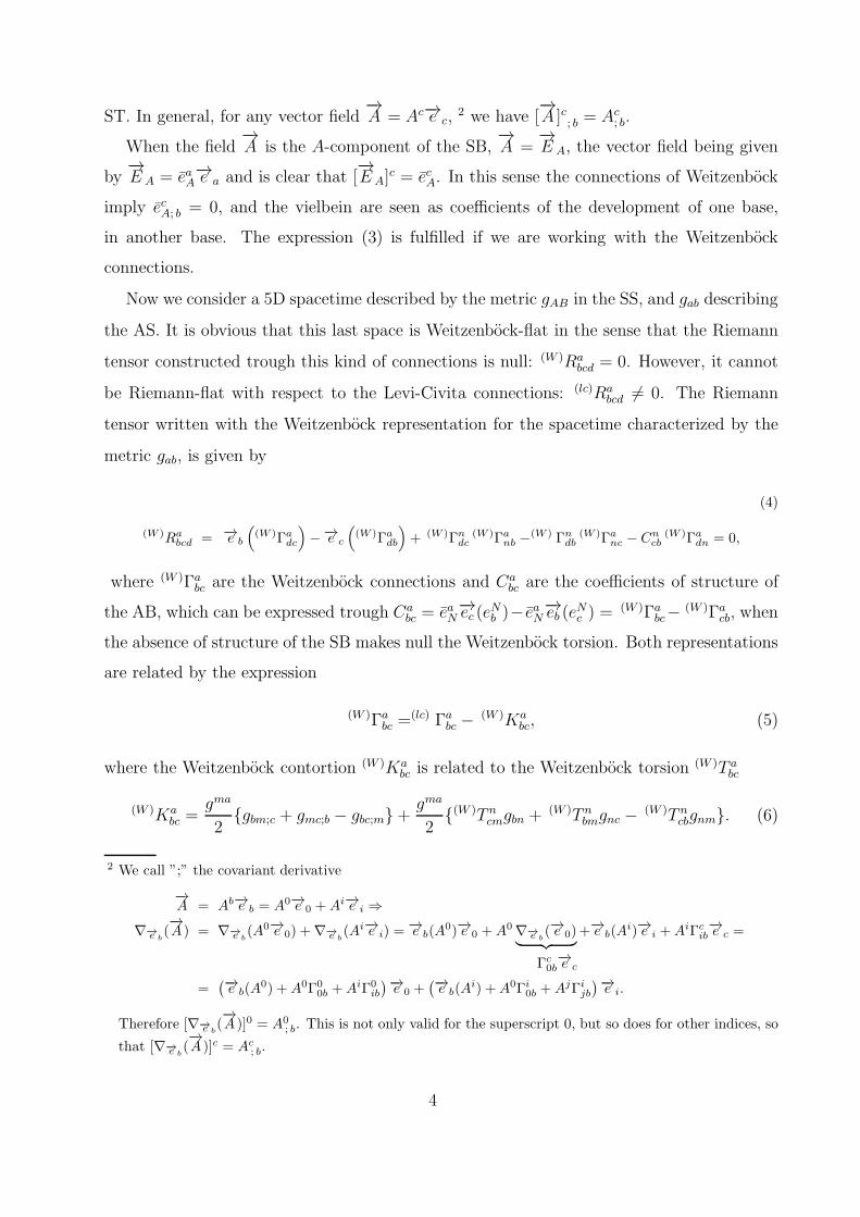
ST. In general, for any vector field−→A = Ac−→e c,

2 we have [−→A ]c; b = Ac

; b.

When the field−→A is the A-component of the SB,

−→A =

−→E A, the vector field being given

by−→E A = eaA

−→e a and is clear that [−→E A]

c = ecA. In this sense the connections of Weitzenbock

imply ecA; b = 0, and the vielbein are seen as coefficients of the development of one base,

in another base. The expression (3) is fulfilled if we are working with the Weitzenbock

connections.

Now we consider a 5D spacetime described by the metric gAB in the SS, and gab describing

the AS. It is obvious that this last space is Weitzenbock-flat in the sense that the Riemann

tensor constructed trough this kind of connections is null: (W )Rabcd = 0. However, it cannot

be Riemann-flat with respect to the Levi-Civita connections: (lc)Rabcd 6= 0. The Riemann

tensor written with the Weitzenbock representation for the spacetime characterized by the

metric gab, is given by

(4)

(W )Rabcd = −→e b

((W )Γa

dc

)

−−→e c

((W )Γa

db

)

+ (W )Γndc

(W )Γanb −

(W ) Γndb

(W )Γanc − Cn

cb(W )Γa

dn = 0,

where (W )Γabc are the Weitzenbock connections and Ca

bc are the coefficients of structure of

the AB, which can be expressed trough Cabc = eaN

−→ec (eNb )− e

aN−→eb (e

Nc ) =

(W )Γabc−

(W )Γacb, when

the absence of structure of the SB makes null the Weitzenbock torsion. Both representations

are related by the expression

(W )Γabc =

(lc) Γabc −

(W )Kabc, (5)

where the Weitzenbock contortion (W )Kabc is related to the Weitzenbock torsion (W )T a

bc

(W )Kabc =

gma

2{gbm;c + gmc;b − gbc;m}+

gma

2{(W )T n

cmgbn +(W )T n

bmgnc −(W )T n

cbgnm}. (6)

2 We call ”;” the covariant derivative

−→A = Ab−→e b = A0−→e 0 +Ai−→e i ⇒

∇−→e b(−→A ) = ∇−→e b

(A0−→e 0) +∇−→e b(Ai−→e i) =

−→e b(A0)−→e 0 +A0 ∇−→e b

(−→e 0)︸ ︷︷ ︸

+−→e b(Ai)−→e i +AiΓc

ib−→e c =

Γc0b−→e c

=(−→e b(A

0) +A0Γ00b +AiΓ0

ib

)−→e 0 +(−→e b(A

i) +A0Γi0b +AjΓi

jb

)−→e i.

Therefore [∇−→e b(−→A )]0 = A0

; b. This is not only valid for the superscript 0, but so does for other indices, so

that [∇−→e b(−→A )]c = Ac

; b.

4

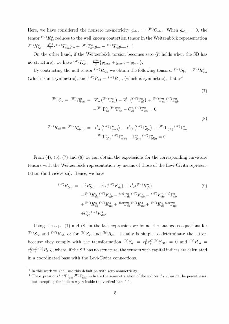
Here, we have considered the nonzero no-metricity gab; c = (W )Qabc. When gab; c = 0, the

tensor (W )Kabc reduces to the well known contortion tensor in the Weitzenbock representation

(W )Kabc =

gma

2{(W )T n

cmgbn +(W )T n

bmgnc −(W )T n

cbgnm}.3.

On the other hand, if the Weitzenbock torsion becomes zero (it holds when the SB has

no structure), we have (W )Kabc =

gma

2{gbm;c + gmc;b − gbc;m}.

By contracting the null-tensor (W )Rabcd we obtain the following tensors: (W )Sbc =

(W )Rabca

(which is antisymmetric), and (W )Rcd =(W )Ra

acd (which is symmetric), that is4

(7)

(W )Sbc =(W )Ra

bca = −→e b

((W )Γa

ac

)−−→e c

((W )Γa

ab

)+ (W )Γn

ac(W )Γa

nb

−(W )Γnab

(W )Γanc − Cn

cb(W )Γa

an = 0,

(8)

(W )Rcd =(W )Ra

a(cd) = −→e a

((W )Γa

(dc)

)−−→e (c

((W )Γa

d)a

)+ (W )Γn

(dc)(W )Γa

na

−(W )Γn(d|a

(W )Γan|c) − Cn

(c|a(W )Γa

|d)n = 0.

From (4), (5), (7) and (8) we can obtain the expressions for the corresponding curvature

tensors with the Weitzenbock representation by means of those of the Levi-Civita represen-

tation (and viceversa). Hence, we have

(W )Rabcd = (lc)Ra

bcd −−→e b(

(W )Kadc) +

−→e c((W )Ka

db) (9)

− (W )Kndc

(W )Kanb −

(lc)Γndc

(W )Kanb −

(W )Kndc

(lc)Γanb

+ (W )Kndb

(W )Kanc +

(lc)Γndb

(W )Kanc +

(W )Kndb

(lc)Γanc

+Cncb

(W )Kadn.

Using the eqs. (7) and (8) in the last expression we found the analogous equations for

(W )Sbc and (W )Rcd, or for (lc)Sbc and (lc)Rcd. Usually is simple to determinate the latter,

because they comply with the transformation (lc)Sbc = eBb eCc

(lc)SBC = 0 and (lc)Rcd =

eDd eCc

(lc)RCD, where, if the SB has no structure, the tensors with capital indices are calculated

in a coordinated base with the Levi-Civita connections.

3 In this work we shall use this definition with zero nonmetricity.4 The expressions (W )Γn

(d|a(W )Γa

n|c) indicate the symmetrization of the indices d y c, inside the perentheses,

but excepting the indices a y n inside the vertical bars ”|”.

5

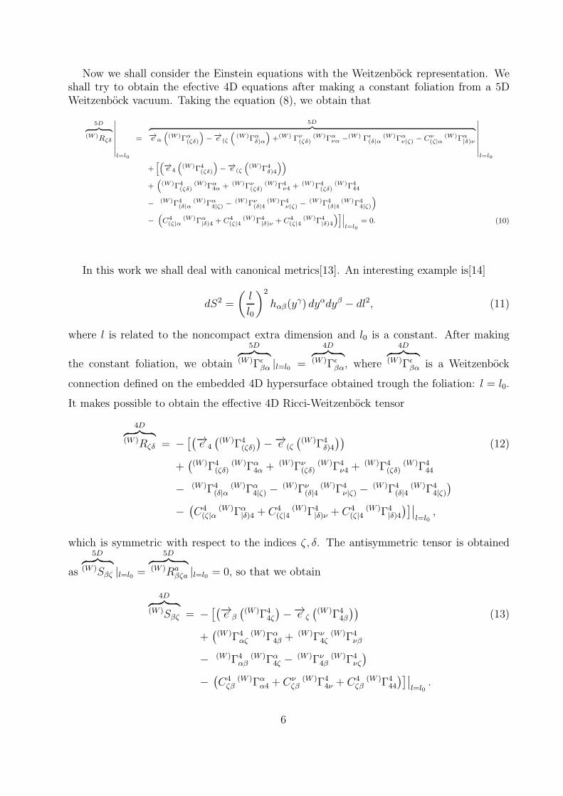
Now we shall consider the Einstein equations with the Weitzenbock representation. Weshall try to obtain the efective 4D equations after making a constant foliation from a 5DWeitzenbock vacuum. Taking the equation (8), we obtain that

5D︷ ︸︸ ︷

(W )Rζδ

∣∣∣∣∣∣∣∣l=l0

=

5D︷ ︸︸ ︷

−→e α

((W )Γα

(ζδ)

)

−−→e (ζ

((W )Γα

δ)α

)

+(W ) Γν(ζδ)

(W )Γανα −(W ) Γǫ

(δ|α(W )Γα

ν|ζ) − Cν(ζ|α

(W )Γα|δ)ν

∣∣∣∣∣∣∣∣l=l0

+[(

−→e 4

((W )Γ4

(ζδ)

)

−−→e (ζ

((W )Γ4

δ)4

))

+((W )Γ4

(ζδ)(W )Γα

4α + (W )Γν(ζδ)

(W )Γ4ν4 + (W )Γ4

(ζδ)(W )Γ4

44

− (W )Γ4(δ|α

(W )Γα4|ζ) −

(W )Γν(δ|4

(W )Γ4ν|ζ) −

(W )Γ4(δ|4

(W )Γ44|ζ)

)

−(

C4(ζ|α

(W )Γα|δ)4 + C4

(ζ|4(W )Γ4

|δ)ν + C4(ζ|4

(W )Γ4|δ)4

)]∣∣∣l=l0

= 0. (10)

In this work we shall deal with canonical metrics[13]. An interesting example is[14]

dS2 =

(l

l0

)2

hαβ(yγ) dyαdyβ − dl2, (11)

where l is related to the noncompact extra dimension and l0 is a constant. After making

the constant foliation, we obtain

5D︷ ︸︸ ︷(W )Γǫ

βα |l=l0 =

4D︷ ︸︸ ︷(W )Γǫ

βα, where

4D︷ ︸︸ ︷(W )Γǫ

βα is a Weitzenbock

connection defined on the embedded 4D hypersurface obtained trough the foliation: l = l0.

It makes possible to obtain the effective 4D Ricci-Weitzenbock tensor

4D︷ ︸︸ ︷(W )Rζδ = −

[(−→e 4

((W )Γ4

(ζδ)

)−−→e (ζ

((W )Γ4

δ)4

))(12)

+((W )Γ4

(ζδ)(W )Γα

4α + (W )Γν(ζδ)

(W )Γ4ν4 +

(W )Γ4(ζδ)

(W )Γ444

− (W )Γ4(δ|α

(W )Γα4|ζ) −

(W )Γν(δ|4

(W )Γ4ν|ζ) −

(W )Γ4(δ|4

(W )Γ44|ζ)

)

−(C4

(ζ|α(W )Γα

|δ)4 + C4(ζ|4

(W )Γ4|δ)ν + C4

(ζ|4(W )Γ4

|δ)4

)]∣∣l=l0

,

which is symmetric with respect to the indices ζ, δ. The antisymmetric tensor is obtained

as

5D︷ ︸︸ ︷(W )Sβζ |l=l0 =

5D︷ ︸︸ ︷(W )Ra

βζa |l=l0 = 0, so that we obtain

4D︷ ︸︸ ︷(W )Sβζ = −

[(−→e β

((W )Γ4

4ζ

)−−→e ζ

((W )Γ4

4β

))(13)

+((W )Γ4

αζ(W )Γα

4β +(W )Γν

4ζ(W )Γ4

νβ

− (W )Γ4αβ

(W )Γα4ζ −

(W )Γν4β

(W )Γ4νζ

)

−(C4

ζβ(W )Γα

α4 + Cνζβ

(W )Γ44ν + C4

ζβ(W )Γ4

44

)]∣∣l=l0

.

6

The Ricci-Weitzenbock scalar curvature can be obtained from a 5D vacuum, as

5D︷ ︸︸ ︷(W )R =

5D︷ ︸︸ ︷

gab (W )Rab =

5D︷ ︸︸ ︷

gαβ (W )Rαβ +

5D︷ ︸︸ ︷

g55 (W )R55 = 0. (14)

Hence, from eq. (14) we can obtain

4D︷ ︸︸ ︷(W )R =

5D︷ ︸︸ ︷

gβγ (W )Rβγ

∣∣∣∣∣∣∣l=l0

=

4D︷ ︸︸ ︷

hβγ (W )Rβγ , (15)

which means that the scalar Ricci-Weitzenbock curvature has the source

4D︷ ︸︸ ︷(W )R = −

5D︷ ︸︸ ︷

g44 (W )R44

∣∣∣∣∣∣∣l=l0

, (16)

and finally the induced Einstein-Cartan-Weitzenbock equations are

4D︷ ︸︸ ︷(W )Gβγ =

4D︷ ︸︸ ︷(W )Rβγ −

1

2

4D︷ ︸︸ ︷

hβγ(W )R = −8πG

4D︷︸︸︷

T(βγ), (17)

4D︷ ︸︸ ︷(W )Sβγ = −8πG

4D︷︸︸︷

T[βγ], (18)

(W )Ra5 = 0, (19)

(W )Sa5 = 0, (20)

where we have taken into account in (18) that gβγ (W )Sβγ = 0. Furthermore, the symmetric

and antisymmetric parts of the energy momentum tensor in eqs. (17) and (18) are given

by

4D︷︸︸︷

T(βγ) = 12(

4D︷︸︸︷

Tβγ +

4D︷︸︸︷

Tγβ ) and

4D︷︸︸︷

T[βγ] = 12(

4D︷︸︸︷

Tβγ −

4D︷︸︸︷

Tγβ ). The equations (17) describe the

dynamics of the gravitational field using the Weitzenbock representation on the effective 4D

hypersurface .

A. Effective 4D dynamics with the Levi-Civita representation.

Now we shall intend to write the curvature and the Ricci tensors (in the Levi-Civita rep-resentation) with respect to the Weitzenbock connections and contortions. The Ricci in theLevi-Civita representation is related to the Ricci tensor in the Weitzenbock representationplus additional terms that depends with contortions and structure

4D︷ ︸︸ ︷

(lc)Rζδ = −→e α

((lc)Γα

(ζδ)

)

−−→e (ζ

((lc)Γα

δ)α

)

+(lc) Γν(ζδ)

(lc)Γανα −(lc) Γǫ

(δ|α(lc)Γα

ν|ζ) − Cν(ζ|α

(lc)Γα|δ)ν

∣∣∣l=l0

= (W )Rζδ +−→e α

(

Kα(ζδ)

)

−−→e (ζ

(

Kαδ)α

)

+Kν(ζδ)K

ανα + (W )Γν

(ζδ)Kανα +Kν

(ζδ)(W )Γα

να

−Kν(δ|αK

αν|ζ) −

(W )Γν(δ|αK

αν|ζ) −Kν

(δ|α(W )Γα

ν|ζ) − Cν(ζ|αK

α|δ)ν . (21)

7

The scalar curvature is4D︷︸︸︷(lc)R = −

5D︷ ︸︸ ︷

g44 (lc)R44

∣∣∣∣∣∣∣l=l0

. (22)

Hence, the Einstein-Cartan equations are given by

4D︷ ︸︸ ︷(lc)Gβγ =

4D︷ ︸︸ ︷(lc)Rβγ −

1

2

4D︷ ︸︸ ︷

hβγ(lc)R = −8πG

4D︷︸︸︷

T(βγ), (23)

4D︷︸︸︷

Sβγ = −8πG

4D︷︸︸︷

T[βγ] = 0, (24)

joined with (W )Ra5 = 0 y (W )Sa5 = 0 that are additional conditions. Here,

4D︷︸︸︷

T(βγ) and

4D︷︸︸︷

T[βγ] are

the symmetric and antisymmetric energy momentum tensors induced on the 4D hypersurface

written in the Levi-Civita representation5.

III. DUAL ACTION AND EQUATIONS OF MOTION

We shall consider the conditions by which we can induce curvature and currents by means

of WIMT[12], on a 5D spacetime represented by cartesian coordinates. The 5D tensor metric

can be written as

[η]AB = diag [1,−1,−1,−1,−1] . (26)

We can construct a AB with interesting cosmological properties if we take the appropriate

vielbein. The action for the gravito-electromagnetic fields in a 5D vacuum can be written

in the form

S =

∫

d5x√

|η|

[R

16 πG−

1

4FABF

AB −λ

2

(AB

;B

)2]

. (27)

5 The equations (24) take into account the Cartan equations which describe spinor contributions.

4D︷︸︸︷

Sβγ −1

2σβγS = −8πG

4D︷︸︸︷

T[βγ]︸︷︷︸

spin

, (25)

where S = σµνSµν , σµν = 1

2 [γµ, γν ] y γµ are the Dirac matrices.

8

In order to obtain the dual currents may be interesting rewrite the last action in terms of

the dual tensors FABC

(28)

S1 =

∫

d5x√

|η|

[R

16 πG−k

4FABCF

ABC −λ

2

(AB

;B

)2]

,

S =

∫

d5x√

|η|

[R

16 πG−

1

4FABF

AB −λ

2

(AB

;B

)2]

.

It is evident that 13!FABCF

ABC = 13! 4εABCDEε

ABCNMFDEFNM = FNMFNM , where we have

used εABCDEεABCNM = 3! 2! (δNDδ

ME − δNE δ

MD ), so that when k = 1

3!, we obtain that both

actions describes the same physical system:

S1 = S.

In our case, when we use the Lorentz gauge and we deal with a 5D vacuum with R =

0, we have S1 ∼ S and both actions give us the same equations of motion. In order

to describe the dual sources of these equations we shall deal with the action S1. The

dynamics of the gravitoelectromagnetic fields obtained taking extreme the action (27)), is

AK;B

;B− (1 − λ)AB

;B;K

= 0. On a 5D vacuum (R = 0), and when we take λ = 1 and the

Lorentz gauge AB;B = 0, they reduce to

�AK = ηBCAK;BC = 0, (29)

that are Klein-Gordon equations for massless fields. The gravitomagnetic currents become

from the solutions for the fields (29). The last equations are compatible with a current which

has its source in

FNB;B = −ηAN

[AM RB

ABM + AB;MT

MBA

], (30)

where we have used (29) and the Lorentz gauge in absence of nonmetricity. We have used

the fact that

FNB;B = ηANηBMFAM ;B = gANAB

;AB − ηBMAN;MB

︸ ︷︷ ︸,

0

9

where clearly we have imposed the absence of currents on the 5D vacuum with respect to

the Levi-Civita representation. Hence

(lc)FNB;B = 0 ⇒ (31)

(W )FNB;B = −

((W )FMB + ηRMAPKB

PR − ηRBAPKMPR

)

KNMB (32)

−((W )FNM + ηRNAPKM

PR − ηRMAPKNPR

)

KBMB,

where (lc)FAB =−→E A(AB) −

−→E B(AA) + AN(C

NAB) y (W )FAB =

−→E A(AB) −

−→E B(AA) +

AN((W )TN

BA + CNAB)

6.

Notice that in eq. (31) we use the covariant derivative with respect to the Christoffel

symbols, but in the expression (32) we use the derivative covariant with respect to the

Weitzenbock connections. Hence, we can adopt both representations in a complementary

mode to describe the 5D vacuum.

The Weitzenbock currents are related by one expression analogous to eq. (31), but more

complicated

(lc)(m)JAB − (W )(m)JAB =

√

|η|

2εABCDE

1

4M [CDE], (33)

tal que M [CDE] = ηCFηDGηEHM[FGH] y definimos M[FGH] de acuerdo con

(34)

M[FGH] =(

AM(W )TM

[FG

)

;H] − 2 (W )TN[FH|

(W )TMN |G]AM − 2 (W )TN

[GH(W )TM

F ]NAM

− (W )TN[FH|

−→EN (A|G]) +

(W )TN[GH|

−→EN (A|F ]) +

(W )TN[FH

−→EG](AN )− (W )TN

[GH

−→E F ](AN ).

Once required the gauve condition (lc)AN;N = 0, it is preserved in the Weitzenbock represen-

tation: (W )An;n = 0 7.

6 Using the expression (lc)ΓABC =(W ) ΓA

BC +KABC it is possible to obtain the following expression between

both Faraday tensors: (lc)FNB = (W )FNB + ηRNAPKBPR − ηRBAPKN

PR. If we make the derivative of

this expression and we use (31), we can check the validity of eq. (32).7 One can show that (lc)eNn ;m = (W )eNn ;m + eNk Kk

nm, but since the Weitzenbock connections comply with(W )eNn ;m = 0, it is possible to express the covariant derivative of the vielbein in the Levi-Civita represen-

tation as a function of the contortion of Weitzenbock: (lc)eNn ;m = eNk Kknm. If we use this on the gauge

condition and we take into account that AN = eNn An, we can prove that (lc)AN;N = 0 ⇒ (lc)An

;n+KmmnA

n =(W )An

;n = 0. Hence, one can show the following equalities:

• (W )An;n = (W )AN

;N ,

10

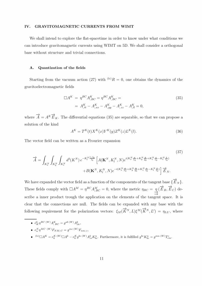
IV. GRAVITOMAGNETIC CURRENTS FROM WIMT

We shall intend to explore the flat-spacetime in order to know under what conditions we

can introduce gravitomagnetic currents using WIMT on 5D. We shall consider a orthogonal

base without structure and trivial connections.

A. Quantization of the fields

Starting from the vacuum action (27) with (lc)R = 0, one obtains the dynamics of the

gravitoelectromagnetic fields

�AK = ηBCAK;BC = ηBCAK

,BC = (35)

= AK, tt − AK

,xx − AK, yy −AK

, zz −AK, ll = 0,

where−→A = AK

−→EK . The differential equations (35) are separable, so that we can propose a

solution of the kind

AK = TK(t)XK(x)Y K(y)ZK(z)LK(l). (36)

The vector field can be written as a Frourier expansion

(37)

−→A =

∫

KNx

∫

KNy

∫

KNz

d3(KN ) e−KN

l

l−l0l0

[

A(KN , KNl , N)e

i(KNx

xx0

+KNy

yy0

+KNz

zz0

−KNt

tt0

)

+B(KN , KNl , N)e

−i(KNx

xx0

+KNy

yy0

+KNz

zz0

−KNt

tt0

)]−→E N .

We have expanded the vector field as a function of the components of the tangent base {−→EN}.

These fields comply with �AM = ηBCAM;BC = 0, where the metric ηBC = η

−→−→(−→E B,

−→E C) de-

scribe a inner product trough the application on the elements of the tangent space. It is

clear that the connections are null. The fields can be expanded with any base with the

following requirement for the polarization vectors: ξM(−→KN , L)ξM(

−→KN , L′) = ηLL′ , where

• ekKηBC (W )AK; BC = gab (W )Ak

;bc,

• eNn ηMC (W )FNM ;C = gmc (W )Fnm; c,

• (lc)�AK = eKk

(W )�Ak − eKk gbc (W )Ak

;nKnbc. Furthermore, it is fulfilled gbcKn

bc = gmn (W )T ccm.

11

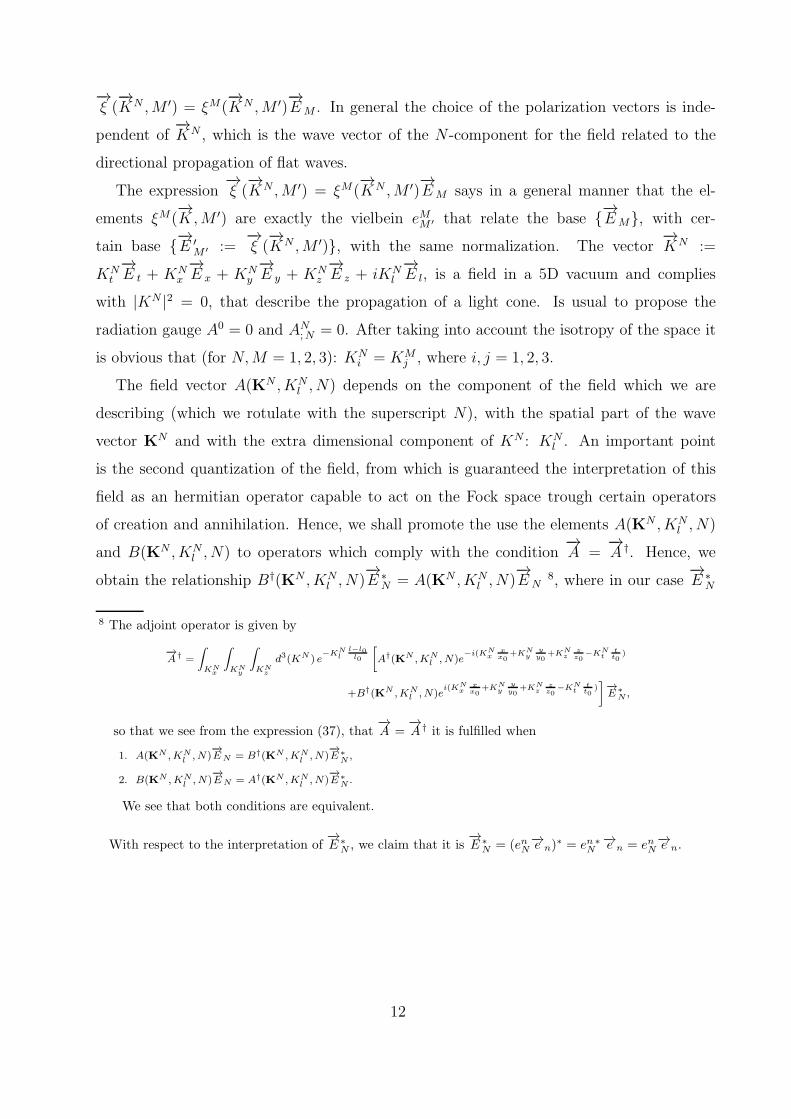
−→ξ (

−→KN ,M ′) = ξM(

−→KN ,M ′)

−→EM . In general the choice of the polarization vectors is inde-

pendent of−→KN , which is the wave vector of the N -component for the field related to the

directional propagation of flat waves.

The expression−→ξ (

−→KN ,M ′) = ξM(

−→KN ,M ′)

−→EM says in a general manner that the el-

ements ξM(−→K,M ′) are exactly the vielbein eMM ′ that relate the base {

−→EM}, with cer-

tain base {−→E ′

M ′ :=−→ξ (

−→KN ,M ′)}, with the same normalization. The vector

−→KN :=

KNt

−→E t + KN

x

−→E x + KN

y

−→E y + KN

z

−→E z + iKN

l

−→E l, is a field in a 5D vacuum and complies

with |KN |2 = 0, that describe the propagation of a light cone. Is usual to propose the

radiation gauge A0 = 0 and AN;N = 0. After taking into account the isotropy of the space it

is obvious that (for N,M = 1, 2, 3): KNi = KM

j , where i, j = 1, 2, 3.

The field vector A(KN , KNl , N) depends on the component of the field which we are

describing (which we rotulate with the superscript N), with the spatial part of the wave

vector KN and with the extra dimensional component of KN : KNl . An important point

is the second quantization of the field, from which is guaranteed the interpretation of this

field as an hermitian operator capable to act on the Fock space trough certain operators

of creation and annihilation. Hence, we shall promote the use the elements A(KN , KNl , N)

and B(KN , KNl , N) to operators which comply with the condition

−→A =

−→A †. Hence, we

obtain the relationship B†(KN , KNl , N)

−→E ∗

N = A(KN , KNl , N)

−→E N

8, where in our case−→E ∗

N

8 The adjoint operator is given by

−→A† =

∫

KNx

∫

KNy

∫

KNz

d3(KN ) e−KN

ll−l0l0

[

A†(KN ,KNl , N)e

−i(KNx

xx0

+KNy

yy0

+KNz

zz0

−KNt

tt0

)

+B†(KN ,KNl , N)e

i(KNx

xx0

+KNy

yy0

+KNz

zz0

−KNt

tt0

)]−→E ∗

N ,

so that we see from the expression (37), that−→A =

−→A † it is fulfilled when

1. A(KN ,KNl, N)

−→EN = B†(KN ,KN

l, N)

−→E ∗

N,

2. B(KN , KNl, N)

−→EN = A†(KN ,KN

l, N)

−→E ∗

N .

We see that both conditions are equivalent.

With respect to the interpretation of−→E ∗

N , we claim that it is−→E ∗

N = (enN−→e n)

∗ = en ∗N

−→e n = enN−→e n.

12

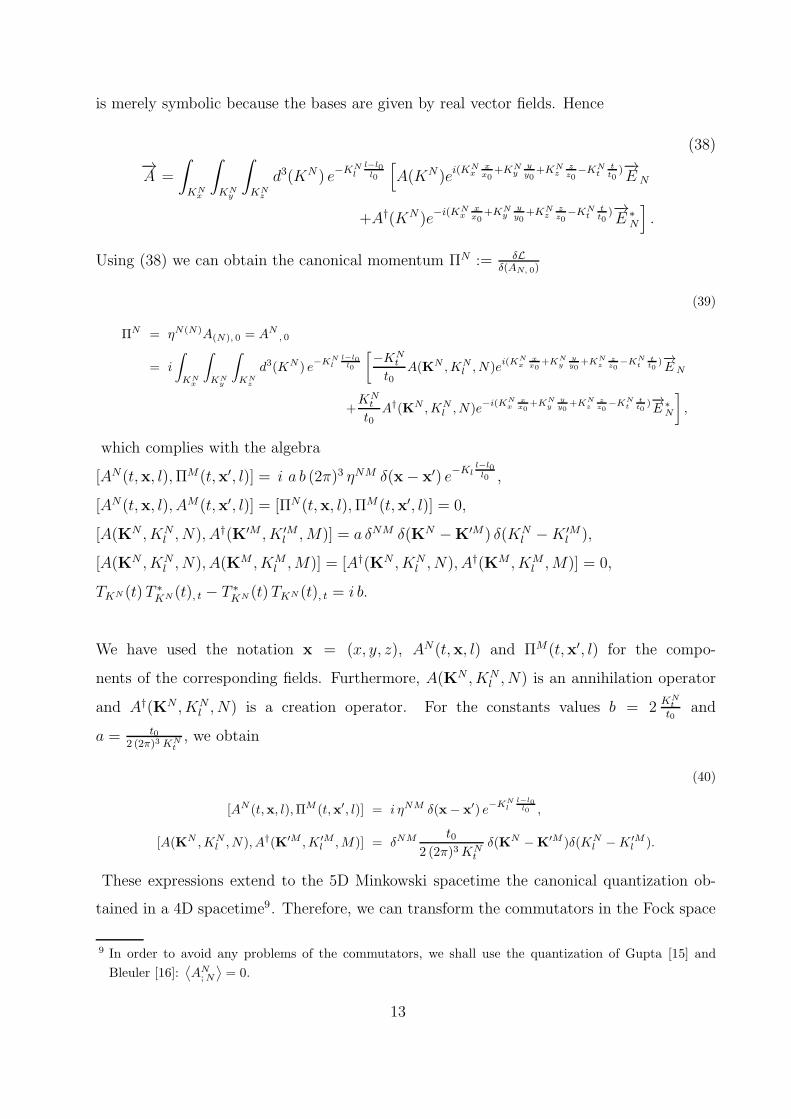
is merely symbolic because the bases are given by real vector fields. Hence

(38)

−→A =

∫

KNx

∫

KNy

∫

KNz

d3(KN ) e−KN

l

l−l0l0

[

A(KN )ei(KN

xxx0

+KNy

yy0

+KNz

zz0

−KNt

tt0

)−→E N

+A†(KN )e−i(KN

xxx0

+KNy

yy0

+KNz

zz0

−KNt

tt0

)−→E ∗

N

]

.

Using (38) we can obtain the canonical momentum ΠN := δLδ(AN, 0)

(39)

ΠN = ηN(N)A(N), 0 = AN, 0

= i

∫

KNx

∫

KNy

∫

KNz

d3(KN ) e−KN

l

l−l0l0

[−KN

t

t0A(KN ,KN

l , N)ei(KN

xxx0

+KNy

yy0

+KNz

zz0

−KNt

tt0

)−→EN

+KN

t

t0A†(KN ,KN

l , N)e−i(KNx

xx0

+KNy

y

y0+KN

zzz0

−KNt

tt0

)−→E ∗

N

]

,

which complies with the algebra

[AN(t,x, l),ΠM(t,x′, l)] = i a b (2π)3 ηNM δ(x− x′) e−Kl

l−l0l0 ,

[AN(t,x, l), AM(t,x′, l)] = [ΠN(t,x, l),ΠM(t,x′, l)] = 0,

[A(KN , KNl , N), A†(K′M , K ′M

l ,M)] = a δNM δ(KN −K′M) δ(KNl −K ′M

l ),

[A(KN , KNl , N), A(KM , KM

l ,M)] = [A†(KN , KNl , N), A†(KM , KM

l ,M)] = 0,

TKN (t) T ∗KN (t), t − T ∗

KN (t) TKN (t), t = i b.

We have used the notation x = (x, y, z), AN(t,x, l) and ΠM(t,x′, l) for the compo-

nents of the corresponding fields. Furthermore, A(KN , KNl , N) is an annihilation operator

and A†(KN , KNl , N) is a creation operator. For the constants values b = 2

KNt

t0and

a = t02 (2π)3 KN

t, we obtain

(40)

[AN (t,x, l),ΠM (t,x′, l)] = i ηNM δ(x− x′) e−KNl

l−l0l0 ,

[A(KN ,KNl , N), A†(K′M ,K ′M

l ,M)] = δNM t0

2 (2π)3KNt

δ(KN −K′M )δ(KNl −K ′M

l ).

These expressions extend to the 5D Minkowski spacetime the canonical quantization ob-

tained in a 4D spacetime9. Therefore, we can transform the commutators in the Fock space

9 In order to avoid any problems of the commutators, we shall use the quantization of Gupta [15] and

Bleuler [16]:⟨AN

;N

⟩= 0.

13

as second rank tensors, in the following manner:

[An(t,x, l),Πm(t,x′, l)] = i gnm δ(x− x′) e−Kn

l

l−l0l0 ,

[A(Kn, Knl , n), A

†(K′m, K ′ml , m)] = gnm

t02 (2π)3Kn

t

δ(Kn −K′m)δ(Knl −K ′m

l ),

where Πm = emMΠM y Km = emMKM . These expressions provide us the algebra in an

arbitrary metric obtained from a 5D Minkowski spacetime, which is free of structure. In

order to illustrate the formalism, in the following section we shall apply it to an de Sitter

expansion, which describes the early inflationary universe.

V. AN EXAMPLE: MONOPOLES FROM A 5D MINKOWSKI SPACETIME

WITH CONTORTION

We shall study an example in which we take as a started spacetime a 5D Minkowski

described with the cartesian coordinates φ(p) = (t, x, y, z, l)p, in which the tensor metric is

given by the orthonormal matrix ηAB (26). We choose a SB which is not coordinated, and

the structure coefficients are given by CII0 =

−e−N

l2, CI

I4 =−e−N

l2and C0

04 =−1l2. The vielbein

transform as enN = diag(1/l, e−N/l, e−N/l, e−N/l, 1), so that we obtain the metric

[g]ab =

ψ2(l) 0 0 0 0

0 ψ2(l) e2N 0 0 0

0 0 ψ2(l) e2N 0 0

0 0 0 ψ2(l) e2N 0

0 0 0 0 −1

, (41)

with ψ2(l) = l2/l20. The arrival spacetime is described by a coordinated base. This implies

that the Weitzenbock torsion in the arrival spacetime will be nonzero. This torsion will

be a possible geometrical source for the emergence of gravito-magnetic monopoles, once

it has been made a constant foliation on the extra noncompact coordinate. The current

components in this case are given by

(lc)(m)Ji = Cj0i, kAj

(1− δki

)= 0, (42)

(W )(m)Ji = ǫijk∂jAk e−Ht, (43)

and (W )(m)J0 =(lc)(m) J0 = 0. Notice that the spatial components of the magnetic currents

decay with time in the Weitzenbock representation. The study of the dynamics for the field

14

fluctuations during a de Sitter inflation in the framework of GEMI was studied with detail

in [17], and goes beyond the scope of this paper. However, as has been demonstrated in eq.

(42), from the point of view of the Levi-Civita representation there are no currents related

to gravito-magnetic sources.

VI. CONCLUSIONS

We have extended the WIMT formalism to GEMI with the aim to show that gravito-

magnetic currents may be obtained, at least in a Weitzenbock representation. The WIMT

formalism was introduced with the idea to generalize the foliation method in the Induced

Matter Theory of gravity, in which foliations which are no static result to be very difficult.

With the WIMT formalism, on can make static foliations from a 5D curved spacetime on

which one defines a 5D vacuum from the point of view of a Weitzenbock representation.

Once done the foliation is possible to pass to the representation of Levi-Civita. It open

a huge versatility to make static foliations to obtain arbitrary 4D hypersurfaces from 5D

curved manifolds, which could be very important for quantum field theories, gravitation,

cosmology, etc.

In particular, we have centered our study of the WIMT in the dual formalization of the

GEMI applied to the cosmology of the early inflationary universe. We have obtained nonzero

gravito-magnetic currents with the representation of Weitzenbock. The currents decrease

exponentially with time with the expansion of the universe, so that at the end of inflation

becomes negligible. It should be agree with present observations. However, these currents

are null in a Levi-Civita representation because in this geometrical representation the base

coordinated has not structure or torsion. In a future work we shall study an example where

gravito-magnetic sources are nonzero in any representation[18].

Acknowledgements

J. M. Romero and M. Bellini acknowledge CONICET (Argentina) and UNMdP for financial

support.

15

[1] P. A. Dirac. Proc. Roy. Soc. A133: 60 (1931).

[2] J. Preskill, Phys. Rev. Lett. 43: 1365 (1979).

[3] A. Linde, Phys. Lett. B327: 208 (1994);

A. Vilenkin, Phys. Rev. Lett. 72: 3137 (1994).

[4] A. Raya, J. E. Madriz Aguilar, M. Bellini, Phys. Lett. B638: 314(2006);

J. E. Madriz Aguilar, M. Bellini, Phys. Lett. B642: 302 (2006).

[5] J. M. Romero, M. Bellini. Phys. Lett. B674: 143(2009).

[6] F. A. Membiela, M. Bellini, Phys. Lett. B674: 152(2009);

F. A. Membiela, M. Bellini, Phys. Lett. B685: 1(2010).

[7] P. S. Wesson, Phys. Lett. B276: 299 (1992);

J. M. Overduin and P. S. Wesson, Phys. Rept. 283: 303 (1997);

T. Liko, Space Sci. Rev. 110: 337 (2004).

[8] J. E. Campbell, A course of Differential Geometry (Charendon, Oxford, 1926);

L. Magaard, Zur einbettung riemannscher Raume in Einstein-Raume und konformeuclidische

Raume. (PhD Thesis, Kiel, 1963).

[9] S. Rippl, C. Romero, R. Tavakol, Class. Quant. Grav. 12: 2411 (1995).

[10] F. Dahia, C. Romero, J. Math. Phys.43: 5804 (2002).

[11] F. Dahia, C. Romero, Class. Quant. Grav. 22: 5005 (2005).

[12] J. M. Romero, M. Bellini, Eur. Phys. J.C73: 2317(2013).

[13] B. Mashhoon, H. Liu, P. S. Wesson, Phys. Lett. B331: 305 (1994);

S. Rippl, C. Romero, R. Tavakol, Class. Quant. Grav. 12: 2411 (1995);

S. S. Seahra, P. S. Wesson, J. Math. Phys. 44: 5664 (2003).

[14] D. S. Ledesma, M. Bellini. Phys. Lett. B581: 1 (2004).

[15] S. Gupta, Proc. Roy. Soc. 63A: 681(1950).

[16] K. Bleuler, Helv. Phys. Acta 23:567 (1950).

[17] F. A. Membiela, M. Bellini, JCAP1010: 001(2010);

F. A. Membiela, M. Bellini, Eur. Phys. J. C72: 2181(2012).

[18] J. M. Romero, M. Bellini, In preparation.

16