lable at ScienceDirect

Renewable Energy 81 (2015) 707e722

Contents lists avai

Renewable Energy

journal homepage: www.elsevier .com/locate/renene

Constraints on extractable power from energetic tidal straits

P. Evans b, *, A. Mason-Jones b, C. Wilson b, C. Wooldridge a, T. O'Doherty b, D. O'Doherty b

a School of Earth and Ocean Sciences, Cardiff University, Main Building, Park Place, Cardiff CF10 3AT, Wales, UKb School of Engineering, Cardiff University, The Parade, Cardiff CF24 3AA, Wales, UK

a r t i c l e i n f o

Article history:Received 17 April 2014Accepted 30 March 2015Available online

Keywords:ADCPHydrodynamicsMarine resourcesAlternative energySite assessmentTidal stream turbines

* Corresponding author. Tel.: þ44 02920 875905.E-mail address: Evansps3@cf.ac.uk (P. Evans).

http://dx.doi.org/10.1016/j.renene.2015.03.0850960-1481/© 2015 Elsevier Ltd. All rights reserved.

a b s t r a c t

National efforts to reduce energy dependency on fossil fuels have prompted examination of macrotidalnearshore sites around the United Kingdom (UK) for potential tidal stream resource development. Anumber of prospective tidal energy sites have been identified, but the local hydrodynamics of these sitesare often poorly understood. Tidal energy developers rely on detailed characterisation of tidal energysites prior to device installation and field trials. Although first-order appraisals may make macrotidaltidal straits appear attractive for development, detailed, site-specific hydrodynamic and bathymetricsurveys are important for determining site suitability for tidal stream turbine (TST) installation. Un-derstanding the ways in which coastal features affect tidal velocities at potential TST development siteswill improve identification and analysis of physical constraints on tidal energy development. This paperpresents and examines tidal velocity data measured in Ramsey Sound (Pembrokeshire, Wales, UK), anenergetic macrotidal strait, which will soon host Wales' first TST demonstration project. While maximumtidal velocities in the strait during peak spring flood exceed 3 m s�1, the northern portion of RamseySound exhibits a marked flood-dominated tidal asymmetry. Furthermore, local bathymetric featuresaffect flow fields that are spatially heterogeneous in three dimensions, patterns that depth-averagedvelocity data (measured and modelled) tend to mask. Depth-averaging can therefore have a significanteffect on power estimations. Analysis of physical and hydrodynamic characteristics in Ramsey Sound,including tidal velocities across the swept area of the pilot TST, variations in the stream flow with depth,estimated power output, water depth and bed slope, suggests that the spatial and temporal variability inthe flow field may render much of Ramsey Sound unsuitable for tidal power extraction. Although theresource potential depends on velocity and bathymetric conditions that are fundamentally local, manyprospective tidal energy sites are subject to similar physical and hydrodynamic constraints. Results ofthis study can help inform site selection in these complicated, highly dynamic macrotidal environments.In order to fully characterise the structure of the tidal currents, these data should be supplemented with3-D modelling, particularly in areas subject to a highly irregular bathymetry and complicated tidalregime.

© 2015 Elsevier Ltd. All rights reserved.

1. Introduction

Global climate change is becoming more widely acknowledgedand, as such, policy makers worldwide are recognising the impor-tance of greenhouse gas emission reductions. Consequently, thereis an international shift towards clean renewable technologies forelectricity generation [1]. Furthermore, the finite nature andgeographical constraints associated with fossil fuels is motivatingthis movement towards finding long term clean and renewablealternatives.

The total estimated tidal-stream (marine-current) resource inthe United Kingdom (UK) exceeds 110 TWh yr�1, a quantity com-parable to the estimate for the rest of Europe, and one that accountsfor approximately 10e15% of the total energy from tidal-streamresources estimated for the world [2]. Of that total, approximately20% is considered extractible [2]. A key document for policy andplanning decisions regarding feasibility studies and site leasing isthe Atlas of UK Marine Renewable Energy Resources [2], whichoffers regional-scale descriptions of marine energy resources.However, the resolution of the Atlas is too coarse to capture thetidal dynamics of complicated nearshore zones such as high-velocity straits. Tidal amplitude and current velocities are func-tions of coastal physical geography and local bathymetry [3e5];

Abbreviations and nomenclature

ADCP acoustic Doppler current profilerCD chart datumTST tidal-stream turbineP power flux (kW m�2)u, v, w instantaneous cross-channel, streamwise and

vertical velocity components (m s�1)u; v;w spatially-averaged cross-channel, streamwise and

vertical velocity components (m s�1)ut ; vt ;wt average cross-channel, streamwise and vertical

velocity over the vertical diameter of a TST sweptarea (m s�1)

vd depth-averaged streamwise velocity (m s�1)x, y, z distances along the cross-channel (eastewest),

streamwise (northesouth) and vertical axes (m)r water density (kg m�3)

P. Evans et al. / Renewable Energy 81 (2015) 707e722708

therefore this lack of local-scale hydrodynamic data suggests largeuncertainties exist in tidal resource estimates [6,7].

Several resource assessments [2,8,9] have identified three pri-mary locations for tidal stream energy development along the coastof Wales: Anglesey [10], Pembrokeshire [11,12], and the BristolChannel (including the Severn Estuary) [13]. The latter is restricteddue to navigational constraints, limited depths, a large tidal range(potential turbine exposure at low spring tides) and relatively lowvelocities [13]. The Welsh Government has set targets to harness4 GW of tidal and wave power by 2025 [14]. Meeting this targetrequires a better understanding of the tidal resource in Wales byconstraining estimates of tidal power through site-specific velocitymeasurements [11e13] and through fully hydrodynamic oceano-graphic numerical modelling [10,15,16].

In 2011, Tidal Energy Ltd. (TEL), a UK-based commercial energycompany, was granted permission to trial its DeltaStream™ tidal-stream turbine device (TST) [17] in Ramsey Sound, a strait inPembrokeshire (Fig. 1) estimated to have an energy potential ofapproximately 75 GWh yr�1 [18]. The original 1.2 MW Delta-Stream™ unit supported three 15 m diameter horizontal-axis tidalturbines mounted on a triangular framewith the centre of the hubsset 12 m from the seabed. However, to prove the technologywithout overcomplicating the design it was decided to install asingle 400 kW turbine on one of the smaller foundations, whichwill still greatly contribute to the energy demands of the commu-nities in St David's [19]. The tip of the DeltaStream™ turbine will beapproximately set at 30 m below CD (Chart Datum), so not torestrict boating activity [17]. The constructed prototype device iscurrently at Pembroke Dock, Wales, awaiting a weather and tidalwindow for deployment. The device is to be installed as part of aone-year demonstration project to test its integrity and power-output capabilities. If successful, the device will be scaled up tofull commercial scale and suitable locations identified for a turbinearray.

Even outside the context of tidal resource development, fewstudies to date have measured directly the effects of bathymetry oncurrent speed and three-dimensional (3-D) velocity structure oftidal flow through confined passages such as straits [20e29].Although research into the effects of TSTs on the environment andthe effects of the environment on devices is becoming moreprevalent, to date, few field studies have investigated the feasibilityof installing these devices in areas that are subject to high currentspeeds [30], which are attractive from an energy generationperspective. Tidal stream turbines are currently being considered

for deployment at sites where local conditions deviate from theideal with complicated velocity profiles, spatial and temporalvariability (over daily and lunar timescales), as well as complexitiesin the seabed topology. The efficiency and functional longevity of aTST device depends on the interaction of the blades and the tidalflow field [31]. Therefore, quantifying the unsteady loading acrossthe turbine's diameter caused by a non-uniform velocity profileacross the face of the turbine is important, as it affects TST per-formance and cumulative wear on the device. These fine-scalecharacteristics of tidal velocity fields tend to be overlooked in as-sessments for potential TST sites.

Motivated by the velocity and bathymetric data gap in tidalresource assessments between coarse-scale theoretical potentialand fine-scale realities, the viability of tidal energy generation foran area in the complicated flow system of Ramsey Sound has beeninvestigated. It should be noted that a vessel-mounted ADCP studywas previously carried out within Ramsey Sound [11] to comparethe flux there against that in the two channels to the west ofRamsey Island. This paper builds on this study by utilising addi-tional data and equipment, while covering a larger area of RamseySound to examine the effect of parameters such as tidal asymmetry,variations in thewater column and vertical velocities on the naturalpower flux. The spatial and temporal patterns in flood and ebbtidal-stream velocities near spring peak and use of these mea-surements to calculate power flux are also quantified. To determinesuitable TST locations within Ramsey Sound, the analysis isextended to examine the vertical velocity profile accounting for thewater depth relative to turbine diameter and swept area, and theseabed gradient, or bed slope, using the dimensional and geometricspecifications of a typical TST. Finally, the effect of depth-averagingtidal velocity data across the entire water column ðvdÞ against thatover the TST swept area ðvtÞ in estimates of extractable power, andin assessments of TST site potential is evaluated. Although thispaper relates to a single site, the same concerns are present at everysite.

2. Methodology

2.1. Study site

Connected to the Irish Sea, Ramsey Sound (Fig. 1) is a straitapproximately 3 km long and 500e1600 m wide, separatingRamsey Island from the Pembrokeshire coastline near St. David'sheadland, Wales. Water depth in the strait is typically between 20and 40 m below CD (where 0 m CD is approximately the level ofLowest Astronomical Tide, LAT), but reaches a maximum depth of66 m CD within a northesouth trending trench. A submergedpinnacle known as Horse Rock dominates the north-easternquadrant of the strait. Roughly conical, this natural obstruction toflow has an estimated diameter of 100 m at its base (50 m at half itsheight) and is approximately 23 m higher than the seabed aroundit. The crest pierces the water surface and dries (according to theAdmiralty Chart) at approximately þ0.9 m CD during spring-tidelows. It should be noted that the data presented here have beenreduced to Chart Datum so that all measurements refer to the samereference point, rather than depth below the water surface.

The tidal hydrodynamics of the Irish Sea to the west of RamseySound are thought to be as a result of a two Kelvin-type waves, onepropagating in a north-easterly direction along St. George's Chan-nel and the other propagating southwards through North Channel[32]. The superposition of these two progressive waves results intwo degenerate amphidromes (zones of negligible tidal range, butstrong tidal currents), characterised by M2 and S2 co-tidal chartsnorth of St. George's Channel [33]. The Eastern Irish Sea is subject tohigh tidal ranges and as such, strong tidal currents are generated as

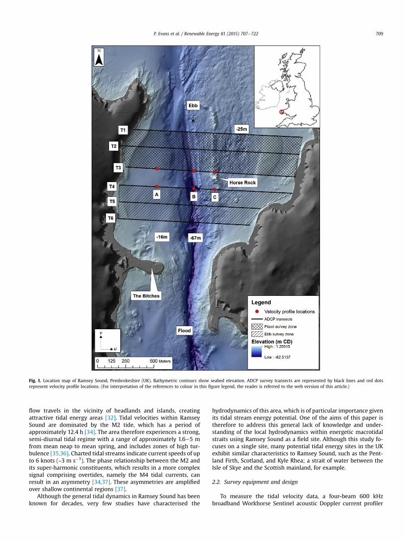
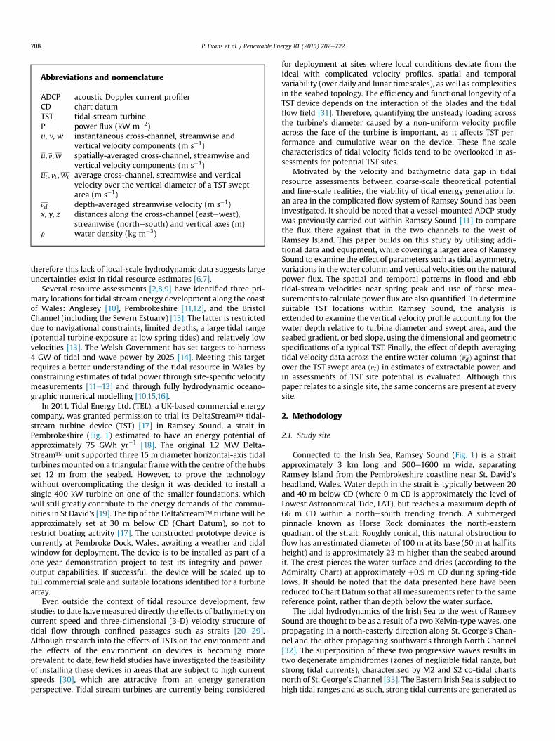
Fig. 1. Location map of Ramsey Sound, Pembrokeshire (UK). Bathymetric contours show seabed elevation. ADCP survey transects are represented by black lines and red dotsrepresent velocity profile locations. (For interpretation of the references to colour in this figure legend, the reader is referred to the web version of this article.)

P. Evans et al. / Renewable Energy 81 (2015) 707e722 709

flow travels in the vicinity of headlands and islands, creatingattractive tidal energy areas [32]. Tidal velocities within RamseySound are dominated by the M2 tide, which has a period ofapproximately 12.4 h [34]. The area therefore experiences a strong,semi-diurnal tidal regime with a range of approximately 1.6e5 mfrom mean neap to mean spring, and includes zones of high tur-bulence [35,36]. Charted tidal streams indicate current speeds of upto 6 knots (~3 m s�1). The phase relationship between the M2 andits super-harmonic constituents, which results in a more complexsignal comprising overtides, namely the M4 tidal currents, canresult in an asymmetry [34,37]. These asymmetries are amplifiedover shallow continental regions [37].

Although the general tidal dynamics in Ramsey Sound has beenknown for decades, very few studies have characterised the

hydrodynamics of this area, which is of particular importance givenits tidal stream energy potential. One of the aims of this paper istherefore to address this general lack of knowledge and under-standing of the local hydrodynamics within energetic macrotidalstraits using Ramsey Sound as a field site. Although this study fo-cuses on a single site, many potential tidal energy sites in the UKexhibit similar characteristics to Ramsey Sound, such as the Pent-land Firth, Scotland, and Kyle Rhea; a strait of water between theIsle of Skye and the Scottish mainland, for example.

2.2. Survey equipment and design

To measure the tidal velocity data, a four-beam 600 kHzbroadband Workhorse Sentinel acoustic Doppler current profiler

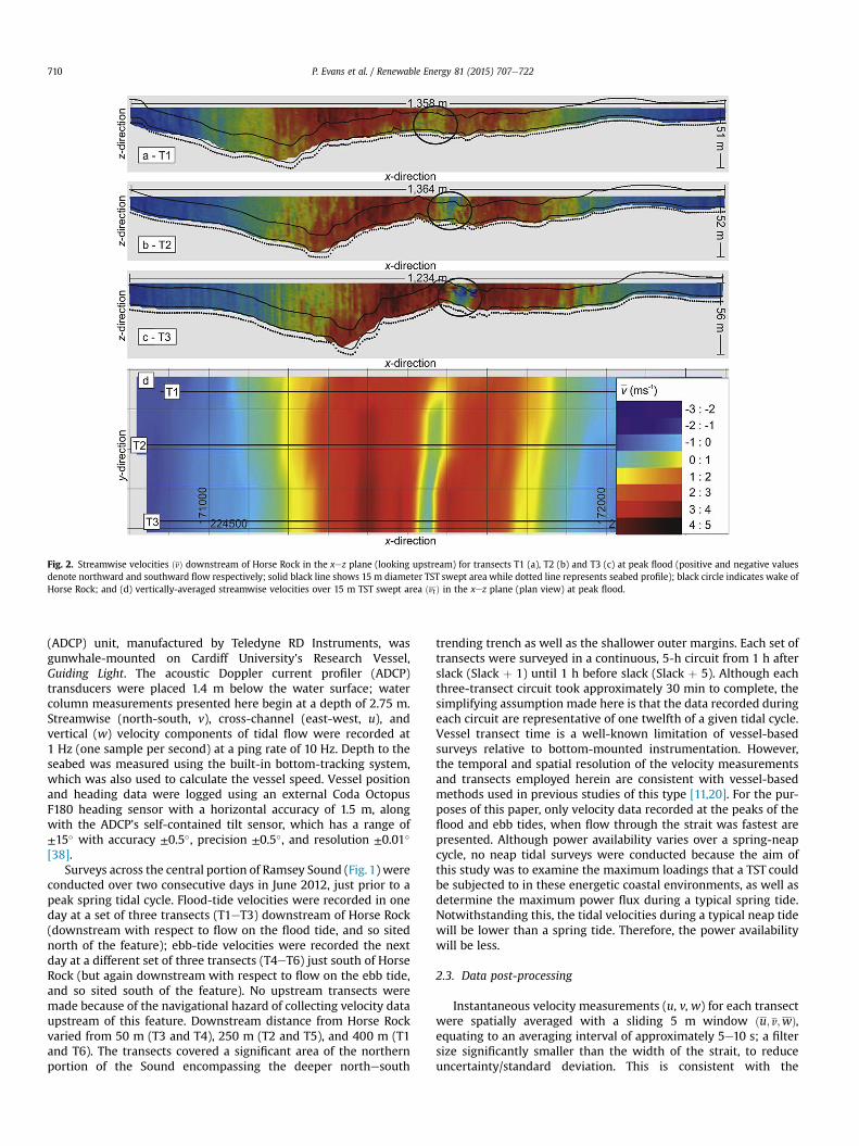
Fig. 2. Streamwise velocities ðvÞ downstream of Horse Rock in the xez plane (looking upstream) for transects T1 (a), T2 (b) and T3 (c) at peak flood (positive and negative valuesdenote northward and southward flow respectively; solid black line shows 15 m diameter TST swept area while dotted line represents seabed profile); black circle indicates wake ofHorse Rock; and (d) vertically-averaged streamwise velocities over 15 m TST swept area ðvtÞ in the xez plane (plan view) at peak flood.

P. Evans et al. / Renewable Energy 81 (2015) 707e722710

(ADCP) unit, manufactured by Teledyne RD Instruments, wasgunwhale-mounted on Cardiff University's Research Vessel,Guiding Light. The acoustic Doppler current profiler (ADCP)transducers were placed 1.4 m below the water surface; watercolumn measurements presented here begin at a depth of 2.75 m.Streamwise (north-south, v), cross-channel (east-west, u), andvertical (w) velocity components of tidal flow were recorded at1 Hz (one sample per second) at a ping rate of 10 Hz. Depth to theseabed was measured using the built-in bottom-tracking system,which was also used to calculate the vessel speed. Vessel positionand heading data were logged using an external Coda OctopusF180 heading sensor with a horizontal accuracy of 1.5 m, alongwith the ADCP's self-contained tilt sensor, which has a range of±15� with accuracy ±0.5�, precision ±0.5�, and resolution ±0.01�

[38].Surveys across the central portion of Ramsey Sound (Fig. 1) were

conducted over two consecutive days in June 2012, just prior to apeak spring tidal cycle. Flood-tide velocities were recorded in oneday at a set of three transects (T1eT3) downstream of Horse Rock(downstream with respect to flow on the flood tide, and so sitednorth of the feature); ebb-tide velocities were recorded the nextday at a different set of three transects (T4eT6) just south of HorseRock (but again downstream with respect to flow on the ebb tide,and so sited south of the feature). No upstream transects weremade because of the navigational hazard of collecting velocity dataupstream of this feature. Downstream distance from Horse Rockvaried from 50 m (T3 and T4), 250 m (T2 and T5), and 400 m (T1and T6). The transects covered a significant area of the northernportion of the Sound encompassing the deeper northesouth

trending trench as well as the shallower outer margins. Each set oftransects were surveyed in a continuous, 5-h circuit from 1 h afterslack (Slack þ 1) until 1 h before slack (Slack þ 5). Although eachthree-transect circuit took approximately 30 min to complete, thesimplifying assumption made here is that the data recorded duringeach circuit are representative of one twelfth of a given tidal cycle.Vessel transect time is a well-known limitation of vessel-basedsurveys relative to bottom-mounted instrumentation. However,the temporal and spatial resolution of the velocity measurementsand transects employed herein are consistent with vessel-basedmethods used in previous studies of this type [11,20]. For the pur-poses of this paper, only velocity data recorded at the peaks of theflood and ebb tides, when flow through the strait was fastest arepresented. Although power availability varies over a spring-neapcycle, no neap tidal surveys were conducted because the aim ofthis study was to examine the maximum loadings that a TST couldbe subjected to in these energetic coastal environments, as well asdetermine the maximum power flux during a typical spring tide.Notwithstanding this, the tidal velocities during a typical neap tidewill be lower than a spring tide. Therefore, the power availabilitywill be less.

2.3. Data post-processing

Instantaneous velocity measurements (u, v, w) for each transectwere spatially averaged with a sliding 5 m window ðu; v;wÞ,equating to an averaging interval of approximately 5e10 s; a filtersize significantly smaller than the width of the strait, to reduceuncertainty/standard deviation. This is consistent with the

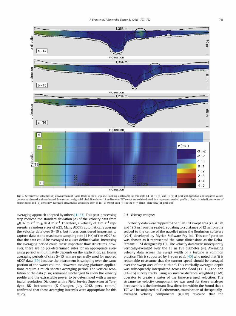
Fig. 3. Streamwise velocities ðvÞ downstream of Horse Rock in the xez plane (looking upstream) for transects T4 (a), T5 (b) and T6 (c) at peak ebb (positive and negative valuesdenote northward and southward flow respectively; solid black line shows 15 m diameter TST swept area while dotted line represents seabed profile); black circle indicates wake ofHorse Rock; and (d) vertically-averaged streamwise velocities over 15 m TST swept area ðvtÞ in the xey plane (plan view) at peak ebb.

P. Evans et al. / Renewable Energy 81 (2015) 707e722 711

averaging approach adopted by others [11,23]. This post-processingstep reduced the standard deviation (s) of the velocity data from±0.07 m s�1 to ± 0.04 m s�1. Therefore, a velocity of 2 m s�1 rep-resents a random error of ±2%. Many ADCPs automatically averagethe velocity data over 5e10 s, but it was considered important tocapture data at the maximum sampling rate (1 Hz) of the ADCP sothat the data could be averaged to a user-defined value. Increasingthe averaging period could mask important flow structures, how-ever, there are no pre-determined rules for an appropriate aver-aging period as it ultimately depends on the application, i.e. longeraveraging periods of circa 5e10 min are generally used for mooredADCP data [39] because the instrument is sampling over the sameportion of the water column. However, moving platform applica-tions require a much shorter averaging period. The vertical reso-lution of the data (1 m) remained unchanged to allow the velocityprofile and the extractable power to be determined with a mean-ingful resolution. Dialogue with a Field Service Supervisor at Tele-dyne RD Instruments (K Grangier, July 2012, pers. comm.)confirmed that these averaging intervals were appropriate for thisstudy.

2.4. Velocity analyses

Velocity data were clipped to the 15 m TST swept area (i.e. 4.5 mand 19.5 m from the seabed, equating to a distance of 12m from theseabed to the centre of the nacelle) using the Eonfusion software(v2.4) developed by Myriax Software Pty Ltd. This configurationwas chosen as it represented the same dimensions as the Delta-Stream™ TST designed by TEL. The velocity datawere subsequentlyvertically-averaged over the 15 m TST diameter ðvtÞ. Averagingvelocity data across the swept width of a turbine is commonpractice. This is supported by Bryden et al. [40] who noted that ‘it isreasonable to assume that the current speed should be averagedover the swept area of the turbine’. This vertically-averaged depthwas subsequently interpolated across the flood (T1eT3) and ebb(T4eT6) survey tracks using an inverse distance weighted (IDW)operator to create a raster of the time-averaged velocities. Thestreamwise velocity component ðvÞ was used for these analysesbecause this is the dominant flow directionwithin the Sound that aTST will be subjected to. Furthermore, examination of the spatially-averaged velocity components ðu; v;wÞ revealed that the

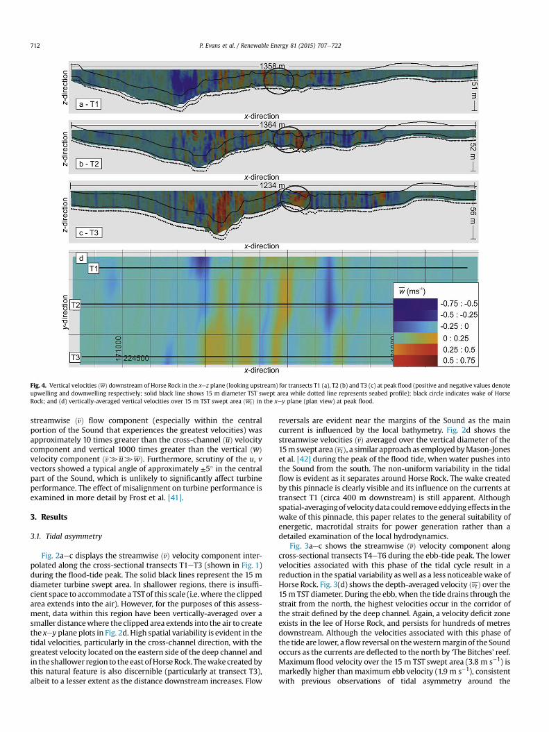
Fig. 4. Vertical velocities ðwÞ downstream of Horse Rock in the xez plane (looking upstream) for transects T1 (a), T2 (b) and T3 (c) at peak flood (positive and negative values denoteupwelling and downwelling respectively; solid black line shows 15 m diameter TST swept area while dotted line represents seabed profile); black circle indicates wake of HorseRock; and (d) vertically-averaged vertical velocities over 15 m TST swept area ðwtÞ in the xey plane (plan view) at peak flood.

P. Evans et al. / Renewable Energy 81 (2015) 707e722712

streamwise ðvÞ flow component (especially within the centralportion of the Sound that experiences the greatest velocities) wasapproximately 10 times greater than the cross-channel ðuÞ velocitycomponent and vertical 1000 times greater than the vertical ðwÞvelocity component ðv[u[wÞ. Furthermore, scrutiny of the u, vvectors showed a typical angle of approximately ±5� in the centralpart of the Sound, which is unlikely to significantly affect turbineperformance. The effect of misalignment on turbine performance isexamined in more detail by Frost et al. [41].

3. Results

3.1. Tidal asymmetry

Fig. 2aec displays the streamwise ðvÞ velocity component inter-polated along the cross-sectional transects T1eT3 (shown in Fig. 1)during the flood-tide peak. The solid black lines represent the 15 mdiameter turbine swept area. In shallower regions, there is insuffi-cient space to accommodate a TSTof this scale (i.e. where the clippedarea extends into the air). However, for the purposes of this assess-ment, data within this region have been vertically-averaged over asmaller distancewhere the clipped area extends into the air to createthe xey plane plots in Fig. 2d. High spatial variability is evident in thetidal velocities, particularly in the cross-channel direction, with thegreatest velocity located on the eastern side of the deep channel andin the shallower region to theeast ofHorseRock. Thewakecreatedbythis natural feature is also discernible (particularly at transect T3),albeit to a lesser extent as the distance downstream increases. Flow

reversals are evident near the margins of the Sound as the maincurrent is influenced by the local bathymetry. Fig. 2d shows thestreamwise velocities ðvÞ averaged over the vertical diameter of the15mswept area ðvtÞ, a similar approach as employedbyMason-Joneset al. [42] during the peak of the flood tide, whenwater pushes intothe Sound from the south. The non-uniform variability in the tidalflow is evident as it separates around Horse Rock. The wake createdby this pinnacle is clearly visible and its influence on the currents attransect T1 (circa 400 m downstream) is still apparent. Althoughspatial-averagingof velocitydata could removeeddyingeffects in thewake of this pinnacle, this paper relates to the general suitability ofenergetic, macrotidal straits for power generation rather than adetailed examination of the local hydrodynamics.

Fig. 3aec shows the streamwise ðvÞ velocity component alongcross-sectional transects T4eT6 during the ebb-tide peak. The lowervelocities associated with this phase of the tidal cycle result in areduction in the spatial variability aswell as a less noticeablewake ofHorse Rock. Fig. 3(d) shows the depth-averaged velocity ðvtÞ over the15m TST diameter. During the ebb, when the tide drains through thestrait from the north, the highest velocities occur in the corridor ofthe strait defined by the deep channel. Again, a velocity deficit zoneexists in the lee of Horse Rock, and persists for hundreds of metresdownstream. Although the velocities associated with this phase ofthe tide are lower, aflow reversal on thewesternmargin of the Soundoccurs as the currents are deflected to the north by ‘The Bitches’ reef.Maximum flood velocity over the 15 m TST swept area (3.8 m s�1) ismarkedly higher than maximum ebb velocity (1.9 m s�1), consistentwith previous observations of tidal asymmetry around the

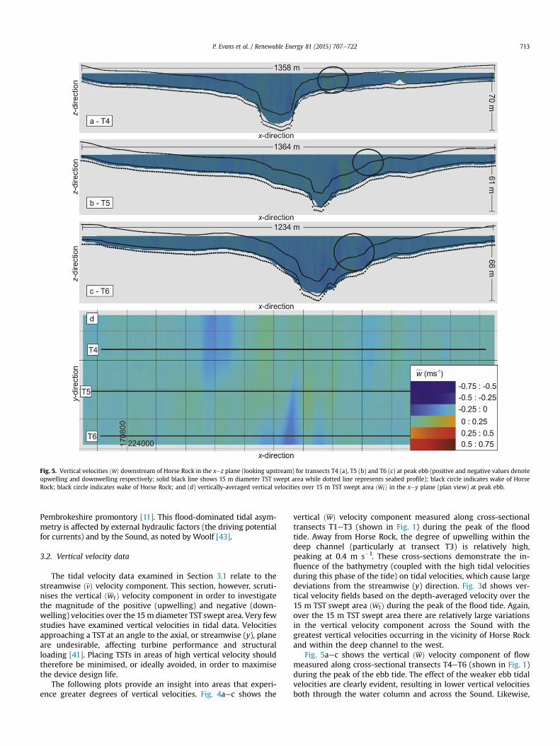
Fig. 5. Vertical velocities ðwÞ downstream of Horse Rock in the xez plane (looking upstream) for transects T4 (a), T5 (b) and T6 (c) at peak ebb (positive and negative values denoteupwelling and downwelling respectively; solid black line shows 15 m diameter TST swept area while dotted line represents seabed profile); black circle indicates wake of HorseRock; black circle indicates wake of Horse Rock; and (d) vertically-averaged vertical velocities over 15 m TST swept area ðwtÞ in the xey plane (plan view) at peak ebb.

P. Evans et al. / Renewable Energy 81 (2015) 707e722 713

Pembrokeshire promontory [11]. This flood-dominated tidal asym-metry is affected by external hydraulic factors (the driving potentialfor currents) and by the Sound, as noted by Woolf [43].

3.2. Vertical velocity data

The tidal velocity data examined in Section 3.1 relate to thestreamwise ðvÞ velocity component. This section, however, scruti-nises the vertical ðwtÞ velocity component in order to investigatethe magnitude of the positive (upwelling) and negative (down-welling) velocities over the 15m diameter TST swept area. Very fewstudies have examined vertical velocities in tidal data. Velocitiesapproaching a TST at an angle to the axial, or streamwise (y), planeare undesirable, affecting turbine performance and structuralloading [41]. Placing TSTs in areas of high vertical velocity shouldtherefore be minimised, or ideally avoided, in order to maximisethe device design life.

The following plots provide an insight into areas that experi-ence greater degrees of vertical velocities. Fig. 4aec shows the

vertical ðwÞ velocity component measured along cross-sectionaltransects T1eT3 (shown in Fig. 1) during the peak of the floodtide. Away from Horse Rock, the degree of upwelling within thedeep channel (particularly at transect T3) is relatively high,peaking at 0.4 m s�1. These cross-sections demonstrate the in-fluence of the bathymetry (coupled with the high tidal velocitiesduring this phase of the tide) on tidal velocities, which cause largedeviations from the streamwise (y) direction. Fig. 3d shows ver-tical velocity fields based on the depth-averaged velocity over the15 m TST swept area ðwtÞ during the peak of the flood tide. Again,over the 15 m TST swept area there are relatively large variationsin the vertical velocity component across the Sound with thegreatest vertical velocities occurring in the vicinity of Horse Rockand within the deep channel to the west.

Fig. 5aec shows the vertical ðwÞ velocity component of flowmeasured along cross-sectional transects T4eT6 (shown in Fig. 1)during the peak of the ebb tide. The effect of the weaker ebb tidalvelocities are clearly evident, resulting in lower vertical velocitiesboth through the water column and across the Sound. Likewise,

Fig. 6. Streamwise velocity profiles ðvÞ for T3 (flood) and T4 (ebb) e Location A (west of deep channel); Location B (within deep channel); and Location C (in the vicinity of HorseRock).

P. Evans et al. / Renewable Energy 81 (2015) 707e722714

the averaged vertical velocities ðwtÞ across the 15 m TST sweptarea (Fig. 5d) are lower when compared with the same phase ofthe flood tide, peaking at approximately �0.13 m s�1 to thesouth-west of Horse Rock as the flow is forced into the deepchannel.

These data demonstrate that the magnitude of the vertical ve-locity component is largely dictated by the streamwise ðvÞ velocitycomponent, i.e. the greater the velocity in this north-south (y) di-rection, the greater the vertical velocity component. Although thebathymetry in the vicinity of the Sound, where ebb tide data areavailable, is still very irregular, the lower velocities associated withthis phase of the tide result in reduced vertical velocities at theexpense of available power. There is therefore a compromise thatneeds to be met in these energetic, macrotidal systems betweensufficient streamwise ðvÞ velocities for power generation andtolerable vertical velocities. Ideally, the seabed should be wide andflat enough to limit vertical velocities and significant variations invelocities with depth.

3.3. Velocity profiles

Velocity profiles of the streamwise ðvÞ velocities at three loca-tions across the Sound are presented in Fig. 6. Negative valuesrepresent southerly flow. Again, these data have been spatiallyaveraged with a sliding 5 m window in the horizontal direction.Three locations, displaying differing hydrodynamic conditions,have been selected: to the west of the deep channel (Location ‘A’ inFig. 1), within the deep channel (Location ‘B’ in Fig. 1) and down-stream of Horse Rock (Location ‘C’ in Fig. 1). These locations wereexamined at the peak of both the flood and ebb tides for the reasonsidentified earlier.

The velocities to the west of the deep channel (Location A)during the peak of the flood (T3) and ebb (T4) tides are relativelylow and uniform through the water column, peaking at 0.5 m s�1

and 0.2 m s�1 respectively. Low flow conditions are experienced atthis location during the peak of both the flood and ebb tides giventheir close proximity to the centre of counter-clockwise (flood)

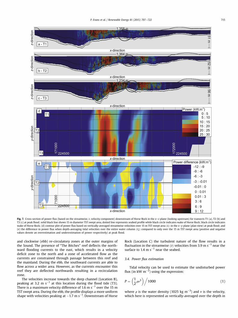
Fig. 7. Cross-section of power flux (based on the streamwise, v, velocity component) downstream of Horse Rock in the xez plane (looking upstream) for transects T1 (a), T2 (b) andT3 (c) at peak flood; solid black line shows 15 m diameter TST swept area, dotted line represents seabed profile while black circle indicates wake of Horse Rock; black circle indicateswake of Horse Rock; (d) contour plot of power flux based on vertically-averaged streamwise velocities over 15 m TST swept area ðvtÞ in the xey plane (plan view) at peak flood; and(e) the difference in power flux when depth-averaging tidal velocities over the entire water column ðvdÞ compared to only over the 15 m TST swept area (positive and negativevalues denote an overestimation and underestimation of power respectively) at peak flood.

P. Evans et al. / Renewable Energy 81 (2015) 707e722 715

and clockwise (ebb) re-circulatory zones at the outer margins ofthe Sound. The presence of “The Bitches” reef deflects the north-ward flooding currents to the east, which results in a velocitydeficit zone to the north and a zone of accelerated flow as thecurrents are constrained through passage between this reef andthe mainland. During the ebb, the southward currents are able toflow across a wider area. However, as the currents encounter thisreef they are deflected northwards resulting in a recirculationzone.

The velocities increase towards the deep channel (Location B),peaking at 3.2 m s�1 at this location during the flood tide (T3).There is a maximum velocity difference of 1.6 m s�1 over the 15 mTST swept area. During the ebb, the profile displays a more uniformshape with velocities peaking at �1.7 m s�1. Downstream of Horse

Rock (Location C) the turbulent nature of the flow results in afluctuation in the streamwise ðvÞ velocities from 3.9 m s�1 near thesurface to 1.4 m s�1 near the seabed.

3.4. Power flux estimation

Tidal velocity can be used to estimate the undisturbed powerflux (in kW m�2) using the expression:

P ¼�12rv3

��1000 (1)

where r is the water density (1025 kg m�3) and v is the velocity,which here is represented as vertically-averaged over the depth in

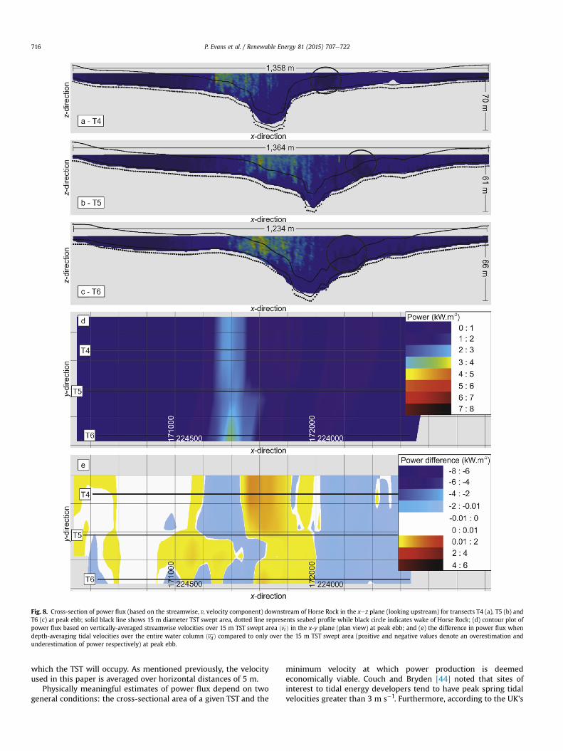
Fig. 8. Cross-section of power flux (based on the streamwise, v, velocity component) downstream of Horse Rock in the xez plane (looking upstream) for transects T4 (a), T5 (b) andT6 (c) at peak ebb; solid black line shows 15 m diameter TST swept area, dotted line represents seabed profile while black circle indicates wake of Horse Rock; (d) contour plot ofpower flux based on vertically-averaged streamwise velocities over 15 m TST swept area ðvt Þ in the x-y plane (plan view) at peak ebb; and (e) the difference in power flux whendepth-averaging tidal velocities over the entire water column ðvdÞ compared to only over the 15 m TST swept area (positive and negative values denote an overestimation andunderestimation of power respectively) at peak ebb.

P. Evans et al. / Renewable Energy 81 (2015) 707e722716

which the TST will occupy. As mentioned previously, the velocityused in this paper is averaged over horizontal distances of 5 m.

Physically meaningful estimates of power flux depend on twogeneral conditions: the cross-sectional area of a given TST and the

minimum velocity at which power production is deemedeconomically viable. Couch and Bryden [44] noted that sites ofinterest to tidal energy developers tend to have peak spring tidalvelocities greater than 3 m s�1. Furthermore, according to the UK's

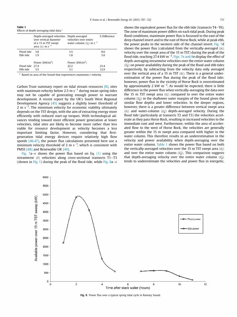
Table 1Effects of depth-averaging tidal data.a

Depth-averaged velocitiesover vertical diameterof a 15 m TST sweptarea ðvtÞ m s�1

Depth-averagedvelocities over entirewater column ðvdÞ m s�1

% Difference

Flood tide 3.8 3.5 8.6Ebb tide 1.9 1.8 5.6

Power (kW/m2) Power (kW/m2)Flood tide 27.4 22.2 23.4Ebb tide 3.5 3.1 12.9

a Based on area of the Sound that experiences maximum v velocity.

P. Evans et al. / Renewable Energy 81 (2015) 707e722 717

Carbon Trust summary report on tidal stream resources [8], siteswith maximum velocity below 2.5 m s�1 during mean spring tidesmay not be capable of generating enough power to warrantdevelopment. A recent report by the UK's South West RegionalDevelopment Agency [45] suggests a slightly lower threshold of2 m s�1. The minimum velocity for economic viability ultimatelydepends on the TST design, with the aim of extracting energy moreefficiently with reduced start-up torques. With technological ad-vances tending toward more efficient power generation at lowervelocities, tidal sites are likely to become more rather than lessviable for resource development as velocity becomes a lessimportant limiting factor. However, considering that first-generation tidal energy devices require relatively high flowspeeds [46,47], the power flux calculations presented here use aminimum velocity threshold of 2 m s�1, which is consistent withPMSS [48] and Renewable UK [49].

Fig. 7aec shows the power flux based on Eq. (1) using thestreamwise ðvÞ velocities along cross-sectional transects T1eT3(shown in Fig. 1) during the peak of the flood tide, while Fig. 8aec

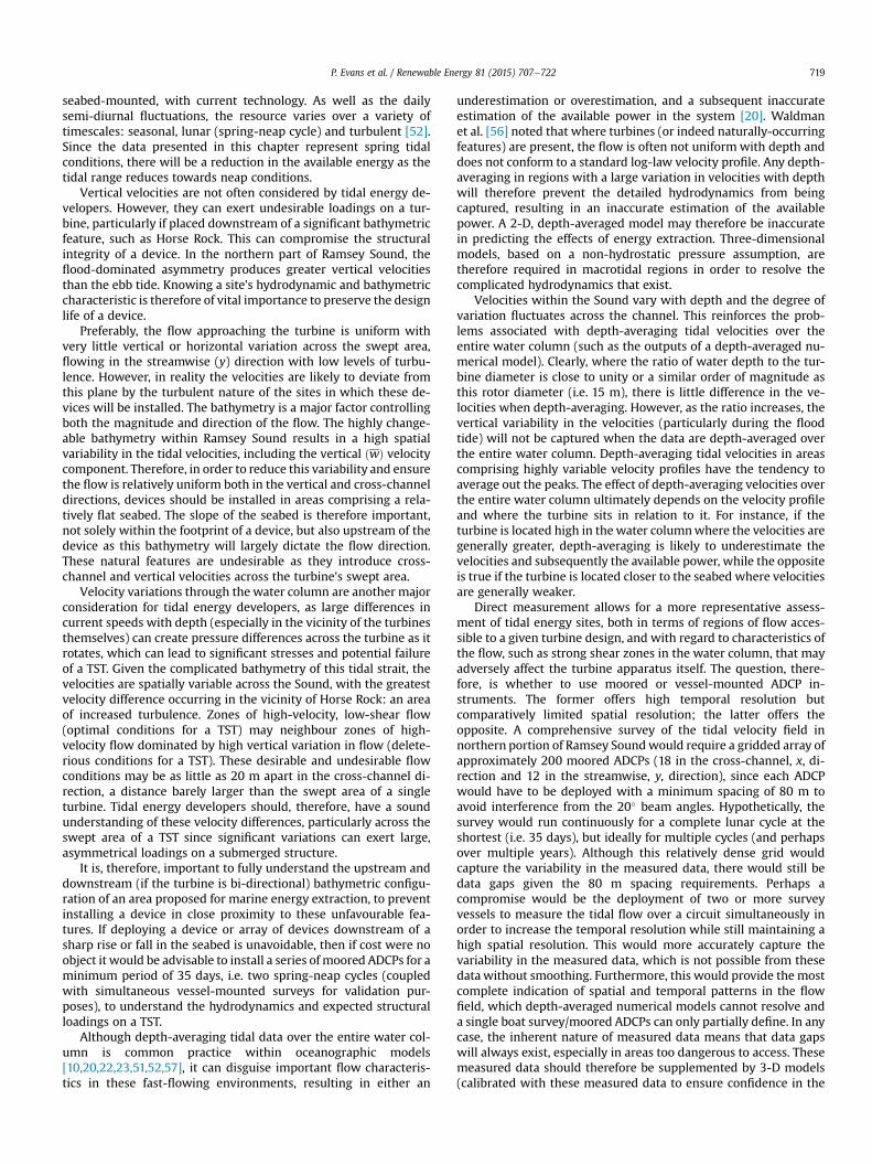
Fig. 9. Power flux over a typical spri

shows the equivalent power flux for the ebb tide (transects T4eT6).The zone of maximum power differs on each tidal peak. During peakflood conditions, maximum power flux is focussed to the east of thedeep channel invert and to the east of Horse Rock, while at peak ebb,the power peaks to the western side of the channel invert. Fig. 7dshows the power flux (calculated from the vertically-averaged ðvtÞvelocity over the swept area of the 15 m TST) during the peak of theflood tide, reaching 27.4 kWm�2. Figs. 7e and 8e display the effect ofdepth-averaging streamwise velocities over the entire water columnðvdÞ on power availability during the peak of the flood and ebb tidesrespectively, by subtracting from the velocity data only averagedover the vertical area of a 15 m TST ðvtÞ. There is a general under-estimation of the power flux during the peak of the flood tide;however, power flux in the vicinity of Horse Rock is overestimatedby approximately 2 kW m�2. As would be expected, there is littledifference in the power fluxwhen vertically-averaging the data overthe 15 m TST swept area ðvtÞ compared to over the entire watercolumn ðvdÞ in the shallower outer margins of the Sound given thesimilar flow depths and lower velocities. In the deeper regions,however, there is a greater difference between vertical swept areaðvtÞ and water-column ðvdÞ depth-averaged velocity. During theflood tide (particularly at transects T2 and T3) the velocities accel-erate as they pass Horse Rock, resulting in increased velocities to theimmediate east and west. Furthermore, within the area of acceler-ated flow to the west of Horse Rock, the velocities are generallygreater within the 15 m swept area compared with higher in thewater column. This therefore results in an underestimation in thevelocity and power availability when depth-averaging over theentire water column. Table 1 shows the power flux based on boththe vertically-averaged velocities over the 15 m TST swept area ðvtÞand over the entire water column ðvdÞ. This comparison suggeststhat depth-averaging velocity over the entire water column ðvdÞtends to underestimate the velocities and power flux in energetic,

ng tidal cycle in Ramsey Sound.

P. Evans et al. / Renewable Energy 81 (2015) 707e722718

macrotidal tidal straits. It is therefore recommended to calculatepower flux over the swept area of a TST.

Temporal variability in the tidal velocity also controls power fluxover daily (semi-diurnal), monthly (spring-neap cycle) and yearlytimescales. Fig. 9 displays the temporal variability of power duringa typical spring flood and ebb tidal cycle, based on the area of theSound that experiences the greatest streamwise ðvtÞ velocities overthe TST swept area. Power across the turbine's 15 m swept areafluctuates over both the flood and ebb tides, peaking at 4840 kWand 620 kW respectively. The flood-dominated tidal asymmetry isclear, with maximum power at the peak of the ebb tide 13% lowerthan that of the equivalent phase of the flood tide.

3.5. Physical constraints of TST deployment

A tool has been developed as part of a separate study using theEonfusion software [50] to identify suitable TST sites based on thevertically-averaged velocities over a 15 m diameter turbine ðvtÞ, thebed slope and water depth. Fig. 10 from Evans et al. [50] is includedfor completeness as it is important to this discussion. This plotshows suitable areas for TST deployment based on a vt value of2 m s�1, a maximum bed slope of 5� and a minimumwater depth of30 m. The resultant velocities have subsequently been converted topower flux using Eq. (1). Only 2% of this portion of the Sound meetthese requirements during the peak of the flood tide and, given thelower velocities associated with the peak of the ebb tide, no areasare viable. Furthermore, suitable areas are extremely limited inextent and therefore depending on the TST design (i.e. TST arrays)could prove impractical.

4. Discussion

This energetic, macrotidal strait exhibits a complicated flowregime, with high spatial variability in tidal velocities and a markedflood-dominated tidal asymmetry to the north of The Bitches reef.Tidal asymmetry, which is the variation in current speed betweenthe flood and ebb phases of the tidal cycle, is an importantparameter to consider when designing a TST device. This parameteris not routinely considered when selecting suitable TST sites, but

Fig. 10. Contour plot of power flux for suitable TST areas at peak flood and ebb based on a2 m s�1, a minimum water depth of 30 m and a maximum seabed slope of 5� .

one that has an important role in quantifying the resource. A 2-Dhydrodynamic TELEMAC model of the area [51] suggests that thevariability between the flood and ebb tides could be due in part tothe narrowing of Ramsey Sound between The Bitches and themainland, as suggested by Fairley et al. [18], which accelerates theflow as it is laterally constrained through the narrow channel.Furthermore, the configuration of the coastline to the north ofRamsey Sound, particularly the promontory of St David's Head,directs the ebbing flow to the west of Ramsey Island.

Tidal asymmetry is not limited to Ramsey Sound with manycoastal areas experiencing this phenomenon [52e55]. Neill et al.[52] examined this parameter in Orkney, Scotland using a high-resolution 3-D ROMS tidal model. Many turbine designs,including TEL's TST, are two-way generating, i.e. turbines are able toharness both the flood and ebb tidal currents. In Ramsey Sound,maximum power flux during the flood tide is approximately 13%higher than the equivalent phase of the ebb tide.

Designing a TST with a yaw system allows the turbine to faceinto the principal tidal flow. This has its advantages, for examplewhere the flood and ebb tidal velocities are of a similar magnitude.However, many coastal areas (as identified by Neill et al. [52]) areeither flood-dominated or ebb-dominated, which raises the ques-tion of the need for such a yaw system if, during the peak of theweaker tidal regime, there is insufficient power available for eco-nomic viability. This research has shown that the northern portionof Ramsey Sound has a flood-dominated tidal asymmetry, withminimal power available during the peak of the ebb tide. Whenaccounting for the turbine's power coefficient (Cp), the extractablepower will be less, which greatly reduces the economic viability. Aspower flux is proportional to the cube of the velocity, even smallchanges in the flow lead to substantial fluctuations in power-output, which is consistent with previous observations of tidalasymmetry [52].

Although the data presented here reflect the peak of a typicalspring flood and ebb tide, the magnitudes of the velocities arelower at other phases of the tidal cycle. This daily fluctuation inenergy results in a further reduction in suitable locations for TSTs,which suggests that this portion of the fast-flowing strait is not aviable energy extraction area for large arrays of TSTs, particularly

minimum vertically-averaged streamwise velocity over the 15 m TST swept area ðvtÞ of

P. Evans et al. / Renewable Energy 81 (2015) 707e722 719

seabed-mounted, with current technology. As well as the dailysemi-diurnal fluctuations, the resource varies over a variety oftimescales: seasonal, lunar (spring-neap cycle) and turbulent [52].Since the data presented in this chapter represent spring tidalconditions, there will be a reduction in the available energy as thetidal range reduces towards neap conditions.

Vertical velocities are not often considered by tidal energy de-velopers. However, they can exert undesirable loadings on a tur-bine, particularly if placed downstream of a significant bathymetricfeature, such as Horse Rock. This can compromise the structuralintegrity of a device. In the northern part of Ramsey Sound, theflood-dominated asymmetry produces greater vertical velocitiesthan the ebb tide. Knowing a site's hydrodynamic and bathymetriccharacteristic is therefore of vital importance to preserve the designlife of a device.

Preferably, the flow approaching the turbine is uniform withvery little vertical or horizontal variation across the swept area,flowing in the streamwise (y) direction with low levels of turbu-lence. However, in reality the velocities are likely to deviate fromthis plane by the turbulent nature of the sites in which these de-vices will be installed. The bathymetry is a major factor controllingboth the magnitude and direction of the flow. The highly change-able bathymetry within Ramsey Sound results in a high spatialvariability in the tidal velocities, including the vertical ðwÞ velocitycomponent. Therefore, in order to reduce this variability and ensurethe flow is relatively uniform both in the vertical and cross-channeldirections, devices should be installed in areas comprising a rela-tively flat seabed. The slope of the seabed is therefore important,not solely within the footprint of a device, but also upstream of thedevice as this bathymetry will largely dictate the flow direction.These natural features are undesirable as they introduce cross-channel and vertical velocities across the turbine's swept area.

Velocity variations through the water column are another majorconsideration for tidal energy developers, as large differences incurrent speeds with depth (especially in the vicinity of the turbinesthemselves) can create pressure differences across the turbine as itrotates, which can lead to significant stresses and potential failureof a TST. Given the complicated bathymetry of this tidal strait, thevelocities are spatially variable across the Sound, with the greatestvelocity difference occurring in the vicinity of Horse Rock: an areaof increased turbulence. Zones of high-velocity, low-shear flow(optimal conditions for a TST) may neighbour zones of high-velocity flow dominated by high vertical variation in flow (delete-rious conditions for a TST). These desirable and undesirable flowconditions may be as little as 20 m apart in the cross-channel di-rection, a distance barely larger than the swept area of a singleturbine. Tidal energy developers should, therefore, have a soundunderstanding of these velocity differences, particularly across theswept area of a TST since significant variations can exert large,asymmetrical loadings on a submerged structure.

It is, therefore, important to fully understand the upstream anddownstream (if the turbine is bi-directional) bathymetric configu-ration of an area proposed for marine energy extraction, to preventinstalling a device in close proximity to these unfavourable fea-tures. If deploying a device or array of devices downstream of asharp rise or fall in the seabed is unavoidable, then if cost were noobject it would be advisable to install a series ofmoored ADCPs for aminimum period of 35 days, i.e. two spring-neap cycles (coupledwith simultaneous vessel-mounted surveys for validation pur-poses), to understand the hydrodynamics and expected structuralloadings on a TST.

Although depth-averaging tidal data over the entire water col-umn is common practice within oceanographic models[10,20,22,23,51,52,57], it can disguise important flow characteris-tics in these fast-flowing environments, resulting in either an

underestimation or overestimation, and a subsequent inaccurateestimation of the available power in the system [20]. Waldmanet al. [56] noted that where turbines (or indeed naturally-occurringfeatures) are present, the flow is often not uniform with depth anddoes not conform to a standard log-law velocity profile. Any depth-averaging in regions with a large variation in velocities with depthwill therefore prevent the detailed hydrodynamics from beingcaptured, resulting in an inaccurate estimation of the availablepower. A 2-D, depth-averaged model may therefore be inaccuratein predicting the effects of energy extraction. Three-dimensionalmodels, based on a non-hydrostatic pressure assumption, aretherefore required in macrotidal regions in order to resolve thecomplicated hydrodynamics that exist.

Velocities within the Sound vary with depth and the degree ofvariation fluctuates across the channel. This reinforces the prob-lems associated with depth-averaging tidal velocities over theentire water column (such as the outputs of a depth-averaged nu-merical model). Clearly, where the ratio of water depth to the tur-bine diameter is close to unity or a similar order of magnitude asthis rotor diameter (i.e. 15 m), there is little difference in the ve-locities when depth-averaging. However, as the ratio increases, thevertical variability in the velocities (particularly during the floodtide) will not be captured when the data are depth-averaged overthe entire water column. Depth-averaging tidal velocities in areascomprising highly variable velocity profiles have the tendency toaverage out the peaks. The effect of depth-averaging velocities overthe entire water column ultimately depends on the velocity profileand where the turbine sits in relation to it. For instance, if theturbine is located high in the water columnwhere the velocities aregenerally greater, depth-averaging is likely to underestimate thevelocities and subsequently the available power, while the oppositeis true if the turbine is located closer to the seabed where velocitiesare generally weaker.

Direct measurement allows for a more representative assess-ment of tidal energy sites, both in terms of regions of flow acces-sible to a given turbine design, and with regard to characteristics ofthe flow, such as strong shear zones in the water column, that mayadversely affect the turbine apparatus itself. The question, there-fore, is whether to use moored or vessel-mounted ADCP in-struments. The former offers high temporal resolution butcomparatively limited spatial resolution; the latter offers theopposite. A comprehensive survey of the tidal velocity field innorthern portion of Ramsey Soundwould require a gridded array ofapproximately 200 moored ADCPs (18 in the cross-channel, x, di-rection and 12 in the streamwise, y, direction), since each ADCPwould have to be deployed with a minimum spacing of 80 m toavoid interference from the 20� beam angles. Hypothetically, thesurvey would run continuously for a complete lunar cycle at theshortest (i.e. 35 days), but ideally for multiple cycles (and perhapsover multiple years). Although this relatively dense grid wouldcapture the variability in the measured data, there would still bedata gaps given the 80 m spacing requirements. Perhaps acompromise would be the deployment of two or more surveyvessels to measure the tidal flow over a circuit simultaneously inorder to increase the temporal resolution while still maintaining ahigh spatial resolution. This would more accurately capture thevariability in the measured data, which is not possible from thesedatawithout smoothing. Furthermore, this would provide the mostcomplete indication of spatial and temporal patterns in the flowfield, which depth-averaged numerical models cannot resolve anda single boat survey/moored ADCPs can only partially define. In anycase, the inherent nature of measured data means that data gapswill always exist, especially in areas too dangerous to access. Thesemeasured data should therefore be supplemented by 3-D models(calibrated with these measured data to ensure confidence in the

P. Evans et al. / Renewable Energy 81 (2015) 707e722720

modelled outputs) to provide a broader understanding of the tidalresource.

Power flux decreases with downstream distance from HorseRock, and the maximum power is localised on either side of thepinnacle as the flow accelerates around this feature. This paper hasindicated that power flux is minimal near the outer margins of theSound. Furthermore, although there appear to be power hotspots inthe high velocity region that separates around Horse Rock, the steepbed slope presents a new complicating factor for TST placement,especially for gravity-based systems [18]. Seabed topology is rarelyflat and conditions vary significantly around the coast. An irregularor undulating seabed is more suited to piled foundations becausebed preparation is very difficult for gravity structures [47]. Arraysthat mount multiple turbines on a single structure (as opposed tothe one tower, typical of wind turbines, for example) requirereasonably low gradient beds. A number of TSTs are gravity-mounted and can only tolerate relatively low bed slopes. TEL'sDeltaStream™ device can tolerate a maximum bed slope of 5� (PBromley, December 2013, pers. comm.), which results in a basewidth of 20 m having a vertical drop of approximately 1.7 m acrossthe structure. Lower bed slopes are desirable since the base has toremain stable. The maximum tolerable bed slope is dependent onthe devicemounting/anchoring arrangement but could be increasedfor a piled device. For the purposes of this study, a gravity-baseddevice or small array of turbines sharing a common structure wasused. Assuming no blasting or excavation of the Ramsey Soundchannel bottom, local bed slope in several locations within thechannel render high-energy zones functionally inaccessible.

Water depth is another limiting factor. The majority of TSTs aredeployed in water depths exceeding 30 m [24] since many devicesextend approximately 20 m from the seabed to the tip of the tur-bine. A minimum 5 m clearance is normally recommended forrecreational activities (small boats, etc.), as well as to minimiseturbulence and wave loading effects on the TSTs and damage fromfloating materials on the assumption that an exclusion zone becreated restricting vessels with a draught greater than 2 m [58].This generally results in a minimum water depth of 25e30 m withthe inclusion of a 5e10 m freeboard. The bathymetry data (Fig. 1)shows that there are large areas that meet this criterion. However,these are generally confined to the deep, steep trench. Bryden et al.[40] noted that where there is no exclusion of shipping, the top tipof the turbine has to be at the lowest astronomical tide (LAT) withadditional safety factors to account for the lowest negative stormsurge (�1.5 m), the trough of a 5mwave (�2.5 m) and shipping andwaves (�5 m). Therefore, based on this guidance and using TEL'sDeltaStream™ device configuration, a 15m diameter rotor with thehub set 12 m from the seabed requires a minimum water depth of33.5 m. However, vessel activity within Ramsey Sound is restrictedto local fishing and coastal vessels, which have a draught rarelyextending 5m below thewater surface. Bryden et al. [40] also notedthat the bottom tip of the turbine must not be within 25% of thewater depth from the seabed. This portion of the water column issubject to large vertical velocity shears due to bed friction.

To takemaximum advantage of the tidal stream resource both inthe UK and on a global scale, it will be necessary to design devicesthat can operate in water depths less than 30 m, subject to navi-gational and other physical constraints. This was realised byPacheco et al. [24] who noted that deploying devices in shallowerwater has the added benefit of being in closer proximity to theelectrical grid and associated infrastructure.

Given the importance of bed slope in determining suitable TSTlocations, a high resolution (2 m in the horizontal plane) bathy-metric grid has been used. This detailed bathymetry accounts forsmall-scale irregularities in the seabed, which are masked by eithercoarser bathymetric grids and/or low mesh resolution; an inherent

limitation of far-field oceanographic models. These models gener-ally employ an unstructured mesh with a relatively coarse gridaway from the area of interest with increasing resolution as dis-tance to the site decreases. However, grid sizes are often still toolarge at the area of interest to capture the local bathymetric irreg-ularities, which, as shown previously, can have a significant influ-ence on the flow. Haverson et al. [59] developed a 2-D depth-averaged TELEMAC model of the Pembrokeshire coast, refined atRamsey Sound with a mesh resolution of approximately 35 m.Aside from the fact that the model is depth-averaged, which hasbeen shown generally to underestimate the velocities in thesemacrotidal straits thereby masking the detailed flow structures, abathymetric resolution of 30 m has been mapped onto the 35 mmesh. This relatively coarse grid is likely to ignore the small-scalebathymetric features, such as Horse Rock, which are highly influ-ential on the local flow field. Much higher resolution bathymetricdata of the area exist (~2 m resolution) and have been used toinform this paper. Embedding this grid into this TELEMAC model(coupled with a finer mesh) would improve the accuracy andconfidence in the modelled outputs (particularly if further valida-tion is undertaken). Sensitivity tests using smaller mesh sizes andideally higher resolution bathymetric grids should be a prerequisitefor these types of models to determine their accuracy. Thesemodels are therefore appropriate for larger-scale far-field model-ling of sediment dynamics, for example, but become problematicwhen attempting to resolve medium- to near-field (i.e. CFD)modelling issues, such as TST array impacts on the local flow fieldusing an extra sink in the momentum equations.

Furthermore, use of these far-field models as a tool to identifyviable TST sites based on bed slope tolerances may not be practi-cable, as the coarser grids can smooth and even ignore importantbathymetric features that may otherwise (i.e. if a higher resolutionbathymetric grid was used) prevent a site from being developed.Until computer technology advances such that finer grids can beutilised to resolve these small-scale features, it is prudent to usethese finer grids outside a numerical model, such as within GIS-based software, to ensure seabed gradients can be accuratelydefined at proposed TST sites.

5. Conclusions

This paper has examined the viability of narrow, fast-flowingtidal straits for TST development, using Ramsey Sound as a fieldsite. The bathymetric configuration of this area largely dictates themagnitude and direction of the tidal currents as they pass throughthe Sound, which gives rise to a high spatial variability and a flood-dominated tidal asymmetry within the northern portion of theSound. This raises questions as to whether a yaw system in thislocation is required. From a structural integrity perspective, it maybe more practical to have a yaw system despite there being a strongtidal asymmetry in order to direct the turbine into the oncomingcurrent, thereby reducing the loading. Site-specific resource as-sessments of any potential tidal energy area should therefore beundertaken prior to the TST design stage.

Depth-averaging streamwise velocity data over the entire watercolumn in these energetic, macrotidal environments generallyunderestimates the velocities and therefore the power flux in thesystem when compared to vertically-averaging over the TST sweptarea. This is likely to result in an inaccurate estimation of theavailable energy in the system. Therefore, reliance on 2-D depth-averaged numerical models in dynamic tidal regions should beavoided and substituted with a 3-D model.

Based on a survey that encompasses a significant portion ofRamsay Sound, very few areas exist (at least with the specificationsof the device intended for Ramsey Sound) where streamwise

P. Evans et al. / Renewable Energy 81 (2015) 707e722 721

velocity ðvtÞ, bed slope and water depth are accounted for. Theseparameters are typically overlooked but essential to extractableresource estimates and for insight into realistic TST performance.Locating a flat area of seabed to install a device with a large foot-print is difficult in areas with an irregular bathymetry. Designing adevice with a smaller footprint would allow a greater area of thechannel to the exploited. The TST design is therefore an importantconsideration since this ultimately dictates viable locations fordeployment. This paper has demonstrated that physical conditionsat energetic tidal straits reduce the extractable areas quiteconsiderably, particularly as TST devices will have to be installed inarrays if they are to achieve viable costs. This viability ultimatelydepends on the TST design, which should be considered after asite's tidal velocity field and bathymetry have been characterised.

Although the data used to inform this paper are related toRamsey Sound, many other tidal regions worldwide exhibit similarphysical and hydrodynamic characteristics. The present findingsare therefore transferrable and can be used to help understand thehydrodynamics at other energetic areas, which will ultimatelydictate the feasibility of and most suitable location for TSTs. Theinterest of the work presented here therefore goes beyond thismacrotidal strait, and ultimately the same methodology for a rangeof TST designs can be applied elsewhere.

Acknowledgements

This work was undertaken as part of the Low Carbon ResearchInstitute Marine Consortium (www.lcrimarine.org) (WEFO:80366). The authors wish to acknowledge the financial support ofWelsh Government, the Higher Education Funding Council forWales, the Welsh European Funding Office and the EuropeanRegional Development Fund Convergence Programme. The authorsalso acknowledge the collaboration of LCRIMarine partners, RNLI StDavid's and St Justinian's Boat Owners Association. The authors alsowish to thank Tidal Energy Ltd. for their valuable advice and sup-port. Warwick Gillespie is also acknowledged for his ongoingtechnical support with the Eonfusion software. Finally, Dr EliLazarus of Cardiff University's School of Earth and Ocean Sciences isacknowledged for his invaluable input into this paper.

References

[1] Denny E. The economics of tidal energy. Energy Policy 2009;37(5):1914e24.[2] Black and Veatch. Tidal stream energy resource and technology summary

report. Carbon Trust; 2005.[3] Easton MC, Woolf DK, Bowyer A. The dynamics of an energetic tidal channel,

the Pentland Firth, Scotland. Cont Shelf Res 2012;48:50e60.[4] Bryden IG, Couch SJ, Owen A, Melville G. Tidal current resource assessment.

Proc IMechE Part A J Power Energy 2007;221:125e35.[5] Dewey R, Richmond D, Garrett C. Stratified tidal flow over a bump. J Phys

Oceanogr 2005;35:1911e27.[6] O'Rourke F, Boyle F, Reynolds A. Tidal energy update 2009. Appl Energy

2010;87:398e409.[7] Cooper B. Enhanced tidal resource assessment within the Western Isles. In:

Wave and tidal 2011; 2011.[8] Black and Veatch Ltd. Phase II UK tidal stream energy resource assessment.

Carbon Trust; 2005.[9] ABPmer. Atlas of UK marine renewable energy resources: technical report.

Department for Business, Enterprise & Regulatory Reform; 2008.[10] Serhadlioglu S, Adcock T, Houlsby G, Draper S, Borthwick A. Tidal stream

energy resource assessment of the Anglesey Skerries. Int J Mar Energy2013;3e4:98e111.

[11] Fairley I, Evans PS, Wooldridge CF, Willis M, Masters I. Evaluation of tidalstream resource in a potential array area via direct measurements. RenewEnergy 2013;57:70e8.

[12] Evans PS, Armstrong S, Wilson C, Fairley I, Wooldridge CF, Masters I. Char-acterisation of a highly energetic tidal energy site with specific reference tohydrodynamics and bathymetry. In: Proc. 10th European wave and tidal en-ergy conference (EWTEC), Aalborg, Denmark; 2013.

[13] Willis M, Masters I, Thomas S, Gallie R, Loman J, Cook A, et al. Tidal turbinedeployment in the Bristol Channel: a case study. Proc ICE Energy 2010;163(3):93e105.

[14] Welsh Government. A low carbon revolution e the Welsh Assembly gov-ernment energy policy statement. Report CMK-22-01-196. 2010.

[15] Walkington I, Burrows R. Modelling tidal stream power potential. Appl OceanRes 2009;31:239e45.

[16] Blunden L, Bahaj A. Tidal energy resource assessment for tidal stream gen-erators. Proc IMechE Part A J Power Energy 2007;221:137e46.

[17] Tidal Energy Limited. DeltaStream demonstrator project Ramsey Sound,Pembrokeshire e non-technical summary. 2009.

[18] Fairley I, Neill SP, Wrobelowski T, Willis M, Masters I. Potential array sites fortidal stream turbine electricity generation off the Pembrokeshire coast. In:Proc. 9th European wave and tidal energy conference (EWTEC), Southampton,UK; 2011.

[19] MEP. MEP webpage on DeltaStream device [Online]. Available: http://www.marineenergypembrokeshire.co.uk/wales-moves-one-step-closer-to-capturing-tidal-energy-potential; 2011.

[20] Easton MC, Harendza A, Wool DK, Jackson AC. Characterisation of a tidalenergy site: hydrodynamics and seabed structure. In: Proc. 9th Europeanwave and tidal energy conference (EWTEC), Southampton, UK; 2011.

[21] Marine Scotland. Pentland Firth and Orkney waters marine spatial planframework & regional locational guidance for marine energy. Aecom andMetoc for the Scottish Government; 2011.

[22] EastonMC,Woolf DK, Pans S. An operational hydrodynamicmodel of a key tidalenergy site: Inner Sound of Stroma, Pentland Firth (Scotland, UK). In: Proc. 3rdinternational conference on ocean energy (ICOE), Bilbao, Spain; 2010.

[23] Neill SP, Elliott AJ. In situ measurements of spring-neap variations to unsteadyisland wake development in the Firth of Forth, Scotland. Estuar Coast Shelf Sci2004;60:229e39.

[24] Pacheco A, Ferreira �O, Carballo R, Iglesias G. Evaluation of the production oftidal stream energy in an inlet channel by coupling field data and numericalmodelling. Energy 2014;71:104e17.

[25] Carballo R, Iglesias G, Castro A. Numerical model evaluation of tidal streamenergy resources in the Ría de Muros (NW Spain). Renew Energy 2009;34:1517e24.

[26] Ramos V, Iglesias G. Performance assessment of tidal stream turbines: aparametric approach. Energy Convers Manag 2013;69:49e57.

[27] Ramos V, Carballo R, �Alvarez M, S�anchez M, Iglesias G. Assessment of theimpacts of tidal stream energy through high-resolution numerical modeling.Energy 2013;61:541e54.

[28] Ramos V, Carballo R, Sanchez M, Veigas M, Iglesias G. Tidal stream energyimpacts on estuarine circulation. Energy Convers Manag 2014;80:137e49.

[29] Sanchez M, Carballo R, Ramos V, Iglesias G. Floating vs. bottom-fixed turbinesfor tidal stream energy: a comparative impact assessment. Energy 2014;72:691e701.

[30] Boake C. Tidal turbine ADCP monitoring in Strangford Lough e 1/10th to fullscale experience. International standards update. In: Proc. 1st Nortek offshorerenewable symposium; 26the27th October 2011. Heathrow, London.

[31] Mason-Jones A, O'Doherty DM, Morris CE, O'Doherty T. Influence of a velocityprofile & support structure on tidal stream turbine performance. Renew En-ergy 2013;52:23e30.

[32] Lewis M, Neill SP, Robins PE, Hashemi MR. Resource assessment for futuregenerations of tidal-stream energy arrays. Energy 2015;83:403e15.

[33] Taylor GI. Tidal friction in the Irish Sea. Philos Trans R Soc 1919;220:1e93.[34] Robins PE, Neill SP, Lewis MJ, Ward SL. Characterising the spatial and tem-

poral variability of the tidal-stream energy resource over the northwest Eu-ropean shelf seas. Appl Energy 2015;147:510e22.

[35] Togneri M, Masters I. Comparison of turbulence characteristics for selectedtidal stream power extraction site. In: Proc. 9th engineering turbulencemodelling and measurements conference, Thessaloniki, Greece; 2012.

[36] Togneri M, Masters I. Comparison of marine turbulence characteristics forsome potential turbine installation sites. In: Proc. 4th international conferenceon ocean energy (ICOE), Dublin, Ireland; 2012.

[37] Pingree RD, Griffiths DK. Sand transport paths around the British Islesresulting from the M2 and M4 tidal constituents. J Mar Biol Assoc U K1979;59:497e513.

[38] Teledyne RD Instruments. Workhorse sentinel datasheet [Online]. Available:http://www.rdinstruments.com/datasheets/wh_sentinel.pdf; 2009.

[39] Yoshikawa Y, Matsuno T, Marubayashi K, Fukudome K. A surface velocityspiral observed with ADCP and HF radar in the Tsushima Strait. J Geophys Res2007;112.

[40] Bryden IG, Naik S, Fraenkel P, Bullen CR. Matching tidal current plants to localflow conditions. Energy 1998;23:699e709.

[41] Frost C, Evans PS,Morris CE,Mason-Jones A, O'Doherty T, O'Doherty D. The effectof axialflowmisalignment on tidal turbineperformance. In: Proc. 1st int. conf. onrenewable energies offshore; 24the26th November 2014. Lisbon, Portugal.

[42] Mason-Jones A, O'Doherty DM, Morris CE, O'Doherty T, Byrne CB, Prickett PW,et al. Non-dimensional scaling of tidal stream turbines. Energy 2012;44:820e9.

[43] Woolf DK. The strength and phase of the tidal stream. Int J Mar Energy2013;3e4:3e13.

[44] Couch SJ, Bryden IG. Tidal current energy extraction: hydrodynamic resourcecharacteristics. Proc Inst Mech Eng Part M J Eng Marit Environ 2006;220(4):185e94.

[45] South-West Regional Development Agency. Offshore renewables resourceassessment and development (ORRAD) project e technical report. 2010.

[46] Harding SF, Bryden IG. Directionality in prospective Northern UK tidal currentenergy deployment sites. Renew Energy 2012;44:474e7.

P. Evans et al. / Renewable Energy 81 (2015) 707e722722

[47] Sustainable Energy Ireland. Tidal & current energy resources in Ireland. 2008.[48] PMSS. Offshore renewables resource assessment and development (ORRAD)

project e technical report. South Wales Regional Development Agency; 2010.[49] Renewable UK. Wave and tidal energy in the UK e state of the industry report.

2011.[50] Evans PS, Allmark M, O'Doherty T. Are energetic tidal straits suitable for po-

wer generation?. In: Proc. 13th world renewable energy congress (WREC);4e8th August 2014. London, UK.

[51] Hashemi MR, Neill SP, Davies AG. A numerical study of wave and currentfields around Ramsey Island e tidal energy resource assessment. In: Proc.XIXth TELEMAC-MASCARET user conference, Oxford, UK; 2012.

[52] Neill SP, Hashemi MR, Lewis MJ. The role of tidal asymmetry in characterizingthe tidal energy resource of Orkney. Renew Energy 2014;68:337e50.

[53] Brown JM, Davies AG. Flood/ebb tidal asymmetry in a shallow sandy estuaryand the impact on net sand transport. Geomorphology 2010;114:431e9.

[54] Iglesias G, Carballo R. Can the seasonality of a small river affect a large tide-dominated estuary? The case of Ría de Viveiro, Spain. J Cont Res 2011;27:1170e82.

[55] Goddijn-Murphy L, Woolf DK, Easton MC. Current patterns in the Inner Sound(Pentland Firth) from underway ADCP data. J Atmos Ocean Technol 2013;30:96e111.

[56] Waldman S, Miller C, Baston S, Side J. Comparison of two hydrodynamicmodels for investigating energy extraction from tidal flows. In: Proc. of the2nd environmental interactions of marine renewable energy technologies(EIMR) conference; 28th Maye2nd June 2014. Stornoway, Isle of Lewis, OuterHebrides, Scotland.

[57] Draper S, Houlsby GT, Oldfield MLG, Borthwick AGL. Modelling tidal energyextraction in a depth-averaged coastal domain. In: Proc. 8th European waveand tidal energy conference (EWTEC), Uppsala, Sweden; 2009.

[58] Legrand C. Assessment of tidal energy resource e marine renewable energyguides. London: EMEC; 2009.

[59] Haverson D, Bacon J, Smith H. Changes to eddy propagation due to tidal arrayat Ramsey Sound. In: Proc. of the 2nd environmental interactions of marinerenewable energy technologies (EIMR) conference; 28th Maye2nd June 2014.Stornoway, Isle of Lewis, Outer Hebrides, Scotland.