arX

iv:1

005.

4699

v1 [

astr

o-ph

.CO

] 2

5 M

ay 2

010

Mon. Not. R. Astron. Soc. 000, 1–10 (2010) Printed 16 December 2013 (MN LATEX style file v2.2)

A High Signal to Noise Map of the Sunyaev-Zel’dovich

increment at 1.1 mm wavelength in Abell 1835

P. F. Horner1⋆, P. D. Mauskopf1⋆, J. Aguirre2, J. J. Bock3, E. Egami4,

J. Glenn5, S. R. Golwala6, G. Laurent5, H. T. Nguyen3

and J. Sayers61 Cardiff School of Physics and Astronomy, Cardiff University, 1 The Parade, Cardiff, CF24 3AA, Wales2 Department of Physics and Astronomy, University of Pennsylvania, 209 South 33rd Street, Philadelphia, PA 191043 Jet Propulsion Laboratory, California Institute of Technology, 4800 Oak Grove Drive, Pasadena, CA911094 Department of Astronomy/Steward Observatory, 933 North Cherry Avenue, Rm. N204, Tucson, AZ 85721-00655 Center for Astrophysics and Space Astronomy & Department of Astrophysical and Planetary Sciences,University of Colorado, 389 UCB, Boulder, CO6 Division of Physics, Mathematics, & Astronomy, California Institute of Technology, Mail Code 59-33,Pasadena, CA 91125

Draft 2010 May 25

ABSTRACT

We present an analysis of an 8 arcminute diameter map of the area around the galaxycluster Abell 1835 from jiggle map observations at a wavelength of 1.1 mm usingthe Bolometric Camera (Bolocam) mounted on the Caltech Submillimeter Observa-tory (CSO). The data is well described by a model including an extended Sunyaev-Zel’dovich (SZ) signal from the cluster gas plus emission from two bright backgroundsubmm galaxies magnified by the gravitational lensing of the cluster. The best-fitvalues for the central Compton value for the cluster and the fluxes of the two mainpoint sources in the field: SMM J140104+0252, and SMM J14009+0252 are foundto be y0 = (4.34 ± 0.52 ± 0.69) × 10−4, 6.5±2.0 ± 0.7 mJy and 11.3±1.9± 1.1 mJy,where the first error represents the statistical measurement error and the second errorrepresents the estimated systematic error in the result. This measurement assumesthe presence of dust emission from the cluster’s central cD galaxy of 1.8 ± 0.5 mJy,based on higher frequency observations of Abell 1835. The cluster image representsone of the highest-significance SZ detections of a cluster in the positive region of thethermal SZ spectrum to date. The inferred central intensity is compared to other SZmeasurements of Abell 1835 and this collection of results is used to obtain values fory0 = (3.60± 0.24)× 10−4 and the cluster peculiar velocity vz = −226± 275 km/s.

Key words: infrared: galaxies – galaxies: clusters: general – methods: data analysis

1 INTRODUCTION

The Sunyaev Zel’dovich (SZ) effect (Sunyeav & Zel’dovich1970) is the redistribution of energy in the Cosmic Mi-crowave Background (CMB) spectrum due to interationsbetween CMB photons and hot electrons along the line ofsight between the surface of last scattering and an observer.The main source for the SZ effect is from the hot gas thatexists in the intra-cluster medium (ICM) of massive galaxyclusters (Birkinshaw 1999; Carlstrom, Holder & Reese 2002;Rephaeli, Sadeh & Shimon 2006). The SZ actually com-prises two effects. The thermal effect consists of a dimming

⋆ E-mail: Piers.Horner@astro.cf.ac.uk (PFH);Philip.Mauskopf@astro.cf.ac.uk (PDM)

or decrement in the apparent brightness of the CMB to-wards a galaxy cluster at low frequencies and a correspond-ing brightening or increment at high frequencies with thenull crossover point at approximately 215 GHz. The kine-matic effect has the spectral dependence of a standard tem-perature shift in the CMB which has the same sign at allfrequencies. The two effects can therefore be distinguishedfrom each other with measurements at multiple frequencies.

Measurements of the amplitude of the SZ thermaldistortion towards a cluster can be combined with mea-surements of the X-ray emission to determine the angu-lar diameter distance, dA, whose value depends on cos-mology (Birkinshaw, Hughes & Arnaud 1991). Estimatesof the Hubble constant have been made using thistechnique for a number of clusters (e.g. Jones (1995);Grainge (1996); Holzapfel et al. (1997); Tsuboi et al. (1998);

2 Horner, et al.

Mauskopf et al. (2000); Reese (2003); Battistelli et al.(2003); Udomprasert et al. (2004)) and can be used to con-strain cosmological models. In addition, because the SZsurface brightness for a cluster with a given mass is al-most independent of redshift, SZ surveys can give infor-mation about the evolution of the number counts of clus-ters vs. redshift. This depends strongly on the evolutionof the so-called dark energy or cosmological constant andtherefore SZ surveys have been identified as one of the keyprobes of the nature of dark energy (e.g. Diego et al. (2002);Weller, Bettye & Kneissl (2002); DeDeo, Spergel & Trac(2005); Albrecht et al. (2006); Bhattacharya & Kosowsky(2007)). A number of dedicated SZ surveys are alreadyproducing results, in particular the Atacama CosmologyTelescope (ACT) and the South Polar Telescope (SPT)(Plagge et al. 2009; Hincks et al. 2009; High et al. 2010).

Most of the SZ detections reported to date have beenmade at low frequencies corresponding to the SZ decre-ment. Follow-up photometric or spectroscopic measurementsof known clusters at higher frequencies would significantlyimprove the precision in the measurement of the kinematicSZ effect as well as constraining possible contamination inthe low frequency data. Measurements at high frequenciescorresponding to the SZ increment suffer from confusionfrom emission from dusty galaxies, including backgroundhigh redshift galaxies amplified by the gravitational lensingof the cluster as well as increased atmospheric contamina-tion from ground-based telescopes. Accurate measurementof the SZ increment requires a combination of angular resolu-tion sufficient to resolve and remove point sources combinedwith high sensitivity and control of systematics necessary todetect the more diffuse SZ signal.

This paper presents analysis of observations of thegalaxy cluster Abell 1835 using the Bolometric Camera(Bolocam) mounted on the Caltech Submillimeter Observa-tory (CSO), situated on the summit of Mauna Kea, Hawaii.We also compare the results of this analysis with other setsof data taken at different wavelengths. Abell 1835 is one ofthe most luminous clusters observed in the ROSAT cata-logue and is well-known as a cooling core cluster. It is alsoknown to contain two lensed sub-mm point sources, SMMJ14009+0252 and SMM J140104+0252 (see e.g. Ivison et al.(2000); Zemcov et al. (2007)).

The paper is organized as follows: Section 2 describesthe observations with the Bolocam instrument; Section 3describes the analysis pipeline developed for processing thedata; Section 4 describes the modelling of the data and thedetermination of the characteristic parameters of the model(as well as the errors in their values), and Section 5 discussesthe results of the analysis of the Bolocam data and theircombination with other literature results.

2 OBSERVATIONS

The data used in this work represents approximately 12.5hours of observations taken over the course of five nightsat the end of January/ beginning of February 2006. Theobservations were made with Bolocam operating at 1.1 mm(275 GHz).

Bolocam consists of an array of 105 operationalneutron-transmutation-doped (NTD) Germanium spider-

web bolometers, capable of observing at 1.1 mm or 2.1 mm(Glenn et al. 1998; Haig et al. 2004). The system is cooledto 270 mK to allow the array to operate close to the photonbackground limit at 1.1 mm. The Bolocam array has a fieldof view of approximately 8 arcmin, and the beam FWHM is∼ 30” at 1.1 mm (and ∼ 60” at 2.1 mm).

The detector is mounted at the Cassegrain focus of theLeighton telescope - the 10.4 m CSO dish. The principalscience targets for the instrument include star forming re-gions in the galaxy, blank-field surveys for dusty extragalac-tic point sources; blank field SZ cluster surveys, and pointedobservations of galaxy clusters.

Observations by Bolocam incorporate a number of dif-ferent scan strategies. The majority of observations useraster scanning or lissajous scanning where the entire tele-scope is constantly in motion modulating the array positionon the sky.

The data presented in this paper was taken using jigglemapping. Jiggle mapping uses a combination of ’chopping’the secondary mirror during observations, i.e. switching thesecondary from side-to-side, and ’nodding’ the telescope, i.e.changing the position of the telescope during a scan. Thebeam moves from being ’on-source’ (imaging the region ofthe target and chopping away from it), to ’off-source’ (imag-ing a nearby region of blank sky and chopping onto the tar-get), then returns to being on-source once again (see Fig. 1).

Jiggle mapping is a means of removing sky backgroundfrom data, and works by differencing signal from so-called’target’ and ’reference’ beams (centered on the science targetand a region of ’blank’ sky, respectively). These beams arealso referred to as ’on’ and ’off’ beams. While jiggle-mappingis an efficient method of subtracting sky-noise, care has tobe taken to ensure that the chop ’throw’ (i.e. the maximumangular dispacement of the secondary during the chop) islarge enough that the off beam does not pick up signal fromthe source itself (subject to mechanical limitations). For thisreason, jiggle-mapping is not always suitable for imagingextended sources, but is good for observing point sources.

The chop frequency for this data set was 2.25 Hz, givinga chop period of ∼ 0.44 s (compared to a sampling rate of0.02 s). The chop throw was 90”, while the displacementbetween on and off beams during the nods was 2.5’. Thetelescope typically remained in the ’on’ or ’off’ phase forperiods of approximately 10 seconds.

The full set of data consisted of fifteen individual setsof observations of approximately 50 minutes each. The ob-servations were separated by shorter observations of planetsand other sources with known position and flux, which couldbe used for the calibration and pointing.

3 PIPELINE DEVELOPMENT

Because jiggle-mapping is a relatively new strategy for Bolo-cam, there was initially no pipeline in place to analyse theraw data. An independent pipeline was written specificallyfor this observing mode.

In its original form, the time-stream data had beensliced (i.e. separated into individual data-vectors represent-ing the signal from individual bolometers during specific ob-servations), but no other processing had taken place. Thepipeline for jiggle data includes the following elements:

A High Signal to Noise Ratio Map of the Sunyaev-Zel’dovich increment at 1.1 mm wavelength in Abell 1835 3

Figure 1. Nodding and acquisition pattern (top). A nod positionof +1 implies the telescope is on-source, whereas nod position -1is when the telescope is off-source. The pattern is a combinationof acquisition and positional data, so that where the pattern fallsto zero this reflects where the telescope is not acquiring data(usually while the dish is moving to a different location on thesky). A sample of the raw data demonstrating the chopping isalso given (bottom).

1. Initial cleaning to remove obvious sources of noiseusing average subtraction;

2. Identifying the nodding sequence;

3. Identifying phase differences between the signal fromthe chop control and the data (due, for example, to differ-ences in timing between the telescope clock and those in thetelescope control terminals);

4. Deconvolving the data for each nod position (’remov-ing’ the chopping);

5. Extracting the signal (differencing the deconvolvedsignal from the nod positions);

6. Calculating errors for the signals;

7. Determining pointing corrections for each map andhence reconstructing the directional information for eachmap;

8. Calibrating the maps;

9. Saving the deconvolved datasets,

10. Coadding maps from individual observations.

3.1 Deconvolving

We deconvolve the chopped data using a fit to the timestream signal monitoring the chopper position corrected fora phase difference between the chopper data and bolometerdata. If the signal being detected by an individual bolometeris modulated by the chopping according to:

F(t) = Fs sin[νct+ φc] (1)

where F(t) is the time(t)-varying flux received by thebolometer, Fs is the flux of the source, νc is the chop fre-quency, φc is the chop phase, one can then multiply this bya fit and integrate according to:

S(t) =

∫

F(t) sin[νf t+ φf ]dt∫

sin2[νf t+ φf ]dt(2)

where νf is the fit frequency, φf is the fit phase.With an accurate enough fit (νf ∼ νc, φf ∼ φc), there-

fore, S(t) → Fs. The value of νf is measured from a fit tothe chopper data, and the integration needs to be over acomplete number of chopping cycles to avoid spurious sig-nal being introduced into the maps.

3.2 Pointing

The individual detector pointing data was reconstructedin three stages. First a map was made of the deconvolveddata. The directional information was taken from the time-streams of azimuth and elevation stored with the raw data(converted to ra and dec) and previously determined offsets(to convert the values stored at the telescope with the actualazimuth and elevation of the centre of the telescope beam)were added. The mean of these values were compared to therecorded position of the source to obtain a ’mean’ offset.

The directional information for the map was then re-constructed to include the mean offsets. The location of thecentre of emission for the source in the map was determinedusing a simple χ2 fit of the data immediately around thecluster to a gaussian. This position was then compared oncemore with the source values to determine a ’fine’ offset.

The directional information was then undated again toinclude both the mean and fine offsets.

3.3 Calibration

The calibration for Bolocam is determined using the resis-tances of the bolometers as determined by the dc level ofthe lock-in amplifier output signal, which is expected to bedirectly related to the flux calibration for a set of obser-vations (see Laurent et al. (2005)). If observations can bemade of a number of sources of known flux at different lev-els of sky loading a plot can be made of the dc level againstcalibration factor. We fit a second-order polynomial to themeasured calibration points to extend the calibration to thefull range of observation conditions. In this way, we can de-termine the correct calibration for an observation within anappropriate range of dc level.

These calibration curves are not expected to change sig-nificantly over time. However, given that the previous setof data was taken in May 2004, using a different scanning

4 Horner, et al.

Figure 2. Calibration data. The May 2004 calibration curve isshown as the solid line. The error bars in this figure are statisticalerrors from the measured data. They do not, therefore, includeintrinsic uncertainty in the source brightness. The data does notdeviate substantially from the May 2004 curve. Legend: Verti-cal crosses: 0420m014; open triangles: 0923p392 4cp39.25; opendiamonds: 1334-127, open squares: 3c371.

technique, we performed a full set of calibration observa-tions roughly every 20 minutes during the science obser-vations. These calibration sources were chosen to be closeto the science observation target and included: 0420m014;0923p392 4cp39.25; 1334−127, and 3c371. The resulting cal-ibration curve is given in Fig. 2.

The observations of the calibrators agree reasonablywell with the May 2004 calibration curve. The point sourcesused in the plot were all secondary sources and as a resultit was not clear how precise or stable their fluxes would be.Given this, the deviations between the old calibration curveand the sources were not considered to be great enough towarrant revising the calibration values and adopting a newfunctional form for the calibration, and the May 2004 cali-bration was used throughout.

4 MODELLING AND PARAMETER

ESTIMATION

Once maps had been made of the individual observations,they were coadded to produce a single image of Abell 1835which was then also convolved with a Gaussian PSF withFWHM ∼ 30.6“ , corresponding to the best-fitting Gaussianto the Bolocam beam (Fig. 3).

A model was produced to simulate the observations andderive estimates of the fluxes of the sources. Fig. 3 clearlyshows the two point sources arranged on either side of theemission from the cluster (which is assumed to be entirelysignal from the SZ). These point sources have been de-tected previously at 850 µm using the Submillimeter Com-mon User Bolometer Array (SCUBA) on the James ClerkMaxwell Telescope (JCMT) (Zemcov et al. 2007) as well asby Ivison et al. (2000). The characteristics of these pointsources, reported by Zemcov et al. (2007) are given in Ta-ble 1.

The SZ emission from the galaxy cluster itself was mod-

elled assuming that the signal was dominated by the thermalSZ and assuming an isothermal beta radial profile:

F(θp) = A(

1 +θpθc

)

(

1

2−

3β

2

)

(3)

where F(θp) is the flux profile of the cluster as a functionof projected angle θp, θc and β are fitting parameters A is ascaling parameter, defined by:

A = ∆ΩI0y0g(x)× 1026 (4)

Here: ∆Ω is the solid angle of the pixels in the (model) map(the map was later convolved with the Bolocam beam suchthat the final flux measurements were given in flux/beam),

I0 = 2hc2

(

kBTCMB

h

)3, is the blackbody emission of the CMB

at the redshift of the cluster, y0 is the so-called ’Comptonparameter’ at the centre of the cluster (the Compton pa-rameter in general, y, can be characterised as:

y =

∫

neσTkBTe

mec2dl (5)

where ne and Te are, respectively, the electron density andelectron temperature along the line of sight), and g(x) isa function that depends on the dimensionless frequency atwhich the observations are being made, x = hν

kBTCMB, as:

g(x) = x4 expx

(expx− 1)2(x coth (x/2)− 4) (6)

The temperature reported in the literature for Abell1835 varies between approx. 8 - 10 keV (e.g. Allen & Fabian(1998); Peterson et al, (2001); Katayama & Hayashida(2004)). At these temperatures, relativistic corrections tothe SZ can be on the order of ∼ 10% and have to be takeninto account during the analysis. We used the correctionspublished by Itoh, Kohyama & Nozawa (1998), up to fifthorder in θ, where:

θ =kBTe

mec2(7)

An ideal sky model was produced including extendedemission from the cluster and emission from the pointsources at positions given by Zemcov et al. (2007). The freeparameters of the model were the cluster geometry (θc andβ); the comptonization (y0), and the fluxes of the two pointsources F1 and F2 (corresponding to SMM J0140104+0252and SMM J14009+0252, respectively). For each set of pa-rameters, we produced a high resolution map with pixel sizeof 1”. This map was then convolved with the Bolocam beamto produce a ’real-sky’ map of the cluster at the resolutionof the telescope. This in turn was then ’observed’ by usingthe data ra and dec values to reproduce the effect of thejiggling, thereby producing a simulation of what we expectto observe given the assumed values of flux (for the pointsources) and y0. Finally, the chopped map was rebinned tothe same pixel size as the raw data maps. By comparingthe maps corresponding to different values of the parame-ters with the data, we construct a multi-parameter likeli-hood space, which could be searched to extract best fittingmodels.

Values for these parameters were determined by search-ing for the set that minimized the χ2 value between themodel map and the data map.

Generally, SZ observations are not able to constrain

A High Signal to Noise Ratio Map of the Sunyaev-Zel’dovich increment at 1.1 mm wavelength in Abell 1835 5

Figure 3. (Top left) S/N map of the raw data, convolved with the Bolocam beam; (top right) 3-parameter fit (β = 0.69, θc = 33.6′′)S/N map convolved with the Bolocam beam, (bottom) Map of residuals, formed by taking the difference between the convolved modeland data S/N maps.

Source id ra (hh:mm:ss) dec (dd:mm:ss) 850 µm Flux (mJy) 450 µm Flux (mJy)

SMM J14011+0252 14:01:04.7 +02:52:25 14.6±1.8 41.9±6.9SMM J14009+0252 14:00:57.5 +02:52:49 15.6±1.9 32.7±8.9

Table 1. Point source positions and fluxes reproduced from Ivison et al. (2000)

the parameters θc and β, since the resolution of such ex-periments is not accurate enough to constrain their val-ues to a better degree of accuracy than equivalent X-ray (or other wavelength) measurements. Recently, how-ever, computer simulations have suggested that using X-ray derived profiles for fitting SZ observations can leadto bias in the derived values of y (Hallman et al. 2007).Furthermore, the values of the profile parameters quotedin the literature can vary considerably (see, e.g. val-ues reported in Jia et al. (2004); Peterson et al, (2001);Schmidt, Allen & Fabian (2001); Zemcov et al. (2007)).

In this work, therefore, a range of approaches have beenadopted. Fits to y, F1 and F2 were made using two differ-ent sets of values for θc and β obtained using Chandra X-raydata and interferometric SZ data from the Owens Valley Ra-

dio Observatory (OVRO) and the Berkeley Illinois MarylandAssociation (BIMA), taken fromLaRoque et al. (2006).

The cores of galaxy clusters can exhibit sharp peaksin emission due to the presence of cooling flows, and forthis reason a single isothermal beta model fit to all theX-ray data in a set of observations is not always suitable.LaRoque et al. (2006) use two different strategies to dealwith this. In the first the X-ray data set is restricted to ex-clude the region within 100 kpc of the X-ray centre, and theprofile parameters are then obtained by a joint fit to thisX-ray data and the entire set of SZ data. It is possible touse the entire SZ dataset since SZ emission has a weakerdependence upon electron density than X-ray observations,and the SZ profile is not expected to be significantly affectedby the presence of cooling flows. (Indeed in general, the SZprofile is less sensitive to the detailed physics in the cores of

6 Horner, et al.

galaxy clusters (Motl et al. 2005).) In the second approachthey employ a double-beta model which has been used to fitall the X-ray data in observations that include emission fromcooling flows (see e.g. Mohr, Mathiesen & Evrard (1999)).LaRoque et al. (2006) also fit to the SZ data only (althoughthis fit is really only to θc since the value of β is fixed to thevalue obtained for the isothermal beta X-ray/ SZ fit).

For the purpose of this analysis the results from theisothermal beta fit to the restricted X-ray data and SZ data(hereafter LaRoque X-ray+SZ) and the fit to the SZ data(hereafter LaRoque SZ only) were used. The values of θ andβ they obtain for these fits are, for the combined X-ray andSZ data: β = 0.69, θc = 33.6′′, and for the SZ-only data:β = 0.70, θc = 50.1′′.

It was decided, therefore, to fit the data from the Bolo-cam observations with five combinations of profile parame-ters: β = 0.69, θc = 33.6′′; β = 0.69, θc = 50.1′′; β = 0.69;θ = 33.6′′, and θ = 50.1′′, where the other parameters arefitted for in each situation.

The goodness of fit for a particular set of parameterswas evaluated using a χ2 test. The value for χ2 for a givenmodel was defined simply as:

χ2 =∑

i

(datai −modeli)2

σi

(8)

where datai denotes the signal in the i’th pixel of thedata map, modeli represents the signal in the i’th pixel ofthe model map, and σi is the noise in the i’th pixel of thenoise map. The best fitting parameters for a given analysisrun were, therefore, those that minimized this value of χ2.

For the cases in which there were four free parametersto be searched through, the individual searches took a longtime to process. The general method of locating a minimumwas to sample the parameter space between ’reasonable’ lim-its, locate a minimum and examine variation in the χ2 val-ues for each parameter while keeping the other parametersfixed. This variation was in general smooth and reasonablyquadratic, so that the first derivatives of the variation wastypically linear. This could easily be fit and an estimatemade of where the first derivative was zero. The limits of thesearch were then reset to centre on the new approximationfor the minimum and the process repeated until the new es-timates of the minima were similar (within some tolerance)to the previous ones. This approach allowed the minimumvalues to be located within a reasonable amount of time.

Errors on the values of the fit parameters were found byderiving the inverse of the Fisher matrix for the observationsand evaluating its diagonal elements. For parameters with agaussian distribution, the Fisher matrix Fij is given by:

Fij =1

2

(

∂2χ2

∂pi∂pj

)

(9)

where pi represents the vector of parameters being fit, andthe second-order differential is evaluated at the value of p atwhich the χ2 value is minimized.

This kind of analysis relies on there being no covari-ance between different pixels in the data maps. The level ofcovariance is expected to be low due to the chopping, andbecause the only cleaning of the data involves an averagesubtraction. This should introduce less pixel to pixel covari-ance than other cleaning methods. Jacknife maps were also

made to check these assumptions, and were found to showno evidence for significant levels of covariance.

The components of Fij were evaluated using a finite dif-ference scheme and arrays of χ2 values around the minimumvalues. The χ2 values were obtained by varying the fit pa-rameters as well as the position of the central emission. Theresults of this analysis are shown in Table 2.

5 RESULTS

The results of Table 2 shows that the 4-parameter fit withθc = 50.1′′ gives the best (χ2) value. The best fit values ofthe central Compton parameter as well as the fluxes of thepoint sources are, therefore, found to be: y0 = (4.19±0.48)×10−4; 7.17±1.84 mJy, and 12.18±1.77 mJy respectively. Theerrors on the values of y0 in Table 2 include statistical er-rors as well as errors due to pointing and uncertainty in themodel parameters. They do not include systematic errors(e.g. due to dust contamination, kinetic SZ, etc.). The sys-tematic uncertainties are discussed in greater detail below.

The value of β for our best fit model is substantiallydifferent from values quoted by other groups, who use X-ray data with much better resolution to calculate their pro-file parameters. It is common practice to treat these mea-surements as more reliable in determining cluster profile pa-rameters (although see Hallman et al. (2007)). Furthermore,since a comparison of our data to that of other groups wasplanned, the cluster model for which intensity measurementswere being compared had to be the same. For these reasons,it was decided that, in forming the comparison with data atother frequencies, the results for the more ’canonical’ valuesthe profile parameters should be used. Of the two fits withmore typical profile parameters, the β = 0.69, θc = 33.6′′

fit has the lower χ2 value, and is the model used for thespectral fitting.

ADDITIONAL SOURCES IN THE FIELD

In order to reliably simulate a series of chopped observa-tions, all sources in the field need to be accounted for. Theβ = 0.69, θc = 33.6′′ fit model is also shown in Fig. 3,convolved with the Bolocam beam. The final map in Fig. 3displays the difference between the model map and the rawdata, convolved with the Bolocam beam to emphasize anydifferences between them. The difference map appears toindicate that the cluster signal and the point sources havebeen removed effectively and that, therefore, the model is areasonable simulation of the data. The signal at the edge ofthe field is mostly spurious. It could be suggested that thereis a ∼ 3-σ detection (in the raw map) of a point source justbelow centre of the image field, but there are no obviouslisted sources located at the position of the candidate detec-tion, and it appears that most likely to be a spurious featureof the noise.

Using noise maps calculated in the analysis, it was pos-sible to form a histogram of the difference between the S/Ndata map and the simulated map (see Fig. 4, where thedata is plotted on logarithmic axes to determine whetherthere was significant deviation between the residuals andthe fit toward the limits of the data). The Gaussian form

A High Signal to Noise Ratio Map of the Sunyaev-Zel’dovich increment at 1.1 mm wavelength in Abell 1835 7

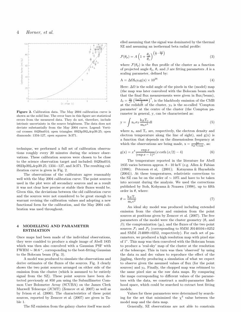
βmodel 0.69 0.69 0.69 – – 0.69 (p)(θc)model (′′) 33.6 50.1 – 33.6 50.1 33.6 (p)

F1 (mJy) 6.48±2.00 6.22±2.08 7.16±1.88 7.09±1.89 7.17±1.84 6.48±2.00F2 (mJy) 11.32±1.92 10.90±1.98 11.98±1.79 12.38±1.82 12.18±1.77 11.32±1.92y0 × 10−4 (4.68±0.48) (4.43±0.49) (6.52±0.64) (4.85±0.47) (4.19±0.40) (4.34±0.52)β 0.69 0.69 0.69 1.20± 0.2 1.60± 0.2 0.69

θc (′′) 33.6 50.1 14.7+2.4−2.2 33.6 50.1 33.6

ra offset (′′) 1.8 1.9 2.1 2.1 2.0 2.0dec offset (′′) 3.6 3.9 2.6 2.8 2.5 3.4χ2 3066 3079 3058 3056 3054 3062

Table 2. Parameter estimates (1 mm Bolocam observations) and χ2 values; Number of degrees of freedom= 3013. (p) denotes that the model included a 1.8 mJy point source at the cluster centre.

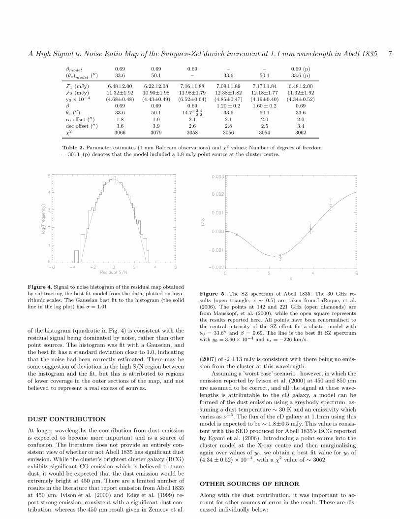
Figure 4. Signal to noise histogram of the residual map obtainedby subtracting the best fit model from the data, plotted on loga-rithmic scales. The Gaussian best fit to the histogram (the solidline in the log plot) has σ = 1.01

of the histogram (quadratic in Fig. 4) is consistent with theresidual signal being dominated by noise, rather than otherpoint sources. The histogram was fit with a Gaussian, andthe best fit has a standard deviation close to 1.0, indicatingthat the noise had been correctly estimated. There may besome suggestion of deviation in the high S/N region betweenthe histogram and the fit, but this is attributed to regionsof lower coverage in the outer sections of the map, and notbelieved to represent a real excess of sources.

DUST CONTRIBUTION

At longer wavelengths the contribution from dust emissionis expected to become more important and is a source ofconfusion. The literature does not provide an entirely con-sistent view of whether or not Abell 1835 has significant dustemission. While the cluster’s brightest cluster galaxy (BCG)exhibits significant CO emission which is believed to tracedust, it would be expected that the dust emission would beextremely bright at 450 µm. There are a limited number ofresults in the literature that report emission from Abell 1835at 450 µm. Ivison et al. (2000) and Edge et al. (1999) re-port strong emission, consistent with a significant dust con-tribution, whereas the 450 µm result given in Zemcov et al.

Figure 5. The SZ spectrum of Abell 1835. The 30 GHz re-sults (open triangle, x ∼ 0.5) are taken from.LaRoque, et al.(2006). The points at 142 and 221 GHz (open diamonds) arefrom Mauskopf, et al. (2000), while the open square representsthe results reported here. All points have been renormalised tothe central intensity of the SZ effect for a cluster model withθ0 = 33.6′′ and β = 0.69. The line is the best fit SZ spectrumwith y0 = 3.60× 10−4 and vz = −226 km/s.

(2007) of -2 ±13 mJy is consistent with there being no emis-sion from the cluster at this wavelength.

Assuming a ’worst case’ scenario , however, in which theemission reported by Ivison et al. (2000) at 450 and 850 µmare assumed to be correct, and all the signal at these wave-lengths is attributable to the cD galaxy, a model can beformed of the dust emission using a greybody spectrum, as-suming a dust temperature ∼ 30 K and an emissivity whichvaries as ν1.5. The flux of the cD galaxy at 1.1mm using thismodel is expected to be ∼ 1.8±0.5 mJy. This value is consis-tent with the SED produced for Abell 1835’s BCG reportedby Egami et al. (2006). Introducing a point source into thecluster model at the X-ray centre and then marginalizingagain over values of y0, we obtain a best fit value for y0 of(4.34± 0.52) × 10−4, with a χ2 value of ∼ 3062.

OTHER SOURCES OF ERROR

Along with the dust contribution, it was important to ac-count for other sources of error in the result. These are dis-cussed individually below:

8 Horner, et al.

Systematic errors Error (as % of result)

Calibration 11.7Kinematic effect 9.0CMB confusion 1.0Dusty galaxies 5.4Dust emission 7.2

Effective temperature +1.5−2.6

Uncertainties in 0.6King model parametersOthers (clumping, etc) 2

Pointing and model 0.52 mJyerror (incl. pointsourceTotal systematic 0.69 mJyTotal error 0.87 mJy

Table 3. Error budget for Abell 1835 observations

Calibration

We estimated the calibration error from the noise-weighteddispersion of the measured point fluxes relative to the May,2004 model. This gives a calibration error of ∼ 10.6%, which,when combined with a 5% error due to uncertainties in theMars model that all the Bolocam fluxes are dependent ongave an overall calibration error of ∼ 11.7%.

Kinematic effect

The kinematic SZ effect (see below) is due to the bulk motionof a cluster. In general, the kinematic effect is much lesssignificant than the thermal effect that has been discussed sofar. The bulk motion of clusters in a concordance cosmologypredicts an rms peculiar velocity of around 300 km/s, butMauskopf et al. (2000) obtain an estimate of the velocity ofAbell 1835 of around 500 km/s. A velocity this high at 273GHz produces a kinematic effect that is approxiamtely 9%of the thermal effect.

Confusion sources

The main sources of confusion in observations of the SZ ef-fect include the CMB background and dusty galaxies. Typ-ical CMB temperature anisotropy signals based on the cur-rent concordance model spectrum was simulated and ’ob-served’ using our scan strategy. These produced an rmsequivalent to a 1.5% error in the measured cluster signal.Dusty galaxies at 1.1 mm contribute an rms signal of ap-proximately 0.5 mJy (e.g. Blain (1998)), which correspondsto a 5.4% error in the measured cluster signal.

Physical model uncertainties

Other sources of error related to the parameters of the phys-ical model of Abell 1835 itself. Uncertainties in the electrongas temperature of 10 - 15 % correspond to an error in theestimate of y0 of up to ∼ 2.5%. LaRoque et al. (2006) re-ports errors on the model parameters θc and β of ±1.0” nand ∼ 0.01, respectively. When these variations are intro-duced into the model to see what effect they have on the

value of y0 obtained by the fit, their effect is found to besmall, and represent an uncertainty on the level of 0.6 %on the final result. Other potential sources of error include(e.g.) clumping in the cluster gas, but the SZ effect is rela-tively insensitive to the detailed physics of cluster gas, theseeffects were estimated as contributing no more than ∼ 2%to the final result.

A breakdown of the error budget for the observationspresented here is given in Table 3.

Y0 ESTIMATES

The value of y0 given by the 4 parameter fit means that theobservations detect the cluster with a significance of 10.5σ.This is one of the highest significance detections of a clus-ter in the positive region of the SZ spectrum to date. Aplot of the SZ spectrum of Abell 1835 based upon these val-ues is given in Fig. 5. These values have were fitted witha spectrum that included kinetic and thermal effects (non-relativistic as well as relativistic). The kinetic effect followsthe form:

Ikinetic = −τeβh(x) (10)

where τ is the optical depth of the cluster gas, given by

y0

(

mc2

kBTe))

, β ≡vzc

(where vz is the peculiar velocity of the

galaxy cluster), and h(x) = x4 exp x

(expx−1)2. The kinetic effect

dominates the SZ spectrum around the null point (ν ∼ 217GHz, x ∼ 1.9), but makes only a small contribution to thespectrum at frequencies above or below this.

The free parameters of the fit to the SZ spectrum were,therefore, y0 (which characterizes the thermal SZ), and vz(which characterizes the kinetic effect). The values of theseparameters that optimized the fit were found to be: y0 =(3.60 ± 0.24) × 10−4, and vz = −226 ± 275 km/s. This isconsistent with previous measurements of vz for Abell 1835Benson et al. (2004); Mauskopf et al. (2000) and representsthe most sensitive test for peculiar velocity in an individualgalaxy cluster using the SZ effect to date.

A High Signal to Noise Ratio Map of the Sunyaev-Zel’dovich increment at 1.1 mm wavelength in Abell 1835 9

6 CONCLUSIONS

The observation and analysis of 1.1 mm Bolocam jiggle-map data of Abell 1835, including details of the processof converting the raw data to maps of the cluster, havebeen discussed. A parameter search has been used to deter-mine the best fit values of the central Compton parameterfor the cluster and the fluxes for the point sources SMMJ140104+0252 and SMM J14009+0252. These values arefound to be y0 = (4.68 ± 0.48 ± 0.82) × 10−4, 6.5±2.0 mJyand 11.3±1.9 mJy, respectively with a statistical signal-to-noise of 10.5, 3.3 and 6.0 respectively. If the model is refinedfurther to include a point source, representing dust emissionfrom the cD galaxy in Abell 1835, the Compton parameterfor the cluster is found to be y0 = (4.34±0.52±0.69)×10−4

The value for y0 was compared to other literature resultsand found to agree well. The SZ spectrum for Abell 1835,based upon these values for y0 was fit with the full SZ form,including both thermal and kinetic effects and relativisticcorrections up to 7th order. The values of y0 and vz whichoptimized this fit were found to be (3.60± 0.24)× 10−4 and−226± 275 km/s, which are both in agreement with previ-ous literature results. It is also concluded that, in order tobetter evaluate the contamination from dust and accuratelycharacterize the spectrum of point sources in the same fieldas SZ clusters more results need to be obtained at shorterwavelengths in order to obtain more a detailed spectral en-ergy distribution.

ACKNOWLEDGMENTS

This work was supported by NSF grants AST-9980846 andAST-0206158. We wish to acknowledge M. Zemcov for pro-viding access to data and for useful discussion, which im-proved the content of this paper significantly. We would alsolike to recognize and acknowledge the cultural role and rev-erence that the summit of Mauna Kea has within the Hawai-ian community. We are fortunate and privileged to be ableto conduct observations from this mountain.

REFERENCES

Albrecht A., Bernstein G., Cahn R. et al., 2006,preprint(astro-ph/0609591)

Allen S. W., Fabian A. C., MNRAS, 297, L57, 1998Battistelli E. S., De Petris M., Lamagna L. et al., 2003,preprint(astro-ph/0303587)

Benson B. A., Church S. E., Ade P. A. R., Bock J. J.,Ganga K. M., Henson C. N., Thompson K. L., 2004, ApJ,617, 829

Bhattacharya S., Kosowsky A., 2007, preprint (astro-ph/0712.0034)

Birkinshaw M., Hughes J. P., Arnaud K. A., 1991, ApJ,376, 466

Birkinshaw M., 1999, Phys. Rep., 310, 97Blain A. W., 1998, MNRAS, 297, 502Carlstrom J. E., Holder G. P., Reese E. D., 2002, ARA&A,40, 643

DeDeo S., Spergel D. N., Trac H., 2005,preprint(astro-ph/0511060)

Diego J. M., Martinez-Gonzalez E., Sanz J. L., Benitez,Silk J., 2002, MNRAS, 331, 556

Edge A. C., Ivinson R. J., Smail I., Blain A. W., Kneib J.-P., 1999, MNRAS, 306, 599

Egami E., Misselt K. A., Rieke G. H. et al., 2006, ApJ, 647,922

Glenn J., Bock J. J., Chattopadhyay G. et al., 1998 in,Proc. SPIE, 3357, 326

Grainge K., 1996, PhD thesis, Cambridge University

Grego L., Carlstrom J. E., Reese E. D., Holder G. P.,Holzapfel W. L., Joy M. K., Mohr J. Patel S., 2001, ApJ,552, 2

Haig D. J., Ade P. A. R., Aguirre J. E. et al., 2004, Proc.SPIE, 5498, 78

Hallman E. J., Burns J. O., Motl P. M., Norman M. L.,2007, preprint (astro-ph/0705.0531)

High F. W., Stalder B., Song J. et al., 2010, preprint(astro-ph/1003.0005)

Hincks A. D., Acquaviva V., Ade P. A. R. et al., 2009,preprint(astro-ph/0907.0461)

Holzapfel W. L., Arnaud M., Ade P. A. R. et al., 1997,ApJ, 480, 449

Itoh, N., Kohyama, Y., Nozawa, S. 1998, ApJ, 502, 7

Ivison R. J., Smail I., Barger A. J., Kneib J.-P., Blain A.W., Owen F. N., Kerr T. H., Cowie L. L., 2000, MNRAS,315, 209

Jia S. M., Chen Y., Lu F. J., Chen L., Xiang F., 2004,A&A, 423, 65

Jones M., ApL Comm., 1995, 32, 347

Katayama H., Hayashida K., Advances in Space ResearchVol. 34, 12, 2519, 2004

LaRoque S. J., Bonamente M., Carlstrom J. E., Joy M. K.,Nagai D., Reese E. D., Dawson K. S., 2006, ApJ, 652, 917

Laurent G. T., Aguirre J. E., Glenn J. et al., 2005, ApJ,623, 742

Mauskopf P. D., Ade P. A. R., Allen S. W. et al., 2000,ApJ, 538, 505

Mohr J. J., Mathiesen B., Evrard A. E., 1999, ApJ, 517,627

Motl P. M., Hallman E. J., Burns J. O., Norman M. L.,2005, ApJ, 623, L63

Peterson J. R., Paerels F. B. S., Kaastra J. S. et al., 2001,A&A, 365, L104

Plagge T., Benson B. A., Ade P. A. R., Aird K. A., BleemL. E., 2009, preprint(astro-ph/0911.2444)

Reese E. D., 2003 in ed. Freedman W. L., Carnegie Obser-vatories Astrophysics Series, Vol. 2, Cambridge UniversityPress

Rephaeli Y., Sadeh S., Shimon M., 2006, preprint(astro-ph/0511626)

Schmidt R. W., Allen S. W., Fabian A. C., 2001, MNRAS,327, 1057

Sunyaev R. A., Zel’dovich Ya. B., 1970, Ap&SS, 7, 3

Tsuboi M., Miyazaki A., Kasuga T., Matsuo H., Kuno N.,1998, PASJ, 50, 169

Udomprasert P. S., Mason B. S., Readhead A. C. S., Pear-son T. J., 2004, pre-print (astro-ph/0408005)

Weller J., Battye R. A., Kneissl R., 2002, Phys. Rev. Lett.,88, 231301

Zemcov M., Borys C., Halpern M., Mauskopf P. D., ScottD., 2007, MNRAS, 376, 1073

10 Horner, et al.

This paper has been typeset from a TEX/ LATEX file preparedby the author.