arX

iv:1

301.

0816

v2 [

astr

o-ph

.CO

] 8

Jul

201

3Draft version July 22, 2013Preprint typeset using LATEX style emulateapj v. 5/2/11

THE ATACAMA COSMOLOGY TELESCOPE: SUNYAEV-ZEL’DOVICH SELECTED GALAXY CLUSTERS AT148GHz FROM THREE SEASONS OF DATA

Matthew Hasselfield1,2, Matt Hilton3,4, Tobias A. Marriage5, Graeme E. Addison2,6, L. Felipe Barrientos7,Nicholas Battaglia8,9, Elia S. Battistelli10,2, J. Richard Bond9, Devin Crichton5, Sudeep Das11,12,Mark J. Devlin13, Simon R. Dicker13, Joanna Dunkley6, Rolando Dunner7, Joseph W. Fowler14,15,

Megan B. Gralla5, Amir Hajian9, Mark Halpern2, Adam D. Hincks9, Renee Hlozek1, John P. Hughes16,Leopoldo Infante7, Kent D. Irwin14, Arthur Kosowsky17, Danica Marsden18,13, Felipe Menanteau16,

Kavilan Moodley3, Michael D. Niemack14,15,19, Michael R. Nolta9, Lyman A. Page15, Bruce Partridge20,Erik D. Reese13, Benjamin L. Schmitt13, Neelima Sehgal21, Blake D. Sherwin15, Jon Sievers1,9,

Cristobal Sifon22, David N. Spergel1, Suzanne T. Staggs15, Daniel S. Swetz14,13, Eric R. Switzer9,Robert Thornton13,23, Hy Trac8, Edward J. Wollack24

Draft version July 22, 2013

ABSTRACT

We present a catalog of 68 galaxy clusters, of which 19 are new discoveries, detected via the Sunyaev-Zel’dovich effect (SZ) at 148 GHz in the Atacama Cosmology Telescope (ACT) survey on the celestialequator. With this addition, the ACT collaboration has reported a total of 91 optically confirmed,SZ detected clusters. The 504 square degree survey region includes 270 square degrees of overlap withSDSS Stripe 82, permitting the confirmation of SZ cluster candidates in deep archival optical data. Thesubsample of 48 clusters within Stripe 82 is estimated to be 90% complete for M500c > 4.5× 1014M⊙

and redshifts 0.15 < z < 0.8. While a full suite of matched filters is used to detect the clusters,the sample is studied further through a “Profile Based Amplitude Analysis” using a statistic derivedfrom a single filter at a fixed θ500 = 5.′9 angular scale. This new approach incorporates the clusterredshift along with prior information on the cluster pressure profile to fix the relationship betweenthe cluster characteristic size (R500) and the integrated Compton parameter (Y500). We adopt aone-parameter family of “Universal Pressure Profiles” (UPP) with associated scaling laws, derivedfrom X-ray measurements of nearby clusters, as a baseline model. Three additional models of clusterphysics are used to investigate a range of scaling relations beyond the UPP prescription. Assuminga concordance cosmology, the UPP scalings are found to be nearly identical to an adiabatic model,while a model incorporating non-thermal pressure better matches dynamical mass measurements andmasses from the South Pole Telescope. A high signal to noise ratio subsample of 15 ACT clusterswith complete optical follow-up is used to obtain cosmological constraints. We demonstrate, usingfixed scaling relations, how the constraints depend on the assumed gas model if only SZ measurementsare used, and show that constraints from SZ data are limited by uncertainty in the scaling relationparameters rather than sample size or measurement uncertainty. We next add in seven clusters fromthe ACT Southern survey, including their dynamical mass measurements, which are based on galaxyvelocity dispersions and thus are independent of the gas physics. In combination with WMAP7these data simultaneously constrain the scaling relation and cosmological parameters, yielding 68%confidence ranges described by σ8 = 0.829 ± 0.024 and Ωm = 0.292 ± 0.025. We consider theseresults in the context of constraints from CMB and other cluster studies. The constraints arisemainly due to the inclusion of the dynamical mass information and do not require strong priors onthe SZ scaling relation parameters. The results include marginalization over a 15% bias in dynamicalmasses relative to the true halo mass. In an extension to ΛCDM that incorporates non-zero neutrinomass density, we combine our data with WMAP7, Baryon Acoustic Oscillation data, and Hubbleconstant measurements to constrain the sum of the neutrino mass species to be

∑ν mν < 0.29 eV

(95% confidence limit).

Subject headings: cosmology:cosmic microwave background – cosmology:observations – galax-ies:clusters – Sunyaev-Zel’dovich Effect

1 Department of Astrophysical Sciences, Peyton Hall, Prince-ton University, Princeton, NJ 08544, USA

2 Department of Physics and Astronomy, University of BritishColumbia, Vancouver, BC, V6T 1Z4, Canada

3 Astrophysics and Cosmology Research Unit, School of Math-ematics, Statistics & Computer Science, University of KwaZulu-Natal, Durban, 4041, South Africa

4 Centre for Astronomy & Particle Theory, School of Physics &Astronomy, University of Nottingham, Nottingham, NG7 2RD,UK

5 Dept. of Physics and Astronomy, The Johns Hopkins Uni-

versity, 3400 N. Charles St., Baltimore, MD 21218-2686, USA6 Department of Astrophysics, Oxford University, Oxford,

OX1 3RH, UK7 Departamento de Astronomıa y Astrofısica, Facultad de

Fısica, Pontificıa Universidad Catolica, Casilla 306, Santiago 22,Chile

8 Department of Physics, Carnegie Mellon University, Pitts-burgh, PA 15213, USA

9 Canadian Institute for Theoretical Astrophysics, Universityof Toronto, Toronto, ON, M5S 3H8, Canada

10 Department of Physics, University of Rome “La Sapienza”,

2 Hasselfield, Hilton, Marriage et al.

1. INTRODUCTION

Galaxy clusters are sensitive tracers of the growth ofstructure in the Universe. The measurement of theirevolving abundance with redshift has the potential toprovide constraints on cosmological parameters that arecomplementary to other measurements, such as the an-gular power spectrum of the cosmic microwave back-ground (CMB; e.g., Hinshaw et al. 2012; Dunkley et al.2011; Keisler et al. 2011; Story et al. 2012), Type Ia su-pernovae (e.g., Hicken et al. 2009; Lampeitl et al. 2010;Suzuki et al. 2012), or baryon acoustic oscillations mea-sured in galaxy correlation functions (e.g., Percival et al.2010).There is a long history of using optical (e.g., Abell

1958; Lumsden et al. 1992; Goto et al. 2002; Lopes et al.2004; Miller et al. 2005; Koester et al. 2007; Hao et al.2010; Szabo et al. 2011; Wen et al. 2009, 2012) andX-ray (e.g., Henry et al. 1992; Bohringer et al. 2004;Burenin et al. 2007; Mehrtens et al. 2012) surveys tosearch for galaxy clusters. Data from such surveysoffered an early indication of an Ωm < 1 universe(e.g., Bahcall & Cen 1992). Recent results have demon-strated the power of modern optical and X-ray sur-veys for constraining cosmology (e.g., Vikhlinin et al.2009b; Mantz et al. 2010b; Rozo et al. 2010). A promis-ing method for both detecting clusters in optical sur-veys and simultaneously providing mass estimates is touse weak gravitational lensing shear selection, and thefirst such samples using this technique have recently ap-peared (e.g., Wittman et al. 2006; Miyazaki et al. 2007).Within the last few years, cluster surveys exploitingthe Sunyaev-Zel’dovich effect (SZ; Sunyaev & Zel’dovich1970) have also begun to deliver cluster samples(e.g., Staniszewski et al. 2009; Marriage et al. 2011;Williamson et al. 2011; Planck Collaboration 2011a;Reichardt et al. 2013) and constraints on cosmologicalparameters (Vanderlinde et al. 2010; Sehgal et al. 2011;Benson et al. 2013; Reichardt et al. 2013).

Piazzale Aldo Moro 5, I-00185 Rome, Italy11 High Energy Physics Division, Argonne National Labora-

tory, 9700 S Cass Avenue, Lemont, IL 60439, USA12 Berkeley Center for Cosmological Physics, LBL and Depart-

ment of Physics, University of California, Berkeley, CA 94720,USA

13 Department of Physics and Astronomy, University of Penn-sylvania, 209 South 33rd Street, Philadelphia, PA 19104, USA

14 NIST Quantum Devices Group, 325 Broadway Mailcode817.03, Boulder, CO 80305, USA

15 Joseph Henry Laboratories of Physics, Jadwin Hall, Prince-ton University, Princeton, NJ 08544, USA

16 Department of Physics and Astronomy, Rutgers, The StateUniversity of New Jersey, Piscataway, NJ 08854-8019, USA

17 Department of Physics and Astronomy, University of Pitts-burgh, Pittsburgh, PA 15260, USA

18 Department of Physics, University of California Santa Bar-bara, CA 93106, USA

19 Department of Physics, Cornell University, Ithaca, NY14853, USA

20 Department of Physics and Astronomy, Haverford College,Haverford, PA 19041, USA

21 Department of Physics and Astronomy, Stony Brook, NY11794-3800, USA

22 Leiden Observatory, Leiden University, PO Box 9513, NL-2300 RA Leiden, Netherlands

23 Department of Physics, West Chester University of Penn-sylvania, West Chester, PA 19383, USA

24 NASA/Goddard Space Flight Center, Greenbelt, MD20771, USA

The thermal SZ effect is the inverse Comptonscattering of CMB photons by electrons within thehot (∼ 107−8K) intracluster medium of galaxy clus-ters. This leads to a spectral distortion in the di-rection of clusters, with the size of the effect beingproportional to the volume-integrated thermal pres-sure and thus, in the adiabatic scenario, the to-tal thermal energy of the cluster gas. Accord-ingly, this is correlated with cluster mass (e.g.,Bonamente et al. 2008; Marrone et al. 2012; Sifon et al.2012; Planck Collaboration et al. 2013). Since the SZsignal is not diminished due to luminosity distance, itis nearly redshift independent; in principle SZ surveyscan detect all clusters in the Universe above a masslimit set by the survey noise level (e.g., Birkinshaw 1999;Carlstrom et al. 2002).Although current SZ cluster samples are small

in comparison to existing X-ray and optical clustercatalogs, they provide very powerful complementaryprobes because they are sensitive to the high mass,high redshift cluster population (e.g., Brodwin et al.2010; Foley et al. 2011; Planck Collaboration 2011b;Menanteau et al. 2012; Stalder et al. 2012). Manystudies (e.g., Hoyle et al. 2011; Mortonson et al. 2011;Hotchkiss 2011; Harrison & Coles 2012) have noted thatthe discovery of a sufficiently massive cluster at high red-shift would be a challenge to ΛCDM cosmology, and theapproximately redshift independent, mass-limited natureof SZ surveys means that they are well suited to revealsuch objects if they exist.In this paper we describe the results of a search for

galaxy clusters using the SZ effect in maps of the celes-tial equator obtained by the Atacama Cosmology Tele-scope (ACT; Swetz et al. 2011). ACT is a 6m telescopelocated in northern Chile that observes the sky in threefrequency bands (centered at 148, 218, and 277GHz) si-multaneously with arcminute resolution. During 2008,ACT surveyed a 455 deg2 patch of the Southern sky,centered on δ = −55 deg, detecting a number of SZ clus-ter candidates of which 23 were optically confirmed asmassive clusters (Menanteau et al. 2010; Marriage et al.2011). The Equatorial survey area, on which we report inthis work, was chosen to overlap the deep (r ≈ 23.5 mag)optical data from the Sloan Digital Sky Survey (SDSS;Abazajian et al. 2009) Stripe 82 region (S82 hereafter;Annis et al. 2011). Optical confirmation of our SZ clus-ter candidates is reported in Menanteau et al. (2013), us-ing data from SDSS and additional targeted optical andIR observations obtained at Apache Point Observatory.All clusters have photometric redshifts, and most havespectroscopic redshifts from a combination of SDSS andnew observations at Gemini South. X-ray fluxes fromthe ROSAT All Sky Survey confirm that this is a mas-sive cluster sample. The overlap of the ACT survey withSDSS has also enabled stacking analyses which charac-terize the SZ-signal as a function of halo mass from op-tically selected samples (Hand et al. 2011; Sehgal et al.2013), as well as a first detection of the kinetic SZ effectfrom the correlation of positions and redshifts of lumi-nous red galaxies with temperature in the ACT maps(Hand et al. 2012).The structure of this paper is as follows. In Section 2

we describe the processing of the ACT data used in thiswork and the cluster detection algorithm. In Section 3

ACT: SZ Selected Galaxy Clusters 3

we describe our approach to relating the cluster signalin filtered SZ maps to cluster mass, and obtain massestimates for our cluster sample. In Section 4 we com-pare our catalog to other SZ, optical, and X-ray selectedcluster catalogs. In Section 5 we obtain constraints oncosmological parameters using the ACT cluster sample.In an Appendix, we present analogous SZ signal mea-surements and mass estimates for ACT’s Southern fieldclusters, using deeper data obtained over the course ofthe 2009-2010 observing seasons.Where it is necessary to adopt a fiducial cosmol-

ogy, we assume Ωm = 0.3, ΩΛ = 0.7, and H0 =70 h70 km s−1 Mpc−1 (h70 = 1), unless stated oth-erwise. Throughout this paper, cluster mass is mea-sured within a characteristic radius with respect to thecritical density such that, e.g., M500c is defined as themass measured within the radius (R500) at which theenclosed mean density is 500 times the critical densityat the cluster redshift. The function E(z) denotes theevolution of the Hubble parameter with redshift (i.e.,E(z) = [Ωm(1 + z)3 +ΩΛ]

1/2 for a universe with Ωk = 0and negligible radiation density). Uncertainties and er-ror bars are specified at the 1-σ level, and posterior dis-tributions are summarized in terms of their mean andstandard deviation unless otherwise indicated.

2. MAPS AND CLUSTER DETECTION

In this section we discuss the detection of galaxy clus-ters in the ACT Equatorial maps at 148GHz. The mapsare filtered to enhance structures whose shape matchesthe Universal Pressure Profile of Arnaud et al. (2010).The final cluster catalog consists of SZ candidates thathave been confirmed in optical or IR imaging.

2.1. Equatorial Maps

ACT’s observations during the 2009 and 2010 seasonswere concentrated on the celestial equator. For this studywe make use of the 504 square degree deep, contiguousregion spanning from 20h16m00s to 3h52m24s in right as-cension and from −207′ to 218′ in declination. Thisregion includes 270 square degrees of overlap with S82,which extends to 20h39m in R.A. and ±115′ in declina-tion. As shown in Figure 1, the S82 region correspondsto the lowest-noise region of the ACT Equatorial maps.The bolometer time-stream data are acquired while

scanning the telescope in azimuth at fixed elevation.Cross-linked data are obtained by observing the samecelestial region at two telescope pointings that produceapproximately orthogonal scan directions. Because thescan strategy was optimized for simultaneous observa-tion with the 148GHz and 218GHz arrays (the centersof which are separated by approximately 33′ when pro-jected onto the sky), the regions beyond declinations of±140′ are not well cross-linked.The ACT data reduction pipeline and map-making

procedure are described in Dunner et al. (2013), in thecontext of ACT’s 2008 data. The time-stream bolometerdata are screened for pathologies and then combined toobtain a maximum likelihood estimate of the microwavesky map (with 0.5′ pixels) for each observing season. Asa result of the cross-linked scan strategy, and the carefultreatment of noise during map making, the ACT mapsare unbiased at angular scales ℓ > 300.

Due to realignments of the primary and secondary mir-rors, the telescope beams vary slightly between seasonsbut are stable over the course of each season. The tele-scope beams are determined from observations of Saturn,using the method described in Hincks et al. (2010), butwith additional corrections to account for ≈ 6′′ RMSpointing variation between observations made on differ-ent nights (Hasselfield et al., in prep.). The effectivebeam for the 148GHz array differs negligibly betweenthe 2009 and 2010 seasons, with a FWHM of 1.4′ andsolid angle (including the effects of pointing variation) of224± 2 nsr.Calibrations of ACT observations are based on fre-

quent detector load curves, and atmospheric opacity wa-ter vapor measurements (Dunner et al. 2013). Absolutecalibration of the ACT maps is achieved by compar-ing the large angular scale (300 < ℓ < 1100) signalfrom the 2010 season maps to the WMAP 95 GHz 7-year maps (Jarosik et al. 2011). Using a cross-correlationtechnique as described in Hajian et al. (2011), an abso-lute calibration uncertainty of ≈ 2% in temperature isachieved (Das et al. 2013). The inter-calibration of 2009and 2010 is measured through a similar cross-correlationtechnique, with less than 2% error.

2.2. Gas Pressure Model

At several stages in the detection and analysis we willrequire a template for the intracluster gas pressure pro-file. To this end we adopt the “Universal Pressure Pro-file” (UPP) of Arnaud et al. (2010, hereafter A10), whichincludes mass dependence in the profile shape and hasbeen calibrated to X-ray observations of nearby clusters.In this section we review the form of the UPP, and ob-tain several approximations that will be used in clus-ter detection (Section 2.3) and cluster property recovery(Section 3).In A10, the cluster electron pressure as a func-

tion of physical radius r is modeled with a gen-eralized Navarro-Frenk-White (GNFW) profile(Nagai, Kravtsov, & Vikhlinin 2007),

p(x) = P0 (c500x)−γ (1 + (c500x)

α)(γ−β)/α

, (1)

where x = r/R500 and P0, c500, γ, α, β are fit parameters.The overall pressure normalization, under assumptionsof self-similarity (i.e., the case when gravity is the soleprocess responsible for setting cluster properties), varieswith mass and redshift according to

P500 =[1.65× 10−3h2

70 keV cm−3]m2/3E8/3(z), (2)

where E(z) is the ratio of the Hubble constant at redshiftz to its present value, and

m ≡ M500c/(3× 1014 h−170 M⊙) (3)

is a convenient mass parameter. Some deviation fromstrict self-similarity may be encoded via an additionalmass dependence in the shape of the profile, yielding aform

P (r) = P500mαp(x)p(x). (4)

In this framework, A10 use X-ray observations of local(z < 0.2) clusters to obtain best-fit GNFW parameters

[P0, c500, γ, α, β] = [8.403 h3/270 , 1.177, 0.3081, 1.0510,

4 Hasselfield, Hilton, Marriage et al.

5.4905], and an additional radial dependence describedreasonably well by αp(x) = 0.22/(1 + 8x3).Because hydrostatic mass estimates are used by A10

to assess the relationship between cluster mass and thepressure profile, there may be systematic differenceswhen one makes use of an alternative mass proxy, suchas weak lensing or galaxy velocity dispersion. Sim-ulations suggest that hydrostatic masses are under-estimates of the true cluster mass (e.g., Nagai et al.2007). However, there is little consensus among recentstudies which compare X-ray hydrostatic and weak lens-ing mass measurements. For example, Mahdavi et al.(2013) find that hydrostatic masses are lower than weaklensing masses by about 10% atR500; Zhang et al. (2010)and Vikhlinin et al. (2009a) find reasonable agreement;while Planck Collaboration et al. (2013) find hydrostaticmasses to be about 20% larger than weak lensing masses.Therefore in our initial treatment of the UPP we neglectthis bias; later we will address this issue by adding de-grees of freedom to allow for changes in the normalizationof the pressure profile.The thermal SZ signal is related to the optical depth for

Compton scattering along a given line of sight. For ourpressure profile, and in the absence of relativistic effects,this Compton parameter at projected angle θ from thecluster center is

y(θ) =σT

mec2

∫ds P

(√s2 + (R500θ/θ500)2

), (5)

where θ500 = R500/DA(z) with DA(z) the angular di-ameter distance to redshift z, σT is the Thomson crosssection, me is the electron mass, and the integral in sis along the line of sight. Relativistic effects change thispicture somewhat, but for convenience we will use theabove definition of y(θ) and apply the relativistic correc-tion only when calculating the SZ signal associated witha particular y.To simplify the expression for the cluster pressure pro-

file, we first consider the mass parameter m = 1 andfactor the expression in equation (5) to get

y(θ,m = 1) = 10A0E(z)2τ(θ/θ500) (6)

where τ(x) is a dimensionless profile normalized to

τ(0) = 1, and 10A0 = 4.950 × 10−5h1/270 gives the nor-

malization. The deviations from self-similarity are weakenough that we may model the changes in the profileshape with mass as simple adjustments to the normal-ization and angular scale of the profile. For the massesof interest here (1 < m < 10) we obtain

y(θ,m) ≈ 10A0E(z)2m1+B0τ(mC0θ/θ500) (7)

with B0 = 0.08 and C0 = −0.025. This approx-imation reproduces the inner signal shape extremelywell, with deviations increasing to the 0.5% level byθ500. For 0.1θ500 < θ < 3θ500, the enclosed signal

(∫ θ

0dθ′ 2πθ′y(θ′,m)) differs by less than 1% from the re-

sults of the full computation. This parametrization of thecluster signal in terms of a normalization and dimension-less profile is not used for cluster detection (Section 2.3),but will motivate the formulation of scaling relations andpermit the estimation of cluster masses (Section 3.1).

The observed signal due to the SZ effect is a change inradiation intensity, expressed in units of CMB tempera-ture:

∆T (θ)

TCMB= fSZ y(θ). (8)

In the non-relativistic limit, the factor fSZ depends onlyon the observed radiation frequency. Integrating thisnon-relativistic SZ spectral response over the nominal148GHz array band-pass, we obtain an effective fre-quency of 146.9 GHz (Swetz et al. 2011). At this fre-quency, the formulae of Itoh et al. (1998) provide a spec-tral factor, including relativistic effects for gas tempera-ture Te, of fSZ(t) = −0.992frel(t) where t = kBTe/mec

2

and frel(t) = 1 + 3.79t − 28.2t2. This results in a 6%correction for a cluster with T = 10keV. We use thescaling relation of Arnaud et al. (2005), t = −0.00848×(mE(z))−0.585, to express the mean temperature depen-dence in terms of the cluster mass and redshift. Thisyields a final form, fSZ(m, z) = −0.992frel(m, z), whichwe use in all subsequent modeling of the SZ signal.The corrections for the ACT cluster sample range fromroughly 3% to 10%.

2.3. Galaxy Cluster Detection

In addition to the temperature decrements due togalaxy clusters, the ACT maps at 148GHz contain con-tributions from the CMB, radio point sources, dustygalaxies, and noise from atmospheric fluctuations andthe detectors. To detect galaxy clusters in the ACT mapswe make use of a set of matched filters, with signal tem-plates based on the UPP through the integrated profiletemplate τ(θ/θ500).We consider signal templates Sθ500(θ) ≡ τ(θ/θ500) for

θ500 = 1.′18 to 27′ in increments of 1.′18. Each fixedangular scale corresponds to a physical scale that varieswith redshift, but can be computed for a given cosmology.For each signal template we form an associated matchedfilter in Fourier space

Ψθ500(k) =1

Σθ500

B(k)Sθ500(k)

N(k)(9)

where B(k) is the product of the telescope beam re-sponse with the map pixel window function, N(k) is the(anisotropic) noise power spectrum of the map, and Σθ500is a normalization factor chosen so that, when appliedto a map containing a beam-convolved cluster signal−∆T [Sθ500 ∗ B](θ) (in temperature units), the matchedfilter returns the central decrement −∆T .Since the total power from the galaxy cluster SZ sig-

nal is low compared to the CMB, atmospheric noise, andwhite noise that contaminate the cluster signal, we esti-mate the noise spectrum N(k) from the map directly.Bright (signal to noise ratio greater than five) pointsources are masked from the map, with the masking ra-dius ranging from 2′ for the dimmest sources to 1 for thebrightest source. A plane is fit to the map signal (weight-ing by the inverse number of samples in each pixel) andremoved, and the map is apodized within 0.2 of the mapedges.For ACT, the effect of the noise term in the matched

filter is to strongly suppress signal below ℓ ≈ 3000 (corre-sponding to scales larger than 7′). When combined with

ACT: SZ Selected Galaxy Clusters 5

20h 30m21h 00m21h 30m22h 00m22h 30m

R.A. (J2000)

020100

+01+02

23h 00m23h 30m00h 00m00h 30m01h 00m

020100

+01+02

Dec.

(J2

00

0)

01h 30m02h 00m02h 30m03h 00m03h 30m

020100

+01+02

20 40 60 80

Sensitivity to central decrement (K)

Figure 1. The portion of the ACT Equatorial survey region considered in this work. It spans from 20h16m00s to 3h52m24s in R.A. andfrom −207′ to 218′ in declination for a total of 504 square degrees. The overlap with Stripe 82 (dashed line) extends only to 20h39m inR.A. and covers ±115′ in declination, for a total of 270 square degrees. Circles identify the optically confirmed SZ-selected galaxy clusters,with radius proportional to the signal to noise ratio of the detection (which ranges from 4 to 13). The gray-scale gives the sensitivity (inCMBµK) to detection of galaxy clusters, after filtering, for the matched filter with θ500 = 5.′9 (see Section 2.3). Inside the Stripe 82 regionthe median noise level is 44 µK, with one quarter of pixels having noise less (respectively, more) than 41 µK (46 µK). Outside Stripe 82,the median level is 54 µK, with one quarter of pixels having less (more) than 47 (64) µK noise. The higher noise, X -shaped regions aredue to breaks in the scan for calibration operations.

the signal template (and beam), the filters form band-passes centered at ℓ ranging from roughly 2500 to 5000.The angular scales probed by the filters are thus suffi-ciently small that filtering artifacts near the map bound-aries are mitigated by the map apodization. While thesuppression of large angular scales disfavors the detectionof clusters with large angular sizes, we apply the full suiteof filters in order to maximize detection probability andto study the features of inferred cluster properties as theassumed cluster scale is varied.The azimuthally averaged real space filter kernel cor-

responding to θ500 = 5.′9 is shown in Figure 2, and com-pared to both the ACT 148GHz beam and the signaltemplate Sθ500 .The true noise spectrum may vary somewhat over the

map due to variations in atmospheric and detector noiselevels, and thus the matched filter Ψθ500(k) might be saidto be sub-optimal at any point. The filter remains un-biased, however, and a reasonable estimate of the signalto noise ratio (S/N) may still be obtained by recognizingthat the local noise level will be highly correlated withthe number of observations contributing to a given mappixel.Prior to matched filtering, the ACT maps are condi-

tioned in the same way as for noise estimation, exceptthat the point sources are subtracted from the maps in-

0 2 4 6 8 10 (arcmin)

0.2

0.0

0.2

0.4

0.6

0.8

1.0 Filter kernel

Cluster template

ACT beam

Figure 2. The azimuthally averaged real space matched filter ker-nel, proportional to Ψ

5.′9(θ), for signal template with θ500 = 5.′9.Shown for reference are the ACT 148GHz beam, and the clustersignal template S

5.′9(θ). While filters tuned to many different an-

gular scales are used for cluster detection (Section 2.3), the 5.′9 filteris used for cluster characterization and cosmology (Section 3.1).

6 Hasselfield, Hilton, Marriage et al.

stead of being masked. (Subsequent analysis disregardsregions near those point sources, amounting to 1% of themap area.) With the application of each filter we obtaina map of ∆T values. A section of a filtered map (forθ500 = 5.′9) is shown in Figure 3.We characterize the noise in each filtered map by

modeling the variance at position x as σ2(x) = σ20 +

σ2hits/nhits(x), where nhits(x) is the number of detector

samples falling in the pixel at x. We fit constants σ0 andσhits by binning in small ranges of 1/nhits. The fit is it-erated after excluding regions near pixels that are strongoutliers to the noise model. Typically such pixels arenear eventual galaxy cluster candidates. Figure 1 showsthe noise map for the θ500 = 5.′9 filter.After forming the signal to noise ratio map

−∆T (x)/σ(x), cluster candidates are identified as allpixels with values exceeding four. The catalog of clustercandidates contains positions, central decrements (∆T ),and the local map noise level. Candidates seen at multi-ple filter scales are cross-identified if the detection posi-tions are within 1′; the cluster candidate positions thatwe list come from the map where the cluster was mostsignificantly detected. We adopt the largest S/N valueobtained over the range of filter scales as the detectionsignificance for each candidate.For a given candidate, the S/N tends to vary only

weakly with the filter scale. The reconstructed cen-tral decrement ∆T varies weakly above filter scales ofθ500 ≈ 3′, as may be seen for the most significantly de-tected clusters in Figure 4. This stabilization occurswhen the assumed cluster size is larger than the truecluster size, because the filter is optimized to return thedifference in the level of the signal at the cluster positionand the level of the signal away from the cluster center.The filter interprets the signal at the cluster position asbeing due to the convolution of the telescope beam withthe cluster signal. The inferred central decrement thusrises rapidly as the assumed θ500 decreases, since totalSZ flux scales as ∆Tθ500

2. As is discussed in Section 3.1,only the results from the θ500 = 5.′9 matched filter areused for inferring masses, scaling relations, and cosmo-logical results. The corresponding physical scale may bedetermined, as a function of redshift, based on clusterdistance.

2.4. Galaxy Cluster Confirmation

The cluster candidates obtained from the 148GHz mapanalysis are confirmed using optical and infrared imag-ing. A complete discussion of this process may be foundin Menanteau et al. (2013). For the purposes of thiswork, we briefly summarize the confirmation process andthe redshift limits of the sample (which must be under-stood in order to derive cosmological constraints). Theselimits differ according to the depth of the optical imagingavailable over a given part of the map.Most cluster candidates are confirmed through the

analysis of SDSS imaging. The ACT Equatorial sur-vey is almost entirely covered by SDSS archival data(Abazajian et al. 2009), with a central strip designed tooverlap with the deep optical data (r ≈ 23.5) in the S82region (Annis et al. 2011), as shown in Figure 1. Foreach ACT cluster candidate with peak S/N > 4, SDSSimages are studied using an iterative photometric anal-

ysis to identify a brightest cluster galaxy (BCG) and anassociated red sequence of member galaxies. A mini-mum richness of Ngal = 15, evaluated within a projected1 h−1 Mpc of the nominal cluster center and within0.045(1 + zc) of the nominal cluster redshift zc, is re-quired for the candidate to be confirmed as a cluster.The redshifts of confirmed clusters are obtained from ei-ther a photometric analysis of the images, from SDSSspectroscopy of bright cluster members, or from targetedmulti-object spectroscopic follow-up. The redshift limitof cluster confirmation using SDSS data alone is esti-mated to be z ≈ 0.8 within S82 and z ≈ 0.5 outside ofS82. Cluster candidates that are not confirmed in SDSSimaging are targeted, in an on-going follow-up campaign,under the assumption that they may be high redshiftclusters.Within the S82 region, 49 of 155 candidates are con-

firmed, with 44 of these confirmations resulting fromanalysis of SDSS data only. Targeted follow-up of thehigh S/N candidates was pursued at the Apache PointObservatory, yielding five more confirmations, all atz > 0.9. All cluster candidates with S/N > 5.1 wereconfirmed as clusters. This is consistent with our es-timate of 1.8 false detections in this region, based onfiltering of simulated noise. The follow-up in the S82 re-gion is deemed complete to a S/N of 5.1, in the sensethat all SZ candidates with ACT S/N > 5.1 have beentargeted. It is thus this sample, and this region, that areconsidered for the cosmological analysis (in addition toa subset of the Marriage et al. (2011) sample; see Sec-tion 5). The completeness within S82, as a function ofmass and redshift, is estimated in Section 3.6.Outside of S82, 19 clusters are confirmed using SDSS

DR8 data. High significance SZ detections in this regionthat are not confirmed in the DR8 data constitute goodcandidates for high redshift galaxy clusters and are beinginvestigated in a targeted follow-up campaign.The confirmed cluster sample may contain a small

number of false positives, due to chance superpositionof a low mass cluster at the location of an otherwise spu-rious SZ candidate. Most of our confirmed clusters areassociated with rich optical counterparts, and thus aretruly massive clusters. However, our search was car-ried out over considerable sky area in the ≈ 150 re-gions around SZ candidates. Assigning an effective areaof 13 square arcminutes to each of these fields yields atotal area of approximately 0.5 square degrees. Fromthe maxBCG catalog (Koester et al. 2007), which in-cludes optical richness measurements for clusters with0.1 < z < 0.3, we expect that the density of clusters sat-isfying our richness criteria in the range 0.1 < z < 0.8is approximately 6 per square degree. We conclude thatroughly three of our low richness confirmed clusters couldpotentially be spurious associations. Such contaminationis not likely to affect the high significance (S/N > 5.1)sample, where the lowest richness is ≈ 30.In Table 7 we present the catalog of 68 confirmed clus-

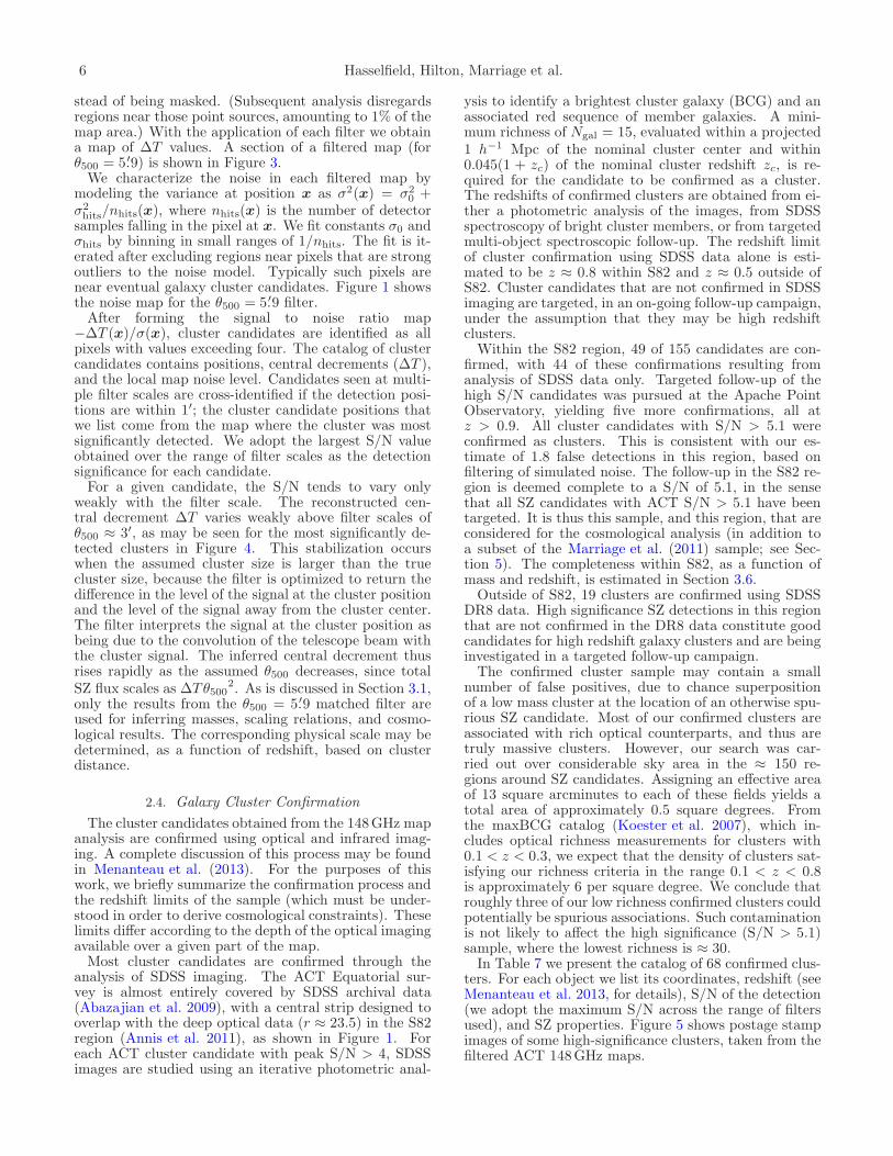
ters. For each object we list its coordinates, redshift (seeMenanteau et al. 2013, for details), S/N of the detection(we adopt the maximum S/N across the range of filtersused), and SZ properties. Figure 5 shows postage stampimages of some high-significance clusters, taken from thefiltered ACT 148GHz maps.

ACT: SZ Selected Galaxy Clusters 7

02h10m02h15m02h20m02h25m02h30mR.A. (J2000)

-01°

0°

+01°

Dec

. (J200

0)

J0218.2-0041(S/N = 5.8)

J0223.1-0056(S/N = 5.8)

J0215.4+0030(S/N = 5.5)

−200 −160 −120 −80 −40 0 40 80 120 160 200∆T (µK)

Figure 3. Section of the 148GHz map (covering 18.7 deg2) match-filtered with a GNFW profile of scale θ500 = 5.′9. Point sources areremoved prior to filtering. Three optically confirmed clusters with S/N > 4.9 are highlighted (see Table 7). Within this area, there are anadditional 11 candidates (4 < S/N < 4.9) which are not confirmed as clusters in the SDSS data (and thus may be spurious detections orhigh-redshift clusters).

500 (arcmin)0

200

400

600

800

1000

1200

1400

T (

K)

0 5 10 15 20500 (arcmin)

0

2

4

6

8

10

S/N

Figure 4. Central decrement and signal to noise ratio as a func-tion of filter scale for the 20 clusters in S82 detected with peakS/N > 5. Top panel : Although the central decrement is a model-dependent quantity, the value tends to be stable for filter scalesof θ500 > 3′. Bottom panel : On each curve, the circular pointidentifies the filter scale at which the peak S/N was observed. Thevertical dashed line shows the angular scale chosen for cluster prop-erty and cosmology analysis, θ500 = 5.′9. Despite the apparent gapnear S/N ≈ 6, the clusters shown represent a single population.

3. RECOVERED CLUSTER PROPERTIES

In this section we develop a relationship between clus-ter mass and the expected signal in the ACT filteredmaps. The form of the scaling relationship between theSZ observable and the cluster mass is based on the UPP,and parameters of that relationship are studied usingmodels of cluster physics and dynamical mass measure-ments. We obtain masses for the ACT Equatorial clus-ters assuming a representative set of parameters.

3.1. Profile Based Amplitude Analysis

Scaling relations between cluster mass and cluster SZsignal strength are often expressed in terms of bulk in-tegrated Compton quantities, such as Y500, which areexpected to be correlated to mass with low intrinsic scat-ter (e.g., Motl et al. 2005; Reid & Spergel 2006). Due toprojection effects, and the current levels of telescope res-olution and survey depth, measurements of Y500 for in-dividual clusters can be obtained only by comparing themicrowave data to a simple, parametrized model for thecluster pressure profile. Such fits may be done directly, orindirectly as part of the cluster detection process throughthe application of one or more matched filters (where thefilters are “matched” in the sense of being tuned to a par-ticular angular scale). In such comparisons, the inferredvalues of Y500 are very sensitive to the assumed clusterscale (i.e., θ500

1), and this scale is poorly constrained bymicrowave data alone.Recent microwave survey instruments make use of spa-

tial filters to both detect and characterize their clus-ter samples, coping with θ500 uncertainty in different

1 M500c = (4π/3) × 500ρc(z)R3500; θ500 = R500/DA(z).

8 Hasselfield, Hilton, Marriage et al.

Figure 5. Postage stamp images (30′ on a side) for the 10 highest S/N detections in the catalog (see Table 7), taken from the filteredACT maps. The clusters are ordered by detection S/N, from top left to bottom right, and each postage stamp shown is filtered at thescale which optimizes the detection S/N. Note that J2327.4−0204 is at the edge of the map. The greyscale is linear and runs from -350µK(black) to +100 µK (white).

ways. For example, the Planck team uses X-ray lu-minosity based masses (Planck Collaboration 2011a) aswell as more detailed X-ray and weak lensing studies(Planck Collaboration et al. 2013) to constrainR500, andobtain Y500 measurements assuming profile shapes de-scribed by the UPP.In cases where suitable X-ray or optical constraints

on the cluster scale are not available, authors have con-structed empirical scaling relations based on alternativeSZ statistics, such as the amplitude returned by someparticular filter (Sehgal et al. 2011), or the maximumS/N over some ensemble of filters (Vanderlinde et al.2010). Recognizing that the cluster angular scale ispoorly constrained by the filter ensemble, recent workfrom the South Pole Telescope has included a marginal-ization over the results returned by the ensemble of fil-ters (e.g., Story et al. 2011; Reichardt et al. 2013). Suchapproaches rely on simulated maps to guide the interpre-tation of their results.For the purposes of using the SZ signal to understand

scaling relations and to obtain cosmological constraints,we develop an approach in which the cluster SZ signalis parametrized by a single statistic, obtained from theACT map that has been filtered using Ψ

5.′9(k). Insteadof using simulations to inform our interpretation of thedata, we develop a framework where the SZ observable isexpressed in terms of the parameters of some underlyingmodel for the cluster pressure profile. In particular, wemodel the clusters as being well described, up to someoverall adjustments to the normalization and mass de-pendence, by the UPP (see Section 2.2).An estimate of the cluster central Compton parameter,

based only on the non-relativistic SZ treatment, is givenby

y0 ≡∆T

TCMBf−1SZ (m = 0, z = 0), (10)

where fSZ(m = 0, z = 0) = −0.992 as explained in Sec-

tion 2.2. This “uncorrected” central Compton parameteris used in place of ∆T to develop an interpretation of theSZ signal. This quantity is uncorrected in the sense thatit is associated with the fixed angular scale filter and doesnot include a relativistic correction.For a cluster with SZ signal described by equation (7),

the value of y0 that we would expect to observe by ap-plying the filter Ψ

5.′9 to the beam-convolved map is

y0 = 10A0E(z)2m1+B0Q(θ500/mC0)frel(m, z) (11)

where

Q(θ) =

∫d2k

(2π)2Ψ

5.′9(k)B(k)

∫d2θ′ eiθ

′ ·kτ(θ′/θ).

(12)

is the spatial convolution of the filter, the beam, and thecluster’s unit-normalized integrated pressure profile. Wenote that in this formalism, θ500 = R500/DA(z) is de-termined by the cluster mass and the cosmology (ratherthan being some independent parameter describing theangular scale of the pressure profile).The response function Q(θ) for the Equatorial clusters

is shown in Figure 6. It encapsulates the bias incurredin the central decrement estimate due to a mismatch be-tween the true cluster size and the size encoded in thefilter, for the family of clusters described by the UPP.While this bias is in some cases substantial (Q ≈ 0.3for clusters with θ500 ≈ 1.5′), the function Q(θ) is notstrongly sensitive to the details of the assumed pressureprofile (as demonstrated in Section 3.3), and the assump-tions underlying this approach are not a significant de-parture from other analyses that rely on a family of clus-ter templates to extract a cluster observable.Equation (11) thus relates y0 to cluster mass and red-

shift while accounting for the impact of the filter on clus-ters whose angular size is determined by their mass andredshift. This relationship can be seen in Figure 7.The essence of our approach, then, is to filter the maps

ACT: SZ Selected Galaxy Clusters 9

0 2 4 6 8 10 12 14500 (arcmin)

0.0

0.2

0.4

0.6

0.8

1.0

Q(

500)

Figure 6. The response function used to reconstruct the clustercentral decrement as a function of cluster angular size (solid line).At θ500 = 5.′9, the filter is perfectly matched and Q = 1. Atscales slightly above 5.′9, Q > 1 because such profiles have highin-band signal despite being an imperfect match, overall, to thetemplate profile. For the definition of Q, see Section 3.1. Dottedline shows analogous function computed under the assumption thatthe cluster signal is described by the Planck Pressure Profile (seeSection 3.3).

with Ψ5.′9(k) and for each confirmed cluster obtain ∆T

and its error. This is equivalent to measuring y0, whichcan then be compared to the right hand side of equa-tion (11). If the cluster redshift is also known, then fora given cosmology the only free parameter in the expres-sion for y0 is the mass parameter, m.2

We refer to this alternative approach, where a familyof pressure profiles is used to model the amplitude of asource in a filtered map, as “Profile Based AmplitudeAnalysis” (PBAA). While we have applied a filter tunedto a particular angular scale, the effects of angular diame-ter distance, telescope beam, and the spatial filtering aremodeled in a way that accounts for the (mass and redshiftdependent) cluster angular scale. For a given cosmology,and having computed Q(θ) based on the UPP, the pa-rameters (A0, B0, and C0) of the scaling relation betweeny0 and mass have a physical significance and can be ver-ified through measurements of y0, redshift, and mass fora suitable set of clusters.While the usage of a single filter clearly simplifies data

processing, the most compelling advantage is that onedoes not suffer from inter-filter noise bias. For exam-ple, when optimizing filter scale, a CMB cold spot near acluster candidate will draw the preferred filter to largerangular scales than would the isolated cluster signal. Thepreferred filter scale is thus driven by the amplitude of lo-cal noise excursions as much as it is driven by the clustersignal. In a single filter context, a CMB cold spot affectsthe amplitude measurement by contributing spurious sig-nal to the apparent cluster decrement; but if CMB hotand cold spots are equally likely, and uncorrelated withcluster positions, then the CMB as a whole acts as aGaussian noise contribution to cluster signal. The ef-fects of coherent noise on large scales are thus somewhat

2 With y0 and z measurements in hand, one could certainlyproceed to solve equation (11) to obtain a mass for each cluster.Because we are treating mass as one of the independent variables,however, such an approach would produce biased mass estimates;see Section 3.2.

0.2 0.4 0.6 0.8 1.0 1.2 1.4Redshift

0.0

0.5

1.0

1.5

2.0

2.5

y 0 (1

0−4)

0

100

200

300

400

500

600

700

−∆T (µ

K)

Figure 7. Prediction, based on the UPP, for cluster signal in amap match-filtered with θ500 = 5.′9, in units of uncorrected centralCompton parameter y0 and apparent temperature decrement −∆Tat 148GHz (Section 3.1). Solid lines trace constant masses of,from top to bottom, M500c = 1015, 7 × 1014, 4 × 1014, and 2 ×

1014 h−170 M⊙. Dotted lines are for the same masses, but with the

scaling relation parameter C = 0.5 to show the redshift sensitivityto this parameter. Above z ≈ 0.5, the scaling behavior of theobservable y0 with redshift is stronger for higher masses becausetheir angular size is a better match to the cluster template andthe redshift dependence in Q does not attenuate the scaling of thecentral decrement, y0 ∝ E(z)2, as much as it does for lower masses.The dashed lines correspond to S/N > 4 and S/N > 5.1, based onthe median noise level in the S82 region.

better behaved if we do not permit the re-weighting ofangular scales to maximize the apparent signal.To achieve the goal of detecting as many clusters as

possible, one should certainly explore a variety of candi-date cluster profiles and apply an ensemble of matchedfilters. However, for cosmological studies, or when try-ing to understand the relationship between observablesin samples that are selected based on one of the ob-servables under study, it is critical to understand theselection function that describes how the population ofobjects in the sample relates to the broader populationof objects in the universe. While we sacrifice a certainamount of signal when choosing a single filter scale to usefor cosmological and scaling relation analysis, we benefitfrom having a simpler selection function.Much of our approach can be simply generalized so

that a suite of filters are used, but with each filter in-tended to correspond to a particular redshift interval.The redshift-dependent angular scales might be selectedto match clusters of a particular mass, for example. Suchan approach benefits from the lack of inter-scale noisebias, because there is no data-based optimization overangular scale. However, interpretation of the signal isthen complicated by the need to consider the impact ofthe full suite of filters on the cluster signal and noise mod-els. Such an approach is tractable, but is not consideredin this work.We also note that θ500 = 5.′9 is chosen because it lies

in a regime of θ500 where the measured y0 statistic forour high significance clusters is approximately constant.Our approach does not require this, however, and couldinstead have used a filter corresponding to some smallerθ500, where signal to noise ratios are, on average, slightlyhigher.In order to compare the predictions of the UPP based

10 Hasselfield, Hilton, Marriage et al.

formalism to models and other data sets, we introducea more general relationship relating cluster mass to theuncorrected central Compton parameter. We allow forvariations in the normalization, mass dependence, andscale evolution through parameters A, B, and C andmodel y0 as

y0 = 10A0+AE(z)2(M/Mpivot)1+B0+B×

Q

[(1 + z

1.5

)C

θ500/mC0

]frel(m, z). (13)

To abbreviate the argument to Q(θ), we will often simplywrite Q(m, z). The exponents (A0, B0, C0) remain fixedto the UPP model values of equations (6) and (7), exceptwhere otherwise noted. For a given data set or model,Mpivot will be chosen to reduce covariance in the fit val-ues of A and B. In Table 1 we present the fit parametersfor various models and data sets discussed in subsequentsections. In order to compare fits from data sets withdifferent Mpivot, we also compute the normalization ex-

ponent Am associated with Mpivot = 3×1014 h−170 M⊙ for

each data set. In these terms, the UPP model describedby equation (11) corresponds to (Am, B, C) = (0, 0, 0).In cases where independent surveys each measure y0

values for a cluster based on following the algorithm de-scribed here, the y0 measurements should not, in general,be compared directly. This is because the filter Ψθ500and the resulting bias factor Q depend on the telescopebeam and the noise spectra of the resulting maps. How-ever, it is possible to filter one set of maps in a way thatmatches the beam and filtering of a preceding analysis.In such cases an independent measurement of y0 is ob-tained, which may be compared between experiments.Such comparisons are likely to be most interesting incases where two telescopes have similar resolution.Alternatively, y0 measurements and redshifts may be

converted, for some particular values of the scaling rela-tion parameters, into physical parameters such as M500c,Y500, or the corrected y0. Such derived quantities maybe compared between experiments that probe differentangular scales. The physical parameters can be updatedas one’s understanding of the scaling relation parametersis improved. The use of y0 thus facilitates the re-use ofthe data in analyses that explore different models for thecluster signal.The uncorrected central Compton parameter measure-

ments (y0) for the ACT Equatorial clusters are presentedin Table 7. They are used in subsequent sections to esti-mate cluster properties (such as corrected SZ quantitiesand mass) and to constrain cosmological parameters. Forthe Southern cluster sample, analogous measurementsare presented in the Appendix. Between the Equatorialand Southern cluster samples, the ACT collaboration hasreported a total of 91 optically confirmed, SZ detectedclusters.

3.2. Cluster Mass and SZ Quantity Estimates

Given measurements of cluster y0 and redshift, onecannot naively invert Equations (11) or (13) to obtaina mass estimate. Because of intrinsic scatter, measure-ment noise, and the non-trivial (very steep) cluster massfunction, the mean mass at fixed SZ signal y0 will belower than the mass whose mean predicted SZ signal is

y0. The bias due to noise is often referred to as “fluxboosting” and can be corrected in a Bayesian analysisthat accounts for the underlying distribution of flux den-sities (Coppin et al. 2005). The bias due to intrinisicscatter, however, is not restricted to the low significancemeasurements. Considering the population of clusters(at fixed redshift) in the (logm, log y0) plane, the locus〈logm| log y0〉 (i.e., the expectation value of the log ofthe mass for a given central Compton parameter) liesat lower mass than 〈log y0| logm〉. This phenomenonhas been discussed in the context of galaxy cluster sur-veys by, e.g., Mantz et al. (2010a, see also the review byAllen, Evrard, & Mantz 2011).The mass of a cluster, however, can be estimated if

one has an expression for the cluster mass function. Weadapt the Bayesian framework of Mantz et al. (2010a)to this purpose. The posterior probability of the massparameter m given the observation yob0 is

P (m|yob0 ) ∝ P (yob0 |m)P (m)

=

(∫dytr0 P (yob0 |ytr0 )P (ytr0 |m)

)P (m) (14)

where ytr0 represents the “true” SZ signal in the absenceof noise, P (yob0 |ytr0 ) is the distribution of yob0 given ytr0and the observed noise δyob0 , and P (m) is proportional tothe distribution of cluster masses at the cluster redshift.The distribution P (ytr0 |m) of the noise-free cluster signalytr0 is assumed to be log-normal about the mean relationgiven by Equation (13), i.e.,

log ytr0 ∼ N(log y0(m, z);σ2int) (15)

with σint denoting the intrinsic scatter.We use the results of Tinker et al. (2008) to compute

the cluster mass function, assuming the fiducial ΛCDMcosmology, with σ8 = 0.8. Scaling the mass functionby the comoving volume element at fixed solid angle, weobtain dN(< m, z)/dz, the number of clusters, per unitsolid angle and per unit redshift, that have mass less thanm. The probability of a cluster in this light cone havingmass m and redshift z may then be taken as P (m, z) ∝d2N(< m, z)/dz dm. We account for redshift uncertaintyby marginalizing the cluster mass function P (m, z) overthe cluster’s redshift error to obtain an effective P (m) atthe observed cluster redshift.The marginalized masses obtained using Equation (14)

are presented in Table 8. For the ACT Southern clustersample, these masses are presented in the Appendix. Ineach case, masses are presented for the UPP scaling re-lation as well as for scaling relation parameters fit to SZsignal models (see Section 3.4) or dynamical mass data(see Section 3.5).A similar approach may be taken to estimate the true

values of SZ quantities, given the observed quantities. Inthis case we are effectively only undoing the noise bias,while intrinsic scatter affects the underlying populationfunction. We are interested in

P (ytr0 |yob0 ) ∝ P (yob0 |ytr0 )P (ytr0 )

= P (yob0 |ytr0 )

∫dm P (ytr0 |m)P (m). (16)

The resulting probability distribution is used to obtain

ACT: SZ Selected Galaxy Clusters 11

0

1

2

3

4

5

6

102 3 4 5 7

M500c (1014h−170 M⊙)

0

2

4

6

8

10

P(log10M

[m])

P(log10M

[y0])

Figure 8. Example probability distributions for cluster mass (up-per panel) and SZ signal strength parametrized as a mass accordingto equation (13) (lower panel). The solid line PDF is the result of adirect inversion of the scaling relation described by equation (13).The corrected PDF (dashed line) is obtained by accounting for theunderlying population distribution (bold line; arbitrary normaliza-tion). The correction is computed according to equation (14) forthe upper panel, and according to equation (16) for the lower panel.Curves shown correspond to ACT–CL J0022.2−0036.

marginalized estimates of y0, θ500 (which should be inter-preted as giving the scale of the pressure profile ratherthan the scale of the mass density profile), Y500 (esti-mated within the SZ-inferred θ500) and Q. These quanti-ties are presented in Table 8, for the UPP scaling relationparameters.In Figure 8 we demonstrate the impact of the steep

mass function on the inferred mass and SZ quantities. Asthe measurement noise decreases, the y0 measurementsare less biased; but any intrinsic scatter in the y0–Mrelation will lead to bias in the naively estimated mass.

3.3. The Planck Pressure Profile

In Planck Collaboration (2012a), data for 62 mas-sive clusters from the Planck all-sky Early Sunyaev-Zel’dovich cluster sample (Planck Collaboration 2011a)are analyzed to obtain a “Planck pressure profile” (PPP)based on measurements of the SZ signal. Integratingthe PPP along lines of sight, the central pressure is 20%lower than the UPP but is higher than the UPP outsideof 0.5R500. Planck finds overall consistency between re-sults obtained with the UPP and the PPP.We assess the difference in inferred mass due to this

alternative pressure profile by re-analyzing the ACT y0using the PPP. A bias functionQ is computed as in Equa-tion (12), but with the normalized Compton profile τ as-sociated to the PPP (see Figure 6). We additionallydetermine scaling parameters, compatible with Equa-

tion (7), of (10A0 , B0, C0) = (4.153 × 10−5h1/270 , 0.12, 0).

Note that while the bias function shows increased sen-sitivity, compared to the UPP, for θ500 < 9′, this iscompensated for by the lower normalization factor 10A0.For the Equatorial cluster sample, we find the PPPmasses to be well described by a simple mean shift ofMPPP

500c = 1.015 MUPP500c , with 3% RMS scatter. Note that

this is only a statement about the dependence of the ACTresults on the assumed pressure profile; experiments that

probe different angular scales may be more or less sensi-tive to such a change.While the change in inferred masses is in this case neg-

ligible, we reiterate that our fully parametrized relation-ship between SZ signal and mass (Equation (13)) allowsfor freedom in the normalization, mass dependence, andevolution of cluster concentration with redshift. Mass orcosmological parameter estimation can be computed af-ter fixing these parameters based on any chosen pressureprofile, model, simulation, or data set; all that is requiredis to compensate for the mismatch of our assumed pres-sure profile to the true mean pressure profile.

3.4. Scaling Relation Calibration from SZ Models

The previous sections have described a general ap-proach that relates cluster mass and redshift to SZ signalin a filtered map, given values for the scaling relation pa-rameters. In this section we obtain scaling relation pa-rameters based on three models for cluster gas physics.While the ACT data will be interpreted using each ofthese results, we do not yet consider any ACT data ex-plicitly.Current models for the SZ signal from clusters include

contributions from non-thermal pressure support, starformation, and energy feedback and are calibrated tomatch detailed hydrodynamical studies and X-ray or op-tical observations (Shaw et al. 2010; Bode et al. 2012).Such models provide a useful testing ground for the as-sumptions and methodology of our approach to predict-ing SZ signal based on cluster mass. While models maysuffer from incomplete modeling of relevant physical ef-fects, they are less vulnerable to some measurement bi-ases (e.g., by providing a cluster mass and alleviating theneed for secondary mass proxies). In order to explorethe current uncertainty in the SZ–mass scaling relation,we consider simulated sky maps based on three modelsof cluster SZ signal that include different treatments ofcluster physics.Our study will center on maps of SZ signal produced

from the SZ models and structure formation simula-tions of Bode et al. (2012, hereafter B12). The N-body simulations (Bode & Ostriker 2003) are obtainedin a Tree-Particle-Mesh framework, in which dark mat-ter halos have been identified by a friends-of-friends algo-rithm. The intracluster medium (ICM) of massive halosis subsequently added, following a hydrostatic equilib-rium prescription, and calibrated to X-ray and opticaldata (Bode, Ostriker, & Vikhlinin 2009). The densityand temperature of the ICM of lower mass halos andthe IGM are modeled as a virialized ideal gas with den-sity (assuming cosmic baryon fraction Ωb/Ωm = 0.167)and kinematics that follow the dark matter.To complement the model of B12, we also consider

the Adiabatic and Nonthermal20 models described inTrac et al. (2011), which make use of the same N-bodyresults as B12. In the Adiabatic model the absence offeedback and star formation leads to a higher gas fractionthan in the B12 model. In the Nonthermal20 model, 20%of the hydrostatic pressure is assumed to be nonthermal,leading to substantially less SZ signal compared to theB12 model. The SZ-mass relations derived from thesetwo models are thus interpreted as, respectively, upperand lower bounds on the SZ signal.The model of B12 differs from those in Trac et al.

12 Hasselfield, Hilton, Marriage et al.

(2011) through a more detailed handling of non-thermalpressure support, which is tied to the dynamical stateof the cluster and is allowed to vary over the clus-ter extent. Both B12 and the similar treatment ofShaw et al. (2010) make use of hydrodynamic simula-tions (Nagai et al. 2007; Lau et al. 2009; Battaglia et al.2012) to understand these non-thermal contributions.To calibrate our scaling relation approach to these

models, we make use of light-cone integrated maps ofthe thermal and kinetic SZ at 145 GHz (constructed asin Sehgal et al. 2010), and the associated catalog of clus-ter positions and masses. A set of 192 non-overlappingpatches of area 18.2 deg2 each are extracted from the sim-ulated map, and convolved with the ACT 148GHz beamto simulate observation with the telescope. The mapsare then filtered with the same filter Ψ

5.′9(k) that wasused for the ACT Equatorial clusters. Because the filter-ing is a linear operation, it is counter-productive to thepurpose of calibration and intrinsic scatter estimation toadd noise (CMB, detector noise) to the simulated signalmap, and so we do not. The uncorrected central decre-ments are extracted and used to constrain the parametersof Equation (13). To probe the high-mass regime, onlythe 257 clusters having M500c > 4.3 × 1014 h−1

70 M⊙ and0.2 < z < 1.4 are considered; the fit is performed aroundMpivot = 5.5× 1014 h−1

70 M⊙. The intrinsic scatter of therelation is also obtained from the RMS of the residuals.For the B12 model, the residuals of the fit are plottedagainst mass in Figure 9.For each of the three models, fit parameters are pre-

sented in Table 1. The mass dependence is consistent,in all cases, with the UPP prediction (B ≈ 0), and ad-ditional redshift dependence is only present in the Non-thermal20 model. Only the Adiabatic model is consistentin its normalization with the UPP value. This is despitethe explicit calibration, in B12, of the mean pressure pro-file to the UPP at R500. The origin of this inconsistencyis due to the relative shallowness of the mean pressureprofile in B12 compared to the UPP. Thus, the profilesin B12 have less total signal within R500, where ACT issensitive.The scaling relation parameters obtained for the Adi-

abatic model are sufficiently close to zero (i.e., to theUPP scaling prediction), that we drop them from fur-ther consideration. While the B12 normalization liessomewhat below the UPP prediction, we note that evenlower normalizations (such as that found in the Nonther-mal20 model) are favored by recent measurements of theSZ contribution to the CMB angular power spectrum(Dunkley et al. 2011; Reichardt et al. 2012).We thus proceed to consider quantities derived from

each of the UPP, B12, and Nonthermal20 scaling rela-tion parameter sets. Mass estimates for the B12 andNonthermal20 models are computed for the ACT Equa-torial cluster sample as described in Section 3.2, and arepresented alongside the UPP estimates in Table 8.

3.5. Scaling Relation Calibration from DynamicalMasses

Sifon et al. (2012, hereafter S12) measure galaxy ve-locity dispersions to obtain mass estimates for clusters inACT’s Southern field. S12 also present the uncorrectedcentral Compton parameter measurements y0 and the

10154×1014 6×1014M500 (h−1

70 M⊙)

−0.5

0.0

0.5

logy 0−l

og(y

0Q(m

,z)f

sz(m

,z))

Figure 9. Residuals of the scaling relation fit for the B12 model(Section 3.4). Only clusters with 0.2 < z < 1.4 and M500c > 4.3×

1014 h−170 M⊙ (indicated by dotted line) are used for the fit. The

scatter in the relation is measured from the RMS of the residuals.

corrected versions y0 obtained as described in Section 3.2and presented in the Appendix. S12 perform power lawfits of both the uncorrected (y0) and corrected (y0) cen-tral Compton parameters to the dynamical masses toestablish scaling relations for those cluster observables.Here, we fit the full scaling relation of equation (13)

to the dynamical mass data for the 16 z > 0.3 clustersfrom the Southern field that were detected by ACT andobserved by S12. We do not use the scaling relationas estimated in S12, because the parametrization of thescaling relation in that study is different. Also, the lin-ear regression that is used in S12 (the bisector algorithmof Akritas & Bershady (1996)) is not suited to predict-ing the SZ signal given only the mass, which is the aimin formulating the cluster abundance likelihood in Sec-tion 5.3

Dynamical masses are estimated in S12 for each clusterbased on an average of 60 member galaxy spectroscopicredshifts. For each cluster, the galaxy velocity dispersionSBI is interpreted according to the simulation based re-sults of Evrard et al. (2008), who find that the dark mat-ter velocity dispersion σDM is related to the halo massM200c by

σDM = σ15

(0.7× E(z) M200c

1015 h−170 M⊙

)α

, (17)

where σ15 = 1082.9± 4 km s−1 and α = 0.3361± 0.0026.By inverting equation (17) and assuming that SBI =σDM, S12 obtain dynamical estimates, which we will de-

note by Mdyn200c, of the halo mass. As discussed in S12 and

Evrard et al. (2008), the systematic bias between galaxyand dark matter velocity dispersions, bv ≡ SBI/σDM, isbelieved to be within 5% of unity. To account for this,and any other potential systematic biases in the dynam-

3 The cluster abundance likelihood assumes a scaling relationwhere y0 is the dependent variable and takes full account of themass function; in this section we will use the likelihood-based ap-proach of Kelly (2007) which includes iterative estimation of thedistribution of the independent variable.

ACT: SZ Selected Galaxy Clusters 13

Table 1Scaling relation parameters

Description Mpivot A Am B C σint

(1014h−170 M⊙)

Universal Pressure Profile (UPP) – – 0 0 0 0.20a

Models (§3.4)B12 5.5 0.111± 0.021 −0.17 ± 0.06 −0.00± 0.20 −0.04± 0.37 0.20Nonthermal20 5.5 −0.003± 0.020 −0.29 ± 0.06 0.00 ± 0.20 0.67± 0.47 0.21Adiabatic 5.5 0.241± 0.020 −0.02 ± 0.06 −0.08± 0.20 0.10± 0.43 0.21

Dynamical mass data (§3.5)All clusters 7.5 0.237± 0.060 −0.21 ± 0.21 0.03 ± 0.51 0 0.31± 0.13Excluding J0102 7.5 0.205± 0.045 −0.11 ± 0.15 −0.28± 0.35 0 0.19± 0.10

Full cosmological MCMC (§5.3)ΛCDM model 7.0 0.079± 0.135 −0.45 ± 0.19 0.36 ± 0.36 0.43± 0.62 0.42± 0.19wCDM model 7.0 0.065± 0.153 −0.46 ± 0.21 0.36 ± 0.35 0.34± 0.65 0.45± 0.20

Note. — Scaling relation parameters, fit to: (i) various SZ models (see Section 3.4); (ii) the dynamical mass data of Sifon et al.(2012) (Section 3.5); (iii) a cosmological MCMC including WMAP data along with the ACT Southern and Equatorial clustersamples and dynamical mass data (Section 5.3). Scaling relation parameters A, B, and C are defined as in equation (13), with

Mpivot chosen to yield uncorrelated A and B. Am is the normalization parameter corresponding to Mpivot = 3 × 1014 h−170 M⊙

and may be compared among rows. Parameters Am, B and C indicate the level of deviation from the predictions based onthe Universal Pressure Profile of Arnaud et al. (2010) (equations (6) and (7); shown for reference). The intrinsic scatter σint isdefined as the square root of the variance of the observed log y0, in the absence of noise, relative to the mean relation defined byequation 13. The parameter C is fixed to 0 when fitting scaling relations to dynamical masses.a This value, based on the B12 model value, is used for results computed for the UPP scaling relation parameters that also requirea value for the intrinsic scatter.

ical mass estimates, we introduce the parameter

βdyn ≡

⟨Mdyn

200c

M200c

⟩. (18)

Based on a velocity dispersion bias of bv = 1.00 ± 0.05,the equivalent mass bias is βdyn = 1.00 ± 0.15. For thepresent discussion, we disregard this bias in order to dis-tinguish its effects from other calibration issues. How-ever, in the cosmological parameter analysis of Section 5we include βdyn as a nuisance parameter and discuss itsimpact on the cosmological parameter constraints.The y0 measurements associated with the Southern

sample of clusters are obtained using a filter matchedto the noise power spectrum of the Southern field mapsused in Sifon et al. (2012). Thus, while the signal tem-plate is the same, the full form of the filter Ψ and theassociated response function Q differ slightly from theones used on the Equatorial data. We apply the samecorrection for selection bias that was used by S12, anddenote the corrected values as ycorr0 .To convert the dynamical masses to M500c values, we

model the cluster halo with a Navarro-Frenk-White pro-file (Navarro et al. 1995) with concentration parametersand uncertainties obtained from the fits of Duffy et al.(2008). For the fit we use a pivot mass of 7.5 ×1014 h−1

70 M⊙, and fix the parameter C to 0 (otherwisethe fit is poorly constrained). We use the likelihood-based approach of Kelly (2007) to fit for the intrin-sic scatter along with the parameters A and B, givenmeasurement errors on both independent and dependentvariables. The scatter is modeled, as before, as an addi-tional Gaussian random contribution to log y0 relative tothe mean relation 〈y0|m, z〉.The fit parameters are presented in Table 1. A sub-

stantial contribution to the scatter in the dynamical massfits comes from the exceptional, merging cluster ACT-CLJ0102−4915 (“El Gordo,” Menanteau et al. 2012): whenthis cluster is excluded from the fit, the scatter drops to0.19±0.10, which is more consistent with fits based solely

on models.In Figure 10 we plot the cluster SZ measurements

against the dynamical masses, along with the best fitscaling relation. The scaling relations from the UPP andfrom the parameters fit to the B12 and Nonthermal20models are also shown. While the fit parameters for thedynamical mass data are consistent with either the B12or Nonthermal20 models, the dynamical mass data liewell below the mean scaling relation predicted by theUPP. These results reinforce the need to consider a broadrange of possible scaling relation parameters, within ourframework based on the UPP. We note, however, thatthe possibility of a systematic difference between dynam-ical masses and other mass proxies must be consideredwhen comparing the parameters obtained in this sectionto other results.

3.6. Completeness Estimate

In this section we estimate the mass, as a functionof redshift, above which the ACT cluster sample withinSDSS Stripe 82 (which we will refer to as the S82 sample)is 90% complete. We consider the S82 sample as a whole(S/N > 4), and also consider the subsample that hascomplete high redshift follow-up (S/N > 5.1).For a cluster of a given mass and redshift, we use the

formalism of Section 3.1 to predict its SZ signal and to in-fer the amplitude yθ500 that we would expect to measurein a map to which filter Ψθ500 has been applied, in theabsence of noise and intrinsic scatter. We then assumethat the cluster occupies a map pixel with a particularnoise level, and consider all possible realizations of thenoise (assumed to be Gaussian) and intrinsic scatter, toget the probability distribution of observed yθ500 values.Applying the sample selection criteria, we thus obtainthe probability of detection for this mass, redshift, filterscale, and map noise level.We obtain the total probability that the cluster will

be detected at a given filter scale by averaging over thedistribution of noise levels in the corresponding filteredmap. The distribution of noise levels in the real filtered

14 Hasselfield, Hilton, Marriage et al.

10153×1014 6×1014M500c (h−1

70 M⊙)

1

0.2

0.3

0.5

0.7

2

3

ycorr

0[E

(z)2Q(z,m

)frel(m,z)]−1

(10−4

)

Figure 10. Corrected central Compton parameter vs. dynami-cal mass for the 16 ACT-detected clusters presented in Sifon et al.(2012) for the Southern sample. Values on y-axis include factor ofE(z)−2, which arises in the derivation of y0 in self-similar mod-els. The high signal outlier is “El Gordo” (ACT-CL J0102−4915,Menanteau et al. 2012), an exceptional, merging system. Thesolid line represents the best fit of equation (13) with Mpivot =

7.5× 1014 h−170 M⊙. The dashed line is for the fit with J0102−4915

excluded. Dotted lines, from top to bottom, are computed forscaling relation parameters corresponding to the UPP, B12 andNonthermal20 (z = 0.5) models.

maps is used to perform this computation. To obtain atotal detection probability for the cluster, we take themaximum of the detection probabilities over the ensem-ble of filters. This assumes that noise and intrinsic scat-ter are strongly covariant between the filter scales, sothat a cluster that is not detected in the optimal filter isvery unlikely to be detected in a sub-optimal filter. Thisassumption may lead to a slight underestimate of the to-tal detection probability. The calculation is repeated toobtain the detection efficiency as a function of mass andredshift.At redshift z, the completeness at mass level M is the

average fraction of all existing clusters with mass greaterthan M that we would expect to detect. The total num-ber of clusters is obtained by integrating the Tinker et al.(2008) mass function at our fiducial cosmology; the aver-age number of detected clusters is obtained by integrat-ing the mass function scaled by the detection efficiency.Such computations are used to obtain the mass, as afunction of redshift, at which the completeness level is90%.The completeness mass levels are shown in Figure 11.

Note that we also show results obtained for the B12scaling relation parameters. In this case we also ob-tained completeness estimates based in part on the fil-tered simulated maps. The central Compton parameterswere measured in the filtered maps, and the S82 noisemodel was applied to generate a detection probability foreach simulated cluster. Because of the small number ofsufficiently high mass clusters in the model simulations,we have compensated for sample variance by reweight-ing the contribution of each cluster to correspond to theTinker et al. (2008) mass function.In summary, the S82 sample with S/N > 4, for which

optical confirmation should be 100% complete for z <

5

6

7

8

9

M90%

B12

(1014h

170M

)

0.0 0.2 0.4 0.6 0.8 1.0 1.2Redshift

4

5

6

M90%

UPP (1014h

170M

)

Figure 11. Estimate of the mass (M500c) above which the ACTcluster sample within S82 is 90% complete (see Section 3.6). Lowerpanel assumes a UPP-based scaling relation with 20% intrinsicscatter; solid line is for S/N > 4 (full S82 sample, valid to z < 0.8),dotted line is for the S/N > 5.1 subsample (valid to z ≈ 1.4). Theupper panel shows analogous limits, but assuming scaling rela-tion parameters obtained for the B12 model (Section 3.4). Circles(crosses) are based on filtering and analysis of B12 model clustersfor the S/N > 4 (5.1) cut. The completeness threshold decreasessteadily above z ≈ 0.6 because clusters at this mass are easily re-solved and the total SZ signal, at constant mass, increases withredshift.

0.8, is estimated to have SZ detection completeness of90% above masses of M500c ≈ 4.5× 1014 h−1

70 M⊙ for z >0.2. The S82 sample having S/N > 5.1, for which opticalconfirmation is 100% complete for z < 1.4, is estimatedto have SZ detection completeness of 90% above massesof M500c ≈ 5.1 × 1014 h−1

70 M⊙ for z > 0.2. (Note inthe latter case, however, that the mass threshold fallssteadily beyond redshift of 0.5.)

3.7. Redshift distribution

While a full cosmological analysis will be undertakenin Section 5, we briefly confirm the consistency of ourcluster redshift distribution with expectations. As in thecosmological analysis, we will select our samples based onthe signal to noise ratio of the uncorrected central decre-ment y0 ± δy0 obtained for each cluster using the filtercorresponding to θ500 = 5.′9. We first consider the S82clusters that have y0/δy0 > 4, over the redshift range0.2 < z < 0.8. Secondly we consider the “cosmolog-ical” sample of clusters, consisting of 15 clusters withy0/δy0 > 5.1 and z > 0.2. The cumulative number den-sity as a function of redshift is shown in Figure 12. Foreach of the two subsamples, we bin the clusters into red-shift bins of width 0.1 and perform a maximum likeli-hood fit (assuming Poisson statistics in each bin) to es-timate σ8. To facilitate comparison with cosmologicalresults presented in Section 5, we assume a flat ΛCDMcosmology with Ωm = 0.25 and ns = 0.96, and fix thescaling relation parameters to the values associated withthe UPP. Cluster count predictions are obtained starting

ACT: SZ Selected Galaxy Clusters 15

0.2 0.4 0.6 0.8 1.0 1.2 1.4Redshift

0

5

10

15

20

25

30

35N

(<z)

S82

Cosmo

Figure 12. Cumulative number counts for two subsamples of thefull cluster catalog for which confirmation is complete. The upperlines are data and model counts for the S82 sample of clustershaving y0/δy0 > 4 and 0.2 < z < 0.8. The lower lines representthe cosmological sample of 15 clusters with fixed-scale y0/δy0 >5.1 and z > 0.2. The model for the counts is obtained from amaximum likelihood fit, with only σ8 as a free parameter. Themodel includes a full treatment of selection effects for the sampleunder consideration.

from the cluster mass function of Tinker et al. (2008),and include all selection effects (intrinsic scatter, noise,and y0/δy0 cut). The fits yield σ8 = 0.782 for the cosmo-logical sample, and σ8 = 0.789 for the S82 sample. Bothof these are consistent with the result of the full cosmo-logical analysis for the UPP scaling relation. The best-fitmodel is a good fit to the data in the sense that the like-lihood score of the data, given the best-fit model, liesnear the median of the likelihood scores for all samplesdrawn from the best-fit model that have the same totalcluster count as the data. For the S82 (respectively, cos-mological) sample, 55% (59%) of such random samplesare less likely. Each of these samples is dominated byclusters with spectroscopic redshift estimates, and thusany features in the distribution cannot be attributed toredshift error.

4. COMPARISON WITH OTHER CATALOGS

In this section we compare the Equatorial cluster cat-alog and the SZ derived cluster properties to those ob-tained by other studies in microwave, X-ray, and opticalwavelengths. While optical studies have good overlapwith our sample in S82 to z < 0.6, previous X-ray and SZsurvey data include only a small fraction of the clusters inour sample. We also examine the question of radio con-tamination of cluster decrements through a comparisonof extrapolated fluxes near our cluster positions relativeto random positions in the field.

4.1. Comparison to Planck Early SZ Sample

We compare our catalog and our derived clusterproperties, to the catalog presented in the Planckall-sky Early Sunyaev-Zel’dovich cluster sample (ESZ;Planck Collaboration 2011a). The ESZ presents 189clusters, of which 4 lie within the ACT Equatorial foot-

print, and of which 2 are detected by ACT. The two clus-ters detected by both Planck and ACT consist of two ofthe three clusters having ACT Y500 exceeding the 50%completeness level of the ESZ. (The third, not matchedto the ESZ, is RCS2 J2327.4−0204.)The two clusters not detected by ACT are low redshift

clusters: Abell 2440 at z = 0.091 and Abell 119 at z= 0.044. Based on their integrated X-ray gas temper-ature measurements of 3.88 ± 0.14 and 5.62 ± 0.12 keV(White 2000), we estimate masses of ≈ 4 × 1014 and7 × 1014 h−1

70 M⊙, respectively; these are well below our90% completeness level (Section 3.6) at these redshifts.For the two clusters detected by both Planck and ACT,

a summary comparison of measured cluster propertiesmay be found in Table 2. MACS J2135.2−0102 is de-tected by ACT, at low significance, inside S82. Abell2355 (ACT-CL J2135.2+0125) is detected by ACT athigh significance (S/N = 9.3) just outside the S82 re-gion. The specifics of each case are discussed below.For ease of comparison, we convert the Planck mea-

surement of the SZ signal within 5R500 through the ESZ-provided conversion factor Y500 = Y5R500

/1.81. We alsouse the ESZ value for θ500 (which is either determinedfrom X-ray luminosity measurements, or from the SZ sig-nal alone) to obtain an approximate value forM500c. TheESZ analysis makes use of the “Standard” version of theUniversal Pressure Profile, which assumes a self-similarscaling relation (see the Appendix of Arnaud et al. 2010).We thus re-analyze the ACT y0 measurements using theprofiles and scaling relation of the Standard UPP to es-timate θ500, Y500, and M500c. The results of this analysisdiffer only slightly from the results obtained using thefull UPP (Table 8).For MACS J2135.2−0102 (z = 0.329), X-ray luminos-

ity data was not available and the ESZ presents the an-gular scale of the cluster based on SZ data alone. Thescale, θ500 = 1.6 ± 1.0′ is the smallest θ500 in the ESZ,and corresponds to a very low mass (≈ 1 × 1014). Sucha mass seems inconsistent with the SZ signal observedby either Planck or ACT. Lensed submillimeter galax-ies have been observed near this cluster (Ivison et al.2010), and the ESZ notes include a reference to possi-ble point source contamination. The ACT measurementis likely to be less contaminated by such emission, sincewe use only 148GHz data where dusty sources are com-paratively dim. This may explain the large difference inY500 inferred by the two telescopes. Overall this clusteris a peculiar case, and it is difficult to draw any usefulconclusions from the disagreement of ACT and Planckmeasurements without more detailed X-ray information.Abell 2355 (ACT–CL J2135.2+0125) is one of the

most significant ACT detections, and one for which theACT analysis implies a very high mass. A spectro-scopic redshift of 0.1244 for this cluster has been ob-tained by Kowalski et al. (1983), and has subsequentlybeen adopted in both the MCXC and the Planck ESZ.However, Sarazin et al. (1982) identify z = 0.231 as amore probable spectroscopic redshift, and this value isadopted by Menanteau et al. (2013), who find it to bemuch more consistent with their photometric estimateof z = 0.25 ± 0.01. Furthermore, the NED4 entry for

4 NASA Extragalactic Database; http://ned.ipac.caltech.edu/.Retrieved July 15, 2012.

16 Hasselfield, Hilton, Marriage et al.

Table 2Comparison of Planck and ACT cluster measurements

Cluster ID Redshift Planck ACTθ500 Y500 M500 θ500 Y500 M500

(arcmin) (10−4 arcmin2) (1014 h−170 M⊙) (arcmin) (10−4 arcmin2) (1014 h−1

70 M⊙)

Early SZ clustersMACS J2135.2-0102 0.325 1.6 ± 1.0 9.8 ± 1.9 0.8 ± 0.8 3.1 ± 0.4 2.5 ± 1.2 2.7 ± 1.0Abell 2355 0.231 5.1 15 ± 4 5.2 5.3 ± 0.2 14.3 ± 2.4 6.3 ± 1.3

Intermediate ResultsAbell 267 0.235 4.5 ± 0.2 9.3 ± 2.3 3.6 ± 0.5 5.4 ± 0.2 13.1 ± 2.4 5.6 ± 1.2RXC J2129.6+0005 0.234 4.7 ± 0.2 7.8 ± 2.0 4.3 ± 0.5 5.2 ± 0.2 11.4 ± 2.5 5.2 ± 1.2Abell 2631 0.275 5.4 ± 0.6 15.5 ± 2.3 9.8 ± 3.3 4.8 ± 0.2 11.5 ± 2.2 6.0 ± 1.3

Note. — Comparison of cluster properties as determined by Planck and by ACT, for two clusters from the ESZ (Planck Collaboration2011a, Section 4.1) and three clusters from Intermediate Results (Planck Collaboration et al. 2013, Section 4.2). For Planck , θ500 isderived from X-ray measurements of M500 for all clusters except MACS J2135.2−0102, for which the angular scale was determined fromthe SZ data only. Planck values for Abell 2355 are corrected to redshift 0.231 as discussed in the text; M500 for this cluster is estimatedfrom X-ray luminosity and thus carries a large (≈ 50%) uncertainty. For the ACT measurements, the angular scale, mass and Y500 ofeach cluster are obtained simultaneously from the 148GHz data assuming that the cluster pressure profile is described by the StandardUPP.

this cluster refers to an unpublished spectroscopic red-shift z = 0.228 obtained from 3 galaxies. In order tocompare the Planck and ACT measurements, we correctthe Planck SZ measurements to z = 0.231.The cluster angular scale used by Planck is obtained

from X-ray luminosity based masses in the MCXC. Wecompute a new mass estimate using the MCXC scalingrelations, correcting the X-ray luminosity for the changesin luminosity distance and K-correction (according to theT = 5 keV tabulation of Bohringer et al. 2004). The re-sulting inferred mass is more than double the estimateobtained for z = 0.1244. The corresponding θ500 isslightly smaller, and so we obtain a crude estimate of theY500 that Planck might have measured if they had usedthis angular scale. From the inspection of Figure 9 ofPlanck Collaboration (2011a), the axis of degeneracy forthe scale and signal measurements lies along Y500 ∝ θα500with α in the range of 0.75 (for resolved clusters) to 1.5(unresolved clusters). We compute the new value assum-ing α = 1, and add 20% error to account for the uncer-tainty in α. This gives Y500 = (15 ± 4)× 10−4 arcmin2.The ACT mass and Y500 are in good agreement with theX-ray mass and our estimate of the resulting Planck SZsignal.Comparison to SZ measurements of three more clusters

detected by Planck may be found in the next section.

4.2. Comparison to Weak Lensing Masses

In this section we examine weak lensing mass mea-surements of 4 clusters in the ACT Equatorial sample.While one is a high redshift cluster discovered by ACT,the other three are well-known moderate redshift clustersthat have been observed by XMM-Newton and Planck .Weak lensing measurements of ACT-CL J0022.2−0036

(z = 0.81) are presented in Miyatake et al. (2013). Su-baru imaging is analyzed and radial profiles of tangentialshear are fit with an NFW profile. They obtain a massestimate ofM500c = 8.4+3.3

−3.0×1014 h−170 M⊙. While consis-

tent with our SZ masses for any of the three model scalingrelations, this mass is higher than the one deduced fromthe UPP scaling relation parameters and more consis-tent with the B12 and Nonthermal20 models. The SZand lensing mass estimates are also consistent with thedynamical mass reported for ACT-CL J0022.2−0036 in

Menanteau et al. (2013).The ACT Equatorial sample also includes 3 clus-

ters (A267, A2361, and RXCJ2129.6+0005) treated byPlanck Collaboration et al. (2013, hereafter PI3) in acomparison of weak lensing mass, X-ray mass proxies,and SZ signal. X-ray data are obtained from the XMM-Newton archive, and weak lensing masses for the clus-ters we consider here originate in Okabe et al. (2010).Each of these clusters is detected by ACT inside S82with S/N > 8.Comparing the ACT UPP based SZ masses to the weak

lensing masses for these three clusters we obtain a meanweighted mass ratio of MUPP

ACT/MWL = 1.3± 0.2. This isconsistent with the mass ratio found by PI3 between X-ray masses and weak lensing masses for their full sampleof 17 objects. For the B12 scaling relation parametersthe ratio is MB12

ACT/MWL = 1.8± 0.3.PI3 also report Y500, measured from Planck ’s multi-

band data using a matched filter, with the scale (θ500) ofthe cluster template fixed using either the X-ray or theweak lensing mass. For each object we see agreement inthe Y500 measurements at the 1 to 2 − σ level, and ourmean ratio is consistent with unity. For θ500 determinedfrom X-ray (weak lensing) mass we find weighted meanratio Y UPP

500,ACT/Y500,P lanck = 0.90± 0.16 (0.98± 0.16).The angular scales, Y500 and M500c obtained by Planck

and ACT are provided in Table 2. The ACT values arecomputed for the Standard version of the UPP, followingour treatment of the ESZ clusters in section 4.1; theseresults are almost indistinguishable from those obtainedwith the full UPP treatment.

4.3. Comparison to SZA Measurements

Higher resolution SZ data can be obtained through in-terferometric observations. Reese et al. (2012) presentSunyaev-Zel’dovich Array (SZA) observations of twoACT Equatorial clusters at 30 GHz. For the high red-shift, newly discovered cluster ACT-CL J0022-0036, aGNFW profile is fit to the 30 GHz SZ signal, and isused to infer the cluster mass assuming an NFW densityprofile and virialization of the gas. This yields a massestimate of M500c = 7.3+1.0

−1.0 × 1014 h−170 M⊙. For Abell

2631 (ACT-CL J2337.6+0016), X-ray and SZ data are

ACT: SZ Selected Galaxy Clusters 17

both used to constrain the density profile, producing amass estimate of M500c = 9.4+4.8

−2.4 × 1014 h−170 M⊙. These

masses are somewhat higher than the ACT results for theUPP scaling relation, and are more consistent with themasses arising from the B12 scaling relation parameters.

4.4. Optical Cluster Catalogs

The extensive overlap of the ACT observations de-scribed in this work with the SDSS means that thereare a number of existing optically selected cluster cata-logs with which the ACT SZ selected cluster sample canbe compared (see also Menanteau et al. 2013). For allthe comparisons described below, we matched each cata-log to the ACT cluster sample using a 0.5Mpc matchingradius, evaluated at the ACT cluster redshift.Several optical cluster catalogues have been extracted

from the SDSS legacy survey (e.g., Goto et al. 2002;Miller et al. 2005; Koester et al. 2007; Szabo et al. 2011;Wen et al. 2009, 2012). For the purposes of this compar-ison, we focus on the MaxBCG catalog (Koester et al.2007) and its successor the GMBCG catalog (Hao et al.2010). Both of these catalogs make use of the color-magnitude red-sequence characteristic of the clusterearly type galaxy population, plus the presence of aBrightest Cluster Galaxy (BCG), to identify clusters.The MaxBCG catalog contains 13,823 clusters, of which492 fall within the footprint of the 148GHz map usedin this work, and is thought to be > 90% complete and> 90% pure for clusters with Ngal > 20 over its entireredshift range (0.1 < z < 0.3). The GMBCG catalogbuilds on this work using the entire SDSS DR7 surveyarea, and is thought to have> 95% completeness and pu-rity for clusters with richness > 20 galaxies and z < 0.48.A total of 1903 of the 55,424 GMBCG clusters fall withinthe ACT footprint.We find that the ACT cluster catalog contains 8 clus-

ters in common with MaxBCG, and 16 clusters in com-mon with the GMBCG catalog. There are no ACT clus-ters at z < 0.3 in the SDSS DR7 footprint that are notcross matched with MaxBCG objects; however, thereare 2 ACT clusters at z < 0.48 (ACT-CL J0348.6−0028and ACT-CL J0230.9−0024) that are not cross matchedwith objects with richness > 20 in the GMBCG cat-alog within the common area5 between the two sur-veys. ACT-CL J0348.6−0028 (z = 0.29) is an opti-cally rich system (Ngal = 56.9 ± 7.5; as measured byMenanteau et al. 2013), while ACT-CL J0230.9−0024 isoptically fairly poor (Ngal = 19.9 ± 4.5). In both cases,Menanteau et al. (2013) find the BCG to have a smalloffset from the SZ position (0.1Mpc for J0348.6 and0.16Mpc for J0230.9). However, neither of these objectshas a plausible cross-match in the full GMBCG cata-log, although we note that there is a GMBCG cluster(J057.14850−00.43348) at z = 0.31 located within a pro-jected distance of 0.65Mpc of ACT-CL J0348.6−0028.We also compared the ACT catalog with that of

Geach, Murphy, & Bower (2011). This catalog is con-structed using the Overdense Red-sequence Cluster Al-gorithm (ORCA; Murphy, Geach, & Bower 2012) and is

5 To determine the overlap between the ACT maps and variousSDSS data releases, we make use of the angular selection functionfrom http://space.mit.edu/~molly/mangle/download/data.html(see Swanson et al. 2008; Hamilton & Tegmark 2004;Blanton et al. 2005, for details).

the first optical cluster catalog available based on thedeep (r ≈ 23.5 mag) SDSS S82 region. It reaches tohigher redshift (z ≈ 0.6) than the catalogs based onthe SDSS legacy survey data (such as GMBCG), andall of the MaxBCG clusters within a 7 deg2 test areaare re-detected (Murphy et al. 2012). We find that 26z < 0.6 ACT clusters are cross-matched with objectsin the Geach et al. catalog. However, there are 24 ACTclusters, which we have optically confirmed using the S82data, that were not detected by Geach et al., and mostof these (19 objects) are at z > 0.6. We also confirmed afurther 4 objects at z > 1 in the S82 region with the ad-dition of Ks-band imaging obtained at the Apache PointObservatory. This suggests that the ACT cluster cataloghas a higher level of completeness for massive clusters athigh redshift compared to current optical surveys.

4.5. X-ray Cluster Catalogs

Clusters are detected in X-rays through thermalbremsstrahlung emission from the intracluster gas, andso X-ray selected cluster surveys are complementary toSZ searches. However, current large area X-ray sur-veys are relatively shallow. The REFLEX cluster catalog(Bohringer et al. 2004) is derived from the ROSAT AllSky Survey data (Voges et al. 1999) and overlaps com-pletely with the ACT survey. The full catalog containsa total of 448 clusters reaching to z = 0.45, from which17 objects fall within the footprint of the ACT Equa-torial maps. We find that only five of these clustersare cross-matched with ACT cluster detections. Thedetected objects are all luminous systems, with LX >3.3 × 1044 erg s−1. The undetected objects are all lowerluminosity (hence lower mass) and are at z < 0.1, whereSZ completeness is low.As discussed in Section 4.1, the Planck ESZ relies on

the M500c values presented in the MCXC (derived fromthe LX −M relation in Arnaud et al. (2010), which hasintrinsic scatter ≈ 50%) to constrain the angular scale ofdetected clusters, and reduce the uncertainty in Y5R500

.The MCXC catalog includes 9 clusters from the ACTEquatorial cluster sample, and 6 clusters from the ACTSouthern cluster sample.Comparing the masses we derive from the UPP scal-

ing relation to the MCXC masses, we obtain a mean ratio

MACT,UPP500c /MMCXC

500c = 1.03±0.19. Adding in the South-ern clusters (see Appendix) we find a ratio of 0.83±0.13.While the Equatorial cluster result is consistent with

the UPP scaling relation, the full sample prefers highermasses. For the B12 scaling relation parameters and the

full sample we find MACT,B12500c /MMCXC

500c = 1.12 ± 0.17.For the Equatorial sample alone, this ratio is 1.41±0.27.The mass ratios are shown in Figure 13.

4.6. Radio Point Sources

Relative to the field, galaxy clusters are observedto contain an excess of radio point sources (e.g.,Cooray et al. 1998). Studies of potential SZ signal con-tamination by radio sources have been carried out at fre-quencies below 50 GHz (e.g., Lin et al. 2009). Thereare, however, few such studies at 150 GHz. RecentlySayers et al. (2013) used Bolocam at 140 GHz to studypossible radio source contamination in 45 massive clus-ters. They found that the SZ signals from only 25% of

18 Hasselfield, Hilton, Marriage et al.

3 4 5 6 7 8 9 10MMCXC

500c (1014h 170 M)

0.0

0.5

1.0

1.5

2.0

2.5

MACT,UPP

500c

/M

MCXC

500c

Equatorial

Southern

Figure 13. Ratio of ACT SZ determined masses to X-ray lu-minosity based masses from the MCXC. ACT masses assume theUPP scaling relation parameters. Error bars on mass include un-certainty from the ACT SZ measurements, and 50% uncertaintyon MCXC masses. The weighted mean ratio is 1.03 ± 0.19 for theEquatorial clusters and 0.83± 0.13 for the full sample.

the sample were contaminated at a level greater than1%. The largest contamination observed was 20% of theSZ signal. We study this phenomenon in the ACT clus-ter sample, using the FIRST catalog of flux densitiesat 1.4GHz (White et al. 1997). The lower flux densitylimit of the catalog is at most 1mJy, and overlaps withthe ACT Equatorial field between R.A. of 21h20m and3h20m.For each source in the FIRST catalog, we extrapolate

the flux density to 148GHz using flux-dependent spec-tral indices computed based on a stacking analysis in theACT 148GHz and 218GHz maps. For the sources of in-terest here, the spectral index ranges from approximately-0.5 (at S1.4 = 10mJy) to -0.8 (at S1.4 = 100mJy).While a single spectral index is inadequate for describ-ing the spectral behavior of radio sources over a decadein frequency, the extrapolation based on stacked ACTdata is a reasonable technique for the purposes of pre-dicting flux densities at ACT frequencies. Given the fewsources found per cluster, the error in the extrapolationwill be dominated by intrinsic scatter in 148GHz fluxdensities (≤ 1mJy) corresponding to a given S1.4 range.This analysis does not take into account the probabilityof source orientation dependence that results in signif-icantly greater observed flux density, as in the case ofblazars. For each of the 63 galaxy clusters lying in theFIRST survey area, we take all sources within 2′ of thecluster position and sum the predicted flux at 148GHz.We find a mean flux density of S148 = 0.94mJy, and the9 most potentially contaminated clusters have flux den-sity between 2.5 and 4.2mJy. Converting these to a peakbrightness in CMB temperature units using the 148GHzbeam, we obtain contamination of 11µK on average and50µK at worst. These levels are substantially higherthan would be expected if total radio flux were not cor-related with cluster position. For random positions, thecontamination is only S148 = 0.2mJy on average, and1% of locations have total flux exceeding 2.4mJy.For the purposes of inferring masses, we are interested

in the impact the point sources may have in the measure-

ment of the uncorrected central decrement. To explorethis, we create a simulated ACT map of the sources us-ing their inferred flux densities at 148GHz and the ACTbeam shape. This map is then filtered with the samematched filter Ψ

5.′9 described in Section 3.1. We obtaina prediction for the contamination level of each cluster bytaking the maximum value in the filtered map within 2′ ofthe cluster position. More than half of the clusters havepredicted contamination less than 13µK and 90% haveless than 30µK (which is smaller than the typical mea-surement uncertainty). The worst contamination predic-tion is associated with ACT-CL J0104.8+0002, at a levelof 59µK (corresponding to 35% of the signal strength,and larger than the cluster noise level of 41µK).We emphasize that the contamination levels given here

are extrapolations based on 1.4 GHz flux, and thus thecontamination at 148GHz for any particular source asso-ciated with a cluster may vary somewhat from the valuesstated. Since such contamination is difficult to model indetail without knowing the spectral indices of individualsources, and since the rate of significant contaminationseems to be quite low, we make no attempt to correct forthis effect. This may introduce a small, redshift depen-dent bias into scaling relation parameters obtained fromthese SZ data.

5. COSMOLOGICAL INTERPRETATION

Cluster count statistics, such as the number density ofclusters above some limiting mass, are particularly sensi-tive to the total matter density (Ωm) and the amplitudeof density fluctuations (as parametrized by, e.g., σ8). Be-cause SZ selected cluster samples can reach to arbitrar-ily high redshift, they also probe parameters, such as thedark energy equation of state parameter w, that describethe recent expansion history.In order to constrain cosmological parameters, we in-

corporate our sample into a Bayesian analysis and com-pute the posterior likelihood of cosmological parametersgiven the cluster data. We begin by outlining the for-malism used to model the probability of our data givenvalues of cosmological and scaling relation parameters.We then demonstrate the constraints achieved by com-bining the ACT cluster data with other data sets.

5.1. Likelihood Formalism

In this section we outline a formalism for determiningthe Bayesian likelihood of cosmological and scaling re-lation parameters given the ACT cluster measurements,including redshift, SZ, and dynamical mass information,when available. Our approach follows previous work indeveloping an expression for the probability of the clus-ter measurements based on the application of Poissonstatistics to finely spaced bins in the multi-dimensionalspace of cluster observables. Such approaches naturallysupport non-trivial sample selection functions, the self-consistent calibration of scaling relations between ob-ject properties (i.e., between mass, SZ signal, and red-shift), and missing data (i.e., the absence of independentmass measurements for some detected clusters). Thisapproach to the comparison of a sample of detected ob-jects to a number density predicted by a model is de-scribed by Cash (1979); Mantz et al. (2010b) present auseful general formalism for dealing with cluster data,applying it to X-ray mass and luminosity measurements

ACT: SZ Selected Galaxy Clusters 19

to obtain cosmological constraints while calibrating themass–luminosity scaling relation. The SZ studies ofSehgal et al. (2011) and SPT (e.g., Benson et al. 2013)have applied similar techniques to SZ and X-ray data.Here, we develop an approach that pays particular at-tention to the uncertainties in the observed quantities,and in which the SZ signal is interpreted through thePBAA approach (Section 3.1).We assume that the cluster data consist of a sam-

ple of confirmed clusters, and that for each cluster anuncorrected central Compton parameter y0 ± δy0 andredshift z ± δz have been measured. The y0 are ob-tained from maps filtered with Ψ

5.′9. In some cases,clusters may also have dynamical mass measurements,

Mdyn500c (see Section 3.5). To parametrize these measure-

ments in a way that is independent of cosmology, wedefine the observed dynamical mass parameter, m ≡

E(z)Mdyn500c/(10

14 h−170 M⊙).

To compare the observed sample to predicted clusternumber densities, we consider all clusters to possess anintrinsic uncorrected central Compton parameter y0

tr,redshift ztr, and mass parameter mtr. These true intrin-sic quantities represent the values one would measure inthe absence of any instrumental noise or astrophysicalcontamination (from, e.g., the CMB). For the SZ signal,

y0tr should be thought of as the measurement we would

make if we applied our filter Ψ5.′9 (i.e., the fixed-scale

filter matched to the noise spectrum of our maps) to amap from which all noise and astrophysical contamina-tion had been removed. The true cluster mass parame-ter, mtr ≡ M500c h70E(ztr) with E(ztr) computed for thetrue cosmology, is representative of the halo mass ratherthan the mass inferred from an observational proxy (suchas galaxy velocity dispersion).We proceed by obtaining the number density of galaxy

clusters in the space of true cluster properties y0tr, mtr,

and ztr. As described in Section 3.2, we make use of thecluster mass function of Tinker et al. (2008) to predict,for cosmological parameters θ, the number of clusters perunit redshift and unit mass within the area of the survey:

n(mtr, ztr|θ) = d2N(< mtr, ztr)/dztrdmtr. (19)

Here we use the notation n(α|β), more commonly usedwith probability densities, to indicate the conditional dis-tribution of clusters with respect to variables α whenvariables β are held fixed.Given mtr, ztr, and scaling relation parameters ψ =

(Am, B, C, σint), the conditional distribution of Comp-

ton parameter values, P (y0tr|mtr, ztr,ψ), is specified by

equations (13) and (15). Summarizing these equations

in our current notation, log y0tr is normally distributed,

log y0tr ∼ N(log y0(m

tr, ztr,ψ);σ2int), (20)

and the mean relation is described by

y0tr(mtr, ztr,ψ) = 10A0+AmE2(ztr)(mtr)1+B0+B×

Q

[(1 + ztr

1.5

)C

θ500/(mtr)C0

]×

frel(mtr, ztr). (21)

This may be used to compute the number density ofclusters in the full space of true cluster properties:

n(y0tr, mtr, ztr|θ,ψ) = P (y0

tr|mtr, ztr,ψ)×

n(mtr, ztr|θ). (22)

In order to compare our observed sample to the model,it is necessary to properly account for the sample selec-tion function, and for the effects of measurement uncer-tainty. This is especially important because our selectionfunction depends explicitly on δy0, and the mass func-tion (and thus the cluster density as a function of y0) isvery steep. This full treatment of uncertainty allows usto include, in the same analysis, regions of the map thathave quite different noise levels.In general, we imagine that the cluster observables

x = (y0, m, z, δy0, δm, δz) are related to the true clus-

ter properties y0tr, mtr, ztr by some probability distribu-

tion P (x|y0tr, mtr, ztr, βdyn). In addition to describing

the scatter of each variable about its true value, andaccounting for the dynamical mass bias through the pa-rameter βdyn (which is defined in Section 3.5), this dis-tribution also includes a description of what measure-ment uncertainties we are likely to encounter for givenvalues of the true cluster properties. For example, whilemost of our sample have spectroscopic redshifts for whichthe measurement uncertainty is negligible, some clusters(particularly at high redshift) have photometric redshiftestimates with relatively large uncertainties (δz ≈ 0.06).Although it may seem awkward to worry about mea-surement uncertainty for clusters that have not been de-tected, it is necessary, formally, to account for the dis-tribution of errors if the sample is defined based on ob-served cluster properties. In our particular case, the fullprobability distribution factors to:

P (x|y0tr, mtr, ztr, βdyn) = P (y0|y0

tr, δy0)P (δy0)×

P (m|mtr, δm, βdyn)P (δm)×

P (z|ztr, δz)P (δz|ztr). (23)

The expression above encodes the following propertiesof the ACT observations:

• For a given cluster, the measurements of y0, m, andz are independent; we do not expect any covariancein the errors. In practice we assume cluster ob-servables are normally distributed about their truevalues (with the exception of m; see next point).

• The probability distribution of m includes the ef-fects of the dynamical mass bias parameter, βdyn;specifically the measured dynamical mass parame-ter m is expected to be normally distributed aboutmean βdynmtr with standard deviation δm.

• The distribution of y0 errors, P (δy0), is indepen-dent of all true cluster properties. In practiceP (δy0) is obtained from the histogram of the noisemap.

• The distribution of m errors, P (δm), is indepen-dent of true cluster properties. In practice theuncertainty in the dynamical masses is related tothe number of galaxies used for the velocity disper-sion measurements. In any case, we do not need

20 Hasselfield, Hilton, Marriage et al.

to understand this distribution in detail, becauseobserved mass is not a factor in sample selection.

• The distribution of z errors, P (δz|ztr), may de-pend on the true cluster redshift. While spec-troscopically measured redshifts are available formany sample clusters, high redshift clusters aremore likely to have only photometric redshift es-timates. In practice, this distribution only enterswhen computing the prediction for the total num-ber of clusters observed within some volume. Forsuitably chosen sample redshift limits, the detailswill not matter (see discussion below).

For a sample selected based on signal to noise ratiothreshold s and observed redshift range [zA, zB], we de-fine the selection function S(y0, z, δy0) to take value unitywhen y0/δy0 > s and z ∈ [zA, zB], and to take value zerootherwise. Then the predicted number density in the6-dimensional space of observables x is

n(x|θ,ψ, βdyn) = S(y0, z, δy0)×∫dy0

trdmtrdztrP (x|y0tr, mtr, ztr, βdyn)×

n(y0tr, mtr, ztr|θ,ψ). (24)

This cluster density function may be used to evaluatethe extent to which the observed cluster data are consis-tent with the model θ,ψ, βdyn. This is achieved, as inCash (1979) by imagining a very fine binning in the spaceof observables. We take bins indexed by α centered at xα

and having (6-dimensional) volume Vα. In the limit ofvery fine bins, the total predicted counts in bin α is well-approximated by Nα(θ,ψ, β

dyn) ≈ Vαn(xα|θ,ψ, βdyn).

Furthermore, the number of observed clusters in bin α,denoted cα, is either 0 or 1.Letting D denote the set of bins in which a cluster

has been observed (i.e., the α where cα = 1), we assumePoisson statistics in each bin, and obtain the probabilityof the data given the model parameters:

P (xi|θ,ψ, βdyn) = P (cα |θ,ψ, β

dyn)

=∏

α

e−Nα(θ,ψ,βdyn)Nα(θ,ψ, βdyn)cα

= e−Ntot(θ,ψ,βdyn)∏

α∈D

Vα n(xα).

(25)

We have defined

Ntot(θ,ψ, βdyn) =

∑

α

Nα(θ,ψ, βdyn)

=

∫d6x n(x|θ,ψ, βdyn), (26)

the total number of clusters that the model predicts willbe detected.In equation (25), the product over occupied bins is only

sensitive to the values of the density function at the lo-cations of the detected clusters. The volume elementsVα depend on the data and the binning, but not on thecosmological or scaling relation parameters. They willthus cancel exactly in any ratio of probabilities compar-ing different models. So we may write the likelihood of

parameters θ,ψ, βdyn given the cluster data xi as

L(θ,ψ, βdyn|xi) = P (xi|θ,ψ, βdyn)

∝ e−Ntot(θ,ψ,βdyn)×∏

i

n(xi|θ,ψ, βdyn), (27)

where i indexes the clusters in the sample.When evaluating this expression in practice, we face

the two related problems of computing the total clus-ter count prediction Ntot, and of computing the numberdensity n(xi|θ,ψ, β

dyn) for each cluster in the sample.Certain simplifications make possible the efficient com-putation of these quantities.When computing n(xi|θ,ψ, β

dyn), we approximateP (δz|ztr) as being constant over the range of ztr underconsideration. This is acceptable because the integralover ztr is restricted to the vicinity of the observed clus-ter redshift zi by the distribution P (zi|z

tr, δz). We thusreplace P (δzi|z

tr) with pi ≡ P (δzi|ztr)|ztr=zi . The pi

can then be factored out of the integral over true clusterproperties in equation (24). When evaluating the like-lihood in equation (27), these pi contribute a constantmultiplicative factor that is independent of parametersθ,ψ, βdyn. So their contribution is irrelevant, and likethe Vα the pi may be dropped from the likelihood ex-pression.When computing Ntot, the procedure is simplified

by first integrating over mtr to obtain the distributionn(y0

tr, ztr|θ,ψ). The integrals over m and δm are triv-ial to perform (independent of the form of P (δm) andthe value of βdyn), because the selection function doesnot depend on m or δm. We may then write Ntot(θ,ψ),dropping the dependence on βdyn. The integral over δy0can be accomplished with P (δy0) based on the noise map.Note that this is essential to properly predict the totalcluster count in cases where the map area under consid-eration includes a variety of local noise levels.It is necessary to consider the impact of P (δz|ztr) in

the evaluation of Ntot. The number of clusters withinan observed redshift range z ∈ [zA, zB] will be approxi-mately equal to the number of clusters with true redshiftztr ∈ [zA, zB]. The difference between these two numbersmay be interpreted as the result of clusters “scattering”over the redshift boundary due to measurement uncer-tainty. The magnitude of this effect is related to the noiselevel δz and the steepness of the distribution n(z) at theboundaries.Two properties of the ACT cluster sample allow us

to avoid dealing with the details of P (δz|ztr). The firstis that we have spectroscopic redshift measurements forall but a small number of high redshift clusters. Thismeans that P (δz|ztr) strongly favors the case of δz ≈ 0at the low redshift sample boundary. Second, our upperredshift limit, which arises based on the depth of opti-cal confirmation observations, is at z = 1.4. Clusters atz = 1.4 are sufficiently rare that uncertainty in δz doesnot greatly affect the total number of clusters within thefull survey volume. For example, at z = 1.4 the pre-dicted cluster number density has fallen off significantlyand the effects of redshift uncertainty can only affect thetotal predicted counts by less than 1%. This is well be-low the error due to sample variance. So provided we use

ACT: SZ Selected Galaxy Clusters 21

a cluster sample for which SZ candidate follow-up (opti-cal/IR confirmation) is complete out to at least z = 1.4,we may disregard redshift uncertainty when computingNtot, and integrate over ztr instead of z and δz.For a more complicated data set (involving a large

number of photometrically obtained redshifts), the distri-bution P (δz|ztr) could be estimated based on the redshifterror data in hand.Finally, in the case that mass data are not available

for some or all of the clusters, we can simply integrateover our ignorance of m. The model and scaling relationparameters give cluster density prediction, marginalizedover the missing data, of

n(y0, z, δy0, δz|θ,ψ) =

∫d(δm)

∫dm n(x|θ,ψ, βdyn).

(28)

The likelihood expression for the mixed case is

L(θ,ψ, βdyn|xi) ∝ e−Ntot(θ,ψ)×∏

i∈M

n(xi|θ,ψ, βdyn)×

∏

i/∈M

n(y0i, zi, δy0i, δzi|θ,ψ), (29)

where M denotes the subset of clusters that have massmeasurements.

5.2. Parameter Constraints for Fixed Scaling Relations

In this section we obtain cosmological parameter con-straints by combining the Equatorial cluster sample withvarious external data sets, with the SZ scaling relationparameters fixed to values indicated by the UPP pre-scription, and by the B12 and Nonthermal20 models.For each case, we fix the scaling relation parameters(Am, B, C, σint) to the values given in Table 1, and do notaccount for any uncertainty in these parameters. Theseresults should thus be viewed as illustrating the poten-tial constraint achievable from these cluster data, shouldthe uncertainty on the scaling relations be reduced. Theconstraints also demonstrate the sensitivity of cosmologi-cal parameter estimates to the different physical assump-tions entering each model.The posterior distributions of cosmological parame-

ters are obtained through Markov Chain Monte Carlo(MCMC) sampling, driven by the CosmoMC software(Lewis & Bridle 2002), with matter power spectra andCMB angular power spectra computed using the CAMBsoftware (Lewis et al. 2000). The ACT Equatorial datacontribute to the likelihood according to equation (29).The cluster sample includes the 15 objects (identified inTable 7) that lie inside sample boundaries defined byredshift range 0.2 < z < 1.4 and signal to noise ratiocut y0/δy0 > 5.1. As discussed in Section 2.4, the cuton y0/δy0 corresponds to the level above which the opti-cal confirmation campaign has successfully confirmed orfalsified all SZ detections.Posterior distributions of parameters for data sets that

do not include ACT cluster information are obtainedfrom chains released with the WMAP seven-year re-sults (WMAP7; Komatsu et al. 2011). In some cases,chains also incorporate data from Baryon Acoustic Os-cillation experiments (BAO; Percival et al. 2010), and

0.2 0.3 0.4

Ωm

0.7

0.8

0.9

1.0

1.1

σ8

Figure 14. Constraints on ΛCDM cosmological parameters fromWMAP7 (black line contours) and ACTcl+BBN+H0 (withoutCMB information). Contours indicate 68 and 95% confidence re-gions. ACT results are shown for three scaling relations: UPP (or-ange contours), B12 (green lines), Nonthermal20 (violet contours).While any one scaling relation provides an interesting complementto CMB information, the results from the three different scalingrelations span the range of parameter values allowed by WMAPmeasurements.

Type Ia supernovae (SNe; Hicken et al. 2009). Whennot constrained by CMB information, ACT cluster dataare combined with results from big bang nucleosynthesis(BBN; Hamann et al. 2008) to constrain the baryon frac-tion and with Hubble constant measurements (denotedH0; Riess et al. 2009). The H0 measurements are alsoused to restrict the parameter space of wCDM modelstudies, emphasizing the role clusters can play in suchcases.We first consider a ΛCDM model with 7 free parame-

ters representing the baryon and cold dark matter densi-ties (Ωb and Ωc), the angular scale of the sound horizon(θA), the normalization (As) and spectral index (ns) ofthe matter power spectrum, the optical depth of reion-ization (τ), and the SZ spectral amplitude (ASZ). Forsimplicity, the SZ spectral amplitude is not explicitly tiedto the cluster scaling relation parameters.The potential for our cluster data to constrain Ωm and

σ8 is demonstrated in Figure 14. In order to emphasizethe impact of cluster studies, we have computed the pa-rameter likelihood for the ACT cluster data in combina-tion with BBN and H0 only (these constrain the baryondensity to Ωbh

2 = 0.022 ± 0.002 and the Hubble con-stant to H0 = 73.9 ± 3.6 km s Mpc−1). We plot themarginalized two-dimensional distribution of parametersσ8 and Ωm, with contours showing the 68% and 95% con-fidence regions. The ACT cluster constraints, withoutCMB information, are seen to nicely complement the re-sults from WMAP7. But the variation in the constraintsbetween models shows the degree to which uncertaintyin the cluster physics diminishes the constraining power.The marginalized parameter values are provided in Ta-ble 3.In a wCDM model (which differs from the

ΛCDM model in that the equation of state param-

22 Hasselfield, Hilton, Marriage et al.

Table 3Cosmological parameter constraints for the ΛCDM model.

Parameter (ΛCDM)Data set Ωch2 Ωm σ8 h σ8(Ωm/0.27)0.3

Without ACT Cluster DataWMAP7 0.111 ± 0.006 0.266 ± 0.029 0.801 ± 0.030 0.710 ± 0.025 0.797 ± 0.053WMAP7 + BAO + H0 0.112 ± 0.003 0.272 ± 0.016 0.809 ± 0.024 0.704 ± 0.014 0.811 ± 0.034

Fixed Scaling Relations (§5.2)BBN + H0 + ACTcl(B12) 0.115 ± 0.024 0.252 ± 0.047 0.872 ± 0.065 0.741 ± 0.036 0.848 ± 0.032WMAP7 + ACTcl(UPP) 0.107 ± 0.002 0.250 ± 0.012 0.786 ± 0.013 0.720 ± 0.015 0.768 ± 0.015WMAP7 + ACTcl(B12) 0.114 ± 0.002 0.285 ± 0.014 0.824 ± 0.014 0.693 ± 0.015 0.837 ± 0.017WMAP7 + ACTcl(Non) 0.117 ± 0.002 0.303 ± 0.016 0.839 ± 0.014 0.680 ± 0.015 0.869 ± 0.018

Dynamical Mass Constraints (§5.3)BBN + H0 + ACTcl(dyn) 0.141 ± 0.042 0.301 ± 0.082 0.975 ± 0.108 0.737 ± 0.037 0.999 ± 0.130WMAP7 + ACTcl(dyn) 0.115 ± 0.004 0.292 ± 0.025 0.829 ± 0.024 0.688 ± 0.021 0.848 ± 0.042WMAP7 + ACTcl(dyn) + BAO + H0 0.114 ± 0.003 0.282 ± 0.016 0.829 ± 0.022 0.696 ± 0.013 0.840 ± 0.031

Note. — Numbers indicate the mean and standard deviation of the marginalized posterior distribution. ACTcl results forscaling relations based on the Universal Pressure Profile (UPP), and the B12 and Nonthermal20 (Non) models do not includemarginalization over scaling relation uncertainties (Section 5.2). ACTcl(dyn) results use Southern and Equatorial cluster data,including dynamical mass measurements for the Southern clusters (Section 5.3).

−1.5

−1.2

−0.9

w

0.18 0.24 0.30

Ωm

0.7

0.8

0.9

1.0

σ8

−1.5 −1.2 −0.9

w

Figure 15. Constraints on wCDM cosmological parameters fromWMAP7+H0 (solid black lines), and WMAP7+ACTcl+H0 forthree scaling relations (B12 scaling relation is green lines; UPPis orange contours; Nonthermal20 is violet contours.)

eter w may deviate from −1), cluster counts aresensitive to the effect of dark energy on the expansionrate of the recent universe. As shown in Table 4, theACT cluster data provides slightly improved constraintson σ8 relative to WMAP7 alone; but the true power ofthe cluster data is to break degeneracies between σ8,Ωm, and w. We present composite parameters definedby σ8(Ωm/0.27)

0.4 and w(Ωm/0.27) to express theseimprovements.In Figure 15, we show 2-d marginalized constraints for

Ωm, σ8, and w. Note that, for this plot only, we haveincluded the H0 prior, to partially break the degeneracybetween these three parameters and to emphasize therole that normalization of the SZ scaling relation playsin this space.Overall, we find no disagreement betweenWMAP7 and

the ACT cluster data for any of the three model-basedscaling relations considered. While the three scaling re-lations produce results that almost completely span the

range of Ωm and σ8 preferred by WMAP7, a better un-derstanding of scaling relation parameters can providesignificant improvements in parameter constraints giveneven a relatively small cluster sample. This is addressedin the next section.

5.3. Parameter Constraints from Dynamical Mass Data

As an alternative to fixing the SZ scaling relation pa-rameters based on models, in this section we performa cosmological analysis using the ACT Southern andEquatorial cluster samples, including the dynamical massinformation for the Southern clusters from Sifon et al.(2012). The two samples are included as separate contri-butions to the likelihood. In this analysis, the dynamicalmasses directly inform the cosmology, while the selectionfunction is understood in terms of the observed SZ signal,through the modeling of the cluster signal with the UPP.In this framework the scaling relation parameters will benaturally constrained to be consistent with the observedsample sizes and with the y0 measurements of the clus-ters that also have dynamical mass measurements.For the Equatorial clusters we apply the same sample

selection criteria used in Section 5.2, and thus include thesame 15 clusters. As before, these clusters contribute tothe likelihood through their observed redshifts and y0measurements.For the Southern cluster sample, we obtain y0 measure-

ments from the three-season 148GHz maps as describedin the Appendix. For the cosmological analysis we re-strict the Southern sample based on a signal to noiseratio threshold of y0/δy0 > 5.7 and an observed redshiftrequirement of 0.315 < z < 1.4. The y0/δy0 thresholdis high enough to exclude new, unconfirmed candidatesin our analysis of the three-season Southern maps. Thelower redshift bound restricts the sample to the clustersfor which Sifon et al. (2012) have measured dynamicalmasses. This yields a sample of seven clusters, whichare identified in Table 9. Of the nine clusters used inSehgal et al. (2011), our sample includes the five clus-ters at z > 0.315. The sample includes the exceptionalcluster ACT-CL J0102−4915; the inclusion or exclusionof this cluster does not change the cosmological param-eter constraints significantly. The contribution from theSouthern clusters to the likelihood is in the form of equa-

ACT: SZ Selected Galaxy Clusters 23

Table 4Cosmological parameter constraints for the flat wCDM model.

Parameter (wCDM)Data set Ωch2 σ8 σ8(Ωm/0.27)0.4 w(Ωm/0.27)

Without ACT Cluster DataWMAP7 0.111 ± 0.006 0.832 ± 0.134 0.790 ± 0.065 -0.95 ± 0.13WMAP7 + SNe 0.111 ± 0.006 0.791 ± 0.042 0.798 ± 0.060 -0.99 ± 0.11

Fixed Scaling Relations (§5.2)WMAP7 + ACTcl(UPP) 0.108 ± 0.002 0.854 ± 0.106 0.766 ± 0.018 -0.90 ± 0.06WMAP7 + ACTcl(B12) 0.115 ± 0.003 0.915 ± 0.111 0.849 ± 0.021 -1.04 ± 0.07WMAP7 + ACTcl(Non) 0.119 ± 0.003 0.915 ± 0.116 0.887 ± 0.023 -1.11 ± 0.08

Dynamical Mass Constraints (§5.3)WMAP7 + ACTcl(dyn) 0.116 ± 0.005 0.921 ± 0.108 0.851 ± 0.052 -1.05 ± 0.11WMAP7 + ACTcl(dyn) + SNe 0.115 ± 0.004 0.835 ± 0.034 0.858 ± 0.049 -1.08 ± 0.10

Note. — Cluster data provide important constraints in the space of σ8, Ωm and w. ACTcl resultsare presented for scaling relations based on the Universal Pressure Profile (UPP), and the B12 andNonthermal20 (Non) models; these do not include marginalization over scaling relation uncertainties.Results constrained using dynamical mass data (dyn) include a full marginalization over SZ scalingrelation parameters.

Table 5Cosmological parameter constraints for the flat wCDM model, for various combinations of WMAP7, ACT cluster data

(with scaling relation constrained using dynamical mass data), and Type Ia Supernovae results.

Parameter (wCDM)Data set Ωch2 Ωm σ8 h w

Without ACT Cluster DataWMAP7 0.111 ± 0.006 0.259 ± 0.096 0.832 ± 0.134 0.753 ± 0.131 -1.117 ± 0.394WMAP7 + SNe 0.111 ± 0.006 0.276 ± 0.020 0.791 ± 0.042 0.697 ± 0.016 -0.969 ± 0.054

Dynamical Mass ConstraintsWMAP7 + ACTcl(dyn) 0.116 ± 0.005 0.237 ± 0.080 0.921 ± 0.108 0.792 ± 0.119 -1.306 ± 0.356WMAP7 + ACTcl(dyn) + SNe 0.115 ± 0.004 0.289 ± 0.017 0.835 ± 0.034 0.691 ± 0.014 -1.011 ± 0.052

tion (27).The data set consisting of this combination of Equato-

rial SZ data and Southern SZ and dynamical mass datais denoted ACTcl(dyn). These data are combined withother data sets in an MCMC approach to parameter es-timation as described in Section 5.2, except that now weallow the SZ scaling relation parameters to vary, assum-ing flat priors over ranges 1.7 < Am < 0.9, −1 < B < 3,−2 < C < 2 and 0 < σ2

int < 2. These priors arenot intended to be informative, but rather to permitthe scaling relation parameters to range freely over val-ues supported by the data. For the dynamical massbias parameter, we apply a Gaussian prior correspond-ing to 1/βdyn = 1.00± 0.15,6 motivated by the results ofEvrard et al. (2008) as described in Section 3.5.

5.3.1. ΛCDM Constraints

The effect of the increased freedom in the scaling rela-tion parameters may be seen in Figure 16, which showsthe confidence regions on σ8 and Ωm, in a ΛCDM model,from ACT cluster data combined with BBN and H0. Thescaling relation parameters are not well constrained with-out some prior information, so for this chain only weinclude a Gaussian prior on the redshift evolution corre-sponding to C = 0.0± 0.5, based on the B12 model fits.Compared to results for fixed scaling relation parame-ters, the distribution of acceptable σ8 and Ωm is broaderand skewed, at fixed Ωm, towards high σ8.

6 This description of the prior is an artifact of our initial im-plementation of the likelihood, where the parameter describing thebias corresponded to 1/βdyn.

0.2 0.3 0.4

Ωm

0.8

1.0

1.2

σ8

Figure 16. Constraints on ΛCDM cosmological pa-rameters from Equatorial and Southern clusters. Re-sults from ACTcl(dyn)+BBN+H0 (violet contours), andWMAP7+ACTcl(dyn) (green contours), which both include fullmarginalization over scaling relation and dynamical mass biasparameters, may be compared to WMAP alone (solid black lines).Dotted line shows constraints for ACTcl+BBN+H0, using thesame cluster sample but with the scaling relation fixed to thecentral values obtained from the dynamical mass fit of Section 3.5;note the similarity to contours in Figure 14 obtained for EquatorialSZ data with B12 fixed scaling relation parameters. Dashed blueline shows WMAP7+ACTcl(dyn), with full marginalization overscaling relation parameters but with βdyn fixed to 1.33.

24 Hasselfield, Hilton, Marriage et al.

0.20 0.25 0.30 0.35

Ωm

0.70

0.75

0.80

0.85

0.90

σ8

Figure 17. Constraints on ΛCDM cosmological parametersfrom the combined Southern and Equatorial cluster samples, in-cluding dynamical mass measurements for the Southern clus-ters and full marginalization over scaling relation parameters.WMAP7 and WMAP7+ACTcl(dyn) are identified as in Fig-ure 16 (solid black line and green contours, respectively).Also shown are WMAP7+BAO+H0 (dotted black line) andWMAP7+ACTcl(dyn)+BAO+H0 (dashed blue lines).

In a ΛCDM model, the addition of ACTcl(dyn) dataimproves the constraints on σ8, Ωm, and h relative toWMAP7 alone by factors of 0.8 to 0.9, as can be seen inFigure 16. WMAP7+ACTcl(dyn) prefers slightly largervalues of σ8 than does WMAP7+BAO+H0. For thecomposite parameter σ8(Ωm/0.27)

0.3, the combinationof WMAP7+BAO+H0+ACTcl(dyn) improves the un-certainty by a factor of 0.6 compared to WMAP7. Pa-rameter values are presented in Table 3 and confidenceregions for σ8 and Ωm are plotted in Figure 17.Within the WMAP7+ACTcl(dyn) chain for ΛCDM

the dynamical mass bias parameter is pushed to βdyn =1.12 ± 0.17 (corresponding to 1/βdyn = 0.91 ± 0.12), asubstantial change given the prior on βdyn. To explorethe consequences of a large systematic bias in the dy-namical mass measurements, we study a ΛCDM chainrun with fixed βdyn = 1.33. We find that σ8 and Ωm

move towards the central values preferred by WMAP7,with parameter uncertainty slightly reduced. The confi-dence contours associated with this chain can be seen inFigure 16.In the chains presented we have not included any in-

trinsic scatter in the relationship between dynamicalmass and halo mass, because the measurement errorson the masses are already at the 20-50% level, and be-cause we do not use dynamical mass in the sample se-lection criteria. However, large levels of intrinsic scat-ter in mdyn, or correlations between mdyn and y0

tr asmass proxies will affect the derived constraints to somedegree. In chains that include a 30% scatter in the dy-namical mass relative to halo mass, the central values ofσ8, Ωm, and σ8(Ωm/0.3)

0.27 decrease by up to 20% oftheir quoted uncertainties. Adding positive correlationto the scatter in mdyn and y0

tr lowers the preferred pa-rameter values further. Running WMAP7+ACTcl(dyn)

0.0

0.3

0.6

∑m

ν(e

V)

0.3 0.4Ω

m

0.6

0.7

0.8

σ8

0.0 0.3 0.6∑m

ν(eV)

Figure 18. Constraints within an extension to ΛCDM that al-lows for non-zero neutrino density. The data sets shown areWMAP7+BAO+H0 (dotted black lines), WMAP7+ACTcl(dyn)(green contours), and WMAP7+ACTcl(dyn)+BAO+H0 (solidblue lines). The total number of relativistic species is fixed toNeff = 3.046.

with an additional constraint that the two proxies scat-ter with correlation coefficient ρ = 0.5, we obtain con-straints σ8 = 0.820 ± 0.025, Ωm = 0.284 ± 0.025, andσ8(Ωm/0.3)

0.27 = 0.832 ± 0.042. The addition of thesetwo effects changes the central parameter constraints byroughly 40% of the quoted uncertainty; limits on the in-trinsic scatter and its correlation between proxies will beimportant in higher precision studies.

5.3.2. Neutrino Mass Constraints

As an extension to ΛCDM, we also run chains wherethe cosmic mass density of neutrinos is allowed to vary.Constraints are interpreted in terms of the sum of theneutrino mass species according to the relation Ωνh

2 =∑ν mν/(93 eV). Combining the ACT cluster data with

WMAP7 and BAO+H0 leads to significant improve-ments in this constraint, as shown in Figure 18 and Ta-ble 6. For WMAP7+BAO+H0+ACTcl(dyn) we obtainan upper limit, at 95% confidence, of

∑mν < 0.29 eV.

The improvement in this constraint is driven by the pref-erence of the ACT cluster data for values of σ8 andΩm that are in the upper range of those consistent withWMAP. Interpretations of this preference are discussedbelow.

5.3.3. wCDM Constraints

Within a wCDM model, we consider the ACTcl(dyn)data in combination with WMAP7 and with SNe(which provides important, complementary con-straints on the recent cosmic expansion history).The WMAP7+ACTcl(dyn) are consistent withWMAP7+SNe, but with a preference (as was found inΛCDM) for slightly higher values of σ8 and Ωm. Theimportance of cluster information is demonstrated by theimprovement, over both WMAP7 and WMAP7+SNe, inthe composite parameter σ8(Ωm/0.27)

0.4 (see Table 4).As a result, the main impact of adding the cluster datato either WMAP7 or WMAP7+SNe is to reduce the

ACT: SZ Selected Galaxy Clusters 25

Table 6Cosmological parameter constraints for ΛCDM, extended with one additional parameter for non-zero

neutrino density.

Parameter (ΛCDM +∑

mν)Data set Ωm σ8 h

∑mν (eV)

95% CL

WMAP7 + BAO + H0 0.282 ± 0.018 0.742 ± 0.053 0.693 ± 0.016 < 0.58WMAP7 + ACTcl(dyn) 0.325 ± 0.041 0.787 ± 0.041 0.663 ± 0.029 < 0.57WMAP7 + ACTcl(dyn) + BAO + H0 0.289 ± 0.018 0.802 ± 0.031 0.690 ± 0.015 < 0.29

Note. — The cluster data greatly assist in breaking the degeneracy between σ8, Ωm, and the neutrinodensity (as parametrized by

∑mν). ACTcl(dyn) results use South and Equatorial cluster data, including

dynamical mass measurements for the Southern clusters (Section 5.3).

−1.2

−1.0

−0.8

w

0.7

0.8

0.9

1.0

σ8

0.25 0.30

Ωm

65

70

75

H0

−1.2 −1.0 −0.8

w

0.7 0.8 0.9 1.0σ8

Figure 19. Constraints on wCDM cosmological parametersfrom the combined Southern and Equatorial cluster samples,with scaling relation parameters constrained based on dynam-ical mass measurements. Data sets shown are WMAP7+SNe(dotted black lines), WMAP7+ACTcl(dyn) (green contours), andWMAP7+ACTcl(dyn)+SNe (solid blue lines). The units of H0

are km s−1 Mpc−1.

uncertainties in σ8 and Ωm by factors of ≈ 0.8. ThewCDM parameter constraints for each combination ofACTcl(dyn) and SNe with WMAP7 are presented inTable 5, with marginalized 2-d confidence regions shownin Figure 19.The slight preference of ACTcl(dyn) for higher val-

ues of σ8 and Ωm than are preferred by WMAP7+SNealone also induces a shift in the posterior distribu-tion for w. The value of the composite parameterw(Ωm/0.27) decreases by almost one standard deviationwhen ACTcl(dyn) are added to WMAP7 + SNe.

5.3.4. Scaling Relation Constraints

The marginalized constraints on the SZ scaling rela-tion parameters derived for the ACTcl(dyn) chains arepresented in Table 1. The parameters indicating devia-tions from self-similar scaling with mass and redshift (Band C) are each consistent with 0, and consistent withthe fits to all models. The intrinsic scatter, σint is some-what higher than the 20% seen in the model results, butit is not well-constrained by these data. Furthermore,since the data span a fairly restricted range of masses,there is significant covariance between Am, B, and σint.

−1

0

1

2

C

0.0

0.5

1.0

σin

t

−1 0

Am

−0.6

0.0

0.6

1.2

B

−1 0 1 2

C

0.0 0.5 1.0σint

Figure 20. Constraints on SZ scaling relation parametersfrom the combined Southern and Equatorial cluster sam-ples, ACTcl(dyn), constrained based on dynamical mass mea-surements in a cosmological MCMC. Green contours arefor WMAP7+ACTcl(dyn) chain; black solid lines are forWMAP7+ACTcl(dyn) but with J0102−4915 excluded fromthe Southern sample. Dotted line shows constraints forACTcl(dyn)+BBN+H0 (i.e., without CMB information), but witha Gaussian prior on C of 0.0 ± 0.5.

The value of A is provided for Mpivot = 7×1014 h−170 M⊙,

chosen to produce negligible covariance between A andB. While the cosmological results change only slightlywhen J0102−4915 is excluded from the Southern clus-ter sample, we note that scaling relation parameters aresomewhat more affected, and in particular that the slopeparameter B drops from 0.36 ± 0.36 to 0.06 ± 0.27 andthe scatter σint drops from 0.42±0.19 to 0.33±0.17. The2-d confidence regions for scaling relation parameters areshown in Figure 20.

5.3.5. Discussion

We note that the constraints on cosmological param-eters are due mostly to the inclusion of the dynami-cal mass measurements for the Southern clusters, ratherthan due to the SZ data of the larger Equatorial sam-ple. However, while the removal of the Equatorial sam-ple from the likelihood computation produces no changein the cosmological parameter constraints, it leads to asignificant weakening in the SZ scaling relation param-eter constraints. This is because the Equatorial sam-

26 Hasselfield, Hilton, Marriage et al.

ple constrains the scaling relation parameters to valuesthat predict sample selection functions consistent withthe Equatorial sample size. By including the EquatorialSZ measurements in the likelihood, we obtain simultane-ous, self-consistent constraints on cosmological parame-ters and the SZ scaling relation parameters. Despite thelow weight of the SZ information in the cosmological pa-rameter constraints, it remains true that the sample isSZ selected and thus approximately mass-limited over abroad range of redshifts.Immediate improvement in the cosmological constrain-

ing power can be obtained through improved calibra-tion of the SZ mass relation. This is underway in theform of a campaign to collect dynamical mass data forthe Equatorial sample (Sifon et al, in prep.). The cur-rent analysis would also benefit from an improved un-derstanding of any systematic biases in the measure-ment of halo mass using galaxy velocity dispersions.In addition to the dynamical mass data, we are pur-suing weak lensing (e.g., Miyatake et al. 2013), X-ray(e.g., Menanteau et al. 2012), and additional SZ (e.g.,Reese et al. 2012) measurements to improve constraintson the SZ–mass scaling relation from the ACT clustersample. All such mass measurements can be easily in-cluded in our formulation. The sample of clusters ap-propriate for our approach to the cosmological analysiswill grow as targeted follow-up on the Equatorial fieldcandidates is completed to lower S/N ratios.While this work presents a new way to quantify the

SZ-mass relation for 1015 M⊙ clusters, we note that it isbut one component of a growing web of observation thattie optical and SZ data together. Recently the Planckteam presented results (Planck Collaboration 2012b) onthe SZ emission from SDSS galaxies that extended theSZ-mass relation down to 1013 M⊙ systems and showedthat the gas properties of dark matter haloes are similarto those in massive clusters.

6. CONCLUSION

The ACT Equatorial maps at 148GHz, along with anoptical and infrared confirmation campaign, have yieldeda sample of 68 confirmed, SZ selected galaxy clusters inthe redshift range from approximately 0.1 to 1.4, in anarea of 504 square degrees. Inside the 270 square degreeoverlap with SDSS Stripe 82, and assuming the scalingrelation parameters associated with the Universal Pres-sure Profile of A10, the sample is estimated to be 90%complete above a mass of M500c ≈ 4.5 × 1014 h−1

70 M⊙.(The completeness level is dependent on the normaliza-tion of the SZ–mass scaling relation; a similar estimateusing the most likely scaling relation parameters froma full cosmological MCMC that incorporates dynami-cal mass information gives a 90% completeness mass of≈ 9× 1014 h−1

70 M⊙.)In order to use the SZ signal to determine cluster mass

and to constrain cosmological parameters, we have de-veloped a framework that predicts the cluster amplitudein a matched-filtered map based on cluster mass and red-shift. The approach naturally handles varying noise lev-els in a map, and can be adapted easily to accommodatealternative cluster pressure profiles and scaling relations.The framework is based on the Universal Pressure Pro-

file of A10, but we obtain alternative normalizationsthrough an analysis of several cluster physics models.

While the normalization obtained directly from the UPPis consistent with X-ray masses from the MCXC, thecalibration to the B12 model is more consistent with dy-namical mass measurements of the ACT Southern clus-ter sample. From this we conclude that it is necessaryto consider a broad range of scaling relation parameterswhen using the cluster data to constrain cosmologicalparameters.We have presented constraints in ΛCDM and wCDM

models using the ACT Equatorial cluster sample for sev-eral fixed normalizations of the SZ scaling relations. Ineach case the cosmological constraints are consistent withWMAP. The results obtained for fixed scaling relationsdemonstrate the potential for such a cluster sample toprovide important new cosmological information, evenfor modest cluster samples, provided the systematics ofthe SZ–mass calibration can be better understood.We have also demonstrated cosmological constraints

based on the combination of SZ measurements and dy-namical mass data, in which the four parameters of theSZ scaling relation are calibrated simultaneously withcosmological parameters. The results provide significantconstraints that are complementary to CMB, BAO, andType Ia Supernovae data. The scaling relation parame-ters obtained in this analysis are consistent with the B12model and inconsistent with the normalization arisingdirectly from the UPP.Our results are consistent with a study of the SZ sig-

nal from the ACT Southern cluster sample (Sehgal et al.2011), as well as the σ8 constraints from the skew-ness analysis of the ACT Equatorial 148GHz maps.(Wilson et al. 2012).While the ACT SZ cluster data prefer matter density

parameters that are at the upper end of those supportedby WMAP7 data, our results are consistent with clusterstudies that incorporate a variety of other mass proxies.They are also in agreement with the recent ACT angularpower spectrum results (Sievers et al, in prep.), whichalso favor the upper limits of σ8 and Ωm permitted byWMAP7.The combined X-ray, fgas, Supernovae, BAO, and

CMB results of Mantz et al. (2010b) produce σ8 = 0.80±0.02 (0.79±0.03) and Ωm = 0.257±0.015 (0.272±0.016)in ΛCDM (wCDM); these results are marginally consis-tent with but lower than the results of our analysis. Forthe ACTcl(dyn)+H0+BBN run in ΛCDM, we computeσ8(Ωm/0.25)

0.47 = 0.87± 0.04, which is higher than, butconsistent with, the value of 0.813 ± 0.027 obtained forthe X-ray cluster study of Vikhlinin et al. (2009b).Using SPT cluster SZ and X-ray mass information,

Reichardt et al. (2013) obtain σ8 and Ωm measurementsin a combined WMAP7, high-ℓ power spectrum, andclusters analysis that lie slightly below the central valuespreferred by CMBmeasurements alone (including Sieverset al, in prep.). From their Figure 5 we also estimate thattheir cluster data in combination with H0 and BBN (i.e.,without CMB information) produce a composite param-eter constraint of σ8(Ωm/0.27)

0.3 = 0.77± 0.05, lower byroughly 1.3-σ than either our WMAP7+ACTcl(dyn) orBBN+H0+ACTcl(dyn) results. Our results are in gen-eral agreement with SPT despite several differences inthe SZ signal interpretation and mass calibration, whichwe summarize here.

ACT: SZ Selected Galaxy Clusters 27

SPT makes use of cluster signal simulations, analo-gous to the B12 models used here, in order to interpretan observable based on signal to noise ratio. In con-trast, our analysis relies instead on the assumption ofa simple relation between mass and the cluster pressureprofile. We test the PBAA approach on simulated mapsbased on models of cluster physics, but we do not usethese models to place priors on the scaling relation pa-rameters. The SPT mass calibration is ultimately de-rived from measurements of YX, defined as the productof the core-excised X-ray temperature and the clustergas mass (Kravtsov et al. 2006). The use of YX as amass proxy has, in turn, been calibrated to weak lensingmasses (Vikhlinin et al. 2009a). The slight preference ofour data for higher values of σ8 and Ωm (for both theACTcl(dyn) and ACTcl(B12) studies) compared to SPTmay indicate a complicated relationship between the var-ious mass proxies.This work was supported by the U.S. National Sci-

ence Foundation through awards AST-0408698 and AST-0965625 for the ACT project, as well as awards PHY-0855887 and PHY-1214379. Funding was also providedby Princeton University, the University of Pennsylva-nia, and a Canada Foundation for Innovation (CFI)award to UBC. ACT operates in the Parque AstronomicoAtacama in northern Chile under the auspices of theComision Nacional de Investigacion Cientıfica y Tec-nologica de Chile (CONICYT). Computations were per-formed on the GPC supercomputer at the SciNet HPCConsortium. SciNet is funded by the CFI under the aus-pices of Compute Canada, the Government of Ontario,the Ontario Research Fund – Research Excellence; andthe University of Toronto.

REFERENCES

Abazajian, K. N., et al. 2009, ApJS, 182, 543Abell, G. O. 1958, ApJS, 3, 211Abell, G. O., Corwin, Jr., H. G., & Olowin, R. P. 1989, ApJS, 70,

1Akritas, M. G., & Bershady, M. A. 1996, ApJ, 470, 706Allen, S. W., Evrard, A. E., & Mantz, A. B. 2011, ARA&A, 49,

409Annis, J., et al. 2011, ApJ submitted (arXiv:1111.6619)Arnaud, M., Pointecouteau, E., & Pratt, G. W. 2005, A&A, 441,

893Arnaud, M., Pratt, G. W., Piffaretti, R., Bohringer, H., Croston,

J. H., & Pointecouteau, E. 2010, A&A, 517, A92 (A10)Bahcall, N. A., & Cen, R. 1992, ApJ, 398, L81Battaglia, N., Bond, J. R., Pfrommer, C., & Sievers, J. L. 2012,

ApJ, 758, 74Benson, B. A., et al. 2013, ApJ, 763, 147Birkinshaw, M. 1999, Phys. Rep., 310, 97Blanton, M. R., et al. 2005, AJ, 129, 2562Bode, P., & Ostriker, J. P. 2003, ApJS, 145, 1Bode, P., Ostriker, J. P., Cen, R., & Trac, H. 2012, ApJ

submitted (arXiv:1204.1762) (B12)Bode, P., Ostriker, J. P., & Vikhlinin, A. 2009, ApJ, 700, 989Bohringer, H., et al. 2000, ApJS, 129, 435—. 2004, A&A, 425, 367Bonamente, M., Joy, M., LaRoque, S. J., Carlstrom, J. E., Nagai,

D., & Marrone, D. P. 2008, ApJ, 675, 106Brodwin, M., et al. 2010, ApJ, 721, 90Burenin, R. A., Vikhlinin, A., Hornstrup, A., Ebeling, H.,

Quintana, H., & Mescheryakov, A. 2007, ApJS, 172, 561Carlstrom, J. E., Holder, G. P., & Reese, E. D. 2002, ARA&A,

40, 643Cash, W. 1979, ApJ, 228, 939Cooray, A. R., Grego, L., Holzapfel, W. L., Joy, M., & Carlstrom,

J. E. 1998, AJ, 115, 1388

Coppin, K., Halpern, M., Scott, D., Borys, C., & Chapman, S.2005, MNRAS, 357, 1022

Das, S., et al. 2013, JCAP submitted (arXiv:1301.1037)Duffy, A. R., Schaye, J., Kay, S. T., & Dalla Vecchia, C. 2008,

MNRAS, 390, L64Dunkley, J., et al. 2011, ApJ, 739, 52Dunner, R., Hasselfield, M., Marriage, T. A., Sievers, J., et al.

2013, ApJ, 762, 10Ebeling, H., Edge, A. C., Bohringer, H., Allen, S. W., Crawford,

C. S., Fabian, A. C., Voges, W., & Huchra, J. P. 1998,MNRAS, 301, 881

Evrard, A. E., et al. 2008, ApJ, 672, 122Foley, R. J., et al. 2011, ApJ, 731, 86Geach, J. E., Murphy, D. N. A., & Bower, R. G. 2011, MNRAS,

413, 3059Goto, T., et al. 2002, AJ, 123, 1807Gralla, M. B., et al. 2011, ApJ, 737, 74Hajian, A., et al. 2011, ApJ, 740, 86Hamann, J., Lesgourgues, J., & Mangano, G. 2008, JCAP, 3, 4Hamilton, A. J. S., & Tegmark, M. 2004, MNRAS, 349, 115Hand, N., et al. 2011, ApJ, 736, 39—. 2012, Physical Review Letters, 109, 041101Hao, J., et al. 2010, ApJS, 191, 254Harrison, I., & Coles, P. 2012, MNRAS, 421, L19Henry, J. P., Gioia, I. M., Maccacaro, T., Morris, S. L., Stocke,

J. T., & Wolter, A. 1992, ApJ, 386, 408Hicken, M., Wood-Vasey, W. M., Blondin, S., Challis, P., Jha, S.,

Kelly, P. L., Rest, A., & Kirshner, R. P. 2009, ApJ, 700, 1097Hincks, A. D., et al. 2010, ApJS, 191, 423Hinshaw, G., et al. 2012, ApJS submitted (arXiv:1212.5226)Hotchkiss, S. 2011, JCAP, 7, 4Hoyle, B., Jimenez, R., & Verde, L. 2011, Phys. Rev. D, 83,

103502Itoh, N., Kohyama, Y., & Nozawa, S. 1998, ApJ, 502, 7Ivison, R. J., et al. 2010, A&A, 518, L35Jarosik, N., et al. 2011, ApJS, 192, 14Keisler, R., et al. 2011, ApJ, 743, 28Kelly, B. C. 2007, ApJ, 665, 1489Koester, B. P., et al. 2007, ApJ, 660, 239Komatsu, E., et al. 2011, ApJS, 192, 18Kowalski, M. P., Ulmer, M. P., & Cruddace, R. G. 1983, ApJ,

268, 540Kravtsov, A. V., Vikhlinin, A., & Nagai, D. 2006, ApJ, 650, 128Lampeitl, H., et al. 2010, MNRAS, 401, 2331Lau, E. T., Kravtsov, A. V., & Nagai, D. 2009, ApJ, 705, 1129Lewis, A., & Bridle, S. 2002, Phys. Rev., D66, 103511Lewis, A., Challinor, A., & Lasenby, A. 2000, Astrophys. J., 538,

473Lin, Y., Partridge, B., Pober, J. C., Bouchefry, K. E., Burke, S.,

Klein, J. N., Coish, J. W., & Huffenberger, K. M. 2009, ApJ,694, 992

Lopes, P. A. A., de Carvalho, R. R., Gal, R. R., Djorgovski,S. G., Odewahn, S. C., Mahabal, A. A., & Brunner, R. J. 2004,AJ, 128, 1017

Lumsden, S. L., Nichol, R. C., Collins, C. A., & Guzzo, L. 1992,MNRAS, 258, 1

Mahdavi, A., Hoekstra, H., Babul, A., Bildfell, C., Jeltema, T., &Henry, J. P. 2013, ApJ, 767, 116

Mantz, A., Allen, S. W., Ebeling, H., Rapetti, D., &Drlica-Wagner, A. 2010a, MNRAS, 406, 1773

Mantz, A., Allen, S. W., Rapetti, D., & Ebeling, H. 2010b,MNRAS, 406, 1759

Marriage, T. A., et al. 2011, ApJ, 737, 61Marrone, D. P., et al. 2012, ApJ, 754, 119Mehrtens, N., et al. 2012, MNRAS, 423, 1024Menanteau, F., et al. 2010, ApJ, 723, 1523—. 2012, ApJ, 748, 7—. 2013, ApJ, 765, 67Miller, C. J., et al. 2005, 130, 968Miyatake, H., et al. 2013, MNRAS, 429, 3627Miyazaki, S., Hamana, T., Ellis, R. S., Kashikawa, N., Massey,

R. J., Taylor, J., & Refregier, A. 2007, ApJ, 669, 714Mortonson, M. J., Hu, W., & Huterer, D. 2011, Phys. Rev. D, 83,

023015Motl, P. M., Hallman, E. J., Burns, J. O., & Norman, M. L. 2005,

ApJ, 623, L63

28 Hasselfield, Hilton, Marriage et al.

Murphy, D. N. A., Geach, J. E., & Bower, R. G. 2012, MNRAS,420, 1861

Nagai, D., Kravtsov, A. V., & Vikhlinin, A. 2007, ApJ, 668, 1Navarro, J. F., Frenk, C. S., & White, S. D. M. 1995, MNRAS,

275, 720Okabe, N., Takada, M., Umetsu, K., Futamase, T., & Smith,

G. P. 2010, PASJ, 62, 811Percival, W. J., et al. 2010, MNRAS, 401, 2148Planck Collaboration. 2011a, A&A, 536, A8—. 2011b, A&A, 536, A26—. 2012a, A&A submitted (arXiv:1207.4061)—. 2012b, A&A submitted (arXiv:1212.4131)Planck Collaboration et al. 2013, A&A, 550, A129 (PI3)Reese, E. D., et al. 2012, ApJ, 751, 12Reichardt, C. L., et al. 2012, ApJ, 755, 70—. 2013, ApJ, 763, 127Reid, B. A., & Spergel, D. N. 2006, ApJ, 651, 643Riess, A. G., et al. 2009, ApJ, 699, 539Rozo, E., et al. 2010, ApJ, 708, 645Sarazin, C. L., Rood, H. J., & Struble, M. F. 1982, A&A, 108, L7Sayers, J., et al. 2013, ApJ, 764, 152Sehgal, N., et al. 2010, ApJ, 709, 920Sehgal, N., et al. 2011, ApJ, 732, 44—. 2013, ApJ, 767, 38Shaw, L. D., Nagai, D., Bhattacharya, S., & Lau, E. T. 2010,

ApJ, 725, 1452Sifon, C., et al. 2012, ApJ submitted (arXiv:1201.0991) (S12)Stalder, B., et al. 2012, ApJ submitted (arXiv:1205.6478)Staniszewski, Z., et al. 2009, ApJ, 701, 32Story, K., et al. 2011, ApJ, 735, L36Story, K. T., et al. 2012, ApJ submitted (arXiv:1210.7231)Sunyaev, R. A., & Zel’dovich, Y. B. 1970, Comments on

Astrophysics and Space Physics, 2, 66

Suzuki, N., et al. 2012, ApJ, 746, 85Swanson, M. E. C., Tegmark, M., Hamilton, A. J. S., & Hill, J. C.

2008, MNRAS, 387, 1391Swetz, D. S., et al. 2011, ApJS, 194, 41Szabo, T., Pierpaoli, E., Dong, F., Pipino, A., & Gunn, J. 2011,

ApJ, 736, 21Tinker, J., Kravtsov, A. V., Klypin, A., Abazajian, K., Warren,

M., Yepes, G., Gottlober, S., & Holz, D. E. 2008, ApJ, 688, 709Trac, H., Bode, P., & Ostriker, J. P. 2011, ApJ, 727, 94Tucker, W. H., Tananbaum, H., & Remillard, R. A. 1995, ApJ,

444, 532Vanderlinde, K., et al. 2010, ApJ, 722, 1180Vikhlinin, A., et al. 2009a, ApJ, 692, 1033—. 2009b, ApJ, 692, 1060Voges, W., et al. 1999, A&A, 349, 389Wen, Z. L., Han, J. L., & Liu, F. S. 2009, ApJS, 183, 197—. 2012, ApJS, 199, 34Werner, N., Churazov, E., Finoguenov, A., Markevitch, M.,

Burenin, R., Kaastra, J. S., & Bohringer, H. 2007, A&A, 474,707

White, D. A. 2000, MNRAS, 312, 663White, R. L., Becker, R. H., Helfand, D. J., & Gregg, M. D. 1997,

ApJ, 475, 479Williamson, R., et al. 2011, ApJ, 738, 139Wilson, M. J., et al. 2012, Phys. Rev. D in press

(arXiv:1203.6633)Wittman, D., Dell’Antonio, I. P., Hughes, J. P., Margoniner,

V. E., Tyson, J. A., Cohen, J. G., & Norman, D. 2006, ApJ,643, 128

Zhang, Y.-Y., et al. 2010, ApJ, 711, 1033

ACT: SZ Selected Galaxy Clusters 29

Table 7Confirmed galaxy clusters in the ACT Equatorial region.

ACT ID R.A. Dec. Redshift Reg. S/N θ500 y0 Alternate ID (ref.)() () (arcmin) (10−4)

ACT–CL J0008.1+0201 2.0418 2.0204 0.36 ± 0.04 DR8 4.7 4.71 0.96 ± 0.21 WHL J000810.4+020112 (1)ACT–CL J0012.0−0046 3.0152 −0.7693 1.36 ± 0.06 S82 5.3 16.47 0.91 ± 0.18ACT–CL J0014.9−0057 3.7276 −0.9502 0.533 S82* 7.8 3.53 1.34 ± 0.18 GMB11 J003.71362-00.94838 (2)ACT–CL J0017.6−0051 4.4138 −0.8580 0.211 S82 4.2 4.71 0.73 ± 0.17 SDSS CE J004.414726-00.876164 (3)ACT–CL J0018.2−0022 4.5623 −0.3795 0.75 ± 0.04 S82 4.4 4.71 0.74 ± 0.17ACT–CL J0022.2−0036 5.5553 −0.6050 0.805 S82* 9.8 1.18 1.35 ± 0.16 WHL J002213.0-003634 (1)ACT–CL J0026.2+0120 6.5699 1.3367 0.65 ± 0.04 DR8 6.3 4.71 0.99 ± 0.16ACT–CL J0044.4+0113 11.1076 1.2221 1.11 ± 0.03 S82 5.5 1.18 0.70 ± 0.15ACT–CL J0045.2−0152 11.3051 −1.8827 0.545 DR8 7.5 3.53 1.31 ± 0.18 WHL J004512.5-015232 (1)ACT–CL J0051.1+0055 12.7875 0.9323 0.69 ± 0.03 S82 4.2 1.18 0.53 ± 0.15 WHL J005112.9+005555 (1)ACT–CL J0058.0+0030 14.5189 0.5106 0.76 ± 0.02 S82 5.0 2.35 0.72 ± 0.15ACT–CL J0059.1−0049 14.7855 −0.8326 0.786 S82* 8.4 2.35 1.24 ± 0.15ACT–CL J0104.8+0002 16.2195 0.0495 0.277 S82 4.3 12.94 0.62 ± 0.15 SDSS CE J016.232412+00.058164 (3)ACT–CL J0119.9+0055 19.9971 0.9193 0.72 ± 0.03 S82 5.0 3.53 0.73 ± 0.15ACT–CL J0127.2+0020 21.8227 0.3468 0.379 S82 5.1 2.35 0.72 ± 0.15 SDSS CE J021.826914+00.344883 (3)ACT–CL J0139.3−0128 24.8407 −1.4769 0.70 ± 0.03 DR8 4.3 1.18 0.54 ± 0.17ACT–CL J0152.7+0100 28.1764 1.0059 0.230 S82* 9.0 3.53 1.30 ± 0.15 Abell 267 (4)ACT–CL J0156.4−0123 29.1008 −1.3879 0.45 ± 0.04 DR8 5.2 2.35 0.67 ± 0.15 WHL J015624.3-012317 (1)ACT–CL J0206.2−0114 31.5567 −1.2428 0.676 S82* 6.9 2.35 0.94 ± 0.14ACT–CL J0215.4+0030 33.8699 0.5091 0.865 S82* 5.5 1.18 0.75 ± 0.15ACT–CL J0218.2−0041 34.5626 −0.6883 0.672 S82* 5.8 2.35 0.82 ± 0.15 GMB11 J034.56995-00.69963 (2)ACT–CL J0219.8+0022 34.9533 0.3755 0.537 S82 4.7 2.35 0.66 ± 0.15 GMB11 J034.94761+00.35956 (2)ACT–CL J0219.9+0129 34.9759 1.4973 0.35 ± 0.02 DR8 4.9 2.35 0.62 ± 0.14 NSCS J021954+013102 (5)ACT–CL J0221.5−0012 35.3925 −0.2063 0.589 S82 4.0 1.18 0.33 ± 0.15 GMB11 J035.40587-00.21967 (2)ACT–CL J0223.1−0056 35.7939 −0.9466 0.663 S82* 5.8 2.35 0.84 ± 0.15 GMB11 J035.79247-00.95712 (2)ACT–CL J0228.5+0030 37.1250 0.5033 0.72 ± 0.02 S82 4.0 1.18 0.56 ± 0.15 GMB11 J037.11459+00.52965 (2)ACT–CL J0230.9−0024 37.7273 −0.4043 0.44 ± 0.03 S82 4.2 8.24 0.63 ± 0.15 WHL J023055.3-002549 (6)ACT–CL J0239.8−0134 39.9718 −1.5758 0.375 DR8 8.8 4.71 1.61 ± 0.18 Abell 370 (4)ACT–CL J0240.0+0116 40.0102 1.2693 0.62 ± 0.03 DR8 4.8 4.71 0.70 ± 0.15 WHL J024001.7+011606 (1)ACT–CL J0241.2−0018 40.3129 −0.3109 0.684 S82 5.1 1.18 0.59 ± 0.15 WHL J024115.5-001841 (1)ACT–CL J0245.8−0042 41.4645 −0.7013 0.179 S82 4.1 10.59 0.61 ± 0.15 Abell 381 (4)ACT–CL J0250.1+0008 42.5370 0.1403 0.78 ± 0.03 S82 4.5 2.35 0.62 ± 0.15ACT–CL J0256.5+0006 44.1354 0.1049 0.363 S82* 5.4 7.06 0.82 ± 0.15 SDSS CE J044.143375+00.105766 (3)ACT–CL J0301.1−0110 45.2925 −1.1716 0.53 ± 0.04 S82 4.2 2.35 0.51 ± 0.15 GMB11 J045.30649-01.17805 (2)ACT–CL J0301.6+0155 45.4158 1.9219 0.167 DR8 5.8 4.71 1.12 ± 0.20 RXC J0301.6+0155 (7)ACT–CL J0303.3+0155 45.8343 1.9214 0.153 DR8 5.2 7.06 1.00 ± 0.20 Abell 409 (4)ACT–CL J0308.1+0103 47.0481 1.0607 0.633 S82 4.8 1.18 0.60 ± 0.15 GMB11 J047.03754+01.04350 (2)ACT–CL J0320.4+0032 50.1239 0.5399 0.384 S82 4.9 3.53 0.72 ± 0.15 SDSS CE J050.120594+00.533045 (3)ACT–CL J0326.8−0043 51.7075 −0.7312 0.448 S82* 9.1 1.18 1.24 ± 0.15 GMBCG J051.70814-00.73104 (8)ACT–CL J0336.9−0110 54.2438 −1.1705 1.32 ± 0.05 S82 4.8 3.53 0.68 ± 0.14ACT–CL J0342.0+0105 55.5008 1.0873 1.07 ± 0.06 S82* 5.9 4.71 0.89 ± 0.15ACT–CL J0342.7−0017 55.6845 −0.2899 0.310 S82 4.6 5.88 0.70 ± 0.15 SDSS CE J055.683678-00.286974 (3)ACT–CL J0348.6+0029 57.1612 0.4892 0.297 S82 5.0 2.35 0.69 ± 0.15 WHL J034837.9+002900 (6)ACT–CL J0348.6−0028 57.1605 −0.4681 0.345 S82 4.7 2.35 0.67 ± 0.15 WHL J034841.5-002807 (6)ACT–CL J2025.2+0030 306.3006 0.5130 0.34 ± 0.02 DR8 6.4 9.41 1.05 ± 0.17 WHL J202512.8+003134 (1)ACT–CL J2050.5−0055 312.6264 −0.9311 0.622 S82* 5.6 1.18 0.83 ± 0.16 GMB11 J312.62475-00.92697 (2)ACT–CL J2050.7+0123 312.6814 1.3857 0.333 DR8 7.4 4.71 1.16 ± 0.16 RXC J2050.7+0123 (7)ACT–CL J2051.1+0056 312.7935 0.9488 0.333 S82 4.1 1.18 0.62 ± 0.17 WHL J205111.1+005646 (6)ACT–CL J2051.1+0215 312.7885 2.2628 0.321 DR8 5.2 5.88 1.36 ± 0.26 RXC J2051.1+0216 (7)ACT–CL J2055.4+0105 313.8581 1.0985 0.408 S82 4.9 3.53 0.77 ± 0.16 WHL J205526.6+010511 (6)ACT–CL J2058.8+0123 314.7234 1.3836 0.32 ± 0.02 DR8 8.3 10.59 1.25 ± 0.15 WHL J205853.1+012411 (1)ACT–CL J2128.4+0135 322.1036 1.5996 0.385 DR8 7.3 5.88 1.34 ± 0.18 WHL J212823.4+013536 (1)ACT–CL J2129.6+0005 322.4186 0.0891 0.234 S82* 8.0 1.18 1.23 ± 0.17 RXC J2129.6+0005 (9)ACT–CL J2130.1+0045 322.5367 0.7590 0.71 ± 0.04 S82 4.4 4.71 0.74 ± 0.17ACT–CL J2135.1−0102 323.7907 −1.0396 0.33 ± 0.01 S82 4.1 8.24 0.68 ± 0.17 WHL J213512.1-010258 (6)ACT–CL J2135.2+0125 323.8151 1.4247 0.231 DR8 9.3 4.71 1.47 ± 0.16 Abell 2355 (4)ACT–CL J2135.7+0009 323.9310 0.1568 0.118 S82 4.0 10.59 0.68 ± 0.17 Abell 2356 (4)ACT–CL J2152.9−0114 328.2375 −1.2458 0.69 ± 0.02 S82 4.4 3.53 0.70 ± 0.17ACT–CL J2154.5−0049 328.6319 −0.8197 0.488 S82* 5.9 3.53 0.95 ± 0.17 WHL J215432.2-004905 (6)ACT–CL J2156.1+0123 329.0407 1.3857 0.224 DR8 6.0 7.06 0.95 ± 0.16 Abell 2397 (4)ACT–CL J2220.7−0042 335.1922 −0.7095 0.57 ± 0.03 S82 4.0 1.18 0.63 ± 0.18 GMB11 J335.19871-00.69024 (2)ACT–CL J2229.2−0004 337.3042 −0.0743 0.61 ± 0.05 S82 4.0 15.29 0.66 ± 0.17ACT–CL J2253.3−0031 343.3432 −0.5280 0.54 ± 0.01 S82 4.0 2.35 0.64 ± 0.17ACT–CL J2302.5+0002 345.6427 0.0419 0.520 S82 4.9 4.71 0.82 ± 0.17 WHL J230235.1+000234 (6)ACT–CL J2307.6+0130 346.9176 1.5161 0.36 ± 0.02 DR8 6.1 2.35 0.95 ± 0.17 WHL J230739.9+013056 (1)ACT–CL J2327.4−0204 351.8660 −2.0777 0.705 DR8 13.1 3.53 2.65 ± 0.21 RCS2 J2327.4−0204 (10)ACT–CL J2337.6+0016 354.4156 0.2690 0.275 S82* 8.2 7.06 1.43 ± 0.18 Abell 2631 (4)ACT–CL J2351.7+0009 357.9349 0.1538 0.99 ± 0.03 S82 4.7 2.35 0.89 ± 0.21

30 Hasselfield, Hilton, Marriage et al.

Table 7 — Continued

ACT ID R.A. Dec. Redshift Reg. S/N θ500 y0 Alternate ID (ref.)() () (arcmin) (10−4)

Note. — Coordinates are in the J2000 standard equinox. Redshifts for which uncertainties are quoted are photometric; all others arespectroscopic (full details can be found in Menanteau et al. 2013). The Region (Reg.) column indicates whether the cluster lies withinthe coverage of SDSS Stripe 82 or in the shallower coverage of SDSS DR8; an asterisk denotes clusters used for the cosmological analysisof Section 5. The signal to noise ratio and filter scale θ500 are provided for the matched filter template that yielded the most significantdetection. The uncorrected central Compton parameter y0 is obtained from maps filtered with the matched filter having θ500 = 5.′9 (seeSection 3.1).References: (1) Wen et al. (2012); (2) Geach et al. (2011); (3) Goto et al. (2002); (4) Abell (1958); (5) Lopes et al. (2004);(6) Wen et al. (2009); (7) Bohringer et al. (2000); (8) Hao et al. (2010); (9) Ebeling et al. (1998); (10) Gralla et al. (2011).

Table 8SZ-derived mass estimates for ACT clusters.

ID θ500 Q(m, z) Y500 MUPP500c MB12

500c Mnon500c Mdyn

500c

(arcmin) (10−4 arcmin2) (1014h−170 M⊙) (1014h−1

70 M⊙) (1014h−170 M⊙) (1014h−1

70 M⊙)

ACT-CL J0008.1+0201 3.3 ± 0.3 0.78 ± 0.05 4.0 ± 1.6 3.9 ± 1.1 5.2 ± 1.6 6.2 ± 2.0 4.9 ± 2.0ACT-CL J0012.0−0046 1.2 ± 0.1 0.28 ± 0.03 1.4 ± 0.5 3.0 ± 0.8 3.9 ± 1.1 3.7 ± 1.0 3.3 ± 1.2ACT-CL J0014.9−0057 2.8 ± 0.1 0.69 ± 0.02 5.0 ± 0.9 5.7 ± 1.1 7.6 ± 1.4 9.0 ± 1.7 8.2 ± 1.9ACT-CL J0017.6−0051 4.6 ± 0.5 0.93 ± 0.04 5.0 ± 2.3 2.9 ± 1.0 3.9 ± 1.4 4.8 ± 1.8 3.4 ± 1.6ACT-CL J0018.2−0022 1.8 ± 0.2 0.45 ± 0.05 1.5 ± 0.6 3.1 ± 0.9 4.0 ± 1.3 4.4 ± 1.4 3.6 ± 1.4ACT-CL J0022.2−0036 2.1 ± 0.1 0.52 ± 0.02 3.8 ± 0.6 5.5 ± 0.9 7.3 ± 1.2 8.0 ± 1.4 7.7 ± 1.6ACT-CL J0026.2+0120 2.2 ± 0.1 0.56 ± 0.03 2.8 ± 0.6 4.4 ± 0.9 5.8 ± 1.2 6.6 ± 1.3 5.8 ± 1.5ACT-CL J0044.4+0113 1.3 ± 0.1 0.32 ± 0.04 1.1 ± 0.4 2.7 ± 0.8 3.5 ± 1.0 3.5 ± 1.1 3.0 ± 1.1ACT-CL J0045.2−0152 2.8 ± 0.1 0.68 ± 0.02 4.8 ± 0.9 5.6 ± 1.1 7.5 ± 1.4 8.8 ± 1.6 8.0 ± 1.9ACT-CL J0051.1+0055 1.7 ± 0.2 0.42 ± 0.06 0.9 ± 0.5 2.2 ± 0.8 2.8 ± 1.1 3.0 ± 1.3 2.2 ± 1.1ACT-CL J0058.0+0030 1.8 ± 0.1 0.45 ± 0.04 1.5 ± 0.5 3.2 ± 0.8 4.1 ± 1.1 4.5 ± 1.3 3.7 ± 1.3ACT-CL J0059.1−0049 2.1 ± 0.1 0.53 ± 0.02 3.5 ± 0.6 5.2 ± 0.9 6.9 ± 1.2 7.6 ± 1.3 7.2 ± 1.5ACT-CL J0104.8+0002 3.5 ± 0.4 0.81 ± 0.06 2.8 ± 1.3 2.6 ± 0.9 3.5 ± 1.2 4.2 ± 1.5 3.0 ± 1.4ACT-CL J0119.9+0055 1.9 ± 0.1 0.47 ± 0.04 1.7 ± 0.5 3.3 ± 0.8 4.3 ± 1.1 4.7 ± 1.3 3.9 ± 1.3ACT-CL J0127.2+0020 3.0 ± 0.2 0.73 ± 0.04 2.8 ± 0.9 3.3 ± 0.9 4.4 ± 1.2 5.3 ± 1.4 4.1 ± 1.4ACT-CL J0139.3−0128 1.6 ± 0.2 0.40 ± 0.06 0.8 ± 0.5 2.1 ± 0.9 2.6 ± 1.1 2.8 ± 1.2 2.1 ± 1.1ACT-CL J0152.7+0100 5.4 ± 0.2 0.98 ± 0.01 13.0 ± 2.3 5.7 ± 1.1 7.9 ± 1.6 9.7 ± 1.9 8.7 ± 2.3ACT-CL J0156.4−0123 2.6 ± 0.2 0.64 ± 0.05 2.1 ± 0.8 3.1 ± 0.9 4.0 ± 1.2 4.7 ± 1.4 3.6 ± 1.4ACT-CL J0206.2−0114 2.2 ± 0.1 0.54 ± 0.02 2.6 ± 0.6 4.3 ± 0.8 5.7 ± 1.1 6.4 ± 1.2 5.7 ± 1.4ACT-CL J0215.4+0030 1.9 ± 0.1 0.47 ± 0.03 1.8 ± 0.5 3.5 ± 0.8 4.5 ± 1.1 5.0 ± 1.2 4.2 ± 1.3ACT-CL J0218.2−0041 2.1 ± 0.1 0.54 ± 0.03 2.2 ± 0.6 3.8 ± 0.8 4.9 ± 1.1 5.6 ± 1.3 4.7 ± 1.3ACT-CL J0219.8+0022 2.2 ± 0.2 0.57 ± 0.05 1.7 ± 0.7 3.0 ± 0.9 3.9 ± 1.2 4.5 ± 1.4 3.5 ± 1.4ACT-CL J0219.9+0129 3.0 ± 0.3 0.73 ± 0.05 2.3 ± 0.9 2.8 ± 0.8 3.7 ± 1.1 4.5 ± 1.4 3.3 ± 1.3ACT-CL J0221.5−0012 1.6 ± 0.2 0.40 ± 0.06 0.5 ± 0.3 1.4 ± 0.6 1.8 ± 0.8 2.0 ± 0.9 1.4 ± 0.7ACT-CL J0223.1−0056 2.1 ± 0.1 0.53 ± 0.03 2.2 ± 0.6 3.8 ± 0.8 5.0 ± 1.1 5.7 ± 1.3 4.8 ± 1.4ACT-CL J0228.5+0030 1.7 ± 0.2 0.42 ± 0.06 1.0 ± 0.5 2.4 ± 0.8 3.0 ± 1.1 3.3 ± 1.3 2.5 ± 1.2ACT-CL J0230.9−0024 2.5 ± 0.3 0.64 ± 0.06 1.9 ± 0.8 2.8 ± 0.9 3.7 ± 1.2 4.3 ± 1.4 3.2 ± 1.4ACT-CL J0239.8−0134 3.9 ± 0.1 0.85 ± 0.01 9.4 ± 1.6 6.7 ± 1.3 9.1 ± 1.7 11.1 ± 2.0 10.3 ± 2.5ACT-CL J0240.0+0116 2.1 ± 0.2 0.53 ± 0.04 1.8 ± 0.6 3.3 ± 0.8 4.3 ± 1.1 4.8 ± 1.3 3.9 ± 1.3ACT-CL J0241.2−0018 1.8 ± 0.2 0.44 ± 0.06 1.1 ± 0.5 2.5 ± 0.9 3.2 ± 1.2 3.6 ± 1.3 2.7 ± 1.2ACT-CL J0245.8−0042 5.0 ± 0.6 0.95 ± 0.04 4.9 ± 2.4 2.5 ± 0.9 3.4 ± 1.3 4.1 ± 1.6 2.8 ± 1.4ACT-CL J0250.1+0008 1.7 ± 0.2 0.41 ± 0.05 1.2 ± 0.5 2.7 ± 0.8 3.5 ± 1.1 3.7 ± 1.2 3.0 ± 1.2ACT-CL J0256.5+0006 3.1 ± 0.2 0.76 ± 0.03 3.4 ± 1.0 3.8 ± 0.9 5.0 ± 1.2 6.1 ± 1.4 4.8 ± 1.5ACT-CL J0301.1−0110 2.0 ± 0.3 0.51 ± 0.07 1.1 ± 0.6 2.2 ± 0.8 2.8 ± 1.1 3.2 ± 1.3 2.3 ± 1.2ACT-CL J0301.6+0155 6.7 ± 0.4 1.01 ± 0.01 15.7 ± 5.0 4.7 ± 1.2 6.6 ± 1.8 8.1 ± 2.1 6.7 ± 2.4ACT-CL J0303.3+0155 6.9 ± 0.6 1.01 ± 0.01 14.9 ± 5.5 4.2 ± 1.2 5.8 ± 1.8 7.1 ± 2.1 5.6 ± 2.3ACT-CL J0308.1+0103 1.9 ± 0.2 0.48 ± 0.05 1.3 ± 0.6 2.7 ± 0.8 3.4 ± 1.1 3.8 ± 1.3 3.0 ± 1.3ACT-CL J0320.4+0032 3.0 ± 0.2 0.72 ± 0.04 2.8 ± 0.9 3.3 ± 0.9 4.4 ± 1.2 5.3 ± 1.4 4.1 ± 1.4ACT-CL J0326.8−0043 3.1 ± 0.1 0.75 ± 0.02 5.5 ± 0.9 5.5 ± 1.0 7.4 ± 1.4 8.9 ± 1.6 7.9 ± 1.9ACT-CL J0336.9−0110 1.2 ± 0.1 0.27 ± 0.03 1.0 ± 0.4 2.5 ± 0.7 3.2 ± 0.9 3.1 ± 0.9 2.7 ± 1.0ACT-CL J0342.0+0105 1.5 ± 0.1 0.37 ± 0.02 1.8 ± 0.4 3.7 ± 0.7 4.8 ± 1.0 4.8 ± 1.0 4.5 ± 1.1ACT-CL J0342.7−0017 3.4 ± 0.3 0.80 ± 0.04 3.2 ± 1.2 3.1 ± 0.9 4.1 ± 1.2 5.0 ± 1.5 3.7 ± 1.4ACT-CL J0348.6+0029 3.5 ± 0.3 0.81 ± 0.04 3.3 ± 1.2 3.1 ± 0.9 4.1 ± 1.2 5.0 ± 1.5 3.7 ± 1.4ACT-CL J0348.6−0028 3.1 ± 0.3 0.75 ± 0.05 2.6 ± 1.0 3.0 ± 0.9 4.0 ± 1.2 4.8 ± 1.5 3.5 ± 1.4ACT-CL J2025.2+0030 3.6 ± 0.2 0.83 ± 0.02 5.5 ± 1.3 4.6 ± 1.0 6.3 ± 1.4 7.7 ± 1.6 6.4 ± 1.8ACT-CL J2050.5−0055 2.2 ± 0.1 0.56 ± 0.04 2.2 ± 0.7 3.8 ± 0.9 4.9 ± 1.2 5.6 ± 1.4 4.7 ± 1.4ACT-CL J2050.7+0123 3.9 ± 0.2 0.85 ± 0.02 6.7 ± 1.4 5.1 ± 1.0 7.0 ± 1.4 8.5 ± 1.7 7.4 ± 1.9ACT-CL J2051.1+0056 3.0 ± 0.4 0.73 ± 0.07 2.1 ± 1.1 2.5 ± 0.9 3.3 ± 1.3 4.0 ± 1.6 2.8 ± 1.4ACT-CL J2051.1+0215 4.0 ± 0.3 0.87 ± 0.03 7.6 ± 2.5 5.3 ± 1.4 7.1 ± 1.9 8.6 ± 2.4 7.2 ± 2.6ACT-CL J2055.4+0105 2.9 ± 0.2 0.70 ± 0.04 2.8 ± 1.0 3.5 ± 0.9 4.6 ± 1.3 5.5 ± 1.5 4.3 ± 1.5ACT-CL J2058.8+0123 4.1 ± 0.2 0.88 ± 0.02 7.8 ± 1.4 5.5 ± 1.1 7.5 ± 1.5 9.2 ± 1.8 8.0 ± 2.0ACT-CL J2128.4+0135 3.5 ± 0.1 0.81 ± 0.02 6.8 ± 1.4 5.7 ± 1.1 7.7 ± 1.6 9.4 ± 1.8 8.3 ± 2.1ACT-CL J2129.6+0005 5.2 ± 0.2 0.97 ± 0.01 11.4 ± 2.4 5.3 ± 1.1 7.3 ± 1.6 9.1 ± 1.9 7.9 ± 2.2ACT-CL J2130.1+0045 1.9 ± 0.2 0.47 ± 0.05 1.6 ± 0.6 3.2 ± 0.9 4.1 ± 1.2 4.5 ± 1.4 3.7 ± 1.4ACT-CL J2135.1−0102 3.1 ± 0.4 0.75 ± 0.06 2.6 ± 1.2 2.8 ± 1.0 3.7 ± 1.3 4.5 ± 1.6 3.2 ± 1.5ACT-CL J2135.2+0125 5.3 ± 0.2 0.97 ± 0.01 14.2 ± 2.4 6.3 ± 1.2 8.7 ± 1.7 10.8 ± 2.1 9.9 ± 2.6ACT-CL J2135.7+0009 7.3 ± 1.0 1.01 ± 0.01 10.8 ± 6.3 2.6 ± 1.1 3.6 ± 1.6 4.3 ± 1.9 2.9 ± 1.8ACT-CL J2152.9−0114 1.9 ± 0.2 0.47 ± 0.05 1.5 ± 0.6 3.0 ± 0.9 3.9 ± 1.3 4.2 ± 1.4 3.4 ± 1.4ACT-CL J2154.5−0049 2.7 ± 0.2 0.68 ± 0.03 3.4 ± 0.9 4.3 ± 0.9 5.7 ± 1.3 6.8 ± 1.5 5.7 ± 1.6ACT-CL J2156.1+0123 4.9 ± 0.3 0.95 ± 0.02 7.9 ± 2.2 4.1 ± 1.0 5.7 ± 1.4 7.0 ± 1.7 5.7 ± 1.8

ACT: SZ Selected Galaxy Clusters 31

Table 8 — Continued

ID θ500 Q(m, z) Y500 MUPP500c MB12

500c Mnon500c Mdyn

500c

(arcmin) (10−4 arcmin2) (1014h−170 M⊙) (1014h−1

70 M⊙) (1014h−170 M⊙) (1014h−1

70 M⊙)

ACT-CL J2220.7−0042 2.0 ± 0.3 0.50 ± 0.07 1.2 ± 0.7 2.5 ± 1.0 3.1 ± 1.3 3.5 ± 1.5 2.6 ± 1.4ACT-CL J2229.2−0004 2.0 ± 0.2 0.49 ± 0.06 1.3 ± 0.7 2.7 ± 1.0 3.4 ± 1.3 3.8 ± 1.5 2.9 ± 1.4ACT-CL J2253.3−0031 2.1 ± 0.3 0.54 ± 0.06 1.5 ± 0.7 2.7 ± 0.9 3.5 ± 1.3 4.0 ± 1.5 3.0 ± 1.4ACT-CL J2302.5+0002 2.5 ± 0.2 0.62 ± 0.04 2.5 ± 0.8 3.7 ± 0.9 4.8 ± 1.3 5.6 ± 1.5 4.6 ± 1.5ACT-CL J2307.6+0130 3.4 ± 0.2 0.80 ± 0.03 4.5 ± 1.2 4.2 ± 1.0 5.7 ± 1.3 6.9 ± 1.6 5.7 ± 1.7ACT-CL J2327.4−0204 2.8 ± 0.1 0.67 ± 0.01 10.1 ± 1.0 9.4 ± 1.5 12.5 ± 2.0 14.3 ± 2.2 14.9 ± 3.0ACT-CL J2337.6+0016 4.8 ± 0.2 0.94 ± 0.01 11.5 ± 2.2 6.1 ± 1.2 8.4 ± 1.7 10.3 ± 2.0 9.3 ± 2.5ACT-CL J2351.7+0009 1.5 ± 0.2 0.36 ± 0.05 1.5 ± 0.7 3.2 ± 1.0 4.0 ± 1.4 4.1 ± 1.5 3.4 ± 1.6

Note. — Mass estimates obtained as described in Section 3.2. The y0-M scaling relation is fixed to either the UPP result, the fitto the B12 model, the fit to Nonthermal20 model (superscript “non”), or the fit to dynamical masses of Sifon et al. (2012) (superscript“dyn”). Masses and SZ quantities are computed from the cluster’s uncorrected central Compton parameter y0 and redshift measurements,including correction for mass function bias. The cluster scale θ500, value of the bias function Q(m, z), and integrated Compton parameterY500 are those inferred from the UPP scaling relation. Uncertainties do not include uncertainty in the scaling relation parameters, butdo include the effects of intrinsic scatter and the measurement uncertainty. SZ and mass errors are highly correlated.

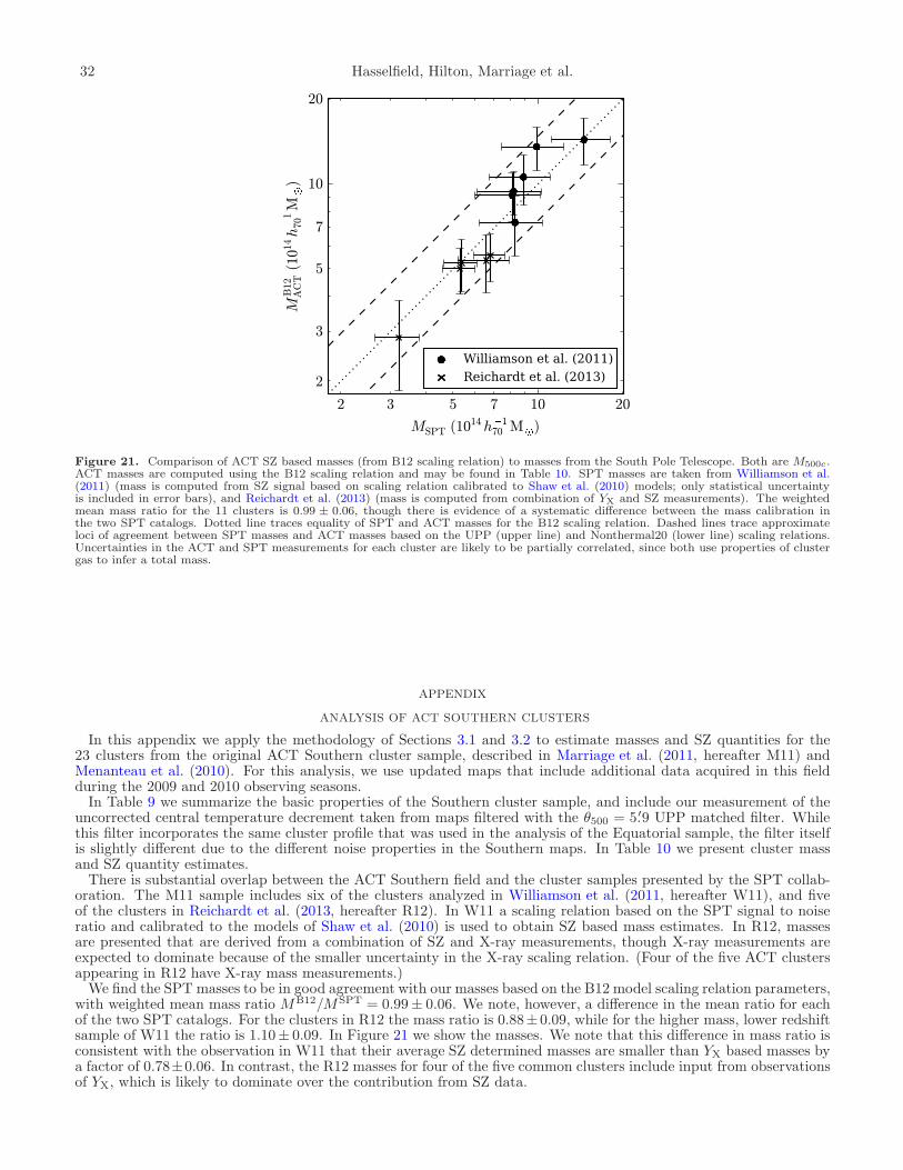
32 Hasselfield, Hilton, Marriage et al.

102 3 5 7 20

MSPT (1014h170 M)

10

2

3

5

7

20

MB12

ACT (1014h

170M

)

Williamson et al. (2011)

Reichardt et al. (2013)

Figure 21. Comparison of ACT SZ based masses (from B12 scaling relation) to masses from the South Pole Telescope. Both are M500c.ACT masses are computed using the B12 scaling relation and may be found in Table 10. SPT masses are taken from Williamson et al.(2011) (mass is computed from SZ signal based on scaling relation calibrated to Shaw et al. (2010) models; only statistical uncertaintyis included in error bars), and Reichardt et al. (2013) (mass is computed from combination of YX and SZ measurements). The weightedmean mass ratio for the 11 clusters is 0.99 ± 0.06, though there is evidence of a systematic difference between the mass calibration inthe two SPT catalogs. Dotted line traces equality of SPT and ACT masses for the B12 scaling relation. Dashed lines trace approximateloci of agreement between SPT masses and ACT masses based on the UPP (upper line) and Nonthermal20 (lower line) scaling relations.Uncertainties in the ACT and SPT measurements for each cluster are likely to be partially correlated, since both use properties of clustergas to infer a total mass.

APPENDIX

ANALYSIS OF ACT SOUTHERN CLUSTERS

In this appendix we apply the methodology of Sections 3.1 and 3.2 to estimate masses and SZ quantities for the23 clusters from the original ACT Southern cluster sample, described in Marriage et al. (2011, hereafter M11) andMenanteau et al. (2010). For this analysis, we use updated maps that include additional data acquired in this fieldduring the 2009 and 2010 observing seasons.In Table 9 we summarize the basic properties of the Southern cluster sample, and include our measurement of the

uncorrected central temperature decrement taken from maps filtered with the θ500 = 5.′9 UPP matched filter. Whilethis filter incorporates the same cluster profile that was used in the analysis of the Equatorial sample, the filter itselfis slightly different due to the different noise properties in the Southern maps. In Table 10 we present cluster massand SZ quantity estimates.There is substantial overlap between the ACT Southern field and the cluster samples presented by the SPT collab-

oration. The M11 sample includes six of the clusters analyzed in Williamson et al. (2011, hereafter W11), and fiveof the clusters in Reichardt et al. (2013, hereafter R12). In W11 a scaling relation based on the SPT signal to noiseratio and calibrated to the models of Shaw et al. (2010) is used to obtain SZ based mass estimates. In R12, massesare presented that are derived from a combination of SZ and X-ray measurements, though X-ray measurements areexpected to dominate because of the smaller uncertainty in the X-ray scaling relation. (Four of the five ACT clustersappearing in R12 have X-ray mass measurements.)We find the SPT masses to be in good agreement with our masses based on the B12 model scaling relation parameters,

with weighted mean mass ratio MB12/MSPT = 0.99± 0.06. We note, however, a difference in the mean ratio for eachof the two SPT catalogs. For the clusters in R12 the mass ratio is 0.88± 0.09, while for the higher mass, lower redshiftsample of W11 the ratio is 1.10± 0.09. In Figure 21 we show the masses. We note that this difference in mass ratio isconsistent with the observation in W11 that their average SZ determined masses are smaller than YX based masses bya factor of 0.78±0.06. In contrast, the R12 masses for four of the five common clusters include input from observationsof YX, which is likely to dominate over the contribution from SZ data.

ACT: SZ Selected Galaxy Clusters 33

Table 9Uncorrected central Compton parameters for the clusters from

Marriage et al. (2011).

ACT ID R.A. Dec. Redshift S/N y0 Alternate ID (ref.)() () (10−4)

ACT–CL J0102−4915* 15.7208 −49.2553 0.870 9.0 3.51 ± 0.43 SPT-CL J0102-4915 (1)ACT–CL J0145−5301 26.2458 −53.0169 0.118 4.0 0.86 ± 0.19 Abell 2941 (2)ACT–CL J0215−5212 33.8250 −52.2083 0.480 4.9 0.79 ± 0.18ACT–CL J0217−5245 34.2958 −52.7556 0.343 4.1 0.79 ± 0.18 RXC J0217.2-5244 (3)ACT–CL J0232−5257 38.1875 −52.9522 0.556 4.7 0.61 ± 0.17ACT–CL J0235−5121 38.9667 −51.3544 0.278 6.2 0.98 ± 0.19ACT–CL J0237−4939 39.2625 −49.6575 0.334 3.9 0.93 ± 0.26ACT–CL J0245−5302 41.3875 −53.0344 0.300 9.1 1.57 ± 0.17 Abell S0295 (4)

SPT-CL J0245-5302 (1)ACT–CL J0304−4921 46.0625 −49.3617 0.392 3.9 1.52 ± 0.32ACT–CL J0330−5227* 52.7250 −52.4678 0.442 6.1 1.23 ± 0.18 Abell 3128 NE (5)ACT–CL J0346−5438 56.7125 −54.6483 0.530 4.4 1.05 ± 0.22ACT–CL J0438−5419* 69.5792 −54.3181 0.421 8.0 1.62 ± 0.13 SPT-CL J0438-5419 (1)ACT–CL J0509−5341* 77.3375 −53.7014 0.461 4.8 0.82 ± 0.14 SPT-CL J0509-5342 (6)ACT–CL J0516−5430 79.1250 −54.5083 0.294 4.6 0.87 ± 0.15 Abell S0520 (4)

SPT-CL J0516-5430 (6)ACT–CL J0528−5259 82.0125 −52.9981 0.768 3.1 0.50 ± 0.13 SPT-CL J0528-5300 (6)ACT–CL J0546−5345* 86.6542 −53.7589 1.066 6.5 0.92 ± 0.14 SPT-CL J0546-5345 (6)ACT–CL J0559−5249* 89.9292 −52.8203 0.609 5.1 0.89 ± 0.14 SPT-CL J0559-5249 (6)ACT–CL J0616−5227* 94.1500 −52.4597 0.684 5.9 1.00 ± 0.15ACT–CL J0638−5358 99.6917 −53.9792 0.222 10.0 1.77 ± 0.15 Abell S0592 (4)

SPT-CL J0638-5358 (1)ACT–CL J0641−4949 100.3958 −49.8089 0.146 4.7 0.58 ± 0.26 Abell 3402 (2)ACT–CL J0645−5413 101.3750 −54.2275 0.167 7.1 1.19 ± 0.17 Abell 3404 (2)

SPT-CL J0645-5413 (1)ACT–CL J0658−5557 104.6250 −55.9511 0.296 11.5 2.65 ± 0.21 1E0657-56/Bullet (7)

SPT-CL J0658-5556 (1)ACT–CL J0707−5522 106.8042 −55.3800 0.296 3.3 0.54 ± 0.21

Note. — Clusters used for cosmological and scaling relation constraints in Section 5 are marked with an asterisk. Redshifts are allspectroscopic, obtained from literature as described in Menanteau et al. (2010) or as presented in Sifon et al. (2012). We provide theS/N of detection as presented in Marriage et al. (2011), for reference. Uncorrected central Compton parameters y0 are obtained from theapplication of a matched filter with θ500 = 5.′9 (see Section 3.1). Alternate IDs are provided for clusters detected before the initial releaseof the Southern sample, and for any cluster appearing in current SPT results. References: (1) Williamson et al. (2011); (2) Abell (1958);(3) Bohringer et al. (2004); (4) Abell et al. (1989); (5) Werner et al. (2007); (6) Reichardt et al. (2013); (7) Tucker et al. (1995).

Table 10SZ-derived mass estimates for the ACT Southern cluster sample of

Marriage et al. (2011).

ID θ500 Q(m, z) Y500 MUPP500c MB12

500c Mnon500c Mdyn

500c

(arcmin) (10−4 arcmin2) (1014h−170 M⊙) (1014h−1

70 M⊙) (1014h−170 M⊙) (1014h−1

70 M⊙)

ACT-CL J0102−4915 2.5 ± 0.1 0.60 ± 0.02 11.5 ± 2.0 10.5 ± 1.8 13.8 ± 2.4 15.0 ± 2.6 16.0 ± 3.5ACT-CL J0145−5301 8.1 ± 0.9 1.02 ± 0.01 16.9 ± 8.2 3.5 ± 1.2 4.8 ± 1.8 5.7 ± 2.2 4.2 ± 2.2ACT-CL J0215−5212 2.5 ± 0.2 0.62 ± 0.05 2.4 ± 1.0 3.5 ± 1.0 4.5 ± 1.4 5.2 ± 1.7 4.1 ± 1.7ACT-CL J0217−5245 3.2 ± 0.3 0.75 ± 0.05 3.2 ± 1.3 3.4 ± 1.0 4.4 ± 1.4 5.3 ± 1.8 4.0 ± 1.7ACT-CL J0232−5257 2.0 ± 0.3 0.49 ± 0.07 1.2 ± 0.7 2.5 ± 1.0 3.1 ± 1.3 3.5 ± 1.5 2.6 ± 1.4ACT-CL J0235−5121 4.1 ± 0.3 0.87 ± 0.03 5.9 ± 2.0 4.1 ± 1.1 5.6 ± 1.5 6.8 ± 1.8 5.4 ± 1.9ACT-CL J0237−4939 3.2 ± 0.5 0.74 ± 0.09 3.1 ± 2.1 3.1 ± 1.4 3.9 ± 1.9 4.6 ± 2.4 3.2 ± 2.1ACT-CL J0245−5302 4.6 ± 0.2 0.92 ± 0.01 12.1 ± 2.0 6.7 ± 1.3 9.2 ± 1.8 11.3 ± 2.1 10.4 ± 2.6ACT-CL J0304−4921 3.5 ± 0.3 0.79 ± 0.05 6.8 ± 2.6 5.7 ± 1.6 7.4 ± 2.3 8.7 ± 2.8 7.3 ± 3.1ACT-CL J0330−5227 3.2 ± 0.1 0.74 ± 0.02 5.4 ± 1.2 5.4 ± 1.1 7.3 ± 1.5 8.7 ± 1.7 7.7 ± 2.0ACT-CL J0346−5438 2.6 ± 0.2 0.62 ± 0.04 3.3 ± 1.1 4.4 ± 1.2 5.7 ± 1.6 6.6 ± 1.9 5.5 ± 2.0ACT-CL J0438−5419 3.6 ± 0.1 0.80 ± 0.01 8.8 ± 1.0 7.0 ± 1.2 9.5 ± 1.6 11.5 ± 1.9 10.9 ± 2.3ACT-CL J0509−5341 2.8 ± 0.1 0.66 ± 0.03 3.1 ± 0.7 4.0 ± 0.8 5.3 ± 1.1 6.3 ± 1.3 5.2 ± 1.4ACT-CL J0516−5430 3.9 ± 0.2 0.85 ± 0.03 5.1 ± 1.3 4.0 ± 0.9 5.4 ± 1.2 6.7 ± 1.5 5.3 ± 1.6ACT-CL J0528−5259 1.6 ± 0.2 0.37 ± 0.05 0.9 ± 0.4 2.3 ± 0.8 2.9 ± 1.0 3.1 ± 1.1 2.4 ± 1.1ACT-CL J0546−5345 1.6 ± 0.1 0.36 ± 0.02 2.0 ± 0.4 3.9 ± 0.7 5.1 ± 0.9 5.2 ± 1.0 4.9 ± 1.1ACT-CL J0559−5249 2.3 ± 0.1 0.56 ± 0.02 2.8 ± 0.6 4.3 ± 0.8 5.7 ± 1.1 6.5 ± 1.3 5.6 ± 1.4ACT-CL J0616−5227 2.2 ± 0.1 0.53 ± 0.02 3.0 ± 0.6 4.6 ± 0.9 6.1 ± 1.2 6.9 ± 1.3 6.2 ± 1.5ACT-CL J0638−5358 6.1 ± 0.2 1.00 ± 0.01 22.4 ± 3.0 7.5 ± 1.4 10.5 ± 2.0 13.0 ± 2.4 12.5 ± 3.2ACT-CL J0641−4949 4.8 ± 1.0 0.93 ± 0.06 2.9 ± 3.2 1.4 ± 0.9 1.8 ± 1.2 2.2 ± 1.4 1.3 ± 1.1ACT-CL J0645−5413 6.9 ± 0.3 1.02 ± 0.01 18.2 ± 4.3 5.1 ± 1.2 7.3 ± 1.7 8.9 ± 2.0 7.7 ± 2.4ACT-CL J0658−5557 5.4 ± 0.1 0.97 ± 0.01 26.6 ± 3.2 10.3 ± 1.9 14.3 ± 2.6 17.6 ± 3.1 18.2 ± 4.3ACT-CL J0707−5522 2.8 ± 0.5 0.69 ± 0.09 1.4 ± 1.1 1.7 ± 0.9 2.2 ± 1.2 2.6 ± 1.4 1.7 ± 1.1

Note. — Columns are as described in Table 8.