arX

iv:a

stro

-ph/

0511

061v

1 2

Nov

200

5DRAFT VERSIONFEBRUARY 3, 2008Preprint typeset using LATEX style emulateapj v. 6/22/04

CORRELATION PROPERTIES OF THE KINEMATIC SUNYAEV-ZEL’DOVICH EFFECT AND IMPLICATIONS FORDARK ENERGY

CARLOS HERNÁNDEZ–MONTEAGUDO,1 L ICIA VERDE,1 RAUL JIMENEZ1 AND DAVID N. SPERGEL2

Draft version February 3, 2008

ABSTRACTIn the context of a cosmological study of the bulk flows in the Universe, we present a detailed study of

the statistical properties of the kinematic Sunyaev-Zel’dovich (kSZ) effect. We first compute analytically thecorrelation function and the power spectrum of the projected peculiar velocities of galaxy clusters. By takinginto account the spatial clustering properties of these sources, we perform a line-of-sight computation of theall-skykSZ power spectrum and find that at large angular scales (l < 10), the local bulk flow should leave avisible signature above the Poisson-like fluctuations dominant at smaller scales, while the coupling of densityand velocity fluctuations should give much smaller contribution. We conduct an analysis of the prospectsof future high resolution CMB experiments (such as ACT and SPT) to detect the kSZ signal and to extractcosmological information and dark energy constraints fromit. We present two complementary methods, onesuitable for “deep and narrow” surveys such as ACT and one suitable for “wide and shallow” surveys suchas SPT. Both methods can constraint the equation of state of dark energyw to about 5-10% when applied toforthcoming and future surveys, and probew in complementary redshift ranges, which could shed some lighton its time evolution. This is mainly due to the high sensitivity of the peculiar velocity field to the onset ofthe late acceleration of the Universe. We stress that this determination ofw does not rely on the knowledge ofcluster masses, although it relies on cluster redshifts andmakes minimal assumptions on cluster physics.

Subject headings:cosmic microwave background – large scale structure of universe

1. INTRODUCTION

The new generation of ground-based high-resolution cos-mic microwave background (CMB) experiments (e.g., theAtacama Cosmology Telescope3 [ACT;Kosowsky (2003);Fowler et al. (2005)] and the South Pole Telescope4

[SPT;Ruhl et al. (2004)]), are designed to scan with very highsensitivity and arcminute resolution the microwave sky. Theirmain goal is the study of the thermal Sunyaev-Zel’dovich(tSZ) effect (Sunyaev & Zel’dovich 1980): the change of fre-quency of CMB photons due to inverse Compton scatteringby hot electrons. Such hot electron plasma are known tobe found in clusters of galaxies, and should also be presentin larger structures, such as filaments and superclusters ofgalaxies. This scattering translates into a redshift indepen-dent distortion of the CMB black body spectrum, making thetSZ effect an ideal tool to probe the baryon distribution in thelarge scales of our Universe at different cosmic epochs. How-ever, this is not the only effect of an electron plasma on theCMB radiation. If a cloud of electrons is moving with somebulk velocity with respect to the CMB frame, then Thomsonscattering by these electrons will imprint new (Doppler in-duced) temperature fluctuations on the CMB photons. Thisis the so called kinematic Sunyaev-Zel’dovich effect (kSZ,Sunyaev & Zeldovich (1972)), which is spectrally indistin-guishable from the intrinsic CMB temperature fluctuations.

Although the kSZ effect is typically an order of magnitudesmaller than the tSZ in clusters of galaxies (and for this rea-son much harder to detect), it encodes precious cosmological

1 Department of Physics and Astronomy, University of Pennsylvania,209 South 33rd St, Philadelphia, PA 19104; carloshm@astro.upenn.edu,lverde,raulj@physics.upenn.edu

2 Department of Astrophysical Sciences, Peyton Hall, Princeton Univer-sity, Princeton, NJ 08540; dns@astro.princeton.edu

3 http://www.hep.upenn.edu/act/4 http://spt.uchicago.edu/

information since it depends on the peculiar velocity field.Indeed, kSZ measurements can yield valuable informationabout the large-scale velocity field, the evolution of the darkmatter potential, and the growth of fluctuations. The studyof large scale velocity fields (cosmic flows) has been an ac-tive research area in the nineties. There have been numerousattempts to measure bulk flows using the large-scale distri-bution of galaxies and their peculiar velocities, and to placeconstraints on the matter power spectrum or the Universematter density, (see reviews of Strauss & Willick (1995) andCourteau & Dekel (2001) and references therein). However,it became clear that these measurements had to be correctedfor systematic errors, such as the biases introduced when cal-ibrating the distances of the galaxies under study, or the nonlinear components of the velocities of those objects. With kSZobservations, by using clusters as tracers of the velocity fields,one is more confident to probe larger (less non-linear) scales.

While there have been no kSZ detections to date, upperlimits on the peculiar velocities of individual clusters havebeen reported by Benson et al. (2003). Such a difficult mea-surement could in principle be hampered by other effectssuch as non-linearities and the complicated physics of theintra-cluster gas. Nagai, Kravtsov, & Kosowsky (2003) haveshown that the kSZ is not diluted by the internal velocitydispersion in the intracluster gas. Ma & Fry (2002) calcu-lated the temperature fluctuations produced by the kSZ inthe non-linear regime using the halo model. Benson et al.(2003) showed that the signal-to-noise of a kSZ measure-ment should be distance independent and suggested com-bining signals from different redshifts. Holder (2002) andAghanim et al. (2004) have discussed how to extract the kSZsignal from maps, while Schäfer et al. (2004) used N-bodysimulations to build templates of kSZ maps in the contextof the Planck mission, and Kashlinsky & Atrio–Barandela(2000) study the possibility of extracting the kSZ dipole from

2

CMB surveys covering a large fraction of the sky. Dueto its weak signal, indirect detection of the kSZ has beenproposed through cross-correlation techniques with weak-lensing (Doré, Hennawi, & Spergel 2004) or old galaxies(DeDeo, Spergel & Trac 2005). As we shall see below, a mea-surement of the kSZ effect would be very valuable, since itwould not only allow us to measure bulk flows of clusters ofgalaxies and test the predictions of the standard model, butalso provide additional constraints on cosmological parame-ters, especially on the equation of state of dark energy.

In this paper we compute the correlation function and thepower spectrum of the kSZ effect. This requires modeling ofthe peculiar velocity field and the cluster population. We ex-plore the prospects for future CMB experiments to measurethe kSZ correlation function, and find that ACT-like experi-ments should be able to detect the kSZ-induced CMB vari-ance at high (∼ 12σ) significance level. Further, we studythe dependence of the kSZ correlation function on the cosmo-logical parameters, and show that it can be used to measurethe equation of state of dark energy (w) if the redshifts of theclusters of galaxies detected in CMB surveys are available.We find that, with the SALT follow up of ACT data or witha wider but shallower (SPT-like) survey, thew parameter canbe constrained with an accuracy of 8% for an ACT scan of400 square degrees. This error should scale inversely with thesquare root of the covered area and hence becomes 5% for a1,000 square degree area. These determinations ofw do notrely on the knowledge of cluster masses, but do rely on clus-ters redshifts and reasonable assumptions on cluster physics.

Unless otherwise stated, throughout this work we shallasume a LCDM cosmological model (Spergel et al. 2003)with Ωm = 0.3, ΩΛ = 0.7, h = 0.72, andσ8 = 0.88. The paperis organised as follows: in Section 2 we study the statisticalproperties of the projected peculiar velocity field and providean analytical expression for the correlation function ofprojected velocities. In Section 3 we compare the kSZ andtSZ effects, and discuss the strategy to enhance the probabil-ities of detecting the former. In Section 4 we compute thecorrelation function and the power spectrum of the kSZ, bothwhen we consider only a given set of clusters present in asurvey or the whole celestial sphere. In Section 5 we outlinetwo methods to estimate the kSZ effect in future CMB clustersurveys and in Section 6 we explore the dependence of kSZmeasurements on cosmological parameters making particularemphasis onw. We conclude in Section 7.

2. THE CORRELATION FUNCTION OF LINE-OF-SIGHTLINEAR PECULIAR VELOCITIES

While the measurement of the kSZ effect of individualclusters is difficult (e.g.,Aghanim et al. (2001); Benson etal.(2003)), in this paper we address the prospects for statisticaldetection of cluster peculiar velocities in future CMB surveys.This requires the knowledge of the ensemble properties ofthe velocity field traced by the galaxy cluster population, towhich we devote the current section. For clarity and futurereference, a statistical description of the linear velocity fieldand related quantities is given in Appendix A.

Throughout this paper, we shall assume that the measuredvelocity field obeys linear theory. However, as noted byColberg et al. (2000), this is not completely fulfilled bycluster velocities, since clusters are peculiar tracers ofthelarge scale matter distribution and showbiased velocities

compared to the expectations provided by the linear theory.Colberg et al. (2000) found that this bias was typically a 30%- 40% effect. Although several attempts have been madeto model this boost in terms of the underlying density field(Sheth & Diaferio 2001; Hamana et al. 2003), in subsequentsections it will be accounted for by simply increasing thecluster velocities by a factorbv = 1.3 (Sheth & Diaferio2001). The goal of this paper is to present a theoreticalcalculation of the detectability of the signal and the fore-casted signal-to-noise: detailed comparison with numericalsimulations are left to future work. Full treatment can beimplemented only with the help of numerical simulationsmatched to a given observing program(see Peel (2005) for arecent study). We must stress that, although some modellingof non-linear effects must be included in this study, clustersare the largest virialised structures known in the Universe,and probe much bigger scales than galaxies. Therefore wemust expect them to be significantly better tracers of thelinear velocity field. Furthermore, as we shall see below, thepeculiar velocity estimator (the kSZ effect) doesnot dependof distance, which avoids the need to use redshift-independentdistance indicators, as opposed to other peculiar velocityestimators.

On large, linear scales, the density and peculiar veloci-ties are related through the continuity equation:∂δk/∂t =−ik · vk/a, wherea andk are the scale factor and comovingFourier mode, respectively. The peculiar velocity of a cluster,as probed by its kSZ effect, can be interpreted as the linearpeculiar velocity field smoothed on comoving scaleR whichcorresponds to the cluster’s massM via

R=

[

3M4πρ

]1/3

, (1)

where ρ is the background matter density. The kSZ effectis sensitive to the line-of-sight component of the velocity,but under the assumption that the velocity field is Gaussianand isotropic (which should be satisfied in the linear regime)the three spatial components of the velocity field must bestatistically independent. Moreover, the power spectrummust completely determine the statistical properties of thevelocity field. Thus, in a given cosmological model, the linearvelocity field power spectrum (which in turn is related tothe matter power spectrum) should univocally determine theangular correlation function (and angular power spectrum)ofthe line-of-sight cluster velocities.

In linear theory, the velocity dispersion smoothed overspheres of comoving radiusR (corresponding to a given clus-ter massM) is given by

σ2vv(R,z) =

(

H(z)

∣

∣

∣

∣

dDδ

dz

∣

∣

∣

∣

)2∫

dk k2 Pm(k)2π2k2

∣

∣W(kR)∣

∣

2, (2)

whereW(kR) is the Fourier transform of the top hat win-dow function,H(z) is the Hubble function,Dδ(z) is the lineargrowth factor andPm(k) is the present day linear matter powerspectrum, (the power spectra at any redshift will be denotedasPδδ(z,k) ≡ D2

δ(z) Pm(k)). Hence the power spectrum of thevelocities is:

Pvv(k) =

(

H(z)

∣

∣

∣

∣

dDδ

dz

∣

∣

∣

∣

)2 Pm(k)k2

= D2vPm(k)

k2, (3)

whereDv ≡ H(z)dDδ/dz is the velocity growth factor. WhencomputingDδ for different Dark Energy models, we used the

3

FIG. 1.— Peculiar velocity growth factor for three different cosmologies: aΛCDM model (ΩL = 0.7,Ωm = 0.3, thick solid line), aΩm = 0.3, flatw = −0.6model (dotted line), andΩm = −1/3 andw = −1/3, (dashed line).

analytical fit provided by Linder (2005):

g(a) = exp∫ a

0d loga

[

(

ΩmH2

0

a3H2(a)

)γ − 1

]

, (4)

whereg(a)≡Dδ(a)/a gives the deviation of the growth factorfrom that of a critical (Ωm = 1) universe, andγ is given by

γ = 0.55+ b[1 + w(z= 1)], (5)

with b = 0.05 if w > −1 andb = 0.02 otherwise.

The growth of the velocity perturbations with redshift mayprovide useful cosmological constraints such as constraints onthe equation of state of dark energy (DeDeo, Spergel & Trac2005). This is illustrated in Fig.(1), where we show theredshift evolution of the velocity growth factor for threedifferent cosmological models: aΛCDM model (ΩΛ = 0.7,Ωm = 0.3, thick solid line), a flat universe withΩm = 0.3 anddark energy equation of state parameterw = −0.6 (dottedline), and another flat model withΩm = 0.3 andw = −1/3,(dashed line). Due to thek2 factor in the denominator ofeq.(3), the signal is weighted by the largest scales, makingthis probe relatively insensitive to the smoothing scale andtherefore to clusters mass. Indeed, if the dependence ofσvvversus mass is approximated by a power law, then one findsthat for the concordance modelσvv ∝ M−0.13.

Having this in mind, we compute here the angular corre-lation function of theline-of-sight(LOS) cluster velocities.Note that Peel (2005) takes a different approach to this calcu-lation. Assuming that we can measure the LOS component ofthe peculiar velocity of a cluster, we compute the quantity

Cvv(θ12) ≡ 〈(

v(x1) ·n1

)(

v(x2) ·n2

)

〉, (6)

wheren1 and n2 denote two different directions in the sky,“connecting” the observer to the cluster positionsx1 andx2andθ12 denotes the angle betweenn1 andn2. We refer thereader to Appendix B for the detailed derivation and here wereport the final expression for this correlation function:

Cvv(θ12) =∑

even l

2l + 14π

cosθ12×

(

2πFl

)∫

k2dk Pvv(k) W(kR1) W(kR2) ×

j l (k[x1 − x2cosθ12]) j l (kx2sinθ12), (7)

In this equation, the factorFl is given by

Fl ≡(l − 1)!!

2l/2 (l/2)!coslπ/2, (8)

and x1,x2 are the (comoving) distances to the clusters,(without loss of generality we have used the convention thatx1 ≥ x2). Here j l (x) denote the spherical Bessel functions andthe summation must take place only overevenvalues ofl ; R1andR2 refer to the linear scales corresponding to the massesof each cluster. Note that we recover eq.(2) in the limit ofθ12 → 0 andx1 → x2.

Fig.(2a) shows the behaviour ofCvv vs θ12 in the concor-danceΛCDM model for a couple of 1014 M⊙ clusters whenthey are both placed at z=0.005 (solid line), both placedat z=0.1 both (dashed line) and when once cluster is atz=0.1 and the other at z=1 (dotted line). In the first (clearlyunrealistic) case, the clusters are so close to us that both arecomoving in the same bulk flow with respect to the CMBframe, giving rise to the dipolar pattern shown by the solidline. In the case where both clusters are atz∼ 0.1 (dashedline), their correlation properties are strongly dependent onθ12, since this angle defines the distance between the clusters.For small angular separation, the clusters are still relativelynearby, and hence their peculiar velocities are correlated, butthis correlation dies as the separation of the clusters increases.The angular distance at which the correlation drops to half itsvalue at zero separation is∼ 10, corresponding to roughly40 h−1 Mpc. Finally, if clusters are very far apart from eachother (thick dotted line), their peculiar velocities are notcorrelated.

An alternative way to present the correlation properties ofthe projected peculiar velocities of the clusters is the veloc-ity field angular power spectrum. In Appendix B, we invertCvv(θ12) into its angular power spectrumCvv

l , i.e.,

Cvv(θ12) =∑

l

2l + 14π

Cvvl Pl (cosθ12). (9)

We find that

Cvvl ≡ 4π

2l + 1

(

lBl−1 + (l + 1)Bl+1)

, (10)

where theBl coefficients are defined by

Bl ≡ 4π

∫

k2dk(2π)3

Pvv(k) j l (kx1) j l (kx2) (11)

Fig.(2)b displays the power spectra for two cases: two verynearby clusters (both at z=0.005, solid line), showing analmost dipolar pattern, and two relatively far away clusters

4

FIG. 2.— Correlation function (top) and corresponding power spectrum(bottom) of the projected peculiar proper velocities. The solid lines observethe case where the two clusters are placed atz = 0.005 from the observer.Dashed lines show the case in which clusters are further,z = 0.01. Finally,the dotted line considers the case where one cluster is located atz = 0.1 andthe other cluster is much further (z = 1). Note the lack of correlation in thiscase.

(both at z=0.1, dashed line), case in which the power istransferred to higher multipoles. The power spectrum for theclusters placed at z=0.005 and z=0.1 is zero.

Here we have characterised the projected peculiar velocityfield at cluster scales. Next, we address the study of the kSZeffect and its comparison with the tSZ effect.

3. THE SUNYAEV-ZEL’DOVICH EFFECTS

3.1. The kinematic Sunyaev-Zel’dovich Effect

The Kinematic Sunyaev-Zel’dovich effect describes theDoppler kick that CMB photons experience when they en-counter a moving cloud of electrons. Since this is simpleThomson scattering, there is no change of the photon fre-quency, and hence it leaves no spectral signatures in the CMBblackbody spectrum. Therefore, this effect is solely deter-mined by the number density of free electrons and their rel-

ative velocity to the CMB frame. An observer will only besensitive to theradial component of the electron peculiar ve-locity, so the expression for the change in brightness temper-ature becomes (Sunyaev & Zel’dovich 1968)

δTkSZ

T0=

∫

dl ne(l ) σT

(

−v ·n

c

)

≡ τ

(

−v ·n

c

)

. (12)

Here, we have assumed that the peculiar velocity is thesame for all electrons.τ stands for the optical depth, andn is a unitary vector giving the direction of observation.This process must take place in two contexts: (1) Whenthe intergalactic medium becomes ionized by the highenergy photons emitted by the first stars, inhomogeneitiesin the electron velocity and density distributions generate akSZ signal which is known as the Ostriker-Vishniac effect.Despite of the large size of ionized structures encounteredbythe CMB photons, the electron density contrast is relativelysmall, and further, we do not know where in CMB maps tolook for this signal because we do not know the location ofthe ionized bubbles which formed during reionization. Theamplitudes and angular scales at which this effect shouldbe visible are model dependent, but can be as high as afew microK in the multipole rangel > 2000, (Santos et al.2003). (2) Clusters of galaxies at lower redshift leave a moreeasily detectable signal. Their high electron density can giverise to values ofτ as high as 10−3 − 10−2, and their peculiarvelocities should be close to 300 kms−1 at z = 0, whichtogether can produce temperature fluctuations of the order of1-10µK. The clusters high optical depth is also responsiblefor large spectral distortions of the CMB generated throughthe thermal Sunyaev-Zel’dovich (tSZ) effect. The tSZ effectis typically an order of magnitude larger than the kSZ andintroduces frequency dependentbrightness temperaturefluctuations which, in the not relativistic limit, change sign at218 GHz. Therefore by combining observations in bands atfrequencies lower and higher than this cross frequency, it ispossible to obtain the cluster position and to characterizethetSZ cluster signal. Once the cluster position is identified theirkSZ contribution should be accessible at 218 GHz. However,as noted by Sehgal, Kosowsky & Holder (2005) and earlierby Holder (2004), even with measurements in three differentfrequencies it may not be possible to obtain a clean estimateof the kSZ effect for a single cluster. We shall show belowthat we are not interested in a very accurate kSZ estimatefor a given cluster, but onunbiasedestimates on our entirecluster sample.

In the next subsection we make a detailed comparison ofthe amplitude of the kSZ and the tSZ effects.

3.2. Comparison of the kSZ and the tSZ effects in clusters ofgalaxies

In what follows we shall describe the galaxy clus-ter population by adopting the model presented inVerde, Haiman & Spergel (2002). This model is basedupon the spherical collapse description of galaxy clusters(Gunn & Gott 1972), and assumes that clusters are isothermaland their gas acquires the virial temperature of the halo. Thehalo mass and redshift distribution is approximated by theformalism presented in Sheth & Tormen (1999). We refer toVerde, Haiman & Spergel (2002) for further details in thismodelling.

5

Both kSZ and tSZ effects can be written as integrals ofsome functionK(r) along the line of sight crossing the cluster,weighted by the electron density:

δTT0

= g(x)∫

dl σT ne(l )K(l ) (13)

For the non-relativistic tSZ g(x) =(

x cothx/2 − 4)

,x ≡ hν/kBT0 is the adimensional frequency in terms ofthe CMB monopoleT0, K = kBTe/(mec2) wherene, Te, me arethe electron density, temperature and mass respectively,σTthe Thomson cross-section andkB the Boltzmann constant.For the kSZ,g(x) ≡ 1, K = −n · v/c, wheren is a unitaryvector pointing along the line of sight, andv is the clusterpeculiar velocity. If clusters are perfectly virialised objects,then one must expect the scalingTe ∝ M2/3. However,following Verde, Haiman & Spergel (2002), the clustermodel should leave some room for some deviations fromsuch scaling, which can be due to internal (non-linear) clusterphysics, deviations from purely gravitational equilibrium,preheating, etc. Our parametrization adoptsTe ∝ M1/ξ, whereξ = 1.5 for a perfectly virialized cluster, but spans the rangefrom 1.5 to 2 in the literature. We shall present results forξ = 1.5, but the sensitivity of our results onξ is minimal.At the same time, the radial peculiar velocity dispersion ofthe clusters,〈

√

(−n ·v/c)2〉 = σvv decreases very slowly withmass (∼ M−0.13), so, at fixed redshift we must expect the ratiokSZ/tSZ to be bigger for low mass clusters, which are morenumerous. Regarding the redshift dependence, clusters tendto be denser at earlier epochs (the productne rv scales roughlyas (1+ z)2), so we must expect larger tSZ and kSZ amplitudesat higher redshifts. However, the dependence of the functionK is different in each case: while clusters are hotter at earliertimes (Te ∝ (1+ z)), velocities have not had so much time togrow as at present epochs (σvv ∝ 1/

√1+ z), and hence the

ratio kSZ/tSZ (∝ 1/(1+ z)3/2) decreases with redshift.

We show these scalings explicitely in Fig.(3), where the thinlines evaluate the tSZ and the kSZ atz = 0 and thick linescorrespond toz = 1. The solid lines provide the amplitudeof the cluster-induced tSZ fluctuations at 222 GHz, which, aswe shall see below, will be taken as our effective frequencyafter accounting for the tSZ relativistic corrections and theeffects related to the finite spectral width of the detectors. Thedashed lines provide the expected rms amplitude of the kSZeffect in clusters: we see that, atz = 0, clusters of massesbelow∼ 1015 M⊙ should produce more kSZ than tSZ flux at222 GHz, at least by a factor of a few. This mass thresholddecreases atz = 1, but so does the typical halo mass at suchredshift (clusters of∼ 1014 M⊙ are very rare objects), so againwe must expect the kSZ to dominate over the tSZ.

4. THE POWER SPECTRUM OF THE KSZ EFFECT

4.1. Model of the cluster population

We next study the kSZ signal generated by the entire pop-ulation of clusters of galaxies by computing its two second-order momenta, i.e., the correlation function and the powerspectrum. For this, it is first necessary to have a model todescribe the population of galaxy clusters in the Universe.We shall adopt the hierarchical scenario in which small scaleoverdensities in the Universe become non-linear and collapsefirst, and then merge and give rise to bigger non-linear struc-tures. The abundance of haloes of a given mass at a given

FIG. 3.— Comparison of the tSZ (solid lines) and kSZ (dashed line) effectsas a function of clusters mass. Thick lines refer to z=1 (where most of theclusters are located for ACT-like surveys), whereas thin lines correspond toz=0. For the majority of clusters, the kSZ flux will be a few times bigger thanthe tSZ flux at 222 GHz.

cosmic epoch or redshift is given by the clusters mass func-tion. We will adopt the Sheth & Tormen (hereafter ST) massfunction (Sheth & Tormen 1999), which will be denoted byn(M,z) ≡ dN(M,z)/dV(z) and provides theaveragenumberdensity of haloes of mass contained betweenM andM + dMat redshiftz. It must not be confused withn(M,x), which istheactualnumber of haloes in that mass range at positionx.The latter can be understood as arandomvariable, the for-mer as itsmean. As it will be useful later, we first computethe mean number of haloes present in two volume elementscentered atx1 andx2:

〈n(M1,x1)n(M2,x2)〉 = n(M1,z1)n(M2,z2) +

δD(M1 − M2)δ3D(x1 − x2)n(M1,z1) +

〈∆[n(M1,x1)]∆[n(M2,x2)]〉. (14)

In this equation,z1 andz2 are the redshift corresponding to po-sitionsx1 andx2 respectively. The first term in the right handside of the equation is merely a constant, but will have its rel-evance, because it will couple with the velocity field as weshall see below. The next term containing the Dirac deltas ac-counts for the (assumed) Poissonian statistics ruling the (dis-crete) number density of sources, and will be referred to asthe Poissonianterm. In the third term,∆[n(M1,x1)] standsfor the deviation with respect to the average halo number den-sity due to the environment, i.e., due to large scale overden-sities, which condition the halo clustering. Therefore, thisthird term describes the spatial clustering of haloes, whichis a biased tracer of the spatial clustering of matter. In theextended Press-Schecter approach it can be shown that thepower spectrum and the correlation function of haloes and un-derlying matter are merely proportional to each other over a

6

wide range of scales. This is commonly expressed by abiasfactor (Mo & White 1996), so that

ξhh(r) = b2(M,z) ξm(r) ; Phh(k) = b2(M,z)Pm(k). (15)

Here ξhh, ξm and Phh(k),Pm(k) stand for halo-halo andmatter correlation function/power spectrum, respectively.Therefore, the third term in the RHS of eq.(14) equalsn(M1,z1)n(M2,z2)b(M1,z1)b(M2,z2)ξm(x1 − x2).

A parallel approach consists in writing the halo mass func-tion as a function of some linear scale matter overdensityδ ≡ (ρ− ρ)/ρ. The number of haloes atx is then approximatedas

n(M,x) = n(M,z) + η +∂n(M,z)

∂δ

∣

∣

∣

∣

δ=0

δ(x) +O[δ2], (16)

whereη is a random variable which introduces the Poisso-nian behaviour of the source counts. In the extended Press-Schechter formalism, it turns out that∂n(M,z)/∂δ

∣

∣

δ=0coin-

cides with the bias factorb(M,z), and by using this it is possi-ble to reproduce eq. (14) from eq.(16). This justifies neglect-ing all higher-order powers ofδ in eq. (16). We have takenδ to be inlinear regime, but, sinceξhh(r) ≃ b2ξmm(r) down toscales comparable to the halo size, we shall use this formalismdown to halo scales.

4.2. A Line of Sight approach for the kSZ effect

We next write the temperature anisotropies induced by thekSZ in clusters of galaxies as an integral along the line ofsight:

∆TkSZ

T0[n] =

∫ r lss

0dr

∑

j

τ j

(

−vj ·n

c

)

Wgasj (r − r j ). (17)

Here,r is the comoving radius integrated to the last scatter-ing surface, and the sum over the indexj represents a sum onall clusters;τ j denotes the opacity in thecenterof the cluster(τ = aσTne,c with ne,c the central electron number density anda the scale factor), and the window functionWgas

j (r − r j) de-notes the gas profile of the cluster. Although we should adoptsome realistic shape for this profile (Komatsu & Seljak 2001),we have adopted a simple Gaussian window with scale radiusequal to the virial radius of the cluster. This is justified since,in Fourier domain, at scales bigger than the cluster size, thewindow function is merely equal to the volume occupied bythe gas, regardless of the shape of the gas profile. This stepsimplifies our computations significantly,anddoes not com-promise the accuracy in the relatively big scales (bulk flowscales) in which we are interested. Note that even if the sumis made over all clusters,only the clusters being intersectedby the line of sight will contribute to the integral. This sumcan be re-written first as an integral and then as a convolution,

∆TkSZ

T0[n] =

∫ r lss

0dr

∫

dM ×(

∫

dy τ (M,z)

(

−v(M ,y) ·n

c

)

n[M,y] Wgas[

M, r − y]

)

=∫ r lss

0dr

∫

dM ×[

(

τ (M,z)

(

−v(M) ·n

c

)

n[

M])

⋆Wgas[

M,z]

]

[r ]. (18)

Note that central optical depth and the window functionhave an intrinsic dependence on redshift. This is due to thefact that clusters formed at higher redshift tend to be moreconcentrated. The symbol⋆ denotes here convolution in realspace.

4.3. Theall skycorrelation function and power spectrum ofthe kSZ effect

If two different lines of sight are now combined to estimatethe angular correlation function, then one obtains that

⟨

∆TkSZ

T0[n1]

∆TkSZ

T0[n2]

⟩

∝⟨

n(M1, r1)

(

v(M1, r1) ·n1

)

n(M2, r2)

(

v(M2, r2) ·n2

)⟩

.

(19)Next we plug eq.(16) and make use of the Cumulant Ex-

pansion Theorem. We must note as well that Poissonian fluc-tuations will be assumed to be independent ofδ, and that forGaussian statistics, the 3- and 4-point functions are zero,justas〈v〉 and〈δ〉. Therefore we are left with a sum of productsof 2-point functions of the form

n(M1,z1)σ2vv(M1,z1) +

n(M1,z1)n(M2,z2)

⟨(

v(M1, r1) ·n1

)(

v(M2, r2) ·n2

)⟩

+

∂n(M1,z1)∂δ

∣

∣

∣

∣

δ=0

∂n(M2,z2)∂δ

∣

∣

∣

∣

δ=0

×[

〈δ(r1)δ(r2)〉⟨(

v(M1, r1) ·n1

)(

v(M2, r2) ·n2

)⟩

+

⟨

δ(r1)

(

v(M2, r2) ·n2

)⟩⟨

δ(r2)

(

v(M1, r1) ·n1

)⟩

+

⟨

δ(r1)

(

v(M1, r1) ·n1

)⟩⟨

δ(r2)

(

v(M2, r2) ·n2

)⟩]

. (20)

Note that the last term is a constant. We refer again toAppendix A where the cross terms〈δ(v · n)〉 are studied. InAppendix C we provide a explicit computation of the powerspectra arising from each of the terms considered in eq.(20).Since the last term introduces no anisotropy, the kSZ powerspectrum is the sum of four contributions: a Poisson term(Poisson), a term proportional to the velocity-velocity cor-relation (vv term), a term proportional to the product of thevelocity-velocity correlation and the density-density correla-tion (vv− dd term), and a term proportional to the density-velocity squared (dv− vd term). Therefore,

Cl = CPl +Cvv

l +Cdd−vvl +Cdv−vd

l . (21)

Fig.(4) displays each of the terms in eq.(21): the thick solidline is the Poisson term, whereas the thick dashed line corre-sponds to thevv term. Although the latter decreases rapidlywith increasingl , at the large scales it dominates over all otherterms, reflecting the presence of the local bulk flow. In an at-tempt to simplify the expressions for these two terms given inAppendix C, we have found the approximate integral

CPl ≈

∫

dzdV(z)

dzdM n(M,z) σ2

vv(M,z)

∣

∣yl (M,z)∣

∣

2

π(22)

7

FIG. 4.— Different components of the all-sky kSZ power spectra:thethick solid line shows the Poisson term, which dominates over the other termsexcept in the lowl limit. In this large scale range, thevvgenerated by the localbulk flow is the one introducing most power, (dashed line). Filled circles anddiamonds show semi-analytical approximations for these two Poissonandvv, respectively (see eqs.(22,23)). Of lower amplitude, the thick dotted lineshows the sum of thedd-vvand thedv-vdterms, (thin dotted lines, note thatthe latter is negative).

for the Poisson term, and

Cvvl ≈

∫

dzdV(z)

dzPvv

(

z,k =l

r(z)

)

×

[∫

dM1

4πn(M,z)

∣

∣yl (M,z)∣

∣

]2

(23)

for thevv term.yl (M,z) is the Fourier transform of the clusterprofile in the sphere,

yl =

(√2πθv

)2

exp−l (l + 1)θ2v/2, (24)

andPvv(k,z) is thek andzdependent velocity power spectrum.θv is the angular size of the cluster virial radius. Filled circlesfor the Poisson term and diamonds for thevv term provide acomparison of these approximations with the exact integrals.Although the amplitudes and slopes are not too disimilar,the approximatedvv term is particularly innacurate at largeangular scales (l < 10). The approximation for the Poissonianterm seems to predict a somewhat correct amplitude at lowl , but a shallower slope, which translates into a smalleramplitude at high multipoles.

The dd-vv and dv-vd terms are shown by the thin dottedlines. We must remark that thedv-vdterm is negative, and weare plotting its absolute value. The sum of both is given by thethick dotted line. The sum of these two terms is particularlyhard to detect, since it never dominates, not at large scales(itis about a factor of 20 below thevv term), nor at small scales,where it is well below the Poisson term.

FIG. 5.— Cluster-cluster kSZ correlation functions for a sample of clusterswith masses above 2×1014M⊙. When forming cluster pairs we require pairconstituents to be at similar redshifts. If we consider all redshifts simultane-ously, we obtain the solid line. The dashed lines correspondto differential-in-redshift cluster-cluster correlation functions: the thick dashed line considersonly clusters aroundz∼ 0.01, whereas the intermediate dashed line corre-sponds toz∼ 0.1 and the thin dashed line toz∼ 1.

4.4. Thecluster-clusterkSZ correlation function

Future high resolution multi frequency CMB experimentslike ACT or SPT can provide kSZ estimates on those regionsof the sky where clusters of galaxies have been identified viatSZ. Therefore one could attempt to measure the velocitiescorrelation function by computing the kSZ correlation func-tion in thisrestrictedset of pixels:

Ccl−clkSZ (θ) =

∑

i1,i2

∑

j1, j2

τ (Mi1,zj1)τ (Mi2,zj2) ×

〈 1c2

(

v(Mi1,zj1) ·n1

)(

v(Mi2,zj2) ·n2

)

〉. (25)

Since the signal comes from clusters which velocities arecorrelated, we should consider pairs close in redshift. Thesolid line in Fig.(5) shows the correlation function to be mea-sured fromall galaxy clusters fromz= 0 uptoz= 4 more mas-sive than 2× 1014h−1M⊙, according to the standardΛCDMcosmology and the Sheth-Tormen mass function. Membersof the cluster pairs must be within∆z= 0.01. Since the kSZamplitude per cluster is typically of few tens of microKelvin,the zero-lag correlation function can be as high as∼ 150 (µK)2, and drops to one half of this value atθ ∼ 2 −3. The thickdashed line shows the correlation function for clusters locatedat z≃ 0.01. As the redshift increases (z≃ 0.1 medium thick-ness dashed line;z≃ 1, thin dashed line), the amplitude atzero lag increases (clusters are more concentrated) and thecorrelation angle decreases. The solid line shows the redshift-integrated cluster-cluster correlation function: the signal isdominated by high redshift clusters, more concentrated andmore numerous per unit solid angle.

Diaferio, Sunyaev & Nusser (2000) pointed out a poten-tially important non-linear aspect that is not included in our

8

modeling: in very massive superclusters, the kSZ effect showstypically a dipolar pattern, plausably caused by the encounterof two oppossite bulk flows at their common attractor’s po-sition. Since our model predicts no dipolar pattern at scalesof a few degrees, such scenario is not accounted for by ourapproach. Hence, in a realistic application the core of suchoverdense regions should be excised from the analyses. Suchmassive structures however are very rare and form at very lateepochs, and their exclusion should not compromise the anal-ysis presented here.

5. CAN THE KSZ EFFECT BE MEASURED?

In this section we outline two different procedures toextract the kSZ signal from future high-resolution and high-sensitivity CMB experiments. The procedures presented heremay be sub-optimal but our aim is to quantify the relativeimportance of difference sources of error and to roughlyforecast the expected signal to noise for those experiments.We defer the developement of an optimal procedure to futurework. We shall try to extract the kSZ signal in a statisticalsense: while previous works (e.g., Aghanim et al. (2004))have addressed the difficulty of separating the kSZ effectfrom potential contaminants (tSZ, radio-source emission,infrared galaxies, CMB, etc) in a given cluster, our approachwill consist on combining the signal coming from subsetsof clusters in such a way that the contribution of the noisesources averages out. As we shall see, the success of thisprocedure will rely on the precision to which theaverageproperties of the potential contaminants are known.

The first approach, which we shall refer to as method (a), isbased on measurements of the kSZ flux and its redshift evo-lution. Its sensitivity to cosmology increases with redshift,and, for this reason it is suited for “deep and narrow” surveystrategies. Here we will use ACT’s specifications. Our secondapproach (method (b)) uses the ratio of kSZ and tSZ inducedtemperature anisotropies. This ratio is particularly sensitive tow atz<

∼0.8 and since cosmic variance for the peculiar velocityfield is more important at low redshifts, this method is moresuitable for “wide and shallow” survey strategies. Here wewill use a survey with specifications similar to those of ACT,but covering 4,000 square degrees and thus with higher noise.These specifications are not too dissimilar from those of SPT,assuming that accurate photometric redshifts can be obtainedfor all SPT clusters.

5.1. Probing the kSZ flux at high redshift

In what follows, we shall use specifications for ACT oneyear data (Gaussian beam with FWHM equal to 2 arcmins,noise amplitude lower than 2µK per beam, and a cleanscanned area of 400 square degrees). ACT observes in threebands: 145, 220 and 250 GHz. We will concentrate on the220 GHz channel, although some knowledge will be assumedto be inferred from the other bands. For instance, the 250GHz channel will be very useful to estimate the level ofinfrared-galaxy emission at lower frequencies. Likewise,the145 GHz channel should be critical when characterizing thetSZ flux from each cluster. For simplicity, we will concentrateon the variance of the kSZ signal, but it is easy to estimate thekSZ angular correlation function introduced in subsection4.4.

The strip covered by ACT should also be surveyed by

FIG. 6.— Typical amplitude of CMB residuals remaining after attemptingto approximate the CMB average within a circular patch of angular radiusθv(given in abscissas) by the CMB average computed within a ring surroundingthe patch of width 10% the patch radius. For most of clusters located atz> 0.3, these residuals will typically be of 3 – 4µK amplitude.

SALT5. Cluster detection via tSZ effect will provide targetsfor optical observations. Alternatively, optical clusteridenti-fication should be possible up toz∼ 1 from SALT’s multi-band imaging using algorithms such as those developed inKim et al. (2002); Miller et al. (2005). Hence, a direct com-parison can be made with tSZ detected cluster sample. SALTspectroscopic follow up will enable to obtain the cluster red-shifts.

The method is as follows:

• For every detected galaxy cluster, we take a patch of ra-dius equal to one projected cluster virial radius. We canuse the edge of significant tSZ emission at other fre-quencies to define this radius. We compute the meantemperature within this patch, and draw a ring sur-rounding it, of width, say, 10% of the virial radius.We next compute the mean temperature within this ringand subtract it from the mean of the patch. This oper-ation should remove most of the CMB contribution tothe average temperature in the patch, but will unavoid-ably leave some residuals, which will be denoted hereasδTres

cmb. These residuals will have two different con-tributions: the first coming from the inaccurate CMBsubtraction, the second one being due to instrumentalnoise residuals,

〈(

δTresCMB

)2〉 = 〈δT2subs〉+

N2

Nbeams. (26)

Nbeamsis the number of beam sizes present in the ring,and N2 is the instrumental noise variance. If we denotethe patch of radius the cluster virial radius asregion 1,and byregion 2the ring surrounding it, it can be easily

5 SALT’s URL site:http://www.salt.ac.za/

9

proved that the first term in the RHS of the last equationreads

〈δT2subs〉 =

1(∆Ω1)2

∫

∆Ω1

∫

∆Ω1

dn1dn2 C(n1,n2) +

1(∆Ω2)2

∫

∆Ω2

∫

∆Ω2

dn1dn2 C(n1,n2) −

2∆Ω1∆Ω2

∫

∆Ω1

∫

∆Ω2

dn1dn2 C(n1,n2). (27)

∆Ω1 and ∆Ω2 denote the solid angles of the patchand the ring, respectively, whereasn1 and n2 denotedirections in the sky andC(n1,n2) is the CMB angularcorrelation function evaluated at the angle separatingthe directionsn1 and n2. The rms fluctuations intro-duced by this residual are plotted in Fig.(6): althoughit can be as high as a few tens of microK for nearbyclusters subtending 30 – 40 arcmins, their effectreduces to a 3 – 4µK for clusters of a few arcminssize, which correspond to most of clusters atz > 0.3to be detected by ACT-like CMB experiments. Thiscontaminant will be dominant over the instrumentalnoise contribution.

• We assume that, by observing the tSZ amplitudes at 145GHz and 250 GHz, it is possible to provide anunbiasedestimate of the mean tSZ contribution to the clusterpatch at 220 GHz. After subtracting the tSZ and CMBcomponents estimates, the temperature in the patch cor-responding to clusteri can be written as

δi = δT resCMB,i + δTtSZ,i + N+ δT int

kSZ,i + TkSZ,i . (28)

δTtSZ,i denotes the tSZ residualsafter substracting theestimated tSZ amplitude. N accounts for contributionof instrumental noise to the patch average, andδT int

kSZ,ifor the residual contribution of internal velocities.According to Diaferio et al. (2005), we assume atypical rms for internal velocities of one third the bulkflow velocity expected for each cluster, and randomorientation (sign); thus we assumeδT int

kSZ,i rms to be1/3 of the bulk-flow induced kSZ amplitude. The firstfour quantities in the RHS of eq.(28) have zero mean,henceδi is anunbiasedestimate of the kSZ amplitudein clusteri.

• We now combine estimates of the kSZ coming fromdifferentclusters in order to estimate the kSZ cluster-cluster correlation function,〈TkSZ,iTkSZ, j〉. As men-tioned in a previous Section, we are interested in com-puting this correlation function by considering pairs ofclusters of similar redshift. Note that we avoid squaringthe kSZ estimate of the same cluster (i = j), since resid-uals would not average out and would introduce a biasin our kSZ variance estimates. Let us assume that thebulk flows occupy a typical scale (named here asco-herence scale) θcoh on the sky. Within this patch alongdirectionn, we can sort all clusters in mass and redshiftbins. LetI , J, L andM denote the mass bins of clustersin a common redshift range centered atzl . By buildingcluster pairs upon all members of these bins, and com-bining different mass bins, it is possible to compute the

following kSZ variance6 estimator at redshiftzl alongthe directionn:

F2kSZ, l (n) ≡

∑

I≤J

wI ,J

NI ,J

∑

i, j

(δiΩi)(δ jΩ j )

/

∑

I≤J

wI ,J. (29)

Ω j stands for thej-th cluster’s solid angle. We remarkthat the kSZ flux depends solely on the cluster’s massand peculiar velocity, and so do our angle-integratedkSZ temperature anisotropies. If we denote byNI andNJ the number of cluster members in bins I and J, re-spectively, then the number of cluster pairs that can beformed by combining these two mass bins is given byNI ,J; NI ,J = NI NJ if I 6= J andNI ,J = NI (NI − 1)/2 for thesame bin (I = J). The indexesi and j run for individ-ual cluster members in each mass bin.wI ,J is a weightfactor, which we define as

wI ,J ≡NI NJ

σ2I σ

2J

=

NI

Ω2I [〈δT res

CMB〉2 + 〈δTtSZ〉2 + 〈(δT intkSZ)

2〉+ N2] I×

NJ

Ω2J[〈(δT res

CMB)2〉+ 〈δT2tSZ〉+ 〈(δT int

kSZ)2〉+ N2]J

, (30)

with the subscriptsI andJ evaluating the brackets inthe corresponding mass bins. The estimator of eq.(29)provides a weighted measurement of the kSZ variance,

〈F2kSZ, l (n)〉 =

∑

I≤J wI ,J (FkSZ, l ,I FkSZ, l ,J)∑

I≤J wI ,J, (31)

with FkSZ, l ,I the expected kSZ amplitude at redshiftzland mass equal to that corresponding to binI . Its formalerror is given by

∆2[F2

kSZ, l (n)] =

2×[

∑

I≤J wI ,J (FkSZ, l ,I FkSZ, l ,J)∑

I≤J wI ,J

]2

+

∑

I ,J,L

wI ,J,L(FkSZ, l ,I FkSZ, l ,L)

/(

∑

I≤J

wI ,J

)2

+

∑

I ,J,M

wI ,J,M(FkSZ, l ,JFkSZ, l ,M)

/(

∑

I≤J

wI ,J

)2

+

1

/

∑

I≤J

wI ,J, (32)

wherewI ,J,L ≡ wI ,JNL/σ2L. Note that the first term in

the RHS of this equation is not sensitive to the numberof clusters within the coherence patch. Such term,containing the squared kSZ expectations for massbins I and J, is associated to the (assumed) intrinsicGaussian nature of the kSZ fluctuations, and it corre-sponds to thecosmic variancecontribution. It will thusscale like the inverse of the survey area when different

6 We integrate temperature fluctuations in the cluster’s area, obtaining aquantity of unitsµK·strad. This integrated temperature fluctuations are es-sentially proportional toflux fluctuations, and for this reason they will bedenoted byFkSZ. One must keep in mind, however, that their units are notJanskys, but microKelvin× stereoradian.

10

coherence patches are combined in the analysis. Theforth term is exclusively due to observational errors,whereas the second and third terms are hybrid: theyshow contributions from both the intrinsic uncertaintyof the velocity field and observational errors. IfNbdenotes the number of mass bins, and we take theweights, the cluster number and theFkSZ equal for allmass bins (σI = σ, NI = N andFkSZ,l ,I = FkSZ,l for everymass binI ), then it can easily be proved that the forthterm scales roughly asσ4/N2/(Nb(Nb + 1)), that is, thesquared variance expected for each cluster over thetotal number of pairs that can be formed. The secondand third terms, in this limit, yieldσ2F2

kSZ,l/(N(Nb +1)),which scales inversely to the number of clusters. Inour case, our kSZ flux estimates will be limited by thecosmic variance term. On the other hand, because ofhaving very few objects, we considered one mass binonly.

• Finally, we combine estimates from theNcoh ≃4π fsky/θ2

coh different projected coherent regions in thesky, wherefsky is the fraction of the sky covered by theCMB experiment, yielding

F2kSZ, l ≡

∑

n

F2kSZ, l (n)

∆2[F2kSZ, l (n)]

/

∑

n

1

∆2[F2kSZ, l (n)]

, (33)

with an uncertainty

∆2[F2

kSZ, l ] = 1

/

∑

n

1

∆2[F2kSZ, l (n)]

. (34)

Note that the size of the coherent patch must depend ofredshift: a bulk flow extenting up to 20h−1Mpc at z=1subtends a degree on the sky, whereas if it is at z≃ 0.05then it subtends around 8 degrees.

We take the effective noise N to have a typical amplitude of5 µK per beam7, and it accounts for both instrumental noiseand the confusion noise associated to unresolved sources.δT res

CMB is computed as stated in eq.(27), and contributestypically with a few microK. Regarding the tSZ residuals,δTtSZ contains the contribution coming from relativistictSZ corrections, and power leakage associated to the finitespectral width of the detectors. We conservatively assumethat the amplitude of these residuals (remaining after the tSZsubstraction) is typically the non-relativistic tSZ temperatureincrement expected at 222 GHz. We approximate the beam asa Gaussian of FWHM equal to 2 arcmins, and take 400 squaredegrees (fsky≃ 10−2) as the clean sky region covered by ACT.ACT’s sensitivity limit is set to cluster above 2×1014 h−1M⊙,and the total number of clusters above this threshold predictedin this region of the sky by our Sheth-Tormen mass functionis roughly 4,400. However, for this analysis we only userelatively bright and big clusters: the product of their angularsize and tSZ temperature decrement at 145 GHz must bebigger than 160µK arcmin2, and this requirement decreasesconsiderably the amount of available clusters.

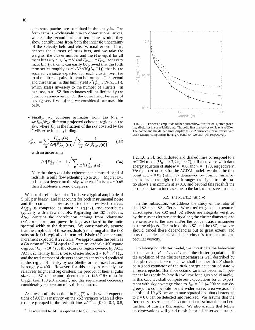
As a result of this section, in Fig.(7) we show our expecta-tions of ACT’s sensitivity on the kSZ variance when all clus-ters are grouped in the redshift binszband

l ≡ [0.02, 0.4, 0.8,

7 The noise level for ACT is expected to be<∼2µK per beam.

FIG. 7.— Expected amplitude of the squared kSZ flux for ACT, aftergroup-ing all cluster in six redshift bins. The solid line line corresponds to aΛCDM.The dotted and the dashed lines display the kSZ variances foruniverses withDark Energy components havingw equal to -0.6 and -1/3, respectively

1.2, 1.6, 2.0]. Solid, dotted and dashed lines correspond toaΛCDM model(Ωm = 0.3,ΩΛ = 0.7), a flat universe with darkenergy equation of statew = −0.6, andw = −1/3, respectively.We report error bars for theΛCDM model: we drop the firstpoint at z = 0.02 (which is dominated by cosmic variance)and focus in the high redshift range: the signal-to-noise ra-tio shows a maximum at z=0.8, and beyond this redshift theerror bars start to increase due to the lack of massive clusters.

5.2. The kSZ/tSZ ratioRIn this subsection, we address the study of the ratio of

the kSZ and tSZ effects. When referring to temperatureanisotropies, the kSZ and tSZ effects are integrals weightedby the cluster electron density along the cluster diameter,andare sensitive to the size and/or the concentration parameterof these objects. The ratio of the kSZ and the tSZ, however,should cancel these dependencies out to great extent, andprovide a cleaner view of the cluster’s temperature andpeculiar velocity.

Following our cluster model, we investigate the behaviourof the statisticR ≡ δTkSZ/δTtSZ in the cluster population. Ifthe evolution of the cluster temperature is well described bythe spherical collapse model, we shall find then thatR shouldbe a good estimator of the dark energy equation of statewat recent epochs. But since cosmic variance becomes impor-tant at low redshifts (smaller volume for a given solid angle),in this case we shall compute our expectations for an experi-ment with sky coverage close tofsky = 0.1 (4,000 square de-grees). To compensate for the wider survey area we assumea noise of 10µK per arcminute squared and that clusters upto z = 0.8 can be detected and resolved. We assume that thefrequency coverage enables contaminant subtraction and ex-traction of clusters tSZ signal. We also assume that followup observations will yield redshift for all observed clusters.

11

These specifications are not too dissimilar to those of the SPTtelescope when combined with photometric follow up.

We shall see that these are precisely the requirementsneeded to obtain cosmological information fromR. However,since in this case the kSZ signal is divided by the tSZ temper-ature decrement (measured at say, 145 GHz), we must be verycareful with the noise contribution to the denominator ofR.Our approach will be to conservatively consider only clusterswhose integrated tSZ temperature decrements are larger than160 µK-arcmin2 at 145 GHz. This implies that tSZ errorswill be typically 5% – 10% of the estimated tSZ temperaturedecrement, and that they can be treated perturbatively as er-rors in the kSZ estimation in the numerator. Therefore, ourmodel for the estimation ofR in a single cluster will be givenby:

r i =δT res

CMB,i + δTtSZ,i + N + δT intkSZ,i + ǫ TkSZ,i + TkSZ,i

TtSZ,i. (35)

Most of the terms of this equation are defined exactly as ineq.(28). The only new term isǫTkSZ,i , which accounts for theextra error introduced by the uncertainty in the denominator,TtSZ,i . HereTtSZ,i is the absolute value of the tSZ decrement ofthe cluster at 145 GHz andǫ was taken to be a normal randomvariable of rms 0.05 (5% error inTtSZ,i which reflects into 5%error inTkSZ,i). We neglect the correlation of the errors inTtSZ,iwith those ofTkSZ,i and takeǫ independent of the other noisesources.

We now write the analogue to eq.(29) as

Rl (n) ≡∑

I≤J

wI ,J

NI ,J

∑

i, j

r ir j

/

∑

I≤J

wI ,J, . (36)

where the weights are defined as

wI ,J ≡NI NJ

σ2I σ

2J

=

NI T2tSZ,I

[〈δT resCMB〉2 + 〈δTtSZ〉2 + 〈(δT int

kSZ)2〉+ ǫ2T2

kSZ,I + N2] I×

NJ T2tSZ,J

[〈(δT resCMB)2〉+ 〈δT2

tSZ〉+ 〈(δT intkSZ)

2〉+ +ǫ2T2kSZ,J + N2]J

. (37)

The estimate ofRl (n) in a redshift bandzl and directionn,together with its uncertainty∆2[Rl (n)] can be obtained fromeqs.(31,32) by simply replacingF2

kSZ,l (n) by Rl (n). Similarly

the expressions forRl and ∆2[Rl ] can be obtained from

eqs.(33,34).

In Fig.(8) we plot the ratioR at different redshifts as itwould be seen by an experiment like SPT. As before, we haveassumed that only clusters above 2×1014 h−1M⊙ can be seen,and grouped all clusters in the redshift binszband

l ≡ [0.02, 0.4,0.8, 1.2, 1.6, 2.0]. The lines refer to the same cosmologi-cal models as in Fig.(7). Note the similarity of this plot andFig.(1). We see thatR is sensitive to cosmology at muchlower redshifts (z<

∼ 0.8) thanFkSZ, and for the sensitivity anal-ysis following in the next Section we have only used the firstthree redshift bins.

FIG. 8.— Expected kSZ/tSZ ratioR as measured by SPT for six redshiftbins. The solid line corresponds to aΛCDM model while the dotted and thedashed lines are for flat models withw equal to -0.6 and -1/3, respectively.

6. KSZ SENSITIVITY TO MEASURING COSMOLOGICALPARAMETERS

We can now explore the dependence of the two statistics in-troduced in the previous Section on cosmological parameters.We define theχ2 as

χ2 ≡∑

l

(

Q2kSZ, l − Q2

kSZ, l

)2

∆2[Q2kSZ, l ]

, (38)

whereQ2kSZ, l can either refer to the angle-averaged kSZ

anisotropy (F) or the kSZ/tSZ ratio (R). The likelihood isthusL ∝ exp− 1

2χ2. We estimate errors using the Fisher ma-trix approach. In principle the parameters that enter in theanalysis areΩm, w, the fraction of cluster mass in the in-tra cluster mediumfICM, the present-day normalization of thematter density fluctuationsσ8 and the reduce Hubble constanth. In practice both methods are non sensitive tofICM, σ8 andh separately for a fixed number of detected clusters, but ontheir combination in the form of an overall amplitude of thekSZ signal, which we shall asign to an amplitude parameterAalone.

We assume thatA is redshift-independent (or that itsscaling in redshift can be constrained) and consider a 20%uncertainty in this normalization, owing to 10% uncertaintyin σ8, fICM andh each, over which we marginalize. We re-mark, however, that our results will be practically insensitiveto the uncertainty onA. In Fig.(9) we show the resultingconstraints in theΩm–w plane. Clearly, theFkSZ method ismore sensitive tow thanR, and their directions of degener-acy are also different, but both distinct to the directions ofdegeneracy corresponding to estimators based upon LargeScale Structure. Indeed, these estimators are restricted tothe low redshift universe, and hence their sensitivity onwis very limited, giving rise to degeneracy direction almostparallel to thew axis, (see, e.g., Fig (11) in Eisenstein et al.

12

FIG. 9.— Contour plots showing the 1 and 2–σ joint confidence region(solid line) and the 1–σ marginalized (dotted line) in theΩm – w plane fortheF2

kSZ(method (a)) andR2 (method (b)) estimations. Method (a) applied toACT (top) with CMB (WMAP 1st year) priors (dashed lines) yields a∼ 8%error onw. This error would drop below 5% if ACT covers 1,000 squaredegrees. Method (b) on a SPT-like survey gives a∼ 12% error onw afterimposing the prior from WMAP’s 1st year data.

(2005) or Fig. (13) in Tegmark et al. (2004)). The constrainton w, marginalized overΩm, is ∼ 12% for FkSZ and∼ 60%for R. As the degeneracy direction in each case is differentto that corresponding to CMB temperature measurements,a combination with analyses of CMB temperature data canbreak the degeneracy. When considering WMAP first yeardata, the marginalised error onw reduces to∼ 8%, ∼ 12%,for FkSZ and R methods, respectively (thick dotted lines).As pointed above, these errors are dominated by the cosmicvariance term present in eq.(32). Therefore, by increasingthesky covered by the experiments, those errors should decreaseas∝ 1/

√

fsky.

These results have been obtained after using a ST massfunction, and assuming that the cluster density was uniform(i.e., we have have considered no biases). The error ampli-tudes and the orientation of the ellipses in Fig (9) dependstrongly on the number of cluster pairs that can be formedin each redshift bin, particularly at the high z end. If theactual sensitivity of future CMB experiments is such that thelower limit on detectable clusters can be relaxed (we believethe limit 2×1014 h−1 M⊙ to be very conservative for ACT’s

FIG. 10.— Differential redshift contribution to the change inχ2 whenprobing models with differentw: approach a) is more sensitive to higherredshifts (thick line), method b) to lower redshifts (thinkline).

noise level), then the resulting number of cluster pairs thatcan be formed would increase considerably, and this wouldreflect on an increased sensitivity tow.

We note that, a priori, the two methods are nicely com-plementary in their redshift ranges sensitive tow as shownin Fig.(10): we find that theF2

kSZ estimation (method a)thick histogram) is sensitive tow at high redshifts (z> 0.5),whereasR for different dark energy models differs at lowredshift and converges atz≈ 1: the sensitivity of this methodis localised mainly at low redshift (thin histogram).

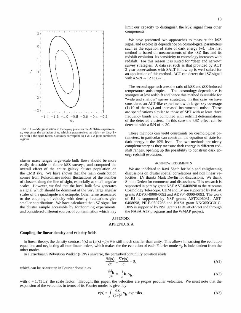
After parametrising the evolution ofw asw(a) = w0 +wa(1−a), with a = 1/(1+ z) the scale factor, we conduct a Fishermatrix analysis considering the parameter set [Ωm, w0, fICM,wa] for the F2

kSZ method. The marginalization in thew0-waplane is given in Fig.(11), which shows this method shouldhave some residual sensitivity onwa (a typical error of∼ 1.75in wa). Note that this error should be improved further aftercombining the two methods proposed here, provided that theyare sensitive to different redshift ranges.

7. CONCLUSIONS

We have studied bulk flows in the large scale structure inthe context of the kSZ effect and future high-sensitivity andhigh-resolution CMB experiments like ACT. Since the kSZeffect is only sensitive to the projected peculiar velocities ofelectron clouds, we have focussed our analysis on the angularcorrelation of radial peculiar velocities in galaxy clusters.We have provided an analytical expression for the angularcorrelation function of projected peculiar velocities in thelinear regime, and interpreted it in the context of local anddistant bulk flows. We have also presented an expression forthe power spectrum of projected linear peculiar velocities.

We have investigated in which redshift and for which

13

FIG. 11.— Marginalisation in thew0-wa plane for the ACT-like experiment.wa expresses the variation ofw, which is parametrised asw(a) = w0 + wa(1−a), with a the scale factor. Contours correspond to 1 & 2-σ joint confidenceregions.

cluster mass ranges large-scale bulk flows should be moreeasily detectable in future kSZ surveys, and computed theoverall effect of the entire galaxy cluster population onthe CMB sky. We have shown that the main contributioncomes from Poissonian/random fluctuations of the numberof clusters along the line of sight, especially at small angularscales. However, we find that the local bulk flow generatesa signal which should be dominant at the very large angularscales of the quadrupole and octupole. Other terms associatedto the coupling of velocity with density fluctuations givesmaller contributions. We have calculated the kSZ signal forthe cluster sample accessible by forthcoming experiments,and considered different sources of contamination which may

limit our capacity to distinguish the kSZ signal from othercomponents.

We have presented two approaches to measure the kSZsignal and exploit its dependence on cosmological parameterssuch as the equation of state of dark energy (w). The firstmethod is based on measurements of the kSZ flux and itsredshift evolution. Its sensitivity to cosmology increases withredshift. For this reason it is suited for “deep and narrow”survey strategies. A data set such as that provided by ACT2 year observations with SALT follow up is well suited foran application of this method. ACT can detect the kSZ signalwith a S/N∼ 12 atz∼ 1.

The second approach uses the ratio of kSZ and tSZ-inducedtemperature anisotropies. The cosmology-dependence isstrongest at low redshift and hence this method is suitable for“wide and shallow” survey strategies. In this case we haveconsidered an ACT-like experiment with larger sky coverage(1/10 of the sky) and increased instrumental noise. Theseare specifications similar to those of SPT with at least threefrequency bands and combined with redshift determinationsof the detected clusters. In this case the kSZ effect can bedetected with a S/N of∼ 30.

These methods can yield constraints on cosmological pa-rameters, in particular can constrain the equation of statefordark energy at the 10% level. The two methods are nicelycomplementary as they measure dark energy in different red-shift ranges, opening up the possibility to constrain dark en-ergy redshift evolution.

ACKNOWLEDGMENTS

We are indebited to Ravi Sheth for help and enlighteningdiscussions on cluster spatial correlations and non linearve-locities. LV thanks Mark Devlin for discussions. We thankSimon Dedeo for comments and discussions. This research issupported in part by grant NSF AST-0408698 to the AtacamaCosmology Telescope. CHM and LV are supported by NASAgrants ADP03-0000-0092 and ADP04-0000-0093. The workof RJ is supported by NSF grants AST0206031, AST-0408698, PIRE-0507768 and NASA grant NNG05GG01G.DNS is supported by NSF grants PIRE-0507768 and throughthe NASA ATP programs and the WMAP project.

APPENDIX

APPENDIX A

Coupling the linear density and velocity fields

In linear theory, the density contrastδ(x) ≡ (ρ(x) − ρ)/ρ is still much smaller than unity. This allows linearising the evolutionequations and neglecting all non-linear orders, which makes the the evolution of each Fourier modeδk is independent from theother modes.

In a Friedmann Robertson Walker (FRW) universe, the perturbed continuity equation reads∂δ(x)∂t

+∇v(x)

a= 0, (A1)

which can be re-written in Fourier domain as∂δk∂t

= −ia

k ·vk , (A2)

with a = 1/(1+ z) the scale factor. Throught this paper, the velocities areproper peculiar velocities. We must note that theexpansion of the velocities in terms of its Fourier modes is given by

v(x) =∫

dk(2π)3

vk exp−ikx, (A3)

14

and that, due to isotropy, the diferent components are independent. The statistical properties of each of them must be, however,identical.

Coming back to eq.(A2), if we denote byDδ(z) the growth factor of the density perturbations, then we canexpress the compo-nent ofvk parallel tok (denoted here byvk ) as

vk = i H (z)dDδ

dz

δkk

. (A4)

H stands for the Hubble function andz for redshift.The power spectrum foranycomponent of the Fourier velocity mode hence reads

Pvv(k) =

(

H(z)dDδ(z)

dz

)2 Pm(k)k2

. (A5)

If we now combineδk andvq, we obtain

〈δkv∗q〉 = (2π)3δD(k − q)Pdv(k) = (2π)3δD(k − q) i H (z)dDδ(z)

dzPm(k)

k. (A6)

Note that this is an imaginary quantity. In this work, we shall find this power spectrum either squared or in a convolution withitself, giving rise to negative power and indicatinganticorrelation.

Finally, we compute the power spectrum of the quantity

φ(x,n1) ≡ δ(x) (v(x) ·n1) =∑

i

δ(x)

(

vi(x)n1i

)

, (A7)

wheren1 stands for the unitary vector connecting an observer with the positionx, and the sum is over the three spatial components.Since a product in real space involves a convolution in Fourier space, the Fourier mode ofφ reads:

φk ,n1=

∑

i

∫

dq(2π)3

δq v1i, k−q n1

i . (A8)

Having this in mind, the average product of two Fourier modesof φ when looking in two different directionsn1 andn2 is:

〈φk , n1φ∗

q, n2〉= (2π)3δD(k −q)

[

cosθ12[

Pδδ ⋆Pvv

]

(k)+(

cosθ12+sinθ12)[

Pδv⋆Pvδ

]

(k)

]

+ (2π)3δD(k)(2π)3δD(q)

(∫

du(2π)3

Pδv(u)

)2

.

(A9)θ12 = arccos(n1 ·n2) is the angle separatingn1 andn2. Without introducing any loss of generality of eq.(A9), we have takenn1 = (0,0,1) andn2 = (0,sinθ12,cosθ12). The symbol⋆ denotes convolution and is present in the first two terms in brackets. Thethird term is non zero only whenk = q = 0.

Before ending this appendix, it is worth to make some remarksupon the redshift and mass dependence of the power spectra wehave computed. The redshift dependence is explicit via the growth factorsDδ andDv. Now, if we are interested in the peculiarvelocity of a given cluster, then the (linear) velocity fieldmust be averaged in a sphere of dimensions corresponding to the clustermass. Something similar can be said about the density field: when studying the dependence of the number of haloes upon theenvironment density, the fieldδ must be smoothed on scales which a priori are dependent on themass of the haloes whose numberdensity we are studying. In this scenario, all Fourier modesof the density and the velocity should be multiplied by the windowfunctions corresponding to the scales within which we are averaging. This introduces a dependence on the masses of the clustersunder study inPδδ, Pvv andPδv.

APPENDIX B

The Angular correlation function of the projected velocities

Let i and j be two components of the Fourier mode of the peculiar velocity field, so that⟨

vik (v j

q)∗⟩

= (2π)3 δD(k − q) δKi j Pvv(k). (B1)

Using this, we can write the average product of projected velocities as:⟨(

v(x1) ·n1

)(

v(x2) ·n2

)⟩

=

15∫

k2dk(2π)3

Pvv(k)

(

W(kR1)W∗(kR2)

)∫

dφd(cosθ)cosθ12 ×

exp−i k[x1cosθ − x2(sinθcosφsinθ12 + cosθ12cosθ)]. (B2)

In this equation, the polar axis for thek integration has been taken along the direction given byn1. θ,φ are the polar andazymuthal angles ofk, andθ12 is the angle separating the two directions of observations,n1 andn2. If we now make use of theRayleigh expansion of the plane wave, i.e.,

exp−ik ·x =∑

l

(−i)l (2l + 1) j l (kx) Pl (µ), (B3)

(whereµ is the cosine of the angle betweenk andx andPl are Legendre polynomials), and also the theorem of additionofLegendre functions (see, e.g., Gradshteyn & Ryzhik 8.794),then one ends up with

⟨(

v(x1) ·n1

)(

v(x2) ·n2

)⟩

=∑

even l

2l + 14π

cosθ12

(

2πFl

)∫

k2dk Pvv(k) W(kR1) W(kR2) j l (k[x1 − x2cosθ12]) j l (kx2sinθ12),

(B4)where the factorFl is given by

Fl ≡(l − 1)!!

2l/2 (l/2)!cosl

π

2, (B5)

j l (x) are the spherical Bessel functions and the summation must take place only overevenvalues ofl . Note that in the limit ofθ12 → 0 andx1 → x2, this expression becomes eq. (2).

At the same time, we can rewrite eq.(B2) as an expansion on Legendre polynomia. Indeed, if we denote byx1 andx2 theposition vectors of the clusters, we can use the Rayleigh expansion of the plane wave for exp(ik ·x1) and exp(−ik ·x2), and write

⟨(

v(x1) ·n1

)(

v(x2) ·n2

)⟩

=∑

l ,l ′

(2l + 1)(2l ′ + 1)(−i)l−l ′∫

dk(2π)3

Pvv(k) cosθ12 j l (kx1) j l (kx2)Pl (µk,x1)Pl ′(µk,x2

), (B6)

with µx,y the cosine of the angle formed by vectorsx andy. Note also thatµx1,x2 = µn1,n2 = cosθ12. Next we apply the addition

theorem of Legendre functions on a spherical triangle formed byn1,n2 andk. As before, we take the polar axis ofk to be alignedwith x1:⟨(

v(x1) ·n1

)(

v(x2) ·n2

)⟩

=∑

l ,l ′

(2l + 1)(2l ′ + 1)(−i)l−l ′∫

dk(2π)3

Pvv(k) cosθ12 j l (kx1) j l (kx2)Pl (µk,x1)

[

Pl ′(µk,x1)Pl ′(µx1,x2) +

2l ′

∑

m=1

Pml ′ (µk,x1

)Pml ′ (µx1,x2) cos(m[φ1 − φ2])

]

. (B7)

Becausedk = k2dksinθdθdφ1, the integration in the azymuthal angle cancels the sum overm in the brackets. Finally, the prod-uctµx1,x2Pl (µx1,x2) can be rewritten, via a Legendre recurrence relation, as a linear combination ofPl−1(µx1,x2) andPl+1(µx1,x2).After putting all this together, we find

⟨(

v(x1) ·n1

)(

v(x2) ·n2

)⟩

=∑

l

2l + 14π

Cvvl Pl (cosθ12) (B8)

where the power spectrum multipolesCvvl are given by

Cvvl =

4π

2l + 1

(

lBl−1 + (l + 1)Bl+1)

(B9)

and theBl ’s are defined as

Bl ≡ 4π

∫

k2dk(2π)3

Pvv(k) j l (kx1) j l (kx2) (B10)

16

APPENDIX C

The all sky kSZ correlation function

Using eq.(18), we can write the average product of kSZ temperature anisotropies along two directionsn1, n2 as

〈δTkSZ

T0(n1)

δTkSZ

T0(n2)〉 =

∫

dr1dr2dM1dM2 dy1dy2τ (M1)τ (M2) Wgas(y1 − r1)Wgas(y2 − r2) ×

〈n(M1,y1)

(

v(y1)c

·n1

)

n(M1,y2)

(

v(y2)c

·n2

)

〉 (C1)

Now we recall our model for the number of haloes of eq.(16) to rewrite the ensemble average in eq.(C1) as

〈n(M1,y1)

(

v(y1)c

·n1

)

n(M1,y2)

(

v(y2)c

·n2

)

〉 = n(M1,z1) δD(M1 − M2) δD(y1 − y2) σ2vv(M1) +

n(M1,z1)n(M2,z2)

⟨(

v(y1)c

·n1

)(

v(y2)c

·n2

)⟩

+∂n(M1,z1)

∂δ

∣

∣

∣

∣

δ=0

∂n(M2,z2)∂δ

∣

∣

∣

∣

δ=0

〈φ(y1,n1)φ(y2,n2)〉c2

(C2)

The first term is the Poisson term, and is zero unless bothn1 andn2 are looking at the same cluster. The second term is thevelocity-velocity (vv) term, and the third contains the coupling of density and velocity studied in Appendix A. Plugging eq.(C2)into eq.(C1) and writing the integrands in terms of integrals in Fourier domain, one finds

〈δTkSZ

T0(n1)

δTkSZ

T0(n2)〉 =

∫

dr1dr2dM1 dy1dk

(2π)3

dq(2π)3

e−i k(r 1−y1)+i q(r 2−y1) Wgask (Wgas

q )∗τ2(M1)n(M1,z1)σ2

vv(M1)c2

+

∫

dr1dr2dM1dM2dk

(2π)3

dq(2π)3

e−i k·r 1+i q·r 2n(M1,z1)n(M2,z2) Wgask (Wgas

q )∗ τ (M1)τ (M2)

⟨

vk ·n1

c

v∗q ·n2

c

⟩

+

∫

dr1dr2dM1dM2dk

(2π)3

dq(2π)3

e−i k·r 1+i q·r 2∂n(M1,z1)

∂δ

∣

∣

∣

∣

δ=0

∂n(M2,z2)∂δ

∣

∣

∣

∣

δ=0

Wgask (Wgas

q )∗τ (M1)τ (M2)

⟨

φk ,n1φ∗

q,n2

c2

⟩

. (C3)

The integration ony1 in the Poisson term generates a Dirac delta onk − q, whereas in the other two terms this Dirac delta arisesnaturally when one computes the ensemble average product ofthe Fourier modes ofv andφ. Hence, the integral onq dissappearsand every integral ends up with a term of the form expik · (r1 − r2). We introduce now the Rayleigh expansion, yielding

expik · (r1 − r2) =∑

l ,l ′

(2l + 1)(2l ′ + 1)(−i)l−l ′ j l (kr1) j l ′ (kr2) Pl (µk,r 1)Pl ′(µk,r 2

), (C4)

and we make use (as in eq.(B7) in Appendix B) of the addition theorem of Legendre polynomia to express those Legendrepolynomia having as argumentµk,r 2

as a sum of Legendre functions ofµk,r 1andµr 1,r 2. Here, as before, we have aligned the

polar axis ofk alongr1 or n1. Also in this case, the integral of the azymuthal angle ofk cancels the contribution of all Legendrefunctions havingm 6= 0, so at the end one is left with

〈δTkSZ

T0(n1)

δTkSZ

T0(n2)〉 =

∑

l

2l + 14π

Pl (cosθ12)

[∫

(4π)2 k2dk(2π)3

dr1dr2 dM1 Wgask (Wgas

q )∗ τ2(M1)σ2

vv(M1)c2

j l (kr1) j l (kr2) +

∫

(4π)2 k2dk(2π)3

dr1dr2dM1dM2 n(M1,z1)n(M2,z2) Wgask (Wgas

q )∗ τ (M1)τ (M2)Pvv(k)

c2j l (kr1) j l (kr2) cosθ12 +

∫

(4π)2 k2dk(2π)3

dr1dr2dM1dM2∂n(M1,z1)

∂δ

∣

∣

∣

∣

δ=0

∂n(M2,z2)∂δ

∣

∣

∣

∣

δ=0

Wgask (Wgas

q )∗ τ (M1)τ (M2)[

Pdd ⋆Pvv]

(k) j l (kr1) j l (kr2) cosθ12 +

∫

(4π)2 k2dk(2π)3

dr1dr2dM1dM2∂n(M1,z1)

∂δ

∣

∣

∣

∣

δ=0

∂n(M2,z2)∂δ

∣

∣

∣

∣

δ=0

Wgask (Wgas

q )∗ τ (M1)τ (M2)[

Pdv⋆Pvd]

(k) j l (kr1) j l (kr2)

(

sinθ12+cosθ12

)]

(C5)As in Appendix A, we have takenn1 = (0,0,1) andn2 = (0,sinθ12,cosθ12). Since different velocity components are not

correlated, and we are only sensitive to the radial projection of the velocity, a cosθ12 dependence appears in thevv term. Forexactly the same reasons we obtained a cosθ12 and a cosθ12 + sinθ12 dependence when computing the power spectrum ofφ inAppendix A. Note that, out of the three terms we found in that computation, we have dropped the last one because it is constantand introduces no anisotropy. Since the power spectra multipoles (Cl ’s) are projections on Legendre polynomia, such projectionmust be applied on cosθ12 and cosθ12 + sinθ12. The projection matrix for cosθ12 will be identical to that given by eq.(B9) inAppendix B. For cosθ12+ sinθ12, it must be computed numerically.

17

Summarising, the power spectra corresponding to each of theterms considered here can be understood as a transformationofsome vectorscX

l ′ (whereX runs forPoisson, vv, dd-vv, dv-vd) by some linear applicationsAXl ,l ′ :

CXl =

∑

l ′

AXl ,l ′c

Xl ′ . (C6)

For the Poisson term,APoissonl ,l ′ is the identity, whereas for thevvand thedd-vvterms we find

Avv, dd−vvl ,l ′ = 4π

[

l δKl−1,l ′

(2l − 1)2+

(l + 1) δKl+1,l ′

(2l + 3)2

]

, (C7)

with δKi, j is the Kronecker delta fori and j. The projection matrix for thedv-vdterm reads

Adv−vdl ,l ′ = 2π

∫ +1

−1dµ (µ+

√

1− µ2)Pl (µ)Pl ′(µ). (C8)

ThecXl vectors for the Poisson,vv, dd-vv, anddv-vdterms are as follows:

• Poisson:

cPoissonl =

2π

∫

k2dk dM(

∆Pl (k,M)

)2, (C9)

with ∆Pl (k,M) being

∆Pl (k,M) =

∫

dr τ σvv[

n(M,z)]1/2

j l (kr)Wgask . (C10)

• vv term:

cvvl =

2π

∫

k2dk

(

∆vvl (k)

)2

, (C11)

with (∆vvl (k))2 given by

(

∆vvl (k)

)2

=∫

dr1 dr2 dM1 dM2 τ (M1,z1)τ (M2,z2) n(M1,z1)n(M2,z2)Wgask (M1,z1)Wgas

k (M2,z2) Pvv(M1,M2,z1,z2,k) j l (kr1) j l (kr2).

(C12)

• dd-vvterm:

cdd−vvl =

2π

∫

k2dk

(

∆dd−vvl

)2

(C13)

with(

∆dd−vvl (k)

)2

=∫

dr1 dr2 dM1 dM2 τ (M1,z1)τ (M2,z2)∂n(M1,z1)

∂δ

∣

∣

∣

∣

δ=0

∂n(M2,z2)∂δ

∣

∣

∣

∣

δ=0

Wgask (M1,z1)Wgas

k (M2,z2) ×

[Pdd ⋆Pvv](M1,M2,z1,z2,k) j l (kr1) j l (kr2). (C14)

• dv-vdterm:

cdv−vdl =

2π

∫

k2dk

(

∆dv−vdl

)2

; (C15)

with(

∆dv−vdl (k)

)2

=∫

dr1 dr2 dM1 dM2 τ (M1,z1)τ (M2,z2)∂n(M1,z1)

∂δ

∣

∣

∣

∣

δ=0

∂n(M2,z2)∂δ

∣

∣

∣

∣

δ=0

Wgask (M1,z1)Wgas

k (M2,z2) ×

[Pdv⋆Pvd](M1,M2,z1,z2,k) j l (kr1) j l (kr2). (C16)

REFERENCES

Aghanim, N., Hansen, S. H., & Lagache, G. 2004, ArXiv Astrophysics e-prints, arXiv:astro-ph/0402571

Aghanim, N., Górski, K. M., & Puget, J.-L. 2001, A& A, 374, 1Benson B. A., et al., 2003, ApJ, 592, 674Colberg, J. M., et al. 2000, MNRAS, 319, 209

Courteau S., Dekel A., 2001, ASPC, 245, 584DeDeo, S., Spergel, D.N. & Trac, H., 2005, ApJ,submitted,

astro-ph/0511060.Diaferio, A., Sunyaev, R. A., & Nusser, A. 2000, ApJL, 533, L71Diaferio, A., et al. 2005, MNRAS, 356, 1477

18

Diego, J. M., Mohr, J., Silk, J., & Bryan, G. 2003, MNRAS, 341,599Doré O., Hennawi J. F., Spergel D. N., 2004, ApJ, 606, 46Eisenstein, D.J. et al., 2005, ApJ,submitted, astro-ph/0511171Fowler et al., 2005, astro-ph/0403137Furlanetto S., Loeb A., 2002, ApJ, 579, 1Gradshteyn, I.S. & Ryzhik, I.M., 1965,Table of Integrals, Series and

Products, Academic Press, Inc.Gunn, J. E., & Gott, J. R. I. 1972, ApJ, 176, 1Hamana, T., Kayo, I., Yoshida, N., Suto, Y., & Jing, Y. P. 2003, MNRAS,

343, 1312Holder G. P., 2002, ApJ, 578, L1Holder G. P., 2004, ApJ, 602, 18Kashlinsky, A. & Atrio–Barandela, F., 2000, ApJ, 536, L67Kim, R. S. J., et al. 2002, AJ, 123, 20Komatsu, E., & Seljak, U. 2001, MNRAS, 327, 1353Komatsu, E, Seljak U., 2002, MNRAS, 336, 1256Kosowsky A., 2003, New Astron.Rev. 47, 939Linder, E.V., 2005, astro-ph/0507263Ma C.-P., Fry J. N., 2002, PhRvL, 88, 211301Miller, C.J. et al., 2005, AJ, (accepted), astro-ph/0503713Mo, H. J., & White, S. D. M. 1996, MNRAS, 282, 347Nagai D., Kravtsov A. V., Kosowsky A., 2003, ApJ, 587, 524

Peebles, P.J.E., 1980, Large Scale Structure of the Universe, Princeton Univ.Press

Peel, A.C., 2005, astro-ph/0501098Ruhl, J., et al. 2004, SPIE, 5498, 11Santos, M. G., Cooray, A., Haiman, Z., Knox, L., & Ma, C.-P. 2003, ApJ,

598, 756Schäfer, B.M., Pfrommer, C., Bartelmann, M., Springel, V. &Hernquist, L.,

2004, MNRAS,submitted, (astro-ph/0407089).Sehgal, N., Kosowsky, A. & Holder, G., 2005, ApJ, in press,

(astro-ph/0504274)Sheth, R. K., & Tormen, G. 1999, MNRAS, 308, 119Sheth, R. K., & Diaferio, A. 2001, MNRAS, 322, 901Spergel D. N., et al. 2003, ApJS, 148, 175Strauss, M. A., & Willick, J. A. 1995, PhR, 261, 271Sunyaev, R. A., & Zeldovich, Y. B. 1972, Comments on Astrophysics and

Space Physics, 4, 173Sunyaev, R. A. & Zel’dovich, I. B. 1980, ARA&A, 18, 537Tegmark, M. et al., 2004, Phys. Rev.D69, 103501Verde, L., Haiman, Z., & Spergel, D. N. 2002, ApJ, 581, 5