Planck early results. X. Statistical analysis of Sunyaev-Zeldovich scaling relations for X-ray...

arX

iv:1

101.

2043

v1 [

astr

o-ph

.CO

] 11

Jan

201

1Astronomy & Astrophysicsmanuscript no. Planck2011-5.2a c© ESO 2011January 12, 2011

Planck early results: Statistical analysis of Sunyaev-Zeldovichscaling relations for X-ray galaxy clusters

Planck Collaboration: N. Aghanim44, M. Arnaud54, M. Ashdown52,73, J. Aumont44, C. Baccigalupi65, A. Balbi28, A. J. Banday72,6,59,R. B. Barreiro49, M. Bartelmann71,59, J. G. Bartlett3,50, E. Battaner75, K. Benabed45, A. Benoıt45, J.-P. Bernard72,6, M. Bersanelli26,39, R. Bhatia33,

J. J. Bock50,7, A. Bonaldi35, J. R. Bond5, J. Borrill58,69, F. R. Bouchet45, M. L. Brown73,52, M. Bucher3, C. Burigana38, P. Cabella28,J.-F. Cardoso55,3,45, A. Catalano3,53, L. Cayon19, A. Challinor74,52,10, A. Chamballu42, R.-R. Chary43, L.-Y Chiang46, C. Chiang18, G. Chon60,73,

P. R. Christensen63,29, E. Churazov59,68, D. L. Clements42, S. Colafrancesco36, S. Colombi45, F. Couchot57, A. Coulais53, B. P. Crill50,64,F. Cuttaia38, A. Da Silva9, H. Dahle47,8, L. Danese65, P. de Bernardis25, G. de Gasperis28, A. de Rosa38, G. de Zotti35,65, J. Delabrouille3,

J.-M. Delouis45, F.-X. Desert41, J. M. Diego49, K. Dolag59, S. Donzelli39,47, O. Dore50,7, U. Dorl59, M. Douspis44, X. Dupac32, G. Efstathiou74,T. A. Enßlin59, F. Finelli38, I. Flores48,30, O. Forni72,6, M. Frailis37, E. Franceschi38, S. Fromenteau3,44, S. Galeotta37, K. Ganga3,43,

R. T. Genova-Santos48,30, M. Giard72,6, G. Giardino33, Y. Giraud-Heraud3, J. Gonzalez-Nuevo65, K. M. Gorski50,77, S. Gratton52,74, A. Gregorio27,A. Gruppuso38, D. Harrison74,52, S. Henrot-Versille57, C. Hernandez-Monteagudo59, D. Herranz49, S. R. Hildebrandt7,56,48, E. Hivon45,

M. Hobson73, W. A. Holmes50, W. Hovest59, R. J. Hoyland48, K. M. Huffenberger76, A. H. Jaffe42, W. C. Jones18, M. Juvela17, E. Keihanen17,R. Keskitalo50,17, T. S. Kisner58, R. Kneissl31,4, L. Knox21, H. Kurki-Suonio17,34, G. Lagache44, J.-M. Lamarre53, A. Lasenby73,52, R. J. Laureijs33,

C. R. Lawrence50, S. Leach65, R. Leonardi32,33,22, M. Linden-Vørnle12, M. Lopez-Caniego49, P. M. Lubin22, J. F. Macıas-Perez56,C. J. MacTavish52, B. Maffei51, D. Maino26,39, N. Mandolesi38, R. Mann66, M. Maris37, F. Marleau14, E. Martınez-Gonzalez49, S. Masi25,

S. Matarrese24, F. Matthai59, P. Mazzotta28, A. Melchiorri25, J.-B. Melin11, L. Mendes32, A. Mennella26,37, S. Mitra50,M.-A. Miville-Deschenes44,5, A. Moneti45, L. Montier72,6, G. Morgante38, D. Mortlock42, D. Munshi67,74, A. Murphy62, P. Naselsky63,29,

P. Natoli28,2,38, C. B. Netterfield14, H. U. Nørgaard-Nielsen12, F. Noviello44, D. Novikov42, I. Novikov63, S. Osborne70, F. Pajot44, F. Pasian37,G. Patanchon3, O. Perdereau57, L. Perotto56, F. Perrotta65, F. Piacentini25, M. Piat3, E. Pierpaoli16, R. Piffaretti54,11⋆, S. Plaszczynski57,

E. Pointecouteau72,6, G. Polenta2,36, N. Ponthieu44, T. Poutanen34,17,1, G. W. Pratt54, G. Prezeau7,50, S. Prunet45, J.-L. Puget44, R. Rebolo48,30,M. Reinecke59, C. Renault56, S. Ricciardi38, T. Riller59, I. Ristorcelli72,6, G. Rocha50,7, C. Rosset3, J. A. Rubino-Martın48,30, B. Rusholme43,

M. Sandri38, D. Santos56, B. M. Schaefer71, D. Scott15, M. D. Seiffert50,7, G. F. Smoot20,58,3, J.-L. Starck54,11, F. Stivoli40, V. Stolyarov73,R. Sunyaev59,68, J.-F. Sygnet45, J. A. Tauber33, L. Terenzi38, L. Toffolatti13, M. Tomasi26,39, M. Tristram57, J. Tuovinen61, L. Valenziano38,

L. Vibert44, P. Vielva49, F. Villa38, N. Vittorio28, B. D. Wandelt45,23, S. D. M. White59, M. White20, D. Yvon11, A. Zacchei37, and A. Zonca22

(Affiliations can be found after the references)

Preprint online version: January 12, 2011

ABSTRACT

All-sky data from thePlancksurvey and the Meta-Catalogue of X-ray detected Clusters ofgalaxies (MCXC) are combined to investigate therelationship between the thermal Sunyaev-Zeldovich (SZ) signal and X-ray luminosity. The sample comprises∼ 1600 X-ray clusters with redshiftsup to∼ 1 and spanning a wide range in X-ray luminosity. The SZ signalis extracted for each object individually and the statistical significanceof the measurement is maximised by averaging the SZ signal inbins of X-ray luminosity, total mass or redshift. The SZ signal is detected at veryhigh significance over more than 2 decades in X-ray luminosity (1043erg/s . L500E(z)−7/3

. 2 × 1045erg/s). The relation between intrinsic SZsignal and X-ray luminosity is investigated and the measured SZ signal is compared to values predicted from X-ray data.Planckmeasurements andX-ray based predictions are found to be in excellent agreement over the whole explored luminosity range. No significant deviation from standardevolution of the scaling relations is detected. For the firsttime the intrinsic scatter in the scaling relation between SZ signal and X-ray luminosityis measured and found to be consistent with the one in the luminosity – mass relation from X-ray studies. There is no evidence for a deficit inSZ signal strength inPlanckdata relative to expectations from the X-ray properties of clusters, underlining the robustness and consistency of ouroverall view of intra-cluster medium properties.

Key words. Galaxy Clusters – Large Scale Structure – Planck

1. Introduction

Clusters of galaxies are filled with a hot, ionised, intra-clustermedium (ICM) visible both in the X-ray band via thermalbremsstrahlung and from its distortion of the Cosmic MicrowaveBackground (CMB) from inverse Compton scattering, i.e., theSunyaev-Zeldovich effect (Sunyaev & Zeldovich 1970, 1972,SZ, hereafter). The SZ signal can be divided into a kinetic SZand a thermal SZ effect, due to bulk and thermal motions of ICMelectrons, respectively. Since the kinetic SZ is a second-order

⋆ Corresponding author: R. Piffaretti,[email protected]

effect, we consider only with the thermal SZ effect. Becauseof the different scaling of SZ and X-ray fluxes with electrondensity and temperature, SZ and X-ray observations are highlycomplementary. The combination of information from these twotypes of observations is powerful for cosmological studiesaswell as for improving our understanding of cluster physics (seeBirkinshaw 1999, for a review). In this framework, it is ofparamount importance to investigate to what degree the ICMproperties inferred from SZ and X-ray data are in agreement.

Unfortunately, there is currently no consensus on whetherpredictions for the SZ signal based on ICM properties derived

1

http://arxiv.org/abs/1101.2043v1

[email protected]

Planck Collaboration:Planckearly results: Statistical analysis of SZ scaling relations for X-ray galaxy clusters

from X-ray observation are in agreement with direct SZ obser-vations, hampering our understanding of the involved physics.Lieu et al.(2006) found evidence for a weaker SZ signal in the3-yearWMAPdata than expected fromROSATobservations for31 X-ray clusters.Bielby & Shanks(2007) reached similar con-clusions using the sameWMAP data and ROSAT sample andadditionalChandradata for 38 clusters. Conversely,Afshordiet al.(2007) found good agreement between the strength of theSZ signal inWMAP3-year data and the X-ray properties of theirsample of 193 massive galaxy clusters.Diego & Partridge(2010)argued that a large contamination from point sources is neededto reconcile the SZ signal seen in theWMAP5-year data withthat inferred from a large sample ofROSATclusters. However,using the same SZ data and a slightly larger but similar sampleof ROSAT clusters,Melin et al. (2010) found good agreementbetween SZ signal and expectations. The latter finding is con-firmed by the work byAndersson et al.(2010), where high qual-ity Chandradata for 15 South Pole Telescope clusters are used.Finally, theWMAP7-year data analysis byKomatsu et al.(2010)argues for a deficit of SZ signal compared to expectations, espe-cially at low masses.

Improved understanding of this issue is clearly desired, sinceit would provide invaluable knowledge about clusters of galax-ies and aid in the interpretation and exploitation of SZ surveyssuch as the South Pole Telescope (SPT,Carlstrom et al. 2009)survey, the Atacama Cosmology Telescope (ACT,Fowler et al.2007), and Planck1 (Tauber et al. 2010). Since August 2009the Plancksatellite has been surveying the whole sky in 9 fre-quency bands with high sensitivity and a relatively high spa-tial resolution.Planckdata thus offer the unique opportunity tofully explore this heavily debated issue. As part of a seriesofpapers onPlanck early results on clusters of galaxies (PlanckCollaboration 2011d,e,f,g,h), we present a study on the rela-tionship between X-ray luminosity and SZ signal the directionof ∼ 1600 objects from the MCXC X-ray clusters compilation(Piffaretti et al. 2010) and demonstrate that there is excellentagreement between SZ signal and expectations from the X-rayproperties of clusters.

The paper is organized as follows. In Sect.2 we brieflydescribe thePlanck data used in the analysis and present theadopted X-ray sample. In Sect.3 we present the baseline modelused in the paper. The model description is rather comprehen-sive because the model is also adopted in the companion pa-pers onPlanck early results on clusters of galaxies (PlanckCollaboration 2011d,e,f,h). Sect.4 describes how the SZ signalis extracted fromPlanckfrequency maps at the position of eachMCXC cluster and how these are averaged in X-ray luminositybins. Our results are presented in Sect.5 and robustness tests aredetailed in Sect.6. Our findings are discussed and summarisedin 7.

When necessary we adopt aΛCDM cosmology withH0 =

70 km/s/Mpc,ΩM = 0.3 andΩΛ = 0.7 throughout the paper.The quantityE(z) is the ratio of the Hubble constant at redshiftz to its present value,H0, i.e.,E(z)2 = Ωm(1+ z)3 + ΩΛ.

The total cluster massM500 is defined as the mass within theradiusR500 within which the mean mass density is 500 timesthe critical density of the universe,ρcrit(z), at the cluster red-

1 Planck (http://www.esa.int/Planck) is a project of the EuropeanSpace Agency (ESA) with instruments provided by two scientific con-sortia funded by ESA member states (in particular the lead countriesFrance and Italy), with contributions from NASA (USA) and telescopereflectors provided by a collaboration between ESA and a scientific con-sortium led and funded by Denmark.

shift: M500 =43π ρcrit(z) 500R3

500. We adopt an overdensity of500 sinceR500 encloses a substantial fraction of the total virial-ized mass of the system while being the largest radius probedincurrent X-ray observations of large samples of galaxy clusters.

The SZ signal is characterized byY500 defined asD2

A(z) Y500 = (σT/mec2)∫

PdV, whereDA(z) is the angular dis-tance to a system at redshiftz, σT is the Thomson cross-section,c the speed of light,me the electron rest mass,P = nekTe thepressure, defined as the product of the electron number densityand temperature and the integration is performed over the sphereof radiusR500. The quantityY500 is proportional to the apparentmagnitude of the SZ signal andD2

A Y500 is the spherically in-tegrated Compton parameter, which, for simplicity, will bere-ferred to as SZ signal orintrinsic SZ signal in the remainder ofthe paper. All quoted X-ray luminosities are cluster rest frameluminosities, converted to the [0.1-2.4] keV band.

2. Data

In the following subsections we present thePlanckdata and theX-ray cluster sample used in our analysis. In order to avoid con-tamination from galactic sources in thePlanckdata we excludethe galactic plane:| b |≤ 14 deg from the maps. In addition, weexclude clusters located less than 1.5× beam full width half max-imum (FWHM) from point sources detected at more than 10σ inany of the single frequencyPlanckmaps, because such sourcescan strongly affect SZ measurements.

2.1. SZ data set

Planck (Tauber et al. 2010; Planck Collaboration 2011a) is thethird generation space mission to measure the anisotropy oftheCMB. It observes the sky in nine frequency bands covering 30–857 GHz with high sensitivity and angular resolution from 31′

to 5′. The Low Frequency Instrument LFI; (Mandolesi et al.2010; Bersanelli et al. 2010; Mennella et al. 2011) covers the30, 44, and 70 GHz bands with amplifiers cooled to 20 K. TheHigh Frequency Instrument (HFI;Lamarre et al. 2010; PlanckHFI Core Team 2011a) covers the 100, 143, 217, 353, 545, and857 GHz bands with bolometers cooled to 0.1 K. Polarization ismeasured in all but the highest two bands (Leahy et al. 2010;Rosset et al. 2010). A combination of radiative cooling and threemechanical coolers produces the temperatures needed for thedetectors and optics (Planck Collaboration 2011b). Two DataProcessing Centers (DPCs) check and calibrate the data andmake maps of the sky (Planck HFI Core Team 2011b; Zacchei etal. 2011). Planck’s sensitivity, angular resolution, and frequencycoverage make it a powerful instrument for galactic and extra-galactic astrophysics as well as cosmology. Early astrophysicsresults are given in Planck Collaboration, 2011e–x.

In this paper, we use only the six temperature channel mapsof HFI (100, 143, 217, 353, 545 and 857 GHz), correspondingto (slightly more than) the first sky survey of Planck. Details ofhow these maps are produced can be found inPlanck HFI CoreTeam(2011b); Planck Collaboration(2011d). At this early stageof the Planck SZ analysis adding the the LFI channel maps doesnot bring significant improvements to our results. We use thefullresolution maps at HEALPix2 nside=2048 (pixel size 1.72′) andwe assume that beams are adequately described by symmetricGaussians with FWHM as given in Table1. Uncertainties in ourresults due to beam corrections, map calibrations and uncertain-ties in bandpasses are small, as shown in Sect.6 below.

2 http://healpix.jpl.nasa.gov

2


Table 1. Values of the beam full width half maximum assumedfor each of the six channel maps of HFI.

frequency [GHz] 100 143 217 353 545 857FWHM [′] 9.53 7.08 4.71 4.50 4.72 4.42FWHM error [′] 0.10 0.12 0.17 0.14 0.21 0.28

2.2. X-ray data set

The cluster sample adopted in our analysis, the MCXC (Meta-Catalogue of X-ray detected Clusters of galaxies), is presentedin detail inPiffaretti et al.(2010). The information provided byall publicly available ROSAT All Sky Survey-based (NORAS,REFLEX, BCS, SGP, NEP, MACS, and CIZA) and serendip-itous (160SD, 400SD, SHARC, WARPS, and EMSS) clustercatalogues was systematically homogenised and duplicate en-tries were carefully handled, yielding a large catalogue ofap-proximately 1800 clusters. For each cluster the MCXC provides,among other quantities, coordinates, redshifts, and luminosities.The latter are central to the MCXC and to our analysis becauseluminosity is the only available mass proxy for such a large num-ber of X-ray clusters. For this reason we will focus here on howthe cluster rest frame luminosities provided by the MCXC arecomputed. Other quantities such as total mass and cluster sizewill be discussed in Sect.3 below, because they are more modeldependent.

In addition to being converted to the cosmology adopted inthis paper and to the [0.1-2.4] keV band (the typical X-ray surveyenergy band), luminosities are converted to that for an overden-sity of 500 (see below). This allows us to minimise the scatteroriginating from the fact that publicly available catalogues pro-vide luminosity measurements within different apertures.

Because cluster catalogues generally provide luminositiesmeasured within some aperture or luminosities extrapolated upto large radii (total luminosities), the luminositiesL500 providedby the MCXC were computed by converting the total luminosi-ties toL500 using a constant factor or, when aperture luminositiesare available, by performing an iterative computation based ontheREXCESS mean gas density profile andL500 – M500 relation.TheREXCESS L500 – M500 calibration is discussed in Sect.3 be-low. While the comparison presented in Section 5.3 ofPiffarettiet al. (2010) indicates that the differences between these twomethods do not introduce any systematic bias, it is clear thatthe iteratively computedL500 are the most accurate. The itera-tive computation was possible for the NORAS/REFLEX, BCS,SHARC, and NEP catalogues. As shown inPiffaretti et al.(2010) the luminositiesL500 depend very weakly on the assumedL500 – M500 relation. Nevertheless, when exploring the differentL500 – M500 relations detailed below, we consistently recomputeL500 using the relevantL500 – M500 relation.

In addition, we supplement the MCXC sample withz ≥ 0.6cluster data in order to enlarge the redshift leverage. These ad-ditional high redshift clusters are collected from the literatureby utilizing the X-Rays Clusters Database BAX3 and perform-ing a thorough search in the literature. For these objects wecol-lect coordinates, redshift, and X-ray luminosity. The luminosityvalues given in the literature are converted to the [0.1-2.4] keVband and adopted cosmology as done inPiffaretti et al.(2010).Because the available luminosities are derived under fairly dif-ferent assumptions (e.g., aperture radius, extrapolationmethods,

3 http://bax.ast.obs-mip.fr/

Fig. 1. Observed [0.1-2.4] keV band luminosities (right verticalaxis) and inferred masses (left vertical axis) as a functionof red-shift. Shown are the MCXC (the NORAS/REFLEX control sub-sample in shown in red) and the supplementary clusters (bluedots).

etc.) we do not attempt to homogenise them to the fiducial lu-minosityL500 as done inPiffaretti et al.(2010). In almost all thecases the adopted luminosity is however either the total luminos-ity (i.e. extrapolated to large radii) or the directly the luminosityL500. Given the fact that the difference between these is of theorder of 10 % and that uncertainties affecting luminosity mea-surement of high redshift clusters are much larger, we treatallluminosities as fiducial luminosityL500.

The MCXC andz ≥ 0.6 supplementary clusters locatedaround the galactic plane (| b |≤ 14 deg) or near bright pointsources (> 10σ, distance< 1.5 × FWHM) are excluded fromthe analysis. The resulting sample comprises of 1603 clusters,with 845 clusters being members of the NORAS/REFLEX sam-ple. There is a total of 33 supplementaryz≥ 0.6 clusters locatedin the sky region selected in our analysis.

In Fig. 1 we show luminosity and mass as a function ofredshift for the whole sample with the NORAS/REFLEX andsupplementaryz ≥ 0.6 clusters displayed with different colors.The figure shows the different clustering in the L-z plane ofRASS (mostly NORAS/REFLEX) and serendipitously discov-ered clusters. The NORAS/REFLEX clusters are central to ourfor many reasons. First, being the most luminous and numerous,they are expected to yield the bulk of the SZ signal from knownclusters. Second, their distribution in the sky is uniform:NORASand REFLEX cover the northern and southern sky, respectively,with the galactic plane excluded (| b |≤ 20 deg). Finally, theNORAS/REFLEX sample was also used inMelin et al.(2010) inan analysis equivalent to the one presented in this work but basedonWMAP-5yr data. For these reasons we use NORAS/REFLEXclusters as control sample in our analysis.

For simplicity, in the remainder of the paper the whole com-pilation of MCXC plus supplementaryz ≥ 0.6 clusters will bereferred to as MCXC. The [0.1-2.4] keV luminosities of the clus-ters in our sample range from 1.53× 1040 to 2.91× 1045 erg s−1,with a median luminosity of 0.95× 1044 erg s−1, and redshiftsrange from 0.0031 to 1.45. Notice that while the adopted sampleessentially comprises all known X-ray clusters in the sky regionof interest, its selection function is unknown. The latter issue andhow we evaluate its impact on our results is discussed in Sect.3.1below.

3


3. The cluster model

Our cluster model is based on theREXCESS, a sample expresslydesigned to measure the structural and scaling properties of thelocal X-ray cluster population by means of an unbiased, repre-sentative sampling in luminosity (Bohringer et al. 2007). Thecalibration of scaling relations and the average structural param-eters of such an X-ray selected sample is ideal because is notmorphologically biased. Furthermore, the gas properties of theREXCESS clusters can be traced byXMM-Newtonup to largecluster-centric distances, allowing robust measurementsat anoverdensity of 500.

Since X-ray luminosity is the only available mass proxy forour large cluster sample, the most fundamental ingredient of thecluster model is the scaling relation between [0.1-2.4] keVbandluminosity and total cluster mass, which is detailed in Sect. 3.1.Given a cluster redshiftz, massM500 and hence cluster sizeR500,the universal pressure profile ofArnaud et al.(2010) is then usedto predict the electronic pressure profile. This allows us topre-dict D2

A Y500, the SZ signal integrated in a sphere of radiusR500as summarised in Sect.3.2. It is important to notice that the es-timated cluster sizeR500 and the universal pressure profile arealso assumed when extracting the SZ signal fromPlanckdata asdetailed in Sect.4 below.

In the following we describe the assumptions at the basisof our fiducial modeland provide the adopted scaling laws. Inaddition, we also discuss how these assumptions are varied inorder to investigate the robustness of our results.

3.1. L500 – M500 relation

For a given [0.1-2.4] keV band luminosityL500 the total massM500 is estimated adopting theREXCESS L500 – M500 relation(Pratt et al. 2009):

E(z)−7/3

(

L500

1044 erg s−1

)

= CLM

(

M500

3× 1014 M⊙

)αLM

. (1)

Because this relation has been calibrated using the low scatterX-ray mass proxyYX (Kravtsov et al. 2006), the parametersCLM andαLM depend on whether the slope of the underlyingM500− YX relation is assumed to be equal to the standard (self-similar) value ofαMYX = 3/5 or it is allowed to be a free pa-rameter, yieldingαMYX = 0.561 (see Eqs. 2 and 3 inArnaudet al. 2010). In the reminder of the paper these two cases willbe referred to asstandardandempirical, respectively. Ourfidu-cial modeladopts theempiricalcase, which reflects the observedmass dependence of the gas mass fraction in galaxy clusters.Itis thus fully observationally motivated.

In addition to these two variations of theL500 – M500 re-lation, we also consider the impact of Malmquist bias on ouranalysis. To this end we perform our analysis using the L – Mcalibrations derived fromREXCESS luminosity data correctedor uncorrected for the Malmquist bias. In the reminder of thepaper these two cases will be referred to as theintrinsic andREXCESS L500 – M500 relations, respectively. Notice that thedifference between theintrinsic andREXCESS L500 – M500 rela-tions is very small at high luminosity (Pratt et al. 2009). Ideally,one should use theintrinsic L500 – M500 relation and compute,for each sample used to construct the MCXC compilation, theobservedL500 – M500 relation according to each survey selectionfunction. Unfortunately this would be possible only for a smallfraction of MCXC clusters because the individual selectionfunc-tions of the samples used to construct it are extremely complexand, in most of the cases, not known or not available. Therefore

Table 2. Values for the parameters of the adoptedLX − M rela-tion. Values are given for thefiducial casewhere the observedREXCESS LX − YX andM − YX are assumed as well as for thethe cases where these two assumptions are varied: i.e. intrinsic(Malmquist bias corrected)LX − YX relation and standard slopeof theM − YX relationαMYX .

αMYX L – M log CLM αLM σlogL−log M

0.561 REXCESS 0.274 1.64 0.1830.561 Intrinsic 0.193 1.76 0.1993/5 REXCESS 0.295 1.50 0.1833/5 Intrinsic 0.215 1.61 0.199

we simply consider the intrinsicL500 – M500 relation as an ex-treme and illustrative case, since it is equivalent to assuming thatselection effects of our X-ray sample are totally negligible. Onthe other hand, in particular for the NORAS/REFLEX controlsample and at high luminosities, theREXCESS L500 – M500 re-lation is expected to be quite close to the one that would beobserved in our sample. For these reasons, ourfiducial modeladopts theREXCESS L500 – M500 relation and theintrinsic caseis used to test the robustness of our results.

These different choices result in four different calibrations oftheL500 – M500 relation. The corresponding best fitting parame-ters are summarised in Table2 (see alsoArnaud et al. 2010). Thetable also lists the intrinsic dispersion in each relation,whichwe use to investigate the effect of scatter in the assumed mass-observable relation in our analysis.

For a givenL500 – M500 relation we estimate, for each clus-ter in our sample, the total massM500 from its luminosityL500.When the latter is computed iteratively (see Sect.2.2), the sameL500 – M500 relation is adopted for consistency. Finally, the clus-ter size or characteristic radiusR500 is computed from its defini-tion: M500 =

43π ρcrit(z) 500R3

500.

3.2. The SZ signal

As shown inArnaud et al.(2010), if standard evolution is as-sumed, the average physical pressure profile of clusters canbedescribed by:

P(r) = P500

(

M500

3× 1014 M⊙

)αP P0

(c500x)γ(1+ (c500x)α)β−γα

, (2)

with x = r/R500 andαP = 1/αMYX −5/3. In the standard case wehaveαP = 0, while in the empirical caseαP = 0.12. Notice thatthe most precise empirical description also takes into accountfor a weak radial dependence of the exponentαP of the formαP = 0.12+ α′P(x). Here we neglect the radially dependent termsince, as shown byArnaud et al.(2010), it introduces a fullynegligible correction.

The characteristic pressureP500 is defined as:

P500 = 1.65× 10−3E(z)8/3

(

M500

3× 1014 M⊙

)2/3

keV cm−3. (3)

The set of parameters [P0, c500, γ, α, β] in Eq. 2 are constrainedby fitting theREXCESS data and depend on the assumed slopeof theM −YX relation. In Table3 we list the adopted best fittingvalues, which, as detailed in Sect.4 below, are also used to opti-mise the SZ signal detection. The table provides the best fittingvalues for the average pressure in thefiducial caseas well as

4


Table 3. Parameters describing the shape of the pressure profile.Values are first given for thefiducial casewhere the observedM−YX relation (with slopeαMYX=0.561) and the average profileof all REXCESS clusters are adopted. The values for the averagecool-core (CC) and morphologically disturbed (MD)REXCESS

profiles, also given inArnaud et al.(2010), and the average pro-file derived assuming a standard slope of theM − YX relation(αMYX = 3/5), are also listed.

αMYX P0 c500 γ α β

All 0.561 8.403 1.177 0.3081 1.0510 5.4905CC 0.561 3.249 1.128 0.7736 1.2223 5.4905MD 0.561 3.202 1.083 0.3798 1.4063 5.4905All 3 /5 8.130 1.156 0.3292 1.0620 5.4807

those describing the profiles of cool-core (CC) and morpholog-ically disturbed (MD) clusters (seeArnaud et al.(2010), TableC.2) that we use to estimate the uncertainties originating fromdeviations from the average profile (see Sect.6). Because of thelarge number of free parameters, there is a strong parameterde-generacy and therefore a comparison of individual parameters inTable3 is meaningless. The parameters for thestandardcase arealso listed in the table.

The model allows us to compute the physical pressure profileas a function of massM500 andz and thus to obtain theD2

A Y500– M500 relation by integration ofP(r) in Eq.2 within a sphere ofradiusR500:

D2A(z) Y500 = 2.925× 10−5I (1)

×(

M500

3× 1014 M⊙

)1

αMYXE(z)2/3 Mpc2, (4)

or, equivalently,

Y500 = 1.383× 10−3I (1)

×(

M500

3× 1014 M⊙

)1

αMYXE(z)2/3

(

DA(z)500 Mpc

)−2

arcmin2, (5)

whereI (1) = 0.6145 andI (1) = 0.6552 are numerical factorsarising from volume integrals of the pressure profile in the em-pirical and standard slope case, respectively (seeArnaud et al.2010, for details). Combining Eqs.1 and4 gives:

D2A(z) Y500 = 2.925× 10−5I (1)

×[

E(z)−7/3

CLM

(

L500

1044 erg s−1

)]1αLY

E(z)2/3Mpc2, (6)

whereαLY = αLM × αMYX . In thefiducial caseαLY = 0.92, im-plying thatY500 D2

A ∝ L1.09500 for our model predictions. The clus-

ter model allows us to predict the volume integrated ComptonparameterD2

A Y500 for each individual cluster in our large X-ray cluster sample from its [0.1-2.4] keV band luminosityL500.These X-ray based prediction can be computed for different as-sumptions about the underlying X-ray scaling relations (stan-dard/empirical and intrinsic/REXCESS cases) and comparedwith the observed SZ signal, whose measurement is detailed inthe next section.

To reiterate, ourfiducial caseassumes:empirical slope ofM−YX relation andREXCESS L500 – M500 relation. If not other-wise stated, in the remainder of the paper results for thefiducial

caseare presented and results obtained by varying the assump-tions are going to be compared to it in Sect.6.

For simplicity the cluster size and SZ signal for theMCXC clusters inPlanck Collaboration(2011d) are providedin the standard M500 − YX slope case. As we show inPlanckCollaboration(2011d) the effects of this on X-ray size and bothpredicted and observed SZ quantities for clusters in the EarlySunyaev-Zeldovich (ESZ) catalog are fully negligible withre-spect to the overall uncertainties.

4. Extraction of the SZ signal

4.1. Individual measurements

The SZ signal is extracted for each cluster individually by cut-ting from each of the six HFI frequency maps 10 × 10 patches(pixel=1.72 arcmin) centered at the cluster position. The result-ing set of six HFI frequency patches is then used to extract thecluster signal by means of multifrequency matched filters (MMF,hereafter). The main features of the multifrequency matched fil-ters are summarised inMelin et al.(2010) and more details canbe found inHerranz et al.(2002) andMelin et al.(2006).

The MMF algorithm optimally filters and combines thepatches to estimate the SZ signal. It relies on an estimate ofthenoise auto- and cross-power-spectra from the patches. Workingwith sky patches centered at cluster positions allows us to getthe best estimates of the local noise properties. The MMF alsomakes assumptions about the spatial and spectral characteristicsof the cluster signal and the instrument. Our cluster model is de-scribed below, for the instrumental response we assumed sym-metric Gaussian beams with FWHM given in Table1.

We determine a single quantity for each cluster from thePlanck data, the normalization of an assumed profile. All theparameters determining the profile location, shape and sizearefixed using X-ray data. We use the profile shape described inSect.3 with c500, α, β andγ fixed to the values given in Table3 and integrate along the line-of-sight to obtain a template forthe cluster SZ signal. The integral is performed by consideringa cylindrical volume and a cluster extent of 5× R500 along theline-of-sight. The exact choice of the latter is not relevant. Thenormalization of the profile is fit using data within a circularaperture of radius 5× R500 for each system in our X-ray clustercatalogue, centering the filter on the X-ray position and fixingthe cluster size toθ500 = R500/DA(z). Notice that the dependenceof cluster size on X-ray luminosity is weak (R500 ∝ L0.2

500 fromEq. 1), implying that MMF measurements are expected to beinsensitive to the details of the underlyingL500 – M500 relation.

The MMF method yields statistical SZ measurement errorsσi on individual meaurements. The statistical error includesun-certainties due to the instrument (beam, noise) and to the astro-physical contaminants (primary CMB, Galaxy, point sources).Obviously, it does not take into account the uncertainties on ourX-ray priors and instrumental properties which will be studiedin Sect.6

The same extraction method is used inPlanck Collaboration(2011h) where the optical–SZ scaling relation with MaxBCGclusters (Koester et al. 2007) are investigated. There are only twodifferences. First, in this paper we use the X-ray scalingL500 –M500 to adapt our filters to the sizes of our clusters while weuse the opticalN200 – M500 relation of Johnston et al.(2007)andRozo et al.(2009) in the other paper. Second, the MaxBCGcatalogue includes∼ 14,000 clusters so we do not build a setof patches for each cluster individually. Instead, we divide thesphere into 504 overlapping patches (10 × 10, pixel=1.72 ar-

5


Fig. 2. Left: Intrinsic SZ signal from a sphere of radiusR500 as a function of the X-ray luminosity for all the clusters in the sampleindividually. Error bars indicate the pure measurement uncertainties based on MMF noise estimates (statistical uncertainties). Reddiamonds show the bin averaged values with thick and thin error bars indicating the statistical (not visible) and bootstrap uncer-tainties, respectively.Right: Zoom onto the scale indicated by the horizontal dotted linesin the left-hand panel. Red symbols anderror bars as in left-hand panel. Green triangles (shifted towards lower values by 20% with respect to diamonds for clarity) show theresult of the same analysis when the signal is estimated at random positions instead of true cluster positions. The associated thickerror bars indicate the statistical uncertainties.

cmin) as inMelin et al. (2010). We also extract SZ signal foreach cluster individually but the clusters are no longer located atthe center of the patch.

Under the assumption that the shape of the adopted pro-file template corresponds to the true SZ signal, our extractionmethod allows us to convert the signal in a cylinder of apertureradius 5× R500 to Y500, the SZ signal in a sphere of radiusR500.By definition the conversion factor is a constant factor for everycluster but depends on the assumed profile. The effect of the un-certainties on the assumed profile are discussed in Sect.6 below.

The intrinsic SZ signalis computed by taking into accountthe angular distance dependence of the observed signal and isexpressed as (DA(z)/500 Mpc)2 Y500. This signal has units ofarcmin2 as for the observed quantity, but its value differs fromthe intrinsic signal in units of Mpc2 by a constant, redshift-independent factor. Making such a conversion allows us to di-rectly compare our measurements with the predictions derivedfrom the model detailed in Sect.3 (see in particular Eq.4 and5).When a specific scaling relation is investigated, the SZ signal isappropriately scaled according to the adopted scaling relationspresented in Sect.3 (e.g., see the left-hand panel of Fig.2).

The SZ signal for all the clusters in our sample is shown as afunction of the [0.1-2.4] keV band X-ray luminosity in the left-hand panel of Fig.2. Assuming standard evolution the intrinsicquantities (DA(z)/500 Mpc)2 Y500 E(z)−2/3 are plotted as a func-tion of L500E(z)−7/3. The figure shows thatPlanckdetects the SZsignal at high significance for a large fraction of the clusters.

4.2. Binned SZ signal

As shown in the left-hand panel of Fig.2 the SZ signal is notmeasured at high significance for all of the clusters. In particu-lar, low luminosity objects are barely detected individually. Wetherefore take advantage of the large size of our sample and av-erage SZ measurements in X-ray luminosity, mass, or redshiftbins. The bin average of the intrinsic SZ signal is defined as theweighted mean of the signal in the bin (with inverse varianceweight,σ−2

i , scaled to the appropriate redshift or mass depen-

dence depending on the studied scaling relation) and the associ-ated statistical errors are computed accordingly. The binning de-pends on the adopted relation and will be detailed in each case.

In the left-hand panel of Fig.2 the binned signal is overlaidon the individual measurements. In this case the SZ signal isaveraged in logarithmically spaced luminosity bins. We mergedthe lowest four luminosity bins into a single bin to obtain a sig-nificant result. The statistical uncertainties, which are depictedby the thick error bars, are not visible in the figure and clearlyunderestimate the uncertainty on the binned values.

A better estimate of the uncertainties in the binned valuescomes from an ensemble of 10,000 bootstrap realisations of theentire X-ray cluster catalogue. Each realisation is analysed inthe same way as the original catalogue and the standard devi-ation of the average signal in each bin is adopted as total er-ror. Bootstrap uncertainties, which take into account bothsam-pling and statistical uncertainties, are shown by the thin errorbars in the left-hand panel of Fig.2. A visual inspection of thefigure indicates that the SZ signal is detected at high signifi-cance over a wide luminosity range. The lack of clear detec-tion at L500E(z)−7/3

. 0.05× 1044erg/s is due to the combinedeffect of low signal and small number of objects. In the com-panion paperPlanck Collaboration(2011h) we explore this lowluminosity (mass) range in more depth. The results of these twocomplementary analysis are summarised and discussed in Sec. 7(see Fig.11and related discussion).

The difference between statistical and bootstrap errors arerendered in more detail in Fig.3, where relative bootstrap uncer-tainties (dot-dashed line) are compared to in-bin relativestatis-tical errors (solid line). The figure shows that forL500E(z)−7/3

.

1044erg/s statistical uncertainties are dominant. This implies thatintrinsic scatter, which is discussed in more detail in Sect.5.3,can only be measured at higher luminosity.

The figure also shows the quantity (1/√

N) × (σraw/Y)(dashed line), which is computed from the unweighted raw scat-terσraw, the bin averageY, and the number of clusters in the binN. The difference between the latter and the relative bootstrap

6


Fig. 3. Bin averaged relative statistical errors (solid line) and rel-ative bootstrap errors (dot-dashed line) are shown as a functionof X-ray luminosity. The numbers given in the legend indicatethe number of objects in each luminosity bin. For comparison,the scaled unweighted standard deviation (dashed line) is shown.

uncertainties in the low luminosity bins is due to the range ofrelative errors on individual measurements in a given bin.

As a robustness check, we have undertaken the analysis asecond time using random cluster positions but keeping all theproperties of our sample (sizes, profile shape). The result isshown by the green triangles in the right-hand panel of Fig.2and, as expected, is consistent with no detection of the SZ sig-nal. This demonstrativenull testclearly shows the efficiency ofthe MMF to pull out the SZ signal from our cluster sample.Additional robustness test are discussed in Sect.6 below.

5. Results

5.1. The D2A Y500 – L500 and D2

A Y500 – M500 relations

The main results of our analysis are summarised in Fig.4. In theleft-hand panel of the figure the individual and luminosity binnedPlanckSZ signal measured at the location of MCXC clusters areshown as a function of luminosity together with the luminosityaveraged model predictions. The latter are computed by averag-ing the model prediction for individual clusters (see Sect.3) withthe same weights as for the measured signal. Notice that SZ sig-nal and X-ray luminosity are intrinsic quantities and are scaledassuming standard evolution. The figure shows the high signif-icance of the SZ signal detection and the excellent agreementbetween measurements and model predictions. The agreementbetweenPlanck measurements and X-ray based predictions isrendered in more detail in the right-hand panel of Fig.4 wherethePlanck-to-model ratio is plotted. Taking into account the to-tal errors given by the bootstrap uncertainties (thin bars in thefigure), the agreement is excellent over a wide luminosity range.We model the observedD2

A Y500 – L500 relation shown in the left-hand panel of Fig.4 by adopting a power law of the form:

Y500 = Y500,L

(

E(z)−7/3L500

1044erg/s

)αL

E(z)βL

(

DA(z)500 Mpc

)−2

, (7)

and fitting directly the individual points shown in the figurerather than the binned data points. We use a non-linear least-squares fit built on a gradient-expansion algorithm (the IDL

Table 5. Bin averages of theD2A Y500 – L500 relation shown

in the left panel of Fig.4. Values are given for the quanti-ties L500 = L500E(z)−7/3 in units of 1044erg/s and Y500 =

Y500E(z)−2/3 (

DA(z)/500 Mpc)2 in units of 10−3 arcmin2. Both

total (i.e., bootstrap) and statistical errors onY500 are listed.

L500 Nr. L500 Y500 ∆Y500 ∆Y500

range Obj. statistical total0.100 - 0.222 152 0.162 0.037 0.006 0.0090.222 - 0.331 130 0.272 0.093 0.009 0.0120.331 - 0.493 144 0.419 0.169 0.010 0.0120.493 - 0.734 175 0.615 0.254 0.012 0.0210.734 - 1.094 190 0.894 0.401 0.013 0.0201.094 - 1.630 177 1.319 0.616 0.016 0.0411.630 - 2.429 149 1.931 0.879 0.022 0.0572.429 - 3.620 121 2.997 1.521 0.026 0.1303.620 - 5.393 100 4.138 2.356 0.038 0.1425.393 - 8.036 51 6.572 3.456 0.076 0.1718.036 - 11.973 26 9.196 5.342 0.126 0.35911.973 - 17.840 9 14.345 7.369 0.236 1.758

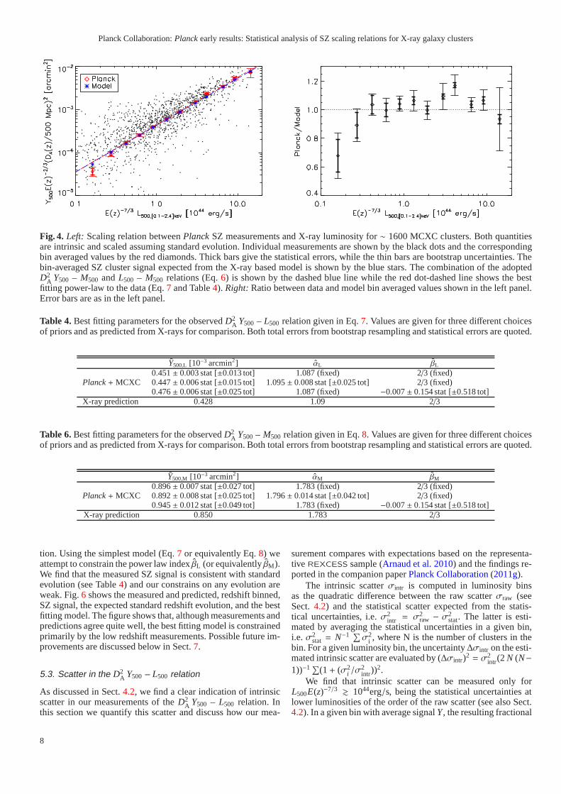
curvefit function). In the fitting procedure, only the statisticalerrors given by the MMF are taken into account. The deriveduncertainties on the best fitting parameters are quoted in Table4 as statistical errors. In addition, uncertainties on the best fit-ting parameters are estimated through the bootstrap proceduredescribed in Sec.4. Each bootstrap catalogue fit leads to a setof parameters whose standard deviation is quoted as the uncer-tainty on the best fitting parameters. Values are given for threedifferent choices of priors as given in Table4, where the best fit-ting parameters are listed. The table also provides the predictionof our X-ray based model for comparison.

Fixing the slope and the redshift dependence of theD2A Y500

– L500 relation, the best fitting amplitude is 0.451×10−3 arcmin2,in agreement with the model prediction 0.428× 10−3 arcmin2 at1.8σ. When keeping the redshift dependence of the relation fixedbut leaving the slope of the relation free, we find agreement be-tween best fitting and predicted slopes at better than 1σ, whilethe amplitudes remain in agreement at 1.3σ. For maximum use-fulness and in particular to facilitate precise comparisons withour findings, we provide, in Table5, the data points shown in theleft-hand panel of Fig.4. For completeness, we also show theD2

A Y500 – M500 relation in Fig.5. In this case the SZ signal isaveraged in logarithmically spaced mass bins, where individualmassesM500 are computed from theL500 – M500 relation in Eq.1. Following the same procedure as for theD2

A Y500 – L500 rela-tion, we fit individual points of theD2

A Y500 – M500 plane with:

Y500 = Y500,M

(

M500

3× 1014M⊙

)αM

E(z)βM

(

DA(z)500 Mpc

)−2

. (8)

The same cases as for theD2A Y500 – L500 relation are considered

and the best fitting parameters are provided in Table6 alongwith the model prediction. Concerning the agreement betweenbest fitting parameters and model predictions, the conclusionsdrawn for theD2

A Y500 – L500 relation obviously apply also fortheD2

A Y500 – M500.

5.2. Redshift evolution

We also considered the case where the redshift evolution of thescaling relations is allowed to differ from the standard expecta-

7


Fig. 4. Left: Scaling relation betweenPlanckSZ measurements and X-ray luminosity for∼ 1600 MCXC clusters. Both quantitiesare intrinsic and scaled assuming standard evolution. Individual measurements are shown by the black dots and the correspondingbin averaged values by the red diamonds. Thick bars give the statistical errors, while the thin bars are bootstrap uncertainties. Thebin-averaged SZ cluster signal expected from the X-ray based model is shown by the blue stars. The combination of the adoptedD2

A Y500 – M500 andL500 – M500 relations (Eq.6) is shown by the dashed blue line while the red dot-dashed line shows the bestfitting power-law to the data (Eq.7 and Table4). Right:Ratio between data and model bin averaged values shown in theleft panel.Error bars are as in the left panel.

Table 4. Best fitting parameters for the observedD2A Y500 – L500 relation given in Eq.7. Values are given for three different choices

of priors and as predicted from X-rays for comparison. Both total errors from bootstrap resampling and statistical errors are quoted.

Y500,L [10−3 arcmin2] αL βL

0.451± 0.003 stat [±0.013 tot] 1.087 (fixed) 2/3 (fixed)Planck+ MCXC 0.447± 0.006 stat [±0.015 tot] 1.095± 0.008 stat [±0.025 tot] 2/3 (fixed)

0.476± 0.006 stat [±0.025 tot] 1.087 (fixed) −0.007± 0.154 stat [±0.518 tot]X-ray prediction 0.428 1.09 2/3

Table 6. Best fitting parameters for the observedD2A Y500 – M500 relation given in Eq.8. Values are given for three different choices

of priors and as predicted from X-rays for comparison. Both total errors from bootstrap resampling and statistical errors are quoted.

Y500,M [10−3 arcmin2] αM βM

0.896± 0.007 stat [±0.027 tot] 1.783 (fixed) 2/3 (fixed)Planck+ MCXC 0.892± 0.008 stat [±0.025 tot] 1.796± 0.014 stat [±0.042 tot] 2/3 (fixed)

0.945± 0.012 stat [±0.049 tot] 1.783 (fixed) −0.007± 0.154 stat [±0.518 tot]X-ray prediction 0.850 1.783 2/3

tion. Using the simplest model (Eq.7 or equivalently Eq.8) weattempt to constrain the power law indexβL (or equivalentlyβM).We find that the measured SZ signal is consistent with standardevolution (see Table4) and our constrains on any evolution areweak. Fig.6 shows the measured and predicted, redshift binned,SZ signal, the expected standard redshift evolution, and the bestfitting model. The figure shows that, although measurements andpredictions agree quite well, the best fitting model is constrainedprimarily by the low redshift measurements. Possible future im-provements are discussed below in Sect.7.

5.3. Scatter in the D2A Y500 – L500 relation

As discussed in Sect.4.2, we find a clear indication of intrinsicscatter in our measurements of theD2

A Y500 – L500 relation. Inthis section we quantify this scatter and discuss how our mea-

surement compares with expectations based on the representa-tive REXCESS sample (Arnaud et al. 2010) and the findings re-ported in the companion paperPlanck Collaboration(2011g).

The intrinsic scatterσintr is computed in luminosity binsas the quadratic difference between the raw scatterσraw (seeSect.4.2) and the statistical scatter expected from the statis-tical uncertainties, i.e.σ2

intr = σ2raw − σ2

stat. The latter is esti-mated by averaging the statistical uncertainties in a givenbin,i.e.σ2

stat = N−1 ∑

σ2i , where N is the number of clusters in the

bin. For a given luminosity bin, the uncertainty∆σintr on the esti-mated intrinsic scatter are evaluated by (∆σintr)2 = σ2

intr(2 N (N−1))−1 ∑

(1+ (σ2i /σ

2intr))

2.We find that intrinsic scatter can be measured only for

L500E(z)−7/3& 1044erg/s, being the statistical uncertainties at

lower luminosities of the order of the raw scatter (see also Sect.4.2). In a given bin with average signalY, the resulting fractional

8


Fig. 5. Scaling relation betweenPlanckSZ signal and and totalmass. Symbols and lines are as in Fig.4.

Fig. 6. Bin averaged SZ signal from a sphere of radiusR500 (Y500)scaled by the expected mass and angular distance dependenceasa function of redshift. ThePlanckdata (red diamonds) and theSZ cluster signal expected from the X-ray based model (bluestars) are shown together with the expected standard redshiftevolution (dahed line). The best fitting model is shown by thedot-dashed line and the 1σ confidence region is limited by thedotted lines. HereM500 is given in units of 3× 1014M⊙.

intrinsic scatterσintr/Y is shown in Fig.7 along with the frac-tional raw and statistical scatters. The estimated intrinsic scatteris of the order of 40− 50% and in agreement with the expec-tations given inArnaud et al.(2010) (σlogY500 = 0.184± 0.024,the range of these values is indicated by the coarse–hatchedre-gion in the figure). Notice that the intrinsic scatter reported inArnaud et al.(2010) is computed for theREXCESS sample andevaluated adoptingXMM-Newtonluminosities and a predictedSZ signal for individual objects based on the same model as-sumed here but relying on the mass proxyYX . Therefore, theintrinsic scatter quoted inArnaud et al.(2010) reflects the in-trinsic scatter in the underlyingL500 – M500 relation. InPlanckCollaboration(2011g), where a sample of clusters detected athigh signal to noise in thePlancksurvey (the ESZ sample, seePlanck Collaboration 2011d) and with high quality X-ray data

Fig. 7. Fractional raw (dot-dashed blue line and triangles), sta-tistical (dot-dot-dashed green line and plus signs), and intrinsic(dashed red line, diamonds, and error bars) scatter on theD2

A Y500– L500 relation. The coarse/fine-hatched regions corresponds tothe 1σ uncertainties on the intrinsic scatter reported inArnaudet al.(2010) andPlanck Collaboration(2011g), respectively.

from XMM-Newtonis used, the intrinsic scatter in theD2A Y500

– L500 relation is found to beσlogY500 = 0.143± 0.016. Thesevalues are shown in Fig.7 by the fine–hatched region. InPlanckCollaboration(2011g) it is found that cool core clusters are re-sponsible for the vast majority of the scatter around the relation.Because the sample used in this study is X-ray selected, we ex-pect it to contain a higher fraction of cool core systems thaninthe ESZ sub–sample studied inPlanck Collaboration(2011g).This implies that the scatter in theD2

A Y500 – L500 relation mea-sured in our sample is expected to be higher than the one foundin Planck Collaboration(2011g), as observed. Given the segre-gation of cool core systems in theD2

A Y500 – L500 reported inPlanck Collaboration(2011g), we investigate the link betweenthe scatter in the relation and cluster dynamical state using ourlarge X-ray sample. To this end we comparePlanckmeasure-ments and the X-ray based predictions (i.e., Eq.6) for individualobjects. In Fig.8 we show the difference betweenPlanckmea-surement and the X-ray based prediction in units of the measure-ment statistical error as a function of X-ray luminosity. Inthefollowing we show that the disagreement between predictionsand model is clearly linked to cluster dynamical state.

Because the dynamical state characterization is not availablefor all the sample we investigate this issue by considering thelargest outliers and search information on their dynamicalstatein the literature. Information is based on the classification ofHudson et al.(2010) if not stated otherwise. We find 13 clus-ters with a predicted signal smaller than thePlanck measure-ment at 5σ. Of these 5 are well known mergers: Coma, A2218(Govoni et al. 2004), 1ES0657, A754 (Govoni et al. 2004),A2163 (Bourdin et al. 2010), 5 are classified as non-cool coreclusters and may therefore be unrelaxed: A2219 (Allen & Fabian1998), A2256, A2255, A0209 (Zhang et al. 2008), A3404 (Prattet al. 2009), and A3266 is a weak cool core cluster. No informa-tion is available for the remaining clusters: A1132 and A3186.Conversely, there are 12 over-predicted clusters at 5σ. Ofthese 5 are strong cool core clusters: RXJ1532.9+3021 (Ebelinget al. 2010), 2A0335, Zw1021.0+0426 (Morandi et al. 2007),A3112, HerA (Bauer et al. 2005) , and A0780. No informa-tion is available for the remaining clusters: A689, ACOS1111,

9


Fig. 8. Difference between thePlanckmeasurement and the X-ray based prediction in units of the measurement statistical er-ror (pure measurement uncertainties based on MMF noise esti-mates) as a function of X-ray luminosity. Outliers at more than5 σ, which are discussed in the text, are labelled by their name.Clusters with SZ signal possibly contaminated by radio sources(see discussion in Sect.6) are shown in red and labelled by theirname.

A3392, J1253.6-3931, J1958.2-3011, and RXCJ0643.4+4214.Notice that the luminosity of A689 is likely to be overesti-mated by a large factor because of point source contamination(Maughan 2008). In addition, for A3186 and ACOS1111 themodel prediction rely on the EMSS luminosity measurementsgiven inGioia & Luppino(1994), which might be unreliable.

Notice that all these> 5σ outliers have luminosities in therange where intrinsic scatter is clearly measured. The highfrac-tion of dynamically perturbed/ cool-core clusters with largelyunder/over predicted SZ signal is confirmed when additionaloutliers at smallerσ are searched. These findings suggest thatthe observed scatter in theD2

A Y500 – L500 relation is linked tothe cluster dynamical state.

6. Robustness of the results

As in the other fourPlanck SZ papers (Planck Collaboration2011d,e,g,h),we test the robustness of our results for the effect ofseveral instrumental, modelling, and astrophysical uncertainties.Tests common to allPlanckSZ papers are discussed in detail inSec. 6 ofPlanck Collaboration(2011d). Of these, calibration andcolor correction effects are relevant for our analysis. Calibrationuncertainties are shown to propagate into very small uncertain-ties on SZ signal measurements (∼ 2%) and color correction isfound to be a∼ 3% effect forPlanckbands.

In the following we report on robustness tests aimed at com-pleting this investigation. We show that our results are robustwith respect to the instrumental uncertainties, that they are in-sensitive to the finest details of our cluster modelling, andthatthey are unaffected by radio source contamination. We show thatrestricting the analysis to the reference homogeneous subsampleof NORAS/REFLEX clusters leads to measurements fully com-patible with what we obtain for the whole sample.

6.1. Beam effects

The beam effects studied inPlanck Collaboration(2011d) arefurther scrutinised by directly estimating their impact onourresults. To this end, the whole analysis is redone by assumingdifferent beam FWHM. For simplicity, we systematically in-crease/decrease the adopted beam FWHM for all channels si-multaneously by adding/removing the conservative uncertaintiesgiven in Table1 from the fiducial beam FWHM values. We findthat the binned SZ signal varies by at most 2% from the valuecomputed using the fiducial beams FWHM.

6.2. Modelling

The effects of changes in the underlying X-ray based modelon our results are investigated by repeating the full analysis asfor thefiducial case, but by assuming the standard slope of theM500− YX relation and/or the intrinsicL500 – M500 relation (seeSect.3). For simplicity, in the following we discuss results ob-tained by varying only one assumption at a time. We find thatthe effect resulting by varying both assumptions is equivalent tothe sum of the effects obtained by varying the two assumptionsseparately.

As expected from the weak dependence of cluster sizeR500on luminosity, the measured SZ signal is barely affected by thesechanges. If the standard slope case is adopted instead of theem-pirical one, the bin averaged SZ signal changes by less than afew percent at all luminosities and the same is found when theintrinsic L500 – M500 relation is adopted. The model predictionsare of course more affected by changes in the assumed scalingrelations. In Fig.9 we contrast thePlanck -to-model ratio ob-tained for the different cases. The figure shows that the assump-tion on the slope of theM500− YX relation has a fully negligibleimpact. On the other hand it shows that the intrinsicL500 – M500relation is not compatible with our measurements (> 5σ dis-crepancy). This finding is not surprising given the fact thatwhenadopting the intrinsicL500 – M500 relation one assumes that se-lection effects of our X-ray sample are negligible. Notice thattheWMAP-5yr data used in the similar analysis byMelin et al.(2010) did not have sufficient depth to come to this conclusion.Furthermore, the agreement of our results for theREXCESS andintrinsic L500 – M500 relations at high luminosity confirms thatMalmquist bias is small for very luminous objects.

6.3. Intrinsic dispersion in the L500 – M500 relation

The intrinsic dispersion in theL500 – M500 relation dominates theuncertainty on the clusters’ sizeR500 in our analysis. We investi-gate how this propagates into the uncertainties on the binned SZsignal by means of a Monte Carlo (MC) analysis of 100 realisa-tions. We use the dispersion given in Table2 and, for each reali-sation, we draw a random mass logM500 for each cluster from aGaussian distribution with mean given by theL500 − M500 rela-tion and standard deviationσlogL−log M/αM. For each realisation,we extract the signal with the new values ofM500 (thusR500).The standard deviation of the SZ signal for the 100 MC realisa-tions in a given luminosity bin is found to be at most∼ 3% of thesignal. Hence, given the size of the total errors on the binned SZsignal (see Fig.3) our conclusions are fully unaffected by thiseffect.

10


6.4. Pressure profile

Furthermore, we investigate how the uncertainties on the as-sumed pressure profile propagates into the uncertainties onthebinned SZ signal. For simplicity, we only quantify the largestpossible effect by redoing the analysis but adopting the pressureprofile parameters for the cool-core and morphologically dis-turbed sub-samples given in Table3, i.e. we assume that all clus-ters in the sample are cool-core or morphologically disturbed.Both of the two resulting sets of binned SZ signal deviate fromthe one derived assuming the universal pressure profile by ap-proximatively 8% in the lowest luminosity bin and decrease lin-early with increasing logL500, becoming approximatively 1% inthe highest luminosity bin. Furthermore the normalizationof Eq.4 changes by less than 3% if the average pressure profiles param-eters of cool-core and morphologically disturbed clustersgivenin Table3 are adopted instead of the ones for the average profile,implying that our SZ signal predictions are robust. Consideringthe total errors and their trend with luminosity, we conclude thatour findings are fully unaffected by the exact shape of the SZtemplate.

6.5. X-ray sample

Because of the reasons detailed in Sect.2.2, we also repeatedour analysis by considering the NORAS/REFLEX control sam-ple and find results fully consistent with those derived for thefull sample. The results are shown in terms ofPlanck-to-modelratio in Fig.10. Notice that in this case the luminosity binning ischosen as to be comparable with that in theWMAP-5yr analysisof Melin et al.(2010). The comparison betweenWMAP-5yr andPlanckresults is discussed in Sec.7 below.

6.6. Radio contamination

In addition we investigated the effect of contamination by radiosources on our results. Most radio sources are expected to have asteep spectrum and hence they should not have significant fluxesat Planck frequencies. However, some sources will show up inPlanckLFI and HFI channels if their radio flux is sufficientlyhigh and/or their spectral index is near zero or positive. Extremeexamples are the Virgo and Perseus clusters that host in their in-terior two of the brightest radio sources in the sky. In the ESZsample (Planck Collaboration 2011d) there are also a few ex-amples of clusters with moderate radio sources in their vicinity(1 Jy or less in NVSS) and still significant signal at LFI (andeven HFI) frequencies. To check for possible contaminationwecombine data from SUMSS (a catalog of radio sources at 0.85GHz, Bock et al.(1999)) and NVSS (a catalog of radio sourcesat 1.4 GHz,Condon et al.(1998)). We have looked at the posi-tions of the clusters in our sample and searched for radio sourcesin a radius of 5 arcmin from the cluster center. We find that 74clusters have a radio source within this search radius in NVSSor SUMSS with a flux above 1 Jy. Among these, 8 have fluxeslarger than 10 Jy, 2 sources larger than 100 Jy and one a extremeradio source with a flux larger than 1 KJy.

As a robustness test, we investigate the impact of contamina-tion by radio sources on our results by excluding clusters hostingradio sources with fluxes larger than 1 or 5 Jy and comparingthe results to those obtained for the full sample. Interestinglywe find that, as expected, the individual SZ signal is on aver-age lower than the X-ray based predictions in clusters that arelikely to be highly contaminated. This is shown in Fig.8 whereclusters associated with radio sources with fluxes larger than 5

Fig. 9. Ratio of binnedPlanckdata points to model for differ-ent model assumptions. Thefiducial model(black diamonds)is shown together with results obtained by varying the underly-ing L500 – M500 relation fromREXCESS to intrinsic (green plussigns), and by varying the slope of the underlyingM500− YX re-lation from empirical to standard (red triangles). Thick bars givethe statistical errors, while the thin bars are bootstrap uncertain-ties.

Jy are shown by the red symbols. However, given the very lowfraction of possibly contaminated clusters, we find that binaver-aged signal is fully unaffected when these are excluded from theanalysis.

7. Discussion and conclusions

As part of a series of papers onPlanck early results on clus-ters of galaxies (Planck Collaboration 2011d,e,f,g,h), we mea-sured the SZ signal in the direction of∼ 1600 objects from theMCXC (Meta-Catalogue of X-ray detected Clusters of galaxies,Piffaretti et al. 2010, see Sect.2.2) in Planckwhole sky data (seeSect.2.1) and studied the relationship between X-ray luminosityand SZ signal strength.

For each X-ray cluster in the sample the amplitude of theSZ signal is fit for by fixing the cluster position and size to theX-ray values and assuming a template derived from the univer-sal pressure profile ofArnaud et al.(2010). The universal pres-sure profile was derived from high quality data fromREXCESS.Recently,Sun et al.(2010) found that the universal pressure pro-file also yields an excellent description of systems with lowerluminosities than those probed withREXCESS. This impliesthat the adopted SZ template is suitable for the entire luminosityrange explored in our work.

The intrinsic SZ signalD2A Y500 is averaged in X-ray lumi-

nosity bins to maximise the statistical significance. The signalis detected at high significance over the X-ray luminosity range1043erg/s. L500E(z)−7/3

. 1045erg/s (see Fig.2).We find excellent agreement between observations and pre-

dictions based on X-ray data, as shown in Fig.4. Our resultsdo not agree with the claim, based on a recentWMAP-7yr dataanalysis, that X-ray data over-predict the SZ signal (Komatsuet al. 2010). Due to the large size and homogeneous nature ofthe MCXC, and the exceptional internal consistency of our clus-ter model, we believe that our results are very robust. Moreover,as reported in Sect.6, we show that our findings are insensitiveto the details of our cluster modelling. Furthermore, we have

11


Fig. 10. Data-to-model ratio forPlanck results for the fullsample (black diamonds) and the NORAS/REFLEX controlsample (green plus signs). TheWMAP-5yr results for theNORAS/REFLEX byMelin et al. (2010) are shown by the redtriangles. Error bars are as in Fig.4.

shown that our results are robust against instrumental (calibra-tion, color correction, beam) and astrophysical (radio contami-nation) uncertainties.

Our results confirm to a higher significance the results of inthe analysis byMelin et al. (2010) based onWMAP-5yr data.This is show in Fig.10 where the data-to-model ratio as a func-tion of luminosity is presented. Luminosity bins are chosenas toas to be comparable with that ofMelin et al.(2010) andPlanckresults are presented for the whole sample used in this work andthe NORAS/REFLEX sample adopted inMelin et al. (2010).In addition to the good agreement between results from the twodata sets, the figure shows that in theWMAP-5yr study byMelinet al.(2010) statistical uncertainties are dominant. As shown inSect.4.2, Planckdata allows us to overcome this limitation andto investigate the intrinsic scatter in the scaling relation betweenintrinsic SZ signalD2

A Y500 and X-ray luminosityL500 (see Sect.5.3). We find a∼ 40% intrinsic scatter in theD2

A Y500 – L500relation and show that it is linked to cluster dynamical state.

The agreement between luminosity binned X-ray predictionsand Planck measurements is reflected in the excellent accordbetween predicted scaling relation and best fitting power lawmodel to theD2

A Y500 – L500 relation. The power law fit, whichis performed on individual data points, is compared byPlanckCollaboration(2011g) to thecalibration derived from a sampleof galaxy clusters detected at high signal to noise in thePlancksurvey (the ESZ sample, seePlanck Collaboration 2011d) andwith high quality X-ray data fromXMM-Newton. As discussedin Planck Collaboration(2011g) the slight differences betweenthe two best fitting relations reflect the difference between theselection of the adopted samples. Indeed, the X-ray sample usedin the present work is X-ray selected and therefore biased to-wards the cool core systems, while the sample used inPlanckCollaboration(2011g) is SZ selected.

As mentioned in Sect.4.2, the luminosity range where weare not able to detect the SZ signal because of the small num-ber of low mass objects (see Fig.2), is explored inPlanckCollaboration(2011h). In the latter analysis we use the opticalcatalogue of∼ 14,000 MaxBCG clusters (Koester et al. 2007)and, in a fully similar way as done in this work, extract the op-tical richness binned SZ signal fromPlanckdata. By combining

Fig. 11. Bottom panel:Comparison between our results (red di-amonds, as in left-hand panel Fig.4) and those obtained byPlanck Collaboration(2011h) (green triangles), where MaxBCGclusters are investigated. X-ray luminosities and associated er-ror bars for the MaxBCG clusters are based on the analysis ofRykoff et al.(2008). Vertical error bars are as in Fig.4 and theX-ray prediction (i.e., Eq.6) is shown by the dashed blue line.Top panel:X-ray luminosity histograms of the MCXC (red) andMaxBCG (green) samples. For the MCXC the width of the barsis equal to the luminosity bin width, while for the MaxBCG weadopt the horizontal error bar shown in the bottom panel.

these results with the X-ray luminosity of the MaxBCG clus-ters measured byRykoff et al. (2008) by stacking RASS data,in Planck Collaboration(2011h) we derive theD2

A Y500 – L500relation for the MaxBCG sample. This result is shown togetherwith the one derived in the present paper in Fig.11. The X-rayluminosity histograms shown in the top panel of the figure high-light the complementarity of the two analyses. The bottom panelof the figure shows agreement between the results from the twodata sets and, very importantly, that observations and predictionsbased on X-ray data agree over a very wide range in X-ray lumi-nosity.

We investigate the evolution of the scaling relation and findit to be consistent with standard evolution. Although redshiftbinned measurements and predictions agree quite well over awide redshift range (see Fig.6), our constrains are weak be-cause the inferred best fitting model is almost completely con-strained by only the low redshift measurements. Given the rele-vance of SZ-selected samples for cosmological studies and theneed of complementary X-ray observations for such studies (seePlanck Collaboration 2011e, and discussion therein), improvedunderstanding of the evolution of SZ-X-ray scaling relations isclearly desired. High quality data similar to those used inPlanckCollaboration(2011g), but for higher redshift clusters will pro-vide tight constrains on evolution, in particular when newly SZdiscovered clusters (seePlanck Collaboration 2011d, and refer-ences therein) with high quality X-ray and optical data willbeincluded.

Acknowledgements.This research has made use of the X-Rays ClustersDatabase (BAX) which is operated by the Laboratoire d’Astrophysique de

12


Tarbes-Toulouse (LATT), under contract with the Centre National d’EtudesSpatiales (CNES). We acknowledge the use of the HEALPix package (Gorskiet al. 2005). A description of the Planck Collaboration and a list of itsmembers,indicating which technical or scientific activities they have been involved in, canbe found athttp://www.rssd.esa.int/Planck.

ReferencesAfshordi, N., Lin, Y., Nagai, D., & Sanderson, A. J. R. 2007, MNRAS, 378, 293Allen, S. W. & Fabian, A. C. 1998, MNRAS, 297, L57Andersson, K., Benson, B. A., Ade, P. A. R., et al. 2010, ArXive-printsArnaud, M., Pratt, G. W., Piffaretti, R., et al. 2010, A&A, 517, A92+Bauer, F. E., Fabian, A. C., Sanders, J. S., Allen, S. W., & Johnstone, R. M. 2005,

MNRAS, 359, 1481Bersanelli, M., Mandolesi, N., Butler, R. C., et al. 2010, A&A, 520, A4+Bielby, R. M. & Shanks, T. 2007, MNRAS, 382, 1196Birkinshaw, M. 1999, Phys. Rep., 310, 97Bock, D., Large, M. I., & Sadler, E. M. 1999, AJ, 117, 1578Bohringer, H., Schuecker, P., Pratt, G. W., et al. 2007, A&A, 469, 363Bourdin, H., Arnaud, M., Mazzotta, P., et al. 2010, ArXiv e-printsCarlstrom, J. E., Ade, P. A. R., Aird, K. A., et al. 2009, ArXive-printsCondon, J. J., Cotton, W. D., Greisen, E. W., et al. 1998, AJ, 115, 1693Diego, J. M. & Partridge, B. 2010, MNRAS, 402, 1179Ebeling, H., Edge, A. C., Mantz, A., et al. 2010, MNRAS, 407, 83Fowler, J. W., Niemack, M. D., Dicker, S. R., et al. 2007, Appl. Opt., 46, 3444Gioia, I. M. & Luppino, G. A. 1994, ApJS, 94, 583Gorski, K. M., Hivon, E., Banday, A. J., et al. 2005, ApJ, 622, 759Govoni, F., Markevitch, M., Vikhlinin, A., et al. 2004, ApJ,605, 695Herranz, D., Sanz, J. L., Hobson, M. P., et al. 2002, MNRAS, 336, 1057Hudson, D. S., Mittal, R., Reiprich, T. H., et al. 2010, A&A, 513, A37+Johnston, D. E., Sheldon, E. S., Tasitsiomi, A., et al. 2007,ApJ, 656, 27Koester, B. P., McKay, T. A., Annis, J., et al. 2007, ApJ, 660,239Komatsu, E., Smith, K. M., Dunkley, J., et al. 2010, ArXiv e-printsKravtsov, A. V., Vikhlinin, A., & Nagai, D. 2006, ApJ, 650, 128Lamarre, J., Puget, J., Ade, P. A. R., et al. 2010, A&A, 520, A9+

Leahy, J. P., Bersanelli, M., D’Arcangelo, O., et al. 2010, A&A, 520, A8+Lieu, R., Mittaz, J. P. D., & Zhang, S. 2006, ApJ, 648, 176Mandolesi, N., Bersanelli, M., Butler, R. C., et al. 2010, A&A, 520, A3+Maughan, B. 2008, in Chandra Proposal, 2653–+

Melin, J., Bartlett, J. G., & Delabrouille, J. 2006, A&A, 459, 341Melin, J., Bartlett, J. G., Delabrouille, J., et al. 2010, ArXiv e-printsMennella et al. 2011, Planck early results 03: First assessment of the Low

Frequency Instrument in-flight performance (Submitted to A&A)Morandi, A., Ettori, S., & Moscardini, L. 2007, MNRAS, 379, 518Piffaretti, R., Arnaud, M., Pratt, G. W., Pointecouteau, E., & Melin, J. 2010,

ArXiv e-printsPlanck Collaboration. 2011a, Planck early results 01: The Planck mission

(Submitted to A&A)Planck Collaboration. 2011b, Planck early results 02: The thermal performance

of Planck (Submitted to A&A)Planck Collaboration. 2011c, Planck early results 07: The Early Release

Compact Source Catalogue (Submitted to A&A)Planck Collaboration. 2011d, Planck early results 08: The all-sky early Sunyaev-

Zeldovich cluster sample (Submitted to A&A)Planck Collaboration. 2011e, Planck early results 09: XMM-Newton follow-up

for validation of Planck cluster candidates (Submitted to A&A)Planck Collaboration. 2011f, Planck early results 10: Statistical analysis of

Sunyaev-Zeldovich scaling relations for X-ray galaxy clusters (Submitted toA&A)

Planck Collaboration. 2011g, Planck early results 11: Calibration of the localgalaxy cluster Sunyaev-Zeldovich scaling relations (Submitted to A&A)

Planck Collaboration. 2011h, Planck early results 12: Cluster Sunyaev-Zeldovich optical Scaling relations (Submitted to A&A)

Planck Collaboration. 2011i, Planck early results 13: Statistical properties ofextragalactic radio sources in the Planck Early Release Compact SourceCatalogue (Submitted to A&A)

Planck Collaboration. 2011j, Planck early results 14: Early Release CompactSource Catalogue validation and extreme radio sources (Submitted to A&A)

Planck Collaboration. 2011k, Planck early results 15: Spectral energy distri-butions and radio continuum spectra of northern extragalactic radio sources(Submitted to A&A)

Planck Collaboration. 2011l, Planck early results 16: The Planck view of nearbygalaxies (Submitted to A&A)

Planck Collaboration. 2011m, Planck early results 17: Origin of the submillime-tre excess dust emission in the Magellanic Clouds (Submitted to A&A)

Planck Collaboration. 2011n, Planck early results 18: The power spectrum ofcosmic infrared background anisotropies (Submitted to A&A)

Planck Collaboration. 2011o, Planck early results 19: All-sky temperature anddust optical depth from Planck and IRAS — constraints on the “dark gas” inour Galaxy (Submitted to A&A)

Planck Collaboration. 2011p, Planck early results 20: New light on anomalousmicrowave emission from spinning dust grains (Submitted toA&A)

Planck Collaboration. 2011q, Planck early results 21: Properties of the interstel-lar medium in the Galactic plane (Submitted to A&A)

Planck Collaboration. 2011r, Planck early results 22: The submillimetre proper-ties of a sample of Galactic cold clumps (Submitted to A&A)

Planck Collaboration. 2011s, Planck early results 23: The Galactic cold corepopulation revealed by the first all-sky survey (Submitted to A&A)

Planck Collaboration. 2011t, Planck early results 24: Dustin the diffuse inter-stellar medium and the Galactic halo (Submitted to A&A)

Planck Collaboration. 2011u, Planck early results 25: Thermal dust in nearbymolecular clouds (Submitted to A&A)

Planck Collaboration. 2011v, The Explanatory Supplement to the Planck EarlyRelease Compact Source Catalogue (ESA)

Planck HFI Core Team. 2011a, Planck early results 04: First assessment of theHigh Frequency Instrument in-flight performance (Submitted to A&A)

Planck HFI Core Team. 2011b, Planck early results 06: The High FrequencyInstrument data processing (Submitted to A&A)

Pratt, G. W., Croston, J. H., Arnaud, M., & Bohringer, H. 2009, A&A, 498, 361Rosset, C., Tristram, M., Ponthieu, N., et al. 2010, A&A, 520, A13+Rozo, E., Rykoff, E. S., Evrard, A., et al. 2009, ApJ, 699, 768Rykoff, E. S., Evrard, A. E., McKay, T. A., et al. 2008, MNRAS, 387, L28Sun, M., Sehgal, N., Voit, G. M., et al. 2010, ArXiv e-printsSunyaev, R. A. & Zeldovich, Y. B. 1970, Comments on Astrophysics and Space

Physics, 2, 66Sunyaev, R. A. & Zeldovich, Y. B. 1972, Comments on Astrophysics and Space

Physics, 4, 173Tauber, J. A., Mandolesi, N., Puget, J., et al. 2010, A&A, 520, A1+Zacchei et al. 2011, Planck early results 05: The Low Frequency Instrument data

processing (Submitted to A&A)Zhang, Y., Finoguenov, A., Bohringer, H., et al. 2008, A&A,482, 451

1 Aalto University Metsahovi Radio Observatory, Metsahovintie 114,FIN-02540 Kylmala, Finland

2 Agenzia Spaziale Italiana Science Data Center, c/o ESRIN, viaGalileo Galilei, Frascati, Italy

3 Astroparticule et Cosmologie, CNRS (UMR7164), Universit´eDenis Diderot Paris 7, Batiment Condorcet, 10 rue A. Domon etLeonie Duquet, Paris, France

4 Atacama Large Millimeter/submillimeter Array, ALMA SantiagoCentral Offices Alonso de Cordova 3107, Vitacura, Casilla 763

13

http://www.rssd.esa.int/Planck


0355, Santiago, Chile

5 CITA, University of Toronto, 60 St. George St., Toronto, ON M5S3H8, Canada

6 CNRS, IRAP, 9 Av. colonel Roche, BP 44346, F-31028 Toulousecedex 4, France

7 California Institute of Technology, Pasadena, California, U.S.A.

8 Centre of Mathematics for Applications, University of Oslo,Blindern, Oslo, Norway

9 Centro de Astrofısica, Universidade do Porto, Rua das Estrelas,4150-762 Porto, Portugal

10 DAMTP, Centre for Mathematical Sciences, Wilberforce Road,Cambridge CB3 0WA, U.K.

11 DSM/Irfu/SPP, CEA-Saclay, F-91191 Gif-sur-Yvette Cedex, France

12 DTU Space, National Space Institute, Juliane Mariesvej 30,Copenhagen, Denmark

13 Departamento de Fısica, Universidad de Oviedo, Avda. CalvoSotelo s/n, Oviedo, Spain

14 Department of Astronomy and Astrophysics, University of Toronto,50 Saint George Street, Toronto, Ontario, Canada

15 Department of Physics & Astronomy, University of BritishColumbia, 6224 Agricultural Road, Vancouver, British Columbia,

Canada

16 Department of Physics and Astronomy, University of SouthernCalifornia, Los Angeles, California, U.S.A.

17 Department of Physics, Gustaf Hallstromin katu 2a, University ofHelsinki, Helsinki, Finland

18 Department of Physics, Princeton University, Princeton, NewJersey, U.S.A.

19 Department of Physics, Purdue University, 525 NorthwesternAvenue, West Lafayette, Indiana, U.S.A.

20 Department of Physics, University of California, Berkeley,California, U.S.A.

21 Department of Physics, University of California, One ShieldsAvenue, Davis, California, U.S.A.

22 Department of Physics, University of California, Santa Barbara,California, U.S.A.

23 Department of Physics, University of Illinois at Urbana-Champaign,1110 West Green Street, Urbana, Illinois, U.S.A.

24 Dipartimento di Fisica G. Galilei, Universita degli Studidi Padova,via Marzolo 8, 35131 Padova, Italy

25 Dipartimento di Fisica, Universita La Sapienza, P. le A. Moro 2,Roma, Italy

26 Dipartimento di Fisica, Universita degli Studi di Milano,ViaCeloria, 16, Milano, Italy

27 Dipartimento di Fisica, Universita degli Studi di Trieste, via A.Valerio 2, Trieste, Italy

28 Dipartimento di Fisica, Universita di Roma Tor Vergata, Via dellaRicerca Scientifica, 1, Roma, Italy

29 Discovery Center, Niels Bohr Institute, Blegdamsvej 17,Copenhagen, Denmark

30 Dpto. Astrofısica, Universidad de La Laguna (ULL), E-38206 LaLaguna, Tenerife, Spain

31 European Southern Observatory, ESO Vitacura, Alonso de Cordova3107, Vitacura, Casilla 19001, Santiago, Chile

32 European Space Agency, ESAC, Planck Science Office, Caminobajo del Castillo, s/n, Urbanizacion Villafranca del Castillo,

14


Villanueva de la Canada, Madrid, Spain

33 European Space Agency, ESTEC, Keplerlaan 1, 2201 AZNoordwijk, The Netherlands

34 Helsinki Institute of Physics, Gustaf Hallstromin katu 2, Universityof Helsinki, Helsinki, Finland

35 INAF - Osservatorio Astronomico di Padova, Vicolodell’Osservatorio 5, Padova, Italy

36 INAF - Osservatorio Astronomico di Roma, via di Frascati 33,Monte Porzio Catone, Italy

37 INAF - Osservatorio Astronomico di Trieste, Via G.B. Tiepolo 11,Trieste, Italy

38 INAF/IASF Bologna, Via Gobetti 101, Bologna, Italy

39 INAF/IASF Milano, Via E. Bassini 15, Milano, Italy

40 INRIA, Laboratoire de Recherche en Informatique, UniversiteParis-Sud 11, Batiment 490, 91405 Orsay Cedex, France

41 IPAG: Institut de Planetologie et d’Astrophysique de Grenoble,Universite Joseph Fourier, Grenoble 1/ CNRS-INSU, UMR 5274,Grenoble, F-38041, France

42 Imperial College London, Astrophysics group, Blackett Laboratory,Prince Consort Road, London, SW7 2AZ, U.K.

43 Infrared Processing and Analysis Center, California Institute ofTechnology, Pasadena, CA 91125, U.S.A.

44 Institut d’Astrophysique Spatiale, CNRS (UMR8617) UniversiteParis-Sud 11, Batiment 121, Orsay, France

45 Institut d’Astrophysique de Paris, CNRS UMR7095, UniversitePierre & Marie Curie, 98 bis boulevard Arago, Paris, France

46 Institute of Astronomy and Astrophysics, Academia Sinica,Taipei,Taiwan

47 Institute of Theoretical Astrophysics, University of Oslo, Blindern,Oslo, Norway

48 Instituto de Astrofısica de Canarias, C/Vıa Lactea s/n, La Laguna,Tenerife, Spain

49 Instituto de Fısica de Cantabria (CSIC-Universidad de Cantabria),Avda. de los Castros s/n, Santander, Spain

50 Jet Propulsion Laboratory, California Institute of Technology, 4800Oak Grove Drive, Pasadena, California, U.S.A.

51 Jodrell Bank Centre for Astrophysics, Alan Turing Building, Schoolof Physics and Astronomy, The University of Manchester, OxfordRoad, Manchester, M13 9PL, U.K.

52 Kavli Institute for Cosmology Cambridge, Madingley Road,Cambridge, CB3 0HA, U.K.

53 LERMA, CNRS, Observatoire de Paris, 61 Avenue del’Observatoire, Paris, France

54 Laboratoire AIM, IRFU/Service d’Astrophysique - CEA/DSM -CNRS - Universite Paris Diderot, Bat. 709, CEA-Saclay, F-91191

Gif-sur-Yvette Cedex, France

55 Laboratoire Traitement et Communication de l’Information, CNRS(UMR 5141) and Telecom ParisTech, 46 rue Barrault F-75634ParisCedex 13, France

56 Laboratoire de Physique Subatomique et de Cosmologie, CNRS,Universite Joseph Fourier Grenoble I, 53 rue des Martyrs, Grenoble,

15


France

57 Laboratoire de l’Accelerateur Lineaire, Universite Paris-Sud 11,CNRS/IN2P3, Orsay, France

58 Lawrence Berkeley National Laboratory, Berkeley, California,U.S.A.

59 Max-Planck-Institut fur Astrophysik, Karl-Schwarzschild-Str. 1,85741 Garching, Germany

60 Max-Planck-Institut fur Extraterrestrische Physik,Giessenbachstraße, 85748 Garching, Germany

61 MilliLab, VTT Technical Research Centre of Finland, Tietotie 3,Espoo, Finland

62 National University of Ireland, Department of ExperimentalPhysics, Maynooth, Co. Kildare, Ireland

63 Niels Bohr Institute, Blegdamsvej 17, Copenhagen, Denmark

64 Observational Cosmology, Mail Stop 367-17, California Institute ofTechnology, Pasadena, CA, 91125, U.S.A.

65 SISSA, Astrophysics Sector, via Bonomea 265, 34136, Trieste, Italy

66 SUPA, Institute for Astronomy, University of Edinburgh, RoyalObservatory, Blackford Hill, Edinburgh EH9 3HJ, U.K.

67 School of Physics and Astronomy, Cardiff University, QueensBuildings, The Parade, Cardiff, CF24 3AA, U.K.

68 Space Research Institute (IKI), Russian Academy of Sciences,Profsoyuznaya Str, 84/32, Moscow, 117997, Russia

69 Space Sciences Laboratory, University of California, Berkeley,California, U.S.A.

70 Stanford University, Dept of Physics, Varian Physics Bldg,382 ViaPueblo Mall, Stanford, California, U.S.A.

71 Universitat Heidelberg, Institut fur Theoretische Astrophysik,Albert-Uberle-Str. 2, 69120, Heidelberg, Germany

72 Universite de Toulouse, UPS-OMP, IRAP, F-31028 Toulouse cedex4, France

73 University of Cambridge, Cavendish Laboratory, Astrophysicsgroup, J J Thomson Avenue, Cambridge, U.K.

74 University of Cambridge, Institute of Astronomy, Madingley Road,Cambridge, U.K.

75 University of Granada, Departamento de Fısica Teorica y delCosmos, Facultad de Ciencias, Granada, Spain

76 University of Miami, Knight Physics Building, 1320 Campo SanoDr., Coral Gables, Florida, U.S.A.

77 Warsaw University Observatory, Aleje Ujazdowskie 4, 00-478Warszawa, Poland

16

Planck early results. X. Statistical analysis of Sunyaev-Zeldovich scaling relations for X-ray...

Documents

Transcript of Planck early results. X. Statistical analysis of Sunyaev-Zeldovich scaling relations for X-ray...