A&A 550, A129 (2013)DOI: 10.1051/0004-6361/201219398c© ESO 2013

Astronomy&

Astrophysics

Planck intermediate results

III. The relation between galaxy cluster mass and Sunyaev-Zeldovich signal�

Planck Collaboration: P. A. R. Ade76, N. Aghanim53, M. Arnaud68, M. Ashdown65,6, F. Atrio-Barandela19, J. Aumont53,C. Baccigalupi75, A. Balbi34, A. J. Banday84,9, R. B. Barreiro61, J. G. Bartlett1,63, E. Battaner86, R. Battye64, K. Benabed54,83,

J.-P. Bernard9, M. Bersanelli31,45, R. Bhatia7, I. Bikmaev21,3, H. Böhringer73, A. Bonaldi64, J. R. Bond8, S. Borgani32,43,J. Borrill14,79, F. R. Bouchet54,83, H. Bourdin34, M. L. Brown64, M. Bucher1, R. Burenin77, C. Burigana44,33, R. C. Butler44,

P. Cabella35, J.-F. Cardoso69,1,54, P. Carvalho6, A. Chamballu50, L.-Y. Chiang57, G. Chon73, D. L. Clements50, S. Colafrancesco42,A. Coulais67, F. Cuttaia44, A. Da Silva12, H. Dahle59,11, R. J. Davis64, P. de Bernardis30, G. de Gasperis34, J. Delabrouille1,

J. Démoclès68, F.-X. Désert48, J. M. Diego61, K. Dolag85,72, H. Dole53,52, S. Donzelli45, O. Doré63,10, M. Douspis53, X. Dupac38,G. Efstathiou58, T. A. Enßlin72, H. K. Eriksen59, F. Finelli44, I. Flores-Cacho9,84, O. Forni84,9, M. Frailis43, E. Franceschi44,M. Frommert18, S. Galeotta43, K. Ganga1, R. T. Génova-Santos60, M. Giard84,9, Y. Giraud-Héraud1, J. González-Nuevo61,75,

K. M. Górski63,88, A. Gregorio32,43, A. Gruppuso44, F. K. Hansen59, D. Harrison58,65, C. Hernández-Monteagudo13,72,D. Herranz61, S. R. Hildebrandt10, E. Hivon54,83, M. Hobson6, W. A. Holmes63, K. M. Huffenberger87, G. Hurier70, T. Jagemann38,

M. Juvela26, E. Keihänen26, I. Khamitov82, R. Kneissl37,7, J. Knoche72, M. Kunz18,53, H. Kurki-Suonio26,41, G. Lagache53,J.-M. Lamarre67, A. Lasenby6,65, C. R. Lawrence63, M. Le Jeune1, S. Leach75, R. Leonardi38, A. Liddle25, P. B. Lilje59,11,M. Linden-Vørnle17, M. López-Caniego61, G. Luzzi66, J. F. Macías-Pérez70, D. Maino31,45, N. Mandolesi44,5, M. Maris43,

F. Marleau56, D. J. Marshall84,9, E. Martínez-González61, S. Masi30, S. Matarrese29, F. Matthai72, P. Mazzotta34, P. R. Meinhold27,A. Melchiorri30,46, J.-B. Melin16, L. Mendes38, S. Mitra49,63, M.-A. Miville-Deschênes53,8, L. Montier84,9, G. Morgante44,

D. Munshi76, P. Natoli33,4,44, H. U. Nørgaard-Nielsen17, F. Noviello64, S. Osborne81, F. Pajot53, D. Paoletti44, B. Partridge40,T. J. Pearson10,51, O. Perdereau66, F. Perrotta75, F. Piacentini30, M. Piat1, E. Pierpaoli24, R. Piffaretti68,16, P. Platania62,

E. Pointecouteau84,9, G. Polenta4,42, N. Ponthieu53,48, L. Popa55, T. Poutanen41,26,2, G. W. Pratt68,��, S. Prunet54,83, J.-L. Puget53,J. P. Rachen22,72, R. Rebolo60,15,36, M. Reinecke72, M. Remazeilles53,1, C. Renault70, S. Ricciardi44, I. Ristorcelli84,9, G. Rocha63,10,

C. Rosset1, M. Rossetti31,45, J. A. Rubiño-Martín60,36, B. Rusholme51, M. Sandri44, G. Savini74, D. Scott23, J.-L. Starck68,F. Stivoli47, V. Stolyarov6,65,80, R. Sudiwala76, R. Sunyaev72,78, D. Sutton58,65, A.-S. Suur-Uski26,41, J.-F. Sygnet54, J. A. Tauber39,L. Terenzi44, L. Toffolatti20,61, M. Tomasi45, M. Tristram66, L. Valenziano44, B. Van Tent71, P. Vielva61, F. Villa44, N. Vittorio34,

B. D. Wandelt54,83,28, J. Weller85, S. D. M. White72, D. Yvon16, A. Zacchei43, and A. Zonca27

(Affiliations can be found after the references)

Received 12 April 2012 / Accepted 10 August 2012

ABSTRACT

We examine the relation between the galaxy cluster mass M and Sunyaev-Zeldovich (SZ) effect signal D2A Y500 for a sample of 19 objects for

which weak lensing (WL) mass measurements obtained from Subaru Telescope data are available in the literature. Hydrostatic X-ray masses arederived from XMM-Newton archive data, and the SZ effect signal is measured from Planck all-sky survey data. We find an MWL−D2

A Y500 relationthat is consistent in slope and normalisation with previous determinations using weak lensing masses; however, there is a normalisation offsetwith respect to previous measures based on hydrostatic X-ray mass-proxy relations. We verify that our SZ effect measurements are in excellentagreement with previous determinations from Planck data. For the present sample, the hydrostatic X-ray masses at R500 are on average ∼20 percentlarger than the corresponding weak lensing masses, which is contrary to expectations. We show that the mass discrepancy is driven by a differencein mass concentration as measured by the two methods and, for the present sample, that the mass discrepancy and difference in mass concentrationare especially large for disturbed systems. The mass discrepancy is also linked to the offset in centres used by the X-ray and weak lensing analyses,which again is most important in disturbed systems. We outline several approaches that are needed to help achieve convergence in cluster massmeasurement with X-ray and weak lensing observations.

Key words. X-rays: galaxies: clusters – galaxies: clusters: intracluster medium – galaxies: clusters: general – cosmology: observations

1. Introduction

Although the Sunyaev-Zeldovich (SZ) effect was discoveredin 1972, it has taken almost until the present day for its po-tential to be fully realised. Our observational and theoretical

� Appendices are available in electronic form athttp://www.aanda.org�� Corresponding author: G. W. Pratt, gabriel.pratt@cea.fr

understanding of galaxy clusters has improved immeasurably inthe last 40 years, of course. But recent advances in detection sen-sitivity, together with the advent of large-area survey capability,have revolutionised the SZ field, allowing vast improvements insensitivity and dynamic range to be obtained (e.g., Pointecouteauet al. 1999; Komatsu et al. 1999; Korngut et al. 2011) and cat-alogues of tens to hundreds of SZ-detected clusters to be com-piled (e.g., Vanderlinde et al. 2010; Marriage et al. 2011; PlanckCollaboration 2011d; Reichardt et al. 2012).

Article published by EDP Sciences A129, page 1 of 20

A&A 550, A129 (2013)

The SZ signal is of singular interest because it is not affectedby cosmological dimming and because the total SZ flux or inte-grated Compton parameter, YSZ, is expected to correlate particu-larly tightly with mass (e.g., Barbosa et al. 1996; da Silva et al.2004; Motl et al. 2005; Nagai 2006; Wik et al. 2008; Aghanimet al. 2009). SZ-detected cluster samples are thus expected torange to high redshift and be as near as possible to mass-selected,making them potentially very powerful cosmological probes.Notwithstanding, a well-calibrated relationship between the to-tal mass and the observed SZ signal is needed to leverage thestatistical potential of these new cluster samples.

In fact, the relationship between mass and YSZ is still poorlydetermined, owing in large part to the difficulty of making suf-ficiently precise measurements of either quantity. Moreover, themajority of mass measurements used to date (e.g., Benson et al.2004; Bonamente et al. 2008; Andersson et al. 2011; PlanckCollaboration 2011f) have relied on X-ray observations that as-sume hydrostatic equilibrium, which many theoretical studiestell us is likely to result in a mass that is systematically underes-timated by about 10–15 percent due to neglect of bulk motionsin the intracluster medium (ICM; e.g. Nagai et al. 2007; Piffaretti& Valdarnini 2008; Meneghetti et al. 2010). This effect is nowcommonly referred to in the literature as the “hydrostatic massbias”.

In this context, weak lensing observations offer an alternativeway of measuring the total mass. As the weak lensing effect isdue directly to the gravitational potential, it is generally thoughtto be unbiased. However, it is a technique that is sensitive to allthe mass along the line of sight, so that projection effects mayplay an important role in adding scatter to any observed rela-tion. In addition, as it only measures the projected (2D) mass,analytical models are needed to transform into the more phys-ically motivated spherical (3D) mass, and this is likely to addfurther noise because of cluster triaxiality (e.g., Corless & King2007; Meneghetti et al. 2010). Furthermore, recent theoreticalwork suggests that some bias may in fact be present in weaklensing observations. The systematic 5–10 percent underesti-mate of the true mass in the simulations of Becker & Kravtsov(2011) is apparently due to the use of a Navarro-Frenk-White(NFW) model that does not describe the data correctly at largeradii. Notwithstanding, the most recent observational resultsfrom small samples of clusters for which both X-ray and weaklensing data are available indicate either that there is good agree-ment between X-ray and weak lensing masses (Zhang et al.2010; Vikhlinin et al. 2009), or that the X-ray mass is system-atically lower than the weak lensing mass by up to 20 percent,with the underestimate being more important at larger radii (e.g.,Mahdavi et al. 2008).

The only investigations of the mass-YSZ relation usingweak lensing masses published to date have been those ofMarrone et al. (2009, 2012), using data from the Local ClusterSubstructure Survey (LoCuSS)1. The first directly compared2D quantites (i.e., cylindrical SZ effect vs. projected mass)within a fixed physical radius of 350 kpc, while the second com-pared the spherically integrated Compton parameter against de-projected mass. In the latter case, a much larger scatter than ex-pected was found, which the authors attributed to line of sightprojection effects in weak lensing mass estimates.

In the present paper we make use of the same weak lens-ing data set from LoCuSS, high quality XMM-Newton archival

1 http://www.sr.bham.ac.uk/locuss/index.php

X-ray data, and SZ observations from the Planck2 All-SkySurvey to investigate the interplay between the different massmeasures and the spherically integrated Compton parameter YSZin 19 clusters of galaxies. We find that for this particular sample,the weak lensing mass-YSZ relation at large radii has a slightlyhigher normalisation than that expected from studies based onhydrostatic X-ray mass estimates. We show that this is due to thehydrostatic X-ray masses being, on average, larger than the cor-responding weak lensing masses, in contradiction with the ex-pectations from numerical simulations. We show that the prob-lem is particularly acute for merging systems and appears to bedue, at least in part, to a systematic difference in the concentra-tion as measured by the two methods. In addition, an offset be-tween the centres used for the X-ray and weak lensing mass de-terminations appears to introduce a secondary systematic effect.

We adopt a ΛCDM cosmology with H0 = 70 km s−1 Mpc−1,ΩM = 0.3 and ΩΛ = 0.7. The factor E(z) =

√ΩM(1 + z)3 + ΩΛ

is the ratio of the Hubble constant at redshift z to its present dayvalue. The variables MΔ and RΔ are the total mass and radius cor-responding to a total density contrast Δ ρc(z), where ρc(z) is thecritical density of the Universe at the cluster redshift; thus, e.g.,M500 = (4π/3) 500 ρc(z) R3

500. The quantity YX is defined as theproduct of Mg,500, the gas mass within R500, and TX, the spec-troscopic temperature measured in the [0.15−0.75] R500 aper-ture. The SZ flux is characterised by YΔ, where YΔ D2

A is thespherically integrated Compton parameter within RΔ, and DA isthe angular-diameter distance to the cluster. All uncertainties aregiven at the 68 percent confidence level.

2. Sample selection and data sets

The present investigation requires three fundamental data sets.The first is a homogeneously analysed weak lensing data set withpublished NFW mass model parameters to enable calculationof the mass at the radius corresponding to any desired densitycontrast. The second is a good quality X-ray observation dataset that allows detection of the X-ray emission to large radius(i.e., at least up to R500). The third is a good quality SZ dataset including high signal-to-noise SZ flux measurements for allsystems.

While there are many weak lensing investigations of individ-ual objects in the literature, lensing observations of moderatelylarge cluster samples are comparatively rare. For the presentcomparison, we chose to use published results from LoCuSS,which is an all-sky X-ray-selected sample of 100 massive galaxyclusters at 0.1 < z < 0.3 drawn from the REFLEX (Böhringeret al. 2004) and eBCS (Ebeling et al. 2000) catalogues, for whichgravitational lensing data from the Hubble Space Telescope andSubaru Telescope are being accumulated. At the time of writ-ing, relevant data from only part of the full sample have beenpublished, as detailed below.

Results from a Subaru weak lensing analysis of 30 LoCuSSclusters have been published by Okabe et al. (2010), who provideNFW mass model parameters for 26 systems. A similar lensinganalysis has been undertaken on a further seven merging systemsby Okabe & Umetsu (2008). Excluding the two of these mergingclusters that are bimodal and thus not resolved in the Planck

2 Planck (http://www.esa.int/Planck) is a project of theEuropean Space Agency (ESA) with instruments provided by two sci-entific consortia funded by ESA member states (in particular the leadcountries France and Italy), with contributions from NASA (USA) andtelescope reflectors provided by a collaboration between ESA and ascientific consortium led and funded by Denmark.

A129, page 2 of 20

Planck Collaboration: The relation between galaxy cluster mass and Sunyaev-Zeldovich signal

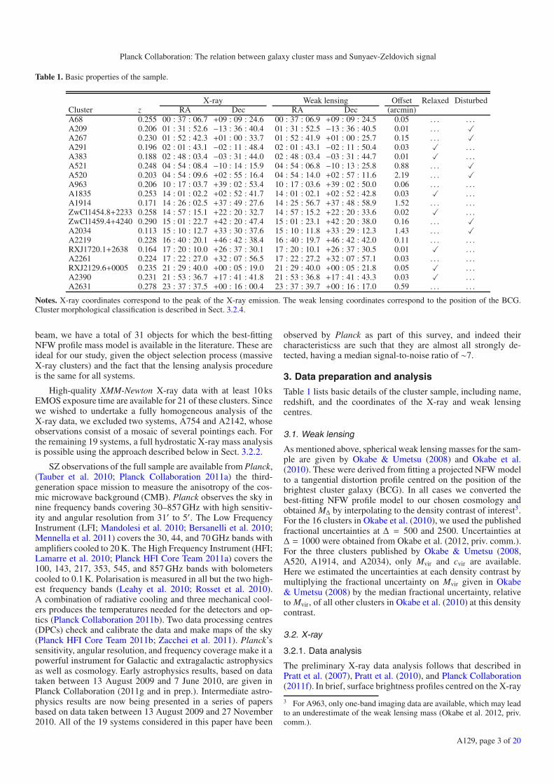
Table 1. Basic properties of the sample.

X-ray Weak lensing Offset Relaxed DisturbedCluster z RA Dec RA Dec (arcmin)A68 0.255 00 : 37 : 06.7 +09 : 09 : 24.6 00 : 37 : 06.9 +09 : 09 : 24.5 0.05 . . . . . .A209 0.206 01 : 31 : 52.6 −13 : 36 : 40.4 01 : 31 : 52.5 −13 : 36 : 40.5 0.01 . . . �A267 0.230 01 : 52 : 42.3 +01 : 00 : 33.7 01 : 52 : 41.9 +01 : 00 : 25.7 0.15 . . . �A291 0.196 02 : 01 : 43.1 −02 : 11 : 48.4 02 : 01 : 43.1 −02 : 11 : 50.4 0.03 � . . .A383 0.188 02 : 48 : 03.4 −03 : 31 : 44.0 02 : 48 : 03.4 −03 : 31 : 44.7 0.01 � . . .A521 0.248 04 : 54 : 08.4 −10 : 14 : 15.9 04 : 54 : 06.8 −10 : 13 : 25.8 0.88 . . . �A520 0.203 04 : 54 : 09.6 +02 : 55 : 16.4 04 : 54 : 14.0 +02 : 57 : 11.6 2.19 . . . �A963 0.206 10 : 17 : 03.7 +39 : 02 : 53.4 10 : 17 : 03.6 +39 : 02 : 50.0 0.06 . . . . . .A1835 0.253 14 : 01 : 02.2 +02 : 52 : 41.7 14 : 01 : 02.1 +02 : 52 : 42.8 0.03 � . . .A1914 0.171 14 : 26 : 02.5 +37 : 49 : 27.6 14 : 25 : 56.7 +37 : 48 : 58.9 1.52 . . . . . .ZwCl1454.8+2233 0.258 14 : 57 : 15.1 +22 : 20 : 32.7 14 : 57 : 15.2 +22 : 20 : 33.6 0.02 � . . .ZwCl1459.4+4240 0.290 15 : 01 : 22.7 +42 : 20 : 47.4 15 : 01 : 23.1 +42 : 20 : 38.0 0.16 . . . �A2034 0.113 15 : 10 : 12.7 +33 : 30 : 37.6 15 : 10 : 11.8 +33 : 29 : 12.3 1.43 . . . �A2219 0.228 16 : 40 : 20.1 +46 : 42 : 38.4 16 : 40 : 19.7 +46 : 42 : 42.0 0.11 . . . . . .RXJ1720.1+2638 0.164 17 : 20 : 10.0 +26 : 37 : 30.1 17 : 20 : 10.1 +26 : 37 : 30.5 0.01 � . . .A2261 0.224 17 : 22 : 27.0 +32 : 07 : 56.5 17 : 22 : 27.2 +32 : 07 : 57.1 0.03 . . . . . .RXJ2129.6+0005 0.235 21 : 29 : 40.0 +00 : 05 : 19.0 21 : 29 : 40.0 +00 : 05 : 21.8 0.05 � . . .A2390 0.231 21 : 53 : 36.7 +17 : 41 : 41.8 21 : 53 : 36.8 +17 : 41 : 43.3 0.03 � . . .A2631 0.278 23 : 37 : 37.5 +00 : 16 : 00.4 23 : 37 : 39.7 +00 : 16 : 17.0 0.59 . . . . . .

Notes. X-ray coordinates correspond to the peak of the X-ray emission. The weak lensing coordinates correspond to the position of the BCG.Cluster morphological classification is described in Sect. 3.2.4.

beam, we have a total of 31 objects for which the best-fittingNFW profile mass model is available in the literature. These areideal for our study, given the object selection process (massiveX-ray clusters) and the fact that the lensing analysis procedureis the same for all systems.

High-quality XMM-Newton X-ray data with at least 10 ksEMOS exposure time are available for 21 of these clusters. Sincewe wished to undertake a fully homogeneous analysis of theX-ray data, we excluded two systems, A754 and A2142, whoseobservations consist of a mosaic of several pointings each. Forthe remaining 19 systems, a full hydrostatic X-ray mass analysisis possible using the approach described below in Sect. 3.2.2.

SZ observations of the full sample are available from Planck,(Tauber et al. 2010; Planck Collaboration 2011a) the third-generation space mission to measure the anisotropy of the cos-mic microwave background (CMB). Planck observes the sky innine frequency bands covering 30–857 GHz with high sensitiv-ity and angular resolution from 31′ to 5′. The Low FrequencyInstrument (LFI; Mandolesi et al. 2010; Bersanelli et al. 2010;Mennella et al. 2011) covers the 30, 44, and 70 GHz bands withamplifiers cooled to 20 K. The High Frequency Instrument (HFI;Lamarre et al. 2010; Planck HFI Core Team 2011a) covers the100, 143, 217, 353, 545, and 857 GHz bands with bolometerscooled to 0.1 K. Polarisation is measured in all but the two high-est frequency bands (Leahy et al. 2010; Rosset et al. 2010).A combination of radiative cooling and three mechanical cool-ers produces the temperatures needed for the detectors and op-tics (Planck Collaboration 2011b). Two data processing centres(DPCs) check and calibrate the data and make maps of the sky(Planck HFI Core Team 2011b; Zacchei et al. 2011). Planck’ssensitivity, angular resolution, and frequency coverage make it apowerful instrument for Galactic and extragalactic astrophysicsas well as cosmology. Early astrophysics results, based on datataken between 13 August 2009 and 7 June 2010, are given inPlanck Collaboration (2011g and in prep.). Intermediate astro-physics results are now being presented in a series of papersbased on data taken between 13 August 2009 and 27 November2010. All of the 19 systems considered in this paper have been

observed by Planck as part of this survey, and indeed theircharacteristicss are such that they are almost all strongly de-tected, having a median signal-to-noise ratio of ∼7.

3. Data preparation and analysis

Table 1 lists basic details of the cluster sample, including name,redshift, and the coordinates of the X-ray and weak lensingcentres.

3.1. Weak lensing

As mentioned above, spherical weak lensing masses for the sam-ple are given by Okabe & Umetsu (2008) and Okabe et al.(2010). These were derived from fitting a projected NFW modelto a tangential distortion profile centred on the position of thebrightest cluster galaxy (BCG). In all cases we converted thebest-fitting NFW profile model to our chosen cosmology andobtained MΔ by interpolating to the density contrast of interest3.For the 16 clusters in Okabe et al. (2010), we used the publishedfractional uncertainties at Δ = 500 and 2500. Uncertainties atΔ = 1000 were obtained from Okabe et al. (2012, priv. comm.).For the three clusters published by Okabe & Umetsu (2008,A520, A1914, and A2034), only Mvir and cvir are available.Here we estimated the uncertainties at each density contrast bymultiplying the fractional uncertainty on Mvir given in Okabe& Umetsu (2008) by the median fractional uncertainty, relativeto Mvir, of all other clusters in Okabe et al. (2010) at this densitycontrast.

3.2. X-ray

3.2.1. Data analysis

The preliminary X-ray data analysis follows that described inPratt et al. (2007), Pratt et al. (2010), and Planck Collaboration(2011f). In brief, surface brightness profiles centred on the X-ray

3 For A963, only one-band imaging data are available, which may leadto an underestimate of the weak lensing mass (Okabe et al. 2012, priv.comm.).

A129, page 3 of 20

A&A 550, A129 (2013)

emission peak were extracted in the 0.3–2 keV band and used toderive the regularised gas density profiles, ne(r), using the non-parametric deprojection and PSF-correction method of Crostonet al. (2006). The projected temperature was measured in an-nuli as described in Pratt et al. (2010). The 3D temperature pro-files, T (r), were calculated by convolving a suitable parametricmodel with a response matrix that takes into account projectionand PSF effects, projecting this model accounting for the biasintroduced by fitting isothermal models to multi-temperatureplasma emission (Mazzotta et al. 2004; Vikhlinin 2006), andfitting to the projected annular profile. Note that in addition topoint sources, obvious X-ray sub-structures (corresponding to,e.g., prominent secondary maxima in the X-ray surface bright-ness) were excised before calculating the density and tempera-ture profiles discussed above.

3.2.2. X-ray mass profile

The X-ray mass was calculated for each cluster as described inDémoclès et al. (2010). Using the gas density ne(r) and temper-ature T (r) profiles, and assuming hydrostatic equilibrium, thetotal mass is given by:

M (≤ R) = −kT (r) rG μmp

[dln ne(r)

dln r+

dln T (r)dln r

]· (1)

To suppress noise due to structure in the regularised gas densityprofiles, we fitted them with the parametric model described byVikhlinin et al. (2006) and used the radial derivative dln ne/dln rgiven by this parametric function fit. The corresponding uncer-tainties were given by differentiation of the regularised densityprofile at each point corresponding to the effective radius of thedeconvolved temperature profile.

Uncertainties on each X-ray mass point were calculated us-ing a Monte Carlo approach based on that of Pratt & Arnaud(2003), where a random temperature was generated at each ra-dius at which the temperature profile is measured, and a cubicspline used to compute the derivative. We only kept random pro-files that were physical, meaning that the mass profile must in-crease monotonically with radius and the randomised tempera-ture profiles must be convectively stable, assuming the standardSchwarzschild criterion in the abscence of strong heat conduc-tivity, i.e., dln T/dln ne < 2/3. The number of rejected profilesvaried on a cluster-by-cluster basis, with morphologically dis-turbed clusters generally requiring more discards. The final massprofiles were built from a minimum of 100 and a maximum of1000 Monte Carlo realisations. The mass at each density con-trast relative to the critical density of the Universe, MΔ, wascalculated via interpolation in the log M− logΔ plane. The un-certainty on the resulting mass value was then calculated fromthe region containing 68 percent of the realisations on each side.

For two clusters, the hydrostatic X-ray mass determinationsshould be treated with some caution. The first is A521, whichis a well-known merging system. Here the gas density profile atlarge radius declines precipitously, yielding a dln ne/dln r valuethat results in an integrated mass profile that is practically a purepower law at large cluster-centric distances. Although we ex-cised the obvious substructure to the north-west before the X-raymass analysis, the complex nature of this system precludes aprecise X-ray mass analysis. The second cluster for which theX-ray mass determination is suspect is A2261, for the more pro-saic reason that the X-ray temperature profile is only detected upto Rdet,max ∼ 0.6 R500 ∼ 0.8 R1000. In the following, we excludethese clusters in cases when the hydrostatic X-ray mass is underdiscussion.

3.2.3. X-ray pressure profile

Using the radial density and temperature information, we alsocalculated the X-ray pressure profile P(r) = ne(r) kT (r). We thenfitted the pressure profile of each cluster with the generalisedNavarro, Frank & White (GNFW) model introduced by Nagaiet al. (2007), viz.,

P(x) =P0

(c500,p x)γ[1 + (c500,p x)α

](β−γ)/α · (2)

Here the parameters (α, β, γ) are the intermediate, outer, andcentral slopes, respectively, c500,p is a concentration parameter,rs = R500/c500,p, and x = r/R500. In the fitting, the outer slopewas fixed at β = 5.49, a choice that is motivated by simula-tions since it is essentially unconstrained by the X-ray data (seeArnaud et al. 2010, for discussion). The best-fitting X-ray pres-sure profile parameters are listed in Table A.1, and the observedprofiles and best-fitting models are plotted in Fig. A.1.

3.2.4. Morphological classification

We divided the 19 clusters into three morphological sub-classesbased on the scaled central density E(z)−2 ne,0, which is a goodproxy for the overall dynamical state (see, e.g., Pratt et al. 2010;Arnaud et al. 2010). The scaled central density was obtainedfrom a β-model fit to the inner R < 0.05 R500 region. Theseven clusters with the highest scaled central density values wereclassed as relaxed4; the six with the lowest values were classedas disturbed; the six with intermediate values were classed asintermediate (i.e., neither relaxed nor disturbed). Strict applica-tion of the REXCESS morphological classification criteria basedon scaled central density and centroid shift parameter 〈w〉 (Prattet al. 2009) results in a similar classification scheme.

Images of the cluster sample ordered by E(z)−2 ne,0 areshown Appendix B. Henceforth, in all figures dealing with mor-phological classification, relaxed systems are plotted in blue,unrelaxed in red and intermediate in black. Scaled X-ray pro-files resulting from the analysis described below, colour-codedby morphological sub-class, are shown in Fig. C.1.

3.3. SZ

The SZ signal was extracted from the six High FrequencyInstrument (HFI) temperature channel maps corresponding tothe nominal Planck survey (i.e., slightly more than 2.5 full skysurveys). We used full resolution maps of HEALPix (Górskiet al. 2005)5 Nside = 2048 and assumed that the beams weredescribed by circular Gaussians. We adopted beam FWHM val-ues of 9.88, 7.18, 4.87, 4.65, 4.72, and 4.39 arcmin for chan-nel frequencies 100, 143, 217, 353, 545, and 857 GHz, re-spectively. Flux extraction was undertaken using the full rel-ativistic treatment of the SZ spectrum (Itoh et al. 1998), as-suming the global temperature TX given in Table 2. Bandpassuncertainties were taken into account in the flux measure-ment. Uncertainties due to beam corrections and map cali-brations are expected to be small, as discussed extensively inPlanck Collaboration (2011d), Planck Collaboration (2011c),Planck Collaboration (2011e), Planck Collaboration (2011f),and Planck Collaboration (2011g).

4 As these systems have the highest scaled central density, they arefully equivalent to a cool core sub-sample.5 http://healpix.jpl.nasa.gov

A129, page 4 of 20

Planck Collaboration: The relation between galaxy cluster mass and Sunyaev-Zeldovich signal

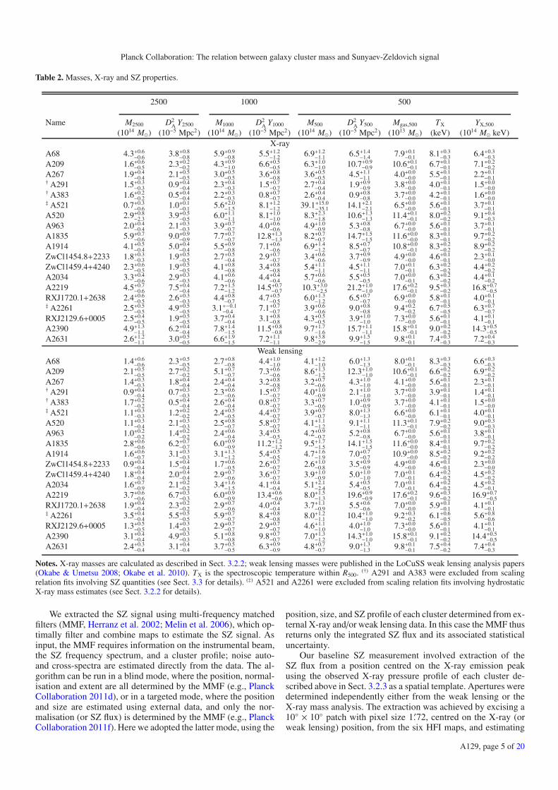
Table 2. Masses, X-ray and SZ properties.

2500 1000 500

Name M2500 D2A Y2500 M1000 D2

A Y1000 M500 D2A Y500 Mgas,500 TX YX,500

(1014 M�) (10−5 Mpc2) (1014 M�) (10−5 Mpc2) (1014 M�) (10−5 Mpc2) (1013 M�) (keV) (1014 M� keV)X-ray

A68 4.3+0.6−0.6 3.8+0.8

−0.8 5.9+0.9−0.8 5.5+1.2

−1.2 6.9+1.2−1.1 6.5+1.4

−1.4 7.9+0.1−0.1 8.1+0.3

−0.3 6.4+0.3−0.3

A209 1.6+0.6−0.5 2.3+0.2

−0.2 4.3+0.9−1.0 6.6+0.5

−0.5 6.3+1.0−1.0 10.7+0.9

−0.9 10.6+0.1−0.1 6.7+0.1

−0.1 7.1+0.2−0.2

A267 1.9+0.4−0.4 2.1+0.5

−0.5 3.0+0.5−0.5 3.6+0.8

−0.8 3.6+0.5−0.5 4.5+1.1

−1.1 4.0+0.0−0.0 5.5+0.1

−0.1 2.2+0.1−0.1† A291 1.5+0.3

−0.3 0.9+0.4−0.4 2.3+0.4

−0.3 1.5+0.7−0.7 2.7+0.4

−0.4 1.9+0.9−0.9 3.8+0.0

−0.0 4.0+0.1−0.1 1.5+0.0

−0.0† A383 1.6+0.2−0.2 0.5+0.4

−0.4 2.2+0.3−0.3 0.8+0.7

−0.7 2.6+0.4−0.4 0.9+0.8

−0.8 3.7+0.0−0.0 4.2+0.1

−0.1 1.6+0.0−0.0‡ A521 0.7+0.3

−0.6 1.0+0.1−0.1 5.6+2.0

−1.5 8.1+1.2−1.2 39.1+15.0

−35.1 14.1+2.1−2.1 6.5+0.0

−0.0 5.6+0.1−0.1 3.7+0.1

−0.1A520 2.9+0.8

−2.3 3.9+0.5−0.5 6.0+1.1

−1.1 8.1+1.0−1.0 8.3+2.3

−1.8 10.6+1.3−1.3 11.4+0.1

−0.1 8.0+0.2−0.2 9.1+0.4

−0.3A963 2.0+0.4

−0.4 2.1+0.3−0.3 3.9+0.7

−0.7 4.0+0.6−0.6 4.9+1.0

−0.9 5.3+0.8−0.8 6.7+0.0

−0.0 5.6+0.1−0.1 3.7+0.1

−0.1A1835 5.9+0.7

−0.6 9.0+0.9−0.9 7.7+0.7

−0.7 12.8+1.3−1.3 8.2+0.7

−0.7 14.7+1.5−1.5 11.6+0.0

−0.0 8.3+0.1−0.1 9.7+0.2

−0.2A1914 4.1+0.5

−0.4 5.0+0.4−0.4 5.5+0.9

−0.8 7.1+0.6−0.6 6.9+1.4

−1.2 8.5+0.7−0.7 10.8+0.0

−0.1 8.3+0.2−0.2 8.9+0.2

−0.2ZwCl1454.8+2233 1.8+0.3

−0.3 1.9+0.5−0.5 2.7+0.5

−0.4 2.9+0.7−0.7 3.4+0.6

−0.6 3.7+0.9−0.9 4.9+0.0

−0.0 4.6+0.1−0.1 2.3+0.1

−0.0ZwCl1459.4+4240 2.3+0.6

−0.5 1.9+0.5−0.5 4.1+0.8

−0.8 3.4+0.8−0.8 5.4+1.1

−1.1 4.5+1.1−1.1 7.0+0.1

−0.1 6.3+0.2−0.2 4.4+0.2

−0.2A2034 3.3+0.4

−0.6 2.9+0.3−0.3 4.1+0.6

−0.6 4.4+0.4−0.4 5.7+0.6

−0.6 5.5+0.5−0.5 7.0+0.0

−0.1 6.3+0.2−0.2 4.4+0.1

−0.2A2219 4.5+0.7

−0.6 7.5+0.4−0.4 7.2+1.5

−1.2 14.5+0.7−0.7 10.3+3.0

−2.5 21.2+1.0−1.0 17.6+0.2

−0.1 9.5+0.3−0.2 16.8+0.7

−0.5RXJ1720.1+2638 2.4+0.6

−0.5 2.6+0.3−0.3 4.4+0.8

−0.7 4.7+0.5−0.5 6.0+1.3

−1.2 6.5+0.7−0.7 6.9+0.0

−0.0 5.8+0.1−0.1 4.0+0.1

−0.1‡ A2261 2.5+0.5−0.5 4.9+0.5

−0.5 3.1+−0.1−0.4 7.1+0.7

−0.7 3.9+0.6−0.6 9.0+0.8

−0.8 9.4+0.2−0.2 6.7+0.5

−0.5 6.3+0.7−0.7

RXJ2129.6+0005 2.5+0.4−0.5 1.9+0.5

−0.5 3.7+0.4−0.4 3.1+0.8

−0.8 4.3+0.5−0.5 3.9+1.0

−1.0 7.3+0.0−0.0 5.6+0.1

−0.1 4.1+0.1−0.1

A2390 4.9+1.3−1.1 6.2+0.4

−0.4 7.8+1.4−1.5 11.5+0.8

−0.8 9.7+1.7−1.6 15.7+1.1

−1.1 15.8+0.1−0.1 9.0+0.2

−0.2 14.3+0.5−0.5

A2631 2.6+1.2−1.1 3.0+0.5

−0.5 6.6+1.9−1.5 7.2+1.1

−1.1 9.8+3.8−2.9 9.9+1.5

−1.5 9.8+0.1−0.1 7.4+0.3

−0.3 7.2+0.4−0.3

Weak lensingA68 1.4+0.6

−0.6 2.3+0.5−0.5 2.7+0.8

−0.8 4.4+1.0−1.0 4.1+1.2

−1.0 6.0+1.3−1.3 8.0+0.1

−0.1 8.3+0.3−0.3 6.6+0.3

−0.3A209 2.1+0.5

−0.5 2.7+0.2−0.2 5.1+0.7

−0.7 7.3+0.6−0.6 8.6+1.3

−1.2 12.3+1.0−1.0 10.6+0.1

−0.1 6.6+0.2−0.2 6.9+0.2

−0.2A267 1.4+0.3

−0.3 1.8+0.4−0.4 2.4+0.4

−0.4 3.2+0.8−0.8 3.2+0.7

−0.6 4.3+1.0−1.0 4.1+0.0

−0.0 5.6+0.1−0.1 2.3+0.1

−0.1† A291 0.9+0.4−0.4 0.7+0.3

−0.3 2.3+0.6−0.6 1.5+0.7

−0.7 4.0+1.0−0.9 2.1+1.0

−1.0 3.7+0.0−0.0 3.9+0.1

−0.1 1.4+0.1−0.1† A383 1.7+0.2

−0.2 0.5+0.4−0.4 2.6+0.4

−0.4 0.8+0.7−0.7 3.3+0.7

−0.6 1.0+0.9−0.9 3.7+0.0

−0.0 4.1+0.1−0.1 1.5+0.0

−0.0‡ A521 1.1+0.3−0.3 1.2+0.2

−0.2 2.4+0.5−0.5 4.4+0.7

−0.7 3.9+0.7−0.7 8.0+1.3

−1.3 6.6+0.0−0.0 6.1+0.1

−0.1 4.0+0.1−0.1

A520 1.1+0.3−0.4 2.1+0.3

−0.3 2.5+0.8−0.7 5.8+0.7

−0.7 4.1+1.1−1.2 9.1+1.1

−1.1 11.3+0.1−0.1 7.9+0.2

−0.2 9.0+0.3−0.3

A963 1.0+0.2−0.2 1.4+0.2

−0.2 2.4+0.6−0.4 3.4+0.5

−0.5 4.2+0.9−0.7 5.2+0.8

−0.8 6.7+0.0−0.0 5.6+0.1

−0.1 3.8+0.1−0.1

A1835 2.8+0.6−0.6 6.2+0.7

−0.7 6.0+0.9−0.9 11.2+1.2

−1.2 9.5+1.7−1.5 14.1+1.5

−1.5 11.6+0.0−0.0 8.4+0.1

−0.1 9.7+0.2−0.2

A1914 1.6+0.6−0.7 3.1+0.3

−0.3 3.1+1.3−1.2 5.4+0.5

−0.5 4.7+1.6−1.9 7.0+0.7

−0.7 10.9+0.0−0.0 8.5+0.2

−0.2 9.2+0.2−0.2

ZwCl1454.8+2233 0.9+0.4−0.4 1.5+0.4

−0.4 1.7+0.6−0.5 2.6+0.7

−0.7 2.6+1.0−0.8 3.5+0.9

−0.9 4.9+0.0−0.0 4.6+0.1

−0.1 2.3+0.0−0.0

ZwCl1459.4+4240 1.8+0.4−0.4 2.0+0.4

−0.4 2.9+0.7−0.6 3.6+0.7

−0.7 3.9+1.0−0.9 5.0+1.0

−1.0 7.0+0.1−0.1 6.4+0.2

−0.2 4.5+0.2−0.2

A2034 1.6+0.7−0.9 2.1+0.2

−0.2 3.4+1.6−1.5 4.1+0.4

−0.4 5.1+2.1−2.4 5.4+0.5

−0.5 7.0+0.1−0.1 6.4+0.2

−0.2 4.5+0.2−0.1

A2219 3.7+0.6−0.6 6.7+0.3

−0.3 6.0+0.9−0.9 13.4+0.6

−0.6 8.0+1.5−1.3 19.6+0.9

−0.9 17.6+0.2−0.1 9.6+0.3

−0.2 16.9+0.7−0.5

RXJ1720.1+2638 1.9+0.4−0.4 2.3+0.2

−0.2 2.9+0.7−0.6 4.0+0.4

−0.4 3.7+1.1−0.9 5.5+0.6

−0.6 7.0+0.0−0.0 5.9+0.1

−0.1 4.1+0.1−0.1‡ A2261 3.5+0.4

−0.4 5.5+0.5−0.5 5.9+0.7

−0.7 8.4+0.8−0.8 8.0+1.2

−1.1 10.4+1.0−1.0 9.2+0.3

−0.2 6.1+0.6−0.5 5.6+0.8

−0.6RXJ2129.6+0005 1.3+0.5

−0.5 1.4+0.3−0.3 2.9+0.7

−0.7 2.9+0.7−0.7 4.6+1.1

−1.0 4.0+1.0−1.0 7.3+0.0

−0.0 5.6+0.1−0.1 4.1+0.1

−0.1A2390 3.1+0.4

−0.4 4.9+0.3−0.3 5.1+0.8

−0.8 9.8+0.7−0.7 7.0+1.3

−1.2 14.3+1.0−1.0 15.8+0.1

−0.1 9.1+0.2−0.2 14.4+0.5

−0.5A2631 2.4+0.3

−0.4 3.1+0.4−0.4 3.7+0.5

−0.5 6.3+0.9−0.9 4.8+0.7

−0.7 9.0+1.3−1.3 9.8+0.1

−0.1 7.5+0.4−0.2 7.4+0.4

−0.3

Notes. X-ray masses are calculated as described in Sect. 3.2.2; weak lensing masses were published in the LoCuSS weak lensing analysis papers(Okabe & Umetsu 2008; Okabe et al. 2010). TX is the spectroscopic temperature within R500. (†) A291 and A383 were excluded from scalingrelation fits involving SZ quantities (see Sect. 3.3 for details). (‡) A521 and A2261 were excluded from scaling relation fits involving hydrostaticX-ray mass estimates (see Sect. 3.2.2 for details).

We extracted the SZ signal using multi-frequency matchedfilters (MMF, Herranz et al. 2002; Melin et al. 2006), which op-timally filter and combine maps to estimate the SZ signal. Asinput, the MMF requires information on the instrumental beam,the SZ frequency spectrum, and a cluster profile; noise auto-and cross-spectra are estimated directly from the data. The al-gorithm can be run in a blind mode, where the position, normal-isation and extent are all determined by the MMF (e.g., PlanckCollaboration 2011d), or in a targeted mode, where the positionand size are estimated using external data, and only the nor-malisation (or SZ flux) is determined by the MMF (e.g., PlanckCollaboration 2011f). Here we adopted the latter mode, using the

position, size, and SZ profile of each cluster determined from ex-ternal X-ray and/or weak lensing data. In this case the MMF thusreturns only the integrated SZ flux and its associated statisticaluncertainty.

Our baseline SZ measurement involved extraction of theSZ flux from a position centred on the X-ray emission peakusing the observed X-ray pressure profile of each cluster de-scribed above in Sect. 3.2.3 as a spatial template. Apertures weredetermined independently either from the weak lensing or theX-ray mass analysis. The extraction was achieved by excising a10◦ × 10◦ patch with pixel size 1.′72, centred on the X-ray (orweak lensing) position, from the six HFI maps, and estimating

A129, page 5 of 20

A&A 550, A129 (2013)

1014 1015

M2500WL [MO • ]

10-5

10-4

E(z

)-2/3 D

A2 Y25

00 [

Mp

c2 ]

Bonamente et al. 2008 (X-ray HE mass)Marrone et al. 2011

1014 1015

M1000WL [MO • ]

10-5

10-4

E(z

)-2/3 D

A2 Y10

00 [

Mp

c2 ]

Marrone et al. 2011

1014 1015

M500WL [MO • ]

10-5

10-4

E(z

)-2/3 D

A2 Y50

0 [

Mp

c2 ]

Planck Collaboration 2011 (X-ray HE mass) Marrone et al. 2011

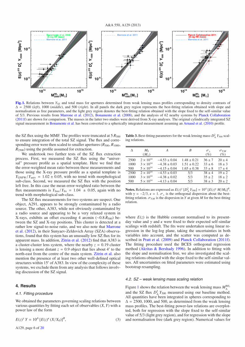
Fig. 1. Relations between YSZ and total mass for apertures determined from weak lensing mass profiles corresponding to density contrasts ofΔ = 2500 (left), 1000 (middle), and 500 (right). In all panels the dark grey region represents the best-fitting relation obtained with slope andnormalisation as free parameters, and the light grey region denotes the best-fitting relation obtained with the slope fixed to the self-similar valueof 5/3. Previous results from Marrone et al. (2012), Bonamente et al. (2008), and the analysis of 62 nearby systems by Planck Collaboration(2011f) are shown for comparison. The masses in the latter two studies were derived from X-ray analyses. The original cylindrically integrated SZsignal measurement in Bonamente et al. has been converted to a spherically integrated measurement assuming an Arnaud et al. (2010) profile.

the SZ flux using the MMF. The profiles were truncated at 5 R500to ensure integration of the total SZ signal. The flux and corre-sponding error were then scaled to smaller apertures (R500, R1000,R2500) using the profile assumed for extraction.

We undertook two further tests of the SZ flux extractionprocess. First, we measured the SZ flux using the “univer-sal” pressure profile as a spatial template. Here we find thatthe error-weighted mean ratio between these measurements andthose using the X-ray pressure profile as a spatial template isYGNFW/Yuniv = 1.02 ± 0.05, with no trend with morphologicalsub-class. Second, we measured the SZ flux with the positionleft free. In this case the mean error-weighted ratio between theflux measurements is Yfree/Yfix = 1.04 ± 0.05, again with notrend with morphological sub-class.

The SZ flux measurements for two systems are suspect. Oneobject, A291, appears to be strongly contaminated by a radiosource. The other, A383, while not obviously contaminated bya radio source and appearing to be a very relaxed system inX-rays, exhibits an offset exceeding 4 arcmin (∼0.8 R500) be-tween the SZ and X-ray positions. This cluster is detected at arather low signal-to-noise ratio, and we also note that Marroneet al. (2012), in their Sunyaev-Zeldovich Array (SZA) observa-tions, found that this system has an unusually low SZ flux for itsapparent mass. In addition, Zitrin et al. (2012) find that A383 isa cluster-cluster lens system, where the nearby z = 0.19 clusteris lensing a more distant z = 0.9 object that lies about 4′ to thenorth-east from the centre of the main system. Zitrin et al. alsomention the presence of at least two other well-defined opticalstructures within 15′ of A383. In view of the complexity of thesesystems, we exclude them from any analysis that follows involv-ing discussion of the SZ signal.

4. Results

4.1. Fitting procedure

We obtained the parameters governing scaling relations betweenvarious quantities by fitting each set of observables (X, Y) with apower law of the form

E(z)γ Y = 10A [E(z)κ (X/X0)]B, (3)

Table 3. Best-fitting parameters for the weak lensing mass-D2A Y500 scal-

ing relations.

Δ M0 A B σ⊥ σY |M(M�) (%) (%)

2500 2 × 1014 −4.53 ± 0.04 1.48 ± 0.21 36 ± 7 20 ± 41000 3 × 1014 −4.38 ± 0.03 1.51 ± 0.22 33 ± 6 18 ± 3500 5 × 1014 −4.15 ± 0.04 1.65 ± 0.38 33 ± 8 17 ± 42500 2 × 1014 −4.53 ± 0.03 5/3 38 ± 4 19 ± 21000 3 × 1014 −4.38 ± 0.02 5/3 35 ± 2 18 ± 2500 5 × 1014 −4.13 ± 0.04 5/3 38 ± 3 20 ± 2

Notes. Relations are expressed as E(z)γ [D2A Y500] = 10A [E(z)κ M/M0]B,

with γ = −2/3, κ = 1. σ⊥ is the orthogonal dispersion about the best-fitting relation. σY |M is the dispersion in Y at given M for the best-fittingrelation.

where E(z) is the Hubble constant normalised to its present-day value and γ and κ were fixed to their expected self-similarscalings with redshift. The fits were undertaken using linear re-gression in the log-log plane, taking the uncertainties in bothvariables into account, and the scatter was computed as de-scribed in Pratt et al. (2009) and Planck Collaboration (2011f).The fitting procedure used the BCES orthogonal regressionmethod (Akritas & Bershady 1996). In addition to fitting withthe slope and normalisation free, we also investigated the scal-ing relations obtained with the slope fixed to the self-similar val-ues. All uncertainties on fitted parameters were estimated usingbootstrap resampling.

4.2. SZ – weak lensing mass scaling relation

Figure 1 shows the relation between the weak lensing mass MWLΔ

and the SZ flux D2A Y500 measured using our baseline method.

All quantities have been integrated in spheres corresponding toΔ = 2500, 1000, and 500, as determined from the weak lensingmass profiles. The best-fitting power-law relations are overplot-ted, both for regression with the slope fixed to the self-similarvalue of 5/3 (light grey region), and for regression with the slopeand normalisation free (dark grey region). Numerical values for

A129, page 6 of 20

Planck Collaboration: The relation between galaxy cluster mass and Sunyaev-Zeldovich signal

10-4

(σT/me c2)/(μe mp) YX [Mpc2]

10-4

DA2 Y

500

[M

pc2 ]

Planck Collaboration 2011

1014 1015

M500Yx [MO • ]

10-5

10-4

E(z

)-2/3 D

A2 Y50

0 [

Mp

c2 ]

Planck Collaboration 2011

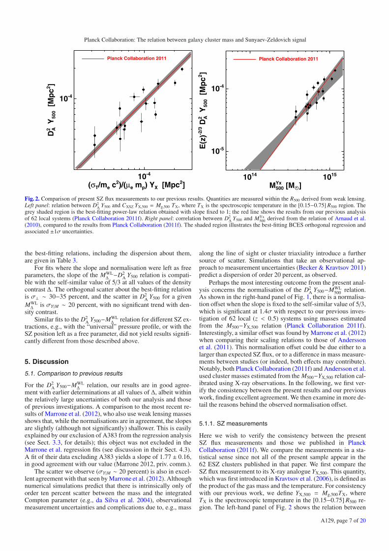
Fig. 2. Comparison of present SZ flux measurements to our previous results. Quantities are measured within the R500 derived from weak lensing.Left panel: relation between D2

A Y500 and CXSZ YX,500 = Mg,500 TX, where TX is the spectroscopic temperature in the [0.15−0.75] R500 region. Thegrey shaded region is the best-fitting power-law relation obtained with slope fixed to 1; the red line shows the results from our previous analysisof 62 local systems (Planck Collaboration 2011f). Right panel: correlation between D2

A Y500 and MYx500 derived from the relation of Arnaud et al.

(2010), compared to the results from Planck Collaboration (2011f). The shaded region illustrates the best-fitting BCES orthogonal regression andassociated ±1σ uncertainties.

the best-fitting relations, including the dispersion about them,are given in Table 3.

For fits where the slope and normalisation were left as freeparameters, the slope of the MWL

Δ−D2

A Y500 relation is compati-ble with the self-similar value of 5/3 at all values of the densitycontrast Δ. The orthogonal scatter about the best-fitting relationis σ⊥ ∼ 30−35 percent, and the scatter in D2

A Y500 for a givenMWLΔ

is σY |M ∼ 20 percent, with no significant trend with den-sity contrast.

Similar fits to the D2A Y500−MWL

Δrelation for different SZ ex-

tractions, e.g., with the “universal” pressure profile, or with theSZ position left as a free parameter, did not yield results signifi-cantly different from those described above.

5. Discussion

5.1. Comparison to previous results

For the D2A Y500−MWL

Δrelation, our results are in good agree-

ment with earlier determinations at all values of Δ, albeit withinthe relatively large uncertainties of both our analysis and thoseof previous investigations. A comparison to the most recent re-sults of Marrone et al. (2012), who also use weak lensing massesshows that, while the normalisations are in agreement, the slopesare slightly (although not significantly) shallower. This is easilyexplained by our exclusion of A383 from the regression analysis(see Sect. 3.3, for details); this object was not excluded in theMarrone et al. regression fits (see discussion in their Sect. 4.3).A fit of their data excluding A383 yields a slope of 1.77 ± 0.16,in good agreement with our value (Marrone 2012, priv. comm.).

The scatter we observe (σY |M ∼ 20 percent) is also in excel-lent agreement with that seen by Marrone et al. (2012). Althoughnumerical simulations predict that there is intrinsically only oforder ten percent scatter between the mass and the integratedCompton parameter (e.g., da Silva et al. 2004), observationalmeasurement uncertainties and complications due to, e.g., mass

along the line of sight or cluster triaxiality introduce a furthersource of scatter. Simulations that take an observational ap-proach to measurement uncertainties (Becker & Kravtsov 2011)predict a dispersion of order 20 percent, as observed.

Perhaps the most interesting outcome from the present anal-ysis concerns the normalisation of the D2

A Y500−MWL500 relation.

As shown in the right-hand panel of Fig. 1, there is a normalisa-tion offset when the slope is fixed to the self-similar value of 5/3,which is significant at 1.4σ with respect to our previous inves-tigation of 62 local (z < 0.5) systems using masses estimatedfrom the M500−YX,500 relation (Planck Collaboration 2011f).Interestingly, a similar offset was found by Marrone et al. (2012)when comparing their scaling relations to those of Anderssonet al. (2011). This normalisation offset could be due either to alarger than expected SZ flux, or to a difference in mass measure-ments between studies (or indeed, both effects may contribute).Notably, both Planck Collaboration (2011f) and Andersson et al.used cluster masses estimated from the M500−YX,500 relation cal-ibrated using X-ray observations. In the following, we first ver-ify the consistency between the present results and our previouswork, finding excellent agreement. We then examine in more de-tail the reasons behind the observed normalisation offset.

5.1.1. SZ measurements

Here we wish to verify the consistency between the presentSZ flux measurements and those we published in PlanckCollaboration (2011f). We compare the measurements in a sta-tistical sense since not all of the present sample appear in the62 ESZ clusters published in that paper. We first compare theSZ flux measurement to its X-ray analogue YX,500. This quantity,which was first introduced in Kravtsov et al. (2006), is defined asthe product of the gas mass and the temperature. For consistencywith our previous work, we define YX,500 = Mg,500TX, whereTX is the spectroscopic temperature in the [0.15−0.75] R500 re-gion. The left-hand panel of Fig. 2 shows the relation between

A129, page 7 of 20

A&A 550, A129 (2013)

1015

M500HE [MO • ]

1015

M50

0Y

x [M

O •]

M500HE = M500

Yx

Morphologically disturbedIntermediate

Relaxed

1014 1015

M500HE [MO • ]

1014

1015

M50

0W

L [

MO •]

M500HE = M500

WL

Morphologically disturbedIntermediate

Relaxed

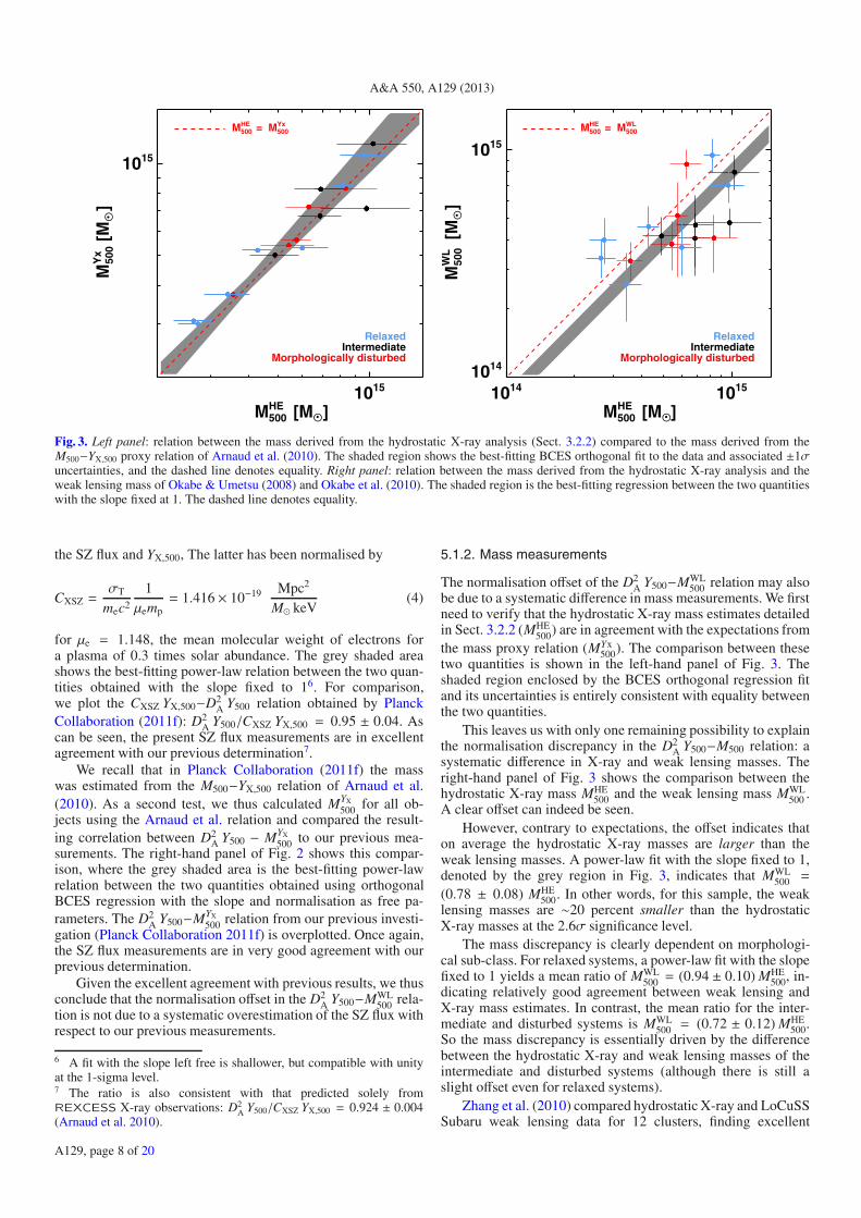
Fig. 3. Left panel: relation between the mass derived from the hydrostatic X-ray analysis (Sect. 3.2.2) compared to the mass derived from theM500−YX,500 proxy relation of Arnaud et al. (2010). The shaded region shows the best-fitting BCES orthogonal fit to the data and associated ±1σuncertainties, and the dashed line denotes equality. Right panel: relation between the mass derived from the hydrostatic X-ray analysis and theweak lensing mass of Okabe & Umetsu (2008) and Okabe et al. (2010). The shaded region is the best-fitting regression between the two quantitieswith the slope fixed at 1. The dashed line denotes equality.

the SZ flux and YX,500, The latter has been normalised by

CXSZ =σT

mec2

1μemp

= 1.416 × 10−19 Mpc2

M� keV(4)

for μe = 1.148, the mean molecular weight of electrons fora plasma of 0.3 times solar abundance. The grey shaded areashows the best-fitting power-law relation between the two quan-tities obtained with the slope fixed to 16. For comparison,we plot the CXSZ YX,500−D2

A Y500 relation obtained by PlanckCollaboration (2011f): D2

A Y500/CXSZ YX,500 = 0.95 ± 0.04. Ascan be seen, the present SZ flux measurements are in excellentagreement with our previous determination7.

We recall that in Planck Collaboration (2011f) the masswas estimated from the M500−YX,500 relation of Arnaud et al.(2010). As a second test, we thus calculated MYX

500 for all ob-jects using the Arnaud et al. relation and compared the result-ing correlation between D2

A Y500 − MYX

500 to our previous mea-surements. The right-hand panel of Fig. 2 shows this compar-ison, where the grey shaded area is the best-fitting power-lawrelation between the two quantities obtained using orthogonalBCES regression with the slope and normalisation as free pa-rameters. The D2

A Y500−MYX

500 relation from our previous investi-gation (Planck Collaboration 2011f) is overplotted. Once again,the SZ flux measurements are in very good agreement with ourprevious determination.

Given the excellent agreement with previous results, we thusconclude that the normalisation offset in the D2

A Y500−MWL500 rela-

tion is not due to a systematic overestimation of the SZ flux withrespect to our previous measurements.

6 A fit with the slope left free is shallower, but compatible with unityat the 1-sigma level.7 The ratio is also consistent with that predicted solely fromREXCESS X-ray observations: D2

A Y500/CXSZ YX,500 = 0.924 ± 0.004(Arnaud et al. 2010).

5.1.2. Mass measurements

The normalisation offset of the D2A Y500−MWL

500 relation may alsobe due to a systematic difference in mass measurements. We firstneed to verify that the hydrostatic X-ray mass estimates detailedin Sect. 3.2.2 (MHE

500) are in agreement with the expectations fromthe mass proxy relation (MYx

500). The comparison between thesetwo quantities is shown in the left-hand panel of Fig. 3. Theshaded region enclosed by the BCES orthogonal regression fitand its uncertainties is entirely consistent with equality betweenthe two quantities.

This leaves us with only one remaining possibility to explainthe normalisation discrepancy in the D2

A Y500−M500 relation: asystematic difference in X-ray and weak lensing masses. Theright-hand panel of Fig. 3 shows the comparison between thehydrostatic X-ray mass MHE

500 and the weak lensing mass MWL500 .

A clear offset can indeed be seen.However, contrary to expectations, the offset indicates that

on average the hydrostatic X-ray masses are larger than theweak lensing masses. A power-law fit with the slope fixed to 1,denoted by the grey region in Fig. 3, indicates that MWL

500 =

(0.78 ± 0.08) MHE500. In other words, for this sample, the weak

lensing masses are ∼20 percent smaller than the hydrostaticX-ray masses at the 2.6σ significance level.

The mass discrepancy is clearly dependent on morphologi-cal sub-class. For relaxed systems, a power-law fit with the slopefixed to 1 yields a mean ratio of MWL

500 = (0.94 ± 0.10) MHE500, in-

dicating relatively good agreement between weak lensing andX-ray mass estimates. In contrast, the mean ratio for the inter-mediate and disturbed systems is MWL

500 = (0.72 ± 0.12) MHE500.

So the mass discrepancy is essentially driven by the differencebetween the hydrostatic X-ray and weak lensing masses of theintermediate and disturbed systems (although there is still aslight offset even for relaxed systems).

Zhang et al. (2010) compared hydrostatic X-ray and LoCuSSSubaru weak lensing data for 12 clusters, finding excellent

A129, page 8 of 20

Planck Collaboration: The relation between galaxy cluster mass and Sunyaev-Zeldovich signal

1 10c500,WL / c500,HE

1

M50

0W

L /

M50

0H

E

RelaxedIntermediate

Morphologically disturbed

0.001 0.010 0.100 1.000X-ray-WL centre offset [R500]

1

M50

0W

L /

M50

0H

E

RelaxedIntermediate

Morphologically disturbed

Fig. 4. Left panel: this plot shows the ratio of weak lensing mass to hydrostatic X-ray mass as a function of the ratio of NFW mass profileconcentration parameter from weak lensing and X-ray analyses. Right panel: the ratio of weak lensing mass to hydrostatic X-ray mass is afunction of offset between X-ray and weak lensing centres. In both panels, the solid line is the best-fitting orthogonal BCES power-law relationbetween the quantities, and the different sub-samples are colour coded.

agreement between the different mass measures [MWL500 = (1.01±

0.07) MHE500]. As part of their X-ray-weak lensing study, Zhang

et al. (2010) analysed the same XMM-Newton data for ten ofthe clusters presented here. For the clusters we have in common,the ratio of X-ray masses measured at R500 is MHE

Zhang,500/MHE500 =

0.83 ± 0.13. This offset is similar to the offset we find betweenthe X-ray and weak lensing masses discussed above, as expectedsince Zhang et al. (2010) found MWL

500 ∼ MHE500. However for re-

laxed systems (four in total), we find good agreement betweenhydrostatic mass estimates, with a ratio of MHE

Zhang,500/MHE500 =

1.00± 0.09. It is not clear where the difference in masses comesfrom, although we note that for some clusters Zhang et al. cen-tred their profiles on the weak lensing centre. This point is dis-cussed in more detail below.

5.2. The mass discrepancy

Our finding that the hydrostatic X-ray masses are larger than theweak lensing masses contradicts the results from many recentnumerical simulations, all of which conclude that the hydrostaticassumption underestimates the true mass owing to its neglect ofpressure support from gas bulk motions (e.g., Nagai et al. 2007;Piffaretti & Valdarnini 2008; Meneghetti et al. 2010). If the weaklensing mass is indeed unbiased (or less biased) and thus, onaverage, more representative of the true mass, then one wouldexpect the weak lensing masses to be larger than the hydrostaticX-ray masses. What could be the cause of this unexpected result?

5.2.1. Concentration

To investigate further, we fitted the integrated X-ray mass pro-files with an NFW model of the form

M(<r) = 4π ρc(z) δc r3s

[ln (1 + r/rs) − r/rs

1 + r/rs

], (5)

where ρc(z) is the critical density of the universe at redshift z, thequantity rs is the scale radius where the logarithmic slope of the

density profile reaches −2, and δc is a characteristic dimension-less density. This model has been shown to be an adequate fit tothe mass profiles of many morphologically relaxed systems (e.g.,Pratt & Arnaud 2002; Pointecouteau et al. 2005; Vikhlinin et al.2006; Gastaldello et al. 2007). We emphasise that for the presentinvestigation we use it only as a convenient fitting formula thatallows direct comparison with the equivalent weak lensing pa-rameterisations. The best-fitting NFW mass model parametersare listed in Table D.1 and plots of the integrated mass profilesand the best-fitting models can be found in Fig. D.1.

Figure 4 shows the ratio of weak lensing to hydrostatic X-raymass at R500 in terms of the ratio of the concentration parame-ter of each NFW mass profile fit. There is a clear trend for themass ratio to depend on the ratio of the concentration param-eters. Indeed, a BCES orthogonal power-law fit to the relationyields

MWL500

MHE500

= 10−0.09±0.03

(c500,WL

c500,HE

)−0.25±0.07

· (6)

This result is extremely robust to the presence of outliers in therelation and to the radial range used to determine the X-ray NFWfit. The median ratio of scale radius to R500,HE is rs/R500,HE =0.35; excluding the three clusters for which rs/R500,HE > 1 yieldsa slope of −0.25±0.11. The result indicates that the weak lensinganalysis finds NFW mass profiles that are, on average, more con-centrated than the corresponding hydrostatic X-ray NFW massprofiles in disturbed systems. As illustrated in Fig. 5, this in turntypically explains the trend for the weak lensing masses to belower than the X-ray masses at R500.

Recent simulations (and some observations) have found thatthe X-ray “hydrostatic mass bias” is radially dependent (e.g.,Mahdavi et al. 2008; Meneghetti et al. 2010; Zhang et al. 2010;Rasia et al. 2012), presumably due to the ICM becoming pro-gressively less virialised the further one pushes into the clusteroutskirts. The difference in concentration that we find here can-not be solved by appealing to such a radially dependent X-ray“hydrostatic mass bias”. If this effect is real, then the hydro-static X-ray mass estimates effectively ignore it, meaning that at

A129, page 9 of 20

A&A 550, A129 (2013)

100 1000Radius [kpc]

1012

1013

1014

1015

M (

< R

) [M

O •]

A2631 X-ray: X-ray centreX-ray: WL centreWeak lensing

0.1 1.0Radius [R500]

1012

1013

1014

1015

M (

< R

) [M

O •]

A2631 X-ray: X-ray centreX-ray: WL centreWeak lensing

Fig. 5. Lensing and X-ray mass profiles for A2631 in h−170 kpc (left panel) and in terms of R500 (right panel).

each radius at which the X-ray mass profile is measured, the truemass would be underestimated and the underestimation wouldbecome worse with radius. The resulting hydrostatic X-ray massprofile would be over-concentrated relative to the true underly-ing mass distribution. Correcting for this effect would reduceeven further the measured X-ray concentration, exacerbating theeffect we see here.

5.2.2. Centre offsets

In the present work, the X-ray and weak lensing analyses arecompletely independent, extending even to the choice of centrefor the various profiles under consideration. We recall that Okabe& Umetsu (2008) and Okabe et al. (2010) centred their weaklensing shear profiles on the position of the BCG. In contrast,our hydrostatic X-ray analysis centres each profile on the X-raypeak after removal of obvious sub-structures8. The fact that atR500 the mass ratio vs. concentration ratio seems to be driven bythe intermediate and disturbed systems (see Fig. 4) suggests thatthe different choice of centre could have a bearing on the results.

We test this in the right-hand panel of Fig. 4, which showsthe weak lensing to hydrostatic X-ray mass ratio as a functionof the offset between the BCG position and the X-ray peak. Aclear trend is visible, in the sense that the larger the offset RX−WLbetween centres in units of R500, the larger the mass discrepancy.Indeed, an orthogonal BCES power-law fit yields

MWL500

MHE500

= 10−0.27±0.07

[RX−WL

R500

]−0.10±0.04

· (7)

Thus at least part of the difference between X-ray and weaklensing mass estimates appears to be due to differences in cen-tring between the two approaches. Although the trend is visiblein each morphological sub-sample, the most extreme deviationsoccur in the intermediate and disturbed systems, which all havethe largest offsets between X-ray and BCG positions. This isa well-known characteristic of the observed cluster population

8 This is in fact required, since otherwise the X-ray analysis wouldgive unphysical results.

(e.g., Bildfell et al. 2008; Sanderson et al. 2009; Haarsma et al.2010).

We tested the effect of using a different centre on the X-raymass for two systems. A2631 displays the largest difference inmass ratio as a function of concentration parameter (i.e., it is theright-most point in the left-hand panel of Fig. 4) and a moder-ate X-ray-weak lensing centre offset ∼0.14 R500. A520 exhibitsthe largest difference in mass ratio as a function of X-ray-weaklensing centre offset (i.e., it is the right-most point in the right-hand panel of Fig. 4), with an X-ray-weak lensing centre offsetof ∼0.40 R500. For A2631, the choice of centre does not signifi-cantly change either the X-ray mass profile or the parameters ofthe NFW model fitted to it, as can be seen in Fig. 5. However,when the X-ray profiles were centred on the weak lensing centrewe were unable to find any physical solution to the hydrostaticX-ray mass equation (Eq. (1)) for A520.

We note that the dependence of the mass ratio on centre shiftis qualitatively in agreement with the results of the simulationsby Rasia et al. (2012). These authors found that the strongestweak lensing mass biases (with respect to the true mass) oc-curred in clusters with the largest X-ray centroid shift, w. Thisconclusion is supported by the clear correlation between 〈w〉 andRX−WL, for which we obtained a Spearman rank coefficient of−0.70 and a null hypothesis probability of <0.001.

5.2.3. Other effects

Several other effects could systematically influence the weaklensing mass measurements of Okabe & Umetsu (2008) andOkabe et al. (2010), and thus contribute to the offset betweenX-ray and weak lensing masses that we find here.

Firstly, a potential bias could arise from dilution of the mea-sured weak lensing signal produced by any cluster galaxies con-tained in the galaxy samples used to measure the tangential dis-tortion profiles. As discussed in Okabe & Umetsu (2008) andOkabe et al. (2010), for all but one cluster considered here(A963), data in two passbands were available, enabling a separa-tion of cluster and background galaxies based on their locationin a colour-magnitude diagram. The sample of assumed back-ground galaxies consisted of two components: a “red sample”

A129, page 10 of 20

Planck Collaboration: The relation between galaxy cluster mass and Sunyaev-Zeldovich signal

with (depending on the available Subaru data) V − i′, V − IC,V − RC, or g′ − RC colours significantly greater than the colourindex of the red sequence formed by early-type cluster galax-ies; and a “blue sample” with significantly lower colour indexthan the red sequence. The red sample should have very littlecontamination, as all normal galaxies redder than the observedred sequence would be predicted to lie at higher redshifts thanthe cluster. By contrast, the blue sample will be contaminated atsome level by cluster dwarf galaxies undergoing significant starformation. Interactions with other galaxies and the intraclustermedium in the central regions of the cluster would tend to de-stroy dwarf galaxies or quench their star formation, producingan observed radial distribution of dwarf galaxies which is muchshallower than that of the bright early-type galaxies (Pracy et al.2004). Hence, while likely present, a small residual contamina-tion of cluster galaxies in the “blue” background galaxy samplewould be difficult to identify and remove without adding morephotometric filters to the data set. A dilution bias systematicallylowering the measured weak lensing masses by a few percentcannot be excluded, and there would also be significant cluster-to-cluster variations in the strength of this effect.

Secondly, the derived cluster masses are sensitive to the es-timated redshift distribution of the gravitationally lensed back-ground galaxies. For the lensing mass measurements of Okabe &Umetsu (2008) and Okabe et al. (2010), the background galaxyredshifts were estimated from the photometric redshift catalogueof galaxies in the COSMOS survey field (Ilbert et al. 2009).Given the depth of the Subaru data, mass measurements of clus-ters in this redshift range (0.1 < z < 0.3) are not very sensi-tive to percent level uncertainties in the photometric redshiftsof the background galaxies. However, a potentially significantbias may arise from effectively excluding gravitational lensingmeasurements of galaxies that are smaller than the point spreadfunctions (PSFs) of the Subaru images without imposing a sim-ilar size cut on the COSMOS galaxy catalogue. This would alsotend to lower the lensing mass estimate by removing the ap-parently smallest (and thus on average more distant) galaxies,resulting in an overestimate of the mean effective backgroundgalaxy redshift compared to the true value.

Thirdly, the weak lensing distortion measurements of Okabe& Umetsu (2008) and Okabe et al. (2010) are based on an im-plementation of the KSB+ method (Kaiser et al. 1995; Luppino& Kaiser 1997; Hoekstra et al. 1998). Tests against simulatedlensing data (Heymans et al. 2006; Massey et al. 2007) indi-cate that this method is generally affected by a multiplicativecalibration bias, underestimating the true lensing signal by upto 15 percent, depending on details in the implementation ofthe method. This would result in an underestimate of the clus-ter masses by the same amount; however, tests of the particularKSB+ implementations of Okabe & Umetsu (2008) and Okabeet al. (2010) against realistic simulated weak lensing data wouldbe required to measure the calibration factor needed to correctfor this effect.

Finally, recent simulations predict that at large radii the truemass distribution departs from the NFW model that was used tofit the tangential shear profile in Okabe & Umetsu (2008) andOkabe et al. (2010). For example, Oguri & Hamana (2011) re-cently investigated the use of smoothly truncated NFW profiles,finding them to be a more accurate description of their simulatedclusters. They predicted that the use of a standard NFW modelwould produce an overestimate of the concentration, and cor-responding underestimation of mass, of order five percent forclusters similar to those studied here. This bias can be min-imised by including the effect of large-scale structure in the shear

measurement uncertainties, thus giving lower statistical weightto the weak lensing measurements at large radii (e.g., Hoekstra2003; Dodelson 2004; Hoekstra et al. 2011b).

Interestingly, while all these effects are individually wellwithin the statistical errors of the mass measurement of a sin-gle cluster, they would all have a tendency to bias the measuredweak lensing masses downwards with respect to their true value.Hence, their cumulative effect (combined with the centre offsets)could go a long way towards explaining the difference betweenX-ray and weak lensing masses.

5.3. Summary

For the present sample, the mass discrepancy between hydro-static X-ray and weak lensing mass measurements is such that, atR500, the X-ray masses are larger by ∼20 percent. This appears tobe due to a systematic difference in the mass concentration foundby the different approaches, which in turn appears to be drivenby the clusters that were classified as intermediate and/or dis-turbed. Such systems also show a clear tendency to have smallerweak lensing to X-ray mass ratios as a function of offset betweenthe X-ray peak and the BCG position. On the other hand there isa mass normalisation offset for relaxed systems, but it is not sig-nificant, as found by previous studies (e.g., Vikhlinin et al. 2009;Zhang et al. 2010).

The results discussed above bring to light three fundamen-tal, interconnected obstacles to a proper comparison of X-rayand weak lensing mass measurements. The first is how to definethe “centre” of a cluster and determine what is the “correct” cen-tre to use. For X-ray astronomers, the obvious choice, once clearsub-structures are excluded, is the X-ray peak or centroid (theseare not necessarily the same). In contrast, since the weak lens-ing signal is most sensitive on large scales, many weak lensinganalyses use the position of the BCG.

For relaxed clusters, the BCG position and the X-ray peakgenerally coincide, so that the question of what centre to choosedoes not arise. However, as numerical simulations will testify,for disturbed clusters neither of these choices is necessarily the“correct” centre, in the sense that often neither coincides withthe true cluster centre of mass. Indeed, Hoekstra et al. (2011a)show that the recovered weak lensing mass at a given densitycontrast depends on the offset of the BCG from the cluster cen-troid and that the mass can be underestimated by up to ten per-cent for reasonable values of centroid offset. This means that forunrelaxed systems with offsets between the position of the X-raypeak and the BCG position, both approaches will likely give in-correct results.

The second obstacle is connected to the fact that X-rays mea-sure close to 3D quantities, while lensing measures 2D quanti-ties, and an analytical model is required to transform betweenthe two. The choice of an NFW model is motivated by its sim-ple functional form and from the fact that it provides a relativelygood fit to both X-ray and weak lensing data. But we shouldnot forget that the original NFW model profile was defined forequilibrium haloes (Navarro et al. 1997), and many subsequentworks have shown that the functional form is not a particularlygood description of non-equilibrium haloes (e.g., Jing 2000).Indeed, very recent work by Becker & Kravtsov (2011) and Bahéet al. (2012) shows that the use of an NFW model profile in aweak lensing context can introduce non-negligible biases intothe mass estimation procedure, primarily because of a departureof the mass distribution from the NFW form at large cluster-centric radii.

A129, page 11 of 20

A&A 550, A129 (2013)

This point is exacerbated by the third obstacle: the fact thatX-rays and weak lensing observations have fundamentally dif-ferent sensitivities to the mass distribution in a cluster. X-raysprobe the central regions, and with present instruments at least,it is difficult to make very precise measurements of the loga-rithmic temperature gradient at and beyond R500. In contrast,this is just the radial range at which weak lensing starts to be-come most sensitive. Certainly, the combination of strong andweak lensing offers much tighter constraints on the inner massdistribution (e.g., Kneib et al. 2003), but precise strong lensingmeasurements are difficult to achieve with ground-based instru-ments.

There are several requirements for future progress on this is-sue. The good agreement found here between mass estimates forrelaxed systems is encouraging and needs to be confirmed fora much larger sample of objects, allowing a more precise ob-servational constraint to be put on the “hydrostatic mass bias”.Additionally, such a sample of relaxed objects will allow con-straints to be put on the irreducible scatter between the differ-ent mass estimates due to the conversion from 2D to 3D quanti-ties. Projects such as the “Cluster Lensing and Supernova Surveywith Hubble” (CLASH; Postman et al. 2012) will surely makegreat progress on these questions. However, a new, or at leastco-ordinated, approach is needed in the case of dynamically dis-turbed systems. Here, numerical simulations can also be used toinform the different analyses and to optimise the mass estima-tion procedure in each case. One possible approach would be touse the centroid of the projected X-ray pressure profile as thepoint around which both X-ray and weak lensing profiles couldbe centred.

Eventually, X-ray and weak lensing mass estimates will beneeded for a representative (or complete) sample of systems. Westress that data quality across such a sample must be as close tohomogeneous as possible. In the case of the X-ray data set, thedata must be sufficiently deep to measure the temperature profileto R500. Similarly stringent data quality will also be required forthe weak lensing data set.

6. Conclusions

A well-calibrated relation between the direct observable andthe underlying total mass is essential to leverage the statisticalpower of any cluster survey. In this paper we presented an in-vestigation of the relations between the SZ flux and the massfor a small sample of 19 clusters for which weak lensing massmeasurements are available in the literature and high-qualityX-ray observations are available in the XMM-Newton archive.This “holistic” approach allowed us to investigate the interde-pendence of the different quantities and to attempt to square thecircle regarding the different mass estimation methods.

Using weak lensing masses from the LoCuSS sample (Okabe& Umetsu 2008; Okabe et al. 2010), we found that the SZ fluxis well correlated with the total mass, with a slope that is com-patible with self-similar, and a dispersion about the best-fittingrelation that is in agreement with both previous observationaldeterminations (Marrone et al. 2012) and simulations that takeinto account observational measurement uncertainty (Becker &Kravtsov 2011). However, at R500, there was a normalisation off-set with respect to that expected from previous measurementsbased on hydrostatic X-ray mass estimates.

We verified that the SZ flux measurements and hydrostaticmass estimates of the present sample are in excellent agree-ment with our previous work (Planck Collaboration 2011f). Thenormalisation offset is due to a systematic difference between

hydrostatic X-ray and weak lensing masses, such that for thisparticular sample the weak lensing masses are 22 ± 8 percentsmaller than the hydrostatic X-ray mass estimates. The differ-ence is essentially driven by the intermediate and morpholog-ically disturbed systems, for relaxed objects, the weak lensingmass measurements are in good agreement with the hydrostaticX-ray estimates.

We examined the possible causes of the mass discrepancy.At R500, the X-ray-weak lensing mass ratio is strongly corre-lated with the offset in X-ray and weak lensing centres. It isalso strongly correlated with the ratio of NFW concentrationparameters, indicating that the mass profiles determined fromweak lensing are systematically more concentrated than the cor-responding X-ray mass profiles in disturbed systems. We arguedthat a radially dependent “hydrostatic mass bias” in the X-rayobservations would exacerbate this effect, and discussed severalother alternative explanations, including dilution and uncertain-ties due to the use of NFW mass profiles to model the weaklensing data set.

Significant progress on the mass calibration of clusters canonly be achieved with a dedicated X-ray-lensing survey of a rep-resentative sample of clusters. Data of sufficient quality are anessential prerequisite for such a survey. X-ray observations withsufficiently deep exposures to measure the temperature at R500are needed, as are optical observations of uniformly high quality.We expect such data to become available in the coming years.

Acknowledgements. We thank N. Okabe and D. Marrone for useful discussions.The present work is partly based on observations obtained with XMM-Newton,an ESA science mission with instruments and contributions directly funded byESA Member States and the USA (NASA). The development of Planck hasbeen supported by: ESA; CNES and CNRS/INSU-IN2P3-INP (France); ASI,CNR, and INAF (Italy); NASA and DoE (USA); STFC and UKSA (UK);CSIC, MICINN and JA (Spain); Tekes, AoF and CSC (Finland); DLR and MPG(Germany); CSA (Canada); DTU Space (Denmark); SER/SSO (Switzerland);RCN (Norway); SFI (Ireland); FCT/MCTES (Portugal); and DEISA (EU). Adescription of the Planck Collaboration and a list of its members, including thetechnical or scientific activities in which they have been involved, can be foundat http://www.rssd.esa.int/Planck.

ReferencesAghanim, N., da Silva, A. C., & Nunes, N. J. 2009, A&A, 496, 637Akritas, M. G., & Bershady, M. A. 1996, ApJ, 470, 706Andersson, K., Benson, B. A., Ade, P. A. R., et al. 2011, ApJ, 738, 48Arnaud, M., Pratt, G. W., Piffaretti, R., et al. 2010, A&A, 517, A92Bahé, Y. M., McCarthy, I. G., & King, L. J. 2012, MNRAS, 421, 1073Barbosa, D., Bartlett, J. G., Blanchard, A., & Oukbir, J. 1996, A&A, 314, 13Becker, M. R., & Kravtsov, A. V. 2011, ApJ, 740, 25Benson, B. A., Church, S. E., Ade, P. A. R., et al. 2004, ApJ, 617, 829Bersanelli, M., Mandolesi, N., Butler, R. C., et al. 2010, A&A, 520, A4Bildfell, C., Hoekstra, H., Babul, A., & Mahdavi, A. 2008, MNRAS, 389, 1637Böhringer, H., Schuecker, P., Guzzo, L., et al. 2004, A&A, 425, 367Bonamente, M., Joy, M., LaRoque, S. J., et al. 2008, ApJ, 675, 106Corless, V. L., & King, L. J. 2007, MNRAS, 380, 149Croston, J. H., Arnaud, M., Pointecouteau, E., & Pratt, G. W. 2006, A&A, 459,

1007da Silva, A. C., Kay, S. T., Liddle, A. R., & Thomas, P. A. 2004, MNRAS, 348,

1401Démoclès, J., Pratt, G. W., Pierini, D., et al. 2010, A&A, 517, A52Dodelson, S. 2004, Phys. Rev. D, 70, 023008Ebeling, H., Edge, A. C., Allen, S. W., et al. 2000, MNRAS, 318, 333Gastaldello, F., Buote, D. A., Humphrey, P. J., et al. 2007, ApJ, 669, 158Górski, K. M., Hivon, E., Banday, A. J., et al. 2005, ApJ, 622, 759Haarsma, D. B., Leisman, L., Donahue, M., et al. 2010, ApJ, 713, 1037Herranz, D., Sanz, J. L., Hobson, M. P., et al. 2002, MNRAS, 336, 1057Heymans, C., Van Waerbeke, L., Bacon, D., et al. 2006, MNRAS, 368, 1323Hoekstra, H. 2003, MNRAS, 339, 1155Hoekstra, H., Franx, M., Kuijken, K., & Squires, G. 1998, ApJ, 504, 636Hoekstra, H., Donahue, M., Conselice, C. J., McNamara, B. R., & Voit, G. M.

2011a, ApJ, 726, 48

A129, page 12 of 20

Planck Collaboration: The relation between galaxy cluster mass and Sunyaev-Zeldovich signal

Hoekstra, H., Hartlap, J., Hilbert, S., & van Uitert, E. 2011b, MNRAS, 412, 2095Ilbert, O., Capak, P., Salvato, M., et al. 2009, ApJ, 690, 1236Itoh, N., Kohyama, Y., & Nozawa, S. 1998, ApJ, 502, 7Jing, Y. P. 2000, ApJ, 535, 30Kaiser, N., Squires, G., & Broadhurst, T. 1995, ApJ, 449, 460Kneib, J.-P., Hudelot, P., Ellis, R. S., et al. 2003, ApJ, 598, 804Komatsu, E., Kitayama, T., Suto, Y., et al. 1999, ApJ, 516, L1Korngut, P. M., Dicker, S. R., Reese, E. D., et al. 2011, ApJ, 734, 10Kravtsov, A. V., Vikhlinin, A., & Nagai, D. 2006, ApJ, 650, 128Lamarre, J., Puget, J., Ade, P. A. R., et al. 2010, A&A, 520, A9Leahy, J. P., Bersanelli, M., D’Arcangelo, O., et al. 2010, A&A, 520, A8Luppino, G. A. & Kaiser, N. 1997, ApJ, 475, 20Mahdavi, A., Hoekstra, H., Babul, A., & Henry, J. P. 2008, MNRAS, 384, 1567Mandolesi, N., Bersanelli, M., Butler, R. C., et al. 2010, A&A, 520, A3Marriage, T. A., Acquaviva, V., Ade, P. A. R., et al. 2011, ApJ, 737, 61Marrone, D. P., Smith, G. P., Richard, J., et al. 2009, ApJ, 701, L114Marrone, D. P., Smith, G. P., Okabe, N., et al. 2012, ApJ, 754, 119Massey, R., Heymans, C., Bergé, J., et al. 2007, MNRAS, 376, 13Mazzotta, P., Rasia, E., Moscardini, L., & Tormen, G. 2004, MNRAS, 354, 10Melin, J., Bartlett, J. G., & Delabrouille, J. 2006, A&A, 459, 341Meneghetti, M., Rasia, E., Merten, J., et al. 2010, A&A, 514, A93Mennella, A., Butler, R. C., Curto, A., et al. 2011, A&A, 536, A3Motl, P. M., Hallman, E. J., Burns, J. O., & Norman, M. L. 2005, ApJ, 623, L63Nagai, D. 2006, ApJ, 650, 538Nagai, D., Kravtsov, A. V., & Vikhlinin, A. 2007, ApJ, 668, 1Navarro, J. F., Frenk, C. S., & White, S. D. M. 1997, ApJ, 490, 493Oguri, M., & Hamana, T. 2011, MNRAS, 414, 1851Okabe, N., & Umetsu, K. 2008, PASJ, 60, 345Okabe, N., Takada, M., Umetsu, K., Futamase, T., & Smith, G. P. 2010, PASJ,

62, 811Piffaretti, R., & Valdarnini, R. 2008, A&A, 491, 71Planck Collaboration 2011a, A&A, 536, A1Planck Collaboration 2011b, A&A, 536, A2Planck Collaboration 2011c, A&A, 536, A9Planck Collaboration 2011d, A&A, 536, A8Planck Collaboration 2011e, A&A, 536, A10Planck Collaboration 2011f, A&A, 536, A11Planck Collaboration 2011g, A&A, 536, A12Planck HFI Core Team 2011a, A&A, 536, A4Planck HFI Core Team 2011b, A&A, 536, A6Pointecouteau, E., Giard, M., Benoit, A., et al. 1999, ApJ, 519, L115Pointecouteau, E., Arnaud, M., & Pratt, G. W. 2005, A&A, 435, 1Postman, M., Coe, D., Benítez, N., et al. 2012, ApJS, 199, 25Pracy, M. B., De Propris, R., Driver, S. P., Couch, W. J., & Nulsen, P. E. J. 2004,

MNRAS, 352, 1135Pratt, G. W., & Arnaud, M. 2002, A&A, 394, 375Pratt, G. W., & Arnaud, M. 2003, A&A, 408, 1Pratt, G. W., Böhringer, H., Croston, J. H., et al. 2007, A&A, 461, 71Pratt, G. W., Croston, J. H., Arnaud, M., & Böhringer, H. 2009, A&A, 498, 361Pratt, G. W., Arnaud, M., Piffaretti, R., et al. 2010, A&A, 511, A85Rasia, E., Meneghetti, M., Martino, R., et al. 2012, New J. Phys., 14, 055018Reichardt, C. L., Stalder, B., Bleem, L. E., et al. 2012 [arXiv:1203.5775]Rosset, C., Tristram, M., Ponthieu, N., et al. 2010, A&A, 520, A13Sanderson, A. J. R., Edge, A. C., & Smith, G. P. 2009, MNRAS, 398, 1698Tauber, J. A., Mandolesi, N., Puget, J., et al. 2010, A&A, 520, A1Vanderlinde, K., Crawford, T. M., de Haan, T., et al. 2010, ApJ, 722, 1180Vikhlinin, A. 2006, ApJ, 640, 710Vikhlinin, A., Kravtsov, A., Forman, W., et al. 2006, ApJ, 640, 691Vikhlinin, A., Burenin, R. A., Ebeling, H., et al. 2009, ApJ, 692, 1033Wik, D. R., Sarazin, C. L., Ricker, P. M., & Randall, S. W. 2008, ApJ, 680, 17Zacchei, A., Maino, D., Baccigalupi, C., et al. 2011, A&A, 536, A5Zhang, Y.-Y., Okabe, N., Finoguenov, A., et al. 2010, ApJ, 711, 1033Zitrin, A., Rephaeli, Y., Sadeh, S., et al. 2012, MNRAS, 420, 1621

1 APC, AstroParticule et Cosmologie, Université Paris Diderot,CNRS/IN2P3, CEA/lrfu, Observatoire de Paris, Sorbonne ParisCité, 10 rue Alice Domon et Léonie Duquet, 75205 Paris Cedex 13,France

2 Aalto University Metsähovi Radio Observatory, Metsähovintie 114,02540 Kylmälä, Finland

3 Academy of Sciences of Tatarstan, Bauman Str., 20, Kazan, 420111Republic of Tatarstan, Russia

4 Agenzia Spaziale Italiana Science Data Center, c/o ESRIN, viaGalileo Galilei, Frascati, Italy

5 Agenzia Spaziale Italiana, Viale Liegi 26, Roma, Italy

6 Astrophysics Group, Cavendish Laboratory, University ofCambridge, J J Thomson Avenue, Cambridge CB3 0HE, UK

7 Atacama Large Millimeter/submillimeter Array, ALMA SantiagoCentral Offices, Alonso de Cordova 3107, Vitacura, Casilla 7630355, Santiago, Chile

8 CITA, University of Toronto, 60 St. George St., Toronto, ON M5S3H8, Canada

9 CNRS, IRAP, 9 Av. colonel Roche, BP 44346, 31028 ToulouseCedex 4, France

10 California Institute of Technology, Pasadena, California, USA11 Centre of Mathematics for Applications, University of Oslo,

Blindern, Oslo, Norway12 Centro de Astrofísica, Universidade do Porto, Rua das Estrelas,

4150-762 Porto, Portugal13 Centro de Estudios de Física del Cosmos de Aragón (CEFCA),

Plaza San Juan, 1, planta 2, 44001 Teruel, Spain14 Computational Cosmology Center, Lawrence Berkeley National

Laboratory, Berkeley, California, USA15 Consejo Superior de Investigaciones Científicas (CSIC), Madrid,

Spain16 DSM/Irfu/SPP, CEA-Saclay, 91191 Gif-sur-Yvette Cedex, France17 DTU Space, National Space Institute, Juliane Mariesvej 30,

Copenhagen, Denmark18 Département de Physique Théorique, Université de Genève, 24 quai

E. Ansermet, 1211 Genève 4, Switzerland19 Departamento de Física Fundamental, Facultad de Ciencias,

Universidad de Salamanca, 37008 Salamanca, Spain20 Departamento de Física, Universidad de Oviedo, Avda. Calvo Sotelo

s/n, Oviedo, Spain21 Department of Astronomy and Geodesy, Kazan Federal University,

Kremlevskaya Str., 18, 420008 Kazan, Russia22 Department of Astrophysics, IMAPP, Radboud University,

PO Box 9010, 6500 GL Nijmegen, The Netherlands23 Department of Physics & Astronomy, University of British

Columbia, 6224 Agricultural Road, Vancouver, British Columbia,Canada

24 Department of Physics and Astronomy, Dana and David DornsifeCollege of Letter, Arts and Sciences, University of SouthernCalifornia, Los Angeles, CA 90089, USA

25 Department of Physics and Astronomy, University of Sussex,Brighton BN1 9QH, UK

26 Department of Physics, Gustaf Hällströmin katu 2a, University ofHelsinki, Helsinki, Finland

27 Department of Physics, University of California, Santa Barbara,California, USA

28 Department of Physics, University of Illinois at Urbana-Champaign,1110 West Green Street, Urbana, Illinois, USA

29 Dipartimento di Fisica e Astronomia G. Galilei, Università degliStudi di Padova, via Marzolo 8, 35131 Padova, Italy

30 Dipartimento di Fisica, Università La Sapienza, P. le A. Moro 2,Roma, Italy

31 Dipartimento di Fisica, Università degli Studi di Milano, via Celoria,16, Milano, Italy

32 Dipartimento di Fisica, Università degli Studi di Trieste, via A.Valerio 2, Trieste, Italy

33 Dipartimento di Fisica, Università di Ferrara, via Saragat 1, 44122Ferrara, Italy

34 Dipartimento di Fisica, Università di Roma Tor Vergata, via dellaRicerca Scientifica, 1, Roma, Italy

35 Dipartimento di Matematica, Università di Roma Tor Vergata, viadella Ricerca Scientifica, 1, Roma, Italy

36 Dpto. Astrofísica, Universidad de La Laguna (ULL), 38206La Laguna, Tenerife, Spain

37 European Southern Observatory, ESO Vitacura, Alonso de Cordova3107, Vitacura, 19001 Casilla, Santiago, Chile

38 European Space Agency, ESAC, Planck Science Office, Caminobajo del Castillo, s/n, Urbanización Villafranca del Castillo,Villanueva de la Cañada, Madrid, Spain

39 European Space Agency, ESTEC, Keplerlaan 1, 2201 AZNoordwijk, The Netherlands

A129, page 13 of 20

A&A 550, A129 (2013)

40 Haverford College Astronomy Department, 370 Lancaster Avenue,Haverford, Pennsylvania, USA

41 Helsinki Institute of Physics, Gustaf Hällströmin katu 2, Universityof Helsinki, Helsinki, Finland

42 INAF – Osservatorio Astronomico di Roma, via di Frascati 33,Monte Porzio Catone, Italy

43 INAF – Osservatorio Astronomico di Trieste, via G.B. Tiepolo 11,Trieste, Italy

44 INAF/IASF Bologna, via Gobetti 101, Bologna, Italy45 INAF/IASF Milano, via E. Bassini 15, Milano, Italy46 INFN, Sezione di Roma 1, Universit‘a di Roma Sapienza, Piazzale

Aldo Moro 2, 00185 Roma, Italy47 INRIA, Laboratoire de Recherche en Informatique, Université

Paris-Sud 11, Bâtiment 490, 91405 Orsay Cedex, France48 IPAG: Institut de Planétologie et d’Astrophysique de Grenoble,

Université Joseph Fourier, Grenoble 1/CNRS-INSU, UMR 5274,38041 Grenoble, France

49 IUCAA, Post Bag 4, Ganeshkhind, Pune University Campus411 007 Pune, India

50 Imperial College London, Astrophysics group, Blackett Laboratory,Prince Consort Road, London, SW7 2AZ, UK

51 Infrared Processing and Analysis Center, California Institute ofTechnology, Pasadena, CA 91125, USA

52 Institut Universitaire de France, 103 bd Saint-Michel, 75005 Paris,France

53 Institut d’Astrophysique Spatiale, CNRS (UMR 8617) UniversitéParis-Sud 11, Bâtiment 121, Orsay, France

54 Institut d’Astrophysique de Paris, CNRS (UMR 7095), 98bis boule-vard Arago, 75014 Paris, France

55 Institute for Space Sciences, Bucharest-Magurale, Romania56 Institute of Astro and Particle Physics, Technikerstrasse 25/8,

University of Innsbruck, 6020 Innsbruck, Austria57 Institute of Astronomy and Astrophysics, Academia Sinica, Taipei,

Taiwan58 Institute of Astronomy, University of Cambridge, Madingley Road,

Cambridge CB3 0HA, UK59 Institute of Theoretical Astrophysics, University of Oslo, Blindern,

Oslo, Norway60 Instituto de Astrofísica de Canarias, C/Vía Láctea s/n, La Laguna,

Tenerife, Spain61 Instituto de Física de Cantabria (CSIC-Universidad de Cantabria),

Avda. de los Castros s/n, Santander, Spain62 Istituto di Fisica del Plasma, CNR-ENEA-EURATOM Association,

via R. Cozzi 53, Milano, Italy63 Jet Propulsion Laboratory, California Institute of Technology, 4800

Oak Grove Drive, Pasadena, California, USA64 Jodrell Bank Centre for Astrophysics, Alan Turing Building, School

of Physics and Astronomy, The University of Manchester, OxfordRoad, Manchester, M13 9PL, UK

65 Kavli Institute for Cosmology Cambridge, Madingley Road,Cambridge, CB3 0HA, UK

66 LAL, Université Paris-Sud, CNRS/IN2P3, Orsay, France67 LERMA, CNRS, Observatoire de Paris, 61 avenue de

l’Observatoire, Paris, France68 Laboratoire AIM, IRFU/Service d’Astrophysique – CEA/DSM –

CNRS – Université Paris Diderot, Bât. 709, CEA-Saclay, 91191 Gif-sur-Yvette Cedex, Francee-mail: gabriel.pratt@cea.fr

69 Laboratoire Traitement et Communication de l’Information, CNRS(UMR 5141) and Télécom ParisTech, 46 rue Barrault, 75634 ParisCedex 13, France

70 Laboratoire de Physique Subatomique et de Cosmologie, UniversitéJoseph Fourier Grenoble I, CNRS/IN2P3, Institut NationalPolytechnique de Grenoble, 53 rue des Martyrs, 38026 GrenobleCedex, France

71 Laboratoire de Physique Théorique, Université Paris-Sud 11 &CNRS, Bâtiment 210, 91405 Orsay, France

72 Max-Planck-Institut für Astrophysik, Karl-Schwarzschild-Str. 1,85741 Garching, Germany

73 Max-Planck-Institut für Extraterrestrische Physik,Giessenbachstraße, 85748 Garching, Germany

74 Optical Science Laboratory, University College London, GowerStreet, London, UK

75 SISSA, Astrophysics Sector, via Bonomea 265, 34136 Trieste, Italy76 School of Physics and Astronomy, Cardiff University, Queens

Buildings, The Parade, Cardiff, CF24 3AA, UK77 Space Research Institute (IKI), Profsoyuznaya 84/32, Moscow,

Russia78 Space Research Institute (IKI), Russian Academy of Sciences,

Profsoyuznaya Str, 84/32, 117997 Moscow, Russia79 Space Sciences Laboratory, University of California, Berkeley,

California, USA80 Special Astrophysical Observatory, Russian Academy of Sciences,

Nizhnij Arkhyz, Zelenchukskiy region, 369167 Karachai-Cherkessian Republic, Russia

81 Stanford University, Dept of Physics, Varian Physics Bldg, 382 viaPueblo Mall, Stanford, California, USA

82 TÜBITAK National Observatory, Akdeniz University Campus,07058 Antalya, Turkey

83 UPMC Univ Paris 06, UMR 7095, 98bis boulevard Arago, 75014Paris, France

84 Université de Toulouse, UPS-OMP, IRAP, 31028 Toulouse Cedex 4,France

85 University Observatory, Ludwig Maximilian University of Munich,Scheinerstrasse 1, 81679 Munich, Germany

86 University of Granada, Departamento de Física Teórica y delCosmos, Facultad de Ciencias, Granada, Spain

87 University of Miami, Knight Physics Building, 1320 Campo SanoDr., Coral Gables, Florida, USA

88 Warsaw University Observatory, Aleje Ujazdowskie 4, 00-478Warszawa, Poland

Pages 15 to 20 are available in the electronic edition of the journal at http://www.aanda.org

A129, page 14 of 20

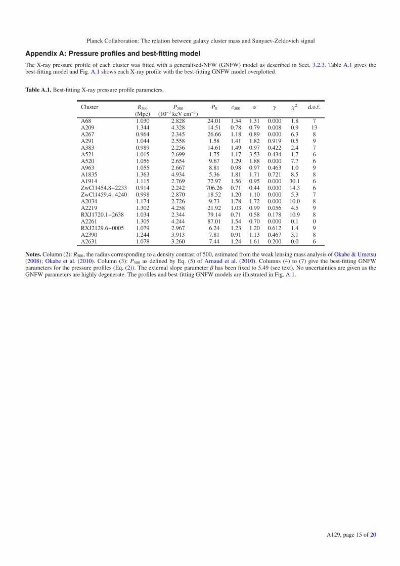
Planck Collaboration: The relation between galaxy cluster mass and Sunyaev-Zeldovich signal

Appendix A: Pressure profiles and best-fitting model

The X-ray pressure profile of each cluster was fitted with a generalised-NFW (GNFW) model as described in Sect. 3.2.3. Table A.1 gives thebest-fitting model and Fig. A.1 shows each X-ray profile with the best-fitting GNFW model overplotted.

Table A.1. Best-fitting X-ray pressure profile parameters.

Cluster R500 P500 P0 c500 α γ χ2 d.o.f.(Mpc) (10−3 keV cm−3)

A68 1.030 2.828 24.01 1.54 1.31 0.000 1.8 7A209 1.344 4.328 14.51 0.78 0.79 0.008 0.9 13A267 0.964 2.345 26.66 1.18 0.89 0.000 6.3 8A291 1.044 2.558 1.58 1.41 1.82 0.919 0.5 9A383 0.989 2.256 14.61 1.49 0.97 0.422 2.4 7A521 1.015 2.699 1.75 1.17 3.53 0.434 1.7 6A520 1.056 2.654 9.67 1.29 1.88 0.000 7.7 6A963 1.055 2.667 8.81 0.98 0.97 0.463 1.0 9A1835 1.363 4.934 5.36 1.81 1.71 0.721 8.5 8A1914 1.115 2.769 72.97 1.56 0.95 0.000 30.1 6ZwCl1454.8+2233 0.914 2.242 706.26 0.71 0.44 0.000 14.3 6ZwCl1459.4+4240 0.998 2.870 18.52 1.20 1.10 0.000 5.3 7A2034 1.174 2.726 9.73 1.78 1.72 0.000 10.0 8A2219 1.302 4.258 21.92 1.03 0.99 0.056 4.5 9RXJ1720.1+2638 1.034 2.344 79.14 0.71 0.58 0.178 10.9 8A2261 1.305 4.244 87.01 1.54 0.70 0.000 0.1 0RXJ2129.6+0005 1.079 2.967 6.24 1.23 1.20 0.612 1.4 9A2390 1.244 3.913 7.81 0.91 1.13 0.467 3.1 8A2631 1.078 3.260 7.44 1.24 1.61 0.200 0.0 6

Notes. Column (2): R500, the radius corresponding to a density contrast of 500, estimated from the weak lensing mass analysis of Okabe & Umetsu(2008); Okabe et al. (2010). Column (3): P500 as defined by Eq. (5) of Arnaud et al. (2010). Columns (4) to (7) give the best-fitting GNFWparameters for the pressure profiles (Eq. (2)). The external slope parameter β has been fixed to 5.49 (see text). No uncertainties are given as theGNFW parameters are highly degenerate. The profiles and best-fitting GNFW models are illustrated in Fig. A.1.

A129, page 15 of 20

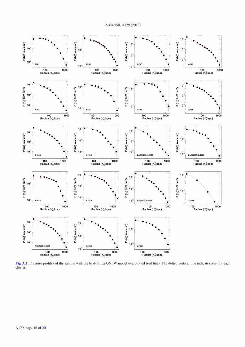
A&A 550, A129 (2013)

100 1000Radius (h70

-1 kpc)

10-3

10-2

P (

h701/

2 keV

cm

-3)

A68

100 1000Radius (h70

-1 kpc)

10-3

10-2

P (

h701/

2 keV

cm

-3)

A209

100 1000Radius (h70

-1 kpc)

10-4

10-3

10-2

P (

h701/

2 keV

cm

-3)

A267

100 1000Radius (h70

-1 kpc)

10-3

10-2

10-1

P (

h701/

2 keV

cm

-3)

A291

100 1000Radius (h70

-1 kpc)

10-3

10-2

10-1

P (

h701/

2 keV

cm

-3)

A383

100 1000Radius (h70

-1 kpc)

10-3

10-2

P (

h701/

2 keV

cm

-3)

A521

100 1000Radius (h70

-1 kpc)

10-3

10-2

P (

h701/

2 keV

cm

-3)

A520

100 1000Radius (h70

-1 kpc)

10-3

10-2

10-1

P (

h701/

2 keV

cm

-3)

A963

100 1000Radius (h70

-1 kpc)

10-3

10-2

10-1

P (

h701/

2 keV

cm

-3)

A1835

100 1000Radius (h70

-1 kpc)

10-3

10-2

10-1

P (

h701/

2 keV

cm

-3)

A1914

100 1000Radius (h70

-1 kpc)

10-3

10-2

10-1

P (

h701/

2 keV

cm

-3)

ZwCl1454.8+2233

100 1000Radius (h70

-1 kpc)

10-3

10-2

P (

h701/

2 keV

cm

-3)

ZwCl1459.4+4240

100 1000Radius (h70

-1 kpc)

10-3

10-2

P (

h701/

2 keV

cm

-3)

A2034

100 1000Radius (h70

-1 kpc)

10-3

10-2

10-1

P (

h701/

2 keV

cm

-3)

A2219

100 1000Radius (h70

-1 kpc)

10-3

10-2

10-1

P (

h701/

2 keV

cm

-3)

RXJ1720.1+2638

100 1000Radius (h70

-1 kpc)

10-2

10-1

P (

h701/

2 keV

cm

-3)

A2261

100 1000Radius (h70

-1 kpc)

10-3

10-2

10-1

P (

h701/

2 keV

cm

-3)

RXJ2129.6+0005

100 1000Radius (h70

-1 kpc)

10-3

10-2

10-1

P (

h701/

2 keV

cm

-3)

A2390

100 1000Radius (h70

-1 kpc)

10-3

10-2

P (

h701/

2 keV

cm

-3)

A2631

Fig. A.1. Pressure profiles of the sample with the best-fitting GNFW model overplotted (red line). The dotted vertical line indicates R500 for eachcluster.

A129, page 16 of 20

Planck Collaboration: The relation between galaxy cluster mass and Sunyaev-Zeldovich signal

Appendix B: Image gallery

Figure B.1 shows the 0.3–2 keV band X-ray image gallery of the cluster sample, arranged from top left to bottom right in order of themorphological characterisation parameter ne,0, the central density. Images are corrected for surface brightness dimming with z, divided by theemissivity in the energy band, taking into account galactic absorption and instrument response, and scaled according to the self-similar model.The colour table is the same for all clusters, so that the images would be identical if clusters obeyed strict self-similarity, and each panel is1.25 R500 on a side.

A1835 ZwCl1454.8+2233 A383 A291

RXJ2129.6+0005 RXJ1720.1+2638 A2390 A963

A2261 A1914 A68 A2219

A2631 A209 ZwCl1459.4+4240 A267

A2034 A520 A521

Fig. B.1. Image gallery.

A129, page 17 of 20

A&A 550, A129 (2013)

Appendix C: Scaled X-ray profiles

Figure C.1 shows the X-ray profiles of the sample. They have been radially scaled by the R500 determined from the M500−YX,500 relation ofPratt et al. (2010; see also Arnaud et al. 2010). Relaxed (or equivalently, cool core) systems are plotted in blue, disturbed systems in red, andintermediate objects in black. The gas density profiles are scaled by the expected self-similar evolution with redshift; the temperature profilesare scaled by the average spectroscopic temperature in the [0.15−0.75] R500 region; the pressure profiles are scaled by P500; the mass profilesare scaled by M500 (also estimated from the M500−YX,500 relation).

0.01 0.10 1.00R [R500

Yx ]

10-4

10-3

10-2

10-1

E(z

)-2 n

e [c

m-3]

0.01 0.10 1.00R [R500

Yx ]

1

T [

T [

0.15

-0.7

5] R

500]

0.01 0.10 1.00R [R500

Yx ]

10-1

100

101

102

P [

P50

0]

0.01 0.10 1.00R [R500

Yx ]

10-3

10-2

10-1

100

M [

M50

0]

Fig. C.1. X-ray profiles scaled by R500 from the M500−YX,500 relation of Arnaud et al. (2010). From left to right, top to bottom: gas density, gastemperature, gas pressure, integrated mass. Cool core systems are plotted in blue, morphologically disturbed objects in red, and intermediatesystems in black. The grey line in the pressure plot is the universal pressure profile of Arnaud et al. (2010).

A129, page 18 of 20

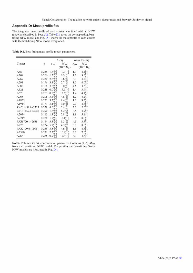
Planck Collaboration: The relation between galaxy cluster mass and Sunyaev-Zeldovich signal

Appendix D: Mass profile fits

The integrated mass profile of each cluster was fitted with an NFWmodel as described in Sect. 5.2. Table D.1 gives the corresponding best-fitting NFW model and Fig. D.1 shows the mass profile of each clusterwith the best-fitting NFW model overplotted.

Table D.1. Best-fitting mass profile model parameters.

X-ray Weak lensingCluster z c500 M500 c500 M500

(1014 M�) (1014 M�)

A68 0.255 1.8+0.2−0.2 10.0+1.2

−1.1 1.9 4.11.21.0

A209 0.206 1.5+0.3−0.2 6.3+0.7

−0.7 1.2 8.61.31.2

A267 0.230 2.8+0.3−0.3 3.6+0.3

−0.2 3.1 3.20.70.6

A291 0.196 3.4+0.3−0.3 2.7+0.3

−0.3 1.0 4.01.00.9

A383 0.188 3.8+0.4−0.4 3.0+0.3

−0.3 4.6 3.30.70.6

A521 0.248 0.0+0.0−0.0 17.9+2.6

−2.3 1.4 3.90.70.7

A520 0.203 0.5+0.2−0.2 12.6+2.7

−2.3 1.4 4.11.11.2

A963 0.206 3.1+0.4−0.4 4.8+0.6

−0.5 1.2 4.20.90.7

A1835 0.253 3.2+0.2−0.2 9.4+0.5

−0.5 1.6 9.51.71.5

A1914 0.171 3.4+0.3−0.3 9.0+0.8

−0.7 2.0 4.71.61.9

ZwCl1454.8+2233 0.258 4.6+0.3−0.3 3.4+0.3

−0.3 2.0 2.61.00.8

ZwCl1459.4+4240 0.290 1.8+0.3−0.3 6.2+1.0

−0.8 3.5 3.91.00.9

A2034 0.113 1.3+0.2−0.2 7.8+1.0

−0.9 1.8 5.12.12.4

A2219 0.228 1.7+0.2−0.2 12.1+1.5

−1.3 3.5 8.01.51.3

RXJ1720.1+2638 0.164 3.5+0.4−0.4 5.3+0.6

−0.6 4.5 3.71.10.9

A2261 0.224 5.7+1.3−1.3 4.3+0.8

−0.7 3.1 8.01.21.1

RXJ2129.6+0005 0.235 3.5+0.3−0.3 4.6+0.3

−0.3 1.6 4.61.11.0

A2390 0.231 2.2+0.3−0.3 10.8+1.5

−1.3 3.2 7.01.31.2

A2631 0.278 0.9+0.3−0.3 12.4+4.0

−3.0 4.1 4.80.70.7

Notes. Columns (3, 5): concentration parameter. Columns (4, 6) M500

from the best-fitting NFW model. The profiles and best-fitting X-rayNFW models are illustrated in Fig. D.1.

A129, page 19 of 20

A&A 550, A129 (2013)

100 1000Radius (h70

-1 kpc)

1011

1012

1013

1014

1015

Mas

(h

70-1 M

O •)

A68

100 1000Radius (h70

-1 kpc)

1012

1013

1014

1015

Mas

(h

70-1 M

O •)

A209

100 1000Radius (h70

-1 kpc)

1012

1013

1014

Mas

(h

70-1 M

O •)

A267

100 1000Radius (h70

-1 kpc)

1012

1013

1014

Mas

(h

70-1 M

O •)

A291

100 1000Radius (h70

-1 kpc)

1012

1013

1014

Mas

(h

70-1 M

O •)

A383

100 1000Radius (h70

-1 kpc)

1012

1013

1014

1015

Mas

(h

70-1 M

O •)

A521

100 1000Radius (h70

-1 kpc)

1012

1013

1014

1015

Mas

(h

70-1 M

O •)

A520

100 1000Radius (h70

-1 kpc)

1012

1013

1014

Mas

(h

70-1 M

O •)

A963

100 1000Radius (h70

-1 kpc)

1012

1013

1014

1015

Mas

(h

70-1 M

O •)

A1835

100 1000Radius (h70

-1 kpc)

1012

1013

1014

1015

Mas

(h

70-1 M

O •)

A1914

100 1000Radius (h70

-1 kpc)

1013

1014

Mas

(h

70-1 M

O •)

ZwCl1454.8+2233

100 1000Radius (h70

-1 kpc)

1012

1013

1014

Mas

(h

70-1 M

O •)

ZwCl1459.4+4240

100 1000Radius (h70

-1 kpc)

1012

1013

1014

Mas

(h

70-1 M

O •)

A2034

100 1000Radius (h70

-1 kpc)

1012

1013

1014

1015

Mas

(h

70-1 M

O •)

A2219

100 1000Radius (h70

-1 kpc)

1012

1013

1014

Mas

(h

70-1 M

O •)

RXJ1720.1+2638

100 1000Radius (h70

-1 kpc)

1013

1014M

as (

h70-1 M

O •)

A2261

100 1000Radius (h70

-1 kpc)

1012

1013

1014

Mas

(h

70-1 M

O •)

RXJ2129.6+0005

100 1000Radius (h70

-1 kpc)

1012

1013

1014

1015

Mas

(h

70-1 M

O •)

A2390

100 1000Radius (h70

-1 kpc)

1012

1013

1014

1015

Mas

(h

70-1 M

O •)

A2631

Fig. D.1. X-ray mass profiles of the sample with the best-fitting NFW model overplotted (red line). The dotted vertical line indicates R500 for eachcluster, determined from the best-fitting NFW model.

A129, page 20 of 20