18th Power Systems Computation Conference Wroclaw, Poland – August 18-22, 2014

A Branch-and-cut Method for Computing Load

Restoration Plan Considering Transmission Network and Discrete Load Increment

Zhijun Qin, Yunhe Hou The University of Hong Kong

Hong Kong, China zjqin@eee.hku.hk

yhhou@eee.hku.hk

Shanshan Liu Electric Power Research Institute

Palo Alto, USA sliu@epri.com

Jie Yan Ecomonic Study Group, MISO

Saint Paul, MN, USA jyan@misoenergy.org

Dahu Li Hubei Electric Power

Dispatching and Communication Center

Wuhan, China

Abstract—This paper proposes an optimization model to compute optimal load restoration plan for the transmission network. The objective of this model is to maximize the load pickup subject to power flow constraints and discrete load increment constraints. This mix-integer optimal power flow model (MIOPF) is solved via a branch-and-cut (B&C) framework. The nodes in the B&C tree are solved by the interior point method. In particular, three cutting planes, namely, the Gomory rounding cut, the knapsack cover cut, and the fixing variable cut, are incorporated into each node of the B&C tree to reduce the scale of the sub-tree. This model can be used to aid the system operators to conduct load restoration actions or draw up a restoration plan. The load restoration plan is obtained by solving a number of co-related MIOPF models till all load increments are restored. The RTS 24-bus test case with 170 load increments (i.e., with 170 binary variables) is used to illustrate complexity of the proposed model and the computational efficiency improvement stemming from the cutting planes.

Keywords— load restoration; optimal power flow; mix-integer nonlinear programing; branch-and-cut; cutting plane

I. INTRODUCTION Widespread blackouts and major outages over the world

serve as strong reminders of the social and economic impact from these failures of power grids. Fast recovery from the interrupted power service will considerably reduce such impact. The North American Electric Reliability Corporation (NERC) has consequently released series of standards [1-3] to enforce the reliability in the context of system restoration.

Although the standards and some general guidelines [4] are provided, the restoration operations are still highly stressful for system operators. After a major outage or blackout event, the system operators in the control center will conduct series of restorative control actions to restart generations, to re-establish transmission networks, and to pick up the interrupted loads, until the power gird recovers to a normal operation condition. This process is highly complicated involving a large number of components, rigorous and time-consuming switching actions, and covers a wide spectrum of technical problems [4]. In addition, the restoration plan prepared off-line may probably

not reflect the actual outage scenarios. The system operators need to identify available resources in time and conduct the restoration based on their experience. Therefore, the need for decision support tools to aid the restoration becomes increasingly vital.

The major difficulties in developing generic decision support tools originate from: 1) the complexity of the restoration process and, 2) the diversity of characteristics of power grids. To simplify the modeling of the entire restoration process, the restoration is divided into several typical stages. Each stage may have a particular concern and some associated mathematical models [5-7]. However, restoration plans of specific power grids still account for numerous particular features and are therefore more comprehensive than some typical stages.

To generalize the system restoration process and to provide comprehensive decision support tools, Electric Power Research Institute (EPRI) of USA has been conducting series closely-related research projects. The concept “Generic Restoration Milestone” (GRMs) has been proposed [8] as one of the achievements from these projects. With the extensible set of GRMs, the specific restoration plan can be defined as the combination of some certain milestones. The implementation of each milestone is achieved by solving configurable optimization models. This concept has actually been realized as a piece of software entitled “System Restoration Navigator” (SRN) as an EPRI’s product [9]. SRN has been released and successfully applied in some EPRI’s members.

The main functionality of SRN so far is to generate the optimal blackstart strategy by a bi-level optimization methodology [8]. In addition, the load restoration in distribution network has been well addressed [10, 11]. The objective of this paper is thus to propose a model and the associated solution method to maximize the interrupted load pickup for the transmission network, which is the main target of the GRM5 (i.e., serve loads in the area). The technical challenges to be addressed are threefold. Firstly, load restoration is a typical multi-stage problem. Secondly, according to NERC’s standard EOP-005 (R6.2.), the location and magnitude of load pickup should account for the voltage and frequency control for security purposes. This requirement implies the inclusion of accurate power flow equations. Thirdly, from the transmission system operators’ viewpoints, the load

This research is supported by National Natural Science Foundation ofChina (51277155), Electric Power Research Institute (EPRI, USA) andresearch Grant Council, Hong Kong SAR, under grant GRF712411and ECS739713.

18th Power Systems Computation Conference Wroclaw, Poland – August 18-22, 2014

demand of a given feeder (i.e., a load increment) from the load bus should be restored all or zero. These factors lead to a multi-stage mix-integer nonlinear programming problem.

The work of this paper is accordingly organized as follows. In section II, the methodology to compute a complete load restoration plan is described. The key point is to divide the load restoration process into a series of co-related steps. The connection of adjacent steps is established. A mix-integer optimal power flow model (MIOPF) is formulated to maximize load pickup for each step. In section III, the branch-and-cut (B&C) method is used to solve the MIOPF model. Three cutting plane methods (briefly as “cuts”), namely, the Gomory rounding cut, the knapsack cover cut, and the fixing variable cut are used in the enumeration of the B&C tree. The illustrative examples are presented in section IV using the RTS 24-bus system with 170 interrupted loads. This case illustrates the computational complexity of the MIOPF model and the dramatic efficiency improvement due to the incorporation of the above cuts.

II. COMOPUTING LOAD RESTORATION PLAN When carrying out load restoration for transmission

network, the system operators in the control center will identify available generation and transmission resources; determine which loads can be restored simultaneously. Then they will work with the field crew to restore some loads and schedule the power grid to a secure steady state by maintaining active and reactive power balance. These actions are repetitive till all loads are restored.

The load restoration is therefore regarded as a multi-step process. The connections between adjacent steps are twofold. Firstly, the total amount of load that can be restored in the current step is determined by the inertia of the synchronized generators due to the frequency security constraints. Secondly, the outputs of generators in the current step are restricted by the outputs of the previous step due to the generators operational constraints.

To assist the system operators to conduct load restoration, we propose a methodology to compute a complete load restoration plan. This methodology consists of the following sub-tasks. 1) Estimate generators operational bounds and the total amount of load pickup. 2) Build an optimization model to compute the maximum load pickup for each step. The optimal solution of this model presents the steady state after restoring the selected loads. 3) Estimate the duration of each step. These sub-tasks are described respectively as follows.

A. Estimation of generators’ operational bounds and total amount of load pickup As a bridge between adjacent steps, the general generator

model proposed in [8] is used to estimate the generators’ operational bounds. As shown in Fig. 1, for the ith generator,

iC is the generator’s capacity, iR is the startup requirement ( 0iR < ), ik is the average ramping rate, ia is the minimum output ratio, P.it is the remaining time for parallel operation.

For the step m, given the end time of the previous step 1mt − , the ith generator’s active power output of the previous step 1

G.m

iP − , and the estimated ramping time τ (set as 15 minutes throughout this paper), the upper bound of generators in the current step is determined as follows.

1 1G. P.

G. 1 1G. P.

, if min{ ( ) , },otherwise

m mm i i

i m mi i i i

P t tP

P t t k C

− −

− −

⎧ + ≤⎪= ⎨ + + −⎪⎩

ττ

(1)

The lower bound is determined as follows. 1 1

G. P.1 1 1

G. G. P. G.1 1

G. P.

, if , if and

max{ ( ) , },otherwise

m mi i

m m m mi i i i i i

m mi i i i i

P t tP P t t P a C

P t t k a C

ττ

τ

− −

− − −

− −

⎧ + ≤⎪= + > ≤⎨⎪ − + −⎩

(2)

P.itik

iCi ia C

iR

Fig. 1. Generic model of generators

To avoid large frequency derivation, the total amount of load pickup L

mP is restricted by the total synchronized generation in the previous step. In other words, L

mP is determined as:

G1 1

L P. G.1

( )( )N

m m mi i i

i

P U t t P Rρ − −

=

= − −∑ , (3)

where NG is the number of generators, ρ is the ratio of load pickup to the total synchronized generation, and ( )U x is a logic function defined as follows.

1 0( )

0 0x

U xx

≥⎧= ⎨ <⎩

(4)

B. MIOPF model to maximize load pickup The MIOPF model is proposed here to assist the system

operators to maximize the load pickup subject to various constraints. In step m, the optimization variables include: 1) generators’ active and reactive outputs G

mP , GmQ ; 2) the voltage

of all buses mV ; 3) the binary array mu representing the on-off state of the unserved load. This model is described as follows.

1) Objective function: The objective of each step is to pick up as many load increments as possible as follows:

TLmax ( )m mΔu P , (5)

where LmΔP is the array of unserved load increment in step m.

18th Power Systems Computation Conference Wroclaw, Poland – August 18-22, 2014

2) Power balance constraints: At the end of each step, a steady-state should be obtained with active power balance and reactive power balance. As a result, the power flow equations are included as equality constraints as follows:

G L L L

G L L L

ˆ ˆRe([ ] ) [ ]ˆ ˆIm([ ] ) [ ]

m m m m m m m m

m m m m m m m m

− − − Δ =

− − − Δ =

P P V Y V C P u

Q Q V Y V C Q u

0

0 , (6)

where mY is the admittance matrix of step m, L L,m mP Q are the arrays of restored load before step m, L L,m mΔ ΔP Q are the arrays of active and reactive demand of unserved load increments in step m, L

mC is the connection matrix of unserved load in step m, [ ]• is to convert an array to a diagonal matrix.

3) Operational constraints: The steady-state at the end of each step should meet with the operational constraints, i.e., the bound of generators, the voltage level, and the transmission constraints of energized branches, as follows:

G G G G G G G G

B B B

, ( ) ( )

,

m m m m m m

m m

≤ ≤ ≤ ≤

≤ ≤ ≤ ≤

P P P Q P Q Q P

V V V S S S , (7)

where G G,Q Q are the arrays of lower and upper bound of

generators’ reactive outputs, ,V V are the arrays of lower and upper bound of bus voltages, B B,S S are the arrays of lower

and upper bound of energized branches. BmS is the array of

apparent power of energized branches in step m. The elements of G

mP and GmP are calculated by (1)~(2). Note that the reactive

power bounds of generators may be dependent of active power bounds.

4) Frequency security constraints: During the 5~20 seconds after the re-closure of breakers to pick up unserved load increments, the generators will provide the frequency response. Hence the frequency will drop under the nominal value. To guarantee that the frequency drop will remain within the accepted level, the total amount of load pickup should not exceed a given threshold as follows:

TL L[ ]m m mPΔ ≤e P u , (8)

where e is the array of 1 with the appropriate size, LmP is

calculated by (3).

C. Estimiation of duration of each step In this paper, the duration of each step is primarily

estimated by the generators ramping rate and the difference of generators active outputs between adjacent steps. Assuming the adjustments of generators are carried out by system operators in parallel, the duration of step m is the maximum ramping time of generators as follows.

1 1P.i G. G. Gmax(max( ,0) / , )m m m m

i i it t t P P k i N− −Δ = − + − ∀ ≤ (9)

D. Procedure of the proposed methodology The procedure to compute the complete load restoration

plan is as follows.

Step 1) Identify the initial state of the power grid, including 0

GP , 0GQ , 0Y , P.it . Set t=0. Set m=1.

Step 2) Calculate GmP , G

mP , LmP by (1)~(3).

Step 3) Establish cranking path to load bus, close loops to reduce overload risk if necessary, update mY accordingly.

Step 4) Build the MIOPF model (5)~(8) and solve it for

GmP , G

mQ , mu , mV .

Step 5) Calculate mtΔ by (9).

Step 6) Set t=t+ mtΔ , P. P.m

i it t t= − Δ . Set P. 0it = if P.it is negative.

Step 7) If all load increments are restored, stop; otherwise set m=m+1, and go to Step 2).

III. BRANCH-AND-CUT ALGORITHM The major computational burden to compute the complete

load restoration plan lies in the solution of a number of MIOPF models. Hence the efficient algorithms need to be identified to obtain this plan within a reasonable CPU time.

In this section, the branch-and-cut (B&C) method is used to solve the MIOPF model motivated by two considerations. 1) The B&C algorithm relies mainly on the solution of the relaxed OPF model, i.e., with continuous dispatchable load model. The solution of this relaxed optimal power flow (OPF) model can be obtained with a wide spectrum of efficient solvers on hand. 2) B&C algorithms are quite efficient in mix-integer linear programming model. Intuitively, it can be used to solve MIOPF model since this model has a separate nonlinear part and the binary part (see constraints in (6) and (8)).

A. Branch-and-cut framework The branch-and-cut method is based on the branch-and-

bound (B&B) framework proposed by Land and Diog [12]. The basic idea is to solve the continuous-relaxation of a given integer programming model (called “root node”) and to branch on one selected integer variable (if it is non-integer in the optimal of the root node). Consequently, the feasible set of the root node is cut and two sub-problems are created for further exploration. For a maximization model, a relaxation model will provide an upper bound (U) for the objective function. The branching process can be carried for each node until:

(1) The node is integer-feasible. Hence a lower bound (L) for the objective function is found. Update L if bigger (better) lower bound is found.

(2) The node is infeasible and not necessary for further branching.

(3) The node generates an objective value less (worst) than the current value of L.

18th Power Systems Computation Conference Wroclaw, Poland – August 18-22, 2014

(4) From the practical viewpoint, this process can be stopped when a satisfactory optimal solution is found as /L U U ε− ≤ , where ε is the termination criterion,

and /L U U− is known as gap .

The B&C method is the extension of B&B by using cutting planes. The cutting planes are incorporated in the B&B method to achieve tighten bound hence cut down the number of nodes in the tree significantly. The cutting planes also help to preprocess the node and impose some heuristics as well [13].

The pseudo code (with a deep-first recursive mode) of the B&C method used to solve MIOPF is shown in Fig. 2.

iu

1iu =0iu =

Fig. 2. Branch-and-cut method to solve MIOPF

B. Incororation of cutting planes The following cutting plane methods are incorporated to

improve the efficiency of enumeration of the B&B tree.

1) Gomory rounding cut

This valid cut of (8) is generated as:

TL L

L Lmin( ) min( )

m mm

m m

P⎢ ⎥ ⎢ ⎥Δ≤⎢ ⎥ ⎢ ⎥Δ Δ⎢ ⎥ ⎣ ⎦⎣ ⎦

P uP P

, (10)

where •⎢ ⎥⎣ ⎦ is the biggest integer less than the input argument.

2) Knapsack cover cut

The first step to generate knapsack cover cut of (8) is to

find one (or more) set C N⊆ such that L. Lm mi

j C

P P∈

Δ >∑ .Then the

knapsack cover cut is: 1ij C

u C∈

< −∑ , where C is the number

of elements in C .

The derivation of the above cuts can be referred to [13].

3) Fixing variable cut

Fixing variables is one of the pre-solve technique that reduce the number of integer variables. Intuitively, after branching on iu , if the model becomes apparently infeasible on setting some other ju to one, ju will be fixed as zero from the node and its descendants. On a broad sense, fixing variables is also adding cuts to the model.

These cuts are generated as the branching process proceeds. Take 1 2 3 4 5 63.5 2.5 4.2 12 3.6 7.0 10u u u u u u+ + + + + ≤ for an example. Assume branching on 1u and 1 1u = . Accordingly it becomes 2 3 4 5 62.5 4.2 12 3.6 7.0 6.5u u u u u+ + + + ≤ . It further becomes 2 3 52.5 4.2 3.6 6.5u u u+ + ≤ by fixing 4 60, 0u u= = for feasibility. Then the Gomory rounding cut is generated by dividing this inequality by 2.5 and rounding as

2 3 51 1 1 2u u u+ + ≤ . Similarly, when 1 0u = , this inequality becomes 2 3 4 5 62.5 4.2 12 3.6 7.0 10u u u u u+ + + + ≤ . Similarly by fixing 4 0u = , it becomes 2 3 5 62.5 4.2 3.6 7.0 10u u u u+ + + ≤ . Besides the Gomory rounding cut, the knapsack cuts with this node can be derived as a group of inequalities as follows:

2 3 5 3 5 7 5 72, 2, 1u u u u u u u u+ + ≤ + + ≤ + ≤ .

C. Selection of branching strategy The branching strategy, i.e., selecting which variable to

branch, is another key point affecting the scale of the enumeration tree. There are some widely-used general-purpose branching strategies, such as maximum fractional branching, pseudo-cost branching, strong branching, etc (see for example [14]). The following two branching strategies are used in this paper for comparison, as these two strategies are easy to calculate.

1) Maximum fractional branching

This branching strategy selects the most closed to 0.5 among those relaxed integer variable. Or mathematically select the variable by:

{ }ˆ ˆmax min(1 , )i iiu u− , (11)

where ˆiu belongs to the optimal solution of the parent nodes.

2) Pseudo-cost branching

This branching strategy branches on the variable that changes the objective function most. For the MIOPF in this paper, the branching variable is selected by:

{ }L. L.ˆ ˆmax min( (1 ), )m mi i i ii

P u P uΔ − Δ . (12)

The effect of maximum fractional branching and pseudo-cost branching on efficiency improvement will be investigated thought case studies in the section IV.

IV. CASE STUDIES In this section, the RTS 24-bus test system is used to

demonstrate the proposed methods. The case studies include the following parts. 1) Present a complete load plan using the proposed methodology. 2) Demonstrate the large computational complexity due to the combination nature of the MIOPF model. Illustrate the efficiency improvement arising from the cuts described in section III. 3) Illustrate the effect of termination criterion ε on reducing overall computational complexity.

The simulation is carried out on a personal computer with 3.4GHZ i7 processor and 6GB RAM. The B&C framework

18th Power Systems Computation Conference Wroclaw, Poland – August 18-22, 2014

and the interior point method for the optimal power flow (OPF) are implemented in MATLAB 2013a.

A. Computational settings The RTS 24-bus system includes 24 buses (10 generation

buses, 17 load buses), 29 transmission lines, 5 transformers, 1 reactor and 1 synchronous condenser. The generating units on the same bus are modelled as one equivalent generator. The equivalent hydro generator on bus 22 severs as the blackstart resource. The other generators are treated as non-blackstart generators. The detailed system data, including the MVA ratings of all branches, are as in [15]. The blackstart strategy is obtained by SRN with the algorithm proposed in [8]. The initial state of the load restoration is based on the end state of blackstart phase, as shown in Table 1, Table 2, Table 3, and Fig. 3.

Assume that the load in each load consists of 10 identical load increments. The target of the load restoration stage is to restore these 170 load increments given the initial state. The voltages of all buses are restricted between 0.90~1.05 p.u. during load restoration process. Set 5%ρ = ( see discussion in [10], [11]).

18 21 22

17

16 19 20

23

13

15

24 11 12

14

3 9 10

1 2 7

4

5

6

8

GeneratorLoad

EnergizedDeenergized

Transformer

Fig. 3. Energized components in the initial state

TABLE I. CHARACTERISTICS OF GENERATORS

Bus Capacity (p.u.)

Start Requirement

(p.u.)

MVar Limit (p.u.)

Ramping Rate

(p.u./hour) 22 3.00 0.00+j0.00 -0.60~0.96 3.0 18 4.00 0.28+j0.21 -0.50~2.00 1.5 16 1.55 0.12+j0.09 -0.50~0.80 1.0 1 1.92 0.15+j0.11 -0.50~0.80 1.0 2 1.92 0.15+j0.11 -0.50~0.80 1.0

15 2.15 0.17+j0.13 -0.50~1.10 1.0 13 5.91 0.25+j0.19 0.00~2.40 1.5 21 4.00 0.28+j0.21 -0.50~2.00 1.0 7 3.00 0.30+j0.23 0.00~1.80 1.0

23 6.60 0.50+j0.38 -1.25~3.10 1.5

TABLE II. INITIAL STATES OF GENERATORS

Bus Time to Parallel

(minutes)

Minimum output

Initial Active (p.u.)

Initial Reactive

(p.u.) 22 0 0% 1.020 0.108 18 0 30% 0.349 -0.116 16 0 50% 0.270 0.184 1 0 50% 0.063 0.087 2 10 50% -0.150 -0.110

15 14 50% -0.170 -0.130 13 29 60% -0.250 -0.190 21 14 30% -0.280 -0.210 7 51 50% -0.300 -0.225

23 80 50% -0.500 -0.380

TABLE III. ENERGIZED BRANCHES OF INITIAL STATE

From Bus To Bus From Bus To Bus 1 3 15 16 2 4 15 24 3 9 16 17 4 9 17 18 7 8 17 22 8 9 18 21

11 13 3 24 11 14 14 16 13 23

TABLE IV. COMPUTATIONAL COMPLEXITY OF RESTORATION PLAN

Step t (mins.)

Nodes in tree Step t

(mins.) Nodes in

tree 1 21.3 3 30 161.7 233 2 38.5 3 31 166.3 233 3 54.0 3 32 171.3 851 4 55.3 3 33 175.7 5 5 56.6 3 34 181.3 1353 6 58.2 3 35 186.7 10137 7 58.9 85 36 192.8 529 8 63.9 71 37 199.3 1727 9 82.4 71 38 206.5 5

10 86.5 71 39 213.7 59 11 87.7 3 40 221.1 5961 12 89.9 123 41 229.0 2411 13 92.7 121 42 237.9 31 14 95.3 103 43 246.6 17 15 97.3 667 44 255.3 249 16 99.1 83 45 264.3 73 17 101.3 83 46 273.2 3703 18 103.9 61 47 282.4 121 19 107.1 581 48 291.7 27349 20 112.0 83 49 299.4 35 21 117.5 1385 50 308.0 923 22 123.7 1401 51 319.2 755 23 127.9 1189 52 331.6 11473 24 132.5 1547 53 344.0 1 25 137.3 465 54 359.0 17 26 143.2 45 55 373.7 15 27 147.8 915 56 388.7 15 28 152.8 2677 57 403.7 1 29 157.8 2467

B. Complete load restoration plan Set 1%ε = . To simplify the case study, the reactive

bounds of generators are set as the 4th column of Table 1.

The complete load restoration plan is obtained by step-by-step computation. This plan includes 57 steps. Each step picks

18th Power Systems Computation Conference Wroclaw, Poland – August 18-22, 2014

up several load increments subject to constraints (6)~(9). The load restoration curves of load buses are shown in Fig. 4. The computational complexities of each step are listed in Table 4. The total duration of load restoration process is 403.7 minutes.

(a)

(b)

Fig. 4. Load pickup in each bus by setting 1%ε = .(a) Bus 1~9. (b) Bus 10,13~16,18~20.

TABLE V. NETWORK OPERATION WITHIN STEPS

Step Actions Reason

11 Energize path 1-2 Close loop

15 Energize path 9-11 Close loop

42 Energize path 9-12-13 Close loop

47 Energize path 8-10-12 Close loop

51 Energize path 2-6-10, put the synchronous condenser on Energize load bus

52 Energize path 1-5-10 Energize load bus

53 Energize path 12-23,10-11 Close loop

54 Energize path 16-19-20-13 Energize load bus

Not all transmission network is restored before load restoration. Particularly in this case, the initial state of transmission network (see Table 3) is a tree. Hence network operations should be conducted during load restoration. The network operations before load pickup actions are listed in Table 5. The main reasons to conduct these operations are: 1) close loop to reduce the risk of overload; 2) establish cranking path to un-energized load.

Note that in step 51, the synchronous condenser is put back on operation. This condenser is treated as an adjustable reactive source in the following steps. The secure dispatch of network operations could be conducted with the aid of some optimization models (see [16] for example). This issue is not the emphasis of this paper, and is thus not covered here.

C. Efficiency improvments by cutting planes Observation on Table 4 shows that, to obtain the complete

load restoration plan, 82,597 OPF sub-problems are solved. The CPU time for this task is around 6,743 seconds.

If the cuts are not incorporated, the computational complexity will be even larger. Take the first step as an example. As shown in Table 6, the cuts play an important part in reducing the number of nodes in the B&C tree. In the early steps of load restoration, fixing variable cut is the most efficient, since the total synchronized generation is limited. In the later steps, fixing variable cut becomes less effective, while the Gomory rounding cut and knapsack cover cut becomes more effective.

TABLE VI. COMPUTATIONAL COMPLEXITY OF STEP 1

Solution Strategy Number of Nodes in B&C tree

No cuts + maximum fractional branching 5,897

No cuts + Pseudo-cost branching 4,391

Gomory rounding cut, knapsack cover cut + Pseudo-cost branching 349

Fixing variable cut + Pseudo-cost branching 3

D. Controlling computation complexity of B&C tree Although the computational complexity has been

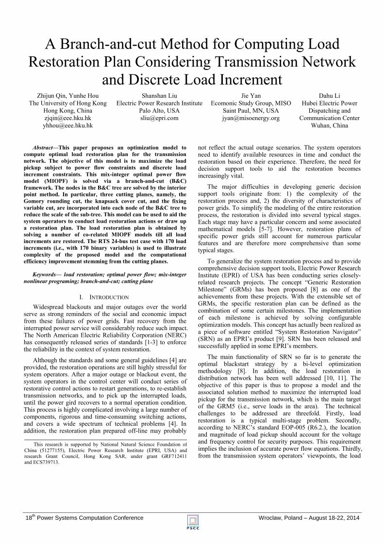
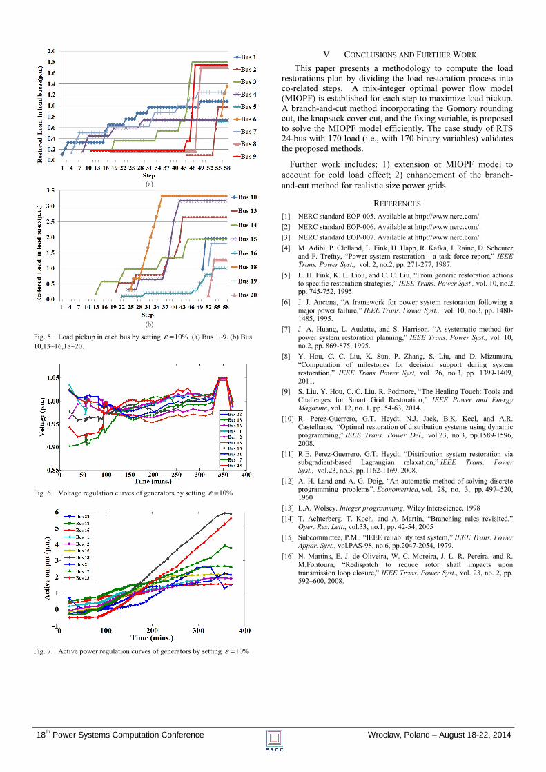
considerably reduced by incorporating cutting planes, the overall efficiency is not satisfactory. On the bright side, the scale B&C tree is controllable by relaxing the termination criterion. The simulation is carried on again by setting 10%ε = . This obtained load restoration plan includes 58 steps. The load restoration duration is 370 minutes. The number of nodes in B&C tree drops to 2340, which is around 2.8% of that by setting 1%ε = . The load restoration curves of load buses are shown in Fig. 5. To maintain the power balance of all buses, the terminal voltages and active power of generators are regulated, as shown in Fig.6 and Fig. 7, respectively.

This load restoration plan, compared to that by setting 1%ε = , has a shorter duration, although with more steps. Such

a result shows that the optimality of each step is not necessary for the optimality of the entire load restoration process.

18th Power Systems Computation Conference Wroclaw, Poland – August 18-22, 2014

(a)

(b)

Fig. 5. Load pickup in each bus by setting 10%ε = .(a) Bus 1~9. (b) Bus 10,13~16,18~20.

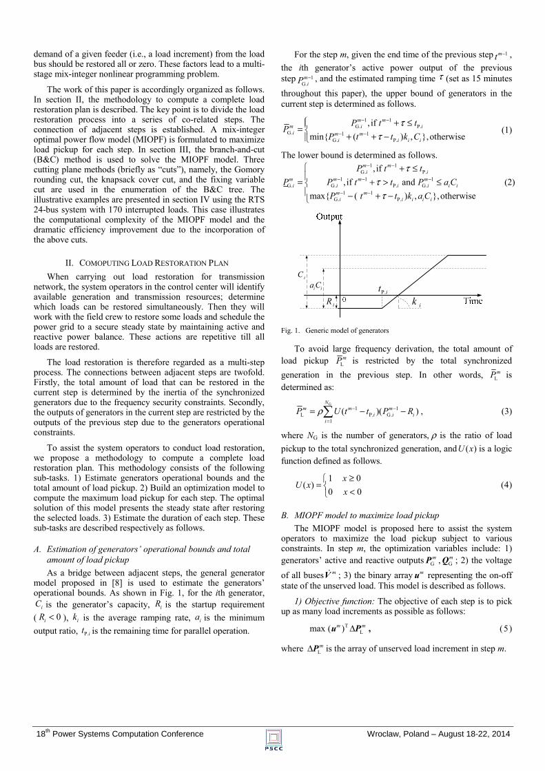
Fig. 6. Voltage regulation curves of generators by setting 10%ε =

V. CONCLUSIONS AND FURTHER WORK This paper presents a methodology to compute the load

restorations plan by dividing the load restoration process into co-related steps. A mix-integer optimal power flow model (MIOPF) is established for each step to maximize load pickup. A branch-and-cut method incorporating the Gomory rounding cut, the knapsack cover cut, and the fixing variable, is proposed to solve the MIOPF model efficiently. The case study of RTS 24-bus with 170 load (i.e., with 170 binary variables) validates the proposed methods.

Further work includes: 1) extension of MIOPF model to account for cold load effect; 2) enhancement of the branch-and-cut method for realistic size power grids.

REFERENCES [1] NERC standard EOP-005. Available at http://www.nerc.com/. [2] NERC standard EOP-006. Available at http://www.nerc.com/. [3] NERC standard EOP-007. Available at http://www.nerc.com/. [4] M. Adibi, P. Clelland, L. Fink, H. Happ, R. Kafka, J. Raine, D. Scheurer,

and F. Trefny, “Power system restoration - a task force report,” IEEE Trans. Power Syst., vol. 2, no.2, pp. 271-277, 1987.

[5] L. H. Fink, K. L. Liou, and C. C. Liu, “From generic restoration actions to specific restoration strategies,” IEEE Trans. Power Syst., vol. 10, no.2, pp. 745-752, 1995.

[6] J. J. Ancona, “A framework for power system restoration following a major power failure,” IEEE Trans. Power Syst., vol. 10, no.3, pp. 1480-1485, 1995.

[7] J. A. Huang, L. Audette, and S. Harrison, “A systematic method for power system restoration planning,” IEEE Trans. Power Syst., vol. 10, no.2, pp. 869-875, 1995.

[8] Y. Hou, C. C. Liu, K. Sun, P. Zhang, S. Liu, and D. Mizumura, “Computation of milestones for decision support during system restoration,” IEEE Trans Power Syst, vol. 26, no.3, pp. 1399-1409, 2011.

[9] S. Liu, Y. Hou, C. C. Liu, R. Podmore, “The Healing Touch: Tools and Challenges for Smart Grid Restoration,” IEEE Power and Energy Magazine, vol. 12, no. 1, pp. 54-63, 2014.

[10] R. Perez-Guerrero, G.T. Heydt, N.J. Jack, B.K. Keel, and A.R. Castelhano, “Optimal restoration of distribution systems using dynamic programming,” IEEE Trans. Power Del., vol.23, no.3, pp.1589-1596, 2008.

[11] R.E. Perez-Guerrero, G.T. Heydt, “Distribution system restoration via subgradient-based Lagrangian relaxation,” IEEE Trans. Power Syst., vol.23, no.3, pp.1162-1169, 2008.

[12] A. H. Land and A. G. Doig, “An automatic method of solving discrete programming problems”. Econometrica, vol. 28, no. 3, pp. 497–520, 1960

[13] L.A. Wolsey. Integer programming. Wiley Interscience, 1998 [14] T. Achterberg, T. Koch, and A. Martin, “Branching rules revisited,”

Oper. Res. Lett., vol.33, no.1, pp. 42-54, 2005 [15] Subcommittee, P.M., “IEEE reliability test system,” IEEE Trans. Power

Appar. Syst., vol.PAS-98, no.6, pp.2047-2054, 1979. [16] N. Martins, E. J. de Oliveira, W. C. Moreira, J. L. R. Pereira, and R.

M.Fontoura, “Redispatch to reduce rotor shaft impacts upon transmission loop closure,” IEEE Trans. Power Syst., vol. 23, no. 2, pp. 592–600, 2008.

Fig. 7. Active power regulation curves of generators by setting 10%ε =