Electronic Load - Metrohm Autolab

Autolab/ Electronic Load

Installation Description

Picture Courtesy of Nedstack Fuel Cell Technology BV

Autolab/Electronic load combination

2 | P a g e


The Autolab range of instruments is limited in terms of maximum current or power that can be supplied to or extracted from an electrochemical cell. When working with high power energy storage or energy conversion devices, the power requirements can often exceed those available with a normal Autolab PGSTAT, even when it is extended with a Booster 10A or 20A.

To meet these experimental requirements, the Autolab can be easily combined with a third-party programmable electronic load.

Modern electronic loads are capable of reaching over 100 A easily. This combination therefore extends the measurable range of the Autolab by decades of current or more.

When the Autolab is combined with an electronic load, the load will sink the current while the Autolab will measure the voltage across the electrochemical cell. The combination of the Autolab and the electronic load requires the dedicated DYNLOAD interface (Article code: LOAD.INT).

Using the DYNLOAD interface, several types of measurements are possible:

• DC measurements at high current densities (up to the maximum current allowed by the load).

• Electrochemical impedance spectroscopy measurements at high current density (up to the maximum current allowed by the load).

Most electronic loads can be controlled in four operation modes:

• Constant current (CC) mode1: current is drawn from the cell until the specified current value is reached.

• Constance voltage (CV) mode: current is drawn from the cell until the cell voltage reaches a specified value.

1 This installation note only covers this operation mode. Please contact Metrohm Autolab for more information on the other modes ([email protected]).

Note

It is also possible to combine the Autolab with a programmable power supply. In this case, the power supply will be used to source high currents to the cell and the Autolab is used to control the voltage across the cell. The use of a programmable power supply is not specifically covered in this manual. More information can be obtained by contacting Metrohm Autolab ([email protected]).

mailto:[email protected]




3 | P a g e

• Constant power (CP) mode: current is drawn from the cell until the output power reaches a specified value.

• Constant resistance (CR) mode: current is drawn from the cell until the resistance to the current flow reaches the specified value.

The constant current (CC) mode is the most suitable for the combination with the Autolab, however the other modes are also available but these modes are affected by ohmic losses and are therefore not accurate.

Warning

When the Autolab is combined with an electronic load, the Autolab will only be used to control the load and measure the cell voltage. The specifications of the Autolab are therefore irrelevant for this application and only the specifications of the electronic load must be selected carefully (see Section 1). The Autolab PGSTAT204/FRA32M is suitable for all the measurements described in this manual.


4 | P a g e

Table of Contents

1 – Choice of the electronic load ....................................................................... 5 2 – Dynload interface part list ........................................................................... 6 3 – Autolab part list .......................................................................................... 8 4 – Electronic load part list ................................................................................ 9 5 – Polarity convention .................................................................................... 10 6 – Connections to the Dynload interface ....................................................... 10

6.1 – Connections without a FRA module .................................................. 10 6.2 – Connections with a FRA32M module ................................................ 12 6.3 – Connections with a FRA2 module ...................................................... 13

7 – Connections to the cell .............................................................................. 14 7.1 – Connections for cell voltages ≤ 10 V ................................................. 14 7.2 – Connections for cell voltages > 10 V ................................................. 15

7.2.1 – Voltage multiplier part list .......................................................... 15 7.2.2 – Connections to the instrument ................................................... 16

8 – Electronic load settings .............................................................................. 17 8.1 – Programming the load (TDI) .............................................................. 18 8.2 – Programming the load (Kikusui) ........................................................ 19 8.3 – Controlling the electronic load .......................................................... 20

8.3.1 – Controlling the electronic load (TDI) ........................................... 20 8.3.2 – Controlling the electronic load (Kikusui) ..................................... 20

9 – NOVA hardware setup .............................................................................. 21 9.1 – Analog input settings ........................................................................ 22 9.2 – Analog output settings ...................................................................... 23

10 – Manual control of the electronic load (DC only) ....................................... 24 11 – Procedure control of the electronic load (DC only) ................................... 27 12 – Recording the output from the electronic load (DC only) ......................... 30 13 – Impedance spectroscopy measurements ................................................. 33

13.1 – External settings .............................................................................. 35 13.1.1 – Settings for V ...................................................................... 35 13.1.2 – Settings for X ...................................................................... 36 13.1.3 – Settings for Y ...................................................................... 36 13.1.4 – Settings for Transfer function ................................................... 37

13.2 – Frequency scan settings .................................................................. 38 13.3 – Sampler settings .............................................................................. 39 13.4 – Plots settings ................................................................................... 41 13.5 – Running a measurement ................................................................. 42

14 – Measurement examples .......................................................................... 44 14.1 – iV/Power curve ................................................................................ 44

14.1.1 – Running the measurement ....................................................... 44 14.2 – Impedance spectroscopy measurement ........................................... 45

Appendix 1 – Specifications of known electronic loads ................................... 48 Appendix 2 – Modification of the FRA2 module .............................................. 49


5 | P a g e

1 – Choice of the electronic load

The electronic load is a critical component of this hardware setup and it should be chosen carefully. Some electronic loads are more suitable for working with a low power energy storage device, while other electronic loads are adapted to very large power output systems.

Many commercially available electronic loads can be used in combination with the Autolab PGSTAT. However, in order to operate in combination with the PGSTAT, the electronic load must fulfil the following requirements:

• Analog external programming to control the setpoint (0-10 V range) • Analog external current monitor for current readout (0-10 V range)

A list of compatible electronic loads can be found in Table 1.

Load Application Bandwidth

Kikusui PLZ164WA Single cells 100 kHz

Kikusui PLZ664WA Single cells, small stacks 100 kHz

TDI RBL 488 Medium stacks 20 kHz

TDI WCL 488 Large stacks 1 kHz

Agilent 6060B Single cells, small stacks 20 kHz

Agilent 3300 Single cells, small stacks 20 kHz

Chroma 6300 Medium stacks 20 kHz

Table 1 – Overview of compatible electronic loads

For small energy storage devices, a low power electronic load is sufficient. For larger devices, more powerful electronic loads are required. Some electronic loads require active cooling for power dissipation.

As a rule, it is not possible to have the following specifications at the same time:

• Full current output even at 0 V cell voltage • High bandwidth (> 1 kHz) • High power

Small electronic loads like the Kikusui PLZ164WA have very high bandwidth ratings and can operate at maximum current even if the cell voltage is 0 V. The maximum power of these loads is however limited, which means that these instruments are suitable for small single cell systems. On the other hand, larger loads like the TDI RBL 488 have high maximum power and sufficient bandwidth, but they require a minimum cell voltage to operate at full power (for example, the TDI RBL 488 requires 3 V DC voltage to operate at 300 A, as shown in Figure 1). These systems are therefore more suitable for large stacked cells.


6 | P a g e

Figure 1 – Contour map of the TDI RBL 488

2 – Dynload interface part list

The Dynload interface kit includes the following items:

1. The Dynload interface (see Figure 2). 2. 15 V power supply 3. A 2 m long BNC cable 4. A 50 Ω terminator plug 5. 6 BNC to SMB adaptor plugs 6. 3 SMB shielded cables (1 m) 7. A BNC splitter

Note

A special Dynload interface version suitable for the Electronic loads supplied by the Japanese brand Kikusui is available on request (see Figure 2). This version is only suitable for the Kikusui loads.


7 | P a g e

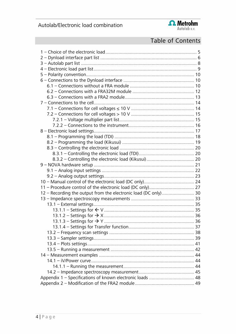
Figure 2 – Two versions of the Dynload interface (left – general purpose interface, right – for Kikusui electronic loads)

The three SMB shielded cables can be fitted with SMB to BNC adaptor plugs. Depending on the type of FRA module used in combination with the LED Driver, these cables can be modified accordingly:

• For the FRA2 module, the cables must be fitted with SMB to BNC adaptors on both ends (see Figure 3).

Figure 3 – Configuration of the SMB cables used in combination with the FRA2 module

• For the FRA32M module, the cables must be fitted with SMB to BNC adaptors on a single end (see Figure 4).

DYNAMIC LOAD

External prog.DAC-1

DSG

Y-FRA/ADC

I-M

15 V+-

To back panel of electronic loadDYNAMIC LOAD

DAC-1

DSG

Y-FRA/ADC

Dynamic load

15 V+-

Dynload FRA Y

Dynl DSG FRA V

E-out FRA X


8 | P a g e

Figure 4 - Configuration of the SMB cables used in combination with the FRA32M module

3 – Autolab part list

The Autolab PGSTAT is used as a voltmeter in combination with the electronic load. This means that the WE and CE connectors provided by the Autolab must not be connected to the cell.

The monitor cable is required for the combination with the electronic load and it must be attached to the front panel of the PGSTAT (see Figure 5).

Dynload FRA Y

Dynl DSG FRA V

E-out FRA X

Warning

Never connect the WE/CE connectors of the Autolab to the electrochemical cell when working in combination with an electronic load. High currents can damage the Autolab!

Note

The monitor cable for the PGSTAT204 is not supplied with the instrument and it must be ordered separately. Please contact [email protected] for more information.



9 | P a g e

Figure 5 – Monitor cable for the PGSTAT204 (above) and the Series 8 PGSTAT128N/302N (below)

4 – Electronic load part list

The electronic load must be connected to the electrochemical cell using cell cables suitable for the expected power drawn from the cell. It is recommended to use thick cables with very low resistivity to avoid ohmic losses.

Additionally, the cables required to connect the Dynload interface to the programming port of the electronic load must be sourced by the end user. The type of cables required depends on the type of electronic load. The connections to the Dynload interface must be BNC.

PGSTAT204

PGSTAT128N/302N

Note

Please refer to the user manual of the electronic load for more information on the connection requirements or contact Metrohm Autolab ([email protected]) for assistance.




10 | P a g e

5 – Polarity convention

The NOVA software, used to control the Autolab and the electronic load connected to it, uses the IUPAC convention for potential and current polarity. Charging (or anodic) currents are indicated with a positive sign. Discharging (or cathodic) currents are indicated with a negative sign.

For this application, working with an electronic load to discharge energy storage or conversion devices, cell voltages will be positive and discharge currents will be negative.

The software can be adjusted to account for this polarity convention.

6 – Connections to the Dynload interface

This section describes the connections required to perform the measurements with the Autolab in combination with an electronic load. The connections depend on the instrument type and configuration. In the rest of this document, an N series Autolab instrument is used, however other instrumental configurations are possible.

6.1 – Connections without a FRA module

If no FRA module is present in the instrument (FRA2 or FRA32M), the connections between the Autolab and the Dynload interface should be as described in Figure 6.

Note

The current indicated on the front panel of the electronic load will be positive.


11 | P a g e

Figure 6 – Connections overview without FRA module

1. Connect the DAC164 output one on the front panel of the Autolab (DAC164 1) to the DAC-1 input of the Dynload interface.

2. Connect the Y-FRA/ADC output of the Dynload interface to the ADC164 input one on the front panel of the Autolab (ADC164 1).

3. The DSG input of the Dynload interface must be shorted with the provided 50 Ohm termination plug (see Figure 7).

Figure 7 – A 50 ohm terminator plug must be used to short the DSG input when this input is not used

DYNAMIC LOAD

External prog.DAC-1

DSG

Y-FRA/ADC

I-M

15 V+-

50 Ω

Note

Make sure that the 50 Ohm plug is connected to the DSG input at all times!


12 | P a g e

6.2 – Connections with a FRA32M module

If a FRA32M module is present in the instrument, the connections between the Autolab and the Dynload interface should be as described in Figure 8.

Figure 8 - Connections with the FRA32M module


2. Connect the Y-FRA/ADC output of the Dynload interface to the ADC164 input one on the front panel of the Autolab (ADC164 1) and using the provided BNC splitter, connect the same signal to the FRA32M Y input.

3. Connect the Eout signal, provided by the monitor cable to the FRA32M X input.

4. Connect the FRA32M V output to the DSG input on the Dynload interface.

DYNAMIC LOAD

External prog.DAC-1

DSG

Y-FRA/ADC

I-M

15 V+-

Eout

Iout

Ein

Note

For the PGSTAT204, use the Vout and Vin provided by the monitor cable instead of DAC164 1 and ADC164 1, respectively.


13 | P a g e

6.3 – Connections with a FRA2 module

If a FRA2 module is present in the instrument, the connections between the Autolab and the Dynload interface should be as described in Figure 9.

Figure 9 – Connections with the FRA2 module


2. Connect the Y-FRA/ADC output of the Dynload interface to the ADC164 input one on the front panel of the Autolab (ADC164 1) and using the provided BNC splitter, connect the same signal to the FRA2 Y input.

3. Connect the Eout signal, provided by the monitor cable to the FRA2 X input.

4. Connect the FRA2 V output to the DSG input on the Dynload interface.

DYNAMIC LOAD

External prog.DAC-1

DSG

Y-FRA/ADC

I-M

15 V+-

Eout

Iout

Ein

Note

For the PGSTAT204, use the Vout and Vin provided by the monitor cable instead of DAC164 1 and ADC164 1, respectively.


14 | P a g e

7 – Connections to the cell

The electronic load (+) is connected to the (+ or cathode) of the cell, and the electronic load (-) is connected to the (- or anode) of the cell.

7.1 – Connections for cell voltages ≤ 10 V

The S and RE cables of the Autolab differential amplifier are connected to the cell under study. The S is connected to the (+) and the RE connected to the (-). The CE and WE connections of the PGSTAT are not used.

Warning

Analog programming of the electronic load requires a modification of the FRA2 module to accept analog signal up to 10 V. A hardware and software modification may be required. More information is provided in the Appendix 2. Please contact Metrohm Autolab ([email protected]) or your local distributor in case of any doubts.

∆𝐸𝐿𝑂𝐴𝐷 = ∆𝐸𝐴𝑈𝑇 − 𝑖𝑅

Warning

The cables connecting the electronic load to the cell must have the lowest possible resistance and should be able to withstand high current densities. Keep in mind that ohmic losses cannot completely be avoided. Most electronic loads have a voltage reversal detection circuit which monitors the cell voltage and shuts down the load when this value becomes negative or lower than a threshold. For electronic loads that are unable to operate at low cell voltages, the maximum current that can be drawn from the cell may be affected by ohmic losses.

Because of ohmic losses, the apparent voltage measured by the load, ∆𝐸𝐿𝑂𝐴𝐷 is always smaller than the voltage measured by the Autolab (∆𝐸𝐴𝑈𝑇) by a value equal to the product of 𝑖 and 𝑅, where 𝑅 is the total resistance of the cables:

Passing 80 A through 10 mΩ cables, leads to 800 mV ohmic drop.

Warning

Never connect the CE and WE from the Autolab PGSTAT to the cell!



15 | P a g e

7.2 – Connections for cell voltages > 10 V

The input range of the Autolab differential amplifier is limited to 10 V. When the cell voltage is larger than 10 V, for example when measuring on large cell stacks, the input voltage of the Autolab can be extended to 100 V by using the Voltage multiplier (Item code: VOLT.MULT).

7.2.1 – Voltage multiplier part list

The Voltage Multiplier kit includes the following items:

1. The Voltage Multiplier box (see Figure 10) 2. A red 30 cm long male banana to banana cable 3. A blue 30 cm long male banana to banana cable

Note

It is recommended to connect the RE and S leads from the PGSTAT as close as possible to the cell.

Important restriction

The Voltage Multiplier reduces the input impedance of the PGSTAT electrometer to ~ 100 kOhm. Only use the Voltage Multiplier when the total impedance of the DUT is very low with respect to the input impedance (typically, 100 Ohm or less).


16 | P a g e

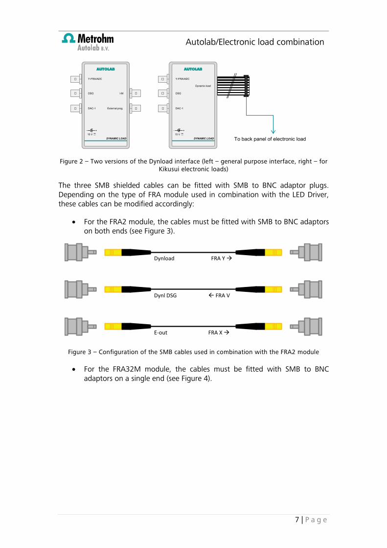
Figure 10 – The Voltage Multiplier

7.2.2 – Connections to the instrument

Connect the voltage multiplier to the differential amplifier. Connect the Sense lead to the S-Pgstat connector and the Reference lead to the RE-Pgstat connector on the voltage multiplier.

The voltage multiplier provides two connections to the DUT. Connect the S-Cell connector to the WE banana connector of the PGSTAT and the positive pole of the DUT using the provided additional red cable. Connect the RE-Cell connector to the CE banana connector of the PGSTAT and the negative pole of the DUT using the provided additional blue cable (see Figure 11).

RE-Pgstat

VOLTAGE MULTIPLIER

RE-cellR4

90kΩ

S-PgstatS-cellR1

90kΩ

R310kΩ

R210kΩ


17 | P a g e

Figure 11 – Wiring diagram of the voltage multiplier between the DUT and the PGSTAT

8 – Electronic load settings

Before the measurements can be performed, it is mandatory to program the electronic load. Please refer to the user manual provided with the electronic load for more information or contact Metrohm Autolab B.V. for setup guidelines ([email protected]).

Most electronic loads have a number of common settings which have to be considered:

• External control (ON/OFF): all electronic loads have a switch which activates or deactivates the external programming capability. This switch must be set to ON.

+ -

Differential amplifierS RE

GND

S RE

+ -

Voltage multiplier

Differential amplifierS RE

GND

S RE

Warning

Connect the green ground cable from the PGSTAT to the GND connector on the voltage multiplier! The ground cable must be connected to the voltage multiplier at all times.



18 | P a g e

• Bandwidth, Slew rate: on some devices, the bandwidth or the slew rate can be set manually. If this is the case, the highest possible value should be used.

• Mode (CC, CV, CP, CR): all electronic loads have four operation modes: constant current (CC), constant voltage (CV), constant power (CP) and constant resistance (CR). For this application, the constant current mode (CC) is required for this application.

• Voltage and current range: some electronic loads provide different voltage and current ranges, which have to be set according to the experimental conditions.

• Cell switch: all electronic loads have a manual cell switch which must be set ON before the measurement starts.

8.1 – Programming the load (TDI)

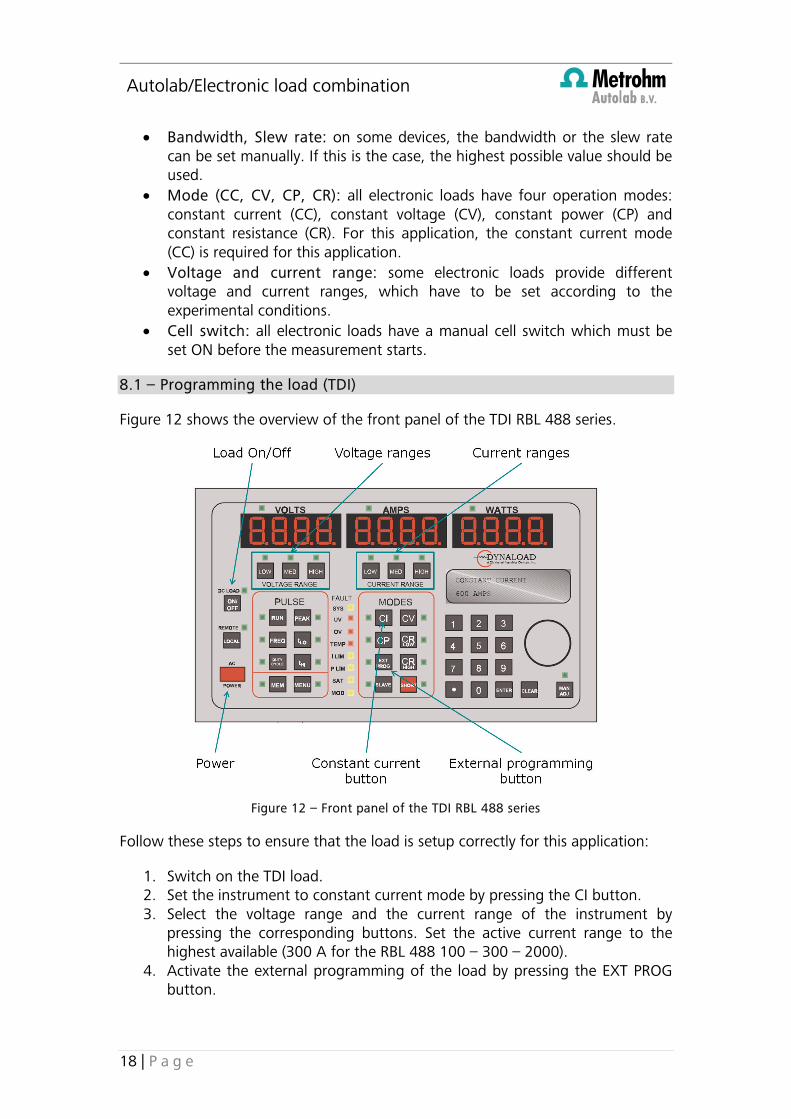
Figure 12 shows the overview of the front panel of the TDI RBL 488 series.

Figure 12 – Front panel of the TDI RBL 488 series

Follow these steps to ensure that the load is setup correctly for this application:

1. Switch on the TDI load. 2. Set the instrument to constant current mode by pressing the CI button. 3. Select the voltage range and the current range of the instrument by

pressing the corresponding buttons. Set the active current range to the highest available (300 A for the RBL 488 100 – 300 – 2000).

4. Activate the external programming of the load by pressing the EXT PROG button.


19 | P a g e

8.2 – Programming the load (Kikusui)

Figure 13 shows the overview of the front panel of the Kikusiu PLZ164WA.

Figure 13 – Front panel of the Kikusiu PLZ164WA

Follow these steps to ensure that the load is setup correctly for this application:

1. Switch on the Kikusui load. 2. Press SHIFT key and SET/VSET key on the front panel. 3. Using the rotating knob, highlight the Configuration menu item and press

the ENTER key. 4. Using the rotating knob, highlight the External menu item and press the

ENTER key. 5. Using the rotating knob, set change the Control menu item to V and the

LoadOn In item to HIGH. 6. Press the SHIFT and SET/VSET keys to return to the main menu. 7. Press the RANGE key to cycle through the different current ranges and set

the active range to the highest available (33 A for the PLZ164WA). 8. Press the MODE key to cycle through the different operation modes and

make sure that the constant current mode (CC) is selected. 9. Press the SLEW RATE key and adjust the slew rate to the highest possible

value, using the rotating knob. 10. Switch the load off and then on again to confirm the changes.


20 | P a g e

8.3 – Controlling the electronic load

The control of the electronic load is achieved by providing an analog (0-10 V) signal from the Dynload interface to the external programming connection of the load.

The output of the Dynload interface in turn is controlled by the output of the DAC164 1 of the Autolab and the FRA2/FRA32M V output, if applicable.

The conversion settings depend on the type of load and are specified in the software.

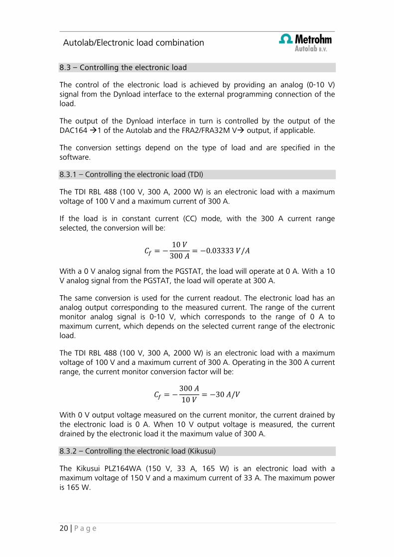
8.3.1 – Controlling the electronic load (TDI)

The TDI RBL 488 (100 V, 300 A, 2000 W) is an electronic load with a maximum voltage of 100 V and a maximum current of 300 A.

If the load is in constant current (CC) mode, with the 300 A current range selected, the conversion will be:

𝐶𝑓 = −10 𝑉

300 𝐴= −0.03333 𝑉/𝐴

With a 0 V analog signal from the PGSTAT, the load will operate at 0 A. With a 10 V analog signal from the PGSTAT, the load will operate at 300 A.

The same conversion is used for the current readout. The electronic load has an analog output corresponding to the measured current. The range of the current monitor analog signal is 0-10 V, which corresponds to the range of 0 A to maximum current, which depends on the selected current range of the electronic load.

The TDI RBL 488 (100 V, 300 A, 2000 W) is an electronic load with a maximum voltage of 100 V and a maximum current of 300 A. Operating in the 300 A current range, the current monitor conversion factor will be:

𝐶𝑓 = −300 𝐴10 𝑉

= −30 𝐴/𝑉

With 0 V output voltage measured on the current monitor, the current drained by the electronic load is 0 A. When 10 V output voltage is measured, the current drained by the electronic load it the maximum value of 300 A.

8.3.2 – Controlling the electronic load (Kikusui)

The Kikusui PLZ164WA (150 V, 33 A, 165 W) is an electronic load with a maximum voltage of 150 V and a maximum current of 33 A. The maximum power is 165 W.


21 | P a g e

If the load is in constant current (CC) mode, with the 33 A current range selected, the conversion will be:

𝐶𝑓 = −10 𝑉33 𝐴

= −0.30303 𝑉/𝐴

With a 0 V analog signal from the PGSTAT, the load will operate at 0 A. With a 10 V analog signal from the PGSTAT, the load will operate at 33 A.

With a 0 V analog signal from the PGSTAT, the load will operate at 0 V. With a 10 V analog signal from the PGSTAT, the load will operate at 150 V.

The same conversion is used for the current readout. The electronic load has an analog output corresponding to the measured current. The range of the current monitor analog signal is 0-10 V, which corresponds to the range of 0 A to maximum current, which depends on the selected current range of the electronic load.

The Kikusui PLZ164WA (150 V, 33 A, 165 W) is an electronic load with a maximum voltage of 150 V and a maximum current of 33 A. The maximum power is 165 W. Operating in the 33 A current range, the current monitor conversion factor will be:

𝐶𝑓 = −33 𝐴10 𝑉

= −3.3 𝐴/𝑉

With 0 V output voltage measured on the current monitor, the current drained by the electronic load is 0 A. When 10 V output voltage is measured, the current drained by the electronic load it the maximum value of 33 A.

9 – NOVA hardware setup

NOVA 1.10 or later is required for this application.

The hardware setup must be specified before the electronic load can be controlled. From the Tools menu, open the hardware setup and specify the configuration of the instrument.

Select the External additional module (see Figure 14).


22 | P a g e

Figure 14 – Specifying the hardware setup

With the External module selected, an additional configuration panel is shown in the frame on the right-hand side of the Hardware setup. This panel can be used to specify the conversion settings required to control the electronic load.

When finished editing the Hardware setup, click the button to close the window.

9.1 – Analog input settings

In the ADC164 – 1 section, the conversion settings required to measure the current from the external output of the electronic load can be defined and saved for future use. The settings depend on the type of load. Please refer to the electronic load user manual for more information.

For the Kikusui PLZ164WA load, used in the examples in Section 8.3.2 of this manual, the settings required to convert the analog signal from the load into the correct current value are shown in Figure 15.


23 | P a g e

Figure 15 – The conversion settings for the Kikusui PLZ164WA electronic load

These settings indicate that the analog signal provided by the Kikusui electronic load, in V, need to be multiplied by -3.3 in order to be converted into current, with the correct polarity.

9.2 – Analog output settings

In the DAC164 – 1 section, the conversion settings control the current setpoint of the electronic load can be defined and saved for future use. The settings depend on the type of load. Please refer to the electronic load user manual for more information.

For the Kikusui PLZ164WA load, used in the examples in Section 8.3.2 of this manual, the settings required to convert the analog signal from the load into the correct current value are shown in Figure 16.

Note

It is possible to save these settings in the Hardware setup for future use by clicking the button on the right-hand side of this panel.

Note

The parameters for other electronic loads are reported in the Appendix of this document.


24 | P a g e

Figure 16 – The conversion settings for control of the Kikusui PLZ164WA electronic load

These settings indicate that in order to control the setpoint of the electronic load, the specified current needs to be divided by -3.3 in order to be converted to the analog signal with the correct polarity. Upper and lower limits can be specified, these are defined by the electronic load.

10 – Manual control of the electronic load (DC only)

Manual control of the electronic load is possible in NOVA provided that the settings are specified correctly (see Section 9).

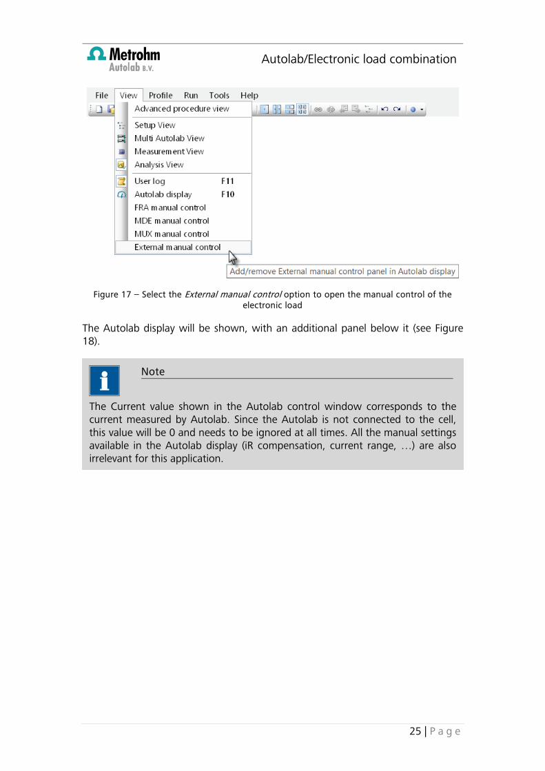
To open the manual control of the electronic load, select the External manual control option from the View menu (see Figure 17).

Note

It is possible to save these settings in the Hardware setup for future use by clicking the button on the right-hand side of this panel.

Note



25 | P a g e

Figure 17 – Select the External manual control option to open the manual control of the electronic load

The Autolab display will be shown, with an additional panel below it (see Figure 18).

Note

The Current value shown in the Autolab control window corresponds to the current measured by Autolab. Since the Autolab is not connected to the cell, this value will be 0 and needs to be ignored at all times. All the manual settings available in the Autolab display (iR compensation, current range, …) are also irrelevant for this application.


26 | P a g e

Figure 18 – The Autolab display window with the External device control panel

To specify the discharge current of the electronic load, click the label in the External device control panel and edit the value as shown in Figure 19. Press the Enter key to validate the value.

Figure 19 – Specifying the discharge current manually

Note

The name shown in the External device control panel (Kikusui PLZ164WA 33 A) depends on the settings specified in the Hardware setup window.


27 | P a g e

11 – Procedure control of the electronic load (DC only)

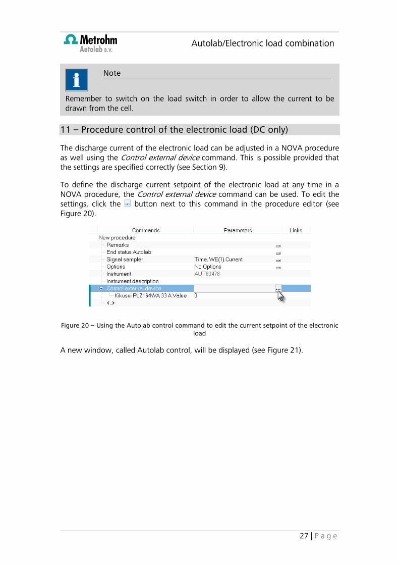
The discharge current of the electronic load can be adjusted in a NOVA procedure as well using the Control external device command. This is possible provided that the settings are specified correctly (see Section 9).

To define the discharge current setpoint of the electronic load at any time in a NOVA procedure, the Control external device command can be used. To edit the settings, click the button next to this command in the procedure editor (see Figure 20).

Figure 20 – Using the Autolab control command to edit the current setpoint of the electronic load

A new window, called Autolab control, will be displayed (see Figure 21).

Note

Remember to switch on the load switch in order to allow the current to be drawn from the cell.


28 | P a g e

Figure 21 – The Autolab control window

The control of the electronic load is available on the Advanced part of this editor (see Figure 22).

Figure 22 – The control of the electronic load is provided on the Advanced part


29 | P a g e

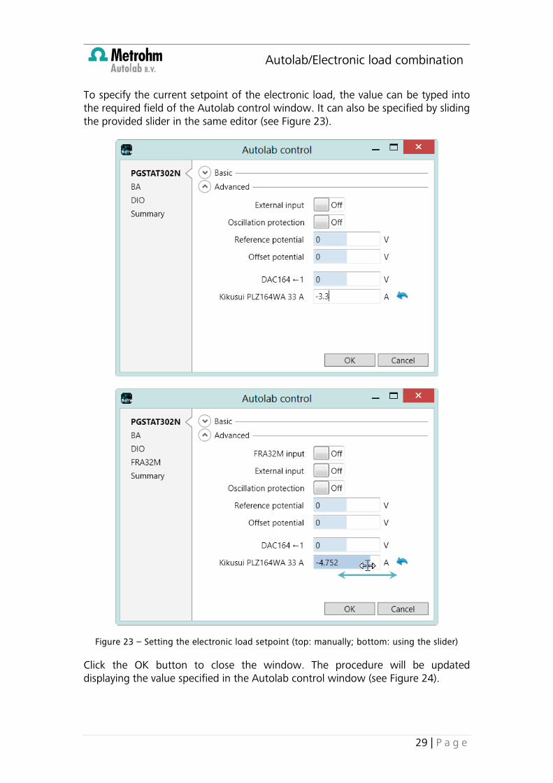
To specify the current setpoint of the electronic load, the value can be typed into the required field of the Autolab control window. It can also be specified by sliding the provided slider in the same editor (see Figure 23).

Figure 23 – Setting the electronic load setpoint (top: manually; bottom: using the slider)

Click the OK button to close the window. The procedure will be updated displaying the value specified in the Autolab control window (see Figure 24).


30 | P a g e

Figure 24 – The updated procedure editor

The parameter provided by the Control external device command can be linked to other commands, like an Input box command or a Repeat for each value command, as show in Figure 25.

Figure 25 – Linking the electronic load setpoint to an Input box command

12 – Recording the output from the electronic load (DC only)

The output of the electronic load is fed back to one of the external inputs of the Autolab. If the conversion settings are specified properly, as indicated in Section 9, the output from the load can be converted directly and recorded by the NOVA software.

To sample the output of the electronic load, the corresponding signal can be added to the Signal sampler, as shown in Figure 26.


31 | P a g e

Figure 26 – Specifying the output signal from the electronic load in the Signal sampler

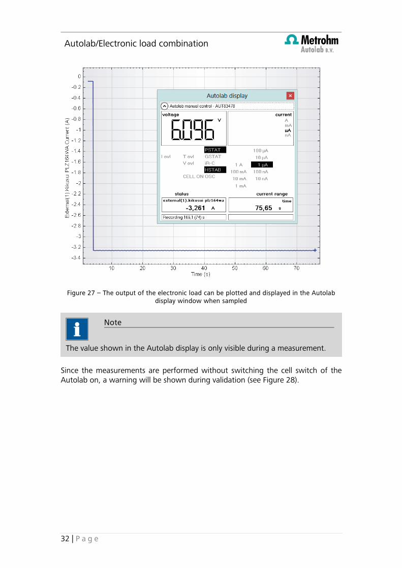
The measured values can be plotted during a measurement and will be displayed in the Autolab display window (see Figure 27).

Note

The output signal of the electronic load can be sampled by any measurement command that uses the Signal sampler.

Warning

The WE(1).Current, WE(1).Power, WE(1).Resistance and WE(1).Charge signals cannot be sampled since the WE is not connected to the cell in the application.


32 | P a g e

Figure 27 – The output of the electronic load can be plotted and displayed in the Autolab display window when sampled

Since the measurements are performed without switching the cell switch of the Autolab on, a warning will be shown during validation (see Figure 28).

Note

The value shown in the Autolab display is only visible during a measurement.


33 | P a g e

Figure 28 – Measurements with an external electronic load trigger a warning during validation

It is possible to right-click this warning message to disable this for further measurements (see Figure 28).

13 – Impedance spectroscopy measurements

Impedance spectroscopy measurements are possible using similar settings as those defined in the Hardware setup of NOVA. A dedicated command, FRA measurement external is available in the Measurement – Impedance group of commands.

To perform a frequency scan using the external electronic load, drag and drop the FRA measurement external command into the procedure editor (see Figure 29).

Note

Impedance spectroscopy measurements require the definition of a DC setpoint on the electronic load. This can be done by using the methods indicated in Sections 10 and 11.


34 | P a g e

Figure 29 – Adding the FRA measurement external command to the procedure

To edit the settings of the FRA measurement external command, click the button next to the command in the procedure editor (see Figure 29).

A new window will be displayed (see Figure 30).

Figure 30 – The FRA editor window


35 | P a g e

This window can be used to specify all the settings required to perform an impedance measurement using the external electronic load.

13.1 – External settings

The parameters on the External section of the FRA editor window are related to the conversion parameters for setting and measuring the setpoint of the electronic load as well as the definition of the transfer function.

13.1.1 – Settings for V

The parameters for the V signal define the conversion factor between the output of the FRA2/FRA32M module and the input of the electronic load.

For this application, set the Unit parameter to A and specify a multiplier (see Figure 31).

Figure 31 – Setting the parameters for the V output

The value of the multiplier depends on the type of electronic load and the settings for the Kikusiu PLZ164WA in 33 A current range will be used in this section. For this load, the multiplier is 0.30303 (10 V / 33 A).

Note



36 | P a g e

13.1.2 – Settings for X

The parameters for the X signal define the conversion factor between the analog output of the Autolab differential amplifier and the X input channel of the FRA2/FRA32M.

For this application, set the name to Potential, set the Unit parameter to V and specify a multiplier of -1 (see Figure 32).

Figure 32 – Setting the parameters for the X input

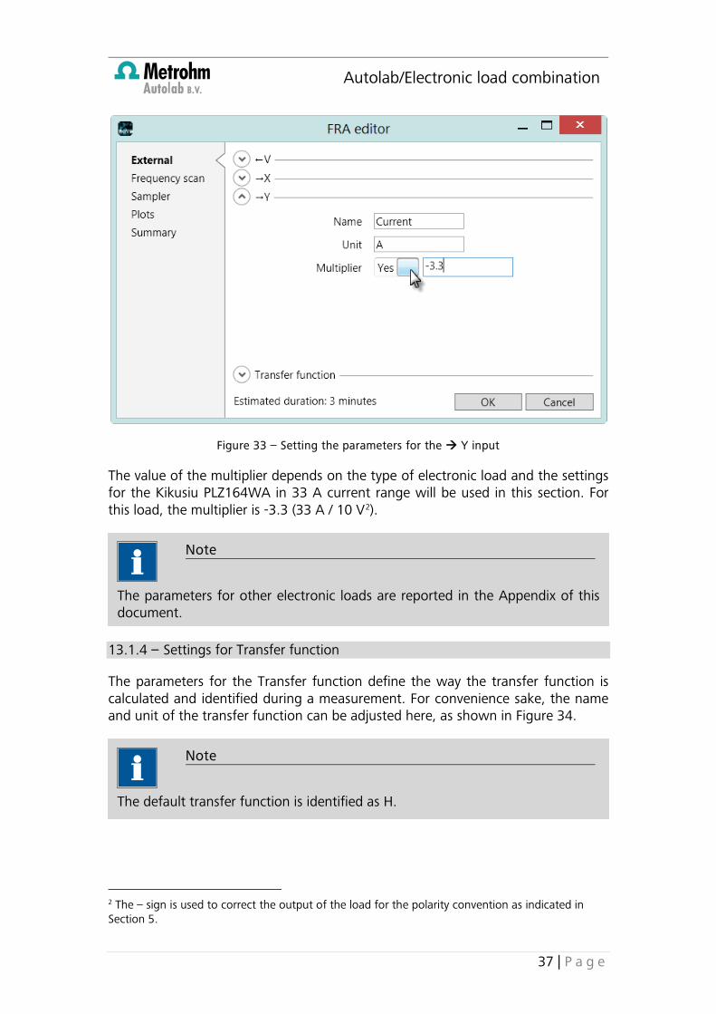
13.1.3 – Settings for Y

The parameters for the Y signal define the conversion factor between the analog output of the electronic load and the Y input channel of the FRA2/FRA32M.

For this application, set the name to Current, set the Unit parameter to A and specify a multiplier (see Figure 32).


37 | P a g e

Figure 33 – Setting the parameters for the Y input

The value of the multiplier depends on the type of electronic load and the settings for the Kikusiu PLZ164WA in 33 A current range will be used in this section. For this load, the multiplier is -3.3 (33 A / 10 V2).

13.1.4 – Settings for Transfer function

The parameters for the Transfer function define the way the transfer function is calculated and identified during a measurement. For convenience sake, the name and unit of the transfer function can be adjusted here, as shown in Figure 34.

2 The – sign is used to correct the output of the load for the polarity convention as indicated in Section 5.

Note


Note

The default transfer function is identified as H.


38 | P a g e

Figure 34 – Specifying the name and units for the transfer function

13.2 – Frequency scan settings

The parameters on the Frequency scan section of the FRA editor window are related to the frequency scan itself.

This section can be used to specify the parameters for the frequency scan (see Figure 35). More information is provided in the Impedance tutorial, provided in the Help menu of Nova.

Note

Make sure that the settings defined on the External section of the FRA editor are adjusted properly before editing the settings on the Frequency scan section.


39 | P a g e

Figure 35 – Defining the settings for the frequency scan

13.3 – Sampler settings

The parameters on the Sampler section of the FRA editor window are related to the signals to sample during the impedance spectroscopy measurement and the acquisition parameters (see Figure 36).

Note

The amplitude value is specified in absolute values.

Warning

Make sure that that the amplitude defined in the FRA editor is smaller than the DC setpoint of the electronic load!


40 | P a g e

Figure 36 – The acquisition parameters are defined on the Sampler section of the FRA editor

The acquisition parameters are predefined for a normal impedance measurement and it is recommended to use the default settings. Additional signals to be measured can be specified in the section:

• Sample time domain: if this option is active, the time domain information will be sampled and stored for both input signals. The time domain information consists of the raw X and Y sine waves. This information can be used evaluate the signal to noise ratio and to evaluate the linearity of the cell response.

• Sample frequency domain: if this option is active, the frequency domain information will be sampled and stored for both input signals. The frequency domain information consists of the calculated FFT results obtained from the measured time domain. The frequency domain information can be used to evaluate the measured frequency contributions.

• Sample DC (active by default): if this option is active, the DC component for both input signals will be sampled and stored.

• Calculate admittance: if this option is active, the admittance will be calculated based on the measured impedance data.

Note

For this application, it is highly recommended to activate the Sample time domain option in order to verify that the sinewaves from the Autolab and electronic load are recorded properly.


41 | P a g e

13.4 – Plots settings

The parameters on the Plots section of the FRA editor window are related to the plotting of the data measured during the impedance spectroscopy measurement and the acquisition parameters (see Figure 37).

Figure 37 – The plot settings are defined on the Plots section of the FRA editor

More information is provided in the Impedance tutorial, provided in the Help menu of Nova.

When all the parameters and settings are specified, click the button to close the FRA editor. The procedure editor will be updated (see Figure 38).

Note

The available plots on the Plots section depend on the signals specified in the Sampler section of the FRA editor.


42 | P a g e

Figure 38 – The procedure editor is updated after all the settings are specified in the FRA editor

13.5 – Running a measurement

Using the recommended settings specified in this Section, impedance measurement can be carried out and displayed as shown in Figure 39.


43 | P a g e

Figure 39 – Example of a typical impedance measurement using an external electronic load

Note

Metrohm Autolab can assist in setting up the experimental conditions and the procedure used to perform the measurements. Contact [email protected] or your local distributor for more information




44 | P a g e

14 – Measurement examples

This section provides a few examples of procedures designed for the combination of the Autolab PGSTAT and an electronic load.

14.1 – iV/Power curve

The combination of the Control external device command and the Repeat for each value command provides the backbone for a complete i/V and power curve measurement, as shown in Figure 40.

Figure 40 – Typical i/V curve of a fuel cell stack

14.1.1 – Running the measurement

Using the Control external device and the Record signals (>1 ms) commands, it is possible to construct a complete procedure to perform an i/V measurement using the electronic load.

Figure 41 shows an example of a suitable procedure for this type of measurement.


45 | P a g e

Figure 41 – Example of a complete procedure used to perform a i/V measurement using an electronic load in combination with the Autolab

These commands are embedded into a Repeat for each value command used to walk through different current values.

The Calculate signal command is used to calculate the power so that it can be plotted against the discharge current.

For more information, please refer to the NOVA user manual.

14.2 – Impedance spectroscopy measurement

The combination of the Control external device command and the FRA measurement external command provides the backbone for a complete impedance spectroscopy measurement, as shown in Figure 42.


46 | P a g e

Figure 42 – Typical Nyquist plots obtained on a fuel cell at 120 A and 200 A DC current, 9 A AC amplitude

Figure 42 shows a typical Nyquist plot that can be obtained with an electronic load. The measurements were obtained at 120 A and 200 A DC current, with a 9 A AC amplitude. The TDI RBL 488 was used for these measurements.

Figure 41 shows an example of a suitable procedure for this type of measurement.


47 | P a g e

Figure 43 – Example of a complete procedure used to perform an impedance spectroscopy measurement using an electronic load in combination with the Autolab

Note

Metrohm Autolab can assist in setting up the experimental conditions and the procedure used to perform the measurements. Contact [email protected] or your local distributor for more information.




48 | P a g e

Appendix 1 – Specifications of known electronic loads

The DC and AC conversion settings are specified in Table 2 and Table 3, respectively.

Load Current

range (A) DAC164 1

Conversion slope ADC164 1

Conversion slope

Kikusui PLZ164WA 33 -3.3 -3.3

Kikusui PLZ664WA 132 -13.2 -13.2

TDI RBL 488 300 -30 -30

TDI WCL 488 1000 -100 -100

Agilent 6060B 60 -6 -6

Agilent 3300 60 -6 -6

Chroma 6300 60 -6 -6

Table 2 – Overview of the DC settings (to be specified in the Hardware setup) for known electronic loads

Load Current

range (A) V Settings Y Settings

Kikusui PLZ164WA 33 0.303 -3.3

Kikusui PLZ664WA 132 0.0757 -13.2

TDI RBL 488 300 0.0333 -30

TDI WCL 488 1000 0.0100 -100

Agilent 6060B 60 0.166 -6

Agilent 3300 60 0.166 -6

Chroma 6300 60 0.166 -6

Table 3 –Overview of the AC settings (to be specified in the FRA measurement external command) for known electronic loads

Note

For information on electronic loads not listed in the Appendix please contact Metrohm Autolab ([email protected]).



49 | P a g e

Appendix 2 – Modification of the FRA2 module

By default, the external inputs of the FRA2 modules shipped before July 2009 (revision number 8.0 and lower) can be used to record analog signals in the ± 5 V range. For some applications, analog signals in the ± 10 V range are required. In order to be able to record voltages between 5 and 10 V, the FRA2 modules with revision numbers lower than 8.1 need to have the extended range offset DACs activated. This requires a simple hardware modification described in this document. Please contact Metrohm Autolab B.V. ([email protected]) or your local distributor in case of any doubts.

The modification described in this document requires the following items:

1. ESD safety kit (see Figure 44) 2. Soldering iron and solder

The modification requires soldering JP2 and JP3 of the analog board of the FRA2 module. Figure 44 shows a picture of the Analog board. The two jumpers are highlighted.

Figure 44 – The FRA2 Analog board (JP2 and JP3 are highlighted)

The two jumpers need to be soldered together.

Remove the FRA2 module from the Autolab frame. To remove the FRA2 module follow the instructions reported the following documents:

The modification described in this document requires the following items:

Warning

Take all the necessary steps to avoid ESD damage to the module by grounding yourself during the handling of the module and the soldering of the jumpers. The use of a ESD safety kit is highly recommended.



50 | P a g e

1. For the PGSTAT128N, PGSTAT302N, PGSTAT302F and PGSTAT100N: All modules – Insert new module in 8-series cabinet.pdf

2. for the PGSTAT12, PGSTAT30, PGSTAT302 and PGSTAT100 All modules – Insert new module in 7-series cabinet.pdf

The FRA2 module consists of 2 PCBs (see Figure 45). One PCB is the digital signal generator (DSG) PCB and the second one is the Analog PCB.

Figure 45 – The FRA2 consists of two PCBs (the DSG on top, and the Analog below)

To access the Analog PCB, the DSG PCB must be detached. To do this, gently push on both sides of the board as shown in Figure 46 and Figure 47.

Note

It is recommended to store the DSG PCB in an ESD safe bag during the modification.


51 | P a g e

Figure 46 – Pressure points on the DSG PCB

Figure 47 – The removed DSG PCB and the Analog PCB of the FRA2 module

Figure 47 shows the FRA2 module, with the removed DSG PSB. Locate JP2 and JP3 on the Analog PCB and close both jumpers by applying a bit a solder.


52 | P a g e

To reassemble the 2 boards, all the holes in the 3 green connectors of the DSG PCB have to be aligned with the matching pins on the FRA2 module assembly (see Figure 48).

Figure 48 – Reassembling the FRA2 module

Reinstall the module in the Autolab following the instructions provided in the installation guides mentioned at the beginning of this section.

After modification of the FRA2 module has been modified, the software needs to be adjusted.

The FRA2 input range is directly specified in the Hardware setup. Start NOVA and open the Hardware setup (Tools – Hardware setup). Locate the FRA offset DAC range toggle at the bottom of the Hardware setup window (see Figure 49).

Note

The factory FRA2CAL.INI file can still be used. No recalibration is required.


53 | P a g e

Figure 49 – The 10 V input range can be specified in the Hardware setup directly

Set this toggle to 10 V as shown in Figure 49. Click OK to close the Hardware setup and save the modifications when prompted.

This modification is permanent.

If necessary, new labels (article codes: CAB.LABEL.FRA2.V10.V and CAB.LABEL.FRA2.V10.XY) can be ordered for the modified FRA2 module (see Figure 50).

Figure 50 – FRA2 10 V input range labels

Electronic Load - Metrohm Autolab

Documents

Transcript of Electronic Load - Metrohm Autolab