Missouri University of Science and Technology Missouri University of Science and Technology

Scholars' Mine Scholars' Mine

Center for Cold-Formed Steel Structures Library Wei-Wen Yu Center for Cold-Formed Steel Structures

01 Apr 1975

Load factors for wind and snow loads for use in load resistance Load factors for wind and snow loads for use in load resistance

factor design criteria factor design criteria

M. K. Ravindra

Theodore V. Galambos

Follow this and additional works at: https://scholarsmine.mst.edu/ccfss-library

Part of the Structural Engineering Commons

Recommended Citation Recommended Citation Ravindra, M. K. and Galambos, Theodore V., "Load factors for wind and snow loads for use in load resistance factor design criteria" (1975). Center for Cold-Formed Steel Structures Library. 62. https://scholarsmine.mst.edu/ccfss-library/62

This Technical Report is brought to you for free and open access by Scholars' Mine. It has been accepted for inclusion in Center for Cold-Formed Steel Structures Library by an authorized administrator of Scholars' Mine. This work is protected by U. S. Copyright Law. Unauthorized use including reproduction for redistribution requires the permission of the copyright holder. For more information, please contact scholarsmine@mst.edu.

WASHINGTON u -NIVERSITY

SCHOOL OF ENGINEERING AN o APPLIED SCIENCE

DEPARTMENT OF CIVIL ENGINEERING

LOAD FACTORS FOR WIND AND SN~ LOADS FOR USE IN LOAD

AND RESISTANCE FACTOR DESIGN CRITERIA

by

M. K. Ravindra

and

T. V. Galambos

Progress Report to the Advisory Committee

of AISI Project 163 "Load Factor Design of Buildings"

Research Report No. 34 Structural Division April 1975

Revised January 1976

LOAD FACTORS FOR WIND AND SNOW LOADS FOR USE IN LOAD

AND RESISTANCE FACTOR DESIGN CRITERIA

by

H. K. Ravind-.ra

and

T. V. Galambos

Research Report No. 34, Structural Division

Civil Engineering Department

Washington University

St. l,ouis, Mo.

April 1975

Revised January 1976

Th1~ rLpnrl presents results of research work

spousoreJ by tlte American Iron and Steel Institute as

AISI P_ruject. lt<3 'Load Factor tx:::si.gn of Steel Buildir~gs'',

ABSTRACT

This report presents the background and the derivations for the

determination of the mean maximum loads and the corresponding load

factors for wind and snow loading for use in Load and Resistance Factor

Design Criteria for steel building structures.

i

1 • INTI~ODlJCTION

This report is concerned with load factors to be used with wind

and snow loads in a design method named "Load and Resistance Factor

Design" (L.R.F.D.). A previous report (l) has presented the general

background oi this design method as well as the basis for its develop-

ment from a first -order probabilistic theory. In L .R .F. D. a structural

design is deemed satisfactory if the computed internal forces, as

determined by structural analysis for the assigned mean loads factored

by appropriare load factors, are sn~ller than or equal to the factored

nominal resistance of each stn1ctural ele.me,lt.:

where

(t/J R ) n k

R n

n r "'"' L LJ i:l

c

y

c. 1

n ~ yo [ T c. y i. Qi

·; ._.1 J i=l 1.

j (1)

factored nominal resistance for limit state k

resistance factor for the appropriate limit state,

accounting for the uncertainties of the resistance

nominal :cet>istauce for the appropriate limit state

y. Q. J 1. 1

factored internal load effect for load j

combination j

influence factor by which the factored load inten-

sity y f2 is translated into a load effect (e.g., an

internal force such as bending moment, shear force,

axial force, torque, etc.) by structural analysis

luad factor accounting or the uncertainties of

the load

load i.ntensit:,,. nr lo<vi dL.te to dead, live, wind, snow,

etc. , load

1.

load factor accounting for the uncertainties of

structural analysis and geometric and structural

idealizations.

It was demonstrated in previous work (1) that the factors 0, y and 0

y. can be expressed in terms of the mean values and the coefficients of ~

variation of the respective random variables, and that the factors are

related to each other through a con~non term called the "safety index" e. This safety index is a measure of the reliability of the structural

element and it is obtained through a process of calibration to an

existing design criterion. In Ref. 1 such a calibration was performed

for structural steel members designed according to the current (1976)

AISC Specification, and a safety index of S = 3 was chosen for the limit

state of strength c.s being 1·epresentative for structures designed accord-

ing to the 1976 AISC Specification.

This present report is concerned with the right side of Eq. l,

i.e., with the load terms corresponding to wind and snow loads. The

load terms to be determined are the load factors y. and the mean load l.

intensities Q. to be used with the L.R.F.D. criteria developed in Ref. 1. ~

According to the load comoinations used in these criteria it will be

necessary to define load factors and mean load intensities for the

maxim:1m lifetime \vind pressure, the maximum annual wind pressure, the

maximum daily wind pressure, and the ma~dmum annual and the maximum

lifetime snov1 load intensity. The development will show how the basic

\vind velocity daL:a given in the distribution maps in ANSI A58.1-1972 (2)

arc to be used in the L.R.F.D. criteria.

The appropri.at(~ load cmnbi11ations involving snow and wind in the

L.Il.F.D. criteria can be enumerated as follows:

2.

3.

Maximum tifetime Hind - Dead

Dead + Instantaneous Live + Maximum Lifet i.me \-lind

Dead + Instantaneous Live +- Maximum Lifetime Snow

Dead + Maximum Li.fet ime Live + Maximum Annual Snow

Dead + Pondi.ng + Maximum Lifetime Snow

Dead + Instantaneous Live +· Maximum Daily Wind + Maximum

Lifetime Temperature

Dead + :tvlaxim•nn Annual HL,d + Maximum Lifetime Snow.

The load factors y are deter·mined according to the formula (1)

y = 1 + 0.55 sv = 1 + 1.65 v (2)

where S = 3 and V is the coefficient of variation of the appropriate

load type.

The idea underlying this list of load combinations is that it is very

un! ikely that two types of loCld effects will simultaneously reach their

maximum lifetime value. Thus t::ach combination includes the dead load,

which is always present, one of the other loads at its maximum lifetime

value, and the other loads at their instantaneous, annual or daily values,

as appropriate. Such a scheme of combining the loads has essentially the

same effect as the use of the 0.75 multiplier used in most current speci-

fications to modify the full nominal code loads in the case of simultaneity

of occurrence. The scheme proposed herein is more reasonable in that it

is possible to utilize the fact that the statistics for the different time

intervals may be different.

2. STATISTICAL PAI{AMETERS OF WIND LOADS -·-·~-·-----··--

In the following, the statistLcal aspects of wind loads on structures

are discussed. The important random variables characterizing the wind load

are the maximum wind speed in the service life of the structure, the annual

maximum wind speed and the daily maximum wind speed. The statistical

parameters of the lifetime maximum wind speed are derived using the data

on the annual maximum wind speed.

2.1 Wind Load Determination According to Current (1976) Practice

The usual practice for calculating the wind loads on buildings and

other structures is to use specified minimum design pressures varied

according to geographical location and height zone above the ground. The

dynamic action of wind on structures is indirectly accounted for in speci­

fying these design pressures. The 1972 version of A58.l of the American

National Standards Institute (2) and the National Building Code of Canada

(3) have included procedures which explicitly recognize the dynamic effects

of wind.

The procedure for calculating the wind loads according to ANSI A58.1 -

1972 is:

l. A mean recurrence interval is selected depending on the intended

operational usage, anticipated life of the structure, degree of wind

sensitivity and risk to human life and property in case of failure. A 50

year mean recurrence interval is recommended by ANSI for the design of

permanent structures. For more important and/or more wind-sensitive

structures a 100 year mean recurrence interval is recommended. For struc­

tures having no human occupants or where there is negligible risk to human

life, the 25 year mean recurrence interval may be used.

2. A basic wind speed is selected from the wind maps of the United

States, corresponding to the mean recurrence interval (Figs. 1, 2 and lA

in Ref. 2). This speed refers to the annual extreme fastest mile velocity.

This fastest-mile wind speed is measured by recording the time required

for a mile of air to pass a fixed point by means of an anemometer which

makes an electrical contact with the passage of each mile of air.

') .

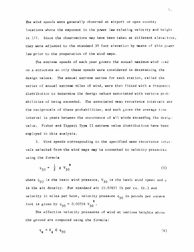
The wind speeds were generally observed at airport or open country

locations where the exponent in the power law relating velocity and height

is 1/7. Since the observations may have been taken at different elevations,

they were adjusted to the standard 30 foot elevation by means of this power

law prior to the preparation of the wind maps.

The extreme speeds of each year govern the annual maximum wind wad

on a structure so only these speeds were considered in determining the

design values. The annual extreme series for each station, called the

series of annual extreme miles of wind, were then fitted with a frequency

distribution to determine the design values associated with variotts prob-

abilities of being exceeded. The associated mean recurrence intervals are

the reciprocals of these probabilities, and each gives the average tine

interval in years between the occurrence of all winds exceeding the desigtl

value. Fisher and Tippett Type II extreme value distributions have been

employed in this analysis.

3. Wind speeds corresponding to the specified mean recurrence inteT ··

vals selected from the wind maps may be converted to velocity pressures

using the formula

(3)

where q30 is the basic wind pressure, v30 is the basic wind speed and p

is the air density. For standard air (0.07651 lb per cu. ft.) and

velocity in miles per hour, velocity pressure q30 in pounds per square

2 foot is given by q30 = 0.00256 v30 .

The effective velocity pressures of wind at various heights above

the ground are computed using the formula:

(4)

6.

where qz is the effective velocity pressure in psf at height z in ft.,

K is a velocity pressure coefficient which depends upon the type of z

exposure and height above ground and G is a gust factor which depends

upon the response characteristics of the structure.

4. The effective velocity pressure varies with height and exposure.

Three categories of exposure are considered: (A) centers of large cities

and very rough, hilly terrain; (B) suburban areas, towns, city outskirts,

wooded areas and rolling terrain; and (C) flat, open country, open flat

coastal belts, and grassland. For convenience, values of q for ordinary z

buildings and structures (qz = qF) and for parts and portions (qz = qp)

have been tabulated in ANSI-A58.1-1972 for a range of speeds as functions

of height and exposure.

The effective velocity pressures given by ANSI A58.1 take into

account the dynamic response to gusts of ordinary buildings and structures

in a direction parallel to the wind. They do not provide for the effects

of vortex shedding or instability due to galloping or flutter. ANSI

recommends a detailed analysis for obtaining the effective velocity

pressure where a dynamic approach to the action of wind gusts is required.

5. The resultant wind pressure p acting on an element of an enclosed

structure is

p = c q - c q p z pi M (5)

where qz equals qF or ~ whichever is appropriate, Cp is the external

pressure coefficient, C . is the internal pressure coefficient and qM is p1

the corresponding effective velocity pressure (given in Tables 5 and 6 in

ANSI A58.1). The pressure coefficients define the pressure acting normally

at local positions on the surface of a building and hence are dependent on

the external shape and orientation of the building with respect to wind.

In general the wind pressure acting on a structure or structural

element can be written as

a W = C q = C K G (0.00256 v30 )

p z p z (6)

7.

where Cp, Kz, G and v30 are all random variables. The mean wind pressure

W and the coefficient of variation of the wind pressure V can be m w

expressed as functions of the corresponding values of the components:

a Wm - [ (C ) (K ) (G) ][ 0.00256 (V30)m]

p m z m m (7)

and

+ (8)

2.2 Lifetime Maximum Wind Velocity

Based on wind velocity data from 141 open country stations, which

were dispersed over the continental U. S., Thorn (4) has suggested that

the maximum annual wind velocity follows a Type II. Extreme Value dis-

tribution. He has shown that the shape parameter K of this distribution

is essentially constant for all stations (K = 9.0). Following is a

derivation of the statistical parameters of the maximum lifetime wind

speed using the probability model proposed by Thorn.

The lifetime (n-years) maximum wind speed Y is the maximum of n

annual maximum wind speeds, x 1 , x2 , ... Xn. Then the probability

Fy (y) = p [ y ~ y J

= P [all n of the X. ~ y ] 1

The annual maximum wind speeds X. may be treated as statistically ~

independent.

FY (y) = P [xi s: y ] P [ x 2 ~ y J p (X ~ y] n

= Fx (y) Fx (y) ••• Fx (y) 1 2 n

(9)

8.

The annual maximum wind speed distribution is assumed to be constant in

time (i.e., X. are identically distributed with the cumulative distribu-1.

tion function FX (x)). Therefore,

(10)

Based on the Type 11. Extreme Value probabilistic distribution Thorn

developed maps for the United States, giving the maximum annual wind

velocities for mean recurrence intervals of 25, 50 and 100 years. The

mean Xm and the cotfficient of variation VX of the annual maximum wind

velocity are obtained using the following expressions:

(11)

-~.-;----·-·\

ru - ~ ) 2 1

p (1 -· -) • K

1 (12)

where x50 is the '')0 year" annual maximum wind velocity (as given in the

ANSI A58.1-1972 wind velocity map for a 50 year recurrence interval- Fig.

1 in Ref. 2). With K = 9 and using a table of gamma functions, VX is

calculated by Eq. 12 to be approximately 0.16.

From Eq. 10

Writing u 1 == u nl/K

exp [- n ( u / ] y

Fy (y) = exp [- (u'/y/ J

(13)

(14)

Therefore Y, th<:~ max imurn <J.nnu-':1 1 wind speed, is also distributed according

to the Type II. r:xrxeme Value probability distribution with the para-

meters of mean 1 ) 1/K

Ym = u' f(l - K = Xm n ( 15)

9.

and coefficient of variation

(16)

Here n is the lifetime of the structure, in years, Y is the mean maximum rn

lifetime wind velocity, X is the mean maximum annual wind velocity (equal m

to 0. 70 times the "n-year" \vind vel,)<.:ity from the n··year .ANSI wind distri-

bution maps) and K = 9. For a 50 year life n = 50 and V = 1.54 X m m

=

1.08 x50 • The following table gives the relevant &tatistical values for

a lifetime of 50 years.

ANSI 50 year

Basic Wind Velocity, x50 60 mph 70 mph 80 mph 90 mph

Mean Maximum Annual

Wind Velocity, Xm = 0. 7 x50 ---~~~ph _____ _:-_~_9_rr_rp_h ______ ._s_6_· _n_tp_h ___ 6_3_n_tp_l_l __ _

Mean Maximum Lifetime

Wind Velocity, Y = X 5(} 19 6.) mph m m

76 mph 86 mph 97 mph ·------

Similar tables can be constructed for the 25 and 100 year life.

2.3 Wind Pressure

The mean wind pressure Tv and the coefficient of variation VW are m

given by Eqs. 7 and 8. In the following the statistics of the contponent

parameters K , G and C are esti.matecl. z p

The velocity pressure coefficient K depends on the type of exposure ,,

and on the height above ground at \..rh:lch the wind pressure is r·equired.

Empirical observations have led ttl the delineation of three exposure

categories (Type A, B and C in AN:3J A5B .1. as described earlier in this

report), and for each t:he variation with height is defined by an exponent

in a power law relationship. The va:dat ion of K with height and exposure z

type is given in Fig. A2 of A.l\lt31·-A':>t:Ll-1972 and the resulting wind pressures

have been tabulated in the same document as Tables 5 and 6 (Table 5 for qF'

lU.

the velocity pressure on the whole structure, and Table 6 for q for parts p

and portions of the structure) for the three exposure types. Since the

velocity pressure coefficient K is used to cover a broad spectrum of z

exposure conditions, its use in calculating the wind pressure will result

in some uncertainty in the prediction, characterized by the coefficient of

variation VK . As the z

relevant information to calculate VK z

able, it will be assumed that VK z

= 0.10 for the purposes of

is not avail-

this report.

The reliability of the gust factor G has been studied by Vickery (5)

and more recently by Ellingwood and Ang (6). The gust factor, as noted

earlier, depends on wind characteristics, terrain and building character-

istics such as natural frequency, damping, geometry and mode shape. How-

ever, the variation in G is limited to a narrow range. Ellinwood and Ang

(6) have shown that the mean gust factor is insensitive to variations in

the natural frequency and the critical damping ratio. This result is

significant because these quantities are often estimated from empirical

expressions. The implication is that refined estimates of the dynamic

characteristics of the system will not improve the mean gust factor

estimation. Vickery (5) has demonstrated that the mean gust factor is

insensitive to the mode shape, hence the actual mode shape is not impor-

tant. Formulas and graphs for the determi-nation of the gust factor are

presented in Sec. A.6.3.4.1 of ANSI-ASB.l-1972, and these have been used

in the development of the pressure tables (Tables 5 and 6 in ANSI-A58.1-

1972). It will be here assumed that the gust factors implied in these

tables are taken to be the mean values for ordinary steel buildings.

Based on the work of Vickery (5) a coefficient of variation VG = 0.12 is

estimated.

The pressure coeffictents, C , are the non-dimensional ratios of p

wind-induced pressures on a building to th.e aynamic pressure (velocity

11.

pressure) of the wind speed that would be measured at the top of the

building in the undisturbed air stream. Pressures on the surfaces of

structures vary considerably with the shape, wind direction and the

profile of the wind velocity. Pressure coefficients are usually deter-

mined from wind tunnel experiments on small-scale building models. It is

essential in most cases that these pressures be measured in a wind tunnel

in which the correct velocity profile is simulated. The pressure coeffi-

cients are all time-averaged values and usually represent spatial

averages. In view of all these assumptions and simplifications, there

will be uncertainty in the prediction of C values. Here, it is assumed p

·that the C values used in the development of the pressure tables in ANSI­p

A58.1-1972 are mean values and that the coefficient of variation VC is p

0.10.

The mean maximum lifetime wind pressure, w1 , the coefficient of m

variation, VW , and the load factor L

Yw , for use in the L.R.F.D. criteria, L

are determined as follows:

W = ( Mean Maximum Lifetime Wind Velocity )2 ANSI 50-Year Wind Pressure L 50-Year ANSI Basic Wind Velocity m

For a life n = 50 years

(WL ) = 1.17 (ANSI 50-Year Wind Pressure) m 50

For a life n = 100 years

(WL ) = 1.36 (ANSI 50-Year Wind Pressure) m 100

For a life n = 25 years

(W1 ) = 1.00 (ANSI 50-Year Wind Pressure) m 25

(17)

(18)

(19)

(20)

The coefficient of variation vw is determined from Eq. 8 as L

2 2 a :a vtv ~· = VK + VG. + 4 vv = + 0.1 + 0.12 + 4 F .. X 0.16

L z 30 = 0.37

where the individual coefficients of variation were taken from the pre-

viously presented estimates. It should be noted that v30 = VX in the

previous section, and that this term predominates in Eq. 8. Should the

other three coefficients of variation be much larger, for example

VC = VK = VG = 0.15, VW would become equal to 0.41, resulting in a p z L

change in the lead factor y only in the second decimal.

The load factor Yw for the mean maximum lifetime wind pressure is, L

from Eq. 2, equal to

Yw = 1 + 0.55 13 vw = 1 + 0.55 x 3 x 0.37 = 1.61-= 1.6 L L

The mean maximum annual wind pressure, WA , the coefficient of m

variation, VW , and the load factor y are determined as follows: A WA

\v = ( Mean Maximum Annual Wind Velocity )2 ANSI 50-Year Wind Pressure A 50-Year ANSI Basic Wind Velocity m

(21)

= 0.49 (ANSI 50-Year Wind Pressure) (22)

The coefficient of variation VW A

mum lifetime wind pressure.

= 0.37 and Yw A

= 1.6, as for the maxi-

The mean maximum daily wind pressure, w0 , the coefficient of m

variation, VW , and the load factor, ytll D D

, and the load factor, Yw , A

are determined as follows:

W = ( Mean Maximum Daily Wind Velosity )2 ANSI 50.;.Year Wind Pr D 50-Year ANSI Basic Wind Velocity essure m

(23)

12.

13.

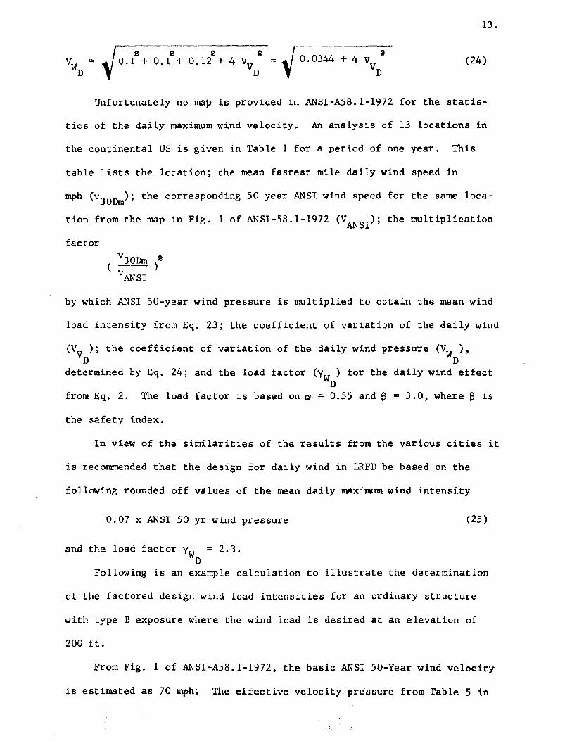
(24)

Unfortunately no map is provided in ANSI-A58.1-1972 for the statis-

tics of the daily maximum wind velocity. An analysis of 13 locations in

the continental US is given in Table 1 for a period of one year. This

table lists the location; the mean fastest mile daily wind speed in

mph (v30Drn); the corresponding 50 year ANSI wind speed for the same loca­

tion from the map in Fig. 1 of ANSI-58.1-1972 (VANS!); the multiplication

factor

v30Dm 2 ( )

vANS!

by which ANSI 50-year wind pressure is multiplied to obtain the mean wind

load intensity from Eq. 23; the coefficient of variation of the daily wind

(VV ); the coefficient of D

determined by Eq. 24; and

variation of the daily wind pressure (VW ), D

the load factor (Yw ) for the daily wind effect D

from Eq. 2. The load factor is based on a = 0.55 and~ = 3.0, where~ is

the safety index.

In view of the similarities of the results from the various cities it

is recommended that the design for daily wind in LRFD be based on the

following rounded off values of the mean daily maximum wind intensity

0.07 x ANSI 50 yr wind pressure (25)

and the load factor Yw = 2.3. D

Following is an example calculation to illustrate the determination

of the factored design wind load intensities for an ordinary structure

with type B exposure where the wind load is desired at an elevation of

200 ft.

From Fig. 1 of ANSI-A58.1-1972, the basic ANSI 50-Year wind velocity

is estimated as 70 tllf>h~ The effective velocity pressure from Table 5 in

14.

ANSI-A58.1-1972 is qF = l..8 psf for a 70 mph..-wirid and a height of 200 ft.

= 1.6 X 1.17 X 18 = 34 psf

y (W ) WL Lm 100

= 1.6 X 1.36 X 18 = 39 psf

Yw (WLm) = l. 6 X l. 00 X 18 = 29 psf L 25

Yw (WArn) = 1.6 X 0.49 X 18 = 14 psf A

Yw (WDm) = 2.3 X 0.07 X 18 = 3 psf D

2.4 .Load Effects Due to Wind in the Structure

In the previous section it was shown that the load factors to be used

with mean wind pressures are equal to 1.6 for the maximum lifetime and

the maximum annual wind, and 2.3 for the maximum daily wind. The develop-

ment of these factors was based on the wind pressure, and the question of

the effect of this wind pressure on the magnitude of the forces in the

member to be designed has not been considered.

When considering this question of the actual load effects due to

wind in a structural component one has to consider the following:

1) In the case of a serviceability limit state the whole building,

including the structure itself and all the non-structural cladding com-

ponents, is intact and there exists a considerable amount of sharing of

the applied wind pressure. The wind pressure resistance is shared by

(1) the structural elements which are intended to carry all the wind-

induced forces, (2) the structural elements which are present but have

not been figured to help in the wind load resisting tasks (e.g., a

"simple" connection in a braced frame is still able to resist some wind

induced moments) and (3) by the "cladding" elements such as the walls,

partitions, slabs, stair-wells, etc.

2) At the ui.timate limit state it may well be that some of the

cladding elements have already been lost or :lt least damaged, and here,

it must be assumed that the rletoigoed structure itself resists the major

15.

share of the wind pressure. Howi>..ver, the mechanism o.f: failure is not a

purely static one, and in some way or other it must involve the dynamic

properties of the building and the du(:cility of the structure. While

failure of b:dldings under ,,_Ln._; force~:: is but imperfectly understood,

there are some parallels tu the failure of steel structures under severe

earthquake motions where strength, ductility and dynamic properties all

play an important part ..

3) Another aspect to be considered is that the nature of the wind

pressures may not be a~ assumed in the previous analysis: e.g., it might

be possible to model the lifetime wind by <.mother distribution (Type I

distribution was used by Al~en in Ref. 7), the statistics of the height,

roughness, gust and shape factors might be inaccurate (Ref. 7), and there

might be a reduction of the wind pressure due to directionality of the

wind (Refs. 7 and 8).

Unfortunately present state of research is not in any way ready yet

to give definitive answers to the questions raised above. This is

especially so in the case nf the ultimate behavior of structures under

wind, where it .i.s difficult to visualize realistically the failure mech-

anism. ln the absence of definite dnswers it is necessary to look

elsewhere for a temporary solution, namely, to present satisfactory design

practice.

The AISC Specification, in Sec. 1.5.6, permits an increase of 33/o of

the allowable stresses for any load combination involving wind. If only

16.

wind induced forces are present, for example, in a tension brace in a

diagonally braced frame, the AISC Specification requires the following

net area:

(A ) = n AISC

p w

0.6 F (4/3) y

The corresponding area required by LRFD is

1.1 X 1.6 X 1.17 P 1.1 X 1.6 X 1.17 P (A ) =

n LRFD --------~--------~w __ w

0 F 0.88 F y y

(26)

(27)

where 1.6 is the previously determined wind load factor Yw' 1.1 is the

analysis factory (Ref. 1), 0 is the resistance factor (0 = 0.88, Ref. 9), 0

and 1.17 is the multiplier which translates the ANSI wind pressure, enter-

ing this example through the code-specified wind force P , into the mean w

.maximum 50 yr. lifetime wind pressure. If one divides Eq. 27 by Eq. 26,

one finds that the brace area required by LRFD is 1.87 times the area

required by AISC. Similar discrepancies are seen to exist for beams and

columns, as shown by the upper curves in Figs. 1 and 3 {for the deriva-

tions see the Appendix). While the wind pressure statistics, on which

the load factor Yw = 1.6 is based, are not by any means without inaccu­

racies, the wind velocity statistics are quite reliable, agreeing with

similar data from Canada and Europe (Refs. 7 and 8). The wind load

factor is as large as it is because the square of twice the coefficient of

variation of the wind velocity must be used (Eq. 8). It is, therefore,

of not too great an advantage to improve the statistical basis for Yw'

because there is not enough to be gained so as to make up the almost

100% difference between the AISC and LRFD designs.

Is the~, the AISC wind design procedure unsafe? It appears to have

served ·sat~s.factorily for steel structures for. quite a number of years

17.

already, and so it can be assumed to be an adequate basis for design.

If then neither the statistical wind pressure data nor current practice

are at fault, it must be assumed that the modeling of wind resistance by

a static structural skeleton is inadequate. As pointed out previously,

present research is unable to provide rational answers, and as a temporary

expedient it is suggested that the wind pressure be modified by a multi­

plier F < 1.0 to bring the I.RFD wind designs in line with current practice.

The appendix gives a calibration procedure for beams and columns, and the

results are given in Figs. 1 and 3, where ratios of LRFD-to-AISC section

requirements are plotted against the wind pressure-to-dead load ratios

for F = 1.0, 0.75, 0.6 and 0.5. The reduction factor F = 0.6 appears to

give a satisfactory ratio between the LRFD and the AISC requirements for

the types of structural elements considered. In order to be somewhat on

the conservative side, however, and to account for situations not covered

in the calibration, it is suggested that the mean wind pressures to be

used in LRFD be multiplied by a reduction factor F :: 0. 75 until further

research permits a more rational method dealing with wind load effects in

structural elements.

In view of the arguments presented above it is recotmnended that the

mean maximum wind pressures as determined in the previous section, be

multiplied by 0. 75 for use in LRFD criteria. However, this modification

is not to be used in the case where overturning is considered.

18.

3. STATISTICAL PARA!ffiTERS OF SNOW LOADS

The statistical aspects of snow loads on structures are discussed

in this section. The parameters of snow loading are derived using

climatological data. It is recognized in the study of load combinations

that the important random variables characterizing the snow load are the

maximum snow load in the service life of the structure and the annual

maximum snow load. The statistical parameters ·Jf the :ifetime maximum

snow load are derived us:Lng the. data on the annual max~~mum sno-v.: load.

The load factor to be applied on the mean lifetime maximum snow load

and on the mean maximum annual snow load are calculated.

3.1 Snow Load Determination According to_Curre.!!!_ (1976) Practice

The current version of the American National Standard (1) - ASS.l-

1972 (2) on minimum design loads in buildings and other structures has

given the following procedure to calculate the snow loads acting on the

structures:

1. A mean recurrence. interval is selected depending on the intend­

ed operational usage and risk to human life and property in case of

failure. A 50-year mean recurrence interval is reconnnended for use for

all permanent structures except those that present an unusually high

degree of hazard to life and property in the event of failure. In the

latter case, a 100-year mean recurrence interval is recormnended. For

structures having no human occupants or where there is negligible risk

to human life, a 25-year mean recurrence interval may be used.

2. A basic snow load is selected using Figs. 3, 4 or A7 in Ref. 2

corresponding to the mean recurrence interval. These figures show the

isolines of ground snow load for portions of the United States.

3. The minimum snow load for the design of ordinary and multiple

series of roofs is determined by multiplying the basic snow load by an

appropriate snow load coefficient. The basic snow load coefficient,

C , is taken as 0.8 and is varied to reflect differences in types and s

slopes of roofs and location (e.g. shielding and valleys).

3.2 Lifetime Maximum Snow Load

The snow load q acting on a structure is a random variable; it is

a function of the ground snow load, wind speed and direction, geometry

of the structure and the temperature gradient between the inside of the

structure and the outside. Isyumov (10) has investigated the influences

of these variables on the snow load acting on a structure. However,

current design practice is to model the roof snow load S as a snow load

coefficient Cs times the ground snow load q. i.e.,

(28)

where both C and q are random variables. The statistics of the ground s

snow load q are obtained from meteorological data. Information on c5 is

obtained by observations relating the roof snow load to the ground snow

load.

From Eq. 28, the mean, S , and the coefficient of variation, V , m s

of roof snow load are calculated as:

(29)

r_·-~---;-·

and V S ~ V V C s + V q (30)

The statistical parameters of the lifetime maximum snow load are

derived using the data on the annual maximum snow load.

19.

Thorn (11) has presented meteorological data on the annual maximum

ground snow loads in different parts of the United States. Figs. 5 and

6, reproduced from Thorn's paper, give the contours of mean and standard

deviation of the logarithms of water equivalent of ground snow. He has

observed that the maximum annual snow load follows a lognormal probabil-

ity density function: _x )3

( v ;

1 X . [ exp { - t [ --cr-.£-.n_m_x_ J } } (31)

~

where X is the maximum annual sno't>r load, X is the median of the random m

variable x~ expressed in terms of (tn X) as . m

... X = exp ( (tn X) J m m (32)

The term (tn X) is the mean of the natural logarithm of the maximum m

annua 1 snow load from Thorn's map (Fig. 5.) and o tn X is the standard

deviation of tn X from the map in Fig. 6. The probability density

function fy(Y) of the lifetime maximum snow l0ad Y can be obtained from

Eq. 31 and Eq. 10. As the integrations involving fX(x) from Eq. 31

cannot be performed in closed form, the mean and the coefficient of

variation of the maximum lifetime snow loads were calculated by Monte

Carlo simulation using Eqs. 31 and 10. Table 2 shows these values for

ten stations selected to reflect the geographical variations of snow

load in the United States. This table lists fox· each station the

values (tn X) and 0'" X (i.e., the mean of the logarithm of the maxi .. m .x.n

mum annual snow load and the standard deviation of tn X, respectively,

as obtained from Figs. 5 and 6), and the mean maximum lifetime snow

load Ym and the coefficient of variation of the maximum lifetime snow

20.

load Vy, as determined by the Monte Carlo simulation. The latter

coefficient of variation is the value V , to be used in Eq. 30. q

Table 2 also gives the statistics of the maximum annual snow load,

i.e., Xm' the mean and VX the coefficient of variation. For the assumed

lognormal distribution X and VX can be computed from the data given in m

Figs. 5 and 6 ··by the relationships

and

X -­m

exp [ (tn X) + m

1 2 (33)

(34)

An approximate value of the mean nmximum lifetime snow load intensity

can be obtained from the expression

Y = X (1 + K VX) m m (35)

where Xm and VX are determined from Eqs. 33 and 34, respectively, and

K = 3.70. The actual value of K, as determined by using Ym from the

Monte Carlo simulation into Eq. 35, is tabulated also in Table 2. This

K varies from 3.1 to 4.1, and K = 3.7 is the average value.

For a given location the designer would look up (tn X)m and ~tn X

from Fig. 5 and 6, compute X , VX and Y from Eqs. 33, 34 and 35, and m m

then determine the mean maximum annual snow load intensity by

= ( 62.4 ) X 12 m

in psf (36)

and the mean lifetime maximum snow load intensity by

= ( 62.4 ) y 12 m in psf (37)

21.

for use in Eq. 29 as appropriate. The ratio 62.4/12 performs the

transformation from inches of H20 to the usual psf units. In order to

permit a more rapid calculation of the mean maximum snow load intensi-

ties, values of qAm and qLm are tabulated in Table 3 for at least one

location for each of the states in the continental US.

It should be pointed out that these values of q apply only insofar

as the charts given by Thorn (Figs. 5 and 6) are valid. Local conditions

in valleys of mountainous regions will require special treatment.

3.3 Evaluation of the Snow Load Factor y s

The load factor y to be applied to the mean snow load S (Eq. 29) s m

is determined by Eq. 2 with the coefficient of variation V from Eq. 30. s

The roof snow load is calculated by multiplying the mean ground snow

22.

load ~by a coefficient C5 • This coefficient depends on the wind speed

and direction, the geometry of the structure and the temperature gradient

between the inside of the structure and the outside. Although some of

these factors have been studied expressing all these influences

by one factor is at best uncertain. ANSI-ASS.l-1972 specifies a basic

snow load coefficient C = 0.8, which is then modified for different s

types of roofs, slopes and locations. Here it will be assumed that C s

determined according to ANSI-A58.1-1972 is a mean value having an assumed

coefficient of variation of Vcs = 0.15. This means that the basic snow

load coefficient C5 = 0.8 lies between 0.56 and 1.04 with a probability

of approximately 95 percent.

The load factor y to be applied to the mean maximum snow loads is s

(38)

23.

where

(39)

Using v :::: v" from Tab 1e 2 fot: the maximllG\ l ifet:l.m;;:: G.! OW load (.)(lC q )_

obtains y varying from 1.43 to 1. 97, from which the ave.:-age of l. 7 is

recommended for use. Thus

y :;;: 1. 7 ( 40) SL

Similarly, using V = V from Table 2. for the cita·:n•.nura ::mnual snow ioad, q X

a variation of y from l. 7 to :2,6, from which the average of 2. 3 is

recommended for use, giving

= 2.3 (41)

4. SUMMARY

This report has developed methods for determining mean wind and

snow load intensities and the corresponding load factors for use with

the Load and Resistance Factor Design Criteria presented in Ref. 1.

The wind load determination for ordinary steel structures involves

the use 1of the reconnnended wind velocity pressure intensities given in

Tables 5 and 6 of "Building Code Requirements for Minimum Desi.gn Loads

in Buildings and Other Structures" (ANSI-A58 .1-19'72). The mean maximum

wind loads are determined by obtaining the value of the velocity pressure

qANSI for the whole structure, qF, from Table 5, or for part of the

structure, qp, from Table 6 of AN~>I-A58.1-1972, as appropriate, for the

type exposure (A, B or C), the height above ground for which the wind

load is required, and for the 50 .:/_ear wind velocity obtained from Fig. 1

of ANSI-A58.1-1972. The mean maximum lifetime wind pressure for use in

24.

the L.R.F.D. ct:·iteria is then determined as follows:

50 yr. life: WLm = 1..17 qANSI

100 yr. life: WLm = 1.36 .qANSI

25 yr. life: ~" :::. 1.00 qANSI Lm

The load factor corresponding to each of these mean ·~o,rind load intensities

is Yw = 1.6. L

= O.l~9 qANSI and Yw A

= 1.6

The mean maximum daily wind pressure is calculated by the formula

= 0.07 qANSI and = 2.3

In case of structures for which the ANSI velocity pressure tables

do not apply, the procedure outlined in this report may be used to

determine maan loads from the velocity pressures calculated by the

detailed mathods provided in the Appendix of ANSI-A58.1··1972.

The mean maxinrum wind pressures obtained above, are to be multiplied

by 0.75 to account for the translation of wind pressure on the structure

to wind load effects on the structural component. This factor is not to

be applied when overturning is considered.

The snow load determination involves the use of data from Figs. S

and 6 of this report for ordinary structures not located i.n special snow

regions.

s = c Cl m s 'm

where Cs i:: the roof snow load coefficient and ~ is either the mean

maximum annual (qAm) or lifetime (q1m) ground snow h1ad intensity, as

appropriate. According to Sec. 7 of ANSI -A58 .1··1972 C :.:. 0.8 shall s

be used unless a modification to account for other than o~dinary roof

conditions is required (see Sec. 7.2.1 of ANSI-A58.l-1972 for the

details of this modification). The mean maximum annual _ground snow

intensity is de.termined by the formula

62.4 12

fexp [ (£n X) + l - m ]

2 (o ~ -'Ill

and the mean maximum lifetime ground. snow intensitv is equal to

;----.. -------·--··-

qLm = qAm (1 + 3.70V exp (O'.en X{~- 1)

where (tn X) is the mean of the logarithm of the water equivalent oJ m

the ground snow (obtained for any location in the US from Fig. 5) and

O'_en X is the standard deviation (from Fig. 6). The corresponding load

factors are y S = 2.3 for the annual snow load and y S = 1. 7 for the A L

lifetime snow load.

Values of qLm and qAm are given in Table 3 for various locations

in the US for a close enough spacing so that the ground snow load

intensity can be directly obtained. It should be pointed out again

that the procedure does not account for special snow regions.

5. ACKNOWLEDGEMENTS

The work in this report was sponsored by the American Iron and

Steel Institute as AISI Projec.t 163 "L0ad Factor Design of Buildings".

The advice and the discussion of the Project Advisor:y Committee is

gratefully ackno·,.rledged. 1'1embers of this group are Nessrs. Viest

(Chairman), Hansell (engineering supervisor), Beedle, Cornell, Gaylord

2).

26.

Gilligan, Hooper, Hilek, Pinkham and Winter. The manuscript was typed

by Mrs. Bletch whose patience in retyping various drafts of this report

is appreciated.

L REFERENCES

1. Galambos, T. V., Ravind:ra, M. K. "Tentative Load and Resistance Factor Design Criteria for Sted. Buildings," Research Repm·t No. 18, vJashington University, St. Lou is, Civil and Environmental Engineering Department, Septembe~ 1973.

2. American National Standards Institute "Building Code Requirements for Hinimum Design Loads in Buildings and Other Structures," ANSI A58.1, 1972, Washington, D. C.

3. National Research Council "National Building Code of Canada," Ottf~wa, 1970.

· 4 • Thorn, H. C. S • "New Distributions of Extreme Winds in the United States," ~~l of the Structural Division, ASCE, Vol. 94, No. ST7, July 1968, pp. 1783-1801.

5. Vickery, B. J. "On the Reliability of Gust Loading Factors, 11 Proceedings of Technical Meeting Concerning Wind Loads on Buildings and Structures, Building Science Series 30, National Bureau of Standards, Washington, D •. c., November 1970, pp. 93;106.

6. Ellingwood, B. R., and Ang, A.H. -s. "A Probabilistic Study of Saf<?ty C-riteria for Design," Civil Engineering Studies, Sn~uctural Researcl1_ Series No. 387, University of Illinois , Urban a , 1. 9 7 2 .

7• Allen, D. E. "Limit States Design - A Probabilistic Study" Canadia11 Jourtlal of Ci·~.ril Engi.11eer.ing, v·ol. 2r No~ 1, ~1~-lrch. 19";~~~.

8. Joint Committee on Structural Safety, CEB - CECM - CIB -· FIP - I.tl-iSE "Basic Data on Loads' Lisbon, March 1974.

9. 11Load and Resistance Factor Design Criteria" Washington University, Draft Manuscript Under .'.Zevi.PI-<, .. Ll.!L }'}/i).

10. Isyumov, N. "An Approach to the Prediction of Snow Loads." BLWT - 9-11, The University of Western Ontario, London, Canad.:, 19/J.

11. Thom, H. C. S. 1'Distribut i.on of 1'-faximum Annual l.Jate.~:: Equivalent of Snow or:. •:he; Ground," Nonthl:y: }'Jeat.her __ Revie~_, Vol. 94, No. ~~.April 1966, pp. 265-271.

7. NOMENCLATURE

Cp External wind pressure coefficient

C . Internal wind pressure coefficient p1

c s

f

F

G

_(ftn

K

K z

n

p

p

Q

q

qAm

X)

q/v'\fSI.

qF

q Lm

q p

qJO

R n

s

s m

m

Roof snow load coefficient

Influence factor translating load intensity into load

effect

Probability density function

Cumulative distribution function

Gust factor

Mean of logarithm of ground snow, from Fig. 1

Coefficient in statistical calculations

Velocity pressure coefficient for wind load

Lifetime, in years

Probability

Effective wind pressure

Load t~ffect

Load intensity

Mean maximum annual ground sno1.v load intensity

ANSI .50-year wind load intensity

Wind lu.1d intensity on whole ftr'Jcture

Mean maximum l:if:etim;.~ ground snow' load :Lntensity

Wind load tn~ensity on part of structure

Hind load . . Htten~aty at 30 ft.

Nominal resistance

Snow load intensity

Mean snow load intensity

')] "-·.

v

WArn

WDm

WLm

X

y

e y

0 J.,n X

Coefficient of variation, subscripts denoting the

appropriate variable

Mean maximum annual wind load intensity

Mean· maximum daily wind load intensity

Mean maximum lifetime wind load intensity

Maximum annual wind velocity or ground snow as a random

variable

Maximum lifetime wind velocity or ground snow as a random

variable

Safety index

Load factor, subscripts denoting the appropriate load

type

Standard deviation of annual maximum snow intensity from

Fig. 2

28.

TABLE 1: Maximum Daily Wind Statistics for 1974

. Location v30Dm vANSI

mph mph

Boston 21 90

Denver 19 80

Minneapolis 18 75

18 80

St. Lcuis 18 70

Kansas City 13 70

Salt Lake City 18 80

Washington, D.C. 17

Dallas 17 70

Atlanta 17 80

Pittsburgh 16 70

Seattle 16 80

New York City 14 RO

0.05

0.06 0.38

0.06 0.33

0.0.5 0.30

0.07 0.37

0.06 0.:59

0.05 0,39

o.os 0.36

0. 06. 0.35

0.04 0.38

0.05 0.33

0.04 0.37

0.03 0.~2

v WD

0.67

0. 78

0.69

0.63

0.76

0.80

0. 80

0.74

0. 72

0.78

0.69

0. 76

0.67

y wr) ,_

2.1

2.3

2.1

2.0

2.3

2.3

2 ')

2.2

2.3

2.1

2.3

2. 1

29.

TABLE 2. STATISTICAL PARAMETERS OF ANNUAL MAXIWJM (X) AND LIFETIME MAXIMUM (y) WATER EQUIVALENT

(INCHES OF WATER) GROUND SNOW

Station Billings Duluth DesMoines Chicago Kansas St.Louis Indianopolis Detroit Albany Hontana Minn. Iowa Ill. City,Mo. Mo. Indiana Mich. N.y.

(in X) * 0.00 1. 25 0.00 -0.10 -0.30 -0.60 -0.50 -0.25 -0.55 m

O'.en X * 0.75 0.40 0.80 0. 70 0.80 0.90 0.75 0.55 0.55

** Ym(in.H20) 5.78 8.73 6.53 4.63 4.84 4.59 3.50 2.78 6.18

** v = v y q 0.45 0.21 0.49 0.41 0.49 0.57 0.45 0.31 0.31

K 3.92 3.11 3.93 3.75 3.94 4.10 3.88 3.48 3.49

Xm ( in . Hz 0) ffo 1.32 3. 78 1.38 1.16 1.02 0.82 0.80 0.91 2.02

v ift X 0.87 0.42 0.95 0.80 0.95 1.12 0.87 0.59 0.59

(Y )approxiftfft m in. H20 5.57 9.65 6.23 4.59 4.61 4.22 3.38 2. 90 6.43

psf 29 50 32 24 24 22 18 15 34

* obtained from Figs. 1 and 2

** for 50 yr. life by Monte Carlo simulation

# from Eqs. 30 and 31

## from Eq. 32 with K = 3.7

Caribou Maine

1.50

0.60

18.00

0.34

3.56

5.37

0.66

18.48

96

(.,..)

0 .

31.

TABLE 3. MEAN SNO\v LOAD INTENSITIES FOR VARIOUS U.S. CITIES

FOR USE IN L.R.F.D. CRITERIA

City State cr£.n X (£.n X) qAm qLm m (psf) (psf)

Birmingham Alabama 0.99 -1.4 2 12

Tucson Arizona .90 -1.5 2 9

Phoenix Arizona .85 -1.0 3 13

Flagstaff Arizona .40 - .5 3 9

Little Rock Arkansas .84 -1.4 2 9

San Francisco ' California .80 -1.0 3 12

Los Angeles California .86 -1.0 3 14

Denver Colorado .60 - .5 4 13

Grand Junction Colorado .85 - .7 4 18

Hartford Connecticut .70 .o 7 26

Dover Delaware .90 - .5 5 24

Atlanta Georgia 0.98 -1.2 3 14

Boise Idaho .85 -1.0 3 13

Pocatello Idaho .35 - .5 3 8

Chicago Illinois .70 - . 1 6 24

Springfield Illinois .82 - .4 5 23

South Bend '

Indiana .70 .0 7 26

Indianapolis Indiana . 75 - .s 4 18

Dubuque Iowa .82 . 1 8 37

Des Moines Iowa .80 - .0 7 32

Kansas City Kansas .80 - .3 5 24

Wichita Kansas .60 - .5 3 13

Louisville Kentucky .60 - .8 4 10

32.

City State O'.tn X (Ln X) m qAm qLm (psf) (psf)

Paducah Kentucky .92 -1.0 3 15

New Orleans ' Louisiana 1.0 -2.0 1 7

Shreveport Louisiana .86 -1.7 1 5

Augusta Maine .60 1.3 23 78

Baltimore Maryland .90 - .5 5 24

Boston Massachusetts .60 .o 6 21

Marquette Michigan .40 1.5 25 64

Detroit Michigan .55 - . 25 5 15

Minneapolis Minnesota .75 .s 11 48

Duluth Minnesota .40 1.2 20 so

Jackson Mississippi 0.95 -1.5 1 10

St. Louis Missouri .90 - .6 4 22

Great Falls Montana .35 .1 6 14

Billings Montana .75 .o 4 29

North Platte Nebraska .40 - .3 6 11

Lincoln Nebraska .82 .2 9 41

Winnemucca Nevada .so -1.0 3 6

Las Vegas Nevada .50 -0.6 2 10

Concord New Hampshire .ss 0.8 13 43

Trenton New Jersey .80 .o 7 32

Raton New Mexico .8 -1.0 3 12

Albuquerque New Mexico .8 -1.3 1 9

Las Cruces New Mexico .9 -1.5 2 9

Albany New York .55 - • 55 11 34

New York New York .80 .0 7 32

Raleigh North Carolina .9 -1.0 3 14

33.

City State O'tn X (tn X) m qAm qLm (psf) (psf)

Wilmington North Carolina 0.95 -1.2 2 13

Bismarck North Dakota .4 .2 9 24

Fargo North Dakota .7 . 1 7 29

Cleveland Ohio .45 .o 6 16

Columbus Ohio .5 - .5 4 11

Cincinnati Ohio .5 - • 7 3 9

Oklahoma City Oklahoma .6 -0.9 3 9

Tulsa Oklahoma • 7 -1.0 2 10

Blue Mountains Oregon .8 .o 7 32

Eugena Oregon • 7 -1.0 2 10

Portland Oregon .7 - .3 5 19

Pittsburgh Pennsylvania .5 - .2 5 14

Harrisburg Pennsylvania • 7 - . 1 6 24

Philadelphia Pennsylvania .8 - .3 5 24

Providence Rhode Island • 7 .o 7 26

Columbia South carolina 0.95 -1.2 2 13

Rapid City South Dakota .5 .0 6 18

Sioux Falls South Dakota .8 .2 9 39

Memphis Tennessee .92 -1.4 2 10

Knoxville Tennessee .88 -0.8 3 17

Amarillo Texas .7 -0.9 3 11

Forth Worth Texas .8 -1.5 2 7

Austin Texas .9 -2.0 1 5

Salt Lake City Utah .25 - .3 4 8

Lake Powell Area Utah .4 -0.8 3 6

Montpelier Vermont .6 1.0 17 58

34.

City State O'J,n X (irn X) qAm qLm m (psf) (psf)

Richmond Virginia .85 - .6 4 20

Seattle washington .6 - .8 3 10

Spokane Washington .6 .o 6 21

Charleston West Virginia .7 - .8 3 12

Green Bay Wisconsin .6 .4 9 32

Madison Wisconsin .8 .o 7 32

Worland Wyoming .6 .o 6 21

Cheyenne Wyoming .35 - .3 4 10

2.5

2.0

1.5

(Z}LRFD

(Z }AJSC

1.6WmX 1.0

1.6WmX 0.6

35.

-----c::t)

-----c::t)

-- ---c::t)

1.0 1 _________ _:1~.6:_:W:nmLx~o~.5:::_ _______ _ ----c::t)

0.5

0 0

AT= 800 ft 2

De = 50 psf

Lc = 50 psf

5 10

Fig. 1 Ratios of Be~m Section Moduli for Beams in an Office Building.

1.5 (Z)LRFD

(Z) AISC

0.5

0

0

1.6WmX 0.6

SHADED AREA SHOWS VARIATION

OF RATIO FOR:

2

200 S ATS 1000 ft 2

50 s De s 100 psf

L c =50 psf

3 4

Fig. 2 Variation of Beam Section Modulus Ratios.

36.

6

3 7.

(Ac) LRED

2·5 (Ac) AISC

2.0 ----co

1.5

1.0

0.5

0 0

1.6WmX 1.0

1.6WmX0.75

1.6WmX0.6

1.6~X0.5

~ = 0.6

De= 50 psf

AT=2000ft 1

5

----CO

----co

----co

10

Fig. 3 Ratios of Column Areas for Simple Column in a Braced Frame Office Building (L = 50 psf).

c

0.5

0 0

(Ac) LRFD

(Ac) A ISC

Fig. 4

1.6 WmX 0.6

SHADED AREAS SHOW RANGE

OF RATIOS FOR:

2

os~s2

1000 ft2 sAT S IO,OOOft2

50 psf s De s 100 psf

3 4

Variation of Column Area Ratios (L = 50 psf) c

38.

5 6

I I,

II!. ,, : i

H---1! .

MONTHLY WEATHER REVIEW

C U L r

Fig. 5- Mean of the logarithms of the water equivalent of ground snow. (From Ref. 11).

Fig. 6 - Standard deviation of the logarithms of the water equivalent of ground snow. (From Ref. 11).

39.

40.

APPENDIX: AISC-VERSUS-LRFD BEAM AND COLUMN DESIGNS UNDER WIND LOADING

The design requirement in Part 2 of the AISC Specification for load

combinations involving wind loads is that for beams

where F = specified yield stress y

= plastic section modulus required according to

Part 2 of the AISC Specification

= influence factor translating the dead load

into a bending moment

= influence factor translating the live load

intensity into a bending moment

= influence factor translating the wind load

intensity into a bending moment

D = code-specified dead load intensity c

L = code-specified live load intensity, reduced in rc

w c =

accordance with ANSI - A58.1 (1972)

code specified wind load intensity according to

ANSI - A58.1 (1972.

An additional requirement is that

(A-1)

(A-2)

It can usually be assumed that both the dead and the live loads act

in the same direction as uniformly distributed loads, and therefore,

cD = cL, and thus the plastic section modulus required by the AISC

Specification under combined wind and gravity loading is equal to

[1.3 CD De] [ 1 + L <w we] z = _!£ + A F D CD De

(A-3) y c

The design requirement for the plastic section modulus in LRFD

for the strength limit state is equal to the following equation

where ¢ = resistance factor, 0 = 0.86 (Ref. 1)

= plastic section modulus required by LRFD

= mean dead load intensity

L = the mean instantaneous live load intensity Im

(Lim= 12 psf, Ref. 1)

W = the mean maximum lifetime wind pressure m

F = a factor, yet to be determined, by which the wind

pressure is reduced to achieve calibration with the

AISC Specification requirement

In addition, it is required that

41.

(A-4)

where L is the mean maximum lifetime live load intensity. The value of m

L is determined by the formula (Ref. 1) m

L = 14.9 + m

(A-6)

in units of psf; AI is the influence area which is equal to twice the

tributary area Ar for beams and 4 Ar for columns.

In Ref. 1 it is shown that D = D , and for a SO yr. life the m c

relationship between the ANSI - A58.1 (1972) code-specified wind pressure

and the mean maximum lifetime wind pressure is W = 1.17 W • Assuming, m c

again; that c 0 = cL' the plastic section modulus required by LRFD is

2 X 12 D

c + 1.6 F x 1.17 (~ ::) } (A-7)

42.

The ratio ZL/ZA is plotted versus the wind load-to-dead load moment a

ratio cw Wc/cD Dc in Fig. 1 for a tributary area of Ar = 800 ft (L = rc

27 psf for an office live load intensity of L = 50 psf, and L = 34 psf) c m

and for a dead load intensity of 50 psf. Curves show the variation of

the ratios of the section moduli for F = 1.0, 0.75, 0.6 and 0.5. It is

evident that if the applied wind pressure is not reduced (i.e., F = 1.0),

LRFD requires considerably larger sections than the AISC Specification.

The left corner of each curve, where the ratio is approximately unity,

corresponds to the case where gravity loading only governs.

From Fig. 1 it appears that F = 0.6 is the best value for the factor

by which the wind pressure is reduced to achieve calibration for the

specific instances for which the curves apply. The curve for F = 0.6 is

reproduced in Fig. 2, where, in addition, shaded areas define the variation

of the ratio of the section moduli for the domain of the parameters indi-

cated. The spread becomes smaller as the wind load participation increases,

and it is largest in the range where the wind load is small. The LRFD-to-

AISC ratio does not, however, go below 90%.

A similar comparison is shown in Figs. 3 and 4 for simple columns in

braced frames. In these figures the ratio of the required column areas is

plotted against the ratio of the code-specified wind load P to the code­w

specified dead load Dc ~·

The AISC column area requirement is

(A-8)

In addition

(A-9)

43.

The LRFD requirements are (Ref. 1)

(A )L 0 F = 1.1 (1.1 A_ D + 2.0 A L1 + 1.6 F P ] c cr -"T m -""T m wn (A-10)

and

(A )L 0 F ~ 1. 1 ( 1. 1 A_ D + 1. 4 A_ L ] c cr -"T m T m (A-ll)

The column parameters are defined in Sec. 1.6 of the AISC Specifica-

tion and in Ref. 1 as follows:

(i a

F -- 0.25 ).. ) F =· ' ·\:.: 1~' 3 a 5 ,,~;, ...1..6.. 2l.

3 + e ./2 - 16/2

for A ~-vz (A-12)

12 F F = I

a a 23 A for A ~vz (A-13)

0 = 0.86 for A !i: 0.16 (A-14)

f/J = 0.90 - 0.25 A for 0.16 ~ A ~ 1.0 (A-15)

0 = 0.65 for A ~ 1.0 (A-16)

2 F = F (1 - 0.25 A ) cr y

for A !!a[z (A-17)

F F - ..:t.. cr a

~ for A ~..[2 (A-18)

The curves i~.Figs. 3 and 4 were determined by setting c0 = c1 and

Pwm = 1.17 Pw' where Pwm is the axial force due to the mean maximum 50 yr.

lifetime wind pressure, and P is the corresponding force due to the ANSI­w

specified wind pressure.

An examination of Figs. 3 and 4 indicates that F = 0.6 is again a

reasonable value for achieving a reasonable correlation with the AISC

design. The spread is much larger than for beams (see Fig. 4), mainly

because of the larger variation of the ratio F /0 F • a cr