
Electricity Markets Modeling Considering Complex Contracts ...
237
School of Engineering – Polytechnic of Porto Department of Electrical Engineering Electricity Markets Modeling Considering Complex Contracts and Aggregators by Tiago André Teixeira Soares A thesis presented in partial fulfillment of the requirements for the degree of Master of Science in Electrical Power Systems Supervisor: Professor Zita Vale, Ph.D. Co-Supervisor: Research Hugo Morais, Ph.D. October 2013
-
Upload
khangminh22 -
Category
Documents
-
view
2 -
download
0
Transcript of Electricity Markets Modeling Considering Complex Contracts ...

School of Engineering – Polytechnic of Porto
Department of Electrical Engineering
Electricity Markets Modeling Considering Complex
Contracts and Aggregators
by
Tiago André Teixeira Soares
A thesis presented in partial fulfillment of the requirements for
the degree of Master of Science in Electrical Power Systems
Supervisor: Professor Zita Vale, Ph.D.
Co-Supervisor: Research Hugo Morais, Ph.D.
October 2013


Electricity Markets Modeling Considering Complex Contracts and Aggregators
October 2013 III
Dedicated to those who love me


Electricity Markets Modeling Considering Complex Contracts and Aggregators
October 2013 V
“Learning is the only thing the mind never exhausts,
Never fears and never regrets”
(Leonardo da Vinci)


Electricity Markets Modeling Considering Complex Contracts and Aggregators
October 2013 VII
Acknowledgements
Firstly, I want to express the deepest gratitude to all those contributed along this route in
some way to this work.
I would like to thank so very special to my supervisors Professor Zita Vale and Hugo Morais by
invaluable support, guidance, availability and critical opinions which have given me in order to
overcome the difficulties that have arisen throughout this work.
I thank my parents, sister, to Cristiana and my closest friends by the stimulus expressed, and
the understanding shown by the importance which always gave to my formation and all my ISEP
colleagues who contributed in somehow to the conduct and completion of this work.
Lastly, I am grateful to GECAD by work conditions which provide to me, and to all the people
who work in GECAD and especially to Tiago, Marco and Joana by the shared moments and the
exchange of experiences and knowledge.
Everyone thank you so much.


Electricity Markets Modeling Considering Complex Contracts and Aggregators
October 2013 IX
Abstract
All over the world, the liberalization of electricity markets, which follows different paradigms,
has created new challenges for those involved in this sector. In order to respond to these challenges,
electric power systems suffered a significant restructuring in its mode of operation and planning. This
restructuring resulted in a considerable increase of the electric sector competitiveness. Particularly,
the Ancillary Services (AS) market has been target of constant renovations in its operation mode as it
is a targeted market for the trading of services, which have as main objective to ensure the operation
of electric power systems with appropriate levels of stability, safety, quality, equity and
competitiveness.
In this way, with the increasing penetration of distributed energy resources including
distributed generation, demand response, storage units and electric vehicles, it is essential to develop
new smarter and hierarchical methods of operation of electric power systems. As these resources are
mostly connected to the distribution network, it is important to consider the introduction of this kind
of resources in AS delivery in order to achieve greater reliability and cost efficiency of electrical power
systems operation.
The main contribution of this work is the design and development of mechanisms and
methodologies of AS market and for energy and AS joint market, considering different management
entities of transmission and distribution networks. Several models developed in this work consider the
most common AS in the liberalized market environment: Regulation Down; Regulation Up; Spinning
Reserve and Non-Spinning Reserve. The presented models consider different rules and ways of
operation, such as the division of market by network areas, which allows the congestion management
of interconnections between areas; or the ancillary service cascading process, which allows the
replacement of AS of superior quality by lower quality of AS, ensuring a better economic performance
of the market.
A major contribution of this work is the development an innovative methodology of market
clearing process to be used in the energy and AS joint market, able to ensure viable and feasible
solutions in markets, where there are technical constraints in the transmission network involving its
division into areas or regions. The proposed method is based on the determination of Bialek
topological factors and considers the contribution of the dispatch for all services of increase of
generation (energy, Regulation Up, Spinning and Non-Spinning reserves) in network congestion. The
use of Bialek factors in each iteration of the proposed methodology allows limiting the bids in the
market while ensuring that the solution is feasible in any context of system operation.
Another important contribution of this work is the model of the contribution of distributed
energy resources in the ancillary services. In this way, a Virtual Power Player (VPP) is considered in
order to aggregate, manage and interact with distributed energy resources. The VPP manages all the
agents aggregated, being able to supply AS to the system operator, with the main purpose of
participation in electricity market. In order to ensure their participation in the AS, the VPP should have
a set of contracts with the agents that include a set of diversified and adapted rules to each kind of
distributed resource.
All methodologies developed and implemented in this work have been integrated into the
MASCEM simulator, which is a simulator based on a multi-agent system that allows to study complex

Tiago André Teixeira Soares
X October 2013
operation of electricity markets. In this way, the developed methodologies allow the simulator to
cover more operation contexts of the present and future of the electricity market. In this way, this
dissertation offers a huge contribution to the AS market simulation, based on models and mechanisms
currently used in several real markets, as well as the introduction of innovative methodologies of
market clearing process on the energy and AS joint market.
This dissertation presents five case studies; each one consists of multiple scenarios. The first
case study illustrates the application of AS market simulation considering several bids of market
players. The energy and ancillary services joint market simulation is exposed in the second case
study. In the third case study it is developed a comparison between the simulation of the joint market
methodology, in which the player bids to the ancillary services is considered by network areas and a
reference methodology. The fourth case study presents the simulation of joint market methodology
based on Bialek topological distribution factors applied to transmission network with 7 buses managed
by a TSO. The last case study presents a joint market model simulation which considers the
aggregation of small players to a VPP, as well as complex contracts related to these entities. The case
study comprises a distribution network with 33 buses managed by VPP, which comprises several kinds
of distributed resources, such as photovoltaic, CHP, fuel cells, wind turbines, biomass, small hydro,
municipal solid waste, demand response, and storage units.

Electricity Markets Modeling Considering Complex Contracts and Aggregators
October 2013 XI
Resumo
A liberalização dos mercados de energia elétrica, considerando de diferentes paradigmas, cria
novos desafios para as entidades que operam neste sector. Em resposta a estes desafios, os sistemas
elétricos de energia sofreram uma reestruturação significativa no seu modo de operação e
planeamento. Este processo de reestruturação originou num aumento considerável da competitividade
do sector elétrico. Como parte integrante dos mercados elétricos, o mercado de serviços de sistema
tem vindo a ser alvo de constantes remodelações no seu modo de operação, visto ser um mercado
direcionado para a negociação de serviços que possuem como principal objetivo assegurar a
exploração dos sistemas elétricos de energia com níveis apropriados de estabilidade, segurança,
qualidade, igualdade e competitividade.
Neste sentido, com a crescente penetração de recursos energéticos distribuídos
nomeadamente a produção distribuída, a gestão da procura (demand response), as unidades de
armazenamento de energia elétrica e os veículos elétricos, torna-se imprescindível desenvolver novas
metodologias de operação dos sistemas elétricos de energia, mais inteligentes e hierarquizadas.
Estando estes recursos maioritariamente ligados à rede de distribuição, é importante considerar a sua
introdução no fornecimento de serviços de sistema com o objetivo de obter uma maior fiabilidade e
eficiência nos custos de operação dos sistemas elétricos.
O principal contributo deste trabalho é a conceção e desenvolvimento de metodologias e
mecanismos de mercado de serviços de sistema e de mercados conjuntos de energia e serviços de
sistema, considerando as diferentes entidades de gestão das redes de transmissão e distribuição. Os
vários modelos desenvolvidos neste trabalho consideram os serviços de sistema mais comuns em
ambiente de mercado liberalizado: Regulation Down; Regulation Up; Spinning Reserve; e Non-
Spinning Reserve. Os modelos apresentados consideram diferentes regras e modos de funcionamento
como a divisão do mercado em áreas da rede, que permite uma gestão do congestionamento nas
interligações entre as áreas, ou o processo de cascata de serviços de sistema (ancillary services
cascading process), que permite a substituição de serviços de sistema de qualidade superior por
serviços de sistema de qualidade inferior, assegurando um melhor desempenho económico do
mercado.
Um grande contributo deste trabalho reside no desenvolvimento de uma metodologia
inovadora de encontro de ofertas a ser utilizada no mercado conjunto de energia e serviços de
sistema, capaz de garantir soluções viáveis e exequíveis em mercados onde existam restrições
técnicas na rede de transmissão que impliquem a sua divisão em áreas ou regiões. O método
proposto baseia-se na determinação dos fatores topológicos de Bialek e considera a contribuição do
despacho da energia e dos serviços de sistema (Regulation Up, Spinning e Non-spinning reserves) no
congestionamento da rede. O uso dos fatores de Bialek em cada iteração da metodologia proposta
permite limitar as ofertas existentes no mercado, garantindo sempre que a solução encontrada é
exequível em qualquer contexto de operação do sistema.
Outro aspeto importante neste trabalho é a modelação de recursos energéticos distribuídos
nos serviços de sistema. Neste sentido, um Virtual Power Player (VPP) é considerado a fim de
agregar, gerir e interagir com os recursos energéticos distribuídos. O VPP gere as necessidades dos
agentes agregados, podendo fornecer serviços de sistema ao operador do sistema, tendo como

Tiago André Teixeira Soares
XII October 2013
principal finalidade a participação no mercado de eletricidade. Para assegurar a sua participação nos
serviços de sistema, o VPP deverá ter um conjunto de contratos com os agentes agregados que
incluirão um conjunto de regras diversificadas e adequadas a cada tipo de recurso distribuído.
Todas as metodologias desenvolvidas e implementadas neste trabalho foram integrados no
simulador MASCEM. Este é um simulador baseado num sistema multiagente que permite estudar a
operação complexa dos mercados de eletricidade. Neste sentido, as metodologias desenvolvidas
permitem ao simulador abranger mais contextos de operação do presente e futuro do mercado de
eletricidade. Neste ponto de vista, esta dissertação oferece uma enorme contribuição na simulação do
mercado de serviços de sistema, baseado em modelos e mecanismos utilizados atualmente em vários
mercados reais, bem como na introdução de metodologias inovadores de encontro de ofertas no
mercado conjunto de energia e serviços de sistema.
Nesta dissertação são apresentados cinco casos de estudo, cada um constituído por vários
cenários. O primeiro caso de estudo ilustra a aplicação de simulação de mercado de serviços de
sistema considerando várias ofertas de agentes de mercado. A simulação do mercado conjunto de
energia e serviços de sistema é exposto no segundo caso de estudo. O terceiro caso de estudo
desenvolve uma comparação entre a metodologia de simulação do mercado conjunto em que as
ofertas dos agentes para os serviços de sistema é considerado por áreas da rede e uma metodologia
de referência. O quarto caso de estudo apresenta a simulação da metodologia do mercado conjunto
com base nos fatores topológicos de distribuição de Bialek aplicado a uma rede de transporte de 7
barramentos gerida por um TSO. O último caso de estudo apresenta a simulação do modelo de
mercado conjunto em que considera a agregação de pequenos agentes de mercado a um VPP, bem
como os contratos complexos associados a estas entidades. Este caso de estudo é constituído por
uma rede de distribuição de 33 barramentos gerida por um VPP que comtempla vários tipos de
recursos, tais como: unidades fotovoltaicas, cogeração, células de combustível, eólicas, biomassa,
mini-hídricas, resíduos sólidos urbanos, demand response, e unidades de armazenamento.

Electricity Markets Modeling Considering Complex Contracts and Aggregators
October 2013 XIII
Acronyms
Notation Description
AC – Alternate Current
AGC – Automatic Generation Control
AMES – Agent-based Modelling of Electricity Systems
AS – Ancillary Services
ASM – Ancillary Services Market
BETTA – British Electricity Trading and Transmission Arrangements
BGSA – British Grid System Agreement
BRP – Balance Responsible Parties
BSC – Balancing and Settlement Code
CAISO – California Independent System Operator
CEGB – Central Electricity Generating Board
CHP – Combined Heat and Power
CMRI – CAISO Market Results Interface
CONOPT – CONtinuous global OPTimizer
CPLEX – Simplex algorithm and C programming
CRR – Congestion Revenue Rights
DAM – Day-Ahead Market
DC – Direct Current
DER – Distributed Energy Resources
DG – Distributed Generation
DICOPT – Discrete and Continuous OPTimizer
DLC – Direct Load Control
DNO Distribution Network Operator
DR – Demand Response
DSO – Distribution System Operator
GCP – Generation Curtailment Power
EMCAS – Electricity Market Complex Adaptive System
ERCOT – Electric Reliability Council of Texas
EV – Electric Vehicle
FCT – Foundation for Science and Technology
FERC – Federal Energy Regulatory Commission
FPN – Final Physical Notifications
GAMS – General Algebraic Modeling System
HASP – Hour-Ahead Scheduling Process
ICL – Interagent Communication Language

Tiago André Teixeira Soares
XIV October 2013
IEEE – Institute of Electrical and Electronics Engineers
IFM – Integrated Forward Market
IPN – Initial Physical Notifications
ISO – Independent System Operator
LINDOGlobal – Linear, Integer, Nonlinear, Dynamic Optimization Global
LMP – Locational Marginal Price
MASCEM – Multi-Agent Simulator of Competitive Electricity Markets
MATLAB – MATrix LABoratory
MCP – Market Clearing Price
MIBEL – Mercado Ibérico de Electricidade
MINLP – Mixed Integer Non-Linear Programming
MIP – Mixed Integer Programming
MO – Market Operator
MPM-RRD – Market Power Mitigation & Reliability Requirements
Determination
MSW – Municipal Solid Waste
NERC – North American Electric Reliability Corporation
NETA – New Electricity Trading Arrangements
NGC – National Grid Company
NGET – National Grid Electricity Transmission
NRC – Nuclear Regulatory Commission
NS – Non-Spinning Reserve
NSD – Non-Supplied Demand
NYISO – New York Independent System Operator
N2EX – Nord Pool Spot NASDAQ OMX Commodities
OAA – Open Agent Architecture
OASIS – Open Access Same-Time Information System
OMIclear – Sociedade de Compensação de Mercados de Energia
OMIE – Operador del Mercado Ibérico de Energia, Spanish pole
OMIP – Operador de Mercado Ibérico de Energia, Portuguese pole
OPF – Optimal Power Flow
PS – Power Systems
RD – Regulation Down
RMR – Reliability Must-Run
RTD – Real-Time Dispatch
RTED – Real-Time Economic Dispatch
RTM – Real-Time Market
RTUC – Real-Time Unit Commitment

Electricity Markets Modeling Considering Complex Contracts and Aggregators
October 2013 XV
RU – Regulation Up
RUC – Residual Unit Commitment
SBP – System Buy Price
SCED – Security Constrained Economic Dispatch
SCUC – Security Constrained Unit Commitment
SEPIA – Simulator for Electric Power Industry Agents
SESAM – Nord Pool Spot’s day-ahead trading system
SG – Smart Grid
SO – System Operator
SP – Spinning Reserve
SSP – System Sell Price
STUC – Short-Term Unit Commitment
TD – Trading Day
TH – Trading Hour
TM – Trading Month
TSO – Transmission System Operator
TY – Trading Year
V2G – Vehicle-to-Grid
VPP – Virtual Power Player
WECC – Western Electricity Coordinating Council


Electricity Markets Modeling Considering Complex Contracts and Aggregators
October 2013 XVII
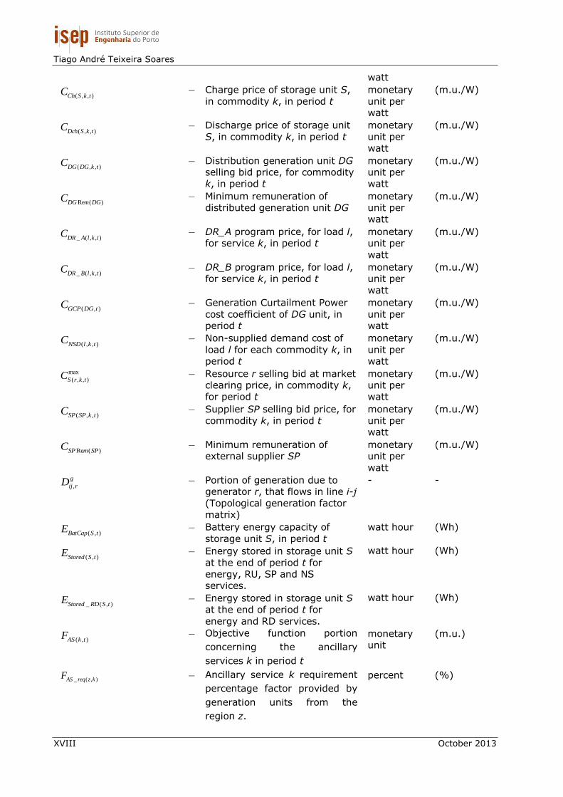
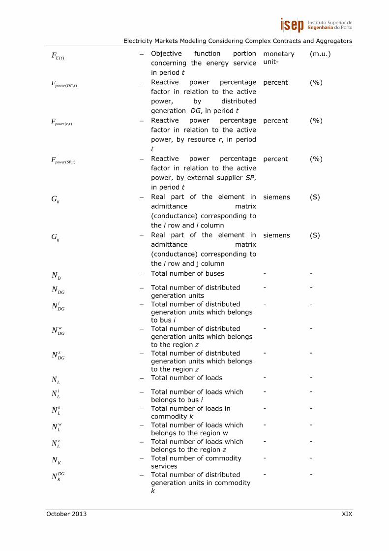
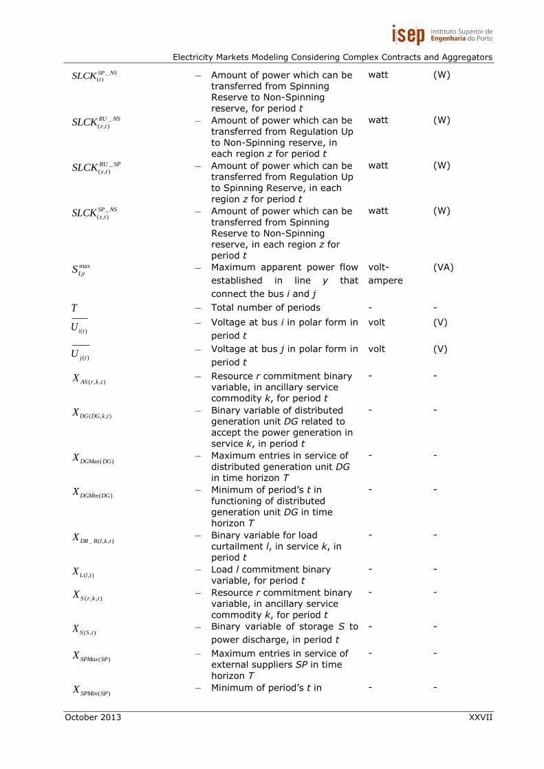
Nomenclature
Notation Description Unit
d
i – Set of nodes supplied directly
from node i
- -
u
i – Set of nodes which supplying
directly node i
- -
t – Elementary period hour (h)
( )c S – Yield of charge process of the
electricity network to the
storage unit S
- (%)
( )d S – Yield of discharge process of
the electricity network to the
storage unit S
- (%)
i – Bus index - -
k – Market component index (1 –
Regulation Down; 2 –
Regulation Up; 3 – Spinning
Reserve; 4 – Non-Spinning
Reserve; 5 – Energy)
- -
l – Load index - -
r – Resource index - -
t – Period index - -
y – Network branch index - -
z – Zone index - -
( )i t – Voltage angle at bus i in period
t
radians (rad)
max
( )i t – Maximum voltage angle at bus i radians (rad)
min
( )i t – Minimum voltage angle at bus i radians (rad)
( )j t – Voltage angle at bus j in period
t
radians (rad)
uA
– Upstream distribution matrix - -
iiB – Imaginary part of the element
in admittance matrix
(susceptance) corresponding to
the i row and i column
siemens (S)
ijB – Imaginary part of the element
in admittance matrix
(susceptance) corresponding to
the i row and j column
siemens (S)
max
( , , )AS r k tC – Resource r selling bid at market
clearing price, in ancillary
service commodity k, for period
t
monetary
unit per
watt
(m.u./W)
max
( , )b l tC – Load l buying at market
clearing price, for period t
monetary
unit per
(m.u./W)
Tiago André Teixeira Soares
XVIII October 2013
watt
( , , )Ch S k tC
– Charge price of storage unit S,
in commodity k, in period t
monetary
unit per
watt
(m.u./W)
( , , )Dch S k tC
– Discharge price of storage unit
S, in commodity k, in period t
monetary
unit per
watt
(m.u./W)
( , , )DG DG k tC – Distribution generation unit DG
selling bid price, for commodity
k, in period t
monetary
unit per
watt
(m.u./W)
Re ( )DG m DGC
– Minimum remuneration of
distributed generation unit DG
monetary
unit per
watt
(m.u./W)
_ ( , , )DR A l k tC – DR_A program price, for load l,
for service k, in period t
monetary
unit per
watt
(m.u./W)
_ ( , , )DR B l k tC – DR_B program price, for load l,
for service k, in period t
monetary
unit per
watt
(m.u./W)
( , )GCP DG tC – Generation Curtailment Power
cost coefficient of DG unit, in
period t
monetary
unit per
watt
(m.u./W)
( , , )NSD l k tC – Non-supplied demand cost of
load l for each commodity k, in
period t
monetary
unit per
watt
(m.u./W)
max
( , , )S r k tC – Resource r selling bid at market
clearing price, in commodity k,
for period t
monetary
unit per
watt
(m.u./W)
( , , )SP SP k tC – Supplier SP selling bid price, for
commodity k, in period t
monetary
unit per
watt
(m.u./W)
Re ( )SP m SPC – Minimum remuneration of
external supplier SP
monetary
unit per
watt
(m.u./W)
,
g
ij rD
– Portion of generation due to
generator r, that flows in line i-j
(Topological generation factor
matrix)
- -
( , )BatCap S tE
– Battery energy capacity of
storage unit S, in period t
watt hour (Wh)
( , )Stored S tE
– Energy stored in storage unit S
at the end of period t for
energy, RU, SP and NS
services.
watt hour (Wh)
_ ( , )Stored RD S tE
– Energy stored in storage unit S
at the end of period t for
energy and RD services.
watt hour (Wh)
( , )AS k tF – Objective function portion
concerning the ancillary
services k in period t
monetary
unit
(m.u.)
_ ( , )AS req z kF
– Ancillary service k requirement
percentage factor provided by
generation units from the
region z.
percent (%)
Electricity Markets Modeling Considering Complex Contracts and Aggregators
October 2013 XIX
( )E tF – Objective function portion
concerning the energy service
in period t
monetary
unit-
(m.u.)
( , )power DG tF
– Reactive power percentage
factor in relation to the active
power, by distributed
generation DG, in period t
percent (%)
( , )power r tF
– Reactive power percentage
factor in relation to the active
power, by resource r, in period
t
percent (%)
( , )power SP tF
– Reactive power percentage
factor in relation to the active
power, by external supplier SP,
in period t
percent (%)
iiG – Real part of the element in
admittance matrix
(conductance) corresponding to
the i row and i column
siemens (S)
ijG – Real part of the element in
admittance matrix
(conductance) corresponding to
the i row and j column
siemens (S)
BN – Total number of buses - -
DGN – Total number of distributed
generation units
- -
i
DGN – Total number of distributed
generation units which belongs
to bus i
- -
w
DGN – Total number of distributed
generation units which belongs
to the region z
- -
z
DGN – Total number of distributed
generation units which belongs
to the region z
- -
LN
– Total number of loads - -
i
LN
– Total number of loads which
belongs to bus i
- -
k
LN
– Total number of loads in
commodity k
- -
w
LN – Total number of loads which
belongs to the region w
- -
z
LN
– Total number of loads which
belongs to the region z
- -
KN – Total number of commodity
services
- -
DG
KN
– Total number of distributed
generation units in commodity
k
- -

Tiago André Teixeira Soares
XX October 2013
R
KN – Total number of resources in
commodity k
- -
S
KN – Total number of storage units
in commodity k
- -
SP
kN – Total number of external
suppliers in commodity k
- -
RN – Total number of resources - -
i
RN – Total number of resources
which belongs to bus i
- -
w
RN – Total number of resources
which belongs to region w
- -
z
RN – Total number of resources
which belongs to region z
- -
i
SN – Total number of storage units S
which belongs to bus i
- -
SPN – Total number of external
suppliers
- -
i
SPN – Total number of external
suppliers which belongs to bus i
- -
w
SPN – Total number of external
suppliers which belongs to the
region w
- -
z
SPN – Total number of external
suppliers which belongs to the
region z
- -
YN – Total number of lines - -
ZN – Total number of regional zones
of ancillary services
- -
( , , )AS r k tP – Resource r scheduled power, in
commodity k (only ancillary
services), for period t
watt (W)
_ ( , , )AS req z k tP
– Active power demand
requirement for the region z, in
ancillary services k, in period t
watt (W)
max
( , , )AS r k tP – Resource r maximum selling
bid power, in commodity k
(only ancillary services), for
period t
watt (W)
min
( , , )AS r k tP – Resource r minimum selling bid
power, in commodity k (only
ancillary services), for period t
watt (W)
( , )b l tP – Load l scheduled power, for
period t
watt (W)
( , )
i
b l tP – Load l scheduled power which
belongs to bus i, for period t
watt (W)
max
( , )b l tP – Load l maximum buying bid
power, for period t
watt (W)
min
( , )b l tP – Load l minimum buying bid
power, for period t
watt (W)
( , )CAP r tP – Maximum power capacity of
resource r, for period t
watt (W)
_ ( , )CAP DG DG tP
– Maximum power capacity of
distributed generation unit DG,
watt (W)

Electricity Markets Modeling Considering Complex Contracts and Aggregators
October 2013 XXI
for period t
_ ( , )CAP SP SP tP
– Maximum power capacity of
external supplier SP, for period
t
watt (W)
( , , )Ch S k tP
– Active power charge of storage
S for commodity k, in period t
watt (W)
( , , )
i
Ch S k tP
– Active power charge of storage
S for commodity k at bus i in
period t
watt (W)
( , , )ChMax S k tP
– Maximum active power charge
of storage S for commodity k in
period t
watt (W)
( , )ChMax S tP
– Maximum global active power
charge of storage S in period t
watt (W)
( , , )Dch S k tP
– Active power discharge of
storage S for commodity k in
period t
watt (W)
( , , )
i
Dch S k tP
– Active power discharge of
storage S for commodity k at
bus i in period t
watt (W)
( , , )DchMax S k tP
– Maximum active power
discharge of storage S for
commodity k in period t
watt (W)
( , )DchMax S tP Maximum global active power
discharge of storage S in period
t.
watt (W)
( , , )DG DG k tP
– Active power generation of
distributed generation unit DG
for each service k, in period t
watt (W)
( , , )
i
DG DG k tP
– Active power generation of
distributed generation unit DG
at bus i, for each service k, in
period t
watt (W)
( , , )
w
DG DG k tP
– Active power generation of
distributed generation unit DG
which belongs to the region w,
for each service k, in period t
watt (W)
( , , )
z
DG DG k tP
– Active power generation of
distributed generation unit DG
which belongs to the region z,
for each service k, in period t
watt (W)
( , , )DGMax DG k tP
– Maximum active power
generation of distributed
generation unit DG, for service
k, in period t
watt (W)
( , , )DGMin DG k tP
– Minimum active power
generation of distributed
generation unit DG, for service
k, in period t
watt (W)
( )DGMin DGP
– Total minimum active power
generation of distributed
generation unit DG
watt (W)
Re ( )DG m DGP
– Total minimum remuneration of
distributed generation unit DG
monetary
unit
(m.u.)

Tiago André Teixeira Soares
XXII October 2013
( )DGVar DGP
– Generation variation of
distributed generator unit DG
between periods
watt (W)
( )Di tP – Active power demand at bus i
in period t
watt (W)
_ ( , , )DR A l k tP
– DR_A active power reduction,
for load l, in service k, in period
t
watt (W)
_ ( , , )
i
DR A l k tP
– DR_A active power reduction,
for load l at bus i, in service k,
in period t
watt (W)
_ ( , , )
w
DR A l k tP
– DR_A active power reduction,
for load l which belongs to the
region w, in service k, in period
t
watt (W)
_ ( , , )
z
DR A l k tP
– DR_A active power reduction,
for load l which belongs to the
region z, in service k, in period
t
watt (W)
_ ( , , )DR AMax l k tP
– DR_A maximum active power
reduction, for load l, in service
k, in period t
watt (W)
_ ( , , )DR B l k tP
– DR_B active power curtailment,
for load l, in service k, in period
t
watt (W)
_ ( , , )
i
DR B l k tP
– DR_B active power curtailment,
for load l at bus i, in service k,
in period t
watt (W)
_ ( , , )
w
DR B l k tP
– DR_B active power curtailment,
for load l which belongs to the
region w, in service k, in period
t
watt (W)
_ ( , , )
z
DR B l k tP
– DR_B active power curtailment,
for load l which belongs to the
region z, in service k, in period
t
watt (W)
_ ( , , )DR BMax l k tP
– DR_B maximum active power
curtailment, for load l, in
service k, in period t
watt (W)
_ lim _ ( , )energy it DG DG tP
– Active power limit obtained by
Bialek factors considering the
energy dispatch, for distributed
generation unit DG, in period t
watt (W)
_ lim ( , )energy it r tP
– Active power limit obtained by
Bialek factors considering the
energy dispatch, for resources
r, in period t
watt (W)
_ lim _ ( , )energy it SP SP tP
– Active power limit obtained by
Bialek factors considering the
energy dispatch, for external
suppliers SP, in period t
watt (W)
_ _ lim _ ( , )energy RU it DG DG tP
– Active power limit obtained by
Bialek factors considering the
energy and Regulation Up
dispatch, for distributed
watt (W)

Electricity Markets Modeling Considering Complex Contracts and Aggregators
October 2013 XXIII
generation unit DG, in period t
_ _ lim ( , )energy RU it r tP
– Active power limit obtained by
Bialek factors considering the
energy and Regulation Up
dispatch, for resources r, in
period t
watt (W)
_ _ lim _ ( , )energy RU it SP SP tP
– Active power limit obtained by
Bialek factors considering the
energy and Regulation Up
dispatch, for external suppliers
SP, in period t
watt (W)
_ _ _ lim _ ( , )energy RU Spinning it DG DG tP
– Active power limit obtained by
Bialek factors considering the
energy, Regulation Up and
Spinning reserve dispatch, for
distributed generation unit DG,
in period t
watt (W)
_ _ _ lim ( , )energy RU Spinning it r tP
– Active power limit obtained by
Bialek factors considering the
energy, Regulation Up and
Spinning reserve dispatch, for
resources r, in period t
watt (W)
_ _ _ lim _ ( , )energy RU Spinning it SP SP tP
– Active power limit obtained by
Bialek factors considering the
energy, Regulation Up and
Spinning reserve dispatch, for
external suppliers SP, in period
t
watt (W)
GP
– Vector of nodal generations watt (W)
( , )GCP DG tP
– Generation Curtailment Power
by DG unit in period t
watt (W)
( , )
i
GCP DG tP
– Generation Curtailment Power
by DG unit at bus i, in period t
watt (W)
GiP
– Active power generation in
node i
watt (W)
( )Gi tP – Active power generation at bus
i in period t
watt (W)
GrP
– Active power generation of
resource r
watt (W)
grossP
– Unknown vector of gross nodal
flows
watt (W)
g
iP
– Unknown gross nodal active
power flow through node i
watt (W)
ijP
– Active power flow in line i-j watt (W)
g
ijP
– Unknown gross line active flow
in line i-j
watt (W)
( )g r
ijP
– Unknown gross line active flow
in line i-j of resources r
watt (W)
( )g SP
ijP
– Unknown gross line active flow
in line i-j of external supplier
SP resource
watt (W)
jP
– Actual total active flow through
node j
watt (W)

Tiago André Teixeira Soares
XXIV October 2013
g
jP
– Unknown gross nodal active
power flow through node j
watt (W)
( , )
i
Load l tP
– Active power demand of load l
at bus i in period t
watt (W)
( )loss tP – Active power losses in period t watt (W)
max
( , )Ly i jP
– Maximum active power flow
established in line y that
connect the bus i and j
watt (W)
( , , )NSD l k tP
– Non-supplied demand for load l
in commodity k in period t
watt (W)
( , , )
i
NSD l k tP
– Non-supplied demand for load l
at bus i in commodity k in
period t
watt (W)
( )Rd tP – Rigid demand for period t watt (W)
_ lim ( , , )req it l k tP
– Active power demand of load l
for ancillary services k, in
period t
watt (W)
_ lim ( , , )
i
req it l k tP
– Active power demand of load l
at bus i for ancillary services k,
in period t
watt (W)
max
_ lim ( , , )req it l k tP
– Maximum active power demand
of load l for ancillary services k,
in period t
watt (W)
_ lim ( , , )
z
req it l k tP
– Active power demand of load l
which belongs to the region z,
for ancillary services k, in
period t
watt (W)
( , , )S r k tP – Resource r scheduled power, in
commodity k, for period t
watt (W)
( , , )
i
S r k tP – Resource r scheduled power, in
commodity k, at bus i for
period t
watt (W)
max
( , , )S r k tP – Resource r maximum selling
bid power, in commodity k, for
period t
watt (W)
min
( , , )S r k tP – Resource r minimum selling bid
power, in commodity k, for
period t
watt (W)
( , , )
w
S r k tP – Resource r scheduled power, in
commodity k, for period t in
region w
watt (W)
( , , )
z
S r k tP – Resource r scheduled power, in
commodity k, for period t in
region z
watt (W)
( , , )SP SP k tP
– Active power acquired from
supplier SP for each service k,
in period t
watt (W)
( , , )
i
SP SP k tP
– Active power acquired from
supplier SP at bus i, for each
service k, in period t
watt (W)
( , , )
w
SP SP k tP
– Active power acquired from
supplier SP which belongs to
the region z, for each service
w, in period t
watt (W)

Electricity Markets Modeling Considering Complex Contracts and Aggregators
October 2013 XXV
( , , )
z
SP SP k tP
– Active power acquired from
supplier SP which belongs to
the region z, for each service k,
in period t
watt (W)
( , , )SPMax SP k tP
– Maximum active power of
external supplier SP for service
k in period t
watt (W)
( )SPMin SPP
– Total minimum active power of
external supplier SP
watt (W)
Re ( )SP m SPP
– Total minimum remuneration of
external supplier SP
monetary
unit
(m.u.)
( )SPVar SPP
– Generation variation of external
supplier SP between periods
watt (W)
( , )
i
b l tQ – Load l scheduled reactive
power at bus i, for period t
volt-
ampere
reactive
(VAr)
( , , )DG DG k tQ
– Reactive power generation of
distributed generation unit DG
for service k in period t
volt-
ampere
reactive
(VAr)
( , , )
i
DG DG k tQ
– Reactive power generation of
distributed generation unit DG
at bus i for service k in period t
volt-
ampere
reactive
(VAr)
( , , )DGMax DG k tQ
– Maximum reactive power
generation of distributed
generation unit DG for service k
in period t
volt-
ampere
reactive
(VAr)
( , , )DGMin DG k tQ
– Minimum reactive power
generation of distributed
generation unit DG for service k
in period t
volt-
ampere
reactive
(VAr)
( )Di tQ – Reactive power demand at bus
i in period t
volt-
ampere
reactive
(VAr)
( )Gi tQ – Reactive power generation at
bus i in period t
volt-
ampere
reactive
(VAr)
( , , )
i
Load l k tQ
– Reactive power demand of load
l at bus i for commodity k in
period t
volt-
ampere
reactive
(VAr)
( , , )
i
NSD l k tQ
– Reactive non-supplied demand
for load l in commodity k in
period t
volt-
ampere
reactive
(VAr)
( , , )S r k tQ – Resource r scheduled reactive
power, in commodity k, for
period t
volt-
ampere
reactive
(VAr)
( , , )
i
S r k tQ – Resource r scheduled reactive
power, in commodity k, at bus i
for period t
volt-
ampere
reactive
(VAr)
max
( , , )S r k tQ – Resource r maximum selling
bid reactive power, in
volt-
ampere
(VAr)

Tiago André Teixeira Soares
XXVI October 2013
commodity k, for period t reactive min
( , , )S r k tQ – Resource r minimum selling bid
reactive power, in commodity
k, for period t
volt-
ampere
reactive
(VAr)
( , , )SP SP k tQ
– Reactive power acquired from
supplier SP in service k in
period t
volt-
ampere
reactive
(VAr)
( , , )
i
SP SP k tQ
– Reactive power generation of
external supplier SP at bus i,
for service k, in period t
volt-
ampere
reactive
(VAr)
( , , )SPMax SP k tQ
– Maximum reactive power of
external supplier SP in service k
in period t
volt-
ampere
reactive
(VAr)
( , )AS k tR – Ancillary service commodity k
active power requirement, for
period t
watt (W)
max
( , )AS k tR – Ancillary service commodity k
maximum required power, for
period t
watt (W)
min
( , )AS k tR – Ancillary service commodity k
minimum required power, for
period t
watt (W)
( , )
z
AS k tR – Ancillary service in region z for
commodity k active power
requirement, for period t
watt (W)
max;
( , )
z
AS k tR – Ancillary service in region z for
commodity k maximum
required power, for period t
watt (W)
min;
( , )
z
AS k tR – Ancillary service in region z for
commodity k minimum
required power, for period t
watt (W)
( , )k tRLXD – Commodity k relaxation down
variable to apply violation
penalties, for period t
watt (W)
( , , )z k tRLXD – Relaxation down variable to
apply violation penalties in each
identified region z, for each
ancillary service k, in period t
watt (W)
( , )k tRLXU – Commodity k relaxation up
variable to apply violation
penalties, for period t
watt (W)
( , , )z k tRLXU – Relaxation up variable to apply
violation penalties in each
identified region z, for each
ancillary service k, in period t
watt (W)
_
( )
RU NS
tSLCK – Amount of power which can be
transferred from Regulation Up
to Non-Spinning reserve, for
period t
watt (W)
_
( )
RU SP
tSLCK – Amount of power which can be
transferred from Regulation Up
to Spinning Reserve, for period
t
watt (W)
Electricity Markets Modeling Considering Complex Contracts and Aggregators
October 2013 XXVII
– Amount of power which can be
transferred from Spinning
Reserve to Non-Spinning
reserve, for period t
watt (W)
_
( , )
RU NS
z tSLCK – Amount of power which can be
transferred from Regulation Up
to Non-Spinning reserve, in
each region z for period t
watt (W)
_
( , )
RU SP
z tSLCK – Amount of power which can be
transferred from Regulation Up
to Spinning Reserve, in each
region z for period t
watt (W)
_
( , )
SP NS
z tSLCK – Amount of power which can be
transferred from Spinning
Reserve to Non-Spinning
reserve, in each region z for
period t
watt (W)
max
LyS – Maximum apparent power flow
established in line y that
connect the bus i and j
volt-
ampere
(VA)
T – Total number of periods - -
( )i tU – Voltage at bus i in polar form in
period t
volt (V)
( )j tU – Voltage at bus j in polar form in
period t
volt (V)
( , , )AS r k tX – Resource r commitment binary
variable, in ancillary service
commodity k, for period t
- -
( , , )DG DG k tX
– Binary variable of distributed
generation unit DG related to
accept the power generation in
service k, in period t
- -
( )DGMax DGX
– Maximum entries in service of
distributed generation unit DG
in time horizon T
- -
( )DGMin DGX
– Minimum of period’s t in
functioning of distributed
generation unit DG in time
horizon T
- -
_ ( , , )DR B l k tX
– Binary variable for load
curtailment l, in service k, in
period t
- -
( , )L l tX – Load l commitment binary
variable, for period t
- -
( , , )S r k tX – Resource r commitment binary
variable, in ancillary service
commodity k, for period t
- -
( , )S S tX
– Binary variable of storage S to
power discharge, in period t
- -
( )SPMax SPX
– Maximum entries in service of
external suppliers SP in time
horizon T
- -
( )SPMin SPX
– Minimum of period’s t in - -
_
( )
SP NS
tSLCK

Tiago André Teixeira Soares
XXVIII October 2013
functioning of external supplier
SP in time horizon T
( )i tV – Voltage magnitude at bus i in
period t
volt (V)
max
( )i tV – Maximum voltage magnitude at
bus i
volt (V)
min
( )i tV – Minimum voltage magnitude at
bus i
volt (V)
( )j tV – Voltage magnitude at bus j in
period t
volt (V)
( , )RLXD k tW – Relaxation down penalty of
commodity k, for period t
monetary
unit per
watt
(m.u./W)
( , , )RLXD z k tW – Relaxation down penalty of
region z, in commodity k, for
period t
monetary
unit per
watt
(m.u./W)
( , )RLXU k tW – Relaxation up penalty of
commodity k, for period t
monetary
unit per
watt
(m.u./W)
( , , )RLXD z k tW – Relaxation up penalty of region
z, in commodity k, for period t
monetary
unit per
watt
(m.u./W)
( , )S S tY
– Binary variable of storage S
related to power charge, in
period t
- -
ijy – Series admittance of line that
connect the bus i and j in polar
form
siemens (S)
_Sh iy – Shunt admittance of line
connected in the bus i in polar
form
siemens (S)

Electricity Markets Modeling Considering Complex Contracts and Aggregators
October 2013 XXIX
Contents:
Acknowledgements .......................................................................................... VII
Abstract .......................................................................................................... IX
Resumo ........................................................................................................... XI
Acronyms ...................................................................................................... XIII
Nomenclature ............................................................................................... XVII
List of Figures ............................................................................................ XXXIII
List of Tables............................................................................................. XXXVII
1. Introduction .................................................................................................. 3
1.1. Background and Motivation ..................................................................... 3
1.2. Objectives ............................................................................................. 8
1.3. Related Projects and Publications ............................................................. 9
1.4. Organization of the Dissertation ............................................................. 10
2. Markets Overview ........................................................................................ 13
2.1. BETTA / N2EX ...................................................................................... 13
2.1.1. Forward and Futures Contract Markets ........................................... 15
2.1.2. Short-term Bilateral Markets ......................................................... 15
2.1.3. Balancing Mechanism ................................................................... 15
2.1.3.1. Ancillary Services ............................................................. 16
2.1.3.2. Imbalance Settlement ....................................................... 18
2.2. CAISO ................................................................................................ 18
2.2.1. Pre-Market ................................................................................. 19
2.2.2. Day-Ahead Market ....................................................................... 21
2.2.3. Real-Time Market ........................................................................ 23
2.2.4. Ancillary Services Market .............................................................. 24
2.2.4.1. Ancillary Service Cascading ............................................... 25
2.2.4.2. Ancillary Services Regions ................................................. 26
2.2.4.3. Ancillary Services Requirements ......................................... 27
2.2.5. Post-Market ................................................................................ 27
Tiago André Teixeira Soares
XXX October 2013
2.3. NASDAQ OMX Commodities Europe/Nord pool ......................................... 28
2.3.1. Financial Market .......................................................................... 29
2.3.2. Elspot – Day-Ahead Market........................................................... 30
2.3.2.1. Bidding Areas .................................................................. 31
2.3.2.2. System Price ................................................................... 33
2.3.2.3. Area Price ....................................................................... 34
2.3.3. Elbas – Intraday Market ............................................................... 35
2.3.4. Balancing Market ......................................................................... 35
2.4. MIBEL ................................................................................................. 37
2.4.1. Financial Markets......................................................................... 38
2.4.2. Day-Ahead Market ....................................................................... 38
2.4.2.1. Market Development Sequence .......................................... 39
2.4.2.2. Market Splitting ............................................................... 40
2.4.3. Intraday Market .......................................................................... 41
2.4.4. Ancillary Services Market .............................................................. 42
2.5. Conclusion .......................................................................................... 44
3. AS Market models ........................................................................................ 49
3.1. Introduction ........................................................................................ 49
3.2. Ancillary Services Market model ............................................................. 56
3.2.1. Problem Description ..................................................................... 56
3.2.2. Mathematical Formulation ............................................................ 57
3.3. Energy and AS Joint Market model ......................................................... 60
3.3.1. Problem Description ..................................................................... 60
3.3.2. Mathematical Formulation ............................................................ 61
3.4. Joint Market model considering AS bidding regions ................................... 62
3.4.1. Problem Description ..................................................................... 63
3.4.2. Mathematical Formulation ............................................................ 64
3.5. Joint Market model considering Bialek coefficients .................................... 67
3.5.1. Problem Introduction ................................................................... 68
3.5.2. Problem Description ..................................................................... 69

Electricity Markets Modeling Considering Complex Contracts and Aggregators
October 2013 XXXI
3.5.3. Mathematical Formulation............................................................. 71
3.6. Joint Market model applied by VPP ......................................................... 73
3.6.1. Problem Description ..................................................................... 74
3.6.2. Mathematical Formulation............................................................. 75
3.7. Conclusions ......................................................................................... 84
4. Case Studies ............................................................................................... 89
4.1. Introduction ........................................................................................ 89
4.2. Case study 1 – Ancillary Services Market model ....................................... 91
4.2.1. Outline ....................................................................................... 92
4.2.2. Results ....................................................................................... 92
4.2.2.1. Scenario 1 – Baseline case ................................................ 92
4.2.2.2. Scenario 2 – Relaxation variables ....................................... 93
4.2.2.3. Scenario 3 – Ancillary Services Cascade process .................. 94
4.2.3. Results analysis........................................................................... 96
4.3. Case study 2 – Energy and AS Joint Market model ................................... 96
4.3.1. Outline ....................................................................................... 97
4.3.2. Results ....................................................................................... 97
4.3.2.1. Scenario 1 – Energy and AS markets (Not-joint) .................. 97
4.3.2.2. Scenario 2 – Energy and AS joint market ........................... 100
4.3.2.3. Comparison of scenarios .................................................. 102
4.3.3. Results analysis.......................................................................... 103
4.4. Case study 3 – AS bidding regions......................................................... 104
4.4.1. Outline ...................................................................................... 104
4.4.2. Results ...................................................................................... 107
4.4.2.1. Scenario 1 – Energy and AS in the same direction ............... 107
4.4.2.2. Scenario 2 – Energy and AS in opposite direction ................ 109
4.4.2.3. Scenario 3 – Energy and AS cascade optimization ............... 111
4.4.3. Results analysis.......................................................................... 111
4.5. Case study 4 – Bialek coefficients .......................................................... 113
4.5.1. Outline ...................................................................................... 113

Tiago André Teixeira Soares
XXXII October 2013
4.5.2. Results ...................................................................................... 115
4.5.2.1. Scenario 1 – Baseline case ............................................... 115
4.5.2.2. Scenario 2 – Base case with Bialek factors ......................... 116
4.5.3. Results analysis ......................................................................... 117
4.6. Case study 5 – Joint Market model applied by VPP .................................. 118
4.6.1. Outline ...................................................................................... 118
4.6.2. Results ...................................................................................... 125
4.6.2.1. Scenario 1 – Baseline case ............................................... 125
4.6.2.2. Scenario 2 – Base case with different bidding regions .......... 129
4.6.2.3. Scenario 3 – DR resources and RLXD variable on AS dispatch134
4.6.2.4. Scenario 4 – Storage units on AS dispatch ......................... 139
4.6.2.5. Scenario 5 – Complex Contracts ....................................... 143
4.6.3. Results analysis ......................................................................... 150
4.7. Conclusions ........................................................................................ 152
5. Conclusions and Future Work ....................................................................... 157
5.1. Main conclusions and contributions ........................................................ 157
5.2. Perspectives for future work ................................................................. 160
References ..................................................................................................... 165
Annexes ........................................................................................................... A
Annex A ................................................................................................... A.1
Annex B ................................................................................................... B.1
Annex C ................................................................................................... C.1

Electricity Markets Modeling Considering Complex Contracts and Aggregators
October 2013 XXXIII
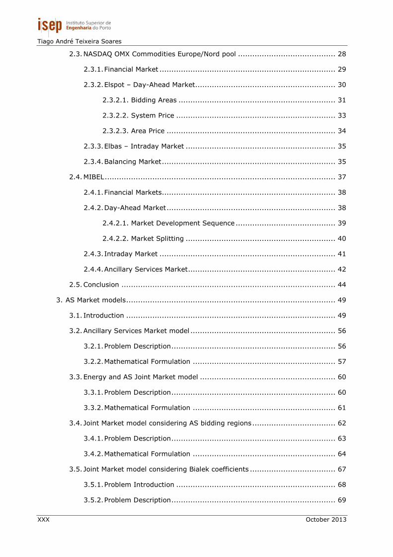
List of Figures
Figure 1.1 – Ancillary services classification [EURELECTRIC-2000]. ............................ 4
Figure 1.2 – The VPP concept from a technical and market standpoint [Morais-
2010b]. .............................................................................................................. 7
Figure 2.1 – BETTA market structure overview [NGET-2012a]. .................................. 14
Figure 2.2 – CAISO market timeline overview [CAISO-2011a]. .................................. 20
Figure 2.3 – Day-ahead CAISO market timeline [CAISO-2011a]. ............................... 23
Figure 2.4 – Ancillary services cascading process. .................................................... 25
Figure 2.5 – CAISO ancillary services regions map [CAISO-2011d]. ........................... 26
Figure 2.6 –Nord Pool market timeline overview [NordPool-2012a]. ........................... 29
Figure 2.7 – Nord Pool financial contracts functioning [NordPool-2012e]. .................... 30
Figure 2.8 – Elspot timeline [NordPool-2012a]. ....................................................... 31
Figure 2.9 – Nord pool market areas map [NordPool-2012g]. .................................... 32
Figure 2.10 – System price determination through purchase and sale curves
intersection [NordPool-2012f]. .............................................................................. 33
Figure 2.11 – Surplus and deficit area price curves determination [NordPool-2012f]. ... 34
Figure 2.12 – Mechanisms for balancing the power system [Nordel-2008]. ................. 36
Figure 2.13 – MIBEL market timeline overview, adapted from [Pereira-2009]. ............. 38
Figure 2.14 – Symmetric market clearing price determination [Pereira-2009]. ............ 40
Figure 2.15 – Intraday market structure sessions [MIBEL-2009]. ............................... 41
Figure 3.1 – MASCEM architecture in [Pinto-2012]. .................................................. 50
Figure 3.2 – Updated MASCEM architecture............................................................. 54
Figure 3.3 – AS market diagram. ........................................................................... 56
Figure 3.4 – Energy and AS joint market diagram. ................................................... 60
Figure 3.5 – Energy and AS joint market diagram considering AS bidding regions. ....... 63
Figure 3.6 – Proportional sharing principle, adapted from [Bialek-1997]. .................... 68
Figure 3.7 – Energy and AS joint market diagram considering Bialek topological
factors. .............................................................................................................. 70
Figure 3.8 – Energy and AS joint market diagram in distribution systems. .................. 74
Figure 4.1 – Energy market clearing price in scenario 1 of energy and AS joint
model. ............................................................................................................... 98
Figure 4.2 – Ancillary services dispatch in scenario 1 of energy and AS joint model. ..... 99
Figure 4.3 – Ancillary services dispatch with cascading mechanism in scenario 1 of
energy and AS joint model. ................................................................................... 100
Figure 4.4 – Energy market clearing price in scenario 2 of energy and AS joint
model. ............................................................................................................... 101
Figure 4.5 – Ancillary services dispatch in scenario 2 of energy and AS joint model. ..... 102

Tiago André Teixeira Soares
XXXIV October 2013
Figure 4.6 – 4-buses network with four branches [Wu-2004]. ................................... 105
Figure 4.7 – Operation costs and execution time in the contingency cases. ................. 109
Figure 4.8 – Power flow of energy and AS dispatch. ................................................. 110
Figure 4.9 – 7-buses network. ............................................................................... 113
Figure 4.10 – 33-buses distribution network configuration in 2040 scenario [Faria-
2010]. ................................................................................................................ 120
Figure 4.11 – AS regions on the 33-buses distribution network. ................................ 122
Figure 4.12 – Energy dispatch by type of resource, in scenario 1 of joint market
model applied by VPP. .......................................................................................... 126
Figure 4.13 – Energy dispatch by distributed generation technologies contribution, in
scenario 1 of joint market model applied by VPP. ..................................................... 126
Figure 4.14 – Type of DR for energy dispatch, in scenario 1 of joint market model
applied by VPP. ................................................................................................... 127
Figure 4.15 – Regulation down dispatch, in scenario 1 of joint market model applied
by VPP. .............................................................................................................. 128
Figure 4.16 – Regulation up dispatch, in scenario 1 of joint market model applied by
VPP. ................................................................................................................... 128
Figure 4.17 – Spinning reserve dispatch, in scenario 1 of joint market model applied
by VPP. .............................................................................................................. 129
Figure 4.18 – Non-spinning reserve dispatch, in scenario 1 of joint market model
applied by VPP. ................................................................................................... 129
Figure 4.19 – Energy dispatch by type of resource, in scenario 2 of joint market
model applied by VPP. .......................................................................................... 130
Figure 4.20 – Overall regions regulation up dispatch. ............................................... 131
Figure 4.21 – Regulation up dispatch by each region. ............................................... 131
Figure 4.22 – Overall regions spinning reserve dispatch. .......................................... 132
Figure 4.23 – Spinning reserve dispatch by each region. .......................................... 133
Figure 4.24 – Overall regions non-spinning reserve dispatch. .................................... 133
Figure 4.25 – Non-spinning reserve dispatch by each region. .................................... 134
Figure 4.26 – Regulation up dispatch considering DR resources. ................................ 135
Figure 4.27 – Types of DR dispatch in each region for RU service. ............................. 136
Figure 4.28 – Types of DR dispatch in each region for SP service. .............................. 136
Figure 4.29 – SP dispatch in region 2, by each resource. .......................................... 137
Figure 4.30 – NS dispatch by network regions, considering DR resources. .................. 138
Figure 4.31 – Types of DR dispatch in each region for NS service. ............................. 139
Figure 4.32 – Regulation down dispatch considering storage units. ............................ 140
Figure 4.33 – Regulation up dispatch considering storage units by network regions. .... 140

Electricity Markets Modeling Considering Complex Contracts and Aggregators
October 2013 XXXV
Figure 4.34 – Spinning reserve dispatch considering storage units by network
regions. .............................................................................................................. 141
Figure 4.35 – Storage charge and discharge share by network regions for SP
dispatch. ............................................................................................................ 142
Figure 4.36 – Non-spinning reserve dispatch considering storage units by network
regions. .............................................................................................................. 142
Figure 4.37 – Storage charge and discharge share by network regions for NS
dispatch. ............................................................................................................ 143
Figure 4.38 – Dispatched energy and operation cost for contract type 1. .................... 144
Figure 4.39 – Dispatched energy and operation cost for contract type 2. .................... 146
Figure 4.40 – Dispatched energy and operation costs for contract type 3. ................... 147
Figure 4.41 – Number of working periods for contract type 4. ................................... 147
Figure 4.42 – Dispatched energy and operation cost for contact type 4. ..................... 148
Figure 4.43 – Maximum number of entries into service. ............................................ 149
Figure 4.44 – Dispatched energy and operation cost for contract type 5. .................... 149
Figure C.1 – Percentage of power given by each kind of resource for energy
dispatch, in scenario 1 of joint market model applied by VPP. .................................... C.6
Figure C.2 – Percentage of DG contribution for energy dispatch, in scenario 1 of joint
market model applied by VPP. ............................................................................... C.6
Figure C.3 – Type of DR contribution in energy dispatch, in scenario 1 of joint market
model applied by VPP. .......................................................................................... C.7
Figure C.4 – Resource contribution for RD, RU, SP and NS dispatch, in scenario 1 of
joint market model applied by VPP. ........................................................................ C.8
Figure C.5 – Resource contribution for energy dispatch, in scenario 2 of joint market
model applied by VPP. .......................................................................................... C.8
Figure C.6 – Energy dispatch by DG technologies contribution, in scenario 2 of joint
market model applied by VPP. ............................................................................... C.8
Figure C.7 – Percentage of DG contribution for energy dispatch, in scenario 2 of joint
market model applied by VPP. ............................................................................... C.9
Figure C.8 – Type of DR for energy dispatch, in scenario 2 of joint market model
applied by VPP. ................................................................................................... C.9
Figure C.9 – Percentage of DR contribution for energy dispatch, in scenario 2 of joint
market model applied by VPP. ............................................................................... C.10
Figure C.10 - Regulation down dispatch, in scenario 2 of joint market model applied
by VPP. .............................................................................................................. C.10
Figure C.11 – DG and external supplier dispatch for regulation up service, in scenario
2 of joint market model applied by VPP. ................................................................. C.11

Tiago André Teixeira Soares
XXXVI October 2013
Figure C.12 – DG and external supplier dispatch for spinning reserve service, in
scenario 2 of joint market model applied by VPP. ..................................................... C.11
Figure C.13 – Regulation down dispatch, in scenario 3 of joint market model applied
by VPP. .............................................................................................................. C.12
Figure C.14 – Resource contribution for regulation down service, in scenario 3 of
joint market model applied by VPP. ........................................................................ C.12
Figure C.15 – Regulation up global dispatch, in scenario 3 of joint market model
applied by VPP. ................................................................................................... C.13
Figure C.16 – Spinning reserve global dispatch, in scenario 3 of joint market model
applied by VPP. ................................................................................................... C.13
Figure C.17 – Spinning reserve dispatch by network region, in scenario 3 of joint
market model applied by VPP. ............................................................................... C.14
Figure C.18 – SP reserve dispatch for region 1, in scenario 3 of joint market model
applied by VPP. ................................................................................................... C.14
Figure C.19 – SP reserve dispatch for region 3, in scenario 3 of joint market model
applied by VPP. ................................................................................................... C.15
Figure C.20 – SP reserve dispatch for region 4, in scenario 3 of joint market model
applied by VPP. ................................................................................................... C.15
Figure C.21 – Non-spinning reserve global dispatch, in scenario 3 of joint market
model applied by VPP. .......................................................................................... C.16
Figure C.22 – Energy dispatch, in scenario 4 of joint market model applied by VPP. ..... C.16
Figure C.23 – Consumption details of energy dispatch, in scenario 4 of joint market
model applied by VPP. .......................................................................................... C.17
Figure C.24 – Storage charge and discharge contribution by network regions for RU
service. .............................................................................................................. C.17

Electricity Markets Modeling Considering Complex Contracts and Aggregators
October 2013 XXXVII
List of Tables
Table 2.1 – Intraday market session schedules [OMIE-2012b]................................... 41
Table 2.2 – Ancillary services summary. ................................................................. 44
Table 3.1 – Market models characterization. ........................................................... 52
Table 4.1 – Case studies characterization. .............................................................. 90
Table 4.2 – Ancillary services dispatch in scenario 1 of AS model. .............................. 93
Table 4.3 – AS dispatch considering relaxation variables........................................... 94
Table 4.4 – Ancillary services dispatch considering AS cascade mechanism. ................ 95
Table 4.5 – AS dispatch comparison related to scenarios 1 and 3 of AS model. ............ 96
Table 4.6 – Energy dispatch in scenario 1 of energy and AS joint model. .................... 98
Table 4.7 – Residual maximum power. ................................................................... 99
Table 4.8 – Energy and AS joint market dispatch. .................................................... 101
Table 4.9 – Costs and market clearing price comparison related to scenario 1 and 2
of energy and AS joint model. ............................................................................... 102
Table 4.10 – 4-buses network features. .................................................................. 105
Table 4.11 – Energy and AS bids. .......................................................................... 106
Table 4.12 – Energy dispatch by operation context in scenario 1 of joint market
model considering AS bidding regions. ................................................................... 107
Table 4.13 – Base case results of energy and AS in same direction. ........................... 108
Table 4.14 – G1 and G2 outage results. .................................................................. 108
Table 4.15 – Branch 1-4 outage results. ................................................................. 108
Table 4.16 – Base case results of energy and AS in opposite direction. ....................... 110
Table 4.17 – AS cascade results. ........................................................................... 111
Table 4.18 – 7-buses features. .............................................................................. 114
Table 4.19 – Generators input data. ....................................................................... 114
Table 4.20 – Energy and AS requirements. ............................................................. 114
Table 4.21 – Energy and AS dispatch in scenario 1 of joint market model considering
Bialek coefficients. ............................................................................................... 115
Table 4.22 – Power flow of energy service and joint market, in scenario 1 of joint
market model considering Bialek coefficients. .......................................................... 116
Table 4.23 – Energy and AS dispatch in scenario 2 of joint market model considering
Bialek coefficients. ............................................................................................... 116
Table 4.24 – Power flow considering Bialek topological factors. .................................. 117
Table 4.25 – Energy and AS upper limits in scenario 1 of joint market model applied
by VPP. .............................................................................................................. 120
Table 4.26 – AS requirements in scenario 1 of joint market model applied by VPP. ...... 121
Tiago André Teixeira Soares
XXXVIII October 2013
Table 4.27 – AS requirements by regions, in scenario 2 of joint market model applied
by VPP. .............................................................................................................. 122
Table 4.28 – Energy and AS upper limits in scenario 2 of joint market model applied
by VPP. .............................................................................................................. 123
Table 4.29 – AS requirements by region, in scenario 3 of joint market model applied
by VPP. .............................................................................................................. 123
Table 4.30 – Energy and AS upper limits, in scenario 3 of joint market model applied
by VPP. .............................................................................................................. 124
Table 4.31 – Demand response types for each service.............................................. 124
Table 4.32 – AS requirements by region in scenario 4 of joint market model applied
by VPP. .............................................................................................................. 125
Table A.1 – Input data for scenario 1 of AS model. .................................................. A.3
Table A.2 – Input data for scenario 2 of AS model. .................................................. A.3
Table A.3 – Input data for scenario 3 of AS model. .................................................. A.3
Table B.1 – Energy and AS joint market data. ......................................................... B.3
Table B.2 – AS market results in scenario 1 of joint model. ....................................... B.3
Table B.3 – AS market results with cascading mechanism in scenario 1 of joint
model. ............................................................................................................... B.4
Table C.1 – Branch data of the 33-bus distribution network. ..................................... C.3
Table C.2 – Distributed generation and external suppliers resources bids features. ...... C.4
Table C.3 – DG and external suppliers bids for RD and RU services. ........................... C.4
Table C.4 – DG and external suppliers bids for SP and NS service. ............................. C.4
Table C.5 – Demand response bids for energy service. ............................................. C.5
Table C.6 – Storage features. ................................................................................ C.5
Table C.7 – AS charge and discharge storage prices. ................................................ C.5

Electricity Markets Modeling Considering Complex Contracts and Aggregators
October 2013 1
Chapter 1
Introduction


Electricity Markets Modeling Considering Complex Contracts and Aggregators
October 2013 3
1. Introduction
This chapter exposes the motivation, the objectives and the contribution of the work
developed in the scope of this dissertation. The importance of ancillary services in the
context of the present and future power systems is explained.
Here it is also presented how the dissertation is organized, as well as its contribution
to the field of study.
1.1. Background and Motivation
The restructuring and consequent deregulation of the electricity sector imposes new
methodologies in the operation and management of Power Systems (PS) [Shahidehpour-
2002]. Therefore, the collaboration between regions and countries is increasingly crucial for
the proper functioning of the overall electricity market. In the last decade, there has been a
continued restructuring of competitive electricity markets based on the electricity sector’s
restructuring process, which introduced a new paradigm in its functioning, particularly in
terms of generation and trading, which began to unfold in a competitive environment. Thus,
the electricity started to be seen as a marketable product resulting in a set of transactions
between players, managed by coordination entities, namely the Market Operator (MO) and
System Operator (SO) and regulatory authorities which supervise the functioning of the
system [Gomes-2007, Shahidehpour-2002].
In this context, to guarantee the good functioning of power systems in a market
environment, adequate Ancillary Services (AS) requirements must be defined. Throughout
their existence, ancillary services have been defined in several different ways in the USA
and in Europe according to the evolution of power systems. In 1995 Kirby et al. defined
ancillary services as “those functions performed by the electrical generating, transmission,
system-control, and distribution system equipment and people that support the basic
services of generating capacity, energy supply, and power delivery” [Kirby-1995]. In the
same year, the Federal Energy Regulatory Commission (FERC) defined ancillary services as
“those services necessary to support the transmission of electric power from seller to
purchaser given the obligations of control areas and transmitting utilities within those
control areas to maintain reliable operations of the interconnected transmission system”
[FERC-1995]. In 2000, EURELECTRIC stated that ancillary services are “those services
provided by generation, transmission and control equipment which are necessary to support
the transmission of electric power from producer to purchaser” [EURELECTRIC-2000]. A few
years later, the same EURELECTRIC established a definition for AS accepted by most of the
countries and the wider scientific community: “Ancillary services are all services required by
the transmission or distribution system operator to enable them to maintain the integrity

Tiago André Teixeira Soares
4 October 2013
and stability of the transmission or distribution system as well as the power quality”
[EURELECTRIC-2004, Braun-2007].
Multiple ways to classify the AS have been developed. The more general AS
classification is based on systems needs in terms of operating requirements. The system
needs of each ancillary service are determined by the Independent System Operator (ISO)
in accordance with specific system operation standards of the market [EURELECTRIC-2000].
AS are classified into three distinct categories of their contribution to specific system
requirements, as illustrated in Figure 1.1.
Figure 1.1 – Ancillary services classification [EURELECTRIC-2000].
The frequency control consists in maintaining the frequency within the given margins
by continuous modulation of active power and it can be obtained through the following
ancillary services [EURELECTRIC-2000, EURELECTRIC-2004]: Automatic Generation
Control; primary regulation; secondary regulation; high frequency response; spinning
reserve, non-spinning reserve; and emergency control auctions.
The voltage control consists in maintaining voltage through injecting or absorbing
reactive power by means of synchronous or static compensation. In general, the voltage
control is organized into a three-level hierarchy [Rebours-2007]: primary, secondary, and
tertiary voltage control.
The system restart consists in sufficient electricity sources that would be available to
restart the power system after a partial or complete blackout. This is mainly obtained
through the restoration capability which is the capability of a generation unit to start up
without an external power supply [EURELECTRIC-2000, EURELECTRIC-2004].

Electricity Markets Modeling Considering Complex Contracts and Aggregators
October 2013 5
During the restructuring of the electric sector around the world, several models of
energy and AS markets have been developed. An aspect shared by several electricity
markets is the existence of a system operator, which can be an ISO, a Transmission System
Operator (TSO) or a Distribution System Operator (DSO), responsible for the reliable real-
time operation and control of the transmission / distribution system which enables the
efficient operation of a competitive energy and AS market [Oren-2001, Papalexopoulos-
2001].
Currently, some electricity markets have been adopting the concept of optimizing
the energy market jointly with the AS market. This optimization model is often called as the
energy and AS joint market. This model, comparing with the traditional model, promotes
economic efficiency of the market reaching to interesting results [Soares-2011]. However,
the joint model used in the real markets does not guarantee a feasible solution. The main
problem is that the model do not consider the impact that the AS may have on network
congestion.
In this context, it becomes essential to develop methodologies to solve the problem
in order to ensure the smooth operation of the system. The methodologies should ensure
the feasibility and reliability of the system and guarantee the quality of power service within
the parameters defined in each market.
An approach that may partially solve the feasibility of the energy and AS joint
market is the AS procurement by areas/regions of the network. The consideration of AS
procurement by network regions allows acquiring and ensuring AS with higher quality at all
points of the network, especially in consumer locations distant from the point of energy
generation. In this way, the regional AS procurement is an approach that may results in
more efficient distribution of reserves, in order to improve the reliability in the event of a
contingency occurring anywhere in the system [Wu-2004].
An approach to solve the problem of feasibility of the energy and AS joint market is
the use of distribution factors (namely the Bialek topological distribution factors) to limit the
energy production of generation units that may cause congestion on the network lines. This
approach involves a complex, sequential and hierarchical analysis of the ancillary services
traded in the market. This approach presents feasible results of the system, avoiding any
network congestion which may occur in traditional approaches.
Based on these assumptions, the operation of electricity and AS markets can
considers different models which determine the course of action of the players involved.
Thus, these models are crucial for the strategic management of sellers and buyers who
operate within each market, particularly for the spot market [Vale-2011]. Decisions on bids
to be submitted must be supported by adequate decision support systems, such as MASCEM
– a Multi-Agent Simulator of Competitive Electricity Markets or EMCAS – Electricity Market
Complex Adaptive System. These systems are based on simulation and they must be able
Tiago André Teixeira Soares
6 October 2013
to model the complex and dynamic nature of the energy and AS market, as well as the
players who act in them, how they interact and how they react to the rules used and to the
actions of other players [Praça-2003, Pinto-2011a]. Furthermore, market simulation
systems must increasingly take into account the players related to new concepts of
generation and operation in the scope of the Smart Grid (SG) paradigm. In this context,
power systems have experienced many changes, mainly due to the increasing introduction
of Distributed Energy Resources (DER) [Thong-2007, Scalari-2008], namely Distributed
Generation (DG) [Morais-2010a], storage units, Electrical Vehicles (EV) with gridable
capability (V2G) [Sousa-2011, Luo-2012] and Demand Response (DR) [Schisler-2008,
Faria-2011]. The introduction of this kind of resources in the distribution systems requires
new management and new operation methods because the methodologies currently used
are not able to deal with the challenges resulting from the new paradigm in distribution
systems operation. In this way, a wide variety of resources may be useful to enable a more
efficient resources’ management by the ISO, DSO and /or Virtual Power Players (VPP) in the
demand supply. Moreover, the DER may be useful at the AS provision level. That is, DER
may participate at a controlled cost in specific conditions, like when there is surplus or
shortage generation in the power system balance.
VPPs that aggregate a set of resources in a given network zone, including DG based
on renewable sources, storage systems, DR and EV, are very relevant players that allow
midsize, small and micro players to act in a competitive environment of energy and AS
markets [Pinto-2011a, Vale-2010].
The VPP will play a major role in the context of SG, aggregating a set of resources
with the objective of maximizing their value and the aggregated players’ profit.
Figure 1.2 illustrates the VPP concept and its possible services from a technical and a
market standpoint. A variety of DER dispersed throughout the distribution network is
combined via communication networks by an aggregator within the framework of a VPP. A
set of services can be provided comprising the participation on electricity markets, as well
as the AS provision.

Electricity Markets Modeling Considering Complex Contracts and Aggregators
October 2013 7
Figure 1.2 – The VPP concept from a technical and market standpoint [Morais-2010b].
In the new paradigm of power systems operation, ISO will consider the existence of
VPPs able to aggregate all kind of small size distributed energy resources, which are unable
to individually engage themselves on the market. This implies that the AS procurement by
the VPP is targeted to the distribution systems. Thus, the VPP should consider the
establishment of complex contracts with the DER in order to ensure reserves levels and
quality of AS appropriate to the needs of the distribution system.
In this context, the operation and control of future distribution network and smart
grid is expected to use the following ancillary services provided by the DSO or by the VPP:
Frequency Control; Voltage Control; Congestion Management; Optimization of Grid Losses
and Fault-Ride-Through Capability service [Braun-2007, Buehner-2010]. The Fault-Ride-
Through Capability service is characterized by the use of this kind of resources through the
VPP management to provide voltage support in case of voltage disturbances in order to
improve the reliability of supply, resulting in an increase of the power quality levels.
This dissertation presents a work that addresses some of the AS problems
mentioned in this subchapter, and it contributes to the continuous development of existing
and new AS market paradigms.

Tiago André Teixeira Soares
8 October 2013
One important point is the development of AS market methodologies, as well as the
energy and AS joint market based on realistic models. Another important point is the
development of an innovative methodology to solve the problem of network congestion
caused by the joint market approach. The inclusion of AS procurement by regions of the
network is other important approach to solve the network congestion and improve the
system reliability.
A main contribution of the work lies on the distribution network AS management by
a VPP, considering a large penetration of DER. The approach includes complex contracts
between the VPP and the DER so that these resources may participate in local AS
management, as well as in AS market.
The inclusion of the proposed and implemented methodologies in the MASCEM
simulator is a additional contribution of the work.
Another benefit of the work is the inclusion of several perspectives of system
analysis, namely ISO, TSO, DSO and VPP in order to integrate the SG paradigm with large
penetration of DER.
1.2. Objectives
The present and future of power systems depends heavily on the ability of energy
and AS markets in dealing with the challenges, which have arisen in a competitive
environment context. The continuous introduction of DER in the energy market through
VPPs, as well as the energy policies adopted by each country/region, can result in a
considerable differentiation of the market functioning for each country. This implies the
need to conduct a continuous development of AS market methodologies in order to ensure
the smooth operation of the power system.
In this context, this dissertation offers a huge contribution in AS market simulation,
based on models and mechanisms used nowadays by many real markets, as well as the
introduction of new methodologies on energy and AS joint market simulation. The
consideration of several perspectives of AS market management (namely, in the ISO, TSO,
DSO and VPP standpoint) is also a contribution of this dissertation.
In the context of energy and AS joint market simulation, the specific objectives
defined for this dissertation were the following:
Research, design and development of real AS market and energy and AS joint
market model;
Integration of AS bidding regions mechanism in energy and AS joint market
in order to improve the system reliability;
Electricity Markets Modeling Considering Complex Contracts and Aggregators
October 2013 9
Development of a innovative methodology in energy and AS management
based on the distribution factors, in order to solve network congestion
problems;
Design and development of a distribution network AS management
methodology considering a large penetration of DER. Inclusion of AS
management in a DSO and VPP standpoint;
Establishment of complex contracts between the VPP and the DER in order to
DER participate in local AS management, as well as in AS market;
Inclusion of all proposed and implemented methodologies in the MASCEM
market simulator.
1.3. Related Projects and Publications
The work developed in the scope of this dissertation partially concerns the objectives
and results of several projects developed in GECAD – the Knowledge Engineering and
Decision Support Research Center. The projects are:
ViP-DiGEM - VIrtual power Producers and DIstributed Generation trading in
Energy Markets (PTDC/ENR/72889/2006);
ID-MAP - Intelligent Decision Support for Electricity Market Players
(PTDC/EEA-EEL/099832/2008);
FIGURE – Flexible and Intelligent Grids for Intensive Use of Renewable
Energy Sources (PTDC/SEN-ENR/099844/2008);
IMaDER – Intelligent Short Term Management of Distributed Energy
Resources in a Multi-Player Competitive Environment (PTDC/SEN-
ENR/122174/2010).
The developed work has resulted in several scientific papers, some of which have
already been published, accepted for publication and/or are under revision. The following
should be referred:
Tiago Soares, Hugo Morais, Bruno Canizes, Zita Vale, “Energy and Ancillary
Services Joint Market Simulation”, EEM11 - 8th International Conference on
the European Energy Market, pp. 262-267, Zagreb, Croatia, 25- 27 May,
2011.
Tiago Soares, Hugo Morais, Pedro Faria, Zita Vale, “Smart Grid Market Using
Joint Energy and Ancillary Services Bids”, IEEE PowerTech, Grenoble, France,
16-20 June, 2013.
Tiago Soares, Gabriel Santos, Pedro Faria, Tiago Pinto, Zita Vale, Hugo
Morais, “Integration in MASCEM of the joint Dispatch of Energy and Reserves
Provided by Generation and Demand Resources”, IEEE ISAP2013 – 17th

Tiago André Teixeira Soares
10 October 2013
International Conference on Intelligent Systems Applications to Power
Systems, Tokyo, Japan, 1-4 July, 2013.
Tiago Soares, Hugo Morais, Zita Vale, “Energy and Ancillary Services Joint
Market Considering Different Bidding Regions” Under revision.
Hugo Morais, Tiago Soares, Pedro Faria, Zita Vale, “VPP Energy Resource
Management in Microgrids Considering Complex Contracts”, Under revision.
1.4. Organization of the Dissertation
This dissertation is organized into five chapters. In addition to the present
introductory chapter, the structure of this dissertation includes four other chapters which
are described in the following topics:
Chapter 2 exposes the design of real markets used in some countries/regions,
namely BETTA, CAISO, Nord Pool and MIBEL markets. In this context, Day-Ahead Market
(DAM), Real-Time Market (RTM) and Ancillary Service Market (ASM) are addressed, in order
to expose and analyze in detail the intrinsic rules of each kind of market in the respective
country/region. The AS market models adopted by each country are idealized according to
the particular needs and characteristics of each one. In this way, this chapter comprises a
good description of the AS market operation in each country, in order to realize the most
significant differences between the models studied. At the end of the chapter, a concise yet
well-founded comparison of the ancillary services markets studied is presented.
Chapter 3 presents an assessment of several problems related to energy and
ancillary services markets. In that chapter, one can find the theoretical basis for solving the
optimization problems of the energy and AS joint market. Besides the presentation of the
models studied based on real markets, a new method for solving the joint market is
proposed.
Chapter 4 presents a set of case studies concerning the models presented in the
previous chapter. The presented case studies are based on real data regarding the AS bids
submitted to the ancillary service market. The last case study is based on a distribution
network with high penetration of DER, namely DG, storage units, and DR. The obtained
results are presented and individually discussed for each problem.
Chapter 5 presents the most important conclusions that resulted from the work
developed. Also here, some future work is proposed.

Electricity Markets Modeling Considering Complex Contracts and Aggregators
October 2013 11
Chapter 2
Ancillary Services Markets Overview


Electricity Markets Modeling Considering Complex Contracts and Aggregators
October 2013 13
2. Markets Overview
In the last decade, the electricity markets evolved under the concept of liberalization
in a competitive environment and allowing the evolution of the Power Systems (PS)
operation [Shahidehpour-2002]. The Electricity markets have as main goal the
improvement of the electricity service efficiency provided to consumers [Kirschen-1997].
Such liberalized markets have a high impact on the actual transmission/distribution
networks, obtaining a reduction of blackouts and a faster response to replace the electrical
system promoting economic efficiency [Mannila-2000].
This chapter presents the structure of the liberalized market in some
countries/states/regions considered the most interesting from the point of view of this
thesis. In this way, the chapter also provides a succinct overview of the functioning of the
United Kingdom (BETTA /N2EX), California (CAISO), Nordic (Nord pool) and Iberian (MIBEL)
electricity markets.
2.1. BETTA / N2EX
The United Kingdom was one of the first countries to restructure its electricity
industry. Under the terms of the Electric Act of 1989, the state-owned Central Electricity
Generating Board (CEGB) was divided into the National Grid Company (NGC), responsible
for transmission, and three generating companies [Heffner-2007].
The British Electricity Trading and Transmission Arrangements (BETTA) is the current
British electricity market system, which began operating in April 2005 replacing the
previous New Electricity Trading Arrangements (NETA) in England and Wales, and the
separate arrangements that existed in Scotland and the British Grid System Agreement
(BGSA). The present market model has a single System Operator (SO) – the NGC – and
includes three separate companies owning broadcasting licenses, in particular, the NGC,
Scottish Power and the Scottish Hydro. Thus, the NGC has a dual function, the owner of a
part of the transmission network and the SO function. In this way, the national regulator
must ensure that the NGC as the SO does not discriminate the other companies owners of
the remaining part of the transmission network for the NGC benefit [Gomes-2007].
BETTA power market is strictly an energy commodity market made up of four
distinct submarkets. The first one is the forward and future market which accommodates
long-term bilateral contracts that extend from months to years ahead. The second is a
short-term bilateral contracts market which consists in day-ahead trading of bilateral
contracts. The third is a balancing mechanism which is the UK real-time market and finally
the fourth submarket is a small imbalance market which contemplates the settlement of

Tiago André Teixeira Soares
14 October 2013
cash flows arising from the balancing process. BETTA market structure and its respective
stages are represented in Figure 2.1.
Figure 2.1 – BETTA market structure overview [NGET-2012a].
Currently, over 90% of the wholesale electricity market is bought and sold by
bilateral contracts between buyers and sellers in over-the-counter markets or in power
exchanges such as the N2EX. The N2EX is the name of the market for United Kingdom
energy contracts operated by NASDAQ OMX Commodities and Nord Pool Spot. The NASDAQ
OMX Clearing is the authorized clearinghouse of the N2EX market [N2EX-2012]. The market
was launched in January 12th 2010 and comprehends the United Kingdom physical power
market solution, including technical trading and clearing, a regulatory framework, as well as
the clearing market procedures and ELEXON approvals of clearinghouse requirements.
ELEXON is the Balancing and Settlement Code (BSC) Company established under the
provisions of the BSC. ELEXON establishes the rules and governance arrangements for
electricity balancing and settlement in UK and also is responsible for ensuring its proper,
effective and efficient implementation [NGET-2012a]. In N2EX spot market, the physical
market is jointly operated by Nord Pool Spot and NASDAQ OMX Commodities, while the
futures market is operated by NASDAQ OMX Commodities. The N2EX power market can be
divided into three submarkets [N2EX-2012]:
The spot market – A continuous market for half-hour contracts, 1-hour
contracts, 2-hour blocks and 4-hour blocks, overnight, block 3+4, peak, off-
peak, extended peak and base;
The prompt market – A prompt market for physically delivered power
providing 4-hour blocks, overnight, block 3+4, peak, off-peak, extended peak

Electricity Markets Modeling Considering Complex Contracts and Aggregators
October 2013 15
and base, weekend and weekly contracts for peak and base load. Identical
contracts in the prompt and spot markets will be moved from the prompt
market to the spot market at the closing of the prompt market at 07 p.m. on
Fridays or two days prior to the beginning of the delivery period to avoid
overlapping contracts;
The Day Ahead Market – A day-ahead spot market auction for physically
delivered power.
2.1.1. Forward and Futures Contract Markets
The forward and futures contract markets (see Figure 2.1) consist of bilateral
contracts markets for firm delivery of electricity which operates from a year or more ahead
the real-time up to 24 hours ahead of the delivery. The markets provide the opportunity for
a seller and buyer to enter into contracts to deliver or take delivery, of a given quantity of
electricity for an agreed price at a specified day and time. The forward and futures contract
market is intended to reflect the electricity trading over extended periods and it represents
the majority of trading volumes. Although the market operates typically up to a year ahead
of real time, trading is possible up to one hour ahead of the delivery (“the gate closure”)
[Heffner-2007, NGET-2012a].
2.1.2. Short-term Bilateral Markets
The Power Exchanges can operate over similar Forward and Futures contract
markets timescales, however trading tends to be concentrated in the last 24 hours as
shown in Figure 2.1. The markets can be fit to the form of exchanges in which participants
trade a series of standardized blocks of electricity. The power exchanges enable sellers and
buyers to fine-tune their rolling half-hour trade contract positions as their own demand and
supply requirements firm up. The markets are firm bilateral markets and participation is
optional. One or more published reference prices are available to reflect trading in power
exchanges [Heffner-2007, NGET-2012a].
2.1.3. Balancing Mechanism
The Balancing Mechanism operates from Gate Closure through real-time (as can be
seen in Figure 2.1) and is managed by the NGC. It was created to ensure that supply and
demand can be continuously matched or balanced in real-time. The mechanism is operated
with the SO acting as the sole counter party to all transactions. Participation in the
balancing mechanism is optional and involves submitting offers and/or bids. This
mechanism operates on a “pay as bid” basis. NGC purchase offers, bids, ancillary services
and other balancing services to match supply and demand, to resolve transmission

Tiago André Teixeira Soares
16 October 2013
constraints and thereby balance the system. As part of this process, NGC must ensure that
the system is run within operational standards and limits. In order to ensure that the
security of supply is effectively and efficiently maintained, the NGC is able to assess the
physical position of market participants. Therefore, all market participants are required to
inform NGC of their planned net physical flows to the system. Initial Physical Notifications
(IPN) are submitted at 11 a.m. of the day-ahead process. These are continually updated
until the Gate Closure when they become the Final Physical Notifications (FPN) [Heffner-
2007, NGET-2012a].
The balancing services include Ancillary Services (AS), offers and bids made in the
balancing mechanism, and other services available to the NGC which can be used to assist
it in the transmission system operation in accordance with the Electricity Act 1989.
2.1.3.1. Ancillary Services
Ancillary Services are part of the Balancing Mechanism and are procured from the
authorized electricity operators, who own and operate generators, and other commercial
entities, generally load customers or aggregators with backup generators and demand
response resources.
According to [Heffner-2007, NETS-2011, NGET-2012a, NGET-2012b], the AS that
are procured by the NGC are the Frequency Response, Regulating Reserve, Fast Reserve,
Standing Reserve, Warming Reserve and Hot Standby Reserve.
Frequency Response – System Frequency is determined by the balance
between aggregate system demand and total generation in real-time.
Frequency falls when the demand is greater than the generation and rises
when the generation is greater than the demand. Frequency Response is the
first AS used to compensate system frequency deviations. This service
operates in real-time in a response time between 1 and 30 seconds. Basically
there are two types of frequency response: the Dynamic Frequency Response
which is a continuously provided service used to manage the normal second
by second changes on the system, and Non-Dynamic Frequency Response
which is usually a discrete service triggered at a defined frequency deviation;
Regulating Reserves – are provided by generation units, controlled by the
system operator that can increase or decrease the generators power output
on a second-by-second basis;
Fast Reserve – provides the rapid and reliable delivery of active power
through an increased output from generation or a reduction in consumption
from demand sources, by receiving an electronic dispatch instruction from
NGC. This service can be supplied by generators and loads, if they meet the
Electricity Markets Modeling Considering Complex Contracts and Aggregators
October 2013 17
following technical requirements: have the capability to delivery within 2
minutes of instruction; have the delivery rate greater than or equal to 25
MW/minute; be able to hold output for at least 15 minutes; deliver minimum
50MW for a single instructable unit or aggregation of more than one unit;
Standing Reserve currently defined by the National Grid as “Short Term
Operating Reserve” – consists in extra power in the form of either generation
or demand to deal with actual demand being greater than forecast demand or
generation less than forecast due to plant breakdowns. This requirement is
met from synchronized and non-synchronized sources. The service provider
must be able to: offer a minimum of 3MW or more of generation or steady
demand reduction; deliver full MW within 240 minutes or less from receiving
instructions from the National Grid; provide full MW for at least 2 hours when
instructed; have a recovery period after provision of reserve of no more than
20 hours; be able to provide the service at least 3 times a week. This service
contemplates two forms of payment: the Availability Payments which service
providers are paid to make their unit/site available for the service within an
availability window, and the Utilization Payments which the service providers
are paid for the energy delivered as instructed by the National Grid, in which
is included the energy delivered in ramping up to and down from the
contracted MW level;
Balancing Mechanism Start-Up Service – consists of a mechanism which
allows NGC to access generation in the balancing mechanism that otherwise
is not planned to run. The service replaces the Warming and Hot Standby
services.
o Warming Reserve – This service was established with the objective of
allowing the NCG to access generation thermal plants that would not
be available in the balancing mechanism because of their slow cold
startup time. The main goal of this kind of reserve is to maintain an
adequate operating margin as contingent reserves. The NCG offers
“Warming” contractual arrangements to generators to facilitate their
willingness to provide “energy readiness” capabilities that can be
converted into timely energy, synchronized reserves or frequency
response services. Load customers are also allowed to provide this
service;
o Hot standby Reserve – are required under certain conditions and
useful when it is necessary to hold some generation in a “state of
readiness” to generate at short term. Under these circumstances, fuel
will be used or energy will be taken to maintain this “state of

Tiago André Teixeira Soares
18 October 2013
readiness” capability so that it can be converted into timely energy,
synchronized reserves or frequency response services. The main
technical requirements that a generator must fulfill to participate in
this service are the ability to take on warmth to reduce the time taken
to synchronize within Balancing Mechanism timescales, and be able to
maintain such a state of readiness to synchronize for an agreed period
of time.
Briefly, the ancillary services system under the Grid Code [NETS-2011, NGET-2012b]
can be divided into three distinct categories presented below. “Part1 System AS” are those
AS which are required for system reasons and which must be provided by users in
accordance with the connection conditions. Frequency Response and Reactive Power are the
most common AS in this Part1. “Part2 System AS” are those optional services (Fast
Reserve, black start capability) set out in the Grid Code, which the user has agreed to make
available, under a bilateral agreement. “Commercial AS” is the third category of AS system
and are constituted by other optional services (Balancing Mechanism Start-Up service) used
by the National Grid Electricity Transmission (NGET) in the operation of the total system.
These optional services are used if these have been agreed to be provided by a player
under an AS agreement or under a bilateral agreement, with payment being dealt under an
AS agreement or in the case of externally interconnected system operators or
interconnector users under any other agreement.
2.1.3.2. Imbalance Settlement
The power flows are metered in real-time to determine the actual quantities of
electricity produced and consumed at each location. The volumes of any imbalance between
participants contractual positions and the actual physical flow is then determined.
Imbalance volumes are settled at System Buy Price (SBP) when the measured
energy is less than the energy traded. On the other hand, the imbalance volumes are
settled at System Sell Price (SSP) when the measured energy is higher than the energy
traded [Heffner-2007, NGET-2012a].
2.2. CAISO
The California Independent System Operator (CAISO) is a non-profit organization
subject to the Federal Energy Regulatory Commission (FERC) regulation. Throughout its
existence, the original design of the California market has been continuously subject to a
process of evaluation and restructuring in order to be improved. The design of the California
market is a system that integrates four processes related to a Pre-Market, Day-Ahead
Market (DAM), Real-Time Market (RTM), and a Post-Market based on nodal marginal pricing

Electricity Markets Modeling Considering Complex Contracts and Aggregators
October 2013 19
[CAISO-2010]. The Pre-Market consists in the process of several activities in preparation for
the DAM. Some of the key activities are related to annual Congestion Revenue Rights
(CRRs) and to the update, test and release of the full network model, which contains all the
intrinsic characteristics of the network. The activities of the Pre-Market and its
characteristics are fully discussed in section 2.2.1. The DAM corresponds to a system which
includes information of the transmission network allowing the CAISO to adjust the
production and load programs, as well as imports and exports, alleviating any congestion of
the transmission network, and ensuring their reliability. This process produces marginal
prices for electricity at each node of the transmission network. The CAISO can assess
whether the DAM program includes sufficient resources related production, to meet the
forecast consumption for the next day and if inadequate, may dispatch other units. The
Ancillary Services market runs simultaneously with the congestion management and the
DAM process to obtain the operating reserves and required regulation [CAISO-2011a,
CAISO-2011b]. The DAM is described in greater detail in section 2.2.2. The RTM runs every
five minutes through a Real-Time Economic Dispatch (RTED) program including security
constraints. This process determines the resources dispatch necessary to meet the
mechanisms of real-time operation. In this market the nodal marginal energy prices are
determined, which are paid to resources that generate energy. These prices can be used to
calculate zonal prices for large geographical areas and paid by consumers covered entities
[CAISO-2011a, CAISO-2011b]. In section 2.2.3 is approached with greater emphasis the
RTM. The Validation of energy production and demand, as well as the LMP price correction
are activities related to procedures of the Post-Market, presented and explained in section
2.2.5.
Figure 2.2 presents a high level description of the DAM and RTM including market
bidding timelines and primary activities discussed in section 2.2.2 and 2.2.3.
2.2.1. Pre-Market
The Pre-Market includes various activities essential for the preparation of the DAM.
The main activities are described as follows: the annual CRRs are financial instruments that
may be used by their holders to offset the possible congestion charges that may arise in the
DAM for energy. This process normally occurs TY-120 (Trading Year-120 days) days before
the start of the current year and is settled based on the marginal cost of the congestion
component of Locational Marginal Price (LMPs) from the Integrated Forward Market (IFM)
[CAISO-2011a]. The full network model is reviewed, updated and tested every three weeks
and consists in a representation of WECC (Western Electricity Coordinating Council) network
model including the CAISO balancing authority area that enables the CAISO to produce a
base market model to use as the basis for formulating the individual market models.

Tiago André Teixeira Soares
20 October 2013
Every 3 weeks
Begin
Markets
Open CRR Market
to Process Annual
CRRS
Transmission
Outage Requests
for Monthly CRRs
Monthly Resource
Adequacy
Verification
Update, Test &
Release Full
Network Model to
Production
Open CRR
Monthly Market
Daily Update of
Demand
Open Day-Ahead Market
and Accept DAM Bids
Review Outage
Requests &
Create Outage
Schedules
Determine OTCs
(TTC-Derates)
Prepare/Publish
Demand
Forecasts & AS
Requirements
Publish OTCs
Update Master
File
Compile PIRP
Data Collect7-day
True Wind
Forecast
Update/Publish ACCs
Determine/Publish ATCs
Determine (OTC-ETC)
Validation of
ETC/TOR/CVR
is Completed
Close Day-Ahead
Market Clean and
Generated Bid Set
Update/Publish
OTCs Determine
RMR & MPM Run
IFM & RUC
Post DAM Validation of
Physical Inter-SC
Trades & System Load
Forecast
Update/Publish
ACCs Publish DA
Schedules Submit
Etags for DA
Open Real-Time Market
for 24 hours on trading
Day
Commit Extremely
Long Star Units
Validate Etags against
Schedules Publish
Interchange Schedules
Perform Control
Area Checkout
Accept Schedule
Changes for ETCs with
Priorities, RT ETC
Schedules, Energy Bids
Close Real-Time Market
Generate Clean Bid Set
Run Hourly MPM/
RRD Followed by
HASP
Post RTM
Validation of
Physical Inter-SC
Trades
Publish Hourly
System Resource
Schedules & AS
Awards
Run Every 15 minutes
RTUC with First Run
Same as HASP to
Produce AS Awards &
Commit Fast Short Units
Run Hourly STUC with
Second Run of RTUC to
Commit Medium Short
Start Units
Update Demand
Forecast
ETC
Run RTED
Review RTED
Results & Issue
Dispatch
Instructions
After
Markets
TY-120
TM-30
TM-31
Starting
TD-7
TD-7
TM-15
TD-3
TD-2
TD-2
TD-2
TD-1
4 pm
6 pm
6 pm
12 am
6 amTD-1
TD-1 9 am
TD-1 10 am
TD-1 10 am
TD-1 10 am
TD-1 1 pm
TD-1 1 pm
TD-1 1 pm
TD-1 3 pm
TD-1 3 pm
TD-1 3 pm
TD TH-75'
TD TH-75'
TD TH-67.5'
TD TH-45'
TD TH-45'
TD TH-67.5'
TD TH-52.5'
TD Every 30 min
TD TH-20'
TD Every 5 minutes
TD Every 5 minutes
Day-Ahead Market Real-Time Market
Figure 2.2 – CAISO market timeline overview [CAISO-2011a].
Electricity Markets Modeling Considering Complex Contracts and Aggregators
October 2013 21
The full network model is used to conduct power flow analysis to manage
transmission constraints for the optimization of each of the CAISO markets [CAISO-2011b].
The opening of the DAM occurs in the TD-7 (Trading Day-7 days) days, in which all DAM
bids are accepted to participate in the DAM market. The pre-market ends in TD-1 until 10
a.m., in which all proposals are validated and published [CAISO-2011a]. The illustration of
the pre-market process is shown in Figure 2.2.
2.2.2. Day-Ahead Market
The DAM design includes a system-wide optimization of resources which considers a
large portion of supply necessary to meet the demand which has been self-scheduled as
price-takers so that it is automatically scheduled in the DAM. The marginal supply needed
to meet the demand is provided by resources that are bid into and scheduled through the
market software [CAISO-2010]. This software optimizes the unit commitment and
scheduling over a 24 hour period using a Mixed Integer Programming (MIP) algorithm with
the objective of minimizing the total bid costs of resources committed and scheduled by the
market software. In this optimization the generation units may submit start-up costs,
minimum load costs and bids for energy above minimum operating levels. If a unit is
started up or scheduled at minimum load during some hours of a day through the DAM, the
unit is eligible for a bid cost recovery payment to ensure that it recovers the full cost of its
start-up and minimum load costs, plus any energy bids that are dispatched. Furthermore,
the market design also considers the co-optimization of energy and AS from resources that
can provide both of these products, as well as the possibility of the AS cascade optimization
which allows the substitution of the AS higher quality for the AS lower quality reserves if
this is a more economic way to meet the minimum requirements for each ancillary service
[CAISO-2011c]. For example, the regulation up may be procured in place of spinning
reserve and/or non-spinning reserve, as well as the spinning reserve in place of non-
spinning reserve, but never the opposite.
The Day-Ahead Market consists in several functions performed in sequence that
determine the hourly Market Clearing Price (MCP) for energy and AS including physical and
“virtual bids” (virtual bid is a bid submitted in the DAM which represents a commitment to
receive revenues for energy at the LMP in the DAM and to make payments), as well as the
incremental procurement in Residual Unit Commitment (RUC), while also determining
Reliability Must-Run (RMR) dispatch levels to meet local reliability requirements and
mitigating bids that may be in excess of local market power mitigation limits. In order to
get the best day-ahead schedule at the lowest cost ensuring local reliability needs, these
processes are co-optimized [CAISO-2011a, CAISO-2011b].

Tiago André Teixeira Soares
22 October 2013
The Market Power Mitigation & Reliability Requirements Determination (MPM-RRD) is
the first market process in the DAM, which consists of two combined processes that run
simultaneously, the MPM and the RRD [CAISO-2011a]. The MPM function consists of a test
to determine which bids are subject to mitigation for local market power based on criteria
pre-specified by the CAISO. On the other hand, the RRD function determines the minimal
and most efficient schedule of the RMR generation to address local reliability in meeting the
CAISO forecast of CAISO demand for the next trading day, and to mitigate the submitted
energy bids from RMR units if they are called to operate under a RMR contract [CAISO-
2011a, CAISO-2011b].
The second market process in the DAM is the IFM that is a market for trading
physical and virtual energy and AS for each trading hour of the next trading day [CAISO-
2011a]. In accordance to [CAISO-2011b], the integrated forward market performs unit
commitment and congestion management clears mitigated or unmitigated bids cleared in
the first process, as well as bids that were not cleared in the first process against bid-in
demand, taking into account transmission limits and honoring technical and inter-temporal
operating constraints, such as minimum run times and procures AS to meet one hundred
percent of the CAISO forecast of CAISO demand requirements. In the IFM is used a Security
Constrained Unit Commitment (SCUC) algorithm that optimizes start-up costs, minimum
load costs, transition costs and energy bids along with any bids for AS as well as self-
schedules submitted by scheduling coordinators.
The RUC is the last market process in the DAM, which consists in a reliability function
for committing resources and procuring RUC capacity not scheduled in the IFM. RUC
capacity is procured in order to meet the difference between the CAISO forecast of CAISO
demand and the demand scheduled in the IFM, for each trading hour of the trading day
[CAISO-2011a]. In other words, the RUC process is designed to allow the CAISO to procure
any additional unloaded capacity necessary to ensure that all projected energy
requirements can be met in real time [CAISO-2010, CAISO-2011c]. This RUC capacity is
selected by a SCUC optimization similarly to the one used in the IFM, adjusted to help
ensuring the deliverability of the energy from the RUC capacity. Furthermore, RUC
anticipates supply and demand over a longer look-ahead time period (default to 72 hours
but it can be up to 168 hours, compared to 24 hours in the IFM). This allows RUC issue
advisory commitment instructions for extremely long-start resources (example of traditional
thermal power plants) which may not be considered in the IFM due to their long-start up
times. In this way, the RUC objective is to ensure sufficient physical capacity that is
available and committed at least cost to meet the adjusted CAISO forecast of CAISO
demand for each hour of the next trading day, subject to transmission and resource
operating constraints [CAISO-2011a, CAISO-2011b].

Electricity Markets Modeling Considering Complex Contracts and Aggregators
October 2013 23
The prices resulting from these processes are used for the DAM settlement. The
detailed DAM timeline is shown in Figure 2.3, showing the execution of the main market
application functions (MPM-RRD, IFM and RUC).
Figure 2.3 – Day-ahead CAISO market timeline [CAISO-2011a].
2.2.3. Real-Time Market
The RTM is a spot market to procure energy and AS, and manage congestion in the
real-time after all the other processes of the DAM have run. This market procures energy to
balance instantaneous demand, reduce supply if demand falls, offer ancillary services as
needed and in extreme conditions, curtail demand. The RTM market opens at 1:00 p.m. of
the day before the trading day and closes 75 minutes before the start of the trading hour.
The results of the RTM are published about 45 minutes before the start of the trading hour
[CAISO-2011b]. The day-ahead schedules form the basis of energy used in real-time along
with day-ahead bids and newly submitted real-time bids. The market subjects bids to
mitigation tests and the Hour-Ahead Scheduling Process (HASP), which produces schedules
for energy and ancillary services based on submitted bids. It produces ancillary services
awards, and financially binding intertie schedules [CAISO-2011a]. The HASP is the hour-
ahead process during the real-time which includes a special hourly run of the Real-Time
Unit Commitment (RTUC). The HASP is also one of the component processes of the RTM,
and combines provisions for the CAISO to issue hourly pre-dispatch instructions to system
resources that submit energy bids to the RTM and for the AS procurement on an hourly
basis from system resources. Furthermore, the process includes provisions for scheduling
coordinators to self-schedule changes to their day-ahead schedules and submit bids to
export energy at scheduling points. The HASP also performs the MPM-RRD procedure with

Tiago André Teixeira Soares
24 October 2013
regards to the bids that will be used in the HASP optimization and in RTM processes for the
same trading hour [CAISO-2010, CAISO-2011c].
In this context, the RTM market basically consists in three processes. These
processes are the RTUC, the Short-Term Unit Commitment (STUC) and the Real-Time
Dispatch (RTD) [CAISO-2011b]. The RTUC runs every fifteen minutes and uses the SCUC
optimization to commit fast-start and some short-start units and to procure any necessary
AS on a fifteen-minute basis. In any given trading hour, the RTUC may commit resources in
the four to seven subsequent fifteen-minute intervals, depending on when the run occurs
during the hour. The STUC runs once per hour near the top of the hour and uses the SCUC
optimization to commit medium-start, short-start and fast-start units to meet the CAISO
demand forecast. The RTD uses a Security Constrained Economic Dispatch (SCED)
algorithm every five minutes throughout the trading hour to determine optimal dispatch
instructions to balance supply and demand.
2.2.4. Ancillary Services Market
The AS market is performed simultaneously with the congestion management
process and the DAM to obtain the regulation and operation reserves needs.
According to [CAISO-2009, CAISO-2010, CAISO-2011a, CAISO-2011b, CAISO-
2011c], the four types of ancillary services that are procured in the DAM and RTM are the
Regulation Down (RD), Regulation Up (RU), Spinning Reserve (SP) and Non-Spinning
Reserve (NS).
Regulation Down is described as the regulation reserve provided by a
resource that can decrease its actual operating level in response to a direct
electronic (AGC – Automatic Generation Control) signal from the CAISO to
maintain standard frequency in accordance with established reliability
criteria;
Regulation Up is a regulation reserve provided by a resource that can
increase its actual operating level in response to a direct electronic (AGC)
signal from the CAISO to maintain standard frequency in accordance with
established reliability criteria, i.e., the RU must be synchronized and able to
receive AGC signals, and be able to deliver the AS award within 10 minutes,
based on the regulating ramp rate of the resource;
Spinning Reserve is described as the portion of the unload synchronized
generating capacity that is immediately responsive to system frequency and
that is capable of being loaded in ten minutes, and capable of running for at
least two hours, i.e., the SP must be synchronized, and be able to deliver the
AS award within 10 minutes;

Electricity Markets Modeling Considering Complex Contracts and Aggregators
October 2013 25
Non-Spinning Reserve is described as the portion of the generating capacity
that is capable of being synchronized and ramping to a specified load in ten
minutes or a load that is capable of being interrupted in ten minutes, i.e., the
resource must be able to increase the generation or reduce demand as
quickly as possible to its bid value (MW) reaching the indicated value in 10
minutes or less after issuance of the instruction. The resource must be
capable of remaining off-line for at least 2 hours.
The ISO uses the RU and the RD to maintain system frequency by balancing
generation and demand. While SP and NS resources, collectively known as operating
reserves, are used to maintain system frequency stability during emergency operating
conditions and major unexpected variations of the load. However, when economically
feasible, the market software will procure more of a higher quality reserve, such as
regulation, to meet the requirement of a lower quality reserve such as the operating
reserves [CAISO-2010, CAISO-2011c]. The CAISO has a DR program, which allows loads
and aggregated loads to participate in the energy and AS market. Through the process for
participating load program provided by the CAISO, individual and aggregated loads of 1 MW
and above can provide AS, according to the participating load technical standard [CAISO-
2006, CAISO-2007a].
2.2.4.1. Ancillary Service Cascading
Under the market design, the CAISO, whenever possible, will increase its purchases
of a specific type of AS that can replace for another AS. By doing so it is expected to reduce
its total cost of procuring AS while meeting reliability requirements. The substitution can
only occur with the purchase of bid-in AS, i.e., substitution may not involve self-provided
AS [CAISO-2011b].
Figure 2.4 – Ancillary services cascading process.
In a more detailed view, the cascading process consists in the procurement of
upward AS by replacing a higher quality AS type to meet the requirement of a lower quality
AS type, if it is economically optimal to do so in the co-optimization process [CAISO-2009,
CAISO-2011a]. The hierarchy of evaluating AS types in the cascaded AS procurement in the

Tiago André Teixeira Soares
26 October 2013
optimization process follows from the highest to lowest and never the opposite way as
shown in Figure 2.4, where the RU is considered the highest upward quality reserve and the
NS is considered the lowest quality reserve [CAISO-2010].
2.2.4.2. Ancillary Services Regions
In order to ensure a proper distribution of AS and reliability of the system, referring
to potential congestion on internal transmission lines to external markets, the CAISO
defines several AS regions that can resolve the congestion and keep a secure reliability
system.
These AS regions consist in networks zones that are used to explicitly impose
regional constraints in the procurement of AS. These AS regions are defined as a set of
nodes. The procurement of resources on each node in the AS region is constrained by a
lower and upper requirement. AS regional constraints reflect transmission limitations
between AS regions that restrict the use of AS procured in one AS region to cover outages
in another AS region and constraints between the regions. To ensure reliability, the AS
regional constraints secure a minimum AS procurement to increase the probability of
deliverability of AS. To each region it is established a maximum AS procurement target, so
that the total AS procurement among RU, SP and NS reflects the current system topology
and deliverability needs [CAISO-2011a].
Currently, in the CAISO there are two AS regions and eight AS sub-regions as shown
in Figure 2.5. The two AS regions are the Expanded System Region that is defined as the
entire CAISO balancing authority area plus all system resources at scheduling points at an
outside boundary of the CAISO, and System Region that is defined as the subset of certified
resources defined in the Expanded System Region that are located internal to the CAISO.
Figure 2.5 – CAISO ancillary services regions map [CAISO-2011d].

Electricity Markets Modeling Considering Complex Contracts and Aggregators
October 2013 27
The eight identified AS sub-regions are embedded within either the system region or
the expanded system region. These AS sub-regions are defined to account for expected
congestion on the transmission interfaces (internal to the CAISO balancing authority area),
as well as other system conditions, that may impact the ability of the CAISO to convert AS
reserves into energy without exacerbating congestion on the paths that are internal to the
CAISO balancing authority area. The eight AS sub-regions are the South of Path 15 sub-
region, the Expanded South of Path 15 sub-region, the South of Path 26 sub-region, the
Expanded South of Path 26 sub-region, the North of Path 15 sub-region, the Expanded
North of Path 15 sub-region, the North of Path 26 sub-region and the Expanded North of
Path 26 sub-region [CAISO-2011a, CAISO-2011d].
Figure 2.5 shows the two AS regions and the eight AS sub-regions which are divided
into two parts. Part a) refers only to those AS regions which include the internal resources
of each AS region. Part b) refers to AS regions besides their own internal resources which
contain system resources at scheduling points at an outside boundary of the CAISO.
2.2.4.3. Ancillary Services Requirements
The requirements for AS regions are determined by CAISO in accordance with the
applicable WECC and North American Electric Reliability Corporation (NERC) reliability
standards and any requirements of the Nuclear Regulatory Commission (NRC) to maintain
the reliability of the CAISO controlled grid [CAISO-2011b]. In this way, the CAISO may
establish a minimum and maximum procurement limits for each AS region, for each
ancillary service, as well for each hour, to ensure regional reliability system. According to
[CAISO-2011a], CAISO can establishes minimum AS requirements for the expanded system
region for each AS type, taking into account hydro-thermal supply resource proportions,
path contingency, path operation transfer capability and largest single contingency.
Generally, the procurement level requirement of RU is around 350 MW, while the
procurement level requirement for RD stands at 400 MW. With regards to the SP and NS
reserve the procurement level is calculated as 7% of peak load of CAISO demand forecast
for each reserve type in the DAM [CAISO-2011e].
2.2.5. Post-Market
The post-market consist in several activities, which the main activities summarize
the data validation of energy production and demand, as well as the LMPs price correction
in which the results may be incorrect. The market validation process can be seen as a two-
phase process [CAISO-2011a]: the first phase correspond to the market validation, which
consists in the opportunity to validate the market results before they are published to Open
Access Same-Time Information System (OASIS) and CAISO Market Results Interface
Tiago André Teixeira Soares
28 October 2013
(CMRI). The Day-Ahead Market allows more time to validate market outcomes before
publishing results. Thus, CAISO expects that invalid Day-Ahead Market result publication in
OASIS and CMRI would be unlikely. On the other hand, for the Real-Time Market, the 5-
minute dispatch interval timeline provides CAISO analysis limited opportunity to identify
and resolve invalid market data or solutions before the publication of the invalid market
prices. In either cases, when prices are determined to be invalid after they are in OASIS,
they would be corrected following the price correction process. The price correction process
is precisely the second phase which is an off-line analysis which occurs after the Market
results are published in OASIS and sent to Market Participants through the CMRI. The
purpose of the validation is to identify and correct prices in any periods with error
conditions or incorrect results. The price validation process ensures that the LMPs used for
Market Settlement are based on the proper data, and that the market solution accurately
reflects the power system conditions and CAISO Operator actions that should have been
considered in the relevant market process. This post-publication market validation process
is completed within a prescribed window of time following each market. All prices published
in OASIS or in other sources are subject to potential correction during the prescribed price
correction window. All prices are considered final after the prescribed price correction
window has expired.
2.3. NASDAQ OMX Commodities Europe/Nord pool
The Nordic power market known as Nord Pool before 1 November 2010 it is
constituted by Norway, Denmark, Sweden, Finland, Estonia and Lithuania. Each of the
Nordic transmission system operators are owners of Nord Pool Spot AS. In recent years, the
financial part of Nord Pool was acquired by NASDAQ OMX Commodities Europe which is a
trade name of NASDAQ OMX Oslo ASA, and is authorized as a commodity derivates
exchange by the Norwegian ministry of finance and supervised by the Norwegian financial
supervisory authority [NASDAQOMX-2010].
NASDAQ OMX Clearing is the trade name of NASDAQ OMX Stockholm AB which is
authorized and supervised as a multi-asset clearinghouse by the Swedish Financial
Supervisory Authority in Sweden, as well as authorized to conduct clearing operation in
Norway by the Norwegian Ministry of Finance [NASDAQOMX-2010].
The deal between NASDAQ OMX and Nord Pool ASA does not include Nord Pool Spot
AS, which will continue physical electricity market trading operations independently
[NASDAQOMX-2010].
The Nord Pool Spot AS essentially consists of two distinct markets – the Elspot which
is a Day-Ahead Market where power is traded for delivery during the next day, and Elbas
which is a continuous intraday market for trading power across the Nordic region, Germany

Electricity Markets Modeling Considering Complex Contracts and Aggregators
October 2013 29
and Estonia [NordPool-2012i]. These two markets together have about 370 players from 20
countries trading in the market, and more than 70% of Nordic power consumption is bought
on Elspot [NordPool-2012a, NordPool-2012b]. However, there are two other markets
present in Nord Pool. The Financial market which is used for price hedging and risk
managing, and the balancing market which is a tool for the Nordic TSO’s to keep balance
between total generation and consumption of power real-time. Figure 2.6 shows the
components of Nord Pool markets, as well as the temporal scale of operation of several
markets.
Figure 2.6 –Nord Pool market timeline overview [NordPool-2012a].
2.3.1. Financial Market
In the financial market are used financial contracts for price hedging and risk
management which is managed by NASDAQ OMX Commodities. The financial contracts
could be daily, weekly, monthly, quarterly and annual contracts, which may have a max
time horizon up to six years. The contracts are negotiated based on the reference price
provided by Nord Pool Spot. Thus, the system price and sometimes the area price
determinate by Elspot can be used as reference price to the financial contracts trading.
Figure 2.7 illustrates how a future financial contract works. In [NordPool-2012e] is
presented a small example which illustrates the financial contract operation.

Tiago André Teixeira Soares
30 October 2013
Figure 2.7 – Nord Pool financial contracts functioning [NordPool-2012e].
Assuming that a producer and a retailer sign a future contract with an hedge price of
65 EUR/MWh for the amount of energy of 4 MWh, and the average system price in the
month concerned turns out to be 66 EUR/MWh, this implies that the producer pays the
retailer 1 EUR/MWh * 4 MWh. In the case of the average system price in the month
concerned turns out to be 63 EUR/MWh, the retailer pays the producer 2 EUR/MWh * 4
MWh. Therefore, the parties have cleared the contract. Hence, the settlement runs via
clearing house, which is supervised by NASDAQ OMX Clearing.
2.3.2. Elspot – Day-Ahead Market
The Elspot consists in a DAM where power is traded for delivery during the next day.
The players place their bids, hour by hour, through Nord Pool Spot’s web-based trading
system (SESAM), which calculation method is based on an application of the social welfare
criteria in combination with market rules. Figure 2.8 show the daily routines timeline of the
DAM where players can put their bids up to twelve days ahead, while the Gate Closure for
the bids with the delivery next day at 12 p.m. When all players have submitted their bids,
the equilibrium between the aggregated supply and demand curves is established for all
bidding areas. The system and area prices are calculated and published normally between
12:30 p.m. and 12:45 p.m. [NordPool-2012a, NordPool-2012c].
The Elspot calculates the system price based on the sale and purchase bids
disregarding the available transmission capacity between the bidding areas in the Nordic
market. The system price is the Nordic reference price for trading and clearing of most
financial contracts. The market is divided into several bidding areas. Whereas, the available
transmission capacity may vary and congest the flow of electrical energy between the
bidding areas, and thereby different area prices are established [NordPool-2012c].

Electricity Markets Modeling Considering Complex Contracts and Aggregators
October 2013 31
Figure 2.8 – Elspot timeline [NordPool-2012a].
The players have the ability to make their bids through three individual bidding
mechanisms completely distinct, or may choose to make their bids by combining these
three mechanisms. In this way, the three bidding mechanisms are described below
[NordPool-2012h]:
Single hourly bid – The player specifies the purchase and/or sales volume for
each hour and may choose between a price dependent and a price
independent bid. Once the price for each hour is determined, a comparison
with a player’s bid for that day establishes the delivery for the player;
Block bid – The block bid consists in a specified volume and price for at least
three consecutive hours. This type of bid mechanism has a particular
condition in which the block bid must be accepted in its entirety, covering the
all hours and the volume specified;
Flexible hourly bid – is a single hour sales bid where the players specify a
fixed price and volume without specified the hour. This implies that the bid
can be dispatched at any time of the day, according to the preference of the
system operator optimization.
2.3.2.1. Bidding Areas
The Nordic power market has adopted a zonal approach to manage the grid
congestion, thus yielding the market split into several areas. The different bidding areas
created by the TSOs help indicating constraints in the transmission systems, and ensuring
that regional market conditions are reflected in the price.

Tiago André Teixeira Soares
32 October 2013
Due to congestion in the transmission system, the bidding areas may get different
prices called area prices. When there are constraints in transmission capacity between two
bidding areas, the power will always go from the low price area to the high price area. Nord
Pool Spot calculates a price for each bidding area for each hour of the following day.
Each participating country in the Nord Pool, through its local TSO, establishes the
number of bidding areas in which the country is splited. In Nord Pool the number of
Norwegian bidding areas can vary. Currently, there are five bidding areas. Sweden is
divided into four bidding areas. Denmark is divided into two areas (Eastern and Western
Denmark). Finland, Estonia and Lithuania constitute one bidding area each one [NordPool-
2012d, NordPool-2012e]. Figure 2.9 presents the map of the Nord Pool, highlighting the
constituent countries and their different bidding areas.
Figure 2.9 – Nord pool market areas map [NordPool-2012g].
In order to correctly originate the bidding areas, one can know that the negotiation
process runs approximately in accordance with the following steps [Bjorndal-2001]:
The market is cleared based on the supply and demand schedule bids given
by the market participants without any grid constraints limitations. This
produces market clear price energy (i.e., the average daily price that
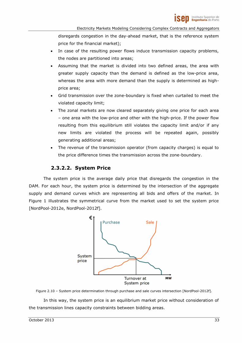
Electricity Markets Modeling Considering Complex Contracts and Aggregators
October 2013 33
disregards congestion in the day-ahead market, that is the reference system
price for the financial market);
In case of the resulting power flows induce transmission capacity problems,
the nodes are partitioned into areas;
Assuming that the market is divided into two defined areas, the area with
greater supply capacity than the demand is defined as the low-price area,
whereas the area with more demand than the supply is determined as high-
price area;
Grid transmission over the zone-boundary is fixed when curtailed to meet the
violated capacity limit;
The zonal markets are now cleared separately giving one price for each area
– one area with the low-price and other with the high-price. If the power flow
resulting from this equilibrium still violates the capacity limit and/or if any
new limits are violated the process will be repeated again, possibly
generating additional areas;
The revenue of the transmission operator (from capacity charges) is equal to
the price difference times the transmission across the zone-boundary.
2.3.2.2. System Price
The system price is the average daily price that disregards the congestion in the
DAM. For each hour, the system price is determined by the intersection of the aggregate
supply and demand curves which are representing all bids and offers of the market. In
Figure 1 illustrates the symmetrical curve from the market used to set the system price
[NordPool-2012e, NordPool-2012f].
Figure 2.10 – System price determination through purchase and sale curves intersection [NordPool-2012f].
In this way, the system price is an equilibrium market price without consideration of
the transmission lines capacity constraints between bidding areas.

Tiago André Teixeira Soares
34 October 2013
2.3.2.3. Area Price
The Area price is the price determined for each bidding area, which is considered the
lines congestion capacity constraints between the bidding areas. However this price is only
calculated when the power flow between bidding areas exceed the trading capacity. In this
case, when the need for transmission exceeds the available transmission capacity, the
prices are lowered in surplus areas and raised in deficit areas, which results in different area
prices. The main goal of the assignment of area prices is the ability to relieve grid
congestion between the bidding areas.
In what concerns the high price in the deficit area, the players will sell more and
purchase less while in the surplus area it is the opposite. In the area price calculation the
transmission capacity between the deficit and the surplus area is used to the maximum. In
this way, the power flow will go from the surplus areas (lower price) to the deficit area
(higher price). Thereby, in the deficit area the sale will give a parallel shift of the supply
curve while in the surplus area the additional purchase will give a parallel shift of the
demand curve [NordPool-2012e, NordPool-2012f].
Following the same principle of system price determination through the intersection
of the supply and demand curve, Figure 2.11 shows the curve of the area pricing
determination for cases of high (deficit) and low (surplus) price.
Figure 2.11 – Surplus and deficit area price curves determination [NordPool-2012f].
As can be seen in the Figure 2.11, through this process one can find a relatively
balance between the area price in the surplus area and in the deficit area. Thereby, the
price is relatively lower in the surplus area and relatively higher in the deficit area.
In the event that power flow in interties in consecutive periods not exceeding the
maximum limit of transmission capacity of interties, the market price of the areas are the
same, so there are no differentiation between areas prices.
Electricity Markets Modeling Considering Complex Contracts and Aggregators
October 2013 35
2.3.3. Elbas – Intraday Market
Elbas is an intraday market for trading power across the Nordic region, Germany,
Estonia and Lithuania. Elbas supplements Elspot and helps secure the necessary balance
between supply and demand in the power market, offering opportunities for risk reduction
as well as increased profit.
As it is known, when it approaches the delivery time of energy in real-time, the
necessary energy forecast is improved to accentuate that the energy forecast traded in DAM
is not adequate for the obtained forecast in real-time. This is due to significant deviations
from production and/or consumption. In this context, incidents may take place between the
closing of Elspot and delivery of the next day. For example, a nuclear power plant may stop
operating, or winds may cause higher power generation than planned at wind turbine
plants. Therefore, players through the Elbas can trade volumes close to real-time to bring
the market back in balance.
After closing of the Elspot auction (at 2 p.m.), capacities available for Elbas trading
during the 24 hours of the following day are published. In Elbas, the trading takes place
every day until one hour before delivery. The prices are set based on a first-come, first-
served principle where lowest sell price and highest buy price come first, regardless of when
a bid is placed [NordPool-2012a, NordPool-2012i and NordPool-2012j].
2.3.4. Balancing Market
The Balancing power market is a tool for the Nordic TSO's to keep balance between
total generation and consumption of power in real time. The TSO have the responsibility to
ensure the demand provision and maintain the transmission grid frequency stable,
according to the limits for the frequency control.
The balancing market culminates in the power adjustments within hours of delivery
of energy, i.e., in this market each TSO negotiates individually with each player in order to
maintain the system balance. In this way, the TSO acquire Ancillary Services, like regulation
reserve and other services, necessary for the complement of system balance [NordPool-
2012k].
The mechanism of balancing of the Nordic electricity market consists in three steps.
The planning, regulation and settlement balance, which are defined in agreements between
the market players (Balance Responsible Parties, BRPs) and the TSOs [Nordel-2008],
described as follows:
The balance planning consists in the obligation of the market players to
balance their portfolios of production and purchase against consumption and
sales on hourly basis;
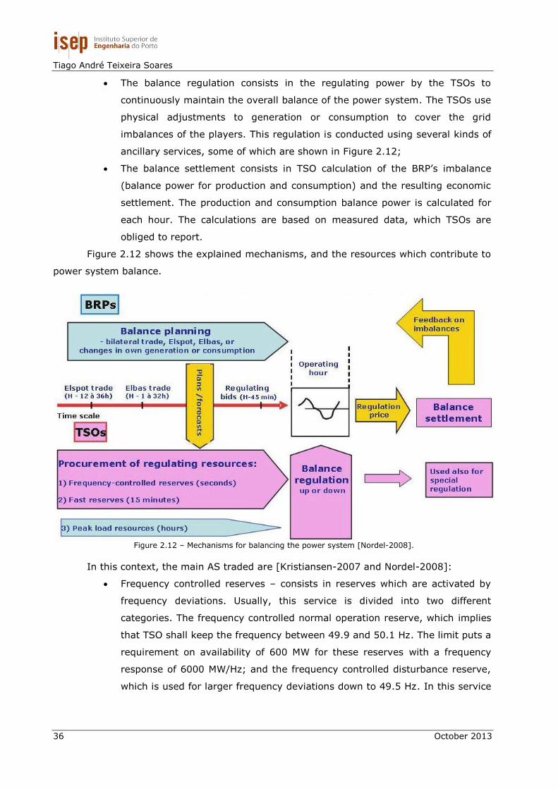
Tiago André Teixeira Soares
36 October 2013
The balance regulation consists in the regulating power by the TSOs to
continuously maintain the overall balance of the power system. The TSOs use
physical adjustments to generation or consumption to cover the grid
imbalances of the players. This regulation is conducted using several kinds of
ancillary services, some of which are shown in Figure 2.12;
The balance settlement consists in TSO calculation of the BRP’s imbalance
(balance power for production and consumption) and the resulting economic
settlement. The production and consumption balance power is calculated for
each hour. The calculations are based on measured data, which TSOs are
obliged to report.
Figure 2.12 shows the explained mechanisms, and the resources which contribute to
power system balance.
Figure 2.12 – Mechanisms for balancing the power system [Nordel-2008].
In this context, the main AS traded are [Kristiansen-2007 and Nordel-2008]:
Frequency controlled reserves – consists in reserves which are activated by
frequency deviations. Usually, this service is divided into two different
categories. The frequency controlled normal operation reserve, which implies
that TSO shall keep the frequency between 49.9 and 50.1 Hz. The limit puts a
requirement on availability of 600 MW for these reserves with a frequency
response of 6000 MW/Hz; and the frequency controlled disturbance reserve,
which is used for larger frequency deviations down to 49.5 Hz. In this service

Electricity Markets Modeling Considering Complex Contracts and Aggregators
October 2013 37
the reserve available is 1000 MW and the frequency response is 2500
MW/Hz;
Fast reserves is a AS which are activated manually, and must be able to
restore the automatic reserve within 15 min;
Peak load resources are resources which can be used by the TSO for balance
regulation. Usually, such peak load resources can take several hours to
activate in situations when the fast reserve should prove insufficient. A peak
load arrangement should be an exceptional and temporary solution to
overcome a critical period. Therefore, the implementation of this service is
supervised by each TSO, because each country has a set of rules adapted to
the needs of their respective power system.
2.4. MIBEL
The Iberian Electricity Market (MIBEL – Mercado Ibérico de la Electricidad) is a
regional electricity market composed by the countries of Portugal and Spain. This market is
based on setting of a market for daily delivery of energy to the next day, with a format
similar to the majority in Europe. This way, the MIBEL consists of three distinct markets,
The Financial market (known as Forward Market) which is used for price hedging and risk
management, the Day-Ahead Market where power is traded for delivery during the next
day, and the intraday market which work as a market adjustment of MIBEL.
The OMIP (Operador de Mercado Ibérico de Energia, Portuguese pole) is responsible
for managing the trading operations in the futures market whose underlying asset is
electricity. The financial market is regulated by OMIclear (Sociedade de Compensação de
Mercados de Energia) which is the Iberian energy clearing house that manages the
settlement system.
The OMIE (Operador del Mercado Ibérico de Energia, Spanish pole) is the managing
entity of the DAM and intraday market, which establishes programs for the sale and
purchase of electricity for the next day. Thus, the OMIE is responsible for conducting
assessments of the DAM and intraday market.
The overall management of the electrical system of each zone is the responsibility of
the respective TSO, which in addition to its usual features, individually manages its own
market for ancillary services. Sometimes the DAM and intraday market is divided into two
zones, each zone corresponding to the respective country. This is due to the limited
capacity of interconnection between the two zones causes interconnection congestion
[MIBEL-2009].
The Ancillary Services market is operated by the TSO of each country. They have to
ensure the contract and settlement of AS, to ensure the balance between production and

Tiago André Teixeira Soares
38 October 2013
consumption, through efficient and competitive mechanisms. The AS to be contracted in the
market are complementary services (explained in subsection 2.4.4). These services are
subject to remuneration and should be contracted based on market mechanisms in a
competitive environment. The adopted model establishes a implicit separation between the
complementary ancillary services to which the system uses on a regular basis (secondary
regulation and regulatory regulation) who are contracted on the basis of asymmetric market
and those which are needed occasionally (synchronous compensation, black start and
interruptible service) based on bilateral contracts [MIBEL-2009].
Figure 2.13 shows the arrangements for procurement existing in MIBEL.
Figure 2.13 – MIBEL market timeline overview, adapted from [Pereira-2009].
2.4.1. Financial Markets
The financial market of MIBEL is an organized market designed for price hedging and
risk management, which is managed by OMIP. In this market, there are three types of
contracts available for trading. The futures contracts which admit physical or financial
settlement, the Forwards contracts which have physical nature and the swaps contracts
which are of financial nature. The futures contracts use the DAM market price as a
reference price, with only financial settlement [MIBEL-2009].
2.4.2. Day-Ahead Market
The Iberian DAM is managed by OMIE and consists of electricity transactions for the
next day, based on the presentation of purchase and sale offers of electric power carried
out by the market players. In this market each player can submit between 1 to 25 bids for
each hour. The bids which players present to the Market Operator (MO) can be simple or

Electricity Markets Modeling Considering Complex Contracts and Aggregators
October 2013 39
complex. However, only the sellers can post simple and complex bids, while the buyers can
only submit simple bids. Simple bids are economical offers for sale energy, in which for
each hour the player establish the amount of energy and its price. The complex bids are
based on simple bids with the introduction of some technical and/or economical conditions,
as described below [OMIE-2012a]:
The indivisibility condition enables to set a minimum operation value, which is
indicated in the first bid of each hour;
Voltage gradient condition allows establish the maximum difference between
the start hour and end hour power of the unit production, which limits the
maximum energy to confer on the basis of the meeting the previous and the
following time, to avoid sudden changes in unit’s production that can not
technically follow the same;
The minimum entries condition consists in the minimal entries in service of a
unit production per day. The unit production refuse to participate in the
outcome of the meeting of the day, if not obtained for all of their production
on an entry exceeding a fixed amount established in euro cents;
The scheduled stop condition allows performing a scheduled stop time a
maximum of three hours, in the case of the unit production has been
removed by the agreement does not meet the condition required for minimal
entries in service. Thus, avoiding stop from it program in the last hour of the
day before to zero in the first hour of the next day, by accepting the first bid
for the first three hours of it offer as simples bids, with the sole condition that
the energy is provided descending the first bid of each hour.
2.4.2.1. Market Development Sequence
The market has a developmental sequence in which the closing hour of the DAM will
be at 10 a.m. the day before the delivery date. The market is based on the process of
meeting supply and demand curves from the bids for sale and purchase. The outcome of
the meeting of the curves will be published at 11 a.m.
After the process of meeting the supply and demand curve, between 11 and 14
hours, with the incorporation of bilateral contracts, one can obtain the daily base operation
dispatch for each system. In this way, the SO analyze and solve possible technical
congestion constraints arising from the process of meeting the DAM of the interconnections
between the two systems and the declaration of bilateral contracts, thus deliver their
programs viable daily duties. After the process of solving technical constraints in the DAM,
the market relating to secondary regulation starts. In this market, players offer their
regulation bids with the respective price, for every hour of the next day. Each bid must

Tiago André Teixeira Soares
40 October 2013
meet a pre-established relationship between the up and down reserve. The final viable daily
dispatch of the DAM is published before the 16 hours and includes the result of the Ancillary
Services (AS) market regarding to the secondary regulation [MIBEL-2009].
Figure 2.14 – Symmetric market clearing price determination [Pereira-2009].
2.4.2.2. Market Splitting
The Iberian market is treated as a single market when there are no violated
congestion constraints at the interconnections between the two systems corresponding to
each country. In certain situations where such constraints are violated, the market is
separated into two distinct price areas, thereby causing the market splitting. In this regard,
based on the process of determining the price exposed in subsection 2.4.2.1, the market
splitting process may result in two different processes for determining the market price
[MIBEL-2009]:
In the situation where the meeting of the supply and demand curves,
resulting in interconnections power flow which not exceeds the
interconnection capacity, the market price is unique to the Iberian system,
since the dispatch has technical and economic viability;
In the case of the meeting of supply and demand curves, resulting in
interconnections power flow which exceeds the interconnection capacity, the
initial market solution is unfeasible, so the two market areas are dealt with
separate supply and demand curves appropriated to each area. However, the
demand curve for the export system is placed as a quantity corresponding to
the interconnection capacity, while the supply curve for the importing system
consists of an equivalent amount. The meeting of the curves for each of the
systems results in different market prices for each market.
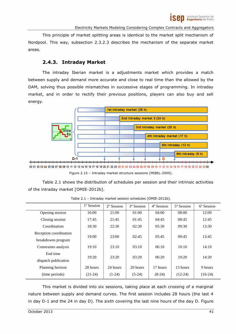
Electricity Markets Modeling Considering Complex Contracts and Aggregators
October 2013 41
This principle of market splitting areas is identical to the market split mechanism of
Nordpool. This way, subsection 2.3.2.3 describes the mechanism of the separate market
areas.
2.4.3. Intraday Market
The intraday Iberian market is a adjustments market which provides a match
between supply and demand more accurate and close to real time than the allowed by the
DAM, solving thus possible mismatches in successive stages of programming. In intraday
market, and in order to rectify their previous positions, players can also buy and sell
energy.
Figure 2.15 – Intraday market structure sessions [MIBEL-2009].
Table 2.1 shows the distribution of schedules per session and their intrinsic activities
of the intraday market [OMIE-2012b].
Table 2.1 – Intraday market session schedules [OMIE-2012b].
1º Session 2º Session 3º Session 4º Session 5º Session 6º Session
Opening session 16:00 21:00 01:00 04:00 08:00 12:00
Closing session 17:45 21:45 01:45 04:45 08:45 12:45
Coordination 18:30 22:30 02:30 05:30 09:30 13:30
Reception coordination
breakdowns program 19:00 23:00 02:45 05:45 09:45 13:45
Constraints analysis 19:10 23:10 03:10 06:10 10:10 14:10
End time
dispatch publication 19:20 23:20 03:20 06:20 10:20 14:20
Planning horizon
(time periods)
28 hours
(21-24)
24 hours
(1-24)
20 hours
(5-24)
17 hours
(8-24)
13 hours
(12-24)
9 hours
(16-24)
This market is divided into six sessions, taking place at each crossing of a marginal
nature between supply and demand curves. The first session includes 28 hours (the last 4
in day D-1 and the 24 in day D). The sixth covering the last nine hours of the day D. Figure
Tiago André Teixeira Soares
42 October 2013
2.15 shows schematically the structure of the intraday market covering all session’s
constituents of the market [MIBEL-2009 and OMIE-2012b].
2.4.4. Ancillary Services Market
In MIBEL, the Ancillary Services market is separated into two markets, individually
managed by the TSO of each respective country.
The AS are divided into two categories [MPGS-2008 and MIBEL-2009]:
Mandatory services, which are not paid and which are encompassed the
voltage regulation, frequency regulation and maintenance of stability;
Complementary services, such as static synchronous compensation and the
reserve, secondary regulation, the interruptible rapid and black start, which
are remunerated through the AS market or through bilateral contracts.
Currently, only secondary regulation and regulatory reserve are remunerated in the
form of competitive market. The other AS can be contracted bilaterally.
Additionally, there is the process of solving the technical constraints that mainly
involves the simulation of the network AC power flow based on economical dispatches
obtained in several electricity markets. In this way, the process of solving the technical
constraints consists of three levels, relative to the DAM, intraday market and real-time
energy delivery managed by the respective TSO.
In the DAM market, the process of solving technical constraints is separated into two
distinct phases. The first phase consists in modifying the procurement program by security
criteria and the second phase consists in the rebalancing of the generation/consumer
system. To this end, the supply units (large groups of thermal and hydro plants) and
consumption for pumping present energy and price bids for mobilization and demobilization
of energy. The players associated with the consumption bids of pumping units are paid by
using the maximum value between the energy bids value given in the process of solving
technical constraints and the bids made on the DAM.
In the event of energy mobilization, the players associated with the generation units
are remunerated by using the minimum value between the energy bids value given in the
process of solving technical constraints and the value of bids submitted and not matched at
the DAM. In case of energy demobilization, selling players are required to pay the energy
price matched at the DAM.
In several sessions of intraday market where arise technical constraints, these are
solved through the elimination of bids that arise, without implying any additional cost to the
system. The costs resulting for the increase in the market clearing price of intraday market,
due to the elimination of bids is supported by consumers.
Electricity Markets Modeling Considering Complex Contracts and Aggregators
October 2013 43
Finally, the third level of the process of solving the technical constraints consists in
the technical constraints detected in real-time which are solved by mobilizing the bids of
regulation reserve. Every hour, any additional costs of resolution of technical constraints in
real-time are remunerated around the consumption made at this time, in proportion to its
consumption in DAM [MPGS-2008, MIBEL-2009 and ERSE-2012].
In order to obtain a better understanding of the AS in the Iberian market, is shown
below the detailed definition of the main AS associated with frequency regulation managed
by the SO of each area [MPGS-2008 and MIBEL-2009]:
The primary regulation is associated with generators statism, which is a
mandatory AS, unpaid for all generators in service. The power variation
resulting from its action should be effected within 15 seconds before
disturbance causing the deviation of frequency below 100 mHz and linearly
between 15 and 30 seconds to deviations in frequency between 100 and 200
mHz;
The secondary regulation (usually known as Spinning Reserve) is a AS
remunerated by market mechanisms, and its valuation is composed of two
parts: the reserve price, valued in accordance with the maximum of the
marginal prices of secondary regulation reserve to “down” and “up” in hourly;
and energy of secondary regulation, valued at the price of the last energy bid
of regulation reserve mobilizes in each hour. The onset of action of the
secondary regulation should take no longer than 30 seconds and its action
should be completed and may be supplemented by action the regulation
reserve (tertiary regulation), no longer than 15 minutes;
The tertiary regulation consist in the variation of the maximum power
generation program that can be carried out in a unit production and/or
balance area in a maximum time of 15 minutes and can be maintained at
least for 2 hours in a row. This reserve is an additional service, paid by
market mechanisms and composed of two parts: minimum reserve of tertiary
regulation and additional reserve. The minimum tertiary regulation is
established by the SO for each period, taking as reference the maximum
losses of production caused directly by the failure of a single element of the
electrical power system, increased by 2% of expected consumption. The
additional regulation reserve aims to guarantee the coverage of the
consumption and operating system where the consumption scheduled by the
SO exceeds by more than 2%, consumption resulting from the production
markets and when the forecast generation loss due to successive failures
and/or delays in the connection or increase of thermal groups is greater than
the tertiary regulation established. The market players present their

Tiago André Teixeira Soares
44 October 2013
regulation reserve bids to up and/or down, between 18 and 21 hours, for
each period of the next day.
2.5. Conclusion
All over the world, electricity restructuring placed several challenges to governments
and to the companies that are involved in generation, transmission and distribution of
electrical energy.
The markets discussed in this section are the result of consequent paradigm shift. In
this regard, special attention was given to the several models and designs of energy and
ancillary services markets.
In this section is presented an overview of ancillary services in different markets, in
which the Table 2.2 represents a summary of the AS adopted by the real market models
studied in this chapter.
Table 2.2 – Ancillary services summary.
Ancillary Services
BETTA CAISO Nord Pool MIBEL
Frequency Regulation
Frequency Response
Regulation Down Frequency
Controlled
Reserve
Primary
Regulation Regulating Reserves
Regulation Up
Fast Reserve Spinning Reserve
Fast Reserves Secondary Regulation
Standing Reserve
Warming
Reserve
Non-Spinning
Reserve Peak load resources
Tertiary Regulation Hot standby
Reserve Replacement Reserve
Voltage Control
Obligatory
Reactive Power AGC Regulation
Obligatory
Reactive Power AGC Regulation
Enhanced Reactive Power
Enhanced Reactive Power
Synchronous Compensation
Back-Up services
Black Start Black Start Black Start Black Start
In Table 2.2 it is possible to identify the differentiation of ancillary services in the
markets studied. However, to describe each service in detail one can realize that in general
the frequency control services are divided into three parts.
When comparing the services identified in the CAISO market with relating to MIBEL,
one can verify that the Regulation Down and Regulation Up refers to the Primary regulation
of MIBEL, while Spinning Reserve refers to Secondary Reserve and the services Non-
Spinning Reserve and Replacement Reserve refers to Tertiary Reserve. Although it is
understood that the markets designs are different, the main services are similar, with some
changes at the level of response time, duration period, as well as the service settlement
mechanisms.
Electricity Markets Modeling Considering Complex Contracts and Aggregators
October 2013 45
Besides the AS for the frequency control deeply covered in this chapter, the Table
2.2 emphasizes other ancillary services, such as services related to voltage control and
Black Start capacity.
Voltage control consists in maintaining voltage through injecting or absorbing
reactive power by means of synchronous or static compensation.
In BETTA the voltage control is divided into two services – the Obligatory Reactive
Power service which is the provision of varying reactive power output (at any given output
the generators may be requested to produce or absorb reactive power to help manage
system voltages close to its point of connection); and the Enhanced Reactive Power service
which is the provision of voltage support that exceeds the minimum technical requirement
of Obligatory Reactive Power service (including synchronous compensation) or reactive
power capability from any other plant or apparatus which can generate or absorb Reactive
Power (including Static Compensation equipment) that is not required to provide the
Obligatory Reactive Power service [NGET-2012a].
The Black Start service is the capability of a generating unit to start up without an
external power supply, called on as a means of restoring supplies following a major failure
on all or part of the network [EURELECTRIC-2004]. This service is common to all markets,
and in the vast majority it is traded through bilateral contracts between generation’s units
and system operators.


Electricity Markets Modeling Considering Complex Contracts and Aggregators
October 2013 47
Chapter 3
Ancillary Services Market models


Electricity Markets Modeling Considering Complex Contracts and Aggregators
October 2013 49
3. AS Market models
This chapter provides an overview of the proposed and implemented simulation
models. Most features of the presented simulation models focuses on characteristics of real
market models. Some of the models consider innovative methodologies for solving the
optimization problem, namely the introduction of Bialek topological factors in the scope of
determination of the impact of Ancillary Services (AS) dispatch in network congestion. Most
of the models are related to the Independent System Operation (ISO) operation. However,
it is also proposed a complete model that addresses the market simulation from the
perspective of a Virtual Power Player (VPP) management. In this way, some particular
characteristics of the VPP management are considered, including the aggregation of several
kinds of energy generation technologies, as well as the introduction of complex contracts
between the VPP and players.
In this chapter five distinct simulating models are available in the scope of the AS
market, energy and ancillary services joint market, applied to different levels of an ISO and
a VPP Operation.
3.1. Introduction
The design and development of simulation models and tools for AS simulation are
essential to allow a proper management of the most varied existing energetic resources. In
that case, the AS procurement by the ISO/VPP must take into account in its simulation
model the characteristics inherent in each technology, as well as ensure market
competitiveness in order to get the best possible management of all resources in a market
environment.
In order to simulate complex models of markets, market players (ISO, VPP and
other players) use tools with the capability of simulating electricity market processes. In
this way, the simulator must be able to deal with the complex reality of the electricity
market and its dynamics evolution. In this context, multi-agent simulators are appropriate
for this kind of problems, because it allows a good flexibility in the electricity markets
simulation, since agents can have different behaviors and interests of each other [Praça-
2003]. Currently, there are several tools which allow simulating the electricity markets
operation, each one with its own characteristic, for example: the Simulator for Electric
Power Industry Agents (SEPIA) is based on a plug and play architecture which allows users
to easily create simulations involving several machines in a network, or in a single machine,
using various processing units [Harp-2000]; the Electricity Market Complex Adaptive
System (EMCAS) is a simulator which uses an agent based approach with agents’ strategies
based on learning and adaptation for electricity markets [Koritarov-2004]; Power Web is a
Web-based market simulator which allows several participants to interact from very distinct
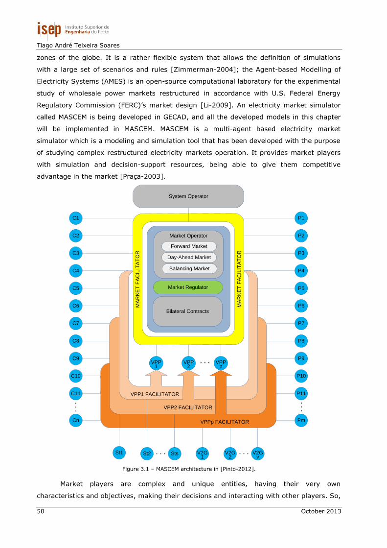
Tiago André Teixeira Soares
50 October 2013
zones of the globe. It is a rather flexible system that allows the definition of simulations
with a large set of scenarios and rules [Zimmerman-2004]; the Agent-based Modelling of
Electricity Systems (AMES) is an open-source computational laboratory for the experimental
study of wholesale power markets restructured in accordance with U.S. Federal Energy
Regulatory Commission (FERC)’s market design [Li-2009]. An electricity market simulator
called MASCEM is being developed in GECAD, and all the developed models in this chapter
will be implemented in MASCEM. MASCEM is a multi-agent based electricity market
simulator which is a modeling and simulation tool that has been developed with the purpose
of studying complex restructured electricity markets operation. It provides market players
with simulation and decision-support resources, being able to give them competitive
advantage in the market [Praça-2003].
VPPp FACILITATOR
VPP2 FACILITATOR
VPP1 FACILITATOR
MA
RK
ET
FA
CIL
ITA
TO
R
MA
RK
ET
FA
CIL
ITA
TO
RMarket Operator
Forward Market
Day-Ahead Market
Balancing Market
Market Regulator
Bilateral Contracts
VPP 1
P6
P5
P7
P3
P2
P4
VPP 2
VPP p
P11
P10
Pm
P8
P1
P9
C6
C5
C7
C3
C2
C4
C11
C10
Cn
C8
C1
C9
System Operator
St1 St2 Sts V2G1
V2G2
V2Gv
.
.
....
. . .. . .
. . .
Figure 3.1 – MASCEM architecture in [Pinto-2012].
Market players are complex and unique entities, having their very own
characteristics and objectives, making their decisions and interacting with other players. So,

Electricity Markets Modeling Considering Complex Contracts and Aggregators
October 2013 51
MASCEM was developed as a multi-agent based simulation tool, modeling the complex
dynamic market players, including their interactions and medium/long-term gathering of
data and experience. MASCEM uses game theory, machine learning techniques, scenario
analysis and optimization techniques to model market agents and to provide them with
decision-support [Vale-2011]. MASCEM includes several negotiation mechanisms usually
found in electricity markets. It can simulate several types of markets, namely: pool
markets, bilateral contracts, balancing markets, forward markets. This implies that each
agent must decide whether to, and how to, participate in each market type. Figure 3.1
presents MASCEM global architecture, proposed in [Pinto-2012], with the representation of
its most important entities and interactions.
As presented in Figure 3.1, there are several entities involved in negotiations in the
scope of electricity markets; this multi-agent model represents all the involved entities and
their relationships. MASCEM multi-agent model includes: a Market Facilitator Agent, Seller
Agents, Buyer Agents, VPP Agents, VPP Facilitator Agents, a Market Operator Agent and a
System Operator Agent [Praça-2003, Vale-2011]. In order to develop a more realistic
simulator it is proposed in this thesis a variety of models for energy and AS negotiation to
be implemented in MASCEM.
A key objective of the proposed models in this thesis is to provide a better simulator
intrinsic ability to simulate energy and AS markets, based on real and current models
functioning of several markets placed on MASCEM. During the models description, some
important contributions of this work are present, namely the energy and AS joint market
simulation, in which is considered the power flow for each utility; the introduction of Bialek
topological factors in solving the network congestion by considering the AS dispatch in the
network flow; and the ancillary services dispatch in the scope of a distribution network
operation with a high penetration of Distributed Energy Resources (DER). To this end, one
can use a novel method for solving the problem. In this way, a brief description of the
characteristics inherent in each proposed simulation model is presented. Table 3.1
summarizes the market models studied in this chapter. The first column of Table 3.1
presents the highlights that characterize each model.
The Ancillary Services Market model consists in the simultaneous optimization of
ancillary services (Regulation Down (RD), Regulation Up (RU), Spinning Reserve (SP), Non-
Spinning Reserve (NS)). Depending on the real market model, these AS may be classified
differently, but in general they have very similar characteristics. Therefore, these AS are
designated by the MIBEL as primary, secondary and tertiary regulation reserves. In the
scope of the simulation, the model includes the possibility of substitution between services
designated by AS cascading. Thus, this model illustrates the basic operation of the AS
market, being used as the reference model for the remaining models presented in this
section.

Tiago André Teixeira Soares
52 October 2013
Table 3.1 – Market models characterization.
Characteristics
Model
Ancillary
Service Market
Energy and AS
joint market
Joint market
considering AS
bidding regions
Joint market
considering
Bialek
coefficients
Joint Market
applied by VPP
Market model AS market Joint Market Joint Market Joint Market Joint market
AS cascading
process Yes Yes Yes No No
Network
operation No No AC OPF
AC OPF with
Bialek
topological
factors
AC OPF with
Bialek topological
factors
Resource
management
goal
Minimization of
ISO operation
costs
Minimization of
ISO operation
costs
Minimization of
ISO operation
costs
Minimization of
ISO operation
costs
Minimization of
VPP operation
costs
AS bidding
regions No No
AS bids and
procurement
by regions of
the network
AS bids and
procurement by
regions of the
network
AS bids and
procurement by
regions of the
network
Relaxation
variables
Ensured by ISO
through
bilateral
contracts
Ensured by
ISO through
bilateral
contracts
Ensured by ISO
through
bilateral
contracts
Ensured by ISO
through
bilateral
contracts
Ensured by the
energy resources
of other regions,
including external
suppliers
Complex
Contracts No No No No
Developed five
types of complex
contracts
between players
and VPP
The Energy and AS Joint Market model is based on a principle of energy and AS joint
market where seller’s agents can make offers simultaneously for the energy and AS
markets with a global maximum power generation limit. This model fits to the basic
principle of the joint market, i.e., the co-optimization of energy and ancillary services
similar to the implemented in several US electricity markets, such as the CAISO, Electric
Reliability Council of Texas (ERCOT) and New York Independent System Operator (NYISO),
in order to obtain the most efficient cost solutions.
The Joint Market model considering AS bidding regions is based on the methodology
of CAISO functioning, which considers the co-optimization of energy and AS, where ancillary
services are procured by network regions. The ISO establishes the AS regions and its

Electricity Markets Modeling Considering Complex Contracts and Aggregators
October 2013 53
respective requirements. The model is able to simulate a regional AS dispatch. Regions are
areas of the network, which implies that each region will be assigned a set of network
nodes. In this model the interties between network regions, follow the same principle of
constraints applied to interties between countries.
The Joint Market model considering Bialek coefficients introduces a new methodology
for energy and AS joint market simulation with consideration of the impact of the dispatch
of all services in the network power flow. This model has the ability to previously analyze
congestion that each AS implies in the network, rejecting solutions that may cause network
congestion. To this end, the model uses the topological factors methodology proposed by
Janusz Bialek in [Bialek-1997]. With this method it becomes possible to know the amount of
power that each generator is supplying to loads, as well as the congestion in lines caused
by each generation unit.
The Joint Market model applied by VPP considers the methodology referred to the
previous model applied in the scope of distribution network operation with high penetration
of DER essentially composed of Distributed Generation (DG), Demand Response (DR) and
storage units, which can be managed by a VPP, as well as the introduction of complex
contracts between VPP and the players in the resources scheduling process.
Related to the VPP management and the players’ goals, a major contribution of this
work lies in the introduction of complex contracts which establish conditions that guarantee
competitive benefits for both parties. The terms of these contracts, include the advantage of
setting clear objectives for generation, remuneration, working time, among others, to
enable the VPP aggregating the most interesting players to their objectives, as well as the
players getting best benefits in the aggregation to an particular VPP when compared to act
alone in the same market or aggregate to other VPPs.
The design, development and application of these methodologies in the simulation
model of the energy and AS joint market, leads to a more cohesive, feasible and applicable
to the simulation of real markets, making these models the main contribution of this work
to the development of MASCEM. The main goal of MASCEM’s is to be able to simulate as
many market models and types of players as possible so it can reproduce in a realistic way
the operation of real electricity markets.
In this way, the implementation of these models in MASCEM makes this a more
robust and, at the same time, a more flexible simulator regarding the simulation of
electricity markets.

Tiago André Teixeira Soares
54 October 2013
VPPp FACILITATOR
VPP2 FACILITATOR
VPP1 FACILITATOR
MA
RK
ET
FA
CIL
ITA
TO
R
MA
RK
ET
FA
CIL
ITA
TO
R
Market Operator
Forward Market
Day-Ahead Market
Balancing Market
Ancillary Services
Market Regulator
Bilateral Contracts
VPP 1
P6
P5
P7
P3
P2
P4
VPP 2
VPP p
P11
P10
Pm
P8
P1
P9
C6
C5
C7
C3
C2
C4
C11
C10
Cn
C8
C1
C9
System Operator
St1 St2 Sts V2G1
V2G2
V2Gv
.
.
....
. . .. . .
. . .
Regulation Down
Regulation Up
Spinning Reserve
Non-Spinning Reserve
Figure 3.2 – Updated MASCEM architecture.
The implementation of the proposed models in the new MASCEM structure will be
similar to the architecture shown in Figure 3.2, in which the part relating to AS refers to the
contribution of the work developed in this dissertation for the simulator continuous
improvement. This enables the MASCEM to be used as a simulation and decision-support
tool for short/medium term purposes.
Computational tools used in models implementation
A detailed description of several tools used in the development of simulation models
of electricity markets are presented below. These tools are used as the basis of operation of
the MASCEM market simulator.

Electricity Markets Modeling Considering Complex Contracts and Aggregators
October 2013 55
MASCEM is developed in OAA1 [OAA-2012] framework and in Java Virtual Machine
1.6.0 [JAVA-2012]. The OAA’s ICL2 is the interface and communication language shared by
all agents, which allows MASCEM to integrate a variety of software modules [Pinto-2011b].
The optimization models to be included in MASCEM to simulate the AS markets are
developed in General Algebraic Modeling System (GAMS) which is a high-level modeling
system for mathematical programming and optimization. It consists of a language compiler
and a stable of integrated high-performance solvers. GAMS is tailored for complex, large
scale modeling applications, and allows the user to build large maintainable models that can
be adapted quickly to new situations [GAMS-2008]. GAMS is specifically designed for
modeling linear, nonlinear and mixed integer optimization problems. The system is
especially useful with large, complex problems. A large number of solvers for mathematical
programming models allow users to solve a huge variety of problems [GAMS-2007]. The
optimization problems related with the proposed models are solved using DICOPT3, CPLEX4,
CONOPT5 and LINDOGlobal6 solvers.
The JAVA agents of MASCEM and the optimization process in GAMS were linked with
the MATrix LABoratory (MATLAB) which is a powerful software of numeric computation,
developed in 1978 by Cleve Moler and Jack Little, cofounders of MathWorks7. The main
characteristic of MATLAB is the use of matrixes as the basic data structure [Graham-2005].
MATLAB is a high-level technical computing language with an interactive environment, ideal
for algorithm development, data visualization, data analysis, and numeric computation.
MATLAB can be used in a wide range of applications, including signal and image processing,
communications, control design, test and measurement, financial modeling and analysis,
and computational biology. Thus, MATLAB is used in several applications in the industry, as
well as in academic activities, and it has been applied to several problems of science and
engineering. MATLAB has toolboxes that allow obtaining the solution for several types of
problems such as the ones related to numerical analysis, data analysis, matrix calculus, and
signal processing. The user can use the available toolboxes or program functions and
routines to solve the envisaged problem [MATLAB-2010]. In the scope of this thesis,
MATLAB is used as a tool for preparation of input data, as well as the organization and
illustration of the results of the optimization. Although via MATLAB it is possible to perform
the optimizations of the presented models, GAMS was chosen as optimization tool, because
1 Open Agent Architecture
2 Interagent Communication Language
3 DIscrete and Continuous OPTimizer
4 Simplex algorithm and C programming
5 CONtinuous global OPTimizer
6 Linear, Integer, Nonlinear, Dynamic Optimization Global
7 The MathWorks, Inc., Natick, United States, 2010, www.mathworks.com

Tiago André Teixeira Soares
56 October 2013
of its advantages in solving optimization problems using deterministic methods compared
with MATLAB.
3.2. Ancillary Services Market model
This section presents a simulation model of a generic AS market, which considers
the optimization of the most common ancillary services in the liberalized market
environment (RD, RU, SP and NS). This model is based on a principle of AS market design –
The Rational Buyer, which is an simultaneous AS auction with downward substitution for the
different commodities (RU, SP, NS) in order to minimize the cost of the AS procurement
[Papalexopoulos-2001].
3.2.1. Problem Description
This model is designed to perform the dispatch of the AS market, based on an
asymmetric pool, considering the four most common AS in the liberalized market
environment. Regulation Down, Regulation Up, Spinning Reserve and lastly the Non-
Spinning Reserve are the AS simulated in this model. In order to be able to understand the
presented model, Figure 3.3 presents a flowchart representative of the structure simulation
model of the operation method of the AS market.
Players’ Bids
RD Offers
RU Offers
SP Offers
NS Offers
Maximum Power Capacity
RD Forecast
RU Forecast
SP Forecast
NS Forecast
AS Requirements
K=2...4 (RU, SP and NS)
Optimization
process
K=1 (RD)
Begin
Optimization
process
RD
Requirement
Satisfied?
Requirement
Satisfied?
Establishement of
market clearing price
and show dispatch
solution
Infeasible - No
Solution
End
Yes
Ancillary Services Dispatch
Ancillary Services Market Model
Establishement of
market clearing price
and show dispatch
solution
ISO Optimization Algorithm
Infeasible - No
Solution
NoYesNo
Figure 3.3 – AS market diagram.
The players acting on the market can present their bids for any of the four AS
previously mentioned, with different capacities and prices for each service.
Electricity Markets Modeling Considering Complex Contracts and Aggregators
October 2013 57
The proposed flowchart presented in Figure 3.3 illustrates the essential processes of
the optimization algorithm of the model. The algorithm is initialized by reading the input
data relating to bids of each AS and the quantities required by ISO for each ancillary
service.
The algorithm is divided into two distinct parts. One of the parts refers to the
Regulation Down, while the other part of the algorithm is relate to the simultaneously
simulation of ancillary services (Regulation Up, Spinning and Non-Spinning Reserve).
The optimization process is performed by the optimization tool GAMS, which contains
several solvers capable of solving the optimization process in multiple ways.
To the RD service, the next step is to select all offers until the service requirement is
met. In the case where the amount required energy by ISO for the service is not satisfied,
the algorithm informs the ISO that the solution is infeasible for this service.
In case the AS requirement have been satisfied, takes place the establishment of the
market clearing price based on the last offer obtained in the dispatch of this service, ending
this part of the algorithm.
With regards to the second part of the algorithm, the next step in the optimization
process considers two possibilities depending on the results of the optimization process. If is
no possible solution, the algorithm informs the ISO that the solution is infeasible. In this
way, the ISO will have to procure, through other trading methods, resources which may
provide the remaining amount of power necessary to satisfy the requirement. In case of
obtaining feasible solutions, the algorithm performs the final process in which presents the
results of market clearing price of all services, as well as the respective dispatches.
The presented algorithm has a drawback which is the difficulty of determining all
possible combinations of all services based on the last bid price corresponding to the market
clearing price. That is, during the optimization, the model should consider the market
clearing price which may give a different dispatch and more economic advantage to what is
determined. Regarding the implemented algorithm, the market clearing price is executed
and the cost that the ISO has to pay is calculated to each player based on the last bid price
dispatched.
3.2.2. Mathematical Formulation
The proposed problem aims to minimize the market clearing price of the AS market.
This problem can be perfectly modeled as an optimization problem. The characteristics of
this problem are complex, yet they leading to the need of using a solver capable of solving
Mixed Integer Non-Linear Programming (MINLP) model. In this regard, the resolution of the
problem can result in solutions based on local minima optimums and, in global optimal
solutions, which is the best possible solution.

Tiago André Teixeira Soares
58 October 2013
The objective function in (3.1) is formulated with the aim of minimizing the total cost
which the ISO has to pay for the AS provided by the players who present their bids in the
AS market. In case of all participants in each ancillary service market can not satisfy the
requirement of each service, the relaxation variables are activated in order to meet the
difference between the required and supported by market players. The ISO procure
resources capable of satisfying the variable through bilateral contracts. These variables
allow the AS dispatch to be feasible in cases where market participants fail to meet the AS
requirements.
Related to these variables, there is a penalty that increases the system operation
costs. However, this penalty is not supported by the ISO, but by all players participating in
the respective service which needed the use of this variable.
max
( , , ) ( , , ) ( , ) ( , ) ( , ) ( , )
1 1 1
min
1,2,3,4
K RN NT
AS r k t AS r k t k t RLXD k t k t RLXU k t
t k r
Minimize f
P C RLXD W RLXU W
k
(3.1)
The power required by each ancillary service which must meet between minimum
and maximum requirements imposed by the ISO for each service k in each period t, is
represented by equation (3.2). Equation (3.3) represents the constraint concerning the
minimum and maximum amount of generation offered by each resource r for service k in
period t.
min max
( , ) ( , ) ( , )
1,..., ; 1,...,
AS k t AS k t AS k t
K
R R R
t T k N (3.2)
min max
( , , ) ( , , ) ( , , )
1,..., ; 1,..., ; 1,...,
AS r k t AS r k t AS r k t
K R
P P P
t T k N r N (3.3)
The Regulation Down constraint is represented by equation (3.4), which establishes
the dispatch of the resources for this service, in period t.
( , ) ( , , ) ( , , )
1
1,..., ; 1
RN
AS k t AS r k t AS r k t
r
R P X
t T k
(3.4)
The Regulation Up constraint is represented by equations (3.5) and (3.6). These
constraints have special nonnegative relaxation variables, which have the principle of
penalties for infringement the equality of the equation. These variables are useful to help
the equation to converge in some special cases. In this way, these variables are used for
cases of failure of generators which do not participate in the market, to ensure the
continuity of RU service in period t, and in cases where the service requirement is less than
the minimal amount of power of the bid, resulting in an excess of generation.

Electricity Markets Modeling Considering Complex Contracts and Aggregators
October 2013 59
In this mathematical formulation, the ancillary service cascading is considered. RU
can be used as SP and/or NS after the RU requirement is met. This AS substitution process
is possible due to the AS hierarchical nature, which allows the replacement of a high quality
reserve for a lower quality reserve, but not the reverse. The substitution of RU self-
provisions for SP or NS is not allowed.
( , ) ( , , ) ( , , ) ( , ) ( , )
1
1,..., ; 2
RN
AS k t AS r k t AS r k t k t k t
r
R P X RLXD RLXU
t T k
(3.5)
_ _ min
( , ) ( ) ( ) ( , )
1,..., ; 2
RU SP RU NS
AS k t t t AS k tR SLCK SLCK R
t T k (3.6)
Equations (3.7) and (3.8) represent the Spinning Reserve constraints which follow
the same principle of the RU constraints. However, SP can only be used in cascade with
Non-Spinning reserve for each period t, thus following the ancillary service hierarchical
nature.
_
( , ) ( , , ) ( , , ) ( , ) ( , ) ( )
1
1,..., ; 3
RN
RU SP
AS k t AS r k t AS r k t k t k t t
r
R P X RLXD RLXU SLCK
t T k
(3.7)
_ min
( , ) ( ) ( , )
1,..., ; 3
SP NS
AS k t t AS k tR SLCK R
t T k (3.8)
The Non-Spinning constraint illustrated in equation (3.9), allows RU and SP to
participate in NS service for each period t.
_ _
( , ) ( , , ) ( , , ) ( , ) ( , ) ( ) ( )
1
1,..., ; 4
RN
RU NS SP NS
AS k t AS r k t AS r k t k t k t t t
r
R P X RLXD RLXU SLCK SLCK
t T k
(3.9)
Equation (3.10) represents the maximum upward capacity limit of resources for the
AS which need the increase of the power generation, in each resource r for period t.
( , , ) ( , )
2
1,..., ; 2,3,4 ; 1,...,
KN
AS k r t CAP r t
k
R
P P
t T k r N
(3.10)
Through the constraints previously explained, the model is able to determine the
best possible solution for the AS market. This simulation model can be used for an ISO, TSO
or a VPP.

Tiago André Teixeira Soares
60 October 2013
3.3. Energy and AS Joint Market model
This section presents a joint market simulation model which was published in
[Soares-2011]. This proposed model is based on a principle of energy and AS market where
agents can make offers for a simultaneous energy and AS markets with a global maximum
energy limit. This joint market model allows the ISO to globally optimize all offers and to
transfer energy between the energy and the AS market.
3.3.1. Problem Description
The model is characterized by designing the joint clearing process of the energy and
AS market. In this way, the market optimization considers the data relating to the supply
and demand energy curves, as well as the AS bids. The main goal of this model is to
combine the energy and AS markets in order to obtain the most economically advantageous
solution. Figure 3.4 shows the diagram of the simulation model.
Players’ Bids AS Requirements
Joint Market Model
Energy Demand OffersEnergy Supply Offers
RD Offers RU Offers
SP Offers NS Offers
Maximum Power Capacity
RD Forecast
RU Forecast
SP Forecast
NS Forecast
Market Operator
ISO Optimization
Joint Market Dispatch
Energy and AS Dispatch
Energy Dispatch
RD Dispatch
RU Dispatch
SP Dispatch
NS Dispatch
Market Clearing Price (MCP)
Energy MCP
RD MCP
RU MCP
SP MCP
NS MCP
Figure 3.4 – Energy and AS joint market diagram.
The model results from the establishment of the order the market price of each joint
market commodity.

Electricity Markets Modeling Considering Complex Contracts and Aggregators
October 2013 61
The optimization process of this model is similar to optimization model presented in
section 3.2.1. The differences consist in the inclusion of energy service in the optimization
process, in which the algorithm for energy service is based on symmetric market model.
This model considers the curve relating to the supply by the generation resources, as well
as the curve relating to the demand. In this algorithm the intersection curves determine the
energy market clearing price. The energy market simulation is simultaneously performed
with the AS market, related to RU, SP and NS services.
3.3.2. Mathematical Formulation
The objective function in (3.11) is formulated with the objective of finding the total
minimal cost taking into account the AS and energy markets bids and rules. This model
simulates a symmetric pool to the energy market, which gets the market system price
through the intersection of the aggregate supply and demand curve in which are
represented all bids and offers of the market. The relaxation variables and their penalties
are used to guarantee the problem convergence.
max max
( , , ) ( , , ) ( , ) ( , ) ( , ) ( , ) ( , ) ( , )
1 1 1 1
min
K R LN N NT
S r k t S r k t k t RLXD k t k t RLXU k t b l t b l t
t k r l
Minimize f
P C RLXD W RLXU W P C
(3.11)
The optimization problem includes the power balance and ancillary service capacity
requirement constraints. Equation (3.12) refers to the power balance constraint for energy
service (k=5) in each period t. The balance should consider the selling bids and the buying
bids, plus the forecasted transmission losses. Since the model does not consider the
technical constraints of the network, it was decided to allocate an amount of power related
to forecasted losses. This constraint also includes the loads which do not participate in the
market – designed by “rigid demand” [Soares-2011]. The rigid demand corresponds to
consumers, in which their only goal is to be fed, regardless of the market clearing price.
Usually, it is also referred to as consumer of last resource [Soares-2011]. The ISO must
ensure the supply of the rigid demand.
( , , ) ( , , ) ( , ) ( , ) ( ) ( )
1 1
1,..., ; 5
R LN N
S r k t S r k t b l t L l t Rd t loss t
r l
P X P X P P
t T k
(3.12)
The constraint referred to the power required by each ancillary service which must
meet the minimum and maximum requirements imposed by the ISO for each service k in
each period t, is the same as presented in the previous model represented by equation
(3.2). Equations (3.13) and (3.14) represent the constraints concerning the minimum and
maximum amount of generation offered by each resource r for each service k, (3.13), as

Tiago André Teixeira Soares
62 October 2013
well as the minimum and maximum quantity of load, that each buying agent submits for
the energy market (3.14).
min max
( , , ) ( , , ) ( , , )
1,..., ; 1,..., ; 1,...,
S r k t S r k t S r k t
K R
P P P
t T k N r N
(3.13)
min max
( , ) ( , ) ( , )
1,..., ; 1,...,
b l t b l t b l t
L
P P P
t T l N
(3.14)
The AS methodology constraints are the same as in the previous model. In this
regard, equations (3.4 to 3.9) are valid for this model.
Equation (3.15) represents the maximum upward limit of generators in energy and
ancillary service capacity, for each resource r, in period t.
( , , ) ( , )
2
1,..., ; 2,3,4,5 ; 1,...,
KN
S k r t CAP r t
k
R
P P
t T k r N
(3.15)
3.4. Joint Market model considering AS bidding regions
An energy and AS joint market simulation model considering different AS bidding
regions is shown in this section. The model provides the AS dispatch for each AS region. An
ancillary services region is a set of network buses, in which resources are capable of
providing AS. All AS regions contemplates the same ancillary services.
This model contains a co-optimization of energy and AS and the offers exchange
between services (RD, RU, SP and NS), based on CAISO market rules with an Alternate
Current Optimal Power Flow (AC OPF). The proposed method considers a new approach to
the problem in which the ancillary services and energy service compete for the use of the
network branches, according to the players’ bids. An advantage of this method over others
is the use of an AC OPF, in which is considered the active and reactive power flow on the
network to the dispatch problem of joint market. Another advantage of this model is the AS
dispatch that is considered for regions of the network. This allows the ISO to have an
increased safety in AS dispatch, by ensuring in case of fault of a large capacity generator.
That is why there are ancillary services scenarios which can respond more easily to possible
events of this kind [Soares-2013].
In order to solve the proposed problem is used a mixed-integer non-linear
programming model.

Electricity Markets Modeling Considering Complex Contracts and Aggregators
October 2013 63
3.4.1. Problem Description
In a simultaneous energy and AS joint market, the ISO optimizes the use of the
transmission network by both energy and AS capacity. In CAISO, congestion management
for AS is performed implicitly through the provision of regional AS requirements. The CAISO
establishes ten AS regions. Each of these regions is a possible scenario for solving network
congestion. Typically, all these scenarios are not used at the same time, because in most
cases of network congestion, the congestions may be solved by strategically combining of
certain scenarios. However, in certain infrequent events there may be network congestion
in which it is imperative to use all the available scenarios. One part of these scenarios only
considers the use of internal resources of the region, while other scenarios consider internal
resources, as well as the inter-ties between other regions [CAISO-2011a].
This model proposes an energy and AS joint market, considering different AS bidding
regions. The objective of the optimization is to minimize the energy and AS costs subject to
the network and the resources participant in the market.
Players’ Bids AS by region
Joint Market Model with AS bidding region
Energy Demand
Offers
Energy Supply
Offers
RD Offers RU Offers
SP Offers NS Offers
Maximum Power Capacity
RD Requirements
RU Requirements
SP Requirements
NS Requirements
Market Operator
ISO Optimization
Network
Features
Joint Market Dispatch
Energy and AS Dispatch
Energy Dispatch
RD Dispatch
RU Dispatch
SP Dispatch
NS Dispatch
Market Clearing Price (MCP)
Energy MCP
RD MCP
RU MCP
SP MCP
NS MCP
Figure 3.5 – Energy and AS joint market diagram considering AS bidding regions.

Tiago André Teixeira Soares
64 October 2013
The model structure proposed to solve the problem is illustrated in detail in Figure
3.5. The optimization module has a complex optimization process, which considers all the
constraints necessary to solve the problem.
The optimization process of this model is an evolution of the algorithm developed in
section 3.3. The algorithm has the particularity of involving an AC OPF included in the
optimization of the energy and AS joint market, where the AS procurement performed by
the ISO is done by network regions.
The optimization module solves the problem formulated in the following subsection.
The results refer to the energy and AS dispatch, as well as the Locational Marginal Price,
which is obtained in each node for each time period from the optimal commitment and
scheduling results.
3.4.2. Mathematical Formulation
The problem presented considers the mathematical formulation described in this
section and aims the optimization of available resources in the various aspects of the
energy and AS joint market. Through this mathematical formulation, the ISO is able to
optimize the energy and AS procurement simultaneously and to use a MINLP model to solve
the problem. The formulation allows the cascading of a high quality AS for a lower quality
one (for example, Regulation Up to Spinning Reserve). The rational procurement behavior
dictates that such substitution should be allowed and should lead to lower overall
procurement costs.
The objective function presented in (3.16) is formulated with the objective of finding
the total minimal cost considering the co-optimization of energy and AS market offers. To
ensure the problem convergence, the relaxation variables and their respective penalties are
used.
max max
( , , ) ( , , ) ( , ) ( , ) ( , ) ( , ) ( , ) ( , )
1 1 1 1
min
K R LN N NT
S r k t S r k t k t RLXD k t k t RLXU k t b l t b l t
t k r l
Minimize f
P C RLXD W RLXU W P C
(3.16)
Equation (3.17) refers to the active power balance constraint (Kirchhoff’s first law) in
each bus i, for each period t.
2
( ) ( ) ( ) ( ) ( ) ( ) ( ) ( ) ( )
( ) ( , , ) ( , , )
1 2
( ) ( , ) ( , )
1
cos sin
1,..., ; 1,..., ; 2,3,4,5
i
i RR K
iL
i t ii i t j t ij i t j t ij i t j t Gi t Di t
j y
N Ni
Gi t S r k t S r k t
r k
Ni
Di t b l t L l t
l
B
V G V V G B P P
P P X
P P X
t T i N k
(3.17)

Electricity Markets Modeling Considering Complex Contracts and Aggregators
October 2013 65
Equation (3.18) refers to the reactive power balance constraint for energy service
(k=5) in each bus i, for each period t.
2
( ) ( ) ( ) ( ) ( ) ( ) ( ) ( ) ( )
( ) ( , , ) ( , , )
1
( ) ( , ) ( , )
1
sin cos
1,..., ; 1,..., ; 5
i
iR
iL
i t j t ij i t j t ij i t j t i t ii Gi t Di t
j y
Ni
Gi t S r k t S r k t
r
Ni
Di t b l t L l t
l
B
V V G B V B Q Q
Q Q X
Q Q X
t T i N k
(3.18)
Bus voltage magnitude and angle limits are represented in equation (3.19). To the
slack bus, the voltage angle and magnitude are fixed and defined to the user.
min max
( ) ( ) ( )
min max
( ) ( ) ( )
1,..., ; 1,...,
i t i t i t
i t i t i t
B
V V V
t T i N
(3.19)
The line thermal limits constraint is essential to restrict the power flow that flows in
each network line and is given by equation (3.20).
*max
( ) ( ) ( ) _ ( )
*max
( ) ( ) ( ) _ ( )
1,..., ; , 1,..., ; ; 1,...,
y
y
i t ij i t j t sh i i t L
j t ij j t i t sh i j t L
B Y
U y U U y U S
U y U U y U S
t T i j N i j y N
(3.20)
The constraint concerning the minimum and maximum amount of active power
generation offered by each resource for service k is the same as presented in the previous
model represented by equation (3.13). Moreover, equation (3.21) represents the constraint,
which considers the minimum and maximum amount of reactive power generation that each
resource must provide depending on the active power generation supplied by himself for
energy service (k=5). The constraint which considers the maximum and minimum quantity
of load that each buying agent submits is the same as the one presented in the previous
model, represented by equation (3.14). Equation (3.22) represents the active power
required by each AS region z that must meet the minimum and maximum requirements
imposed by the ISO for each AS region z and service k, in each period t.
min max
( , , ) ( , , ) ( , , )
max max
( , , ) ( , , ) ( , )
1,..., ; 5; 1,...,
S r k t S r k t S r k t
S r k t S r k t power r t
R
Q Q Q
Q P F
t T k r N
(3.21)
min; max;
( , ) ( , ) ( , )
1,..., ; 1,..., ; 1,...,
z zz
AS k t AS k t AS k t
K Z
R R R
t T k N z N
(3.22)

Tiago André Teixeira Soares
66 October 2013
Regulation Down constraint is represented by equation (3.23), which establishes the
regional dispatch of the generators for this ancillary service (k=1) for each period t. For
every AS requirement related to a specific region z, both internal resources of the region z,
as well as external resources of the regions w may participate in this service.
( , ) ( , , ) ( , , ) ( , , ) ( , , )
1 1
1,..., ; 1; 1,..., ;
z wR RN N
z z z w w
AS k t S r k t S r k t S r k t S r k t
r r
Z
R P X P X
t T k z and w N w z
(3.23)
Regional Regulation Up (k=2) constraint is represented by equations (3.24) and
(3.25). The ancillary service cascading is considered. Relaxation variables are used for
cases where the generators participants in the market cannot meet the AS requirement, to
ensure the continuity of RU service in period t. Assuming that the service is dispatched in a
particular region z, the resources of other regions w of the network can participate in the
dispatch of region z, since the dispatch of region w is ensured and the resource has the
capacity to provide in the service of region z without violating the network congestion
constraints.
( , ) ( , , ) ( , , ) ( , , ) ( , , ) ( , , ) ( , , )
1 1
1,..., ; 2; 1,..., ;
z wR RN N
z z z w w
AS k t S r k t S r k t S r k t S r k t z k t z k t
r r
Z
R P X P X RLXD RLXU
t T k z and w N w z
(3.24)
min;_ _
( , ) ( , ) ( , ) ( , )
1,..., ; 2; 1,...,
zz RU SP RU NS
AS k t z t z t AS k t
Z
R SLCK SLCK R
t T k z N (3.25)
Equations (3.26) and (3.27) represent the regional Spinning Reserve (k=3)
constraints. Following the same constraints in the regional RU service, SP constraints are
similar with the difference that the SP can only be used in cascade with Non-Spinning
reserve in each region z, for each period t.
_
( , ) ( , , ) ( , , ) ( , , ) ( , , ) ( , , ) ( , , ) ( , )
1 1
1,..., ; 3; 1,..., ;
z wR RN N
z z z w w RU SP
AS k t S r k t S r k t S r k t S r k t z k t z k t z t
r r
Z
R P X P X RLXD RLXU SLCK
t T k z and w N w z
(3.26)
min;_
( , ) ( , ) ( , )
1,..., ; 3; 1,...,
zz SP NS
AS k t z t AS k t
Z
R SLCK R
t T k z N (3.27)
Equation (3.28) refers to the constraint of Non-Spinning reserve by regions, which
allows the RU and SP of the same region to participate in the regional NS service for each
period t.

Electricity Markets Modeling Considering Complex Contracts and Aggregators
October 2013 67
( , , ) ( , , ) ( , , ) ( , , )
1 1( , )
_ _
( , , ) ( , , ) ( , ) ( , )
1,..., ; 4; 1,..., ;
z wR RN N
z z w w
S r k t S r k t S r k t S r k tzr rAS k t
RU NS SP NS
z k t z k t z t z t
Z
P X P XR
RLXD RLXU SLCK SLCK
t T k z and w N w z
(3.28)
The maximum upward limit constraint of resources in ancillary service and energy
capacity, for each resource r and period t is the same as presented in the previous model
represented by equation (3.15).
Equation (3.29) illustrates the constraint in which for each region and ancillary
service, internal resources of a given region and ancillary service must ensure at least
percentage factor of the regional AS requirement. This rule is ensured by the variable
percentage factor of the regional AS requirement.
( , , ) ( , , ) ( , ) _ ( , )
1
1,..., ; 1,2,3,4 ; 1,...,
zRN
z z z
S r k t S r k t AS k t AS req z k
r
Z
P X R F
t T k z N
(3.29)
3.5. Joint Market model considering Bialek coefficients
This section proposes energy and AS joint market simulation model which includes
the use of an AC OPF to determine the network power flow. The power flow considers all
services available on the market which may cause network congestion (namely, energy,
Regulation Up, Spinning Reserve and Non-Spinning Reserve). In order to simulate the
congestion that each service imposes on the network, a complex and innovative simulation
method was developed based on the methodology of topological factors developed by
Bialek.
This methodology is crucial for the joint market simulation, as that ensures always a
technically and economically feasible and viable solution. Many real markets, during the
initial process of day-ahead market do not proceed to the technical validation of the
economic dispatch obtained for the energy and AS. Only later the technical validation of the
dispatch and its respective adjustments is undertaken. The developed methodology
proceeds simultaneously to the energy and AS dispatch, ensuring the viability of technical
dispatches. Thus, it is ensured that the simulated dispatches are perfectly feasible.
The proposed model mechanism and its simulation processes are discussed and
explained in this section. The proposed model consists essentially in four distinct simulation
phases. The first corresponds to the energy dispatch and consequent determination of
Bialek factors. The second, concerns the simultaneous energy and RU dispatch, based on
generation limits calculated via the topological factors in the previous phase. The third step
is intended for simultaneous simulation of energy, RU and SP services, considering the

Tiago André Teixeira Soares
68 October 2013
factors calculated in the previous phase. Finally, the fourth and last phase claims the joint
simulation of all services based on simulations of the previous phases.
3.5.1. Problem Introduction
In a simultaneous energy and AS joint market, the ISO optimizes the use of the
transmission network by both energy and AS capacity. This model proposes the use of a
method to solve the network congestion by establishing the energy and AS dispatch in a
shared way according to the favorable lines congestion.
This way, the energy service must have greater importance in the use of line
capacity of the network, i.e., the power flow related to the energy service should have
greater influence in the use of network branches, followed by the RU reserve, the SP
reserve service, and finally the NS reserve service. This hierarchical nature refers to the
importance that each service has on the network. Therefore, the proposed simulation model
to solve the network congestion will have to understand and respect the hierarchy of the
system.
In this context, the method implemented in the model is based on the proportional
sharing, which is a method for calculating the sharing that each generator has in the
network lines. The method satisfies the Kirchhoff’s Current Law. It assumes that the
network node is a perfect mixer of incoming flows. Moreover, the principle is fair as it treats
all incoming and outgoing flows in the same way [Bialek-1996, Bialek-1997 and Su-2001].
The main principle used to trace the flow of electricity is illustrated in Figure 3.6, in which
two of the four lines are inflows and the other two lines are outflows.
Figure 3.6 – Proportional sharing principle, adapted from [Bialek-1997].
The total power flow through bus i is 40 MW + 60 MW = 100 MW of which 70% is
supplied by outflows to line i-m and 30% to line i-l. It is assumed that each MW leaving the
bus contains the same proportion of inflows. Hence the 70 MW outflowing in line i-m
consists in the following proportions:
Supplied by line j-i, and

Electricity Markets Modeling Considering Complex Contracts and Aggregators
October 2013 69
Supplied by line k-i. In same direction, the sharing for the line i-l are as follows:
Supplied by line j-i, and
Supplied by line k-i.
The Proportional Sharing principle treats all the incoming and outflowing flows in the
same way.
A topological distribution factors for generation and load was proposed in [Bialek-
1997] in order to apply the method at a computer level to facilitate the calculation of the
sharing factors of generators in network lines and loads. The method determine the
generators which are supplying a particular load, the amount of each generator is making of
a transmission/distribution line and what is the contribution of each generator’s to the
system losses. The method is not limited to incremental changes and is applicable for both
active and reactive power. This method starts from a power flow solution; the first step of
the method is to identify the buses reached by the power produced of each generator; then
it determines the sets of buses supplied by the same generators. Through the proportional
sharing assumption, it is then possible to calculate the contribution of each generator to the
loads and flows.
3.5.2. Problem Description
The method presented in the previous subsection can be integrated into the
simulation model of energy and AS joint market in order to prevent congestion problems of
the lines by limiting the generation capacity of each individual generator at the level of
energy and AS dispatch.
The model structure proposed to solve the problem is illustrated in detail in Figure
3.7. The optimization module has a complex optimization process, which considers all the
constraints necessary to solve the problem. In the optimization module, the algorithm
presents a general view of the problem.
In order to better understand the algorithm implemented, the flowchart illustrating
the functioning of the algorithm developed to solve the problem is explained step by step.
The methodology for solving the problem starts by optimizing the energy service (first
step). This first step consists in the energy resources dispatch for energy service in order to
get the power flow which flows in the network. After the power flow and generators
dispatch determination, one can obtain the Bialek topological factors. As described above,
through the Bialek factors it is possible to obtain the sharing that each generator has in the
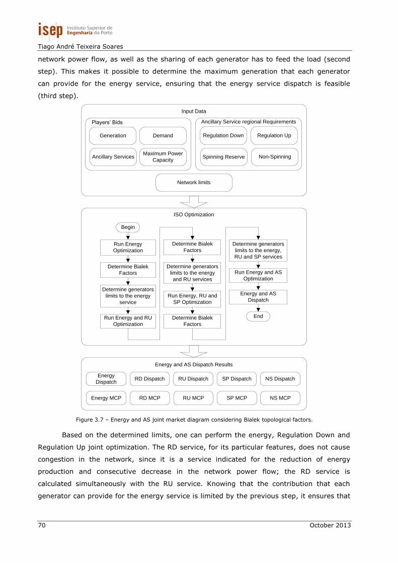
Tiago André Teixeira Soares
70 October 2013
network power flow, as well as the sharing of each generator has to feed the load (second
step). This makes it possible to determine the maximum generation that each generator
can provide for the energy service, ensuring that the energy service dispatch is feasible
(third step).
Input Data
Generation Demand
Ancillary ServicesMaximum Power
Capacity
Players’ Bids
Regulation Down Regulation Up
Spinning Reserve Non-Spinning
Ancillary Service regional Requirements
Network limits
ISO Optimization
Run Energy
Optimization
Begin
Determine Bialek
Factors
Determine generators
limits to the energy
service
Run Energy and RU
Optimization
Determine Bialek
Factors
Determine generators
limits to the energy
and RU services
Run Energy, RU and
SP Optimization
Determine Bialek
Factors
Determine generators
limits to the energy,
RU and SP services
Run Energy and AS
Optimization
Energy and AS
Dispatch
End
Energy and AS Dispatch Results
Energy
DispatchRD Dispatch RU Dispatch SP Dispatch NS Dispatch
Energy MCP RD MCP RU MCP SP MCP NS MCP
Figure 3.7 – Energy and AS joint market diagram considering Bialek topological factors.
Based on the determined limits, one can perform the energy, Regulation Down and
Regulation Up joint optimization. The RD service, for its particular features, does not cause
congestion in the network, since it is a service indicated for the reduction of energy
production and consecutive decrease in the network power flow; the RD service is
calculated simultaneously with the RU service. Knowing that the contribution that each
generator can provide for the energy service is limited by the previous step, it ensures that

Electricity Markets Modeling Considering Complex Contracts and Aggregators
October 2013 71
the energy and RU joint optimization do not violate the thermal limitations of the network
branches.
In the fifth step, with the data related to the energy and RU dispatch and its power
flow, the Bialek factors are again calculated. After the conclusion of the Bialek factors
determination, it is estimated the contributions that each generator has in the network
power flow for the energy and RU service, i.e., it is determined the maximum generation
that each generator can provide in the energy and RU joint service optimization (sixth
step).
The seventh step is the energy, RU and SP joint optimization. In this optimization
process, the sum of the energy and RU dispatch for each generator is restricted to the limits
calculated in the previous step. Besides this constraint, the generators are limited by the
other constraint determined in the third step of the algorithm (corresponding to the
maximum limit of each generator production for the energy service). The eighth step
consists in determining the Bialek factors in the energy, RU and SP joint optimization
(seventh step). The ninth step is the determination of the sharing that each generator has
in the network power flow on the energy, RU and SP joint optimization in order to conceive
the maximum generation limits that each generator can dispatch.
The tenth step refers to the energy and all ancillary services joint optimization. In
the simulation process, the maximum limits that each generator can dispatch according to
previous simulations of energy and ancillary services are considered. This way, this
optimization includes constraints related to the third, sixth and ninth steps. Thus, the
dispatch obtained in the previous step reflects the final dispatch of energy and ancillary
services, being perfectly feasible.
This model of energy and ancillary services optimization supported by the topological
methodology developed by Bialek, provides credible simulations for the joint market in what
is considered real constraints related to the physical characteristics of the transport and
distribution of electricity. All constraints considered in this model are presented at a very
detailed level in the next subsection.
3.5.3. Mathematical Formulation
The proposed problem formulation considers the energy and AS market simulation in
a liberalized environment.
The formulation includes the use of method to identify the contribution of each unit
generation on the network branches congestion. Based on this method, it is possible to
simulate each energy and AS dispatch, ensuring that the schedule dispatch is feasible. In
order to achieve a proper and adequate perception of the implied formulation problem in

Tiago André Teixeira Soares
72 October 2013
this section it is exposed the formulation engaging the entire problem discussed in the
introduction section of the problem.
The algorithm presented below for the calculation of generators sharing in the active
power flow of each network branch is based on the example discussed in the introductory
section of the problem of topological Bialek factors.
Therefore, the following equations are fundamental for solving the problem. The sum
of the actual demand of a particular load, plus the allocated part of the total transmission
loss is referred to as the gross demand. Assuming that is an unknown gross nodal power
flow through node i, and is an unkown gross line flow in line i-j, the gross power balance
equation at node i, when looking at the inflows is defined as [Bialek-1997]:
1,...,
ui
g g
i ij Gi
j
B
P P P
i N
(3.30)
Where is set of nodes supplying directly the node and is the generation in
node i. As
, the flow
can be replaced by
. If the transmission
losses are small, it can be assumed that
, where is the actual flow from
node j in line j-i and is the actual total flow through node j. Under this assumption
equation (3.30) can be rewritten as presented in equation (3.31) or (3.32):
1,...,
ui
g
ijg g
i j Gi
j j
B
PP P P
P
i N
(3.31)
u gross GA P P
(3.32)
Where is the unknown vector of gross nodal flows, is the vector of nodal
generations and the distribution matrix. This matrix is sparse and non-symmetric with its
(i,j) elements equal to: 1 for i=j; for . If there is
then and
its element is presented in the next equation. This equation shows how i-th gross nodal
power is supplied from all the generators in the system.
1
1
BN
g
i u Grirr
P A P (3.33)
The gross outflow in line i-j can be calculated, using the proportional sharing, as
presented in the equation (3.34).
1
,
1
B
g g Nij ijg g g
ij i u Gr ij r Grg g irri i
d
i
P PP P A P D P
P P
j
(3.34)

Electricity Markets Modeling Considering Complex Contracts and Aggregators
October 2013 73
In the equation, is the set of nodes supplied directly from node i and
. This equation represents the topological generation distribution
factor that is a portion of generation due to r-th generator that flows in line i-j.
Standard formulation for preventing congestion on a energy and ancillary
services basis.
This algorithm is used to calculate the generator sharing in each network branch. In
this way, the calculation of the limits necessary to restrict generation of each generator was
developed as follows:
( )
max
_ lim( , ) ( , , ) ( , ) max
( , )
1,..., ; 1,..., ; 1,..., ; 5
B
di
g rNiji
energy r t S r k t Ly i j ij
j Ly i j
B R
PP P P P
P
t T i N r N k
(3.35)
( )
max
_ _ lim( , ) ( , , ) ( , ) max2 ( , )
1,..., ; 1,..., ; 1,..., ; 2,5
kr B
di
g rN Niji
energy RU r t S r k t Ly i j ij
k j Ly i j
B R
PP P P P
P
t T i N r N k
(3.36)
( )
max
_ _ _ lim( , ) ( . , ) ( , ) max2 ( , )
1,..., ; 1,..., ; 1,..., ; 2,3,5
kr B
di
g rN Niji
energy RU Spinning r t S r k t Ly i j ij
k j Ly i j
B R
PP P P P
P
t T i N r N k
(3.37)
The equations (3.35), (3.36) and (3.37) refer to the calculation of the limits imposed
in the simulation model joint market for resources r. is the effective dispatch of
resource r obtained in the simulation market, for service k in each period t. is the
maximum capacity of active power in line i-j. refers to the power flow in line i-j.
refers to the sharing of power generated by resource r on the line i-j.
3.6. Joint Market model applied by VPP
The continued increase of DER penetration in distribution systems raises the need to
adopt new market models which considers the particular characteristics of the inherent
resources in distribution systems.
In this context, the concept of VPP is important as it allows the aggregation of DER
(mainly composed of DG, DR and storage units). Therefore, the VPP optimal management
of its resources may enable small players to participate in the market with low risk related
to their bids. Thus, the VPPs are able to participate and organize a variety of available
markets such as the energy and AS markets.

Tiago André Teixeira Soares
74 October 2013
The AS applied to the Smart Grid concept, in the scope of the distribution network is
still a subject under study. However, some authors have theories about AS best suited to be
traded in the market, as well as the development of new AS suited to a distribution network
in order to ensure system stability [Braun-2007, Buehner-2010].
In this context, this section proposes an energy and AS joint market model which
considers the several players aggregated by VPPs. This model enables the VPP optimization
of its resources and the trading between them and the small players. In order to perform
such trade, complex contracts were designed to allow both players and VPPs to trade
between them with special conditions established in the contracts.
3.6.1. Problem Description
The energy and AS joint market simulation problem in the context of the distribution
system behaves identically to that established for the transmission system. Thus, any
methodology developed in this section contemplates the methodology developed in the
previous model in order to ensure always a viable and feasible solution of the energy and
AS dispatches.
The methodology developed in this section includes the bidding of ancillary services
for regions of the network, based on several resources technologies, in which the DR
programs and storage charge and discharge bids are included. Besides this, the relaxation
variables are considered in each region of the distribution system.
Input Data
Distributed
Generation
Demand
Response
Suppliers Storage
Players’ Bids
Regulation Down Regulation Up
Spinning Reserve Non-Spinning
Ancillary Service regional Requirements
Distribution Network limitsComplex Contracts
VPP Optimization
Energy and AS Dispatch Results
Energy
DispatchRD Dispatch RU Dispatch SP Dispatch NS Dispatch
Energy MCP RD MCP RU MCP SP MCP NS MCP
Figure 3.8 – Energy and AS joint market diagram in distribution systems.

Electricity Markets Modeling Considering Complex Contracts and Aggregators
October 2013 75
Complex contracts are considered in the scope of the energy dispatch, in order to
enable a greater range of trading between players and the VPP. The architecture of the
developed model is illustrated in Figure 3.8. The input data module comprises all kinds of
players bids, the conditions related to complex contracts, technical data relating to the
distribution network, and AS requirements previously established by the VPP.
The VPP optimization module is based on the optimization model of section 3.5 with
the inclusion of constraints related to the model presented in this section.
The results module illustrates the dispatches of each service inherent to market
model and its market clearing prices.
3.6.2. Mathematical Formulation
The proposed problem formulation considers the use of market aggregator’s agents
(VPPs) for the management of several type of resource in the network. Through contracts
between the VPP and the players, the VPP has a total ability to manage the aggregated
players’ resources, in order to ensure the control and stability of the network. The VPP are
capable of aggregate all kind of DER, mainly DG based on renewable energy resources, and
other DER, including DR and storage units. In this way, through the formulation the VPP can
simulate the management according to its objectives.
The model allows trading between players and VPPs based on complex contracts
which may be beneficial for small players that could participate in the market through the
aggregation of a VPP, and also be beneficial for the VPP to ensure the aggregation of
players that gives the best benefits in its optimal management.
The objective function presented in (3.38) has the main goal of minimizing the VPP
operation costs taking into account several kinds of complex contracts between the VPP and
the players, while satisfying the consumer needs. The following costs are separated into two
distinct parts: energy and ancillary services.
4
( ) ( , )
1 1
min
T
E t AS k t
t k
Minimize f
F F
(3.38)
Equation (3.39) shows the objective function costs concerning the energy part, in
which are considered the following costs: DG costs, costs with energy acquisition to
external suppliers, storage discharge and charge costs, DR program costs for reduction and
curtailment, costs of Non-Supplied Demand (NSD) and Generation Curtailment Power (GCP)
costs for DG units.

Tiago André Teixeira Soares
76 October 2013
( )
( , , ) ( , , ) ( , , ) ( , , )
1 1
_ ( , , ) _ ( , , ) _ ( , , ) _ ( , , )
1 1
( , ) ( , ) ( , , ) ( , , )
1 1
( ,
SP DG
L L
DG S
E t
N N
SP SP k t SP SP k t DG DG k t DG DG k t
SP DG
N N
DR A l k t DR A l k t DR B l k t DR B l k t
l l
N N
GCP DG t GCP DG t Dch S k t Dch S k t
DG S
Ch S
F
P C P C
P C P C
P C P C
P
, ) ( , , ) ( , , ) ( , , )
1 1
1,..., ; 5
S LN N
k t Ch S k t NSD l k t NSD l k t
S l
C P C
t T k
(3.39)
The objective function costs concerning the ancillary services parts contain some
differences when compared to the energy part. The costs associated with ancillary services
are represented in equation (3.40) and they are: DG costs, costs with power acquisition to
external suppliers, storage discharge and charge costs, DR program costs for reduction and
curtailment and relaxation variables penalties.
( , )
( , , ) ( , , ) ( , , ) ( , , )
1 1
_ ( , , ) _ ( , , ) _ ( , , ) _ ( , , )
1 1
( , , ) ( , , ) ( , , ) ( , , )
1 1
SP DG
L L
Z Z
AS k t
N N
SP SP k t SP SP k t DG DG k t DG DG k t
SP DG
N N
DR A l k t DR A l k t DR B l k t DR B l k t
l l
N N
z k t RLXD z k t z k t RLXU z k t
z z
F
P C P C
P C P C
RLXD W RLXU W
P
( , , ) ( , , ) ( , , ) ( , , )
1 1
1,..., ; 1, 2,3, 4
S SN N
Dch S k t Dch S k t Ch S k t Ch S k t
S S
C P C
t T k
(3.40)
Equation (3.41) refers to the active power balance constraint (Kirchhoff’s first law) in
each bus i, including ancillary services k, for each period t.
2
( ) ( ) ( ) ( ) ( ) ( ) ( ) ( ) ( )
( ) ( , , ) ( , , ) ( , )
1 2 1 2 1
( , , ) _ ( ,
1 2
cos sin
i
i i iDG SPDG SP DGK K
i SS K
i t ii i t j t ij i t j t ij i t j t Gi t Di t
j y
N N NN Ni i i
Gi t DG DG k t SP SP k t GCP DG t
DG k SP k DG
N Ni
Dch S k t DR A l k
S k
V G V V G B P P
P P P P
P P
, ) _ ( , , )
1 2
4
( ) ( , ) ( , , ) ( , , ) ( , , ) _ ( , , )
1 1 5 1 1 5 1 2
1,..., ; 1,..., ; 2,3,4,
i LL K
ii S i L i LSL K L K L K
N Ni i
t DR B l k t
l k
NN N N N N Ni i i i i
Di t Load l t Ch S k t Ch S k t NSD l k t req limit l k t
l S k k l k l k
B
P
P P P P P P
t T i N k 5
(3.41)
Equation (3.42) refers to the reactive power balance constraint for energy service
(k=5) in each bus i, for each period t.

Electricity Markets Modeling Considering Complex Contracts and Aggregators
October 2013 77
2
( ) ( ) ( ) ( ) ( ) ( ) ( ) ( ) ( )
( ) ( , , ) ( , , )
1 1
( ) ( , , ) ( , , )
1 1
sin cos
1,..., ; 1,..., ; 5
i
i iDG SP
i iL L
i t j t ij i t j t ij i t j t i t ii Gi t Di t
j y
N Ni i
Gi t DG DG k t SP SP k t
DG SP
N Ni i
Di t Load l k t NSD l k t
l l
B
V V G B V B Q Q
Q Q Q
Q Q Q
t T i N k
(3.42)
Bus voltage magnitude and angle limits are the same as presented in the previous
model represented by equation (3.19). The line thermal limits constraint is the same as
presented in the previous model represented by equation (3.20).
The constraint concerning the minimum and maximum amount of active power
generation offered by each external supplier for service k is represented on equation (3.43).
Equation (3.44) concerns the reactive power limits for each supplier. This equation also
considers the reactive power percentage factor regarding the active power. This implies that
each resource is related to a generation limit of reactive power, according to its active
power limit. In the same perspective, equations (3.45) and (3.46) refer to the minimum
and maximum active and reactive power generation offered by DG units.
( , , ) ( , , )0
1,..., ; 1,..., ; 1,...,
SP SP k t SPMax SP k t
SP K
P P
t T SP N k N
(3.43)
( , , ) ( , , )
( , , ) ( , , ) ( , )
0
1,..., ; 1,..., ; 5
1,..., ; 1,..., ; 5
SP SP k t SPMax SP k t
SP
SPMax SP k t SPMax SP k t power SP t
SP
Q Q
t T SP N k
Q P F
t T SP N k
(3.44)
( , , ) ( , , ) ( , , ) ( , , ) ( , , )
( , , ) ( , ) ( , , ) ( , , )
1,..., ; 1,..., ; 1,...,
1,..., ; 1,..., ; 1,...,
DGMin DG k t DG DG k t DG DG k t DGMax DG k t DG DG k t
DG K
DG DG k t GCP DG t DGMax DG k t DG DG k t
DG K
P X P P X
t T DG N k N
P P P X
t T DG N k N
(3.45)
( , , ) ( , , ) ( , , ) ( , , ) ( , , )
( , , ) ( , , ) ( , )
1,..., ; 1,..., ; 5
1,..., ; 1,..., ; 5
DGMin DG k t DG DG k t DG DG k t DGMax DG k t DG DG k t
DG
DGMax DG k t DGMax DG k t power DG t
DG
Q X Q Q X
t T DG N k
Q P F
t T DG N k
(3.46)

Tiago André Teixeira Soares
78 October 2013
Equations (3.47) and (3.48) refer to the Direct Load Control (DLC) demand response
capacities, namely the reduction – DR_A – curtailment – DR_B – programs, respectively.
The reduction program (DR_A) corresponds to a decrease in the consumption and the
curtailment program (DR_B) corresponds to the curtailment of the whole consumption of a
determined load l. For the RD service constraints (3.47) and (3.48) are true whenever the
maximum limit of each Type of DR is equal to 0. This happens to be considered DR of type
DLC, which lacks the flexibility to participate in the RD service.
_ ( , , ) _ ( , , )
1,..., ; 1,..., ; 2,3,4,5
DR A l k t DR AMax l k t
L
P P
t T l N k
(3.47)
_ ( , , ) _ ( , , ) _ ( , , )
1,..., ; 1,..., ; 2,3,4,5
DR B l k t DR BMax l k t DR B l k t
L
P P X
t T l N k
(3.48)
The storage technical limits in each period t are restricted by several distinct
constraints. These constraints are shown from equation (3.49) to equation (3.61) for all
services. For services of increased generation (energy, RU, SP and NS) are considered
constraints from (3.49) to (3.56). For the energy and RD joint balance are considered
constraints from (3.57) to (3.61). Regarding equation (3.49), it refers to the non-
simultaneity of the storage charge and discharge energy.
( , ) ( , ) 1
1,..., ; 1,...,
S t S t
S
X Y
t T S N
(3.49)
The battery balance (energy, RU, SP and NS) is established in equation (3.50) with
the energy remaining from the previous period and the charge/discharge in the period t for
each storage unit.
( , ) ( , 1) ( ) ( , , ) ( , , )
2 2( )
1
1,..., ; 1,..., ; 1
K KN N
Stored S t Stored S t c S Ch S k t Dch S k t
k kd S
S
E E P t P t
t T S N t
(3.50)
The charge limit for each storage unit considering the battery charge rate is given by
equation (3.51).
( , , ) ( , , ) ( , )
1,..., ; 1,..., ; 1,...,
Ch S k t ChMax S k t S t
S K
P P Y
t T S N k N
(3.51)
Equation (3.52) indicates the storage charge limit considering the battery balance.
( ) ( , , ) ( , ) ( , 1)
2
1,..., ; 1,..., ; 1
KN
c S Ch S k t BatCap S t Stored S t
k
S
P t E E
t T S N t
(3.52)
Electricity Markets Modeling Considering Complex Contracts and Aggregators
October 2013 79
The discharge limit for each storage unit considering the battery discharge rate is
presented in equation (3.53).
( , , ) ( , , ) ( , )
1,..., ; 1,..., ; 1,...,
Dch S k t DchMax S k t S t
S K
P P X
t T S N k N
(3.53)
Equation (3.54) shows the storage battery discharge limit considering the battery
balance.
( , , ) ( , 1)
2( )
1
1,..., ; 1,..., ; 1
KN
Dch S k t Stored S t
kd S
S
P t E
t T S N t
(3.54)
The maximum battery charge limit for the services of increasing generation is shown
in equation (3.55). This equation relates the flexibility of the storage units in the AS of
increase generation (RU, SP and NS) can reduce the charge that acquire in the service
energy. For this, the sum of the charge storage variable of these ancillary services must not
exceed the value of the charge variable scheduled in energy service.
4
( , , ) ( , , )
5 2
1,..., ; 1,...,
KN
Ch S k t Ch S k t
k k
S
P P
t T S N
(3.55)
The maximum battery discharge limit for the services of increasing generation is
shown in equation (3.56).
( , , ) ( , )
2
1,..., ; 1,...,
KN
Dch S k t DchMax S t
k
S
P P
t T S N
(3.56)
The battery balance for energy and RD is determined in equation (3.57).
1 5
_ ( , ) _ ( , 1) ( ) ( , , ) ( , , )
1 5
1 5
( , , ) ( , , ) ( , , )
1 5( )
1
1,..., ; 1,..., ; 1; 1,5
Stored RD S t Stored RD S t c S Ch S k t Ch S k t
k k
Dch S k t Dch S k t Dch S k t
k kd S
S
E E P P t
P P P t
t T S N t k
(3.57)
Equation (3.58) indicates the storage charge limit considering the energy and RD
battery balance.
1 5
( ) ( , , ) ( , , ) ( , ) _ ( , 1)
1 5
1,..., ; 1,..., ; 1
c S Ch S k t Ch S k t BatCap S t Stored RD S t
k k
S
P P t E E
t T S N t
(3.58)
Equation (3.59) concerns the storage battery discharge limit considering the energy
and RD battery balance.
Tiago André Teixeira Soares
80 October 2013
1 5
( , , ) ( , , ) _ ( , 1)
1 5( )
1
1,..., ; 1,..., ; 1
Dch S k t Dch S k t Stored RD S t
k kd S
S
P P t E
t T S N t
(3.59)
The maximum battery charge limit for the energy and RD is shown in equation
(3.60).
1 5
( , , ) ( , , ) ( , )
1 5
1,..., ; 1,...,
Ch S k t Ch S k t ChMax S t
k k
S
P P P
t T S N
(3.60)
The last constraints on the storage units, concerns to the maximum battery
discharge limit for the energy and RD is shown in equation (3.61). This equation relates the
flexibility of the storage units in the RD service can reduce the discharge that was
scheduled in the service energy. For this, discharge storage variable of RD service must not
exceed the value of the discharge variable scheduled in energy service.
1
( , , ) ( , , )
5 1
1,..., ; 1,...,
KN
Dch S k t Dch S k t
k k
S
P P
t T S N
(3.61)
Equation (3.62) relates to each AS requirement in a given region z, in period t. In
order to be able to simulate the AS in a network and obtain the corresponding power flow, it
is necessary to locate where is the AS requirement bus. Towards the AS requirement be
divided by network regions, it was established that each load l belonging to a particular
region z, composes part of the AS requirement of the region z. In this way, the sum of each
AS requirement of each load l, must match the regional requisite set by the SO. Thus, it
becomes possible to determine the power flow for each ancillary service.
_ lim ( , , ) _ ( , , )
1
1,..., ; 1,2,3,4 ; 1,..., ;
zLN
z
req it l k t AS req z k t
l
Z
P P
t T k z N
(3.62)
Equation (3.63) refers to the minimum amount that each load l can consume in each
AS, i.e., is the maximum individual requirement of ancillary services in period t.
max
_ lim ( , , ) _ lim ( , , )
1,..., ; 1,..., ; 1,2,3,4 ; 1,..., ;
req it l k t req it l k t
L Z
P P
t T l N k z N
(3.63)
The constraint that concerns the balance of each AS is equation (3.64). For all AS
region, the sum of resources relating to external suppliers, DG and DR is sufficient to meet
the requirement of all regional ancillary service, in period t.

Electricity Markets Modeling Considering Complex Contracts and Aggregators
October 2013 81
( , , ) ( , , ) _ ( , , ) _ ( , , )
1 1 1
( , , ) ( , , ) _ ( , , )
1 1
1,..., ; 1,2,3,4 ; 1,..., ;
SP DG L
S Z
N N N
SP SP k t DG DG k t DR A l k t DR B l k t
SP DG l
N N
Dch S k t Ch S k t AS req z k t
S z
Z
P P P P
P P P
t T k z N
(3.64)
Through equation (3.65) it is guaranteed that internal resources of a given region
must ensure at least a percentage factor of the AS requirement of the region. This rule is
ensured by the variable percentage factor. All resources of the region z must be able to
guarantee at least half of the requirement that region. However, if this is infeasible, the
service can be purchased through the relaxation variables with a respective economic
penalty.
( , , ) ( , , ) _ ( , , ) _ ( , , )
1 1 1
( , , ) ( , , ) ( , , ) ( , , ) _ ( , , ) _ ( , )
1
1,..., ; 2,3,4 ; 1,..., ;
z z zSP DG L
zS
N N Nz z z z
SP SP k t DG DG k t DR A l k t DR B l k t
SP DG l
Nz z
Dch S k t Ch S k t z k t z k t AS req z k t AS req z k
S
Z
P P P P
P P RLXD RLXU P F
t T k z N
(3.65)
Typically, the RLXD variable corresponds to the relaxation variable of the problem
used by the VPP in order to make the dispatch simulation always feasible. This variable
corresponds to a certain amount of power which is provided directly by the VPP, which may
be available through bilateral contracts with large power plants. In order to simulate the
physical location of that variable it is proposed that this variable comprises the network
resources allocated in a region w different from the problematic region z, since the thermal
constraints of the lines allows that. In equation (3.66) the methodology adopted is
implemented.
( , , ) ( , , ) _ ( , , ) _ ( , , )
1 1 1
( , , ) ( , , ) ( , , )
1
1,..., ; 1,2,3,4 ; 1,..., ;
w w wSP DG L
wS
N N Nw w w w
SP SP k t DG DG k t DR A l k t DR B l k t
SP DG l
Nw w
Dch S k t Ch S k t z k t
S
Z
P P P P
P P RLXD
t T k w N z w
(3.66)
Equation (3.67) represents the maximum upward limit of generation of external
suppliers and DG units, related to energy and ancillary services.
( , , ) _ ( , )
2
( , , ) _ ( , )
2
1,..., ; 1,...,
1,..., ; 1,...,
K
K
N
SP SP k t CAP SP SP t
k
SP
N
DG DG k t CAP DG DG t
k
DG
P P
t T SP N
P P
t T DG N
(3.67)

Tiago André Teixeira Soares
82 October 2013
Considering that the VPP can establish contracts with the owners of the resources
and consumers installed in the network, several kinds of contracts are presented in
equation (3.68) to equation (3.72).
The minimum generation in the time horizon contract is represented in equation
(3.68). This contract concerns the minimum limit of energy (considering energy, RU, SP and
NS services) produced by the generator in a 24-hour period, i.e., the contract ensures that
the producer, if dispatched, produces at least the minimum limit defined a priori.
( , , ) ( )
1 2
( , , ) ( )
1 1
1,...,
1,...,
K
K
NT
SP SP k t SPMin SP
t k
SP
NT
DG DG k t DGMin DG
t k
DG
P P
SP N
P P
DG N
(3.68)
The minimum remuneration contract in the time horizon imposes a minimum limit of
remuneration for the whole 24 hours, ensuring a minimum remuneration, regardless the
energy produced in each hourly period, considering the energy, RU, SP and NS services.
This contract is represented by equation (3.69).
( , , ) ( , , ) Re ( )
1 1
( , , ) ( , , ) Re ( )
1 1
1,...,
1,...,
K
K
NT
SP SP k t SP SP k t SP m SP
t k
SP
NT
DG DG k t DG DG k t DG m DG
t k
DG
P C P
SP N
P C P
DG N
(3.69)
The variation of generation contract between periods refers to the gradient of
generation in each period. This contract sets for each period of one hour a limit for the
increase/decrease power generation according to the previous period. This contract
considers the energy, RU, SP and NS services and it is represented by equation (3.70).
( , , ) ( , , 1) ( )
2 2
( , , ) ( , , 1) ( )
2 2
1,..., ; 1,...,
1,..., ; 1,...,
K K
K K
N N
SP SP k t SP SP k t SPVar SP
k k
SP
N N
DG DG k t DG DG k t DGVar DG
k k
DG
P P P
t T SP N
P P P
t T DG N
(3.70)
The contract’s minimum of periods t functioning in time horizon T refers to a
minimum period of generation during the overall period of 24 hours. Producers with this
type of contract are dispatched for a number of consecutive periods; thereby, they can
reduce start-up costs. This contract is represented by equation (3.71) and it is considered
for energy, RU, SP and NS services.
Electricity Markets Modeling Considering Complex Contracts and Aggregators
October 2013 83
( , , ) ( )
1
( , , ) ( )
1
1,..., ; 2,3,4,5
1,..., ; 2,3,4,5
T
SP SP k t SPMin SP
t
SP
T
DG DG k t DGMin DG
t
DG
X X
SP N k
X X
DG N k
(3.71)
The maximum entries in service contract consist in a maximum number of entries in
service throughout the 24 hours. This contract is applied to the energy, RU, SP and NS
services. In this context, the producer is forced to ensure stability from generation to avoid
being excluded from the selection of production for the period established. This contract is
represented by equation (3.72).
( , , 1)
( , , ) ( , , 1) ( )
1
( , , 1)
( , , ) ( , , 1) ( )
1
0
1,..., ; 2,3,4,5
0
1,..., ; 2,3,4,5
SP SP k t
T
SP SP k t SP SP k t SPMax SP
t
SP
DG DG k t
T
DG DG k t DG DG k t DGMax DG
t
DG
if X
X X X
SP N k
f X
X X X
DG N k
(3.72)
The constraints presented in equations (3.73) and (3.74) represent the limits of each
resource obtained through Bialek factors. At this stage, the limits considered relate to the
calculation of sharing that each resource has on the network, considering only the energy
dispatch and its network power flow. Through the limits set it is possible to know from the
outset that in any energy and AS joint simulation, the network dispatch becomes feasible.
( , , ) _ lim_ ( , )
1,..., ; 1,..., ; 5
SP SP k t energy SP SP t
SP
P P
t T SP N k
(3.73)
( , , ) _ lim_ ( , )
1,..., ; 1,..., ; 5
DG DG k t energy DG DG t
DG
P P
t T DG N k
(3.74)
Equations (3.75) and (3.76) consider the maximum limits of DG and external
suppliers, obtained through Bialek factors. In this case the factors are calculated based on
the energy and Regulation Up optimal dispatch, as well as the network power flow to the
optimal dispatch. Thus, the energy and the services (RU and SP) joint optimization, the sum
of the production of a particular resource for energy and RU must be less than or equal to
the threshold obtained through the Bialek factors.

Tiago André Teixeira Soares
84 October 2013
( , , ) _ _ lim_ ( , )
2
1,..., ; 1,..., ; 2,5
KN
SP SP k t energy RU SP SP t
k
SP
P P
t T SP N k
(3.75)
( , , ) _ _ lim_ ( , )
2
1,..., ; 1,..., ; 2,5
KN
DG DG k t energy RU DG DG t
k
DG
P P
t T DG N k
(3.76)
The maximum limits for each resource unit which restricts the generation related to
services of energy, RU and SP are present in equations (3.77) and (3.78). Based on the
dispatch of energy, RU and SP services, the methodology described in the problem in the
introduction section, allows simulating the energy and all ancillary services joint market,
knowing that constraints between (3.73) and (3.78) limit each resource in order to obtain
an dispatch with the features and not to violate the physical network constraints, i.e., not
causing network congestion. Therefore, by optimizing the solution becomes perfectly
feasible.
( , , ) _ _ _ lim_ ( , )
2
1,..., ; 1,..., ; 2,3,5
KN
SP SP k t energy RU Spinning SP SP t
k
SP
P P
t T SP N k
(3.77)
( , , ) _ _ _ lim_ ( , )
2
1,..., ; 1,..., ; 2,3,5
KN
DG DG k t energy RU Spinning DG DG t
k
DG
P P
t T DG N k
(3.78)
3.7. Conclusions
Throughout the evolution of the electric market in a liberalized environment, the
modeling of markets has varied according to the characteristics inherent in the structure of
power systems in the region in which the market are included.
The models presented in this thesis, and more specifically in this section, address
the simulation of energy and ancillary services joint market.
Through the models studied it is possible to understand the operation of real
markets, as the models based on information inherent in several real market models.
The energy and AS joint market simulation is a model that can match the highlight
the economic efficiency, as explained in this section. In this context, several real markets
use this methodology to obtain the lowest possible cost in the management of energy
resources.
The concept of AS procurement by network regions is new in the perspective of the
MASCEM markets simulation. Thus, the third model is an added value in the continuous
development of this simulation tool.
Electricity Markets Modeling Considering Complex Contracts and Aggregators
October 2013 85
Certain real markets use a simulation model of ancillary services market by regions,
wherein the ISO divides the network into several regions. Thus, the regional AS are
dispatched according to regional requirements. However, not always the existing resources
in a given region are sufficient to meet the required demand, which implies the use of
generators outside the region and interties lines between regions in order to cope with the
demand required. These scenarios are used for critical cases of congestion emphasized in
the system over the experience of operation of the SO, resulting in different market prices
between regions.
The joint model with AS bidding regions contemplates the AS simulation by regions
and have a variable which allows the SO to ensure that is sufficient generation to provide
the region. Moreover, the model guarantees that at least 50% of the output provided by
generator units of this region in order ensures good competitive resources, as well as the
reliability of the system, relieving the congestion of interties between regions.
The joint market model considering bialek factors presented in this chapter proposes
a joint market methodology able to get the best economic solution, ensuring the feasibility
of the solution of the all services on the market. That is, the model is based on the
methodology of the Bialek topological factors to ensure the feasibility of the dispatch of
each service in market trading. Through this model both the ISO and VPP can simulate the
market, ensuring from the beginning a viable and feasible solution. Whereas through the
market, the conventional methodology performs a provisional dispatch of all services, to
further verify the feasibility of the dispatch. Then, the dispatch is adjusted according to the
technical features of the network in order to achieve a feasible solution.
In this way, the proposed model has the advantage of ensuring a feasible dispatch
for all services traded in the market, presumably faster and without the need for
adjustments.
On the continuous increase in the introduction of technologies based on the concept
of renewable energy, require a different management of network resources. In this way, the
aggregation of resources for a VPP becomes increasingly central to the participation of these
resources in the market. In this point of view, resource management can be performed by
VPP in order to participate in the market, which focuses on global management of all
resources. In this context, the studied models are able to adapt to the required
management level either by the VPP or by the ISO.
The joint model applied by VPP focuses on resource management by the VPP,
considering the constraints of congestion caused by power flow in the network. The model
contemplates an innovative approach able to provide dispatches for all services which does
not violate any network technical constraint. Thus, the method always provides feasible and
viable dispatches of the energy and ancillary services joint market.

Electricity Markets Modeling Considering Complex Contracts and Aggregators
October 2013 87
Chapter 4
Case Studies


Electricity Markets Modeling Considering Complex Contracts and Aggregators
October 2013 89
4. Case Studies
This chapter presents several case studies which illustrate the application of the
proposed models (presented in chapter 3) and their respective performance. The presented
case studies have been chosen to cover a diversity of situations and involved players,
allowing demonstrating the proposed models. The results obtained are presented and
discussed for each model. At the end of the chapter some general conclusions are made.
4.1. Introduction
A large diversity of the features of the developed models leads to the need of
creating several individual case studies. After this introduction section, which explains the
organization of the present chapter, the following sections report the case studies
concerning each model presented in chapter 3. Finally, the conclusion section presents the
main conclusions of this chapter. Table 4.1 summarizes the scenarios developed for each
case study. Each developed scenario has its own characteristics that distinguish it from the
other scenarios. In the first column of Table 4.1 are presented several parameters which
characterize the models and make distinctions between them.
The Case study 1 – Ancillary Services Market model, refers to a generic AS market
simulation model with incorporation of the ancillary services cascading process. This case
study was divided into three scenarios. The first scenario considers the AS market
simulation in its most simplified way. The second scenario considers the market simulation
with the recourse to relaxation variables in order to return a feasible solution. The third
scenario considers a comparison between the market simulation of AS with the cascading
process and the first scenario developed in order to verify the benefits of the AS cascade
process.
The Case study 2 – Energy and AS Joint Market model is based on energy and AS
joint market simulation. This case study is composed of two scenarios and a subsection
which performs a comparison of both scenarios. The first scenario shows the simulation
results of the separated market, in which simulates the energy dispatch separately from the
AS dispatch. The second scenario shows the simultaneous simulation of the joint market. A
comparison of the two scenarios described above is presented in the last subsection of the
case study.
The Case study 3 – AS bidding regions considers the joint market simulation with the
bids for ancillary services to be performed by network regions. In this case study, the
proposed method is compared with a reference method. This case study is divided into
three scenarios. The first scenario considers the joint market simulation in which the power
flow resulting for energy service and AS is in the same direction. On the other hand, the
second scenario considers the market simulation in which the power flow resulting for

Tiago André Teixeira Soares
90 October 2013
energy service and AS flows in opposite directions. The third scenario considers the market
simulation with AS cascade process, showing the advantages of this methodology.
Table 4.1 – Case studies characterization.
Characteristics
Model
Ancillary Service
Market
(Case Study 1)
Energy and AS
joint market
(Case Study 2)
Joint market
considering AS
bidding regions
(Case Study 3)
Joint market
considering
Bialek
Coefficients
(Case Study 4)
Joint Market in
DNO/VPP
operation
(Case Study 5)
Market model AS market Joint Market Joint Market Joint market Joint Market
Bids Asymmetric
Market
Symmetric
Market
Symmetric
Market
Symmetric
Market
VPP/players
contracts
AS cascading
process Yes Yes Yes No No
Network
operation No No
Transmission
Network with 4
buses
considering AC
OPF
Transmission
Network with 7
buses
considering AC
OPF
Distribution
Network with 33
buses
considering AC
OPF with Bialek
topological
factors
Resource
management
goal
Minimization of
ISO operation
costs
Market Clearing
Price
Market Clearing
Price
Market Clearing
Price
Minimization of
VPP operation
costs
AS bidding
regions No No
AS bids and
requirement by
two regions of
the network
No
AS bids and
procurement by
four regions of
the network
Relaxation
variables
Ensured by ISO
through bilateral
contracts
Ensured by ISO
through bilateral
contracts
Ensured by ISO
through bilateral
contracts
Ensured by ISO
through bilateral
contracts
Ensured by the
energy
resources of
other regions,
including
external
suppliers
Complex
Contracts No No No No
Five types of
complex
contracts
between players
and VPP

Electricity Markets Modeling Considering Complex Contracts and Aggregators
October 2013 91
The Case study 4 – Bialek coefficients considers the joint market using the
innovative methodology for solving network congestion. The methodology is based on the
Bialek topological factors. The case study is divided into two scenarios. The first scenario
presents the results of market simulation without consideration of the methodology of
solving the network congestion. The second scenario considers the use of Bialek topological
factors together with the joint market simulation. The results of this scenario are compared
with the results of the first scenario. In this way, there is the great advantage of use the
developed methodology, which always ensures a feasible solution.
The Case study 5 – Joint Market model applied by VPP considers the joint market
simulation applied regarding a distribution network operation. Therefore, the operation is
controlled by a VPP which manages the energy resources available in the distributed
network. In this case study it is applied the developed methodology of the energy and AS
joint market simulation which considers the contribution of all services in the network
congestion. The developed methodology based on the Bialek topological factors is evidenced
in all scenarios in this case study. Thus, the case study is divided into four distinct
scenarios. The first scenario consists in the joint market simulation in the scope of a VPP
management with application of the developed methodology to ensure viable and feasible
solutions. The second scenario is based on the first scenario with the introduction of bids of
distributed energy resources be made for network regions (the network was divided into
four distinct regions). The third scenario is based on the second scenario in which adds the
introduction of DR and relaxation variables in the ancillary services for the network regions.
The fourth scenario considers all the inherent characteristics of third scenario with the
inclusion of storage units in the ancillary services provision for each network region. The
fifth and final scenario maintains the ideology of the previous scenarios with inclusion of
complex contracts between players and VPP. These contracts were associated with DG units
for the energy service.
4.2. Case study 1 – Ancillary Services Market model
This case study refers to the model developed in section 3.2. After a brief
introduction to the considered scenarios with the corresponding input data, the results are
presented and some conclusions are made.
Three scenarios compose the case study. The first scenario corresponds to the base
scenario of the case study and refers to the market simulation. The usefulness of the
relaxation variables is proven in the second scenario, in which the ISO has an obligation to
contract other resources through bilateral contracts, ensuring the feasibility of ancillary
services dispatch. An ancillary services market simulation with the inclusion of the AS

Tiago André Teixeira Soares
92 October 2013
cascade process is presented in the last scenario. Moreover, this scenario also provides a
comparison between the AS market simulation with and without AS cascade process.
4.2.1. Outline
The ancillary services model described in section 3.2 considers simultaneous
optimization of AS market. In order to simulate the developed model, a set of input data
relevant to the type of problem was used.
In this case study, three scenarios are considered in order to observe carefully the
results from the proposed methodology.
Therefore, the input data for each scenario are available in the Annex A, tables A1,
A2 and A3, and they include essential features for the simulation. These features include
the following aspects:
Bids that each player performs in the market
AS requirements imposed by the System Operator (SO)
The input data for the first scenario consists of real data available at the CAISO web
site [CAISO-2007b].
4.2.2. Results
The results of this case study are based on the referred scenarios and approaches.
The first scenario is the baseline scenario of the case study, which besides being analyzed
individually, is compared with another scenario in order to know the benefits of the
implemented methodology.
4.2.2.1. Scenario 1 – Baseline case
AS cascading is important in order to make the market more competitive, and
achieve lower overall cost in contracting power required for the AS dispatch.
Table 4.2 shows the results of the AS dispatch, to the simplest methodology of the
AS market simulation.
Regarding to the RD dispatch, the Regulation Down requirement is about 150 MW,
from which 111 MW are dispatched by “Bid 5” and the remaining 39 MW are supplied by
“Bid 8”. “Bid 8” has a bid price of 4.8 m.u./MW, corresponding to the market clearing price
for this service. Although “Bid 4” contains a bid price of 4.0 m.u./MW, the generation
minimum limit of this bid is 60 MW. Thus, the “Bid 4” is not dispatched for not fitting the
requirement of 39 MW, resulting that a bid with a higher price to be dispatched.
Each of the AS dispatches is related to the market clearing price. This market
clearing price is used to calculate the final cost of the market. Each player is remunerated
at the market clearing price of each ancillary service.

Electricity Markets Modeling Considering Complex Contracts and Aggregators
October 2013 93
Table 4.2 – Ancillary services dispatch in scenario 1 of AS model.
Bids Regulation Down Regulation Up Spinning Reserve
Non-Spinning Reserve
Total (MW)
MW m.u./MWh MW m.u./MWh MW m.u./MWh MW m.u./MWh
1 0 10.0 0 5.0 0 10.5 0 10.0 0 2 0 8.0 70 4.5 0 9.2 0 11.0 70 3 0 8.0 0 5.2 0 8.5 0 10.2 0 4 0 4.0 50 5.0 65 8.3 0 10.6 115
5 111 3.5 0 6.3 0 8.9 59 9.0 59 6 0 9.0 0 6.0 0 8.8 0 11.0 0 7 0 7.0 0 7.5 0 9.3 0 10.5 0 8 39 4.8 0 6.5 0 8.6 0 10.4 0 9 0 9.0 0 5.5 0 8.3 0 10.3 0 10 0 10.0 80 4.0 85 8.0 91 9.0 256
Contracted Service (MW)
150 200 150 150 650
Service Requirement
(MW) 150 200 150 150 650
Market Clearing Price (m.u./MWh)
4.8 5.0 8.3 9.0 Total
(m.u.)
Total Cost (m.u.)
720 1000 1245 1350 4315
Section 4.2.2.3 shows a comparison between scenarios in which it is evidenced the
differences between the method with or without AS cascading.
4.2.2.2. Scenario 2 – Relaxation variables
This scenario demonstrates the use of certain variables directed to the relaxation of
the dispatch problem when there are special negative events for market stability, in which
the forecast capability of these events is poor.
The variables RLXD and RLXU are penalties to the optimization problem for not
meeting the AS requirements imposed by the SO. Therefore, the RLXD penalty is applied
when the minimum power requirement of an increase generation AS is higher than the sum
of maximum power offer by all agents in AS market, i.e., when there is a lack of power to
achieve the requirement. In turn, the RLXU penalty is applied when the maximum power
requirement of increased generation AS is less than the minimum power of the agent with
lower minimum limit of power, i.e., when there is the limit of minimum power of the most
lower agent is higher than the maximum AS requirement.
The penalty for each variable has a very high price. For this case study it was
established for both variables a penalty of 100 m.u./MW.
The results of the AS simulation considering the use of the relaxation variables are
presented in Table 4.3. In this table, it is possible to see the use of RLXD variable by NS
service, as well as the contribution of the RLXU variable to the SP dispatch.

Tiago André Teixeira Soares
94 October 2013
Table 4.3 – AS dispatch considering relaxation variables.
Bids Regulation
Down Regulation Up
Spinning Reserve
Non-Spinning Reserve
Total (MW)
MW m.u./MWh MW m.u./MWh MW m.u./MWh MW m.u./MWh
1 0 10.0 0 15.0 0 5.0 30 7.0 30 2 0 8.0 0 10.0 0 9.0 25 4.0 25 3 0 8.0 0 8.2 0 8.5 30 6.0 30 4 0 4.0 76 5.0 0 7.2 36 4.6 112
5 100 3.5 0 7.0 0 4.0 15 9.0 15 6 0 9.0 0 14.6 55 8.0 19 11.0 74 7 0 7.0 0 8.5 0 7.3 20 10.5 20 8 0 4.8 0 10.6 0 6.6 62 4.0 62 9 0 9.0 39 6.5 0 4.3 35 5.3 74 10 0 10.0 85 4.0 0 9.0 60 5.0 145
Contracted Service (MW)
100 200 55 332 687
RLXD - 0 100.0 0 100.0 68 100.0 68
RLXU - 0 100.0 5 100.0 0 100.0 5
Service Requirement
(MW) 100 200 50 400 750
Market Clearing
Price
(m.u./MWh)
3.5 6.5 8.0 11.0 Total
(m.u.)
Total Cost (m.u.)
350 1300 400 4400 6450
Cost penalty for players
(m.u.) 0 0 500 6800 7300
The power of these penalties is contracted by the SO to special agents, with special
contracts for this kind of emergency service.
When penalties are applied, they are not included in the cost of each service to be
hired by the SO, i.e., not increasing even more the market clearing price. These penalties
are applied to all agents who participate in the service. In several real markets, these
penalties costs are accounted for each AS, in which the SO share the cost by the number of
agents participating in that service [CAISO-2009].
4.2.2.3. Scenario 3 – Ancillary Services Cascade process
This scenario shows the results of simultaneous optimization of all AS. The
simulation model provides the possibility of AS cascading when it is economically more
efficient, which implies that a high quality reserve can replace a lower quality one.
In this context, the present subsection compares the scenario presented in section
4.2.2.1 (Scenario 1) related to the scenario shown in Table 4.4 (Scenario 3) of this present
section.
In this way, it is clear the use of AS cascade shown in Table 4.4. Through Table 4.4,
one can verify that the RU service hired more power than the necessary to meet their

Electricity Markets Modeling Considering Complex Contracts and Aggregators
October 2013 95
needs. This happened as it was triggered the AS substitution through the slack variables.
This implies that players who offered their bids in the RU service, have partially satisfied the
SP service and fully satisfied the NS service, thus making the AS joint dispatch more
economical for the SO. Therefore, to meet their own needs and those of other services, the
RU service (SP and NS), resulted in a higher market clearing price for the RU service, than
if it had just met their own needs. However, as the bids for SP service and especially for NS
service are clearly more expensive, the increase in the market price of the RU service
reward makes the system more economically advantageous, regarding the market price
that would be charged on NS service if there was no possibility of AS cascade.
Table 4.4 – Ancillary services dispatch considering AS cascade mechanism.
Bids Regulation Down Regulation Up
Spinning Reserve
Non-Spinning Reserve
Total (MW)
MW m.u./MWh MW m.u./MWh MW m.u./MWh MW m.u./MWh
1 0 10.0 80 5.0 0 10.5 0 10.0 80 2 0 8.0 85 4.5 0 9.2 0 11.0 85
3 0 8.0 80 5.2 0 8.5 0 10.2 80 4 0 4.0 70 5.0 50 8.3 0 10.6 120 5 111 3.5 0 6.3 0 8.9 0 9.0 0 6 0 9.0 0 6.0 0 8.8 0 11.0 0 7 0 7.0 0 7.5 0 9.3 0 10.5 0 8 39 4.8 0 6.5 0 8.6 0 10.4 0 9 0 9.0 0 5.5 0 8.3 0 10.3 0
10 0 10.0 85 4.0 50 8.0 0 9.0 135
Contracted Service (MW)
150 400 100 0 650
AS Cascading (Slacks)
-
RU to SP SP to NS
- - 50 5.2 0 8.3
RU to NS -
150 5.2
Service Used
(MW) 150 200 150 150 650
Market Clearing Price
(m.u./MWh)
4.8 5.2 8.3 0.0 Total
(m.u.)
Total Cost (m.u.)
720 2080 830 0 3630
The only difference regarding to input data of both scenarios available in Annex A
refers to the maximum and minimum requirements for each service, which for the third
scenario, these requirements are not equal to the ones presented in the first scenario. With
this, there is leeway for the slacks to be used. The results in Table 4.4 show the AS dispatch
with clearances resulting in a total cost of approximately 3630 m.u., while the total cost of
the AS dispatches without slacks is around 4315 monetary units, as shown in Table 4.5 to
compare the scenarios.
As seen in Table 4.5 the information of dispatch and market clearing prices was
obtained for each AS and each simulated scenario. Comparing the two scenarios it is
noticeable the difference between the total cost of both scenarios. This comparison

Tiago André Teixeira Soares
96 October 2013
validates the formulation implemented, taking into account that the AS cascade process can
obtain a lower final cost, which meets the main goal to SO for ancillary services, that is to
guarantee AS quality at the lowest possible cost.
Table 4.5 – AS dispatch comparison related to scenarios 1 and 3 of AS model.
Market Dispatch
Regulation Down Regulation Up Spinning Reserve Non-Spinning
Reserve Total
Cascade No
Cascade Cascade
No Cascade
Cascade No
Cascade Cascade
No Cascade
Cascade No
Cascade
Contracted Service (MW)
150 150 400 200 100 150 0 150 650 650
Market Clearing
Price (m.u./MWh)
4.8 4.8 5.2 5.0 8.3 8.3 0.0 9.0 -
Total Cost (m.u.)
720 720 2080 1000 830 1245 0 1350 3630 4315
From the results obtained it can be concluded that the model considers the AS
substitution, which enables a more economical global AS dispatch, without affecting the
reliability of power systems.
4.2.3. Results analysis
In this case study, the simultaneous simulation model of AS market was applied. The
main goal of the problem is to minimize costs for the SO. The optimization was performed
in GAMS using the MINLP model. In order to know the characteristics and abilities of the
model, three scenarios able to express the advantages and disadvantages were developed.
In the first scenario shows the simulation model in a simple way, which lies in a AS
simulation, considering only the players involved in these service.
In the second scenario, importance was given to the use of relaxation variables of
the problem. These variables guarantee that the AS requirement is satisfied and related to
a penalty, regardless the ability of the players who participate in the service.
The third and final scenario shows the AS simultaneous optimization model
considering the advantage of using the AS cascade process outlined in implemented model.
Also in the section, on the last scenario, it is established a comparison between the results
obtained in the first scenario and the last scenario. In this way, one can verify the
difference between the possible variations of the model, in which it is clear that considering
the AS substitution results in a more economic optimization for the SO.
4.3. Case study 2 – Energy and AS Joint Market model
This subsection presents a case study which illustrates the implementation of the
proposed methodology described in section 3.3, in order to perform the energy and AS joint

Electricity Markets Modeling Considering Complex Contracts and Aggregators
October 2013 97
market model. This case study was published in [Soares-2011] and it has been
implemented in a multi-agent electricity market simulator (MASCEM) with the objective of
providing the simulator with greater flexibility on electricity markets simulation. The main
objective of this model is the minimization of costs of joint market for the SO. This
subsection includes an outline of the problem, as well as the input data necessary for the
simulation model. The results are reported together with some conclusions related to the
problem.
4.3.1. Outline
An energy and ancillary services joint market model is implemented in this case
study, which is based on the model presented in section 3.3. In order to simulate the
developed model a set of input data necessary for the operation of the simulation program
has been used.
In this case study are tested two scenarios for the model developed in order to
properly understand the main issue to solve the problem.
Annex B provides Table B.1 which contains the input data for solving the problem.
These input data include the power and AS seller bids for a set of 10 players based on real
offers proposed in CAISO, the buying bids for a set of 10 players, and the values of the
required power reserve for each service. Table B.1 also presents the minimum and
maximum capacity requirement for each service, constant forecast losses, rigid demand
contracted with ISO and energy prices.
4.3.2. Results
This subsection presents the results of this case study. Two scenarios were drafted
to give an overview of the possibilities to solve the individual energy and ancillary services
market, as well as the joint market. The third subsection shows the comparison between
the two scenarios mentioned above.
In this context, the first scenario is based on the separate market simulation for
energy and ancillary services. The second scenario concerns the joint market simulation.
Finally, the last subsection presents a comparison between the two scenarios presented and
draws some conclusions on the advantages and disadvantages of using the joint market
simulation model.
4.3.2.1. Scenario 1 – Energy and AS markets (Not-joint)
The scenario presented in this section concerns the separate optimization of the
energy and ancillary services market. In this way, the results are the ones of a sequential
process simulation. This process is given by the following steps:

Tiago André Teixeira Soares
98 October 2013
Optimization of the energy market
Determination of available power
Optimization of the AS market
The first step results in the simulation of the energy market based on the initial input
data from Table B.1 in Annex B. Table 4.6 presents the result of the energy dispatch and
power purchase bids dispatched in the market. Besides the energy market ensures the load
variable related to power purchase bids, it should ensure the supply of rigid demand and
the forecast losses in the system, regardless of the market price.
In this way, the rigid demand and forecasts losses correspond to the regulated
supply which arises in the highest part of the demand curve using the price cap of the
market. In order to include the rigid demand and the forecast losses in the simulation, the
optimization algorithm assigns a very high price for these parcels on the demand curve in
order to ensure that these parcels are provided in a market environment.
Table 4.6 – Energy dispatch in scenario 1 of energy and AS joint model.
Bids Sellers Buyers
Quantity (MW) Price (m.u./MWh) Quantity (MW) Price (m.u./MWh)
1 430 2.1 300 7.0 2 350 3.6 0 5.0 3 480 5.2 0 4.1
4 450 5.8 300 7.7 5 67 6.3 350 8.8 6 270 3.5 350 9.9
7 299 2.8 0 4.5 8 0 9.2 0 3.9 9 345 4.5 300 7.5 10 369 3.9 0 5.5
Rigid Demand - - 1300 -
Forecasts losses - - 160 -
Figure 4.1 illustrates the energy dispatch with all the considerations listed above.
Figure 4.1 – Energy market clearing price in scenario 1 of energy and AS joint model.
The second step of the simulation concerns the determination of the maximum
capacity of generation bids for the participants in the AS market. In order to obtain the

Electricity Markets Modeling Considering Complex Contracts and Aggregators
October 2013 99
maximum capacity of generation bids, it is necessary to calculate the difference between
the power used by each bid in the energy market and the limit of “Max Power” set out in
Table B.1 from Annex B. Therefore, Table 4.7 includes the values used for each bid in the
AS market. The bids which participated with its full available capacity in the energy dispatch
present values of “Residual Max Power” different from 0, as seen in Table 4.7. This is due to
the threshold established in each bid for the energy which does not correspond exactly to
their maximum capacity generation, as seen in Table B.1.
Table 4.7 – Residual maximum power.
Bid Residual Max Power (MW)
1 20 2 50 3 20 4 30
5 233 6 10 7 21 8 405 9 55 10 31
The third step results in the AS market simulation considering the limits determined
in the previous step. This way, results of the AS market considering a simple process and
the inclusion of cascading process are presented.
Figure 4.2 illustrates the dispatch of each ancillary service according to the energy
required by the system operator for these services. In this case, only the participant bids in
each service can provide this service.
Figure 4.2 – Ancillary services dispatch in scenario 1 of energy and AS joint model.

Tiago André Teixeira Soares
100 October 2013
According to the ancillary services simultaneous market model with AS cascade
process, it is possible to reduce the operation costs for the ISO. Therefore, Figure 4.3
illustrates the AS dispatch when there is the ancillary services cascading.
Figure 4.3 – Ancillary services dispatch with cascading mechanism in scenario 1 of energy and AS joint model.
By comparing the results presented in Figure 4.2 and Figure 4.3, one can concluded
that the market clearing price of Spinning Reserve decreases from 9.0 m.u./MWh to 8.0
m.u./MWh corresponding to a power decrease from 150 MW to 114 MW. In compensation,
the Regulation Up provides more 36 MW (236 MW) with a market clearing price equal to 8.3
m.u./MWh, in order to cascade energy to SP, thus reducing the overall costs of AS. The
cascading allows a better optimization of AS, combining the three services (RU, SP and NS).
In Table B.2 and Table B.3 are the exact values of the bids which participate in the AS and
the market clearing price for each ancillary service. The variables of the cascading process,
usually called slacks, and its respective price can be seen in Table B.3.
4.3.2.2. Scenario 2 – Energy and AS joint market
The implemented energy and AS joint market model is presented in this scenario.
The joint market simulation considers the simultaneous dispatch of energy and
Ancillary Services. From the perspective of the ISO, this model allows a better optimization
of the power capacity of each agent participating in the markets. This limit does not affect
the Regulation Down dispatch, since this service is a component for the frequency control
when there is excess of generation.

Electricity Markets Modeling Considering Complex Contracts and Aggregators
October 2013 101
In this context, Figure 4.4 presents the market clearing price of the energy market.
It is considered that the market has to provide a rigid demand as well as the load bids.
After satisfying this mandatory demand, the market price is determined, in accordance with
the selling and buying bids. The rigid demand and forecasts losses are represented in the
figure by the initial offer at high price (15 m.u./MWh) in the demand curve, knowing what
impact these parameters have in obtaining the market clearing price.
Figure 4.4 – Energy market clearing price in scenario 2 of energy and AS joint model.
The simultaneous dispatch of the joint market is presented in Table 4.8. This table
comprises information on the dispatch of each service with its respective market clearing
price, as well as the transfer power in AS cascading process.
Table 4.8 – Energy and AS joint market dispatch.
Bids Regulation
Down Regulation Up
Spinning Reserve
Non-Spinning Reserve
Energy Loads Total (MW)
MW m.u./MWh MW m.u./MWh MW m.u./MWh MW m.u./MWh MW m.u./MWh MW m.u./MWh
1 0 10.0 0 15.0 10 5.0 0 7.0 430 2.1 300 7.0 440 2 40 8.0 5 8.1 0 9.0 45 4.0 350 3.6 0 5.0 400 3 0 8.0 44 7.1 0 8.5 0 6.0 456 5.2 0 4.1 500 4 60 4.0 50 5.0 30 7.2 41 4.6 359 5.8 300 7.7 480 5 100 3.5 65 7.0 24 4.0 0 9.0 191 6.3 350 8.8 280 6 0 9.0 0 14.6 10 8.0 0 11.0 270 3.5 350 9.9 280 7 40 7.0 0 7.2 0 7.3 21 4.0 299 2.8 0 4.5 320 8 10 4.8 0 8.3 60 6.6 0 10.5 0 9.2 0 3.9 60 9 0 9.0 2 6.5 10 4.3 43 5.3 345 4.5 300 7.5 400 10 0 10.0 40 4.0 0 9.0 0 5.0 360 3.9 0 5.5 400
Contracted
Service (MW)
250 206 144 150 3060 1600 2210
Slacks -
RU to SP SP to NS
- - - - 6 8.1 0 8.0 RU to NS
- 0 8.1
Market Clearing
Price (m.u./MW)
8.0 8.1 8.0 5.3 6.3 6.3 Total
(m.u.)
Total Cost (m.u.)
2000 1668.6 1152 795 19278 10080 14813.6

Tiago André Teixeira Soares
102 October 2013
Furthermore, it is possible to identify individual costs that each service represents
for the system operator, as well as the overall cost of the market. The total cost of the
market operation is determined based on the sum of the costs of energy and ancillary
services dispatches. In order to better understand the simulated market, Figure 4.5
graphically shows the ancillary services dispatch. The market clearing price is obtained
through the intersection of supply curve and the AS requirement.
Figure 4.5 – Ancillary services dispatch in scenario 2 of energy and AS joint model.
4.3.2.3. Comparison of scenarios
This section introduces a comparison of the scenarios described in the previous
sections (4.3.2.1 and 4.3.2.2) for the energy and AS joint market model.
Table 4.9 – Costs and market clearing price comparison related to scenario 1 and 2 of energy and AS joint model.
Market Price (m.u./MWh)
Service AS Market Energy
Market
Join
Market Balance
No slack Slack
Regulation Down 8.0 8.0 - 8.0 0.0
Regulation Up 8.3 8.3 - 8.1 0.2
Spinning Reserve 9.0 8.0 - 8.0 0.0
Non-Spinning
Reserve 9.0 9.0 - 5.3 3.7
Energy - - 6.3 6.3 0.0
Total Cost (m.u.) 6360.0 6220.8 9198.0
14813.6 605.2 15418.8

Electricity Markets Modeling Considering Complex Contracts and Aggregators
October 2013 103
In this way, Table 4.9 shows the market clearing price for each service for both
scenarios, as well as the market total cost involved in the scenarios. In this context, it is
presented an overview on the differences between the scenarios in order to highlight the
economic performance of each scenario.
The total cost for the AS market in the separated market model without considering
the AS cascade process is 6360.0 (m.u.). The value corresponds to the quantities presented
in section 4.3.2.1, Figure 4.2. The values 6220.8 m.u. (AS cascading process) and 9198.0
m.u. (energy dispatch) are obtained in the same way, but using the values which
correspond to AS cascade process presented in Figure 4.3 (a Table B.3 of the Annex B) and
to the energy market presented in Table 4.6.
According to these results the AS costs are less expensive when it is activated the
AS cascade process. In this point of view, the total cost of the separate market which
considers the AS cascade process is smaller when compared to the more simplistic separate
market. In this market it was obtained an overall cost of 15418.8 (m.u.). This process was
carried out in order to be compared with the joint market scenario. It can be concluded that
the joint market ensures a better solution than the individual optimization of energy and
ancillary services markets. This case study presents a difference of 605.2 m.u. This
difference arises from the comparison of costs between the joint market (14813.6 m.u.)
and the sum of the costs of separated energy and AS market (15418.8 m.u.). This is due to
the market clearing price obtained in the joint market regarding the Regulation Up and Non-
Spinning services that are lower than the one obtained by the separate market simulation.
4.3.3. Results analysis
An energy and ancillary services joint market model is the methodological basis of
the problem addressed in this case study. Thus, the problem lies in the energy and AS joint
market simulation, with the main goal of minimizing the costs involved in the problem to
the system operator. The optimization has been performed on GAMS optimization tool using
their solvers.
The case study was developed in accordance with the possibility of showing the
intrinsic features of the model developed, and the case study is divided into three distinct
parts.
Firstly, a scenario capable of identifying step by step the characteristics in each
market simulation was developed. This means that a simulation was developed for the
individual energy market and the AS market.
The second part of the case study refers to the energy and AS joint market
simulation, in which it is consider the true essence of the proposed model.

Tiago André Teixeira Soares
104 October 2013
The third part comprises a comparison of previous scenarios in order to highlight the
advantages that the use of joint market may bring to the operation mode of markets.
The main advantage of the joint market is the ability of the combination of several
bids for energy and AS. Thus it is possible to combine the contribution that each bid has on
all services dispatches (except the Regulation Down service), according to the “Max Power”
capacity of the bid. The solutions presented by this market model may not be technically
possible when considering technical constraints of the network. In this way, the system
operator must verify that the solution presented meets the technical validation of network
constraints. In case the dispatch provided by the model violates the technical constraints, it
is subject to readjustments in order to become a feasible solution.
4.4. Case study 3 – AS bidding regions
A case study is proposed in this section to implement the market model exposed in
subsection 3.4. The presented case study is based on the energy and ancillary services joint
market considering different bidding regions. The case study performs a comparison
between the model described in section 3.4 and the model published by [Wu-2004]. The
developed model considers an Alternate Current (AC) Optimal Power Flow (OPF) while the
reference model is based on a Direct Current (DC) OPF. By using an AC OPF, it is possible to
determine the active and reactive power flow on the network, as well as the losses
associated to the system. In this way, the market simulation presents the results of the
dispatches closer to the reality, which is an advantage of the proposed method relative to
the reference method.
The main goal of the model is to minimize the costs of the joint market dispatch, in
which the AS requirements imposed by the ISO are defined by network regions. A brief
introduction to the problem and the required input data, as well as the simulation results
and the respective conclusions are presented in this section.
4.4.1. Outline
This case study illustrates the implementation of the energy and AS joint market
model considering different bidding regions. To simulate this case study it is necessary a set
of input data capable of demonstrating the comparison between the proposed method and
the reference method.
Therefore, the case study is compared with [Wu-2004], which uses a 4-node
network with four branches. Based on this network, [Wu-2004] uses an DC OPF in this
methodology to determine network power flow. To obtain a more realistic simulation, an AC
OPF, is proposed. In this way, it was considered the network shown in Figure 4.6 with a few
changes.

Electricity Markets Modeling Considering Complex Contracts and Aggregators
October 2013 105
Figure 4.6 – 4-buses network with four branches [Wu-2004].
The features included in the network are presented in Table 4.10, and correspond to
the resistance and inductance characteristics of the network. To include the network
characteristics in this case study it has been used the lines characteristics of Institute of
Electrical and Electronics Engineers (IEEE) 14 Bus test case [Group-1973].
Table 4.10 – 4-buses network features.
Bus i Bus j Resistance (p.u.) Inductance (p.u.) Line Capacity (MVA)
1 4 0.05695 0.17388 40
2 3 0.05403 0.22304 50
2 4 0.04699 0.19797 50
3 4 0.05811 0.17632 50
Table 4.11 presents the bids related to the energy and the AS of the reference
paper, without considering the requirements of the AS and their contingencies which give
rise to the AS regions identified in [Wu-2004].
In this way, the simulation of the proposed methodology not considering the AS
requirements and contingencies is performed, in order to obtain the energy optimal
dispatch. Three scenarios were simulated involving the energy dispatch according to the
exposed in the reference method. The execution of several operation contexts was
performed so that the developed methodology obtains solutions according to several
situations that can arise during the network operation. In this way, four operation context
containing different parameters at the generation unit contribution of generation were
simulated. The first operation context summarizes the base case which assumes that all
generators may be in service. The second operation context considers that the generation
unit G1 is out of service, while the third operation context considers that the generation unit
G2 is out of service. The last operation context considers that the branch 1-4 is disabled.
These operation contexts were performed for Scenario 1.
Based on [Wu-2004], the loads L1 (export), L2, L3 have fixed schedules of 20 MW,
30 MW and 100 MW, respectively.

Tiago André Teixeira Soares
106 October 2013
Table 4.11 shows the bids made by each generation unit for all services. The bids
information provided by Table 4.11 are a fundamental part of the basis of the scenarios
studied in this case study.
Table 4.11 – Energy and AS bids.
Methodology Reference [Wu-2004] Proposed methodology
Resources G1 G2 G3 G1 G2 G3
Energy Bid price (m.u./MWh) 10 30 45 10 30 45
RD Bid price (m.u./MW) - - - 10 15 20
RU Bid price (m.u./MW) - - - 10 20 30
SP Bid price (m.u./MW) 5 15 35 5 15 35
NS Bid price (m.u./MW) - - - 15 10 40
Total Bid Capacity (MW) 100 200 300 100 200 300
The AS requirements considered in the control area are listed below. RD requirement
was established in 50 MW. The RU requirement has a range of values between the
minimum and maximum of 50 MW to 100 MW. Following the same principles of the RU
cascade, the SP requirement has a range from 100 MW to 150 MW, while the NS
requirement has a fixed value of 50 MW.
In order to establish the regions and their requirements, it was assumed the same
constraints established in [Wu-2004] for each AS, which implies that the imports between
regions may not exceed 50% of each AS requirement of this region. Thus, in each AS
requirement, Region 1 may not provide more than 50% of AS requirements of Region 2.
The total production of all regions should ensure at least the supply of each AS
requirement. Based on [Wu-2004] the resources of the Region 3 must ensure at least 85%
of the AS requirement.
In this way, the contingencies discussed above gave rise to the following AS regions:
Region 1 contains Node 1, Region 2 contains all network nodes, Region 3 contains Node 3.
For SP reserve:
Region 1: G1 ≤ 50
Region 2: G1 + G2 + G3 ≥ 100
Region 3: G3 ≥ 85
For other AS:
Region 1: G1 ≤ 25
Region 2: G1 + G2 + G3 ≥ 50
Region 3: G3 ≥ 42.5
The results are divided into three scenarios. The first scenario considers the joint
market simulation with the Ancillary Services power flow in the same direction as the
energy power flow predetermined in the case study.
In the second scenario certain changes are imposed in the input data, in order to
obtain a power flow simulation concerning the energy and AS are in opposite directions.

Electricity Markets Modeling Considering Complex Contracts and Aggregators
October 2013 107
The third and final scenario discusses the ability of AS cascade by the proposed
model, since the reference model does not incorporate this versatility in its methodology.
4.4.2. Results
4.4.2.1. Scenario 1 – Energy and AS in the same direction
An energy and AS joint simulation approach with the same direction in the power
flow is carefully explained in this scenario.
This case considers all the energy and AS bids shown in Table 4.11, based on [Wu-
2004]. In this way, by analyzing the data from Table 4.11 it is possible to see that G1 is the
cheapest producer in several services.
When comparing the dispatches between the proposed methodology and the
reference method, it seems that a discrepancy between the two methods is mainly due to
the consideration of lines losses and reactive power, as can been seen in Table 4.12.
Considering the reactive power in the line implies that the energy that flows in line contains
an active and reactive share. Thus, the capacity of active power flowing in the line is
smaller compared to the reference method.
Regarding the comparison of the operation contexts, it is verified in last operation
context that in the reference method generator G1 do not participate in the dispatch, in
which it is considered the disabling of branch 1-4. Once the branch is disabled, generation
unit G1 can supply the load allocated to its bus, which does not appear in reference
method. Thus, this scenario cause some mismatch between the dispatches, with the
dispatch related to the reference method does not provide all the required loads.
Table 4.12 – Energy dispatch by operation context in scenario 1 of joint market model considering AS bidding regions.
Energy Schedule (MWh) Reference [Wu-2004] Proposed methodology
Base Case 60.0 85.0 5.0 58.7 79.9 11.9
G1 outage 0.0 115.0 35.0 0.0 109.7 40.8
G2 outage 60.0 0.0 90.0 57.8 0.0 92.7
Branch1-4 outage 0.0 105.0 25.0 20.0 99.7 30.8
Table 4.13 shows the results of the base case simulation, with the comparison of the
results obtained based on reference [Wu-2004]. Thus, as can see the energy and AS
dispatch results are identical. The generator G1 uses the full capacity of branch 1-4 to
dispatch the energy; however, it can provide the RD service, as this service does not enter
directly into the competition with energy and others AS, because it is a decrease service
production and not the opposite.
The LMP obtained in the methodology is rather different to the reference method. In
the developed methodology the determination of the LMP considers not only the active

Tiago André Teixeira Soares
108 October 2013
power, but also the system losses and congestion in the network. In this way, these
characteristics are the causes of deviations of the comparison between LMP.
Table 4.13 – Base case results of energy and AS in same direction.
Methodology Reference [Wu-2004] Proposed methodology
Resources G1 G2 G3 G1 G2 G3
Energy Schedule (MWh) 60.0 85.0 5.0 58.7 79.9 11.4
RD Bid Award (MW) - - - 7.5 0.0 42.5
RU Bid Award (MW) - - - 0.0 7.5 42.5
SP Bid Award (MW) 0.0 15.0 85.0 0.0 15.0 85.0
NS Bid Award (MW) - - - 0.0 7.5 42.5
LMP (m.u./MWh) 10.0 30.0 45.0 10.0 32.9 41.4
The contingencies G1 outage and G2 outage provide different energy and AS
dispatches, as shown in Table 4.14. In G1 outage generators G2 and G3 are required to
provide the load in node 1. In this way, there is the high LMP of 39.3 m.u./MWh at node 1,
as evidenced when G1 is not available, the node 1 LMP increases about 20 m.u./MWh. In
what concerns the contingency G2 outage, one can verify a similar trend to the previous
LMP in node 2. This is due to the fact that the G3 is more expensive to provide energy and
AS.
Table 4.14 – G1 and G2 outage results.
Methodology Proposed methodology
(G1 outage) Proposed methodology
(G2 outage)
Resources G1 G2 G3 G1 G2 G3
Energy Schedule (MWh) 0.0 109.7 40.3 57.8 0.0 92.2 RD Bid Award (MW) 0.0 7.5 42.5 7.5 0.0 42.5
RU Bid Award (MW) 0.0 7.5 42.5 0.0 0.0 50.0 SP Bid Award (MW) 0.0 15 85 0.0 0.0 100.0 NS Bid Award (MW) 0.0 7.5 42.5 0.0 0.0 50.0 LMP (m.u./MWh) 39.3 35.0 43.6 10.0 40.7 40.8
Branch 1-4 outage contingency implies that the network is divided into two distinct
operation areas. The G1 only has to ensure that L1 is provided. Thus, node 1 LMP
corresponds to the G1 energy bid price, as shown in Table 4.15.
In the context of island operation, generators G2 and G3 compete between
themselves to provide the loads and meet the AS requirements.
Table 4.15 – Branch 1-4 outage results.
Methodology Proposed methodology
Resources – Branch 1-4 outage G1 G2 G3
Energy Schedule (MWh) 20.0 99.7 30.3
RD Bid Award (MW) 0.0 0.0 50.0
RU Bid Award (MW) 0.0 7.5 42.5
SP Bid Award (MW) 0.0 15 85
NS Bid Award (MW) 0.0 7.5 42.5
LMP (m.u./MWh) 10.0 35.0 43.6

Electricity Markets Modeling Considering Complex Contracts and Aggregators
October 2013 109
The network regions applied to ancillary services helps ensuring the system
reliability in the desired control area. The stipulated control area comprises buses 2, 3 and
4. All AS requirements are designed to the control area.
With the constraint related to region 1, it is intended to limit the import of power
from Bus 1 to the control area. With the region 3 the internal generation unit of this region
(the generator G3) has a strong role in contributing to ancillary services. Since this
generation unit is, in general, the most expensive unit, one way to ensure the stability of
the power flow in the control area is through the ancillary services. By defining the AS
procurement by regions, it is possible to establish rules for supplying with resources for
each region.
With Table 4.13 one can verify that the market simulation establishes the AS
dispatch for generator G3, to the minimum as possible generation required by the
constraint of region 3. This is because the network is stable at that point. In the case where
generator G2 is outage and affect the energy dispatch (Table 4.14), the ancillary services
which increase generation are fully guaranteed by generator G3, thus ensuring the stability
of the control area.
Operation costs and the execution time for each contingency scenario are shown in
Figure 4.7. It seems that the scenario in which G1 is outage, the scenario is the most
expensive in the overall energy and AS operation costs, since generator G1 has the energy
and three of the four AS most inexpensive, regarding the competing generators.
Figure 4.7 – Operation costs and execution time in the contingency cases.
4.4.2.2. Scenario 2 – Energy and AS in opposite direction
This scenario considers specific changes in order to condition power flow in opposite
directions of energy and AS.

Tiago André Teixeira Soares
110 October 2013
In this context, in order to simulate the previously described situation, it becomes
necessary to change some assumptions used in the previous scenario. Therefore, the
changes are related to the generators bids and the capacity of the network branches:
The energy bid of G1 is increased to 80 m.u./MWh;
The capacity of Branch 1-4 is reduced to 10 MVA in both directions.
The simulation results based on changes described above are shown in Table 4.16.
The evidenced results show that the G1 energy bid is too expensive to participate in energy
dispatch; however, this bid is forced to supply in energy service due to the fact that the
maximum export capacity of Bus 4 to the Bus 1 is limited to 10 MVA (branch 1-4). So, G1
must generate at least 10 MW in energy service, since the load on Bus 1, has 20 MW of
energy requirement. On the other hand, the generator G1 can generate up to 20 MW on
ancillary services, in order not to exceed the limit set in branch 1-4 of 10 MVA. In the
Spinning reserve service, generation unit G1 is the cheapest resource supplying 15 MW,
since the constraint of Region 3 implies the participation of generation unit G3 at least 85%
of the service requirement, in this case corresponding to 85 MW.
Table 4.16 – Base case results of energy and AS in opposite direction.
Methodology Reference [Wu-2004] Proposed methodology
Resources G1 G2 G3 G1 G2 G3
Energy Schedule (MWh) 10.0 110.0 30.0 10.7 104.3 35.0
RD Bid Award (MW) - - - 7.5 0.0 42.5
RU Bid Award (MW) - - - 0.0 7.5 42.5
SP Bid Award (MW) 10.0 5.0 85.0 15.0 0.0 85.0
NS Bid Award (MW) - - - 0.0 7.5 42.5
LMP (m.u./MWh) 80.0 30.0 45.0 73.8 35.0 43.6
Figure 4.8 shows the power flow of the network at the end of the market simulation
getting the dispatch of all services (energy and ancillary services).
G1
Node #1 Node #4
Node #3
Node #2
5.4
-11.1
5.7
43.9
G2
Energy - 30 MW
RU - 10 MW
SP - 20 MW
NS - 10 MW
G3
Energy - 100 MW
RU - 40 MW
SP - 80 MW
NS - 40 MW
Energy - 20 MW
Figure 4.8 – Power flow of energy and AS dispatch.
The constraint of region 3 ensures that the internal generation units of the region
must provide at least 85% of the AS requirements of control area. Therefore, it seems that
the export of generator G1 is limited not only by the branch, but also by the ancillary

Electricity Markets Modeling Considering Complex Contracts and Aggregators
October 2013 111
services bidding regions. Otherwise, generator G1 would have a major contribution in the
ancillary services dispatch.
4.4.2.3. Scenario 3 – Energy and AS cascade optimization
This scenario deals with the possibility of AS cascade. AS cascade has as the basic
principle the possibility of using RU as SP and/or NS after the RU requirement is met. In the
same direction, the SP can be used as NS after the SP requirement is met.
In order to simulate the AS cascade dispatch, it is necessary to change the AS bids
price. In this way, it was amended the following condition:
The RU bid of G3 is decreased to 5 m.u./MWh.
Considering the simulation based on the previous scenario simulation data (section
4.4.2.2), it is easy to understand that the RU service can partially replace the SP and NS
requirements. In this case, the RU service provides 5 MW to the SP service and 10 MW to
NS service, as shown in Table 4.17. This can happen when the high quality service dispatch
is less expensive than a lower quality service dispatch. In practice, this situation is very
unusual, since usually a high quality reserve is more expensive than a lower quality
reserve.
Table 4.17 – AS cascade results.
Methodology Proposed methodology with AS Cascade mechanism
Resources G1 G2 G3
Energy Schedule (MWh) 10.7 104.3 35.0
RD Bid Award (MW) 7.5 0.0 42.5 RU Bid Award (MW) 0.0 0.0 62.5
SP Bid Award (MW) 10.0 0.0 85.0
NS Bid Award (MW) 0.0 0.0 42.5 LMP (m.u./MWh) 73.8 35.0 43.6
4.4.3. Results analysis
This case study was developed regarding the possibility of showing the intrinsic
characteristics of the model developed in comparison with the case study of the reference
method published in [Wu-2004]. The case study is divided into three different scenarios.
The first scenario reports the comparison of the proposed methodology with the
reference methodology, considering the energy and AS power flow in the same direction. In
this scenario the AS dispatch is simulated according to certain situations that may occur
from the energy operation context. Some generation units as well as the network branches
can be outage, affecting not only the energy dispatch, but also the ancillary services. In this
way, the joint dispatch considering “G1 outage” is the scenario more expensive which
imposes an addition of about 14% in the operation costs, comparing to the base case. With

Tiago André Teixeira Soares
112 October 2013
the generation unit “G1 outage”, the LMP of bus 1 is considerably higher (about 75%) than
the base case.
The second scenario of this case study compares two methods with regard to the
energy and AS power flow in opposite directions. This scenario is not so common, because
the AS is usually supplied by generators of large capacity on the network. However, it can
happen on certain contexts of the power systems operation. In this way, one can evaluate
the responsiveness of the model for such cases. The results show that in some branches the
power flow related to the AS runs in the opposite direction to the energy, resulting in the
mathematical annulment of power flows in the branch. It can be concluded that generator
G2 located in the bus 2 exports 10 MW through branches 2-4 and 1-4 to the bus 1, while in
the spinning reserve dispatch, the generation unit G1 exports 10 MW through branch 1-4 to
bus 4. This confirms an opposite flow between energy and AS. Thus it is shown that the
method allows the energy and ancillary services dispatch with opposite power flow.
The third and last scenario refers to the simulation model considering the possibility
of the AS cascade process being actuated, thus reducing operation costs for the ISO.
Through the cascade process, the operation costs in this scenario decreased approximately
2% regarding the base scenario. It can be concluded that this methodology may show an
advantage in the economic efficiency of the market.
All methods have their advantages and disadvantages inherent to the particular form
of solving the problem. In comparison to reference methods, the main advantages of the
proposed methodology are: considering the AC power flow on the network; the inclusion of
all AS (namely, RD, RU, SP and NS) procurement by the ISO in competitive market
environment, as well as the possibility of AS cascade substitution optimization, if there is
more economically advantages. Another important advantage identified is the differences in
the formulation to solve the problem between both methods, in which the proposed model
is presented in section 3.4. Therefore, the scenarios presented highlight the differences
between the two methods at the level of LMPs at each network node. It is somewhat
significant, implying that operating costs are lower in those particular cases in the reference
method. However, the reference methodology considers only the energy and network
contingencies in the LMP calculation, while the proposed method in the LMP calculation
considers the energy, losses and network contingencies. Thus, through the LMP calculation
of the proposed methodology has a clearly closer approximation to the reality of the power
systems operation.
The main disadvantage identified is mainly due to the simulation time to solve the
problem. Although the execution time of the reference method is not available, it should be
faster, in order to the reference methodology be less complex and also implemented in
linear programming. In this context, the proposed methodology may have some difficulties
to be fast enough for the real-time market with a huge number of input data.

Electricity Markets Modeling Considering Complex Contracts and Aggregators
October 2013 113
Regarding the ancillary services bids being made through the regions of the network,
it is verified that this methodology does not necessarily imply a prejudice in the ISO
operation costs. In a normal operation context (the energy base case dispatch), the use of
AS increases the ISO operation costs. However, in critical operation context of
contingencies presented when "G2 outage" or even "Branch 1-4 outage", it is clear that
bidding by region and the respective constraints associated to each region makes the
system more robust and prepared to deal with inconveniences cases of generation outage,
which may be little predictable. In this way, the ancillary service market simulation
considering different bidding regions prevent the system to have much import energy,
reinforcing the benefit of the internal generation units in the network operation to ensure
high levels of system reliability.
Briefly, the presented case study is based on the reference method and was
compared with the proposed methodology, demonstrating how the proposed methodology is
effective to solve the envisaged problem, and showing its applicability to real markets.
4.5. Case study 4 – Bialek coefficients
This section presents a case study regarding the model proposed in section 3.5. It
considers the simulation of a joint market with an AC OPF and a new methodology based on
Bialek topological factors for solving of network constraints and congestion caused by all AS
scheduling.
4.5.1. Outline
The case study is divided into two scenarios. One of the scenarios considers the join
market simulation using an AC OPF for simulating the characteristics of the network.
G1
Bus 1
L1
Bus 5
Branch 1-5
Bus 3
Bra
nch
3-5
Bus 4Branch 3-4
L4
Branch 4-5
L3G3
Bus 6
Bra
nch
4-6
Bus 7
Branch 6-7
Bus 2
L2
G2
L5
Branch 2-7Branch 4-7
Branch 2-4
Figure 4.9 – 7-buses network.

Tiago André Teixeira Soares
114 October 2013
The second scenario is based on the previous scenario with the inclusion of the
methodology developed using the method of Bialek topological factors. The scenarios
presented in this chapter use a transmission network with 7 buses illustrated in Figure 4.9.
The characteristics related to resistance, inductance and thermal limit of each branch
used in the network are presented in Table 4.18.
Table 4.18 – 7-buses features.
Bus i Bus j Resistance (p.u.) Inductance (p.u.) Line Capacity (MVA)
1 5 0.05695 0.17388 40
2 4 0.05403 0.22304 50
2 7 0.04699 0.19797 50
3 4 0.05530 0.21430 50
3 5 0.05559 0.18837 50
4 5 0.04866 0.20977 20
4 6 0.04999 0.20654 50
4 7 0.05722 0.18656 50
6 7 0.05811 0.17632 50
Table 4.19 shows the characteristics of generators and loads connected on the
network, where Qt is the quantity of power and Pe is the bid price.
Table 4.19 – Generators input data.
Resources
Energy Regulation Down Regulation Up Spinning Reserve Non-Spinning
Reserve Maximum
Capacity (MW)
Qt (MW)
Pe (m.u./MW)
Qt (MW)
Pe (m.u./MW)
Qt (MW)
Pe (m.u./MW)
Qt (MW)
Pe (m.u./MW)
Qt (MW)
Pe (m.u./MW)
1 100 10 100 10 100 20 100 10 100 15 100
2 200 15 200 15 200 10 200 15 200 20 200
3 300 20 300 20 300 15 300 20 300 10 300
Table 4.20 presents the energy and Ancillary services requirements for each load on
the network. The requirements of ancillary services (Regulation Up, Spinning and Non-
Spinning Reserve) for Loads 1 and 2 were set to 10 MW, in order to provide situations of
opposites power flow caused by the dispatches of all services for increased generation.
Thus, it is possible to highlight the main advantages and disadvantages of the models used
in each scenario of this case study.
Table 4.20 – Energy and AS requirements.
Loads Energy
Regulation Down
Regulation Up Spinning Reserve
Non-Spinning Reserve
Qt (MW) Qt (MW) Qt (MW) Qt (MW) Qt (MW)
1 20 2 10 10 10
2 30 3 10 10 10
3 100 10 10 10 10
4 50 5 5 3.5 3.5
5 77 7.7 7.7 5.39 5.39

Electricity Markets Modeling Considering Complex Contracts and Aggregators
October 2013 115
4.5.2. Results
4.5.2.1. Scenario 1 – Baseline case
This subsection shows the simulation results of the energy and ancillary services
joint market using an AC OPF (baseline case).
Table 4.21 shows the results relating to each service dispatch obtained in the
market. The solution proposed is only possible if all services are been dispatched at the
same time.
In fact, the dispatch of all services has a hierarchy in which the energy service is the
first to be dispatched. In this way, one must ensure that the dispatch of energy service is
feasible. In the results presented, it seems that energy dispatch alone is not feasible. For
the generator G2 was awarded a dispatch of about 149.70 MW; however, the branches
which connect Bus 2 (where generator G2 is coupled) to other buses is limited to 50 MVA in
each branch. The load coupled to Bus 2 has a consumption of 30 MW. In seems that there
is congestion on the branches (149.70-50-50-30=19.70), making the energy dispatch
infeasible.
Table 4.21 – Energy and AS dispatch in scenario 1 of joint market model considering Bialek coefficients.
Generator Energy
Regulation Down
Regulation Up Spinning Reserve
Non-Spinning Reserve
Qt (MW) Qt (MW) Qt (MW) Qt (MW) Qt (MW)
1 41.05 27.7 0 0 0
2 149.70 0 0 0 0
3 86.25 0 42.82 38.89 38.89
In this way, the energy dispatch only becomes feasible when it is considered the
power flow resulting from the energy, Regulation Up, Spinning and Non-Spinning
dispatches. This happens because the Load related to Bus 2 has a considerable requirement
for Regulation Up, Spinning and Non-Spinning services, and the requirements of these
services are supplied by the generation unit G3. This implies that for each ancillary service
the generation unit G3 causes a opposite power flow regarding the energy dispatch power
flow, which decreases mathematically the power flow that flows in branches between Bus 2
and Bus 3. Moreover, with a simultaneous market simulation, the optimization process
allows the combination of the services dispatch, so that the simultaneous dispatch of all
services does not violate the thermal limits of the branches. However, when analyzing the
dispatch independently, it seems that the energy dispatch is unfeasible.
In the context of independent analysis of the energy dispatch, Table 4.22 represents
the power flow of energy service imposed on network. Thus, it is possible to verify that the
particular energy dispatch is infeasible, since it violates the thermal limits of the branch 2-4
and the branch 2-7.

Tiago André Teixeira Soares
116 October 2013
Table 4.22 – Power flow of energy service and joint market, in scenario 1 of joint market model considering Bialek
coefficients.
Bus i Bus j Power flow for energy service Overall power flow Line Capacity
(MVA) Active (MW) Apparent (MVA) Active (MW) Apparent (MVA)
1 5 21.05 22.42 -8.95 11.51 40
2 4 65.15 65.64 44.20 48.76 50
2 7 54.55 55.18 45.50 48.51 50
3 4 -2.17 6.18 48.30 48.31 50
3 5 -11.58 11.65 28.55 28.88 50
4 5 -9.47 11.83 -19.59 20.00 20
4 6 33.09 34.60 48.58 49.90 50
4 7 -10.68 10.69 1.47 4.05 50
6 7 -43.83 45.43 -46.92 50.00 50
Therefore, one can conclude that the simultaneous dispatch of all services traded in
the market may not be feasible in the power systems operation.
4.5.2.2. Scenario 2 – Base case with Bialek factors
The scenario described in this subsection considers the energy and ancillary services
joint market simulation according to the methodology developed in section 3.5. Through
this method it is possible to ensure the dispatch feasibility for each service, and the results
presented in this subsection related to the desired simulation. The simulation is performed
according to the hierarchical structure of the services considered in the market.
Table 4.23 shows the simulation results of the joint market which include the
innovative methodology. The solution presented reports that each dispatch is feasible.
Through Table 4.23 it is possible to verify that the power flow of the energy dispatch
obtained through the developed methodology follows the same direction of power flow from
the energy dispatch shown in the previous scenario. However, it seems that through this
new methodology, the joint or individual services dispatches are feasible.
Table 4.23 – Energy and AS dispatch in scenario 2 of joint market model considering Bialek coefficients.
Generator Energy
Regulation Down
Regulation Up Spinning Reserve
Non-Spinning Reserve
Qt (MW) Qt (MW) Qt (MW) Qt (MW) Qt (MW)
1 49.09 27.7 0 0 0
2 129.41 0 10.27 10.14 7.13
3 98.50 0 32.54 28.75 31.76
In this scenario and following the reasoning of the previous observation, generator
G2 was awarded a dispatch of 129.41 MW for energy service as it can be seen in Table
4.23. In this way, considering the characteristics of the network, the generator G2 does not
cause congestion in the network. Generator G2 obtained an energy dispatch of 129.41 MW,
about 30 MW of its generation was used to supply the load L2. This generator contributed
approximately 49.81 MW for branch 2-4 with thermal limit of 50 MVA and also

Electricity Markets Modeling Considering Complex Contracts and Aggregators
October 2013 117
approximately 49.60 MW for branch 2-7 with a thermal limit of 50 MVA. Thus, it is clear
that the obtained dispatch for energy service is feasible. However, the feasibility of the
presented solution is very close to the maximum limit allowed by the network features, as it
can be seen in Table 4.24, which presents the values of the power flow resulting from the
market simulation. Table 4.24 shows the power flow in network regarding the energy
dispatch and to all services, simultaneously. In this way, it seems that in some branches of
the network, the power flow has reached the maximum limit of the power allowed to flow
on the branch. Branch 4-5 is exploited to its limits due to generator G1 allocated on Bus1,
that is a generation unit cheaper for energy service compared to other generators, as well
as the thermal limits of the branch that are more restricted than in other branches.
Table 4.24 – Power flow considering Bialek topological factors.
Bus i Bus j Power flow for energy service Overall power flow Line Capacity
(MVA) Active (MW) Apparent (MVA) Active (MW) Apparent (MVA)
1 5 29.08 30.23 -0.91 3.14 40
2 4 49.81 50.00 48.68 50.00 50
2 7 49.60 50.00 48.27 49.26 50
3 4 9.00 11.85 40.71 41.05 50
3 5 -10.00 10.69 20.84 21.24 50
4 5 -19.07 20.00 -19.91 20.00 20
4 6 35.70 37.59 47.62 48.41 50
4 7 -8.45 9.25 -0.35 1.64 50
6 7 -41.31 42.53 -47.88 49.45 50
4.5.3. Results analysis
This case study was developed in order to demonstrate the advantages of the
developed methodology. The case study is divided into two distinct scenarios.
The first scenario describes a joint market simulation based on the use of an AC OPF,
in which it is verified the infeasibility of the solutions presented by the method, due to all
services considered in the power flow.
The second scenario presents the simulation results of the market based on the
developed methodology which considers the use of an AC OPF and the Bialek topological
factors, in order to ensure a feasible dispatch for each service on the market. In this way,
the sequential dispatch of energy, Regulation Up, Spinning and Non-Spinning reserve are
feasible regardless of the hierarchical structure of the services.
The main advantage of the method developed compared to the methodology in the
first scenario is the guarantee of obtaining feasible solutions, regardless of the services
considered in the market.
The main disadvantages are related to the execution time of the market clearing
price process, for which in first scenario there is a execution time of around 3 seconds,
while in the second scenario, the execution time of simulation is about 9 seconds. This

Tiago André Teixeira Soares
118 October 2013
disadvantage tends to prevail more when increasing the complexity of the problem, when
considering more complex constraints in the market simulation.
Another disadvantage concerns to the operation costs. The first scenario has an
operational cost of around 7626 (m.u.), while the second scenario involves operation costs
of around 8014.75 (m.u.). This implies an increase of 5% in operation costs.
In networks with greater amount of resources, it is assumed that the market
clearing price is considerably more preponderant, thus yielding different operation costs
which are considerably significant to the ISO.
4.6. Case study 5 – Joint Market model applied by VPP
Based on the model proposed in section 3.6, this section presents a case study
illustrating the proposed problem.
The case study presents the results of simulation of an energy and ancillary service
joint optimization, in which are implemented the following particular characteristics of the
model:
The use of an AC power flow for energy and ancillary services, considering
the Bialek topological factors;
The division of the network into regions for the AS;
The introduction of Distributed Energy Resources (DER), namely Distributed
Generation (DG) units which contemplates technologies related to wind,
photovoltaic, small hydro units, Combined Heat and Power (CHP), Municipal
Solid Waste (MSW), Biomass and Fuel Cell, as well as Direct Load Control
Demand Response (DR) types (Reduce and Cut) and storage units;
Complex contracts between the VPP and the owners of generation units.
Besides contemplating a brief introduction of the problem addressed, this section
presents all the input data used for the simulation model.
Several scenarios are considered in order to provide the reader with all the
characteristics surrounding the problem and its resolution method adopted. At the end of
this section important conclusions are drawn, showing the usefulness and feasibility of the
developed model.
4.6.1. Outline
In the context of Smart Grid operation, an energy and AS joint market optimization
considering different bidding regions and complex contracts are discussed in this case
study. In order to obtain representative results of the desired simulation, it was considered
the use of input data based on [Faria-2010], with some modifications described throughout
this section. These changes were developed in order to better display the impact of the

Electricity Markets Modeling Considering Complex Contracts and Aggregators
October 2013 119
proposed algorithm in the simulation performed. The results are divided into five distinct
scenarios.
The first scenario contemplates the energy and AS joint market considering the use
of Bialek topological factors, in order to prevent congestion on the network branches.
In second scenario are considered the AS network regions. This implies that players
make bids for their region, although they may participate in other regions if they have the
availability to do so after the requirement be fulfilled in their region, and that are
economically advantageous for the VPP.
The third scenario demonstrates the potential use of DR in regional AS dispatch.
Besides the DR this scenario shows the use of a relaxation variable. This variable is
associated with a high penalty, which is only activated when there is a lack or excess of
generation for AS negotiated in regional market environment. All resources available in
network regions may participate in the dispatch of this kind of variable.
The fourth scenario comprises the flexibility of the storage units in the ancillary
services delivery. It is considered the possibility of decreasing the power charge or
discharge in ancillary services, taking into account the power scheduled in the energy
service.
In the fifth and final scenario, complex contracts in negotiations between the players
and the VPP for energy service are introduced. The complex contracts covered in this
scenario are the minimum limit of remuneration or power generation, as well as the
minimum number of consecutive hours in operation among other contracts.
The case studies presented in this chapter use a distribution network with 33-bus
that can be found in [Baran-1989, Faria-2010]. Figure 4.10 shows the projection of 33-bus
distribution network in 2040 with Distributed Generation (DG) spread over the network
[Faria-2010]. In this figure, the solid lines represent the branches that are used, and the
dashed lines represent the branches that can be used in a reconfiguration scenario. In
Annex C, Table C.1 presents the resistance, inductance and thermal limit of each branch
used in this distribution network.
In Figure 4.10 the DG units are represented by different colors, which identify the
used generation technology. Additionally, the installed power is indicated. For the year
2040, this network includes 66 DG units (32 photovoltaic, 15 CHP, 8 fuel cell, 5 wind farms,
3 biomass, 2 small hydro and 1 MSW). For the case studies presented in this chapter, it is
considered that the VPP has the obligation of buying all the generation power from
photovoltaic units. The input data relating to the characteristics of the DG and the prices
applied for the energy service are provided in Annex C, Table C.2. In this context, Annex C
also provides data for each AS, decomposing into two tables. Table C.3 and Table C.4
contains illustrative prices for each ancillary service.

Tiago André Teixeira Soares
120 October 2013
Figure 4.10 – 33-buses distribution network configuration in 2040 scenario [Faria-2010].
All input data presented below are related to the first scenario. The maximum limit
that each resource can provide to the ancillary services corresponds to a percentage of the
maximum limit of resource production. The values considered in the base case study are
presented in Table 4.25. Thus, for Regulation down service each resource has the capacity
to reduce power until the limit of maximum power reduction, which is equivalent to 5% of
the maximum limit of overall selling bid, for Regulation Up each resource is limited to
produce up to 5% of the maximum limit of global production, while for the other ancillary
services (SP and NS) each resource is limited to produce up to 10% of the maximum limit
of global production.
Table 4.25 – Energy and AS upper limits in scenario 1 of joint market model applied by VPP.
Services Percentage of maximum overall production (%)
Energy 100
Regulation Down 5 Regulation Up 5 Spinning Reserve 10 Non-Spinning Reserve 10
Additionally, the network contains 32 loads distributed by each bus. Each of the 32
loads contains specific requirements. Likewise, each load is related to Direct Load Control
(DLC) DR, which contains the Reduce and Cut types. The Reduce type considers the

Electricity Markets Modeling Considering Complex Contracts and Aggregators
October 2013 121
possibility of gradual decrease in the consumption of the load, while the Cut type involves a
load curtailment with a fixed power. The DR is associated with energy service for all
scenarios, although in scenarios three to five the DR is considered for the ancillary services.
The input data related to the DR are in Annex C, Table C.5.
Regarding to the AS bids related to the DR, these bids are assigned based on the
characteristics of DR energy bids. For both types of DR (Reduce and Cut), the amount of
power of the bids available for RD and RU services corresponds to 10 % of the total
required demand. While for SP and NS services corresponds to 7% of the total required
load. The price for each type of DR and for each AS corresponds to 80% of the price of DR
for energy service, provided in Annex C, in Table C.5.
Besides the features mentioned above, storage units are included in the network. In
Annex C, Table C.6 illustrates the characteristics relating to these resources. The
characteristics inherent in the storage units consist in battery capacity, charge and
discharge power rate, amount of energy stored in batteries in previous state (the amount of
initial energy in the batteries) and its charging and discharging prices.
The AS requirements imposed by the VPP are provided in Table 4.26, an element of
the case studies presented. These requirements were obtained through the consideration of
percentage of energy peak load in each time period. The percentages of initial values
considered are established to be in line with the best view of the characteristics of the
presented scenarios. The minimum and maximum values of AS requirements shown in the
Table 4.26, consider the time horizon of 24 periods.
Table 4.26 – AS requirements in scenario 1 of joint market model applied by VPP.
Ancillary Services Requirement
Minimum (kW) Maximum (kW) Peak Load (%)
Regulation Down 139.7 181.1 2.5 Regulation Up 139.7 181.1 2.5
Spinning Reserve 279.4 362.3 5.0 Non-Spinning Reserve 279.4 362.3 5.0
The second scenario aims to simulate the energy and ancillary services joint market
considering different AS bidding regions.
In this way, it is described below the implied changes to the input data base in order
to be able to obtain simulation results for the proposed scenario. The base distribution
network underwent some minor changes. These changes are due to the possibility of
considering the AS dispatches for individual network regions and they are described below.
As one can see in Figure 4.11, the network is divided into four distinct regions. (Region 1 –
red background; Region 2 – blue background; The Region 3 – yellow background; finally,
the Region 4 – green background).

Tiago André Teixeira Soares
122 October 2013
In the context of the dispatch by network regions, the VPP should provide AS
requirements for each region, in order to be possible to obtain the dispatch for each region.
The AS requirements for each region are shown in Table 4.27.
Figure 4.11 – AS regions on the 33-buses distribution network.
However, in AS dispatch to a particular region, other regions can participate in the
dispatch, but the participation of other regions is limited to 50% of region requirement.
Table 4.27 – AS requirements by regions, in scenario 2 of joint market model applied by VPP.
Regions Ancillary Services Requirement (kW)
Minimum Mean Maximum
1
Regulation Down 18.186 21.810 24.367 Regulation Up 18.186 21.810 24.367
Spinning Reserve 36.371 43.620 48.734 Non-Spinning Reserve 36.371 43.620 48.734
2
Regulation Down 53.307 62.798 68.992 Regulation Up 53.307 62.798 68.992 Spinning Reserve 106.614 125.595 137.985 Non-Spinning Reserve 106.614 125.595 137.985
3
Regulation Down 35.145 41.588 46.039 Regulation Up 35.145 41.588 460.39 Spinning Reserve 70.291 83.177 92.078 Non-Spinning Reserve 70.291 83.177 92.078
4
Regulation Down 33.051 38.306 41.730
Regulation Up 33.051 38.306 41.730 Spinning Reserve 66.102 76.611 83.461 Non-Spinning Reserve 66.102 76.611 83.461

Electricity Markets Modeling Considering Complex Contracts and Aggregators
October 2013 123
The maximum limit that each resource (DG and external supplier) can provide for a
particular service underwent some changes, being these changes are related to the increase
of the maximum limit of generation for the Regulation Up, Spinning and Non-Spinning
services. The maximum limit of the overall production doubled, and the limits for each
resource of each service are shown in Table 4.28. Thus, this change allows increasing the
probability of obtaining feasible solutions.
Table 4.28 – Energy and AS upper limits in scenario 2 of joint market model applied by VPP.
Services Percentage of maximum overall production (%)
Energy 100
Regulation Down 5 Regulation Up 10 Spinning Reserve 25 Non-Spinning Reserve 15
The third scenario is based on energy and the AS joint market simulation considering
the introduction of DR and relaxation variables on ancillary services dispatch, is presented
in this section. In order to obtain the desired scenario, one can proceed to some change of
the input data regarding the input data of the case study presented in the second scenario.
In this way, one can consider some significant changes on AS requirements by
region. Table 4.29 shows the ancillary services requirements for each region imposed by the
VPP. By comparing Table 4.29 with Table 4.27 of the previous scenario, there is an addition
in the requirements for the RU and SP services in each region. Although it was possible to
change the prices of the DR resources in order to become more competitive, it was
preferred to make changes in the power requirements. The change of values of power
requirements was chosen because the DR contribution has a major impact in the dispatch,
and because it is possible to activate the relaxation variables, for lack of sufficient
generation to provide the service dispatch in a particular region.
Table 4.29 – AS requirements by region, in scenario 3 of joint market model applied by VPP.
Regions Ancillary Services Requirement (kW)
Minimum Mean Maximum
1
Regulation Down 18.186 21.810 24.367
Regulation Up 45.465 54.525 60.918 Spinning Reserve 109.113 130.860 146.202 Non-Spinning Reserve 36.371 43.620 48.734
2
Regulation Down 53.307 62.798 68.992 Regulation Up 133.268 156.995 172.480
Spinning Reserve 319.842 376.785 413.955 Non-Spinning Reserve 106.614 125.595 137.985
3
Regulation Down 35.145 41.588 46.039 Regulation Up 87.863 103.970 115.098 Spinning Reserve 210.873 249.531 276.234 Non-Spinning Reserve 70.291 83.177 92.078
4
Regulation Down 33.051 38.306 41.730 Regulation Up 82.628 95.765 104.325
Spinning Reserve 198.306 229.833 250.383 Non-Spinning Reserve 66.102 76.611 83.461
Tiago André Teixeira Soares
124 October 2013
The maximum production limits of each resource (DG and external supplier) for each
service have been changed. These changes are shown in Table 4.30, which imposes the
maximum limit production of each DG and external suppliers for each service, depending on
the overall limit of resource production. In this way, the percentage values for each existing
service in Table 4.30 correspond to a percentage of the overall value which the resource
can provide for a certain service. These values assume that the maximum limit of global
production corresponds to the sum of all services which produce energy (energy, Regulation
Up, Spinning and Non-Spinning reserve).
Table 4.30 – Energy and AS upper limits, in scenario 3 of joint market model applied by VPP.
Services Percentage of maximum overall production (%)
Energy 100 Regulation Down 5 Regulation Up 5 Spinning Reserve 5 Non-Spinning Reserve 10
In order to obtain a considerable dispatch of DR for ancillary services, was
established for each load the maximum limits for DLC DR types (Reduce and Cut) regarding
each ancillary service. Table 4.31 shows the range of values that fall within the DR
resources for each service. In this way, the main changes relate to services (RU and NS), in
which the capacity of each resource can offer in the market is equivalent to the portion of
energy service. Thus, these resources will have greater participation and influence in the
dispatch of their respective services. Furthermore, it was established that the Spinning
Reserve requirement would be three times higher than the used in the base case. In the
same direction, the Regulation Up requirement suffered an increase equivalent to 250% of
the values presented in the base scenario mentioned in this case study.
Each value shown in the Table 4.31 refers to the maximum limit that each type of
DR can achieve in terms of limits for the DR energy service. Therefore, the dispatch of the
DR of type Reduce may involve this resource up to a maximum limit equivalent to the used
in the energy service.
Table 4.31 – Demand response types for each service.
DR Percentage of maximum limit of DR in energy service (%)
Reduce Cut
Regulation Up 100 100 Spinning Reserve 10 10
Non-Spinning Reserve 100 100
The fourth scenario considers an energy and AS joint market simulations with the
inclusion of storage units bids in the ancillary services procurement. Beyond these
considerations, this scenario comprises all the features developed in previous scenarios.
However, several changes were implemented in the input data, as well as the increment of
new data necessary to perform this scenario.

Electricity Markets Modeling Considering Complex Contracts and Aggregators
October 2013 125
Table 4.32 shows the requirement for each ancillary service according to the regions
of the network. By comparing this table with Table 4.27, one can verify that the difference
between these two AS requirements tables happens for Regulation Down service. For this
scenario it was established the change of the RD requirement in order to verify the
possibility of contribution of storage resources in this dispatch. In this way, the RD
requirement is five times higher than the stipulated in the base case which corresponds to
12.5% of the load power service value.
Table 4.32 – AS requirements by region in scenario 4 of joint market model applied by VPP.
Regions Ancillary Services Requirement (kW)
Minimum Mean Maximum
1
Regulation Down 90.929 109.050 121.836 Regulation Up 18.186 21.810 24.367
Spinning Reserve 36.371 43.620 48.734 Non-Spinning Reserve 36.371 43.620 48.734
2
Regulation Down 266.535 313.988 344.962 Regulation Up 53.307 62.798 68.992 Spinning Reserve 106.614 125.595 137.985 Non-Spinning Reserve 106.614 125.595 137.985
3
Regulation Down 175.727 207.942 230.195 Regulation Up 35.145 41.588 46.039 Spinning Reserve 70.291 83.177 92.078 Non-Spinning Reserve 70.291 83.177 92.078
4
Regulation Down 165.255 191.528 208.652
Regulation Up 33.051 38.306 41.730 Spinning Reserve 66.102 76.611 83.461 Non-Spinning Reserve 66.102 76.611 83.461
The prices of charge and discharge energy from the storage units for AS were based
on the power service price. These values are available in Table C.7, Annex C.
4.6.2. Results
4.6.2.1. Scenario 1 – Baseline case
In the energy and AS joint market, the power flow that each service implies in the
network must be adapted to the technical constraints of the network and services. In this
regard, the energy and AS market simulation is sequentially executed in order to ensure the
feasibility and reliability of the power system.
The simulation process comprises the phases described in the introduction model of
the section 3.5. Thus, for energy, RU and SP services Bialek methodology is used to
determine the Bialek topological factors based on the power flow of each service, restrict
network resources with the purpose of preventing network congestion. The final dispatch
results of the joint simulation are based on the calculated limits during the process.
Hereupon, Figure 4.12 illustrates the energy dispatch for the 24-hour period and the
subsequent portion of the resources used in the dispatch.

Tiago André Teixeira Soares
126 October 2013
The percentage of influence that each resource type comprises the energy dispatch
is given by Figure C.1 of Annex C. This figure provides a simplistic overview of the share
that each kind of resource has in dispatch. In the energy dispatch the share supplied by DG
resources is significant, although much of the energy is provided by the external supplier.
Figure 4.12 – Energy dispatch by type of resource, in scenario 1 of joint market model applied by VPP.
As it is known, the DG comprises several production technologies. Therefore, Figure
4.13 illustrates the amount of energy which was supplied by each DG technology to the
energy dispatch, while Figure C.2 of Annex C illustrates the percentage contribution of each
DG technology to be more easily perceptible the importance that each technology has on
energy dispatch for each hour period.
Figure 4.13 – Energy dispatch by distributed generation technologies contribution, in scenario 1 of joint market model applied by VPP.
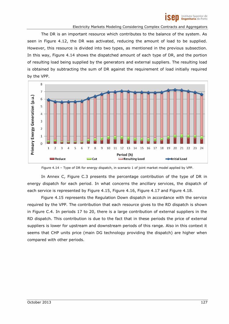
Electricity Markets Modeling Considering Complex Contracts and Aggregators
October 2013 127
The DR is an important resource which contributes to the balance of the system. As
seen in Figure 4.12, the DR was activated, reducing the amount of load to be supplied.
However, this resource is divided into two types, as mentioned in the previous subsection.
In this way, Figure 4.14 shows the dispatched amount of each type of DR, and the portion
of resulting load being supplied by the generators and external suppliers. The resulting load
is obtained by subtracting the sum of DR against the requirement of load initially required
by the VPP.
Figure 4.14 – Type of DR for energy dispatch, in scenario 1 of joint market model applied by VPP.
In Annex C, Figure C.3 presents the percentage contribution of the type of DR in
energy dispatch for each period. In what concerns the ancillary services, the dispatch of
each service is represented by Figure 4.15, Figure 4.16, Figure 4.17 and Figure 4.18.
Figure 4.15 represents the Regulation Down dispatch in accordance with the service
required by the VPP. The contribution that each resource gives to the RD dispatch is shown
in Figure C.4. In periods 17 to 20, there is a large contribution of external suppliers in the
RD dispatch. This contribution is due to the fact that in these periods the price of external
suppliers is lower for upstream and downstream periods of this range. Also in this context it
seems that CHP units price (main DG technology providing the dispatch) are higher when
compared with other periods.

Tiago André Teixeira Soares
128 October 2013
Figure 4.15 – Regulation down dispatch, in scenario 1 of joint market model applied by VPP.
Regarding the Regulation Up service, Figure 4.16 illustrates the RU dispatch for each
hour. In this figure it is possible to see the participation which DG resources have in service
dispatch. Considering the total energy dispatched in 24 periods of one hour, based on
Figure C.4 it is known that DG satisfies the requirement of Regulation Up required by the
VPP in the market, about 28%, which implies that the remaining part is provided by the
external supplier.
Figure 4.16 – Regulation up dispatch, in scenario 1 of joint market model applied by VPP.
The dispatch regarding the SP reserve is represented by Figure 4.17. In Annex C,
Figure C.4 presents the percentage of energy that each resource type supplies to the
Spinning Reserve requirement.

Electricity Markets Modeling Considering Complex Contracts and Aggregators
October 2013 129
Figure 4.17 – Spinning reserve dispatch, in scenario 1 of joint market model applied by VPP.
Figure 4.18 represents the NS dispatch. The overall contribution which DG and
external supplier provides for the service is shown in Figure C.4 of Annex C.
Figure 4.18 – Non-spinning reserve dispatch, in scenario 1 of joint market model applied by VPP.
With these figures which represent the dispatch for each service, it is possible to
highlight some variations in the energy and AS dispatch, since the maximum capacity of
each bid is conditioned according to the maximum power limit constraint for the services of
production addition, concerning the model of section 3.6.
4.6.2.2. Scenario 2 – Base case with different bidding
regions
The division of AS requirements by network regions has as primary goal the
prevention of any congestion in the network. Therefore, the areas of the network where

Tiago André Teixeira Soares
130 October 2013
their lines have high probabilities of congestion are delimited. In this way, the methodology
implemented becomes important, preventing from network problems. However, the solution
becomes more expensive from the viewpoint of the dispatch of resources, since at least
50% of each AS requirement must be provided for the resources of this region. Thus, in
order to be able to compare the results obtained with the base case in section 4.6.2.1, the
dispatch of each AS for each region can be exposed in a global view.
The energy dispatch for the scenario described in this subsection is shown in Figure
4.19, in which it is possible to verify that there was a decrease in the resource use of DR
and discharge of storage units, compared to the scenario presented in the previous
subsection. This is due to the simple fact that the maximum limit of overall production has
been changed in this scenario, in which the maximum limit of overall production
corresponds exactly to the sum of the maximum limit of each service of increase
generation. In this way, the DR and storage resources are typically more expensive than
some of the DG resources. Thus, it originates a bigger contribution of the DG resources to
the energy dispatch than the DR resources.
Figure 4.19 – Energy dispatch by type of resource, in scenario 2 of joint market model applied by VPP.
In Annex C, Figure C.5 represents the percentage that each type of resource has in
the energy dispatch. Figure C.6 and Figure C.7 show the contribution and importance that
each type of DG technology has in energy dispatch, respectively. These graphs allow
identifying in detail the variation of the generation cycle of each kind of resource over the
period of one day. The amount of types of DR dispatched is given by Figure C.8 and Figure
C.9 in which it is visible the low priority that this kind of resource has in this scenario. This
is due to the increase in the maximum limit of global generation, which allows the use of
larger amounts of power in energy dispatch on the part of generators.

Electricity Markets Modeling Considering Complex Contracts and Aggregators
October 2013 131
Regarding the AS dispatch, the market simulation is performed for each of the
regions, in order to obtain the global AS dispatch in the network. This implies that each
region has its own AS dispatch. Accordingly, in order to be able to observe the impact which
this methodology has in the scope of global ancillary services, Figure 4.20 illustrates the
amount of generation dispatched by the generators of the different regions for Regulation
Up service. In turn, the Regulation Down dispatch is provided in Annex C, Figure C.10.
Figure 4.20 – Overall regions regulation up dispatch.
In each region, the generators from the region are forced to provide at least 50% of
the RU requirement for this region. This implies that regions in which the production cost is
lower than other regions, will have a tendency to produce more than the necessary for their
service in order to deliver energy to other regions according to the network technical limits.
These events are easily visible in Figure 4.21.
Figure 4.21 – Regulation up dispatch by each region.
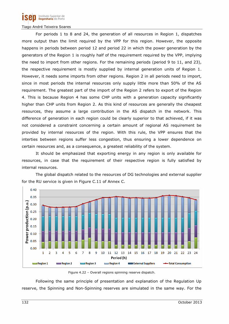
Tiago André Teixeira Soares
132 October 2013
For periods 1 to 8 and 24, the generation of all resources in Region 1, dispatches
more output than the limit required by the VPP for this region. However, the opposite
happens in periods between period 12 and period 22 in which the power generation by the
generators of the Region 1 is roughly half of the requirement required by the VPP, implying
the need to import from other regions. For the remaining periods (period 9 to 11, and 23),
the respective requirement is mostly supplied by internal generation units of Region 1.
However, it needs some imports from other regions. Region 2 in all periods need to import,
since in most periods the internal resources only supply little more than 50% of the AS
requirement. The greatest part of the import of the Region 2 refers to export of the Region
4. This is because Region 4 has some CHP units with a generation capacity significantly
higher than CHP units from Region 2. As this kind of resources are generally the cheapest
resources, they assume a large contribution in the AS dispatch in the network. This
difference of generation in each region could be clearly superior to that achieved, if it was
not considered a constraint concerning a certain amount of regional AS requirement be
provided by internal resources of the region. With this rule, the VPP ensures that the
interties between regions suffer less congestion, thus ensuring a lower dependence on
certain resources and, as a consequence, a greatest reliability of the system.
It should be emphasized that exporting energy in any region is only available for
resources, in case that the requirement of their respective region is fully satisfied by
internal resources.
The global dispatch related to the resources of DG technologies and external supplier
for the RU service is given in Figure C.11 of Annex C.
Figure 4.22 – Overall regions spinning reserve dispatch.
Following the same principle of presentation and explanation of the Regulation Up
reserve, the Spinning and Non-Spinning reserves are simulated in the same way. For the

Electricity Markets Modeling Considering Complex Contracts and Aggregators
October 2013 133
Spinning reserve, the overall dispatch is represented by Figure 4.22. The dispatch which
concern the AS requirement imposed by the VPP for each region is shown in Figure 4.23.
In the Spinning reserve dispatch, the external supplier is not dispatched at any
period of the simulation. This is due to the combination of possibilities inherent to the
optimization process. For this service, it seems that Regions 3 and 4 are exporting regions
with a large impact, mainly in the supply of Region 2 requirement, which remains a typically
import region.
Figure 4.23 – Spinning reserve dispatch by each region.
The global Spinning Reserve dispatch is shown in Figure C.12 of Annex C.
With regards to Non-Spinning service, the global dispatch for this service is
illustrated by Figure 4.24, while the dispatch for each region and its requirement is
represented in Figure 4.25.
Figure 4.24 – Overall regions non-spinning reserve dispatch.

Tiago André Teixeira Soares
134 October 2013
Regarding the Non-Spinning reserve dispatch, the results show that a considerable
part of the energy necessary to dispatch this service between periods 2 to 7 is provided by
the external suppliers. This is due to a set of specific situations. First, the limit of production
implemented in the model based on Bialek factors, which do not allow that the production
of each energy resource for Non-Spinning reserve exceeds the limits calculated in order to
make the energy and ancillary services joint dispatch unfeasible. Another frequent situation
arises when the overall maximum limits of a generator is reached (the sum of production
dispatched to services of energy, RU, SP and NS reach its maximum production capacity).
These two conditions combined give rise to the need for dispatching external suppliers and,
expensive generators with some freedom of production to meet the service requirements
for each region.
Figure 4.25 – Non-spinning reserve dispatch by each region.
In Annex C, Figure C.12 illustrates the global dispatch of the service considering the
types of resources surrounding the dispatch of the referred service.
4.6.2.3. Scenario 3 – DR resources and RLXD variable on AS
dispatch
In this scenario the results for the introduction of the types of DR and relaxation
variables of the problem for the ancillary services are presented. From the point of view of
energy service, this scenario does not involve significant changes in the energy dispatch,
this occurs due to the maximum limits of resources for the energy service that has not
changed. In this way, the results and conclusions of this scenario focus on the AS
dispatches.
The Regulation Down dispatch does not consider the use of types of DR established
in the model. The types of DR consider only the load reduction, which is infeasible for the

Electricity Markets Modeling Considering Complex Contracts and Aggregators
October 2013 135
RD service. This service hires resources to reduce generation or increase the consumption
in the network. Thus, the proposed types of DR are not suitable for this service.
In this context, Figure C.13 and Figure C.14 in Annex C provide the dispatch and
their percentage of contribution of each resource to the RD service.
With regards to the Regulation Up service, the contribution of Demand Response is
quite considerable. In Figure 4.26 it is possible to see a large participation of DR in regional
dispatch of RU. In this way, the types of DR are fairly useful for the RU dispatch, thereby
reducing the operation cost compared to the service requirement, if provided only by DG
technologies and external suppliers. In Annex C one can find the global dispatch of the RU
reserve in Figure C.15.
Figure 4.26 – Regulation up dispatch considering DR resources.
In the context of the widespread use of DR for RU service and for each region of the
network, Figure 4.27 presents the contribution of each Type of DR in each region for this
service.
Depending on the region, the contribution of each Type of DR may vary
considerably. For example in Regions 1, 2 and 3 there is a greater participation of DR
Reduce type, while in Region 4, the DR Cut is clearly superior to the DR Reduce. Briefly, the
Demand Response Cut type to the loads of Region 4 is less expensive, and has, therefore, a
greater contribution in the regulation up dispatch.
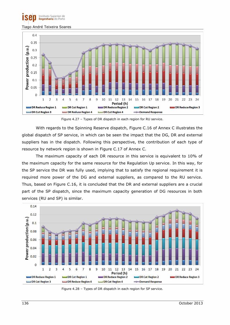
Tiago André Teixeira Soares
136 October 2013
Figure 4.27 – Types of DR dispatch in each region for RU service.
With regards to the Spinning Reserve dispatch, Figure C.16 of Annex C illustrates the
global dispatch of SP service, in which can be seen the impact that the DG, DR and external
suppliers has in the dispatch. Following this perspective, the contribution of each type of
resource by network region is shown in Figure C.17 of Annex C.
The maximum capacity of each DR resource in this service is equivalent to 10% of
the maximum capacity for the same resource for the Regulation Up service. In this way, for
the SP service the DR was fully used, implying that to satisfy the regional requirement it is
required more power of the DG and external suppliers, as compared to the RU service.
Thus, based on Figure C.16, it is concluded that the DR and external suppliers are a crucial
part of the SP dispatch, since the maximum capacity generation of DG resources in both
services (RU and SP) is similar.
Figure 4.28 – Types of DR dispatch in each region for SP service.

Electricity Markets Modeling Considering Complex Contracts and Aggregators
October 2013 137
Figure 4.28 illustrates the DR dispatch by network regions for the SP service.
Comparing Figure 4.28 with Figure 4.27 (concerning the RU dispatch) one can see an
increased contribution of the DR Cut type in regions 2 and 3.
In this context, the use of almost the total generation capacity of DG and DR
resources leads to the availability of using relaxation variables when resources fail to
generate enough energy to supply the load.
The use of relaxation variables are typically used in two different ways. Firstly, the
relaxation variables can only be used in the optimization process as a means for the VPP to
identify the situation in which the dispatch is infeasible, creating a problem to VPP towards
solving the problem of infeasible solution.
Secondly, the VPP knows through the relaxation variables what are the problems of
the dispatch, and through bilateral contracts with generation units it ensures the feasibility
of the dispatch. This is the way normally used by the ISO or VPP to solve the problem of the
infeasible dispatch.
The model developed presents a third way of looking at the problem, which consists
in the procurement of resources in the market optimization that could contribute to the
feasibility of the dispatch regarding all regions. However, from the beginning one does not
know in which regions of the network these situations can happen. In this way, it is possible
to implement a constraint on the model which uses the resources of other regions of the
network to meet the requirement of a particular region.
In this context, Figure 4.29 shows the Spinning Reserve dispatch of region 2 in
which is evident the use of the relaxation variable RLXD.
Figure 4.29 – SP dispatch in region 2, by each resource.
In this case, the relaxation variable will be entirely provided by the external supplier,
because the DG and DR were completely used in all regions of the network. All internal

Tiago André Teixeira Soares
138 October 2013
resources of region 2 have insufficient capacity to provide at least 50% of the Spinning
requirement of its region. In this way, the generation provided by the external supplier for
the variable is remunerated at a high price, in which the relaxation variable is only used to
achieve the 50% of the regional AS requirement, since it is mandatory to offset at least
50% of requirement be provided by the internal resources of the region. It can be
concluded that the relaxation variable complements the needs of generation in case of
internal resources of the region being insufficient to provide partial or full regional AS
requirement.
The respective regional dispatch to the remaining network regions can be found in
Annex C, Figure C.18, Figure C.19 and Figure C.20.
Regarding to the Non-Spinning reserve dispatch, one can verify that the DG and DR
generation are practically sufficient to meet the load in all time periods except for the period
corresponding to hour 3.
In this way, the regional NS service dispatch is illustrated in Figure 4.30 (the global
dispatch of the service by all kind of resources is shown in Figure C.21 and presented in
Annex C).
Figure 4.30 – NS dispatch by network regions, considering DR resources.
Regarding the contribution of DR in this service dispatch (Figure 4.31), it seems that
regions 3 and 4 cover a greater sharing of types of DR while regions 1 and 2 contemplates
greater involvement of DG in these regions dispatch. This is mainly due to the price and
generation capacities provided by DR resources in certain regions of the network.
The types of DR can be very useful in the stability of power systems. Through the
scenario presented is clear the need to consider these resources in the complex managing
of ancillary services.

Electricity Markets Modeling Considering Complex Contracts and Aggregators
October 2013 139
Figure 4.31 – Types of DR dispatch in each region for NS service.
These resources may reach a more economical management of the energy and AS
joint market. However, it is important to note that the excessive use of a particular
resource type is not good for the stability and management of all kind of resources in the
power systems. Briefly, this scenario shows the potentiality of DR in a efficient ancillary
services dispatch, as well as the use of generators in special cases, such as situations in
which the internal energy generation in a region is not enough to satisfy the AS
requirements imposed by the VPP. In these cases, the implemented relaxation variables
are a way to ensure the feasible dispatch of ancillary services.
4.6.2.4. Scenario 4 – Storage units on AS dispatch
The introduction of storage units in the energy and AS joint procurement is critical to
the proper management of network resources. Due to its particular characteristics, the
storage units can adapt properly to the AS. Their ability to charge and discharge energy
allows a careful management by the VPP regarding the load curve. These resources can be
used to charge energy in times of energy excess, as well as discharge energy in peak load
situations. In this context, its adaptability to ancillary services is an added value to the VPP
management. Therefore, the main function of storage units in the smart grid paradigm is to
ensure ancillary services. In this way, the results and conclusions presented in this scenario
are mainly directed to the management of these resources in the ancillary services
procurement.
The energy dispatch results obtained in this scenario can be found in Annex C,
Figure C.22 and Figure C.23. In these figures it is visible a small storage charge in off peak
hours, which shows that the energy stored in these hours can be used in ancillary services
in other periods.
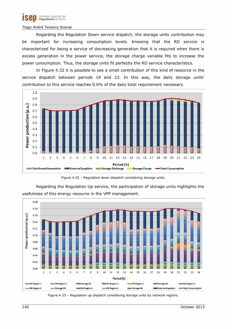
Tiago André Teixeira Soares
140 October 2013
Regarding the Regulation Down service dispatch, the storage units contribution may
be important for increasing consumption levels. Knowing that the RD service is
characterized for being a service of decreasing generation that it is required when there is
excess generation in the power service, the storage charge variable fits to increase the
power consumption. Thus, the storage units fit perfectly the RD service characteristics.
In Figure 4.32 it is possible to see a small contribution of this kind of resource in the
service dispatch between periods 19 and 23. In this way, the daily storage units’
contribution to this service reaches 0.6% of the daily total requirement necessary.
Figure 4.32 – Regulation down dispatch considering storage units.
Regarding the Regulation Up service, the participation of storage units highlights the
usefulness of this energy resource in the VPP management.
Figure 4.33 – Regulation up dispatch considering storage units by network regions.

Electricity Markets Modeling Considering Complex Contracts and Aggregators
October 2013 141
Figure 4.33 shows the contribution of these resources in the RU dispatch by network
regions. In periods 21 and 22, it is visible the storage units contribution from regions 2 and
4 in the service dispatch. Thus, it appears that there is a large set of several kinds of
energy resources from different regions that compete with each other. In these two periods,
it was also observed that the external suppliers do not participate in the dispatch. Figure
C.24, Annex C illustrates in detail the storage unit participation by network regions, as well
as the amount of charge and discharge of these resources in this service.
The storage share in SP service follows the same methodological principle of RU
service. Figure 4.34 illustrates the SP service dispatch, considering the DG, DR, external
suppliers and storage resources by network regions. In this figure it is possible to see a
considerable share of storage in SP dispatch in several periods of the day. This kind of
resources contributes in around 10% of the global generation necessary to meet the daily
service requirement. The largest share of this resource occurred in period 21 with around
46%, while period 3 corresponds to the period with lower share of around 0.5%. The
maximum contribution of storage units in period 21 is justified by the price of external
suppliers during this period to be higher than the storage price. The period 21 corresponds
to the maximum peak of the external suppliers price in relation to all period range. Thus, it
appears that the contribution of external suppliers is lower when compared to other periods.
Figure 4.34 – Spinning reserve dispatch considering storage units by network regions.
The amount of energy per network region may be seen in detail in Figure 4.35. One
of the ways of storage units to participate in this service involves the discharge of energy.
Another way is by decreasing the charge of the storage acquired in energy service; i.e. the
storage unit which charge in energy service may participate in the SP service, by reducing
the charge that acquired in energy service. This occurred for storage units from region 2

Tiago André Teixeira Soares
142 October 2013
between the periods 3 and 6, with greater emphasis in periods 5 and 6. The storage
contribution through discharge energy tends to become more noticeable during peak
periods (periods of increased energy consumption). Furthermore, the storage units from
region 2 were those which participated with more power to satisfy the service.
Figure 4.35 – Storage charge and discharge share by network regions for SP dispatch.
Regarding the Non-Spinning Reserve service, Figure 4.36 illustrates the storage, DG,
DR and external suppliers’ resources participation by network regions in the scope of the NS
service dispatch. The storage contribution in the daily service dispatch reached 5% of the
total supply of the service. The use of the storage units in the service reduces the need for
external suppliers to participate in it.
Figure 4.36 – Non-spinning reserve dispatch considering storage units by network regions.

Electricity Markets Modeling Considering Complex Contracts and Aggregators
October 2013 143
Through Figure 4.37 it is noticeable the involvement of the storage resources from
period 9 to period 23, with greater preponderance in the range between 20 and 23. In
general, the region which occupies most of these resources to meet the service requirement
is region 2. Nearly 43.9% of the total energy supplied by the storage comes from region 2,
43.6% comes from region 4 and the remaining 12.5% are provided by region 3, while the
storage of region 1 have no share in the dispatch. In period 21 there is a higher share of
storage in the hourly service dispatch – about 32% of the total energy supplied.
Figure 4.37 – Storage charge and discharge share by network regions for NS dispatch.
4.6.2.5. Scenario 5 – Complex Contracts
The increasing use of distributed energy resources, namely DG, DR and storage units
in the power system, requires a continuous adaptability of the management of these
resources. In this way, the aggregation of small players with a VPP is especially important
for these resources in the competitive environment of the electricity market. However, the
aggregation of all kinds of resources is important for the VPP which can have greater
amplitude in its strategies during the trade in a competitive environment increasingly
complex.
In order to achieve a proper management of the available resources and the goals,
the VPP must match the contract conditions established with the resources. However,
players can choose from the available set of VPPs which are interested in their aggregation,
or to act individually in the smart grid context. In order to encourage the aggregation of the
most interesting players, the VPPs need to propose competitive contracts conditions that
guarantee competitive benefits to these players [Vale-2011].
This scenario includes all the methodology involving the model presented in section
3.6. Besides the methodology used in the previous scenario, this scenario adds the
involvement of several specific and complex contracts, namely the minimum generated

Tiago André Teixeira Soares
144 October 2013
energy in period t and in time horizon T, the power gradient between periods, the minimum
remuneration in time horizon T, the number of working hours and a maximum number of
times that each generator enters in the service.
The application of these contracts is reflected in the scope of the electricity market
for the energy and ancillary services. In order to demonstrate the issues that the contracts
mentioned above provide to the energy and ancillary services, it was developed a set of
simulations capable of illustrating the usefulness of these contractual conditions within the
market for both perspectives of the VPP and the owners of power generation units
addressed in the distribution network of this case study.
The simulations are based on the input data regarding the base case, with a few
changes for each simulation of each type of contract. The set of simulations has the purpose
of providing a better perception and understanding of the capacity of each contract of
influencing the resource management, thereby accommodating the objectives of the
producers and the needs of the VPP.
The first type of contract introduced in this scenario concerns the minimum limit of
energy produced by the generator in a 24-hour period, i.e., the contract ensures that the
producer, if dispatched, produces at least the minimum limit defined a priori.
To simulate this contract, it was established a minimum limit of energy throughout
the day by portions of maximum capacity production of the day.
Figure 4.38 – Dispatched energy and operation cost for contract type 1.
Figure 4.38 shows the impact of minimum daily scheduled energy contracts used by
wind farms in the VPP operation cost and in the total energy dispatched for producers with
this type of contract. The minimum daily energy values imposed in the contracts are based
on the wind generation forecast. As it can be seen in Figure 4.38, the scheduled wind

Electricity Markets Modeling Considering Complex Contracts and Aggregators
October 2013 145
energy in the base case already uses a large percentage of available wind energy (almost
50%). However, when it requires the total use of generating capacity of wind energy, it
causes a radical increase in the VPP operation costs.
At 75% of the imposed minimum schedule energy, the operation cost does not
increase significantly. This is beneficial to the owners of wind turbines, since the
considerable increase in power generation (about 17.3%) does not imply a large increase in
the VPP operation costs (about 0.48%). Thus, the wind players are quite favoured with this
situation.
The second type of contract refers to the gradient of generation in each period. This
contract sets for each period of 1 hour a limit for the increase/decrease power generation
according to the previous period.
To simulate this contract, one can change the data relating to external suppliers. In
this way, it was established a value of power generated by the external supplier for the
period prior to the beginning of the simulation.
Knowing that the simulation is performed for the period of 1 hour with a time
horizon of 24 hours, the amount of power established for the initial period (t-1) corresponds
almost to the power dispatched by the external supplier in t=1 related to the base case.
Each simulation comprises a value of the gradient of generation relatively small in
order to limit very high levels of variation of generation. In this way, the gradient values of
generation used for contract simulation vary between 0.25% and 5% of the power
dispatched at (t-1).
The results of the simulations considering maximum generation gradient contracts
applied to the external supplier are shown in Figure 4.39. In this figure it is possible to see
the development of the total energy generated throughout the period, and the VPP
operation costs, according to the imposed maximum gradient.
It can be concluded that for this scenario the contracts imposing maximum gradient
values over 2.50% have a strong impact on the perspective of the operating costs of VPP.
For these cases a variation of the energy produced by the external supplier means a
substantial increase in the operation costs. This is caused by the need of the VPP to contract
more expensive resources to compensate the generation decrease of production of external
suppliers. However, when reducing the generation gradient of external supplier at low
levels, the difference in operation costs is not that much relevant because the external
suppliers lose importance in the dispatch, since it is necessary to hire more expensive
generation units with greater flexibility in variation of the generation between operating
periods. This leads to the reduction of the global generation of external supplier.

Tiago André Teixeira Soares
146 October 2013
Figure 4.39 – Dispatched energy and operation cost for contract type 2.
The third type of contract imposes a minimum limit of remuneration for the whole 24
hours, i.e., it ensures a guaranteed minimum remuneration, regardless the energy
produced in each hourly period.
In order to simulate the desired contract, it is necessary to amend the input data of
the base case presented below. The simulation of the contract is divided into several
simulations by parcels of the desired minimum remuneration. In this way, in the simulation
it is imposed the minimum remuneration desired by percentage of the maximum possible
remuneration.
The considered contract is established between a Fuel Cell unit and the VPP. This
contract types imposes a minimum remuneration for the Fuel Cell unit throughout the time
horizon. The minimum remuneration levels were determined for each Fuel Cell unit,
according to its maximum generation capacity and the hourly energy price. The results are
shown in Figure 4.40.
In Figure 4.40 it seems that with the gradual increase of the charge of minimum
remuneration, there is a slight variation in the VPP operation cost. This happens due to the
influence the capacity of power generation of Fuel Cell units has in the VPP resource
management. In other words, the capacity of power generation of the Fuel Cell units is
relatively small when compared to all the available resources in the network. The last two
levels of imposed remuneration provide a growing increase in the VPP operation costs.
However, the variation of the VPP operation costs between the minimum and maximum
level of remuneration does not exceed 1.2%.
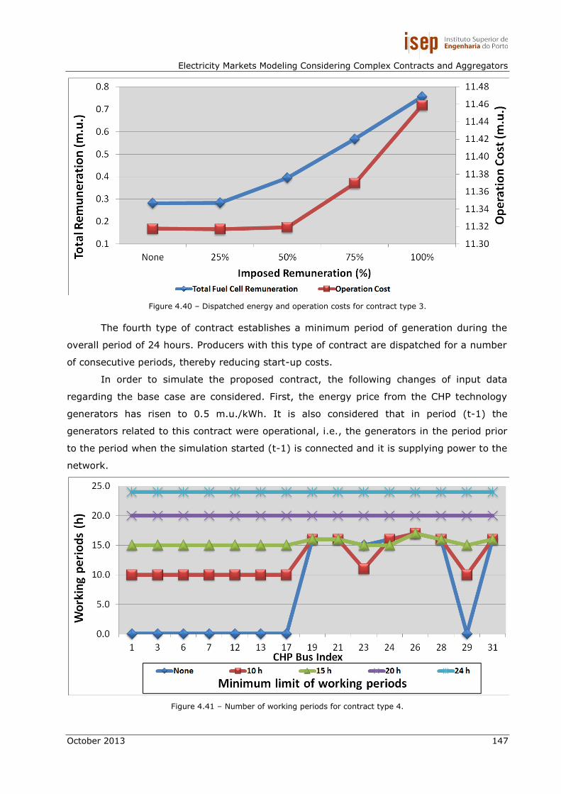
Electricity Markets Modeling Considering Complex Contracts and Aggregators
October 2013 147
Figure 4.40 – Dispatched energy and operation costs for contract type 3.
The fourth type of contract establishes a minimum period of generation during the
overall period of 24 hours. Producers with this type of contract are dispatched for a number
of consecutive periods, thereby reducing start-up costs.
In order to simulate the proposed contract, the following changes of input data
regarding the base case are considered. First, the energy price from the CHP technology
generators has risen to 0.5 m.u./kWh. It is also considered that in period (t-1) the
generators related to this contract were operational, i.e., the generators in the period prior
to the period when the simulation started (t-1) is connected and it is supplying power to the
network.
Figure 4.41 – Number of working periods for contract type 4.

Tiago André Teixeira Soares
148 October 2013
Figure 4.41 and Figure 4.42 show the results of the simulations considering the CHP
generators contracts that impose a minimum number of working periods. Generally, the
CHP presents low generation costs, therefore most CHP units are dispatched during many
time periods. If it is set an increase in the energy price generated by CHP, of course, the
number of working periods decreases considerably. Setting a minimum number of working
periods by scale illustrated in Figure 4.41, one can conclude that the CHP units related to
the buses between 1 and 17 are considered more expensive generators, when compared to
other neighbours resources of these CHP units.
In Figure 4.42 it is noticeable that the inclusion of this contract in the resource
management is not expensive, because the increase in VPP operation costs with the total
introduction of the contract (stipulating that all CHP generators participate in the market in
the 24 periods) is less than 1.8% over the base case.
Figure 4.42 – Dispatched energy and operation cost for contact type 4.
This contract is particularly suited to certain distributed generation technologies,
capable of generating a constant amount of energy over a time horizon of 24 hours. The
CHP technology is tailored for this type of contract, because besides getting a constant
production, this technology has a slow cold startup which does not allow its system
operation to be in constant intermittency (on/off). Moreover, the system startup has a
considerable cost in managing this system.
The fifth and final contract consists in a maximum number of entries in service
throughout the 24 hours. In this context, the producer is forced to ensure stability from
generation to avoid being excluded from the selection of production for the period
established.
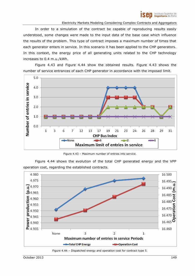
Electricity Markets Modeling Considering Complex Contracts and Aggregators
October 2013 149
In order to a simulation of the contract be capable of reproducing results easily
understood, some changes were made to the input data of the base case which influence
the results of the problem. This type of contract imposes a maximum number of times that
each generator enters in service. In this scenario it has been applied to the CHP generators.
In this context, the energy price of all generating units related to the CHP technology
increases to 0.4 m.u./kWh.
Figure 4.43 and Figure 4.44 show the obtained results. Figure 4.43 shows the
number of service entrances of each CHP generator in accordance with the imposed limit.
Figure 4.43 – Maximum number of entries into service.
Figure 4.44 shows the evolution of the total CHP generated energy and the VPP
operation cost, regarding the established contracts.
Figure 4.44 – Dispatched energy and operation cost for contract type 5.

Tiago André Teixeira Soares
150 October 2013
Comparing the results of the base scenario (without contract – “None”), with the
more rigid enforcement of this contract, the global energy dispatch of CHP generators
increased about 0.16%, while the VPP operation costs increased about 0.52%.
Generally, the VPP can use this kind of contract to apply to CHP plants players,
which also may want to set this kind of contract with the VPP in order to obtain generation
stability, reducing the costs related to the system startup, and sometimes the need to work
in the minimum load limit possible to maintain its system in a state of “readiness” to be
ready to supply power at any time. Thus, this contract could be a feature or complement to
other contracts.
4.6.3. Results analysis
The amount of distributed energy resources in power systems has increasing
significantly in the past years. In the future, power systems will have to deal with large-
scale integration of DG, types of DR and storage units. These resources can be crucial for
the energy dispatch and for participation in ancillary services, in order to ensure the
stability and security of supply requirements from the network and consumers.
In this context, the case study developed presents a perspective on the value and
complexity of the proposed model. With this purpose, the case study was divided into five
distinct parts, in which the complexity of each scenario gradually increases.
Firstly, it was developed a base scenario which considers the simulation of energy
and ancillary service joint market implemented in a distribution network with extensive
introduction of DER, using an AC optimal power flow. In this simulation, both the energy
and ancillary services compete for power flow in the network. For this purpose, it has been
used the Bialek topological factors method for solving this problem proposed in section 3.5.
The method allows knowing the contribution of each generator in line congestion. Thus, it
becomes possible to simulate which AS congestion causes in the network. In this way, it is
known that the dispatch obtained for all services are feasible, implying that when AS are
needed the prior dispatch is very close to reality, not requiring major readjustments,
preventing a considerable increase in the operation costs of ancillary services for the VPP.
The second scenario includes all the features of the first scenario, with the biddings
of the players in the market related to AS that can be made by network regions. The
players from each region propose their bids in the market for different regions. The ability
of the VPP of acting with mutual function of economical and technical management allows
the VPP to manage the resources according to the rule, in which the generation units of
each region should ensure the supply of at least 50% of the necessary requirement of the
region in which they are located. This model allows the VPP prevent from potential
congested lines in the border regions. The regions are established according to a forecast of

Electricity Markets Modeling Considering Complex Contracts and Aggregators
October 2013 151
possible congestion of an important supply zone, not causing energy not supplied, and also
ensuring network stability.
The third scenario includes the use of DR resources participating in the AS dispatch.
The types of DR (namely Cut and Reduce) can be an important resource in the network
stability. However, the DR is typically used a few times in a year, as the goal of the system
is to produce and to supply energy and not excessively to reduce the load [Walawalkar-
2010]. In addition, this scenario includes the use of relaxation variables for each AS, and
consequently for each region. This variable has the purpose of maintaining the network
stability by lack or excess generation in each region. The presented model allows the
generation units in regions with excess of generation (relaxation variable = 0) to participate
in requirements in other regions. The VPP has to procure generation units which are capable
of filling this variable without affecting network stability.
The fourth scenario considers the use of storage units in AS provision. The particular
features of this kind of resources allow a greater management flexibility of energy and
especially the ancillary services by the VPP. Due to the storage units’ flexibility to charge
and discharge along the time period, they can be used to store energy during low cost
periods and discharge at peak periods. In this way, these resources can provide a good
alternative for the diagram loads management compared to traditional resources. However,
these resources have a greater impact in AS, because they are more expensive than
traditional resources, thereby they do not regularly contribute to the energy service.
Moreover, the energy storage capacity is limited, not having a large storage capacity. Thus,
these resources are suited to the participation in the AS dispatch.
The fifth and final part of this case study includes all the features of the previous
parts and introduces complex contracts between the VPP and players. The implemented
methodology considers several types of complex contracts which enable players to impose
relevant constraints when they establish contracts.
Complex contracts are very important to enable the aggregated players to achieve
their goals. Although they make the energy resource management more complex,
depending on the contract, its impact can be significant in the VPP operation costs. For the
first contract types, the VPP operation costs increased about 20%; however, the last type of
contract had an impact of about 1,2%. In this way, the VPP management should consider
players’ contracts which have clear and tangible objectives, beneficial for both parties.
In this case study, one can identify some advantages and disadvantages of the
proposed methodology. Some of the clearest advantages of this methodology is the
flexibility in adapting to several considerations which may arise in a energy and AS joint
market, including: the possibility of splitting the AS procurement for regions of the network;
the increasing importance of DR resources in the network management, and negotiating a
good part of complex contracts existing in the market. However, the main advantage of this

Tiago André Teixeira Soares
152 October 2013
methodology and contribution from the common markets is the ability to dispatch all
services (energy and ancillary services) in a hierarchical way without compromising the
stability of the network and the technical constraints related to the network. This advantage
was only possible through the implementation of topological Bialek factors based on
proportional sharing methodology.
Regarding the disadvantages, it seems that the execution time of the method is
slightly long, about 20 minutes of complete execution of the market. In this way, the
methodology fits perfectly in the simulation of day-ahead market.
Briefly, it can be concluded that the proposed methodology is effective to solve the
envisaged problem and to be implemented in MASCEM. This model proposes an energy and
AS joint market simulation considering the possibilities of AS bidding regions, the large
introduction of DER, complex contracts and especially the use of AC power flow using the
topological Bialek factors, which allows the simulator to have greater flexibility and to
control strategies from the standpoint of the VPP and players.
4.7. Conclusions
This subsection presents the main conclusions of the case studies related to the
simulation of AS market models. The case studies presented were carefully selected in order
to demonstrate the most relevant features regarding to the market models studied. In this
context, the case studies cover a diversity of possible situations in a competitive
environment, in both perspectives of the ISO/VPPs and the remaining players participating
in the energy and AS joint market.
The first case study is the base model of the AS market simulation used in the
development of the remaining models. In this case study, the results are shown regarding
the simulation of the ancillary services (RD, RU, SP and NS) and the usefulness of the AS
cascade system in the model. In this way, it is possible to verify that the simulation of the
AS market, with the possibility of cascade process between services, may result in economic
savings in the scope of the market optimization developed by the ISO. The last scenario of
this case study shows the economic advantage of considering the AS market model with the
possibility of ancillary services cascading. The economic savings presented in the scenario
are about 16% compared to the simple simulation of the AS market in which the AS
cascade is not considered.
The results of an energy and AS joint market model are presented in the second
case study. In this case study, it is easy to verify the economic advantage to the ISO
through the simultaneous and compact simulation of energy and AS market. The third
scenario of this case study shows the comparison of results obtained through the simulation
of separate market and joint market. In this scenario, it seems that the joint market

Electricity Markets Modeling Considering Complex Contracts and Aggregators
October 2013 153
simulation has an economic efficiency of about 4%, when comparing to the separate market
for energy and AS market.
The third case study presents the comparison results of the proposed model in
section 3.4 with a reference method proposed in [Wu-2004]. The model developed
considers the joint market with the AS bids to be offered by regions of the network. The
major differences between the developed model and the reference method is the use of an
AC OPF capable of determining the active and reactive power flow in the network, instead of
the DC model used in reference methodology. The LMP calculation of each node in the
model developed considers the LMP of energy, system losses and network congestion, while
in the reference method only considers the LPM of energy and network congestion.
Furthermore, the possibility of AS cascade existing in the model developed is not considered
in the reference model. In this way, the results of this case study show that the developed
methodology introduces a clear approach to the reality of the power systems operation.
The fourth case study considers the electricity market model developed in section
3.5, based on the principle of Bialek topological factors methodology. In order to
demonstrate the feasibility of the proposed methodology it was used a transmission
network with 7 buses in this case study. The major advantage of the method is the
demonstration of the feasibility by considering all services (energy and ancillary services) in
the network congestion. The disadvantages are summarized by the execution time of the
optimization process of the method, as well as the increased of operation costs for the ISO.
The last case study considers the innovative methodology developed in section 3.6
which uses the Bialek topological factors in order to obtain the feasibility of services
dispatches included in the model, as well as the introduction of complex constraints related
to the players/VPPs established contracts. The case study considers a distribution network
of 33 buses and the use of DER, consisting mainly in DG (namely, photovoltaic, wind, CHP,
Biomass, MSW, small hydro and Fuel Cell), DR and Storage units.
Firstly, this case study presents the results of joint market simulation which
considers the use of an AC OPF and Bialek topological factors so that the solutions
presented are feasible throughout the simulation process for each service. The energy
dispatch shows that the DR has an important contribution in this schedule, about 12%,
while the DG is about 29% and the storage unit has a minimal effect of about 1% in the
dispatch.
After the energy dispatch, through the Bialek topological factors it is possible to
determine the contribution that each resource has in the network flow. This contribution
limits the resources for the remaining services according to the contribution which can still
offer in view of the technical constraints of the network, at the level of congestion of
network branches. This provides an optimization initially more expensive regarding the
objective function value; however, this method ensures the feasibility of the dispatch for

Tiago André Teixeira Soares
154 October 2013
each service, thus benefiting a final anticipated dispatch in respect to the usual processes in
real markets.
Regarding the use of DR resources to participate in the AS, they comprise a large
part of the dispatch, and in some regions of the network they may reach 50% of the
dispatch of an ancillary service to the respective region. This happens in cases when these
resources are less expensive, or when the DG resources and external suppliers are limited
to supply loads due to lines’ congestion.
The storage units’ participation in AS provision illustrates the versatility that this kind
of resource can have when ensuring the balance and stability of power system. In this way,
the obtained results show that the major purpose of the resources, from the VPP
standpoint, involves the power systems stability. Thus, their participation emerges in
periods of greater preponderance namely the periods between 20 and 22.
With regards to complex contracts, these are used to allow the VPPs establishing
contracts with players in order to define beneficial conditions for both parties. In this case
study, the VPP operating costs increased about 20%. However, this increase was not
detected for all contracts established. In this way, the results of the last contracts studied in
the case study have an impact of 1,2% in the VPP resource management.
All the simulations of the case studies presented in this chapter were developed in
GAMS software using a deterministic approach, the Mixed-Integer Non-Linear Programming
(MINLP). This technique ensures obtaining the global optimal in each optimization, which
means that throughout the process simulation the best possible solution was always
obtained. The execution time of most of the models presented in this work does not exceed
3 minutes of simulation. However, the methodology simulated in the last case study is quite
complex, in which the dispatch of energy and each AS, considering AS bidding in different
network regions, the introduction of all kind of resources in markets participation, as well as
the use of complex contracts between players related to DG resources with the VPP,
originate a quite long execution time of the sequential process of complete determination of
this model, reaching 20 minutes of the total model simulation.

Electricity Markets Modeling Considering Complex Contracts and Aggregators
October 2013 155
Chapter 5
Conclusions and Future Work


Electricity Markets Modeling Considering Complex Contracts and Aggregators
October 2013 157
5. Conclusions and Future Work
This chapter presents the most significant conclusions of the work developed. It
includes a critical analysis of the proposed methodology and the obtained results in order to
highlight the objectives achieved and the contribution to the state of the art and, most
importantly, to the future electricity market mechanisms. Furthermore, some perspectives
related to future work are introduced.
5.1. Main conclusions and contributions
Ancillary Services (AS) are crucial to maintain and control the stability of power
systems. Currently, and more in the future, AS markets will be influenced by a large set of
different Distributed Energy Resources (DER). These new players can participate directly in
the market or aggregated to some agents, such a Virtual Power Players. Due to the
continuous increase of players with several kinds of DER, the development of new
methodologies becomes necessary to provide flexible mechanisms to the energy and AS
negotiation.
This dissertation focuses on the development and implementation of new market
mechanisms for energy and AS, considering several players involved in the electricity
market. A comprehensive work has been developed in order to address several objectives
and different perspectives of AS management. In this way, the AS management from the
Independent System Operator (ISO) and Virtual Power Player (VPP) standpoint were
considered, taking into account the features of the players involved in each model.
The development of a model capable of simulating the joint market using a Alternate
Current (AC) Optimal Power Flow (OPF) model for the simulation of technical constraints of
the network; the introduction of an innovative method (Bialek topological factors)
considering the ancillary services dispatch in the network congestion calculation, in order to
prevent network congestion during the dispatch of all ancillary services considered in the
market; and complex contracts implemented in order to enable the negotiation between
players and VPPs, results in a complete and complex simulation model very close to current
markets, as well as the main contribution of this dissertation.
The proposed models are based on California Independent System Operator (CAISO)
market rules. CAISO is a nonprofit public entity subject to the FERC regulation, which
operates the transmission facilities of all participants in power systems, and dispatches the
generation units and the loads. The CAISO market includes several competitive and
liberalized market mechanisms. An interesting market mechanism in the development of
this dissertation is the energy and AS joint optimization. Therefore, in this work it was
studied and adapted some of the innovative aspects of the CAISO market. The following
CAISO rules were implemented and tested in joint energy and AS market:

Tiago André Teixeira Soares
158 October 2013
The use of relaxation variables in optimization problem, which always ensures
obtaining results of the AS dispatch, regardless of the operation context;
AS cascading mechanism;
Energy and AS joint optimization;
AS bidding by operation network regions.
All the models developed include the Regulation Down (RD), Regulation Up (RU),
Spinning reserve (SP) and Non-Spinning Reserve (NS). The models also include several
market mechanisms with different objectives for improving the market model. The
relaxation variables are used to obtain an economic dispatch regardless of the operation
context. Other mechanism is the AS cascading process, which is used to improve the
economic efficiency of AS management.
The establishment of AS bids by network regions is a market mechanism used by the
ISO in order to mitigate/avoid network congestion. For each region, part of the AS
requirements (about 50%) is provided exclusively by internal energy resources of that
region. The main advantage of this market mechanism is to decrease the probability of
having network congestion in regions tendentiously problematic, as well as to improve the
reliability and quality of the energy service. However, this mechanism does not ensure the
technical and economical best solution.
The energy and AS joint market model do not ensure the solution feasibility. The
main problem is that the model does not consider the impact that the AS may have on the
network congestion. In order to solve this issue, an innovative methodology was developed
to solve the network congestion caused by the simultaneous market clearing process of the
joint market.
This methodology is based on Bialek topological distribution factors. The major
contribution of this methodology is to always ensure a feasible solution of the energy and
AS dispatch in any operation context. In what concerns the model runtime, it suits the ISO
operation requirements. This methodology allows finding a better solution than the
traditional methodology, guaranteeing the feasibility of the system, avoiding any network
congestion that may occur in the traditional methodology.
The effectiveness of the proposed methodology is reflected in the results, since the
operation costs are lower when compared with the traditional market methodology which
needs further network congestion analysis to solve the congestion that the AS can cause in
the network.
Other important contribution proposed in this dissertation is the inclusion of DER in
AS such as Regulation Down, Regulation Up, Spinning and Non-Spinning reserve. In this
way, an aggregator agent was proposed in order to manage and interact with a wide variety
of DER, like Distribution Generation (DG) (mainly based on renewable energy sources),
Demand Response (DR), and storage systems. The VPP is an agent that aggregates all kind
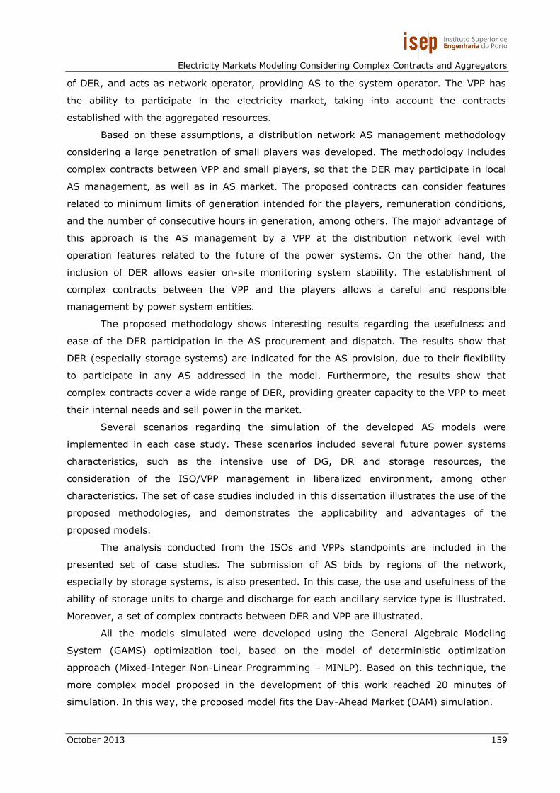
Electricity Markets Modeling Considering Complex Contracts and Aggregators
October 2013 159
of DER, and acts as network operator, providing AS to the system operator. The VPP has
the ability to participate in the electricity market, taking into account the contracts
established with the aggregated resources.
Based on these assumptions, a distribution network AS management methodology
considering a large penetration of small players was developed. The methodology includes
complex contracts between VPP and small players, so that the DER may participate in local
AS management, as well as in AS market. The proposed contracts can consider features
related to minimum limits of generation intended for the players, remuneration conditions,
and the number of consecutive hours in generation, among others. The major advantage of
this approach is the AS management by a VPP at the distribution network level with
operation features related to the future of the power systems. On the other hand, the
inclusion of DER allows easier on-site monitoring system stability. The establishment of
complex contracts between the VPP and the players allows a careful and responsible
management by power system entities.
The proposed methodology shows interesting results regarding the usefulness and
ease of the DER participation in the AS procurement and dispatch. The results show that
DER (especially storage systems) are indicated for the AS provision, due to their flexibility
to participate in any AS addressed in the model. Furthermore, the results show that
complex contracts cover a wide range of DER, providing greater capacity to the VPP to meet
their internal needs and sell power in the market.
Several scenarios regarding the simulation of the developed AS models were
implemented in each case study. These scenarios included several future power systems
characteristics, such as the intensive use of DG, DR and storage resources, the
consideration of the ISO/VPP management in liberalized environment, among other
characteristics. The set of case studies included in this dissertation illustrates the use of the
proposed methodologies, and demonstrates the applicability and advantages of the
proposed models.
The analysis conducted from the ISOs and VPPs standpoints are included in the
presented set of case studies. The submission of AS bids by regions of the network,
especially by storage systems, is also presented. In this case, the use and usefulness of the
ability of storage units to charge and discharge for each ancillary service type is illustrated.
Moreover, a set of complex contracts between DER and VPP are illustrated.
All the models simulated were developed using the General Algebraic Modeling
System (GAMS) optimization tool, based on the model of deterministic optimization
approach (Mixed-Integer Non-Linear Programming – MINLP). Based on this technique, the
more complex model proposed in the development of this work reached 20 minutes of
simulation. In this way, the proposed model fits the Day-Ahead Market (DAM) simulation.

Tiago André Teixeira Soares
160 October 2013
Lastly, all the methodologies proposed and implemented were included in the Multi-
Agent Simulator of Competitive Electricity Markets (MASCEM). MASCEM is a simulator which
depicts the study of complex restructured electricity markets operation. In this way, the
methodologies developed in this dissertation provide additional methodological bases to
MASCEM, for the simulation of the present and future operation of the energy and AS
market.
5.2. Perspectives for future work
Throughout the development of this work, several ideas have arisen to potentially
proceed with the evolution of the present work. Some of the envisaged concepts are closely
connected to new FCT projects which were recently initiated, namely the following projects:
IMaDER – Intelligent Short Term Management of Distributed Energy
Resources in a Multi-Player Competitive Environment (PTDC/SEN-
ENR/122174/2010);
MAN-REM – Multi-Agent Negotiation and Risk Management in Electricity
Markets (PTDC/EEA-EEI/122988/2010).
Among the many advances that the development of this work gave opportunity to,
allowing future works and scientific findings, some future developments can be referred:
Improvement of AS optimization methodologies considering the several levels
of AS management (ISO, TSO, DSO and VPP);
Introduction of all kind of DER in the market or in the VPP, mainly consisting
of DG technologies, Electric Vehicles (EV), types of DR considering different
kind of consumers (Large and medium Industrial, Large, medium and small
Commerce, and Domestic consumer) and storage units;
Enable players to submit more complex bids, taking into account in the
dispatch process, the constraints related to startup costs of some
technologies, minimal load costs regarding the state of readiness of a
generator to enter in service at a certain time to fill a gap of generation, and
generation ramps related to features of each AS;
Develop and implement a AS management tool where it is possible to identify
and evaluate the risk of the bids that a VPP can run in the market;
The ability of the tool has appropriate methodologies of learning the
knowledge of the market in which the VPP operates.
The suggestions for improving the energy and AS market simulation, indicated as
future work, are part of the objectives to continuously improve MASCEM simulator, with the
objective of providing the users of the simulator with a wide range of simulation tools which

Electricity Markets Modeling Considering Complex Contracts and Aggregators
October 2013 161
can be adapted to the different characteristics of each market, as well as the consideration
of new trends that might arise in the competitive market environment.


Electricity Markets Modeling Considering Complex Contracts and Aggregators
October 2013 163
References


Electricity Markets Modeling Considering Complex Contracts and Aggregators
October 2013 165
References
[Baran-1989] M. Baran and F. Wu, “Network reconfiguration in distribution
systems for loss reduction and load balancing”, IEEE
Transactions on Power Delivery, vol. 4, pp. 1401-1407, 1989.
[Bialek-1996] J. Bialek, “Tracing the flow of electricity”, IEEE Proceedings on
Generation, Transmission and Distribution, vol. 143, no. 4, pp.
313-320, July 1996.
[Bialek-1997] J. Bialek, “Topological generation and load distribution factors
for supplement charge allocation in transmission open access”,
IEEE Transactions on Power Systems, vol. 12, no. 3, pp. 1185-
1193, August 1997.
[Bjorndal-2001] M. Bjorndal and K. Jornsten, "Zonal pricing in a deregulated
electricity market," Energy Journal, vol. 22, no. 1, pp. 51-73,
2001
[Braun-2007] M. Braun, “Technological Control Capabilities of DER to Provide
Future Ancillary Services”, International Journal of Distributed
Energy Resources, vol. 3, no. 3, pp. 191-206, Technology &
Science Publishers, Kassel, Germany, 2007
[Buehner-2010] V. Buehner, B. Buchholz, “Provision of Ancillary Services by
RES”, International Council on Large Electric Systems, August
2010
[CAISO-2006] CAISO, “Process for Participating Load Program (Ancillary
Services/Supplemental Energy)”, Available from:
www.caiso.com, 2006.
[CAISO-2007a] CAISO, “Participating Load Technical Standard”, Technical
Standard, Available from: www.caiso.com, 2 February 2007.
[CAISO-2007b] CAISO, “OASIS – Public Bids”, Available from:
oasishis.caiso.com, 2007.
[CAISO-2009] CAISO, “Market Optimization Details”, Technical Bulletin,
Available from: www.caiso.com, 19 November 2009
[CAISO-2010] CAISO, “Market Issues & Performance”, Annual Report - 2009,
Available from: www.caiso.com, April 2010.
[CAISO-2011a] CAISO, “Business Practice Manual for Market Operations”,
Version 23, Available from: www.caiso.com, 9 December 2011.
[CAISO-2011b] CAISO, “Fifth Replacement FERC Electric Tariff”, Available from:
www.caiso.com, 1 December 2011.

Tiago André Teixeira Soares
166 October 2013
[CAISO-2011c] CAISO, “Market Issues & Performance”, Annual Report – 2010,
Available from: www.caiso.com, April 2011
[CAISO-2011d] CAISO, “Full Network Model Pricing Node Mapping”, Available
from: www.caiso.com, 21 December 2011.
[CAISO-2011e] CAISO, “Market Optimization” Business Practice Manual for
Market Optimizations, Available from: www.caiso.com, 9
December 2011.
[ERSE-2012] ERSE – Entidade Reguladora dos Serviços Energéticos,
“Resolução de Restrições Técnicas”, Available from:
www.erse.pt, July 2012.
[EURELECTRIC-2000] EURELECTRIC, “Connection Rules for Generation and
Management of Ancillary Services”, May 2000.
[EURELECTRIC-2004] EURELECTRIC, “Ancillary Services – Unbundling Electricity
Products – an Emerging Market”, February 2004.
[Faria-2010] P. Faria, Z. Vale and J. Ferreira, “DemSi – A demand response
Simulator in the context of intensive use of distributed
generation”, IEEE International Conference on Systems Man
and Cybernetics (SMC), pp. 2025-2032, 2010.
[Faria-2011] P. Faria, Z. Vale, “Demand response in electrical energy supply:
An optimal real time pricing approach”, Energy, vol. 36, pp.
5374-5384, August 2011.
[FERC-1995] Edison Electric Institute, Ancillary Services, FERC Open Access
NOPR Technical Conference Report, Washington DC, November
1995.
[GAMS-2007] GAMS Development Corporation, “GAMS – The Solver Manuals”,
Washington DC, USA, 2007.
[GAMS-2008] R. E. Rosenthal, “GAMS – A User’s Guide”, GAMS Development
Corporation, Washington DC, USA, 2008.
[Gomes-2007] M. Gomes, “Novos Mecanismos de Mercado de Energia Eléctrica
e de Serviços Auxiliares Eléctricos”, PhD. Thesis, FEUP, January
2007.
[Graham-2005] I. Graham, “MATLAB manual and introductory tutorials”, Bath
University Computing Service, Bath, UK, February 2005.
[Group-1973] W. Group, “Common Format For Exchange of Solved Load Flow
Data”, Power Apparatus and Systems, IEEE Transactions on,
vol. PAS-92, no. 6, pp. 1916-1925, November 1973.
[Harp-2000] S.A. Harp, S. Brignone, B.F. Wollenberg and T. Samad, “Sepia:

Electricity Markets Modeling Considering Complex Contracts and Aggregators
October 2013 167
A Simulator for Electric Power Industry Agents”, IEEE Control
Systems Magazine, vol. 20, no. 4, pp. 83-69, August 2000.
[Heffner-2007] G. Heffner, C. Goldman, M. Kintner-Meyer, B. Kirby, “Loads
Providing Ancillary Services: Review of International
Experience”, Technical Appendix: Market Descriptions, EOLBNL,
May 2007.
[JAVA-2012] Java programming language – homepage, Available from:
www.java.com, August 2012
[Kirby-1995] B. Kirby, E. Hirst and J. VanCoevering, “Identification and
Definition of Unbundled Electric Generation and Transmission
Services, ORNL/CON-415”, Oak Ridge National Laboratory,
March 1995.
[Kirschen-1997] D. Kirschen, R. Allan, G. Strbac, “Contributions of Individual
Generators to Loads and Flows”, IEEE Transactions on Power
Systems, vol. 12, no. 1, February 1997.
[Koritarov-2004] V. Koritarov, “Real-World Market Representation with Agents:
Modeling the Electricity Market as a Complex Adaptive System
with an Agent-Based Approach”, IEEE Power & Energy
magazine, pp. 39-46, August 2004.
[Kristiansen-2007] T. Kristiansen, “The Nordic approach to market-based provision
of ancillary services”, Energy Police, March 2007.
[Li-2009] H. Li and L. Tesfatsion, “Development of Open Source Software
for Power Market Research: The AMES Test Bed”, Journal of
Energy Markets, vol. 2, no. 2, pp. 111-128, June 2009.
[Luo-2012] Z. Luo, Z. Hu, Y. Song. Z. Xu, H. Liu, L. Jia, H. Lu, “Economic
Analyses of Plug-in Electric Vehicle Battery Providing Ancillary
Services”, IEEE International Electric Vehicle Conference (IEVC),
pp. 1-5, March 2012.
[Mannila-2000] T. Mannila, J. Hovila, P. Trygg, K. Laitimen, “The electricity
production and market liberalization in the European Union”,
International conference on Power System Technology, vol. 3,
pp. 1641-1645, 2000.
[MATLAB-2010] MATLAB, “Introduction - Product Overview”, The MathWorks,
Inc., Natick, USA, 2010.
[MIBEL-2009] Conselho de Reguladores do MIBEL, “Descrição do
funcionamento do MIBEL”, November 2009
[Morais-2010a] H. Morais, P. Kadar, P. Faria, et al, “Optimal scheduling of a

Tiago André Teixeira Soares
168 October 2013
renewable micro-grid in an isolated load area using mixed-
integer linear programming”, Renewable Energy, vol. 35, pp.
151-156, 2010.
[Morais-2010b] H. Morais, “Energy Resources Management”, Student Poster,
IEEE Power & Energy Society, PESGM Minneapolis, Minnesota,
USA, July 2010.
[MPGS-2008] REN, “Manual de Procedimentos do Gestor do Sistema”,
December 2008.
[N2EX-2012] N2EX, “Physical and financial market”, Available from:
www.n2ex.com, April 2012.
[NASDAQOMX-2010] NASDAQ OMX Commodities Europe, “Legal Notice”, Available
from: www.nasdaqomxcommodities.com, 13 June 2010
[NETS-2011] National Electricity Transmission System, “Seven Year
Statement - Chapters”, Available from: www.nationalgrid.com,
May 2011
[NGET-2012a] National Grid Electricity Transmission plc, “GB Seven Year
Statement”, Available from: www.nationalgrid.com, April 2012
[NGET-2012b] National Grid Electricity Transmission plc, “The Grid Code”,
Issue 4, Revision 11, Available from: www.nationalgrid.com, 16
March 2012
[Nordel-2008] Nordel, “Description of Balance Regulation in the Nordic
Countries”, March 2008.
[NordPool-2012a] Nord Pool Spot AS, “Europe’s Leading Power Markets”, Available
from: www.nordpoolspot.com, 10 July 2012
[NordPool-2012b] Nord Pool Spot AS, http://www.nordpoolspot.com/About-us/,
July 2012
[NordPool-2012c] Nord Pool Spot AS, http://www.nordpoolspot.com/TAS/Day-
ahead-market-Elspot/, July 2012
[NordPool-2012d] Nord Pool Spot AS, http://www.nordpoolspot.com/How-does-it-
work/Bidding-areas/, July 2012
[NordPool-2012e] Nord Pool Spot AS, “The Nordic Electricity Exchange and the
Nordic Model for a Liberalized Electricity Market”, Available
from: www.nordpoolspot.com, July 2012
[NordPool-2012f] Nord Pool Spot AS, http://www.nordpoolspot.com/How-does-it-
work/Day-ahead-market-Elspot-/Price-calculation/, July 2012
[NordPool-2012g] Nord Pool Spot AS, http://www.npspot.com/Market-
data1/Maps/Power-System-Overview/Power-System-Map/, July

Electricity Markets Modeling Considering Complex Contracts and Aggregators
October 2013 169
2012
[NordPool-2012h] Nord Pool Spot AS, http://www.nordpoolspot.com/TAS/Day-
ahead-market-Elspot/Order-types/, July 2012
[NordPool-2012i] Nord Pool Spot AS,
http://www.nordpoolspot.com/TAS/Intraday-market-Elbas/,
July 2012
[NordPool-2012j] Nord Pool Spot AS, http://www.nordpoolspot.com/How-does-it-
work/Intraday-market-Elbas/, July 2012
[NordPool-2012k] Nord Pool Spot AS, “Balancing Power”, Available from:
www.nordpoolspot.com, July 2012
[OAA-2012] Open Agent Architecture – homepage, Available from:
www.ai.sri.com/~oaa/, August 2012
[OMIE-2012a] OMIE, “Mercado Diário”, Available from: http://www.omie.es,
July 2012
[OMIE-2012b] OMIE, “Mercado Intradiário”, Available from:
http://www.omie.es, July 2012.
[Oren-2001] S. Oren, “Design of Ancillary Service Markets”, Proceedings of
the 34th Hawaii International Conference on System Sciences,
January 2001.
[Papalexopoulos-2001] A. Papalexopoulos, H. Singh, “On the Various Design Options
for Ancillary Services Markets”, Proceedings of the 34th Hawaii
International Conference on System Sciences, January 2001.
[Pereira-2009] V. Pereira, “Fornecimento de Serviços de Sistema no Sistema
Eléctrico Nacional”, MSc. Thesis, ISEG ,July 2009
[Pinto-2011a] T. Pinto, H. Morais, P. Oliveira, Z. Vale, I. Praça, C. Ramos, “A
new approach for multi-agent coalition formation and
management in the scope of electricity markets”, Energy, vol.
36, no. 8, pp. 5004-5015, August 2011.
[Pinto-2011b] T. Pinto, “Adaptive Learning in Agents Behaviour: A Framework
for Electricity Markets Simulation”, MSc. Thesis, ISEP, October
2011.
[Pinto-2012] T. Pinto, H. Morais, Z, Vale and I. Praça, “Multi-Agent
Negotiation for Coalition Formation and Management in
Electricity Markets”, Negotiation and Argumentation in MAS –
Applications, F. Lopes, H. Coelho (Eds), Bentham e-books,2012.
[Praça-2003] I. Praça, C. Ramos, Z. A. Vale, M. Cordeiro “MASCEM: A Multi-
Agent System that Simulates Competitive Electricity Markets”,

Tiago André Teixeira Soares
170 October 2013
IEEE Intelligent Systems, vol. 18, no. 6, pp. 54-60, November-
December 2003.
[Rebours-2007] Y. Rebours, D. Kirschen, M. Trotignon, S. Rossignol, “A Survey
of Frequency and Voltage Control Ancillary Services – Part I:
Technical Features”, IEEE Transactions On Power Systems, vol.
22, no. 1, pp. 350-257, February 2007.
[Scalari-2008] S. Scalari, G. Valtorta, R. Giglioli, F. Pilo, R. Caldon, S.
Massucco, C. Nucci, A. Testa, “An Italian facility to test
distributed energy resources management for SmartGrids”, IET-
CIRED. Seminar – SmartGrids for Distribution, June 2008.
[Schisler-2008] K. Schisler, T. Sick, K. Brief, “The role of demand response in
ancillary services markets”, IEEE PES T&D Exposition and
Conference, Chicago, USA, April 2008.
[Shahidehpour-2002] M. Shahidehpour, H. Yamin, and Z. Li, “Market Operations in
Electric Power Systems: Forecasting, Scheduling and Risk
Management”, John Wiley & Sons, 2002.
[Soares-2011] T. Soares, H. Morais, B. Canizes, Z. Vale, “Energy and Ancillary
Services Joint Market Simulation”, EEM11 – 8th International
Conference on the European Energy Market, pp. 262-267,
Zagreb, Croatia, 25-27 May, 2011.
[Soares-2013] Tiago Soares, Hugo Morais, Zita Vale, “Energy and Ancillary
Services Joint Market Considering Different Bidding Regions”,
Energy Policy, Under revision.
[Sousa-2011] T. Sousa, H. Morais, Z. Vale, P. Faria, J. Soares, “Intelligent
Energy Resource Management Considering Vehicle-to-Grid: A
Simulated Annealing Approach”, Accepted for Publication on
IEEE Transaction on Smart Grid, Special Issue on
Transportation Electrification and Vehicle-to-Grid Applications,
2011.
[Su-2001] Ching-Tzong Su and Ji-Horng Liaw, “Power Wheeling Pricing
Using Power Tracing and MVA-KM Method”, IEEE Porto Power
Tech Conference, Porto, Portugal, September 2001.
[Thong-2007] V. Van Thong, J. Driesen, R. Belmans, “Using Distributed
Generation to Support and Provide Ancillary Services”, May
2007
[Vale-2010] Z. Vale, P. Faria, P. Morais, H. Khodr, M. Silva, P. Kadar,
“Scheduling distributed energy resources in an isolated grid –

Electricity Markets Modeling Considering Complex Contracts and Aggregators
October 2013 171
An artificial neural network approach”, Power and Energy
Society General Meeting, July 2010.
[Vale-2011] Z. Vale, T. Pinto, I. Praça, H. Morais, "MASCEM - Electricity
markets simulation with strategically acting players", IEEE
Intelligent Systems, vol. 26, n. 2, pp. 9-17, April 2011.
[Walawalkar-2010] R. Walawalkar, S. Fernands, N. Thakur, K. Chevva, “Evolution
and current status of demand response (DR) in electricity
markets: Insights from PJM and NYISO”, Energy, vol. 35, n. 4,
pp. 1553-1560, April 2010.
[Wu-2004] T. Wu, G. Angelidis, Z. Alaywan and A. Papalexopoulos,
“Regional Ancillary Services Procurement in Simultaneous
Energy/Reserve Markets”, IEEE Power Systems Conference and
Exposition, 10-13 October 2004.
[Zimmerman-2004] R.D. Zimmerman and R.J. Thomas, “PowerWeb: a tool for
evaluating economic and reliability impacts of electric power
market designs”, IEEE PES Power Systems Conference and
Exposition, vol. 3, pp. 1562-1567, October 2004.


Electricity Markets Modeling Considering Complex Contracts and Aggregators
October 2013
Annexes


Electricity Markets Modeling Considering Complex Contracts and Aggregators
October 2013 A.1
Annex A
Data from the Case Study – AS model


Electricity Markets Modeling Considering Complex Contracts and Aggregators
October 2013 A.3
Table A.1 shows the input data for the first scenario of the case study in section 4.2.
In this table arise features concerning the quantities and prices of each AS that each player
offers to the market, as well as the requirements of each AS imposed by the SO.
Table A.1 – Input data for scenario 1 of AS model.
Table A.2 shows the input data used in the case study of section 4.2 for the second
scenario.
Table A.2 – Input data for scenario 2 of AS model.
Table A.3 shows the input data used in the case study of section 4.2 for the third
scenario.
Table A.3 – Input data for scenario 3 of AS model.


Electricity Markets Modeling Considering Complex Contracts and Aggregators
October 2013 B.1
Annex B
Data from the Case Study – Energy and
AS joint market model


Electricity Markets Modeling Considering Complex Contracts and Aggregators
October 2013 B.3
Table B.1 shows the input data necessary for the case study of the section 3.3.
Table B.1 – Energy and AS joint market data.
Table B.2 shows the AS dispatch without AS cascade, as well as the market price
associated to each AS and their cost to the SO.
Table B.2 – AS market results in scenario 1 of joint model.
Bids Regulation Down Regulation Up
Spinning Reserve
Non-Spinning Reserve
Total
(MW) MW m.u./MWh MW m.u./MWh MW m.u./MWh MW m.u./MWh
1 0 10.0 0 15.0 10 5.0 10 7.0 20
2 0 8.0 0 8.1 5 9.0 45 4.0 50
3 40 8.0 0 7.1 20 8.5 0 6.0 20
4 60 4.0 4 5.0 11 7.2 15 4.6 30
5 100 3.5 65 7.0 24 4.0 14 9.0 103
6 0 9.0 0 14.6 10 8.0 0 11.0 10
7 40 7.0 0 7.2 0 7.3 21 4.0 21
8 10 4.8 100 8.3 60 6.6 0 10.5 160
9 0 9.0 0 6.5 10 4.3 45 5.3 55
10 0 10.0 31 4.0 0 9.0 0 5.0 31
Contracted Service (MW)
250 200 150 150 750
Market Clearing Price (m.u./MWh)
8.0 8.3 9.0 9.0 Total
(m.u.)
Total Cost (m.u.)
2000 1660 1350 1350 6360
Table B.3 Shows the AS dispatch with AS cascade, and moreover shows the market
clearing price of each AS, and the cost associated with each ancillary service, and the
overall cost to the SO.
Tiago André Teixeira Soares
B.4 October 2013
Table B.3 – AS market results with cascading mechanism in scenario 1 of joint model.
Bids Regulation Down Regulation Up
Spinning Reserve
Non-Spinning Reserve
Total
(MW) MW m.u./MWh MW m.u./MWh MW m.u./MWh MW m.u./MWh
1 0 10.0 0 15.0 10 5.0 10 7.0 20
2 0 8.0 5 8.1 0 9.0 45 4.0 50
3 40 8.0 5 7.1 0 8.5 15 6.0 20
4 60 4.0 30 5.0 0 7.2 0 4.6 30
5 100 3.5 65 7.0 24 4.0 14 9.0 103
6 0 9.0 0 14.6 10 8.0 0 11.0 10
7 40 7.0 0 7.2 0 7.3 21 4.0 21
8 10 4.8 100 8.3 60 6.6 0 10.5 160
9 0 9.0 0 6.5 10 4.3 45 5.3 55
10 0 10.0 31 4.0 0 9.0 0 5.0 31
Contracted Service (MW)
250 236 114 150 750
Slacks -
RU to SP SP to NS
- 36 8.3 0 9.0
RU to NS -
0 8.3
Service Used
(MW) 250 200 150 150 650
Market
Clearing Price (m.u./MWh)
8.0 8.3 8.0 9.0 Total
(m.u.)
Total Cost (m.u.)
2000 1958.8 912 1350 6220.8

Electricity Markets Modeling Considering Complex Contracts and Aggregators
October 2013 C.1
Annex C
Data from the Case Study – Joint Market
model applied by VPP


Electricity Markets Modeling Considering Complex Contracts and Aggregators
October 2013 C.3
Table C.1 shows the resistance, inductive reactance, capacitive susceptance and the
thermal limit.
Table C.1 – Branch data of the 33-bus distribution network.
Branch
number Bus Out Bus In R (Ohm) XL (Ohm)
BC
(Siemens)
Thermal limit
(MVA)
1 0 1 0.1332 0.0471 0 4.5
2 1 2 0.7122 0.2517 0 4.5
3 1 18 0.2699 0.0954 0 4.5
4 2 3 0.3890 0.1048 0 3.29
5 2 22 0.6039 0.2134 0 4.5
6 3 4 0.1911 0.0515 0 3.29
7 4 5 0.7262 0.1957 0 3.29
8 5 6 1.0514 0.2833 0 3.29
9 5 25 1.0656 0.2872 0 3.29
10 6 7 0.2007 0.0541 0 3.29
11 7 8 0.3822 0.1030 0 3.29
12 8 9 1.4984 0.4038 0 3.29
13 9 10 0.5528 0.1488 0 3.29
14 10 11 0.6033 0.1626 0 3.29
15 11 12 0.7618 0.2053 0 2.29
16 12 13 1.3157 0.3546 0 3.29
17 13 14 0.7472 0.2014 0 3.29
18 14 15 0.3280 0.0884 0 3.29
19 15 16 3.0084 0.8107 0 3.29
20 16 17 0.8190 0.2207 0 3.29
21 18 19 1.0241 0.3620 0 4.5
22 19 20 0.6518 0.2304 0 4.5
23 20 21 1.2973 0.4585 0 4.5
24 22 23 1.2944 0.4575 0 4.5
25 23 24 0.1497 0.0529 0 4.5
26 25 26 0.2901 0.0782 0 3.29
27 26 27 1.0810 0.2913 0 329
28 27 28 0.8209 0.2212 0 3.29
29 28 29 0.5180 0.1396 0 3.29
30 29 30 0.9946 0.2680 0 3.29
31 30 31 0.3169 0.0854 0 3.29
32 31 32 0.3481 0.0938 0 3.29

Tiago André Teixeira Soares
C.4 October 2013
Table C.2 shows information regarding DG and external supplier’s resources to
energy service to be used as input data base for the case studies discussed.
Table C.2 – Distributed generation and external suppliers resources bids features.
Type of generator
Number of units
Total installed power (kW)
Energy price (m.u./kWh) Minimum Mean Maximum
Photovoltaic 32 528 0.08 0.1398 0.254 Wind 5 490 0.05 0.0652 0.08 Hydro 2 70 0.032 0.0432 0.049
Biomass 3 350 0.06 0.2653 0.65 MSW 1 10 0.03 0.0484 0.056 CHP 15 1,240 0.0001062 0.0179 0.065
Fuel Cell 8 235 0.095 0.1021 0.11
Total of DG 66 2,923 - - -
External suppliers
1 15,000 0.015 0.0434 0.07
Total 67 17,923 - - -
The input data relating to AS bids (Regulation Down and Regulation Up) are shown
in Table C.3.
Table C.3 – DG and external suppliers bids for RD and RU services.
Type of generator
Regulation Down price (m.u./kWh) Regulation Up (m.u./kWh) Minimum Mean Maximum Minimum Mean Maximum
Photovoltaic 0.088 0.15378 0.2794 0.088 0.15378 0.2794
Wind 0.055 0.07172 0.088 0.055 0.07172 0.088 Hydro 0.0352 0.04752 0.0539 0.0352 0.04752 0.0539
Biomass 0.066 0.29183 0.715 0.066 0.29183 0.715 MSW 0.033 0.05324 0.0616 0.033 0.05324 0.0616 CHP 0.000117 0.01969 0.0715 0.000117 0.01969 0.0715
Fuel Cell 0.1045 0.11231 0.121 0.1045 0.11231 0.121 External
suppliers 0.0165 0.04774 0.077 0.0165 0.04774 0.077
The input data relating to AS bids (Spinning Reserve and Non-Spinning Reserve) are
shown in Table C.4.
Table C.4 – DG and external suppliers bids for SP and NS service.
Type of generator
Spinning Reserve price (m.u./kWh) Non-Spinning Reserve price
(m.u./kWh) Minimum Mean Maximum Minimum Mean Maximum
Photovoltaic 0.096 0.16776 0.3048 0.1 0.17475 0.3175
Wind 0.06 0.07824 0.096 0.0625 0.0815 0.1 Hydro 0.0384 0.05184 0.0588 0.04 0.054 0.06125
Biomass 0.072 0.31836 0.78 0.075 0.331625 0.8125 MSW 0.036 0.05808 0.0672 0.0375 0.0605 0.07 CHP 0.000127 0.02148 0.078 0.000133 0.022375 0.08125
Fuel Cell 0.114 0.12252 0.132 0.11875 0.127625 0.1375 External
suppliers 0.018 0.05208 0.084 0.01875 0.05425 0.0875

Electricity Markets Modeling Considering Complex Contracts and Aggregators
October 2013 C.5
Table C.5 shows the input data of DR bids for energy service.
Table C.5 – Demand response bids for energy service.
DR
Reduce (kW) Cut (kW) Minimum Mean Maximum Minimum Mean Maximum
0.0071 0.0222 0.2502 0.0071 0.0181 0.1475
Reduce (m.u./kWh) Cut (m.u./kWh) Minimum Mean Maximum Minimum Mean Maximum
0.1 0.1312 0.8 0.09 0.223 1.2
Table C.6 shows the storage units features.
Table C.6 – Storage features.
Storage
features
Initial
state
(kWh)
Charge
Capacity
(kWh)
Discharge
Capacity
(kWh)
Maximum
Capacity
(kW)
Price charge
(m.u./kWh)
Price
Discharge
(m.u./kWh)
Minimum 0.03 0.8 0.4 0.1 0.4 0.45
Mean 0.056 0.8 0.4 0.1 0.475 0.525
Maximum 0.08 0.8 0.4 0.1 0.55 0.6
Table C.7 illustrates the charge and discharge prices used by storage units for all
ancillary services.
Table C.7 – AS charge and discharge storage prices.
AS Storage features Minimum Mean Maximum
Price charge (m.u./kWh)
Regulation Down 0.04 0.0475 0.055
Regulation Up 0.02 0.0238 0.0275
Spinning Reserve 0.028 0.0333 0.0385
Non-Spinning Reserve 0.02 0.0238 0.0275
Price Discharge (m.u./kWh)
Regulation Down 0.045 0.0525 0.06
Regulation Up 0.0225 0.0263 0.03
Spinning Reserve 0.0315 0.0368 0.042
Non-Spinning Reserve 0.0225 0.0263 0.03

Tiago André Teixeira Soares
C.6 October 2013
Figure C.1 shows the percentage of power given by each kind of resource for energy
dispatch.
Figure C.1 – Percentage of power given by each kind of resource for energy dispatch, in scenario 1 of joint market model applied by VPP.
The percentage contribution of each DG technology has on energy dispatch is given
by Figure C.2.
Figure C.2 – Percentage of DG contribution for energy dispatch, in scenario 1 of joint market model applied by VPP.

Electricity Markets Modeling Considering Complex Contracts and Aggregators
October 2013 C.7
Figure C.3 shows the contribution of type of DR in energy dispatch.
Figure C.3 – Type of DR contribution in energy dispatch, in scenario 1 of joint market model applied by VPP.
Figure C.4 shows the percentage of power given by each kind of resource for
ancillary services dispatch.
Regulation Down Regulation Up
Spinning Reserve Non-Spinning Reserve
Tiago André Teixeira Soares
C.8 October 2013
Figure C.4 – Resource contribution for RD, RU, SP and NS dispatch, in scenario 1 of joint market model applied by
VPP.
Figure C.5 shows the percentage of power given by each kind of resource for energy
dispatch for scenario presented in section 4.6.2.2.
Figure C.5 – Resource contribution for energy dispatch, in scenario 2 of joint market model applied by VPP.
The contribution that each type of DG technology has in energy dispatch is given by
Figure C.6.
Figure C.6 – Energy dispatch by DG technologies contribution, in scenario 2 of joint market model applied by VPP.

Electricity Markets Modeling Considering Complex Contracts and Aggregators
October 2013 C.9
Figure C.7 reflects the percentage of DG production in energy dispatch.
Figure C.7 – Percentage of DG contribution for energy dispatch, in scenario 2 of joint market model applied by VPP.
Figure C.8 illustrates the sharing of each type of DR on energy dispatch as well as
the load really dispatched.
Figure C.8 – Type of DR for energy dispatch, in scenario 2 of joint market model applied by VPP.

Tiago André Teixeira Soares
C.10 October 2013
The percentage of importance which DR resource has in energy dispatch is given by
Figure C.9.
Figure C.9 – Percentage of DR contribution for energy dispatch, in scenario 2 of joint market model applied by VPP.
Figure C.10 shown the Regulation down dispatch considering different bidding
regions.
Figure C.10 - Regulation down dispatch, in scenario 2 of joint market model applied by VPP.

Electricity Markets Modeling Considering Complex Contracts and Aggregators
October 2013 C.11
Figure C.11 shows the dispatch of the generators and external suppliers to
Regulation Up reserve, without differentiating the region which generation corresponds.
Figure C.11 – DG and external supplier dispatch for regulation up service, in scenario 2 of joint market model applied by VPP.
Figure C.12 shows the dispatch of the generators and external suppliers to Spinning
Reserve.
Figure C.12 – DG and external supplier dispatch for spinning reserve service, in scenario 2 of joint market model applied by VPP.

Tiago André Teixeira Soares
C.12 October 2013
Figure C.13 shows the Regulation Down dispatch relating to scenario of section
4.6.2.3.
Figure C.13 – Regulation down dispatch, in scenario 3 of joint market model applied by VPP.
Figure C.14 shows the percentage of power given by each kind of resource for RD
dispatch for scenario presented in section 4.6.2.3.
Figure C.14 – Resource contribution for regulation down service, in scenario 3 of joint market model applied by VPP.

Electricity Markets Modeling Considering Complex Contracts and Aggregators
October 2013 C.13
The RU dispatch for the third scenario (section 4.6.2.3), is represented by Figure
C.15.
Figure C.15 – Regulation up global dispatch, in scenario 3 of joint market model applied by VPP.
Figure C.16 represents the global dispatch of Spinning Reserve for 24 hours period in
respect to the third scenario presented in section 4.6.2.3.
Figure C.16 – Spinning reserve global dispatch, in scenario 3 of joint market model applied by VPP.
Tiago André Teixeira Soares
C.14 October 2013
The Spinning Reserve dispatch for each network region is given by the Figure C.17.
Figure C.17 – Spinning reserve dispatch by network region, in scenario 3 of joint market model applied by VPP.
The SP dispatch for Region 1, considering all kind of resources is given by Figure
C.18.
Figure C.18 – SP reserve dispatch for region 1, in scenario 3 of joint market model applied by VPP.

Electricity Markets Modeling Considering Complex Contracts and Aggregators
October 2013 C.15
The SP dispatch for Region 3, considering all kind of resources is given by Figure
C.19.
Figure C.19 – SP reserve dispatch for region 3, in scenario 3 of joint market model applied by VPP.
The SP dispatch for Region 4, considering all kind of resources is given by Figure
C.20.
Figure C.20 – SP reserve dispatch for region 4, in scenario 3 of joint market model applied by VPP.

Tiago André Teixeira Soares
C.16 October 2013
Figure C.21 represents the global dispatch of Non-Spinning Reserve for 24 hours
period in respect to the third scenario presented in section 4.6.2.3.
Figure C.21 – Non-spinning reserve global dispatch, in scenario 3 of joint market model applied by VPP.
Figure C.22 illustrates the energy dispatch for 24 hours period.
Figure C.22 – Energy dispatch, in scenario 4 of joint market model applied by VPP.

Electricity Markets Modeling Considering Complex Contracts and Aggregators
October 2013 C.17
Figure C.23 presents all kinds of consumption assured by the energy dispatch
(includes storage charge and active power losses).
Figure C.23 – Consumption details of energy dispatch, in scenario 4 of joint market model applied by VPP.
The storage unit contribution by network regions to Regulation Up service is given by Figure
C.24 – Storage charge and discharge contribution by network regions for RU service.
Figure C.24 – Storage charge and discharge contribution by network regions for RU service.