Evaluating Performance of Inflation Forecasting Models of Pakistan
37
1 Evaluating Performance of Inflation Forecasting Models of Pakistan Muhammad Nadim Hanif and Muhammad Jahanzeb Malik 1 Abstract This study compares the forecasting performance of various models of inflation for a developing country estimated over the period of last two decades. Performance is measured at different forecast horizons (up to 24 months ahead) and for different time periods when inflation is low, high and moderate (in the context of Pakistan economy). Performance is considered relative to the best amongst the three usually used forecast evaluation benchmarks – random walk, ARIMA and AR(1) models. We find forecasts from ARDL modeling and certain combinations of point forecasts better than the best benchmark model, the random walk model, as well as structural VAR and Bayesian VAR models for forecasting inflation for Pakistan. For low inflation regime, upper trimmed average of the point forecasts out performs any model based forecasting for short period of time. For longer period, use of an ARDL model is the best choice. For moderate inflation regime different ways to average various models’ point forecasts turn out to be the best for all inflation forecasting horizons. The most important case of high inflation regime was best forecasted by ARDL approach for all the periods up to 24 months ahead. In overall, we can say that forecasting performance of different approaches is state dependent for the case of developing countries, like Pakistan, where inflation is occasionally high and volatile. Key Words: Inflation, Forecast Evaluation, Random Walk model, AR(1) model, ARIMA model, ARDL model, Structural VAR model, Bayesian VAR model, Trimmed Average. 1. Introduction Monetary policy is more effective when it is forward looking (Faust and Wright (2013) and Svensson (2005)). Central banks forecast inflation considering all possible relevant factors. State Bank of Pakistan (being central bank of the country) can only have some control 2 over the future inflation. This raises the prominence of inflation forecasting in monetary policy making 3 . We understand, inflation forecasts are the main critical input in the deliberations pertaining to the monetary policy decisions of SBP 4 . In its annual report on the state of economy, SBP publishes its inflation forecast for the upcoming fiscal year but, mostly, different from the target given by the government 5 . SBP started publishing its 1 The authors belong to Research Department of State Bank of Pakistan (SBP). The views in this study are not those of SBP. Authors are thankful to Ali Choudhary for his valuable comments on the first draft of this paper. Authors would also like to thank anonymous referees for their useful comments which helped improve this study. 2 ‘Some’ rather than the perfect control. It is because of the fact that during the ‘lag period’ *which was found to be up to 24 months in a case study of Pakistan by Qayyum et al (2005) over the period of 1991:03 to 2004:12] between monetary policy action and its results, ‘other’ variables also affect inflation in Pakistan; like in other developing countries, in particular. Such ‘other’ variables include fiscal decisions (like changes in sales tax rate and/or the financing ‘mix’ of the budget deficit) of the government, internal factors (such as local supply shocks like floods in Pakistan in 2009), external factors (such as global commodity price shock like that of 2008) and inflation expectations etc. 3 Inflation forecasting is of immense importance to households and businesses as well. 4 In addition to the results of inflation expectations (telephonic) survey conducted every two months by Research Department of SBP. For details see SBP Annual Report on the state of Pakistan economy for the year 2012-13. 5 The government of Pakistan announces its target for inflation (and economic growth) in its annual development plan which is released just before the annual budget presentation in the Parliament. And, there is a gap of almost 5 to 6 months in the announcement of the inflation target and the publication of SBP annual report. It helps SBP to better see the inflation at the year end. SBP also publishes its inflation forecast in its quarterly reports (on the state of economy of the country). SBP does not provide any detail about its inflation forecasting approaches/models, however.
Transcript of Evaluating Performance of Inflation Forecasting Models of Pakistan

1
Evaluating Performance of Inflation Forecasting Models of Pakistan
Muhammad Nadim Hanif and Muhammad Jahanzeb Malik1
Abstract
This study compares the forecasting performance of various models of inflation for a developing country
estimated over the period of last two decades. Performance is measured at different forecast horizons (up to 24
months ahead) and for different time periods when inflation is low, high and moderate (in the context of Pakistan
economy). Performance is considered relative to the best amongst the three usually used forecast evaluation
benchmarks – random walk, ARIMA and AR(1) models. We find forecasts from ARDL modeling and certain
combinations of point forecasts better than the best benchmark model, the random walk model, as well as
structural VAR and Bayesian VAR models for forecasting inflation for Pakistan. For low inflation regime, upper
trimmed average of the point forecasts out performs any model based forecasting for short period of time. For
longer period, use of an ARDL model is the best choice. For moderate inflation regime different ways to average
various models’ point forecasts turn out to be the best for all inflation forecasting horizons. The most important
case of high inflation regime was best forecasted by ARDL approach for all the periods up to 24 months ahead. In
overall, we can say that forecasting performance of different approaches is state dependent for the case of
developing countries, like Pakistan, where inflation is occasionally high and volatile.
Key Words: Inflation, Forecast Evaluation, Random Walk model, AR(1) model, ARIMA model, ARDL model,
Structural VAR model, Bayesian VAR model, Trimmed Average.
1. Introduction
Monetary policy is more effective when it is forward looking (Faust and Wright (2013) and
Svensson (2005)). Central banks forecast inflation considering all possible relevant factors. State Bank of
Pakistan (being central bank of the country) can only have some control2 over the future inflation. This
raises the prominence of inflation forecasting in monetary policy making3. We understand, inflation
forecasts are the main critical input in the deliberations pertaining to the monetary policy decisions of
SBP4. In its annual report on the state of economy, SBP publishes its inflation forecast for the upcoming
fiscal year but, mostly, different from the target given by the government5. SBP started publishing its
1 The authors belong to Research Department of State Bank of Pakistan (SBP). The views in this study are not those of SBP.
Authors are thankful to Ali Choudhary for his valuable comments on the first draft of this paper. Authors would also like to thank anonymous referees for their useful comments which helped improve this study. 2 ‘Some’ rather than the perfect control. It is because of the fact that during the ‘lag period’ *which was found to be up to 24
months in a case study of Pakistan by Qayyum et al (2005) over the period of 1991:03 to 2004:12] between monetary policy action and its results, ‘other’ variables also affect inflation in Pakistan; like in other developing countries, in particular. Such ‘other’ variables include fiscal decisions (like changes in sales tax rate and/or the financing ‘mix’ of the budget deficit) of the government, internal factors (such as local supply shocks like floods in Pakistan in 2009), external factors (such as global commodity price shock like that of 2008) and inflation expectations etc. 3
Inflation forecasting is of immense importance to households and businesses as well. 4 In addition to the results of inflation expectations (telephonic) survey conducted every two months by Research Department
of SBP. For details see SBP Annual Report on the state of Pakistan economy for the year 2012-13. 5 The government of Pakistan announces its target for inflation (and economic growth) in its annual development plan which is
released just before the annual budget presentation in the Parliament. And, there is a gap of almost 5 to 6 months in the announcement of the inflation target and the publication of SBP annual report. It helps SBP to better see the inflation at the year end. SBP also publishes its inflation forecast in its quarterly reports (on the state of economy of the country). SBP does not provide any detail about its inflation forecasting approaches/models, however.

2
inflation forecast regularly only from FY2005-06. How good are Pakistan’s inflation forecast, is the
research question of this study. [Inflation] forecast needs to be good in order to be useful in [monetary
policy] decision making process (Clark and McCracken, 2011). In figure 1 (of Appendix) we show the
government inflation target, SBP forecast for annual inflation and the observed annual (12 month
average) inflation; for the years for which we could find the (numerical) inflation target in the
government’s relevant documents. SBP inflation forecasts are closer to observed inflation, while targets
differ significantly. Of course, there are different approaches/models to forecast inflation. Establishing
which approach/model forecasts Pakistan’s inflation in a better way involves formal evaluation of
resultant forecasts.
There is no dearth of literature on exploring what determines inflation and on forecasting
inflation. But relatively less number of studies have attempted to evaluate the inflation forecasts. Those
which are prominent include Bokil and Schimmelpfennig (2006), Bukhari and Feridun (2006), Haider and
Hanif (2009), and Riaz (2012) for the case of Pakistan; and Atkeson and Ohanian (2001), Elliot and
Timmermann (2008), Stock and Watson (2008), Norman and Richards (2012), and Antipin et al (2014)
for the case of developed countries like US and Australia6. Rather than going into the details we would
like to opine that even in the case of forecast evaluation with reference to developed countries like US
(see for example, Atkeson and Ohanian, 2001), most of the studies focused upon overall inflation regime
except a few like Stock and Watson (2008). Stock and Watson (2008) found the performance of inflation
forecasting models to be episodic; and different models are found to be the best performing for
different time periods. However, none of earlier studies on Pakistan have attempted to provide point
inflation forecast evaluation for different inflation regimes like low, medium and high inflation periods.
Furthermore, these different studies have used different modeling approaches to forecast inflation.
These include single equation models, vector autoregression models and some sort of leading indicator
models. To the best of our knowledge, no one has compared various models in a single study. In this
paper, considering varying inflation environment, as is in developing countries, and suitability of
different approaches to model inflation when there are competing inflation determinants; we have
evaluated point inflation forecasts from different models, and from different approaches to combine
model based forecasts. To the best of our knowledge, ours is the first study which uses one-sided
trimmed averaging to combine inflation forecasts in case of a developing country to see if such
averaging works best during extreme inflation periods. We evaluate these forecasts to arrive at some
guidance for decision makers about the appropriate approaches, under specific inflation regime, to rely
on inflation forecast.
Inflation in Pakistan has, in the recent past, been higher and more volatile (in absolute sense)
making a difficult job of forecasting even more difficult7. By analyzing the monthly inflation data for the
last two decades (July 1992 to June 20148); we classify the inflation in Pakistan in three regimes: low,
high, and moderate. In this study we have estimated various time series models of inflation in Pakistan
6 For summary of a few selected studies see Appendix.
7 Pakistan just ended a first five (consecutive) year period (FY08 to FY12) of double digit inflation in the country’s history (since
1947). 8 Fiscal year in Pakistan runs from July to June.

3
for the purpose of forecasting inflation9 and evaluating the forecast ability of these estimated models,
and ‘forecast combinations’ there from, for (i) different horizons (3 months to 24 months ahead) and (ii)
for different inflation regimes (low, high, and moderate). These regimes are obtained on the basis of
Zeileis et al (2003) structural change test and reported in the table 1 (d) of appendix. Considering the
sample size we test for maximum two breaks splitting the data in three regimes and selection is based
on Bayesian Information Criterion.
Rest of the paper is organized as follows. In the next section we discuss about the measure of
inflation we use to model for forecasting. Then we spell out the models we have estimated to forecast
inflation for Pakistan economy and describe the data and methodology used. In section 4 we compare
the performance of these estimated models generating pseudo out of sample (unconditional) point
forecast for inflation in Pakistan in varying inflationary environment – low, moderate and high10; and for
different horizons ahead. In the final section we conclude.
2. Choosing Measure of Inflation to Forecast
Modeling inflation entails the basic question: which measure of inflation we should choose to
model for forecasting? In Pakistan, we have different measures of general trend in prices in the country.
Pakistan Bureau of Statistics (PBS), the national statistical agency, is responsible for collection,
compilation and dissemination of prices related data/indices. Such indices include GDP deflator,
Consumer Price Index (CPI), Wholesale Price Index (WPI) and Sensitive Price Index (SPI). Within the
basket of CPI, we also have an exclusion based measures of core prices index and that is for Non-Food
Non-Energy (NFNE) group. Another measure of core inflation for which PBS has recently started
publishing data is ‘20 percent trimmed core inflation’. In calculating ‘20 percent trimmed core inflation’,
10 percent of items showing extreme price changes each from top and bottom are excluded from the
CPI basket.
SPI is the most frequently available price index but it covers only necessities and just 17 cities.
GDP deflator is the most comprehensive one but is available less frequently. WPI does not cover the
services, however. Core inflation is the one measure which SBP considers important in discussion in its
flagship publications; but it is not the target inflation variable. So we are left with CPI. Government of
Pakistan announces annual inflation target which is basically for ‘12 month average of Year on Year (YoY)
change in CPI’. In this study, by inflation we mean YoY change in the CPI.
3. Models, Dataset and Methodology
In order to have accurate forecast of inflation we need to understand what best explains the
inflation. Theoretically there are various explanations to the macro level behaviour of inflation including
the quantity theory of money; Phillips curve; and structuralists’ explanation of inflation. The
contribution of (broad) money growth in inflation in Pakistan (as has been documented by Nasim (1997),
9 Which should, in any way, not be considered as inflation forecasting models of the State Bank of Pakistan.
10 See Table 1 (b) of Appendix for the levels of low, medium and high inflation in the context of Pakistan.

4
Hanif and Batool (2006), Riazuddin (2008) etc), relationship between output gap and inflation (as
reported by Bukhari and Khan, 2008), and structuralists’ explanation of inflation in the context of
developing countries like Pakistan (as discussed in Bilqees, 1988) deserve attention to make inflation
forecasts. While exploring the role of supply and demand shocks as drivers of inflation, Khan and Hanif
(2012) suggested that in addition to monetary factors, supply side disturbances should also be taken
into account for better understanding of, and ‘handle’ on inflation in Pakistan.
Obviously, all the relevant forces cannot be modeled in one framework. We have used different
approaches to see what explains inflation in different competing empirical models. These include single
equation as well as multiple equations models. For single equation modeling we have used ARDL
approach. For the case of multivariate time series analysis we have used Sims’ (1980) vector
autoregression (VAR) approach. Expecting improvement in forecast accuracy, the VAR models have also
been estimated using Bayesian approach. We know that the number of coefficients to be estimated,
even for a moderate VAR, is large and thus usual (maximum likelihood) estimates may not have
desirable properties. If we apply, however, Bayesian estimation, better accuracy is expected due to a
reasonable reduction in the parameters to be estimated and thus we can expect improved forecast
accuracy (see Canova (2007), Robertson (2000) for details) from Bayesian VAR forecasts.
We do not expect all the variables in this study11 to be integrated of order 1; rather we will have
a set of variables which are mixture of stationary and non-stationary variables. We will take difference
of non-stationary variables and consider the stationary variables in levels following the practice in the
literature. Forecasts based upon first differencing approach would be robust to (unobserved) shifts
(Hendry and Clements, 2003); if any, during the estimation period.
Before going into the empirical results from the estimated models, a few words on conceptual
framework of each of these models are necessary.
3.1 Single Equation Inflation Forecasting Models
The simple monetarist model is based on the quantity theory of money. We can say that there is
a positive relationship between changes in money supply and the inflation in the long run. According to
most of the studies, inflation in Pakistan has been a monetary phenomenon. For example, Riazuddin
(2008) has explored how money growth has interacted historically with inflation in Pakistan and found
inflation to be a monetary phenomenon. He found that three-fourths times high (low) broad money
growth was followed by high (low) inflation next year during the period of his study (1958-2007). We
ourselves have observed this; though in different manner: as far back as we can find the information on
the annual targets of money supply growth and those of inflation in the history of Pakistan, we observe
that any deviation from the target money growth (money surprise) has resulted in deviation from
inflation target (inflation surprise) next year (see figure 2 in Appendix). This also suggests the
Monetarists’ proposition and thus one can say that inflation is mostly a monetary phenomenon in
Pakistan. While modeling inflation, in addition to broad money supply growth, we also consider
11
For the list of variables used in this study, see Table 1(c) of Appendix.

5
weighted average lending rate (WALR) charged by the commercial banks to the private sector
(borrowings).
Following the inflation-unemployment relationship (the Phillips Curve), we can say that a
positive output gap12 indicates that inflation is building up in the economy and a negative output gap
suggests disinflation (or even deflation) is approaching. Interestingly, output gap has also served the role
of a ‘leading indicator for inflation in Pakistan since 195113. Before deciding on how to get output we
need to think of what is best proxy for output on monthly basis. Here, in this study, we consider large
scale manufacturing (LSM) production as proxy for output for the period of study (July 1992 to June
2014)14.
From the supply side factors, the most important variable which determines inflation in Pakistan is the
global commodity prices, as one quarter of inputs in the manufacturing sector of Pakistan are imported
(Choudhary et al, 2012). Amongst the global commodities, the most important is the crude oil which
historically constitutes one-third of overall import bill of Pakistan. Petroleum products’ prices are
important as these affect the CPI inflation directly (being part of its basket) as well as indirectly (as it
affects the cost of production – through electricity prices and transportation fares) in the country.
Inflation related expectations also play their role in inflation dynamics. Particularly, observed inflation is
found to follow the inflations expectations path in Pakistan at least in recent times15. In case of
developing countries, particularly Pakistan, we do not have long time series pertaining to inflation
expectations of people16. However, we can also proxy inflation expectations using oil prices because fuel
prices are observed to play a major role in the ‘formation of inflation expectation in Pakistan’ in the
‘SBP-IBA inflation expectations survey’ as found in Abbas, Beg, and Choudhary (2015). Considering its
importance, we can use global crude oil price in modeling inflation for Pakistan. We estimate an inflation
forecasting model comprising output gap, changes in oil price17, WALR, and M2 growth along with
inflation inertia. The lagged terms of inflation captures the inflation persistence which has been
documented in the literature as one of the features of inflation in Pakistan (See Hanif et al 2012).
We have used autoregressive distributed lag (ARDL) modeling for estimation of the single equation
models. Considering the lags in the transmission mechanism of monetary policy (as well as other)
12
The difference between level of output produced by the country and the potential (which we proxy by estimating trend use Hodrick-Prescott (1997) filter) of the economy is called output gap. 13
If we look at the figure 3 of the Appendix, we can see negative relation between inflation and unemployment. If we look at figure 4 we can point out that when output gap was ‘positive or expanding’ (‘negative or shrinking’) more than three out of four times inflation increased (decreased) in Pakistan in the following year. While doing this (satellite) analysis for Pakistan economy upon annual data from 1951 to 2013; the output gap is measured by the percent deviation observed overall real GDP from its potential GDP and inflation is measured by the 12 month average of YoY change in CPI. 14
There are various reasons to consider LSM instead of overall observed GDP. We know in case of developing countries we do not have output data at higher frequency (like quarterly / monthly) and thus we need to proxy output with some relevant variable for which high frequency data is available. Second reason pertains to the fact that in developing countries it is the industrial sector which is main user of the banks’ credit. Lastly, manufacturing industry has backward (with agriculture sector) and forward (with services sector) linkages in Pakistan. Thus it can be used as a proxy for overall economic activity in the country 15
SBP Annual Report for FY13 16
SBP-IBA telephone survey on inflation expectation of households is only a recent attempt in this context. 17
It is local currency oil price index (so that exchange rate need not to be incorporated separately in this model).

6
variables in affecting inflation in the country, we utilized up to 13 lags in this type of modeling except for
broad money growth. For board money growth we have used up to 24 lags in the model selection
process18. Within these maximum lags, the actual lag selection has been done on the basis of Akaike
(1974) information criterion. We name this first model as an ARDL1. For details, see Appendix.
We know that it is not only the petroleum products’ prices which matter, prices of other
international commodities, like food, also matter in determining general price level in developing
countries like Pakistan19. What matters more – global crude oil prices or overall international commodity
prices - is an empirical question. Thus, we have estimated another structural equation model which we
name ‘ARDL2’ by considering world consumer price index. It is not only the international commodity
price changes which impact the general price level in the importing country, but the changes in
country’s exchange rate may also have implications for domestic inflation as it is the local currency price
which is accounted for in the various price indices compiled by the national statistical agencies. In the
case of a developing country like Pakistan where households anchor their inflationary outlook to retail
petroleum prices (which are direct function of global crude oil prices) and commercial enterprises focus
on the current and (expected) future value of the Pak Rupee20; we need to consider both the overall
global commodity prices index (inclusive of international crude oil prices) and exchange rate, Pak Rupees
per US dollar21, as determinants of inflation in the country. Rather than focusing upon the output gap (as
in ARDL1), in this (another) model we directly consider the (industrial) production in the country. Thus,
ARDL2 estimates inflation as function of changes in ‘overall global commodity prices index’, domestic
industrial production growth, growth in broad money demand, and depreciation / appreciation of ‘Pak
Rupee / US dollar parity’. For details, see Appendix.
3.2 Multiple Equations Inflation Forecasting VAR Models
Now we move towards multiple equations models. We use Sims (1992) like VAR models. These
are, again, based upon the variables which are found significant in the existing empirical literature
pertaining to inflation in Pakistan. Since we have used relevant economic theory in defining the
relationships amongst the variables modeled to forecast inflation; the joint dynamics of variables are
represented by structural VAR modeling. We can classify the earlier work on Pakistan [like by Khan and
Schimmelpfennig (2006), Agha et al (2005)] into a monetary structural VAR model (MVAR), a credit
structural VAR model (CVAR) and external structural VAR (EVAR) model. We can use these VAR models
separately as well as in a comprehensive way.
18
For example, according to Qayyum et al (2005) monetary expansion/contractions take up to 24 months to impact inflation in Pakistan. In another study, Choudhary et al 2011 reported in the price setting survey of Pakistani firms that complete pass through of petroleum prices reaches Pakistani products prices after 9 months. 19
See for example Hanif 2012 for detailed links of global food price changes and food inflation in Pakistan. The share of imported goods in total consumption in Pakistan is one-fifth (Ali, 2014). 20
SBP Annual Report on the state of (Pakistan) economy, for FY13, page 4. 21
Almost 90 percent of international trade transactions of Pakistan are denominated in US dollars.

7
3.2.1 Monetary Aggregates Focused Inflation Forecasting VAR Models
Khan and Schimmelpfennig (2006) explored a simple monetary model where economic agents
are assumed to hold money for transaction purposes, as a store of value and speculative purpose.
Assuming velocity of money to be constant; inflation results if money growth exceeds the nominal
income growth. But, is it the price channel or the quantity channel of monetary transmission mechanism
which work through the economy to attempt achieve inflation target? Before the period under study,
Pakistan had been explicitly using monetary aggregate targeting to maintain monetary stability in the
country. Country started financial sector reforms and restructuring including the areas of monetary
management. SBP transitioned from direct instruments to indirect instruments of monetary
management in the country. After some transition period in the 1990s, Pakistan abandoned monetary
aggregate targeting in late 2000s and moved towards use of changes in short term interest rate (called
discount rate or more specifically 3-days reverse repo rate in Pakistan) to achieve price stability
(without being prejudice to economic growth). But, Pakistan’s departure from monetary aggregates
targeting and formal use of changes in 3-days reverse repo rate to signal monetary policy stance does
not necessarily mean that monetary aggregates have no use in predicting future inflation in the country.
An increase in discount rate (policy rate of the central bank) increases the weighted average lending
rates (charged by commercial banks to private borrowers) and reduces demand for money and thus
inflation. That simply means: (i) discount rate (DISR) is exogenous to the system and thus affects all
disturbances (in weighted average lending rates (WALR), growth in reserve money (M0), growth in
broad money (M2)22 and inflation); (ii) weighted average lending rates (WALR) affect all variables in the
system other than the discount rate; (iii) growth in reserve money affects the disturbances in broad
money growth and inflation, (iv) Growth in broad money affect the disturbances of inflation, and (v)
Inflation does not affect the disturbances of any other variable in the system. We call this as MVAR1
model. We can see that we do not consider the income here in MVAR1 model. We have also estimated
another monetary VAR model where we bring in the representation of real sector by putting output gap
before inflation (and exclude the WALR). We call this MVAR2 model. These MVAR models are also
explained in the Appendix.
3.2.2 Credit Focused Inflation Forecasting VAR Models
Credit channel is considered as an important channel of monetary policy transmission
mechanism. Bernanke and Blinder (1988) has constructed a theoretical model for studying the impact of
this channel on economy. A version of this model with slight changes is constructed by Montes and
Machado (2013) for a developing country and finds that supply of credits affects both employment and
output gap and thus has an impact on inflation. While studying the relative importance of various
monetary policy channels for Pakistan, Agha et al (2005) observed that, over the period of their study,
commercial banks played a major role in monetary policy transmission mechanism with private sector
credit as the leading indicator as it affected aggregate demand (and thus inflation) in the country. While
studying the role of credit market frictions in the transmission of monetary shocks in Pakistan,
22
Following Kapetanios et al (2007) we have considered both the high powered money as the broad money in this monetary VAR model.

8
Choudhary et al (2012) also found support of the view that existence of credit channel is relevant for
developing economies. Thus, to consider the role of private sector credit we also build a private credit
based structural VAR model for forecasting inflation in Pakistan. Being a developing country we know
that government also borrows from banking system to finance its budget deficit. We observe that, at
times, government borrowing from banking system serves as a leading indicator of inflation in
Pakistan 23 . In addition to role of government borrowing (for budgetary spending) in boosting
consumption, government borrowing for financing the budget deficit also anchors the inflationary
expectations in developing countries like Pakistan. Thus, along with the private sector credit and
(related) weighted average lending rate, we have also considered government borrowing (from the
banking system) and related interest rate (T-bill rate) to predict inflation in Pakistan. The recursive
structure of this credit structural VAR (CVAR) model assumes: (i) discount rate is exogenous to the
system and thus affects all disturbances in T-Bill Rates (TBLR), growth in public sector borrowing (GPSB),
weighted average lending rate, growth in private sector credit (GPSC) and inflation, (ii) T-Bill rate affect
all variables in the system other than discount rate, (iii) growth in public sector borrowing affect all
variables in the system other than discount rate and T-Bill rate, (iv) changes in lending rate affect the
disturbances of private sector credit and inflation, (v) changes in private sector credit affect the
disturbances of inflation and (vi) Inflation does not affect the disturbances of other variables in the
system. We call this CVAR1 model. Again, like in monetary VAR model above, we considered another
credit VAR model by incorporating large scale manufacturing growth in the country - placing it before
inflation in the model. We call this CVAR2 model. Another credit VAR model is also estimated by
excluding T-Bill rate from CVAR2. We call this CVAR3 model.
3.2.3 External Sector Inclusive Models for Forecasting Inflation
In the aforementioned monetary and credit based multivariate models, we can see one aspects missing
in those models and that is the external sector. Now we consider external sector with and without
incorporating the monetary sector. For output side of the economy, we will again consider the large
scale manufacturing (LSM) production as a proxy.
There are various ways through which Pakistan economy is impacted by the external sector. These
include the following: (i) Global oil prices24. (ii) Overall international commodity prices. (iii) Pakistanis
working overseas also send significant amount of money in the form of workers’ remittances to
maintain their families in the country. Workers’ remittances proved to be very important for Pakistan as
it has been financing a significant proportion of its trade deficit since years25 and thus helps keep
balance of payments difficulties mostly. For example, during FY13 remittances financed over two-thirds
of Pakistan’s trade deficit. It helps pare pressures upon exchange rate and thus matters in maintaining
price stability in the country. (iv) Pakistan being importer of almost one quarter of manufacturing sector
intermediates; exchange rate matters for price setting behaviour of firms in the country and thus cannot 23
At least for the case of ‘non-food, non-energy, excluding house rent index (NFNENHRI)’ inflation in Pakistan. 24
Oil Price is considered as an important factor affecting inflation [and output] in an economy. Many studies have considered it including Bernanke et al (1997), and Hamilton and Herrera (2004). 25
During the period of study (FY1993 to FY2014) Pakistan received workers’ remittances of US$114.4 billion, against trade deficit of US$143.1 billion. Thus, workers’ remittances financed about 80 percent of country’s trade deficit during the last two decades.

9
be ignored in inflation forecasting model. For this purpose we have earlier considered US dollar – rupee
parity in single equations modeling. What we can also consider other than the US dollar – Pak rupee
parity is the real effective exchange rate of Pakistan, which actually covers the country’s exchange rate
policy in relatively broader manner. (v) For the exports demand of Pakistan’s surplus output what
matters is the global business cycle. We know US industrial output can be used as a proxy for demand
for Pakistan’s exports (being top most exports destination for Pakistan) as well as for the global business
cycle (being largest global economy in the world at least during the period of this study).
We have considered aforementioned external sector candidate variables in three different external
sector structural VAR models, differentiated mainly by the consideration of international crude oil price
versus overall global commodity prices. We name these EVAR1, EVAR2, and EVAR3. In the first model
we assumes that (i) movements in International crude oil prices (GOLP) are exogenous to the system
and thus affects all disturbances of a) growth in foreign (US) industrial production index (GFIP), b)
growth in worker’s remittances (GWRM), c) changes in real effective exchange rate (CRER), d) change in
industrial production of large scale manufacturing (CLSM) in Pakistan, and inflation (GCPI) in Pakistan;
(ii) GFIP affects all variables in the system other than GOLP; (iii) GWRM affects all variables in the system
except GOLP and GFPI, (iv) growth in real effective exchange rate affect CLSM and inflation, (v) demand
pressures in the economy, gauged by changes in industrial production index of large scale
manufacturing (CLSM), affect the disturbances in inflation; and (iv) inflation does not affect the
disturbances of any other variables in the system.
In another setting of external VAR model, which we call EVAR2, we have considered changes in overall
international commodity prices instead of crude oil price only. Other variables included here in this
structural VAR model are depreciation / appreciation in nominal exchange rate (US dollar – Pak rupee
parity), broad money growth, changes in large scale industrial production, and inflation26. The recursive
structure of this model assumes that (i) world commodity prices changes (WCPC) or foreign inflation27 is
exogenous to the system and thus affects all disturbances of a) changes nominal exchange rate28 (CNER)
of the country, b) growth in broad money supply (M2) in Pakistan, c) real economic growth (proxy by
CLSM) in the country, , and inflation (GCPI) in Pakistan, (ii) shocks to changes in nominal exchange rate
does affect the disturbances of all other variables in the system except global inflation, (iii) Growth in
broad money affect the disturbances of inflation and the change in industrial production of large scale
manufacturing (CLSM) in Pakistan, (iv) shock to demand, measured by growth in industrial production of
large scale manufacturing (CLSM) in Pakistan, does not affect other variables in the system except
inflation, and (v) inflation does not affect the disturbances of any other variables in the system except
changes in nominal exchange rate. Thus, there is consideration of bi-directional feedback: from inflation
to exchange rate as well as from exchange rate to inflation in the country.
26
This model is closer to Almounsor (2010) which is an IMF study to explore inflation dynamics in Yemen. 27
Considering the importance of oil imports, being one-third of overall imports in Pakistan; we considered global oil prices in EVAR1 setting. However, we cannot ignore the non-oil imports as well because these are more than the oil imports and that foreign consumption constitute about 20 percent of over overall consumption in the country (Ali, 2014). Thus, here in EVAR2 we consider global inflation rather than global oil prices changes only. 28
In terms of Pak Rupees per US dollar.

10
In another setting of external VAR model, we introduced SBP policy interest rate, after the global crude
oil price changes and changes in global industrial production, in the EVAR1 model and we name it EVAR3
model.
3.2.4 A Comprehensive Model for Inflation Forecasting
To test the validity of the claim by Diebold and Lopez (1996) that it is always optimal to combine
information for forecasting purpose (compared to combining the forecasts from different sets of
inflation); we thought to considered all the monetary, fiscal, external and real sector variables in one
structural VAR model, in another model, and we call this a comprehensive VAR model (CMVAR). It is
specified in the following order: changes in global crude oil price, depreciation /appreciation in Pak
Rupee / US Dollar parity, discount rate, growth in broad money supply, changes in large scale
manufacturing and inflation. By considering the broad money supply growth we have implicitly
considered the behaviour of public sector borrowing and thus fiscal sector as well; since M2 includes
banking system’s claims upon private as well as government sectors. In that sense of considering all the
sectors of the economy we have called it comprehensive VAR model (CMVAR).
3.3 Multiple Equations Inflation Forecasting Bayesian VAR Models
We don’t have more than 7 variables in any of the VAR models discussed above. Still we know
that there can be degrees of freedom problem simply because we have monthly dataset and we initially
include 13 lags at maximum along with seasonal dummies. We then decide about appropriate lag length
based on Akaik (1974) information criterion. Even if we consider only the estimation of a moderate VAR,
for example, 6 variables model29 where we have to include 6 lags of each variable, we have to estimate
222 parameters. The usual ML estimates are unlikely to have good properties. This is the typical case
where small sample size in real situations makes the coefficient estimation and inference imprecise.
Doan, Litterman and Sims (1984) suggest the application of Bayesian procedures in the estimation of the
parameters of the VAR in case of small sample size. Bayesian VAR (BVAR) improves the accuracy of
estimates and subsequent forecasts by introducing appropriate prior information into the model. It is
equivalent to assume a probability distribution for coefficients. An important and empirically successful
example of such a prior is Minnesota prior. The Minnesota priors make the large number of parameters
to depend on relatively much smaller number of hyper parameters. Minnesota (Litterman) prior is of the
form where normal prior is assumed for coefficients and fixed error variance covariance matrix as
estimated by OLS. Here priors are the functions of small number of hyper parameters. We need to
specify these hyper parameters only. For this study we have used the benchmark (as given in Canova
(2007)) values for a general tightness parameter, a decay parameter and a parameter for lags of other
variables as (0.2, 1, 0.5) implying a relatively loose prior on the VAR coefficients. Bayesian methodology
29
In the above described VAR models we have 7 variables in only one model (EVAR3). All others have at most 6 variables.

11
involves updating of prior distribution by sample information contained in the likelihood function to
form a posterior distribution30.
In Bayesian estimation better accuracy is expected due to a reasonable reduction in the
parameters to be estimated, and thus forecast accuracy can be improved. In an assessment, Robertson
(2000) has shown that VARs with Minnesota priors produce better forecasts to those of say univariate
models. An important thing is that even if prior is false this approach may reduce the MSE of estimates
(Canova, 2007). We have estimated aforementioned VAR models (with highest suffix) using Bayesian
approach as well and named them with adding B in the prefix, that is, BMVAR, MCVAR, BEVAR, and
BCMVAR.
3.4 Simple and Trimmed Averages of Forecasts
By this point we have discussed ways to forecast inflation in Pakistan by combining information
ranging from single equation modeling to monetary VAR, credit VAR, external VAR, and comprehensive
VAR models. We now see if we get improvement in the forecast accuracy by combining the forecasts.
There are various studies which have used simple and trimmed mean approaches to combine the
forecasts. Such studies include Stock and Watson (2004), Akdogan et al (2012), and Meyer and Venkatu
(2014). Different models may be getting affected differently by the structural instabilities (pointed out
as the biggest enemy of forecasts by Clements and Hendry, 1998) and thus averaging may improve the
forecasts which are affected differently by the potential break(s). Easiest way to combine forecast is to
take simple average (arithmetic mean) of forecasts obtained by different models. That is what we have
used in this study. Many poor forecasts here may drag down the performance of simple averaging of
the (inflation) forecast. This can be handled by using trimmed mean31 of forecasts. In addition to simple
averaging of point inflation from the aforementioned models, we have also evaluated if the trimmed32
mean helps improve inflation forecasts in case of Pakistan. Trimmed average may be a useful tool for
moderate inflation regime and may not be that useful for low or inflation regimes, however. To see if
one-sided trimming33 is useful for extreme inflation environment, we have also evaluated lower
trimmed and upper trimmed means of inflation forecasts from different models.
3.5 Benchmark Models
In addition to all above models, we also estimated different models used in the literature as
benchmarks for inflation forecasts evaluation. We find use of random walk or RW (like in Atkeson and
Ohanian (2001)); autoregressive moving average model of integration of order 1 or ARIMA (like in
Narayan and Cicarelli (1982), Claus and Claus (2002), Benkovskis (2008) and Adebiyi et al (2014)); and
autoregressive model of order 1 or (AR(1) (like in Faust and Wright (2013)) as benchmark models. We
30
There is a need to account for uncertainty about future realization of structural shocks and parameter estimation. These two sources of uncertainty are tackled in a quite straightforward way where we treat both shocks and parameters as random in Bayesian approach. 31
Other could be to use median of forecasts from all the models. 32
We arrange all the inflation forecasts from different models and trim 25 percent of the forecasts from each side before averaging the forecasts. Thus we average the forecasts of middle 50 percent best forecasts compared to the benchmark model’s forecast. 33
Trimming 25 percent of forecasts from one side only.

12
first compare all these benchmarks to see which one performs best to forecast inflation in the case of
Pakistan during different inflation regimes and for different forecast horizons considered in our study.
The best amongst these three benchmarks is used as a benchmark in our study to evaluate inflation
forecasting through different models/approaches as described above.
The random walk (RW) model we estimate is with drift. It contains the first lag of inflation as
regressor with unit coefficient. Autoregressive model of order 1, AR (1), with drift is also considered.
Contrary to the RW model, the coefficient of (first) lagged regressor is estimated in an AR(1) model. In
case of ARIMA model to forecast headline inflation for Pakistan, the model is finalized based upon
Akaike Information Criterion (AIC); after selecting the order of differencing for both seasonal and non
seasonal unit roots. Since we have used monthly data frequency, the estimated ARIMA model is allowed
to include seasonal AR and MA terms.
The dataset used is from Jul 1992 to June 2014. Dividing the dataset in two halves, the models
are first estimated up to June 2002 and forecasted from July 2002 to June 2004 that is form one month
ahead to 24 months ahead34 and then one data point is increased and same process is repeated and so
on. We calculate RMSE and relative RMSE (RRMSE) for different forecast horizons. The RRMSE is
calculated relative to the best benchmark model which makes the comparison of different models
meaningful. The value of RRMSE less than unit for any estimated model implies that its forecast
performance is better than the benchmark model; and a value greater than unity implies otherwise.
As we highlighted in the figure 1 (in the appendix), there was significant impact of global commodity prices shock of 2008 upon inflation in Pakistan when it converted from single digit level to double digits. Thus, it is important to check if there are breaks in the time series data for inflation in Pakistan during the study period. We found two breaks one at Dec 2007 and second at Jul 2009. For dating the structural break(s) we followed Zeileis et al (2003) dynamic programming algorithm.
Using these two breaks points, we have divided overall period studied in the paper as low, high
and moderate inflation regimes35. In addition to looking at the relative performance of different models
(relative to the best benchmark model) considered in this study for forecasting inflation in Pakistan; we
have also looked into their comparative performance under different inflation regimes: low, high and
moderate.
4. Pseudo Out of Sample Forecast Performance
Pseudo out of sample point forecast performance is reported in the Tables 2(a) through 2(c) of
the appendix for low, high and moderate inflation environment. The numbers in these tables are root
mean square errors (RMSE) relative the ‘best’ benchmark model. It is common practice in applied
econometrics literature to compare the forecasting performance of different forecasting models relative
to some benchmark model. Which model is to serve as the benchmark model here? There are various
models, ranging from RW, ARIMA to AR(1) model, reported in the literature and used as benchmark
34
The length of the forecast horizon largely depends upon the how long the changes in policy instruments take to affect the inflation (and economic growth, if any) in the country. Such period (known as ‘lag period’ in the literature) has been found to be 24 months (see Qayyum et al, 2005). 35
For mean inflation levels during different inflation regimes, see Table 1 (b) of the appendix.

13
model for forecasts evaluation. We have first checked which of these three approaches generates best
inflation forecasts for Pakistan. We find that none of the ARIMA and AR(1) is able to beat random walk
approach for forecasting inflation for Pakistan during period of this study. Now we are going to compare
the performance of the various inflation forecasting approaches against the RW model; which we find as
the best one, amongst the usually used benchmarks, for the case of inflation forecasting in a developing
country like Pakistan.
Row (i) of Tables 2(a) through 2(c) contains forecast horizon period (h). Forecast horizons are
reported from 3 to 24 months ahead, with an interval of 3 months. Rows (ii) to (xvi) contain relative
RMSE for ARDL1, ARDL2, MVAR1, MVAR2, CVAR1, CVAR2, CVAR3, EVAR1, EVAR2, EVAR3, CMVAR,
BMVAR, BEVAR, BCVAR, and BCMBVAR models respectively. In the rows (xvii) of these tables we have
reported relative RMSE pertaining to inflation forecasts based upon the ‘simple average’ of all the 15
models. Below this, we have reported row (xviii) which contains relative RMSE pertaining to inflation
forecasts based upon the ‘trimmed average’ of all the 15 models. Then, we have also reported relative
RMSE pertaining to inflation forecasts based upon the ‘upper trimmed average’ and ‘lower trimmed
average’ of all the 15 models36 in rows (xix) and (xx) respectively.
If we look at the results in rows (ii) to (xvii) of tables 2(a) to 2(c) we note the following. In most
of the states and for majority of the inflation forecasting horizons simple average of forecasts works
best for forecasting inflation in Pakistan except for high inflation state. In case of high inflation regime
ARDL type modeling works best to forecast inflation in a developing country like Pakistan. If any
approach other than simple averaging or ARDL turns out to be the best one, it is monetary indicators
based VAR or Bayesian VAR model. But such are only 3 out of 24 cases (8 reported cases of inflation
forecast horizons and there are 3 states – low, high and moderate). When we experimented to see if
trimming helps improving the averaging forecast’s performance, we find the answer in affirmative. We
reported results; by including a row (numbered xviii) pertaining to 25 percent (from each sides) trimmed
means of forecasts from all the 15 inflation forecasting models used in this study. However, we were
surprised to see neither the simple average nor the trimmed average was useful in forecasting inflation
in Pakistan during the high inflation regime in the country. We thought if one sided trimming is going to
useful in extreme regimes. To see this we introduce two more rows (xix, and xx), containing relative
RMSE pertaining to inflation forecasts based upon the ‘upper (25 percent) trimmed average’ and ‘lower
(25 percent) trimmed average’ of all the 15 models. We do not see here any of the multiple equation
VAR type model to perform better, for forecasting inflation in Pakistan, than the ARDL and various forms
of averaging. In the following we discuss results reported in Tables 2(a) to 2(c) in some detail.
When relative RMSE is unity, it means the performance of inflation forecast model being
compared is as good as that of RW model. In case it is greater (less) than unity, it means RW model
performs better (poorer) than the model being compared. In each of the columns containing relative
RMSE in Tables 2(a) to 2(c), the minimum relative RMSE is shown as a bold number to highlight which
approach is the best for forecasting inflation in Pakistan at different horizons relative to the RW model.
36
Similar results are also presented in tables 3.3 (a) through 3.3(c) of the appendix where we have provided RMSE relative to ARIMA as benchmark. Tables 4.3 (a) through 4.3(c) of the appendix contain RMSE relative to AR(1) as benchmark.

14
Now, if we look in the tables 2(a) to 2(c) we find that almost all the (classical) VAR models in
almost all the states/horizons perform poorer than the random walk model for forecasting inflation in
Pakistan. As discussed in the literature, performance of Bayesian VAR models in better compared to
their (classical) VAR models for all the three states of inflation – low, high and moderate – in Pakistan.
Some of the Bayesian VAR models (like BMVAR and BCMVAR) perform better than RW model but only in
case of low and moderate inflation regimes. In case of moderate inflation regime in Pakistan even
Bayesian VARs models fail to beat to the RW model in inflation forecasting at different horizons (except
for a couple of cases of longer term horizons). ARDL modeling beats Bayesian VAR models, however, in
most of the cases.
Simple averaging of forecasts leaves little room for any of the multiple equations modeling to
for perform best. Once we use trimmed mean approach we find expect for high inflation regime, only
one or other form of averaging is the best way to forecast inflation in developing countries like Pakistan.
Upper trimmed averaging (for shorter horizons i.e. up to 6 months a head) and ARDL modeling (for
longer horizons) provide best forecasts compared to the benchmark (RW) model for forecasting inflation
in Pakistan during the low inflation environment. In case of moderate inflation, different ways to
average the inflation forecasts work best to forecasts inflation in Pakistan. Simple ‘averaging’ and even
the ‘lower trimmed averaging’ all the models’ forecasts could not turn to be the best way to forecast
inflation in a developing country like Pakistan during the high inflation regime. A (structural) ARDL
modeling approach does the best job of forecasting inflation in Pakistan during the high inflation regime
in the country. The reason could be simple: the ARDL modeling includes economic theory guided choice
of predictors in the context of single equation models. Economic theory might help fight against the
structural instabilities which are the biggest enemy of forecasting (Clements and Hendry, 1998,
Giacomini, 2014). This type of modeling needs no theoretical restrictions (which are used in SVAR
modeling), like in reduced form models which can potentially affect their forecast accuracy. Czudaj
(2011) also found that though the Phillips curve forecasts outperform simple AR forecasts of Euro area
rate of inflation but ARDL forecasting model improves upon the Phillips curve forecasts.
Similar results are also presented in tables 3(a) through 3(c) of the appendix where we have
provided RMSE relative to ARIMA as benchmark. Tables 4 (a) through 4(c) of the appendix contain RMSE
relative to AR(1) as benchmark. Choice of benchmark does not change main results of our study as we
discussed above with reference to RW model as (best) benchmark model.
5. Conclusion
This paper primarily is an attempt to evaluate the models, from a suit of competing models, to
see which can perform better than some benchmark model for generating judgment free point forecasts
of inflation at different horizons for the case of Pakistan, where inflation is volatile being a developing
country. We have been able to establish that some approaches to forecast inflation in Pakistan are
better than the benchmark model (and competing models) for different forecast horizons and across
different regimes of low, high and moderate inflation. However, there is no single approach which

15
outperforms all others across all states and for all forecast horizons used in this study to produce point
forecast of inflation in Pakistan.
Inflation forecasting models’ performance is state dependent at least in the case of Pakistan. An
ARDL type of modeling consisting of variables like changes in oil prices, exchange rate dynamics, real
economic activity behaviour, and monetary growth turned out to be the best model for Pakistan for
predicting inflation, for all horizons considered in this study, when it is going to be on higher side (like
during December 2007 to June 2009). In high inflation environment in Pakistan even ‘the lower trimmed
average of the point forecasts from different competing models’ produces poorer forecasts compared to
(structural) ARDL modeling. In moderate inflation environment averaging inflation forecasts, from
different models, beat all type of models’ forecasts for all the forecasting horizons. When inflation is
low, Upper trimmed averaging (for up to 6 months a head) and ARDL modeling (for longer horizons) is
the best way to forecast inflation in Pakistan.

16
References:
Abbas, H., S. Beg, and M.A. Choudhary (2015), “Inflation Expectations and Economic Perceptions in a
Developing Country Setting,” dsqx.sbp.org.pk/ccs/survey%20information/paper.pdf
Adebiyi, A, A. Adewumi, A, O. and Ayo, C, K (2014), “Comparison of ARIMA and Artificial Neural
Networks Models for Stock Price prediction”, Journal of Applied Mathematics
Agha et al (2005), “Transmission Mechanism of Monetary Policy in Pakistan”, SBP Research Bulletin, 1, 1.
Akdogan, K., Baser, S., Chadwick, M.G., Erutug, D., Hulagu, T. Kosem, S., Ogunc, F., Ozmen, M.U., and
Tekatli, N. (2012), “Short term Inflation Forecasting Models for Turkey and a Forecast Combination
Analysis,” Turkiye Cumhuriyet Merkez Bankasi Working Paper No. 12/09.
Akaike, H. (1974), "A new look at the statistical model identification", IEEE Transactions on Automatic
Control, 19. 6, 716–723,
Ali, Amjad (2014), “Share of imported goods in consumption of Pakistan,” SBP Research Bulletin, Vol. 10
No. 1
Antipin. J, Boumidiene. F. J and Osterholm. P (2014), “Forecasting Inflation Using Constant Gain Least
Squares”, Australian Economic Papers, Flinders University, University of Adelaide and Wiley Publishing.
Atkeson, A. and L. Ohanian (2001), “Are Philips Curves useful for Forecasting Inflation?,” Federal Reserve
Bank of Minneapolis Quarterly Review, 25 (1)
Almounsor, A. (2010), “Inflation Dynamics in Yemen: An Empirical Analysis,” IMF working paper No. 144
Bai. J, Perron. P (2003), “Computation and Analysis of Multiple Structural Change Models” Journal of
Applied Econometrics, 18, 1-22
Benkovskis. K (2008), “Short-Term Forecasts of Latvia’s Real Gross Domestic Product Growth Using
Monthly Indicators”, Working paper of Latvijas Banka, ISBN 9984-676-40-4
Bernanke et al (1997), "Systematic Monetary Policy and the Effects of Oil Price Shocks," Brookings
Papers on Economic Activity, Economic Studies Program, The Brookings Institution, vol. 28(1), 91-157.
Bilquees (1988), “Inflation in Pakistan: Empirical Evidence on the Monetarist and Structuralist
Hypothesis”, PDR, 2.
Bokil. M and Schimmelpfennig. A (2006), “Three Attempts at Inflation Forecasting in Pakistan”, The
Pakistan Development Review, 45, 3, 341-368
Bukhari, S. A.H.A.S, and S.U. Khan (2008), “Estimating Output Gap for Pakistan Economy: Structural and
Statistical Approaches,” SBP Research Bulletin, 4, 1

17
Bukhari. S. M. H and Feridun. M (2006), “Forecasting Inflation through Econometric Models: An
Empirical study of Pakistani Data”, Doğuş Üniversitesi Dergisi, 7, 1, 39-47
Canova. F (2007), “G-7 Inflation Forecasts: Random walk, Philips Curve or What Else?,” Macroeconomic
Dynamics, 11, pp: 1-30
Choudhary, M.A., A. Ali, S. Hussain, and V.J. Gabriel (2012), “Bank Lending and Monetary Shocks:
Evidence from a Developing Economy,” SBP Working Paper 45.
Choudhary, M. A., S. Naeem, A. Faheem, N. Hanif, and F. Pasha (2011), “Formal Sector Price Discoveries,
Preliminary Results from a Developing Country,” SBP Working Paper No. 42 and Discussion Paper No. 10,
Department of Economics, University of Surrey, UK.
Choudhary, M.A. Sajawal Khan, Nadim Hanif, and Muhammad Rehman (2012), Procyclical Monetary
Policy and Governance, SBP Research Bulletin, Vol. 8 No. 1
Clark, T.E. and M.W. McCracken (2011), “Advances in Forecast Evaluation,” FRB St. Louis Working Paper
No. 025B.
Claus, E. and Claus, I. (2002), “How many jobs? A leading indicator model of New Zealand employment,”
New Zealand Treasury Working Paper 02/13
Clements, M. P. and D.F. Hendry (2001), "Forecasting With Difference-Stationary and Trend-Stationary
Models," Econometrics Journal, Royal Economic Society, Volume 4 No. 1, pp: S1-S19.
Czudaj, Robert (2011), “Improving Phillips Curve Based Inflation Forecasts: A Monetary Approach for the
Euro Area,” Banks and Bank Systems, Volume 6, Issue 2, pp 5-14.
Diebold, F.X. and J.A. Lopez (1996), “Forecast Evaluation and Combination,” in G.S. Maddala and C.R.
Rao (eds.), Handbook of Statistics, Amsterdam: North Holland.
Doan. T, Litterman. R. B and Sims. C.A (1983), “Forecasting and Conditional Projection Using Realistic
Prior Distributions” NBER Working Paper No. 1202.
Elliott. G and Timmermann. A (2008), "Economic Forecasting," Journal of Economic Literature, American
Economic Association, vol. 46(1), 3-56
Faust, J. and Wright, J, H. (2013) “Forecasting Inflation”, A chapter in the book “Economic Forecasting”
Vol. 2A, Elsevier.
Giacomini, Raffaella (2014), “Economic Theory and Forecasting: The Lessons from Literature,” The
Econometric Journal, (Accepted Article: http://onlinelibrary.wiley.com/doi/10.1111/ectj.12038/pdf).
Haider. A and Hanif. M. N (2009), “Inflation Forecasting in Pakistan using Artificial Neural Networks”,
Pakistan Economic and Social Review, 47, 1, 123-138

18
Hamilton, J. D and Herrera, A. M. (2004), "Oil Shocks and Aggregate Macroeconomic Behavior: The Role
of Monetary Policy: Comment," Journal of Money, Credit and Banking, Blackwell Publishing, Volume 36,
No. 2, pp: 265-86.
Hanif, M. N. and I. Batool (2006), “Openness and Inflation: A Case Study of Pakistan,” Pakistan Business
Review, Karachi, Vol. 7 No. 4
Hanif, M.N., Malik, M.J. and Iqbal, J. (2012), “Intrinsic Inflation Persistence in Pakistan, SBP Working
Paper No. 52.
Hanif, M. Nadim (2012), “A note on Food Inflation in Pakistan,” Pakistan Economic and Social Review,
Volume 50, No. 2, pp: 183-206
Hendry, D. F. and M. P. Clements (2003), "Economic Forecasting: Some Lessons From Recent Research,"
Economic Modelling, Elsevier, Volume 20 No. 2, pp: 301-329.
Hodrick, R. J. and Prescott, E. C. (1997), Postwar U.S. Business Cycles: An Empirical Investigation,”
Journal of Money, Credit and Banking, 29, 1-16.
Irfan. M (2010), “A review of the Labour Market Research at PIDE 1957-2009”, History of PIDE series-5
Khan. M. S and Schimmelpfennig. A (2006), “Inflation in Pakistan”, PDR, 45:2, 185:202
Konstantins Benkovskis, 2008. "Short-Term Forecasts of Latvia's Real Gross Domestic Product Growth
Using Monthly Indicators," Working Papers 2008/05, Latvijas Banka.
Montes, G, C. and Machado, C, C. (2013), “Credibility and Credit Channel Transmission of Monetary
Policy Theoretical Model and Econometric Analysis”, Journal of Economic Studies, 40, 4, 469-492.
Khan, Mahmood ul Hassan, and M. Nadim Hanif (2012) “Role of Demand and Supply Shocks in Driving
Inflation: A Case Study of Pakistan,” Journal of Independent Studies and Research, 10, 2
Meyer, Brent and Guhan Venkatu (2014), “Trimmed Mean Inflation Statistics: Just Hit the One in the
Middle,” FRB Atlanta Working Paper Number 2014-3.
Narayan, J. and Cicarelli, J. (1982), “A Note on the Informational Contents of Alternative Forecasting
Benchmarks,” Eastern Economic Journal, 8(4)
Nasim, Anjum (1997), “Determinants of inflation in Pakistan,” State Bank of Pakistan
Norman, D. and A. Richards (2012), “Forecasting Performance of Single Equation Models of Inflation,”
The Economic Record, 88 (280) pp: 64-78
Qayyum, A., S. Khan and I. Khawaja (2005), “Interest rate Pass through in Pakistan: Evidence from a
Transfer function Approach,” Pakistan Development Review, 44 (4), Part II, pp: 975-1001

19
Riaz. M (2012), “Forecast Analysis of Food Price Inflation in Pakistan: Applying Rationality Criterion for
VAR Forecast” Developing Country Studies, 2, 1
Riazuddin (2008), “An Exploratory Analysis of Inflation Episodes in Pakistan,” The Lahore Journal of
Economics, (September), pp 63-93.
Robertson, John C. (2000), “Central Bank Forecasting: An International Comparison,” Federal Reserve
Bank of Atlanta Economic Review, Second Quarter, pp: 21-32.
Sims. C. A (1980),"Macroeconomics and Reality", Econometrica, January 1980, 1-48.
Sims. C. A (1992), “Interpreting the Macroeconomic Time series Facts: The Effects of Monetary Policy”,
European Economic Review, 36, 975-1011
Stock, J.H. and M.W. Watson (2004), “Combination Forecasts of Output Growth in Seven Country Data
Set,” Journal of Forecasting, 23, 405-430.
Stock. J. H and Watson. M. W (2008) "Phillips curve inflation forecasts," Conference Series ;
[Proceedings], Federal Reserve Bank of Boston, vol. 53.
Svensson. L. E. O (2005), "Monetary Policy with Judgment: Forecast Targeting," International Journal of
Central Banking, International Journal of Central Banking, vol. 1(1), May.
Zeileis A., Kleiber, C. and Kramer, W. (2003), “Testing and Dating of Structural Changes in Practice”,
Computational Statistics and Data Analysis, 44, 109-123
20
Appendix:
Models used in this study
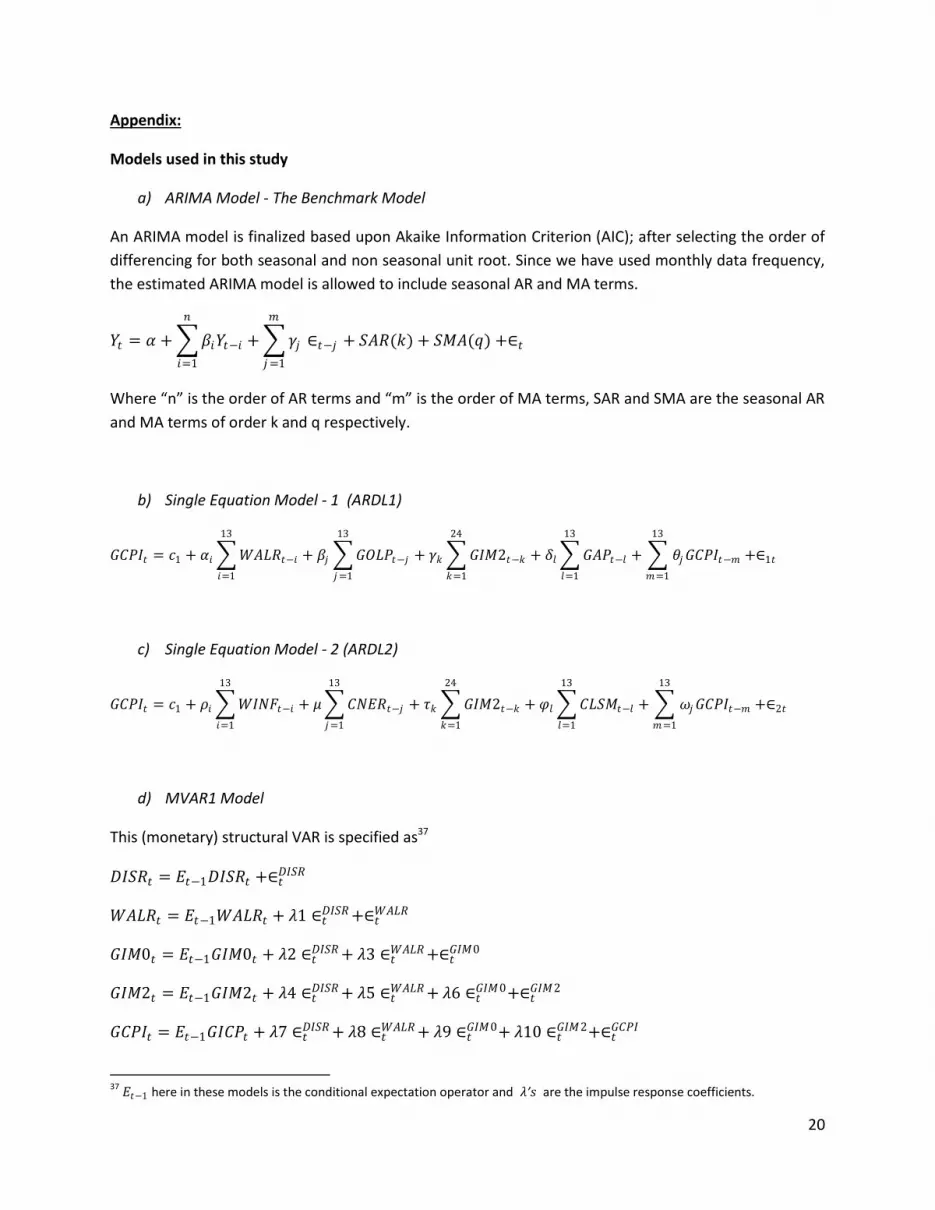
a) ARIMA Model - The Benchmark Model
An ARIMA model is finalized based upon Akaike Information Criterion (AIC); after selecting the order of
differencing for both seasonal and non seasonal unit root. Since we have used monthly data frequency,
the estimated ARIMA model is allowed to include seasonal AR and MA terms.
𝑌𝑡 = 𝛼 + 𝛽𝑖𝑌𝑡−𝑖
𝑛
𝑖=1
+ 𝛾𝑗 ∈𝑡−𝑗
𝑚
𝑗=1
+ 𝑆𝐴𝑅(𝑘) + 𝑆𝑀𝐴(𝑞) +∈𝑡
Where “n” is the order of AR terms and “m” is the order of MA terms, SAR and SMA are the seasonal AR
and MA terms of order k and q respectively.
b) Single Equation Model - 1 (ARDL1)
𝐺𝐶𝑃𝐼𝑡 = 𝑐1 + 𝛼𝑖 𝑊𝐴𝐿𝑅𝑡−𝑖
13
𝑖=1
+ 𝛽𝑗 𝐺𝑂𝐿𝑃𝑡−𝑗
13
𝑗=1
+ 𝛾𝑘 𝐺𝐼𝑀2𝑡−𝑘
24
𝑘=1
+ 𝛿𝑙 𝐺𝐴𝑃𝑡−𝑙
13
𝑙=1
+ 𝜃𝑗𝐺𝐶𝑃𝐼𝑡−𝑚
13
𝑚=1
+∈1𝑡
c) Single Equation Model - 2 (ARDL2)
𝐺𝐶𝑃𝐼𝑡 = 𝑐1 + 𝜌𝑖 𝑊𝐼𝑁𝐹𝑡−𝑖
13
𝑖=1
+ 𝜇 𝐶𝑁𝐸𝑅𝑡−𝑗
13
𝑗=1
+ 𝜏𝑘 𝐺𝐼𝑀2𝑡−𝑘
24
𝑘=1
+ 𝜑𝑙 𝐶𝐿𝑆𝑀𝑡−𝑙
13
𝑙=1
+ 𝜔𝑗𝐺𝐶𝑃𝐼𝑡−𝑚
13
𝑚=1
+∈2𝑡
d) MVAR1 Model
This (monetary) structural VAR is specified as37
𝐷𝐼𝑆𝑅𝑡 = 𝐸𝑡−1𝐷𝐼𝑆𝑅𝑡 +∈𝑡𝐷𝐼𝑆𝑅
𝑊𝐴𝐿𝑅𝑡 = 𝐸𝑡−1𝑊𝐴𝐿𝑅𝑡 + 𝜆1 ∈𝑡𝐷𝐼𝑆𝑅 +∈𝑡
𝑊𝐴𝐿𝑅
𝐺𝐼𝑀0𝑡 = 𝐸𝑡−1𝐺𝐼𝑀0𝑡 + 𝜆2 ∈𝑡𝐷𝐼𝑆𝑅 + 𝜆3 ∈𝑡
𝑊𝐴𝐿𝑅 +∈𝑡𝐺𝐼𝑀0
𝐺𝐼𝑀2𝑡 = 𝐸𝑡−1𝐺𝐼𝑀2𝑡 + 𝜆4 ∈𝑡𝐷𝐼𝑆𝑅 + 𝜆5 ∈𝑡
𝑊𝐴𝐿𝑅 + 𝜆6 ∈𝑡𝐺𝐼𝑀0+∈𝑡
𝐺𝐼𝑀2
𝐺𝐶𝑃𝐼𝑡 = 𝐸𝑡−1𝐺𝐼𝐶𝑃𝑡 + 𝜆7 ∈𝑡𝐷𝐼𝑆𝑅 + 𝜆8 ∈𝑡
𝑊𝐴𝐿𝑅 + 𝜆9 ∈𝑡𝐺𝐼𝑀0+ 𝜆10 ∈𝑡
𝐺𝐼𝑀2+∈𝑡𝐺𝐶𝑃𝐼
37
𝐸𝑡−1 here in these models is the conditional expectation operator and 𝜆′𝑠 are the impulse response coefficients.

21
It gives us the following recursive structural VAR system:
𝑌𝑇 = 𝐴𝑌𝑇−1 + 𝐵 ∈𝑡
Where 𝑌 = (𝐷𝐼𝑆𝑅, 𝑊𝐴𝐿𝑅, 𝐺𝐼𝑀0,𝐺𝐼𝑀2, 𝐺𝐶𝑃𝐼) , ∈= (∈𝐷𝐼𝑆𝑅 ,∈𝑊𝐴𝐿𝑅 ,∈𝐺𝐼𝑀0 ,∈𝐺𝐼𝑀2 ,∈𝐺𝐶𝑃𝐼 ) and
𝐵 =
1 0 0 0 0𝜆1 1 0 0 0𝜆2 𝜆3 1 0 0𝜆4 𝜆5 𝜆6 1 0𝜆7 𝜆8 𝜆9 𝜆10 1
e) MVAR2 Model
This (monetary) structural VAR2 is specified as38
𝐷𝐼𝑆𝑅𝑡 = 𝐸𝑡−1𝐷𝐼𝑆𝑅𝑡 +∈𝑡𝐷𝐼𝑆𝑅
𝐺𝐼𝑀0𝑡 = 𝐸𝑡−1𝐺𝐼𝑀0𝑡 + 𝜆1 ∈𝑡𝐷𝐼𝑆𝑅 +∈𝑡
𝐺𝐼𝑀0
𝐺𝐼𝑀2𝑡 = 𝐸𝑡−1𝐺𝐼𝑀2𝑡 + 𝜆2 ∈𝑡𝐷𝐼𝑆𝑅 + 𝜆3 ∈𝑡
𝐺𝐼𝑀0+∈𝑡𝐺𝐼𝑀2
𝐺𝐴𝑃𝑡 = 𝐸𝑡−1𝐺𝐴𝑃𝑡 + 𝜆4 ∈𝑡𝐷𝐼𝑆𝑅 + 𝜆5 ∈𝑡
𝐺𝐼𝑀0+ 𝜆6 ∈𝑡𝐺𝐼𝑀2+∈𝑡
𝐺𝐴𝑃
𝐺𝐶𝑃𝐼𝑡 = 𝐸𝑡−1𝐺𝐼𝐶𝑃𝑡 + 𝜆7 ∈𝑡𝐷𝐼𝑆𝑅 + 𝜆8 ∈𝑡
𝐺𝐼𝑀0+ 𝜆9 ∈𝑡𝐺𝐼𝑀2+ 𝜆10 ∈𝑡
𝐺𝐴𝑃 +∈𝑡𝐺𝐶𝑃𝐼
It gives us the following recursive structural VAR system:
𝑌𝑇 = 𝐴𝑌𝑇−1 + 𝐵 ∈𝑡
Where 𝑌 = (𝐷𝐼𝑆𝑅, 𝐺𝐼𝑀0,𝐺𝐼𝑀2, 𝐺𝐴𝑃, 𝐺𝐶𝑃𝐼) , ∈= (∈𝐷𝐼𝑆𝑅 , ∈𝐺𝐼𝑀0 ,∈𝐺𝐼𝑀2,∈𝐺𝐴𝑃 ,∈𝐺𝐶𝑃𝐼) and
𝐵 =
1 0 0 0 0𝜆1 1 0 0 0𝜆2 𝜆3 1 0 0𝜆4 𝜆5 𝜆6 1 0𝜆7 𝜆8 𝜆9 𝜆10 1
f) CVAR1 Model
This (credit) structural VAR is specified as
𝐷𝐼𝑆𝑅𝑡 = 𝐸𝑡−1𝐷𝑖𝑠𝑟𝑡 +∈𝑡𝐷𝐼𝑆𝑅
38
𝐸𝑡−1 here in these models is the conditional expectation operator and 𝜆′𝑠 are the impulse response coefficients.

22
𝑇𝐵𝐿𝑅𝑡 = 𝐸𝑡−1𝑇𝐵𝐿𝑅𝑡 + 𝜆1 ∈𝑡𝐷𝐼𝑆𝑅 +∈𝑡
𝑇𝐵𝐿𝑅
𝐺𝑃𝑆𝐵𝑡 = 𝐸𝑡−1𝐺𝑃𝐵𝑆𝑡 + 𝜆2 ∈𝑡𝐷𝐼𝑆𝑅 + 𝜆3 ∈𝑡
𝑇𝐵𝐿𝑅 +∈𝑡𝐺𝑃𝑆𝐵
𝑊𝐴𝐿𝑅𝑡 = 𝐸𝑡−1𝑊𝐴𝐿𝑅𝑡 + 𝜆4 ∈𝑡𝐷𝐼𝑆𝑅 + 𝜆5 ∈𝑡
𝑇𝐵𝐿𝑅+ 𝜆6 ∈𝑡𝐺𝑃𝑆𝐵 +∈𝑡
𝑊𝐴𝐿𝑅
𝐺𝑃𝑆𝐶𝑡 = 𝐸𝑡−1𝐺𝑃𝑆𝐶𝑡 + 𝜆7 ∈𝑡𝐷𝐼𝑆𝑅 + 𝜆8 ∈𝑡
𝑇𝐵𝐿𝑅+ 𝜆9 ∈𝑡𝐺𝑃𝑆𝐵 + 𝜆10 ∈𝑡
𝑊𝐴𝐿𝑅 +∈𝑡𝐺𝑃𝑆𝐶
𝐺𝐶𝑃𝐼𝑡 = 𝐸𝑡−1𝐺𝐶𝑃𝐼𝑡 + 𝜆11 ∈𝑡𝐷𝐼𝑆𝑅 + 𝜆12 ∈𝑡
𝑇𝐵𝐿𝑅+ 𝜆13 ∈𝑡𝐺𝑃𝑆𝐵 + 𝜆14 ∈𝑡
𝑊𝐴𝐿𝑅+ 𝜆15 ∈𝑡𝐺𝑃𝑆𝐶 +∈𝑡
𝐺𝐶𝑃𝐼
It gives us the following recursive structural VAR system:
𝑌𝑇 = 𝐴𝑌𝑇−1 + 𝐵 ∈𝑡
Where 𝑌 = 𝐷𝐼𝑆𝑅, 𝑇𝐵𝐿𝑅, 𝐺𝑃𝑆𝐵, 𝑊𝐴𝐿𝑅, 𝐺𝑃𝑆𝐶, 𝐺𝐶𝑃𝐼 ,
∈= (∈𝐷𝐼𝑆𝑅 , ∈𝑇𝐵𝐿𝑅 ,∈𝐺𝑃𝑆𝐵 , ∈𝑊𝐴𝐿𝑅 ,∈𝐺𝑃𝑆𝐶 ,∈𝐺𝐶𝑃𝐼)and
𝐵 =
1 0 0 0 0 0𝜆1 1 0 0 0 0𝜆2 𝜆3 1 0 0 0𝜆4 𝜆5 𝜆6 1 0 0𝜆7 𝜆8 𝜆9 𝜆10 1 0𝜆11 𝜆12 𝜆13 𝜆14 𝜆15 1
g) CVAR2 Model
This (credit) structural VAR is specified as
𝐷𝐼𝑆𝑅𝑡 = 𝐸𝑡−1𝐷𝑖𝑠𝑟𝑡 +∈𝑡𝐷𝐼𝑆𝑅
𝑇𝐵𝐿𝑅𝑡 = 𝐸𝑡−1𝑇𝐵𝐿𝑅𝑡 + 𝜆1 ∈𝑡𝐷𝐼𝑆𝑅 +∈𝑡
𝑇𝐵𝐿𝑅
𝐺𝑃𝑆𝐵𝑡 = 𝐸𝑡−1𝐺𝑃𝐵𝑆𝑡 + 𝜆2 ∈𝑡𝐷𝐼𝑆𝑅 + 𝜆3 ∈𝑡
𝑇𝐵𝐿𝑅 +∈𝑡𝐺𝑃𝑆𝐵
𝑊𝐴𝐿𝑅𝑡 = 𝐸𝑡−1𝑊𝐴𝐿𝑅𝑡 + 𝜆4 ∈𝑡𝐷𝐼𝑆𝑅 + 𝜆5 ∈𝑡
𝑇𝐵𝐿𝑅+ 𝜆6 ∈𝑡𝐺𝑃𝑆𝐵 +∈𝑡
𝑊𝐴𝐿𝑅
𝐺𝑃𝑆𝐶𝑡 = 𝐸𝑡−1𝐺𝑃𝑆𝐶𝑡 + 𝜆7 ∈𝑡𝐷𝐼𝑆𝑅 + 𝜆8 ∈𝑡
𝑇𝐵𝐿𝑅+ 𝜆9 ∈𝑡𝐺𝑃𝑆𝐵 + 𝜆10 ∈𝑡
𝑊𝐴𝐿𝑅 +∈𝑡𝐺𝑃𝑆𝐶
𝐶𝐿𝑆𝑀𝑡 = 𝐸𝑡−1𝐶𝑃𝐿𝑆𝑀𝑡 + 𝜆11 ∈𝑡𝐷𝐼𝑆𝑅 + 𝜆12 ∈𝑡
𝑇𝐵𝐿𝑅+ 𝜆13 ∈𝑡𝐺𝑃𝑆𝐵 + 𝜆14 ∈𝑡
𝑊𝐴𝐿𝑅 + 𝜆15 ∈𝑡𝐺𝑃𝑆𝐶 +∈𝑡
𝐶𝐿𝑆𝑀
𝐺𝐶𝑃𝐼𝑡 = 𝐸𝑡−1𝐺𝐶𝑃𝐼𝑡 + 𝜆16 ∈𝑡𝐷𝐼𝑆𝑅 + 𝜆17 ∈𝑡
𝑇𝐵𝐿𝑅+ 𝜆18 ∈𝑡𝐺𝑃𝑆𝐵 + 𝜆19 ∈𝑡
𝑊𝐴𝐿𝑅+ 𝜆20 ∈𝑡𝐺𝑃𝑆𝐶 + 𝜆21 ∈𝑡
𝐶𝐿𝑆𝑀
+∈𝑡𝐺𝐶𝑃𝐼
It gives us the following recursive structural VAR system:
𝑌𝑇 = 𝐴𝑌𝑇−1 + 𝐵 ∈𝑡

23
Where
𝑌 = 𝐷𝐼𝑆𝑅, 𝑇𝐵𝐿𝑅, 𝐺𝑃𝑆𝐵, 𝑊𝐴𝐿𝑅, 𝐺𝑃𝑆𝐶, 𝐶𝐿𝑆𝑀, 𝐺𝐶𝑃𝐼 ,
∈= (∈𝐷𝐼𝑆𝑅 , ∈𝑇𝐵𝐿𝑅 ,∈𝐺𝑃𝑆𝐵 , ∈𝑊𝐴𝐿𝑅 ,∈𝐺𝑃𝑆𝐶 ,∈𝐶𝐿𝑆𝑀 ,∈𝐺𝐶𝑃𝐼),
and
𝐵 =
1 0 0 0 0 0 0𝜆1 1 0 0 0 0 0𝜆2 𝜆3 1 0 0 0 0𝜆4 𝜆5 𝜆6 1 0 0 0𝜆7 𝜆8 𝜆9 𝜆10 1 0 0𝜆11 𝜆12 𝜆13 𝜆14 𝜆115 1 0𝜆16 𝜆17 𝜆18 𝜆19 𝜆20 𝜆21 1
h) CVAR3 Model
This (credit) structural VAR is specified as
𝐷𝐼𝑆𝑅𝑡 = 𝐸𝑡−1𝐷𝑖𝑠𝑟𝑡 +∈𝑡𝐷𝐼𝑆𝑅
𝐺𝑃𝑆𝐵𝑡 = 𝐸𝑡−1𝐺𝑃𝑆𝐵𝑡 + 𝜆1 ∈𝑡𝐷𝐼𝑆𝑅 +∈𝑡
𝐺𝑃𝑆𝐵
𝑊𝐴𝐿𝑅𝑡 = 𝐸𝑡−1𝑊𝐴𝐿𝑅𝑡 + 𝜆2 ∈𝑡𝐷𝐼𝑆𝑅 + 𝜆3 ∈𝑡
𝐺𝑃𝑆𝐵 +∈𝑡𝑊𝐴𝐿𝑅
𝐺𝑃𝑆𝐶𝑡 = 𝐸𝑡−1𝐺𝑃𝑆𝐶𝑡 + 𝜆4 ∈𝑡𝐷𝐼𝑆𝑅 + 𝜆5 ∈𝑡
𝐺𝑃𝑆𝐵 + 𝜆6 ∈𝑡𝑊𝐴𝐿𝑅 +∈𝑡
𝐺𝑃𝑆𝐶
𝐶𝐿𝑆𝑀𝑡 = 𝐸𝑡−1𝐶𝐿𝑆𝑀𝑡 + 𝜆7 ∈𝑡𝐷𝐼𝑆𝑅 + 𝜆8 ∈𝑡
𝐺𝑃𝑆𝐵 + 𝜆9 ∈𝑡𝑊𝐴𝐿𝑅+ 𝜆10 ∈𝑡
𝐺𝑃𝑆𝐶 +∈𝑡𝐶𝐿𝑆𝑀
𝐺𝐶𝑃𝐼𝑡 = 𝐸𝑡−1𝐺𝐶𝑃𝐼𝑡 + 𝜆11 ∈𝑡𝐷𝐼𝑆𝑅 + 𝜆12 ∈𝑡
𝐺𝑃𝑆𝐵 + 𝜆13 ∈𝑡𝑊𝐴𝐿𝑅 + 𝜆14 ∈𝑡
𝐺𝑃𝑆𝐶 + 𝜆15 ∈𝑡𝐶𝐿𝑆𝑀+∈𝑡
𝐺𝐶𝑃𝐼
It gives us the following recursive structural VAR system:
𝑌𝑇 = 𝐴𝑌𝑇−1 + 𝐵 ∈𝑡
Where 𝑌 = 𝐷𝐼𝑆𝑅, 𝐺𝑃𝑆𝐵, 𝑊𝐴𝐿𝑅, 𝐺𝑃𝑆𝐶, 𝐶𝐿𝑆𝑀, 𝐺𝐶𝑃𝐼 ,
∈= (∈𝐷𝐼𝑆𝑅 , ∈𝐺𝑃𝑆𝐵 ,∈𝑊𝐴𝐿𝑅 ,∈𝐺𝑃𝑆𝐶 ,∈𝐶𝐿𝑆𝑀 ,∈𝐺𝐶𝑃𝐼),
and
𝐵 =
1 0 0 0 0 0𝜆1 1 0 0 0 0𝜆2 𝜆3 1 0 0 0𝜆4 𝜆5 𝜆6 1 0 0𝜆7 𝜆8 𝜆9 𝜆10 1 0𝜆11 𝜆12 𝜆13 𝜆14 𝜆15 1

24
i) EVAR1 Model
This (external) structural VAR is specified as
𝐺𝑂𝐿𝑃𝑡 = 𝐸𝑡−1𝐺𝑂𝐿𝑃𝑡 +∈𝑡𝐺𝑂𝐿𝑃
𝐺𝐹𝐼𝑃𝑡 = 𝐸𝑡−1𝐺𝐹𝐼𝑃𝑡 + 𝜆1 ∈𝑡𝐺𝑂𝐿𝑃+∈𝑡
𝐺𝐹𝐼𝑃
𝐺𝑊𝑅𝑀𝑡 = 𝐸𝑡−1𝐺𝑊𝑅𝑀𝑡 + 𝜆2 ∈𝑡𝐺𝑂𝐿𝑃+ 𝜆3 ∈𝑡
𝐺𝐹𝐼𝑃+∈𝑡𝐺𝑊𝑅𝑀
𝐶𝑅𝐸𝑅𝑡 = 𝐸𝑡−1𝐶𝑅𝐸𝑅𝑡 + 𝜆4 ∈𝑡𝐺𝑂𝐿𝑃+ 𝜆5 ∈𝑡
𝐺𝐹𝐼𝑃 + 𝜆6 ∈𝑡𝐺𝑊𝑅𝑀 +∈𝑡
𝐶𝑅𝐸𝑅
𝐶𝐿𝑆𝑀𝑡 = 𝐸𝑡−1𝐶𝑃𝐿𝑆𝑀𝑡 + 𝜆7 ∈𝑡𝐺𝑂𝐿𝑃+ 𝜆8 ∈𝑡
𝐺𝐹𝐼𝑃 + 𝜆9 ∈𝑡𝐺𝑊𝑅𝑀 + 𝜆10 ∈𝑡
𝐶𝑅𝐸𝑅+∈𝑡𝐶𝐿𝑆𝑀
𝐺𝐶𝑃𝐼𝑡 = 𝐸𝑡−1𝐺𝐶𝑃𝐼𝑡 + 𝜆11 ∈𝑡𝐺𝑂𝐿𝑃+ 𝜆12 ∈𝑡
𝐺𝐹𝐼𝑃 + 𝜆13 ∈𝑡𝐺𝑊𝑅𝑀 + 𝜆14 ∈𝑡
𝐶𝑅𝐸𝑅+ 𝜆15 ∈𝑡𝐶𝐿𝑆𝑀+∈𝑡
𝐺𝐶𝑃𝐼
It gives us the following recursive structural VAR system
𝑌𝑇 = 𝐴𝑌𝑇−1 + 𝐵 ∈𝑡 , Where
𝑌 = 𝐺𝑂𝐿𝑃, 𝐺𝐹𝐼𝑃, 𝐺𝑊𝑅𝑀, 𝐶𝑅𝐸𝑅, 𝐶𝐿𝑆𝑀, 𝐺𝐶𝑃𝐼 , ∈= (∈𝐺𝑂𝐿𝑃 ,∈𝐺𝐹𝐼𝑃 ,∈𝐺𝑊𝑅𝑀 ,∈𝐶𝑅𝐸𝑅 ,∈𝐶𝐿𝑆𝑀 ,∈𝐺𝐶𝑃𝐼) and
𝐵 =
1 0 0 0 0 0𝜆1 1 0 0 0 0𝜆2 𝜆3 1 0 0 0𝜆4 𝜆5 𝜆6 1 0 0𝜆7 𝜆8 𝜆9 𝜆10 1 0𝜆11 𝜆12 𝜆13 𝜆14 𝜆15 1
j) EVAR2 Model
This (external) structural VAR is specified as:
𝑊𝐶𝑃𝐶𝑡 = 𝐸𝑡−1𝑊𝐶𝑃𝐶𝑡 +∈𝑡𝑊𝐶𝑃𝐶
𝐶𝑁𝐸𝑅𝑡 = 𝐸𝑡−1𝐶𝑁𝐸𝑅𝑡 + 𝜆1 ∈𝑡𝑊𝐶𝑃𝐶+ 𝜆2 ∈𝑡
𝐺𝐶𝑃𝐼+∈𝑡𝐶𝑁𝐸𝑅
𝐺𝐼𝑀2𝑡 = 𝐸𝑡−1𝐺𝐼𝑀2𝑡 + 𝜆3 ∈𝑡𝑊𝐶𝑃𝐶+ 𝜆4 ∈𝑡
𝐶𝑁𝐸𝑅+∈𝑡𝐺𝐼𝑀2
𝐺𝐿𝑆𝑀𝑡 = 𝐸𝑡−1𝐺𝐿𝑆𝑀𝑡 + 𝜆5 ∈𝑡𝑊𝐶𝑃𝐶+ 𝜆6 ∈𝑡
𝐶𝑁𝐸𝑅+ 𝜆7 ∈𝑡𝐺𝐼𝑀2 +∈𝑡
𝐺𝐿𝑆𝑀
𝐺𝐶𝑃𝐼𝑡 = 𝐸𝑡−1𝐺𝐶𝑃𝐼𝑡 + 𝜆8 ∈𝑡𝑊𝐶𝑃𝐶+ 𝜆9 ∈𝑡
𝐺𝐿𝑆𝑀 + 𝜆10 ∈𝑡𝐺𝐼𝑀2+ 𝜆11 ∈𝑡
𝐶𝑁𝐸𝑅+∈𝑡𝐺𝐶𝑃𝐼
It gives us the following recursive structural VAR system:

25
𝑌𝑇 = 𝐴𝑌𝑇−1 + 𝐵 ∈𝑡
Where 𝑌 = 𝑊𝐶𝑃𝐶, 𝐶𝑁𝐸𝑅, 𝐺𝐼𝑀2, 𝐺𝐿𝑆𝑀, 𝐺𝐶𝑃𝐼 and ∈= (∈𝑊𝐶𝑃𝐶 ,∈𝐶𝑁𝐸𝑅 ,∈𝐺𝐼𝑀2 ,∈𝐺𝐿𝑆𝑀 ,∈𝐺𝐶𝑃𝐼) and
𝐵 =
1 0 0 0 0𝜆1 1 0 0 𝜆2
𝜆3 𝜆4 1 0 0𝜆5 𝜆6 𝜆7 1 0𝜆8 𝜆9 𝜆10 𝜆11 1
k) EVAR3 Model
This (external) structural VAR is specified as
𝐺𝑂𝐿𝑃𝑡 = 𝐸𝑡−1𝐺𝑂𝐿𝑃𝑡 +∈𝑡𝐺𝑂𝐿𝑃
𝐺𝐹𝐼𝑃𝑡 = 𝐸𝑡−1𝐺𝐹𝐼𝑃𝑡 + 𝜆1 ∈𝑡𝐺𝑂𝐿𝑃+∈𝑡
𝐺𝐹𝐼𝑃
𝐷𝐼𝑆𝑅𝑡 = 𝐸𝑡−1𝐷𝐼𝑆𝑅𝑡 + 𝜆2 ∈𝑡𝐺𝑂𝐿𝑃+ 𝜆3 ∈𝑡
𝐺𝐹𝐼𝑃 +∈𝑡𝐷𝐼𝑆𝑅
𝐶𝑅𝐸𝑅𝑡 = 𝐸𝑡−1𝐶𝑅𝐸𝑅𝑡 + 𝜆4 ∈𝑡𝐺𝑂𝐿𝑃+ 𝜆5 ∈𝑡
𝐺𝐹𝐼𝑃 + 𝜆6 ∈𝑡𝐷𝐼𝑆𝑅 +∈𝑡
𝐶𝑅𝐸𝑅
𝐺𝑊𝑅𝑀𝑡 = 𝐸𝑡−1𝐺𝑊𝑅𝑀𝑡 + 𝜆7 ∈𝑡𝐺𝑂𝐿𝑃+ 𝜆8 ∈𝑡
𝐺𝐹𝐼𝑃+ 𝜆9 ∈𝑡𝐷𝐼𝑆𝑅 + 𝜆10 ∈𝑡
𝐶𝑅𝐸𝑅+∈𝑡𝐺𝑊𝑅𝑀
𝐶𝐿𝑆𝑀𝑡 = 𝐸𝑡−1𝐶𝐿𝑆𝑀𝑡 + 𝜆11 ∈𝑡𝐺𝑂𝐿𝑃+ 𝜆12 ∈𝑡
𝐺𝐹𝐼𝑃 + 𝜆13 ∈𝑡𝐷𝐼𝑆𝑅 + 𝜆14 ∈𝑡
𝐶𝑅𝐸𝑅+ 𝜆15 ∈𝑡𝐺𝑊𝑅𝑀 +∈𝑡
𝐶𝐿𝑆𝑀
𝐺𝐶𝑃𝐼𝑡 = 𝐸𝑡−1𝐺𝐶𝑃𝐼𝑡 + 𝜆16 ∈𝑡𝐺𝑂𝐿𝑃+ 𝜆17 ∈𝑡
𝐺𝐹𝐼𝑃 + 𝜆18 ∈𝑡𝐷𝐼𝑆𝑅 + 𝜆19 ∈𝑡
𝐶𝑅𝐸𝑅+ 𝜆20 ∈𝑡𝐺𝑊𝑅𝑀 + 𝜆21 ∈𝑡
𝐶𝐿𝑆𝑀
+∈𝑡𝐺𝐶𝑃𝐼
It gives us the following recursive structural VAR system
𝑌𝑇 = 𝐴𝑌𝑇−1 + 𝐵 ∈𝑡 , Where
Where; 𝑌 = 𝐺𝑂𝐿𝑃, 𝐺𝐹𝐼𝑃, 𝐷𝐼𝑆𝑅, 𝐶𝑅𝐸𝑅, 𝐺𝑊𝑅𝑀, 𝐶𝐿𝑆𝑀, 𝐺𝐶𝑃𝐼 ,
∈= ( ∈𝐺𝑂𝐿𝑃 , ∈𝐺𝐹𝐼𝑃 , ∈𝐷𝐼𝑆𝑅 ,∈𝐶𝑅𝐸𝑅 ,∈𝐺𝑊𝑅𝑀 ,∈𝐶𝐿𝑆𝑀 ,∈𝐺𝐶𝑃𝐼) and
and
𝐵 =
1 0 0 0 0 0 0𝜆1 1 0 0 0 0 0𝜆2 𝜆3 1 0 0 0 0𝜆4 𝜆5 𝜆6 1 0 0 0𝜆7 𝜆8 𝜆9 𝜆10 1 0 0𝜆11 𝜆12 𝜆13 𝜆14 𝜆115 1 0𝜆16 𝜆17 𝜆18 𝜆19 𝜆20 𝜆21 1

26
l) CMVAR Model
This (comprehensive) structural VAR is specified as:
𝐺𝑂𝐿𝑃𝑡 = 𝐸𝑡−1𝐺𝑂𝐿𝑃𝑡 +∈𝑡𝐺𝑂𝐿𝑃
𝐶𝑅𝐸𝑅𝑡 = 𝐸𝑡−1𝐶𝑅𝐸𝑅𝑡 + 𝜆1 ∈𝑡𝐺𝑂𝐿𝑃+∈𝑡
𝐶𝑅𝐸𝑅
𝐷𝐼𝑆𝑅𝑡 = 𝐸𝑡−1𝐷𝐼𝑆𝑅𝑡 + 𝜆2 ∈𝑡𝐺𝑂𝐿𝑃+ 𝜆3 ∈𝑡
𝐶𝑅𝐸𝑅+∈𝑡𝐷𝐼𝑆𝑅
𝐺𝐼𝑀2𝑡 = 𝐸𝑡−1𝐺𝐼𝑀2𝑡 + 𝜆4 ∈𝑡𝐺𝑂𝐿𝑃+ 𝜆5 ∈𝑡
𝐶𝑅𝐸𝑅+ 𝜆6 ∈𝑡𝐷𝐼𝑆𝑅 +∈𝑡
𝐺𝐼𝑀2
𝐶𝐿𝑆𝑀𝑡 = 𝐸𝑡−1𝐶𝐿𝑆𝑀𝑡 + 𝜆7 ∈𝑡𝐺𝑂𝐿𝑃+ 𝜆8 ∈𝑡
𝐶𝑅𝐸𝑅+ 𝜆9 ∈𝑡𝐷𝐼𝑆𝑅 + 𝜆10 ∈𝑡
𝐺𝐼𝑀2+∈𝑡𝐶𝐿𝑆𝑀
𝐺𝐶𝑃𝐼𝑡 = 𝐸𝑡−1𝐺𝐶𝑃𝐼𝑡 + 𝜆11 ∈𝑡𝐺𝑂𝐿𝑃+ 𝜆12 ∈𝑡
𝐶𝑅𝐸𝑅+ 𝜆13 ∈𝑡𝐷𝐼𝑆𝑅 + 𝜆14 ∈𝑡
𝐶𝐼𝑀2+ +𝜆15 ∈𝑡𝐶𝐿𝑆𝑀+∈𝑡
𝐺𝐶𝑃𝐼
It gives us the following recursive structural VAR system
𝑌𝑇 = 𝐴𝑌𝑇−1 + 𝐵 ∈𝑡 , Where
Where,
𝑌 = 𝐺𝑂𝐿𝑃, 𝐶𝑅𝐸𝑅, 𝐷𝐼𝑆𝑅, 𝐶𝐼𝑀2,𝐶𝐿𝑆𝑀, 𝐺𝐶𝑃𝐼 ,
∈= ( ∈𝐺𝑂𝐿𝑃 , ∈𝐶𝑅𝐸𝑅 ,∈𝐷𝐼𝑆𝑅 , ∈𝐶𝐼𝑀2,∈𝐶𝐿𝑆𝑀 ,∈𝐺𝐶𝑃𝐼)
and
𝐵 =
1 0 0 0 0 0𝜆1 1 0 0 0 0𝜆2 𝜆3 1 0 0 0𝜆4 𝜆5 𝜆6 1 0 0𝜆7 𝜆8 𝜆9 𝜆10 1 0𝜆11 𝜆12 𝜆13 𝜆14 𝜆15 1

27
Table 1 (a) : Selected Literature on Inflation Forecast Evaluation-Developing Countries
Study Country/Frequency/ Sample/Variable of interest
Model and other Variables
Findings Forecast Evaluation: Benchmark Criterion
Riaz (2012) Pakistan. Quarterly. 1975-2008. Food and general CPI inflation (YoY)
VAR Model. Real GDP, M2, Interest rate and Exchange rate
Food Inflation forecasts are found to be efficient and fulfill the criteria of weak and strong rationality. This conclusion does not hold for General Inflation.
No Benchmark Root Mean Square Error (RMSE), Mean Absolute Error (MAE), Mean Absolute Percentage Error (MAPE) and Theil’s Inequality Coefficient (TIC)
Haider and Hanif (2009)
Pakistan. Monthly Data for General YOY inflation From July 1993 to June 2007
AR (1), ARIMA and ANN
ANN is found to be better than AR (1) and ARIMA based on RMSE for 12 month forecasts.
ARIMA Benchmark RMSE
Bokil and Schimmelpfennig (2006)
Pakistan. Monthly Data for July 1998 to December 2004 general 12 month average inflation
Leading Indicator Model (LIM), VAR Model and ARIMA model. Broad Money, Reserve Money, Credit to Private Sector, Six Months Treasury Bills Rate Large Scale Manufacturing Index and Output Gap.
LIM is considered to be the best model for the forecast of six months July 2004 to Dec 2004. The LIM model containing broad money growth, private sector credit growth and lags of inflation has the minimum RMSE.
No Benchmark. RMSE
Bukhari and Feridun (2006)
Pakistan. Monthly Data 1991 to 2004 CPI inflation
ARIMA and VAR. CPI, WPI, M2 and Weighted Average Lending Rates
ARIMA model performs better than VAR according to relative MSE.
ARIMA Benchmark Relative RMSE

28
Table 1 (a) Selected Literature on Inflation Forecast Evaluation-Developed Countries
Study Country/Frequency/ Sample/Variable of interest
Model and other Variables
Findings Forecast Evaluation: Benchmark Criterion
Atkeson and Ohanian (2001)
USA Quarterly 1965 Q4 to 1999Q4 CPI Core CPI PCE Deflator
NAIRU Philips Curve
15 Year recursive forecast reveals that Philips Curve forecasts are better than naïve forecast
Benchmark used is Random Walk Model.
Norman and Richards (2012)
Australia Quarterly 1982Q1-2009Q4 CPI Inflation Trimmed Mean QoQ Inflation
Philips Curve, Mark-up Model, Distributed lag model and GPT Philips Curve VAR FAVAR
GPT Philips Curve model outperforms VAR and FAVAR forecasts.
Benchmark used is Random Walk Model.
Elliot and Timmermann (2008)
USA Monthly 1959:1 2003:12 CPI MoM Inflation
AR, BVAR, Exponential Smoothing, STAR and ANN
Simple Average forecast is the best and exponential smoothing is the second best for recursive forecasts.
No Benchmark. MSE of model using Giacomini and White (2006) approach.
Antipin et al (2014)
Australia, Sweden, UK and USA Quarterly 1970 Q1- 1985Q1 CPI QoQ Inflation
AR (p) AR (p) model by constant gain least squares CGLS is better than OLS
Benchmark AR (p) Relative RMSE.
Stock and Watson (2008)
USA Quarterly 1953 Q1- 2008Q1 CPI, CPI core, PCE-all, PCE-core and GDP Deflator QoQ Inflation
157 distinct Models and 35 combination forecasts
Performance of Philips curve is episodic. For instance in late 90’s its forecasts were better than AR (p) model. In mid 90’s univariate benchmark models outperform other multivariate models.
Benchmark AR (p) and Random Walk model. Relative RMSE

29
0
5
10
15
20
25
19
92
19
93
19
94
19
95
19
96
19
97
19
98
19
99
20
00
20
01
20
02
20
03
20
04
20
05
20
06
20
07
20
08
20
09
20
10
20
11
20
12
20
13
20
14
Pe
rce
nt
Figure 1: Observed and Target/SBP Forecast of 12-month Average YoY Inflation
SBP AR Inflation Forecast (mid point) Inflation Observed Inflation Target
Global Commodity Price Shock
-6.0
-4.0
-2.0
0.0
2.0
4.0
6.0
8.0
10.0
FY94 FY95 FY96 FY97 FY98 FY99 FY00 FY01 FY02 FY03 FY04 FY05 FY06 FY07 FY08 FY09 FY10
Fig: 2 Inflation and Money Surprise (%)
Inflation Surprise Lagged Money Surprise

30
Table 1 (b) : Some Stylized Facts about Inflation in Pakistan
Period Minimum Average Maximum Dispersion Regime
Jul 1958 to Jun 2014 -10.32 7.7 37.81 8.8 Overall inflation data availability39
Jul 1992 to Jun 2014 1.41 9.0 24.86 4.3 Estimation period of this study
Jul 2002 to Nov 2007 1.41 6.6 11.10 2.5 Low-inflation period
Dec 2007 to Jun 2009 8.79 18.0 24.86 5.2 High-inflation period
Jul 2009 to Jun 2014 5.13 10.2 15.45 2.5 Moderate-inflation period
Source: Pakistan Bureau of Statistics and authors’ calculations
39
Consistent data for all the other variables used in this study is not readily available for this entire period. That is why our inflation forecast evaluation analysis is over the period of Jul 1992 to Jun 2014.
0
5
10
15
20
25
30
35
0 2 4 6 8 10
I
n
f
l
a
t
i
o
n(
%)
Unemployment Rate (%)
Figure 3: Inflation Unemployment Trade off (1973-2013)
Sources: Pakistan Bureau of Statistics
5
5
6
6
7
7
8
0 5 10 15 20
1993-2013
-5
0
5
10
15
20
25
30
35
-0.40
-0.30
-0.20
-0.10
0.00
0.10
0.20
0.30
0.40
0.50
19
51
19
53
19
55
19
57
19
59
19
61
19
63
19
65
19
67
19
69
19
71
19
73
19
75
19
77
19
79
19
81
19
83
19
85
19
87
19
89
19
91
19
93
19
95
19
97
19
99
20
01
20
03
20
05
20
07
20
09
20
11
20
13
Figure 4: Output and Inflation nexus in Pakistan
Output gap Inflation - Lead (RHS)
Correlation =0.23
Source: Pakistan Bureau of Statistics and authors calculations

31
Table 1 (c): List of Variables
Variable Source
Pakistan’s overnight reverse repo rate (discount rate) SBP*
(Weighted average) lending rate charged by commercial banks in Pakistan SBP
Pakistan’s reserve money (M0) SBP
Pakistan’s broad money (M2) SBP
Pakistan’s consumer price index (CPI) PBS**
Global oil price (average of 3 spot crude oil prices - Brent, WTI# and Dubai Fathah) IFS***
United States industrial production index IFS
Remittances sent to Pakistan by Pakistanis working abroad SBP
Real effective exchange rate (of Pak Rupee) IFS
Nominal exchange rate (Pak Rupee per US$) IFS
Pakistan’s large scale manufacturing index PBS
World commodities’ price index IFS
Cut-off rates of 6 months Treasury Bills (Government of Pakistan) SBP
(Pakistan) Government borrowing from the banking system SBP
Private sector credit disbursed by commercial banks in Pakistan SBP
Pakistan’s real GDP PBS
Pakistan local oil (high speed diesel, petrol super and kerosene oil) prices’ index PBS
Pakistan’s unemployment rate PBS
#: West Texas Intermediate. *: State Bank of Pakistan. **: Pakistan Bureau of Statistics. ***: International Financial Statistics of International Monetary Fund.
Table 1 (d): Zeileis (2003) Structural Change Test
No of Breaks Date of Break BIC
0 786.3
1 December 2007 725.2
2 December 2007 ,July 2009 675.0*
*: BIC attained its minimum while we searched for two breaks.

32
Table: 2 (a) RMSE (Relative to RW model as benchmark) for Jul 2002 to Nov 2007 (Low Inflation Regime)
Table: 2 (b) RMSE (Relative to RW model as benchmark) for Dec 2007 to Jun 2009 (High Inflation Regime)
(i) Model : h 3 6 9 12 15 18 21 24
(ii) ARDL1 3.67 2.99 0.57 0.80 0.89 1.10 0.27 0.61
(iii) ARDL2 2.95 4.53 0.45 0.43 0.54 1.06 0.19 0.38
(iv) MVAR1 1.25 1.37 1.22 1.15 1.11 1.13 1.21 1.31
(v) MVAR2 1.23 1.32 1.23 1.28 1.28 1.29 1.37 1.41
(vi) CVAR1 1.50 1.92 1.91 2.08 2.31 2.61 3.12 4.04
(vii) CVAR2 1.84 2.42 2.50 2.87 3.62 5.01 7.66 12.38
(viii) CVAR3 1.97 2.45 2.58 3.03 3.88 5.31 7.92 12.29
(ix) EVAR1 1.50 1.39 1.17 1.21 1.40 1.57 1.68 1.73
(x) EVAR2 1.13 1.17 1.18 1.22 1.23 1.29 1.35 1.43
(xi) EVAR3 1.60 1.71 1.41 1.65 2.28 3.39 5.29 8.18
(xii) CMVAR 1.27 1.45 1.31 1.33 1.29 1.34 1.45 1.51
(xiii) BMVAR 0.99 0.97 0.97 0.97 0.96 0.96 0.97 0.98
(xiv) BEVAR 1.02 1.02 1.02 1.03 1.03 1.04 1.05 1.05
(xv) BCVAR 1.03 1.04 1.04 1.07 1.08 1.11 1.15 1.17
(xvi) BCMVAR 0.99 0.97 0.96 0.97 0.97 0.97 0.99 1.00
(xvii) Simple Average 0.93 0.99 1.03 1.07 1.14 1.31 1.68 2.36
(xviii) Trimmed Average 0.92 0.94 0.98 1.01 1.04 1.06 1.09 1.11
(xix) U- Trimmed Average 0.72 0.73 0.75 0.73 0.74 0.81 0.78 0.81
(xx) L- Trimmed Average 0.99 1.03 1.05 1.10 1.18 1.36 1.78 2.55
Bold values are the minimum values at each forecast horizon (i.e. in each column). Bold RRMSE are all less than 1.
(i) Model : h 3 6 9 12 15 18 21 24
(ii) ARDL1 0.47 0.37 0.41 0.44 0.22 0.30 0.46 0.71
(iii) ARDL2 0.47 0.36 0.40 0.69 0.24 0.37 0.51 0.54
(iv) MVAR1 0.98 1.04 1.13 1.22 1.28 1.39 1.50 1.60
(v) MVAR2 0.72 0.82 0.96 1.05 0.91 0.74 0.65 1.16
(vi) CVAR1 1.10 1.17 1.31 1.50 1.73 2.05 2.47 2.94
(vii) CVAR2 1.11 1.17 1.31 1.50 1.73 2.04 2.46 2.92
(viii) CVAR3 1.12 1.18 1.33 1.53 1.78 2.12 2.59 3.12
(ix) EVAR1 0.98 1.08 1.23 1.60 2.01 2.50 3.16 3.80
(x) EVAR2 0.93 0.97 1.03 1.08 0.91 0.66 0.63 0.80
(xi) EVAR3 1.05 1.12 1.24 1.54 1.79 2.05 2.32 2.52
(xii) CMVAR 0.79 0.81 0.84 0.93 1.12 1.43 1.73 1.82
(xiii) BMVAR 0.89 0.90 0.92 0.93 0.92 0.93 0.93 0.86
(xiv) BEVAR 0.95 1.01 1.12 1.27 1.42 1.65 1.90 2.13
(xv) BCVAR 0.95 1.01 1.10 1.21 1.33 1.50 1.70 1.87
(xvi) BCMVAR 0.87 0.89 0.92 0.96 0.98 1.03 1.08 1.05
(xvii) Simple Average 0.86 0.91 0.98 1.10 1.21 1.36 1.57 1.76
(xviii) Trimmed Average 0.90 0.93 0.95 1.19 1.34 1.53 1.67 1.49
(xix) U- Trimmed Average 0.77 0.74 0.60 0.73 0.88 0.97 1.06 0.76
(xx) L- Trimmed Average 0.95 1.00 0.97 1.29 1.50 1.74 2.04 2.14
Bold values are the minimum values at each forecast horizon (i.e. in each column). Bold RRMSE are all less than 1.

33
Table: 2 (c) RMSE (Relative to RW model as benchmark) for Jul 2009 to Jun 2014 (Moderate Inflation Regime)
(i) Model : h 3 6 9 12 15 18 21 24
(ii) ARDL1 1.40 1.66 2.53 3.12 0.65 1.14 1.43 2.14
(iii) ARDL2 1.34 1.40 1.51 2.04 0.60 0.85 1.19 1.92
(iv) MVAR1 1.16 1.29 1.26 1.15 1.13 0.99 0.79 0.63
(v) MVAR2 1.30 1.62 1.58 1.40 1.30 1.10 0.92 0.79
(vi) CVAR1 1.23 1.92 2.76 2.70 2.55 2.28 1.41 1.22
(vii) CVAR2 1.01 1.08 1.13 1.12 1.11 1.03 0.90 0.81
(viii) CVAR3 1.13 1.49 1.69 1.51 1.44 1.08 0.85 0.78
(ix) EVAR1 1.93 2.75 3.41 3.38 2.93 2.25 1.13 0.75
(x) EVAR2 1.22 1.50 1.51 1.28 1.12 1.19 1.35 1.42
(xi) EVAR3 1.70 2.24 2.54 2.33 2.01 1.81 1.47 1.31
(xii) CMVAR 1.53 1.90 1.99 1.87 1.57 1.23 0.90 0.68
(xiii) BMVAR 1.11 1.24 1.28 1.20 1.21 1.14 1.01 0.86
(xiv) BEVAR 1.02 1.10 1.09 1.05 1.10 1.05 0.93 0.85
(xv) BCVAR 1.14 1.31 1.39 1.36 1.37 1.31 1.16 1.03
(xvi) BCMVAR 1.03 1.10 1.07 1.02 1.06 1.00 0.90 0.77
(xvii) Simple Average 0.85 0.95 0.85 0.74 0.71 0.66 0.67 0.67
(xviii) Trimmed Average 0.88 1.02 0.82 0.83 0.87 0.81 0.69 0.60
(xix) U- Trimmed Average 0.92 0.94 0.82 0.82 0.91 0.85 0.73 0.61
(xx) L- Trimmed Average 0.94 1.41 1.03 0.96 0.67 0.62 0.71 0.66
Bold values are the minimum values at each forecast horizon (i.e. in each column). Bold RRMSE are all less than 1.

34
Table: 3 (a) RMSE (Relative to ARIMA model as benchmark) for Jul 2002 to Nov 2007 (Low Inflation Regime)
Table: 3 (b) RMSE (Relative to ARIMA model as benchmark) for Dec 2007 to Jun 2009 (High Inflation Regime)
(i) Model : h 3 6 9 12 15 18 21 24
(ii) ARDL1 3.65 3.00 0.57 0.79 0.89 1.10 0.27 0.60
(iii) ARDL2 2.93 4.54 0.45 0.43 0.54 1.06 0.19 0.38
(iv) MVAR1 1.24 1.38 1.22 1.15 1.11 1.12 1.21 1.31
(v) MVAR2 1.22 1.32 1.23 1.28 1.27 1.29 1.36 1.40
(vi) CVAR1 1.49 1.92 1.91 2.08 2.30 2.60 3.11 4.02
(vii) CVAR2 1.83 2.42 2.50 2.86 3.61 5.00 7.64 12.33
(viii) CVAR3 1.96 2.46 2.58 3.03 3.87 5.29 7.89 12.23
(ix) EVAR1 1.49 1.40 1.17 1.21 1.39 1.56 1.68 1.72
(x) EVAR2 1.13 1.18 1.18 1.22 1.23 1.29 1.35 1.42
(xi) EVAR3 1.59 1.71 1.41 1.64 2.28 3.38 5.27 8.14
(xii) CMVAR 1.26 1.45 1.31 1.33 1.29 1.34 1.44 1.51
(xiii) BMVAR 0.98 0.97 0.97 0.97 0.96 0.96 0.97 0.98
(xiv) BEVAR 1.01 1.02 1.02 1.02 1.03 1.04 1.05 1.05
(xv) BCVAR 1.02 1.04 1.04 1.06 1.08 1.11 1.14 1.16
(xvi) BCMVAR 0.99 0.97 0.96 0.97 0.97 0.97 0.99 1.00
(xvii) Simple Average 0.92 0.99 1.03 1.07 1.14 1.30 1.68 2.35
(xviii) Trimmed Average 0.91 0.94 0.97 1.01 1.04 1.06 1.09 1.10
(xix) U- Trimmed Average 0.71 0.73 0.75 0.73 0.74 0.81 0.78 0.81
(xx) L- Trimmed Average 0.98 1.03 1.05 1.09 1.18 1.36 1.77 2.54
Bold values are the minimum values at each forecast horizon (i.e. in each column). Bold RRMSE are all less than 1.
(i) Model : h 3 6 9 12 15 18 21 24
(ii) ARDL1 0.45 0.33 0.32 0.30 0.13 0.15 0.19 0.24
(iii) ARDL2 0.46 0.32 0.31 0.47 0.14 0.18 0.21 0.19
(iv) MVAR1 0.95 0.93 0.88 0.82 0.75 0.68 0.61 0.55
(v) MVAR2 0.70 0.73 0.75 0.71 0.53 0.36 0.27 0.40
(vi) CVAR1 1.06 1.04 1.03 1.02 1.01 1.01 1.01 1.01
(vii) CVAR2 1.07 1.04 1.03 1.01 1.01 1.00 1.00 1.01
(viii) CVAR3 1.08 1.05 1.04 1.04 1.04 1.04 1.06 1.07
(ix) EVAR1 0.95 0.96 0.97 1.08 1.18 1.23 1.29 1.31
(x) EVAR2 0.90 0.86 0.80 0.73 0.53 0.33 0.26 0.28
(xi) EVAR3 1.02 0.99 0.97 1.04 1.04 1.01 0.95 0.87
(xii) CMVAR 0.76 0.72 0.66 0.63 0.65 0.70 0.71 0.63
(xiii) BMVAR 0.86 0.80 0.72 0.63 0.54 0.46 0.38 0.30
(xiv) BEVAR 0.91 0.90 0.88 0.86 0.83 0.81 0.77 0.73
(xv) BCVAR 0.92 0.90 0.86 0.82 0.78 0.74 0.69 0.64
(xvi) BCMVAR 0.84 0.79 0.72 0.65 0.57 0.51 0.44 0.36
(xvii) Simple Average 0.83 0.81 0.77 0.75 0.71 0.67 0.64 0.61
(xviii) Trimmed Average 0.87 0.83 0.74 0.81 0.78 0.75 0.68 0.51
(xix) U- Trimmed Average 0.74 0.66 0.47 0.50 0.51 0.48 0.43 0.26
(xx) L- Trimmed Average 0.92 0.89 0.76 0.88 0.88 0.85 0.83 0.74
Bold values are the minimum values at each forecast horizon (i.e. in each column). Bold RRMSE are all less than 1.

35
Table: 3 (c) RMSE (Relative to ARIMA model as benchmark) for Jul 2009 to Jun 2014 (Moderate Inflation Regime)
(i) Model : h 3 6 9 12 15 18 21 24
(ii) ARDL1 1.18 1.45 2.19 2.81 0.60 1.05 1.34 1.99
(iii) ARDL2 1.13 1.23 1.30 1.84 0.56 0.78 1.12 1.79
(iv) MVAR1 0.97 1.13 1.09 1.04 1.04 0.91 0.74 0.59
(v) MVAR2 1.09 1.42 1.37 1.26 1.20 1.01 0.86 0.73
(vi) CVAR1 1.04 1.68 2.39 2.44 2.36 2.08 1.32 1.14
(vii) CVAR2 0.85 0.95 0.98 1.01 1.02 0.94 0.84 0.75
(viii) CVAR3 0.95 1.31 1.46 1.37 1.33 0.99 0.80 0.72
(ix) EVAR1 1.63 2.41 2.95 3.05 2.71 2.06 1.05 0.70
(x) EVAR2 1.03 1.32 1.31 1.16 1.03 1.09 1.26 1.33
(xi) EVAR3 1.43 1.96 2.20 2.10 1.86 1.65 1.37 1.23
(xii) CMVAR 1.28 1.67 1.73 1.69 1.45 1.13 0.84 0.64
(xiii) BMVAR 0.93 1.09 1.11 1.09 1.12 1.05 0.94 0.80
(xiv) BEVAR 0.86 0.97 0.94 0.95 1.02 0.96 0.87 0.79
(xv) BCVAR 0.96 1.15 1.21 1.22 1.27 1.20 1.09 0.96
(xvi) BCMVAR 0.87 0.96 0.92 0.92 0.98 0.92 0.84 0.72
(xvii) Simple Average 0.71 0.83 0.74 0.67 0.66 0.61 0.63 0.62
(xviii) Trimmed Average 0.74 0.89 0.71 0.75 0.80 0.74 0.64 0.56
(xix) U- Trimmed Average 0.77 0.82 0.71 0.74 0.85 0.78 0.68 0.57
(xx) L- Trimmed Average 0.79 1.24 0.89 0.87 0.62 0.56 0.66 0.62
Bold values are the minimum values at each forecast horizon (i.e. in each column). Bold RRMSE are all less than 1.

36
Table: 4 (a) RMSE (Relative to AR(1) model as benchmark) for Jul 2002 to Nov 2007 (Low Inflation Regime)
Table: 4 (b) RMSE (Relative to AR(1) model as benchmark) for Dec 2007 to Jun 2009 (High Inflation Regime)
(i) Model : h 3 6 9 12 15 18 21 24
(ii) ARDL1 3.64 2.94 0.56 0.78 0.87 1.06 0.26 0.57
(iii) ARDL2 2.93 4.45 0.44 0.42 0.53 1.02 0.18 0.36
(iv) MVAR1 1.24 1.35 1.20 1.13 1.08 1.09 1.16 1.24
(v) MVAR2 1.22 1.29 1.21 1.26 1.24 1.24 1.31 1.34
(vi) CVAR1 1.49 1.89 1.88 2.04 2.24 2.51 2.98 3.83
(vii) CVAR2 1.83 2.38 2.46 2.81 3.52 4.83 7.32 11.74
(viii) CVAR3 1.96 2.41 2.53 2.97 3.77 5.12 7.57 11.65
(ix) EVAR1 1.49 1.37 1.15 1.18 1.36 1.51 1.61 1.64
(x) EVAR2 1.12 1.15 1.16 1.20 1.20 1.25 1.29 1.35
(xi) EVAR3 1.59 1.68 1.38 1.61 2.22 3.27 5.05 7.75
(xii) CMVAR 1.26 1.42 1.29 1.30 1.26 1.29 1.39 1.44
(xiii) BMVAR 0.98 0.95 0.95 0.95 0.94 0.93 0.93 0.93
(xiv) BEVAR 1.01 1.01 1.00 1.01 1.00 1.00 1.01 1.00
(xv) BCVAR 1.02 1.02 1.02 1.04 1.05 1.07 1.10 1.11
(xvi) BCMVAR 0.99 0.95 0.95 0.95 0.94 0.94 0.95 0.95
(xvii) Simple Average 0.92 0.98 1.01 1.05 1.11 1.26 1.61 2.24
(xviii) Trimmed Average 0.91 0.92 0.96 0.99 1.01 1.02 1.04 1.05
(xix) U- Trimmed Average 0.71 0.72 0.73 0.72 0.72 0.78 0.75 0.77
(xx) L- Trimmed Average 0.98 1.01 1.03 1.07 1.14 1.31 1.70 2.42
Bold values are the minimum values at each forecast horizon (i.e. in each column). Bold RRMSE are all less than 1.
(i) Model : h 3 6 9 12 15 18 21 24
(ii) ARDL1 0.25 0.33 0.51 0.74 0.43 0.63 0.95 1.14
(iii) ARDL2 0.26 0.33 0.50 1.16 0.47 0.78 1.05 0.86
(iv) MVAR1 0.53 0.95 1.42 2.03 2.47 2.94 3.13 2.57
(v) MVAR2 0.39 0.75 1.21 1.75 1.76 1.56 1.36 1.85
(vi) CVAR1 0.59 1.07 1.65 2.51 3.34 4.35 5.15 4.70
(vii) CVAR2 0.60 1.07 1.65 2.50 3.33 4.33 5.12 4.67
(viii) CVAR3 0.60 1.08 1.68 2.56 3.43 4.50 5.39 4.98
(ix) EVAR1 0.53 0.99 1.55 2.67 3.88 5.30 6.57 6.08
(x) EVAR2 0.50 0.88 1.29 1.81 1.75 1.41 1.30 1.28
(xi) EVAR3 0.57 1.02 1.56 2.57 3.45 4.34 4.83 4.03
(xii) CMVAR 0.43 0.74 1.06 1.56 2.16 3.02 3.60 2.92
(xiii) BMVAR 0.48 0.82 1.15 1.55 1.77 1.97 1.93 1.37
(xiv) BEVAR 0.51 0.92 1.42 2.12 2.75 3.51 3.96 3.41
(xv) BCVAR 0.51 0.92 1.39 2.03 2.56 3.18 3.54 2.99
(xvi) BCMVAR 0.47 0.81 1.16 1.60 1.89 2.18 2.24 1.68
(xvii) Simple Average 0.47 0.83 1.23 1.85 2.34 2.88 3.26 2.82
(xviii) Trimmed Average 0.48 0.85 1.19 1.99 2.58 3.24 3.47 2.39
(xix) U- Trimmed Average 0.41 0.68 0.75 1.22 1.70 2.06 2.21 1.22
(xx) L- Trimmed Average 0.51 0.91 1.22 2.16 2.90 3.68 4.25 3.42
Bold values are the minimum values at each forecast horizon (i.e. in each column). Bold RRMSE are all less than 1.

37
Table: 4 (c) RMSE (Relative to AR(1) model as benchmark) for Jul 2009 to Jun 2014 (Moderate Inflation Regime)
(i) Model : h 3 6 9 12 15 18 21 24
(ii) ARDL1 1.41 1.67 2.56 3.20 0.68 1.26 1.66 2.57
(iii) ARDL2 1.35 1.41 1.53 2.10 0.63 0.94 1.38 2.31
(iv) MVAR1 1.16 1.30 1.28 1.18 1.18 1.09 0.92 0.76
(v) MVAR2 1.30 1.63 1.60 1.43 1.35 1.21 1.06 0.95
(vi) CVAR1 1.23 1.93 2.79 2.77 2.67 2.50 1.63 1.47
(vii) CVAR2 1.01 1.09 1.14 1.14 1.16 1.13 1.04 0.98
(viii) CVAR3 1.13 1.50 1.71 1.55 1.50 1.19 0.98 0.93
(ix) EVAR1 1.94 2.77 3.45 3.47 3.06 2.47 1.30 0.90
(x) EVAR2 1.23 1.51 1.53 1.31 1.17 1.31 1.56 1.72
(xi) EVAR3 1.70 2.26 2.57 2.39 2.10 1.99 1.70 1.58
(xii) CMVAR 1.53 1.92 2.02 1.92 1.64 1.36 1.04 0.83
(xiii) BMVAR 1.11 1.25 1.29 1.23 1.27 1.26 1.16 1.04
(xiv) BEVAR 1.02 1.11 1.10 1.07 1.15 1.16 1.08 1.02
(xv) BCVAR 1.14 1.32 1.41 1.39 1.44 1.45 1.34 1.24
(xvi) BCMVAR 1.04 1.10 1.08 1.05 1.11 1.10 1.04 0.93
(xvii) Simple Average 0.85 0.95 0.86 0.76 0.74 0.73 0.77 0.80
(xviii) Trimmed Average 0.88 1.02 0.83 0.86 0.91 0.89 0.79 0.72
(xix) U- Trimmed Average 0.92 0.94 0.83 0.84 0.96 0.93 0.84 0.74
(xx) L- Trimmed Average 0.94 1.42 1.04 0.99 0.70 0.68 0.82 0.80
Bold values are the minimum values at each forecast horizon (i.e. in each column). Bold RRMSE are all less than 1.