Diffusion processes and the Fokker-Planck equation (some ideas...)

SDE andFokker-Planck

equation

E. Savin

Introduction

SDE

First-ordersystems

Stochasticintegrals

Diffusionprocesses

Numericalsolutions

Stochasticmodeling

Numericalschemes

StochasticHamiltoni-ans

,

Diffusion processesand the Fokker-Planck equation (some ideas...)

E. Savin1,2

1Computational Fluid Dynamics Dept.Onera, France

2Mechanical and Civil Engineering Dept.Ecole Centrale Paris, France


equation

E. Savin

Introduction

SDE

First-ordersystems

Stochasticintegrals

Diffusionprocesses

Numericalsolutions

Stochasticmodeling

Numericalschemes


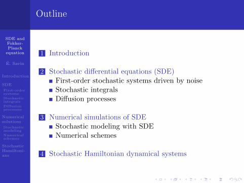
Outline

1 Introduction

2 Stochastic differential equations (SDE)First-order stochastic systems driven by noiseStochastic integralsDiffusion processes

3 Numerical simulations of SDEStochastic modeling with SDENumerical schemes

4 Stochastic Hamiltonian dynamical systems


equation

E. Savin

Introduction

SDE

First-ordersystems

Stochasticintegrals

Diffusionprocesses

Numericalsolutions

Stochasticmodeling

Numericalschemes


Linear or non linear dynamical systems

Discrete linear dynamical system:

M :q `D 9q `Kq “ F ptq ,

or for u “ pq,pq, p “M 9q:

9uptq “

„

0 M´1

´K ´DM´1

uptq `

„

0I

F ptq , up0q “ u0 .

Non-linear dynamical system, e.g. the Duffing oscillator:

M :q `D 9q `Kq `K0q3 “ F ptq ,

or:9uptq “ bpu, tq ` aF ptq , up0q “ u0 ,

with bpu, tq “

ˆ

M´1p´DM´1p´Kq ´K0q

3

˙

, a “

ˆ

01

˙

.


equation

E. Savin

Introduction

SDE

First-ordersystems

Stochasticintegrals

Diffusionprocesses

Numericalsolutions

Stochasticmodeling

Numericalschemes


Example: free vibrations of a single oscillator

9Uptq “d

dt

ˆ

qM 9q

˙

“

„

0 M´1

´K ´DM´1

looooooooomooooooooon

´L

Uptq , Up0q “ U0 ,

where U0 is a r.v. with marginal PDF π0pu0q.

Formally Uptq “ fpU0, tq “ e´LtU0 and the marginalPDF at time t, πpu; tq, is given by the causalityprinciple (lecture #1):

π0pu0q “ πpfpu0, tqqdetp∇ufq .

It yields the conservation equation of the PDF:

0 “dπ0

dt“ Btπ `∇u ¨ pπ 9uq “ Btπ `∇u ¨ Jpπq

with J the probability flux and Jpπq “ ´πLu theconstitutive behavior.


equation

E. Savin

Introduction

SDE

First-ordersystems

Stochasticintegrals

Diffusionprocesses

Numericalsolutions

Stochasticmodeling

Numericalschemes


Outline

1 Introduction





equation

E. Savin

Introduction

SDE

First-ordersystems

Stochasticintegrals

Diffusionprocesses

Numericalsolutions

Stochasticmodeling

Numericalschemes


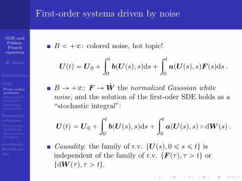
First-order stochastic differential equation

A general first-order stochastic differential equation for theprocess U indexed on R` with values in Rq:

9Uptq “ bpU , tq ` apU , tqF ptq , Up0q “ U0 ,

with the data:

u, t ÞÑ bpu, tq : Rq ˆ R` Ñ Rq the drift function;u, t ÞÑ apu, tq : Rq ˆ R` ÑMq,ppRq the scatteringoperator;U0 is an r.v. in Rq with known marginal PDF π0pu0q;F ptq “ pF1ptq, . . . Fpptqq is a second-order Gaussianrandom process indexed on R with values in Rp, alsocentered, stationary, such that F1ptq, . . . Fpptq aremutually independent and mean-square continuous,with:

SF pωq “ S01r´B,BspωqrIps , S0 ą 0 , B ą 0 .


equation

E. Savin

Introduction

SDE

First-ordersystems

Stochasticintegrals

Diffusionprocesses

Numericalsolutions

Stochasticmodeling

Numericalschemes


First-order systems driven by noise

B ă `8: colored noise, hot topic!

Uptq “ U0 `

ż t

0bpUpsq, sqds`

ż t

0apUpsq, sqF psqds .

B Ñ `8: F Ñ 9W the normalized Gaussian whitenoise, and the solution of the first-oder SDE holds as a“stochastic integral”:

Uptq “ U0 `

ż t

0bpUpsq, sqds`

ż t

0apUpsq, sq ˝ dW psq .

Causality: the family of r.v. tUpsq, 0 ď s ď tu isindependent of the family of r.v. tF pτq, τ ą tu ortdW pτq, τ ą tu.


equation

E. Savin

Introduction

SDE

First-ordersystems

Stochasticintegrals

Diffusionprocesses

Numericalsolutions

Stochasticmodeling

Numericalschemes


White noiseDefinition

Definition

The normalized Gaussian white noise Bptq ” 9W ptqwith values in Rp is the Gaussian stochastic processindexed on R, centered, stationary, with the spectraldensity matrix:

SBpωq “1

2πIp .

Since B1ptq, . . . Bpptq are uncorrelated and jointlyGaussian, they are mutually independent.

B is not second order ~Bptq~2 “ş

TrSBpωqdω “ `8.

This definition holds in the sense of generalized stochastic processes ϕ ÞÑBpϕq : DpT q Ñ L2

pΩ,Rpq where DpT q is the set of C8 functions havinga compact support within T Ď R.


equation

E. Savin

Introduction

SDE

First-ordersystems

Stochasticintegrals

Diffusionprocesses

Numericalsolutions

Stochasticmodeling

Numericalschemes


White noiseDefinition

White noise.


equation

E. Savin

Introduction

SDE

First-ordersystems

Stochasticintegrals

Diffusionprocesses

Numericalsolutions

Stochasticmodeling

Numericalschemes


Wiener processDefinition

The white noise is the (generalized) derivative of the Wienerprocess, or Brownian motion.

Definition

The (normalized) Wiener process W ptq with values in Rp isthe stochastic process indexed on R`, s.t.:

W1ptq, . . .Wpptq are mutually independent;

W p0q “ 0 almost surely (a.s.);

If 0 ď s ă t ă `8 let ∆W ps, tq “W ptq ´W psq, then:

@m and 0 ă t1 ă t2 ă ¨ ¨ ¨ ă tm ă `8, W p0q,∆W p0, t1q, ∆W pt1, t2q, ... ∆W ptm´1, tmq are mutuallyindependent r.v. (independent increments);∆W ps, tq is a Gaussian, centered, second-order r.v.with C∆W ps, tq “ pt´ sqIp.


equation

E. Savin

Introduction

SDE

First-ordersystems

Stochasticintegrals

Diffusionprocesses

Numericalsolutions

Stochasticmodeling

Numericalschemes


Wiener processCharacterization

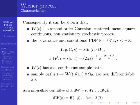
Consequently it can be shown that:

W ptq is a second-order Gaussian, centered, mean-squarecontinuous, non stationary stochastic process;

the covariance and conditional PDF for 0 ď t, s ă `8:

CW pt, sq “ Minpt, sqIp ,

πtpv1; t` s|v; tq “ p2πsq´

p2 e´

v1´v2

2s ;

W ptq has a.s. continuous sample paths;

sample paths t ÞÑW pt, θq, θ P Ωθ, are non differentiablea.s.

As a generalized derivative with dW “ pdW1, . . .dWpq:

dW pϕq “ Bp´ 9ϕq , @ϕ P DpRq .


equation

E. Savin

Introduction

SDE

First-ordersystems

Stochasticintegrals

Diffusionprocesses

Numericalsolutions

Stochasticmodeling

Numericalschemes


Wiener processCharacterization

Wiener process in R3.


equation

E. Savin

Introduction

SDE

First-ordersystems

Stochasticintegrals

Diffusionprocesses

Numericalsolutions

Stochasticmodeling

Numericalschemes


Stochastic integralsDefinition

Let Xptq be a stochastic process indexed by R` witha.s. continuous sample paths.

Assume the r.v. tXpsq, 0 ď s ď tu are independent ofthe r.v. t∆W pt, τq, τ ą tu: a non anticipative process,then

ż t

0XpsqdλW psq

“ l. i.p.KÑ`8

Kÿ

k“1

rp1´ λqXptkq ` λXptk`1qs∆W ptk, tk`1q ,

for any partition 0 “ t1 ă t2 ă ¨ ¨ ¨ ă tK`1 “ t of r0, tswith max

1ďkďKptk`1 ´ tkq Ñ

KÑ`80.


equation

E. Savin

Introduction

SDE

First-ordersystems

Stochasticintegrals

Diffusionprocesses

Numericalsolutions

Stochasticmodeling

Numericalschemes


Stochastic integralsApplication to stochastic differential calculus

A simple example–remind ∆W9∆t12 for the real-valued

Wiener process W :

ż t

0W psqdλW psq “

1

2W ptq2 `

ˆ

λ´1

2

˙

t ,

from which one deduces the stochastic differential:

dλpW ptq2q “ 2W ptqdW ptq ` p1´ 2λqdt .

More generally (λ “ 0 is called the Ito formula):

dλpfpW ptqq “ f 1pW ptqqdW ptq `

ˆ

1

2´ λ

˙

f2pW ptqqdt .


equation

E. Savin

Introduction

SDE

First-ordersystems

Stochasticintegrals

Diffusionprocesses

Numericalsolutions

Stochasticmodeling

Numericalschemes


Stochastic integralsStratonovich-Ito

If λ “ 12 the usual differential calculus applies, and the

solution of SDE holds as a Stratonovich integral (1966):

Uptq “ U0 `

ż t

0bpUpsq, sqds`

ż t

0apUpsq, sq ˝ dW psq .

If λ “ 0, its solution holds as an Ito integral (1944):

Uptq “ U0 `

ż t

0bpUpsq, sqds`

ż t

0apUpsq, sqdW psq ,

where:

bpu, tq “ bpu, tq `1

2aT∇ua .

Uptq is a Markov process.


equation

E. Savin

Introduction

SDE

First-ordersystems

Stochasticintegrals

Diffusionprocesses

Numericalsolutions

Stochasticmodeling

Numericalschemes


Markov processesDefinition

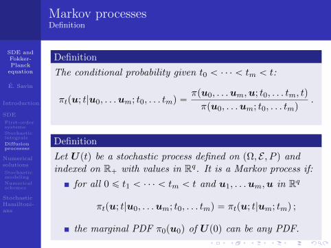
Definition

The conditional probability given t0 ă ¨ ¨ ¨ ă tm ă t:

πtpu; t|u0, . . .um; t0, . . . tmq “πpu0, . . .um,u; t0, . . . tm, tq

πpu0, . . .um; t0, . . . tmq.

Definition

Let Uptq be a stochastic process defined on pΩ, E , P q andindexed on R` with values in Rq. It is a Markov process if:

for all 0 ď t1 ă ¨ ¨ ¨ ă tm ă t and u1, . . .um,u in Rq

πtpu; t|u0, . . .um; t0, . . . tmq “ πtpu; t|um; tmq ;

the marginal PDF π0pu0q of Up0q can be any PDF.


equation

E. Savin

Introduction

SDE

First-ordersystems

Stochasticintegrals

Diffusionprocesses

Numericalsolutions

Stochasticmodeling

Numericalschemes


Markov processesChapman-Kolmogorov equation

A Markov process is fully characterized by:

its marginal PDF πpu; tq,and its transition PDF πtpu; t|v; sq, 0 ď s ă t ă `8,with

πpu; tq “

ż

Rq

πtpu; t|v; sqπpv; sqdv .

πt satisfies the Chapman-Kolmogorov equation:

πtpu; t|u1; t1q “

ż

Rqπtpu; t|v; sqπtpv; s|u1; t1qdv , t1 ă s ă t .

Homogeneous Markov process:

πtpu; t|v; sq “ πtpu; t´ s|v; 0q , 0 ď s ă t ă `8 .

The Brownian motion is a Markov process.


equation

E. Savin

Introduction

SDE

First-ordersystems

Stochasticintegrals

Diffusionprocesses

Numericalsolutions

Stochasticmodeling

Numericalschemes


Diffusion processesDefinition

Definition

The Rq–valued Markov process Uptq with a.s. continuoussample paths and transition PDF πtpv; s|u; tq is a diffusionprocess if @ε ą 0 (but not necessarily small), @u P Rq thefirst moments of its increments are such that for h ą 0:

ż

vúěεπtpdv; t` h|u; tq “ ophq ,

ż

vúăεpv ´ uqπtpdv; t` h|u; tq “ hbpu, tq ` ophq ,

ż

vúăεpv ´ uq b pv ´ uqπtpdv; t` h|u; tq “ hσpu, tq ` ophq ,

where b P Rq and σ PMq,qpRq symmetric, positive.


equation

E. Savin

Introduction

SDE

First-ordersystems

Stochasticintegrals

Diffusionprocesses

Numericalsolutions

Stochasticmodeling

Numericalschemes


Diffusion processesInterpretation

Continuity: particles moving on sample paths of adiffusion process only make small jumps, or theprobability of moving a distance ε goes to zero as h goesto zero no matter how small ε is.

Drift: those particles can have a net mean velocity b.

Diffusion: particles spread as time increases with therate Trσ. Entropy increases while the phase spacecontracts, thus some information (energy) gets lost.

Upt` hq ´Uptq « hbpUptq, tq ` σ12 pUptq, tq∆W pt, t` hq .


equation

E. Savin

Introduction

SDE

First-ordersystems

Stochasticintegrals

Diffusionprocesses

Numericalsolutions

Stochasticmodeling

Numericalschemes


Fokker-Planck equation

The marginal PDF π and transition PDF πt of a diffusionprocess satisfy the Fokker-Planck equation:

Btπ `∇u ¨

ˆ

πb´1

2∇u ¨ pπσq

˙

“ 0 ,

with πpu0; 0q “ π0pu0q and limhÓ0 πtpu; t`h|v; tq “ δpu´vq.ż

RqfpuqBtπtpu; t|v; sqdu “ lim

hÓ0

1

h

ż

Rqfpuq pπtpu; t` h|v; sq ´ πtpu; t|v; sqqdu

“ limhÓ0

1

h

ż

Rqπtpu; t|v; sq

„ż

Rqfpu1qπtpu

1; t` h|u; tqdu1 ´ fpuq

du (C-K)

“ limhÓ0

1

h

ż

Rqπtpu; t|v; sq

ż

Rq

`

fpu1q ´ fpuq˘

πtpu1; t` h|u; tqdu1du (norm.)

“ limhÓ0

1

h

ż

Rqπtpu; t|v; sq

ż

u1´uăε

`

fpu1q ´ fpuq˘

πtpu1; t` h|u; tqdu1du , @f P C 2

0 .

Then use a Taylor expansion for f , definitions of drift and diffusion, andintegrate by parts.


equation

E. Savin

Introduction

SDE

First-ordersystems

Stochasticintegrals

Diffusionprocesses

Numericalsolutions

Stochasticmodeling

Numericalschemes


Ito’s stochastic differential equations (ISDE)Solutions

dU “ bpU , tqdt` apU , tqdW , Up0q “ U0 ,

with the regularity assumptions:

bpu, tq ` apu, tq ď Kp1` uq ,

bpu1, tq ´ bpu, tq ` apu1, tq ´ apu, tq ď Ku1 ´ u .

1 Then the SDE has a unique solution, with a.s.continuous sample paths. If in addition b and a areindependent of t, Uptq is homogeneous.

2 If t ÞÑ bpu, tq and t ÞÑ apu, tq are continuous, Uptq isalso a diffusion process with σ “ aaT.


equation

E. Savin

Introduction

SDE

First-ordersystems

Stochasticintegrals

Diffusionprocesses

Numericalsolutions

Stochasticmodeling

Numericalschemes


Ito’s stochastic differential equations (ISDE)Example: Black-Scholes1 model

The relative variation of a stock Uptq with constant(annualized) drift rate µ and volatility σ:

dU

U“ µdt` σdW , Up0q “ U0 .

Transformation to a Stratonovich SDE:

dU

U“

ˆ

µ´σ2

2

˙

dt` σ ˝ dW , Up0q “ U0 ,

for which “normal rules of integration” apply:

Uptq “ U0 eσW ptq`pµ´σ2

2qt .

The Fokker-Planck equation:

Btπ ` µBupπuq ´σ2

2B2upπu

2q “ 0 , πpu; 0q “ π0puq .

1Fischer Black (1938–1995), Myron Scholes (1941–): American financial economists.

M. Scholes received the Sveriges Riksbank Prize in Economic Sciences in Memory of A.Nobel in 1997 for this model for valuing options, together with Robert Morton (1944–).


equation

E. Savin

Introduction

SDE

First-ordersystems

Stochasticintegrals

Diffusionprocesses

Numericalsolutions

Stochasticmodeling

Numericalschemes


Outline

1 Introduction





equation

E. Savin

Introduction

SDE

First-ordersystems

Stochasticintegrals

Diffusionprocesses

Numericalsolutions

Stochasticmodeling

Numericalschemes


First-order stochastic differential equation

A general first-order stochastic differential equation for theprocess U indexed on R` with values in Rq:

#

9Uptq “ bpU , tq ` apU , tqF ptq , t ą 0 ,

Up0q “ U0 ,

with the data:

u, t ÞÑ bpu, tq : Rq ˆ R` Ñ Rq the drift function;

u, t ÞÑ apu, tq : Rq ˆ R` ÑMq,ppRq the scatteringoperator;

U0 is an r.v. in Rq with known marginal PDF π0pu0q;

F ptq “ pF1ptq, . . . Fpptqq is a second-order Gaussianrandom process indexed on R` with values in Rp,centered, mean-square continuous.


equation

E. Savin

Introduction

SDE

First-ordersystems

Stochasticintegrals

Diffusionprocesses

Numericalsolutions

Stochasticmodeling

Numericalschemes


Markovian realizationDefinition

Definition

F ptq indexed on R` with values in Rp, second-order,Gaussian, centered and mean-square continuous admits aMarkovian realization if:

$

&

%

F ptq “HV ptq , t ě 0 ,9V ptq “ PV ptq `QBptq , t ą 0 ,V p0q “ V 0 a.s.

where V 0 is a Gaussian r.v. in Rn, V ptq is a diffusionprocess indexed on R` with values in Rn, P ,Q PMnpRq,H PMp,npRq, <etλjpP qu ă 0.

This is equivalent to a linear Ito stochastic differential equation.

V 0 „ N p0,Σ0q where Σ0 “ş`8

0eτP QQT eτP

T

dτ .


equation

E. Savin

Introduction

SDE

First-ordersystems

Stochasticintegrals

Diffusionprocesses

Numericalsolutions

Stochasticmodeling

Numericalschemes


Physically realizable processDefinition

Definition

F ptq indexed on R with values in Rp, second-order,mean-square stationary and continuous, centered, isphysically realizable if DH P L2pRq, suppH Ď R`, s.t.:

F ptq “

ż t

´8

Hpt´ τqBpτqdτ ,

or equivalently SF pωq “1

2πpHpωqpHpωq˚, @ω P R.

A necessary and sufficient condition (Rozanov 1967):

ż

R

lnpdetSF pωqq

1` ω2dω ą ´8 .


equation

E. Savin

Introduction

SDE

First-ordersystems

Stochasticintegrals

Diffusionprocesses

Numericalsolutions

Stochasticmodeling

Numericalschemes


Markovian realizationExistence for a physically realizable process

Theorem

A necessary and sufficient condition:

SF pωq “RpiωqRpiωq˚

2π|P piωq|2, or Hpωq “

Rpiωq

P piωq,

where:

P pzq is a polynomial of degree d on C with realcoefficients and roots in the half-plane <epzq ă 0,

Rpzq is a polynomial on C with coefficients in Mp,npRqand degree r ă n.

The Markovian realization always exists in infinitedimension n “ `8.


equation

E. Savin

Introduction

SDE

First-ordersystems

Stochasticintegrals

Diffusionprocesses

Numericalsolutions

Stochasticmodeling

Numericalschemes


First-order SDE (cont’d)

A non linear first-order stochastic differential equation forthe process Zptq “ pUptq,V ptqq indexed on R` with valuesin Rν , ν “ q ` n:

#

dZptq “ bzpZ, tqdt` azdW , t ą 0 ,

Zp0q “ Z0 ,

where Z0 “ pU0,V 0q,

bzpu,v, tq “

„

bpu, tq ` apu, tqHvPv

, az “

„

0 00 Q

,

and W ptq is the Wiener process in Rν .


equation

E. Savin

Introduction

SDE

First-ordersystems

Stochasticintegrals

Diffusionprocesses

Numericalsolutions

Stochasticmodeling

Numericalschemes


Numerical integration of SDEStrong convergence

"

dUptq “ bpU, tqdt` apU, tqdW ptq , t ą 0 ,Up0q “ U0 a.s.

Definition

An approximation pUjqj converges with strong order k ą 0 ifDKj ą 0:

E!ˇ

ˇ

ˇUpj∆tq ´ Uj

ˇ

ˇ

ˇ

)

ď Kjp∆tqk .

The sample paths of the approximation U should be close tothose of the Ito process.


equation

E. Savin

Introduction

SDE

First-ordersystems

Stochasticintegrals

Diffusionprocesses

Numericalsolutions

Stochasticmodeling

Numericalschemes


Numerical integration of SDEWeak convergence

"

dUptq “ bpU, tqdt` apU, tqdW ptq , t ą 0 ,Up0q “ U0 a.s.

Definition

An approximation pUjqj converges with weak order k ą 0 iffor any polynomial g DKg,j ą 0:

ˇ

ˇ

ˇE tgpUpj∆tqqu ´ EtgpUjqu

ˇ

ˇ

ˇď Kg,jp∆tq

k .

The probability distribution of the approximation should beclose to that of the Ito process in order to get a goodestimate of the expectation (gpuq “ u) or the variance(gpuq “ u2), for example.


equation

E. Savin

Introduction

SDE

First-ordersystems

Stochasticintegrals

Diffusionprocesses

Numericalsolutions

Stochasticmodeling

Numericalschemes


Time discrete approximationsExplicit 0.5–order methods

Assume that v and a are independent of time t (thusUptq is a diffusion process), and let tj “ j∆t,bj “ bpUjq, aj “ apUjq, U0 „ π0pdu0q, G „ N p0, 1q.Ito SDE: the Euler-Maruyama scheme (1955),

Uj`1 “ Uj ` bj∆t` aj?

∆tG ,

U0 “ U0 .

Stratonovich SDE: the Euler-Heun scheme (1982),

Uj`1 “ Uj ` bj∆t` aj?

∆tG ,

aj “1

2

”

aj ` a´

Uj ` aj?

∆tG¯ı

,

U0 “ U0 .

Both have a strong order k “ 12 (vs. k “ 1 for ordinary

differential equations) and a weak order k “ 1.


equation

E. Savin

Introduction

SDE

First-ordersystems

Stochasticintegrals

Diffusionprocesses

Numericalsolutions

Stochasticmodeling

Numericalschemes


Time discrete approximationsExplicit 1–order methods

The Milstein scheme (1974):

Uj`1 “ Uj ` bλ,j∆t` aj?

∆tG`1

2aja

1j∆tpG

2 ` 2λ´ 1q ,

U0 “ U0 ,

where λ “ 0 (Ito SDE) or λ “ 12 (Stratonovich SDE).

The Runge-Kutta Milstein scheme (1984):

Uj`1 “ Uj ` bλ,j∆t` aj?

∆tG`1

2aj a

1j∆tpG

2 ` 2λ´ 1q ,

aj a1j “ p∆tq

´ 12

”

a´

Uj ` aj?

∆t¯

´ aj

ı

,

U0 “ U0 .

Both have strong and weak orders k “ 1 (under mildconditions on b and a).


equation

E. Savin

Introduction

SDE

First-ordersystems

Stochasticintegrals

Diffusionprocesses

Numericalsolutions

Stochasticmodeling

Numericalschemes


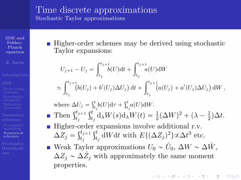
Time discrete approximationsStochastic Taylor approximations

Higher-order schemes may be derived using stochasticTaylor expansions:

Uj`1 ´ Uj “

ż tj`1

tj

bpUqdt`

ż tj`1

tj

apUqdW

»

ż tj`1

tj

`

bpUjq ` b1pUjq∆Uj

˘

dt`

ż tj`1

tj

`

apUjq ` a1pUjq∆Uj

˘

dW ,

where ∆Uj “şt

tjbpUqdτ `

şt

tjapUqdW .

Thenştj`1

tj

şttj

dλW psqdλW ptq “12p∆W q

2 ` pλ´ 12q∆t.

Higher-order expansions involve additional r.v.∆Zj “

ştj`1

tj

şttj

dWdt with Etp∆Zjq2u9∆t3 etc.

Weak Taylor approximations U0 „ U0, ∆W „ ∆W ,∆Zj „ ∆Zj with approximately the same momentproperties.


equation

E. Savin

Introduction

SDE

First-ordersystems

Stochasticintegrals

Diffusionprocesses

Numericalsolutions

Stochasticmodeling

Numericalschemes


Outline

1 Introduction





equation

E. Savin

Introduction

SDE

First-ordersystems

Stochasticintegrals

Diffusionprocesses

Numericalsolutions

Stochasticmodeling

Numericalschemes


Canonical equations

Q P Rq the position, P P Rq the momentum, H theHamiltonian (independent of time), F the nonconservative forces,

9Q “∇pHpQ,P q ,9P “ ´∇qHpQ,P q ` F pQ,P , 9W q ,

where F pq,p,fq “ ´fpHqG∇pH` gpHqSf and 9W awhite noise.

Example: Duffing oscillator driven by white noise,

M :Q`D 9Q`KQ`K0Q3 “ g0S0

9W

then Ec “ 12M

9Q2, Ep “ 12KQ

2 ` 14K0Q

4 and P “ B 9qEc,thus:

HpQ,P q “ 1

2M´1P 2 `

1

2KQ2 `

1

4K0Q

4 .


equation

E. Savin

Introduction

SDE

First-ordersystems

Stochasticintegrals

Diffusionprocesses

Numericalsolutions

Stochasticmodeling

Numericalschemes


Fokker-Planck equation

The associated Fokker-Planck equation for thetransition PDF πtpq

1,p1; t1|q,p; tq reads:

Btπ ` tπ,Hu ´∇p ¨ Jpπq “ 0 ,

with the Poisson bracket and probability flux beingdefined as:

tπ,Hu “∇qπ ¨∇pH´∇pπ ¨∇qH ,

Jpπq “ π

„

fpHqG`1

2gpHqg1pHqSST

∇pH

`1

2gpHq2SST∇pπ .


equation

E. Savin

Introduction

SDE

First-ordersystems

Stochasticintegrals

Diffusionprocesses

Numericalsolutions

Stochasticmodeling

Numericalschemes


Summary

What’s new?

Non linear filtering of white noise,A (high-dimensional) PDE for the marginal andtransition PDF of diffusion processes,Stochastic integrals,Numerical simulations of SDE,Application to non linear dynamical systems.

What’s left?

Numerical solutions of the FKE,Computation of second-order quantities of diffusionprocesses.


equation

E. Savin

Introduction

SDE

First-ordersystems

Stochasticintegrals

Diffusionprocesses

Numericalsolutions

Stochasticmodeling

Numericalschemes


Further reading...

A. Friedman: Stochastic Differential Equations and Applications,vol. I & II, Academic Press (1975);

P.E. Kloeden, E. Platen: Numerical Solution of StochasticDifferential Equations, 3rd ed., Springer (1999);

B.K. Øksendal: Stochastic Differential Equations: An Introductionwith Applications, 6th ed., Springer (2003);

C. Soize: The Fokker-Planck Equation for Stochastic DynamicalSystems and its Explicit Steady State Solutions, World Scientific(1994);

D. Talay: Simulation of stochastic differential systems. InProbabilistic Methods in Applied Physics (P. Kree & W. Wedig,eds.), pp. 54-96. Lecture Notes in Physics 451, Springer (1995).

http://store.doverpublications.com/0486453596.html

http://store.doverpublications.com/0486453596.html

http://dx.doi.org/10.1007/978-3-662-12616-5

http://dx.doi.org/10.1007/978-3-662-12616-5

http://dx.doi.org/10.1007/978-3-642-14394-6

http://dx.doi.org/10.1007/978-3-642-14394-6

http://dx.doi.org/10.1142/9789814354110

http://dx.doi.org/10.1142/9789814354110

http://dx.doi.org/10.1142/9789814354110

http://dx.doi.org/10.1007/3-540-60214-3_51

http://dx.doi.org/10.1007/3-540-60214-3_51

http://dx.doi.org/10.1007/3-540-60214-3_51

Diffusion processes and the Fokker-Planck equation (some ideas...)

Documents

Transcript of Diffusion processes and the Fokker-Planck equation (some ideas...)