1

Preface

From April 18 through 22, 2005, Schloß Ringberg at Lake Tegernsee has provided the much enjoyedvenue of a Workshop on Interdisciplinary Aspects of Turbulence. The origin of this workshop dates backto the summer of 2003 when Christian Beck expressed his interest and support in an interdisciplinarymeeting on turbulence which one of us, Friedrich Kupka, suggested to be held and to be hosted as partof the activities of the hydrodynamics group of the MPI for Astrophysics at Garching near Munich inGermany.

The workshop was attended by 43 participants from 12 countries plus a few additional participantsfrom the Munich area attending on a day-by-day basis. This crowd could just be handled by the seatingand dining facilities at the Ringberg Castle.

As the term “turbulence” is used for an enormous variety of phenomena, at least some commongrounds had to be suggested as preferred topics for contributions to the workshop. A very distin-guishing feature of turbulence which was chosen for this purpose is its superior mixing capabilitycompared to, for example, kinematic processes. A detailed quantitative prediction of how turbulentmixing occurs has turned out to be an extremely difficult problem. This has been demonstrated bywork in astrophysics, atmospheric physics, ocean physics, and engineering.

The workshop hence brought together researchers from these four fields and from the fields of non-linear dynamics and statistical mechanics who are interested in turbulent mixing, self-organisation oflarge scale structures, and related properties of turbulence and the interdisciplinary aspects underlyingthese questions. The venue and size of the workshop were very appropriate to help vivid discussionwithin each individual field and also among the different fields, so as to share common problems andlearn from one another.

Topics discussed during the workshop included the different approaches of modelling and simu-lations used in the various areas, the possibilities of testing them within individual areas throughobservation (and including statistical methods), the conclusions drawn on the underlying physics andmathematics – or the lack of them ! –, and most importantly, an intercomparison as well as aninterchange of methods and views with researchers working in the different areas represented at theconference.

A total of 40 contributions of varying length has been presented as part of the workshop programmewhich also featured a number of separate discussion sessions. The following Proceedings contain acollection of extended abstracts of 30 of the contributions which were presented at the workshop. Anelectronic version of it is available at:www.mpa-garching.mpg.de/mpa/publications/proceedings/proceedings-en.html

PDF files of the talks of several participants are posted on the workshop webpage:www.mpa-garching.mpg.de/hydro/Turbulence/

References related to oral contributions not included in this volume can be found at pp. 182.We are grateful to our co-members of the Scientific Organizing Committee of this workshop –

Christian Beck (Queen Mary, Univ. of London, UK), Hans Burchard (Baltic Sea Res. Institute, Ger-many), Vittorio Canuto (GISS/NASA, USA), Berengere Dubrulle (CNRS Service d’Astrophysique,CE Saclay, France), Wolfgang Hillebrandt (MPI for Astrophysics), Friedrich Kupka (chair, MPI forAstrophysics), Martin Oberlack (TU-Darmstadt, Germany), Sergej Zilitinkevich (Finnish Meteorolog-ical Institute, Helsinki, Finland) – who helped us in inviting participants who all vividly interactedwith each other not only among their own but also across other disciplines as well.

2

The success of the workshop, of course, also depended on the financial support by the Max-Planck-Gesellschaft via the Dr. Ernst Rudolf Schloeßmann foundation and, needless to say, on the enormousefficiency and friendliness of Mr. Hormann and his crew. We would also like to express our gratitudeto Fr. Maria Depner for her help in arranging accommodation of the workshop participants and inpreparing these proceedings.

Garching, August 2005

Friedrich Kupka Wolfgang Hillebrandt

3

List of participants Institute

Alain Arneodo ENS Lyon, FranceHelmut Baumert IAMARIS, Hamburg, GermanyChristian Beck Queen Mary University, London, UKEberhard Bodenschatz LASSP Cornell University, Ithaca, NY, USA

& MPI f. Dynamics and Self-Organization, Gottingen, GermanyVittorio M. Canuto NASA GISS, New York, NY, USAKwing Lam Chan HKUST, Hong KongPierre-Henri Chavanis University Paul Sabatier, Toulouse, FranceFrancois Daviaud CEA Saclay, FranceBerengere Dubrulle CEA Saclay, FranceJens Ewald RWTH Aachen, GermanySergei Fedotov University of Manchester, UKBoris Galperin University of South Florida, St. Petersburg, FL, USAToshiyuki Gotoh Nagoya Institute of Technology, JapanMartin Greiner Siemens Munich, GermanyVladimir Gryanik AWI Bremerhaven, GermanyStefan Heitmann University of Hamburg, GermanyChristiane Helling ESTEC, AD, Noordwijk, The NetherlandsWolfgang Hillebrandt MPI f. Astrophysics, Garching, GermanyFrank Jenko IPP Garching, GermanyAlan Kerstein Sandia Nat. Lab., Livermore, CA, USASpyridon Kitsionas Astrophys. Inst. Potsdam, GermanyFriedrich Kupka MPI f. Astrophysics, Garching, GermanyDmitrii Mironov DWD, Offenbach am Main, GermanyWolf-Christian Muller IPP Garching, GermanyJens Niemeyer University of Wurzburg, GermanyMartin Oberlack TU Darmstadt, GermanyDirk Olbers AWI Bremerhaven, GermanyJoachim Peinke University of Oldenburg, GermanyAndrea Rapisarda INFN Catania, ItalyFriedrich Ropke MPI f. Astrophysics, Garching, GermanyIan W. Roxburgh Queen Mary University, London, UKWolfram Schmidt University of Wurzburg, GermanyJohn V. Shebalin NASA JSC, Houston, TX, USAJoel Sommeria CORIOLIS Grenoble, FranceChantal Staquet INPG Grenoble, FranceAttilio Stella INFN Padova, ItalySemion Sukoriansky BGU Beer-Sheva, IsraelConstantino Tsallis Brazilian Center for Res. in Physics, Rio De Janeiro, Brasil

& Santa Fe Institute, NM, USALars Umlauf Baltic Sea Research Institute Warnemunde, GermanySylvie Vauclair Lab. d’Astrophysique, Obs. Midi-Pyrenees, Toulouse, FranceAchim Weiss MPI f. Astrophysics, Garching, GermanyHua Xia Plasma Res. Lab., The Austr. Nat. Univ., Canberra, AustraliaMatteo Zampieri ISAC-CNR Bologna, ItalySergej S. Zilitinkevich FMI, University of Helsinki, Finland

4

Contents

Superstatistical turbulence modelChristian Beck 6

Statistical mechanics of 2D turbulence with a prior vorticity distributionP.H. Chavanis 11

Measured stochastic processes for turbulence and nonlinear dynamicsJ. Peinke, St. Barth, F. Bottcher, M. Waechter, R. Friedrich 16

Multiscaling and turbulent-like behavior in self-organized criticalityA.L. Stella, M. De Menech 21

A multifractal formalism for vector-valued random fields based on waveletanalysis: application to turbulent velocity and vorticity 3D numerical dataP. Kestener, A. Arneodo 24

Stochastic energy-cascade process for n+1-dimensional small-scale turbulenceJ. Cleve, J. Schmiegel, M. Greiner 29

A one-dimensional stochastic model for turbulence simulationA.R. Kerstein 31

Parameter estimation for algebraic Reynolds stress modelsStefan Heitmann 36

Turbulent mixing and entrainment in density driven gravity currentsS. Decamp, J. Sommeria 42

Superstatistics and atmospheric turbulenceS. Rizzo, A. Rapisarda 52

Interaction of internal gravity waves with a unidirectional shear flowC. Staquet 56

A Level Set Based Flamelet Model for the Prediction of Combustionin Spark Ignition EnginesJ. Ewald, N. Peters 68

Broken symmetry and coherent structure in MHD turbulenceJ.V. Shebalin 77

Energy spectrum and transfer flux in Hydrodynamic and MHD turbulenceT. Gotoh, K. Mori 93

Turbulent transport in magnetized plasmasF. Jenko 99

Dynamo and Alfven effect in MHD turbulenceWolf-Christian Muller, R. Grappin 102

5

Radiatively-driven convection in ice-covered lakes:observations, LES, and bulk modellingDmitrii V. Mironov 105

Non-local features of turbulence in stably stratifiedgeophysical boundary layersSergej S. Zilitinkevich 112

A new spectral theory of turbulent flows with stable stratificationS. Sukoriansky, B. Galperin 115

Anisotropic large-scale turbulence and zonal jets in computer simulations,in the laboratory, on giant planets and in the oceanB. Galperin, S. Sukoriansky, N. Dikovskaya 125

Stratified Shear turbulence at very high Reynolds numbersHelmut Z. Baumert 133

On the validity of the Millionshchikov quasi-normality hypothesisfor convective boundary layer turbulenceV. M. Gryanik, J. Hartmann 135

Turbulent convection in astrophysics and geophysics - a comparisonF. Kupka 141

Situations in stars where thermohaline convection(fingers regime) is expected to take placeS. Vauclair 149

The need for small-scale turbulence in atmospheres of substellar objectsChristiane Helling 152

Flow Patterns and Transitions in Rotating ConvectionK.L. Chan 159

Gravoturbulent Fragmentation: Star formation and the interplaybetween gravity and interstellar turbulenceS. Kitsionas, R.S. Klessen 161

Turbulent Combustion in Type Ia Supernova ModelsF.K. Ropke, W. Hillebrandt 168

Subgrid Scale Models for Astrophysical TurbulenceW. Schmidt, J.C. Niemeyer 172

The FEARLESS Cosmic Turbulence ProjectJ.C. Niemeyer, W. Schmidt, C. Klingenberg 175

6

Superstatistical turbulence model

Christian Beck

School of Mathematical Sciences, Queen Mary, University of London, Mile End Road, London E14NS, UK

Abstract

Recently there has been some progress in modeling the statistical properties of turbulent flows usingsimple superstatistical models. Here we briefly review the concept of superstatistics in turbulence. Inparticular, we discuss a superstatistical extension of the Sawford model and compare with experimentaldata.

Turbulence is a spatio-temporal chaotic dynamics generated by the Navier-Stokes equation

~v = −(~v∇)~v + ν∆~v + ~F . (1)

In the past 5 years there has been some experimental progress in Lagrangian turbulence measurements,i.e. tracking single tracer particles in the turbulent flow. Due to the measurements of the Bodenschatz[1, 2, 3] and Pinton groups [4, 5] we now have a better view of what the statistics of a single test particlein a turbulent flow looks like. The recent measurements have shown that the acceleration ~a as well asvelocity difference ~u = ~v(t+ τ)−~v(t) on short time scales τ exhibits strongly non-Gaussian behavior.This is true for both, single components as well as the absolute value of ~a and ~u. Moreover, there arecorrelations between the various components of ~a, as well as between velocity and acceleration. Thecorresponding joint probabilities do not factorize. Finally, the correlation functions of the absolutevalue |~a| and |~u| decay rather slowly.

How can we understand all this by simple stochastic models? There is a recent class of modelsthat are pretty successful in explaining all these statistical properties of Lagrangian turbulence (aswell as of other turbulent systems, such as Eulerian turbulence [6, 7, 8], atmospheric turbulence[9, 10, 11] and defect turbulence [12]). These are turbulence models based on superstatistics [13].Superstatistics is a concept from nonequilibrium statistical mechanics, in short it means a ‘statisticsof statistics’, one given by ordinary Boltzmann factors and another one given by fluctuations of anintensive parameter, e.g. the inverse temperature, or the energy dissipation, or a local variance. Whilethe idea of fluctuating intensive parameters is certainly not new, it is the application to spatio-temporally chaotic systems such as turbulent flow that makes the concept interesting. The firstturbulence model of this kind was introduced in [14], in the meantime the idea has been furtherrefined and extended [15, 16, 3, 8]. The basic idea is to generate a superposition of two statistics, inshort a ‘superstatistics’, by stochastic differential equations whose parameters fluctuate on a relativelylarge spatio-temporal scale. In Lagrangian turbulence, this large time scale can be understood bythe fact that the particle is trapped in vortex tubes for quite a while [3]. Superstatistical turbulencemodels reproduce all the experimental data quite well. An example is shown in Fig. 1. The theoreticalprediction which fits the data perfectly is given by

p(a) =1

2πs

∫ ∞

0dββ−1/2 exp

−(log(β/µ))2

2s2

e−

12βa2 (2)

with µ = e12s2 and only one fitting parameter, s2 = 3.0. A similar formula as eq. (2) was already

considered in [17], though without a dynamical interpretation in terms of a stochastic differentialequation with fluctuating parameters.

7

1e-09

1e-08

1e-07

1e-06

1e-05

0.0001

0.001

0.01

0.1

1

10

-60 -40 -20 0 20 40 60

p(a)

a

’LN-superstatistics’’R=200’’R=690’’R=970’

Figure 1: Probability density of an acceleration component of a tracer particle as measured by Bo-denschatz et al. [1, 2]. The solid line is a theoretical prediction based on lognormal superstatistics(s2 = 3) [16].

The key ingredient of superstatistical models is to start from a known model generating Gaussianbehaviour, and extend it to a superstatistical version exhibiting ‘fat tails’. In general, in these typesof models one has for some dynamical variable a the stationary long-term density

p(a) =

∫ ∞

0

√β

2πf(β)e−

12βa2dβ, (3)

where f(β) is some suitable probability density of a fluctuating parameter β. The function f(β) fixesthe type of superstatistics under consideration. In particular, it is responsible for the shape of thetails [18]. Note the mixing of two statistics, that of a and that of β.

In Lagrangian turbulence, one may first start from a Gaussian turbulence model, the Sawfordmodel [19, 20]. This model considers the joint stochastic process (a(t), v(t), x(t)) of an arbitrarycomponent of acceleration, velocity and position of a Lagrangian test particle, and assumes that theyobey the stochastic differential equation

a = −(T−1L + t−1

η )a− T−1L t−1

η v

+√

2σ2v(T

−1L + t−1

η )T−1L t−1

η L(t) (4)

v = a (5)

x = v, (6)

L(t): Gaussian white noiseTL and tη: two time scales, with TL >> tη,TL = 2σ2

v/(C0 ε)tη = 2a0ν

1/2/(C0ε1/2)

ε: average energy dissipationC0, a0: Lagrangian structure function constantsσ2v variance of the velocity distributionRλ =

√15σ2

v/√νε Taylor scale Reynolds number.

8

For our purposes it is sufficient to consider the limit TL → ∞, which is a good approximation for largeReynolds numbers. In that limit the Sawford model reduces to just a linear Langevin equation

a = −γa+ σL(t) (7)

with

γ =C0

2a0ν−1/2ε1/2 (8)

σ =C

3/20

2a0ν−1/2ε. (9)

Note that this is a Langevin equation for the acceleration, not for the velocity, in marked contrast toordinary Brownian motion.

Unfortunately, the Sawford model predicts Gaussian stationary distributions for a, and is thus atvariance with the recent measurements. So how can we save this model?

As said before, the idea is to generalize the Sawford model with constant parameters to a super-statistical version. To construct a superstatistical extension of Sawford model, we replace in the aboveequations the constant energy dissipation ε by a fluctuating one. One formally defines a varianceparameter [16]

β :=2γ

σ2=

4a0

C20

ν1/2 1

ε3/2, (10)

where ε fluctuates. Now, if β varies on a large spatio-temporal scale, and is distributed with thedistribution f(β), one ends up with eq. (3) describing the long-term marginal distribution of thesuperstatistical dynamics (7). This is basically the type of model introduced in [14], there with f(β)chosen to be a χ2-distribution. Models based on χ2-superstatistics yield good results for atmosphericturbulence [9, 10], and ultimately lead to Tsallis statistics [21]. On the other hand, for laboratoryturbulence experiments one usually obtains better agreement with experimental data if f(β) is alognormal distribution. In view of eq. (10) this is clearly motivated by Kolmogorov’s ideas of alognormally distributed ε [22].

Superstatistical models are not restricted to Lagrangian turbulence but can be also formulatedfor Eulerian turbulence [7, 14]. Fig. 2 shows that also here one obtains excellent agreement withexperimental data: Probability densities p(u) of longitudinal velocity differences u are well fitted bylognormal superstatistics on all scales. The parameter s2 varies with the scale. In fact, not only thedistribution p(u) but also the distribution f(β) can be directly measured in experiments [8], and thetwo can be consistently connected via the superstatistics formalism. Jung and Swinney [8] have alsoexperimentally confirmed a simple scaling relation between β and the fluctuating energy dissipationε.

It should be noted that if we know the probability densities p(u) analytically, as well as thedependence of the parameter s2 on the scale r, we can also calculate moments of velocity differencesand thus determine scaling exponents ζm defined by

〈um〉 ∼ rζm .

Many different models of ζm can be constructed in such a way [16, 23, 24]. For further stochasticmodels, see e.g. [25, 26, 27].

References

[1] A. La Porta, G.A. Voth, A.M. Crawford, J. Alexander, and E. Bodenschatz, Nature 409, 1017(2001)

9

0

0.1

0.2

0.3

0.4

0.5

-3 -2 -1 0 1 2 3

p(u)

u

’experiment’’LN-superstatistics’

Figure 2: Experimentally measured histogram of velocity differences in a Taylor-Couette experiment[6], and comparison with a superstatistical prediction (s2 = 0.28).

[2] G.A. Voth et al., J. Fluid Mech. 469, 121 (2002)

[3] A.M. Reynolds, N. Mordant, A.M. Crawford and E. Bodenschatz, New Journal of Physics 7, 58(2005)

[4] N. Mordant, P. Metz, O. Michel, and J.-F. Pinton, Phys. Rev. Lett. 87, 214501 (2001)

[5] L. Chevillard, S.G. Roux, E. Leveque, N. Mordant, J.-F. Pinton, and A. Arneodo, Phys. Rev.Lett. 91, 214502 (2003)

[6] C. Beck, G.S. Lewis and H.L. Swinney, Phys. Rev. 63E, 035303(R) (2001)

[7] C. Beck, Physica 193D, 195 (2004)

[8] S. Jung and H.L. Swinney, cond-mat/0502301

[9] S. Rizzo and A. Rapisarda, in Proceedings of the 8th Experimental Chaos Conference, Florence,AIP Conf. Proc. 742, 176 (2004) (cond-mat/0406684)

[10] S. Rizzo and A. Rapisarda, cond-mat/0502305

[11] F. Bottcher, St. Barth, and J. Peinke, nlin.AO/0408005

[12] K. E. Daniels, C. Beck, and E. Bodenschatz, Physica 193D, 208 (2004)

[13] C. Beck and E.G.D. Cohen, Physica 322A, 267 (2003)

[14] C. Beck, Phys. Rev. Lett. 87, 180601 (2001)

[15] A. Reynolds, Phys. Rev. Lett. 91, 084503 (2003)

[16] C. Beck, Europhys. Lett. 64, 151 (2003)

[17] B. Castaing, Y. Gagne, and E.J. Hopfinger, Physica 46D, 177 (1990)

10

[18] H. Touchette and C. Beck, Phys. Rev. 71E, 016131 (2005)

[19] B.L. Sawford, Phys. Fluids A3, 1577 (1991)

[20] S.B. Pope, Phys. Fluids 14, 2360 (2002)

[21] C. Tsallis, J. Stat. Phys. 52, 479 (1988)

[22] A.N. Kolmogorov, J. Fluid Mech. 13, 82 (1962)

[23] C. Beck, Physica 295A, 195 (2001)

[24] C. Beck, Chaos, Solitons and Fractals 13, 499 (2002)

[25] A.K. Aringazin and M.I. Mazhitov, cond-mat/0408018

[26] J.-P. Laval, B. Dubrulle, and S. Nazarenko, Phys. Fluids 13, 1995 (2001)

[27] B. Jouault, M. Greiner, P. Lipa , Physica 136D, 125 (2000)

11

Statistical mechanics of 2D turbulence with a prior vorticity distribution

P.H. Chavanis

Laboratoire de Physique TheoriqueUniversite Paul Sabatier118, route de Narbonne31062 Toulouse, France

Abstract

We adapt the formalism of the statistical theory of 2D turbulence in the case where the Casimirconstraints are replaced by the specification of a prior vorticity distribution. A new relaxation equationis obtained for the evolution of the coarse-grained vorticity. It can be used as a thermodynamicalparametrization of forced 2D turbulence (determined by the prior), or as a numerical algorithm toconstruct arbitrary nonlinearly dynamically stable stationary solutions of the 2D Euler equation.

Two-dimensional incompressible flows with high Reynolds numbers are described by the 2D Eulerequations

∂ω

∂t+ u · ∇ω = 0, ω = −∆ψ, u = −z×∇ψ, (1)

where ω is the vorticity and ψ the streamfunction. The 2D Euler equations are known to develop acomplicated mixing process which ultimately leads to the emergence of a large-scale coherent structure,typically a jet or a vortex. Jovian atmosphere shows a wide diversity of structures: Jupiter’s greatred spot, white ovals, brown barges,... One question of fundamental interest is to understand andpredict the structure and the stability of these equilibrium states. To that purpose, Miller [1] andRobert & Sommeria [2] have proposed a statistical mechanics of the 2D Euler equation. The idea is toreplace the deterministic description of the flow ω(r, t) by a probabilistic description where ρ(r, σ, t)gives the density probability of finding the vorticity level ω = σ in r at time t. The observed (coarse-grained) vorticity field is then expressed as ω(r, t) =

∫ρσdσ. To apply the statistical theory, one

must first specify the constraints attached to the 2D Euler equation. The circulation Γ =∫ωdr

and the energy E = 12

∫ωψdr will be called robust constraints because they can be expressed in

terms of the coarse-grained field ω (the energy of the fluctuations can be neglected). These integralscan be calculated at any time from the coarse-grained field ω(r, t) and they are conserved by thedynamics. By contrast, the Casimir invariants If =

∫f(ω)dr, or equivalently the fine-grained moments

of the vorticity Γf.g.n>1 =∫ωndr =

∫ρσndσdr, will be called fragile constraints because they must be

expressed in terms of the fine-grained vorticity. Indeed, the moments of the coarse-grained vorticityΓc.gn>1 =

∫ωndr are not conserved since ωn 6= ωn (part of the coarse-grained moments goes into fine-

grained fluctuations). Therefore, the moments Γf.g.n>1 must be calculated from the fine-grained fieldω(r, t) or from the initial conditions, i.e. before the vorticity has mixed. Since we often do notknow the initial conditions nor the fine-grained field, the Casimir invariants often appear as “hiddenconstraints” [3].

The statistical theory of Miller-Robert-Sommeria is based on two assumptions: (i) it is assumedthat we know the initial conditions (or equivalently the value of all the Casimirs) in detail (ii) itis assumed that mixing is efficient and that the evolution is ergodic so that the system will reach

12

at equilibrium the most probable (most mixed) state. Within these assumptions1, the statisticalequilibrium state of the 2D Euler equation is obtained by maximizing the mixing entropy

S[ρ] = −∫ρ ln ρ drdσ, (2)

at fixed energy E and circulation Γ (robust constraints) and fixed fine-grained moments Γf.g.n>1 (fragileconstraints). This optimization principle is solved by introducing Lagrange multipliers, writing thefirst order variations as

δS − βδE − αδΓ −∑

n>1

αnδΓf.g.n = 0. (3)

In the approach of Miller-Robert-Sommeria, it is assumed that the system is strictly describedby the 2D Euler equation so that the conservation of all the Casimirs has to be taken into account.However, in geophysical situations, the flows are forced and dissipated at small scales (due to convectionin the jovian atmosphere) so that the conservation of the Casimirs is destroyed. Ellis et al. [6] haveproposed to treat these situations by fixing the conjugate variables αn>1 instead of the fragile momentsΓf.g.n>1. If we view the vorticity levels as species of particles, this is similar to fixing the chemicalpotentials instead of the total number of particles in each species. Therefore, the idea is to treat thefragile constraints canonically, whereas the robust constraints are still treated microcanonically. Thispoint of view has been further developed in Chavanis [7]. The relevant thermodynamical potentialis obtained from the mixing entropy (2) by using a Legendre transform with respect to the fragileconstraints [7]:

Sχ = S −∑

n>1

αn Γf.g.n . (4)

Expliciting the fine-grained moments, we obtain the relative entropy

Sχ[ρ] = −∫ρ ln

[ρ

χ(σ)

]drdσ, (5)

where we have defined the prior vorticity distribution

χ(σ) ≡ exp

−

∑

n>1

αnσn

. (6)

We shall assume that this function is imposed by the small-scale forcing. Assuming ergodicity, thestatistical equilibrium state is now obtained by maximizing the relative entropy Sχ at fixed energy Eand circulation Γ (no other constraints). The conservation of the Casimirs has been replaced by thespecification of the prior χ(σ). Writing δSχ − βδE − αδΓ = 0, and accounting for the normalizationcondition

∫ρdσ = 1, we get the Gibbs state

ρ(r, σ) =1

Z(r)χ(σ)e−(βψ+α)σ with Z =

∫ +∞

−∞χ(σ)e−(βψ+α)σdσ. (7)

This is the product of a universal Boltzmann factor by a non-universal function χ(σ) fixed by theforcing. The coarse-grained vorticity is given by

ω =

∫χ(σ)σe−(βψ+α)σdσ∫χ(σ)e−(βψ+α)σdσ

= F (βψ + α) with F (Φ) = −(ln χ)′(Φ), (8)

1Some attempts have been proposed to go beyond the assumptions of the statistical theory. For example, Chavanis& Sommeria [4] consider a strong mixing limit in which only the first moments of the vorticity are relevant instead of thewhole set of Casimirs. On the other hand, Chavanis & Sommeria [5] introduce the concept of maximum entropy bubbles

(or restricted equilibrium states) in order to account for situations where the evolution of the flow is not ergodic in thewhole available domain but only in a subdomain.

13

where χ(Φ) =∫ +∞−∞ χ(σ)e−σΦdσ. It is easy to show that F ′(Φ) = −ω2(Φ) ≤ 0, where ω2 = ω2−ω2 ≥ 0

is the local centered variance of the vorticity, so that F is a decreasing function [8]. Therefore, thestatistical theory predicts that the coarse-grained vorticity ω = f(ψ) is a stationary solution of the 2DEuler equation and that the ω−ψ relationship is a monotonic function which is increasing at negativetemperatures β < 0 and decreasing at positive temperatures β > 0 since ω ′(ψ) = −βω2. We also notethat the most probable vorticity 〈σ〉(r) of the distribution (7) is given by [9]:

〈σ〉 = [(lnχ)′]−1(βψ + α), (9)

provided (lnχ)′′(〈σ〉) < 0. This is also a stationary solution of the 2D Euler equation which usuallydiffers from the average value ω(r) of the distribution (7) except when χ(σ) is gaussian. We notethat the ω − ψ relationship predicted by the statistical theory can take a wide diversity of forms(non-Boltzmannian) depending on the prior χ(σ). The coarse-grained vorticity (8) can be viewed asa sort of superstatistics as it is expressed as a superposition of Boltzmann factors (on the fine-grainedscale) weighted by a non-universal function χ(σ) [3]. Furthermore, the coarse-grained vorticity (8)maximizes a generalized entropy (in ω-space) of the form [10]:

S[ω] = −∫C(ω)dr, (10)

at fixed circulation and energy (robust constraints). Writing δS − βδE − αδΓ = 0 leading to C ′(ω) =−βψ − α and ω′(ψ) = −β/C ′′(ω), and comparing with Eq. (8), we find that C is a convex function(C ′′ > 0) determined by the prior χ(σ) encoding the small-scale forcing according to the relation [3]:

C(ω) = −∫ ω

F−1(x)dx = −∫ ω

[(ln χ)′]−1(−x)dx. (11)

The preceding relations are also valid in the approach of Miller-Robert-Sommeria except that χ(σ) isdetermined a posteriori from the initial conditions by relating the Lagrange multipliers αn>1 to theCasimir constraints Γf.g.n>1. In this case of freely evolving flows, the generalized entropy (10) dependson the initial conditions, while in the case of forced flows considered here, it is intrinsically fixed bythe prior vorticity distribution.

In that context, it is possible to propose a thermodynamical parameterization of 2D forced turbu-lence in the form of a relaxation equation that conserves circulation and energy (robust constraints)and that increases the generalized entropy (10) fixed by the prior χ(σ). This equation can be ob-tained from a generalized Maximum Entropy Production (MEP) principle in ω-space [10] by writingthe coarse-grained 2D Euler equation in the form Dω/Dt = −∇ · ωu = −∇ · J and determining theoptimal current J which maximizes the rate of entropy production S = −

∫C ′′(ω)J · ∇ωdr at fixed

energy E =∫

J · ∇ψdr = 0, assuming that the energy of fluctuations J2/2ω is bounded. Accordingto this principle, we find that the coarse-grained vorticity evolves according to [10, 7]:

∂ω

∂t+ u · ∇ω = ∇ ·

D

[∇ω +

β(t)

C ′′(ω)∇ψ

], ω = −∆ψ, (12)

β(t) = −∫D∇ω · ∇ψd2r∫D (∇ψ)2

C′′(ω)d2r

, D ∝ ω1/22 =

1√C ′′(ω)

, (13)

where β(t) is a Lagrange multiplier enforcing the energy constraint E = 0 at any time. Theseequations increase the entropy (H-theorem S ≥ 0) provided that D > 0, until the equilibrium state(8) is reached. The diffusion coefficient D is not determined by the MEP but it can be obtained from

14

a Taylor’s type argument leading to expression (13)-b [7]. This diffusion coefficient, related to thestrength of the fluctuations, can “freeze” the relaxation in a sub-region of space (“bubble”) and accountfor incomplete relaxation and lack of ergodicity [11, 12]. The relaxation equation (12) belongs to theclass of generalized Fokker-Planck equations introduced in Chavanis [10]. This relaxation equationconserves only the robust constraints (circulation and energy) and increases the generalized entropy(11) fixed by the prior vorticity distribution χ(σ). It differs from the relaxation equations proposedby Robert & Sommeria [13] for freely evolving flows which conserve all the constraints of the 2D Eulerequation (including all the Casimirs) and increase the mixing entropy (2). In Eqs. (12)-(13), thespecification of the prior χ(σ) (determined by the small-scale forcing) replaces the specification of theCasimirs (determined by the initial conditions). However, in both models, the robust constraints Eand Γ are treated microcanonically (i.e. they are rigorously conserved). Furthermore, in the two-levels case ω ∈ σ0, σ1, the two approaches are formally equivalent and they amount to maximizing ageneralized entropy (10) similar to the Fermi-Dirac entropy at fixed circulation and energy [12]. In theviewpoint of Miller-Robert-Sommeria, this entropy describes the free merging of a system with twolevels of vorticity σ0 and σ1 while in the other view point, it describes the evolution of a forced systemwhere the forcing has two intense peaks described by the prior χ(σ) = χ0δ(σ − σ0) + χ1δ(σ − σ1) [7].

The relaxation equations (12)-(13) can also be used as a numerical algorithm to construct stablestationary solutions of the 2D Euler equation. Indeed, Ellis et al. [6] have shown that the maximizationof a functional of the form (10) at fixed energy and circulation determines a stationary solution ofthe 2D Euler equation of the form ω = f(ψ), where f is monotonic, which is nonlinearly dynamicallystable. Since the stationary solution of Eqs. (12)-(13) maximizes S at fixed E and Γ (by construction),this steady solution of the relaxation equations is also a nonlinearly dynamically stable stationarysolution of the 2D Euler equations (1). Thus, by changing the convex function C(ω) in Eq. (12), wecan numerically construct a wide diversity of stable solutions of the 2D Euler equations. This is apotentially interesting procedure because it is usually difficult to solve the differential equation −∆ψ =f(ψ) directly and be sure that the solution is (nonlinearly) dynamically stable. These nonlinearlystable steady states can be an alternative to the statistical equilibrium state in case of incompleterelaxation, when the system has not mixed efficiently (non-ergodicity) so that the statistical predictionfails. In case of incomplete relaxation we cannot predict the equilibrium state but we can try toreproduce it a posteriori.

Finally, we have proposed in [10] to develop a phenomenological/effective statistical theory of 2Dturbulence to deal with complex situations. The idea is that some types of entropy functional S[ω] (inω-space) may be more appropriate than others to describe a given physical situation. For example,the enstrophy functional turns out to be relevant in certain oceanic situations [14] and the Fermi-Dirac type entropy in jovian flows [15, 8]. Certainly, other functionals of the same “class” wouldwork as well for these systems. In addition, other classes of functionals S[ω] may be relevant in othercircumstances. Therefore, as a simple and practical procedure to describe a given system, we proposeto pick a functional S[ω] in the “class of equivalence” appropriate to that system and use it in theparameterization (12)-(13). We can thus describe the time evolution of the system on the coarse-grained scale. This approach is not completely predictive because we need to know in advance whichtype of entropy S[ω] describes best such and such situation. In practice, it must be determined bytrying and errors (e.g. by comparing with oceanic data). But once a specific entropy has been foundfor a physical situation, we can work with it for different initial conditions specified by the robustconstraints E and Γ (the effect of the Casimirs is reported in the chosen form of entropy S[ω]). Theidea is that the entropy S remains the same while E and Γ are changed. The problem is rich and non-trivial even if S has been fixed because bifurcations can occur depending on the control parametersE, Γ. This heuristic approach can be viewed as a simple attempt to account for the influence of theCasimirs while leaving the problem tractable. We use the fact that the Casimirs lead to non-standard

15

(i.e. non-Boltzmannian) ω − ψ relationships at equilibrium which are associated with non-standardforms of entropy S[ω] in ω-space. We propose to fix the S-functional depending on the situation. Wedo not try to predict its form, but rather to adjust it to the situation contemplated. This is based onthe belief that some functionals S[ω] are more relevant than others for a given system. Whether thisis the case or not remains to be established. All the ideas presented here can be generalized to thecase of quasi-geostrophic or shallow-water equations [8].

References

[1] J. Miller, Phys. Rev. Lett. 65 (1990) 2137.

[2] R. Robert and J. Sommeria, J. Fluid Mech. 229 (1991) 291.

[3] P.H. Chavanis, Coarse-grained distributions and superstatistics [cond-mat/0409511]

[4] P.H. Chavanis and J. Sommeria, J. Fluid Mech. 314 (1996) 267.

[5] P.H. Chavanis and J. Sommeria, J. Fluid Mech. 356 (1998) 259.

[6] R. Ellis, K. Haven and B. Turkington, Nonlinearity 15 (2002) 239.

[7] P.H. Chavanis, Physica D 200 (2005) 257.

[8] P.H. Chavanis and J. Sommeria, Phys. Rev. E 65 (2002) 026302.

[9] N. Leprovost, B. Dubrulle and P.H. Chavanis, Dynamics and thermodynamics of axisymmetricflows: I. Theory [physics/0505084]

[10] P.H. Chavanis, Phys. Rev. E 68 (2003) 036108.

[11] R. Robert and C. Rosier, J. Stat. Phys. 86 (1997) 481.

[12] P.H. Chavanis, J. Sommeria and R. Robert, Astrophys. J. 471 (1996) 385.

[13] R. Robert and J. Sommeria, Phys. Rev. Lett. 69 (1992) 2776.

[14] E. Kazantsev, J. Sommeria and J. Verron, J. Phys. Oceanogr. 28 (1998) 1017.

[15] F. Bouchet and J. Sommeria, J. Fluid Mech. 464 (2002) 165.

16

Measured stochastic processes for turbulence and nonlinear dynamics

J. Peinke1, St. Barth1, F. Bottcher1, M. Waechter1, R. Friedrich2

1 Institute of Physics, Carl von Ossietzky University,D-26 111 Oldenburg, Germany2 Institute for Theoretical Physics, University of Munster,Wilhelm-Klemm-Str. 9, D- 48149 Munster, Germany

Abstract

For the characterization of complex structures we present an approach which is based on the theoryof stochastic Markov processes. With this analysis we achieve a characterization of the systems whosecomplexity may be based on nonlinear noisy dynamics or multiscale features like multifractal scaling.We show how based on the estimations of Kramers-Moyal coefficients it is possible to reconstruct frompure, parameter free data analysis the stochastic equations in form of a Fokker-Planck or a Langevinequation.

Introduction

The better understanding of complex systems is still a scientific challenge. Often the question is posedto characterize given data with respect to its complexity. In a first step one can split this task intotwo aspects [1].(1) There are systems with a pronounced scale dependent complex structure like this is the casefor the well known problem of turbulence. Here it is believed that it is the cascade like processof large vorticities creating smaller ones as the smaller create even smaller ones and so on, whichcauses the complexity. This cascade procedure leads to a scale dependent disorder or, respectively,the scale dependent complexity of a turbulent field, whose understanding is still considered as onemajor unsolved scientific problem.(2) Besides these scale dependent complex structures there is the second class of systems characterizedby nonlinear dynamics which may become more sophisticated by the involvement of noise. Systemswhose complexity is given by nonlinear dynamics evolving in time, like chaotic systems, we call timedependent complex systems. Definitely this classification is not a rigorous one, systems of hierarchicalcoupled nonlinear dynamical subsystems are some how intermediate.

In this contribution we want to summarize recent works which showed ways how to characterizecomplex systems of both categories in a more complete way. Namely, in these works it was worked outhow to reconstruct in a parameter free way to reconstruct nonlinear stochastic equations from givendata. These reconstructed stochastic equations, given as a Fokker-Planck equation or a Langevinequation enables to achieve the general n-scale joint statistics of a scale dependent complex system,and accordingly the underlying nonlinear evolution equations for a time dependent complex system.

Turbulence – scale dependent complexity

As already mentioned, the profound understanding of turbulence is up to now regarded as an unsolvedproblem. Although the basic equations of fluid dynamics, namely the Navier Stokes equations, areknown for more than 150 years, a general solution of these equations for high Reynolds numbers, i.e.for turbulence, is not known. Even with the use of powerful computers no rigorous solutions can beobtained. Thus for a long time there has been the challenge to understand at least the complexity of

17

an idealized turbulent situation, which is taken to be isotropic and homogeneous. This case will leadus to the well known intermittency problem of turbulence, which is nothing else than the occurrenceof heavy tailed, non-Gaussian statistics. The central question is to understand the mechanism whichleads to this anomalous statistics (see [2, 3, 4]).

The intermittency problem of turbulence can be reduced to the question about the statistics ofthe velocity differences over different distances l, measured by the so-called increments q(l, x) = u(x+l) − u(x). Usually the velocity increments are taken from the velocity component in direction of thedistance vector l, the so-called longitudinal velocity increments. By the use of energy considerations,a simple l-dependence of q(l, x) was proposed. It can be shown that the dissipation of energy takesplace on small scales, namely, scales smaller than the so-called Taylor length θ. On the other hand,the turbulence is generated by driving forces injecting energy into the flow on large scales, l > L0,where L0 is given by the correlation length. Thus the cascade process causes the transition of q(l, x) toq(l′, x) with l′ < l, where the same amount of energy is transferred from one scale to another as long asL0 > l, l′ > θ. This range is called the inertial range, where the turbulent field develops independentlyfrom boundary conditions and dissipation effects. It has been proposed that in this range universalfeatures of turbulence arise.

Kolmogorov proposed that the disorder of turbulence expressed by the statistics of q(l, x) andits n-th order moments < q(l, x)n > should depend only on transferred energy ε and the scale l:< q(l, x)n >= f(ε, l). By simple dimensional arguments it follows that

< q(l, x)n > = < εn/3 > ln/3. (1)

The simplest ansatz is to take ε as a constant, thus the Kolmogorov scaling n/3 of 1941 is obtained[5]. Based on some comments of Landau, Kolmogorov and Oboukhov proposed in a refined modelwith a lognormal distribution for ε, i.e. not ε but lnε has a Gaussian distribution, and obtained for< εn/3 > an additional scaling term, leading to the so-called intermittency [6] correction [7]

< q(l, x)n > = lξn with ξn =n

3− µ

n(n− 3)

18and n ≥ 2 (2)

with 0.25 < µ < 0.5 . The form of the scaling exponent ξn, which is related to multifractal scalingbehavior, has been heavily debated during the last decades (for further details see [2]).

Here we want to point out that this nonlinear scaling exponent ξn, has the direct consequence thatthe probability densities of p(q(l, x)) cannot be Gaussian, but must change their form with the scalel.

The velocity increment specifies the complexity of the turbulent velocity field between two mea-surement points separated by the length scale l. As a next step, taking somehow the cascade idealiterally, the velocity increment q(l, x) is regarded as a stochastic variable in the scale l. Completeinformation about this stochastic process would be available from the knowledge of not only the onescale properties like < q(l, x)n > or p(q(l, x)) but properties of all possible n-scales given by thejoint probability density functions (PDF) p(q1, q2, q3, . . . ; qn). (Note we use here a simplified notation:q(li, x) = qi.) Since this is practically impossible to obtain for empirical data, suitable simplificationsare needed.

As a first simplification we will require the process to be Markovian. In this case the n-scale jointPDF factorize into chains of two-scale conditional PDF p(qi+1|qi) describing the probability of findingthe increment qi+1 on the scale li+1 under the condition that another increment qi on a larger scale li isfound. It follows that now the complete stochastic information is already available from the knowledgeof the two-scale conditional PDF. This simplification can be tested by evaluating

p(q1|q2, . . . , qn) = p(q1|q2) (3)

18

which is feasible for experimental data, at least for n = 3. Our second simplification requires the noiseincluded in the process to be Gaussian distributed.

Given these two conditions, it is known [8] that the process obeys a Fokker-Planck equation

− ∂

∂lp(q, l|q0, l0) =

− ∂

∂qD(1)(q, l) +

∂2

∂q2D(2)(q, l)

p(q, l|q0, l0). (4)

which describes the evolution of the conditional PDF from larger to smaller length scales (Note dueto this direction of the process we have inserted the − prefactor). The Fokker-Planck equation isdetermined by the two Kramers-Moyal-coefficients D(1)(q, l) and D(2)(q, l), where D(1) is commonlydenoted as drift term, describing the deterministic part of the process, and D (2) as diffusion term,determined by the variance of a Gaussian, δ-correlated noise. Here we should note that there aredifferent methods to verify that actually for given data the noise has these features (cf. [9, 10]).Equivalently, the Langevin equation

− d

dlq(l) = D(1)(q, l) +

√D(2)(q, l) Γ(l) (5)

describes the process in the scale domain, using identical coefficients D (1) and D(2), together with theGaussian, δ-correlated noise term Γ(l).

To derive the Kramers-Moyal coefficients D(k)(q, l) (and thus obtain a Fokker-Planck or Langevinequation), the limit ∆l → 0 of the conditional moments has to be performed [8, 11]:

D(k)(q, l) = lim∆l→0

M (k)(q, l,∆l)/l , (6)

M (k)(q, l,∆l) :=l

k!∆l

+∞∫

−∞

(q − q)k p (q, l − ∆l|q, l) dq. (7)

This procedure is described in more detail in [9, 12]. For this contribution, it is sufficient to see fromEqs. (6) and (7) that the Fokker-Planck equation can directly be obtained from experimental data bythe estimation of two-scale conditional PDF.

Based on this procedure we were able to reconstruct directly from the given data the correspondingstochastic processes. Knowing these processes one can perform numerical solutions (see [9, 12, 13]).

It is easily seen that this method can also be applied to other scale dependent complex stuructureslike rough surfaces [12, 14, 15], to financial data [13, 16] or the cosmic background radiation [17].

nonlinear dynamics – time dependent complexity

It is straight forward to extend the above mentioned method for the analysis of time series. Theobjection is now to reconstruct from given data q(t) the dynamical equation

d

dtq(t) = D(1)(q, t) +

√D(2)(q, t) Γ(t). (8)

To achieve this from given data the conditional probabilities p(q(t+ τ)|q(t)) for fixed values q(t) andtheir corresponding conditional moments, i.e. the Kramers-Moyal coefficients, have to be estimated[18, 19]. This method has been successfully applied to various problems in the field of complexdynamical systems like the analysis of noisy chaotic electrical circuits [19], stochastic dynamics of metalcutting [20], systems with feedback delay [21], meteorological processes like wind-driven SouthernOcean variability [22, 23] traffic flow data [24] and the dynamics of particles of different sizes in a

19

running avalanche [25]. A quantitative comparison of this method of time series analysis with othersis reported in [26].

As a further application also data spoiled by measurement noise can be treaded with this method.The basic idea here is that instead of the dynamical variable q(t) a variable y(t) = q(t) + σ(t) isanalyzed, where σ(t) represents an additive measurement noise. The conditional moments are nowperformed with y(t). A proper stochastic calculation shows how even in this case the underlyingdynamics can be reconstructed [27].

Acknowledgements

Helpful discussion with St. Luck, A. Nawroth, Ch. Renner, Th. Schneider, and M. Siefert areacknowledged.

References

[1] J. Peinke, Ch. Renner and R. Friedrich, in Complexity from microscopic to macroscopic scales:Coherence and large deviations, edts. A. T. Skjeltrop and T. Vicsek (Kluwer Academic publishers,Dordrecht 2002) p. 151 - 169.

[2] U. Frisch, Turbulence (Cambridge University Press, Cambridge, 1995).

[3] K. R. Sreenivasan and R. A. Antonia, Annu. Rev. Fluid Mech. 29, 435-472 (1997).

[4] R. Friedrich and J. Peinke, Physica D 102, 147 (1997).

[5] A. N. Kolmogorov, C.R. Acad. Sci. U.R.S.S., 30, 301 (1941).

[6] Here it should be noted that the term ”intermittency” is used frequently in physics for differentphenomena, and may cause confusions. This turbulent intermittency is not equal to the intermit-tency of chaos. There are also different intermittency phenomena introduced for turbulence.

[7] A.N. Kolmogorov, J. Fluid Mech. 13, 82 (1962).

[8] H. Risken, The Fokker-Planck equation (Springer, Berlin, 1984).

[9] C. Renner, J. Peinke, and R. Friedrich, J. Fluid Mech. 433, 383 (2001).

[10] P. Marcq and A. Naert, Phys. Fluids 13, 2590 (2001).

[11] A. N. Kolmogorov, Math. Ann. 104, 415 (1931).

[12] M. Waechter, F. Riess, T. Schimmel, U. Wendt, and J. Peinke, Eur. Phys. J. B 41, 259 (2004),preprint arxiv:physics/0404015.

[13] Ch. Renner, J. Peinke and R. Friedrich, Physica A 298, 499-520 (2001).

[14] M. Waechter, F. Riess, H. Kantz, and J. Peinke, Europhys. Lett. 64, 579 (2003), preprintarxiv:physics/0404021.

[15] G. R. Jafari et al., Phys. Rev. Lett. 91, 226101 (2003).

[16] M. Ausloos and K. Ivanova, Phys. Rev. E 68, 046122 (2003).

20

[17] F. Ghasemi, A. Bahraminasab, S. Rahvar, and M. Reza Rahimi Tabar, preprint arxiv:astro-phy/0312227 (2003).

[18] S. Siegert, R. Friedrich, J. Peinke, Physics Letters A 234, 275-280 (1998)

[19] R. Friedrich, S. Siegert, J. Peinke, St. Luck, M. Siefert, M. Lindemann, J. Raethjen, G. Deuschl,G. Pfister, Physics Letters A 271, 217 (2000)

[20] J. Gradisek, I. Grabec, S. Siegert, R. Friedrich, Mechanical Systems and Signal Processing 16(5), 831 (2002).

[21] T. D. Frank, P. J. Beek, R. Friedrich, Phys. Lett. A 328, 219 (2004); T. D. Frank, R. Friedrich,P.J. Beek, Stochastics and Dynamics 9, 44 (2004).

[22] P. Sura, S.T. Gille, Journal of Marine Research 61, 313 (2003).

[23] P. Sura, Journal of the Atmospheric Sciences 60, 654 (2003).

[24] S. Kriso, R. Friedrich, J. Peinke, P. Wagner, Physics Letters A 299, 287 (2002).

[25] M. Kern , O. Buser , J. Peinke , M. Siefert , and L. Vulliet Physics Letters A 336, 428 (2005).

[26] E. Racca and A. Porporato Phys. Rev.E 71, 027101 (2005).

[27] M. Siefert, A. Kittel, R. Friedrich, and J. Peinke. Europhys. Lett. 61, 466 (2003).

21

Multiscaling and turbulent-like behavior in self-organized criticality

A.L. Stella, M. De Menech2

1 Dipartimento di Fisica “Galileo Galilei” and Sezione INFN, Universita di Padova, Italy2 Max-Planck-Institut fur Physik komplexer Systeme, Dresden, Germany

The prototype model of self-organized criticality, the Bak–Tang–Wiesenfeld (BTW) sandpile intwo dimensions [1, 2], has a remarkable history [3], rich of developments and with some surprising andcontradictory aspects. In spite of being the most extensively studied model of transport in systemsslowly driven out of equilibrium, this sandpile remained for long very controversial as far as the scalingproperties of some avalanche quantities are concerned [4]. Recently this led many authors to focustheir attention on other models [5], with more standard and transparent avalanche scalings and withpresumed better applicability. On the other hand, when they proposed their sandpile, BTW hadclearly in mind that this could mimic qualitatively some features of turbulence. In this phenomenonfluid flow obeys the non–linear Navier–Stokes equation and evolves under random perturbations intoa stationary state with scale invariant velocity correlations [6]. In the turbulent inertial regime acontinuous, non-dissipative transport of energy occurs from large to small length scales. This remindssome BTW sandpile features: sand transport is driven by random grain addition, and is controlledby non-linear local threshold mechanisms (toppling rule). Furthermore, the avalanches following eachgrain addition have scale invariant probability distributions for quantities like the number of topplings,the area, etc.

In spite of the original expectations, an analogy between self organized BTW critical dynamicsand turbulence could not be established until very recently [9]. More generally, the possible relationbetween self-organized criticality and turbulence remained for long an obscure and controversial issue,and the recent literature had a tendency to emphasize differences [7], rather than analogies [8].

In Ref. [10] it was first shown that the scaling of the probability distribution of the number oftopplings in the BTW avalanches can be consistently described within a multifractal framework.Suspects that this distribution could obey some form of multiscaling rather than simple scaling wereexpressed long before [11], but surprisingly got scarce attention in the subsequent literature. Theevidence of multiscaling for the probability distribution of the number of topplings and other BTWavalanche quantities is presently based on analysis of extensive data for sandpiles of size up to 4096×4096 [12]. Calling P (s, L) the probability to have an avalanche with s topplings in a sandpile of sizeL, such analysis shows that

〈sq〉 =∑

P (s, L)sq ∼ Lσq (1)

with a nonlinear q-dependence of σq indicating multiscaling. Models like the Manna stochastic sand-pile [5] show instead a linear dependence, as appropriate for simple finite size scaling [10, 13].

The physical origin of the BTW multiscaling was identified [13] in the long range time correlationsexisting for the toppling sizes of the waves [14, 3] into which avalanches can be decomposed. Thesewaves are distinguished by the number of times the avalanche seed site has toppled, and can beregarded as bursts within each avalanche. The scaling properties of waves, when sampled globallyover a sequence of many avalanches, are well understood [14]. If measured in terms of interocurringwaves, the correlation time of wave sizes grows approximately as L0.7 [13]. As discussed below, ontemporal scales shorter than the correlation time, the statistics of waves shows novel, unexpectedfeatures [9].

These peculiar correlations, not anticipated before, are also a very important feature of the BTWmodel in view of possible applications. Indeed, the absence of correlations between the sizes of suc-cessive avalanches has been indicated [7] as a serious handicap of the BTW and similar models in

22

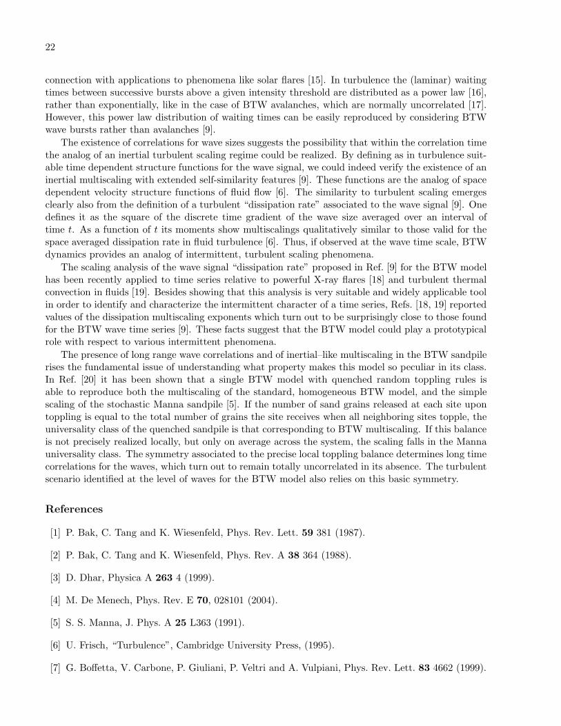
connection with applications to phenomena like solar flares [15]. In turbulence the (laminar) waitingtimes between successive bursts above a given intensity threshold are distributed as a power law [16],rather than exponentially, like in the case of BTW avalanches, which are normally uncorrelated [17].However, this power law distribution of waiting times can be easily reproduced by considering BTWwave bursts rather than avalanches [9].

The existence of correlations for wave sizes suggests the possibility that within the correlation timethe analog of an inertial turbulent scaling regime could be realized. By defining as in turbulence suit-able time dependent structure functions for the wave signal, we could indeed verify the existence of aninertial multiscaling with extended self-similarity features [9]. These functions are the analog of spacedependent velocity structure functions of fluid flow [6]. The similarity to turbulent scaling emergesclearly also from the definition of a turbulent “dissipation rate” associated to the wave signal [9]. Onedefines it as the square of the discrete time gradient of the wave size averaged over an interval oftime t. As a function of t its moments show multiscalings qualitatively similar to those valid for thespace averaged dissipation rate in fluid turbulence [6]. Thus, if observed at the wave time scale, BTWdynamics provides an analog of intermittent, turbulent scaling phenomena.

The scaling analysis of the wave signal “dissipation rate” proposed in Ref. [9] for the BTW modelhas been recently applied to time series relative to powerful X-ray flares [18] and turbulent thermalconvection in fluids [19]. Besides showing that this analysis is very suitable and widely applicable toolin order to identify and characterize the intermittent character of a time series, Refs. [18, 19] reportedvalues of the dissipation multiscaling exponents which turn out to be surprisingly close to those foundfor the BTW wave time series [9]. These facts suggest that the BTW model could play a prototypicalrole with respect to various intermittent phenomena.

The presence of long range wave correlations and of inertial–like multiscaling in the BTW sandpilerises the fundamental issue of understanding what property makes this model so peculiar in its class.In Ref. [20] it has been shown that a single BTW model with quenched random toppling rules isable to reproduce both the multiscaling of the standard, homogeneous BTW model, and the simplescaling of the stochastic Manna sandpile [5]. If the number of sand grains released at each site upontoppling is equal to the total number of grains the site receives when all neighboring sites topple, theuniversality class of the quenched sandpile is that corresponding to BTW multiscaling. If this balanceis not precisely realized locally, but only on average across the system, the scaling falls in the Mannauniversality class. The symmetry associated to the precise local toppling balance determines long timecorrelations for the waves, which turn out to remain totally uncorrelated in its absence. The turbulentscenario identified at the level of waves for the BTW model also relies on this basic symmetry.

References

[1] P. Bak, C. Tang and K. Wiesenfeld, Phys. Rev. Lett. 59 381 (1987).

[2] P. Bak, C. Tang and K. Wiesenfeld, Phys. Rev. A 38 364 (1988).

[3] D. Dhar, Physica A 263 4 (1999).

[4] M. De Menech, Phys. Rev. E 70, 028101 (2004).

[5] S. S. Manna, J. Phys. A 25 L363 (1991).

[6] U. Frisch, “Turbulence”, Cambridge University Press, (1995).

[7] G. Boffetta, V. Carbone, P. Giuliani, P. Veltri and A. Vulpiani, Phys. Rev. Lett. 83 4662 (1999).

23

[8] J. Davidsen and M. Paczuski, Phys. Rev. E 66 050101(R) (2002); S. Hergarten and H. J. Neuge-bauer, Phys. Rev. Lett. 88 238501 (2002).

[9] M. De Menech and A. L. Stella, Physica A 309 289 (2002).

[10] C. Tebaldi, M. De Menech and A. L. Stella, Phys. Rev. Lett. 83 3952 (1999).

[11] L. P. Kadanoff , S. R. Nagel, L. Wu and S. Zhou. Phys. Rev. A 39 6524 (1989).

[12] M. De Menech and A. L. Stella, in preparation.

[13] M. De Menech and A. L. Stella, Phys. Rev. E 62 R4528 (2000).

[14] E. V. Ivashkevich, D. V. Ktitarev and V. B. Priezzhev, Physica A 209 347 (1994).

[15] E. T. Lu and R. J. Hamilton, Astrophys. J. 380 L89 (1991).

[16] M. Baiesi, M. Paczuski and A. L. Stella, cond–mat/0411342.

[17] See, however, M. Baiesi and C. Maes, cond–mat/0505274.

[18] A. Bershadskii and K. R. Sreenivasan, Eur. Phys. J. B 35 513 (2003).

[19] K. R. Sreenivasan, A. Bershadskii and J. J. Niemela, Physica A 340 574 (2004).

[20] R. Karmakar, S. S. Manna and A. L. Stella, Phys. Rev. Lett. 94, 0880002 (2005).

24

A multifractal formalism for vector-valued random fields based on waveletanalysis: application to turbulent velocity and vorticity 3D numerical data

P. Kestener1, A. Arneodo2

1 CEA-Saclay, DSM/DAPNIA/SEDI, 91191 Gif-sur-Yvette, France2 Laboratoire de Physique, Ecole Normale Superieure de Lyon, 46 allee d’Italie, 69364 Lyon Cedex07, France

The multifractal formalism was introduced in the context of fully-developed turbulence data analy-sis and modeling to account for the experimental observation of some deviation to Kolmogorov theory(K41) of homogenous and isotropic turbulence [1]. The predictions of various multiplicative cascademodels, including the weighted curdling (binomial) model proposed by Mandelbrot [2], were tested us-ing box-counting (BC) estimates of the so-called f(α) singularity spectrum of the dissipation field [3].Alternatively, the intermittent nature of the velocity fluctuations were investigated via the computa-tion of the D(h) singularity spectrum using the structure function (SF) method [4]. Unfortunately,both types of studies suffered from severe insufficiencies. On the one hand, they were mostly limitedby one point probe measurements to the analysis of one (longitudinal) velocity component and tosome 1D surrogate approximation of the dissipation [5]. On the other hand, both the BC and SFmethodologies have intrinsic limitations and fail to fully characterize the corresponding singularityspectrum since only the strongest singularities are a priori amenable to these techniques [6].

In the early nineties, a wavelet-based statistical approach was proposed as a unified multifractaldescription of singular measures and multi-affine functions [6]. Applications of the so-called wavelettransform modulus maxima (WTMM) method have already provided insight into a wide varietyof problems, e.g., fully developed turbulence, econophysics, meteorology, physiology and DNA se-quences [7, 8]. Later on, the WTMM method was generalized to 2D for multifractal analysis of roughsurfaces [9], with very promising results in the context of the geophysical study of the intermittentnature of satellite images of the cloud structure [10, 11] and the medical assist in the diagnosis in dig-itized mammograms [11, 12]. Recently the WTMM method has been further extended to 3D analysisof scalar data and applied to dissipation and enstrophy 3D numerical data issue from isotropic tur-bulence direct numerical simulations (DNS) [13, 14]. Thus far, the multifractal description has beenmainly devoted to scalar measures and functions. In the spirit of a preliminary theoretical study ofself-similar vector-valued measures by Falconer and O’Neil [15], we generalize the WTMM method tovector-valued random fields with the specific goal to achieve a comparative 3D vectorial multifractalanalysis of DNS velocity and vorticity fields [14, 16].

Let us note V(x = (x1, x2, x3)), a 3D vector field with square integrable scalar components Vj(x),j = 1, 2, 3. Along the line of the 3D WTMM method [13, 14], let us define 3 wavelets ψi(x) = ∂φ/∂xi(x)for i = 1, 2, 3 respectively, where φ(x) is a scalar smoothing function well localized around |x| = 0.The wavelet transform (WT) of V at point b and scale a is the following tensor [14, 16]:

Tψ[V](b, a) =

Tψ1 [V1] Tψ1 [V2] Tψ1 [V3]Tψ2 [V1] Tψ2 [V2] Tψ2 [V3]Tψ3 [V1] Tψ3 [V2] Tψ3 [V3]

, (1)

where

Tψi[Vj ](b, a) = a−3

∫d3r ψi

(a−1(r − b)

)Vj(r). (2)

In order to characterize the local Holder regularity of V, one needs to find the direction that locallycorresponds to the maximum amplitude variation of V. This can be obtained from the singular value

25

decomposition (SVD) [17] of the matrix (Tψi[Vj ]) (Eq. (1)):

Tψ[V] = GΣHT , (3)

where G and H are orthogonal matrices (GTG = HTH = Id) and Σ = diag(σ1, σ2, σ3) with σi ≥ 0,for 1 ≤ i ≤ 3. The columns of G and H are referred to as the left and right singular vectors, and thesingular values of Tψ[V] are the non-negative square roots σi of the d eigenvalues of Tψ[V]TTψ[V].Note that this decomposition is unique, up to some permutation of the σi’s. The direction of thelargest amplitude variation of V, at point b and scale a, is thus given by the eigenvector Gρ(b, a)associated to the spectral radius ρ(b, a) = maxj σj(b, a). One is thus led to the analysis of thevector field Tψ,ρ[V](b, a) = ρ(b, a)Gρ(b, a). Following the WTMM analysis of scalar fields [9, 13, 14],let us define, at a given scale a, the WTMM as the position b where the modulus Mψ[V](b, a) =|Tψ,ρ[V](b, a)| = ρ(b, a) is locally maximum along the direction of Gρ(b, a). These WTMM lie onconnected surfaces called maxima surfaces (see Figs 1b,c and 1e,f). In theory, at each scale a, oneonly needs to record the position of the local maxima of Mψ (WTMMM) along the maxima surfacestogether with the value of Mψ[V] and the direction of Gρ. These WTMMM are disposed alongconnected curves across scales called maxima lines living in a (3+1) space (x, a). The WT skeleton isthen defined as the set of maxima lines that converge to the (x1, x2, x3) hyperplane in the limit a→ 0+.The local Holder regularity of V is estimated from the power-law behavior Mψ[V]

(Lr0(a)

)∼ ah(r0)

along the maxima line Lr0(a) pointing to the point r0 in the limit a → 0+, provided the Holderexponent h(r0) be smaller than the number nψ of zero moments of the analyzing wavelet ψ [18]. Asfor scalar fields [6, 9, 13], the tensorial WTMM method consists in defining the partition functions:

Z(q, a) =∑

L∈L(a)

(Mψ[V](r, a))q ∼ aτ(q) , (4)

where q ∈ R and L(a) is the set of maxima lines that exist at scale a in the WT skeleton. Then byLegendre transforming τ(q), one gets the singularity spectrum D(h) = minq(qh− τ(q)), defined as theHausdorff dimension of the set of points r where h(r) = h. Alternatively, one can compute the meanquantities:

h(q, a) =∑

L∈L(a)

ln |Mψ[V](r, a)| Wψ[V](q,L, a) ,

D(q, a) =∑

L∈L(a)

Wψ[V](q,L, a) ln(Wψ[V](q,L, a)

),

(5)

where Wψ[V](q,L, a) =(Mψ[V](r, a)

)q/Z(q, a) is a Boltzmann weight computed from the WT skele-

ton. From the scaling behavior of these quantities, one can extract h(q) = lima→0+ h(q, a)/ ln a andD(q) = lima→0+ D(q, a)/ lna and therefore the D(h) spectrum.

In References [14, 16], one can find the results of some test-applications of the tensorial WTMMmethod to a 2D vector situation. Here we will report the results of the first application of thismethodology to the velocity (v) and vorticity (ω) fields generated by DNS of isotropic turbulence byLeveque using a pseudo spectral method solver. The DNS were performed using 2563 mesh points ina 3D periodic box. The Taylor microscale is Rλ = 140. In Fig. 1 are illustrated the computation ofthe WT modulus maxima surfaces together with the local maxima (WTMMM) of Mψ for one 3Dsnapshot of the velocity and the vorticity field. In Fig. 2 are reported the results corresponding tosome averaging over 18 snapshots of (256)3 DNS run [16]. As shown in Figs. 2a and 2b, both theZ(q, a) and h(q, a) partition functions display rather nice scaling properties for q = −4 to 6, exceptat small scales (a . 21.5σW ) where some curvature is observed in the log-log plots likely induced bydissipation effects [1, 19]. Linear regression fit of the data (Fig. 2a) in the range 21.5σW ≤ a ≤ 23.9σW

26

Figure 1: 3D wavelet transform analysis of the velocity and vorticity fields from (2563) DNS by Leveque(Rλ = 140). ψ is the third order radially symmetric analyzing wavelet (the smoothing function φ(x) isthe isotropic mexican hat). Velocity field: (a) A snapshot of v(x) using a 64 gray level coding; in (b)a = 22σW and (c) a = 23σW , are shown the TWT modulus maxima surfaces; from the local maxima(WTMMM) of Mψ along these surfaces originates a black segment whose length is proportional toMψ and direction is along Gρ(x, a). Vorticity field: (d), (e) and (f) are equivalent to (a), (b) and(c) but for the vorticity field ω(x). σW = 13 pixels.

yields the nonlinear τv(q) and τω(q) spectra shown in Fig. 2c, the hallmark of multifractality. Forthe vorticity field, τω(q) is a decreasing function; hence h(q)(= ∂τ(q)/∂q)< 0 and the support of theD(h) singularity spectrum expands over negative h values as shown in Fig. 2d. In contrast τv(q) is anincreasing function which implies that h(q) > 0 as the signature that v is a continuous function. Letus point out that the so-obtained τv(q) curve significantly departs from the linear behavior obtainedfor 18 (256)3 realizations of vector-valued fractional Brownian motions B1/3 of index H = 1/3, in goodagreement with the theoretical spectrum τ

B1/3(q) = q/3 − 3. But even more remarkable, the resultsreported in Fig. 2b for h(q, a) suggest, up to statistical uncertainty, the validity of the relationshiphω(q) = hv(q)− 1. Actually, as shown in Fig. 2d, Dω(h) and Dv(h) curves are likely to coincide aftertranslating the later by one unit on the left. This is to our knowledge the first numerical evidencethat the singularity spectra of v and ω might be so intimately related: Dv(h + 1) = Dω(h) (a resultthat could have been guessed intuitively by noticing that ω = ∇ ∧ v involves first order derivativesonly) [16]. Finally, let us note that, for both fields, the τ(q) and D(h) data are quite well fitted bylog-normal parabolic spectra [19]:

τ(q) = −C0 +C1q − C2q2/2 ,

D(h) = C0 − (h− C1)2/2C2 .

(6)

Both fields are found singular almost everywhere: Cv0 = −τv(q = 0) = Dv(q = 0) = 3.02 ± 0.02

and Cω0 = 3.01 ± 0.02. The most frequent Holder exponent h(q = 0) = C1 (corresponding to themaximum of D(h)) takes the value Cv

1 ' Cω1 + 1 = 0.34 ± 0.02. Indeed, this estimate is much closerto the K41 prediction h = 1/3 [1] than previous experimental measurements (h = 0.39 ± 0.02) based

27

Figure 2: Multifractal analysis of Leveque DNS velocity (•) and vorticity () fields (d = 3, 18 snap-shots) using the tensorial 3D WTMM method; the symbols () correspond to a similar analysis ofvector-valued fractional Brownian motions, BH=1/3. (a) log2 Z(q, a) vs log2 a; (b) hω(q, a) vs log2 aand hv(q, a) − log2 a vs log2 a; the solid and dashed lines correspond to linear regression fits over21.5σW . a . 23.9σW . (c) τv(q), τω(q) and τ

B1/3(q) vs q; (d) Dv(h + 1), Dω(h) vs h; the dashedlines correspond to log-normal regression fits with the parameter values Cv

2 = 0.049 and Cω2 = 0.055;

the dotted line is the experimental singularity spectrum (Cδv//2 = 0.025) for 1D longitudinal velocity

increments [19].

on the analysis of longitudinal velocity fluctuations [19]. Consistent estimates are obtained for C2

(that characterizes the width of D(h)): Cv2 = 0.049 ± 0.003 and Cω2 = 0.055 ± 0.004. Note that these

values are much larger than the experimental estimate C2 = 0.025± 0.003 derived for 1D longitudinalvelocity increment statistics [19]. Actually they are comparable to the value C2 = 0.040 extractedfrom experimental transverse velocity increments [19b].

To conclude, we have generalized the WTMM method to vector-valued random fields. Preliminaryapplications [14, 16] to DNS turbulence data have revealed the existence of an intimate relationshipbetween the velocity and vorticity 3D statistics that turn out to be significantly more intermittentthan previously estimated from 1D longitudinal velocity increments statistics. This new methodologylooks very promising to many extents. Thanks to the SVD, one can focus on fluctuations that arelocally confined in 2D (mini σi = 0) or in 1D (the two smallest σi are zero) and then simultaneouslyproceed to a multifractal and structural analysis of turbulent flows. The investigation along this lineof vorticity sheets and vorticity filaments in DNS is in current progress. We are very grateful to E.Leveque for allowing us to have access to his DNS data and to the CNRS under GDR turbulence.

References

[1] U. Frisch, Turbulence (Cambridge Univ. Press, Cambridge, 1995).

[2] B. B. Mandelbrot, J. Fluid Mech. 62, 331 (1974).

[3] C. Meneveau and K. R. Sreenivasan, J. Fluid Mech. 224, 429 (1991).

28

[4] G. Parisi and U. Frisch, in Turbulence and Predictability in Geophysical Fluid Dynamics and ClimateDynamics, edited by M. Ghil et al. (North-Holland, Amsterdam, 1985), p. 84.

[5] E. Aurell et al., J. Fluid Mech. 238, 467 (1992).

[6] J. F. Muzy, E. Bacry, and A. Arneodo, Phys. Rev. E 47, 875 (1993), Int. J. of Bifurcation and Chaos 4,245 (1994); A. Arneodo, E. Bacry, and J. F. Muzy, Physica A 213, 232 (1995).

[7] A. Arneodo et al., Ondelettes, Multifractales et Turbulences : de l’ADN aux croissances cristallines(Diderot Editeur, Art et Sciences, Paris, 1995).

[8] The Science of Disasters : climate disruptions, heart attacks and market crashes, edited by A. Bunde, J.Kropp, and H. Schellnhuber (Springer Verlag, Berlin, 2002).

[9] A. Arneodo, N. Decoster and S. G. Roux, Eur. Phys. J. B 15, 567 (2000) ; N. Decoster, S. G. Roux, andA. Arneodo, Eur. Phys. J. B 15, 739 (2000).

[10] A. Arneodo, N. Decoster, and S. G. Roux, Phys. Rev. Lett. 83, 1255 (1999). S. G. Roux, A. Arneodo, andN. Decoster, Eur. Phys. J. B 15, 765 (2000).

[11] A. Arneodo et al., Advances in Imaging and Electron Physics, 126, 1 (2003).

[12] P. Kestener et al., Image Anal. Stereol. 20, 169 (2001).

[13] P. Kestener and A. Arneodo, Phys. Rev. Lett. 91, 194501 (2003).

[14] P. Kestener, Ph.D. thesis, University of Bordeaux I, 2003.

[15] K. J. Falconer and T. C. O’Neil, Proc. R. Soc. Lond. A 452, 1433 (1996).

[16] P. Kestener and A. Arneodo, Phys. Rev. Lett. 93, 044501 (2004); P. Kestener and A. Arneodo, StochasticEnvironmental Research and Risk (2005), in press.

[17] G. H. Golub and C. V. Loan, Matrix Computations, 2nd ed. (John Hopkins University Press, Baltimore,1989).

[18] Note that if hi(r0) are the Holder exponent of the 3 scalar components Vi(r0) of V, then h(r0) = mini hi(r0).

[19] (a) A. Arneodo, S. Manneville, and J. F. Muzy, Eur. Phys. J. B 1, 129 (1998); (b) Y. Malecot et al., Eur.Phys. J. B 16, 549 (2000); (c) J. Delour, J. F. Muzy, and A. Arneodo, Eur. Phys. J. B 23, 243 (2001).

29

Stochastic energy-cascade process for n+1-dimensional small-scale turbulence

J. Cleve1, J. Schmiegel2, M. Greiner3

1 Untere Weidenstraße 21, D–81543 Munchen, Germany; email: jochen cleve@web.de2 Thiele Centre for Applied Mathematics in Natural Science, Aarhus University, DK-8000 Aarhus,Denmark; email: schmiegl@imf.au.dk3 Corporate Technology, Information&Communications, Siemens AG, D-81730 Munchen, Germany;email: martin.greiner@siemens.com

The classical Kolmogorov picture of fully developed small-scale turbulence suggests the scalingform

〈∆vnl 〉 ∼ lζn ∼⟨εn/3l

⟩ln/3 ∼ ln/3−τn/3 (1)

of the structure functions within the inertial range ηlL, confined within the dissipation and integralscales η and L. ∆vl is a velocity increment and εl a coarse-grained amplitude of the energy dissipation.However, the observed scaling of 〈∆vnl 〉 as well as 〈εnl 〉 is rather poor. This raises the question: if itexists, what is the appropriate observable to detect rigorous scaling? The answer [2, 3, 4] is, two-pointcorrelations

〈εn1(x)εn2(x+ l)〉 ∼(L

l

)τn1n2

(2)

of the energy dissipation reveal a rigorous scaling over almost the entire inertial range η<l≤L. Thishas been demonstrated for various data sets. It has also given rise to a new puzzle, that for largeReynolds numbers the intermittency exponent appears not to be universal, but to depend on the flowgeometry.

From a theoretical perspective, these observational findings call for an elegant stochastic descriptionof the energy-cascade process. Prototype models are random multiplicative cascade processes [7, 8,13, 6]. However, due to their inherent hierarchy of scales these models are not homogeneous inspace. A spatially homogeneous and causal model generalization has been presented in Ref. [12]. Itsparameters are fully determined from the lowest-order two-point correlations (2). With no room forfurther adjustments, this model is also capable to describe the observed three-point statistics

〈εn1(x1)εn2(x2)ε

n3(x3)〉 ∼(

L

x3 − x1

)α13(

L

x2 − x1

)α12(

L

x3 − x2

)α23

(3)

with high precision. Moreover, it also explains the scale correlations observed for breakup coefficientsas an artifact of the observation [5]; see also previous work [10, 11, 1, 9] on this topic.

References

[1] J. Cleve and M. Greiner, Phys. Lett. A 273 (2000) 104.

[2] J. Cleve, M. Greiner and K.R. Sreenivasan, Europhys. Lett. 61 (2003) 756.

[3] J. Cleve, M. Greiner, B.R. Pearson and K.R. Sreenivasan, Phys. Rev. E 69 (2004) 066316.

[4] J. Cleve, T. Dziekan, J. Schmiegel, O.E. Barndorff-Nielsen, B.R. Pearson, K.R. Sreenivasan andM. Greiner, Phys. Rev. E 71 (2005) 026309.

[5] J. Cleve, J. Schmiegel and M. Greiner, in preparation.

30

[6] H. Eggers, T. Dziekan and M. Greiner, Phys. Lett. A 281 (2001) 249.

[7] M. Greiner, H. Eggers and P. Lipa, Phys. Rev. Lett. 80 (1998) 5333.

[8] M. Greiner, J. Schmiegel, F. Eickemeyer, P. Lipa and H. Eggers, Phys. Rev. E 58 (1998) 554.

[9] M. Greiner and B. Jouault, Fractals 10 (2002) 321.

[10] B. Jouault, P. Lipa and M. Greiner, Phys. Rev. E 59 (1999) 2451.

[11] B. Jouault, M. Greiner and P. Lipa, Physica D 136 (2000) 125.

[12] J. Schmiegel, J. Cleve, H. Eggers, B. Pearson and M. Greiner, Phys. Lett. A 320 (2004) 247.

[13] M. Wolf, J. Schmiegel and M. Greiner, Phys. Lett. A 266 (2000) 276.

31

A one-dimensional stochastic model for turbulence simulation

A.R. Kerstein

Combustion Research Facility, Sandia National Laboratories, Livermore, CA 94551-0969, USA

Abstract

A stochastic model for one-dimensional (1D) simulation of 3D hydrodynamic turbulence, denotedone-dimensional turbulence (ODT), is motivated and introduced by describing the development paththat led to the present formulation.

One-dimensional models of turbulent premixed combustion

The research effort described here began with an effort to develop a minimal model of turbulentpremixed combustion. The initial outcome was a formulation in which the instantaneous state of aturbulent flame is idealized as a bit vector (row of integers 0 or 1) in which each pair of adjacent bitsinteracts in two ways.

First, each 0 is converted into a 1 at a mean rate B times the number (0, 1, or 2) of adjacentbits in state 1. This process represents laminar burning with laminar flame speed L/B, where L isthe nominal spatial separation of adjacent bits. Note that there is some subtlety even at this levelof description. The middle bit in a 101 configuration is deemed to burn twice as fast as in a 100 or001 configuration because flames consume it from both sides, which is a reasonable but not uniquelyplausible idealization of flame propagation. Also, this is a random process but could be plausiblyformulated as a deterministic process.

Second, each pair of adjacent bits is exchanged (e.g. 01 to 10, 10 to 01, 00 and 11 unaffected) at amean rate R, thus idealizing turbulent advection with eddy diffusivity RL2. (Note that bits executesimple random walks with event rate 2R.) Like laminar burning, this process is random in time,namely a Poisson process with mean event rate R for each bit pair. Model dynamics are governed byone non-dimensional parameter, γ = R/B, which can be viewed as an idealization of the quantity u ′/Sthat governs 3D turbulent combustion, where u′ is the rms velocity fluctuation and S is the laminarflame speed. The mean number of 0-to-1 conversions per time interval 1/B is then the model analogof uT /S, where uT is the turbulent burning velocity.

For a step-function initial bit profile, this process relaxes to statistically steady propagation thatcaptures some qualitative features of turbulent premixed combustion [1]. It has been shown that modelanalog of uT is governed by the KPP velocity-selection principle in the large-γ limit [2]. To improvethe physical realism of this formulation, it was extended by allowing exchanges of the positions ofnon-adjacent bit pairs, idealizing the effects of turbulent eddies of various sizes [3].

Linear-eddy model

Though bit-pair exchange over a range of bit separations reflects the range of eddy motions in turbu-lence, it does not reflect the coherence of eddy motions, meaning that a large eddy displaces a largervolume of fluid in a given direction than does a small eddy. Accordingly, an exchange process denotedblock inversion was introduced, involving the reversal of the order of bits j through j+l−1 to representa size-l eddy [4]. This change was necessitated by the application of the 1D approach to diffusive scalarmixing rather than flame propagation; bit-pair exchange gives far too rapid length-scale reduction inthis context. This artifact occurs also for flame propagation, but is less severe in that context because

32

uT is more sensitive to the distance and frequency of the largest bit displacements than to the amountof fluid transported.

Block inversion introduces scalar discontinuities at eddy endpoints. From a spectral viewpoint,this corresponds to transfer of scalar fluctuations from finite wave-number k to k = ∞, violating thespectral locality of length-scale reduction that is a hallmark of the inertial-range turbulent cascade[5].

To remedy this artifact, the scalar-mixing formulation, denoted the linear-eddy model (LEM), wasimproved by introducing a new exchange process, termed the triplet map [6]. In fact, this is not apair exchange, but rather, a permutation of cell indices j through j + l− 1. Taking l to be a multipleof 3, the triplet map permutes the cell indices into the new order j, j + 3, j + 6, . . . , j + l − 3, j +l − 2, j + l − 5, j + l − 8, . . . , j + 4, j + 1, j + 2, j + 5, j + 8, . . . , j + l − 4, j + l − 1. Thisoperation reduces the separation of any pair of cells by no more than a factor of three, thus satisfyingthe scale locality of length-scale reduction. It is the simplest of a family of permutations that preservescale locality, and is optimal in that no other member of the family enforces as low a bound on themaximum scale-reduction factor.

LEM is parameterized by a Peclet number Pe, which is the eddy diffusivity associated with trans-port by the triplet-map sequence divided by the molecular diffusivity (which is the diffusive-mixinganalog of the laminar flame speed in premixed combustion). On this basis, LEM has been usedto study the dependencies of turbulent mixing and reaction processes on Pe and on the initial andboundary conditions imposed on one or more scalar profiles that evolve on the 1D domain [7]-[13].

One-dimensional turbulence

LEM simulates mixing induced by parametrically specified turbulent advection. To obtain a modelthat, instead, predicts turbulent flow evolution, profiles of one or more velocity components wereintroduced on the 1D domain, and the random selection of individual eddies (here parameterizedby j, l, and time of eddy occurrence) was generalized [14]. In LEM, the eddy rate is a prescribedfunction of l, reflecting known inertial-range cascade scalings, and also depends on j if the flow isspatially inhomogeneous. In the predictive flow model, denoted one-dimensional turbulence (ODT),the sampling rate for each eddy (parameterized by j and l) is a function of the instantaneous flow state,based on turbulence production and dissipation mechanisms that are conventionally used to estimateeddy time scales [15]. A key distinction here is that conventional estimation based on mixing-lengthphenomenology is applied to quantities subject to some form of averaging or filtering, but in ODT,mixing-length phenomenology is applied to instantaneous property profiles that are not subject toaveraging or filtering.

In ODT, the molecular process that evolves concurrently with eddy events (i.e., the analog oflaminar flame propagation in premixed combustion and molecular diffusivity in LEM) is molecularviscosity, as prescribed by the viscous-dissipation term of the momentum equation. The correspond-ing non-dimensional parameter that governs constant-property flow evolution in ODT is a Reynoldsnumber, Re. In ODT, as in 3D flow simulation, the nominal Reynolds number is defined in termsof domain geometry and flow initial and boundary conditions, but the turbulent Reynolds number,defined in terms of u′, the mean energy dissipation rate, and the kinematic viscosity, is an outcome ofsimulated flow evolution rather than an input.

Velocity profiles in ODT do not advect fluid, but they influence triplet-map advection through theirrole in determining eddy-sampling rates. In this sense they are auxiliary variables, but in addition,they are the flow observables. The tight two-way coupling between velocity-profile evolution andeddies (triplet maps advect velocity profiles) maintains overall consistency of velocity statistics andmapping-induced transport.

33

Buoyancy effects have been incorporated into ODT, and buoyant stratified flows have been studiedextensively [14]-[20]. In fact, buoyancy alone (velocity profiles omitted) is a sufficient input to eddyrate determination to provide a reasonable representation of some flows of interest, motivating asimplification of ODT that is termed density-profile evolution (DPE) [14], [16]. ODT has also beenused to study free-shear flow [21]-[23] and combustion [24]-[26].

1D substructure within 3D flow solvers

Both LEM and ODT have been used as subgrid models within large-eddy simulations (LES). LESwith LEM-based subgrid closure has been applied to turbulent combustion [27]-[28]. ODT has beenused as a near-wall momentum closure for LES of channel flow [29] and as a bulk momentum closurefor LES of decaying homogeneous turbulence [30].

A concept for full multi-physics subgrid closure using ODT has been articulated [31] and hasbeen further refined in recent unpublished work. The strategy is as follows. Three flow solutions areadvanced concurrently. In each, the 3D domain (assume a Cartesian mesh of cubic control volumes) isspatially refined in one of the three coordinate directions. The intersections of this refinement (stackof thin slices) with the set of 3D control volumes defines a 2D array of ODT domains filling the 3Ddomain. On a fast time scale, ODT processes evolve within individual ODT domains (here assumingcompressible treatment; 1D gas dynamics plus eddy events). On a slow time scale, 3D effects areintroduced by fluxing flow variables laterally between adjacent ODT domains within a given array.

The lateral fluxes are based on property transfers across the corresponding interfaces during ODTevolution on 1D domains normal to those interfaces. In this manner, each array of ODT domainsaligned in a given direction provides the other arrays with the information needed for closure oflateral fluxes between the ODT domains on those arrays.

This synergistic coupling of the three flow solutions (i.e., evolution on the three arrays of ODTdomains) results in self-contained flow evolution based only on ODT-level variables. Because thisformulation is compressible (or pseudo-compressible for low-Mach-number applications), it does notrequire a 3D solve of a Poisson equation to enforce continuity. Hence, filtering or averaging at the3D-control-volume level is not needed except to generate output statistics.

This formulation involves much of the methodology developed for ODT-based 3D simulation ofincompressible flow [30], but the incorporation of 1D gas dynamics into ODT will be a major extensioninvolving considerable technical uncertainty. For example, application of a triplet map to a dilatationalflow automatically introduces a form of vortical-acoustic coupling, but it remains to be determinedwhether this representation is physically realistic.

Full multi-physics treatment requires various extensions of the ODT model itself, such as treatmentof flows with large density contrasts (demonstrated recently [23]) and multiphase phenomena (oneaspect of which has been addressed [32]). Progress toward full multi-physics treatment will involve aseries of further incremental steps.

Discussion

The one-dimensional stochastic simulation method described here is an outgrowth of an approachthat was initially intended as an idealized conceptual model of turbulent combustion. This effort wasmotivated the recognition that interactions between turbulence and microscale phenomena involvequalitatively different physical behavior than turbulent flow evolution per se, and therefore may requiremodeling treatments that are fundamentally different from those developed for other purposes, e.g., forweather forecasting or airfoil design. The effort has evolved from fundamental study to developmentof a computational methodology that might provide useful predictive capabilities beyond what ispresently available. The essential benefit of the approach in this context is the ability to provide

34

spatial resolution in 1D rather than 3D, with commensurate reduction of computational cost. Currentefforts focus on demonstrating predictive capability of this approach that will establish it as a cost-effective alternative to existing computational models of multi-physics turbulent flow.

Acknowledgement

This research was partially supported by the U.S. Department of Energy, Office of Basic EnergySciences, Division of Chemical Sciences, Geosciences, and Biosciences. Sandia National Laboratoriesis a multi-program laboratory operated by Sandia Corporation, a Lockheed Martin Company, for theUnited States Department of Energy under contract DE-AC04-94-AL85000.

References

[1] A.R. Kerstein, J. Stat. Phys. 45 (1986) 921.

[2] M. Bramson, P. Calderoni, A. De Masi, P.A. Ferrari, J.L. Lebowitz, and R.H. Schonmann, J.Stat. Phys. 45 (1986) 905.

[3] A.R. Kerstein, Proc. Combust. Inst. 21 (1988) 1281.

[4] A.R. Kerstein, Combust. Sci. Tech. 60 (1988) 391.

[5] U. Frisch, Turbulence: The Legacy of A.N. Kolmogorov (1995) Cambridge.

[6] A.R. Kerstein, Combust. Sci. Tech. 81 (1992) 75.

[7] A.R. Kerstein, Phys. Fluids A 3 (1991) 1110.

[8] A.R. Kerstein, J. Fluid Mech. 231 (1991) 361.

[9] A.R. Kerstein, J. Fluid Mech. 240 (1992) 289.

[10] P.A. McMurtry, T.C. Gansauge, A.R. Kerstein, and S.K. Krueger, Phys. Fluids A 5 (1993) 1023.

[11] M.A. Cremer, P.A. McMurtry, and A.R. Kerstein, Phys. Fluids 6 (1994) 2143.

[12] A.R. Kerstein and P.A. McMurtry, Phys. Rev. E 50 (1994) 2057.

[13] A.R. Kerstein, M.A. Cremer, and P.A. McMurtry, Phys. Fluids 7 (1995) 1999.

[14] A.R. Kerstein, J. Fluid Mech. 392 (1999) 277.

[15] A.R. Kerstein and S. Wunsch, Bound. Layer Meteorol. (2005) in press.

[16] A.R. Kerstein, Dyn. Atmos. Oceans 30 (1999) 25.

[17] T.D. Dreeben and A.R. Kerstein, Int. J. Heat Mass Transf. 43 (2000) 3823.

[18] S. Wunsch and A.R. Kerstein, Phys. Fluids 13 (2001) 702.

[19] S. Wunsch, Phys. Fluids 15 (2003) 1442.

[20] S. Wunsch and A.R. Kerstein, J. Fluid Mech. 528 (2005) 173.

[21] A.R. Kerstein and T.D. Dreeben, Phys. Fluids 12 (2000) 418.

35

[22] A.R. Kerstein, Wm.T. Ashurst, S. Wunsch, and V. Nilsen, J. Fluid Mech. 447 (2001) 85.

[23] Wm.T. Ashurst and A.R. Kerstein, Phys. Fluids 17 (2005) 025107.

[24] T. Echekki, A.R. Kerstein, J.-Y. Chen, and T.D. Dreeben, Combust. Flame 125 (2001) 1083.

[25] J.C. Hewson and A.R. Kerstein, Combust. Theor. Model. 5 (2001) 669.

[26] J.C. Hewson and A.R. Kerstein, Combust. Sci. Tech. 174 (2002) 35.

[27] V.K. Chakravarthy and S. Menon, Flow Turb. Combust. 65 (2000) 133.

[28] V.K. Chakravarthy and S. Menon, Combust. Sci. Tech. 162 (2001) 175.

[29] R.C. Schmidt, A.R. Kerstein, S. Wunsch, and V. Nilsen, J. Comput. Phys. 186 (2003) 317.

[30] R.C. Schmidt, R. McDermott, and A.R. Kerstein, Sandia National Laboratories ReportSAND2005-0206 (2005).

[31] A.R. Kerstein, Computer Phys. Commun. 148 (2002) 1.

[32] J.R. Schmidt, Ph.D. thesis, Univ. of Arizona (2004).

36

Parameter estimation for algebraic Reynolds stress models

Stefan Heitmann

Zentrum fur Modellierung und Simulation,Fachbereich Mathematik, Univ. Hamburg, Germany

Abstract

Algebaric Reynolds stress models have been proven to be a powerful and inexpensive tool to predictturbulent stresses. In this study, the sensitivity of these models on their coefficients is investigated.Using standard mathematical optimization techniques it is studied whether predictions can be im-proved by tuning the model coefficients. As test problem the turbulent round jet as experimentallyinvestigated by [4] is chosen. Improvement is found by tuning the model coefficients. However, fornon-homogeneous turbulence there is a fundamental flaw in the modeling approach associated withthe weak equilibrium assumption.

Introduction

Turbulence models based on the transport equations for the individual Reynolds stresses are about toreplace the standard two-equation models in scientific and industrial flow computations. The effortof carrying further transport equations is usually prohibitively expensive and there is considerableinterest in appropriate algebraic approximations.

Algebraic Reynolds stress models

Starting from the exact Reynolds stress transport equation, assuming infinite Reynolds number andinvoking the assumption that the turbulence is close to its equilibrium state (weak equilibrium assump-tion), the Reynolds stress equations can be simplified significantly. The weak equilibrium assumptionstates that for the Reynolds stress anisotropy tensor bij = uiuj/(2K) − 1/3δij convective and third-order (turbulent diffusion) terms balance with the time-rate-of-change terms, i.e.,

∂bij∂t

+ Uk∂bij∂xk

+D(bij) ≈ 0, (1)

with mean flow components Uk and turbulent diffusion D(bij). Now, the system of partial differentialequations is reduced to the following set of nonlinear algebraic equations,

2bij(P − ε) = Pij + φij −2

3εδij , (2)

where Pij = −(uiuk∂Uj/∂xk+ujuk∂Ui/∂xk) is the corresponding production term, φij is the pressure-strain model while P = 1/2Pkk = −2KbijSij and ε are production and dissipation rate of turbulentkinetic energy, respectively. The pressure-strain model φij is usually modelled in terms of the meanstrain rate and rotation rate tensors, Sij = 1/2(∂Ui/∂xj+∂Uj/∂xi) andWij = 1/2(∂Ui/∂xj−∂Uj/∂xi)as

φij = −2

(C0

1 + C11

P

ε

)bij + C2Sij + C3

(bikSkj + bjkSik −

2

3bmnSmnδij

)

+C4(bikWjk + bjkWik),

37

where C1 −C4 are coefficients. Inserting the pressure-strain model, the corresponding algebraic equa-tion for the Reynolds stress anisotropy reads

bij = g

(α1Sij + α2(SikWkj −WikSkj) + α3(S

2ij −

1

3δijS

2kk)

). (3)

For convenience, strain rate and rotation tensors are non-dimensionalized by the eddy turnover timescale K/ε, such that S∗

ij = K/ε ·Sij ,W ∗ij = K/ε ·Wij are now dimensionless quantities. The ’*’ will be

omitted in the following. The coefficients g and αi are related to the coefficients of the pressure-strainmodel by

g = 2 · (C01 + P/ε(C1

1 + 1) − 1)−1, α1 = (C2 − 4/3)/2, α2 = (C4 − 2)/2, α3 = (C3 − 2)/2. (4)

Note that due to the appearance of the production term P = −bijSij in g on the right hand side of(3) this is still an implicit relation for the anisotropies bij . Its solution requires the solution of a cubicequation, e.g. [1]. However, in the present study the production term P is assumed to be known. Forconvenience, we define new coefficents βi(i = 1, 2, 3) which incorporate both g and αi, (i = 1, 2, 3),

βi = g · αi, (i = 1, 2, 3).

It might be noted that the turbulence model given by equation (3) is strictly valid only in homogeneousturbulence where mean flow gradients are constant. It is therefore expected that in non-homogeneousturbulence the coefficients are not universal. This has already been pointed out in early publications(e.g., [2], [3]).

The round jet

We choose the turbulent round jet as an example for a non-homogeneous turbulent flow. High resolu-tion experimental data are provided by [4]. The round jet is stationary and has only one direction ofhomogeneity, the azimuthal direction. Therefore it is a demanding task for the turbulence model (3).In the following, we will refer to the axial and the radial direction as x1- and x2-direction, respectively.Additional features of the round jet are depicted in figure 1. Part (a) shows the radial profile of thedimensionless shear stress. It raises from zero at the axes to a constant value of about 0.14 over alarge region and finally getting smaller in the outer region. This is typical for free shear flows [5].Part (b) depicts the ratio of turbulent kinetic energy production P over dissipation ε. As the ratiois always smaller than one, the dissipation of turbulent kinetic energy must be balanced by transportprocesses which make the turbulence non-local. Part (c) shows the ratio of mean flow time scale andturbulence time scale. Based on the shear rate S = (2SijSij)

1/2 the appropriate mean flow time scaleis S−1 whereas the turbulence time scale is K/ε. Turbulence modelling is often based on simplifiedturbulence conditions in which the time scale ratio is either large or small. Whereas a large ratioallows the application of Rapid Distortion Theory (e.g., [6]), a small ratio allows the turbulence scalesto have time to equilibrate with the slowly changing mean flow. The most basic flow of this type isdecaying turbulence where S is zero. Part (c) reveals that neither of these requirements applies in theround jet where SK/ε is neither large nor small but on the order of unity.

Linear Optimization

We wish to find the set of coefficients β = (β1, β2, β3)T which, inserted in equation (3), reproduces the

experimental data for the components bij of the anisotropy tensor as close as possible. Additionally,

38

0 0.02 0.04 0.06 0.08 0.1 0.12 0.14 0.16 0.180

0.05

0.1

0.15

<uv

>/2

K

dimensionless shear stress

0 0.02 0.04 0.06 0.08 0.1 0.12 0.14 0.16 0.180

0.2

0.4

0.6

0.8

P/ε

Ratio Production/Dissipation

0 0.02 0.04 0.06 0.08 0.1 0.12 0.14 0.16 0.180

1

2

3

S⋅ k

/ε

η=r/(x−x0)

S⋅ k/ε

(a)

(b)

(c)

Figure 1: Features of the turbulent round jet. The dimensionless coordinate η is the ratio of radialand axial distance from the flow origin.

coefficient C01 C1

1 C2 C3 C4

Reference [7] 1.5 0 0.8 1.75 1.31

Reference [8] 1.8 0 0.8 2.00 1.11

Reference [9] 1.7 0.90 0.36 1.25 0.45

Table 1: Range of coefficients of the pressure-strain model according to several authors

the coefficients are subject to certain constraints which are dictated by physical considerations. Thecorresponding least-squares minimization task reads as

1

2||M · β − d||2 = min,

A · β ≤ c, (5)

where M represents the coefficient matrix, d the data vector, and A, c describe the linear system ofequations for constraints on β. Different coefficients of the pressure-strain model C1 − C4 have beenproposed by different authors [7], [8], [9] as shown in table 1. These proposals, the observed range of0 ≤ P/ε ≤ 0.8 and the application of equation (4) allow to estimate constraints on the coefficientsβi, (i = 1, 2, 3). However, we extend the admissible range for β2 and β3 to positive values somewhatarbitrarily,

−0.4 ≤ β1 ≤ 0,−0.6 ≤ β2 ≤ 0.8,−0.3 ≤ β3 ≤ 0.8.

Three approaches were tested. For reference, the values derived from the LRR-model [7] were taken.They read

βLRR

= (1 + 2P/ε)−1(−4/15,−1/8,−0.345)T . (6)

In the second one, the coefficients were assumed to be constant and the best constants are determinedfrom the optimization procedure (5). In the third approach, the coefficients are assumed to be linear

39

functions of the Reynolds stress anisotropy invariants II = −1/2bijbij and III = 1/3bijbjkbki and thenormalized production-over-dissipation ratio P/ε− 1, i.e.,

βi = β(0)i + β

(1)i · II + β

(2i ) · III + β

(3)i · (P/ε− 1), (i = 1, 2, 3) (7)

which will be referred to as the ’variable-coefficient-approach’. The invariants and the produc-tion/dissipation ratio serve to describe the flow regime and are appropriate candidates for a generalscaling. The algorithm ’lsqlin’ from the commercial software package MATLAB 7.0.1 [10] is used tosolve the above optimization problem. It might be worth noting that from a physical point of viewthe shear stress term b12 is the most important quantity. It is therefore questionable whether it is theright strategy to determine an error in the L2-sense thus ignoring the dominant role of b12 over theother three stresses. This issue might be addressed in further studies.

Numerical results

Figure 2 displays the computed anisotropies applying the model equation (3) along with the coefficientsfrom [7], given by equation (6). The agreement of the computed values (thin lines) with measureddata (thick lines) is poor. The model fails to predict the typical free shear flow feature of the constantvalue of b12 over the range 0.06 ≤ η ≤ 0.17. Additionally, the slope of the b12-profile is overestimatednear the centre axis. The centre axis values of the normal stresses are far from the observed ones butmore striking is that even the qualitative behaviour of the profile is not predicted correctly. Wherethe observed profiles become smaller the computed ones increase and vice versa. In summary, thecomputed normal stresses tend to return to isotropy much faster than the experimental data indicate.

0 0.05 0.1 0.15 0.20

0.05

0.1

0.15

0.2

η

b 12

η

0 0.05 0.1 0.15 0.2−0.05

0

0.05

0.1

0.15

η

b 11

0 0.05 0.1 0.15 0.2−0.08

−0.06

−0.04

−0.02

0

0.02

0.04

η

b 22

0 0.05 0.1 0.15 0.2

−0.05

0

0.05

η

b 33

Figure 2: Reynolds stress anisotropies from experiment (thick lines) and computed with the coefficientsproposed by [7], see equation (6) (thin lines).

For constant coefficients, the best agreement between model and data is achieved for the followingvector of coefficients:

β = (−0.065, 0.082, 0.027)T .

40

coefficient β(0)i β

(1)i β

(2)i β

(3)i range of βi

β1 -0.44 -20.3 -946 -0.33 −0.218 ≤ β1 ≤ 0

β2 -0.75 -43.0 -40.8 -0.98 0.094 ≤ β2 ≤ 0.800

β3 0.00 -1.89 -121 -0.02 0.004 ≤ β3 ≤ 0.045

Table 2: Computed values for the variable-coefficients approach (7)

For the variable-coefficients approach (7), the best agreement is achieved for the values listed in table 2.The corresponding computed profiles are depicted in figure 3. It is clearly seen that both approaches

0 0.05 0.1 0.15 0.20

0.05

0.1

0.15

0.2

η

b 12

0 0.05 0.1 0.15 0.2−0.05

0

0.05

0.1

0.15

η

b 11

0 0.05 0.1 0.15 0.2−0.08

−0.06

−0.04

−0.02

0

0.02

0.04

η

b 22

0 0.05 0.1 0.15 0.2−0.08

−0.06

−0.04

−0.02

0

0.02

0.04

0.06

η

b 33

Figure 3: Reynolds stress anisotropies from experiment (thick lines) and computed with constant(dotted lines) and variable coefficients (thin solid lines).

improve the slope of the b12-profile. The variable-coefficients approach is even able to predict arather constant value for b12. Unfortunately, the normal stress anisotropies have not been improvedsignificantly compared to figure 2. The profile of b33 is in reasonable agreement with the experimentaldata. However, this is the smallest quantity. For the variable-coefficients approach it is found thatclose to the centre axis the normal stress profiles exhibit at least the correct qualitative behaviour.From a further analysis it is found that it is mainly the first part of (3), i.e. the downgradient part,that creates the unrealistic decrease of b11 and increase of b22. The observed ratios −b11/S11 and−b22/S22 that might be regarded as the ’normal stress eddy viscosities’ are found to change signat η ≈ 0.08 and 0.06, respectively and reach absolute values as high as 60. That means that thedowngradient assumption for the normal stresses b11 and b22 leads to poor results and the other twoterms of our model (3) are not able to compensate for its deficiency. It might be speculated thatthe local assumption inherent in the downgradient hypothesis and the model (3) underestimates theinertia of the normal stresses which evolve more slowly than the corresponding mean strain rates S11

and S22. This interpretation is supported by the fact that the profile of b33 is in good agreement withdata. Apparently, the underlying weak equilibrium assumption (1) is well justified for the azimuthal(the ’3’) component where the mean flow is zero. In constrast, the same assumption might not be

41

justified for the axial and radial direction, respectively. Here, the turbulence does not instantaneouslyadjust to local mean flow conditions. A more appropriate algebraisation procedure to replace equation(1) is currently under investigation.

Acknowledgements

We are indebted to Prof. William George for kindly providing his experimental results that were usedin this work.

References

[1] S.S. Girimaji, Phys. Fluids 9 (1997) 1067.

[2] O. Zeman and H. Tennekes, J. Atmos. Sci. 32 1975 1808.

[3] O. Zeman, Ann. Rev. Fluid Mech. 13 (1981) 253.

[4] H. J. Hussein, S. Capp, and W. K. George, J. Fluid Mech. 258 (1994) 31.

[5] H. Tennekes and J. L. Lumley, A first course in turbulence. Cambridge MA:MIT Press (1972)

[6] S. C. Crow, J. Fluid Mech. 33 (1968) 1.

[7] B. E. Launder, G. J. Reece, and W. Rodi, J. Fluid Mech. 68 (1975) 537.

[8] D. B. Taulbee, Phys. Fluids 4 (1992) 2555.

[9] C. G. Speziale, S. Sarkar, and T. B. Gatski, J. Fluid Mech. 227 (1991) 245.

[10] The MathWorks, Inc., Natick, MA, US

42

Turbulent mixing and entrainment in density driven gravity currents

S. Decamp, J. Sommeria

LEGI / Coriolis (UMR 5519, CNRS-UJF-INPG), 21 av. des Martyrs, 38041 Grenoble, France

Abstract

We study gravity currents flowing down a uniform slope in a homogeneous media with rotation. Thosedense overflows are of particular interest in oceanography, as it is an important mechanism in renewingdeep water as part of the global thermohaline convective cycle which has a strong impact on climate.The large Coriolis turntable (Grenoble) is used to study at the laboratory scale, a gravity current insimilarity with the oceanic scales.

The propagation of such currents is strongly influenced by rotation, and its dynamics is turbulentand unstable, which produces the mixing with the ambient. The experiments are used to determinethe stabilization depth of the main current along the coast, to measure the mixing and friction effectsin a rotating system and to observe development of instabilities, also seen in the ocean. Scalinglaws are derived from the initial parameters, describing the main properties of the flow in geostrophicequilibrium along the slope, such as its position, width, velocity or density. These scaling laws supposethat the buoyancy flux is conserved, which is verified by the experimental data analysis. The intensityof the turbulent stress in these overflows is also investigated, and compared to the formation of cycloniceddies.

Introduction

Plumes are flows generated by a density contrast between a continuous source fluid and its environ-ment, modifying the global distribution of temperature and salinity. In oceanography, these denseoverflows on a continental slope are very active as they take part in the production of the NorthAtlantic deep waters. Cold water from Nordic seas or salty water from the Mediterranean Sea descendinto the Atlantic ocean over a sill, resulting in mass exchange with high density gradient, instabilitiesand generation of mesoscale vortices. Observation of the dense overflow in the Denmark strait is pos-sible from in-situ measurements of density [1]. Cooling of warm and salty waters from the Gulf streamin the Nordic seas generates the descent and spreading of the denser water masses created, whichthen propagate along the East Greenland coast, as shown in figure 1. This overflow is schematicallyreproduced in laboratory experiments described below.

The bottom friction effects and the turbulent mixing process involved in these dense currents hasbeen studied by theoretical, numerical and experimental analysis, usually in non-rotating systems, asreviewed by Simpson [2]. The first experiments performed to study the gravity current front, on anon-rotating slope, were carried out by Ellison and Turner [3]. When the dense current flows down thecontinental slope, entrainment of the ambient fluid causes mixing. In the case of a two-dimensionalplume on a slope (of inclination α) in a non-rotating system, Ellison and Turner [3] suggested thatthe entrainment is proportional to the mean velocity U in the downslope direction x, with a propor-tionality constant E. The mixing and turbulent entrainment theory has been further developed byTurner [4], assuming that the entrainment parameter is a function of the Richardson number E(R i).The mass continuity equation of the gravity current of height h, and the momentum conservationequation are (for a homogeneous environment at rest, and bottom friction effects negligible compared

43

Figure 1: Thickness of the dense layer of the gravity current (for densities σθ > 27.81Kg.m−3)obtained from the Poseidon / Aranda dataset (1996-98). Bathymetry contours in meters (from Smithand Sandwell) are drawn in black. The Greenland coast is visible on the upper left corner. Figurefrom Kase et al. [1]

to entrainment):d(Uh)

dx= E U and

d(U2 h)

dx= g′ h sinα

Assuming similarity of profiles, the gravity current thickness will increase linearly in distance to thesource dh/dx = E(Rio). The turbulent entrainment rate was measured experimentally [4] and can berepresented to a good accuracy by

E =0.08 − 0.1Rio

1 + 5Riowhere Rio =

g′ h cosα

U2

The actual parameterization in oceanic numerical models make use of these theories, even thoughthe Coriolis effect was missing in the experiments. These mixing model have been extended to densitystratified environments by Baines [5], but the experiments show that it is not appropriate. Theresulting downflow has a uniform thickness until it reaches its level of equal density. A model basedon observations of the flow has been derived, describing the turbulent transfers in term of localentrainment, detrainment and drag coefficients.

But the Coriolis effect due to the earth rotation, induces significant changes on large-scale flowsdynamics (Griffiths [6]). Laboratory experiments have been performed in rotating systems like White-head et al. [7] who observed the generation of cyclonic vortices, similar to eddies seen in the Denmarkstrait. Other experiments in quasi-laminar regime with no turbulent mixing confirmed this behaviour(Lane-Serff and Baines [8] or Etling et al. [9]). In fact several types of flows are observed in rotatingexperiments, as characterized by Cenedese et al. [10]: A laminar regime where no mixing occursbetween the current and the ambient fluid; a wave regime also described by Shapiro and Zatsepin[11] where wave perturbation appear at the interface between the dense fluid and the ambient; andan unstable regime with generation of periodic cyclonic vortices in the ambient fluid, over the gravitycurrent, modifying its propagation.

In fact, the Coriolis facility at LEGI (Grenoble) is the only turntable which allows the study of afully turbulent gravity current strongly influenced by rotation. Thanks to its large dimension (13m indiameter), inertial regimes that characterize the ocean dynamics are approached.

44

The purpose of this study is to determine experimentally the main characteristics of a gravitycurrent flowing down a slope in a rotating system. It is important to measure the effects of bottomfriction influencing the current’s final stabilized position along the slope, and the effects of mixing dueto entrainment and detrainment with the ambient fluid, that controls the density of the gravity currentand its velocity. Development of instabilities generating large cyclonic eddies propagating along theincline slope, is also observed.

Experimental setup

The experiments are performed on the large Coriolis turntable (Grenoble) with the experimental setupdescribed in figure 2. The gravity current is created by salty water injected with a constant flux, in theambient fluid of uniform lower density. The controlled parameters are: the initial density differencebetween the gravity current and the environment g ′o = ∆ρ/ρo; the initial flow flux Qo (generallyexpressed as the buoyancy flux Bo = g′o Qo); and the rotation period T of the turntable giving theCoriolis parameter f = 4π/T . Values of those experimental parameters are listed in table 3

ρ

oρ

oQ ,

miroir

camera

laser

f/2

ρ ,T(y) (y)

. . . ..

..... ....

xy

z

sondes.C

o

o

.

αpente

sW

D

Figure 2: Schematic representation and picture of the experimental setup, with the position of theprobes and laser.

The dense fluid starts flowing down the incline slope s of 2m wide, 10m long and 15o of inclination.It behaves as a gravity current in self-similarity, with intense mixing occurring at the interface withthe ambient fluid, as visualized in figures 3. It is then deflected by the Coriolis force and reachesan equilibrium depth, in a state of geostrophic balance along the slope, with nearly horizontal meanvelocities. However a small part of the fluid moves downward in the bottom viscous boundary layer.It is subject to a friction driven instability, as seen in figure 3a. Another instability, of baroclinic kind,is observed over the main current, generating large vortices stretching over the whole water depth,which greatly modifies the current propagation.

Velocity fields are measured by particle image velocimetry (PIV). The current is seeded with parti-cles illuminated by a laser sheet directed along the slope at different heights from the bottom. Probesare also used to record density variations at different locations.

Similarity between laboratory and oceanic scales

The similarity between experiments and the oceanic scale is determined by keeping non-dimensionalnumbers constant. From the six dimensional parameters listed in table 3, one can define four indepen-dent non-dimensional parameters. These are usually defined in terms of the initial current thicknessho, width Lo and velocity Vo. These quantities are indirectly set by the flow rate Qo = ho Lo

2 Vo, or therelated buoyancy flux Bo = g′o Qo. To connect them to the known parameters, it is assumed that the

45

a b

Figure 3: Visualization of the gravity current: a. The current (red dye) splits into a geostrophicallybalanced jet flowing along the slope and a thin viscous layer descending the slope. The main currentis subjected to baroclinic instabilities which induce cyclonic vortices. These extend over the wholewater depth, as visualized by the black dye released above the current. b. The vertical cut (fluoresceinilluminated by a vertical laser sheet along the oblique line drawn in figure a) shows that the currentthickness decreases at the beginning of the slope before growing because of turbulent mixing.

gravity current has an initial speed Vo = c1√g′o ho (where c1 = 0.5, resulting from measurements),

and that the dense fluid adjusts itself in geostrophic equilibrium in the hydrostatic approximation (for

large scales): f Vo = g′o ho

Lo.

From these relations, the thickness, width and velocity can then be expressed as:

Lo

Voho

Inlet channel

ho =

√2 f Bog′o

=4 V 2

o

g′o(1)

Lo = 2

(2Bof3

) 14

=4 Vof

(2)

Vo =1

2(2 f Bo)

1/4 (3)

The current width Lo is an important length scale as it should not exceed the width of the slope.This implies that

LoW

= 2 5/4 f -3/4 B 1/4o W 1,

which is one of the non-dimensional parameter of table 3, kept small and constant. The width W ofthe sloping bottom is considered sufficiently large so that it does not restrict the current width.

From the initial parameters (the Coriolis parameter f , the initial buoyancy flux Bo and the gravityacceleration projected onto the horizontal (s g ′o)), only one non-dimensional number can be derived:

M = s g′o f-5/4 B -1/4

o 2 3/4 =sg′of Vo

=topographic slope

initial geostrophic slope(4)

This important quantity is also the ratio of the topographic slope s over the natural slope of theisopycnals given by the initial geostrophic equilibrium (ho / Lo = f Vo / g′o).

The Burger number based on the initial width and velocity of the current is always constant:

Ro =√g′o ho

/(f Lo) = 1/2

46

Finally, the Reynolds number based on the initial current height Re = Vo ho / ν =ν -1 (f Bo)

3/4 g′o-1 2 -1/4 is of the order of 2000 or higher in most experiments. Even though this

value is much smaller than an oceanic case, it is admitted that global entrainment and turbulentmixing properties do not depend on the Reynolds number for values higher than 1000. This similarityexplained in table 3 shows that a typical experiment reproduces a continental slope of 122km wideand 3km deep.

Similarity : from laboratory Reference oceanic oceanicto oceanic scale experiment example 1 example 2

Dimensional parameters

Slope height D [m] 0.5 3000 3000Slope width W [m] 1.94 122 000 11 600

Coriolis parameter f = 4ΠT [s−1] 0.314 10−4 10−4

Reduced gravity g′o = g∆ρρo

[ms−2] 0.3 0.02 1.8 10−4

Buoyancy source flux Bo = g′oQo [m4s−3] 2.4 10−4 1.3 105 9.2Viscosity ν [m2s−1] 10−6 10−6 10−6

Dimensionless parameters

Topographic slope s = DW 25.8 % 2.5 % 25.8 %

Mixing number M = s g′of Vo

4.44

Reynolds number Re = Vo hoν 2.3 104 2.8 109 2.5 107

Normalized width 25/4 f−3/4 B1/4o

W 0.25

Table 3: Simplified description of the similarity made to go from laboratory experiments to oceanicscales: The first column represent to typical experiment used as a reference; the second column is atypical oceanic case where dimensionless parameters are conserved, except for the topographic slope;the third column is a less realistic case for which the slope is preserved as well, the source volume fluxis then very large with small density difference.

Scaling laws on the overflow

In order to analyse all the data obtained from the experiments, some scaling laws have been introduced.

The parameter M introduced in the similarity assumption can also be interpreted as a represen-tation of the mixing. If M is small, there is no mixing and the current stays in the same state. Whileif M is large, the current will reach a new state of geostrophic equilibrium along the slope. Thegravitational acceleration is balanced by the Coriolis effect, so that the slope of the interface of thedense current is equal to the topographic slope. The along-slope speed (known as the Nof velocity) isthen:

U = g′ s / f

As the flow is deviated by the Coriolis effect, the associated length scale is L = U / f , with a velocityalso expressed as U = c2

√g′ h.

It is assumed that the initial buoyancy flux is conserved Bo = ho Lo Vo g′o / 2 = h L U g′.

The dynamics of the current depends only on the initial buoyancy flux, and not on the other initialparameters. Far enough from the source, the flow seems to forget its initial mass (g ′o) and momentum(Qo) fluxes. It depends only on the buoyancy flux Bo. This is equivalent to the classical self-similarity

47

assumption for turbulent plumes or jets, which has been extended here to gravity currents on a slopingbottom, in presence of rotation.

A very important parameter is therefore the typical length scale Lo (equation 2) as it depends onlyon the buoyancy flux, and scales with the Rossby radius of deformation.

From these estimates, some simple scaling laws are derived on the ratio of flow quantities alongthe slope to their initial values, as a function of M :

g′

g′o=

c1/22 2 3/4

M ∝ 1

M(5)

h

ho= c -3/2

2 2 -5/4 M ∝M (6)

U

Vo= c 1/2

2 2 3/4 , independent of M (7)

The characteristics of the current along the slope depend only on the initial buoyancy flux conserved

(or equivalently on the length scale Lo ∝ f−3/4 B1/4o ) and not on the initial conditions.

Experimental analysis

It is possible to check experimentally the assumption made to derive these scaling laws from the PIVmeasurements in planes parallel to the sloping bottom. An example is presented on figure 6a. Densityprofiles also enable to determine the width or thickness of the gravity current, and to quantify themixing process.

The first result concerns the depth reached by the flow in equilibrium along the slope. It isdetermined by measuring the position of the maximum mean velocity along the slope at a distanceLo from the inlet channel (see figure 6a). This distance scales with the Rossby radius of deformation(Loc1 = (2 Bo f

−3)1/4) as shown by the graph 4. The downslope excursion is found to be (2.32 ±0.05) (Lo c1), as obtained by Lane-Serff and Baines [8] for smaller Rossby numbers.

To summarize the experimental data, plots of the scaling laws are drawn. Figure 5a) shows the ratioof the mean velocity of jet along the slope (measured from PIV) over the initial velocity (calculatedfrom equation 3). It is found to be independent of M as obtained from the scaling analysis.

Figure 5b) is a graph of the ratio of the reduced gravity of the current (measured by conductivityprobes as the maximum density excess at 7.2m from the inlet channel) over the initial reduced gravity(known). This ratio is inversely proportional to M as expected.Values of g′/g′o emphasize the intense mixing occurring at the interface with the ambient fluid, mainlyat the beginning of the descent of the overflow. Thereafter the geostrophically balanced jet flowingalong the slope suffers very little mixing.

Those results confirm that the fluid dynamics only depends on the initial buoyancy flux. Thefluid is in geostrophic equilibrium along the sloping bottom and M is the important parameter withthe length scale Lo. This behaviour is also obtained from the mean along-slope velocity U profiles(made in the downslope direction), performed at the distance Lo from the channel. Those profiles,drawn in figure 6b are normalized in velocities by U/Vo and in position by y/Lo. All the curves of theexperiments performed superimposed, even for runs with completely different initial parameters. Thisemphasizes once again that there is a kind of universal law predicting the pattern of the flow such asthe along-slope velocity, the position of equilibrium or the width of the gravity current.

48

0

20

40

60

80

100

120

140

0 10 20 30 40 50 60

Dow

nslo

pe d

ista

nce

y [c

m]

Rossby deformation radius (2 Bo f -3)1/4 [cm]

Lane-Serff and BainesExperimental dataLinear fit : dist = 2.32 Lo c1

Figure 4: Downslope distance reach by the gravity current, as a function of the Rossby radius ofdeformation based on the initial height of the gravity current.

a

0

0.1

0.2

0.3

0.4

0.5

0.6

0.7

0 1 2 3 4 5 6 7

c 1 U

/ V

o

M

Experimental dataLinear fit U / Vo = 0.45 / c1

b0

0.1

0.2

0.3

0.4

0.5

0.6

0.7

0.8

1 2 3 4 5 6 7

g’ /

g’o

M

0.75%1.5%3.0%

scaling law

Figure 5: Measured ratio of velocities: UVo

= cst, and measured mixing rate in the main current:g′

g′o∝ 1

M as a function of M

−60−40−20020406080100

0

20

40

60

80

100

120

140

160

hori

zont

al d

owns

lope

dis

tanc

e y

[cm

]

Inlet channeldistance from the channel x [cm]

Lo

downslope line of velocity profilea.

0

0.5

1

1.5

2

2.5

0 0.5 1 1.5 2 2.5 3 3.5

U /

Vo

y / Lob.

0.75% 40s 0.64L/s Lo=47cm0.75% 40s 1.68L/s Lo=60cm0.75% 60s 0.77L/s Lo=67cm1.5% 40s 0.77L/s Lo=59cm1.5% 40s 1.68L/s Lo=71cm1.5% 47s 1.68L/s Lo=81cm3.0% 40s 0.77L/s Lo=70cm3.0% 40s 0.98L/s Lo=74cm

Figure 6: a. Example of velocity field obtained for the main current by PIV with a laser sheet parallelto the slope at a distance of 2cm. b. Downslope profiles of the mean along-slope velocity U made atthe distance Lo from the inlet channel

49

Cyclonic eddies

The frequency of the cyclonic vortices is obtained either from density records at a fixed position, orfrom velocity variations over the current. In both cases, the oscillations observed correspond to thepassing vortices. Figure 7 shows that the ratio of the vortices period over the turntable period isconstant. This is compatible with vortices created by a baroclinic instability.

0

0.5

1

1.5

2

2.5

3

0 1 2 3 4 5 6 7

Tcy

clon

es /

Tta

ble

M

Figure 7: Ratio of the cyclones period over the turntable period.Tcyclones

Tturntable' 2

Mean velocities and turbulent stress

The velocity fields, averaged in time, can be used to investigate the intensity of velocity fluctuationsdue to horizontal turbulence, and the Reynolds shear stress. Figure 8a) is an example of a velocityprofile perpendicular to a central streamline of the current. The velocity is maximum at the center.The same graph also contains plots of the turbulent intensity of the transverse and longitudinal ve-

locity fluctuations (√u′2 ,

√v′2). These intensities strongly depend on the cyclonic vortex formation

and propagation. Different kind of trajectory for the cyclones are observed, depending on the densecurrent thickness. When the current is thick, eddies are carried along in its wake, and they stay overit. Velocity fluctuations are therefore significant. But if the gravity current thickness is smaller, thecyclones propagation is controlled by the beta effect corresponding to the sloping bottom, and eddiesleave the current to follow their own trajectory. Velocity fluctuations are weaker in that case. Thisshows that the thickness of the gravity current over the height of the water column over it, is animportant parameter that has not been taken into account in the scaling set previously.

The second graph of figure 8 is a plot of the mean value of the product u′v′, which is the turbulentshearing stress apart from a factor ρ. The curve is asymmetric about the center of the current. It ispositive where the mean shear (derivative of u) is negative and vice-versa. The sign of the Reynoldsshear stress correspond to the transport of momentum away from the center of the gravity current,participating to the spreading of the flow due to horizontal turbulence. The value obtained for theReynolds stress is similar to that obtained for a self-preserving axisymmetric turbulent jet (Fukushimaet al. [12])

However from these PIV measurements, only horizontal exchanges can be analysed. It is notpossible to deduce the characteristics of vertical turbulence, nor of mixing due to entrainment. Precisevertical velocity profiles are needed to analyse those momentum and salinity turbulent fluxes.

50

a−0.6 −0.4 −0.2 0 0.2 0.4

−0.2

0

0.2

0.4

0.6

0.8

1

abscissa along perpendicular / position of the perpendicular along the streamline

Vel

ocity

/ u m

ax

u / umax

v / umax

urms

/ umax

vrms

/ umax

b−0.6 −0.4 −0.2 0 0.2 0.4

−0.015

−0.01

−0.005

0

0.005

0.01

0.015

abscissa along the perpendicular / position of the perpendicular along the streamline

u’v’

/ u

max

2

Figure 8: a. Mean velocity profiles on a perpendicular to a streamline position, with turbulentintensities of the velocity fluctuations across the gravity current. b. Corresponding turbulent shearstress.

Conclusions

The dynamics of a dense water overflow on a continental slope has been reproduced in a laboratory,including small scale turbulent mixing: effects of rotation and density stratification are reproduced indynamical similarity, and the gravity current is fully turbulent.

The existence of a self-similar gravity current on a slope in a rotating system has been demonstratedby experimental results. The scaling laws for such flows has been obtained. The mixing of this currentwith the surrounding fluid has then been characterized, providing support for modeling of turbulencein such systems.

Acknowledgements

This work has been supported by DGA (grant EPSHOM CA2003/01/CMO) and by the programPATOM of INSU.

References

[1] R.H. Kase et al., Structure and variability of the Denmark strait overflow : Model and observa-tions. J. Geophys. Res. 108, C6 (2003) 3181.

[2] J.E. Simpson, Gravity currents in the laboratory, atmosphere, and ocean. Ann. Rev. Fluid Mech.14 (1982) 213-234.

[3] T.H. Ellison and J.S. Turner, Turbulent entrainment in stratified flows. J. Fluid Mech. 6 (1959)423-448.

[4] J.S. Turner, Turbulent entrainment: the development of the entrainment assumption, and itsapplication to geophysical flows. J. Fluid Mech. 173 (1986) 431-471.

[5] P.G. Baines, Mixing in flows down gentle slopes into stratified environments. J. Fluid Mech. 443(2001) 237-270.

[6] R.W. Griffiths, Gravity currents in rotating systems. Ann. Rev. Fluid Mech. 18 (1986) 59-89.

51

[7] J.A. Whitehead et al., Experimental observations of baroclinic eddies on a sloping bottom. J.Geophys. Res. 95 (1995) 9585-9610.

[8] G.F. Lane-Serff and P.G. Baines, Eddy formation by overflows in stratified water. J. Phys.Oceanogr. 30 (2000) 327-337.

[9] D. Etling et al., Experiments with density currents on a sloping bottom in a rotating fluid. Dyn.Atmos. Oceans 31 (2000) 139-164.

[10] C Cenedese et al., A dense current flowing down a sloping bottom in a rotating fluid. J. Phys.Oceanogr. 34 (2004) 188-203.

[11] G.I. Shapiro and A.E. Zatsepin, Gravity current down a steeply inclined slope in a rotating fluid.Ann. Geophysicae 15 (1997) 366-374.

[12] C. Fukushima et al., Investigation of the mixing process in an axisymmetric turbulent jet usingPIV and LIF. in, Laser Techn. for Fluid Mech. Springer, Berlin (2002) 339-356.

52

Superstatistics and atmospheric turbulence

S. Rizzo1, A. Rapisarda2

1 E.N.A.V. S.p.A., U.A.A.V. Firenze, Italy2 Dipartimento di Fisica e Astronomia, CACTUS Group Universita di Catania and INFN sezione diCatania Via S. Sofia 64, I-95123 Catania, Italy

Introduction

In this very short contribution we summarize some recent results on wind velocity data recorded atFlorence airport. More details can be found in the proceedings of two recent conferences [1] andin a long paper in preparation [2]. In particular we show that one can describe this example ofatmospheric turbulence by means of the superstatistics approach proposed by Beck and Cohen [3].The latter justifies the successful application of Tsallis generalized statistics in different fields [4], andmore specifically in turbulence experiments [5, 6].

Discussion of the results

The wind velocity measurements, were taken at Florence airport for a time interval of six months, fromOctober 2002 to March 2003. Data were recorded by using two anemometers, each one mounted on a 10m high pole, located at a distance of 900 m. The sampling frequency was 3.3·10−3Hz. Despite this lowfrequency, we found many similarities with microscopic turbulence data. We investigated correlations,spectral distributions as well as probability density functions of velocity components of returns anddifferences. In the following we discuss only returns of the longitudinal velocity components measuredby one of the two anemometers. We consider the one closest to the runway head 05 and labeledRWY05. Returns are defined by the following expression

x(t)τ = V RWY 05x (t+ τ) − V RWY 05

x (t) , (1)

Vx(t) being the longitudinal velocity component at time t and τ being a fixed time interval. The sameanalysis was done also for the transversal components and for velocity difference between the twoanemometers with similar results [1, 2].

Our data show very strong correlations and power spectra with the characteristic -5/3 law in thehigh-mid portion of the entire spectrum [1]. No significant difference was found for day and nightperiods, when air traffic is almost absent.

The superstatistics formalism proposed recently by C. Beck and E.G.D. Cohen is a general andeffective description for nonequilibrium systems [3]. One can consider the fluctuations of an intensivequantity, for example the temperature, by introducing an effective Boltzmann factor

B(E) =

∫ ∞

0f(β)e−βEdβ , (2)

where f(β) is the probability distribution of the fluctuating variable β. Thus one gets for the proba-bility distribution

P (E) =1

ZB(E) , (3)

with the normalization given by Z =∫ ∞0 B(E)dE . One can imagine a collection of many cells, each of

one with a defined intensive quantity, in which a test particle is moving. In our atmospheric turbulence

53

studies, the time series of the wind velocity recordings, are characterized by a fluctuating variance,so the returns (1), cannot be assumed to be a ”simple” Gaussian process. They show a very highintermittent behavior stronger than that one usually found in small-scale fluid turbulence experiments.

Figure 1: (a) Variance fluctuations of the longitudinal wind velocity component for the anemometerRWY05 obtained with a moving time window τ of one hour. (b) Standardized pdf of the fluctuatingvariance corresponding to figure (a) (open points) are compared with a Gamma distribution (full line)and with a Log-normal distribution (dashed line). The two curves share the same mean σ0 = 1.57and variance Σ = 0.96 extracted from experimental data.

In our analysis we considered the following quantities: (i) the wind velocity returns x defined byeq.(1), (ii) the corresponding variance of the returns x, which we indicate with σ, (iii) the fluctuationsof σ, whose variance we indicate with the symbol Σ.

Using a fixed time interval τ , we extracted from the experimental data the distribution for thefluctuations of the longitudinal wind component variance. This was done in order to cut the timeseries in ”small” pieces in which the signal is almost Gaussian and then apply superstatistics theory.This fluctuating behavior of σ is plotted in Fig.1 (a) for a time interval τ = 1 hour. In Fig. 1 (b)we then plot the probability distribution of the variance σ for τ = 1 hour. In this figure we plot forcomparison a Gamma (full curve) and a Log-normal (dashed curve) distribution characterized by thesame average and variance extracted from the experimental data. In this sense, the curves are notfits of the data. The comparison clearly shows that the Gamma distribution is able to reproduce verynicely the experimental distribution of the σ fluctuations. This is at variance with the Log-normaldistribution which is usually adopted in microscopic turbulence and which in this case is not able toreproduce the experimental data. A similar behavior holds for different time intervals. Then followingref.[3] one gets for the Gamma distribution

f(β) =1

bΓ(c)

(β

b

)c−1

e−β/b , (4)

with

c =

(σ(β)

b

)2

=1

q − 1, bc =< β >= β0 , (5)

where 2c is the actual number of effective degrees of freedom and b is a related parameter. Inserting

54

−8 −6 −4 −2 0 2 4 6 810

−4

10−3

10−2

10−1

100

P(X

)

X=(xτ−<xτ>)/σ)

τ = 1 hre

q , q = 1.37

τ = 3 hrse

q , q = 1.31

τ = 24 hrsGaussian

Figure 2: Comparison between standardized longitudinal velocity returns pdfs for three differenttime intervals (τ = 1, 3, 24 hours)and the q-exponential curves with the q-value extracted from theparameter c of the Gamma distribution shown in the previous figure. A Gaussian pdf is also shownfor comparison as dashed curve. See text.

this distribution into the generalized Boltzmann factor (2), one then gets the q-exponential curve [4]

P (x) = (1 − (1 − q)β0E(x))1

1−q . (6)

In our case we have E = 12x

2 with x defined by eq.(1) [1, 2, 3]. Considering the fluctuations ofthe variance σ of the returns x, we get the following correspondence with the original superstatisticsformalism

β = στ , σ(β) = Σ(στ ) , β0 =< στ >= σ0 . (7)

Therefore , for the Gamma distributions which describes the experimental variance fluctuations, weobtain the characteristic value c = 2.70 if τ = 1 hour. If τ = 3 hours we get c = 3.22. From thesevalues, using eq. (5), we have the corresponding q-values q = 1.37 and q = 1.31. In Fig.2 we plot theprobability density function P (x) of the experimental longitudinal returns for different time intervals,i.e. 1 hour (full circles), 3 hours (open diamonds) and 24 hours (open squares). For comparison weplot a Gaussian distribution (dashed curve) and the q-exponential curves (6) characterized by theq-values extracted from the Gamma distributions for τ = 1 and τ = 3 respectively. The q-exponentialcurves reproduce very well the experimental data which, on the other hand, are very different fromthe Gaussian pdf. However one can notice that for a very long time interval, i.e. τ =24 hours, thedata are not so far from being completely decorrelated and therefore the corresponding experimentalpdf is closer to the Gaussian curve.

In a similar way one can extract theoretical curves which reproduce the pdfs of the wind velocitydifferences with similar entropic q-values. In that case, however, an asymmetry correction has to beconsidered to better reproduce the tails of the pdfs [1, 2].

55

Conclusions

We have studied a temporal series of wind velocity measurements recorded at Florence airport for aperiod of six months. The statistical analysis for the velocity components shows strong intermittentfluctuations which exhibit power-law pdfs. Applying the superstatistics formalism, it is possible toextract a Gamma distribution from the probability distributions of the variance fluctuations of winddata. The characteristic parameter c of this Gamma distribution gives the entropic index q of theTsallis q-exponential distribution, which is then able to reproduce very well the velocity returns anddifferences pdfs.

Acknowledgements

We would like to thank C. Beck for several discussions.

References

[1] S. Rizzo and A. Rapisarda, 8th Experimental Chaos Conference,14-17 June 2004, Florence, Italy,AIP Conference proceedings Vol. 742, p.176, [cond-mat/0406684]; and Proceedings of the Inter-natioanl workshop on ”Complexity, Metastability and Nonextensivity”, C. Beck, G. Benedek, A.Rapisarda and C. Tsallis Eds. World Scientific in press [cond-mat/0502305].

[2] S. Rizzo and A. Rapisarda, (2005) to be submitted.

[3] C. Beck and E.G.D. Cohen Physica A 322 (2003) 267.

[4] C. Tsallis J. Stat. Phys. 52 (1988) 479. For a recent review see for example C. Tsallis, Physica D193 (2004) 3 and the other papers published in the same volume.

[5] C. Beck, G.S. Lewis and H.L. Swinney Phys. Rev. E 63 (2001) 035303; C.N. Baroud andH.L. Swinney Physica D 284 (2003) 21; L.F. Burlaga and A.F. Vinas Geophysical ResearchLetters 31 (2004) L16807.

[6] S. Jung, H.L. Swinney [cond-mat/0502301].

56

Interaction of internal gravity waves with a unidirectional shear flow

C. Staquet

Laboratoire des Ecoulements Gophysiques et Industriels,BP 53 38041 Grenoble cedex 9, France

Abstract

We investigate the interaction of a small-amplitude internal gravity wave packet with a unidirectionalshear flow in a stably-stratified rotating fluid. Ray equations and three-dimensional direct numericalsimulations of the Boussinesq equations are solved for this purpose. We focus on the situation wherethe intrinsic frequency Ω of the wave packet increases as the packet propagates into the shear flow,due to the horizontal dependence of this flow. We show that the wave packet is trapped in theneighbourhood of the Ω = N surface (where N is the local Brunt-Vaisala frequency) and alwaysdissipates there, possibly through breaking. The wave packet is not able to induce any significanteffect upon the shear flow except when the latter is inertially unstable.

Geophysical context

Internal gravity wave motions are ubiquitous in stably-stratified fluids, being created by the buoyancyforce. In geophysical flows, internal gravity waves generally interact with a large scale shear flow: forinstance, the shear flow is the wind in the atmosphere [6] or a current in the ocean [2]. The former caseis very common: the blowing of a wind over a mountain range generates lee waves which next interactwith the wind. Recent research in the Sun has revealed that the differential rotation that exists inthis star creates a very strong shear at the basis of the convective zone, which must interact with thewaves that are produced there [23]. How does this shear flow interact with the waves is unknown. Ananalogous interaction occurs when the waves encounter a temperature (or a density) front. Actually,when Coriolis effects come into play, such a front creates a vertical shear via the thermal wind balanceso that the wave interact with both a density front and a shear. And when there is no large scaleshear or density front, as in the deep ocean, the wave field interacts with the shear flow it induces.

Ray theory

In the following, we focus upon the interaction of internal gravity waves with a large scale horizontalshear flow ~U , and, when rotation is present, with a density front as well. The medium is assumed tobe infinite.

We consider a monochromatic wave of intrinsic frequency Ω and wave vector ~k (or a wave packetwith main intrinsic frequency and wave vector Ω and ~k). The intrinsic frequency is the frequencymeasured in a frame of reference attached to the shear flow. In a stably-stratified medium withconstant Brunt-Vaisala frequency N rotating with angular velocity f/2, Ω and ~k are linked by thedispersion relation

cos2θ =Ω2 − f2

N2 − f2, (1)

where θ is the angle that ~k makes with the horizontal.The simplest, and main, effect of the interaction on the internal wave is the change of the intrinsic

wave frequency through the Doppler effect:

ω0 = Ω + ~k.~U, (2)

57

ω0 being the frequency of the source that emits the waves. This source is supposed to be fixed in theframe of reference relative to which ~U is measured. Ω changes as the wave propagates in the changingvelocity field, and may approach its lower or upper bound. In this case, further propagation is nolonger possible and, in the linear limit, the wave may either be trapped or reflected. Two academicsituations are usually considered. Within an atmospheric context, the mean flow is a horizontal windwith a vertical shear U(z)~ix; within an oceanic context, the mean flow is a horizontal current with ahorizontal shear U(y)~ix.

The change in Ω as the wave packet propagates into the current is most easily predicted within theWKB approximation (see [16], for a very clear presentation of this approximation). This approximationrelies upon the assumption that the properties of the fluid medium that affect the wave propagation(~U and N , in the present case) vary slowly in time and space relative to the wave intrinsic frequencyand wavelength respectively. Hence, the medium may be assumed to be uniform and steady over alength scale of order |~k|−1 and over a time of order Ω−1. Under this assumption, the evolution ofthe wave vector is known along a ray (defined as d~x/dt = ~cg + ~U) and is driven by the gradients ofthe ambient velocity and buoyancy fields. In this paper, we shall consider that the fluid medium issteady (i.e. ∂U/∂t = 0, ∂N/∂t = 0). In this case, the absolute frequency is constant along a ray:dω0/dt = 0, where d/dt = ∂/∂t + (~cg + ~U).∇ denotes the material derivative following a ray. Theequations governing the refraction of the wave vector along a ray, known as the ray equations, are:

dkidt

= − ∂Ω

∂N

∂N

∂xi− kj

∂Uj∂xi

, (3)

that is, in the present case, with U = (U(y, z), 0, 0) and N(y, z)

dkxdt

= 0 (4)

dkydt

= − ∂Ω

∂N

∂N

∂y− kx

∂U

∂y, (5)

dkzdt

= − ∂Ω

∂N

∂N

∂z− kx

∂U

∂z. (6)

As for the relative frequency, it changes along a ray according to the equation

dΩ

dt= −cgikx

dU

dxi, (7)

where cgi is the component of the group velocity along the direction xi.

Changes of the wave amplitude are inferred from the conservation of wave action. For any slowlyvarying background, the action A = E/Ω, where E is the wave-induced energy, satisfies the conserva-tion equation [7]:

∂A

∂t+ ∇.[(~cg + ~U)A] = 0. (8)

Equation (8) implies that the action contained in a small volume δV moving with the absolute groupvelocity is conserved, that is

d(AδV )

dt= 0. (9)

The form of the WKB theory we use is the approximation of geometrical optics but, for simplicity,the terminology WKB approximation will be employed hereafter.

58

cz

z − x) k

c

c = 0Critical level : z=zc

k

ω

g xi

U(z

U

+ U(z)

0

Figure 1: Sketch of a wave packet approaching a critical level z = zc, within the WKB approximation.Two rays are shown in the vertical (x, z) plane, with ~cg+U(z)~ix being the absolute group velocity. Theintrinsic frequency of the wave packet at the critical level, ω0 − U(zc)kx (using the Doppler relation(1)) vanishes there.

Horizontal mean flow with a vertical shear U(z)~ix

This situation was first investigated without rotation effect, when a wave packet propagates upwardsin a vertical shear flow such that its intrinsic frequency decreases. If there exists an altitude at whichΩ vanishes, the wave cannot propagate beyond this altitude, known as the critical level. Hence thecritical level acts as a wave filter. This level is also defined as the altitude at which the component ofthe phase velocity of the wave along the wind direction equals the wind velocity (Figure 1).

The first theoretical approach to this problem was performed by Bretherton [6], who consideredthe Boussinesq equations in a non-rotating frame, linearized about a basic state defined by the windand a linear stratification, under the WKB approximation. Note that this approximation implies thatthe Richardson number (Ri = N 2/(dU/dz)2) is much larger than 1 everywhere [16]. For a wave packetapproaching the critical level, Bretherton [6] showed that the vertical component of the group velocitycgz decreases as η2, where η is the distance of the wave packet to the critical level, while kz increases asη−1. From the dispersion relation (1), Ω → 0 (since kx and ky are constant). Even if these results arecorrect as the critical level is approched, the WKB approximation diverges in the immediate vicinityof that level. The theory predicts that this level is reached in an infinite time (so that there shouldbe no transmitted component) and that the wave-induced energy increases without bound, as η−1.

Relaxing the WKB approximation, but still considering the linearized equations of motions andassuming that the Richardson number is everywhere greater than 0.25, Booker and Bretherton [5]showed that, for a monochromatic wave, momentum is actually transferred from the wave to the meanflow at the critical level, except for a weak transmitted component whose energy is the incident waveenergy reduced by the factor exp[−2π(Ric−1/4)1/2], where Ric is the value of the Richardson numberat the critical level. The transfer of momentum to the mean flow is manifested as a discontinuity inthe vertical flux of wave-induced horizontal momentum ρu′w′(z) at the critical level (where the bardenotes an average over a horizontal wavelength); this flux is otherwise constant with altitude in theabsence of critical level [9]. No component is reflected in this linear limit.

For a high enough wave amplitude, the incoming wave-induced energy is higher than that absorbedby the shear flow and, consequently, the energy density increases in the neighbourhood of the trappinglevel. Breaking eventually occurs, thereby partly dissipating the accumulated energy (since momentumis conserved however, momentum will be locally deposited by the breaking waves). This process iswell-known to occur in the atmosphere. However [15], there is a subtle effect which implies that, unlessviscous effects are too strong, the linear theory always fails after some time: as the wave approachesthe critical level, its intrinsic phase velocity decreases faster than the wave-induced velocity alongthe wind direction does because of absorption so that their ratio, which is one measure of the wavesteepness, increases. Hence, breaking may occur as well.

59

(a) (b)

Figure 2: Laboratory experiment of an internal gravity wave interacting with a vertical shear flow.Both the shear flow and the wave field are created by a moving topography. (a) The wave amplitudeis small enough for complete absorption of the wave field by the shear flow to occur; (b) for a largerwave amplitude, the wave breaks below the critical level (from [14]).

This situation was studied in detail through several experimental works (f.i. [13], [14]) and isexemplified in Figure 2a for a weak amplitude wave and in Figure 2b for a large amplitude wave. Areview of the breaking processes can be found in Staquet and Sommeria [19] and in Staquet [21], [22].

The work of Booker and Bretherton [5] was extended to rotating flows by Jones [11] and by Wurteleet al. [24]. Using a linearized approach, Jones [11] showed that, in addition to the classical critical level(characterized by Ω = 0), two additional singular levels exist, corresponding to Ω = ±f . His papercontains another important result: in a rotating fluid, the vertical flux of wave-induced horizontalmomentum is no longer conserved (away from the critical level). It should be replaced by the verticalflux of wave-induced angular momentum for this conservation property to hold again (away fromthe singular levels). Wurtele et al. [24] further showed that the wave becomes evanescent in theneighbourhood of the critical level (since the wave can only propagate for Ω2 > f2) so that the onlyeffective singular levels are those where Ω2 = f2. Wurtele et al. [24] also investigated numerically thesituation of a time developing wave, being emitted from a source at t = 0. In this case, the singularitydevelops in time as well : at early times, the propagating wave crosses the Ω = f (for instance) leveland decays in the evanescent region. As time elapses and the wave reaches a steady state (i.e. itsamplitude becomes constant), the singularity develops but non linear effects develop as well. As aresult, the wave breaks in the neighbourhood of the singular level and a reflected component is emitted;the wave would be absorbed at the singular level in a linear regime. These results are thus analogousto those found by Booker and Bretherton [5] at a critical level in a non rotating fluid. Wurtele et al.[24] also showed that the behaviour is notably different for a continuous spectrum of frequencies (suchas a lee wave generated by a flow over an arbitrary topography), in which case no singular behaviouris encountered.

In the discussion above, the monochromatic wave propagates in the shear flow so that its intrin-sic frequency decreases. When the wave propagates in a shear flow so that its intrinsic frequencyincreases, it reflects onto the horizontal plane where Ω = N , in the linear limit. Jones [12] showedthat overreflection occurs when the local Richardson number is smaller than 0.25 somewhere, thatis, the shear flow is potentially unstable; the wave extracts energy from that flow when reflecting.When nonlinear effects come into play (due to the high initial amplitude of the wave for instance) andthe background shear flow is stable, Sutherland [18] showed that a horizontally periodic wave packet

60

tyy=yt

c

k

k

xt) k = N

0 xU gh + U(y) ix

h

h

−U(y Trapping plane: 0ω

Figure 3: Sketch of a wave packet approaching a trapping plane, within the WKB approximation, andpropagating against the current (~k.~U = kx.U < 0). Two rays are shown in the horizontal (x, y) plane,with ~cgh + U(y)~ix being the component of the absolute group velocity in that plane. The intrinsicfrequency of the wave packet, ω0 − U(yt)kx, from the Doppler relation, is equal to the Brunt-Vaisalafrequency at the trapping plane (adapted from [20]).

permanently deposits momentum to the mean flow at altitudes close to and below the reflecting level;when the wave packet is horizontally compact, a substantial part of the finite amplitude wave packetenergy may be transmitted.

Horizontal mean flow with a horizontal shear U(y)~ix

Theoretical results.

The behaviour of an internal gravity wave packet in a horizontally sheared current U(y)~ix was studiedthirty years ago within an oceanographic context, using the linear theory in the WKB approximation[10], [16], [4], [1], [3]. Coriolis effects are ignored in all studies except in Olbers’ work. When the wavepacket enters into the current and propagates against it so that its intrinsic frequency increases (Eq.(7) with xi = y), it cannot propagate beyond the position yt at which Ω = N . The mean flow beingbarotropic, this position actually is a vertical plane if N is constant; this plane is hereafter referred toas the trapping plane (Figure 3).

Since the properties of the medium in which the wave propagates vary only with y, kx and kzremain unchanged (as well as ω0 as already noted, because the medium is steady). From the lineardispersion relation (1), one easily infers that ky goes to infinity as Ω → N . More precisely, it can beshown from WKB theory that ky ∼ η−1/2 as η → 0, where η refers again to the distance of the wavepacket to the trapping plane; moreover, cgy ∼ η3/2 and cgx, cgz → 0 as well [20]. The latter propertyimplies that the wave packet slows down in the neighbourhood of the trapping plane so that its energydensity locally increases (in other words, the wave-induced energy accumulates in the neighbourhoodof this plane). However, the WKB theory also predicts that this energy tends to infinity (E ∼ η−3/2)and that the trapping plane is reached in an infinite time. As in the critical level situation, the twolatter results are unphysical and stem from the failure of the WKB theory in the immediate vicinityof the trapping plane. Olbers [16] actually noted that, if E ∼ η−µ, the asymptotic behaviour of thewave is regular or singular depending upon whether µ < 1 or µ ≥ 1. In the former case, the wavereaches the plane in a finite time, and this plane is for instance a reflexion plane. In the latter case, thewave reaches the plane in an infinite time; very strong gradients of the wave-induced Reynolds stressform in the close neighbourhood of the plane, which yield momentum exchange with the mean flow.Information upon the actual wave behaviour when µ ≥ 1 can be obtained by solving the linearizedequations of motions. Ivanov and Morozov [10] thus found that the total wave-induced energy may

61

indeed increase, as opposed to the critical level situation studied by Booker and Bretherton [5]. Inthis situation, momentum is transferred from the shear flow to the wave, so that the potential forwave breaking exists. The three-dimensional numerical study of Staquet and Huerre [20], whereofa summary is provided below, shows that an inertia-gravity wave packet may indeed break in theneighbourhood of a trapping plane.

When the wave propagates along the current such that its intrinsic frequency decreases, ky de-creases as well. If ky decays down to zero, Ω reaches a minimum value Ωmin, obtained by setting ky to0 in the dispersion relation. The behaviour of the wave as Ω → Ωmin may be guessed by using WKBtheory. Note that the theory becomes less and less valid as the plane gets closer since the wavelengthalong the y-direction increases. Assuming that the theory remains valid, ky ∼ η1/2, cgy ∼ η1/2 andE ∼ η−1/2 as η → 0. Here, according to Olbers [16], µ = 1/2 so that the Ω = Ωmin plane is a reflexionplane for the wave.

Ollers et al. [17] solved numerically the equation for the amplitude of a hydrostatic internal gravitywave emitted away from the shear flow and propagating toward it. The wave behaviour (transmitted,reflected, over-reflected) depends upon the stability of the shear flow. When the latter flow is inertiallystable, the wave is always reflected, with a possible transmitted component. When the shear flow isinertially unstable by contrast, over-reflection is possible, with a reflection coefficient up to 3.25 (forthe case considered in the paper). One may wonder whether a high enough reflexion coefficient wouldnot lead to the instability of the reflected wave. Note the analogy between this behaviour and thatfound by Jones [12] for an unstable vertical shear flow.

Numerical results.

The behaviour of a wave packet in a rotating, constant-N medium propagating into a barotropicshear flow U(y)~ix has been investigated numerically by Staquet and Huerre [20]. The shear flowconsists of a horizontal shear layer (with a tanh profile) while the wave packet is a plane wave whoseamplitude is modulated by a gaussian function along the y-direction. The parameters of the wave(its wave vector), of the shear flow (its maximum amplitude) and of the medium (the Brunt-Vaisalaand Coriolis frequencies) are chosen so that (i) the wave intrinsic frequency increases as the wavepropagates in the shear flow and (ii) a trapping plane exists.

The wave behaviour is illustrated in Figure 4 for a cyclonic shear flow (that is, the vorticity ofthe shear flow is of the same sign as the Coriolis frequency). Constant contours of the density fieldare displayed at successive times in a vertical (y, z) plane. At t = 0 (Figure 4a), the wave packetis hardly visible due to its small steepness (s = 0.26). Because the horizontal shear flow does notdisplace the isopycnals, it is not visible either. Since N is constant, the trapping plane is a verticalplane and its intersection with the (y, z) plane is marked with a vertical line in the Figure. The wavepacket exhibits two major changes as it propagates toward the shear flow: the isopycnals steepen andthe wave amplitude increases. The former effect is accounted for by noting that, as ky increases, theincompressibility condition reduces to kyuy + kzuz ' 0. Hence, the vector (ky, kz) is perpendicular tothe phase lines in the (y, z) plane. Since ky → +∞ while kz remains constant, the phase lines steepen.The second effect results from the trapping of the wave. The local increase of the wave amplitudemakes the wave packet break (Figure 4e) and small-scale motions are produced. The latter motionsare quickly dissipated however because the primary wave packet is not forced. As well, the shear flowis hardly modified by the momentum deposit that occurs during wave breaking.

The stage of the flow that follows breaking dramatically changes when the shear flow is anticyclonic(Figure 5). Indeed, in this situation, the shear flow is subjected to an inertial instability, through whichsmall-scale motions are most amplified. The point is that the small-scale motions resulting from wavebreaking act as a perturbation to the shear flow, which triggers the instability. The medium is therefore

62

−6 −4 −2 0 2 4 60

1

2

3

4

5

y

z

−6 −4 −2 0 2 4 60

1

2

3

4

5

y

z

(a) (b)

−6 −4 −2 0 2 4 60

1

2

3

4

5

y

z

−6 −4 −2 0 2 4 60

1

2

3

4

5

y

z

(c) (d)

−6 −4 −2 0 2 4 60

1

2

3

4

5

y

z

−6 −4 −2 0 2 4 60

1

2

3

4

5

y

z

(e) (f)

Figure 4: Interaction of a wave packet (confined along the y-direction only) with a barotropic cyclonicshear layer. Constant contours of the density field are displayed at successive times, expressed inBrunt-Vaisala periods; (a) t = 0, (b) t = 1.9, (c) t = 3.8, (d) t = 4.6, (e) t = 5.6, (f) t = 11.4. Thevertical line in frame (a) marks the trapping plane.

considerably modified by the breaking of the wave in this situation, because it initiates the inertialinstability of the (very energetic) shear flow. The latter instability results in momentum and masstransport: the shear of the background flow is weakened and a passive scalar is transported across thetrapping plane, namely across the shear flow [20].

Horizontal mean flow with both a horizontal and a vertical shear

What does happen if a wave packet in a stably-stratified rotating medium interacts with a (thermalwind) balanced shear flow ~U(y, z) involving both a horizontal and a vertical shear? As discussed above,the situation is not simple. For instance, when the intrinsic frequency Ω increases and approaches N ,the wave packet should be reflected by the vertical shear ∂U/∂z but trapped by the horizontal shear

63

−6 −4 −2 0 2 4 60

1

2

3

4

5

y

z

−6 −4 −2 0 2 4 60

1

2

3

4

5

y

z

(a) (b)

−6 −4 −2 0 2 4 60

1

2

3

4

5

y

z

−6 −4 −2 0 2 4 60

1

2

3

4

5

y

z

(c) (d)

−6 −4 −2 0 2 4 60

1

2

3

4

5

y

z

−6 −4 −2 0 2 4 60

1

2

3

4

5

y

z

(e) (f)

Figure 5: Interaction of a wave packet (confined along the y-direction only) with a barotropic anticy-clonic shear layer. Constant contours of the density field are displayed at successive times, expressedin Brunt-Vaisala periods (a) t = 0, (b) t = 1.9, (c) t = 3.8, (d) t = 4.6, (e) t = 4.8, (f) t = 9.4. Thevertical line in frame (a) marks the trapping plane (from [20]).

∂U/∂y. Also, since the shear flow satisfies the thermal wind balance, a buoyancy field B(y, z) exists

as well such that f∂U

∂z= −∂B

∂y.

We have investigated this situation in a simple context, when a wave packet confined both in they and z directions interacts with a horizontal shear layer with a sinusoidal vertical dependency [8].We chose the parameters such that Ω first increases because of the horizontal shear of the backgroundflow. We explored the parameter range by solving the ray equations and performed three-dimensionaldirect numerical simulations (DNS) to investigate the influence of nonlinear effects on the behaviourof the wave packet.

A general behaviour is observed in the WKB theory, which is illustrated in Figure 6. The raytrajectories are displayed in frame (a) and the intrinsic frequency Ω is plotted versus time in frame

64

(b). In frame (a), the wave packet at initial time is represented by a set of twenty rays aligned alongtwo perpendicular segments. The Ω = N surface, plotted with a thick dashed line, displays twoimportant locations when the interaction with the shear flow is considered: (i) where the local radiusof curvature is minimum, corresponding to a maximum value of ∂U/∂y (location 1) and where thelocal radius of curvature is maximum, corresponding to a minimum value of ∂U/∂y (location 2). Inthe former case, the Ω = N surface is nearly vertical and is a trapping surface; in the latter case, thesurface is nearly horizontal and is reflecting. All rays propagate toward the Ω = N surface and reachit, either in the neighbourhood of location 1 or of location 2. In the former case (location 1), the raysare trapped at the surface and propagate along it downward, with a nearly vertical group velocity,toward location 2. Note that the group velocity has strongly decreased when location 1 is reached.All rays sooner or later reach location 2 and reflect there. The rays then propagate in the interior ofthe shear flow within a wave guide made by the Ω = N surface. Frame (a) also displays grey points,at which the steepness of the wave packet exceeds 1. This suggests that breaking may occur there,resulting in irreversible mass and momentum transport. Note however that WKB theory is no longervalid at the trapping plane (and at a reflecting surface) and that, most importantly as we shall see,molecular effects have been ignored in this analysis.

−10 −5 0 5 10−8

−6

−4

−2

0

2

4

6

8

10

y

z

0 50 100 150 2001.5

2

2.5

3

3.5

4

4.5

time

Ω/f,

N/f

(a) (b)

Figure 6: WKB predictions. (a) Trajectories of rays at t = 127.3 BVP (Brunt-Vaisala period) in a vertical(y, z) plane. The rays start from the initial wave packet location. The thick dashed line marks the intersectionof the Ω = N trapping surface with the (y, z) plane and dotted lines represent contours of the shear flow velocityU(y, z). Light grey circles are plotted at each time the steepness along a given ray exceeds the value of 1. (b)Temporal evolution of the intrinsic frequency Ω of the wave packet normalized by the Coriolis frequency f .Dashed line: WKB prediction for a central ray; solid line: DNS result at the packet centre; dotted line: N/f .Results are compared over the duration of the DNS (t=240, that is 38.2 BVP) (from [8]).

DNS results are displayed in Figure 7 through constant contours of the fluctuating buoyancy fieldb′ about the backgound field B. It should be stressed that the steepness of the wave packet is twicesmaller than in the barotropic case and that the varying horizontal shear (∂U/∂y) is smaller by afactor 16. Hence, the wave-shear interaction, which scales like s2∂U/∂y, is smaller by a factor 50. Theinteraction between the shear flow and the wave packet is therefore weak and one may consider thatthe buoyancy fluctuations displayed in Figure 7 solely belong to the wave field. The DNS behaviour isclose to the WKB prediction up to the time the wave packet reaches the trapping surface at location 2(at t ' 176 ' 28 BVP). This is attested in frame b) where the intrinsic frequency predicted by WKBtheory and the numerical simulation are compared. Molecular effects deeply change the subsequentwave packet behaviour in the DNS, for two reasons. First, ky increases as the packet approches thetrapping surface, implying that small scales along the y-direction are produced. These small scales

65

y

z

−15 −10 −5 0 5 10 150

1

2

3

4

5

6

7

8

9

10

−0.03

−0.02

−0.01

0

0.01

0.02

y

z

−15 −10 −5 0 5 10 150

1

2

3

4

5

6

7

8

9

10

−0.02

−0.01

0

0.01

0.02

0.03

(a) (b)

y

z

−15 −10 −5 0 5 10 150

1

2

3

4

5

6

7

8

9

10

−0.03

−0.02

−0.01

0

0.01

0.02

0.03

y

z

−15 −10 −5 0 5 10 150

1

2

3

4

5

6

7

8

9

10

−0.004

−0.003

−0.002

−0.001

0

0.001

0.002

0.003

0.004

(c) (d)

Figure 7: DNS results. Constant contours of the fluctuating buoyancy field b′ are plotted in a vertical (y, z)plane at successive times (in unit of Brunt-Vaisala period): (a) t=0; (b) t=8.9, (c) t=13.4, (d) t=28. In frame(a), dotted lines represent contours of the shear flow velocity U(y, z). The surface Ω = N is displayed with asolid line on all frames (from [8]).

are very sensitive to molecular effects. The second reason, connected to the first, is that the packetslows down as it approaches the trapping plane, which makes it also prone to molecular effects. Asa consequence, the nearly steady, small-scale packet is dissipated locally and does not penetrate intothe wave guide.

Conclusion

A single internal gravity wave packet interacting with an inertially stable shear flow is unlikely tomodify its environment: in the cases we consider, the wave packet is trapped by the shear flow anddissipates locally, possibly through breaking. In geophysical flows however, waves are most oftengenerated by a permanent source (like the interaction of the tide with the topography in the ocean)or, at least, are emitted during a long time with respect to their intrinsic period. Since the wavepacket slows down as it approches the trapping surface, a continuous emission of such packets wouldresult in their superposition in the neighbourhood of the trapping surface, and possibly in strongermean flow changes. We also showed that an entirely different behavior is observed when the shearflow is inertially unstable (a situation which may occur at the equator), because the breaking wavetriggers the instability.

Despite the academic character of our study, a geophysical implication of our work can be proposed.Thus, because the waves are unable to cross the shear flow and are dissipated in its neighbourhood, we

66

expect weaker internal gravity wave activity to be found inside large-scale geophysical vortices thanoutside.

Acknowledgements

Computations have been performed at the french computer center IDRIS.

References

[1] Badulin SI, Shrira VI and Tsimring LS 1985. The trapping and vertical focusing of internal wavesin a pycnocline due to the horizontal inhomogeneities of density and currents. J. Fluid Mech.158:199–218.

[2] Badulin SI, Vasilenko VM and Golenko NN 1990. Transformation of internal waves in the equa-torial Lomonosov current. Atmospheric and Oceanic Physics. 26 (2):110–117.

[3] Badulin SI and Shrira VI 1993. On the irreversibility of internal-wave dynamics due to wavetrapping by mean flow inhomogeneities. Part 1. Local analysis. J. Fluid Mech. 251:21–53.

[4] Basovich AY and Tsimring LS 1984. Internal waves in a horizontally inhomogeneous flow. J. FluidMech. 142:233–249.

[5] Booker JR and Bretherton FP 1967. The critical layer for internal gravity waves in a shear flow.J. Fluid Mech. 27:513–539.

[6] Bretherton FP 1966. The propagation of groups of internal gravity waves in a shear flow. Quart.J. Roy. Met. Soc. 92:466–480.

[7] Bretherton FP 1968. Propagation in slowly varying wave guides. Proc. Roy. Soc. LondonA302:555–577.

[8] Edwards NRE and Staquet C 2005. Focusing of an inertia-gravity wave packet by a baroclinicshear flow. Dynamics Atmos. Oceans 40:91–113.

[9] Eliassen A and Palm E 1961. On the transfer of energy in stationary mountain waves. Geofys.Pub. 22:1-23.

[10] Ivanov YA and Morozov YG 1974. Deformation of internal gravity waves by a stream withhorizontal shear. Okeanologie 14:457–461.

[11] Jones WJ 1967. Propagation of internal gravity waves in fluids with shear flow and rotation. J.Fluid Mech. 30:439–449.

[12] Jones WJ 1968. Reflexion and stability of waves in stably stratified fluids with shear flow: anumerical study. J. Fluid Mech. 34:609–624.

[13] Koop CG 1981. A preliminary investigation of the interaction of internal gravity waves with asteady shearing motion. J. Fluid Mech. 113:347–386.

[14] Koop CG and McGee B 1986. Measurements of internal gravity waves in a continuously stratifiedshear flow. J. Fluid Mech. 172:453-480.

[15] McIntyre ME 2000. On global-scale atmospheric circulations. In Perspectives in Fluid Dynamics,ed GK Batchelor, HK Mofatt , MG Worster, Cambridge University Press, 557–624.

67

[16] Olbers DJ 1981. The propagation of internal waves in a geostrophic current. J. Phys. Oceanogr.11:1224–1233.

[17] Ollers MC, Kamp LPJ, Lott F, Van Velthoven PFJ, Kelder HM and Sluijter FW 2003. Propaga-tion properties of inertia-gravity waves through a barotropic shear layer and application to theAntarctic polar vortex. Quart. J. Roy. Met. Soc., 129-B:2495.

[18] Sutherland BR 2001. Finite-amplitude internal wave-packet dispersion and breaking. J. FluidMech. 429:343–380.

[19] Staquet C and Sommeria J 2002. Mixing by breaking internal gravity waves: from instabilities toturbulence. Annual Reviews Fluid Mech 34:559-593.

[20] Staquet C and Huerre G 2002. On transport across a barotropic shear flow by breaking inertia-gravity waves. Phys. Fluids 14(6):1993–2006.

[21] Staquet C 2004. Gravity and inertia-gravity internal waves: breaking processes and inducedmixing. Surveys in Geophysics, 25(3-4):281–314.

[22] Staquet C 2005. Internal gravity waves in geophysical fluids. CISM Lecture Notes No 288,Springer-Verlag, to appear.

[23] Talon S, Kumar P and Zahn JP 2002. Angular Momentum Extraction by Gravity Waves in theSun. Astrophys. J. Letters, 574:L175–L178.

[24] Wurtele MG, Datta A and Sharman RD 1996. The propagation of gravity-inertia waves and leewaves under a critical level. J. Atmos. Sciences, 53(11):1505.

68

A Level Set Based Flamelet Model for the Prediction of Combustionin Spark Ignition Engines

J. Ewald, N. Peters

Institut fur Technische Mechanik, RWTH Aachen UniversityTemplergraben 64, D–52056 Aachen, Germany

Abstract

A Flamelet Model based on the Level Set approach for turbulent premixed combustion is presented.The original model [11, 12] is enhanced in order to consistently model the evolution of the premixedflame from laminar into a fully developed turbulent flame. This is accomplished by establishing a linearrelationship between the thickness of the turbulent flame brush and the turbulent burning velocity.Starting from there a model for the initial flame propagation of a spherical spark kernel immediatelyafter ignition and for the flame propagation in 3D space is derived. In contrast to other models, thesame physical modeling assumptions are employed for the phase initially after spark ignition and forthe later phases of flame propagation. The model is applied to a test case in an homogeneous chargeSpark Ignition (SI) engine.

Introduction

With respect to laminar premixed flames, Williams [19] postulated a kinematic equation for theadvection of the laminar flame based on the scalar G. The laminar approach then was subsequentlyextended by Peters [10] to turbulent premixed flames. Due to the kinematic Level Set approachemployed, the turbulent burning velocity sT is model input into the kinematic equation and not areaction rate defined per unit volume. This approach therefore overcomes problems in case that the(laminar or turbulent) flame thickness becomes small in comparison to the numerical grid used in theproblem simulation and in that limit, the reaction rate would become a delta peak, which is difficult tobe integrated numerically. Furthermore the interaction of the different physical phenomena of diffusionand reaction that establish the structure of the premixed flame are physically correctly representedby employing the burning velocity which is an eigenvalue of the premixed problem posed [9].

The first turbulent combustion model was then refined [11] by sub-dividing the flamelet combustionregime into the corrugated flamelets regime, in which large scale turbulence is active and the thinreaction zones regime, in which small scale turbulence dominates. In the latter regime, the smallestturbulent scales act on the laminar flamelet. This is the cause of the so-called bending effect, by whicha decrease of the turbulent burning velocity is predicted for smaller Damkhler numbers.

The turbulent G-Equation concept was already successfully used for Spark Ignition (SI) Engineapplications, cf. Dekena et al. [5] or Tan et al. [16, 15]. In these works, two different models, one forspark ignition and the phase immediately thereafter, and the other for the propagation of the fullyturbulent developed flame at later stages of the combustion process were used. The spark ignitionmodels in both cases predict lower turbulent burning velocities for the developing turbulent flamekernel than the turbulent burning velocity expression in [11] which assumes a fully developed flame.After a user given time period, the models are switched to the latter model equation.

In this work, a unified approach for the flame propagation during the phase immediately afterignition and one the turbulent flame is developed is presented. The key idea is to consistently relatethe thickness of the turbulent flame brush to the turbulent burning velocity. Immediately after ignition

69

the thickness of the turbulent flame brush is zero – except for the laminar flame thickness – and laminarflame propagation is predicted.

The unified approach then is cast into two different numerical representations, one for the numericalintegration in 3D space on the numerical grid of the problem. The other representation assumes thespark kernel to be spherical which allows for a grid-independent description of the developing spark,therefore overcoming to a certain extent the necessity to refine the computational grid at the positionof ignition. Also, due to the geometry of the spark kernel assumed, effects of kernel curvature caneasily be assessed.

Unsteady Premixed Combustion Model

The turbulent premixed combustion flamelet model by Peters [11, 12] is based on three quantities

which are G, the mean flame front position, the variance of the flame brush G′′2 = `2f,t which is relatedto the turbulent flame thickness `f,t, and the turbulent flame surface area ratio σt.

At the mean flame front position G = G0, the kinematic equation

〈ρ〉 ∂G∂t

+ 〈ρ〉∇G · ~u = 〈ρ〉D′tκ|∇G| + (ρsT )|∇G| (1)

is applied while outside of this surface the distance constraint |∇G| = 1 is imposed. Since eqn. (1)is pertinent to the class of Level Sets, appropriate numerical solving techniques need to be employed,cf. [2, 13, 8]. The two terms on the r.h.s. are due to the modeling of the turbulent flame propagation.

The last term describes the averaged turbulent mass burning rate (ρsT ) and the first influences dueto curvature κ ≡ ∇ · (∇G/|∇G|) of the mean front.

The equation for the variance is modeled in analogy to the variance equation for a passive scalar[12]

〈ρ〉 ∂G′′2

∂t+ 〈ρ〉∇G′′2 · ~u = ∇ ·

(〈ρ〉Dt∇G′′2

)+ 2 〈ρ〉Dt(∇G)2 − cs 〈ρ〉 G′′2

ε

k(2)

with the last two terms on the r.h.s. being the turbulent production and dissipation, respectively.The relationship between the turbulent burning velocity sT and the flame propagation of the

laminar flamelet sL is established by σt as:

sT = (1 + σt)sL . (3)

Here, σt is determined by an algebraic equation to be

σt =`f,t`f

− b23

4b1

√3cµcsSct

+

√b43

16b21

3cµcsSct

+csb

23

2

`fsL

ε

k

, (4)

which establishes a linear relationship between the ratio of the turbulent to laminar flame thickness`f,t/`f and the turbulent flame surface area ratio. The term in braces is only dependent on propertiesof the laminar flamelet and the turbulent time scale of the flow. The expression (4) has been chosensuch that for `f,t being in equilibrium with the integral length scale of the surrounding flow, turbulentburning velocity expressions as presented in [12] again are recovered. The laminar flame thicknessis defined with respect to the ratio of the thermal conductivity and the heat capacity of the flame,evaluated at the position at the inner layer of the flame:

`f =1

ρusL

λ

cp

∣∣∣∣0

, (5)

70

Symbol Value definition/origin

a4 0.37 Bray [3]b1 2.0 experimental data [1]b3 1.0 experimental data [4]c0 0.44 = Cε1 − 1, [11]c1 4.63 DNS, [18]

c2 1.01 =

√3cµcs4Sct

c1b23

b1c3 4.63 = c1b

23

cs 2.0 [10, 11]Sct 0.7

Table 4: Constants for the level set based turbulent premixed combustion model.

The equation for the variance is modeled in analogy

(2)

with the last two terms on the r.h.s. being the turbulent

a)

rK⇐humK

Qht

⇑Qspk

⇓

mK(t)TK(t)

G = G0

b)

rK

(x0, y0, z0)

Figure 1: a) Energy balance between the spark plug electrodes

Figure 1: a) Energy balance between the spark plug electrodes and the spark kernel. b) Connectionbetween spark kernel radius rK and filtered G-field.

where ρu indicates the unburnt gas mixture density and ‘0’ refers to the inner layer position.

The turbulent diffusivity in the curvature term of eqn. (1) in this work is expressed in analogy toa mixing length approach as

D′t =

√cµcs2Sct

`f,tk1/2 , (6)

therefore the magnitude of the modification of the turbulent burning velocity due to curvature of themean flame front is dependent on the thickness of the turbulent flame. The constants in eqn. (6) againare chosen such that for a state of equilibrium with the turbulent flow, the standard relationship forthe turbulent diffusivity of a scalar, Dt = νt/Sct, is obtained.

Spark ignition modeling

For the spark ignition model, the same physical modeling assumptions are used as for turbulentpremixed flame propagation in 3D space with respect to the turbulent burning velocity and theexpression for the variance (2). Additionally, kernel expansion effects due to electrical spark energyand the effect of kernel curvature will be accounted for. The thermodynamical analysis is carried outsimilar to Tan [17]. As a first approximation of the model it is assumed that the initial spark kernel isspherical with a given initial position and radius. During the growth of this kernel to a fully turbulentflame the kernel will be assumed to be subjected to convection of the background flow.

The energy balance depicted in figure 1a reads

Qspk + Qchem − Qht =dH

dt− humK − V

dp

dt, (7)

71

where H represents the spark thermal and plasma enthalpy. Qspk denotes the gross electrical energytransfer from the electrodes and Qht the heat loss to the electrodes. Qchem accounts for the heatrelease caused by combustion. hu denotes the specific enthalpy of the unburnt gas mixture which isadded to the spark by (laminar or turbulent) flame propagation through the mass stream mK .

The effect of spark energy deposited into the kernel and heat losses to the electrodes are relatedto each other thus forming an effectivity coefficient ηeff , in the following assumed to be approximately0.3:

Qht ≈ (1 − ηeff)Qspk . (8)

The equation of continuity gives the following ordinary differential equation for the increase ofspark kernel mass:

dmK

dt= mK = 4πr2

K ρusT,κ . (9)

Here rK is the radius of the kernel and sT,κ an expression for the flame propagation which takes intoaccount the turbulent burning velocity and the effect of laminar and turbulent kernel curvature asdone in equation (1). The radius can be readily obtained by

rK = 3

√3mK

4πρb; (10)

however, the density of the gas in the spark ρb needs to be known which is – depending on ignitionconditions – lower than the density of adiabatically burned gas due to plasma effects of the electricalenergy which cause an increased kernel temperature. In order to approximate this temperature TKeqn. (7) needs to be further modified.

The derivative of the kernel enthalpy gives

dH

dt= mKhK + hKmK (11)

and the heat release due to premixed combustion can be expressed as

Qspk = mK(had − hu) . (12)

The burning velocity sT,κ – modified by curvature effects – can be deduced from (1), in which thecurvature of the spherical kernel amounts to κ = 2/rK .

sT,κ = sT − 2

rKD′t (13)

An equation describing the thickness of the flame brush can be deduced from (2) by assuming uniformturbulent profiles:

dG′′2spk

dt= 2Dt, spk − cs

ε

kspk

G′′2spk (14)

For engine combustion G′′2 = G′′2spk = 0 as initial condition. The spark only sees only those

turbulent eddies which are smaller equal diameter of the eddy itself. When the flame kernel reachesa specified size rK,end, the model is switched to the 3D equations.

72

Figure 2: Unstructured computational grid of the closed engine geometry highlighting the modeledspark plug. This mesh comprises 302,000 grid cells.

Bore 86mmStroke 86mmDisplacement 0.5LCompression Ratio 10.3Engine speed 2000 rpmMAP 95 kPaIntake mixture: propane/air w. φ = 0.6Spark Timing 40BTDCSpark Energy 60 J/sInitial Spark Radius rK,0 = 1mm

Table 5: Operating parameters of the engine

Results

Basis of the model computation is a optical test engine operated in homogeneous charge mode fueledwith a lean propane/air mixture [6]. The operating parameters are listed in table 5. The numericalcomputations were carried out by the code AC-FluX by Advanced Combustion GmbH, a Finite Volumebased CFD simulation tool that operates on unstructured meshes and is able to perform adaptive localgrid refinement during calculation.

The simulation was carried out employing two meshes, one with the intake ports modeled. Afterintake valve closure, the calculation was interrupted at 90 degrees Crank Angle before Top DeadCenter (CA BTDC) and the solution at this time step was mapped onto a new grid featuring a closedgeometry which is shown in figure 2.

For the laminar flamelet calculation, laminar burning velocity correlations according to Mller etal. [7] were employed with a correction of the burnt gas temperature in order to account for the effectsof rest gas in the previous cycle, which was assumed here otherwise as inert. For the flame diffusivityλ/cp, the correlation for hydrocarbons due to [14] was used as basis.

In figure 3, a comparison of measured and calculated cylinder pressure is depicted. In figure 4 boththe evolution of the mean flame front surface and the global mass burning rate are plotted. It canbe seen, even although both quantities cannot be directly compared to each other quantitatively, theincrease in mass burning is preceded by the increase in surface of the mean flame front. This can beexplained by the fact that initially, flame propagation is close to laminar and it takes approximately5CA after ignition to develop turbulent flame propagation. The area of the mean flame front surfaceG = G0 increases until about -3CA while the heat release increases until approx. 2CA after TopDead Center (ATDC). This can be explained by most parts of the flame coming into contact with thewall region. After that, another increase of mean flame front surface can be observed, which does not

73

1000

2000

3000

4000

5000

6000

-40 -20 0 20 40

Cyl

inde

rpr

essu

rep

[kPa]

Crank Angle [deg]

ExperimentSimulation

0

0.5

1

1.5

2

2.5

3

3.5

4

-40 -30 -20 -10 0 10 20 30 40 500

0.05

0.1

0.15

0.2

0.25

0.3

mea

nfla

me

fron

tsur

face

[10−

3m

2]

glob

alm

ass

burn

ing

rate

[kg/s

]

Crank Angle [deg]

area(G = G0)mass burning rate

Figure 3: Comparison of cylinder pressures Figure 4: Plot of the mean flame front surface(measured on the left ordinate) and the globalmass burning rate (measured on the right ordi-nate) during the combustion phase.

contribute to a repeated increase in flame surface because the flame propagates in the squish region.Shortly after Top Dead Center (TDC), a sharp peak in mass burning rate is observed. 3D imageanalysis of the simulation shows that at TDC (see figure 8b) in the in-cylinder region opposing thespark plug a substantial area of the mean flame front surface is visible that is rapidly reduced by flamepropagation when the flame burns out in this region and continues to propagate into the squish regionfurther. This observation is also supported by the slope of the area(G = G0) plot in figure 4, whichshows at the same time a steep decrease.

These observations are also supported by the results displayed in fig. 5. The quantity m ′′ is equal tothe mass burning rate (ρsT ), averaged on the total mean flame surface area. Also the turbulent flamesurface area ratio σt is averaged over the total mean flame surface area. It can be seen that the profileof σt predicts the evolution of the laminar flame kernel into a moderately turbulent flame to take placewithin 5CA. As a comparison, the turbulent time scale k/ε at the spark plug immediately prior toignition spans for this engine speed 13CA. Immediately after Top Dead Center, both maximum valuesof averaged σt and mass burning rates are reached which coincide with the location of maximum heatrelease.

The main mechanism that drives the development of the turbulent flame can be explained bythe comparison of the turbulent flame brush thickness `f,t with the turbulent length scale. In orderto facilitate the comparison, a turbulent length scale is defined for this purpose assuming produc-tion=dissipation and neglecting the temporal and spatial derivatives in eqn. (2). The result is the“algebraic flame brush thickness”

`f,t,alg ≡√

2cµcsSct

k3/2

ε. (15)

Both the turbulent length scale and the flame brush thickness are again averaged over the mean flamefront surface area and therefore describe the turbulent scale that the flame sees. Both quantities areincreasing in time, while the turbulent flame brush thickness due to the initial condition starts atzero and remains smaller than the turbulent length until immediately after TDC. This is explainedby the spatial distribution of the turbulent scales, which are small in vicinity to the wall and also inthe region of the spark plug and increase towards the inner region of the combustion chamber. Theflame therefore is ignited in regions where small turbulent eddies prevail and then later on expands

74

The simulation was carried out employing two meshes,one with the intake ports modeled. After intake valve clo-

BTDC and thesolution at this time step was mapped onto a new grid fea-

For the laminar flamelet calculation, laminar burning] were

employed with a correction of the burnt gas temperature inorder to account for the effects of rest gas in the previouscycle, which was assumed here otherwise as inert. For the

, the correlation for hydrocarbons

, a comparison of measured and calculatedboth the evolu-

tion of the mean flame front surface and the global mass

02468

10121416182022

-40 -30 -20 -10 0 10 20 30 40 500

20

40

60

80

100

120

140

flam

esu

rfac

ear

eara

tio[−

]

mas

sbu

rnin

gra

te[k

g/(

m2s)

]

Crank Angle [deg]

σtm′′

00.5

11.5

22.5

33.5

44.5

5

-40 -30 -20 -10 0 10 20 30 40 50

turb

.len

gths

[mm

]

Crank Angle [deg]

`f,t`t

Figure 5: Qualitative comparison of turbulentflame surface area ratio σt area weight averagedon the G = G0 surface (left ordinate) and thearea weight averaged flame surface area massburning rate m′′ (right ordinate).

Figure 6: Comparison of turbulent flame brushthickness `f,t and turbulent length scale `f,t,algaveraged on the mean flame front surface.

into regions with larger turbulent eddies. The turbulent flame brush thickness requires time to followthat increase in turbulent length.

The combustion regime in which the engine operates in that mode is depicted in figure 7. Theratios v′/sL and `f,t,alg/`f are logarithmically averaged over the mean flame front surface. The averageof these quantities indicate that the combustion predominantly takes place in the corrugated flameletsregime [11]. Until TDC the dimensionless turbulence intensity v ′/sL remains approximately constant.After this point, this quantity decreases again since the flame burns out close to the wall and propagatesin the squish region.

Acknowledgements

The authors gratefully acknowledge the contribution of the engine data by Andreas Lippert, ToddFansler, and Michael Drake and the computational mesh by Mark Huebler, all from the PowertrainSystems Research Lab, General Motors R&D in Warren, MI.

References

[1] R. G. Abdel-Gayed and D. Bradley. A two-eddy theory of premixed turbulent flame propagation.Phil. Trans. of the Royal Soc. of London A, 301(1457):1–25, 1981.

[2] D. Adalsteinsson and J. A. Sethian. The fast construction of extension velocities in level setmethods. Journal of Computational Physics, 148:2–22, 1999.

[3] K. N. C. Bray. Studies of the turbulent burning velocity. Proc. Roy. Soc. Lond., A 431:315–335,1990.

[4] G. Damkohler. Der Einfluss der Turbulenz auf die Flammengeschwindigkeit in Gasgemischen.Zeitschr. f. Elektrochemie, 46(11):601–626, 1940.

[5] M. Dekena and N. Peters. Combustion modeling with the G-Equation. Oil & Gas Sci. Tech. –Rev. IFP, 54(2):265–270, 1999.

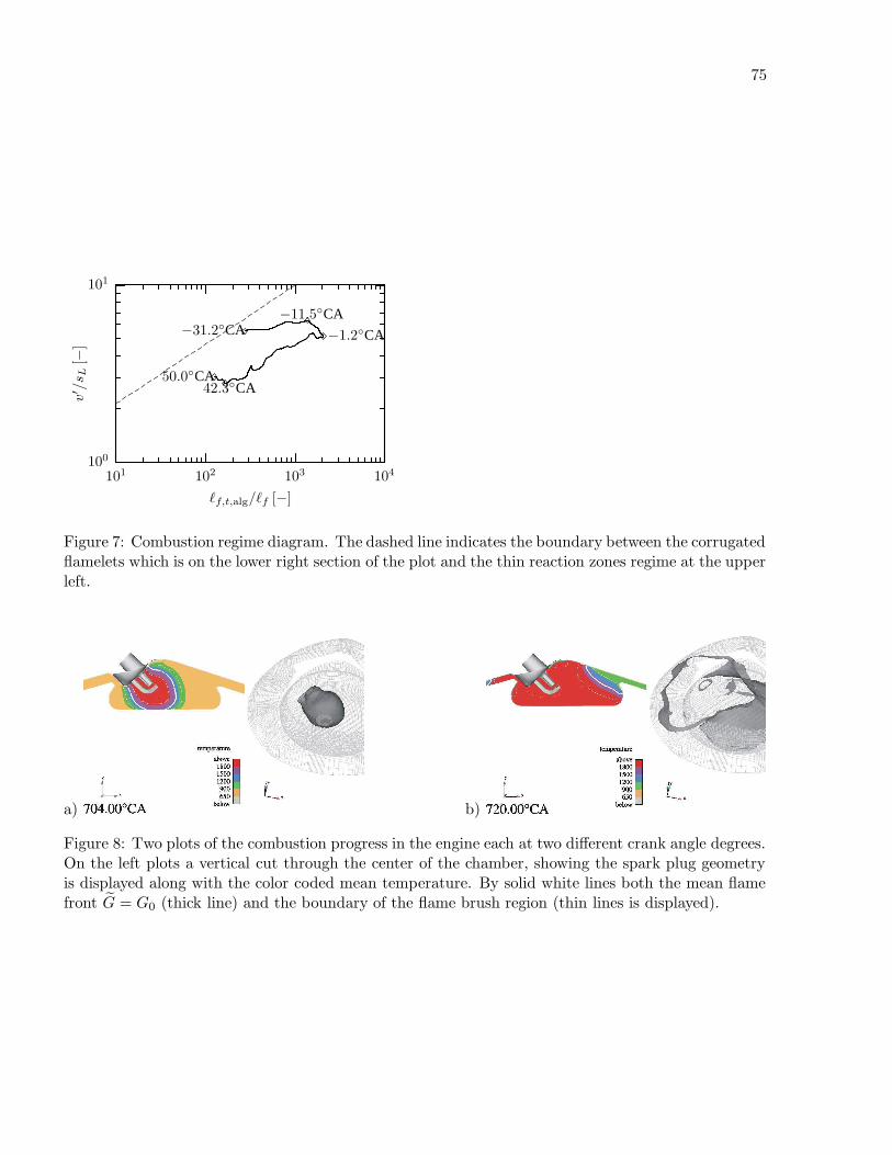
75

100

101

101 102 103 104

v′/s

L[−

]

`f,t,alg/`f [−]

−1.2CA−31.2CA−11.5CA

42.3CA50.0CA

Figure 7: Combustion regime diagram. The dashed line indicates the boundary between the corrugatedflamelets which is on the lower right section of the plot and the thin reaction zones regime at the upperleft.

a) b)

Figure 8: Two plots of the combustion progress in the engine each at two different crank angle degrees.On the left plots a vertical cut through the center of the chamber, showing the spark plug geometryis displayed along with the color coded mean temperature. By solid white lines both the mean flamefront G = G0 (thick line) and the boundary of the flame brush region (thin lines is displayed).

76

[6] A. M. Lippert, T. D. Fansler, and M. C. Drake. High-speed imaging and CFD modeling of spraysand combustion in a spray-guided spark ignition direct injection engine. In 6th Int. Symp. onInternal Combustion Diagnostics, Baden-Baden, Germany, June 15–16 2004.

[7] U. C. Muller, M. Bollig, and N. Peters. Approximations for burning velocities and marksteinnumbers for lean hydrocarbon and methanol flames. Combust. Flame, 108:349–356, 1997.

[8] S. Osher and R. Fedkiw. Level Set Methods and Dynamic Implicit Surfaces. Springer, 2003.

[9] N. Peters. Fifteen Lectures on Laminar and Turbulent Combustion. Ercoftac Summer School,September 14-28 1992. Institut fur Technische Mechanik, RWTH Aachen, 1992.

[10] N. Peters. A spectral closure for premixed turbulent combustion in the flamelet regime. J. FluidMech., 242:611–629, 1992.

[11] N. Peters. The turbulent burning velocity for large scale and small scale turbulence. J. FluidMech., 384:107–132, 1999.

[12] N. Peters. Turbulent Combustion. Cambridge University Press, 2000.

[13] J. A. Sethian. Fast marching methods. SIAM Review, 41(2):199–235, 1999.

[14] M. D. Smooke and V. Giovangigli. Formulation of the premixed and nonpremixed test prob-lems. In M. D. Smooke, editor, Reduced Kinetic Mechanisms and Asymptotic Approximations forMethane-Air Flames, volume 384 of Lecture Notes in Physics, pages 1–28. Springer-Verlag, 1990.

[15] Z. Tan, S. C. Kong, and R. D. Reitz. Modeling premixed and direct injection SI engine combustionusing the G-equation model. SAE Technical Paper Series, no. 2003-01-1843, 2003.

[16] Z. Tan and R. Reitz. Modeling ignition and combustion in spark-ignition engines using a levelset method. SAE Technical Paper Series, no. 2003-01-0722, 2003.

[17] Z. Tan and R. D. Reitz. Development of G-Equation combustion model for direct injection SIengine simulations. In 13th Int. Multidim. Engine Modeling User’s Group Meeting, Detroit, MI,March 2 2003.

[18] H. Wenzel. Direkte numerische Simulation der Ausbreitung einer Flammenfront in einem homo-genen Turbulenzfeld. Dissertation, RWTH Aachen University, 2000.

[19] F. A. Williams. Turbulent combustion. In J. Buckmaster, editor, The Mathematics of Combustion,pages 97–131. SIAM, Philadelphia, 1985.

77

Broken symmetry and coherent structure in MHD turbulence

J.V. Shebalin

NASA Johnson Space Center, Houston, Texas 77058 USA

Abstract

The statistical theory of ideal magnetohydrodynamic (MHD) turbulence is extended to cases with andwithout rotation, and with and without a mean magnetic field. One notable result is the discoveryof a new ideal invariant, the ‘parallel helicity,’ which arises when rotation and mean magnetic fieldvectors are aligned. Numerical results from several long-time simulations of five general cases on a323 grid are presented. The basic equations and statistical theory are symmetric under the parity orcharge reversal transformations. However, the presence of invariant cross, magnetic or parallel helicitydynamically breaks this symmetry, because these helicities are pseudoscalars under parity or chargereversal (or both). The basic theoretical result is that ideal MHD turbulence is, in general, non-ergodicdue to the decomposability of the constant energy surface in phase space. This non-ergodicity can bemanifested in the appearance of coherent structure as long as magnetic or parallel helicity is invariant.The fact that MHD turbulence inherently contains coherent structure in certain general cases mayhave important implications for dynamo theory.

Introduction

In this paper we study ideal (i.e., non-dissipative), homogeneous, three-dimensional (3-D), incom-pressible, magnetohydrodynamic (MHD) turbulence in a rotating frame of reference with and withouta mean magnetic field. Ideal MHD turbulence without rotation and without a mean magnetic field hasenergy, cross helicity and magnetic helicity as invariant integrals, but rotation removes cross helicityand a mean magnetic field removes magnetic helicity from the set of invariant integrals. However,there is a new invariant integral which arises when the angular velocity of rotation and the meanmagnetic field are both non-zero and collinear. This new invariant will be called the parallel helicityand it is a linear combination of the cross and magnetic helicities.

Absolute equilibrium ensemble theory for these various cases of ideal MHD turbulence (with andwithout rotation, and with and without a mean magnetic field) is presented here. The theory is gener-ally non-ergodic, due to the presence of invariant helicities, and this non-ergodicity can be manifestedin the appearance of coherent structure, although this is not necessary. Here, the five general cases ofideal, magnetized, rotating MHD turbulence are examined, both analytically and by numerical simu-lation. Although real (i.e., dissipative) turbulence is not considered here, recent numerical simulationshave demonstrated that real 2-D MHD turbulence appears to have behavior similar to that seen inthe ideal limit [Shebalin 2005]

The results presented here may have relevance to a number of physical systems. Rotating, magne-tized MHD turbulence seems to arise within and around the earth, the sun, distant stars, and otherastrophysical plasmas, as well as in magnetically confined laboratory plasmas. In the present work, weassume that the source of the mean magnetic field is fixed with respect to rotation, e.g., a global solarmagnetic field that permeates relatively small, local regions within the solar convection zone. Whilelarge-scale processes in the sun have been investigated elsewhere [Brun 2004, Fan 2004], the physicalarenas we wish to study are small regions, within an extensive magneto-fluid, where turbulence canbe considered homogeneous and incompressible, and where an externally imposed, constant magneticfield can be considered to be co-rotating with the small volume of interest.

78

To reiterate, the homogeneous MHD turbulence considered in this paper is ideal. Dissipation is,of course, critical in realistic rotating, magnetized MHD turbulence, and various aspects of such flowshave been studied by many authors (see, for example, [Canuto 1986]). However, an investigation ofdissipative 3-D MHD turbulence with particular regard to symmetry and ergodicity is beyond thescope of this work, and will, for the present, be deferred. Nevertheless, the results presented in thispaper may still be relevant to real turbulence, since the most important effects to be demonstratedmanifest themselves most strongly at the smallest dynamical wave numbers of the flow, i.e., the largesteddies, where dissipation has the weakest effect.

Basic Equations

The non-dimensional form of the MHD equations in a rotating frame of reference with constant angularvelocity Ωo and a mean (i.e., uniform and constant) magnetic induction Bo are

∂ω

∂t= ∇∧ [u ∧ (ω + 2Ωo) + j ∧ (b + Bo)] + ν∇2ω, (1)

∂b

∂t= ∇∧ [u ∧ (b + Bo)] + η∇2b. (2)

(See, for example, [Lesieur 1997] and [Biskamp 2003]. Also, in the above and following sets of equa-tions, ‘∧’ denotes the vector cross product.)

In addition to equations (1) and (2), we also have

∇ · u = 0, ω = ∇∧ u,

∇ · b = 0, j = ∇∧ b. (3)

In equations (1), (2) and (3), u, ω, b and j are the turbulent velocity, vorticity, magnetic induction andelectric current density, respectively, of the magneto-fluid. (The equations of rotating Navier-Stokesfluid turbulence arise if b = Bo = 0.)

If we set ν = 0 in (1) and η = 0 in (2), we obtain the equations of ‘ideal’ MHD turbulence. Whileany real flows have ν 6= 0 and η 6= 0, a study of ideal turbulence produces some interesting theoreticalresults that may help in understanding aspects of real turbulence, particularly at larger scales ofthe flow where dissipation is minimal. In the next two sections we will examine some theoreticalconsiderations, and following these, the numerical solution of eqs. (1) and (2).

Ideal MHD Turbulence

At this point, it is useful to ‘uncurl’ eq. (1), to produce the velocity equation for MHD turbulence:

∂u

∂t= −∇p′ + u ∧ (ω + 2Ωo) + j ∧ (b + Bo) + ν∇2u. (4)

Here, the ‘total pressure’ is p′ = p+ 12 u

2 − 12 (r ∧ Ωo)

2, where p is the thermodynamic pressure andthe last term in p′ is the centrifugal potential. The pressure can, as usual, be determined by takingthe divergence of both sides of eq. (4) and solving the resulting Poisson’s equation. In doing so, thereis an ambiguity related to the choice of origin for r, but this does not effect the dynamics of thehomogeneous, incompressible magneto-fluid.

Let us define the vector potential a by b = ∇ ∧ a and ∇ · a = 0. We can then uncurl eq. (2) toproduce an equation for a:

∂a

∂t= −∇Φ + u ∧ (b + Bo) + η∇2a. (5)

79

In eq. (5), Φ is the electric potential.Next, define the volume average of a quantity φ(r) in a periodic box of side length 2π as

[φ] ≡ (2π)−3

∫φ(r)d3x. (6)

Since all functions are periodic, we can use equations (1) through (6), along with integration by partsto derive the following relations:

dE

dt= −2 (νΩ + ηJ) , (7)

dHC

dt= Ωo · [b ∧ u] − 1

2(ν + η) [j · ω] , (8)

dHM

dt= Bo · [b ∧ u] − η [j · b] . (9)

Above, we have the (volume-averaged) energy E, enstrophy Ω, mean-squared current J , cross helicityHK and magnetic helicity HM :

E =1

2

[u2 + b2

], Ω =

1

2

[|ω|2

], J =

1

2

[|j|2

], (10)

HC =1

2[u · b] , HM =

1

2[a · b] . (11)

At this point we note that if Ωo = σBo, i.e., if Ωo and Bo are non-zero and parallel, then eq. (8)can be added to −σ times eq. (9) to yield

dHP

dt= −1

2(ν + η) [j · ω] − η [j · b] , HP ≡ HC − σHM . (12)

The quantity HP will be called the ‘parallel helicity.’When ν = η = 0, equations (7), (8), (9) and (12) lead us immediately to the invariant integrals

for MHD turbulence for various values of Bo and Ωo. First, if Bo = Ωo = 0, then E, HC and HM

are all constant. Second, if Bo 6= 0 but Ωo = 0, then E and HC are constant, but not HM . Third, ifBo = 0 but Ωo 6= 0, then E and HM are constant, but not HC . Fourth, if Bo 6= 0 and Ωo 6= 0, withBo ∧ Ωo 6= 0, then only E is constant. Fifth, if Bo 6= 0 and Ωo 6= 0, with Ωo = σBo, then E andHP are the only constants of the motion. The parallel helicity HP is a new invariant for 3-D MHDturbulence, one that occurs only when Bo and Ωo are non-zero and collinear.

These various cases are placed in Table 6 for easier reference. Note that Case II can be thought ofas a particular example of Case V, one for which σ = 0, while Case III can be thought of as anotherexample of Case V, one for which σ → ∞. Thus, we see that as a mean field is applied or an overallrotation is imposed or both, the number of invariants drop from three to two to one.

Absolute Equilibrium Ensembles

As is well known, the existence of integral invariants allows ideal MHD turbulence to be describedby Gibbsian statistical mechanics. The theory was initiated by [Lee 1952], partially developed by[Kraichnan 1973, 1975], [Frisch 1975] and [Fyfe 1976], and then extended by [Shebalin 1982, 1983,1989, 1996, 2002] and [Stribling 1990]. The physical fields u and b are represented by truncated

80

Case Mean Field Rotation Invariants

I Bo = 0 Ωo = 0 E, HC , HM

II Bo 6= 0 Ωo = 0 E, HC

III Bo = 0 Ωo 6= 0 E, HM

IV Bo 6= 0 Ωo ∧Bo 6= 0 EV Bo 6= 0 Ωo = σBo E, HP

Table 6: Invariants for ideal MHD turbulence (HP ≡ HC − σHM ).

Fourier series, whose coefficients are the ‘interacting particles’ of the canonical ‘absolute equilibriumensemble’:

u(x) =∑

0<|k|≤K

u(k) eik·x, (13)

b(x) =∑

0<|k|≤K

b(k) eik·x. (14)

The wave vectors k in k-space have integer components between −N/2 and +N/2, while the corre-sponding discrete set of position vectors x in x-space have components that are integer multiples of2π/N , where N is the number of grid points in each dimension. The ‘isotropic truncation’ radius isK, which is chosen to ensure that retained coefficients fit within a sphere in k-space; the exact valueof K is dictated by algorithmic requirements [Patterson 1971]. Since u and b are both real, theircoefficients satisfy a ‘reality condition’, e.g., u(k) = u∗(−k), where ‘∗’ denotes complex conjugation.Thus, only half of the k in the sums (13) and (14) are independent. Let the total number of k in thesesums be N , so that the number of independent k is

N ′ =1

2

∑

0<|k|≤K

1 =1

2N . (15)

The number N ′ will appear again in later formulas.The probability distribution function D of the absolute equilibrium ensemble, for Case I in Table

6, has the form

D ∼ exp(−αE − βHC − γHM ). (16)

The function D is normalized by requiring that its integral over the whole phase space defined by theindependent Fourier coefficients be unity. In regard to the other cases in Table 6, eq. (16) applies asfollows: Case II, set γ = 0; Case III, set β = 0; Case IV, set β = γ = 0; and in Case V, set γ = −σβ,so that eq. (16) becomes

D ∼ exp(−αE − βHP ). (17)

Thus, to determine various ensemble predictions for Cases II through V in Table 6, we merely takepreviously determined results for Case I ([Frisch 1975], [Shebalin 1989, 1994, 2002], [Stribling 1990])and substitute for β and γ as indicated above.

Using (16), ensemble predictions for moments of the u(k) and b(k) can now be made for thedifferent cases in Table 6. Denoting the ensemble prediction of a quantity Q(k) by 〈Q(k)〉, the

predicted first-order moments are 〈u(k)〉 =⟨b(k)

⟩= 0 for all cases. The ensemble predictions for

second-order moments are given in Table 7 for the five cases listed in Table 6.

81

Case⟨|u(k)|2

⟩ ⟨|b(k)|2

⟩

I 3α(δ2 − γ2/k2) 3αδ2

δ4 − α2γ2/k2 δ4 − α2γ2/k2

II 3α/δ2 3α/δ2

III 3/α 3α

α2 − γ2/k2

IV 3/α 3/α

V 3α(δ2 − σ2β2/k2) 3αδ2

δ4 − σ2α2β2/k2 δ4 − σ2α2β2/k2

Table 7: Second-order moments (δ2 = α2 − β2/4).

In Table 7, the modal expectation values are for |u(k)|2 = |uR(k)|2 + |uI(k)|2 and |b(k)|2 =|bR(k)|2 + |bI(k)|2, and the real and imaginary parts of these have equal share (i.e., one half of theexpected values in Table 7). Also, the expectation values of the modal helicities are

⟨uS(k) · bS(k)

⟩= − β

2α

⟨|bS(k)|2

⟩,

S = R, I (18)⟨aS(k) · bS(k)

⟩= α

⟨|uS(k)|2 − |bS(k)|2

⟩.

The second-order moments in Table 7 are functions of the inverse temperatures α, β and γ, whichmust be determined. Previous work ([Shebalin 1989, 1994, 2002]) has shown that α, β and γ can beexpressed in terms of one variable parameter, which can be chosen to be the expectation value of themagnetic energy EM = 〈EM 〉, where EM = 1

2

[|b|2

]. Using E = 〈E〉, HC = 〈HC〉 and HM = 〈HM 〉,

we have for Case I,

α =3N ′EM

EM (E − EM ) −H2C

, (19)

β = −2αHC

EM, (20)

γ = αE − 2EM

HM. (21)

Note that while E , HC and HM are constant to within canonical fluctuations, EM can vary appreciably.The inverse temperatures α, β and γ can be determined by minimizing an entropy functional with

respect to variation of a free parameter [Khinchin 1949], [Shebalin 1982, 1996] (here, the parameteris EM ). This gives us a priori values for α, β and γ, which can then be placed in the expressions inTable 7 to predict the shape of the ideal spectra for Case I. (One could also use the time-averagedvalue of EM to give approximate, but still fairly accurate, a posteriori estimates of α, β and γ.)

Recall that the basic equations (1) and (2) are invariant under the discrete classical symmetrytransformations P (parity, or coordinate inversion: x → −x), C (charge reversal: e → −e), and

82

(if ν = η = 0) T (time reversal: t → −t). However, helicities are not invariant under P and C[Shebalin 1998]. In eqs. (19) – (21), HC and HM are pseudoscalars under P and C, while the energiesE and EM are scalars. (Under time-reversal, HC and HM are scalars.) Therefore, it is clear from eqs.(20) and (21) that β is a pseudoscalar under P and C, and γ is a pseudoscalar under P , so that βHC

and γHM are scalars under P or C. Furthermore, eq. (19) indicates that α is a scalar under P or C.Thus, both the governing equations (1) and (2), and the probability density functions (16) and

(17) are invariant under P , C and T . The importance of this is the following. The phase space Γ ofthe absolute equilibrium ensemble of ideal MHD turbulence is defined by the independent componentsof the Fourier modes u(k) and b(k) for 0 < k ≤ K; let the dimension of this phase space be denotedby NΓ. In this phase space, the quadratic form E defines a hypersurface, and |HC | and |HM | definetwo hypersurfaces each, all of dimension NΓ − 1. (We use |HC | and |HM | since both signs of HC andHM are included in the statistical theory, by symmetry.)

The hypersurface defined by E is the surface of constant energy ΓE [Khinchin 1949]. The hy-persurface ΓE will generally be broken into disjoint regions, in all cases except Case IV of Table 6,because either HC or HM (or both) or HP are additional invariants. In each case in Table 6, it isthe intersection of ΓE with all the hypersurfaces associated with both signs of the invariant helicitiesthat is the subset of the phase space Γ on which the phase point can reside. In Case I, there are fourdisjoint components, in Cases II, III and V, there two disjoint components, and in Case IV, there isonly one component [Shebalin 1998].

As an example, let us consider Case I of Table 6, for which there are three invariant integrals. Thesurface of constant energy ΓE has dimension NΓ − 1, and this intersects with the surfaces of constant±HC and ±HM to confine the phase point to subsets of Γ of dimension NΓ − 3. Let SC = sgn HC

and SM = sgn HM , where SC , SM ∈ +,−. Also let ΓE(SC , SM ) denote the component of ΓE onwhich HC and HM have signs SC and SM , respectively. Since SC and SM are set functions whichseparate one component from another, the components ΓE(SC , SM ) with different values of SC andSM are disjoint (rather, effectively disjoint since we have a canonical ensemble).

Thus, the ensemble phase space contains a surface of constant energy ΓE that has subsetsΓE(SC , SM ) on which essentially all ensemble phase points reside. The union of all these subsetsis the subset of Γ containing, with non-vanishing probability, all of the phase points that make up thetheoretical ensemble. Call this union the ‘reduced’ surface of constant energy Γ ′

E:

Γ′E = ΓE(+,+) ∪ ΓE(+,−) ∪ ΓE(−,+) ∪ ΓE(−,−). (22)

It is clear that under P and C, Γ′E → Γ′

E because Γ′E has the topological structure given in (22),

i.e., a structure that ensures symmetry under P and C (and, of course, T ).

Inverse Temperatures

Equations (19), (20) and (21), are used to determine the inverse temperatures α, β and γ, respectively,for Case I. These equations can be used for Cases II-V by making the substitutions discussed followingthe probability distribution function (16). Also, for Cases II and IV, the substitution γ = 0 isequivalent to the assignment EM = 1

2 E in eq. (21). Making the various replacements leads to theresults in Table 8 (for more detail, see [Shebalin 2002]).

The inverse temperatures α and β for Case V are determined as follows. First, if γ = −σβ, theneqs. (19), (20) and (21) can be used to show that α and β satisfy two algebraic equations:

αE + βHP = 6N ′, (23)

αE − βHP +

(β +

4/a2

β

)HC = 0. (24)

83

In fact, eqs. (19), (20) and (21) were originally found by setting up three similar algebraic equations[Shebalin 1989]. Let us now define p, which is constant to within canonical fluctuations, and c, whichis a variable parameter:

p =HP

E and c =HC

E . (25)

Equations (23) and (24) can be solved to yield

α(c) =3N ′

E3p− 2c± p [1 + 16c(p− c)]

12

2p− c(1 + 4p2), (26)

β(c) =3N ′

E1 − 8cp∓ p [1 + 16c(p− c)]

12

2p− c(1 + 4p2). (27)

Here, the sign ± is chosen so that α > 0 and so that the second order moments in Table 7 are positive.

Case α β γ

I 3N ′EM −2αHC/EM α(E − 2EM )/HM

EM (E − EM ) −H2C

II 6N ′E −4αHC/E 0

E2 − 4H2C

III 3N ′ 0 α(E − 2EM )/HM

E − EM

IV 6N ′/E 0 0

V eq. (26) eq. (27) −σβ

Table 8: Inverse temperatures for Cases I–V.

Numerical Simulation

The MHD equations (1) and (2) were solved by a Fourier spectral transform method [Canuto 1988,Boyd 2001] on an N 3 grid, where N = 32. The non-linear terms in eqs. (1) and (2) were de-aliasedby the Orzsag-Patterson technique of shifted-grids [Patterson 1971]. The de-aliasing technique setsthe maximum wave vector magnitude in eqs. (13) and (14) to K =

√2N/3, corresponding to K2 =

227. The equations were integrated forward in time by a ‘partially corrected’ third-order method[Gadzag 1976]. The time step size for all runs was ∆t = 10−3. The initial conditions are such thatthe kinetic and magnetic Fourier modes have random phases and satisfy

|u(k)| = |b(k)| ∼ k exp(−k2/k2p) at t = 0. (28)

The kinetic and magnetic energy spectra, defined as the modal energies integrated over solid anglein k-space, are EK(k) and EM (k), respectively. Using (28), these energy spectra can be seen to have

84

the form

EK(k) ≈ EM (k) ∼ k4 exp(−2k2/k2p) at t = 0. (29)

For all runs reported here, the initial peak wave number is kp = 4.

Run Case Bo Ωo

A0 I (0, 0, 0) (0, 0, 0)A1 II (0, 0, 1) (0, 0, 0)A2 III (0, 0, 0) (1, 0, 0)A3 IV (0, 0, 1) (1, 0, 0)A4 V (0, 0, 1) (0, 0, 1)A5 V (0, 0, 1

2 ) (0, 0, 1)A6 V (0, 0, 1) (0, 0, 1

2 )

Table 9: Ideal MHD Simulations (ν = η = 0).

Seven runs are presented here. These all had the same initial conditions (E = 1.0000, HC = 0.3567and HM = 0.1398 at t = 0). The values of Bo and Ωo associated with these runs are given in Table9. In all of the runs in Table 9 the energy E is conserved to within 0.2%, although the kinetic andmagnetic energies can fluctuate significantly – (20% initially and about 3% when the ideal MHDturbulence is in equilibrium).

For brevity, a minimum number of figures will be shown here. Rather, we will include such figuresfor a future publication [Shebalin 2005a]. Suffice it to say that the runs in Table 9 behaved as expected,i.e., HC was conserved in Runs A0 and A1, while HM was conserved in Runs A0 and A2. Also, HP , acanonical invariant in Run A4, behaved as predicted, while HC and HM were no longer invariant. Thebehavior of HP for Runs A5 and A6 was also a canonical invariant, as it was for Run A4. The valuesof HP for A6, A4 and A5 were 0.2868 (σ = 0.5), 0.2169 (σ = 1.0) and 0.0771 (σ = 2.0), respectively.These were not linear in σ, though a determination of the exact functional dependence is beyond thescope of the present work.

As an example of the efficacy of the statistical theory, we use eqs. (26) and (27) to predict theaverage energy spectrum for Run A4, and this is shown in Figure 1. The numerical average is takenover the last quarter of the run (t = 1500 to 2000). Using the formulas (26) and (27) with s andc as defined in eq. (25), and E , HC and HM determined by averaging from t = 0 to 2000, we getα = 1.593067, β = −1.290033 = −γ. However, the low-k values of Eav(k) are very sensitive to thevalue of β; adjusting this value to β = −1.303590 gives the fit in Figure 1. The goodness-of-fit in Figure1 is typical of what is seen when the statistical theory is applied to any of the ideal cases in Table9. Also, equilibrium spectra show no anisotropy because, in these ideal cases, there is no dissipation.(The difference between isotropic ideal spectra and anisotropic real spectra in the presence of a meanmagnetic field was first explained in [Shebalin 1982, 1983].)

However, absolute equilibrium ensemble theory, as originally formulated ([Kraichnan 1973, 1975],[Frisch 1975], [Fyfe 1976]) predicts that all Fourier modes will have zero mean, and this is not nec-essarily so in any given ideal MHD simulation. In Figure 2, the evolution of the Fourier modes fork = (1, 0, 0) in Run A0 is presented. The non-zero components of all of the independent Fourier modesu(k) and b(k) define a phase space of large dimension (here, the dimension is about 105). Figure 2 isessentially a projection of the phase trajectory into a plane; if the ensemble predictions were correct,then the projected phase trajectory would be a random walk centered on the origin. That it is not isevident in Figure 2, where the initial point of the trajectory is close to the origin, but after a transition

85

100

10110

0

101

102

k

NumericalPredicted

α = 1.593067

β = −1.303590 = −γ

Eav

(k)

Figure 1: Predicted and numerically averaged (t = 1500 to 2000) spectra for Run A4 in Table 9.

lasting from t = 0 to about t = 30, the phase point appears to arrive at an attractor in phase space.This behavior can also be seen when modes with other values of k = |k| = 1 are examined. However,when k > 1, the mean of the Fourier modes appears to be zero. Thus, non-ergodicity is manifestedin the modes with the lowest value of k, as simulated time averages do not match predictions of thestatistical theory.

In addition to examining the detailed behavior of individual modes, we can also examine time-averaged behavior of all modes by defining the ‘coherent energies’ E c, EcK and Ec

M :

Ec = EcK +EcM , EcK ≡ 1

2

∑

k

|〈u(k)〉T |2 , EcM ≡ 1

2

∑

k

|〈u(k)〉T |2 . (30)

The Fourier coefficients in the sum are time-averaged, e.g.:

⟨b(k)

⟩T

≡ 1

T

∫ T

0b(k, t)dt. (31)

If the dynamical system were ergodic, Ec would tend to zero with time; if not, the non-zero meanFourier modes effectively define a coherent structure in ideal MHD turbulence. The appearance ofcoherent structures has been noted before in long-time 2-D simulations [Shebalin 1989, 2005] and insome preliminary 3-D runs [Shebalin 1994]; here we see them for long-time 3-D runs. The explanationfor these coherent structures then, as now, lies in the disjoint nature of phase space [Shebalin 1998].

In Figure 3, the coherent energy for Runs A0–A4 are presented. It is clear that whenever magnetichelicity remains an invariant (Runs A0 and A2), that the coherent energy E c is relatively large.Furthermore, when coherent energy is evident, it is primarily magnetic, as in Runs A0 and A2, forwhich Ec

M ≈ 0.12 at t = 2000; the difference between Ec for Runs A0 and A2 in Figure 3 is dueto Ec

K ∼ 0.06 for Run A0 and EcK ∼ 0 for Run A2. (Remember that total energy is E = 1). We

also see in Figure 3 that Ec for Run A4 settles into a small, but non-zero value; this is due to thepresence of HM in the invariant HP , as will be discussed presently. (Although these are ideal runs,similar behaviour has been seen in long-time dissipative 2-D MHD runs, where ν 6= 0 and η 6= 0[Shebalin 2005].)

86

0 10 20 30 40 50

0

10

20

30

40

50

k = (1,0,0)

t = 0 to 2000

Re

Imu

y(k)

uz(k)

bz(k)

by(k)

t = 0

Figure 2: Projection of the phase trajectory for Case I in Table 6 (Run A0 in Table 9).

100

101

102

10310

−4

10−3

10−2

10−1

100

Time

A0A1A2A3A4

EC

Figure 3: Coherent energy for Runs A0 – A4 in Table 9.

87

One interesting point to note is that although the theoretically predicted and numerically observedideal MHD spectra are quite close, as in Figure 1, the ensemble prediction is that all of the power in thespectrum for a given value of k is due to zero-mean Fourier modes, while numerical simulations showsus that, in the case of k = 1, much of the energy seems locked up in the non-zero-mean part of themode, as Figure 2 clearly shows. This was seen before in ideal 2-D MHD turbulence [Shebalin 1982,1989, 1994, 2005], and it appears again here in ideal 3-D MHD turbulence.

Another interesting point is that Runs A1 and A3 in Figure 3 have coherent energies that do notlevel off but appear to fall exponentially towards zero. This indicates that magnetic helicity is criticalto the appearance of coherent structure in ideal MHD turbulence, since it is either an invariant orpart of an invariant (HP ) in those runs that do have non-zero coherent energy. In Runs A1 and A3,the presence of non-zero Bo eliminates HM as an ideal invariant, due to the first term on the rightside of equation (9). In Run A3, Bo and Ωo are non-zero and not parallel, so that only E is an idealinvariant; in this case we expect the phase surface ΓE of the absolute equilibrium ensemble to haveonly one component, so that all Fourier modes do, in fact, have zero mean. However, In Run A1, HC

is still an ideal invariant, along with E, yet there appears to be no coherent energy. In this lattercase, the surface of constant energy ΓE must still have two disjoint components. The reason for theappearance of zero-means in Run A1 is as follows.

When Bo 6= 0 but Ωo = 0, as in Run A1 (Case II of Table 6), we have two invariants, E and HC ,and these can be transformed into two equivalent invariants E+ and E−,

E± = E ± 2HC =1

2

[|u ± b|2

]=

1

2

[|z±|2

]. (32)

The quantities E+ and E− are the energies associated with the Elsasser variables [Elsasser 1956]

z+ = u + b, z− = u − b. (33)

Thus, we have two separate sets of variables, each having its own unique invariant. The phase spaceΓ of the Fourier modes u(k) and b(k) is a ‘direct sum space’ [Halmos 1958],

Γ = Γ+⊕ Γ−. (34)

Here, Γ+ is the phase space of the z+(k) and Γ− is the phase space of the z−(k).

Using the Elsasser variables (33), the energy and cross helicity can be written as

E =1

4

[|z+|2 + |z−|2

], HC =

1

8

[|z+|2 − |z−|2

]. (35)

Thus, in Case II of Table 6, invariant energy and cross helicity are equivalent to the two invariantenergies E+ and E−.

The set of Elsasser Fourier modes z+(k) are constrained to move on a hypersphere Γ+E+ in their

phase space Γ+, and the variables z−(k) are constrained to move on a hypersphere Γ−E− in their phase

space Γ−. If HM is not an invariant, then there is no constraint on where the z+(k) can move on thehypersphere Γ+

E+ , and where the z−(k) can move on the hypersphere Γ−E− , in which case the surface

of constant energy for, say, HC > 0 is Γ+E+× Γ−

E−, i.e., a product space [Hocking 1988] between Γ+E+

and Γ−E− .

Suppose that E+ = E1 and E− = E2, with E1 > E2. The product space in this case is Γ+E1× Γ−

E2.

Under P or C, we have HC → −HC , which implies z+(k) z−(k), so that, now, E+ = E2 andE− = E1. Thus, Under P or C, a second component product space Γ+

E2× Γ−

E1appears. Therefore, the

88

−−−−

ΓΓ−

2

ΓΓ−

1

Figure 4: Phase space structure for Case II of Table 6.

reduced constant energy surface for Case II of Table 6 is

[Γ+E1× Γ−

E2

]∪

[Γ+E2× Γ−

E1

]= Γ′

E

(36)[Γ+E1× Γ−

E2

]∩

[Γ+E2× Γ−

E1

]= ∅.

Since Γ′E has two disjoint components, as shown in (36), the system is non-ergodic. [The surface of

constant energy ΓE is broken into two components of smaller dimension (Γ′E , the union of nested

‘hyper-tori’), rather than four components as in (22), because HM is not invariant here.]To visualize this disjoint structure, consider Figure 4, which pertains to Case II of Table 6, repre-

sented by Run A1 in Table 9. The ensemble average is over both components (gray and black), whilea time average is taken only over the gray or the black component. Here, the subspaces Γ+

E1,2and

Γ−E2,1

in the union of direct product spaces are hyperspheres and thus symmetric about their respectiveorigins, so that the Elsasser variables have zero mean values for Case II of Table 6.

In terms of the Elsasser variables (33), the magnetic helicity can be written as

HM =1

4

∑

k

k · [z+R(k) − z−R(k)] ∧ [z+

I (k) − z−I (k)]. (37)

In Cases I and III of Table 6, the presence of a constant HM introduces a constraint which serves todecompose the nested hypertori Γ+

E1×Γ−

E2and Γ+

E2×Γ−

E1into two components each, for a total of four

components of the reduced surface of constant energy Γ′E , as shown in (22). In this case we have

coherent structure, in addition to non-ergodicity as evinced in the behavior of the coherent energiesfor Runs A0 and A2 in Figure 3. Also, in Case V, where HP = HC − σHM is an ideal invariant, bothHC and HM affect the topology of the available phase space, as seen in the behavior of the coherentenergy for Run A4 in Figure 3.

Broken Ergodicity

Here, a summary of the preceding results is given, along with a more detailed discussion of ‘brokenergodicity’. It has been noted in Section 4 that the governing equations (1) and (2), and the probability

89

density functions (16) and (17) are invariant under P , C and T , while HC , HM and HP are not. Thereason is that the probability densities (16) and (17) are invariant because the inverse temperaturesβ and γ are pseudoscalars, so that the products βHC , γHM and βHP are scalars. Thus, whenthe integration over all of phase space required to determine an ensemble expectation value is doneanalytically, it includes regions with both signs of the helicities HC , HM and HP , which automatically

leads to 〈u(k)〉 =⟨b(k)

⟩= 0.

Note that the expectation values of the pseudoscalars (under P or C) HC and HM (for Case I)can be written in terms of the scalar (under P or C) partition function Z =

∫DdΓ as

HC = −∂lnZ

∂β, HM = −∂lnZ

∂γ. (38)

Since β and γ are themselves pseudoscalars, the relations (38) are invariant under P or C (or T ).Therefore, one may state that the theory predicts the signs of the scalars βHC and γHM , rather thanthe signs of HC or HM alone. Alternatively, one may say that the absolute values |HC | and |HM | arepredicted and that ensemble expectation values are taken over those parts of the energy surface whereHC = ±HC and HM = ±HM .

However, when a numerical simulation is run, a given invariant helicity HC or HM will be eitherpositive or negative and will remain so during the dynamical evolution. Therefore, the symmetryof absolute equilibrium ensemble theory is dynamically broken, and ensemble predictions are notnecessarily the same as time averages. That they are not the same is clear from the evidence presented

in Section 5, especially in the comparison of the time averages 〈u(k)〉T and⟨b(k)

⟩T, which are

generally nonzero for k = 1, with the ensemble averages for k = 1, which are zero. Some cases of idealMHD turbulence, as described by absolute equilibrium ensemble theory, are clearly not ergodic sinceensemble expectation values (analytical integrations) and time averages (numerical integrations) arenot equal. This situation is often called broken ergodicity [Palmer 1982].

Even if we did not happen to observe the inequality of time and ensemble averages the non-ergodicity found in MHD turbulence is essentially tied to the decomposability or indecomposability ofthe surface of constant energy ΓE in phase space. This is the content of the Khinchin-Birkhoff theorem[Khinchin 1949, pp 55–57]: ‘the metric indecomposability of the surfaces of constant energy is anecessary and sufficient condition for a positive answer to the ergodic problem . . . ’. The essential pointis that if metric decomposability occurs (i.e., a surface of constant energy has disjoint components),then the system is non-ergodic, and conversely, if the surface of constant energy cannot be broken intodisjoint components, then the system is ergodic.

We note again that the occurrence of nonzero mean values of first-order time-averaged moments

such as 〈u(k)〉T and⟨b(k)

⟩T

(i.e., coherent structure) is sufficient for non-ergodicity, but not neces-

sary. In the discussion of the Elsasser variables (33), it was seen in eqs. (36) and in Fig. 4 that thesurface of constant energy consisted of the union of two disjoint subpaces, indicating non-ergodicity.However, the coherent energy for Run A1 in Figure 3 is clearly falling to zero, indicating a lack ofcoherent structure. Thus, non-ergodicity is due to the presence of at least one invariant helicity (whosesign serves as the set function that differentiates between unconnected components).

Conclusion

The results presented here are not exhaustive, and further studies are necessary to understand thedetailed effects that varying the parameter σ, the initial values of HC and HM , the magnitudes anddirections of Bo and Ωo as well as the Rossby number, Ro ≡

√Ω/2Ωo, where the enstrophy Ω is

90

defined in eq. (10). However, several novel features have been presented here. These include thediscovery of a new integral invariant, the parallel helicity HP .

A major topic requiring further investigation is a precise characterization of how the presence ofinvariant integrals affects the topology of the available phase space. A step in this direction is therealization that use of the Elsasser variables allows the invariant components of the surface of constantenergy ΓE to be represented as a union of the disjoint, direct product subspaces Γ+

E1×Γ−

E2and Γ+

E2×Γ−

E1

called the reduced surface Γ′E ; see eq. (36). If E and HC are constant, but not HM , then motion over

the hyperspheres Γ+E1,2

and Γ−E2,1

produces a zero-mean time average, as evidenced here numerically by

examining the time evolution of the coherent energy. The manifest symmetry of the Γ+E1,2

and Γ−E2,1

about their respective origins, in fact, requires that mean values of the various Fourier components bezero. However, when HM or HP are constant, the surface of constant energy is broken into additionaldisjoint components (in the case of constant HP , the dependence on σ is a topic requiring furtherinquiry).

The results given here pertain to ideal 3-D MHD turbulence, and an important question is how thebroken ergodicity observed in this non-dissipative flow might also appear in realistic, i.e., dissipative,3-D MHD turbulence. Results from 2-D simulations or real turbulence [Shebalin 2005] indicate thatbroken ergodicity is still present, so perhaps similar effects will be seen in real 3-D flows. A numericalinvestigation into this would benefit from a large computational grid, in order to make the maximumwave number in the Fourier space as large as possible. Going to a large grid, of course, greatlyincreases numerical run times, so that a numerical investigation in which several important parametersare systematically varied may require a long-term research commitment; thus, smaller grids may stillprove useful. Further studies should also show the connection between broken ergodicity, selectivedecay and inverse cascades more clearly. In addition, analytical theories of MHD turbulence do notcurrently offer any explanations of the behavior reported in this paper, and perhaps this will be seenas an inducement for an extension of these theories.

Finally, an essential physical feature uncovered here (and in previous work) is, in specific cases,the presence of coherent structure in MHD turbulence. We have observed numerically that, in anumber of cases, coherent structures seem to arise spontaneously in MHD turbulence. This hints atthe possibility that magnetic dynamo activity may be more an inherent feature of MHD turbulenceand less an induced phenomenon due to rotation and convection. It may turn out that rotation andconvection (for example, in the earth’s outer core or in the sun’s convective zone) are needed as sourcesof turbulence, and may also affect the level of coherent energy attained, but that it is the turbulenceitself that contains all that is required for dynamo action: broken ergodicity.

Acknowledgements

I wish to thank Dr. Friedrich Kupka of the Max-Planck-Institute for Astrophysics for organizing asplendid ‘Workshop on Interdisciplinary Aspects of Turbulence’ at the Ringberg Castle in Bavaria,18-22 April 2005, where the talk related to this paper was presented.

References

[Biskamp 2003] D. Biskamp, “Magnetohydrodynamic Turbulence,” Cambridge U. P., UK, 2003, Chap. 2.

[Boyd 2001] J. P. Boyd, “Chebyshev and Fourier Spectral Methods,” 2nd Ed., Dover, Mineola, NY, 2001.

[Brun 2004] A. S. Brun, M. S. Miesch and J. Toomre, Global-scale turbulent convection and magneticdynamo action in the solar envelope, Ap. J., 614 (2004) 1073–1098.

91

[Canuto 1988] C. Canuto, M. Y. Hussaini, A. Quateroni, and T. A. Zang, “Spectral Methods in FluidDynamics,” Springer-Verlag, New York, 1988.

[Canuto 1986] V. M. Canuto, and G. J. Hartke, Convective turbulence with rotation and magnetic fields,Astron. Astrophys., 168 (1986) 89–104.

[Elsasser 1956] W. M. Elsasser, Hydromagnetic Dynamo Theory, Rev. Mod. Phys., 28 (1956) 135–163.

[Fan 2004] Y. Fan, Magnetic fields in the solar convection zone, Living Rev. Solar Phys., 1 (2004) 1–63.

[Frisch 1975] U. Frisch, A. Pouquet, J. Leorat, and A. Mazure, Possibility of an inverse cascade of magnetichelicity in magnetohydrodynamic turbulence, J. Fluid Mech., 68 (1975) 769–778.

[Fyfe 1976] D. Fyfe and D. Montgomery, High beta turbulence in two-dimensional magneto-hydrodynamics, J. Plasma Phys., 16 (1976) 181–191.

[Gadzag 1976] J. Gadzag, Time-differencing schemes and transform methods, J. Comp. Phys., 20 (1976)196–207.

[Halmos 1958] P. R. Halmos, “Finite-Dimensional Vector Spaces,” Van Nostrand, Princeton, 1958, pp 28–32.

[Hocking 1988] J. G. Hocking and G. S. Young, “Topology,” Dover, New York, 1988, pp 21–23.

[Khinchin 1949] A. I. Khinchin, “Mathematical Foundations of Statistical Mechanics,” Dover, New York,1949, 137-145.

[Kraichnan 1973] R. H. Kraichnan, Helical turbulence and absolute equilibrium, J. Fluid Mech., 59 (1973)745–752.

[Kraichnan 1975] R. H. Kraichnan, Statistical dynamics of two-dimensional flows, J. Fluid Mech., 67 (1975)155–175.

[Kraichnan 1988] R. H. Kraichnan and R. Panda, Depression of nonlinearity in decaying isotropic turbulence,Phys. Fluids, 31 (1988) 2395–2397.

[Lee 1952] T. D. Lee, On some statistical properties of hydrodynamical and magneto-hydrodynamicalfields, Q. Appl. Math., 10 (1952) 69–74.

[Lesieur 1997] M. Lesieur, “Turbulence in Fluids,” 3rd Ed., Kluwer, Dordrecht, 1997, Chap. II.

[Palmer 1982] R. G. Palmer, Broken ergodicity, Adv. Phys., 31 (1982) 669–735.

[Patterson 1971] G. S. Patterson and S. A. Orszag, Spectral calculation of isotropic turbulence: Efficientremoval of aliasing interaction, Phys. Fluids, 14 (1971) 2538–2541.

[Shebalin 1982] J. V. Shebalin, Anisotropy in MHD turbulence due to a mean magnetic field, Ph.D. Disser-tation, College of William and Mary, 1982.

[Shebalin 1983] J. V. Shebalin, W. H. Matthaeus, and D. Montgomery, Anisotropy in MHD turbulence dueto a mean magnetic field, J. Plasma Phys., 29 (1983) 525–47.

[Shebalin 1989] J. V. Shebalin, Broken ergodicity and coherent structure in homogeneous turbulence, PhysicaD, 37 (1989) 173–191.

[Shebalin 1994] J. V. Shebalin, Broken symmetry in ideal magnetohydrodynamic turbulence, Phys. Plasmas,1 (1994) 541–547.

[Shebalin 1996] J. V. Shebalin, Absolute equilibrium entropy, J. Plasma Phys. 56 (1996) 419–427.

92

[Shebalin 1998] J. V. Shebalin, Phase space structure in ideal homogeneous turbulence, Phys. Lett. A, 250(1998) 319–322.

[Shebalin 2002] J. V. Shebalin, The statistical mechanics of ideal homogeneous turbulence, NASA TP-2002-210783, Johnson Space Center, Houston, TX, 2002.

[Shebalin 2005] J. V. Shebalin, Theory and simulation of real and ideal magnetohydrodynamic turbulence,Discrete & Continuous Dynamical Systems B, 5 (2005) 153–175.

[Shebalin 2005a] J. V. Shebalin, Ideal MHD Turbulence with Rotation and Mean Magnetic Field, J. PlasmaPhys., submitted (2005).

[Stribling 1990] T. Stribling and W. H. Matthaeus, Statistical properties of ideal three-dimensional magne-tohydrodynamics, Phys. Fluids B, 2 (1990) 1979–1988.

93

Energy spectrum and transfer flux in Hydrodynamic and MHD turbulence

T. Gotoh, K. Mori

Graduate School of Engineering, Engineering Physics,Nagoya Institute of Technology, Nagoya, 466-8555, Japan

Abstract

Transfer flux of the kinetic energy, passive scalar variance and of the total energy in MHD turbulence isstudied. It is found by direct numerical simulation and spectral theory of turbulence that the transferin the mean flux is local in scale, and that the energy transfer in 4-dimensions is more efficient thanthat in 3d. Fluctuations of the transfer flux around its mean value become positive and negative andare very intermittent as the scale decreases.

Introduction

In turbulence at large Reynolds numbers, energy is pumped in at the rate εin per unit mass andunit time at macroscopic scale L, transferred at the rate Π to smaller scales by nonlinear interactionthrough the inertial range, and then it is dissipated into heat at the rate εout at scale η due to molecularviscosity [1, 2]. When turbulence is in a steady state, the averages of the above three rates are equal:εin = Π = εout. Also for a passive scalar convected by turbulence and for the MHD turbulence thesame dynamics can be expected, in which the transferred quantities are the variance of the scalarfluctuations and the sum of the kinetic and magnetic energy, respectively. The transfer flux Π (σ) dueto the nonlinear interaction, where σ is NS (Navier Stokes), θ (scalar), or M (MHD), is the mostfundamental quantity in the turbulence dynamics. The transfer occurs in stepwise (local cascadeprocess) or in a radiative way (nonlocal process) in scale space. We have examined the statisticalnature of Π(σ) by using direct numerical simulation (DNS) of the isotropic NS, scalar, and MHDturbulence from the view points of (1) degree of locality of the mean transfer flux in wavenumberspace, (2) its dependency on the Reynolds number, (3) effects of spatial dimensions, (4) fluctuationsof the flux around its mean value.

Mean transfer flux

We assume that the turbulent fields are statistically homogeneous, isotropic, and in a steady state.Spectra of the kinetic energy, magnetic energy, and the scalar variance are defined as

⟨u2

⟩

2=

∫ ∞

0E(k, t)dk,

⟨b2

⟩

2=

∫ ∞

0Eb(k, t)dk,

⟨θ2

⟩

2=

∫ ∞

0Eθ(k, t)dk, (1)

respectively, where 〈 〉 denotes ensemble average. The equations for the spectra are

(∂

∂t+ 2νk2

)E(k, t) = TNS(k, t), (2)

(∂

∂t+ (ν + µ)k2

)EM (k, t) + (ν − η)k2ER(k, t) = TM (k, t), (3)

(∂

∂t+ 2κk2

)Eθ(k, t) = Tθ(k, t). (4)

94

where EM (k) = E(k) +Eb(k) and ER(k) = E(k) −Eb(k). We consider the only case of ν = η = κ inwhich the contributions from the molecular action to the transfer flux are the same. Functions TNS ,TM , and Tθ denote the energy, scalar, and MHD energy transfer functions, respectively and arise fromthe nonlinear and/or convective terms in the fundamental equations. The mean transfer flux Π (σ) isdefined as [1, 2, 3, 4]

Π(σ)(k, t) =

∫ ∞

kTσ(k

′, t)dk′. (5)

Physical meaning of the transfer flux is the total amount of the energy, scalar variance, or the MHDenergy transferred from all the Fourier components below k to those higher than k by triad interactions.On the other hand, the transfer functions Tσ’s are those quantities transferred to the wavenumber k,and generally of the form of

Tσ(k) =

∫∫

∆Sσ(k, p, q)dpdq, (6)

Sσ(k, p, q) = 2Real (Mσ : 〈wσ(p)wσ(q)wσ(−k)〉) , (7)

where Mσ(k) is a geometric factor arising from the nonlinear or convective terms, and wσ(k) denotesthe Fourier amplitude of the velocity, magnetic vectors or passive scalar. In the triad interactionk = p + q, we define the scale disparity parameter α as the ratio of the longest to the shortestwavenumber: [3, 4]

α =Max(k, p, q)

Min(k, p, q). (8)

When α is close to unity, it means that fluid motions of similar size interact, while when α is verylarge, motions at very large and very small scales interact. Thus, α measures the degree of locality ornonlocality of the interactions among different scales. The mean transfer flux of Eq. (5) is written asfollows,

Π(σ)(k)

ε(σ)=

∫ ∞

1W (σ)(α, k)

dα

α, (9)

W (σ)(α, k) =1

ε(σ)

∫ ∞

kdk′

∫ ∞

0dp′

∫ ∞

0dq′ Sσ(k

′, p′, q′, α), (10)

where ε(σ) denotes the mean dissipation rate for the kinetic and magnetic energy, or the passive scalarvariance. W (σ)(α, k) represents the fractional contributions to the total mean transfer flux from theinteractions in the range [α, α+ dα] at wavenumber k [3, 4, 5, 6, 7, 8, 9, 10, 11].

Figures 1 and 2 show the energy spectra in steady state in which curves are compensated bymultiplying k5/3 [13, 14]. It is clearly seen that the spectra of the kinetic and passive scalar havesmall but finite width of flat portion at Rλ = 427, indicating that they obey the k−5/3 spectrum,but it is difficult to definitely decide whether or not EM (k) ∝ k−5/3 at Rλ = 160 [14, 20, 21]. Forthese spectra, we have computed W (σ), which are shown in Figs. 3 and 4 [15]. The W (σ) curvesattain the maxima at about α = 2 and slowly decay for large α, which indicates that the transfer ofthe energy and scalar variance is local in scale. The smooth curves for W (NS) and W (θ) show thetheoretical prediction by the spectral theory of turbulence (Lagrangian Renormalized Approximation,LRA) [15, 23]) which agrees well with the DNS curves. W (M) is very similar to W (NS) in spite ofthe difference in the Reynolds numbers. Since in the MHD turbulence the kinetic energy dominatesthe total energy spectrum in the low wavenumber range as seen in Fig.2, the effects of the magneticfield on the transfer flux are expected to be small, which in turn implies that the locality of Π (NS) isinsensitive to the Reynolds numbers.

95

0.1

1

0.01 0.1 1

com

pens

ated

ene

rgy

spec

tra

kη

CK=1.61

COC=0.68

E(k),Reλ=258E(k),Reλ=435

Eθ(k),Peλ=145Eθ(k),Peλ=235

Fig.1 Compensated energy spectrumk5/3ε−2/3E(k) and the scalar spectrumk5/3ε1/3χ−1Eθ(k) at Rλ = 427. TheKolmogorov and Obukhov-Corrsin con-stants are K = 1.61± 0.09 and COC =0.68± 0.04, respectively.

10-3

10-2

10-1

100

101

10-2 10-1 100 101

ν-5/4

ε-1/4

(kη)

5/3 E

(k)

kη

E (k)Eb(k)

EM(k)

Fig.2 Compensated energy spectra

k5/3ε−2/3E(k), k5/3ε−2/3b Eb(k), and

k5/3ε−2/3totalEM (k) at Rλ = 160.

−0.2

0

0.2

0.4

0.6

0.8

1

1.2

1 10 100 1000

W(α

,k),

Wθ(

α,k

)

α

W(α,k), kη=0.017Wθ(α,k), kη=0.017

W(α) LRAWθ(α) LRA

Fig.3 Comparison of W (NS)(α) andW (θ)(α) at Rλ = 427. Smooth curvesare the results of the spectral theory ofturbulence (LRA).

-0.2

0

0.2

0.4

0.6

0.8

1

1.2

1 10 100 1000

W(α

)

α

WNS(α)(k=15.5-17.5)WM(α)(k=8.5-9.5)

Fig.4 Comparison of W (NS)(α) (Rλ =427) and W (M)(α) (Rλ = 160).

Dimension effects

In order to see effects of the spatial dimension on the transfer of the kinetic energy in scale space,we have examined the decaying NS turbulence in 4-dimensions and compared with the 3-dimensionalturbulence [16]. The initially Gaussian random velocity field with a support compact spectrum wasintegrated in time. The total kinetic energy and the average energy dissipation are defined by Ed(t) =d(U2

0 /2) =⟨u2(x, t)

⟩/2 and dEd(t)/dt = −εd, respectively, where d = 3 or 4, so that the energy in

one direction is the same for both dimensions.

Variation of εd(t)/εd(0) is shown in Fig.5. The dissipation rates attain the maxima at aboutk0U0t ∼ 1 in both dimensions. Initially the ratio ε4(0)/ε3(0) is about 4/3, but later ε4(t)/ε4(0)becomes larger than ε3(t)/ε3(0). This fact indicates that the energy transfer in 4d is more efficient thanin 3d. Correspondingly to this, we observed that the normalized energy flux function Πd(k, t)/εd(t)was larger in 4d than in 3d (figures not shown). The decay of the normalized turbulent energy isshown in Fig.6; the curves are well fitted by (t− t0)

−n with n = 1.35 in 3d and n = 1.60 in 4d, wheret0 ≈ 0 [17, 18]. The larger exponent in 4d is due to the larger energy transfer rate.

96

0

0.2

0.4

0.6

0.8

1

1.2

1.4

0 1 2 3 4 5 6 7 8

ε– (t

)/ ε–

(0)

k0U0t

d=3d=4

Fig.5 The variation of the energy dis-sipation rate in 4d and 3d.

0.01

0.1

1

0.1 1

log (

E(t

)/E

(0))

log t

d=3d=4

(t−t0)−1.35

(t−t0)−1.60

Fig.6 The decay of turbulent energy in4d and 3d. Lines are the best fit ones.

10−12

10−10

10−8

10−6

10−4

10−2

100

102

-1000 -500 0 500 1000

σΠ~

P(Π~

,r)

(Π~−⟨Π~ ⟩)/σΠ~

Fig.7 P (Π, r). rn = 2n−1∆x, n =1, · · · , 10, ∆x = 2π/N , Rλ = 427.Curves are from the inner to outer asn decreases.

10−12

10−10

10−8

10−6

10−4

10−2

100

102

-1000 -500 0 500 1000

σΠ~

θP(Π~

θ,r)

(Π~ θ−⟨Π~ θ⟩)/σΠ~ θ

Fig.8 P (Πθ, r). rn = 2n−1∆x, n =1, · · · , 10, ∆x = 2π/N , Rλ = 427.Curves are from the inner to outer asn decreases.

Fluctuations of the transfer flux

It is very interesting and important to know how much the flux fluctuates around its mean. Theprobability density function (PDF) of the transfer flux is suitable for this purpose, but we needexpression for the transfer flux in the physical space. We use surrogate expression for the flux in thephysical space defined in terms of the structure functions by

Π(x, r) = − (δuL(x, r))3

r, Πθ(x, r) = −δuL(x, r) (δθ(x, r))2

r, (11)

which are motivated by the 4/5 and 4/3 laws [19, 22]. The means of the two members of Eq.(11) are

equal to Π(NS)(r) =⟨Π(x, r)

⟩= εNS , and Π(θ)(r) =

⟨Πθ(x, r)

⟩= εθ for the separation distance r

in the inertial range, respectively.

Figures 7 and 8 show PDF’s of Π and Πθ for Rλ = 427 and Sc = 1. Both PDF’s have cusps atsmall amplitudes, and tails that become longer for large amplitudes as r decreases. Π and Πθ takepositive or negative values, meaning that the energy and the scalar variance are transferred in bothdirections, from small to large scales and from large to small scales. The PDF of Πθ is more positivelyskewed than that of Π, which means that large negative amplitudes of the scalar transfer flux occurless frequently than large positive amplitudes. This is due to the fact that there is no pressure term

97

in the equation of the passive scalar, so that the scalar variance undergoes straining more persistentlyand efficiently by the velocity field [15].

Summary

We have examined the nature of the transfer flux in the NS, MHD, and passive scalar turbulence.The mean transfers are local in scale, which means that those quantities are transferred in stepwiseby the interaction among similar size of scales of motion. This is consistent with the conventionalunderstanding. It was also suggested that the locality in the transfer flux was insensitive to theReynolds numbers. The fluctuations of the flux around the mean value are very intermittent, andboth strong positive and negative fluctuations can occur, but they cancel mostly, and yield only smallmean value of the flux as net effects. When the spatial dimension was increased from 3 to 4, it wasfound that the transfer of the kinetic energy was enhanced when compared to the case in 3d. This isdue to the fact that the role of the pressure in 4d becomes less important and strong velocity gradientsoccur more frequently than in 3d.

Acknowledgements

T.G thanks Dr. Kupka and Max Planck Institute for their hospitality during workshop. The Daikofoundation is acknowledged for his partial finantial support. The Nagoya University Computation Cen-ter and the Computer Center of the National Fusion Science of Japan are acknowledged for providingthe computational resources.

References

[1] U. Frisch, Turbulence: The Legacy of A. N. Kolmogorov, Cambridge University Press. (1995).

[2] T. Gotoh, An introduction to the turbulence theory (in Japansese), Asakura Shoten (1998).

[3] R. H. Kraichnan, Phys. Fluids 9 1728 (1966).

[4] R. H. Kraichnan, J. Fluid Mech. 47 (1971).

[5] J. A. Doramadzki and R. S. Rogallo, Phys. Fluids A2 413 (1990).

[6] Y. Zhou, Phys. Fluids A5 1092 (1993).

[7] Y. Zhou, Phys. Fluids A5 2511 (1993).

[8] P. K. Yeung, Phys. Fluids 6 2245 (1994).

[9] P. K. Yeung, J. G. Brasseur, and Q. Wang, J. Fluid Mech. 283 43 (1994).

[10] J. A. Brasseur and C. H. Wei, Phys. Fluids 6 642 (1994).

[11] Y. Zhou, P. K. Yeung, and J. G. Brasseur, Phys. Rev. E 53 1261 (1996).

[12] T. Gotoh, D. Fukayama & T. Nakano, Phys. Fluids, 14 (2002) 1065-1081.

[13] T. Watanabe and T. Gotoh, New J. Phys. http://www.iop.org/EJ/abstract/1367-2630/6/1/E03/(2004).

[14] K. Mori, Direct Numerical Simulation of MHD turbulence NIT Master Thesis (in Japanese)(2005).

[15] T. Gotoh and T. Watanabe, Submitted to J. of Turbulence, (2005).

[16] E. Suzuki, T. Nakano, N. Takahashi, and T. Gotoh, Submitted to Phys. of Fluids. (2005).

[17] M. Oberlack, PAMM Proc. Appl. Math. Mech. 1 (2002) 294.

[18] P. A. Davidson, Turbulence, Oxford (2004).

[19] A. N. Kolmogorov, Dokl. Akad. Nauk SSSR 30, 9 (1941). Dokl. Akad. Nauk SSSR, 32, 16-18(1941).

[20] D. Lohse and A. Muller-Groeling, Phys. Rev. Lett. 74 1747 (1995),

98

[21] D. Lohse and A. Muller-Groeling, Phys. Rev. E, 54 395 (1996).

[22] A. M. Yaglom, Dokl.Akad. Nauk SSSR 69, (1949) 743.

[23] Y. Kaneda, J. Fluid Mech. 107 131 (1981).

99

Turbulent transport in magnetized plasmas

F. Jenko

MPI fur Plasmaphysik, Boltzmannstr. 2, D-85748 Garching, Germany

Abstract

This is a brief introduction to the area of plasma turbulence from a theoretical perspective. Hopefully,it stimulates some cross-disciplinary exchanges and collaborations.

Introduction

As is widely known, turbulent flows play a central role in magnetic confinement fusion (MCF) research.Turbulence, known for its high transport rates, causes the magnetic device to ’leak’. While in theabsence of turbulence, it would be possible to create a burning (i.e., self-sustaining) plasma in atable-top device, real MCF experiments tend to have linear extensions of the order of 5-10 m. Whilethis ’brute-force’ solution (building bigger and thus more expensive experiments) to the turbulenceproblem works, there is a significant amount of work being done to characterize, understand, andcontrol plasma turbulence. Encouraging results in this respect were obtained in the mid 1990s, whenit became possible to create so-called ’internal transport barriers’ in which the turbulent diffusivitiesare suppressed by up to an order of magnitude over radially extended regions. This discovery showedthat turbulence control is indeed possible. The present contribution is meant as a brief introductionto the area of plasma turbulence from a theoretical perspective.

Plasma turbulence versus fluid turbulence

The classic example of a turbulent system is that of a neutral fluid at high Reynolds number. Itstheoretical description is based on the Navier-Stokes equation, and many of its basic features can bedescribed in the framework of Kolmogorov’s scaling theory. Since many readers will be familiar withthis kind of turbulent dynamics, it might be useful to introduce plasma turbulence by stressing thesimilarities and differences with respect to fluid turbulence.

First, turbulence in magnetized plasmas is quasi-two-dimensional. The strong background mag-netic field leads to a strong anisotropy in the plasma particles’ motion. While they are able to movemore or less freely (up to magnetic mirror effects) along the magnetic field lines, the cross-field mo-tion is restricted to slow drifts of the gyrocenters. This is reflected in the fact that the correlationlengths of the turbulent fluctuations are, respectively, of the order of 10 m and 1 cm. One maythus consider the turbulent dynamics to occur in planes perpendicular to the background magneticfield which are then coupled by the parallel motion. Interestingly, the simplest theoretical descriptionof plasma turbulence, which is based on the two-dimensional model by Hasegawa and Mima [1], isisomorphic to the Charney equation in geophysics. This fact leads to close links between those twoareas of research. Moreover, the Hasegawa-Mima-Charney equation is similar to the two-dimensionalNavier-Stokes equation. This allows for many useful comparisons between these two systems.

Second, plasma turbulence is not universal. While in fluid turbulence, one is usually interestedin the small spatial scales characterizing the inertial range which exhibit universal behavior, plasmaturbulence is subject to a variety of drive and saturation mechanisms on different spatio-temporalscales. This means that often, an inertial range (in the strict sense of the word) does not exist. It iscommon to name the type of turbulence for a given set of plasma parameters after its dominant drive

100

mechanism, i.e., after a certain microinstability caused by radial gradients in the background density,electron temperature and/or ion temperature. Under typical circumstances, the turbulent transportin a plasma is dominated by the ’drive range’ scales, and simulations of the large-eddy type may beperformed, keeping the inertial range rather small and neglecting backscatter effects which tend tocomplicate respective investigations in fluid systems.

Third, plasma turbulence may be studied within a number of frameworks, ranging from simplefluid models to fully kinetic ones, and from simple 2D geometries to complicated 3D ones. So whilethere is little doubt that ab initio simulations are to be based on the so-called gyrokinetic equation(here, the fast gyrophase dependence has been removed analytically) in full toroidal geometry, it turnsout to be useful to also study reduced systems. The latter allow for the identification of basic physicalprocesses in systems that are easier to understand. On the other hand, the more complicated modelsare necessary to avoid artefacts from over-simplifications, and they also allow for direct comparisonswith experimental results. Thus such a multi-level approach is very helpful.

Some special aspects of plasma turbulence: Structure formation, multi-scale dy-namics, and particle statistics

One of the most fascinating aspects of plasma turbulence research is the tendency of the turbulentsystem to form spatial and spatio-temporal structures. As has been discovered a few years ago, thedominant eddies are sometimes strongly elongated in the radial (background gradient) direction.[2]These structures were named ’streamers’, and their importance lies in the fact that the associated tur-bulent transport can exceed basic mixing-length type estimates by more than one order of magnitude.On the other hand, plasma turbulence is also often characterized by strong shear flows whose poten-tial (stream function) depends solely on the radial coordinate.[3] These ’zonal flows’ are also observedin a large number of other physical systems, ranging from laboratory shallow water experiments toatmospheric jets to zonal flows on the solar system’s giant planets to accretion disks. Some examplesare presented in other contributions to this book of proceedings. Since streamers and zonal flows areassociated with flows in different perpendicular directions, one might expect that the plasma shows atendency to create states which are dominated by either one or the other. Simulations confirm thisintuition, and experiments looking for turbulent structures are also underway. The understandingof structure formation has seen some progress in recent years, but a lot of physics remains to beunravelled.

Another challenge in plasma turbulence research has to do with the fact that it tends to bedriven simultaneously by several microinstabilities on different spatio-temporal scales. Only veryrecently have multi-scale simulations become feasible. The first of their kind are shown in Ref. [4].This work allows for the conclusion that, in general, the superposition principle is violated. Someunderlying mechanisms are discussed in that paper. More work is underway. In particular, the idea ofcatastrophy-like transitions between different flow states has been put forward by Itoh and co-workers(see Refs. [23,25] in Ref. [4]). It will be a prime goal in our future work to verify or else falsify thisscenario, especially since it might be closely linked to the physics of transport barriers in which theturbulent diffusivities are suppressed by up to an order of magnitude over radially extended regions.

A third area of active research centers around the statistics of passive particles in turbulent plasmas.Although the transported plasma particles are usually not passive, this simplification still allows forvaluable insights into the turbulent dynamics. E.g., Vlad and co-workers have shown in a seriesof papers since 1998 (see Ref. [5] and references therein) that their newly developed ’decorrelationtrajectory method’ is able to capture the trapping of particles in turbulent eddies, an effect whichis lost if the commonly used Corrsin approximation is used. Recently, we were able to confirm theirresults by means of direct numerical simulations.[6] In the presence of finite Larmor radius effects,

101

the transport coefficients can even increase with respect to the zero Larmor radius limit, in contrastto naive expectations. Moreover, it was shown that particles embedded in a turbulent plasma mayexhibit ’strange’ (i.e., non-Gaussian) kinetics which can be described as a continuous time randomwalk (CTRW).[7] Such an approach may be of help in the attempt to understand nonlocal transportphenomena in MCF plasmas which cannot be captured by a conventional (Fickian) diffusion Ansatz.

Final remarks

In this short note, we tried to give the reader at least a flavor of some of the pressing open problemsin plasma turbulence research. What makes this field particularly interesting is that it combinesfundamental issues like structure formation or the statistics of particles in turbulent fields with thequest for a novel source of energy. We believe that an intensified dialogue between people working inplasma physics and those working in neighboring areas like fluid dynamics, geophysics, or astrophysics,would be beneficial to both sides. Maybe this paper is useful in that respect.

Acknowledgements

I would like to thank my co-workers T. Dannert and T. Hauff for valuable discussions, and theHelmholtz-Gesellschaft for financial support in the framework of the Helmholtz-University YoungInvestigators Group “Theory and ab initio simulation of plasma turbulence.”

References

[1] A. Hasegawa and K. Mima, Phys. Rev. Lett. 39 (1977) 205; Phys. Fluids 21 (1978) 87.

[2] F. Jenko, W. Dorland, M. Kotschenreuther M, and B.N. Rogers, Phys. Plasmas 7 (2000) 1904.

[3] P.H. Diamond, S.I. Itoh, K. Itoh, and T.S. Hahm, Plasma Phys. Control. Fusion 47 (2005) R35.

[4] F. Jenko, Journal of Plasma and Fusion Research SERIES 6 (2004) 11.

[5] M. Vlad et al., Plasma Phys. Control. Fusion 46 (2004) 1051.

[6] T. Hauff and F. Jenko, to be published.

[7] D. del-Castillo-Negrete, B.A. Carreras, and V.E. Lynch, Phys. Rev. Lett. 94 (2005) 065003.

102

Dynamo and Alfven effect in MHD turbulence

Wolf-Christian Muller1, R. Grappin2

1 Max-Planck-Institut fur Plasmaphysik, 85748 Garching, Germany2 Observatoire Paris-Meudon, 92195 Meudon, France

This extended abstract reports a spectral relation between residual and total energy, ERk = |EM

k −EKk | and Ek = EK

k + EMk respectively, as well as the influence of an imposed mean magnetic field on

the spectra. The proposed physical picture, which is confirmed by accompanying direct numericalsimulations, embraces two-dimensional MHD turbulence, globally isotropic three-dimensional systemsas well as turbulence permeated by a strong mean magnetic field. The results have direct implicationson the current understanding of the energy cascade in MHD turbulence.

In the following reference is made to two high-resolution pseudospectral direct numerical simula-tions of incompressible MHD turbulence which we regard as paradigms for isotropic (I) and anisotropic(II) MHD turbulence. The dimensionless MHD equations

∂tω = ∇× [v × ω − b× (∇× b)] + µ∆ω (1)

∂tb = ∇× (v × b) + η∆b (2)

∇ · v = ∇ · b = 0 . (3)

are solved in a 2π-periodic cube with spherical mode truncation to reduce numerical aliasing errors[1]. The equations include the flow vorticity, ω = ∇×v, the magnetic field expressed in Alfven speedunits, b, as well as dimensionless viscosity, µ, and resistivity, η.

Figure 1: Total (solid), kinetic (dashed), and magnetic (dotted) energy in a 10243 simulation ofdecaying isotropic MHD turbulence (left) and in a 10242 × 256 simulation of anisotropic turbulencepermeated by a strong mean magnetic field, b0 = 5 (right, spectra are based on field perpendicularfluctuations). The dash-dotted line in the graph on the left illustrates a k−3/2 power-law while thedashed horizontals indicate k−5/3-behavior (left) and k−3/2-scaling (right). The dash-dotted curveon the right shows the high-k part of the field-parallel total energy spectrum. The inset displaysthe difference in the perpendicular total energy spectrum when switching resolution from 5122 (dash-dotted) to 10242 (solid).

Simulation I evolves globally isotropic freely decaying turbulence represented by 10243 Fouriermodes. Total kinetic and magnetic energy are initially equal with EK = EM = 0.5. The dissipation

103

Figure 2: Compensated and space-angle-integrated residual energy spectrum, ERk =

∣∣EMk −EK

k

∣∣, forthe same systems as in Fig. 1 (isotropic:left, mean magnetic field: right). The dash-dotted line depictsscaling expected for a total energy spectrum following Iroshnikov-Kraichnan scaling.

parameters are set to µ = η = 1 × 10−4. Case II is a 10242 × 256 forced turbulence simulation withan imposed constant mean magnetic field of strength b0 = 5 in units of the large-scale rms magneticfield ' 1 with µ = η = 9 × 10−5.

Fourier-space-angle integrated spectra of total, magnetic, and kinetic energy for case I are shownin Fig. 1 (left). To neutralize secular changes as a consequence of turbulence decay, amplitudenormalization assuming a Kolmogorov total energy spectrum, Ek → Ek/(εµ

5), ε = −∂tE, withwavenumbers given in inverse multiples of the associated dissipation length, `D ∼ (µ3/ε)1/4. Clearly,

Kolmogorov scaling applies for the total energy in the well-developed inertial range, 0.01<' k

<' 0.1.

In case II, pictured in Fig. 1 (right), strong anisotropy is generated due to turbulence depletionalong the mean magnetic field, b0. This is visible when comparing the normalized and time-averagedfield-perpendicular one-dimensional spectrum, Ek⊥ =

∫ ∫dk1 dk2E(k⊥, k1, k2) (solid line) with the

field-parallel spectrum, defined correspondingly and adumbrated by the dash-dotted line in Fig. 1(right).

While there is no discernible inertial range in the parallel spectrum, its perpendicular counterpart

exhibits an interval with Iroshnikov-Kraichnan scaling, Ek⊥ ∼ k−3/2⊥ [2, 3]. This is in contradiction

with the anisotropic cascade phenomenology of Goldreich and Sridhar for strong turbulence predicting

Ek⊥ ∼ k−5/3⊥ [4].

The observation that field-parallel fluctuations are restricted to large scales while the perpendicularspectrum extends more than half a decade further suggests that the strong b0 constrains turbulenceto quasi-two-dimensional field-perpendicular planes as is well known and has been shown for thisparticular system [5].

Another intriguing feature of system II is that EKk ' EM

k with only slight dominance of EM (cf.Fig. 1, right) in contrast to the growing excess of spectral magnetic energy with increasing spatial scalefor case I. Both states presumably represent equilibria between two competing nonlinear processes:

field-line deformation by turbulent motions on the spectrally local time scale τNL ∼ `/v` ∼(k3EK

k

)−1/2

leading to magnetic field amplification (turbulent small-scale dynamo) and energy equipartition byshear Alfven waves with the characteristic time τA ∼ `/b0 ∼ (kb0)

−1 (Alfven effect).

By using the spectral EDQNM equation for the residual energy in spectrally local and non-localapproximations [6] and by assuming that the residual energy is a result of a dynamic equilibriumbetween turbulent dynamo and Alfven effect, one obtains for stationary conditions and in the inertial

104

range,

ERk ∼ kE2

k ∼(τAτNL

)2

Ek . (4)

with τA ∼ (kb0)−1, where b0 is the mean magnetic field carried by the largest eddies, b0 ∼ (EM)1/2,

and by re-defining τNL ∼ `/(v2` + b2`)

1/2 ∼ (k3Ek)−1/2. The modification of τNL is motivated by the

fact that turbulent magnetic fields are generally not force-free so that magnetic pressure and tensioncontribute to eddy deformation as well.

Apart from giving a prediction which allows to verify the proposed model of nonlinear interplaybetween kinetic and magnetic energy, relation (4) also has some practical utility. It is a straightforwardconsequence of (4) that the difference between possible spectral scaling exponents, which is typicallysmall and hard to measure reliably, is enlarged by a factor of two in ER

k . Even with the limitedReynolds numbers in today’s simulations such a magnified difference is clearly observable (e.g. dash-dotted lines in Figs. 1 and 2).

In summary, based on the structure of the EDQNM closure equations for incompressible MHDa model of the nonlinear spectral interplay between kinetic and magnetic energy is formulated. Thequasi-equilibrium of turbulent small-scale dynamo and Alfven effect leads to a relation linking totaland residual energy spectra, in particular ER

k ∼ k−7/3 for Ek ∼ k−5/3 and ERk ∼ k−2 for Ek ∼

k−3/2. Both predictions are confirmed by high-resolution direct numerical simulations of isotropicturbulence exhibiting Kolmogorov scaling and forced anisotropic turbulence displaying Iroshnikov-Kraichnan scaling perpendicular to the mean field direction. The findings limit the possible validityof the Goldreich-Sridhar phenomenology to MHD turbulence with weak mean magnetic fields andemphasize the important role of the Iroshnikov-Kraichnan picture for a large class of turbulent MHDsystems.

References

[1] A. Vincent and M. Meneguzzi, Journal of Fluid Mechanics 225, 1 (1991).

[2] P. S. Iroshnikov, Soviet Astronomy 7, 566 (1964), [Astron. Zh., 40:742, 1963].

[3] R. H. Kraichnan, Physics of Fluids 8, 1385 (1965).

[4] P. Goldreich and S. Sridhar, Astrophysical Journal 485, 680 (1997).

[5] W.-C. Muller, D. Biskamp, and R. Grappin, Physical Review E 67, 066302 (2003).

[6] R. Grappin, A. Pouquet, and J. Leorat, Astronomy and Astrophysics 126, 51 (1983).

105

Radiatively-driven convection in ice-covered lakes:observations, LES, and bulk modelling

Dmitrii V. Mironov2

German Weather Service, Offenbach am Main, Germany

Introduction

Convection driven by radiation heating is discussed. Such regime of convection is encountered in ice-covered fresh-water lakes in late spring, when the snow cover overlying the ice disappears and the solarradiation penetrates the ice. The solar heating is vertically inhomogeneous, the upper layers gain moreheat than the lower layers. As the water temperature is below the temperature of maximum density,volumetric radiation heating raises the water density leading to gravitational instability that drivesconvective motions. The structure of the evolving temperature profile shows evidence of penetrativeconvection.

Following the pioneering study by Birge [2] and the first systematic study of radiatively-drivenconvection in an ice-covered fresh-water lake by Farmer [5], a number of observational and modellingstudies have been performed that extended our knowledge of radiatively-driven convection in ice-covered lakes (summaries are given in [5] and [18]). In this note, a brief summary of some recentfindings is presented. A bulk mixed-layer scaling suitable for radiatively-driven convection, the flowstructures present in the convective boundary layer (CBL), some turbulence statistics, and a bulkmodel of radiatively-driven CBL are briefly discussed. The reader is referred to [1], [5], [6], [7], [9],[10], [13], [14], [16], [17] and [18] for a more detailed account.

Data

Measurements of temperature fluctuations beneath the ice were taken in Lake Vendyurskoe duringthe period 19–24 April 1999, using a temperature microstructure profiler [6]. The dissipation rateε of turbulence kinetic energy (TKE) was determined by fitting the Batchelor-type model tempera-ture spectrum to the measured temperature spectra (see [6] for details of the procedure). The datapresented in Fig. 2(a) are the result of averaging over eleven profiles.

Large-eddy simulation (LES) data reported in [14], [13] and [18] are used. Convection is simulatedin a rectangular domain, doubly periodic in the horizontal x and y directions. Cases T1, T2 and T4 arethe low resolution runs with 64×64×64 grid points. Case L1 has higher resolution with 144×144×100grid points in the x, y and z directions, respectively. Cases T1 and L1 mimic the CBL observed inLake Vendyurskoe, Karelia, north-western Russia, 21–23 April 1995 ([9], [10]). Case T2 mimics theCBL observed in Lake Peters, Alaska, 16 May – 19 June 1959 [1]. A two-band approximation of thedecay law for the kinematic flux of solar radiation (i.e. the radiation heat flux divided by density andspecific heat of water), I(t, z) = Is(t)[a1 exp(−γ1z) + a2 exp(−γ2z)], is used in cases T1 and L1, and aone-band approximation (a1 = 1 and a2 = 0) in case T2. Estimates of the solar radiation flux Is at thelower surface of the ice, of the fractions a1 and a2 of the total radiation flux for different wavelengthbands, and of the attenuation coefficients γ1 and γ2 are taken from measurements. Case T4 is similarto case T1, but a one-band approximation of the decay law is used, and the surface radiation flux is

2Corresponding address: Deutscher Wetterdienst, Abteilung Meteorologische Analyse und Modellierung, AP2003,Kaiserleistr. 29/35, D-63067 Offenbach am Main, Germany. Phone: +49-69-8062 2705, fax: +49-69-8062 3721, email:dmitrii.mironov@dwd.de

106

set to an artificially large value. Further details of the simulations performed are given in [14], [13]and [18].

The turbulence statistics are derived by averaging over horizontal planes and over a number ofrecorded time steps. The sampling period covers several large-eddy turnover times, following the modelspin-up period. The turbulence quantities are normalised by the convective scales [18] of length, h−δ,velocity, wR = [−(h − δ)BR]1/3, and temperature, θR = I(δ)/wR, prior to time averaging. Here,

BR = β[θ(δ)]I(δ) + β[θ(h)]I(h) − 2(h − δ)−1∫ hδ Idz is the buoyancy flux scale, and β = β(θ) is the

buoyancy parameter that depends on temperature θ. These scales are pertinent to convection drivenby radiation heating which is not confined to the boundary but is distributed over the water column.The depth h to the CBL bottom is defined from the ice-water interface to the level in the entrainmentzone where the vertical buoyancy flux is a minimum. The depth δ of the stably stratified surface layerthat separates a convectively mixed layer from the lower surface of the ice is defined from the ice-waterinterface to the level of the first zero-crossing of the vertical buoyancy flux. Results from simulationsof radiatively-driven convection are compared with the results from simulation of boundary-layerconvection driven by the surface buoyancy flux. The LES data from the case R0 reported in [12] areused, where the now classical Deardorff ([3], [4]) convective scales, h, w∗ = (βQsh)

1/3 and θ∗ = Qs/w∗,Qs being the surface temperature flux, are used to make turbulent quantities dimensionless.

The flow structure

Figure 1 illustrates the flow structure in simulation L1 of radiatively-driven convection and in simu-lation R0 of convection driven by the surface buoyancy flux. The x − y plane vertical-velocity andtemperature snapshots are taken halfway through the CBL. Elongated patterns of descending mo-tions and of positive temperature anomalies are readily identified in case L1. These patterns form aquasi-regular mesh. The picture is rather different from that in simulation R0 of the CBL driven bythe surface buoyancy flux. More isolated structures often referred to as convective plumes are readilyidentified in the central part of the surface-flux-driven CBL (see e.g. [11], [19] and [15] for discussions).

Mixed-layer scaling

Figure 2(a) shows the TKE dissipation rate from measurements and from LES. Numerical and em-pirical data agree closely with each other. The dissipation rate profiles made dimensionless with thelength scale h− δ and the velocity scale wR show a clear tendency to group together, whereas the di-mensional values of ε (not shown) differ by more than an order of magnitude between the simulations.Figure 2(b) shows the dimensionless TKE obtained from LES. Although the dimensional TKE values(not shown) differ significantly between the four cases, dimensionless TKE profiles group togethernicely. This lends considerable support to the mixed-layer scaling based on h− δ and wR ([5], [18]).

Skewness

Figure 3 shows the vertical velocity skewness Sw =⟨w′3

⟩/⟨w′2

⟩3/2and the temperature skewness

Sθ =⟨θ′3

⟩/⟨θ′2

⟩3/2. Primes denote turbulent fluctuations. The LES approximations to the ensemble

means are denoted by angle brackets. In both simulations L1 and R0, the vertical velocity field and thetemperature field are positively skewed, indicating that the downdraughts and positive temperatureanomalies are more localised than updraughts and negative temperature anomalies. Both Sw and Sθare larger in simulation R0 than in simulation L1, the difference in Sθ being larger in the mid-CBLthan the difference in Sw. As the skewness is indicative of the importance of non-local effects inturbulence, Figure 3 suggests that turbulence in the radiatively-driven CBL is less non-local thanin the CBL driven by the surface buoyancy flux. This result is corroborated by the analysis of the

107

−2.6 0 2.6

w/wR

−6.5 0 6.5

θ/θR

x/L

y/L

0 0.2 0.4 0.6 0.8 1 0

0.2

0.4

0.6

0.8

1

x/L

0 0.2 0.4 0.6 0.8 1

−2.6 0 2.6

w/w*

−5.8 0 5.8

θ/θ*

x/L

y/L

0.2 0.4 0.6 0.8 1

0.2

0.4

0.6

0.8

1

x/L0.2 0.4 0.6 0.8 1

Figure 1: Horizontal cross-sections of the dimensionless vertical-velocity fluctuations, w/wR and w/w∗,and of the dimensionless temperature fluctuations, θ/θR and θ/θ∗, about their horizontal means forsimulation L1 – upper panels, and for simulation R0 – lower panels. L is the numerical domain size inthe x and y horizontal directions. Red (blue) colours correspond to high (low) values of w/wR,w/w∗,θ/θR and θ/θ∗ as shown with the colour scale bars. Lines are zero contours.

108

(a)

0.01 0.1 11.2

1

0.8

0.6

0.4

0.2

0

ε(h-δ)/wR3

(z-δ

)/(h

-δ)

(b)

0.05 0.1 0.2 0.5 11.2

1

0.8

0.6

0.4

0.2

0

e/wR2

Figure 2: (a) dimensionless TKE dissipation rate ε(h−δ)/w3R and (b) dimensionless turbulence kinetic

energy e/w2R versus dimensionless depth (z − δ)/(h− δ). Heavy dotted curve shows measurements in

Lake Vendyurskoe [6]. Thin curves show LES data ([14], [13], [18]) for simulation L1 – solid curves,T1 – dot-dashed curves, T2 – short-dashed curves, and T4 – long-dashed curves.

-0.5 0 0.5 1 1.51.2

1

0.8

0.6

0.4

0.2

0

Sw

z/h

-1 0 1 21.2

1

0.8

0.6

0.4

0.2

0

Sθ

Figure 3: Vertical profiles of the vertical-velocity skewness Sw and of the temperature skewness Sθfor simulations L1 of radiatively-driven convection – solid curves, and R0 of convection driven by thesurface buoyancy flux – dashed curves.

budget of the temperature variance ([14], [13]). The relative importance of the third-order turbulenttransport term in the temperature variance budget (not shown) is reduced in case L1 as compared toR0.

109

Mixed-layer model

A bulk mixed-layer model is developed and applied to simulate the CBL deepening ([16], [17], [18]).The model is based one a four-layer self-similar representation of the evolving temperature profile,where a stably stratified surface layer, a convectively mixed layer, an interfacial entrainment layer,and a stably stratified quiescent layer are distinguished. A stationary solution to the heat transferequation is used to describe the structure of the stably stratified layer just beneath the ice [1]. Thestructure of the entrainment layer is approximated by the zero-order temperature jump [8]. Theevolution equation for the mixed-layer depth, the so-called entrainment equation, is derived, usingthe TKE budget equation integrated over the mixed layer and the mixed-layer scaling. The modelis favourably tested against data from observations in a number of temperate and polar lakes [18].Figure 4 illustrates the model performance.

An extension of the mixed-layer model for the case of salt water is proposed and tested againstobservations ([7], [18]). Although the salinity is very low in most temperate and polar lakes, itsdynamical effect can be significant when the water temperature is close to the temperature of maximumdensity.

0 1 2 3 4

0

10

20

30

40

z, m

θ − θf, K

Figure 4: Successive temperature profiles in Lake Peters, Alaska, 16 May – 19 June 1959. θf is thefresh-water freezing point. Solid curves are computed with the mixed-layer model. Symbols showmeasured profiles [1]. A one-band approximation of the exponential decay law for solar radiation fluxis used with γ = 0.3 m−1. The surface radiation flux Is increases linearly from 4 · 10−7 K·m·s−1 to8 · 10−6 K·m·s−1 over the period of simulation.

110

Concluding remarks

Apart from being a prominent example of naturally occurring convective flows, a deep insight into thestructure and transport properties of radiatively-driven convection in ice-covered lakes is importantin many respects. An understanding of convection under the ice during spring is required for accurateinterpretation and prediction of chemical and biological processes in lakes. For example, convectivemotions help suspend non-motile phytoplankton species in the surface layer, enhancing their growth.Radiatively-driven convection in ice-covered lakes provides an excellent test case for turbulence models.It is a rare example of geophysical convective flows where there is no mean shear. Data sets generatedthrough measurements in ice-covered lakes and through LES can be used to test and further developturbulence models of convective flows.

Acknowledgements

This work was partially supported by the EU Commissions through the Projects INTAS-97-0734 andCARTUM (EC Contract Mas3-CT98-0172).

References

[1] Barnes, D. F., and J. E. Hobbie, 1960: Rate of melting at the bottom of floating ice. GeologicalSurvey Research – Short Papers in the Geological Sciences, B392-B394.

[2] Birge, E. A., 1910: The apparent sinking of ice in lakes. Science, 32, 81–82.

[3] Deardorff, J. W., 1970: Preliminary results from numerical integrations of the unstable planetaryboundary layer. J. Atmos. Sci., 27, 1209–1211.

[4] Deardorff, J. W., 1970: Convective velocity and temperature scales for the unstable planetaryboundary layer and for Rayleigh convection. J. Atmos. Sci., 27, 1211–1213.

[5] Farmer, D. M., 1975: Penetrative convection in the absence of mean shear. Quart. J. Roy. Meteor.Soc., 101, 869–891.

[6] Jonas, T., A. Y. Terzhevik, D. V. Mironov, and A. Wuest, 2003: Investigation of radiatively-driven convection in an ice covered lake using temperature microstructure technique. J. Geophys.Res., 108, 14-1–14-18. doi:10.1029/2002JC001316

[7] Kirillin, G., D. Mironov, and A. Terzhevik, 2001: Radiatively-driven convection in ice-coveredlakes: the effect of salt concentration. Proc. of the 6th Workshop on Physical Processes in NaturalWaters, X. Casamitjana, Ed., University of Girona, Girona, Spain, 199–203.

[8] Lilly, D. K., 1968: Models of cloud-topped mixed layers under a strong inversion, Quart. J. Roy.Meteor. Soc., 94, 292–309.

[9] Malm, J., A. Terzhevik, L. Bengtsson, P. Boyarinov, A. Glinsky, N. Palshin, and M. Petrov,1997: Temperature and salt content regimes in three shallow ice-covered lakes. 1. Temperature,salt content, and density structure. Nordic Hydrology, 28, 99–128.

[10] Malm, J., A. Terzhevik, L. Bengtsson, P. Boyarinov, A. Glinsky, N. Palshin, and M. Petrov, 1997:Temperature and salt content regimes in three shallow ice-covered lakes. 2. Heat and mass fluxes.Nordic Hydrology, 28, 129-152. Nordic Hydrology, 28, 129–152.

111

[11] Mason, P. J., 1989: Large-eddy simulation of the convective atmospheric boundary layer. J.Atmos. Sci., 46, 1492–1516.

[12] Mironov, D. V., 2001: Pressure-potential-temperature covariance in convection with rotation.Quart. J. Roy. Meteor. Soc., 127, 89–110.

[13] Mironov, D. V., 2001: Penetrative convection driven by the radiation heating: a study of springconvection in ice-covered lakes. Proc. of the 2001 International Symposium on EnvironmentalHydraulics, Arizona State University, Tempe, Arizona, USA.

[14] Mironov, D. V., S. D. Danilov, and D. J. Olbers, 2001: Large-eddy simulation of radiatively-driven convection in ice-covered lakes. Proc. of the 6th Workshop on Physical Processes in NaturalWaters, X. Casamitjana, Ed., University of Girona, Girona, Spain, 71–75.

[15] Mironov, D. V., V. M. Gryanik, C.-H. Moeng, D. J. Olbers, and T. H. Warncke, 2000: Verti-cal turbulence structure and second-moment budgets in convection with rotation: a large-eddysimulation study. Quart. J. Roy. Meteor. Soc., 126, 477–515.

[16] Mironov, D. V., and A. Yu. Terzhevik, 1998: Spring convection in an ice-covered lake: obser-vations, scaling and a simple mixed-layer model. Proc. 3rd Workshop on Physical Processes inNatural Waters, B. Boehrer and M. Schimmele, Eds., UFZ-Umweltforschugszentrum Leipzig-Halle GmbH, Sektion Gewasserforschung Magdeburg, Magdeburg, Germany, 79–83.

[17] Mironov, D. V., and A. Yu. Terzhevik, 2000: Spring convection in ice-covered fresh-water lakes.Izv. RAS. Fizika Atmosfery i Okeana, 36, 681–688. (in Russian; English translation: Izvestiya,Atmospheric and Oceanic Physics, p. 627–634)

[18] Mironov, D., A. Terzhevik, G. Kirillin, T. Jonas, J. Malm, and D. Farmer, 2002: Radiativelydriven convection in ice-covered lakes: Observations, scaling, and a mixed layer model. J. Geophys.Res., 107,7-1–7-16. doi:10.1029/2001JC000892

[19] Schmidt, H., and U. Schumann, 1989: Coherent structure of the convective boundary layer derivedfrom large-eddy simulation. J. Fluid Mech., 200, 511–562.

[20] Zilitinkevich, S. S., 1991: Turbulent Penetrative Convection. Avebury Technical, Aldershot, 179pp.

112

Non-local features of turbulence in stably stratifiedgeophysical boundary layers

Sergej S. Zilitinkevich1,2

1 Division of Atmospheric Sciences, University of Helsinki, Finland(postal address: FMI, Vuorikatu 15 A, P.O. Box 503, 00101 Helsinki, Finland;e-mail: Sergej.Zilitinkevichfmi.fi)2 Nansen Environmental and Remote Sensing Centre / Bjerknes Centre for Climate Research, Bergen,Norway

Summary

Turbulent boundary layers control the exchange processes between the atmosphere and the ocean/ice/land. The key practical problem is to determine the momentum, energy and matter fluxes in awide range of boundary-layer regimes from stable and neutral to convective. This paper focuses onrecently recognised non-local mechanisms typical of stable stratification, first of all, on the effect ofthe free-flow stability on vertical transports in turbulent boundary layers. This work is motivated bynecessity to improve boundary-layer parameterisations in modern, very high resolution environmentalmodels, particularly, in coupled atmosphere-hydrosphere-biosphere models. Theoretical results arecompared with data from large-eddy simulation (LES) and data from field or lab experiments.

It is common knowledge that basic features of the stable boundary layer (SBL) exhibit a noticeabledependence on the free-flow static stability and baroclinicity. However, the concern of the traditionalboundary-layer meteorology was almost without exception the barotropic nocturnal SBL, which de-velops at mid latitudes on the background of a neutral or slightly stable residual layer. The latterseparates the SBL from the free atmosphere. It is not surprising that the nature of turbulence in thenocturnal SBLs is basically local, and their integral features do not depend on the properties of the freeflow. The near-surface and the inner portions of these layers are well described by the Monin-Obukhovand the Nieuwstadt similarity theories, respectively. The nocturnal SBLs are sufficiently accuratelymodelled using traditional, comparatively simple local closure schemes.

An alternative type of the SBL frequently observed in Polar and coastal regions is the long-livedSBL that is the layer in which the stable stratification is maintained day and night. Then no residuallayer is observed, so that the SBL is placed immediately below the stably stratified free flow. Underthese conditions, the turbulent transports of momentum and scalars even in the surface layer - faraway from the SBL outer boundary - depend on the free-flow Brunt-Visl frequency, N . Furthermore,integral measures of the long-lived SBLs (their depths and the resistance law functions) depend on Nand also on the baroclinic shear, S. One of essential mechanisms responsible for non-local features ofthe long-lived SBLs is the damping effect of N on vertical extension of coherent eddies in the upperpart of the SBL. The above reasoning obviously calls for revision of the traditional theory. The papersquoted in References and reflected in this presentation include the following developments:

• Generalised scaling for the surface layer turbulence accounting for the distant effect of the free-flow stability. In the nocturnal SBL, this scaling is consistent with the classical Monin-Obukhovtheory.

• SBL depth formulation accounting for the free-flow stability, baroclinicity and non-steady pro-cesses. It covers a wide range of regimes overlooked in earlier works and shows quite narrowlimits of applicability of the widely used bulk Richardson number approach. For the truly neutral

113

planetary boundary layer it yields the Rossby-Montgomery depth-scale and for the nocturnalSBL, the Zilitinkevich depth-scale.

• Generalised SBL bulk resistance and heat/mass transfer laws accounting for the effects of thefree-flow stability and baroclinicity on the A, B, C and D-stability functions. The inclusionof the dependences on N and S results in essential collapse of LES data on these functions.Thus the resistance and heat/mass transfer laws are rehabilitated as a practical tool the SBLparameterisation. This approach has no alternative in very shallow SBLs, where traditionalsurface-later flux-profile relationships become inapplicable.

The above theoretical results are verified against LES and atmospheric data. The new theoryanswers a number of questions, which looked puzzling until present, in particular, how well-developedturbulence is maintained in the stable surface layer at much larger Richardson numbers than theclassical theory permits. It affords development of principally improved SBL parameterisations foruse in applied environmental models.

The physical nature of the stably stratified turbulent layers in the ocean is principally the sameas in the long-lived atmospheric SBL. In both cases large eddies in the boundary layer are stronglyaffected by the static stability in the adjacent free flow (the thermocline in the ocean or lakes), whichcauses considerable reduction of the vertical extension of the vertical turbulent length scales. Thus theabove developments could be reformulated in oceanographic term and after appropriate modification(in particular including the Langmuir circulations) and validation employed in ocean modelling.

References

[1] S. Zilitinkevich and D.V. Mironov, A multi-limit formulation for the equilibrium depth of a stablystratified boundary layer. Boundary-Layer Meteorol., 81, 325-351 (1996).

[2] S. Zilitinkevich, P.-E. Johansson, D.V. Mironov and A. Baklanov, A similarity-theory model forwind profile and resistance law in stably stratified planetary boundary layers. Journal of WindEngineering and Industrial Aerodynamics, 74-76, 209-218 (1998).

[3] S. Zilitinkevich and P. Calanca, An extended similarity-theory for the stably stratified atmosphericsurface layer. Quart. J. Roy. Met. Soc., 126, 1913-1923 (2000).

[4] V. Perov, and S. Zilitinkevich, Application of an extended similarity theory for the stably stratifiedatmospheric surface layer to the HIRLAM. HIRLAM Newsletter, 35, 137-142 (2000).

[5] V. Perov, S. Zilitinkevich and K.-I Ivarsson, Implementation of new parameterisation of thesurface turbulent fluxes for stable stratification in the 3-D HIRLAM. HIRLAM Newsletter, 37,60-66 (2001).

[6] S. Zilitinkevich, A. Baklanov, J. Rost, A.-S. Smedman, V. Lykosov and P. Calanca, Diagnosticand prognostic equations for the depth of the stably stratified Ekman boundary layer. Quart. J.Roy. Met. Soc., 128, 25-46 (2002).

[7] S. Zilitinkevich, Third-order transport due to internal waves and non-local turbulence in thestably stratified surface layer. Quart. J. Roy. Met. Soc., 128, 913-925 (2002).

[8] T. Soomere and S.S. Zilitinkevich, Supplement to ”Third-order transport due to internal wavesand non-local turbulence in the stably stratified surface layer”. Quart. J. Roy. Met. Soc., 128,1029-1031 (2002).

114

[9] S.S. Zilitinkevich, V.L. Perov and J.C. King, Near-surface turbulent fluxes in stable stratification:calculation techniques for use in general circulation models. Quart. J. Roy. Met. Soc., 128, 1571-1587 (2002).

[10] S.S. Zilitinkevich and A. Baklanov, Calculation of the height of stable boundary layers in practicalapplications. Boundary-Layer Meteorol., 105, 389-409 (2002).

[11] S.S. Zilitinkevich and I.N. Esau, On integral measures of the neutral, barotropic planetary bound-ary layers. Boundary-Layer Meteorol., 104, 371-379 (2002).

[12] S.S. Zilitinkevich and I.N. Esau, The effect of baroclinicity on the depth of neutral and stableplanetary boundary layers. Quart. J. Roy. Met. Soc., 129, 3339-3356 (2003).

[13] S.S. Zilitinkevich and I.N.Esau, Resistance and heat transfer laws for stable and neutral planetaryboundary layers: Old theory, advanced and re-evaluated. Quart. J. Roy. Met. Soc.., in press(2005).

115

A new spectral theory of turbulent flows with stable stratification

S. Sukoriansky1, B. Galperin2

1Department of Mechanical Engineering, Ben-Gurion University of the Negev, Beer-Sheva 84105, Israel2College of Marine Science, University of South Florida, St. Petersburg, FL 33701, USA

Introduction

Turbulence is one of the principal unsolved problems in physics. Difficulties in the theory of turbulencestem from strong nonlinearity of the equations of motion. Various instabilities at large Reynoldsnumber Re lead to excitation of secondary flows, such as vortices and waves, developing on differentspatial and temporary scales. Nonlinear interactions between motions on various scales generate highlyirregular, “stochastic” flow field. Solutions exist only for simplest flows that are locally isotropic anddepend on a single nondimensional parameter Re.

In the context of geophysical, planetary and astrophysical turbulence, turbulent flows are furthercomplicated by such factors as spatial anisotropy and waves. On relatively small scales, gravity forcecauses density stratification and emergence of internal gravity waves. On larger scales, Coriolis force,caused by the planetary rotation, leads to flow quasi-two-dimensionalization and emergence of inertialwaves. On yet larger, planetary scales, the variation of the Coriolis force with latitude, or the so-called β-effect, leads to the emergence of Rossby waves and flow zonalization. Models of turbulenceused to simulate all these flows must be capable of accounting for different effects on different scales.Reynolds averaging does not differentiate between scales lumping them all together. On the otherhand, a spectral approach does account for scale-specific phenomena. This presentation is concernedwith the development of a spectral model for turbulent flows with stable density stratification.

Basics of the new spectral theory of turbulent flows with stable stratification

The theory is developed for a fully three-dimensional turbulent flow field with imposed vertical, sta-bilizing temperature gradient. The flow is governed by the momentum, temperature and continuityequations in the Boussinesq approximation,

∂u

∂t+ (u∇)u − αgT e3 = ν0∇2u− 1

ρ∇P + f0, (1)

∂T

∂t+ (u∇)T +

dΘ

dzu3 = κ0∇2T, (2)

∇u = 0, (3)

where, P is the pressure, ρ is the constant reference density, ν0 and κ0 are the molecular viscosityand diffusivity, respectively, α is the thermal expansion coefficient, g is the acceleration due to gravitydirected downwards, and T is the fluctuation of mean temperature Θ. The external solenoidal forcef0 mimics the effect of large-scale instabilities and maintains turbulence in a statistically steady state.Note that the temperature equation (2) does not involve a separate forcing implying that the temper-ature fluctuations are excited by the velocity fluctuations.

The central problem in solving Eqs. (1-3) is dealing with the nonlinearity. Another, but less se-vere problem is caused by the coupling of equations (1) and (2). It would be natural to think of aperturbative solution based upon the expansion in powers of Re. However, with large Re, this expan-sion would be strongly divergent.

116

The spectral approach appears to be the most appropriate to deal with both problems. The generalidea of this approach: since Re is small for smallest scales of motion, one can derive a perturbativesolution for these small scales. Then, using this solution, one can perform averaging over infinitesimalband of small scale modes. This averaging yields corrections to “effective” or “eddy” viscosity anddiffusivity. Then, one repeats this procedure for the next band of smallest scales, etc. In this pro-cess of successive small scale modes elimination the eddy viscosity and eddy diffusivity increase whileeffective Re based upon eddy viscosity remains O(1).

Fourier-transformed velocity and temperature equations

Using continuity equation (3), eliminate pressure from the momentum equation. Then, write themomentum equation in a self-contained form using formal solution to the temperature equation:

uβ(k) = Gαβ(k)f0α(k) − i

2Gαβ(k)Pαµν(k)

∫uµ(q)uν(k − q)

dq

(2π)4, (4)

T (k) = GT (k)fT (k) − iGT (k)kα

∫uα(q)T (k − q)

dq

(2π)4, (5)

where k = (ω,k) is a four-dimensional vector in Fourier space. The velocity Green function, Gαβ(k),has a non-diagonal tensorial structure that reflects the anisotropy introduced by stable stratification,

Gαβ(ω,k) = G(ω,k) [δαβ +A(ω,k)Pα3(k)δβ3] . (6)

The auxiliary Green function, G(ω,k), is given by

G(ω,k) =(−iω + νhk

2 + νzk23

)−1, (7)

and the temperature Green function is

GT (ω,k) =(−iω + κhk

2 + κzk23

)−1, (8)

where νh, νz, κh and κz are horizontal and vertical eddy viscosities and eddy diffusivities, and Pαβ(k)is the projection operator. The function A(ω,k) in Eq. (6) is given by

A(ω,k) = − N2

(−iω + νhk2 + νzk2

3

) (−iω + κhk2 + κzk2

3

)+N2 sin2 φ

, (9)

where N ≡(αg dΘdz

)1/2is the buoyancy, or Brunt-Vasala frequency, and φ is the angle between k and

the vertical. Note that the complex poles in (9) are due to the presence of N in the denominator ofA. These poles reflect the appearance of internal waves in turbulent flow field. Finally, the forcing inEq. (5) is

fT (k) = −dΘdzu3(k), (10)

expressing the fact that the temperature fluctuations are governed by the velocity fluctuations.

117

Quasi-Normal Scale Elimination Model (QNSE)

We seek the solutions in the form of the Langevin equations:

uα(ω,k) = Gαβ(ω,k)fβ(ω,k), (11)

T (ω,k) = −dΘdzGT (ω,k)u3(ω,k). (12)

Here, fβ(ω,k) is a stochastic force which represents the stirring of a given velocity mode by all othermodes. It is postulated to be Gaussian, solenoidal, zero-mean, white noise in time and homogeneousin space. Thus,

〈fα(ω,k)fβ(ω′,k′)〉 ∼ εk−3Pαβ(k)δ(ω + ω′)δ(k + k′). (13)

The Green functions Gαβ(ω,k) and GT (ω,k) include effective viscosities and diffusivities and describethe damping of a mode k by nonlinear interactions with all other modes. The method based uponEqs. (11) and (12) is a mapping of the Fourier-transformed velocity and temperature fields ontoquasi-Gaussian fields whose modes are governed by the Langevin equations. The parameters of themapping, i.e., eddy viscosities and eddy diffusivities, are calculated using systematic process of suc-cessive averaging over small shells of velocity and temperature modes that eliminates them from theequations of motion. To ensure correct energy balance, the amplitude of the modal forcing is relatedto the dissipation rate ε and the buoyancy destruction, i.e., balance is enforced between energy gaindue to the eddy forcing and energy loss due to the eddy damping. The energy budget is systematicallyadjusted for every mode.

Corrections to effective viscosities and diffusivities

The mathematical procedure of the small-scale modes elimination algorithm is mathematically involvedand cannot be described here; the details are given in [1]. Analytical expressions for corrections forthe inverse velocity and temperature Green functions after one step in the small-scale eliminationprocedure are:

∆G−1αβ(ω, k, k3) = Pαµθ(k)

∫ >

Pνσβ(k − q)Gθν(ω − Ω, |k − q|, k3 − q3)Uµσ(Ω, q, q3)dq dΩ

(2π)4, (14)

∆G−1T (ω, k, k3) = kαkβ

∫ >

Uαβ(Ω, q, q3)GT (ω − Ω, q, q3)dq dΩ

(2π)4, (15)

where the velocity correlation tensor is

Uµσ(q) = 2Dq−3Gαµ(q)G∗βσ(q)Pαβ(q) (16)

and∫ >

means that the integration is performed over the shell of the smallest scales that are beingeliminated. These corrections, in turn, yield corrections to effective viscosities and diffusivities. Dueto anisotropy, corrections to viscosities and diffusivities are different in the vertical and horizontaldirections. Terms proportional to k2

3 and k2h contribute to corrections in the vertical and horizontal

directions, respectively. Finally, a coupled system of four differential equations is obtained to calcu-late all corrections. This system can be solved analytically for weak and numerically for arbitrarystratification to obtain scale-dependent, horizontal and vertical eddy viscosities and diffusivities.

118

0.01 0.1 1 10 1000

0.5

1

1.5

2

2.5

Figure 1: Horizontal and vertical eddy viscosities and diffusivities normalized with the correspondingvalue of the eddy viscosity in the neutral case, νn, as functions of k/kO, kO = (N3/e)1/2 is the Ozmidovwave number. Dashed vertical line indicates the maximum wave number threshold of internal wavegeneration in the presence of turbulence, Eq. (20).

QNSE model results

Figure 1 demonstrates different behavior of horizontal and vertical eddy viscosities and eddy diffu-sivities with increasing stable stratification. While vertical viscosity and diffusivity are suppressedcompared to their values in neutral stratification, their horizontal counterparts are enhanced. Also,while under the action of strong stable stratification the vertical eddy diffusivity becomes very small,the vertical eddy viscosity retains a finite value compared to its corresponding neutral value.

Modification of the internal wave dispersion relation by turbulence

An approach based upon the Langevin equations provides a convenient framework for characterizationof nonlinear waves. Indeed, write the Langevin equation (11) as

G−1αβ(ω,k)uβ(ω,k) = fα(ω,k). (17)

This equation describes linear, forced, stochastic oscillator whose eigenfrequencies are given by thesecular equation

det[G−1αβ(ω,k)

]= 0 (18)

119

which yields the dispersion relation for internal waves in the presence of turbulence:

ω = ω0

1 −(k

kO

)4/3

(κzνn

− νzνn

)cos2 θ +

(κhνn

− νhνn

)sin2 θ

4 sin θ

2

1/2

. (19)

In the limit of strong stratification, classical dispersion relation for linear waves, ω = N sin θ, isrecovered. At small scales, turbulence dominates. Criterion for waves generation is:

kt(θ) = kO

∣∣∣∣∣4 sin θ(

κzνn

− νzνn

)cos2 θ +

(κhνn

− νhνn

)sin2 θ

∣∣∣∣∣

3/2

' 32kO| sin θ|3/2. (20)

RANS modeling

Invoking the energy balance equation, the turbulent exchange coefficients can be recast in terms ofthe gradient Richardson number, Ri = N 2/S2, or Froude number, Fr = ε/NK, where S is the meanshear and K is the turbulence kinetic energy, see Fig. 2.

0.01 0.1 10

0.5

1

1.5

2

2.5

Ri

0.1 1 100

0.5

1

1.5

2

2.5

Fr

Figure 2: Horizontal and vertical turbulent exchange coefficients normalized with νn as functions ofRi and Fr.

Following conclusions can be inferred from Fig. 2:

• For Ri > 0.1, both vertical viscosity and diffusivity decrease, with the diffusivity decreasing fasterthan the viscosity (supposedly, due to the mixing from internal gravity waves);• While, with increasing stratification, the vertical eddy diffusivity becomes small, the vertical eddyviscosity remains equal to about 25% of its neutral value. This behavior indicates that internal wavesare more effective in mixing the momentum than the scalar;• Horizontal mixing increases with Ri; the model accounts for flow anisotropy;• The crossover from neutral to stratified flow regime is replicated as a sharp drop in the vertical eddy

120

viscosities and eddy diffusivities compared to their neutral values;• These results suggest that the critical Ri does not exist - turbulence survives even under very strongstable stratification.

Comparison with experimental data

Vertical turbulent Prandtl number is important characteristic of momentum and temperature mixingunder the action of stable stratification. We have compared QNSE model predictions with laboratorydata from [2] and observations from [3]; see Figs. 3 and 4. In both cases the agreement was very goodeven for large values of Ri.

Figure 3: Vertical turbulent Prandtl number as a function of Ri. Data points are laboratory measure-ments from [2]; solid line represents QNSE models results.

Figure 4: Inverse Prandtl number, Pr−1t = κz/νz, as a function of Ri. Experimental data points are

from [3].

121

Turbulence spectra

Due to the flow anisotropy, traditional 3D energy spectrum provides only limited information. Various1D spectra were computed analytically for weak stratification:

E1(k3) =8

(2π)4

∫U11(ω,k)dωdk1dk2 = 0.626 ε2/3 k

−5/33 + 0.214N 2k−3

3 . (21)

The QNSE model reproduces the k−33 spectrum; the transition from the Kolmogorov −5/3 to stable

stratification dominated −3 spectrum takes place on large scales. The coefficients in Eq. (21) are invery good agreement with experimental data and LES [4].

For other 1D spectra one obtains:

E3(k1) =8

(2π)4

∫U33(ω,k)dωdk2dk3 = 0.626 ε2/3 k

−5/33 − 0.704N 2k−3

3 , (22)

E3(k3) =8

(2π)4

∫U33(ω,k)dωdk1dk2 = 0.47 ε2/3 k

−5/33 − 0.143N 2k−3

3 . (23)

The anisotropization of the flow field manifests itself as energy increase in the horizontal velocitycomponents at the expense of their vertical counterpart.

Comparison with experimental data: Composite spectrum of the vertical shear inthe upper ocean

Composite spectrum of the vertical shear in the upper ocean was compiled in [5]; it has never beenderived theoretically. We have succeeded to derive it analytically from the QNSE model in the limitof weak stable stratification, k/kO ≥ 1; see Fig. 5. Note that although Eq. (21) has been derived inthe asymptotics k/kO ≥ 1, we have extended this solution beyond this range for illustration of the −3slope.

Figure 5: Composite spectrum of the vertical shear in the upper ocean: data is from [5], the solid lineis Eq. (21).

122

0

50

100

150

200

250

300

350

400

450

282 284 286 288 290 292 294 296

Hei

ght (

m)

Potential Temperature (K)

<- PT(t=0)

Potential_Temperature_IOP-9, 2300 UTC (initial profile)Potential_Temperature_IOP-9, 0630 UTC, obs

Potential_Temperature_IOP-9, 0630 UTC, modelPotential_Temperature_IOP-9, 0730 UTC, obs

Potential_Temperature_IOP-9, 0730 UTC, model

0

50

100

150

200

250

300

350

400

450

0 2 4 6 8 10 12 14 16

Hei

ght (

m)

Wind speed (m/s)

<- PT(t=0)

wind_speed_IOP-9, t=2300 UTC (initial profile)wind_speed_IOP-9, t=0630 UTC, obs

wind_speed_IOP-9, t=0630 UTC, modelwind_speed_IOP-9, t=0730 UTC, obs

wind_speed_IOP-9, t=0730 UTC, model

Figure 6: Evolution of the potential temperature (left panel) and wind (right panel) profiles inCASES99 as simulated by the new K − ε model.

A new K − ε model

Based upon the QNSE theory, we have developed a new K − ε model. The effect of stratificationwas incorporated in the ε-equation similarly to the effect of rotation in the Detering & Etling (1985)model [6]. The new model has been implemented in the 1D version of the weather forecast modelHIRLAM and tested against observational data collected in several campaigns. Details of the newmodel and extensive comparisons with data are given in [7]. Here we show only several examplesof these comparisons in order to demonstrate good agreement between the data and new modelpredictions.

Conclusions

• The QNSE is a quasi-normal spectral model; its derivation is maximally proximate to first principles;• The QNSE model explicitly resolves horizontal-vertical anisotropy induced by stable stratification;• The model accounts for the combined effect of turbulence and waves;• Anisotropic turbulent viscosities and diffusivities are in good agreement with experimental data;• Anisotropic spectra are calculated; it is demonstrated that the energy of the horizontal flow compo-nents increases at the expense of vertical component;• Transition from the Kolmogorov to the N 2k−3

3 spectra for the 1D, E1(k3) spectrum is derived ana-lytically for the first time;• Model yields modification of the classical dispersion relation for internal waves that accounts forturbulence;• Model provides subgridscale closures for both LES and RANS;• Theory has been implemented in K − ε model of stratified ABL;• This K − ε model applies to engineering flows and ABL with/without effects of rotation and strati-fication using invariant set of constants;• Good agreement with CASES99, BASE and SHEBA data sets has been found for cases of moderateand strong stable stratification.

123

0

50

100

150

200

250

300

350

262 264 266 268

Hei

ght (

m)

Potential Temperature (K)

<- PTo

0

50

100

150

200

250

300

350

252 256 260 264 268

Hei

ght (

m)

Potential Temperature (K)

<- PTo

Figure 7: Vertical profiles of mean potential temperature (PT) for the cases of moderate (left panel)and strong (right panel) stable stratification simulated with the new (solid line) and standard (dashed-dotted line) K − ε models. The LES results by Kosovic and Curry (2000) [8] are shown by asterisks.The initial PT profiles (marked as PT0) are shown by straight solid lines.

Acknowledgments

This research has been partially supported by the US Army Research Office and Israel Science Foun-dation.

References

[1] S. Sukoriansky, B. Galperin and I. Staroselsky, Phys. Fluids (2005), in review.

[2] P. Huq and E. Stewart, J. Phys. Oceanogr. (2005) in preparation.

[3] P. Monti, H.J.S. Fernando, M. Princevac, W.C. Chan, T.A. Kowalewski, and E. R. Pardyjak, J.Atmos. Sci., 59 (2002) 2513.

[4] G. Carnevale, M. Briscolini and P. Orlandi, J. Fluid Mech. 427 (2001) 205.

[5] A. Gargett, P. Hendricks, T. Sanford, T. Osborn and A. Williams III, J. Phys. Oceanogr., 11(1981) 1258.

[6] H. Detering and D. Etling, Bound.-Layer Meteor., 33 (1985) 113.

[7] S. Sukoriansky, B. Galperin and V. Perov, Bound.-Layer Meteor. (2005) in press.

[8] B. Kosovic and J.A. Curry, J. Atmos. Sci., 57 (2000) 1052.

124

0

50

100

150

200

250

300

350

-2 0 2 4 6 8 10 12

Hei

ght (

m)

Wind velocity U, V (m/s)

<- Uo

<-Vo

0

50

100

150

200

250

300

350

-2 0 2 4 6 8 10 12H

eigh

t (m

)Wind velocity U,V (m/s)

<-Uo

<-Vo

Figure 8: Vertical profiles of mean horizontal wind components, U and V , simulated with the newand standard K − ε models. The initial profiles are marked as U 0 and V 0, respectively. The order ofthe panels and the description of the lines and asterisks are the same as in Fig. 7.

0

50

100

150

200

250

300

232 236 240 244 248

Hei

ght (

m)

Potential Temperature (K)

<- PTo

0

50

100

150

200

250

300

2 4 6 8 10

Hei

ght (

m)

Wind speed (m/s)

Figure 9: Vertical profiles of potential temperature (left panel) and wind speed (right panel) in SHEBAexperiment. The observational data is represented by asterisks, the simulations with the new K − εmodel are shown by thin solid lines. The short dashed lines refer to the case in which the verticaladvection is not accounted for.

125

Anisotropic large-scale turbulence and zonal jets in computer simulations,in the laboratory, on giant planets and in the ocean

B. Galperin1, S. Sukoriansky2, N. Dikovskaya2

1College of Marine Science, University of South Florida, St. Petersburg, FL 33701, USA2Department of Mechanical Engineering, Ben-Gurion University of the Negev, Beer-Sheva 84105, Israel

Introduction

Planetary rotation, stable density stratification, geometrical constraints etc. lead to quasi-two-dimen-sionalization of the atmospheric and oceanic circulation on large scales. On even larger scales, thecirculations are affected by the latitudinal variation of the Coriolis parameter (β-effect). The β-effect breaks the horizontal isotropy of the flow field and facilitates its self-organization in the zonal(east-west) direction giving rise to quasi-one-dimensional structures - zonal jets. The basic physics ofanisotropic turbulence with the β-effect can be captured by a two-dimensional (2D) vorticity equationsolved on a plane tangential to the spherical planetary surface (the so called β-plane approximation)or on the entire surface of a rotating sphere. Anisotropic properties of this vorticity equation andtheir manifestation in computer simulations, terrestrial and planetary environment are the subject ofthis presentation.

Computer simulations

In 2D setting with small-scale forcing and without large-scale drag, vorticity equation does not have asteady-state solution because due to inverse cascade, energy propagates to ever smaller wave numbermodes. A steady state can be attained in flows where large-scale drag is introduced. Importantquestions then arise about the physical nature of this steady-state and its sensitivity to the choiceof the drag, i.e., about the universality of the steady state. Due to the importance of these issues,simulations with and without the drag will be discussed separately.

Unsteady simulations

There exist numerous studies of the 2D vorticity equation on β-plane; Chekhlov et al. [1] haveprovided detailed analysis of anisotropic energy transfer and anisotropic spectrum. They consideredforced, non-steady-state vorticity equation,

∂ζ

∂t+∂

(∇−2ζ, ζ

)

∂(x, y)+ β

∂

∂x

(∇−2ζ

)= νo∇2ζ + ξ, (1)

where ζ is the fluid vorticity, νo is the molecular viscosity, and ξ is the forcing; x and y are directedeastward and northward, respectively; the constant β is the background vorticity gradient describingthe latitudinal variation of the normal component of the Coriolis parameter, f = f0 +βy; the forcing ξwas concentrated around some high wave number kξ, was supplying energy to the system with the rateε, and was assumed random, zero-mean, Gaussian and white noise in time. By equating the isotropicturbulence turnover time and the period of the Rossby wave, one can find a transitional wave numberseparating regions of turbulence and Rossby wave domination,

kt(φ) = kβ cos3/5 φ, kβ = (β3/ε)1/5, φ = arctan(ky/kx). (2)

The contour (2) in Fourier space has been coined “the dumb-bell shape” by Vallis and Maltrud [2] or“lazy 8” by Holloway [3]. While the β-effect and ensuing flow anisotropy are relatively weak for the

126

modes k > kβ, the modes inside the dumbbell are strongly anisotropic and Rossby wave dominated.Furthermore, we have established by direct calculation that there exists strong anisotropic energy fluxto zonal modes from all other modes which rapidly increases for smaller modes [1]. As a result, theenergy spectrum becomes strongly anisotropic. For zonal (φ → ±π/2) and non-zonal, or residual(φ 6= ±π/2) components, the following spectral distributions were established:

EZ(k) = CZβ2k−5, φ = ±π/2; CZ 0.3 to 0.5, (3)

ER(k) = CKε2/3k−5/3, φ 6= ±π/2; CK 4 to 6. (4)

A similar anisotropic spectral distribution was later found on the surface of a rotating sphere [4, 5].In this case, β should be replaced by Ω/R, where Ω and R are the angular velocity and the radius ofthe sphere, respectively. The zonal and residual spectra can then be written as

EZ(n) = CZ(Ω/R)2n−5, CZ ' 0.5, m = 0 (5)

ER(n) = CKε2/3n−5/3, CK 4 to 6, m 6= 0., (6)

where n and m are the zonal and meridional wave numbers, respectively, for spherical harmonics(precise definitions of EZ(n) and ER(n) are given in [5]). The transitional wave number kβ , definedin Eq. (2), should be replaced by nβ = [(Ω/R)3/ε]1/5 in spherical geometry.

Steady-state simulations and the nature of universality

When large-scale drag is present, the balance between small-scale energy injection and large-scaleenergy withdrawal makes a steady-state solution possible. To understand the physical nature of thissolution, the following important questions need to be addressed:

• What is the parameter range that admits the steady-state regime?• How sensitive is the steady state to the large-scale friction?• How sensitive is the steady state to the forcing?• Is the steady state stochastic?

In our previous investigation [5, 6] it was found that the functional representation of the large-scalefriction should be close to the linear (Rayleigh) drag; higher-order inverse Laplacian formulation (theso-called hypofriction) is expected to distort the inverse energy cascade and lead to a non-universalbehavior. In addition, the steep zonal spectrum results in very slow evolution of the flow field; if τis characteristic time scale of the large-scale drag, then the establishment of a steady-state has du-ration of about 10 τ while to assemble sufficient statistics for spectral analysis, one needs to extendintegration to about 100 τ [7]. Keeping these requirements in mind, we have investigated the natureof the steady-state in a series of long-term simulations using the 2D vorticity equation on the surfaceof a rotating sphere. It was found that the parametric range which admits the flow regime with thespectrum (5)-(6) is restricted by the following criteria:

(a) forcing acts on scales largely unaffected by β-effect;(b) nβ/nfr should be at least half a decade, to ensure sufficient inertial range (nfr is the wave numbercharacterizing the large-scale drag);(c) nfr ≥ 4 – large-scale drag is relatively small yet large enough to prevent accumulation of energyin the largest available planetary modes;(d) small-scale dissipation is large enough to suppress the enstrophy subrange.

127

Parameter range delineated by these criteria is shown as triangle on Fig. 1. All simulations withparameters complying with these limitations are shown as dots concentrated within the triangle; theypoint to the existence of the universal anisotropic flow regime. On the other hand, most of the tri-angles and stars pertain to simulations whose parameters are outside of the aforementioned triangle;they reveal lack of universal behavior [8, 9].

0 10 20 30 40 50 600

2

4

6

8

10

12

14

16

B13B14B15

C4

C5

C6

C7

C12

D1D2

D3

D6

D10

D17

D19

D22

E1E2,

E4

Dn13, F42

G2

Dn16

Dn9

0 10 20 30 40 50 600

2

4

6

8

10

12

14

16

B13

B14B15

C4

C5

C6

C7

C12

D1D2

D3

D6

D10

D17

D19

D22

E1E2,

E4

Dn13, F42

G2

Dn16

Dn9

EZ(n)~n−5

njet

nβ

G4

Dn10 F41,

Dn4

F40, F44,

F14 G5

D21

F39

F43,

C2B5

B6

D0

D18

D20

Dn5

B4 B3

F45 a

b

b

a

c

B2

Figure 1: Parameter space of different flow regimes in β-plane turbulence.

Let us now collate information about manifestations of this universal flow regime in real world.

The Grenoble experiment

Recently, Read et al. [10] have conducted an experiment in the world’s largest rotating tank (knownas the Coriolis facility; its diameter is about 14 m) in Grenoble, France. The small-scale forcing wasdelivered by a thin layer of salt carefully sprayed over the water surface; it generated small convectiveplums. The experiments included cases of both straight and sloping bottom; the latter was to create atopographic β-effect. The jet-like structures (zonation) developed in sloping bottom experiments only.The energy spectrum became anisotropic; the non-zonal spectrum preserved the −5/3 slope while thezonal spectrum became much steeper and exhibited the tendency to attain the theoretical −5 slopegiven by Eq. (3) with the value of CZ close to 0.5.

Anisotropic turbulence and large-scale circulation on giant planets

Large-scale circulation in the cloud layers of the outer planets is a good candidate for the developmentof the aforementioned anisotropic flow regime for the following reasons:

• large-scale planetary flows are two-dimensionalized due to the actions of stable stratification, rota-tion, geometrical constraints, etc.;• the outer planets are gaseous, they don’t have solid boundaries, such that their large-scale frictionis relatively low;

128

• convective cells, solar and/or internal heating may provide the necessary small-scale forcing thatwould give rise to anisotropic inverse energy cascade;• the Burger number, Bu = (Ld/R)2, is small for all outer planets [11], leaving the possibility for flowbarotropization and development of the anisotropic inverse cascade in the barotropic mode (here, Ldis the first baroclinic Rossby deformation radius);• the inertial range is large since nβ/nfr ∼ 10 to 102;• small nfr allows considerable energy accumulation in the barotropic mode such that it may dominatethe movement of the clouds and, thus, determines the shape of the cloud tracks.

Spectral analysis of zonal flows on the outer planets may help to determine the nature of their at-mospheric circulations. Such analysis was performed using observational data from Voyager 1 and 2and Hubble Space Telescope; its results are summarized on Fig. 2 borrowed from [5]. As one can see,

−100 0 100 200 300 400 500

−50

0

50

u_init

100

101

10−10

10−5

n

E(n) 0.5*(Ω/R)2n−5

−100 0 100 200

−50

0

50

100

101

10−5

100

n

−600 −400 −200 0 200 400

−50

0

50

100

101

10−5

100

n

−100 0 100 200

−50

0

50

data

100

101

10−10

10−5

E(n) 0.5*(Ω/R)2n−5

90N

−90S

Jupiter

Saturn

90N

−90S

90N

−90S

Uranus

u,m/s

Neptune

90N

−90S

Figure 2: Top row: observed zonal profiles deduced from the motion of the cloud layers; bottom row:observed zonal spectra (solid lines and asterisks) and theoretical zonal spectra Eq. (5) (dashed lines)on the giant planets [all spectra are normalized with their respective values of (Ω/R)2]. (Note that thedata for Uranus is very limited and only gives an idea of the spectral amplitude but not the slope.)

theoretical and observed spectra agree in both slope and the amplitude. A detailed discussion can be

129

found in [11].

Direction of the equatorial jets in simulations on rotating sphere

Numerous simulations with 2D vorticity equation on the surface of a rotating sphere produced west-ward equatorial jets. Although such jets agree with the circulation on Uranus and Neptune, they areat variance with the equatorial jets on Jupiter and Saturn. This indeed could be a serious limitationof the barotropic models. We have conducted a series of long-term simulations to investigate this issuein detail; the results are summarized on Fig. 3. Obviously, the idea that the equatorial jet produced

−0.02 0 0.02−1

0

1

µ

−0.01 0 0.01−1

0

1

µ

−0.02 0 0.02−1

0

1

µ

−0.02 0 0.02−1

0

1

µ

−5 0 5

x 10−3

−1

0

1

µ

−0.02 −0.01 0 0.01−1

0

1µ

−0.02 0 0.02−1

0

1µ

−0.05 0 0.05−1

0

1

uavr

*cosθ

µ

−0.05 0 0.05−1

0

1

µ

−0.1 0 0.1−1

0

1

µ

eps1omg05C6

eps1omg0.25C7

eps3omg1E4 eps1omg1C4

eps02omg05B15

eps02omg05B6

eps5omg2D10

eps25omg4G2

eps25omg4G4

eps25omg4G5

µ=sinθ

Figure 3: Zonal velocity profiles from various simulations using 2D vorticity equation on the surfaceof a rotating sphere.

in barotropic simulations is always directed westward is fallacious although a certain preference to theformation of westward equatorial jets was noticeable. Generally, the flow field was slowly evolvingand meandering in the north-south direction as a whole such that the equatorial jets could be eithereastward or westward; there were even situations when the equatorial jet did not exist at all. Slowfluctuations of the flow field and dramatic changes in the direction of the equatorial jet indicate that(a) the flow field was stochastic and (b) long-term simulations with any model are required to fullyunderstand the nature of the equatorial circulation.

The ocean-Jupiter connection

Eddy-permitting simulations of general oceanic circulation have consistently showed systems of sub-surface narrow zonal jets filling the entire ocean domain; see, e.g., [12] for the Atlantic and [13] for

130

the North Pacific. Recently, the narrow zonal jets signature has also been detected in the maps of thesurface geostrophic currents obtained from satellite altimetry [14]. Comparing the visual appearanceof the alternating zonal jets on the outer planets and in the ocean, Fig. 4 (source: [15]), one mayquestion whether or not the resemblance between the two is more than just a coincident. To answer

Figure 4: (a) Composite view of the banded structure of the disk of Jupiter taken by NASAs Cassinispacecraft on December 7, 2000 (image credit: NASA/JPL/University of Arizona); (b) zonal jets at1000 m depth in the North Pacific Ocean averaged over the last five years of a 58-year long computersimulation [13]. The initial flow field was reconstructed from the Levitus climatology; the flow evolutionwas driven by the ECMWF climatological forcing. Shaded and white areas are westward and eastwardcurrents, respectively; the contour interval is 2 cm/s.

this question, a spectral analysis of a 5-year long model-generated data set for the North Pacific [13]was performed. A 60 in longitude sector of the Pacific was carved out. This sector was repeated 6fold in the northern hemisphere, mirror-reflected relative to the equator and repeated 6 more fold inthe southern hemisphere to assemble a global dataset on the sphere. A spectral analysis in sphericalharmonics was performed to calculate both zonal and residual spectra [15]. The calculated spectrumwas averaged over the last 5 years of a 58-year long integration starting from the Levitus climatology.As the simulated jets exhibit an equivalent barotropic structure, the analysis is based on the verticalaverage from the surface to 500 m depth. The results of this analysis are shown on Fig. 5. Theaveraged zonal and non-zonal oceanic spectra are presented in Fig. 5a. A −5 slope is immediatelyevident for the zonal flows. Similarly to the case of giant planets (Figs. 5b and 5c), this slope extendsupward to the dominant scale of the zonal jets yet for smaller n the spectrum becomes flat. Theuniversality of EZ(n) is supported not only by the −5 slope, but also by the constancy of CZ ' 0.5for all cases. The energy spectrum for the nonzonal components, ER(n), exhibits a slope close to−5/3 over the range n = 60 − 120. The departure of ER(n) from the −5/3 slope for n > 120 couldbe attributed to various factors, such as the interaction between barotropic and baroclinic modes, theeffect of direct forcing, damping by the bottom topography, etc. Currently, the resolution of the dataand the surface coverage are insufficient to determine ER(n) for the flows on outer planets. Let usemphasize that both zonal and residual spectra of the horizontal currents have been obtained herefrom fully 3D, realistic simulations of the circulation in the north Pacific rather than from idealizedbarotropic 2D simulations used so far in theoretical studies.

For comparison, EZ(n) and ER(n) obtained from a model of 2D flow on a rotating sphere [5] areshown in Fig. 5e. These spectra are averaged over the equivalent of about 300 years. As could beexpected, longer averaging produces smoother spectra. The observed zonal spectra for Jupiter andSaturn (Figs. 5b and 5c) are, in fact, instantaneous spectra since the characteristic time for the large-scale variability on these planets, obtained by simple energy balance arguments [16], is larger than

131

Figure 5: Averaged and instantaneous zonal (thick solid lines) and non-zonal (thin solid lines) energyspectra on rotating planets with small Bu (top row) and in barotropic 2D simulations on a rotatingsphere [5] (bottom row); the high wave number spikes on the latter correspond to the small-scaleforcing. All spectra are non-dimensionalized such that EZ(1) = CZ . Idealized −5 (thick dashed lines)and −5/3 (thin dashed lines) slopes are superimposed, based upon equations (5) and (6).

the time of observations. Recent long-term observations of the Jupiter jets confirm low variability ofthe off-equatorial jets main features. Note that the equatorial jets on the gas giants may be governedby different mechanisms (e.g., deep rotating convection) and their variability may be higher. Finally,Fig. 5d shows a typical instantaneous zonal spectrum from the 2D simulation. Large fluctuations arecharacteristic of all instantaneous spectra. Instantaneous spectra (not shown here) in the ocean alsoexhibit fluctuations of a similar magnitude.

The universal energy spectra of the zonal flows in terrestrial ocean, planetary atmospheres and the lab-oratory suggest that the jets are maintained by the momentum flux from the eddies of smaller scales.(In physical space, the convergence of eddy momentum flux balances the large-scale damping of thejets.) A rigorous confirmation of the presence of the inverse energy cascade requires consideration ofthe scale-by-scale budget of zonal kinetic energy which has not been performed yet.

Conclusions

• Both zonal and residual (when available) spectra found in the Grenoble experiment, on giant planets,and in the subsurface oceanic circulation follow the same anisotropic distribution as those in computersimulations;• The coefficient CZ appears to be the same for all flows; CZ ' 0.5 may be a universal constant;• Mid-depth zonal jets in the ocean and those on outer planets are governed by the same non-lineardynamics and appear to be quasi-barotropic;

132

• Cassini mission may provide better observational evidence for zonal jets’ vertical structure for bothJupiter and Saturn;• The Grenoble experiment links together data from the outer planets, subsurface oceanic circulationand computer simulations and seems to confirm that all these flows are governed by strongly non-lineardynamics with anisotropic inverse energy cascade;• Mid-depth zonal jets may be important for climate dynamics as they are the fastest currents in thedeep ocean.

Acknowledgments

This research has been partially supported by the US Army Research Office and by the Israel ScienceFoundation.

References

[1] A. Chekhlov, S.A. Orszag, S. Sukoriansky, B. Galperin and I. Staroselsky, Physica D, 98 (1996)321.

[2] G.K Vallis and M.E. Maltrud, J. Phys. Oceanogr., 23 (1993) 1346.

[3] G. Holloway, in Predictability of Fluid Motions, eds. G. Holloway and B.J. West, pp. 593–599,American Institute of Physics, New York (1984).

[4] H.-P. Huang, B. Galperin and S. Sukoriansky, Phys. Fluids, 13 (2001) 225.

[5] S. Sukoriansky, B. Galperin and N. Dikovskaya, Phys. Rev. Lett., 89 (2002) 124501.

[6] S. Sukoriansky, B. Galperin and A. Chekhlov, Phys. Fluids, 11 (1999) 3043.

[7] B. Galperin and S. Sukoriansky, in Marine Turbulence - Theories, Observations and Models, eds.H. Baumert, J. Simpson and J. Sundermann, Ch. 56, Cambridge University Press (2005).

[8] S. Danilov and D. Gurarie, Phys. Fluids, 16 (2004) 2592.

[9] S. Danilov and V.M. Gryanik, J. Atm. Sci., 61 (2004) 2283.

[10] P.L. Read, Y.H. Yamazaki, S.R. Lewis, P.D. Williams, K. Miki-Yamazaki, J. Sommeria, H. Didelleand A. Fincham, Geophys. Res. Lett., 31 (2004) Art. No. L22701.

[11] K. Menou, J. Y.-K. Cho, S. Seager, and B. M. S. Hansen, Astrophys. J., 587 (2003) L113.

[12] A. Treguier, N. Hogg, M. Maltrud, K. Speer, and V. Thierry , J. Phys. Oceanogr., 33 (2003) 580.

[13] H. Nakano and H. Hasumi, J. Phys. Oceanogr., 35 (2005) 474.

[14] N. A. Maximenko, B. Bang and H. Sasaki, Geophys. Res. Lett., in press.

[15] B. Galperin, H. Nakano, H.-P. Huang and S. Sukoriansky, Geophys. Res. Lett, 31 (2004) L13303,doi:10.1029/2004GL019691.

[16] B. Galperin, S. Sukoriansky and H.-P. Huang, Phys. Fluids, 13 (2001) 1545

133

Stratified Shear turbulence at very high Reynolds numbers

Helmut Z. Baumert

Institute for Applied Marine and Limnic Studies – IAMARISHamburg, Germany; e-mail: baumert@iamaris.net

At infinitely high Reynolds numbers turbulence may be treated as a gas of elementary vortex couples(special Batchelor couples called vorticons) forming tangles of closed lines (∼ smoke rings). Similarto Brownian particles in a plane, in a (not necessarily plane) cross section through a tangle the‘footprints’ of those lines perform chaotic movements. When colliding, due to their spin they mayeither be annihilated or chaotically reflected. The latter case represents diffusion of turbulence, theformer its dissipation.

The statistical treatment of this simplistic mechanic image gives a system of parabolic equations(reaction-diffusion system) for turbulence kinetic energy, k, and enstrophy, Ω. It is free of empiricalparameters and describes experiments very well, including stratified turbulence and its collapse intointernal gravity waves. At solid walls, application of the adiabatic boundary condition for the turbu-lence kinetic energy leads for the non-stratified case directly to the logarithmic law of the wall withoutany further assumptions. The von-Karman constant is analytically derived as 1/

√2 · π ≈ 0.399.

In the stratified case we find the Monin-Obukhov scaling, Φ = 1 + 4 · z/LMO, where LMO isthe Monin-Obukhov length and z the distance from the wall. The Prandtl-Kolmogorov relationreads in this image KM = cµ k

2/ε with cµ = π−2 ≈ 0.101 where ε = kΩ/π is the dissipation rateand KM the eddy viscosity. With the Monin-Obukhov length the Monin-Obukhov scaling readsΦ = 1+4 · z/LMO and the turbulent Prandtl number function is σ = KM/KH = 1

2/(1− τ2/T 2) whichfor structural equilibrium gives the following simple function of the gradient Richardson number, Rg:σ = 1

2/(1−2 ·Rg). Here τ = 2π/Ω is the time scale of turbulence and T is the period of the buoyancyoscillations.

Although the theory does not contain any spectral information (the dissipation is treated as aninstantaneous point process of vorticon annihilation), the closure is compatible with a Kolmogorovspectrum and a Kolmogorov constant as follows, CK = 2

3 · π2/3 ≈ 1.43.

This image of turbulence compares well with observations by Businger et al. (1971), Dickey &Mellor (1980), Rohr et al. (1988) as well as with ideas by Van Atta (1999) and by D’Asaro & Lien(2000).

One of the consequences of the new view offered here is the necessity to not longer neglect thoseshort internal waves which are continuously generated by shear turbulence. They need to be takeninto account in the momentum balance through their internal wave drag. This means that the totalmomentum flux in MO layers should almost vanish because the internal-wave drag 〈u w〉 almostcompensates the Reynolds stress 〈u′ w′〉.

The author thanks Hartmut Peters in Miami for his contributions to the present theory, BorisGalperin in St. Petersburg/FL, Semion Sukoriansky in Beer-Sheva and Sergey Zilitinkevich in Helsinkifor important hints. Major parts of the talk may be found in [1, 2] in greater detail.

[1] Baumert, H. Z. and H. Peters, Ch. 3 in: Marine Turbulence – Theories, Observations and Models(eds.: Baumert, H. Z., Simpson, J. and J. Sundermann). Cambridge Univ. Press, 2005, 630 pp.and one CD-ROM.

[2] Baumert, H. Z., Ch. 4 and 5 in [1]: Marine Turbulence – Theories, Observations and Models.

[3] D’Asaro, E. A., and R.-C. Lien, J. Phys. Oceanography , 30, 1,669 – 1,678, 2000 b.

134

[4] Dickey, T. D. and G. L. Mellor, J. Fluid Mech., 99, 37 – 48, 1980.

[5] Businger, J. A., J. C. Wyngaard, Y. Izumi, and E. F. Bradley, J. Atmos. Sci., 28, 181 – 189,1971.

[6] Rohr, J. J. et al., J. Fluid Mech., 195, 77–111, 1988 a; 188, 1 – 33, 1988 b.

[7] Van Atta, C. W., A generalized Osborn-Cox model for estimating fluxes in nonequilibrium stablystratified turbulent shear flows, J. Marine Systems, 21, 103 – 112, 1999.

135

On the validity of the Millionshchikov quasi-normality hypothesisfor convective boundary layer turbulence

V. M. Gryanik1,2, J. Hartmann1

1 Alfred Wegener Institute for Polar and Marine Research, Bremerhaven, Germany2 A. M. Obukhov Institute of Atmospheric Physics, Russian Academy of Sciences, Moscow, Russia

Abstract

The Millionshchikov hypothesis of quasi-normal (Gaussian) distribution of the one-point fourth-ordermoments fails for convective boundary layer conditions. This is because the effect the of the semi-organized coherent structures (plumes) leads to skewed distributions, the third-order moments arenon-zero. New closures for fourth-order moments are suggested which take into account the selforganization of flow into coherent structures. These new closures depend on skewnesses. They are invery good agreement with the aircraft measurements and large-eddy simulation data.

Introduction

The Millionshchikov hypothesis [1], [2] states that in higher-order turbulence closure (HOC) modelsthe one-point fourth-order moments (FOM) can be approximated as quasi-normal (Gaussian) even ifthe third-order moments (TOM) are non-zero. For a long time this hypothesis was adopted withoutdiscussion in a large number of turbulence closure models (see e.g., [3], [4]). Recent theoretical studies(e.g., [5], [6], [7]), analyses of measurements (e.g. [6], [8]), and large-eddy simulation (LES) data(e.g. [6], [7]) indicate that the Millionshchikov hypothesis fails for the FOM of vertical velocity andtemperature in convective boundary layer (CBL) conditions, while the FOM of horizontal along andacross wind components are close to Gaussian. In this paper we discuss (following [6], [7]) the problemof refinement of the Millionshchikov hypothesis as applied to CBL conditions. We begin with showingthat the Gaussian parameterisation for FOM is a poor approximation for moments involving verticalvelocity and temperature fluctuations.

Testing of the Millionshchikov hypothesis versus data and LES

In Figure 1 the FOM are plotted versus their Gaussian parameterisations

a′b′c′d′ = a′b′ · c′d′ + a′c′ · b′d′ + a′d′ · b′d′, (1)

where a′, b′, c′, d′ are fluctuations of vertical w′, along wind u′, cross wind v′ velocity components andtemperature θ′. The measurements and LES data are plotted at the ordinate, and the parameterisa-tions at the abscissae.

The aircraft measurements (dots) are obtained during the ARTIST-campaign [9] in a convectivelydriven boundary layer over the ocean with 8-12 m/s wind speed. The LES data (solid lines) are froma simulation of a convective boundary layer with 12 m/s geostrophic wind speed, which is describedin detail in [10]. Both data sets are scaled by Deardorff scaling.

All FOM involving the vertical velocity component or the temperature are significantly largerthan their Gaussian prediction. Thus the Gaussian parameterisation systematically underestimatesthese FOMs, and gives an estimation of a lower bound for all these moments. Both aircraft mea-surements and LES data show that the Millionshchikov hypothesis is applicable to horizontal velocitycomponents.

136

0.5 1.0 1.53(

__v′2)2/w*

4

0.5

1.0

1.5__v′4/w*

4σ2

fLES = 0.90

σ2fac = 0.97

0 0.1 0.2 0.3(2

__wu

2+

__w2

__u2)/w*

4

0

0.1

0.2

0.3____w′2u′2/w*

4σ2

fLES = 0.76

σ2fac = 0.39

0 0.1 0.2 0.3(2

__wv

2+

__w 2

__v2)/w*

4

0

0.1

0.2

0.3____w′2v′2/w*

4σ2

fLES = 0.76

σ2fac = 0.60

0 10 20 30 40 503

__θ′2

___w′θ′/w*θ*

3

0

10

20

30

40

50____w′θ′3/w∗θ∗

3 σ2fLES = 0.91

σ2fac = 0.80

0 2 4 6(__w′2

__θ′2+2

___w′θ′

2)/w*

2θ*2

0

2

4

6____w′2θ′2/w*

2θ∗2

σ2fLES = 0.75

σ2fac = 0.52

0 0.5 1.0 1.53(

__u′2)2/w*

4

0

0.5

1.0

1.5__u′4/w*

4σ2

fLES = 0.99

σ2fac = 0.95

0 0.5 1.03(

__w′2)2/w*

4

0

0.5

1.0

__w′4/w*

4

σ2fLES = 0.68

σ2fac = 0.67

1 10 102

3(__θ′2)2/θ*

4

1

10

102

__θ′4/θ*

4 σ2fLES = 0.96

σ2fac = 0.84

0 0.5 1.0 1.53

__w′2

___w′θ′/w*

3θ*

0

0.5

1.0

1.5____w′3θ′/w*

3θ∗

σ2fLES = 0.75

σ2fac = 0.38

Figure 1: Aircraft measurements (dots) and LES results (solid lines) of fourth order moments (ordi-nates) versus their parameterisations (abscissae) based on the Gaussian assumption Eqs. (1). σf arethe explained variances.

As an indication for the suitability of the parameterisation we calculate the explained variancesσ2f = 1 − (yi − f(xi))2/(yi − y)2, where yi are the aircraft measurements and LES data, respectively,

and f(xi) are the corresponding parameterisations. For the vertical wind component of the LES data,

the Gaussian parameterisation 3w′22

only explains 68% of the variance of w′4, and for the aircraftdata 67%. The agreement is worse for some cross moments for the aircraft data, since measurementaccuracy contributes significantly to the unexplained variance. The LES data do not suffer such errorsand lead to higher values of the explained variance.

The LES data are plotted as a continuous line in the order of increasing height. The loops inthese plots, especially for the moments w′4, w′3θ′ and w′2θ′2 represent an ambiguity of the relationdepending on height. The ambiguity of the Gaussian parameterisation is an unphysical feature andan the essential disadvantage of any parameterisation.

137

The refinement of the Millionshchikov hypothesis and new expressions for FOM

The drawbacks of the parameterisations (1) are linked to the fact that they do not include the effectsof the coherent structures [11] that are typical of CBL turbulence. In [6], [7] we assumed that deviationof statistics from the Gaussian behaviour is caused by the most energetic CBL coherent structures -plumes. The plume flow is characterized by narrow strong updrafts of warm air surrounded by widedowndrafts of cold air. The plumes statistics is modeled with the help of 16-delta probability densityfunction (PDF) [7]

P (w′, θ′, u′, v′) = [puwfrδ(w′ − wu)δ(θ

′ − θw) + pdcfrδ(w′ − wd)δ(θ

′ − θc)+

pucfrδ(w′ −wu)δ(θ

′ − θc) + pdwfrδ(w′ − wd)δ(θ

′ − θw)]δ(u′ − uf )δ(v′ − vr)+

[puwbrδ(w′ − wu)δ(θ

′ − θw) + pdcbrδ(w′ − wd)δ(θ

′ − θc)+

pucbrδ(w′ − wu)δ(θ

′ − θc) + pdwbrδ(w′ − wd)δ(θ

′ − θw)]δ(u′ − ub)δ(v′ − vr)+

[puwflδ(w′ − wu)δ(θ

′ − θw) + pdcflδ(w′ − wd)δ(θ

′ − θc)+

pucflδ(w′ −wu)δ(θ

′ − θc) + pdwflδ(w′ − wd)δ(θ

′ − θw)]δ(u′ − uf )δ(v′ − vl)+

[puwblδ(w′ − wu)δ(θ

′ − θw) + pdcblδ(w′ − wd)δ(θ

′ − θc)+

pucblδ(w′ − wu)δ(θ

′ − θc) + pdwblδ(w′ − wd)δ(θ

′ − θw)]δ(u′ − ub)δ(v′ − vl), (2)

where δ(y) is the Dirac delta function. Here all p are the joint probabilities, and indices u, d, w, c, f, b, l, rserve to denote updraft, downdraft, warm, cold, forward, backward, left, right fluctuations, respec-tively. Thus puwfr, pdcfr are the joint probabilities of warm updraft wu, θw and cold downdraft wd, θctogether with the joint probability pucfr, pdwfr of cold updraft wu, θc and warm downdraft wd, θw inalong wind forward component uf with deviation to the right vr. The joint probabilities puwfl, pdcfl,pucfl, pdwfl are the probabilities of warm updraft, cold downdraft, cold updraft and warm downdraftof the along wind forward component with deviation to the left vl. The remaining joint probabilitiespuwbr, pdcbr, pucbr, pdwbr and puwbl, pdcbl, pucbl, pdwbl of along wind backward streams ub with deviationsto the right vr and left vr, respectively, are defined in the same way.

The PDF model (2) is the generalization of the traditional mass-flux 2-delta PDF model [12], [13]and 3-delta PDF models of [6] and [14].

Straightforward calculation of FOM using the PDF (2) leads to the FOM which are not functionsof SOM only, but of TOM as well. Precisely, the FOM are quadratic functions of the skewnesses

Sy = (y′3)/y′23/2

). Thus a measure of deviation of statistics from the Gaussian behaviour is providedby the skewnesses of vertical Sw, the along wind Su, cross wind Sv horizontal velocity componentsand temperature Sθ.

Assuming that effects of the semi-organized coherent structures (plumes) are dominating in thelimit of large skewnesses, and that in the limit of small skewnesses the FOM follow the Millionshchikovhypothesis, we suggest to generalise the Millionshchikov hypothesis to the new FOM closure:

w′4 = a3

(1 + d3S

2w

)w′2

2, (3)

θ′4 = a4

(1 + d4S

2θ

)θ′2

2, (4)

w′3θ′ = a5

(1 + d5S

2w

)w′2 w′θ′, (5)

w′θ′3 = a6

(1 + d6S

2θ

)θ′2w′θ′, (6)

w′2θ′2 = a7(1 + d7Cwθ

1 + 2C2wθ

SwSθ)(w′2θ′2 + 2w′θ′

2), (7)

138

for vertical velocity and temperature fluctuations, and in a similar way for vertical velocity andhorizontal velocity fluctuations, e.g.

u′4 = a8

(1 + d8S

2u

)u′2

2, (8)

v′4 = a9

(1 + d9S

2v

)v′2

2, (9)

w′2u′2 = a10(1 + d10Cwu

1 + 2C2wu

SwSu)(w′2u′2 + 2w′u′

2), (10)

w′2v′2 = a11(1 + d11Cwv

1 + 2C2wv

SwSv)(w′2v′2 + 2w′v′

2). (11)

Here

Cwθ =w′θ′

w′21/2θ′2

1/2, Cwu =

w′u′

w′21/2u′2

1/2, Cwv =

w′v′

w′21/2v′2

1/2(12)

and ai, (i = 3, ..., 11) and di, (i = 3, ..., 11) are dimensionless parameters.

Assumption of Gaussian behaviour in the limit of zero skewness leads to

ai = 3 (i = 3, ..., 6, 8, 9), ai = 1 (i = 7, 10, 11), (13)

and requirement of 16-delta pdf in the limit of large skewness leads to

di =1

3(i = 3, ..., 6, 8, 9), di = 1 (i = 7, 10, 11). (14)

Such a choice is in agreement with (i) dimensional analysis, (ii) tensor invariance, (iii) symmetryconditions, and (iv) realisability requirements. Our parameterisations for FOM (eqs. (3) to (11)) arereversible in time, i.e. the moments remain the same under the transformation t→ −t, similar to theGaussian parameterisations (eqs. (1)). This parameterisation was called universial model in [6], [7].

Testing of new FOM versus data and LES

In Figure 2 we compare the refined Millionshchikov parameterisations given by eqs. (3) to (11) againstmeasurements and LES data. Judging by the explained variance, almost all moments show a betteragreement for both aicraft measurements and LES data. The exception is the FOM of the across windcomponent v′4, which is virtually unchanged, since the skewness of v is very small.

We emphasize that the ambiguity in the relation between actual and parameterised moments hasdisappeared, which could be seen from the collapsed loop in the LES data. The absence of ambiguityshows that our new parameterisations are selfconsistent and physically grounded.

We also tested the parameterisations (3) to (11) with LES simulation data obtained for 4 and 0 m/sgeostrophic wind speed with all other boundary layer parameters unchanged. These data confirm in thesame way the unsuitability of the Millionshchikov hypothesis and show significantly better agreementwith our new formulations.

Conclusions

The measurements and LES data at CBL conditions show poor performance of the Millionshchikovhypothesis. The results presented in Figures 1 and 2 show that the Millionshchikov hypothesis is notsuited for parameterisation of FOM involving the vertical velocity and temperature at CBL conditions.

The new parameterisations (3) to (11) have better a skill in predicting the FOM, and can beused either to reduce the number of degrees of freedom of the traditional moment equations or to

139

0.5 1.0 1.53(1+1/3Sv

2)(__v′2)2/w*

4

0.5

1.0

1.5__v′4/w*

4σ2

fLES = 0.90

σ2fac = 0.97

0 0.1 0.2 0.3(__w′2

__u′2+2

___w′u′

2+ SwSu

___w′u′ σwσu)

0

0.1

0.2

0.3

/w*4

____w′2u′2/w*

4σ2

fLES = 0.90

σ2fac = 0.45

0 0.1 0.2 0.3(__w′2

__v′2+2

___w′v′

2+ SwSv

___w′v′ σwσv)

0

0.1

0.2

0.3

/w*4

____w′2v′2/w*

4σ2

fLES = 0.90

σ2fac = 0.61

0 10 20 30 40 503(1+1/3Sθ

2)__θ′2

___w′θ′/w*θ*

3

0

10

20

30

40

50____w′θ′3/w∗θ∗

3 σ2fLES = 0.96

σ2fac = 0.95

0 2 4 6(__w′2

__θ′2+2

___w′θ′

2+ SwSθ

___w′θ′ σwσθ)

0

2

4

6

/w*2θ*

2

____w′2θ′2/w*

2θ∗2

σ2fLES = 0.94

σ2fac = 0.88

0 0.5 1.0 1.53(1+1/3Su

2)(__u′2)2/w*

4

0

0.5

1.0

1.5__u′4/w*

4σ2

fLES = 0.99

σ2fac = 0.95

0 0.5 1.03(1+1/3Sw

2)(__w′2)2/w*

4

0

0.5

1.0

__w′4/w*

4

σ2fLES = 0.97

σ2fac = 0.93

1 10 102

3(1+1/3Sθ2)(

__θ′2)2/θ*

4

1

10

102

__θ′4/θ*

4 σ2fLES = 0.983

σ2fac = 0.996

0 0.5 1.0 1.53(1+1/3Sw

2)__w′2

___w′θ′/w*

3θ*

0

0.5

1.0

1.5____w′3θ′/w*

3θ∗

σ2fLES = 0.92

σ2fac = 0.73

Figure 2: Aircraft measurements (dots) and LES results (solid lines) of fourth order moments (ordi-nates) versus the new parameterisations Eqs. (3) to (11) (abscissae). σf are the explained variances.

generate new closure schemes. Since the parameterisations (3) to (11) express the FOM in terms ofsecond-order moments and TOM, the minimal closure model for convective conditions should be aTOM closure model, see e.g. [6].

The new parameterisations are quite general. A recent study [15] shows that eqs. (3) to (7) is agood approximation for FOM in deep-ocean convection with rotation conditions. Kupka has shownthat eqs. (3) to (7) can be used for parameterising FOM of convection in stars (see the article of F.Kupka in this volume). Furthermore, the parameterisation ist also applicable for passive scalars likethe moisture in polar conditions [16].

Acknowledgements

We are glad to thank V.M. Canuto, F. Kupka, V. Lykossov and D. Mironov for fruitful discussionsand very helpful comments and suggestions.

140

References

[1] M.D. Millionshchikov, Doklady Acad. Nauk SSSR, 32, (1941) 611.

[2] A.C. Monin, A.C., A.M. Yaglom, Statistical Fluid Mechanics. Nauka, Moscow (1965). (Englishtranslation, 1971).

[3] J.C. Andre, G. De Moor, P. Lacarrere, R. du Vachat, J. Atmos. Sci., 33, (1976) 476.

[4] V.M. Canuto, F. Minotti, C. Ronchi, R.M. Ypma, O. Zeman, J. Atmos. Sci., 51, (1994) 1605.

[5] V.M. Canuto, Y. Cheng, A. Howard, J. Atmos. Sci., 58, (2001) 1169.

[6] V.M. Gryanik, J. Hartmann, J. Atmos. Sci., 59, (2002) 2729.

[7] V.M. Gryanik, J. Hartmann, S. Raasch, M. Schroter, J. Atmos. Sci., in press, (2005).

[8] S. Alberghi, A. Maurizi, E. Tampieri, J. Applied. Meteorology., 41, (2002) 885.

[9] J. Hartmann, F. Albers, S. Argentini, A. Bochert, U. Bonafe, W. Cohrs, W., A. Conidi, D. Freese,T. Georgiadis, A. Ippoliti, L. Kaleschke, C. Lupkes, U. Maixner, G. Mastrantonio, F. Ravegnani,A. Reuter, G. Trivellone, A. Viola, Berichte zur Polarforschung, 305, (1999) 81pp.

[10] S. Raasch, M. Schroter, Meteorol. Z., 10, (2001) 363.

[11] R. Salmon, Lectures on Geophysical Fluid Dynamics. Oxford Univ. Press, New York (1998).

[12] S.S. Zilitinkevich, V.M. Gryanik, V.N. Lykossov, D.V. Mironov, (1999) J. Atmos. Sci., 56, (1999)3463.

[13] C.L. Lappen, D.A. Randall, J. Atmos. Sci., 58, (2001) 2021.

[14] D.M. Mironov, V.M. Gryanik, V.N. Lykossov, S.S. Zilitinkevich, J. Atmos. Sci., 56, (1999) 3478.

[15] M. Losch. Geophys. Res. Lett. 31, (2004) L23301.

[16] Hartmann, J., Lupkes, C., Spiess, T., Buschmann, M.(2004). Airborne flux measurements byHELIPOD over arctic leads, Fourth Annual Meeting of the European Meteorological Society,Nice, France, 26-30 September 2004.

141

Turbulent convection in astrophysics and geophysics - a comparison

F. Kupka

Max-Planck-Institute for Astrophysics, Karl-Schwarzschild Str. 1,D-85741 Garching, Germany, e-mail: fk@mpa-garching.mpg.de

Abstract

Energy transport by turbulent convection is studied in both astrophysics and geophysics. We brieflyoutline the physics of convection as well as the differences between astrophysical and geophysicalturbulent convective flows. The case of convection in stars including our sun is described in moredetail. Reynolds stress models have been suggested for quantitative predictions for both stellar andgeophysical convection. One of the main problems of such models is how to account for the influenceof the observed large scale coherent structures. We discuss a possible solution which has first beensuggested for the convective planetary boundary layer and show how it performs when applied toconvection in our sun.

Astrophysical and geophysical convection

Both astrophysics and geophysics deal with systems where a fluid with a density ρ is stratified asa function of depth by gravitational forces such that ρtop < ρbottom. In this case a temperaturestratification Ttop < Tbottom can become unstable, as hot fluid moving upwards expands (adiabatically)by an amount sufficiently large for its density to become smaller than the density of the surrounding,colder fluid at the new location further upwards. The result of this process is a net buoyancy forcewhich drives the convective motions. Such a buoyancy driven instability can occur in stars as well asin the atmosphere and the oceans of the earth. The resulting flow carries heat, provides an efficientway of mixing within the fluid, and in case of hot plasmas (i.e. in stars) it may also create a magneticdynamo and hence a (variable) magnetic field. The sun is a good example for such dynamo processes.

Astrophysical and geophysical convection involve huge length scales L and velocities U . The lattermay be as large as 1/3 of the speed of sound (as in the sun, for instance). Scales of a few km(terrestrial) or even several 10000 to 100000 km (astrophysical) are to be compared with the scales ofdissipation in the mm to cm range, where viscous effects dominate. The resulting Reynolds numbersRe = UL/ν (ν is the kinematic viscosity, [ν] = cm2 sec−1) are of the order of 108 (geophysical) to1014 (astrophysical). Consequently, as Re 1, the non-linear terms in the Navier-Stokes equationssuch as U∇U completely dominate over the linear ones which involve viscosity and astrophysical aswell as geophysical convection are examples of turbulent flows. They are well known to feature largescale, coherent structures such as granules in the case of the sun, downdrafts in the case of the oceanand the sun, or thermals in the case of the convective planetary boundary layer of the earth.

What are the main differences between astrophysical and geophysical convection ? Let us focuson stellar convection for the astrophysical case. There, a heat source such as nuclear fusion or heatstored from preceeding evolutionary phases of the star, which is located in its central “core” or aspherical shell around this core, provides the energy input into the “convection zone” from below (orinside). Cooling is taking place through radiation (or conduction) at the top of such convection zones.A mean molecular weight gradient (due to a change of the ratio of H over He) may further enhanceor inhibit convection. Stellar convection is hence intrinsically global (taking place within a sphere orshell). It generates a highly compressible flow and is characterised by a very low Prandtl number, theratio of kinematic viscosity to thermometric conductivity (10−10 . . . 10−6, i.e. radiative heat transfer

142

works much better in stars than conductive heat transfer does in air or water). The importance ofrotation varies from case to case. Magnetic fields always seem to go hand in hand with this typeof convection, but in more simple models they are usually neglected (the main argument being thatthe magnetic fields cover only a small fraction of the surface area and contain only a small fractionof the total energy of the convection zone). Cooling mostly occurs by radiation, especially close tothe surface. Stellar convection is ultimately driven by one or several of the following: high opacity,which reduces the efficiency of radiative transport (thus steepening the temperature gradient); partialionisation, which lowers the adiabatic temperature gradient (thus making the fluid more unstable toconvection as well); or high luminosity, i.e. a high energy input from below (which requires a steeptemperature gradient to transport that amount of flux). The latter is more important in hot, massivestars, while the former two are found in the outer layers of cooler, less massive stars. This includesour sun and thus solar convection as a special case.

In geophysical convection, the source of heating or cooling is external (cold air above the openwater arctic ocean; the day time sun heating the surface underneath the planetary boundary layer).It varies on a number of time scales (contrary to the much more continuously operating heat sourceof stars) and is usually coupled to shear flows which are ultimately driven by rotation (winds, globalcurrents). Mean molecular weight gradients are even more important than in the stellar case. Butgeophysical convection zones only occur in limited domains within a thin sphere. Compressibility isless important than in the stellar case and magnetic fields can be neglected for most problems (exceptfor the laminar convection in the earth’s mantle). Radiative cooling may be important in some cases(such as lakes – see the contribution by D. Mironov in this volume – or the cooling of clouds), butthere are also cases were it can be neglected as well (dry convective planetary boundary layer). Finally,the Prandtl number is of order unity in most geophysical cases (between about 0.7 for air and 6 forwater). Nevertheless, convection in the atmosphere and in the ocean is a highly turbulent flow with atendency of forming large scale coherent structures with remarkable similarities to their astrophysical,stellar counterparts (cf. flow patters in [14] and [11]).

Solar and stellar convection

The notion that stars with masses greater than about 1.1 times the solar one (M) have convectivecores is now generally accepted in astrophysics. The central “convective sphere” is a consequenceof the high energy production in these stars and the resulting high luminosity is in agreement withobservations. However, these central convection zones do not reach the stellar surface. Probinghas hence to be done through indirect methods which rely, for instance, on pulsational and otherinstabilities these stars can have. Direct observations of stellar convection are easily possible for starswith about one solar mass or less. There, the convective flow is cooled through radiation which isdirectly emitted into space. The convective motions leave their imprint on the observable radiationfield through velocity Doppler shifts and intensity variations. This direct way of probing is restrictedto layers visible from outside. For the sun this includes only the top ∼ 500 km of a convection zonepredicted to be 180000 km deep. The latter has been confirmed through indirect methods, particularlyhelioseismology, which aims at reconstructing the solar density and sound speed profile from observed(few ppm large) oscillations of our sun. Detection of stellar surface convection, which is not connectedto the core region, is possible also for stars slightly more massive than the sun, although the higherrotational velocities found for these objects make measurements more difficult.

Our sun is the best studied example of stellar convection. The solar convection zone is characterisedby the following properties. Its overall geometry is that of a convective shell within a rotating sphere.The zone features a density contrast of 625,000 and a temperature contrast of 350 between the bottomand the top. It has a depth of 30% of the solar radius. The average Mach number of the flow is about

143

10−4 and the Rossby number Ro = U/(fL) ∼ 0.1 (f is the rotation rate). It generates solar magneticfields and the solar activity cycle.

The visible part of the solar convection zone is dominated by large scale, upwards moving structuresknown as granules which are embedded into a network of rapid and narrow downdrafts. The averagegranule diameter is found to be around 1100 km. Near the surface the flow reaches Mach numbers of0.3, i.e. velocities of 2 to 3 km s−1. Ro is around 300 for the granules, hence rotation plays only anindirect role. The key physical process driving motions near the surface is the cooling of fluid. Thisresults in cold and dense gas sinking as drafts which give way to gas pushing upwards from below.The best geophysical counterpart to this process is perhaps convection in the oceans. The similaritiesinclude not only high Re numbers, but also a similar topological structure due to cooling from aboveand a Rossby number of 10 to 25, i.e. Ro 1. This makes a comparison between the two particularlyinteresting, despite the different cooling mechanism and Prandtl number.

Numerical hydrodynamical simulations have become the favourite tool to study solar granulation.From a theoretical viewpoint such calculations are large eddy simulations (LES), because they resolvethe large length scales which carry most of the kinetic energy and which are subject to most of theradiative cooling. The unresolved scales are accounted for through simplified models. Detailed com-parisons between such simulations and observed data have successfully been done for the calculationsby [15] and subsequent numerical simulations based on their work. Observed parameters investigatedinclude granulation sizes and life times, Doppler broadening of spectral lines, and indirect tests suchas oscillation frequencies and amplitudes of the average solar radiation field. Further corroborationcame from numerical simulations such as those by [14] which differ in the numerical methods used,assumptions made on the microphysics (equation of state, etc.) and on the unresolved scales, as well asin the treatment of the boundaries of the numerical simulation boxes. They predict the same averageflow velocities, temperature profiles, energy fluxes, and so forth. This confirms the robustness of thenumerical modelling of solar surface convection.

Why are astrophysicists interested in modelling stellar convection ? Convection has fundamentaleffects on stellar radii and luminosities, on the energy distribution of the emitted radiation, and asa result of all that on the actual observational parameters we find for a star with a given mass andchemical composition at a certain age of its evolution. Another reason is the superior mixing capabilityof turbulent convection compared to diffusion processes. Trace elements such as 7Li and 9Be canbe destroyed by nuclear fusion at temperatures low enough (2.5 to 3.5 106 K) to make the actualdepth of convection zones a distinguishing factor in the observable chemical composition. Throughmixing convective cores have access to much more hydrogen than their radiative counterparts. Thus,convection changes observational features (spectral line shapes, ...), global properties (radius, ...),as well as stellar structure and evolution (life times during different phases, ...). Unfortunately, sofar the non-linear, turbulent nature of stellar convection has prevented the successful derivation ofa general, fully predictive theory of this process from first principles only. Numerical simulations ofstellar convection provide an expensive, case-to-case approach which cannot be hooked into a generalstellar evolution code just as a global circulation simulation or a terrestrial climate simulation cannotbe coupled to simulations of individual tropical storm systems. Moreover, numerical simulations ofturbulent convection are not full “ab-initio” calculations either. Further progress in our theories onturbulent convection is thus one of the most wanting questions in stellar astrophysics, but arguablyalso in various geophysical disciplines.

Reynolds stress models

The Reynolds stress approach is a versatile formalism to model turbulent convection in global evolutioncalculations. The main idea behind Reynolds stress models is to derive equations from the original

144

Navier-Stokes equations in which the mean flow components and the mean stratification are seperatedfrom fluctuations around those mean values. The same procedure can also be applied to other fieldssuch as concentration of helium in a star or salt in the ocean. The most urging problem encounteredin the Reynolds stress approach is the fact that due to the non-linearity of the original equations anyequation derived for a certain fluctuating quantity, e.g. velocity u′, depends on products of (usually)several of the involved fluctuating quantities (u′u′, ...). Those products are neither small nor dothey normally cancel each other. Thus, approximations beyond the original Navier-Stokes equationsbecome inevitable. To proceed only ensemble averages of the fluctuating quantities are considered.The goal of the Reynolds stress approach is to derive a closed set of equations for the mean values(of temperature, etc.) and some of the lower order moments of the fluctuations around them. Thepredictive capabilties of models based on this approach have to be challenged by observational dataor by numerical simulations. Lack of a general theory of turbulent flows, or convective flows forthat matter, puts severe limits on the range of application for such models, because their underlyingapproximations are often based on similarity arguments or motivated by mathematical simplicity. Thisis the main reason why current diffusion type algebraic models are sought to be replaced for by morecomplex ones which, for instance, account for non-locality and asymmetries in the turbulent flow.

The most advanced suite of turbulent convection models for both astrophysics and geophysicswas proposed in a series of papers by [1], [2], [4], and [5]. The models suggest a set of differentialequations for the turbulent kinetic energy q2, the squared temperature fluctuations θ2, the (convective)temperature flux wθ, the vertical turbulent kinetic energy w2, and the kinetic energy dissipation rateε, which is coupled to the equations for the mean structure of the system. Various models werealso suggested for the higher order correlations (third order moments) in those papers. Successfulcomparisons to numerical large eddy simulations and a water tank experiment were presented in [3]and [5] and corroborated applicability to the dry convective planetary boundary layer.

For applications to stars, this approach was adapted in [9] to account for the fact that in opticallythin media such as stellar atmospheres, were radiation directly escapes into space, small length scalesare preferably damped (i.e. cooled) compared to large ones [9]. This is caused by large scales beingless transparent to radiation. In this form, the model was used in a code for computing the structureof stellar envelopes — the outer layers of a star which are not hot enough to ignite nuclear fusion.Comparisons of convective enthalpy flux as well as vertical and horziontal root mean square velocitiesbetween this new model, a traditional one which neglects non-locality and flow topology, and numeri-cal simulations were presented in [9] for the case of main sequence A-stars. The latter have a mass of1.5 to 2.5 M and shallow surface convection zones. In [12] this comparison was extended to envelopesof various types of white dwarfs (remanents of stars with about half to one M which have shallowsurface convection zones during parts of their long cooling phase taking place after nuclear fusion hascompletely stopped). While the traditional convection model strongly underestimates the extent ofconvective mixing when compared to numerical simulations, the new model is found to agree qualita-tively very well (and also quantitatively). This is achieved without readjusting parameters when goingfrom the case in [9] to the case discussed in [12], whereas the old model requires major adjustmentsof one of its parameters to match at least some results. Looking at observational constraints (surfacevelocities, spectral energy distribution in the visual range) the new model also performs much better([9], [12]) than its predecessor.

As the model is successful for such stars, why not use it for the sun as well ?

Coherent structures

The cases studied in [9] and [12] are characterised by rather small values of (velocity) skewness

(Sw = w3/w23/2

) within convectively unstable regions. Although the convectively mixed parts of

145

-1e+08

-8e+07

-6e+07

-4e+07

-2e+07

0

2e+07

4e+07

6e+07

0 10 20 30 40 50 60 70 80 90 100

<w

θ2 >

linear depth: top=0, bottom=100

model 3J, Pr=1, stable-unstable-stable, max(Fconv)=25%, idealised microphysics

3D simulation dataGH 2002 expression with 3D data

present model using 3D data

Figure 1: Models for the flux of temperature fluctuations tested with simulation data from [13] for ashallow convection zone with low skewness. The unstable zone is located between 30 and 55 on thelinear depth scale. Results are not scaled but given in dimensional units.

these convection zones are rather large (9 to 10 pressure scale heights, i.e., e-folding distances of thetotal pressure), the actually unstable regions are small (one or two convection zones which are 1 to 1.5pressure scale heights deep). The solar case is very different with a huge convectively unstable regionof 20 pressure scale heights. Both surface observations and numerical simulations indicate large valuesof Sw for it. Most of the solar convection zone is very close to adiabatic, as radiative losses are verysmall. The convection zones studied in [9] and [12] are quite the opposite: their temperature gradientsare far from adiabatic, because radiative transfer is still efficient enough to transport a large fractionof the total flux.

A look at numerical simulations of convection with idealised microphysics (perfect gas, param-eterised radiative conductivity) is instructive. Fig. 1 shows that the model used in [9] and [12] tocompute the correlation wθ2 is only roughly corresponding to the directly evaluation of this quantityfrom a numerical simulation presented in [13]. Although the simulation was done for a much lower Renumber and higher Pr number than in stars, it resembles many other aspects of the cases discussed in[9] and [12] such as size of the convectively unstable zone and the amount of convective flux in unitsof total flux. A similar calculation for a much deeper convection zone with less radiative contributionsto energy transport (Kupka and Muthsam, to be published) shows the mismatch between model andsimulation becoming unacceptable for wθ2 (up to a factor of 10 inside the convection zone). The casesfor which the model developed in [5] and used by [9] and [12] has been successful were all charac-terised by |Sw| ≤ 1 which also holds for the bulk part of the original problem, the convective planetaryboundary studied in [3]. But in deep convection zones, |Sw| > 1 is found for extended regions.

The skewness of turbulent convective flows is directly related to their flow topology. The latter is aconsequence of the boundary conditions of a convection zone (heating from below, cooling from above,or both) and the non-local nature of the flow. Local excess cooling at the solar surface, for example,

146

-2

-1.5

-1

-0.5

0

0.5

1

10 11 12 13 14 15 16 17 18

<w

θ2 > /

(<w

2 >0.

5 <θ2 >

)

depth as a function of ln(P) [cgs units]

solar granulation, case D from Robinson et al. 2003, MNRAS 340, 923

3D simulation dataGH 2002 expression with 3D simulation data

Figure 2: Normalised flux of temperature fluctuations from simulations [14] compared to a modelexpression suggested in [7]. Horizontally averaged pressure P measures depth.

gives rise to downdrafts while fluid is pushing upwards around them. This creates the structure weobserve ([15]). It leads to the intrinsic inhomogeneity of turbulent convection and to the existence oflarge scale coherent structures.

As the coherent structures are responsible for the main fraction of energy transport, result fromthe non-local nature of turbulent convection, and are characterised by their skewness, a better modelfor third order moments such as w3 and wθ2 is probably a key to improve Reynolds stress modelsof convection. After all, third order moments represent non-locality within these models ([1] andreferences therein). They can be related to skewness and the relative size of areas of up- and downflow([4] and references in [7]). A model which accounts for the influence of coherent structures on third andfourth order moments has been proposed by [7] (see also the contribution of Gryanik and Hartmann inthis volume). The model suggests an interpolation between the two limiting cases of zero skewness andvery large skewness and generalises previous expressions for these correlation functions. It has beensuccessfully tested with aircraft measurements and numerical simulations of the convective planetaryboundary layer ([7], [8]). In addition, it was tested by [10] using numerical simulations of oceanconvection. Fig. 2 shows another (yet unpublished) test using solar granulation simulation data from[14]. The approximative expression wθθ3/θ2 matches almost exactly that one obtained from a directevaluation of wθ2. The match is all the more remarkable as it extends over many pressure scale heightsfrom the observable surface (around ln(P ) ∼ 11) well into the solar interior. Fig. 1 confirms a similarsuccess for the shallow convection zone studied by [13] (the larger deviation below that convectionzone, around a depth of 70, is in a region dominated by the much higher viscosity of that case).Fig. 3 shows a test for the fourth order moment wθ3. A perfect model would yield a straight line at 1.Clearly, the model proposed by [7] does a much better job than the standard one (which had implicitlybeen assumed also in the Reynolds stress model used in [3], [5], [9], and [12]). The deviations are large

147

0

0.5

1

1.5

2

2.5

3

3.5

10 11 12 13 14 15 16 17 18

<w

θ3 >si

mul

atio

n / <

wθ3 >

clos

ure

depth as a function of ln(P) [cgs units]

solar granulation, case D from Robinson et al. 2003, MNRAS 340, 923

GH 2002 model with 3D simulation dataquasi-normal model with 3D simulation data

Figure 3: Similar to Fig. 2 but showing the ratio of simulation results to model expressions (withinput data from simulations) for the flux of the cube of temperature fluctuations.

(factor of 2) only near the (artificial) boundaries of the simulation domain.

An alternative model was suggested by [6] (and discussed by V.M. Canuto at this workshop).The advantage of their formalism is to offer a complete Reynolds stress model which has already beentested for the planetary boundary layer using aircraft data, rather than just approximations for certainterms in the Reynolds stress equations, as proposed by [7] and [8]. However, it has not been testedyet using ocean or solar simulation data.

As this example shows the exchange of ideas on turbulent convection modelling is possible despitevery different parameter ranges are encountered (Pr number) and specific physical processes (radiation,...) are interacting with the flow. There are quite a few benefits from an such exchange of ideas. Moreminds working on related problems may share their knowledge and a larger or at least differentparameter space can be accessed. A particular quantity may be directly measurable in one field thusproviding more insight into the physics influencing it and may become more clear. Questions suchas: “How universal is a particular model ?” might be sensibly posed. — And perhaps more likely beanswered ?

Acknowledgements

I would like to express my gratitude to H.J. Muthsam and F.J. Robinson for permission to use theirnumerical simulation data.

References

[1] V. M. Canuto, Astrophys. Jour. 392 (1992) 218

148

[2] V. M. Canuto, Astrophys. Jour. 416 (1993) 331

[3] V. M. Canuto, F. Minotti, C. Ronchi, R. M. Ypma and O. Zeman, Jour. Atmos. Sci. 51 (1994)1605

[4] V. M. Canuto and M. Dubovikov, Astrophys. Jour. 493 (1998) 834

[5] V. M. Canuto, Y. Cheng and A. Howard, Jour. Atmos. Sci. 58 (2001) 1169

[6] Y. Cheng, V. M. Canuto and A. M. Howard, Jour. Atmos. Sci. (2005) in press

[7] V. M. Gryanik and J. Hartmann, Jour. Atmos. Sci. 59 (2002) 2729

[8] V. M. Gryanik, J. Hartmann, S. Raasch and M. Schroter, J. Atmos. Sci., (2005) in press

[9] F. Kupka and M. H. Montgomery, Mon. Not. Roy. Astr. Soc. 330 (2002) L6

[10] M. Losch, Geophys. Res. Lett. 31 (2004) L23301

[11] D. V. Mironov, V. M. Gryanik, C.-H. Moeng, D. J. Olbers and T. H. Warncke, Quart. Jour. Roy.Meteorol. Soc. 126 (2000) 477

[12] M. H. Montgomery and F. Kupka, Mon. Not. Roy. Astr. Soc. 350 (2004) 267

[13] H. J. Muthsam, W. Gob, F. Kupka, W. Liebich and J. Zochling, Astron. & Astrophys. 293 (1995)127

[14] F. J. Robinson, P. Demarque, L. H. Li, S. Sofia, Y. C. Kim, K. L. Chan and D. B. Guenther,Mon. Not. Roy. Astr. Soc. 340 (2003) 923

[15] R. F. Stein and A. Nordlund, Astrophys. Jour. 499 (1998) 914

149

Situations in stars where thermohaline convection(fingers regime) is expected to take place

S. Vauclair

Laboratoire d’astrophysique, Observatoire Midi-Pyrenees, Toulouse,France

Thermohaline convection

Thermohaline convection (fingers regime) is a wellknown process in oceanography : warm saltedlayers on the top of cool unsalted ones rapidly diffuse downwards even in the presence of stabilizingtemperature gradients. When a blob is displaced downwards, it wants to go further down due to itsoverweight compared to the surroundings, but at the same time the fact that it is hotter contradicts thistendancy. When the salt gradient is large compared to the thermal gradient, salted water normallymixes down until the two effects compensate. Then thermohaline convection begins. While themedium is marginally stable, salted blobs fall down like fingers while unsalted matter goes up around.This process is commonly known as “salt fingers” (Stern 1960, Kato 1966, Veronis 1965, Turner 1973,Turner and Veronis 2000, Gargett and Ruddick 2003). The reason why the medium is still unstableis due to the different diffusivities of heat and salt (for this reason it is also called “double-diffusiveconvection”). A warm salted blob falling down in cool fresh water sees its temperature decrease beforethe salt has time to diffuse out: the blob goes on falling due to its weight until it mixes with thesurroundings.

The condition for the salt fingers to develop is related to the density variations induced by tem-perature and salinity perturbations. Two important characteristic numbers are defined:

• the density anomaly ratio

Rρ = α∇T/β∇S (1)

where α = −( 1ρ∂ρ∂T )S,P and β = ( 1

ρ∂ρ∂S )T,P while ∇T and ∇S are the average temperature and salinity

gradients in the considered zone• the so-called “Lewis number”

τ = κS/κT = τT/τS (2)

where κS and κT are the saline and thermal diffusivities while τS and τT are the saline and thermaldiffusion time scales.

The density gradient is unstable and overturns into dynamical convection for Rρ < 1 while thesalt fingers grow for Rρ ≥ 1. On the other hand they cannot form if Rρ is larger than the ratio ofthe thermal to saline diffusivities τ−1 as in this case the salinity difference between the blobs andthe surroundings is not large enough to overcome buoyancy (Huppert and Manins 1973, Gough andToomre 1982, Kunze 2003).

Salt fingers can grow if the following condition is satisfied:

1 ≤ Rρ ≤ τ−1 (3)

The stellar case

Thermohaline convection may occur in stellar radiative zones when a layer with a larger mean molec-ular weight sits on top of layers with smaller ones (Kato 1966, Spiegel 1969, Ulrich 1972, Kippenhahnet al 1980). In this case ∇µ = dlnµ/dlnP plays the role of the salinity gradient while the difference∇ad −∇ (where ∇ad and ∇ are the usual adiabatic and local (radiative) gradients dlnT/dlnP ) plays

150

the role of the temperature gradient. When ∇ad is smaller than ∇rad, the temperature gradient isunstable against convection (Schwarszchild criterion) which corresponds to warm water below coolwater in oceanography. In the opposite case the temperature gradient is stable but the medium canbecome convectively unstable if:

∇crit =φ

δ∇µ + ∇ad −∇ < 0 (4)

where φ = (∂ ln ρ/∂ ln µ) and δ = (∂ ln ρ/∂ ln T ) When this situation occurs, convection firsttakes place on a dynamical time scale and the µ enriched matter mixes down with the surroundingsuntil ∇crit vanishes. Then marginal stability is achieved and thermohaline convection may begin as a“secular process”, namely on a thermal time scale (short compared to the stellar lifetime!).

Stellar situations in which fingers should occur

Such an effect has previously been studied for stars with a helium-rich accreted layer (Kippenhahnet al 1980). It was also invoked for helium-rich stars in which helium is supposed to accumulate dueto diffusion in a stellar wind (as proposed by Vauclair 1975) and for roAp stars in case some heliumaccumulation occurs (Vauclair et al 1991).

A new interesting situation where thermohaline convection should occur is related to exoplanetshosts stars. These stars present a metallicity excess compared to stars in which no planets have beendetected. This result is confirmed by all recent observations. However the reason for this excess isstill a subject of debate: is it primordial, is it the result of accretion or both? If hydrogen poor matteris accreted on the top of a main-sequence type star with normal abundances, it creates an inverseµ-gradient which may lead to thermohaline convection. Comparing the stellar case with the watercase, we can guess that metallic fingers will form if the following condition is verified :

1 ≤ |δ(∇ad −∇)

φ(∇µ)| ≤ τ−1 (5)

with τ = Dµ/DT = τT/τµ where DT and Dµ are the thermal and molecular diffusion coefficients whileτT and τµ are the corresponding time scales.

The study of thermohaline mixing in stars is far from trivial. Detailed comparisons of numericalsimulations and laboratory experiments in the water case have recently been published (Gargett andRuddick 2003) but the stellar case may be different as mixing then occurs in a compressible stratifiedfluid.

Although approximative, the computations show that metallic matter accreted onto a star shouldnot stay in the outer layers: it first turns over due to dynamical convection and then goes on diffusingdue thermohaline convection. This type of convection should be studied in the future with numericalsimulation. It may also have important effects in A-type chemically peculiar stars where the combinedeffect of gravity and radiative acceleration can lead to metal accumulation in internal stellar layers.

References

[1] Gargett, A., Ruddick, B. 2003, ed., Progress in Oceanography, vol 56, issues 3-4, pages 381-570,special issues on “Double diffusion in Oceanography”,

[2] Gough, D.O., Toomre, J., 1982, J.Fluid Mech, 125, 75

[3] Huppert, H.E., Manins, P.C. 1973, Deep-Sea Research, 20, 315

151

[4] Kato, S., 1966, PASJ, 18, 374

[5] Kunze, E. 2003, Progress in Oceanography, 56, 399

[6] Kippenhahn, R., Ruschenplatt, G., Thomas, H.C. 1980, A&A, 91, 175

[7] Spiegel, E. 1969, Comments on Ap and Space Phys ; 1, 57

[8] Stern, M.E., 1960, Tellus, 12, 2

[9] Turner, J.S.1973, Buoyancy effects in fluids, Cambridge University Press

[10] Turner, J.S., Veronis, G. 2000 journal fluid dynamics, 405, 269

[11] Ulrich, R.K., 1972, Astrophys. Jour., 172, 165

[12] Vauclair, S.1975, A&A, 45, 233

[13] Vauclair, S., Dolez,N., Gough, D.O. 1991, A&A, 252, 618

[14] Veronis, G.J., 1965, Marine Res.,21, 1

152

The need for small-scale turbulence in atmospheres of substellar objects

Christiane Helling

Scientific and Research Support Department,ESTEC/ESA, Noordwijk, The Netherlands

Abstract

Brown dwarfs and giant gas planets are substellar objects whose spectral appearance is determinedby the chemical composition of the gas and the solids/liquids in the atmosphere. Atmospheres ofsubstellar objects possess two major scale regimes: large-scale convective motions + gravitationalsettling and small-scale turbulence + dust formation. Turbulence initiates dust formation spot-likeon small scale, while the dust feeds back into the turbulent fluid field by its strong radiative cooling.Small, imploding dust containing areas result which eventually become isothermal. Multi-dimensionalsimulations show that these small-scale dust structures gather into large-scale structures, suggestingthe formation of clouds made of dirty dust grains. The chemical composition of the grains, andthereby the chemical evolution of the gas phase, is a function of temperature and depends on thegrain’s history.

Introduction

The first brown dwarf Gliese 229B has been discovered 10 years ago by direct imaging (Kulkarni &Golimovsky 1995). These faint (L∗ = 10−7 . . . 10−1L), cool (Teff = 500 . . . 3200K), and small (M∗ =0.01 . . . 0.08M) objects bridge the physical and chemical gap between the classical understanding ofstars (M∗ > 0.08M) and planets (M∗ < 0.01M). Much closer by, direct images revels spotty, cloudy,and vortex surface pattern in the giant planet atmospheres in our own solar system (by the Cassiniand Galileo spacecrafts fly-bys of Saturn and Jupiter, respectively) which guide our imagination forsubstellar but extra-solar atmospheres. The other major source of information is the measurement ofthe energy distribution of the stellar radiative flux emerging from the object’s atmosphere (e.g. forGliese 229B Oppenheimer et al. 1998). The interpretation of the resulting spectral energy distributiondemands a certain compleatness3 of the adopted substellar atmosphere model. Substellar atmospheres,i.e. giant gas planets and brown dwarfs, are very cool and therefore exhibit a rich molecular– andsolid–/liquid–phase chemistry. Transitions between the phase regimes are to be expected. Therefore,models of substellar atmospheres – as the interface to the physical and the chemical state of theobject – need to represent the circuit of dust (Helling 1999, Woitke & Helling 2003) which includesthe formation of dust, the chemical composition of dust and gas, gravitational settling (rain), itsfeedback on the dust formation process, and element replenishment by upward convective motions inaddition to hydrodynamics and radiative transfer. In contrast to terrestrial planets which possess theirsolid surface as continues source of seed particles4, the actual formation of the first (solid or liquid)surface out of the gas phase has to be considered in substellar atmospheres. Convection is an efficientmechanism to continuously and intermittently dredge up fresh, uncondensed gaseous material fromthe very bottom of the atmosphere. The convection furthermore serves as turbulence engine inside

3e.g. in modeling the molecular regime, chemistry and hydrodynamics4Seed particles on Earth are called aerosols which are for instance volcanic dust and tire particles, or they come from

fire in the tropics and from smoke-tracks.

153

τsink =Hp

~v

dr

15 min . . . 8 month dust settling

(a = 100µm . . . 0.1µm)

τconv = lconvvconv

20 min . . . 3.5 h large scale

convection

τgr = 〈a〉χnet 0.1 s . . . 1 1/2 min dust growth

(a = 0.1µm . . . 100µm)

τwave = L|U |+cs

0.3 . . . 3 s wave propagation

τnuc = ρL0

J∗≈ 10−3 s seed formation

τnum ≈ Re3L105 5 · 105 yr 103 floating-point

(≈ 2×age of mankind) operationsper cell and ∆twith 1 gigaflop

Table 10: Time scales of the processes involved in the circuit of dust in a substellar atmosphere.Temperature T , density ρ, pressure scale height Hp, convective velocity vconv, and velocity of soundcs are adopted from the model results by Allard et al. (2001) and Tsuji (2002). For more details onτsink see (Woitke & Helling 2003).

the atmosphere. Consequently, modeling and understanding a substellar atmosphere means to modeland to understand a reactive, dust forming, turbulent fluid field.

Catching the small scales

Classical models for substellar atmospheres represent the whole turbulent scale spectrum by onlyone scale, the mixing length. These models have given very reasonable fits to observed spectra incertain wavelength regimes but are challenged by the progress in observational techniques which leadto observations e.g. with higher resolutions and at longer wavelength (λ > 12µm). Other models likeReynolds stress and LES are in progress, all of them being challenged by the closure problem, i.e. thetreatment of the smallest, unresolved scales.

In order to provide insight and understanding of the small scale regimes of a substellar atmosphere,the interaction of turbulence and dust formation has been studied by utilizing 1D and 2D simulations inthe present work. The general phenomenology of a substellar atmosphere model can be demonstratedby estimating the time scale of the individual processes (Table ). The gravitational settling time scaleof grains τsink is the largest and is comparable to a typical convective mixing time for large grains.The smallest time is needed by the formation of seed particles out of the gas phase. The dust growthtime scale is of the order of the crossing time of an acoustic wave. Hence, two time regimes appear: (i)a quasi-static regime governed by gravitational settling and large-scale convective motions, and (ii) adynamic regime governed by the dust formation and small-scale waves (turbulence). Actually, a thirdregime (iii) is to be faced which concerns the computing time needed to resolve the turbulent problem(last entry Table ). In order to tackle regime (iii), the small-scale regime (ii) was investigated. Here,gravitational settling can be neglected and convection acts only indirectly as turbulence driver.

The following system of dimensionless equations has been solved where Eqs. 1– 3 are the equationof continuity, of motion, and the energy equation, respectively. The source term in Eqs. 3 is due to

154

Figure 1: The feedback between turbulence and dust formation in a 1D simulation of interactionturbulence elements. The time evolution of all quantities is depicted at the site of maximum super-position of the turbulence elements.Parameter: Tref = 1900K, TRE = 1634K, ρref = 10−4g/cm3, M=0.1 (uref = 3 · 104cm/s), tref = 3s,lref = 105cm. [numerical parameter: Nx = 500, Nk = 500, ∆x = 3.94 · 102cm, lmax = lref/2]1st row: l.h.s. – ρ density, r.h.s. – p pressure; 2nd row: l.h.s. – T temperature (cross – time ofmaximum wave superposition), r.h.s. – u fluid velocity; 3rd row: l.h.s. – log J∗/n<H> nucleationrate [1/s], r.h.s. – log〈a〉 mean grain size [cm]; 4th row: l.h.s. – Vtot =

∑Vs cumulative volumes

[%] (orange - VMgSiO3[s], brown - VMgSiO3[s]

+ VSiO2[s], green - VMgSiO3[s]

+ VSiO2[s]+ VFe[s] , light blue -

VMgSiO3[s]+VSiO2[s]

+VFe[s] +VAl2O3[s], dark blue - VMgSiO3[s]

+VSiO2[s]+VFe[s] +VAl2O3[s]

+VTiO2[s]), r.h.s.

– log ny number density of gaseous key species for dust formation [1/cm3] (orange - Mg, brown - SiO,green - Fe, light blue - AlOH, black - TiO2).

155

radiative cooling modeled by a relaxation ansatz.

(ρ)t + ∇ · (ρv) = 0 (1)

(ρv)t + ∇ · (ρv v) = − 1

M2∇P − γ

M2

Frρg (2)

(ρe)t + ∇ · (v[ρe+ P ]) = Rdκ (T 4RE − T 4) (3)

(ρLj)t + ∇ · (v ρLj) = Danucd SejJ∗ + Dagr

d

jχnet

3ρLj−1 (4)

(ρεx)t + ∇ · (v ρεx) = −R∑

r=1

(νnucr ElDanuc

d3√

36πNl J∗ + νgrr ElDagr

d nx,rvrel,xαr ρL2) (5)

Equations 4 (j = 0, 1, 2, 3; ρLj(~x, t) =∫ ∞V`f(V, ~x, t)V j/3 dV dust moments, f(V, ~x, t) grain size distri-

bution function) model the dust formation as two step-process, namely, seed formation and mantlegrowth/evaporation being the first and the second source term, respectively. Equations 5 are elementconservation equation for each chemical element εx (x= Mg, Si, O, Fe, Al, Ti) involved in the dustformation processes, hence each source term in Eqs. 4 is a sink for Eqs. 5 (Helling et al. 2001 fordetails). A strong coupling exists between Eqs. 1– 3 (5 equations) and Eqs. 4, 5 (11 equations) dueto the dust opacity κ since it changes by order of magnitudes if dust forms.

Turbulence ↔ Dust formation

The feedback between turbulence and dust formation can be studied in detail by 1D simulations.Interacting turbulence elements are modeled as superimposing expansion waves. Figure demonstratesthe time evolution of the system at the site of constructive wave interaction.Turbulence −→ Dust formation:At about the time of superposition (black cross on T–curve, l.h.s. 2nd row), the nucleation thresh-old temperature (here for TiO2 seed formation) is crossed and dust nucleation is initiated, hence thenucleation rate J∗ increases. Many solid compounds are already thermally stable at such low tem-peratures which results in a very rapid growth of a mantle on the surface of the seed particles (hereMg2SiO4[s], SiO2[s], Fe[s], Al2O3[s], TiO2[s]). As the amount of dust formed increases, the opacity κof the dust-gas mixture increases by order of magnitudes. Therefore, the radiative cooling causes thetemperature T to drop considerably (l.h.s., 2nd row). A classical instability establishes where thereason supports the cause. The cooler the gas, the more dust forms, the faster the temperature dropsetc. This run-away effect stops if all condensible material was consumed or if the temperature is toolow for further efficient nucleation. The time of maximum nucleation rate corresponds to a minimumin mean grain size because suddenly the available gaseous material is needed for a much larger numberof grains.Dust formation −→ Turbulence:The strong temperature gradient causes a strong raise in density by a moderate pressure gradient.Without such a strong cooling, pressure equilibrium should adjust. Hence, the dust forming areasimplode and cause a considerable disturbance of the velocity field (here up to 10%). A feedback-loopturbulence ⇒ dust formation ⇒ turbulence established as result of non-linear coupling of the modelequations.Chemistry:Figure depicts in the lowest two panels the strong feedback of the turbulent dust formation processon the chemical composition of the dust grains and on the remaining gas phase. The cumulativedust volumes (l.h.s., 4th row) show that the dust composition changes according to the temperature

156

from Mg2SiO4[s]/SiO2[s]/Fe[s]–rich (40%/40%/10%) with Al and Ti – oxide impurities to a mean graincomposition of 55% SiO2[s], 25% Fe[s], and 10% Mg2SiO4[s] with Al and Ti – oxide impurities. Thechemical composition of the dust is also imprinted in the element abundances of the gas phase andthe molecular abundances adjust accordingly.

Dust clouds growing from small −→ large

1D simulations allow a very detailed investigation of the physio-chemical interactions but fail to explain2– or 3–dimensional phenomena like cloud or vortex formation as it was suggested by observationsof Saturn’s and Jupiter’s atmospheres. The study of the formation and the possible appearance oflarge scale dust clouds in substellar atmospheres was performed utilizing a model for driven turbulence.Turbulence is modeled by the superposition of Nk modes each having a Kolmogoroff velocity amplitude(for details Helling et al. 2004). Convection is believed to drive the turbulence in a real substellaratmosphere. The 2D simulation (Fig. ) is started from a homogeneous, dust free medium whichconstantly is disturbed by the turbulence driving from the left, the right and the bottom side duringthe simulation.

During the initial phase of the simulations small scale nucleation events occur where turbulencecauses the local temperature to drop below the nucleation threshold (compare Sect. ). Observe thata locally maximum J∗ in Fig. a) is immediately followed by an subsequent increase in nd (panelb). These dusty areas tend to increase as the fluid motion transports the dust into areas with a stillundepleted gas phase. And indeed, as the simulation proceeds in time, larger and more compactcloud-like dust structures are formed (panel c). These large-scale structures are the result of thehydrodynamic fluid motion which gathers more and more dust also by the vortices appearing in thevelocity field. Note the mushroom-like structure evolving e.g. in the right lower corner in panel c).Strong radiative cooling causes these dusty areas to become isothermal. Eventually, the cloud willleave the test volume or it will get disrupted and the small-scale fragments move out of sight. Thewhole dust cloud formation cycle can start again only if metal species (Mg, Si, Fe, Al, Ti, O) arereplenished from outside like it has to be expected to occur by convection in a substellar atmosphere(panel d).

Conclusion

Substellar atmospheres, i.e. atmospheres of giant gas planets and brown dwarfs, possess two scaleregimes: (i) the large-scale convection causing element replenishment of the upper atmosphere andthe counteracting gravitational settling of dust causing an element depletion of the upper atmosphere(ii) small-scale turbulence and dust formation establishing a feedback loop.

Regime (i) can be considered as quasi-static with view on the dust formation process. The dynamicregime (ii) is determined by the turbulence initiating spot-like dust formation on small spatial scales.The strong radiative cooling by dust results in an implosion of the dust forming areas which eventuallybecome isothermal. Velocity disturbances occur which feed back into the turbulent fluid field. Theresulting mesoscopic flow gathers the dust in even larger, more compact cloud-like structures. Thefinal chemical composition of the grain is a function of the grains history.

Acknowledgements

The ESA research fellowship program at ESTEC is acknowledged. W. Traub and M. Fridlund arethanked for discussion on aerosols. Most of the literature search has been performed with the ADSsystem.

157

a) t = 0.369 s b) t = 0.391 s

c) t = 6.4 s d) t = 25 s

Figure 2: Tref = 2100K, TRE = 1980K, g = 105 g/cm2, ρref = 3.16 · 10−4g/cm3, M=1 (uref =3 · 105cm/s), tref = 0.3, lref = 105cm [numerical parameter: Nx × Ny = 128 × 128, Nk = 500,∆x = 3.94 · 102cm, lmax = lref/2]log nd number of dust particles – false color (red = max, blue = min), log J∗ nucleation rate – contourlines (green = max, red = min), ~v = vx + vy fluid velocity – vector arrows.

158

References

[1] Allard, F., Hauschildt, P.H., Alexander, D.R., Tamanai, A., Schweitzer, A. 2001, ApJ 556, 357

[2] Helling Ch., Oevermann M., Luttke M., Klein R., Sedlmayr E. 2001, A&A 376, 194

[3] Helling Ch., Klein R., Woitke, P., Nowak, U., Sedlmayr E. 2004, A&A 423, 657

[4] Kulkarni, S., Golimovsky, D. 1995, STScI-1995-48

[5] Oppenheimer, B.R., Kulkarni, S.R., Matthews, K., van Kerkwijk, M.H. 1998, ApJ 502, 932

[6] Tsuji, T. 2002, ApJ 575, 264

[7] Woitke P., Helling Ch. 2003, A&A 399, 297

[8] Woitke P., Helling Ch. 2004, A&A 414, 335

159

Flow Patterns and Transitions in Rotating Convection

K.L. Chan

The Hong Kong University of Science & Technology

Turbulent rotating convection frequently occurs in stars and planets. The process is so complexthat its study often needs to resort to numerical simulations, especially since deep stratification iscommonly involved. In an astrophysical context, the circulation is global, and ideally, the flows shouldbe studied with a global model. In most instances, however, such is impractical due to the unaffordabledemand on computing resources. Besides the long integration time required for thermal relaxation,the situation is worsened by the requirement of higher resolutions and shorter time steps in fastrotation situations. Therefore, some researchers adopt the convection-in-a-box approach [1, 2] whichcan only look at the idealized local behavior. A similar approach has long been used in geophysics;idealized atmospheric flows (predominantly two-dimensional) have been studied in localized f-planesand beta-planes. The results have been very useful in providing understanding for the basic flowprocesses.

Here, we report a rather special result from our numerical study of localized, deep, turbulent,rotating convection. The domain of each computation is a rectangular box termed ‘f-box’, a la f-plane.The angular velocity vector is held fixed in each case, but the flows are very much three-dimensional,and in particular the Coriolis force generated by the vertical velocity cannot be ignored.

Our main result can be summarized by a few sentences: Medium scale (width ∼ a few scaleheights) coherent structures (flow patterns) are ubiquitous in rotating convection flows. The forms ofthe coherent structures depend on the Coriolis number (Co ≡ LΩ/V, reciprocal of the Rossby number)as well as the aspect ratio of the f-box. Pattern changes induce corresponding qualitative changes in theturbulence characteristics (e.g. moments of the fluctuating quantities). Therefore, coherent structuresare crucial for the understanding of rotating convection. They are more fundamental than the conceptof Reynolds stress. This conclusion is drawn from studying over one hundred cases of numericalexperiments covering different input fluxes from the bottom, different latitudes (φ), different rotationrates (Ω), and different grid sizes. The corresponding locations of the boxes are from the equator tothe North pole, and the range of Coriolis number is from 0 to 18.

The so-called coherent structures are essentially rolls tilted in different ways and thus presentingdifferent impressions – either as convective rolls lying horizontally or slightly tilted, or as vortices withsome possible tilts from the vertical.

When the rotation rate is low (Co < 1), there is a negative shear in the mean zonal flow (eastwardflow decreases with height) that has a linear vertical profile and spans the full depth of the convectionzone (except at the pole, see [3]). It is basically a consequence of the conservation of angular momentum[4]. In the low latitudes (< 45), vague features of east-west aligned rolls first appear; they can beunderstood as cloud streets [5] or in terms of preferential growth of linear modes [6]. The roll featureis most prominent at the equator.

When Co gets above 1, the alignment of the low-latitude rolls changes from east-west to north-south. Correspondingly the zonal-meridional component of the Reynolds stress changes from removingto feeding angular momentum towards the equator. The negative shear is compressed to shallowerand shallower layers in the top region. The local value of Co remains low (V higher, L lower) there.

160

Remnant traces of east-west rolls can still be detected in this top region. In the lower region, themean zonal flow tends to zero [3].

The alignment transition at the equator, however, occurs at a much higher Co (between 3 and6). Before that the shear in the zonal flow stays negative and linear throughout the depth of theconvection zone. Beyond a critical Co, it flips abruptly to a positive linear shear[7]. The positive shearis associated with the dominance of cyclonic rolls over anticyclonic rolls (all north-south aligned).For the same reason given in the previous paragraph, there is a shallow negative shear layer at thetop of the convection zone. This process is important for explaining the occurrence of equatorialsuperrotation near the surface of the sun and the giant planets.

Coherent cyclonic structures in the form of vortices appear in the other latitudes around the sameCo. The sizes of the vortices decrease towards the pole (as the value of the parameter f = 2Ω sinφincreases). These structures are accompanied by spotty horizontal distributions of thermal fieldsand possess very large horizontal velocities. Their presence induces a big drop in the coherence ofthe thermal variables with the vertical velocity. For example, the correlation coefficient between thetemperature fluctuation and the vertical velocity drops from the general level of 0.75 to 0.15.

A further transition of flow pattern is found in non-equatorial regions when Co reaches about 12 -18. Anticylonic vortices become the dominant feature. They are stronger and larger than the cyclonicvortices which still persist. This process may be important for the generation of the Great Red Spotand White Ovals in the Jovian atmosphere.

Acknowledgements

The research is supported by the Research Grant Council of Hong Kong (HKUST6119/02P).

References

[1] D.H. Hathaway and R.C.J. Sommerville, J. Fluid Mech. 126 (1983) 75.

[2] N.H. Brummell, T.L. Clune, and J. Toomre, ApJ 570 (2002) 825.

[3] K.L. Chan, ApJ 548 (2001) 1102.

[4] P.A. Gilman, and P.V. Foukal, ApJ 229 (1979) 1179.

[5] D.K. Lilly, J. Atmos. Sci. 23 (1966) 481.

[6] D.H. Hathaway, P.A. Gilman, and J. Toomre, Geophys. Astrophys. Fluid Dyn. 13 (1979) 289.

[7] K.L. Chan, in 3D Stellar Evolution, Astron. Soc. Pacific Conf. Series, 293 (2003) 168.

161

Gravoturbulent Fragmentation: Star formation and the interplaybetween gravity and interstellar turbulence

S. Kitsionas, R.S. Klessen

Astrophysikalisches Institut Potsdam, An der Sternwarte 16, D-14482, Potsdam,Germany

Introduction

Star clusters form by gravoturbulent fragmentation of interstellar gas clouds. The supersonic tur-bulence ubiquitously observed in Galactic molecular gas generates strong density fluctuations withgravity taking over in the densest and most massive regions. Once such dense cloud regions becomegravitationally unstable, collapse sets in to build up stars and star clusters.

Turbulence plays a dual role. On global scales it provides support, while at the same time it canpromote local collapse. Stellar birth is thus intimately linked to the dynamical behavior of the parentalgas cloud, which determines when and where protostellar cores form, and how they contract and growin mass via accretion from the surrounding cloud material to build up stars. Slow, inefficient, isolatedstar formation is a hallmark of turbulent support, whereas fast, efficient, clustered star formationoccurs in its absence.

In this proceedings paper we discuss the dynamical complexity arising from the interplay betweensupersonic turbulence and self-gravity and introduce the process of gravoturbulent fragmentation (Σ ).The fact that Galactic molecular clouds are highly filamentary can be explained by a combination ofcompressional flows and shear (Σ ). The dynamical evolution of nascent star clusters is very complex.This strongly influences the stellar mass spectrum (Σ ). The equation of state (EOS) plays a pivotalrole in the fragmentation process. Under typical cloud conditions, massive stars form as part of denseclusters. However, for gas with effective polytropic index greater than unity star formation becomesbiased towards isolated massive stars, which may be of relevance for understanding Pop III stars (Σ ).

Spatial Distribution and Timescale

Supersonic turbulence plays a dual role in star formation. While it usually is strong enough tocounterbalance gravity on global scales it will usually provoke collapse locally. For further referencessee the reviews by Larson [15] and Mac Low & Klessen [17]. Turbulence establishes a complex networkof interacting shocks, where regions of high-density build up at the stagnation points of convergentflows. These gas clumps can be dense and massive enough to become gravitationally unstable andcollapse when the local Jeans length becomes smaller than the size of the fluctuation. However,the fluctuations in turbulent velocity fields are highly transient. They can disperse again once theconverging flow fades away [25]. Even clumps that are strongly dominated by gravity may get disruptedby the passage of a new shock front [19].

For local collapse to result in the formation of stars, Jeans unstable, shock-generated, densityfluctuations must, therefore, collapse to sufficiently high densities on time scales shorter than thetypical time interval between two successive shock passages. Only then do they ‘decouple’ from theambient flow pattern and survive subsequent shock interactions. The shorter the time between shockpassages, the less likely these fluctuations are to survive. The overall efficiency of star formationdepends strongly on the wavelength and strength of the driving source [5, 9], (see also Σ ). Bothregulate the amount of gas available for collapse on the sonic scale where turbulence turns fromsupersonic to subsonic [24].

162

The velocity field of long-wavelength turbulence is dominated by large-scale shocks which arevery efficient in sweeping up molecular cloud material, thus creating massive coherent structures.These exceed the critical mass for gravitational collapse by far. The situation is similar to localisedturbulent decay, and quickly a cluster of protostellar cores builds up. Prominent examples are theTrapezium Cluster in Orion with a few thousand young stars. However, this scenario also appliesto the Taurus star forming region which is historically considered as a case of isolated stellar birth.Its stars have formed almost simultaneously within several coherent filaments which apparently arecreated by external compression [2]. This renders it a clustered star forming region in the sense of theabove definition.

The efficiency of turbulent fragmentation is reduced if the driving wavelength decreases. There isless mass at the sonic scale and the network of interacting shocks is very tightly knit. Protostellarcores form independently of each other at random locations throughout the cloud and at random times.There are no coherent structures with multiple Jeans masses. Individual shock generated clumps areof low mass and the time interval between two shock passages through the same point in space issmall. Hence, collapsing cores are easily destroyed again. Altogether star formation is inefficient, andstars are dispersed throughout the cloud.

Altogether, we call this intricate interaction between turbulence on the one side and gravity on theother – which eventually leads to the transformation of some fraction of molecular cloud material intostars as described above – gravoturbulent fragmentation. To give an example, we discuss in detail thegravitational fragmentation in shock-produced filaments that closely resembles structures observed inthe Taurus star forming region.

Gravitational Fragmentation of a Filament in a Turbulent Flow

In Taurus, large-scale turbulence is thought to be responsible for the formation of a strongly filamentarystructure [2]. Gravity within the filaments should then be considered as the main mechanism forforming stars. Following earlier ideas by Larson [14], Hartmann [4] has shown that the Jeans lengthwithin a filament, and the timescale for it to fragment are given by

λJ = 1.5 T10 A−1V pc, (1)

τ ∼ 3.7 T1/210 A−1

V Myr. (2)

where T10 is the temperature in units of 10K, and AV is the visual extinction through the center of thefilament. By using a mean visual extinction for starless cores of AV ∼ 5, Eq. 1 gives a characteristicJeans length of λJ ∼ 0.3 pc, and collapse should occur in about 0.74Myr. Indeed, there are 3−4 youngstellar objects per parsec which agrees well with the above numbers from linear theory of gravitationalfragmentation of filaments [4].

In order to test these ideas, we resort to numerical simulations. We analyse a smoothed particlehydrodynamics (SPH; [3, 22]) calculation of a star forming region that was specifically geared to theTaurus cloud. Numerical implementation, performance and convergence properties of the method arewell tested against analytic models and other numerical schemes in the context of turbulent supersonicastrophysical flows [9, 10, 11, 18].

This simulation has been performed without gravity until a particular, well defined elongatedstructure is formed. We then turn on self-gravity. This leads to localised collapse and a sparse clusterof protostellar cores builds up. Timescale and spatial distribution are in good agreement with findingsin Taurus [4]. For illustration, we show eight column density frames of the simulation in Fig. 1. Thefirst frame shows the structure just before self-gravity is turned on, and we note that the filamentforms cores in a fraction of Myr. The time-step between frames is 0.1Myr. The mean surface densityfor the filament is 0.033 g cm−2, corresponding to a visual extinction of ∼7.5. Using Eqs. 1 and 2 this

163

Figure 1: Evolution of the column density of an SPH simulation. The filament in the first frame (beforeself-gravity is turned on) shows that turbulence is responsible in forming this kind of structures. Thesmall bar in the bottom-left of each frame denotes the Jeans length (Eq. 1) at this time. At later times,self-gravity is turned on and the filament suffers gravitational fragmentation on a free-fall timescale(Eq. 2).

value gives a Jeans length of λJ ∼ 0.2 pc, and a collapsing timescale of τ ∼ 0.5Myr. Note from Fig. 1that the first cores appear roughly at t ∼ 0.3Myr, although the final structure of collapsed objects isclearly defined at t = 0.5Myr. The typical separation between protostellar cores (black dots in Fig.1) is about the Jeans length λJ .

This example demonstrates that indeed turbulence is able to produce a strongly filamentary struc-ture and that at some point gravity takes over to form collapsing objects, the protostars. However,the situation is quite complex. Just like in Taurus, the filament in Fig. 1 is not a perfect cylinder, thecollapsed objects are not perfectly equally spaced as predicted by idealised theory, and protostars donot form simultaneously but during a range of times (between t ≈ 0.3 and 0.6Myr). Even though thetheory of gravitational fragmentation of a cylinder roughly applies, it becomes clear from looking atFig. 1 that the properties of the star forming region not only depend on the conditions set initiallybut are influenced by the large-scale turbulent flow during the entire evolution. Gravoturbulent frag-mentation is a continuous process that shapes the accretion history of each protostar in a stochasticmanner [7].

Mass Spectra of Clumps and Protostellar Cores

The dominant parameter determining stellar evolution is the mass. We discuss now how the finalstellar masses may depend on the gravoturbulent fragmentation process, and analyse four numericalmodels which span the full parameter range from strongly clustered to very isolated star formation[8].

Fig. 2 plots the mass distribution of all gas clumps, of the subset of Jeans critical clumps, and ofcollapsed cores. We show four different evolutionary phases, initially just when gravity is ‘switched on’,and after turbulent fragmentation has lead to the accumulation ofM∗ ≈ 5%, M∗ ≈ 30% andM∗ ≈ 60%of the total mass in protostars. In the completely pre-stellar phase the clump mass spectrum is verysteep (about the Salpeter slope, −2.33, or less) at the high-mass end. It has a break and gets shallowerbelowM ≈ 0.4 〈MJ〉 with slope −1.5. The spectrum strongly declines beyond the SPH resolution limit.

164

Figure 2: Mass spectra of all gas clumps (thin lines), of the subset of Jeans unstable clumps (thin lines,hatched distribution), and of collapsed cores (protostars: hatched thick-lined histograms). Differentevolutionary phases are defined by the fraction of mass converted into protostars and are indicated inthe upper right corner of each plot. Masses are binned logarithmically and normalised to the averageJeans mass 〈MJ〉. The vertical line shows the SPH resolution limit. Shown also are two power-lawspectra with ν = −1.5 and ν = −2.33 [8].

Individual clumps are hardly more massive than a few 〈MJ〉. Gravitational evolution modifies thedistribution of clump masses considerably. As clumps merge and grow bigger, the spectrum becomesflatter and extends towards larger masses. Consequently the number of cores that exceed the Jeanslimit increases. This is most evident in the Gaussian model of decayed turbulence, where the clumpmass spectrum exhibits a slope −1.5.

The mass spectrum depends on the wavelength of the dominant velocity modes. Small-scaleturbulence does not allow for massive, coherent and strongly self-gravitating structures. Togetherwith the short interval between shock passages, this prohibits efficient merging and the build up of alarge number of massive clumps. Only few clumps become Jeans unstable and collapse to form stars.

165

This occurs at random locations and times. The clump mass spectrum remains steep. Increasing thedriving wavelength leads to more coherent and rapid core formation, resulting in a larger number ofprotostars.

Long-wavelength turbulence or turbulent decay produces a core mass spectrum that is well ap-proximated by a log-normal distribution. It roughly peaks at the average thermal Jeans mass 〈MJ〉of the system [9, 10] and is comparable in width with the observed IMF [12]. However, this is stilldebated [20]. The log-normal shape of the mass distribution may be explained by invoking the centrallimit theorem [26], as protostellar cores form and evolve through a sequence of highly stochastic events(resulting from supersonic turbulence and/or competitive accretion).

Effects of the Equation of State

So far, we focused only on isothermal models of molecular clouds. More generally, however, the balanceof heating and cooling in a molecular cloud can be described by a polytropic EOS, P = Kργ , whereK is a constant, and P, ρ and γ are thermal pressure, gas density and polytropic index, respectively.A detailed analysis by Spaans & Silk [23] suggests that 0.2 < γ < 1.4 in the interstellar medium.

Figure 3: Top: 3-D distribution of the gas and protostars for different γ. Bottom: Mass spectraof gas clumps (thin lines) and of protostars (collapsed cores: hatched thick-lined histograms) for thecorresponding cube above. The percentage shows the fraction of total mass accreted onto protostars.The vertical line shows the SPH resolution limit. Shown also are two power-law spectra with ν = −1.5(dashed-line) and ν = −2.33 (dotted line). (Figure adopted from Li et al. [16].)

Li, Klessen & Mac Low [16] carried out detailed SPH simulations to determine the effects ofdifferent EOS on gravoturbulent fragmentation by varying γ in steps of 0.1 in otherwise identicalsimulations. Fig. 3 illustrates how low γ leads to the build-up of a dense cluster of stars, while highvalues of γ result in isolated star formation. It also shows that the spectra of both the gas clumps andprotostars change with γ. In low-γ models, the mass distribution of the collapsed protostellar coresat the high-mass end is roughly log-normal. As γ increases, fewer but more massive cores emerge.

166

When γ > 1.0, the distribution is dominated by high mass protostars only, and the spectrum tends toflatten out. It is no longer described by either a log-normal or a power-law. The clump mass spectra,on the other hand, do show power-law behavior at the high mass side, even for γ > 1.0.

This suggests that in a low-γ environment stars tend to form in clusters and with small masses.On the other hand, massive stars can form in small groups or in isolation in gas with γ > 1.0.

The formation of isolated massive stars is of great interest, as usually, massive stars are found inclusters. There are indications of isolated massive stars or very small groups of massive stars in thebulge of M51 [13] as well as observations of massive, apparently isolated field stars in both the Largeand Small Magellanic Clouds [21]. This is consistent with our models assuming γ > 1.0.

High resolution simulations of the formation of Population III stars [1] suggest that in very metal-deficient gas only one massive object forms per pregalactic halo. In the early Universe, inefficientcooling due to the lack of metals may result in high γ. Our models then suggest weak fragmentation,supporting the hypothesis that the very first stars build up in isolation.

This is further backed up by investigations that show that the characteristic mass for fragmentationnot only depends on the average thermal Jeans mass, but also on the detailed changes of the polytropicindex γ with density [6].

Acknowledgements

We thank Javier Ballesteros-Paredes, Yuexing Li, Anne-Katharina Jappsen, Stefan Schmeja, andMordecai Mac Low for continuing discussions and collaborations. RSK acknowledges support by theEmmy Noether Programme of the Deutsche Forschungsgemeinschaft (grant no. KL1358/1).

References

[1] Abel, T, Bryan, G., & Norman, M. L., 2002, Science, 295, 5552, 93

[2] Ballesteros-Paredes, J., Hartmann, L., Vazquez-Semadeni, E., 1999, ApJ, 527, 285

[3] Benz, W., 1990, in The Numerical Modeling of Nonlinear Stellar Pulsations, ed. J. R. Buchler(Dordrecht: Kluwer), 269

[4] Hartmann, L. 2002, ApJ, 578, 914

[5] Heitsch, F., Mac Low, M.-M., Klessen, R. S., 2001, ApJ, 547, 280

[6] Jappsen, A.-K., Klessen, R. S., Larson, R. B., Li, Y., Mac Low, M.-M., 2005, A&A, 435, 611

[7] Klessen, R. S., 2001a, ApJ, 550, L77

[8] Klessen, R. S., 2001b, ApJ, 556, 837

[9] Klessen, R. S., Burkert, A., 2000, ApJS, 128, 287

[10] Klessen, R. S., Burkert, A., 2001, ApJ, 549, 386

[11] Klessen, R. S., Heitsch, F., Mac Low, M.-M., 2000, ApJ, 535, 887

[12] Kroupa, P., 2002, Science, 295, 82

[13] Lamers, H. J. G. L. M., et al., 2002, ApJ, 566, 818

[14] Larson, R. B., 1985 MNRAS, 214, 379

167

[15] Larson, R. B., 2003, Rep. Prog. Phys., 66, 1651

[16] Li, Y., Klessen, R. S., Mac Low, M.-M., 2003, ApJ, 592, 975

[17] Mac Low, M.-M., Klessen, R. S., 2004, Rev. Mod. Phys., 76, 125

[18] Mac Low, M.-M., Klessen, R. S., Burkert, A., Smith, M. D., 1998, Phys. Rev. L., 80, 2754

[19] Mac Low, M.-M., McKee, C. F., Klein, R. I., Stone, J. M., Norman, M. L., 1994, ApJ, 433, 757

[20] Martel, H., Evans II, N. J., Shapiro, P. R., ApJ, submitted (astro-ph/0505008)

[21] Massey, P., ApJS, 141, 81

[22] Monaghan, J. J., 1992, ARA&A, 30, 543

[23] Spaans, M., Silk, J., 2000, ApJ, 538, 115

[24] Vazquez-Semadeni, E., Ballesteros-Paredes, J., Klessen, R. S., 2003, ApJ, 585, L131

[25] Vazquez-Semadeni, E., Shadmehri, M., Ballesteros-Paredes, J., 2002, ApJ, submitted (astro-ph/0208245)

[26] Zinnecker, H., 1984, MNRAS, 210, 43

168

Turbulent Combustion in Type Ia Supernova Models

F.K. Ropke, W. Hillebrandt

Max-Planck-Institut fur Astrophysik, Karl-Schwarzschild-Str. 1, D-85741 Garching, Germany

Abstract

We review the astrophysical modeling of type Ia supernova explosions and describe numerical methodsto implement numerical simulations of these events. Some results of such simulations are discussed.

Astrophysical and numerical models

Type Ia supernovae (SNe Ia) are among the brightest and most energetic explosions observed in theUniverse. For a short time they can outshine an entire galaxy consisting of some hundred billionsof stars. Assuming that SNe Ia originate from a single stellar object, only two sources of explosionenergy come into consideration: the gravitational binding energy of the star and its nuclear energy.Since for the particular class of SNe Ia no compact object is found in the remnant, they are usuallyassociated with thermonuclear explosions of white dwarf (WD) stars consisting of carbon and oxygen.The currently favored astrophysical model assumes it to be part of a binary constellation and toaccrete matter from the companion until it comes close to the limiting Chandrasekhar mass. At thisstage, the central density of the WD reaches values at which nuclear burning of carbon towards heavierelements ignites. After a simmering phase of several hundreds of years, a thermonuclear runaway in atiny region close to the center leads to the formation of a thermonuclear flame.

The astrophysical interest in SNe Ia is – among other things – founded on their relevance forcosmology. On the basis of an empirical calibration relating their peak luminosities with the shapes oftheir lightcurves they are a suitable tool to determine cosmological distances. The geometrical surveyof the Universe performed in this way led to one of the greatest surprises of modern astrophysicspointing to the fact that the Universe is predominantly made of a so far unknown “dark energy”component. SNe Ia distance measurements may in the future possibly contribute to the determinationof the equation of state of this dark energy. However, the empirical calibration applied here urgentlycalls for a theoretical explanation and ongoing SN Ia cosmology projects crucially depend on increasingthe accuracy of the measurements by getting a handle on the systematic errors. This is achievableonly on the basis of a better understanding of the mechanism of SN Ia explosions.

To this end, we attempt to model SN Ia explosions from “first principles” in conjunction withdetailed comparison with observations of nearby objects. The goal is to construct numerical modelsas parameter-free as possible.

Such a SN Ia explosion model has to describe the propagation of the thermonuclear flame fromthe WD’s center outwards. Hydrodynamics in principle allows for two distinct modes here. One isthe so-called deflagration mode, in which the subsonic flame is mediated by the thermal conductionof the degenerate electrons, and the other is a supersonic detonation in which the flame is driven bysound waves.

A prompt detonation has been ruled out as a valid model for SNe Ia, since the entire star isincinerated with sound speed here. Therefore the material has no time to pre-expand and is burned athigh densities where the nuclear reactions terminate in iron group elements. This is in disagreementwith observations showing that intermediate mass elements need to be produced as well. Hence, theflame must start out subsonically in the deflagration mode. However, a laminar deflagration flame is

169

much too slow to release sufficient energy to explode the star. The main issue of SN Ia models is thusto identify mechanisms to accelerate the flame propagation.

This is the point where turbulence comes into play. The interaction of the flame with turbulentmotions defines burning in SNe Ia as a problem of turbulent combustion. The flame propagating fromthe center of the star outwards produces an inverse density stratification in the gravitational field ofthe WD leaving light and hot nuclear ashes behind while the fuel in front of it is dense and cold.The resulting Rayleigh-Taylor instability leads to the formation of burning bubbles that buoyantlyrise into the fuel. The shear flows at the interfaces of these bubbles are characterized by a Reynoldsnumber of about 1014 and the Kelvin-Helmholtz instability generates turbulent eddies. These decayin a turbulent energy cascade and the flame interacts with eddies on a wide range of scales. In thisway, the flame becomes corrugated and its surface area is enlarged. This enhances the net burningrate and accelerates the flame propagation. A later transition of the flame propagation mode is stillhypothetical and not further discussed here.

For a numerical implementation of the deflagration SN Ia model, the scale down to which theflame interacts with turbulent motions has to be considered. This is the so-called Gibson scale, atwhich turbulent velocity fluctuations of the cascade reach values comparable with the laminar flamespeed. At the beginning of the explosion (the WD star has a radius of about 2000 km and ignitesinside the first ∼100 km), the Gibson scale is of the order of 104 cm. The flame width, however, isless than a millimeter. Due to this huge scale separation, turbulent eddies interact with the flameonly in a kinematic way but leave the internal flame structure unaffected. Thus, burning proceeds inthe so-called flamelet regime of turbulent combustion for most parts of the explosion process. Withthree-dimensional simulations on scales of the WD star, it is possible to reach resolutions down toless than a kilometer. Of course, these simulations need to take into account effects of turbulence onsmaller (unresolved) scales, which is implemented via a sub-grid scale model (cf. the contribution ofW. Schmidt et al.). Complementary small-scale simulations are provided to test the assumptions offlame propagation around and below the Gibson scale.

One has to keep in mind, however, that the explosion process takes place on an expanding back-ground. Due to the energy release, the WD expands. With lower fuel densities, the flame structurebroadens and the laminar flame speed decreases [1]. Therefore the Gibson scale becomes smaller andeventually, in the very late phases of the explosion, turbulent eddies may be capable of penetratingthe flame structure so that the distibuted burning regime is entered.

The numerical implementation of the outlined SN Ia model on scales of the WD star follows[2] in a large eddy simulation (LES) approach. The resolved hydrodynamics is described by thePrometheus implementation [3] of a higher-order Godunov scheme. Turbulence on unresolved scalesis taken into account with a sub-grid scale model. Seen from scales of the WD, the flame appearsas a sharp discontinuity separating the fuel from the ashes. Its propagation is modeled via the levelset method [4], where the flame velocity is set by the physics of the flamelet regime. Here, flamepropagation completely decouples from the microphysics of the burning and is determined by theturbulent velocity fluctuations on the grid scale which are known from the sub-grid scale model. Thenuclear reactions are implemented in the simplified approach of [5].

Results

Numerical simulations on the basis of the outlined model have been shown to lead to explosions of theWD star. A flame ignited near the center of the star (cf. top left panel of Fig. 1) develops the typical“mushroom”-like features due to buoyancy instabilities (cf. top right panel of Fig. 1). It becomesincreasingly wrinkled and the generated turbulence accelerates the flame propagation. In this way,the flame incinerates considerable fractions of the material (cf. bottom left panel of Fig. 1) and the

170

t = 0.0 s t = 0.3 s

t = 0.6 s t = 10.0 s

Figure 1: Snapshots from a SN Ia explosion simulation. The WD star is indicated by the volumerendering of the logarithm of the density and the isosurface corresponds to the flame front. Thesnapshot at t = 10.0 s is not on scale with the other images. (Simulation from [6])

energy release is sufficient to gravitationally unbind the WD star. A snapshot of the density structureof the remnant after the burning has ceased is shown in the bottom right panel of Fig. 1, wherethe imprints of turbulent burning are clearly visible. The most vigorously exploding model so farreleased about 7 × 1051 erg of energy [7]. Another important global quantity to asses the explosionprocess is the mass of produced 56Ni, because its radioactive dacay powers the visible event. In thementioned simulation, 0.4M of 56Ni were obtained. Both values are within the range of expectationfrom observations, albeit on the low side. First synthetic light curves have been derived from explosionsimulations [8] and compare well with observations.

However, current deflagration models of SNe Ia seem to have difficulties reproducing observedspectra. A spectrum of the late (“nebular”) phase at day 350 after explosion was recently derived [9]from a very simple simulation. Although reproducing the broad iron lines of observed spectra well, itshowed strong indication of unburnt material at low velocities which is not seen in the observations.Both features, however, share a common origin. The rising bubbles filled with ashes distribute irongroup elements over a wide range in velocity space and thus give rise to broad iron lines. At the sametime, downdrafts in between these bubbles transport unburnt material towards the center producingthe strong oxygen and carbon lines which are absent in the observations.

171

This problem may in part be attributed to the simplicity of the underlying explosion simulation.It was performed on only one octant of the star with rather low resolution and the flame was ignitedin a very artificial shape. Nonetheless, it seems likely that physical ingredients are still missing inthe explosion model. In particular, burning at late phases was ignored as yet. Fuel consumption wasceased when the flame reached densities of unburnt material below 107 g cm−3, because the distributedburning regime is expected to be entered here. A recent approach [10], however, modeled the transitionbetween the turbulent burning regimes by assuming flamelet scaling for the flame propagation velocityabove this density threshold and by applying Damkohler’s limit for the thin reaction zone regime [11]below. The result strongly supports the conjecture that an implementation of burning at low densitiesmay help to cure current problems of the deflagration SN Ia model.

References

[1] F.X. Timmes and S.E. Woosley, ApJ 396 (1992) 649.

[2] M. Reinecke, W. Hillebrandt, J.C. Niemeyer, R. Klein, and A. Grobl, A&A 347 (1999) 724.

[3] B.A. Fryxell and E. Muller, MPA Green Report 449 (Max-Planck-Institut fur Astrophysik,Garching, 1989).

[4] S. Osher and J.A. Sethian, J. Comp. Phys. 79 (1988) 12.

[5] M. Reinecke, W. Hillebrandt, and J.C. Niemeyer, A&A 386 (2002) 936.

[6] F.K. Ropke and W. Hillebrandt, A&A 431 (2005) 635.

[7] C. Travaglio, W. Hillebrandt, M. Reinecke, and F.-K. Thielemann, A&A 425 (2004) 1029.

[8] E. Sorokina and S. Blinnikov, in “From Twilight to Highlight: The Physics of Supernovae”(Springer-Verlag, Berlin Heidelberg, 2003) 268.

[9] C. Kozma, C. Fransson, W. Hillebrandt, C. Travaglio, J. Sollerman, M. Reinecke, F.K. Ropke,and J. Spyromillio, submitted to A&A (astro-ph/0504299).

[10] F.K. Ropke and W. Hillebrandt, A&A 429 (2005) L29.

[11] G. Damkohler, Z. f. Electrochem. 46 (1940) 601.

172

Subgrid Scale Models for Astrophysical Turbulence

W. Schmidt, J.C. Niemeyer

Lehrstuhl fur Astronomie, Institut fur Theoretische Physik und Astrophysik,Universitat Wurzburg, Am Hubland, D-97074 Wurzburg, Germany

We discuss a localised subgrid scale (SGS) model for fluid dynamical simulations which is based onthe dynamical equation for the SGS turbulence energy ksgs in the Germano consistent decomposition[1]. Using standard closures, this equation can be written in the following form [3, 4]:

(∂

∂t+ v · ∇

)ksgs −

1

ρ∇ ·

(ρCκ∆effk1/2

sgs ∇ksgs

)=

(CAgeff + Cν∆eff |S∗|2

)k1/2sgs −

(2

3+ Cλ

)ksgsd− Cε

k3/2sgs

∆eff.

(1)

Here, v is the velocity, |S∗|2 is the norm of the trace-free rate of strain tensor, and d is the divergenceof the resolved flow in a large-eddy simulation. The effective cutoff length is denoted by ∆eff . Theremaining parameters in the above equation are related to the different closures. For the rate ofenergy transfer the well known eddy-viscosity closure is applied. The strength of the localised modelis the determination of the eddy-viscosity parameter Cν from local structural properties of the resolvedflow by means of a dynamical procedure [6]. The underlying similarity hypothesis was adopted from[5]. The closure parameters Cλ and Cε are related to pressure and viscous dissipation, respectively.For these parameters as well as the SGS turbulent diffusivity parameter Cκ, statistical methods areapplied [4]. The first term on the left hand side of equation (1) is kind of an Archimedian forcewhich accounts for the production of turbulence due to the buoyancy of SGS density perturbations.In turbulent combustion problems, the effective gravity geff is determined by the density contrastbetween ash and fuel [7].

We implemented the SGS model for the three-dimensional numerical simulation of type Ia super-novae with the methodology outlined in [8]. The astronomical phenomenon called type Ia supernova iscurrently explained by the thermonuclear explosion of a white dwarf composed of carbon and oxygenwhich approaches the Chandrasekhar limit as a consequence of gas accretion from a companion star[9]. The explosion is the consequence of a runaway which is initiated when the central density andtemperature exceed a certain threshold and thermonuclear flames are generated. Since the mass den-sity of the nuclear ash is less than the density of the unburned material, Rayleigh-Taylor instabilitiesproduce turbulent convective flow. It is known that turbulence greatly enhances the burning processby increasing the flame surface area and, consequently, the energy generation rate. This non-linearburning process incinerates and disrupts the whole star in a matter of a second [2].

Because of the enormous Reynolds numbers, it is impossible to resolve the flow and the structureof the flame surface completely. In a large-eddy simulation of the explosion, the flame fronts aretherefore propagated with a turbulent flame speed, st, which becomes asymptotically proportional to

the SGS turbulence velocity qsgs =√

12ksgs in the turbulent burning regime [10, 11]:

st '2√3qsgs (2)

The structure of the flame front and the dynamics of qsgs for two particular instants of a simulationwith 3843 finite-volume cells is illustrated in Fig. 1 and 2. Slightly less than half a second afterthe ignition (Fig. 1) the flame geometry still resembles the axisymmetric initial condition, although

173

Figure 1: Three-dimensional visualisation of the flame front in thermonuclear supernova simulationat time t = 0.45 s after ignition (left). The colour shading indicates the SGS turbulence velocityin logarithmic scaling. Contour sections illustrating the various contributions to the SGS dynamicsdetermined by equation (1) in a two-dimensional section perpendicular to the x-axis are shown on theright.

the sinusoidal perturbations have evolved into mushroom-like shapes which are characteristic for theRayleigh-Taylor instability. One can also see secondary instabilities on top of the larger structures.The burned material in the interior of the flames is highly turbulent as becomes apparent from therate of production and dissipation, respectively, shown in contour sections on the right of Fig. 1. Theproduction includes only the contributions from turbulent energy transfer across the cutoff length.Buoyancy effects on subgrid scales, on the other hand, are typically weak compared to the energytransfer. It is a hallmark of the localised model that the transfer of energy is concentrated in smallregions which appear as white spots in the contour plot. At t = 0.75 s (Fig. 1), the flames exhibit anintricate structure which has been formed by turbulent eddies on many different scales. Turbulence isalready declining but the rate of nuclear energy generation is still high because of the very large flamesurface area. However, the star is rapidly expanding at this time and, in consequence, the burningprocess will be quenched a few tenths of a second later.

The numerical simulation of type Ia supernovae is particularly challenging for a SGS model becausethe evolution of the burning process is highly sensitive to the flame speed which, in turn, is coupledto SGS turbulence. Moreover, the flow is both transient and inhomogeneous. As a result of recentinvestigations we conclude that the predictions of the supernova simulations are significantly alteredby the localised SGS model.

Acknowledgements

We thank F. Ropke for kindly providing the co-moving grid implementation which enabled us toachieve high spatial resolution of the flames in our simulations. This work was supported by theAlfried Krupp Prize for Young University Teachers of the Alfried Krupp von Bohlen und HalbachFoundation.

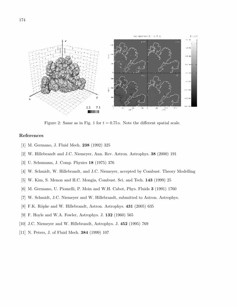
174

Figure 2: Same as in Fig. 1 for t = 0.75 s. Note the different spatial scale.

References

[1] M. Germano, J. Fluid Mech. 238 (1992) 325

[2] W. Hillebrandt and J.C. Niemeyer, Ann. Rev. Astron. Astrophys. 38 (2000) 191

[3] U. Schumann, J. Comp. Physics 18 (1975) 376

[4] W. Schmidt, W. Hillebrandt, and J.C. Niemeyer, accepted by Combust. Theory Modelling

[5] W. Kim, S. Menon and H.C. Mongia, Combust. Sci. and Tech. 143 (1999) 25

[6] M. Germano, U. Piomelli, P. Moin and W.H. Cabot, Phys. Fluids 3 (1991) 1760

[7] W. Schmidt, J.C. Niemeyer and W. Hillebrandt, submitted to Astron. Astrophys.

[8] F.K. Ropke and W. Hillebrandt, Astron. Astrophys. 431 (2005) 635

[9] F. Hoyle and W.A. Fowler, Astrophys. J. 132 (1960) 565

[10] J.C. Niemeyer and W. Hillebrandt, Astrophys. J. 452 (1995) 769

[11] N. Peters, J. of Fluid Mech. 384 (1999) 107

175

The FEARLESS Cosmic Turbulence Project

J.C. Niemeyer1, W. Schmidt1, C. Klingenberg2

1 Lehrstuhl fur Astronomie, Universitat Wurzburg, Am Hubland, D-97074 Wurzburg, Germany2 Institut fur Angewandte Mathematik und Statistik, Universitat Wurzburg, Am Hubland,D-97074 Wurzburg, Germany

Abstract

We plan to develop, implement, and apply a new numerical scheme for modeling turbulent, multiphaseastrophysical flows such as galaxy cluster cores and star forming regions. The method combines thecapabilities of adaptive mesh refinement (AMR) and large-eddy simulations (LES) to capture localizedfeatures and to represent unresolved turbulence, respectively; it will therefore be referred to as FluidmEchanics with Adaptively Refined Large- Eddy SimulationS or FEARLESS. Recent advances inthe field of dynamical subgrid-scale (SGS) models for LES of thermonuclear supernovae enable us toformulate a self-consistent SGS model on adaptive meshes based on local similarity arguments forturbulent transport. Continuing our promising first tests, we intend to implement a full dynamicalSGS model into the existing AMR hydrocode enzo, followed by simulations of turbulent star formingclouds and galaxy cluster turbulence.

Turbulence in astrophysical phenomena

Many problems of astrophysical hydrodynamics share two important attributes: First, the ubiquitouspresence of spatially localized features such as shocks, clumps, or composition discontinuities thatneed to be numerically resolved or at least adequately modeled; and second, large Reynolds numbersof the baryonic component indicating that fully developed, i.e. space-filling, turbulence is responsiblefor the mixing and dissipation properties of the gas almost everywhere. Despite great advances incomputational fluid dynamics, an accurate handling of both aspects has so far proven to be verydifficult as specialized numerical techniques have seemed to be mutually incompatible.

Our project aims at significantly improving this situation. The following three fields are amongthe most important problems of theoretical astrophysics that our approach may contribute to.

Turbulence in star formation

The efficiency, initial mass function (IMF), and feedback of star formation affects nearly every aspectof theoretical astrophysics. It is well known that turbulence plays a key role in the fragmentation ofself-gravitating gas and in its support against gravity [1, 2]. The contribution of turbulence to thestatistical properties of the IMF by turbulent fragmentation [3, 4] and to the transport of angularmomentum during the collapse [5] are at the center of current theoretical and computational investi-gations. Furthermore, planned facilities such as alma and jwst will enable us to observe the earliestepochs of star formation in the universe.

The irregular shapes of molecular clouds and their complex emission line profiles indicate thatthe gas motions are supersonic and vigorously turbulent. Supersonic turbulence produces localizedstructures such as shocks and clumps which are amplified by gravity and cooling instabilities. Resolvingthese features while simultaneously accounting for the presence of low-amplitude turbulence elsewhereis one of the most challenging problems of computational astrophysics. Many simulations of turbulentstar formation have used the Lagrangian method of smoothed particle hydrodynamics (SPH) (see

176

[2] for a review) whose capabilities for modeling turbulence are limited, however, as a result of itsnumerical diffusivity.

Only recently has adaptive mesh refinement (AMR) been employed for modeling supersonic tur-bulence in gas clouds [6, 4]. This work has demonstrated the potential of AMR to simulate turbulencein principle, opening a promising new approach that we intend to follow and improve in our project.

Primordial star formation at redshifts z ≈ 30 − 40 plays a special role both theoretically andobservationally because of its relevance for the early chemical and gravitational evolution of galaxies[7]. The pioneering AMR simulations of Abel, Bryan and Norman [8, 5] have shown the importanceof angular momentum transport during the collapse and the absence of fragmentation of the centralcore. It will be interesting to see whether the effect of turbulence refinement (sec. ) in FEARLESSwill have a noticeable impact on these results. Together with supersonic self-gravitating turbulence,the collapse of a primordial gas cloud will provide a well-defined test bed for comparisons of theFEARLESS scheme with previous computations.

Turbulence in galaxy cluster cores

Understanding the evolution of the largest gravitationally bound structures in the universe has beenone of the most active and successful fields of research in modern astrophysics. On the theoretical side,much of this progress is a result of the great advances in computational cosmological hydrodynamics,i.e. the numerical modeling of self-gravitational fluids consisting of cold dark matter and baryonic gas,coupled to a variety of relevant physical processes such as radiative cooling, supernova feedback, andchemical enrichment. The core of these models usually consists of an N-body code for the gravitationalsector coupled to an Eulerian hydro solver. Great progress has been made regarding the resolutionof localized structures using adaptive mesh refinement (AMR) for grid-based solvers or Lagrangianmethods like smoothed particle hydrodynamics (SPH) [9, 10, 11]. Turbulence on unresolved scales,on the other hand, has in most cases been neglected in cosmological hydrodynamical simulations.

Examples for the many reasons to improve numerical models of galaxy clusters are the search fora solution of the cooling flow problem, the explanation of the rich substructure of cool cluster coresseen with X-ray instruments such as xmm and chandra, and the fascinating prospect for directlydetecting cluster turbulence with the astro-e2 xrs high-resolution spectrometer. We will addresseach of these problems in the following paragraphs.

X-ray observations of cluster cores have detected less cool gas than predicted by cooling-flow models[12], suggesting that the mass deposition rate of cool gas is suppressed by an unknown mechanism.Various solutions for this problem have been proposed, including feedback from star formation andsupernovae [13], turbulence induced by large-scale gas motions [14], and buoyant plasma bubbles fromAGN activity [15]. We expect hydrodynamical simulations of the latter two phenomena to be greatlyimproved by using FEARLESS (due to the turbulence refinement effect, sec. ) and the level set methodfor non-diffusive interfaces, respectively.

Observations with X-ray satellites have also shown evidence of spatially localized substructurestermed “cool fronts”, “cool bullets”, and “cool filaments” in galaxy cluster cores. Their most likelyorigin is a combination of radiative cooling and star formation feedback resulting in a picture ofhierarchical mergers of cool subclusters [16]. Simulations of such structures involving multiple fluidphases separated by a numerically unresolvable interface are usually limited by the inherent diffusivityof the hydrodynamical scheme. Again, significant improvements can be expected by using interfacetracking methods such as the level set scheme proposed in our project.

Finally, the potential detection of turbulent gas motions in their X-ray spectra with the upcomingastro-e2 mission further strengthens the need for highly resolved, self-consistent simulations of clusterturbulence [17, 18]. Comparisons of observations with detailed simulations will help to differentiate

177

between the various proposed mechanisms to ameliorate the cooling flow problem summarized above,all of which are expected to give rise to turbulence.

Modeling of type Ia supernova explosions

Owing, among other things, to their potential as cosmological distance indicators, type Ia supernovaehave received widespread attention. Numerous observational campaigns are underway (e.g., the Euro-pean Supernova Collaboration [19], the essence project [20], and the Nearby Supernova Factory [21]),allowing us to compare theoretical models with observed spectra and light curves in unprecedenteddetail.

The present consensus model for supernovae of type Ia is the thermonuclear explosion of a Chan-drasekhar mass white dwarf [22]. The burning process proceeds as subsonic deflagration which isdriven by turbulence [23, 24]. The production of turbulence is a consequence of Rayleigh-Taylor in-stabilities due to the lower mass density of nuclear ash as compared to the density of unprocessedmaterial [25].

By means of massively parallel computation on present day supercomputers, the three-dimensionalnumerical simulation of type Ia supernova explosions has become feasible [26]. However, only thelargest dynamical scales can be numerically resolved because the Reynolds numbers are huge andthe corresponding number of degree of freedoms is beyond the capability of even the most powerfulcomputers today. Thus, one of the major challenges is to account for the interaction between turbulenteddies and the flame propagation on unresolved length scales. This is achieved by means of a subgrid-scale model [23].

The assumption that type Ia supernovae are the result of a pure deflagration has been challengedbecause the corresponding numerical models fail to predict certain observational features correctly.Perhaps the most severe problem is the significant amount of unburnt carbon and oxygen at low radialvelocities which occur in present deflagration models. Apart from that, the total amount of nickel andthe energy output are still short of typical observational values [27, 28]. A delayed detonation scenariohas been proposed which apparently resolves these difficulties [29, 30]. The transition from a subsonicdeflagration phase to a supersonic detonation is hypothetical, and no plausible mechanism has beenfound in the particular case of thermonuclear combustion in white dwarfs [31]. On the other hand,new developments in the area of the deflagration model suggest that highly turbulent deflagrationsmay suffice to match observational features of type Ia supernovae. In particular, advances have beenmade with more realistic initial conditions, enhanced resolution with non-static grids, and improvedsubgrid scale models [28, 32] (see also ). In any case, more powerful numerical techniques are requiredin order to settle the issue of the actual explosion mechanism.

Numerical Modeling Techniques

Adaptive mesh refinement

Considerable progress has been made in modeling as much flow structure as possible by direct nu-merical computation. The most powerful method for the treatment of non-steady flows exhibitingsignificant anisotropy and high degrees of intermittency is adaptive mesh refinement (AMR). AMRis based on Eulerian continuum mechanics with a hierarchy of grid patches to approximate the flowon various levels of resolution [33]. In localized regions developing structure on comparatively smalllength scales, a higher level of refinement is applied while smoother portions of the flow are treatedwith coarser grids. Astrophysical problems for which AMR is particularly well suited include strongshocks [34] and gravitational collapse [35] among many other applications [10]. All cases exhibit locallysteep gradients of the state variables and/or rapid spatiotemporal changes in the velocity field.

178

Only recently, first steps have been taken to explore the ability of AMR to model fully developedturbulence [6]. The authors have demonstrated that AMR can exploit the fact that dissipation isconcentrated in spatial regions of dimension less than three at any instant of time. This is true evenfor homogeneous turbulence which is commonly considered as “space filling” based on the properties ofits ensemble average. Although a detailed comparison of turbulence modeled with AMR and uniformgrid simulations remains to be done, it is already clear that AMR is one of the few candidates tosignificantly extend the range of numerically achievable Reynolds numbers.

However, in the case of astrophysically relevant Reynolds numbers unmanageable levels of refine-ment would be required in order to resolve the dissipative scales. Moreover, AMR suffers from anintrinsic inconsistency when applied to turbulent flows: As new levels of refinement are added, thevelocity on the smallest scales is initially smooth, in contrast with the physical requirement of velocityfluctuations on all scales above the viscous (Kolmogorov) scale. As sketched in fig. 1, this inconsistencywill be resolved in FEARLESS by using the subgrid-scale turbulence as an energy buffer (sec. ).

Large eddy simulations

In engineering applications as well as other fields of computational fluid dynamics, large eddy simula-tions (LES) have been in use over several decades [36]. There is no hierarchy of dynamically changinggrid patches but one static grid that may be equidistant or unstructured. The conservation laws ofhydrodynamics are solved by means of spectral or finite-volume methods. Subgrid scale eddies ofsize smaller than the grid resolution cannot be resolved by the numerical scheme. The stress exertedby subgrid scale eddies onto resolved eddies that results in the transfer of kinetic energy from largertowards smaller scales is accounted for by a heuristic model, a so-called subgrid-scale (SGS) model[37]. An exact treatment of subgrid scale turbulence is impossible due to the non-linearity in thedynamical equations which entails the fundamental closure problem in turbulence theory.

The selection of an appropriate SGS model is a notorious problem because of the considerablevariety of models that have been proposed. In astrophysical fluid dynamics, many researchers choosethe minimal solution of letting numerical dissipation drain kinetic energy from the resolved flow.Engineers and atmospheric scientists, on the other hand, have recognized that numerical dissipationis an insufficient solution at best [38, 39]. Turbulent burning in thermonuclear supernova explosionsis one of the few examples in astrophysics where a proper SGS model has been applied so far [23, 40].

LES is limited, however, in its representation of highly transient and localized phenomena. Thisproblem can be traced back to the fact that all SGS models are in some way based on the notion ofsimilarity. In other words, an LES must resolve the flow to an extent that turbulence becomes nearlyisotropic and scale-invariant towards the smallest resolved length scales. The anisotropy of the flowstemming from large-scale features, such as boundary conditions and mechanical forces, is then mostlyconfined in the range of “large eddy scales”. Under the conditions mentioned above, however, thisoften becomes infeasible using a static grid approach. In this case, AMR would do a much better jobapart from the drawback that it fails to account for small-scale turbulence.

Combining AMR and LES

Few attempts has been made so far to apply AMR in combination with a subgrid-scale (SGS) model.The outcome would be a FEARLESS scheme with locally adapting resolution (for a recent proposalalong these lines, see [41]). The central idea is to track turbulent regions in the flow and to explicitlycompute any transient or anisotropic features by means of AMR. For each grid patch, an SGS modelwith the corresponding cutoff scale must then be invoked in order to capture the effect of yet smaller,unresolved velocity fluctuations. The following conceptual and technical questions have kept thedevelopment of FEARLESS from progressing very far until now:

179

grid scale

grid scale

integral scale Kolmogorov scale

injection ofturbulence

thermalmotionsinertial range turbulence

b) standard AMR

c) FEARLESS

resolved flow smooth flow, thermal energy

resolved flow subgrid−scale turbulent energythermal energy

a) physical scales

Figure 1: Comparison of the physical length scales of fully developed turbulence (a) with the partitionbetween resolved kinetic energy, unresolved kinetic energy, and thermal energy without (standardAMR, (b)), and with (FEARLESS, (c)) an SGS model for unresolved turbulence. The arrows at thegrid scale in (b) and (c) represent the variability of the grid scale in AMR and are meant to clarifythe turbulence refinement effect.

1. How can the central similarity arguments of LES that are usually formulated in Fourier spacebe transferred to a grid with locally varying resolution?

2. How can filters be implemented self-consistently across AMR patches?

3. How does subgrid-scale turbulence propagate between regions of varying resolution?

4. How can grid refinement and derefinement be made consistent with the presence of turbulentvelocity fluctuations that become resolved or unresolved?

Owing to our experience using localized SGS models in supernova Ia research [40, 42, 43], we arenow able to answer questions 1 and 2, while 3 and 4 are currently under investigation.

We expect the most noticeable difference between FEARLESS and standard AMR simulations tobe the turbulence refinement effect related to point 4 above. Assuming the existence of a turbulentcascade on all scales above the (unresolvable) Kolmogorov length, the addition of grid patches mustaccount self-consistently for the kinetic energy of previously unresolved fluctuations that become a partof the resolved flow (cf. fig. 1). We intend to implement this effect by explicitly forcing fluctuations onthe newly created small scales and subtracting the corresponding amount of energy from the subgrid-scale energy of the SGS model. The inverse process of derefinement will be handled accordingly byadding the appropriate kinetic energy to the SGS energy. Hence, the SGS model can be used asan energy buffer for grid resolution changes, in addition to its usual application to mimic turbulentmixing and dynamical pressure.

In situations with a large number of refinement levels, as typically encountered in the examplesof sec. , the turbulence refinement effect can potentially become the dominant source of turbulent

180

fluctuations on small scales. This is one of our main motivations for revisiting these problems with aFEARLESS approach.

Acknowledgements

The research of JCN and WS is supported by the Alfried Krupp Prize for Young University Teachersof the Alfried Krupp von Bohlen und Halbach Foundation.

References

[1] R. B. Larson, Rept. Prog. Phys. 66, 1651 (2003), astro-ph/0306595.

[2] M.-M. Mac Low and R. S. Klessen, Rev. Mod. Phys. 76, 125 (2004), astro-ph/0301093.

[3] P. Padoan and A. Nordlund, (2004), astro-ph/0411474.

[4] P. Padoan, A. Kritsuk, M. Norman, and A. Nordlund, (2004), astro-ph/0411480.

[5] T. Abel, G. L. Bryan, and M. L. Norman, Science 295, 93 (2002).

[6] A. G. Kritsuk, M. L. Norman, and P. Padoan, Astrophys. J. Lett. (2004), astro-ph/0411626,submitted.

[7] S. C. O. Glover, (2004), astro-ph/0409737.

[8] T. Abel, G. L. Bryan, and M. L. Norman, Astron. & Astrophys. 540, 39 (2000), astro-ph/0002135.

[9] B. W. O’Shea, K. Nagamine, V. Springel, L. Hernquist, and M. L. Norman, (2003), astro-ph/0312651.

[10] M. L. Norman, (2004), astro-ph/0402230.

[11] M. L. Norman, (2004), astro-ph/0403079.

[12] H. Bohringer, K. Matsushita, E. Churazov, Y. Ikebe, and Y. Chen, Astron. & Astrophys. 382,804 (2002).

[13] G. M. Voit and G. L. Bryan, Nature 414, 425 (2001).

[14] Y. Fujita, T. Matsumoto, and K. Wada, (2004), astro-ph/0407368.

[15] M. Bruggen and C. R. Kaiser, Nature 418, 301 (2002).

[16] J. O. Burns, P. M. Motl, M. L. Norman, and G. L. Bryan, (2003), astro-ph/0309836.

[17] R. A. Sunyaev, M. L. Norman, and G. L. Bryan, Astronomy Letters 29, 783 (2003).

[18] Y. Fujita, T. Matsumoto, K. Wada, and T. Furusho, (2004), astro-ph/0412353.

[19] S. Benetti et al., Mon. Not. Roy. Astr. Soc. 348, 261 (2004).

[20] T. Matheson et al., (2004), astro-ph/0411357.

[21] W. M. Wood-Vasey et al., New Astronomy Review 48, 637 (2004).

[22] F. Hoyle and W. A. Fowler, Astrophys. J. 132, 565 (1960).

181

[23] J. C. Niemeyer and W. Hillebrandt, Astrophys. J. 452, 769 (1995).

[24] W. Hillebrandt and J. C. Niemeyer, Annu. Rev. Astron. Astrophys. 38, 191 (2000).

[25] A. M. Khokhlov, Astrophys. J. 449, 695 (1995).

[26] M. Reinecke, W. Hillebrandt, and J. C. Niemeyer, Astron. & Astrophys. 391, 1167 (2002).

[27] V. N. Gamezo, A. M. Khokhlov, E. S. Oran, A. Y. Chtchelkanova, and R. O. Rosenberg, Science299, 77 (2003).

[28] F. K. Ropke and W. Hillebrandt, Astron. & Astrophys. (2004), astro-ph/0408296, submitted.

[29] A. M. Khokhlov, Astron. & Astrophys. 245, 114 (1991).

[30] V. N. Gamezo, A. M. Khokhlov, and E. S. Oran, Physical Review Letters 92, 211102 (2004).

[31] J. C. Niemeyer, Astrophys. J. 523, L57 (1999).

[32] W. Schmidt, J. C. Niemeyer, and W. Hillebrandt, A novel flame speed model for turbulentdeflagration in type Ia supernovae, in preparation, 2005.

[33] M. J. Berger and J. Oliger, J. Comp. Physics 53, 484 (1984).

[34] M. J. Berger and P. Colella, J. Comp. Physics 82, 64 (1989).

[35] B. W. O’Shea et al., Introducing Enzo, an AMR Cosmology Application, in Adaptive MeshRefinement - Theory and Applications, edited by T. Plewa, T. Linde, and V. Weirs, SpringerLecture Notes in Computational Science and Engineering, 2004, astro-ph/040304.

[36] M. Lesieur and O. Metais, Annu. Rev. Fluid Mech. 28, 45 (1996).

[37] P. Sagaut, Large Eddy Simulation for Incompressible Flows (Springer, 2001).

[38] P. J. Mason, J. Atmos. Sci. 46, 1492 (1988).

[39] J. C. R. Hunt, J. C. Kaimal, and J. E. Gaynor, Q. J. R. Meteorol. Soc. 114, 827 (1988).

[40] W. Hillebrandt et al., Simulations of Turbulent Thermonuclear Burning in Type Ia Supernovae,in Analysis and Numerics of Conservation Laws, edited by G. Warnecke, Springer-Verlag, 2004,astro-ph/0405209.

[41] S. M. Mitran, A comparison of adaptive mesh refinement approaches for large eddy simulation,online http://www.amath.unc.edu/Faculty/mitran/amrles.html.

[42] W. Schmidt, Turbulent Thermonuclear Combustion in Degenerate Stars, PhD thesis, Fac-ulty of Physics, Technical University of Munich, 2004, online http://tumb1.biblio.tu-muenchen.de/publ/diss/ph/2004/schmidt.html.

[43] W. Schmidt, W. Hillebrandt, and J. C. Niemeyer, Level set simulations of turbulent thermonucleardeflagration in degenerate carbon and oxygen, submitted to Combust. Theory Modelling, 2004.

182

References related to further contributions

The following references are directly related to further contributions given as oral presentations duringthe workshop.

1. Francois Daviaud SPEC, CEA/SaclayF-91191 Gif sur Yvette cedex, Francee-mail: daviaud@drecam.saclay.cea.fr

M. Bourgoin, L. Marie, F. Petrelis, C. Gasquet, A. Guigon, J-B. Luciani, M. Moulin, F. Namer,J. Burguete, A. Chiffaudel, F. Daviaud, S. Fauve, P. Odier, J.-F. Pinton. MHD measurementsin the von Karman sodium experiment Phys. Fluids 14, 3046 (2002).

F. Petrelis, M. Bourgoin, L. Marie, J. Burguete, A. Chiffaudel, F. Daviaud, S. Fauve, P. Odierand J.-F. Pinton Nonlinear magnetic induction by helical motion in a liquid sodium turbulentflow. Phys. Rev. Lett. 90, 174501 (2003).

J. Burguete, L. Marie, F. Daviaud and J. Leorat Homogeneous dynamo: numerical analysis ofexperimental von Karman type flows Eur. Phys. J. B 33, 469 (2003).

2. Berengere Dubrulle

Groupe Instabilite et TurbulenceCNRS, Service d’Astrophysique, CE Saclay, Lorme des Merisiers, 709F-91191 Gif sur Yvette Cedex, France, e-mail: bdubru@drecam.saclay.cea.fr

F. Hersant, B. Dubrulle, and J.-M. Hure, Turbulence in circumstellar disks Astron. & Astrophys.429, 531-542 (2005).

Berengere Dubrulle, Olivier Dauchot, Francois Daviaud, Pierre-Yves Longaretti, Denis Richard,Jean-Paul Zahn Stability and turbulent transport in Taylor-Couette flow from analysis of exper-imental data, to appear in Physics of Fluids (2005).

3. Sergei Fedotov

School of Mathematics, The University of Manchester, M60 1QD UKe-mail: s.fedotov@manchester.ac.uk

Sergei Fedotov, Matthias Ihme, and Heinz Pitsch Stochastic mixing model with power law decayof variance, Phys. Rev. E. 71, 016310 (2005)

4. Dirk Olbers

Alfred Wegener Institute for Polar and Marine ResearchPostfach 120161, 27515 Bremerhaven, Germanye-mail: dolbers@awi-bremerhaven.de

Interpreting eddy fluxes Carsten Eden, Richard J. Greatbatch, and Dirk Olbers re-submitted toJour. Phys. Oceanogr. (2005).

183

5. Lars Umlauf

Physical Oceanography and Instrumentation, Baltic Sea Research Institute Warnemundeaddress: P.O. Box 301161, D-18112 Rostock-Warnemunde, Germanye-mail: lars.umlauf@io-warnemuende.de

Burchard, H., and K. Bolding, Comparative analysis of four second-moment turbulence closuremodels for the oceanic mixed layer, J. Phys. Oceanogr., 31, 1943-1968, 2001.

Umlauf, L, Modelling the effects of horizontal and vertical shear in stratified turbulent flows,Deep-Sea Res. II, 52, 1181-1201, 2005.

Umlauf, L., and H. Burchard, A generic length-scale equation for geophysical turbulence models,J. Mar. Res., 61, 235-265, 2003.

Umlauf, L., and H. Burchard, Second-order turbulence closure models for geophysical boundarylayers. A review of recent work, Cont. Shelf Res., 25, 795-827, 2005.

6. Hua Xia

Plasma Research Lab, Research School of Physical Sciences & EngineeringThe Australian National University, Canberra, ACT 0200e-mail: hua.xia@anu.edu.au

Shats M.G., Xia H., Punzmann H. Spectral condensation of turbulence in plasmas and fluidsand its role in low-to-high phase transitions in toroidal plasma, Physical Review E, 71, 046409(2005)

Further material and references given during oral presentations at the workshop by Eberhard Boden-schatz, Vittorio M. Canuto, and Constantino Tsallis can be found in a volume of the Lecture Notesin Physics Series on the main topics of this workshop (to be published in 2006). For PDF versions ofsome of these presentations see: http://www.mpa-garching.mpg.de/hydro/Turbulence/