On non-stationarity of dynamic systems

www.elsevier.com/locate/chemolab

Chemometrics and Intelligent Laboratory Systems 73 (2004) 119–129

On non-stationarity of dynamic systems

Satu-Pia Reinikainena,*, Kari Aaljokib, Agnar Hoskuldssonc

aLappeenranta University of Technology, P.O. Box 20, 53851 Lappeenranta, FinlandbNeste Engineering, P.O. Box 310, 06101 Porvoo, Finland

cTechnical University of Denmark, IPL, Bldg. 358, 2800 Lyngby, Denmark

Received 24 July 2003; accepted 25 November 2003

Available online 10 March 2004

Abstract

Past years have shown great advances in measurement instrumentation. Many chemical companies are using near infrared (NIR)

instruments for process control, because they can offer various advantages compared to traditional on-line analysers. These new instruments

use often, e.g., partial least square (PLS) models for predicting the results, and their success depends mostly on the quality of the spectra and

the models. However, there is a need for new methods that can handle data from these modern instruments. Typically, a large amount of data

is received and needs to be processed. This data usually show very low rank. Covariance structure of dynamic systems tends to vary over

time. Here some procedures to find stable solutions to linear dynamic systems with low rank are presented. Subsets of variables and samples

to be included in a model are considered. The procedures are based on the H-principle of mathematical modelling. The basic idea is to

approximate the solution by rank one parts. Each of them is found by optimising the estimation and prediction part of the model. The aim is

to balance improvement in fit and precision. Therefore, the present methods give better prediction results than traditional methods that are

based on exact solutions. Within few seconds the algorithms can provide with solutions of models having hundreds or thousands of variables.

The procedure is described mathematically and demonstrated for a dynamic industrial case. It is shown how the algorithms can provide

solutions involving NIR data for process control. The method is simple to apply and the motivation of the procedure is obvious for industrial

applications. It can be used, e.g., when modelling on-line systems.

D 2003 Elsevier B.V. All rights reserved.

Keywords: Dynamic models; H-principle; Low rank solutions; Supervision of processes; Subset selection; Partial least square (PLS)

1. Introduction only the quality of end batch. Therefore, it can also reveal

Past years have shown great advances in measurement

instrumentation. Sensors and optical instruments have be-

come very popular to measure quality characteristics of

various products, e.g., near infrared (NIR) has been adopted

for accurate on-line process control during the past 15 years

in a wide range of applications. There are several aspects

why NIR instruments are used for on-line process control.

The cost savings of NIR measurements related to improved

control and product quality is often achieved. The NIR

instrument can provide results significantly faster compared

to traditional laboratory analysis. In batch processes, it

allows to estimate the quality of the final product several

times within a manufacturing cycle, instead of analysing

0169-7439/$ - see front matter D 2003 Elsevier B.V. All rights reserved.

doi:10.1016/j.chemolab.2003.11.015

* Corresponding author. Tel.: +358-5-6212112, GSM: +358-40-

7301851; fax: +358-5-6212199.

E-mail addresses: [email protected] (S.-P. Reinikainen),

[email protected] (K. Aaljoki), [email protected] (A. Hoskuldsson).

problems early allowing early corrective actions. Also, e.g.,

safety aspects can be seen as one of the advantages due to

intrinsically safe measurement probes and fibre optics.

The NIR instrument provides a lot of data, which are

nowadays cheap to store, and to send onwards. Thus, a large

amount of data that need to be processed is received. This data

usually show very low rank. Chemometrics methods have

been found to be very useful for extracting information from

NIR spectra [1] and there is great interest for using the NIR

technology for measurements of phenomena of different

types. However, there is still a great need for new methods

that can handle data from these modern types of instruments

[2,3]. Therefore, it is important to illustrate closer the matters

concerning finding good solutions.

Here NIR data from measurements of beer [12] shall be

considered. Sixty-one spectra were measured together with

a quality measure for beer. A closer analysis by the CovProc

method revealed that it would be optimal to work with

variables (wavelengths) from 411 to 450. Thus X is here

S.-P. Reinikainen et al. / Chemometrics and Intelligent Laboratory Systems 73 (2004) 119–129120

61� 40 and the quality values Y is a 61 vector. The solution

vector B=(b1,b2,. . .,b40) is a 40-vector. PLS regression is

applied to these data. The data are auto-scaled (centred and

scaled to unit variance), and the solution vector is computed

for dimensions 1, 2 until 20 for the auto-scaled data. Thus,

20 estimates are computed for say, b1. There are no

numerical problems in computing the full rank solution

based on 40 dimensions. It would be the linear least squares

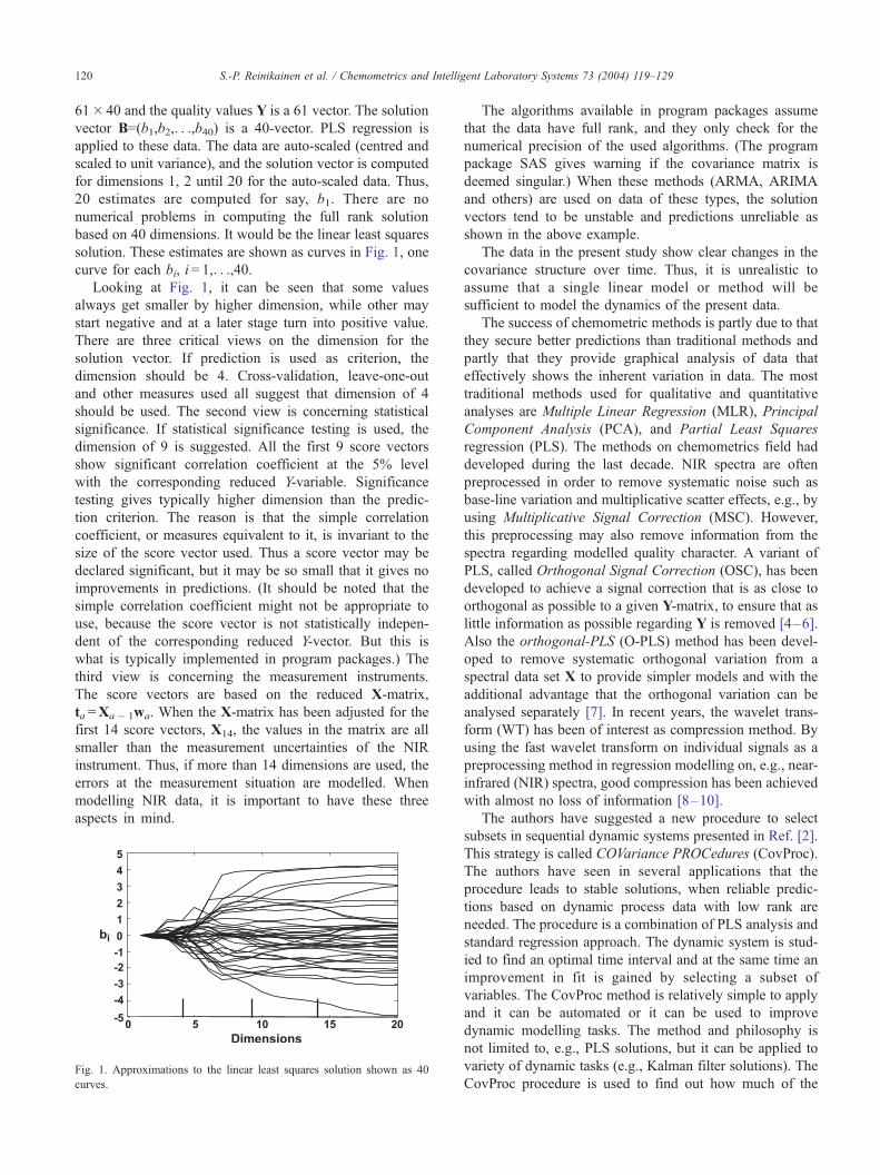
solution. These estimates are shown as curves in Fig. 1, one

curve for each bi, i = 1,. . .,40.Looking at Fig. 1, it can be seen that some values

always get smaller by higher dimension, while other may

start negative and at a later stage turn into positive value.

There are three critical views on the dimension for the

solution vector. If prediction is used as criterion, the

dimension should be 4. Cross-validation, leave-one-out

and other measures used all suggest that dimension of 4

should be used. The second view is concerning statistical

significance. If statistical significance testing is used, the

dimension of 9 is suggested. All the first 9 score vectors

show significant correlation coefficient at the 5% level

with the corresponding reduced Y-variable. Significance

testing gives typically higher dimension than the predic-

tion criterion. The reason is that the simple correlation

coefficient, or measures equivalent to it, is invariant to the

size of the score vector used. Thus a score vector may be

declared significant, but it may be so small that it gives no

improvements in predictions. (It should be noted that the

simple correlation coefficient might not be appropriate to

use, because the score vector is not statistically indepen-

dent of the corresponding reduced Y-vector. But this is

what is typically implemented in program packages.) The

third view is concerning the measurement instruments.

The score vectors are based on the reduced X-matrix,

ta =Xa� 1wa. When the X-matrix has been adjusted for the

first 14 score vectors, X14, the values in the matrix are all

smaller than the measurement uncertainties of the NIR

instrument. Thus, if more than 14 dimensions are used, the

errors at the measurement situation are modelled. When

modelling NIR data, it is important to have these three

aspects in mind.

Fig. 1. Approximations to the linear least squares solution shown as 40

curves.

The algorithms available in program packages assume

that the data have full rank, and they only check for the

numerical precision of the used algorithms. (The program

package SAS gives warning if the covariance matrix is

deemed singular.) When these methods (ARMA, ARIMA

and others) are used on data of these types, the solution

vectors tend to be unstable and predictions unreliable as

shown in the above example.

The data in the present study show clear changes in the

covariance structure over time. Thus, it is unrealistic to

assume that a single linear model or method will be

sufficient to model the dynamics of the present data.

The success of chemometric methods is partly due to that

they secure better predictions than traditional methods and

partly that they provide graphical analysis of data that

effectively shows the inherent variation in data. The most

traditional methods used for qualitative and quantitative

analyses are Multiple Linear Regression (MLR), Principal

Component Analysis (PCA), and Partial Least Squares

regression (PLS). The methods on chemometrics field had

developed during the last decade. NIR spectra are often

preprocessed in order to remove systematic noise such as

base-line variation and multiplicative scatter effects, e.g., by

using Multiplicative Signal Correction (MSC). However,

this preprocessing may also remove information from the

spectra regarding modelled quality character. A variant of

PLS, called Orthogonal Signal Correction (OSC), has been

developed to achieve a signal correction that is as close to

orthogonal as possible to a given Y-matrix, to ensure that as

little information as possible regarding Y is removed [4–6].

Also the orthogonal-PLS (O-PLS) method has been devel-

oped to remove systematic orthogonal variation from a

spectral data set X to provide simpler models and with the

additional advantage that the orthogonal variation can be

analysed separately [7]. In recent years, the wavelet trans-

form (WT) has been of interest as compression method. By

using the fast wavelet transform on individual signals as a

preprocessing method in regression modelling on, e.g., near-

infrared (NIR) spectra, good compression has been achieved

with almost no loss of information [8–10].

The authors have suggested a new procedure to select

subsets in sequential dynamic systems presented in Ref. [2].

This strategy is called COVariance PROCedures (CovProc).

The authors have seen in several applications that the

procedure leads to stable solutions, when reliable predic-

tions based on dynamic process data with low rank are

needed. The procedure is a combination of PLS analysis and

standard regression approach. The dynamic system is stud-

ied to find an optimal time interval and at the same time an

improvement in fit is gained by selecting a subset of

variables. The CovProc method is relatively simple to apply

and it can be automated or it can be used to improve

dynamic modelling tasks. The method and philosophy is

not limited to, e.g., PLS solutions, but it can be applied to

variety of dynamic tasks (e.g., Kalman filter solutions). The

CovProc procedure is used to find out how much of the

S.-P. Reinikainen et al. / Chemometrics and Intelligent Laboratory Systems 73 (2004) 119–129 121

historical data (of past time points, of lags, of variables)

should be used at each time point such that the linear model

is optimal in certain sense.

The present approach to study changes in covariance

structure is to use the H-principle of mathematical model-

ling [11]. The basic idea is to carry out analysis of non-

stationarity in steps and at each step compute a rank one

approximation to the solution. This rank one solution is

based on optimising the balance between the improvement

in fit and the associated precision that can be obtained by

such an improvement in the solution. Thus, each of the rank

one part is a result of optimisation task involving fit and

precision, such that all parts are in certain sense optimal at

the respective step of the analysis. The approach gives the

possibility of studying the variation of parameters over time

and to identify the behaviour of the dynamic system. A

collection of measures that describe the changes over time is

defined and it is shown how they can assist in improving the

predictions for the dynamic system in question.

The focus of this paper is application and extensions of

the CovProc method [2]. Here the results in Ref. [2] are

extended to situation, where there is dominant non-statio-

narity in data. It is also shown how the CovProc method can

be used in traditional statistical process control methods.

The theory is illustrated by on-line NIR data, which is used

to predict the product quality. It is shown that the proposed

approach using the CovProc approach can provide with the

precision in the predictions that are needed for these difficult

production data.

2. Models and algorithm

Suppose that there are given values of the instrumental

variables that have been collected in a matrix X. A common

assumption in standard linear regression is to assume that

the response variable can be derived linearly from X apart

from small random values that are assumed normally

distributed. It can be written as y =Xb + e, or yfN(Xb,r2I). This indicates that the residuals have the same vari-

ance, r2. The linear least squares method is concerned in

finding the value of b that minimises the measure of fit,

AXb� yA2!min. The exact solution, b1, to this task is

given by b1=(XTX)� 1XTy. Sometimes there is a requirement

that the solution vector in some sense should be as small as

possible. This can be included in the optimisation task as

minimising the sum bTUb +AXb� yA2!min. The exact

solutions are b2=(XTX +U)� 1XTy. The matrix U can be the

unity matrix, I, a constant times the unity matrix, kI, the

covariance matrix for the b’s or some other positive definite

matrix. A common choice for U is kI, where the constant k is

chosen by some external condition, e.g., the value that gives

the smallest leave-one-out predictions. This is used in the

Ridge Regression method. In the algorithm below

S =XTX +U, where U is any positive semidefinite matrix.

Very many methods in process control can be ‘mapped’ into

the algorithm that is considered in this paper by appropriate

choices of the U matrix.

The literature on dynamic modelling is large, and there

are several statistical program packages available for dy-

namic modelling. However, many of these present the

dynamic modelling from statistics point of view, but the

procedures are not often satisfactory, when an industrial data

set that has reduced rank is considered. The basic reason is

that the procedures compute the exact (unbiased) solutions.

It is expected that the users carry out a significance testing

in order to reduce the model appropriately. It is also

assumed that the data fit well except for some small random

noise, which is not necessarily true when an industrial data

set is involved. Also the fact that the industrial data often

have singular or almost singular covariance matrix causes

unstable solutions. These questions and CovProc procedures

have been considered closer in Refs. [2,3].

The basic idea of the CovProc approach is to build on

relatively few but reliable components. It is based on the H-

principle of mathematical modelling that shall be considered

closer. H-principle is a recommendation of how one should

carry out the modelling procedure for any mathematical

model:

(1) Carry out the modelling in steps. You specify how you

want to look at the data at this step by formulating how

the weights are computed.

(2) At each step compute expressions for (i) improvement

in fit, DFit, and (ii) the associated prediction,

DPrecision.

(3) Compute the solution that maximises the product

DFit�DPrecision.

(4) In case the computed solution improves the prediction

abilities of the model, the solution is accepted. If the

solution does not provide this improvement, it stops.

(5) The data are adjusted for what has been selected and

start again at (1).

The main motivation for this approach is the prediction

aspect of the model. When a new sample, x0, is available,

the response values Y(x0) are estimated from the regression

equation. The prediction variance for the estimated response

values for a standard regression model is,

VarðYðx0ÞÞ ¼ ½YTðI � XðXTXÞ�1XTÞY�

� xT0 ðXTXÞ�1x0=ðN � KÞ

Assuming normal distribution, (XTX)� 1 and [YT(I�X

(XTX)� 1XT)Y] are stochastically independent, hence both

must to be modelled, if one wants to control the prediction

variance. The H-principle suggests that a weight vector

w that gives us a solution of step 3 should be found [11].

In the CovProc approach, the basic idea is to follow the

H-principle and carry out the modelling task in steps. At

each step a score vector t as t =Xw is computed. The


CovProc method is concerned with finding an optimal

weight vector w. In Ref. [12] it was shown that each step

in PLS regression consists of two independent parts. The

first is to find the weight vector w. This is done by finding

the eigenvector associated with the largest eigenvalue of the

eigenvalue task: XTYYTXw = kw. The second part is to

compute the score vector, loading vector, change in regres-

sion coefficients and other things. Finding the weight vector

w is specific for the PLS regression. Most other types of

linear regression can be obtained by appropriate choices of

the weight vector. This property is used in the CovProc

method. The starting point is the weight vector found by the

eigenvalue task. The values of the weight vector w are

sorted according to the numerical values. Starting with the

numerically largest weight the score vector is computed. It

is checked how well it performs. Then the weight vector is

expanded with the second largest weight and a new score

vector is computed. This is continued until all values of the

eigenvector have been used. The weights chosen are the

ones that give optimal score vector. Here it is the size of the

improvement in fit AYTtA2/(tTt). The procedure can be

viewed as follows: ‘‘The matrix X is expanded by adding

new columns that correspond to the largest weights. It is

expanded until a maximal improvement in fit is obtained,

when the weights come from the eigen system. This is

carried out for each score vector’’. The matrix X is also

expanded by adding rows (samples). The results of the

CovProc method is thus that at a given time point, a certain

amount of variables should be used and a given amount of

previous samples should be used.

The CovProc method here is formulated in terms of a

general covariance matrix S =XTX +U, where U is any

positive semidefinite matrix. As mention above, it can be

shown that many of the linear methods that are used in

process control (e.g., Kalman filter method) can be formu-

lated as special choices of the U matrix. Thus the present

algorithm extends the CovProc approach to different process

control methods. In the present study, the authors have

experimented with different types of updating methods like

Kalman filter methods, but the main emphasis for the

company that provided with the data are simple predictions.

The authors found that the best predictions were obtained,

when U was chosen as 0, U = 0. Therefore, the case study

only contains the results for U = 0. The algorithm in Ap-

pendix A is formulated for general U.

The steps of the CovProc method are summarised in

Appendix A. The algorithm that the authors have used for

the case study is also given. In the appendix, some of the

numerical properties of the algorithm are also shown. It

should be emphasised that the modelling task consists of

two steps. The first step is to find the weight vector w. PLS

regression selects the weight vector as an eigenvector. Other

regression methods are based on other choices for the

weight vector. In the CovProc method, the starting points

are the weights found by the PLS method. By sorting the

weights, the columns (variables) of X are found that are

reliable to work with. On the basis of the order found, the

weights are determined such that maximal fit is obtained.

When such a weight vector has been found, the score

vector t is computed. The regression is carried out using this

score vector. The X is adjusted for this score vector, and the

analysis continues again to find an optimal weight vector at

this step [2]. In case there are many variables, it is often

necessary to be careful in finding the weight vector w. A

collection of methods has been developed that optimise the

choice of w [2]. In CovProc method, two main aspects are

considered: (1) a large score space should be achieved, and

(2) the model should give as good fit as possible.

As already discussed, the procedure is basically indepen-

dent of the specific model in question. The present method

can easily be applied to several subspace methods, which

present an important collection of methods for analysing

dynamic systems [13]. Also, time dependent models [14],

(Kalman filtering, Bayesian methods, time series analysis)

can use the present method to improve the modelling task.

3. Analysis of non-stationarity

The algorithms proposed to analyse the systems are often

illustrated with simulated data. However, when applying the

methods to industrial data, the results and particularly the

predictions are often worse, because there are often more

features in the data than specified by the model. Therefore,

the procedure is best illustrated by an industrial case study.

The NIR data originate from an oil refinery and, in the

present example, it is used to model one product quality

variable. The data include spectra from one NIR instrument

measured during a relatively long time period (Fig. 2) and it

represents a reasonable amount of process variation and

shows several cases of effects of sample handling problems

on spectra. Only a data set from one NIR instrument and one

regularly determined quality variable were selected to dem-

onstrate the procedures. However, there are seven on-line

NIR instruments at the plant, and they provide about 7000

spectra daily. Based on the NIR data over 200 models are

used to estimate approximately 85,000 different values,

which are used for automatic on-line process control.

Accurate process control depends on the availability of the

reliable on-line continuous data and the reliable estimates.

Therefore, the mathematical procedures should be automat-

ed and provide the accurate estimates within few seconds

for process optimisation.

In the present example, the non-stationarity analyses are

described by modelling only one quality variable (Y). The

variable describes content of some aromatic compounds in

the process stream. The reference Y concentrations are

determined with laboratory analysis, and they are used for

calibration. However, the on-line sampling frequency of NIR

instrument is higher than the laboratory one. The NIR spectra

are pretreated (normalised, etc.) as it is routine at the plant. To

clarify the results and illustrations, the most informative

Fig. 2. In case study, data were measured automatically from a plant during a relative long time period.


wavelengths are preselected based on a priori knowledge of

the data. This selection of subset of wavelengths is not a

critical issue, when using the procedure suggested here. The

original data matrix X was 83� 461. A closer study of the

data suggested that besides X, also the lagged values of X,

X� 1, and the lagged value of y, y� 1 should be included. A

new X matrix was performed as [X X� 1 y� 1], and it had

82 = 83� 1 rows and 923 = 2� 461 + 1 columns. In the first

case, only the present values of spectral data were consid-

ered as description variables.

In non-stationarity analysis the first question was: how

the correlation between X and y during time? This was

answered by dividing the samples into four (time) intervals,

21, 21, 20 and 20. The first 21 samples were from the first

period and so on. Fig. 3 gives the squared correlation

coefficient between the variables and the response variable.

From the figure, it can be seen that the first 21 samples show

Fig. 3. Squared correlation coefficients with 99% confidence limit: variables on

studied.

very little correlation with the response variable. The

horizontal line corresponds to the 99% significance limit

for the correlation coefficient. It shows that for the last 20

samples there are many variables that show high degree of

correlation with the response variable.

In the process control situation, it is important to look

back and study what samples and variables that should be

used at the present situation. In the following analysis, it is

assumed that the analysis is started at the last sample and

looked back. The first task is to compute the squared

correlation coefficients for all the samples, last 75% or 62

samples, last 50% or 41 samples and last 25% or 20

samples. This is shown in Fig. 4. From the figure, it can

be seen that the first peak is broader and larger, which

indicates possibilities of improvement of the modelling task,

if only the last part of the samples is used. Note that the 99%

significance line in the lower right figure is 0.52 = 0.25 for

axis: X(t), X(t� 1) and Y(t� 1). Samples from four time intervals were

Fig. 4. Squared correlation coefficients with 99% confidence limit: variables on axis: X(t), X(t� 1) and Y(t� 1). Process was studied by looking back from the

present sample.


20 samples. When looking at the figures, the immediate

impression is that the number of samples that should be used

is somewhere between 20 and 41.

In order to give some light on how many samples back

that should be used, a sequence of PLS regression was

carried out on the data, where one sample was removed at a

time. The total number of samples was 83. A PLS regression

was carried out for samples 1 to 83, then for 2 to 83, then 3

to 83 and so on. The last PLS regression was carried out for

samples 69 to 83, i.e., for 15 samples. Fig. 5 gives the R2

values for the 69 PLS-regressions. Fig. 5 shows increasing

values of the R2 measure of fit. It can be seen that the R2

value for four components is relatively constant for the last

13 regressions. It indicates that 30 and 35 samples in the

regression analysis should be used.

Fig. 5. In order to give some light on how many samples back that should

be used, a sequence of PLS regression was carried out on the data, where

samples were removed one at a time. Total number of samples was 83.

The CovProc regression is finding the largest values of

R2 but at the same time securing as large score vectors as

possible. It may be interesting to see, what the maximal

values of R2 are, when a similar procedure is used. This is

shown in Fig. 6. It shows that a considerable improvement

is possible by finding the set of variables that should be

used at each step of the regression, when finding the score

vector. The figure shows that R2 equal 98% or more was

found for the last 30 samples or so and for fewer samples.

It also shows that there may be only three components

needed, if 30 or so samples are used. Fig. 6 also shows

that a value of R2 equal to 99.5% was obtainable for 15

samples. This result may not be reliable because the

CovProc procedure is finding the largest possible increase

Fig. 6. The CovProc regression is finding the largest values of R2 but at the

same time securing as large score vectors as possible. The highest R2 values

were obtained in a model based on 15 samples. The result should be

validated by, e.g., cross-validation.

Fig. 7. The regression coefficients, which were found by the 68 CovProc regressions presented in Fig. 6.


in the R2 value across a sequence of variables that are

specified by the weight vector found. The result must be

validated by for instance cross-validation.

It is also useful to look at the variation in the regression

coefficients of the score vectors. Fig. 7 shows the regression

coefficients that were found by the 68 CovProc regression

used in Fig. 6. Fig. 7 shows a lot of variation in the regression

coefficients. The large variation in the regression coefficients

is partly due to the search at each step for a score vector giving

maximal increase in the R2 value. The large variation in the

regression coefficients emphasises the importance of choos-

ing good data for the prediction of future samples.

As a conclusion, the figures show a lot of variation in the

numbers that are typically computed in regression analysis.

The figures also emphasise that a careful study is needed to

find the samples and variables that should be used. The

authors have not found it appropriate to define measures of

non-stationarity. It is usually better to carry out a similar

analysis as the one shown here.

4. Results and discussion

The dynamic behaviours in data are described with score

vectors of a PLS model in Fig. 8. The score vectors decom-

pose the data matrix X and they show what has been used of

it. Thus, the plots of ta versus tb show the sample (time)

variation inX data and how they can describeY. Fig. 8 reveals

that the process (samples) has been changing with the time.

The dynamic behaviour can be clearly seen. The samples

from different time periods clustered, even though there were

no clear groups found. This was seen as a sign that the

covariance structure has changed and that it could not be

expected that the same model would be valid over the whole

time period. In this case, the change should not only concern

the solution vector found in dynamic modelling, but the

whole model should be changed. The result is interpreted

with measures of fit and precision in Table 1. It can be seen

that using the whole NIR data only 92.3% of the Y variance

could be explained. The prediction error from cross-valida-

tion was 3.5. For reliable process control, this was not

accurate enough, and the modelling task had to be improved

with subset selection. The number of latent components was

selected based on cross-validation criteria and H-error.

In non-stationarity analysis the spectral variables are

sorted based on their correlation with the quality variable.

These variables are introduced to the model at blocks of five

variables. Also the samples are divided into blocks of five

samples. At each step of iteration introduced in the previous

chapter, the number of variables is increased until the

criterion is fulfilled. The number of samples is increased

and the modelling procedure is started all over again. In the

following example of non-stationarity analysis, two cases

were studied. In the first case only, the present values of

spectral data were considered as description variables and in

the second case also the lagged values (X� 1 and y� 1) were

included. The results in both cases were very similar. In both

cases, the procedures suggested that 4 latent components, 30

samples and only 15 variables (wavelengths) should be

included. With these models approximately 97% of the Y

variance could be explained. The prediction error from

cross-validation was in first case 1.4 and in second case

0.8. Thus, with the lagged values the precision (uncertainty)

on the model was improved. Both results were clearly better

Fig. 8. The score vectors (ti) interpret the time variation in X data.


than the results achieved by using whole data, and are

therefore more suitable for process control and optimisation.

The results based on the X with lagged values are shown in

Table 1. The modelling procedure can be viewed closer. Fig.

9 presents R2 values and prediction error from cross-vali-

dation, when the number of components, the number of

variables and the number of samples were increased. It can

be clearly seen that the prediction error increased, when the

number of variables or the number of samples was in-

creased. Some improvement in precision was gained by

increasing the number of latent variables. However, the

prediction error measure increased at any dimension of

model, when number of X variables or samples was

increased. This may indicate, e.g., changes in covariance

structure. The improvement in fit was mainly gained by

increasing the number of latent variables. The improvement

in fit was also dependent on number of variables and

samples. When new samples and longer time period was

introduced to the model the R2 value begun to decrease.

When new X variables were included, the fit was at first

improved. However, when the number of variables was

Table 1

(A) Results from a PLS model, in which 463 wave numbers combine the X mat

variables: (1) number of latent components, (2) variation of X used (%), (3) variat

coefficient, (6) covariance explained, (7) estimated standard deviationffiffiffiffiffiffiffiffiffiffiffiffiffiffivarðyðx

pvalidation

1 2 3 4 5 6

No. SR2(X) SR2(Y)ffiffiffiffiffiffiffiffiffiffiffiffiffiYVY

N � A

rcorr(yi, ti) AyiVtiA

(A) X includes all the NIR wave numbers

1 43.56 36.33 7.12 0.60 6.83

2 78.08 58.59 5.78 0.59 5.13

3 84.92 89.07 2.99 0.86 3.01

4 89.72 92.28 2.53 0.54 0.73

5 92.93 93.90 2.26 0.46 0.42

6 97.77 94.38 2.19 0.28 0.25

(B) Original X included the lagged values, from which 15 were selected

1 93.28 87.18 1.08 0.93 2.99

2 96.81 90.36 0.95 0.49 0.04

3 99.98 93.39 0.80 0.56 0.10

4 99.99 97.09 0.55 0.49 0.001

expanded over some certain number, the fit begun to lower.

The procedure stopped with a model with four latent

variables, in which it can be seen that the optimum model

could be combined, when the modelling task was carried out

with sample blocks containing 30 samples and 15 variables.

The R2 and precision of the model were remarkably better

than when the model with whole data with all wave

numbers and samples were computed.

When a CovProc regression model was computed based

on this analysis, i.e., by using 30 samples and 4 latent

variables, the R2 value for this model is 98.0%. In the

CovProc modelling procedure, the first step is to compute w.

Then variables starting from the highest absolute w are

sorted. After that the new X matrix according to the measure

of fit in the order of sizes of w is expanded. The criterion to

stop the subset selection is the maximum of the fit measure.

Thus, each step the solution with nonzero values of w,

which give the best fit, is extracted and X matrix is adjusted

[2]. At first step only one variable with nonzero value were

selected. However, at the second step 129 and on third step

2 nonzero values were found. This result is not studied

rix, and (B) results from non-stationarity analysis: 30 samples in block, 15

ion of Y explained (%), (4) residual standard deviation of Y, (5) correlationffiffiffiffiffiffiffiffiffiffiffiffiffioÞÞ0:75 , (8–9) estimated biases, (10) mean of prediction error from cross-

7 8 9 10

std(y(x0)) Bias Ay� yoAmedian

Bias Ay� yoAmaximum

Pred. error

7.36 4.55 16.70 9.30

6.12 3.70 18.28 6.73

3.23 1.28 7.56 4.32

2.80 1.09 6.20 3.54

2.54 0.80 4.93 4.01

2.52 0.88 3.60 4.03

1.13 0.61 3.02 1.30

1.04 0.42 2.55 1.39

0.93 0.33 1.19 0.99

0.68 0 0 0.79

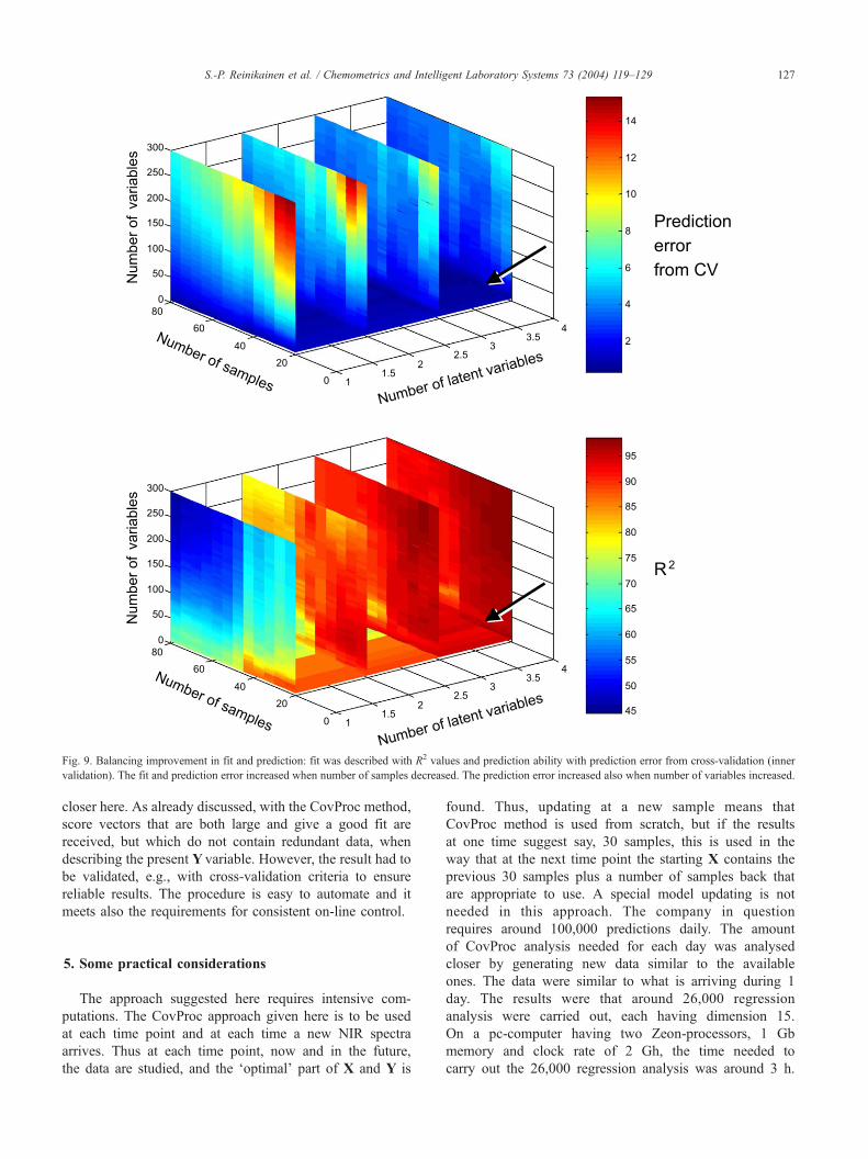
Fig. 9. Balancing improvement in fit and prediction: fit was described with R2 values and prediction ability with prediction error from cross-validation (inner

validation). The fit and prediction error increased when number of samples decreased. The prediction error increased also when number of variables increased.


closer here. As already discussed, with the CovProc method,

score vectors that are both large and give a good fit are

received, but which do not contain redundant data, when

describing the present Y variable. However, the result had to

be validated, e.g., with cross-validation criteria to ensure

reliable results. The procedure is easy to automate and it

meets also the requirements for consistent on-line control.

5. Some practical considerations

The approach suggested here requires intensive com-

putations. The CovProc approach given here is to be used

at each time point and at each time a new NIR spectra

arrives. Thus at each time point, now and in the future,

the data are studied, and the ‘optimal’ part of X and Y is

found. Thus, updating at a new sample means that

CovProc method is used from scratch, but if the results

at one time suggest say, 30 samples, this is used in the

way that at the next time point the starting X contains the

previous 30 samples plus a number of samples back that

are appropriate to use. A special model updating is not

needed in this approach. The company in question

requires around 100,000 predictions daily. The amount

of CovProc analysis needed for each day was analysed

closer by generating new data similar to the available

ones. The data were similar to what is arriving during 1

day. The results were that around 26,000 regression

analysis were carried out, each having dimension 15.

On a pc-computer having two Zeon-processors, 1 Gb

memory and clock rate of 2 Gh, the time needed to

carry out the 26,000 regression analysis was around 3 h.


It shows that today the pc’s are so fast that there is not a

problem to carry out such intensive computations that are

needed here and get an answer within seconds after a new

NIR spectra has arrived.

The data received from the company had many miss-

ing values. For some data up to 40% of the data values

were missing, in some cases most of the spectra. When

much of recent data are missing, one needs to be very

careful with the modelling procedure. Therefore, in the

implementation procedure of the CovProc method there

must be considerations concerning the question if a

reliable prediction at a given time point can be made,

but otherwise there is in principle no problem in handling

missing values in a similar way as is handled by the

NIPALS algorithm. There is also another difficult issue in

the implementation of the CovProc method in the online

environment of the company. That is one that the NIR

spectra arrive at faster rate than the values of the response

variables. Therefore, it may be difficult to synchronise

precisely the two types of data, X-samples (NIR spectra)

and Y-samples (concentrations), which is required for the

modelling task.

Robustness is another important issue, because the

measurement values at the company are not always

reliable. There are many aspects of the robustness that

need to be taken into account in online operating environ-

ments. Each value in the weight vector is based on a

linear relationship between a variable and the response

variables. This can be replaced by some robust measure

of covariation. The score vector is a sum of the weighted

variables (wixi). Other choices than the sum can be used

which also can be used in computing predicted score

values. When a score vector has been found, there can be

used different measures to express the relationship be-

tween the score vector and Y. There is not any problem

in incorporating these more robust measures in the

CovProc method in order to make the weight vector,

the score vector and the relationship more robust, but

these robustness considerations are outside the scope of

this paper.

6. Conclusions

In the last decade, both the amount and the complex-

ity of generated data have increased remarkably. Extract-

ing useful and valuable information from these data is a

complicated task. Without control of the data, it is very

likely to be drowned in the data. When the number of

analysers and measurements increases, it becomes obvi-

ous that some automated system and continuous valida-

tion are absolutely necessary. Particularly for on-line

control reliable predictions for response variables and

stable solutions that can be automated are wanted. In

the present industrial case, the solution that can provide

100,000 reliable estimates every day is desired. This

paper applies the CovProc method to select both sub-

systems of variables and optimal timeframe in order to

model non-stationary systems. The procedures presented

here provide with solutions that give acceptable predic-

tions for on-line control using the NIR instruments. The

methods were found to work well with NIR data con-

taining over 1000 variables and very low rank. In spite

of the massive number of variables, the procedures are

numerically very fast, and there are no problems, numer-

ically or time-wise, in providing with all the daily

predictions that are needed and as fast as required for

on-line control. The use of reliable advanced process

control can be a huge benefit to those who choose to

use this technology. It will result in a more robust

process, better products, more uniform results, and a

huge cost savings for the manufacturer.

Appendix A. CovProc method in steps

In order to simplify the reading of this paper, the basic

steps of the CovProc method are given here. For further

details of the steps see Ref. [2]. The method starts with Y

matrix and X matrix, in which the lags may have been

included. The matrices have been divided into subsets of

samples based on some other criteria. For each of the sample

subsets the CovProc procedure is carried out in steps to

select the subset from X matrix:

1. Carry out the PLS regression. Find weights for a PLS

component, w.

2. Arrange weights according to their absolute values, AwA.3. Include the variables stepwise starting from the highest

AwA. At each step, compute the corresponding wr, tr, and

the measure of fit: AY’trA2/(tr’tr).

wr ¼ ð0; . . . ; 0;wi; 0; . . .wj; . . . 0;wK ; 0 . . .Þ and tr

¼ Xwr:

The nonzero values in wr are the r numerically largest

values. Select variables based on the maximum of the fit

measure found, for r= 1,2,. . .,K, where K is the number

of X-variables. The w’s are computed as wi =YVxi.4. Adjust the X by corresponding score vector (tr).

5. Start over at (1) to select more variables.

The algorithm in analysis of non-stationarity is as follows:

The method begins with the same X and Y matrices as

found by CovProc method.

(0) Initialise variables. X0 =X, S0= S, Y0 =Y, E0= IK,B=0.For a=1,2,. . ., K.(1) Find the weight vector wa.

wa is the left eigenvector of (XTY) associated withthe largest singular value.


(2) Compute

loading vector pa: pa= Sa� 1wa,score vector ta=Xa� 1wa,scaling constant da: da=1/wa

TSa� 1wa.(3) Transformation vectors va:

va ¼ Ea�1wa;

Adjust transformation matrix: Ea =Ea� 1� davapaT.

(4) Compute new solution coefficients B:

qa ¼ ðXTYÞTva:

Ba ¼ Ba�1 þ davaqTa ;

(5) Adjust S: Sa = Sa� 1� dapapaT.

(6) Adjust covariance: (XTY)=(XTY)� dapaqaT.

(7) Adjust X: Xa=Xa� 1� datapaT.

(8) Adjust Y: Ya =Ya� 1� dataqaT.

(9) Check if this step has improved the prediction aspect of

the model, and if ka or da are not too small. If it pays to

continue, start a new iteration at 1.

The steps 7 and 8 are not necessary. The score vectors

can be computed afterwards as T=XV. The covariance

(XTY) need not be equal to Xa� 1T Ya� 1. The covariance

is the right hand terms in the set of linear equations. The

results of this algorithm are expansions of the matrices as

follows:

X ¼ d1t1pT1 þ d2t2p

T2 þ . . .þ dAtApT

A þ . . .þ dKtKpTK

¼ TDPT:

S ¼ d1p1pT1 þ d2p2p

T2 þ . . .þ dApApT

A þ . . .þ dKpKpTK

¼ PDPT:

S�1 ¼ d1v1vT1 þ d2v2vT

2 þ . . .þ dAvAvTA þ . . .þ dKvKvT

K

¼ VDVT:

B ¼ d1v1qT1 þ d2v2qT

2 þ . . .þ dAvAqTA þ . . .þ dKvKqT

K

¼ VDQT:

Here the vectors are collected in a matrix, e.g.,

T=(t1,t2,. . .,tK). D is a diagonal matrix with da’s in the

diagonal. The decomposition of S is a rank one reduction,

meaning that the rank of say, Sa is one less than that of

Sa� 1. (Follows from Sawa = 0). Thus SK will be the zero

matrix. The matrix V satisfies VTP=D� 1, or viTpj = dij/di,

where dij = 0 for i p j and 1 for i = j. It can also be written as

(VD1/2)T(PD1/2) = I or VDPT = I. The score vectors (ta) are

not orthogonal, tiTtj p 0 for i p j. The idea of the algorithm is

simultaneously to decompose S and approximate S� 1 with

the aim to optimise the quality of the predictions derived

from the model.

This algorithm is carried out for each time point t.

These equations can be applied to several linear dynamic

procedures [3]. If S =XTX, the algorithm reduces to PLS

regression. In that case the score vectors become orthog-

onal, TTT=D� 1.

One can view the algorithm as an approximation,

B ¼ S�1XTY ¼ ðd1v1vT1 þ . . .Þðd1p1t�T1 þ . . .Þ

Y ¼ ðd1v1tT1 þ . . .ÞY ¼ ðd1v1qT1 þ . . .Þ:

Note that only A terms in the expansions are used. The

choice of the weight vector w at each step reflects the

covariance that is left. The expansion stops, when there is no

covariance left, XaTYai0. The algorithm works with four

sets of vectors. The weight vectors W are found such that at

each step the prediction of the model is optimised. The score

vectors T show the variation in X that is used for the

solution found. The loading vectors P show how S has

been decomposed. Finally, the transformation vectors V

show how the loading vectors are derived from S, P= SV.

These vectors can be used in graphical analysis, when

studying dynamic behaviour in process [3].

References

[1] M. Blanco, I. Villarroya, NIR spectroscopy: a rapid-response analy-

tical tool, Trends Anal. Chem. 21 (4) (2002) 240–250.

[2] S.-P. Reinikainen, A. Hoskuldsson, COVPROC method: strategy in

modeling dynamic systems, J. Chemom. 17 (2003) 130–139.

[3] S.-P. Reinikainen, K. Aaljoki, A. Hoskuldsson, Analysis of linear

dynamic systems of low rank, Comp. Chem. Eng. (2003) (submitted

for publication).

[4] S. Wold, H. Antti, F. Lindgren, J. Ohman, Orthogonal signal correc-

tion of near-infrared spectra, Chemom. Intell. Lab. Syst. 44 (1998)

175–185.

[5] A. Hoskuldsson, Subset selection in PLS regression, Chemometr.

Intell. Lab. Syst. 55 (2001) 23–38.

[6] S. Wold, J. Trygg, A. Berglund, H. Antti, Some recent develop-

ments in PLS modelling, Chemom. Intell. Lab. Syst. 58 (2) (2001)

131–150.

[7] J. Trygg, S. Wold, Orthogonalized projections to latent structures

(O-PLS), J. Chemom. 16 (3) (2002) 119–128.

[8] J. Trygg, S. Wold, PLS regression on wavelet compressed NIR spec-

tra, Chemom. Intell. Lab. Syst. 42 (1998) 209–220.

[9] L. Eriksson, J. Trygg, E. Johansson, R. Bro, S. Wold, Orthogonal

signal correction, wavelet analysis, and multivariate calibration of

complicated process fluorescence data, Anal. Chim. Acta 420

(2000) 181–195.

[10] J. Trygg, N. Kettaneh Wold, L. Wallbacks, 2-D wavelet analysis and

compression of on-line industrial process data, J. Chemom. 15 (2001)

299–319.

[11] A. Hoskuldsson, Prediction Methods in Science and Technology,

Thor Publishing, Copenhagen, 1996, ISBN 87-985941-0-9.

[12] A. Hoskuldsson, PLS regression methods, J. Chemom. 2 (1988)

211–228.

[13] P. Van Overschee, B. De Moor, Subspace Identification for Linear

Systems, Kluwer Academic Publishing, Dordrecht, 1996.

[14] R.E. Kalman, A new approach to linear filtering and prediction prob-

lems, J. Basic Eng. (1960 March) 35–45.

On non-stationarity of dynamic systems

Documents

Transcript of On non-stationarity of dynamic systems