The Dynamic Effects of Hurricanes in the US: The Role of

Non-Disaster Transfer Payments

Tatyana Deryugina

May 2011 CEEPR WP 2011-007

A Joint Center of the Department of Economics, MIT Energy Initiative and MIT Sloan School of Management.

The Dynamic Effects of Hurricanes in the US: The Role ofNon-Disaster Transfer Payments

Tatyana Deryugina�

Massachusetts Institute of Technology

The most recent version can be found at http://econ-www.mit.edu/�les/6166

May 20, 2011

Abstract

We know little about the dynamic economic impacts of natural disasters. I examine the effect ofhurricanes on US counties' economies 0-10 years after landfall. Overall, I �nd no substantial changesin county population, earnings, or the employment rate. The largest empirical effect of a hurricaneis observed in large increases in government transfer payments to individuals, such as unemploymentinsurance. The estimated magnitude of the extra transfer payments is large. While per capita disaster aidaverages $356 per hurricane in current dollars, I estimate that in the eleven years following a hurricane anaffected county receives additional non-disaster government transfers of $67 per capita per year. Privateinsurance-related transfers over the same time period average only $2:4 per capita per year. Theseresults suggest that a non-trivial portion of the negative impact of hurricanes is absorbed by existingsocial safety net programs. The �scal costs of natural disasters are thus much larger than the cost ofdisaster aid alone. Because of the deadweight loss of taxation and moral hazard concerns, the bene�ts ofpolicies that reduce disaster vulnerability, such as climate change mitigation and removal of insurancesubsidies, are larger than previously thought. Finally, the substantial increase in non-disaster transferssuggests that the relative resilience of the United States to natural disasters may be in part due to varioussocial safety nets.

1 Introduction

Extreme weather events are a large and growing source of negative economic shocks. Larger populationdensities, ecosystem alteration, and population movements to hazardous areas are causing real damagesfrom natural disasters to rise (Board on Natural Disasters, 1999). World insured losses have exceeded $11

�I am deeply grateful to Amy Finkelstein and Michael Greenstone for invaluable feedback and guidance. I thank MariyaDeryugina, Joseph Doyle, Kerry Emanuel, Josh Gottlieb, Tal Gross, Jerry Hausman, Daniel Keniston, Steven Levitt, Randall Lewis,Anup Malani, Gilbert Metcalf, Kevin Murphy, Jim Poterba, Mar Reguant-Rido, Julian Reif, Joseph Shapiro, and Chad Syversonfor useful discussions and feedback. I also thank participants in MIT Public Finance Lunch and Political Economy Breakfast,University of Chicago Applied Microeconomics Lunch, and Harvard Environmental Economics Lunch. A big thanks to StephanieSieber for help with spatial data. Jenna Weinstein provided excellent research assistance. Support from the MIT Energy Fellowshipand the National Science Foundation is gratefully acknowledged.

1

billion per year every year since 1987, reaching $53 billion in 2004 (Kunreuther and Michel-Kerjan, 2007).1

Economic losses between 1992 and 2001 averaged $49 billion a year (Freeman et al., 2003). Damages arelikely to continue growing as climate change is expected to increase the number and intensity of extremeevents and to change their spatial distribution (Meehl et al., 2007; Schneider et al., 2007). One estimateis that damages will reach $367 billion a year by 2050, a 750 percent increase in real terms (Freeman etal., 2003). However, the economic impacts of extreme weather are neither predetermined nor random: theydepend not only on the meteorological strength of the event, but also on the policies and infrastructure inplace (e.g. Zeckhauser, 1996). The exogenous cause of a natural catastrophe is weather, but the differencebetween an extreme weather event and a disaster is partly man-made. To date, we know very little about theeconomic impacts of natural disasters over time or the role of institutions and policy in mitigating them.Governments spend billions of dollars annually on disaster relief and mitigation programs. And, al-

though this is rarely discussed in relation to disaster policy, they also fund transfer programs designed forgeneral economic downturns, such as unemployment insurance, welfare, and food stamps. These may infact act as a buffer when an extreme weather event occurs, even in absence of direct disaster aid. Ignoringtraditional transfer programs would then attribute too much of the resilience of a developed economy to itswealth or disaster-speci�c response policies. In addition, the �scal cost of disasters will appear smaller thanit actually is.I study the county-level empirical economic effects of hurricanes, which are one of the most damaging

weather events in the US. Speci�cally, I look at the effects of hurricanes in the 1980's and 1990's fromzero to ten years after landfall. I use a simple difference-in-differences framework and focus on changesin population, earnings, employment, and various transfer payments. In addition, I semi-parametricallyestimate the post-hurricane economic dynamics, which paints a richer picture of how a county adjusts tothis negative shock. My goal is to identify the economic margins along which adjustment takes place (e.g.,population movements versus labor market changes) and to understand the role of government spendingin post-disaster economics within US counties. I interpret my estimates using a simple spatial equilibriumframework, which suggests that transfers prevent relocation and generally act as a buffer against both disasterand non-disaster negative capital shocks. Some of the results in this paper may apply to capital shocks moregenerally. The main advantages to using hurricane incidence as an indicator for a capital shock are thathurricanes are exogenous and their onset is known precisely. This is typically not the case with other typesof capital shocks.My results suggest that the potential negative economic consequences of the hurricane may be sub-

stantially mitigated through non-disaster social safety net programs. I �nd that per capita unemploymentinsurance payments are on average 22 percent higher in the eleven years following the hurricane whileoverall transfer payments are 2:1 percent higher. Correspondingly, there is no change in population, theemployment rate, or wages. In addition to the funds provided through an of�cial disaster declaration, whichaverage $356 (2008 dollars) per capita per hurricane during my study period, I estimate that in the elevenyears following a hurricane, an affected area receives transfers from the government to individuals averaging

1Unless stated otherwise, all monetary amounts have been converted to 2008 dollars using the Consumer Price Index. Uninsuredlosses are dif�cult to estimate, but a rule of thumb is that they are at least as large as the insured losses in developed countries andat least ten times larger in developing ones.

2

$67 per capita per year or about $640 per capita in present discounted value. Transfers from businesses toindividuals (mostly insurance payments) increase temporarily as well, but add only an estimated $23 to percapita transfers over the eleven years. Together, the transfers represent a large fraction of the immediatedamages, which FEMA estimates to be $1; 278 per capita for the major hurricanes during my study period.2

This suggests that non-disaster policy, in addition to disaster aid and wealth, may be an important factor inexplaining the relative resilience to natural disasters in the United States.My estimates imply that the �scal impact of natural disasters is nearly twice as large if non-disaster trans-

fers are also considered. Although in the simplest public �nance framework transfers are welfare-neutral,in practice the deadweight loss of taxation is estimated to be 12-30% of revenue (Ballard et al., 1985; Feld-stein, 1999). Finally, because transfers are not paid for by the people receiving them, they may create moralhazard problems, leading individuals to live in riskier places than they would with actuarially fair insurance.Transfers may be welfare-improving once the hurricane has occurred but their welfare implications are muchless clear in the long run.I consider the effects of hurricanes on the construction sector because it is a proxy for how post-hurricane

capital adjustment takes place. Although I do �nd positive effects on construction wages immediately afterthe hurricane, employment shrinks three to eight years after the hurricane. Nine to ten years later, there is asign of an upward movement in employment, suggesting that the decline in the construction sector may betemporary. The decline corresponds to a decrease in new single family home construction. I �nd suggestiveevidence that over time part of the construction sector activity moves to the neighboring unaffected counties.These results suggest that longer-run effects should be an important point of focus when studying the effectsof idiosyncratic regional shocks.I also �nd evidence of changes in the age structure of the county, but no change in its racial composition.

In particular, there is an increase in the fraction of population under 20 years of age and a decrease in thefraction of population 65 and older. However, the pattern of these changes is inconsistent with the transferincreases, implying that the change in transfers is not being driven by changes in the age structure.Finally, I look at heterogeneity in the impact of hurricanes by the pre-hurricane median income and

housing value of a county. I �nd quantitative as well as qualitative differences between counties in the topand bottom quartiles. Ten years after a hurricane, the increases in per capita unemployment payments andoverall transfers are substantially higher in low-housing value counties than in high-housing value counties.In addition, trend break and mean shift tests reveal that, although ten years after a hurricane there is no sig-ni�cant difference in per capita earnings changes between the bottom and top quartiles, there are differencesin their post-hurricane paths.I contribute to two main strands of the natural disaster literature. The �rst focuses on the economic

impacts of natural disasters, typically considering a single outcome or single event (Leiter et al., 2008;Brown et al., 2006) and looking at effects from one to four quarters (Strobl and Walsh, 2008) to three tofour years after the event (Murphy and Strobl, 2009). In one of the few studies to consider long-run effects,Hornbeck (2009) �nds that the US Dustbowl had persistent effects on land values and land use practices.Belasen and Polachek (2008) estimate that earnings in Florida counties affected by a hurricane increase

2Minor hurricanes, which are in my data but not in FEMA's estimates, are generally less damaging.

3

sharply and remain higher two years after the hurricane. Brown, Mason, and Tiller (2006) estimate thathurricane Katrina had a negative but temporary effect on local employment zero to six months after. Strobl(2008) estimates that coastal counties affected by major hurricanes subsequently experience lower per capitaincome growth. I add to this literature by looking at a comprehensive set of outcomes for a large sample ofdisasters over a longer time period and connecting the outcomes together in a cohesive framework.The second related strand of literature examines the importance of area characteristics, institutions and

wealth in determining disaster-related losses and deaths (Kahn, 2005; Skidmore and Toya, 2005; Nordhaus,2006). Skidmore and Toya (2002) �nd that a higher frequency of climatic disasters is correlated with higherrates of human capital accumulation. Kahn (2005) �nds that a country's institutional quality is inverselyrelated to the number of disaster-related deaths. I contribute to this literature by looking at the economiceffects of disasters rather than the damages they cause and by considering the role of transfer payments andwithin-country heterogeneity.In the most closely related study, Yang (2008) estimates the effect of hurricanes on international �-

nancial �ows and �nds that four-�fths of the estimated damages are replaced in poorer countries by bothinternational aid and remittances. In richer countries, the increase in lending by multilateral institutions isoffset by similar declines in private �nancial �ows. I contribute to this strand of literature by focusing onthe role of non-disaster transfer programs in post-disaster economics. Like Yang, I consider the impact ofhurricanes on monetary transfers but focus on within-country �ows related to social and private insurance.In addition, there is a literature considering the short-run economic effects of temperature �uctuations

(e.g. Dell et al., 2009; Deschenes and Greenstone, 2007a and 2007b; Jones and Olken, 2010) and relatingthese to climate change. Climate change is forecast to increase the intensity of hurricanes, which, all elseequal, will raise the damages they cause by more than one-for-one. In this paper, I underscore the additional�scal and long-term economic impacts which are currently not incorporated by simple measures of initialdamages. My results suggest that climate-induced hurricane intensi�cation may have larger negative conse-quences than previously thought. This in turn implies that the bene�ts of mitigation, including policies thatdiminish the effect of climate change and removal of insurance subsidies, are larger.The rest of the paper is organized as follows. Section 2 presents the conceptual framework. Section

3 provides background information on hurricanes and US federal disaster aid. Section 4 describes thesetting, data and empirical strategy. Sections 5 and 6 present and discuss the results, respectively. Section 7concludes and contains suggestions for further research.

2 Conceptual Framework

Hurricanes in the US can be thought of as negative capital shocks; except for Hurricane Katrina, they do notcause substantial loss of life in the modern US. Thus, I use a simple production function framework to guidethe discussion of the results. I describe how economic outcomes evolve following a capital shock undervarious assumptions about moving costs, capital adjustment costs and the ability of individuals to receivetransfer payments instead of working.3

3For a simple formal model and simulation results, see the online "Model Appendix": http://econ-www.mit.edu/�les/6350

4

Suppose that there are many identical locations, so that changes in one location will not have substantiveeffects on other locations. Representative �rms in each location produce a homogenous good with somestandard production function F (K;L) ; where K is capital and L is labor. Capital and labor are comple-ments. Now suppose that one location experiences a negative capital shock. Generally, what happens topopulation, labor supply, and wages depends on capital and individual mobility costs, as well as the pres-ence of unemployment insurance or other transfer programs. If capital is perfectly mobile, a capital shockwill have no effect on the equilibrium population or any other economic indicators because adjustment willbe immediate. This is regardless of whether there are individual moving costs or transfer programs.If capital is not perfectly mobile, there will be observed changes in the local economy. If individuals

face zero moving costs, there will be no change in the wage, but a decline in the population. This is intuitive:without moving costs, individuals will only stay in the area if they are at least as well off as before. Becausethe destruction of capital lowers the wage rate, all else equal, individuals will respond by decreasing theirlabor supply until the wage rate is equal to the pre-shock wage. Because of zero moving costs, decreasinglabor supply will be equivalent to moving, as individuals who were choosing to work before will simplycostlessly switch to another location. Thus, in the case where capital is not perfectly mobile but individualsare, transfers will play no role in the post-hurricane dynamics. The degree to which population falls dependson how immobile or slow-adjusting capital is.When both capital and individuals are not perfectly mobile, we expect to see a decline in the wage rate.

As long as some of the individuals have negligible moving costs, the population will also fall. Unlike inthe previous case, individuals may also decrease their labor supply without moving away, so there maybe a decline in the employment rate. The relative decline of population and labor supply depends on therelationship between moving costs and disutility of labor supply. For example, if both moving costs anddisutility of labor supply are high, the fall in the employment rate relative to the fall in population will belarger than if moving costs are low.If, in addition to imperfectly mobile capital and imperfectly mobile individuals, there are transfer pay-

ments, the population decline will be weakly smaller than without transfers, while the change in total laborsupply and the wage rate relative to the no transfer case is ambiguous. Per capita labor supply should fallmore as some individuals take the outside option of transfers instead of working. This will counteract thedecrease in wages due to the lower capital. Likewise, some individuals will chose to take transfers and re-main in the area instead of moving away.4 This implies that the net effect on total labor supply is ambiguous:although labor supply per capita is lower than in the no transfer case, there are more people remaining in thearea relative to the no transfer case.In Table 1, I summarize the predictions of this framework following a negative capital shock under

various assumptions about the mobility of capital and individuals, as well as the availability of transferpayments. If capital is perfectly mobile (Columns 1 and 2), a negative capital shock will have no effect onany economic indicators, regardless of individuals' mobility costs and transfer availability. If capital is notperfectly mobile, there are no transfers, and moving is costless (�rst row of Column 3) wages will remain

4Transfer payments can be either a decreasing function of the wage (i.e., compensate individuals living in an area for lowerwages, as in Notowidigdo, 2010) or unemployment insurance payments that the individual can choose instead of working.

5

unchanged, but population will fall. In the presence of moving costs but no transfer payments (�rst rowof Column 4), the fall in the population will be smaller, while the decline in wages will be larger. Whenthere are employment-related transfer payments but no moving costs (second row of Column 3), the fall incapital will have the exact same effect as in the no transfer case and the total amount of transfers going to anarea will remain unchanged. Finally, when there are both transfer payments and moving costs (second rowof Column 4), the fall in utility resulting from a negative capital shock will be buffered by transfers. Thepresence of transfers will lead some individuals to cease working while remaining in the area, lowering thenumber of people who leave and causing the drop in labor supply to be larger than the drop in population.The fall in wages will be smaller than in the no-transfer case.To summarize, if capital is perfectly mobile (or close to it), I expect to �nd no change in the economy

following a hurricane. If capital is somewhat immobile but individual mobility costs are negligible, I expectto �nd decreases in population but no changes in transfer payments. Finally, if capital adjustment costsand individual moving costs are both non-trivial, transfer payments �owing into the area should increase.The degree to which population falls will re�ect both the magnitude of the moving costs and the capitaladjustment costs.The presence of transfer payments weakly increases welfare for individuals living in the area relative

to the no transfer case. However, as I discuss later, whether transfer payments increase social welfare isunclear.

3 Hurricanes and Federal Disaster Aid

3.1 Hurricanes in the United States

Hurricanes that affect the US form in the Atlantic Ocean. The Atlantic hurricane season lasts from Junethrough November, with most hurricanes forming in August and September. Warm humid air over the oceancreates storms known as "tropical disturbances". If circulating winds develop, the disturbance becomes atropical cyclone. Prevailing winds and currents move the cyclone across the ocean, where it gains andloses strength based on the favorability of conditions. When cyclones encounter cold water or land, theylose strength quickly and dissipate. Sometimes a circular area with low internal wind speeds, called the"eye", develops in the system's center. Although the entire storm system can span a few hundred miles,the perimeter of the eye (the "eyewall") is where the strongest winds are found. Wind intensity declinesquickly as one moves away from the eyewall (or the center of the storm, if there is no eye). The outer partsof the hurricane are called "spiral bands"; these are characterized by heavy rains but typically do not havehurricane-force winds. Hurricanes that make it to land create widespread wind and �ood damage: physicaldamages from hurricanes in the US have averaged $4.4 billion per hurricane (2008 dollars) or $7.4 billionper year between 1970 and 2005 and $2.2 billion per hurricane or $3.7 billion per year if 2005 is excluded.5

For hurricane data, I use the Best Tracks (HURDAT) dataset from the National Oceanic and AtmosphericAdministration (NOAA).6 It contains the location of the storm center and wind speed (in six hour intervals)

5Author calculations using data from Nordhaus (2006). I use 2008 dollars throughout the paper.6Available from http://www.nhc.noaa.gov/pastall.shtml#hurdat

6

for each North Atlantic cyclone since 1851. To determine which counties the storm passed through, I assumethat the storm path is linear between the given points. Data on storm width are unfortunately not collected;this adds some measurement error. But because the eye of the hurricane is typically not very large, andcounties through which the eye passes suffer much more extensive damage (as I show later), this shouldnot be a problem for the estimation.7 Although the hurricane data span a long time period, annual county-level economic data are only available for 1970-2006. Because the main econometric speci�cation has tenbalanced leads and lags (i.e. each lead and lag is estimated using the same set of hurricanes), I estimate theeconomic effects of hurricanes that occurred between 1980 and 1996.North Atlantic cyclones are classi�ed by maximum 1-minute sustained wind speeds using the Saf�r-

Simpson Hurricane Scale. A storm is considered a hurricane if maximum 1-minute sustained wind speedsexceed 74 miles per hour. Category 3 and higher hurricanes have wind speeds greater than 111 mph and arecalled "major hurricanes". Category 1 and 2 hurricanes are "minor hurricanes", characterized by maximumwind speeds of 74 � 110 mph. A tropical storm is a cyclone with wind speeds of 39 - 73 miles per hour.Cyclones with lower wind speeds are called "tropical depressions". Between 1980 and 1996, there were onaverage 5:6 North Atlantic hurricanes per year, with at least two hurricanes each year and three years withten or more hurricanes. About a third (1.9 out of 5.6) of hurricanes are major hurricanes. Less than a third(1.5 out of 5.6) of all hurricanes that form make landfall, and about half of the landfalling hurricanes (0.7out of 1.5) are major hurricanes.US hurricanes are geographically concentrated. Most of the landfalling hurricanes over this time period

occur in Alabama, Georgia, Florida, Louisiana, Mississippi, North Carolina, South Carolina, Texas, andVirginia (hereafter the "hurricane region"). Figure 1 shows the geographic distribution of hurricane hits thatoccurred between 1980 and 1996, as well as the control counties used in subsequent analysis (selected usingpropensity score matching). Out of the hurricane region counties, 127 experience one or more hurricanesbetween 1980 and 1996 (119 experience only one hurricane). Only 19 counties outside the hurricane regionexperience any hurricanes during this time and virtually all the major hurricanes occur within the 9 stateslisted above. I therefore limit my analysis to this region. Although it may be preferable to focus on themajor hurricanes, they are relatively rare (there are only 8 between 1980 and 1996). For this reason, I focuson the 21 minor and major hurricanes that affected the hurricane region during that time.

3.2 Destructiveness of Hurricanes

In order to gauge the potential economic impact of hurricanes, it is helpful to look at the damages they causein absolute terms and relative to other US disasters.To provide evidence on the absolute level of damages caused by hurricanes, I use estimates of direct

damages from HAZUS-MH, published by FEMA.8 Table 2 shows the summary statistics of the effectsof the eight major hurricanes that affected the hurricane region between 1980 and 1996. HAZUS-MH issoftware meant to help state, local, and Federal government of�cials prepare for disasters and to help theprivate sector estimate risk exposure. The software combines scienti�c and engineering knowledge with

7See Appendix A for a discussion of the distribution of eye diameters.8Available by request from http://www.fema.gov/plan/prevent/hazus/index.shtm

7

detailed historic data to produce damage estimates that are likely to be more accurate than those madeusing simpler estimates or reports. In addition to simulating hypothetical damages, HAZUS contains highlydetailed damage estimates of past major hurricanes. These damage estimates are shown in Table 2.Panel A summarizes the estimated effects in the counties which, according to the Best Tracks data, were

in the path of the hurricane's center (I refer to these as "centrally affected" counties). On average, thesecounties suffered $406 million in damages to buildings (with a standard deviation of about $2 billion) orabout 1:46% (with a standard deviation of 3:85%) of the total building value. The maximum county-levelbuilding damage was $20 billion while the maximum loss as a percent of total building value was 23:6%:HAZUS-MH also provides estimates of non-structural losses, such as building content and inventory

losses, as well as estimates of the number of households displaced by the disaster. Total losses (includingbuilding damages) average $571 million per county with a standard deviation of $3:7 billion. The largesttotal loss on a county level over this period was $35:4 billion. On average, about 1,500 households (with astandard deviation of 10,700) are displaced as a result of a central hit by a major hurricane and 450 peoplerequire temporary shelter. Per capita total damages average $1; 280 with a standard deviation of about$3; 340:

Panel B shows the estimated effects of the hurricane on counties that are listed as affected in the FEMAsimulations but do not have the center of the storm passing through them ("peripherally affected" counties).The damage estimates are much smaller. For example, the average damage to buildings is only $8:6 millionor about 65 times smaller than the average damage in a centrally affected county. The maximum damage inperipherally affected counties is $390 million, which is smaller than the mean damage in centrally affectedcounties. The average loss ratio is 0:15%; which is about 10 times smaller than the loss ratio in centrallyaffected counties. Per capita total losses are also about 10 times smaller, averaging $113 per capita, and totallosses are about 50 times smaller. Only 12 households are estimated to be displaced, on average, and only3 people require temporary shelter. Thus, although the omission of these counties from the analysis mayintroduce some measurement error, it should not affect the estimates much.The above estimates provide evidence both on the level of a hurricane's damage and on the likely impor-

tance of including counties not directly in the storm's path. It should be noted that the damage estimates arean upper bound on the average destructiveness of the hurricanes in my sample because my sample includesminor as well as major hurricanes. Unfortunately, FEMA does not provide detailed damage estimates forminor hurricanes. A theoretical result is that the energy carried by the wind increases with the third power ofwind speed. The average maximum wind speed in a county that was centrally affected by a major hurricanebetween 1980 and 1996 is 124 miles per hour, while the average maximum wind speed in a county centrallyaffected by a minor hurricane is 86 miles per hour. If the power carried by the wind translates directly intodestructiveness, a back of the envelope calculation implies that a 124 miles per hour hurricane would causeabout three times more damage than an 86 miles per hour hurricane. This, in turn, would imply that theaverage minor hurricane in my sample caused about $190 million in total damages per centrally affectedcounty. Although this is not as large as the damage caused by major hurricanes, it is a non-trivial amountfor a local economy and may affect subsequent economic outcomes.I now address the relative damages caused by hurricanes. I regress three different damage statistics

8

on measures of hurricane strength and other natural event indicators. The regression speci�cations are asfollows:

Dct = ac + at + �1Major_hurricanect + �2Minor_hurricanect+ 1Floodct + 2Tornadoct + 3Severe_stormct + "ct

and

Dct = ac + at +5Xk=1

�k1 [Categoryct = k] + 1Floodct

+ 2Tornadoct + 3Severe_stormct + "ct

c = county; t = year

Dct is log of property damages, property damages per capita or the log of �ood insurance paymentsin that county. 9 All damage measures are in 2008 dollars. Major_hurricanect is an indicator forCategory 3, 4, and 5 storms, while Minor_hurricanect is an indicator for Category 1 and 2 storms.1 [Categoryct = k] is an indicator variable equal to 1 if the hurricane is classi�ed as a Category k hur-ricane. Because there are very few Category 4 and 5 hurricanes, I combine them in the second equation.The Flood; Tornado; and Severe_storm indicators are equal to 1 if the county was reported as havingat least one of these events over the year. These, along with hurricanes, are the most common and dam-aging meteorological events in the US. Other rarer events in the region include droughts, wild�res, andheat. Thus, the reference category is a combination of these extreme events and no reported extreme events.Finally, ac and at are county and year �xed effects.I estimate these two equations for the nine states in the hurricane region.10 The results are shown in

Table 3. Column 1 compares the log of damages for different disasters. A major hurricane increases thereported property damages by 4:2 log points or over 400%. In levels, this implies that a major hurricaneincreases the total damages in a county by about $760; 000 (2008 dollars). The next most damaging eventis a minor hurricane, which increases property damages by 2:4 log points or about $110; 000. In contrast,tornadoes, �oods, and severe storms increase property damages by 2:1 ($76; 000) ; 0:9 ($15; 000) ; and1:0 ($18; 000) log points (dollars), respectively. A similar pattern holds when the dependent variable isproperty damages per capita, although some of the point estimates become statistically insigni�cant. Thisis possibly because hurricane-prone counties are more populous. Column 4 shows the effect of hurricanesbroken down by category. As expected, Category 1 hurricanes are the least damaging, causing an extra 2:2

9Data on damages and extreme weather events other than hurricanes are from the Hazards & Vulnerability Research Institute(2009) and are based on weather service reports by local government of�cials. Data on �ood claims and liabilities are from theConsolidated Federal Funds Report (CFFR).

10The results for all US counties are similar.

9

log points of damage ($84; 000), while Category 4 and 5 storms are the most damaging, increasing propertydamages by 4:6 log points ($1; 100; 000). The least damaging hurricane is about as damaging as a tornado,and more damaging than a �ood or severe storm.An important caveat is that the damage measures are estimates made by local of�cials soon after the

occurrence of the event. Using hurricane-level damage data from Nordhaus (2006), I estimate the directdamages from hurricanes to be about $3:7 billion per year between 1970 and 2004, in 2008 dollars. Giventhat there are on average 1.5 landfalling hurricanes per year, the estimates in this section appear to understatethe per-county damage of hurricanes (and possibly of other disasters as well) by at least a factor of ten.However, as long as the damage measurements do not exhibit differential bias for hurricanes, �oods, storms,and tornadoes, these numbers are valid for comparing the relative magnitudes of the different events.Column 3 shows the effect of various extreme weather events on �ood payments. Major hurricanes

increase �ood claims by about 3:1 log points or about $1:1 million, while minor hurricanes increase themby 1:5 log points or about $190; 000. The mean insurance liability in the sample is $538 million. Torna-does have no signi�cant impact on �ood claims and the estimated effect of a severe storm is signi�cantlynegative.11 Floods increase claims by only about 0:5 percentage points.When the effect of a hurricane is broken down further, Category 3 storms are estimated to have the

largest effect, raising �ood insurance payments by about 3:1 log points. Category 1 and 2 hurricanes raise�ood-related insurance payments by 1:1 and 2:8 log points, respectively. Category 4 and 5 storms increasethem by 3 log points.The �ood insurance payments are likely to be a lower bound on total insurance payments for two reasons.

First, in addition to �ood damage, the wind associated with hurricanes creates massive damage, which iscovered by homeowner's insurance. Second, the �scal year of the US government ends on September 30th.Some �ood insurance claims originating in August and September (the peak hurricane time) may be settledin the same �scal year, while some may not appear until the following year. Despite all the caveats, theseestimates imply that hurricanes are the most destructive of the common US disasters, which makes them animportant phenomenon to study.

3.3 Federal Disaster Aid

This section summarizes US federal disaster spending between 1980 and 1996. Federal disaster aid is givento a county if the state's governor �les a request and provides evidence that the state cannot handle thedisaster on its own. The �nal decision about whether to declare a disaster is made by the US President. Ifthe request is approved, federal money can be used to repair public structures and to make individual andbusiness grants and loans. Grants to individuals are made only up to the amount of uninsured damages.The Federal Emergency Management Agency (FEMA) also provides personnel, legal help, counseling, andspecial unemployment insurance for people unemployed due to the disaster. Although there is some long-term recovery spending in extreme cases, most of the transfers to individuals occur within six months of thedeclaration and most of the public infrastructure spending occurs within two-three years (FEMA, personal

11The comparison category is not "no extreme weather event", but a combination of this indicator and other, rarer, weather events.Some of these, such as heat waves, may be more damaging than the average severe storm.

10

communication).Between 1980 and 1996, the federal government spent $6:4 billion (2008 dollars) on hurricane-related

disaster aid and $23:1 billion on other disasters.12 The bulk of the non-hurricane disaster spending ($10:1billion) was due to the Northridge earthquake in 1994. Excluding the Northridge earthquake impliesthat hurricane-related spending accounts for about a third of all disaster aid. This number includes alldeclaration-related spending by FEMA, including assistance given for infrastructure repair, individual grants,as well as mitigation spending. The Small Business Administration also offers subsidized loans to affectedindividuals and businesses, which are not included here. Spending by the state and local governments is alsoexcluded. By law, the state pays some of the cost of disaster aid, but its share cannot exceed 25%. Thus,state spending comprises at most a third of the federal spending. Unfortunately, annual county data on dis-aster spending over time is not available, so I cannot incorporate disaster spending into my main empiricalframework. However, there are data that allow me to directly compute the county-by-hurricane amount ofdisaster transfers.Table 4 shows the summary statistics for federal aid related to hurricanes between 1980 � 1996.13

Because data on federal disaster aid is provided on the level of a declaration, which includes multiplecounties in a state, an assumption about how the money is divided among counties is necessary. As I showin the previous section, counties through which the center of the storm passes experience much more damagethan peripherally affected counties. Therefore, a natural assumption is that the money is split among onlythose counties and the rest can be ignored. Another natural assumption is that the money is divided amongthe included counties in proportion to the population in each county. Panel A shows the total and per capitafederal aid transfers assuming that only centrally affected counties are given aid. The average amount ofaid given to counties experiencing hurricanes was $58:7 million. Counties experiencing major hurricanesreceived about 2.5 times as much on average, $128�133million. The standard deviations of aid for countiesthat experienced hurricanes are all larger than the mean, ranging from $187 to over $460 million. Note thatthis period excludes Hurricane Katrina and the 2004 hurricane season, in which four hurricanes affectedFlorida. Thus, even "business as usual" hurricane seasons are associated with non-trivial amounts of federalspending.Per capita spending in 1980-1996 averaged $356 per hurricane and $412 per major hurricane (2008

dollars). An extreme assumption of a uniform split across counties (which is unlikely to be true) leads to alarger per-capita average of $1; 137 per hurricane and $2; 018 per major hurricane.Panel B shows the same statistics assuming that the money is divided among all counties included in

the declaration, not just centrally affected ones. This implies spending of $8:4 � 8:9 million per county,$24:6 � 30:0 million per centrally affected county, and $59:2 � 73:4 million per county centrally affectedby a major hurricane. Per capita spending estimates range from $52 to $187 in the proportional split caseand from $160 to $954 in the uniform split case.In the results section, I use the preferred number of $356 per capita as a benchmark to compare spend-

ing by disaster relief agencies to the extra spending associated with the hurricane triggering other transfer12Data on spending are from the PERI Presidential Disaster Declarations database (Sylves and Racca, 2010).13Summary statistics for other times periods are similar, with the caveat that real spending on hurricane-related declarations is

rising over time.

11

programs.

4 Empirical Strategy

4.1 Sample of Analysis

Ideally, one would estimate the effect of hurricanes by looking at differences over time between counties inthe hurricane region that do and do not experience a hurricane between 1980 and 1996. However, �nding avalid control group is not straightforward. In Table 5, I compare characteristics and trends of counties thatdo not experience any hurricanes between 1980 and 1996 with counties that experience one hurricane.14

Columns 1 and 2 of Panel A show the 1970 characteristics of hurricane region counties that experience ahurricane between 1980 and 1996 and the difference from counties with no hurricanes. Nearly �fty percentof 119 counties that experience one hurricane are coastal, compared to forty-one percent of 811 counties thathave not had hurricanes over this period. Counties that experience hurricanes are about �fty percent morepopulous than non-hurricane counties and have lower population densities. These differences are statisticallysigni�cant (as shown in Column 3). Counties with hurricanes also have larger per unemployment insurancepayments, but smaller per capita transfers from the federal government. However, differences in levels arenot problematic because county �xed effects are included in every speci�cation. However, differences inlevels may be indicative of differences in trends. In Panel A, I test for differential trends between 1970 and1979 (before any hurricanes in the sample occur) for the time-varying characteristics. In this case, Columns 1and 2 show the trend in the hurricane counties and their difference from the trend in non-hurricane counties.Only two variables show differential trends for these two groups of counties: per capita transfers fromgovernment and per capita family assistance, both signi�cant at the 5% level.Another way to construct the control group is by requiring balance in pre-hurricane covariates and hur-

ricane risk.15 I construct a hurricane risk variable using historic (1981-1970) hurricane data. I predictcounties' propensity to be hit by hurricanes by spatially smoothing observed hurricane hits. I then usetwo-nearest neighbor propensity score matching to select a control group from the no-hurricane sample.16

Column 4 shows the difference between the hurricane counties and the propensity matched control group,while Column 5 shows the p-value of this difference. In general, propensity score matching eliminates dif-ferences in levels and trends for all variables except population, whose trend and level differences continueto be signi�cant at the 5% level. Because the sample in Column 4 is more similar to the treatment groupthan the sample in Column 2, I use the former as my preferred control group.I discuss results using other samples in the robustness section (including using only the counties that

experience a hurricane between 1980 and 1996). I show that these do not affect the estimates qualitativelyand have only a moderate quantitative effect. I also address the problem of potentially different time trends

14I omit the few counties that experience more than one hurricane between 1980 and 1996. Results are similar if counties withmore than one hurricane are included.

15Matching is based on all outcome variables, although some are not shown due to space constraints.16Using two-nearest neighbor rather than nearest neighbor matching ensures that the number of counties in the control group is

approximately equal to the number of counties in the treatment group. When nearest neighbor matching is used, some non-hurricanecounties are assigned as nearest neighbors multiple times, resulting in a control group that's much smaller than the treatment group.

12

by relying on mean shift and trend break tests.

4.2 Economic and Demographic Data

Annual county-level outcomes such as unemployment payments, population, and earnings come from eitherthe Regional Economic Information System (REIS), while sector-speci�c employment, wages and numberof establishments come from County Business Patterns (CBP). County-level population by race and ageare from Surveillance Epidemiology and End Results (SEER) population database. Data on single familyhousing starts are from McGraw-Hill. All four series span the years 1970-2006.I de�ne the employment rate as the ratio of total employment to the number of people aged �fteen

and older.17 An establishment is de�ned as a single physical location of a �rm with paid employees. Netearnings by place of residence (which I later refer to as simply "net earnings") include wage and salarydisbursements, supplements to wages and salaries, and proprietors' income, less contributions for govern-ment social insurance. Earnings do not include transfer payments. Earnings by place of work are convertedto earnings by residence by the Bureau of Economic Analysis (BEA) using a statistical adjustment. Onaverage, the construction sector represents slightly over 10% of all establishments, employees, and wages.Unemployment insurance compensation consists primarily of standard state-administered unemploy-

ment insurance schemes, but also includes unemployment compensation for federal employees, railroadworkers, and veterans. Total transfers from government to individuals include unemployment insurance. Inaddition, the category includes income maintenance (e.g., Supplemental Security Income or SSI), familyassistance, retirement and disability insurance bene�ts, medical bene�ts (Medicare and Medicaid), veter-ans' bene�ts, and federal education and training assistance. Transfers from businesses to individuals consistprimarily of net insurance settlements and personal injury liability payments to non-employees.Disaster-related transfers are technically included in the measure of total transfers from the government.

However, these are computed by assuming that national estimates are distributed in proportion to populationto all the counties in the US. Thus, these will not affect the estimation once year �xed effects are included.

4.3 Event Study Regression Framework

In this section, I outline the procedure used to estimate the economic effects of a hurricane. I �rst employan event study framework. Speci�cally, I regress outcomes on hurricane indicators 10 years before and aftera hurricane, controlling for county, year, and coastal-by-year �xed effects. It would be ideal to estimatethe effects of major and minor hurricanes separately, but there are too few major hurricanes for a preciseestimation of their effect.18 Thus, I focus on the effect of all hurricanes. The identifying assumption is that,conditional on the location and the year, the occurrence of a hurricane is uncorrelated with unobservables.This is reasonable because even forecasting the severity of the hurricane season as a whole is dif�cult,much less the paths those hurricanes will take. Although there is no cause to believe that hurricanes are

17Annual county-level unemployment rates are not available until 1990.18If I restrict the sample to estimate ten leads and lags using the same county-hurricane-year observations, I end up with less than

30 counties that experience major hurricanes. In contrast, there are 119 counties that experience a major or minor hurricane whenthe same restrictions are imposed.

13

endogenous when proper controls are included, I estimate the leads of a hurricane to test for the presence ofdifferential trends.The basic event study framework for estimating the year-by-year effect of a hurricane up to ten years

after its occurrence is:

Oct =10X

�=�10��Hc;t�� + �

�11ct + �11ct + �c + �t + 1 [coastal]�t + "ct (1)

c = county; t = year; � = lag

Oct is some economic outcome, as described in the data section. Hct is a hurricane indicator, equal to 1if the county is reported to have experienced any hurricane in year t, according to the NOAA Best Tracksdata. I normalize the effect the year before the hurricane, � = �1; to zero:

���11ct ; �11ct

are indicators for

hurricanes outside the estimation window. �c and �t are county and year �xed effects.1 [coastal]�t is a set of year �xed effects for coastal counties, as de�ned by the NOAA's Strategic

Environmental Assessments Division. Including this interaction term is necessary because coastal countiesare more likely to experience hurricanes and may experience different growth trajectories. For example, thepopulation data show that the coastal population has grown disproportionately in the past 30 years.I combine hurricane indicators into two-year bins to increase the power of the estimation.19 The com-

bined lags are years 1 and 2, 3 and 4, 5 and 6, 7 and 8, 9 and 10. The combined leads are -1 and -2, -3 and-4, -5 and -6, -7 and -8, -9 and -10. The assumption needed for this estimation procedure to be valid is thatthe effects of a hurricane for the years that are grouped together have the same sign and distribution. Year 0,which is the year that the hurricane makes landfall in a county, is not combined because the assumption thatthe effects in year 0 and year 1 are similar may not hold.

Oct = �0Hct +�1X�=�5

��2� max fHc;t�2� ;Hc;t�2��1g (2)

+

5X�=1

��2� max fHc;t�2�+1;Hc;t�2�g

+��11ct + �11ct + �c + �t + 1 [coastal]�t + "ct

The coef�cient �0 corresponds to year 0, which is the year in which the hurricane makes landfall in thecounty. For example, 1989 is year 0 for Hurricane Hugo, one of the hurricanes in my sample, and 1992 isyear 0 for Hurricane Andrew.The notation for the hurricane bins is unconventional, but straightforward. max fHc;t�2�+1;Hc;t�2�g

takes the maximum of the county's hurricane indicators in subsequent years, grouping them as describedabove. The set

P5�=1 ��2� max fHc;t�2�+1;Hc;t�2�g thus represents the causal effects of a hurricane 1-10

19Results using year-by-year hurricane indicators are qualitatively similar, but noisier. The full set of results is available uponrequest.

14

years following its occurrence. It can be written out as ��2max fHc;t�1;Hc;t�2g+��4max fHc;t�3;Hc;t�4g+::: + ��10max fHc;t�9;Hc;t�10g : The reference category is "hurricane one or two years from now", cor-responding to max fHc;t+1;Hc;t+2g : The coef�cients of interest is the set of hurricane lags

���2�

�=5�=1

and the estimated immediate impact of a hurricane, �0. The average effect of combined years -1 and -2 isassumed to be 0, so the estimated coef�cients should be interpreted as the change relative to the two yearsbefore the hurricane.I do not use damages estimates as the independent variable for several reasons. County-level property

damage estimates between 1960 and 2009 are available from the Spatial Hazard Events and Losses Database(SHELDUS).20 To my knowledge, this is the only database that contains county-level damage estimates forall hurricanes over this period of time. However, the data are estimates made by local emergency of�cialsfairly close to the time of occurrence. At best, they appear to be very imprecise, as discussed in Section3. Second, damage is not only a function of the hurricane's strength, but of local characteristics such asconstruction practices and population density, which may be correlated with economic trajectories. Finally,damages may be endogenous with respect to the variable of interests. For example, communities withlower chances of recovery may be damaged relatively more because of poor construction. The countywith heavier damages, all else equal, may be in decline or may be less prepared to deal with the disasteroverall. Alternatively, the county with larger absolute damages may be more af�uent and able to recovermore quickly (for example, because of better access to credit, coordination, or governance).Because there may be unobserved heterogeneity across hurricanes, I also restrict the sample of hurri-

canes to those for which I can estimate the full set of leads and lags. In practice, this means I am estimatingthe effects using hurricanes that occurred between 1980 and 1996. To maximize my sample size, I createindicator variables for the county 10 years before and after it experienced a hurricane that was taken out ofthe sample (i.e., counties that were affected between 1960-1979 and 1997-2006). This allows me to excludecertain county-year observations from the estimation without excluding the county completely. I also restrictmy sample to counties that have a continuous record for each outcome variable in order to avoid biasing myresults.Many of the outcome variables are autocorrelated as well as correlated with each other. Appendix

B shows the empirical auto- and cross-correlation in the outcome variables. The autocorrelation createsmulticollinearity concerns, which is why it is useful to rely on joint tests of signi�cance to determine whetherthere are signi�cant effects.

4.4 Differences in Differences Regression Framework

The basic results suggest that hurricanes may have an effect on the mean of the economic variable, its trend,or both. In addition to estimating the effect for each time period, I also test for trend breaks and meanshifts in the outcome variable. The trend break speci�cation tests for a change in the slope of the economicoutcome after the hurricane, while the mean shift speci�cation tests for a change in the mean, assuming thatthere is no change in trend. These speci�cations summarize the net effect of a hurricane more conciselyand are more powerful when the assumption of linear trends holds. In addition, if the assumption of parallel

20Hazards & Vulnerability Research Institute (2009). Available from http://webra.cas.sc.edu/hvri/products/sheldus.aspx

15

trends does not hold, the trend break test is useful for determining whether the hurricane has a signi�cantimpact on the economy.The regression equation for testing for a mean shift controlling for an overall time trend is:

Oct = �1 � 1[Hurr in past 10 years]ct + �11post11ct + ��11pre11ct (3)

+ 11[Hurr within 10 years]ctt+ 21[Hurr outside 10 years]ctt

+�c + �t + 1 [coastal]�t + "ct

Oct is some economic outcome, such as population or the employment rate. 1[Hurr in past 10 years]ct isan indicator variable equal to 1 if county c has experienced a hurricane in the ten years prior to and includingt. Thus, �1 is the variable of interest, representing the average change in the outcome in the eleven yearsafter the hurricane (the year of the hurricane and ten subsequent years).Because my data span a large time period, including a single linear trend variable may be overly restric-

tive. Thus, I separately control for the trend in the ten years before and eleven years following and includingthe hurricane year with the variable 1[Hurr within 10 years]ctt. 1[Hurr within 10 years]ct is an indicatorequal to 1 if county c experienced a hurricane in the ten years before or in the ten years after time t: 2, thecoef�cient on 1[Hurr outside 10 years]ct; controls for the overall trend in hurricane counties outside of thetwenty-one year window of interest.I include indicator variables post11ct and pre11ct to ensure that I am comparing the eleven-year post-

hurricane mean to the ten-year pre-hurricane mean. These are equal to 1 if county c in year t experienceda hurricane eleven or more years ago or will experience a hurricane eleven or more years in the future. Asbefore, I control for county, year, and coastal-county-by-year �xed effects with �c; �t; and 1 [coastal]�t.The growth rate in outcomes may also be affected by a hurricane. To test for a change in the linear trend

following a hurricane (i.e., a trend break model), I add an additional variable to the equation above:

Oct = �1 � 1[Hurr in past 10 years]ct + �2 � 1[Hurr in past 10 years]ctt (4)

+ 11[Hurr within 10 years]ctt+ 21[Hurr outside 10 years]ctt

+�11post11ct + ��11pre11ct + �c + �t + 1 [coastal]�t + "ct

1[Hurr in past 10 years]ctt is the interaction of the eleven-year post-hurricane indicator with year. Asabove, 1[Hurr within 10 years]ctt controls for the average trend in the ten years before and ten years after thehurricane. Because I want to compare trends ten years before the hurricane to eleven years after, I includeindicators for hurricanes (post11ct and pre11ct) as well as linear hurricane-speci�c trends (1[Hurr outside10 years]ctt) outside of this window of interest.The test for a mean shift without a trend break amounts to testing �1 = 0 in equation (3); while the test

for a mean shift with a trend break amounts to testing �1 = 0 and �2 = 0 in equation (4). For the trend breaktest, I also calculate the hurricane-driven change in the outcome �ve years after the hurricane (the year of

16

the hurricane and four subsequent years) and eleven years after the hurricane (the year of the hurricane andten subsequent levels). This is equivalent to calculating �1+5 � �2 for the �ve-year change and �1+10 � �2for the eleven-year change. Note that the mean shift test restricts the hurricane-driven change to be identicalin each year following the hurricane.

4.5 Heterogeneity of Effects by Wealth

Understanding the determinants of the post-disaster economic trajectory is important for policy design.The wealth of an area, such as income and house values, is likely to be important in determining howits economics are affected by a hurricane. The poor typically have lower access to credit. If they cannotborrow, their labor supply or mobility response following a capital shock may differ from richer individuals.Speci�cally, credit constraints can cause the poor to supply labor inef�ciently or prevent them from moving,which exacerbates the negative welfare effect of the initial shock. Other factors can also be at play: forexample, Masozera et al. (2007) �nd that poor neighborhoods are less likely to have �ood insurance andvehicles, suggesting that they may have a harder time dealing with the disaster's aftermath.Whether wealth is measured by house values or median income may matter for the estimated hetero-

geneity in post-hurricane economics because hurricanes destroy housing. The median home value may be agood proxy for the absolute level of the wealth shock experienced by an area's residents. Income could bean important predictor of post-disaster economics because it may proxy for borrowing constraints, amongother things.To look at the effects of wealth on post-hurricane dynamics, I interact the county's quartile for (a) 1970

median housing value and (b) 1970 median income with the hurricane indicator ten years before and afterits occurrence. The data on income and housing values are from the Census. As in the main trend breakand mean shift speci�cations, I compare the means and trends of low and high-income counties before andafter the hurricane. First, I estimate a mean shift model that allows for an overall time trend, but has nodifferential time trends after the hurricane:

Oct = �TOP1 � 1[Hurr in past 10 years]ct � TOP c1970 (5)

+�BOT1 � 1[Hurr in past 10 years]ct �BOT c1970+Controlsct + "ct

Oct is some economic outcome, as before. TOP c1970 is an indicator equal to 1 if the county was in thetop quartile in 1970 while BOT c1970 is the corresponding indicator for being in the bottom quartile. Thus,the changes in the mean are relative to counties that are in the two middle quartiles. To test for a differentialchange in the mean, I compare the estimated mean shift for the counties in the upper quartile of income(�TOP1 ) to the mean shift in the bottom quartile (�BOT1 ). Speci�cally, I compute �BOT1 � �TOP1 and whetherthis is statistically different from 0. Controlsct ensures that I am comparing the ten year pre-hurricanemeans to the eleven year post-hurricane means. It includes a quartile-speci�c trend variable for the 21-yearwindow around the hurricane (minus ten years to plus ten years), as well as a set of year, county, and coastal-

17

by-year �xed effects, indicators for hurricanes outside the time window of interest, and trends outside thewindow of interest.In order to test for a trend break, it is necessary to add two more variables which capture post-hurricane

changes in the trend by quartile:

Oct = �TOP1 � 1[Hurr in past 10 years]ct � TOP c1970 (6)

+�BOT1 � 1[Hurr in past 10 years]ct �BOT c1970+�TOP2 1[Hurr in past 10 years]ct � TOP c1970t

+�BOT2 1[Hurr in past 10 years]ct �BOT c1970t

+Controlsct + "ct

To test for a differential change in the top and bottom quartile counties, I compare the 10-year change inthe top quartile (�TOP1 +10 � �TOP2 ) to the 10-year change in the bottom quartile

��BOT1 + 10 � �BOT2

�: As

in trend break equation (4), Controlsct ensures that I am estimating trend changes in the eleven years afterthe hurricane relative to the ten years before and includes the same set of �xed effects and quartile-speci�ctrends. In addition to the variables included for equation (5), it includes quartile-speci�c post-hurricaneindicators to allow for a mean shift.Due to the small sample of hurricanes and affected counties, it is dif�cult to estimate the importance

of these variables precisely, so these results should be taken as suggestive. Note that the quartile indicatorsalso capture other differences between areas, such as race and other demographics. This means that theestimated coef�cient should not be interpreted as the marginal effect of having more expensive housing, butas the effect on the average high housing value county in the hurricane region.The average median family income in a county that experienced one hurricane between 1980 and 1996 is

$40; 000 (2008 dollars), with a standard deviation of $9; 595. The bottom ten percent of counties has medianincomes of $30; 991 and lower, while the top ten percent has median incomes of $51; 954 and higher. Thevariation in median housing values is similar, with a mean of $59; 297, a standard deviation of $17; 585,and tenth and ninetieth percentiles of $37; 894 and $82; 580, respectively. The distribution of median familyincome and housing values for the hurricane region as a whole is similar.

5 Empirical Results

5.1 Dynamic Effects of Hurricanes

In this section, I present the estimated effects of a hurricane. I graph the coef�cients from equation (2)in Section 4. Because the results suggest that hurricanes have lasting effects and that there may be somedifferential pre-trends, following each �gure is a table with the results of the trend break and mean shift testsdescribed in equations (3) and (4). All monetary �gures are in 2008 dollars. Standard errors are clusteredby county. Each regression includes year, county, and year-by-coastal �xed effects, as well as indicators for

18

hurricanes occurring outside of the estimation window of interest. The point estimates from the �gures areshown in Appendix Tables A1-A4.The disaggregated results and the trend break/mean shift estimates are complementary. The trend break

and mean shift tests may pick up effects that are not detectable in a single year. However, they may missnon-monotonic dynamic effects. Thus, I view both as important in understanding post-hurricane economics.Figure 2 shows the impact of a hurricane on the construction sector, measured in terms of employment,

wages, and the number of �rm locations. In addition, I present estimates of changes in per capita singlefamily home construction. The y-axis shows the estimated coef�cient and the 95% con�dence interval.The x-axis represents the number of years since the hurricane; thus, negative numbers refer to leads of thehurricane variable. Because the coef�cients are estimated from two-year bin variables, they are plotted at themidpoint of the two years (e.g., the point estimate for 1 and 2 years post-hurricane is plotted at 1.5 years).The coef�cient for the two-year bin grouping years -1 and -2 (one and two years before the hurricane) isassumed to be 0.Looking at the effects of the hurricane on the construction sector is useful for determining whether there

are any effects of a hurricane that are observable a year or more after the event. Overall, these estimatesclearly show that there are signi�cant effects of a hurricane years after its occurrence. After remainingunchanged in the year of the hurricane, employment falls to 7� 19% below pre-hurricane levels (implying70 � 170 fewer construction workers).21 The number of establishments is about 3:2% higher in the yearof the hurricane and 3:7% higher the subsequent year (implying 2 � 3 more construction establishments.They subsequently return to their pre-hurricane levels. Construction wages increase in years 1 � 4, by5:4 � 7:7% ($1; 400 � 2; 000), suggesting there may be a change in the composition of labor demand(e.g., more demand for specialized workers) or lower labor supply. The overall decline indicates a drop inconstruction demand three to eight years later: either less housing is being built or existing housing is beingrepaired less. This is possibly due to repairs being moved up temporally because of the hurricane. However,it is not clear whether the decline is temporary; nine to ten years later, the construction sector employmentis still signi�cantly lower than the year before the hurricane, but appears to be slowly increasing. Per capitasingle family housing starts are 5:7% lower in the year of the hurricane and 9:7% lower 3-4 years later(implying 0:2 � 0:4 fewer housing units per 1,000 people), with no signi�cant changes in other years. Thehurricane lags are jointly signi�cant at the 1% level for all the outcomes.Table 6 shows the mean shift and trend break test results corresponding to Figure 2. There is a sig-

ni�cant trend break in construction employment, establishments, and per worker wages, and the estimatedcoef�cients follow the pattern seen in Figure 2. Speci�cally, the number of construction �rm locations (es-tablishments) declines by 1:3% each year. Construction employment is on average 9:0% lower in the tenyears following the hurricane, and declines by 2:0% per year. Wages increase by an average of 7:0%; butthen fall by an additional 1:1% each year. From the trend break speci�cation, I estimate that constructionemployment is 19% lower �ve years after the hurricane and 29% lower at the end of my estimation sample,ten years after landfall.

21I estimate this by computing e(�l+�)� e(�), where � is the mean of the outcome and �l is the estimated effect of the hurricanel years ago. This gives the approximate hurricane-driven change for logged variables.

19

One possible interpretation of the decline in the local construction sector is spatial; the constructionactivity may have simply shifted to nearby counties without any aggregate effect. The implications ofspatial changes, while non-trivial for the local economy, are different than if there's a general downturn inthe housing market. However, I also estimate that per capita housing starts fall by about 7:6% on average,which indicates a substantial decrease in construction demand. Thus, the downturn in the local constructionsector is not solely driven by spatial shifts in construction activity.Figure 3 shows the estimated effect of a hurricane on population and demographics. Population does

not change signi�cantly in any given year and the effects of a hurricane zero to ten years after are not jointlysigni�cant. The fraction of black residents is signi�cantly lower in the years after the hurricane, but pre-trends suggest that further testing is necessary. The fraction of residents who are 65 and older falls steadilyfollowing the hurricane, while the fraction of those under 20 years of age steadily grows.Trend break and mean shift tests in Table 8 indicate that there are no signi�cant changes in the mean or

trend of population or the fraction of residents who are black. There is indeed evidence of a change in theage structure of the county. In particular, the fraction of population under 20 is 0:0036 higher 10 years afterthe hurricane, a 1% increase: The fraction over 65 is 0:0058 lower, a 4:7% decrease relative to the mean.These changes are signi�cant at the 10% and 5% levels, respectively.Figure 4 shows the effect of a hurricane on the employment rate, earnings, and transfers. There is

no change in the employment rate. Per capita net earnings by residents and the employment rate show asigni�cant pre-hurricane trend, as evidenced by the signi�cance of the joint test of hurricane leads, but nochange following the hurricane. Overall per capita transfers from the government to individuals increaseby 1:2% in the year of the hurricane and are 1:8 � 2:5% larger in subsequent years. Per capita transfers toindividuals from businesses immediately increase by 11:6% following a hurricane.In Table 8, I show the results of the mean shift and trend break tests for the outcomes shown in Figure

4. The mean shift test indicates a 2% average increase in per capita government to individual transfers,equivalent to about $67 per person per year. Per capita business to individual transfers in the eleven yearsfollowing the hurricane are estimated to be 3% higher than the pre-hurricane transfers, or about $2:4 peryear. There are no signi�cant changes in the trends of any of these variables. Assuming a 3% discount rate,the present discounted value (PDV) of all government transfers is about $640 per capita, and the PDV oftransfers from businesses is $23 per capita. Thus, post-hurricane transfers from general social programs arelarger than transfers from disaster-speci�c programs and much larger than insurance payments.Figure 6 looks at speci�c types of government transfers: namely, family assistance, public medical ben-

e�ts (i.e., Medicaid and Medicare), SSI payments, and unemployment insurance. Per capita unemploymentinsurance payments increase immediately by 14:2% and are 18� 30% higher in years one through ten aftera hurricane. Family assistance payments are 2:9% lower in the year of the hurricane, but subsequently riseto 7 � 10% above their pre-hurricane average. SSI is estimated to fall, but the variable clearly exhibits asigni�cant pre-trend. All of the increases appear to be temporary: per capita UI is the only variable that'ssigni�cantly higher ten years later and appears to be coming back down to pre-hurricane levels.Table 9 shows the corresponding mean shift and trend break tests. On average, per capita unemployment

bene�ts increase by 22%, equivalent to about $19 per person per year. Assuming a 3% discount rate,

20

the present discounted value (PDV) of the unemployment payments is about $180 per capita. Per capitamedical bene�ts increase by about 4.6% on average, but the dollar equivalent of the increase is very small.The overall increase in per capita family assistance payments is only marginally signi�cant and the dollarequivalent of the increase is likewise small.

5.2 Heterogeneity of Effects by Wealth

In this section, I focus on the heterogeneity in the post-hurricane employment rate, per capita earnings,population, and transfer payments. In Table 10, I show the results of the mean shift and trend break tests bythe quartile of median housing value. There are no signi�cant differences in population or employment ratechanges. Per capita earnings increase on average in low housing value counties and subsequently decrease(relative to counties in the two middle quartiles). The reverse pattern holds in high housing values counties,so that ten years after the hurricane, per capita earnings changes are not estimated to be signi�cantly differentbetween high and low housing value counties.Changes in per capita overall transfers from the government and per capita unemployment insurance

are also qualitatively different for bottom and top quartiles of housing value (relative to counties in the twomiddle quartiles). Per capita transfers from the government are substantially higher in low-value countieswhile in high-value counties they are substantially lower on average. Per capita unemployment insuranceincreases by 0:21 log points more in low-value counties than in medium-value counties and shows an upwardtrend while remaining unchanged in high-value counties. These results highlight interesting qualitativedifferences between counties of different housing values and suggest that government transfers may playa larger role in low housing value counties in the aftermath of a hurricane. Appendix Table A5 showsthe corresponding estimates for high-income and low-income counties. The estimates generally follow thepattern in Table 10.Overall, hurricanes appear to produce differences (some lasting and some temporary) in areas that differ

in incomes and housing values, but the mechanism for how and why this occurs cannot be determined withthe current data. The differential increase in per capita transfers reinforces the idea that these may also playan important role in absorbing the impact of the shock. Because heterogeneity in the post-hurricane eco-nomic dynamics should be an important factor for policy design, potential explanations such as differentialcredit constraints and moving costs deserve further detailed study.

5.3 Robustness

In this section, I report the results of various checks to verify that the results in the previous section arerobust and to examine the variation in the magnitude of estimated effects. Overall, the qualitative result ofhigher transfer payments with no corresponding change in other variables is robust across different samples,and the magnitude of the estimated increase is relatively stable.Joint tests of the lead hurricane indicators in Appendix Tables A1-A4 suggest that there are pre-trends

in some of the hurricane variables. One explanation for the signi�cance of these lead coef�cients is that

21

hurricane-prone areas have a different time trend. Combined with the fact that outcomes are autocorrelated,this implies that leads of the hurricane variable are likely to be signi�cant spuriously, due to the omittedvariable bias. Unfortunately, the paucity of hurricanes does not allow me to estimate a county-speci�c trendand include year and county �xed effects at the same time. In Appendix C, I use a Monte Carlo simulation todemonstrate that the pre-trends are not likely to affect the qualitative estimates in this case. In addition, theoverall time trend is estimated to be insigni�cant in all trend break tests except for per capita unemploymentand SSI payments and the fraction of population that is black (which are all estimated to be decreasing inthe hurricane counties).In the �rst robustness test, I restrict the sample to only counties affected once by a hurricane between

1980 and 1996 (in other words, only the treated group). Although the sample is smaller, the basic resultsstill hold. The estimated amount of extra government transfers is somewhat larger, but comparable to theoriginal estimates. The only substantial difference is that, in addition to the mean increase, unemploymentpayments show an upward trend of about 2:7% per year. Per capita UI payments are estimated to be 39%higher �ve years after the hurricane and 53% higher eleven years after the hurricane.Another robustness sample includes a control group that's constructed using only historic hurricane data

and propensity score matching (recall that the main control group was also matched by 1970 covariates).The simple risk-based matching also yields results that are very similar to the main sample and in somecases produces more precise estimates.One other concern with the basic speci�cation and sample is that there may be spatial effects. In other

words, a neighbor of a centrally affected county may also be affected. This could be either due to un-measured hurricane destruction, as discussed in Section 3, or because of spatial economic spillovers. Thespillovers can be positive or negative, so the sign of the bias created by spatial effects is ambiguous. Tosee if spatial spillovers are a concern, I omit unaffected neighbors of counties that experience hurricanesfor eleven years after the hurricane. There is no signi�cant fall in construction employment but a 1:2%decline in the number of establishments. As before, the average construction wage increases by an averageof 8:5% following the hurricane but shows no downward trend in this sample. This suggests that some of thehurricane county's construction activity moves to the neighboring counties, implying that hurricanes maypermanently affect the business patterns in centrally affected and neighboring counties.One other potential confounder is that those likely to receive government transfers may be moving into

the counties affected by hurricanes from nearby counties so that there is no aggregate impact on transfers,only a compositional change. One way to test for this is to look at changes in transfers on the state level.Unfortunately, the affected population represents 11% of the state population on average. Thus, the powerto detect an aggregate affect is low. Instead, I look at the changes in transfers in counties whose center iswithin 50 miles from the center of the affected county (including the affected county itself). This distanceshould be large enough to capture potential compositional changes, but not so large that the power to detecta change in transfers is reduced.The results are generally very similar. In the ten years following a hurricane, employment in the 50-mile

radius is unaffected. Per capita transfers from the government increase by 2:2% on average and show anincreasing trend of 0:4% per year following the hurricane. Per capita unemployment insurance payments

22

increase by 26:6% on average and show an increasing trend of 4% per year. The only substantive differencebetween this and the other samples is that per capita earnings are estimated to decline by an extra 0:57% peryear following the hurricane. Finally, including all the counties in the hurricane region as controls also leadsto similar results.Adding state-by-year �xed effects to the basic speci�cation generally makes the results insigni�cant.

This is not surprising given the autocorrelation of the outcomes and relatively few counties in the affectedsample. In particular, transfers from businesses to individuals are no longer estimated to be signi�cantlyhigher. As these represent insurance payment, which should increase following a hurricane, this suggeststhat including state-by-year �xed effects is overly conservative.

6 Interpretation and Discussion

The construction estimates show that hurricanes have non-monotonic medium-run effects on that sector,with an initial increase in wages followed by a gradual return to pre-hurricane levels three to eight yearsafter the hurricane. At the same time, there is a fall in single family housing starts. However, the effectson general economic variables, such as population, employment, and wages, are insigni�cant. Although theUS has a developed disaster response system, my estimates suggest that traditional social safety nets, suchas unemployment insurance, also play an important role in post-disaster economics. The largest empiricaleffect of a hurricane is on non-disaster transfer programs, the transfers from which increase substantiallyafter a hurricane. For a county with the average population of 78; 000, the estimated increase of $640 percapita in non-disaster government transfers translates to a total of $50 million. This is much larger than theestimated disaster aid, which contributes $356 per capita, and could have non-trivial �scal implications in thefuture if climate change intensi�es the strength of hurricanes. Together, disaster and non-disaster transfersrepresent a large fraction of the direct damages caused by the hurricane. These estimates also imply thatthe �scal impact of natural disasters is more than twice as large if non-disaster transfers are also considered.Although in the simplest public �nance framework transfers are welfare-neutral, in practice the deadweightloss of taxation is estimated to be 12� 30% of revenue (Ballard et al., 1985; Feldstein, 1999). Assuming a15% deadweight loss implies a real cost of $53 per capita per hurricane for disaster transfers ($4:1 millionfor a county with a population of 78; 000) and $96 ($7:5 million) per capita per hurricane for non-disastertransfers. Taking the upper estimate of 30% doubles these estimates. Moreover, the marginal deadweightloss of taxation, which is the relevant cost if we're considering mitigating the effect of hurricanes, is thoughtto be much larger. Feldstein (1999) estimates it to be $1 � $2 per dollar of revenue. Thus, this additionalcost of hurricanes to society is not trivial.Of course, the estimate that non-disaster transfers are 1:5 � 2 times larger than disaster transfers does

not imply that they are 1:5� 2 times as important. The designs of the disaster and non-disaster governmentprograms suggest that they may be complementary. Social insurance programs may �ll an important gap leftby current disaster policy and private insurance markets. Disaster transfers target individuals immediatelyimpacted by the disaster and provide funds to restore public infrastructure. Disaster aid to individuals makesup only about 39% of total disaster aid; the rest is allocated to activities such as debris cleanup and restoration

23

of public buildings and roads (FEMA, personal communication). Private insurance targets individuals whosustain disaster losses in the form of property damage. Non-disaster social insurance programs, such asunemployment insurance, are able to target individuals who are affected indirectly.Although the US has a disaster-related unemployment insurance program (it is included in the �gure for

disaster-related transfers), it provides bene�ts only to those who can show that they lost their jobs directlyas a result of the disaster. Individuals who lose their jobs as a result of an economic downturn monthsto years later would be unable to claim these bene�ts. If there are lasting economic effects (as seemsto be the case with US hurricanes), people may be affected months to years following the disaster. Inthat case, disaster aid and property insurance are not helpful, but standard social safety net programs willbe automatically triggered. The presence of these programs can thus serve as insurance against delayedeffects of natural disasters. As discussed in the conceptual framework, non-disaster transfers may buffer theeconomic shock of a hurricane and also explain why there are no large changes in population, employmentor wages. According to the World Labour Report 2000, seventy-�ve percent of the world's unemployedare not receiving any bene�t payments (International Labour Organization, 2000). In addition to makingindividuals vulnerable to economic shocks, my analysis suggests that a lack of social safety nets also hasimplications for the economic recovery of an area following a natural disaster.One possible explanation for the increase in unemployment payments and overall government transfers

is changes in the demographic composition of an area. This change in the age composition is inconsistentwith the changes in non-disaster transfers. Total government transfers include social security and disabilitypayments. There is no a priori reason to think that a larger number of young people and a decline inthe number of elderly would increase the total transfers. Young people are more likely to be unemployedthan the elderly, but most of the people in the "under 20 years old" category are unlikely to be receivingunemployment insurance payments. When I separate the category "20 to 64 years old" into ten-year agecategories, I �nd that there is no change in the fraction or log of population that is between 20 and 29, 30and 39, or 40 and 49 years old. There is a slight increase in the fraction of population that is between 50and 64, but it is not large enough to explain the increases in transfers. This age group makes up about 14%of the total population. To explain a non-trivial part of the increase in government transfers, each person inthis age group would have to be receiving an implausibly large amount of them.This demographic change does raise concerns about other unobserved changes in the population. How-

ever, to the extent that the changes in unobservable characteristics are correlated with the changes in observ-able ones, this is not likely to be an issue. Disaggregated estimates indicate that the compositional changeis gradual, while the increases in the unemployment insurance and overall transfers are immediate and non-monotonic. If the non-disaster transfers were driven by demographic changes, the change in the age pro�leshould correspond to the change in transfers. As the two differ, it's likely that the demographic change isanother effect of the hurricane that is unrelated to the change in transfers.One possible explanation for the demographic change is a change in the composition of job opportunities

that makes the county a relatively less attractive place to retire and a relatively more attractive place to raisechildren. Another is different risk preferences across different ages combined with updated beliefs followingthe hurricane. If the elderly are more risk averse, they will be more reluctant to live in a hurricane-prone

24

area. Population as a whole may not decrease if housing prices adjust to compensate for the increase in theperceived risk of living in the county.Whether the presence of unemployment insurance for those living in disaster areas is welfare-improving

on a national level is not straightforward. On one hand, the presence of insurance against economic lossesnot covered by homeowner's and �ood insurance is a bene�t when individuals are risk averse or creditconstrained. Theoretically, they may allow credit constrained individuals to avoid moving costs duringrebuilding. However, disaster risk is not currently accounted for in unemployment insurance premiums.This subsidizes business activity in disaster-prone areas, which decreases social welfare. Thus, disaster andnon-disaster transfers may be creating a moral hazard problem. In addition, there are many other distortionsin insurance and aid policy that discourage insurance and encourage people to live in disaster-prone areas.This makes even a theoretical welfare analysis of unemployment insurance dif�cult.

7 Conclusion

If current demographic and economic trends continue, damages from natural disasters will increase, bothin absolute terms and as a percentage of GDP. In addition, climate change is projected to increase the fre-quency and intensity of extreme weather events. Projections for future increases in disaster damages due toclimate change are highly uncertain but thought to be large. A country's infrastructure and institutions havebeen identi�ed as important determinants of the impact of extreme weather events, both theoretically andempirically. Thus, informed policy has the potential to reduce the damages caused by extreme weather andmitigate its economic impacts. However, the economic impacts of extreme weather are understudied. Mostof the literature to date has focused on studying damages or very short-run impacts on isolated variables; acomprehensive picture of post-disaster economic dynamics is lacking.I estimate the medium-run economic effects of hurricanes on US counties, focusing on population,

employment, wages, and transfers to individuals. Population, the employment rate and wages are largelyunaffected in the ten years following the hurricane, while construction employment and new housing startsdecline substantially.I �nd that hurricanes have large and persistent effects on non-disaster transfer payments. Real transfers

from traditional safety net programs over the eleven years following the hurricane (including the year of thehurricane) are estimated to total $640 per capita, much larger than the disaster-related transfers of $356 percapita. Insurance payments increase temporarily in the year of the hurricane but add only an estimated $23per capita in present discounted value.Most of the transfers from traditional safety net programs are estimated to occur later than government

disaster transfers and insurance payments typically occur, suggesting that traditional safety net programsare �lling in a gap in public and private disaster insurance. Private insurance in this case is best suited totargeting those who lose their homes, but traditional social insurance may target those who are affected bythe dynamic economic effects of the disaster.Transfer programs designed for general economic downturns, such as unemployment insurance and

food stamps, can act as buffers against adverse economic impacts following destruction. First, this has

25

implications for the actual costs of a disaster: in addition to money spent on disaster relief, extreme weatherhas �scal effects on other government transfer programs. Second, ignoring traditional transfer programsattributes too much of a developed economy's resilience to its wealth or disaster response policies and notenough to general social policies.My results also show gradual demographic changes in the affected county. The fraction of the population

under 20 increases while the fraction of the population 65 and older falls. These changes could be caused bydifferential economic opportunities for different demographic groups or by updated beliefs about risk andrisk preferences that vary across groups. Finally, a county's wealth and housing stock value also seems tomatter for earnings and transfer trajectories. Whether this is because of different decisions or constraints ofindividuals or because of differential hurricane impacts is an area for future research.My �ndings have several suggestive policy implications. First, policymakers should consider the po-

tential role of non-disaster programs in recovery. Second, they may want to incorporate disaster-relatedunemployment risk into the design of social safety net programs to avoid moral hazard issues. Third, as the�scal costs of disasters are larger than previously thought, implementing mitigation programs is correspond-ingly more bene�cial. Admittedly, I cannot estimate what the effects of a US hurricane would be withoutsocial insurance programs using the current data. Given that much of the world's population does not haveaccess to social or disaster insurance and is at an increasing risk of natural disasters, the causal effect ofsocial insurance on disaster impacts and whether it creates moral hazard are two other areas that deservefurther study. Estimating the impact of federal disaster aid is another important area for future research.

8 References

Ballard, C., Shoven, J. and J. Whalley. 1985. "The Welfare Cost of Distortions in the United States TaxSystem: A General Equilibrium Approach", NBER Working Paper 1043.Belasen, A. and S. Polachek. 2008. "How Hurricanes Affect Employment and Wages in Local Labor

Markets", IZA Discussions Paper No. 3407.Board on Natural Disasters. 1999. "Mitigation emerges as major strategy for reducing losses caused by

natural disasters", Science 284: 1943�1947.Brown, S., Mason, S. and R. Tiller. 2006. "The effect of Hurricane Katrina on employment and unem-

ployment", Monthly Labor Review, August: 52-69.Meehl, G.A., T.F. Stocker, W.D. Collins, P. Friedlingstein, A.T. Gaye, J.M. Gregory, A. Kitoh, R. Knutti,

J.M. Murphy, A. Noda, S.C.B. Raper, I.G. Watterson, A.J. Weaver and Z.-C. Zhao. 2007. "Global ClimateProjections." In: Climate Change 2007: The Physical Science Basis. Contribution of Working Group I tothe Fourth Assessment Report of the Intergovernmental Panel on Climate Change [Solomon, S., D. Qin,M. Manning, Z. Chen, M. Marquis, K.B. Averyt, M. Tignor and H.L. Miller (eds.)]. Cambridge UniversityPress, Cambridge, United Kingdom and New York, NY, USA.Dell, M., Jones, B., and B. Olken. 2009. "Temperature Shocks and Economic Growth: Evidence from

the Last Half Century", Working Paper.Deschenes, O., and M. Greenstone. 2007a. "Climate Change, Mortality, and Adaptation: Evidence from

26

Annual Fluctuations in Weather in the US", NBER Working Paper 13178.Deschenes, O., and M. Greenstone. 2007b. "The Economic Impacts of Climate Change: Evidence from

Agricultural Output and Random Fluctuations in Weather", American Economic Review, 97 (1): 354�385.Feldstein, M. 1999. "Tax Avoidance And The Deadweight Loss Of The Income Tax", The Review of

Economics and Statistics, 81(4): 674-680.Freeman, P., Keen, M., and M. Mani. 2003. "Dealing with Increased Risk of Natural Disasters: Chal-

lenges and Options", IMF Working Paper 03/197.Hazards & Vulnerability Research Institute (2009). The Spatial Hazard Events and Losses Database for

the United States, Version 7.0 [Online Database]. Columbia, SC: University of South Carolina. Availablefrom http://www.sheldus.org.Hornbeck, R. 2009. �The Enduring Impact of the American Dust Bowl: Short and Long-run Adjust-

ments to Environmental Catastrophe," NBER WP 15605.International Labour Of�ce. 2000. World Labour Report 2000: Income Security and Social Protection

in a Changing World, Geneva International Labour Of�ce, 2000.Jones, B., and B. Olken. 2010. "Climate Shocks and Exports", American Economic Review Papers and

Proceedings, forthcoming.Kahn, M. 2005. "The Death Toll from Natural Disasters: The Role of Income, Geography, and Institu-

tions", Review of Economics and Statistics, 87(2): 271-284.Leiter, A., Oberhofer, H., and P. Raschky. 2008. "Productive disasters? � Evidence from European �rm

level data". Wharton WP 2008-04-14.Masozera, M., Bailey, M. and C. Kerchner. 2007. "Distribution of impacts of natural disasters across

income groups: A case study of New Orleans", Ecological Economics, 63: 299-306.Murphy, A. and E. Strobl. 2009. "The Impact of Hurricanes on Housing Prices: Evidence from US

Coastal Cities", Working Paper.Nordhaus, W. 2006. "The Economics of Hurricanes in the United States", NBER WP 12813.Notowidigdo, M. 2010. "The Incidence of Local Labor Demand Shocks", Working Paper.Okazaki, T. Ito, K., and A. Imaizumi. 2009. "Impact of Natural Disasters on Industrial Agglomeration:

The Case of the 1923 Great Kanto Earthquake", WP CIRJE-F-602.Schneider, S.H., S. Semenov, A. Patwardhan, I. Burton, C.H.D. Magadza, M. Oppenheimer, A.B. Pit-

tock, A. Rahman, J.B. Smith, A. Suarez and F. Yamin. 2007. Assessing key vulnerabilities and the riskfrom climate change." Climate Change 2007: Impacts, Adaptation and Vulnerability. Contribution of Work-ing Group II to the Fourth Assessment Report of the Intergovernmental Panel on Climate Change, M.L.Parry, O.F. Canziani, J.P. Palutikof, P.J. van der Linden and C.E. Hanson, Eds., Cambridge University Press,Cambridge, UK, 779-810.Skidmore, M. and H. Toya. 2002. "Do Natural Disasters Promote Long-Run Growth?", Economic

Inquiry, 40 (4): 664-687.Skidmore, M. and H. Toya. 2005. "Economic Development and the Impacts of Natural Disasters",

Working Paper.Strobl, E. 2009. "The Economic Growth Impact of Hurricanes: Evidence from US Coastal Counties",

27

The Review of Economics and Statistics, forthcoming.Strobl, E. and F. Walsh. 2008. "The Re-Building Effect of Hurricanes: Evidence from Employment in

the US Construction Industry", IZA Discussion Paper No. 3544.Sylves, R. and D. Racca. 2010. "All About Presidential Disaster Declarations," sponsored by Public

Entity Risk Institute. Newark, DE: University of Delaware, www.peripresdecusa.org, last accessed March2009.Weatherford, C.L. and W.M. Gray. 1988. "Typhoon Structure as Revealed by Aircraft Reconnaissance.

Part II: Structural Variability", Monthly Weather Review, 116 (May): 1044 - 1056.Yang, D. 2008. "Coping with Disaster: The Impact of Hurricanes on International Financial Flows,

1970-2002," The B.E. Journal of Economic Analysis & Policy, 8(1), Article 13.Zeckhauser, R. 1996. "The Economics of Catastrophes", Journal of Risk and Uncertainty, 12: 113-140.

28

Appendix A. Distribution of Eye Diameters

Because eye diameters are related to the size of the affected area but the relevant data are not systematicallycollected, I have to consider how not observing the diameter might impact estimates of a hurricane's effect.The most comprehensive information on the characteristics of North Atlantic storms come from air recon-naissance data analyzed by Weatherford and Gray (1988). About 15% of cyclones in the data have eyes lessthan 18:6 miles in diameter, 25% have eyes 18:6 � 37:3 miles in diameter (average is 27:3 miles), and 8%had larger eyes (the largest was 149miles). Most (53%) had no discernible eye and very few had eyes largerthan 49:7 miles in diameter. Thus, nearly 70% of all hurricane eyes appear to not be very large.

Appendix B. Cross- and Auto-correlation in Outcome Variables

In Appendix Tables A6-A8, I show some of the cross-correlation and autocorrelation coef�cients of thevariables used in the analysis (in logs), taking out year and county �xed effects.Table A6 shows that total unemployment payments are signi�cantly and positively correlated with total

wages and employment, although the magnitudes are not large (8:6 and 6:3%, respectively), while unem-ployment payments per capita are negatively correlated with these variables (�23:1% and �32:9%, respec-tively). Earnings per capita are negatively correlated with income maintenance payments (the magnitude is�6:4%) while total earnings are positively correlated (21%). State and local tax receipts are highly positivelycorrelated with both total earnings (82:3%) and earnings per capita (58:8%).Table A7 shows the correlation between the construction sector variables and other economic outcomes.

The number of construction �rms, employees, wages, and payroll are heavily correlated with overall earn-ings and earnings per capita and the magnitudes are large. A 10% increase in earnings per capita is associatedwith a 7:3% increase in the number of construction �rms, a 10:6% increase in the number of constructionemployees, and 12:6% and 2:3% increases in total construction payroll and wages, respectively.Table A8 focuses on the autocorrelation between the outcome variables. The autocorrelation coef�cients

are all signi�cant at the 1% level and range from 0.095 for construction wages per worker to 0.986 for overallbusiness receipts. Total population and government transfers to individuals and non-pro�ts are also heavilycorrelated, while earnings per capita, business transfers to individuals, and payroll wages per worker areamong the least correlated (although the correlation coef�cients are still between 0:275 and 0:693). Thisalso leads to an R-squared that is nearly equal to 1.These cross- and auto-correlations present some challenges for the estimation. In particular, it may be

more dif�cult to estimate the effect of a hurricane in a given time period precisely. For this reason, I relyon both joint and individual signi�cance testing when interpreting the results. Because I can identify theprecise onset of a hurricane, I can still estimate its duration and net impact fairly accurately.

29

Appendix C. Risk-related Trends, Autocorrelation and Lead Signi�cance: aMonte Carlo Analysis

The F-tests of hurricane lead indicators indicate that they are signi�cant for many economic outcomes. Inthis section, I use a Monte Carlo simulation to show how this can arise when, in addition to autocorrelation,there is an unobserved time trend that is correlated with hurricane risk and discuss how this affects myestimates. Both heterogeneous time trends and autocorrelation appear to be present in my sample.I generate a sample of 1000 "counties" that are observed for 30 time periods. I randomly assign 5% of

the observations to experience an "event". In addition, each county is assigned an unobserved risk variablewhich is correlated with the occurrence of the event. The outcome of interest is determined as follows:

Outcomect = �Eventct + Outcomec;t�1 + �y �Riskc + "ct

Eventct is the event indicator for county c in year t. Riskc is a uniform variable between zero and one,multiplied by the mean of the event indicator for the county (this implies that Riskc will be correlated withEc [Event]). I assume that � = 10, = 0:9; and � = 0:001: "cy is standard normal and is identically andindependently distributed across counties and time periods.The risk variable captures the possibility that time trends are related to a county's propensity to be

affected by hurricanes. This could be because the county is investing increasing amounts of mitigation overtime, insurance is becoming more widely available and adopted or because people are slowly leaving thearea as they realize the hazard they face. Alternatively, as the economy becomes wealthier, people maydisproportionately prefer to live in hurricane-prone places if there is risk aversion or if wealthier people aremore able to weather the shock of a hurricane. All of these factors could produce unobserved heterogeneityin the time trend.Following the generation of the Monte Carlo sample, I estimate two regression speci�cations similar to

those in the paper. One of them includes leads and the other considers lags only. These are speci�ed asfollows:

Outcomect =5X

�=�5��Eventc;t�� + �

6ct + �

�6ct + �c + "ct

and

Outcomect =5X�=0

��Eventc;t�� + �6ct + �c + "ct

���6ct ; �

6ct

are indicator variables for the "event" outside of the estimation window of interest. Thus,

this estimation is analogous to the estimation of the effect of hurricanes on the US, with f��g�=5�=0 being theestimated effect of the event 0-5 years after relative to the pre-event outcome. Note that the estimated effect

30

of the "event" in years other than 0 is entirely due to the autocorrelation in the outcome variable and is alsopossibly affected by the unobserved time trend heterogeneity.Appendix Table A9 shows the theoretical and estimated effects of the event 0 - 5 time periods after and

2 - 5 periods before its occurrence. Although the theoretical effects of lead variables are zero when no timetrends are present, separate and joint tests indicate that all leads negatively affect the outcome. Including thelagged outcome variable does not change the signi�cance of the leads. The inclusion of leads also appearsto bias the estimated effect of an event down.Despite the presence of risk-related time trends, the estimated coef�cients of lags appear to be fairly

close to the theoretical effect, although they are biased downwards. A priori, it is not clear whether theinclusion of leads will decrease or increase the bias; this depends on whether the time trend is positive ornegative.I do not include the lagged outcome variable in my analysis of hurricanes because the large number

of �xed effects combined with high autocorrelation makes the estimation ill-behaved. County and time�xed effects are likely to be more important to include. Moreover, I am interested in the overall effectsof hurricanes, including through autocorrelation. The lagged hurricane indicators implicitly capture theautocorrelation and any non-standard dynamic that may occur following a hurricane (for example, the non-monotonicity of the construction sector response).

31

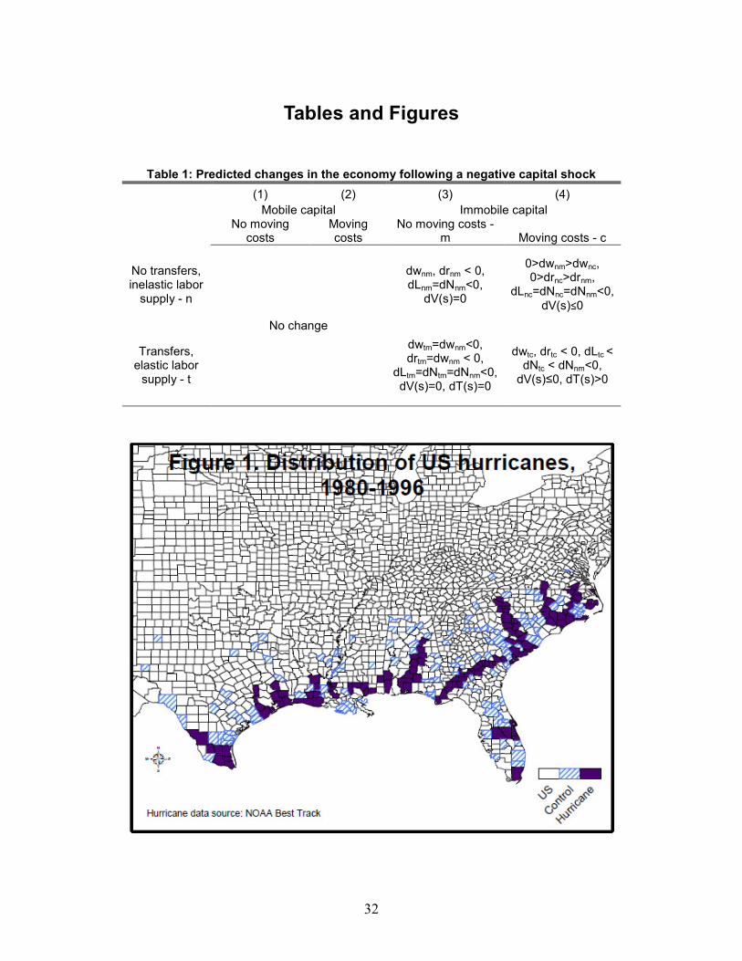
32

Tables and Figures

Table 1: Predicted changes in the economy following a negative capital shock

(1) (2) (3) (4)

Mobile capital Immobile capital No moving

costs Moving costs

No moving costs - m Moving costs - c

No transfers, inelastic labor

supply - n

No change

dwnm, drnm < 0, dLnm=dNnm<0,

dV(s)=0

0>dwnm>dwnc, 0>drnc>drnm,

dLnc=dNnc=dNnm<0,

dV(s)≤0

Transfers, elastic labor

supply - t

dwtm=dwnm<0, drtm=dwnm < 0,

dLtm=dNtm=dNnm<0, dV(s)=0, dT(s)=0

dwtc, drtc < 0, dLtc <

dNtc < dNnm<0, dV(s)≤0, dT(s)>0

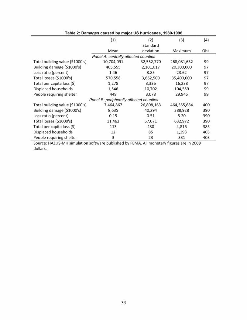
33

Table 2: Damages caused by major US hurricanes, 1980-1996

(1) (2) (3) (4)

Mean

Standard

deviation Maximum Obs.

Panel A: centrally affected counties

Total building value ($1000's) 10,704,091 32,552,770 268,081,632 99

Building damage ($1000's) 405,555 2,101,017 20,300,000 97

Loss ratio (percent) 1.46 3.85 23.62 97

Total losses ($1000's) 570,558 3,662,500 35,400,000 97

Total per capita loss ($) 1,278 3,336 16,238 97

Displaced households 1,546 10,702 104,559 99

People requiring shelter 449 3,078 29,945 99

Panel B: peripherally affected counties

Total building value ($1000's) 7,464,867 26,808,163 464,355,684 400

Building damage ($1000's) 8,635 40,294 388,928 390

Loss ratio (percent) 0.15 0.51 5.20 390

Total losses ($1000's) 11,462 57,071 632,972 390

Total per capita loss ($) 113 430 4,816 385

Displaced households 12 85 1,193 403

People requiring shelter 3 23 331 403

Source: HAZUS-MH simulation software published by FEMA. All monetary figures are in 2008

dollars.

34

Table 3: Determinants of property damages in hurricane region1

(1

) (2

) (3

) (4

) (5

) (6

)

Log d

am

ages

Per

cap

ita

dam

ages

Flo

od

in

sura

nce

pa

ym

en

ts

(log)

Log d

am

ages

Per

cap

ita

dam

ages

Flo

od

in

sura

nce

pa

ym

en

ts

(log)

Majo

r hurr

ica

ne

4.2

36

678.2

79

3.0

90

(0.4

26)*

**

(309.7

95)*

(0

.410)*

**

Min

or

hurr

ica

ne

2.4

17

65.1

84

1.5

15

(0.2

50)*

**

(46.0

66)

(0.2

47)*

**

Cate

gory

= 1

2.1

51

72.7

35

1.1

31

(0.2

97)*

**

(57.5

67)

(0.2

63)*

**

Cate

gory

= 2

3.2

53

39.0

28

2.7

69

(0.4

11)*

**

(19.1

73)*

(0

.492)*

**

Cate

gory

= 3

4.0

49

710.2

13

3.1

00

(0.3

11)*

**

(399.2

46)

(0.4

71)*

**

Cate

gory

= 4

or

5

4.6

42

607.0

60

3.0

19

(0.9

15)*

**

(316.1

98)*

(0

.850)*

**

Torn

ado

2.0

61

12.5

07

-0

.008

2.0

61

12.4

41

-0

.011

(0.1

97)*

**

(6.8

47)

(0.0

70)

(0.1

96)*

**

(7.1

74)

-0.0

70

F

lood

0.8

62

0.3

80

0.7

62

0.8

64

0.2

99

0.7

58

(0.1

02)*

**

(5.6

90)

(0.0

65)*

**

(0.1

02)*

**

(5.7

57)

(0.0

65)*

**

Se

vere

sto

rm

0.9

58

8.9

52

-0

.205

0.9

56

9.0

75

-0

.201

(0.1

80)*

**

(3.9

15)*

(0

.078)*

**

(0.1

81)*

**

(4.2

13)*

(0

.079)*

*

Dep

var

mean

(media

n)

9.3

1 (

9.6

6)

11.0

0 (

0.0

9)

10.8

7 (

10.8

0)

9.3

1 (

9.6

6)

11.0

0 (

0.0

9)

10.8

7 (

10.8

0)

Observ

ations

18,5

92

24,3

31

7,0

29

18,5

92

24,3

31

7,0

29

R-s

quare

d

0.4

5

0.0

8

0.4

2

0.4

5

0.0

8

0.4

2

Sta

ndard

err

ors

(clu

ste

red b

y c

ounty

) in

pare

nth

eses.

* sig

nific

ant

at 1

0%

; **

sig

nific

ant at 5%

; **

* sig

nific

ant

at 1%

. D

am

ages a

nd f

loo

d c

laim

s a

re in

curr

ent

dolla

rs. In

clu

des c

ounty

and y

ear

fixed e

ffects

. P

ropert

y d

am

age d

ata

is f

rom

S

HE

LD

US

. F

lood

insura

nce p

aym

ents

data

is f

rom

the C

onso

lidate

d F

edera

l F

unds R

ep

ort

(C

FF

R).

Tim

e p

eriod is

1980-1

99

6 f

or

dam

ages, 1

983-1

996 f

or

flood

cla

ims.

1A

labam

a, F

lori

da, G

eorg

ia, Lou

isia

na,

Mis

sis

sip

pi, N

ort

h C

aro

lina,

Sou

th C

aro

lina, T

exas, and V

irg

inia

.

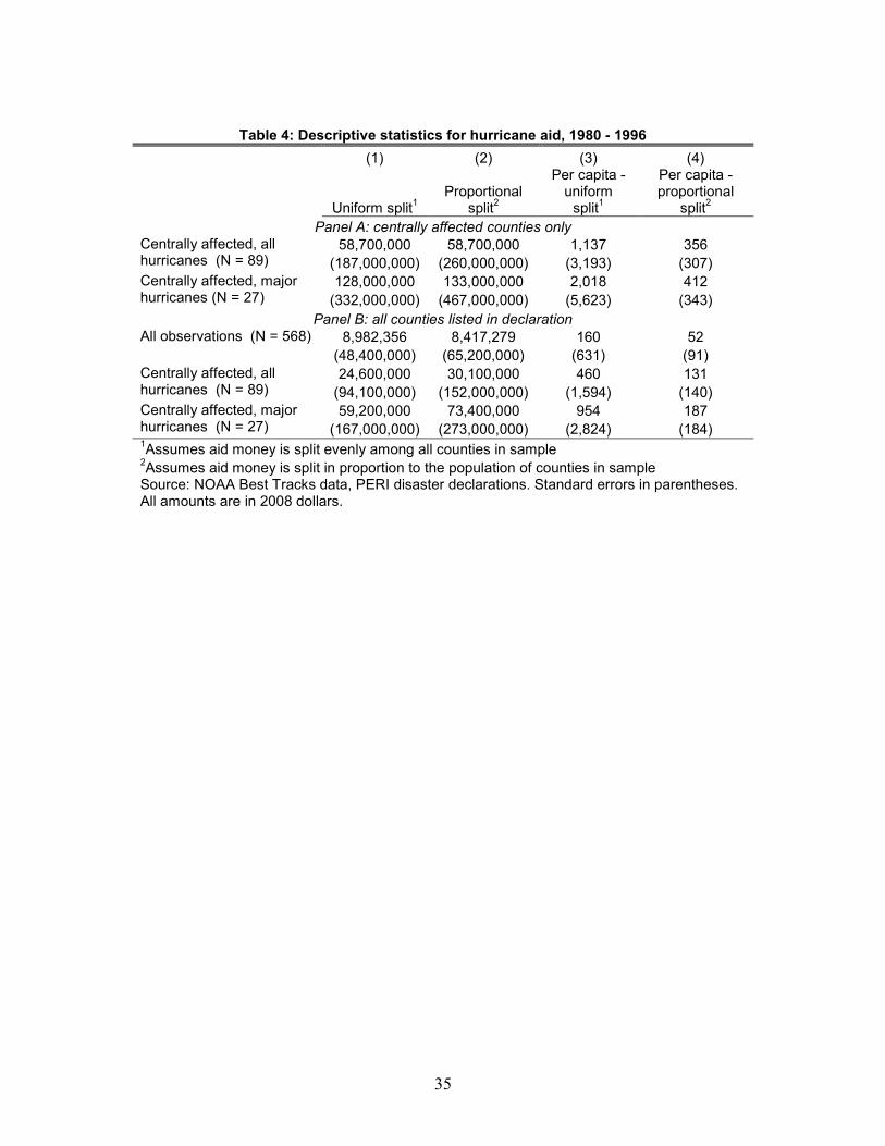
35

Table 4: Descriptive statistics for hurricane aid, 1980 - 1996

(1) (2) (3) (4)

Uniform split1

Proportional split

2

Per capita - uniform

split1

Per capita - proportional

split2

Panel A: centrally affected counties only Centrally affected, all hurricanes (N = 89)

58,700,000 58,700,000 1,137 356

(187,000,000) (260,000,000) (3,193) (307)

Centrally affected, major hurricanes (N = 27)

128,000,000 133,000,000 2,018 412

(332,000,000) (467,000,000) (5,623) (343)

Panel B: all counties listed in declaration All observations (N = 568) 8,982,356 8,417,279 160 52

(48,400,000) (65,200,000) (631) (91)

Centrally affected, all hurricanes (N = 89)

24,600,000 30,100,000 460 131

(94,100,000) (152,000,000) (1,594) (140)

Centrally affected, major hurricanes (N = 27)

59,200,000 73,400,000 954 187

(167,000,000) (273,000,000) (2,824) (184) 1Assumes aid money is split evenly among all counties in sample

2Assumes aid money is split in proportion to the population of counties in sample

Source: NOAA Best Tracks data, PERI disaster declarations. Standard errors in parentheses. All amounts are in 2008 dollars.

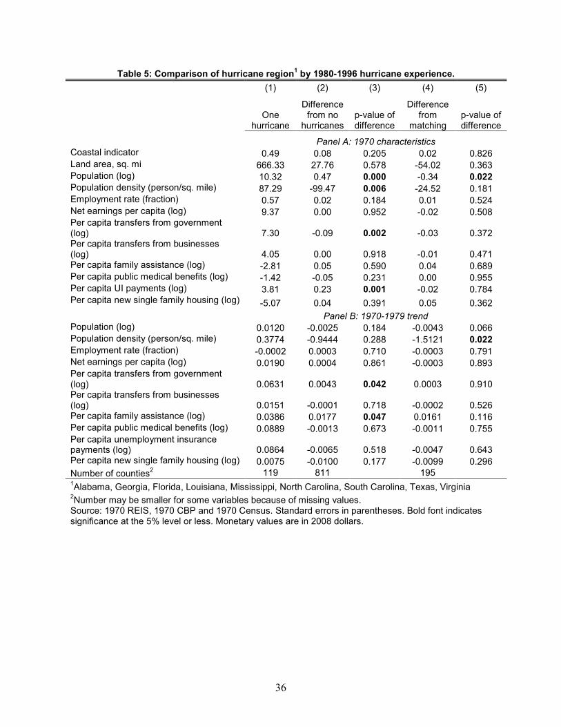
36

Table 5: Comparison of hurricane region1 by 1980-1996 hurricane experience.

(1) (2) (3) (4) (5)

One hurricane

Difference from no

hurricanes p-value of difference

Difference from

matching p-value of difference

Panel A: 1970 characteristics

Coastal indicator 0.49 0.08 0.205 0.02 0.826 Land area, sq. mi 666.33 27.76 0.578 -54.02 0.363 Population (log) 10.32 0.47 0.000 -0.34 0.022 Population density (person/sq. mile) 87.29 -99.47 0.006 -24.52 0.181 Employment rate (fraction) 0.57 0.02 0.184 0.01 0.524 Net earnings per capita (log) 9.37 0.00 0.952 -0.02 0.508 Per capita transfers from government (log) 7.30 -0.09 0.002 -0.03 0.372 Per capita transfers from businesses (log) 4.05 0.00 0.918 -0.01 0.471 Per capita family assistance (log) -2.81 0.05 0.590 0.04 0.689 Per capita public medical benefits (log) -1.42 -0.05 0.231 0.00 0.955 Per capita UI payments (log) 3.81 0.23 0.001 -0.02 0.784 Per capita new single family housing (log) -5.07 0.04 0.391 0.05 0.362 Panel B: 1970-1979 trend Population (log) 0.0120 -0.0025 0.184 -0.0043 0.066 Population density (person/sq. mile) 0.3774 -0.9444 0.288 -1.5121 0.022 Employment rate (fraction) -0.0002 0.0003 0.710 -0.0003 0.791 Net earnings per capita (log) 0.0190 0.0004 0.861 -0.0003 0.893 Per capita transfers from government (log) 0.0631 0.0043 0.042 0.0003 0.910 Per capita transfers from businesses (log) 0.0151 -0.0001 0.718 -0.0002 0.526 Per capita family assistance (log) 0.0386 0.0177 0.047 0.0161 0.116 Per capita public medical benefits (log) 0.0889 -0.0013 0.673 -0.0011 0.755 Per capita unemployment insurance payments (log) 0.0864 -0.0065 0.518 -0.0047 0.643 Per capita new single family housing (log) 0.0075 -0.0100 0.177 -0.0099 0.296

Number of counties2 119 811 195

1Alabama, Georgia, Florida, Louisiana, Mississippi, North Carolina, South Carolina, Texas, Virginia

2Number may be smaller for some variables because of missing values.

Source: 1970 REIS, 1970 CBP and 1970 Census. Standard errors in parentheses. Bold font indicates significance at the 5% level or less. Monetary values are in 2008 dollars.

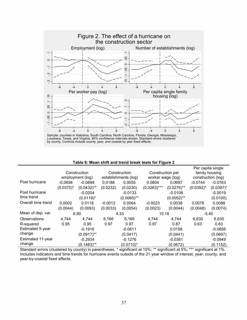
37

-.3

-.2

-.1

0.1

-8 -4 0 4 8

Employment (log)

-.15

-.1

-.05

0.0

5.1

-8 -4 0 4 8

Number of establishments (log)-.

1-.

05

0.0

5.1

.15

-8 -4 0 4 8

Per worker pay (log)

-.2

-.1

0.1

.2

-8 -4 0 4 8

Per capita single familyhousing (log)

Sample: counties in Alabama, South Carolina, North Carolina, Florida, Georgia, Mississippi,Louisiana, Texas, and Virginia. 95% confidence intervals shown. Standard errors clusteredby county. Controls include county, year, and coastal by year fixed effects.

Figure 2. The effect of a hurricane onthe construction sector

Table 6: Mean shift and trend break tests for Figure 2

Construction employment (log)

Construction establishments (log)

Construction per worker wage (log)

Per capita single family housing

construction (log) Post hurricane -0.0698 -0.0899 0.0188 0.0055 0.0804 0.0697 -0.0744 -0.0763

(0.0375)* (0.0432)** (0.0232) (0.0230) (0.0263)*** (0.0276)** (0.0392)* (0.0397)* Post hurricane time trend

-0.0204 -0.0133 -0.0108 -0.0019

(0.0119)* (0.0065)** (0.0052)** (0.0100) Overall time trend 0.0002 0.0118 -0.0012 0.0064 -0.0023 0.0038 0.0078 0.0088

(0.0044) (0.0093) (0.0033) (0.0054) (0.0023) (0.0044) (0.0048) (0.0074) Mean of dep. var. 6.90 4.33 10.16 -5.40

Observations 4,744 4,744 6,166 6,166 4,744 4,744 6,630 6,630

R-squared 0.95 0.95 0.97 0.97 0.87 0.87 0.63 0.63 Estimated 5-year change

-0.1916 -0.0611 0.0158 -0.0856

(0.0917)** (0.0417) (0.0441) (0.0697) Estimated 11-year change

-0.2934 -0.1276 -0.0381 -0.0949

(0.1483)** (0.0710)* (0.0672) (0.1152)

Standard errors (clustered by county) in parentheses. * significant at 10%; ** significant at 5%; *** significant at 1%. Includes indicators and time trends for hurricane events outside of the 21 year window of interest, year, county, and year-by-coastal fixed effects.

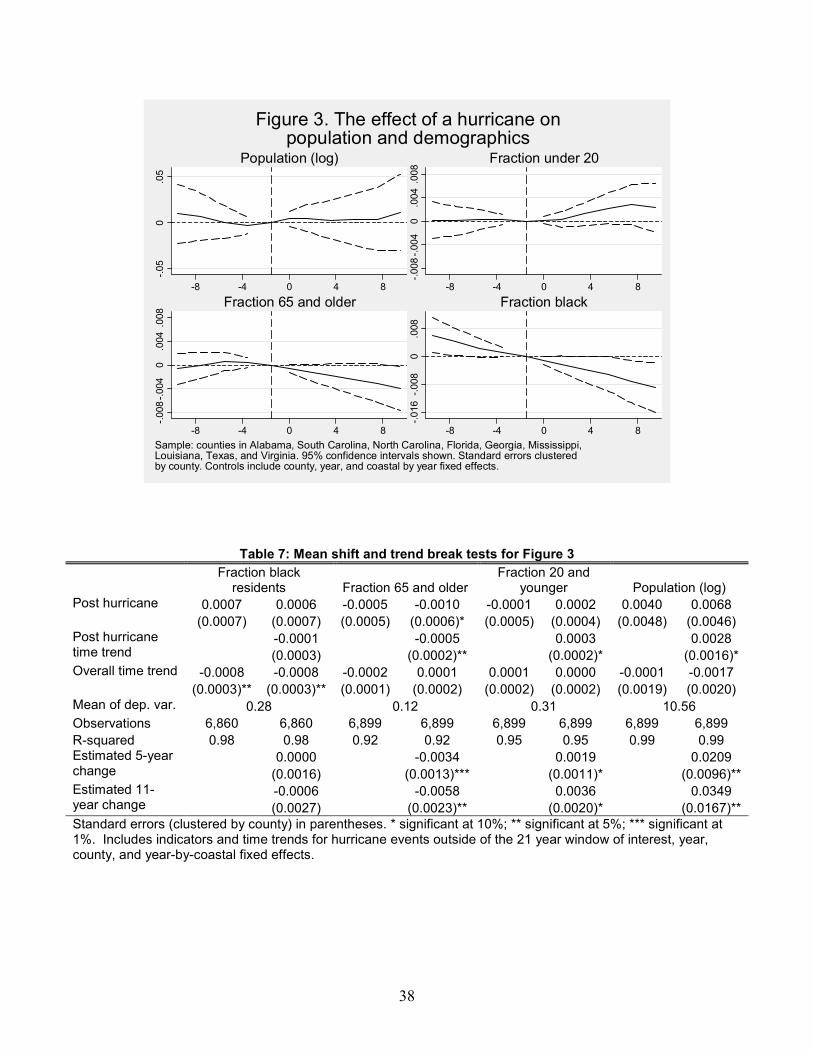
38

-.05

0.0

5

-8 -4 0 4 8

Population (log)

-.008

-.004

0.0

04

.008

-8 -4 0 4 8

Fraction under 20-.

008

-.004

0.0

04

.008

-8 -4 0 4 8

Fraction 65 and older

-.016

-.008

0.0

08

-8 -4 0 4 8

Fraction black

Sample: counties in Alabama, South Carolina, North Carolina, Florida, Georgia, Mississippi,Louisiana, Texas, and Virginia. 95% confidence intervals shown. Standard errors clusteredby county. Controls include county, year, and coastal by year fixed effects.

Figure 3. The effect of a hurricane onpopulation and demographics

Table 7: Mean shift and trend break tests for Figure 3

Fraction black residents Fraction 65 and older

Fraction 20 and younger Population (log)

Post hurricane 0.0007 0.0006 -0.0005 -0.0010 -0.0001 0.0002 0.0040 0.0068

(0.0007) (0.0007) (0.0005) (0.0006)* (0.0005) (0.0004) (0.0048) (0.0046) Post hurricane time trend

-0.0001 -0.0005 0.0003 0.0028

(0.0003) (0.0002)** (0.0002)* (0.0016)* Overall time trend -0.0008 -0.0008 -0.0002 0.0001 0.0001 0.0000 -0.0001 -0.0017

(0.0003)** (0.0003)** (0.0001) (0.0002) (0.0002) (0.0002) (0.0019) (0.0020) Mean of dep. var. 0.28 0.12 0.31 10.56

Observations 6,860 6,860 6,899 6,899 6,899 6,899 6,899 6,899

R-squared 0.98 0.98 0.92 0.92 0.95 0.95 0.99 0.99 Estimated 5-year change

0.0000 -0.0034 0.0019 0.0209

(0.0016) (0.0013)*** (0.0011)* (0.0096)** Estimated 11-year change

-0.0006 -0.0058 0.0036 0.0349

(0.0027) (0.0023)** (0.0020)* (0.0167)**

Standard errors (clustered by county) in parentheses. * significant at 10%; ** significant at 5%; *** significant at 1%. Includes indicators and time trends for hurricane events outside of the 21 year window of interest, year, county, and year-by-coastal fixed effects.

39

-.02

-.01

0.0

1.0

2.0

3

-8 -4 0 4 8

Fraction employed

-.06

-.04

-.02

0.0

2.0

4

-8 -4 0 4 8

Per capita earnings (log)-.

02

0.0

2.0

4

-8 -4 0 4 8

Per capita transfers fromgovernment (log)

0.0

5.1

.15

.2

-8 -4 0 4 8

Per capita transfers frombusinesses (log)

Sample: counties in Alabama, South Carolina, North Carolina, Florida, Georgia, Mississippi,Louisiana, Texas, and Virginia. 95% confidence intervals shown. Standard errors clusteredby county. Controls include county, year, and coastal by year fixed effects.

Figure 4. The effect of a hurricane onemployment, earnings, and transfers

Table 8: Mean shift and trend break tests for Figure 4

Employment rate (fraction)

Per capita transfer from government (logs)

Per capita transfer from businesses (logs)

Per capita net earnings (log)

Post hurricane 0.0019 0.0025 0.0205 0.0200 0.0302 0.0328 0.0061 0.0044

(0.0057) (0.0063) (0.0071)*** (0.0068)*** (0.0152)** (0.0120)*** (0.0136) (0.0151) Post hurricane time trend

0.0006 -0.0005 0.0027 -0.0017

(0.0013) (0.0023) (0.0037) (0.0031) Overall time trend -0.0007 -0.0010 -0.0016 -0.0013 0.0007 -0.0008 0.0011 0.0021

(0.0009) (0.0013) (0.0012) (0.0017) (0.0022) (0.0005) (0.0012) (0.0024) Mean of dep. var. 0.58 0.58 8.09 8.09 4.37 4.37 9.61 9.61 Estimated mean change (levels) 3.40E-03 4.46E-03 67.40 65.84 2.43 2.65 91.55 65.68

Observations 6,860 6,860 6,860 6,860 6,706 6,706 6,860 6,860

R-squared 0.87 0.87 0.96 0.96 0.87 0.87 0.90 0.90 Estimated 5-year change

0.0054 0.0177 0.0463 -0.0043

(0.0113) (0.0137) (0.0110)*** (0.0275) Estimated 11-year change

0.0084 0.0153 0.0598 -0.0129

(0.0174) (0.0244) (0.0280)** (0.0427)

Standard errors (clustered by county) in parentheses. * significant at 10%; ** significant at 5%; *** significant at 1%. Includes indicators and time trends for hurricane events outside of the 21 year window of interest, year, county, and year-by-coastal fixed effects.

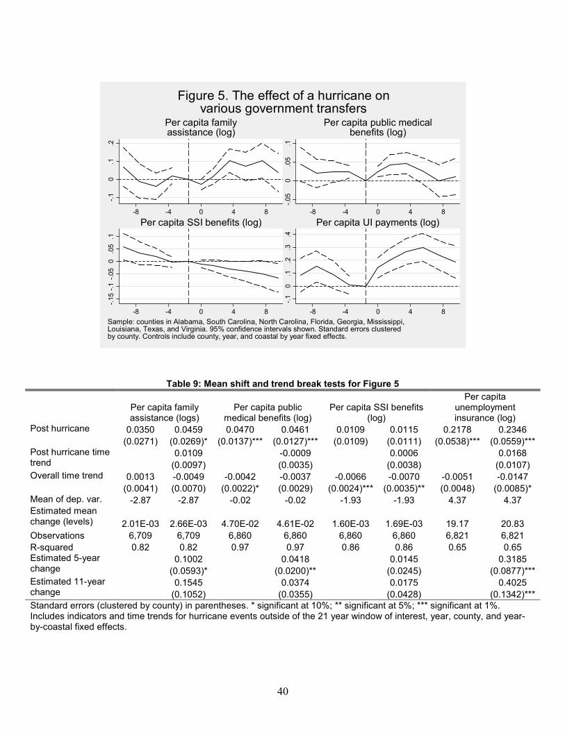
40

-.1

0.1

.2

-8 -4 0 4 8

Per capita familyassistance (log)

-.05

0.0

5.1

-8 -4 0 4 8

Per capita public medicalbenefits (log)

-.15

-.1

-.05

0.0

5.1

-8 -4 0 4 8

Per capita SSI benefits (log)

-.1

0.1

.2.3

.4

-8 -4 0 4 8

Per capita UI payments (log)

Sample: counties in Alabama, South Carolina, North Carolina, Florida, Georgia, Mississippi,Louisiana, Texas, and Virginia. 95% confidence intervals shown. Standard errors clusteredby county. Controls include county, year, and coastal by year fixed effects.

Figure 5. The effect of a hurricane onvarious government transfers

Table 9: Mean shift and trend break tests for Figure 5

Per capita family assistance (logs)

Per capita public medical benefits (log)

Per capita SSI benefits (log)

Per capita unemployment insurance (log)

Post hurricane 0.0350 0.0459 0.0470 0.0461 0.0109 0.0115 0.2178 0.2346

(0.0271) (0.0269)* (0.0137)*** (0.0127)*** (0.0109) (0.0111) (0.0538)*** (0.0559)*** Post hurricane time trend

0.0109 -0.0009 0.0006 0.0168

(0.0097) (0.0035) (0.0038) (0.0107) Overall time trend 0.0013 -0.0049 -0.0042 -0.0037 -0.0066 -0.0070 -0.0051 -0.0147

(0.0041) (0.0070) (0.0022)* (0.0029) (0.0024)*** (0.0035)** (0.0048) (0.0085)* Mean of dep. var. -2.87 -2.87 -0.02 -0.02 -1.93 -1.93 4.37 4.37 Estimated mean change (levels) 2.01E-03 2.66E-03 4.70E-02 4.61E-02 1.60E-03 1.69E-03 19.17 20.83

Observations 6,709 6,709 6,860 6,860 6,860 6,860 6,821 6,821

R-squared 0.82 0.82 0.97 0.97 0.86 0.86 0.65 0.65 Estimated 5-year change

0.1002 0.0418 0.0145 0.3185

(0.0593)* (0.0200)** (0.0245) (0.0877)*** Estimated 11-year change

0.1545 0.0374 0.0175 0.4025

(0.1052) (0.0355) (0.0428) (0.1342)***

Standard errors (clustered by county) in parentheses. * significant at 10%; ** significant at 5%; *** significant at 1%. Includes indicators and time trends for hurricane events outside of the 21 year window of interest, year, county, and year-by-coastal fixed effects.

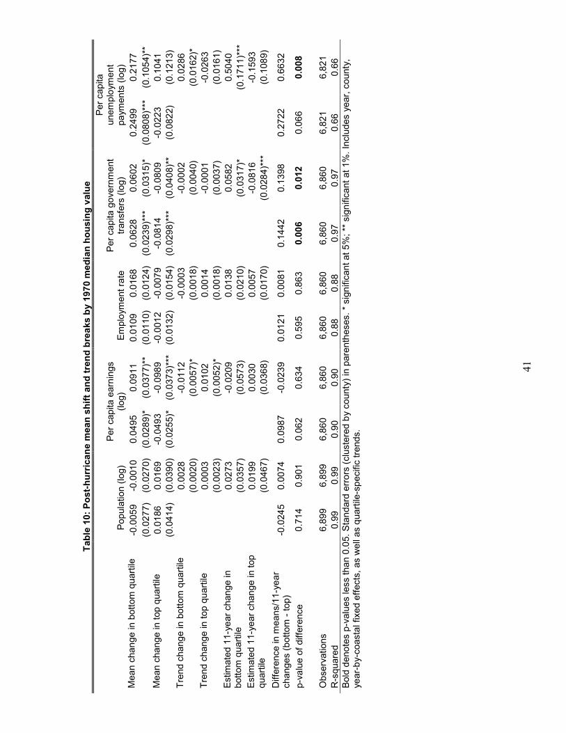
41

Table 10: Post-hurricane mean shift and trend breaks by 1970 median housing value

Pop

ula

tion (

log)

Per

cap

ita e

arn

ings

(log)

Em

plo

ym

ent ra

te

Per

cap

ita g

overn

ment

transfe

rs (

log)

Per

cap

ita

unem

plo

ym

en

t pa

ym

en

ts (

log)

Mean

chan

ge in b

ott

om

quart

ile

-0.0

05

9

-0.0

01

0

0.0

495

0.0

911

0.0

109

0.0

168

0.0

628

0.0

602

0.2

499

0.2

177

(0.0

27

7)

(0.0

27

0)

(0.0

28

9)*

(0

.037

7)*

* (0

.011

0)

(0.0

12

4)

(0.0

23

9)*

**

(0.0

31

5)*

(0

.080

8)*

**

(0.1

05

4)*

* M

ean

chan

ge in t

op q

uart

ile

0.0

186

0.0

169

-0

.049

3

-0.0

98

9

-0.0

01

2

-0.0

07

9

-0.0

81

4

-0.0

80

9

-0.0

22

3

0.1

041

(0.0

41

4)

(0.0

39

0)

(0.0

25

5)*

(0

.037

3)*

**

(0.0

13

2)

(0.0

15

4)

(0.0

29

8)*

**

(0.0

40

8)*

* (0

.082

2)

(0.1

21

3)

Tre

nd c

hange in b

ott

om

quart

ile

0.0

028

-0

.011

2

-0.0

00

3

-0.0

00

2

0.0

286

(0.0

02

0)

(0.0

05

7)*

(0

.001

8)

(0.0

04

0)

(0.0

16

2)*

T

rend c

hange in t

op q

uart

ile

0.0

003

0.0

102

0.0

014

-0

.000

1

-0.0

26

3

(0.0

02

3)

(0.0

05

2)*

(0

.001

8)

(0.0

03

7)

(0.0

16

1)

Estim

ate

d 1

1-y

ear

chan

ge in

bottom

quart

ile

0.0

273

-0

.020

9

0.0

138

0.0

582

0.5

040

(0.0

35

7)

(0.0

57

3)

(0.0

21

0)

(0.0

31

7)*

(0

.171

1)*

**

Estim

ate

d 1

1-y

ear

chan

ge in top

quart

ile

0.0

199

0.0

030

0.0

057

-0

.081

6

-0.1

59

3

(0.0

46

7)

(0.0

36

8)

(0.0

17

0)

(0.0

28

4)*

**

(0.1

08

9)

Diffe

rence in m

eans/1

1-y

ea

r changes (

bottom

- top)

-0.0

24

5

0.0

074

0.0

987

-0

.023

9

0.0

121

0.0

081

0.1

442

0.1

398

0.2

722

0.6

632

p-v

alu

e o

f diffe

rence

0.7

14

0.9

01

0.0

62

0.6

34

0.5

95

0.8

63

0.006

0.012

0.0

66

0.008

Observ

ations

6,8

99

6,8

99

6,8

60

6,8

60

6,8

60

6,8

60

6,8

60

6,8

60

6,8

21

6,8

21

R-s

quare

d

0.9

9

0.9

9

0.9

0

0.9

0

0.8

8

0.8

8

0.9

7

0.9

7

0.6

6

0.6

6

Bold

deno

tes p

-valu

es less than 0

.05. S

tan

dard

err

ors

(clu

ste

red b

y c

ounty

) in

pare

nth

eses. *

sig

nific

ant at

5%

; **

sig

nific

ant

at 1%

. In

clu

des y

ear,

co

unty

, ye

ar-

by-c

oasta

l fixed e

ffects

, as w

ell

as q

uart

ile-s

pecific

tre

nds.

42

Appendix Tables

Table A1: The effect of a hurricane on the construction sector

Construction employment

(log)

Construction establishments

(log)

Construction per worker wage

(log)

Per capita single family housing

construction (log) T = - 9 or - 10 -0.096 -0.044 -0.044 -0.073

(0.073) (0.043) (0.037) (0.056) T = - 7 or - 8 -0.082 -0.045 -0.038 -0.066

(0.056) (0.034) (0.030) (0.056) T = - 5 or - 6 -0.088 -0.021 -0.002 -0.071

(0.041)** (0.026) (0.028) (0.042)* T = - 3 or - 4 -0.038 -0.005 -0.028 -0.012

(0.026) (0.017) (0.023) (0.033)

T = 0 -0.021 0.032 0.038 -0.057

(0.028) (0.013)** (0.026) (0.023)**

T = 1 or 2 -0.071 0.037 0.077 -0.009

(0.034)** (0.019)* (0.027)*** (0.035) T = 3 or 4 -0.160 -0.030 0.054 -0.097

(0.046)*** (0.025) (0.026)** (0.047)** T = 5 or 6 -0.193 -0.047 0.034 -0.079

(0.052)*** (0.029) (0.027) (0.049) T = 7 or 8 -0.155 -0.059 -0.009 -0.017

(0.055)*** (0.034)* (0.024) (0.055) T = 9 or 10 -0.117 -0.014 0.011 0.028

(0.063)* (0.037) (0.026) (0.061) Mean of dep. var. 6.903 4.330 10.155 -5.396 Observations 4,744 6,166 4,744 6,630 R-squared 0.95 0.97 0.87 0.63 p-value of all leads F-test 0.279 0.655 0.345 0.305 p-value of all lags F-test 0.000 0.000 0.005 0.000 p-value of T=0 to T=4 lags F-test 0.001 0.000 0.020 0.003

Standard errors (clustered by county) in parentheses. * significant at 5%; ** significant at 1%. Includes year, county, and year-by-coastal fixed effects.

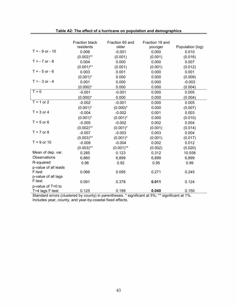
43

Table A2: The effect of a hurricane on population and demographics

Fraction black residents

Fraction 65 and older

Fraction 19 and younger Population (log)

T = - 9 or - 10 0.006 -0.001 0.000 0.010

(0.002)** (0.001) (0.001) (0.016) T = - 7 or - 8 0.004 0.000 0.000 0.007

(0.001)** (0.001) (0.001) (0.012) T = - 5 or - 6 0.003 0.001 0.000 0.001

(0.001)* 0.000 0.000 (0.009) T = - 3 or - 4 0.001 0.000 0.000 -0.003

(0.000)* 0.000 0.000 (0.004)

T = 0 -0.001 -0.001 0.000 0.005

(0.000)* 0.000 0.000 (0.004)

T = 1 or 2 -0.002 -0.001 0.000 0.005

(0.001)* (0.000)* 0.000 (0.007) T = 3 or 4 -0.004 -0.002 0.001 0.003

(0.001)* (0.001)* 0.000 (0.010) T = 5 or 6 -0.005 -0.002 0.002 0.004

(0.002)** (0.001)* (0.001) (0.014) T = 7 or 8 -0.007 -0.003 0.003 0.004

(0.003)** (0.001)* (0.001) (0.017) T = 9 or 10 -0.009 -0.004 0.002 0.012

(0.003)** (0.001)** (0.002) (0.020) Mean of dep. var. 0.285 0.123 0.312 10.558 Observations 6,860 6,899 6,899 6,899 R-squared 0.98 0.92 0.95 0.99 p-value of all leads F-test 0.066 0.095 0.271 0.245 p-value of all lags F-test 0.091 0.378 0.011 0.124 p-value of T=0 to T=4 lags F-test 0.125 0.199 0.040 0.150

Standard errors (clustered by county) in parentheses. * significant at 5%; ** significant at 1%. Includes year, county, and year-by-coastal fixed effects.

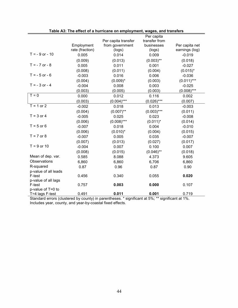
44

Table A3: The effect of a hurricane on employment, wages, and transfers

Employment rate (fraction)

Per capita transfer from government

(logs)

Per capita transfer from businesses

(logs) Per capita net earnings (log)

T = - 9 or - 10 0.005 0.014 0.009 -0.019

(0.009) (0.013) (0.003)** (0.018) T = - 7 or - 8 0.005 0.011 0.001 -0.027

(0.008) (0.011) (0.004) (0.015)* T = - 5 or - 6 -0.003 0.016 0.006 -0.036

(0.004) (0.009)* (0.003) (0.011)*** T = - 3 or - 4 -0.004 0.008 0.003 -0.025

(0.003) (0.005) (0.003) (0.008)***

T = 0 0.000 0.012 0.116 0.002

(0.003) (0.004)*** (0.026)*** (0.007)

T = 1 or 2 -0.002 0.018 0.013 -0.003

(0.004) (0.007)** (0.003)*** (0.011) T = 3 or 4 -0.005 0.025 0.023 -0.008

(0.006) (0.008)*** (0.011)* (0.014) T = 5 or 6 -0.007 0.018 0.004 -0.010

(0.006) (0.010)* (0.004) (0.015) T = 7 or 8 -0.007 0.005 0.035 -0.007

(0.007) (0.013) (0.027) (0.017) T = 9 or 10 -0.004 0.007 0.100 0.007

(0.008) (0.015) (0.046)** (0.018) Mean of dep. var. 0.585 8.088 4.373 9.605 Observations 6,860 6,860 6,706 6,860 R-squared 0.87 0.96 0.87 0.90 p-value of all leads F-test 0.456 0.340 0.055 0.020 p-value of all lags F-test 0.757 0.003 0.000 0.107 p-value of T=0 to T=4 lags F-test 0.491 0.011 0.001 0.719

Standard errors (clustered by county) in parentheses. * significant at 5%; ** significant at 1%. Includes year, county, and year-by-coastal fixed effects.

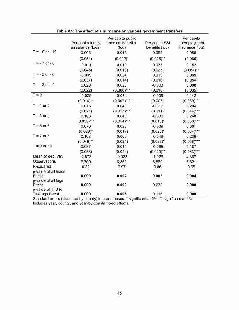
45

Table A4: The effect of a hurricane on various government transfers

Per capita family assistance (logs)

Per capita public medical benefits

(log) Per capita SSI benefits (log)

Per capita unemployment insurance (log)

T = - 9 or - 10 0.068 0.043 0.059 0.085

(0.054) (0.022)* (0.026)** (0.066) T = - 7 or - 8 -0.011 0.019 0.033 0.152

(0.048) (0.019) (0.023) (0.061)** T = - 5 or - 6 -0.039 0.024 0.019 0.089

(0.037) (0.014) (0.016) (0.054) T = - 3 or - 4 0.020 0.023 -0.003 0.008

(0.022) (0.008)*** (0.010) (0.035)

T = 0 -0.029 0.024 -0.009 0.142

(0.014)** (0.007)*** (0.007) (0.039)***

T = 1 or 2 0.015 0.043 -0.017 0.204

(0.021) (0.013)*** (0.011) (0.044)*** T = 3 or 4 0.103 0.046 -0.030 0.268

(0.033)*** (0.014)*** (0.015)* (0.050)*** T = 5 or 6 0.070 0.026 -0.039 0.301

(0.039)* (0.017) (0.020)* (0.054)*** T = 7 or 8 0.103 0.000 -0.049 0.239

(0.049)** (0.021) (0.026)* (0.056)*** T = 9 or 10 0.037 0.011 -0.065 0.187

(0.053) (0.024) (0.029)** (0.063)*** Mean of dep. var. -2.873 -0.023 -1.926 4.367 Observations 6,709 6,860 6,860 6,821 R-squared 0.82 0.97 0.86 0.65 p-value of all leads F-test 0.000 0.002 0.002 0.004 p-value of all lags F-test 0.000 0.000 0.278 0.000 p-value of T=0 to T=4 lags F-test 0.000 0.005 0.113 0.000

Standard errors (clustered by county) in parentheses. * significant at 5%; ** significant at 1%. Includes year, county, and year-by-coastal fixed effects.

46

Table A5: Post-hurricane mean shift and trend breaks by county income

Pop

ula

tion (

log)

Per

cap

ita e

arn

ings

(log)

Em

plo

ym

ent ra

te

Per

cap

ita g

overn

ment

transfe

rs (

log)

Per

cap

ita

unem

plo

ym

en

t pa

ym

en

ts (

log)

Mean

chan

ge in b

ott

om

quart

ile

-0.0

22

4

-0.0

23

5

0.0

534

0.0

696

0.0

133

0.0

186

0.0

571

0.0

724

0.1

898

0.1

445

(0.0

20

7)

(0.0

20

1)

(0.0

23

6)*

* (0

.030

0)*

* (0

.011

4)

(0.0

13

0)

(0.0

18

6)*

**

(0.0

23

0)*

**

(0.0

85

1)*

* (0

.099

2)

Mean

chan

ge in t

op q

uart

ile

0.0

144

0.0

152

-0

.036

5

-0.0

63

8

0.0

046

-0

.000

4

-0.0

79

8

-0.1

09

5

-0.0

04

0

0.0

334

(0.0

34

4)

(0.0

33

3)

(0.0

24

1)

(0.0

34

6)*

(0

.016

0)

(0.0

17

5)

(0.0

23

7)*

**

(0.0

31

1)*

**

(0.1

02

3)

(0.1

32

8)

Tre

nd c

hange in b

ott

om

quart

ile

0.0

047

-0

.006

6

-0.0

00

2

-0.0

03

4

0.0

386

(0.0

01

8)*

**

(0.0

05

4)

(0.0

01

6)

(0.0

03

1)

(0.0

14

8)*

* T

rend c

hange in t

op q

uart

ile

-0.0

00

2

0.0

056

0.0

010

0.0

061

-0

.007

5

(0.0

02

0)

(0.0

04

4)

(0.0

01

5)

(0.0

02

6)*

* (0

.013

5)

Estim

ate

d 1

1-y

ear

chan

ge in

bottom

quart

ile

0.0

235

0.0

033

0.0

162

0.0

381

0.5

301

(0.0

28

5)

(0.0

52

7)

(0.0

18

9)

(0.0

28

7)

(0.1

65

9)*

**

Estim

ate

d 1

1-y

ear

chan

ge in top

quart

ile

0.0

137

-0

.007

8

0.0

097

-0

.048

4

-0.0

41

6

(0.0

38

4)

(0.0

31

1)

(0.0

17

7)

(0.0

21

7)*

* (0

.110

2)

Diffe

rence in m

eans/1

1-y

ea

r changes (

bottom

- top)

-0.0

36

8

0.0

098

0.0

898

0.0

111

0.0

087

0.0

065

0.1

369

0.0

865

0.1

939

0.5

717

p-v

alu

e o

f diffe

rence

0.4

82

0.8

14

0.044

0.9

89

0.7

34

0.8

68

0.001

0.0

92

0.2

53

0.017

Observ

ations

6,8

99

6,8

99

6,8

60

6,8

60

6,8

60

6,8

60

6,8

60

6,8

60

6,8

21

6,8

21

R-s

quare

d

0.9

9

0.9

9

0.9

0

0.9

0

0.8

8

0.8

8

0.9

7

0.9

7

0.6

6

0.6

6

Bold

deno

tes p

-valu

es less than 0

.05. S

tan

dard

err

ors

(clu

ste

red b

y c

ounty

) in

pare

nth

eses. *

sig

nific

ant at

5%

; **

sig

nific

ant

at 1%

. In

clu

des y

ear,

co

unty

, ye

ar-

by-c

oasta

l fixed e

ffects

, as w

ell

as q

uart

ile-s

pecific

tre

nds.

47

Table A6: the co-movement of local economic indicators

Tota

l unem

plo

ym

en

t pa

ym

en

ts (

log)

Per

cap

ita

unem

plo

ym

en

t pa

ym

en

ts (

log)

Earn

ings p

er

capita

(lo

g)

Net

earn

ings

(log)

Sta

te r

eceip

ts (

log)

Tota

l em

plo

ym

ent

(log)

0.0

63

-0

.329

(0.0

35)*

(0

.032)*

**

Tota

l w

ag

es p

aid

(log)

0.0

86

-0

.231

(0.0

31)*

**

(0.0

26)*

**

Net e

arn

ings p

er

capita

(lo

g)

0.5

88

(0.1

03)*

**

Net e

arn

ings (

log)

0.8

23

(0.0

31)*

**

Incom

e

main

tenance (

log)

-0.0

64

0.2

10

(0.0

08)*

**

(0.0

22)*

**

Observ

ations

33,8

44

34,7

67

33,8

22

34,7

45

36,8

09

36,8

09

12,1

68

12,1

68

R-s

quare

d

0.9

1

0.9

1

0.6

2

0.6

2

0.8

5

0.9

8

0.9

7

0.9

6

Sta

ndard

err

ors

(clu

ste

red b

y c

ounty

) in

pare

nth

eses.

* sig

nific

ant

at 1

0%

; **

sig

nific

ant at 5%

; **

* sig

nific

ant

at 1%

. In

clu

des c

ounty

and y

ear

fixed e

ffects

.

Table A7: the co-movement of the local construction sector with earnings

Tota

l esta

blis

hm

ents

(log)

Tota

l em

plo

ym

ent

(log)

Tota

l pa

y (

log)

Per

work

er

pa

y (

log)

Net e

arn

ings p

er

capita

(lo

g)

0.7

33

1.0

58

1.2

59

0.2

29

(0.0

56)*

**

(0.0

78)*

**

(0.0

89)*

**

(0.0

26)*

**

Net e

arn

ings (

log)

0.8

99

0.9

61

1.1

37

0.1

82

(0.0

27)*

**

(0.0

36)*

**

(0.0

42)*

**

(0.0

13)*

**

Observ

ations

34,3

52

34,3

52

30,8

72

30,8

72

31,7

51

31,7

51

29,7

43

29,7

43

R-s

quare

d

0.9

7

0.9

6

0.9

5

0.9

4

0.9

5

0.9

4

0.7

8

0.7

8

Sta

ndard

err

ors

(clu

ste

red b

y c

ounty

) in

pare

nth

eses.

* sig

nific

ant

at 1

0%

; **

sig

nific

ant at 5%

; **

* sig

nific

ant

at 1%

. In

clu

des c

ounty

and y

ear

fixed e

ffects

.

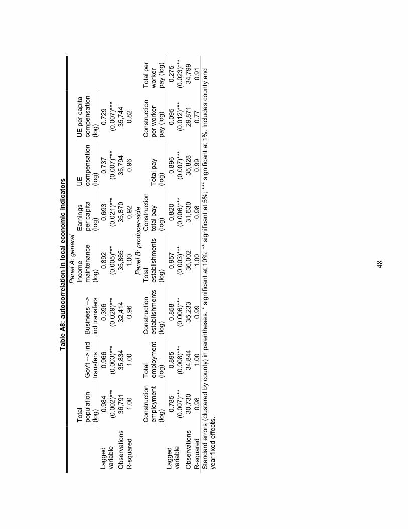
48

Table A8: autocorrelation in local economic indicators

Panel A: general

Tota

l popu

latio

n

(log)

Gov't -

-> in

d

transfe

rs

Busin

ess -

->

ind t

ransfe

rs

Incom

e

main

tenance

(log)

Earn

ings

per

capita

(log)

UE

com

pensation

(log)

UE

per

capita

com

pensation

(log)

Lagg

ed

vari

ab

le

0.9

84

0.9

66

0.3

96

0.8

92

0.6

93

0.7

37

0.7

29

(0.0

02)*

**

(0.0

03)*

**

(0.0

29)*

**

(0.0

05)*

**

(0.0

21)*

**

(0.0

07)*

**

(0.0

07)*

**

Observ

ations

36,7

91

35,8

34

32,4

14

35,8

65

35,8

70

35,7

94

35,7

44

R-s

quare

d

1.0

0

1.0

0

0.9

6

1.0

0

0.9

2

0.9

6

0.8

2

Panel B: producer-side

Constr

uction

em

plo

ym

ent

(log)

Tota

l em

plo

ym

ent

(log)

Constr

uction

esta

blis

hm

ents

(log)

Tota

l esta

blis

hm

ents

(log)

Constr

uction

tota

l pa

y

(log)

Tota

l pa

y

(log)

Constr

uction

per

work

er

pa

y (

log)

Tota

l per

work

er

pa

y (

log)

Lagg

ed

vari

ab

le

0.7

85

0.8

95

0.8

58

0.9

57

0.8

20

0.8

96

0.0

95

0.2

75

(0.0

07)*

**

(0.0

08)*

**

(0.0

06)*

**

(0.0

03)*

**

(0.0

06)*

**

(0.0

07)*

**

(0.0

12)*

**

(0.0

23)*

**

Observ

ations

30,7

30

34,8

44

35,2

33

36,0

02

31,6

30

35,8

28

29,8

71

34,7

99

R-s

quare

d

0.9

8

1.0

0

0.9

9

1.0

0

0.9

8

0.9

9

0.7

7

0.9

1

Sta

ndard

err

ors

(clu

ste

red b

y c

ounty

) in

pare

nth

eses.

* sig

nific

ant

at 1

0%

; **

sig

nific

ant at 5%

; **

* sig

nific

ant

at 1%

. In

clu

des c

ou

nty

an

d

ye

ar

fixed e

ffects

.

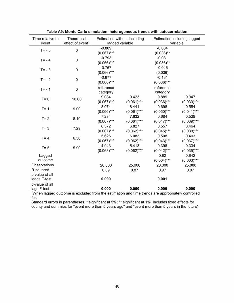
49

Table A9: Monte Carlo simulation, heterogeneous trends with autocorrelation

Time relative to event

Theoretical effect of event

1

Estimation without including lagged variable

Estimation including lagged variable

T= - 5 0 -0.809 -0.084

(0.067)*** (0.036)**

T= - 4 0 -0.793 -0.081

(0.066)*** (0.036)**

T= - 3 0 -0.767 -0.046

(0.066)*** (0.036)

T= - 2 0 -0.877 -0.131

(0.066)*** (0.036)***

T= - 1 0 reference category

reference category

T= 0 10.00 9.084 9.423 9.889 9.947

(0.067)*** (0.061)*** (0.036)*** (0.030)***

T= 1 9.00 8.074 8.441 0.698 0.554

(0.066)*** (0.061)*** (0.050)*** (0.041)***

T= 2 8.10 7.234 7.632 0.684 0.538

(0.067)*** (0.061)*** (0.047)*** (0.039)***

T= 3 7.29 6.372 6.827 0.557 0.464

(0.067)*** (0.062)*** (0.045)*** (0.038)***

T= 4 6.56 5.626 6.083 0.508 0.403

(0.067)*** (0.062)*** (0.043)*** (0.037)***

T= 5 5.90 4.943 5.413 0.398 0.334

(0.068)*** (0.062)*** (0.042)*** (0.035)***

Lagged outcome

0.82 0.842

(0.004)*** (0.003)***

Observations 20,000 25,000 20,000 25,000

R-squared 0.89 0.87 0.97 0.97 p-value of all leads F-test 0.000

0.001

p-value of all lags F-test 0.000 0.000 0.000 0.000 1When lagged outcome is excluded from the estimation and time trends are appropriately controlled

for. Standard errors in parentheses. * significant at 5%; ** significant at 1%. Includes fixed effects for county and dummies for "event more than 5 years ago" and "event more than 5 years in the future".