RS2

Dynamic Analysis Theory Manual

© 2021 Rocscience Inc.

1

Table of Contents 1. Introduction .......................................................................................................................................... 4

1.1 Overview ....................................................................................................................................... 4

1.2 Ground response analysis ............................................................................................................. 4

1.2.1 Equivalent linear analysis ...................................................................................................... 4

1.2.2 Fully Nonlinear analysis......................................................................................................... 6

1.3 Governing equation ...................................................................................................................... 7

1.3.1 Newmark integration ............................................................................................................ 7

1.3.2 Solution for nonlinear problems ........................................................................................... 8

2 Numerical model consideration .......................................................................................................... 11

2.1 Loading and boundary condition ................................................................................................ 11

2.1.2 Absorb Boundary Condition ................................................................................................ 11

2.1.3 Transmit Boundary Condition ............................................................................................. 14

2.2 Dynamic Data Analysis ................................................................................................................ 17

2.2.1 Data Input ........................................................................................................................... 17

2.2.2 Amplitude Spectrum ........................................................................................................... 18

2.2.3 Response Spectrum ............................................................................................................ 18

2.2.4 Arias Intensity ..................................................................................................................... 19

2.2.5 Baseline Correction ............................................................................................................. 19

2.3 Time step ..................................................................................................................................... 22

2.4 Damping ...................................................................................................................................... 23

2.4.1 Rayleigh Damping ............................................................................................................... 23

2.4.2 Hysteretic Damping ............................................................................................................. 26

2.4.3 Damping in practical application ........................................................................................ 28

2.5 Natural frequencies analysis ....................................................................................................... 28

2.6 Deconvolution ............................................................................................................................. 29

2.6.1 Rigid base ............................................................................................................................ 29

2.6.2 Compliance base ................................................................................................................. 30

2.6.3 Base selection ..................................................................................................................... 30

2.7 Liquefaction ................................................................................................................................ 32

2.7.1 Liquefaction susceptibility .................................................................................................. 32

2.7.2 Liquefaction initiation ......................................................................................................... 33

2

2.7.3 Liquefaction damage ........................................................................................................... 34

2.7.4 Standard practice ................................................................................................................ 35

2.7.5 Effective stress analysis using RS2/RS3 ............................................................................... 36

2.8 Dynamic modelling ..................................................................................................................... 37

2.8.1 Geometry and initial static condition ................................................................................. 38

2.8.2 Calibrate input data ............................................................................................................ 39

2.8.3 Determine appropriate boundary condition and dynamic loading .................................... 39

2.8.4 Determine material properties and damping parameters ................................................. 40

2.8.5 Assign location to monitor dynamic data and carry out simulation ................................... 40

References .................................................................................................................................................. 41

3

List of Figures Figure 2.1 Definition Sketch for Tractions .................................................................................................. 13

Figure 2.2 Dampers for Absorb Boundary Conditions ................................................................................ 14

Figure 2.3 Damper for Transmit Boundary Conditions ............................................................................... 15

Figure 2.4 Pressure distribution on dam for approximate solution (After Westergaard, 1933) (Eqn. 2.7) 17

Figure 2.5 Schematic of a SDOF system ...................................................................................................... 19

Figure 2.6 Acceleration, Velocity, and Displacement Trends over Time .................................................... 20

Figure 2.7 Original and Corrected Displacement Comparison.................................................................... 21

Figure 2.8 Original and Corrected Acceleration Comparison ..................................................................... 21

Figure 2.9 Damping Ratio Plot, 20% damping at 2 and 8 Hz....................................................................... 24

Figure 2.10 Degradation Curve ................................................................................................................... 27

Figure 2.11 Within/outcrop Motion Demonstration .................................................................................. 31

Figure 2.12 State criteria for flow liquefaction susceptibility (After Kramer, 1996) .................................. 33

Figure 2.13 Zone of susceptibility to flow liquefaction (After Kramer, 1996) ............................................ 34

Figure 2.14 Zone of susceptibility to cyclic mobility (After Kramer, 1996) ................................................. 34

Figure 2.15 Process of earthquake-induced settlement from dissipation of seismically induced excess

pore pressure (After Kramer, 1996) ............................................................................................................ 35

Figure 2.16 Typical boundary condition for dynamic source inside the interested domain ...................... 39

Figure 2.17 Typical boundary condition for seismic analysis ...................................................................... 40

4

1. Introduction

1.1 Overview The dynamic module allows users to perform dynamics analysis in plane strain and axisymmetric mode.

The calculation is based on implicit time integration which is unconditionally stable. The time step is

mainly control by the accuracy of the results by checking the integration error as discussed in Governing

equation and Time step. Dynamic analysis can also be used together with seepage analysis to generate

pore pressure during the ground shaking. Using the dynamic analysis option in RS2, user will be able to

simulate most common applications in earth engineering involving motion and movement induced by

dynamic load as well as excess pore pressure generated by the cyclic load. Some examples include:

• Vibration machine

• Micro seismic induced by mining procedure such as rock bust, explosion

• Soil liquefaction associates with excess pore pressure induced by earthquake

The nature and distribution of earthquake damage is strongly influenced by the response of soils to

cyclic loading. This response is controlled in large part by the mechanical properties of the soil.

Geotechnical earthquake engineering encompasses a wide range of problems involving many types of

loading and many potential mechanisms of failure, and different soil properties influence the behavior

of the soil for different problems. For many important problems, particularly those dominated by wave

propagation effects, only low levels of strain are induced in the soil. For other important problems, such

as those involving the stability of masses of soil, large strains are induced in the soil. The behavior of

soils subjected to dynamic loading is governed by what have come to be popularly known as dynamic

soil properties. Those dynamic soil properties are out of cope of this manual. Interested readers can

refer to Krammer (1996) for more detail.

Although the “Equivalent linear” method was widely used, the full nonlinear method was used in RS2.

Section Ground response analysis will discuss and compare 2 methods in details. The formulation and

implementation of the fully nonlinear methods will be provided in sections Governing equation and

Verifications and calibration of dynamic module of RS2 can be found in the RS2 Online Help.

1.2 Ground response analysis Although equivalent linear and nonlinear methods are both used to solve ground response analysis

problems, their formulations and underlying assumptions are quite different. In order to justify which

method is used in RS2, some details in the two methods are needed to be discussed.

1.2.1 Equivalent linear analysis

In the equivalent-linear method (Seed and Idriss 1969), a linear analysis is performed with the specified

soil stiffness. Initially, some values were assumed for damping ratio and shear modulus in the various

regions of the model. A constant shear modulus (G) was used during the entire earthquake record and

the peak shear strains was recorded for each element. The shear modulus is then modified according a

5

specified G reduction function and damping ratio based on laboratory curves that relate damping ratio

and shear modulus to amplitude of cycling shear strains. and the process is repeated. This iterative

procedure continues until the required G modifications are within a specified tolerance. It is worth

noting that G is a constant while stepping through the earthquake record. G and damping ratio may be

modified for each pass through the record, but remains constant during one pass. At this point, it is said

that “strain-compatible” values of damping and modulus have been found, and the simulation using

these values is representative of the response of the real site. Besides that, some of the disadvantage of

the equivalent linear methods can be described as follows:

• The inherent linearity of equivalent linear analyses can lead to spurious resonances (i.e., high levels

of amplification that result from coincidence of a strong component of the input motion with one of

the natural frequencies of the equivalent linear soil deposit). Since the stiffness of an actual

nonlinear soil changes over the duration of a large earthquake, such high amplification levels will

not develop in the field. Additionally, in the case where both shear and compressional waves are

propagated through a site, the equivalent-linear method typically treats these motions

independently. Therefore, no interaction is allowed between the two components of motion.

Moreover, the interference and mixing phenomena that occur between different frequency

components in a nonlinear material are missing from an equivalent linear analysis.

• The use of an effective shear strain in an equivalent linear analysis can lead to an oversoftened and

overdamped system when the peak shear strain is much larger than the remainder of the shear

strains, or to an undersoftened, underdamped system when the shear strain amplitude is nearly

uniform. The material constitutive model is also built into the method: it consists of a stress strain

curve in the shape of an ellipse. Although this pre-choice relieves the user of the need to make any

decisions, the flexibility to substitute alternative shapes is removed.

• It is commonly accepted that, during plastic flow, the strain-increment tensor is related to some

function of the stress tensor, giving rise to the “flow rule” in plasticity theory. However, elasticity

theory (as used by the equivalent-linear method) relates the strain tensor (not increments) to the

stress tensor. Plastic yielding, therefore, is modeled somewhat inappropriately.

• Equivalent linear models imply that the strain will always return to zero after cyclic loading thus no

permanent deformation was accounted for.

• The equivalent linear approach is restricted to total stress analyses thus it cannot account for the

generation and dissipation of pore pressures during and following earthquake shaking.

• For one dimension analysis, equivalent linear analyses can be much more efficient than nonlinear

analyses, particularly when the input motion can be characterized with acceptable accuracy by a

small number of terms in a Fourier series. However, as the power, speed, and accessibility of

computers have increased in recent years, the practical significance of differences in the efficiency

of one-dimensional ground response analyses has decreased substantially. In addition, the different

modes of vibration associated with the extra degrees of freedom in the two-dimensional and three

dimensional cases complicate the computation of the maximum shear strain, require the use of

another material parameter (such as Poisson's ratio) in addition to the shear modulus, and produce

much more complicated stress paths.

6

1.2.2 Fully Nonlinear analysis

In contrast with Equivalent Linear method, only one run is done with a fully nonlinear method (apart

from parameter studies, which are done with both methods), because nonlinearity in the stress-strain

law is followed directly by each element as the solution marches on in time. RS2 and RS3 have a very

extensive material library that can be used for a wide varieties of material behaviors, users can refer to

(link to our material models)) for more details. Main characteristics of the methods can be described as

follows

• The method follows any prescribed nonlinear constitutive relation. If a hysteretic- type model is

used and no extra damping is specified, then the damping and tangent moduli are appropriate to

the level of excitation at each point in time and space, since these parameters are embodied in the

constitutive model. If Rayleigh or local damping is used, the associated damping coefficients remain

constant throughout shaking. Refer Damping section for more details.

• Using a nonlinear material law, interference and mixing of different frequency components occur

naturally.

• Irreversible displacements and other permanent changes are modeled automatically.

• A proper plasticity formulation is used in all of the built-in models whereby plastic strain increments

are related to stresses.

• Both shear and compressional waves are propagated together in a single simulation, and the

material responds to the combined effect of both components. For strong motion, the coupling

effect can be very important. For example, normal stress may be reduced dynamically, thus causing

the shearing strength to be reduced in a frictional material.

• The key different between the 2 methods is that the formulation for the nonlinear method can be

written in terms of effective stresses. Consequently, the generation and dissipation of pore

pressures during and following shaking can be modeled.

Fully nonlinear methods have the enormously beneficial capability of computing pore pressures (hence

effective stresses) and permanent deformations. The two factors play most important role in analysis

geomaterial under seismic load. As a result, the method has been widely used by many authors for

analysis and design of earth structures subjected to seismic loading recently (Zeng et al. 2008,

Brandenberg and Manzari, 2018)

The accuracy with which they can be computed, however, depends on the accuracy of the constitutive

models on which they are based. While great progress in the constitutive modeling of soils has been

made recently, additional refinement is required before precise a priori predictions of permanent

displacement are possible.

Although the method follows any stress-strain relation in a realistic way, it turns out that the results are

quite sensitive to seemingly small details in the assumed constitutive model. The various nonlinear

models built into RS2/RS3 are intended primarily for use in quasi-static loading, or in dynamic situations

where the response is mainly monotonic (e.g., extensive plastic flow caused by seismic excitation). A

good model for dynamic soil/structure interaction would capture the hysteresis curves and energy-

7

absorbing characteristics of real soil. In particular, energy should be absorbed from each component of a

complex waveform composed of many component frequencies. (In many models, high frequencies

remain undamped in the presence of a low frequency (some of those are Norsand (Jefferies,1993),

Bounding Surface Plasticity (Pietruszczak and Stolle, 1987) and one proposed by Dafalias and Manzari

(2007) which were also included in RS2/RS3). However, those models required many parameters that

might not be easy to determine in real situation. It is possible to add additional damping into the

existing RS2/RS3 constitutive models in order to simulate the inelastic cyclic behavior. It is also possible

to simulate cyclic laboratory tests on the new model, and derive modulus and damping curves that may

be compared with those from a real target material. The model parameters may then be adjusted until

the two sets of curves match. This procedure is described in Damping

Also, users are free to experiment with candidate models, writing a model in C++ and loading as a DLL

(dynamic link library) file. (Linked to user defined model section)

1.3 Governing equation

1.3.1 Newmark integration

Time integration in RS2/RS3 was developed based on Newmark’s family of methods which is the most

widely used family of implicit methods of direct time integration for solving semi-discrete equations of

motion. The Newmark method is based on the following assumptions:

�̇�𝑡+∆𝑡 = �̇�𝑡 + ∆𝑡[(1 − 𝛾)�̈�𝑡 + 𝛾�̈�𝑡+∆𝑡] (1.1)

And

𝑋𝑡+∆𝑡 = 𝑋𝑡 + ∆𝑡�̇�𝑡 + (∆𝑡)2[(1

2− 𝛽) �̈�𝑡 + 𝛽�̈�𝑡+∆𝑡] (1.2)

In RS2/RS3, similar scheme proposed by Newmark (1959) was used. It is an unconditionally stable

scheme with constant acceleration over the time step ∆𝑡, equal to the average of the accelerations at

the ends of the time step in which case 𝛾 = 1/2 and 𝛽 = 1/4. In addition to Eqn (1.1) and (1.2), for

solution of displacements, velocities and accelerations at time 𝑡 + ∆𝑡 , the equilibrium equations of

motion are also considered at time 𝑡 + ∆𝑡 :

𝑀�̈�𝑡+∆𝑡 + 𝐶�̇�𝑡+∆𝑡 + 𝐾𝑋𝑡+∆𝑡 = 𝑅𝑡+∆𝑡 (1.3)

8

Solving Eqn (1.2) for �̈�𝑡+∆𝑡 in terms of 𝑋𝑡+∆𝑡 and then substitute for �̈�𝑡+∆𝑡 in Eqn (1.1), we obtain

equations for �̈�𝑡+∆𝑡 and �̇�𝑡+∆𝑡 each in terms of the unknown displacements 𝑋𝑡+∆𝑡 only. Substitution of

these two expressions for �̈�𝑡+∆𝑡 and �̇�𝑡+∆𝑡 into Eqn (1.3) gives a system of simultaneous equations

which can be solved for 𝑋𝑡+∆𝑡 :

[𝐾 +𝛾

𝛽∆𝑡𝐶 +

1

𝛽(∆𝑡)2𝑀] 𝑋𝑡+∆𝑡 = 𝑅𝑡+∆𝑡

+𝐶 {𝛾

𝛽∆𝑡𝑋𝑡 + (

𝛾

𝛽− 1) �̇�𝑡 + ∆𝑡 (

𝛾

2𝛽− 1) �̈�𝑡}

−𝑀 {1

𝛽(∆𝑡)2𝑋𝑡 +

1

𝛽∆𝑡�̇�𝑡 + ∆𝑡 (

1

2𝛽− 1) �̈�𝑡} (1.4)

The matrix 𝐾 +𝛾

𝛽∆𝑡𝐶 +

1

𝛽(∆𝑡)2 𝑀 in Eqn (1.4) is usually referred to as the ‘effective stiffness matrix’ and

will henceforth be denoted by �̂�. Some assumption on the form of 𝐶 is necessary for damped structural

systems. If Rayleigh damping is assumed, then it is given by Bathe (1982)

𝐶 = 𝑎𝑀 + 𝑏𝐾 (1.5)

where 𝑎 and 𝑏 are given Rayleigh constants.

The algorithm operates as follows: we start at 𝑡 = 0; initial conditions prescribe 𝑋0 and �̇�0 (from these

and the equations of equilibrium at 𝑡 = 0 we find �̈�0, if �̈�0 is not prescribed); then Eqn (1.4) is solved for

𝑋∆𝑡; Eqn (1.2) is solved for �̈�∆𝑡, and Eqn (1.1) is solved for �̇�∆𝑡; then Eqn (1.4) yields 𝑋2∆𝑡 and so on.

1.3.2 Solution for nonlinear problems

In this section we extend the solution algorithms for linear problems described in the previous section to

account for nonlinear behaviour. The following two basic modifications are required.

9

1. The equivalent internal (nodal) elastic resisting forces (of the continuum or structure), for small

displacement and linearly elastic problems, 𝐹𝑖𝑛𝑡 = 𝐾𝑋 must be replaced by its nonlinear counterpart

(involving large deformations and/or the physical behavior of nonlinear materials), given by

𝐹𝑖𝑛𝑡 = ∫ 𝐵𝑇𝜎(𝜖)𝑑𝑉𝑉

(1.6)

at each stage of the computations. 𝜎 is the nonlinear stress, 𝐵 is the appropriate strain-displacement

matrix; for large deformation problems, 𝐵 itself is a function of the displacements, 𝑋. 𝐹𝑖𝑛𝑡 will be

denoted by 𝑁(𝑋) in this section.

2. In order for the displacements and stresses to satisfy fully the nonlinear conditions of the problem, it

is generally necessary to perform an equilibrium iteration sequence at each time step or pre-selected

time steps.

In implicit methods equilibrium conditions are considered at the same time step for which solution is

sought. If the solution is known at time 𝑡 and we wish to obtain the displacements, etc., at time 𝑡 + ∆𝑡,

then the following equilibrium equations are considered at time 𝑡 + ∆𝑡 for the nonlinear case:

𝑀�̈�𝑡+∆𝑡 + 𝐶�̇�𝑡+∆𝑡 + 𝑁(𝑋)𝑡+∆𝑡 = 𝑅𝑡+∆𝑡 (1.7)

where the equivalent internal force vector, 𝑁(𝑋), at time 𝑡 + ∆𝑡 is given by

𝑁(𝑋)𝑡+∆𝑡 = ∫ [𝐵𝑡+∆𝑡]𝑇𝜎(𝜖)𝑡+∆𝑡𝑑𝑉𝑉

(1.8)

𝑁(𝑋) is a nonlinear algebraic function of displacement, 𝑋, corresponding to the type of constitutive

material law defined as

𝜎 = 𝑓(𝜖) (1.9)

where 𝑓 is a specific function.

10

In developing equations for the implicit integration, a formula for predicting the internal forces 𝑁(𝑋) at

time 𝑡 + ∆𝑡 in terms of the internal forces at time 𝑡 is needed. For this purpose, two approaches

towards linearization are used: the tangent stiffness method and the linear stiffness pseudo-force

method. In the former, the internal nodal forces are predicted by

𝑁(𝑋)𝑡+∆𝑡 = 𝑁(𝑋)𝑡 + 𝐾(𝑋)𝑡𝛿𝑋 (1.10)

Where 𝐾(𝑋)𝑡 is the tangential stiffness matrix evaluated from conditions at time 𝑡 and 𝛿𝑋 = 𝑋𝑡+∆𝑡 −

𝑋𝑡. In the pseudo-force method, the internal forces are predicted by

𝑁(𝑋)𝑡+∆𝑡 = 𝐾(𝑋)𝑡+∆𝑡 + 𝑃(𝑋)𝑡 (1.11)

Where 𝐾 is the linear stiffness matrix and 𝑃(𝑋)𝑡 is the pseudo-force vector which accounts for the non-

linearities. The pseudo-force is either taken at time 𝑡 or extrapolated to 𝑡 + ∆𝑡 from its value at 𝑡.

Substituting Eqn (1.10) into Eqn (1.7) we have

𝑀�̈�𝑡+∆𝑡 + 𝐶�̇�𝑡+∆𝑡 + 𝐾(𝑋)𝑡𝛿𝑋 = 𝑅𝑡+∆𝑡 − 𝑁(𝑋)𝑡 (1.12)

A finite element formulation of the above equation was given recently by Nelson and Mak (1982). The

solution of Eqn (1.12) yields, in general, an approximate displacement increment, 𝛿𝑋. To improve the

solution accuracy and to avoid the development of numerical instabilities it is generally necessary to

employ iteration within each time step, or at selected time steps, in order to maintain equilibrium. In

this case Eqn (1.12) can be conveniently expressed in the form

𝑀�̈�𝑡+∆𝑡𝑖 + 𝐶�̇�𝑡+∆𝑡

𝑖 + 𝐾(𝑋)𝑡∆𝑋𝑖 = 𝑅𝑡+∆𝑡 − 𝑁(𝑋)𝑡+∆𝑡𝑖−1 (1.13)

𝛿𝑋𝑡+∆𝑡𝑖 = 𝛿𝑋𝑡+∆𝑡

𝑖−1 + ∆𝑋𝑖; 𝑖 = 1,2,3, … (1.14)

Where the super script 𝑖 denotes the equilibrium iteration. For the first iteration (𝑖 = 1) Eqn (1.13)

corresponds to Eqn (1.12), where ∆𝑋1 = 𝛿𝑋, 𝑋𝑡+∆𝑡0 = 𝑋𝑡, 𝑋𝑡+∆𝑡

1 = 𝑋𝑡 and 𝑁(𝑋)𝑡+∆𝑡0 = 𝑁(𝑋)𝑡. The

11

vector of effective nodal forces 𝑁(𝑋)𝑡+∆𝑡𝑖−1 is equivalent to the element stresses in the configuration

corresponding to displacements 𝑋𝑡+∆𝑡𝑖−1 .

In the solution of equation system (1.13) two basic approaches are followed. If a pseudo-force

formulation is followed, the stiffness matrix 𝐾(𝑋), is kept at a constant (initial) value, with dynamic

equilibrium being maintained by successive iteration by varying the pseudo-force on the right hand side

term in Eqn (1.13). Alternatively, in the tangent stiffness method the stiffness matrix 𝐾(𝑋), is allowed

to vary throughout the computation, with the term 𝐾(𝑋)𝑡+∆𝑡𝑖−1 being replaced by an equilibrium

correction term.

2 Numerical model consideration

2.1 Loading and boundary condition In RS2/RS3, dynamic loads can be applied to nodes. The loading data can be inputted in one of the four

options: force, displacement, velocity, and acceleration. The data should be a set of time histories.

Dynamic boundary condition is a set of constraints represents the effect of the boundary. Six types of

dynamic boundary conditions are available in RS2/RS3, which are absorb, transmit, damper, nodal mass,

tied, and hydro mass.

2.1.1 Load Type

The load types available in RS2/RS3 can be divided into external force loads and prescribed motion

loads. The force type is applied to the model similar to static line loads and are essentially external

forces that can vary over time and are applied at nodes.

Displacement, velocity and acceleration loads are prescribed motion loads because they define the

motion nodes are to have during the dynamic simulation. In RS2/RS3, nodes with a dynamic load that

prescribes motions are restrained in the applicable direction and they are translated the necessary

displacement amount as dictated by the loading function.

If the dynamic load type is velocity or acceleration, the inputted load histories need to be integrated in

order to obtain the displacement history that will be applied to the restrained nodes. Since the loading

function is always discrete, numerical integration is performed using the trapezoid rule.

Prescribed motion loads that are defined in only one direction, either X or Y, is restrained in the

direction the load is defined and free to move in the other direction.

2.1.2 Absorb Boundary Condition

Absorb boundary condition is an artificial boundary condition that attempts to reproduce the infinite

boundary behavior of the soil medium. That is to say the absorb boundaries absorb incoming shear and

pressure waves as if the model was not actually bounded. The above properties also apply to transmit

boundary conditions as will be discussed in the next section.

12

Most absorbing boundary conditions can be classified in two broad categories: global and local. In a

global scheme, each boundary node is fully coupled to all other boundary nodes in both space and time.

In a local scheme, the solution at any time step depends only on the current node and the current time

step, and perhaps a few neighbouring points in time and space. Generally speaking, global boundaries

are exact (although exact solutions are rarely attained in practice). Local boundaries are approximate

but appear much more attractive for numerical implementation than global boundaries.

RS2/RS3 employed the local absorb boundary condition proposed by Lysmer and Kuhlemeyer (1969)

who used viscous boundary tractions (dashpots) to absorb incident waves. For a vertical boundary

defined by 𝑥 = 𝑎 the tractions can be written as

𝑓𝑥 = −𝜌𝑉𝑝

𝜕𝑢

𝜕𝑡

,

𝑓𝑦 = −𝜌𝑉𝑠

𝜕𝑣

𝜕𝑡

(2.1)

Where 𝑓𝑥 and 𝑓𝑦 are tractions applied to the surface 𝑑𝑆 of the interface, which is assumed to be

coplanar with the wave front (see Figure 2.1), and 𝜃 is the angle of incidence in Figure 1. 𝜌 is the density,

𝑢 and 𝑣 are displacements, 𝑉𝑝 is primary (P) wave velocity, 𝑉𝑠 is secondary (S) wave velocity, and 𝑡 is

time.

The P-wave is a dilatational wave involving no rotation, and the S-wave is a shear wave involving no

dilatation. These two types of waves propagate independently of each other and at different velocities.

The velocities 𝑉𝑝 and 𝑉𝑠 can be calculated as,

𝑉𝑝 = √𝜆 + 2𝜇

𝜌= √

𝐸(1 − 𝜐)

(1 + 𝜐)(1 − 2𝜐)𝜌 (2.2)

𝑉𝑠 = √𝜇

𝜌= √

𝐸

2(1 + 𝜐)𝜌 (2.3)

where 𝜆 and 𝜇 are the Lamé constants, 𝐸 is the elasticity modulus, and 𝜐 is the Poisson ratio.

13

Figure 2.1 Definition Sketch for Tractions (After Neilsen and Babtie, 2006)

The boundary condition is completely effective at absorbing body waves approaching the boundary at

normal incidence 𝜃 = 0 in Figure 2.1). For oblique angles of incidence, or for evanescent waves, there is

still energy absorption, but it is not perfect. Lysmer and Kuhlemeyer’s viscous boundary is still one of the

most popular methods today; it is widely used in industry, and it is the only absorbing boundary

available in RS2/RS3. An absorb boundary is an implicit viscous boundary, meaning it is unconditionally

stable (Cohen & Jennings, 1983). Moreover, given the large uncertainty associated with earthquake

prediction, the accuracy of the method is acceptable for earthquake engineering purpose. However, it is

still advisable to leave a relatively large margin between the boundary and the central region of the

model.

The assumption of the absorb boundaries is that the waves present in the system will propagate

according to the soil material’s shear and pressure wave velocities. The boundary therefore is

constructed from two dampers at the external boundary, one perpendicular and the other tangential to

the boundary orientation, whose damping coefficient is proportional to the wave velocities. The

damping coefficients 𝐶𝑃 and 𝐶𝑆 can be determined as,

𝐶𝑃 = 𝜌 ∙ 𝑙0 ∙ 𝑉𝑃 (2.4)

𝐶𝑆 = 𝜌 ∙ 𝑙0 ∙ 𝑉𝑆 (2.5)

Where the subscripts 𝑃 and 𝑆 signify perpendicular and tangential (shear) directions. 𝜌 is the soil mass

density and 𝑙0 is the length of external boundary that is attributed to that absorbing boundary element.

Since the dashpot damper's coefficient is solely dependent on the material properties of the solid

element the boundary is attached too, the boundaries require no input values. If the boundary is applied

14

on a line segment that borders elements with different material properties, an average value for

modulus and density will be used in the damping coefficient calculation.

The dampers that are created in the absorb boundary are attached to the node on the external

boundary and to a rigid base as shown in Figure 2.2 below.

Figure 2.2 Dampers for Absorb Boundary Conditions

2.1.3 Transmit Boundary Condition

As mentioned above, the absorb boundary conditions were designed to absorb outgoing waves. They

can be used without further modification when the source of excitation is within the model (e.g.

vibrating machinery). When the excitation originates from outside the model, for instance as an

incoming seismic wave, the absorb boundary conditions need to be extended. In earthquake

engineering the incoming wave field is usually specified as a suite of independent orthogonal

acceleration time histories (Nielsen and Babtie, 2006). These histories are converted into time-varying

tractions and applied to the base of the model where they become vertically propagating P- and S-

waves.

The transmit boundary condition, which also called the free-field boundary condition, is another

artificial boundary condition that does not reflect waves. Transmit boundary conditions are only

available to lateral boundaries of the model. One role for transmit boundary conditions is to absorb the

waves originated from inside of the model which reach lateral boundaries. Secondly, transmitting

boundary conditions also accounts for the free-field motion from outside of the area that included in the

model.

Input seismic motion originates from outside of the main model. It is represented by free-field motion as

a set of load histories along the sides of the model. In a method described by Zienkiewicz et al. (1989)

and Wolf (1988), so-called free-field soil columns are defined on either side of the main model as

illustrated in Figure 2.17 in Section Determine appropriate boundary condition and dynamic loading. The

columns are solved in parallel with the main model. The technique implies that information only travels

15

from the free field to the main mesh, not vice versa. In this way, the response of the free field is not

influenced by soil-structure interaction within the main model – a bold assumption, but probably

justified if the columns are placed at some distance from the central region of the model.

The total boundary traction is composed of two terms: one due to the viscous dashpots that absorb

radiating energy and one due to the free-field motion which is assumed to be undisturbed by the

presence of irregularities within the main model. The normal and shear tractions, 𝑓𝑛 and 𝑓𝑠 respectively,

are therefore written as

𝑓𝑛 = 𝜌𝑉𝑝 (𝜕𝑢′

𝜕𝑡−

𝜕𝑢

𝜕𝑡) + 𝑙𝑥𝜎′

𝑥

,

𝑓𝑠 = 𝜌𝑉𝑠 (𝜕𝑣′

𝜕𝑡−

𝜕𝑣

𝜕𝑡) + 𝑙𝑥𝜏′

𝑥𝑦

(2.6)

Where prime denotes quantities evaluated in the free-field, 𝑙𝑥 = 1 if an outward normal points in the

positive 𝑥 direction, and 𝑙𝑥 = −1 if an outward normal points in the negative 𝑥 direction. The first term

in Eqn (2.6) is the traction due to dashpots as proposed by Lysmer and Kuhlemeyer. The second term is

the stress due to free-field wave propagation, plus any static reactions.

Both dampers (𝐶𝑃 and 𝐶𝑆) are involved in transmit boundary conditions. The graphic illustration can be

understood as the integration of absorb boundary condition and transmit wave from external source to

the model as shown in Figure 2.3. The damper in perpendicular direction (𝐶𝑃) is attached to a restrained

external virtual node rather than being rigid (see Figure 2.3). This is done so that if applied motion is

prescribed to an external boundary with a transmit boundary, that applied motion is provided to the

external virtual node. In this way the transmit boundary allows the input wave motion to enter the soil

system while absorbing shear and pressure waves that would be leaving the soil domain.

Figure 2.3 Damper for Transmit Boundary Conditions

2.1.4 Damper Boundary Condition

16

Should the user wish to provide dashpot dampers in the model with values that differ from the absorb

boundaries they may do so using the damper boundary. The x and y direction damping coefficients may

be inputted individually and the boundary need not be applied on the entire line segment.

2.1.5 Nodal Mass Boundary Condition

Typically, the mass of the system is being contributed solely from the solid elements in the model. The

mass at the nodes is derived from the density of the material attributed to an element and from the

element's area. Nodal mass elements allow extra mass to be introduced into the model. The user

specifies the mass and then selects which nodes will receive the additional mass.

2.1.6 Tie Boundary Condition

For this type of boundary condition, the user needs to select two vertical boundaries with the same

height. The pair of nodes with the same elevation on the boundary will be restrained to have the same

movement.

2.1.7 Hydro Mass Boundary Condition

Hydro mass boundary condition models the effect of hydrodynamic of water. The method is based on

the formulation of Westergaard (1933) for vertical dam.

The seismic motion of a straight rigid concrete gravity dam of height ℎ with an infinite reservoir can be

mathematically expressed in terms of the theory of elasticity of solids based on the formulation

provided by Lamb (1932). The exact solution of the problem with horizontal and vertical motion of the

water (plane strain) was given by Westergaard in the form of a stress (pressure) distribution in the

water. The approximate solution for Westergaard’s formula simplified from the exact solution was also

developed as given in Eqn (2.7) below. In RS2/RS3, Westergaard’s approximate solution was applied for

hydro mass boundary condition.

𝑝 = 0.875𝛼(ℎ𝑦)0.5

(2.7)

Where the axis 𝑦 is vertical downward (see Figure 2.4), 𝛼 is the maximum horizontal acceleration of

foundation divided by 𝑔, and 𝑔 is the acceleration due to gravity (𝑔 = 32.2 𝑓𝑡/𝑠𝑒𝑐2).

The solution expressed by Eqn (2.7) was derived with the following assumptions:

- The dam upstream face is straight and vertical,

- The dam does not deform and is considered to be a rigid block,

- dam sinusoidal oscillations are horizontal,

- Small motions are assumed during earthquake,

- The problem is defined in 2-D space,

- Period of free vibration of the dam, 𝑇0, needs to be significantly smaller than the period of

vibration, 𝑇, of the earthquake (resonance is not expected),

17

- Non-dimensional horizontal acceleration of 𝛼 = 0.1, and

- The effect of water compressibility was found to be small in the range of the frequencies that

are supposed to occur in the oscillations due to earthquake.

Figure 2.4 Pressure distribution on dam for approximate solution (After Westergaard, 1933) (Eqn. 2.7)

It is noted that the Westergaard’s formula only apply to vertical dams. In RS2, the formulation was

modified to account for the angle of the slope.

2.2 Dynamic Data Analysis The dynamic data analysis section in RS2/RS3 allows the user to perform analysis on their input dynamic

data. The analysis presents data information, provides means of modifications to increase data accuracy

and stability, and outputs a set of new data.

There are several main purposes for a dynamic data analysis.

1. To determine the Rayleigh damping of an input motion, a defined natural frequency range is a

prerequisite. The natural frequency range can be acquired based on the power spectrum

analysis.

2. The properties of data input are showcased with the three generated plots: Amplitude Spectrum

(Power Spectrum), Response Spectrum, and Arias Intensity.

3. Filter out the noise of data (i.e., cut off high frequencies) to improve wave stability.

4. The data input can be corrected by means of filtering in dynamic data analysis. The human error

of the data input is eliminated.

Each will be explained in the section.

2.2.1 Data Input

The dynamic data analysis begins with data input. Three forms of dynamic loading data input are

available: acceleration-time history, velocity-time history, and displacement-time history.

18

The properties of the data input are presented with three plots: Amplitude Spectrum (Power Spectrum),

Response Spectrum, and Arias Intensity. It is noted that the first data point must start at time t = 0s for

the amplitude spectrum generation.

2.2.2 Amplitude Spectrum

Applying a fast Fourier transform (FFT) to either acceleration or velocity input depending on the user’s

choice, an amplitude spectrum (Power vs. Frequency (Hz) plot) is generated. The user can then select

the natural frequency range based on power distribution over frequency components. The chosen

natural frequency range should include most of the data, as well as all important data. The critical

frequency, which is defined by where the power peaks, is considered one important data point. The

natural frequency range helps determine the Rayleigh damping of input motion. Under the Filter

Spectrum section, with the stated minimum and maximum frequencies, the user can obtain Power vs.

Frequency (Hz) data within the range.

2.2.3 Response Spectrum

Response spectrum analysis is a method to estimate the structural response to an input motion during

dynamic events such as earthquakes. A response spectrum is a function of natural period of vibration of

the structure and its damping level. The generated Spectral acceleration vs. Period plot shows the peak

response of the structure.

The peak response is analyzed using single degree of freedom (SDOF) systems as shown in Figure 2.5. By

Newton’s Law, the equilibrium of a SDOF system is given as

𝑚�̈� + 𝑐(�̇� − �̇�) + 𝑘(𝑋 − 𝑏) = 0 (2.8)

Where 𝑚 is the mass of the moving base, 𝑐 is the linear viscous damping coefficient, 𝑘 is the linear

elastic stiffness coefficient, 𝑋 is the displacement of the center of mass, and 𝑏 is the input motion as a

function of time.

Divide Eqn (2.8) by mass, the equation can be written as

�̈� + 2𝜁𝜔0�̇� + 𝜔02𝑋 = 2𝜁𝜔0�̇� + 𝜔0

2𝑏 (2.9)

Where 𝜔0 is the natural frequency, 𝜔0 = √𝑘

𝑚 , and 𝜁 is the damping ratio, 𝜁 =

𝑐

2√𝑘𝑚.. It can be seen that

the response spectrum is dependent on natural frequency and damping ratio, given an input motion.

With a numerical time stepping, assuming a linear function of time, the equation of motion between the

time step 𝑡𝑖 and 𝑡𝑖+1 can be solved by

19

�̈�𝑟 + 2𝜁𝜔0�̇�𝑟 + 𝜔02𝑋𝑟 = − (�̈�(𝑡𝑖) +

�̈�(𝑡𝑖+1) − �̈�(𝑡𝑖)

𝑡𝑖+1 − 𝑡𝑖

(𝑡 − 𝑡𝑖)) (2.10)

Where 𝑋𝑟 is the relative displacement between the mass and the base, 𝑋𝑟 = 𝑋 − 𝑏.

Figure 2.5 Schematic of a SDOF system

A response spectrum is created given a time history, a maximum period, and a damping ratio. In

RS2/RS3, the user needs to input the time history. The maximum period and damping ratio can be

modified in the dialog.

2.2.4 Arias Intensity

The Arias Intensity (𝐼𝐴) determines the intensity of shaking by measuring the acceleration of transient

seismic waves (Lenhardt, 2007). Given the acceleration, velocity, or displacement time history, 𝐼𝐴 can be

calculated by the time-integral of the square of the ground acceleration as (Arias, 1970),

𝐼𝐴 =𝜋

2𝑔∫ 𝑎(𝑡)2

𝑇𝑑

0

𝑑𝑡

(2.11)

Where 𝐼𝐴 is the Arias Intensity representing the square root of the energy per mass in unit m/s, 𝑔 is

acceleration due to gravity, 𝑇𝑑 is duration of signal above threshold for practical reasons, 𝑎 is

acceleration, and 𝑡 is time.

In RS2/RS3, 𝐼𝐴 (m/s) vs. time (s) for the user to observe the Arias intensity change over time.

2.2.5 Baseline Correction

If an acceleration is provided as prescribed motion, the time history will be integrated twice in order to

obtain the displacement that will be applied to the restrained node. Typically, the resultant acceleration

history does not contain equal area below and above the horizontal axis.

20

This inequality will result in a velocity history with a nonzero residual constant velocity, which will in turn

generate a steadily increasing displacement history. This phenomenon is displayed visually in Figure 2.6

below that overlays normalized acceleration, velocity and displacement histories. Therefore, baseline

correction is required to minimize the overall drift of velocity and displacement.

Figure 2.6 Acceleration, Velocity, and Displacement Trends over Time

2.2.5.1 Cutoff Method

The cutoff method is one way to perform baseline correction. This approach offsets the velocity by a

constant value so that the velocity may terminate on a value of zero. The offset is essentially the

constant of integration that is ignored when calculating the integral of the acceleration numerically as

shown in Eqn (2.12) below.

∫ 𝑎(𝑡)𝑑𝑡 = 𝑣(𝑡) + 𝐶 (2.12)

The method implemented in RS2 begins by determining the cutoff time where acceleration history stops

undulating and remains close to zero. The acceleration is integrated twice to determine the

displacement history. The velocity offset is taken to be the negative value of the displacement at the

cutoff time divided by the cutoff time as shown in Eqn (2.13) below.

𝐶 = −𝑑(𝑡𝑐𝑢𝑡𝑜𝑓𝑓)

𝑡𝑐𝑢𝑡𝑜𝑓𝑓 (2.13)

0 5 10 15 20

Time [s]

Acceleration Velocity Displacement

Cutoff Point

21

The velocity history then is modified by subtracting this offset to all data entries and velocity beyond the

cutoff point is taken to be zero. Integrating the modified velocity produces a displacement history that

starts and ends at zero and retrains the general displacement shape, as shown in Figure 2.7 below.

Figure 2.7 Original and Corrected Displacement Comparison

Using the corrected displacement the effective acceleration time history can be generated by applying

numerical differentiation twice. The comparison is displayed in Figure 2.8 below and it apparent that

there is some amount amplitude loss, but it is not significant.

Figure 2.8 Original and Corrected Acceleration Comparison

2.2.5.2 Sinusoid Method

One other way to offset the baseline to zero is by sinusoid method. Prior to baseline correction,

similarly, velocity and displacement histories are obtained through double integration of acceleration

0 2 4 6 8 10 12 14 16 18 20

Displacement Corrected Displacement

0 2 4 6 8 10 12 14 16 18 20

Acceleration Acceleration Derived From Corrected Data

22

history. Then, a sine wave is added to the time-history data, in the order to offset the baseline of

displacement data to zero. To minimize the impact on dominant data information, the sine wave should

be subject to low frequencies. This method is based on the cosine tapering method, where low-

frequency cosine tapers are added to the ends of the data, so that end data is able to undergo a smooth

transient to zero (Jones, Kalkan, and Stephens, 2017).

In RS2/RS3, the sinusoid method can be applied to both velocity and displacement data. It indicates that

alternatively, a low-frequency sine wave can be directly added to displacement history which makes the

displacement residual value to zero.

2.3 Time step For explicit schemes the time step size is generally restricted by the stability criterion, as represented by

a critical step size. However, for unconditionally stable implicit schemes, the step size is governed

entirely by accuracy considerations. When single step algorithms are employed, an ‘error per step’

method is often used for the step size. In this one seeks to choose the step size in such a manner that

the local error of each step is roughly equal to a prescribed tolerance. A simple yet effective time step

control proposed by Zienkiewicz and Xie (1991) was used in RS2/RS3. Time step was also adjusted so

that it will capture peaks in time history input. The details of implementation are described below.

At the beginning of the simulation, initial time step t0 is calculated based on element size and

stiffnesses. Consequently, throughout the calculation, the time step was adjusted so that the error

estimator is less than an predetermine tolerance.

The local error may be estimated as (Zienkiewicz and Xie (1991))

𝜂𝑅 =‖𝑒‖

‖𝑋‖𝑚𝑎𝑥 (2.14)

Where

𝜂 = ‖𝑒‖ =1

2∆𝑡2 (𝛽2 −

1

3) ‖�̈�𝑛+1 − �̈�𝑛‖ (2.15)

The error per step is used for step size control, which requires that the step size be so chosen that the

local error in each step is roughly equal to a prescribed tolerance. In RS2/RS3 the tolerance value was

selected as 1e-4. Whenever the error norm is smaller than the tolerance, the solution is accepted, and

the time integration proceeds to the next step without changing the step size. However, when the error

norm exceeds the upper limit the step size needs to be reduced. In such circumstances, to ensure the

accuracy of the numerical solution, the calculation will return to the start of the current step and do the

calculations again with the new step size calculated as

23

∆𝑡𝑛𝑒𝑤 = √�̅�𝑡/𝜂3

∆𝑡𝑜𝑙𝑑 (2.16)

2.4 Damping In a homogeneous linear elastic material, stress waves travel indefinitely without change in amplitude.

This type of behavior cannot occur, however, in real materials. The amplitudes of stress waves in real

materials, such as those that comprise the earth, attenuate with distance. This attenuation can be

attributed to two sources, one of which involves the materials through which the waves travel and the

other the geometry of the wave propagation problem.

For a dynamic analysis, the damping in the numerical simulation should reproduce in magnitude and

form the energy losses in the natural system when subjected to a dynamic loading. In soil and rock,

natural damping is mainly hysteretic (i.e., independent of frequency – see Gemant and Jackson 1937,

and Wegel and Walther 1935). It is difficult to reproduce this type of damping numerically. First, many

simple hysteretic functions do not damp all components equally when several waveforms are

superimposed. Second, hysteretic functions lead to path-dependence, which makes results difficult to

interpret. However, if a constitutive model that contains an adequate representation of the hysteresis

that occurs in a real material is found, then no additional damping would be necessary.

In time-domain programs, Rayleigh damping is commonly used to provide damping that is approximately

frequency-independent over a restricted range of frequencies. Although Rayleigh damping embodies two

viscous elements (in which the absorbed energy is dependent on frequency), the frequency-dependent

effects are arranged to cancel out at the frequencies of interest.

An alternative damping algorithm is hysteretic damping. This form of damping allows strain-dependent

modulus and damping functions to be incorporated directly into the FLAC simulation. This makes it

possible to make direct comparisons between calculations made with the equivalent-linear method and a

fully nonlinear method, without making any compromises in the choice of constitutive model.

Normally, the combination of the two damping should be used to approximate representation of cyclic

energy dissipation for constitutive model that do not account for material damping such as Mohr

Coulomb, etc... Details of the two damping will be discussed in detail in the following sections.

2.4.1 Rayleigh Damping

Rayleigh damping was originally used in the analysis of structures and elastic continua, to damp the natural oscillation modes of the system. RS2/RS3 allows the user to introduce Rayleigh damping to the model. With this type of damping, the damping matrix that relates the damping force and velocity of the system is expressed solely in terms of the stiffness and mass matrix of the system. In this way the damping becomes proportional to the mass and stiffness of the system.

24

𝐶 = 𝛼𝑀 × 𝑀 + 𝛽𝐾 × 𝐾 (2.17)

Rayleigh damping of vibration mode 𝑖(𝜁𝑖) is given by:

𝜁𝑖 =1

2(

𝛼

𝜔𝑖+ 𝛽𝜔𝑖) (2.18)

Where 𝜔𝑖 is the undamped natural frequency of 𝑖 th mode shape.

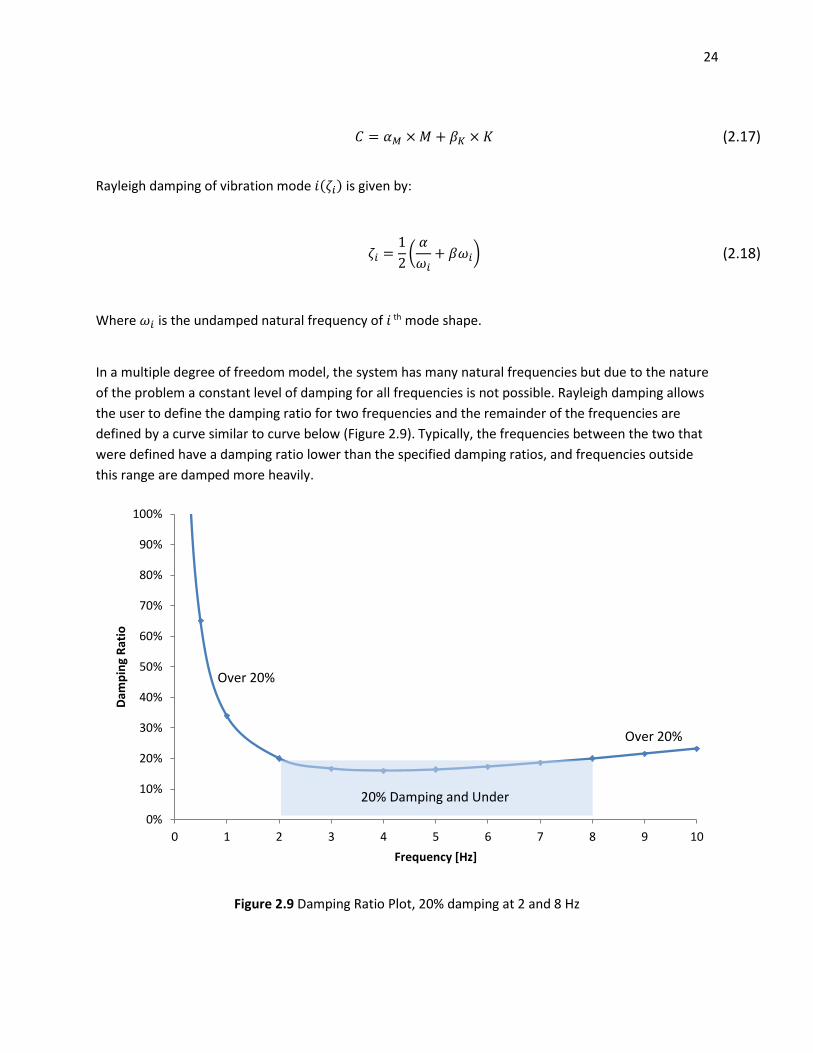
In a multiple degree of freedom model, the system has many natural frequencies but due to the nature

of the problem a constant level of damping for all frequencies is not possible. Rayleigh damping allows

the user to define the damping ratio for two frequencies and the remainder of the frequencies are

defined by a curve similar to curve below (Figure 2.9). Typically, the frequencies between the two that

were defined have a damping ratio lower than the specified damping ratios, and frequencies outside

this range are damped more heavily.

Figure 2.9 Damping Ratio Plot, 20% damping at 2 and 8 Hz

0%

10%

20%

30%

40%

50%

60%

70%

80%

90%

100%

0 1 2 3 4 5 6 7 8 9 10

Dam

pin

g R

atio

Frequency [Hz]

20% Damping and Under

Over 20%

Over 20%

25

The user therefore may specify the two frequencies and the damping ratio they are to damp. The

program will then calculate the alpha and beta values. Alternatively, the user may specify the alpha and

beta values explicitly. Setting alpha and beta to zero will produce a system that is undamped resulting in

the transient response of the system to never dissipate. RS2/RS3 provide an interactive chart to see the

damping value for a range of frequencies to facilitate the correct selection of the dominant frequencies.

For geological materials, damping commonly falls in the range of 2 to 5% of critical; for structural

systems, 2 to 10% is representative (Biggs 1964). Also, see Newmark and Hall (1982) for recommended

damping values for different materials. In analyses that use one of the plasticity constitutive models

(e.g., Mohr-Coulomb), a considerable amount of energy dissipation can occur during plastic flow. Thus,

for many dynamic analyses, only a minimal percentage of damping (e.g., 0.5%) may be required.

Further, dissipation will increase with amplitude for stress/strain cycles that involve plastic flow.

For many problems, the important frequencies are related to the natural mode of oscillation of the

system. Examples of this type of problem include seismic analysis of surface structures such as dams, or

dynamic analysis of underground excavations. For a continuous, elastic system (e.g., a one-dimensional

elastic bar), the speed of propagation, 𝑉𝑝, for p-waves is given by Eqn (2.2) and for s-waves by Eqn (2.3).

If shear motion of the bar gives rise to the lowest natural mode, then 𝑉𝑠 is used in the preceding

equation; otherwise, 𝑉𝑝 is used if motion parallel to the axis of the bar gives rise to the lowest natural

mode.

However, for most of the problem, a wave- length for the fundamental mode of a particular system

cannot be estimated in this way, user can use Natural frequencies analysis to calculate the dominant

frequencies of the system and select the appropriate Rayleigh damping values for the range of

frequencies of interested.

An alternative way is carried out a preliminary without any damping (for example, see Dynamic

Verification 1 (link to the verification). A representative natural period may be estimated from time

histories of velocity or displacement.

Hudson et al. (1994) proposed to set the first frequency equal to the natural frequency of soil layer (𝜔𝑖 = 2𝜋𝑉𝑠/4𝐻) and the second frequency equal to 𝑛𝜔𝑖, where 𝑛 is the closest odd number greater than the ratio of the fundamental frequency of the input motion at the model base and natural frequency of soil layer. For example, if natural frequencies of input motion and soil layer are 3.3 and 1.0 Hz, respectively, the ratio would be 3.3/1.0=3.3; hence, n =5.0. Note that 𝑛 is desired to be odd number because 𝑖th natural frequency of a soil layer is odd multiples of frequency of the fundamental vibration mode of the soil layer.

Equation below presents the 𝑖th natural frequency of a soil layer with height 𝐻 and average shear wave velocity 𝑉𝑠 :

26

𝑓𝑖 =𝑉𝑠

4𝐻(2𝑖 + 1) (2.19)

For typical geotechnical engineering, complex geometry was normally encounter and it is not realistic to use the Eqn (2.19). Users should use Natural frequencies analysis to calculate the first frequency. The frequency from input motion used to calculate the second frequency can be determined using the Dynamic Data Analysis.

2.4.2 Hysteretic Damping

The equivalent linear method has been used widely despite its short comings. Among those are the

assumption of linearity during the solution process, and missing of effective stress analysis, which leads

to pore pressure generation. Although the fully nonlinear method employed by RS2/RS3 are capable to

model the realistic behaviors of wave propagation, there is a need to be able to directly use the same

degrading curve used by equivalent linear methods.

The hysteretic damping will be described in this section to be used as a sole damping scheme or to be

used together with Rayleigh damping. Note that Rayleigh damping may not be needed when hysteretic

damping was employed unless to remove high frequencies noise with an appropriate level of stiffness

damping. More detail will be discussed in Section Damping in practical application.

Modulus degradation curves which was often used in equivalent linear method imply a nonlinear

stress/strain curve. RS2/RS3 have many formulas to simulate a wide range of nonlinear stiffness curve

(link to this https://www.rocscience.com/help/rs3/pdf_files/theory/Constitutive_models_Manual/2-

Elastic_Models.pdf) assuming that the stress depends only on the strain and not on the number of circle

or time. For example, a typical modulus degradation curve for sand can be easy match with one of the

formulae provided in RS2/RS3:

𝐸𝑚𝑎𝑥 = 𝐸0 (𝑏𝑝 + 𝑎

𝑝𝑟𝑒𝑓 + 𝑎)

𝛼

(2.20)

𝐸 = 𝐸𝑚𝑎𝑥 (1 + 𝑎𝛾

𝛾𝑦)

𝑟

(2.21)

where 𝐸𝑚𝑎𝑥 is the maximum elastic modulus, 𝐸0 is the elastic modulus at reference pressure, 𝐸 is the

elastic modulus, 𝑝 is the mean stress, assuming compression positive, 𝑝𝑟𝑒𝑓 is the reference pressure,

and 𝑎, 𝑏, 𝛼, 𝛾𝑦, and 𝑟 are the material parameters. The deviatoric strain, 𝛾, depends on the loading

history in this case.

Once the direction of loading is changed the stiffness regains a maximum recoverable value in the order

of its initial value, 𝐸𝑚𝑎𝑥. When an increment of strains is applied to the material, each principal direction

27

is checked for a possible change in the loading direction. This option can be used to mimic the hysteretic

behavior of soils in dynamic loading, but it is not a robust constitutive model for this purpose, since this

phenomenon is best described by using deviatoric hardening plasticity models.

Using the parameter table (Table 2.1), the degradation curve generated was matched very well as

shown in Figure 2.10.

Table 2.1 Parameter Table for the Modulus Degradation Curve

Poisson’s Ratio 0.286

Residual Young’s Modulus (kPa) 2000

Initial E (kPa) 2.57e+08

a Parameter 0

b Parameter 1

m Parameter 0

Pref (kPa) 100

Alpha 1.155

Gamma Y 0.002

r Parameter -0.6

Figure 2.10 Degradation Curve

28

The reference data set is the modulus reduction curve for sand (Seed & Idriss 1970 – “upper range”)

from the file supplied with the SHAKE-91 code download. (http://nisee.berkeley.edu/software/ )

2.4.3 Damping in practical application

For low level of cyclic strain and an ideal uniform soil, both damping schemes yield similar results,

provided that the levels of damping set for both are consistent with the levels of cyclic strain

experienced. However, when the system is nonuniform (e.g., layers of quite different properties), then

cyclic strain levels may be different in different locations and at different times. Using hysteretic

damping, these different strain levels produce realistically different damping levels in time and space,

while constant and uniform Rayleigh damping parameters can only reproduce the average response.

As yield is approached, neither Rayleigh damping nor hysteretic damping account for the energy

dissipation of extensive yielding. Thus, irreversible strain occurs externally to both schemes, and

dissipation is represented by the yield model (e.g., Mohr-Coulomb). Under this condition, the mass-

proportional term of Rayleigh damping may inhibit yielding because rigid-body motions that occur

during failure modes are erroneously resisted. Hysteretic damping may give rise to larger permanent

strains in such a situation, but this condition is usually believed to be more realistic compared to one

using Rayleigh damping.

However, there are a need to use Rayleigh damping in geotechnical dynamics in most of the cases as

follow:

1. To account for energy dissipation at very small shear strain levels. Note that even at low

deformation levels, soil behavior is irreversible. Constitutive models may not be capable of

appropriately simulating this when stress-state is located within the yield surface. There is no

energy dissipation at very low cyclic strain levels in most of the degradation curve used in

equivalent linear method as well. To avoid low-level oscillation, some small value of Rayleigh

stiffness damping may be used (i.e. 0.2%-0.5%).

2. To damp out the spurious oscillations occurring in high frequency domain: without introducing

any artificial damping such as Rayleigh damping, some high frequency noises develop in the

model which often cause serious problem in the numerical analysis by triggering instability of

the computation process especially models that consist of high stiffness element. Alternatively,

user can use numerical damping by specify Newmark parameters in Eqs 1.4 𝛾 = 0.6 and 𝛽 =

0.3025.

2.5 Natural frequencies analysis Natural Frequency analysis often used in structural dynamic investigate the resonant frequencies of a

design. This analysis type helps users ensure that the natural modes of vibration are well away from

environmental forcing frequencies that a design might encounter during service. For geotechnical

engineering, the analysis is useful when designing a foundation for a vibration source such as machinery

29

equipment, rocket launch base, etc. Another important use of the analysis type is to be used to

determine appropriate Rayleigh Damping parameter.

A linear system with multiple degrees of freedom (DOFs) can be characterized by a matrix equation of

the type

𝑀�̈� + 𝐶�̇� + 𝐾𝑋 = 𝑓(𝑡) (2.22)

where 𝑀 is the mass matrix, 𝐶 is the damping matrix, and 𝐾 is the stiffness matrix. The DOFs are placed

in the row vector 𝑋 and the forces in 𝑓(𝑡).

The free vibration problem is then described by the matrix equation

(−𝜔2𝑀 + 𝑖𝜔𝐶 + 𝐾)𝑋𝑒𝑖𝜔𝑡 = 0 (2.23)

Where 𝜔 is the natural frequency, 𝑖 is the mode shape. Eqn (2.23) forms a complex eigenvalue problem.

Formally, the eigenvalues can be solved by finding

𝑑𝑒𝑡(−𝜔2𝑀 + 𝑖𝜔𝐶 + 𝐾) = 0 (2.24)

In practice, other methods are used if there are more than a few DOFs. The number of eigenvalues is

usually the same as the number of DOFs. Strictly speaking, the number of eigenvalues equals the rank of

the mass matrix.

Lanczos method was used in RS2/RS3 to extract eigenvalues of the model. Since continuum model was

mostly used in geotechnical engineering, the number of eigenvalues is often very large. Users will need

to specify minimum and maximum frequencies to decrease the computational time.

2.6 Deconvolution User can input the seismic motion into RS2 using two options:

• A rigid base

• A compliant base

2.6.1 Rigid base

Input motion (acceleration, velocity or displacement) is applied directly to the nodes of the mesh. The

base still reflects the downward wave propagation back to the model

30

2.6.2 Compliance base

Compliance will be activated when user select the “Compliance base” option in the dynamic load

dialogue. When compliance base option is selected, the applied motion will be transformed to applied

force using the following relation:

𝐹𝑛 = (𝜌𝑉𝑝)𝑣𝑛 (2.25)

𝐹𝑠 = (𝜌𝑉𝑠)𝑣𝑠 (2.26)

Where 𝐹𝑛 is the force normal to the base, 𝐹𝑠 is the force parallel to the base, 𝜌 is the soil mass density,

𝑉𝑝 is the velocity of pressure wave, 𝑉𝑠 is the velocity of shear wave, 𝑣𝑛 is the input motion velocity

normal to the base, 𝑣𝑠 is the input motion velocity parallel to the base.

Note that the input motion and the motion from RS2/RS3 may not be matched using compliance base

since the output from the programs is the results of both upward and downward wave, whereas the

input is only upward part of the wave propagation.

2.6.3 Base selection

The choice of rigid or compliance base depends on whether the earthquake motion to be applied at the

base of the model is “outcrop motion” or “within motion”. Outcrop motions are recorded on top of a

rock layer, while within motions are either recorded at a specific depth from soil surface or computed by

performing a site response analysis. The former is rare because it is not easy to maintain an

accelerogram below ground surface.

As shown in Figure 2.11 below, using the outcrop motion that recorded on top of a rock layer, user can

use 1D site response analysis (Shake (Schnabel et. al. 1972), DeepSoil (Hashash and Park 2001)) to

compute the outcrop/within motion at the interested depth from the recorded motion. The computed

motion is then applied at the base of the model in RS2/RS3 as an input seismic motion.

It is always useful to verify the outcrop motion of the surface in RS2 against the input crop motion in 1D

site response program to make sure that the input seismic motion in RS2/RS3 was accurate. User can

refer to Verification 16 (link to this dynamic verification 16) for such procedure.

31

Figure 2.11 Within/outcrop Motion Demonstration

Depending on the type of computed motion from 1D site response, the choice of the base is as follow:

• Rigid base will be used if input earthquake is a within motion.

• Compliance base if input earthquake is an outcrop motion.

Appropriate base selection is required to simulate wave downward and upward propagation when

earthquake motion hits the base of the model. Propagation of upward and downward waves are

simulated already in computation of a within motion in site response analysis. The within motion is

actually the upward wave which propagates towards the ground surface. Therefore, there is no need for

compliant base. On the other hand, outcrop motion consists of both upward and downward propagating

waves. Compliant base boundary condition is required to absorb the downward wave which would

result in propagation of just the upward component of the outcrop motion.

In summary, the input motion for the base in RS2/RS3 should consist only the upward part of the wave

propagation. Thus, if the input is within motion (which only consist of upward wave) then the rigid base

can be use. However, if the input is outcrop motion (which include both upward and downward waves)

then the compliance base needs to be used to absorb the downward wave.

32

2.7 Liquefaction Liquefaction has been studied extensively by hundreds of researchers around the world since the

earthquake in Alaska (1964) with Mw = 9.2 followed by the Niigata earthquake (Ms = 7.5) with their

devasting liquefaction-induced damage (Kramer, 1996). The term liquefaction, originally coined by

Mogami and Kubo (1953), has historically been used in conjunction with a variety of phenomena that

involve soil deformations caused by monotonic, transient, or repeated disturbance of saturated

cohesionless soils under undrained conditions. The generation of excess pore pressure under undrained

loading conditions is a hallmark of all liquefaction phenomena (Kramer, 1996). The tendency for dry

cohesionless soils to density under both static and cyclic loading is well known. When cohesionless soils

are saturated, however, rapid loading occurs under undrained conditions, so the tendency for

densification causes excess pore pressures to increase and effective stresses to decrease. Liquefaction

phenomena that result from this process can be divided into two main groups: flow liquefaction and

cyclic mobility.

Flow liquefaction produces the most dramatic effects of all the liquefaction-related phenomena-

tremendous instabilities known as flow failures. Flow liquefaction can occur when the shear stress

required for static equilibrium of a soil mass (the static shear stress) is greater than the shear strength of

the soil in its liquefied state. Once triggered the large deformations produced by flow liquefaction are

actually driven by static shear stresses. The cyclic stresses may simply bring the soil to an unstable state

at which its strength drops sufficiently to allow the static stresses to produce the flow failure. Flow

liquefaction failures are characterized by the sudden nature of their origin, the speed with which they

develop, and the large distance over which the liquefied materials often move.

Cyclic mobility is another phenomenon that can also produce unacceptably large permanent

deformations during earthquake shaking. In contrast to flow liquefaction, cyclic mobility occurs when

the static shear stress is less than the shear strength of the liquefied soil. The deformations produced by

cyclic mobility failures develop incrementally during earthquake shaking. In contrast to flow liquefaction,

the deformations produced by cyclic mobility are driven by both cyclic and static shear stresses.

In order to evaluate liquefaction hazard, liquefaction susceptibility, liquefaction triggers and post-

liquefaction damage need to be considered.

2.7.1 Liquefaction susceptibility

Not all soils are susceptible to liquefaction; consequently, the first step in a liquefaction hazard

evaluation is usually the evaluation of liquefaction susceptibility. If the soil at a particular site is not

susceptible, liquefaction hazards do not exist, and the liquefaction hazard evaluation can be ended.

There are several factors that need to be considered such as historical, geological, compositional and

soil condition.

• Liquefaction only occurs in saturated soil thus the susceptibility will decrease as the

groundwater depth increase. The effects of liquefaction are most commonly observed at site

where ground level is within few meters of the ground surface (Kramer, 1996). Loose fill such as

hydraulic fills in dams and mine tailing piles are also susceptible to liquefaction.

33

• Although liquefaction phenomena have been thought that it was limited to sand, nonplastic silt

or coarse silt with bulky particle shape were also so found susceptible to liquefaction (Ishihara,

1984). Liquefaction in gravelly soil was also observed (Evans and Seed, 1987) because of

membrane penetration. However, the liquefaction can only happen in gravelly soil when the

impermeable layers exist. Soil with uniform grain distribution also more susceptible than well

grade soil.

• Steady state line (SSL) can also be used to evaluate soil liquefaction susceptibility (Castro and

Poulos, 1977, Poulos, 1981). Soil with state under the SSL (dense soil) is not susceptible to

liquefaction whereas soil whose state lies above SSL (loose soil) only if the shear stress is larger

than the soil’s residual shear strength (Figure 2.12). Cyclic mobility in other hand can occurs in

both loos and dense soil. Please note that under given loading conditions, any sand will reach a

unique combination of effective confining pressure, shear strength, and density at large strains.

The combination can be described graphically by a steady-state line. The position of the steady-

state line is most strongly influenced by grain size and grain shape characteristics. The behavior

of a sand is strongly related to its position relative to the steady-state line.

Figure 2.12 State criteria for flow liquefaction susceptibility (After Kramer, 1996)

2.7.2 Liquefaction initiation

The generation of excess pore pressure is the key to the initiation of liquefaction. Without changes in

pore pressure, hence changes in effective stress, neither flow liquefaction nor cyclic mobility can occur.

The different phenomena can, however, require different levels of pore pressure to occur. However,

please note that there are few exceptions where the reduction in effectives stress was not caused by

excess pore pressure (i.e. in a constant volumetric test with no applied forces, the decrease in contacts

forces causing the decrease in effective stress).

Flow liquefaction is initiated when the principal effective stress ratio reaches a critical value under

undrained, stress-controlled conditions. The stress state at the initiation of flow liquefaction can be

described graphically in stress path space by the flow liquefaction surface. Initial states that plot in the

shaded region of Figure 2.13 are susceptible to flow liquefaction. Once the effective stress path of an

element of soil reaches the flow liquefaction surface (see Kramer, 1996), additional straining will induce

34

additional excess pore pressure and the available shearing resistance will drop to the steady-state

strength.

Cyclic mobility can produce high excess pore pressures and low effective stresses, but unidirectional

movement will cause the soil to dilate. The increased shearing resistance produced by dilation will arrest

soil movement so that flow slides cannot develop. Initial states that plot in the shaded region of Figure

2.14 are susceptible to cyclic mobility. Note that cyclic mobility can occur in both loose and dense soils

(the shaded region of Figure 2.14 extends from very low to very high effective confining pressures and

corresponds to states that would plot both above and below the SSL).

Figure 2.13 Zone of susceptibility to flow liquefaction (After Kramer, 1996)

Figure 2.14 Zone of susceptibility to cyclic mobility (After Kramer, 1996)

2.7.3 Liquefaction damage

Deformation failures, such as lateral spreading, develop incrementally during the period of earthquake

shaking. For strong levels and/or long durations of shaking, deformation failures can produce large

displacements and cause significant damage. In some cases, settlement induced by pore pressure

dissipation (Figure 2.15) may causes distress to structures supported on shallow foundations, damage to

35

utilities that serve pile-supported structures, and damage to lifelines that are commonly buried at

shallow depths. Depend on the permeability and compressibility of sand layers, the settlement can take

up to a day to complete.

Figure 2.15 Process of earthquake-induced settlement from dissipation of seismically induced excess pore pressure (After Kramer, 1996)

2.7.4 Standard practice

The standard practice approach uses three separate analyses to respond to the three aspects: a

triggering analysis, a flow slide analysis, and a displacement analysis (Byrne et. al., 2006)

• Triggering Analysis: A triggering analysis involves comparing the cyclic stress ratio (CSR) caused

by the design earthquake with the cyclic resistance ratio (CRR) that the soil has because of its

density. The result is expressed in terms of a factor of safety against triggering liquefaction,

𝐹𝑡𝑟𝑖𝑔 = 𝐶𝑅𝑅/𝐶𝑆𝑅. 𝐹𝑡𝑟𝑖𝑔 in the range 1 to 1.4 are generally considered acceptable and assure

that seismic displacements will be small and tolerable (Byrne and Anderson, 1991, Youd et al.,

2001). Our program Settle3D has a very comprehensive method of Triggering Analysis.

Interested user can find more detail at

(https://www.rocscience.com/help/settle/pdf_files/theory/Settle3D_Liquefaction_Theory_Man

ual_v4.pdf)

• Flow slide analysis: The factor of safety against a flow slide, 𝐹𝑓𝑙𝑜𝑤 is computed from standard

limit equilibrium analysis procedures using a post-liquefaction strength in those zones predicted

to liquefy from the triggering analysis. Post-liquefaction strengths are based on field experience

during past earthquakes and are significantly lower than values obtained from direct testing of

undisturbed samples at in situ void ratios. Post liquefaction strength may be expressed directly

in terms of penetration resistance, 𝑠𝑢 as suggested by Seed and Harder (1990) or as a strength

ratio 𝑠𝑢/𝜎′𝑣𝑜 (Olson and Stark, 2002). This step can be easily carried out using our Slope stability

program such as Slide2/Slide3

36

• Seismic Displacements: Seismic displacements that arise during shaking are commonly based on

Newmark (1965) who modelled a potential sliding block of soil as a rigid mass resting on an

inclined plane. The acceleration that would just cause yielding and movement down the plane is

called the yield acceleration (𝑎𝑦) in gravity units, and corresponds to the seismic coefficient, k,

that would reduce the factor of safety to unity. Yielding at the base and displacement down the

plane is instigated each time the base acceleration exceeds the yield acceleration and causes the

block to move in discontinuous steps during the period of strong shaking. Peak accelerations

greater than the yield acceleration imply an instantaneous factor of safety less than unity. This

does not imply failure, but some limited displacement that can be calculated from the equation

of motion and the prescribed earthquake motion. Note that the standard practice approach of

the past evaluated dynamic stability based on factor of safety and a seismic coefficient. This past

procedure is generally not appropriate and should be replaced by a displacement approach such

as the simple one proposed by Newmark. Seismic displacements associated with liquefaction

can also be estimated from empirical equations (Youd et al. (2002), Olson and Stark (2002) and

Seed and Harder (1990)). Settle induced by pore pressure dissipation after the earthquake can

also predicted using relationships for volumetric reconsolidation strain as a function of

equivalent uniform cyclic stress ratio (Wu 2002). Note that Newmark method was also included

in our Slide program.

The standard practice of liquefaction analysis has a number of shortcomings: The three aspects of

liquefaction; triggering, flow slide, and displacements are addressed in three separate analyses. In fact,

they are part of a single liquefaction response in which pore pressure rises and liquefaction occurs at

different rates and times in various zones of the earth structure causing the response of the structure to

change as it softens. Redistribution of excess pore pressure may create more severe conditions, and

finally dissipation and reconsolidation occur as the soil regains its strength. No direct account of these

aspects is considered in state-of practice procedures, and in particular no direct account of pore

pressure generation and redistribution effects on response is considered. These shortcomings can lead

to predicted response that is not realistic, and remedial designs that can be overly conservative, or

unsafe depending on site conditions (Byrne et. al., 2006)

2.7.5 Effective stress analysis using RS2/RS3

This procedure addresses the liquefaction response taking pre-triggering, triggering, and post-triggering

aspects into account in a single analysis that more closely simulates conditions in the field. The strength

and stiffness of soil is governed by effective stress, and so it is desirable to evaluate seismic response of

soil in terms of effective stresses. In RS2/RS3, two most common effective stress analysis were provided:

• Loose coupled model: Pore pressure generation and liquefaction are caused by the tendency of

soil to contract when subjected to cyclic shear loading. Martin et al. (1975) presented a 4

parameters shear-volume coupling model for predicting the increment of volumetric

compaction per load cycle. Based on this concept Martin et al. developed the first dynamic

effective stress model in which shear strains were evaluated in each element allowing the pore

pressure rise at the end of each shear cycle to be computed. The total rise in pore pressure for

undrained conditions is simply the sum of the pore pressure increments. The strength and

37

moduli are reduced in each element in accordance with the drop in effective stress as pore

pressure rise occurs. Dissipation of excess pore pressure can also be accounted for by allowing

flow between elements. More details can be found at the material model detail page

https://www.rocscience.com/help/rs2/pdf_files/verification/RS2_Dynamics_Verification.pdf#pa

ge=62. The Finn model can adequately capture the pore pressure rise up to the point of

triggering of liquefaction for level ground conditions, in order to simulate the post liquefaction

response where dilation and pore pressure drop occurs during each load cycle, user need to

specify a residual strength and a nominal shear stiffness as described in section Hysteretic

Damping.

• Fully coupled models: The most accurate and general methods for representation of soil

behavior are based on advanced constitutive models that use basic principles of mechanics to

describe observed soil behavior for (a) general initial stress conditions, (b) a wide variety of

stress paths, (c) rotating principal stress axes, (d) cyclic or monotonic loading, (e) high or low

strain rates, and (f) drained or undrained conditions. Such models generally require a yield

surface that describes the limiting stress conditions for which elastic behavior is observed, a

hardening law that describes changes in the size and shape of the yield surface as plastic

deformation occurs, and a flow rule that relates increments of plastic strain to increments of

stress. The Cam-Clay (Roscoe and Schofield, 1963) and modified Cam-Clay (Roscoe and Burland,

1968) models were among the first of this type. Improvements in the prediction of shear strains

have resulted from the use of multiple nested yield loci within the yield surface (Mroz, 1967;

Prevost, 1977) and the development of bounding surface models (Dafalias and Popov, 1979)

which incorporate a smooth transition from elastic to plastic behavior. By imposed zero

volumetric strain for undrained condition, the effective stresses and excess pore pressure can be

computed. In RS2, the following models are provided:

o Manzari and Dafalias (Manza and Dafalias, 2007)

o Bounding Surface Plasticity (Pietruszczak and Stolle, 1987)

o Norsand (Jefferies,1993)

Although advanced constitutive models allow considerable flexibility and generality in modeling the

response of soils to cyclic loading, their description usually requires many more parameters than

equivalent linear models or cyclic nonlinear models. Evaluation of these parameters can be difficult, and

the parameters obtained from one type of test can be different from those obtained from another.

Although the use of advanced constitutive models will undoubtedly increase, these practical problems

have, to date, limited their use in geotechnical earthquake engineering practice.

2.8 Dynamic modelling A numerical model can help us to understand a physical process which may confirm our thinking or can

even adjust our thinking. Finite element analysis in general is a tool to enhance engineer judgement but

not to replace it. A clear picture of the whole system may not be able to be predicted at the beginning,

but a very rough estimation of an expected behavior should be made before starting modelling process.

38

Main questions of the simulated problems should be clearly defined at the beginning of the analysis. If

internal force of a structure is the main concern then much of the effort should be spent on modelling

structure component details whereas if deformation is the confirmation then support structure can be

simplified using equivalent properties such as stiffness and strength.

Similar to any other geotechnical finite element modelling, there are several most important aspects

when carrying out an analysis:

• In geotechnical engineering, the “construction material” is natural ground (soil and rock) and

not man-made such as concrete and steel, fabricated to predefined specifications. This

inevitably means that the material is inhomogeneous, its mechanical and hydraulic behavior is

not easily formulated in mathematical terms and material parameters are difficult to determine.

Even with a perfect site investigation scheme, significant uncertainties remain with respect to

the soil profile and thus with the geotechnical model which forms the basis for the numerical

model.

• Installation processes, such as construction of piles, diaphragm walls, stone columns, mixed-in-

place columns, jet grout panels, have an influence on the stress regime in the soil, which is still

extremely difficult, if not impossible, to quantify numerically.

• Geometric simplification has to be introduced (2D vs 3D), and the domain of the model to be

analyzed may not always be easily identified.

It is recommended that a numerical simulation should be start simple to understand the basic

mechanism of a problem. It is almost impossible to include all the details on site into a “model”. A real

geometry should be simplified by removing irregular boundaries and stratigraphy. Elastic materials

should be used as a start of the simulation. Then numerical experiments or parametric study may be

carried out to evaluate the effects of each components on the model. Based on the experiment found

out, more attention will be paid to ones that have more effects on the model.

Given that practice in mind, a dynamic model generally includes the following steps:

1. Create geometry and set up initial static condition

2. Calibrate input data (seismic load, motion record, etc.)

3. Determine appropriate boundary conditions and apply load

4. Determine material properties and damping coefficient

5. Assign location to monitor dynamic data and carried out simulation

The descriptions for each step will be given in below. Details of each step are provided in our dynamic

tutorials (https://www.rocscience.com/help/rs2/tutorials/New_Dynamic_Data_Analysis.htm,

https://www.rocscience.com/help/rs2/tutorials/RS2__Dynamic_Analysis_of_Machine_Foundation.htm)

2.8.1 Geometry and initial static condition

Prior to a dynamic analysis, an equilibrium static condition should be determined. A static analysis is carried out with appropriate considerations such as material properties, construction stages to establish

39

in situ stresses and pore pressure. It is especially very important because of initial stress in triggering liquefaction (See section Error! Reference source not found.). Note that since the hysteretic damping curve normally starts from zero strain, it should be activated even in the static simulations to avoid asymmetric behaviors.

2.8.2 Calibrate input data

The motion record properties will be examined using various tools available in RS2/RS3 such as

amplitude spectrum, response spectrum and arias intensity. Noise associated with high frequencies

should be filter out. Although in RS2/RS3, amplitude spectrum can be determined using either

acceleration or velocity, it is recommended that filtering should be applied on velocity since most of the

wave equation from material properties were based on velocities. Base line correct should also be

carried out to made adjustment to machine errors. (see Error! Reference source not found.)

2.8.3 Determine appropriate boundary condition and dynamic loading

Dynamic analysis can be activated in the project setting under “Stages” option. As the option was turned

on, the restraint condition (displacement, roller or fixed) at the external boundary should be turned off.

It can be done by specifying staging factors when applying boundary conditions at static stages. At

dynamic stages, depends on the location of the dynamic sources, appropriate boundary condition

should be assigned.

Dynamic model generally can be classified into two main categories:

• Dynamic wave was generated inside the domain considered: machine foundation, mining

explosive are examples for this type of analysis. Wave reflection should be avoided at the

boundary of the models thus absorb boundary conditions (see Absorb Boundary Condition)

should be applied to all sides of models excepts free surface. A typical boundary condition can

be found in Figure 2.16 below.

Figure 2.16 Typical boundary condition for dynamic source inside the interested domain

• Dynamic wave was generated from outside of the interested domain: seismic analysis is a typical

example for this type of analysis. Wave reflection also need to be avoided at the model

boundary. Besides that, the seismic wave from outside domain should also be transmitted to

40

the model. Figure 2.17 show a typical boundary condition for this type of analysis. For two sides

of the model, the transmit condition should be applied (see Transmit Boundary Condition). A

compliance base or a rigid base will be used depending on the input motion type (see section

Error! Reference source not found.).

Figure 2.17 Typical boundary condition for seismic analysis

2.8.4 Determine material properties and damping parameters

If pore pressure build-up and dissipation is not in interested and/or the material is not coarse-grain materials, for the shake of simplicity, undrained parameters can be used (undrained stiffness and strength). However, for most of the dynamic simulation, pore pressure generation is the area on main interest for triggering liquefaction and seismic damage evaluation (Section Error! Reference source not found.). The material behaviors will be set to undrained and effective parameter will be utilized together with fluid (water) modulus. RS2/RS3 employed special elements based on mixed form UP formulation to overcome incompressible volumetric strain associated with undrained material (Zienkiewicz et al, 2005). Damping parameters are also should be determined in this step. Hysteretic damping should be derived from a simple cyclic direct shear test simulation to compare with degradation curve (see Hysteretic Damping). In order to determine Rayleigh damping, a natural frequencies analysis can be carried out to determine the most dominant frequencies. Having the dominant frequencies, the second frequency used in the Rayleigh’s damping can be easy determine using the process specified in Rayleigh damping section using the maximum frequencies from motion record. The model is then analyzed with only elastic properties and without any damping to confirm the shear strain range as well as the dominant frequencies. The hysteretic damping and Rayleigh damping may need to adjust to be more appropriate with strain level and dominant frequencies of the model.

2.8.5 Assign location to monitor dynamic data and carry out simulation

After calibrating material properties and damping parameters were checked. The model is run with

damping parameters and strength properties. Since data for the whole simulation cannot be store,

location of interested need to be specified to be recorded. Once specified, stress, strain, velocity,

acceleration, displacement and pore pressure will be recorded. Motion recorded at the input location

41

should be match with input motion. Stress strain relationship can be used to see the effect of hysteretic

damping, pore pressure generation/dissipation can be used to evaluate triggering of liquefaction.

References

Arias, A. (1970). A measure of earthquake intensity. Seismic Design for Nuclear Power Plants, The M.I.T.

Press, 438-483.

Bathe, K.J. (1982). Finite Element Procedures in Engineering Analysis, pp. 449-556. Prentice-Hall,

Englewood Cliffs.

Biggs, J. M. (1964). Introduction to structural dynamics. New York: McGraw-Hill.

Brandenberg, S.J. and Manzari, M.T. (2018). Proceeding of geotechnical earthquake engineering and soil

dynamics V. Austin, Texas, June 10-13, 2018.

Byrne, P. M. and Wijewickreme, D. (2006, October 1-4). Liquefaction resistance and post-liquefaction

response of soils for seismic design of buildings in greater Vancouver [Paper presentation]. In Sea to Sky

Geotechnique: 59th Canadian Geotechnical Conference & 7th Joint CGS/IAH-CNC Groundwater Specialty

Conference, Vancouver, Canada (pp. 1267-1278).

Byrne, P. M., Naesgaard, E., and Seid-Karbasi, M. (2006, October 1-4). Analysis and design of earth

structures to resist seismic soil liquefaction [Paper presentation]. In Sea to Sky Geotechnique: 59th

Canadian Geotechnical Conference & 7th Joint CGS/IAH-CNC Groundwater Specialty Conference,

Vancouver, Canada (pp. 1-24).

Cohen, M. and Jennings, P.C. (1983). Silent boundary methods for transient analysis. In T. Belytschko

and T.J.R. Hughes (Eds.), Computational Methods for Transient Analysis (Vol 1).

Dafalias, Y.F and Manzari, M.T (2004) Simple Plasticity Sand Model Accounting for Fabric Change Effects

Journal of Engineering Mechanics, 2004, 130(6): 622-634

Dafialias, Y.F. and Popov, E.P. (1979). A model for nonlinearly hardening materials for complex loading.

Acta Mechanica, 21(3), 173-192.

Hashash, Y.M.A. and Park, D. (2002). Viscous damping formulation and high-frequency components in

deep deposits. Soil Dynamics and Earthquake Engineering, 22 (7), 611-624.

Jefferies, M. G. (1993) Nor-Sand: a simple critical state model for sand. Geotechnique, 43, No 1, 91-103

Jones, J., Kalkan, E., and Stephens, C. (2017). Processing and review interface for strong-motion data

(PRISM) software, version 1.0.0—Methodology and automated processing. U.S. Geological Survey Open-

File Report. 2017–1008, 81 p. 2017, available at https://pubs.er.usgs.gov/publication/ofr20171008 (last

visited 10/16/2020).

42

Kramer, S.L. (1996). Geotechnical earthquake engineering. Upper saddle River, New Jersey: Prentice Hall.

Lamb, H. (1932). Hydrodynamics. Cambridge.

Lenhardt, W.A. (2007). Earthquake-Triggered Landslides in Austria – Dobratsch Revisited. Jahrbuch der

Geologischen Bundesanstalt. Archived from the original on 2011-05-31.

Lysmer, J. and Kuhlemeyer, R.L. (1969). Finite dynamic model for infinite media, ASCE J., Engineering

Mechanics Division, 95(EM4), 859-876.

Martin, G.R., Finn, W.D.L. and Seed, H.B. (1975). Fundamentals of liquefaction under cyclic loading.

ASCE, J., Geotechnical Engineering Division, 101(5), 423-438.

Mroz, Z. (1967). On the description of anisotropic work hardening. Journal of Mechanics and Physics of

Solids, 15, (163-175).

Nelson, R.B. and Mak, R. (1982). A method for improving numerical stability of implicit time integration

for non-linear dynamic structural response. Nuclear Engineering and Design, 70(1), 37-43.

Newmark, N.M. (1959). A method of computation for structural dynamics. ASCE J., Engineering

Mechanics Division, 85(3), 67-94.

Newmark, N. M. and Hall, W.J. (1982). Earthquake spectra and design. Berkeley, California: Earthquake

Engineering Research Institute.

Nielsen, A.H. and Babtie, J. (2006). Absorbing boundary conditions for seismic analysis in ABAQUS.

http://www.simulia.com/download/solutions/architecture_cust%20references/architecture_absorbing_

auc06_babtie.pdf

Olson, S. M. and Stark, T.D. (2002). Liquefied strength ratio from liquefaction flow failure case histories.

Canadian Geotechnical Journal, 39, 629–647.

Pietruszczak, S., and Stolle, D.F.E. (1987) Modelling of sand behaviour under earthquake excitation.

International journal for numerical and analytical methods in geomechanics. vol. 11, 221-240 (1987)

Roscoe, K.H. and Burland, J.B. (1968, March). On the generalized stress-strain behavior of 'wet' clay

[Paper presentation]. In J. Heyman and F.A Leckie. Engineering Plasticity. University Press, Cambridge

(535-609).

Schnabel, P. B., Lysmer, J., and Bolton Seed, H. (1972). SHAKE: A computer program for earthquake

response analysis of horizontally layered sites, (Report No. UCB/EERC-71/12). University of California,

Berkeley, California: Earthquake Engineering Research Center.

43

Seed, R.B. and Harder, L.F. (1990). SPT-based analysis of cyclic pore pressure generation and undrained

residual strength. In Proceedings of the H.B. Seed Memorial Symposium (vol. 2, pp. 351–376). Bi-Tech

Publishing Ltd.

Westergaard, H. M. (1933). Water pressures on dams during earthquakes. ASCE Transactions, pp.418-433.

Wolf, J.P. (1988). Soil-structure interaction analysis in time domain. Prentice Hall.

Youd, T.L., Hansen, C.M., and Bartlett, S.F. (2002). Revised multi-linear regression equations for

prediction of lateral spread displacement. ASCE J., Geotechnical and Geoenvironmental Engineering

Division, 128, 1007- 1017.

Zeng, D., Manzari, M.T., and Hiltunen, D.R. (2008, May 18-22). Proceedings of geotechnical earthquake

engineering and soil dynamics IV, Sacramento, California.

Zienkiewicz, O.C., Bicanic, N. and Shen, F.Q. (1989). Earthquake input definition and the transmitting

boundary conditions. In I.S. Doltsinis (Ed.), Advances in Computational Nonlinear Mechanics I (pp. 109-

138). Springer-Verlag.

Zienkiewicz, O.C., Taylor, R.L., and Zhu, J.Z. (2005). The finite element method: its basis and

fundamentals. 6th ed. Butterworth-Heinemann.