SIMPLIFIED APPROACH FOR THERMO FLUID-DYNAMIC ANALYSIS

OF LOOPED DISTRICT HEATING NETWORK

Elisa Guelpa1, Vittorio Verda2*

1 Energy Department, Politecnico di Torino,

C.so Duca degli Abruzzi 24, 10129 Torino, Italy,

e-mail: elisa.guelpa@polito.it

2 Energy Department, Politecnico di Torino,

C.so Duca degli Abruzzi 24, 10129 Torino, Italy,

e-mail: vittorio.verda@polito.it

Keywords: district heating, modelling, compact model, black box model, network modelling, smart thermal grids

Abstract

DH network modelling constitute a crucial way for simulating the system responses to changes in operating

conditions. These modifications can be planned for increasing the DH efficiency (such as heat storage

installation or optimization of operations) or they can be unexpected, such as the occurrence of malfunctions

or pipeline breakups.

In this framework, an important issue regards the possibility of simulating of the entire DH networks. DH

networks can be fully modelled through a numerical approach, which considers fluid flow and transient

heat transfer. The model is based on conservation equations and it has been validated by comparison with

experimental data of the Turin district heating network. In some cases, i.e. when a) super-real time

simulations b) very large network c) optimization through heuristic methods are considered, faster

computational approaches can be useful for simulating thermal fluid-dynamic within the network. The goal

of this work consists in proposing a compact model for the simulation of DH network for obtaining a

significantly the computational costs without compromising its reliability.

1. Introduction

The competitiveness of DH derives from the use of various sources and high efficiency plants for house

heating and domestic hot water production in densely populated areas [1.2]. DH allows a higher exploitation

of renewable sources [3-5], efficient technologies [6, 7] and waste heat [8, 10]. Furthermore, the

simultaneous production of thermal energy and electricity significantly decreases the fuel consumption for

building heating with a consequent reduction of carbon emissions. As a consequence, district heating system

is one of the most convenient technology for house heating in urban areas [11, 12] and it allows a reduction

of primary energy consumption to about 50% with respect to the use of condensing boilers [13].

Optimal control, design and management [14, 15] are crucial points for reducing primary energy

consumption and pollutant production and increasing economic benefit from selling heat and electricity. In

this framework, modelling of DH system is a crucial point in order to analyze effects of changes in a) the

network topology b) system management c) operations d) power plants and storage capacity. Typical

applications deals with thermal storage [16-18] or virtual storage [19,20] installation. is For this reason

modeling has been widely applied in both DH design [21, 22] and management [23, 24] phases.

The most common modelling approaches are physical and black box approaches. Physical models rely on

the definition and solution of the physical problem on a computational domain, which is the entire DH

network pipeline. The non-linear problem that characterize the DHN fluid-dynamic is solved by numerical

methods that are often computationally expensive. Physical models require the topological description of

the network and allows evaluating mass flows and temperature distributions in the network.

In black box approaches, the nonlinearity is overcome using standard transfer functions or neural networks.

In order to build and validate these kinds of models, a certain amount of experimental data, or simulation

results, are necessary [25, 26].

In the literature various different types of physical models have been developed, such as loop equation

method [27], aggregated models [28] (applied to 20 km long network, with 1079 nodes and 10 MW of

maximum heat production) and node based model [29]. Both aggregated and node-based models do not

solve fluid-dynamic and thermal transient problems in all the network nodes [30]. In [30] the thermal fluid-

dynamic problem has been solved for a medium size network, neglecting heat losses.

When extended DH networks are considered, the computational cost becomes a crucial characteristic of a

simulation tool. This is due to the large number of nodes and branches included in the network. Indeed the

solution of the thermal fluid-dynamic problem may require very high computational resources. An

alternative approach has to be used in these cases.

As far as no modelling of extended network is presented in the literature, in the present paper the main

strength of the physical approach are combined with the compactness of the black box model. This is done

for achieving fast solution of fluid dynamic problem in extended DH networks. The circulation of the water

within the network loops is computed through a black box approach while mass flows and temperature are

evaluated by solving the mass and energy conservation equation for all the nodes of the network. It allows

keeping computational expenses as low as possible, with a negligible error.

2. Methodology

2.1 Physical model description (full model)

Physical description of DH networks usually rely on a one dimensional model based on the description of

the network through a graph based approach [31]. Namely, each pipe of the network is considered as branch

that starts from a node, the inlet node, and ends in another node, the outlet node. Incidence matrix A is used

to describe the connection between nodes and branches of the network. A general element Aij is equal to 1

or -1 if the branch j enters or exits the node i and 0 otherwise. A includes as many rows as the number of

nodes and as many columns as the number of branches.

The thermal fluid-dynamic model here used includes the mass and energy conservation equations applied

to all the nodes and the momentum conservation equation to all the branches. The mass balance equation

written using matrix form is:

0 extGGA , (1)

G is the vector including the mass flow rates in branches and Gext the vector includes the mass flow rates

exiting the nodes towards the extern.

The steady-state momentum conservation equation is considered for all the branches of the network,

considering an incompressible fluid, neglecting the velocity change within a single pipe and including the

gravitational term in the static pressure. This can be written in a matrix form as described in (6)

pumps

T pYPAYG , (2)

where the diagonal matrix Y represents the fluid dynamic conductance of branches:

1

2

1

2

1

k

kLD

f

S

GRY

(3)

The dependence of Y on pressure makes the system of equation non-linear, as already mentioned in the

introduction section. The solution of the mass and momentum equations is performed using a SIMPLE

(semi implicit method for pressure linked equation) algorithm [32], which is a common guess and correction

method use for solving Navier Strokes equations.

The energy conservation equation is written neglecting conduction in the fluid along the network and

volumetric heat release within the control volume. The energy equation is written in transient form because

the thermal capacity cannot be neglected and the temperature perturbations travel the network with the fluid

speed. The matrix equation, including an equation for each network nodes, assumes the following form:

𝑴�̇� + 𝑲𝑻 = 𝒈 (4)

Where M is the mass matrix that includes the coefficient of the unsteady term, K is the stiffness matrix,

including the terms multiply by T and g is the known term.

The model equations are detailed in the simple and matrix form in Table Further details on the method are

available in [33].

Mass conservation

equation

Momentum conservation equation Energy conservation equation

Extended form ∑𝐺𝑖𝑛 −∑𝐺𝑜𝑢𝑡 = G𝑒𝑥𝑡 (pin − pout) =1

2

f

DLG2

ρS2+1

2∑βkk

G2

ρS2− t

𝜕(𝜌𝑐∆𝑇)𝑖𝜕𝑡

∆𝑉𝑖 +∑𝑐𝐺𝑗𝑗

𝑇𝑗 = 𝑈𝑇𝑂𝑇(𝑇𝑖 − 𝑇𝑒𝑛𝑣)

Matrix form 𝐀 ∙ 𝐆 + 𝐆𝐞𝐱𝐭 = 0 𝐆 = 𝐘 ∙ 𝐀T ∙ 𝐏 + 𝐘 ∙ 𝐭 𝑴�̇� + 𝑲𝑻 = 𝒈

Solution Method SIMPLE SOLVER FOR LINEAR EQUATION

SYSTEM

Computational

cost (for the

examined

network)

1,7 s 10-?

Table 1 Full model details

2.2 Compact model description

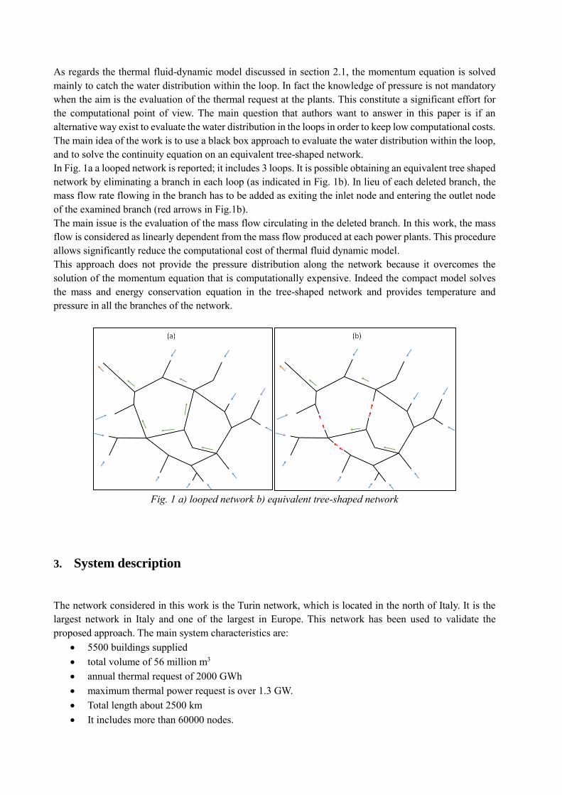
As regards the thermal fluid-dynamic model discussed in section 2.1, the momentum equation is solved

mainly to catch the water distribution within the loop. In fact the knowledge of pressure is not mandatory

when the aim is the evaluation of the thermal request at the plants. This constitute a significant effort for

the computational point of view. The main question that authors want to answer in this paper is if an

alternative way exist to evaluate the water distribution in the loops in order to keep low computational costs.

The main idea of the work is to use a black box approach to evaluate the water distribution within the loop,

and to solve the continuity equation on an equivalent tree-shaped network.

In Fig. 1a a looped network is reported; it includes 3 loops. It is possible obtaining an equivalent tree shaped

network by eliminating a branch in each loop (as indicated in Fig. 1b). In lieu of each deleted branch, the

mass flow rate flowing in the branch has to be added as exiting the inlet node and entering the outlet node

of the examined branch (red arrows in Fig.1b).

The main issue is the evaluation of the mass flow circulating in the deleted branch. In this work, the mass

flow is considered as linearly dependent from the mass flow produced at each power plants. This procedure

allows significantly reduce the computational cost of thermal fluid dynamic model.

This approach does not provide the pressure distribution along the network because it overcomes the

solution of the momentum equation that is computationally expensive. Indeed the compact model solves

the mass and energy conservation equation in the tree-shaped network and provides temperature and

pressure in all the branches of the network.

Fig. 1 a) looped network b) equivalent tree-shaped network

3. System description

The network considered in this work is the Turin network, which is located in the north of Italy. It is the

largest network in Italy and one of the largest in Europe. This network has been used to validate the

proposed approach. The main system characteristics are:

5500 buildings supplied

total volume of 56 million m3

annual thermal request of 2000 GWh

maximum thermal power request is over 1.3 GW.

Total length about 2500 km

It includes more than 60000 nodes.

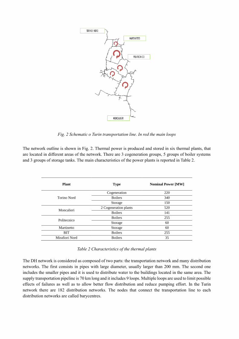
Fig. 2 Schematic o Turin transportation line. In red the main loops

The network outline is shown in Fig. 2. Thermal power is produced and stored in six thermal plants, that

are located in different areas of the network. There are 3 cogeneration groups, 5 groups of boiler systems

and 3 groups of storage tanks. The main characteristics of the power plants is reported in Table 2.

Plant Type Nominal Power [MW]

Torino Nord

Cogeneration 220

Boilers 340

Storage 150

Moncalieri 2 Cogeneration plants 520

Boilers 141

Politecnico Boilers 255

Storage 60

Martinetto Storage 60

BIT Boilers 255

Mirafiori Nord Boilers 35

Table 2 Characteristics of the thermal plants

The DH network is considered as composed of two parts: the transportation network and many distribution

networks. The first consists in pipes with large diameter, usually larger than 200 mm. The second one

includes the smaller pipes and it is used to distribute water to the buildings located in the same area. The

supply transportation pipeline is 70 km long and it includes 9 loops. Multiple loops are used to limit possible

effects of failures as well as to allow better flow distribution and reduce pumping effort. In the Turin

network there are 182 distribution networks. The nodes that connect the transportation line to each

distribution networks are called barycentres.

4. Results

In this section, mass flow rates obtained with both the full and the compact model have been reported and

compared. In Fig. 3 the value of mass flow rates in the deleted branches are depicted. Both mass flows

evaluated by solving the momentum equation and mass flow obtained through the simplified approach are

reported. Three different thermal loads have been considered in the analysis: 30%, 60% and 90% of the

maximum thermal load that can be provided to the network. The sign of the mass flow rates reported in

Fig. 3 is due to the direction of the flow respect to the reference one. It is possible to notice that in all the

considered cases the compact model correctly detects the direction of the flow. Furthermore, the error

performed in the prediction of the mass flow rate value is low in all the cases considered.

Fig. 3 Mass flow rates in the deleted branches, obtained through momentum equation and simplified

approach

In order to better visualize the performance of the compact model, the errors performed in mass flow rates

calculation are shown in Fig. 4. The figure reports the percentage relative error in the mass flow rate

evaluation for three load values. Only the cases when the mass flow rate is not negligible are considered in

the analysis. Error are always lower than 5 %. These results are particularly encouraging as regards the use

of simplified method to compute the mass flows in looped network.

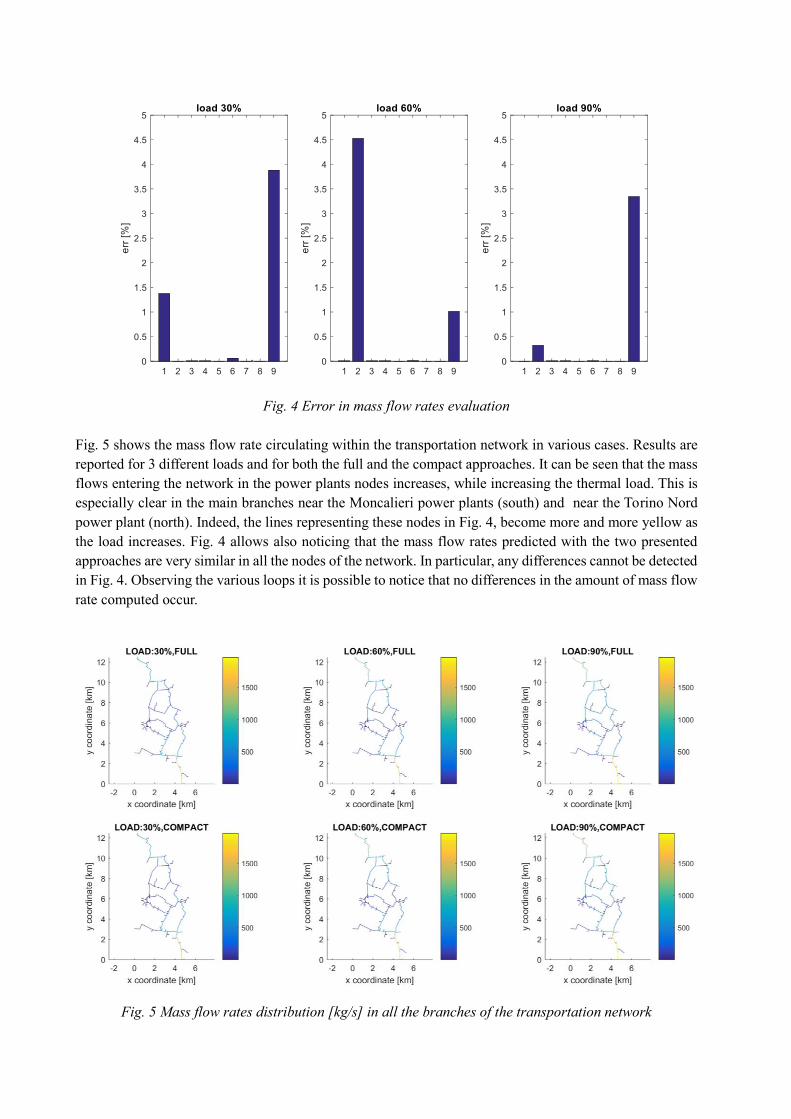
Fig. 4 Error in mass flow rates evaluation

Fig. 5 shows the mass flow rate circulating within the transportation network in various cases. Results are

reported for 3 different loads and for both the full and the compact approaches. It can be seen that the mass

flows entering the network in the power plants nodes increases, while increasing the thermal load. This is

especially clear in the main branches near the Moncalieri power plants (south) and near the Torino Nord

power plant (north). Indeed, the lines representing these nodes in Fig. 4, become more and more yellow as

the load increases. Fig. 4 allows also noticing that the mass flow rates predicted with the two presented

approaches are very similar in all the nodes of the network. In particular, any differences cannot be detected

in Fig. 4. Observing the various loops it is possible to notice that no differences in the amount of mass flow

rate computed occur.

Fig. 5 Mass flow rates distribution [kg/s] in all the branches of the transportation network

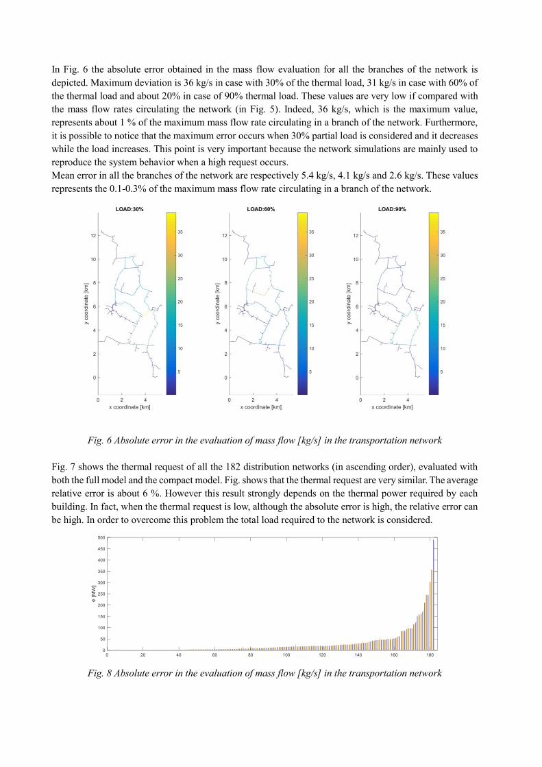
In Fig. 6 the absolute error obtained in the mass flow evaluation for all the branches of the network is

depicted. Maximum deviation is 36 kg/s in case with 30% of the thermal load, 31 kg/s in case with 60% of

the thermal load and about 20% in case of 90% thermal load. These values are very low if compared with

the mass flow rates circulating the network (in Fig. 5). Indeed, 36 kg/s, which is the maximum value,

represents about 1 % of the maximum mass flow rate circulating in a branch of the network. Furthermore,

it is possible to notice that the maximum error occurs when 30% partial load is considered and it decreases

while the load increases. This point is very important because the network simulations are mainly used to

reproduce the system behavior when a high request occurs.

Mean error in all the branches of the network are respectively 5.4 kg/s, 4.1 kg/s and 2.6 kg/s. These values

represents the 0.1-0.3% of the maximum mass flow rate circulating in a branch of the network.

Fig. 6 Absolute error in the evaluation of mass flow [kg/s] in the transportation network

Fig. 7 shows the thermal request of all the 182 distribution networks (in ascending order), evaluated with

both the full model and the compact model. Fig. shows that the thermal request are very similar. The average

relative error is about 6 %. However this result strongly depends on the thermal power required by each

building. In fact, when the thermal request is low, although the absolute error is high, the relative error can

be high. In order to overcome this problem the total load required to the network is considered.

Fig. 8 Absolute error in the evaluation of mass flow [kg/s] in the transportation network

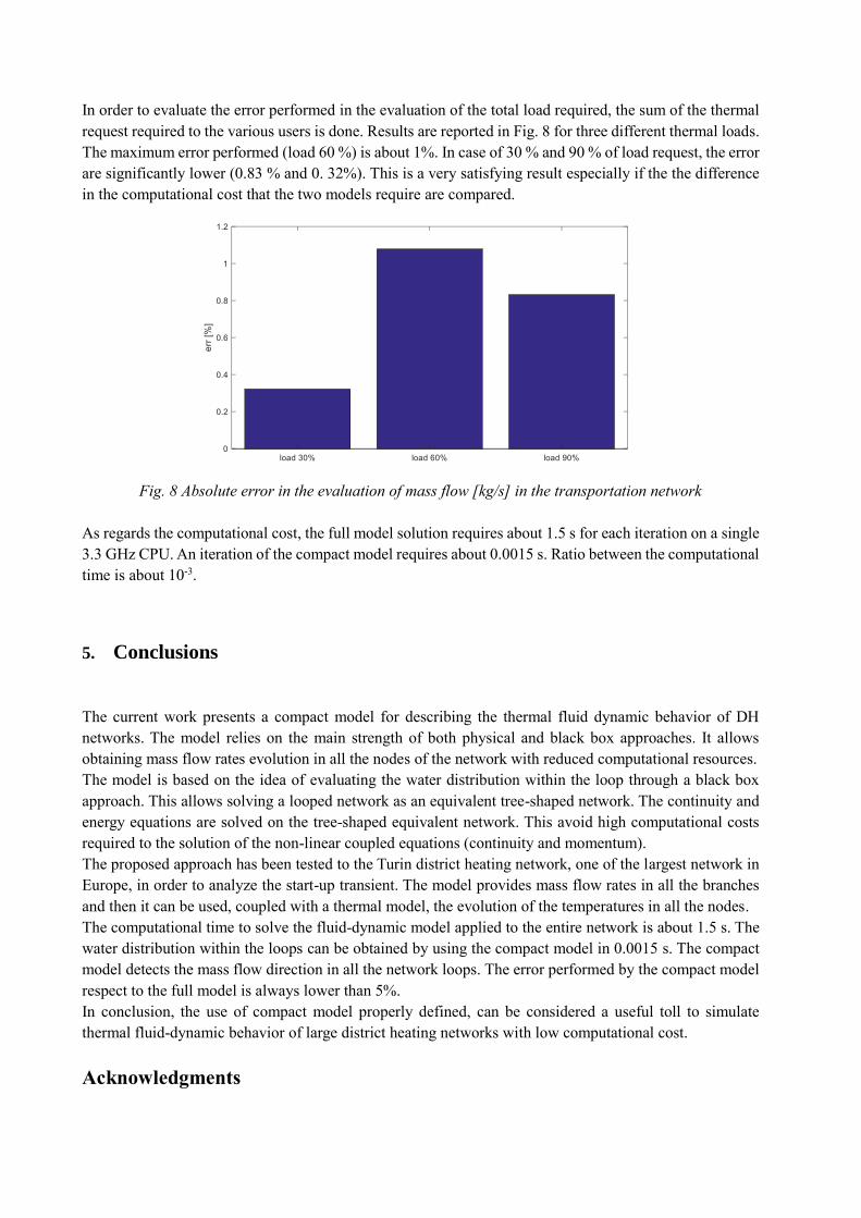
In order to evaluate the error performed in the evaluation of the total load required, the sum of the thermal

request required to the various users is done. Results are reported in Fig. 8 for three different thermal loads.

The maximum error performed (load 60 %) is about 1%. In case of 30 % and 90 % of load request, the error

are significantly lower (0.83 % and 0. 32%). This is a very satisfying result especially if the the difference

in the computational cost that the two models require are compared.

Fig. 8 Absolute error in the evaluation of mass flow [kg/s] in the transportation network

As regards the computational cost, the full model solution requires about 1.5 s for each iteration on a single

3.3 GHz CPU. An iteration of the compact model requires about 0.0015 s. Ratio between the computational

time is about 10-3.

5. Conclusions

The current work presents a compact model for describing the thermal fluid dynamic behavior of DH

networks. The model relies on the main strength of both physical and black box approaches. It allows

obtaining mass flow rates evolution in all the nodes of the network with reduced computational resources.

The model is based on the idea of evaluating the water distribution within the loop through a black box

approach. This allows solving a looped network as an equivalent tree-shaped network. The continuity and

energy equations are solved on the tree-shaped equivalent network. This avoid high computational costs

required to the solution of the non-linear coupled equations (continuity and momentum).

The proposed approach has been tested to the Turin district heating network, one of the largest network in

Europe, in order to analyze the start-up transient. The model provides mass flow rates in all the branches

and then it can be used, coupled with a thermal model, the evolution of the temperatures in all the nodes.

The computational time to solve the fluid-dynamic model applied to the entire network is about 1.5 s. The

water distribution within the loops can be obtained by using the compact model in 0.0015 s. The compact

model detects the mass flow direction in all the network loops. The error performed by the compact model

respect to the full model is always lower than 5%.

In conclusion, the use of compact model properly defined, can be considered a useful toll to simulate

thermal fluid-dynamic behavior of large district heating networks with low computational cost.

Acknowledgments

This work has been conducted within the European Project H2020-LCE-2016-2017 PLANET (Planning and

operational tools for optimizing energy flows and synergies between energy networks)

References

[1] Lund H., Moller B., Mathiesen B.V., Dyrelund A, The role of district heating in future renewable energy

systems. Energy 2010; 35: 1381–1390.

[2] Verda, V., Guelpa, E., Kona, A., & Russo, S. L. (2012). Reduction of primary energy needs in urban

areas trough optimal planning of district heating and heat pump installations. Energy, 48(1), 40-46.

[3] Fahlén, E., & Ahlgren, E. O. (2009). Assessment of integration of different biomass gasification

alternatives in a district-heating system. Energy, 34(12), 2184-2195.

[4] Lindenberger, D., Bruckner, T., Groscurth, H. M., & Kümmel, R. (2000). Optimization of solar district

heating systems: seasonal storage, heat pumps, and cogeneration. Energy, 25(7), 591-608.

[5] Yildirim, N., Toksoy, M., & Gokcen, G. (2010). Piping network design of geothermal district heating

systems: Case study for a university campus. Energy, 35(8), 3256-3262.

[6] Casisi, M., Pinamonti, P., & Reini, M. (2009). Optimal lay-out and operation of combined heat & power

(CHP) distributed generation systems. Energy, 34(12), 2175-2183.

[7] Ziębik, A., & Gładysz, P. (2012). Optimal coefficient of the share of cogeneration in district heating

systems. Energy, 45(1), 220-227.

[8] Fang, H., Xia, J., Zhu, K., Su, Y., & Jiang, Y. (2013). Industrial waste heat utilization for low

temperature district heating. Energy policy, 62, 236-246.

[9] Holmgren, K. (2006). Role of a district-heating network as a user of waste-heat supply from various

sources–the case of Göteborg. Applied energy, 83(12), 1351-1367.

[10] Coss S, Guelpa E, Rebillard C, Verda V, Le-Corre O. Industrial waste heat integration for providing

energy service to district heating networks. Proceedings of ECOS 2016. Portoroz, Slovenia, June 19-23

June 2016.

[11] Li, Y., Fu, L., Zhang, S., & Zhao, X. (2011). A new type of district heating system based on distributed

absorption heat pumps. Energy, 36(7), 4570-4576.

[12] Sciacovelli, A., Guelpa, E., & Verda, V. (2014). Multi-scale modeling of the environmental impact and

energy performance of open-loop groundwater heat pumps in urban areas. Applied Thermal

Engineering, 71(2), 780-789.

[13] V. Verda, G. Baccino, A. Sciacovelli, S. Lo Russo (2012). Impact of District Heating and Groundwater Heat Pump

Systems on the Primary Energy Needs in Urban Areas. Applied Thermal Engineering.

10.1016/j.applthermaleng.2012.01.047

[14] Benonysson, A., Bøhm, B., & Ravn, H. F. (1995). Operational optimization in a district heating system.

Energy conversion and management, 36(5), 297-314.

[15] Brundu, F. G., Patti, E., Osello, A., Del Giudice, M., Rapetti, N., Krylovskiy, A., ... & Acquaviva, A.

(2017). IoT Software Infrastructure for Energy Management and Simulation in Smart Cities. IEEE

Transactions on Industrial Informatics, 13(2), 832-840.

[16] Wang, H., Yin, W., Abdollahi, E., Lahdelma, R., & Jiao, W. (2015). Modelling and optimization of

CHP based district heating system with renewable energy production and energy storage. Applied Energy,

159, 401-421.

[17] da Cunha, J. P., & Eames, P. (2016). Thermal energy storage for low and medium temperature

applications using phase change materials–a review. Applied energy, 177, 227-238.

[18] Sciacovelli, A., Guelpa, E., & Verda, V. (2014). Second law optimization of a PCM based latent heat

thermal energy storage system with tree shaped fins. International Journal of Thermodynamics, 17(3), 145-

154.

[19] Guelpa, E., Barbero, G., Sciacovelli, A., & Verda, V. (2017). Peak-shaving in district heating systems

through optimal management of the thermal request of buildings. Energy, 137, 706-714.

[20] Verda, V., Guelpa, E., Sciacovelli A., F. G., Acquaviva, A., & Patti. (2016). Thermal peak load shaving

through users request variations. International Journal of Thermodynamics, 19(3), 168-176.

[21] Dalla Rosa A, Li H, Svendsen S. Method for optimal design of pipes for low-energy district heating,

with focus on heat losses. Energy 2011; 36(5): 2407-2418.

[22] Ancona MA, Melino F, PerettoA. An Optimization Procedure for District Heating Networks. Energy

Procedia 2014; 61: 278-281.

[23] Li L, Zaheeruddin M. A control strategy for energy optimal operation of a direct district heating

system. International Journal of energy research 2004; 28(7): 597-612.

[24] Sciacovelli, A., Guelpa, E., & Verda, V. (2013, November). Pumping cost minimization in an existing

district heating network. In ASME 2013 International Mechanical Engineering Congress and Exposition

(pp. V06AT07A066-V06AT07A066). American Society of Mechanical Engineers.

[25] Keçebaş A, Yabanova İ. Thermal monitoring and optimization of geothermal district heating systems

using artificial neural network: A case study. Energy and Buildings 2012;50: 339-346.

[26] Guelpa E, Toro, C, Sciacovelli A, Melli R, Sciubba E, Verda, V. Optimal operation of large district

heating networks through fast fluid-dynamic simulation. Energy 2016;102: 586-595.

[27] StevanovicVD, Prica S, Maslovaric B, Zivkovic B, Nikodijevic S. Efficient numerical method for

district heating system hydraulics. Energy Conversion and Management 2007; 48: 1536–1543.

[28] Larsen HV, Palsson H, Bøhm B, Ravn HF. Aggregated dynamic simulation model of district heating

networks. Energy Conversion and Management 2002; 43: 995–1019.

[29] Benonysson A, Bohm B,Ravn HF. Operational optimization in a district heating system. Energy

Conversion and Management 1995; 36: 297-314.

[30] StevanovicVD, Zivkovic B, Prica S, Maslovaric B, Karamarkovic V, Trkulja V. Prediction of thermal

transients in district heating systems. Energy Conversion and Management 2009; 50: 2167–2173.

[31] HararyF.,GraphTheory.Narosa Publishing House, New Delhi;1995.

[32] PatankarS.V. Numerical Heat Transfer and Fluid Flow;1980.

[33] Guelpa E., Sciacovelli A., & Verda V. (2017). Thermo-fluid dynamic model of large district heating

networks for the analysis of primary energy savings. Energy.