A Simplified Fluid Dynamics Model of Ultrafiltration

University of Massachusetts Amherst University of Massachusetts Amherst

ScholarWorks@UMass Amherst ScholarWorks@UMass Amherst

Masters Theses Dissertations and Theses

March 2022

A Simplified Fluid Dynamics Model of Ultrafiltration A Simplified Fluid Dynamics Model of Ultrafiltration

Christopher Cardimino University of Massachusetts Amherst

Follow this and additional works at: https://scholarworks.umass.edu/masters_theses_2

Recommended Citation Recommended Citation Cardimino, Christopher, "A Simplified Fluid Dynamics Model of Ultrafiltration" (2022). Masters Theses. 1152. https://doi.org/10.7275/28205018 https://scholarworks.umass.edu/masters_theses_2/1152

This Open Access Thesis is brought to you for free and open access by the Dissertations and Theses at ScholarWorks@UMass Amherst. It has been accepted for inclusion in Masters Theses by an authorized administrator of ScholarWorks@UMass Amherst. For more information, please contact [email protected].

https://scholarworks.umass.edu/

https://scholarworks.umass.edu/masters_theses_2

https://scholarworks.umass.edu/etds

https://scholarworks.umass.edu/masters_theses_2?utm_source=scholarworks.umass.edu%2Fmasters_theses_2%2F1152&utm_medium=PDF&utm_campaign=PDFCoverPages

https://doi.org/10.7275/28205018

https://scholarworks.umass.edu/masters_theses_2/1152?utm_source=scholarworks.umass.edu%2Fmasters_theses_2%2F1152&utm_medium=PDF&utm_campaign=PDFCoverPages

mailto:[email protected]

A Simplified Fluid Dynamics Model of Ultrafiltration

A Thesis Presented

By

Christopher R Cardimino

Submitted to the Graduate School of the

University of Massachusetts Amherst in partial fulfillment

of the requirements for the degree of

Master of Science in Mechanical Engineering

February 2022

Mechanical and Industrial Engineering

A Simplified Fluid Dynamics Model of Ultrafiltration

A Thesis Presented

By

Christopher R. Cardimino

Approved as to style and content by:

________________________________________________

Yossi Chait, Chair

________________________________________________

Christopher Hollot, Member

________________________________________________

Govind Srimathveeravalli, Member

_____________________________________________

Sundar Krishnamurty, Department Head

Mechanical and Industrial Engineering

iii

ABSTRACT

A SIMPLIFIED FLUID DYNAMICS MODEL OF ULTRAFILTRATION

FEBRUARY 2022

CHRISTOPHER CARDIMINO, B.S. UNIVERSITY OF MASSACHUSETTS AMHERST

M.S.M.E., UNIVERSITY OF MASSACHUSETTS AMHERST

Directed by: Professor Yossi Chait

In end-stage kidney disease, kidneys no longer sufficiently perform their intended functions,

for example, filtering blood of excess fluid and waste products. Without transplantation or

chronic dialysis, this condition results in mortality. Dialysis is the process of artificially

replacing some of the kidney’s functionality by passing blood from a patient through an external

semi-permeable membrane to remove toxins and excess fluid. The rate of ultrafiltration – the

rate of fluid removal from blood – is controlled by the hemodialysis machine per prescription by

a nephrologist. While essential for survival, hemodialysis is fraught with clinical challenges. Too

high a fluid removal rate could result in hypotensive events where the patient blood pressure

drops significantly which is associated with adverse symptoms such as exhaustion, fainting,

nausea, and cramps, leading to decreased patient quality of life. Too low a fluid removal rate, in

contrast, could leave the patient fluid overloaded often leading to hypertension, which is

associated with adverse clinical outcomes.

Previous work in our lab demonstrated via simulations that it is possible to design an

individualized, model-based ultrafiltration profile with the aim of minimizing hypotensive events

during dialysis. The underlying model using in the design of the individualized ultrafiltration

profile is a simplified, linearized, continuous-time model derived from a nonlinear model of the

patient’s fluid dynamics system. The parameters of the linearized model are estimated from

actual patient’s temporal hematocrit response to ultrafiltration. However, the parameter

identification approach used in the above work was validated using limited clinical data and

often failed to achieve accurate estimation. Against this backdrop, this thesis had three goals: (1)

obtain a new, larger set of clinical data, (2) improve the linearized model to account for missing

iv

physiological aspects of fluid dynamics, and (3) develop and validate a new approach for

identification of model parameters for use in the design of individualized ultrafiltration profiles.

The first goal was accomplished by retrofitting an entire in-center, hemodialysis clinic in

Holyoke, MA, with online hematocrit sensors (CliC devices), Wi-Fi boards, and a laptop with a

radio receiver. Treatment data was wirelessly uploaded to a laptop and redacted files and manual

treatment charts were made available for our research per approved study IRB.

The second goal was accomplished by examining the nonlinear system of equations

governing the relevant dynamics and simplifying the model to an identifiable case.

Considerations of refill not accounted for fully in previous works were integrated into the

linearized model, adding terms but making it generally more accurate to the underlying

dynamics.

The third goal was accomplished by developing an algorithm to identify major system

parameters, using steady-state behavior to effectively reduce the number of parameters to

identify. The system was subsequently simulated over an established range for all remaining

parameters, compared to collected data, with the lowest RMS error case being taken as the set of

identified parameters.

While intra-patient identified individual model parameters were associated with a high

degree of variability, the system’s steady-state gain and time constants exhibited more consistent

estimations, though the time constants still had high variability overall. Parameter sensitivity

analysis shows high sensitivity to small changes in individual model parameters. The addition of

refill dynamics in the model constituted a significant improvement in the identifiability of the

measured dynamics, with up to 70% of data sets resulting in successful estimates. Unmodelled

dynamics, resulting from unmeasured input variables, resulted in about 30% of measured data

sets unidentifiable. The updated model and associated parameter identification developed in this

thesis can be readily integrated with the model-based design of individualized UFR profile.

v

TABLE OF CONTENTS Page

ABSTRACT……………………………………………………………………………………………….iii

List of Tables……………………………………………………………………………………………..vii

List of Figures……………………………………………………………………………………………viii

Nomenclature……………………………………………………………………………………………..ix

CHAPTER

1 INTRODUCTION ................................................................................................................ 1

2.1 Individualized UFR profiles ............................................................................................... 3

2 PROBLEM STATEMENT & THESIS CONTRIBUTIONS ..................................................... 4

3 CLINICAL DATA ACQUISITION ......................................................................................... 5

3.1 Clinical Data Collection ................................................................................................ 5

3.2 Clinical Data Analysis .................................................................................................. 6

4 MODELING ......................................................................................................................... 8

4.1 Literature Review ......................................................................................................... 8

4.2 Nonlinear Model in “Individualization of Ultrafiltration in Hemodialysis” ........................ 8

4.3 The Linearized Model in [8] .........................................................................................12

4.3.1 Accuracy of Linearization .....................................................................................14

4.4 Model Correction to Account for Refill Dynamics ........................................................15

5 PARAMETER IDENTIFICATION APPROACH ...................................................................17

5.1 Identification Method in “Individualization of Ultrafiltration in Hemodialysis” ................17

5.2 Nonlinear Least-Squares Parameter Iteration .............................................................17

5.2.1 Piecewise Analysis ..............................................................................................18

5.3 Final Approach ............................................................................................................20

5.4 Determination of Outlier Treatment Profiles ................................................................21

6 PARAMETER SENSITIVITY ..............................................................................................22

7 PARAMETER ESTIMATION RESULTS .............................................................................28

7.1.1 Patient 7 ..............................................................................................................28

7.1.2 Patient 6 ..............................................................................................................31

7.1.3 Patient 8 ..............................................................................................................33

7.1.4 Patient 11 ............................................................................................................34

vi

7.1.5 Patient 15 ............................................................................................................35

7.1.6 Patient 17 ............................................................................................................37

7.1.7 Patient 18 ............................................................................................................40

7.1.8 Patient 27 ............................................................................................................40

7.1.9 Patient 29 ............................................................................................................41

7.1.10 Patient 31 ............................................................................................................44

7.1.11 Patient 32 ............................................................................................................45

7.1.12 Patient 37 ............................................................................................................45

7.2 Summary of Key Intra-patient Estimation Results .......................................................46

8 DISCUSSION ....................................................................................................................48

8.1.1 Model Consistent with Clinical Data .....................................................................48

8.1.2 Transient Responses not Included in the Model ...................................................57

8.2 Long Term Projected Output .......................................................................................58

8.3 Parameter Estimation of a Second UFR Step Response ............................................59

8.4 Overall Limitations ......................................................................................................60

9 CONCLUSIONS .................................................................................................................62

10 FUTURE DIRECTIONS ..................................................................................................65

REFERENCES .........................................................................................................................66

vii

LIST OF TABLES Table Page

4.1 – Model Parameters and Definitions ................................................................................ 10

4.2 – Model Parameter Values Used in Figure 5.2 Plots ....................................................... 15

7.1 – Patient 7 Numerical Data ............................................................................................... 30



7.4 – Patient 11 Numerical Data ............................................................................................. 34






7.10 – Patient 31 Numerical Data ........................................................................................... 44



7.13 – Gain and Time Constants with Variabilities ............................................................... 47

8.1 - Gain and Time Constants with Variabilities ................................................................. 51

viii

LIST OF FIGURES Figure Page

1.1 – Diagram of Hemodialysis................................................................................................. 2

4.1 – Diagram of two-compartment modeling ......................................................................... 9

4.2 – Linearization Accuracy Assessment ............................................................................ 14

6.1 – Sensitivity of K vs. α ...................................................................................................... 23

6.2 – Sensitivity of K vs β ....................................................................................................... 24

6.3 – Sensitivity of K vs Kred ................................................................................................. 25

6.4 – Sensitivity of α vs τRED ................................................................................................... 26

7.1 – Patient 7 Day 105 ............................................................................................................ 29

7.2 – Patient 6 Day 107 ............................................................................................................ 31

7.3 – Patient 8 Day 107 ............................................................................................................ 33

7.4 – Patient 15 Day 133 .......................................................................................................... 35

7.5 – Patient 17 Day 107 .......................................................................................................... 37

7.6 – Patient 17 Day 107 Treatment Chart ............................................................................. 38

7.7 – Patient 17 Day 138 Long-Term Estimation ................................................................... 39

7.8 – Patient 29 Day 117 .......................................................................................................... 41

7.9 – Patient 29 Day 100 .......................................................................................................... 42

7.10 – Patient 29 Day 107 ........................................................................................................ 43

ix

NOMENCLATURE ESKD End-Stage Kidney Disease Vieu Initial interstitial compartment volume in

euhydrated state

ARA American Renal Associates mi Interstitial Protein Mass

HD Hemodialysis Ql Lymphatic Flow

IRB Institutional Review Board Pv Venous Pressure

VRBC Red Blood Cell Volume Pip Plasma Collid Osmotic Pressure (mmHg)

Kf Filtration Coefficient Δp Hydrostatic Pressure Gradient (mmHg)

Po Offset Pressure COV Coefficient of Variation

UF Ultrafiltration

UFR Ultrafiltration Rate

Vpeu Initial intravascular

compartment volume in

euhydrated state

mp Intravascular Protein Mass

Pc Hydrostatic Capillary

Pressure

Pi Interstitial Pressure

πi Interstitial Collid Osmotic

Pressure

Δπ Osmotic Pressure Gradient

x2 Interstitial Volume

a, b, c, d, r,

f, g, h, l,

Kc1, Kc2, Kc3

Dimensionless Parameters in

Nonlinear Fluid Dynamic

Model

1

1 INTRODUCTION In end-stage kidney disease (ESKD), the human body is unable to perform typical

functions in terms of filtering blood of excess fluid and toxins, as the kidneys have low operation

capacity noted in [1]. The shortage of kidneys for organ transplantation – currently the best

medical solution to this disease – remains a serious societal issue yet to be resolved. Long-term

management of ESKD relies on the artificial filtering of blood, a process known as hemodialysis

(HD). Developed in the early 20th century, HD can be performed by a variety of different

methods, one of which is ultrafiltration (UF), [2] which is the focus of this thesis. An initial

surgical intervention to create an external access to blood circulation is required for HD, with

treatments occurring multiple times per week for hours at a time. [2] While many medical

processes have seen major advances in the last several decades, treatments such as HD have

largely stagnated, and clinical outcomes have seen only limited improvements. [2]

The method of UF, shown in Figure 1.1, relies on passing a patient’s blood through a

closed, external circuit which includes a dialyzer – an artificial kidney of sorts – comprising a

blood compartment on one side of a semi-permeable membrane with a dialysate fluid on the

other side. [3] The filtration coefficient of the semi-permeable membrane separating the blood

and dialysate fluid, as well as the pressure gradient between the two fluids control the fluid-

removal rate. The amount of fluid to be removed in each treatment is prescribed by the treating

clinician but can be actively modified during the treatment if conditions require changed. Many

HD machines have 3-5 pre-programed ultrafiltration rate (UFR) profiles, but none are

individualized to the patient’s fluid dynamics.

2

Figure 1.1: Diagram of hemodialysis process, detailing the path of blood from removal to return

to the body. Retrieved from Shutterstock with appropriate licensing. [4]

The process of removing excess fluid from ESKD patients using HD, while essential for

lifesaving, can have adverse short- and long-term clinical outcomes. Short term outcomes

include hypotension and the associated events, and long-term outcomes range from fatigue and

decreased quality of life, to shortened life span. [5] While longer HD treatments, which results in

lower UFR values, have been associated with improved clinical outcomes, this option is not

practical for in-center treatments due to logistical constraints and patient resistance. [6] There is

an increased interest in improving fluid management during HD treatments in order to improve

outcomes. [7] It has been suggested that individualization of UFR profiles should be a key

3

strategy in an overall effort to improve fluid management outcomes. [7][8] This state of affairs

provided the motivation for the research described in this thesis.

1.1 Individualized UFR profiles

Individualized UFR profile in [8] can be designed, for example, to maintain patient

hematocrit below a specified time-dependent critical level throughout treatment. An overall

critical value of hematocrit has been proposed as part of improved fluid management [refs].

Current pre-programmed UFR profiles in many HD machines (e.g., linear and exponential) fail

to offer such an individualization goal due a patients’ intra- and inter-treatment fluid dynamics

variability. Such an individualization would be a function of many factors including, amount of

fluid volume to be removed, treatment time, and maximal allowed UFR, and other unmeasurable

physiological and pathophysiological responses. [8]

Recently, a new method for the design of individualized UFR profiles was proposed in

[8] which relies on a patient’s fluid dynamics model during HD. The model used in [8] is a

nonlinear system of equations governing the interstitial and intravascular fluid dynamics in a

patient. The dynamics is driven by osmotic and static pressure differentials created by the

initiation of UF and is a function of a number of biological variables. These include amounts of

proteins in the body, a generalized inter-compartmental filtration coefficient, and initial fluid

volumes, all of which are difficult or not feasible to measure on a routine basis. The large

number of unknown parameters in this nonlinear model make it a poor candidate for use in UFR

profile design, given the paucity of available measurements. Therefore, Rammah in [7][8]

proposed a simplified model with reduced number of parameters obtained by a linearization of

the nonlinear system about initial volumes, with the assumption of constant parameter values.

Parameters were identified through a linear-least squares algorithm applied to the discrete-time

linearized model [8].

We have shown in a recent numerical study that the system identification approach used

in [8] exhibits technical challenges stemming from noisy data, parameters at different scales, and

a linearization. The focus of this thesis is on the development and experimental validation of a

new methodology for optimal parameter estimation of patient hemodynamics model from

measured data.

4

2 PROBLEM STATEMENT & THESIS CONTRIBUTIONS The main hypothesis of this thesis is that the complex hemodynamics of a patient’s

interstitial and intravascular spaces during HD can be accurately identified by a linearized

system model only knowing patient hematocrit and UF rate step changes during treatment. The

aims of this thesis are:

(1) To design a system identification scheme for identifying parameters of a patient

hematocrit dynamics model during HD which can be readily used in connection with the

individualized UFR profile design method of [8], and

(2) To analyze intra- and inter-patient estimated fluid dynamics models over several HD

treatments.

Achieving these goals involved the following three tasks:

1. Collection of clinical data from hemodialysis sessions,

2. Updating the model and devising a parameter identification method to conform with

measured hematocrit behavior, and

3. Analysis of model identification results.

5

3 CLINICAL DATA ACQUISITION The success of the ultrafiltration design in [8] relies on establishing a suitable system model

and accurately identifying parameters. We also wish to gain an understanding of intra-patient

variability, which can only be studied with several collected instances of patient data, requiring a

clinical setting. Central to the success of this research topic is the adequate collection of data for

subsequent analysis. The ARA clinic in Holyoke was graciously retrofitted by the manufacturer

with CliC units for just this purpose, which enabled the high-quality collection of data for use in

model development and analysis. All procedures of research were approved by the attached IRB

filing, (supplemental document 1).

3.1 Clinical Data Collection

Data collection took place in the ARA Holyoke, MA clinic, conducted alongside the

normal personnel and medical professionals of the site. Patients enrolled in the study had been

receiving treatment from the site prior to the commencement of the study, with treatment profiles

having been determined through previous treatments. Staff at the clinic were instructed to not use

the CliC monitoring devices to drive changes in treatment initially. Each patient was assigned a

unique four-digit identifying number to distinguish them from other patients.

A laptop, disconnected for the internet, was positioned within wireless range of all

treatment chairs, equipped with a radio receiver and CLM Printer software which together served

to receive and save Clic data files. After a patient is seated and connected to the HD machine,

and immediately before the start of UF, the nurse would enter appropriate commands into the

HD machine software to enable data collection and transfer at a later time, including a 4-digit

patient identifier. Upon conclusion of HD treatment, the staff member in charge of turning over

the machine to prepare it for the next patient selected print in the machine software in order to

send the treatment data file of the prior patient to the computer. Upon receiving the data, a

MATLAB script entitled “clean_data.m” (attached in code repository) opened each file in

succession, stripped out identifying markers, extracted only the relevant columns, and saved the

data in a new file. Additionally, this script added a further layer of obfuscation to the patient

identification by converting the four-digit number to a two-digit number. Patient treatment sheets

were also scanned with identifying or sensitive information redacted off and relabeled with the

patient’s two-digit identifier for reference.

6

This process did not go without difficulties. For different reasons many data files from

many treatments did not transmit to the laptop. The reasons for this include operator error, I/O

software issues on the laptop, and other unknown issues. In other cases, in the raw data files, the

patient’s four-digit identifier was missing. In such cases, an effort was made to correlate the

treatment start time as noted on the data file with the treatment start times on the treatment

charts. As the number on the charts is recorded from the screen at commencement of treatment,

most cases of incomplete data files were identified. Patient data files and chart-recorded

ultrafiltration rates were separated into folders named for each two-digit patient number for

analysis. Timestamp data was likewise stripped out to prevent patient correlation. Any data

stored on this researcher laptop fully satisfy the IRB guidelines with any HIPPA the identifying

information permanently stripped from patient charts and data files. Overall, many of these

difficulties contributed to limited data sets being collected for each patient.

The data collection ran from March 2020 to June 2020, which correlated to the start of the

COVID-19 pandemic. As a result, many considerations previously thought unproblematic were

thrown into flux. The clinic was forced to shift many patients and appointments around between

days and facilities, introducing new patients for only a single treatment or two each, rendering

data file collection problematic at best. Some early patients that were being examined no longer

had data files collected, and I was unable to visit the clinic to examine progress. Thus, data

collection relied on internal staff who were coping with the swift changes brought on. With each

of these factors in mind, an average patient only had 4.4 measurements collected, following the

elimination of patients with only a single data set to process. I would like to extend my greatest

thanks to the staff of the clinic who aided in the collection of this data throughout this process,

despite the additional strains put on them due to this pandemic.

3.2 Clinical Data Analysis

A second MATLAB 2020a code “folder_analysis.m” was used to open each patient folder in

sequence and run the identification algorithm detailed in Section 6. The output of the analysis

code included all relevant identified parameters, as well as identified plots (examples of which

may be seen in section 8 as well as Appendix A). Identified parameters were also saved in

spreadsheet form with associated day to an excel file to facilitate result comparisons. Examples

of these excel spreadsheets for each patient may be seen in section 8. Analysis of these results as

7

detailed in Section 9 was then preformed manually or with the assistance of codes structured

specifically for the analysis at hand using these generated files.

8

4 MODELING

4.1 Literature Review

In this thesis we focus on modeling work originated in [9], which aimed to develop and

validate a model for the fluid dynamic system between interstitial and intravascular space during

hemodialysis. The model was identified in this study by determining the various parameters

included in the equations through clinical methods on 13 patients and comparing the model

output to collected volume change data when excess blood volume is removed.

In [10], changes in relative blood volume were modelled a simplified system model based

on a smaller number of, and appropriateness of the model was established using again using

clinical data.

In [11], parameter sensitivity analysis of the model in [10] was carried out. A simulation

model was developed in [11], based on the equations in [9], and modified 13 parameter values

from their determined baseline values to match responses in the linearized function analyzed in

[10].

More recently, [8] proposed a new method for the design of individualized UF profiles

based on the model in [11]. The model was further simplified using linearization around

equilibrium (UF=0) followed by discretization. This model comprised of 3 parameters which are

functions of the 13 parameters in the underlying nonlinear model of [11]. The parameters of the

simplified model in [8] were estimated using a linear least-squares problem. Subsequent analysis

at our lab revealed that this algorithm was fraught with technical issues and could not

successfully estimate parameters in many data sets.

Next, we describe through analysis of the underlying assumptions taken in the derivation

of the simplified model in [8], our model refinements made for purposes of achieving a more

accurate parameter identification.

4.2 Nonlinear Model in “Individualization of Ultrafiltration in Hemodialysis”

A two-compartment model for patient fluid volume shown in Figure 5.1 (as illustrated in

and extracted from [8]) is used to approximate the complex fluid dynamics system in the human

body. This model incorporates static and oncotic pressure differences between the interstitial and

intravascular compartments, as well as flow through the lymphatic system. The following

9

equations describe the dynamics with the nomenclature described below in table 5.1. These

equations are derived from the first appearance in the linearization model described in [7].

Figure 4.1: A schematic of the simplified of the two-compartment fluid dynamic model.[8]

10

Table 4.1: Modeling variables and parameters used in both nonlinear and linearized systems, as

well as their respective meanings.

x1 Intravascular Volume (L) x2 Interstitial Volume (L)

VRBC Red Blood Cell Volume (L) a, b, c, d, r,

f, g, h, l,

Kc1, Kc2, Kc3

Dimensionless Parameters

Kf Filtration Coefficient

(L/min/mmHg)

Po Offset Pressure (mmHg)

U Ultrafiltration Rate (L/min) Vieu Initial interstitial compartment

volume in euhydrated state (L)

Vpeu Initial intravascular

compartment volume in

euhydrated state (L)

mi Interstitial Protein Mass (g)

mp Intravascular Protein Mass (g) Ql Lymphatic Flow (L/min)

Pc Hydrostatic Capillary

Pressure (mmHg)

Pv Venous Pressure

Pi Interstitial Pressure (mmHg) Pip Plasma Collid Osmotic Pressure

(mmHg)

πi Interstitial Collid Osmotic

Pressure (mmHg)

Δp Hydrostatic Pressure Gradient

(mmHg)

Δπ Osmotic Pressure Gradient

(mmHg)

1 1 10

2 2 20

(0)

(0)

= − + − =

= − =

f l

f l

x Q Q u x x

x Q Q x x (4.1)

In Eq. 4.1, x1 denotes intravascular volume and x2 denotes interstitial volume. With the

equations for the osmotic and oncotic pressure differentials (Δπ and Δp, respectively) the flow

volume per minute across the capillary membrane may be determined which forms the basis of

most of the refill flow (Qf).

( )f fQ K p = − (4.2)

The lymphatic flow (Ql), limited using hyperbolic tangent term to a maximum flow of g, is

driven by oncotic pressure differentials.

tanh( )l iQ g h P l= + (4.3)

11

The oncotic and osmotic pressure differentials driving the refill and lymphatic flow are described

as follows:

1

,

2

, 2

,

2 3

1 2 3

2 3

1 1 1

2 3

1 2 3

2 3

2 2 2

100

100

100

= +

+= + +

= + +

= + +

= + +

c v o

f

RBCv

RBC P eu

i

i eu

i eu

c p c p c p

p

c i c i c ii

P P P

V xP d r

V V

a x bP

V xc

V

k m k m k m

x x x

k m k m k m

x x x

(4.4)

with the flow from interstitial (x2) to intravascular (x1) being well defined through these

equations, and UFR being known, it is possible to track the hematocrit changes, this being a

function of the intravascular compartment volume alone.

1

RBC

RBC

VHCT

V x=

+ (4.5)

Equations (4.1) -(4.5) form our model relating the input UFR and the output hematocrit,

assuming the knowledge of initial conditions. In this time-invariant model, the parameters are

fixed throughout the treatment, and initial flow between compartments is assumed to be zero for

identification purposes. Each of the compartments is assumed to have an initial static volume

prior to UF beginning.

We note that [8] discussed the identifiability of the unknown parameters in the model (4.1) -

(4.5) when only HCT and UFR data is available. Weak parameter sensitivity is noted within

patients for the parameters of the nonlinear model, and as a result [8] fixed all parameters outside

of compartment volumes in the nonlinear model a priori based on data from earlier papers.

12

Therefore, reducing the number of parameters for identification as well as determining a fixed

range of uncertainty was a goal in the design of the linearized model as presented in [8].

4.3 The Linearized Model in [8]

The model-based design of an individualized UFR profile at the initial segment of an HD

treatment requires the model (Eq. 4.1-45.5) to be parameterized in real time which is an

impossible task. In [8] a simplified model to facilitate fast online parameter estimation using

from data at the start of an HD treatment was introduced, as required for a design of UF profiles.

To that end, [8] proposed using a linearized model, described about a given equilibrium point.

For example, assuming that the 2-pool fluid dynamics model is in steady-state with no UFR or

refill flows, the following model is derived by assuming small changes in all states about their

equilibrium values, x10 and x20 (see Appendix B for details of linearization).

( ) ( )

( ) ( )

( )

1 1 10 2 20 10 0

2 1 10 2 20 20

0 1 10

10

20

0

0

0

(0)

x x x x x x u u

x x x x x x

HCT HCT K x x

x

x

HCT HCT

− − + − + − +

− − − +

− −

=

=

=

(4.6)

The terms K, α, and β, are functions of the parameters in the nonlinear model as described below

(see Appendix A for details).

13

( )2

10

12 3

1 2 310

2 3 4

, , 10 10 10

2 3

1 2 3

2 3 4

20 20 20 , 20

,

100 2 3100

1002 3

100

−

=+

+= + + + + +

= + + + −

+

RBC

RBC

f

f c p c p c pRBCf

RBC p eu RBC p eu

fc i c i c if

i eu

i eu

VK

V x

K d f k m k m k mV xK

V V V V x x x

Kk m k m k m bK a

x x x V x

V c

2 20

, ,20 20,

, ,

100 100sech 100

100 100

+

− + + +

i eu i eu

i eu

i eu i eu

xh a h b h bg h a

V Vx xV c

V V c

(4.7)

The final input-output relation between the input UFR and the output HCT can be derived

using Laplace transform. Transforming the linearized model above results in:

10 201 10 1 2

10 202 20 1 2

100 1

( ) ( ) ( ) ( )

( ) ( ) ( )

( ) ( )

− − + + − −

− − − +

− +

x xX s s x X s X s U s

s s

x xX s s x X s X s

s s

K xHCT s HCT K X s

s

(4.8)

Finally, using straightforward algebraic steps we arrive at the simplified transfer function model.

( )

( )

( )

( )

K sHCT s

U s s s

+=

+ +(4.9)

Note that this model has only three variables, K, α, and β.

14

4.3.1 Accuracy of Linearization

By definition, the linearization is accurate only for small perturbations in all signals about

their respective equilibrium levels. To validate this assumption, we simulated the nonlinear

model (4.1) -(4.5) at various UFR profiles with model parameters as defined in Table 4.1 and

compared the corresponding responses with those obtained from the linear model (4.9) using

identical UFR profiles and K, α, and β computed from the parameters in Table 4.1 and equations

(4.7).

Figure 4.2: Linearization accuracy assessment of the model (YY) for model parameters and

UFR data in Table 5.1. 1: UFR of 1500 mL/hr transitioning to 1800 mL/hr at 60 minutes, initial

HCT of 38.54%. 2: UFR of 1200 mL/hr transitioning to 900 mL/hr at 60 minutes, initial HCT of

38.54%. 3: UFR of 900 mL/hr transitioning to 1200 mL/hr at 60 minutes, initial HCT of 32.69%.

15

Table 4.2: Model parameters for nonlinear-linearization comparison.

a 0.006 b -198

c -45 d 0.01

r -30 f 1.46

g 0.045 Kc1 0.21

Kc2 0.0016 Kc3 9*10-6

h 0.7672 Kf 0.0057

l 0.045 mi 210 g

mi 210 g Vrbc 2 L

Po 13.2 mmHg Vpeu 3 L

Vieu 11 L

An excellent agreement between HCT responses from the nonlinear (4.1) -(4.5) and

linearized (4.9) models is observed in Figure 5.2 at various UFR steps at t = 0 and different

initial conditions. An excellent agreement is also observed in the response to a second UFR step

at a later time during treatment, t = 60 min. Between 0-60 minutes, the maximum absolute

difference in hematocrit for each case 1, 2, and 3 respectively were 0.05%, 0.02%, and 0.09%

within the first 60 minutes after a UFR step change which are each extremely low. This confirms

the suitability of the linearized model for this application. When examining clinically gathered

data, more significant deviations were noted in the refill rate, leading to a correction in the model

described next.

4.4 Model Correction to Account for Refill Dynamics

The simplified model (4.9), derived about an equilibrium state, does not include refill term.

Clearly, even under the assumption of small perturbation, any UF change would induce refill

which is an instantaneous function of pressure differential.

( )f fQ K p = − (4.10)

16

Actual refill dynamics, not explicit in (4.9), is reported to exhibit lag of 15-30 minutes to reach

its maximal value for a constant UF step change. To capture refill yet enjoy the simplification

offered by linearization, one can think of a single input to the linearized model (4.9) which is the

net flow to the intravascular compartment x1, i.e., the difference between UFR and refill flows

(by assumption UFR results in Qf flowing into x1)

( ) ( )0 0f f fUFR UFR Q Q UFR Q− − − = − (4.11)

We further assume that the final value of refill is a between 0% (no refill) and 100% (max refill)

of the value of the UFR step, and that its dynamics can be modeled as first order system:

( )0( ) 1 reduction

t

f REDQ t UFR UFR K e

− = − −

(4.12)

where Kred is a reduction factor on the overall UFR scaled between 0 and 1 and tau is a rime

constant set to give an exponential curvature to this term. Therefore, the net flow, or a modified

input Umod can be described by

mod R( ) [1 (1 )]reduction

t

EDU t K e

−

= − − (4.13)

Steady state flat HCT response, i.e., negligible to no hematocrit change over time, corresponds to

a reduction factor of KRED = 1. While this modification now accounts for actual refill dynamics,

it adds two additional parameters, KRED and τreduction, that must be identified.

For future sections, the following will be referenced as functions of combined

parameters:

1

SYS

RED reduction

KGain

=

+

=+

=

(4.14)

17

5 PARAMETER IDENTIFICATION APPROACH

The model developed in Chapter 5, while simplified, requires an estimation of unknown

parameters in order to design an individualized UF profile. The parameter identification

approach in [8], which was based on least squares formulation, suffered several technical issues.

In this thesis, we examined several identification methods with particular consideration was paid

to having a “simple” to implement algorithm easily integrated into hemodialysis machines.

These factors all came into consideration in the design process of our system identification

approach as described next.

5.1 Identification Method in “Individualization of Ultrafiltration in Hemodialysis”

In [8] a linear least-squares identification approach was defined using the discrete-time

model of the fluid dynamics model described in Eqn. (5.9). Examination of this method revealed

some drawbacks, particularly one assumption that was applied in ill-conditioned cases but could

not be supported on a technical level. In addition, identification in the presence of noisy data

would often result in estimated parameters outside their expected range, [8] and/or the overall

agreement between simulated response and data would suffer. As a result, there was a clear need

to adopt and/or develop a different algorithm. Section 4 motivated to desire to reduce the number

of parameters, and next we describe several parameter identification methods considered for this

purpose.

5.2 Nonlinear Least-Squares Parameter Iteration

In this approach, a nonlinear, iterative least squares formulation was considered. This

approach would function by perturbing the parameters a small amount to gauge the change in fit

of simulated response vs. data via RMS error from the alteration of parameters, then computing

and applying a small change iteratively until the RMS error in the system is minimized. This

approach allowed for each of the parameters to be modified gradually, however, it tended to

converge to a local minima often resulting in nonphysical values of beta being computed. Since β

is directly proportional to the steady state solution, it rendered the estimated parameters

unusable.

To rectify this problem, β was initially scaled within the iterative approach such that it

would not change as much through each iteration of the algorithm. While scaling has helped with

18

the convergence of β, it did not remove the problem of it being pushed to nonphysical ranges in

iteration. It appeared to be the case that as beta was so low (on the order of 10-2), iterative

approaches converging on parameter values were ill-equipped to converge to adequate problem

solutions due to the small values in question. Other approaches were briefly considered without

much success and will not be reviewed here.

Based on the initial experience with several parameter estimation approaches, it was

decided to examine the model in order to exploit specific characteristics of the response with the

aim of developing a more suitable approach.

5.2.1 Piecewise Analysis

The response of the fluid dynamics model, Eq. (4.9), to a constant UF step comprises two

segments, transient and steady-state. Specifically, at steady state, the relation between the input

and the response, so-called system’s gain, can be rewritten as a function to compute β in terms of

the steady state slope, K, α, and the UF profile applied. The β parameter has been observed in

numerical computations using table 5.1 to generally compute to one order of magnitude

compared to K and α, and thus this is an invaluable exploitation of model behavior to inform on

identification approach. Using this approach, it was possible to define the entire estimation of the

hemodynamic system response in terms of K and α, as well as known input quantities. Among

the major impacts of this change is the ability to use methods of identifying the system once

deemed to be computationally intensive, as now there are only two major parameters to iterate on

(K and α), instead of three (K, α, and β).

For practical future use in HD units, solutions that do not require proprietary parameter

identification software are desired instead of packaged algorithms that add complexity and cost.

As such, a grid-search approach becomes practical to use now, in which a large grid is created

with all possible permutations of K and α, the grids then being applied to the problem and used

to compute the minimum-error parameter set. When three parameters were present in the system,

this approach was somewhat intensive, as to even generate matrices of sufficient resolution to be

meaningful, the size would be unsupportable by MATLAB (and incidentally the RAM of the

computer in question).

The benefits to using a grid search system are twofold when using only two parameters in

it – firstly, the problem of converging to a local minima is resolved. As long as the grid

19

boundaries are sufficiently large and the resolution sufficiently small, then the reached global

minima can be assumed to be sufficiently accurate. Secondly, the identification process itself

runs far faster than all prior approaches, with no iteration involved or non-converging loops

possible, the system being a strict computation of the simulation output, and subsequent

comparison to the hematocrit data set input. This gridding approach relies on the grid being high

enough resolution between parameters to accurately identify the global-minima parameter

values.

Use of the grid search system proved highly effective in the identification of parameters,

working well and yielding accurate results when applied to noise-added simulated system

models. As these were simulated sets with the underlying parameters known, it was possible to

compare converged upon parameter results with the theoretical computed ones. With the

establishment of a working identification approach with regards to simulated data sets, this

approach may be applied to actual collected data sets to determine any problems or differences,

if present. As the simulation model represents an idealized version of the system, some

differences are generally expected. In the case of the patient data, what is observed in many cases

that is substantially different from our model is the existence of ‘flat’ profiles, where despite a

substantial UFR, patient hematocrit remains constant throughout or after a short transient.

20

5.3 Final Approach

To account for the effects of flat steady-state profiles, the gain of the model is expanded

to be a function of both the reduction factor (KRED) introduced in Eq. 5.12 and the steady state

gain of equation 5.9, the rationale of which is described in chapter 5. Therefore, a method must

be determined to provide an a priori estimate for either of these factors to maintain the capability

to compute the identification within a reasonable timeframe. As the gain in Eq. 5.9 is based off

of internal model parameters, the reduction factor KRED is chosen for this estimation. In order to

do so, we examine the relative angle trajectory of the steady state of the hematocrit (y) vs. time

(x) when plotted. An angle of 55 degrees or higher is determined as the ‘baseline’ where no

reduction in steady state is applied. For angles below this, scaling down to zero degrees (flat

profiles), we define an arctangent term that linearly scales a reduction factor (KRED), scaling up

to 1. To account for variance in the flat profiles caused by noise, any computed reduction factor

of 0.95 or above was reset to 1, such that there is no effective UFR on the system in steady state.

With this reduction factor being determined, we may apply algorithmic methods to

determine the remaining parameters, K, α, β, and τreduction. Worthy of note is that the combined

parameter:

1

+ (5.1)

also is the internal time constant of the system and may affect the terms in the estimation when

the reduction factor time constant is introduced. Term 1.1 is defined as τsys. As before, a grid-

search approach is defined which creates a grid containing all possible combinations of K and α,

with β being calculated from the steady state slope, and KRED being determined from the angular

approach defined above. The time constant on the reduction factor, τreduction, is looped through,

with the grid approach being conducted for each value of τreduction. This results in the

determination of the global minimum RMS error between collected data and simulated response,

the parameters of which are stored as the identified system. This approach is robust enough to

determine parameters through noise consistently, and by using the gridded approach, forces all

parameters to remain in the physical regime. As the reduction factor is determined in advance

21

and the simulation must start from a specific initial hematocrit, this method is susceptible to

influences from outlier treatment profiles caused by errors in treatment or starting conditions.

5.4 Determination of Outlier Treatment Profiles

As expected, actual responses measured during HD treatments can exhibit dynamics that cannot

be accounted for with the model under same UFR input (5.9). As a result, such responses should

be recognized prior to applying identification to avoid inaccurate or misleading results.

Conditions that are known to results in unmodelled dynamics include needle misplacement (Fig

8.5) which affect local recirculation and lead to very different hematocrit profiles. While

treatment sheets note any such events, since they are not integrated with most electronic health

records, we are able to recognize such instances manually on a case-by-case basis.

Outlier dynamics, those exhibiting significant refill dynamics without any change in

treatment UFR profile, are especially challenging. For example, a patient hematocrit can reach

expected equilibrium rate, then at some point later in the treatment change its slope indicating a

corresponding refill change. Figure 8.3 depicts such an instance. While changes in hemodynamic

response to treatment are expected as fluid is removed, they are not included in our model (5.9)

as the required variables necessary to be added are not available. Specifically, factors such as

changes in blood pressure, caused either by treatment or simply by nervousness can drive some

of these changes, factors which cannot be easily integrated into the two-compartment model

used. Additional, similar impacts can be caused by initial conditions existing in the HD system.

While the CliC monitoring devices do not flag beginning treatment until one minute of consistent

hematocrit readings, so-called ‘false starts’ are still possible, and lead to inaccurate readings.

These cases are typically characterized by very low starting hematocrit, or very rapid changes in

hematocrit within the first few minutes of treatment. While somewhat harder to isolate than the

prior cases, these are nonetheless eliminated from analysis where noted.

22

6 PARAMETER SENSITIVITY In modelling the response of a system, it is essential to avoid over-parameterization. That

is, the model includes more parameters than are needed based on either the actual model or the

nature of the data available for estimation. As a result, an over-parametrized model is more likely

to have worse fit to the data. Therefore, sensitivity analysis which analyzes over parametrization

is paramount in any parameter estimation process. For example, the sensitivity analysis tool in

Simulink accomplishes this by generating simulations with randomized parameters and

comparing the RMS error to generate a 2-dimensional heat map of most accurate to least model

fit measure. By comparing the heat maps, with a parameter on each axis over multiple data sets

to ensure this is consistently observed in the same manner, it is possible to analyze the model fits

sensitivity with respect to the 2 parameters in the map. Observing Figure 7.1 as an example case,

we can observe the lowest error (most accurate region) is within the bottom right corner in the

darkest blue, marked by the black circumscribed region. This indicates that the lowest error is

observed for high K and low α values. Error values increase, and therefore the accuracy gets

worse, in a stratified pattern with increasing α value and decreasing K value, until reaching the

highest error, in the regions indicated by the red perimeter. These indicators are used for each of

the following plots, Figures 7.1-7.4.

23

Figure 6.1: Heatmap comparing the influence of parameters K and α on the system model

compared to a data set of patient 29. Blue indicates higher accuracy to the data set utilized. The

region surrounded in black indicates high sensitivity in that region, and the region circumscribed

in red indicates low sensitivity.

24

Figure 6.2: Heatmap comparing the influence of parameters K and β on the system model

compared to a data set of patient 29. Blue indicates higher accuracy to the data set utilized. The

region surrounded in black indicates high sensitivity in that region, and the region circumscribed

in red indicates low sensitivity.

25

Figure 6.3: Heatmap comparing the influence of parameters K and the reduction factor (Kred)

on the system model compared to a data set of patient 29. Blue indicates higher accuracy to the

data set utilized. The region surrounded in black indicates high sensitivity in that region, and the

region circumscribed in red indicates low sensitivity.

26

Figure 6.4: Heatmap comparing the influence of parameters α and the reduction factor time

constant (τRED) compared to a data set of patient 29. Blue indicates higher accuracy to the data

set utilized. The region surrounded in black indicates high sensitivity in that region, and the

region circumscribed in red indicates low sensitivity.

As indicated by the heat maps above, there is a narrow band of the K and alpha parameter

values that produce the most accurate estimation results in the regime of high K and low α.

Additionally, when examining β vs. either K or α, β does not seem to have an overall impact on

the accuracy, seen by the broad value sets of β for which accuracy is highest. This is particularly

notable since due to β’s low value it is assumed that there would be a great degree of sensitivity

to this parameter, but this does not seem to be the case here.

It is observed in Figure 6.4 that there is a far greater sensitivity to α in the model

compared to the time constant from refill/reduction factor. While the τSYS parameter ranges from

7-14 minutes for optimal accuracy, α is highly restricted to below 0.05, less than 5% of its

allowed range. In a similar manner, the KRED and K parameter are examined in relation to one

another. Notably, when comparing the two there appears to be a triangular region (maximum

reduction and maximum K to zero reduction and medium K). This indicates as expected a

27

proportional relationship between the parameters, as at steady state the reduction effectively acts

as a multiplier on K.

28

7 PARAMETER ESTIMATION RESULTS In this chapter we report parameter estimation results using the ID method presented in

Chapter 6. A total of 77 measurements were collected from 25 patients, with each treatment

being recorded as a single measurement. Of these patients, due to several data collection

limitations, only a single data file was recorded for 8 patients and those were removed from

analysis for reasons noted in Section 4.1. Each subsection contains the identification results of a

single patient. In some cases, identified data sets were excluded from the statistical analysis, the

main reasons being a) the initial hematocrit data point does not coincide with the first UF step, b)

the data set is identified as flat in steady-state, or c) other reasons such as needle misplacement.

The results for each patient are presented in terms of plots that compare measure data

with the simulated response from the estimated model (4.8) and a table summarizing identified

parameters and other key variables at each measurement day available for that patient. For

brevity, except for representative plots, all other plots can be found in Appendix A. In particular,

a plot representing good data is shown in section 8.1.1, and a plot representing known external

effects such as needle adjustment in section 8.1.6.

Following the intra-patient results, we describe intra-patient parameter variability using

means and standard deviations. Finally, we briefly present prediction results and estimation

results for subsequent UFR step change later in the HD treatment.

7.1.1 Patient 7

Figure 8.1 shows a comparison between measured HCT data at one of the measured treatments

vs. the estimation. The data in Figure 8.1 includes the initial time span used for parameter

estimation and the subsequent 25 minutes for validation purpose. Overall parameter estimation

results for all measured treatment days are presented in Table 8.1. The 5 identified model

parameters, Kred, K, α, β, and τreduction, along with key computed variables, Gain, τRED, and τSYS as

defined in Equation 5.14. Replications of day number (column 1) indicate that the patient

underwent changes in UFR, the new value of which can be seen in the corresponding column

and row. Each UFR change was a step change, which are processed and implemented near-

instantaneously. To protect PHI, per IRB, day represents the difference between actual treatment

date and an unrelated start date.

29

Figure 7.1: Measured Hematocrit (HCT), identified HCT and UFR profile. The black solid line

indicates the region used for parameter identification, the green dashed line indicates the

validated response using identified parameters, and ultrafiltration rate. Time of 0 corresponds to

start of HD treatment.

30

Table 7.1: Patient 7 numerical data from system identification. Time constant (τ) terms are in

units of minutes, and Gain is defined as HCT*hr/mL.

DAY HCT(0) UFR(mL/hr) Kred K α β Gain τsys τreduction

105 0.35 1120 0.28 0.06 0.01 0.01 0.03 52.74 14

133 0.38 1200 0.84 0.07 0.04 0.02 0.02 16.54 12

138 0.36 1100 0.89 0.20 0.31 0.05 0.03 2.81 4

147 0.35 1120 1.00 0.62 0.01 0.00 0.00 100.00 1

152 0.35 1100 0.55 0.04 0.04 0.08 0.03 8.24 13

77 0.28 1100 0.94 0.15 0.05 0.01 0.03 16.57 11

84 0.32 750 1.00 0.33 0.01 0.00 0.00 100.00 1

84 0.32 1130 1.00 1.00 1.00 0.00 0.00 1.00 1

Mean 0.70 0.10 0.09 0.03 0.03 0.35 2.48

Standard Deviation 0.25 0.06 0.11 0.03 0.00 0.03 1.94

31

7.1.2 Patient 6

Table 7.2 summarizes the results of model parameter estimation and key parameter

values. An example of near-flat hematocrit response at steady-state, typical to this patient, is

shown in Figure 7.2.

Figure 8.2: Hematocrit (left axis) vs. time (bottom) for measured data, as well as corresponding

identified profile. The black solid line indicates the region used for profile identification, with the

green dashed line indicating the projection into the future of this model. Ultrafiltration rate is

indicated on the right axis and is a fixed rate throughout this treatment period.

32

Table 7.2: Parameter estimation results for Patient 6. Time constant (τ) terms are in units of

minutes, and Gain is defined as HCT*hr/mL.


107 0.33 1240 0.90 0.06 0.01 0.01 0.02 61.91 14

107 0.33 1340 0.00 0.04 0.75 1.55 0.03 0.44 15

138 0.33 1380 0.70 0.13 0.02 0.00 0.02 41.97 1

142 0.32 670 0.15 0.09 0.35 0.44 0.05 1.27 6

142 0.33 1410 1.00 0.01 1.00 0.00 0.00 1.00 1

142 0.34 1470 0.73 0.02 0.28 11.40 0.02 0.09 4

152 0.32 1110 0.87 0.06 0.04 0.03 0.03 14.35 15

Mean 0.65 0.09 0.11 0.12 0.03 29.87 9.00


33

7.1.3 Patient 8

Table 7.3 shows the results of patient parameter identification, as well as other key

parameter values. Figure 7.3 displays treatment data and identification for patient 8, day 107.

This case depicts an abrupt change in hematocrit at 50 minutes from an unknown source,

meriting the key inclusion here.





34




107 0.38 1270 0.37 0.03 1.00 4.22 0.02 0.19 12

138 0.33 1400 1.00 0.35 0.01 0.00 0.00 100.00 1

147 0.35 1290 0.31 0.03 0.04 0.17 0.02 4.72 10

154 0.33 1300 0.69 0.05 0.01 0.01 0.02 55.62 14

89 0.35 1250 1.00 0.36 0.01 0.00 0.00 100.00 1

96 0.38 1220 0.02 0.03 1.00 39.08 0.03 0.02 1

Mean 0.46 0.04 0.35 1.47 0.02 20.18 12.00


7.1.4 Patient 11

Table 7.4 indicates system identification results for patient 11.

Table 7.4: Patient 11 numerical data from system identification Time constant (τ) terms are in



112 0.3194 800 0.2 0.17 0.08 0.005669 0.01125 11.67279 15

112 0.3253 620 0.9 0.16 0.19 94.05 0.159677 0.010611 3

112 0.3256 300 1 0.86 0.01 0.006226 0.33 61.62791 1

114 0.3099 550 0.6 0.45 0.01 0.000827 0.034364 92.36364 1

Mean 0.4 0.31 0.045 0.003248 0.022807 52.01822 8


35

7.1.5 Patient 15

Table 7.5 contains the system identification results for patient 15. Figure 7.4 indicates the

identified response for patient 15, day 133 compared to collected data. Note the scaling on the

left y-axis, indicating that the hematocrit does not appreciably vary over 70 minutes of treatment.





36




133 0.30 750 0.86 0.10 0.01 0.01 0.04 62.16 1

133 0.30 300 1.00 0.18 0.99 0.00 0.00 1.01 1

142 0.31 400 1.00 0.67 0.01 0.00 0.00 100.00 1

142 0.31 470 0.28 0.12 0.97 1.25 0.07 0.45 3

147 0.32 500 1.00 0.01 1.00 0.00 0.00 1.00 1

152 0.32 550 1.00 0.57 0.01 0.00 0.00 100.00 1

Mean 0.57 0.11 0.49 0.63 0.05 31.30 4.00


37

7.1.6 Patient 17

Figure 7.5 compares measured with simulated hematocrit responses to UF over estimation

and validation spans. Figure 7.6 is the redacted treatment chart for day 107 (Figure 7.5) and

indicates a needle readjustment. Figure 7.7 depicts the long-term tracking of identified system to

collected data over the entire treatment span. Table 7.6 reports all identified parameters for each

treatment day of patient 17.

Figure 7.5: Patient 17 day 107 hematocrit and system identification simulation. Subplot

indicates long term data and corresponding identified system simulation.

38

Figure 7.6: Patient 17 day 107 patient treatment chart, indicating a needle adjustment taking

place between 7:00 and 7:35, 39-74 minutes following treatment start.

39

Figure 7.7: Patient 17 long-term behavior for day 138. Patient data is indicated by blue dots. The

region used to estimate parameters is denoted by the green line, while the long-term projection is

indicated in yellow. Subplot zooms in on region of estimation.




107 0.31 510 0.00 0.13 0.10 0.12 0.07 4.58 15

112 0.30 490 0.47 0.29 0.05 0.01 0.06 15.78 1

119 0.27 510 0.48 0.96 0.35 0.02 0.06 2.68 1

135 0.30 690 0.55 0.31 0.07 0.01 0.04 12.32 5

138 0.32 850 0.28 0.12 0.07 0.03 0.04 9.84 4

154 0.37 310 0.90 0.34 0.01 0.00 0.09 73.12 15

154 0.39 390 1.00 1.00 1.00 0.00 0.00 1.00 1

Mean 0.45 0.42 0.14 0.02 0.05 10.15 2.75


40

7.1.7 Patient 18

Table 7.7 records the system identification results for patient 18.




119 0.32 860 0.50 0.03 0.05 0.00 0.00 20.00 14

135 0.31 730 0.46 0.01 1.00 0.00 0.00 1.00 3

135 0.31 560 1.00 0.01 1.00 0.00 0.00 1.00 15

138 0.34 1070 0.79 0.73 0.31 0.01 0.03 3.11 1

138 0.36 950 0.63 0.15 1.00 0.26 0.03 0.80 4

154 0.36 860 0.47 0.02 0.08 0.00 0.00 12.50 9

70 0.35 570 1.00 0.74 0.01 0.00 0.00 100.00 1

70 0.35 510 1.00 1.00 1.00 0.00 0.00 1.00 1

Mean 0.71 0.44 0.66 0.13 0.03 1.95 2.50


7.1.8 Patient 27

Table 7.8 records the system identification results for patient 27.




107 0.35 480 1.00 1.00 0.01 0.00 0.00 100.00 1

119 0.36 740 0.27 0.30 0.19 0.03 0.04 4.51 13

119 0.37 600 -0.21 0.07 0.12 11.24 0.07 0.09 15

138 0.37 860 0.80 0.41 0.01 0.00 0.03 91.91 1

138 0.40 560 1.00 0.01 1.00 0.00 0.00 1.00 1

0 0.00 0 0.00 0.00 0.00 0.00 0.00 0.00 0

149 0.35 340 0.35 0.24 0.03 0.02 0.09 20.67 15

149 0.36 350 0.82 0.09 1.00 9.41 0.08 0.10 15

Mean 0.31 0.27 0.11 0.03 0.07 12.59 14.00


41

7.1.9 Patient 29

Figures 7.8-7.10 depict identified responses compared with collected hematocrit data, as

well as providing the UFR. Note the scaling on the hematocrit indicates that these responses

occur over a very small hematocrit range and are broadly flat. Table 7.9 records the identified

parameters and corresponding statistics.





42





43





44




100 0.35 670 0.84 0.26 0.15 0.03 0.04 5.58 3

107 0.34 670 0.86 0.05 0.02 0.11 0.04 7.62 12

117 0.33 940 0.75 0.06 0.05 0.05 0.03 9.84 12

0 0.00 0 0.00 0.00 0.00 0.00 0.00 0.00 0

121 0.33 800 0.78 0.15 0.02 0.01 0.04 38.10 1

121 0.33 840 0.49 1.00 0.68 0.03 0.04 1.42 1

140 0.33 870 0.69 0.08 0.04 0.03 0.03 14.64 13

145 0.34 1030 1.00 0.17 0.01 0.00 0.00 100.00 1

Mean 0.783845 0.12 0.056 0.045341 0.036824 15.15561 8.2


7.1.10 Patient 31

Table 7.10 reports system identification results for patient 31.




121 0.3259 1050 0.190916 0.12 0.28 0.098601 0.031252 2.641301 9

145 0.3237 1250 0.284581 0.03 0.02 0.108883 0.025345 7.758992 11

149 0.3356 1130 1 0.26 0.01 0 0 100 1

Mean 0.237749 0.075 0.15 0.103742 0.028298 5.200147 10

Standard Deviation 0.046833 0.045 0.13 0.005141 0.002954 2.558846 1

45

7.1.11 Patient 32





112 0.3271 680 1 0.72 0.01 0 0 100 1

119 0.3091 600 0.740517 0.21 0.07 0.020622 0.047787 11.03488 1

135 0.3098 830 0.761958 0.13 0.08 0.028864 0.034468 9.18577 10

135 0.3325 710 0.535774 0.05 1 5.01453 0.041687 0.166264 1

138 0.3171 800 0.318961 0.16 0.48 0.155497 0.03915 1.573571 5

Mean 0.607146 0.166667 0.21 0.068328 0.040468 7.264739 5.333333


7.1.12 Patient 37





105 0.3614 750 0 0.12 0.34 0.235506 0.049106 1.7376 15

112 0.3518 600 0.899412 0.97 0.05 0.002559 0.047222 19.02635 1

133 0.352 1000 0.899412 0.52 0.01 0.000576 0.028333 94.55129 1

133 0.3903 690 0.523778 1 0.19 0.008537 0.043001 5.036834 10

82 0.3356 800 0.614287 0.11 0.02 0.009918 0.036465 33.42487 11

Mean 0.136667 0.082661 0.044264 0.3496 716.6667 18.06294 9


46

7.2 Summary of Key Intra-patient Estimation Results

Table 7.13 combines the reduction factor at steady state with the gain within the model

transfer function from equation (4.9) and reports the mean and standard deviation of this

combined parameter for each patient. The time constant term from the model is also reported

here again, for ease of comparison. This provides a clean and clear way to examine the inter-

patient differences in the relevant parameters, as well as a quick reference for the inter-patient

variability. Inclusion of coefficient of variation here also allows a reference for the relative

impact of the standard deviation as compared to the mean.

47

Table 7.13: Gains and time constant averaged and standard deviations for all patient initial steps

for which the steady-state slope is nonzero.

Patient Number Gain

Mean ± SD

(COV)

Time Constant (system),

Minutes Mean ± SD

(COV)

Time Constant (refill),

Minutes Mean ± SD

(COV)

6 0.014 ± 0.019

(1.36)

29.9 ± 23.6

(0.789)

9.00 ± 5.79

(0.64)

7 0.0081 ± 0.0080

(0.987)

19.4 ± 17.5

(0.902)

2.48 ± 1.94

(0.78)

8 0.013 ± 0.0053

(0.41)

20.2 ± 25.1

(1.24)

12.00 ± 1.63

(0.14)

11 0.011 ± 0.0034

(0.31)

34.7 ± 41.1

(1.18)

6.33 ± 6.18

(0.98)

15 0.027 ± 0.022

(0.81)

31.3 ± 30.85

(0.986)

4.00 ± 1.00

(0.25)

17 0.027 ± 0.005

(0.021)

10.2 ± 4.8

(0.471)

2.75 ± 1.79

(0.65)

18 0.0084 ± 0.0029

(0.35)

1.95 ± 1.16

(0.595)

2.50 ± 1.50

(0.6)

27 0.045 ± 0.019

(0.42)

12.6 ± 8.1

(0.643)

14.00 ± 1.00

(0.11)

29 0.0077 ± 0.0018

(0.24)

15.2 ± 11.9

(0.783)

8.20 ± 5.11

(0.62)

31 0.022 ± 0.005

(0.23)

5.2 ± 2.6

(0.5)

10.00 ± 1.00

(0.1)

32 0.016 ± 0.0097

(0.61)

7.3 ± 4.1

(0.562)

5.33 ± 4.51

(0.85)

37 0.023 ± 0.019

(0.83)

18.1 ± 12.9

(0.713)

9.00 ± 5.89

(0.65)

48

8 DISCUSSION

The results presented in Chapter 8 highlight the challenges associated with modelling

human physiology. Here, we discuss intra- and inter-patient parameter estimation results, then

follow with a description of strengths and limitations of our modelling and parameter estimations

approach.

Not unexpectedly, we observed that the response of a patient to UF can vary significantly

from one HD treatment to another. On any given day, the measured HCT response can nicely

supports our model, Eq. (4.7), leading to successful parameter estimation, while the measured

HCT response at a different HD treatment – a week later but under similar treatment parameters

– can exhibit dynamics that is not included in our model. Unfortunately, such unmodelled

dynamics cannot be simply added to the model under the constraint of having only HCT

measurements and UFR input.

By construction, the expected hematocrit response of the system model described by Eq.

(4.7) to a step UFR change from equilibrium comprises two parts: (a) the initial transients

modelled by a 1st-order exponential rise, and (b) the steady state response modelled by a constant

HCT increase which parallels the constant UFR profile. When the measured response follows

both parts within reasonable accuracy – in approximately 70% of data sets -- our ID algorithm

(Chapter 4) can successfully estimate model parameters. The remaining approximately 30% of

data sets pose a challenge to our approach for reasons as discussed below. We first discuss

results from successful estimations, followed by examining limitations of our approach.

8.1.1 Model Consistent with Clinical Data

The model (5.7) supported the measured dynamics in approximately 70% the data sets: a

mono-exponential transient followed by a constant positive steady-state HCT slope, albeit with

some noise. To test if a data set conforms to (5.7) model, we initially fit a line to the response

starting 10-15 minutes following the initiation of HD treatment as detailed in section 6.3. For

positive slope cases, the system identification algorithm (Chapter 6.1) checks in place for poor

fitting and large variability on the linear slope fit. Subsequently, the time constant for the initial

exponential transients is estimated as described in Section 6. Extremely low or high time

constant estimations were eliminated from the analysis due to high time constants creating

49

effects violating our assumptions of dynamics having settled when steady-state slope is

estimated, and extremely low time constants being indicative of poorly isolated transient

dynamics as detailed in Section 6.

Next, we discuss results from model parameter estimations in terms of key input-output

parameters system time constant τSYS, and gain, Gain, with the gain notably being modified with

the reduction factor term to conform to the true steady state value identified as in (8.1).

1

(1 )

sys

REDK KGain

=+

− =

+

(8.1)

Additionally, we will examine the reduction factor time constant KRED to determine the effect it

has on the identified system. Analysis of individual parameter statistics follows. We begin our

analysis by examining responses of few patients, 17, 7, and 29, to illustrate intra-patient

parameter variability and potential outlier data sets skewing statistics in results.

Observations from patient 17 along with brief discussions of patients 7 and 29 will lead

into a broader discussion of the variance in Gain and τSYS terms. These parameters will be

examined across all patients for variance intra-patient, as well as discussing the variations of the

mean parameter values inter-patient. Fast and slow time constants are discussed with reference to

patient 31, which will branch into a discussion of the impact of ultrafiltration rate on identified

parameter values. The effect of different ultrafiltration rates on estimated parameters is presented

using patients 32 and 29. Finally, we discuss data sets corresponding to the same patient with

similar conditions which result in different estimated parameters.

The Gain of patient 17 exhibits small variability across 5 treatment data sets. The

coefficient of variation is 0.21 despite larger differences in UFR and initial hematocrit across the

5 data sets (see Table (7.6)). This relatively low Gain variability was initially unexpected, as it is

a function of individual parameters which have large variability. Specifically, mean ± SD of ,

Kred and β, are 0.05 ± 0.04, 0.53 ± 0.34, and 0.24 ± 0.35, respectively. The parameter K has

larger variability (0.42 ± 0.32). Days 119 and 154 seem to drive up the SD and call into question

the strength of examining individual parameters in the model for identifying the system.

50

The estimate of τSYS is strongly affected by the estimate of τRED made at the initial step.

Two of the 5 estimates were fixed at the maximum allowed value of 15 min and one at the

minimum allowed 1 min, with an overall mean ± SD of 10.15 ± 4.80 min. In contrast, the other 2

estimates were 4 and 5 min, which are considered reasonably close to one another. There are

considerations on two of the 15-minute cases that provide additional context to the specific

results, day 112 having a low β parameter which reduced the Gain, and day 154 having an

unusually long system time constant as well. Effectively, these disparities indicate that these two

cases may not be representative of data sets for which the converged parameters are accurate to

the broad index of cases. The variability in these parameters, particularly in τSYS, is seen in the

sensitivity analysis as well (Chapter 7), where τSYS could vary by a large amount yet have

negligible impact on the accuracy of the result, as long as the α parameter was maintained within

a specific range.

This pattern is further confirmed by examining patient 29’s data, with dynamics ranging

from cases matching (4.7), flat response cases, and cases that do not conform to the model (4.7).

Gain is again noted to have a low coefficient of variation 0.24 (0.0077 ± 0.0018), while the

variance in system time constant remains high (15.1 ± 11.9 min), coefficient of variation of

0.783. The reduction factor time constant (τRED) fares no better (8.20 ± 5.11) minutes and a

coefficient of variation of 0.62. These observations provide an indication of low variability in the

Gain parameter, though having mixed results in both time constants, observing generally high

variability.

The observations above made in terms of specific patients, can be extended for the entire

cohort using Table 8. For ease of reference, Table 8.13 is copied into Table 9.1 below.

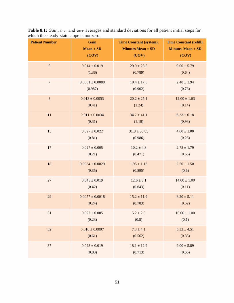
51

Table 8.1: Gain, τSYS and τRED averages and standard deviations for all patient initial steps for

which the steady-state slope is nonzero.

Patient Number Gain

Mean ± SD

(COV)

Time Constant (system),

Minutes Mean ± SD

(COV)

Time Constant (refill),

Minutes Mean ± SD

(COV)

6 0.014 ± 0.019

(1.36)

29.9 ± 23.6

(0.789)

9.00 ± 5.79

(0.64)

7 0.0081 ± 0.0080

(0.987)

19.4 ± 17.5

(0.902)

2.48 ± 1.94

(0.78)

8 0.013 ± 0.0053

(0.41)

20.2 ± 25.1

(1.24)

12.00 ± 1.63

(0.14)

11 0.011 ± 0.0034

(0.31)

34.7 ± 41.1

(1.18)

6.33 ± 6.18

(0.98)

15 0.027 ± 0.022

(0.81)

31.3 ± 30.85

(0.986)

4.00 ± 1.00

(0.25)

17 0.027 ± 0.005

(0.21)

10.2 ± 4.8

(0.471)

2.75 ± 1.79

(0.65)

18 0.0084 ± 0.0029

(0.35)

1.95 ± 1.16

(0.595)

2.50 ± 1.50

(0.6)

27 0.045 ± 0.019

(0.42)

12.6 ± 8.1

(0.643)

14.00 ± 1.00

(0.11)

29 0.0077 ± 0.0018

(0.24)

15.2 ± 11.9

(0.783)

8.20 ± 5.11

(0.62)

31 0.022 ± 0.005

(0.23)

5.2 ± 2.6

(0.5)

10.00 ± 1.00

(0.1)

32 0.016 ± 0.0097

(0.61)

7.3 ± 4.1

(0.562)

5.33 ± 4.51

(0.85)

37 0.023 ± 0.019

(0.83)

18.1 ± 12.9

(0.713)

9.00 ± 5.89

(0.65)

52

With notable exceptions, mainly patients with response data sets with low gain, it can be

observed that for the aggregated gain parameter, Gain, the coefficient of variation remains

generally below 0.35 in 5 of the cases and is above 0.35 in the remaining patients. The

coefficient of variation only goes above one in a single case, patient 6. As the reduction factor is

bundled into this gain calculation, this provides a true indication of how refill plays into the

system in the long-term and is the best measure in our model of steady-state behavior. Note

when discussing system reduction factor’s role, it must remain between 0 and 1, as refill cannot

be reversed in our model, or more simply, drawing from a pool cannot cause more fluid to enter

than was removed. The τRED was chosen to be a value between 1 and 15 minutes, which was

chosen due to the general time observed for transients to die out in initial modeling and

simulations. While this can lead to cases when reduction factor time constant runs up right

against the limits, it is overall the best current estimate of where the bounds of the time constant

should lie.

Patient 17, returning to as a representative sample an example, has a gain of (0.027 ±

0.005) a coefficient of variability of 0.21. This is in a patient with 6 data sets, indicating that this

patient has low overall variability in gain identification. The system time constant is less

consistent, having a mean of 10.2 minutes, and a standard deviation of 4.2 minutes, variability

coefficient of 0.471. This variance being more substantial indicates that the patient’s refill is

stimulated at various rates on different days or possibly due to differing initial conditions, with

no time constant in particular being consistent. Further information bolstering this assessment is

seen in examining the refill time constant, with a mean of 2.75 min and a coefficient of variation

of 0.65. The difference in these time constants indicates some inconsistency in patient

hemodynamics, affirming the high variability compared to gain.

Such system time constant variability also occurs in 4 other patients (Patients 7, 8, 11,

and 15) with the coefficients of variation of the time constants often equaling up to 0.8 or more.

Similarly, the reduction factor time constant has such a coefficient of variation in patients 11 and

32. Only two system time constants coefficients of variation are equal to or below 0.5 (patients

17 and 31) indicating a high level of variance across patients in the trial for the system time

constant term, which in turn indicates somewhat of an unpredictability in the rate the system

settles into steady-state. 4 patients (8, 15, 27, and 31) exhibit coefficients of variation below 0.5

for the reduction factor time constant, slightly better than the system time constant. This could be

53

due to the limiting of the reduction factor time constant to the 1-15 minute range, while the

system time constant is theoretically allowed to range up to 100 minutes. Rationale for the time

constant variance will be explored further in long term estimation accuracy, as well as when

algorithmic limitations are discussed in further detail.

Examining more specific days in patients yields interesting considerations in the behavior

of refill over time, as it is clearly not consistent and may bias results. Patient 31 has two data

sets, day 121 and 135, (the third day 149 is erroneously identified as a flat profile in steady state)

where the identified plot is visually offset from the collected data in places, possibly due to the

patient having an especially extended time constant that is not identified (particularly in Figure

A126). Additionally, at 30 minutes on day 121 (Figure A124) we observe the hematocrit profile

flattens to have near-zero slope even though the UFR profile is relatively high at 1050 mL/hr.

Prior to this, however, both profiles track with limited visual error, meriting deeper examination

of initial conditions (Table 7.1.10). The initial hematocrit in these cases is very similar, and the

ultrafiltration rate is also comparable, days 121 and 135 being 1050 and 1250 mL/hr,

respectively. The estimated Gain, in both cases, approximately 0.31 and 0.25, are similar. The

identifications of τSYS and τRED are also similar enough, apart from the system time constant for

day 121 at 2.6 minutes. As this is low, this will cause the system portion to settle quickly and any

transient being more subject to the reduction factor. In examining specific parameters, the β

parameters are extremely similar, while the K and α parameters having a large disparity. The

reduction factor is substantially similar for these cases. Overall, this again indicates the concept

that the gain and time constants are often easier to identify than individual parameters, and may

be meaningful quantities, though in general time constant variability remains high.

Patient 32 (Figs. A130 – A138) exhibits mixed identification results due to limited

hematocrit change, which will be used as an example for such cases. For the cases of day 119,

135, and 138, it visually appears that the identification was successful, with the simulation

tracking to the collected data. Day 135 is particularly of note, since the simulation exhibits

behavior consistent with two very different time constants, and the collected data has behavior

consistent with refill changing 30 minutes into treatment. Day 119 indeed has two different time

constants of 11 minutes for the system, and 1 minute for the system time constant, which is

exceptionally low.

54

Patient 32’s system gain estimates (no reduction factor applied) vary between 0.035 and

0.048 (0.040 ± 0.0067), with the reduction factor having a large range of approximately 0.3-0.75

(0.61 ± 0.25). Hematocrit remains about the same for each case, around 0.305. Patient 32

exhibits more variance in parameters than other cases observed, with the α (0.21 ± 0.23) and β

(0.068 ± 0.076) parameters having a standard deviation exceeding the mean. Interestingly, the

Ksys parameter (0.17 ± 0.040) has a lower variance than the other parameters, standing somewhat

unique alongside the intra-patient statistics of other patients. Day 119 and day 135 are both

similar across all parameters, reduction factor, K, α, and β. This is a particularly interesting point,

as the only major difference between these two cases is the reduction factor time constant, which

due to the high reduction factor is non-negligible in this analysis. Nonetheless, this parameter

similarity indicates that parameters can be identified similarly between data sets of a patient,

though due to observations in other patients this seems to be a rare occurrence.

Figures such as 7.8 (patient 29 day 117) has a middling to high UFR of 940 mL/hr, which

is more than sufficient to instigate refill, based on observations made in analyzing patient data.

Identification can proceed, as the profile is not entirely flat, and is identified with a 0.75

reduction factor. Similar cases are seen for this patient where all their reduction factors are high

due to relatively flat recorded profiles. Similar initial hematocrits are observed each day for this

patient, being between 33% and 34%, and similar UFRs are present on each day. When

comparing aggregate parameters, the gain is very low compared to other patients, and the

standard deviation is very low for the gain. This indicates that this patient’s gain is consistent,

and very low throughout the data sets analyzed. Again, more substantial variance is observed in

time constant results. Despite the low variance in gain, each individual parameter displays

substantial variance, with the mean values for K, α, and β nearly equaling the standard deviation

of each in the identification. Through this, it can be discerned that for profiles with limited

hematocrit change (high refill) more of a challenge is presented than for cases with higher gain.

Overall, both system and reduction factor time constant have a more pronounced

variability than the gain parameter intra-patient. It seems to be the case for the patients observed

that individual parameters are very ill-suited to forming statistics for, with the examination of

combined parameters being the more ideal approach. Due to the low variability on the gain

parameter generally, along with the higher variability on τRED and τSYS, it seems to be indicative

55

of more predictability in steady-state behavior for a patient than behavior in transient. This is due

to dynamics not accounted for in our modeling as will be further explored in section 9.4.

8.1.1.1 The Estimation Algorithm Does Not Apply to Flat HCT Steady State Behavior

While flat, or near-flat, steady-state HCT slopes are consistent with expected responses,

that is, when refill matches UFR, such cases pose a numerical limitation on our system

identification. When examining the data obtained, one of the results found was the prevalence of

‘flat’ hematocrit profiles, cases where despite the application of UF, patient hematocrit does not

appreciably change, either initially or at steady state after some transient. In these cases, by

definition, during identification the reduction factor was set to 1. Mathematically speaking, this

indicates that the rate of refill in the system matches the rate of fluid removal precisely. As this is

only in steady state, this approach allows the time constant for reduction factor, τRED, to still be

present, allowing the system to still have a transient before settling into a flat steady state

hematocrit. This approach clearly will make the estimation of steady state gain more difficult, as

there is none in this system, and as the identification process couples the steady state gain to time

constant results are affected.

The numerical limitation posed by flat steady-state slopes stems from how the parameter

is estimated. Specifically, the gain of the system is computed using the slope of the system,

corrected for the reduction factor. For flat cases, this slope can only be zero. As a result, when β

is computed as a function of K and alpha, the result is that beta can only be zero, due to the

computed slope being used as a multiplier in the function as seen in Eq. 9.2 below.

0( )

0 ( )

K

K

=

+

+=

(8.2)

With β = 0, the response simplifies to:

(1 (1 ))

( ) (1 )

t

tautUFR e K

HCT t e

−

− − − = − (8.3)

which acts as an exponential decay term with an associated gain, reaching zero gain in steady

state. As the system hematocrit does not appreciably change, a poor estimate of the reduction

56

factor’s time constant is obtained, leading to inaccurate evaluations of when steady state is

reached.

As an example of this occurring, in the case of patient 7, two individual day cases (Figs

A19 and A21) are noted where the hematocrit profiles are not entirely flat but have very high

reduction factors (Kred) (0.84 and 0.89, respectively) comparative to other data sets between

patients and within patient 7. These were chosen as they allow for estimation to take place fully,

as opposed to reduction factors of 1 where the gain can only be computed as zero. As with

agreement in data sets where steady state was a clearly positive and linear slope, similar Gain is

observed across the identifications of the parameters, the grouping being even closer than patient

17, being (0.026 ± 0.0005) (no reduction factor), though the systems have vastly different time

constants (τSYS, [19.4 ± 17.5, COV 0.902] and τRED, [2.48 ± 1.94 COV 0.78]) despite the Gain

being nearly identical, which remain consistent with other patients observed in terms of accurate

gain estimation and variable time constants.

While patient 29 has a data set appearing as flat, it is not quite as extreme as seen in other

patients, with a reduction factor of 0.85. Interestingly day 107 and day 100 have the same UFR,

comparable initial hematocrits, and similar computed reduction factors but show drastically

different responses. Day 117 has a response that is not flat, and is consistent with the

expectations of the model, and has a higher UFR. A lower gain factor of 0.75 is also computed

for day 117. Notable differences between day 117 and the other patient 29 data sets are a higher

UFR, as well as slightly different starting hematocrits between all three cases. This difference

could point to slight differences in refill instigating these variations in hematocrit response to

UF, especially in the day 117 case. Effectively, the higher UFR could be sufficient in these cases

at the level they are to overcome the refill amount that would typically generate a flat profile.

The responses seen in the numerical results indicates that flat data sets are not simple to

identify despite initially promising results on the Gain parameter combination. This is an

unanticipated result as initially it would seem that the gain parameter combination would be the

most difficult to get right in a flat data set. The likely reason for this parameter coming out

consistently is in fact the use of the reduction factor to estimate refill, as it allows for a

normalization of system behavior in steady state, leading to a better estimate of gain. This cannot

make up for the fact that in flat profiles the transient is not as distinct, and if the transient is

57

indistinct, the K and α parameters will have worse estimations, leading to a poor calculation of β,

leading in turn to poor Gain, τSYS and τRED calculations.

8.1.2 Transient Responses not Included in the Model

In approximately 30% of measured data sets, the observed HCT dynamics is notably

different from the expected behavior described by the model (5.9). Causes, general unknown, but

may include food intake, patient keeps moving on the chair, and hypotensive events. Other

causes are related to the dialysis procedure itself. Misleading initial hematocrit data is possible

under certain conditions: initially, the external lines an access is connected to passes through are

filled with saline solution, and as treatment initiates the blood mixes with the saline until the line

is filled entirely with blood. This is determined by when the hematocrit reading is stable for a

period, at which point a signal is given to start treatment. Dialysis staff is instructed to wait few

minutes for HCT stabilization before UF is turned on. If the saline is not completely cleared from

the line, a false initial hematocrit reading is observed, invalidating the applicability of our model

(5.9). Needle mis- and re-placement, often at the start of HD session, introduce HCT transients

not otherwise predicted by (5.9), especially when UFR is fixed. The challenge with such

instances is that it still might be possible to estimate model parameters, however, the underlying

dynamics is not expected from out model. an example of which can be seen in Figures 7.5-7.6.

The chart indicates a needle adjustment sometime between 7-7:30. The hematocrit profile shows

a change around the 15 minutes mark (actual treatment time of 7:15), while the UFR profile

remained fixed. Therefore, our model does not match the dynamics observed in this treatment.

This case is particularly notable as visually the agreement of the estimation to the patient data

indicates a well-identified system over the estimation span, but examining the variables obtained

yields a near-zero reduction and a slightly higher gain than normal. Without knowledge of the

initial needle misplacement, it would be difficult to determine that the variables identified were

subject to abnormal data conditions, and as patient data and estimation align initially, there is

nothing obviously wrong on the surface of the estimation. This is a key point to address, as not

all data sets that conform to the expectations of the model on their surface conform to the

modeling in practice, and their limitation in the modeling process that must be accounted for as

well. Additionally, as this was the only case of needle misplacement noted, it cannot be

determined here if all data sets with needle misplacement have this hematocrit behavior, or if

58

other behavior can occur. It is even possible that there are data sets we have with minor needle

misplacement we remain unaware of.

A certain behavior is noted particularly in the identified systems of patient 29 (Figure

7.9) that merits further discussion, the small dip in the estimate during the response. The reason

for this dip is a result of the additional time constant associated with reduction factor (τRED) for

refill in the system. As the reduction factor in these cases is so high and the time constant is

relatively slow, the reduction takes a significant amount of time to affect the system and the

additional dynamics can be clearly seen. While in the nonlinear model derived for the system this

sort of behavior is impossible, the modifications made to the linearized model to account for

refill create these dynamics. While this does not affect the data, it is an aspect to keep in mind

when analyzing the parameters converged upon. As the RMS error of the model response

compared to the data is used to establish the ‘best’ parameters, this may be established by having

a significant time delay in the system which visually may not represent the exact behavior of the

data. As such it remains an important step to visually verify the model response compared to the

data in cases to ensure consistency and accuracy of findings.

In addition to these behaviors, patient 33 (Figures A139-A146) exhibits behavior opposed

to the expectations of the ultrafiltration process, where hematocrit drops when ultrafiltration

begins in each case. This is likely due to overload state of the patient, as their hematocrit is very

low starting out (27.5% - 30%). This is a clear case where the system identification cannot

function due to the expected behavior from modeling not matching with the behavior of the data

collected. Ultrafiltration draws excess fluid from the intravascular compartment, and therefore it

is expected that the volume will deplete as fluid is removed, even with refill from the interstitial

compartment. In this patient’s cases, this refill exceeds the rate of fluid loss, and therefore causes

compartment volume to increase, thus decreasing hematocrit. This is a clear reversal of

expectations from the model as developed, and therefore cannot be properly analyzed at this

stage.

8.2 Long Term Projected Output

The system identification process takes place over the initial, short span of time,

approximately up to thirty minutes following the imitation of UFR. This leaves out much of the

remaining dynamics taking place later during treatment, generally after the first sixty minutes.

59

We observe, for example Figure 8.5, where refill either seems to stop or slow down suddenly,

and drastic increases in slope occurs. In contrast, there are instances where refill suddenly

increases without apparent cause, causing a flattening in the HCT response, in some cases even

drops in hematocrit, as in Figure A106.

Long-term results are intrinsically tied to the steady-state behavior of the patient, and

therefore the more accurate that estimation is in the patient the more viable long-term results will

be for practical use. However, in most patients, other factors, primarily the nonlinearity of the

response and ANS response to dialysis, but also factors such as albumin level and oxygen

saturation, none are part of our model, will influence response of this longer time frame. For

example, Figure 8.7 shows the long-term behavior of the model identified for a case with a

relatively linear slope in steady-state. Despite matching up precisely in the region used for

identification, following this region there is offset between the estimated and actual slopes. Even

outside of drastic refill changes such as are in figures A124 and A106 among others, Figure 8.7

shows a case where even a seemingly linear slope can have a slightly inaccurate identification.

The region of estimation for the steady-state slope can be expanded to attempt to isolate this

slope more accurately, however in doing so the problem of measurement noise affecting results

is again encountered. Ultimately, as expected due to the limited time range over which our model

is effective, the identification seems to be more effective in determining short-term behavior near

the transient then in determining the longer-term trends of patient hematocrit. The response over

the longer time range will therefore require a separate estimation which should result in different

parameters.

8.3 Parameter Estimation of a Second UFR Step Response

In some HD treatment, there is a UF step change at some point in the treatment. Parameter

estimation of this response is significantly more difficult to estimate due to several factors.

Nevertheless, some observations can be made concerning the parameters and combinations of

parameters during transitions. The primary of these is that without exception, the system time

constant following a UFR step change is extremely fast, effectively approaching zero. Given that

refill has already reached its steady state from the initial UFR step, it appears to respond rapidly

to the new UFR. Further research is required on this topic to determine specific implications and

factors involved in estimating model parameters after a second UFR step change.

60

8.4 Overall Limitations

There are several limitations of our study as follows. The first among these is the

incapability of the identification to accurately estimate flat or near-flat data sets. As the

identification requires the use of the steady-state slope to estimate the overall parameters, a

steady-state slope of zero leaves numerical deficiencies in the solution, and thus these cases are

unidentifiable at this stage. It is worthy of note that flat hematocrit profiles indicate strong refill

from interstitial to intravascular space, and this refill is often indicative of fewer hypotensive

events, the overall goal of profile individualization. In addition to cases with strong refill,

systemic errors in treatment also interfere with identification, and in practice can only be noted

through treatment notes.

There are treatment-related factors that adversely affect the validity of our approach. Such

factors, including needle misplacement, food intake, and initial transients in refill between our

modeled compartments, are not part of the original nonlinear model, and therefore, not part of

the linearized model. Other factors can translate into time-varying parameters, also not

unaccounted for in the modeling. The most notable of these is the filtration coefficient, Kf, which

regulates the flow between interstitial and intravascular space. This parameter has been shown to

have substantial fluctuations over treatment periods, and substantial changes in this parameter

will lead to differences in patient response. As noted in Section 2.3, this broadly has influence on

the long-term output, which can influence the accuracy of identifications over the course of an

entire treatment.

Algorithmic limitations are also presented, with Figure A27 being representative of these.

As the algorithm functions by determining the steady-state slope, errors in the determination of

this term can lead to vast errors in the overall identification. In A27, what can be observed is

behavior where despite visual indications to the contrary, the steady state slope is identified as

being zero, which in turn results in the algorithm failing to identify any meaningful parameters.

This misidentification is due to the small fluctuations lowering the hematocrit in places in

steady-state, which in turn causes the linear fit slopes of hematocrit over time to be both negative

and positive, eventually converging to a most-often occurrence of zero. This behavior is noted in

Figure A128 as well, for patient 31, day 149 where a dip in hematocrit at approximately 25

minutes seems to generate the image of a flat profile in the analysis algorithm. Visual assistance

61

in the identification of slope would assist in eliminating these edge-cases, while pointing to

minor flaws in the identification algorithm.

Despite the limitations of the modelling and system identification approach, parameters are

shown to be identifiable in the aggregate gain and time constant parameters in 70% of measured

data sets. The model is sensitive to each of the parameters identified, indicating the importance

of accurate identification of each.

62

9 CONCLUSIONS

Dialysis is a critical treatment method for end-stage kidney disease, replacing the

function of kidneys when they can no longer filter excess fluid and toxins on their own. While

the treatment is very common, it has not seen much modernization or evolution in methods,

which this thesis addresses in part.

In this thesis, we focused on extending recent results derived in our lab which developed

a method for computing an individualized UFR profile based on a simplified model of a patient’s

fluid dynamics during hemodialysis. Specifically, we focused on the development and validation

of a dedicated parameter identification technique that can be integrated with the UFR profile

design method. The contributions of this thesis are threefold: (1) acquisition of unique clinical

data, (2) improving the simplified fluid dynamics model, and (3) development of a new system

identification technique. This study was approved by the IRB at the University of Massachusetts,

Amherst.

Actual treatment data was acquired via a collaboration with Crit-Line Technologies, a

division of Fresenius Medical Care North America, which enabled the construction of an

autonomous data acquisition system. The company’s device (CliC) is integrated within its

hemodialysis machine giving clinical staff real-time hematocrit data at a one-minute interval.

These devices were located at the American Renal Associates Inc. (ARA) in-center dialysis

facility in Holyoke, Massachusetts. Special Wi-Fi boards were retrofitted into each HD machine,

and at the end of each HD treatment, treatment data was downloaded to a dedicated laptop with a

special radio board. Downloaded data files included coded patient study ID, relative blood

volume change and oxygen level at a 1-minute interval. Separately, we collected redacted charts

from each treatment comprising UFRs and other treatment notes at a 30-minute interval. In all,

20 HD patients participated in the study, and a total of 77 treatment data sets were collected over

a 3-month period.

A key limitation of the simplified model used in the UFR profile design method was its

restriction to a no refill condition. To overcome this limitation, since a step UFR is expected to

elicit fluid refill from the interstitial compartment as observed in clinical data, we modified the

simplified fluid dynamics model to explicitly include refill term dynamics. However, the

modified model comprises 5 unknown parameters compared with 3 in the original model.

63

The main goal in the development of our parameter identification technique was an

automatic estimation from measured data of the 5 model parameters. To determine the steady-

state and transient regions on an autonomous basis, linear fits are performed over 10-minute-long

regions beginning 10 minutes following initiation of UF. Each slope is stored, and a histogram of

slopes is used to determine the most frequent occurrence, which serves as the identified slope.

From the beginning of the data to the first instance of this slope serves as the transient portion of

data. Certain measured data cannot be used with this technique. Data that exhibits unmodelled

dynamics, such as when patient intakes food, moves, misplaced needle placement, and

autonomic nervous system input, resulting in significant effect on the fluid dynamics. In

addition, the modified model included a linear combination of UFR and refill which makes

system ID mathematically impossible when HCT is flat, i.e., refill rate being equal to the UFR.

There was significant intra-patient estimated parameters variability, particularly related to

the fluid dynamics time-constant which varied by up to a factor of 5. This large variability could

be related to patient not being in true steady-state following priming – possibly due to priming

fluid not fully circulated in the system – something we are unable to verify. In contrast, steady

state properties of the model, steady-state gain and refill reduction factor had only moderate

intra-patient variability. Steady-state gain is identified with consistent values intra-patient, when

there is sufficient data following the model’s predicted response, with low variability even with

different UFRs. Both the gain and reduction factor when combined have low coefficient of

variation in patients despite differences in initial hematocrit and fluid removal rate during

treatment. Combined, these two factors indicate that when patients reach steady state, their

hematocrit responses to constant UFRs are more predictable as refill transients are not

confounding our results. The system time constant is not identified with consistent values intra-

patient, exhibiting high coefficient of variation for all but two patients for the system time

constant and four for reduction factor time constant. A potential explanation for this is there are

assumptions of transient dynamics made such as the presence of steady-state compartment

volume and these may not be present in patients, affecting the transient with factors that are not

accounted for in the modeling. Comparing parameters inter-patient shows large differences

between each patient’s identified parameters, as well as the combination of parameters such as

gain and time constant. This variability confirms different patients having different responses to

treatment, even when examining cases with similar initial hematocrit and UFRs. Similar gain

64

values intra-patient indicates the possibility for treatment to be predictable and individualized in

select patient cases, however, identification of time constants requires future work to determine

if better prediction of this term can be achieved.

The design of an individualized UFR profile could prove to be a key step to improving

the lives and treatment outcomes of patients undergoing dialysis, and a key point of that process

is the identification of an accurate system model. The identification procedure detailed here is

shown to have low variability in the identification of Gain and reduction parameters in steady

state, indicating a capability to predict short term treatment trajectories, with long-term cases

remaining less predictable likely due to unmodeled hemodynamics. By integrating observations

from clinical data into the development of the system model, we can better model the dynamics

of the patient, and better able to predict patient response to treatment application.

65

10 FUTURE DIRECTIONS

There are several possible topics for future work in this area. Flat steady-state HCT

responses cannot be handled by the algorithm, hence a fast estimation algorithm that can

overcome this limitation would constitute an important contribution. Several factors could be

involved such as O2 Sat and patient Albumin levels, and a determination of a possible correlation

between these parameters and steady-state response could potentially assist in the determination

of model reduction factor, ultimately leading to more accurate results in parameter estimation in

such cases and in all cases, in general.

Better understanding of the long term HCT dynamics, especially following a second UFR

step change, would constitute another contribution. Our initial analysis showed that such cases

are characterized by fast system time constants, that is, transitional behavior being all but non-

existent.

Finally, as this thesis resulted in an updated model to be used with the method for design of

the individualized ultrafiltration profile, the profile design method necessitates an appropriate

update for this model change.

66

REFERENCES

[1] Facts About Chronic Kidney Disease. (2020, September 01). Retrieved December 10, 2020,

from https://www.kidney.org/atoz/content/about-chronic-kidney-disease

[2] Bosch J.P., Geronemus R., Glabman S., Moutoussis G., Kahn T., von Albertini B. (1980)

Ultrafiltration in Patients with Endstage Renal Disease. In: Cooper A.R. (eds)

Ultrafiltration Membranes and Applications. Polymer Science and Technology, vol

13. Springer, Boston, MA. https://doi.org/10.1007/978-1-4613-3162-9_37

[3] Ofsthun NJ, Leypoldt JK. Ultrafiltration and backfiltration during hemodialysis. Artif

Organs. 1995 Nov;19(11):1143-61. doi: 10.1111/j.1525-1594.1995.tb02276.x. PMID:

8579527.

[4] Dialysis Process Illustration. Retrieved December 22, 2020, from

https://www.shutterstock.com/image-vector/dialysis-process-illustration-767190277

[5] Hemodialysis. (2019, July 23). Retrieved December 22, 2020, from

https://www.mayoclinic.org/tests-procedures/hemodialysis/about/pac-20384824

[6] Frequent Long Dialysis : Why Do Length and Frequency Help? (n.d.). Retrieved December

22, 2020, from https://www.kidneynews.org/kidney-news/features/frequent-long-dialysis-

why-do-length-and-frequency-help

[7] Abohtyra, R., Hollot, C., Germain, M., Chait, Y., & Horowitz, J. (2018). Personalized

Ultrafiltration Profiles to Minimize Intradialytic Hypotension in End-Stage Renal Disease.

2018 IEEE Conference on Decision and Control (CDC). doi:10.1109/cdc.2018.8619152

[8] Abohtyra R, Chait Y, Germain MJ, Hollot CV, Horowitz J. Individualization of

Ultrafiltration in Hemodialysis. IEEE Trans Biomed Eng. 2019 Aug;66(8):2174-2181.

doi: 10.1109/TBME.2018.2884931. Epub 2018 Dec 4. PMID: 30530307; PMCID:

PMC6691497.

[9] Schneditz, D. Pathophysiology of refilling. Issues in Nephrosciences 6.96. 1996. ISBN – 88-

85453-57-0.

[10] Zhu F, Kappel F, Leonard EF, Kotanko P, Levin NW. Modeling of change in blood volume

and extracellular fluid volume during hemodialysis. Annu Int Conf IEEE Eng Med Biol

Soc. 2013;2013:1506-9. doi: 10.1109/EMBC.2013.6609798. PMID: 24109985.

[11] Goncalves, A. Model-Based Feedback Control for Hemodialysis Treatment of Chronic

Kidney Disease Patients. 2015. Unpublished.

A Simplified Fluid Dynamics Model of Ultrafiltration

Documents

Transcript of A Simplified Fluid Dynamics Model of Ultrafiltration