Simplified Theodolite Calibration for Robot Metrology

Ibrahim A. Sultan School of Science and Engineering University of Ballarat PO Box 663 Ballarat VIC 3353 Australia John G. Wager Department of Mechanical and Materials Engineering The University of Western Australia Nedlands WA 6907 Australia

Keywords: Calibration – Robot - Theodolite – Kinematic Model – Epipolar Abstract:

Theodolites represent a well-established 3D-point-measuring technology. However

when used for robot applications they have to be properly calibrated to fulfil the

necessary accuracy requirements. The theodolite calibration methods, which have

been reported in the literature, involve the use of costly sophisticated equipment not

easily available to most users. Therefore, a new simplified calibration technique is

presented based on the use of a graduated precision bar suspended freely to align with

the vertical direction.

To develop efficient mathematical models, the theodolites will be regarded as 2R

open-ended mechanisms with the end-effector axis directed along the line of sight.

The proposed models are then coded in a computer program designed to verify the

validity of the technique presented. The simulation results will be presented at the

end of the paper.

-2-

1. Introduction and Literature Survey:

It is essential for robot calibration to precisely measure the spatial characteristics of

the end-effector at many locations and compare the measured quantities with their

corresponding nominal values using a suitable mathematical procedure. To acquire

the necessary spatial measurements, researchers have implemented different

approaches that range from simple conventional contact methods such as dial

indicators and mechanical fixtures to costly automated laser-tracking systems.

Some factors should be examined before any particular three-dimensional (3D)

measuring system is decided upon. The first factor to consider here would be the

level of precision desired for the collected data and how it compares with the

established precision of the proposed measuring approach. This is particularly

important because the improved positioning accuracy of the calibrated robot

manipulator is limited by the accuracy of the measurement system employed.

Economical viability of the measuring system as weighed against the expected gain of

the calibration work is another factor to consider during the selection process.

Measuring systems vary in cost according to the level of automation, precision and

operating skills involved. Also the time required to collect the data might be a factor

to consider in some applications, especially in production environment where the

robot has already been in operation and the calibration process is only a part of a

scheduled maintenance routine. In such a case, a low-cost, simply built and readily

used system may be a preferred option. The system, which was designed by Everett

and Ives (1996), is a representative example in this regard. This short-range system

-3-

uses LED beam trip switches to define the spatial location of a sphere attached to the

end-effector.

Generally, measuring systems may be broadly classified according to the amount of

spatial data they return per one measurement. Usually, six parameters are needed to

locate a solid object in space. Three of these parameters may represent the XYZ

Cartesian location of any point on the object whilst the other three parameters are

intended to report the angular orientation of the object. For robot calibration, it is

preferable that the measuring system employed is able to return all the six spatial

characteristics of the end-effector and therefore produce full-pose measurements.

Even though it is long established that the spatial measurement of angles is a difficult

task to achieve, a system capable of generating complete, six parametric,

measurements was reported by Vincze et al (1994). The system uses a single laser

beam to measure the Cartesian location of a target attached to the end-effector while

the orientation is determined by analysing the intensity profile of the reflected beam.

The system, which is fully automated, is able to track and measure random

movements of the robot in space. Other laser tracking systems were reported by Van

Brussel (1990) and Nakamura et al (1994). These systems however seem to produce

only partial-pose measurements of the end-effector spatial locations. This is in fact

the case with the overwhelming majority of the measuring systems already in

existence. They mostly generate information related to the spatial position of a point

attached to the end-effector. The automated theodolite system designed by Driels and

Pathre (1991) is a good example of these systems. This system is different in the

sense that it uses a charge-coupled device (CCD) and an image-analysis technique to

track an illuminated spot attached to the end-effector. A CCD camera is mounted on

-4-

a stepper-motor-driven, two revolute-joint mechanism similar to that used on

theodolites to facilitate the tracking performance. A single CCD camera system was

also successfully used by Preising and Hsia (1991) to calibrate a robot arm. In this

system, the image of 36 infinitesimal disks of known dimensions, inscribed on a plate

attached to end-effector, was analysed to calculate the required spatial information.

Point measuring systems are widely used for robot calibration where researchers may

use only the spatial positions of a measured point attached to an end-effector in a

mathematical procedure to compute the corresponding values of the geometric

parameters of the robotic structures. Some of these systems use laser interferometry

to measure positioning errors along one of the axes of a given Cartesian frame.

Examples of these systems are presented by Tang and Liu (1993) and Legnani et al

(1996), where the robot is made to move along linear paths in the direction of either

the Y- or X-axis, parallel to a laser beam, and linear errors are measured.

A more generalised point measuring technique is achieved through the use of

coordinate measuring machines (CMM). These are mostly built out of three

prismatic-joints where the joint-axes are directed along the three axes of a Cartesian

frame. The Cartesian location of any target located within the machine work space

will be displayed once it comes in contact with a probe. Mooring et al (1991) present

a good example of these systems where the positioning errors of a PUMA-type robot

are directly measured.

The method of triangulation is often used to measure the spatial locations of points.

In this method, two, or more, lines are made to intersect at the point whose spatial

-5-

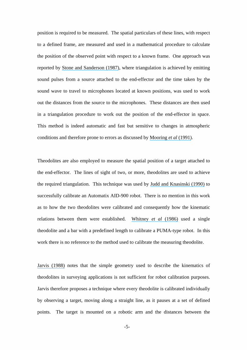
position is required to be measured. The spatial particulars of these lines, with respect

to a defined frame, are measured and used in a mathematical procedure to calculate

the position of the observed point with respect to a known frame. One approach was

reported by Stone and Sanderson (1987), where triangulation is achieved by emitting

sound pulses from a source attached to the end-effector and the time taken by the

sound wave to travel to microphones located at known positions, was used to work

out the distances from the source to the microphones. These distances are then used

in a triangulation procedure to work out the position of the end-effector in space.

This method is indeed automatic and fast but sensitive to changes in atmospheric

conditions and therefore prone to errors as discussed by Mooring et al (1991).

Theodolites are also employed to measure the spatial position of a target attached to

the end-effector. The lines of sight of two, or more, theodolites are used to achieve

the required triangulation. This technique was used by Judd and Knasinski (1990) to

successfully calibrate an Automatix AID-900 robot. There is no mention in this work

as to how the two theodolites were calibrated and consequently how the kinematic

relations between them were established. Whitney et al (1986) used a single

theodolite and a bar with a predefined length to calibrate a PUMA-type robot. In this

work there is no reference to the method used to calibrate the measuring theodolite.

Jarvis (1988) notes that the simple geometry used to describe the kinematics of

theodolites in surveying applications is not sufficient for robot calibration purposes.

Jarvis therefore proposes a technique where every theodolite is calibrated individually

by observing a target, moving along a straight line, as it pauses at a set of defined

points. The target is mounted on a robotic arm and the distances between the

-6-

measurement points are determined by a laser interferometric system. The kinematic

relations between two theodolites are then established by mutual observation of

spatial targets located within the work volume. The sophisticated equipment used to

calibrate theodolites in this work made it possible to use the absolute, rather than

relative, location of the observed point in the mathematical model. However such a

level of sophistication is rarely possible to attain in an industrial situation and as such

defeats the purpose of simplicity for which theodolites are used for robot calibration.

The procedure is also prone to error accumulation which may result from both

positioning errors of the robotic arm and the laser interferometer. The method results

in theodolites calibrated only in the narrow portion of the work volume which is

relevant to the straight line along which the target is moved.

Driels and Pathre(1991) also calibrated a single theodolite, which was built to carry a

CCD camera. In this work a CMM was employed to calibrate the theodolite in a

limited portion of the work volume using the kinematic notation described by Hayati

(1983).

This paper reports a proposed procedure for the calibration of a two-theodolite

module. The procedure, which is referred to as the Vertical-Observation-Lines

method, involves the use of a published kinematic notation referred to as the -model.

The main aspects of this notation is described in the attached appendix, but more

details may be sough in a work Sultan and Wager (1999). The same notation was also

used by Sultan and Wager (2001) successfully to calibrate an industrial six-axes

robot.

-7-

2. The Method of Vertical-Observation-Lines:

In the present work the theodolites were made to observe two points, Pi1 and Pi2

whose position vectors in a base Cartesian frame are, 1ip and 2ip respectively. The

two points are separated by a known distance, l i , along a line parallel to the vertical

axis of the base frame. This line will be referred to, in the following discussion, as

the vertical-observation-line or VO-line for short. In other words, the two observed

points are made to share both the x- and y-coordinates and their relative position

vector, il , is fully defined, in a base Cartesian frame, as follows;

l i = 0 x + 0 y + l i z (1)

where x, y and z are unit vectors parallel to the corresponding axes of the base frame

and the length, l i , is accurately measured.

The same position vector when calculated as observed by the theodolites using their

erroneous geometric parameters and then transformed to the base frame is referred to

in this discussion as ip . This vector can be expressed as follows;

p x y zixi

yi

zip p p (2)

where pxi , py

i and pzi are the X-, Y- and Z-components respectively of the

position vector ip . The scalar quantities, pxi , py

i and pzi are expressed in

functional forms as follows;

),( qθ iix

ix fp , ),( qθ ii

yiy fp and ),( qθ ii

ziz fp (3)

where iθ , is a vector of the eight theodolite-angles (obtained from observations)

which correspond to VO-line number i and q is a vector encompassing the system’s

21 geometric parameters. These 21 parameters will be detailed in section (3) below.

-8-

The VO-lines method is useful in the formulation of the mathematical model, because

it provides three equations, instead of the common one length equation, per two

observations. Each equation describes the relative error in a direction parallel to one

of the three perpendicular axes of the base frame. Two more equations can also be

written per a VO-line to describe the kinematic consistency of the observation

process. This will bring the number of useful equations per line to five; hence

decreasing the number of observations required for the calibration process.

In the present work, VO-lines with different lengths and altitudes would be moved

around in the work volume from one location to the other and at each location, i, two

points separated by different lengths, l i , are observed. Therefore; the following error

equation can be written at every location of the VO-line;

iii lpe (4)

where ei is the dimensional error vector associated with the VO-line number i in

directions parallel to the corresponding axes of the base frame.

After the VO-line was moved through an adequate number of locations distributed

around the work volume resulting in the compilation of an adequate number of error

equations, a suitable least-squares technique may be implemented for the

mathematical realisation of the procedure. The models proposed here for theodolite

calibration are presented in the next section.

-9-

3. Mathematical Procedure:

A two-theodolite module is shown in figure (1). The figure also shows the VO-line

number i with the observation target points Pi1 and Pi2 separated by a distance li. In

the present discussion, spatial characteristics of the left-hand side (LHS) theodolite

are designated by the subscript L while the subscript R is used for the spatial

characteristics of the right-hand side (RHS) theodolite.

The -model frames are attached to the links of both theodolites as shown in figure

(1). The frames are assigned according to the conventions presented in the appendix

as follows;

1. X0Y

0Z

0 is the base frame.

2. XL1

YL1

ZL1

is constructed about the near-vertical joint-axis of the LHS theodolite

and this frame will be referred to as the L1-frame.

3. XL2

YL2

ZL2

is constructed about the near-horizontal joint-axis of the LHS theodolite

and it will be referred to as the L2-frame.

4. XLY

LZ

L is constructed about the line of sight of the LHS theodolite. This frame is

referred to, here, as the L-frame.

5. XR1

YR1

ZR1

is constructed about the near-vertical joint-axis of the RHS theodolite

and will be referred to as the R1-frame.

6. XR2

YR2

ZR2

is constructed about the near-horizontal joint-axis of the RHS theodolite

and this frame will be referred to as the R2-frame.

7. XRY

RZ

R is constructed about the line of sight of the RHS theodolite and is referred

to, in the present discussion, as the R-frame.

-10-

It is worth noting here that the z-axis of the base frame is made to coincide with the

absolute vertical direction and intersect the z-axis of the L1-frame. The point of

intersection is the origin of both the base frame and the L1-frame. Moreover, the y-

axis of the base frame is made to intersect the z-axis of the R1-frame. These frames

are related, according to the conventions of the -model, by the following sets of 21-

parameters;

{aR2

, bR2

, R2

and R2

} relate the R-frame to the R2-frame,

{aR1

, bR1

, R1

and R1

} relate the R2-frame to the R1-frame,

{aR0

, R0

and R0

} relate the R1-frame to the base-frame,

{aL2

, bL2

, L2

and L2

} relate the L-frame to the L2-frame,

{aL1

, bL1

, L1

and L1

} relate the L2-frame to the L1-frame and

{0 and

0} relate the L1-frame to the base frame.

The values of i-angles are selected as follows;

L2

= 0.0, L1

= 0.0, R2

= 0.0, R1

= 0.0, 0 = /2.

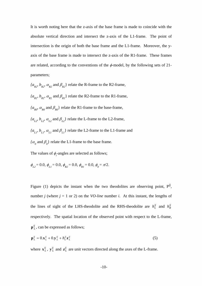
Figure (1) depicts the instant when the two theodolites are observing point, Pij,

number j (where j = 1 or 2) on the VO-line number i. At this instant, the lengths of

the lines of sight of the LHS-theodolite and the RHS-theodolite are hLij and hR

ij

respectively. The spatial location of the observed point with respect to the L-frame,

p Lij , can be expressed as follows;

ijL

ijL

ijL

ijL

ijL h zyxp .0.0 (5)

where x Lij , y L

ij and zLij are unit vectors directed along the axes of the L-frame.

-11-

The position vector of the same point with respect to the R-frame, p Rij , can be written

as follows;

ijR

ijR

ijR

ijR

ijR h zyxp .0.0 (6)

where x Rij , y R

ij and zRij are unit vectors directed along the axes of the R-frame.

The technique of homogeneous transformation is used here to express both the

position vectors in equations (5) and (6) with respect to the base-frame. In this case,

the transformed position vectors can be equated as follows;

11 2

2

1

1

0

0

2

2

1

1

0

02

21

102

21

10

ijRR

RR

RR

ijLL

LL

LL

R

R

R

R

L

L

L

Lp

TTTTTTp

TTTTTT

(7)

where the T-matrices are constructed as outlined in the appendix. These matrices

encompass the model parameters together with the joint-displacements of theodolites.

Substituting for p Lij and p R

ij in equation (7) and performing the due matrix

multiplication produces the following vector relation;

ijR

ijL

ijL

ijL

ijR

ijR hh

0000ppzz (8)

where ijR0

z and ijL0

z are unit vectors directed along the Z-axes of the R-frame and the

L-frame respectively as expressed with respect to the base-frame. The position

vectors, ijR0

p and ijL0

p , locate the origins of the R-frame and the L-frame respectively

with respect to the base-frame.

-12-

The following system of linear equations, which relates to point number ij, can be

worked out from equation (8);

ij

ijL

ijRij

h

h00 pZ

(9)

where ij0Z and ij

0p take the following forms;

230 00

ijL

ijR

ij zzZ (10)

and

130 00

ijR

ijL

ij ppp (11)

The values of hLij and hR

ij could now be worked out by applying a least-squares

technique to equation (9) as follows;

ijTijijTij

ijL

ijR

h

h00

1

00 pZZZ

(12)

Equation (12) yields the following expression for hLij ;

ijij

ijR

ijL

ijLh 002)(1

1

00

pzzz

(13)

where ij0z is given as follows;

ijL

ijL

ijR

ijR

ij

0000)(0 zzzzz (14)

Once the length, hLij is calculated; the position vector, ij

0p , which relates the spatial

location of the observed point with respect to the base-frame could be worked out as

follows;

ijL

ijL

ijL

ij h000 zpp (15)

-13-

The differential form of equation (15) may be expressed as follows;

k

ijLij

Lk

ijLij

Lk

ijL

k

ij

q

h

qh

qq

0

000 zzpp

(16)

where qk refers to the geometric parameter number k and,

k

ijR

ijLij

RijL

ijL

k

ijij

k

ijij

ijR

ijLk

ijL

qh

qqq

h

)(

)(2)(1

100

00

00

00

002

zzzz

zp

pz

zz

(17)

The above concepts may now be applied to equation (4) to obtain a differential error

form for the VO-line number i as follows;

kk k

i

k

iiii q

qq

21

1

20

102

01

0 )(pp

lpp (18)

where 10ip and 2

0ip are calculated using equation (15) and the numerical values of the

parameters as obtained in the previous iteration. The differential vectors k

i

q 1

0p and

k

i

q 2

0p are as given in equation (16).

Equation (18) produces three scalar error equations per a VO-line to use for the

calibration analysis. Two more equations per line (i.e. a single equation for every

observed point) can also be obtained and utilized for the analysis. These two

equations are relevant to the kinematic consistency of the theodolite module as

described in the next section.

-14-

4. Kinematic Consistency:

The expressions in equations (7) and (8) indicate that both theodolites must indeed be

observing the same point, number ij, in order to ensure the accuracy of measurements.

To achieve that, a kinematic consistency index may be proposed and used for the

analysis by re-writing equation (8) in the following linear form;

0ppzz

1

0000

ijL

ijR

ijR

ijL

ijL

ijR h

h

(19)

For equation (19) to have a solution, the determinant of the system matrix must be

equal to zero. Geometrically, this means that the intersecting axes, ijR0

z and ijL0

z must

fall in the same plane as the vector ijR

ijL 00

pp . This is equivalent to the co-planarity

constraint, which is utilised in the field of computer vision to establish the elements of

the epipolar geometry. In this geometry, the lines linking the centres of the cameras

must fall in one plane with the intersecting optical rays of the cameras. Since these

optical rays are relevant to a pair of corresponding points on two images, geometric

relationships can be used to construct the necessary transformation information.

Adequate information on the epipolar geometry may be sought in textbooks by Xu

and Zhang (1996) and by Hartley and Zissermann (2000) or in papers by Xu (1995),

Zhang (1998) and Zissermann and Maybank (1993).

In the present work, the kinematic consistency is quantified by calculating the

determinant of the matrix given in equation (19). This determinant is referred to in

the following discussion as the Kinematic Consistency Index, KCI. As such, the

value of ijKCI , which is relevant to point ij, may be expressed as follows;

)()(0000

ijL

ijR

ijR

ijL

ijKCI zzpp (20)

-15-

Equation (20) can then be manipulated into the following from;

)()(000000

ijR

ijR

ijL

ijL

ijL

ijR

ijKCI zpzzpz (21)

This last expression (21) produces two extra equations (one for every observed point)

to use for the VO-line. The differential form of ijKCI is expressed as follows;

)()(

)()(

00

000

000

000

0

ijR

ijR

k

ijL

k

ijR

ijRij

LijL

ijL

k

ijR

k

ijL

ijLij

Rk

ij

qqqqq

KCIzp

zzpzzp

zzpz

(22)

For model implementation, ijKCI is used as follows;

kk k

ijij q

q

KCIKCI

21

1

)0(

(23)

where ijKCI is calculated numerically from equation (21) using the values obtained

during the previous iteration for the system parameters and k

ij

q

KCI

is evaluated from

equation (22).

After the data related to a total of n VO-lines are collected and the corresponding

aggregate 5n1 error vector, e, is worked out, the overall error equation of the model

may be expressed as follows;

e = J q (24)

where J is the, 5n21, aggregate Jacobian matrix of the model.

The solution of the over-determined system in equation (24) may be obtained by the

use of a suitable least-squares technique as follows;

(JT J )q = JT e (25)

-16-

The output of equation (25) is the vector of differential parameters, q. The iterations

stop when the norm of this vector is less than or equal to a small predefined value.

The values of the system parameters are updated for each iteration such that the

vector of parameters, qr, which may be used in iteration number r is worked out as

follows;

qr = qr-1 qr-1 (26)

where qr-1 is the vector of differential parameters obtained at iteration number r1.

The Levenberg-Marquardt technique can be implemented to solve the system given in

equation (25) as follows;

(JT J + I)q = JT e (27)

where I is a 2121 identity matrix and is a non-negative coefficient selected in such

a manner that the matrix (JT J + I) is always positive definite.

In this technique, the user selects a suitable value for and this value is gradually

decreased as the solution converges to a minimum to retain the favourable

convergence properties of Gauss-Newton method. Useful insights into this strategy

are available in publications by Mooring et al (1991) and Marquardt (1963).

The system in equation (24) could also be solved by the use of a suitable Kalman

filter technique, which involves a recursive stepwise estimation procedure. In this

technique, which may be reviewed in Mooring et al (1991) or Bay (1993), the data

collected for one VO-line may be used to estimate the system parameters. The values

of these parameters would then be improved by the sequential use of the data

-17-

collected in connection with other VO-lines one at a time. This method may be best

suited for the autonomous, on-the-fly, calibration methods rather than aggregate batch

data-collection techniques.

The mathematical procedure proposed in this section was performed, symbolically, on

a computer algebra package and the resulting output was coded in a computer

program. The input to the program consists of the theodolite angles that correspond

to all VO-lines simulated in conjunction with the nominal ideal values of the model

parameters.

The computer program was successfully used to obtain a calibrated model for a two-

theodolite module. The results of the simulation work are given in the next section.

5. Simulation and Results:

The mathematical model presented in sections (3) and (4) was used in a computer

program designed to simulate the calibration process of a two-theodolite module. The

input to the program consists of the set of nominal geometric parameters in addition to

the theodolite angles (i.e. iθ ) identifying the spatial positions of vertical lines-

attached points. These angles are, normally, obtained from observations.

The nominal values of the system geometric parameters are shown in table (1), where

the angles are given in radians and lengths are in millimetres. The values in this table

were obtained by assuming that the two theodolites would be erected and levelled at a

distance 2400.0 from one another. Both lines-of-sight are assumed to be initially

parallel to the X0– axis and lying in the xy-plane of the X

0Y

0Z

0- frame (i.e. the base

-18-

frame). Without loss of generality, this configuration is meant to represent the home

position (where all joint angles may be equated to zero) of the two-theodolite module.

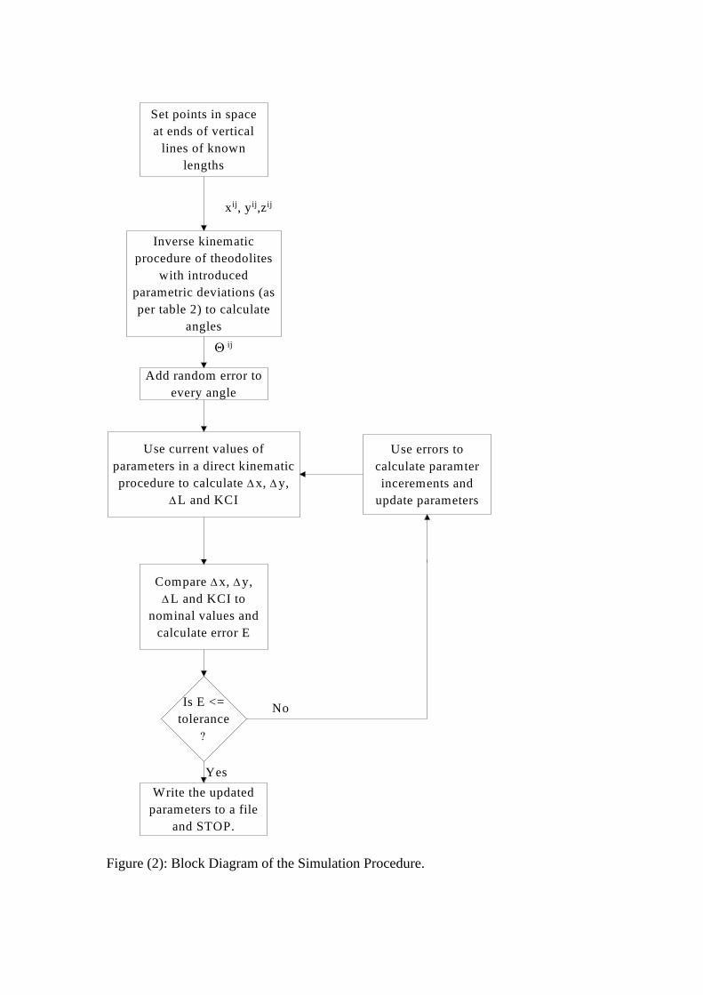
The details of the calibration procedure are described in figure (2). The inverse

kinematic procedure, pointed out in the figure, is performed to calculate the angular

displacements of the theodolite joints in order for the line of sight to shoot at a point

whose spatial coordinates are known. If the joint angles are given, then a direct

kinematic procedure may be performed to calculate the spatial location of the

observed point. The details of both the inverse and the direct kinematic procedures

may be sought in works on robot kinematics; e.g. Sultan (2000).

As figure (2) indicates, small constant deviations were intentionally incorporated into

the nominal values of the theodolite geometric parameters to simulate a real life

situation. Table (2) shows the new values of these geometric parameters after small

deviations were added.

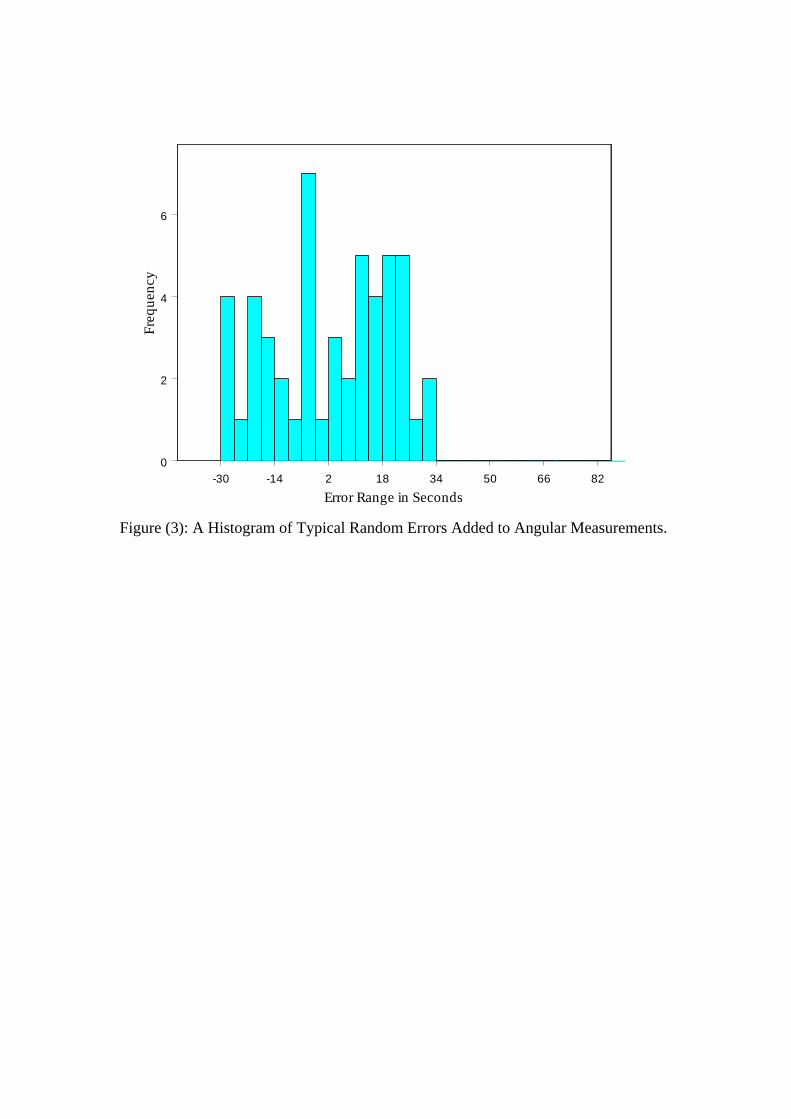
Also, the angles obtained from observations were incremented by random errors

introduced to simulate the effects of sensor resolutions. These errors were generated

by a random function available in the C-compiler used for the simulation. A

histogram representation of these errors is shown in figure (3), whereby the mean

error and the standard deviations are given as 1.88 seconds and 17.59 seconds

respectively.

Calibration procedure has been performed, as described in figure (2), and the resulting

calibrated values for the theodolites’ geometric parameters are given in table (3). A

-19-

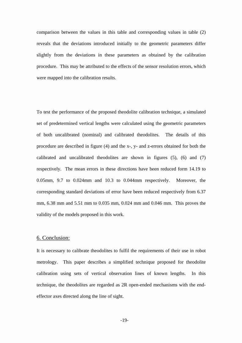
comparison between the values in this table and corresponding values in table (2)

reveals that the deviations introduced initially to the geometric parameters differ

slightly from the deviations in these parameters as obtained by the calibration

procedure. This may be attributed to the effects of the sensor resolution errors, which

were mapped into the calibration results.

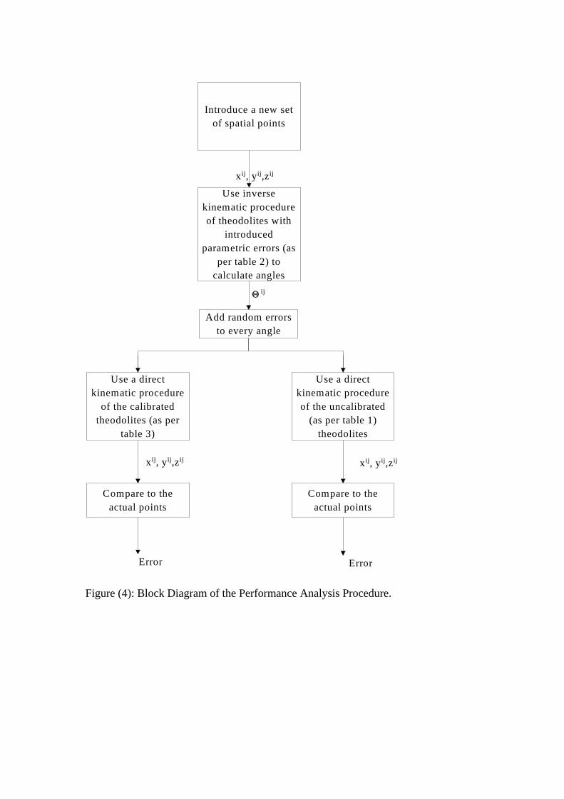
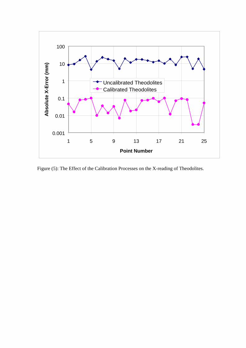
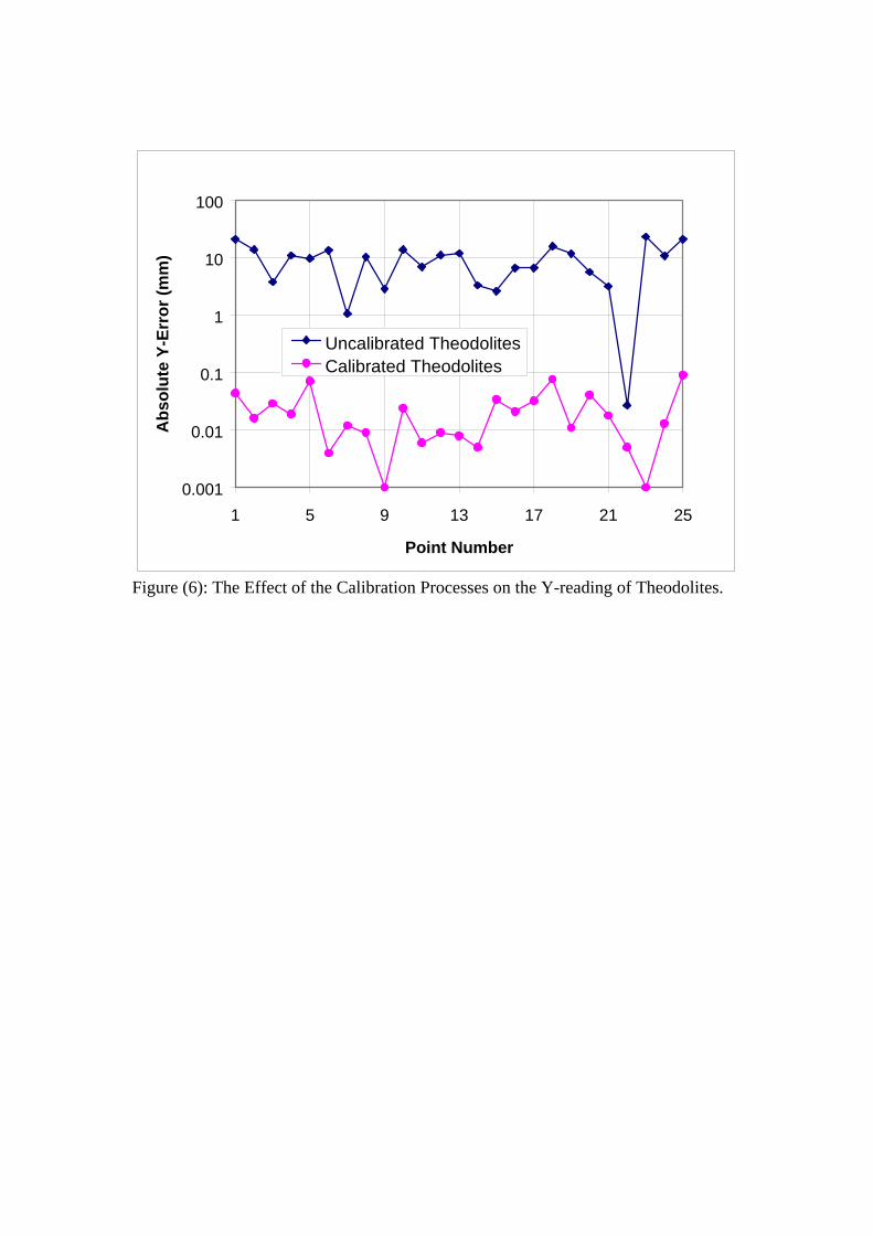
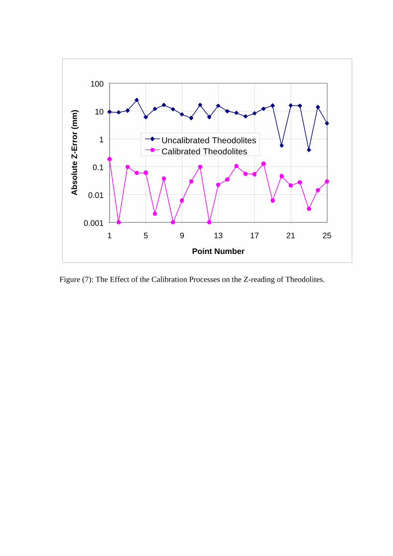
To test the performance of the proposed theodolite calibration technique, a simulated

set of predetermined vertical lengths were calculated using the geometric parameters

of both uncalibrated (nominal) and calibrated theodolites. The details of this

procedure are described in figure (4) and the x-, y- and z-errors obtained for both the

calibrated and uncalibrated theodolites are shown in figures (5), (6) and (7)

respectively. The mean errors in these directions have been reduced form 14.19 to

0.05mm, 9.7 to 0.024mm and 10.3 to 0.044mm respectively. Moreover, the

corresponding standard deviations of error have been reduced respectively from 6.37

mm, 6.38 mm and 5.51 mm to 0.035 mm, 0.024 mm and 0.046 mm. This proves the

validity of the models proposed in this work.

6. Conclusion:

It is necessary to calibrate theodolites to fulfil the requirements of their use in robot

metrology. This paper describes a simplified technique proposed for theodolite

calibration using sets of vertical observation lines of known lengths. In this

technique, the theodolites are regarded as 2R open-ended mechanisms with the end-

effector axes directed along the line of sight.

-20-

Mathematical models were developed using a non-singular kinematic representation

and coded in a computer program, which was then employed successfully in program

designed to simulate the calibration process. The simulation results indicate the

suitability of the proposed technique for theodolite calibration applications.

Appendix: The -model

The kinematic aspects of the -model notation are shown in figure (8). The model is

established by introducing an intermediate Cartesian system between the joint-frames

number i and i+1. The Z-axis of the new frame, which is referred to as the i-frame,

lies in a plane parallel to the XiYi-plane and at a distance, di, equal to the linear joint-

displacement from it. In case of a rotary joint, di may be set equal to zero. This Z-

axis, which may be referred to as Zi, is initially set by the user at a constant angle, i,

from the Xi-axis. i, which is measured in a right-handed sense about Zi, is selected

to ensure that Zi may not be parallel to Zi+1. The Xi-axis of the i-frame is then

established in a plane perpendicular to both Zi and Zi. The i-frame is then used to

establish a Cartesian system, Xi+1Yi+1Zi+1, about the Zi+1-axis in a DH-fashion.

The i-frame and the (i+1)-frame are on the same rigid link and perform the same

displacement (di or i) along or about the Zi respectively.

The transformation, iTi+1, from the (i+1)-frame to the i-frame may now be expressed

as follows,

iTi+1 =

iTi iT

i+1 (A1)

-21-

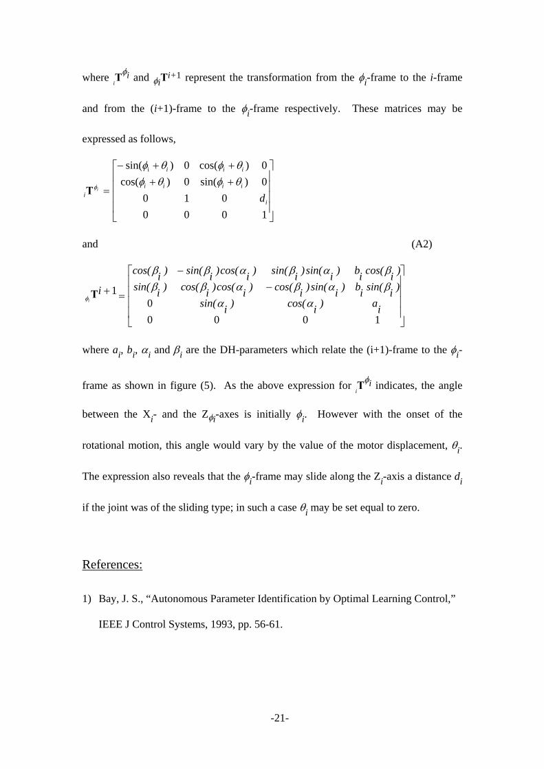
where iTi and iT

i+1 represent the transformation from the i-frame to the i-frame

and from the (i+1)-frame to the i-frame respectively. These matrices may be

expressed as follows,

i

i i i

i i i i

i

i

dT

sin( ) cos( )

cos( ) sin( )i 0 0

0 0

0 1 0

0 0 0 1

and (A2)

ii i i i i i i

i i i i i i i

i i ii

10

0 0 0 1

T

cos( ) sin( )cos( ) sin( )sin( ) b cos( )

sin( ) cos( )cos( ) cos( )sin( ) b sin( )

sin( ) cos( ) a

where ai, bi, i and i are the DH-parameters which relate the (i+1)-frame to the i-

frame as shown in figure (5). As the above expression for iTi indicates, the angle

between the Xi- and the Zi-axes is initially i. However with the onset of the

rotational motion, this angle would vary by the value of the motor displacement, i.

The expression also reveals that the i-frame may slide along the Zi-axis a distance di

if the joint was of the sliding type; in such a case i may be set equal to zero.

References:

1) Bay, J. S., “Autonomous Parameter Identification by Optimal Learning Control,”

IEEE J Control Systems, 1993, pp. 56-61.

-22-

2) Driels, M. R. and Pathre, U. S., “Vision-Based Automatic Theodolite for Robot

Calibration,” IEEE Trans. on Robotics and Automation, Vol. 7, No. 3, June 1991,

pp. 351-360.

3) Everett, L. J. and Ives, T. W., “A Sensor Used for Measurements in the

Calibration of Production Robots,” IEEE Trans., on Robotics and Automation,

Vol. 12, No. 1, February 1996, pp. 121-125.

4) Everett, L. J., “Research Topics in Robot Calibration,” Robot Calibration. Edited

by Bernhardt, R. and Albright, S. L. Chapman & Hall, London, 1993.

5) Hartley, R. and Zissermann, A., “Multiple View Geometry in Computer Vision,”

Cambridge University Press, 2000.

6) Hayati, S., “Robot Arm Geometric Link Parameter Estimation,” In Proceedings of

22nd IEEE Conf. on Decision and Control, Dec. 1983, pp. 1477-1483.

7) Jarvis, J. F., “Calibration of Theodolites,” In Proceedings of IEEE Int. Conf. on

Robotics and Automation, 1988, pp. 952-954.

8) Judd, R. P and Knasinski, A. B., “A Technique to Calibrate Industrial Robots with

Experimental Verification,” IEEE Trans. on Robotics and Automation, Vol. 6, No.

1, Feb. 1990, pp. 20-30.

9) Legnani, J., Mina, C. and Trevelyan, J., “Static Calibration of Industrial

Manipulators: Design of an Optical Instrumentation and Application to Scara

Robot,” J. Robotics Systems, July 1996, pp. 445-460.

-23-

10) Marquardt, D. W., “An Algorithm for Least-Squares Estimation of Nonlinear

Parameters,” J. Soc. Industrial Appl. Math., Vol. 11, No. 2, June 1963, pp. 431-

441.

11) Mooring, B. W., Roth, Z. S. and Driels, M. R., “Fundamentals of Manipulator

Calibration,” John Wiley & Sons, New York, 1991.

12) Nakamura, O., Goto, M., Toyda, K., Takai, N., Kurosawa, T. and Nakamata, T.,

“A Laser Tracking Robot-Performance Calibration System Using a Ball-Seated

Bearing Mechanisms and a Spherically Shaped Cat’s-Eye Retroreflector,” Rev.

Sc. Instrum., 65 (4), April 1994, pp. 1006-1011.

13) Preising, B. and Hsia, T. C., “Robot Performance Measurement and Calibration

Using a 3D Camera Vision System,” In Proceedings of IEEE Int. Conf. on

Robotics and Automation, Sacramento, April 1991, pp. 2079-2084.

14) Stone, H. W. and Sanderson, A. C., “A Prototype Arm Signature Identification

System,” Proceedings of IEEE Int. Conf. on Robotics and Automation, Raleigh,

1987, pp. 175-182.

15) Sultan, I. A. and Wager, J G, “User-controlled kinematic modelling,” Int. J.

Advanced Robotics, 1999, Vol 12, No. 6.

16) Sultan, I. A., “On the Positioning of Revolute-Joint Manipulators,” Int. J. of

Robotic Systems, Vol. 17, No. 8, August 2000, pp 429-438.

17) Sultan, I. A. and Wager, J. G., “A Technique for the Independent-axis Calibration

of Robot Manipulators with Experimental Verification,” Int. J. of Computer

Integrated Manufacturing, Vol 14. No 4, July 2001.

-24-

18) Tang, G. and Liu, L., “Robot Calibration Based on a Single Laser Displacement

Meter,” Mechatronics, Vol. 3, 1993.

19) Vincze, M., Prenninger, J. P. and Gander H., “A Laser Tracking System to

Measure Position and Orientation of Robot End Effectors Under Motion,” The Int.

J Robotic Research, Vol. 13, No. 4, August 1994, pp. 305-314.

20) Whitney, D. E., Lozinski, C. A. and Rourke, J. M., “Industrial Robot Forward

Calibration Method and Results,” ASME Journal of Dynamic Systems,

Measurement and Control, Vol. 108, March 1986, pp 1-8.

21) Xu., Gang, “Unification of Stereo, Motion and Object Recognition via Epipolar

Geometry,” 2nd Int. Asian Conf. on Computer Vision, Singapore, 1995.

22) Xu, G. and Zhang, Z., “Epipolar Geometry in Stereo, Motion and Object

Recognition- A Unified Approach,” Kluwer Academic Press, 1996.

23) Zhang, Z., “Determining the Epipolar Geometry and its Uncertainty: A Review,”

Int. J. Computer Vision, Vol. 27, No. 2, pp 161-195, March 1998.

24) Zissermann, A. and Maybank, S. J., “A Case Against Epipolar Geometry,” 2nd Int.

Europe-US Workshop on Invariance, Ponta Delgada, Azores, Oct 1993.

-25-

List of Figures

Figure (1): -Model Assignment for a Two-Theodolite Module.

Figure (2): Block Diagram of the Simulation Procedure. Figure (3): A Histogram of Typical Random Errors Added to Angular Measurements. Figure (4): Block Diagram of the Performance Analysis Procedure. Figure (5): The Effect of the Calibration Processes on the x-reading of Theodolites. Figure (6): The Effect of the Calibration Processes on the y-reading of Theodolites. Figure (7): The Effect of the Calibration Processes on the z-reading of Theodolites. Figure (8): The Kinematic Notation of the -Model.

List of Tables

Table (1): Nominal Values of System Parameters.

Table (2): Intentionally Deviated Values of System Parameters. Table (3): Calibrated Values of System Parameters.

Figure (1): -Model Assignment for a Two-Theodolite Module.

1iRh

1iLh

.

.Z0

ZL1

ZL2 ZR2

ZR1

X0

Y0

pi1

pi2

ZLZR

L1

L2 R2

R1

X0

XL2

Z0

ZL2

XL1

ZL1

XL1

Y0

XL

XRXR1ZR1

YR1

ZR2

XR2

LHS Theodolite RHS Theodolite

li

Set points in spaceat ends of vertical

lines of knownlengths

xij, yij,zij

Inverse kinematicprocedure of theodolites

with introducedparametric deviations (asper table 2) to calculate

angles

Use current values ofparameters in a direct kinematicprocedure to calculate x, y,

L and KCI

Use errors tocalculate paramterincerements and

update parameters

Is E <=tolerance

Compare x, y,L and KCI to

nominal values andcalculate error E

No

Write the updatedparameters to a file

and STOP.

Add random error toevery angle

Yes

ij

Figure (2): Block Diagram of the Simulation Procedure.

0

2

4

6

Freq

uenc

y

-30 -14 2 18 34 50 66 82

Error Range in Seconds

Figure (3): A Histogram of Typical Random Errors Added to Angular Measurements.

Introduce a new setof spatial points

Use inversekinematic procedureof theodolites with

introducedparametric errors (as

per table 2) tocalculate angles

Add random errorsto every angle

Use a directkinematic procedure

of the calibratedtheodolites (as per

table 3)

Use a directkinematic procedureof the uncalibrated

(as per table 1)theodolites

Compare to theactual points

Compare to theactual points

Error Error

xij, yij,zij

xij, yij,zijxij, yij,zij

ij

Figure (4): Block Diagram of the Performance Analysis Procedure.

0.001

0.01

0.1

1

10

100

1 5 9 13 17 21 25

Point Number

Ab

solu

te X

-Err

or

(mm

)

Uncalibrated TheodolitesCalibrated Theodolites

Figure (5): The Effect of the Calibration Processes on the X-reading of Theodolites.

0.001

0.01

0.1

1

10

100

1 5 9 13 17 21 25

Point Number

Ab

solu

te Y

-Err

or

(mm

)

Uncalibrated TheodolitesCalibrated Theodolites

Figure (6): The Effect of the Calibration Processes on the Y-reading of Theodolites.

0.001

0.01

0.1

1

10

100

1 5 9 13 17 21 25

Point Number

Ab

solu

te Z

-Err

or

(mm

)

Uncalibrated TheodolitesCalibrated Theodolites

Figure (7): The Effect of the Calibration Processes on the Z-reading of Theodolites.

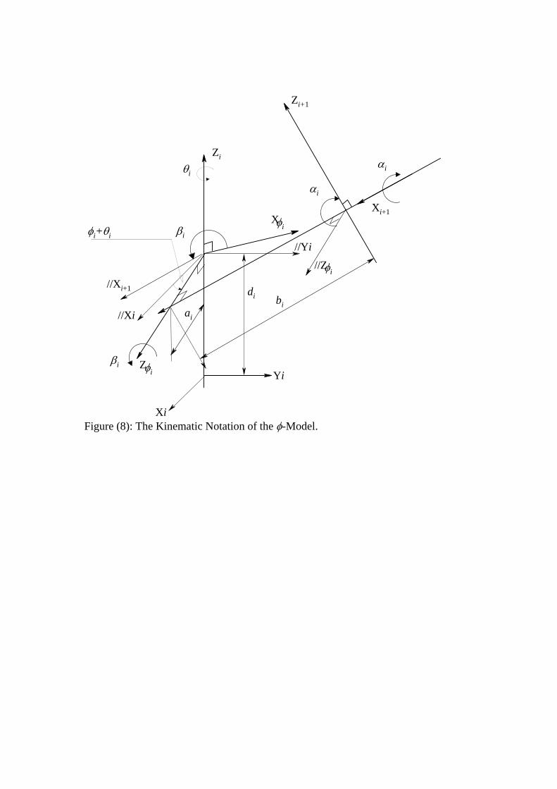
Figure (8): The Kinematic Notation of the -Model.

Zi

//Xi

//Yi

Zi+1

Xi+1

//Xi+1

//Zi

Zi

Xii

i

ai

bi

i

i

Xi

Yi

di

i

i+i

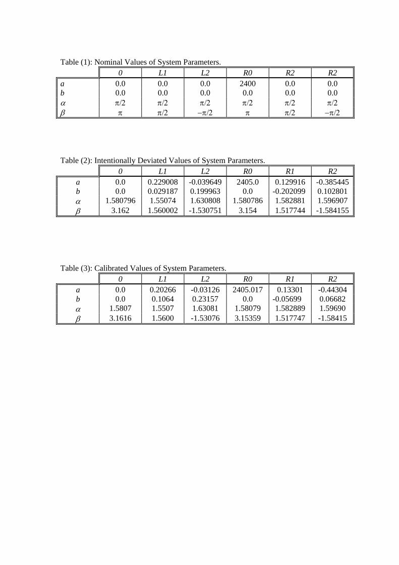
Table (1): Nominal Values of System Parameters. 0 L1 L2 R0 R2 R2 a 0.0 0.0 0.0 2400 0.0 0.0 b 0.0 0.0 0.0 0.0 0.0 0.0 Table (2): Intentionally Deviated Values of System Parameters.

Table (3): Calibrated Values of System Parameters.

0 L1 L2 R0 R1 R2 a 0.0 0.229008 -0.039649 2405.0 0.129916 -0.385445 b 0.0 0.029187 0.199963 0.0 -0.202099 0.102801 1.580796 1.55074 1.630808 1.580786 1.582881 1.596907 3.162 1.560002 -1.530751 3.154 1.517744 -1.584155

0 L1 L2 R0 R1 R2 a 0.0 0.20266 -0.03126 2405.017 0.13301 -0.44304 b 0.0 0.1064 0.23157 0.0 -0.05699 0.06682 1.5807 1.5507 1.63081 1.58079 1.582889 1.59690 3.1616 1.5600 -1.53076 3.15359 1.517747 -1.58415