Metrology and Simulation with Progressive

Addition Lenses

by

Dulce Gonzalez Utrera

Copyright c© Dulce Gonzalez Utrera 2018

A Dissertation Submitted to the Faculty of the

College of Optical Sciences

In Partial Fulfillment of the RequirementsFor the Degree of

Doctor of Philosophy

In the Graduate College

The University of Arizona

2 0 1 8

3

Acknowledgments

First and foremost, my sincere appreciation and gratitude to my advisor Dr. JimSchwiegerling for his mentorship, his guidance and his constant support throughoutthese years. I would also like to thank the committee members Dr. Dae Wook Kimand Dr. Ron Liang, for their valuable feedback.

Thank you to my collegues in the Visual and Ophthalmic Optics Lab: Eddie LaVilla,Brian Redman, Carmen Paleta, Carl Chancy, William Duncan, Ashley Valdez, YuYan, Sean Ashley, Jieun Ryu, Martin Chao-Hsiung Tseng, Ethan Tank, Soheila Boo-jari, Yuqiao Han for their valuable comments and help throughout the completion ofmy PhD .

I would like to thank Marıa and Mohan for being true friends and my support through-out these years. Your friendship has been irreplaceable.

I am thankful to Oscar, whose constant encouragement and endless patience havehelped me come this far. Thank you to my family, especially to my parents and mybrother without whom I would not be here.

Finally, all my gratitude to Liliana, Poonam, Sandra, Phillipi, Rodolfo, Itzel, Itzel,Gaby, Pabli, Ismael, Juan Manuel and all my friends for making my time in Tucsona unique experience.

I would like to acknowledge CONACyT and TRIF University of Arizona for theirfinancial support.

4

Dedication

To my loving grandmothers, Dolores and Catalina.

5

Table of Contents

List of Figures . . . . . . . . . . . . . . . . . . . . . . . . . . . . . . . . . 7

List of Tables . . . . . . . . . . . . . . . . . . . . . . . . . . . . . . . . . . 10

Abstract . . . . . . . . . . . . . . . . . . . . . . . . . . . . . . . . . . . . . 11

Chapter 1. INTRODUCTION . . . . . . . . . . . . . . . . . . . . . . . 121.1. The Eye . . . . . . . . . . . . . . . . . . . . . . . . . . . . . . . . . . 121.2. Presbyopia . . . . . . . . . . . . . . . . . . . . . . . . . . . . . . . . . 141.3. Treatments. . . . . . . . . . . . . . . . . . . . . . . . . . . . . . . . . 17

1.3.1. Intraocular Lenses . . . . . . . . . . . . . . . . . . . . . . . . 171.3.2. Contact Lenses . . . . . . . . . . . . . . . . . . . . . . . . . . 201.3.3. Reading Glasses and Bifocal Spectacles. . . . . . . . . . . . . 221.3.4. Progressive Addition Lenses Design . . . . . . . . . . . . . . . 23

1.4. Motivation . . . . . . . . . . . . . . . . . . . . . . . . . . . . . . . . . 27

Chapter 2. METROLOGY OF PROGRESSIVE ADDITION LENSES 292.1. Profilometer. . . . . . . . . . . . . . . . . . . . . . . . . . . . . . . . 32

2.1.1. Profilometer Specifications. . . . . . . . . . . . . . . . . . . . 322.1.2. Data Collection. . . . . . . . . . . . . . . . . . . . . . . . . . . 332.1.3. Fitting Data. . . . . . . . . . . . . . . . . . . . . . . . . . . . 342.1.4. Profilometer Results . . . . . . . . . . . . . . . . . . . . . . . 37

2.2. Coordinate Measuring Machine . . . . . . . . . . . . . . . . . . . . . 412.3. Phase-Shifting and Phase Unwrapping . . . . . . . . . . . . . . . . . 452.4. SCOTS . . . . . . . . . . . . . . . . . . . . . . . . . . . . . . . . . . 46

2.4.1. Principle . . . . . . . . . . . . . . . . . . . . . . . . . . . . . . 472.4.2. Experimental Setup . . . . . . . . . . . . . . . . . . . . . . . . 472.4.3. Results . . . . . . . . . . . . . . . . . . . . . . . . . . . . . . . 48

2.5. UV Deflectometry . . . . . . . . . . . . . . . . . . . . . . . . . . . . . 502.5.1. Theory . . . . . . . . . . . . . . . . . . . . . . . . . . . . . . . 512.5.2. Illumination System . . . . . . . . . . . . . . . . . . . . . . . 532.5.3. Experimental Setup . . . . . . . . . . . . . . . . . . . . . . . . 552.5.4. System Calibration . . . . . . . . . . . . . . . . . . . . . . . . 572.5.5. Fitting Data . . . . . . . . . . . . . . . . . . . . . . . . . . . . 612.5.6. Calibration Sphere . . . . . . . . . . . . . . . . . . . . . . . . 632.5.7. Results . . . . . . . . . . . . . . . . . . . . . . . . . . . . . . . 642.5.8. Conclusions and Future Work . . . . . . . . . . . . . . . . . . 66

Table of Contents—Continued

6

Chapter 3. SIMULATION OF MULTIFOCAL VISION . . . . . . . . 683.1. Theory and Image Simulation. . . . . . . . . . . . . . . . . . . . . . . 683.2. Algorithm Overview. . . . . . . . . . . . . . . . . . . . . . . . . . . . 703.3. Psf Database Creation. . . . . . . . . . . . . . . . . . . . . . . . . . 71

3.3.1. Lens-Eye Model . . . . . . . . . . . . . . . . . . . . . . . . . . 723.3.2. Point Spread Function Interpretation. . . . . . . . . . . . . . . 753.3.3. Point Spread Function Scaling . . . . . . . . . . . . . . . . . . 763.3.4. Point Spread Function Interpolation . . . . . . . . . . . . . . 773.3.5. Point Spread Function Scaling . . . . . . . . . . . . . . . . . . 82

3.4. Realistic Simulation . . . . . . . . . . . . . . . . . . . . . . . . . . . . 893.4.1. Wide Field Angle and Distortion . . . . . . . . . . . . . . . . 903.4.2. Image Size. . . . . . . . . . . . . . . . . . . . . . . . . . . . . 923.4.3. Image Segmentation and Depth of Field. . . . . . . . . . . . . 963.4.4. RGB Color Model. . . . . . . . . . . . . . . . . . . . . . . . . 99

3.5. Algorithm Implementation. . . . . . . . . . . . . . . . . . . . . . . . 1013.6. Results. . . . . . . . . . . . . . . . . . . . . . . . . . . . . . . . . . . 103

3.6.1. Results for Three Different Regions. . . . . . . . . . . . . . . . 1033.6.2. High Performance Computer. . . . . . . . . . . . . . . . . . . 1043.6.3. Final Simulation. . . . . . . . . . . . . . . . . . . . . . . . . . 106

Chapter 4. CONCLUSIONS AND FUTURE WORK . . . . . . . . . 109

Appendix A. Zernike Coefficients . . . . . . . . . . . . . . . . . . . . . 112

Appendix B. Source code used to perform Simulation of Multi-focal Vision. . . . . . . . . . . . . . . . . . . . . . . . . . . . . . . . . 113

References . . . . . . . . . . . . . . . . . . . . . . . . . . . . . . . . . . . . 121

7

List of Figures

Figure 1.1. Eye anatomy. . . . . . . . . . . . . . . . . . . . . . . . . . . . . 13Figure 1.2. Example of a close object through a presbyopic eye. . . . . . . . 15Figure 1.3. Amplitude of accommodation vs. age. From [1]. . . . . . . . . . 16Figure 1.4. AcriSof IQ ReSTOR multifocal IOL Image [2]. . . . . . . . . . 19Figure 1.5. Alcon Multifocal Contact Lenses [3]. . . . . . . . . . . . . . . . 21Figure 1.6. Bifocal Spectacles. Visible change in power between distance and

near region. The lower image shows the abrupt change in magnification(from [4]) . . . . . . . . . . . . . . . . . . . . . . . . . . . . . . . . . . . 23

Figure 1.7. Zones of a Progressive Addition Lens. The right image shows thesmooth transition in magnification from the distance region to the nearregion. (from [4]) . . . . . . . . . . . . . . . . . . . . . . . . . . . . . . 25

Figure 2.1. Interferogram of the Progressive Addition Lens under test. . . . 31Figure 2.2. MarSurf CD 120 Linear Profilometer. . . . . . . . . . . . . . . . 33Figure 2.3. Progressive Addition Lens measured by Profilometer. . . . . . . 34Figure 2.4. Freeform Surface from Profilometer data. . . . . . . . . . . . . 37Figure 2.5. Freeform Surface from Profilometer data with low terms removed. 38Figure 2.6. Differences in micrometers from Profilometer Data and Surface

Fitting. . . . . . . . . . . . . . . . . . . . . . . . . . . . . . . . . . . . . 39Figure 2.7. Mean Curvature of Zernike Surface. . . . . . . . . . . . . . . . . 40Figure 2.8. Sample points from the Coordinate Measuring Machine. . . . . 42Figure 2.9. Differences from CMM Data and Fitting Data. . . . . . . . . . 43Figure 2.10. Freeform Surface Fitting using CMM Data. . . . . . . . . . . . 43Figure 2.11. Comparison between profilometer data and CMM data. . . . . 44Figure 2.12. Curvature Maps of the freeform surface. . . . . . . . . . . . . . 44Figure 2.13. SCOTS experimental setup. . . . . . . . . . . . . . . . . . . . . 48Figure 2.14. Differences between profilometer and SCOTS data (b) Differences

between profilometer and SCOTS data after a 180 degrees rotation. . . . 49Figure 2.15. Differences between profilometer data and average of rotations. 50Figure 2.16. PMMA Transmission Plot. . . . . . . . . . . . . . . . . . . . . 52Figure 2.17. Fringe projection with an LED λ = 365nm. . . . . . . . . . . . 54Figure 2.18. Irradiance profile at the screen with lateral displacement. (a) 10

mm (b) 25 mm (c) 30 mm (d) 35 mm. . . . . . . . . . . . . . . . . . . . 55Figure 2.19. Linear Relation of irradiance profile phase shift in function of

lateral displacement of the object. . . . . . . . . . . . . . . . . . . . . . 56Figure 2.20. Deflectometry Experimental Setup. . . . . . . . . . . . . . . . . 57Figure 2.21. Reflected fringes into calibration Sphere. . . . . . . . . . . . . . 58Figure 2.22. (a) Intersection of lines. (b) Original Data. (c) Nominal Grid. . 58

List of Figures—Continued

8

Figure 2.23. Comparison between Nominal Grid and Undistorted Data. . . . 61Figure 2.24. (a) Original map Phase in X from Reference Sphere. (b) Undis-

torted map Phase in X from Reference Sphere. . . . . . . . . . . . . . . 61Figure 2.25. (a) Original map Phase in Y from Reference Sphere. (b) Undis-

torted map Phase in Y from Reference Sphere. . . . . . . . . . . . . . . 62Figure 2.26. Reconstructed Sphere. . . . . . . . . . . . . . . . . . . . . . . . 64Figure 2.27. Sphere Mean Curvature and Cylinder power. . . . . . . . . . . 65Figure 2.28. (a) Original map Phase in X from PAL under test. (b) Undis-

torted map Phase in X from PAL under test. . . . . . . . . . . . . . . . 65Figure 2.29. (a) Original map Phase in Y from PAL under test. (b) Undis-

torted map Phase in Y from PAL under test. . . . . . . . . . . . . . . . 66Figure 2.30. Reconstructed PAL surface. . . . . . . . . . . . . . . . . . . . . 66Figure 2.31. Reconstructed PAL surface. . . . . . . . . . . . . . . . . . . . . 67

Figure 3.1. Lens-Eye model layout in OpticStudio Zemax design software. . 74Figure 3.2. Lens-eye model used for point spread function calculation. The

stop is at the center of rotation of the eye, 27 mm from the back vertexof the spectacle. The field of view is sampled with a Cartesian grid. . . 74

Figure 3.3. psf sampling for different object distances (a) Near Distance.(b) Intermediate Distance. (c) Far distance. . . . . . . . . . . . . . . . . 75

Figure 3.4. Subsections of basis functions . . . . . . . . . . . . . . . . . . . 78Figure 3.5. Bilinear interpolation example. . . . . . . . . . . . . . . . . . . 79Figure 3.6. Region 1 analysis. . . . . . . . . . . . . . . . . . . . . . . . . . 80Figure 3.7. Differences between psf found by interpolation and psf found

using raytracing code. The psf compared is at the center of Region 1,(x, y) = (−21,−15). . . . . . . . . . . . . . . . . . . . . . . . . . . . . . 80

Figure 3.8. Examples of different regions for far field, where the Point SpreadFunction differs in function of glaze angle. . . . . . . . . . . . . . . . . . 83

Figure 3.9. Interpolated psf and the psf obtained with raytracing for Re-gions 2, 3 and 4. . . . . . . . . . . . . . . . . . . . . . . . . . . . . . . . 84

Figure 3.10. Interpolated psf and the psf obtained with raytracing for Re-gions 5, 6 and 7. . . . . . . . . . . . . . . . . . . . . . . . . . . . . . . . 85

Figure 3.11. Differences of extrapolation and psf obtained using Zemax. . . 86Figure 3.12. Angular relation between pixel angular size and point spread

function angular size. . . . . . . . . . . . . . . . . . . . . . . . . . . . . 87Figure 3.13. Comparison of the interpolated psf based on the psf database

and its down-sampled version created to match the angular subtense ofpixels in the simulation scene. . . . . . . . . . . . . . . . . . . . . . . . . 88

Figure 3.14. Samsung gear 360 Camera. . . . . . . . . . . . . . . . . . . . . 90

List of Figures—Continued

9

Figure 3.15. Example of scene with three object depths taken with the Sam-sung Gear 360 camera. . . . . . . . . . . . . . . . . . . . . . . . . . . . 91

Figure 3.16. Example of a grid with positive main and edge distortion applied. 92Figure 3.17. Example of a grid with negative main and edge distortion applied. 92Figure 3.18. Example of undistorted scene using GIMP image manipulation

software, with three object depths taken with the Samsung Gear 360camera. . . . . . . . . . . . . . . . . . . . . . . . . . . . . . . . . . . . 93

Figure 3.19. Cellphone picture taken at d = 200mm from camera. . . . . . . 94Figure 3.20. (a) Original Picture FOV = 82o, Nx = 1296 pixels (b) Cropped

Picture FOV = 60o,Nx′ = 949 pixels. . . . . . . . . . . . . . . . . . . . 96Figure 3.21. Examples of the cellphone at different depths. Everything rela-

tive assuming a field of view FOV = 60o equal at Nx = 1296 pixels. . . . 97Figure 3.22. Basis functions in Region 7, at three different object depths. . . 97Figure 3.23. Simulation of the same object at different planes of the scene. 98Figure 3.24. Masked images at different depth planes. . . . . . . . . . . . . 99Figure 3.25. Color Object. . . . . . . . . . . . . . . . . . . . . . . . . . . . 100Figure 3.26. Object decomposed in three RGB channels. . . . . . . . . . . . 101Figure 3.27. Graphic representation of the first step of the algorithm applied.

The psf that corresponds to a determined pixel in the image is searched,if the psf does not exist, interpolation is performed. . . . . . . . . . . . 102

Figure 3.28. Graphic representation of the second step in the algorithm ap-plied. The psfs are weighted by the correspondent pixel value. . . . . . 102

Figure 3.29. Graphic representation of the third step in the algorithm applied.Contribution of psfs at each pixel are summed to get the final value foreach pixel. . . . . . . . . . . . . . . . . . . . . . . . . . . . . . . . . . . 103

Figure 3.30. Simulation results for Far Field and Mid-Field. . . . . . . . . . 104Figure 3.31. Simulation results for different Near Field distances. . . . . . . 105Figure 3.32. Comparison of Near Field visual performance. . . . . . . . . . 105Figure 3.33. Complete simulated 3 depths scene for Near field d1 = 200mm,

d2 = 300mm and d3 = 400mm. . . . . . . . . . . . . . . . . . . . . . . . 106Figure 3.34. Complete simulated 3 depths scene for Near field d4 = 500mm

and d5 = 660mm . . . . . . . . . . . . . . . . . . . . . . . . . . . . . . . 107

10

List of Tables

Table 2.1. Coefficient of the Zernike Standard Polynomial. . . . . . . . . . . 49Table 2.2. Distortion Coefficients. . . . . . . . . . . . . . . . . . . . . . . . 60

Table 3.1. Examples of regions to analyze. . . . . . . . . . . . . . . . . . . 81

Table A.1. PAL 37 Zernike Coefficients. . . . . . . . . . . . . . . . . . . . . 112

11

Abstract

The condition in which the eye loses the ability to focus on near objects is called

presbyopia. The use of Progressive Addition Lenses (PALs) is one alternative to

treat this condition. PALs have a continuous change in power from the top of the

lens to the bottom to avoid abrupt change in power. The increment of power in

progressive addition lenses is accomplished by increasing the lens curvature from the

upper part of the lens to the lower part of it. PALs consist of one freeform surface that

provides this power change and the other surface is typically spherical (or aspheric)

with its shape chosen to meet the wearers distance prescription.

Because of its application, progressive lenses should be prescribed, made and

tested in a very short period of time. A variety of testing methods have been devel-

oped through the years. However, these tests are designed to test symmetric optical

elements, or use additional optics that are very expensive. What is needed is a new

technique that can overcome these difficulties in an economic and fast way. In this

dissertation, several methods were implemented to test the freeform surface shape

of a Progressive Addition Lens. Two different types of methods were used: contact

methods such as the use of a linear profilometer, and a Coordinate Measurement

Technique (CMM); non-contact methods such as the SCOTS Test by refraction, and

ultraviolet (UV) deflectometry.

Besides surface shape, acceptance of progressive addition lenses must be studied.

A methodology to characterize the visual performance of Progressive Addition Lenses

is presented with scene simulation of how the wearer sees through the spectacle.

Simulated images are obtained by calculating the point spread function through a

lens-eye model in function of gaze angle. A modified superposition technique which

interpolates the psfs for different gaze angles, as well as at different object distances is

developed and used to create simulated images. Such scene simulations would allow

patients to examine the variety of tradeoffs with the various treatment modalities and

make a suitable choice for treatment.

12

Chapter 1

INTRODUCTION

1.1 The Eye

The eye is an amazingly sophisticated optical system. Despite the complexity of this

very important structure, we rarely stop to think about the fitness and suitability of

its design. We do not tend to focus on the deterioration of its performance with age

until the errors create significant impact on our visual abilities. Consequently, this

section focuses on the elements that comprise this organ, as well as looking at their

performance with age and some of the creative appliances that have been created to

mitigate this deleterious effects.

The main structure of the eye is a sphere approximately 24 mm in diameter, which

is partially surrounded by three layers [5]. The first layer is the sclera, a flexible tissue

that surrounds all the eyeball except for the cornea; this is the white part of the eye.

Inside the sclera, there is the choroid, a thick layer, which serves as structural support

for the retina. This last layer, the retina, is essentially a photosensitive sensor, which

converts incoming light into electric signals that the ultimately brain interprets as

images [6]. Figure 1.1 shows the basic anatomy of the human eye.

From an optical system perspective, following the light path of an object being

viewed by the eye, the first optical element of the eye is the cornea. This is a positive

lens that contributes about two-thirds of the power of the eye due to the high change

in refractive index at its front surface. Following the cornea, there is a chamber

which contains the aqueous humor, a watery fluid that supplies nutrients to the

cornea. These two components constitute the anterior chamber of the eye. The next

component that appears is the iris, which serves as the aperture stop of the system.

13

Figure 1.1. Eye anatomy..

Two muscles that by expanding and contracting control the pupils size, depending

on the ambient environmental light. Normally, for a bright scene the pupil contracts

to a minimum aperture of approximately 2 mm, and for a dark scene the pupil can

expand to upwards of 8 mm in diameter.

For the purposes of this dissertation, the most important elements of this optical

system are the crystalline lens, the zonules and the ciliary muscles. Unlike the cornea,

the crystalline lens is a gradient refractive index lens with a variable power. The

crystalline lens is surrounded by the ciliary muscles, which are a ring of muscles that

are attached to edge of the crystalline lens by the zonules. The curvature, thickness

and diameter of the crystalline lens are controlled by the expansion and contraction

of the ciliary muscles. When the ciliary muscles relax, the zonules are pulled taught

and the curvatures of the crystalline lens surfaces are reduced. When the ciliary

muscles contract, the tension on the zonules is reduced and the surface curvatures of

the crystalline lens increase. The curvature changes induced by flexing and relaxing

14

the ciliary muscles enable the crystalline lens to vary in power from about 20 diopters

in the relaxed state to upwards of 34 diopters in the fully contracted state of the

young eye.

Following the crystalline lens is the posterior chamber. The posterior chamber is

filled with the vitreous humor, a jelly-like substance that provides support for the eye

and maintains is round shape. Finally, the inner surface of the eye is lined with the

retina. The retina consists of an array of photoreceptors that absorb incident photons

and converts them to an electrical signal that is transmitted along nerve fibers along

the optic nerve to the visual cortex in the brain. The brain ultimately interprets these

signals and creates the images we perceive.

1.2 Presbyopia

The eye is a complex and amazing optical system. However, as with any other organ,

it is vulnerable to the aging process and to different diseases. In this dissertation,

we will discuss one special problem that all human beings have when they get older.

Presbyopia is the condition in which the eye loses the ability to focus on near objects.

The function of the crystalline lens in the eye is to change its shape to focus at

different object distances, changing the eyes refractive power. This action is called

accommodation and happens when the ciliary muscle contracts or expands the tension

on the zonules, allowing the crystalline lens to change focus from far to near vision.

Accommodation is measured clinically by taking an object and moving it closer to

the subject until a blurry image is detected. Vergence is a measure of object distance

given in units of diopters. The vergence of an object is the reciprocal of the distance

(in meters) between the subject and the object being viewed. The accommodation

amplitude, also measured in units of diopters, is simply the difference in object ver-

gence between the nearest object the subject can view clearly and the farthest object

that can be viewed clearly [7]. For example, reading distance is typically taken as

15

33cm, which corresponds to an object vergence of 3 diopters. A distant object can

be considered to be infinitely far away, with an object vergence of 0 diopters. For a

subject that can just clearly adjust focus between the distant object and the reading

distance is said to have an amplitude of accommodation of 3 diopters.

With aging, a loss of accommodation amplitude appears. The eye can no longer

change its power sufficiently to bring near object into focus on the retina. Now instead

close objects are imaged behind the retina, leading to a blurry image such as the one

shown in Figure 1.2 of a food label.

Figure 1.2. Example of a close object through a presbyopic eye..

This loss of accommodation is a normal condition called presbyopia (Greek for old

eye). Although the exact age of occurrence depends on different conditions for every

person, presbyopia usually starts to have significant impact on vision around the age

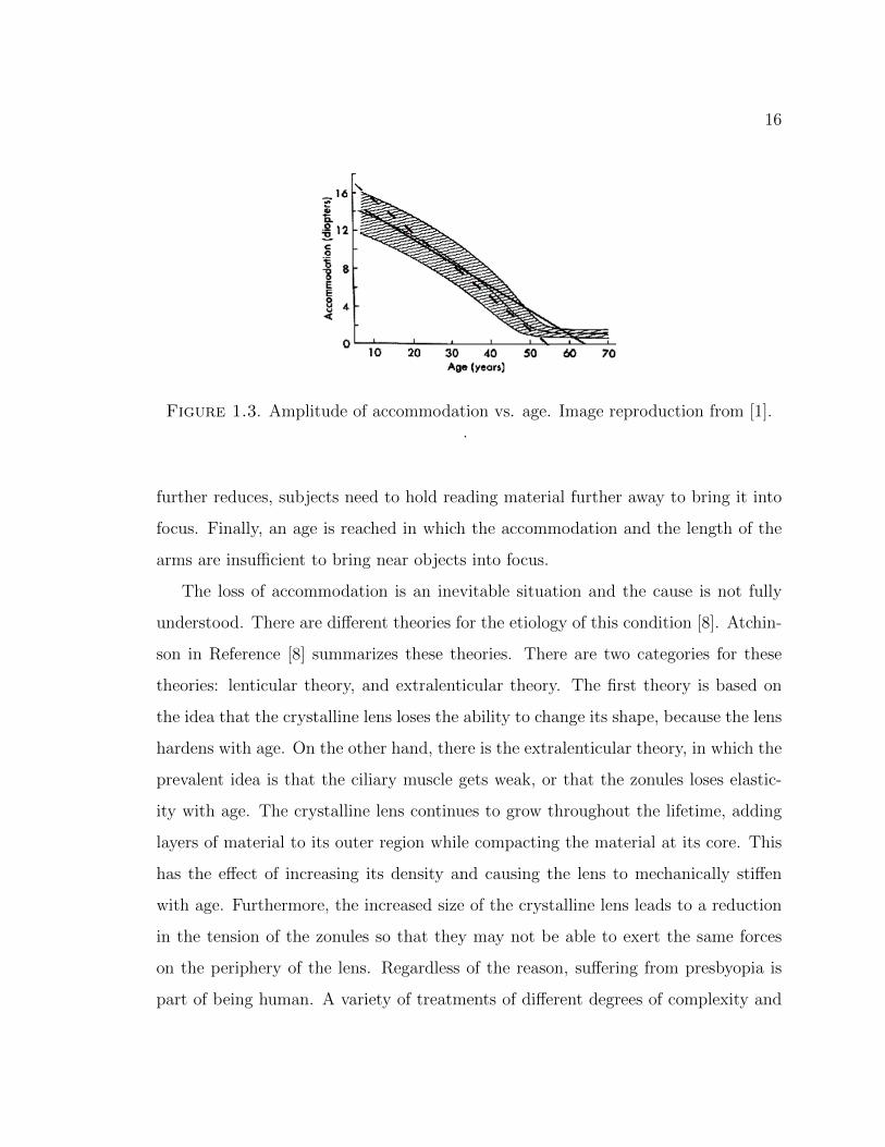
of 40. Figure (1.3) shows a plot of the amplitude of accommodation as a function of

age.

The young eye can typically accommodate 14 diopters. This range steadily de-

creases over the years, but is rarely noticeable to subjects younger than 40 since they

can still comfortably read. However, after the age of 40, subjects typically start by

needing to fully accommodate or maximally flex their ciliary muscles to bring near

objects into focus. This exertion leads to eye strain. As the accommodative range

16

Figure 1.3. Amplitude of accommodation vs. age. Image reproduction from [1]..

further reduces, subjects need to hold reading material further away to bring it into

focus. Finally, an age is reached in which the accommodation and the length of the

arms are insufficient to bring near objects into focus.

The loss of accommodation is an inevitable situation and the cause is not fully

understood. There are different theories for the etiology of this condition [8]. Atchin-

son in Reference [8] summarizes these theories. There are two categories for these

theories: lenticular theory, and extralenticular theory. The first theory is based on

the idea that the crystalline lens loses the ability to change its shape, because the lens

hardens with age. On the other hand, there is the extralenticular theory, in which the

prevalent idea is that the ciliary muscle gets weak, or that the zonules loses elastic-

ity with age. The crystalline lens continues to grow throughout the lifetime, adding

layers of material to its outer region while compacting the material at its core. This

has the effect of increasing its density and causing the lens to mechanically stiffen

with age. Furthermore, the increased size of the crystalline lens leads to a reduction

in the tension of the zonules so that they may not be able to exert the same forces

on the periphery of the lens. Regardless of the reason, suffering from presbyopia is

part of being human. A variety of treatments of different degrees of complexity and

17

invasiveness have been developed to deal with this condition.

1.3 Treatments

In this section, some treatments to help alleviate the effects of presbyopia are briefly

explained. These treatments can be classified into two groups. The first one consists

in treatments that require surgery to replace the eye lens with an artificial one. On

the other hand, the second class of treatments consist of therapies that involve the use

of external appliances, such as contact lenses, reading glasses, bifocals and progressive

addition lenses.

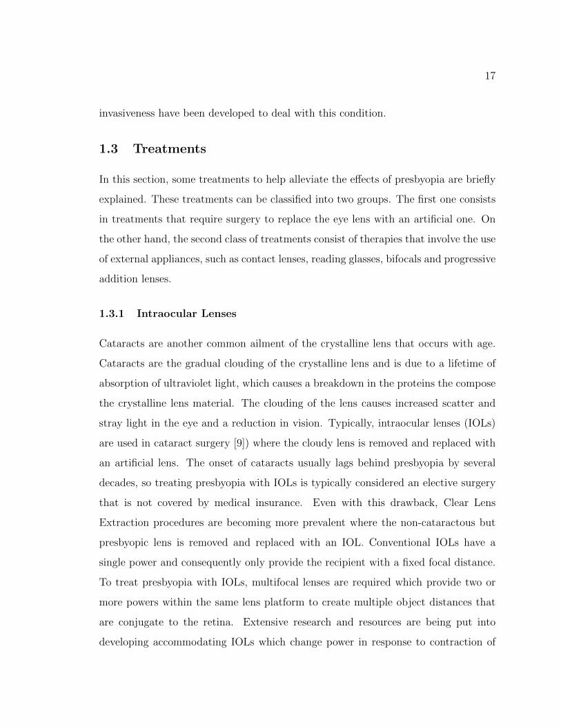
1.3.1 Intraocular Lenses

Cataracts are another common ailment of the crystalline lens that occurs with age.

Cataracts are the gradual clouding of the crystalline lens and is due to a lifetime of

absorption of ultraviolet light, which causes a breakdown in the proteins the compose

the crystalline lens material. The clouding of the lens causes increased scatter and

stray light in the eye and a reduction in vision. Typically, intraocular lenses (IOLs)

are used in cataract surgery [9]) where the cloudy lens is removed and replaced with

an artificial lens. The onset of cataracts usually lags behind presbyopia by several

decades, so treating presbyopia with IOLs is typically considered an elective surgery

that is not covered by medical insurance. Even with this drawback, Clear Lens

Extraction procedures are becoming more prevalent where the non-cataractous but

presbyopic lens is removed and replaced with an IOL. Conventional IOLs have a

single power and consequently only provide the recipient with a fixed focal distance.

To treat presbyopia with IOLs, multifocal lenses are required which provide two or

more powers within the same lens platform to create multiple object distances that

are conjugate to the retina. Extensive research and resources are being put into

developing accommodating IOLs which change power in response to contraction of

18

the ciliary muscle. While progress has been made on a truly accommodating IOL,

this technology is still on the horizon.

There are many types of multifocal intraocular lenses that can used to compen-

sate the eyes loss of accommodation. Among them are refractive multifocal lenses,

diffractive multifocal lenses and accommodative lenses. An extensive review of the

commercially available intraocular lenses can be found in Reference [10]. Refractive

multifocal lenses were the original choice for multifocal lenses. They consisted of

multiple regions within the lens aperture that contained different refractive powers.

A common configuration for refractive multifocal lenses is a series of annular zones

of alternating high and low power. Light passing through the low power regions

from distance objects is focused to the retina, whereas light from near objects pass-

ing through the high power regions also focuses on the retina. In this manner, the

lens acts as a bifocal. However, since these lenses are located within the eye, both

optical regions are simultaneously active. This means that in addition to the foci

described above, there is also extraneous light where light from the distant object

passes through the high power regions and light from the near object passes through

the near region creating out-of-focus images on the retina. Consequently, in-focus and

out-of-focus images are projected onto the retina simultaneously. This effect is call

Simultaneous Vision and has the effect of reducing the contrast of the in-focus image.

Refractive multifocal lenses have been largely abandoned these days and have been

replaced with diffractive multifocal lenses because diffractive multifocal lenses tend

to have less issues with the out-of-focus components. Diffractive multifocal lenses are

the polar analog of a diffraction grating. A binary diffraction grating disperses light

into a multitude of diffraction orders. Each order has a diffraction efficiency which

describes the amount of energy going into each order. The angle of the diffraction

order is dependent upon the grating period. The diffraction efficiency can also be

tailored into specific orders by blazing the diffraction grating and changing its step

height. For a multifocal diffractive IOL, the grating is now in polar form where the

19

grating period follows the Fresnel zones of the lens. Blazing the diffractive zones and

adjusting the step height of the blaze can concentrate most of the energy into two

diffraction orders leading to a bifocal lens. In Figure 1.4, an example of an apodized

bifocal diffractive IOL, marketed by Alcon is shown. The steps following the Fresnel

zones of the lens are evident in the central portion of the lens. The term apodized

here has a slightly different meaning than what is familiar in optical engineering.

Here, apodized means that the step heights of the diffractive zones gradually reduce

towards the periphery of the lens. This allows the diffractive lens blend seamlessly

into a refractive lens in the periphery which helps mitigate some of the side effects of

simultaneous vision.

Figure 1.4. AcriSof IQ ReSTOR multifocal IOL [2]..

Diffractive multifocal IOLs still have some side effects to be considered. For ex-

ample, at night halos and diffraction rings can appear around lights. These lenses

are far from perfect, but represent an improvement over refractive multifocal IOLs.

20

To fully eliminate the bad effects of simultaneous vision, a truly accommodating IOL

is needed. Accommodating IOLs have been pursued which modify the power of the

eye by either moving axially within the eye or by changing their surface curvatures

in response to constriction of the ciliary muscles. However, reliable accommodating

IOLs have not reached the market yet and remain an unsolved challenge in treating

presbyopia.

Regardless of the form of the multifocal IOL, this route for treating presbyopia

is highly invasive since it requires surgery and is expensive. There are less expensive

and easily reversible options available.

1.3.2 Contact Lenses

The use of multifocal contact lenses is another option to treat presbyopia. There are

several treatments that use this ophthalmic device in different ways to achieve the

same goal. Indubitably, all of them have present their own advantages and disadvan-

tages.

One of the presbyopic contact lens correction techniques is monovision. This

treatment consists of the patient wearing a contact lens in one eye to correct for near

distance and wearing a distance correcting contact lens in the other eye. Simultaneous

vision in this case takes a slightly different form, where one eye has a sharp image from

near objects and blurry images from distant objects and vice versa in the fellow eye.

This treatment modality can work because the brain tends to suppress the blur caused

by one eye [11]. However, similar complaints of glare and halos occur with monovision

as with that of the multifocal IOLs described above. Furthermore, monovision tends

to impede depth perception since the two eyes are focused differently.

The use of bifocal and multifocal contact lenses is another option to be considered.

Historically, bifocal contact lenses operate in much the same manner as the refrac-

tive multifocal IOLs described above. The contact lens consists of different regions

21

containing different powers to achieve simultaneous vision. Diffractive multifocal con-

tact lenses have been larger avoided for comfort reasons. The discrete steps of the

diffractive lens tend to irritate the corneal surface or the eyelid depending upon which

surface the diffractive pattern is placed. The modern form of multifocal contact lenses

is typically an aspheric lens with a smooth change in radius of curvature towards its

periphery, changing the power progressively at different radial regions. In effect these

aspheric lenses introduce high spherical aberration to extend the depth of focus of

the lens [12]. The drawback of this spherical aberration, of course, is a reduction in

image quality and contrast associated with an aberrated system. Figure 1.5 shows an

example of an aspheric progressive multifocal contact lens.

Figure 1.5. Alcon Multifocal Contact Lenses [3]..

Simulations of images, as they are seen in different multifocal contact and IOLS

has already been done in the Laboratory of Visual and Ophthalmic Optics of the

University of Arizona [13]. A portion of this dissertation is devoted to extending

these techniques to the spectacle lens-based presbyopia treatments describe in more

detail below.

22

1.3.3 Reading Glasses and Bifocal Spectacles

Loss of accommodation translates into difficulty in focusing on close objects. To treat

presbyopia at least two types of prescriptions are needed: a far distance correction and

a near distance correction (reading section). This is why the easiest and most common

solution to treating presbyopia is the use of reading glasses. These are spectacles that

are only worn when reading close objects. A second pair of glasses may be required

to see distant objects if the person additionally suffers from refractive error. The

difficulty associated with reading glasses is that it cannot be worn all the times. The

wearer has to put on reading glasses for near tasks and them remove them (or replace

them with another pair of glasses) to perform distance tasks. In addition, situations

where rapid switching between near and far objects become awkward at best, such

as the situation of driving and then looking at the dashboard.

Bifocal spectacles help to solve this problem by having two different prescriptions

in the same spectacle frame. The first bifocals are attributed to Benjamin Franklin,

who cut two spectacle lenses with different prescriptions in half and put one half of

one, and other from the other into a frame. However, although both regions had

good optical quality, the separation is annoying to the wearer. Although their design

has been improving with time, one of the problems is the abrupt change in power

between these two regions, and the distraction of the visible line between them [14].

The power change causes an abrupt increase in magnification for objects appearing

in the lower (near vision) region of the lenses. This magnification change can cause

issues with tasks such as walking down stairs. There are also cosmetic considerations

associated with bifocal spectacles as many people feel old when their glasses have the

telltale line across them.

The abrupt change in power between regions is shown in Figure 1.6.

23

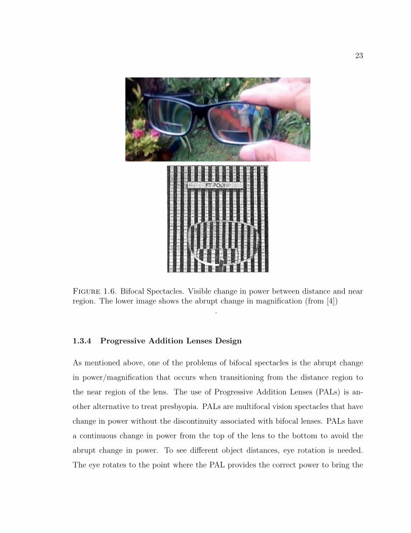
Figure 1.6. Bifocal Spectacles. Visible change in power between distance and nearregion. The lower image shows the abrupt change in magnification (from [4])

.

1.3.4 Progressive Addition Lenses Design

As mentioned above, one of the problems of bifocal spectacles is the abrupt change

in power/magnification that occurs when transitioning from the distance region to

the near region of the lens. The use of Progressive Addition Lenses (PALs) is an-

other alternative to treat presbyopia. PALs are multifocal vision spectacles that have

change in power without the discontinuity associated with bifocal lenses. PALs have

a continuous change in power from the top of the lens to the bottom to avoid the

abrupt change in power. To see different object distances, eye rotation is needed.

The eye rotates to the point where the PAL provides the correct power to bring the

24

object of regard into focus. One tradeoff of PALs though is the presence of unwanted

astigmatism in the lower periphery of the lens, which can cause visual discomfort to

the wearer.

The increment of power in progressive addition lenses is accomplished by increas-

ing the lens curvature from the upper part of the lens to the lower part of it. PALs

typical typically consist of one freeform surface the provides this power change and

the other surface is typically spherical (or aspheric) with its shape chosen to meet

the wearers distance prescription. To create a smooth and continuous freeform sur-

face, the lateral regions of the lower portion of the lens necessarily have shapes that

introduce unwanted astigmatism [15].

In general terms, as shown in Figure 1.7, the structure of Progressive Addition

Lenses consists in four zones:

1. Distance Zone.

2. Intermediate Zone or Progressive Corridor.

3. Near or Reading Zone.

4. Blending Region.

The intermediate zone, also called progressive corridor, is the transition where the

power increases gradually from the distance prescription to the highest power of the

lens in the near region. The length and width of the corridor is determined by the

design of the PAL and it follows the Minkwitz theorem described below.

The near zone, at the lower part of the lens, is the region with the highest spherical

power. Because of the linear relation between spherical power and curvature, this zone

is the steepest one. As mentioned before, to join this region with the distance zone

without visible discontinuities, the freeform surface must gradually change shape from

the distance curvature to the near curvature. In doing so, the side effect is that the

areas on either side of the progressive corridor and the near zone have large levels of

surface astigmatism leading to poor visual performance when viewing through these

25

Figure 1.7. Zones of a Progressive Addition Lens. The right image shows thesmooth transition in magnification from the distance region to the near region. (from[4])

.

areas. These zones without good visual quality are called blending regions.

The organization of the various power zones of the PAL require the wearer to

adapt new eye rotation and head alignment strategies for viewing objects at different

distances. When viewing distant objects through the upper portion of the lens, the

wearer can typically scan their eyes across the horizontal field. However, when viewing

intermediate objects such as a computer screen, the progressive corridor is narrow

and the whole width of the computer screen will not be sharp if the eye scans along

the horizontal field. Instead, the wearer tends to align their eyes in the progressive

corridor and uses their head to scan back and forth to keep the ideal portion of the

intermediate power zone in line with their line of sight. Although the near region is

slightly wider than the progressive corridor, a similar head scanning requirement is

needed for near objects.

An important concept of progressive addition lenses is the umbilical line. Along

this line spherical power increases towards the lower part of the lens. The local surface

curvature along the umbilical line is the same in the two principal directions, meaning

26

zero astigmatism is introduced along its path. However, the surface astigmatism

increases when moving away from the umbilical line. The Minkwitz Theorem is a

description of how the astigmatism changes when moving away from the umbilical

line and it is important for understanding different designs of Progressive Addition

Lenses.

The Minkwitz theorem states that the amount of change in cylinder power (∆cyl)

in a region near the umbilical line, is approximately twice the change in spherical

power added (∆Add) along this line.

∆cyl ≈ 2 ∆Add. (1.3.1)

This theorem opens the discussion about two different design philosophies of Pro-

gressive Addition Lenses: hard design and soft design.

Hard design PALs have a short progressive corridor, permitting rapid access to

different zones with eye rotation. In these designs, the distance and near vision areas

are wider. However, following the Minkwitz theorem, when a rapid change in spherical

power add occurs, there is a rapid increase in astigmatism on either side of the

progressive corridor and therefore high intensity aberration in the blending regions.

Because the big amount of peripheral distortion and astigmatism, the adaptation

period is more difficult.

On the other hand, in soft design PALs, the spherical power change from the

distance to near region is spread over a long distance. This leads to a progressive

corridor that is wider and larger. Thus, there is less distortion at the peripheral view.

One disadvantage compared to the hard design is that the areas at distance and near

vision zones are narrower. These soft designs are good for new presbyopes, because

the gradual change in unwanted astigmatism provides an easier period of adaptation.

Progressive addition lenses are a good option when looking for continuous vision

from far to near distance. Despite the disadvantages mentioned above, new techniques

27

are emerging in the fabrication field, allowing custom freeform surfaces to compensate

wearer needs. Nowadays, each design is customized to fit the frame and patient

prescription [16]-[17], therefore new techniques of surface verification are needed.

1.4 Motivation

As a consequence of the variety of solutions to treat presbyopia and the advantages

and disadvantages of these treatments, the patient who suffers from this condition

has to make an informed decision of what method will fit their needs.

With the technological advances in fabrication, such as freeform surfacing, the

design of PALs can be customized for different patients. Nonetheless, surface char-

acterization is as important as the fabrication process. Due to the application of

progressive addition lenses, they should be tested in a very short period of time.

For this reason, in the first part of this dissertation different techniques of freeform

metrology are presented.

Besides surface shape, acceptance of progressive addition lenses must be studied.

This is a subjective measurement, and usually two types of studies are applied: wearer

trial and preference trial. In the first one, the wearer uses one model for several days

and then evaluates its performance. For the second one, the preference trial, subjects

are given two different models and then they decide which one they prefer [18]. Such

studies are time consuming and expensive. Furthermore, it is difficult to provide the

wide range of lens forms that are available.

In the second part of this dissertation, a methodology to characterize the visual

performance of Progressive Addition Lenses is presented. Scene simulation of how

the wearer see through the spectacle is obtained by calculating the point spread

function through a lens-eye model in function of gaze angle. Such scene simulations

would allow patients to examine the variety of tradeoffs with the various treatment

modalities and make a suitable choice for treatment, or at the very least narrow the

28

list of choices prior to dispensing.

Characterizing the shape of the surface constitutes a challenge because of the dif-

ficulty of testing these freeform surfaces due to their large departure from a spherical

shape. For the same reason, the PSF that defines the lens is highly shift variant, so

a simple convolution of the PSF and the scene is not enough to create a simulated

scene.

In this dissertation, four different methods to test the freeform surface are ex-

plained. After characterization of the surface form, a modified superposition tech-

nique which interpolates the PSFs for different gaze angles, as well as at different

object distances is developed and used to create simulated images that the patient

can use to decide if progressive lenses are the right option.

29

Chapter 2

METROLOGY OF PROGRESSIVE ADDITION

LENSES

Optical design theory and raytracing tools provide a powerful platform to design

and simulate optical components. Increased computational power has led to ease of

design of wildly aspheric and freeform surfaces. However, there remains a non-trivial

path from design to fabrication and testing of these surfaces. Accurate measurements

of an optical surface, defined as metrology, is an important step in building a high-

performance optical system. The surface form can only achieve what can be measured

and limitations on metrology makes the fabricator blind to the source of errors in an

assembled system.

Because of the characteristics of the surface to achieve a continuity of different

optical powers through the lens, there are several fabrication techniques for Progres-

sive Addition Lenses. The original PALs were created using slumping glass process.

This process consists on heating an initial piece of glass on a ceramic slumping block

initially created with the freeform surface shape, the goal is to obtain glass molds to

use them for the production of plastic lenses. However, because heat is involved in the

process, material properties of the glass and ceramic have to be taken into account

to design the shape of the ceramic slumping block. To overcome these problems,

numerical modelling is used for designing the surface [19].

Nowadays, diamond turning machining is employed to fabricate PALs, usually

tool servo is used. Fast tool servo (FTS) and slow tool servo (STS) can manufacture

the surface of non-rotation symmetry by controlling the position of the cutting tool

with high accuracy [20]. One example of fabrication of PALs using FTS is found in

reference [21]. The FTS uses a voice coil actuator to drive the cutting tool. The

30

process to fabricate the progressive addition lens consists in use a sphere as base and

cut it to achieve the freeform surface. Two diamond tools are used, the first one for

rough cutting and the second one for finish the cutting. After finishing, the surface

has to be polished to remove the marks.

Interferometric tests are very powerful techniques to detect phase change between

the reference beam and the tested beam. However, because of the non-symmetric

nature of Progressive Addition Lenses (PALs), interferometric testing of these lenses

needs more complex configurations and more expensive optical elements. PALs typi-

cally are meniscus lenses. The freeform surface of the PAL can appear on either the

concave or convex surface. Furthermore, the surfaces of PALs are fast. In general,

fast convex surfaces are difficult to test interferometrically even if they are spherical

since they require a fast transmission sphere and a large aperture to ensure coverage

of the surface. Front surface PALs add an extra degree of complexity with the steep

aspheric departure from a best fit sphere. Computer-Generated Hologram to compen-

sate the wavefront of freeform surfaces under test are often used to test aspheric and

freeform optics [22]. CGHs can be expensive and each PAL design would require a

unique CGH. There are also alignment challenges with CGHs that limit the through-

put of testing these surfaces in a manufacturing environment. Without a CGH, it is

difficult or impossible to get the surface shape from interference patterns, as demon-

strated in Figure 2.1 due to the aliasing that occurs. This aliasing observed in the

interferogram happens because the freeform surface departs from the spherical refer-

ence surface used, leading to errors in the results. Therefore, reliable measurement

of custom PAL profiles for various presbyopic prescriptions is an important challenge

to overcome using traditional metrology techniques.

The interference pattern shown in Figure 2.1, is from a KODAK Progressive Ad-

dition Lens. The freeform surface is on the convex side of the lens. The nominal

radius of curvature of this surface is R = 83.728mm and the diameter of the lens is

Dlens = 80mm. The labeled add power of the lens is 1.00 to 3.00 in 0.25 Diopter

31

Figure 2.1. Interferogram of the Progressive Addition Lens under test, using ZYGOinterferometer with a reference sphere F/1.5.

.

steps. This lens is used throughout the dissertation for analysis and measured by

different techniques.

Because of its application, these spectacles have to be fabricated and tested in

a very fast way. To decrease the price and testing time, several techniques to test

Progressive Addition Lenses were studied, such as using a lateral shear interferometer

to measure power variation as it is demonstrated in Reference [23], in this technique

the PAL under test is placed in such a way that the light after the lens is collimated.

The light is reflected by the front surface and the surface back of a plane parallel plate

of glass the beams are sheared a distance s. The beams are not perfectly collimated

and therefore interference fringes appear. The principle here is that the space between

fringes is inversely proportional to the local power of the lens. Another approach to

characterized Progressive Addition Lenses is test them with a modified Hartmann

test. In this case, the plate with holes is replaced with a circular scanning laser

beam, simulating the eye looking at different directions of the lens. One positive

sensitive detector recovered the light spot after the lens. This light spot is analyzed

and is expressed in Fourier series to recover the spherical power, and astigmatism at

32

different angles [24].

In this dissertation, several methods were implemented to test the freeform sur-

face shape of a Progressive Addition Lens. Two different types of methods were used:

contact methods such as the use of a linear profilometer, and a Coordinate Measure-

ment Technique (CMM); non-contact methods such as the SCOTS Test by refraction,

and ultraviolet (UV) deflectometry.

2.1 Profilometer

The mathematical description of the freeform surface from the Kodak Progressive

Addition lens is unknown. In general, manufacturers keep the progressive surface

design proprietary. There is limited information regarding designs available in the

academic and patent literature. At best some patents will provide a sag table of the

surface that can be fit and analyzed, but these arent widely available and tend to

be the same design across multiple patents. Since the ideal shape of the Kodak lens

used here is lacking, a reference or gold standard with which to compare is needed.

We found this reference by using a linear profilometer available in the Visual and

Ophthalmic Optics Laboratory. However, one trade-off of this instrument is that it is

a contact profilometer. This means that the tip makes physical contact with the piece

under test. Although contact force between the tip and the surface can be controlled,

material and mechanical properties of the surface under test must be consider to avoid

the risk of damaging the part.

2.1.1 Profilometer Specifications

The instrument used to measure the freeform surface from the Progressive Addition

lens was a linear profilometer MarSurf XC 2 with CD 120 drive unit, (Mahr Federal,

Providence, RI). This measuring station is a contact profilometer with two probe

arms of length 175mm, and 350mm. The tip radius of the probe arms is 25µm.

33

This instrument works on a traversing length inX of 0.2mm to 120mm (0.0079in×

4.72in). The measuring range in Z is 50mm.

The resolution in Z depends on the stylus tip used. For the 350mm probe arm

the resolution is 20.38µm. Meanwhile for the 175mm probe arm it has a resolution

of 0.19mm. The resolution in Z, relative to the measuring system is 0.04µm. The

contact measuring force range is 1mN to 120mN . The PAL in mounted on an x− y

stage. The probe arm is dragged across the surface to measure its sag.

Figure 2.2. MarSurf CD 120 Linear Profilometer..

2.1.2 Data Collection

It is traditionally assumed that the piece under test is rotationally symmetrical and

the profilometer is used to measure one profile with high accuracy. Nonetheless, in

the case of testing freeform optics, one profile is not enough to get the full description

of the surface. Therefore, multiple scans must be performed.

To perform the measurements, the tip used had dimensions of 350 × 33mm due

34

Figure 2.3. (a) Progressive Addition Lens under test mounted on a linear stage.(b) Discrete data obtained from the Profilometer after 31 profile measurements, theorigin is at the center of the lens.

.

to the size of the lens and the smoothness surface. The PAL is mounted on a linear

stage and laterally translated between scans. We performed 31 profiles along the X

axis, translating the lens every 2.5mm along the Y axis. The scans started at one

side of the lens and the stage was driven in the same direction for subsequent scans.

This technique helps to reduce errors occurring from backlash in the stage.

The data obtained from the profilometer is in the coordinate system of the instru-

ment. To fit the data, all the points were translated to a coordinate system where

the origin is at the center of the lens. Following translation, the data are masked into

a circle of radius r = 37.5mm.

2.1.3 Fitting Data

Due to the circular shape of an optical element, one set of functions usually used in

the optics field is the Zernike polynomials. These have very convenient mathematical

properties over the unit circle. They are orthogonal have continuous derivatives, are

related to aberrations and depending on the number of terms can described very

complex shapes [25].

The surface shape can be represented as a linear combination of Zernike polyno-

35

mials, given by

z (ρ, θ) =∑n,m

an,mZmn (ρ, θ) , (2.1.1)

where the definition of the Zernike polynomials is

Zmn =

{Nmn R

|m|n (ρ) cosmθ for m ≥ 0,

−Nmn R

|m|n (ρ) sinmθ for m < 0,

(2.1.2)

where the index n is the radial order and defines the maximum polynomial order of

R|m|n . The azimuthal frequency is indicated by the index m, an integer that must

satisfy |m| ≤ n. The normalization constant Nmn is defined by

Nmn =

√2n+ 2

1 + δm0

. (2.1.3)

The radials polynomials are given by

R|m|n (ρ) =

(n−|m|)/2∑s=0

(−1)2(n− s)!

s![n+|m|

2− s]![n−|m|

2− s]!. (2.1.4)

In the case of using sampled data, the orthogonality property of the Zernike poly-

nomials on the unit circle is no longer valid. However, if the data is well sampled over

a circle, the coefficients of the expansion can be found using a least-square method

as it is described in Reference [25].

Assume the matrix operation

Ax = b, (2.1.5)

where b is a column vector with the measured data from the profilometer z(ρi, θi),

with N the number of sample points.

36

b = [z(ρ1, θ1) z(ρ2, θ2) z(ρ3, θ3) ... z(ρN , θN)]T . (2.1.6)

The matrix A is defined by

A =

Z0

0(ρ1, θ1) Z−11 (ρ1, θ1) Z11(ρ1, θ1) ... Znmax

nmax(ρ1, θ1)

Z00(ρ2, θ2) Z−11 (ρ2, θ2) Z1

1(ρ2, θ2) ... Znmaxnmax

(ρ2, θ2). . . . .. . . . .. . . . .

Z00(ρN , θN) Z−11 (ρN , θN) Z1

1(ρN , θN) ... Znmaxnmax

(ρN , θN)

. (2.1.7)

Each column corresponds to a different Zernike polynomial and it has j + 1 number

of columns, where j is given by

j =n(n+ 2) +m

2. (2.1.8)

Each row corresponds to the Zernike polynomial evaluated at each point (ρi, θi) and it

has N number of rows. The unknown that we want to determine is the column vector

x that has j+1 elements and it contains the expansion coefficients that represent the

measured data as a linear expansion.

x = (a0,0 a1,−1 a1,1 ... anmax,nmax)T . (2.1.9)

To solve for x in Equation 2.5.4 we assumed that the matrix A has many more

rows than columns N >> j + 1. In this case, both sides of the equation is multiplied

by AT

ATAx = ATb. (2.1.10)

37

Now, solving for x multiplying both sides of the equation by the inverse of the

matrix ATA we get

x = [ATA]−1ATb. (2.1.11)

The column vector x will give us the Zernike expansion coefficients of the fitted

data.

2.1.4 Profilometer Results

The 2D set of discrete measurement points is fitted to a set of Zernike polynomials

using the method described by [25]. The data obtained from the profilometer are in

Cartesian coordinates (x, y) and are transformed to spherical coordinates (ρ, θ) due

to the nature of Zernike polynomials.Surface maps of is the fits are shown in Figure

2.4 for two different numbers of expansion terms.

Figure 2.4. Freeform Surface from Profilometer data of a Kodak Progressive Spec-tacle Lens. (a) 37 Zernike Terms. (b) 231 Zernike Terms.

.

By subtracting the low order Zernike terms, of the residual surface height is re-

vealed to understand how the radius of curvature varies to get different optical power.

38

In Figure 2.5 the freeform surfaces with 4 Zernike terms removed are shown. The

terms removed are the first Zernike terms, piston, tilt x, tilt y, and power or defocus.

This allows to see the asymmetric nature of the PAL.

Figure 2.5. Freeform Surface from Profilometer data with low terms removed. (a)37Zernike Terms. (b) 231 Zernike Terms.

.

Although the surfaces look similar. When we analyzed the fitted surfaces with

the original data obtained from the profilometer. We found important differences,

as is shown in Figure 2.6. Analyzing the differences, we found a RMS value for 37

Zernike terms of RMS = 0.16µmm. In the case of the 231 terms, we found a RMS

value of RMS = 6.79µm. This is because at the edge of the lens, the fitting is not

well behaved.

As shown in Figure 2.6, the profilometer lines are present in the residual data.

The source of these errors is likely backlash, and straightness and flatness errors in

the translation stage. The fitting coefficients are shown in Appendix A.

The properties of PAL surfaces are typically illustrated with maps of the average

local surface power and local surface astigmatism. To analyze the local curvature of

the freeform surface, differential geometry and the ”Fundamental Forms” are used.

These expressions allow a pair of principal curvatures to be computed. The principal

curvatures are the steepest curvature and flattest curvature at a given point on the

39

Figure 2.6. Differences in micrometers from Profilometer Data and FiSurface Fit-ting. (a) 37 Zernike Terms (b) 231 Zernike Terms.

.

surface. The principal curvatures are always orthogonal to one another. The mean

curvature at a given point is calculated as the average of the principal curvatures.

The different between the steep curvature and the flat curvature is used to determine

the surface astigmatism. In Cartesian coordinates, the Fundamental Forms are given

by

• First Fundamental Form

E = 1 +

(∂f

∂x

)2

F =

(∂f

∂x

)(∂f

∂y

)G = 1 +

(∂f

∂y

)2

• Second Fundamental Form

L =∂2f/∂2x

(EG− F 2)1/2M =

∂2f/∂x∂y

(EG− F 2)1/2N =

∂2f/∂2y

(EG− F 2)1/2

where f is a two dimensional function describing the surface sag. Based on the

Fundamental Forms, the mean curvature H can be computed, where

H =EN +GL+ 2FM

2(EG− F 2)=

1

2(κ1 + κ2). (2.1.12)

40

The spherical power of the surface is related to the mean curvature by the following

Equation

φ = (n′ − n)C =(n′ − n)

R. (2.1.13)

Figure 2.7. Mean Curvature of Zernike Fit calculated using the Fundamental Forms.(a) Local Spherical (b) Local Cylinder.

.

However, the Power map for the spectacle lens is calculated by adding the back

surface power of the PAL. Here, the back surface power is assumed to be constant

(i.e. the back surface is a sphere) and that the PAL is a thin lens meaning that the

surface powers simply add to give the total power.

The mean curvature for the surface fitting is shown in Figure 2.7(a). The lowest

curvature (blue region) of the lens is at the center part, and the curvature increases

progressively to the bottom part of the lens. From Equation 2.1.13, optical power has

a linear dependence on curvature, then the higher power is at the reading section.

The Gaussian curvature is calculated from the Fundamental Forms as

K =LN −M2

EG− F 2= κ1κ2. (2.1.14)

Every point in a continues surface z = f (x, y) has two principal curvatures κ1

and κ2, minimum and maximum curvature through this point.

41

κ1 = H + sqrt(H2 −K), (2.1.15)

κ2 = H − sqrt(H2 −K). (2.1.16)

The difference between the maximum principal curvature and the minimum prin-

cipal curvature is related to the local cylinder power. A map of this difference is

shown in Figure 2.7(b). As expected at the center and along the progressive corridor,

the surface has low astigmatism. Meanwhile, at the lower lateral edges corresponding

to the blend regions, the surface astigmatism is markedly increased. This cylinder

power introduces astigmatism to wearers of progressive addition lenses when viewing

objects through these portions of the lens.

From the analysis described in this section, the surface described by 37 Zernike

expansion terms is used as the reference when compared to other modalities for mea-

suring this freeform surface.

2.2 Coordinate Measuring Machine

In 1959, the first appearance of the Coordinate Measuring Machine (CMM) was at

the International Machine Tool exhibition in Paris. Ferranti, a British company, de-

veloped the CMM to overcome the challenges of measuring precision components [26].

Through the years, this instrument has been evolving. One important achievement

was the introduction of a touch trigger probe by Renishaw in the early 1970s. This

technological advance and the addition of a motorized probe head in the 1980’s, al-

lowed the CMM to have automatic and accurate 3D measurements for different tested

components.

The CMM is a contact metrology instrument that consists of a test probe that

moves in three directions X,Y and Z. This device gives the Cartesian position of the

test probe. The difference with this and the profilometer is that a random sample

42

of points across the surface under test is provided. Effectively, a point cloud of the

surface is created and the sampling can be adjusted by simply touching the probe more

densely in a given region. One of the advantages of the CMM over the profilometer,

is that the x,y and z coordinates are given by the same instrument, avoiding the

backlash and other travel errors introduced by the translation stage.

Figure 2.8. Sample points from the Coordinate Measuring Machine (a) Data Set 1.(b) Data Set 2. (c) Data Set 3

.

To obtain the sag data of the PAL, the Coordinate Measurement Machine in the

College of Optical Sciences is used. This is a CMM Tesa Micro-hite. The size is

18′′ × 28′′ × 16′′. The PAL is mounted to a granite table and the surface is measured

with with different patterns. These patterns are shown in Figure 2.8.

Three sets of discrete data from the surface are obtained, and these data are fit

using the method described previously in Section 2.1.3. The differences between the

measured data and the fitted data to 37 Zernike terms are shown in Figure 2.9.

The RMS errors for each set are the followings: Set 1 RMS1 = 0.0137mm, set 2

RMS2 = 0.0141mm, and set 3 RMS3 = 0.0122mm.

An average of the three data sets was taken and analyzed. The average RMS =

13.3µm. A representation of the surface is shown in in Fig. 2.10(a).After removing

the lower terms, we get the surface shown in Fig. 2.10(b).

A comparison between the profilometer data and the CMM data with the low

43

Figure 2.9. Differences from CMM Data and Fitting Data. (a) Data Set 1 (b) DataSet 2 (c) Data Set 3.

.

Figure 2.10. (a) Freeform Surface Fitting to 37 Zernike terms. (b)Freeform surfacewith low Zernike terms removed.

.

terms removed is presented in Figure 2.11. We found and RMS error of RMS =

0.0262mm and a PV = 0.1956mm. Most of the differences occur at the extreme

edges of the lens.

The mean curvature was computed using Equation 2.1.12. The color map shown

in Figure 2.12(a) shows the expected behavior of a progressive addition lens. The

increment of curvature from the top to the bottom of the lens. This could be trans-

lated into an increment of the optical power, from the far region to the near region

of a progressive addition lens.

44

Figure 2.11. Comparison between profilometer data and CMM data, with RMS =0.0262mm and a Peak of Valley value PV = 0.1956mm.

.

Figure 2.12. Curvature Maps of the freeform surface of a Progressive AdditionLens. (a) Mean Curvature Local Spherical. (b) Local Cylinder

.

Taking the differences between the principal curvatures of the surface, the cylinder

power is found. As shown in Figure 2.12(b), the surface astigmatism again increases

in the lower periphery, illustrating the behavior expected for a progressive addition

lens.

After analyzing both contact methods to measure the freeform surface from the

progressive addition lens, interesting properties of these spectacle lenses are found.

The freeform surface introduces a power variation without discontinuity across the

45

lens and allows the wearer to see different object distances clearly. Yet, this surface

also introduces cylinder power, especially in the blend regions, that leads to image

blur when viewing through these regions.

Although these properties can be studied, the problem with these methods as

described before is that they are contact methods, and there is risk of scratching

the surface. Another problem with these contact methods is the time that takes to

perform all the measurements. For these reasons, the following non-contact methods

are explored. Both of the non-contact methods described below use the phase shifting

technique to extract surface information. Phase shifting and the associated phase

unwrapping techniques are explained in the following section.

2.3 Phase-Shifting and Phase Unwrapping

The principle of phase-shifting is used as a baseline for the following non-contact

metrology methods. Therefore, a brief explanation is provided in this section. These

metrology techniques use a simusoidal light pattern projected onto the test surface

[27]. The sinusoidal or fringe pattern is shifted N times by 2π/N , where 2π corre-

sponds to one complete period of the sinusoid. The shifted pattern is recorded at

each of the N locations. In the following cases, a four-step method is used, meaning

N = 4. To retrieve the phase at each point on the surface the following expression is

used

Ψ = arctan

(−I2 − I4I1 − I4

)(2.3.1)

where I1, I2, I3, I4 are the irradiance patterns of each measurement, given by

46

I1 (x, y; 0) = I ′ (x, y) + I ′′ (x, y) cos [Ψ (x, y)] ,

I2(x, y; π

2

)= −I ′′ (x, y) sin [Ψ (x, y)] ,

I3 (x, y; π) = I ′ (x, y)− I ′′ (x, y) cos [Ψ (x, y)] ,

I4(x, y; 3π

2

)= I

′′(x, y) sin [Ψ (x, y)] .

(2.3.2)

From Equation (2.3.1), the phase is recovered using the arctangent function. A

drawback of this function is that has principal values in the range of −π to π,When

the phase value exceeds this range, the phase is wrapped back into this range. Con-

sequently, the phase can only be known to some integer multiple of 2π. To solve

this ambiguity, well-known algorithms to unwrap the phase, must be applied. In

this work, Goldsteins algorithm has been applied for the analyses performed in this

dissertation.

After unwrapping the phase, we can use the data to find the slope information of

the surface. Fringes in X and Y must be projected to get the local slopes in both

directions.

2.4 SCOTS

The Software Configurable Optical Test System (SCOTS) was used to test the PAL

surface [28]. SCOTS is a very powerful tool to test optical surfaces fast, accurately

and in an inexpensive way. This technique was previously used to test the Large Syn-

optic Survey Telescope tertiary mirror (LSST M3) and the Giant Magellan Telescope

(GMT) primary mirror [29]. In recent works, it has been shown that this technique

can be used to test refractive optical systems by measuring simple refraction elements

[30] and testing the Large Binocular Telescope (LBT) secondary mirror null corrector

[31] .

47

2.4.1 Principle

The SCOTS principle, which is based on a reverse Hartmann test, is implemented in

a simple configuration. An LCD screen illuminates the test surface with a pattern,

replacing the traditional Hartmann Plate. A CCD camera with an external stop,

represents the point source in the Hartmann test. A laptop is used to collect the

images of the pattern presented on the LCD screen and reflected or transmitted from

the test surface [28]. SCOTS measures the transverse ray aberration by finding the

correspondence between the screen pixel location and the pixels on the CCD sensor.

The transverse ray aberration can be used to find the test objects wavefront slopes

[32] which in turn can be integrated using a polynomial fit or by zonal integration to

give the wavefront and the surface departure from the ideal shape [31].

2.4.2 Experimental Setup

After obtaining the surface shape as explained in Section 2.1, the lens specifications

are input into a ZEMAX model of the entire SCOTS system and the distances between

the LCD and the camera are set keeping in mind that the CCD sensor area needs to

cover the entire PAL surface.

In the SCOTS setup, as is shown in Fig. 2.13, the lens was mounted in a tip

and tilt stage for alignment with the freeform surface facing the LCD screen. The

distance chosen between the LCD and the test lens was z = 715 mm, and from the

test lens to the pinhole z = 1120 mm. We used an LCD screen of 1280 x 1024 pixels

with a pitch of 0.2940 mm, a digital CCD camera with a lens of focal length f = 50

mm, and a computer. The PAL is measured in transmission and the spherical surface

currently is assumed to be perfectly spherical.

To measure the transverse ray aberration, the correspondence between the LCD

screen pixels and the CCD pixels needs to be determined. To find this mapping, phase

shifted sinusoidal patterns are displayed on the LCD screen oriented in both the x

48

Figure 2.13. SCOTS experimental setup.

and y directions. These fringes were green to improve the contrast of the images.

Considerations of the pupil size and contrast are made. The image data are collected

and compared to the ZEMAX model. The results are presented below.

2.4.3 Results

After data reduction, a comparison between the surface in the ZEMAX model and

the measured surface is presented. It is important to mention that to separate the

measurement error associated with the testing setup from the errors inherent to the

test lens, repeated measurements rotating the lens by 180 degrees are captured. Figure

2.15 shows the differences between the profilometer data and the SCOTS data for

orientations of 0 and 180 degrees. For 0 degrees a wavefront RMS = 12.2µm is

found, while for 180 degrees the wavefront RMS = 13.9µm.

By direct subtraction of both maps reoriented to one another, the difference in

RMS error is 1.8µm. Averaging the results from the rotation, the wavefront RMS

difference between the surface shape obtained with the profilometer data, and that

49

Figure 2.14. (a) Differences between profilometer and SCOTS data (b) Differencesbetween profilometer and SCOTS data after a 180 degrees rotation (low order termsremoved).

.

from SCOTS is 12.3µm. Table 2.1 lists the wavefront errors departing from the ideal

surface from the SCOTS test in the coefficients of the Zernike standard polynomial.

The results show that the dominated errors were Astigmatism (Z6) and Trefoil (Z9).

Zernike StandardPolynomial Coefficient

Zernike StandardPolynomial Coefficient

Astigmatism Sin (Z5) 4.48 Coma Cos (Z8) 3.9424Astigmatism Cos (Z6) 6.7001 Trefoil Sin (Z9) 6.0743

Coma Sin(Z7) 0.4103 Trefoil Cos (Z10) 2.6722

Table 2.1. Coefficient of the Zernike Standard Polynomial.

SCOTS can be used to test Progressive Addition Lenses with an average wavefront

RMS of 1.8µm, after removing low order terms. The profilometer measurements are

limited by the accuracy of the repeated scans. While the profilometer is capable

of highly accurate 1D scans, our addition of the translation stage likely introduced

larger errors in the 2D cases through backlash and runout in the stage. However, by

rotating the PAL between measurements, the error in the profilometer model and the

50

Figure 2.15. Differences between profilometer data and average of rotations..

measurement error of the SCOTS system can be separated to estimate the capabilities

of the SCOTS system. The remaining discrepancies between the profilometry data

and the SCOTS test are likely due to errors introduced by the back surface of the PAL.

The back surface is assumed to be spherical so that the ZEMAX model can recover

the progressive surface. Ideally, the back surface of the PAL should be measured by

another means to incorporate its effect into the model. Traditional interferometry

would be able to measure this back surface accurately since it is nearly spherical.

2.5 UV Deflectometry

The next technique to measure the Progressive Addition Lens is UV Deflectometry.

The SCOTS test described above was performed in transmission and consequently, the

back surface of the lens needs to be accurately known to back out the characteristics

51

of the freeform surface. Here, deflectometry in reflection is performed. One of the

problems of testing the freeform surface of the PAL in reflection is the presence of

ghost reflections due to the back surface. Both the anterior and posterior surfaces

will reflect fringe patterns and in regions where these patterns overlap, the fringe

contrast tends to become low. To avoid issues with the parasitic fringes from the

back surface, a common technique is to temporarily coat the unwanted surface to

reduce is reflectivity. This coating however slows down the testing and it would be

beneficial to remove this step. To reduce unwanted reflections from the back surface,

the transmission properties of the lens material will be used instead.

In Figure 2.16, a Transmission Plot for the PMMA is shown. At approximately

λ = 365nm, the transmission of the PMMA is T ≈ 10%, which means that the

reflection from the front surface at this wavelength isR ≈ 90%. If fringes are projected

at this wavelength, the spurious reflections from the back surface are greatly reduced.

Figure 2.16 shows the same scene was taken under different lighting conditions to

demonstrate the transmissivity of the PMMA. The left image depicts looking through

the lens at a target with a UV camera and UV illumination. The lack of transmission

through the lens obscures the target. The right image shows the same scene captured

with a cellphone camera with visible illumination. In the wavelength region, the lens

is transparent and the target is clearly visible to the camera.

2.5.1 Theory

To overcome the new challenges of testing freeform optical elements, different tech-

niques have been studied to measure specular surfaces without contact.

One technique that has had successful results, in comparison with interferomet-

ric methods, is Phase Measuring Deflectometry. This technique measures the light

deflection after the reflection or transmission from the surface under test [34].

Phase Measuring Deflectometry has been used to measure different ophthalmic

52

Figure 2.16. PMMA Transmission Plot, emphasizing transmission at λ = 365nm .Image reproduction from Rocoes Electro-optics.LTD [33].

.

elements. One example is the implementation of a deflectometric setup to measure

the shape of a freeform IOL lens [35],and the measurement of the local curvature of

the freeform surface of Progressive Addition Lenses [36].

However, this technique has some problems when testing transparent objects be-

cause of the reflections of the back surfaces. The reflection of the back surface and

the front surface are superimposed. Several methods have been applied to overcome

these problems [37]. One of them is the use of multiple fringe projections and work

with an algorithm to separate the signals.

The second one is UV deflectometry, but because there are not spatial modulators

at this wavelength, another approach has to be taken: Shift Line deflectometry. This

technique instead of using a sinusoidal pattern, uses a line of UV light moved by a

linear stage [36].

Here, a simple method to create a screen with a UV sinusoidal pattern is developed

to enable UV deflectometry. This sinusoidal pattern, in turn, reflects from the surface

under test and is captured by a camera.

Deflectometry consists of examining the distortions of phase shifted sinusoidal

patterns reflected from the surface under test. These patterns reflected from the

surface encode the local slope of the surface in their phase as given by Equation 2.5.1.

53

φ = d tan (2α) (2.5.1)

where φ is the phase, d is the distance from the screen to the surface, and α is the

local slope.

To find a correlation between pixels in the CCD camera and fringes in the screen.

Phase shifting techniques are employed, as it is explained in section 2.3, the same

pattern phase shifted is projected onto the freeform surface and a series of pictures

are taken. Later, phase unwrapping techniques are used to recover the local slopes of

the surface.

2.5.2 Illumination System

To create the UV pattern, we used a high-power LED of wavelength λ = 365nm from

Marktech Optoelectronics. This is an ultraviolet emitter working 500mA at 3.6V ,

with a view angle of 120◦.

The fringes are projected onto a ground glass screen using a projection-condenser

illumination system. This system is used because of a need for uniform illumination.

This type of system consists on a condenser lens that images the light source into

the plane of another lens called the projector lens. The condenser lens should be the

faster one. A transparent object placed next to the condenser lens will be imaged by

the projector lens onto the image plane.

In the setup, the condenser lens, focal length of f1 = 35mm is placed at a distance

of d1 = 101.5mm from the LED source. A transparency with the fringe pattern is

placed next to the condenser lens. The second lens, or projection lens of focal length

f2 = 50mm is placed at a distance 2 = 53.4 from the first lens, and the image screen

is 785.3 from the second lens. Thorlabs UV lenses were used. A schematic diagram

of the illumination system is shown in Figure 2.17.

The object was a binary line pattern printed on a transparency with a spatial

54

Figure 2.17. Fringe projection with an LED λ = 365nm..

frequency of f = 1.5lp/mm. This object is mounted on a linear stage to enable phase

shifting the pattern. The image of the object is a sinusoidal pattern in the screen

(ground glass) due mainly to high frequency losses from the aberrations associated

with the projection lens. To characterize the required phase shifts, a relation between

the distance displaced by the linear stage in the object plane and the resultant phase

shift of the pattern on the image screen is found.

Pictures of the pattern on the image screen are captured and analyzed in MAT-

LAB. A profile of the projected image is fit to a sinusoidal pattern such that

y(∆d) = Asin (2πBx+ C(∆d)π) , (2.5.2)

where A is the amplitude, ∆D the displacement of the linear stage in mm, and

C (∆D) the phase shift as a function of the lateral displacement.. Eleven profiles

are captured, displacing the translation stage every ∆D = 0.05mm. In Figure 2.18,

examples of some of the irradiance profiles through the captured images are shown

along with the fitted sinusoid.

To find the lateral displacement corresponding to a phase shift the pattern of π/2,

55

Figure 2.18. Irradiance profile at the screen with lateral displacement. (a) 10 mm(b) 25 mm (c) 30 mm (d) 35 mm.

.

the phase shift C (∆D) is plotted against the lateral displacement ∆D,to find a linear

relation. This linear relationship is shown in Figure 2.19. A translation of the object

∆D = 0.15mm corresponds to a phase shift the irradiance pattern of π/2.

2.5.3 Experimental Setup

After constructing the illumination system and characterizing the phase shift, the

PAL is mounted next to the image screen.

One consideration in setting up the deflectometry system is the size of the piece

under test. The projection pattern should be big enough to cover all the surface

area of the test part. Even though the focal lengths and the distances were carefully

chosen to get a magnification of m = 14.6, the PAL had to be very close to the

screen dscreen−lens = 40mm to cover the entire part. This proximity creates another

complication in the pronounced angle that the lens made with respect to the screen

56

Figure 2.19. Linear Relation of irradiance profile phase shift in function of lateraldisplacement of the object.

.

and the location of the camera. An optimal position trying to cover the major part

of the test surface was found and all images were captured from this location.

As mentioned in Section 2.5.1, fringes in orthogonal directions should be projected

to recover the local surface in two directions.

The camera used to take pictures, was a Sony XC-EU50 1/2′′ CCD. It has an appli-

cable wavelength sensitivity range of 300− 420 nm with a near ultraviolet sensitivity

in the i-line, 365nm. The camera is monochrome with a 768x494 pixel resolution.

The CCD horizontal driving frequency is 14.318MHz, and the CCD vertical driving

frequency is 15.734kHz.

The lens used was a 25mm Standard UV Fixed Focal Length Lens, with a wave-

length range of 2301200nm. A 1/2′′ sensor, and a field of view of FOV = 14◦ and a

working distance of 230−∞mm.

57

Figure 2.20. Experimental Setup Deflectometry System λ = 365nm..

2.5.4 System Calibration

Due to the complicated geometry of the setup, a calibration method is proposed. After

fixing the position of the projection screen and the camera. A calibration sphere is

placed; this sphere is chosen to have a radius of curvature Rsphere = 77mm, close to

the base curvature of the freeform surface of the progressive lens.

Phase shifting, and phase unwrapping techniques are applied to the reference

sphere. However, the resultant images are distorted because of the angle between the

camera and the lens. As shown in Figure 2.21, circular shape of the lens appears to

be an ellipse.

The method proposed is to find a transformation to map the reflected curved

fringes into the sphere to straight lines, representing the slopes in x and y direction

of the reference sphere.

First, the pictures of the vertical lines were superimposed over the horizontal lines

creating a mesh as shown in Figure 2.22(c). The coordinates of the intersections of

the lines are found (xN , yN) as shown in Figure 2.22(a) and 2.22(b). A nominal grid

58

Figure 2.21. Reflected fringes into calibration Sphere..

is created with equally space points as shown in Figure 2.22(c).

Figure 2.22. (a) Intersection of lines. (b) Original Data. (c) Nominal Grid..

The new coordinates are expressed by

x′(u, v) = a1u+ a2v + a3u2 + a4uv + a5v

2 + a6u3 + a7u

2v + a8v2u+ a9v

3,y′(u, v) = b1u+ b2v + b3u

2 + b4uv + b5v2 + b6u

3 + b7u2v + b8v

2u+ b9v3.

(2.5.3)

The goal is to find the coefficients that map the original coordinates (xN , yN) to

59

the nominal grid (x′N , y′N). To find the expansion coefficients of the transformation,

the square fit method is applied to find the new x coordinates, and then to find the

new y coordinates. As described in Section 2.1.3, consider the matrix equation

Ax = b, (2.5.4)

The matrix A has N rows, where N is the number of sample points, and M

columns, where M is the number of terms to fit in this case M = 9. The matrix A

is given by

A =

x1 y1 x21 x1y1 y21 x31 x21y1 y21x1 y31x2 y2 x22 x2y2 y22 x32 x22y2 y22x2 y32. . . . . . . . .. . . . . . . . .. . . . . . . . .xN yN x2N xNyN y2N x3N x2NyN y2NxN y3N

. (2.5.5)

The vector x is a column vector of M elements, containing the expansion coeffi-

cients that have to be determined.

x = (a1 a2 a3 . . . aM)T . (2.5.6)

y = (b1 b2 b3 . . . bM)T . (2.5.7)

The vector b is a column vector of N elements, given by

b = (x′1 x′2 x′3 . . . x′N)T. (2.5.8)

b = (y′1 y′2 y′3 . . . y′N)T. (2.5.9)

Finally, the vector of expansion coefficients is given by

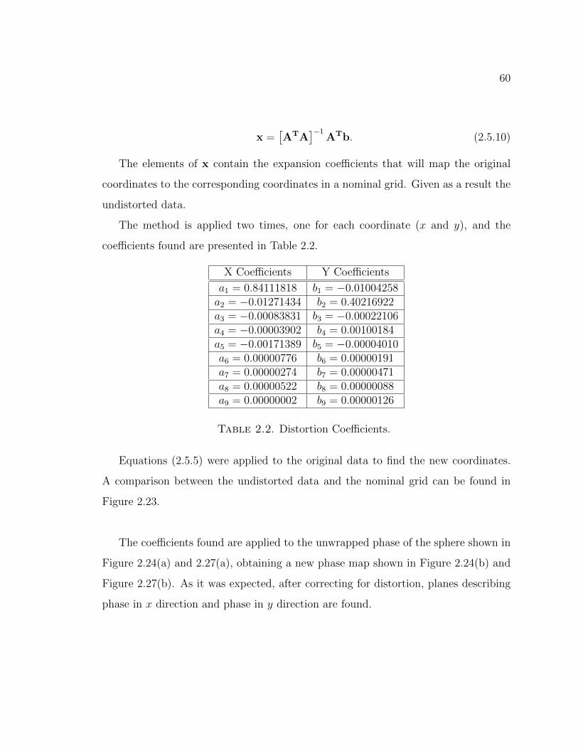
60

x =[ATA

]−1ATb. (2.5.10)

The elements of x contain the expansion coefficients that will map the original

coordinates to the corresponding coordinates in a nominal grid. Given as a result the

undistorted data.

The method is applied two times, one for each coordinate (x and y), and the

coefficients found are presented in Table 2.2.

X Coefficients Y Coefficients

a1 = 0.84111818 b1 = −0.01004258a2 = −0.01271434 b2 = 0.40216922a3 = −0.00083831 b3 = −0.00022106a4 = −0.00003902 b4 = 0.00100184a5 = −0.00171389 b5 = −0.00004010a6 = 0.00000776 b6 = 0.00000191a7 = 0.00000274 b7 = 0.00000471a8 = 0.00000522 b8 = 0.00000088a9 = 0.00000002 b9 = 0.00000126

Table 2.2. Distortion Coefficients.

Equations (2.5.5) were applied to the original data to find the new coordinates.

A comparison between the undistorted data and the nominal grid can be found in

Figure 2.23.

The coefficients found are applied to the unwrapped phase of the sphere shown in

Figure 2.24(a) and 2.27(a), obtaining a new phase map shown in Figure 2.24(b) and

Figure 2.27(b). As it was expected, after correcting for distortion, planes describing

phase in x direction and phase in y direction are found.

61

Figure 2.23. Comparison between Nominal Grid and Undistorted Data..

Figure 2.24. (a) Original map Phase in X from Reference Sphere. (b) Undistortedmap Phase in X from Reference Sphere.

.

2.5.5 Fitting Data

The data obtained after applying the distortion transformation, is related to the

surface slopes of the surface under test [25]. The phase maps in x leads to a set of N

slopes in the xP direction, and the phase maps in y leads to a set of N slopes in the

yP direction. Where N is the number of sample points, in this case number of pixels

that covers the surface area. This set is given by

62

Figure 2.25. (a) Original map Phase in Y from Reference Sphere. (b) Undistortedmap Phase in Y from Reference Sphere.

.

{∂zP (xPk, yPk)

∂xP,∂zP (xPk, yPk)

∂yP

}, (2.5.11)

where k = 1 . . . N . This data is represented as a linear combination of the cartesian

derivatives of the Zernike polynomials.

slopesx =∑

n,m an,m∂Zm

n (ρx,ρy)

∂ρxand slopesy =

∑n,m an,m

∂Zmn (ρx,ρy)

∂ρy(2.5.12)

The expansion coefficients for the gradient data are the expansion coefficients for

the fit of the surface shape (within a constant offset). Then the surface shape can be

expressed by

z (ρx, ρy) =∑n,m

an,mZmn (ρx, ρy) , (2.5.13)

To fit the gradient data to the derivatives of the Zernike polynomials, the method

used is similar to the one described in Section 2.1.3, consider the matrix operation

Ax = b, (2.5.14)

63

In this case, the matrix A has 2N rows, and contains the derivatives values of the

Zernike polynomials. The first N rows correspond to the N slopes in the xp values

followed by N rows of the N slopes in the yp direction.

A =

∂Z−1−1 (xP1,yP1)

∂xP... ∂Znmax

nmax (xP1,yP1)∂xP

. . .∂Z−1−1 (xPN ,yPN )

∂xP. ∂Znmax

nmax (xPN ,yPN )∂xP

∂Z−1−1 (xP1,yP1)

∂yP.

∂Znmaxnmax1(xP1,yP1)

∂yP

. . .∂Z−1−1 (xPN ,yPN )

∂yP... ∂Znmax

nmax (ρx,ρy)

∂yP

(2.5.15)

The vector x, contains the expansion coefficients data

x = (a0,0 a1,−1 a1,1 . . . anmax,nmax)T , (2.5.16)

and the column vector b the measured gradient

b =

[∂zP (xP1, yP1)

∂xP

∂zP (xPN , yPN)

∂xP

∂zP (xP1, yP1)

∂yP. . .

∂zP (xPN , yPN)

∂yP

]T.

(2.5.17)

The vector of the expansion coefficients is again

x =[ATA

]−1ATb. (2.5.18)

Because the A matrix, is at the derivative, the piston coefficient is not included.

Then this coefficient normally is set when the surface is zero at the origin.

2.5.6 Calibration Sphere

The method outlined in Section 2.5.4 is applied to the phase results obtained from the

sphere. The data is fitted to 4 Zernike terms. The pixel size in mm is pixel size =

0.1781mm. A scale factor is found by calculating the sag theoretical value of the

sphere at the edge of the area used D = 21.37mm.

64

SAG = R−

√√√√(R2 −(D

2

)2), (2.5.19)

whereR = 77mm. SAG (21.37) = 0.7451mm. The scale factor found is scale factor =

0.4565mm. The sphere map removing tip and tilt in mm is shown in Figure 2.26.

Figure 2.26. Reconstructed Sphere..

2.5.7 Results

Phase shifting, and phase unwrapping techniques are used to obtain the phase maps

for the freeform surface of the Progressive Addition Lens. To undistort the data,

the coefficients found in the calibration step are applied to the PAL phase maps, the

final undistorted phase maps are shown in Figures 2.28(b) and 2.29(b). The data is

normalized.

After applying the method outlined above to the gradient data, the recovered

surface is fitted to 45 Zernike terms. The reconstructed freeform surface of the Pro-

gressive Addition Lens is shown in Figure 2.30.

65

Figure 2.27. Sphere Mean Curvature and Cylinder power..

Figure 2.28. (a) Original map Phase in X from PAL under test. (b) Undistortedmap Phase in X from PAL under test.

.

The scale factor previously found in Section 2.5.6 is applied to the data to find

the surface map in mm. The Fundamental Forms for differential geometry mentioned

before are applied to find the mean curvature related to spherical power and cylinder

power. The PAL spherical power map and Cylinder power map are shown in Figures

2.31.

66

Figure 2.29. (a) Original map Phase in Y from PAL under test. (b) Undistortedmap Phase in Y from PAL under test.

.

Figure 2.30. Reconstructed PAL surface..

2.5.8 Conclusions and Future Work

A new calibration method was proposed in order to recover the surface shape of

the Progressive Addition Lens using a reference sphere. The distortion coefficients to

obtain planes that represent the slopes in x and y direction of the reference sphere were

67

Figure 2.31. Reconstructed PAL surface..

found. However, the area to test is minimum because of the geometry of the system

and the contrast of the reflected fringes at the edge of the lens. The reconstructed

surface of the calibration sphere was used to find the scale factor that converts phase

into mm. This scale factor is used to find surface height in mm of the PAL. The

mean curvature and the cylinder power of the progressive addition lens didnt match

the expected behavior of the Progressive Addition Lens. There are several reasons to

consider, one is that the orientation and the area of the lens under test did not include

the region of interest. Other reason is that other method to consider the geometry

of the system has to be included. Future work by implementing another calibration

method is suggested.

68

Chapter 3

SIMULATION OF MULTIFOCAL VISION

In Chapter 2, the freeform surface of a progressive addition lens is characterized by

a mathematical approach. This is a very important process to see if the optical

element is well fabricated and meets the design specifications. However, in terms of

ophthalmic artifacts, acceptance by the wearer has the same importance as surface

verification. If the wearer does not feel comfortable with the treatment used or has

visual artifacts, it is as useless as a not well fabricated spectacle lens.

As explained in Chapter 1, there is a variety of progressive addition lens designs.

The biggest trade-off is that PALs introduce unwanted aberrations not acceptable to

all the patients. In this chapter, a new technique of realistic simulation is used as a

suitable tool to give a preliminary insight into PALs performance. These simulations

can allow the designer to understand the implications of various design choices, as

well as provide an understanding of the required tolerances on freeform surface.

3.1 Theory and Image Simulation

The most important concept of this chapter is the notion of the point spread function

(psf), also called the impulse response of an imaging optical system. It is the image

of a perfect point source through the optical system. The psf is a metric of optical

performance, serving as an indicator of the aberrations in a lens. If the system is

diffraction limited, the psf will be the Airy pattern. In the presence of aberrations,

the psf spreads out and its peak value diminishes leading to blurry of the point.

For scene simulation, each point in the scene can be considered a point source

weighted by the local irradiance and spectral content. The simulated image is a su-

perposition of all of the psfs from the scene. In general, the psfs will be dependent

69

upon the field position of the point source. The shape of the psfs will change from

point to point and creating a simulation with this superposition is computationally

intensive because of the need to recalculate the psf at each point in the field. To

accelerate the simulation, scene simulation is usually achieved by convolving the sys-

tem point spread function formed by an optical system with a scene. This technique

assumes that the psf is shift invariant, so the psf only needs to be calculated once.

Further increases in speed are achieved by performing this operation in Fourier do-

main using the convolution theorem and the computational optimization of the Fast

Fourier Transform (FFT).

The convolution theorem states that in a linear shift invariant system (LSI), a

convolution operation between the input f (x, y) and the impulse response h (x, y) in

space domain, is equivalent to a multiplication operation in Fourier domain [38].

g (x, y) = f (x, y)h (x, y) G (ξ, η) = F (ξ, η)H (ξ, η) (3.1.1)

The following diagram illustrates this theorem, where psf (x, y) is the impulse

response of the system, o (x, y) is the system input and i (x, y) the system output

[39].

.

Nonetheless, optical systems have a shift variant point spread function, this means

that the psf changes for different fields. To simulate shift variant cases, the scene is

divided into regions over which the psf is approximately the same (i.e. isoplanatic

patches), convolution is performed, and then all the regions are added to complete the

70

whole scene. Care must be taken using this technique. The field must be sufficiently

sampled to ensure the variation in psfs is adequately sampled and the individual

areas need to be blended to avoid artifacts at the edges of the regions. Raytracing

software, such as Zemax OpticStudio (Zemax, LLC, Kirkland, WA), performs image

simulation by sampling psf on a grid over a specific field of view, the psf for each pixel

is then interpolated from the nearest psfs. Each point spread function is convolved

with the corresponding pixel to obtain the final image [40]. Furthermore, image

simulations using this technique typically only assume a single object plane. Due to

the progressive addition lenses nature, consideration of different object plane depths

has to be added.

As explained in Chapter 1, the different powers of a progressive addition lens

are selected by eye rotation and head movement. Furthermore, the wearer is typ-

ically looking at objects at multiple distances, using the upper portion of the lens

for distance objects and the lower portion of the lens to read. Therefore, in this

dissertation, a different approach to scene simulation is used. The image simulation

was built up by a superposition of psfs calculated across the field, as well as for a

multitude of depths. In effect, a three-dimensional matrix of psfs is created and a

three-dimensional scene processed to create the simulation. Details are explained in

the following sections.

3.2 Algorithm Overview

In this section, an overview of the method used to perform scene simulation is pre-

sented. The method was implemented into a MATLAB script that in general terms

consists in the following steps. The MATLAB script is contained in the Appendix.

1. Divide the image into the three RGB channels to process each separately.

2. Divide the field of view to simulate into the number of pixels for each image, in

this manner each pixel will correspond to a certain field in the scene.

71

3. Choose the distance where the object plane is located.

4. Find the corresponding psf in the data base previously stored into .mat file.

5. Choose between these options: a) The psf exists. b) The psf doesnt exist:

choose the 4 nearest point spread functions to the field of view, interpolate to

get the correspondent psf at that field.

6. The point spread function is weighted by the RGB value at the corresponding

pixel, the output psf is stored into a new matrix.

7. All the point spread functions are added to get the final values for each channel.

8. All the three-color channels are recombined up to obtain the simulated scene.

From the size of the image to simulate, to the optical system and the creation

of the psf database employed, several factors must be considered to perform this

process. In the following sections each step will be explained in detail.

3.3 Psf Database Creation

Before implementing the algorithm described in Section 3.2, a psf database has to be

created. Due to the nature of the lens, the point spread function is not shift invariant,

quickly changing at different points in the field. It also depends on depth information

for each object.

This database is built by simulating the optical system under study in Zemax

OpticStudio (Zemax, LLC, Kirkland, WA), sampling a field of view of FOV = ±30o,

that corresponds to the field of view of the eye, by an 11× 11 grid, and collecting the

corresponding point spread function at every field. To do this, a MATLAB script was

written to interface with Zemax for the collection of the psf map, field in X, field in

Y , pixel size in mm and the depth location of the field.

72

In Zemax, there are two options to calculate the psf of an optical system: the

Huygens psf and the FFT psf . The Huygens psf uses physical optics propagation

to determine the electric field amplitude and the irradiance pattern given the wave-

front shape in the exit pupil. While, this technique can be more accurate in some

systems, the FFT psf technique provides advantanges in computation time. In this

dissertation, it is sufficient to use FFT psf to minimize computational time. It is

important to know how Zemax calculates the point spread function of an optical sys-

tem. In theory, it is computed by tracing a grid of rays from a point to the image

plane, then tracing back to the exit pupil, and calculating the optical path difference

at this plane. This in effect gives the pupil function of the system for a given field

point. The modulus-squared Fourier transform of this pupil function is then the FFT

psf [41]. Even with the computational efficiency of the FFT , the sheer number of

FFTs needed to do shift variant simulations can rapidly make the simulation process

infeasible and the psf database seeks to find a balance between computation time and

simulation accuracy.

The psf database consists on a .mat file for different depth locations of the fields.

Every .mat file contains information from the Zemax simulation output. The psf

map is an image represented by Nx × Ny pixels. It is important to consider that

depending on the field of view, the pixel size in mm will change. To ensure proper

scaling in the final simulation, the pixel dimensions have to be stored to a uniform

physical size for of all the psfs, as explained more in detail in the following sections.

3.3.1 Lens-Eye Model

The optical system to characterize the progressive addition lens was simulated using

raytracing software. It consists of a lens of diameter Dlens = 75mm, that is described

by a combination of one Zernike surface (obtained from the methods described in

Chapter 2) and a back surface represented by a perfect sphere of radius of curvature

73

R = 83.728mm. The surfaces are separated by a center thickness t = 10.2mm, and

PMMA material. Besides the Zernike surface, the parameters used to describe the

PAL, were obtained from the product specification and processing guide of the Kodak

progressive Lens [42].

The eye is simulated by a simplified system that facilitates the action of eye

rotation. The simplified eye is simulated simply an aperture, considered to be in bright

lighting conditions, having a diameter of Dstop = 3mm. The model is represented by

the aperture stop located at the center of rotation of the eyeball, 27mm from the

vertex of the back surface of the spectacle [6]. At this position, a paraxial lens with

focal length f = 16.6mm is added. The focal length of the paraxial lens matches

the mean ocular power of the eye φ = 60.24D. It is important to remember, that

PALs are used as treatment for presbyopia when the eye loses accommodation. For

this reason, it is safe to assume a fixed focal length for the paraxial lens for all object

distances. Finally, the image plane is fixed at the paraxial lenss focal point. The

optical layout of the system is shown in Figure 3.1. In this manner, simply selecting

different object fields has the same effect as the eye rotating to look at that field. The

aberrations associated with the eye are assumed to be negligible compared to those

introduced by the progressive lens. For a 3mm pupil, this is a reasonable assumption.

For this analysis, the human eye field of view is ±30◦ and the field was sampled

every 6◦ to get a 11×11 grid as it is shown in Figure 3.2. This sampling was sufficient,

because later bilinear interpolation is applied to find the psf at locations between

sampled points. Verification of this sampling is provided in more detail below. Eye

rotation is effectively accomplished by selecting the various fields in Figure 3.2. For

example, the dark blue field bundle in the figure represents the eye looking through

the left side of the lens, whereas the green field bundle in the figure represents the

eye looking through the top portion of the lens.

After creation of the Zemax model, a MATLAB script is used to retrieve the point

spread functions information. This process is repeated for different depth locations

74

Figure 3.1. Lens-Eye model layout in OpticStudio Zemax design software..

Figure 3.2. Lens-eye model used for point spread function calculation. The stopis at the center of rotation of the eye, 27 mm from the back vertex of the spectacle.The field of view is sampled with a Cartesian grid.

.

of the field. The number of .mat files matches the number of depths available to

perform the simulation. The collection of .mat files, is the so called psf database.

75

3.3.2 Point Spread Function Interpretation

To understand progressive addition lenses behavior, a qualitative analysis of set of

point spread functions for three different depths of field is presented. These planes,

shown in Figure 3.3, represent far distance, intermediate distance, and near distance.

In far field region represented in Figure 3.3(a), the well-defined point spread func-

tions at the top of the lens show that the best performance of the lens happens when

the eye views distant objects through this region. At the bottom of the lens, however,

the point spread functions have their energy distributed into the tails of the function,

leading to a blurry image when viewing distant objects through this region. As ex-

pected, unwanted astigmatism also appears in the elongated point spread functions

at the periphery of the lens.

Figure 3.3. psf sampling for different object distances (a) Near Distance. (b)Intermediate Distance. (c) Far Distance.

.

The opposite effect happens when analyzing near region, represented by an object

distance so = 600mm (Figure 3.3(c)). In this case, at the bottom of the lens, the psfs

are sharp and well defined within a small region corresponding to approximately X

angles of 0 to 10 degrees. Meanwhile at the top of the lens, the point spread functions

size increases considerably in the near case. Again, enlarged astigmatic point spread

functions appear at the edges of the lens. This means that when viewing near objects

76

through the lens, the eye has a narrow region in the lower portion of the lens where

the image is sharp. However, the near objects would be blurry if viewed through any

of the other regions of the lens.

At mid-distance, the well-defined point spread functions are located around the

center of the lens, representing the corridor of the progressive addition lens. This

corridor connects the upper distance viewing region with the lower near viewing

region of the lens. Blurry psf regions are presented at the top, bottom and at the

edges of the field of view.

This psf behavior can be related to results obtained in Chapter 2, by knowing

that the optical power of an optical element is linearly dependent on the curvature of

the surface. As shown previously in Figure 2.10(a), there is an increase of curvature

towards the bottom of the lens. With more optical power at this lower region of the

lens, closer objects are better focused when viewing through this part. Examples are

shown later in this chapter.

3.3.3 Point Spread Function Scaling

Another fact to consider is that the point spread functions obtained from the Zemax

simulation are images with the same dimensions in pixels (Nxpsf ×Nypsf ), but with

different pixel size in mm. Because a comparison between point spread functions and

a bilinear interpolation will be performed, there is a need to have uniform size for all

the elements when the database is created.

To scale all the point spread functions to the same size, a convenient size is chosen

to cover the blurriest/biggest point spread function. This reference is chosen to be

the on-axis field element from an object located at a distance d = 200mm. The size of

this psf map is 130× 130 pixels. From raytracing code, the physical size of one pixel

is obtained (∆xpsf ). Thus, the physical size in millimeters of the reference image can

be calculated sizeref = Nxpsf ×∆xpsf .

77

As expected, the physical size of all the samples will be different. To match all

sizes of these images, two actions were performed according the following conditions:

1. If sizepsf > sizepsf−ref , a pad operation is executed, inserting pixels to achieve

the desired size.

2. If sizepsf < sizepsf−ref , a crop operation is executed, removing pixels to achieve

the desired size.

where sizepsf is the size in physical units of the point spread function under analysis.

However, the number of pixels will differ between samples, and a uniform size is

desired. After performing the described operations, it is safe to use the MATLAB

function resize. This function applies an interpolation of the values to keep the size

in mm but varies the sampling in pixels. Now, the physical size and the number of

pixels will match, having accomplished the uniformity for the size in pixels and in

physical units for all the point spread functions at different field and depth. Note

that by using the largest anticipated psf as the reference image, the cropping done in

action 2 above has minimal impact on the energy contained in all of the psfs within

the database.

3.3.4 Point Spread Function Interpolation

Once the sampling and scaling is performed, the psfs are decomposed into a set

of basis functions. These functions were chosen from adjacent fields of view. The

psf functions between the basis functions are approximated by interpolating the

expansion coefficients of the decomposition. Examples of seven regions for the distant

object field are shown in Figure 3.4. These examples show different zones of the lens

where similar psf functions are used for the interpolation. The interpolated psf is

compared with psfs calculated directly from raytracing software for the same field

point to provide a validation of the interpolation technique.

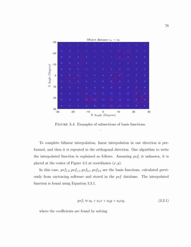
78

Figure 3.4. Examples of subsections of basis functions..

To complete bilinear interpolation, linear interpolation in one direction is per-

formed, and then it is repeated in the orthogonal direction. One algorithm to write

the interpolated function is explained as follows. Assuming psfi is unknown, it is

placed at the center of Figure 3.5 at coordinates (x, y).

In this case, psf1,2, psf1,1, psf2,1, psf2,2 are the basis functions, calculated previ-

ously from raytracing software and stored in the psf database. The interpolated

function is found using Equation 3.3.1.

psfi ≈ a0 + a1x+ a2y + a3xy, (3.3.1)

where the coefficients are found by solving

79

Figure 3.5. Bilinear interpolation example..

1 x1 y1 x1y11 x1 y2 x1y21 x2 y1 x2y11 x2 y2 x2y2

a0a1a2a3

=

psf1,1psf1,2psf2,1psf2,2

. (3.3.2)

The coefficients are given by

a0 = psf1,1x2y2(x1−x2)(y1−y2) + psf1,2x2y1

(x1−x2)(y2−y1) + psf2,1x1y2(x1−x2)(y2−y1) + psf2,2x1y1

(x1−x2)(y1−y2) ,

a1 = psf1,1y2(x1−x2)(y2−y1) + psf1,2y1

(x1−x2)(y1−y2) + psf2,1y2(x1−x2)(y1−y2) + psf2,2y1

(x1−x2)(y2−y1) ,

a2 = psf1,1x2(x1−x2)(y2−y1) + psf1,2x2

(x1−x2)(y1−y2) + psf2,1x1(x1−x2)(y1−y2) + psf2,2x1

(x1−x2)(y2−y1) ,

a3 = psf1,1(x1−x2)(y1−y2) + psf1,2

(x1−x2)(y2−y1) + psf2,1(x1−x2)(y2−y1) + psf2,2

(x1−x2)(y1−y2) .

(3.3.3)

To show the performance of the method, a grid of psfs in raytracing software

is computed. The raytraced psfs at various points in the field are compared to the

interpolated psfs at the same field location. Region 1 is used as example in Figure

3.6 to show interpolation between psfs that are clearly shift variant.

The psf at field (x, y) = (−21,−15), comparable to the center of Region 1 is

found by interpolation. This interpolated psf is compared to the one calculated at

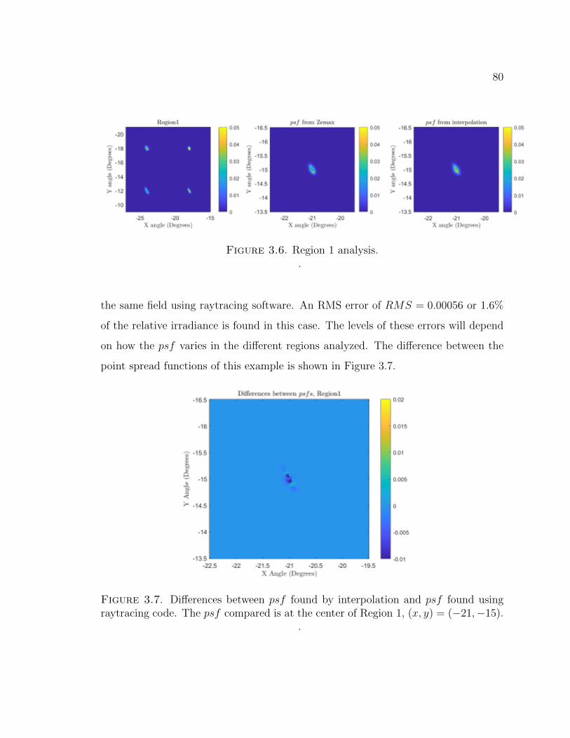
80

Figure 3.6. Region 1 analysis..

the same field using raytracing software. An RMS error of RMS = 0.00056 or 1.6%

of the relative irradiance is found in this case. The levels of these errors will depend

on how the psf varies in the different regions analyzed. The difference between the

point spread functions of this example is shown in Figure 3.7.

Figure 3.7. Differences between psf found by interpolation and psf found usingraytracing code. The psf compared is at the center of Region 1, (x, y) = (−21,−15).

.

81

The regions used as examples are summarized in Table 3.1. The table shows the

coordinates of the psf position taken from the generated grid, which are the field

coordinates of the interpolated psf . The RMS error and the absolute difference is

presented.

Region

A(Upper

LeftCorner)

(Degrees)

B(UpperRight

Corner)(Degrees)

C(Lower

LeftCorner)

(Degrees)

D(LowerRight

Corner)(Degrees)

Fieldto

find RMS

Maxabs

Difference

1 −24,−18 −18,−18 −24,−12 −18,−12 −15,−21 0.00056 0.02102 −24, 0 −18, 0 −24, 6 −18, 6 −21, 3 0.00039 0.00763 −12, 18 −6, 18 −12, 24 −6, 24 −9, 21 0.00055 0.01214 12,−24 18,−24 12,−18 18,−18 15,−21 0.00051 0.02345 6, 0 12, 0 6, 6 12, 6 9, 3 0.00059 0.01816 24, 12 30, 12 24, 18 30, 18 27, 15 0.00066 0.00747 6, 24 12, 24 6, 30 12, 30 9, 27 0.00015 0.0017

Table 3.1. Examples of regions to analyze.

Figure 3.8 shows the four basis functions for the remaining six regions. As ex-

pected, the differences are dependent on the analyzed region, as shown in Figure

3.11. The change in shape of the psfs taken as the basis functions to interpolate

the new one is related to the differences obtained. A comparison between the ray-

traced and the interpolated psfs for each region are shown in Figure 3.9 and Figure

3.10. A more significant RMS error is found when the point spread function lacks

similarity with its neighbors. In Figure 3.11(f), the four-point spread functions used

to interpolate the intermediate points in region 7 are almost isoplanatic. In contrast

the psfs in Region 6 that have a considerable change. Each psf shows astigmatism,

but the two psfs on the left are at a tight line focus, whereas the two psfs on the

right have additional blurring. The results show that the interpolation works worse

when there is a quick change of the psf between regions. To decrease this error, the

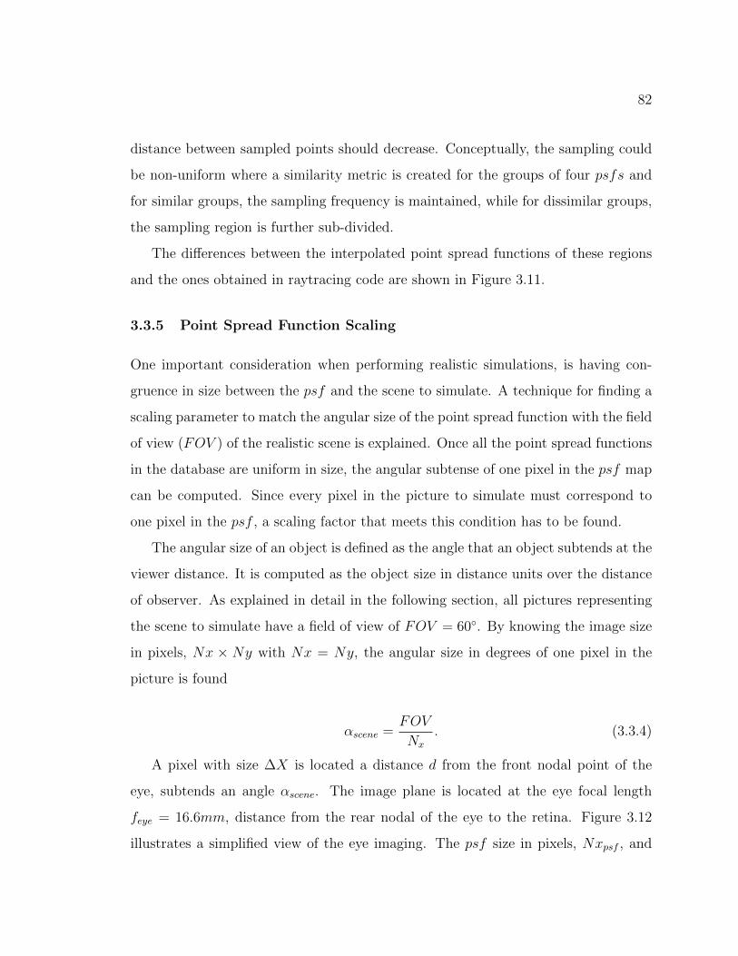
82

distance between sampled points should decrease. Conceptually, the sampling could

be non-uniform where a similarity metric is created for the groups of four psfs and

for similar groups, the sampling frequency is maintained, while for dissimilar groups,

the sampling region is further sub-divided.

The differences between the interpolated point spread functions of these regions

and the ones obtained in raytracing code are shown in Figure 3.11.

3.3.5 Point Spread Function Scaling

One important consideration when performing realistic simulations, is having con-

gruence in size between the psf and the scene to simulate. A technique for finding a

scaling parameter to match the angular size of the point spread function with the field

of view (FOV ) of the realistic scene is explained. Once all the point spread functions

in the database are uniform in size, the angular subtense of one pixel in the psf map

can be computed. Since every pixel in the picture to simulate must correspond to

one pixel in the psf , a scaling factor that meets this condition has to be found.

The angular size of an object is defined as the angle that an object subtends at the

viewer distance. It is computed as the object size in distance units over the distance

of observer. As explained in detail in the following section, all pictures representing

the scene to simulate have a field of view of FOV = 60◦. By knowing the image size

in pixels, Nx × Ny with Nx = Ny, the angular size in degrees of one pixel in the

picture is found

αscene =FOV

Nx

. (3.3.4)

A pixel with size ∆X is located a distance d from the front nodal point of the

eye, subtends an angle αscene. The image plane is located at the eye focal length

feye = 16.6mm, distance from the rear nodal of the eye to the retina. Figure 3.12

illustrates a simplified view of the eye imaging. The psf size in pixels, Nxpsf , and

83

Figure 3.8. Examples of different regions for far field, where the Point SpreadFunction differs in function of glaze angle.

.

the psf pixel size in distance units, ∆Xpsf , are the same for all different depths as

explained previously in Section 3.3.3. Therefore, the psf angular size in degrees αpsf

84

Figure 3.9. Interpolated psf and the psf obtained with raytracing for Regions 2,3 and 4.

.

85

Figure 3.10. Interpolated psf and the psf obtained with raytracing for Regions 5,6 and 7.

.

86

Figure 3.11. Differences of extrapolation and psf obtained using Zemax..

87

is given by

αpsf =∆Xpsf

feye× 180

π. (3.3.5)

Figure 3.12. Angular relation between pixel angular size and point spread functionangular size.

.

By knowing, the angular size of one pixel in the scene, and the angle that subtends

one pixel in the psf , the unknown factor needed to match αpsf and αscene is found

scale factor =αsceneαpsf

, (3.3.6)

scale factor =feye × FOV∆Xpsf ×Nx

× π

180. (3.3.7)

To find the new psf size in pixels, Nx′psf , the original psf is divided by scale

factor.

Nx′psf =Nxpsf

scale factor. (3.3.8)

88

In this work, feye = 16.6mm, FOV = 60o, ∆Xpsf = 0.0024mm, and Nx =

1296 pixels, and Nxpsf = 23 pixels, obtaining a new psf size of

Nx′psf ≈ 23 pixels. (3.3.9)

Figure 3.13. Comparison of the interpolated psf based on the psf database andits down-sampled version created to match the angular subtense of pixels in thesimulation scene.

.

Figure 3.13 shows a comparison of an interpolated psf based on the psf database

and its down-sampled version which is created so that the angular subtense of each psf

pixel now matches the angular subtense of the pixels in the scene to be simulated.

This downsampling also has the effect of reducing the errors associated with the

interpolation process since small differences in the fine structure of the psf are merged

into a single pixel in the downsampled version.

Until now, the considerations to create the psf database have been explained. In

the following sections, the considerations for the scene to simulate will be treated in

detail.

89

3.4 Realistic Simulation

In this dissertation, computational imaging is used to create a real scene simulation as

seen through a progressive addition lens. Computational imaging is image formation

that requires digital computer techniques [43]. A captured image is used that after

image processing will provide insight of how the patient will see through an ophthalmic

correction for presbyopia.

Several attempts have been done to simulate realistic scenes through the eye op-

tical system. One method uses the concept of Depth Point Spread Function (DPSF).

Each DPSF is a histogram of rays normal to the wavefront from a patient eye ob-

tained using a Shack Hartmann sensor. These DPSFs are defined at different depths

and they are in object space. After obtaining the DPSFs, depth images of the scene

to simulate are created. The depth images are convolved with the corresponding

DPSF, that are assumed to be isoplanatic. After convolution, the depth images are

composited into a single vision-realistic image [44].

Another attempt to simulate scenes through progressive addition lenses is with

the construction of a tri-dimensional psf matrix. Each psf is dependent on the angle

of gaze and on the object depth. With this information, a trilinear interpolation is

performed to find the psf at each pixel. Because of computational time the assump-

tion that the psf is the same for a pixel area is made. The scene is decomposed into

the RGB channels and each psf is weighted by the pixel value. the final image is

obtained with a superposition of the resultant images. The simulated images are for

a field of view of FOV = 20◦ [45].

In this work, the method proposed uses a psf grid found for different depths using

raytracing code. Each point spread function is calculated for each pixel.

The image to simulate must represent the eyes field of view ±30◦. Once this

condition is accomplished, it is safe to assume that every pixel in the image will

match the pixel angular size in the psf map.

90

The image will be taken with a Samsung Gear 360 Camera. This camera uses

a CMOS sensor of 8.4MPx2 F2.2 lens 360◦ Dual Lens: up to15MP (5472 × 2736)

Single Lens: up to 3MP (2304× 1296). It is shown in Figure 3.14.

Figure 3.14. Samsung gear 360 Camera.

The camera was chosen because it covers a wide field of view, that can capture

the head movement at different parts of a real-world scene. For this work, in order

to show the algorithm performance, only one lens was used.

3.4.1 Wide Field Angle and Distortion

A scene with three different object depths is created. It consists of three planes. The

first plane is a cellphone, representing a near object. The second plane is a computer

screen that represents an intermediate object distance. Finally, a plane is represented

by distant objects. Images are captured with the Samsung Gear 360 camera, and the

final image dimensions is 2304 × 1296. An example of one of the raw images taken

with the camera is shown in Figure 3.15.

As is readily apparent in Figure 3.15, this camera has a fish eye lens. These

types of lenses have two important characteristics that impact this work. First, as

mentioned previously, these lenses can achieve a full field of view. However, to achieve

this convenient feature, these lenses also introduce high levels of distortion. The form

91

Figure 3.15. Example of scene with three object depths taken with the SamsungGear 360 camera.

.

of the distortion introduced is barrel distortion. To use the image from this camera

system in the simulations, a camera calibration is needed. Such a calibration has

already been developed for fish eye lenses [46]. This process consists of determining the

intrinsic parameters of the camera. To correct for distortion, the distortion coefficients

are typically needed.

The free software GIMP 2, was used to undistort the image to simulate. This

image manipulation software allows us to correct main and edge distortion. In this

software, main distortion refers to the amount of spherical correction introduced in

the image. Edge distortion is the amount of spherical correction introduced at the

edges of the image. If the value of distortion is positive the software makes the image

convex, as shown in Figure 3.16. On the contrary if the value is negative, the software

makes the image concave [47]. The different effect applying the same amount of edge

and main distortion is shown in Figures 3.16 and 3.17.

92

Figure 3.16. Example of a grid with positive main and edge distortion applied..

Figure 3.17. Example of a grid with negative main and edge distortion applied..

After finding the optimal parameters, or amount of each distortion type to add.

This filter was applied to the images used for the final simulation. The undistorted

image for the example shown before, is shown in Figure 3.18. This was an im-

age undistorted using GIMP 2 software, with values of maindistortion = −90 and

edgedistortion = +26.

3.4.2 Image Size

As mentioned in section 3.3.5, the field of view covered by the scene must match the

field of view of the eye modeling done previously so that the angular size of one pixel

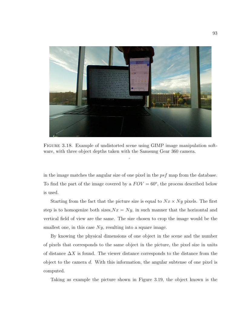
93

Figure 3.18. Example of undistorted scene using GIMP image manipulation soft-ware, with three object depths taken with the Samsung Gear 360 camera.

.

in the image matches the angular size of one pixel in the psf map from the database.

To find the part of the image covered by a FOV = 60o, the process described below

is used.

Starting from the fact that the picture size is equal to Nx×Ny pixels. The first

step is to homogenize both sizes,Nx = Ny, in such manner that the horizontal and

vertical field of view are the same. The size chosen to crop the image would be the

smallest one, in this case Ny, resulting into a square image.

By knowing the physical dimensions of one object in the scene and the number

of pixels that corresponds to the same object in the picture, the pixel size in units

of distance ∆X is found. The viewer distance corresponds to the distance from the

object to the camera d. With this information, the angular subtense of one pixel is

computed.

Taking as example the picture shown in Figure 3.19, the object known is the

94

Figure 3.19. Cellphone picture taken at d = 200mm from camera..

cellphone, then

∆X =Xphone

Nxphone= ∆Y, (3.4.1)

where Xphone is the cellphone size in millimeters and Nxphone is the number of pixels

that corresponds to Xphone. By knowing the pixel size and the distance from object

to camera d, the angular size of one pixel αscene was computed

αscene =∆X

d, (3.4.2)

with the information found, the field of view of the whole picture is given by

FOVscene(Degrees) = (Nx × αscene)×180

π. (3.4.3)

The visual field for the human eye model is approximately FOVeye = ±30 degrees.

To assure that all the picture represents 60◦, the image is cropped to the appropriate

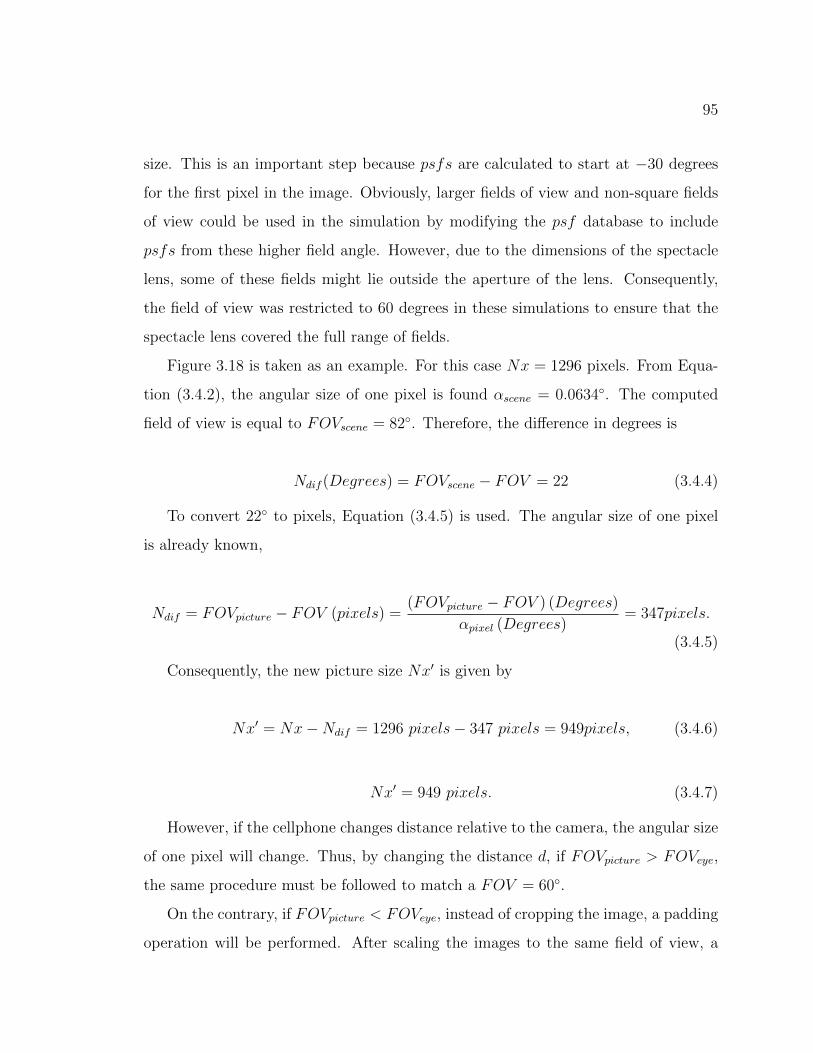
95

size. This is an important step because psfs are calculated to start at −30 degrees

for the first pixel in the image. Obviously, larger fields of view and non-square fields

of view could be used in the simulation by modifying the psf database to include

psfs from these higher field angle. However, due to the dimensions of the spectacle

lens, some of these fields might lie outside the aperture of the lens. Consequently,

the field of view was restricted to 60 degrees in these simulations to ensure that the

spectacle lens covered the full range of fields.

Figure 3.18 is taken as an example. For this case Nx = 1296 pixels. From Equa-

tion (3.4.2), the angular size of one pixel is found αscene = 0.0634◦. The computed

field of view is equal to FOVscene = 82◦. Therefore, the difference in degrees is

Ndif (Degrees) = FOVscene − FOV = 22 (3.4.4)

To convert 22◦ to pixels, Equation (3.4.5) is used. The angular size of one pixel

is already known,

Ndif = FOVpicture − FOV (pixels) =(FOVpicture − FOV ) (Degrees)

αpixel (Degrees)= 347pixels.

(3.4.5)

Consequently, the new picture size Nx′ is given by

Nx′ = Nx−Ndif = 1296 pixels− 347 pixels = 949pixels, (3.4.6)

Nx′ = 949 pixels. (3.4.7)

However, if the cellphone changes distance relative to the camera, the angular size

of one pixel will change. Thus, by changing the distance d, if FOVpicture > FOVeye,

the same procedure must be followed to match a FOV = 60◦.

On the contrary, if FOVpicture < FOVeye, instead of cropping the image, a padding

operation will be performed. After scaling the images to the same field of view, a

96

Figure 3.20. (a) Original Picture FOV = 82o, Nx = 1296 pixels (b) CroppedPicture FOV = 60o,Nx′ = 949 pixels.

.

resize of the images is performed, so that all the images have the same number of

pixels.

Examples of the cellphone at different distances from the viewer are shown in

Figure 3.21. As expected, the angular size changes inversely proportional to the

observer distance. The total angular size of a closer object is bigger than the angular

size of the same object at a far distance.

3.4.3 Image Segmentation and Depth of Field

In real-world, objects are located at different distances from our eyes, so every object

has different depth. To analyze progressive addition lenses, creating scenes with these

multiple depths is an important feature because the psfs change considerably between

planes, looking at the same field angle. In Figure 3.22, the change is appreciable for

the same part of the lens depending where the object is.

As a consequence, every object in the scene located at a certain depth has to be

97

Figure 3.21. Examples of the cellphone at different depths. Everything relativeassuming a field of view FOV = 60o equal at Nx = 1296 pixels.

.

Figure 3.22. Basis functions in Region 7, at three different object depths..

98

simulated using the psfs calculated at the correspondent depth. In the psf database,

psfs for different depths are collected. Nevertheless, a measure to separate the scene

into different depth planes is performed for the simulation. The objects in the scene

are simulated to be planar at their respective depths. This approximation is reason-

able since the cellphone and laptop screen are planar and the distant landscapes can

effectively be treated as being at infinity with regards to the camera.

To demonstrate how each plane is seen through the lens at different distances

from the observer, the algorithm outlined previously is used for the same image. The

scene was divided in three different depths, at the top far distance, at the center

intermediate distance and at the bottom near distance. In image shown in Figure

3.23, it is noticeable that at the near object region, astigmatism is presented at the

edges of the bottom part of the lens, and the letters are sharper at the center bottom

part. Analyzing the distant power portion of the lens, all the top part of the image

is now in focus. The progressive corridor is appreciated, by the r and s letters that

are the representation of objects at mid-distance.

Figure 3.23. Simulation of the same object at different planes of the scene..

As mentioned in Section 3.4.1, a scene with three different depths of field is created.

99

In this way, the distance to the objects was known. Thus, the procedure to isolate

different planes consists of masking the objects to isolate them into their appropriate

depth plane. In this work, masking means to identify the region of interest and assign

a zero value to the rest of the image. After performing this action, the masked image

is saved.

The masked images used for this work are shown in Figure 3.24. These images

were undistorted and rescaled as described previously, and every image represents a

60◦ field of view. Having the planes separated, the algorithm described in Section

3.2 is applied and then the images are recombined to get the final simulation. This

process is explained with more detail in the following section.

Figure 3.24. Masked images at different depth planes..

3.4.4 RGB Color Model

The physiology of the eye includes three color receptors called cones. These cones

can perceive red, blue and green, a combination of these colors described the color

world that we see. Digital representation of an image is based on the principle of

human perception of color. Digital images have individual pixels that are RGB (red,

100

green and blue). The combination of these colors reproduces a large range or gamut

of colors in a display [48].

In this work, a color scene is used. Each pixel is represented by three values, red,

green and blue. Because the proposed method consists on scaling the psfs correspond-

ing to one pixel with the respective value, the image is divided into its three-color

channels, and each channel is processed by the algorithm separately. Conceptually,

the psf database could be created with psfs corresponding to red, green and blue

wavelengths. However, for this simulation only monochromatic psfs are used. The

eye inherently has a high level of chromatic aberration, with nearly 2 diopters varia-

tion in power across the visible spectrum. The visual system has a remarkable ability

to suppress the chromatic aberration of the eye and color fringing effects are rarely

noticeable to people. Consequently, the dispersion associated with the spectacle lens

material is ignored in the simulations without much impact on the results.

Figure 3.25 is an example of a digital color image. As it was explained before,

this can be decomposed into three different channels.

Figure 3.25. Color Object..

The decomposition into three color channels of this image is shown in Figure 3.26.

Now, each image has only one value per pixel, and the proposed simulation method

101

is applied for each channel separately.

Figure 3.26. Object decomposed in three RGB channels..

3.5 Algorithm Implementation

Until now, different aspects have been considered to prepare the point spread function

database and the image to simulate. Now that everything is ready, the MATLAB

Script is applied to the image. Knowing that each pixel in the image represents a

fraction of the FOVeye = 60o, the program searches the corresponding psf for each

pixel in the psf grid. If the psf does not exist, bilinear interpolation is performed as

previously described.

The pixel value from the scene image is read, and the point spread function is

weighted by the value for each color channel.

The point spread function is represented by an array of pixels, so that the adjacent

pixels of the current pixel under study are affected by the tails of the psf . To take

into account this contribution, all the contributions from the various psfs (either

directly or from the tails of adjacent psfs) are summed to get the final pixel value.

A graphic representation of this step can be found in Figure 3.29.

102

Figure 3.27. Graphic representation of the first step of the algorithm applied. Thepsf that corresponds to a determined pixel in the image is searched, if the psf doesnot exist, interpolation is performed.

.

Figure 3.28. Graphic representation of the second step in the algorithm applied.The psfs are weighted by the correspondent pixel value.

.

This process is repeated for each color channel. The results are stored in a single

matrix. Therefore, each matrix represents one RGB channel. The matrices are then

recombined to obtain the final RGB image.

The results of image simulation with three object depths are described in the

103

Figure 3.29. Graphic representation of the third step in the algorithm applied.Contribution of psfs at each pixel are summed to get the final value for each pixel.

.

following section. The simulated scene is from the point of view of a person looking

out a window, while working at a laptop computer and viewing a cellphone. Since the

cellphone distance can be moved, images from the same scene moving the cellphone

closer and further away are shown.

3.6 Results

Assuming the far objects are at dinf → ∞, the intermediate object of the laptop

screens is at dmid = 930mm from the camera, and the near object of the cellphone is

at variable distances of d1 = 200mm, d2 = 300mm, d3 = 400mm, d4 = 500mm, and

d5 = 660mm.

3.6.1 Results for Three Different Regions

The pictures shown in Figure 3.24 are used as the base images in the simulation. Each

picture is decomposed into RGB channels, and the psf corresponding to the respective

object distance is found. The image size in pixels is Nx × Ny = 1296pixels ×

1296pixels. Therefore, from Equation 3.3.9 the psf size is 23 × 23pixels. Before

recombining the images, the result for each depth is shown in Figure 3.30.

The resultant images for near objects are obtained by using the images shown in

Figure 3.32 and the corresponding set of psfs. As expected, the sharpest image is

104

Figure 3.30. Simulation results for Far Field and Mid-Field..

the one representing the object at a distance d = 660mm, this distance matches the

prescription for near zone of the PAL.

To better appreciate the effect of the progressive addition lens at different dis-

tances, the region with legible print was selected, and a comparison of the same

letters are shown in Figure 3.32. The letters are blurriest and the contrast is reduced

when the cellphone is closer to the observer. When the cellphone is at the prescribed

distance, the letters are sharp.

3.6.2 High Performance Computer

The algorithm has to be executed one time for each scene depth per RGB channel.

Taking into account that the computational time will depend on the number of pixels

of the image, and the psf map size. The required time to perform a simulation

increases considerably even for modest dimensions for these variables. Due to the

amount of simulations required to show the effects of a progressive addition lenses,

and the number of pixels of each image, a personal computer was inadequate to

105

Figure 3.31. Simulation results for different Near Field distances..

Figure 3.32. Comparison of Near Field visual performance..

perform these calculations in a timely fashion. Consequently, other means were used

to complete the simulation.

One useful resource at The University of Arizona is the availability of a High

Performance Computer (HPC) cluster. This resource is available for students and

professors associated to the University of Arizona. Due to the computation time of

106

the simulations, the HPC was used to perform the simulation for different regions at

different depths in parallel.

The computer resource used for these simulations is the Ocelote. It has 46 new

compute nodes with Nvidia P100 GPU’s [49].

Although the time per scene was around 24 hours, the advantage of using this

computer is that the calculations can run in parallel, so instead of waiting 7 days per

7 images, the waiting time was 1 day for all the images.

3.6.3 Final Simulation

After the algorithm was applied to all of the images, the results for near, intermediate

and far field were superimposed to get the final image. The resultant images are shown

in Figure 3.33 and 3.34.

Figure 3.33. Complete simulated 3 depths scene for Near field d1 = 200mm, d2 =300mm and d3 = 400mm.

.

By recombining the images some problems became visible. The edges from images

at different distances, are not smooth. To avoid this problem an alpha blending

technique has been previously used [13]. In general terms, this technique takes the

boundaries of the objects and assigns a transparency values between 1 and 0 (white

107

Figure 3.34. Complete simulated 3 depths scene for Near field d4 = 500mm andd5 = 660mm.

.

and black). Even though alpha blending is not a physical phenomenon, this operation

results in a color blending at the edges which gives a more realistic appearing result.

As shown in Figure 3.33 and 3.34, simulations of multifocal vision have been

successfully performed. With the creation of the psf database, final simulations were

obtained at different depths and gaze angle of the wearer. These images could give a

preliminary insight of the perception of the world when looking through different parts

of a progressive addition lens. This fact is useful to explain that new eye movements

and head movements have to be learned to take advantage of this ophthalmic artifact.

The simulated images show congruence between the freeform shape obtained in

Chapter 2 with the ideal performance of a progressive addition lens. Unwanted aber-

rations at the edge of the lens are visible and may impact on the wearer decision to

use PALs.

In this dissertation simulation of multifocal vision of one PAL is performed to

108

show the performance of the method. However, the approach used can be generalized

for different lenses with different prescriptions, field of view considered, and objects

at different depths. Computational time can be reduced by using the HPC.

As it was explained, these lenses have the peculiarity that depending on head

movements and eye movements the resultant image is different. Future work have to

be done to continue developing all the possible movements that can be achieved when

wearing progressive addition lenses.

109

Chapter 4

CONCLUSIONS AND FUTURE WORK

In Chapter 1, the principal components of the optical system of the eye were briefly

outlined to understand a condition that every human being develops when aging:

Presbyopia. Common treatments for presbyopia were reviewed. Since there are trade-

offs with each option, the wearer must make an informed decision as to which treat-

ment is most suitable for their needs. One such treatment that will be the focus of

this dissertation is the Progressive Addition Lens (PAL). The optical design of PALs

is only the beginning of providing a beneficial treatment to the presbyope. PALs

need to be accurately fabricated and high quality metrology is needed to verify the

accuracy of the surface form. Furthermore, an understanding of the impact of various

design choices on the perceived image of the wearer is needed to ensure comfort. This

dissertation studied different techniques for the surface validation of PALs, as well

as, provided insight into their on-eye performance. The particularities in the design

of the freeform optical surface and their effect on the wearer were also explained.

Chapter 2 discusses the freeform surface verification of a KODAK Progressive

Addition Lens. Four different metrology techniques were applied to measure the

freeform surface of the PAL. The first two contact methods, the stylus profilometer

and the Coordinate Measurement Machine, were used to get a point cloud of the

freeform surface. These data were fitted to Zernike polynomials to get a mathematical

description of the surface. Mean Curvature and Cylinder power maps were obtained

to present the variation without discontinuity of optical power, as well as the presence

of astigmatism over the surface.

Two non-contact methods for the freeform surface of the PAL were also presented.

The first, SCOTS by refraction, gave a difference between the surface shape obtained

110

with the profilometer data and that from SCOTS. The discrepancy between the mea-

sures is likely due to assumptions made in the SCOTS procedure. Most notably, the

back surface of the PAL was assumed to be spherical. As explained in Chapter 2, a

perfect spherical surface was used in the Zemax model. In reality, the back surface will

have its own inherent shape that will deviate from a true sphere and will introduce

additional aberrations into the transmitted pattern in the SCOTS test. Future work

to better characterize the back surface is required to isolate the effects of the freeform

surface. Since the back surface is nearly spherical, this characterization could be done

with traditional interferometry. An additional improvement to the SCOTS testing

would be a distortion correction of the camera used.

UV Deflectometry was proposed in this dissertation as the second non-contact

method. The proposed system used UV light to take advantage of the fact that

PMMA lens material is opaque in this wavelength region. The opacity avoids ghost

reflections from the back surface and parasitic fringes. For the method, a UV LED

and Koehler illumination was used. However, in this configuration the fringe pattern

needed to be projected onto a diffuser screen placed near the PAL. In turn the diffuser

screen required the camera system to be at a large oblique angle to the test surface.

The oblique angle makes it difficult to view the reflection from the entire convex test

surface, as well as makes the aperture of the lens appear elliptical in the captured

image. Using a reference sphere with a radius of curvature close to the radius of

curvature of the freeform surface under test, a novel calibration method based on the

correction by distortion was presented. Proof of concept of this method is shown.

While some obliquity between the projector and the camera is needed for the

deflectometry technique, the configuration should be modified to help reduce the

current angle. One option would be to use the UV LED as the source with a Digital

Mirror Device (DMD). DMDs are at the heart of digital light projectors and using

a DMD would enable projecting the fringes directly onto the test surface and enable

the camera to be better placed for measurement.

111

Chapter 3 examines the surface shape relation with the visual performance of the

PAL. By using the recovered surface in Chapter 2, simulation of three-dimensional

images for multifocal vision was performed based on the psfs obtained using raytracing

code. A psf database was created for different fields of view and different object

depths. An algorithm was proposed where interpolated psfs for different fields of

view were obtained. Preliminary images for a real scene were obtained, simulating

what the wearer will see through progressive addition lenses at different glaze angles.

An improvement for the simulation techniques would be a new method to get smooth

transitions between the various depth planes. As previously explained, these spectacle

lenses have the particularity that the image they produce is different depending on

the head movement and eye rotation. Simulation of different orientation of the head

and eye rotations needs to be performed.

The 360 camera can be useful to cover different parts of the real-world simulating

head movement. The simulations were performed using only one lens, but the full 360-

degree field of vision can be implemented. Furthermore, the scene can be composed of

objects that are precisely localized, accurately positioned and a trilinear interpolation

can be implemented to find the intermediate psf at many different depth planes. The

main limitation to this implementation is computation time. Another important

aspect is to test is whether PAL wearers have the same perception with real scenes

and with simulation. If this connection is made, then the simulator can be used for

virtually developing and testing new lenses.

The metrology techniques in this research demonstrated a new technique without

expensive optical elements for the characterization of a freeform surface shape. After

surface characterization, simulated images were presented for giving insight into the

visual effects of PALs. While these results demonstrate the feasibility of UV deflec-

tometry testing and simulation of PAL surface, the preceding suggestions for future

work would lead to highly useful tools for the designer.

112

Appendix A

Zernike Coefficients

Zernike Term Coefficient

Z00 −4.7180157

Z11 −3.5617096e− 02

Z−11 2.3376195e− 01Z0

2 −2.8049186e+ 00Z−22 1.6454016e− 02Z2

2 1.1759363e− 01Z−13 8.0809995e− 02Z1

3 1.3185891e− 03Z−33 2.2177069e− 02Z3

3 5.7142848e− 03Z0

4 −5.8313036e− 02Z2

4 6.2111703e− 03Z−24 −1.5268369e− 02Z4

4 3.9797824e− 02Z−44 −6.7483869e− 03Z1

5 2.3821696e− 03Z−15 −1.3839537e− 02Z3

5 −7.9774266e− 03Z−35 −1.3605726e− 02

Zernike Term Coefficient

Z55 −7.2969642e− 03

Z−55 −1.8477838e− 03Z0

6 3.2297570e− 04Z−26 2.7415363e− 03Z2

6 −2.2802097e− 03Z−46 3.7286833e− 03Z4

6 −9.9409519e− 03Z−66 2.6577480e− 03Z6

7 4.7804542e− 03Z−17 2.2723415e− 03Z1

7 −2.4705662e− 04Z−37 3.2513658e− 03Z3

7 3.2424832e− 03Z−57 −2.7655744e− 04Z5

7 3.4022549e− 03Z−77 6.9019242e− 05Z7

7 3.1857329e− 04Z0

8 −2.7129996e− 03

Table A.1. 37 Zernike Coefficients after fitting.

113

Appendix B

Source code used to perform Simulation of

Multifocal Vision.

%Main program .t ic%Open image t h a t r e p r e s e n t s the scene .

rgbImage = imread ( ’ scene . jpg ’ ) ;rgbImage=double ( rgbImage ) ;

%Decomposed i t i n t o RGB channe l s .redChannel=double ( rgbImage ( : , : , 1) ) ;greenChannel = double ( rgbImage ( : , : , 2) ) ;blueChannel = double ( rgbImage ( : , : , 3) ) ;A=redChannel ;B=greenChannel ;C=blueChannel ;

s i zeY=s ize (A, 1 ) ;s izeX=s ize (A, 2 ) ;

% Load p s f databased .f a r=’ ps f images37Zern 11x11 . mat ’ ;i n t=’ psf images37Zern 11x11 933mm . mat ’ ;near=’ psf images37Zern 11x11 660mm . mat ’ ;

image s f a r=load ( f a r ) ;image s in t=load ( i n t ) ;images near=load ( near ) ;

depth = [ 6 6 0 ; 9 3 0 ; 2 0 0 0 ] ;f i e l d y =[ image s f a r . p s f images ( : ) . f i e l d Y ] ;f i e l d x =[ image s f a r . p s f images ( : ) . f i e l d X ] ;

% Choose depth to s i m u l a t e .depth 1 =660;

114

p i t ch =6;c ropS i z e =32;

[ f i e l d X d e g r e e s , f i e l d Y d e g r e e s ]=meshgrid ( linspace (−30 ,30 ,s izeX ) , linspace (−30 ,30 , s izeY ) ) ;

n e w f i l t e r S i z e 2=f loor ( c ropS i z e /2) ;

f i n a l=padarray ( zeros ( s ize (A) ) , [ n e w f i l t e r S i z e 2n e w f i l t e r S i z e 2 ] ) ;

f i n a l g r e e n=padarray ( zeros ( s ize (A) ) , [ n e w f i l t e r S i z e 2n e w f i l t e r S i z e 2 ] ) ;

f i n a l b l u e=padarray ( zeros ( s ize (A) ) , [ n e w f i l t e r S i z e 2n e w f i l t e r S i z e 2 ] ) ;

%Performed B i l i n e a r i n t e r p o l a t i o n and s u p e r p o s t i o n o f p s f sf o r d i f f e r e n t

%RGB Channel .for i i =1: s izeXfor j j =1: s izeY

[ minFieldX , maxFieldX]= getNearF ie lds ( f i e l d x , f i e l d X d e g r e e s ( j j ,i i ) , p i t ch ) ;

[ minFieldY , maxFieldY]= getNearF ie lds ( f i e l d y , f i e l d Y d e g r e e s ( j j ,i i ) , p i t ch ) ;

images=image s f a r ;

i f minFieldX==maxFieldX && minFieldY==maxFieldYps f=findFie ldPSF ( minFieldX , minFieldY , images ) ;p s f=i m r e s i z e ( psf , [ c ropSize , c ropS i z e ] ) ;else

[ A1 region1 ]= findFie ldPSF ( minFieldX , minFieldY , images ) ;[ B1 reg ion1 ]= findFie ldPSF ( maxFieldX , minFieldY , images ) ;[ C1 reg ion1 ]= findFie ldPSF ( minFieldX , maxFieldY , images ) ;[ D1 region1 ]= findFie ldPSF ( maxFieldX , maxFieldY , images ) ;

p s f=myInterpo l3cases ( f i e l d X d e g r e e s ( j j , i i ) , f i e l d Y d e g r e e s ( j j ,i i ) , A1 region1 , B1 region1 , C1 region1 , D1 region1 , minFieldX, maxFieldY , maxFieldX , minFieldY , c ropS i z e ) ;

end

115

new ps f r ed= A( j j , i i ) .∗ ps f ;new ps f g reen= B( j j , i i ) .∗ ps f ;new ps f b lue= C( j j , i i ) .∗ ps f ;B red= padarray ( zeros ( s ize (A) ) , [ n e w f i l t e r S i z e 2

n e w f i l t e r S i z e 2 ] ) ;B green= padarray ( zeros ( s ize (A) ) , [ n e w f i l t e r S i z e 2

n e w f i l t e r S i z e 2 ] ) ;B blue= padarray ( zeros ( s ize (A) ) , [ n e w f i l t e r S i z e 2

n e w f i l t e r S i z e 2 ] ) ;for k= 1 : length ( new ps f r ed )B red (1+( j j −1) : length ( new ps f r ed )+( j j −1) , k+(( i i −1) ) )=

new ps f red ( : , k ) ;B green (1+( j j −1) : length ( new ps f g reen )+( j j −1) , k+(( i i −1) ) )=

new ps f g reen ( : , k ) ;B blue (1+( j j −1) : length ( new ps f b lue )+( j j −1) , k+(( i i −1) ) )=

new ps f b lue ( : , k ) ;endf i n a l=f i n a l+B red ;f i n a l g r e e n=f i n a l g r e e n+B green ;f i n a l b l u e=f i n a l b l u e+B blue ;

endend

%Normalized datar ed out=f i n a l . /max( f i n a l ( : ) ) ;r ed out=imcrop ( red out , [ n e w f i l t e r S i z e 2 , n e w f i l t e r S i z e 2 , s ize (

A, 2 ) , s ize (A, 1 ) ] ) ;g reen out=f i n a l g r e e n . /max( f i n a l g r e e n ( : ) ) ;g reen out=imcrop ( green out , [ n e w f i l t e r S i z e 2 , n e w f i l t e r S i z e 2 ,

s ize (A, 2 ) , s ize (A, 1 ) ] ) ;b lue out=f i n a l b l u e . /max( f i n a l b l u e ( : ) ) ;b lue out=imcrop ( blue out , [ n e w f i l t e r S i z e 2 , n e w f i l t e r S i z e 2 ,

s ize (A, 2 ) , s ize (A, 1 ) ] ) ;

%Add channe l s to g e t f i n a l sceneoutput=cat (3 , ( r ed out ) , ( g reen out ) , ( b lue out ) ) ;

dlmwrite ( ’ r e d f a r 0 8 2 8 . txt ’ , r ed out ) ;dlmwrite ( ’ g r e e n f a r 0 8 2 8 . txt ’ , g reen out ) ;

116

dlmwrite ( ’ b l u e f a r 0 8 2 8 . txt ’ , b lue out ) ;

toc

Functions c a l l e d by main program .%

%%%%%%%%%%%%%%%%%%%%%%%%%%%%%%%%%%%%%%%%%%%%%%%%%%%%%%%%%%%%%%%%%%%%%%%%%%%%%%%%%%%%%%%%%%%%%%%%%%%%%

% Function Developed by Dulce .% Visua l and Ophthalmic Opt ics Lab , C o l l e g e o f O p t i c a l

Sciences , U n i v e r s i t y o f% Arizona , Tucson , AZ. Ju ly 2018%

%%%%%%%%%%%%%%%%%%%%%%%%%%%%%%%%%%%%%%%%%%%%%%%%%%%%%%%%%%%%%%%%%%%%%%%%%%%%%%%%

%% Given a p o i n t in the f i e l d f u n c t i o n r e t u r n s the maximum and

minimum f i e l d% in obne d i r e c t i o n .%%

%%%%%%%%%%%%%%%%%%%%%%%%%%%%%%%%%%%%%%%%%%%%%%%%%%%%%%%%%%%%%%%%%%%%%%%%%%%%%%%%

function [ minField , maxField ]= getNearF ie ld s ( f i e l d , f i e l d 2 f i n d, p i t ch )

[ d i f , ind min ]=min(abs ( f i e l d−f i e l d 2 f i n d ) ) ;

i f d i f==0minField=f i e l d ( ind min ) ;maxField=f i e l d ( ind min ) ;elseop (1 )=abs ( ( f i e l d ( ind min )−p i t ch )− f i e l d 2 f i n d ) ;op (2 )=abs ( ( f i e l d ( ind min )+p i t ch )− f i e l d 2 f i n d ) ;

[ newField , indNewField ]=min( op ( : ) ) ;

i f indNewField==1

117

nextF ie ld=f i e l d ( ind min )−p i t ch ;e l s e i f indNewField==2nextF ie ld=f i e l d ( ind min )+pi t ch ;end

minField=min( f i e l d ( ind min ) , nextF ie ld ) ;maxField=max( f i e l d ( ind min ) , nextF ie ld ) ;

end

end

%%%%%%%%%%%%%%%%%%%%%%%%%%%%%%%%%%%%%%%%%%%%%%%%%%%%%%%%%%%%%%%%%%%%%%%%%%%%%%%%%%%%%%%%%%%%%%%%%%%%%%

% Function Developed by Dulce .% Visua l and Ophthalmic Opt ics Lab , C o l l e g e o f O p t i c a l

Sciences , U n i v e r s i t y o f% Arizona , Tucson , AZ. November 2017%

%%%%%%%%%%%%%%%%%%%%%%%%%%%%%%%%%%%%%%%%%%%%%%%%%%%%%%%%%%%%%%%%%%%%%%%%%%%%%%%%

%% Function l o o k s f o r PSF, f o r f i e l d X and f i e l d Y. Inputs

f o r t h i s% f u n c t i o n are f i e l d s and the f i l e wi th a l l the f i e l d s (

normal ly a . mat% output f i l e from f u n c t i o n getPSF .m) .% The output i s PSF Matrix , and the index in the main f i l e .%%

%%%%%%%%%%%%%%%%%%%%%%%%%%%%%%%%%%%%%%%%%%%%%%%%%%%%%%%%%%%%%%%%%%%%%%%%%%%%%%%%

%% USAGE (SAMPLE CODE)% fi leName =’ ps f images11x11256 . mat ’ ;% [A, index ]= findFie ldPSF (−24, −24, f i leName ) ;%

%%%%%%%%%%%%%%%%%%%%%%%%%%%%%%%%%%%%%%%%%%%%%%%%%%%%%%%%%%%%%%%%%%%%%%%%%%%%%%%%

118

function [A, index ]= findFie ldPSF ( f i e ldX , f i e ldY , images )xsubFie ld=f i e l d X ;ysubFie ld=f i e l d Y ;

% images=openPSFf i l es ( depth 1 , depth ) ;% images=load ( f i leName ) ;

for i i =1: length ( images . p s f images )i f images . p s f images ( i i ) . f i e l d X==xsubFie ld (1 ) & images .

p s f images ( i i ) . f i e l d Y==ysubFie ld (1 )A=fl ipud ( images . p s f images ( i i ) .map) ;index=i i ;endend

%%%%%%%%%%%%%%%%%%%%%%%%%%%%%%%%%%%%%%%%%%%%%%%%%%%%%%%%%%%%%%%%%%%%%%%%%%%%%%%%%%%%%%%%%%%%%%%%%%%%%%

% Function Developed by Dulce .% Visua l and Ophthalmic Opt ics Lab , C o l l e g e o f O p t i c a l

Sciences , U n i v e r s i t y o f% Arizona , Tucson , AZ. March 2018%

%%%%%%%%%%%%%%%%%%%%%%%%%%%%%%%%%%%%%%%%%%%%%%%%%%%%%%%%%%%%%%%%%%%%%%%%%%%%%%%%

%% Function i n t e r p o l a t e PSF us ing B i l i n e a r i n t e r p o l a t i o n .

Equations can be% found in h t t p s :// en . w i k i p e d i a . org / w i k i /

B i l i n e a r i n t e r p o l a t i o n ) , g i ven a s e t% of b a s i s f u n c t i o n s , 4 corners and the c o o r d i n a t e s to

i n t e r p o l a t e . P i x e l s% in t h i s case% The input parameters are 4 matr ices wi th the PSF t h a t are

going to be% used to g e t the i n t e r p o l a t i o n , the p i x e l s p o s i t i o n o f t h i s

matr ices x1 , x2 , y1 ,% and y2 ( be c a r e f u l l wi th how matlab read p i x e l s ) , and the

f i n a l s i z e o f% the PSF. 64 works f ine , 256 k i l l s computer .

119

% The output w i l l be the i n t e r p o l a t e d matrix .% ( Program t h a t c a l l s t h i s code : ’ p r i n c i p a l .m’ )%%

%%%%%%%%%%%%%%%%%%%%%%%%%%%%%%%%%%%%%%%%%%%%%%%%%%%%%%%%%%%%%%%%%%%%%%%%%%%%%%%%

%% USAGE (SAMPLE CODE)% pos i t ionX =10;% pos i t ionY =10;% c r o p S i z e =64;% x1 =1;% y1=1;% x2 =25;% y2 =25;%% out ( posi t ionX , pos i t ionY ) . i n t e r p o l a t i o n=myInterpo l ( posi t ionX

, posi t ionY , A,B,C,D, x1 , y2 , x2 , y1 , c r o p S i z e ) ;%

%%%%%%%%%%%%%%%%%%%%%%%%%%%%%%%%%%%%%%%%%%%%%%%%%%%%%%%%%%%%%%%%%%%%%%%%%%%%%%%%

function [ out ]= myInterpo l3cases (x , y , A,B,C,D, x1 , y1 , x2 , y2 ,c ropS i z e )

%Arrays to i n t e r p o l a t eQ12=A;Q22=B;Q11=C;Q21=D;

i f x1==x2

out =((y2−y ) /( y2−y1 ) )∗Q11+((y−y1 ) /( y2−y1 ) )∗Q12 ;% out =((y2−y ) /( y2−y1 ) )∗Q22+((y−y1 ) /( y2−y1 ) )∗Q21 ;out=i m r e s i z e ( out , [ c ropSize , c ropS i z e ] ) ;

e l s e i f y1==y2out =((x2−x ) /( x2−x1 ) )∗Q12+((x−x1 ) /( x2−x1 ) )∗Q22 ;% out =((x2−x ) /( x2−x1 ) )∗Q11+((x−x1 ) /( x2−x1 ) )∗Q21 ;

120

out=i m r e s i z e ( out , [ c ropSize , c ropS i z e ] ) ;

else%Find C o e f f i c i e n t s B i l i n e a r i n t e r p o l a t i o na0= ( ( Q11∗x2∗y2 ) / ( ( x1−x2 ) ∗( y1−y2 ) ) ) +((Q12∗x2∗y1 ) / ( ( x1−x2 ) ∗( y2−y1 ) ) ) +((Q21∗x1∗y2 ) / ( ( x1−x2 ) ∗( y2−y1 ) ) ) +((Q22∗x1∗y1 ) / ( ( x1−x2 ) ∗( y1−y2 ) ) ) ;

a1= ( ( Q11∗y2 ) / ( ( x1−x2 ) ∗( y2−y1 ) ) ) +((Q12∗y1 ) / ( ( x1−x2 ) ∗( y1−y2 ) ) )+((Q21∗y2 ) / ( ( x1−x2 ) ∗( y1−y2 ) ) ) +((Q22∗y1 ) / ( ( x1−x2 ) ∗( y2−y1 ) ) );

a2= ( ( Q11∗x2 ) / ( ( x1−x2 ) ∗( y2−y1 ) ) ) +((Q12∗x2 ) / ( ( x1−x2 ) ∗( y1−y2 ) ) )+((Q21∗x1 ) / ( ( x1−x2 ) ∗( y1−y2 ) ) ) +((Q22∗x1 ) / ( ( x1−x2 ) ∗( y2−y1 ) ) );

a3= (Q11/( ( x1−x2 ) ∗( y1−y2 ) ) )+(Q12/( ( x1−x2 ) ∗( y2−y1 ) ) )+(Q21/( ( x1−x2 ) ∗( y2−y1 ) ) )+(Q22/( ( x1−x2 ) ∗( y1−y2 ) ) ) ;

%X,Y to f i n d

i i=x ;j j=y ;

out=i m r e s i z e ( a0+(a1∗ i i )+(a2∗ j j )+(a3∗ i i ∗ j j ) , [ c ropSize , c ropS i z e] ) ;

endend

121

References

[1] C. M. Schor, “Accommodation and Presbyopia.” [Accessed: 2018-11-07].

[2] A. VisionCare, “Multifocal intraocular lenses: Restor and tecnis multifocal iol.”[Accessed: 2018-10-31].

[3] A. VisionCare, “Alcon multifocal contact lenses.” [Accessed: 2018-10-31].

[4] R. D. Blum, W. Kokonaski, V. S. Iyer, J. N. Haddock, and M. Mattison-Shupnick, “Multifocal lens having a progressive optical power region and dis-continuity,” Nov. 13 2012. US Patent 8,308,295.

[5] P. Artal, “Optics of the eye and its impact in vision: a tutorial,” Advances inOptics and Photonics, vol. 6, no. 3, pp. 340–367, 2014.

[6] J. Schwiegerling, “Field guide to visual and ophthalmic optics,” Spie, 2004.

[7] L. A. Ostrin and A. Glasser, “Accommodation measurements in a prepresbyopicand presbyopic population,” Journal of Cataract & Refractive Surgery, vol. 30,no. 7, pp. 1435–1444, 2004.

[8] D. A. Atchison, “Accommodation and presbyopia,” Ophthalmic and PhysiologicalOptics, vol. 15, no. 4, pp. 255–272, 1995.

[9] R. Gil-Cazorla, S. Shah, and S. A. Naroo, “A review of the surgical options for thecorrection of presbyopia,” British Journal of Ophthalmology, pp. bjophthalmol–2015, 2015.

[10] A. Lichtinger and D. S. Rootman, “Intraocular lenses for presbyopia correction:past, present, and future,” Current opinion in ophthalmology, vol. 23, no. 1,pp. 40–46, 2012.

[11] S. Jain, I. Arora, and D. T. Azar, “Success of monovision in presbyopes: re-view of the literature and potential applications to refractive surgery,” Survey ofophthalmology, vol. 40, no. 6, pp. 491–499, 1996.

[12] E. S. Bennett, “Contact lens correction of presbyopia,” Clinical and experimentaloptometry, vol. 91, no. 3, pp. 265–278, 2008.

[13] W. J. Duncan, Visual Acuity Estimation from Simulated Images. PhD thesis,University of Arizona, 2016.

[14] T. E. Fannin and T. Grosvenor, Clinical optics. Butterworth-Heinemann, 2013.

122

[15] C. This, “The optics of free-form progressive lenses,”

[16] D. J. Meister and S. W. Fisher, “Progress in the spectacle correction of pres-byopia. part 1: Design and development of progressive lenses,” Clinical andexperimental optometry, vol. 91, no. 3, pp. 240–250, 2008.

[17] D. J. Meister and S. W. Fisher, “Progress in the spectacle correction of presby-opia. part 2: Modern progressive lens technologies,” Clinical and experimentaloptometry, vol. 91, no. 3, pp. 251–264, 2008.

[18] D. R. Pope, “Progressive addition lenses: history, design, wearer satisfactionand trends,” in Vision Science and Its Applications, p. NW9, Optical Society ofAmerica, 2000.

[19] D. Lochegnies, P. Moreau, F. Hanriot, and P. Hugonneaux, “3d modelling ofthermal replication for designing progressive glass moulds,” New Journal of Glassand Ceramics, vol. 3, no. 01, p. 34, 2013.

[20] Z. Yin, Y. Dai, S. Li, C. Guan, and G. Tie, “Fabrication of off-axis asphericsurfaces using a slow tool servo,” International Journal of Machine Tools andManufacture, vol. 51, no. 5, pp. 404–410, 2011.

[21] Y. Y. Li, J. J. Chen, H. H. Feng, C. Li, J. Qu, and H. Chen, “Freeform manufac-turing of a progressive addition lens by use of a voice coil fast tool servo,” in 7thInternational Symposium on Advanced Optical Manufacturing and Testing Tech-nologies: Advanced Optical Manufacturing Technologies, vol. 9281, p. 92810Q,International Society for Optics and Photonics, 2014.

[22] M. F. Kuchel, “Interferometric measurement of rotationally symmetric as-pheric surfaces,” in Optical Measurement Systems for Industrial Inspection VI,vol. 7389, p. 738916, International Society for Optics and Photonics, 2009.

[23] J. C. Wyant and F. D. Smith, “Interferometer for measuring power distributionof ophthalmic lenses,” Applied optics, vol. 14, no. 7, pp. 1607–1612, 1975.

[24] C. Castellini, F. Francini, and B. Tiribilli, “Hartmann test modification for mea-suring ophthalmic progressive lenses,” Applied optics, vol. 33, no. 19, pp. 4120–4124, 1994.

[25] J. Schwiegerling, Optical specification, fabrication, and testing. SPIE Press, 2014.

[26] I. M. CMM Solutions, “Cmm history, fifty years of cmm history leading up tomeasuring revolution.” [Accessed: 2018-11-12].

123

[27] G. P. Butel, G. A. Smith, and J. H. Burge, “Optimization of dynamic structuredillumination for surface slope measurements,” in Interferometry XVI: Techniquesand Analysis, vol. 8493, p. 84930S, International Society for Optics and Photon-ics, 2012.

[28] P. Su, R. E. Parks, L. Wang, R. P. Angel, and J. H. Burge, “Software configurableoptical test system: a computerized reverse hartmann test,” Applied Optics,vol. 49, no. 23, pp. 4404–4412, 2010.

[29] P. Su, M. Khreishi, T. Su, R. Huang, M. Z. Dominguez, A. V. Maldonado, G. P.Butel, Y. Wang, R. E. Parks, and J. H. Burge, “Aspheric and freeform surfacesmetrology with software configurable optical test system: a computerized reversehartmann test,” Optical Engineering, vol. 53, no. 3, p. 031305, 2013.

[30] M. Z. Dominguez, L. Wang, P. Su, R. E. Parks, and J. H. Burge, “Softwareconfigurable optical test system for refractive optics,” in 22nd Congress of theInternational Commission for Optics: Light for the Development of the World,vol. 8011, p. 80116Q, International Society for Optics and Photonics, 2011.

[31] W. Zhao, R. Huang, P. Su, and J. H. Burge, “Aligning and testing non-nulloptical system with deflectometry,” in Optical System Alignment, Tolerancing,and Verification VIII, vol. 9195, p. 91950F, International Society for Optics andPhotonics, 2014.

[32] D. Malacara, Optical shop testing. John Wiley & Sons, 2007.

[33] Rocoesy, “Pc/pmma.” [Accessed: 2018-09-27].

[34] C. Faber, E. Olesch, R. Krobot, and G. Hausler, “Deflectometry challenges in-terferometry: the competition gets tougher!,” in Interferometry XVI: Techniquesand Analysis, vol. 8493, p. 84930R, International Society for Optics and Photon-ics, 2012.

[35] A. Speck, B. Zelzer, M. Kannengießer, A. Langenbucher, and T. Eppig, “Inspec-tion of freeform intraocular lens topography by phase measuring deflectometricmethods,” Applied optics, vol. 52, no. 18, pp. 4279–4286, 2013.

[36] M. C. Knauer, J. Kaminski, and G. Hausler, “Phase measuring deflectometry:a new approach to measure specular free-form surfaces,” in Optical Metrology inProduction Engineering, vol. 5457, pp. 366–377, International Society for Opticsand Photonics, 2004.

[37] C. Faber, M. C. Knauer, and G. Hausler, “Can deflectometry work in presenceof parasitic reflections?,” in Proc. DGaO, vol. 110, p. A10, 2009.

124

[38] J. W. Goodman, Introduction to Fourier optics. Roberts and Company Publish-ers, 2005.

[39] J. S. Tyo and A. S. Alenin, Field guide to linear systems in optics. SPIE Press,2015.

[40] Z. L. M. Nicholson., “How to simulate high resolution images-zemax knowledge-base, october 31, 2008..” [Accessed: 2018-11-05].

[41] Z. L. B. Goodwin., “What is the difference between the fft and huygens psf?-zemax knowledgebase, october 30, 2015..” [Accessed: 2018-06-25].

[42] Kodak, “Tips product specification & processing guide kodak polarized progres-sive lens with nupolartm technology, march, 2000.” [Accessed: 2018-10-12].

[43] L. Marc, “New techniques in computational photography, computer science de-partment .stanford university..” [Accessed: 2018-09-09].

[44] B. A. Barsky, “Vision-realistic rendering: simulation of the scanned foveal imagefrom wavefront data of human subjects,” in Proceedings of the 1st Symposiumon Applied perception in graphics and visualization, pp. 73–81, ACM, 2004.

[45] J. A. Rodrıguez Celaya, P. Brunet Crosa, N. Ezquerra, and J. Palomar, “A vir-tual reality approach to progressive lenses simulation,” in XV Congreso Espanolde Informatica Grafica, 2005.

[46] S. Shah and J. Aggarwal, “Intrinsic parameter calibration procedure for a (high-distortion) fish-eye lens camera with distortion model and accuracy estimation,”Pattern Recognition, vol. 29, no. 11, pp. 1775–1788, 1996.

[47] G. documentation, “Lens distortion.” [Accessed: 2018-11-06].

[48] R. C. Gonzalez, R. E. Woods, et al., “Digital image processing,” 2002.

[49] T. U. of Arizona, “High performance computing, information technology.” [Ac-cessed: 2018-10-31].