Simplified seismic analysis procedures for elevated tanks considering fluid–structure–soil...
19
DOI: http://dx.doi.org/10.12989/sem.2005.21.1.101
Transcript of Simplified seismic analysis procedures for elevated tanks considering fluid–structure–soil...
Structural Engineering and Mechanics, Vol. 21, No. 1 (2005) 101-119 101
Seismic evaluation of fluid-elevated tank-foundation/soil systems in frequency domain
R. Livaoglu† and A. Dogangun‡
Karadeniz Technical University, Department of Civil Engineering, 61080, Trabzon, Turkey
(Received October 8, 2004, Accepted May 24, 2005)
Abstract. An efficient methodology is presented to evaluate the seismic behavior of a Fluid-ElevatedTank-Foundation/Soil system taking the embedment effects into accounts. The frequency-dependent conemodel is used for considering the elevated tank-foundation/soil interaction and the equivalent spring-massmodel given in the Eurocode-8 is used for fluid-elevated tank interaction. Both models are combined toobtain the seismic response of the systems considering the sloshing effects of the fluid and frequency-dependent properties of soil. The analysis is carried out in the frequency domain with a modal analysisprocedure. The presented methodology with less computational efforts takes account of; the soil and fluidinteractions, the material and radiation damping effects of the elastic half-space, and the embedmenteffects. Some conclusions may be summarized as follows; the sloshing response is not practically affectedby the change of properties in stiff soil such as S1 and S2 and embedment but affected in soft soil. Onthe other hand, these responses are not affected by embedment in stiff soils but affected in soft soils.
Key words: fluid-structure-foundation/soil interaction; elevated tanks; freqency domain analaysis.
1. Introduction
The water supply is essential to control the fires that usually occur during earthquakes, which
cause a great deal of damage and loss of life. Therefore, the elevated tanks should remain functional
in the post-earthquake period to ensure water supply in earthquake-affected regions. However,
several elevated tanks were damaged or collapsed during the past earthquakes. Although this type of
structures and their reliability against failure under seismic load are of critical concern, upsetting
experiences were shown by the damage to the staging of elevated tank in some earthquakes
occurred in different regions of the World (Haroun and Ellaithy 1985). That is why, the seismic
behavior of the elevated tanks should be well known, furthermore, they must be designed to be
earthquake resistant.
As known, all structures are affected by the soil-structure interaction with varying emphasis on the
earthquake excitation. This interaction should be considered for the structures with large slenderness
and heavy mass. Moreover, if the structure is an elevated tank, the fluid-structure interaction effects
should be considered, as well.
There have been numerous studies done for the dynamic behavior of the fluid storage tanks and
† Doctor, Corresponding author, E-mail: [email protected]‡ Associate Professor
DOI: http://dx.doi.org/10.12989/sem.2005.21.1.101
102 R. Livaoglu and A. Dogangun
most of them have a connection with the ground level cylindrical tanks. Contrary to this
circumstance, very few studies are related to both the underground and the elevated tanks. It is
generally assumed that the elevated tanks are fixed to the ground. Therefore, concentration is
focused on the dynamic behavior of the fluid and/or the supporting structure. How the subsoil
affects the dynamic behavior of the elevated tanks has not been generally discussed in these studies.
Almost all existing studies about this subject for the elevated tanks are summarized as follows:
Haroun and Ellaithy (1985) developed a model including an analysis of a variety of elevated rigid
tanks undergoing translation and rotation. The model considers fluid sloshing modes; and it assesses
the effect of tank wall flexibility on the earthquake response of the elevated tanks. Resheidat and
Sunna (1986) investigated the behavior of a rectangular elevated tank considering the soil-
foundation-structure interaction during earthquakes. They neglected the sloshing effects on the
seismic behavior of the elevated tanks and the radiation damping effect of soil. Haroun and Temraz
(1992) analyzed models of two-dimensional X-braced elevated tanks supported on the isolated
footings to investigate the effects of the dynamic interaction between the tower and the supporting
soil-foundation system but they neglected the sloshing effects. As seen from the studies mentioned
above, very few studies have been carried out on the soil-structure interaction effects for the
elevated tanks and the frequency-dependent soil properties have not been considered in these
studies. Therefore, it is necessary that new studies relevant to the fluid-structure-foundation/soil
interaction for the elevated tanks should be carried out by using the frequency-dependent cone
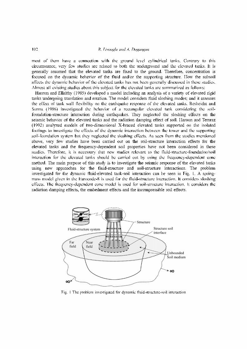
method. The main purpose of this study is to investigate the seismic response of the elevated tanks
using new approaches for the fluid-structure and soil-structure interactions. The problem
investigated for the dynamic fluid-elevated tank-soil interaction can be seen in Fig. 1. A spring-
mass model given in the Eurocode-8 is used for the fluid-structure interaction. It considers sloshing
effects. The frequency-dependent cone model is used for soil-structure interaction. It considers the
radiation damping effects, the embedment effects and the incompressible soil effects.
Fig. 1 The problem investigated for dynamic fluid-structure-soil interaction

Seismic evaluation of fluid-elevated tank-foundation/soil systems in frequency domain 103
2. Spring-mass model for fluid-structure interaction
The equivalent spring-mass models have been proposed by some researchers considering the
dynamic behavior of the fluid inside a container as shown in Fig. 2. Housner (1963) suggested that
an equivalent impulsive mass and a convective mass should represent the dynamic behavior of the
fluid as an approximation of the two mass model. The other researchers like Bauer (1964) and
Veletsos with co-workers (1984) proposed similar methods including additional higher modes of the
convective masses. Then, a more simplified approach has been elaborated by Malhotra et al. (2000).
This spring-mass model has been used by Eurocode 8 (2003). To the literature, although only the
first convective mass may be considered (Housner 1963), additional higher-modes of convective
masses may also be included (Chen and Barber 1976, Bauer 1964) in the ground supported tanks. A
single convective mass is generally used for practical design of the elevated tanks (Haroun and
Housner 1981) and the higher modes of the sloshing have negligible influence on the forces exerted
on the container even if the fundamental frequency of the structure is in the vicinity of one of the
natural frequencies of the sloshing (Haroun and Ellaithy 1985). As practical analysis is presented in
this study, only one convective mass is considered in the numerical example.
Housner (1963) has suggested a simplified analysis procedure for the fixed-base elevated tanks
(Fig. 3). In this approach, two masses (m1 and m2) are assumed uncoupled and the earthquake forces
on the support are estimated by considering two separate single-degree-of-freedom systems. The
mass of m1 represents only the sloshing of the convective mass (mc), the mass of m2 consists of the
impulsive mass of the fluid (mi), the mass derived by the weight of the container (mv) and by some
parts of the self-weight of the supporting structure (mss; two-thirds of the supporting structure
Internet Explorer 브라우저 시작.lnkFig. 3 The two-mass model for the elevated tanks
Fig. 2 The equivalent spring-mass model of the fluid
104 R. Livaoglu and A. Dogangun
weight is recommended in ACI 371R (1998) and the total weight of it is by Priestley et al. (1986)).
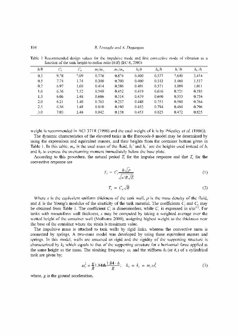
The dynamic characteristics of the elevated tanks in the Eurocode-8 model may be determined by
using the expressions and equivalent masses, and their heights from the container bottom given in
Table 1. In this table, mw is the total mass of the fluid, hi’ and hc’ are the heights used instead of hi
and hc to express the overturning moment immediately below the base plate.
According to this procedure, the natural period Ti for the impulse response and that Tc for the
convective response are
(1)
(2)
Where s is the equivalent uniform thickness of the tank wall, ρ is the mass density of the fluid,
and E is the Young’s modulus of the elasticity of the tank material. The coefficients Ci and Cc may
be obtained from Table 1. The coefficient Ci is dimensionless, while Cc is expressed in s/m1/2. For
tanks with nonuniform wall thickness, s may be computed by taking a weighted average over the
wetted height of the container wall (Molhotra 2000), assigning highest weight to the thickness near
the base of the container where the strain is maximum value.
The impulsive mass is attached to tank walls by rigid links, whereas the convective mass is
connected by springs. A two-mass model was developed by using these equivalent masses and
springs. In this model, walls are assumed as rigid and the rigidity of the supporting structure is
characterized by k2 which equals to that of the supporting structure for a horizontal force applied at
the same height as the mass. The sloshing frequency ωc and the stiffness k1 (or kc) of a cylindrical
tank are given by;
(3)
where, g is the ground acceleration.
Ti Cih ρ
s/R E
--------------------=
Tc Cc R=
ωc
2 g
R---1.84th
1.84 h⋅R
------------------= ; k1 kc mcωc
2= =
Table 1 Recommended design values for the impulsive mode and first convective mode of vibration as afunction of the tank height-to-radius ratio (h/R) (EC-8, 2003)
h/R Ci Cc mi/mw mc/mw hi/h hc/h hi’/h hc’/h
0.3 9.28 2.09 0.176 0.824 0.400 0.521 2.640 3.414
0.5 7.74 1.74 0.300 0.700 0.400 0.543 1.460 1.517
0.7 6.97 1.60 0.414 0.586 0.401 0.571 1.009 1.011
1.0 6.36 1.52 0.548 0.452 0.419 0.616 0.721 0.785
1.5 6.06 1.48 0.686 0.314 0.439 0.690 0.555 0.734
2.0 6.21 1.48 0.763 0.237 0.448 0.751 0.500 0.764
2.5 6.56 1.48 0.810 0.190 0.452 0.794 0.480 0.796
3.0 7.03 1.48 0.842 0.158 0.453 0.825 0.472 0.825

Seismic evaluation of fluid-elevated tank-foundation/soil systems in frequency domain 105
3. Soil-structure interaction
In the dynamic soil-structure-interaction analysis, a bounded structure (which may be linear or
nonlinear), consisting of the actual structure and an adjacent irregular near field soil, will interact
with the unbounded (infinite or semi-infinite) far field soil, assumed to be linear elastic.
There are different ways to consider the soil-structure interaction. First of them is the modifying
method that can be constructed by modifying the fixed base solution of the structural system
(Veletsos and Meek 1974). This method has been widely used in the studies (Aviles and Suarez
2001) and the codes such as ATC-1978 (Veletsos etc. 1988), FEMA 368-369 (2001), and Eurocode-
8 (2003). To represent the property of the elastic or viscoelastic half-space accurately, the spring and
dashpots are required to depend on the frequency of excitation (Wu and Smith 1995). The second
one is the substructure method that can consider the frequency-dependent or independent dynamic
stiffness and the damping of the soil/foundation system. If the frequency-dependent dynamic
stiffness or the damping is required to be considered, the governing equation for the structure-
foundation system is expressed and solved in the frequency domain using Fourier or Laplace
transformation (Wu and Smith 1995, Aviles and Perez-Rocha 1998, Takewaki 2003). The third one
is the direct method. Here, finite element and boundary element methods or a mixture of these are
used in the time or frequency domain (Wolf and Song 1996a, 1996b, Wolf 2003).
The most striking feature in an unbounded soil is the radiation of energy towards infinity, leading
to so-called radiation damping even in a linear system. Mathematically, in a frequency-domain
analysis, the dynamic stiffness relating the amplitudes of the displacements to those of the
interaction forces in the nodes of the structure-soil interface of the unbounded soil is a complex
function. This occurs when the unbounded soil consists of a homogeneous half-space (Wolf 2002).
Therefore, Wolf and Meek (1992, 1993) have proposed a cone model, an example of the
substructure method, for evaluating the dynamic stiffness and the effective input motion of a
foundation on the ground. Wolf and Preisig (2003) adopted this method for the layered half-space.
Compared to more rigorous numerical methods, this cone model requires only a simple numerical
manipulation within reasonable accuracy (Wolf 1994, Takewaki 2003).
Simple physical models representing the unbounded soil can be applied as follows: the effect of
the interaction of the soil and the structure on the response of the latter would be negligible in some
cases and need not to be considered in the other cases. This is applied, for example, to a flexible
high-rise structure with a small mass where the influence of the higher modes on the seismic
response remains small. Exciting the base of the structure with the prescribed earthquake motion is
then possible. For load applied directly to the structure, the soil can be represented by a static spring
or the structure can even be regarded as built-in (Wolf 1994, 2002). These static stiffnesses are
expressed in the literature with different theory. From all, the Boussinesq theory can be summarized
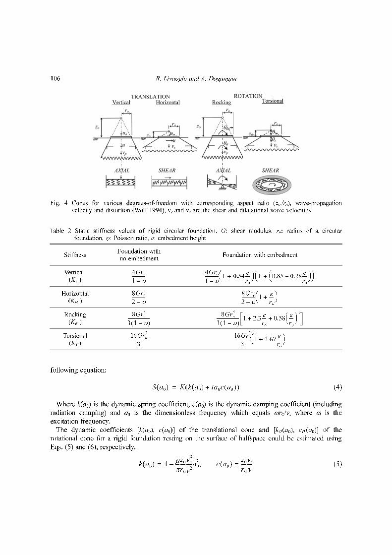
as follows: when a homogeneous halfspace is statically loaded, the variations of displacements with
the increasing depth are assumed as in Fig. 4. The shape is also like a truncated cone, for the
dynamic loading. Static stiffness of this truncated cone in a circular rigid foundation can be
expressed as in Table 2.
In the above table Kv, KH, KR and KT are the vertical, horizontal, rocking and torsional stiffnesses
of a circular foundation, respectively. For other geometrical shapes, these are given for square and
rectangular shapes by Wolf (1994) and for other arbitrary shape by Dobry and Gazetas (1986) and
Gazetas and Tassoulas (1987). Since the stiffness is frequency-dependent in the dynamic loading,
these static stiffnesses are used for calculating the dynamic stiffness [S(a0)] estimated by the
106 R. Livaoglu and A. Dogangun
following equation:
(4)
Where k(a0) is the dynamic spring coefficient, c(a0) is the dynamic damping coefficient (including
radiation damping) and a0 is the dimensionless frequency which equals ωr0/vs where ω is the
excitation frequency.
The dynamic coefficients [k(a0), c(a0)] of the translational cone and [kθ (a0), cθ (a0)] of the
rotational cone for a rigid foundation resting on the surface of halfspace could be estimated using
Eqs. (5) and (6), respectively.
(5)
S a0( ) K k a0( ) ia0c a0( )+( )=
k a0( ) 1µ
π---
z0
r0----
vs
2
v2
----a0
2–= , c a0( )
z0
r0----
vs
v----=
Fig. 4 Cones for various degrees-of-freedom with corresponding aspect ratio (zo /ro), wave-propagationvelocity and distortion (Wolf 1994), vs and vp are the shear and dilatational wave velocities
Table 2 Static stiffness values of rigid circular foundation, G: shear modulus, r0: radius of a circularfoundation, υ: Poisson ratio, e: embedment height
StiffnessFoundation with no embedment
Foundation with embedment
Vertical (Kv )
Horizontal(KH )
Rocking(KR )
Torsional(KT )
4Gro
1 υ–------------
4Gro
1 υ–------------ 1 0.54
e
ro
----+⎝ ⎠⎛ ⎞ 1 0.85 0.28
e
ro
----–⎝ ⎠⎛ ⎞
+⎝ ⎠⎛ ⎞
8Gro
2 υ–------------
8Gro
2 υ–------------ 1
e
ro
----+⎝ ⎠⎛ ⎞
8Gro
3
3 1 υ–( )--------------------
8Gro
3
3 1 υ–( )-------------------- 1 2.3
e
ro
---- 0.58e
ro
----⎝ ⎠⎛ ⎞
3
+ +
16Gro
3
3---------------
16Gro
3
3--------------- 1 2.67
e
ro
----+⎝ ⎠⎛ ⎞
Seismic evaluation of fluid-elevated tank-foundation/soil systems in frequency domain 107
(6)
For the horizontal motion, a truncated cone moves with the shear wave velocity (v = vs) and the
aspect ratio (z0/r0) of the cone is equal to (2 − υ)π/8. In this circumstance µ is zero for all values of
Poisson ratios (υ). For the vertical motion, truncated cone moves with dilatational wave velocity
(vp) and µθ = 0 for . The velocity of the truncated cone is v = 2vs and the aspect ratio (z0/r0)
is equal to for interval. Trapped mass for this interval can be
estimated by using Eq. (7) and Eq. (8).
Similar to the horizontal motion, the truncated cone moves with the shear wave velocity (v = vs)
for the torsional motion and the aspect ratio of the cone is equal to 9π/32. The value of µ is zero
for all values of Poisson ratios under this circumstance. For the rocking motion, the truncated cone
velocity is equal to vp, µθ = 0 for . The truncated cone moves with v = 2vs and the aspect
ratio is equal to for and the trapped mass for this Poisson ratio
interval can be estimated using Eq. (9) and Eq. (10). It should be noted that for , soil
is nearly incompressible. This behavior corresponds to trapped soil beneath the foundation, which
moves as a rigid body in phase with the foundation. A close match is achieved by defining the
trapped mass (∆M) to be
(7)
where
(8)
for the vertical motion and the trapped mass moment of inertia (∆Mθ)
(9)
where
(10)
for the rocking motion. In the intermediate and higher frequency ranges, the dynamic stiffness
coefficient is governed by the damping coefficient, as c(a0) is multiplied by a0 in contrast to k(a0).
Both cv (a0) and cH (a0) of the cone model produce very accurate results in this frequency ranges
(Wolf 1994). Whereas in the lower-frequency range (a0 < 2) and for , which is of practical
importance, the cone’s results overestimate (radiation) damping to certain extent, especially in the
vertical motion (Wolf 1994).
4. Practical procedure for the systems including embedment and incompressible
soil effects
Initially, to determine all the system response to the dynamic excitation, the system must be
kθ a0( ) 14
3---
µθ
π-----
z0r0----
vs
2
v2
----a0
2–
1
3---
a0
2
r0v
z0vs
---------⎝ ⎠⎛ ⎞
2
a0
2+
-----------------------------–= cθ a0( )z0vs
3r0v----------
a0
2
r0v
z0vs
---------⎝ ⎠⎛ ⎞
2
a0
2+
-----------------------------=
υ 1/3≤1 υ–( ) v/vs( )2π/4 1/3 υ< 1/2≤
υ 1/3≤1 υ–( ) v/vs( )29π/32 1/3 υ< 1/2≤
1/3 υ< 1/2≤
M∆ µρr03
=
µ 2 4π υ1
3---–⎝ ⎠
⎛ ⎞,=
Mθ∆ µθρr05
=
µθ 0 3π υ1
3---–⎝ ⎠
⎛ ⎞,=
υ 1/3≤
108 R. Livaoglu and A. Dogangun
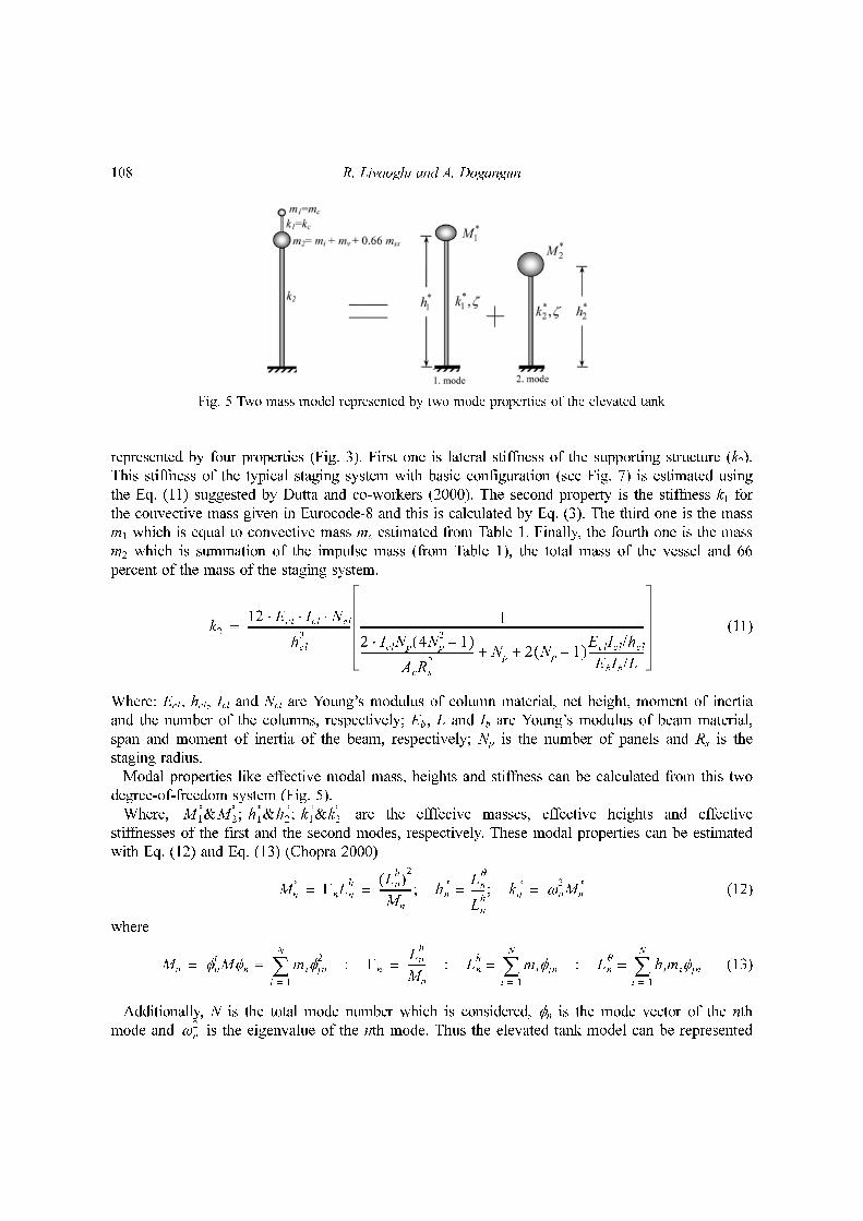
represented by four properties (Fig. 3). First one is lateral stiffness of the supporting structure (k2).
This stiffness of the typical staging system with basic configuration (see Fig. 7) is estimated using
the Eq. (11) suggested by Dutta and co-workers (2000). The second property is the stiffness k1 for
the convective mass given in Eurocode-8 and this is calculated by Eq. (3). The third one is the mass
m1 which is equal to convective mass mc estimated from Table 1. Finally, the fourth one is the mass
m2 which is summation of the impulse mass (from Table 1), the total mass of the vessel and 66
percent of the mass of the staging system.
(11)
Where: Ecl, hcl, Icl and Ncl are Young’s modulus of column material, net height, moment of inertia
and the number of the columns, respectively; Eb, L and Ib are Young’s modulus of beam material,
span and moment of inertia of the beam, respectively; Np is the number of panels and Rs is the
staging radius.
Modal properties like effective modal mass, heights and stiffness can be calculated from this two
degree-of-freedom system (Fig. 5).
Where, are the efffecive masses, effective heights and effective
stiffnesses of the first and the second modes, respectively. These modal properties can be estimated
with Eq. (12) and Eq. (13) (Chopra 2000)
(12)
where
(13)
Additionally, N is the total mode number which is considered, φn is the mode vector of the nth
mode and is the eigenvalue of the nth mode. Thus the elevated tank model can be represented
k2
12 Ecl Icl Ncl⋅ ⋅ ⋅
hcl
3---------------------------------------
1
2 IclNp 4Np
21–( )⋅
AcRs
2------------------------------------------- Np 2 Np 1–( )
EclIcl/hcl
EbIb/L---------------------+ +
-----------------------------------------------------------------------------------------------------------=
M 1
*&M 2
*; h1
*&h2
*; k1
*&k2
*
Mn* ΓnLn
h Ln
h( )2
Mn
------------; hn* Ln
θ
Ln
h-----= ; kn
* ωn
2Mn
*= = =
Mn φn
tMφn miφjn
2
i 1=
N
∑= : Γn
Ln
h
Mn
------- : Ln
hmiφjn
i 1=
N
∑= : Ln
θhimiφjn
i 1=
N
∑== =
ωn2
Fig. 5 Two mass model represented by two mode properties of the elevated tank

Seismic evaluation of fluid-elevated tank-foundation/soil systems in frequency domain 109
with two single-degree-of-freedom systems. Because of the absolute differences between the
sloshing stiffness kc and the stiffness of the supporting system k2, it should be assumed that the first
mode represents the sloshing and the second one is concerned with the impulsive mode.
The behavior of single-degree-of-freedom system mentioned above has to be separately calculated
in case of soil Poisson ratio for soil and . Because, the trapped or
additional mass (∆M) must be considered in case of (Fig. 6). Since, more important
motions for this type of structures except some special circumstances are the horizontal and the
rocking, this type of motion has to be considered for analyzing the fluid-elevated tank-foundation/
soil systems. Then the calculated internal forces or displacement can be combined with any one of
the modal combination techniques i.e., ABS, SRSS, CQC etc. (Chopra 2000).
For the system given in Fig. 6, the force-displacement relationship in the horizontal direction and
the moment-rotation relationship in the rocking interaction are formulated in frequency domain as
(14)
(15)
where, and are the dynamic stiffness coefficients including ground damping
effects of the circular foundation/soil system. The dynamic stiffnesses [( ) and ( )]
for the horizontal and rocking motions depending on the dimensionless frequency are approximated
as below;
(16)
(17)
where ζg is the material damping ratio of the soil, and are the radiation-damping
ratios for the horizontal and rocking motion of the soil to be estimated as;
υ 1/3≤( ) 1/3 υ< 1/2≤( )1/3 υ< 1/2≤
P0 ω( ) KHkHζg
a0( )u0 ω( )r0
vs
----KHcHζg
a0( )u· 0 ω( )+= SHζg
a0( )ub ω( )=
M0 ω( ) Kθkθζg
a0( )θb ω( )r0
vs
----Kθ cθζg
a0( )θ·b ω( )+= Sθζ
g
a0( )θb ω( )=
kHζg
cHζg
kθζg
, , cθζg
SHζg
a0( ) Sθζg
a0( )
SHζg
a0( ) KHkHζg
a0( ) 1 2iζH a0( ) 2iζg+ +( )=
Sθζg
a0( ) Kθkθζg
a0( ) 1 2iζθ a0( ) 2iζg+ +( )=
ζH a0( ) ζθ a0( )
Fig. 6 Dynamic model of structure and soil for horizontal and rocking motions
110 R. Livaoglu and A. Dogangun
(18)
For a system of three-degrees-of-freedom, the dynamic equilibrium can be formulated for as:
(19)
(20)
(21)
Eqs. (19), (20) and (21) can be written with some elimination as below:
(22)
where and are expressed using as;
(23)
Eqs. (22) and (23) yield the following equation:
(24)
If the same equations were written for , Eq. (22) could be written as
(25)
where ub(ω) and hθb(ω) are expressed using u(ω) as;
ζH a0( )a0cH a0( )2kH a0( )---------------------, ζθ a0( )
a0cθ a0( )2kθ a0( )--------------------==
υ 1/3≤
Mn*ω
2u ω( ) ub ω( ) hθb ω( )+ +[ ]– kn
*1 2iζ+( )u ω( )+ Mn
*ω
2ug ω( )=
Mn*ω
2u ω( ) ub ω( ) hθb ω( )+ +[ ]– SHζ
g
a0( )ub ω( )+ Mn*ω
2ug ω( )=
Mn*hω
2u ω( ) ub ω( ) hθb ω( )+ +[ ]– Sθζ
g
a0( )θb ω( )+ Mn*hω
2ug ω( )=
ωsn
2
ω2
-------- 1 2iζ+( ) 1– 1– 1–
1– SHζ
g
a0( )
Mn
*ω
2-------------------- 1 – 1–
1– 1– Sϑζ
g
a0( )
Mn
*h2ω
2------------------- 1–
u ω( )
ub ω( )
hθb ω( )⎩ ⎭⎪ ⎪⎨ ⎬⎪ ⎪⎧ ⎫ 1
1
1⎩ ⎭⎪ ⎪⎨ ⎬⎪ ⎪⎧ ⎫
ug ω( )=
ub ω( ) hθb ω( ) u ω( )
ub ω( )ωsn
21 2iζ+( )
SHζg
a0( )
Mn*
--------------------
------------------------------u ω( )= hn
*θb ω( )
ωsn
21 2iζ+( )
Sθζg
a0( )
Mn*hn
*2-------------------
------------------------------u ω( )=
u ω( ) 1
1
ω2
------Mn
*
SHζg
a0( )--------------------–
ω2Mn
*hn*2
Sθζg
a0( )---------------------
1
ωsn
21 2iζ+( )
------------------------------–– 1 2iζ+( )ωsn
2
--------------------------------------------------------------------------------------------------------------------------------------ug ω( )=
1/3 υ< 1/2≤
ωsn
2
ω2
-------- 1 2iζ+( ) 1– 1– 1–
1– SHζ
g
a0( )
Mn
*ω
2-------------------- 1 – 1–
1– 1– Sϑζ
g
a0( )
Mn
*h2ω
2-------------------
Mθ∆
Mn
*h2
------------– 1–
u ω( )
ub ω( )
hθb ω( )⎩ ⎭⎪ ⎪⎨ ⎬⎪ ⎪⎧ ⎫ 1
1
1⎩ ⎭⎪ ⎪⎨ ⎬⎪ ⎪⎧ ⎫
ug ω( )=

Seismic evaluation of fluid-elevated tank-foundation/soil systems in frequency domain 111
(26)
The lateral displacement depending on the structural rigidity was derived using Eqs. (25) and (26)
in the incompressible soil as below:
(27)
Where, is the square of the angular frequency of the fixed base single-degree-of-
freedom system, ug(ω) is the effective input motion in the frequency domain. It may be obtained by
means one of the transformation techniques like Fourier and Laplace. i.e., Using Fourier
transformation, the displacements in the time domain ug(t) can be expressed in the frequency
domain as;
(28)
The solution in the frequency domain can be expressed in the time domain using inverse Fourier
transformation like Eq. (29).
(29)
5. Numerical example
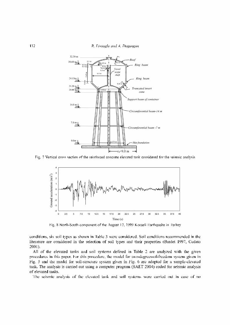
A reinforced concrete elevated tank with a container capacity of 900 m3 is considered in seismic
analysis (Fig. 7). The elevated tank has a frame supporting structure in which columns are
connected by the circumferential beams at regular interval at 7 m and 14 m height level. The tank
container is Intze type. The container and the supporting structure have been used as a typical
project in Turkey up to recent years. Young’s modulus and the weight of concrete per unit volume
are taken to be 32,000 MPa and 25 kN/m3, respectively. The container is filled with the water
density of 1,000 kg/m3. Calculated modal properties are mt = 1,281,000 kg, mc = 281,000 kg, ki =
846,000 N/m, k2 = 32,900,000 N/m.
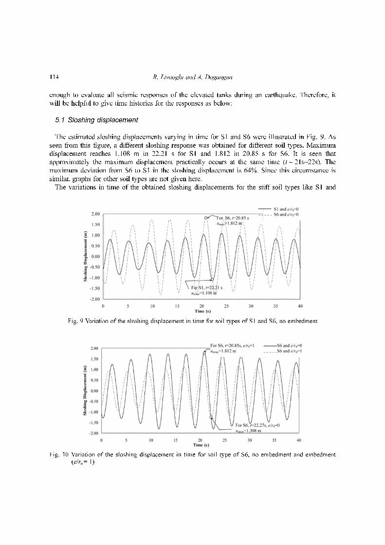
In the seismic analysis, it is assumed that the tank is subjected to North-South component of the
August 17, 1999 Kocaeli Earthquake in Turkey (Fig. 8). The ground acceleration of North-South
component of this earthquake was taken into consideration for approximately forty seconds.
While the damping in the convective mode (the first mode) may be accepted as 0.5%, for the
second mode as the impulsive mode accepted as 5% for the reinforced concrete supporting system.
To evaluate variations of the dynamic parameters in the elevated tanks depending on soil
ub ω( )ωsn
21 2iζ+( )
SHζg
a0( )
Mn*
--------------------
------------------------------u ω( )= hn
*θb ω( )
ωsn
21 2iζ+( )
Sϑζg
a0( )
Mn
*h2
-------------------Mθ∆
Mn
*h2
------------ω2
–
---------------------------------------------u ω( )=
u ω( )ug ω( )
ωsn
21 2iζ+( ) 1
ω2
------1
ωsn
21 2iζ+( )
------------------------------–Mn
*
SHζg
a0( )--------------------
1
Sϑζg
a0( )
Mn
*h2
-------------------Mθ∆
Mn
*h2
------------ω2
–
---------------------------------------------––
--------------------------------------------------------------------------------------------------------------------------------------------------------------=
ωsn
2=ksn
* /Mn*( )
ug ω( ) ug t( )exp iω t–( ) td∞–
∞
∫=
u t( ) 1
T--- u ω( )exp iω t( ) ωd
∞–
∞
∫=
112 R. Livaoglu and A. Dogangun
conditions, six soil types as shown in Table 3 were considered. Soil conditions recommended in the
literature are considered in the selection of soil types and their properties (Bardet 1997, Cudato
2001).
All of the elevated tanks and soil systems defined in Table 2 are analyzed with the given
procedures in this paper. For this procedure, the model for two-degrees-of-freedom system given in
Fig. 5 and the model for soil-structure system given in Fig. 6 are adopted for a sample-elevated
tank. The analysis is carried out using a computer program (SAET 2004) coded for seismic analysis
of elevated tanks.
The seismic analysis of the elevated tank and soil systems were carried out in case of no
Fig. 7 Vertical cross section of the reinforced concrete elevated tank considered for the seismic analysis
Fig. 8 North-South component of the August 17, 1999 Kocaeli Earthquake in Turkey

Seismic evaluation of fluid-elevated tank-foundation/soil systems in frequency domain 113
embedment (e/ro = 0) and embedment (e/ro = 1). The obtained peak values and their times for the
maximum sloshing displacements, roof displacements, base shear forces and overturning base
moments are given in Tables 4 and 5, respectively.
As seen from Tables 4 and 5, the embedment affects the values of seismic structural responses
such as the roof displacement, base shear and overturning moment. Its effects on the value of the
sloshing displacement is practically negligible. It is generally expected that when soil gets softer,
displacements tend to increase and shear forces tend to decrease. As can be realized from Tables 4
and 5, these trends may not satisfy all soil types.
Only peak values may be seen adequately for practically design purposes. However, it is not
Table 3 Properties of the considered soil types
Soil types
ζg
E(kN/m2)
G(kN/m2)
Ec
(kN/m3)γ
(kg/m3 )
υvs
(m/s)vp
(m/s)
S1 5.00 7000000 2692310 9423077 2000 0.30 1149.1 2149.89
S2 5.00 2000000 769230 2692308 2000 0.30 614.25 1149.16
S3 5.00 500000 192310 673077 1900 0.35 309.22 643.68
S4 5.00 150000 57690 201923 1900 0.35 169.36 352.56
S5 5.00 75000 26790 160714 1800 0.40 120.82 295.95
S6 5.00 35000 12500 75000 1800 0.40 82.54 202.18
Table 4 Results obtained from seismic analysis in case of no embedment
Soiltypes
Maximum sloshing displacement, us
Maximum roof displacement, u
Maximum base shear force, V
Maximum overturning base moment, Mo
time (s) value (m) time value (m) time value (kN) time (s) value (kNm)
S1 22.21 1.108 5.38 0.098 4.89 4691.9 4.89 119990
S2 22.21 1.127 6.34 0.116 4.89 4673.3 4.89 119460
S3 22.22 1.153 9.52 0.104 4.89 4594.3 4.89 117210
S4 22.26 1.282 9.60 0.127 4.89 4359.1 4.89 110720
S5 22.33 1.489 9.73 0.148 4.89 4182.6 4.89 106750
S6 20.85 1.812 7.82 0.154 4.89 4579.0 4.89 130290
Table 5 Results obtained from seismic analysis in case of embedment (e/ro = 1)
Soil types
Maximum sloshing displacement, us
Maximum roof displacement, u
Maximum base shear force, V
Maximum overturning base moment, Mo
time (s) value (m) time value (m) time value (kN) time (s) value (kNm)
S1 22.21 1.103 5.37 0.094 4.89 4697.6 4.89 120150
S2 22.21 1.107 5.38 0.098 4.89 4692.7 4.89 120010
S3 22.21 1.114 9.50 0.095 4.89 4672.9 4.89 119440
S4 22.22 1.147 9.52 0.103 4.89 4605.3 4.89 117520
S5 22.24 1.192 9.55 0.113 4.89 4510.5 4.89 114850
S6 22.27 1.308 9.63 0.129 4.89 4337.7 4.89 110230
114 R. Livaoglu and A. Dogangun
enough to evaluate all seismic responses of the elevated tanks during an earthquake. Therefore, it
will be helpful to give time histories for the responses as below:
5.1 Sloshing displacement
The estimated sloshing displacements varying in time for S1 and S6 were illustrated in Fig. 9. As
seen from this figure, a different sloshing response was obtained for different soil types. Maximum
displacement reaches 1.108 m in 22.21 s for S1 and 1.812 in 20.85 s for S6. It is seen that
approximately the maximum displacement practically occurs at the same time (t = 21s~22s). The
maximum deviation from S6 to S1 in the sloshing displacement is 64%. Since this circumstance is
similar, graphs for other soil types are not given here.
The variations in time of the obtained sloshing displacements for the stiff soil types like S1 and
Fig. 9 Variation of the sloshing displacement in time for soil types of S1 and S6, no embedment
Fig. 10 Variation of the sloshing displacement in time for soil type of S6, no embedment and embedment(e/ro = 1)
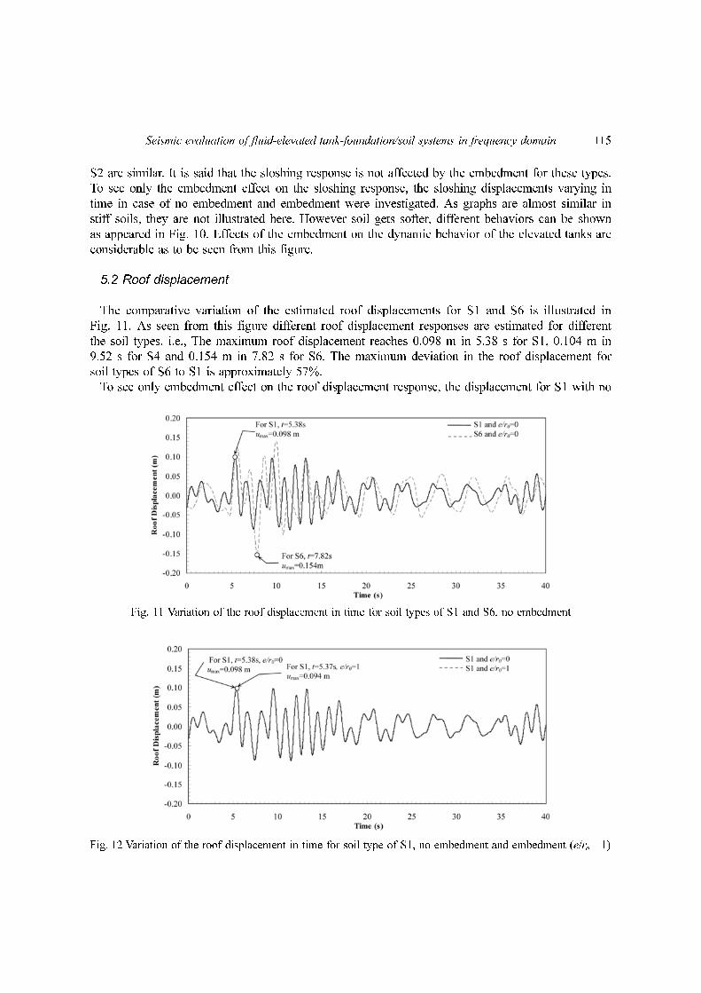
Seismic evaluation of fluid-elevated tank-foundation/soil systems in frequency domain 115
S2 are similar. It is said that the sloshing response is not affected by the embedment for these types.
To see only the embedment effect on the sloshing response, the sloshing displacements varying in
time in case of no embedment and embedment were investigated. As graphs are almost similar in
stiff soils, they are not illustrated here. However soil gets softer, different behaviors can be shown
as appeared in Fig. 10. Effects of the embedment on the dynamic behavior of the elevated tanks are
considerable as to be seen from this figure.
5.2 Roof displacement
The comparative variation of the estimated roof displacements for S1 and S6 is illustrated in
Fig. 11. As seen from this figure different roof displacement responses are estimated for different
the soil types. i.e., The maximum roof displacement reaches 0.098 m in 5.38 s for S1, 0.104 m in
9.52 s for S4 and 0.154 m in 7.82 s for S6. The maximum deviation in the roof displacement for
soil types of S6 to S1 is approximately 57%.
To see only embedment effect on the roof displacement response, the displacement for S1 with no
Fig. 12 Variation of the roof displacement in time for soil type of S1, no embedment and embedment (e/ro = 1)
Fig. 11 Variation of the roof displacement in time for soil types of S1 and S6, no embedment
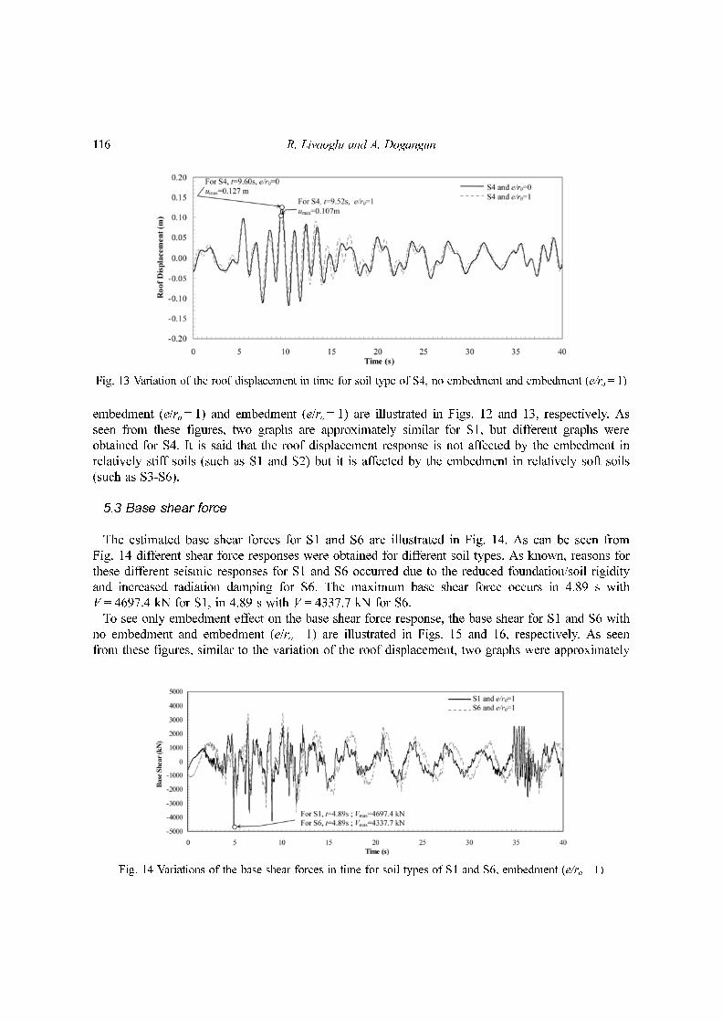
116 R. Livaoglu and A. Dogangun
embedment (e/ro = 1) and embedment (e/ro = 1) are illustrated in Figs. 12 and 13, respectively. As
seen from these figures, two graphs are approximately similar for S1, but different graphs were
obtained for S4. It is said that the roof displacement response is not affected by the embedment in
relatively stiff soils (such as S1 and S2) but it is affected by the embedment in relatively soft soils
(such as S3-S6).
5.3 Base shear force
The estimated base shear forces for S1 and S6 are illustrated in Fig. 14. As can be seen from
Fig. 14 different shear force responses were obtained for different soil types. As known, reasons for
these different seismic responses for S1 and S6 occurred due to the reduced foundation/soil rigidity
and increased radiation damping for S6. The maximum base shear force occurs in 4.89 s with
V = 4697.4 kN for S1, in 4.89 s with V = 4337.7 kN for S6.
To see only embedment effect on the base shear force response, the base shear for S1 and S6 with
no embedment and embedment (e/ro = 1) are illustrated in Figs. 15 and 16, respectively. As seen
from these figures, similar to the variation of the roof displacement, two graphs were approximately
Fig. 13 Variation of the roof displacement in time for soil type of S4, no embedment and embedment (e/ro = 1)
Fig. 14 Variations of the base shear forces in time for soil types of S1 and S6, embedment (e/ro = 1)

Seismic evaluation of fluid-elevated tank-foundation/soil systems in frequency domain 117
same as for S1, but different graphs were obtained for S6. It is said that the base shear force
response is not affected by the embedment in relatively stiff soils (such as S1 and S2) but it is
affected by the embedment in relatively soft (i.e., S3-S6).
6. Conclusions
A simple procedure is proposed for seismic analysis of fluid-elevated tank-foundation/soil
systems. The procedure provides not only an estimation of the base shear, overturning moment and
displacement of supporting system but also the sloshing displacement. A computer program was
coded for the seismic analysis of the elevated tanks considering interaction effects. Analysis with
this procedure needs less computer memory capacity and shorter CPU times.
The sloshing response is not practically affected by soil properties and embedment in stiff soils
such as S1, S2. Similarly, roof displacement and base shear force responses are also not affected by
the embedment in relatively stiff soils but they are affected by the embedment in relatively soft
soils.
Generally, when soil gets softer, the roof displacements increase, the base shear and overturning
moment decrease. However, if an earthquake is considered in the analysis, this may lead to wrong
assessment of the seismic response. Therefore, to prevent misleading results, time history analyses
Fig. 15 Variation of the base shear force in time for soil type of S1, no embedment and embedment (e/ro = 1)
Fig. 16 Variation of the base shear force in time for soil type of S6, no embedment and embedment (e/ro = 1)
118 R. Livaoglu and A. Dogangun
are necessary in case that soil-structure interaction is not negligible.
It is seen that the results obtained in relatively stiff soils (like S1 and S2) overestimate radiation
damping in the lower-frequency range. It should be noted that soil-structure interaction has less
importance in such soil conditions.
It is recommended that more numerical examples analyzed for different soil types and foundation
conditions. Furthermore, the procedure presented here can be used with other substructure methods.
Acknowledgements
This study constitutes some parts of the first author’s doctoral research. We thank to reviewers
who gave useful comments on this paper.
References
ACI 371R-98. (1995), American Concrete Institute, “Guide to the analysis design and construction of concrete-pedestal water tower”.
Aviles, J. and Perez-Rocha, E.L. (1998), “Effect of foundation embedment during building-soil structureinteraction”, Earthq. Eng. Struct. Dyn., 27, 1523-1540.
Aviles, J. and Suarez, M. (2002), “Effective periods and damping of building-foundation systems includingseismic wave effects”, Eng. Struct., 24, 553-562.
Bardet, P.J. (1997), Experimental Soil Mechanics, Prentice Hall, Upper Saddle River, New Jersey 07458.Bauer, H.F. (1964), Fluid Oscillations in the Containers of a Space Vehicle and Their Influence Upon Stability,
NASA TR R-187.Chen, C.P. and Barber, R.B. (1976), “Seismic design of liquid storage tanks to earthquakes”, Int. Symposium on
Earthquake Structural Engineering, St. Louis Missouri, II: 1231.Chopra, K.A. (2000), Dynamics of Structures: Theory and Applications to Earthquake Engineering, Prentice-Hall
International Inc.Coduto, P.D. (2001), Foundation Design: Principles and Practices : Second Edition, Prentice Hall, Upper Saddle
River, New Jersey.Dobry, R. and Gazetas, G. (1986), “Dynamic response of arbitrarily-shaped foundations”, ASCE. Geotechnical
Engineering Division. J., 113(2), 109-135.Dutta, S.C., Jain, S.K. and Murty, C.V.R. (2000), “Assessing the seismic torsional vulnerability of elevated tanks
with RC frame-type staging”, Soil Dyn. Earthq. Eng., 19, 183-197.Eurocode-8. (2003), Design of Structures for Earthquake Resistance-Part 4 (Draft No:2): Silos, Tanks and
Pipelines, European Committee for Standardization, 65p.FEMA 368. (2000), The 2000 NEHRP Recommended Provisions for New Buildings and Other Structures Part
1: Provision, NEHRP.FEMA 369. (2000), The 2000 NEHRP Recommended Provisions for New Buildings and Other Structures Part
2: Commentary, NEHRP.Gazetas, G. and Tassoulas, J.L. (1987), “Horizontal stiffness of arbitrarily-shaped embedded foundations”, ASCE.
Geotechnical Engineering Division. J., 113(5), 440-457.Haroun, M.A. and Ellaithy, M.H. (1985), “Seismically induced fluid forces on elevated tanks”, J. Technical
Topics in Civil Eng., 111(1), 1-15.Haroun, M.A. and Temraz, M.K. (1992), “Effects of soil-structure interaction on seismic response of elevated
tanks”, Soil Dyn. Earthq. Eng., 11(2), 73-86.Haroun, M.A. and Housner, G.W. (1981), “Seismic design of liquid storage tanks”, J. Tech. Councils. ASCE,
107(1), 191-207.Housner, G.W. (1963), “Dynamic behavior of water tanks”, Bulletin of the Seismological Society of the America ,
Seismic evaluation of fluid-elevated tank-foundation/soil systems in frequency domain 119
53, 381-387.Meek, J.W. and Wolf, J.P. (1994), “Cone models for embedded foundation”, J. Geotechnical Eng., ASCE,
120(1), 60-80.Priestley, M.J.N., Davidson, B.J., Honey, G.D., Hopkins, D.C., Martin, R.J., Ramsey, G., Vessey, J.V. and Wood,
J.H. (1986), Seismic Design of Storage Tanks, Recommendation of a Study Group the New Zealand Society forEarthquake Engineering, New Zealand.
Resheidat, R.M. and Sunna, H. (1986), “Behavior of elevated storage tanks during earthquakes”, Proc. the 3thU.S. Nat. Conf. on Earthquake Engineering, 2143-2154.
SAET-2004. (2004), “A computer program for seismic analysis of elevated tanks considering fluid-structure-soilinteraction”, Karadeniz Technical University.
Takewaki, I., Takeda, N. and Uetani, K. (2003), “Fast practical evaluation of soil-structure interaction ofembedded structure”, Soil Dyn. Earthq. Eng., 23, 195-202.
Veletsos, S.A., Prasad, M.A. and Tang, Y. (1988), “Design approaches for soil structure interaction”, NationalCenter for Earthquake Engineering Research, Technical Report NCEER-88-00331.
Veletsos, A.S. and Meek, J.M. (1974), “Dynamics of behaviour of building-foundation systems”, Earthq. Eng.Struct. Dyn., 3, 121-138.
Veletsos, A.S. (1984), Seismic Response and Design of Liquid Storage Tanks, Guidelines for the Seismic Designof Oil and Gas Pipeline Systems. ASCE, New York, 255-461.
Wolf, J.P. and Song, C.H. (1996a), Finite-Element Modeling of Unbounded Media. Chichester: John Wiley &Sons.
Wolf, J.P. and Song, C. (1996), “Consistent infinitesimal finite element cell method - a boundary finite-elementprocedure”, Third Asian-Pacific Conf. on Computational Mechanics, Seoul, Korea, 16-18 September 1996.
Wolf, J.P. (1994), Foundation Vibration Analysis Using Simple Physical Models, Prentice-Hall, EnglewoodCliffs.
Wolf, J.P. (2002), “Some cornerstones of dynamic soil-structure interaction”, Eng. Struct., 24, 13-28.Wolf, J.P. (2003), “Dynamic stiffness of foundation embedded in layered halfspace based on wave propagating
cones”, Earthq. Eng. Struct. Dyn., 32, 1075-1098.Wolf, J.P. and Meek, J.W. (1993), “Cone models for a soil layer on a flexible rock half-space”, Earthq. Eng.
Struct. Dyn., 22, 185-193.Wolf, J.P. and Meek, J.W. (1992), “Cone models for homogeneous soil”, J. Geotechnical Eng., ASCE, 118, 686-
703.Wolf, J.P. and Preisig, M. (2003), “Dynamic stiffness of foundation embedded in layered halfspace based on
wave propagation in cones”, Earthq. Eng. Struct. Dyn., 32, 1075-1098.Wolf, J.P. (2003), The Scaled Boundary Element Method, John Wiley&Sons.Wu, W. and Smith, A. (1995), “Efficient modal analysis for structures with soil-structure interaction”, Earthq.
Eng. Struct. Dyn., 24, 283-289.