A Wavelet-Based Test for Stationarity
17
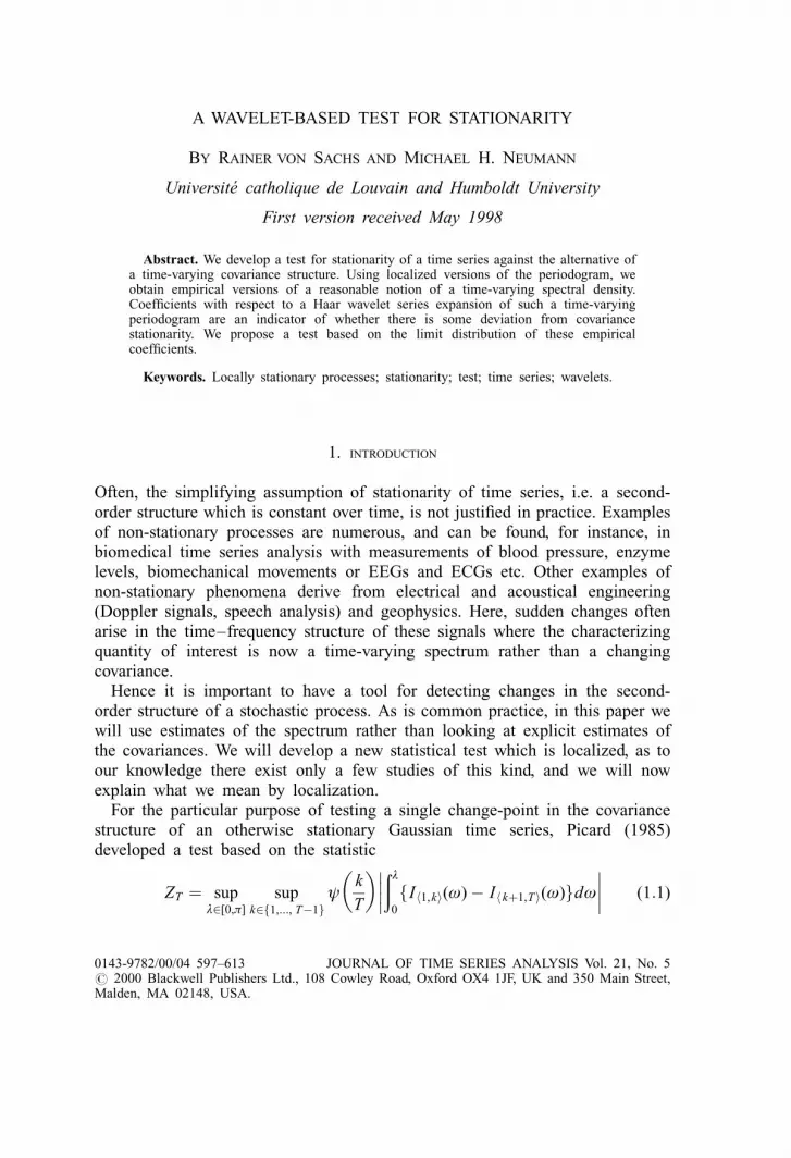
A WAVELET-BASED TEST FOR STATIONARITY BY RAINER VON SACHS AND MICHAEL H. NEUMANN Universite ´ catholique de Louvain and Humboldt University First version received May 1998 Abstract. We develop a test for stationarity of a time series against the alternative of a time-varying covariance structure. Using localized versions of the periodogram, we obtain empirical versions of a reasonable notion of a time-varying spectral density. Coefficients with respect to a Haar wavelet series expansion of such a time-varying periodogram are an indicator of whether there is some deviation from covariance stationarity. We propose a test based on the limit distribution of these empirical coefficients. Keywords. Locally stationary processes; stationarity; test; time series; wavelets. 1. INTRODUCTION Often, the simplifying assumption of stationarity of time series, i.e. a second- order structure which is constant over time, is not justified in practice. Examples of non-stationary processes are numerous, and can be found, for instance, in biomedical time series analysis with measurements of blood pressure, enzyme levels, biomechanical movements or EEGs and ECGs etc. Other examples of non-stationary phenomena derive from electrical and acoustical engineering (Doppler signals, speech analysis) and geophysics. Here, sudden changes often arise in the time–frequency structure of these signals where the characterizing quantity of interest is now a time-varying spectrum rather than a changing covariance. Hence it is important to have a tool for detecting changes in the second- order structure of a stochastic process. As is common practice, in this paper we will use estimates of the spectrum rather than looking at explicit estimates of the covariances. We will develop a new statistical test which is localized, as to our knowledge there exist only a few studies of this kind, and we will now explain what we mean by localization. For the particular purpose of testing a single change-point in the covariance structure of an otherwise stationary Gaussian time series, Picard (1985) developed a test based on the statistic Z T sup º2[0,ð] sup k2f1,..., T 1g l k T º 0 f I h1, ki (ø) I h k1, T i (ø)gd ø (1:1) 0143-9782/00/04 597–613 JOURNAL OF TIME SERIES ANALYSIS Vol. 21, No. 5 # 2000 Blackwell Publishers Ltd., 108 Cowley Road, Oxford OX4 1JF, UK and 350 Main Street, Malden, MA 02148, USA.
-
Upload
independent -
Category
Documents
-
view
3 -
download
0
Transcript of A Wavelet-Based Test for Stationarity
A WAVELET-BASED TEST FOR STATIONARITY
BY RAINER VON SACHS AND MICHAEL H. NEUMANN
Universite catholique de Louvain and Humboldt University
First version received May 1998
Abstract. We develop a test for stationarity of a time series against the alternative ofa time-varying covariance structure. Using localized versions of the periodogram, weobtain empirical versions of a reasonable notion of a time-varying spectral density.Coef®cients with respect to a Haar wavelet series expansion of such a time-varyingperiodogram are an indicator of whether there is some deviation from covariancestationarity. We propose a test based on the limit distribution of these empiricalcoef®cients.
Keywords. Locally stationary processes; stationarity; test; time series; wavelets.
1. INTRODUCTION
Often, the simplifying assumption of stationarity of time series, i.e. a second-order structure which is constant over time, is not justi®ed in practice. Examplesof non-stationary processes are numerous, and can be found, for instance, inbiomedical time series analysis with measurements of blood pressure, enzymelevels, biomechanical movements or EEGs and ECGs etc. Other examples ofnon-stationary phenomena derive from electrical and acoustical engineering(Doppler signals, speech analysis) and geophysics. Here, sudden changes oftenarise in the time±frequency structure of these signals where the characterizingquantity of interest is now a time-varying spectrum rather than a changingcovariance.
Hence it is important to have a tool for detecting changes in the second-order structure of a stochastic process. As is common practice, in this paper wewill use estimates of the spectrum rather than looking at explicit estimates ofthe covariances. We will develop a new statistical test which is localized, as toour knowledge there exist only a few studies of this kind, and we will nowexplain what we mean by localization.
For the particular purpose of testing a single change-point in the covariancestructure of an otherwise stationary Gaussian time series, Picard (1985)developed a test based on the statistic
ZT � supë2[0,ð]
supk2f1,..., Tÿ1g
øk
T
� ������ë0
fIh1,ki(ù)ÿ Ihk�1,Ti(ù)gdù���� (1:1)
0143-9782/00/04 597±613 JOURNAL OF TIME SERIES ANALYSIS Vol. 21, No. 5# 2000 Blackwell Publishers Ltd., 108 Cowley Road, Oxford OX4 1JF, UK and 350 Main Street,Malden, MA 02148, USA.

where ø is a suitable weight function and Ih1,ki and Ihk�1,Ti are periodograms onthe segments X 1, . . ., X k and X k�1, . . ., XT, respectively. This method has beengeneralized by Giraitis and Leipus (1992) to the case of linear processes, and hasbeen modi®ed by Rozenholc (1995) by using tapered periodograms. The test ofPicard is based on estimates of the (possibly time-varying) spectral functionF(ë) � � ë
0f (ù)dù. In contrast, we intend to use estimates of the (possibly time-
varying) spectral density directly. The relative merits of smoothing-based testsbased on local characteristics like densities versus non-smoothing tests based oncumulative characteristics are discussed in a different context by Rosenblatt(1975) and Ghosh and Huang (1991). The essential message is that non-smoothing tests look primarily at global deviations, and are therefore well suitedfor detecting classical Pitman alternatives of the form f � f0 � nÿ1=2 g, where ndenotes the sample size. On the other hand, smoothing-based tests focus on morelocalized deviations, and are consequently more powerful for detectingalternatives of the form f � f 0 � nÿä g(:=nÿã) for suitable ä, ã. 0.
In the present paper we develop a test of stationarity which is based on thefollowing general idea: using special segmentations we test on a change of theautocovariance structure from segment to segment. To be more speci®c, we usea wavelet decomposition of an appropriate notion of a time-varying spectraldensity. A model which allows for a rigorous asymptotic theory in this contextis developed by Dahlhaus (1997), who introduced the concept of locallystationary processes. However, we think that our proposed test procedure isapplicable in more general terms.
Some technical prerequisites for our test can be taken from Neumann andvon Sachs (1997), where an estimator of a time-varying spectral densityf (u, ù) was developed. It is a multiple test with the null hypothesis ofstationarity H0: f (u, ù) � f (ù), where each subtest checks the signi®cance ofa particular coef®cient á j,k; j9,k9 �
� �f (u, ù)ø j,k(u)ö j9,k9(ù)du dù in our de-
composition with respect to some set of bivariate wavelet functionsfø j,k(u)ö j9,k9(ù)g j,k; j9,k9. Note that under H0 all of these coef®cients are equalto zero. To get estimates of the coef®cients á j,k; j9,k9 we consider two naturalcandidates for empirical versions of f (u, ù). First, we can use segmentedperiodograms IhK,Li(ù) as used in Dahlhaus (1997) and von Sachs and Schneider(1996), which are calculated on segments corresponding to the particular waveletø j,k(u) in the time direction. Second, we can employ the so-called pre-periodogram introduced in Neumann and von Sachs (1997). This second methodhas advantages of adaptivity in the process of estimating the evolutionaryspectral density.
Using an asymptotic result for the marginal distributions of our estimates ofá j,k; j9,k9, we obtain an appropriate critical value via Bonferroni's inequality. Weprove that the error of the ®rst kind is asymptotically not greater than thenominal error and we give a brief discussion on the power of our test. Thepracticability of this method for moderate sample sizes is investigated bysimulations which are reported in Section 4. In addition we apply our methodto a set of tremor data from neurobiology.
598 R. VON SACHS AND M. H. NEUMANN
# Blackwell Publishers Ltd 2000
2. SOME BASIC CONCEPTS FOR NON-STATIONARY PROCESSES
2.1. A framework for non-stationary processes: a model of local stationarity
The null hypothesis is simply that the time series fXtg is covariance stationary.Non-stationarity is basically de®ned as any arbitrary deviation from covariancestationarity. To de®ne non-stationarity on the level of spectral densities, we haveto ®nd an appropriate extension of the de®nition of the spectral densitygeneralizing from the stationary case. A particular framework which also allowsfor rigorous asymptotic theory has recently been developed by Dahlhaus (1997).The basic idea of his model may be explained as follows. In order to estimatesome object of interest (parameter, function, . . .) consistently, one needs anincreasing amount of information about each feature of this object. Indepen-dence or weak dependence of the observed data is one part of a possible set ofsuf®cient conditions for that. If the object of interest is of in®nite dimension,e.g. a curve, we also have to bound its complexity appropriately. In non-parametric regression, an asymptotic with a ®xed function on a bounded intervalis often taken as the target, and independent observations are made with anincreasingly ®ne grid of design points which then guarantee a growing amount ofinformation about the true function on every subinterval. In order to actuallyhave such an increasing amount of information about the function at any pointx0, we have to be able to gain some information about f (x0) from theobservations corresponding to design points close to x0. This is guaranteed byappropriate smoothness assumptions on the regression function f. Dahlhaus usesbasically this approach to de®ne an appropriate framework for the asymptotictheory of non-stationary processes. He keeps the central parameters of a timeseries, the mean and the covariance structure, ®xed and links them to a set ofobservations X 1, . . ., X T on a growing time horizon by an appropriate rescalingof time. This leads to the following de®nition.
DEFINITION 2.1 (DAHLHAUS, 1997). A sequence of stochastic processesX t,T (t � 1, . . ., T ) is called locally stationary with transfer function A0 andtrend ì if there exists a representation
X t,T � ìt
T
� ���ðÿð
A0t,T (ù)exp(iùt)dî(ù) (2:1)
where
(i) î(ù) is a stochastic process on [ÿð, ð] with î(ù) � î(ÿù), Eî(ù) � 0and orthonormal increments, i.e. covfdî(ù), dî(ù9)g � ä(ùÿ ù9)dù,cumfdî(ù1), . . ., dî(ùk)g � ç(
Pkj�1ù j)hk(ù1, . . ., ùkÿ1)dù1 . . . dùk , where
cumf. . .g denotes the cumulant of order k, jhk(ù1, . . ., ùkÿ1)j < constk forall k (with h1 � 0, h2(ù) � 1) and ç(ù) �P1j�ÿ1ä(ù� 2ð j) is the period 2ðextension of the Dirac delta function;
(ii) there exists a positive constant K and a smooth function A(u, ù) on
WAVELET-BASED TEST FOR STATIONARITY 599
# Blackwell Publishers Ltd 2000
[0, 1] 3 [ÿð, ð] which is 2ð-periodic in ù, with A(u, ÿù) � A(u, ù), suchthat for all T
supt,ù
����A0t,T (ù)ÿ A
t
T, ù
� ����� < KTÿ1: (2:2)
A(u, ù) and ì(u) are assumed to be continuous in u.
REMARK 2.1. In (2.1), t denotes a time point in the set f1, 2, . . ., Tg while udenotes a time point in the rescaled interval [0, 1], i.e. u � t=T . Note that (2.1)does not de®ne a ®ner and ®ner discretized continuous-time process as T tendsto in®nity. Rather, it means that more and more data of the same localstructure, given by A(t=T , ù), are observed with increasing T. Simple examplesare given by a stationary process modulated by a time-changing variance (asin Dahlhaus, 1996, Example 1.1(i)) and by autoregressive moving-average(ARMA) processes with time-varying coef®cients (cf. our simulated examples inSection 4). A more elaborate example for a model of a time-varying spectrumarising from mobile radio communication can be found in von Sachs andSchneider (1996).
This concept now allows for the de®nition of a time-varying spectral density.
DEFINITION 2.2. As the evolutionary spectrum of fX t,Tg given in (2.1) wede®ne for u 2 (0, 1)
f (u, ù) � limT!1
1
2ð
X1s�ÿ1
cov(X [uTÿs=2],T ; X [uT�s=2],T )exp(ÿiùs) (2:3)
where X t,T is de®ned according to (2.1) with A0t,T (ù) � A(0, ù) for t , 1 and
A0t,T (ù) � A(1, ù) for t . T.
Under the smoothness assumptions on A(u, ù) as given in Section 3.1 below,this evolutionary spectrum equals f (u, ù) � jA(u, ù)j2, and is uniquely de®ned.For stationary processes this spectral density becomes constant in time, i.e.f (u, ù) � f (ù); hence the class of locally stationary processes is a truegeneralization including stationary processes.
Note that (2.3) could have been derived also on a purely heuristic levelwithout the theory of locally stationary processes. If we assume that thecovariances decay at a suf®ciently fast rate as the lag order tends to in®nity,and that the covariance structure changes slowly over time (which is inaccordance with the idea of rescaling), then De®nition 2.2 is obviously areasonable generalization of the spectral density for stationary processes.Actually, since the covariances decay as the lag length increases, f (u0, ù) ismainly determined by covariances of the Xt with ju0T ÿ tj small. Hence, thede®nition of f (u0, ù) is already automatically localized in some sense.Furthermore, since the covariance structure is nearly the same over small
600 R. VON SACHS AND M. H. NEUMANN
# Blackwell Publishers Ltd 2000
segments, the de®nition of f (u, ù) is also stable in u, which means in turn thatit is reasonable to include some X ts with small ju0T ÿ tj in the de®nition ofthe spectrum near u0.
2.2. Two time-varying periodograms
We discuss now the two possibilities for de®ning local periodograms for non-stationary processes which we will use as the main parts of our test onstationarity. Assume for simplicity that ì � 0. In the case of non-stationary timeseries it is natural to consider ®tting time series models on small segments.Accordingly, we can also consider the usual periodogram on small segments as astarting point for further inference. This has been proposed by Dahlhaus (1997)for the purpose of ®tting certain time series models locally to a non-stationaryprocess, and by von Sachs and Schneider (1996) as a starting point for a waveletestimator of the evolutionary spectrum. In the non-tapered case, such a localperiodogram has the form
IN (u, ù) � 1
2ðN
����XN
s�1
X [uTÿN=2�s],T exp(ÿiùs)
����2:REMARK 2.2. Note that the role of the parameter N, which is usually
assumed to obey N !1 and N=T ! 0 as T !1, is twofold. First, itdelivers a cut-off point above which higher lags are not incorporated in thede®nition of the periodogram. Actually, IN (u, ù) contains only estimates of thecovariances up to lag N ÿ 1; hence, too small a value of N will introduce somebias. Second, the de®nition of IN (u, ù) already contains some smoothing in thetime direction. In other words, the parameter N acts in two opposite ways as asmoothing parameter: whereas small values of N restrict the resolution in thefrequency direction, large N restricts the resolution in the time direction. Ofcourse, according to the uncertainty principle (see, for example, Priestley, 1981,p. 835), there is no loss due to the fact that the number of lags beingincorporated in the segmented periodogram is not greater than the timewindow. Nevertheless, problems can occur with such a global parameter N. Atany point u0 there exists a choice of N � N (u0) which is connected to the`bandwidth of stationarity' hu; for the latter see Dahlhaus (1996). So an ingeneral time-varying hu over [0, 1] would call for possibly very differentsegment lengths N (u) over [0, 1]. Moreover, there is the additional importantproblem of how to perform a data-driven choice of N. Usually, this parameteris chosen before one starts the `smoothing machinery', i.e. before one getsinformation about the order of magnitude of the bandwidth of stationarity.
To avoid these shortcomings, Neumann and von Sachs (1997) introduced adifferent empirical version of f (u, ù). The basic idea is to avoid any kind ofpre-smoothing at this stage, which amounts to choosing the time window as
WAVELET-BASED TEST FOR STATIONARITY 601
# Blackwell Publishers Ltd 2000

small as possible and the lag window as large as possible. These considerationsled Neumann and von Sachs (1997) to the de®nition
I(u, ù) � 1
2ð
Xk:1<[uTÿk=2],[uT�k=2]<T
X [uTÿk=2],T X [uT�k=2],T exp(iùk) (2:4)
which was called the `pre-periodogram'. It was used in Neumann and von Sachs(1997) as a starting point for a wavelet estimator of the evolutionary spectraldensity and was also applied in Dahlhaus (1999) to establish local likelihoodmethods as a tool for ®tting semiparametric time series models to locallystationary processes.
REMARK 2.3. (i) In contrast to the usual periodogram, both non-stationaryversions provide an appropriate localization in time. While this is obvious forthe segmented periodogram IN (u, ù), the localization is achieved in a moreimplicit way by I(u, ù). Actually, since EX [uTÿk=2],T X [uT�k=2],T tends to zero asjkj ! 1, I(u, ù) also re¯ects the local covariance structure for t around uT.
(ii) An obvious advantage of the pre-periodogram over the segmentedperiodogram is that the choice of the appropriate bandwidths in the time andfrequency directions is completely left to the major smoothing step. In contrastto IN (u, ù), the pre-periodogram has a diverging variance as T !1. However,it turns out that smoothing in time and smoothing in frequency both lead to avariance reduction; see also the calculations in Neumann and von Sachs (1997).This fact also explains why the wavelet estimator of the evolutionary spectraldensity considered in Neumann and von Sachs (1997) attains similar rates ofconvergence to the estimator based on the segmented periodogram consideredin von Sachs and Schneider (1996).
3. THE TEST
3.1. Derivation of the test statistic
The test we intend to devise will be based on a decomposition of an empiricalversion of f (u, ù) with respect to a certain system of Haar wavelet functions.Anticipating their later use on the intervals [0, 1] and [0, ð], respectively, wede®ne
ø(u) � 1 if 0 < u < 1=2
ÿ1 if 1=2 , u < 1
�and
ö(ù) � 1=ð1=2 for 0 < ù < ð:
Furthermore, we set
ø j,k(u) � 2 j=2ø(2 juÿ k) and ö j,k(ù) � 2 j=2ö(2 jùÿ kð)
602 R. VON SACHS AND M. H. NEUMANN
# Blackwell Publishers Ltd 2000
k � 0, . . ., 2 j ÿ 1:
In the following we estimate the coef®cients
á j,k; j9,k9 ��1
0
�ð0
f (u, ù)ø j,k(u)ö j9,k9(ù)du dù
which may be interpreted as measures for the local contrast in the time direction.Under the null hypothesis H0: f (u, ù) � f (ù), all of these coef®cients are equalto zero. This means that we have to test the hypothesis á j,k; j9,k9 � 0 for all( j, k; j9, k9).
In sharp contrast to the problem of estimating f (u, ù), where the use ofwavelets of higher regularity may lead to better rates of convergence than thatof Haar wavelets, there is no such gain in the context of testing. The functionsø j,k do a perfect job of detecting differences, whereas the scaling functionsö j,k are used to stabilize the spectral estimate.
A natural estimate based on the segmented periodogram is
~á(1)j,k; j9,k9 �
�1
0
�ð0
[Ih[k2ÿ j T ],[(k�1=2)2ÿ j T ]i(ù)÷fu 2 [k2ÿ j, (k � 12)2ÿ j]g
� Ih[f(k�1=2)2ÿ j�1gT],[(k�1)2ÿ j T ]i(ù)÷fu 2 [(k � 12)2ÿ j, (k � 1)2ÿ j]g]
3 ø j,k(u)ö j9,k9(ù)du dù
� 2( j� j9)=2 1
ð1=2
�(k9�1)2ÿ j9ð
k92ÿ j9ðfIh[k2ÿ j T],[(k�1=2)2ÿ j T ]i(ù)
ÿ Ih[f(k�1=2)2ÿ j�1gT],[(k�1)2ÿ j T ]i(ù)gdù (3:1)
where
IhK,Li(ù) � 1
2ð(Lÿ K � 1)
����XL
t�K
X t exp(ÿiùt)
����2is the ordinary periodogram for the segment X K , . . ., XL. In words, we pick asegment in the time±frequency plane which is determined by the indices( j, k; j9, k9) of wavelet and scaling functions, respectively. On the two halves ofthis segment in time we calculate integrated periodograms, and if these show asigni®cant difference we reject the null hypothesis of stationarity.
For the purposes of asymptotic considerations, in order to control the bias ofthe coef®cients ~á(1)
j,k; j9,k9, we assume that the dyadic segment lengths Nj �Nj(T ) � 2ÿ( j�1)T ful®l Nj � T 1=2. Note that, in our situation, there is noadditional segmentation bias of order O(N=T ) as we estimate integrals of thespectrum over pre-de®ned dyadic segments. We de®ne our assumption asfollows.
WAVELET-BASED TEST FOR STATIONARITY 603
# Blackwell Publishers Ltd 2000

(A1) 2 j � o(T 1=2):
Analogously, we obtain for the pre-periodogram
~á(2)j,k; j9,k9 �
�1
0
�ð0
I(u, ù)ø j,k(u)ö j9,k9(ù)du dù
� 2( j� j9)=2 1
ð1=2
�(k9�1)2ÿ j9ð
k92ÿ j9ð
3
�(k�1=2)2ÿ j
k2ÿ j
I(u, ù)duÿ�(k�1)2ÿ j
(k�1=2)2ÿ j
I(u, ù)du
( )dù: (3:2)
For simplicity of notation, we use the multi-index I � ( j, k; j9, k9). Let
I T � fI j0 < j� j9 < log2(JT ), 0 < k < 2 j ÿ 1, 0 < k9 < 2 j9 ÿ 1g (3:3)
be the set of indices that correspond to those ~á(i)I s to be used in our test, where
JT � O(T 1ÿr) (3:4)
for some r. 0.To complete the construction of the test, we have to know at least the
asymptotic distribution of the ~á I s. It will turn out that, under naturalconditions, a large number of these ~á I are asymptotically normally distributed.Since it is natural in this non-parametric context to base the test on anincreasing number of ~á I s, we need an appropriate formulation of this fact interms of probabilities of large deviations.
We use the following assumptions.
(A2) (a) supu,ùjA(u, ù)j,1:(b) inf u,ùjA(u, ù)j > k for some k. 0.(c) A(u, ù) has a uniformly bounded total variation with respect to
both time u and frequency ù, i.e. supuTV[0,ð]fA(u, :)g,1 andsupùTV[0,1]fA(:, ù)g,1.
(A3) Let A(u, s) :� (1=2ð)�
A(u, ù)exp(iùs)dù, s 2 Z, u 2 [0, 1]. Thenassume
(a) Ós supujA(u, s)j,1(b) ÓsTV[0,1]fA(:, s)g,1
where TV[0,1]fA(:, l)g denotes the total variation of the Fouriertransform A(:, l) of A(:, ù) as a function of the ®rst argumentu 2 [0, 1].
(A4) sup1< t1<TfPT
t2,..., t k�1jcum(X t1,T , . . ., X t k ,T )jg < Ck(k!)1�ã for all k �2, 3, . . ., where ã > 0.
604 R. VON SACHS AND M. H. NEUMANN
# Blackwell Publishers Ltd 2000

REMARK 3.1. Conditions (A2) and (A3) are ful®lled in particular if A(u, ù)is differentiable in both arguments with uniformly bounded partial derivatives.We decided to use these weaker assumptions to allow for jumps off (u, ù) � jA(u, ù)j2 in time u. An important class of processes which ful®lthese assumptions are time-varying ARMA processes with coef®cient functionswhich can have jumps in time. In the case of MA, for example, condition (A3)simpli®es considerably, being only a condition on the summability and the timevariation of the MA coef®cients. Furthermore, it was shown in Neumann(1994) that (A4) is ful®lled if fXtg is á-mixing with coef®cients á(s) <K exp(ÿbjsj) and
EjXtjk < Ck(k!)r for all k: (3:5)
Relation (3.5) is known to be satis®ed for many distributions that can be foundin the literature for an appropriate choice of r. In Johnson and Kotz (1970) wecan ®nd closed forms of higher order cumulants of the exponential, gamma andinverse Gaussian distributions, which show that this condition is satis®ed forr � 0. The need for a positive r occurs in the case of a heavier-taileddistribution, which could arise as the distribution of a sum of weakly dependentrandom variables.
PROPOSITION 3.1. Suppose that Assumptions (A1)±(A4) are ful®lled. LetÄT � C(log T )1=2 for any ®xed C ,1. Then
Pf�(~áI ÿ á I )=ó I > xg � f1ÿÖ(x)gf1� o(1)gholds uniformly in ÿ1 < x < ÄT and I 2 I T, where Ö(x) � � x
ÿ1 j(t)dtdenotes the standard normal cumulative distribution function and
ó 2I � 2ðTÿ1
�1
0
�ð0
f 2(u, ù)ø2j,k(u)ö2
j9,k9(ù)du dù� o(Tÿ1)� O(2ÿ j9Tÿ1):
The proof of this proposition is analogous to that of Proposition 3.1 inNeumann and von Sachs (1997), and is therefore omitted. Note, however, thathere, by (A3), part (b), we use slightly stronger assumptions on the smoothnessof A(u, ù), basically to allow for the use of less regular Haar scaling functionsö(ù).
As a minimum prerequisite for our test we have to de®ne a consistentestimate of the variance ó 2
I of ~áI . Under H0, with�ø2
j,k(u)du � 1, we have
ó 2I � 2ðTÿ1
�ð0
f 2(ù)ö2j9,k9(ù)dù� o(Tÿ1)� O(2ÿ j9T ÿ1):
Whereas it is rather laborious to estimate the O(2ÿ j9Tÿ1) term caused by fourth-order cumulants, the estimation of the ®rst term is quite easy. Since, for theordinary periodogram Ih1,Ti(ù),
EI2h1,Ti(ù) � 2 f 2(ù)� o(1) as T !1
WAVELET-BASED TEST FOR STATIONARITY 605
# Blackwell Publishers Ltd 2000
we propose to estimate ó 2I simply by
ó 2I �
ð
T
�ð0
I2h1,Ti(ù)ö2
j9,k9(ù)dù: (3:6)
From well-known properties of the periodogram, it follows that
P(T jó 2I ÿ ó 2
I j. Tÿä) � O(Tÿë)
for suitable ä. 0 and arbitrarily large ë,1.Let á be the nominal level of our test. Since a result on the joint distribution
of the ~á I s does not exist, we use a slightly conservative approach viaBonferroni's inequality and de®ne áT � á=jI T j. Then our test rejects H0 if
j~á I j. ó IÖÿ1(1ÿ áT=2) for any I 2 I T : (3:7)
Although our simple approach for estimating ó 2I neglects terms caused by
fourth-order cumulants, there are basically two settings under which theasymptotic error of the ®rst kind does not exceed the desired error. This isobviously the case if the time series is Gaussian. Furthermore, since the termfrom the fourth-order cumulants becomes negligible when j9!1, our test isalso correct if j9!1. The assumption of j9!1 appears to be very naturalin our fully non-parametric context.
THEOREM 3.1. Suppose that (A1)±(A4) are ful®lled. Furthermore, supposeeither (i) that fXtg is Gaussian, or (ii) that j9!1. Then
PH0fj~á I j. ó IÖ
ÿ1(1ÿ áT=2) for any I 2 I Tg < á� o(1):
3.2. A brief discussion on the power of the test
Although the focus is often primarily on errors of the ®rst kind, the power is animportant quantity to compare different competing tests. Since no result on thejoint distribution of the ~á I s is available, asymptotically exact power calculationsseem to be out of reach. Nevertheless, some insight into the power properties ofour test is provided by looking at certain special cases in the space ofalternatives. First, from Proposition 3.1 we obtain, for 0 , â, 1ÿ á, that
Pfj~á I j < ó IÖÿ1(1ÿ áT=2) for all I 2 I Tg < â (3:8)
if there exists an I 2 I T such that
já I j > CâTÿ1=2flog(T )g1=2 (3:9)
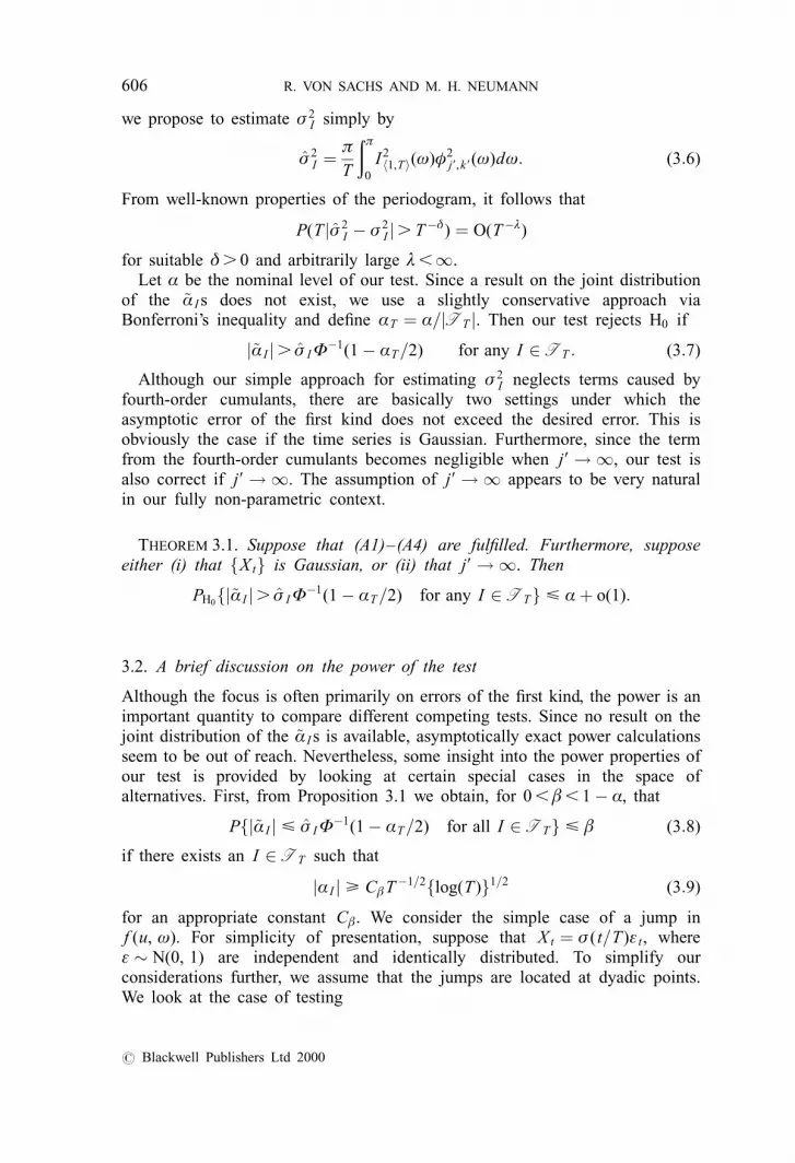
for an appropriate constant Câ. We consider the simple case of a jump inf (u, ù). For simplicity of presentation, suppose that X t � ó (t=T )å t, whereå � N(0, 1) are independent and identically distributed. To simplify ourconsiderations further, we assume that the jumps are located at dyadic points.We look at the case of testing
606 R. VON SACHS AND M. H. NEUMANN
# Blackwell Publishers Ltd 2000
H0: ó (u) � ó0
against
H1: ó (u) � ó0 u 2 [0, 1=2) [ (1=2� 2ÿ j0 , 1]
ó0 � cT u 2 [1=2, 1=2� 2ÿ j0 ]
�where ó0 . 0 is ®xed, and we look for the minimal value of cT that guarantees a`non-trivial power', i.e. â, 1ÿ á. The parameter j0 . 0 is used to model atransient deviation from stationarity. Now it is easy to see that
maxk,k9fjá j,k; j9,k9jg � cT 2ÿ j9=2[2ÿ j0 2 j=2 ^ 2ÿ j=2] (3:10)
where the maximum is attained for (k � 1=2)2ÿ j � 1=2. The right-hand side of(3.10) is maximized by the choice j9 � 0 and j � j0. Hence, (3.9) implies thatcT � ~Câ2 j0=2Tÿ1=2flog(T )g1=2 is a suf®cient height of transient jump in ó (u) oflength 2ÿ j0 . Deviations from ó0 of short duration are modelled by j0 �j0(T)!1 in our simpli®ed context. Hence, it is necessary to incorporatewavelets on these ®ne scales j0 in order to be able to detect such a jump ofminimal height.
So far, bivariate wavelet bases with mixed scale indices have rarely beenused in the statistical literature. However, in our opinion their use has importantadvantages for detecting localized deviations from a time-constant spectraldensity. We refer to the examples of the next section.
4. A NUMERICAL STUDY
We now apply our new test procedures to some simulated examples which givean indication of the performance both on the null hypothesis of stationarity andon the alternative, i.e. with a spectrum f (u, ù) which is not constant in time u.Most of our simulations concern the test based on the segmented periodogram,i.e. with coef®cients ~á(1)
j,k; j9,k9 as given in (3.1), though we also show the use ofthe pre-periodogram as in (3.2). Note that in all our simulated examples thetechnical conditions of the previous section are ful®lled, as we consider Gaussianautoregressive processes. However, as this speci®c choice is due only to theconvenience of the simulation algorithms, we would like to emphasize that thechosen examples have some generic character and could have been realized bysimulating other classes of weakly dependent processes. This robustness is alsocon®rmed by the successful application of our proposed method to our ®nalexample of a real data set.
We start with simulation of some stationary processes, all of lengthT � 1024, by generation of pseudo-random standard normal få tg and, possibly,transformation to some low-order autoregressive process with time-constantspectral density f (ù). For testing the null hypothesis H0 we use the followingset of seven Haar wavelet coef®cients:
WAVELET-BASED TEST FOR STATIONARITY 607
# Blackwell Publishers Ltd 2000
I7,1 � f( j, k; 0, 0)j0 < j < 2, 0 < k < 2 j ÿ 1g:That is, in the frequency direction we start with only the Haar scaling functionö00(ù) on the coarsest scale. This also enters in Equation (3.6) for determiningan estimate ó 2
I for the unknown variance ó 2I . Fixing the nominal level of our test
to á � 0:1 we measure the error of the ®rst kind e0 in counting the exceedencesin (3.7) based on the normal quantile q7,1 for áT � á=jI7,1j � 1=70, which isq7,1 � 2:45:
The ®rst three examples are the standard normal white noise å t, anautoregressive process of order 1, X t � a1 X tÿ1 � å t with parameter a1 � ÿ0:9,and an AR(1) process with a1 � 0:9. In 1000 simulation runs we observed thefollowing rates e0 of false rejection: for Example 1 (white noise), e0 � 0:105;for Example 2 (a1 � ÿ0:9), e0 � 0:109; and for Example 3 (a1 � 0:9),e0 � 0:134. We note that the number of simulation runs is large enough toensure a small enough standard deviation over these pseudo-independent runs,and we observe empirical levels which are quite close to the nominal levelá � 0:1.
In the following examples of non-stationary processes, we simulate theperformance on the alternative H1 to get an idea about the error e1 of thesecond kind. For this we simulated two time-varying autoregressive processes,which can be considered as quite typical examples of realizations of a non-stationary process motivated from Model (2.1):
X t,T �Xp
i�1
ai
t
T
� �X tÿi,T � å t
with autoregressive parameters ai � ai(t=T ) being functions which change overtime.
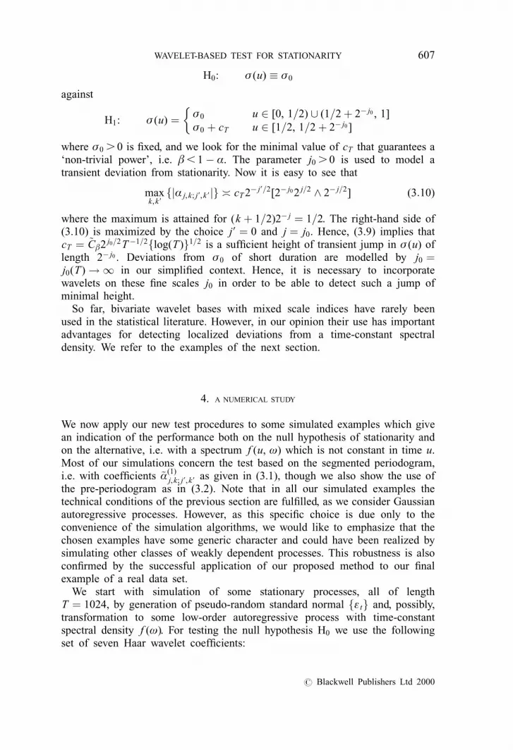
The ®rst, our Example 4, can be considered as a symbolic transient, i.e. shortnon-stationarity of considerable size but short duration (note the similarity tothe simpli®ed example of Section 3.2). We start from a stationary AR(2)process X t � a1 X tÿ1 � a2 X tÿ2 � å t with a1 � ÿ0:5, a2 � 0:2, up to timet � T=2. Then, for the short interval t 2 [T=2, T=2� T=64] we switch toYt � CX t with some parameter C . 1 that we will vary appropriately. Finallyfor t . T=2� T=64 we jump back to the original process Xt. In exactly thesame way as above for the simulations of the stationary Examples 1±3, theerror rates of the second kind e1 � e1(C) depend, of course, on C. For Cvarying between 1.50 (`small jump'), 1.65 (`medium jump') and 1.75 (`largejump') we observe a monotonically falling error e1(C � 1:50) � 0:275,e1(C � 1:65) � 0:121, e1(C � 1:75) � 0:055, by counting the frequency offailure of detection of the jump. This is compatible with the performance onthe null hypothesis H0. We display the time-varying (piecewise in u constant)spectrum of this example, with C � 1:65, in Figure 1. Observe the higherintensity in the short-duration segment in time.
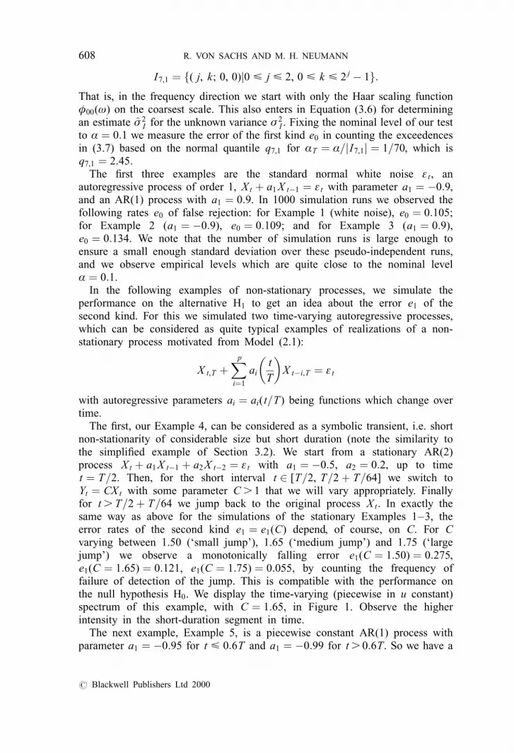
The next example, Example 5, is a piecewise constant AR(1) process withparameter a1 � ÿ0:95 for t < 0:6T and a1 � ÿ0:99 for t . 0:6T. So we have a
608 R. VON SACHS AND M. H. NEUMANN
# Blackwell Publishers Ltd 2000
peak in the spectrum at zero frequency which gets sharper for the secondsegment of piecewise stationarity. Observe the plot in Figure 2 with higherintensity in the second time segment. Using the same set-up as for Examples1±4 and testing only seven wavelet coef®cients will lead to a high error of thesecond kind of e1 � e1(7) � 0:543. It seems that for this and the next example,it is no longer suf®cient to only use the scaling function in frequency ö00(ù)
FIGURE 1. Example 4: True spectrum of AR(2) process `transient with medium-size jump'(C � 1:65).
FIGURE 2. Example 5: True spectrum of piecewise constant AR(1) process.
WAVELET-BASED TEST FOR STATIONARITY 609
# Blackwell Publishers Ltd 2000
on the coarsest level j9 � 0: we need to include also some splitting in thefrequency domain, to detect signi®cant differences by wavelet coef®cientsobtained by integrating over smaller segments in the frequency direction. Thisseems to be necessary whenever the time-changing spectrum shows a higherspatial variability, as for the process of this example 5 with a lot of spectralmass concentrated around zero frequency. So now our new sets of incorporatedindices are
I7,2 � f( j, k; j9, k9)j0 < j < 2, 0 < k < 2 j ÿ 1; j9 � 1, 0 < k9 < 2 j9 ÿ 1gwith 14 coef®cients, and
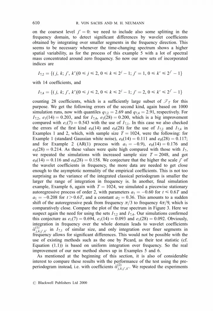
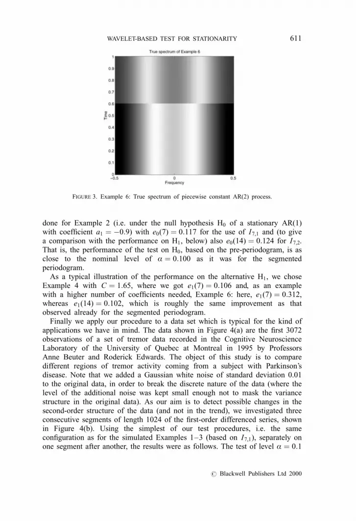
I7,4 � f( j, k; j9, k9)j0 < j < 2, 0 < k < 2 j ÿ 1; j9 � 2, 0 < k9 < 2 j9 ÿ 1gcounting 28 coef®cients, which is a suf®ciently large subset of I T for thispurpose. We get the following errors of the second kind, again based on 1000simulation runs, now with quantiles q7,2 � 2:69 and q7,4 � 2:91, respectively. ForI7,2, e1(14) � 0:203, and for I7,4, e1(28) � 0:200, which is a big improvementcompared with e1(7) � 0:543 with the use of I7,1. In this case we also checkedthe errors of the ®rst kind e0(14) and e0(28) for the use of I7,2 and I7,4 inExamples 1 and 2, which, with sample size T � 1024, were the following: forExample 1 (standard Gaussian white noise), e0(14) � 0:111 and e0(28) � 0:117;and for Example 2 (AR(1) process with a1 � ÿ0:9), e0(14) � 0:176 ande0(28) � 0:214. As these values were quite high compared with those with I7,we repeated the simulations with increased sample size T � 2048, and gote0(14) � 0:116 and e0(28) � 0:158. We conjecture that the higher the scale j9 ofthe wavelet coef®cients in frequency, the more data are needed to get closeenough to the asymptotic normality of the empirical coef®cients. This is not toosurprising as the variance of the integrated classical periodogram is smaller thelarger the range of integration in frequency is. In another, ®nal simulationexample, Example 6, again with T � 1024, we simulated a piecewise stationaryautoregressive process of order 2, with parameters a1 � ÿ0:60 for t < 0:6T anda1 � ÿ0:208 for t . 0:6T, and a constant a2 � 0:36. This amounts to a suddenshift of the autoregressive peak from frequency ð=3 to frequency 4ð=9, which iscomparatively close. Compare the plot of the true spectrum in Figure 3. Here wesuspect again the need for using the sets I7,2 and I7,4. Our simulations con®rmedthis conjecture as e1(7) � 0:694, e1(14) � 0:093 and e1(28) � 0:092. Obviously,integration in frequency over the whole domain leads to wavelet coef®cients~á(1)
j,k; j9,k9 in I7,1 of similar size, and only integration over ®ner segments infrequency allows for signi®cant differences. This would not be possible with theuse of existing methods such as the one by Picard, as their test statistic (cf.Equation (1.1)) is based on uniform integration over frequency. So the realimprovement of our new method shows up in Examples 5 and 6.
As mentioned at the beginning of this section, it is also of considerableinterest to compare these results with the performance of the test using the pre-periodogram instead, i.e. with coef®cients ~á(2)
j,k; j9,k9. We repeated the experiments
610 R. VON SACHS AND M. H. NEUMANN
# Blackwell Publishers Ltd 2000
done for Example 2 (i.e. under the null hypothesis H0 of a stationary AR(1)with coef®cient a1 � ÿ0:9) with e0(7) � 0:117 for the use of I7,1 and (to givea comparison with the performance on H1, below) also e0(14) � 0:124 for I7,2.That is, the performance of the test on H0, based on the pre-periodogram, is asclose to the nominal level of á � 0:100 as it was for the segmentedperiodogram.
As a typical illustration of the performance on the alternative H1, we choseExample 4 with C � 1:65, where we got e1(7) � 0:106 and, as an examplewith a higher number of coef®cients needed, Example 6: here, e1(7) � 0:312,whereas e1(14) � 0:102, which is roughly the same improvement as thatobserved already for the segmented periodogram.
Finally we apply our procedure to a data set which is typical for the kind ofapplications we have in mind. The data shown in Figure 4(a) are the ®rst 3072observations of a set of tremor data recorded in the Cognitive NeuroscienceLaboratory of the University of Quebec at Montreal in 1995 by ProfessorsAnne Beuter and Roderick Edwards. The object of this study is to comparedifferent regions of tremor activity coming from a subject with Parkinson'sdisease. Note that we added a Gaussian white noise of standard deviation 0.01to the original data, in order to break the discrete nature of the data (where thelevel of the additional noise was kept small enough not to mask the variancestructure in the original data). As our aim is to detect possible changes in thesecond-order structure of the data (and not in the trend), we investigated threeconsecutive segments of length 1024 of the ®rst-order differenced series, shownin Figure 4(b). Using the simplest of our test procedures, i.e. the samecon®guration as for the simulated Examples 1±3 (based on I7,1), separately onone segment after another, the results were as follows. The test of level á � 0:1
FIGURE 3. Example 6: True spectrum of piecewise constant AR(2) process.
WAVELET-BASED TEST FOR STATIONARITY 611
# Blackwell Publishers Ltd 2000

did not reject stationarity in the ®rst and the third segment, whereas it rejectedthe null hypothesis for the second segment. This seems to be highly plausibleas by inspection a possible break point can be anticipated in the region shortlybefore data point 2000, whereas the oscillation behaviour in the segmentsoutside this neighbourhood seems to be rather homogeneous. This is inaccordance with the ®ndings of the neurologists who attributed only twodifferent regimes of tremor activity to this particular part of the data.
Summarizing, our (simulated) examples have shown that the two testprocedures not only seem to keep the nominal level on H0, but also showsuf®cient power on H1. As the method based on the pre-periodogram did notlead to a signi®cant improvement for most simple simulated examples, werecommend the use of the algorithmically much faster method based on thesegmented periodogram. However, an estimator based on two-dimensionaltensor wavelet coef®cients of the pre-periodogram investigated in Neumann andvon Sachs (1997) proved useful for situations of considerably differentregularity of the time-dependent spectrum f (u, ù) in time and frequency. Webelieve none the less that there are situations where it might be necessary to
FIGURE 4. Example 7: Tremor data.
612 R. VON SACHS AND M. H. NEUMANN
# Blackwell Publishers Ltd 2000
run a pre-periodogram based test, e.g. if a lot of frequency resolution would benecessary, or where a situation of long-range dependence might call for theneed to incorporate a long range of lags, even for a locally changing spectrumin time. A de®nite advantage, however, is that we can consider the possibilityof performing both estimation and testing simultaneously with the same non-parametric method. That is, we can use the empirical wavelet coef®cients of thevery estimation method we have chosen to perform the test for stationarity, andwill possibly bene®t, at least in the estimation, if we use the pre-periodogram.
ACKNOWLEDGEMENTS
The authors thank the University of Kaiserslautern and the SFB 373 at HumboldtUniversity for making mutual research visits possible. Special thanks go toProfessor Anne Beuter, Cognitive Neuroscience Laboratory of the University ofQuebec at Montreal, and to Professor Roderick Edwards, now at the Departmentof Mathematics and Statistics, University of Victoria, Canada, for collecting andproviding the tremor data (Example 7 of Section 4).
REFERENCES
DAHLHAUS, R. (1996) Asymptotic statistical inference for nonstationary processes with evolutionaryspectra. Athens Conference on Applied Probability and Time Series Analysis, Vol. II (ed. P. M.Robinson, M. Rosenblatt), Lect. Notes Stat. 115, 145±59. New York: Springer.
б (1997) Fitting time series models to nonstationary processes. Ann. Stat. 25, 1±37.б (1999) A likelihood approximation for locally stationary processes. BeitraÈge zur Statistik 56,
UniversitaÈt Heidelberg.GHOSH, B. K. and HUANG, W.-M. (1991) The power and optimal kernel of the Bickel±Rosenblatt
test for goodness of ®t. Ann. Stat. 19, 999±1009.GIRAITIS, L. and LEIPUS, R. (1992) Testing and estimating in the change-point problem of the
spectral function. Lithuanian Math. J. 32, 15±29.JOHNSON, N. L. and KOTZ, S. (1970) Distributions in Statistics. Continuous Univariate
DistributionsÐ1, 2. New York: Wiley.NEUMANN, M. H. (1994) Spectral density estimation via nonlinear wavelet methods for stationary
non-Gaussian time series. Statistics Research Report SRR 028-94, CMA, Australian NationalUniversity, Canberra.
б and VON SACHS, R. (1997) Wavelet thresholding in anisotropic function classes and applicationto adaptive estimation of evolutionary spectra. Ann. Stat. 25, 38±76.
PICARD, D. (1985) Testing and estimating change-points in time series. Adv. Appl. Probab. 17,841±67.
PRIESTLEY, M. B. (1981) Spectral Analysis and Time Series, Vol. 2. London: Academic Press.ROSENBLATT, M. (1975) A quadratic measure of deviation of two-dimensional density estimates and
a test of independence. Ann. Stat. 3, 1±14.ROZENHOLC, Y. (1995) Non-parametric tests of change-point with tapered data. Technical Report
PMA-553. Universite Paris Jussieu.VON SACHS, R. and SCHNEIDER, K. (1996) Wavelet smoothing of evolutionary spectra by non-linear
thresholding. Appl. Comp. Harmonic Anal. 3, 268±82.
WAVELET-BASED TEST FOR STATIONARITY 613
# Blackwell Publishers Ltd 2000