Wavelet-Based Modelling of

Spectral BRDF Data

L. Claustres, Y. Boucher, and M. Paulin

Luc Claustres has completed his Ph.D. at the Institut de Recherche en Informa-

tique de Toulouse (IRIT), Université Paul Sabatier (UPS), 118 Route de Narbonne,

31062 Toulouse Cedex 4, France.

E-mail: Luc.Claustres@irit.fr

Tel: +33 (0)5 61 55 83 29

Fax: +33 (0)5 61 55 62 58

Yannick Boucher is a Research Engineer at the Département d’Optique Théorique

et Appliquée (DOTA), Office National d’Etudes et de Recherches Aérospatiales

(ONERA), BP 4025, 2 Avenue Edouard Belin, 31055 Toulouse Cedex 4, France.

E-mail: Yannick.Boucher@onecert.fr

Tel: +33 (0)5 62 25 26 26

Fax: +33 (0)5 62 25 25 88

Mathias Paulin is an Associate Professor at the UPS, and Researcher at the

IRIT.

E-mail: Mathias.Paulin@irit.fr

1

Abstract

The Bidirectional Reflectance Distribution Function (BRDF) is an im-

portant surface property, and is commonly used to describe reflected light

patterns. However, the BRDF is a complex function since it has four an-

gular degrees of freedom and also depends on the wavelength. The direct

use of BRDF data set may be inefficient for scene modelling algorithms for

example. Thus, models provide compression and additional functionalities

like interpolation. One common way consists in fitting an analytical model

to the measurements data set using an optimization technique. But this ap-

proach is usually restricted to a specific class of surfaces, to a limited angu-

lar or spectral range, and the modelling quality may strongly depends on the

optimization algorithm chosen. Moreover, analytical models are unable to

actually handle the BRDF dependence on wavelength.

In this paper we present a new numerical model for acquired spectral

BRDF to overcome these drawbacks. This model is based on a separation

between the spectral and the geometrical aspect of BRDF, each of them

projected into the appropriate wavelet space. After a brief introduction to

BRDF, advantages of wavelets and the construction of the model are ex-

plained. Then, the performances of modelling are presented and discussed

for a large collection of measured and synthetic BRDF data sets. At last, the

robustness of the model is tested with synthetic noisy BRDF data.

1 Introduction

The Bidirectional Reflectance Distribution Function (BRDF) characterises the

light reflection on surfaces, and is thus used in several domains like scene mod-

elling, image synthesis, optical scattering or remote sensing. The BRDF depends

2

on five parameters at least: two angles for the incident light direction, two angles

for the output direction, and the wavelength. As a consequence, spectral and di-

rectional data sets are usually huge, which leads to an unwieldy storage problem.

Moreover measurement data sets do not allow a continuous representation of the

reflectance. These drawbacks are avoided by modelling. Considerable attention

has been given in recent years to the elaboration of BRDF models and also to their

classification [1] [2]. Two modelling strategies are widely used:

• explicit models that need an explicit description of the surface in term of

simple elements or structures,

• implicit models that do not require an explicit description of the surface

but are based on phenomenological approaches or representations of the

measurements.

The new wavelet-based numerical model presented in this paper belongs to this

last category. It has been designed to efficiently represent, in term of compression

and computing time, the spectral BRDF data of all kind of surfaces as long as a

measured data set is available.

Section 2 introduces the definition of the BRDF and its properties, then ex-

plains the main shortcomings to analytical modelling and particularly to themeasure-

and-fitapproach. Section 3 presents the general formulation of the wavelet trans-

form, and its most useful properties. Section 4 describes previous approaches to

numerical BRDF modelling using wavelets and the method used to construct our

new BRDF model is developed. Section 5 discusses modelling results achieved on

real acquired BRDFs as well as synthetic BRDF data set. Section 6 addresses the

model sensitivity to multiplicative and additive noise with realistic noise levels.

We conclude and point out lines of future research in Section 7.

3

2 BRDF definition and properties

2.1 Definition

The Bidirectional Reflectance Distribution Function (BRDF) is a distribution in

the mathematical point of view, which describes the relationship between the in-

coming irradiance and the radiance reflected or scattered by a surface. Usually,

the BRDF expression is relative to the target’s local space [3]:

fr(ωi, ωr, λ) =dLr(ωr, λ)

dEi(ωi, λ)

=dLr(ωr, λ)

Li(ωi, λ) cos θidωi

, (1)

whereEi is the incoming irradiance, andLi (respectivelyLr) is the incoming

(respectively outgoing) radiance in lighting directionωi = (θi, φi) (respectively

viewing directionωr = (θr, φr)). This definition ignores polarization, time varia-

tion, frequency shift, and surface position dependence in order to reduce complex-

ity. This BRDF definition is accurate enough for most remote sensing applications

and scene modelling purposes. BRDF support is then reduced toH2i × H2

r × RwhereH2

i is the incident hemisphere,H2r is the reflection hemisphere, andR the

wavelength space.

2.2 Physical Properties

The BRDF has four important and interesting properties:

1. Non-negativity: BRDF value is strictly positive

fr(θi, φi, θr, φr, λ) ≥ 0 (2)

4

2. Helmholtz reciprocity: the behavior of the surface is independent of the

luminous flux direction [4] , i.e.

fr(θi, φi, θr, φr, λ) = fr(θr, φr, θi, φi, λ) (3)

3. Energy conservation: the energy reflected by the surface is not greater than

the incoming energy on the surface, i.e. for each possible incoming direc-

tion ωi and outgoing directionωr (assuming integration over wavelength is

implied)

dΦr

dΦi

=

∫H2

i

∫H2

r

fr(ωi, ωr)Li(ωi) cos θi cos θrdωidωr

∫H2

i

Li(ωi) cos θidωi

<= 1, (4)

wheredΦi (respectivelydΦr) is the incoming (respectively outgoing) lumi-

nous flux

4. Isotropy: for a lot of surfaces the reflectance does not change with respect

to the surface orientation (isotropicBRDF), i.e. for any wavelength

fr(θi, φi, θr, φr) = fr(θi, 0, θr, |φr − φi|) = fr(θi, θr, φ = |φr − φi|) (5)

otherwise the BRDF is said to beanisotropic.

For measurements on homogeneous surfaces, Equation(3) allows to simplify

BRDF data sets [5]. This simplification is often used in image synthesis. How-

ever for real measurements on heterogeneous surfaces, this equation is not strictly

applicable.

2.3 Modelling BRDF

BRDF is an input data of several applications including target and background sig-

nature modelling, radiative transfer simulation, and inversion of thematic physical

5

models. However, the large amount of measurement samples needed to accurately

describe the BRDF does not allow the use of raw data, and modelling is usually

required. Indeed lots of applications, like scene modelling, manage many differ-

ent BRDFs at the same time and memory requirement can be easily prohibitive.

On the one hand a model has to provide a good compression scheme. On the

other hand we are interested in a convenient, accurate, and efficient representa-

tion. These reasons mainly explain the success of analytical models, but these

models are not well-suited for spectral BRDF modelling of arbitrary surfaces.

Actually, model parameters for most surfaces are not directly available. Ad-

vanced numerical optimization techniques retrieve the best parameter values by

minimizing a distance between modelled and measured data. This modelling

can suffer from numerical instabilities in non-linear fitting routines, and results

strongly depend on initial conditions. Secondly, analytical models, either phe-

nomenological or based on a physical theory, lack generality. Physically-based

models start with specific assumptions about the surface and are only able to

predict the reflectance of surfaces that closely match those assumptions. Phe-

nomenological models are custom-made and are not suitable for arbitrary BRDF.

Moreover, as the viewing angle of the sensor increases, the effects of BRDF be-

come exacerbated, and significantly affect the accuracy in off-nadir views. Thus,

most analytical models become not appropriate in these cases. Therefore, mod-

els should cover the entire range of possible angles of incidence and reflection.

At last, to the best of our knowledge, no analytical model explicitly handles the

wavelength dependence of the BRDF.

These reasons press us to develop a new numerical BRDF model, more gen-

eral as it does not rely on either specific assumptions or physical theory. The

6

main idea is to project the BRDF measurement data set onto a new space, which

is usually more efficient and convenient. Primer representations based on projec-

tive methods for BRDF modelling usedspherical harmonics[6] [7] [8]. But the

evaluation cost of these functions is prohibitive due to theirglobal supporton the

sphere. Wavelets arelocally defined, consequently they are faster. Furthermore

they offer a better and more flexible compression scheme. There are also some

mathematical constructions of wavelets based on spherical harmonics [9] [10] but

they have no concrete application and are still at a formal state.

3 Wavelet theory

3.1 Introduction

Wavelets have become very popular during the last decade due to many of their

interesting properties [11] [12]:

• compression: able to manage large data sets

• multiresolution: a reconstruction at different levels of accuracy is possible

• efficiency: the reconstruction of the signal is done in a logarithmic time

according to the number of samples

• denoising: small and localized signal variations are avoided by the com-

pression

Moreover wavelets handle low-frequency signals with localized high-frequencies

very well. They should be naturally adapted to the strong variations of acquired

BRDFs (specular peak, hot-spot phenomenon).

7

3.2 Definition

The discrete wavelet transform is a filtering operation that separates a signal into a

low-frequency part (approximation) and a high-frequency part (details), via con-

volution (projection on a wavelet function basis). Then separating again, recur-

sively, the approximation part, the discrete wavelet transform leads to a decom-

position at differentresolutionsor scales. The more general formulation of the

discrete wavelet transform of a sampled functionf can be written as follows:

f =∑

k

ak0ϕ

k0 +

n∑

j=0

∑m

dmj ψm

j (6)

ψmj (respectivelyϕk

j ) is the wavelet (respectively scaling) function numberm (re-

spectivelyk) at decomposition level numberj. The first one encodes the details

while the second one encodes the approximation of the sampled functionf . The

corresponding projection coefficientsdmj andak

j are computed using fast recursive

algorithms. Computing scaling and wavelet coefficients from a fine resolution to

a coarser resolution is calledanalysis:

akj =

∑

l

h̃k,lj al

j+1 (7)

dmj =

∑

l

g̃m,lj al

j+1 (8)

The inverse operation, consisting in retrieving the finest approximation starting

from coarser level, is calledsynthesis:

alj+1 =

∑

k

hk,lj ak

j +∑m

gm,lj dm

j (9)

Wavelet transform may be viewed as a filtering operation where coefficientsh̃, g̃

are analysis filters andh, g are synthesis filters. Wavelet compression consists in

removing weak wavelet coefficients (setting their values to zero) in the final de-

composition of the function (equation 6). The analysis process computes the final

8

decomposition of the function (wavelet transform) while the synthesis process re-

constructs the function from its compressed version (inverse wavelet transform).

The main thing to notice is that this formulation isgenericbecause it does not rely

on a particular wavelet function or support space. As a consequence, algorithms

are pretty similar for any transform. There is only one requirement: the support

space must be aHilbert space [13].

4 Wavelet-based BRDF modelling

4.1 Introduction

A parallel can be drawn between the analytical approach [14] and a numerical

approach based on wavelets. Indeed, the spirit of both methods is very similar and

both modelling process are illustrated on Figure 1. Theinverse modeconsists in

retrieving the model’s parameters from the measurement data set. In the analytical

case a numerical optimization is performed while in the numerical case wavelet

transform and compression are applied. Thedirect modeconsists in computing the

BRDF value for any possible incoming/outgoing direction and wavelength, from

the model’s parameters. In the analytical case the model formula is evaluated

while in the numerical case the inverse wavelet transform and an interpolation

scheme are applied. The better the model is, the lower the distance between the

original and the simulated BRDF is. Before the complete presentation of the

modelling process in the next sections, we present previous work on wavelet-

based BRDF modelling.

9

4.2 Previous work

Schröder et al. [15] are the first researchers to mention the use of wavelets for

BRDF modelling. They introducespherical waveletsto efficiently represent func-

tions on the sphereS2. A function defined overS2 is approximated by a piece-

wise constant function over a set of triangles almost regular in term of solid angle

1. The triangle set is constructed using a recursive subdivision starting from an oc-

tahedron (or a tetrahedron on the hemisphereH2). At each level the triangles are

subdivided into four children, then projected on the sphere, until a givenaccuracy

level(Figure 2).

Schröder et al. define a multiresolution analysis in the space of finite energy

functions defined overS2 thanks to thelifting cheme[16]. The spherical wavelet

basis (Figure 3) is a Haar-like basis derived from the well-known Haar basis [17]

[18]. The most important thing to notice is that this construction isparameter-

ization independent, which is not the case of a previous method introduced by

[19] using tensor product. But the work of Schröder et al. is still restricted to

function defined overH2 while BRDF is potentially a 5D function defined over

H2×H2×R (incident and outgoing direction, and wavelength). In fact, spherical

wavelets are suitable for directional-hemispherical reflectance, or BRDF at a fixed

incident direction, without taking into account the dependence on wavelength.

A more complete model was presented by Lalonde et al. [20]. They use mul-

tidimensional wavelets (4D) on the real line to handle BRDF at fixed wavelength,

which requires a mapping fromH2 × H2 to R4. The use ofNusseltembed-

ding [21], to compromise on the matter of redundancy at the poles, provides an

elegant solution but cannot entirely avoid the distortion introduced by the map-

1Generating a uniform distribution of points on the sphere is still an open problem

10

ping. This representation is still stronglyparameterization dependent. The global

control of the compression (thresholding) induced by the single multidimensional

wavelet transform is also one of the most important drawbacks of this representa-

tion. Nevertheless, this work should be easily extended to include the dependence

on wavelength (with an additional dimension).

4.3 Model description

In this section we introduce a new BRDF model based on wavelets. Our contribu-

tion is to separate the BRDF into a spectral part defined overR and a directional

or geometrical part defined overH2. Each part is projectedindependentlyon the

appropriate wavelet space, that is using spherical wavelets for the angular depen-

dence, and one-dimensional wavelets for the dependence on wavelength. We have

chosen thestandardapproach [11] that uses product of decompositions to trans-

form multidimensional signals, in contrast with thenon-standardapproach [11]

(used by Lalonde), which consists in building multidimensional wavelet bases

from one-dimensional bases using a tensor product of basis functions. The key

idea is to perform multipleatomic transforms, that is to say transforms defined

over a single space (not a product of spaces), instead of using a single multi-

dimensional transform. The last method is theoretically more efficient, but the

former has many advantages.

First we can increase the compression ability by exploiting the coherence in

each space in addition to the coherence in the hidden dimension-connections. Sec-

ondly apartial transform or reconstruction can be computed, i.e. we do not need

to perform the complete 5D transform. Indeed, we can choose which spaces will

be used, providing a more flexible model that allows the representation of all kind

11

of BRDF: isotropic, anisotropic, spectral or at a fixed wavelength. At last, our

approach does not require any mapping since the model is naturally defined on

the support of the BRDF.

4.3.1 BRDF projection

The initial step of our method consists in projecting the BRDF measurement data

set into the appropriate wavelet spaces. A first recursive subdivision is used to

store BRDF data according to the incoming direction. Each triangle of the subdi-

vision stores the directional-hemispherical reflectance distribution corresponding

to the direction aimed by the triangle centre. Then, a second recursive subdi-

vision is used to store the reflectance data according to the outgoing direction.

Each triangle stores a real value, or a spectrum in the spectral case. Two spherical

wavelet transforms are applied in the case of a BRDF at a fixed wavelength (on

incoming and outgoing directions). In the case of a spectral BRDF, an additional

level is required: a one-dimensional wavelet transform is applied on each BRDF

spectrum.

Although only one wavelet basis is available for the spherical transform, many

bases are available for the dependence on wavelength since one-dimensional bases

are common [11]. Our model selects the best basis according to the modelling

error among a set of 52 different bases. Nevertheless, many bases belong to

the same family but differ from one another in their properties (vanishing mo-

ments, support width, order, etc.): Daubechies [22], Symmlet [11], Coiflet [23],

Battle-Lemarié [24], Beylkin [23], Adelson [25], FBI [26], Vaidyanathan [27] An-

tonini [28], Villasenor [29] [30] [31], Burt-Adelson [11], Brislawn [32], Cohen-

Daubechies-Feauveau (CDF) [33], Spline [11], Odegard [34], and Pseudo-Coiflet

12

[35]. The restriction to the use of the Haar basis on the recursive subdivision is

not annoying because this basis is well-suited to signals with discontinuities as

shown by Schröder [15]. It will be efficient for BRDF modelling of shiny sur-

faces with narrow peaks, which are very common in scene representing artificial

surfaces. Moreover, it allows a fast sampling scheme based on the multiresolution

of the wavelet decomposition to perform importance sampling of the BRDF. This

technique can dramatically reduce the variance of Monte Carlo simulations [36]

intensively used into radiative transfer codes.

In fact, isotropic BRDFs are simpler than anisotropic ones, and this property

can be used to simplify the transform process. Indeed, any BRDF value can be

recovered from the BRDF data in the plane whereφi = 0, by a rotation ofφ

around the local surface normal. So the spherical wavelet transform on incoming

directions is not relevant here, since we do not store all BRDF measurements but

only a small part according to the plane whereφi = 0. Avoiding this transform

is possible without any fuss using the standard approach, while it is not possible

with the non-standard approach, which would require the elaboration of a specific

3D model instead of the general 5D model. With our approach, we simply have

to ignore the atomic wavelet transform onH2i and to perform both other atomic

transforms onH2r andR.

The technical details of the model, as well as the algorithms and the data

structures needed for implementation can be found in [36]. We have put the source

code for a wavelet-based representation of different radiometric terms into a C++

library calledThe Discrete Wavelet Transform Library(DWTL). The DWTL is

part of theRay Of Lightproject, and is available for free at http://www.realistic-

rendering.org.

13

4.3.2 Compression strategy

Wavelet coefficients express local signal coherence at different levels according to

a specific norm. If a coefficient is weak, there will be no strong variation between

two levels, so the lowest level will approximate information without introducing

a large error. Thus, wavelet compression is simply done by removing weak coef-

ficients of the projected BRDF.

In our modelling approach, the wavelet compression is performed in each

space where the transform took place. The coherence between directional-hemispherical

reflectances according to incoming direction is fully used. The same for spec-

tra coherence and for BRDF values according to reflected direction. At last, the

coherence according to wavelength for spectral BRDFs is also used. We have

demonstrated in [36] that for a given error level we can reach a better compres-

sion ratio than obtained by Lalonde.

Usually, multidimensional wavelet transform uses a single threshold, which

implies a global error control. We have prefered to use a global threshold for

eachspace. Furthermore, we have set up an adaptive threshold, starting from each

global threshold, by scaling the threshold according to the local level of the BRDF.

4.3.3 BRDF reconstruction

The inverse wavelet transform only allows the reconstruction of the original dis-

crete BRDF, starting from the compressed version. But many applications, such

as radiative transfer codes, require a BRDF continuously defined for all combi-

nations of incident angles, reflected angles, and wavelengths. Consequently, we

have interpolated the BRDF values after the reconstruction. A detailed study of

interpolation techniques is out of the scope of this paper, and is not related to the

14

wavelet representation. Indeed, the estimation of a functionf for arbitrary con-

figurations, where only a sampled version off is available, is a central problem in

signal processing [37].

Here we use well-known interpolation methods depending on the require-

ments: forC0 BRDF, we use linear interpolation for the spectral part and barycen-

tric interpolation over the triangles [38] for the directional one; for a more contin-

uous BRDF (C2), we use cubic B-Splines [37] for the spectral part and Clough-

Tocher interpolant [39] for the directional one.

5 Results

For determining the performances of the model, we need estimators of the differ-

ence between the original BRDF and the simulated one after an analysis-synthesis

cycle. Particularly, we have chosen the relative errorsεr1 andεr

2 in term ofL1 and

L2 norms according to compression ratio:

εr1 =

1

n

∑

i

|f ′i − fi|fi

(10)

εr2 =

√√√√ 1

n

∑

i

(f ′i − fi)

f 2i

2

(11)

wherefi are the values of the original BRDF,f ′i are the values of the reconstructed

BRDF from its compressed version, andn is the total number of samples in the

measurement data set. The compression ratiorc is the ratio of the initial number

of measurement points to the final number of remaining wavelet coefficients after

compression. It is related to the compression ratetc (percentage of initial data

removed by compression) by the following expression:

tc = 100− (100

rc

)

15

The number of wavelet coefficients for a compression ratio of 1:1 is equal to the

initial number of samples for the measured BRDF, i.e. the BRDF is just projected

into the wavelet spaces without any compression. A small initial error appears

for this projection becauseS2 is sampled regularly in term of(θ, φ) angles for

the BRDF measurement and not regularly in term of solid angle as the recursive

subdivision does.

5.1 Data

In this paper we present results achieved on measured and simulated BRDFs. Real

BRDFs have been measured by the goniometer set up at the ONERA [40], over

a wide variety of surfaces. We have selected artificial targets (cloth, plastic, ply-

wood, spectralon, velvet), but also natural ones (green and dry grass, wood, sand).

The total number of measurement points is 485,376 for one material (476 direc-

tions and 1024 wavelengths). The precision of the measurement is better than 5%

in the spectral range 420-950 nm with a spectral resolution of 3 nm and a spec-

tral sampling of 0.5 nm. However, we have used here a spectral sampling step

of 5 nanometers, which is fine enough for our requirements. Zenithal angles are

sampled every ten degrees, and the relative azimuth angle every twenty degrees.

5.2 Estimation of the modelling error

5.2.1 Reflectance spectra

Because our BRDF representation has two independent parts, one for the direc-

tional aspect of the data, and one for the spectral aspect of the data, these two parts

can be used as stand-alone representations.

16

For this reason, we have first tested the spectrum modelling with reflectance

spectra extracted from measured BRDFs at fixed incoming and outgoing direc-

tion, but also with other radiometric terms such as spectral measured radiance and

emissivity. The Figure 4 shows the compression rate achieved according to dif-

ferent wavelet bases, for a constant modelling errorεr2 = 2 %, and on different

acquired spectra. A graphical representation of the reconstructed spectra is shown

in Figures 5 and 6, corresponding respectively to the spectral emissivity of a paint,

and the spectral radiance of sand, with different compression ratios.

Table 1 contains more quantitative results and shows that our model is efficient

to represent many different kind of spectrum with a small number of samples from

the initial data. In this table, r1 (respectively r2) is a green grass (respectively

paint) reflectance measured in the spectral range 0.3-4 microns; l1 (respectively

l2) is a sand (respectively canopy) radiance measured in the spectral range 0.3-

13.6 microns; e1 and e2 are IR paint emissivities measured in the spectral range

2.5-21 microns. Moreover, the model provides a smooth profile for the spectrum

by removing the noise. Even if the modelling error growths with the compression

ratio, we think that, in many cases, a better spectral profile is reconstructed, be-

cause of the denoising. This interesting property will be investigated precisely in

Section 5.3.

5.2.2 Isotropic BRDF

BRDF for fixed wavelengths : Table 2 presents compression ratios and corre-

sponding modelling errors for acquired isotropic BRDFs at different fixed wave-

lengths. All measurement data sets can be compressed up to 64:1 with a globalL1

andL2 error<10%, except the plastic one. This sample is the most specular (dif-

17

fuse and specular parts differ by a factor 100), with a large peak leading to a large

discontinuity. As the wavelet transform is basically a filtering operation, a high

compression ratio smooths the specular peak. However, the specular peak is well-

preserved with a medium compression rate. Moreover, we have shown in [41] that

wavelet modelling has similar performances than the analytical modelling at fixed

wavelength for diffuse surfaces, and better ones for specular surfaces.

Figure 7 shows the plots of the BRDF of three different samples (cloth, sand,

and dry grass) for a fixed incoming direction and azimuth angle. The worst re-

sults, apart from the plastic one, are achieved for the dry grass (Table 2), which is

the measurement with the lowest BRDF level (about 0.03sr−1). Thus, for a con-

stant noise level, the signal-to-noise ratio (SNR) is weaker and the signal is lower.

In this case the model hardly makes the difference between BRDF variations and

noise (Figure 7c). In contrast, modelling is accurate for the sand and the cloth

sample, even for some radical thresholds. The wavelet-based representation cor-

rectly handles the backscattering of the sand sample (Figure 7b) and the relative

"specularity" of the cloth sample (Figure 7a).

Spectral BRDF : Table 3 shows results achieved on isotropic spectral BRDF

data. For each compression ratio, the best wavelet basis selected by the model is

given. Modelling error according to compression is often better than it is in the

case of a fixed wavelength (especially for the plastic BRDF). All available mea-

surement data sets can be compressed up to 128:1 and a globalL1 error<10% and

L2 error<20%. The main reason is the smooth spectral variations of the BRDFs.

The behaviour of the model is compared to the measurements, as illustrated in

Figure 8 for the cloth target and two different wavelet bases and compression ra-

tios. In addition to the modelling error, the spectral shape might be a criterion for

18

the wavelet basis selection. Indeed, this shape strongly depends on properties of

the chosen basis.

However few materials present larger errors than those obtained in the case of

fixed wavelength. One possible explanation is influence of the noise, which is not

spectrally flat. Actually, our data are especially noisy in the range 400-450 nm

and the compression removes this noise, that introduces an error with no physical

signification (Figure 9), which only represents the difference between the original

noisy spectrum and the simulated denoised one.

5.2.3 Anisotropic BRDF

The goniometer of the ONERA is fully automatic for isotropic measurement, but

for anisotropic measurement, a manual rotation is applied to the sample between

each acquisition, resulting in an unwieldy process. This is the reason why we

have measured a single anisotropic material (a glazed velvet), with an azimuth

angle step of fifteen degrees. The final number of samples was 6,309,888 for the

whole BRDF data set. The velvet sample presents pronounced directional effects

(anisotropy), and the detection limit of the device is reached in some part of the

measured BRDF. In those parts, the overall signal level is very low and the (SNR)

is very weak. To be more exhaustive in the fixed wavelength case, we have also

tested the performances of the model with synthetic BRDF data sets.

BRDF for fixed wavelengths : Table 4a presents the modelling error for the

anisotropic velvet BRDF data set and for a synthetic BRDF data set generated

using the anisotropic Ward’s BRDF model [42]. Until a compression ratio of 16:1,

modelling is as good for the velvet as for the synthetic data. Beyond this ratio,

the L2 error becomes very large for the velvet sample unlike for the synthetic

19

BRDF, while theL1 error is still good in both cases. This phenomenon is here

again probably induced by the noise of the measurements on the velvet. Indeed,

relativeL2 error is more sensitive to modelling errors for low BRDF levels. As

wavelet compression smoothes the BRDF and removes the noise, the modelling

error always raises with the compression ratio, even if denoising is, in some cases,

an interesting property of the model.

Spectral BRDF : In the spectral case, as far as we know, no analytical BRDF

models are available, so the performances of the model have only been estimated

with the glazed velvet data set. As expected, we have noticed the same increase

of theL2 error with compression ratio, but more strongly marked (see Table 4b).

The most probable reason is that the SNR of the measurement device depends on

the wavelength and is relatively weak in some regions of the spectrum. Indeed,

some measured BRDF values in the range 400-450nm are negative because of the

noise, that has no physical meaning. To ensure the non-negativity rule (Equation

2), we have replaced these negative values by a low BRDF bound. This process

introduces yet virtual discontinuities in the smooth BRDF spectra with, as a con-

sequence, oscillations around the discontinuities after compression (Figure 10).

This effect, known as the Gibbs Phenomenon [43], may explain, at least partly,

the largeL2 observed error.

5.3 Noise sensitivity

Robustness is one of the most important properties desirable for modelling of

measurement data set. In particular, measured BRDF data are always more or

less noisy, and the model should be proof against measurement noise. In this

20

Section we estimate the sensitivity of our model according to Gaussian additive

and multiplicative noises.

5.3.1 Data

First of all, a BRDF data set had to be chosen for this study. Since measurements

are noisy by nature, we have used a synthetic data set to test the robustness of

the model, so as to be able to parameter the noise level. We have built a vir-

tual measurement data set using the Phong’s BRDF model [44], which calculates

the directional variations of the synthetic BRDF. At this first directional kernel,

we have added a spectraly-dependent kernel. Its spectral profileS(λ) is a unit

frequency-varying sine curve with an amplitude of±20 %, with no physical re-

alism but that allows us to test the performance from smooth to strong spectral

variations between 0.5 and 1 micron:

S(λ) = 1 + 0.2 ∗ cos(2 ∗ π ∗ λ/λ0) with λ0 = −150/500 ∗ λ + 350nm,

whereλ belongs to the range[500nm, 1000nm]. For each possible directions set,

the spectrum is scaled by the BRDF level computed through the evaluation of

the Phong’s model, and modulated byS(λ). Spectral sampling is done every 2

nanometer and the recursive subdivision level for the spherical wavelet projection

is equal to 3, which results in a set of 449,792 samples.

Secondly, we have taken care to set realistic noise levels for this experiment.

For convenience, we have not considered the spectral variation of the noise. The

additive noise level has been estimated from a simple dark measurement on a

perfect absorber. This level is about10−3sr−1 at nadir viewing for the considered

measurement device. A realistic additive noise follows a law in1/ cos θr [45], and

we have also taken this effect into account to closely match the device noise.

21

Multiplicative noise level can be estimated from the standard deviation of real

and spectraly flat measured BRDFs. For our device, this level is about0.2 %, and

does not depend on angular variations. To perform a more complete evaluation,

we have not limited ourselves to these levels and have also included several higher

noise levels.

5.3.2 Method

We have constructed two initial data sets for this test. The first one was the com-

pressed version of the synthetic BRDF, using a Villasenor wavelet basis and a

compression ratio of 8:1 (case I). The second one was using a Brislawn wavelet

basis and a compression ratio of 16:1 (case II). The modelling error introduced by

the compression is presented in Table 5.

The method consists in adding noise to the initial BRDF data sets according

to a chosen noise type and level. A first comparison is performed, called "initial

case", to evaluate the impact of the noise without any compression. Then, the

noisy data set is compressed with the same configuration used for cases I and II.

The final step for the completion of the test consists in comparing the simulated

sets to the original one as illustrated in Figure 11.

For a more qualitative evaluation, we also includespectral anglecomparisons.

The spectral angle is a physically-based spectral criterion that supplies the spec-

tral similarity between two spectra by calculating the angle between them, treat-

ing them as vectors in a space with dimensionality equal to the number of bands

[46]. Usually, a spectral angle< 0.1 radian means that spectra are very sim-

ilar. We choose three different spectral anglesas1, as2, andas3, correspond-

ing respectively to the following configurations:[θi1 = θr1 = 60, φ1 = 180],

22

[θi2 = θr2 = 60, φ2 = 0], and[θi3 = 60, θr3 = 30, φ3 = 180].

5.3.3 Results for multiplicative noise

Table 6 summarizes the results achieved on noisy data in the multiplicative case.

One can see that the model is able to remove low noise level with the highest

compression ratio (case IIa and IIb). The modelling error is quite similar to the

one obtained for compressed noise-free data (initial cases I and II). On the other

hand, the lowest compression ratio is not sufficient to denoise the data. Neverthe-

less, compression always provides a beneficial effect on the noisy spectrum, since

the shape of the spectrum after compression is closer to the original noise-free

spectrum, as shown by the different values of the spectral angle. Moreover, for

the highest noise level, the modelling error induced by the noise is larger than the

one induced by the compression. This error is reduced by a large amount as the

compression ratio increases.

Figure 12 shows a close-up for a multiplicative noise of 5% (case IIc) in the

range 500-600 nm. One can see that the model is not sensitive to the noise, be-

cause the compressed noise-free BRDF spectrum closely match the compressed

noisy BRDF spectrum. The small offset between these two spectra is due to the

compression in the geometrical domain (spherical wavelet transform) that gener-

ates a spectral approximation in the neighbourhood of a given direction by aver-

aging spectra around.

Figure 13 represents the four BRDF sets (noise-free uncompressed, noise-free

compressed, noisy uncompressed, and noisy compressed) at fixed wavelength and

fixed incoming direction. Here again, the compressed noisy set is closer to the

original set than the uncompressed noisy set.

23

5.3.4 Results for additive noise

Table 6 contains the results achieved on noisy data in the additive case. The noise

increases with the reflection angleθr with respect to the law in1/ cos θr. At

grazing angles, the high noise level explains that the difference between the com-

pressed noisy set and the original one is larger than in the multiplicative case.

However, the model presents the same overall behaviour: compression always

improves the similarity between compressed noisy and noise free data sets, as

shown by the spectral angles values, even at grazing angles.

Figure 13 represents the four BRDF sets (noise-free uncompressed, noise-free

compressed, noisy uncompressed, and noisy compressed) for an additive noise

level of 5 ∗ 10−3sr−1 (case If) at fixed incoming and outgoing directions in the

range 800-900 nm. The compressed noisy BRDF set is very similar to the com-

pressed noise-free BRDF set. Moreover, variations due to the noise cannot be

confused with the spectral BRDF variations.

6 Conclusion and future work

We have presented a new BRDF model based on wavelets to overcome the main

shortcomings to analytical modelling. This model is suitable and efficient for any

kind of BRDF measurement data set, without any spectral or angular range lim-

itation. It has been tested against many different surface samples and the model

agrees reasonably well with the measurements, even for some radical compression

thresholds. Usually, isotropic BRDFs can be compressed up to 64:1 with a global

relative error < 10%. The model is less impressive on anisotropic BRDFs, but

the main reason is certainly the poorer quality of the measurement in this case.

24

Indeed, results are still pretty good with a synthetic anisotropic BRDF data set.

Moreover we have demonstrated the denoising capability of the model for syn-

thetic BRDF data sets. The model is very robust to moderate but realistic noise

levels, for multiplicative noise as well as additive noise, and the compressed noisy

BRDF data set is always closer to the original noise-free data set than the uncom-

pressed noisy data set.

Nevertheless, some work remains to be done. Interpolation schemes in the

specific case of BRDF should be more deeply investigated. Another perspective

is to improve spherical wavelet bases. We should for instance use the work of

Bonneau [47] about the design of Haar-like bases thanks tosemi-orthogonality.

In the same way, one-dimensional basis selection should be more efficient using

thebest basisalgorithm [48]. At last, we left as future work the use of the wavelet

projection for classification, like Kaewpijit did [49] for hyperspectral data.

Acknowledgements

We specially thank Sophie Lacherade, Emmanuel Christophe and Christophe Mi-

esch for their contributions to the final version of this paper.

25

References

[1] N.S. Goel. Models of vegetation canopy reflectance and their use in esti-

mation of biophysical parameters from reflectance data. InRemote Sensing

Reviews, volume 4, pages 1–212, 1988.

[2] B. Pinty, N. Gobron, J.-L. Widlowski, S. A. W. Gerstl, M. M. Verstraete,

M. Antunes, C. Bacour, F. Gascon, J.-P. Gastellu, N. Goel, S. Jacquemoud,

P. North, W. Qin, and R. Thompson. Radiation Transfer Model Intercompar-

ison (RAMI) Exercise.Journal of Geophysical Research, 106(D11):11,937–

11,956, 2001.

[3] F. E. Nicodemus, J. C. Richmond, J. J. Hsia, I. W. Ginsberg, and T. Limperis.

Geometric Considerations and Nomenclature for Reflectance. Monograph

161, National Bureau of Standards (US), October 1977.

[4] M. Minnaert. The Principle of Reciprocity in Lunar Photometry.Astrophys-

ical Journal, 93:403–410, 1941.

[5] W.C. Snyder. Reciprocity of the BRDF in Measurements and Models of

Structured Surfaces.IEEE Transactions on Geoscience and Remote Sensing,

36(2):685–691, 1998.

[6] B. Cabral, N. Max, and R. Springmeyer. Bidirectional Reflection Functions

from Surface Bump Maps. InComputer Graphics (ACM SIGGRAPH ’87

Proceedings), volume 21, pages 273–281, 1987.

[7] Francois Sillion, James R. Arvo, Stephen H. Westin, and Donald P. Green-

berg. A Global Illumination Solution for General Reflectance Distributions.

26

In Computer Graphics (ACM SIGGRAPH ’91 Proceedings), volume 25,

pages 187–196, July 1991.

[8] Stephen H. Westin, James R. Arvo, and Kenneth E. Torrance. Predicting Re-

flectance Functions From Complex Surfaces. InComputer Graphics (ACM

SIGGRAPH ’92 Proceedings), volume 26, pages 255–264, July 1992.

[9] W. Freeden and U. Windheuser. Spherical Wavelet Transform and its Dis-

cretization, Tech. Rep. 125. Technical report, Universität Kaiserslautern

Fachbreich Mathematik, Kaiserslautern , Germany, 1994.

[10] M. Conrad and J. Prestin.Multiresolution on the Sphere, pages 165–202.

Springer-Verlag, Heidelberg, 2001.

[11] I. Daubechies.Ten Lectures on Wavelets. Society for Industrial and Applied

Mathematics, Philadelphia, 1992.

[12] S. Mallat.A Wavelet Tour of Signal Processing. Academic Press, San Diego,

1999.

[13] M. R. Raghuveer and S.B. Ajit.Wavelet Transforms : Introduction to Theory

and Applications. Addison-Wesley, Reading, 1999.

[14] M. M. Verstraete, B. Pinty, and R. E. Dickinson. A physical model of the

bi-directionnal reflectance of vegetation canopies.Journal of Geophysical

Research, 95(20):755–765, 1990.

[15] Peter Schroder and Wim Sweldens. Spherical Wavelets: Efficiently Repre-

senting Functions on the Sphere. InComputer Graphics Proceedings, An-

nual Conference Series, 1995 (ACM SIGGRAPH ’95 Proceedings), pages

161–172, 1995.

27

[16] Wim Sweldens. The Lifting Scheme: A Construction of Second Generation

Wavelets.SIAM Journal on Mathematical Analysis, 29(2):511–546, 1998.

[17] M. Girardi and W. Sweldens. A New Class of Unbalanced Haar Wavelets

that form an Unconditional Basis for Lp on General Measure Spaces. Tech-

nical Report 1995:2, Departement of Mathematics, University of South Car-

olina, Carolina, May 1995.

[18] M. Mitrea. Singular Integrals, Hardy Spaces and Clifford Wavelets.Com-

munications of the ACM, 32(6):343–349, 1980.

[19] S. Dahlke, W. Damen, E. Schmitt, and I. Weinreich. Multiresolution Analy-

sis and Wavelets on S2 and S3, Tech. Rep. 104. Technical report, Institut fur

Geometrie und Angewandete Mathematik, Aachen , Germany, 1994.

[20] P. Lalonde and A. Fournier. A Wavelet Representation of Reflectance

Functions. IEEE Transactions on Visualization and Computer Graphics,

3(4):329–336, August 1997.

[21] Robert R. Lewis and Alain Fournier. Light-Driven Global Illumination with

a Wavelet Representation. InRendering Techniques ’96 (Proceedings of the

Seventh Eurographics Workshop on Rendering), pages 11–20, New York,

NY, 1996. Springer-Verlag/Wien.

[22] I. Daubechies. Orthonormal Bases of Compactly Supported Wavelets.Com-

munications on Pure and Applied Mathematics, 41:909–996, 1988.

[23] G. Beylkin, R. Coifman, and V. Rokhlin. Fast Wavelet Transforms and

Numerical Algorithms I. Communications on Pure Applied Mathematics,

44(2):141–183, 1991.

28

[24] S.G. Mallat. A Theory for Multiresolution Signal Decomposition: the

Wavelet Representation.IEEE Transactions on Part. Anal. and Mach. Int.,

11:674–693, 1989.

[25] E. H. Adelson, E. P. Simoncelli, and R. Hingorani. Orthogonal Pyramid

Transforms for Image Coding. InProceedings of SPIE, volume 845, pages

50–58, 1987.

[26] Jonathan N. Bradley and Christopher M. Brislawn. The FBI Wavelet/Scalar

Quantization Standard for Gray-Scale Fingerprint Image Compression.

Technical Report LA-UR-93-1659, Los Alamos National Laboratory, 1993.

[27] P. P. Vaidyanathan and P.-Q. Huong. Lattice Structures for Optimal Design

and Robust Implementation of Two-Channel Perfect-Reconstruction QMF

Banks. IEEE Transactions on Acoustics, Speech, and Signal Processing,

36(1):81–94, 1988.

[28] M. Antonini, M. Barlaud, P. Mathieu, and I. Daubechies. Image Coding

using Wavelet Transform.IEEE Transactions on Image Processing, 1:205–

220, 1992.

[29] J.D. Villasenor, B. Bellzer, and B. Liao. Wavelet Filter Evaluation for Image

Compression. IEEE Transactions on Image Processing, 4(8):1053–1060,

1995.

[30] M.J. Tsai, J. Villasenor, and F. Chen. Stack-run Image Coding.IEEE Trans-

actions on Circuits and Systems for Video Technology, 6:519–521, 1996.

[31] Tilo Strutz and Erika Müller. Wavelet Filter Design For Image Compression.

29

[32] C. M. Brislawn. Classification of Nonexpansive Symmetric Extension

Transforms for Multirate Filter Banks.Applied and Computational Har-

monic Analysis, 3:337–357, 1996.

[33] A. Cohen, I. Daubechies, and J.C. Feauveau. Biorthogonal Bases of Com-

pactly Supported Wavelets.Communications on Pure and Applied Mathe-

matics, 45:485–560, 1992.

[34] J. Odegard and C. Burrus. Smooth Biorthogonal Wavelets for Applications

in Image Compression. InProceedings of DSP Workshop, 1996.

[35] Adam Finkelstein, Charles E. Jacobs, and David H. Salesin. Multiresolution

Applications in Computer Graphics: Curves, Images, and Video.Computer

Graphics, 30(Annual Conference Series):281–290, 1996.

[36] L. Claustres, M. Paulin, and Y. Boucher. BRDF Measurement Modelling

using Wavelets for Efficient Path Tracing.Computer Graphics Forum,

22(4):701–716, 2003.

[37] W. H. Press, S. A. Teukolsky, W. T. Vetterling, and B. P. Flannery.Numerical

Recipes in C, The Art of Scientific Computing, second edition. Cambridge

University Press, Cambridge, 1992.

[38] James D. Foley, Andries van Dam, Steven K. Feiner, and John F. Hughes.

Computer Graphics, Principles and Practice, Second Edition. Addison-

Wesley, Reading, Massachusetts, 1990.

[39] David Salesin, Daniel Lischinski, and Tony DeRose. Reconstructing Illu-

mination Functions with Selected Discontinuities. InThird Eurographics

Workshop on Rendering, pages 99–112, Bristol, UK, May 1992.

30

[40] G. Serrot, M. Bodilis, X.Briottet, and H. Cosnefroy. Presentation of a new

BRDF Measurement Device.Proceeding SPIE, 3494:34–40, 1998.

[41] L. Claustres, Y. Boucher, and M. Paulin. Spectral brdf modeling using

wavelets. InProceedings of SPIE, Wavelet and Independent Component

Analysis Applications IX, AeroSense 2002 Conference, volume 4738, pages

33–43, 2002.

[42] Gregory J. Ward. Measuring and Modeling Anisotropic Reflection. InCom-

puter Graphics (ACM SIGGRAPH ’92 Proceedings), volume 26, pages 265–

272, July 1992.

[43] H. Jeffreys and B. S. Jeffreys.The Gibbs Phenomenon in Methods of Mathe-

matical Physics, 3rd ed.Cambridge University Press, Cambridge, England,

1988.

[44] Robert R. Lewis. Making Shaders More Physically Plausible. InFourth

Eurographics Workshop on Rendering, number Series EG 93 RW, pages 47–

62, Paris, France, June 1993.

[45] Y. Boucher, C. Deumié, C. Amra, L. Pinard, J.M. Mackowski, S. Mainguy,

L. Hespel, and J.F. Perelgritz. Round Robin of Painted Targets BRDF Mea-

surements. InProceedings of SPIE, Targets and Backgrounds VI, AeroSense

2000 Conference, volume 4029, pages ??–??, 2000.

[46] F.A. Kruse, A.B. Lefkoff, J.B. Boardman, K.B. Heidebrecht, A.T. Shapiro,

P.J. Barloon, and A.F.H. Goetz. The Spectral Image Processing System

(SIPS) - Interactive Visualisation and Analysis of Imaging Spectrometer

Data.Remote Sensing of Environment, 44:145–163, 1993.

31

[47] G. P. Bonneau. Optimal Triangular Haar Bases for Spherical Data. InIEEE

VIS’99 Proceedings, 1999.

[48] R. Coifman and M. V. Wickerhauser. Entropy Based Methods for Best Basis

Selection.IEEE Transactions on Information Theory, 38(2):719–746, 1992.

[49] S. Kaewpijit, J. Le Moigne, and T. El-Ghazawi. Spectral data reduction via

wavelet decomposition. InProceedings of SPIE, Wavelet and Independent

Component Analysis Applications IX, AeroSense 2002 Conference, volume

4738, pages 56–63, 2002.

32

Brief biographies

Luc Claustres received the M.S. and Ph.D. degrees both in

Computer Science from the Université Paul Sabatier (UPS), Institut de Recherche

en Informatique de Toulouse (IRIT), Toulouse, France, in 2000 and 2003, respec-

tively. He was also Assistant Professor at the UPS from 2000 to 2003. He joined

the CS company in the Fall of 2003, where presently he holds the rank of Research

Engineer. His areas of research interest are physically-based rendering using ac-

quired radiometric terms, radiative transfer simulation, signal processing using

wavelets and real-time character animation.

Yannick Boucher received the Engineer degree in Physics in

1988 from the Ecole Nationale Supérieure de Physique (ENSPM), Marseille,

France. He entered at the Office National d’Etudes et Recherches Aérospatiales

(ONERA) as a Research Scientist in 1990 for working on laser reference star for

adaptive optics. He jointed the Thermo-Optics Research Unit of the Optics De-

partment (DOTA/QDO) of the ONERA Toulouse Center in 1997. His research

was then focused on the measurement and modelling of spectral and directional

optical properties of targets and backgrounds. He has now the responsibility of

the studies on hyperspectral imagery.

33

Mathias Paulin completed is Ph.D. in Computer Science at

the Institut de Recherche en Informatique de Toulouse (IRIT) in Decembre 1995.

In 1996, he was Assistant Professor at the Université Paul Sabatier (UPS) and

became Associate Professor in 1997. He is now leading theVisualisation and

Renderingresearch group at IRIT. His research interests include physically based

rendering, high quality real-time rendering and advanced architecture for com-

puter graphics.

34

Tables

rc 8:1 16:1 32:1

Case εr1 εr

2 εr1 εr

2 εr1 εr

2

r1 1.4 2 3.2 4.2 8.6 13

r2 0.68 1.2 1 1.8 2.3 4.5

l1 3.5 6.5 4.9 9.2 6.1 11

l2 9.5 16 14 22 25 32

e1 0.57 0.76 0.87 1.1 1.6 2.1

e2 0.94 1.2 1.9 2.3 4.6 5.6

Table 1: Relative modelling error (%) achieved on different measured spectra for

a large set of compression ratios.

35

BRDF spectralon 800nm cloth 700nm plastic 700nm

rc εr1 εr

2 εr1 εr

2 εr1 εr

2

1:1 0.014 0.06 0.054 0.27 0.091 0.65

2:1 0.091 0.15 0.53 0.77 0.24 0.7

8:1 0.52 0.65 1.4 1.9 1.1 1.6

16:1 0.85 1 2.3 3.1 9.3 14

64:1 1.6 2 3.8 5.2 54 113

128:1 1.9 2.4 4.4 6 52 113

256:1 2.8 3.3 4.9 6.8 47 113

BRDF green grass 800nm dry grass 600nm sand 800nm

rc εr1 εr

2 εr1 εr

2 εr1 εr

2

1:1 0.081 0.4 0.065 0.29 0.089 0.41

2:1 0.53 0.79 0.26 0.46 0.28 0.53

8:1 1.5 1.8 2.1 2.6 1.1 1.4

16:1 2.1 2.7 3.1 3.7 1.7 2.2

64:1 3.3 4.2 6.2 7.6 2.7 3.3

128:1 5.2 7 9.8 12 5.6 7.7

256:1 7.3 10 10 13 6.1 8

Table 2: Relative modelling errors (%) achieved on isotropic BRDFs at fixed

wavelength acquired with our goniometer.

36

BRDF spectralon plywood cloth

rc εr1 εr

2 basis εr1 εr

2 basis εr1 εr

2 basis

1:1 0.078 0.36 - 0.26 1.2 - 0.53 2.8 -

2:1 0.18 0.41 FBI 0.43 1.3 CDF3_5 1.3 3.2 Coiflet1

8:1 0.27 0.46 Villasenor5 0.65 1.4 CDF3_5 6 10 CDF3_1

16:1 0.36 0.54 Villasenor5 0.73 1.4 CDF2_8 7.1 12 CDF3_1

64:1 0.5 0.74 Villasenor1 1.3 2.2 Villasenor2 7.4 12 Coiflet1

128:1 0.63 0.92 CDF2_2 2 3 Villasenor1 9.5 16 BurtAdelson

256:1 0.92 1.1 Villasenor1 4.4 6.3 Villasenor1 11 19 CDF2_4

BRDF sand plastic wood

rc εr1 εr

2 basis εr1 εr

2 basis εr1 εr

2 basis

1:1 0.25 1 - 0.42 2.9 - 0.14 1.2 -

2:1 0.58 1.1 Villasenor6 0.75 3 Coiflet4 0.72 1.6 Daubechies3

8:1 0.71 1.2 Symmlet4 1.7 4.9 Coiflet4 0.93 1.9 Daubechies3

16:1 1.1 1.6 Symmlet6 2 5.1 Daubechies10 3.1 7.5 CDF4_4

64:1 1.6 2.2 Villasenor3 8 13 Brislawn2 4.4 9.4 Villasenor2

128:1 2.4 3 Symmlet6 8.8 20 CDF4_4 5.6 11 CDF4_4

256:1 2.8 3.5 Villasenor3 15 30 Brislawn2 7.8 12 Villasenor6

Table 3: Relative modelling errors (%) achieved on spectral isotropic BRDFs

acquired with our goniometer.

37

(a)

BRDF velvet Ward

rc εr1 εr

2 εr1 εr

2

1:1 0.05 1.2 0 0

2:1 0.059 1.5 0.32 0.076

8:1 4.8 11 3.1 5.4

16:1 7.6 15 8.5 15

32:1 9.6 62 13 22

64:1 15 227 16 28

128:1 19 236 17 30

(b)

BRDF velvet

rc εr1 εr

2 basis

1:1 1.3 4.5 -

2:1 2.9 7.1 CDF3_5

4:1 3.1 7.7 CDF3_5

8:1 6.3 25 Villasenor18_10

16:1 12 40 Brislawn2

32:1 17 52 Villasenor1

Table 4: Relative modelling errors (%) achieved on anisotropic BRDFs acquired

with our goniometer: (a) at a fixed wavelength of 650nm, (b) for a spectral range

400-950 nm.

38

case I II

εr1 (%) 1.3 2.7

εr2 (%) 1.7 4

as1 0.017 0.037

as2 0.017 0.037

as3 0.017 0.037

Table 5: Initial modelling error for virtual BRDF noise free data and two

different compression ratios.

39

level 0.2% (a) 1% (b) 5% (c)

case initial I II initial I II initial I II

εr1 (%) 0.25 1.8 2.7 1.2 1.9 2.8 6.2 3.2 3.4

εr2 (%) 0.28 2.5 4 1.4 2.5 4 7 4.4 4.7

as1 0.0028 0.024 0.037 0.013 0.024 0.037 0.068 0.048 0.049

as2 0.0029 0.024 0.037 0.013 0.024 0.037 0.069 0.024 0.037

as3 0.0026 0.024 0.037 0.013 0.025 0.037 0.067 0.025 0.033

Table 6: Relative modelling errors and spectral angle values for virtual BRDF

data with different levels of multiplicative noise.

40

level 2.5 ∗ 10−4 (d) 10−3 (e) 5 ∗ 10−3 (f)

case initial I II initial I II initial I II

εr1 (%) 0.76 1.4 2.8 3 2.5 3.6 15 10 10

εr2 (%) 1.3 1.9 4 5.2 4.3 5.1 26 20 18

as1 0.0039 0.017 0.038 0.015 0.018 0.037 0.079 0.057 0.052

as2 0.0042 0.017 0.037 0.017 0.017 0.037 0.086 0.027 0.036

as3 0.0024 0.017 0.037 0.0096 0.016 0.035 0.048 0.016 0.033

Table 7: Relative modelling errors and spectral angle values for virtual BRDF

data with different levels of additive noise.

41

List of figures

Figure 1: BRDF modelling process: (a) analytical approach, (b) numerical ap-

proach.

Figure 2: Hemispherical subdivision at level 0, 1, and 2 starting from a tetrahe-

dron. Each triangle is split into four children almost equal in term of solid angles

at each subdivision step.

Figure 3: Multiresolution analysis on the sphereS2: (a) scaling functions defined

on a triangle, (b) wavelet functions defined on a triangle.

Figure 4: Compression rates achieved according to different wavelet bases, for a

constant modelling errorεr2 = 2 %, on different acquired spectra.

Figure 5: Spectrum reconstruction of an acquired paint emissivity from different

compression ratios.

Figure 6: Spectrum reconstruction of an acquired sand radiance from different

compression ratios.

Figure 7: Different reconstructed BRDF compared to measurements: (a) cloth

BRDF in the principal planeφi = 0◦ for θi = 60◦ (450nm), (b) sand BRDF in the

principal planeφi = 0◦ for θi = 60◦ (700nm), (c) dry grass BRDF in the plane

φ = 40◦ for θi = 50◦ (800nm).

Figure 8: Spectral isotropic BRDF of the cloth target reconstructed with two dif-

ferent wavelet bases and compression ratios, represented here forθi = θr = 60◦,

φ = 180◦.

Figure 9: Spectral isotropic BRDF of the spectralon panel reconstructed with two

different wavelet bases and compression ratios. The compression smooths the

BRDF and removes the noise (θi = θr = 30◦, φ = 180◦).

Figure 10: Illustration of the Gibbs Phenomenon for the reconstructed velvet

42

BRDF. Negative values in the original BRDF are clamped to10−6 (θi = 0◦,

θr = 10◦, φi = φr = 0◦).

Figure 11: Method of the model sensitivity to BRDF measurement noise.

Figure 12: Comparison of the different BRDF sets (noise-free uncompressed,

noise-free compressed, noisy uncompressed, and noisy compressed) for a mul-

tiplicative noise level of 5% and a compression ratio of 16:1 (θi = 60◦, θr = 30◦,

φ = 180◦).

Figure 13: Identical to previous figure but in the principal planeφi = 0◦ for

θi = 60◦ (800nm).

Figure 14: Comparison of the different BRDF sets (as in Figure 12) for an addi-

tive noise level equal to5 ∗ 10−3 and a compression ratio of 8:1 (θi = θr = 60◦,

φ = 0◦).

43

Figures

Figure 1:

44

Figure 2:

45

(a) (b)

Figure 3:

46

Figure 4:

47

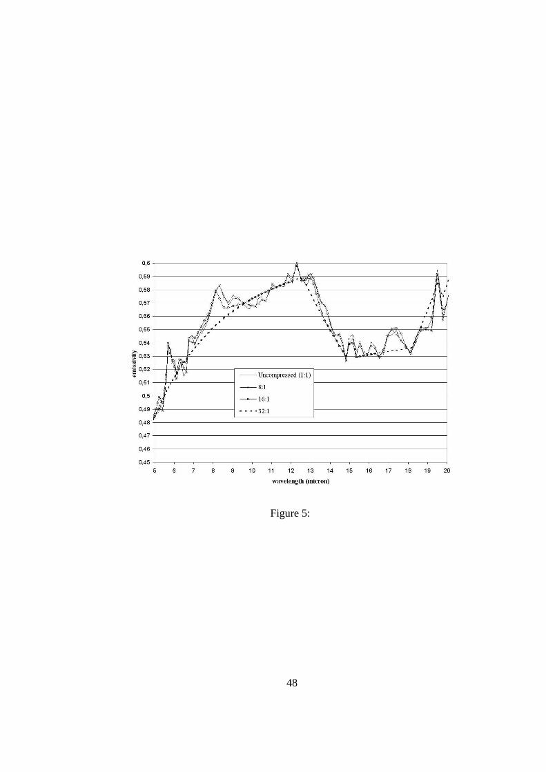
Figure 5:

48

Figure 6:

49

(a)

(b)

(c)

Figure 7:

50

Figure 8:

51

Figure 9:

52

Figure 10:

53

uncompressednoise free

compressednoise free

uncompressednoisy

compressednoisy

compression

(case I,II)

compression

(case I,II)

comparisonmultiplicative noise

(case a,b,c)additive noise(case d,e,f)

comparison

initialcomparison

indirectcomparison

Figure 11:

54

Figure 12:

55

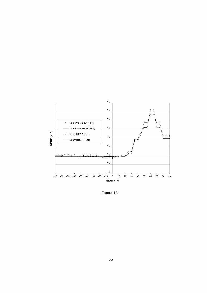
Figure 13:

56

Figure 14:

57