Spectral and statistical properties

of high-gain parametric down-conversion

Spektrale und statistische Eigenschaften

der parametrischen Fluoreszenz bei hoher

optisch-parametrischer Verstarkung

Der Naturwissenschaftlichen Fakultat

der Friedrich-Alexander-Universitat Erlangen-Nurnberg

zur

Erlangung des Doktorgrades Dr. rer. nat.

vorgelegt von

Kirill Spasibko

aus Moskau

2019

arX

iv:2

007.

1299

9v1

[qu

ant-

ph]

25

Jul 2

020

Als Dissertation genehmigt

von der Naturwissenschaftlichen Fakultat

der Friedrich-Alexander-Universitat Erlangen-Nurnberg

Tag der mundichen Prufung: 20.12.2019

Vorsitzender des Promotionsorgans: Prof. Dr. Kreimer

Gutachter: PD Dr. Chekhova

Gutachter: Prof. Dr. Joly

Gutachter: Prof. Dr. Lundeen

Fur Vera, Sofia und alle unsere Kuscheltiere

Summary

This thesis is devoted to high-gain parametric down-conversion (PDC). PDC is mostly

known in the low-gain (spontaneous) regime, in which the correlated photon pairs are

produced. Spontaneous PDC (SPDC) plays a very important role for quantum optics

as a variety of quantum states is produced via SPDC, including, for instance, entangled

Bell states or photon-number states. Moreover, SPDC finds its applications in metrology,

cryptography, imaging, and lithography.

In the high-gain case PDC leads to generation of bright states having up to hun-

dreds mW mean power. With such states almost any nonlinear optical interaction or

light-matter interaction becomes more efficient. Even being macroscopically bright, the

produced states maintain nonclassical properties as, for example, the fluctuations of elec-

tric field quadratures are squeezed below the shot-noise level.

The high-gain PDC could be used not only in the same applications as SPDC, it also

can provide new ones. For example, PDC is in use in the LIGO and GEO600 gravitational-

wave detectors, because squeezing increases the sensitivity of interferometry.

High-gain PDC has many remarkable spectral and statistical properties, which are

in the focus of this work. The thesis discusses them in detail, both theoretically and

experimentally, and shows how high-gain PDC could be used.

The description starts from the PDC generation in normal and anomalous group ve-

locity dispersion ranges. The spectrum and mode content of high-gain PDC is considered

as well as their change with the parametric gain are demonstrated.

Then, there are the interference effects emerging from the PDC correlations presented,

namely the macroscopic analogue of the Hong-Ou-Mandel interference. In addition, it is

shown how spatial and temporal walk-off matching could be used for the generation of

giant narrowband twin beams.

Finally, the statistical properties of high-gain PDC are reviewed as well as their use

for multiphoton effects is demonstrated. Photon-number fluctuations of PDC are studied

via normalized correlation functions and probability distributions. These fluctuations

enhance the generation efficiency for multiphoton effects by orders of magnitude and lead

to tremendously fluctuating light described by heavy-tailed photon-number probability

distributions.

i

Zusammenfassung

Diese Arbeit befasst sich mit der experimentellen und theoretischen Untersuchung der

parametrischen Fluoreszenz bei hoher optisch-parametrischer Verstarkung. Im Gegen-

satz zur parametrische Fluoreszenz bei geringer Verstarkung, wobei die Photonenpaare

erzeugt werden, ist das Regime hoher Verstarkung noch vergleichsweise wenig erforscht.

Parametrische Fluoreszenz ist bedeutsam fur die Quantenoptik und wird z.B. in der

Metrologie, Kryptographie, Bildgebung und Lithografie angewendet.

Bei hoher Verstarkung entstehen extrem helle Lichtzustande, die bis zu hundert Milli-

watt mittlere Leistung haben konnen. Solchen Zustande sind viel effizienter fur nicht-

lineare optische Effekte und Licht-Materie-Wechselwirkungen. Obwohl die bei hoher

Verstarkung erzeugten Lichtzustande makroskopisch hell sind, zeigen sie nichtklassische

Eigenschaften.

Die bei hoher optisch-parametrischer Verstarkung erzeugte parametrische Fluoreszenz

hat außergewohnliche spektrale und statistische Eigenschaften, die im Mittelpunkt dieser

Arbeit stehen. Die Arbeit beschreibt diese Eigenschaften nicht nur theoretisch und ex-

perimentell, sondern zeigt auch realisierbare Anwendungen.

ii

Contents

1 Introduction 2

2 Parametric down-conversion (PDC) 5

2.1 PDC process . . . . . . . . . . . . . . . . . . . . . . . . . . . . . . . . . . . 5

2.1.1 Quadrature squeezing . . . . . . . . . . . . . . . . . . . . . . . . . . 5

2.1.2 Twin-beam squeezing . . . . . . . . . . . . . . . . . . . . . . . . . . 6

2.2 High-gain vs. spontaneous PDC (SPDC) . . . . . . . . . . . . . . . . . . . 7

3 Wavelength-angular spectrum of PDC 9

3.1 Introduction . . . . . . . . . . . . . . . . . . . . . . . . . . . . . . . . . . . 10

3.1.1 Frequency-wavevector spectrum . . . . . . . . . . . . . . . . . . . . 11

3.1.2 X-shaped spatiotemporal coherence . . . . . . . . . . . . . . . . . . 12

3.1.3 Wavelength-angular spectrum and the λ4 factor . . . . . . . . . . . 15

3.1.4 PDC correlations and eigenmodes . . . . . . . . . . . . . . . . . . . 16

3.2 PDC in the anomalous group velocity dispersion (GVD) range . . . . . . . 18

3.2.1 PDC at zero GVD . . . . . . . . . . . . . . . . . . . . . . . . . . . 19

3.2.2 Experimental setup . . . . . . . . . . . . . . . . . . . . . . . . . . . 20

3.2.3 Wavelength-angular spectra and correlation functions (CF) . . . . . 21

3.2.4 Possible applications of PDC in the anomalous GVD range . . . . . 23

3.3 Broadening of PDC spectrum . . . . . . . . . . . . . . . . . . . . . . . . . 23

3.3.1 Experimental setup . . . . . . . . . . . . . . . . . . . . . . . . . . . 23

3.3.2 Measurement of the spectral broadening . . . . . . . . . . . . . . . 25

3.4 Measurement of PDC correlations . . . . . . . . . . . . . . . . . . . . . . . 26

3.4.1 PDC correlations in the noise of intensity difference . . . . . . . . . 26

3.4.2 Measurement of the joint spectral intensity (JSI) . . . . . . . . . . 28

3.5 Schmidt number and non-phase-matched sum frequency generation . . . . 30

3.5.1 The pump reconstruction . . . . . . . . . . . . . . . . . . . . . . . . 30

3.5.2 Schmidt number measurement . . . . . . . . . . . . . . . . . . . . . 31

4 Twin-beam correlations in PDC 35

4.1 Introduction . . . . . . . . . . . . . . . . . . . . . . . . . . . . . . . . . . . 36

iii

4.1.1 Hong-Ou-Mandel (HOM) interference . . . . . . . . . . . . . . . . . 36

4.1.2 Fock states interference . . . . . . . . . . . . . . . . . . . . . . . . . 37

4.2 Macroscopic HOM interference . . . . . . . . . . . . . . . . . . . . . . . . . 38

4.2.1 Theoretical description: CF and variance of the difference signal . . 38

4.2.2 Experimental results: HOM dip and HOM peak . . . . . . . . . . . 43

4.3 Interference on a beam splitter (BS) . . . . . . . . . . . . . . . . . . . . . . 45

4.3.1 Twin beams and phase fluctuations . . . . . . . . . . . . . . . . . . 45

4.3.2 Experimental setup . . . . . . . . . . . . . . . . . . . . . . . . . . . 46

4.3.3 Measurement of the twin-beam interference . . . . . . . . . . . . . 48

4.3.4 Interference of the classical beams . . . . . . . . . . . . . . . . . . . 50

4.3.5 Possible applications of the BS interference . . . . . . . . . . . . . . 51

4.4 Giant twin-beam generation . . . . . . . . . . . . . . . . . . . . . . . . . . 52

4.4.1 Walk-off effects in SPDC and high-gain PDC . . . . . . . . . . . . . 52

4.4.2 Twin-beam generation along the pump Poynting vector . . . . . . . 53

4.4.3 Experimental setup: temporal walk-off matching . . . . . . . . . . . 54

4.4.4 Twin-beam generation using temporal walk-off matching . . . . . . 56

4.4.5 Possible applications of the spatial and temporal walk-off matching 58

5 High-gain PDC as a pump for multiphoton effects 59

5.1 Introduction . . . . . . . . . . . . . . . . . . . . . . . . . . . . . . . . . . . 59

5.1.1 Fluctuations of light: coherent, thermal, and superbunched . . . . . 60

5.1.2 Multimode light and its measurement . . . . . . . . . . . . . . . . . 63

5.1.3 Filtering of the multimode light . . . . . . . . . . . . . . . . . . . . 64

5.2 Measurement of correlation functions and probability distributions . . . . . 66

5.2.1 Experimental setup . . . . . . . . . . . . . . . . . . . . . . . . . . . 66

5.2.2 Thermal and superbunched BSV: correlation functions . . . . . . . 68

5.2.3 Thermal and superbunched BSV: probability distributions . . . . . 70

5.3 Statistical enhancement of multiphoton processes . . . . . . . . . . . . . . 72

5.3.1 Experimental setup . . . . . . . . . . . . . . . . . . . . . . . . . . . 73

5.3.2 Second, third, and forth harmonic generation from BSV . . . . . . . 75

5.3.3 BSV fluctuations: possible applications . . . . . . . . . . . . . . . . 79

5.4 Extreme events, extreme bunching, and heavy-tailed distributions . . . . . 79

5.4.1 Theoretical description: nonlinear processes from fluctuating light . 81

5.4.2 Optical harmonic generation: extreme events . . . . . . . . . . . . . 86

5.4.3 Supercontinuum generation: Pareto photon distribution . . . . . . . 89

5.4.4 Extreme bunching: outlook and possible applications . . . . . . . . 93

6 Conclusion 94

A List of acronyms and abbreviations 96

iv

Acknowledgments 97

Bibliography 98

v

Author’s publications

Scopus ID: 54421216700 ORCID ID: 0000-0001-6667-5084

Discussed in the thesis

1. M. Manceau, K. Yu. Spasibko, G. Leuchs, R. Filip, and M. V. Chekhova. Indefinite-

mean Pareto photon distribution from amplified quantum noise. Phys. Rev. Lett.

123, 123606 (2019).

DOI: 10.1103/PhysRevLett.123.123606

2. D. A. Kopylov, K. Yu. Spasibko, T. V. Murzina, and M. V. Chekhova. Study of

broadband multimode light via non-phase-matched sum frequency generation. New

J. Phys. 21, 033024 (2019).

DOI: 10.1088/1367-2630/ab0a7c

3. K. Yu. Spasibko, D. A. Kopylov, V. L. Krutyanskiy, T. V. Murzina, G. Leuchs, and

M. V. Chekhova. Multiphoton effects enhanced due to ultrafast photon-number

fluctuations. Phys. Rev. Lett. 119, 223603 (2017).

DOI: 10.1103/PhysRevLett.119.223603

4. K. Yu. Spasibko, D. A. Kopylov, T. V. Murzina, G. Leuchs, and M. V. Chekhova.

Ring-shaped spectra of parametric downconversion and entangled photons that

never meet. Opt. Lett. 41, 2827-2830 (2016).

DOI: 10.1364/OL.41.002827

5. A. M. Perez, K. Yu. Spasibko, P. R. Sharapova, O. V. Tikhonova, G. Leuchs, and

M. V. Chekhova. Giant narrowband twin-beam generation along the pump-energy

propagation direction. Nat. Commun. 6, 7707 (2015).

DOI: 10.1038/ncomms8707

6. K. Yu. Spasibko, F. Toppel, T. Sh. Iskhakov, M. Stobinska, M. V. Chekhova, and

G. Leuchs. Interference of macroscopic beams on a beam splitter: phase uncertainty

converted into photon-number uncertainty. New J. Phys. 16, 013025 (2014).

DOI: 10.1088/1367-2630/16/1/013025

vi

7. T. Sh. Iskhakov, K. Yu. Spasibko, M. V. Chekhova, and G. Leuchs. Macroscopic

Hong-Ou-Mandel interference. New J. Phys. 15, 093036 (2013).

DOI: 10.1088/1367-2630/15/9/093036

8. T. Sh. Iskhakov, A. M. Perez, K. Yu. Spasibko, M. V. Chekhova, and G. Leuchs.

Superbunched bright squeezed vacuum state. Opt. Lett. 37, 1919-1921 (2012).

DOI: 10.1364/OL.37.001919

9. K. Yu. Spasibko, T. Sh. Iskhakov, and M. V. Chekhova. Spectral properties of

high-gain parametric down-conversion. Opt. Express 20, 7507-7515 (2012).

DOI: 10.1364/OE.20.007507

Other publications

1. O. Kovalenko, K. Yu. Spasibko, M. V. Chekhova, V. C. Usenko, and R. Filip.

Feasibility of quantum key distribution with macroscopically bright coherent light.

Opt. Express 27, 36154-36163 (2019).

DOI: 10.1364/OE.27.036154

2. E. Knyazev, K. Yu. Spasibko, M. V. Chekhova, and F. Ya. Khalili. Quantum

tomography enhanced through parametric amplification. New J. Phys. 20, 013005

(2018).

DOI: 10.1088/1367-2630/aa99b4

3. K. Yu. Spasibko, M. V. Chekhova, and F. Ya. Khalili. Experimental demonstration

of negative-valued polarization quasiprobability distribution. Phys. Rev. A 96,

023822 (2017).

DOI: 10.1103/PhysRevA.96.023822

4. F. Sciarrino, G. Vallone, G. Milani, A. Avella, J. Galinis, R. Machulka, A. M.

Perego, K. Y. Spasibko, A. Allevi, M. Bondani, and P. Mataloni. High degree of

entanglement and nonlocality of a two-photon state generated at 532 nm. Eur.

Phys. J. ST 199, 111-125 (2011).

DOI: 10.1140/epjst/e2011-01507-y

vii

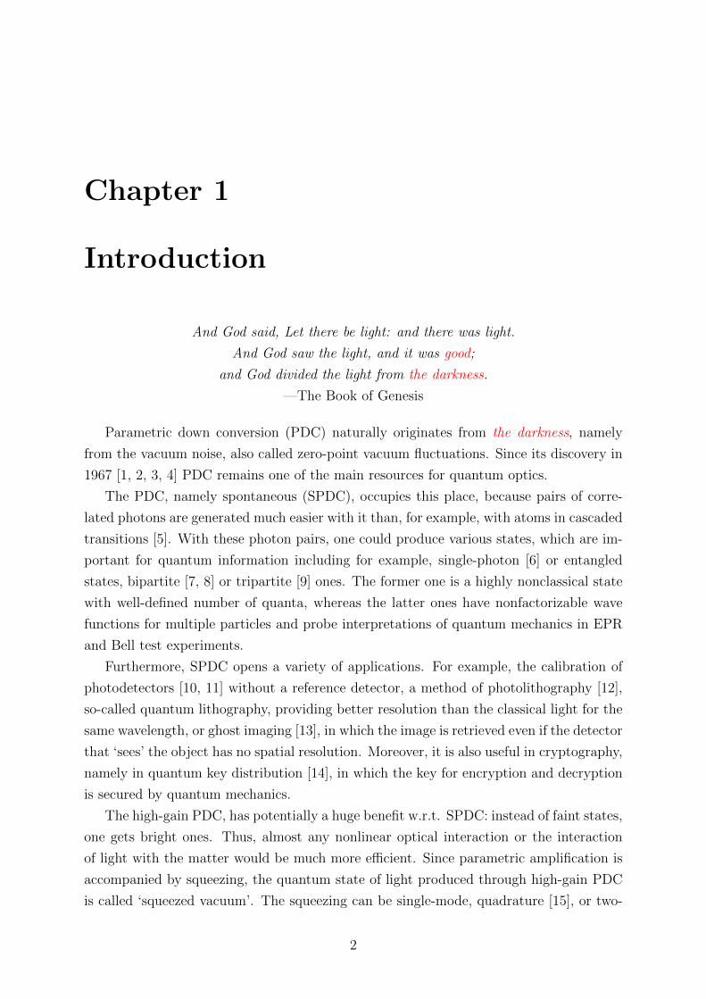
Chapter 1

Introduction

And God said, Let there be light: and there was light.

And God saw the light, and it was good;

and God divided the light from the darkness.

—The Book of Genesis

Parametric down conversion (PDC) naturally originates from the darkness, namely

from the vacuum noise, also called zero-point vacuum fluctuations. Since its discovery in

1967 [1, 2, 3, 4] PDC remains one of the main resources for quantum optics.

The PDC, namely spontaneous (SPDC), occupies this place, because pairs of corre-

lated photons are generated much easier with it than, for example, with atoms in cascaded

transitions [5]. With these photon pairs, one could produce various states, which are im-

portant for quantum information including for example, single-photon [6] or entangled

states, bipartite [7, 8] or tripartite [9] ones. The former one is a highly nonclassical state

with well-defined number of quanta, whereas the latter ones have nonfactorizable wave

functions for multiple particles and probe interpretations of quantum mechanics in EPR

and Bell test experiments.

Furthermore, SPDC opens a variety of applications. For example, the calibration of

photodetectors [10, 11] without a reference detector, a method of photolithography [12],

so-called quantum lithography, providing better resolution than the classical light for the

same wavelength, or ghost imaging [13], in which the image is retrieved even if the detector

that ‘sees’ the object has no spatial resolution. Moreover, it is also useful in cryptography,

namely in quantum key distribution [14], in which the key for encryption and decryption

is secured by quantum mechanics.

The high-gain PDC, has potentially a huge benefit w.r.t. SPDC: instead of faint states,

one gets bright ones. Thus, almost any nonlinear optical interaction or the interaction

of light with the matter would be much more efficient. Since parametric amplification is

accompanied by squeezing, the quantum state of light produced through high-gain PDC

is called ‘squeezed vacuum’. The squeezing can be single-mode, quadrature [15], or two-

2

mode, polarization [16] or photon-number one [17], meaning that the fluctuations of the

quadrature amplitude, one of the Stokes parameters, or the photon-number difference in

two modes is below the shot-noise level. Even Bell’s inequalities could be, in principle,

violated [18]. Interestingly, these nonclassical features remain even if the state becomes

macroscopical; for example, entanglement [19] and twin-beam squeezing [20] is observed

for the states containing more than 105 photons. Therefore, the squeezed vacuum with

the macroscopical number of photons is called bright squeezed vacuum (BSV).

The high-gain PDC could be used not only in the same applications as SPDC, like

quantum key distribution [21, 22] or absolute calibration of photodetectors [23, 24], but

also it can provide new applications. For example, squeezing increases the sensitivity of

optical imaging [25] and interferometry [26] and consequently becomes important for live

cell imaging, where one should use the lowest possible photon dose [27], and gravitational-

wave detectors, where the detected signals are extremely weak. These detectors serve as

a major successful example since the squeezing is used operationally at GEO600 [28], at

LIGO it has been tested [29] and is in use starting from 1st of April 2019.

However, it still requires some hard work to show how good high-gain regime is. This

thesis respectively takes a step in such a direction as it summarizes the major part of

author’s research work devoted to the spectral and statistical properties of high-gain PDC.

Moreover, it highlights some potential applications, which could be useful for science and

industry. Most essential results have already been published being presented in Author’s

publications.

This thesis is organized as follows. Chapter 2 introduces the basic theoretical founda-

tions of PDC and clarifies the difference between spontaneous and high-gain regimes.

Chapter 3 is devoted to the wavelength-angular spectrum of PDC and presents the

results published in Refs. [30, 31, 32]. Firstly, it describes the PDC generation in the

normal and anomalous group velocity dispersion (GVD) ranges. In the second case, the

spectrum is restricted in both the angle and the wavelength. The shape of the spectrum

suggests a new type of spatiotemporal coherence. Afterwards there is the broadening

of the spectrum at high gain explained and demonstrated. Both the total spectral and

the correlation widths get broader as the gain increases. Finally, the chapter presents a

method for the reconstruction of the joint spectral intensity (JSI) and as well as a way to

get the number of modes, namely the Fedorov ratio or the Schmidt number.

Chapter 4 to a larger extend focuses on the twin-beam correlations and summarizes

the results of Refs. [33, 34, 35]. It starts with the interference effects emerging from

these correlations and explains the Hong-Ou-Mandel (HOM) effect and interference of

Fock states on a beam splitter (BS). Besides that, the chapter deals with the macroscopic

analogue of the HOM interference and the way how the Fock states interference can be

accessed using twin beams. Finally, the chapter shows how spatial and temporal walk-off

matching could be used for giant narrowband twin-beam generation.

3

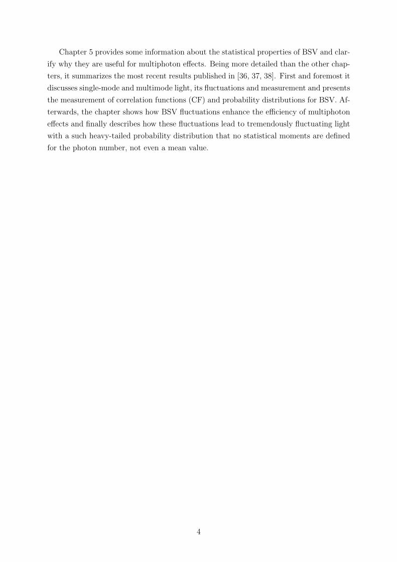
Chapter 5 provides some information about the statistical properties of BSV and clar-

ify why they are useful for multiphoton effects. Being more detailed than the other chap-

ters, it summarizes the most recent results published in [36, 37, 38]. First and foremost it

discusses single-mode and multimode light, its fluctuations and measurement and presents

the measurement of correlation functions (CF) and probability distributions for BSV. Af-

terwards, the chapter shows how BSV fluctuations enhance the efficiency of multiphoton

effects and finally describes how these fluctuations lead to tremendously fluctuating light

with a such heavy-tailed probability distribution that no statistical moments are defined

for the photon number, not even a mean value.

4

Chapter 2

Parametric down-conversion (PDC)

In which we are introduced to PDC and some features, and the stories begin.

2.1 PDC process

Parametric down-conversion occurs in nonlinear medium with nonzero second-order sus-

ceptibility χ(2). In this process each converted pump photon (p) produces two daughter

photons, signal (s) and idler (i). This process is called parametric, because there is no

energy transfer between photons and the medium, and it is down-conversion, because the

frequencies of produced photons are below the one of the pump. The frequencies ω and

wave vectors1 k are related through the energy and momentum conservation laws:

ωp = ωs + ωi, kp = ks + ki. (2.1)

PDC can be described as the optical parametric amplification (OPA) of the vacuum

noise in many modes [39, 40]. Although these modes differ by many parameters, like

frequency, wave vector, or polarization, the most important issue is whether signal and

idler photons are indistinguishable or not. In the first case, the OPA at each mode should

be described as single-mode, in the second one, the two-mode picture is needed. The both

cases are introduced using the quantum description of the electric field.

2.1.1 Quadrature squeezing

In the case of a single-mode OPA, the output photon creation and annihilation operators,

a† and a, are related with the input ones, a†0 and a0, with the Bogolyubov transforma-

tion [39],

a = a0 coshG+ a†0 sinhG, (2.2)

1Here and further on the bold symbols are used for vectors, e.g. k ≡ (kx, ky, kz).

5

arising from the Heisenberg equation of motion and the corresponding Hamiltonian, the

parametric gain G characterizes the amplification strength2.

Unfortunately, the operators a and a† can not be measured, because they are not

Hermitian, a 6= a†. Moreover, they do not commute, [a, a†] = 1.

Nevertheless, applying homodyne detection one can measure the quadratures q and

p, the quantum analogues of the real and imaginary parts (cosinusoidal and sinusoidal

components) of the electric field,

q ≡ a+ a†√2

and p ≡ a− a†

i√

2. (2.3)

The OPA does not change the mean values of the quadratures and for the vacuum

input state the mean values are zero, 〈q〉 = 〈p〉 = 〈q0〉 = 〈p0〉 = 0. However, the noise

changes: the quadrature noise becomes antisqueezed,

〈∆q2〉 = e2G〈∆q20〉, (2.4)

for one quadrature while squeezed,

〈∆p2〉 = e−2G〈∆p20〉, (2.5)

for the other one w.r.t. the vacuum noise3, 〈∆q20〉 = 〈∆p2

0〉 = 1/2. Therefore, the state

produced by an unseeded OPA is called the squeezed vacuum.

Remarkably, this vacuum contains energy, i.e. photons. The mean number of photons,

corresponding to the photon-number operator N ≡ a†a, is

〈N〉 = sinh2G. (2.6)

With 〈N〉 1 the vacuum will be not only squeezed, but also bright. BSV can be

extremely bright; in the following chapters one finds the cases with G > 15 corresponding

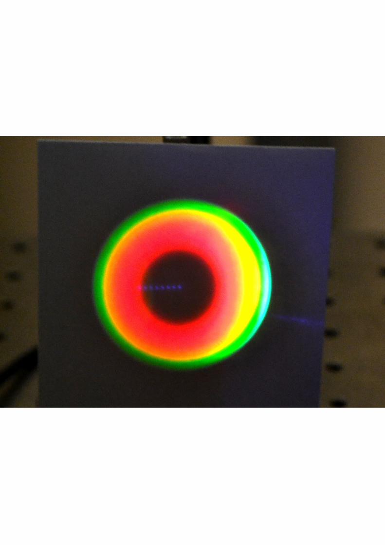
to 〈N〉 > 3× 1012 photons! The cover for chapter 1 shows one of the examples: vacuum

is amplified so strongly that it is visible on a piece of paper.

2.1.2 Twin-beam squeezing

Similar approach applies also to two-mode OPA. The Bogolyubov transformations for the

signal and idler modes are

as = as0 coshG+ a†i0 sinhG and ai = ai0 coshG+ a†s0 sinhG. (2.7)

2Actually, the gain G depends on many parameters, which will be discussed a bit later (section 3.1.1).3This noise is typical for a coherent state produced, for example, by a shot-noise limited laser.

6

This time the commutation relations look as follows:

[as, a†s] = 1, [as, ai] = 0, [as, a

†i ] = 0, (2.8)

and the ones with replacement s ↔ i [39]. The quadrature squeezing can be observed

with two-mode OPA too4; two-mode quadratures that depend on both as and ai should

be measured [42].

However, another type of squeezing is commonly in use: two-mode or twin-beam one.

Instead of the quadrature noise, the one of photon-number difference between the signal

and idler modes is measured. Indeed, for the signal and idler beams not only the numbers

of photons are the same,

〈Ns〉 = 〈Ni〉 = sinh2G, (2.9)

but also all moments of photon-number difference, 〈(Ns − Ni)n〉, are equal to zero. The

same applies to the central moments, like variance. It is certainly squeezed below the

shot-noise level, 〈∆(Ns − Ni)2〉 = 〈Ns + Ni〉, which is the noise for two independent

coherent beams.

Thus, the number of photons in the signal and idler beams is always the same, and

therefore they are called twin beams and the squeezing is twin-beam one5.

2.2 High-gain vs. spontaneous PDC (SPDC)

The previous section describes the properties of BSV. Apart from that, its wave function

can be expressed as a series over Fock (m-photon) states |m〉. Hence, an unseeded single-

mode OPA gives [43]

|Ψ1 〉 =1

coshG

∞∑m=0

(2m)!

22m(m!)2(tanhG)2m |2m〉, (2.10)

an unseeded two-mode one [44],

|Ψ2 〉 =1

coshG

∞∑m=0

(tanhG)m |m〉s |m〉i. (2.11)

In both cases BSV is a state of light with only even photon numbers: either all photons

are in the same mode, or they are equally distributed between two modes.

The case of SPDC is the one where the parametric gain G is small. It is usually the

4The opposite applies as well: one can observe twin-beam squeezing with a single-mode OPA [41].5The polarization squeezing is similar, because the Stokes operators are equal to the photon-number

difference in two polarization modes, e.g. S1 = nH − nV for horizontal and vertical modes.

7

case: for a continuous-wave (CW) pump laser G ∼ 10−3 − 10−4. In this case four- and

higher-photon contributions are negligibly small w.r.t. two-photon one. Thus, either a

two-photon state,

|Φ1 〉 = c0 |0〉+ c2 |2〉, (2.12)

or an entangled photon pair,

|Φ2 〉 = c0 |0〉s |0〉i + c1 |1〉s |1〉i, (2.13)

is produced in superposition with the vacuum. Here c0,1,2 are renormalized constants

from Eqs. (2.10) and (2.11). The constant c0 is often omitted, because it is approximately

equal to unity. As mentioned in chapter 1, these two states are of a great importance for

quantum optics. They are produced via SPDC in hundreds of experiments.

Due to low gain, 〈N〉 is also small, 10−6− 10−8 photons, being much smaller than the

effective brightness of zero-point vacuum fluctuations6. The produced photons, therefore,

do not enhance the generation rate and it is the same along the nonlinear medium (Fig. 2.1,

left).

However, this is not the case in the high-gain regime. If one reaches G > 1, for example

by using strong pulsed pump laser, 〈N〉 is larger than one photon. This drastically

enhances the generation rate, because the photons produced at the beginning of the

nonlinear medium seed the generation at the end. Therefore, the generation rate and the

number of produced photons increase exponentially along the nonlinear medium (Fig. 2.1,

right). Hence, as long as one reaches the high-gain regime, it is extremely easy to make

the state brighter and brighter.

pump

signal

idler

pumpsignal

idler

Figure 2.1: Schematic representation of the generation rate along the nonlinear mediumat low (left) and high gain (right).

6Actually, vacuum fluctuations have no brightness but in order to explain spontaneous effects one canintroduce it effectively. This effective brightness comes from the noncommutativity of a and a† and isequal to one photon per each mode of the field.

8

Chapter 3

Wavelength-angular spectrum of

PDC

My drawing was not a picture of a hat.

It was a picture of a boa constrictor digesting an elephant. ...

The grown-ups always need explanations.

—Antoine de Saint-Exupery, The Little Prince

This chapter discusses the PDC spectrum, namely it shape and properties. Firstly,

it describes how one can calculate the spectrum, introduces the concept of coupled spa-

tial and temporal coherence, explains the common asymmetry of measured wavelength-

angular PDC spectra, and discusses PDC correlations and eigenmodes.

Apart from that, the chapter deals with the special features that arise when PDC

is generated in the anomalous GVD range. Moreover, there is the unusual type of

wavelength-angular PDC spectrum presented, which suggests a new type of spatiotem-

poral coherence and entanglement of photon pairs. One can obtain an entangled photon

pair with the photons being never at the same point at the same time.

Afterwards there is the broadening of PDC spectra at high gain regime demonstrated;

both the total and the correlation spectral widths get broadened. In addition, the asym-

metry of PDC spectra is discussed in more details.

Finally, the chapter presents the method for JSI reconstruction via covariance mea-

surement, which could be directly applied for the reconstruction of BSV eigenmodes,

namely Schmidt modes. Moreover, there is one more method briefly explained which

gives access to the number of modes via non-phase-matched sum frequency generation

(SFG).

9

3.1 Introduction

As one could have noticed, e.g. from the cover for chapter 1, PDC is usually highly broad-

band in frequency and wave vector. This should be taken into account. Unfortunately,

the analytical description of high-gain PDC is possible only under certain approxima-

tions. One of the ways is the assumptions of a stationary, plane-wave, and undepleted

pump [39, 45] and infinite transverse dimensions of a nonlinear medium. They lead to

strict energy and transverse momentum conservations laws1,

Ωs = −Ωi ≡ Ω, qs = −qi ≡ q, (3.1)

where Ωs,i ≡ ωs,i − ωs0,i0 is a frequency shift w.r.t. the central frequency ωs0,i0 and qs,i is

the transverse (w.r.t kp) component of ks,i.

Under this approximation the input-output transformations (2.7) look as follows [39,

45]:

as(q,Ω) = as0(q,Ω)Us(q,Ω) + a†i0(−q,−Ω)Vs(q,Ω),

ai(q,Ω) = ai0(q,Ω)Ui(q,Ω) + a†s0(−q,−Ω)Vi(q,Ω), (3.2)

where Us,i and Vs,i are the functions of gain G. In general, the functions Us,i and Vs,i have

lengthy expressions, which can be greatly simplified for certain cases. Therefore, the full

expressions from Ref. [45] are not presented, only the simplified ones for each particular

case. Here it is critical that the gain functions satisfy the unitarity conditions,

|Us,i(q,Ω)|2 − |Vs,i(q,Ω)|2 = 1,

Us(q,Ω)Vi(−q,−Ω) = Ui(−q,−Ω)Vs(q,Ω), (3.3)

which provide the commutation relations

[as(q,Ω), a†s(q, Ω)] = δ(q − q)δ(Ω− Ω),

[as(q,Ω), ai(q, Ω)] = 0, [as(q,Ω), a†i (q, Ω)] = 0, (3.4)

and the ones with the replacement s↔ i. Here δ(x) is the Dirac delta function.

1The condition for longitudinal momentum is not so strict, because the length of nonlinear mediumis finite.

10

3.1.1 Frequency-wavevector spectrum

The PDC spectrum S(q,Ω) can be obtained using transformations (3.2). Indeed, the

spectrum is equal to the normalized mean number 〈Ns,i〉 of emitted photons,

S(q,Ω) =〈Ns,i(q,Ω)〉max (〈Ns,i〉)

, (3.5)

where 〈Ns,i(q,Ω)〉 = 〈a†s,i(q,Ω)as,i(q,Ω)〉. The operators as,i are taken at the end of a

nonlinear medium and vacuum operators as0,i0 are considered at the beginning. Then,

〈Ns,i(q,Ω)〉 = |Vs,i(q,Ω)|2 =

(G

G(q,Ω)sinhG(q,Ω)

)2

, (3.6)

where

G(q,Ω) =

√G2 − (∆(q,Ω)L)2

4(3.7)

and

∆(q,Ω) = ksz(q,Ω) + kiz(−q,−Ω)− kp. (3.8)

Here ∆(q,Ω) is the longitudinal phase mismatch, ksz and kiz are the longitudinal compo-

nents of ks,i, the function G(q,Ω) gives the parametric gain at nonzero mismatch. At zero

mismatch, ∆(q,Ω) = 0, the mean number 〈Ns,i(q,Ω)〉 of photons reaches its maximum,

the function G(q,Ω) equals to G, the parametric gain at exact phase matching, and the

Eq. (3.6) transforms into Eq. (2.9).

Finally, the spectrum is

S(q,Ω) =

(G

G(q,Ω)

sinhG(q,Ω)

sinhG

)2

. (3.9)

At low gain, G→ 0, S(q,Ω) transforms into the well-known sinc solution2 [39],

S(q,Ω) = sinc2

(∆(q,Ω)L

2

). (3.10)

Here and further on the gain G at exact phase matching is considered to be a constant

value determined by the pumping and nonlinear medium [39],

G =2π

c

√ωs0 ωi0nsni

χ(2)LEp, (3.11)

2sinc(x) is defined as sin(x)/x.

11

where χ(2) is the second-order susceptibility for the interaction ωp → ωs0 + ωi0, ns,i is

the refractive index at ωs0,i0, L is the length of nonlinear medium, Ep is the pump field

amplitude. This assumption is valid for a small frequency detuning, Ω ωs0,i0, and

a small emission angle, meaning that q ≡ |q| |ks,i|. However, in practice Eq. 3.11

often gives an imprecise result, and therefore it is always better to measure the gain

experimentally, for example using the simple method described later in section 3.3.

Let us apply Eq. (3.9) to some particular case. In the simplest case, PDC is generated

in a uniaxial nonlinear crystal and both signal and idler photons are polarized ordinary,

i.e. perpendicular to the principal plane3. To satisfy the phase-matching condition,

∆(q,Ω) = 0, the pump is usually polarized extraordinary, i.e. in the principal plane.

This type of interaction is labeled e→ oo and called type-I.

Moreover, if the pump spatial walk-off is neglected, the spectrum will depend only on

the modulus q of transverse wave vector and be radially symmetric w.r.t. kp direction [39].

This symmetry can be seen from the cover for chapter 1. Therefore, S(q,Ω) can be plotted

as a function of only qx, S(qx,Ω), without loosing any information4.

The spectrum S(qx,Ω) is plotted for beta barium borate (BBO) crystal with a 10 mm

length and collinear frequency-degenerate phase matching, ∆(q = 0,Ω = 0) = 0 and

ωs0 = ωi0 = ωp/2, for the pump wavelength λp = 400 nm. The spectra for SPDC (top)

and high-gain PDC (bottom) are shown in Fig. 3.1.

The spectrum is symmetric w.r.t. the central point (qx = 0, Ω = 0). It has a char-

acteristic ‘X’ shape and is practically unbounded, both in the frequency and in the wave

vector, due to the fact that the mismatch gained by frequency detuning from degenerate

collinear PDC can be compensated by noncollinear emission.

For high-gain PDC the spectrum is considerably broader. Moreover, the characteris-

tic lobes provided by sinc function disappear, because at high gain the generation rate

increases exponentially along the nonlinear crystal and the most photons are produced at

its end. The effective length of the medium decreases, which leads to the broadening of

the spectrum. This effect is demonstrated experimentally in section 3.3.

3.1.2 X-shaped spatiotemporal coherence

This characteristic shape has an interesting feature: the spectrum is nonfactorizable,

S(q,Ω) 6= Sq(q)SΩ(Ω). It leads to a nonfactorizable first-order CF G(1)(ξ, τ), which

characterizes spatial and temporal coherence of an electromagnetic field5, having an ‘X’

shape as well [46]. The latter means that the coherence is neither spatial nor temporal,

but has a more complicated structure, which will be clarified in this section.

3In uniaxial crystals it is the plane containing wave vector k and optic axis.4Here and further on the second variable is set to be zero, e.g. S(qx,Ω) ≡ S(qx, qy = 0,Ω).5Here and further on ξ and τ mean space and time delays, respectively.

12

Figure 3.1: Normalized frequency-wavevector spectrum S(qx,Ω) for SPDC (top) and high-gain PDC with G = 10 (bottom).

Indeed, the CF G(1)(ξ, τ) by virtue of the generalized Wiener–Khinchine theorem [47]

is the Fourier transform (FT) of the spectrum6,

G(1)(ξ, τ) =

∫∫dqdΩS(q,Ω)ei(Ωτ+q · ξ). (3.12)

The spectrum is radially symmetric, therefore the CF G(1) depends only on ξ ≡ |ξ| and

can be considered as G(1)(ξx, τ).

The modulus of the resulting spatiotemporal CF, |G(1)(ξx, τ)|, is shown in Fig. 3.2

(top). For light with such CF the time and space coherence cannot be measured separately,

on the contrary, the coherence can be still retrieved at large spatial delays by an additional

temporal delay and vice versa.

This was demonstrated in the double-pinhole experiment [46, 47] similar to the famous

Young’s double-slit one. In the Young’s experiment the interference visibility is the largest

at the point symmetric w.r.t. both pinholes. If the distance between the pinholes is larger

than the width of the central G(1) maximum, the interference disappears.

6The transform in this form provides only the envelope of the CF G(1) without fast oscillations withan optical period in time and wavelength in space. However, mainly the envelope is important, becauseit defines an interferometric visibility.

13

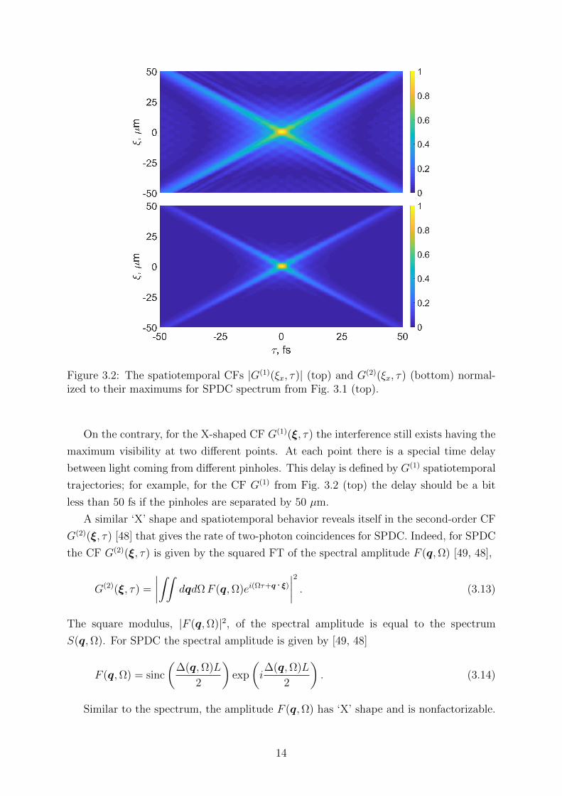
Figure 3.2: The spatiotemporal CFs |G(1)(ξx, τ)| (top) and G(2)(ξx, τ) (bottom) normal-ized to their maximums for SPDC spectrum from Fig. 3.1 (top).

On the contrary, for the X-shaped CF G(1)(ξ, τ) the interference still exists having the

maximum visibility at two different points. At each point there is a special time delay

between light coming from different pinholes. This delay is defined by G(1) spatiotemporal

trajectories; for example, for the CF G(1) from Fig. 3.2 (top) the delay should be a bit

less than 50 fs if the pinholes are separated by 50 µm.

A similar ‘X’ shape and spatiotemporal behavior reveals itself in the second-order CF

G(2)(ξ, τ) [48] that gives the rate of two-photon coincidences for SPDC. Indeed, for SPDC

the CF G(2)(ξ, τ) is given by the squared FT of the spectral amplitude F (q,Ω) [49, 48],

G(2)(ξ, τ) =

∣∣∣∣∫∫ dqdΩF (q,Ω)ei(Ωτ+q · ξ)∣∣∣∣2 . (3.13)

The square modulus, |F (q,Ω)|2, of the spectral amplitude is equal to the spectrum

S(q,Ω). For SPDC the spectral amplitude is given by [49, 48]

F (q,Ω) = sinc

(∆(q,Ω)L

2

)exp

(i∆(q,Ω)L

2

). (3.14)

Similar to the spectrum, the amplitude F (q,Ω) has ‘X’ shape and is nonfactorizable.

14

Therefore, the second-order CF G(2) has the shape similar to the first-order CF G(1), the

only major difference being that G(2) is narrower (see Fig. 3.2). In this case the ‘X’ shape

means that the spatial degrees of freedom of a photon pair are entangled to its temporal

degrees of freedom; this effect is called X entanglement [48].

3.1.3 Wavelength-angular spectrum and the λ4 factor

The variables (q,Ω) are natural for the theoretical description of PDC, yet, not for the

measurement techniques. In reality, one measures the radiation within a certain angular

aperture ∆θx∆θy and wavelength interval ∆λ, thereby acquiring the wavelength-angular

spectrum, Sθλ(θx, θy, λ), which differs from the change of variables in the frequency-

wavevector spectrum, SqΩ(θx, θy, λ) ≡ S[q(θx, θy, λ),Ω(λ)], meaning that the wavelength-

dependent Jacobian should be taken into account.

Indeed, the total energy for a unit interval should be the same,

Sθλ(θx, θy, λ)dθxdθydλ = S(q,Ω)dqdΩ. (3.15)

Under the assumptions of small angles, θx,y 1 and a constant refractive index n within

the PDC band7, the Jacobian is equal to 8π3n2c/λ4. Therefore,

Sθλ(θx, θy, λ) ∼ SqΩ(θx, θy, λ)

λ4. (3.16)

The constant factor is not important, because the spectra are usually normalized to their

maximums. One can get the same λ4 factor from considerations based on the dependence

of the mode size on the wavelength [39, 31, 50].

This λ4 factor is often forgotten in Sθλ theoretical plots or in experimental S(q,Ω)

ones. The asymmetry along the wavelength is either not explained at all [47] or attributed

to losses [51].

Nevertheless, in many cases the spectrum SqΩ(θx, θy, λ) is useful without any correc-

tion; then it has the meaning of a tuning curve, which shows the phase-matched wave-

lengths and angles without the information on the relative brightness. As an example,

SqΩ(θx, λ) is shown not only for collinear degenerate phase matching considered before,

but also for nondegenerate and noncollinear degenerate ones (Fig. 3.3). The phase match-

ing can be changed by tuning the angle φ between kp and the optic axis; the change in

the pump refractive index changes the pump wave vector, which, in its turn, affects the

phase matching.

7Both assumptions are fairly valid for PDC: the angles are mostly below 0.1 radian and the change ofthe refractive index is below 1%.

15

Figure 3.3: The spectrum SqΩ(θx, λ) for collinear degenerate (φ = 29.18) and nonde-generate (φ = 28 and 28.6), and noncollinear degenerate (φ = 29.8 and 30.5) phasematching. θx is calculated outside the BBO crystal.

3.1.4 PDC correlations and eigenmodes

Previously the total PDC spectrum was discussed assuming a stationary and plane-wave

pump, which leads to δ-correlated signal and idler photons. However, in many cases this

is not true; the correlation width is important.

Therefore, all possible frequencies and wave vectors should be considered8. For exam-

ple, for the state |Φ2 〉 (2.13) the main term,∣∣Φ2 〉 = c1 |1〉s |1〉i, changes to [52, 53, 54]

∣∣Φ2 〉 =

∫∫∫∫dqsdqidΩsdΩi F (qs, qi,Ωs,Ωi) |1〉s |1〉i. (3.17)

Here F (qs, qi,Ωs,Ωi) is the joint spectral amplitude (JSA), which is also known as two-

photon amplitude. JSA is the probability amplitude for signal and idler photons to be

emitted with wave vectors qs,i and frequencies Ωs,i.

The JSA F (qs, qi,Ωs,Ωi) fully characterizes the state. Unfortunately, in the general

form the JSA is too complicated, as it depends on 6 independent variables; until now

there are only few attempts [54] to deal with all variables together.

At first, one usually separates spatial and temporal degrees of freedom. Experimentally

it could be done by angular filtering in the collinear direction or frequency filtering at the

degenerate wavelength. In the frequency domain [53], the JSA can be expressed as9

F (Ωs,Ωi) = exp

(−(Ωs + Ωi)

2τ 2d

8 ln 2

)sinc

(∆(Ωs,Ωi)L

2

)exp

(i∆(Ωs,Ωi)L

2

), (3.18)

here the pump pulse duration10 τd is taken into account and the longitudinal mismatch

8One can also add the polarization degree of freedom.9The collinear emission is assumed, qs = qi = 0.

10For non-bandwidth-limited or CW pump it is replaced by the coherence time.

16

∆(Ωs,Ωi) depends on both signal and idler frequencies.

Then, one measures only the JSI, the squared modulus of the JSA, so the JSA phase is

ignored. With these assumptions the spatiotemporal and phase effects are lost; however,

it is still possible to describe some effects.

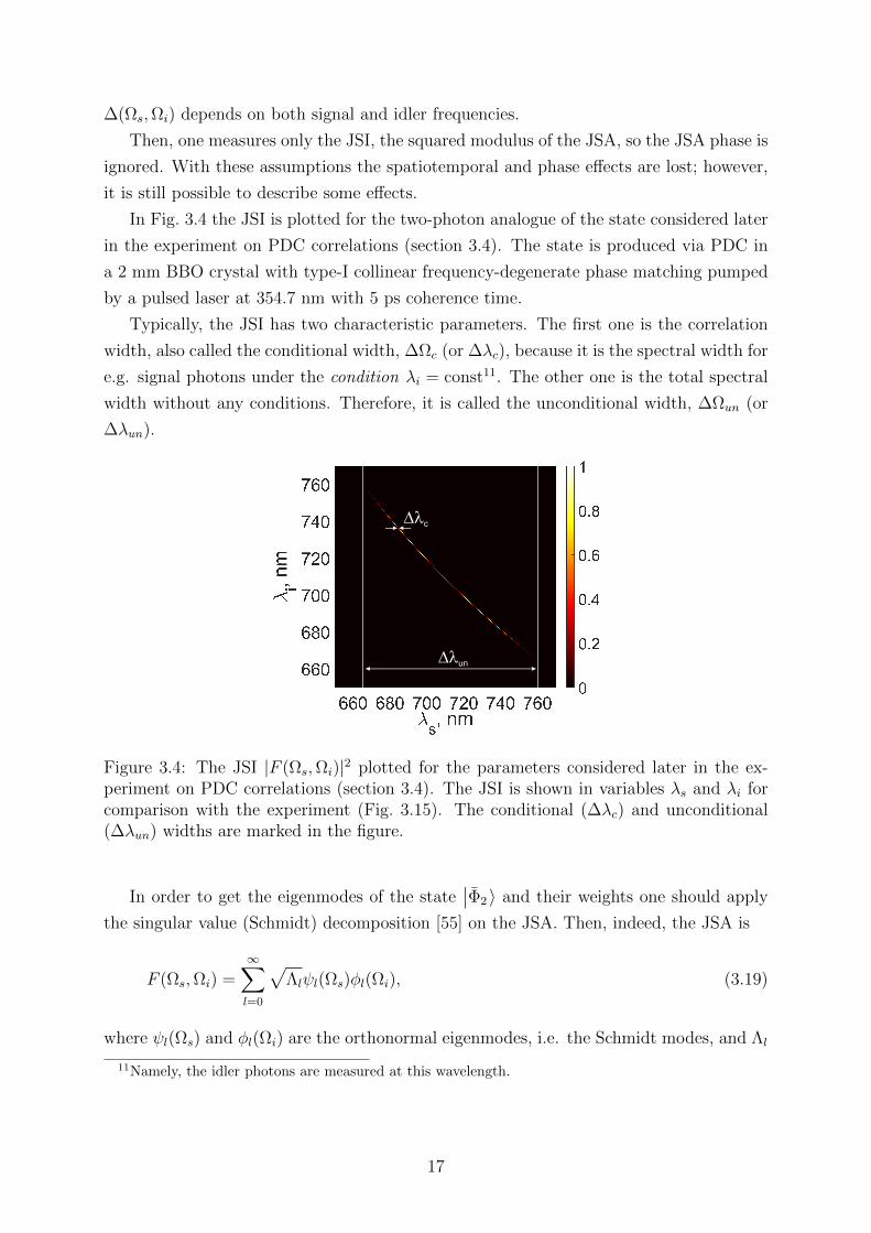
In Fig. 3.4 the JSI is plotted for the two-photon analogue of the state considered later

in the experiment on PDC correlations (section 3.4). The state is produced via PDC in

a 2 mm BBO crystal with type-I collinear frequency-degenerate phase matching pumped

by a pulsed laser at 354.7 nm with 5 ps coherence time.

Typically, the JSI has two characteristic parameters. The first one is the correlation

width, also called the conditional width, ∆Ωc (or ∆λc), because it is the spectral width for

e.g. signal photons under the condition λi = const11. The other one is the total spectral

width without any conditions. Therefore, it is called the unconditional width, ∆Ωun (or

∆λun).

Dlc

Dlun

Figure 3.4: The JSI |F (Ωs,Ωi)|2 plotted for the parameters considered later in the ex-periment on PDC correlations (section 3.4). The JSI is shown in variables λs and λi forcomparison with the experiment (Fig. 3.15). The conditional (∆λc) and unconditional(∆λun) widths are marked in the figure.

In order to get the eigenmodes of the state∣∣Φ2 〉 and their weights one should apply

the singular value (Schmidt) decomposition [55] on the JSA. Then, indeed, the JSA is

F (Ωs,Ωi) =∞∑l=0

√Λlψl(Ωs)φl(Ωi), (3.19)

where ψl(Ωs) and φl(Ωi) are the orthonormal eigenmodes, i.e. the Schmidt modes, and Λl

11Namely, the idler photons are measured at this wavelength.

17

are the corresponding weights, i.e the Schmidt coefficients. The latter are normalized as

∞∑l=0

Λl = 1. (3.20)

In this case the effective number K of modes is [56]

K =

(∞∑l=0

Λ2l

)−1

. (3.21)

It is called the Schmidt number and provides the degree of entanglement [55], namely the

dimensionality of the state, for example, for information processing in quantum comput-

ing [57].

The Schmidt number can be also assessed without the JSA measurement and the

Schmidt decomposition. As it is shown in Ref. [58], in many cases the number K is equal

to the Fedorov ratio R [59], the ratio of unconditional and conditional widths,

R ≡ ∆Ωun

∆Ωc

. (3.22)

Thus, the degree of entanglement can be estimated just from two measured JSI widths.

The Schmidt-mode description can be used not only at low gain, but also at high one.

In the first approximation the Schmidt modes are the same as in the low gain12 [61], only

a redistribution of the Schmidt coefficients happens,

Λl =(vl)

2∑∞l=0(vl)2

, (3.23)

since the number of photons produced by each mode, (vl)2, changes with the gain. Here

vl = sinh(Gl) andGl = G√

Λl is the parametric gain for mode l. Due to this redistribution,

the number K of modes decreases and the width ∆Ωc increases [61].

3.2 PDC in the anomalous group velocity dispersion

(GVD) range

The previous section describes PDC with X-shaped spectrum. This is the usual case,

PDC is generated in the visible range or close to it. That is the range of normal GVD in

the crystal, (∂2k/∂ω2)|ωp/2 > 0.

However, if the pump wavelength goes into the infrared (IR) range, GVD becomes

anomalous, (∂2k/∂ω2)|ωp/2 < 0. In this range the spectrum is restricted in wavelengths

12Actually, the Schmidt modes are broadened a bit with the gain [60].

18

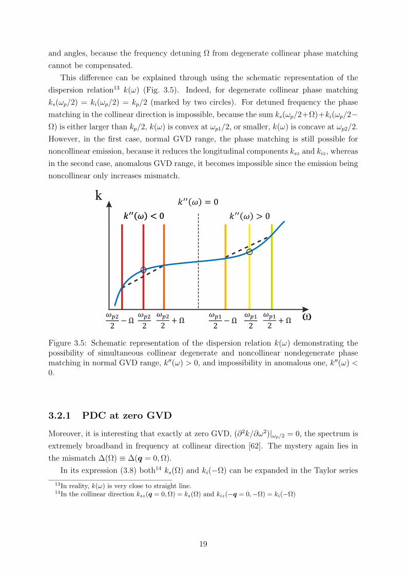
and angles, because the frequency detuning Ω from degenerate collinear phase matching

cannot be compensated.

This difference can be explained through using the schematic representation of the

dispersion relation13 k(ω) (Fig. 3.5). Indeed, for degenerate collinear phase matching

ks(ωp/2) = ki(ωp/2) = kp/2 (marked by two circles). For detuned frequency the phase

matching in the collinear direction is impossible, because the sum ks(ωp/2+Ω)+ki(ωp/2−Ω) is either larger than kp/2, k(ω) is convex at ωp1/2, or smaller, k(ω) is concave at ωp2/2.

However, in the first case, normal GVD range, the phase matching is still possible for

noncollinear emission, because it reduces the longitudinal components ksz and kiz, whereas

in the second case, anomalous GVD range, it becomes impossible since the emission being

noncollinear only increases mismatch.

Figure 3.5: Schematic representation of the dispersion relation k(ω) demonstrating thepossibility of simultaneous collinear degenerate and noncollinear nondegenerate phasematching in normal GVD range, k′′(ω) > 0, and impossibility in anomalous one, k′′(ω) <0.

3.2.1 PDC at zero GVD

Moreover, it is interesting that exactly at zero GVD, (∂2k/∂ω2)|ωp/2 = 0, the spectrum is

extremely broadband in frequency at collinear direction [62]. The mystery again lies in

the mismatch ∆(Ω) ≡ ∆(q = 0,Ω).

In its expression (3.8) both14 ks(Ω) and ki(−Ω) can be expanded in the Taylor series

13In reality, k(ω) is very close to straight line.14In the collinear direction ksz(q = 0,Ω) = ks(Ω) and kiz(−q = 0,−Ω) = ki(−Ω)

19

around Ω = 0. Thus,

∆(Ω) = (ks(0) + ki(0)− kp) +∞∑l=1

[k(l)s (0) + (−1)lk

(l)i (0)

] Ωl

l!. (3.24)

The first term is equal to zero due to phase matching. In the general case k′s(0) 6= k′i(0) and

the term with l = 1 defines the width of the spectrum. This is the case for nondegenerate

phase matching (see Fig. 3.3). Yet, in case of degenerate one, k′s(0) = k′i(0), only the

term with l = 2 plays a role. Therefore, the spectral width in the collinear direction is

much broader in the degenerate case than in the nondegenerate one; just compare the

cases with φ = 29.18 and 28.6 (Fig. 3.3).

At zero GVD only the term with l = 4 is nonzero, therefore, the phase matching is

extremely broad. It is much broader than in the case of any degenerate phase matching

and can cover more than 100 THz [63]. This fact is used in works on parametric generation

and amplification [64, 65, 66].

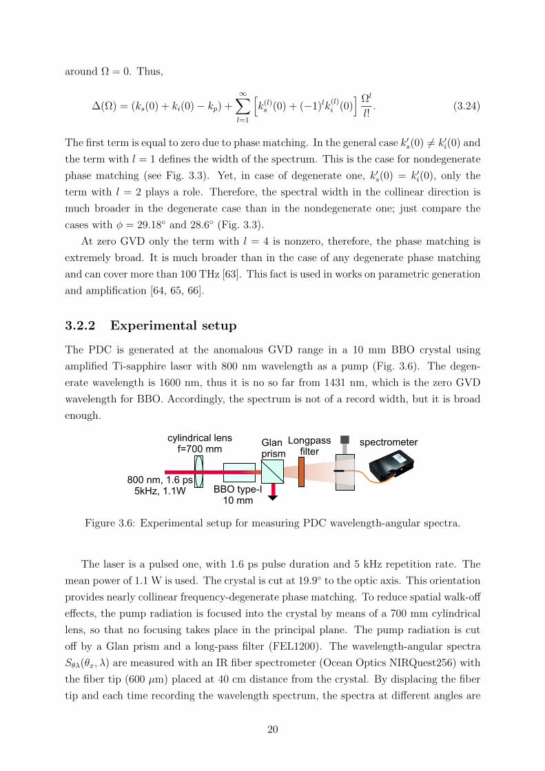
3.2.2 Experimental setup

The PDC is generated at the anomalous GVD range in a 10 mm BBO crystal using

amplified Ti-sapphire laser with 800 nm wavelength as a pump (Fig. 3.6). The degen-

erate wavelength is 1600 nm, thus it is no so far from 1431 nm, which is the zero GVD

wavelength for BBO. Accordingly, the spectrum is not of a record width, but it is broad

enough.

cylindrical lensf=700 mm

BBO type-I 10 mm

800 nm, 1.6 ps5kHz, 1.1W

Glanprism

Longpassfilter

spectrometer

Figure 3.6: Experimental setup for measuring PDC wavelength-angular spectra.

The laser is a pulsed one, with 1.6 ps pulse duration and 5 kHz repetition rate. The

mean power of 1.1 W is used. The crystal is cut at 19.9 to the optic axis. This orientation

provides nearly collinear frequency-degenerate phase matching. To reduce spatial walk-off

effects, the pump radiation is focused into the crystal by means of a 700 mm cylindrical

lens, so that no focusing takes place in the principal plane. The pump radiation is cut

off by a Glan prism and a long-pass filter (FEL1200). The wavelength-angular spectra

Sθλ(θx, λ) are measured with an IR fiber spectrometer (Ocean Optics NIRQuest256) with

the fiber tip (600 µm) placed at 40 cm distance from the crystal. By displacing the fiber

tip and each time recording the wavelength spectrum, the spectra at different angles are

20

obtained. The angular scanning is done in the horizontal direction, in which the pump

beam is not focused.

3.2.3 Wavelength-angular spectra and correlation functions (CF)

The spectra for φ = 19.87 and 19.98 are obtained by combining the wavelength spectra

at different angles into 2D plot. They are presented in Fig. 3.7 together with the corre-

sponding theoretical spectra calculated using the approach discussed in section 3.1.1.

Figure 3.7: Experimental [(a), (b)] and theoretical [(c), (d)] wavelength-angular spectraSθλ for crystal orientations φ = 19.87 [(a), (c)] and φ = 19.98 [(b), (d)].

The spectra are indeed restricted in both wavelength and angle. At exact collinear

frequency-degenerate phase matching, φ = 19.87, the spectrum has the shape of a spot

while, with the crystal detuned from this orientation, φ = 19.98, the shape resembles

a ring. With the tuning in the other direction, the smaller angle φ, the phase matching

disappears. As described in section 3.1.3 the intensity decreases toward long wavelengths

due to the λ4 factor. Also one could notice that the experimental ring-shaped spectrum

[panel (b)] is brighter at the large angles. This is caused by the spatial walk-off effect that

will be described in section 4.4.

The spectrum Sθλ, as shown in Fig. 3.7 (b,d), converted to S(q,Ω) acquires an ideal

ring shape (Fig. 3.8). Similarly to the X-shaped case (see Fig. 3.1) it is nonfactorizable

21

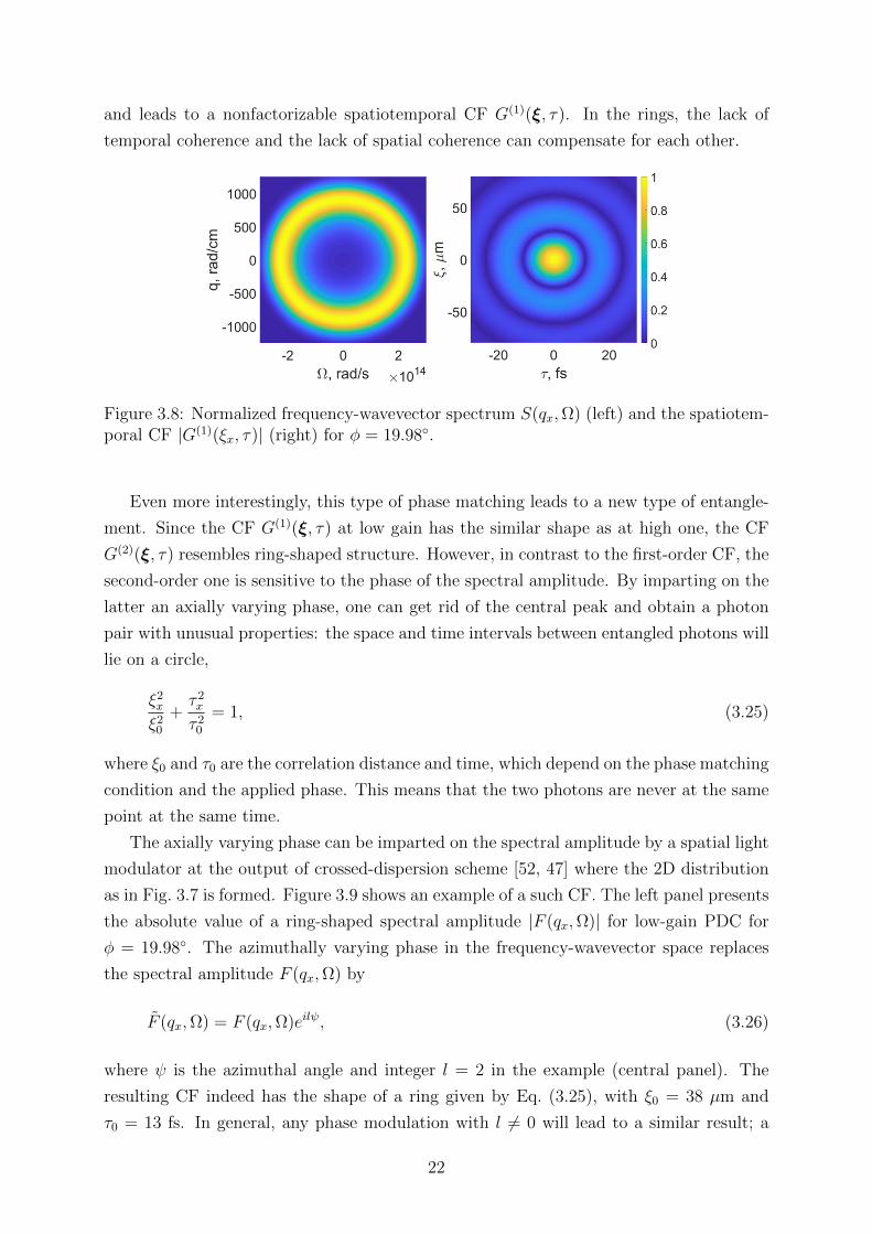
and leads to a nonfactorizable spatiotemporal CF G(1)(ξ, τ). In the rings, the lack of

temporal coherence and the lack of spatial coherence can compensate for each other.

Figure 3.8: Normalized frequency-wavevector spectrum S(qx,Ω) (left) and the spatiotem-poral CF |G(1)(ξx, τ)| (right) for φ = 19.98.

Even more interestingly, this type of phase matching leads to a new type of entangle-

ment. Since the CF G(1)(ξ, τ) at low gain has the similar shape as at high one, the CF

G(2)(ξ, τ) resembles ring-shaped structure. However, in contrast to the first-order CF, the

second-order one is sensitive to the phase of the spectral amplitude. By imparting on the

latter an axially varying phase, one can get rid of the central peak and obtain a photon

pair with unusual properties: the space and time intervals between entangled photons will

lie on a circle,

ξ2x

ξ20

+τ 2x

τ 20

= 1, (3.25)

where ξ0 and τ0 are the correlation distance and time, which depend on the phase matching

condition and the applied phase. This means that the two photons are never at the same

point at the same time.

The axially varying phase can be imparted on the spectral amplitude by a spatial light

modulator at the output of crossed-dispersion scheme [52, 47] where the 2D distribution

as in Fig. 3.7 is formed. Figure 3.9 shows an example of a such CF. The left panel presents

the absolute value of a ring-shaped spectral amplitude |F (qx,Ω)| for low-gain PDC for

φ = 19.98. The azimuthally varying phase in the frequency-wavevector space replaces

the spectral amplitude F (qx,Ω) by

F (qx,Ω) = F (qx,Ω)eilψ, (3.26)

where ψ is the azimuthal angle and integer l = 2 in the example (central panel). The

resulting CF indeed has the shape of a ring given by Eq. (3.25), with ξ0 = 38 µm and

τ0 = 13 fs. In general, any phase modulation with l 6= 0 will lead to a similar result; a

22

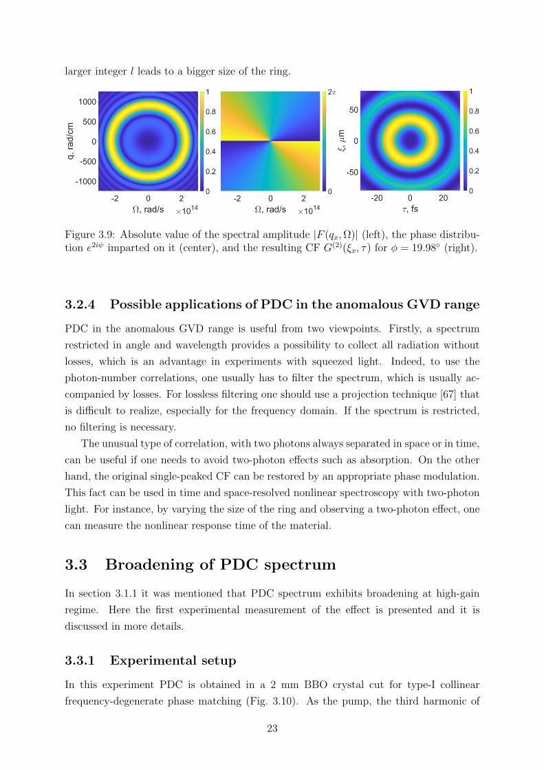
larger integer l leads to a bigger size of the ring.

Figure 3.9: Absolute value of the spectral amplitude |F (qx,Ω)| (left), the phase distribu-tion e2iψ imparted on it (center), and the resulting CF G(2)(ξx, τ) for φ = 19.98 (right).

3.2.4 Possible applications of PDC in the anomalous GVD range

PDC in the anomalous GVD range is useful from two viewpoints. Firstly, a spectrum

restricted in angle and wavelength provides a possibility to collect all radiation without

losses, which is an advantage in experiments with squeezed light. Indeed, to use the

photon-number correlations, one usually has to filter the spectrum, which is usually ac-

companied by losses. For lossless filtering one should use a projection technique [67] that

is difficult to realize, especially for the frequency domain. If the spectrum is restricted,

no filtering is necessary.

The unusual type of correlation, with two photons always separated in space or in time,

can be useful if one needs to avoid two-photon effects such as absorption. On the other

hand, the original single-peaked CF can be restored by an appropriate phase modulation.

This fact can be used in time and space-resolved nonlinear spectroscopy with two-photon

light. For instance, by varying the size of the ring and observing a two-photon effect, one

can measure the nonlinear response time of the material.

3.3 Broadening of PDC spectrum

In section 3.1.1 it was mentioned that PDC spectrum exhibits broadening at high-gain

regime. Here the first experimental measurement of the effect is presented and it is

discussed in more details.

3.3.1 Experimental setup

In this experiment PDC is obtained in a 2 mm BBO crystal cut for type-I collinear

frequency-degenerate phase matching (Fig. 3.10). As the pump, the third harmonic of

23

a Nd:YAG laser with the wavelength λp = 354.7 nm, pulse duration 18 ps, repetition rate

1 kHz, and the energy per pulse up to 0.1 mJ is used. The coherence time of the pump is

less than the pulse duration and equal to 5 ps. The pump is focused by a 1 m lens into

the crystal and reflected after it by a dichroic mirror (DM). The pump power is controlled

with a power meter (PM).

Nd: YAG 3ω

PM

CCDDM

BBO 2mmtype-I

Figure 3.10: Experimental setup for measuring the spectral broadening.

This experiment is devoted to the frequency domain, therefore the nonfactorazibility of

S(q,Ω) is removed via the filtering in the collinear direction, being done with an aperture

placed in the far-field zone. The emission angle selected this way is 0.17 (inside the

crystal).

All radiation passing through the aperture is focused on the input slit of a HORIBA

Jobin Yvon Micro HR monochromator equipped with a CCD array. The spectral mea-

surements are performed with the best possible resolution 0.2 nm.

0 20 40 60 800

2

4

6

PD

C in

ten

sity

, re

l. u

nits

Pump power, mW0 20 40 60 80

1E-3

0,01

0,1

1

10

Pump power, mW

Figure 3.11: The dependence of the PDC intensity on the pump power (points) and itsfit (line) with Eq. (3.27) in linear (left) and log-linear (right) scales.

In all measurements, the spectral properties are studied depending on the parametric

gain G, which is found from the nonlinear dependence of PDC intensity I on the pump

power P (see Fig. 3.11). The fitting function [68],

I = I0 sinh2(B√P ), (3.27)

is based on Eqs. (2.6) and (3.6) with the fitting parameters I0 and B. The gain should

be measured around the zero mismatch, otherwise instead of G one gets some averaged

value of G, see Eqs. (3.6) and (3.7). In this experiment the PDC should be well filtered

24

in q and Ω near the collinear frequency-degenerate point. After the fitting, each pump

power corresponds to a certain gain value, G = B√P .

3.3.2 Measurement of the spectral broadening

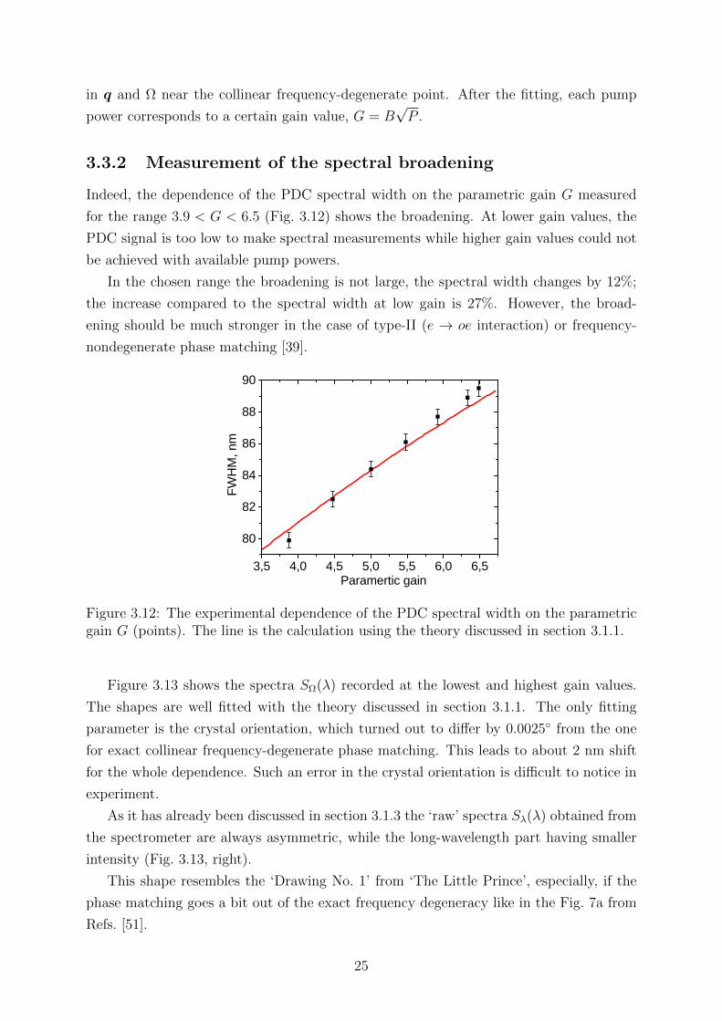
Indeed, the dependence of the PDC spectral width on the parametric gain G measured

for the range 3.9 < G < 6.5 (Fig. 3.12) shows the broadening. At lower gain values, the

PDC signal is too low to make spectral measurements while higher gain values could not

be achieved with available pump powers.

In the chosen range the broadening is not large, the spectral width changes by 12%;

the increase compared to the spectral width at low gain is 27%. However, the broad-

ening should be much stronger in the case of type-II (e → oe interaction) or frequency-

nondegenerate phase matching [39].

3 , 5 4 , 0 4 , 5 5 , 0 5 , 5 6 , 0 6 , 58 08 28 48 68 89 0

FWHM

, nm

P a r a m e r t i c g a i n

Figure 3.12: The experimental dependence of the PDC spectral width on the parametricgain G (points). The line is the calculation using the theory discussed in section 3.1.1.

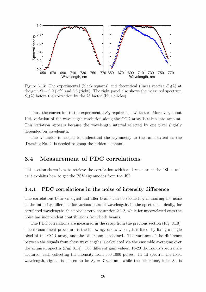
Figure 3.13 shows the spectra SΩ(λ) recorded at the lowest and highest gain values.

The shapes are well fitted with the theory discussed in section 3.1.1. The only fitting

parameter is the crystal orientation, which turned out to differ by 0.0025 from the one

for exact collinear frequency-degenerate phase matching. This leads to about 2 nm shift

for the whole dependence. Such an error in the crystal orientation is difficult to notice in

experiment.

As it has already been discussed in section 3.1.3 the ‘raw’ spectra Sλ(λ) obtained from

the spectrometer are always asymmetric, while the long-wavelength part having smaller

intensity (Fig. 3.13, right).

This shape resembles the ‘Drawing No. 1’ from ‘The Little Prince’, especially, if the

phase matching goes a bit out of the exact frequency degeneracy like in the Fig. 7a from

Refs. [51].

25

650 670 690 710 730 750 770Wavelength, nm

650 670 690 710 730 750 7700,0

0,2

0,4

0,6

0,8

1,0

Wavelength, nm

Spectr

al density

Figure 3.13: The experimental (black squares) and theoretical (lines) spectra SΩ(λ) atthe gain G = 3.9 (left) and 6.5 (right). The right panel also shows the measured spectrumSλ(λ) before the correction by the λ4 factor (blue circles).

Thus, the conversion to the experimental SΩ requires the λ4 factor. Moreover, about

10% variation of the wavelength resolution along the CCD array is taken into account.

This variation appears because the wavelength interval selected by one pixel slightly

depended on wavelength.

The λ4 factor is needed to understand the asymmetry to the same extent as the

‘Drawing No. 2’ is needed to grasp the hidden elephant.

3.4 Measurement of PDC correlations

This section shows how to retrieve the correlation width and reconstruct the JSI as well

as it explains how to get the BSV eigenmodes from the JSI.

3.4.1 PDC correlations in the noise of intensity difference

The correlations between signal and idler beams can be studied by measuring the noise

of the intensity difference for various pairs of wavelengths in the spectrum. Ideally, for

correlated wavelengths this noise is zero, see section 2.1.2, while for uncorrelated ones the

noise has independent contributions from both beams.

The PDC correlations are measured in the setup from the previous section (Fig. 3.10).

The measurement procedure is the following: one wavelength is fixed, by fixing a single

pixel of the CCD array, and the other one is scanned. The variance of the difference

between the signals from these wavelengths is calculated via the ensemble averaging over

the acquired spectra (Fig. 3.14). For different gain values, 10-20 thousands spectra are

acquired, each collecting the intensity from 500-1000 pulses. In all spectra, the fixed

wavelength, signal, is chosen to be λs = 702.4 nm, while the other one, idler λi, is

26

scanned around degenerate wavelength (709.3 nm), from 700 nm to 720 nm.

700 705 710 715 720

0,1

1

Wavelength, nm700 705 710 715 720

0,0

0,2

0,4

0,6

0,8

1,0V

aria

nce

, re

l. u

nits

Wavelength, nm

Figure 3.14: Variance of the difference between PDC intensities at given wavelength,702.4 nm, and scanned wavelengths, 700-720 nm, for the parametric gain G = 6.4 (black),6.5 (red), and 6.8 (blue) in linear (left) and log-linear (right) scales. The variance isnormalized to the maximum of the last curve.

Each variance distribution contains two ‘dips’ and one ‘peak’. The left-hand (auto-

correlation) dip is caused by correlations existing within a single mode. The dip goes down

to zero because the variance is identically zero when the reading of a pixel is subtracted

from itself. The dip is surrounded by the oscillating noise, which in its respect is an

artifact and should therefore not be considered.

The right-hand (cross-correlation) dip is caused by correlations between signal and

idler beams, with the wavelengths related as λ−1s + λ−1

i = λ−1p , i.e. in accordance with

energy conservation law [Eq. (2.1)]. Respectively, the peak at degenerate wavelength,

709.3 nm, occurs due to superbunching that is to be discussed in chapter 5.

In more detail, the variance of photon-number difference is [69]

〈∆(Ns−Ni)2〉 = (g(2)

ss −1)〈Ns〉2 +(g(2)ii −1)〈Ni〉2−2(g

(2)si −1)〈Ns〉〈Ni〉+〈Ns+Ni〉, (3.28)

where g(2)12 is the second-order normalized CF,

g(2)12 ≡

〈: N1N2 :〉〈N1〉〈N2〉

, (3.29)

where 1, 2 means s, i and 〈: · · · :〉 denotes normal ordering.

Outside of the peak PDC has thermal statistics15, g(2)ss = g

(2)ii = 2, and outside of the

dips the correlations are absent, g(2)si = 1. Therefore, at the background 〈∆(Ns − Ni)

2〉 =

2〈N〉2, if 〈Ni〉 = 〈Ns〉 ≡ 〈N〉 1. In the peak g(2)ii = 3 + 1/〈N〉, therefore the variance

is equal to 3〈N〉2 for large 〈N〉. In the cross-correlation dip g(2)si = 2 + 1/〈N〉 and the

15The statistical properties will be discussed in more details in chapter 5.

27

variance should be zero. However, this complete noise suppression can be observed only

under strict requirements [70], e.g. perfect mode matching and 100% detection efficiency,

that are not satisfied in the experiment.

The Eq. (3.28) is not valid in the auto-correlation dip, because it is obtained under

the assumption of commuting signal as and idler ai photon creation (or annihilation)

operators, see Eq. (2.8). However, it is clear that the variance of the number of photons

subtracted from itself is equal to zero, 〈∆(Ns − Ns)2〉 = 0.

According to Eq. (3.28), the peak in Fig. 3.14 should be 50% higher than the back-

ground value, independently of the gain G. In all dependences, only a 30±5% increase of

the variance is seen. This difference can be attributed to the insufficient frequency selec-

tion. As to the cross-correlation dip, the imperfect mode matching reduces its depth; the

value at the dip is 40± 5% of background one. At smaller gain values, the measurement

is not accurate enough to reveal the correlations.

Another observation from Fig. 3.14 is that the peak width is smaller than the width

of the dips. Accurate fitting by Gaussian functions yields, in the case of G = 6.5, the

values of 0.26 ± 0.06 nm, 0.45 ± 0.06 nm, and 0.52 ± 0.06 nm for the peak, auto- and

cross-correlation dips, respectively.

The spectral widths of the dips coincide with the spectral widths of the CF g(2) and

at low gain should be given by the pump bandwidth; this results in ∆λ = 0.15 nm

at wavelengths around 709 nm. The larger width at a higher gain is explained by the

redistribution of the Schmidt coefficients, see Eq. (3.23). From simplified argumentation

it can be explained by nonlinear dependence of PDC intensity on the pump one. At

the ‘top’ of the pump pulse the gain is larger than on the slopes; so the most photons

are produced there. For this reason, the effective pulse width decreases and the effective

pump ‘bandwidth’ increases. The same should happen in the spatial domain; indeed, it

is shown experimentally [58] that the angular correlation width (speckle size) increases

with the gain.

As to the peak, its width, theoretically, should be narrower than the correlation width

by a factor of 2. Simply it can be understood as follows: for the dip one wavelength (λs)

is fixed, the other one (λi) is scanned, whereas for the peak both wavelengths are kind of

scanned together due to the superbunching requirement16, λs = λi. The observed widths

of 0.26± 0.06 nm for the peak and 0.52± 0.06 nm for the dip are in agreement with these

considerations.

3.4.2 Measurement of the joint spectral intensity (JSI)

As it was discussed in section 3.1.4, the more complete information about correlations

can be obtained by measuring the 2D distribution of some quantity, as a function of both

16Signal and idler photons should have exactly the same wavelength, because superbunching is observedonly if each pixel of a CCD array used in spectrometer detect both photons.

28

wavelengths λs and λi. As such quantity, one can choose the variance of the difference

signal as in Fig. 3.14, but it is more natural to measure the covariance of the signals at

two wavelengths,

cov(Ns, Ni) ≡ 〈NsNi〉 − 〈Ns〉〈Ni〉 = (g(2)si − 1)〈Ns〉〈Ni〉. (3.30)

A bit latter it will be shown that it is equal, up to a constant factor, to the JSI.

The covariance gives a full account of pairwise correlations, which now manifest them-

selves as peaks (Fig. 3.15). As for Fig. 3.14, the auto-correlation peaks occur on the

straight line λs = λi and the cross-correlation ones are on the line λ−1s + λ−1

i = λ−1p . The

superbunched peak also reveals itself.

The cross-correlation peaks represent the JSI, similar to the two-photon case (see

Fig. 3.4): its cross-section gives the conditional width, while its projections on the axes

λs and λi provide the unconditional ones. As it was discussed in the previous section,

these widths are different from the ones for the SPDC case, and therefore the number of

modes is different. Namely, in the low-gain case the full spectral width is estimated to

be 70.2 nm and the correlation width is to be 0.15 nm, which results in the Fedorov ratio

R ≈ 470, while at the parametric gain G = 6.5 the corresponding widths are 89.5±0.5 nm

and 0.52± 0.06 nm, respectively, which gives the ratio R = 172± 20.

Figure 3.15: 2D distribution of covariance cov(Ns, Ni) (left) and its zoomed central part(right) for the gain G = 6.5. It is normalized to its maximum value. Note that onlycross-correlation peaks correspond to the JSI.

The analogy between the covariance and the JSI can be understood using the Schmidt

modes, see section 3.1.4. The covariance is equal to [71]

cov[Ns(Ωs), Ni(Ωi)] =

∣∣∣∣∣∞∑l=0

ulvlψl(Ωs)φl(Ωi)

∣∣∣∣∣2

, (3.31)

29

where ul = cosh(Gl).

At low gain ulvl ∼ Gl and the covariance is equal to JSI up to a factor G. This mea-

surement is similar to the registration of coincidences (g(2) measurement) [51]; indeed, at

low gain the CF g(2)si 1 and cov(Ns, Ni) ∝ g

(2)si , see Eq. (3.30). At high gain the covari-

ance again provides JSI, because ul ≈ vl and the Schmidt coefficients are redistributed,

see Eq. (3.23).

Accordingly, the singular value decomposition [Eq. (3.19)] of√

cov[Ns(Ωs), Ni(Ωi)]

gives the shapes of reconstructed Schmidt modes, ψl(Ωs) and φl(Ωi), and the correspond-

ing Schmidt coefficients, Λl. The latter should be normalized according to Eq. (3.20).

In Fig. 3.15 the JSI ‘sits’ on the background17 that repeats the total PDC spectrum.

This background could degrade the quality of the reconstructed modes; in experiment, it

could be eliminated by single-shot measurements synchronized with the laser pulses [71,

72].

Interestingly, a similar method has been applied to characterize the intensity corre-

lations in fiber optical solitons [73] and to get the spatiotemporal correlations [74, 75].

Finally, there is another, quite elegant, method for the JSI reconstruction called the stim-

ulated emission tomography [76, 77].

3.5 Schmidt number and non-phase-matched sum fre-

quency generation

This section explains how one can assess the number of modes using non-phase-matched

SFG. Despite the fact that the main part of work was done by Denis Kopylov, the author’s

contribution in the experimental and theoretical work was significant. Therefore, the

experiment is briefly discussed below.

3.5.1 The pump reconstruction

As it has been already discussed, BSV has two characteristic parameters: the total spectral

width and the correlation width. What will happen if we add the second nonlinear crystal

and generate the sum frequency from BSV? These two characteristic parameters should

manifest themselves.

In our experiment the BSV is produced via PDC, the same way as in the experiment

on PDC generation in the anomalous GVD range (section 3.2). The produced BSV is

filtered to a single spatial mode in the collinear direction and then sharply focused into

a 1 mm lithium niobate (LiNbO3) crystal where SFG occurs through ee→ e interaction

without phase matching. The generated light is separated from the BSV and measured

with a visible spectrometer with 1.3 nm resolution.

17It looks red in the figure.

30

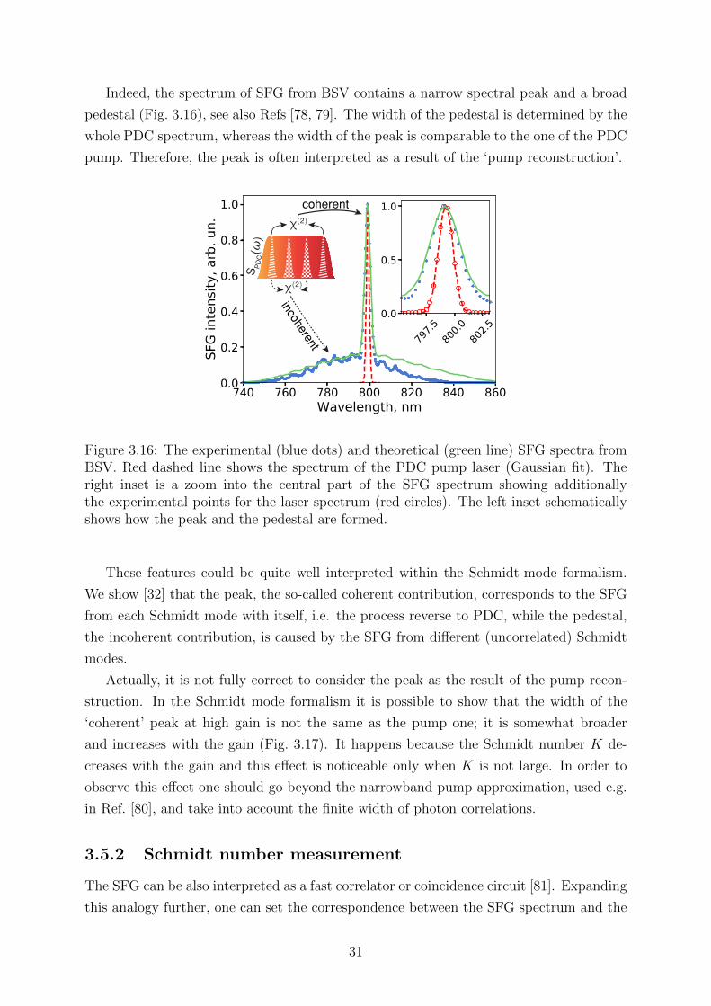
Indeed, the spectrum of SFG from BSV contains a narrow spectral peak and a broad

pedestal (Fig. 3.16), see also Refs [78, 79]. The width of the pedestal is determined by the

whole PDC spectrum, whereas the width of the peak is comparable to the one of the PDC

pump. Therefore, the peak is often interpreted as a result of the ‘pump reconstruction’.

χ()

χ()

𝜔

Figure 3.16: The experimental (blue dots) and theoretical (green line) SFG spectra fromBSV. Red dashed line shows the spectrum of the PDC pump laser (Gaussian fit). Theright inset is a zoom into the central part of the SFG spectrum showing additionallythe experimental points for the laser spectrum (red circles). The left inset schematicallyshows how the peak and the pedestal are formed.

These features could be quite well interpreted within the Schmidt-mode formalism.

We show [32] that the peak, the so-called coherent contribution, corresponds to the SFG

from each Schmidt mode with itself, i.e. the process reverse to PDC, while the pedestal,

the incoherent contribution, is caused by the SFG from different (uncorrelated) Schmidt

modes.

Actually, it is not fully correct to consider the peak as the result of the pump recon-

struction. In the Schmidt mode formalism it is possible to show that the width of the

‘coherent’ peak at high gain is not the same as the pump one; it is somewhat broader

and increases with the gain (Fig. 3.17). It happens because the Schmidt number K de-

creases with the gain and this effect is noticeable only when K is not large. In order to

observe this effect one should go beyond the narrowband pump approximation, used e.g.

in Ref. [80], and take into account the finite width of photon correlations.

3.5.2 Schmidt number measurement

The SFG can be also interpreted as a fast correlator or coincidence circuit [81]. Expanding

this analogy further, one can set the correspondence between the SFG spectrum and the

31

0 2 4 6 8 10 120

0.51.01.52.02.53.03.5

, nm

G

Figure 3.17: Calculated bandwidth of the SFG peak vs. the PDC gain G0 for the firstSchmidt mode; at low gain, G0 1, the peak bandwidth is equal to the PDC pumpbandwidth.

conditional and unconditional bandwidths. The width of the peak, ∆Ωcoh, corresponds

to the first one, while the width of the pedestal, ∆Ωincoh, to the second one.

It implies that the ratio of the widths, R = ∆Ωincoh/∆Ωcoh, has a similar meaning

as the Fedorov ratio [Eq. (3.22)]. Similarly, the ratio R should be equal to the Schmidt

number K. To test this statement, we calculate K and R for different values of pump

pulse duration (Fig. 3.18); indeed, the result is that R = K.

0.5 1.0 1.5 2.0, ps

5

10

15

20

25

K, R

Figure 3.18: The Schmidt number K (blue line) and the ratio R (green dots) calculatedfor the experimental parameters from section 3.2 as functions of the PDC pump pulseduration.

In experiment we get the ratio Rexp ≈ 13, which is smaller than the expected one

Rtheor = 19.5. It happens because the BSV spectrum is partially cut due to experimental

imperfections, which leads to a reduced bandwidth ∆Ωincoh. The estimate for the Schmidt

number is correct only for frequency-independent losses, the ones that depends on the

32

frequency change the result. The same applies if the SFG phase matching is not broad

enough; that is why it is important to make the SFG broadband, e.g. by avoiding the

phase matching.

The major possible limitation is that the method requires a presence of the coherent

peak, which can be observed as long as signal-idler correlations are not completely lost.

The peak is pronounced if its spectral intensity is higher than the pedestal one. Therefore,

the ratio of the peak and pedestal spectral intensities quantifies the quality of signal-idler

correlations; in Fig. 3.16 this ratio is equal to 7.3± 0.9.

- 4 4 0 - 4 2 0 - 4 0 0 - 3 8 0 - 3 6 00 , 00 , 51 , 01 , 52 , 02 , 53 , 0

Peak

to pe

desta

l inten

sity ra

tio

A p p l i e d G D D , f s 2

Figure 3.19: The ratio of the peak and pedestal spectral intensities vs. applied GDD.

In particular, the loss of these correlations can occur due to the group delay dispersion

(GDD), which leads to the time delay between the signal and idler photons. Sometimes one

can prevent it with dispersion-compensating methods. In the other setup we successfully

demonstrate this together with Hani Abou Hadba [82]. Indeed, as shown in Fig. 3.19, the

peak is retrieved and the peak to pedestal ratio reaches its maximum, if the correct GDD

(-400 fs2) is applied.

33

Chapter 4

Twin-beam correlations in PDC

The Signal and the Idler are twin brothers.

Who is more valuable for Physics?

We say the Idler and we mean the Signal,

We say the Signal and we mean the Idler.

—Derivative on Vladimir Mayakovsky’s poem

This chapter focuses on some interesting effects emerging from signal-idler correlations.

It starts with the interference of signal and idler beams on a 50% BS, the HOM effect,

and the Fock states interference, which are greatly considerable for quantum optics.

Further, there is the macroscopic HOM interference, the case of bright twin beams,

demonstrated. Although the standard measurement technique leads to a very low visibil-

ity, a modified technique provides a visibility close to unity. Applying this technique the

interference manifests itself as a peak, which additionally provides the information about

the PDC spectral properties, including the number of temporal modes.

Afterwards, the chapter focuses on the statistics at the BS outputs, which is similar

to the one obtained for the Fock states interference. The phase fluctuations are converted

into photon-number fluctuations manifesting themselves in a U-shaped photon-number

distribution.

Finally, it is shown how spatial and temporal walk-off matching can be used for giant

narrowband twin-beam generation. If one of the twin beams is emitted along the pump

Poynting vector or its group velocity matches that of the pump, the generation of both

beams will be drastically enhanced; the effect is exemplified on the chapter’s cover. This

enhancement leads to a considerable narrowing of the wavelength and angular spectrum.

35

4.1 Introduction

4.1.1 Hong-Ou-Mandel (HOM) interference

In 1987 Hong, Ou, and Mandel suggested a method for measuring subpicosecond time

intervals between photons using the interference on a 50% BS [83]. If signal and idler

photons come to BS exactly at the same time, they always leave it from the same output

port, never from the different ones.

In experiment one measures the number of coincidences at the BS outputs, namely the

number of events, when the photons are detected at the same time, i.e. in coincidence.

This measurement, up to a constant factor, gives the second-order CF g(2)12 [68]. If the

photons come to the BS at the same time, the number of coincidences drops drastically;

so, a narrow ‘dip’ in the coincidence rate is observed, if the delay between signal and idler

photons is scanned. Therefore, the HOM effect is often called ‘the HOM dip’, although

under certain conditions it manifests itself as a peak [84].

The effect happens due to the destructive interference of the probability amplitudes

for both photons to be transmitted and to be reflected (Fig. 4.1). The key point here

is that the photons should be indistinguishable in all characteristics such as wavelength,

polarization, wave vector, etc.; any distinguishability degrades the HOM effect visibility.

s

i

s

i

s

i

s

i

1

2

1

2

1

2

1

2

a b c d

Figure 4.1: Four possible two-photon incidents on a BS: one photon is transmitted andthe second one is reflected (a,b), both photons are reflected (c), and both photons aretransmitted (d). For indistinguishable photons the last two cases interfere destructively.

This feature allows to use the HOM interference for characterizing distinguishabil-

ity [85] and as an identity test for single-photon states [86], including ones generated from

two different sources, like crystals [87] or molecules [88].

As it was suggested in the pioneering work [83], the effect can be used to measure time

intervals with high accuracy, because the width of the dip could be extremely small, up to

a few femtoseconds [89]; for example, the HOM effect was used to measure the tunneling

time [90].

The width of the dip is twice smaller [91] than the one of the first-order CF G(1)(τ)

and is not affected by GVD [92]. Due to these features the HOM effect is proposed to use

in the quantum version of optical coherence tomography (OCT) [93, 94].

36

In the quantum OCT the signal photons travel though the sample before the BS,

while the idler ones are passing the delay line, which introduces a variable time delay.

The positions of the HOM dips give the positions of reflecting/scattering layers in the

sample. The resolution of the quantum OCT is twice higher than the one of the standard

OCT for the same bandwidth of light. Furthermore, the method is not sensitive to the

acquired GDD.

4.1.2 Fock states interference

The HOM interference can be considered as a special case of Fock states |N 〉 interference

on a 50% BS. Indeed, if the vacuum and higher photon contributions to the PDC state

[Eq. (2.11)] are neglected, the interference just transforms the state |1〉s |1〉i into |2〉1 |0〉2+

|0〉1 |2〉2. Therefore, at each BS output, e.g. the output number 1, the probability P (N1)

to get N1 = 1 photon is zero, see Fig. 4.2 (left).

0 1 20,00

0,25

0,50N=1

P(N

1)

N1

0 5 10 15 20 25 30 35 400,00

0,05

0,10

0,15N=20

N1

0 200 400 600 800 10000,00

0,01

0,02

0,03N=500

N1

Figure 4.2: Probability distributions P (N1) at one of the BS outputs for the interferenceof Fock states |N 〉: N = 1 (left), 20 (center), and 500 (right).

The increase of N leads to a more complicated distribution [95],

P (N1 = 2m) =1

22N

(2m

m

)(2N − 2m

N −m

)and P (N1 = 2m+ 1) = 0, (4.1)

where(kl

)is the binomial coefficient. The examples for N = 20 and 500 are shown in

Fig. 4.2 (center and right). The maximal probabilities are at N1 = 0 and 2N , meaning

that all 2N photons go together to one output, and the envelope manifests an ‘U’ shape.

Moreover, the odd photon numbers do not occur at all; unfortunately, at high N this is

hardly distinguishable.

The distribution (4.1) is called the discrete arcsine one [95]. This type of distribution

occurs also in a classical random walk [95]. The distribution (4.1) provides the proba-

bility that a random walker visited the initial point for the last time on step N1 after

2N steps have been made. However, the position of the same walker after 2N steps is

given by binomial distribution. Exactly the same binomial law describes the probability

distribution for distinguishable, non-interfering, Fock states at the BS inputs [95].

37

Such a U-shaped distribution appears due to the general property of a BS: it converts

phase fluctuations into amplitude ones and vice versa [96, 97]. Indeed, the photon-number

difference is zero and the phase difference is uncertain for Fock states at the inputs, at

the same time after the BS the photon-number difference fluctuates a lot, whereas the

phase difference is certain up to the Heisenberg limit, 1/2N [98].

Differently it can be understood from ‘the conservation law for the sum of correlations

and fluctuations’ [96]. The sum of the second-order auto-CFs G(2)11 = 〈: N2

1 :〉 and G(2)22 =

〈: N22 :〉 for outputs 1 and 2, respectively, and the doubled cross-CF G

(2)12 = 〈: N1N2 :〉 is

the same before and after BS,

G(2)11 +G

(2)22 + 2G

(2)12 = const. (4.2)

For the Fock states the photons numbers at the inputs do not fluctuate and are highly

correlated; hence, at the output the drop of correlations is accompanied by an increase in

fluctuations.

4.2 Macroscopic HOM interference

The introduction described the HOM interference for a pair of photons neglecting the

higher photon contributions in SPDC. However, these contributions exist and degrade the

HOM effect visibility [99]. Moreover, the visibility reduces even more if many modes are

involved. Here for observing the HOM effect with bright beams an alternative approach is

suggested, which is based on the measurement of the normalized variance of the difference

signal, which in its turn is robust against multimode detection [70].

4.2.1 Theoretical description: CF and variance of the difference

signal

The theoretical treatment is based on the model described in section 3.1. Like in the

several previous sections, only the frequency domain, q = 0, and one spatial mode are

considered. Assuming that the signal (s) and idler (i) beams arrive at a 50% BS with a

relative delay τ , the BS transformations for the output (1, 2) take the form

a1(t) =as(t− τ) + ai(t)√

2, a2(t) =

−as(t− τ) + ai(t)√2

, (4.3)

where the operators as,i(t) are related with as,i(Ω), see Eq. (3.2), via the inverse FT.

At this stage three important aspects should be discussed. Firstly, the problem of

multimode detection appearing if the detector is not fast enough. In this case the fluctua-

tions and correlations are averaged over the detection time T . Thus, the photon numbers,

38

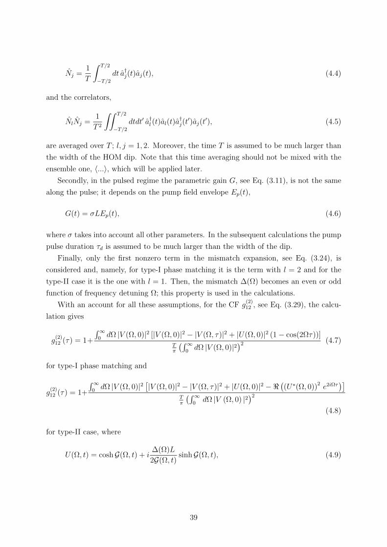
Nj =1

T

∫ T/2

−T/2dt a†j(t)aj(t), (4.4)

and the correlators,

NlNj =1

T 2

∫∫ T/2

−T/2dtdt′ a†l (t)al(t)a

†j(t′)aj(t

′), (4.5)

are averaged over T ; l, j = 1, 2. Moreover, the time T is assumed to be much larger than

the width of the HOM dip. Note that this time averaging should not be mixed with the

ensemble one, 〈...〉, which will be applied later.

Secondly, in the pulsed regime the parametric gain G, see Eq. (3.11), is not the same

along the pulse; it depends on the pump field envelope Ep(t),

G(t) = σLEp(t), (4.6)

where σ takes into account all other parameters. In the subsequent calculations the pump

pulse duration τd is assumed to be much larger than the width of the dip.

Finally, only the first nonzero term in the mismatch expansion, see Eq. (3.24), is

considered and, namely, for type-I phase matching it is the term with l = 2 and for the

type-II case it is the one with l = 1. Then, the mismatch ∆(Ω) becomes an even or odd

function of frequency detuning Ω; this property is used in the calculations.

With an account for all these assumptions, for the CF g(2)12 , see Eq. (3.29), the calcu-

lation gives

g(2)12 (τ) = 1+

∫∞0dΩ |V (Ω, 0)|2 [|V (Ω, 0)|2 − |V (Ω, τ)|2 + |U(Ω, 0)|2 (1− cos(2Ωτ))]

Tπ

(∫∞0dΩ |V (Ω, 0)|2

)2 (4.7)

for type-I phase matching and

g(2)12 (τ) = 1+

∫∞0dΩ |V (Ω, 0)|2

[|V (Ω, 0)|2 − |V (Ω, τ)|2 + |U(Ω, 0)|2 −<

((U∗(Ω, 0))2 e2iΩτ

)]Tπ

(∫∞0

dΩ |V (Ω, 0) |2)2

(4.8)

for type-II case, where

U(Ω, t) = coshG(Ω, t) + i∆(Ω)L

2G(Ω, t)sinhG(Ω, t), (4.9)

39

V (Ω, t) =G(t)

G(Ω, t)sinhG(Ω, t), (4.10)

G(Ω, t) is given by Eq. (3.7) taking into account the pump field [Eq. (4.6)] envelope and

< means the real part.

The CF g(2)12 (τ) is calculated for both types of phase matching, see Figs. 4.3 and 4.4. For

type-I case the same configuration as for the calculation of frequency-angular spectrum

(section 3.1.1) is used, a 10 mm BBO crystal pumped by 400 nm laser; for type-II case,

the experimental configuration considered later in the experiment on HOM interference

(section 4.2.2). In this case not only the phase matching, but also the pumping wavelength

is different, 354.7 nm.

-100 -50 0 50 1000,0

5,0x103

1,0x104

1,5x104

g(2

)

t, fs-100 -50 0 50 100

0,000,011,00

1,01

t, fs-100 -50 0 50 100

t, fs

Figure 4.3: The HOM effect obtained via the g(2)12 measurement for type-I phase matching

and gain G = 0.001 (left), 1.5 (center), and 10 (right).

-3 -2 -1 0 1 2 30,0

5,0x104

1,0x105

1,5x105

g(2

)

t, ps-3 -2 -1 0 1 2 3

0,00,11,0

1,1

1,2

1,3

t, ps-3 -2 -1 0 1 2 3

t, ps

Figure 4.4: The HOM effect obtained via the g(2)12 measurement for type-II phase matching

and gain G = 0.001 (left), 1.5 (center), and 7.5 (right).

As expected, at low gain (G = 0.001) the HOM dip has very good visibility, because

the CF g(2) is high outside of the dip. As it is known, the shape of the dip is similar to the

shape of the CF G(1)(τ) [91]. For type-I case both shapes are smooth, whereas for type-II

one they are triangular. For type-II case the dip is shifted from zero, because the delay

between the signal and idler photons exists already after the crystal due to the difference

40

in the group velocities for an ordinary and extraordinary waves. The idler photons always

arrive earlier than the signal ones [100].

As the gain increases, the HOM visibility [101, 99],

V ≡

∣∣∣g(2)12 (∞)− g(2)

12 (0)∣∣∣

g(2)12 (∞)

, (4.11)

drops drastically: from unity to almost zero. It happens because the CF g(2) outside of

the dip decreases and at the same time at τ = 0 it is always equal to unity. This value,

g(2)12 (0) = 1, is given by four- and higher-photon contributions in PDC and it is absent

for ideal pairs of indistinguishable photons [88]. However, for SPDC it could be ignored,

because the CF g(2) is high outside of the dip.

The width and shape of the HOM dip change with the gain due to the fact that the

spectrum changes, see section 3.1.1. For the considered type-I case (Fig. 4.3) the width

first increases from 28.2 fs (G = 0.001) to its maximum of 31.6 fs (G = 1.5) and then

decreases, for G = 10 it is equal to 24.6 fs; the same happens for the type-II case (Fig. 4.3):

1.27 ps (G = 0.001), 1.53 ps (G = 1.5), and 0.99 ps (G = 7.5). Moreover, for the type-II

case the dip shifts closer to zero, because most photons are produced at the end of the

crystal; the correlations demonstrate the same behavior [100].

At the same time, the HOM effect can be observed with a high visibility by measuring,

instead of the CF, the variance of photon-number difference 〈∆N2−〉, N− ≡ N1−N2, which

is convenient to normalize to the mean sum of photon numbers, 〈N+〉 ≡ 〈N1 + N2〉. In

this case it has a meaning of so-called noise reduction factor, which is widely used for

twin beams, see e.g. Ref. [25].

Indeed, the calculation gives

〈∆N2−〉(τ)

〈N+〉= 1 +

∫∞0dΩ |V (Ω, 0)|2 [|V (Ω, τ)|2 + |U(Ω, 0)|2 cos(2Ωτ)]∫∞

0dΩ |V (Ω, 0)|2

(4.12)

for type-I phase matching and

〈∆N2−〉(τ)

〈N+〉= 1 +

∫∞0dΩ |V (Ω, 0)|2

[|V (Ω, τ)|2 + <

((U∗(Ω, 0))2 e2iΩτ

)]∫∞0dΩ |V (Ω, 0)|2

(4.13)

for type-II one. If the variance of the photon-number difference is measured versus the

delay between the signal and idler beams, a peak is observed instead of the dip (Figs. 4.5

and 4.6). The HOM visibility, defined in the same way as in Eq. (4.11), is 100%. The

rest of the behavior is exactly the same as in the case of g(2) measurement.

As long as only small, dip-size, time delays are considered, the pump pulse duration is

not important unless it is femto- or picosecond one. However, one might notice a variation

of the background level in the right panels of Figs. 4.4 and 4.6, because the calculations

41

-100 -50 0 50 1000

1

22

ΔN

/N-

+

t, fs-100 -50 0 50 1000

5

10

t, fs-100 -50 0 50 1000

1x108

2x108

t, fs

Figure 4.5: The HOM effect in the dependence of 〈∆N2−〉/〈N+〉 on the time delay for

type-I phase matching and gain G = 0.001 (left), 1.5 (center), and 10 (right).

-3 -2 -1 0 1 2 30

1

2

2Δ

N/N

-+

t, ps-3 -2 -1 0 1 2 3

0

5

10

t, ps-3 -2 -1 0 1 2 3

0,0

5,0x105

1,0x106

t, ps

Figure 4.6: The HOM effect in the dependence of 〈∆N2−〉/〈N+〉 on the time delay for

type-II phase matching and gain G = 0.001 (left), 1.5 (center), and 7.5 (right).

are made with a finite pulse duration (18 ps) of the pump. The envelope is assumed to

be Gaussian,

Ep(t) = Ep0e−2 ln 2(t/τd)2 , (4.14)

with the duration of the pulse τd.

The normalized variance of the difference 〈∆N2−〉/〈N+〉 is plotted within a broad range

of delays for the case of type-I phase matching and τd = 4 ps, see Fig. 4.7. The background

(pedestal) drops to unity, which is the shot-noise level, for delays larger than τd. At higher

gain the pedestal drops faster, because the PDC pulse shrinks; this effect is similar to the

increase of the correlation width discussed in section 3.4. Therefore, the ratio between

the peak and pedestal widths, similarly to the SFG case (section 3.5.2), should provide

the number modes, namely the number Mtemp of temporal modes, which is equal to the

number of frequency modes and also often called the number of longitudinal modes.

The CF g(2)12 shows the same behavior, but instead of decrease the background increases.

It does not go to unity, because both detectors still measure signal and idler beams, the

signal and idler photons just do not overlap on the BS. Therefore, the CF g(2)12 at large

delay reflects the total number, Mtot, of the detected modes. The latter could be obtained

from BSV statistical properties, namely from Eq. (5.14) and the statistics of signal and

42

-2 0 20

1x108

2x108

t, ps-2 -1 0 1 2

0,000,011,00

1,01

1,02

g(2

)

t, ps-2 0 2

0

5

10

t, ps

2Δ

N/N

-+

Figure 4.7: The normalized variance of the difference 〈∆N2−〉/〈N+〉 within a broad range

of delays for type-I phase matching and gain Gmax ≡ σLEp0 = 1.5 (left) and 10 (center).

For the last case also the CF g(2)12 (right) is presented.

idler beams, which will be discussed in chapter 5.

4.2.2 Experimental results: HOM dip and HOM peak

Here the author’s theory is presented as well as the experimental results, mainly obtained

by Timur Iskhakov, showing a nice agreement between the theory and experiment.

The interfering twin beams are obtained in two 5 mm BBO crystals with type-II phase

matching in the collinear frequency-degenerate regime. The crystals are placed close to

each other, so that they are equivalent to a single 10 mm crystal, and pumped by 18 ps

pulses of the third harmonic of a Nd:YAG laser at wavelength 354.7 nm. The HOM effect

is observed by changing the time delay between signal and idler photons. This delay is

introduced by the delay line made of a polarizing BS (PBS) and two quarter-wave plates

oriented at 45 w.r.t. PBS.

-20 -10 0 10 200

1x104

2x104

3x104

DS

-2/S

+,

rel.

un

its

t, ps-20 -10 0 10 20

1,04

1,06

1,08

1,10

1,12

t, ps

g(2

)

Figure 4.8: The HOM effect in the g(2)12 (left) and 〈∆S2

−〉/〈S+〉 (right) dependence on thedelay (black points) for gain G = 7.5. For the latter also the theoretical dependence (redline) according to Eq. (4.13) is presented.

The experimental dependences perfectly agree with the theory, see Fig. 4.8. In the

g(2)12 measurement the visibility of the HOM effect is small; furthermore, a complicated

43

structure of the dip could be hardly resolved. The value of g(2)12 (0) does not reach unity

due to experimental imperfections.

On the contrary, the variance of the difference 〈∆S2−〉/〈S+〉 measured simultaneously

presents all features ideally detailed with almost 100% visibility. Here S1,2 ∝ N1,2 are the

signals from the detectors1. There is only one fitting parameter, the height of the peak,

used in the theoretical dependence (red line). The pedestal in the theory is narrower than

in the experiment by about 15%, which could be caused by the fact that the pump pulses

are a bit longer than 18 ps.

From the g(2) value outside of the dip we get the total number of modes, Mtot ≈ 10.

At the same time from the widths ratio in 〈∆S2−〉/〈S+〉 we get the number of temporal

modes, Mtemp ≈ 8. Hence, there are about 1.25 spatial modes, which is a reasonable

value, because the spatial filtering is not perfect.

5 , 5 6 , 0 6 , 5 7 , 0 7 , 50 , 9

1 , 0

1 , 1

1 , 2

Peak

width

, ps

P a r a m e t r i c g a i n

Figure 4.9: Theoretical (red line) and experimental (black points) widths of the centralpeak in the 〈∆S2

−〉/〈S+〉 dependence presented versus the parametric gain G.

- 1 5 - 1 0 - 5 0 5 1 0 1 50 , 00 , 20 , 40 , 60 , 81 , 0

∆S-2 /S +, re

l. unit

s

τ , p s

Figure 4.10: The HOM effect for a 20 mm of BBO and G = 12.5: theoretical (red line)and experimental (black points) 〈∆S2

−〉/〈S+〉 dependences.

1More details follow in section 4.3.2.

44

The peak width changes with the gain (Fig. 4.9) due to the spectral broadening (see

section 3.3). We observe about 20% narrowing by changing the gain G from 5.5 to 7.5,

which agrees with the theoretical expectations.

Moreover, in the setup described in section 4.3.2 the author also measures the HOM

effect in order to overlap the signal and idler pulses on the BS. Currently a 20 mm of

BBO and G = 12.5 are used (Fig. 4.10). Although the number of temporal modes is small

and therefore Eq. (4.13) is not fully reliable for this case, there is still a nice agreement

between the theory and experiment.

4.3 Interference on a beam splitter (BS)

This section considers in details the photon statistics at the BS output in the case of twin

beams at the inputs and, namely, how the phase fluctuations are converted into photon-

number ones. It is also shown how this effect could be mimicked by classical beams with

an artificially mixed phase.

4.3.1 Twin beams and phase fluctuations

As it was discussed in section 4.1.2, the interference of Fock states leads to a broad U-

shaped photon-number distribution at the BS outputs. The photon-number difference

does not fluctuate at the input and is completely uncertain at the output, whereas the

phase difference is completely uncertain at the input and does not fluctuate at the output,

suggesting applications in phase super-resolution. However, the Fock states are extremely

difficult to obtain.

Fortunately, twin beams have similar features. As it was mentioned in section 2.1.2,

the photon-number difference is zero and does not fluctuate. For example, in Ref. [102]

the photon-number difference is squeezed 7.8 dB below the shot-noise level. Similar is the

situation with the phase difference: it is completely uncertain2.

Accordingly, similar to the Fock states interference, the twin-beam one should provide

a phase super-resolution. However, this is difficult to observe; although, the photon-

number difference is zero, the total number of photons could be very different, see

Eq. (2.11), because each of the beams is in a thermal state. Fortunately, these fluc-

tuations could be suppressed using a postselection on the sum of photon numbers. This

could be done using an additional detector [20, 103] or with the same ones as used for the

main measurement [102].

Interestingly, similar has been predicted [104] and discovered [105] for Bose-Einstein

condensates with pair correlations. They also have strong fluctuations in the total number

of correlated atoms and ultralow ones in the difference of populations with the spins up

2Note that the sum of phases is certain and equal to the pump phase.

45

and down. By implementing a ‘beam splitter’ an interferometric sensitivity 1.6 dB below

the shot noise limit was shown. Moreover, the problem of strong fluctuations is solved in

the same way: the condition on the total number of correlated atoms is applied, namely

this number should be within the certain boundaries.

Furthermore, one can use an additional trick3 for observing a U-shaped distribution.

For the interfering Fock states, see Eq. 4.1, the shape of the distribution remains the same

regardless of whether P (N1), P (N−), or P (N−/N+) is plotted (Fig. 4.11). However, there

is a big difference in the case of twin beams: for P (N1) and P (N−) distributions the ‘U’

shape smears out, because the positions of maxima are different for the different Fock

states. Therefore, some postselection discussed above is necessary. Yet, for P (N−/N+)

distribution the positions are the same, and therefore the selection is not necessary, instead

of postselection one can use the whole dataset.

P(N )1

N0 2N N1

P(N)-

0-2N 2N N-0-1 1

N-

N+

( )P

N /N- +

Figure 4.11: Schematic probability distributions P (N1) (left), P (N−) (center), andP (N−/N+) (right) at the BS output for the case of interfering Fock states |N 〉.

4.3.2 Experimental setup

The experimental setup is presented in Fig. 4.12. The twin beams are generated in four 5

mm BBO crystals with the collinear frequency-degenerate type-II phase matching pumped

by the same laser as in the experiment on spectral broadening (section 3.3). The crystals

have optic axes tilted in opposite directions to reduce the effect of spatial walk-off4 [106].

The pump is focused using a 6:1 telescopic system. After the crystals the pump is cut off

by two dichroic mirrors (DM1,2) and a long-pass filter (red glass, RG).

As it was discussed, for type-II phase matching the signal and idler photons are always

delayed w.r.t. each other; a delay line is used to compensate for that. The beams are

split on a PBS (PBS1) and then propagate along different paths to mirrors M1 and M2,

respectively. The position of mirror M1 can be changed roughly using a micrometer and

accurately with a piezoelectric actuator (PE). Polarization of the beams is then rotated

by 90 after a double pass through quarter-wave plates (λs/4) oriented at 45 w.r.t. PBS1.

Therefore, both beams exit through the same output port of PBS1. The delay is controlled

3Interestingly, a similar one is used also in Ref. [105] for atoms.4More details about this effect will follow in section 4.4.

46

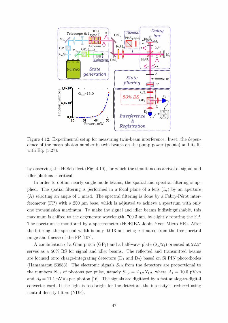
G =13.0max

Power, mW

Ph

oto

n n

um

ber

1

BBO type II

l /4

l /2

GP

l /2

D

2

Telescope 6:1

Stategeneration

Delayline

PBS

A

Interference&

Registration

RG

DM1

D

2DM

M

GP

L

2M

1M

s

sLs4 5mm×

FP

Statefiltering

S1

S2

1

2

50% BS

NDF

PEl /2PBS s2

Thermal

Nd:YAG

3w 2ww

GP3M

3w

3w

2w

l /23w

l /22w

CoherentBB

1

2 2

1

Figure 4.12: Experimental setup for measuring twin-beam interference. Inset: the depen-dence of the mean photon number in twin beams on the pump power (points) and its fitwith Eq. (3.27).

by observing the HOM effect (Fig. 4.10), for which the simultaneous arrival of signal and

idler photons is critical.

In order to obtain nearly single-mode beams, the spatial and spectral filtering is ap-

plied. The spatial filtering is performed in a focal plane of a lens (Ls) by an aperture

(A) selecting an angle of 1 mrad. The spectral filtering is done by a Fabry-Perot inter-

ferometer (FP) with a 250 µm base, which is adjusted to achieve a spectrum with only

one transmission maximum. To make the signal and idler beams indistinguishable, this

maximum is shifted to the degenerate wavelength, 709.3 nm, by slightly rotating the FP.

The spectrum is monitored by a spectrometer (HORIBA Jobin Yvon Micro HR). After

the filtering, the spectral width is only 0.013 nm being estimated from the free spectral

range and finesse of the FP [107].

A combination of a Glan prism (GP2) and a half-wave plate (λs/21) oriented at 22.5

serves as a 50% BS for signal and idler beams. The reflected and transmitted beams

are focused onto charge-integrating detectors (D1 and D2) based on Si PIN photodiodes

(Hamamatsu S3883). The electronic signals S1,2 from the detectors are proportional to

the numbers N1,2 of photons per pulse, namely S1,2 = A1,2N1,2, where A1 = 10.0 pV×s

and A2 = 11.1 pV×s per photon [16]. The signals are digitized by a fast analog-to-digital

converter card. If the light is too bright for the detectors, the intensity is reduced using

neutral density filters (NDF).

47

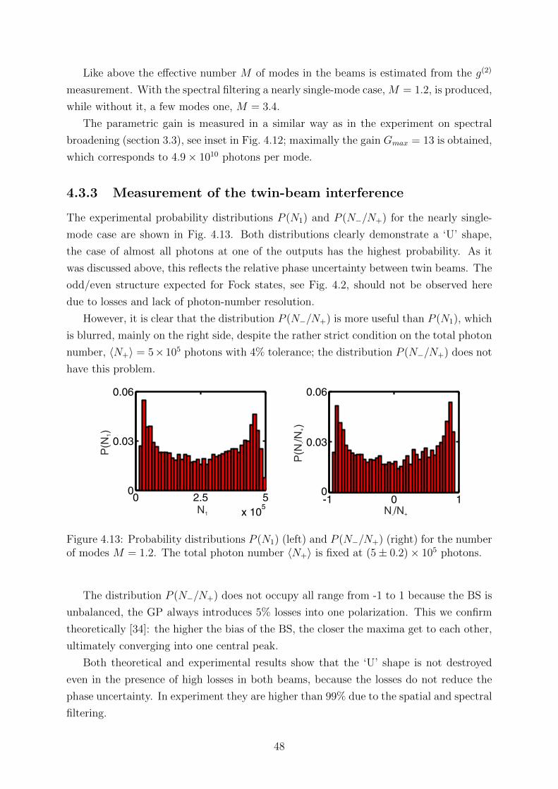
Like above the effective number M of modes in the beams is estimated from the g(2)

measurement. With the spectral filtering a nearly single-mode case, M = 1.2, is produced,

while without it, a few modes one, M = 3.4.

The parametric gain is measured in a similar way as in the experiment on spectral

broadening (section 3.3), see inset in Fig. 4.12; maximally the gain Gmax = 13 is obtained,

which corresponds to 4.9× 1010 photons per mode.

4.3.3 Measurement of the twin-beam interference

The experimental probability distributions P (N1) and P (N−/N+) for the nearly single-

mode case are shown in Fig. 4.13. Both distributions clearly demonstrate a ‘U’ shape,

the case of almost all photons at one of the outputs has the highest probability. As it

was discussed above, this reflects the relative phase uncertainty between twin beams. The

odd/even structure expected for Fock states, see Fig. 4.2, should not be observed here

due to losses and lack of photon-number resolution.

However, it is clear that the distribution P (N−/N+) is more useful than P (N1), which

is blurred, mainly on the right side, despite the rather strict condition on the total photon

number, 〈N+〉 = 5× 105 photons with 4% tolerance; the distribution P (N−/N+) does not

have this problem.

P(N

)1

N1

P(N

/N)

-+

N /N- +

Figure 4.13: Probability distributions P (N1) (left) and P (N−/N+) (right) for the numberof modes M = 1.2. The total photon number 〈N+〉 is fixed at (5± 0.2)× 105 photons.

The distribution P (N−/N+) does not occupy all range from -1 to 1 because the BS is

unbalanced, the GP always introduces 5% losses into one polarization. This we confirm

theoretically [34]: the higher the bias of the BS, the closer the maxima get to each other,

ultimately converging into one central peak.

Both theoretical and experimental results show that the ‘U’ shape is not destroyed

even in the presence of high losses in both beams, because the losses do not reduce the

phase uncertainty. In experiment they are higher than 99% due to the spatial and spectral

filtering.

48

The theory also shows that the ‘U’ shape disappears for the number of modes M > 2.

Without the frequency filtering, M = 3.4, indeed the experiment yields a peaked distri-

bution (Fig. 4.14). In the multimode case the ‘U’ shape smears out due to independent

photon-number fluctuations in different modes.

P(N

/N)

-+

N /N- +

Figure 4.14: Probability distribution P (N−/N+) for the number of modes M = 3.4.

P(N

/N)

-+

N /N- + N /N- + N /N- +

N /N- +N /N- +

P(N

/N)

-+

(a) (b) (с)

(d) (e)

Figure 4.15: Probability distributions P (N−/N+) for the number of modes M = 1.2 anddifferent ratios of the input photon numbers: 1 : 1 (a), 1 : 3 (b), 1 : 5 (c), 1 : 17 (d), and1 : ∞ (e).

The interference of non-equally populated signal and idler beams is also studied by

introducing the losses in one of the beams (Fig. 4.15). Notably, the shape remains concave

up to a considerable, 5:1, ratio between the input photon numbers (panel c). This feature

49

is mentioned in Ref. [104] in connection with the robustness of phase resolution to an

imbalance between twin beams. For a higher imbalance, the ‘U’ shape transforms into

a single peak (panels d,e), similarly to the case of Fock states [95]. Note that a single

peak also appears for the case of two independent (distinguishable) Fock states at the BS

inputs.

4.3.4 Interference of the classical beams

The ‘U’ shape can be also observed for classical beams with fluctuations in the relative

phase increased artificially; this classical analogy was pointed out in Ref. [95]. To demon-

strate this analogy a thermal or coherent beam is used with the following strategy applied

to it: the beam is split in two, the phase of one of the beams is varied, both beams are

overlapped on the BS, and the distribution P (N−/N+) is measured at the output.

As a thermal radiation, one of the twin beams is used. To separate the signal beam

from the idler one another PBS (PBS2, see Fig. 4.12) is introduced. Using a half-wave

plate (λs/22) at 22.5 the signal beam is split on the PBS1 and the latter one interferes

at the 50% BS. To randomize the phase, a varying voltage is applied to the PE actuator.

The resulting distribution demonstrates the ‘U’ shape if the phase is randomized and it

becomes peaked if the phase is fixed (Fig. 4.16).

-1 0 10

0.03

0.06

P(N

/N)

-+

N /N- + N /N- +

Figure 4.16: Probability distributions P (N−/N+) for the case of two input thermal stateswith a randomized (left) and fixed (right) relative phase. For the latter, three typicaldistributions for the different phases are shown: all photons are divided equally betweenthe detectors (b) or go together to the detectors D1 (c) and D2 (a).

As a coherent beam, the second harmonic of a Nd:YAG laser (Nd:YAG 2ω) at wave-

length 532 nm is used (see Fig. 4.12). As in the case of thermal light, a half-wave plate

(λ2ω/2) oriented at 22.5 followed by PBS1 is used to split the beam. The beam block

(BB), the long-pass filter (RG), and the FP interferometer are removed in this case. The

probability distribution P (N−/N+) shows the same ‘U’ shape if the phase is randomized

(Fig. 4.17, left). It is narrower than the one for the thermal case due to the nonideal

interference caused by the fact that optical elements are not optimized for 532 nm.

50

-1 0 10

0.03

0.06

P(N

/N)

-+

N /N- +

-1 0 10

0.035

0.07

P(cosφ)

cosφ

Figure 4.17: Probability distributions P (N−/N+) for the case of two coherent states witha randomized phase at the inputs (left). As an analogy also the distribution P (cosϕ) forthe randomized phase ϕ is shown (right).

The origin of the ‘U’ shape here can be simply understood from the distribution

P (cosϕ) for the phase ϕ distributed uniformly at [0 2π] (Fig. 4.17, right). Indeed, if

two beams with equal intensities and the phase difference ϕ interfere on a 50% BS, the

intensity difference between the outputs is proportional to cosϕ.

It should be stressed that in contrast to a pure twin-beam state [108], U-shaped

distributions observed for classical light do not lead to any phase super-resolution, because

the phase fluctuations are increased artificially by ‘mixing’ the state.

4.3.5 Possible applications of the BS interference

The BS interference could have an important application for quantum state engineering.

The distributions shown in Fig. 4.15 clearly demonstrate the following tendency: the

more symmetric are photon numbers at the input, the more asymmetric they are at the

output, and vice versa. This suggests that the BS interference could be used for filtering

two-mode macroscopically populated states of light with either close or much different

photon numbers [109].

Indeed, from the initial two-mode state one can tap off a small portion, which is

directed to a BS, where these two modes interfere. The measurement at the BS outputs

will show that the photon numbers in the initial modes are likely equal or different.

Depending on the result and desired filtering, the main part of the state will be used or

not used later, for example one can perform a postselection or open/close some special

shutter. Since the measurement does not provide information about the photon numbers

at the input ports of BS, this filter would select only the modulus of the photon-number

difference but not the sign of this difference.

This feature could be useful for macroscopic qubits, α |Φ〉 + β |Φ⊥ 〉, considered in

Ref. [110], the states obtained after amplifying a single-photon polarization qubit, α |1〉+

51

β |1〉⊥, in an OPA. The amplification keeps the information encoded in a qubit, but it is

difficult to extract it due to a big effective overlap in the photon number distributions for

the basis qubits |Φ〉 and |Φ⊥ 〉. The filter described above reduces this overlap and at the

same time maintains quantum superpositions.

4.4 Giant twin-beam generation

This section is devoted to the amplification of twin beams and, in particular, it considers

an application of the walk-off matching, spatial and temporal, to the generation of giant

narrowband twin beams. Such an amplifier could be considered as a highly tunable optical

parametric generator (OPG) without any cavity.

4.4.1 Walk-off effects in SPDC and high-gain PDC

Walk-off effects are caused by the difference between the velocities and directions of energy

and phase propagation. The most famous manifestation is the phenomenon of double

refraction caused by the birefringence of anisotropic materials. In this case the Poynting

vector is non-collinear to the wave vector. For example, in uniaxial crystals this is the

case for an extraordinarily polarized light [111]. Similarly, the longitudinal (temporal)

walk-off appears because the energy of a pulse travels at a different speed than its phase.

Since in nonlinear optical processes the phase matching determines the frequency-

wavevector spectrum, interacting pulses are often group mismatched and separate in space

and time during the propagation. This limits the length of nonlinear interactions for short

pulses and focused beams.

This is definitely the case for high-gain PDC: the exponential amplification is provided

only if the produced photons are overlapped in space and time with the pump ones.

For example, for the case of type-I phase matching the pump is polarized extraordinary

whereas signal and idler beams, ordinary, therefore only the former exhibits the spatial

walk-off. The situation with the temporal walk-off is similar: the group velocities of the

pump and the PDC beams are different, as they have different frequencies.

The spatial walk-off can be, in principle, eliminated by a using non-critical phase-

matching, double-crystal configuration, used in the experiment on BS interference (sec-

tion 4.3.2), or periodically poled materials. Unfortunately, the temporal walk-off is almost

inevitable.

For SPDC in its respect these effects are less important, because the produced photons

do not enhance the generation rate. Therefore, the walk-off effects lead only to an asym-

metry of the frequency-angular spectrum [112, 113], rather than to a beamlike emission

shown below.

52

4.4.2 Twin-beam generation along the pump Poynting vector

This section is intended to show that the twin-beam generation can be drastically en-

hanced, if one of the beams is emitted along the pump Poynting vector. This experiment

was done by Angela Perez, the author’s contribution was the explanation of some impor-

tant properties of the effect and the data processing.

Twin beams are produced in a 5 mm BBO crystal with the collinear frequency-

degenerate type-I phase matching, which corresponds to the optic axis angle φ = 32.97.

The pump, the same laser as in the experiment on spectral broadening (section 3.3), is

focused into the crystal to 60 µm size.

The angular spectra captured by using a digital photographic camera are shown in

Fig. 4.18. One could see strongly enhanced beamlike emission in green spectral range

(panel a). The color is modified due to saturation of the camera; a snapshot with a

neutral density filter (panel b) clearly demonstrates this. The green beam is the only one

of the twins, the signal one. Moreover, it is the idler beam that propagates along the

pump Poynting vector; it belongs to the IR range and is not visible (see Fig. 4.19, white

dot).

c d

Angle, rad0 0.1-0.1

a b e

Angle, rad0 0.1-0.1

Angle, rad0 0.1-0.1

Angle, rad0 0.1-0.1

Angle, rad0 0.1-0.1

Angle

, ra

d

0

0.1

-0.1

Figure 4.18: Snapshots with a photographic camera show the spectra of high-gain PDC atdifferent crystal orientations: 32.97 (a,b), 33.4 (c), 33.7 (d), and 34.0 (e). Additionalstripes in panels d,e appear due to reflections in the crystal. A snapshot with a neutraldensity filter (b) shows colors without saturation.

By tilting the crystal we change the phase matching and the spectral range for the

beamlike emission (Fig. 4.18, panels c-d). As the idler wavelength approaches the visible

range, both left and right parts of the ring become pronounced (panel e).

In order to show both enhanced beams we install a bandpass filter centered at the

degenerate wavelength and orient the crystal to the angle φ = 34.9 (Fig. 4.19, red dots).

The angular distribution is recorded by a CCD camera (Fig. 4.20, left panel). One can

hardly see the whole ring of emission, yet, there is a strong peak in the walk-off direction

as well as in the symmetrical one w.r.t. to the pump. At the other orientations of the

crystal, the emission at 710 nm is much weaker (right panel): twin beams observed in the

walk-off direction are brighter than the near-collinear emission by more than two orders

in magnitude. The theory provides the same result [35].

53

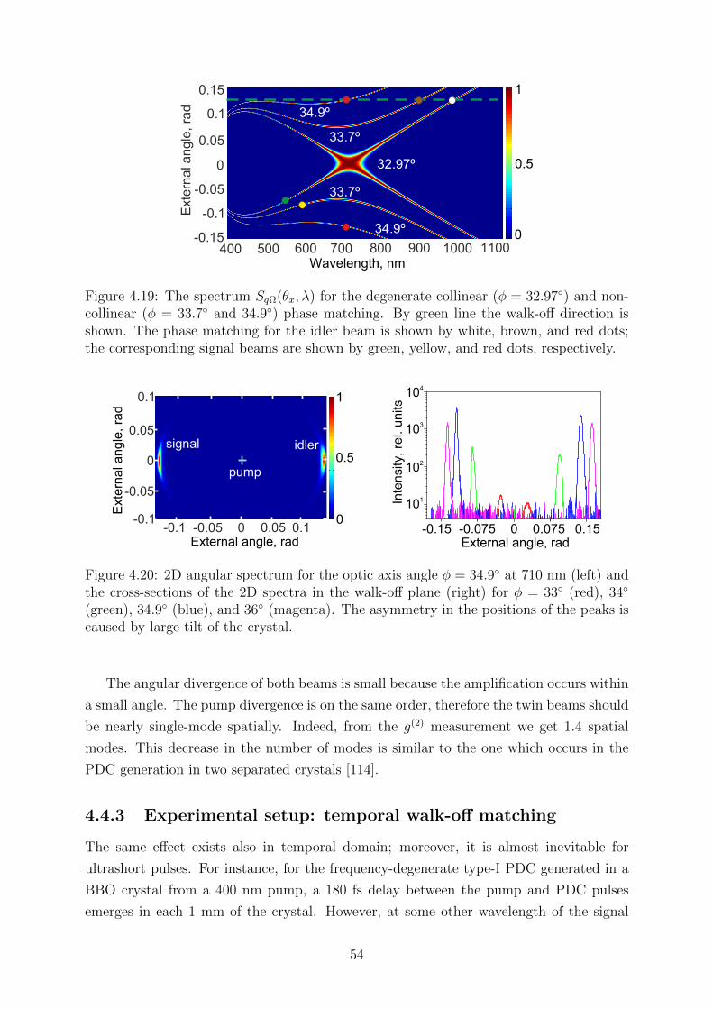
a

800700600500 1000400 900

0.1

0.05

0

-0.15

0.15

-0.05

-0.1Ext

ern

al a

ngle

, ra

d

32.97º

34.9º

33.7º

1

0.5

01100

Wavelength, nm

34.9º

33.7º

Figure 4.19: The spectrum SqΩ(θx, λ) for the degenerate collinear (φ = 32.97) and non-collinear (φ = 33.7 and 34.9) phase matching. By green line the walk-off direction isshown. The phase matching for the idler beam is shown by white, brown, and red dots;the corresponding signal beams are shown by green, yellow, and red dots, respectively.

0External angle, rad-0.05 0.05

0.05

0

-0.1 0.1

0.1

-0.05

-0.1

Ext

ern

al a

ngle

, ra

d

pump

signal idler

1

0

0.5

-0.15 -0.075 0 0.075 0.15

410

Inte

nsi

ty, re

l. units

External angle, rad

310

210

110

Figure 4.20: 2D angular spectrum for the optic axis angle φ = 34.9 at 710 nm (left) andthe cross-sections of the 2D spectra in the walk-off plane (right) for φ = 33 (red), 34

(green), 34.9 (blue), and 36 (magenta). The asymmetry in the positions of the peaks iscaused by large tilt of the crystal.

The angular divergence of both beams is small because the amplification occurs within

a small angle. The pump divergence is on the same order, therefore the twin beams should

be nearly single-mode spatially. Indeed, from the g(2) measurement we get 1.4 spatial

modes. This decrease in the number of modes is similar to the one which occurs in the

PDC generation in two separated crystals [114].

4.4.3 Experimental setup: temporal walk-off matching

The same effect exists also in temporal domain; moreover, it is almost inevitable for

ultrashort pulses. For instance, for the frequency-degenerate type-I PDC generated in a

BBO crystal from a 400 nm pump, a 180 fs delay between the pump and PDC pulses

emerges in each 1 mm of the crystal. However, at some other wavelength of the signal

54

beam, its group velocity can be equal to that of the pump (Fig. 4.21). The phase matching

can then be fulfilled using noncollinear emission. Note that only one pulse, signal or idler,

has to propagate together with the pump one, its twin will be amplified as well, similarly

to the spatial walk-off matching case.

450 500 550 600 650 700Wavelength, nm

1.72

1.74

1.76

1.78

Gro

up

ve

locity,

cm

/c

×1010

Figure 4.21: Group velocity in a BBO crystal for the extraordinary polarized light at400 nm (blue line) and the ordinary polarized one at different wavelengths (green line)for the angle φ = 29.18.

The group velocity matching is realized for type-II PDC (Fig. 4.22). The frequency-

doubled radiation of the Ti-sapphire laser, which is the same as used in the experiment

on PDC generation in the anomalous GVD range (section 3.2), is used as a pump. The

pump has 400 nm wavelength, 1.4 ps pulse duration, and up to 700 mW mean power.

screen

СL1

4x5mm BBO type II

CL2

DM

camera

o-beam

SM

120 160 200 240

610

PD

C in

ten

sity

, re

l. u

nits

Pump power, mW

510

410

310

Figure 4.22: Left: experimental setup for observing the effect of temporal walk-off match-ing (left). Right: the dependence of the PDC intensity on the pump power (points) andits fit with Eq. (3.27) (line).

The length of the nonlinear medium is changed by using either one 5 mm BBO crystal

or four ones stacked together with 3 mm spaces between them. In the last case each

crystal is adjusted to the phase matching individually keeping the same direction of the

optic axis for all crystals. Therefore, they work in the same way as a single 20 mm crystal.

The pump is focused into the crystals differently for both cases, with a 12:1 cylindrical

telescope (CL1 and CL2) and with a 500 mm cylindrical lens, respectively. Accordingly,

55

it leads to 680 µm and 130 µm width in the plane orthogonal to principal one. The tighter

focusing is required in a shorter crystal, which, in its turn, leads to a Rayleigh length too

small for the four-crystal stack. The pump beam is kept wide enough (3.4 mm) in the

principal plane to minimize the effect of spatial walk-off discussed above.

After the crystals, the pump radiation is cut off by a dichroic mirror (DM) and the

ordinary, signal, beam (o-beam) is observed on a screen placed at 76 cm distance from

the crystals. The signal beam is studied without overlapping with the idler one, because

in type-II PDC the ordinary beam is shifted in angle w.r.t. to the extraordinary one.

The screen has a ruler pasted to it, so the external angles of emission can be determined

from the coordinate on the screen. The example was already presented on the chapter’s

cover. This time the full PDC ring is not observed, because the apertures of the crystals

restrict the beam in vertical direction. The spectra on the screen are captured by a

photographic camera.

Alternatively, the spectra is measured at different angles in the same way as in the

experiment on PDC generation in the anomalous GVD range (section 3.2). A 400 µm

multimode fiber connected to a spectrometer (Ocean Optics HR4000) is placed at 87 cm

distance from the crystals and scanned in the direction orthogonal to the pump propaga-

tion. The parametric gain is measured in a similar way as in the experiment on spectral

broadening (section 3.3), see Fig. 4.22 (right panel).

4.4.4 Twin-beam generation using temporal walk-off matching

The spectra SqΩ(θx, λ) of the ordinary beam for positive angles are shown in Fig. 4.23a for

φ = 31, 34.5, and 37.5. Green arrows mark the angles corresponding to the wavelengths

at which the group velocity of the signal beam matches that of the pump. One should

expect a considerable amplification at these wavelengths in the case of long crystal and

high gain.

Indeed, the snapshots of intensity distributions on the screen (Fig. 4.23b-g) clearly

demonstrate the effect. For twin beams generated in a 20 mm of BBO (panels b–d),

there is huge amplification within a relatively narrow spectral range, while for 5 mm

crystal (panels e–g) the spectrum is more uniform over frequency. The angle, at which

amplification occurs, depends on the orientation; this clearly shows that it is not related

to the spatial walk-off.

For the quantitative characterization of the effect, the frequency spectra are recorded

at different angles for the crystal orientation φ = 37.5 (Fig. 4.24). Each angle corresponds

to a peak at a different wavelength, see Fig. 4.23a. The measurements are performed for

a 20 mm and a 5 mm of BBO choosing 637.5 nm wavelength as a reference one. At this

wavelength the parametric gain is kept the same, G = 8.6, for both cases.

For twin beams generated in four crystals the peak at the group-velocity-matching

56

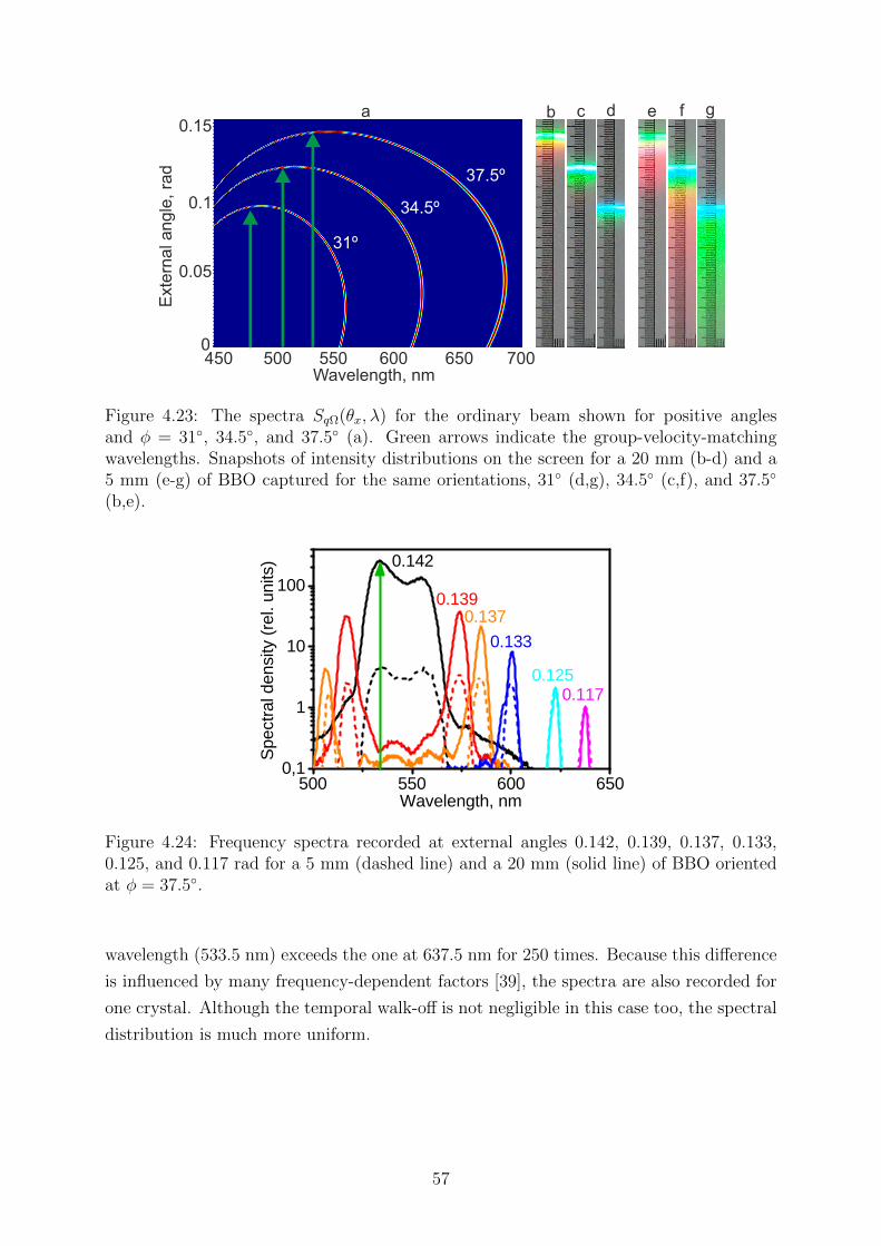
a b c d e f g0.15

0.1

0.05

0

Ext

ern

al a

ngle

, ra

d

Wavelength, nm450 500 550 600 650 700

31º

34.5º

37.5º

Figure 4.23: The spectra SqΩ(θx, λ) for the ordinary beam shown for positive anglesand φ = 31, 34.5, and 37.5 (a). Green arrows indicate the group-velocity-matchingwavelengths. Snapshots of intensity distributions on the screen for a 20 mm (b-d) and a5 mm (e-g) of BBO captured for the same orientations, 31 (d,g), 34.5 (c,f), and 37.5

(b,e).

5 0 0 5 5 0 6 0 0 6 5 00 , 1

1

1 0

1 0 0

0 . 1 1 70 . 1 2 5

0 . 1 3 30 . 1 3 7

0 . 1 3 9

Spec

tral d

ensity

(rel. u

nits)

W a v e l e n g t h , n m

0 . 1 4 2

Figure 4.24: Frequency spectra recorded at external angles 0.142, 0.139, 0.137, 0.133,0.125, and 0.117 rad for a 5 mm (dashed line) and a 20 mm (solid line) of BBO orientedat φ = 37.5.

wavelength (533.5 nm) exceeds the one at 637.5 nm for 250 times. Because this difference

is influenced by many frequency-dependent factors [39], the spectra are also recorded for

one crystal. Although the temporal walk-off is not negligible in this case too, the spectral

distribution is much more uniform.

57

4.4.5 Possible applications of the spatial and temporal walk-off

matching

Although, the spatial walk-off matching is known and used in parametric oscillators [115],

we demonstrate the directionality of the twin beams achieved without using a cavity.

Moreover, the wavelength of the enhanced emission is tunable within a broad range [116].

The possibility for building of such a OPG has been stated by David Klyshko long ago [39]:

‘Given powerful pulse pumping, PDC passes into a fairly intense parametric superlumi-

nescence5, which provides a source of smoothly frequency-tunable short (up to 10−12 sec)

light pulses’.

Furthermore, the idler beam is a source of tunable broadband IR radiation, which is

especially convenient because its twin is maintained in the visible range.

The temporal walk-off matching could be especially useful for generating twin beams

in cavities and whispering-gallery mode resonators [117], where, due to the large quality

factor, nonlinear interaction occurs on a very large distance. If the group velocity of

down-converted radiation coincides with that of the pump, strong twin-beam generation

can be realized even from short pulses. Moreover, near resonances in medium the pump

group velocity could differ from the signal or idler ones significantly, thereby providing

additional possibilities for engineering the spectrum.

5In other words, high-gain PDC.

58

Chapter 5

High-gain PDC as a pump for

multiphoton effects

Money in a bank account is something important, but certainly not physical.

As such it can take any value without necessitating the expenditure of energy.

It is just a number!

—Nassim Taleb, The Black Swan

BSV has an interesting statistics and serves as a useful source for multiphoton effects.

Both aspects are discussed in detail in this chapter. Firstly, the fluctuations of light and

their measurement are considered, in particular, how they change in the multimode case

and after the spectral filtering.

Then, it is shown that BSV has very strong photon-number fluctuations and, namely,

there are the measured CFs and probability distributions presented. This makes BSV

useful for pumping nonlinear effects, because their efficiency increases dramatically, what

is demonstrated using the generation of the second (SH), third (TH), and fourth (FH)

harmonics as an example.

Finally, it is shown that the generated harmonics fluctuate even more than BSV and

have unusual statistics. They have a lot of extreme events and are described by heavy-

tailed photon-number distributions. Furthermore, if supercontinuum is generated from

BSV, even more exceptional photon-number distributions appear. We manage to observe

power-law (Pareto) probability distributions with power exponents less than 2 leading to

indefinite mean values and higher-order moments.

5.1 Introduction

Although the fluctuations of light have been previously discussed a bit, they still are to

be analyzed deeper.

59

5.1.1 Fluctuations of light: coherent, thermal, and superbunched

The fluctuations of photon number is a stochastic process, and therefore they can be

described using different statistical characteristics. Although moments and CFs were

mostly used in the previous chapters, probability distributions provide the most complete

information.

They can be obtained by applying different approaches as, e.g., the quantum mechani-

cal approach, the most rigorous one, used before. Unfortunately, in many cases it is quite

complicated, and therefore in these cases the semi-classical or even classical approach

becomes more preferable as long as it gives reasonable outcomes. Let us explain here the

difference between approaches and justify their applicability.

In the semi-classical approach the electric field is considered classically, whereas the

detection process as a quantum. Using such a treatment and, namely, by describing the

probability of photoelectric emission in a detector exposed by fluctuating electric field,

one obtains the Mandel formula [118, 40],

p(m) =1

m!

∫ ∞0

Nme−NP (N)dN, (5.1)

which links the semi-classical approach with the classical one. Here P (N) is the photon-

number distribution1 in the classical approach, p(m), in the semi-classical one, and N,m

are the corresponding photon numbers.

Using Eq.(5.1) the mean values and the variances are related as

〈m〉 = 〈N〉, 〈∆m2〉 = 〈N〉+ 〈∆N2〉. (5.2)

The main difference is caused by shot-noise fluctuations, which arise in the semi-classical

case and do not appear in the classical one. Of course, the quantum mechanical approach

provides them too, moreover, they can be suppressed as well, which does not happen in

semi-classical description, 〈∆m2〉 ≥ 〈N〉.This difference can be exemplified by coherent light. In the semi-classical approach

p(m) has the Poissonian distribution [40],

pcoh(m) =1

m!〈N〉me−〈N〉, (5.3)

and 〈∆m2〉 = 〈N〉, while in the classical case, the Dirac delta one, Pcoh(N) = δ(N−〈N〉),and 〈∆N2〉 = 0. The shot-noise contribution is essential here, because it leads to a

nonzero variance.

Yet, the situation is different for more fluctuating light. For example, chaotic or

1Rigorously it is an intensity distribution, since ‘photons’ do not appear in the classical picture.Nevertheless, it is called photon-number distribution to be consistent in the thesis.

60

thermal light has the Bose-Einstein photon-number distribution [40],

pth(m) =〈N〉m

(〈N〉+ 1)m+1, (5.4)

in the semi-classical approach and a negative-exponential distribution,

Pth(N) =1

〈N〉e−

N〈N〉 , (5.5)

in the classical one. The variances are 〈∆m2〉 = 〈N〉2 + 〈N〉 and 〈∆N2〉 = 〈N〉2, respec-

tively. They are equal at 〈N〉 1, in this case the classical approach provides a correct

result. This is the case in general: if 〈∆N2〉 〈N〉, the classical approach (often) can be

used.

The CFs g(n) are defined differently in all three approaches [119]. In the classical one,

it is done through moments,

g(n) ≡ 〈Nn〉

〈N〉n, (5.6)

in the semi-classical approach via factorial moments,

g(n) ≡ 〈m(m− 1) . . . (m− n+ 1)〉〈m〉n

, (5.7)

and in the quantum approach with normally-ordered operators,

g(n) ≡ 〈: Nn :〉

〈N〉n. (5.8)

The CFs defined this way take the same values for the same state of light in all three

approaches as long as the distributions P (N) and p(m) exist at all.

Following the definitions, the n-th order CF g(n)coh = 1 for coherent light and g

(n)th = n!

for thermal one. In particular, for the latter g(2)th = 2, which is larger than for coherent

light. In this case the photons tend to bunch together, therefore thermal light is referred

to as a ‘bunched’ one.

Thermal light is produced by various effects and sources, which can be either ‘true’

chaotic sources, like stars [120] and light emitting diodes [121], or their analogues, like

multimode lasers [122] and rotating ground glass discs [123].

Particularly noteworthy that for BSV generated in the twin-beam configuration, each

beam, signal or idler, is in a true thermal state [124]. In order to observe this thermal

state, the two beams should be distinguishable, namely some detector2 should distinguish

2The detector is meant in a broad sense. For example, the generation of optical harmonics can be alsoconsidered as such a ‘detector’.

61

them.

For degenerate BSV, i.e. in the case of indistinguishable signal and idler beams, the

photon-number distribution is different. It contains only even numbers of photons [119,

36],

psb(2m) =(2m)!

22m(m!)2

〈N〉m

(〈N〉+ 1)m+1/2, psb(2m+ 1) = 0, (5.9)

and its variance is twice larger than for thermal light, 〈∆m2〉 = 2〈N〉2 + 2〈N〉. For this

strongly nonclassical state, see Eq. (2.10), the quantum mechanical approach should be

used.

However, if one neglects the fine structure3 of distribution (5.9), at 〈N〉 1 its

envelope is well-described by the gamma distribution [125] with the shape parameter 1/2

and the scale parameter 1/(2〈N〉) [126, 127],

Psb(N) =1√

2π〈N〉Ne−

N2〈N〉 . (5.10)

The variance 〈∆N2〉 = 2〈N〉2 and the CF g(n)sb = (2n− 1)!! provided by this distribution

are justified for large 〈N〉. The CFs are higher than for thermal light; for this reason

the degenerate BSV is often called ‘superbunched’, ‘extrabunched’, or ‘superthermal’

light [128, 36, 129, 130].

To compare the CFs for coherent and thermal light and superbunched BSV the de-

pendence of g(n) on the order n is shown in Fig. 5.1. The difference increases fast with n;

due to this fact, the fluctuating light is useful for multiphoton processes, an example will

be shown in section 5.3.

2 3 4 5 6 7 81 0 01 0 11 0 21 0 31 0 41 0 51 0 6

g(n)

nFigure 5.1: The CF g(n) on the order n for coherent (black) and thermal light (red) andsuperbunched BSV (blue).

The coherent light can be also described by means of the classical approach, but this

3For example, if the detector has no photon-number resolution.

62

description is not strict. In this case the Dirac delta distribtion should be replaced by the

Gaussian one,

P (N) =1

σ√

2πe−

(N−〈N〉)2

2σ2 , (5.11)

following the fact that the Poissonian distribution tends to the Gaussian one for large

〈N〉. The variance 〈∆N2〉 = σ2 should be set ‘by hand’ to the shot-noise contribution

〈N〉.

5.1.2 Multimode light and its measurement

The distributions (5.5) and (5.10) and the expressions for CFs g(n)th and g

(n)sb are obtained

for single-mode light. If multimode light is measured they will be valid only provided that

the detector traces all photon-number fluctuations and this will be the case only under

the condition of spatially and temporary single-mode detection [68, 40]. The latter means

that the detection area4 and time are (much) smaller than the coherence area and time,

namely smaller than the spatial and temporal size of the detected mode. Otherwise several

modes are detected and both the probability distributions and the CFs are different from

the single-mode ones.

In the case of M -mode detection, the probability distributions change. For indepen-

dent modes the multimode distributions can be obtained using the probability theory and

the fact that the probability distribution of a sum of two or more independent variables

is given by the convolution of their probability distributions [125].

Therefore, for M equally-populated modes the probability distribution (5.5) for ther-

mal light changes to [118, 131]

Pth,M(N) =NM−1

(M − 1)!

(M

〈N〉

)Me−

MN〈N〉 , (5.12)

and the distribution (5.10) for superbunched BSV becomes

Psb,M(N) =NM/2−1

Γ(M2

) ( M

2〈N〉

)M/2

e−MN2〈N〉 , (5.13)

where Γ(x) is the gamma function. Both distributions approach the Gaussian one (5.11)

for a large M .

At the same time, the CFs tend to unity for large M . In particular, the second-order

CF for M -mode light is [68, 40]

g(2)M = 1 +

g(2)1 − 1

M, (5.14)

4In the case of a multipixel detector, e.g. a CCD camera, each pixel is a separate detector.

63

where g(2)1 is the single-mode CF.

The last expression provides a possibility to estimate the total number M of detected

modes from the g(2) measurement if the single-mode statistics is known; exactly this

method is applied in all chapters of this thesis.

5.1.3 Filtering of the multimode light

The condition of single-mode detection can be fulfilled for multimode radiation not only

by means of a small and fast detector, but also through Fourier filtering. Such filtering

can be considered in two different ways: either as a method to shape the light itself or

as a part of detection process. In the first picture, the light is considered to be strongly

filtered to a single mode and then detected. In the second one, the filtering ‘stretches’ the

time and area of intensity fluctuations, so that a big and slow detector can resolve them.

Although the first picture is quite obvious, the second one may cause objections.

Below it is shown that the filtering does not change the normalized intensity moments for

thermal light and superbunched BSV, which are further considered experimentally. Only

the temporal domain is considered, the spatial one can be taken into account similarly.

Indeed, the normalized CF describing intensity correlations is [40]

g(n)(t1, . . . , tn) ≡ G(n)(t1, . . . , tn)∏ni=1 G

(1)(ti), (5.15)

where

G(n)(t1, . . . , tn) ≡ 〈n∏i=1

E(−)(ti)E(+)(ti)〉. (5.16)

Here E(+)(t) = [E(−)(t)]∗ is the analytical signal, defined as

E(+)(t) ≡∫ ∞

0

dω e−iωtE(ω), (5.17)

and E(ω) is the FT of the real electric field E(t).

The field for thermal light and BSV can be described as a Gaussian random pro-

cess with zero mean value [126]. The higher-order CFs can be therefore represented as

combinations of the first-order ones [126, 118, 40]. For example,

G(2)(t, t+ τ) = G(1)(t)G(1)(t+ τ) + |G(t, t+ τ)|2 + |〈E(+)(t)E(+)(t+ τ)〉|2, (5.18)

where G(t, t + τ) ≡ 〈E(−)(t)E(+)(t + τ)〉 is the first-order CF of the electric field. It is

related with the spectrum |E(ω)|2 via Wiener-Khinchin theorem [126, 118], namely via

inverse FT, and reaches the maximum value at τ = 0.

64

Keeping only the dependence on the time difference (stationarity), g(2)(τ) ≡ g(2)(t, t+

τ), one obtains

g(2)(τ) = 1 + |γ(τ)|2 +|〈E(+)(t)E(+)(t+ τ)〉|2

[G(1)(t)]2, (5.19)

where γ(τ) ≡ G(t, t+ τ)/G(1)(t).

As far as thermal light is considered, only the first two terms in Eq. (5.19) are nonzero;

one obtains the Siegert relation [132, 40]. Although the filtering changes the spectrum

and therefore changes the correlation time and the γ(τ) shape, γ(0) is always unity.

The generalized Siegert relation is more complicated, but the tendency is the same.

So, the CFs g(3)(τ1, τ2) ≡ g(3)(t, t+τ1, t+τ2) and g(4)(τ1, τ2, τ3) ≡ g(4)(t, t+τ1, t+τ2, t+τ3)

depend only on the combination of γ(τj − τi) (i, j = 0, 1, 2 or 0, 1, 2, 3 with τ0 = 0) [132].

Therefore, the CFs g(3)(0, 0) and g(4)(0, 0, 0) do not depend on filtering.

The same can be shown also for superbunched BSV. In this case the last term in

Eq. (5.19) can be nonzero as well [133]. In the simplest case of δ-correlated signal and

idler beams, see section 3.1, detuned from the central frequencies by Ωs and Ωi [39] one

gets

〈E(Ωs)E(Ωi)〉 = δ(Ωs + Ωi)〈E(Ωs)E(Ωi)〉. (5.20)

Thus, using Eq. (5.17) the last term in Eq. (5.18) at τ = 0 is

∣∣〈[E(+)(t)]2〉∣∣2 =

∣∣∣∣∫ Ωmax

−Ωmax

dΩs〈E(Ωs)E(−Ωs)〉∣∣∣∣2 , (5.21)

where 2Ωmax is the spectral width determined by the filtering. This filtering should be

around the central BSV frequency, ωs0 = ωi0 = ωp/2.

Signal and idler fields in BSV have the same amplitude and opposite phases5, E(−Ωs) =

[E(Ωs)]∗; thus,

∣∣〈[E(+)(t)]2〉∣∣2 =

(∫ Ωmax

−Ωmax

dΩs〈|E(Ωs)|2〉)2

. (5.22)

By virtue of the Wiener-Khinchin theorem [126, 118], the last expression equals exactly6

to [G(t, t)]2 = [G(1)(t)]2. Therefore, g(2)(0) = 3, regardless of the filtering.

5If one assumes that the pump phase is equal to zero, see section 4.3 for more details.6Note that the exponent in the Wiener-Khinchin theorem disappears, because the delay is zero, τ = 0.

65

5.2 Measurement of correlation functions and prob-

ability distributions

Here it is demonstrated that BSV has high photon-number fluctuations and, namely, the

measurement of probability distributions and CFs for thermal and superbunched BSV is

presented.

5.2.1 Experimental setup

The experimental setup is shown in Fig. 5.2. BSV is produced in the same BBO crystal

and with the same Ti-sapphire pump laser as in the experiment on PDC generation in the

anomalous GVD range (section 3.2). The collinear frequency-degenerate configuration is

used, see Fig. 3.7a. This time the pump is brighter, 2.5 W mean power, and is cut off with

dichroic mirrors (DM) and a longpass filter. With such pumping the gain G = 15.3± 0.5

is reached7.

BBOLaser

IR PDDM

4f

A BP

angularfiltering

frequency filtering

Figure 5.2: Experimental setup for measuring the statistics of thermal and superbunchedBSV.

The CFs and probability distributions are measured using a PIN diode-based IR

charge-integrating detector (IR PD) with neither spatial nor temporal resolution within a

pulse, therefore, as discussed in the previous section, filtering is needed in order to trace

intensity fluctuations. Angular filtering is made with an aperture (A) in the focal plane

of a 200 mm lens and frequency filtering, either with bandpass filters (BP) or with a

4f -monochromator (4f) containing two diffraction gratings, two lenses, and a slit. After

each filtering the beam is collimated.

The detector has the same design as the one used in the visible range, see section 4.3.2,

but is based on an InGaAs photodiode (Hamamatsu G12180-020A). It has a dynamic

range from few thousands to several millions of photons per pulse, a quantum efficiency

of 85% at 1600 nm, and an electronic noise equivalent to 1600 photons per pulse. Similarly

to the visible one, it produces electronic pulses with the area S = AIRN , where N is the

input number of photons and AIR = 5.0 ± 0.4 pV×s is the calibration coefficient at

1600 nm.

7For the crystal orientation that maintains the BSV fluctuations, see below Fig. 5.7.

66

This coefficient is obtained from the calibration measurement, which ideally should

be done with a low-noise laser. Such a laser at 1600 nm was not available, therefore for

calibration a radiation at 1064 nm of the first harmonic of the Nd:YAG laser is used,

which has been already used in the experiment on spectral broadening (section 3.3). The

pulse energy is measured with a power meter8 and then attenuated in a controlled way

using neutral density filters and two polarizers. The pulse energy is converted thereafter

to the number of photons per pulse. Therefore, each signal from the detector corresponds

to a certain photon number.

0 1x106 2x106 3x1060,0

2,0x10-6

4,0x10-6

6,0x10-6

8,0x10-6

1,0x10-5

1,2x10-5

Sig

nal,

V´s

Number of photons103 104 105 106

10-8

10-7

10-6

10-5

Number of photons

Figure 5.3: The dependence of the signal from IR detector on the input number of photonsat 1064 nm (points) and its linear fit (line) in linear (left) and log-log (right) scales.

8 0 0 1 0 0 0 1 2 0 0 1 4 0 0 1 6 0 00 , 00 , 20 , 40 , 60 , 81 , 01 , 21 , 4

Photo

sens

itivity,

A/W

W a v e l e n g t h , n mFigure 5.4: Photosensitivity in A/W for Hamamatsu G12180-020A photodiode (black)and the dependence corresponding to a 100% quantum efficiency (red).

Indeed, the detector shows nearly linear response on the input signal (Fig. 5.3). From

the linear fit of the dependence one gets the calibration coefficient at wavelength 1064 nm,

8The measured power should be divided by a repetition rate.

67

for different wavelengths the detector’s response is different, and, therefore, the coeffi-

cient is recalculated using the photosensitivity dependence provided by the manufacturer

(Fig. 5.4).

The photosensitivity is usually provided in amperes per watt; however, these units are

not so convenient to use, because we are more interested in a quantum efficiency, which

shows with what probability an incoming photon produces an electron. When working

with such dependencies the author notices one helpful rule of thumb: a 100% quantum

efficiency in A/W equal to an inverse energy of incoming photon in eV.

5.2.2 Thermal and superbunched BSV: correlation functions

The CF g(2) angular dependence is measured by scanning an aperture in the horizontal

and vertical directions with an angular resolution of 0.5 mrad (Fig. 5.5). The scanning is

performed with 7 nm filtering around 1600 nm, which is done by using two 10 nm bandpass

filters with a Gaussian transmission profile placed one after another; the transmission band

in this case is given by the convolution of transmission profiles and, therefore, it decreases

by 30%.

-2 -1 0 1 21,6

1,8

2,0

2,2

2,4

2,6

g(2

)

External angle, mrad-10 -5 0 5 10

2,0

2,2

2,4

2,6

2,8

3,0

External angle, mrad

Figure 5.5: The CF g(2) vs. the external angle in the horizontal (left) and vertical (right)directions.

Indeed, the CF g(2) reveals the fluctuations: its value is far above unity. It manifests

a peak with 1.3 mrad width in the horizontal direction (left panel) and remains constant

along all spectrum in the vertical one (right). This is largely due to the pump focusing

and the restricted angular spectrum.

The angular dependence of CF g(2) shows that the BSV is single-mode in the vertical

direction and multimode in the horizontal one. In this experimental configuration the su-

perbunching, g(2) > 2, could be observed only for the collinear selection of modes, because

both signal and idler photons should be detected at the same time. If the superbunching

is observed for all possible angles, it means that the BSV is single-mode in this direction.

68

In both cases the value g(2) = 3 is not achieved due to insufficient frequency filtering.

The same problem we had quite a while ago and, therefore, we got similar result with the

CF g(2) = 2.4− 2.5 at the maximum [36].

In order to improve the measurement a 4f -monochromator with a 150 µm slit, pro-

viding a 2.3 nm resolution, is implemented (Fig. 5.6, left). In this case the peak reveals

the expected statistics: for degenerate BSV the CF g(2) = 2.96 ± 0.05, for nondegener-

ate one, 2.01 ± 0.03. For the other CFs the situations is the same, one gets the peaks

with similar widths; the CF g(4) is shown as an example (right panel). It is equal to

102± 6 and 21.6± 0.9 for degenerate and nondegenerate BSV, respectively, meeting well

the theoretical expectations.

1580 1590 1600 1610 1620

2,0

2,2

2,4

2,6

2,8

3,0

g(2

)

Wavelength, nm 1580 1590 1600 1610 16200

20

40

60

80

100

g(4

)

Wavelength, nm

Figure 5.6: The second-order g(2) (left) and fourth-order g(4) (right) CFs vs. the wave-length.

However, the BSV is so bright that it experiences further SH generation (SHG) in

the BBO crystal, 1440 − 1780 nm → 720 − 890 nm. This process acts on the BSV as a

nonlinear absorber, it reduces fluctuations by absorbing more photons from higher energy

bursts [134, 135].

The contribution of this process can be tuned by tilting the crystal closer or further

from the exact phase-matching position, because the SHG efficiency depends on the phase

mismatch. The CF g(2) is measured depending on the crystal orientation φ (Fig. 5.7,

left). With the crystal oriented at the angle φ smaller than required for the exact phase

matching, 19.87, strong photon-number fluctuations are maintained and the CF g(2)

reaches its theoretical value, while for the larger φ the CF keeps decreasing. This occurs

because at the smaller angles there is no phase matching whereas at the larger ones, it

exists, see section 3.2. This effect will be used to vary the BSV statistics in section 5.3.

For the same reason, the CF g(2) also depends on the pump power (Fig. 5.7, right),

because the brighter is the BSV, the more efficient is the unwanted SHG. This dependence

is obtained without sufficient frequency filtering, therefore the CF g(2) does not reach the

value 3 even at low powers.

69

19,7° 19,8° 19,9° 20,0° 20,1° 20,2° 20,3°1,5

2,0

2,5

3,0g

(2)

Optic axis angle1,2 1,4 1,6 1,8 2,0 2,2 2,4

1,4

1,6

1,8

2,0

2,2

2,4

2,6

Pump power, W

Figure 5.7: The CF g(2) for the collinear degenerate BSV depending on the crystal orien-tation φ (left) and the pump power (right).

5.2.3 Thermal and superbunched BSV: probability distributions

0,0

5,0x10-3

1,0x10-2

Pro

babili

ty

0,0 2,0x104 4,0x104 6,0x104 8,0x104 1,0x1050,0

1,0x10-2

2,0x10-2

3,0x10-2

Pro

babili

ty

Number of photons per pulse

Figure 5.8: Experimental photon-number histograms (red points) for the thermal (top)and superbunched (bottom) BSV. Theoretical distributions [(5.5) and (5.10)] are shownby black lines. Blue lines show the convolution of theoretical distributions with the noisedistribution (5.11)

The probability distributions of photon number reveal the fluctuations as well. In

Fig. 5.8 the experimental probability distributions are plotted for the thermal BSV filtered

at 1585 nm (top) and for the superbunched one at 1600 nm (bottom). Both distributions

are very broad, they decay slowly in linear scale, therefore it is better to present them

in log-log or log-linear ones (Fig. 5.9). In these scales one can see that the superbunched

70

102 103 104 105 106

10-5

10-4

10-3

10-2

10-1

Pro

ba

bili

ty

Number of photons per pulse

10-5

10-4

10-3

10-2

Pro

ba

bili

ty

0,0 5,0x105 1,0x10610-5

10-4

10-3

10-2

0,0 5,0x105 1,0x10610-5

10-4

10-3

10-2

Figure 5.9: The same data as in Fig. 5.8, but in log-log and log-linear (insets) scales.For the superbunched BSV the thermal (black dashed line) and Poissonian (green line)distributions are also shown with the same mean value.

distribution decays slower than the thermal one; to highlight the difference the thermal

distribution (5.5) with the same mean value (dashed line) is added in the inset in the

bottom panel.

The distributions are much broader than the one for coherent light. The same inset

also shows the Poissonian distribution (green line) with the same mean value, which looks

rather like the Dirac delta distribution under such binning.

Both distributions are in a good agreement with the theoretical ones, (5.5) and (5.10),

with no fitting parameters (black lines). The mean values 〈N〉 are taken from the experi-

mental data, 1.33×105 and 7.6×104 photons per pulse for the thermal and superbunched

BSV, respectively.

As one can see from Figs. 5.8 and 5.9, the experimental histograms deviate from the

theoretical distributions at low photon numbers. For this the dark noise of the detector

is largely responsible, its distribution for the IR detector shown in Fig. 5.10.

This noise is well described by the Gaussian distribution (5.11) with zero mean value

and standard deviation σ = 1600 photons taken from the experimental data. Being

independent from the fluctuations of detected light, the dark noise just add to the light

fluctuations, and therefore the detected light should be described by the convolution of

light and noise probability distributions.

The convolution of Eq. (5.11) with Eq. (5.5) perfectly coincides with the experimental

71

101 102 103 104

10-5

10-4

10-3

10-2

Pro

babili

ty

Number of photons per pulse

-5,0x103 0,0 5,0x1030,0

2,0

4,0

Pro

ba

bili

ty

x10-3

Figure 5.10: Experimental photon-number histograms (red points) for the IR detectornoise in linear (top) and log-log (bottom) scales. The Gaussian distribution (5.11) isshown by black line.

histogram for the thermal BSV without any fitting parameters, see Figs. 5.8 and 5.9

(top, blue lines); for the superbunched BSV the situation is the same, the convolution of

Eq. (5.11) with Eq. (5.10) is presented in the bottom panels (blue lines).

5.3 Statistical enhancement of multiphoton processes

In the previous section it was demonstrated that BSV has very strong photon-number

fluctuations. Here it is to show how these fluctuations increase the efficiency of miltiphoton

effects.

Indeed, the rate R(n) of an n-photon effect generally scales as the n-th order CF g(n)

of the incident light [136, 137, 138, 139],

R(n) ∼ g(n)〈N〉n. (5.23)

Accordingly, the statistical efficiency ξ(n) of an n-photon effect [122, 140, 141, 142, 143],

defined as

ξ(n) ≡ R(n)

〈N〉n, (5.24)

72

should scale with the CF g(n).

This enhancement has been demonstrated for the SHG [141, 142, 143], two-photon

absorption [144, 121], and multiphoton ionization [122, 145] from different sources with

thermal-like statistics, namely a light emitting diode [121], lasers below threshold [141,

143], and multimode lasers [122, 144, 145, 142]. The latter ones have intensity fluctuations

due to the contributions of different temporal modes.

Ref. [122] deserves a special consideration since in this work the authors used a highly

nonlinear process, 11-photon ionization of Xe atoms, leading to a dramatic enhancement.

11! ≈ 107.6 factor is expected and, indeed, about 106.9 was obtained in the experiment!

The statistics was varied by changing the number of modes in nanosecond laser pulses.

Unfortunately, fluctuations of thermal-like sources are usually either slow or the sources

themselves are not so bright. As it will be shown below, BSV is notable here, because

its fluctuations are not only stronger than the thermal ones, see Fig. 5.9, but they can be

extremely fast as well.

5.3.1 Experimental setup

The experimental setup is shown in Fig. 5.11. The first part of the experimental setup

is the same as in the experiment on CF measurement (section 5.2.1), but now the IR

detector is used for monitoring the mean photon number and the statistics of BSV. A

beam sampler (BS) reflects 0.6% of the BSV power to it.

BBOLaser

DM

4f

A PDLiNbO3IR PDSP

BS

Figure 5.11: Experimental setup for optical harmonics generation from BSV.

In order to get a spatially single-mode beam, the BSV is filtered only in the horizontal

direction with a 140 µm slit, because the BSV is already single-mode in the vertical

one (see Fig. 5.5, right). The BSV beam is collimated with a 300 mm cylindrical lens

thereafter and shows a good quality (Fig. 5.12, left).

As before the 4f -monochromator is used for frequency filtering; unfortunately, it trans-

mits maximally 75 nm bandwidth, therefore the full BSV spectrum (Fig. 3.7) cannot be

used. Furthermore, a larger bandwidth would lead to problems with chromatic aberra-

tions. After the spectral filtering the beam quality remains quite good (Fig. 5.12, right).

The main BSV beam is tightly focused by a 3.1 mm lens on the surface of a 1 mm

LiNbO3 crystal doped with 5.1% of MgO [146], which has been already used in the

experiment on Schmidt number measurement (section 3.5). The crystal has its optic axis

73

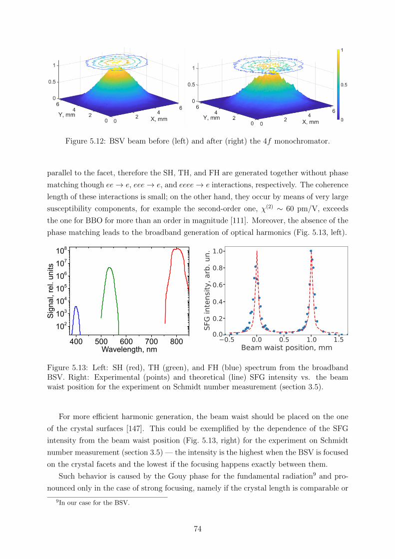
Figure 5.12: BSV beam before (left) and after (right) the 4f monochromator.

parallel to the facet, therefore the SH, TH, and FH are generated together without phase

matching though ee→ e, eee→ e, and eeee→ e interactions, respectively. The coherence

length of these interactions is small; on the other hand, they occur by means of very large

susceptibility components, for example the second-order one, χ(2) ∼ 60 pm/V, exceeds

the one for BBO for more than an order in magnitude [111]. Moreover, the absence of the

phase matching leads to the broadband generation of optical harmonics (Fig. 5.13, left).

400 500 600 700 800

102

103

104

105

106

107

108

Sig

nal,

rel. u

nits

Wavelength, nm

Figure 5.13: Left: SH (red), TH (green), and FH (blue) spectrum from the broadbandBSV. Right: Experimental (points) and theoretical (line) SFG intensity vs. the beamwaist position for the experiment on Schmidt number measurement (section 3.5).

For more efficient harmonic generation, the beam waist should be placed on the one

of the crystal surfaces [147]. This could be exemplified by the dependence of the SFG

intensity from the beam waist position (Fig. 5.13, right) for the experiment on Schmidt

number measurement (section 3.5) — the intensity is the highest when the BSV is focused

on the crystal facets and the lowest if the focusing happens exactly between them.

Such behavior is caused by the Gouy phase for the fundamental radiation9 and pro-

nounced only in the case of strong focusing, namely if the crystal length is comparable or

9In our case for the BSV.

74

larger than the Rayleigh length of focused beam. The phase shifts by π before and after

the waist leading to the corresponding phase shift in the nonlinear polarization. Thus,

the harmonic radiation generated before and after the waist interferes destructively, which

results into a low generation efficiency if the waist is placed in the bulk material.

The optical harmonics are separated from the BSV and from each other by short-

pass (SP) and bandpass filters. The harmonic photon numbers are measured with a

fiber-coupled avalanche photodiode (APD, Perkin&Elmer SPCM-AQRH-16) or with the

visible detector used in the experiment on BS interference (section 4.3.2).

It is important to keep the detectors in the linear range defined by the dark noise and

the saturation level. For APD the ’saturation’ occurs because the detector cannot detect

more than one photon per pulse. Therefore, the probability of single-photon events should

be much higher than the one of two-photon events; the detector’s response is nonlinear

otherwise.

However, a utilization of fluctuating light is not so straightforward. The probability

of high-energy spikes is relatively high and the nonlinear response sometimes affected

the measurements despite author’s attempts to avoid it. Note that the ‘noisier’ light is

detected, the more this issue comes into play.

In order to get the harmonics generation efficiency in absolute units the power ratio

between the tapped off and the main BSV beams is estimated; thereby the detection and

transmission losses for the generated harmonics are taken into account. The transmis-

sion losses in the generated harmonics are caused by the filters used for the harmonics

separation and the quantum efficiency of the APD. The detection efficiencies are equal

to 33% for the SH, 37% for the TH, and 3.6% for the FH. The internal losses (reflection

and absorption) of the LiNbO3 crystal are not taken into account, because they are part

of the generation efficiency.

The power ratio between the tapped off and the main BSV beams for the generation

of different harmonics is controlled by means of various neutral density filters and a film

polarizer to avoid the saturation of the detectors. The resulting ratio between the tapped

off and the main BSV beams is 1.4× 10−2 for the SHG, 6.0× 10−5 for the TH generation

(THG), and 3.6× 10−6 for the FH generation (FHG). Note that the calculated ratio and

losses affect only the generation efficiency in absolute units, not its enhancement due to

statistics.

5.3.2 Second, third, and forth harmonic generation from BSV

Firstly, the optical harmonics are measured from the BSV spectrally filtered to 3.3 nm.

The dependence of the output mean photon number 〈Nnω〉, corresponding to the rate

R(n), on the BSV photon number 〈N〉 is shown in Fig. 5.14 (filled squares). Meanwhile,

the detection and transmission losses are taken into account.

75

1 0 7 1 0 8 1 0 9 1 0 1 0 1 0 1 11 0 - 4

1 0 - 3

1 0 - 2

1 0 - 14ω3ω

nω ph

oton n

umbe

r

B S V p h o t o n n u m b e r

2ω

Figure 5.14: Measured dependence of the SH (red), TH (green) and FH (blue) photonnumber on the pump photon number with the pump being BSV (filled squares) andpseudo-coherent light (empty circles). Theoretical fits are shown by lines.

All harmonics show correct power dependences, which are obtained from the linear fit

in log-log scale (Table 5.1, second column). A bit lower value for the FHG comes from

the APD nonlinearity discussed above, because the FH radiation has exceptionally high

fluctuations; these fluctuations will be discussed in the next section.

n Exponent A(n)BSV /A

(n)pc g

(n)BSV /g

(n)pc η

(n)max × 100%

2 1.98± 0.01 2.86± 0.08 2.94± 0.06 (3.2± 0.3)× 10−7

3 3.05± 0.06 13.6± 0.8 14.5± 0.6 (1.38± 0.12)× 10−9

4 3.59± 0.07 71± 6 63± 2 (4.9± 0.7)× 10−10

Table 5.1: The power exponents, the statistical enhancement values (A(n)BSV /A

(n)pc ), the

ratios of the CFs g(n)BSV /g

(n)pc , and the maximal generation efficiencies η

(n)max from Fig. 5.14.

The statistical efficiencies [Eq. (5.24)] can be obtained from the fits with the corre-

sponding dependencies, fn(x) = A(n)xn, n = 2, 3, 4 (Fig. 5.14, solid lines). The maximal

harmonic generation efficiencies η(n)max ≡ 〈Nnω〉/〈N〉 are shown in Table 5.1 (fifth column).

This has to be compared with the usual situation in which the harmonics are generated

from coherent light. In the absence of a coherent source with exactly the same wavelength

and pulse duration as the BSV, a pseudo-coherent source is created by reducing the

photon-number fluctuations through postselection.

From the measured dataset only pulses, in which the number of photons in the BSV

lies within the certain boundaries, the postselection window, are chosen, namely only for

those pulses the data on the harmonics are further processed. The CFs for the postselected

data decrease almost to unity when the postselection window for the BSV signal becomes

narrower. Fig. 5.15 (left panel) shows the third-order CF g(3) (black solid line) as a

function of the window size as an example. At the same time, the number of TH counts

(green dashed line) for the chosen pulses within this window decreases.

76

0 25 50 75 1000

2

4

6

8

10

12

14g

(3)

Window size, % of full signal range

0

1000

2000

3000

4000

TH

co

un

ts w

ith

in w

ind

ow

0 2 4 6 8 10 12 140,0

2,0x10-3

4,0x10-3

6,0x10-3

TH

co

un

ts p

er

pu

lse

g(3)

Figure 5.15: Left: the CF g(3) (black solid line) and the number of TH counts (greendashed line) for the postselected data vs. the size of postselection window. Right: THcounts per pulse (points) vs. the CF g(3); the linear fit is shown by red line.

Thus, the post-selection window is chosen to be as small as possible, but simultaneously

large enough for the photon number to be measurable with a reasonably small uncertainty

after the post-selection. The minimal values of CFs obtained this way for our data are

g(2) = 1.010 ± 0.002, g(3) = 1.020 ± 0.003, g(4) = 1.10 ± 0.007. After the post-selection,

the number of counts per pulse is linear in the corresponding CF (Fig. 5.15, right).

The power dependences for different harmonics generated from this pseudo-coherent

source are plotted in Fig. 5.14 by empty circles. One can see that the statistical efficiency is

indeed considerably higher for the BSV. The enhancement factors are shown in Table 5.1

(third column) together with the ratios of CFs for the BSV and the pseudo-coherent

source (forth column). As expected, there is an agreement between the two.

The FH is produced with a reduced value of g(4) = 69± 2 due to the unwanted SHG

in the BBO crystal discussed above. A brighter pump is needed for the FHG, because its

efficiency is lower. At the same time, the brighter pump leads to the brighter parasite SH

and more suppressed BSV fluctuations, see Fig. 5.7.

To compare the efficiency of harmonics generation from the superbunched BSV with

the one for the thermal BSV, the BSV wavelength is scanned around the degeneracy point,

1600 nm, and measure the rates of the SH around 800 nm, the TH around 533 nm, and

the FH around 400 nm. The obtained statistical efficiencies ξ(n) are plotted in Fig. 5.16,

together with the corresponding BSV CFs. By scanning the wavelength, the thermal BSV

turns into the superbunched one and the value of ξ(n) follows the one of g(n).

Next, it is shown that the generation efficiency scales with the CF value also in the case

of broadband BSV. As discussed, the generation of optical harmonics can be considered as

a fast multiphoton detector [148, 81], which follows the fast fluctuations; in other words,

the condition of single-mode detection discussed in section 5.1.3 is realized despite the

fact that the BSV has many modes.

In order to change the statistics the unwanted SHG (Fig. 5.7) is used. As discussed,

77

1590 1600 1610

0,4

0,6

0,8

1,0

SH

effi

cie

ncy,

arb

. u

nits

BSV wavelength, nm

1,0

1,5

2,0

2,5

3,0a 2w

g(2

)

1590 1600 16100,0

0,2

0,4

0,6

0,8

1,0

TH

effi

cie

ncy

, a

rb.

un

its

BSV wavelength, nm

0

2

4

6

8

10

12

14

16

18

b 3w

g(3

)

1590 1600 16100,0

0,2

0,4

0,6

0,8

1,0

FH

effi

cie

ncy

, a

rb.

un

its

BSV wavelength

0

10

20

30

40

50

60

70

c

g(4

)

4w

Figure 5.16: SH (a), TH (b) and FH (c) statistical efficiencies ξ(n) (points) as well as thecorresponding g(n) values (solid lines) measured vs. the BSV wavelength. For comparison,the expected efficiencies for coherent light are shown by dashed lines.

1.5 2.0 2.5 3.00.0

0.2

0.4

0.6

0.8

1.0

HG

effi

cie

ncy

, a

rb.

un

its

(2)g

2w

4 6 8 10 12 14 16

3w

(3)g0 20 40 60 80 100

4w

(4)g

Figure 5.17: Statistical efficiencies ξ(n) (points) of the SH (left), TH (middle) and FH(right) from the broadband BSV show linear dependences on the corresponding CFs g(n).Solid lines show linear fits, ξ(n) ∼ g(n).

this effect reduces the fluctuations and CFs; by tilting the BBO crystal the latter can

be reduced from their original values down to g(2) = 1.55 ± 0.05, g(3) = 3.5 ± 0.2, and

g(4) = 7.1± 0.5.

Figure 5.17 shows that even for 75 nm broad BSV, the statistical efficiencies ξ(n) of the

SHG (left), THG (middle), and FHG (right) follow the CFs. As already mentioned, our

78

detector resolves only pulse-to-pulse fluctuations and the measured CFs are reduced due

to multimode detection, see section 5.1.2. Therefore, the CFs g(n) are measured under

the narrowband, 2.5 nm, filtering. The filtering allows one to retrieve the correct values

of CFs, see section 5.1.3. Therefore, for each orientation of the BBO crystal first the CF

g(n) is measured with the narrowband filtering and immediately after that, the efficiency

ξ(n) is measured. Due to this fact, rather large error bars appear in the axis of abscissas.

5.3.3 BSV fluctuations: possible applications

The results for optical harmonic generation illustrate that BSV is a useful source for

multiphoton effects in general. For example, BSV as a pump will be beneficial for the

multiphoton microscopy of fragile structures [149] including biological objects [150, 27].

Indeed, the harmonics are generated without phase matching from low mean powers (few

nW – tens of µW) and, according to Fig. 5.14, a certain rate of a four-photon effect is

achieved with BSV having the mean power about three times less than in the case of

coherent pumping. This can increase the sensitivity while not overcoming the damage

threshold, what becomes critical in the case of live cell imaging, where one should use the

lowest possible photon dose [27].

As mentioned above, BSV has ultrafast fluctuations. Here a bandwidth of 9 THz is

used, what corresponds to the correlation time of 80 fs, but one can achieve times an order

of magnitude shorter, see chapter 2. Such behavior cannot be mimicked by any external

intensity modulation [151]. With such timescales BSV is useful for ultrafast spectroscopy,

for example for the testing of materials response time. Although here a single spatial

mode is used, the multimode spatial structure will not change the noisy behavior of BSV.

One can use the whole frequency and angular spectrum of BSV for exciting multiphoton

effects [79].

Finally, unlike a pulsed coherent source, BSV has two typical times, the pulse duration

and the correlation time, see section 4.2. Both parameters can be tuned in a broad range,

which can be used in the two-dimensional fluorescence spectroscopy [152, 153] exploiting

a two-photon absorption effect. Moreover, the photon fluxes are drastically higher than

in the case of photon pairs.

5.4 Extreme events, extreme bunching, and heavy-

tailed distributions

In the previous section it was shown that BSV fluctuations increase the efficiency of

multiphoton effects. Here it is demonstrated that the light produced with BSV as a

pump fluctuates even more. It has an exceptional statistics with a lot of extreme events.

79

The existence of such events is a fascinating phenomenon in natural and social sciences,

because they could lead to catastrophic changes in the system despite being quite rare.

One famous example is ‘rogue waves’ in ocean [154] that comes from sailor’s fairy-tails.

For centuries sailors have been telling about giant waves that appear from nowhere and

disappear immediately. These stories were considered as a myth until first time such a

wave has been detected instrumentally on the New Year Eve 1995 at the Draupner oil

platform located in the North Sea. Importantly, these rogue waves have their analogues

in nonlinear optics [155], mainly for supercontinuum generation in optical fibers [156].

What is the definition for a rogue wave? There are several ones, but the most general

one is the following [157]: ‘a rogue wave is a wave that is much higher than others around

it, and which has a habit of appearing unpredictably’. It means that the process is chaotic

or random and its fluctuations are higher than the usual, namely equilibrium, ones. For

light the latter indicates a deviation from thermal statistics [Eq. (5.5)].

The corresponding probability distributions are called ‘heavy-tailed’ [158]. The ‘heav-

iest’ is the power-law (Pareto) distribution,

P (x) ∝ 1

x(1+α), (5.25)

with the Pareto index α > 0.

Originally it arises from the observations of Italian sociologist Vilfredo Pareto, who at

the beginning of the 20th century noted that 80% of land in Italy belongs to the 20% of

population. In its respect, such spreading leads to the power-law probability distribution.

Pareto’s observations give rise to the famous ‘80/20 rule’ or Pareto principle: 20% of the

input, e.g. resources or efforts, accounts for 80% of the output, e.g. rewards or results.

The Pareto distributions are often employed for the social quantities [159], for example

for the frequency of words and surnames, number of received telephone calls and hits on

websites, intensity of wars and terrorist attracts, and the impact of academic papers, of

course. The most outrageous is the distribution of income and wealth, the richest 1%

accumulate almost the same as the rest 99% of the population [160], being attributable

to the very non-uniform behavior of different people [161], namely due to the difference

between the ones who live on salary and the ones whose sources of income are investments

and bonuses.

Mostly the social quantities are just numbers, they could take any value, whereas

in the natural sciences it is not so straightforward. Nevertheless, the Pareto distribu-

tions appear in biology [162], astrophysics [163], geophysics [164], and condensed matter

physics [165, 166]. In optics they appear in scattering [167, 168] or highly nonlinear

phenomena [169, 170, 130]. In the latter, the Pareto distributions appear due to the ex-

ponential amplification of an initially broad distribution, which is one of the main origins

of power-law scalings [171].

80

However, the power laws can be very different. If the power exponent, 1 + α, is

less than 2, the mean value and higher moments are indefinite; such an example for

supercontinuum pumped by BSV is presented below. Furthermore, other heavy-tailed

distributions appear if the optical harmonics are generated from BSV.

5.4.1 Theoretical description: nonlinear processes from fluctu-

ating light

Here a theoretical description of harmonic and four-wave mixing (FWM) generation from

fluctuating light is presented. The description is based on probability distributions and

despite its simplicity it wonderfully explains the obtained experimental results on the har-

monic and supercontinuum generation discussed in sections 5.4.2 and 5.4.3, respectively.

Despite complexity of supercontinuum generation the model can be applied to it as well

since the elementary physical process behind is FWM. Notably, a quite similar approach

was also used in Ref. [169].

In the absence of pump depletion, the number Nnω of generated photons for the

nth harmonic scales as the nth power of the number Nω of photons in the fundamental

radiation,

Nnω = KNnω , (5.26)

where K is related to the conversion efficiency.

The distribution Pnω(Nnω) for the harmonic radiation is obtained from the one Pω(Nω)

of the fundamental radiation [125, 126], as Pnω(Nnω)dNnω = Pω(Nω)dNω. Thus, using

Eq. (5.26) one can get

Pnω(Nnω) =Pω

(n√Nnω/K

)n n√KN1−1/n

nω

. (5.27)

It follows that the mth moment of the harmonic radiation is proportional to the nmth

moment of the fundamental radiation, 〈Nmnω〉 = Km〈Nnm

ω 〉. As a result, the CFs g(m)nω can

be obtained from the ones for the fundamental radiation [172, 143],

g(m)nω =

g(mn)ω(g

(n)ω

)m . (5.28)

At first, let us consider the simplest case of bright coherent pump. In this case the

variance increases for the harmonic radiation, 〈∆N2nω〉 ∼ 〈Nnω〉2−1/n at 〈Nω〉 1, and as a

result the harmonic radiation is not shot-noise limited. However, all CFs g(m)nω are equal to

unity since the CF g(n)ω = 1. Moreover, like the original distribution (5.11), the probability

81

distribution Pnω(Nnω) remains ‘bell-shaped’. Therefore, the probability of extreme events

with Nnω 〈Nnω〉 remains negligible. Note that since the distribution (5.11) is used, the

description is not fully strict.

However, the situation is very different for input light with larger photon-number

fluctuations. For the nth harmonic of thermal light, see Eq. (5.5), one can get

Pnω(Nnω) =n√n!

n n√〈Nnω〉N1−1/n

nω

e− n

√n! Nnω〈Nnω〉 , (5.29)

while pumping with superbunched BSV [Eq. (5.10)] gives

Pnω(Nnω) =2n√

(2n− 1)!!

n√

2π 2n√〈Nnω〉N1−1/2n

nω

e− 1

2n√

(2n−1)!! Nnω〈Nnω〉 . (5.30)

The distribution (5.29) is the Weibull distribution [173] with the shape parameter 1/n and

the scale parameter 〈Nnω〉/n!, the distribution (5.30) is the generalized Gamma distribu-

tion [174] with the shape parameters 1/2 and 1/n and the scale parameter 2n〈Nnω〉/(2n−1)!!. Both distributions are heavy-tailed.

Indeed, to characterize the tail of a probability distribution, one can use the comple-

mentary cumulative distribution function (CCDF) [173],

C(N) =

∫ ∞N

P (N ′)dN ′, (5.31)

also known as the survival function. The probability distribution is called heavy-tailed if

its tail index, defined as

β = limN→∞

H(N)/N, (5.32)

is equal to zero [158]. Here H(N) = − ln C(N) is the hazard function.

For thermal light [Eq. (5.5)], the CCDF is

Cth(N) = e−N〈N〉 , (5.33)

for superbunched BSV [Eq. (5.10)],

Csb(N) = Erfc

[√N

2〈N〉

], (5.34)

where Erfc is the complementary error function. Then, the index β is equal to 1/〈N〉 and

1/(2〈N〉), respectively. Hence, both distributions are not heavy-tailed. Furthermore, now

it is clear that the tail index β = 0 means that the distribution decays slower than the

82

exponential distribution (5.5).

The experimental H(N)/N with the data taken from Fig. 5.9 are presented in Fig. 5.18

together with the theoretical curves calculated from Eqs. (5.33) and (5.34). The curves

fully demonstrate this behavior: at large N they tend to the corresponding theoretical

indices β. The thermal (black points and gray line) and superbunched BSV (red points

and pink line) distributions have the same tail index if the mean photon number for the

first one is twice as large as for the second one.

102 103 104 105 106

10-5

10-4

10-3

sb

th

SC

3w, sb

2w, th

H(N

)/N

Number of photons per pulse

2w, sb

Figure 5.18: Experimental (points) and theoretical (lines) H(N)/N for the thermal (th)and superbunched (sb) BSV presented in Fig. 5.9, the second (2ω) and third (3ω) har-monics presented in Fig. 5.22, and the supercontinuum (SC) presented in Fig. 5.26. Forthe SC, the theoretical values are calculated from a fit with the Pareto distribution.

For optical harmonics, the CCDF is

Cnω(Nnω) = e− n

√n! Nnω〈Nnω〉 (5.35)

for thermal pumping [Eq. (5.5)] and

Cnω(Nnω) = Erfc

2n

√(2n− 1)!! Nnω

〈Nnω〉√2

(5.36)

for superbunched BSV one [Eq. 5.10]. In both cases the index β tends to zero, therefore

both distributions are heavy-tailed. In Fig. 5.18 the theoretical H(N)/N (cyan, yellow,

and magenta lines) are plotted from Eqs. (5.35) and (5.36) together with the experimental

data from Fig. 5.22 (blue, dark yellow, and purple points). All curves show fast tendency

to zero, which increases with the harmonic number n and is more pronounced for the

fundamental radiation with larger fluctuations. In other words, superbunched BSV pump

makes the tail heavier than the thermal one.

83

In the case of FWM the number NF of photons is given by the equation similar to the

one, see Eq. (2.6), describing PDC,

NF = sinh2 κNω, (5.37)

but the gain scales linearly with the pump photon number Nω [175]. The value κ charac-

terizes the interaction strength and as before the pump is supposed to be undepleted.

Similar to the harmonics case, from the pump photon-number distribution P (Nω) the

FWM ones are obtained:

PFWM(NF ) =e−

arcsinh√NF

κ〈Nω〉

2κ〈Nω〉√NF (1 +NF )

(5.38)

for thermal pumping [Eq. (5.5)] and

PFWM(NF ) =e−

arcsinh√NF

2κ〈Nω〉√8πκ〈Nω〉NF (1 +NF )arcsinh

√NF

(5.39)

for superbunched BSV one [Eq. (5.10)]. Both distributions are shown in Fig. 5.19.

410 610 810 1010NF

210

-410

-1010P(N

)FWM

F

-710

-1310

Figure 5.19: Calculated photon-number distribution for FWM from thermal [Eq. (5.38),black] and superbunched [Eq. (5.39), red] BSV with the gain κ〈Nω〉 = 0.5 (dashed line)and 2.5 (solid line). The blue line shows the distribution for multimode superbunchedBSV pumping [Eq. (5.45)] with κ〈Nω〉 = 2.5 and M = 5.

The corresponding CCDFs are

CFWM(NF ) = e−arcsinh

√NF

κ〈Nω〉 (5.40)

and

CFWM(NF ) = Erfc

√arcsinh√NF

2κ〈Nω〉

(5.41)

for thermal and superbunched BSV pumping, respectively.

Both CCDFs are of the form x−αL(x), where L(x) is a slowly varying function [158],

84

i.e. limx→∞ L(tx)/L(x) = 1, for any t > 1. They both have the same tail as the Pareto

distribution (5.25),

C(NF ) ∝ 1

(NF )α, (5.42)

with the same exponent α, i.e. they are tail equivalent10 to it.

The tail exponents tend to 1/(2κ〈Nω〉) for the distribution (5.40) and 1/(4κ〈Nω〉) for

the distribution (5.41). In other words, BSV pumping leads to twice smaller exponent α

than pumping with thermal light with the same power. In both cases the exponent goes

below unity for sufficiently bright pump and then all moments are indefinite.

The first scaling is straightforward; since arcsinh(x) = ln(x+√x2 + 1),

ln[CFWM(NF )

]= −arcsinh

√NF

κ〈Nω〉≈ − ln(NF )

2κ〈Nω〉= ln

(N−1/2κ〈Nω〉F

)at NF →∞. (5.43)

The second scaling can be found similarly by using the asymptotic for the error function,

Erfc(√x) ∼ exp(−x)/(

√πx).

These Pareto-like distributions are surely heavy-tailed; the tail index β tends to zero

as the photon number tends to infinity. Moreover, the tendency is faster than for any

harmonic; the experimental H(N)/N (green points in Fig. 5.18) fitted with the Pareto

distribution illustrate this behavior.

As discussed in section 5.1.2, the probability distributions are different for multimode

light. Here the single-mode detection with the multimode pumping is assumed. This will

be the experimental case considered below; we are able to filter the supercontinuum very

well, but we cannot do it with the pump at the same time.

Similarly to the single-mode case, from the pump multimode distributions (5.12) and

(5.13) the FWM photon-number distributions are obtained:

PFWM,M(NF ) =e−

arcsinh√NF

κ〈Nω〉/M (arcsinh√NF )M−1

2√NF (NF + 1) (M − 1)! (κ〈Nω〉/M)M

(5.44)

for M -mode thermal pumping and

PFWM,M(NF ) =e−

arcsinh√NF

2κ〈Nω〉/M (arcsinh√NF )M/2−1

2√NF (NF + 1) Γ

(M2

)(2κ〈Nω〉/M)M

(5.45)

for M -mode superbunched BSV one. The corresponding CCDFs are

CFWM,M(NF ) =Γ(M, arcsinh

√NF

κ〈Nω〉/M

)(M − 1)!

(5.46)

10If limx→∞ C1(x)/C2(x) = 1, then C1(x) and C2(x) are tail equivalent [158].

85

and

CFWM,M(NF ) =Γ(M2, arcsinh

√NF

2κ〈Nω〉/M

)Γ(M2

) , (5.47)

respectively. Here Γ(s, x) is the upper incomplete Gamma function.

Since Γ(s, x) ∼ xs−1e−x at x→∞, one can get the tail exponents

α =M

2κ〈Nω〉and α =

M

4κ〈Nω〉(5.48)

for distributions (5.46) and (5.47), respectively. Thus, the exponents linearly increase with

the number M of modes for the same mean number 〈Nω〉 of pump photons. This can be

seen from Fig. 5.19: the distribution (5.45) for the gain κ〈Nω〉 = 2.5 and M = 5 (blue

line) has nearly the same scaling as the single-mode one (5.39) for the gain κ〈Nω〉 = 0.5

(red dashed line).

5.4.2 Optical harmonic generation: extreme events

The optical harmonics are generated in the same setup as in the experiment on statistical

enhancement (section 5.3.1). In order to demonstrate that the generated harmonic be-

comes extremely ‘noisy’ the CFs g(2)nω are measured for each harmonic in a Hanbury Brown

– Twiss setup [120]. After the LiNbO3 crystal the harmonic radiation is collimated by a

3.1 mm lens, splitted using an achromatic half-wave plate and a Glan prism, and fed in

two APDs. The photocount pulses are sent to a coincidence circuit and the correlation

function is found from the numbers of coincidences and single counts in detectors [68].

Fig. 5.20 shows the second-order CF g(2)nω for SH, TH, FH from Eq. (5.28) generated

from thermal light (shaded) and superbunched BSV (colored). The expected values are

very high, moreover, they increase with the harmonic number and for more fluctuating

pump. The second-order CF g(2)nω is equal to 6 for SH from thermal light [143, 131] and

to 184 for FH from superbunched BSV.

The experimental results are in good agreement with the theory. They show a huge

increase of fluctuations in the generated optical harmonics. The observed CF g(2) =

110± 20 for the FH from the superbunched BSV is close to the maximal values reported

in the literature [176, 177]. It is lower than the expected value of 184 due to the unwanted

SHG discussed above, see section 5.2.2; nevertheless, it is in agreement with Eq. (5.28) if

the measured values of g(8)ω and g

(4)ω are used.

As discussed it is important to keep the probability of two-photon events per detector

much lower than the one for single-photon events, especially for highly fluctuating light.

At high mean photon number the probability of two-photon events within a single pulse

is too high, which leads to the effect similar to the saturation of both detectors and to the

86

2w 3w 4w1

10

100

g(2)

Figure 5.20: Measured second-order CFs g(2)nω for the harmonics generated from the su-

perbunched (filled circles) and thermal (empty circles) BSV. The theoretical values areshown by filled and shaded color bars, respectively.

resulting reduction of the measured CF g(2). At the same time, at small mean number

of photons the count rates are too low for a precise measurement and the dark noise

contribution (about 9× 10−4 counts per pulse), despite being subtracted, strongly affects

the measurement.

0,0 0,2 0,4 0,6 0,8 1,0 1,2 2,0 2,250

100

150

200

250300350

Noise

g(2

)

Mean counts/pulse ´ 103

Saturation

Figure 5.21: Dependence of the measured CF g(2) for the FH on the mean number ofcounts per pulse (points). The expected value of g(2) calculated from Eq. (5.28) for themeasured BSV statistics is shown by dashed line.

Fig. 5.21 shows, as an example, the measurement of CF g(2) for the FH radiation versus

the detected photon number, which is varied by attenuating the beam. This procedure

should not change the value of g(2) due to its invariance to losses. The measured value is

trustable only within a narrow range of mean photon numbers. During the measurements

discussed above the mean photon number is kept within this range. Note that the ‘sat-

uration border’ moves to the higher mean photon numbers for the less fluctuating light

while the ‘noise border’ remains the same for the all measurements.

The probability distributions for the radiation of different harmonics are measured

87

using the visible detector described in section 4.3.2. Due to the low efficiency of the pro-

cesses it was impossible to measure the FH and the TH from the thermal BSV. Moreover,

for the same reason the TH is produced from the superbunched BSV with already a bit

reduced fluctuations, similarly to the FH for the measurements with APD.

102 103 104 105 10610-6

10-5

10-4

10-3

10-2

10-1

Pro

babili

ty

Number of photons per pulse

10-6

10-5

10-4

10-3

10-2

10-1

Pro

babili

ty

10-6

10-5

10-4

10-3

10-2

10-1P

robabili

ty

0 0.05 0.10

50

100

N/<

N>

Time, s

0 0.05 0.10

100

200N

/<N

>

Time, s

0 0.05 0.10

200400600

N/<

N>

Time, s

(a)

(b)

(с)

0 1x10510-6

10-4

10-2

0 1x10510-6

10-4

10-2

0 1x10510-6

10-4

10-2

Figure 5.22: Photon-number histograms for the SH generated from the thermal (a) andsuperbunched BSV (b), and the TH generated from the superbunched BSV (c). Theexperimental data are shown by red points in log-log and log-linear scales (bottom leftinsets). The theoretical distributions with an account for the photodetector noise areshown by black lines. To emphasize rogue-wave behavior, the thermal distribution (5.5)is shown by dashed lines in the insets. The top right insets show 0.1 s time traces withthe largest extreme event.

The histograms for the measured harmonics are shown in Fig. 5.22 by red points. They

are in a perfect agreement with the theoretical distributions [Eqs. (5.29) and (5.30), solid

lines] taking into account the noise distribution in a similar way as in the measurement

of BSV photon-number distributions (section 5.2.3). This time the detector’s noise is

equivalent to 270 photons per pulse. Again, it is reasonable to emphasize that the fitting

parameters are not used, the mean values 〈Nnω〉 are taken from the experimental data

88

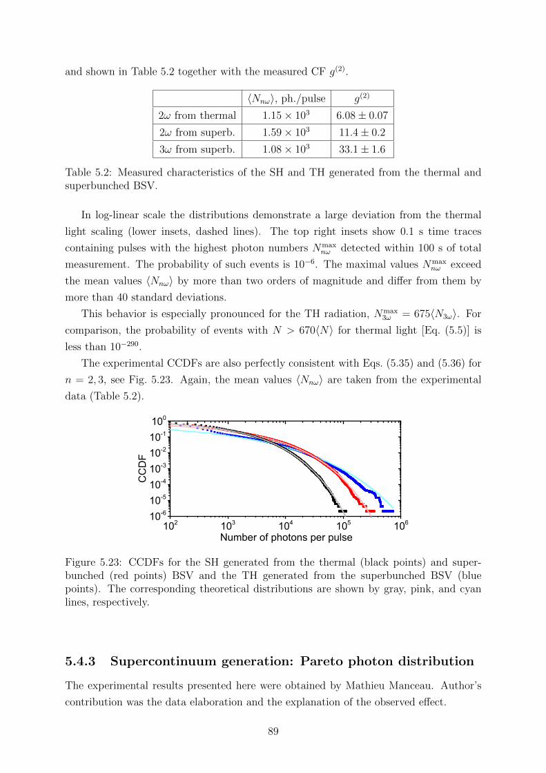
and shown in Table 5.2 together with the measured CF g(2).

〈Nnω〉, ph./pulse g(2)

2ω from thermal 1.15× 103 6.08± 0.07

2ω from superb. 1.59× 103 11.4± 0.2

3ω from superb. 1.08× 103 33.1± 1.6

Table 5.2: Measured characteristics of the SH and TH generated from the thermal andsuperbunched BSV.

In log-linear scale the distributions demonstrate a large deviation from the thermal

light scaling (lower insets, dashed lines). The top right insets show 0.1 s time traces

containing pulses with the highest photon numbers Nmaxnω detected within 100 s of total

measurement. The probability of such events is 10−6. The maximal values Nmaxnω exceed

the mean values 〈Nnω〉 by more than two orders of magnitude and differ from them by

more than 40 standard deviations.

This behavior is especially pronounced for the TH radiation, Nmax3ω = 675〈N3ω〉. For

comparison, the probability of events with N > 670〈N〉 for thermal light [Eq. (5.5)] is

less than 10−290.

The experimental CCDFs are also perfectly consistent with Eqs. (5.35) and (5.36) for

n = 2, 3, see Fig. 5.23. Again, the mean values 〈Nnω〉 are taken from the experimental

data (Table 5.2).

Number of photons per pulse102 103 104 105 106

10-6

10-5

10-4

10-3

10-2

10-1

100

CC

DF

Figure 5.23: CCDFs for the SH generated from the thermal (black points) and super-bunched (red points) BSV and the TH generated from the superbunched BSV (bluepoints). The corresponding theoretical distributions are shown by gray, pink, and cyanlines, respectively.

5.4.3 Supercontinuum generation: Pareto photon distribution

The experimental results presented here were obtained by Mathieu Manceau. Author’s

contribution was the data elaboration and the explanation of the observed effect.

89

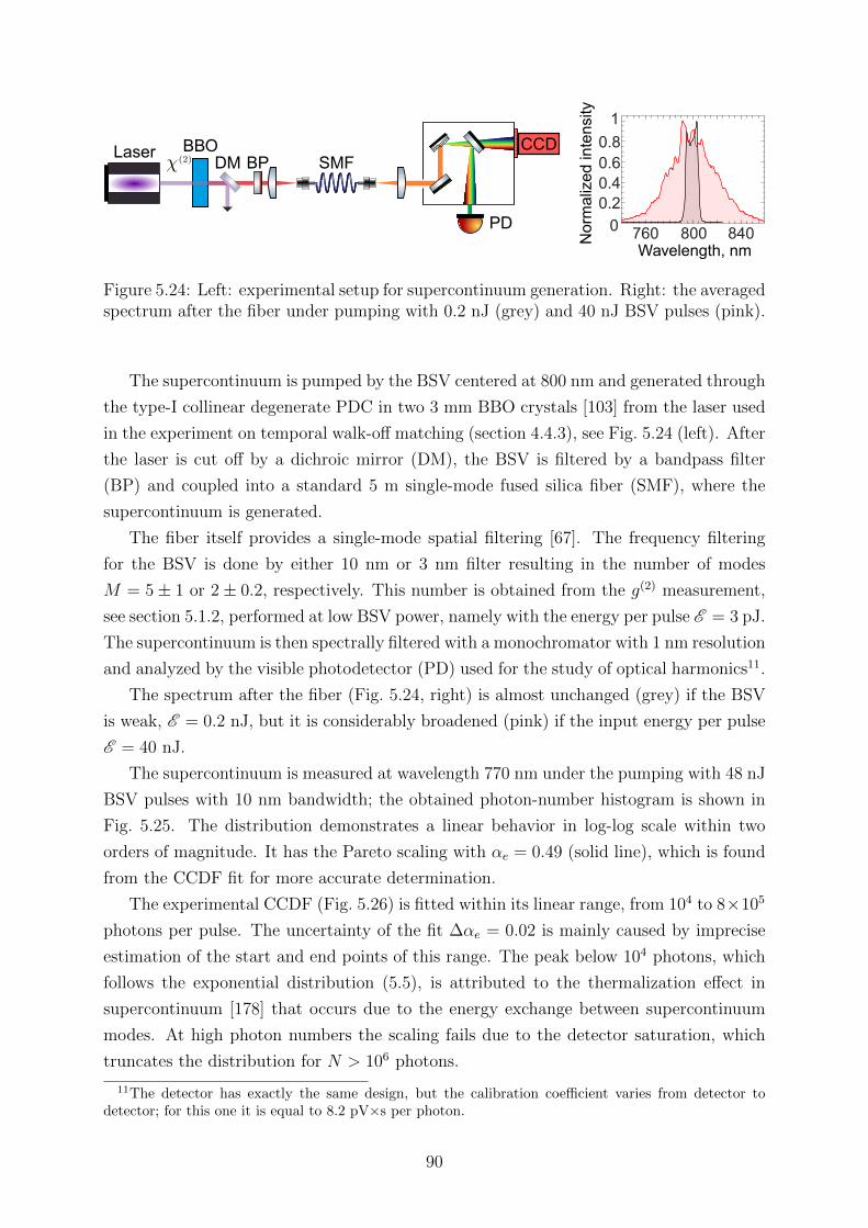
Norm

aliz

ed in

tensity

0

0.2

1

Wavelength, nm800760 840

0.4

0.6

0.8BBOLaser

PD

CCDDM BP SMF

Figure 5.24: Left: experimental setup for supercontinuum generation. Right: the averagedspectrum after the fiber under pumping with 0.2 nJ (grey) and 40 nJ BSV pulses (pink).

The supercontinuum is pumped by the BSV centered at 800 nm and generated through

the type-I collinear degenerate PDC in two 3 mm BBO crystals [103] from the laser used

in the experiment on temporal walk-off matching (section 4.4.3), see Fig. 5.24 (left). After

the laser is cut off by a dichroic mirror (DM), the BSV is filtered by a bandpass filter

(BP) and coupled into a standard 5 m single-mode fused silica fiber (SMF), where the

supercontinuum is generated.

The fiber itself provides a single-mode spatial filtering [67]. The frequency filtering

for the BSV is done by either 10 nm or 3 nm filter resulting in the number of modes

M = 5± 1 or 2± 0.2, respectively. This number is obtained from the g(2) measurement,

see section 5.1.2, performed at low BSV power, namely with the energy per pulse E = 3 pJ.

The supercontinuum is then spectrally filtered with a monochromator with 1 nm resolution

and analyzed by the visible photodetector (PD) used for the study of optical harmonics11.

The spectrum after the fiber (Fig. 5.24, right) is almost unchanged (grey) if the BSV

is weak, E = 0.2 nJ, but it is considerably broadened (pink) if the input energy per pulse

E = 40 nJ.

The supercontinuum is measured at wavelength 770 nm under the pumping with 48 nJ

BSV pulses with 10 nm bandwidth; the obtained photon-number histogram is shown in

Fig. 5.25. The distribution demonstrates a linear behavior in log-log scale within two

orders of magnitude. It has the Pareto scaling with αe = 0.49 (solid line), which is found

from the CCDF fit for more accurate determination.

The experimental CCDF (Fig. 5.26) is fitted within its linear range, from 104 to 8×105

photons per pulse. The uncertainty of the fit ∆αe = 0.02 is mainly caused by imprecise

estimation of the start and end points of this range. The peak below 104 photons, which

follows the exponential distribution (5.5), is attributed to the thermalization effect in

supercontinuum [178] that occurs due to the energy exchange between supercontinuum

modes. At high photon numbers the scaling fails due to the detector saturation, which

truncates the distribution for N > 106 photons.

11The detector has exactly the same design, but the calibration coefficient varies from detector todetector; for this one it is equal to 8.2 pV×s per photon.

90

N/<

N>

0

50

100

150

200

time, s

Pro

ba

bili

ty

Number of photons per pulse

0 0.05 0.1

-610

-510

-410

-310

-210

-110

010

410

510

610

-1.49P ~ N

Figure 5.25: Photon-number histogram for the supercontinuum pumped with 48 nJ pulsesof BSV (points), and the Pareto distribution (5.25) with α = 0.49 (solid line). The insetshows a 0.1 s time trace with the largest extreme event.

103 104 105 10610-4

10-3

10-2

10-1

100

CC

DF

Number of photons per pulse

Figure 5.26: CCDF for the supercontinuum from Fig. 5.25 (red points), its fit (blue line)with Eq. (5.42) leading to the exponent αe = 0.49, and Eq. (5.42) with α = 0.53 (blackline) obtained from the maximum likelihood estimator α [Eq. (5.49)].

The other method for the exponent estimation is suggested in Refs. [171, 159]. It is

so-called maximum likelihood estimator α given by

α = 1 + s

[s∑l=1

ln

(Nl

Nmin

)]−1

. (5.49)

Here Nmin is the photon number at which the Pareto scaling starts, Nl are the observed

photon numbers larger than Nmin, and s is the dataset size after excluding N < Nmin.

For the distribution from Fig. 5.25 it gives α = 0.53, which is similar to the obtained

exponent αe. In Fig. 5.26 the Pareto distribution with α = 0.53 is shown by black line.

In order to test that the exponent depends on the BSV power and its number of modes,

we measure the probability distributions for the supercontinuum with the BSV energy per

91

pulse reduced to 30 nJ. The results are shown in Fig. 5.27. For the pumping with 10 and

3 nm bandwidth the fits of CCDFs provide exponents αe = 0.64 and 0.31, respectively,

meaning that the variation of BSV power and bandwidth provides a possibility to control

the exponent of the Pareto distribution for supercontinuum.

Pro

babili

ty

Number of photons per pulse

-610

-510

-410

-310

-210

-110

010

310 410 510 610

-1.64P ~ N

-1.31P ~ N

Figure 5.27: Photon-number histograms for the supercontinuum pumped by 30 nJ BSVpulses with 10 nm (red points) and 3 nm (black points) bandwidth and their Pareto fitswith α = 0.64 and 0.31, respectively.

Surprisingly, the simple FWM theory provides not only the Pareto scaling, it also gives

the reasonable exponents. The theoretical exponents αt are estimated from Eq. (5.48)

using the corresponding number M of modes and the gain κ〈Nω〉 of the process. We

get the gain κ〈Nω〉 = 4 ± 0.5 and 2.5 ± 0.5 for the energy per pulse E = 48 and 30 nJ,

respectively, from the nonlinear dependence similar to the one obtained for BSV, see

section 3.3. The uncertainties in both measurements lead to the relative error δαt = 25%.

E , ∆λω αe αt 〈NF 〉, ph./pulse

Fig. 5.25 48 nJ, 10 nm 0.49 0.31 1.18× 104

Fig. 5.27 30 nJ, 10 nm 0.64 0.5 6.5× 103

30 nJ, 3 nm 0.31 0.2 5.6× 103

Table 5.3: Characteristics of the supercontinuum photon-number distributions. E and∆λω are the BSV energy per pulse and bandwidth, respectively; αe and αt are the exper-imental and theoretical exponents; 〈NF 〉 is the mean number of photons.

The theoretical Pareto exponents αt are somewhat smaller than the experimental ones

(Table 5.3). Such a difference could be caused by the approximations made, which are

actually not true. For example, the undepleted-pump approximation; as one can see from

Fig. 5.24 (right) the intensities of the BSV at 800 nm and the obtained supercontinuum

are comparable. Moreover, it is not taken into account that the supercontinuum is so

92

strong that it also produces FWM sidebands. Finally, our gain estimation is very crude,

because the mean value 〈NF 〉 is not defined for the exponent α < 1.

5.4.4 Extreme bunching: outlook and possible applications

The power-law probability distributions shown in Figs. 5.25 and 5.27 have very unusual

features. With the power exponent less than 2, α < 1, the mean number of photons is not

defined and depends on the time of observation, making this distribution much different

from the ones reported by the others [169, 170, 130]. Similar to the fractal ‘coastline

paradox’ [179], where the coastline appears to be longer, the better one measures, the

mean photon number will be the higher, the more data are used to determine it, 〈NF 〉 ∝s1/α−1, where s is the dataset size [171]. This fractal-like behavior is typical for the

Pareto distributions with indefinite mean values [180]. Of course, in a real experiment

the distribution gets always truncated through some physical mechanisms. For example,

the coastline contains no details less than a centimeter. Therefore, the coastline length is

also defined if it is measured with a centimeter accuracy.

Superbunching has interesting consequences for photon subtraction experiments [181].

In a photon subtraction experiment a quantum state of light |ψ〉 is fed to a BS, after which

a single-photon detector can register a reflected photon. Provided that the detector

registers a single photon, the state of light after the BS is the photon-subtracted one,

|ψ′〉 ∝ a|ψ〉. Counterintuitively, the photon-subtracted state has the mean photon number

increased by a factor g(2) compared to the initial state [182, 183].

Furthermore, the g(2) measurement can be indeed considered as a photon subtraction

experiment, because the mean number of photons in the state |ψ′〉 is equal to the mean

number of coincidences. In our paper [38] we perform such experiment for the supercon-

tinuum and get a 140 times increase of the mean photon number. This drastic increase

in the mean photon number shows that the optical harmonics or supercontinuum can be

brought out of equilibrium by the subtraction process much more efficiently than thermal

light or superbunched BSV. As a result, much more work could be, in principle, extracted,

which makes the supercontinuum a useful resource for proof-of-principle tests of quantum

thermodynamics [183].

The radiation with strong fluctuations in the photon number can be also useful in the

ghost imaging [13, 184], where the contrast of the image is given by the CF g(2) [185, 186].

In particular, recently the time-domain ghost imaging has been demonstrated with the

incoherent supercontinuum [187], although without high photon-number fluctuations. It

is significant that the use of supercontinuum with the Pareto photon-number distribution

will drastically increase the contrast.

93

Chapter 6

Conclusion

This thesis has presented the detailed research on different spectral and statistical prop-

erties of high-gain PDC and its potential applications.

Firstly, it was shown that in the anomalous range of group velocity dispersion the

PDC spectrum is restricted in both angle and wavelength. Such a spectrum provides

a possibility to collect all radiation without losses, which in its respect is an advantage

for experiments with squeezed light. Moreover, the ring-shaped frequency-wavevector

spectrum provides a new type of spatiotemporal coherence and entanglement of photon

pairs. One can obtain an entangled photon pair with the photons being never at the

same point at the same time. Such a pair could be used in the time- and space-resolved

nonlinear spectroscopy with two-photon light.

Secondly, the broadening of the total and correlation spectral widths in the high-

gain regime has been demonstrated. Apart from that, the asymmetry of PDC frequency

spectra has been explained. Moreover, two methods for studying the mode structure and

correlation properties of PDC have been developed. The first one is based on the PDC

fluctuations, while the second one uses the spectral properties of sum frequency generation

from PDC.

Thirdly, a macroscopic analogue of Hong-Ou-Mandel interference was measured and

discussed. Although for high flux of entangled photons the standard measurement tech-

nique based on the second-order correlation function leads to a very low visibility, a

modified technique based on the normalized variance of the difference signal provides a

visibility close to unity. With this technique, the interference manifests itself as a peak,

which additionally provides the information about the PDC spectral properties.

Fourthly, the photon statistics after the interference of twin beams on a 50% beam

splitter were analyzed. In this interference the intrinsic phase fluctuations between twin

beams are converted into photon-number ones. This photon-number uncertainty is ob-

served as a ‘U’ shape in the output photon-number distribution. It is typical for the

interference of high-order Fock states and could have an important application for quan-

tum state engineering. The effect was also mimicked by classical beams with an artificially

94

mixed phase.

Fifthly, it has been demonstrated that the spatial and temporal walk-off matching can

be used for giant narrowband twin-beam generation. If one of the twin beams is emitted

along the pump Poynting vector or its group velocity matches that of the pump, the gen-

eration of both beams is drastically enhanced. This enhancement leads to a considerable

narrowing of the wavelength and angular spectrum; thus, one can use these effects for

building a highly tunable optical parametric generator without any cavity.

Sixthly, the measured normalized correlation functions and probability distributions

show that BSV produced via PDC has strong and ultrafast photon-number fluctuations.

The correlation functions can be measured under narrowband filtering, since the filtering

does not change their maximum values. Moreover, strong photon-number fluctuations

enhance efficiency of multiphoton effects and this enhancement has been demonstrated

for the generation of the second, third, and forth optical harmonics. For the latter one

the generation efficiency is enhanced two orders of magnitude compared to the pumping

with coherent light. This could be particularly useful for the multiphoton microscopy of

fragile structures, including biological objects, in which the damage threshold plays an

important role. Furthermore, BSV could be applied in the ultrafast spectroscopy and

two-dimensional fluorescence spectroscopy.

Lastly, the generated harmonics fluctuate even more than BSV and have an excep-

tional statistics. The photon numbers are described by heavy-tailed photon-number dis-

tributions, events whose magnitude exceeds the mean value by more than 100 times were

observed rather frequently. Furthermore, for the supercontinuum generated from BSV,

the power-law photon-number distributions with the power exponents less than 2 were

observed. As a result, these distributions decay so slowly, that the mean photon number is

indefinite, to say nothing of higher moments. Such fluctuating statistics could be notably

useful for quantum thermodynamics and ghost imaging.

In the end, the author believes that high-gain PDC will take an important place

in science and industry, and therefore hopes that this thesis would be helpful for both

communities.

95

Appendix A

List of acronyms and abbreviations

APD avalanche photodiode

BBO beta barium borate

BS beam splitter

BSV bright squeezed vacuum

CCDF complementary cumulative distribution function

CF correlation function

CW continuous-wave

FH fourth harmonic

FHG fourth harmonic generation

FT Fourier transform

FWM four-wave mixing

GDD group delay dispersion

GVD group velocity dispersion

HOM Hong-Ou-Mandel

IR infrared

JSA joint spectral amplitude

JSI joint spectral intensity

OCT optical coherence tomography

OPA optical parametric amplification

OPG optical parametric generator

PBS polarizing beam splitter

PDC parametric down-conversion

SFG sum frequency generation

SH second harmonic

SHG second harmonic generation

SPDC spontaneous parametric down-conversion

TH third harmonic

THG third harmonic generation

96

Acknowledgments

First of all, I would like to thanks my supervisor, Maria, who introduced and guided me

though the world of quantum optics, spent a lot of hours and days in the discussions

about how the things should be done and arranged, tried to improve my presentations

and writing skills, in particular the way how this thesis is written. Hopefully, in the end

we always found a good solution. Thank you really a lot!

The second thanks goes to Timur and Olga, who were the first people I met in the

quantum optics lab, my first co-supervisors, microchiefs. You explained me a lot of

practical stuff. Thank you!

One more big thanks goes to Farid, who showed me how theoreticians work. With a

lot of efforts I learned how to calculate analytically the difficult stuff. Thank you!

Thank you, Gerd, it was great to be part of MPL and the Leuchs division in particular.

Thanks 4piPAC Group for good-neighborhood in FAU offices and shared lab. Special

thanks to Markus for helping with the German summary.

Radim, Tatiana, Olga, Vlad, Ulrik, Eugene, Polina, Falk, Victor, and Denis, thank

you a lot for the nice and productive collaboration!

Thanks the QuaRad – Chekhova research group! Andrea, Mathieu, Angela, Gaetano,

Hani, Felix, Cameron, Sascha, Luo, Mickey, Tomas, and Paula, thank you a lot for long-

term and short-term work cooperation, for the help with the equipment and guidance!

Sorry for the criticism at group meetings, sometimes it was too harsh.

Finally, my biggest thanks goes to Vera

and Sofia. We’ll be friends Forever, won’t

we? My life is becoming much better with

you. You are the best, I love you very very

much!!!

Piglet sidled up to Pooh from behind.

‘Pooh!’ he whispered.

‘Yes, Piglet?’

‘Nothing,’ said Piglet, taking Pooh’s paw.

‘I just wanted to be sure of you.’

97

Bibliography

[1] D. N. Klyshko. Coherent photon decay in a nonlinear medium. Sov. Phys. JETP

Letters, 6:23, July 1967.

[2] S. E. Harris, M. K. Oshman, and R. L. Byer. Observation of tunable optical para-

metric fluorescence. Phys. Rev. Lett., 18:732–734, May 1967.

[3] D. Magde and H. Mahr. Study in ammonium dihydrogen phosphate of spontaneous

parametric interaction tunable from 4400 to 16 000 A. Phys. Rev. Lett., 18:905–907,

May 1967.

[4] S. A. Akhmanov, V. V. Fadeev, R. V. Khokhlov, and O. N. Chunaev. Quantum

noise in parametric light amplifiers. Sov. Phys. JETP Lett., 6:85, 1967.

[5] S. J. Freedman and J. F. Clauser. Experimental test of local hidden-variable theo-

ries. Phys. Rev. Lett., 28:938–941, Apr 1972.

[6] A. I. Lvovsky, H. Hansen, T. Aichele, O. Benson, J. Mlynek, and S. Schiller.

Quantum state reconstruction of the single-photon Fock state. Phys. Rev. Lett.,

87:050402, Jul 2001.

[7] Z. Y. Ou and L. Mandel. Violation of Bell’s inequality and classical probability in

a two-photon correlation experiment. Phys. Rev. Lett., 61:50–53, Jul 1988.

[8] Y. H. Shih and C. O. Alley. New type of Einstein-Podolsky-Rosen-Bohm experiment

using pairs of light quanta produced by optical parametric down conversion. Phys.

Rev. Lett., 61:2921–2924, Dec 1988.

[9] D. Bouwmeester, J.-W. Pan, M. Daniell, H. Weinfurter, and A. Zeilinger. Observa-

tion of three-photon Greenberger-Horne-Zeilinger entanglement. Phys. Rev. Lett.,

82:1345–1349, Feb 1999.

[10] D. C. Burnham and D. L. Weinberg. Observation of simultaneity in parametric

production of optical photon pairs. Phys. Rev. Lett., 25:84–87, Jul 1970.

98

[11] A. A. Malygin, A. N. Penin, and A. V. Sergienko. Absolute calibration of the sensi-

tivity of photodetectors using a biphotonic field. Sov. Phys. JETP Lett., 33(10):477–

480, 1981.

[12] M. D’Angelo, M. V. Chekhova, and Y. H. Shih. Two-photon diffraction and quan-

tum lithography. Phys. Rev. Lett., 87:013602, Jun 2001.

[13] T. B. Pittman, Y. H. Shih, D. V. Strekalov, and A. V. Sergienko. Optical imaging

by means of two-photon quantum entanglement. Phys. Rev. A, 52:R3429–R3432,

Nov 1995.

[14] T. Jennewein, C. Simon, G. Weihs, H. Weinfurter, and A. Zeilinger. Quantum

cryptography with entangled photons. Phys. Rev. Lett., 84:4729–4732, May 2000.

[15] L.-A. Wu, H. J. Kimble, J. L. Hall, and H. Wu. Generation of squeezed states by

parametric down conversion. Phys. Rev. Lett., 57:2520–2523, Nov 1986.

[16] T. Iskhakov, M. V. Chekhova, and G. Leuchs. Generation and direct detection of

broadband mesoscopic polarization-squeezed vacuum. Phys. Rev. Lett., 102:183602,

May 2009.

[17] O. Jedrkiewicz, Y.-K Jiang, E. Brambilla, A. Gatti, M. Bache, L. A. Lugiato, and

P. Di Trapani. Detection of sub-shot-noise spatial correlation in high-gain paramet-

ric down conversion. Phys. Rev. Lett., 93:243601, Dec 2004.

[18] K. Roso lek, M. Stobinska, M. Wiesniak, and M. Zukowski. Two copies of the

Einstein-Podolsky-Rosen state of light lead to refutation of EPR ideas. Phys. Rev.

Lett., 114:100402, Mar 2015.

[19] T. Sh. Iskhakov, I. N. Agafonov, M. V. Chekhova, and G. Leuchs. Polarization-

entangled light pulses of 105 photons. Phys. Rev. Lett., 109:150502, Oct 2012.

[20] T. Sh. Iskhakov, V. C. Usenko, R. Filip, M. V. Chekhova, and G. Leuchs. Low-noise

macroscopic twin beams. Phys. Rev. A, 93:043849, Apr 2016.

[21] L. S. Madsen, V. C. Usenko, M. Lassen, R. Filip, and U. L. Andersen. Continuous

variable quantum key distribution with modulated entangled states. Nat. Commun.,

3:1083, 2012.

[22] T. Gehring, V. Handchen, J. Duhme, F. Furrer, T. Franz, C. Pacher, R. F. Werner,

and R. Schnabel. Implementation of continuous-variable quantum key distribu-

tion with composable and one-sided-device-independent security against coherent

attacks. Nat. Commun., 6:8795, 2015.

99

[23] G. Brida, I. P. Degiovanni, M. Genovese, M. L. Rastello, and I. Ruo-Berchera.

Detection of multimode spatial correlation in PDC and application to the absolute

calibration of a CCD camera. Opt. Express, 18(20):20572–20584, Sep 2010.

[24] H. Vahlbruch, M. Mehmet, K. Danzmann, and R. Schnabel. Detection of 15 dB

squeezed states of light and their application for the absolute calibration of photo-

electric quantum efficiency. Phys. Rev. Lett., 117:110801, Sep 2016.

[25] G. Brida, M. Genovese, and I. Ruo Berchera. Experimental realization of sub-shot-

noise quantum imaging. Nat. Photonics, 4(4):227–230, 2010.

[26] C. M. Caves. Quantum-mechanical noise in an interferometer. Phys. Rev. D,

23:1693–1708, Apr 1981.

[27] R. Cole. Live-cell imaging. Cell Adhes. Migr., 8(5):452–459, 2014.

[28] The LIGO Scientific Collaboration. A gravitational wave observatory operating

beyond the quantum shot-noise limit. Nat. Phys., 7(12):962–965, 2011.

[29] The LIGO Scientific Collaboration. Enhanced sensitivity of the LIGO gravitational

wave detector by using squeezed states of light. Nat. Photonics, 7(8):613–619, 2013.

[30] K. Yu. Spasibko, D. A. Kopylov, T. V. Murzina, G. Leuchs, and M. V. Chekhova.

Ring-shaped spectra of parametric downconversion and entangled photons that

never meet. Opt. Lett., 41(12):2827–2830, Jun 2016.

[31] K. Yu. Spasibko, T. Sh. Iskhakov, and M. V. Chekhova. Spectral properties of

high-gain parametric down-conversion. Opt. Express, 20(7):7507–7515, Mar 2012.

[32] D. A. Kopylov, K. Yu. Spasibko, T. V. Murzina, and M. V. Chekhova. Study of

broadband multimode light via non-phase-matched sum frequency generation. New

J. Phys., 21(3):033024, Mar 2019.

[33] T. Sh. Iskhakov, K. Yu. Spasibko, M. V. Chekhova, and G. Leuchs. Macroscopic

Hong–Ou–Mandel interference. New J. Phys., 15(9):093036, Sep 2013.

[34] K. Yu. Spasibko, F. Toppel, T. Sh. Iskhakov, M. Stobinska, M. V. Chekhova, and

G. Leuchs. Interference of macroscopic beams on a beam splitter: phase uncertainty

converted into photon-number uncertainty. New J. Phys., 16(1):013025, Jan 2014.

[35] A. M. Perez, K. Yu. Spasibko, P. R. Sharapova, O. V. Tikhonova, G. Leuchs, and

M. V. Chekhova. Giant narrowband twin-beam generation along the pump-energy

propagation direction. Nat. Commun., 6:7707, 2015.

100

[36] T. Sh. Iskhakov, A. M. Perez, K. Yu. Spasibko, M. V. Chekhova, and G. Leuchs.

Superbunched bright squeezed vacuum state. Opt. Lett., 37(11):1919–1921, 2012.

[37] K. Yu. Spasibko, D. A. Kopylov, V. L. Krutyanskiy, T. V. Murzina, G. Leuchs, and

M. V. Chekhova. Multiphoton effects enhanced due to ultrafast photon-number

fluctuations. Phys. Rev. Lett., 119:223603, Nov 2017.

[38] M. Manceau, K. Yu. Spasibko, G. Leuchs, R. Filip, and M. V. Chekhova. Indefinite-

mean Pareto photon distribution from amplified quantum noise. Phys. Rev. Lett.,

123:123606, Sep 2019.

[39] D. N. Klyshko. Photons and Nonlinear Optics. Gordon and Breach Science Pub-

lishers (New York), 1988.

[40] D. Klyshko. Physical Foundations of Quantum Electronics. World Scientific (Sin-

gapore), 2011.

[41] R. Schnabel, W. P. Bowen, N. Treps, T. C. Ralph, H.-A. Bachor, and P. K. Lam.

Stokes-operator-squeezed continuous-variable polarization states. Phys. Rev. A,

67:012316, Jan 2003.

[42] V. D’Auria, S. Fornaro, A. Porzio, S. Solimeno, S. Olivares, and M. G. A. Paris.

Full characterization of Gaussian bipartite entangled states by a single homodyne

detector. Phys. Rev. Lett., 102:020502, Jan 2009.

[43] P. Marian. Higher-order squeezing and photon statistics for squeezed thermal states.

Phys. Rev. A, 45:2044–2051, Feb 1992.

[44] M. V. Chekhova, G. Leuchs, and M. Zukowski. Bright squeezed vacuum: Entangle-

ment of macroscopic light beams. Opt. Commun., 337:27–43, 2015.

[45] E. Brambilla, A. Gatti, M. Bache, and L. A. Lugiato. Simultaneous near-field and

far-field spatial quantum correlations in the high-gain regime of parametric down-

conversion. Phys. Rev. A, 69:023802, Feb 2004.

[46] O. Jedrkiewicz, A. Picozzi, M. Clerici, D. Faccio, and P. Di Trapani. Emergence of

X-shaped spatiotemporal coherence in optical waves. Phys. Rev. Lett., 97:243903,

Dec 2006.

[47] O. Jedrkiewicz, M. Clerici, A. Picozzi, D. Faccio, and P. Di Trapani. X-shaped

space-time coherence in optical parametric generation. Phys. Rev. A, 76:033823,

Sep 2007.

101

[48] A. Gatti, E. Brambilla, L. Caspani, O. Jedrkiewicz, and L. A. Lugiato. X entangle-

ment: The nonfactorable spatiotemporal structure of biphoton correlation. Phys.

Rev. Lett., 102:223601, Jun 2009.

[49] M. V. Chekhova. Two-photon spectron. JETP Lett., 75(5):225–226, Mar 2002.

[50] S. Lemieux, E. Giese, R. Fickler, M. V. Chekhova, and R. W. Boyd. A primary

radiation standard based on quantum nonlinear optics. Nat. Phys., 15:529–532,

2019.

[51] S.-Y. Baek and Y.-H. Kim. Spectral properties of entangled photon pairs generated

via frequency-degenerate type-I spontaneous parametric down-conversion. Phys.

Rev. A, 77:043807, Apr 2008.

[52] A. V. Burlakov, M. V. Chekhova, D. N. Klyshko, S. P. Kulik, A. N. Penin, Y. H.

Shih, and D. V. Strekalov. Interference effects in spontaneous two-photon parametric

scattering from two macroscopic regions. Phys. Rev. A, 56:3214–3225, Oct 1997.

[53] Yu. M. Mikhailova, P. A. Volkov, and M. V. Fedorov. Biphoton wave packets in

parametric down-conversion: Spectral and temporal structure and degree of entan-

glement. Phys. Rev. A, 78:062327, Dec 2008.

[54] J. Perina Jr. Waves in spatio-spectral and -temporal coherence of evolving ultra-

intense twin beams. Sci. Rep., 9(1), 2019.

[55] C. K. Law, I. A. Walmsley, and J. H. Eberly. Continuous frequency entanglement:

Effective finite hilbert space and entropy control. Phys. Rev. Lett., 84:5304–5307,

Jun 2000.

[56] J. H. Eberly. Schmidt analysis of pure-state entanglement. Laser Phys., 16(6):921–

926, Jun 2006.

[57] S. Lloyd and S. L. Braunstein. Quantum computation over continuous variables.

Phys. Rev. Lett., 82:1784–1787, Feb 1999.

[58] G. Brida, A. Meda, M. Genovese, E. Predazzi, and I. Ruo-Berchera. Systematic

study of the PDC speckle structure for quantum imaging applications. J. Mod.

Opt., 56(2-3):201–208, 2009.

[59] M. V. Fedorov, M. A. Efremov, P. A. Volkov, and J. H. Eberly. Short-pulse or

strong-field breakup processes: a route to study entangled wave packets. J. Phys.

B, 39(13):S467–S483, Jun 2006.

102

[60] P. R. Sharapova, G. Frascella, M. Riabinin, A. M. Perez, O. V. Tikhonova,

S. Lemieux, R. W. Boyd, G. Leuchs, and M. V. Chekhova. Properties of bright

squeezed vacuum at increasing brightness. Phys. Rev. Research, 2:013371, Mar

2020.

[61] P. Sharapova, A. M. Perez, O. V. Tikhonova, and M. V. Chekhova. Schmidt modes

in the angular spectrum of bright squeezed vacuum. Phys. Rev. A, 91:043816, Apr

2015.

[62] D. Strekalov, A. B. Matsko, A. Savchenkov, and L. Maleki. Quantum-correlation

metrology with biphotons: where is the limit? J. Mod. Opt., 52(16):2233–2243,

2005.

[63] M. Tiihonen, V. Pasiskevicius, A. Fragemann, C. Canalias, and F. Laurell. Ultra-

broad gain in an optical parametric generator with periodically poled KTiOPO4.

Appl. Phys. B, 85(1):73–77, Oct 2006.

[64] P. S. Kuo, K. L. Vodopyanov, M. M. Fejer, D. M. Simanovskii, X. Yu, J. S. Har-

ris, D. Bliss, and D. Weyburne. Optical parametric generation of a mid-infrared

continuum in orientation-patterned gaas. Opt. Lett., 31(1):71–73, Jan 2006.

[65] K. A. O’Donnell and A. B. U’Ren. Observation of ultrabroadband, beamlike para-

metric downconversion. Opt. Lett., 32(7):817–819, Apr 2007.

[66] H.-H. Lim, O. Prakash, B.-J. Kim, K. Pandiyan, M. Cha, and B. K. Rhee. Ultra-

broadband optical parametric generation and simultaneous RGB generation in pe-

riodically poled lithium niobate. Opt. Express, 15(26):18294–18299, Dec 2007.

[67] A. M. Perez, P. R. Sharapova, S. S. Straupe, F. M. Miatto, O. V. Tikhonova,

G. Leuchs, and M. V. Chekhova. Projective filtering of the fundamental eigenmode

from spatially multimode radiation. Phys. Rev. A, 92:053861, Nov 2015.

[68] O. A. Ivanova, T. Sh. Iskhakov, A. N. Penin, and M. V. Chekhova. Multiphoton

correlations in parametric down-conversion and their measurement in the pulsed

regime. Quantum Electron., 36(10):951, 2006.

[69] T. Iskhakov, A. Allevi, D. A. Kalashnikov, V. G. Sala, M. Takeuchi, M. Bon-

dani, and M. Chekhova. Intensity correlations of thermal light. Eur. Phys. J. ST,

199(1):127–138, Nov 2011.

[70] T. Sh. Iskhakov, E. D. Lopaeva, A. N. Penin, G. O. Rytikov, and M. V. Chekhova.

Two methods for detecting nonclassical correlations in parametric scattering of light.

JETP Lett., 88(10):660–664, Jan 2008.

103

[71] M. A. Finger, N. Y. Joly, P. St. J. Russell, and M. V. Chekhova. Characterization

and shaping of the time-frequency Schmidt mode spectrum of bright twin beams

generated in gas-filled hollow-core photonic crystal fibers. Phys. Rev. A, 95:053814,

May 2017.

[72] L. Beltran, G. Frascella, A. M. Perez, R. Fickler, P. R. Sharapova, M. Manceau,

O. V. Tikhonova, R. W. Boyd, G. Leuchs, and M. V. Chekhova. Orbital angular

momentum modes of high-gain parametric down-conversion. J. Opt., 19(4):044005,

Mar 2017.

[73] S. Spalter, N. Korolkova, F. Konig, A. Sizmann, and G. Leuchs. Observation of

multimode quantum correlations in fiber optical solitons. Phys. Rev. Lett., 81:786–

789, Jul 1998.

[74] A. Allevi, O. Jedrkiewicz, E. Brambilla, A. Gatti, J. Perina, O. Haderka, and

M. Bondani. Coherence properties of high-gain twin beams. Phys. Rev. A,

90:063812, Dec 2014.

[75] O. Haderka, R. Machulka, J. Perina, A. Allevi, and M. Bondani. Spatial and spectral

coherence in propagating high-intensity twin beams. Sci. Rep., 5:14365, 2015.

[76] M. Liscidini and J. E. Sipe. Stimulated emission tomography. Phys. Rev. Lett.,

111:193602, Nov 2013.

[77] B. Fang, O. Cohen, M. Liscidini, J. E. Sipe, and V. O. Lorenz. Fast and highly

resolved capture of the joint spectral density of photon pairs. Optica, 1(5):281–284,

Nov 2014.

[78] I. Abram, R. K. Raj, J. L. Oudar, and G. Dolique. Direct observation of the second-

order coherence of parametrically generated light. Phys. Rev. Lett., 57:2516–2519,

Nov 1986.

[79] O. Jedrkiewicz, J.-L. Blanchet, A. Gatti, E. Brambilla, and P. Di Trapani. High

visibility pump reconstruction via ultra broadband sum frequency mixing of intense

phase-conjugated twin beams. Opt. Express, 19(14):12903–12912, Jul 2011.

[80] B. Dayan. Theory of two-photon interactions with broadband down-converted light

and entangled photons. Phys. Rev. A, 76:043813, Oct 2007.

[81] S. Sensarn, G. Y. Yin, and S. E. Harris. Generation and compression of chirped

biphotons. Phys. Rev. Lett., 104:253602, Jun 2010.

[82] H. Abou Hadba. Entangled Photons Recombination from Broadband Parametric

Down-Conversion. Master Thesis, 2018.

104

[83] C. K. Hong, Z. Y. Ou, and L. Mandel. Measurement of subpicosecond time intervals

between two photons by interference. Phys. Rev. Lett., 59:2044–2046, Nov 1987.

[84] S. P. Walborn, A. N. de Oliveira, S. Padua, and C. H. Monken. Multimode Hong-

Ou-Mandel interference. Phys. Rev. Lett., 90:143601, Apr 2003.

[85] F. Toppel, A. Aiello, and G. Leuchs. All photons are equal but some photons are

more equal than others. New J. Phys., 14(9):093051, Sep 2012.

[86] C. Santori, D. Fattal, J. Vuckovic, G.S. Solomon, and Y. Yamamoto. Indistinguish-

able photons from a single-photon device. Nature, 419(6907):594–597, 2002.

[87] P. J. Mosley, J. S. Lundeen, B. J. Smith, P. Wasylczyk, A. B. U’Ren, C. Silberhorn,

and I. A. Walmsley. Heralded generation of ultrafast single photons in pure quantum

states. Phys. Rev. Lett., 100:133601, Apr 2008.

[88] R. Lettow, Y. L. A. Rezus, A. Renn, G. Zumofen, E. Ikonen, S. Gotzinger, and

V. Sandoghdar. Quantum interference of tunably indistinguishable photons from

remote organic molecules. Phys. Rev. Lett., 104:123605, Mar 2010.

[89] M. B. Nasr, S. Carrasco, B. E. A. Saleh, A. V. Sergienko, M. C. Teich, J. P. Torres,

L. Torner, D. S. Hum, and M. M. Fejer. Ultrabroadband biphotons generated via

chirped quasi-phase-matched optical parametric down-conversion. Phys. Rev. Lett.,

100:183601, May 2008.

[90] A. M. Steinberg, P. G. Kwiat, and R. Y. Chiao. Measurement of the single-photon

tunneling time. Phys. Rev. Lett., 71:708–711, Aug 1993.

[91] A. V. Burlakov, M. V. Chekhova, O. A. Karabutova, and S. P. Kulik. Collinear

two-photon state with spectral properties of type-I and polarization properties of

type-II spontaneous parametric down-conversion: Preparation and testing. Phys.

Rev. A, 64:041803, Sep 2001.

[92] A. M. Steinberg, P. G. Kwiat, and R. Y. Chiao. Dispersion cancellation in a measure-

ment of the single-photon propagation velocity in glass. Phys. Rev. Lett., 68:2421–

2424, Apr 1992.

[93] A. F. Abouraddy, M. B. Nasr, B. E. A. Saleh, A. V. Sergienko, and M. C. Teich.

Quantum-optical coherence tomography with dispersion cancellation. Phys. Rev.

A, 65:053817, May 2002.

[94] M. B. Nasr, B. E. A. Saleh, A. V. Sergienko, and M. C. Teich. Demonstration

of dispersion-canceled quantum-optical coherence tomography. Phys. Rev. Lett.,

91:083601, Aug 2003.

105

[95] R. A. Campos, B. E. A. Saleh, and M. C. Teich. Quantum-mechanical lossless beam

splitter: SU(2) symmetry and photon statistics. Phys. Rev. A, 40:1371–1384, Aug

1989.

[96] D. N. Klyshko. Quantum optics: quantum, classical, and metaphysical aspects.

Phys.-Usp., 37(11):1097–1122, Nov 1994.

[97] T. Kim, O. Pfister, M. J. Holland, J. Noh, and J. L. Hall. Influence of decorrelation

on Heisenberg-limited interferometry with quantum correlated photons. Phys. Rev.

A, 57:4004–4013, May 1998.

[98] M. J. Holland and K. Burnett. Interferometric detection of optical phase shifts at

the Heisenberg limit. Phys. Rev. Lett., 71:1355–1358, Aug 1993.

[99] O. Cosme, S. Padua, F. A. Bovino, A. Mazzei, F. Sciarrino, and F. De Martini.

Hong-Ou-Mandel interferometer with one and two photon pairs. Phys. Rev. A,

77:053822, May 2008.

[100] E. Brambilla, L. Caspani, L. A. Lugiato, and A. Gatti. Spatiotemporal structure

of biphoton entanglement in type-II parametric down-conversion. Phys. Rev. A,

82:013835, Jul 2010.

[101] Z. Y. Ou, J.-K. Rhee, and L. J. Wang. Photon bunching and multiphoton interfer-

ence in parametric down-conversion. Phys. Rev. A, 60:593–604, Jul 1999.

[102] T. Sh. Iskhakov, V. C. Usenko, U. L. Andersen, R. Filip, M. V. Chekhova, and

G. Leuchs. Heralded source of bright multi-mode mesoscopic sub-poissonian light.

Opt. Lett., 41(10):2149–2152, May 2016.

[103] M. Manceau, G. Leuchs, F. Khalili, and M. Chekhova. Detection loss tolerant

supersensitive phase measurement with an SU(1,1) interferometer. Phys. Rev. Lett.,

119:223604, Nov 2017.

[104] P. Bouyer and M. A. Kasevich. Heisenberg-limited spectroscopy with degenerate

Bose-Einstein gases. Phys. Rev. A, 56:R1083–R1086, Aug 1997.

[105] B. Lucke, M. Scherer, J. Kruse, L. Pezze, F. Deuretzbacher, P. Hyllus, O. Topic,

J. Peise, W. Ertmer, J. Arlt, L. Santos, A. Smerzi, and C. Klempt. Twin matter

waves for interferometry beyond the classical limit. Science, 334(6057):773–776,

2011.

[106] R. E. Slusher, P. Grangier, A. LaPorta, B. Yurke, and M. J. Potasek. Pulsed

squeezed light. Phys. Rev. Lett., 59:2566–2569, Nov 1987.

106

[107] M. Born and E. Wolf. Principles of Optics (Fourth Edition). Pergamon (Oxford),

1970.

[108] P. M. Anisimov, G. M. Raterman, A. Chiruvelli, W. N. Plick, S. D. Huver, H. Lee,

and J. P. Dowling. Quantum metrology with two-mode squeezed vacuum: Parity

detection beats the Heisenberg limit. Phys. Rev. Lett., 104:103602, Mar 2010.

[109] M. Stobinska, F. Toppel, P. Sekatski, A. Buraczewski, M. Zukowski, M. V.

Chekhova, G. Leuchs, and N. Gisin. Filtering of the absolute value of photon-

number difference for two-mode macroscopic quantum superpositions. Phys. Rev.

A, 86:063823, Dec 2012.

[110] F. De Martini, F. Sciarrino, and C. Vitelli. Entanglement test on a microscopic-

macroscopic system. Phys. Rev. Lett., 100:253601, Jun 2008.

[111] V. G. Dmitriev, G. G. Gurzadyan, and D. N. Nikogosyan. Handbook of Nonlinear

Optical Crystals (Third Edition). Springer (Berlin), 1999.

[112] M. V. Fedorov, M. A. Efremov, P. A. Volkov, E. V. Moreva, S. S. Straupe, and

S. P. Kulik. Anisotropically and high entanglement of biphoton states generated in

spontaneous parametric down-conversion. Phys. Rev. Lett., 99:063901, Aug 2007.

[113] A. Cavanna, A. M. Perez, F. Just, M. V. Chekhova, and G. Leuchs. Compensation

of anisotropy effects in the generation of two-photon light. Opt. Express, 22(8):9983–

9992, Apr 2014.

[114] A. M. Perez, T. Sh. Iskhakov, P. Sharapova, S. Lemieux, O. V. Tikhonova, M. V.

Chekhova, and G. Leuchs. Bright squeezed-vacuum source with 1.1 spatial mode.

Opt. Lett., 39(8):2403–2406, Apr 2014.

[115] G. M. Gale, M. Cavallari, T. J. Driscoll, and F. Hache. Sub-20-fs tunable pulses in

the visible from an 82-MHz optical parametric oscillator. Opt. Lett., 20(14):1562–

1564, Jul 1995.

[116] A. Cavanna, F. Just, P. R. Sharapova, M. Taheri, G. Leuchs, and M. V. Chekhova.

Tunable optical parametric generator based on the pump spatial walk-off. Opt.

Lett., 41(3):646–649, Feb 2016.

[117] J. U. Furst, D. V. Strekalov, D. Elser, A. Aiello, U. L. Andersen, Ch. Marquardt,

and G. Leuchs. Quantum light from a whispering-gallery-mode disk resonator. Phys.

Rev. Lett., 106:113901, Mar 2011.

[118] L. Mandel and E. Wolf. Optical Coherence and Quantum Optics. Cambridge Uni-

versity Press (Cambridge), 1995.

107

[119] D. N. Klyshko. The nonclassical light. Phys.-Usp., 39(6):573–596, 1996.

[120] R. Hanbury Brown and R. Q. Twiss. A test of a new type of stellar interferometer

on Sirius. Nature, 178:1046, 1956.

[121] A. Jechow, M. Seefeldt, H. Kurzke, A. Heuer, and R. Menzel. Enhanced two-photon

excited fluorescence from imaging agents using true thermal light. Nat. Photonics,

7(12):973–976, 2013.

[122] C. Lecompte, G. Mainfray, C. Manus, and F. Sanchez. Laser temporal-coherence

effects on multiphoton ionization processes. Phys. Rev. A, 11:1009–1015, Mar 1975.

[123] F. Ferri, D. Magatti, A. Gatti, M. Bache, E. Brambilla, and L. A. Lugiato. High-

resolution ghost image and ghost diffraction experiments with thermal light. Phys.

Rev. Lett., 94:183602, May 2005.

[124] P. R. Tapster and J. G. Rarity. Photon statistics of pulsed parametric light. J.

Mod. Opt., 45(3):595–604, 1998.

[125] R. V. Hogg and A. T. Craig. Introduction to Mathematical Statistics. Macmillan

(New York), 1978.

[126] S. A. Akhmanov, Y. E. Dyakov, and A. S. Chirkin. Vvedinie v Statisticheskuyu

Radiofiziku i Optiku. Nauka (Moscow), 1981.

[127] G. Leuchs, R. J. Glauber, and W. P. Schleich. Dimension of quantum phase space

measured by photon correlations. Phys. Scr., 90(7):074066, 2015.

[128] F. Boitier, A. Godard, N. Dubreuil, P. Delaye, C. Fabre, and E. Rosencher. Photon

extrabunching in ultrabright twin beams measured by two-photon counting in a

semiconductor. Nat. Commun., 2:425, 2011.

[129] Y. Zhou, F. Li, B. Bai, H. Chen, J. Liu, Z. Xu, and H. Zheng. Superbunching

pseudothermal light. Phys. Rev. A, 95:053809, May 2017.

[130] S. B. Alves, H. L. D. de S. Cavalcante, G. F. de Oliveira, T. P. de Silans, I. Vidal,

M. Chevrollier, and M. Oria. Controlling the intensity statistics of speckle patterns:

From normal to subthermal or superthermal distributions. Phys. Rev. A, 99:033838,

Mar 2019.

[131] A. Allevi and M. Bondani. Direct detection of super-thermal photon-number statis-

tics in second-harmonic generation. Opt. Lett., 40(13):3089–3092, 2015.

[132] P.-A. Lemieux and D. J. Durian. Investigating non-gaussian scattering processes

by using nth-order intensity correlation functions. J. Opt. Soc. Am. A, 16(7):1651–

1664, Jul 1999.

108

[133] D. N. Klyshko and A. V. Masalov. Photon noise: observation, squeezing, interpre-

tation. Phys.-Usp., 38(11):1203, 1995.

[134] J. Krasinski and S. Dinev. Influence of nonlinear effects on the statistical properties

of a high power density laser beam. Opt. Commun., 18(4):424 – 426, 1976.

[135] G. Leuchs. Photon Statistics, Antibunching and Squeezed States. Springer (Boston),

1986.

[136] J. Ducuing and N. Bloembergen. Statistical fluctuations in nonlinear optical pro-

cesses. Phys. Rev., 133:A1493–A1502, Mar 1964.

[137] P. Lambropoulos, C. Kikuchi, and R. K. Osborn. Coherence and two-photon ab-

sorption. Phys. Rev., 144:1081–1086, Apr 1966.

[138] B. R. Mollow. Two-photon absorption and field correlation functions. Phys. Rev.,

175:1555–1563, Nov 1968.

[139] G. S. Agarwal. Field-correlation effects in multiphoton absorption processes. Phys.

Rev. A, 1:1445–1459, May 1970.

[140] N. B. Delone and A. V. Masalov. Multiphoton detectors of laser radiation. Opt.

Quant. Electron., 12(4):291–301, Jul 1980.

[141] Y. Qu and S. Singh. Photon correlation effects in second harmonic generation. Opt.

Commun., 90(1-3):111–114, 1992.

[142] Y. Qu and S. Singh. Second-harmonic generation and photon bunching in multimode

laser beams. Phys. Rev. A, 47:3259–3263, Apr 1993.

[143] Y. Qu and S. Singh. Measurements of photon statistics in second-harmonic gener-

ation. Phys. Rev. A, 51:2530–2536, Mar 1995.

[144] T. N. Smirnova and E. A. Tikhonov. Efficiency of two-photon absorption in single-

frequency and multifrequency laser radiation fields. Sov. J. Quantum Electron.,

7(5):621–623, May 1977.

[145] T. U. Arslanbekov, N. B. Delone, A. V. Masalov, S. S. Todirashku, and A. G.

Fainshtein. Multiphoton processes in the radiation field of a multimode laser. Sov.

Phys. JETP, 72:907–917, Mar 1977.

[146] G. Kh. Kitaeva, K. A. Kuznetsov, I. I. Naumova, and A. N. Penin. Influence of

structural defects on the optical properties of Mg:LiNbO3 single crystals. Quantum

Electron., 30(8):726–732, Aug 2000.

109

[147] V. V. Rostovtseva, S. M. Saltiel, A. P. Sukhorukov, and V. G. Tunkin. Generation of

higher optical harmonics in focused beams. Sov. J. Quantum Electron., 10(5):616–

620, May 1980.

[148] A. Pe’er, B. Dayan, A. A. Friesem, and Y. Silberberg. Temporal shaping of entangled

photons. Phys. Rev. Lett., 94:073601, Feb 2005.

[149] V. K. Valev, A. V. Silhanek, Y. Jeyaram, D. Denkova, B. De Clercq, V. Petkov,

X. Zheng, V. Volskiy, W. Gillijns, G. A. E. Vandenbosch, O. A. Aktsipetrov,

M. Ameloot, V. V. Moshchalkov, and T. Verbiest. Hotspot decorations map plas-

monic patterns with the resolution of scanning probe techniques. Phys. Rev. Lett.,

106:226803, Jun 2011.

[150] F. Helmchen and W. Denk. Deep tissue two-photon microscopy. Nat. Methods,

2(12):932–940, 2005.

[151] I. Straka, J. Mika, and M. Jezek. Generator of arbitrary classical photon statistics.

Opt. Express, 26(7):8998–9010, Apr 2018.

[152] M. G. Raymer, A. H. Marcus, J. R. Widom, and D. L. P. Vitullo. Entangled photon-

pair two-dimensional fluorescence spectroscopy (EPP-2DFS). J. Phys. Chem. B,

117(49):15559–15575, 2013.

[153] K. E. Dorfman, F. Schlawin, and S. Mukamel. Nonlinear optical signals and spec-

troscopy with quantum light. Rev. Mod. Phys., 88:045008, Dec 2016.

[154] C. Kharif and E. Pelinovsky. Physical mechanisms of the rogue wave phenomenon.

Eur. J. Mech. B-Fluid., 22(6):603–634, 2003.

[155] N. Akhmediev, B. Kibler, F. Baronio, M. Belic, W.-P. Zhong, Y. Zhang, W. Chang,

J. M. Soto-Crespo, P. Vouzas, P. Grelu, et al. Roadmap on optical rogue waves and

extreme events. J. Opt., 18(6):063001, 2016.

[156] D. R. Solli, C. Ropers, P. Koonath, and B. Jalali. Optical rogue waves. Nature,

450(7172):1054–1057, 2007.

[157] N. Akhmediev and E. Pelinovsky. Editorial – introductory remarks on “Discussion &

debate: Rogue waves – towards a unifying concept?”. Eur. Phys. J. ST, 185(1):1–4,

Jul 2010.

[158] S. Foss, D. Korshunov, and S. Zachary. An Introduction to Heavy-Tailed and Subex-

ponential Distributions. Springer Science & Business Media (New York), 2013.

[159] A. Clauset, C. Shalizi, and M. Newman. Power-Law Distributions in Empirical

Data. SIAM Review, 51(4):661–703, 2009.

110

[160] A. Shorrocks, J. Davies, and R. Lluberas. Global Wealth Report 2018. Credit Suisse

Research Institute (Zurich), 2018.

[161] V. M. Yakovenko and J. B. Rosser. Colloquium: Statistical mechanics of money,

wealth, and income. Rev. Mod. Phys., 81:1703–1725, Dec 2009.

[162] K. Zhao, B. S. Tseng, B. Beckerman, F. Jin, M. L. Gibiansky, J. J. Harrison,

E. Luijten, M. R. Parsek, and G. C. L. Wong. Psl trails guide exploration and

microcolony formation in Pseudomonas aeruginosa biofilms. Nature, 497(7449):388–

391, 2013.

[163] E. T. Lu and R. J. Hamilton. Avalanches and the distribution of solar flares.

Astrophys. J., 380:L89–L92, Oct 1991.

[164] F. Taubert, R. Fischer, J. Groeneveld, S. Lehmann, M.S. Muller, E. Rodig, T. Wie-

gand, and A. Huth. Global patterns of tropical forest fragmentation. Nature,

554(7693):519–522, 2018.

[165] F. D. Stefani, J. P. Hoogenboom, and E. Barkai. Beyond quantum jumps: Blinking

nanoscale light emitters. Phys. Today, 62(2):34–39, 2009.

[166] G. Campi, A. Bianconi, N. Poccia, G. Bianconi, L. Barba, G. Arrighetti, D. In-

nocenti, J. Karpinski, N. D. Zhigadlo, S. M. Kazakov, M. Burghammer, M. V.

Zimmermann, M. Sprung, and A. Ricci. Inhomogeneity of charge-density-wave or-

der and quenched disorder in a high-Tc superconductor. Nature, 525(7569):359–362,

2015.

[167] P. Barthelemy, J. Bertolotti, and D. S. Wiersma. A Levy flight for light. Nature,

453:495, 2008.

[168] N. Mercadier, W. Guerin, M. Chevrollier, and R. Kaiser. Levy flights of photons in

hot atomic vapours. Nat. Phys., 5(8):602–605, 2009.

[169] D. Borlaug, S. Fathpour, and B. Jalali. Extreme value statistics in silicon photonics.

IEEE Photon. J., 1(1):33–39, Jun 2009.

[170] J. Kasparian, P. Bejot, J.-P. Wolf, and J. M. Dudley. Optical rogue wave statistics

in laser filamentation. Opt. Express, 17(14):12070–12075, 2009.

[171] M. E. J. Newman. Power laws, Pareto distributions and Zipf’s law. Contemp. Phys.,

46(5):323–351, 2005.

[172] M. C. Teich and G. J. Wolga. Multiple-photon processes and higher order correlation

functions. Phys. Rev. Lett., 16:625–628, Apr 1966.

111

[173] J. Beirlant, Y. Goegebeur, J. Segers, and J. L. Teugels. Statistics of Extremes:

Theory and Applications. Wiley (New York), 2005.

[174] B. M. Bell. Generalized gamma parameter estimation and moment evaluation.

Commun. Stat. - Theory Methods, 17(2):507–517, 1988.

[175] M. A. Finger, T. Sh. Iskhakov, N. Y. Joly, M. V. Chekhova, and P. St. J. Russell.

Raman-free, noble-gas-filled photonic-crystal fiber source for ultrafast, very bright

twin-beam squeezed vacuum. Phys. Rev. Lett., 115:143602, Sep 2015.

[176] S. Meuret, L. H. G. Tizei, T. Cazimajou, R. Bourrellier, H. C. Chang, F. Treussart,

and M. Kociak. Photon bunching in cathodoluminescence. Phys. Rev. Lett.,

114:197401, May 2015.

[177] S. Meuret, T. Coenen, H. Zeijlemaker, M. Latzel, S. Christiansen, S. Conesa-Boj,

and A. Polman. Photon bunching reveals single-electron cathodoluminescence ex-

citation efficiency in InGaN quantum wells. Phys. Rev. B, 96:035308, Jul 2017.

[178] A. Picozzi, J. Garnier, T. Hansson, P. Suret, S. Randoux, G. Millot, and D.N.

Christodoulides. Optical wave turbulence: Towards a unified nonequilibrium ther-

modynamic formulation of statistical nonlinear optics. Phys. Rep., 542(1):1–132,

2014.

[179] B. Mandelbrot. How long is the coast of Britain? Statistical self-similarity and

fractional dimension. Science, 156(3775):636–638, 1967.

[180] K. Park, G. Kim, and M. Crovella. On the relationship between file sizes, transport

protocols, and self-similar network traffic. In Proc. 4th Int. Conf. Network Protocols

(ICNP’96), pages 171–180, Oct 1996.

[181] A. Zavatta, V. Parigi, M. S. Kim, and M. Bellini. Subtracting photons from ar-

bitrary light fields: experimental test of coherent state invariance by single-photon

annihilation. New J. Phys., 10(12):123006, Dec 2008.

[182] Yu. I. Bogdanov, K. G. Katamadze, G. V. Avosopiants, L. V. Belinsky, N. A.

Bogdanova, A. A. Kalinkin, and S. P. Kulik. Multiphoton subtracted thermal states:

Description, preparation, and reconstruction. Phys. Rev. A, 96:063803, Dec 2017.

[183] J Hlousek, M Jezek, and R Filip. Work and information from thermal states after

subtraction of energy quanta. Sci. Rep., 7(1):13046, 2017.

[184] A. Gatti, E. Brambilla, M. Bache, and L. A. Lugiato. Ghost imaging with ther-

mal light: Comparing entanglement and classical correlation. Phys. Rev. Lett.,

93:093602, Aug 2004.

112

[185] I. N. Agafonov, M. V. Chekhova, T. Sh. Iskhakov, and L.-A. Wu. High-visibility

intensity interference and ghost imaging with pseudo-thermal light. J. Mod. Opt.,

56(2-3):422–431, 2009.

[186] K. W. C. Chan, M. N. O’Sullivan, and R. W. Boyd. High-order thermal ghost

imaging. Opt. Lett., 34(21):3343–3345, Nov 2009.

[187] C. Amiot, P. Ryczkowski, A. T. Friberg, J. M. Dudley, and G. Genty. Supercontin-

uum spectral-domain ghost imaging. Opt. Lett., 43(20):5025–5028, Oct 2018.

113