Spectral Soil Analysis & Household Surveys
63
LSMS GUIDEBOOK October 2017 Spectral Soil Analysis & Household Surveys A Guidebook for Integration Sydney Gourlay, Ermias Aynekulu, Calogero Carletto, and Keith Shepherd 0 .2 .4 .6 .8 kdensity acidifiedcarbon 0 1 2 3 4 SR Good Quality SR Fair Quality SR Poor Quality (Top-Soil) MAPS: Organic Carbon & SR Quality Public Disclosure Authorized Public Disclosure Authorized Public Disclosure Authorized Public Disclosure Authorized
-
Upload
khangminh22 -
Category
Documents
-
view
0 -
download
0
Transcript of Spectral Soil Analysis & Household Surveys

LSMS GUIDEBOOKOctober 2017
Spectral Soil Analysis & Household Surveys
A Guidebook for Integration
Sydney Gourlay, Ermias Aynekulu, Calogero Carletto, and Keith Shepherd
0.2
.4.6
.8kd
ensi
ty a
cidi
fiedc
arbo
n
0 1 2 3 4
SR Good Quality SR Fair QualitySR Poor Quality
(Top−Soil)MAPS: Organic Carbon & SR Quality
Pub
lic D
iscl
osur
e A
utho
rized
Pub
lic D
iscl
osur
e A
utho
rized
Pub
lic D
iscl
osur
e A
utho
rized
Pub
lic D
iscl
osur
e A
utho
rized

Sydney Gourlay World Bank
Ermias Aynekulu World Agroforestry Centre
Calogero Carletto World Bank
Keith Shepherd World Agroforestry Centre
Spectral Soil Analysis & Household Surveys
A Guidebook for Integration
LSMS GUIDEBOOKOctober 2017

ABOUT LSMSThe Living Standards Measurement Study (LSMS), a survey program housed within the World Bank’s Development Data Group, provides technical assistance to national statistical offices in the design and implementation of multi-topic household surveys. Since its inception in the early 1980s, the LSMS program has worked with dozens of statistical offices around the world, gener-ating high-quality data, developing innovative technologies and improved survey methodologies, and building technical capacity. The LSMS team also provides technical support across the World Bank in the design and implementation of household surveys and in the measurement and monitoring of poverty.
ABOUT THIS SERIESThe LSMS Guidebook Series offers information on best practices related to survey design and implementation. While the Guide-books differ in scope, length, and style, they share a common objective: to provide statistical agencies, researchers, and practi-tioners with rigorous yet practical guidance on a range of issues related to designing and fielding high-quality household surveys. The Series aims to achieve this goal by drawing on the experience accumulated from decades of LSMS survey implementation, the expertise of LSMS staff and other surveys experts, and new research using LSMS data and methodological validation studies.
Copyright © 2017 The World Bank.
Rights and PermissionsThis work is available under the Creative Commons Attribution 3.0 IGO license (CC BY 3.0 IGO) http://creativecommons.org/licenses/by/3.0/igo. Under the Creative Commons Attribution license, you are free to copy, distribute, transmit, and adapt this work, including for commercial purposes, under the following condition:
Attribution—Please cite the work as follows: Gourlay, S., Aynekulu, E., Carletto, C., & Shepherd, K., 2017.
Spectral Soil Analysis & Household Surveys. Washington, DC: World Bank.
DisclaimerThe findings, interpretations, and conclusions expressed in this Guidebook are entirely those of the authors. They do not necessarily represent the views of the International Bank for Reconstruction and Development/World Bank and its affiliated organizations, or those of the Executive Directors of the World Bank or the governments they represent.
Living Standards Measurement Study (LSMS) World Bank Development Data Group (DECDG) [email protected] www.worldbank.org/lsms data.worldbank.org
Cover images: Gourlay, S., ICRAF Cover design and layout: Deirdre Launt

TABLE OF CONTENTSABBREVIATIONS AND ACRONYMS .................................................................................................................. ivACKNOWLEDGMENTS ........................................................................................................................................ vEXECUTIVE SUMMARY ........................................................................................................................................ viPART I – BACKGROUND AND DEFINITIONS...................................................................................11. INTRODUCTION ..................................................................................................................................................................................... 1
2. USES OF OBJECTIVE SOIL HEALTH MEASURES FROM HOUSEHOLD SURVEYS ....................................................................... 4
3. CONCEPTS AND DEFINITIONS ........................................................................................................................................................... 4
4. METHODOLOGICAL OPTIONS IN MEASURING SOIL HEALTH .................................................................................................. 6
4.1 Subjective assessment ............................................................................................................................................................................................................64.2 Laboratory analysis ..................................................................................................................................................................................................................74.3 Remote sensing & digital soil mapping ............................................................................................................................................................................84.4 Future possibilities ...................................................................................................................................................................................................................9
PART II – AN ASSESSMENT OF METHODOLOGICAL OPTIONS IN MEASURING SOIL QUALITY ........105. THE LSMS METHODOLOGICAL VALIDATION PROGRAM ........................................................................................................... 10
6. FARMERS’ SUBJECTIVE ASSESSMENT ................................................................................................................................................. 10
7. LABORATORY ANALYSIS ...................................................................................................................................................................... 18
7.1 Predictions from soil spectra............................................................................................................................................................................................ 187.2 Summary statistics ................................................................................................................................................................................................................ 18
8. GEOSPATIAL DATA ................................................................................................................................................................................ 23
9. COMPARISON OF METHODS ............................................................................................................................................................. 23
9.1 Laboratory analysis and geospatial data ...................................................................................................................................................................... 239.2 Subjective assessment and laboratory analysis ......................................................................................................................................................... 24
PART III – IMPLEMENTING SPECTRAL SOIL ANALYSIS IN HOUSEHOLD SURVEYS: A STEP-BY-STEP GUIDE .......................................................................................................................................................3110. CONSIDERATIONS FOR SAMPLE DESIGN .................................................................................................................................... 31
11. IN THE FIELD: SOIL SAMPLE COLLECTION ON AGRICULTURAL PLOTS .............................................................................. 33
11.1 Preparation for fieldwork ................................................................................................................................................................................................ 3311.2 Soil sample collection protocol .................................................................................................................................................................................... 36
12. IN THE LAB(S): SOIL PROCESSING AND LABORATORY ANALYSIS .......................................................................................... 41
12.1 Soil processing ..................................................................................................................................................................................................................... 4112.2 Laboratory analysis: Spectroscopy .............................................................................................................................................................................. 45
PART IV – CONCLUSIONS .....................................................................................................................................46REFERENCES ............................................................................................................................................................................................... 47
ANNEXES ..................................................................................................................................................................................................... 49
ANNEX 1 – KEY DEFINITIONS USED IN THE UGANDA NATIONAL PANEL SURVEY 2011/12 ............................................... 49
ANNEX 2 – SUBJECTIVE QUESTIONS ON SOIL QUALITY .............................................................................................................. 51
ANNEX 3 – CORRELATION OF SOIL PROPERTIES FROM LASER AND MAPS ............................................................................. 52
ANNEX 4 – COST ESTIMATES FOR KEY EQUIPMENT AND PROCESSES ..................................................................................... 53
ANNEX 5 – GLOSSARY............................................................................................................................................................................. 54

ABBREVIATIONS AND ACRONYMSAfSIS Africa Soil Information Service
AgSS Agricultural Sample Survey (Ethiopia)
CAPI computer-assisted personal interviewing
CR compass and rope area measurement, also referred to as traversing
CSA Central Statistical Agency of Ethiopia
DSM digital soil mapping
EA enumeration area
FAO Food and Agriculture Organization of the United Nations
GPS global positioning system
Ha hectare
ICRAF World Agroforestry Centre
IR infrared spectroscopy
LASER Land and Soil Experimental Research study, Ethiopia
LDSF Land Degradation Surveillance Framework
LSMS Living Standards Measurement Study
LSMS-ISA Living Standards Measurement Study – Integrated Surveys on Agriculture
MAPS Methodological Experiment on Measuring Maize Productivity, Variety, and Soil Fertility, Uganda
MIR mid-infrared diffuse reflectance spectroscopy
NIR near-infrared diffuse reflectance spectroscopy
SR self-reported, also referred to as farmer-reported
SSA spectral soil analysis
TXRF total x-ray fluorescence spectroscopy
UBOS Uganda Bureau of Statistics
UN United Nations
UNEP United Nations Environment Programme
XRD x-ray powder diffraction spectroscopy
iv v

ACKNOWLEDGMENTSThis document was made possible by generous funding from UK Aid. The authors would like to thank Alemayehu Ambel, Wil-bert Vundru Drazi, Talip Kilic, Simone Pieralli, Asmelash Haile Tsegay, and Alberto Zezza for their inputs during fieldwork imple-mentation and preparation and review of this Guidebook. Fieldwork for the methodological experiments was executed in partnership with the Central Statistical Agency of Ethiopia and the Uganda Bureau of Statistics. Our greatest appreciation goes to these partners for their dedication to these studies. This Guidebook has large areas of overlap with a companion research paper (Gourlay et al., 2017), which has a specific emphasis on the analysis of the data from the above-mentioned methodolog-ical experiment in Ethiopia.
Data from the Land and Soil Experimental Research (LASER) study is available for download now from the Living Standards Measurement Study (LSMS) website, as are other national LSMS Integrated Surveys on Agriculture (ISAs) and methodological
experiment data. Find them here: www.worldbank.org/lsms
iv v

vi vii
EXECUTIVE SUMMARYThis Guidebook is intended to be a reference for survey practitioners looking for guidance on integrating soil health testing in household and farm surveys. The role of soil in agrarian societies is unquestionable, yet the complex nature of soil makes it much more challenging to measure than agricultural inputs such as fertilizers or pesticides. Historically, household surveys either include subjective questions of farmer assessment or rely on national-level soil maps to control for land quality, if any-thing at all. Recent scientific advances in laboratory soil analysis—via spectral soil testing—have opened the door to more rapid, cost-effective objective measurement of soil health in household surveys. This Guidebook explores the nascent possibility of integrating plot-level soil testing in household surveys through a presentation of results comparing various soil assessment methods and a step-by-step guide for practical implementation.
In partnership with the World Agroforestry Centre (ICRAF), the Living Standards Measurement Study of the World Bank’s Development Data Group set out to validate (1) the feasibility of implementing spectral soil analysis in household surveys, and (2) the value of subjective farmer assessments of soil quality compared with objective measures in order to determine the need for objective soil analysis, specifically in low-income, smallholder agricultural contexts. These objectives were met by imple-menting two methodological validation studies, one in Ethiopia and one in Uganda. In both studies, plot-level soil samples were collected following identical international best-practice field protocols and analyzed using wet chemistry and spectral analysis methods at ICRAF’s Soil-Plant Spectral Diagnostics Laboratory. Additionally, plot managers were administered a series of sub-jective questions that are often used to gauge soil health in national household surveys. These studies resulted in two uniquely rich datasets that allow for comparison of subjective indicators of soil quality against laboratory results. Both laboratory and subjective results can also be compared with publicly available geospatial data, as all plots were georeferenced.
How do subjective assessments of soil health compare to laboratory measures?
The results from the two methodological studies suggest that farmer assessments of soil health inadequately capture the over-all state of soil quality and fail to untangle the complexities enough to inform specific policy decisions. Subjective questions aim to capture soil health through soil color, texture, type, and farmer-reported overall soil quality.1 In both studies, soil color is consistently correlated with key soil properties, such as organic carbon content, with black soils having greater health than soils reported as white, light, or red. Soil texture, collected in a categorical manner, is also found to be a significant predictor of organic carbon content, with reportedly coarse soils having lower carbon content than those reported as fine, which is in line with expectations that sandier soils hold fewer nutrients.
Results on farmer assessments of overall soil quality are less reassuring, however. Farmers’ ability to assess overall soil quality, as measured by both organic carbon content and a variety of soil quality indices, varies by study. In Ethiopia, the organic carbon content in soils reported as “good” is only marginally higher (and with marginal statistical significance) than in soils reported as “poor.” There is no significant difference between the mean carbon content in plots reported as “good” and “fair” in Ethiopia, although a significant difference is observed in Uganda. Analysis using household fixed effects in Ethiopia suggests that respon-dents do not rank plots appropriately even within households, at least in terms of the overall soil quality. The strength of the relationship between the subjective overall soil quality and laboratory results vary by study, raising doubt about the reliability of subjective assessment.
While subjective assessments have the benefit of cost and time efficiency, and in turn lower rates of missing data, they suffer from a weak correlation with objective measures as well as a lack of variation within households. In households that cultivated more than one plot, more than 63 percent of households reported the same soil quality, more than 67 percent reported the same soil color, and more than 64 percent reported the same texture on all plots in both the Ethiopia and Uganda studies. This pattern persists even in Ethiopia, where the average number of plots cultivated is very high. For example, of households that cultivated eight plots, nearly 70 percent reported the same soil color on all plots. The lack of variation may be due to truly similar soil properties, the lack of effort or knowledge on the part of the respondent, or simply the inability of the coarse cat-egorical variables to capture gradations in soil properties. While the convenience of subjective soil assessments is tempting,
1 The terms soil fertility, soil health, and soil quality are used interchangeably throughout the Guidebook.

vi vii
the unreliable relationship with objectively measured data and the lack of intrahousehold variation may limit the usefulness of the data, even in informing decisions at a regional or national scale.
Soils can exhibit a wide range of variation across sample studies, within enumeration areas, and even within households, depend-ing on the context. A comparison of plot-level soil testing and geospatial data from the Africa Soil Information Service (AfSIS) suggests that the geospatial data fail to capture the degree of variation in key soil properties, namely organic carbon, in enu-meration areas with high variation. On the whole, the correlation between the plot-level methodological data and the AfSIS carbon content is 0.59 in Ethiopia and 0.56 in Uganda. In both studies, the mean carbon content reported by AfSIS is higher than that observed in the plot-level soil analysis. This implies that integrating spectral-based methods in household surveys can reduce uncertainties in assessing soil quality, and hence, improve smallholder agricultural statistics.
Practical guidance for spectral soil analysis in household surveys
Soil testing at the plot level in conjunction with a household survey is largely unexplored territory. The knowledge gained in the implementation of the two methodological validation studies, together with ICRAF’s operational and analytical expertise related to soil sampling and analysis, drives the content of this Guidebook. First, detailed, step-by-step guidance on planning and implementing a household survey with a component on soil sample collection and analysis is provided. Instructions on imple-mentation include all topics from training to shipment to the laboratory, including considerations for sampling, equipment and training needs, specific in-field protocols, and soil-processing requirements. A section on laboratory analysis familiarizes the practitioner with what one can expect from the laboratory and how to best prepare for the final output.
The experience of the two studies suggests that integrating spectral soil analysis with household surveys is feasible, given the proper budget and timeframe. The ease of implementation can be increased with a few simple steps, such as using barcode labeling or using local infrastructure for soil sample processing. Collecting samples will increase the amount of time enumer-ators spend with a given household but potentially not to a debilitating degree. Soil sampling took approximately 40 minutes per plot on average in Ethiopia and 24 minutes per plot in Uganda. It is important to budget for extra fieldwork time and fuel, however, as the soil samples must be delivered to the laboratory within five to seven days of collection to prevent organic matter from decomposing when soils are wet.
Given the emerging nature of this type of research, and the complexities of soil quality measurement, we encourage further validation of such projects, particularly under soil conditions different from those presented here.
KEY GUIDEBOOK HIGHLIGHTS AND RECOMMENDATIONS
● Soil spectroscopy has made it feasible to integrate soil monitoring into household surveys. Such methodological improvements in smallholder agricultural statistics inform decision making.
● Soil sample collection took approximately 40 minutes per plot in Ethiopia and 24 minutes per plot in Uganda, including a set of enumerator observations on soil texture and other properties.
● Farmer-reported soil color and texture consistently predict organic carbon content, but with limited strength.
● The relationship between farmer assessments of overall soil quality and objectively measured indicators varies by study, suggesting a lack of consistency in the ability of the subjective survey questions to capture the true state of the soil.
● Subjective indicators exhibit little intrahousehold variation:
○ In each study, more than 63 percent of households cultivating more than one plot report the same overall quality on all plots.
○ In each study, more than 67 percent of households cultivating more than one plot report the same soil color on all plots.

1
Part 1 - Background and Definitions
Soil is a key input in agricultural production and analysis. This Guidebook offers practical guidance for integrating spectral soil analysis into household survey operations, particularly in low-income, smallholder farmer contexts. It is geared toward survey practitioners and includes guidance on what to consider in eval-uating competing methods for measuring soil health, the trade-offs incurred when relying on subjective soil assessments, and how to implement soil sample collection in the field. The recommendations are based on purposely designed methodological validation studies on integrating soil monitoring via spectral soil analysis into household surveys by the Living Standards Measurement Study of the World Bank, the World Agroforestry Centre, the Statistical Agency of Ethiopia, and the Uganda Bureau of Statistics.
INTRODUCTIONRenewed interest in raising agricultural productivity to meet food security needs and increasing the resilience of agricul-tural systems in low- and middle-income countries, espe-cially in sub-Saharan Africa, makes understanding soil health constraints and trends ever more important. Measuring and monitoring soil health are fundamental to developing a sound knowledge of problems and solutions for sustainable crop pro-duction and land management (Sanchez et al., 2009; Takoust-ing et al., 2016). Much of the current analysis on agricultural productivity is hampered by the lack of consistent, good-qual-ity data on soil health and how it is changing under past and current management. Direct systematic measurement of soil health as part of household-level data collection has rarely been attempted owing to the high costs of soil sampling and analysis. This Guidebook explores the nascent possibility of integrating plot-level spectral soil testing into household sur-veys, while also analyzing the measurement error associated with current approaches, subjective assessment, and geospatial modeled outputs.
Linking soil health information to socioeconomic household survey data provides an important opportunity for enhancing our understanding of trends in soil health and their impact on crop productivity among smallholders, as well as the coping
mechanisms adopted by farmers faced with deteriorating soil conditions. The new systematic surveillance frameworks for consistent monitoring of soil and land health have been developed based on digital sensing technology. In particular, new rapid low-cost technology for assessing soil character-istics using infrared spectroscopy has made soil health char-acterization feasible in large studies (Shepherd & Walsh, 2002, 2007). These techniques are now being supplemented by other light-based techniques using laser and x-ray spectroscopy and applied to sampling schemes in large areas of sub-Saharan Africa under the AfSIS project (Hengl et al., 2015).
Soil health information is of interest to many different audi-ences and for different purposes. The ideal measurement scheme would be tuned to the exact purpose and context for which it is required. It is rarely feasible, however, to develop and refine methods for every situation. Hence this Guidebook describes a procedure based on that recently implemented in two methodological experiments and suitable for a systematic measurement of soil health as part of household-level data collection. This procedure provides a general sense of survey design requirements and implementation considerations and may be modified to fit specific study objectives and data needs. The results of the studies also illustrate the benefit of includ-ing objective measurement of soil health in household surveys with an agricultural focus. The target users of this Guidebook

PART 1 - BACKGROUND AND DEFINITIONS 2
include survey practitioners, technical staff of relevant govern-ment agencies and research institutes, and researchers inter-ested in micro-level analyses in which household and plot-level data are necessary, as are integrated data on household behav-ior, socioeconomic characteristics, and agricultural practices.
The World Bank Living Standards Measurement Study–Inte-grated Surveys on Agriculture (LSMS-ISA) initiative includes multitopic, national panel household surveys with a strong focus on agriculture that are implemented in numerous coun-tries in sub-Saharan Africa. As part of this initiative, and with funding from UK Aid, the World Bank LSMS team implemented the Minding the (Agricultural) Data Gap methodological research program aimed at improving the quality and rele-vance of agricultural statistics. The methodological research activities span seven topics: (1) land area measurement, (2) soil fertility, (3) rainfall, (4) labor inputs, (5) skill measurement, (6) production of continuous and extended-harvest crops, and (7) computer-assisted personal interviewing for agricultural data. This Guidebook is based on the soil fertility component of the project, which evaluated both the feasibility of integrat-ing soil-quality analysis into household socioeconomic data collection operations and the local knowledge of farmers in assessing their soil quality.
This document is anchored in the Ethiopia Land and Soil Experimental Research (LASER) study and the Uganda Meth-odological Experiment on Measuring Maize Productivity, Vari-ety, and Soil Fertility (MAPS), implemented respectively by the Ethiopia Central Statistical Agency (CSA) and the Uganda Bureau of Statistics (UBOS), under a partnership between the World Bank LSMS and the World Agroforestry Centre (ICRAF). Fieldwork consisted of implementing a variety of subjective farmer-estimated indicators of soil quality as well as conventional and spectral soil analysis, resulting in unique plot-level datasets. By comparing subjective and objective measures of soil properties, the data allow for analysis of the impacts of relying on subjective farmer estimates of soil qual-ity for policy-based decision making. The results from the two methodological studies suggest that farmer assessments of soil health inadequately capture the overall state of soil quality and fail to untangle the complexities sufficiently to inform specific policy decisions.
This Guidebook uses the protocols, experiences, and lessons learned from the Ethiopia LASER and Uganda MAPS studies to provide a step-by-step guide to integrating soil collection and analysis into household surveys. It focuses on household sur-vey operations in low-income countries and implementation
challenges that are often encountered in these contexts, but protocols are also relevant in higher-income contexts. Wher-ever possible, implementation steps and strategies are gener-alized to the fundamental requirements and complemented by the specific approach used in the two studies. The soil sampling and measurements implemented in the studies, and in this Guidebook, were derived from AfSIS protocols and adapted to fit sampling from agricultural plots.
The Guidebook begins with a review of the uses of soil health measurements from household surveys and a discussion of basic concepts, definitions, and methodological options in measuring soil quality (Part I). Part II presents an assessment of the performance of the various methods. In this section, the key results from LASER and MAPS are presented, including an assessment of the comparative performance of the subjective and objective methods and a brief comparison of plot-level soil analysis with publicly available geospatial soil data. The objec-tive laboratory analysis and subjective farmer assessments of soil health are analyzed in terms of accuracy, cost, time, fea-sibility of implementation in large scale surveys, and sensitiv-ity to problems in survey implementation. Part III tackles the specifics of integrating spectral soil analysis into household surveys, including a step-by-step guide to collecting soil sam-ples from agricultural plots and key considerations for soil processing and analysis, particularly those relevant for survey practitioners engaging with soil laboratory analysis. A summary of main messages is provided in the concluding chapter, which also highlights areas where further validation work is needed, including the use of in-field tools.

3 MEASURING THE ROLE OF LIVESTOCK IN THE HOUSEHOLD ECONOMY
BOX 1 — KEY SOIL PROPERTIES AND THEIR ROLE IN AGRICULTURAL PRODUCTION
The information in this box draws heavily from the FAO Soils Portal (http://www.fao.org/soils-portal/soil-survey/soil-properties).
Soil properties are divided into three main categories: physical, chemical, and biological. The primary focus of this document is on physical and chemical properties, which are analyzed through spectral soil analysis.
Key physical properties:
● Texture: Determined by the components of sand, silt, and clay, each of which is based on the granularity of the soil. Texture can affect other soil properties such as soil nutrient content and water-holding capacity.
● Soil structure: A function of the soil texture that affects plant root growth, water movement, and resistance to erosion.
● Color: Generally determined by organic matter content and degree of oxidation. May be used as a qualitative indica-tor of organic, salt, and carbonate content, though not necessarily a strong predictor of exact soil properties.
● Other physical properties include depth, consistency, porosity, density, and water characteristics. Refer to the FAO Soils Portal for more detail (http://www.fao.org/soils-portal).
Key chemical properties:
● pH: A measure of acidity, ranging from 3.5 (acidic) to 9.5 (alkaline) in soils. There is an optimal level for each crop, with most crops performing best with a pH of 6.5.
● Cation exchange capacity (CEC): An indicator of the maximum quantity of cations the soil can hold. A higher CEC implies greater fertility and nutrient retention capacity.
● Organic carbon: Improves physical soil properties, CEC, and water-holding capacity. Organic carbon also prevents nutrient leaching and enables mineral availability to plants. Soil organic matter is primarily made up of organic carbon and holds most of the soil nutrients. Additionally, organic carbon stabilizes soil pH levels. A greater organic carbon content implies greater soil health.
● Nitrogen: Nitrogen is critical to plant growth. Plant-available nitrogen comes in the form of the cation ammonium or the anion nitrate. Raw organic nitrogen in the soil is not readily available to plants directly.
● Micro- and macronutrients: Macronutrients are critical for plant development, and a high quantity is needed (nitro-gen, phosphorus, potassium, calcium, sulfur, and magnesium). Micronutrients are needed but in smaller quantities (boron, chlorine, manganese, iron, zinc, copper, molybdenum, nickel, and cobalt).
Key biological properties:
● Soil biota, including flora (plants), fauna (animals), and microorganisms: Perform functions that contribute to the soil’s development, structure, and productivity.
● Soil flora: Aids in soil structure and porosity and in supplying soil organic matter via shoot and root residue.
● Soil fauna: Work as soil engineers, initiating breakdown of dead plant and animal material, ingesting and processing large amounts of soil, burrowing pores for water and air movement, mixing soil layers, and increasing aggregation.

PART 1 - BACKGROUND AND DEFINITIONS 4
2. USES OF OBJECTIVE SOIL HEALTH MEASURES FROM HOUSEHOLD SURVEYSDetailed and spatially disaggregated soil data, when integrated with data on farming practices, can inform our understanding of the effects of household-specific soil management strategies and the most appropriate strategies to encourage going forward. The data can assist in targeting agricul-tural interventions regarding optimal crop selec-tion, fertilizer selection and application rate, and the potential for the use of micronutrient-enriched or otherwise improved seeds.
Soil health is at the root of agricultural production. As the pressures on agriculture increase with growing populations and changing climates, understanding the details of soil proper-ties is essential in designing and implementing appropriate soil management practices. The complexity of soil and its interac-tion with crops means that there is no blanket soil manage-ment practice (refer to Box 1 for a description of properties). Rather, decisions must be made with respect to site-specific conditions. Integrating plot-level soil analysis into household surveys that collect household- or plot-specific data on farm-ing practices and socioeconomic structure allows for the anal-ysis of when, where, and by whom the appropriate farming practices are employed, given plot-specific soil conditions. Such information can be used to improve extension services, target specific groups of farmers, and identify primary con-straints in improving productivity. Detailed soil data with high spatial resolution, such as at the plot level, can inform numer-ous forward-looking decisions such as optimal crop or variety for the conditions and optimal fertilizer use (including type and application rate). These data can also serve to monitor soil health over time, as well as assist with the adaptation of agriculture to climate change. As Lal (2009) clearly states, with respect to climate change, “adaptation is crucial to survival.”
Collecting detailed data on soil health, including micronu-trient levels, at the household level has the potential to ben-efit human health. Deficiencies of micronutrients, such as in iron, zinc, and vitamin A, afflict populations worldwide (Tulchin-sky, 2010). Insufficient intake of key micronutrients, especially during early childhood, can have severe implications for health and human capital outcomes. Relatively recent advancements have been made to bridge the gap between micronutrient poor soils and micronutrient content in plants themselves.
Welch and Graham (2004) and Lal (2009) have demonstrated the potential of biofortification of micronutrients in the seeds of staple crops to improve nutritional outcomes. Because plants require micronutrients for growth, enriching seeds with micronutrients that the soil lacks could result in increased crop yield and resistance to disease, thereby increasing the abundance of food, while also improving its nutritional value. Bouis (2003) argues that these improvements in production may result in high uptake by farmers. Better yet, he makes a case that enriching staple crops with micronutrients is one of the more cost-effective nutritional solutions available. Col-lecting data on micronutrient levels in soils at the household level, as through spectral soil analysis, would help target such seed biofortification programs by identifying where soils are micronutrient poor and which nutrients in particular they lack.
In addition to these potential uses of detailed soil data, per-haps the most frequent use of soil data is in agricultural pro-ductivity analysis. Including accurate soil health measures in production functions is a key step toward controlling for the unobserved plot-level heterogeneity that is often claimed to determine both outcomes and key explanatory variables and that could result in biased coefficient estimates. As will be illustrated in the following sections, farmer-reported measures of soil health are not effective controls in agricultural produc-tivity analysis. Similarly, using national-level soil maps may not capture the same level of variation across space as plot-level soil analysis, but this issue is largely left for future validation.
3. CONCEPTS AND DEFINITIONSHolding, parcel, field, and plot are concepts with internationally accepted statistical definitions. Soil fertility testing in household surveys can take place at any of these levels. The objectives of the survey and the variation in soils in the study area should be considered when deciding at which level to col-lect soil samples.
Any measurement effort must start with a clear definition of the objectives and what exactly needs to be measured to reach said objectives.2 Before turning to methods, therefore, this section briefly reviews concepts and definitions that are relevant when designing a survey involving the measurement of the quality of agricultural land.
In agricultural surveys and censuses the primary statistical unit is the agricultural holding, whereas in population-based surveys it is generally the household. According to FAO (2005, p. 21):
2 This section draws heavily on FAO (2005).

5 MEASURING THE ROLE OF LIVESTOCK IN THE HOUSEHOLD ECONOMY
An agricultural holding is an economic unit of agricultural production under single management comprising all livestock kept and all land used wholly or partly for agricultural production purposes, with-out regard to title, legal form, or size. Single manage-ment may be exercised by an individual or household, jointly by two or more individuals or households, by a clan or tribe, or by a juridical person such as a corporation, cooperative, or government agency. The holding’s land may consist of one or more parcels, located in one or more separate areas or in one or more territorial or administrative divisions, providing the parcels share the same production means, such as labor, farm buildings, machinery. or draught animals.
According to the “housekeeping-concept” adopted by the United Nations (2008, p. 100):
The concept of household is based on the arrange-ments made by persons, individually or in groups, for providing themselves with food and other essentials for living. A household may be either (a) a one-person household, that is to say, a person who makes pro-vision for his or her own food and other essentials for living without combining with any other person to form a multi-person household or (b) a multi-per-son household, that is to say, a group of two or more persons living together who make common provision for food and other essentials for living. The persons in the group may pool their resources and may have a common budget; they may be related or unrelated persons or constitute a combination of persons both related and unrelated.
The definitions used in household surveys generally relate pretty closely to these international standards, although one should be aware of existing differences across countries, and of the implications of differences in definitions for the resulting statistics, which may be particularly large for certain groups in the population (Grosh & Glewwe, 2000; Beaman & Dillon, 2012; Randall & Coast, 2015).
In agricultural surveys, the holdings may pertain to the household sector or to the nonhousehold sector (e.g., cor-porate farms). This Guidebook focuses specifically on the household sector. While definitions of the household may vary from survey to survey, there is generally fairly strong cor-respondence between agricultural holdings and households with own-account agriculture. Two main exceptions occur: (1) when two or more units make up a household (which may
mean sharing meals or sleeping under the same roof) but manage land or livestock separately, or (2) when a house-hold operates land or livestock jointly with another house-hold or group of households (FAO, 2005). Some countries opt for adopting criteria in agricultural surveys whereby the agri-cultural and household holdings coincide. Chapter 3 in FAO (2005) describes in detail the advantages and issues implied by different options in defining the primary statistical unit.
While not all agricultural holdings have land, most normally do. According to the FAO (2005, p. 81):
A holding is divided into parcels, where a parcel is any piece of land, of one land tenure type, entirely sur-rounded by other land, water, road, forest, or other features not forming part of the holding or form-ing part of the holding under a different land tenure type. A parcel may consist of one or more plots or plots adjacent to each other. The concept of a parcel used in the agricultural census may not be consis-tent with that used in cadastral work. The reference period is a point of time, usually the day of enumer-ation. A distinction should be made between a par-cel, a field, and a plot. A field is a piece of land in a parcel separated from the rest of the parcel by easily recognizable demarcation lines, such as paths, cadas-tral boundarieboundary, and/or hedges. A field may consist of one or more plots, where a plot is a part or whole of a field on which a specific crop or crop mixture is cultivated.
There are at least three reasons why survey designers need to have these definitions in mind when planning a survey. First, it is important to convey these concepts clearly and consistently to enumerators and respondents (as well as to data users) if data are to be collected and used consistently. Second, it is necessary at the survey design stage to consider the infor-mation that needs to be collected at each level. This depends on a number of factors, including the planned use of the data (e.g., what types of analyses are going to be conducted at farm versus plot level), the way that enumerators are best able to conduct the interviews, and the way respondents are best able to answer the questions. Third, the adoption of internation-ally agreed definitions is bound to increase the international comparability of the data being collected. As an example of good practice in adhering to international definitions, Annex 1 reproduces the guidance provided by the Uganda Bureau of Statistics to enumerators in the implementation of its National Panel Survey. The definition of the measurement level must be

PART 1 - BACKGROUND AND DEFINITIONS 6
explicitly stated before commencement of the survey, as local definitions may vary across countries.
In deciding the level at which to conduct soil testing, sur-vey designers should consider the objectives of the survey, the type of analytical uses that are envisaged for the data, and the expected variation of soil within the sample area. If the study area includes little variation in soil type and quality, as observed in national soil maps, for example, it may be sufficient to draw from only one parcel or plot per household. However, if high variation is expected and/or the primary objective is plot-level productivity analysis, soil sampling from more than one plot per household may be the preferred approach. Sim-ilarly, surveys aimed at analyzing gender dimensions of agri-cultural productivity and resource distribution would benefit greatly from plot-level measurements.
4. METHODOLOGICAL OPTIONS IN MEASURING SOIL HEALTHSoil fertility is a highly complex subject, rendering its measurement challenging and expensive. Household surveys have often relied on subjective assessments of soil quality because that method is inexpensive. However, recent advances in technology have made the use of spectral analysis more affordable, rapid, and accurate, increasing its potential for use in household surveys.
4.1 SUBJECTIVE ASSESSMENTIn a household survey setting, collecting data on subjective indicators of soil health is undoubtedly the most inexpensive method. Rather than spend time visiting agricultural plots to measure soil quality, household surveys often ask respondents directly for their assessment of the soil through one or more questions. These questions often aim at capturing the overall soil quality level (in a categorical manner) as well as key soil quality indicators, such as soil color and texture. Additional questions may be asked about the incidence of erosion, any erosion management techniques in practice, and the use of organic and chemical inputs. Data on farming practices such as tillage, crop rotation, and the use of cover crops may also be included. An example of a subjective soil module can be found in Annex 2.
One might assume that respondents who spend ample time working on the land would be able to assess the health of the soil with reasonable accuracy. Soil health, however, is a highly
complex subject, and this assumption can be misguided, as illustrated below. Several factors are worth considering when deciding whether to use subjective assessments.
First, given the utility of plot-level data for agricultural pro-ductivity analysis, subjective assessments of soil health should be provided at the plot level rather than farm level, where relevant.
Second, the corresponding plot manager, or one of the plot managers in case of joint management, should ideally answer for each plot, which raises the possibility of interviewing mul-tiple respondents per household. Because the appropriate respondent(s) may not be available to answer questions during the time that the survey team or the enumerator will be vis-iting the associated enumeration area (EA), the use of proxy respondents will be one of the factors mediating the reliability of the information sought.
Third, whether interviewing one or more respondents per household, the benchmark or reference point used by the respondent(s) as part of the subjective assessment matters. In rural areas where mobility is limited, a respondent’s refer-ence is only the soil in and around his or her farm. This per-son’s assessment of soil quality will, therefore, be relative to the soil he or she observes nearby. In areas with little vari-ation in soil properties, it may prove difficult for farmers to determine whether an agricultural plot has good, average, or poor soil. More broadly, as with most subjective assessments, the answers provided by the respondents are expected to be correlated with their observable as well as unobservable attributes.
Fourth, it may not be clear to respondents that the inten-tion is to isolate the quality of the soil itself and not other plot characteristics or production outcomes. Findings by Tittonell et al. (2008) suggest that farmers have a “holistic” view of soils; rather than assessing the soil properties explicitly, they often incorporate other components such as overall agricultural productivity and likelihood of crop theft, for example.
Despite these difficulties, the negligible cost of including subjective assessment of soil health as part of a household survey makes it an attractive proposition. Because subjective assessment does not require traveling to the agricultural plot itself, the resulting data will suffer from a lower rate of item nonresponse compared with methods that require plot visita-tion. However, the convenience of collecting subjective assess-ments of soil quality may come at the cost of data quality and granularity. This issue will be reviewed in Part II.

7 MEASURING THE ROLE OF LIVESTOCK IN THE HOUSEHOLD ECONOMY
4.2 LABORATORY ANALYSISObjective measurement of soil properties, through labora-tory testing, is preferable to subjective assessment in several ways. Laboratory analysis bypasses the subjective nature of farmer estimates, eliminating bias due to farmer character-istics. Objective measurement also allows for a much more detailed view of soil quality, reporting levels of a multitude of individual elements and nutrients, thus increasing the scope of application of the data. The advantages of laboratory anal-ysis do not come without cost, however. Below, the primary options in laboratory soil analysis—conventional wet chemis-try and soil spectroscopy—are described, as are their advan-tages and disadvantages.
4.2.1 CONVENTIONAL SOIL ANALYSISAccepted as the gold standard in soil testing, conventional soil analysis sets the benchmark for accuracy. It does, however, come with significant costs and implementation requirements that limit the scale up of the method into large-scale house-hold surveys. Conventional soil analysis includes traditional wet chemistry methods for soil nutrient extraction, as well as basic physical analysis such as measurement of water-holding capacity. There are several approaches to nutrient extraction in conventional wet chemistry; among the most common is the Mehlich 3 extractant method. The Mehlich 3 method estimates levels of plant-available micro- and macronutrients (Mehlich, 1984).
Conventional analysis is widely accepted as accurate, but it is time intensive, costly, and destructive, and it is occasionally difficult to get reproducible results. The wet chemistry com-ponent involves mixing the soil sample with an extractant solution, such as Mehlich 3, destroying the sample and pre-venting any further analysis of it. The destructive nature of conventional soil testing, therefore, eliminates the repeatability of analysis. This weakness is addressed in the following section on spectral analysis.
The conventional soil analysis methods require intense man-ual intervention and therefore take a relatively long time to complete. On average, conventional testing takes a full day to analyze about 40 samples. Related to time requirements, and most important for scalability, is cost. The full suite of conven-tional wet chemistry testing can cost approximately US$60 per sample.
4.2.2 SPECTRAL ANALYSIS: SOIL SPECTROSCOPY FOR PREDICTING SOIL PROPERTIESSpectral soil analysis, or soil spectroscopy, offers a relatively rapid, low-cost, nondestructive alternative to conventional soil testing. While still relying on conventional analysis for refer-ence measures, soil spectroscopy minimizes costs by predict-ing soil property measurements from the conventional analysis results of a small subsample (10–25 percent of the full sample) to the full sample using spectral signatures.
Soil spectroscopy uses the simplicity of light—the interac-tion of electromagnetic radiation with matter—to character-ize the physical and biochemical composition of a soil sample. Light is shone on a soil sample, and the reflected light, after interaction with the sample, is collected at different wave-lengths by a detector. The resulting pattern of reflected or absorbed light at different wavelengths is referred to as a spectrum. Infrared spectral signatures (visible-near-infrared, near infrared, or mid-infrared) detect molecular vibrations that respond to the mineral and organic composition of soil or plant materials. Spectral signatures thus provide both an integrated signal of functional properties as well as the ability to predict a number of conventionally measured soil prop-erties (Nocita et al., 2015). See Figure 1 for an example of a spectral signature.
Infrared spectroscopy (IR) is now routinely used for anal-yses of a wide range of materials in laboratory and process control applications in agriculture, food and feed technology, geology, and biomedicine (Shepherd & Walsh, 2007). The mid infrared (MIR, 2.5-25 μm) wavelength region was investigated for nondestructive analyses of soils and can potentially be usefully applied to predict a number of important soil phys-ical, chemical, and biological properties, including soil tex-ture, mineral composition, organic carbon and water content (hydration, hygroscopic, and free pore water), iron form and amount, carbonates, soluble salts, and aggregate and particle size distribution (Shepherd & Walsh, 2004). Importantly, these properties also largely determine the capacity of soils to per-form various production, environmental, and engineering func-tions. IR enables soil-sampling density (samples per unit area) to be greatly increased with little increase in analytical costs. Depending on the equipment used, up to 400 samples can be analyzed per day, with an approximate cost of US$5 per infrared sample.

PART 1 - BACKGROUND AND DEFINITIONS 8
The AfSIS uses spectral diagnostics, including IR, total x-ray fluorescence spectroscopy (TXRF), x-ray diffraction spec-troscopy (XRD), and laser diffraction particle size analysis (LDPSA) techniques to measure soil functional properties on tens of thousands of georeferenced soil samples in a consis-tent way at a continental scale. The low-cost, high-throughput spectroscopy methods are being used both as a front-line screening technique for development of pedotransfer func-tions and for the direct development of indicators of soil func-tional properties (Minasny & Hartemink, 2011). This has been facilitated by recently developed analytical protocols, including modern laboratory infrastructure at the World Agroforestry Centre (ICRAF) Soil-Plant Spectral Diagnostics Laboratory. The AfSIS approach is being adopted in Ethiopia (Ethiopian Soil Information Service [EthioSIS]), Ghana (Ghana Soil Infor-mation Service [GhaSIS]), Nigeria (Nigeria Soil Information Service [NiSIS], Tanzania (Tanzania Soil Information Service [TanSIS]), and elsewhere. Large-scale efforts commenced in Ethiopia in 2012 under the EthioSIS project implemented by the Ethiopian Agricultural Transformation Agency (www.ata.
gov.et). The national soil-mapping project includes intensive use of soil spectrometry, among other techniques.
Soil spectroscopy estimates of soil properties may not be as accurate as reference soil analyses (wet chemistry), although an examination of the predictive power of spectroscopy in Part III suggests very little concern. Spectroscopy can, however, improve soil resource assessments, as more samples can be analyzed for a given budget (Nocita et al., 2015).
In addition to offering a lower per-sample cost, the cost-ef-fectiveness of spectral analysis can increase as the base of reference samples for a given area increases. That is, although spectroscopy relies on a subsample of conventional soil anal-ysis results (requiring a survey to also implement a small num-ber of conventional tests), if these already exist for the region from a previous study, the existing results can be used again, bypassing the need to conduct any conventional analysis. The library of conventional testing results is continuously growing, improving future spectral prediction models and reducing the need for new measurement efforts.
While lab-based soil analyses provide high-quality results, some projects may find it too expensive to continually moni-tor soil health this way at a larger scale (Aynekulu et al., 2011). The implementation of soil analyses in the field by means of portable spectroscopy could allow assessment of soil health using a larger number of sampling locations compared with that offered by lab-based methods. Portable spectroscopy is less accurate, however, than lab-based methods, owing to envi-ronmental factors present during the in-situ measurement, such as soil moisture, ambient light, temperature, and con-dition of the soil surface, which partly mask the absorption features of some soil properties (Ji et al., 2014).
4.3 REMOTE SENSING & DIGITAL SOIL MAPPINGNational or regional digital soil maps offer a potential solution for integrating soil characteristics with agricultural household survey data, particularly when agricultural plots are georefer-enced. Improvements in technology have increased both the quantity and quality of geospatial soil data available to the pub-lic (for free or for purchase). Digital soil mapping (DSM) is the creation of a geographically referenced soil database generated at a given resolution by using field and laboratory observation methods coupled with environmental data. One example of the application of DSM is the mapping of soil properties across Africa at 250-meter resolution by Hengl et al. (2015) using
Figure 1 — Example of soil spectral signatures of four samples from the Ethiopia LASER study with different levels of soil organic carbon.
Source: Authors' calculations.

9 MEASURING THE ROLE OF LIVESTOCK IN THE HOUSEHOLD ECONOMY
the field data collected by the AfSIS project and other covari-ates, including legacy data (e.g., from the existing ISRIC-WISE and SOTER databases)3. Figure 2 shows a sample image of the 250-m resolution maps for soil organic carbon and pH in Ethi-opia. The EthioSIS project, briefly discussed above, will result in a digital soil map of Ethiopia that is expected to be com-pleted imminently. The project uses remote sensing technology, conventional wet chemistry methods, and soil spectroscopy to produce a grid-based, national-level digital soil map. The project, although not yet complete at the national level, has already shown great success in identifying nutrient deficien-cies so that farmers can adjust fertilizing blends accordingly (Ethiopian ATA, 2017).
Digital soil maps may offer maps of individual soil prop-erties, such as that illustrated in Figure 2, or aggregate mea-sures of soil health. The Harmonized World Soil Database, for example, provides a global map of soil quality broken down into categorical terms according to the Global Agro-ecological Zones Assessment for Agriculture, in addition to individual soil parameters (Fischer et al., 2008).
Soil maps derived from satellite imagery and other covari-ates like terrain and climate, sentinel site analysis, or a com-bination of the two vary tremendously in resolution. While using existing soil maps can potentially cut down on survey costs compared with plot-level soil testing through spectral or conventional methods, there are trade-offs in geographic resolution that ought to be considered.
3 ISRIC-WISE: International Soil Reference and Information Centre - World Inventory of Soil Emission Potentials; SOTER: Soil and Terrain.
4.4 FUTURE POSSIBILITIESThe future for rapid, low-cost soil health testing is bright. The rate of technological advancement suggests that handheld devices will be able to estimate key soil properties in the field in the relatively near future. Most of the current hand-held devices focus on a few soil parameters, like soil organic carbon, but as of yet there is no comprehensive method like the lab-based soil spectrometer. Aitkenhead et al. (2016), for instance, developed a mobile phone application to estimate soil organic matter. Additional research is underway by the United States Department of Agriculture to design a mobile phone application that could estimate soil properties based on soil color read through the application (Herrick et al., 2013). There is potential for the Alpha spectrometer, with analytical capabil-ities comparable to the laboratory spectrometer, to be cus-tomized for in-field use, yet consistency in soil preparation, soil moisture, ambient light, and soil surface conditions pose chal-lenges in accurately estimating soil properties in situ (Wenjun et al., 2014). The proposed methods could significantly increase the scalability of soil testing in household surveys but would first need to undergo extensive validation.
Figure 2 — Soil Organic Carbon (%, left) and pH (right) Maps of Ethiopia
Source: Hengl et al., 2015

10
Part II – An Assessment of Methodological Options in Measuring Soil Quality
5. THE LSMS METHODOLOGICAL VALIDATION PROGRAM The LSMS, ICRAF, CSA, and UBOS collaborated to carry out validation studies in Ethiopia and Uganda, in which plot-level soil samples were analyzed through spectral soil testing alongside farmer assess-ment of soil quality.
The value of collecting detailed, high-quality, spatially disaggre-gated soil data and integrating those data with household sur-veys has been largely supported by the literature. The means by which these data should be collected, however, is less explored. Household surveys, when they do collect soil data, often do so by subjective means. The benefits of implementing subjective farmer assessments of soil quality over objective methods are twofold: (1) low cost; including questions on soil quality in an existing questionnaire instrument comes with a negligible cost and time for implementation; and (2) low item nonresponse in the resulting data. However, the value of the data collected by these subjective means must be validated against objective measures in order to assess the trade-offs between these benefits and potential data quality costs.
To address the gaps in the literature on soil data collection methods and integration in household surveys, the LSMS has prioritized soil health measurement in its research agenda. The remainder of this Guidebook is based on methodological validation studies in Ethiopia and Uganda. These studies set out to test the traditionally relied-upon farmer assessments of soil quality against the gold-standard method (conventional analysis) and the more plausible alternative in objective mea-surement, spectral soil analysis. The methods are reviewed with an eye not only to accuracy and cost, but also to ease of implementation and potential for scale-up. The questions on subjective assessment were selected from national LSMS-ISA surveys and supplemented by enumerator observation
of specific properties. Farmer assessments were made at the dwelling rather than upon direct observation of the plot, in order to gauge the value of the questions in large-scale surveys where plot visitation is prohibitive. Conventional and spectral soil analyses were completed by ICRAF. The studies are briefly described in Box 2.4
In what follows, the results of each of the soil testing meth-ods are presented independently, and the accuracy of subjec-tive indicators of soil quality are in turn compared with the objective measures derived from the laboratory analysis. The laboratory results are subsequently compared with a single national-level soil map to potentially illustrate the value of plot-level soil analysis over existing geospatial datasets.
6. FARMERS’ SUBJECTIVE ASSESSMENTBefore the collection of physical soil samples, a series of sub-jective plot-level questions was administered to the self-iden-tified “best-informed” household member on each cultivated plot.5 These questions ranged from “what is the soil quality of your crop field?” with a categorical coded response to ques-tions on soil color and texture. In MAPS, respondents were asked about the overall quality of the plot in addition to the overall quality of the soil specifically. On 74 percent of the plots, soil was listed as one of the top three criteria for eval-uating the quality of a plot. Box 3 elaborates on the top three criteria respondents use to rate their plots. An excerpt from the LASER questionnaire is available in Annex 2. It is worth noting that the subjective questions were administered at the dwelling, not upon direct respondent observation of the soils, as these studies were aimed at assessing farmer knowledge
4 The analysis that follows is presented in greater analytical detail in the companion research paper to this Guidebook, which focuses only on the Ethiopia data (Gourlay et al., 2017).
5 In MAPS, farmers were asked subjective soil questions only about plots on which maize was planted.

11 MEASURING THE ROLE OF LIVESTOCK IN THE HOUSEHOLD ECONOMY
for larger-scale surveys that may not allow for visitation of each plot.
While subjective assessments of soil quality are both cost- and time-efficient, the quality of the data has not been vali-dated. Also of concern is the ability of subjective questions to capture the necessary level of detail and intrahousehold variation. Summary statistics of the subjective questions included in the LASER and MAPS studies are found in Table 1. In each study, very few plots reportedly had “poor” soil quality (5 percent in LASER, 8 percent in MAPS), and the remainder
of plots were allocated nearly evenly across “good” and “fair” quality categories. Figure 3 suggests that farmers use soil color and texture as key indicators of soil quality. Dark and fine-tex-tured soils were often categorized as good, while red and course-textured soils were often categorized as poor. This result agrees with Karltun et al. (2013), who found that crop yield, indicator plants, soil softness, and soil color were useful indicators that farmers use to judge soil quality in Ethiopia. More specific questions, such as those on soil color and tex-ture, appear to capture more variation, at least across the full
BOX 2 – DESCRIPTION OF THE METHODOLOGICAL EXPERIMENTS IN ETHIOPIA AND UGANDA
The dataset for Ethiopia comes from the Land and Soil Experimental Research (LASER) study. The LASER study involved methodological validation of plot area measurement, soil fertility testing, and measurement of maize production. Soil testing was conducted on up to two randomly selected plots per household. The questionnaires were administered using computer-assisted personal interviewing (CAPI). Professional enumerators were hired based on past performance with the Central Statistical Agency and previous experience with CAPI (meaning some degree of familiarity with the technology). Soil sampling was conducted from September to December 2013 (post-planting) in three zones of the Oromia region in Ethiopia (Borena, East Wellega, and West Arsi). In total, 85 enumeration areas (EAs) were randomly selected using the Central Statistical Agency of Ethiopia’s Agricultural Sample Survey (AgSS) as the sampling frame. Within each EA, 12 households were randomly selected from the AgSS household listing completed in September 2013. Partners in the study include the Central Statistical Agency of Ethiopia, the World Agroforestry Centre (ICRAF), and the World Bank. Spectral soil analysis was conducted at ICRAF’s Soil-Plant Spectral Diagnostics Laboratory in Nairobi, Kenya. Soil processing was completed at three locations: Awassa Agricultural Research Center, Ambo University, and Yabello Pastoral and Dryland Agricultural Research Center.
The dataset for Uganda comes from the Methodological Experiment on Measuring Maize Productivity, Variety, and Soil Fertility (MAPS) study. The MAPS study involved soil fertility testing, DNA fingerprinting of maize leaf and grain samples for variety identification, and measurement of maize productivity through crop-cutting and high-resolution satellite imagery-based remote sensing. The sample consists of maize plots only, with one plot randomly selected per household. Plot selection was random but stratified on cropping pattern (pure stand versus intercropped). The questionnaires were administered using CAPI and Survey Solutions software. Professional enumerators were hired based on past performance with the Uganda Bureau of Statistics. Soil sampling was conducted from April to June 2015 (post-planting) in four districts of Uganda’s Eastern region, known for maize production (Serere, Sironko, Iganga, and Mayuge). In total, 75 EAs were randomly selected using the 2014 Census frame. Sironko and Serere each include 15 EAs, while Iganga and Mayuge have 45 EAs total. Within each EA, 12 households were randomly selected (with 6 pure stand and 6 intercropped maize-growing households where possible). Partners in the study include the Uganda Bureau of Statistics (UBOS), ICRAF, and the World Bank. Spectral soil analysis was conducted at ICRAF’s Soil-Plant Spectral Diagnostics Laboratory in Nairobi, Kenya. Soil processing was conducted by laboratory technicians from the National Agricultural Research Organization (NARO) at the National Forest Research Institute of Uganda in Kampala.
In both studies, subjective plot-level soil assessment was conducted at the dwelling before visiting the selected plots for soil sample collection. The respondent was the self-identified most-knowledgeable household member for that particular plot (usually the plot manager). Enumerators were instructed not to influence the farmer’s assessment. Fieldwork protocols required that soil samples were delivered to soil-processing labs within five to seven days of collection in order to prevent decomposition of organic matter (which can occur when soils are wet or damp). Subsamples of the soils collected in the LASER and MAPS studies are stored at ICRAF for future use.

PART II – AN ASSESSMENT OF METHODOLOGICAL OPTIONS IN MEASURING SOIL QUALITY 12
sample.6 The data from the surveys supported by the LSMS-ISA also suggest that at a national scale, soil texture often offers more variation than overall soil quality estimates (see Figure 4, panels A and B).
6 Evidence from both studies suggests that some respondents may not be able to differentiate between soil type and color. In those observations in which soil type was indicated as “other, specify,” the respondent indicated a color as the other type.
1st Criterion 2nd Criterion 3rd Criterion
soil crop yieldtopographic location (hillside, valley, etc.) moisture availabilitysurrounding vegetation othernone reported
MAPS: Criteria for Plot Quality
BOX 3 — HOW DO FARMERS JUDGE PLOT QUALITY?
Learning from the lessons of LASER, the MAPS study introduced a question geared towards understanding how respondents rate the quality of their plots. What criteria do they use? The pie charts below break down the top three criteria used by respondents when rating the quality of their plots as “good”, “fair”, or “poor”. Soil was indicated as one of the top three criteria on over 74% of plots.

13 MEASURING THE ROLE OF LIVESTOCK IN THE HOUSEHOLD ECONOMY
Table 1 — Subjective Soil Assessment SummaryLASER MAPS
Number * 1677 100% 892 100%
Soil Quality
Good 708 42% 399 45%
Fair 886 53% 423 47%
Poor 83 5% 70 8%
Soil Color
Black 638 38% 426 48%
Red 760 45% 62 7%
White/Light Grey 264 16% 98 11%
Yellow 15 1% ● ●
Brown ● ● 299 34%
Other ● ● 7 1%
Soil Type
Sandy 359 21% 233 26%
Clay 901 54% 80 9%
Loam/Mix of Sand and Clay 351 21% 559 63%
Other 66 4% 20 2%
Soil Texture
Very Fine 56 3% 41 5%
Fine 869 52% 468 52%
Between Coarse and Fine 586 35% 307 34%
Coarse 158 9% 72 8%
Very Coarse 8 0.5% 4 0.4%
Incidence of:
Erosion 266 16% 304 34%
Erosion Controls 654 39% 248 28%
Crop Rotation 1127 67% 630 71%
Zero Till 93 6% 15 2%
Organic Fertilizer ° 297 18% 85 10%
Inorganic Fertilizer 425 25% 138 15.5%
* Includes households with at least one soil sample.
° Organic fertilizer includes manure and compost for MAPS
● Category not applicable for respective study; question response categories altered across studies based on discussion with local field staff
Source: Authors’ calculations.

PART II – AN ASSESSMENT OF METHODOLOGICAL OPTIONS IN MEASURING SOIL QUALITY 14
010
2030
4050
Perc
ent
BLACK RED WHITE/LIGHT
SR Good Quality SR Poor Quality
LASER: Farmer Identified Soil Color & Quality
020
4060
Perc
ent
FINE BETWEEN COARSE AND FINE COARSE
SR Good Quality SR Poor Quality
LASER: Farmer Identified Soil Texture & Quality
020
4060
Perc
ent
BLACK RED WHITE/LIGHT BROWN
SR Good Quality SR Poor Quality
MAPS: Farmer Identified Soil Color & Quality0
2040
6080
Perc
ent
FINE BETWEEN COARSE AND FINE COARSE
SR Good Quality SR Poor Quality
MAPS: Farmer Identified Soil Texture & Quality
Figure 3
0.2
.4.6
.8Pe
rcen
t (%
)
Ethiopia 2013/14* Malawi 2013 Nigeria 2015/16 Uganda 2013/14*
* Ethopia and Uganda reported at the parcel level, not plot level
Self−Reported Soil Quality: LSMS−ISA Surveys
Good Fair Poor
Figure 4 A

15 MEASURING THE ROLE OF LIVESTOCK IN THE HOUSEHOLD ECONOMY
Descriptive analysis on intrahousehold variation, however, reveals a slightly different story. Table 2 attempts to describe the intrahousehold variation captured by each subjective indi-cator by reporting the percentage of households reporting the same indicator for all cultivated plots (excluding those that cultivate only one plot). Based on this approach, the overall soil quality variable has the most intrahousehold variation. This is not a particularly surprising result as this variable could be thought of as a relative measure by respondents (for example, plot 1 is better than plot 2). Conceivably, it is less likely that respondents would consider an indicator like color to be a relative indicator.
The results reported in Table 2 are useful for comparing variation across subjective questions but must be taken with a grain of salt when making conclusions about levels of intra-household variation as the number of plots cultivated are not accounted for here. Figure 5 disaggregates the data from Table 2 into the number of plots cultivated per household and illustrates the lack of intrahousehold variation in overall soil quality and color. In both MAPS and LASER, about 80 percent of households that cultivated two plots reported the same overall quality for both plots. MAPS data exhibit more varia-tion, with about 40 percent of households that cultivate four plots reporting the same quality on all plots, compared with approximately 70 percent in LASER. The results for variation in soil color are similar (see Figure 5). While the lack of vari-ation may partially reflect true homogeneity of soils within household, the rough granularity of the categorical subjective questions leaves much to be desired. Besides the improve-ments in accuracy, an advantage of the objective soil measure-ments is the refined scale on which soil is measured, allowing for distinction between seemingly similar soils.
020
4060
Lepto
sol
Cambis
ol
Vertiso
l
Luvis
olMixe
dOthe
r
Sandy
Betwee
n San
dy & C
lay ClayOthe
r
Sandy Clay
Mix of
Sand a
nd C
lay
Rich C
layey
Loam
Loam
yOthe
r
Sandy
Loam
Sandy
Clay
Loam
Black C
layOthe
r− −
Ethiopia 2013/14* Malawi 2013 Nigeria 2015/16 Uganda 2013/14*
Perc
ent (
%)
* Ethiopia and Uganda reported at the parcel level, not plot level
Self−Reported Soil Type: LSMS−ISA Surveys
Table 2 — Intrahousehold Variation (% of households with more than one cultivated plot reporting the same indicator across all plots)
LASER MAPS
% Std. Dev. % Std. Dev.
Overall Quality 63% 0.48 64% 0.48
Type 71% 0.45 68% 0.47
Color 73% 0.45 67% 0.47
Texture 68% 0.47 64% 0.48
Mean Plot Count 4.98 2.61
N 788 488
Source: Authors’ calculations.Note: MAPS includes only maize plots.
Figure 4 B

PART II – AN ASSESSMENT OF METHODOLOGICAL OPTIONS IN MEASURING SOIL QUALITY 16
0.2
.4.6
.81
Perc
ent (
%)
1 2 3 4 5 6 7 8 9 10Number of Cultivated Plots
MAPS data includes only maize plots.
Note: Limited to households with <= 10 plots for LASER and <=5 plots for MAPS.
Households Reporting No Variation in Overall Soil Quality
LASER MAPS
0.2
.4.6
.81
Perc
ent (
%)
1 2 3 4 5 6 7 8 9 10Number of Cultivated Plots
MAPS includes only maize plots.
Note: Limited to househods with <=10 plots for LASER and <=5 plots for MAPS.
Households Reporting No Variation in Soil Color
LASER MAPS
Figure 5
In addition to the subjective questions asked to respon-dents, enumerators were asked to record their own observa-tions while on the plot. Enumerator observations were sought only for plots from which soils were sampled for laboratory testing and are therefore not available for all cultivated plots within the household. Enumerators recorded the soil color using the same color categories as the household respon-dents. Their assessment of soil texture was slightly different, however. Rather than assess texture on the basis of “fine,” “coarse,” etc., they recorded (1) the percentage of rock or gravel coverage (in a categorical manner), and (2) whether the soil was “smooth,” “gritty,” or “neither” upon completion of the ribbon test and in-field texture analysis (detailed in Sec-tion 11.2.2 below).
One might expect respondent- and enumerator-reported soil color to align closely. While the color is the same more often than not, there are some notable discrepancies between the color reported by the farmer and that reported by the enumerator.7 Table 3 presents a matrix of respondent- and enumerator-reported soil colors. Particularly concerning is the discrepancy on soils that the enumerator has reported as “white/light,” as 45 percent and 24 percent of respondents reported these as black soils in MAPS and LASER, respectively.
7 It is possible that differences in moisture content contributed to observed differences in the color reported by farmers and enumerators. That is, enumerators were instructed to wet a handful of soil as part of their texture analysis procedure and could have reported the color of the wet soil. However, this is not likely to explain contradictions observed in very different soil color categories.
The following section will illustrate the importance of the soil color indicator.
A comparison of respondent-reported soil texture and enu-merator indication of rock/gravel percentage and in-field tex-ture yields the expected results, even if not entirely precise. Looking at Table 4, increased gravel percentage should indicate a coarser texture and vice versa. This is indeed reflected in the greater concentration of “fine” soils in the lower-gravel-per-centage categories. Similarly, there is a greater concentration of “fine” soils in the enumerator-reported “smooth” cate-gory. Although the majority of the data move in the expected direction, with enumerator observation reflecting respondent assessment, the presence of discrepancies illustrates the noisy nature of subjective data.

17 MEASURING THE ROLE OF LIVESTOCK IN THE HOUSEHOLD ECONOMY
Table 3 — Enumerator Observation versus Respondent Assessment: Soil Color
Respondent Reported Soil Color
Black Red White/Light Yellow Brown Other Total
Enum
erat
or R
epor
ted
Soil
Col
or
LASER
Black 72% 22% 7% 0% ● ● 100%
Red 13% 77% 9% 0% ● ● 100%
White/Light 24% 25% 50% 1% ● ● 100%
Yellow 18% 18% 35% 29% ● ● 100%
MAPS
Black 73% 4% 8% ● 15% 0% 100%
Red 48% 37% 4% ● 9% 2% 100%
White/Light 45% 1% 43% ● 10% 1% 100%
Brown 21% 7% 8% ● 63% 1% 100%
Other* 50% 25% 25% ● 0% 0% 100%
Note: Row percentages reported.* <= 20 observations (row-wise)
● Category not applicable for respective study
Source: Authors’ calculations.
Table 4 — Enumerator Observation versus Respondent Assessment: Soil Texture
Respondent Reported Soil Texture
Very Fine Fine Between Coarse Very Coarse Total
Enum
erat
or R
epor
ted
Roc
k &
G
rave
l Con
tent
LASER
< 5% 4% 54% 35% 7% 0% 100%
5 - 40% 1% 40% 36% 22% 2% 100%
> 40% 0% 13% 38% 38% 13% 100%
MAPS
< 5% 5% 57% 30% 8% 0% 100%
5 - 40% 1% 34% 55% 9% 1% 100%
> 40%* 0% 13% 63% 25% 0% 100%
Enum
erat
or R
epor
ted
Text
ure LASER
Smooth 4% 60% 31% 4% 0% 100%
Gritty 2% 35% 39% 23% 1% 100%
Neither 2% 46% 41% 9% 1% 100%
MAPS
Smooth 6% 67% 23% 4% 0% 100%
Gritty 2% 33% 51% 13% 1% 100%
Neither* 10% 40% 40% 10% 0% 100%
Note: Row percentages reported.* <= 20 observations (row-wise)
● Category not applicable for respective study
Source: Authors’ calculations.

PART II – AN ASSESSMENT OF METHODOLOGICAL OPTIONS IN MEASURING SOIL QUALITY 18
7. LABORATORY ANALYSISLaboratory analysis consisted of conventional soil analysis via wet chemistry methods and a series of spectral soil analyses. The suite of spectral analyses included the following tests: mid-infrared diffuse reflectance spectroscopy (MIR), laser diffraction particle size distribution analysis (LDPSA), x-ray methods for soil mineralogy (XRD), and total element analy-sis (TXRF). MIR and LDPSA spectral tests were conducted on all top- and subsoil samples (n = 3,611), while the x-ray tests, XRD and TXRF, were conducted on the same 10 percent on which conventional testing was executed. Ultimately, approx-imately 50 variables were predicted for each top- and subsoil sample, containing both chemical and physical soil properties. For details on the prediction methods, refer to Shepherd and Walsh (2002).8 To lend confidence to the method, the predic-tive power is first illustrated, followed by summary statistics of the predicted data.
7.1 PREDICTIONS FROM SOIL SPECTRAFigure 6 illustrates the predictive power of the mid-infrared spectroscopy on key soil properties, while Table 5 summa-rizes select predicted properties, disaggregated by top- and subsoil. The predictive models are successful in that, of the variables predicted, the lowest correlation between predicted value and actual value (using the reference sample upon which CSA was conducted) was 0.942 (prediction of phosphorous concentration using Mehlich 3 method, in MAPS). The highest correlation was in the prediction of total carbon concentra-tion in MAPS by TXRF, with a rho of 0.994. Key soil properties such as organic carbon (%), total nitrogen (%), clay (%), and pH were strongly predicted with correlation coefficients of 0.98 or greater.
7.2 SUMMARY STATISTICSMean values of key soil properties are reported in Table 6, by soil depth. LASER data exhibit a higher level of organic carbon content, with greater variation, than the MAPS samples. Sig-nificant differences are observed between the top- and sub-soil samples. In addition to the means, the t-test significance level for the difference in means between top- and subsoil
8 The data presented in this Guidebook was predicted using a Random Forest model. Since writing of this Guidebook, ICRAF has begun using an improved prediction method, namely, an ensemble method. This revised method combines the Random Forest model with other approaches, in an effort to limit overfitting. The data released for LASER and MAPS, therefore, may differ slightly in that the data predicted via the ensemble approach will be made public.
are also reported in Table 6. Levels of all presented proper-ties are significantly different between top- and subsoil, with the exception of exchangeable magnesium in MAPS, which is not significantly different. The significant difference in val-ues validates the need to collect and analyze both a top- and subsoil sample, but the magnitude of the difference may not warrant the added cost depending on particular study objec-tives. The rooting depth of the crop(s) of interest should be considered when determining if top- and/or subsoils should be tested, as it is preferable to test the soil properties at the level at which the plant absorbs the majority of its nutrients (Lorenz and Lal, 2005).
In addition to variation across soil depths, the levels of key soil properties vary across administrative zones and districts. Figure 7 illustrates the distribution of organic carbon and pH by administrative zone for LASER and by district for MAPS. While variation across a large administrative area such as a zone or district may be expected, variation is also present within enumeration areas. This explored in Section 9.1 below

19 MEASURING THE ROLE OF LIVESTOCK IN THE HOUSEHOLD ECONOMY
0.5
11.
5Pr
edic
tion
0 .5 1 1.5Reference
Fitted values 45 degree line
correlation 0.983
total nitrogen
05
1015
Pred
ictio
n
0 5 10 15Reference
Fitted values 45 degree line
correlation 0.985
organic carbon
020
000
4000
060
000
Pred
ictio
n
0 20000 40000 60000Reference
Fitted values 45 degree line
correlation 0.981
potassium0
.51
1.5
2Pr
edic
tion
0 .5 1 1.5 2Reference
Fitted values 45 degree line
correlation 0.976
electrical conducivity
020
4060
8010
0Pr
edic
tion
0 20 40 60 80 100Reference
Fitted values 45 degree line
correlation 0.988
clay
45
67
89
Pred
ictio
n
4 5 6 7 8 9Reference
Fitted values 45 degree line
correlation 0.985
pH
Figure 6

PART II – AN ASSESSMENT OF METHODOLOGICAL OPTIONS IN MEASURING SOIL QUALITY 20
Table 5 — Predictive Power of Random Forest Model
Variable
Correlation (Predict, Reference)
LASER MAPS
acidified carbon 0.985 0.993
acidified nitrogen 0.983 0.984
cec - 0.986
clay 0.988 0.980
ecd 0.976 0.974
exac 0.963 0.947
exbas 0.985 0.988
m3al 0.985 0.981
m3b 0.967 0.956
m3ca 0.985 0.987
m3cu 0.982 0.973
m3fe 0.987 0.966
m3k 0.976 0.945
m3mg 0.983 0.987
m3mn 0.977 0.975
m3na 0.978 0.950
m3p 0.958 0.942
m3s 0.961 0.960
m3zn 0.946 0.944
ph 0.985 0.985
psi 0.983 0.990
sand 0.984 0.980
silt 0.986 0.969
total carbon 0.984 0.994
total nitrogen 0.983 0.984
N 355 180
Note: “m3” prefix indicates measure using Mehlich 3 method.
Source: Authors’ calculations.

21 MEASURING THE ROLE OF LIVESTOCK IN THE HOUSEHOLD ECONOMY
Table 6 — Spectral Soil Analysis Summary Statistics
Select Soil Properties
LASER MAPS
Topsoil (0-20 cm)
Subsoil (20-50 cm)
Difference in means
Topsoil (0-20 cm)
Subsoil (20-50 cm)
Difference in Means
Mean Mean Mean Mean
Physical
% Sand 12.2 11.8 * 22.6 20.1 ***
% Clay 65.0 67.3 *** 56.7 63.2 ***
% Silt 22.6 20.8 *** 20.2 17.1 ***
Chemical
pH 6.3 6.3 *** 6.4 6.3 ***
Cation Exchange Capacity (CEC) - - - 13.9 13.1 **
Macronutrients:
Acidified (Organic) Carbon (%) 3.3 2.8 *** 1.5 1.2 ***
Total Nitrogen (%) 0.28 0.24 *** 0.12 0.10 ***
Exchangeable Calcium (mg kg^-1) + ° 3445 3193 *** 1736 1588 ***
Exchangeable Potassium (mg kg^-1)+° 742 663 *** 240 224 **
Exchangeable Magnesium (mg kg^-1)*° 540 510 *** 277 272 -
Micronutrients:
Iron (mg kg^-1)+ 160 148 *** 142.3 138.6 *
Zinc (mg kg^-1)+ 5.6 5.11 *** 4.8 4.5 **
Exchangeable Manganese (mg kg^-1)+ 182 173 *** 218.9 236.1 ***
N 1599 872
Note: Data limited to plots with both top- and subsoil samples.
+ Extracted with Mehlich 3 method
* Extracted with wet method
*** p<0.01, ** p<0.05, * p<0.1
°Units for MAPS converted from cmol/kg using conversion factors found here: http://www.aora.org.au/pdf/Interpreting_soil_tests_DHall.pdf; 200:1 for calcium, 120:1 for magnesium, 390:1 for potassium.
Source: Authors’ calculations.

PART II – AN ASSESSMENT OF METHODOLOGICAL OPTIONS IN MEASURING SOIL QUALITY 22
0.2
.4.6
Den
sity
0 2 4 6 8 10Organic Carbon (%)
East Wellega Borena West Arsi
0.2
.4.6
.81
Den
sity
5 6 7 8 9pH
East Wellega Borena West Arsi
0.2
.4.6
.81
Den
sity
0 1 2 3 4Organic Carbon
Iganga Mayuge Serere Sironko
0.5
11.
5D
ensi
ty
5 6 7 8pH
Iganga Mayuge Serere Sironko
Figure 7 — Distribution of Organic Carbon (%) and pH, by Administrative Area: Top-Soils
LASER
MAPS

23 MEASURING THE ROLE OF LIVESTOCK IN THE HOUSEHOLD ECONOMY
8 GEOSPATIAL DATAIn order to provide a brief comparison of the plot-level soil analysis results of this project with publicly available geospa-tial data, soil organic carbon content was extracted from soil property maps of Africa (Hengl et al., 2015). The AfSoil-Grids250m dataset is the result of a careful combination of the Africa Soil Profiles point database, the AfSIS Sentinel Site point datasets, and remote sensing imagery. Using these two point datasets, with more than 28,000 sample points in total, and an additional set of covariates, spatial predictions were made using a random forests model (Hengl et al., 2015). The AfSoil-Grids250m spatial data contains predictions of several soil functional properties critical to agriculture including organic carbon, total nitrogen, pH, cation exchange capacity, bulk den-sity, and sand, silt, and clay fractions, among others (Hengl et al., 2015).
While comparison ought to be made to more than one source of geospatial data, AfSIS data is among the highest-res-olution geospatial soil data currently available in public data-sets (250-meter resolution) for Ethiopia and Uganda (http://africasoils.net). It also may be the most comparable to the methodological studies presented here, as both are conducted following similar methods. For these reasons, the comparisons made here may present an upper bound of comparability, at least in this particular context. Values were extracted from the AfSIS geospatial dataset using the GPS coordinates of the specific plots. In the following section, comparison is made between organic carbon content (%) as measured by plot-level spectral testing and that indicated in the AfSIS map.
9. COMPARISON OF METHODSGiven the complexity of soil and the varying needs of different crops and agricultural systems, assessing the overall quality of soil at an objective level is difficult. Comparing categorical sub-jective questions to the array of objective measurements and evaluating how well those subjective data assess the true soil quality is even more challenging. This is necessary, however, to motivate and validate the need to conduct objective analysis instead of, or in addition to, subjective assessment. If subjective soil quality assessment sufficiently captures the information attained through laboratory analysis, this costly analysis can be forgone. Additionally, if soil maps generated through remote sensing and other geospatial data accurately reflect plot-level soil analysis, national soil maps, which are becoming increas-ingly available, could be used rather than conducting detailed laboratory analysis.
This section first analyzes the correlation between labora-tory results and two national-level soil map sources and then attempts to explain which subjective questions most accu-rately reflect laboratory results and how well they do so.
9.1 LABORATORY ANALYSIS AND GEOSPATIAL DATAA brief comparison of the AfSIS AfSoilGRids250m data and plot-level spectral soil testing results from LASER and MAPS is conducted to demonstrate the value added in conducting such plot-level tests. Table 7 summarizes the mean organic carbon content observed in LASER, MAPS, and AfSIS. Organic carbon is used here as a proxy for overall soil health. The dif-ference in means between both methodological datasets and the respective AfSIS data is statistically different from zero at the 1 percent level. Although the magnitude of the difference may be immaterial depending on the research question of interest, it is important to note that the correlation between the two measures is only 0.59 and 0.56 in LASER and MAPS, respectively. In both LASER and MAPS, the mean carbon con-tent is lower than that measured by AfSIS. Drilling down to the zone and district level in LASER and MAPS, respectively,
Table 7 — Organic Carbon Levels in LASER, MAPS, and AfSIS Geospatial DataTopsoil
MeanCor-
relation NStudy AFSIS
LASER
Total 3.35 3.48 0.586 1674
Borena Zone 2.83 2.65 0.636 494
West Arsi Zone 3.83 3.80 0.417 591
East Wellega Zone 3.66 3.49 0.403 589
EAs with lowest 25% variance 2.78 2.88 0.715 412
EAs with highest 25% variance 3.74 3.77 0.387 429
MAPS
Total 1.51 2.12 0.559 879
Iganga District 1.27 1.74 -0.001 327
Mayuge District 1.29 2.07 0.305 200
Serere District 1.32 1.49 0.321 180
Sironko District 2.42 3.56 0.330 172
EAs with lowest 25% variance 1.55 2.21 0.482 208
EAs with highest 25% variance 1.56 1.95 0.450 224
Source: Authors’ calculations.

PART II – AN ASSESSMENT OF METHODOLOGICAL OPTIONS IN MEASURING SOIL QUALITY 24
reveals inconsistency in the concordance of plot-level and AfSIS results. A notable deviation is found in the Iganga district of Uganda, where the correlation between the two measures is negative and not statistically different from zero.
Concerns about the use of geospatial data are often related to its ability to capture variation in soil properties within small areas. Indeed, a closer look at the correlation between the spectral analysis and the geospatial data reveals that the cor-relation falls when limiting the sample to the EAs with the highest quartile of variance in carbon content (as measured by spectral analysis). In EAs with the highest variance, correlation is only 0.39 and 0.45, while in EAs with the lowest variance, the correlation is 0.72 and 0.48 in LASER and MAPS, respec-tively (refer to Table 7). Surprisingly, in EAs with the highest variance there is no significant difference between the mean in LASER and AfSIS (although the difference in means is sig-nificantly different in MAPS).
Figure 8 presents scatter plots of the organic carbon lev-els as levels as measured by the geospatial data and plot-level results. The two sources of data are positively correlated, but not without error, suggesting that geospatial data may be suf-ficient for certain types of analysis. Further validation, against various sources of geospatial data, is necessary to draw stron-ger conclusions.
9.2 SUBJECTIVE ASSESSMENT AND LABORATORY ANALYSISIt is critical to explore how subjective questions on soil health correlate with plot-level laboratory measures. Understanding the relationship between specific questions and their ability to explain true soil properties is important for both question-naire design, to ensure the most appropriate questions are included, and for data analysis. We first analyze the ability of subjective questions to predict soil carbon levels, a proxy for overall soil health. Subsequently, in order to incorporate more of the rich laboratory data and better capture the dynamic nature of the soil, we construct three variations of soil quality indices. Descriptive analysis and basic ordinary least squares (OLS) regressions are used to identify which subjective ques-tions, if any, significantly predict changes in the soil quality indicators. All analyses are conducted using topsoil (at a depth of 0–20 centimeters [cm]) measurements unless otherwise specified.
9.2.1 ORGANIC CARBON AS A PROXYOrganic carbon is often argued to be the best single prop-erty to serve as a proxy for overall soil quality. It is highly cor-related with other key soil health indicators (chemical, physical, and biological), such as total nitrogen (with a correlation coef-ficient greater than 0.95 in both LASER and MAPS, in the top- and subsoils; refer to Annex 3). Organic carbon is generally correlated positively with crop yield (Bennett et al., 2010). It affects important functional processes in soil like the stor-age of nutrients (mainly nitrogen), water-holding capacity, and
02
46
810
12Af
SIS
0 2 4 6 8 10 12LASER
line of equality line of best fit
Organic Carbon Content (%): LASER vs. AfSIS
02
46
AfSI
S
0 2 4 6MAPS
line of equality line of best fit
Organic Carbon Content (%): MAPS vs. AfSIS
Figure 8 — Overall Scatter Plots

25 MEASURING THE ROLE OF LIVESTOCK IN THE HOUSEHOLD ECONOMY
microbial activities (Lal, 2016). This section explores the ques-tion of how well subjective assessments of soil quality reflect objectively measured organic carbon levels.
Figure 9, panels A and B, illustrates the distribution of soil organic carbon by soils reported as “good,” “fair,” and “poor” by respondents in LASER and MAPS, respectively. If a farmer’s overall assessment of soil quality clearly reflects carbon lev-els, we would expect to see the carbon distributions shifted with the distribution for “good” soil furthest to the right and “poor” furthest left. On the contrary, the distributions appear very similar to one another.
Descriptive analysis suggests that the relationship between subjective overall soil quality and organic carbon levels is highly variable across study regions, implying a lack of reliabil-ity in subjective estimates. The results for LASER and MAPS differ in a number of ways. First and foremost, in the LASER data, the mean carbon content in “fair” soils is slightly greater than that in “good” soils, although the difference is not statis-tically significant. In MAPS, however, the mean carbon content by subjective soil quality is as expected, with higher carbon content in good soils. The carbon content in “good” soils is greater than that in “fair” soils (with statistical significance), and the content in “fair” soils is greater than that in “poor” soils (also with statistical significance). In terms of distribution, Kolmogorov-Smirnov tests of equality of distribution suggest that in LASER topsoil, the distribution of carbon content is only significantly different between soils reported as “good” and “poor,” and “fair” and “poor,” but not between “good” and “fair.” None of the carbon distributions is significantly different
in LASER subsoil across soils reported as “good,” “fair,” and “poor.” In MAPS, the only carbon distributions that are not statistically different are between “fair” and “poor” (in both the top- and subsoil). Table 8 summarizes these findings.
To incorporate the other subjective questions on soil health and their relationship with organic carbon levels, an ordinary OLS regression is executed with organic carbon on the left-hand side and subjective soil quality, color, and texture on the right. Table 9 presents the results. As seen above, the value of the subjective assessment of overall soil quality varies by study, with results from LASER contrary to expectations (“fair” soil has higher carbon content than “good” soil) and with limited statistical significance. In MAPS, however, the coefficients on overall soil quality are in the expected direction and hold greater statistical significance. The results from both studies suggest that subjective soil color and texture are more con-sistent predictors of organic carbon content, as black and fine soils have a higher carbon content than the other respec-tive comparative categories (as expected). The analysis was repeated while controlling for manager characteristics such as education and sex, and results are consistent with those reported in Table 9. Other controls that might explain levels of soil carbon, such as crop rotation and input use, are not included here as the objective is not to assess the determi-nants of carbon levels, but rather to determine the relation-ship between subjective questions and objectively measured carbon content.
Figure 9 — Distribution of Organic Carbon by SR Soil Quality
0.1
.2.3
.4.5
dens
ity
0 2 4 6 8 10 12
SR Good Quality SR Fair QualitySR Poor Quality
(Top−Soils)LASER: Organic Carbon & SR Quality
0.2
.4.6
.8kd
ensi
ty a
cidi
fiedc
arbo
n
0 1 2 3 4
SR Good Quality SR Fair QualitySR Poor Quality
(Top−Soil)MAPS: Organic Carbon & SR Quality

PART II – AN ASSESSMENT OF METHODOLOGICAL OPTIONS IN MEASURING SOIL QUALITY 26
9.2.2 SOIL QUALITY INDICESWhile carbon is commonly used as a proxy for soil health, it may not be the primary limiting factor of soils in the sample. To achieve a more dynamic measure of soil quality, multiple indices are created and modeled against subjective soil quality indicators. From the existing literature, it appears a consensus does not exist on the optimal soil quality index construction. For the purposes of this Guidebook, two approaches to soil quality indices were implemented following the guidance set forth by Mukherjee and Lal (2014) in their comparison of three approaches to soil quality indices. For additional detail on the construction of these selected indices as well as addi-tional approaches using the same LASER data, refer to Gour-lay et al. (2017).
A simple additive and a weighted additive approach were adapted from Mukherjee and Lal (2014). The indices proposed by Mukherjee and Lal include three components: root devel-opment capacity, water storage capacity, and nutrient storage capacity. Data are available only for the construction of the nutrient storage component, which is 40 percent of the weight of the complete weighted additive soil quality index. There-fore, results presented here only indicate constraints related to nutrient storage capacity.
Mukherjee and Lal (2014) used their expertise and existing literature to assign linear scores to relevant soil properties ranging from 0 to 3 based on the constraint posed by the level of the specific property. These linear scores are summed to
Table 8 — Distribution of Organic Carbon Content Across Subjective Quality CategoryLASER
Mean Organic Carbon (%)
Difference of Means Difference of Distribution
Good Fair Poor Good Fair Poor
Topsoil
Good 3.36 - * - **
Fair 3.37 - * - **
Poor 3.10 * * ** **
Subsoil
Good 2.82 - - - -
Fair 2.84 - - - -
Poor 2.74 - - - -
MAPS
Mean Organic Carbon (%)
Difference of Means Difference of Distribution
Good Fair Poor Good Fair Poor
Topsoil
Good 1.60 ** *** * **
Fair 1.47 ** ** * -
Poor 1.24 *** ** ** -
Subsoil
Good 1.34 *** *** *** ***
Fair 1.20 *** *** *** -
Poor 1.00 *** *** *** -
*** p<0.01, ** p<0.05, * p<0.1
Difference in means: T-test
Difference in distribution: K-Smirnov test
Source: Authors’ calculations.

27 MEASURING THE ROLE OF LIVESTOCK IN THE HOUSEHOLD ECONOMY
create the simple additive soil quality index (SA SQI). While Mukherjee and Lal assign scores for a multitude of soil prop-erties, data in the LASER study allow for the inclusion of pH, organic carbon content (%), total nitrogen content (%), and electrical conductivity, the properties that together make up the nutrient storage capacity component. Unlike the weighted additive index (discussed below), the SA SQI is not normalized on the sample and therefore provides an indicator of overall soil quality that is not relative to the study sample.
The weighted additive index, referred to henceforth as the WA SQI, was constructed by assigning linear scores to the rel-evant soil properties (pH, soil electrical conductivity, organic carbon [%], and total nitrogen [%]), normalizing the scores for each individual property over the sample and then apply-ing the indicated weights and summing the scores.9 The linear scores for each included property ranged from 0 to 1 and were determined by dividing all observations by the high-est value in the sample for soil properties in which a higher value is more beneficial (carbon and nitrogen) and dividing all observations by the lowest value in the sample for properties
9 Scores for each of the four soil properties were normalized as (observation score – sample min)/(sample max – sample min). Weights were applied as follows: pH (0.3); electrical conductivity (0.3); organic carbon (0.2); total nitrogen (0.2). Scores and weights taken from Mukherjee and Lal (2014).
in which a lower value is preferred. Soil electrical conductiv-ity and pH have an optimal range, and these were treated as such.10 This method follows Mukherjee and Lal (2014), who learn from Karlen and Stott (1994) and Fernandes et al. (2011).
To understand the relationship between the subjective ques-tions and soil quality as measured by the above indices, simple OLS regression was conducted. Table 10 presents the results for both LASER and MAPS. The first specification includes only the overall soil quality as reported by the farmer. Then soil color and texture are included individually. The fourth specification includes all three subjective indicators: soil color, texture, and overall soil quality. Similar to the results found when using carbon as a proxy for soil quality, soil color comes through as a strong predictor of soil quality, with red and light soils having a lower index score, and therefore a lower nutrient storage capacity, than black soils. In MAPS, subjec-tive soil texture also comes through with the expected sign and statistical significance, with coarser soils (corresponding to greater sand and gravel percentage) having a lower nutri-ent storage capacity. The coefficients on overall subjective soil
10 For properties that have an optimal range, the observations were split into those above and below the critical thresholds (as defined by Mukherjee and Lal, 2014), with those below the threshold treated as though a higher value is preferred and those above the threshold treated as though a lower value is preferred.
Table 9 — Soil Organic Carbon and Subjective Indicators: Regression AnalysisLASER MAPS
Topsoil Subsoil Topsoil Subsoil
Dependent Variable: Organic Carbon (%)
Self-Reported Soil Quality
Fair 0.003 0.143** 0.017 0.107* -0.134** -0.075 -0.135*** -0.078*
Poor -0.265** 0.023 -0.085 0.124 -0.355*** -0.168** -0.338*** -0.172***
Self-Reported Color (Collapsed, ‘Black’ Omitted)
Red -0.588*** -0.355*** -0.203*** -0.197***
White/Light -0.586*** -0.496*** -0.451*** -0.354***
Brown N/A N/A 0.053 -0.018
Self-Reported Soil Texture (Collapsed, ‘Fine’ Omitted)
Between Coarse and Fine -0.022 0.017 -0.441*** -0.348***
Coarse -0.265** -0.202** -0.511*** -0.405***
Constant 3.364*** 3.674*** 2.825*** 3.023*** 1.602*** 1.800*** 1.341*** 1.514***
N 1677 1677 1665 1665 872 872 878 878
R2 0.002 0.060 0.000 0.037 0.018 0.157 0.022 0.132
*** p<0.01, ** p<0.05, * p<0.1
Robust standard errors.
Source: Authors’ calculations.

PART II – AN ASSESSMENT OF METHODOLOGICAL OPTIONS IN MEASURING SOIL QUALITY 28
Tabl
e 10
— S
oil Q
ualit
y In
dice
s an
d Su
bjec
tive
Indi
cato
rs: R
egre
ssio
n A
naly
sis
Dep
ende
nt
Var
iabl
e:
LASE
RM
APS
Sim
ple
Add
itiv
e SQ
IW
eigh
ted
Add
itiv
e SQ
I (no
rmal
ized
ov
er s
ampl
e)Si
mpl
e A
ddit
ive
SQI
Wei
ghte
d A
ddit
ive
SQI (
norm
aliz
ed o
ver
sam
ple)
Self-
Rep
orte
d So
il Q
ualit
y
Fair
-0.0
240.
138*
-0.0
09**
-0.0
02-0
.101
-0.0
55-0
.025
***
-0.0
16**
Poor
-0.3
75*
-0.0
11-0
.017
**-0
.005
-0.3
73**
*-0
.211
***
-0.0
60**
*-0
.033
***
Self-
Rep
orte
d C
olor
(C
olla
psed
, ‘B
lack
’ Om
itte
d)
Red
-0.6
23**
*-0
.640
***
-0.0
33**
*-0
.032
***
-0.3
32**
*-0
.233
***
-0.0
55**
*-0
.041
***
Whi
te/L
ight
-0.8
89**
*-0
.866
***
-0.0
27**
*-0
.025
***
-0.3
54**
*-0
.234
***
-0.0
82**
*-0
.065
***
Bro
wn
N/A
N/A
N/A
N/A
0.00
90.
114
-0.0
22**
*-0
.007
Self-
Rep
orte
d So
il Te
xtur
e (C
olla
psed
, ‘Fi
ne’ O
mit
ted)
Bet
wee
n C
oars
e an
d Fi
ne-0
.067
-0.0
2-0
.008
*-0
.005
-0.4
51**
*-0
.436
***
-0.0
64**
*-0
.056
***
Coa
rse
-0.4
28**
*-0
.239
*-0
.015
**-0
.009
-0.4
99**
*-0
.449
***
-0.0
78**
*-0
.063
***
Con
stan
t4.
640*
**5.
039*
**4.
675*
**5.
001*
**0.
461*
**0.
475*
**0.
460*
**0.
478*
**2.
432*
**2.
415*
**2.
552*
**2.
589*
**0.
506*
**0.
510*
**0.
517*
**0.
536*
**
N16
7716
7716
7716
7716
7716
7716
7716
7787
287
287
287
287
287
287
287
2
R2
0.00
20.
048
0.00
60.
052
0.00
50.
041
0.00
40.
043
0.01
20.
022
0.06
30.
084
0.03
30.
077
0.11
80.
180
Dep
ende
nt
Var
. Mea
n4.
610.
462.
360.
49
Dep
ende
nt
Var
. Std
. Dev
.1.
590.
080.
910.
10
***
p<0.
01, *
* p<
0.05
, * p
<0.
1
Rob
ust
stan
dard
err
ors.
Not
e: T
opso
ils o
nly.
Sour
ce: A
utho
rs’ c
alcula
tions
.
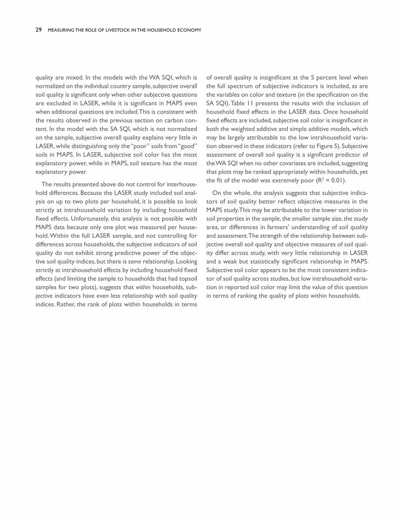
29 MEASURING THE ROLE OF LIVESTOCK IN THE HOUSEHOLD ECONOMY
quality are mixed. In the models with the WA SQI, which is normalized on the individual country sample, subjective overall soil quality is significant only when other subjective questions are excluded in LASER, while it is significant in MAPS even when additional questions are included. This is consistent with the results observed in the previous section on carbon con-tent. In the model with the SA SQI, which is not normalized on the sample, subjective overall quality explains very little in LASER, while distinguishing only the “poor” soils from “good” soils in MAPS. In LASER, subjective soil color has the most explanatory power, while in MAPS, soil texture has the most explanatory power.
The results presented above do not control for interhouse-hold differences. Because the LASER study included soil anal-ysis on up to two plots per household, it is possible to look strictly at intrahousehold variation by including household fixed effects. Unfortunately, this analysis is not possible with MAPS data because only one plot was measured per house-hold. Within the full LASER sample, and not controlling for differences across households, the subjective indicators of soil quality do not exhibit strong predictive power of the objec-tive soil quality indices, but there is some relationship. Looking strictly at intrahousehold effects by including household fixed effects (and limiting the sample to households that had topsoil samples for two plots), suggests that within households, sub-jective indicators have even less relationship with soil quality indices. Rather, the rank of plots within households in terms
of overall quality is insignificant at the 5 percent level when the full spectrum of subjective indicators is included, as are the variables on color and texture (in the specification on the SA SQI). Table 11 presents the results with the inclusion of household fixed effects in the LASER data. Once household fixed effects are included, subjective soil color is insignificant in both the weighted additive and simple additive models, which may be largely attributable to the low intrahousehold varia-tion observed in these indicators (refer to Figure 5). Subjective assessment of overall soil quality is a significant predictor of the WA SQI when no other covariates are included, suggesting that plots may be ranked appropriately within households, yet the fit of the model was extremely poor (R2 = 0.01).
On the whole, the analysis suggests that subjective indica-tors of soil quality better reflect objective measures in the MAPS study. This may be attributable to the lower variation in soil properties in the sample, the smaller sample size, the study area, or differences in farmers’ understanding of soil quality and assessment. The strength of the relationship between sub-jective overall soil quality and objective measures of soil qual-ity differ across study, with very little relationship in LASER and a weak but statistically significant relationship in MAPS. Subjective soil color appears to be the most consistent indica-tor of soil quality across studies, but low intrahousehold varia-tion in reported soil color may limit the value of this question in terms of ranking the quality of plots within households.

PART II – AN ASSESSMENT OF METHODOLOGICAL OPTIONS IN MEASURING SOIL QUALITY 30
Table 11 — Soil Quality Indices and Subjective Indicators: Regression Analysis, with Household Fixed Effects
LASER
Dependent Variable: Simple Additive SQI Weighted Additive SQI (normalized over sample)
Self-Reported Soil Quality
Fair -0.188 -0.172 -0.015** -0.012*
Poor -0.109 -0.096 -0.033*** -0.030**
Self-Reported Color (Collapsed, Black’ Omitted)
Red -0.049 -0.041 -0.014 -0.013
White/Light 0.165 0.191 0.004 0.006
Brown N/A N/A N/A N/A
Self-Reported Soil Texture (Collapsed, ‘Fine’ Omitted)
Between Coarse and Fine -0.252* -0.238 -0.021** -0.020**
Coarse 0.047 0.096 -0.027* -0.023
Constant 4.841*** 4.732*** 4.822*** 4.899*** 0.467*** 0.463*** 0.467*** 0.479***
N 1384 1384 1384 1384 1384 1384 1384 1384
R2 0.003 0.002 0.006 0.011 0.010 0.005 0.010 0.023
*** p<0.01, ** p<0.05, * p<0.1
Household fixed effects, robust standard errors.
Note: Topsoils only.
Source: Authors’ calculations.

31
Part III – Implementing Spectral Soil Analysis in Household Surveys: A Step-By-Step Guide10. CONSIDERATIONS FOR SAMPLE DESIGNThe approach to sampling will vary with the objec-tive of the survey, the sampling frame, and resource availability, among other factors. The sample design must be such that it leads to an unbiased sample of households and their agricultural lands. Depending on the scope of the study and/or the homogeneity of soils in the study region, one may elect to sample soils from one or more agricultural plots per house-hold. Similarly, the degree of clustering may vary (i.e., number of households selected per enumera-tion area). Survey practitioners are encouraged to engage with a sampling expert in the survey design phase.
Sampling frameworks, the strategies by which households and agricultural lands are selected, are designed to reduce sampling error, avoid biased selection of sampling sites, and guide where and how many samples to include in a given study. It is vital to be clear on the decision or sets of decisions that the mea-surement will support before designing the sampling frame-work, bearing in mind that the main purpose of measurement is to reduce decision uncertainty. Because this Guidebook is focused on implementing soil testing in household surveys, it is working under the assumption that the household is the primary sampling unit and that the study has its own prede-termined household sample selection protocol. This chapter therefore focuses primarily on additional factors that need to be taken into consideration when integrating soil testing with the household survey.
Randomizing soil collection sites within the target area or sampling strata is important to provide unbiased estimates of
carbon stocks and other land health indicators within a stra-tum and allow inference to be made to the whole area. Pro-viding unbiased data on the statistical distribution of variables not only is useful for reporting the prevalence of land health problems (e.g., low soil carbon content), but also provides a means of setting local reference values (defining what is low, moderate, or high), which can in turn be conditioned on various factors (e.g., soil texture). A small probability sample generally provides much more useful information than a large biased sample.
The sampling design should be driven by the objectives of the study. Before designing the sample, it must be clear what level of representativeness is desired (if any) and the geo-graphic area of interest. If the study is targeting specific crops and/or populations, that too must be made explicit.
Once the objectives are clear, the following questions must be addressed:
1. How many households will be included in the sample?
2. How many agricultural plots from each household will be subject to soil testing?
3. How many soil samples will be collected from each plot?
4. Where will the soil samples be collected within the plot?
Questions 1 and 2 are study-specific decisions and must be made with the objectives in mind. It may be the case that the aim is to integrate soil sampling into an existing household survey, in which case the household selection is completed without regard for the soil component.

PART III – IMPLEMENTING SPECTRAL SOIL ANALYSIS IN HOUSEHOLD SURVEYS: A STEP-BY-STEP GUIDE 32
Questions 3 and 4 are more generalizable. Depending on the expected variation in the soils, the average size of the agri-cultural plots in the study area, and the method through which the sample collection sites are identified, it is likely sufficient to test a single topsoil sample and a single subsoil sample from each selected plot. Soils provide different types of support to crops at different depths, and crops vary in their soil depth requirements. Maize, for instance, requires deeper soil than teff (Calviño et al. 2003; Evert et al., 2009). Thus, it is gener-ally advisable to test both top- and subsoil samples, but this should be reviewed in light of the crop of interest and overall study objectives.
Question 4, the location of sample collection points within the plot, is critical, and fortunately the most straightforward to implement. If the aim is to assess the soil quality of the plot as a whole (and not a specific point within the plot), the soil sample collection points must make up a representative sam-ple. Therefore, it is strongly recommended to use composite samples. The process of physically collecting the soil samples, as well as the identification of where the samples should be collected, question 4, are discussed in detail in the following section. For an example of a sampling strategy, refer to Box 4, which describes the sampling strategy for the Ethiopia LASER study.
BOX 4 — SAMPLING STRATEGY FOR LASER
The objectives of the LASER study were multifaceted and included indicators related to soil properties, crop type, and socioeco-nomic characteristics, among others. Additionally, the focus was on methodological validation rather than producing nationally rep-resentative statistics. Because there were multiple indicators, calculating the sample size based on the variance of a single indicator was not the preferred approach. Instead, a multistage nested approach using a practical allocation of enumeration areas (EAs) across agroecological zones was used.
Given the methodological focus of the study, it was preferable to implement a smaller-scale survey operation that could be closely supervised. Yet it was also imperative that the study area include substantial variation in soil properties so that soil quality measure-ment methods could be compared in different contexts. Therefore, the study was limited to a single administrative region. Oromia was selected because it represents a large area of Ethiopia and encompasses areas with great variation in rainfall, elevation, and agroecological zone.
The sample was restricted further to three administrative zones of the Oromia region, which were selected based primarily on agroecology and geographic diversity. Secondary consideration was made for the availability of local soil research centers that could be used for soil processing. The three selected zones are East Wellega, West Arsi, and Borena. Using the Agricultural Sample Survey (AgSS) of the Central Statistical Agency of Ethiopia (CSA) as the sampling frame, a total of 85 EAs were selected using a practical allocation and implicit stratification of EAs across agroecological zones. Finally, within each EA, 12 agricultural households were randomly selected from the AgSS household listing completed in September 2013.
The decision-making process for the number of plots subject to soil testing per household was driven by not only the desire to allow for a comparison of subjective and objective measures of soil quality while controlling for household characteristics (there-fore, requiring more than one plot to be selected per household), but also the low expected variation of soil properties across plots cultivated by the same household (assuming geographic proximity). Up to two plots were measured per household. First, if any plots contained pure-stand maize, one was randomly selected. Then, a second plot was randomly selected from the remaining cultivated plots irrespective of crop type. If no plots contained pure-stand maize, two plots were randomly selected. The preference for maize in the first plot selection was purely to satisfy the maize crop-cutting component of the study. The random plot selection was completed by the computer assisted personal interviewing (CAPI) application to prevent selection bias.
The determination of the number of samples per plot was based on the existing AfSIS Land Degradation Surveillance Framework (LDSF). From each crop field, one composite sample was collected from the topsoil (0–20 cm depth) from four points and one central sample from the subsoil (20–50cm depth). Ideally, composite samples would be collected for the top- and subsoils rather than a single central subsoil sample. If resources allow, a composite sample at each depth is recommended. The guidelines presented here will reflect this recommendation
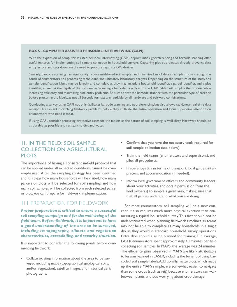
33 MEASURING THE ROLE OF LIVESTOCK IN THE HOUSEHOLD ECONOMY
11. IN THE FIELD: SOIL SAMPLE COLLECTION ON AGRICULTURAL PLOTSThe importance of having a consistent in-field protocol that can be applied under all expected conditions cannot be over-emphasized. After the sampling strategy has been identified and it is clear how many households will be visited, how many parcels or plots will be selected for soil sampling, and how many soil samples will be collected from each selected parcel or plot, you can prepare for fieldwork implementation.
11.1 PREPARATION FOR FIELDWORKProper preparation is critical to ensure a successful soil sampling campaign and for the well-being of the field team. Before fieldwork, it is important to have a good understanding of the area to be surveyed, including its topography, climate and vegetation characteristics, accessibility, and security situation.
It is important to consider the following points before com-mencing fieldwork:
• Collate existing information about the area to be sur-veyed including maps (topographical, geological, soils, and/or vegetation), satellite images, and historical aerial photographs.
• Confirm that you have the necessary tools required for soil sample collection (see below).
• Train the field teams (enumerators and supervisors), and pilot all procedures.
• Prepare logistics in terms of transport, local guides, inter-preters, and accommodation (if needed).
• Inform local government officers and community leaders about your activities, and obtain permission from the land owner(s) to sample a given area, making sure that that all parties understand what you are doing.
For most enumerators, soil sampling will be a new con-cept. It also requires much more physical exertion than enu-merating a typical household survey. This fact should not be underestimated when planning fieldwork timelines as teams may not be able to complete as many households in a single day as they would in standard household survey operations. Extra days should also be planned for training. On average, LASER enumerators spent approximately 40 minutes per field collecting soil samples. In MAPS, the average was 24 minutes. The efficiency gains observed in MAPS are likely attributable to lessons learned in LASER, including the benefit of using bar-coded soil sample labels. Additionally, maize plots, which made up the entire MAPS sample, are somewhat easier to navigate than some crops (such as teff) because enumerators can walk between plants without worrying about crop damage.
BOX 5 – COMPUTER ASSISTED PERSONAL INTERVIEWING (CAPI)
With the expansion of computer assisted personal interviewing (CAPI) opportunities, georeferencing and barcode scanning offer useful features for implementing soil sample collection in household surveys. Capturing plot coordinates directly prevents data entry errors and cuts down on the need to procure separate GPS devices.
Similarly, barcode scanning can significantly reduce mislabeled soil samples and minimize loss of data as samples move through the hands of enumerators, soil processing technicians, and ultimately laboratory analysts. Depending on the structure of the study, soil sample identification labels may be lengthy and complex, as they may include a household identifier, a parcel identifier, and a plot identifier, as well as the depth of the soil sample. Scanning a barcode directly with the CAPI tablet will simplify the process while increasing efficiency and minimizing data entry problems. Be sure to test the barcode scanner with the particular type of barcode before procuring the labels, as not all barcode formats are readable by all hardware and software combinations.
Conducting a survey using CAPI not only facilitates barcode scanning and georeferencing, but also allows rapid, near-real-time data receipt. This can aid in catching fieldwork problems before they infiltrate the entire operation and focus supervisor attention on enumerators who need it most.
If using CAPI, consider procuring protective cases for the tablets as the nature of soil sampling is, well, dirty. Hardware should be as durable as possible and resistant to dirt and water.

PART III – IMPLEMENTING SPECTRAL SOIL ANALYSIS IN HOUSEHOLD SURVEYS: A STEP-BY-STEP GUIDE 34
Enumerator training must be thorough and convey the seri-ousness of sampling and handling soils with great care. Soil samples are quite fragile; testing results can be biased if the samples are not handled properly. Contamination of soil sam-ples (as a result of inadequately cleaned equipment, for exam-ple) or failure to dry wet soil samples within 5–10 days of collection can lead to misrepresented results. Training should include a theoretical overview of the motivation for the study (field teams will need to explain this to respondents), review of key concepts and terminology, review of the enumerator manual (which can be based on this Guidebook), and group and individual hands-on training.
In each study, 2–3 days were dedicated to soil training, and 1–3 days were devoted to field practice. Training for the soil components of LASER and MAPS was conducted by an expert from ICRAF to ensure the use of best practices. While hands-on training was the most effective, it was imperative that the strategy, terminology, and importance of each step were reviewed in a classroom setting before the distribution of equipment and the outdoor demonstration.
All equipment must be procured before enumerator train-ing, for use in plot practice. The list of equipment appears in Box 6, and cost estimates for key equipment appear in Annex 4.

35 MEASURING THE ROLE OF LIVESTOCK IN THE HOUSEHOLD ECONOMY
BOX 6 — EQUIPMENT REQUIRED FOR SOIL SAMPLE COLLECTION
Below is a list of the basic tools and materials necessary for soil sample collection from agricultural plots. Unless otherwise noted, it is recommended to have one unit per enumerator. Cost estimates for key equipment are provided in Annex 4.
a) GPS device, preferably with ability to store coordinates (and land area, if desired by study)
b) Soil auger marked at 20 cm and 50 cm from tip
Note: Auger heads are designed differently for different types of soil. That is, sandy soils require a different auger head than clay soils. Distribute materials to field teams accordingly.
c) Measuring tape
d) Plastic sample bags (at least 400-gram capacity): 4 bags per parcel/plot subject to soil sampling
e) Buckets: 2 per enumerator, preferably of different colors so as to easily distinguish top- and subsoils.
f) Mixing trowel or spade
g) Water bottle filled with water (with hose, or punch a small hole in the cap)
h) A board, tray, or plastic sheet for coning and quartering; a clean plastic bag can also suffice
i) Labels or barcodes
j) Permanent marker pens
k) Stationery like pencils and a field notebook.
l) Texture chart for hand classification (see Figure 14)
a) b)
c)
e), f)

PART III – IMPLEMENTING SPECTRAL SOIL ANALYSIS IN HOUSEHOLD SURVEYS: A STEP-BY-STEP GUIDE 36
11.2 SOIL SAMPLE COLLECTION PROTOCOL This section presents a step-by-step protocol for ensuring that a representative soil sample is col-lected from each field. Composite samples, those collected from multiple points in the plot, are sug-gested to increase representativeness.
Soil sampling on agricultural plots requires that enumerators enter and use an auger in the plot. Thus, there is a risk of a small area of crop damage in the area of sampling.11 Stable soil properties will not be affected by the time of sample collec-tion. For some crops, such as maize, sampling is possible ear-lier in the agricultural season because samples can be taken from between the plants. For other crops such as teff, it may be necessary to wait until the harvest is completed to avoid excessive crop damage. If possible, try to collect soil samples without causing much damage to the crop by timing the sam-ple collection appropriately. It is also advisable to avoid soil sampling when the soil is too wet because it will be difficult and may require a lot of time to collect and dry.
11 Originally, the intention was to conduct bulk density analysis as well as the conventional and spectral soil testing as part of LASER. However, the bulk density test requires a metal plate (approximately 40 cm x 40 cm) to be laid in the plot. During fieldwork training it was determined that the bulk density plate caused undue damage to the crop, and therefore it was excluded from the study.
11.2.1 PLOT LAYOUTAs mentioned above, the location of the soil sample collec-tion points are derived from the AfSIS LDSF 1,000-m2 design (Figure 10), placed over the center of the crop plot. The AfSIS LDSF design serves as an initial template for soil sampling but may need to be modified to accommodate agricultural plots that are too small or irregularly shaped to contain a 1,000-m2 soil sample plot (see Figure 11). The protocol implemented in LASER and MAPS and recommended for future studies is as follows:12
Step 1: Define the field center point by measuring halfway along the longest side and halfway along the shortest side of the field (Figure 10). Record the GPS coordinates of the plot center, or save the waypoints in the GPS unit with the appropriate label. The coordinates may also be saved in the GPS device.
Step 2: Using a measuring tape, measure out the distance (12.2 m) from the center point (point 1; Figure 10) directly uphill (where applicable) to the second point (point 2).
12 In both MAPS and LASER, a composite sample was collected from the topsoil, but only a single subsoil sample was collected from the center point. However, if resources allow, a composite sample is recommended for both the top- and subsoils. Therefore, this Guidebook describes a protocol in which composite samples are collected at both depths.
Agricultural plot
1
d = 12.2 m
Area = 1000 m2
1
2
4 3
Sampling plot
Figure 10 — Sample plot layout in a crop plot, with four points (dotted circles). The distance between the center point and the other three points is 12.2 meters, which represents a 1,000-square-meter sampling plot.

37 MEASURING THE ROLE OF LIVESTOCK IN THE HOUSEHOLD ECONOMY
Step 3: Mark points 3 and 4 at 120 and 240 degrees from the up-point (point 2), respectively, and 12.2 meters from the center point. The angles can be measured using a compass or estimated once the field team develops experience in plot layout.
The distance should be corrected when plots fall on steep terrain (slope > 10 degrees). Use the following formula to cal-culate the distance from the center point to the other point (for slope > 10 degrees):
Take the cosine values from the backside of your clinome-ter if you have one, or you may prepare and print a cosine table to carry in the field. You can also get cosine values from the Internet if you have Internet connectivity in the field. For instance, for a field with a 15-degree slope, the slope distance will be 12.2 m/0.9659 = 12.6 m.
In many contexts, agricultural plots can be quite small and/or irregularly shaped. In these circumstances, the AfSIS LDSF design may not fit within the plot boundaries. If the plot is too small, the point should be placed 2 meters inside the boundary
in order to limit border/edge effects. It may also be the case that plots are irregularly shaped and cannot accommodate the LDSF format. Figure 11 provides examples of alternative sample collection points aimed at achieving soil samples rep-resentative of the full plot.
11.2.2 SOIL SAMPLINGIn general, it is advisable to test both a top- and subsoil sample in order to capture variation in key soil properties at different depths, which in turn affect crops differently. The decision to analyze top- and subsoil samples should be reviewed in light of the crop of interest and overall study objectives. This Guide-book describes the scenario in which samples are collected from two depth ranges (0–20 cm and 20–50 cm). Every plot selected for soil sampling is subject to the following:
• One composite topsoil sample collected at 0–20 cm. This sample is collected from four points within the plot (points 1–4 in Figure 10).
• One composite subsoil sample collected at 20–50 cm. This sample is collected from four points within the field (points 1–4 in Figure 10). If necessary, subsoil may be collected from a single central point for cost-savings, but a composite sample is recommended.
Figure 11— Layout of soil sample collection for plots of different shapes and sizes
2
134
1
1
3
2
1
2
34
(b) (c) (d)(a)
c
b
a
d
Source: Authors.Note: Agricultural plots have different shapes and sizes that may require the sample collection layout to be modified. Examples: (a) shape and size of the crop plot allow a 1,000-m2 sampling layout; take a composite sample from four points; (b) crop plot is less than 100 m2; take sample from one point only; (c) shape of the crop plot does not allow an LDSF type of layout; take a composite sample from three points, (d) one side of the crop plot does not allow a full LDSF type of layout; leave a 2-m buffer from the boundary for point 2 (place it closer to center point) and take a composite sample from four points.

PART III – IMPLEMENTING SPECTRAL SOIL ANALYSIS IN HOUSEHOLD SURVEYS: A STEP-BY-STEP GUIDE 38
11.2.2.1 IN-FIELD SAMPLING PROCEDUREThe in-field sampling procedure is as follows:
Step 1: Mark the auger at 20 and 50 cm (e.g., using a permanent marker).
Step 2: Place the auger in the center sampling point, and begin to auger straight down. You will use the same auger for all depths. If augering becomes crooked, stop and start a new hole, otherwise you will get an inaccurate measurement of the depth.
Step 3: Auger down to a depth of 20 cm, and transfer all of the soil from the auger into the bucket designated for topsoil.
Step 4: The next sample is from 20–50 cm. Continue augering (in the same 0–20-cm hole) until you reach the 50-cm mark on the auger. Empty the soil from the auger into the separate bucket designated for subsoil.
Step 5: Repeat step 3 for the remaining collection points on the field (points 2–4 on Figures 10 and 11). Place all top- and subsoils collected into the bucket des-ignated for each depth. Now you will have two buckets that contain composite samples from all four collections points for the top- and subsoils. Mix each bucket with a trowel, cleaning the trowel between buckets.
Step 6: If the auger was not able to reach the desired depth (due to depth restrictions from a rock layer, for example), record the auger depth restriction (the maximum depth attainable).
Step 7: Conduct the in-field soil texture analysis (see Figures 13 and 14).
Step 8: Conduct the coning and quartering procedure for the topsoil and subsoil separately. The end result should be approximately 400 grams (g) of topsoil and 400 g of subsoil. Instructions for the procedure are found in the section below (Figure 12).
Step 9: Bag and label the samples with the household identification, plot identification, depth of the soil sample, and auger depth restriction (if applicable).
If the soil is very dry, it may be difficult to auger and collect all of the soil from the depth increment; in this case prewetting the soil before augering each increment may be helpful.
11.2.2.2 SUB-SAMPLING VIA “CONING AND QUARTERING”Normally, soil-sampling procedures lead to collection of more soil than necessary for analysis. To get a representative sam-ple of the appropriate volume, a standardized and consistent procedure must be followed. For this purpose, it is necessary to use the method of coning and quartering described below (and seen in Figure 12b). Continue the coning and quartering technique on the topsoil and subsoil samples to obtain a rep-resentative 400-g subsample of soil for processing and analysis. The process for coning and quartering is as follows:
Step 1: Place the sample on a strong, clean plastic sheet or similar material (Figure 12b).
Step 2: Thoroughly mix the soil sample, and spread the samples into a conical pile.
Step 3: Further mix the soil by circumventing the cone symmetrically, repeatedly taking a spatula full of soil from the base and transferring the soil to the apex of the cone.
Step 4: Ensure the spatula is large enough to reach center of the cone. Circumvent the cone twice.
Step 5: Flatten the cone to a height of about 1 cm (Figure 12b).
Step 6: Use a flat spatula or ruler to divide the pile into quarters with two perpendicular lines (Figure 12b).
Step 7: Select one pair of opposite quarters as the sample to be retained.
Step 8: If the sample is still too large, then repeat the procedure from the beginning.
Step 9: Take the representative subsample (about 400 g), and place it in a plastic bag. Label the bag, and place an extra label tag inside the bag.

39 MEASURING THE ROLE OF LIVESTOCK IN THE HOUSEHOLD ECONOMY
Figure 12 — Soil Sample Collection and Subsampling
Figure 13 — Soil Texture by Feel: Steps
(a) (b)
TEXTURE BY FEEL ON SOIL SAMPLES
Step 1: Starting with the topsoil sample, moisten a handful of soil using water from the water bottle until the soil has a putty-like consistency but free water does not escape when ball is squeezed (a).
Step 2: Shape the soil into a ball. If the ball retains its shape, move to step 3.
Step 3: Using your thumb and forefinger, form a ribbon with the soil by smearing the ribbon with your thumb (b). Observe if the soil is shiny or dull.
Step 4: Measure the length of the ribbon when it breaks and record it in the questionnaire (c) The ribbon should be measured in millimeters (mm).
Step 5: Classify the texture according to the flow chart (Figure 14) and report in the questionnaire whether it is smooth, gritty, or neither.
(c)
(b)
(a)
(a) Soil sample collection (b) Soil subsampling via coning and quartering
(a)
(b)
(c)
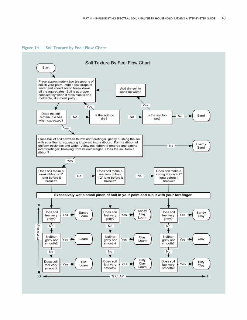
PART III – IMPLEMENTING SPECTRAL SOIL ANALYSIS IN HOUSEHOLD SURVEYS: A STEP-BY-STEP GUIDE 40
Figure 14 — Soil Texture by Feel: Flow Chart

41 MEASURING THE ROLE OF LIVESTOCK IN THE HOUSEHOLD ECONOMY
11.2.2.3 IN-FIELD SOIL TEXTURE ANALYSISSoil texture is the amount of sand, silt, and clay in the soil and is important for determining many soil properties including aggregation, structure, and water and air movement through the soil. This section provides instruction on determining if the soil texture is smooth, gritty, or neither smooth nor gritty (Fig-ures 13 and 14). Figure 13 also illustrates the soil ribbon test, which acts as a proxy for soil structure and texture.
11.2.2.4 SOIL SAMPLE LABELINGLabeling is critical. To ensure that results from soil analysis are linked to the correct household and plot, several pieces of information must be captured. The unique household identi-fier, the parcel and/or plot identifier, and the depth of the soil sample must be listed on the sample bag (with a duplicate label placed inside the bag in case of damage to the outer label and for use by the laboratory). The labeling scheme used in LASER is illustrated in Table 12.
For example, for a plot with Household ID 3108, parcel ID 03, and plot ID 02, you would have the following labels:
• 3108–03–02 0–20 cm
• 3108–03–02 20–50 cm
In case of soil depth restrictions, indicate the actual depth in the label. For example, the subsoil label for a site where a soil depth restriction occurred at a depth of 35 cm would be the following:
• 3108–03–02 20–35 cm
Sample IDs should be legibly recorded with a permanent marker on the outside of the plastic bags. A paper label con-taining the same information (written in pen or pencil) should also be placed inside the bags.
When possible, the use of barcoded labels is highly encour-aged, especially for surveys administered via CAPI. Preordered barcodes with serialized numbers printed on them can greatly reduce data entry problems. A duplicate of every barcode should be ordered such that one barcode is placed on the outside of the bag and the second is placed inside the bag (without the backing peeled so it is not sticky). The duplicate bag can then be easily used by the laboratory, as they will likely take a subsample of the soil and store it in a separate bag. Ensure that the type of barcode you choose can be read by the CAPI hardware and software. This protocol was followed in MAPS, and fieldwork time was reduced.
11.2.2.4 SOIL SAMPLING SUMMARYThe process to collect soil samples from agricultural plots is a multistage process but is not overly technical. Enumerators can be trained to effectively implement the modified AfSIS LDSF sample layout, collect soils via augering, subsample the collected subsoils via coning and quartering, test the texture of the soils, and properly label the samples. A summary of the steps in soil sample collection is found in Table 13.
12. IN THE LAB(S): SOIL PROCESSING AND LABORATORY ANALYSISSection 12 describes the stages of soil processing and testing. While much of the content is directly relevant to the lab-oratories where drying, processing, and analysis take place, it is essential for survey practitioners to fully understand the process.
12.1 SOIL PROCESSINGBefore analysis, soil samples must be processed. This involves drying, crushing, sieving, weighing, and subsampling the soils. The process by which this was completed in LASER and MAPS is outlined below.
Table 12 — Examples of Soil Sample Labels used in LASER
Label for soil samples Number of samples Note
HHHH-PP-FF 0-20 cm 1 HHHH = household; PP = parcel; FF = plot
HHHH-PP-FF 20-50 cm 1
Total 2

PART III – IMPLEMENTING SPECTRAL SOIL ANALYSIS IN HOUSEHOLD SURVEYS: A STEP-BY-STEP GUIDE 42
Step
Agricultural Plot
Top soil (0-20 cm)
Sub-soil (20 -50 cm)
Step 1: Using the soil auger collect topsoil (0–20 cm) from the four points and place in a bucket (Figure 12a). *
Step 2: Using the soil auger, collect subsoil (20–50 cm) from the four points and place in a separate bucket. *
Step 3: Analyze the texture and measure the ribbon size for the top- and subsoils according to the instructions in Figures 13 and 14. * *Step 4: Take a representative (about 400 g) subsample of the top- and subsoils following the coning and quartering procedure, and place them in separate plastic bags. Label the bags accordingly (as in Table 12 or as otherwise determined by the project). Place an extra label inside the sample bag. * *Step 5: If there are auger depth restrictions, adjust the label accordingly. For example, if the auger will only dig to 15 cm, label the sample as HHID-parcel ID – Plot ID 0–15 cm (rather than 0–20 cm). * *
Table 13 — Major Steps in Soil Sample Collection
12.1.1 SCOPE AND APPLICATIONAll soil samples should be transported to a regional labora-tory for processing using this standard operating procedure. Soil laboratories found in various national and regional agri-cultural research institutes and academic institutions found closer to a study area could be used for soil processing. The LASER study used the soil laboratory facilities and technicians from the Awassa Agricultural Research Center (for West Arsi), Ambo University (for Wellega), and Yabello Pastoral and Dry-land Agricultural Research Center (for Borena). In MAPS, all soil processing was conducted at Uganda’s National Forestry Resources Research Institute in Kampala. Soil drying and/or processing may be conducted in-country before transporta-tion to the regional laboratories to avoid changes in soil prop-erties from storage of wet samples and to reduce the cost of shipping a large volume of soils. In the case of LASER and MAPS, samples were dried, sieved, and weighed before being shipped to ICRAF for analysis. Note that the drying of samples is critical and should be completed within a week of collection in order to minimize any decomposition of organic material, especially in wet soils.
12.1.2 PRINCIPLESSampling and sample processing, or pretreatment, make up an important stage of soil analysis because conclusions about a site are often based on the analysis of representative soil sam-ples collected during this stage. Because of high spatial varia-tion in the soil, it is important that the process followed should lead to the collection of a sample that is truly representative
of the site. Errors in sampling and sample pretreatment can influence the final results of a soil analysis.
Soil collected from an agricultural plot is a mix of gravel (fraction of soil with a diameter of > 2 mm), sand (fraction between 0.05 mm and 2.0 mm), silt (fraction between 0.002 mm and 0.05 mm), and clay (fraction smaller than 0.002 mm). Since the contribution of the gravel fraction to the dynam-ics of soil nutrient cycles and supply to plants is minimal, it is excluded from the analysis and reporting of plant-available nutrients. During the preparation of soil samples, this fraction should not be crushed and pulverized, because then it would be considered part of the fine soil and result in low values of the analyses owing to the dilution effect. However, aggre-gates of > 2 mm formed by fine particles have to be crushed in order to pass through a 2-mm sieve and be included in the analysis. Normally, soil-sampling procedures lead to the col-lection of more than the required amount of soil, and to get a representative sample of the necessary volume, it is important to follow standardized and consistent procedures of coning and quartering.
12.1.3 LAB PROCEDURES: SOIL PROCESSINGSoil processing involves sample reception, drying, crushing and sieving, and subsampling of fine particles, all while ensuring the health and safety of the lab technicians. Soil processing does not require technical equipment. It requires only the items

43 MEASURING THE ROLE OF LIVESTOCK IN THE HOUSEHOLD ECONOMY
listed in Box 7 and a clean working environment with space for drying the soil samples. The procedures for soil processing are described here in a step-by-step fashion.
12.1.3.1 SOIL SAMPLE RECEPTION
• Lay out the samples received in order of labeling, and check against the master list of samples received from the plot. If barcoded labels are used, the lab can simply scan the inventory.
• Make detailed notes in a laboratory record book of any labeling discrepancies or problems due to damaged sam-ple bags or lost samples.
12.1.3.2 DRYINGStep 1: Spread the soil out as a thin layer into shallow
trays or plastic or paper sheets. It is important to ensure that no material from a sample is lost or discarded (Figure 15).
Step 2: Break up clods as far as possible to aid drying. Take care to avoid crushing gravel-sized particles.
Step 3: Great care should be taken at all stages to ensure that sample labels remain with the samples.
Step 4: Exercise care to avoid contamination from dust, plaster, or other potential contaminants during
drying, as soils are subjected to trace element analysis.
Step 5: Air dry the samples in shade, not sun. Drying can also be done in a large room, custom-made solar dryer, or a forced-air oven at 40° C.
Step 6: Drying time will depend on the condition of the samples and ambient conditions, but the samples should be thoroughly dried.
BOX 7 – EQUIPMENT REQUIRED FOR SOIL PROCESSING ACTIVITIESBelow is a list of the basic tools and materials necessary for soil processing. Soil processing involves drying the soils, crushing and sieving them to ensure that only the fine portion of the soils is analyzed, and weighing out a smaller subsample for laboratory analysis.
• Drying trays
• Wooden rolling pin
• 2-mm sieve
• Plastic sheet
• Markers
• Brown paper bags (size 5)
• Balance
• Plastic zip-lock bags
• Particulate respirator (e.g., N95 of 3M brand)
• Nitrile gloves
• Damp cloth
• Forced-air drying oven (optional)
Figure15.DryingofMAPSsoilsamples
Figure 15 — Drying of MAPS Soil Samples

PART III – IMPLEMENTING SPECTRAL SOIL ANALYSIS IN HOUSEHOLD SURVEYS: A STEP-BY-STEP GUIDE 44
12.1.3.3 CRUSHING AND SIEVINGStep 1: Spread the sample onto a plastic sheet on a solid
table (Figure 16).
Step 2: Using a wooden rolling pin, crush the sample enough to allow it to pass through a 2-mm sieve.
Step 3: While crushing, remove any plant materials (e.g., roots) and any possible pieces of gravel (making sure they are gravel and not soil aggregates) and place in a separate pile (the coarse fraction).
Step 4: Pass the crushed sample through the 2-mm sieve. DO NOT use the sieve as a grinder; i.e., do not rub or mash the soil on the sieve, but shake the sieve gently to allow the soil to pass through. If a large amount of soil needs to be sieved, it is easier to do it in small batches rather than all at one time.
Step 5: Place whatever remains on the sieve back onto the plastic sheet and crush again gently. Then pass again through the 2-mm sieve.
Step 6: Transfer anything that now remains on the sieve into the coarse fraction pile
Step 7: The whole sample should be processed, and no material should be discarded. You will remain with two fractions:
• The coarse fraction (> 2 mm), which cannot pass
through the sieve. Discard the coarse fraction.
• The soil fines (< 2 mm), which have passed through the sieve.
Step 8: Clean off the table with a damp cloth to remove soil dust, to prevent contamination from one sample to another.
12.1.3.4 SUBSAMPLING OF FINE FRACTIONSStep 1: If the weight of the soil fines is more than 400
g, subsample the soil fines using coning and quartering to give about 350–400 g of fine soil.
Step 2: Continue the coning and quartering technique on all samples to obtain a representative 20-g subsample of soil fines for shipping to the laboratory designated for specialized spectral analysis.
Step 3: Place the 20-g subsample in a zip-lock polythene bag labeled properly. All of the 20-g samples will be delivered to the lab conducting the spectral analysis.
Step 4: Place the remaining +/-350-g sample of soil fines into a strong size-5 brown paper bag, labeled properly, and store for possible future use. Note: This is when you will need a duplicate barcode or other label (with the same identification information).
Step 5: A select subset of the 350-g soil fine samples will be tested with conventional analysis. This is typically in the range of 10–25 percent of all samples. The exact samples will be identified following completion of the spectral analysis on all samples, thereby showing the variation of soil properties present in the samples. The selected 350-g reference samples will be shipped to the ICRAF Soil-Plant Spectral Diagnostics Lab in Nairobi or other diagnostic lab for reference analyses. Soil fine samples that are not shipped should be stored at the regional laboratory in case they are needed for future analysis.
Figure 16 — Sample Crushing and Sieving
Figure16.Samplecrushingandsieving

45 MEASURING THE ROLE OF LIVESTOCK IN THE HOUSEHOLD ECONOMY
12.1.3.5 SOIL PROCESSING: HEALTH AND SAFETY
• Wear nitrile gloves to reduce the incidence of skin con-tact with potentially contaminated soil and to reduce the risk of cross-contamination.
• Wear a respirator that covers the mouth and nose to filter out harmful dust particles. Inhaling such particles irritates the nostrils and sinuses and may lead to lung diseases.
• Refer to the site-specific health and safety plan for other safety concerns and applicable personal protective equip-ment.
12.2 LABORATORY ANALYSIS: SPECTROSCOPYWhile all technical analysis will be conducted by expert technicians, the information below regarding the processes followed by the laboratory will equip survey practitioners with the background necessary to plan and implement a successful study.
Soils samples can be analyzed for chemical (e.g., nitro-gen) and physical properties (e.g., texture) at the Soil-Plant Spectral Diagnostics Lab of the World Agroforestry Centre (Figure 16) or other laboratory with the necessary equipment
and expertise. All soil samples are scanned for mid-infrared soil spectroscopy (IR) and laser diffraction particle size dis-tribution analysis (LDPSA), while 10–25 percent from the total sample are subject to reference analysis (including con-ventional wet chemistry, x-ray methods for soil mineralogy [XRD], and total element analysis [TXRF]), which is used to calibrate and validate MIR-spectral prediction for the remain-ing samples (75–90 percent).
Results from the conventional and spectral soil testing are presented to the end user in the form of a dataset, complete with all identification variables (which are necessary to merge the data with the household survey) and soil-quality indica-tors included in the testing. Whenever possible, make the data publicly available, as this will increase the visibility of the data by making them available to researchers, students, and policy figures. However, household surveys require a degree of con-fidentiality. Exact coordinates of households, agricultural plots, or soil collection points must not be released.
Figure 17 — Left: MIR spectrometer. Right: a team of three from the LSMS project of the World Bank and the Central Statistical Agency (CSA) of Ethiopia attending a three-day soil infrared spectroscopy exposure training at ICRAF’s Soil-Plant Spectral Diagnostics Laboratory in Nairobi.

46
Part IV – Conclusions
This Guidebook provides a step-by-step guide to implementing spectral soil analysis in household sur-veys as well as providing results of two methodolog-ical studies, both of which illustrate the inability of subjective farmer assessment to adequately capture true soil properties.
Knowledge of soil quality indicators and overall health is becoming increasingly important as food security issues become more pressing and climate change threatens to change the face of agriculture. Soil health, both perceived and actual, can have impacts on the targeting and uptake of improved agricultural practices, which can improve both the quality and quantity of food produced. For instance, Marenya and Barrett (2009) show that fertilizer effectiveness, and in turn farmers’ demand for fertilizer, are dependent on soil carbon content. However, results of the LASER and MAPS studies suggest that subjective soil quality indicators fail to effectively reflect true levels of organic carbon, limiting the value of subjective assess-ments of soil quality in policymaking.
Asking a farmer to categorically rate overall soil quality has limited benefit. This particular subjective soil quality question does not successfully consistently distinguish between soil car-bon levels or predict soil quality index scores, at least within these methodological research studies. Subjective questions on soil color and texture are more effective at predicting soil quality index scores and organic carbon content, but the low explanatory power of these variables leaves much to be desired. Furthermore, the severe lack of variation in subjec-tive soil quality indicators given by households reporting on multiple plots calls the value of this approach into question.
Evidence from the LASER and MAPS studies suggests that subjective farmer assessments of soil quality poorly explain objective laboratory results and lack intrahousehold variation. Spectral analysis has been proven to near-perfectly predict key soil parameters as measured by conventional wet chemistry methods, while also providing highly detailed data that can be useful in policy aimed at increasing agricultural output and
nutritional value, such as fertilizer input programs, as well as in agricultural productivity analysis.
From a fieldwork implementation standpoint, the LASER and MAPS studies suggest that it is feasible to integrate soil spectroscopy into socioeconomic household panel surveys. The methodology is a relatively rapid and cost-effective soil measurement technique that could unlock further understand-ing of the effects of farm management practices and changes in soil health over time.
The body of research on implementing spectral soil testing in household surveys, and validating objective measurements against subjective assessments, is at an early stage. Given the emerging nature of this type of research, and the complexi-ties of soil-quality measurement, we encourage further val-idation of such projects, particularly under soil conditions different from those presented here. Additional research is also needed to validate the use of the growing number of tools and methods for in-field soil analysis. As these methods are developed with increasing capabilities, their accuracy must be assessed against standard methods, such as conventional and spectral soil analysis, before they can be reliably used in household surveys.

47
REFERENCES
AfSIS (Africa Soil Information Service). (2014). Africa Soil Information Service. Retrieved from http://www.africasoils.net.
Aitkenhead, M., Donnelly, D., Coull, M., & Gwatkin, R. (2016). Estimating soil properties with a mobile phone. In Hartemink, A. E., & Minasny, B. (Eds.), Digital Soil Morphometrics (pp. 89–110). New York: Springer.
Aynekulu, E., Vågen T.-G., Shephard, K., & Winowiecki, L. (2011). A protocol for modeling, measurement and monitoring soil carbon stocks in agricultural landscapes. Version 1.1. Nairobi: World Agroforestry Centre.
Aynekulu, E., Carletto, C., Gourlay, S., & Shepherd, K. (2016). Soil sampling in household surveys: Experience from Ethiopia. Washington, DC, and Nairobi: World Bank and World Agroforestry Centre. Retrieved from http://go.worldbank.org/PYIZRV60K0
Beaman, L., & Dillon, A. (2012). Do household definitions matter in survey design? Results from a randomized survey experiment in Mali. Journal of Development Economics, 98(1), 124–135.
Bennett, L. T., Mele, P. M., Annett, S., & Kasel, S. (2010). Examining links between soil management, soil health, and public benefits in agricultural landscapes: An Australian perspective. Agriculture, Ecosystems and Environment, 139, 1–12.
Bouis, H. E. (2003). Micronutrient fortification of plants through plant breeding: Can it improve nutrition in man at low cost? Proceedings of the Nutrition Society, 62, 403–411.
Calviño, P. A., Andrade, F. H., & Sadras, V. O. (2003). Maize yield as affected by water availability, soil depth, and crop management. Agronomy Journal, 95, 275–281. doi:10.2134/agronj2003.2750
Ethiopian ATA (Agricultural Transformation Agency). (2017). EthioSIS. Retrieved from https://www.ata.gov.et/highlighted-deliverables/ethiosis/
Evert, S., Staggenborg, S., & Olson, B.L.S. (2009). Soil Temperature and Planting Depth Effects on Tef Emergence. Journal of Agronomy and Crop Science, 195, 232–236. doi: 10.1111/j.1439-037X.2008.00343.x
FAO. (1986). Ethiopian highlands reclamation study. Final Report, AG:UTF/ETH/037/ETH. Rome: Food and Agriculture Organization of the United Nations.
FAO. (2005). A system of integrated agricultural censuses and surveys. FAO Statistical Development Series, 11. Rome: Food and Agriculture Organization of the United Nations.
Fernandes, J. C., Gamero, C. A., Rodrigues, J. G. L., & Miras-Avalos, J. M. (2011). Determination of the quality index of a Paleudult under sunflower culture and different management systems. Soil and Tillage Research, 112, 167–174.
Fischer, G., Nachtergaele, F., Prieler, S., van Velthuizen, H. T., Verelst, L., & Wiberg, D. (2008). Global agro-ecological zones assessment for agriculture (GAEZ 2008). Laxenburg, Austria, and Rome, Italy: International Institute for Applied Systems Analysis and Food and Agriculture Organization of the United Nations.
Gourlay, S., Aynekulu, E., Shepherd, K., & Carletto, C. (2017). Collecting the dirt on soils: Advancements in plot-level soil testing and implications for agricultural statistics. Policy Research Working Paper 8057. Washington, DC: World Bank . Retrieved from http://documents.worldbank.org/curated/en/748621494523429244/Collecting-the-dirt-on-soils-advancements-in-plot-level-soil-testing-and-implications-for-agricultural-statistics
Grosh, M., & Glewwe, P. (2000). Designing household survey questionnaires for developing countries: Lessons from 15 years of the Living Standards Measurement Study. Volumes 1, 2, and 3. Washington, DC: World Bank.
Hengl, T., Heuvelink, G. B. M., Kempen, B., Leenaars, J. G. B., Walsh, M. G., Shepherd, K. D., et al. (2015). Mapping soil properties of Africa at 250 m resolution: Random forests significantly improve current predictions. PLoS ONE, 10(6), e0125814. doi:10.1371/journal.pone.0125814
Herrick, J. E., Urama, K. C., Karl, J. W., Boos, J., Johnson, M. V. V., Shepherd, K. D., Hempel, J., Bestelmeyer, B. T., Davies, J., Guerra, J. L., & Kosnik, C. (2013). The global Land-Potential Knowledge System (LandPKS): Supporting evidence-based, site-specific land use and management through cloud computing, mobile applications, and crowdsourcing. Journal of Soil and Water Conservation, 68(1), 5A–12A.

REFERENCES 48
Ji, W., Shi, Z., Huang, J. & Li, S. (2014). In situ measurement of some soil properties in paddy soil using visible and near-infrared spectroscopy. PLoS ONE, 9, 1–11.
Karlen DL, Stott D.E. (1994). A framework for evaluating physical and chemical indicators of soil quality. In: Doran JW, Coleman DC, Bezdicek DF, Stewart BA, editors. Defining soil quality for a sustainable environment. Madison, WI: Soil Science Society of America. pp. 53–72.
Karltun, E., Lemenih, M., & Tolera, M. (2013). Comparing farmers’ perception of soil fertility change with soil properties and crop performance in Beseku, Ethiopia. Land Degradation and Development, 24, 228–235.
Lal, R. (2009). Soil degradation as a reason for inadequate human nutrition. Food Security, 1, 45–57.
Lal, R. (2016). Soil health and carbon management. Food and Energy Security, 5(4), 212–222.
Lorenz, K., & Lal, R. (2005). The depth distribution of soil organic carbon in relation to land use and management and the potential of carbon sequestration in subsoil horizons. Advances in Agronomy, 88, 35–66.
Marenya, P., & Barrett, C. B. (2009). Soil quality and fertility use rates among smallholder farmers in western Kenya. Agricultural Economics, 40(5), 561–572.
Mehlich, A. (1984). Mehlich-3 soil test extractant: A modification of Mehlich-2 extractant. Communications in Soil Science and Plant Analysis, 15(12), 1409–1416.
Minasny, B., & Hartemink, A. E. (2011). Predicting soil properties in the tropics. Earth-Science Reviews, 106(1–2), 52–62.
Mukherjee, A., & Lal, R. (2014). Comparison of soil quality index using three methods. PLoS ONE, 9(8), e105981. doi:10.1371/journal.pone.0105981
Nocita, M., Stevens, A., van Wesemael, B., Brown, D. J., Shepherd, K. D., Towett, E., Vargas, R., & Montanarella, L. (2015). Soil spectroscopy: An opportunity to be seized. Global Change Biology, 21(1), 10–11. doi:10.1111/gcb.12632
Randall, S., & Coast, E. (2015). Poverty in African households: The limits of survey and census representations. Journal of Development Studies, 51(2), 162–177.
Sanchez, P. A., Denning, G. L., & Nziguheba, G. (2009). The African Green Revolution moves forward. Food Security, 1(1), 37–44.
Shepherd, K. D., & Walsh, M. G. (2002). Development of reflectance spectral libraries for characterization of soil properties. Social Science Society of American Journal, 66(3), 988– 998.
Shepherd, K. D., & Walsh, M. G. (2004). Diffuse reflectance spectroscopy for rapid soil analysis. In Lal, R. (Ed.), Encyclopedia of Soil Science. New York: Marcel Dekker.
Shepherd, K. D., & Walsh, M. G. (2007). Infrared spectroscopy: Enabling an evidence-based diagnostic surveillance approach to agricultural and environmental management in developing countries. Journal of Near Infrared Spectroscopy, 15, 1–19.
Takoutsing, B., Weber, J., Aynekulu, E., Martín, J. A. R, Shepherd, K. D., Sila, A., Tchoundjeu, Z., & Diby, L. (2016). Assessment of soil health indicators for sustainable production of maize in smallholder farming systems in the highlands of Cameroon. Geoderma, 276, 64–73.
Tittonell, P., Shepherd, K. D., Vanlauwe, B., & Giller, K. E. (2008). Unravelling the effects of soil and crop management on maize productivity in smallholder agricultural systems of western Kenya: An application of classification and regression tree analysis. Agriculture, Ecosystems and Environment, 123, 137–150.
Tulchinsky, T. H. (2010). Micronutrient deficiency conditions: Global health issues. Public Health Reviews, 32(1), 243–255.
United Nations. (2008). Principles and recommendations for population and housing censuses revision 2. New York: United Nations, Department of Economics and Social Affairs, Statistics Division.
Welch, R. M., & Graham, R. D. (2004). Breeding for micronutrients in staple food crops from a human nutrition perspective. Journal of Experimental Botany, 55(396), 353–364.
Wenjun, J., Zhou, S., Jingyi, H., & Shuo, L. (2014). In situ measurement of some soil properties in paddy soil using visible and near-infrared spectroscopy. PLoS One, 9. doi:10.1371/journal.pone.0105708

49
ANNEXES
Annex 1
Key Definitions Used in the Uganda National Panel Survey 2011/12
These definitions are from the Interviewer’s Manual of Instructions for Uganda National Panel Survey 2011/12 – Agriculture Module, Uganda Bureau of Statistics.
Agricultural Holding
1. This is an economic unit of agricultural production under single management comprising all livestock kept and all land used wholly or partly for agricultural production purposes, without regard to title, legal form, or size. Single man-agement may be exercised by an individual or by a household, jointly by two or more individuals or households, by a clan or tribe or a cooperative or government parastatal.
2. A holding may consist of one or more parcels located in one or more separate areas, provided the parcels share the same production means utilized by the holding, such as labor, farm buildings, farm implements, and machinery or drought animals. The requirements of sharing the same production means should be fulfilled to a great degree to justify the consideration of various parcels as components of one economic unit.
3. In the case of a family which lives together and shares meals, all parcels cultivated by the household members will con-stitute one holding. On the other hand, if part of land is cultivated by relatives who live separately, even though they share work on the land, each of them will normally know which parcels/plots belong to them. In this case, the total area is not a holding, but several holdings, depending on the number of persons having claim to the parcels in question.
4. Some of the area of the holding may be cultivated, fallow, under forest trees, belonging to the holder, or may be wholly and partly used for grazing livestock.
5. The following points will assist in getting the concept of holding clearer:
(i) There are holdings that do not have a significant area, e.g., poultry or piggery units or hatcheries for which much land is not absolutely necessary.
(ii) There are holdings that may be operated by holders who have another occupation in addition to being holders.
(iii) There may be holdings that may be operated jointly by two or more individuals.
(iv) Land which is open to communal grazing is not considered a holding.

KEY DEFINITIONS USED IN THE UGANDA NATIONAL PANEL SURVEY 2011/12 50
Parcel
1. A parcel is a contiguous piece of land with identical (uniform) tenure and physical characteristics. It is entirely surrounded by land with other tenure and/or physical characteristics or infrastructure e.g., water, a road, forest, etc., not forming part of the holding. This implies that a parcel is part of a holding that is physically separate from other parts of the holding. A holding is made up of one or more parcels.
Plot
1. A plot is defined as a contiguous piece of land within the parcel on which a specific crop or a crop mixture is grown. A par-cel may be made up of one or more plots.
Total Holding Area
1. Total holding area is the area of all parcels that are operated by the holder. Forestland and other land owned and/or used by the holder should be included. Land rented from others and operated by the holder should be included in the holding. But land owned by the holder but rented to others should not be included in calculating the holding area. It should be, however, noted that information on parcels owned by the household, but rented to others (operated by others) will be collected in this survey even if it will be excluded in computing total holding area (cultivated area) at the analysis stage.
2. The holding area includes land under crops and pastures as well as land occupied by farm buildings. Land area of the holder’s house is also included in the total holding area if the house is not located outside the holding (e.g., a house for residential pur-poses in a village or town) and is not used solely for residential purposes. It should be noted that data on nonagricultural land in general and residential land in particular irrespective of the location is collected in the socioeconomic questionnaire under Section 13: Non-Agricultural Land by All Households and Agricultural Land by Non-Agriculturalists.
3. The total area of a holding practicing shifting cultivation should include area under crops during the reference period and areas prepared for cultivation but not sown or planted at the time of enumeration. It should exclude land abandoned prior to the reference period. Holders having access to communal grazing land should not include their estimated share of such land in their total land area.

51
Annex 2
Subjective Questions on Soil Quality Below is an excerpt from the Ethiopia LASER post-planting questionnaire. The questions below were administered to the most knowledgeable household member for each cultivated field. The full questionnaire and data are available on the LSMS website (worldbank.org/lsms).
SOIL
PARCEL ID
FIELD ID
5. What is the predominant soil type of this [FIELD]?READ ANSWERS
6. What is the color of the soil?READ ANSWERS
7. What is the soil quality of this [FIELD]?READ ANSWERS
8. How do you know the soil quality of [FIELD]?READ ANSWERS
9. What is the texture of the soil on this [FIELD]?READ ANSWERS
SANDY..............................1CLAY..................................2MAINLY MIXTURE OF SAND AND CLAY.......................3OTHER (SPECIFY)..........4.
BLACK............................1RED..................................2WHITE/LIGHT..............3YELLOW.........................4OTHER (SPECIFY)........5
.
SCIENTIFICALLY TESTED..................1OWN EXPERIENCE........2OTHER PERSON.......3OTHER (SPECIFY).....4
.
GOOD.............1FAIR..................2POOR..............3.
10. Were there any problems with erosion on [FIELD] this agricultural season?
11. What is the cause of these erosion problems?
12. Is [FIELD]? prevented from erosion?
13. What is the way of preventing erosion on [FIELD]?
YES..............1NO.......2 (12)
YES..............1NO.......2 (14)
WIND..............................1RAIN................................2ANIMALS........................3CULTIVATION WHICH DOES NOT COMPLY WITH SOIL CONSERVATION....4OTHER (SPECIFY)........5.
TERRACING...........................1WATER CATCHMENTS......2AFFORESTATION.................3PLOUGH ALONG THE CONTOUR .....................4OTHER (SPECIFY).................5.
VERY FINE........................1FINE...................................2BETWEEN COARSE AND FINE................3COARSE...........................4VERY COARSE................5
.

SUBJECTIVE QUESTIONS ON SOIL QUALITY 52A
nnex
3 C
orre
latio
n of
Soi
l Pro
pert
ies
from
LA
SER
and
MA
PSLA
SER
Tops
oil
Org
anic
C
arbo
nTo
tal N
itro
gen
pHSa
nd (
%)
Silt
(%
)C
lay
(%)
Exch
ange
able
A
cids
Exch
ange
able
B
ases
Pota
ssiu
mPh
osph
orou
sB
oron
Org
anic
Car
bon
1
Tota
l Nit
roge
n0.
961
1
pH-0
.170
-0.1
511
Sand
(%
)-0
.236
-0.2
590.
350
1
Silt
(%
)0.
342
0.28
10.
125
0.52
01
Cla
y (%
)-0
.092
-0.0
39-0
.248
-0.8
39-0
.882
1
Exch
ange
able
Aci
ds0.
204
0.17
9-0
.671
-0.3
19-0
.188
0.28
1
Exch
ange
able
Bas
es0.
217
0.20
90.
715
-0.0
340.
123
-0.0
49-0
.394
1
Pota
ssiu
m0.
508
0.50
80.
235
0.10
40.
420
-0.3
07-0
.093
0.30
51
Phos
phor
ous
0.53
40.
552
0.23
60.
333
0.51
4-0
.475
-0.0
910.
308
0.66
31
Bor
on0.
537
0.58
60.
528
0.00
80.
200
-0.1
15-0
.186
0.64
50.
534
0.58
91
MA
PS
Tops
oil
Org
anic
C
arbo
nTo
tal N
itro
gen
pHSa
nd (
%)
Silt
(%
)C
lay
(%)
Cat
ion
Exch
ange
C
apac
ity
Exch
ange
able
A
cids
Exch
ange
-ab
le B
ases
Exch
ange
able
Po
tass
ium
Phos
pho-
rous
Org
anic
Car
bon
1
Tota
l Nit
roge
n0.
963
1
pH0.
118
0.06
11
Sand
(%
)-0
.757
-0.7
490.
098
1
Silt
(%
)-0
.311
-0.2
950.
221
0.61
71
Cla
y (%
)0.
682
0.67
1-0
.118
-0.9
36-0
.807
1
Cat
ion
Exch
ange
Cap
acit
y0.
863
0.85
40.
238
-0.6
13-0
.179
0.52
81
Exch
ange
able
Aci
ds0.
023
0.09
2-0
.291
0.09
7-0
.044
-0.0
550.
050
1
Exch
ange
able
Bas
es0.
867
0.84
80.
350
-0.6
07-0
.139
0.51
20.
984
-0.0
251
Exch
ange
able
Pot
assi
um0.
833
0.88
00.
190
-0.6
34-0
.241
0.56
80.
908
0.09
90.
896
1
Phos
phor
ous
0.20
30.
221
0.48
90.
172
0.43
9-0
.246
0.41
60.
152
0.45
10.
402
1
Bor
on0.
540
0.52
80.
560
-0.3
42-0
.004
0.28
20.
493
-0.0
370.
584
0.54
60.
504
Sour
ce: A
utho
rs’ c
alcula
tions
.
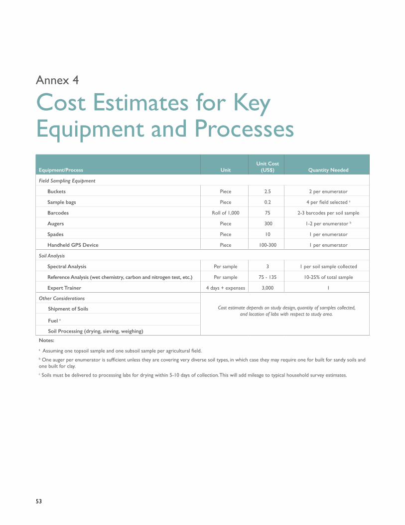
53
Annex 4
Cost Estimates for Key Equipment and Processes
Equipment/Process UnitUnit Cost
(US$) Quantity Needed
Field Sampling Equipment
Buckets Piece 2.5 2 per enumerator
Sample bags Piece 0.2 4 per field selected a
Barcodes Roll of 1,000 75 2-3 barcodes per soil sample
Augers Piece 300 1-2 per enumerator b
Spades Piece 10 1 per enumerator
Handheld GPS Device Piece 100-300 1 per enumerator
Soil Analysis
Spectral Analysis Per sample 3 1 per soil sample collected
Reference Analysis (wet chemistry, carbon and nitrogen test, etc.) Per sample 75 - 135 10-25% of total sample
Expert Trainer 4 days + expenses 3,000 1
Other Considerations
Cost estimate depends on study design, quantity of samples collected, and location of labs with respect to study area.
Shipment of Soils
Fuel c
Soil Processing (drying, sieving, weighing)
Notes:
a Assuming one topsoil sample and one subsoil sample per agricultural field.b One auger per enumerator is sufficient unless they are covering very diverse soil types, in which case they may require one for built for sandy soils and one built for clay.c Soils must be delivered to processing labs for drying within 5-10 days of collection. This will add mileage to typical household survey estimates.

54
Annex 5
Glossary
Agroecological zone Geographic area categorized by similar climactic conditions, such as elevation, temperature, and rainfall.
Bulk density A measure of soil compaction; the weight of soil in a given volume.
Field A piece of land in a parcel separated from the rest of the parcel by easily recognizable demarcation lines, such as paths, cadastral boundaries, and/or hedges. A field may consist of one or more plots. Definition according to FAO (2005).
Parcel Any piece of land, of one land tenure type, entirely surrounded by other land, water, road, forest, or other features not forming part of the holding, or forming part of the holding under a different land tenure type. A parcel may consist of one or more fields or plots adjacent to each other. Definition according to FAO (2005).
Plot A part or whole of a field on which a specific crop or crop mixture is cultivated. Definition according to FAO (2005).
Waypoint Also referred to as a geographic coordinate. Waypoints, or coordinates, identify the position of a single point in terms of a designated coordinate system.

Living Standards Measurement Studywww.worldbank.org/lsms
data.worldbank.org
SELECT LSMS GUIDEBOOKS
The Use of Non-Standard Units for the Collection of Food QuantityGbemisola Oseni, Josefine Durazo, and Kevin McGee
July 2017
Measuring the Role of Livestock in the Household Economy Alberto Zezza, Ugo Pica-Ciamarra, Harriet K. Mugera, Titus Mwisomba, and Patrick Okell
November 2016
Land Area Measurement in Household SurveysGero Carletto, Sydney Gourlay, Siobhan Murray, and Alberto Zezza
August 2016
Measuring Asset Ownership from a Gender PerspectiveTalip Kilic and Heather Moylan
April 2016
Measuring Conflict Exposure in Micro-Level SurveysTilman Brück, Patricia Justino, Philip Verwimp, and Andrew Tedesco
August 2013