SPECTRAL AND PSEUDO-SPECTRAL METHODS FOR PARABOLIC PROBLEMS W I T H

NON PERIODIC BOUNDARY C O N D I T I O N S

C. CANUTO (1) . A . QUARTERONI (2)

ABSTRACT - The advection-diffusion equation is approximated by Chebyshev and Legendre spectral and pseudo-spectral methods. Stability results in the energy norm and error estimates in terms of the discretization parameter and of the regularity of the solution in weighted Sobolev norms are presented.

Introduction.

In this paper we analyze spectral and pseudo-spectral methods for the one-dimensional advection-diffusion equation

(,) u t - v u = + ( b (x) u),,+bo (x) u=] (t, x)

submitted to Dirichlet boundary conditions in the interval I = ( - - 1 , 1). Approx- imations based on Chebyshev and Legendre polynomial expansions are considered. The pseudo-spectral schemes are essentially collocation methods at the nodes of the Gauss-Lobatto integration formulas related to the Chebyshev and Legendre weights.

Spectral approximations of problem (*) have been first developed by GOTTLIEB and ORSZAC [5] in the case of constant coefficients, and by GOTTLIEB [4] when b=bo=O and v depends on x. They establish stability in some kind of L 2 norm, and convergence when the solution is infinitely smooth.

- - Received October 6, 1980. (i) Istituto di Matematica Applicata - P.zza L. Da Vinci 27100 Pavia. (2) Istituto di Analisi Numerica del C. N. R. C.so C. Alberto, 5 - 27100 Pavia.

198 C. CANUTO - A. QUARTERONI: Spectral and pseudo-spectral

The aim of this paper is to provide stability results in the energy norm, and error estimates in terms of the discretization parameter (the polynomial degree) and of the regularity of u in weighted Sobolev norms. Essential tools of our analysis are the equivalence between discrete and continuous Sobolev norms for polynomials, together with an asymptotic estimate of the error between exact and discrete Gauss-Lobatto integration. This is obtained using some inter- polation and orthogonal projection operators whose approximation properties have been investigated in [1, 8].

The limit case v--> 0 is not explicitely investigated, even if we emphasize the dependence of the error on v.

We recall that equation (,) submitted to periodic boundary conditions can be approximated by Fourier methods invo!ving trigonometric polynomials (see e. g. [5, 7]). The techniques employed in this paper can be successfully applied to the theoretical analysis of these methods.

For a given weight function ~ > 0 over I we define

L2~ ( / )={ r I ---> R [ r is measurable and (r r + oo },

with (r r 1 6 2 (x) r (x) co (x) dx, and f1r162 r For any integer k>__0 I

we set

H*~, (I)={r (I) I d '~ r (I), O<_m<_k},

with the norm

k

11r z Ildmr 'm~O

The space H'~ (I) is defined by interpolation for non integral s. Finally we set H'o.~ ( I ) - - { r ( I ) [ r ( - - 1 ) = r (1)=0}.

Throughout this paper C will denote a generic constant, positive and independent of the discretization parameter N and of u.

1. Some results concerning the continuous problems.

We recall hereafter some known results about parabolic problems in the framework of weighted Sobolev spaces. They will be used in next sections; we add the proofs for convenience of the reader.

Let v>O be a real number, h e w 1,~ (I) and b~eL ~ (I) be given; for any ]-=/(t,x) and Uo=U0 (x) we consider the parabolic problem (T>0)

methods/or parabolic problems with non periodic etc. 199

(1.1) i u t - - v u = + ( b u ) . + b o u = [ in ]0, T ] •

u ( t , x ) = O on ] O , T ] X F

u (0, x) = Uo (x) in I.

Throughout this paper we shall consider two different weight functions over h c o = l , i. e., the Legendre weight, and co(x)=(1--xa) -l/z, i. e., the Chebyshev weight of the first kind. We assume that u e U (H*~) and u~eL 2 (L2). In addition we assume (for simplicity) that

(1.2) 1 b . + b o - - 1 -2- -2-be~ in I.

We set (formally)

ao,: H~o, (I) • HI~ (I) -+ R, a~ (u, v) = f ux (vco)x dx. I

LEMMA 1.1. There exist three positive constants 13, y, 8 such that ]or any veHlo,o, (I) and [or any ueHl~ (I) we have

(1.3) llvllo. - llv ito, (Poincard inequality),

(1.4) a~ (v, v)_>y [Iv]]21,0,,

(1.5) (u, Ilu=llo, Ilv=llo, �9

PROOF. (i) If CO= 1 these results are well known, as a~, is the normal inner product of H'o (I).

(ii) Consider now the weight co (x)=(1--x=) -'/2.

a - The property (1.3) follows immediately from the forthcoming result:

LEMMA 1.1. There exists a positive constant a such that

(1.6) r

PROOF. We note that

200 C. CANUTO - A . QUARTERONI: Spectral and pseudo-spectral

1 I 1

1 g'--}fv2o~ (Ix, f vZcodx< fv=~l~-~x dX< o 6 o

so it is sufficient to prove that

1 I

0 o

dx if v (O)=O.

Setting v ( x ) = f v~ (~ d~, we have 0

I 1 i

1 " edx" f l y 'x'12 1 dx=j" (x. /V, ,{ , d~)x-'" jl--x-i

o o 0

Then, by an inequality of Hardy's type (see [6, Lemma 10.1]), we can bound 1

the last term by c f (v~ (x)x-~/4) 2 dx and (1.6) holds. []

0

b - To prove (1.4) we note that for any veH~o.,~ (I) we have:

(1.7) a~ (~ , ~ ' ) = - - f ~'xx ~' ,O dx= f vx2 ~ dx+ f vx v ,ox dx= 1 I I

1 ----fv2~o dx+ -~.f {v2).o).dx= I I

= / " (v~) z 1 " ~o dx-- -~- J vz oJ= dx. I I

On the other hand, as co==(l+2xZ)/(1-xZ) 5/z, using the identity

~oS--~o=+2 (a~.) 2 co-l= 0

we also have

(1.8) f i f a,~ (v, v) = [(v CO)x[ z co -t dx +-i- vZ .cos dx. I I

methods ]or parabolic problems with non periodic etc. 201

Then

f v z w,,x dx <_ 5 f v z cos dx I I

and from (1.8) it follows

f v2 ~o~x dx<_6 a~ (v, v). I

By (1.7) we obtain

a~o (v, v) >_.f (v2 2 co dx-- 3a~o (v, v), I

and finally

1

whence (1.4) by (1.3).

c- We have for any ueH~o~ (I) and veH~o,o (I)

f I I

; ux v a~dx =(fu~ (v co~ co -~) co dx <_( ;u,2 co dx ) m . ( . f v2 (co~o_~) 2 co dx f /2. I I I I

Since ~oxco-~=x~o 2, the continuity property (1.5) holds due to (1.6). [] Throughout this paper fl, y, 8 will denote the constants defined by (1.3),

(1.4) and (1.5) respectively. Setting V=H~o,~ (I), by lemma 1.1 we deduce that a~ is continuous and

coercive in V. We consider the following weak formulation of (1.1):

(1.9) t u (t)eV, t -a . e.; u (O)=uo,

(ut,r162162 (Lr ~/r t-a. e.

PROPOSITION 1.1. The ]oltowing a priori estimate holds

202 C. CaNUTO - A . QUARTERONI: Spectral and pseudo-spectral

(1.1o) [[UlIL~ <L2) +~VIIulIv<H,> ~ c (lluol[o,~+ II/11 v <v~> )

where C is a positive constant independent o/ v.

PROOF. Setting qS=u in (1.9) and using (1.4) we have

(~.11) 1 d

Integration by parts shows that

(1.12) ((bu)~+bou, uL,= ( ( 1 b 1 b:,+ o - -~ b-~)u2 co dx>O I

where the last inequality holds by (1.2). Hence (1.10) holds by (1.11) and the Gronwall lemma. []

REMARK 1.1. Condition (1.2) is unnecessary to get (1.10); however, if (1.2) is violated, the constant C appearing in (1.10) depends on v. On the other hand, (1.2) is not a restrictive condition; there exists a suitable 2eR+ (see [2]) such that (1.2) can be achieved by the classical change of variable u (t)---> eat u (t).

[]

2. Spectral methods to approximate (1.1).

Let {p~}%=0 denote the family of polynomials which are orthonormal with respect to the inner product (.,.)~, i. e.,

(2.1) (p,, p ,~)~=8 . . . .

It is well known that

(2.2) ~ueL2~ (I) u = 2; un pn, u , = (u, p,)~.

p,=2nLn, with 2n=V 2-n " / _t_12 .2 and Ln is the n-th degree Legendre If o)~---1 then

polynomial which satisfies L, (1)=1. If co (x)=(1--x:) -1/~ then pn=-c,T,, with

r~= 1/t/~,, v , = t / - ~ (n> 1), and Tn is the n-th degree Chebyshev polynomial of the first kind such that T, (1)=1 (see, e. g., DAvis and RAmNOWITZ [3]). For any integer N _ 0 the set spanned by {pn}U,=o coincides with the space Pu of

methods for parabolic problems with non periodic etc. 203

polynomials of degree _<N over I. Define

(2.3) VN={•ePN [ ~ (-- 1 )=~ (1)=0}.

Let UoseVN be a suitable approximation of u0. The spectral approximation of (1.1) is the following:

i find uNeH I (V,) such that

(2.4) i(U~c,t,~)~+va~(uN, q3)+((buN)x+boUN,~)~=(],~)~ ~ c V N , t -a . e. t UN (0) = UoN .

Arguing as in the proof of proposition 1.1 we can state the following stability result.

PROPOSITION 2.1. We have

(2.s) IIu,,ll L. <v~) + r II.NI! V<H, ) --<C (II.oNIIo,~,+ II/[[L=<L= ))" [ ]

REMARK 2.1. Consider for instance the Legendre case. A set of basis functions for VN is given by {L~ with

(2.6) L~ - ILo if n is even

( L1 if n is odd.

This basis is no more orthogonal; as a matter of fact, setting

I 0 if n + m is odd

Knm=2~J.m3n,n - ~,o 2 if n and m are even

[2~ 2 if n and rn are odd,

it follows easily from (2.1) that

(2.7) (L~176 2<_n, m<_N.

Defining

(2.8) P~ L~ (I)---> VN, (u--P~ u, r VOeVN,

a simple calculation ~hows that

204 C. CANUTO - A. QUARTERONI: Spectral and pseudo-spectral

x ~r ~u0202 if m is even A

(2.9) P~ X UiL~ X UiKim--um--, , 2<_m<_N. j=2 =2 ] ̂

f~uz).i z if m is odd

Similar arguments hold for the Chebyshev case. Then, by the help of the projection operator PON, (2.4) can be written equivalently as follows:

UN, t+P~ LuN = P% L UN(O)=Uo,N

where

LuN = -- vuN, xx + (bUN)x+ bo uN .

Define now

(2.10) [IN: V--> VN, a ~ ( u - - H N u , ~ ) - ~ O ~ t ~ c V N .

We have the estimate (cfr. MADAY and QUARTERONI [8])

(2.11) V ' u e H % ( I ) CIV, ~r>_l, [IU--HNUII , <--ClluII , .

. IN "-~ O<lz<_ 1

[N(3~-wz-L I </z__< min (2, o')

in both Legendre and Chebyshev cases.

By classical techniques we can prove the following theorems; in the

proofs we shall use the notations: u = H x u, e=u- -uN , p = u - - u .

THEOREM 2.1. Assume u c L ~ ( H % ) , ut~L2(H%) Jor some a>_l, and take uoN = HN Uo. Then

(2.12) IlU--UNIIL,(L2 ) <__CN-~{IIUllL.(H%) + [[Utl]L2(H% ) }.

PROOF. By (1.9) and (2.10) it follows that

(2.13) (ut, (J)~+va~ (u, 0)+((b~)x + b o u , 0)~----(/, q~)~,+

+(pt+(bp),~+bop,~))~ ~t(gcVN, t - a . e.

methods for parabolic problems with non periodic etc. 205

and so by comparison with (2.4) we have

t (e,, O)~ + va~ (e, O) + ( (be)~ + bo e, ~)~=(pt+ (bp)~ + bo p, 0)~

(2.14) ~beVN, t- a. e.

~e (0)--0.

Set now ~b=e in (2.14); we have

e)~ <2y Ilbpll%+ ~lle~ll% (2.15) ((bp)x, -- v), "

a matter of fact, by (1.5) applied with u = ] (bp) (if) dff and v = e we As have --1

s ((bp)x, e)~= - I bP (eco)x d x ~ 8 [lbpllo,~ [ l e x l l o , ~ �9

. 3

I

Then (2.15) holds. By (2.14) and (2.15) we get

~-Ile[ld = lexll~o,~ <_{ llp,ll% + C llbpll% + o.~-bvy I [[bo p[l%,~ t +2 llell=o,o

so by the Gronwall lemma we deduce

t

llello,~+t/u \i/2 /1 , (2.16) \ d

o

• [IPlIL~(L,o)) ~te [0 , T],.

By the error estimate (2.11) and the triangular inequality

Ilu-u41L. (L2o~- < I1~11 L-(L~o~ + IlellL. (L'~

[]

THEOREM 2.2. Under the same hypotheses of the previous theorem we have

we obtain (2.12).

206

(2.17) gTll(u-u~).l l L~ (L,.)

iJ a)---1 we have in addition

(2.18) I / ~ l ( u - u~')*llz - (u)

PROOF.

C. CANUTO - A. QUARTERONI: Spectral and pseudo-spectral

_<_c N '-~ (ll<l u (Ho~) + [[u~II u (H ~-i)};

~CN'-~{II~*II L~<m) + Ilu,llL2<m> }.

(i) and the following triangular inequality

T

<, _< < , + (jll ll, V o

The estimate (2.17) is an immediate consequence of (2.16), (2.11)

v d Ile'll~~ T ~ a~ (e, e) ~ (--(be),--bo e + pt+ (bp)x + bo p, et) ~

1 1 -<-- 1]e,11%+2 -~- {llbl[ w,.- u) ( l ie*Il l+ [lP*[[�89 +

§ ~ . ([[ell~o+ Ilpl[%)+ [[p,lr0}. (I)

1 Ignoring the term ~-Ile, ll%_>o, by (2.11) and (2.12) it follows that

d v -~T&o (e, e ) Z C , N 1-~' (][u[[ L2 (H,) -t- llutll L2 (H ~) ) + C a Ile.l?o �9

The Gronwall lemma and the triangular inequality lead to (2.18) []

3. Pseudo-spectral methods to approximate (1.1).

We denote by {xj,~oi}~=o the nodes and the weights of the Gauss-Lobatto integration formula reIated to the weight co. With the notations of the previous section we recali that ,the nodes {xt} are the roots of the polynomial p=pn+t--pn-l,

so x o = - l and xN=l ( in the Chebyshev case we have xj=cos ( - z r + ~-)) . It is

(ii) Setting r in (2.14) we obtain

methods [or parabolic problems with non periodic etc.

well known (cfr., e. g., DAWS and RABINOWITZ [3]) that

207

f N (3.1) g (x)co (x) dx= Z g (xi)coi ~gePm-1 �9 j=o

I

We define an interpolation operator Pc by

(3.2) P~: C~ Pcu(x/)=u(xi)

it satisfies (see CaNUTO and QUARTEROm [1])

O<_]<_N;

1 (3.3) MueH%, (I), ~> -~-, O<lt<a

tN 2~-" if CO (X)-~--(1--X2) -1/2

tlu-Pcull"'~<Cllull~'~• if co--1.

Setting _,v

(3.4) ~ ~, ~b e C o (7) (~b, ff)N.~ = Z q~ (xi) ~ (xi) coi j=o

by (3.1) it follows that

(3.5) (~b, ff)N,~=($, ~)~ if $.~rJePm_t;

moreover we have

(3.6) (~, ~)N.~ = (Pc q~, ~b)N,~ ~/O,~eC~

Then

P c u - - Z u k p k , U~=(u, pN)N.~'(IIpu]IN.~)-', Uk=(u, pk)u.~ O ~ k ~ N - - 1 kRO

where we set ' i

(3.7) I Ir I.,o -

From now on we assume that b0eC ~ (~, b e C ' (~, uoeco (~, f e c o ([0, T],XI-). The pseudo-spectral approximation of (1.1) is given by the collocation problem

208 C. CANUTO - A. QUARTERONI: Spectral and pseudo-spectral

(3.8)

find uceC 1 (Pu) such that ! uc, t (xj) -- vu .... (xi) + (bu~)x (xj) + bo uc (xi) = t (xj)

/ = 1 . . . . . N - - l ,

l uc (xo) = u~ (x~) = 0,

uc (0, xj) = Uo (xj) ] = 0 . . . . . N.

t - a . e.

By the help of (3.4) and (3.6), the problem (3.8) can be written equivalently as follows:

(3.9)

l f ind u~aC ~ (VN) such that

(uc, t, r v (u ..... r Uc, r = (],~r162

[uc (0) = Pc uo .

t - a . e.

LEMMA 3.1. For both Legendre and Chebyshev weights the norms [[. []N,~, and l I" l lo,~ are uniformly equivalent over Pu, i. e.

(3,1o) c, IIr [lr ~zr

and C1, Cz are two positive constants independent o] N. This result has been proved by the authors in [ 1]~.

[]

THEOREM 3.1. The pseudo-spectral problem (3.9) is stable; namely we have

(3.11)

T

,luc,.L. L2, +v ,jucx, j (/,,, o o

PROOF. We set r in (3.9) and we obtain

(3.12) 1 d 2 dt [[uc]]z~'~--v (u . . . . uc)u,~=(L Uc)N,~ --((buc)x+bo uc, uc)u,~ t - a . e.

By (3.5) and (1.4) we get

(3 .13) - v (uc.=, uc),,.~= - v (uc,=, uc)o.~= a~ (u. uc)>--vr [luo,~][~o.~.

Furthermore we have

methods [or parabolic problems with non periodic etc. 209

I(/, uo)~,J ~_~(llfll2N,o+ rl.clr'~,~)

(3.14) I(bouc, U~)N,~[ <]]boll L ~ (I)[]u~lI2N'~

I((bu~,)x, U~)N,~[ --< IJbilw,,~ (z)[ludl2~,~+ ~ IIb[I ~ (z) ylluc,.41'~,~.

lJ \1) Finally, noting that by (3.10) c ~ I J . ~ , ~ I I ~ N , ~ < _ - z - II~.xpl~0,~, by (3.~2), (3A3) and

(3.14) it follows that

dt

1 + Ifbfl w~,- (i) + 2~ jfblr~L~ (~) )lr"~fl ~,~"

Now the inequality (3.11) follows by integration in t and the Gronwall lemma.

We have C<C~ (exp ( l / v ) ) , where C~ is independent of v. [] We note that the right hand side of (3.11) can be uniformly bounded by

C (llu0][ L* (I) 4- ]l]ll r 2 (L ~ (I)))"

In view o,f the discussion about the convergence of the pseudo-spectral solution u~ to u we introduce the LZ~-projection operator

(3.15) PN: L2~, (I) --+ PN, (U--PN U, 0)~,:0 ~zCePN.

The following error estimate has been proved by the authors in [1]:

t N 3/2)'u-r O-~/A-~ ~ min (1, ~r) (3.16) ~Zueft% (I)' I lu-p~ ull"~ <-C lluIl"~ ~N ~-'~:-~ 1~_~_~.

LEMMA 3.2. For any ~ = E ~NpNCL2~ (I) we have

A

(3.17) 10N]--~ [[r ~ N ~ I .

Moreover, setting

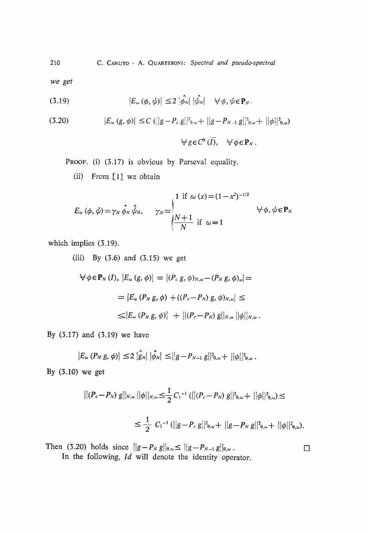
(3.18) E~ (~, ~) = (~, ~)N,~-- (~, r ~ r ~ 6 0 (~,

210

we get

(3.19)

(3.20)

C . C A N U T O - A . O U A R T E R O N I : Spectral and pseudo-spectral

A ^

tE. (r ~)[ _<2 [r v~ , CePN.

IE~ (g, ~)1 _<C (]lg--Po gl?0~o-t- Ilg-P~-~ gll=o-+ 1I~[5~)

~r ~ V ~ e P u .

PRooF. (i) (3.17) is obvious by Parseval equality.

(ii) From [ 1], we obtain

1 if co ( x ) = ( 1 - x ~ ) -~/2

I N + if a ~ l 1 N

which implies (3.19).

(iii) By (5.6) and (3.15) we get

~6q~ePu (I), [E~ (g. q~)[ ---- [(Pc g, (b)N,~-- (Pu g, r

= [E. (P~ g. ~b) +((Pc--Ps) g, 0)m.] --<

~IE, (Pug, r + II(ec-Pu)gll~ II~[ko.

By (3.17) and (3.19) we have

A A

IE. (Pug, r Igul Ir _<tlg-Pu-,g[12o,~+ IIr �9

By (3.10) we get

][(Pc--Pu) gIlu,~ [[@][N,~--<Ic, - ' ([[(Pc--Pu) g[12o,~+ [[~b[12o,~)_ <

< 1 - ~ c, -1 (llg-P=gtS,~+ IIg-P,,gll:o,.+ lloli~,~).

Then (3.20) holds since [Ig--YN g][o,~- < IIg-PN-~ gIIo,~. L-] In the following, Id will denote the identity operator.

methods for parabolic problems with non periodic etc.

THEOREM 3.2. W e have

(3.21)

where

(3.22)

(3.23)

+ I[uo-P~ uollo,~+ IlU--I-IN Utt Z ~ (Z2) + Ilu--Ha Ut] L z (tt'~) +

+ Ilut-nN u,fl L~ (Z~) + Ilu,--PN-, u, II L= (t~) + I l l -Pc fl g~ (z=~) +

+ H/-PN-'/llt=(Z~ ) + R (u))

211

R ( u ) = I[u--PNu]JL2(L2 ) + II(bu)~--P~_, (bu),llU(LZ ) i] boeR, beP,,

n (u)= I](bo u)--PN_, (b~ u)l ] L2 (L:~) + II(b~ u)--Pc (bo u)llL2 (LZ) q-

+ ll(Id-P~)[bo (U--I1NU)]ItL2(L2) + [I(bu),--nN_~ (bu).,[[LZ(D~) +

+ [[(bu),--Pc (buhl[ LZ (L2o) + I](ld--n~) [b (U--HN U)]~I[ LZ (LZ)

otherwise.

PROOF. Let us set u=H~cu, e=u--uc , p = u - - u , and

G (p) = p t + (bp)x+ bop.

We note that by (3.5)

- v (u ..... ~) N,~=va~, (uc, ~) u

hence by (3.9) we get

(uc,,, r + va~ (uc, r + ((buc)x + bouc, r (1, r

Using (2.13) we obtain

l (et, O)N,~+va~ (e, r + ((be)x+ bo e, r

(3.24) ]=(G (p), r (~, O)+Eo~ (bou+(bu)~, r (1, r !

~e (0) = (nN-P~) uo.

~beVN, t- a. e.

212 C. CANUTO - A. QUARTEROm: Spectral and pseudo-spectral

To provide an upper bound for the right hand side, we consider separately the different terms.

(i) Evaluation o/ I IG (p) llo,~.

Noting that //~ commutes with time differentiation, we get

(3.25) IIG (p)llo.-< I[u,-n~ ut[[o,co-J-C Ilu-H~ ut[,,o

with C depending on I]bI[ w~,-(I) and on lib011Z~ (Z)"

(ii) Evaluation o/ Eo, (L ~).

By (3.20) it follows that

(5.26) IE,~ 0 ~, ~b)[ <__.C (Ill--Pc fllzo,~ J - [[f--PN-1 fll2o,o,--~- Ilk[leo,co)

(iii) Evaluation o/E~ (ut, q~).

Since utcPN by (3.19) we get

^ ^ ^

and by (3.17)

^ m

Iz~l = I ( u , - . , , ;~)~+ (u,, p~)~l <-Ilu,-n~ .,tfo.o+ Ilu,-P~-~ u, llo~.

Then we have

(3.27) Ie~ (E,~)I-< [lu,-m, utll~,~+Plu,-PN-~u,l]~o,~+ 11~112o,~.

(iv) Evaluation of E~ (bou+(bu)x, ~).

Assume first that b,0cR and boP,. In this case "boUCPN and (bu).~cPN, so by (3.19) we get

A

Ie. (bo ~+(~)~, ~)[ _<_2 19~--2N11~,,I

~N: (bo if, pN)o, ~N: ((bu'3~. ;~)~.

By (3.17) we have

methods [or parabolic problems with non periodic etc. 213

IGI -< Ibol (llu-H~ ullo,~+ Ilu-nN-, ullo,~) ^

Iz d < II(Id--PN_~) (b Fix ~)=11o,~--<

ll(zd-P~-~) (b~)xllo,~ + II(rd--P~-~) (b~--b ~ .)x!lo,~_<

II(Id- PN_,) (bu)=~l[0,~+ C ilbu--b fin ull,,o, by (3.16) with /z--~=O) whence

(3.28) IE~(b,ou+(bu)x,r _<C (llu--Cr,, u![1,~+ Ilu--PN-lullo,~

+ I[(td-PN_,) (bu)xI[o,~).

C is a constant depending on Ilbll wl,~ and Ib0l.

Consider now the general case in which no assumption is made on the coefficients b,0 and b. By (5.20) we get

(3.29) IE~ (bo u + (bu)x, r <C (Ilia-Pc) bo u[12o,~+ II(Id-Pc) (b~)xllZo~+

if-Jl(Id--PN_,) bo~tjl2o,~o-k ]](ld--PN_I) (bu)xI]2o,~+ IIr

by (3.16) we obtain

(3.30) [[(ld--nN_~) bou][o,~<_ [](Id--PN_~) bo u[lo,~-k [[bo[] L ~ (I) ][u--HN u[[o,~

(3.31) II(Zd-PN-~) (bu).~llo,~_< [I(Zd--PN-I) (bu)=llo,~+ [[bllw, ,. (~) I I~-H~.Ik~.

Furthermore we get

(3.32) llqd-P~) bo ~ifo,~_< II(rd-Pc) bo ullo.~+ II(rd-P~) (bo (u-Sr~ u))lfo,~

(3.33) ]l(Id--n~) (bu)~[[o,~___ II(Id--P~) (bu),~l[,o.~+ ]l(Id--n~) (b (U--HN u))~]lo,~.

(v) Set now r in (3.24); by (3.24) . . . . . (3.33) it follows that

(3.34) ~- I]ell~,~+va~ (e, e)+(boe+(be)~,e)N,~<_

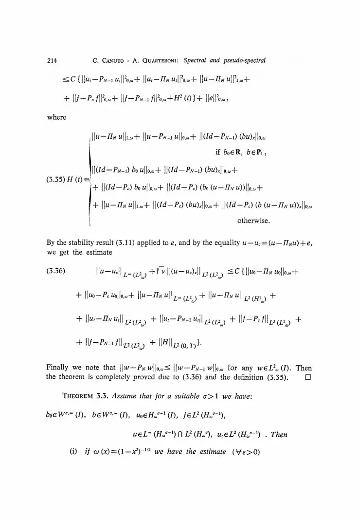
214 C. CANUTO - A. QUARTERONI: Spectral and pseudo-spectral

<~C {ttut--P,v_, u,ll%,~+ Ilu,-nN u,ll~o,~+ I I . -nN uII2,,o+

+ Il i-Pc/[ l%,~+ I I /-PN-,/ I I%,~+H 2 (t)}+ llell~o,~,

where

i[[u-II~ u[]l,~+ [[u--PN-1 U][0,~+ [[(Id--PN_1) (bu)x[Io,~

i if boeR, beP1,

)H(Id--PN-1) bo ullo,~+ ]](Id--PN_I) (bu)~]]o,o,+ (3.35) H (t)

I :++ ]](Id--Pc) bo U[[o,~+ [ l(Id-Pc) (bo (u-I1N u))[Io,~+

II.-rz~ ulll,~+ [[(r_d-Pc) (bu).llo,~+ Ildd-Pc) (b (u-nN u)).llo,~

otherwise.

By the stability result (3.11) applied to e, and by the equality u - uc = (u-- llNu) + e, we get the estimate

(3.36) I lu-ucllL. ( v ) +Y'-~ II(u-uc)xllz2(L2j ---c {Iluo-uN uollo.~+

+ ltuo-P~ ~ollo.,+ I lu -n~ all L- (r.~o) + I lu -n~ al ly (n,,) +

+ I I~ , -n~ u,II v (%) + Ilu,-P~-1 u,ll v (L2~,) + lit-Pc 111 v (vo) +

+ I I / -P~-, t l l :v(v~) + I Ir~l l L, (o, r) }.

Finally we note that II~-P~ ~11o,~-< II~-PN-, ~11o,~ fo~ any weL2o, (I). Then the theorem is completely proved due to (5.36) an, d the definition (5.35). []

THEOREM 3.3. Assume that ]or a suitable ~> 1 we have:

b o e W ~'~ (I), b e W ~,~ (I), u o e H J -~ (I), l e e (HJ-b,

u e L ~ ( H J - b N L 2 ( H J ) , u ~ e E ( H J - b . T h e n

(i) i] ~o (x)-'(1--x2) -~/2 we have the estimate (~/e>0)

methods lor parabolic problems with non periodic etc. 215

(3.37) llu--ucllL~ (L=~) +I'~tE(U--U~)~II L~ (L~> ~

i N 1-~ K (uo, 1, u, ut) if boeR, bePt

<CX N' - " K (Uo, f, u, ut)-t--N 5/4+~-" Ilull L2 (m~)

otherwise

(ii) if ,co-- 1 we have the estimate ( ~ e > 0,)

(3.38) Ilu--ucIIL. (L~) § J" ~ II(u-uc)~ll L~(L,) ~

i N /2-r iv(. (Uo, f, u, ut) if b0cR, beP1

<--CX N3/2-~ K (uo, 1, u, u t )+ N 7/4+'-~' IlulIL2 (m>

t otherwise,

where

(3.39)

K (uo, t, u, u~)= luoll~-,,~+ ll/llL~ r + llull L- <H~-') +

C is a suitable constant depending on e, Itboll w ~ (I) and IlblIw=.. (i)"

PROOF. The error estimates (5.37) and (5.38) can be achieved by previous theorem and results (2.11), (3.3), (3.16),concerning the approximation pro- perties of the operators/ /x, Pc and IN. We must only be careful to estimate the term R (u) which appears in (3.22) and (3.23). If boeR and beP1 we get:

(3.40) N '-~ [lull L~ R ( u ) ~ C {N -~ llull L~ (too) + Ilbll w ~ (i) (H~o) }"

For evaluating (3.23) we set now for convenience e (co)=O if ~o (x)=(1--x2) -1/2, and e ( c o ) = l / 2 if c o ~ l . We have

[[bo U-- PN (bo U)[I L2 (L~ ) ~ C Ilbol! w~ ~ (I) N -~ ]lull L~ (H=~) ;

[[bo u - P c (bo u)[] L2 (L~) ~ C ]]bol[w~. (I) N~(~)-~ ]lull L 2 (H~) ;

216 C. CANUTO - A . QUARTERONI: Spectral and pseudo-spectral

l l ( td- Pc) (bo (u--Hx u))IlL2 (L~) ~ C N ~(~)-~n-~ Ilbo (u--Hn u)[[ D (Hcol/2+ Q <~

~ c llbolt w~,2+,,= (r) L= (m~)

II(bu)~-PN (bu).~j] L2 (L2 ) ~ c llbll we,- (~) m '-= tlullL~(m~) ;

~ c Ilbll w~,= (~) N ~'~>+'-~ Ilull L~ (m . ) ;

]](ld-P~) (b (U--IIN U))~ll L2 (L2~) ~ C N ~'~)-m-~ Ilb (u-~q~ u)ll v (H~,-~) ~

_ < c libll w~,~+,.-(~)N~(~)-, ,~-, (m~) -

This completes the proof of the theorem. []

ADDED IN PROOF. Instead of (3.8), one can consider the following pseudo- spectral problem:

find u~cC ~ (Pu) such that

(3.8)'

uc, t (x j ) - -vu .... (xi)-t- [Pc (but)Ix (xi)+bo uc (xj) =1 (xi)

j = l . . . . . N - - l , t - a . e.,

u~ (xo) = uc (xN) = O,

uc (0, xj)--Uo (x i) / = 0 . . . . . N.

In this scheme, differentiation in the first-order term is done via the Fast Fourier Transform algorithm, and one does not need to know the derivative of b at the nodes.The analysis of stability and convergence for (3.8)' can be carried out by the arguments of Sect. 3. However, one can take advantage from the fact that the first-order term is now a polynomial of degree N--1. Then the proof can be considerably simplified due to the relation (3.5) which can be used in different points of it. The new error estimate is as follows:

. J i u - u c H L . (L~) "<Z C N 1-~ K (u~), f, u, ut),

with K (Uo, J, u, ut) defined in (5.39), for both Chebyshev and Legendre points.

methods ]or parabolic problems with non periodic etc. 217

R E F E R E N C E S

[1] C. CANUTO, A. QUARTERONI, Approximation results ]or orthogonaI polynomials in SoboIev spaces, Math. Comp. (1982), to appear.

[2] C. CANUTO, A. QUAR'rERONL Error estimates Jot spectral and pseudo-spectral approx- imations of hyperbolic equations, SIAM I. Numer. Anal. (1982), to appear.

[3] P. J. DAVIS, P. RABINOWITZ, Methods of Numerical Integration (1975), Academic Press, New York.

[4] D. GOTTLIEB, The stability o/ the pseudo-spectral Chebyshev methods, ICASE Report 79-17, Institute for Computer Applications in Science and Engineering, Hampton, VA, 1979.

[5] D. GOTTLIEB, S. A. ORSZAG, Numerical Analysis of Spectral Methods: Theory and Applications, CBMS Regional Conference Series in Applied Mathematics 26, SIAM, Philadelphia, 1977.

[6] J. LIoNs, E. MAGENES, Non Homogeneous Boundary Value Problems and applications (1972), 1, Springer Verlag, Berlin-Heidelberg-New York.

[7] H. O. KREISS, J. OLmZR, Stability o] the Fourier method, SIAM J. Numer. Anal., 16, (1979), 421-433.

[8] Y. MADAY, A. QUARTERONI, Legendre and Chebyshev spectral approximations of Burgers' equation, Numer. Math., 57 (1981), 321-332.